Embed Size (px)
Citation preview
Circular 1515
Field Observations During the Sixth Microwave Water and Energy Balance
Experiment (MicroWEX-6): from June 19 through November 30, 20061
Fei Yan, Hwan Hee Han, Ruofan Yang, Joaquin Casanova, Jasmeet Judge,
Jennifer Jacobs, Orlando Lanni, and Larry Miller2
1. This document is Circular 1515, one of a series of the Agricultural and Biological Engineering Department, Florida Cooperative Extension Service, Institute of Food and Agricultural Sciences, University of Florida. First published May 2007. Reviewed July 2010. Please visit the EDIS Web site at http://edis.ifas.ufl.edu for more publications.
2. Fei Yan is a graduate research assistant of University of Florida (UF); Hwan Hee Han is a graduate research assistant of University of New Hampshire (UNH); Ruofan Yang and Joaquin Casanova are graduate research assistants of UF; Jasmeet Judge is an assistant professor and director of Center for Remote Sensing of UF (email: [email protected]); Jennifer Jacobs is an associate professor of UNH; and Orlando Lanni and Larry Miller are Engineers of UF. All authors except Hwan Hee Han and Jennifer Jacobs are affiliated with the Agricultural and Biological Engineering Department, Institute of Food and Agricultural Sciences, University of Florida, Gainesville, 32611. Hwan Hee Han and Jennifer Jacobs are with the Civil Engineering Department, University of New Hampshire, Durham, NH 03824.
The Institute of Food and Agricultural Sciences (IFAS) is an Equal Opportunity Institution authorized to provide research, educational information and other services only to individuals and institutions that function with non-discrimination with respect to race, creed, color, religion, age, disability, sex, sexual orientation, marital status, national origin, political opinions or affiliations. U.S. Department of Agriculture, Cooperative Extension Service, University of Florida, IFAS, Florida A. & M. University Cooperative Extension Program, and Boards of County Commissioners Cooperating. Millie Ferrer-Chancy, Interim Dean
2
TABLE OF CONTENTS
1. INTRODUCTION..........................………………………………………………………………………………... 1
2. OBJECTIVES……………………………………………………………………………………………………… 1
3. FIELD SETUP……………………………………………………………………………………………………… 1
4. SENSORS…………………………………………………………………………………………………………… 4
4.1 University of Florida Microwave Radiometer Systems……………………….………………………… 4
4.1.1 University of Florida C-band Microwave Radiometer (UFCMR).………………………………….. 4
4.1.1.1 Theory of operation…………………..………………………………………………... 6
4.1.2 University of Florida L-band Microwave Radiometer (UFLMR)…………………………….. 7
4.1.2.1 Theory of operation…………………..……………………………………………….. 9
4.2 Eddy Covariance System………………………………………………………………………………… 11
4.2.1 East Eddy Covariance System………………………………………………………………… 11
4.2.2 West Eddy Covariance System………………………………………………………………… 12
4.3 Net Radiometer…………………………………………………………………………………………. 12
4.4 Thermal Infrared Sensor………………………………………………………………………………… 13
4.5 Air Temperature and Relative Humidity……………………………………………………………....... 13
4.6 Canopy Air Temperature………………………………………………………………………………… 13
4.7 Soil Moisture and Temperature Probes…………………………………………………………………. 14
4.8 Precipitation……………………………………………….…………………………………………..... 14
4.9 Soil Heat Flux Plates……………………………………………………………………………………. 15
5. VEGETATION SAMPLING……………………………………………………………………………………. 15
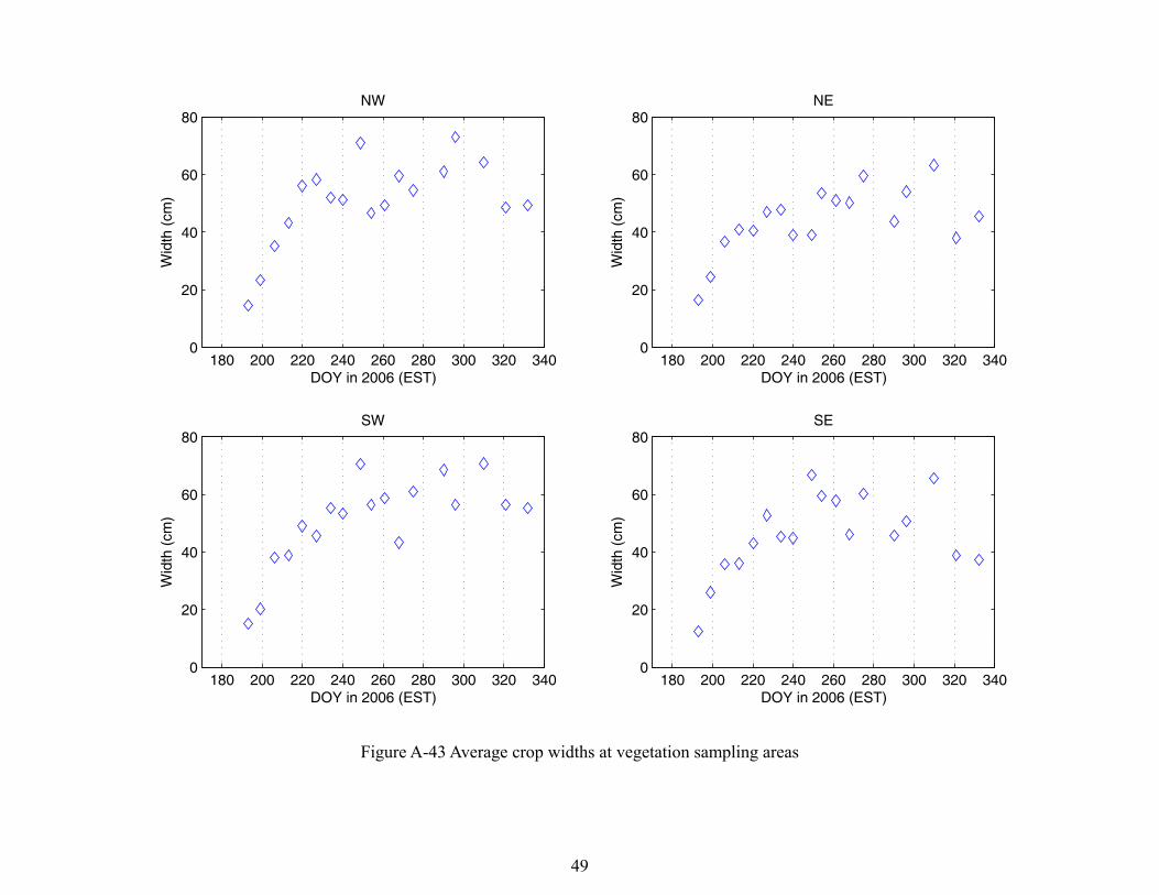
5.1 Height and Width …………………………………………………………………………………… 15
5.2 Leaf Area Index (LAI) …………………………………………………………………………………. 15
5.3 Green and Dry Biomass………………………………………………………………………………… 15
5.4 Vertical Distribution of Moisture in the Canopy……………………………………………………...… 15
5.5 Lint Yield……………………………………………………………………………………………….. 16
6. WELL SAMPLING……………………………………………………………………………………………… 16
6.1 Water level measurement……………………………………………………………………………….. 16
7. FIELD LOG……………………………………………………………………………………………………… 17
8. REFERENCES…………………………………………………………………………………………………… 25
9. ACKNOWLEDGMENTS ………………………………………………………………………………………. 25
A. FIELD OBSERVATIONS………………………………………………………………………………………. 26
1
1. INTRODUCTION
For accurate prediction of weather and near-term climate, root-zone soil moisture is one of the most crucial components driving the surface hydrological processes. Soil moisture in the top meter is also very important because it governs moisture and energy fluxes at the land-atmosphere interface and it plays a significant role in partitioning of the precipitation into runoff and infiltration. Energy and moisture fluxes at the land surface can be estimated by Soil-Vegetation-Atmosphere-Transfer (SVAT) models. These models are typically used in conjunction with climate prediction models and hydrological models. Even though the biophysics of moisture and energy transport is well-captured in most current SVAT models, the computational errors accumulate over time and the model estimates of soil moisture diverge from reality. One promising way to significantly improve model estimates of soil moisture is by assimilating remotely sensed data that is sensitive to soil moisture, for example microwave brightness temperatures, and updating the model state variables. The microwave brightness at low frequencies (< 10 GHz) is very sensitive to soil moisture in the top few centimeters in most vegetated surfaces. Many studies have been conducted in agricultural areas such as bare soil, grass, soybean, wheat, pasture, and corn to understand the relationship between soil moisture and microwave remote sensing. Most of these experiments conducted in agricultural regions have been short-term experiments that captured only a part of growing seasons. It is important to know how microwave brightness signature varies with soil moisture, evapotranspiration (ET), and biomass in a dynamic agricultural canopy with a significant biomass (4-6 kg/m2) throughout the growing season.
2. OBJECTIVES
The goal of MicroWEX-6 was to understand the land-atmosphere interactions during the growing season of cotton, and their effect on observed microwave brightness signatures at 6.7 GHz and 1.4 GHz, matching that of the satellite-based microwave radiometers, AMSR, and the SMOS mission, respectively. Specific objectives of MicroWEX-6 are:
1. To collect passive microwave and other ancillary data to develop and calibrate a dynamic microwave brightness model for cotton.
2. To collect energy and moisture flux data at land surface and in soil to develop and calibrate a dynamic SVAT model for cotton.
3. To evaluate feasibility of soil moisture retrievals using passive microwave data at 6.7 and 1.4 GHz for the growing cotton canopy.
3. FIELD SETUP
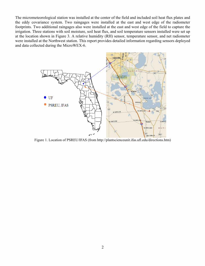
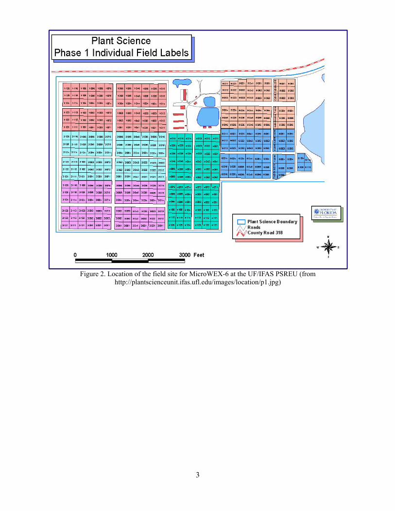
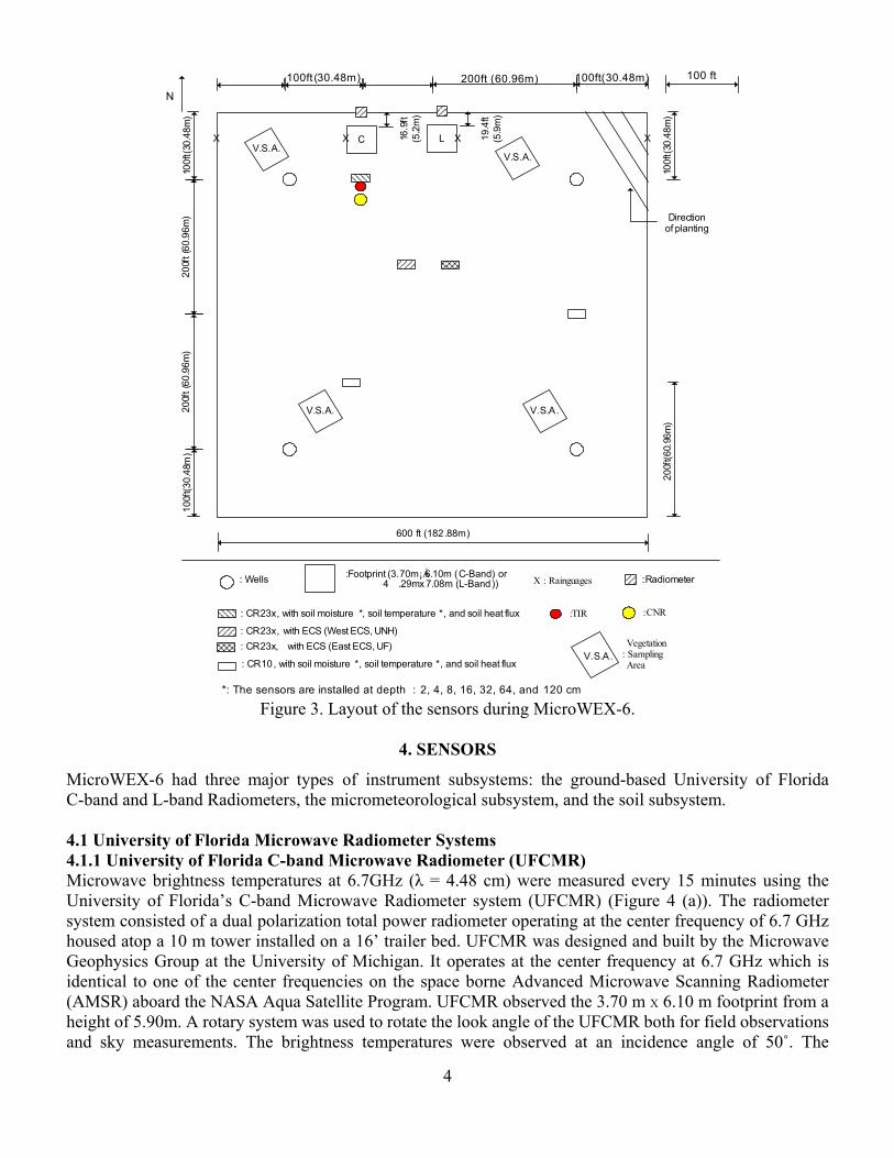
MicroWEX-6 was conducted by the Center for Remote Sensing, Agricultural and Biological Engineering Department at the Plant Science Research and Education Unit (PSREU), IFAS, Citra, FL. Figures 1 and 2 show the location of the PSREU and the study site for the MicroWEX-6, respectively. The study site was located at the west side of the PSERU. The dimensions of the study site were a 183 m X 183 m. A linear move system was used for irrigation. The cotton was planted on June 19 (Day of Year (DoY) 170) in 2006, at an orientation 60º from East as shown in Figure 3. The crop spacing was 8 cm (3.1 inches) and the row spacing was 76.2 cm (30 inches). Instrument installation began on June 20 (DoY 171). The instruments consisted of a ground-based microwave radiometer system and micrometeorological stations. The ground-based microwave radiometer system was installed at the location shown in Figure 3, facing south to avoid the radiometer shadow interfering with the field of view as seen in Figure 3.
2
The micrometeorological station was installed at the center of the field and included soil heat flux plates and the eddy covariance system. Two raingages were installed at the east and west edge of the radiometer footprints. Two additional raingages also were installed at the east and west edge of the field to capture the irrigation. Three stations with soil moisture, soil heat flux, and soil temperature sensors installed were set up at the location shown in Figure 3. A relative humidity (RH) sensor, temperature sensor, and net radiometer were installed at the Northwest station. This report provides detailed information regarding sensors deployed and data collected during the MicroWEX-6.
Figure 1. Location of PSREU/IFAS (from http://plantscienceunit.ifas.ufl.edu/directions.htm)
3
Figure 2. Location of the field site for MicroWEX-6 at the UF/IFAS PSREU (from
http://plantscienceunit.ifas.ufl.edu/images/location/p1.jpg)
4
C
100 ft
: Wells
: CR23x, with soil moisture *, soil temperature *, and soil heat flux
: CR10, with soil moisture *, soil temperature *, and soil heat flux
:Footprint (3.70m¡Á6.10m (C-Band) or 4 .29mx 7.08m (L-Band)) :Radiometer
N
16.9
ft(5
.2m
)
600 ft (182.88m)
100ft(30.48m)
100f
t(30.
48m
)10
0ft(
30.4
8m)
200f
t(60
.96m
)20
0ft(
60.9
6m)
200ft (60.96m)100ft (30.48m)
100f
t(30
.48m
)
: CR23x, with ECS (West ECS, UNH)
200f
t(60.
96m
)
*: The sensors are installed at depth : 2, 4, 8, 16, 32, 64, and 120 cm
Directionof planting
X : Rainguages
XX X
:TIR :CNR
V.S.A. Vegetation: Sampling Area
V.S.A.
V.S.A. V.S.A.
V.S.A.L 19
.4ft
(5.9
m)
X
: CR23x, with ECS (East ECS, UF)
Figure 3. Layout of the sensors during MicroWEX-6.
4. SENSORS
MicroWEX-6 had three major types of instrument subsystems: the ground-based University of Florida C-band and L-band Radiometers, the micrometeorological subsystem, and the soil subsystem. 4.1 University of Florida Microwave Radiometer Systems 4.1.1 University of Florida C-band Microwave Radiometer (UFCMR) Microwave brightness temperatures at 6.7GHz (λ = 4.48 cm) were measured every 15 minutes using the University of Florida’s C-band Microwave Radiometer system (UFCMR) (Figure 4 (a)). The radiometer system consisted of a dual polarization total power radiometer operating at the center frequency of 6.7 GHz housed atop a 10 m tower installed on a 16’ trailer bed. UFCMR was designed and built by the Microwave Geophysics Group at the University of Michigan. It operates at the center frequency at 6.7 GHz which is identical to one of the center frequencies on the space borne Advanced Microwave Scanning Radiometer (AMSR) aboard the NASA Aqua Satellite Program. UFCMR observed the 3.70 m X 6.10 m footprint from a height of 5.90m. A rotary system was used to rotate the look angle of the UFCMR both for field observations and sky measurements. The brightness temperatures were observed at an incidence angle of 50˚. The

5
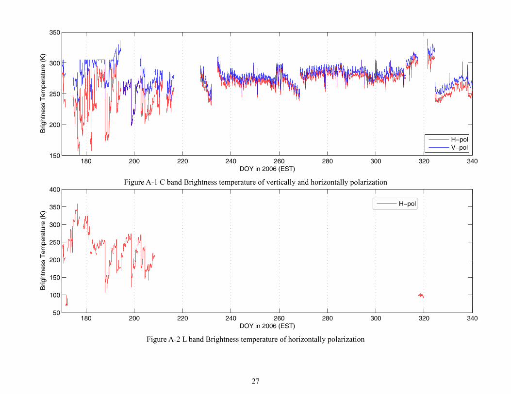
radiometer was calibrated at least once every week with a microwave absorber as warm load and measurements of sky at several angles as cold load. Figures 4 (b) and 4 (c) show the close-up of the rotary system and the antenna of the UFCMR, respectively. Table 1 lists the specifications of UFCMR. Figure A-1 shows the V- & H-pol brightness temperatures observed during MicroWEX-6.
Table 1. UFCMR specifications Parameter Qualifier Value Frequency Center 6.7 GHz Bandwidth 3 dB 20 MHz
3 dB V-pol elevation a 23°
3 dB V-pol azimuth b 21° 3 dB H-pol elevation c 21°
Beamwidth
3 dB H-pol azimuth d 23° Isolation > 27 dB Polarizations Sequential V/H Receiver temp 437 K Noise Figure From Trec 3.99 dB RF gain 85 dB
1 sec 0.71 K NEDT 8 sec 0.25 K
(a). sidelobes < -33 dB, (b). sidelobes < -28 dB, (c). sidelobes < -27 dB, (d). sidelobes < -35 dB
Figure 4 (a).The UFCMR system

6
Figure 4 (b) and (c). The side view of the UFCMR showing the rotary system and the front view of the
UFCMR showing the receiver antenna. 4.1.1.1 Theory of operation UFCMR uses a thermoelectric cooler (TEC) for thermal control of the Radio Frequency (RF) stages for the UFCMR. This is accomplished by the Oven Industries “McShane” thermal controller. McShane is used to cool or heat by Proportional-Integral-Derivative (PID) algorithm with a high degree of precision at 0.01°C. The aluminum plate to which all the RF components are attached is chosen to have sufficient thermal mass to eliminate short-term thermal drifts. All components attached to this thermal plate, including the TEC, use thermal paste to minimize thermal gradients across junctions. The majority of the gain in the system is provided by a gain and filtering block designed by the University of Michigan for the STAR-Light instrument (De Roo, 2003). The main advantage of this gain block is the close proximity of all the amplifiers, simplifying the task of thermal control. This gain block was designed for a radiometer working at the radio astronomy window of 1400 to 1427 MHz, and so the receiver is a heterodyne type with downconversion from the C-band RF to L-band. To minimize the receiver noise figure, a C-band low-noise amplifier (LNA) is used just prior to downconversion. To protect the amplifier from saturation due to out of band interference, a relatively wide bandwidth, but low insertion loss, bandpass filter is used just prior to the amplifier. Between the filter and the antenna are three components: a switch for choosing polarization, a switch for monitoring a reference load, and an isolator to minimize changes in the apparent system gain due to differences in the reflections looking upstream from the LNA. The electrical penetrations use commercially available weatherproof bulkhead connections (Deutsch connectors or equivalent). The heat sinks have been carefully located employing RTV (silicone sealant) to seal the bolt holes. The radome uses 15mil polycarbonate for radiometric signal penetration. It is sealed to the case using a rubber gasket held down to the case by a square retainer. The first SMA connection is an electromechanical latching, which is driven by the Z-World control board switches between V- and H-polarization sequentially. The SMA second latching which switches between the analog signal from the first switch and the reference load signal from a reference load resistor sends the analog signal to a isolator, where the signals within 6.4 to 7.2 GHz in radiofrequency are isolated. Then the central frequency is picked up by a 6.7 GHz bandpass filter, which also protects the amplifier to saturation. A Low Noise Amplifier (LNA) is used to eliminate the noise figure and adjust gain. A mixer takes the input from the LNA and a local oscillator to output a 1.4 GHz signal to STAR-Lite. After the Power Amplifier and Filtering Block (Star-Lite back-end), the signal is passed through a Square Law Detector and a Post-Detection Amplifier (PDA). UFCMR is equipped with a microcontroller that has responsibility for taking measurements, monitoring the thermal environment, and storing data until a download is requested. A
7
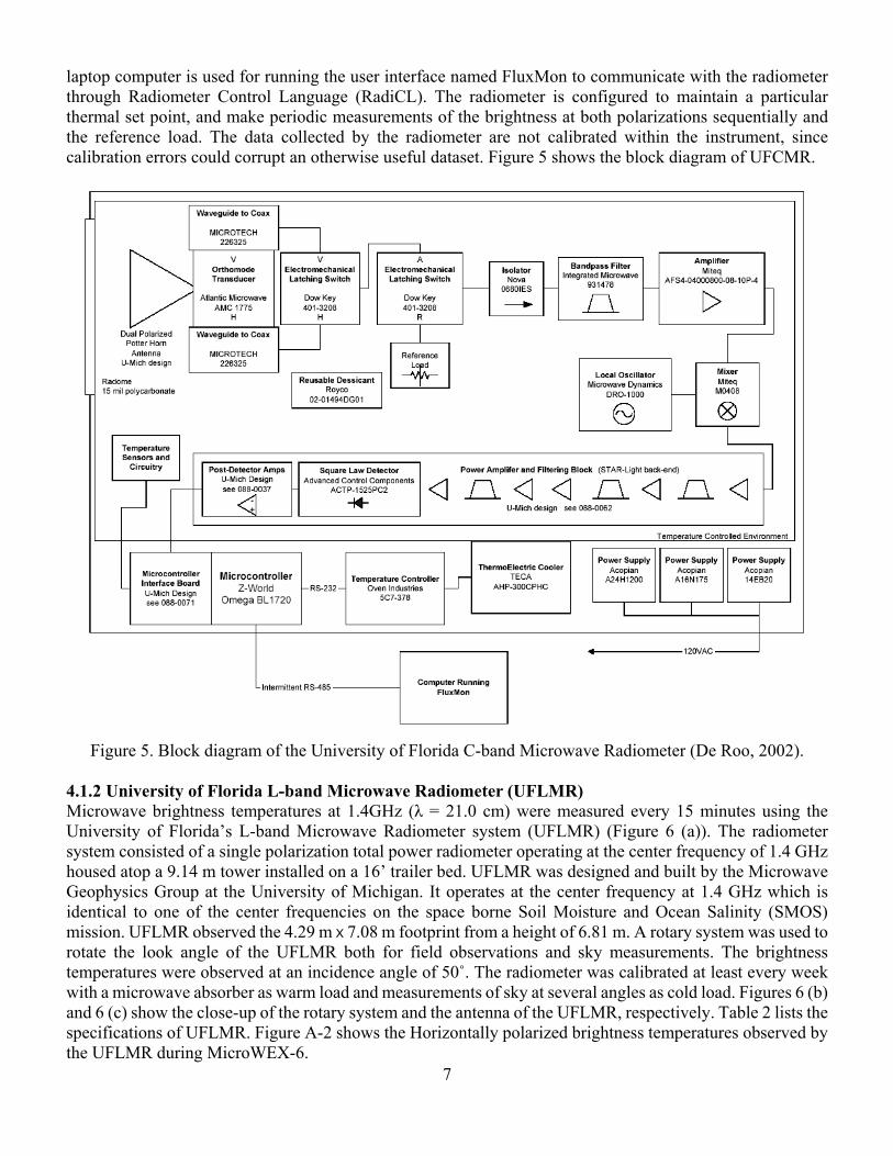
laptop computer is used for running the user interface named FluxMon to communicate with the radiometer through Radiometer Control Language (RadiCL). The radiometer is configured to maintain a particular thermal set point, and make periodic measurements of the brightness at both polarizations sequentially and the reference load. The data collected by the radiometer are not calibrated within the instrument, since calibration errors could corrupt an otherwise useful dataset. Figure 5 shows the block diagram of UFCMR.
Figure 5. Block diagram of the University of Florida C-band Microwave Radiometer (De Roo, 2002).
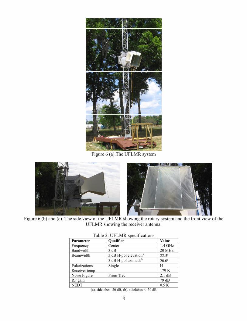
4.1.2 University of Florida L-band Microwave Radiometer (UFLMR) Microwave brightness temperatures at 1.4GHz (λ = 21.0 cm) were measured every 15 minutes using the University of Florida’s L-band Microwave Radiometer system (UFLMR) (Figure 6 (a)). The radiometer system consisted of a single polarization total power radiometer operating at the center frequency of 1.4 GHz housed atop a 9.14 m tower installed on a 16’ trailer bed. UFLMR was designed and built by the Microwave Geophysics Group at the University of Michigan. It operates at the center frequency at 1.4 GHz which is identical to one of the center frequencies on the space borne Soil Moisture and Ocean Salinity (SMOS) mission. UFLMR observed the 4.29 m X 7.08 m footprint from a height of 6.81 m. A rotary system was used to rotate the look angle of the UFLMR both for field observations and sky measurements. The brightness temperatures were observed at an incidence angle of 50˚. The radiometer was calibrated at least every week with a microwave absorber as warm load and measurements of sky at several angles as cold load. Figures 6 (b) and 6 (c) show the close-up of the rotary system and the antenna of the UFLMR, respectively. Table 2 lists the specifications of UFLMR. Figure A-2 shows the Horizontally polarized brightness temperatures observed by the UFLMR during MicroWEX-6.
8
Figure 6 (a).The UFLMR system
Figure 6 (b) and (c). The side view of the UFLMR showing the rotary system and the front view of the
UFLMR showing the receiver antenna.
Table 2. UFLMR specifications Parameter Qualifier Value Frequency Center 1.4 GHz Bandwidth 3 dB 20 MHz
3 dB H-pol elevation a 22.5° Beamwidth 3 dB H-pol azimuth b 20.0°
Polarizations Single H Receiver temp 179 K Noise Figure From Trec 2.1 dB RF gain 79 dB NEDT 0.5 K
(a). sidelobes -20 dB, (b). sidelobes < -30 dB
9
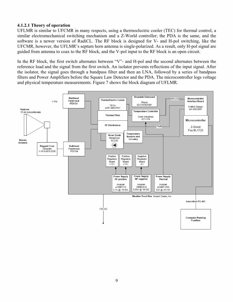
4.1.2.1 Theory of operation UFLMR is similar to UFCMR in many respects, using a thermoelectric cooler (TEC) for thermal control, a similar electromechanical switching mechanism and a Z-World controller; the PDA is the same, and the software is a newer version of RadiCL. The RF block is designed for V- and H-pol switching, like the UFCMR, however, the UFLMR’s septum horn antenna is single-polarized. As a result, only H-pol signal are guided from antenna to coax to the RF block, and the V-pol input to the RF block is an open circuit. In the RF block, the first switch alternates between “V”- and H-pol and the second alternates between the reference load and the signal from the first switch. An isolator prevents reflections of the input signal. After the isolator, the signal goes through a bandpass filter and then an LNA, followed by a series of bandpass filters and Power Amplifiers before the Square Law Detector and the PDA. The microcontroller logs voltage and physical temperature measurements. Figure 7 shows the block diagram of UFLMR.
10
Figure 7. Block diagram of the University of Florida L-band Microwave Radiometer (De Roo, 2003).
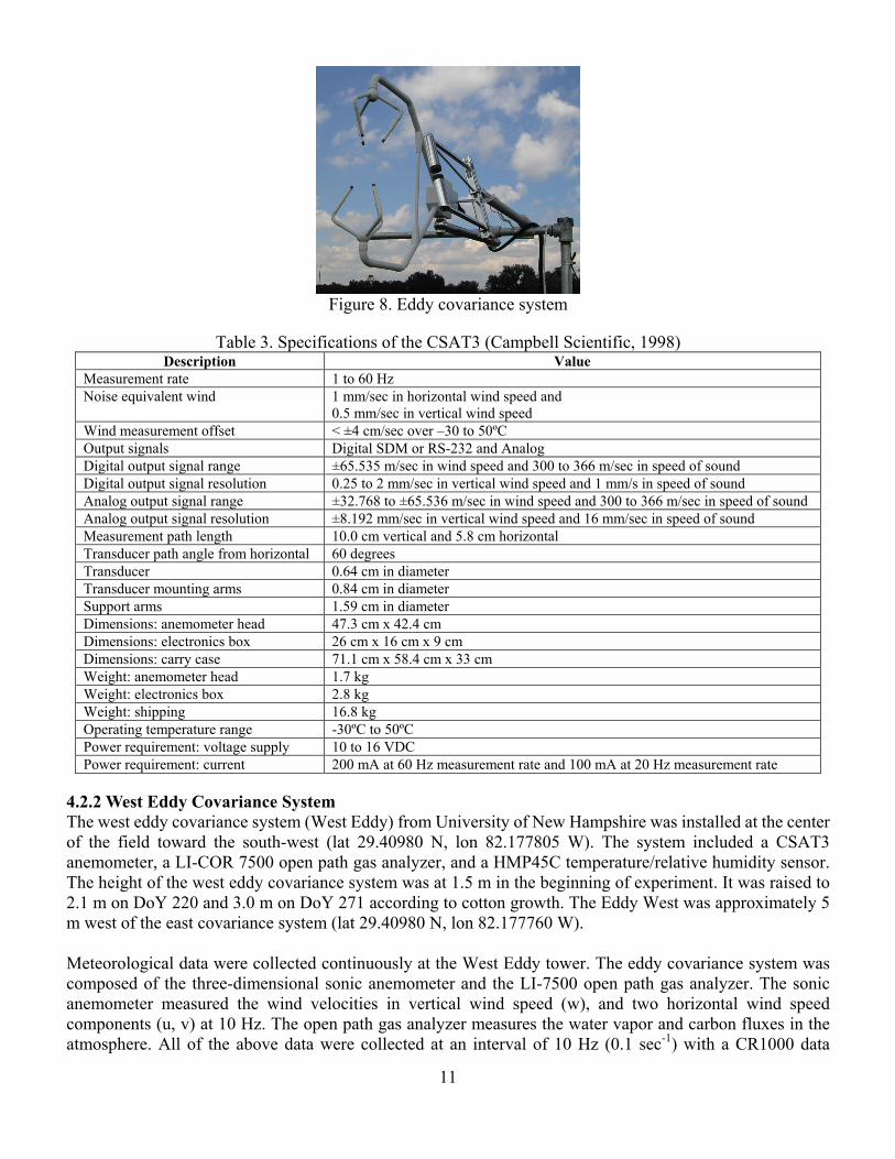
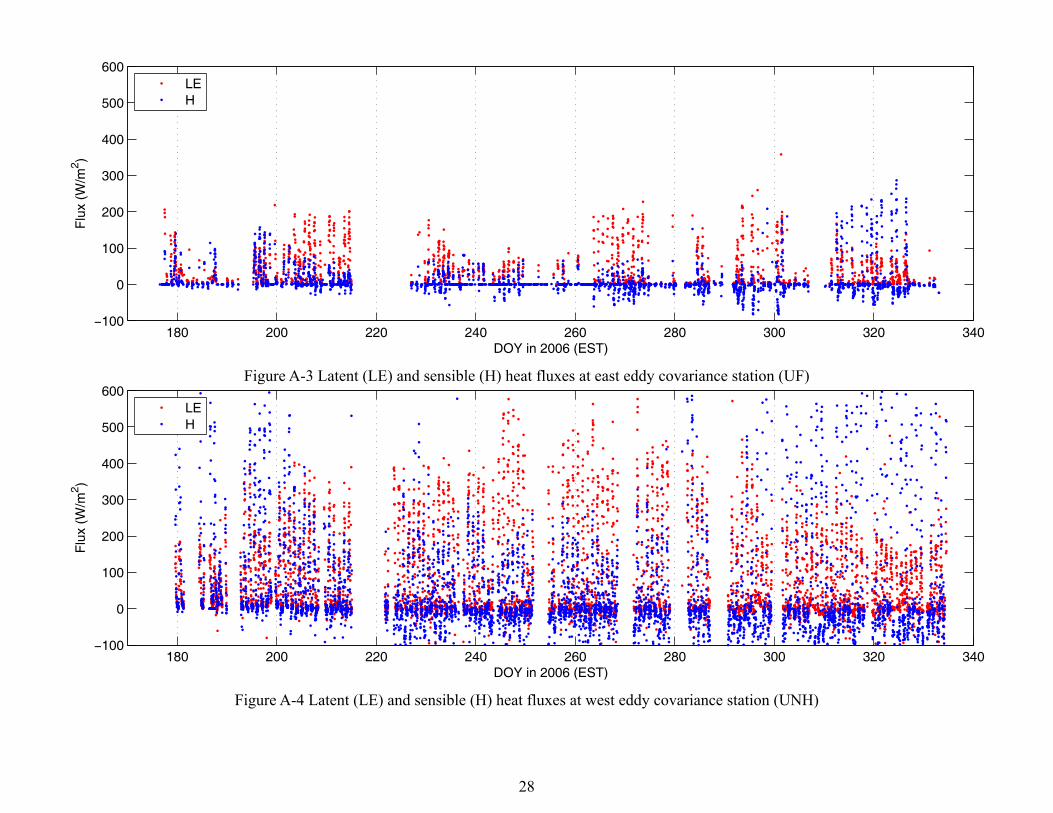
4.2 Eddy Covariance System 4.2.1 East Eddy Covariance System A Campbell Scientific eddy covariance system was located at the center of the field, as shown in Figure 3. The system included a CSAT3 anemometer and KH20 hygrometer as shown in Figure 8. The CSAT3 is a three dimensional sonic anemometer, which measures wind speed and the speed of sound on three non-orthogonal axes. Orthogonal wind speed and sonic temperature are computed from these measurements. The KH20 measures the water vapor in the atmosphere. Its output voltage is proportional to the water vapor density flux. Latent and sensible heat fluxes were measured every 30 minutes. The height of the eddy covariance system was 2.14 m from the ground and the orientation of the system was 225° toward southwest. On DoY 186 the sensor was moved to a height of 1.66 m. On DoY 220 the sensor was moved to a height of 2.10 m. On DoY 275 the sensor was moved to a height of 3.10 m. On DoY 289 the sensor was moved to a height of 2.90 m. On DoY 291 the sensor was moved to a height of 2.75 m. A list of specifications of the CSAT3 is shown in Table 3. Data collected by the eddy covariance system have been processed for coordinate rotation (Kaimal and Finnigan, 1994; Wilczak et al., 2001), WPL (Webb et al., 1980), oxygen (van Dijk et al., 2003), and sonic temperature corrections (Schotanus et al., 2003). Figure A-3 shows the processed latent and sensible heat fluxes observed during MicroWEX-6.
11
Figure 8. Eddy covariance system
Table 3. Specifications of the CSAT3 (Campbell Scientific, 1998)
Description Value Measurement rate 1 to 60 Hz Noise equivalent wind 1 mm/sec in horizontal wind speed and
0.5 mm/sec in vertical wind speed Wind measurement offset < ±4 cm/sec over –30 to 50ºC Output signals Digital SDM or RS-232 and Analog Digital output signal range ±65.535 m/sec in wind speed and 300 to 366 m/sec in speed of sound Digital output signal resolution 0.25 to 2 mm/sec in vertical wind speed and 1 mm/s in speed of sound Analog output signal range ±32.768 to ±65.536 m/sec in wind speed and 300 to 366 m/sec in speed of sound Analog output signal resolution ±8.192 mm/sec in vertical wind speed and 16 mm/sec in speed of sound Measurement path length 10.0 cm vertical and 5.8 cm horizontal Transducer path angle from horizontal 60 degrees Transducer 0.64 cm in diameter Transducer mounting arms 0.84 cm in diameter Support arms 1.59 cm in diameter Dimensions: anemometer head 47.3 cm x 42.4 cm Dimensions: electronics box 26 cm x 16 cm x 9 cm Dimensions: carry case 71.1 cm x 58.4 cm x 33 cm Weight: anemometer head 1.7 kg Weight: electronics box 2.8 kg Weight: shipping 16.8 kg Operating temperature range -30ºC to 50ºC Power requirement: voltage supply 10 to 16 VDC Power requirement: current 200 mA at 60 Hz measurement rate and 100 mA at 20 Hz measurement rate
4.2.2 West Eddy Covariance System The west eddy covariance system (West Eddy) from University of New Hampshire was installed at the center of the field toward the south-west (lat 29.40980 N, lon 82.177805 W). The system included a CSAT3 anemometer, a LI-COR 7500 open path gas analyzer, and a HMP45C temperature/relative humidity sensor. The height of the west eddy covariance system was at 1.5 m in the beginning of experiment. It was raised to 2.1 m on DoY 220 and 3.0 m on DoY 271 according to cotton growth. The Eddy West was approximately 5 m west of the east covariance system (lat 29.40980 N, lon 82.177760 W). Meteorological data were collected continuously at the West Eddy tower. The eddy covariance system was composed of the three-dimensional sonic anemometer and the LI-7500 open path gas analyzer. The sonic anemometer measured the wind velocities in vertical wind speed (w), and two horizontal wind speed components (u, v) at 10 Hz. The open path gas analyzer measures the water vapor and carbon fluxes in the atmosphere. All of the above data were collected at an interval of 10 Hz (0.1 sec-1) with a CR1000 data

12
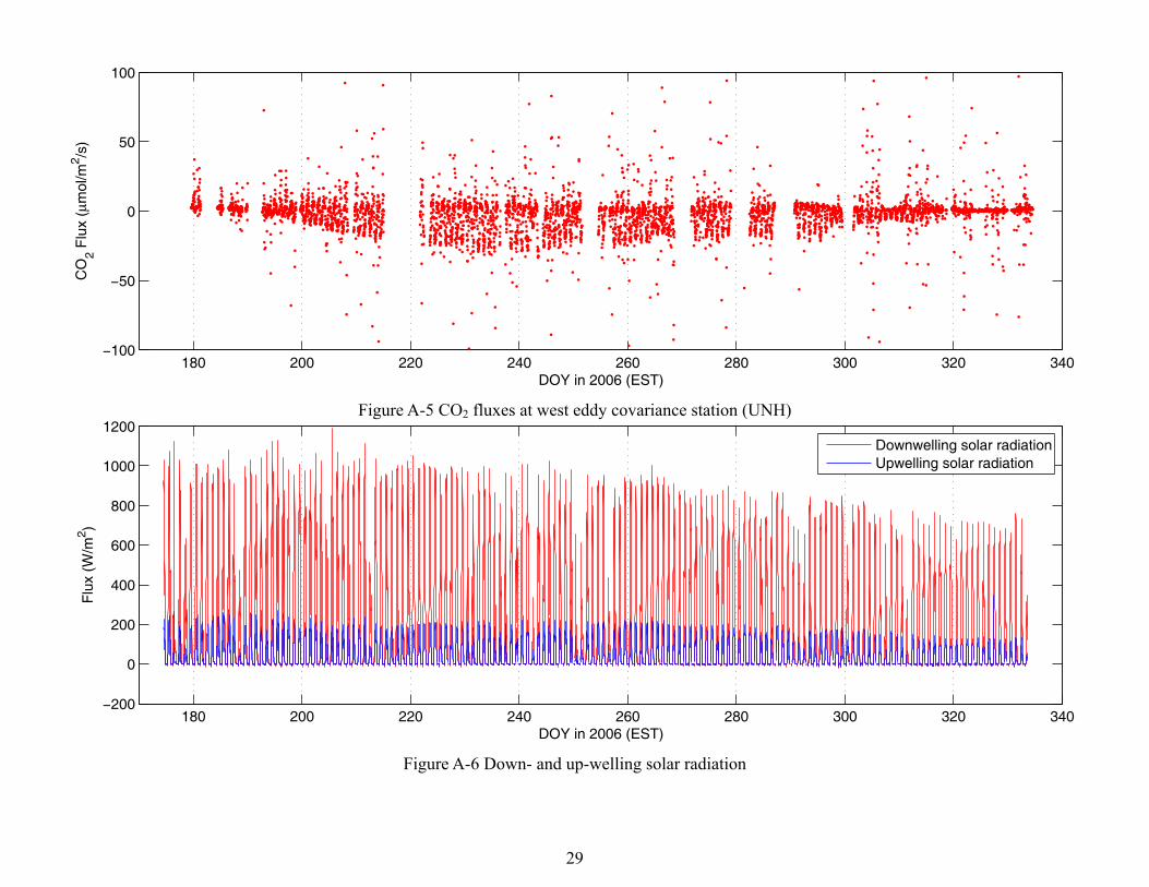
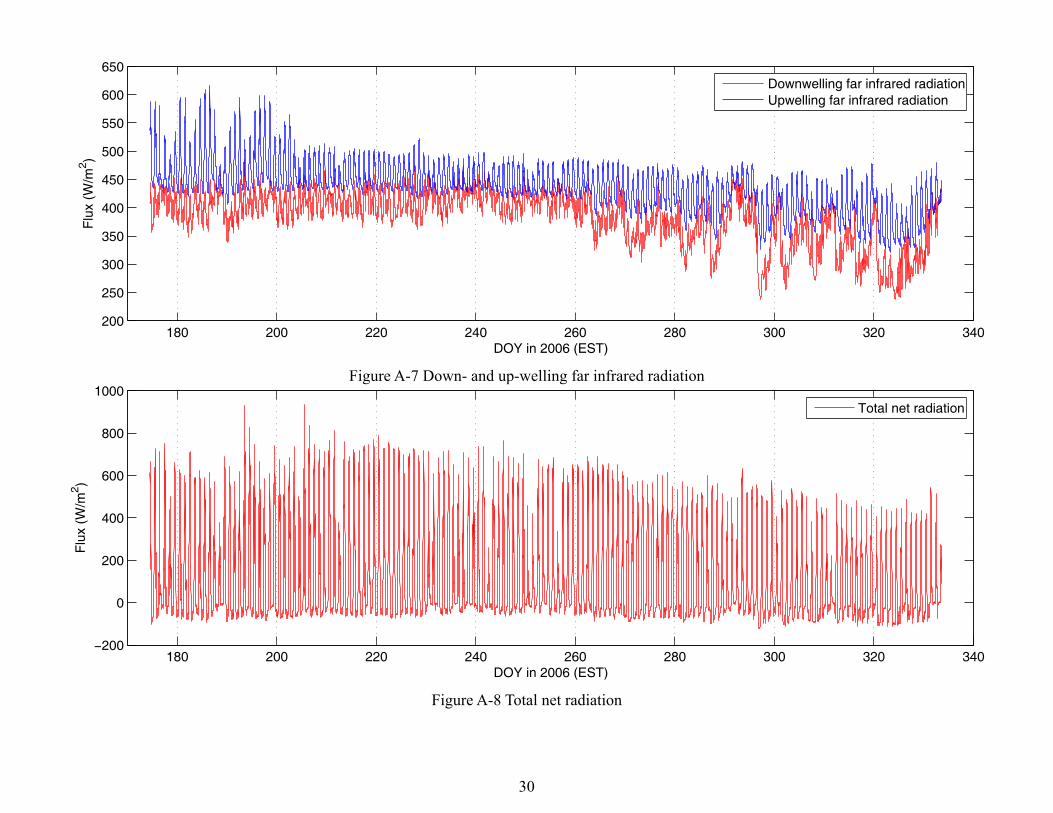
logger (Campbell Scientific. Inc., Logan, UT). Data sets were compiled as 30 minutes averages with the EdiRe data software (University of Edinburgh, ver.1.4.3.1129). Figure A-4 shows latent and sensible heat fluxes observed during MicroWEX-6. Figure A-5 shows CO2 flux observed during MicroWEX-6. 4.3 Net Radiometer A Kipp and Zonen CNR-1 four-component net radiometer (Figure 9) was located at the center of the field to measure up- and down-welling short- and long-wave infrared radiation. The sensor consists of two pyranometers (CM-3) and two pyrgeometers (CG-3). The sensor was installed at the height of 2.66 m above ground and facing south. Table 4 shows the list of specifications of the CNR-1 net radiometer. Figure A-6 shows the down- and up -welling solar (shortwave) wave radiation observed during MicroWEX-6 and Figure A-7 the down- and up -welling far infrared (longwave) radiation observed during MicroWEX-6. Figure A-8 shows the net total radiation observed during MicroWEX-6.
Figure 9. CNR-1 net radiometer
Table 4. Specifications of the CNR-1 net radiometer (Campbell Scientific, 2005a)
Description Value Measurement spectrum: CM-3 305 to 2800 nm Measurement spectrum: CG-3 5000 t o50000 nm Response time 18 sec Sensitivity 10 to 35 μV/(W/m2) Pt-100 sensor temperature measurement DIN class A Accuracy of the Pt-100 measurement ± 2 K Heating Resistor 24 ohms, 6 VA at 12 volt Maximum error due to heating: CM-3 10 W/m2 Operating temperature -40º to 70ºC Daily total radiation accuracy ± 10% Cable length 10 m Weight 4 kg
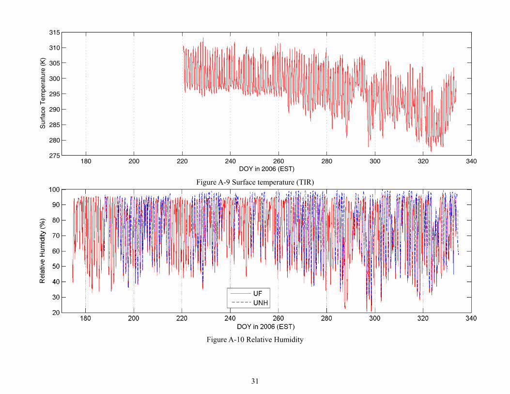
4.4 Thermal Infrared Sensor An Everest Interscience thermal infrared sensor (4000.3ZL) was co-located with the net radiometer to observe skin temperature at nadir. It was replaced by Apogee instruments IRR-PN on August 8. Table 5 shows the list of specifications of the thermal infrared sensor. Figure A-9 shows the surface thermal infrared temperature observed during MicroWEX-6.
Table 5. Specifications of the thermal infrared sensor (IRR-PN) Description Value Field of view 18°half angle
Target temp. 40 μV per ºC difference from sensor body
Output
Sensor body temp. 0-2500 mV
13
Table 5. [continued] -10 to 65 ºC ±0.2 ºC absolute accuracy
±0.1 ºC uniformity ±0.05 ºC repeatability
Accuracy
-40 to 70 ºC ±0.5 ºC absolute accuracy ±0.3 ºC uniformity ±0.1 ºC repeatability and uniformity
Optics Germanium lens Wavelength range 8-14 μm (corresponds to atmospheric window) Response time < 1 second to changes in target temperature Input power 2.5 V excitation Operating environment
-55 to 80 ºC; 0 to 100 % RH (non-condensing) Water resistant, designed for continuous outdoor use
Cable 4.5 meters twisted, shielded 4 conductor wire with Santoprene casing.
Dimensions 6 cm long by 2.3 cm diameter Mass 190 g
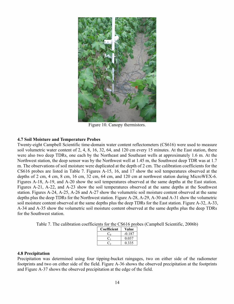
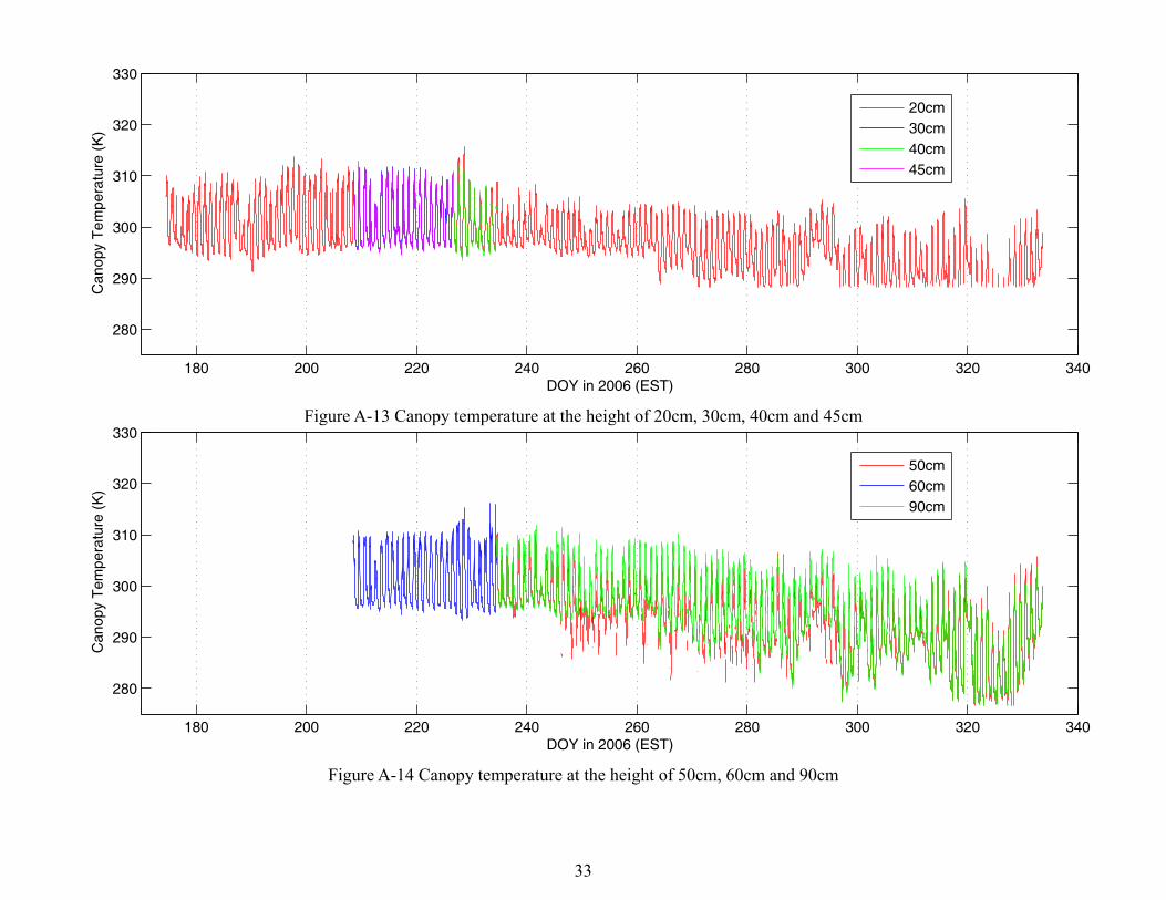
4.5 Air Temperature and Relative Humidity Air temperature and relative humidity were measured every 15 minutes at the Northwest station using a Campbell Scientific HMP45C Temperature and Relative Humidity Probe (Campbell Scientific, 2006c). Figure A-10 shows the relative humidity and Figure A-11 shows the air temperature observations during MicroWEX-6. 4.6 Air Temperature in the canopy Air temperature, at five heights within the canopy, was measured every 15 minutes at the Northwest station using thermistors on a PVC pipe, as shown in Figure 10. The heights were adjusted as the canopy grew, listed in Table 6. Figure A-12, 13, and 14 show the observations of canopy temperature during MicroWEX-6.
Table 6. Canopy thermistor heights
DoY Measurement heights (cm) 173 0,5,10,15,20 208 0,15,30,45,60 226 0,20,40,60 234 0,20,50,90
14
Figure 10. Canopy thermistors.
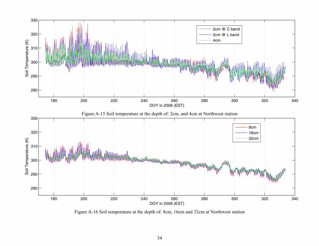
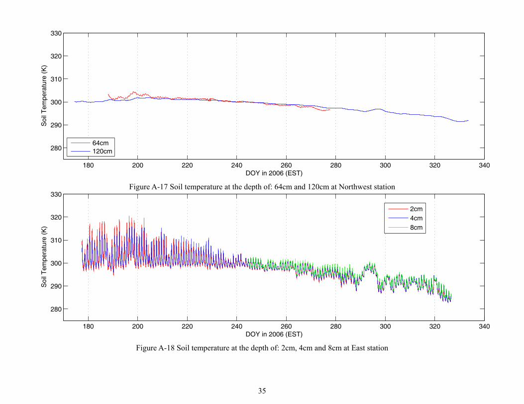
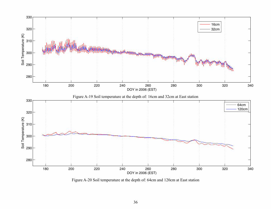
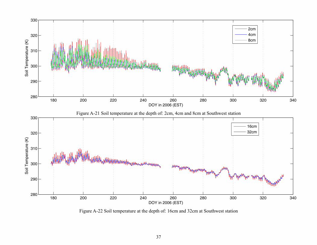
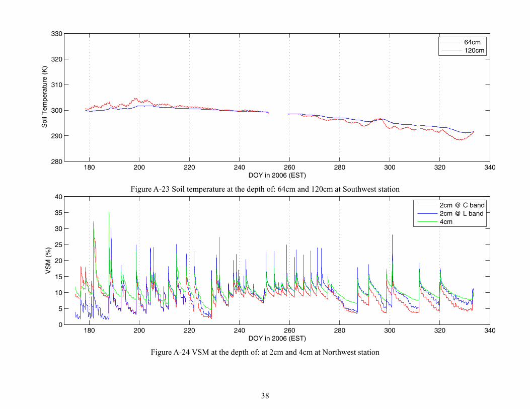
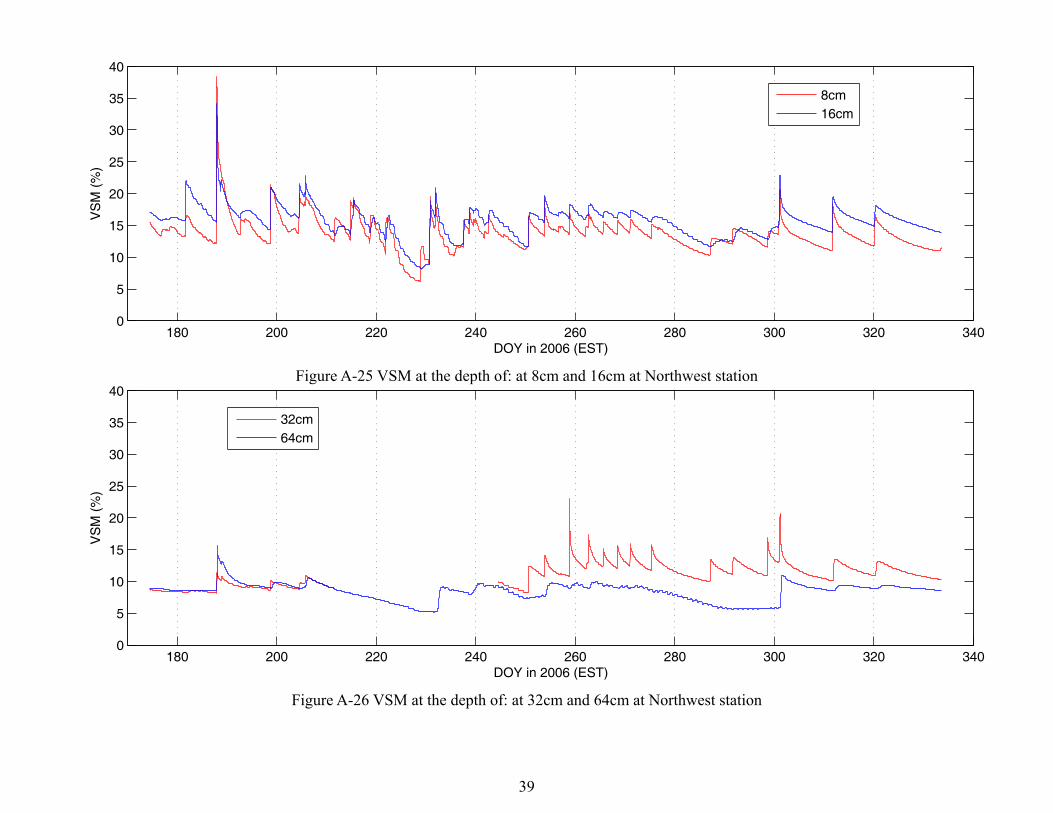
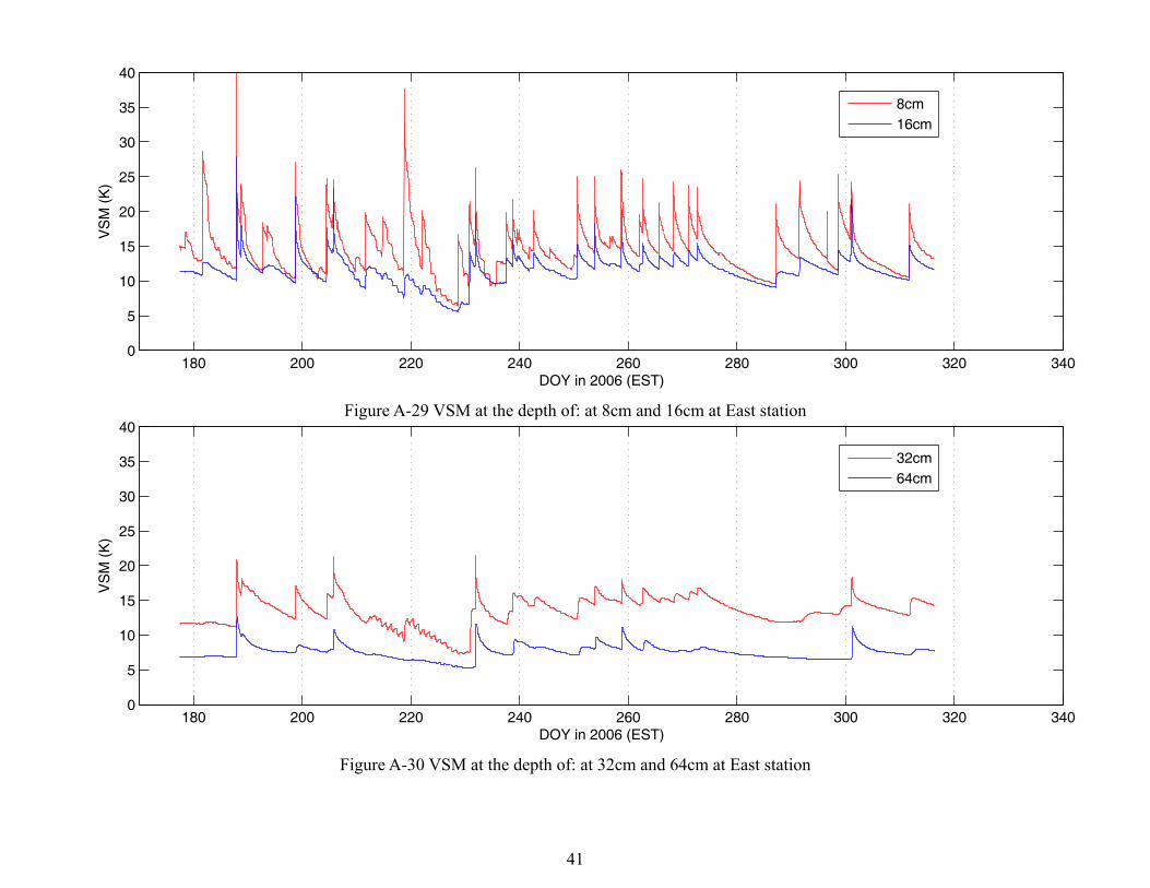
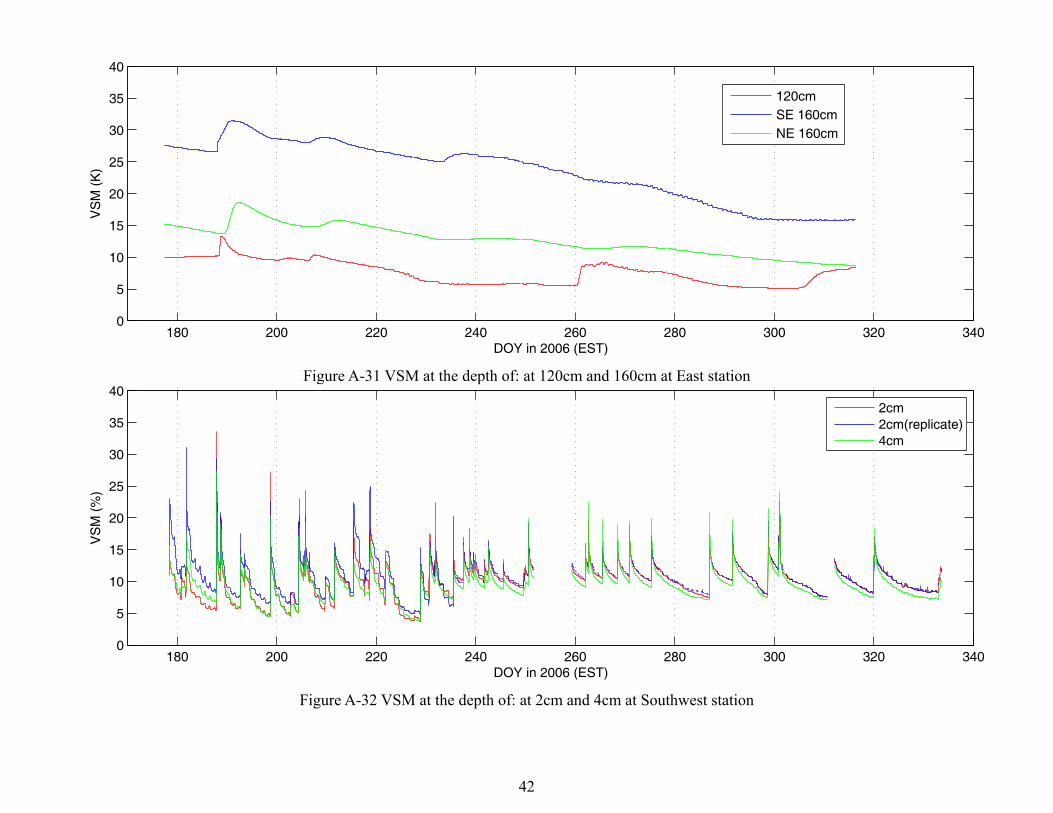
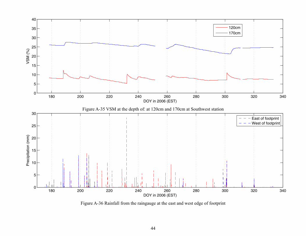
4.7 Soil Moisture and Temperature Probes Twenty-eight Campbell Scientific time-domain water content reflectometers (CS616) were used to measure soil volumetric water content of 2, 4, 8, 16, 32, 64, and 120 cm every 15 minutes. At the East station, there were also two deep TDRs, one each by the Northeast and Southeast wells at approximately 1.6 m. At the Northwest station, the deep sensor was by the Northwest well at 1.45 m, the Southwest deep TDR was at 1.7 m. The observations of soil moisture were duplicated at the depth of 2 cm. The calibration coefficients for the CS616 probes are listed in Table 7. Figures A-15, 16, and 17 show the soil temperatures observed at the depths of 2 cm, 4 cm, 8 cm, 16 cm, 32 cm, 64 cm, and 120 cm at northwest station during MicroWEX-6. Figures A-18, A-19, and A-20 show the soil temperatures observed at the same depths at the East station. Figures A-21, A-22, and A-23 show the soil temperatures observed at the same depths at the Southwest station. Figures A-24, A-25, A-26 and A-27 show the volumetric soil moisture content observed at the same depths plus the deep TDRs for the Northwest station. Figure A-28, A-29, A-30 and A-31 show the volumetric soil moisture content observed at the same depths plus the deep TDRs for the East station. Figure A-32, A-33, A-34 and A-35 show the volumetric soil moisture content observed at the same depths plus the deep TDRs for the Southwest station.
Table 7. The calibration coefficients for the CS616 probes (Campbell Scientific, 2006b) Coefficient Value
C0 -0.187 C1 0.037 C2 0.335
4.8 Precipitation Precipitation was determined using four tipping-bucket raingages, two on either side of the radiometer footprints and two on either side of the field. Figure A-36 shows the observed precipitation at the footprints and Figure A-37 shows the observed precipitation at the edge of the field.
15
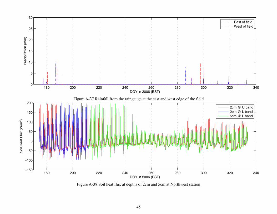
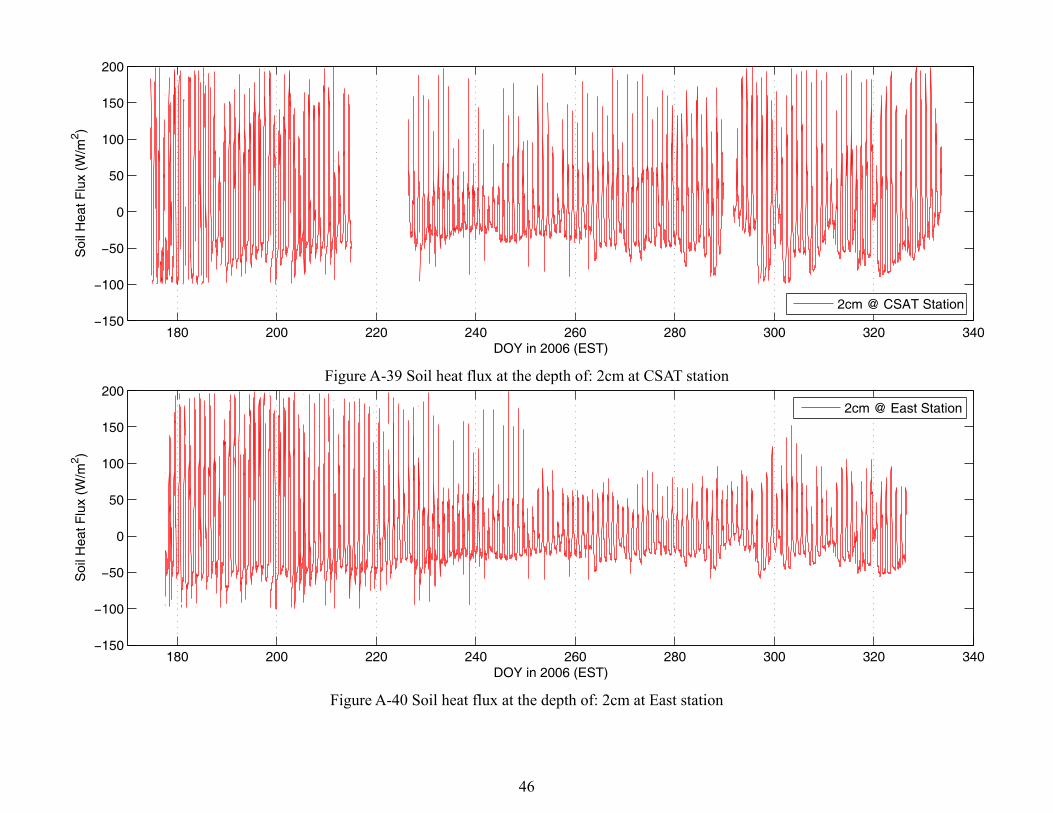
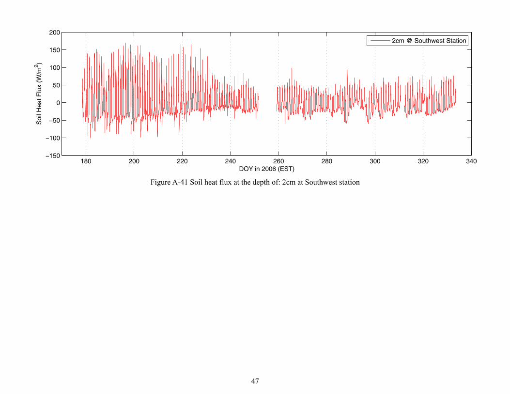
4.9 Soil Heat Flux Plates Two Campbell Scientific soil heat flux plates (HFT-3) were used to measure soil heat flux at the depth of 2 cm at the Northwest station. The depth of soil heat flux plate at L band changed to 5cm at September 11 (DoY 254). The CSAT, East, and Southwest stations each had one SHF plate at 2cm. Figure A-38 shows the soil heat fluxes observed at depths of 2cm and at 5cm at the northwest station during MicroWEX-6. Figure A-39 shows the soil heat fluxes observed at 2cm at CSAT station. Figure A-40 shows the soil heat fluxes observed at 2cm at the East station. Figure A-41 shows the soil heat fluxes observed at 2cm at southwest station.
5. VEGETATION SAMPLING
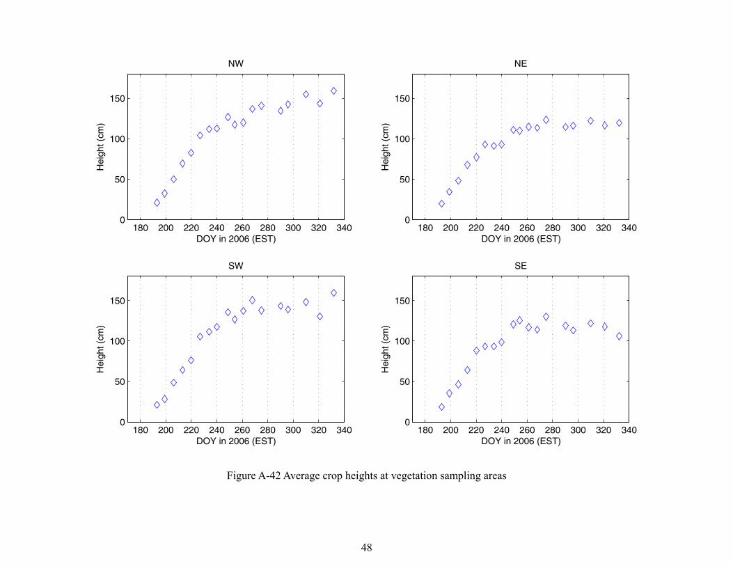
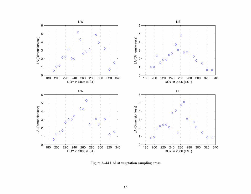
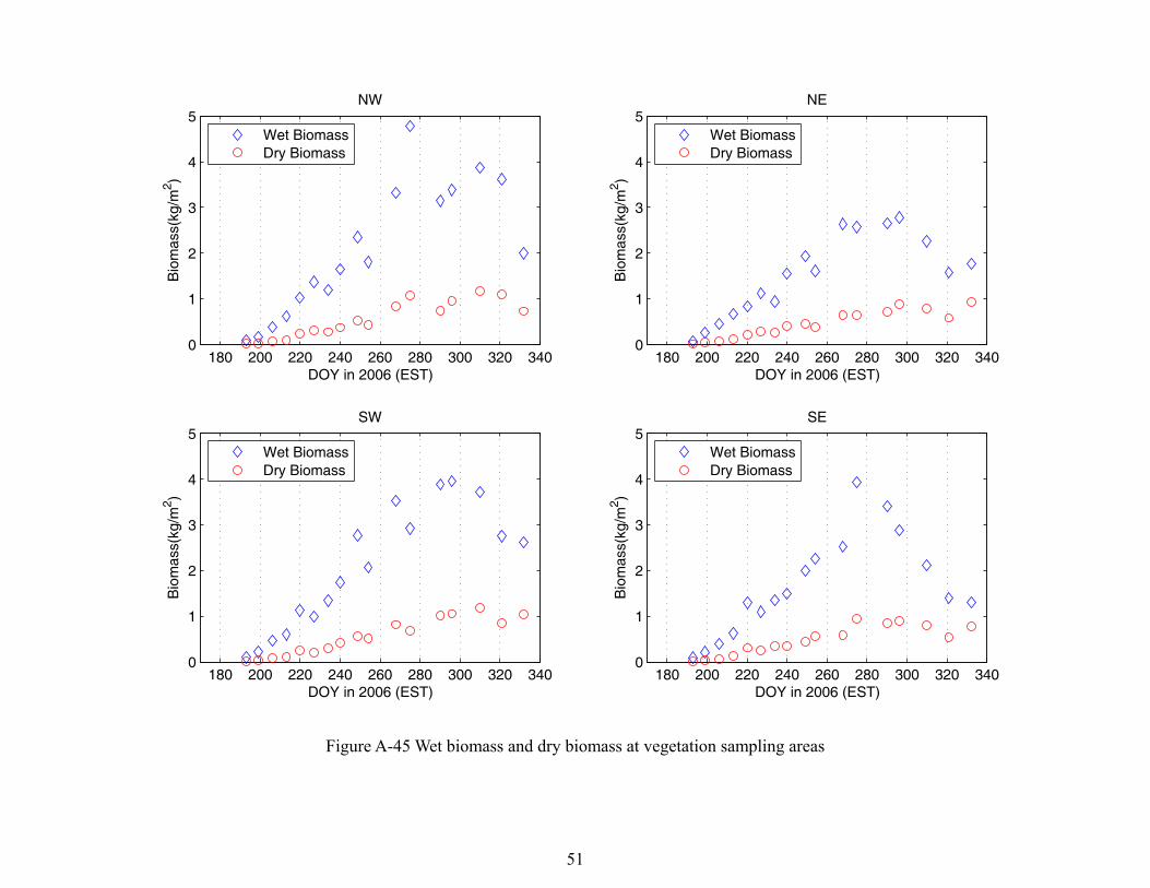
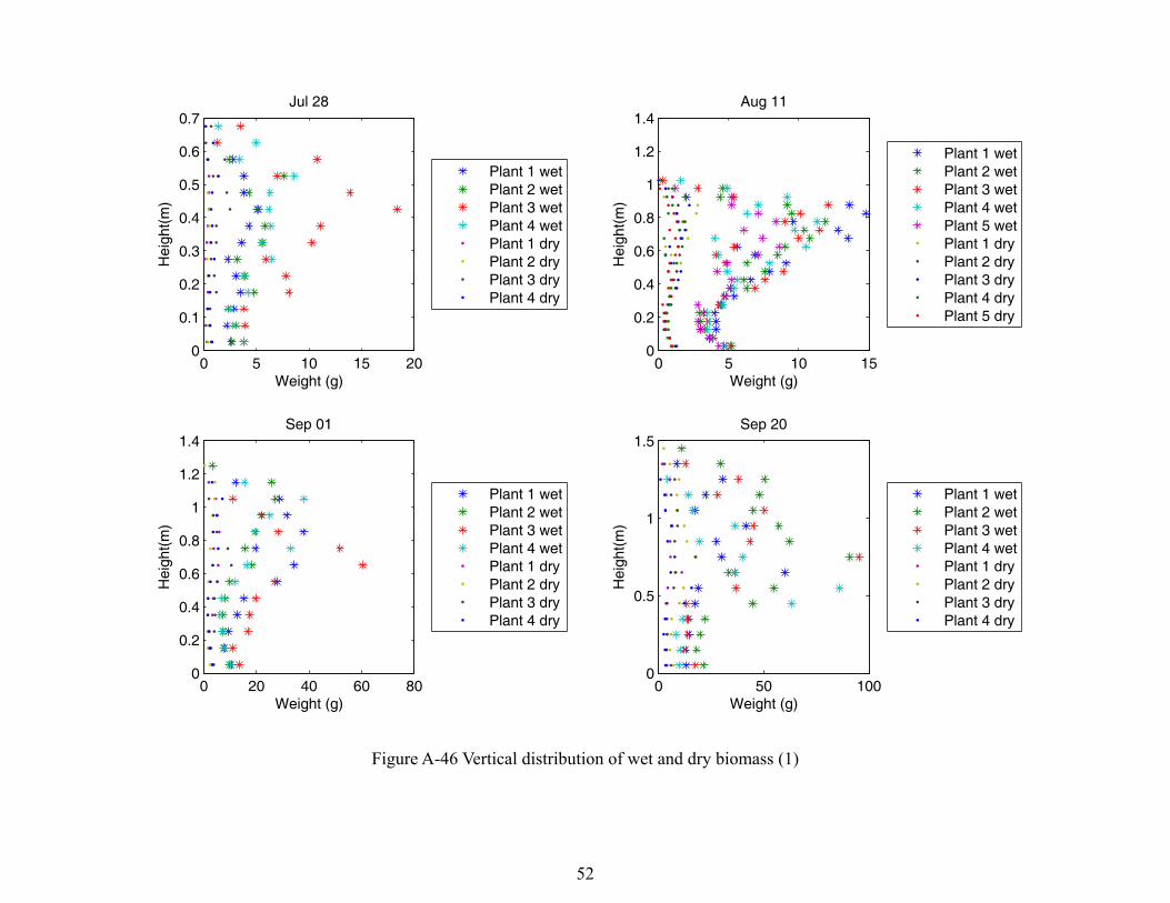
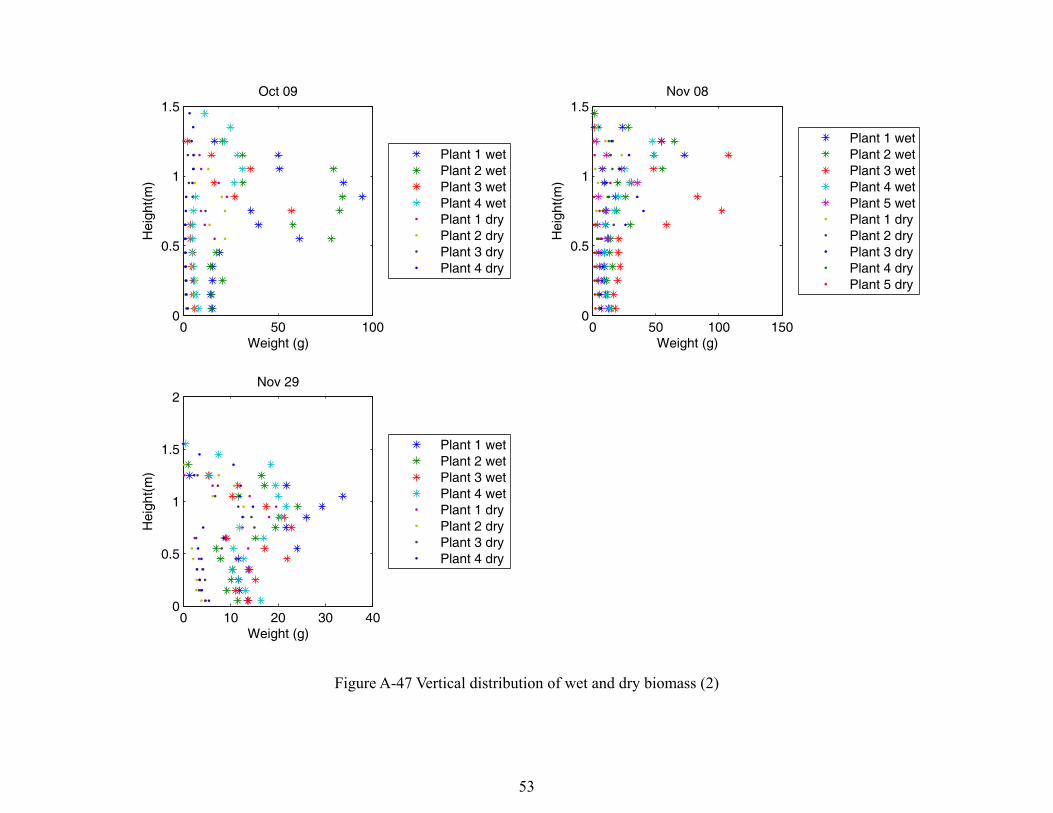
Vegetation properties such as stand density, row spacing, height, biomass, and LAI were measured weekly during the early season and biweekly during late season. The crop density derived from the stand density and row spacing was measured at the first two samplings since the cotton seeds were planted in the fixed spacing and the germination rate is over 70% throughout the field. The specific measurements include height, biomass, and LAI. In the whole season, the vegetation samplings were conducted on four spatially distributed sampling locations (Figure 3). It was designed to characterize the spatial variability of the vegetation properties in the study site. 5.1 Height and Width Crop height and width were measured by placing a measuring stick at the soil surface to average height of the crop. Four representative plants were selected to obtain heights inside each vegetation sampling area. Figures A-42 and A-43 show the crop heights and widths during MicroWEX-6 5.2 LAI LAI was measured with a Li-Cor LAI-2000 in the inter-row region with 4 cross-row measurements. The LAI-2000 was set to average 2 locations into a single value for each vegetation sampling area so one observation was taken above the canopy and 4 beneath the canopy; in the row, ¼ of the way across the row, ½ of the way across the row, and ¾ of the way across the row. This gave a spatial average for row crops of partial cover. LAI for each of the sampling areas is shown in Figure A-44. 5.3 Green and Dry Biomass Each biomass sampling included one row. The sampling length was measured the same as length during stand density measurement. The sample started in-between two plants and ended at the next midpoint that is also greater than or equal to one meter away from the starting point. The plants within this length were cut at the base, separated into leaves, stems, and bolls, and weighed immediately. The samples were dried in the oven at 70ºC for 48 hours and their dry weights were measured. Figure A-45 shows the wet and dry biomass observed during MicroWEX-6. 5.4 Vertical Distribution of Moisture in the Canopy Wet and dry biomass of discrete vertical layers of individual cotton plants were measured. Seven samplings were conducted during MicroWEX-6, with four plants on July 28 (DoY 209), five plants on Aug 10 (DoY 222), four plants on Sep 1 (DoY 244), four plants on Sep 20 (DoY 263), four plants on Oct 9(DoY 282), five plants on Nov 8 (DoY 312), and four plants on Nov 29 (DoY 333). Each sampling was conducted by selecting a representative sample of plants along a row. The plants were taken out of the ground, with roots still attached, and taken indoors to prevent moisture loss. Each plant sample was carefully laid out on a metal sheet with grid spacing of 2 cm, as shown in Figure 11. The leaves and bolls were “arranged” to closely match their natural orientation in the field. The plants collected on July 28 and Aug 11 were sliced every 5cm, and those collected on the other date were sliced every 10cm. The sample in each layer was weighed, both fresh and after drying in the oven at 70 ºC for 48 hours. Figures A-46, 47 show the wet and dry weight of
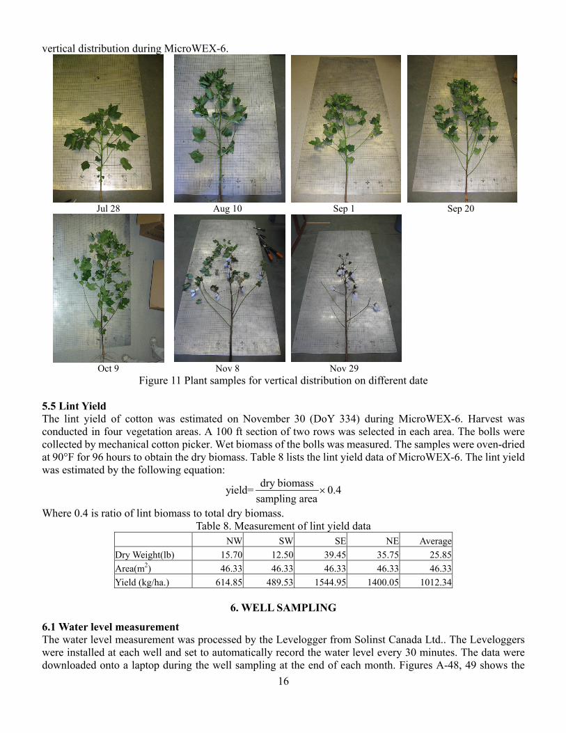
16
vertical distribution during MicroWEX-6.
Jul 28 Aug 10 Sep 1 Sep 20
Oct 9 Nov 8 Nov 29 Figure 11 Plant samples for vertical distribution on different date
5.5 Lint Yield The lint yield of cotton was estimated on November 30 (DoY 334) during MicroWEX-6. Harvest was conducted in four vegetation areas. A 100 ft section of two rows was selected in each area. The bolls were collected by mechanical cotton picker. Wet biomass of the bolls was measured. The samples were oven-dried at 90°F for 96 hours to obtain the dry biomass. Table 8 lists the lint yield data of MicroWEX-6. The lint yield was estimated by the following equation:
dry biomassyield= 0.4sampling area
×
Where 0.4 is ratio of lint biomass to total dry biomass. Table 8. Measurement of lint yield data
NW SW SE NE Average Dry Weight(lb) 15.70 12.50 39.45 35.75 25.85 Area(m2) 46.33 46.33 46.33 46.33 46.33 Yield (kg/ha.) 614.85 489.53 1544.95 1400.05 1012.34
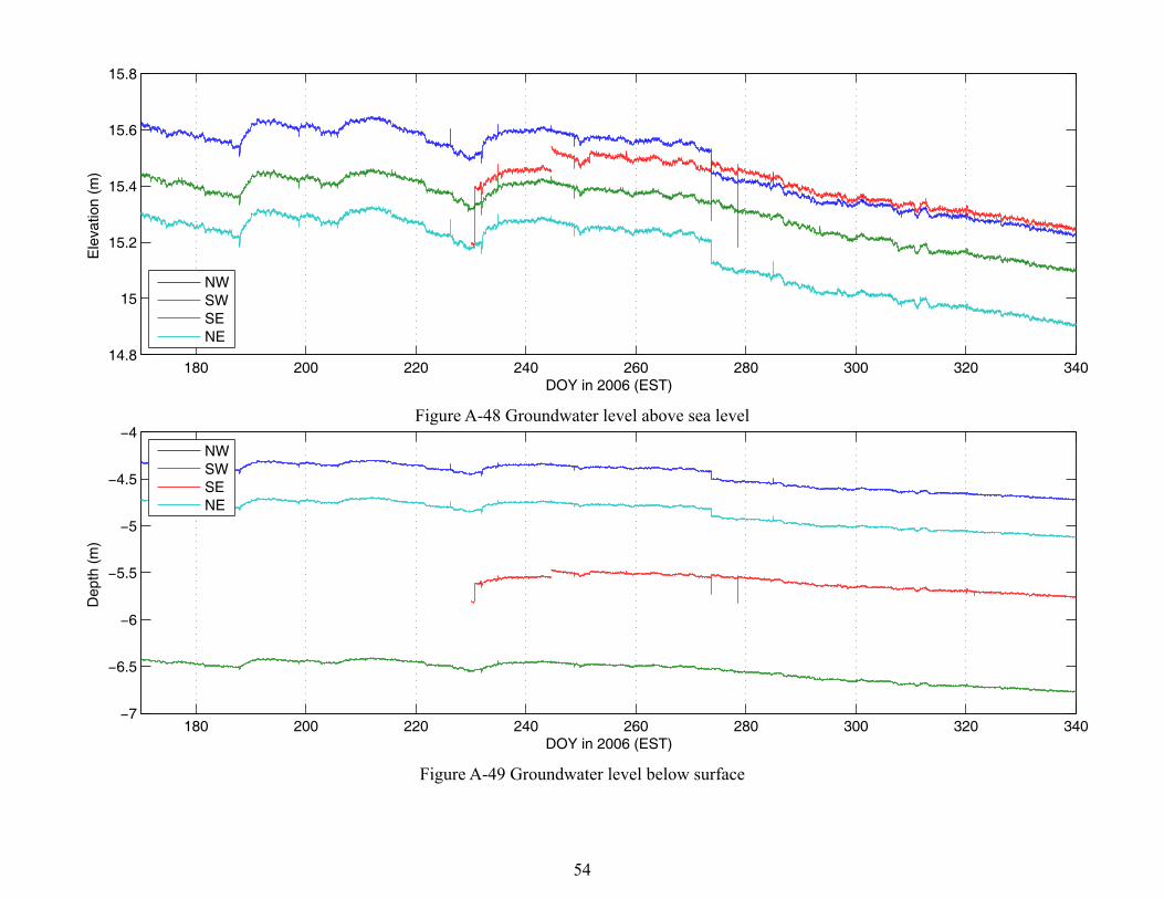
6. WELL SAMPLING
6.1 Water level measurement The water level measurement was processed by the Levelogger from Solinst Canada Ltd.. The Leveloggers were installed at each well and set to automatically record the water level every 30 minutes. The data were downloaded onto a laptop during the well sampling at the end of each month. Figures A-48, 49 shows the

17
water table elevation and depth during MicroWEX-6.
18
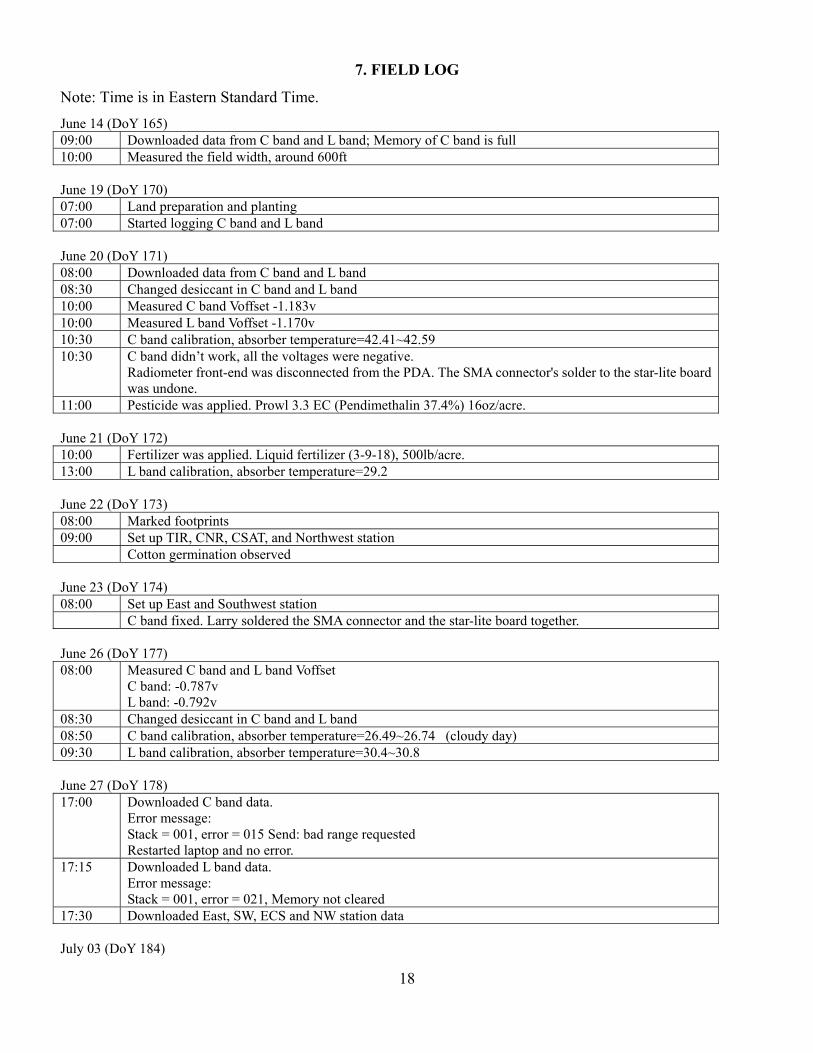
7. FIELD LOG
Note: Time is in Eastern Standard Time. June 14 (DoY 165) 09:00 Downloaded data from C band and L band; Memory of C band is full 10:00 Measured the field width, around 600ft June 19 (DoY 170) 07:00 Land preparation and planting 07:00 Started logging C band and L band June 20 (DoY 171) 08:00 Downloaded data from C band and L band 08:30 Changed desiccant in C band and L band 10:00 Measured C band Voffset -1.183v 10:00 Measured L band Voffset -1.170v 10:30 C band calibration, absorber temperature=42.41~42.59� 10:30 C band didn’t work, all the voltages were negative.
Radiometer front-end was disconnected from the PDA. The SMA connector's solder to the star-lite board was undone.
11:00 Pesticide was applied. Prowl 3.3 EC (Pendimethalin 37.4%) 16oz/acre. June 21 (DoY 172) 10:00 Fertilizer was applied. Liquid fertilizer (3-9-18), 500lb/acre. 13:00 L band calibration, absorber temperature=29.2� June 22 (DoY 173) 08:00 Marked footprints 09:00 Set up TIR, CNR, CSAT, and Northwest station Cotton germination observed June 23 (DoY 174) 08:00 Set up East and Southwest station C band fixed. Larry soldered the SMA connector and the star-lite board together. June 26 (DoY 177) 08:00 Measured C band and L band Voffset
C band: -0.787v L band: -0.792v
08:30 Changed desiccant in C band and L band 08:50 C band calibration, absorber temperature=26.49~26.74�(cloudy day) 09:30 L band calibration, absorber temperature=30.4~30.8� June 27 (DoY 178) 17:00 Downloaded C band data.
Error message: Stack = 001, error = 015 Send: bad range requested Restarted laptop and no error.
17:15 Downloaded L band data. Error message: Stack = 001, error = 021, Memory not cleared
17:30 Downloaded East, SW, ECS and NW station data July 03 (DoY 184)
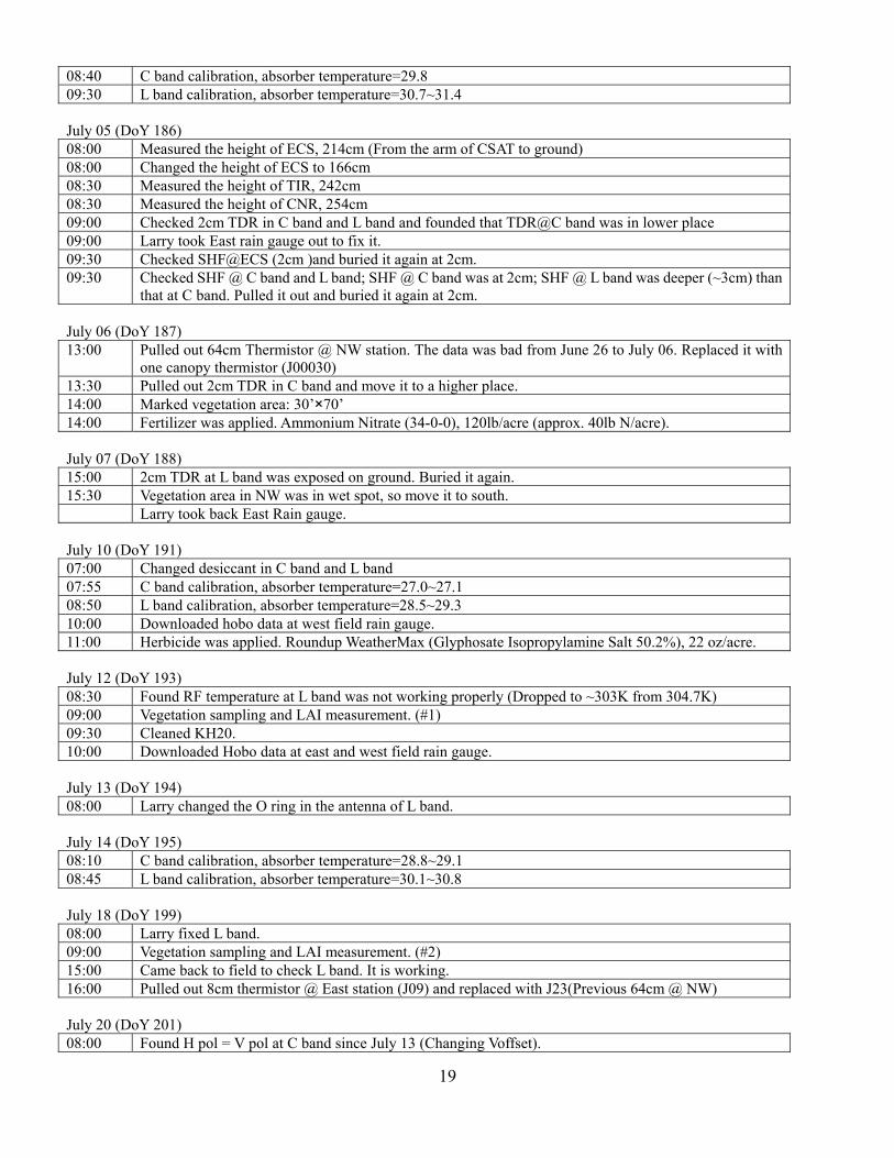
19
08:40 C band calibration, absorber temperature=29.8� 09:30 L band calibration, absorber temperature=30.7~31.4� July 05 (DoY 186) 08:00 Measured the height of ECS, 214cm (From the arm of CSAT to ground) 08:00 Changed the height of ECS to 166cm 08:30 Measured the height of TIR, 242cm 08:30 Measured the height of CNR, 254cm 09:00 Checked 2cm TDR in C band and L band and founded that TDR@C band was in lower place 09:00 Larry took East rain gauge out to fix it. 09:30 Checked SHF@ECS (2cm )and buried it again at 2cm. 09:30 Checked SHF @ C band and L band; SHF @ C band was at 2cm; SHF @ L band was deeper (~3cm) than
that at C band. Pulled it out and buried it again at 2cm. July 06 (DoY 187) 13:00 Pulled out 64cm Thermistor @ NW station. The data was bad from June 26 to July 06. Replaced it with
one canopy thermistor (J00030) 13:30 Pulled out 2cm TDR in C band and move it to a higher place. 14:00 Marked vegetation area: 30’×70’ 14:00 Fertilizer was applied. Ammonium Nitrate (34-0-0), 120lb/acre (approx. 40lb N/acre). July 07 (DoY 188) 15:00 2cm TDR at L band was exposed on ground. Buried it again. 15:30 Vegetation area in NW was in wet spot, so move it to south. Larry took back East Rain gauge. July 10 (DoY 191) 07:00 Changed desiccant in C band and L band 07:55 C band calibration, absorber temperature=27.0~27.1� 08:50 L band calibration, absorber temperature=28.5~29.3� 10:00 Downloaded hobo data at west field rain gauge. 11:00 Herbicide was applied. Roundup WeatherMax (Glyphosate Isopropylamine Salt 50.2%), 22 oz/acre. July 12 (DoY 193) 08:30 Found RF temperature at L band was not working properly (Dropped to ~303K from 304.7K) 09:00 Vegetation sampling and LAI measurement. (#1) 09:30 Cleaned KH20. 10:00 Downloaded Hobo data at east and west field rain gauge. July 13 (DoY 194) 08:00 Larry changed the O ring in the antenna of L band. July 14 (DoY 195) 08:10 C band calibration, absorber temperature=28.8~29.1� 08:45 L band calibration, absorber temperature=30.1~30.8� July 18 (DoY 199) 08:00 Larry fixed L band. 09:00 Vegetation sampling and LAI measurement. (#2) 15:00 Came back to field to check L band. It is working. 16:00 Pulled out 8cm thermistor @ East station (J09) and replaced with J23(Previous 64cm @ NW) July 20 (DoY 201) 08:00 Found H pol = V pol at C band since July 13 (Changing Voffset).
20
08:40 C band calibration, absorber temperature=34.24~34.30� 09:20 L band calibration, absorber temperature=33.55~33.40� July 21 (DoY 202) 8:00-10:00 Orlando calibrated Rain gauge. 08:00 Larry replaced switch on C band. 09:00 Larry hooked up 8cm thermistor @ East station. 09:00 Changed desiccants in C band. 09:15 C band calibration, absorber temperature=30.30~31.30� 11:00 Herbicide was applied. Roundup WeatherMax (Glyphosate Isopropylamine Salt 50.2%), 24 oz/acre. July 25 (DoY 206) 15:00 Vegetation sampling and LAI measurement. (#3) July 27 (DoY 208) 09:00 Changed desiccants in C band and L band. 09:30 L band calibration, absorber temperature=32.50~32.81� 11:00 C band calibration, absorber temperature=33.96~34.62� 11:00-11:30 Changed height of canopy thermistor
20 cm ->60 cm 15 cm ->45 cm 10 cm ->30 cm 5 cm ->15 cm 0 cm ->0 cm
10:00 Cleaned KH20 July 28 (DoY 209) 09:00 Vertical distribution of moisture in the canopy. (#1) August 1 (DoY 213) 08:30 Found no AC Power at the site. 09:00 Vegetation sampling and LAI measurement. (#4) 09:30 AC power recovered. 10:00 Can’t connect to L band, East Station and SW station. 10:00 Lowered L band to ground. August 2 (DoY 214) 13:00 Fertilizer was applied. Ammonium Nitrate (34-0-0), 125lb/acre. August 3 (DoY 215) 08:00 Found linear system above C band foot print. (Irrigation started last night, but the linear stopped midway)09:00 C band calibration, absorber temperature=31.63~32.73� 09:20 Jim Boyer resumed irrigation. August 4 (DoY 216) 09:00 Larry took the L band back to lab. August 8 (DoY 220) 08:00 Vegetation sampling and LAI measurement. (#5) 09:00 Found C band power unplugged. Plugged it again. 09:30 Larry changed the height of ECS to 2.1m (From the arm of CSAT to ground) 09:30 Larry changed the program of NW CR23. 10:00 Couldn’t connect to ECS.
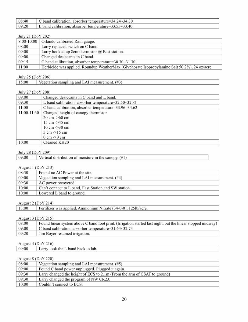
21
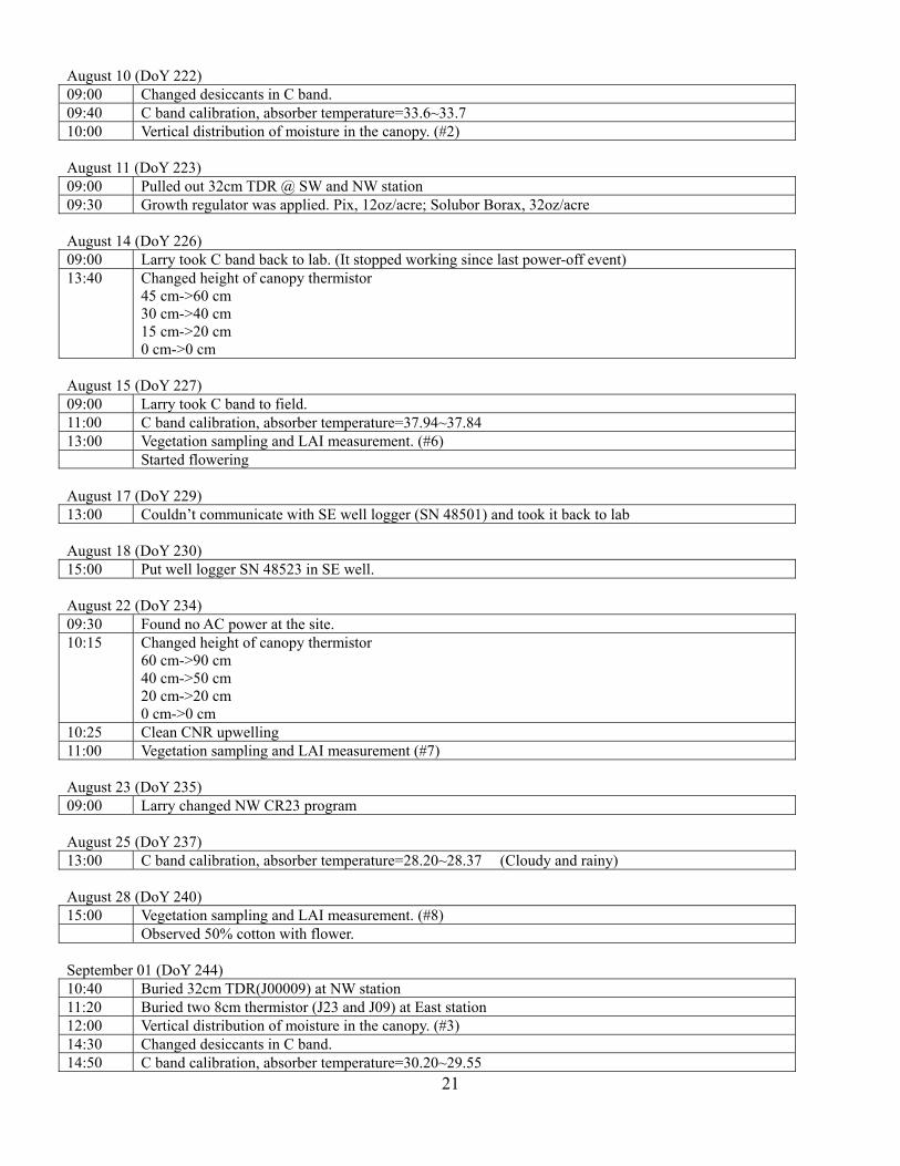
August 10 (DoY 222) 09:00 Changed desiccants in C band. 09:40 C band calibration, absorber temperature=33.6~33.7� 10:00 Vertical distribution of moisture in the canopy. (#2) August 11 (DoY 223) 09:00 Pulled out 32cm TDR @ SW and NW station 09:30 Growth regulator was applied. Pix, 12oz/acre; Solubor Borax, 32oz/acre August 14 (DoY 226) 09:00 Larry took C band back to lab. (It stopped working since last power-off event) 13:40 Changed height of canopy thermistor
45 cm->60 cm 30 cm->40 cm 15 cm->20 cm 0 cm->0 cm
August 15 (DoY 227) 09:00 Larry took C band to field. 11:00 C band calibration, absorber temperature=37.94~37.84� 13:00 Vegetation sampling and LAI measurement. (#6) Started flowering August 17 (DoY 229) 13:00 Couldn’t communicate with SE well logger (SN 48501) and took it back to lab August 18 (DoY 230) 15:00 Put well logger SN 48523 in SE well. August 22 (DoY 234) 09:30 Found no AC power at the site. 10:15 Changed height of canopy thermistor
60 cm->90 cm 40 cm->50 cm 20 cm->20 cm 0 cm->0 cm
10:25 Clean CNR upwelling 11:00 Vegetation sampling and LAI measurement (#7) August 23 (DoY 235) 09:00 Larry changed NW CR23 program August 25 (DoY 237) 13:00 C band calibration, absorber temperature=28.20~28.37� (Cloudy and rainy) August 28 (DoY 240) 15:00 Vegetation sampling and LAI measurement. (#8) Observed 50% cotton with flower. September 01 (DoY 244) 10:40 Buried 32cm TDR(J00009) at NW station 11:20 Buried two 8cm thermistor (J23 and J09) at East station 12:00 Vertical distribution of moisture in the canopy. (#3) 14:30 Changed desiccants in C band. 14:50 C band calibration, absorber temperature=30.20~29.55�
22
15:00 Checked all SHF and only SHF at SW was exposed. Buried all SHF again.
September 05 (DoY 248) 11:00 Growth regulator was applied. Pix, 12oz/acre; Solubor Borax, 80oz/acre, Karate with Zeon Technology
(Lambda-cyhalothrin 22.8%), 2.56oz/acre. September 06 (DoY 249) 09:00 Vegetation sampling and LAI measurement. (Started standing on the chair to measure LAI) (#9) September 08 (DoY 251) 13:30 C band calibration, absorber temperature=28.39~29.48� (Very cloudy, little rain) September 11 (DoY 254) 12:00 Vegetation sampling and LAI measurement. (#10) 15:10 Checked west footprint rain gauge 15:20 Changed the depth of SHF at L band to 5 cm 15:40 Cleaned KH20 Observed peak bloom. September 13 (DoY 256) 13:30 C band calibration, absorber temperature=28.25~28.40� (Rainy) September 18 (DoY 261) 14:00 Vegetation sampling.(Finished LAI measurement and didn’t finish vegetation sampling) (#11) September 20 (DoY 263) 13:00 Changed desiccants in C band. 13:20 C band calibration, absorber temperature=31.12~31.90� 14:15 Cleaned CSAT3 and KH20 15:00 Vertical distribution of moisture in the canopy. (#4) September 25 (DoY 268) 14:00 No AC power. Recovered later. 15:00 Vegetation sampling and LAI measurement. (#12) Some data of SW station was missing September 27 (DoY 270) 10:05 C band calibration, absorber temperature=30.54~32.20� 12:00 Checked west foot print rain gauge. September 28 (DoY 271) Observed open bolls near C band October 02 (DoY 275) 13:00-14:15 Changed the height of ECS to 3.10 m. (From the arm of CSAT3 to ground) 15:00 Vegetation sampling and LAI measurement. (#13) October 04 (DoY 277) 12:30 Changed desiccants in C band. 13:00 C band calibration, absorber temperature=31.72~32.04� 14:00 Found west and east hobo stopped working from last collection (July 12) October 09 (DoY 282)
23
13:00 Vertical distribution of moisture in the canopy. (#5) October 13 (DoY 286) 13:00 C band calibration, absorber temperature=34.23~35.22� 14:00 2 cm thermistor at C band was exposed. Buried it. October 14 (DoY 287) 09:00 Hwan found the east ECS fallen over. October 16 (DoY 289) 15:00 Set up ECS; The height from the arm of CSAT3 to ground is 2.90 m. October 17 (DoY 290) 14:00 Vegetation sampling and LAI measurement. (#14) 15:00 Helped Hwan to set up his eddy tower. Two out of eight in SW vegetation sample have open bolls.
Seven out of ten in NE vegetation sample have open bolls. There is no open boll in NW and SE vegetation sample.
Observed 25% of cotton with open bolls. October 18 (DoY 291) 13:00 Found ECS tower fell over again.(Irrigation system hit tower) 14:00 Set up the ECS tower; The height from the arm of CSAT3 to ground is 2.75 m. 15:00 Cleaned KH20 October 19 (DoY 292) 14:10 C band calibration, absorber temperature=31.16~31.30�.(Cloudy day) 14:20 Destroyed the honeycomb inside the west footprint rain gauge. 14:30 Checked and tested the west footprint rain gauge.(Remove the data of west rain gauge around 3:30 PM of
DoY 292) 15:00 Destroyed the nest inside the East station October 23 (DoY 296) 13:00 Found SHF at ECS was exposed. Buried it. 14:00 Vegetation sampling and LAI measurement. (#15) Eight out of nine in NW vegetation sample have open bolls.
Nine out of nine in SW vegetation sample have open bolls. Seven out of nine in SE vegetation sample have open bolls. Five out of eight in NE vegetation sample have open bolls.
Observed 80% cotton with open bolls October 25 (DoY 298) 11:30 Started irrigation. 13:30 Changed desiccants in C band. 13:50 C band calibration, absorber temperature=28.51~29.02� 14:00 Destroyed two honeycomb in C band and two honeycomb in L band November 01 (DoY 305) (Time after DoY 305 is EST) 14:25 C band calibration, absorber temperature=31.75~32.54� November 06 (DoY 310) 16:00 Vegetation sampling and LAI measurement. (#16) 17:00 Cleaned KH20 Observed more than 95% cotton with open bolls.
24
Open bolls percentage (# of open bolls / # of total bolls) = 35% November 08 (DoY 312) 09:00 Cotton defoliant was applied. Def 6 (S,S,S-Tributylphosphorotrithioate), 24oz/acre; Prep (Ethephon
55.4%), 24oz/acre. 09:20 C band calibration, absorber temperature=20.32~22.00� 10:00 Measured Voffset before change, V=-0.788v
Changed the gain and measured Voffset, V=-0.789v. Found C band still saturated.
11:00 Vertical distribution of moisture in the canopy (#6) November 13 (DoY 317) 09:00 Took C band back to lab. 11:00 Set up L band but didn’t cover it. So the temperature was not stable. November 17 (DoY 321) 09:00 Set up C band with Orlando.
C band was not saturated without metal cover, but became saturated with the metal cover. 11:00 Vegetation sampling and LAI measurement. (#17) Open bolls percentage (# of open bolls / # of total bolls) = 60 ~ 70% November 20 (DoY 324) 10:00 Larry fixed C band and it started working (Not saturated) 11:50 C band calibration, absorber temperature=15.70~15.92� November 22 (DoY 326) 13:00 Cleaned KH20 November 28 (DoY 332) 15:00 Vegetation sampling and LAI measurement. (#20)
Separated the cotton plant into four parts: stem, open bolls, shell of open bolls, closed bolls. Open bolls (Without the shell) will be used for yield estimation.
November 29 (DoY 333) 15:00 Vertical distribution of moisture in the canopy (#7) November 30 (DoY 334) 09:00 Took L band back to lab. 10:00 Helped staff harvest in four places (Near vegetation sample area)
Each harvest area covered two rows and 100ft long. Measured the weight of harvest cotton
14:00 Removed all sensors in SW station 16:00 Removed 1.2m and 0.64m sensors in East station December 01 (DoY 335) 09:00 Removed all sensors in NW station and East station. December 07 (DoY 341) 11:50 C band calibration, absorber temperature=19.68~20.78� 12:00 Put all harvest cotton into drier. Set temperature 90F December 11 (DoY 345) 09:00 Measured the weight of dried harvest cotton.
25
8. REFERENCES
Campbell Scientific, CSAT3 Three Dimensional Sonic Anemometer Instruction Manual, Campbell Scientific Inc., Logan, UT, 1998.
Campbell Scientific, HFT3 soil heat flux plate instruction manual, Campbell Scientific Inc., Logan, UT, 2003. Campbell Scientific, CNR1 Net Radiometer Instruction Manual, Campbell Scientific Inc., Logan, UT, 2006a. Campbell Scientific, CS615 andCS625 water content reflectometers instruction manual, Campbell Scientific Inc., Logan, UT,
2006b. Campbell Scientific, Campbell Scientific Model HMP45C Temperature and Relative Humidity Probe instruction manual,
Campbell Scientific Inc., Logan, UT, 2006c. Apogee Instruments Inc, Infrared Radiometer, Model IRR-PN, Apogee Instruments Inc, Logan, UT 84321, 2007 J. C. Kaimal and J. J. Finnigan, Atmospheric Boundary Layer Flows, Oxford University Press, New York, NY, 1994. R. D. De Roo, University of Florida C-band Radiometer Summary, Space Physics Research Laboratory, University of
Michigan, Ann Arbor, MI, March, 2002. R. D. De Roo, TMRS-3 Radiometer Tuning Procedures, Space Physics Research Laboratory, University of Michigan, Ann
Arbor, MI, March, 2003. P. Schotanus, F. T. M. Nieuwstadt, and H. A. R. DeBruin, “Temperature measurement with a sonic anemometer and its
application to heat and moisture fluctuations,” Bound.-Layer Meteorol., vol. 26, pp. 81-93, 2003. A. van Dijk, W. Kohsiek, and H. A. R. DeBruin, “Oxygen sensitivity of krypton and Lyman-alpha hygrometer,” J. Atmos.
Ocean. Tech., vol. 20, pp. 143-151., 2003. A. van Dijk, A. F. Moene, and H. A. R. DeBurin, The Principles of Surface Flux Physics: Theory, Practice, and Description
of the ECPACK Library, http://www.met.wau.nl/projects/jep/ E. K. Webb, G. I. Pearman, and R. Leuning, “ Correction of flux measurements for density effects due to heat and water
vapor transfer,” Quart. J. Roy. Meteorol., Soc., vol. 106, pp. 85-100, 1980. J. M. Wilczak, S. P. Oncley, and S. A. Stage, “Sonic anemometer tilt correction algorithms,” Bound.-Layer Meteorol., vol. 99,
pp. 127-150, 2001. University of Edinburgh, EdiRe data software, http://www.geos.ed.ac.uk/abs/research/micromet/EdiRe/
9. ACKNOWLEDGEMENTS
The authors would like to acknowledge Mr. James Boyer and his team at the PSREU, Citra, Florida for excellent field management. MicroWEX-6 was supported by grant from NASA-NIP (Grant number: 0005065) and the Earth Science Directorate, NSF (Grant number: EAR-0337277).
26
A. FIELD OBSERVATIONS
Figure Captions Figure A-1 Vertically and horizontally polarized C band Brightness temperature………………………………27 Figure A-2 Horizontally-polarized L band Brightness temperature……………….………………………………27 Figure A-3 Latent (LE) and sensible (H) heat fluxes at east eddy covariance station (UF) …………………………28 Figure A-4 Latent (LE) and sensible (H) heat fluxes at west eddy covariance station (UNH) ………………………28 Figure A-5 CO2 fluxes at west eddy covariance station (UNH) …………………………………………………………29 Figure A-6 Down- and up-welling solar radiation………………………………………………………………………29 Figure A-7 Down- and up-welling far infrared radiation………………………………………………………………30 Figure A-8 Total net radiation……………………………………………………………………………………………30 Figure A-9 Surface temperature (TIR)……………………………………………………………………………………31 Figure A-10 Relative Humidity……………………………………………………………………………………………31 Figure A-11 Air temperature………………………………………………………………………………………………32 Figure A-12 Canopy temperature at the height of 0cm, 5cm, 10cm and 15cm…………………………………………32 Figure A-13 Canopy temperature at the height of 20cm, 30cm, 40cm and 45cm………………………………………33 Figure A-14 Canopy temperature at the height of 50cm, 60cm and 90cm………………………………………………33 Figure A-15 Soil temperature at the depth of: 2cm, and 4cm at Northwest station……………………………………34 Figure A-16 Soil temperature at the depth of: 8cm, 16cm and 32cm at Northwest station……………………………34 Figure A-17 Soil temperature at the depth of: 64cm and 120cm at Northwest station…………………………………35 Figure A-18 Soil temperature at the depth of: 2cm, 4cm and 8cm at East station……………………………………35 Figure A-19 Soil temperature at the depth of: 16cm and 32cm at East station…………………………………………36 Figure A-20 Soil temperature at the depth of: 64cm and 120cm at East station………………………………………36 Figure A-21 Soil temperature at the depth of: 2cm, 4cm and 8cm at Southwest station………………………………37 Figure A-22 Soil temperature at the depth of: 16cm and 32cm at Southwest station…………………………………37 Figure A-23 Soil temperature at the depth of: 64cm and 120cm at Southwest station…………………………………38 Figure A-24 VSM at the depth of: at 2cm and 4cm at Northwest station………………………………………………38 Figure A-25 VSM at the depth of: at 8cm and 16cm at Northwest station……………………………………………39 Figure A-26 VSM at the depth of: at 32cm and 64cm at Northwest station……………………………………………39 Figure A-27 VSM at the depth of: at 120cm and 145cm at Northwest station…………………………………………40 Figure A-28 VSM at the depth of: at 2cm and 4cm at East station………………………………………………………40 Figure A-29 VSM at the depth of: at 8cm and 16cm at East station……………………………………………………41 Figure A-30 VSM at the depth of: at 32cm and 64cm at East station……………………………………………………41 Figure A-31 VSM at the depth of: at 120cm and 160cm at East station…………………………………………………42 Figure A-32 VSM at the depth of: at 2cm and 4cm at Southwest station………………………………………………42 Figure A-33 VSM at the depth of: at 8cm and 16cm at Southwest station………………………………………………43 Figure A-34 VSM at the depth of: at 32cm and 64cm at Southwest station……………………………………………43 Figure A-35 VSM at the depth of: at 120cm and 170cm at Southwest station…………………………………………44 Figure A-36 Rainfall from the raingauge at the east and west edge of footprint………………………………………44 Figure A-37 Rainfall from the raingauge at the east and west edge of the field………………………………………45 Figure A-38 Soil heat flux at the depth of: 2cm and 5cm at Northwest station…………………………………………45 Figure A-39 Soil heat flux at the depth of: 2cm at CSAT station………………………………………………………46 Figure A-40 Soil heat flux at the depth of: 2cm at East station…………………………………………………………46 Figure A-41 Soil heat flux at the depth of: 2cm at Southwest station……………………………………………………47 Figure A-42 Average crop heights at vegetation sampling areas…………………………………………………………48 Figure A-43 Average crop widths at vegetation sampling areas…………………………………………………………49 Figure A-44 LAI at vegetation sampling areas……………………………………………………………………………50 Figure A-45 Wet biomass and dry biomass at vegetation sampling areas………………………………………………51 Figure A-46 Vertical distribution of wet and dry biomass (1)……………………………………………………………52 Figure A-47 Vertical distribution of wet and dry biomass (2)……………………………………………………………53 Figure A-48 Groundwater level above sea level …………………………..………………………………………………54 Figure A-49 Groundwater level below surface …………………………………………………………………...………54
27
180 200 220 240 260 280 300 320 340150
200
250
300
350
Brig
htne
ss T
empe
ratu
re (
K)
DOY in 2006 (EST)
H−polV−pol
Figure A-1 C band Brightness temperature of vertically and horizontally polarization
180 200 220 240 260 280 300 320 34050
100
150
200
250
300
350
400
Brig
htne
ss T
empe
ratu
re (
K)
DOY in 2006 (EST)
H−pol
Figure A-2 L band Brightness temperature of horizontally polarization
28
180 200 220 240 260 280 300 320 340−100
0
100
200
300
400
500
600F
lux
(W/m
2 )
DOY in 2006 (EST)
LEH
Figure A-3 Latent (LE) and sensible (H) heat fluxes at east eddy covariance station (UF)
180 200 220 240 260 280 300 320 340−100
0
100
200
300
400
500
600
Flu
x (W
/m2 )
DOY in 2006 (EST)
LEH
Figure A-4 Latent (LE) and sensible (H) heat fluxes at west eddy covariance station (UNH)
29
180 200 220 240 260 280 300 320 340−100
−50
0
50
100C
O2 F
lux
(μm
ol/m
2 /s)
DOY in 2006 (EST)
Figure A-5 CO2 fluxes at west eddy covariance station (UNH)
180 200 220 240 260 280 300 320 340−200
0
200
400
600
800
1000
1200
Flu
x (W
/m2 )
DOY in 2006 (EST)
Downwelling solar radiationUpwelling solar radiation
Figure A-6 Down- and up-welling solar radiation
30
180 200 220 240 260 280 300 320 340200
250
300
350
400
450
500
550
600
650
Flu
x (W
/m2 )
DOY in 2006 (EST)
Downwelling far infrared radiationUpwelling far infrared radiation
Figure A-7 Down- and up-welling far infrared radiation
180 200 220 240 260 280 300 320 340−200
0
200
400
600
800
1000
Flu
x (W
/m2 )
DOY in 2006 (EST)
Total net radiation
Figure A-8 Total net radiation
31
180 200 220 240 260 280 300 320 340275
280
285
290
295
300
305
310
315
Sur
face
Tem
pera
ture
(K
)
DOY in 2006 (EST)
Figure A-9 Surface temperature (TIR)
Figure A-10 Relative Humidity

32
Figure A-11 Air temperature
180 200 220 240 260 280 300 320 340
280
290
300
310
320
330
Can
opy
Tem
pera
ture
(K
)
DOY in 2006 (EST)
0cm5cm10cm15cm
Figure A-12 Canopy temperature at the height of 0cm, 5cm, 10cm and 15cm
33
180 200 220 240 260 280 300 320 340
280
290
300
310
320
330
Can
opy
Tem
pera
ture
(K
)
DOY in 2006 (EST)
20cm30cm40cm45cm
Figure A-13 Canopy temperature at the height of 20cm, 30cm, 40cm and 45cm
180 200 220 240 260 280 300 320 340
280
290
300
310
320
330
Can
opy
Tem
pera
ture
(K
)
DOY in 2006 (EST)
50cm60cm90cm
Figure A-14 Canopy temperature at the height of 50cm, 60cm and 90cm
34
180 200 220 240 260 280 300 320 340
280
290
300
310
320
330
Soi
l Tem
pera
ture
(K
)
DOY in 2006 (EST)
2cm @ C band2cm @ L band4cm
Figure A-15 Soil temperature at the depth of: 2cm, and 4cm at Northwest station
180 200 220 240 260 280 300 320 340
280
290
300
310
320
330
Soi
l Tem
pera
ture
(K
)
DOY in 2006 (EST)
8cm16cm32cm
Figure A-16 Soil temperature at the depth of: 8cm, 16cm and 32cm at Northwest station
35
180 200 220 240 260 280 300 320 340
280
290
300
310
320
330
Soi
l Tem
pera
ture
(K
)
DOY in 2006 (EST)
64cm120cm
Figure A-17 Soil temperature at the depth of: 64cm and 120cm at Northwest station
180 200 220 240 260 280 300 320 340
280
290
300
310
320
330
Soi
l Tem
pera
ture
(K
)
DOY in 2006 (EST)
2cm4cm8cm
Figure A-18 Soil temperature at the depth of: 2cm, 4cm and 8cm at East station
36
180 200 220 240 260 280 300 320 340
280
290
300
310
320
330
Soi
l Tem
pera
ture
(K
)
DOY in 2006 (EST)
16cm32cm
Figure A-19 Soil temperature at the depth of: 16cm and 32cm at East station
180 200 220 240 260 280 300 320 340
280
290
300
310
320
330
Soi
l Tem
pera
ture
(K
)
DOY in 2006 (EST)
64cm120cm
Figure A-20 Soil temperature at the depth of: 64cm and 120cm at East station
37
180 200 220 240 260 280 300 320 340280
290
300
310
320
330
Soi
l Tem
pera
ture
(K
)
DOY in 2006 (EST)
2cm4cm8cm
Figure A-21 Soil temperature at the depth of: 2cm, 4cm and 8cm at Southwest station
180 200 220 240 260 280 300 320 340280
290
300
310
320
330
Soi
l Tem
pera
ture
(K
)
DOY in 2006 (EST)
16cm32cm
Figure A-22 Soil temperature at the depth of: 16cm and 32cm at Southwest station
38
180 200 220 240 260 280 300 320 340280
290
300
310
320
330
Soi
l Tem
pera
ture
(K
)
DOY in 2006 (EST)
64cm120cm
Figure A-23 Soil temperature at the depth of: 64cm and 120cm at Southwest station
180 200 220 240 260 280 300 320 3400
5
10
15
20
25
30
35
40
VS
M (
%)
DOY in 2006 (EST)
2cm @ C band2cm @ L band4cm
Figure A-24 VSM at the depth of: at 2cm and 4cm at Northwest station
39
180 200 220 240 260 280 300 320 3400
5
10
15
20
25
30
35
40
VS
M (
%)
DOY in 2006 (EST)
8cm16cm
Figure A-25 VSM at the depth of: at 8cm and 16cm at Northwest station
180 200 220 240 260 280 300 320 3400
5
10
15
20
25
30
35
40
VS
M (
%)
DOY in 2006 (EST)
32cm64cm
Figure A-26 VSM at the depth of: at 32cm and 64cm at Northwest station

40
180 200 220 240 260 280 300 320 3400
5
10
15
20
25
30
35
40
VS
M (
%)
DOY in 2006 (EST)
120cm145cm
Figure A-27 VSM at the depth of: at 120cm and 145cm at Northwest station
180 200 220 240 260 280 300 320 3400
5
10
15
20
25
30
35
40
VS
M (
K)
DOY in 2006 (EST)
2cm2cm(replicate)4cm
Figure A-28 VSM at the depth of: at 2cm and 4cm at East station
41
180 200 220 240 260 280 300 320 3400
5
10
15
20
25
30
35
40
VS
M (
K)
DOY in 2006 (EST)
8cm16cm
Figure A-29 VSM at the depth of: at 8cm and 16cm at East station
180 200 220 240 260 280 300 320 3400
5
10
15
20
25
30
35
40
VS
M (
K)
DOY in 2006 (EST)
32cm64cm
Figure A-30 VSM at the depth of: at 32cm and 64cm at East station
42
180 200 220 240 260 280 300 320 3400
5
10
15
20
25
30
35
40
VS
M (
K)
DOY in 2006 (EST)
120cmSE 160cmNE 160cm
Figure A-31 VSM at the depth of: at 120cm and 160cm at East station
180 200 220 240 260 280 300 320 3400
5
10
15
20
25
30
35
40
VS
M (
%)
DOY in 2006 (EST)
2cm2cm(replicate)4cm
Figure A-32 VSM at the depth of: at 2cm and 4cm at Southwest station

43
180 200 220 240 260 280 300 320 3400
5
10
15
20
25
30
35
40
VS
M (
%)
DOY in 2006 (EST)
8cm16cm
Figure A-33 VSM at the depth of: at 8cm and 16cm at Southwest station
180 200 220 240 260 280 300 320 3400
5
10
15
20
25
30
35
40
VS
M (
%)
DOY in 2006 (EST)
32cm64cm
Figure A-34 VSM at the depth of: at 32cm and 64cm at Southwest station
44
180 200 220 240 260 280 300 320 3400
5
10
15
20
25
30
35
40
VS
M (
%)
DOY in 2006 (EST)
120cm170cm
Figure A-35 VSM at the depth of: at 120cm and 170cm at Southwest station
180 200 220 240 260 280 300 320 3400
5
10
15
20
25
30
Pre
cipi
tatio
n (m
m)
DOY in 2006 (EST)
East of footprintWest of footprint
Figure A-36 Rainfall from the raingauge at the east and west edge of footprint
45
180 200 220 240 260 280 300 320 3400
5
10
15
20
25
30
Pre
cipi
tatio
n (m
m)
DOY in 2006 (EST)
East of fieldWest of field
Figure A-37 Rainfall from the raingauge at the east and west edge of the field
180 200 220 240 260 280 300 320 340−150
−100
−50
0
50
100
150
200
Soi
l Hea
t Flu
x (W
/m2 )
DOY in 2006 (EST)
2cm @ C band2cm @ L band5cm @ L band
Figure A-38 Soil heat flux at depths of 2cm and 5cm at Northwest station
46
180 200 220 240 260 280 300 320 340−150
−100
−50
0
50
100
150
200S
oil H
eat F
lux
(W/m
2 )
DOY in 2006 (EST)
2cm @ CSAT Station
Figure A-39 Soil heat flux at the depth of: 2cm at CSAT station
180 200 220 240 260 280 300 320 340−150
−100
−50
0
50
100
150
200
Soi
l Hea
t Flu
x (W
/m2 )
DOY in 2006 (EST)
2cm @ East Station
Figure A-40 Soil heat flux at the depth of: 2cm at East station
47
180 200 220 240 260 280 300 320 340−150
−100
−50
0
50
100
150
200S
oil H
eat F
lux
(W/m
2 )
DOY in 2006 (EST)
2cm @ Southwest Station
Figure A-41 Soil heat flux at the depth of: 2cm at Southwest station
48
180 200 220 240 260 280 300 320 3400
50
100
150H
eigh
t (cm
)
DOY in 2006 (EST)
NW
180 200 220 240 260 280 300 320 3400
50
100
150
Hei
ght (
cm)
DOY in 2006 (EST)
NE
180 200 220 240 260 280 300 320 3400
50
100
150
Hei
ght (
cm)
DOY in 2006 (EST)
SW
180 200 220 240 260 280 300 320 3400
50
100
150
Hei
ght (
cm)
DOY in 2006 (EST)
SE
Figure A-42 Average crop heights at vegetation sampling areas
49
180 200 220 240 260 280 300 320 3400
20
40
60
80
Wid
th (
cm)
DOY in 2006 (EST)
NW
180 200 220 240 260 280 300 320 3400
20
40
60
80
Wid
th (
cm)
DOY in 2006 (EST)
NE
180 200 220 240 260 280 300 320 3400
20
40
60
80
Wid
th (
cm)
DOY in 2006 (EST)
SW
180 200 220 240 260 280 300 320 3400
20
40
60
80
Wid
th (
cm)
DOY in 2006 (EST)
SE
Figure A-43 Average crop widths at vegetation sampling areas
50
180 200 220 240 260 280 300 320 3400
1
2
3
4
5
6
LAI(
Dim
ensi
onle
ss)
DOY in 2006 (EST)
NW
180 200 220 240 260 280 300 320 3400
1
2
3
4
5
6
LAI(
Dim
ensi
onle
ss)
DOY in 2006 (EST)
NE
180 200 220 240 260 280 300 320 3400
1
2
3
4
5
6
LAI(
Dim
ensi
onle
ss)
DOY in 2006 (EST)
SW
180 200 220 240 260 280 300 320 3400
1
2
3
4
5
6
LAI(
Dim
ensi
onle
ss)
DOY in 2006 (EST)
SE
Figure A-44 LAI at vegetation sampling areas
51
180 200 220 240 260 280 300 320 3400
1
2
3
4
5
Bio
mas
s(kg
/m2 )
DOY in 2006 (EST)
NW
Wet BiomassDry Biomass
180 200 220 240 260 280 300 320 3400
1
2
3
4
5
Bio
mas
s(kg
/m2 )
DOY in 2006 (EST)
NE
Wet BiomassDry Biomass
180 200 220 240 260 280 300 320 3400
1
2
3
4
5
Bio
mas
s(kg
/m2 )
DOY in 2006 (EST)
SW
Wet BiomassDry Biomass
180 200 220 240 260 280 300 320 3400
1
2
3
4
5
Bio
mas
s(kg
/m2 )
DOY in 2006 (EST)
SE
Wet BiomassDry Biomass
Figure A-45 Wet biomass and dry biomass at vegetation sampling areas
52
0 5 10 15 200
0.1
0.2
0.3
0.4
0.5
0.6
0.7
Weight (g)
Hei
ght(
m)
Jul 28
Plant 1 wetPlant 2 wetPlant 3 wetPlant 4 wetPlant 1 dryPlant 2 dryPlant 3 dryPlant 4 dry
0 5 10 150
0.2
0.4
0.6
0.8
1
1.2
1.4
Weight (g)
Hei
ght(
m)
Aug 11
Plant 1 wetPlant 2 wetPlant 3 wetPlant 4 wetPlant 5 wetPlant 1 dryPlant 2 dryPlant 3 dryPlant 4 dryPlant 5 dry
0 20 40 60 800
0.2
0.4
0.6
0.8
1
1.2
1.4
Weight (g)
Hei
ght(
m)
Sep 01
Plant 1 wetPlant 2 wetPlant 3 wetPlant 4 wetPlant 1 dryPlant 2 dryPlant 3 dryPlant 4 dry
0 50 1000
0.5
1
1.5
Weight (g)
Hei
ght(
m)
Sep 20
Plant 1 wetPlant 2 wetPlant 3 wetPlant 4 wetPlant 1 dryPlant 2 dryPlant 3 dryPlant 4 dry
Figure A-46 Vertical distribution of wet and dry biomass (1)
53
0 50 1000
0.5
1
1.5
Weight (g)
Hei
ght(
m)
Oct 09
Plant 1 wetPlant 2 wetPlant 3 wetPlant 4 wetPlant 1 dryPlant 2 dryPlant 3 dryPlant 4 dry
0 50 100 1500
0.5
1
1.5
Weight (g)
Hei
ght(
m)
Nov 08
Plant 1 wetPlant 2 wetPlant 3 wetPlant 4 wetPlant 5 wetPlant 1 dryPlant 2 dryPlant 3 dryPlant 4 dryPlant 5 dry
0 10 20 30 400
0.5
1
1.5
2
Weight (g)
Hei
ght(
m)
Nov 29
Plant 1 wetPlant 2 wetPlant 3 wetPlant 4 wetPlant 1 dryPlant 2 dryPlant 3 dryPlant 4 dry
Figure A-47 Vertical distribution of wet and dry biomass (2)
54
180 200 220 240 260 280 300 320 34014.8
15
15.2
15.4
15.6
15.8E
leva
tion
(m)
DOY in 2006 (EST)
NWSWSENE
Figure A-48 Groundwater level above sea level
180 200 220 240 260 280 300 320 340−7
−6.5
−6
−5.5
−5
−4.5
−4
Dep
th (
m)
DOY in 2006 (EST)
NWSWSENE
Figure A-49 Groundwater level below surface