This content has been downloaded from IOPscience. Please scroll down to see the full text.

Download details:

IP Address: 128.118.88.48

This content was downloaded on 12/08/2014 at 07:18

Please note that terms and conditions apply.

Fidelity and entanglement fidelity for infinite-dimensional quantum systems

View the table of contents for this issue, or go to the journal homepage for more

2014 J. Phys. A: Math. Theor. 47 335304

(http://iopscience.iop.org/1751-8121/47/33/335304)

Home Search Collections Journals About Contact us My IOPscience

Fidelity and entanglement fidelity forinfinite-dimensional quantum systems

Li Wang1, Jinchuan Hou1 and Xiaofei Qi2

1Department of Mathematics, Taiyuan University of Technology, Taiyuan 030024,Peopleʼs Republic of China2Department of Mathematics, Shanxi University, Taiyuan 030006, Peopleʼs Republicof China

E-mail: wangli5257@sina.com, jinchuanhou@aliyun.com andxiaofeiqisxu@aliyun.com

Received 16 March 2014, revised 26 June 2014Accepted for publication 30 June 2014Published 6 August 2014

AbstractInstead of unitary freedom for finite-dimensional cases, bi-contractive freedomin the operator-sum representation for quantum channels of infinite-dimen-sional systems is established. Specifically, if the channel sends every pure stateto a finite rank state, then the isometric freedom feature holds. Then, a methodof computing entanglement fidelity and a relation between quantum fidelityand entanglement fidelity for infinite-dimensional systems are obtained. Inaddition, upper and lower bounds of the quantum fidelity, and their connectionto the trace distance, are also provided.

Keywords: quantum states, quantum channels, fidelity, entanglement fidelity,trace distancePACS numbers: 03.67.-a, 03.65.Db

1. Introduction

In quantum mechanics, a quantum system is associated with a separable complex Hilbertspace, H. A quantum state is a density operator, ρ ∈ ⊆H H( ) ( ), which is positive and hastrace 1. Here, H( ) and H( ) stand for the algebras of all bounded linear operators and alltrace-class operators T with∥ ∥ = < ∞†T T TTr (( ) )Tr

12 , respectively. Denote by H( ) the set

of all states acting on H. H( ) is a closed convex set of the unit sphere of H( ). Recall that astate ρ ∈ H( ) is a pure state (that is, a rank one projection) if and only if ρ ρ=2 ; it is amixed state if and only if ρ ρ≠2 .

Quantum fidelity, which is a very useful measure of closeness between states that hasseveral nice properties, plays an important role in quantum information theory and quantumcomputation, and has deep connection to quantum entanglement, quantum chaos, and

Journal of Physics A: Mathematical and Theoretical

J. Phys. A: Math. Theor 47 (2014) 335304 (17pp) doi:10.1088/1751-8113/47/33/335304

1751-8113/14/335304+17$33.00 © 2014 IOP Publishing Ltd Printed in the UK 1

quantum phase transitions (for example, see [1–4] and the references therein). Recall that thequantum fidelity of states ρ and σ in H( ) is defined to be

ρ σ ρ σρ=F ( , ) Tr . (1.1)1 2 1 2

Specifically, if ρ ψ ψ= | ⟩⟨ | is a pure state, then ρ σ ψ σ ψ σ ψ= | ⟩ = ⟨ | | ⟩F F( , ) ( , ) .Assume that < ∞Hdim . Uhlmann in [5] (see also [6]) proved that

ρ σ ψ ϕ= |⟨ | ⟩|F ( , ) max , where the maximum is over all purifications ψ| ⟩ of ρ and ϕ| ⟩ of σ . In[1], the relationship between the quantum fidelity and the classical fidelity was given:

ρ σ =F F p q( , ) min ( , )E m m{ }m , where the minimum is over all positive operator-valuedmeasure (POVMs) E{ }m , and ρ=p ETr ( )m m , σ=q ETr ( )m m are the probability distributionsfor ρ and σ corresponding to E{ }m . Recently, Hou and Qi generalized the above properties toinfinite-dimensional systems in [7], and proved that the equality ρ σ ψ ϕ= |⟨ | ⟩|F ( , ) max stillholds. However, the relationship between the quantum fidelity and the classical fidelity for theinfinite-dimensional systems is not the same as that in the finite-dimensional case. Indeed, if

= ∞Hdim , then ρ σ =F F p q( , ) inf ( , )E m m{ }m , and the infimum attains the minimum if andonly if ρ and σ meet certain conditions.

Besides the quantum fidelity, the entanglement fidelity is another kind of importantfidelity associated with a quantum channel and a state.

Recall that a quantum channel is a trace-preserving, completely positive linear map from H( ) into K( ). By [8–10], every channel →H K: ( ) ( ) has an operator-sum repre-sentation (or a Kraus form)

∑ρ ρ==

†E E( ) , (1.2)k

N

k k1

where ⩽ ⩽ ∞N1 and ⊆=E H K{ } ( , )k kN

1 is a sequence of bounded operators from H intoK with ∑ ==

†E E IkN

k k1 . In the representation equation (1.2), Eks are called the operationelements or Kraus operators of the quantum channel . The representation equation (1.2) isnot unique. The operation elements =E{ }i i

N1 can be chosen so that they are a linearly

independent set and, in this case, N is called the length of . If = < ∞H ddim , it is wellknown that the length of is not greater than d2, and the sequences =E{ }i i

N1 and =F{ }j j

M1 of

operation elements of any two representations of are connected by a unitary matrix,= ∈U u M( )ij N Mmax { , } , such that = ∑ =F u Ej i

Nij i1 , = …j M1, 2, , . This basic and useful

feature is called the unitary freedom in the operator-sum representation for quantum channels.However, it is not known if the unitary freedom in the operator-sum representation forchannels is still valid for infinite-dimensional systems. As the infinite-dimensional systems(i.e., the continuous systems) are also important in quantum world, this question is natural andworth investigating.

For a state ρ ∈ H( ) and a quantum channel →H H: ( ) ( ), the entanglementfidelity is defined by

ρ ψ ψ ψ ψ ψ ψ ψ= ⊗ = ⊗F F I I( , ) ( , ( )( )) ( )( ) , (1.3)2

where ψ| ⟩ ∈ ⊗H H is a purification of ρ. Several useful properties of entanglement fidelityin both finite-dimensional and infinite-dimensional cases can be found in [1, 7]. Therefore,there is an important property of entanglement fidelity, which states that for any ρ ∈ H( )and any quantum channel with operation elements E{ }i , we have

∑ρ ρ= ( )F E( , ) Tr . (1.4)i

i2

J. Phys. A: Math. Theor 47 (2014) 335304 Li Wang et al

2

This means that the entanglement fidelity, ρF ( , ), defined in equation (1.3) does not dependon the choice of purifications of ρ. Furthermore, in the case where < ∞Hdim , by applyingthe unitary freedom feature, it is shown in [11] that one can choose operation elements E{ }i of in equation (1.4), so that

ρ ρ= ( )F E( , ) Tr . (1.5)12

Then, it is natural to ask whether or not such a result still holds for infinite-dimensionalsystems.

For a finite-dimensional case, an interesting connection between quantum fidelity andentanglement fidelity is also found in [12] for states and quantum channels: If there existssome η > 0 such that the fidelity inequality

ψ ψ ψ ψ ψ ψ ψ ψ η= ⩾ −F ( , ( )) ( ) 1 (1.6)2

holds for all ψ| ⟩ in the support of ρ, then the entanglement fidelity inequality

ρ η⩾ −F ( , ) 1 (3 2) (1.7)

holds. It is not obvious whether or not ‘equation 1.6 ⇒ equation 1.7’ still holds for infinite-dimensional systems.

The purpose of this paper is to answer the three questions above. We also generalizesome inequalities concerning entanglement fidelity, quantum fidelity, and trace distance ofquantum states for infinite-dimensional systems.

Throughout this paper, H and K are separable complex Hilbert spaces of any dimension,and ⟨· | ·⟩ stands for the inner product in both of them. H K( , ) ( H( ) when K = H) is theBanach space of all (bounded linear) operators from H into K with operator norm ∥ · ∥. For

∈A H( ), denote by †A the adjoint of A. ∈A H( ) is called positive, denoted by ⩾A 0, ifψ ψ⟨ | | ⟩ ⩾A 0 for all ψ| ⟩ ∈ H ; it is unitary if = =† †A A AA I ; it is isometric if =†A A I . If A isself-adjoint (that is, if = †A A ), we denote by +A and −A the positive part and the negativepart of A, respectively. For ρ ∈ ⊗H K( ), ρ ρ= ⊗ITr ( ) ( Tr )( )K H is a state in H( ), whichis called the reduced state of ρ. A unit vector, ψ| ⟩ ∈ ⊗H K , is said to be a purification of astate, ρ, on H if ρ ψ ψ= | ⟩⟨ |Tr ( )K . For any positive number N or = ∞N , l N( )2 stands for theN-dimensional separable complex Hilbert space, ξ ξ∑ | | < ∞= ={{ } : }i i

NiN

i1 12 .

2. Bi-contractive freedom in operator-sum representations for channels

Let →H K: ( ) ( ) be a quantum channel. For a finite-dimensional case, it is well-knownthat we have the unitary freedom in the operator-sum representation for ([1, 8], and also[13, 14]), which provides some insight into the derivation of the Kraus form given inequation (1.2). However, the approach for a finite-dimensional case is no longer valid forinfinite-dimensional quantum channels. In fact, the situation for an infinite-dimensional caseis very different, and what we can achieve is the following result, which we called the bi-contractive freedom in operator-sum representation for channels.

For = …i M1, 2, , and = …j N1, 2, , with ⩽ ∞M N, , a M × N matrix, =W w( )ij , issaid to be contractive if its operator norm, ∥ ∥ ⩽W 1, as an operator from l N( )2 into l M( )2

according to the standard orthonormal basis.

Theorem 2.1. (Bi-contractive freedom in operator-sum representation) Let H K, be infinite-dimensional separable complex Hilbert spaces. Assume that Φ Φ →H K, : ( ) ( )1 2 are twoquantum channels with operator-sum representations Φ = ∑ †X A XA( ) i i i1 and

J. Phys. A: Math. Theor 47 (2014) 335304 Li Wang et al

3

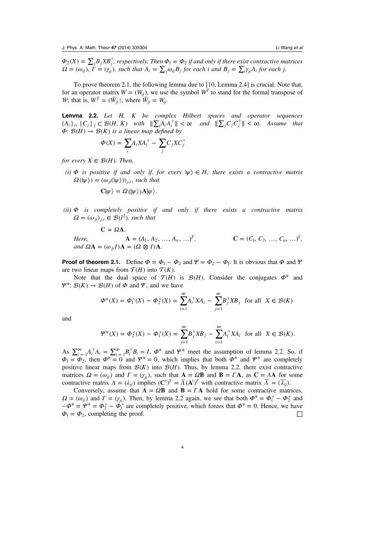
Φ = ∑ †X B XB( ) j j j2 , respectively. Then Φ Φ=1 2 if and only if there exist contractive matricesΩ ω Γ γ= =( ), ( )ij ji , such that ω= ∑A Bi j ij j for each i and γ= ∑B Aj i ji i for each j.

To prove theorem 2.1, the following lemma due to [10, Lemma 2.4] is crucial. Note that,for an operator matrix =W W( )ij , we use the symbol WT to stand for the formal transpose ofW; that is, = ˜W W( )T

ji , where ˜ =W Wji ij.

Lemma 2.2. Let H, K be complex Hilbert spaces and operator sequences⊂A C H K{ } , { } ( , )i i j j with ∥∑ ∥ < ∞†A Ai i i and ∥∑ ∥ < ∞†C Cj j j . Assume that

Φ →H K: ( ) ( ) is a linear map defined by

∑ ∑Φ = −† †X A XA C XC( )i

i ij

j j

for every ∈X H( ). Then,

(i) Φ is positive if and only if, for every ψ| ⟩ ∈ H , there exists a contractive matrixΩ ψ ω ψ| ⟩ = | ⟩( ) ( ( )) ,ji j i, such that

ψ Ω ψ ψ=C A( ) .

(ii) Φ is completely positive if and only if there exists a contractive matrixΩ ω= ∈ l( ) ( )ji j i,

2 , such that

Ω=C A.

Here, = … …A A AA ( , , , , )nT

1 2 , = … …C C CC ( , , , , )nT

1 2 ,and Ω ω Ω= = ⊗I IA A A( ) ( )ji .

Proof of theorem 2.1. Define Φ Φ Φ= −1 2 and Ψ Φ Φ= −2 1. It is obvious that Φ and Ψare two linear maps from H( ) into K( ).

Note that the dual space of H( ) is H( ). Consider the conjugates Φ* and Ψ* →K H: ( ) ( ) of Φ and Ψ , and we have

∑ ∑Φ Φ Φ* = − = − ∈* *

=

∞†

=

∞†X X X A XA B XB X K( ) ( ) ( ) for all ( )

ii i

jj j1 2

1 1

and

∑ ∑Ψ Φ Φ* = − = − ∈* *

=

∞†

=

∞†X X X B XB A XA X K( ) ( ) ( ) for all ( ).

jj j

ii i2 1

1 1

As ∑ = ∑ ==∞ †

=∞ †A A B B Ii i i i i i1 1 , Φ* and Ψ* meet the assumption of lemma 2.2. So, if

Φ Φ=1 2, then Φ* = 0 and Ψ* = 0, which implies that both Φ* and Ψ* are completelypositive linear maps from K( ) into H( ). Thus, by lemma 2.2, there exist contractivematrices Ω ω= ( )ij and Γ γ= ( )ji , such that Ω=A B and Γ=B A, as Λ=C A for somecontractive matrix Λ λ= ( )ij implies Λ=† †C A( ) ( )T T with contractive matrix Λ λ= ( )ij .

Conversely, assume that Ω=A B and Γ=B A hold for some contractive matrices,Ω ω= ( )ij and Γ γ= ( )ji . Then, by lemma 2.2 again, we see that both Φ Φ Φ* = −* *

1 2 andΦ Ψ Φ Φ− * = * = −* *

2 1 are completely positive, which forces that Φ* = 0. Hence, we haveΦ Φ=1 2, completing the proof. □

J. Phys. A: Math. Theor 47 (2014) 335304 Li Wang et al

4

Corollary 2.3. Let H K, be infinite-dimensional separable complex Hilbert spaces. Assumethat Φ Φ →H K, : ( ) ( )1 2 are any two quantum channels with operator-sum representa-tions Φ = ∑ †X A XA( ) i i i1 and Φ = ∑ †X B XB( ) j j j2 , respectively. If there exists an isometricmatrix, =U u( )ij , such that = ∑A u Bi j ij j for each i, then Φ Φ≡1 2.

Proof. By this assumption, we have = UA B. As U is an isometric matrix, =†U U I , theidentity matrix, so ∥ ∥ = ∥ ∥ =†U U 1 and = =† †U U UB B A. By theorem 2.1, one getsΦ Φ=1 2. □

We give an example to illustrate theorem 2.1 and corollary 2.3.

Example. Let | ⟩ =∞i{ } i 0 be an orthonormal basis of a complex separable Hilbert space, H.

For a real number κ > 0, let be a quantum channel of this system, which has an operator-sum representation

∑ρ κ ρ κ ρ= ∈=

∞†S S H( ) ( ) ( ) for ( ),

l

l l

0

where

κ κ κ

κ κ κ

κ κ κ

= =

= + = …

= − = …

+ + +

+ + +

( )

( )

S S T

S T T i

S T T i

( ) ( )1

2( ),

( )1

2( ) ( ) , 0, 1, 2,

( )1

2( ) ( ) , 0, 1, 2,

i i i

i i i

0 1 0

2 2 2 1 2 2

2 3 2 2 2 1

with

∑κκ κ κ

=+ + +

− = …= −−

TC

l n n l( )1

1 1 1, 0, 1, 2, ,l

n

l ln

20

2n l n

and = !! − !Cl n

l

n l n( ).

On the other hand, let 1 be the phase conjugation channel, which is a single-modeBosonic Gaussian channel. By [15], 1 has an operator-sum representation

∑ρ κ ρ κ ρ= ∈=

∞†T T H( ) ( ) ( ) for ( ).

l

l l1

0

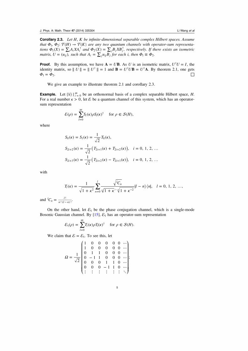
We claim that = 1. To see this, let

⎛

⎝

⎜⎜⎜⎜⎜⎜⎜

⎞

⎠

⎟⎟⎟⎟⎟⎟⎟

Ω =

⋯⋯⋯

− ⋯⋯

− ⋯⋮ ⋮ ⋮ ⋮ ⋮ ⋮ ⋱

1

2

1 0 0 0 0 01 0 0 0 0 00 1 1 0 0 00 1 1 0 0 00 0 0 1 1 00 0 0 1 1 0

;

J. Phys. A: Math. Theor 47 (2014) 335304 Li Wang et al

5

then

⎛

⎝

⎜⎜⎜⎜⎜

⎞

⎠

⎟⎟⎟⎟⎟

⎛

⎝

⎜⎜⎜⎜⎜

⎞

⎠

⎟⎟⎟⎟⎟

κκ

κΩ

κκ

κ⋮

⋮

= ⋮

⋮

S

S

S

T

T

T

( )( )

( )

( )( )

( ).

l l

0

1

0

1

Obviously, Ω is an isometry, but not unitary, as Ω Ω ΩΩ= ≠† †I . In fact, Ω = UV , where Vis the unilateral shift defined by | ⟩ = | + ⟩V i i 1 and U is the unitary operator defined by

| ⟩ = | ⟩ − | + ⟩U i i i2 ( 2 2 1 )1

2and | + ⟩ = | ⟩ + | + ⟩U i i i2 1 ( 2 2 1 )1

2, = …i 0, 1, 2, . Thus,

both Ω and Ω† are contractive and

⎛

⎝

⎜⎜⎜⎜⎜

⎞

⎠

⎟⎟⎟⎟⎟

⎛

⎝

⎜⎜⎜⎜⎜

⎞

⎠

⎟⎟⎟⎟⎟

κκ

κΩ

κκ

κ⋮

⋮

= ⋮

⋮

†

T

T

T

S

S

S

( )( )

( )

( )( )

( ).

l l

0

1

0

1

Therefore, by theorem 2.1, κ =∞S{ ( )}l i 0 is another sequence of Kraus operators of the phase

conjugation channel. □In the event that one of channels, Φ1 or Φ2, is an elementary channel (i.e.,

Φ = ∑ =†X A XA( ) i

Mi i1 1 and Φ = ∑ =

†X B XB( ) jN

j j2 1 with one of M N, being finite), the unitaryfreedom property is still true, and we will call it the unitary freedom for elementary channels;it can be regarded as a generalization of the finite-dimensional case. Its proof is also differentfrom that of a finite-dimensional case.

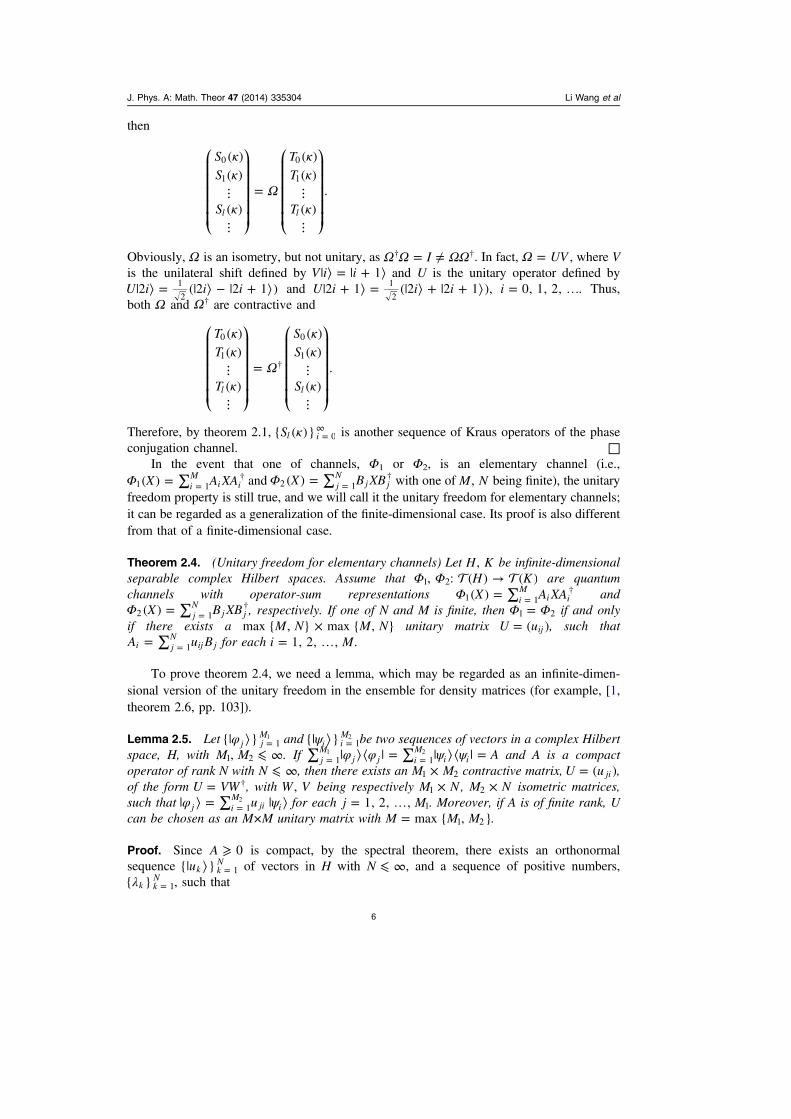
Theorem 2.4. (Unitary freedom for elementary channels) Let H K, be infinite-dimensionalseparable complex Hilbert spaces. Assume that Φ Φ →H K, : ( ) ( )1 2 are quantumchannels with operator-sum representations Φ = ∑ =

†X A XA( ) iM

i i1 1 andΦ = ∑ =

†X B XB( ) jN

j j2 1 , respectively. If one of N and M is finite, then Φ Φ=1 2 if and onlyif there exists a ×M N M Nmax { , } max { , } unitary matrix =U u( )ij , such that

= ∑ =A u Bi jN

ij j1 for each = …i M1, 2, , .

To prove theorem 2.4, we need a lemma, which may be regarded as an infinite-dimen-sional version of the unitary freedom in the ensemble for density matrices (for example, [1,theorem 2.6, pp. 103]).

Lemma 2.5. Let φ| ⟩ ={ }j jM

11 and ψ| ⟩ ={ }i i

M1

2 be two sequences of vectors in a complex Hilbertspace, H, with ⩽ ∞M M,1 2 . If φ φ ψ ψ∑ | ⟩⟨ | = ∑ | ⟩⟨ | == = Aj

Mj j i

Mi i1 1

1 2 and A is a compactoperator of rank N with ⩽ ∞N , then there exists an ×M M1 2 contractive matrix, =U u( )ji ,of the form = †U VW , with W V, being respectively ×M N1 , ×M N2 isometric matrices,such that φ ψ| ⟩ = ∑ | ⟩= uj i

Mji i1

2 for each = …j M1, 2, , 1. Moreover, if A is of finite rank, Ucan be chosen as an M×M unitary matrix with =M M Mmax { , }1 2 .

Proof. Since ⩾A 0 is compact, by the spectral theorem, there exists an orthonormalsequence | ⟩ =u{ }k k

N1 of vectors in H with ⩽ ∞N , and a sequence of positive numbers,

λ ={ }k kN

1, such that

J. Phys. A: Math. Theor 47 (2014) 335304 Li Wang et al

6

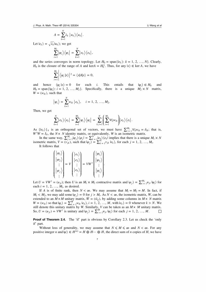
∑λ==

A u u .k

N

k k k

1

Let λ| ⟩ = | ⟩e uk k k ; we get

∑ ∑ψ ψ == =

e e ,i

M

i ik

N

k k

1 1

2

and the series converges in norm topology. Let = | ⟩ = …H e k Nspan{ : 1, 2, , }k0 . Clearly,H0 is the closure of the range of A and = ⊥A Hker 0 . Thus, for any | ⟩ ∈x Aker , we have

∑ ψ = ==

x x A x 0,i

M

i1

22

and hence ψ⟨ | ⟩ =x 0i for each i. This entails that ψ| ⟩ ∈ Hi 0 andψ= | ⟩ = …H i Mspan{ : 1, 2, , }i0 2 . Specifically, there is a unique ×M N2 matrix,

=W w( )ik , such that

∑ψ = = …=

w e i M, 1, 2, , .ik

N

ik k

1

2

Then, we get

⎛⎝⎜⎜

⎞⎠⎟⎟∑ ∑ ∑ ∑ψ ψ= =

= = = =

e e w w e e .k

N

k k

i

M

i ik l

N

i

M

il ik k l

1 1 , 1 1

2 2

As | ⟩e{ }k k is an orthogonal set of vectors, we must have δ∑ == w wiM

il ik lk12 ; that is,

=†W W IN , the N × N identity matrix, or equivalently, W is an isometric matrix.In the same way, φ φ∑ | ⟩⟨ | = ∑ | ⟩⟨ |= = e ej

Mj j k

Nk k1 1

1 implies that there is a unique ×M N1

isometric matrix, =V v( ),jk such that φ| ⟩ = ∑ | ⟩= v ej kN

jk k1 , for each = …j M1, 2, , 1.It follows that

⎛

⎝

⎜⎜⎜⎜⎜⎜⎜

⎞

⎠

⎟⎟⎟⎟⎟⎟⎟

⎛

⎝

⎜⎜⎜⎜⎜⎜

⎞

⎠

⎟⎟⎟⎟⎟⎟

⎛

⎝

⎜⎜⎜⎜⎜⎜⎜

⎞

⎠

⎟⎟⎟⎟⎟⎟⎟

φ

φ

φ

ψ

ψ

ψ

⋮

⋮

= ⋮

⋮

= ⋮

⋮

†V

e

e

e

VW .

j k i

1

2

1

2

1

2

Let = =†U VW u( )ji ; then U is an ×M M1 2 contractive matrix and φ ψ| ⟩ = ∑ | ⟩= uj iM

ji i12 for

each = …i M1, 2, , 1, as desired.If A is of finite rank, then < ∞N . We may assume that = =M M M1 2 . In fact, if

<M M1 2, we may add some φ| ⟩ = 0j for >j M1. As < ∞N , the isometric matrix, W, can beextended to an M ×M unitary matrix, ˜ = ˜W w( )ij , by adding some columns in M × N matrix

=W w( )ik so that ψ| ⟩ = ∑ | ⟩= w ei kM

ik k1 , = …i M1, 2, , , with | ⟩ =e 0k whenever >k N . Westill denote this unitary matrix by W. Similarly, V can be taken as an M × M unitary matrix.So, = = †U u VW( )ji is unitary and φ ψ| ⟩ = ∑ | ⟩= uj i

Mji i1 for each = …j M1, 2, , . □

Proof of Theorem 2.4. The ‘if’ part is obvious by Corollary 2.3. Let us check the ‘onlyif’ part.

Without loss of generality, we may assume that ⩽ ⩽ ∞N M and < ∞N . For anypositive integer n and ψ| ⟩ ∈ = ⊕ ⋯ ⊕H H H Hn( ) , the direct sum of n copies of H, we have

J. Phys. A: Math. Theor 47 (2014) 335304 Li Wang et al

7

∑ ∑ψ ψ ψ ψ= ∈=

†

=

† ( )A A B B K . (2.1)i

M

in

in

i

N

in

in n

1

( ) ( )

1

( ) ( ) ( )

Since the operator in equation (2.1) is of finite rank, by lemma 2.5, equation (2.1) impliesthat there exists an M ×M unitary matrix, ψ=ψU u( ( ))ij , such that

∑ψ ψ ψ= = …=

A u B i M( ) , 1, 2, , .in

j

M

ij jn( )

1

( )

Here we write Bj = 0 whenever >j N . Equivalently, we have shown that, for any ψ| ⟩ ∈ H n( ),there is a unitary operator, ∈ψU l M( ( ))2 , such that

ψ ψ= ⊗ψ( )U IA B , (2.2)n n( ) ( )

where

⎛

⎝

⎜⎜⎜⎜⎜

⎞

⎠

⎟⎟⎟⎟⎟

⎛

⎝

⎜⎜⎜⎜⎜

⎞

⎠

⎟⎟⎟⎟⎟=

⋮=

⋮

A

A

A

B

B

B

A Band .n

n

n

Mn

n

n

n

Mn

( )

1( )

2( )

( )

( )

1( )

2( )

( )

It follows from equation (2.2) that, for any vectors ψ ψ| ⟩ … | ⟩ ∈ H, , n1 , by lettingψ ψ ψ| ⟩ = | ⟩ ⊕ ⋯ ⊕ | ⟩ ∈ Hn

n1

( ),

ψ ψ= ⊗ψ( )U IA B (2.3)k k

holds for each = …k n1, 2, , . Equation (2.3) means that, for any positive number, ε > 0,and any vectors, ψ ψ| ⟩ … | ⟩ ∈ H, , n1 , we can always find a unitary, ∈U l M( ( ))2 , such that

ψ ε⊗ ∈ ∈ ∥ − ∥ < = …{ }( )U I H K k nB T A T( ) , : ( ) , 1, 2 , .Mk

( )

Therefore,

∩ ⊗ ∈ ≠ ∅{ }( )U I U l MA B( ) ( ) : ( ) is unitary2

holds for any strong operator topology (SOT)-neighborhood A( ) of A, which entails that Alies in the SOT-closure of ⊗ ∈U I U l MB{( ) : ( ( )) is unitary}2 . It is well known that theSOT-closure of the set ∈U U H{ : ( ) is unitary} is ∈V V H{ : ( ) is isometric} ([16, pp373]). Therefore, there is an isometric matrix, = ∈V v l M( ) ( ( ))ij

2 , such that

= ⊗V IA B( ) ;

that is, = ∑A v Bi j ij j for each = …i M1, 2, , . Let W be the M × N matrix consisting of firstN columns of V; then, as < ∞N , W can be extended to an M × M unitary matrix, =U u( )ij ,and we still have = ∑ =A u Bi j

Nij j1 for each = …i M1, 2, , .

Consequently, †U is unitary and = ⊗ =† †U I UB A A( ) . □

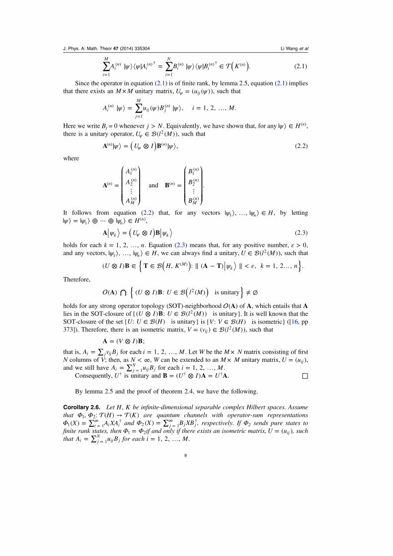
By lemma 2.5 and the proof of theorem 2.4, we have the following.

Corollary 2.6. Let H K, be infinite-dimensional separable complex Hilbert spaces. Assumethat Φ Φ →H K, : ( ) ( )1 2 are quantum channels with operator-sum representationsΦ = ∑ =

∞ †X A XA( ) i i i1 1 and Φ = ∑ =∞ †X B XB( ) j j j2 1 , respectively. If Φ2 sends pure states to

finite rank states, then Φ Φ=1 2if and only if there exists an isometric matrix, =U u( )ij , suchthat = ∑ =A u Bi j

Nij j1 for each = …i M1, 2, , .

J. Phys. A: Math. Theor 47 (2014) 335304 Li Wang et al

8

Remark 2.7. In theorem 2.4, if we also require that both =A{ }i iM

1 and =B{ }j jN

1 are linearlyindependent sets; then we have a very simple proof. In fact, in this situation Φ Φ=1 2 impliesthat = < ∞M N and, by lemma 2.2, there exist N × N contractive matrices, =W w( )ij and

=V v( )ji , such that = WA B and = VB A. Since =A{ }i iM

1 is linearly independent,= =W WVA B A implies that WV = I. Therefore, the contractive matrix, W, is invertible

with =−W V1 still contractive. This clearly forces that W is isometric, and hence unitary,as < ∞N .

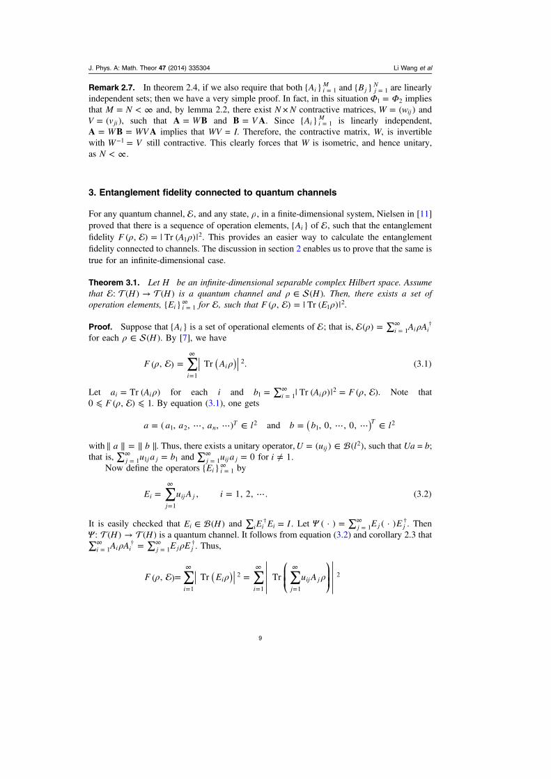
3. Entanglement fidelity connected to quantum channels

For any quantum channel, , and any state, ρ, in a finite-dimensional system, Nielsen in [11]proved that there is a sequence of operation elements, A{ }i of , such that the entanglementfidelity ρ ρ= | |F A( , ) Tr ( )1

2. This provides an easier way to calculate the entanglementfidelity connected to channels. The discussion in section 2 enables us to prove that the same istrue for an infinite-dimensional case.

Theorem 3.1. Let H be an infinite-dimensional separable complex Hilbert space. Assumethat →H H: ( ) ( ) is a quantum channel and ρ ∈ H( ). Then, there exists a set ofoperation elements, =

∞E{ }i i 1 for , such that ρ ρ= | |F E( , ) Tr ( )12.

Proof. Suppose that A{ }i is a set of operational elements of ; that is, ρ ρ= ∑ =∞ †A A( ) i i i1

for each ρ ∈ H( ). By [7], we have

∑ρ ρ==

∞

( )F A( , ) Tr . (3.1)i

i

1

2

Let ρ=a ATr ( )i i for each i and ρ ρ= ∑ | | ==∞b A FTr ( ) ( , )i i1 1

2 . Note thatρ⩽ ⩽F0 ( , ) 1. By equation (3.1), one gets

= ⋯ ⋯ ∈ = ⋯ ⋯ ∈( )a a a a l b b l( , , , , ) and , 0, , 0,nT T

1 22

12

with∥ ∥ = ∥ ∥a b . Thus, there exists a unitary operator, = ∈U u l( ) ( )ij2 , such that Ua = b;

that is, ∑ ==∞ u a bj j j1 1 1 and ∑ ==

∞ u a 0j ij j1 for ≠i 1.Now define the operators =

∞E{ }i i 1 by

∑= = ⋯=

∞

E u A i, 1, 2, . (3.2)i

j

ij j

1

It is easily checked that ∈E H( )i and ∑ =†E E Ii i i . Let Ψ · = ∑ ·=∞ †E E( ) ( )j j j1 . Then

Ψ →H H: ( ) ( ) is a quantum channel. It follows from equation (3.2) and corollary 2.3 thatρ ρ∑ = ∑=

∞ †=

∞ †A A E Ei i i j j j1 1 . Thus,

⎛⎝⎜⎜

⎞⎠⎟⎟ ∑ ∑ ∑ρ ρ ρ= =

=

∞

=

∞

=

∞

( )F E u A( , ) Tr Tri

i

i j

ij j

1

2

1 1

2

J. Phys. A: Math. Theor 47 (2014) 335304 Li Wang et al

9

⎛⎝⎜⎜

⎞⎠⎟⎟

∑ ∑ ∑ ∑

∑ ∑

∑

ρ

ρ

ρ ρ

= =

= =

= =

=

∞

=

∞

=

∞

=

∞

=

∞

=

∞

=

∞

( )

( )

( )

u A u a

u a u A

u A E

Tr

Tr

Tr Tr .

i j

ij j

i j

ij j

j

j j

j

j j

j

j j

1 1

2

1 1

2

1

12

1

12

1

12

12

The proof is finished. □

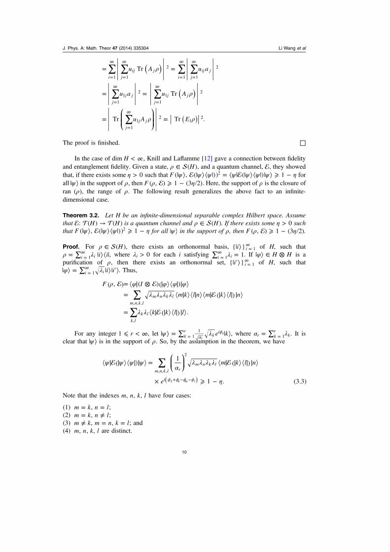
In the case of < ∞Hdim , Knill and Laflamme [12] gave a connection between fidelityand entanglement fidelity. Given a state, ρ ∈ H( ), and a quantum channel, , they showedthat, if there exists some η > 0 such that ψ ψ ψ ψ ψ ψ ψ η| ⟩ | ⟩⟨ | = ⟨ | | ⟩⟨ | | ⟩ ⩾ −F ( , ( )) ( ) 12 forall ψ| ⟩ in the support of ρ, then ρ η⩾ −F ( , ) 1 (3 2). Here, the support of ρ is the closure ofran ρ( ), the range of ρ. The following result generalizes the above fact to an infinite-dimensional case.

Theorem 3.2. Let H be an infinite-dimensional separable complex Hilbert space. Assumethat →H H: ( ) ( ) is a quantum channel and ρ ∈ H( ). If there exists some η > 0 suchthat ψ ψ ψ η| ⟩ | ⟩⟨ | ⩾ −F ( , ( )) 12 for all ψ| ⟩ in the support of ρ, then ρ η⩾ −F ( , ) 1 (3 2).

Proof. For ρ ∈ H( ), there exists an orthonormal basis, | ⟩ =∞i{ } i 1 of H, such that

ρ λ= ∑ | ⟩⟨ |=∞ i ii i1 , where λ > 0i for each i satisfying λ∑ ==

∞ 1i i1 . If φ| ⟩ ∈ ⊗H H is apurification of ρ, then there exists an orthonormal set, | ′⟩ =

∞i{ } i 1 of H, such thatφ λ| ⟩ = ∑ | ⟩| ′⟩=

∞ i ii i1 . Thus,

∑

∑

ρ φ φ φ φλ λ λ λ

λ λ

= ⊗=

=

F I

m k l n m k l n

k k l l

( , ) ( )( )

( )

( ) .

m n k l

m n k l

k l

k l

, , ,

,

For any integer ⩽ < ∞r1 , let ψ λ| ⟩ = ∑ | ⟩α

ϕ= e kk

rk

i1

1

r

k , where α λ= ∑ =r kr

k1 . It isclear that ψ| ⟩ is in the support of ρ. So, by the assumption in the theorem, we have

⎛⎝⎜

⎞⎠⎟ ∑ψ ψ ψ ψ

αλ λ λ λ

η

=

× ⩾ −ϕ ϕ ϕ ϕ+ − −( )

m k l n

e

( )1

( )

1 . (3.3)

m n k l rm n k l

i

, , ,

2

k n m l

Note that the indexes m n k l, , , have four cases:

(1) = =m k n l, ;(2) = ≠m k n l, ;(3) ≠ = =m k m n k l, , ; and(4) m n k l, , , are distinct.

J. Phys. A: Math. Theor 47 (2014) 335304 Li Wang et al

10

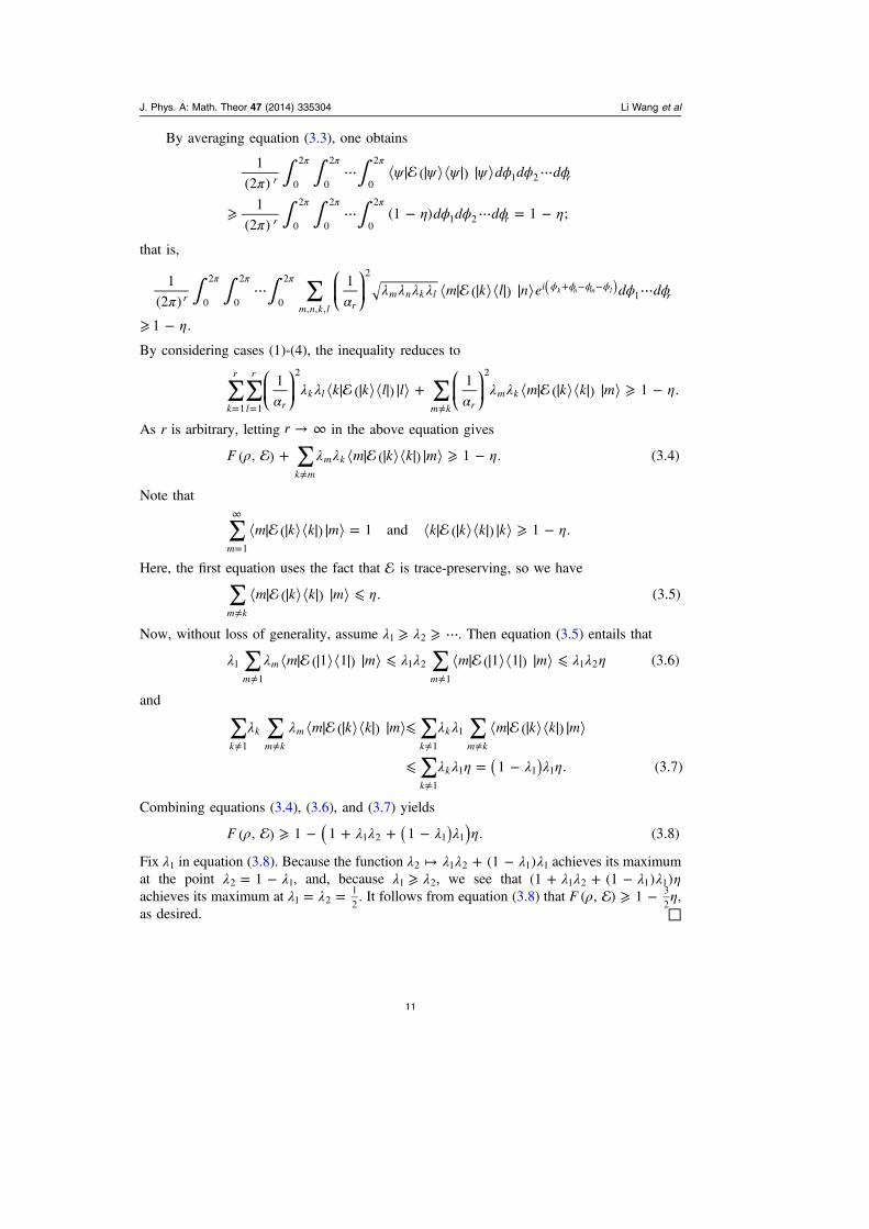
By averaging equation (3.3), one obtains

∫ ∫ ∫

∫ ∫ ∫π

ψ ψ ψ ψ ϕ ϕ ϕ

πη ϕ ϕ ϕ η

⋯ ⋯

⩾ ⋯ − ⋯ = −

π π π

π π π

d d d

d d d

1

(2 )( )

1

(2 )(1 ) 1 ;

r r

r r

0

2

0

2

0

2

1 2

0

2

0

2

0

2

1 2

that is,

⎛⎝⎜

⎞⎠⎟ ∫ ∫ ∫ ∑

π αλ λ λ λ ϕ ϕ

η

⋯ ⋯

⩾ −

π π πϕ ϕ ϕ ϕ+ − −( )m k l n e d d

1

(2 )

1( )

1 .

rm n k l r

m n k li

r0

2

0

2

0

2

, , ,

2

1k n m l

By considering cases (1)-(4), the inequality reduces to

⎛⎝⎜

⎞⎠⎟

⎛⎝⎜

⎞⎠⎟ ∑∑ ∑

αλ λ

αλ λ η+ ⩾ −

= = ≠

k k l l m k k m1

( )1

( ) 1 .k

r

l

r

rk l

m k rm k

1 1

2 2

As r is arbitrary, letting → ∞r in the above equation gives

∑ρ λ λ η+ ⩾ −≠

F m k k m( , ) ( ) 1 . (3.4)k m

m k

Note that

∑ η= ⩾ −=

∞

m k k m k k k k( ) 1 and ( ) 1 .m 1

Here, the first equation uses the fact that is trace-preserving, so we have

∑ η⩽≠

m k k m( ) . (3.5)m k

Now, without loss of generality, assume λ λ⩾ ⩾ ⋯1 2 . Then equation (3.5) entails that

∑ ∑λ λ λ λ λ λ η⩽ ⩽≠ ≠

m m m m( 1 1 ) ( 1 1 ) (3.6)m

m

m

1

1

1 2

1

1 2

and

∑ ∑ ∑ ∑

∑

λ λ λ λ

λ λ η λ λ η

⩽

⩽ = −≠ ≠ ≠ ≠

≠( )

m k k m m k k m( ) ( )

1 . (3.7)

k

k

m k

m

k

k

m k

k

k

1 1

1

1

1 1 1

Combining equations (3.4), (3.6), and (3.7) yields

ρ λ λ λ λ η⩾ − + + −( )( )F ( , ) 1 1 1 . (3.8)1 2 1 1

Fix λ1 in equation (3.8). Because the function λ λ λ λ λ↦ + −(1 )2 1 2 1 1 achieves its maximumat the point λ λ= −12 1, and, because λ λ⩾1 2, we see that λ λ λ λ η+ + −(1 (1 ) )1 2 1 1

achieves its maximum at λ λ= =1 21

2. It follows from equation (3.8) that ρ η⩾ −F ( , ) 1 3

2,

as desired. □

J. Phys. A: Math. Theor 47 (2014) 335304 Li Wang et al

11

4. Bounds of quantum fidelity and connection to the trace distance

In [17], Miszczak et al gave the upper and lower bounds of quantum fidelity for finite-dimensional systems and showed that, for any ρ σ ∈ H, ( ) with < ∞Hdim ,

ρ σ ρ σ ρ σ⩽ ⩽E F G( , ) ( , ) ( , ), (4.1)2

where

ρ σ ρσ ρσ ρσρσ= + −E ( , ) Tr ( ) 2 (Tr( )) Tr ( ) (4.2)2

and

ρ σ ρσ ρ σ= + − −( )( )( ) ( )G ( , ) Tr ( ) 1 Tr 1 Tr (4.3)2 2

are called sub-fidelity and super-fidelity of ρ and σ , respectively. One of main advantages ofsub-fidelity and super-fidelity is that it is possible to design feasible schemes to measure it inan experiment [17], so the relation (4.1) may be useful in future research. Note that, in [21],two measures of distance between quantum processes based on the super-fidelity werepresented.

Our first result in this section claims that the inequalities in equation (4.1) still hold forthe infinite-dimensional systems.

Theorem 4.1. Let H be an infinite-dimensional separable complex Hilbert space. Then forany ρ σ ∈ H, ( ), we have

ρ σ ρ σ ρ σ⩽ ⩽E F G( , ) ( , ) ( , ).2

Proof. Let | ⟩ =∞i{ } i 1 be any orthonormal basis of H. For any positive integer n, denote by Hn

and Pn the n-dimensional subspace spanned by | ⟩ | ⟩ ⋯ | ⟩n{ 1 , 2 , , } and the projection onto Hn,respectively. Then, for any | ⟩ ∈x H , we have ξ= ∑ | ⟩=

∞x ii i1 for some ξ ∈i withξ∑ | | = ∥| ⟩∥=

∞ xi i12 2 and ξ| ⟩ = ∑ | ⟩=P x in i

ni1 . For any ρ σ ∈ H, ( ), define

ρ α ρ σ β σ= =− −P P P Pand ,n n n n n n n n1 1

where α ρ= P PTr ( )n n n and β σ= P PTr ( )n n n . Then, regarding ρ σ,n n as states acting on finite-dimensional space Hn = PnH, we have, by equation (4.1),

ρ σ ρ σ ρ σ⩽ ⩽E F G( , ) ( , ) ( , ) (4.4)n n n n n n2

with

ρ σ ρ σ ρ σ ρ σ ρ σ= + −( )E ( , ) Tr( ) 2 Tr( ) Tr ( ) (4.5)n n n n n n n n n n2

and

ρ σ ρ σ ρ σ= + − −( )( )( ) ( )G ( , ) Tr( ) 1 Tr 1 Tr . (4.6)n n n n n n2 2

It is obvious that

α β= =→∞ →∞lim 1, lim 1

nn

nn

J. Phys. A: Math. Theor 47 (2014) 335304 Li Wang et al

12

and

ρ ρ σ σ− = − =→∞ →∞

SOT lim , SOT lim ;n

nn

n

that is, ρ ρ∥ − | ⟩ ∥ →x( ) 0n and σ σ∥ − | ⟩ ∥ →x( ) 0n hold for any | ⟩ ∈x H . Here, SOTdenotes the strong operator topology. By [18], one gets

ρ ρ σ σ= =→∞ →∞lim and lim

nn

nn

under the trace-norm topology. These ensure that

⎛⎝⎜

⎞⎠⎟ρ σ ρ σ ρ σ ρ σ ρσ

ρσ ρσρσ

+ − =

+ −

→∞( )lim Tr ( ) 2 Tr ( ) Tr ( ) Tr ( )

2 (Tr ( )) Tr ( ) ,

nn n n n n n n n

2

2

⎜ ⎟⎛⎝

⎞⎠ρ σ ρ σ ρσ

ρ σ

+ − − =

+ − −

→∞( )( )

( )( )( ) ( )

( ) ( )

lim Tr ( ) 1 Tr 1 Tr Tr ( )

1 Tr 1 Tr ,

nn n n n

2 2

2 2

and

ρ σ ρ σ=→∞

F Flim ( , ) ( , ) .n

n n2 2

It follows from equations (4.4)-(4.6) that

ρσ ρσ ρσρσ ρ σ ρσ

ρ σ

+ − ⩽ ⩽

+ − −( )( )( ) ( )FTr ( ) 2 (Tr( )) Tr ( ) ( , ) Tr ( )

1 Tr 1 Tr ,

2 2

2 2

which completes the proof of the theorem. □

Let H be a Hilbert space with any dimension and ρ σ ∈ H, ( ). Recall that the tracedistance between states ρ and σ is defined by

ρ σ ρ σ ρ σ= ∥ − ∥ = −D ( , )1

2

1

2Tr , (4.7)Tr

where | | = †( )A A A1 2

. The following bounds of the trace distance in terms of quantum fidelity

ρ σ ρ σ ρ σ− ⩽ ⩽ −F D F1 ( , ) ( , ) 1 ( , ) (4.8)2

were obtained in [1] and [7], respectively, for finite-dimensional and infinite-dimensionalcases. Furthermore, for finite-dimensional cases, [19] and [20] gave a tighter lower bound anda new upper bound, respectively, for ρ σD ( , ) in terms of super-fidelity; that is,

ρ σ ρ σ− ⩽G D1 ( , ) ( , ) (4.9)

and

ρ σ τ ρ σ⩽ −D G( , )2

1 ( , ) , (4.10)

where τ ρ σ= −rank( ).We will show that the inequalities (4.9) and (4.10) still hold for states in infinite-

dimensional systems. More precisely, we have the following result.

J. Phys. A: Math. Theor 47 (2014) 335304 Li Wang et al

13

Theorem 4.2. Let H be an infinite-dimensional separable complex Hilbert space. Then forany ρ σ ∈ H, ( ), we have

⎧⎨⎩⎫⎬⎭ρ σ ρ σ ρ σ τ ρ σ− ⩽ ⩽ − −G D E G1 ( , ) ( , ) min 1 ( , ) ,

21 ( , ) ,

where τ ρ σ= −rank( ).

To prove theorem 4.2, we need a lemma.

Lemma 4.3. For any ρ σ ∈ H, ( ), let +P and −P be the projections onto the closure of theranges of ρ σ− +( ) and ρ σ− −( ) , respectively. Then the following four inequalities hold:

ρ ρ σ ρσ− ⩾ −+ +( )( ) ( )P PTr Tr ( ) , (4.11)2

ρ ρ ρ ρσ− ⩾ −− −( )( ) ( )P PTr Tr ( ) , (4.12)2

σ σ σ ρσ− ⩾ −+ +( )( ) ( )P PTr Tr ( ) , (4.13)2

and

σ σ ρ ρσ− ⩾ −− −( )( ) ( )P PTr Tr ( ) . (4.14)2

Proof. Here, we only give the proof of inequality (4.11). Other inequalities are treatedsimilarly.

In fact, for any ρ σ ∈ H, ( ), noting that ρ < I , we have

ρ ρ σ ρσ

ρ ρ σ ρσ ρ σ ρ ρ σ

ρ σ ρ ρ σ ρ σ ρ σ ρ

ρ σ ρ σ

− − −

= − − + = − − −

= − − − = − − −

⩾ − − − =

+ +

+ +

+ + + +

+ +

( )( )

( )( )

( )

( )( ) ( ) ( ) ( )( ) ( )

P P

P P

P P

P

Tr Tr ( )

Tr Tr (( ) ( ))

Tr ( ) Tr ( ) Tr ( ) Tr ( )

Tr ( ) Tr ( ) 0;

2

2

that is, inequality (4.11) is true. □

Proof of theorem 4.2. Combining the inequalities (4.11)-(4.14), we get

ρ ρ σ ρσ ρ ρσ− ⩾ − + −+ −( ) ( ) ( )P PTr Tr ( ) Tr ( ) (4.15)2

and

σ σ σ ρσ ρ ρσ− ⩾ − + −+ −( ) ( ) ( )P PTr Tr ( ) Tr ( ) . (4.16)2

The inequalities (4.15)-(4.16) imply that

ρ ρ σ σ σ ρσ ρ ρσ− − ⩾ − + −+ −( ) ( ) ( ) ( )P PTr Tr Tr ( ) Tr ( ) . (4.17)2 2

J. Phys. A: Math. Theor 47 (2014) 335304 Li Wang et al

14

Note that

ρ σ ρ σ ρ σ ρ σ

ρ σ σ ρ

ρ σ σ ρ σ ρ

σ ρ

= − = − − −

= − + −

= + + + − −

= − −

+ −

+ + − −

+ + − − + −

+ −

( )

( )

( )

( ) ( )

( ) ( ) ( )

( )

( ) ( )

( ) ( ) ( )

( )

D P P

P P P P

P P P P P P

P P

( , )1

2Tr

1

2Tr ( ) ( )

1

2Tr Tr Tr Tr

1

2Tr Tr Tr Tr Tr Tr

1 Tr Tr . (4.18)

By equations (4.17)-(4.18), we see that

ρ σ ρ ρ σ σ σ ρ

σ ρσ ρ ρσρσ

+ − − ⩾ − −

+ − + −= −

+ −

+ −

( ) ( ) ( )( )

( )( )

D P P

P P

( , ) Tr Tr 1 Tr Tr

Tr ( ) Tr ( )

1 Tr ( ).

2 2

It follows that

ρ σ ρ σ− ⩽G D1 ( , ) ( , ).

Thus, the inequality equation (4.9) holds.The inequality ρ σ ρ σ⩽ −D E( , ) 1 ( , ) is an immediate consequence of theorem 4.1

and the inequality (4.8).Now let us prove that the inequality equation (4.10), i.e.

ρ σ τ ρ σ⩽ −D G( , )2

1 ( , ) ,

still holds for an infinite-dimensional case, where τ ρ σ= −rank( ).Note that the product of square roots in the expression of ρ σG ( , ) (as shown in

equation (4.3) is the geometric mean between the linear entropies of ρ and σ . It then followsfrom the inequality of arithmetic and geometric means that

ρ σρ σ

−+

−⩾ − −

( ) ( ) ( ) ( )1 Tr

2

1 Tr

21 Tr 1 Tr . (4.19)

2 22 2

As ρ σ ρ σ ρ σ ρσ∥ − ∥ = − = + −Tr ( ( ) ) Tr ( ) Tr ( ) 2 Tr ( )HS2 2 2 2 , the inequality

equation (4.19) can be re-expressed as the following inequality after summation of ρσTr ( )to its both sides:

ρ σ ρ σ⩾ − ∥ − ∥ ⩾ ⩾G1 11

2( , ) 0, (4.20)HS

2

where, ∥ ∥ = †X : Tr (X X)HS is the Hilbert-Schmidt norm defined for an arbitrary Hilbert-Schmidt operator, X. Specifically, ρ σ− ⩾G1 ( , ) 0 and ρ σ− =G1 ( , ) 0 if and only ifρ σ= , and in turn, if and only if ρ σ =D ( , ) 0.

Now, it follows immediately that the inequality equation (4.10) holds if τ = ∞.Therefore, we may assume in the sequel that τ ρ σ= − < ∞rank( ) . Let

λ λ λ⩾ ⩾ ⋯ >τ 01 2 be the nonzero singular values of ρ σ− . Then, ρ σ λ∥ − ∥ = ∑τ= ,i iTr 1

ρ σ λ∥ − ∥ = ∑τ=[ ]i iHS 1

2 12 . Following from the Cauchy-Schwarz inequality, we have

ρ σ τ ρ σ∥ − ∥ ⩽ ∥ − ∥ . (4.21)Tr HS

J. Phys. A: Math. Theor 47 (2014) 335304 Li Wang et al

15

On the other hand, observe that, by equation (4.20),

ρ σ ρ σ∥ − ∥ ⩽ − G2[1 ( , )] . (4.22)HS

Combining equations (4.21) and (4.22), we get the inequality

ρ σ ρ σ τ ρ σ τ ρ σ= ∥ − ∥ ⩽ ∥ − ∥ ⩽ −D G( , )1

2 2 2[1 ( , )] .tr HS

Hence, we have shown that the other inequality,

⎧⎨⎩⎫⎬⎭ρ σ ρ σ τ ρ σ⩽ − −D E G( , ) min 1 ( , ) ,

21 ( , ) ,

holds, completing the proof. □

5. Conclusions

The unitary freedom in the operator-sum representation for quantum channels of finite-dimensional quantum systems is a basic and very useful feature in quantum informationscience. Applying a recent result found by Hou on characterizing completely positive gen-eralized elementary operators, we, instead of establishing the unitary freedom, establish thebi-contractive freedom feature in the operator-sum representation for quantum channels ofinfinite-dimensional systems. Though we do not know whether or not we still have the unitaryfreedom for infinite-dimensional systems in general, the unitary freedom feature holds forelementary channels. In cases where the channel sends pure states to finite rank states, theisometric freedom feature is valid. These features may be used to study quantum channelsfurther and generalize some nice properties of entanglement fidelity obtained for finite-dimensional cases. For instance, letting ρ be a state in an infinite-dimensional Hilbert space,H, and be a quantum channel of the system, we show that the following properties are true:(1) there exists an operator-sum representation · = ∑ ·=

∞ †E E( ) ( )i i i1 of such that theentanglement fidelity ρ ρ= | |F E( , ) Tr ( )1

2; (2) if there exists some η > 0 such that thequantum fidelity of the pure state, ψ| ⟩, and the image state, ψ ψ| ⟩⟨ |( ), satisfies that

ψ ψ ψ ψ η| ⟩⟨ | | ⟩⟨ | ⩾ −F ( , ( )) 1 for all ψ| ⟩ in the support of ρ, then the entanglement fidelityρ η⩾ −F ( , ) 1 (3 2). The first property gives an easier way of computing entanglement

fidelity and the last property implies that, for both finite-dimensional and infinite-dimensionalsystems, if the fidelity is kept high for all pure states, then the entanglement fidelity is kepthigh for all states. Therefore, to preserve a quantum state and its entanglement accurately, it issufficient to keep the fidelity of storage high, provided this is done for all pure states con-cerned. In addition, we also establish some inequalities between quantum fidelity, ρ σF ( , ),sub-fidelity, ρ σE ( , ), super-fidelity, ρ σG ( , ), and the trace distance, ρ σD ( , ), for infinite-dimensional systems. It is known that some inequalities holding for finite-dimensional sys-tems may no longer be valid for infinite-dimensional cases. However, we show that the basicinequalities (3) ρ σ ρ σ ρ σ⩽ ⩽E F G( , ) ( , ) ( , )2 and (4) ρ σ ρ σ− ⩽G D1 ( , ) ( , )

ρ σ ρ σ⩽ − −τE Gmin { 1 ( , ) , 1 ( , ) }2

still hold for any states ρ σ, in infinite-dimen-sional systems.

Acknowledgments

The authors wish to give their thanks to the referees whose helpful comments improved theoriginal manuscript.

J. Phys. A: Math. Theor 47 (2014) 335304 Li Wang et al

16

This work is partially supported by the National Natural Science Foundation of China(11171249, 11101250) and Youth Foundation of Shanxi Province (2012021004).

References

[1] Nielsen M A and Chuang I L 2000 Quantum Computation and Quantum Information (Cambridge:Cambridge University Press)

[2] Giorda P and Zanardi P 2010 Quantum chaos and operator fidelity metric Phys. Rev. E 81 017203[3] Wang X-G, Sun Z and Wang Z-D 2009 Operator fidelity susceptibility: an indicator of quantum

criticality Phys. Rev. A 79 012105[4] Lu X-M, Sun Z, Wang X-G and Zanardi P 2008 Operator fidelity susceptibility, decoherence, and

quantum criticality Phys. Rev. A 78 032309[5] Uhlmann A 1976 The ‘transition probability’ in the state space of a *-algebra Rep. Math. Phys. 9

273–9[6] Uhlmann A 2011 Transition probability (fidelity) and its relatives Found. Phys. 41 288–98[7] Hou J-C and Qi X-F 2012 Fidelity of states in infinite dimensional quantum systems Science

China G: Physics, Mechanics and Astronomy 55 1820–7[8] Choi M-D 1975 Completely positive linear maps on complex matrix Lin. Alg. Appl. 10 285–90[9] Shirokov M E 2010 Continuity of the von Neumann entropy Commun. Math. Phys. 296 625–54[10] Hou J-C 2010 A characterization of positive linear maps and criteria of entanglement for quantum

states J. Phys. A: Math. Theor. 43 385201[11] Barnum H, Knill E and Nielsen M A 2000 On quantum fidelities and channel capacities IEEE

Trans. Info. Theor. 46 1317–29[12] Knill E and Laflamme R 2000 A theory of quantum error-correcting codes Phys. Rev. Lett.

84 2525[13] Miszczak J A 2011 Singular value decomposition and matrix reordering in quantum information

theory Int. J. Mod. Phys. C 22 897–918 (arXiv:1011.1585)[14] Pearle P 2012 Simple derivation of the Lindblad equation Eur. J. Phys. 33 805–22

(arXiv:1204.2016)[15] Ivan J S, Sabapathy K and Simon R 2011 Operator-sum representation for Bosonic Gaussian

channels Phys. Rev. A 84 042311 (arXiv:1012.4266)[16] Kadison R V and Ringrose J R 1986 Fundamentals of the Theory of Operator Algebras vol I, II

(London: Academic Press)[17] Miszczak J A, Puchala Z, Horodecki P, Uhlmann A and Życzkowski K 2009 Sub- and super-

fidelity as bounds for quantum fidelity Quantum Inf. Comput. 9 103[18] Zhu S and Ma Z-H 2010 Topologies on quantum states Phys. Lett. A 374 1336–41[19] Miszczak J and Puchala Z 2009 Bound on trace distance based on super-fidelity Phys. Rev. A 79

024302[20] Mendonca P E M F, Napolitano R d J, Marchiolli M A, Foster C J and Liang Y-C 2008 Alternative

fidelity measure between quantum states Phys. Rev. A 78 052330[21] Puchala Z, Miszczak J A, Gawron P and Gardas B 2011 Experimentally feasible measures of

distance between quantum operations Quant. Inf. Proc. 10 1–12 (arXiv:0911.0567)

J. Phys. A: Math. Theor 47 (2014) 335304 Li Wang et al

17