Embed Size (px)
Citation preview
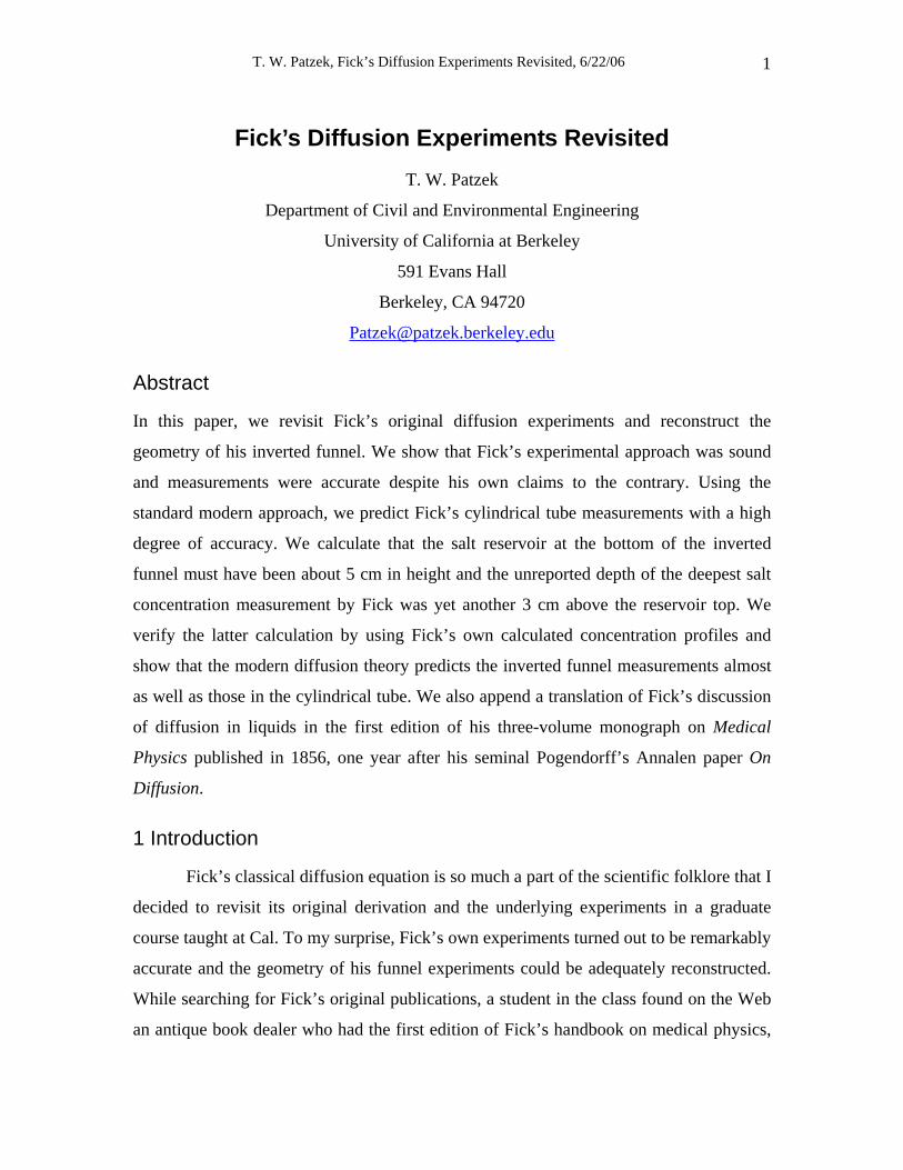
T. W. Patzek, Fick’s Diffusion Experiments Revisited, 6/22/06 1
Fick’s Diffusion Experiments Revisited T. W. Patzek
Department of Civil and Environmental Engineering
University of California at Berkeley
591 Evans Hall
Berkeley, CA 94720
Abstract
In this paper, we revisit Fick’s original diffusion experiments and reconstruct the
geometry of his inverted funnel. We show that Fick’s experimental approach was sound
and measurements were accurate despite his own claims to the contrary. Using the
standard modern approach, we predict Fick’s cylindrical tube measurements with a high
degree of accuracy. We calculate that the salt reservoir at the bottom of the inverted
funnel must have been about 5 cm in height and the unreported depth of the deepest salt
concentration measurement by Fick was yet another 3 cm above the reservoir top. We
verify the latter calculation by using Fick’s own calculated concentration profiles and
show that the modern diffusion theory predicts the inverted funnel measurements almost
as well as those in the cylindrical tube. We also append a translation of Fick’s discussion
of diffusion in liquids in the first edition of his three-volume monograph on Medical
Physics published in 1856, one year after his seminal Pogendorff’s Annalen paper On
Diffusion.
1 Introduction
Fick’s classical diffusion equation is so much a part of the scientific folklore that I
decided to revisit its original derivation and the underlying experiments in a graduate
course taught at Cal. To my surprise, Fick’s own experiments turned out to be remarkably
accurate and the geometry of his funnel experiments could be adequately reconstructed.
While searching for Fick’s original publications, a student in the class found on the Web
an antique book dealer who had the first edition of Fick’s handbook on medical physics,
T. W. Patzek, Fick’s Diffusion Experiments Revisited, 6/22/06 2
which I quickly purchased. I then asked my neighbor who is German by birth and
education to help me in the translation of the relevant sections of the book and she kindly
agreed. The book was written by Fick as an account of physics applicable to medicine
and it brings interesting insights into Fick’s way of thinking about diffusion and osmosis,
see Appendix A. The book section on the diffusion in liquids is more personal and
somewhat different from the two famous papers published one year earlier (Fick 1855;
Fick 1855).
This paper is a simple evaluation of Fick’s original experiments based on the
theory of diffusion presented so well in (Hirschfelder 1954) and (Bird 1960). For an
exquisite and brief discussion of the various theories of diffusion developed over the
decades by Maxwell, Stefan, Onsager, Chapman and Enskog, Eckart and Meixner, and
many others, one may refer to (Truesdell 1962).
Fick’s theory of diffusion is almost as old as the theories of heat conduction by
Fourier (Fourier 1807; Fourier 1822) and viscosity by Newton. While originally it was
too primitive to reveal any ideas of principle, Maxwell soon1 gave it a rational basis in
his kinetic theory of gas mixtures and Stefan (Stefan 1871) cleared away the specifically
kinetic details to achieve an inclusive phenomenological theory, see (Truesdell 1966) for
further details.
2 Background
For convenience, a few pertinent equations describing diffusion will be listed
here. A full derivation may be found in, e.g., (Bird 1960). Let Bv denote the velocity of
constituent2 B of a fluid mixture with respect to a stationary coordinate system, and
define this velocity as by taking a snapshot of instantaneous velocities of the molecules of
B. For a mixture of constituents, we define the local mass-average velocity as cN
1 Maxwell published four important papers on gas theory, the first of which, “Illustrations of the Dynamical Theory of Gases,” appeared in 1860, and contained Maxwell’s first theory of diffusion. See (Garber 1986) for details. 2 “Constituent” denotes a chemical species or a pseudo-component.
T. W. Patzek, Fick’s Diffusion Experiments Revisited, 6/22/06 3
1 1
1
c c
c
N N
B B B BB B
N
BB
v vv
ρ ρ
ρρ
= =
=
= =∑ ∑
∑ (1)
Thus vρ is the local rate at which mass passes through a unit area perpendicular to v .
Similarly, we may define a local molar average velocity as
* 11
1
cc
c
NN
B BB BiB
N
BB
c vc vv
cc
==
=
= =∑∑
∑ (2)
Thus is the local rate at which moles pass through a unit area perpendicular to *cv *v .
In flow systems one is often interested in the velocity of a given constituent with
respect to or , rather than with respect to a stationary coordinate system. This leads
to the following definition of the diffusion velocities:
v *v
(3) ( )
* *( )
diffusion velocity of to
diffusion velocity of to D B B
D B B
v v v B v
v v v B
≡ − =
≡ − =
relative
relative *v
These velocities measure the motion of constituent B in a fluid relative to the local mean
motion of the fluid.
Now we can define the different mass and molar fluxes. The mass or molar flux
of constituent B is defined as a vector whose magnitude is equal to the mass or moles of
constituent B that pass through a unit area per unit time. The motion may be referred to
stationary coordinates, to the local mass-average velocity, v , or to the local molar-
average velocity, *v . Thus the mass and molar flux densities relative to stationary
coordinates are
( ) ( )mass, molarm B B B n B B Bj v j c vρ= = (4)
T. W. Patzek, Fick’s Diffusion Experiments Revisited, 6/22/06 4
The mass and molar flux densities relative to the mass-average velocity are v
(5) ( | ) ( ) ( | ) ( )mass, molarm v B b D B n v B B D Bj v j c vρ= =
and the mass and molar flux densities relative to the molar-average velocity are *v
(6) * ** *( ) ( )( | ) ( | )
mass, molarB D B B D Bm v B n v Bj v j c vρ= =
Again, one should remember that the definition of a mass flux density is incomplete until
both the units and the frame of reference are given.
By analogy with the flux of energy in one-dimensional systems:
( ) (Fourier's law for constant ),y pdq c Tdy
α ρ ρ= − pc (7)
one may define the mass flux of constituent 1 in a binary system 12 as
1 12 1( ) (Fick's law for constant )ydj Ddy
ρ ρ= − (8)
Note that the total mass density, ρ , of the mixture is uniform, i.e., constant given a
constant temperature. Here α is the thermal diffusivity, is the heat capacity, is
the diffusion coefficient, and
pc 12D
1ρ is the mass density of constituent 1.
If the fluid density is not uniform, one defines the mass diffusivity in a
binary system in an analogous fashion:
12 21D D=
*( | )1 12 1 12 1( | )1mass, molarm v n v
j D w j cD xρ= ∇ = ∇ (9)
T. W. Patzek, Fick’s Diffusion Experiments Revisited, 6/22/06 5
Note that Eq. (9) is purely kinematic, i.e., it involves only the dimensions of length and
time, and it must be justified from an independent dynamic theory that invokes forces.
It may easily be shown (Bird 1960) that the mass or molar diffusion fluxes in Eq.
(9) are also given by
*
2
( | )1 ( )1 1 ( ) 12 11
2
( )1 1 ( ) 12 1( | )11
m v m m BB
n n Bn vB
j j w j D w
j j x j cD x
ρ=
=
= − = − ∇
= − = − ∇
∑
∑ (10)
These two relationships are of special importance for this paper.
3 Fick’s cylindrical tube experiment
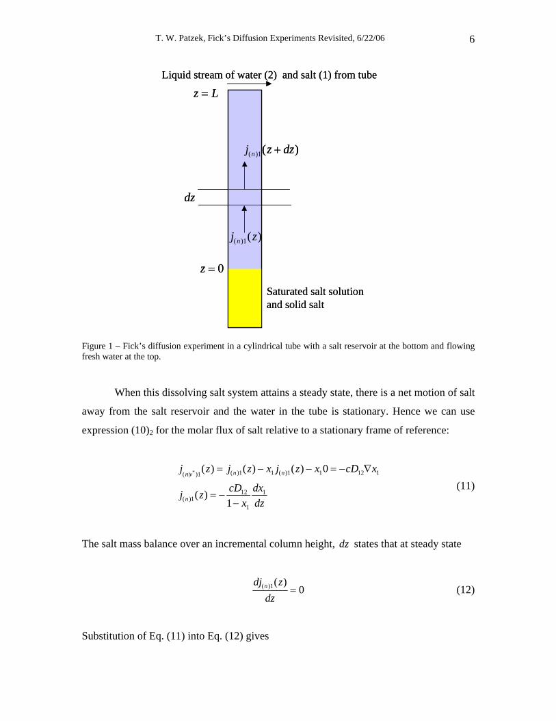
Fick’s experiment (Fick 1855) in a cylindrical tube is shown in Figure 1. At
, salt (1) diffuses into fresh water (2), while solid salt in a salt reservoir dissolves,
replenishing the diffusing salt, and maintaining the saturated salt concentration at
z L=
0z = .
A stream of fresh water sweeps the salt emerging from the tube, keeping the zero salt
concentration at z L= . The whole system is at constant (albeit unknown) temperature
and pressure. The mixture of salt and water is assumed ideal, i.e., each component
activity is equal to its mole fraction.
T. W. Patzek, Fick’s Diffusion Experiments Revisited, 6/22/06 6
0z =
z L=
Saturated salt solutionand solid salt
Liquid stream of water (2) and salt (1) from tube
dz
( )1( )nj z
( )1( )nj z dz+
0z =
z L=
Saturated salt solutionand solid salt
Liquid stream of water (2) and salt (1) from tube
dz
( )1( )nj z
( )1( )nj z dz+
Figure 1 – Fick’s diffusion experiment in a cylindrical tube with a salt reservoir at the bottom and flowing fresh water at the top.
When this dissolving salt system attains a steady state, there is a net motion of salt
away from the salt reservoir and the water in the tube is stationary. Hence we can use
expression (10)2 for the molar flux of salt relative to a stationary frame of reference:
* ( )1 1 ( )1 1 12 1( | )1
12 1( )1
1
( ) ( ) ( ) 0
( )1
n nn v
n
j z j z x j z x cD x
cD dxj zx dz
= − − = −
= −−
∇
(11)
The salt mass balance over an incremental column height, dz states that at steady state
( )1( )0ndj z
dz= (12)
Substitution of Eq. (11) into Eq. (12) gives
T. W. Patzek, Fick’s Diffusion Experiments Revisited, 6/22/06 7
12 1
1
01
d cD dxdz x dz
⎛ ⎞=⎜ ⎟−⎝ ⎠
(13)
We shall assume that is nearly independent of concentration. Indeed the literature
data show that for 0.1-1 normal salt solutions. The saturated salt
concentration is about 36g NaCl/100g of water or 26g NaCl/100g solution at room
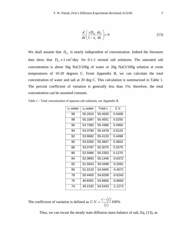
temperatures of 10-20 degrees C. From Appendix B, we can calculate the total
concentration of water and salt at 20 deg C. This calculation is summarized in
12D
212 1 cm /dayD ≈
Table 1.
The percent coefficient of variation is generally less than 1%; therefore, the total
concentration can be assumed constant.
Table 1 – Total concentration of aqueous salt solutions, see Appendix B.
c1-water c5-water Total c C.V.
99 55.2915 55.4635 0.5408
98 55.1087 55.4551 0.5255
96 54.7360 55.4386 0.4956
94 54.3790 55.4478 0.5123
92 53.9682 55.4133 0.4498
90 53.5350 55.3667 0.3653
88 53.0787 55.3075 0.2579
86 52.5986 55.2353 0.1270
84 52.0893 55.1446 -0.0372
82 51.5643 55.0498 -0.2091
80 51.0133 54.9405 -0.4072
78 50.4400 54.8208 -0.6243
76 49.8391 54.6856 -0.8693
74 49.2182 54.5433 -1.1273
The coefficient of variation is defined as C.V. 100%c c
c−
=
Thus, we can recast the steady state diffusion mass balance of salt, Eq. (13), as
T. W. Patzek, Fick’s Diffusion Experiments Revisited, 6/22/06 8
1
1
1 1
1 01
(0) 0.0976, ( ) 0
d dxdz x dzx x
⎛ ⎞=⎜ ⎟−⎝ ⎠
L= =
(14)
This equation can be easily solved (Bird 1960) and the result is
1 1
1 1
1 1 (1 (0) 1 (0)
z
) Lx x Lx x
⎛− −= ⎜− −⎝ ⎠
⎞⎟ (15)
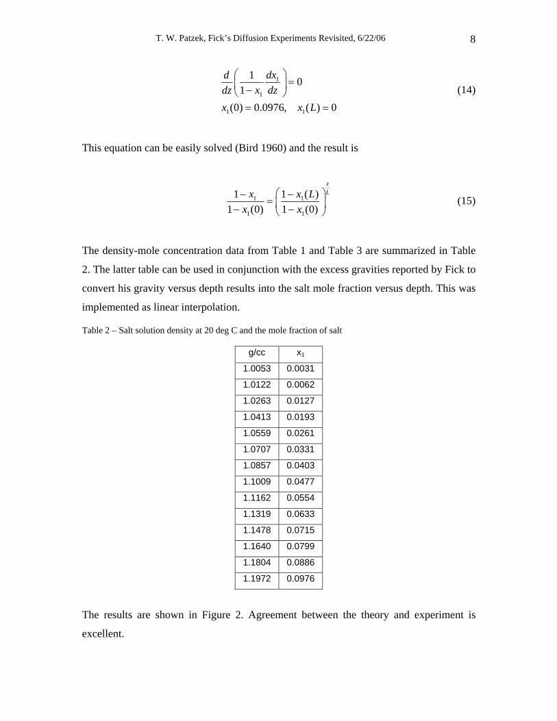
The density-mole concentration data from Table 1 and Table 3 are summarized in Table
2. The latter table can be used in conjunction with the excess gravities reported by Fick to
convert his gravity versus depth results into the salt mole fraction versus depth. This was
implemented as linear interpolation.
Table 2 – Salt solution density at 20 deg C and the mole fraction of salt
g/cc x1
1.0053 0.0031
1.0122 0.0062
1.0263 0.0127
1.0413 0.0193
1.0559 0.0261
1.0707 0.0331
1.0857 0.0403
1.1009 0.0477
1.1162 0.0554
1.1319 0.0633
1.1478 0.0715
1.1640 0.0799
1.1804 0.0886
1.1972 0.0976
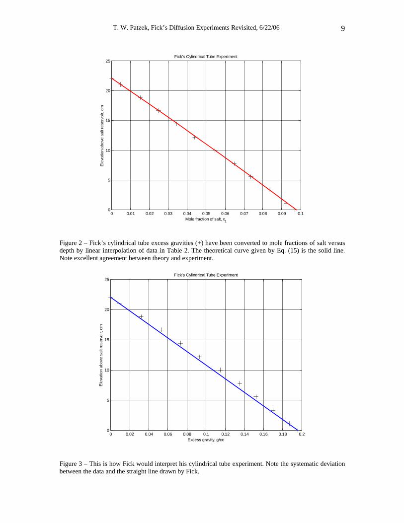
The results are shown in Figure 2. Agreement between the theory and experiment is
excellent.
T. W. Patzek, Fick’s Diffusion Experiments Revisited, 6/22/06 9
0 0.01 0.02 0.03 0.04 0.05 0.06 0.07 0.08 0.09 0.10
5
10
15
20
25Fick's Cylindrical Tube Experiment
Ele
vatio
n ab
ove
salt
rese
rvoi
r, cm
Mole fraction of salt, x1
Figure 2 – Fick’s cylindrical tube excess gravities (+) have been converted to mole fractions of salt versus depth by linear interpolation of data in Table 2. The theoretical curve given by Eq. (15) is the solid line. Note excellent agreement between theory and experiment.
0 0.02 0.04 0.06 0.08 0.1 0.12 0.14 0.16 0.18 0.20
5
10
15
20
25Fick's Cylindrical Tube Experiment
Ele
vatio
n ab
ove
salt
rese
rvoi
r, cm
Excess gravity, g/cc
Figure 3 – This is how Fick would interpret his cylindrical tube experiment. Note the systematic deviation between the data and the straight line drawn by Fick.
T. W. Patzek, Fick’s Diffusion Experiments Revisited, 6/22/06 10
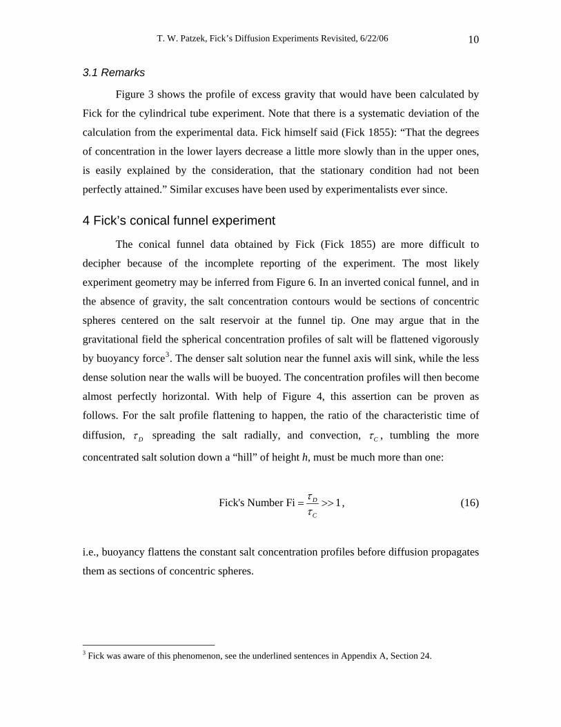
3.1 Remarks
Figure 3 shows the profile of excess gravity that would have been calculated by
Fick for the cylindrical tube experiment. Note that there is a systematic deviation of the
calculation from the experimental data. Fick himself said (Fick 1855): “That the degrees
of concentration in the lower layers decrease a little more slowly than in the upper ones,
is easily explained by the consideration, that the stationary condition had not been
perfectly attained.” Similar excuses have been used by experimentalists ever since.
4 Fick’s conical funnel experiment
The conical funnel data obtained by Fick (Fick 1855) are more difficult to
decipher because of the incomplete reporting of the experiment. The most likely
experiment geometry may be inferred from Figure 6. In an inverted conical funnel, and in
the absence of gravity, the salt concentration contours would be sections of concentric
spheres centered on the salt reservoir at the funnel tip. One may argue that in the
gravitational field the spherical concentration profiles of salt will be flattened vigorously
by buoyancy force3. The denser salt solution near the funnel axis will sink, while the less
dense solution near the walls will be buoyed. The concentration profiles will then become
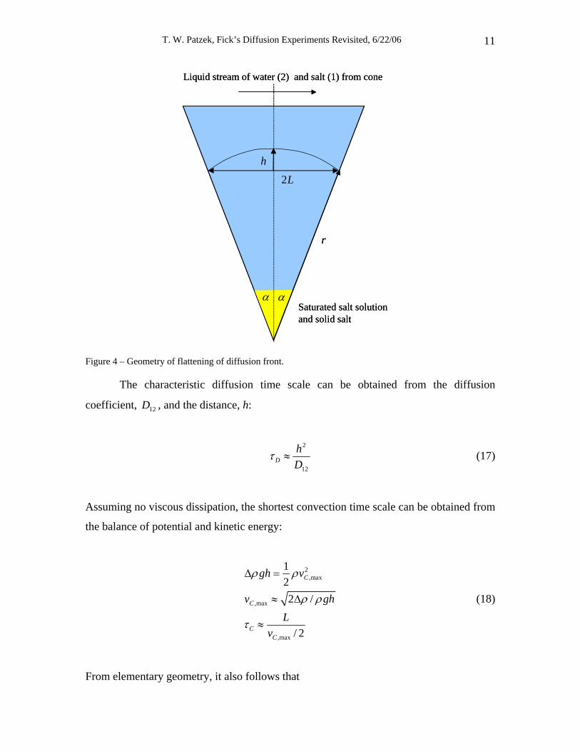
almost perfectly horizontal. With help of Figure 4, this assertion can be proven as
follows. For the salt profile flattening to happen, the ratio of the characteristic time of
diffusion, Dτ spreading the salt radially, and convection, Cτ , tumbling the more
concentrated salt solution down a “hill” of height h, must be much more than one:
Fick's Number Fi 1D
C
ττ
= >> , (16)
i.e., buoyancy flattens the constant salt concentration profiles before diffusion propagates
them as sections of concentric spheres.
3 Fick was aware of this phenomenon, see the underlined sentences in Appendix A, Section 24.
T. W. Patzek, Fick’s Diffusion Experiments Revisited, 6/22/06 11
Saturated salt solutionand solid salt
Liquid stream of water (2) and salt (1) from cone
h
r
2L
ααSaturated salt solutionand solid salt
Liquid stream of water (2) and salt (1) from cone
h
r
2L
αα
Figure 4 – Geometry of flattening of diffusion front.
The characteristic diffusion time scale can be obtained from the diffusion
coefficient, , and the distance, h: 12D
2
12D
hD
τ ≈ (17)
Assuming no viscous dissipation, the shortest convection time scale can be obtained from
the balance of potential and kinetic energy:
2,max
,max
,max
122 /
/ 2
C
C
CC
gh v
vL
v
ρ ρ
ghρ ρ
τ
Δ =
≈ Δ
≈
(18)
From elementary geometry, it also follows that
T. W. Patzek, Fick’s Diffusion Experiments Revisited, 6/22/06 12
sin ,(1 cos )
L rh r
αα
== −
(19)
By combining Eqs. (16) - (19), one obtains the following criterion
2 3/ 2 5/ 212
12
3/ 2
125
2/ (1 cos )Fi 1,2sin2 / 2
2 sin2 (1 cos )
crit
gh D r g gDL g h
Dr rg
α ρα ρ
αα
′− Δ′≈ = >> ≡′
⎡ ⎤>> ≡ ⎢ ⎥
′ −⎢ ⎥⎣ ⎦
(20)
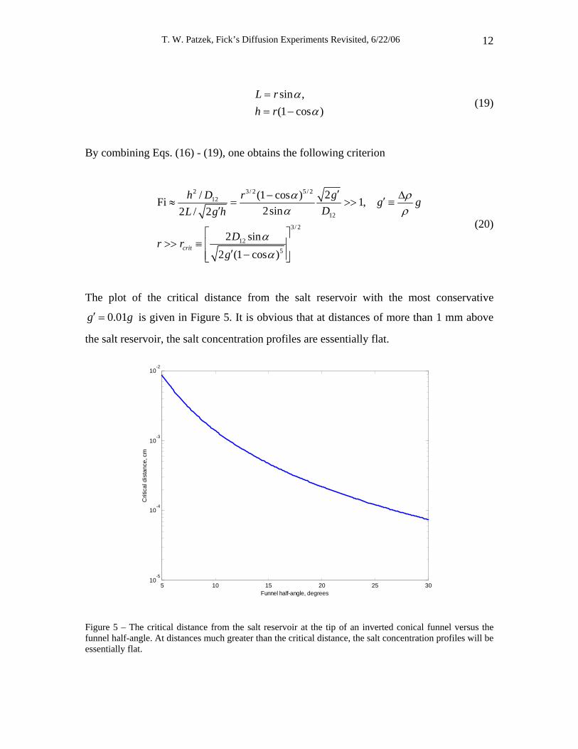
The plot of the critical distance from the salt reservoir with the most conservative
is given in 0.01g′ = g Figure 5. It is obvious that at distances of more than 1 mm above
the salt reservoir, the salt concentration profiles are essentially flat.
5 10 15 20 25 3010
-5
10-4
10-3
10-2
Funnel half-angle, degrees
Crit
ical
dis
tanc
e, c
m
Figure 5 – The critical distance from the salt reservoir at the tip of an inverted conical funnel versus the funnel half-angle. At distances much greater than the critical distance, the salt concentration profiles will be essentially flat.
T. W. Patzek, Fick’s Diffusion Experiments Revisited, 6/22/06 13
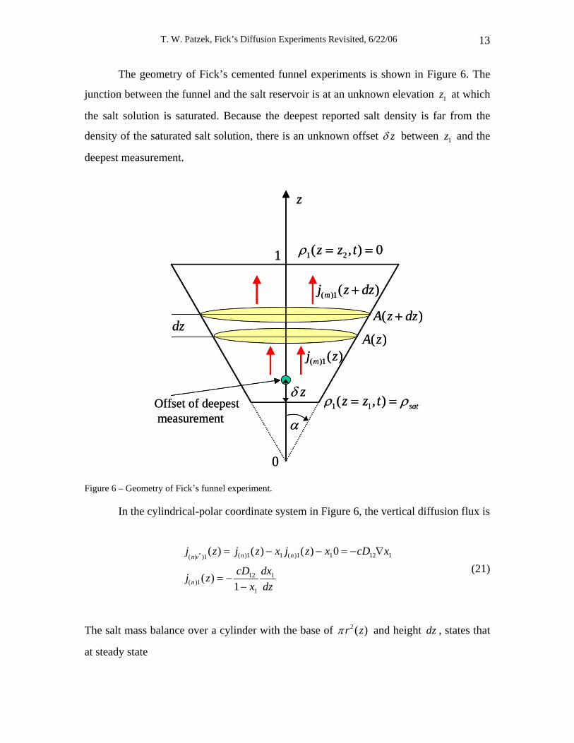
The geometry of Fick’s cemented funnel experiments is shown in Figure 6. The
junction between the funnel and the salt reservoir is at an unknown elevation at which
the salt solution is saturated. Because the deepest reported salt density is far from the
density of the saturated salt solution, there is an unknown offset
1z
zδ between and the
deepest measurement.
1z
z
( )A z dz+
( )A zdz
( )1( )mj z
( )1( )mj z dz+
1 1( , ) satz z tρ ρ= =
1 2( , ) 0z z tρ = =
0
1
α
zδOffset of deepestmeasurement
z
( )A z dz+
( )A zdz
( )1( )mj z
( )1( )mj z dz+
1 1( , ) satz z tρ ρ= =
1 2( , ) 0z z tρ = =
0
1
α
zδOffset of deepestmeasurement
Figure 6 – Geometry of Fick’s funnel experiment.
In the cylindrical-polar coordinate system in Figure 6, the vertical diffusion flux is
* ( )1 1 ( )1 1 12 1( | )1
12 1( )1
1
( ) ( ) ( ) 0
( )1
n nn v
n
j z j z x j z x cD x
cD dxj zx dz
= − − = −
= −−
∇
(21)
The salt mass balance over a cylinder with the base of and height dz , states that
at steady state
2 ( )r zπ
T. W. Patzek, Fick’s Diffusion Experiments Revisited, 6/22/06 14
( )
( )
2( )1
2( )1
( ) ( ) 0,
( ) 0
n
n
d r z j zdzd z j zdz
=
=. (22)
Substitution of Eq. (21) into Eq. (22) and assumption of constant give 12cD
2 1
1
1 1 1 2
1 0,1
( ) 0.0976, ( ) 0.
d dxzdz x dzx z x z
⎛ ⎞=⎜ ⎟−⎝ ⎠
= =
(23)
Equation (23) can be readily solved (Bird 1960) and the result is
1
1 2
1/ 1/1/ 1/
1 1 2
1 1 1 1
1 ( ) 1 ( )1 ( ) 1 ( )
z zz zx z x z
x z x z
−−⎛ ⎞− −
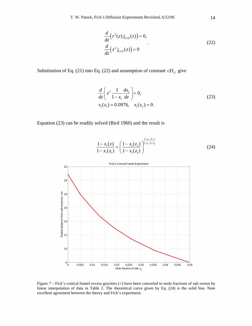
= ⎜ ⎟− −⎝ ⎠ (24)
0 0.005 0.01 0.015 0.02 0.025 0.03 0.035 0.04 0.045 0.058
10
12
14
16
18
20
22Fick's Conical Funnel Experiment
Rad
ial d
ista
nce
from
sal
t res
ervo
ir, c
m
Mole fraction of salt, x1
Figure 7 – Fick’s conical funnel excess gravities (+) have been converted to mole fractions of salt versus by linear interpolation of data in Table 2. The theoretical curve given by Eq. (24) is the solid line. Note excellent agreement between the theory and Fick’s experiment.
T. W. Patzek, Fick’s Diffusion Experiments Revisited, 6/22/06 15
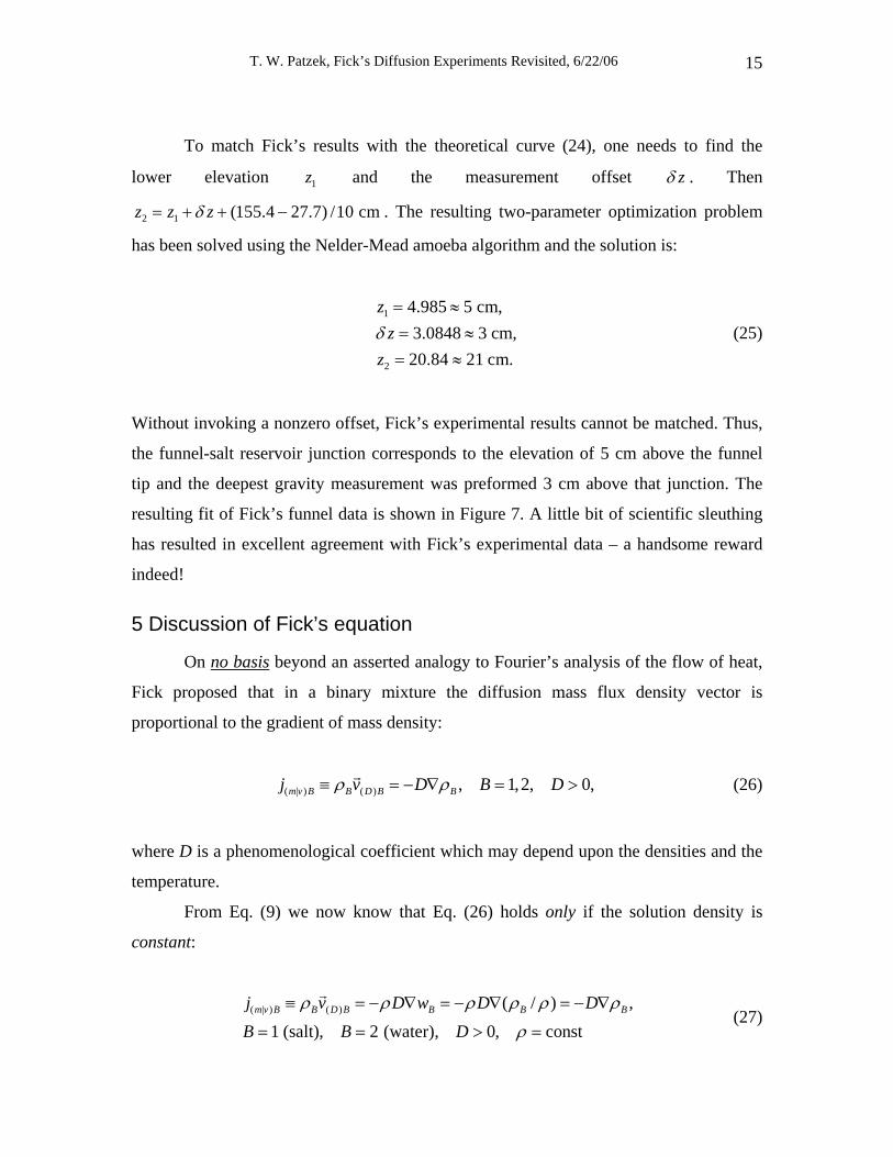
To match Fick’s results with the theoretical curve (24), one needs to find the
lower elevation and the measurement offset 1z zδ . Then
2 1 (155.4 27.7) /10 cmz z zδ= + + − . The resulting two-parameter optimization problem
has been solved using the Nelder-Mead amoeba algorithm and the solution is:
1
2
4.985 5 cm,3.0848 3 cm,20.84 21 cm.
zz
zδ= ≈= ≈= ≈
(25)
Without invoking a nonzero offset, Fick’s experimental results cannot be matched. Thus,
the funnel-salt reservoir junction corresponds to the elevation of 5 cm above the funnel
tip and the deepest gravity measurement was preformed 3 cm above that junction. The
resulting fit of Fick’s funnel data is shown in Figure 7. A little bit of scientific sleuthing
has resulted in excellent agreement with Fick’s experimental data – a handsome reward
indeed!
5 Discussion of Fick’s equation
On no basis beyond an asserted analogy to Fourier’s analysis of the flow of heat,
Fick proposed that in a binary mixture the diffusion mass flux density vector is
proportional to the gradient of mass density:
( | ) ( ) , 1,2, 0,m v B B D B Bj v D B Dρ ρ≡ = − ∇ = > (26)
where D is a phenomenological coefficient which may depend upon the densities and the
temperature.
From Eq. (9) we now know that Eq. (26) holds only if the solution density is
constant:
( | ) ( ) ( / ) ,1 (salt), 2 (water), 0, const
m v B B D B B B Bj v D w D DB B D
ρ ρ ρ ρ ρ ρ
ρ
≡ = − ∇ = − ∇ = − ∇
= = > = (27)
T. W. Patzek, Fick’s Diffusion Experiments Revisited, 6/22/06 16
Because densities of Fick’s salt solutions varied by almost 20%, Fick in fact was
mistaken in asserting Eq. (26). His subsequent diffusion equation was derived from a
shell mass balance between two horizontal planes dz apart.
Based on the mass balance shown in Figure 6, Fick derived the following
equation:
( )
1( )1 ( )1
1( )1
( ) ( , ) ( ) ( , ) ( )
1 ( ) ( , )( )
m m
m
A z dz j z t A z j z dz t A z dzt
A z j z tt A z z
ρ
ρ
∂= − +
∂∂ ∂
= −∂ ∂
+ (28)
Instead of inserting the salt mass flux density from Eq. (10) (he did not know this
equation), Fick asserted Eq. (26), and obtained the following equation:
2
1 12
1( )
dADt z A z dz
1
zρ ρ⎛∂ ∂ ∂
= +⎜∂ ∂ ∂⎝ ⎠
ρ ⎞⎟ . (29)
At steady state, and in the conical funnel whose radius is given as ( ) (tan )r z zα= ,
Fick simplified equation (29) and solved it:
21 1
2
21 1
2 0
( )
d ddz z dz
Cz Cz
ρ ρ
ρ
+ =
= −, (30)
The two constants and “…are to be so determined, that for a certain z
(where the cone is cut off and rests upon the salt reservoir
1C 2C4) 1ρ is equal to perfect
4 Fick used y instead of 1ρ and x instead of z. So his “certain distance x“ becomes in our notation. 1z z=
T. W. Patzek, Fick’s Diffusion Experiments Revisited, 6/22/06 17
saturation; and for a certain value of z which corresponds to the base of the funnel5, 1ρ
becomes =0.” Thus
1 2 1 1( ) 0, ( ) 0.196 g/cc.satz z z zρ ρ ρ= = = = = (31)
If Fick knew about Eq. (10), then instead of Eq. (30) he would have probably
written:
21
1 1
1 1( ) 0,1 1
d dx d dxcD A z zdz x dz dz x dz
⎛ ⎞ ⎛ 1 ⎞= =⎜ ⎟ ⎜− −⎝ ⎠ ⎝⎟⎠
(32)
and he would have obtained Eq. (23).
0 0.02 0.04 0.06 0.08 0.1 0.128
10
12
14
16
18
20
22Fick's Conical Funnel Experiment
Ele
vatio
n ov
er c
one
tip, c
m
Excess gravity, g/cc
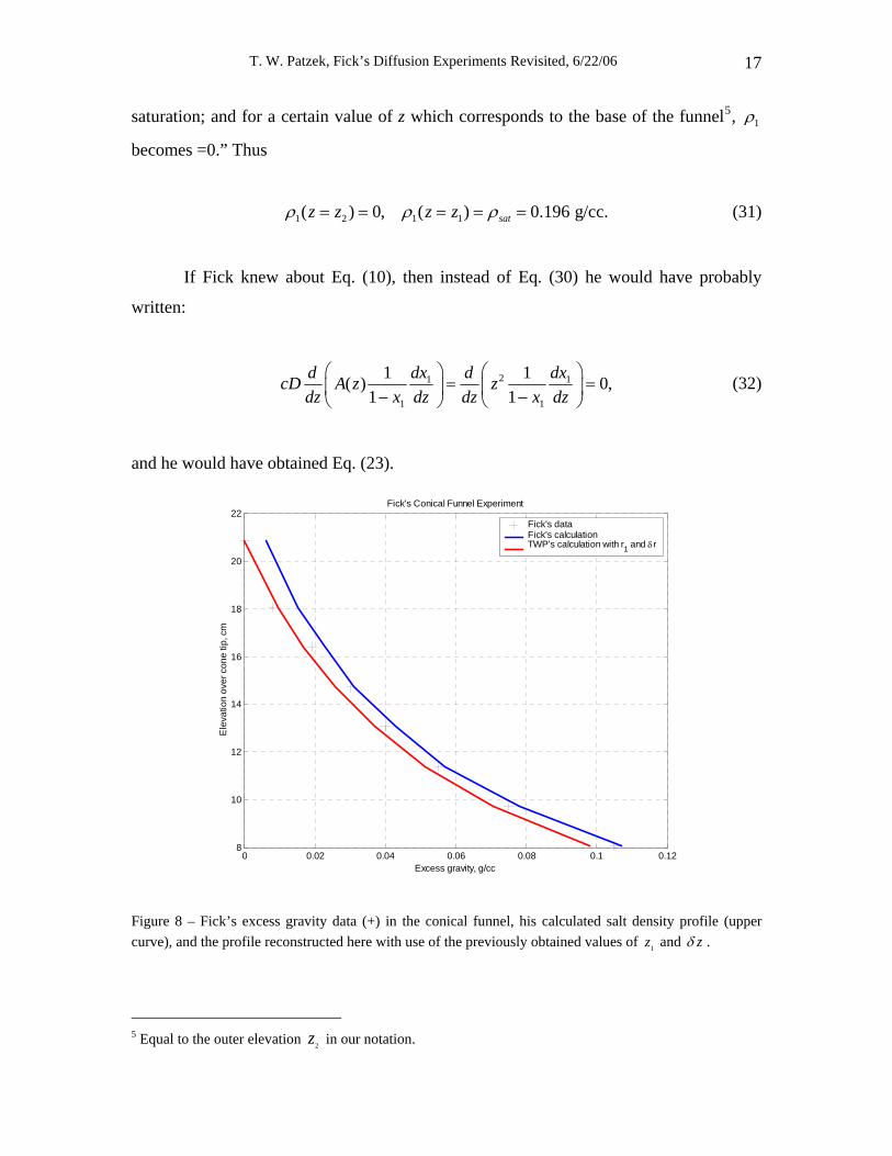
Fick's data Fick's calculation TWP's calculation with r1 and δr
Figure 8 – Fick’s excess gravity data (+) in the conical funnel, his calculated salt density profile (upper curve), and the profile reconstructed here with use of the previously obtained values of and 1z zδ .
5 Equal to the outer elevation in our notation. 2z
T. W. Patzek, Fick’s Diffusion Experiments Revisited, 6/22/06 18
Because Fick does not report these “certain values of z,” to obtain the two
constants we must use the elevation of the funnel base, and the offset of the deepest
measurement calculated above. The two constants in Eq. (30) are then readily calculated
as . In the paper, however, Fick lists his calculated salt
density profile! The raw data, Fick’s calculation and the present calculation are shown in
1 2-0.0616, C 1.2843C = =
Figure 8. Agreement between the reconstructed solution and Fick’s ‘exact’ calculation is
very good indeed. The latter comparison confirms validity of the elevations (or axial
distances) listed in Eq. (25). Of course, because of the incorrect form of the governing
equation, the solutions shown in Figure 8 are nowhere nearly as good as the solution
shown in Figure 7.
6 Conclusions
In general, Fick’s equation (29) is not entirely correct. For the concentrated salt
solutions, one may not assert that mass density 1ρ is the appropriate unit of
concentration, and that constρ = . As it stands, after the sign correction, Fick’s original
equation can only be applied to dilute solutions and to such tubes of variable cross-
section whose walls are orthogonal to the surfaces of constant concentration. This does
not detract however from Fick’s great physical insight, and from his creative and quite
accurate6 experimental technique!
7 Acknowledgements
The financial support for this work was provided by PV Technologies, Inc. I
would like to thank Ms. Karin Lloyd-Mumford for her patience and tenacity in translating
Fick’s difficult prose. I am grateful to Prof. T. N. Narasimhan for sharing his insights into
the theories of diffusion and copies of the out-of-print books and papers. I would also like
to thank Dr. Mark Jellinek for sketching the gravitational equilibration equations (16)-
(18). Finally, I would like to thank the Spring 2000, E241 Class for the excellent
questions about diffusion.
6 Fick remained modest about his approach: ”…This method (of weighing an immersed glass bulb to determine density) creates little confidence at first sight, nevertheless preliminary experiments showed it to be sufficiently accurate.”
T. W. Patzek, Fick’s Diffusion Experiments Revisited, 6/22/06 19
8 References
Achmatowicz, O., et al., Ed. (1954). Chemical Calendar, Vol. I (in Polish). Warsaw,
PWN.
Achmatowicz, O., et al., Ed. (1954). Chemical Calendar, Vol. 2, Part II (in Polish).
Warsaw, PWN.
Bird, R. B., Stewart, W. E., and Lightfoot, E. N. (1960). Transport Phenomena. New
York, John Wiley & Sons, Inc.
Fick, A. (1855). “On Liquid Diffusion.” The London, Edinburgh, and Dublin
Philosophical Magazine and Journal of Science 10 - Fourth Series(July-September): 30-
39.
Fick, A. (1855). “Ueber Diffusion (On Diffusion).” Annalen der Physik und Chemie von
J. C. Pogendorff 94: 59-86.
Fourier, J. B. J. (1807). “Théorie des mouvements de la chaleur dans le corps solides.”
French Academy.
Fourier, J. B. J. (1822). Theory of Heat (Théorie Analytique del la Chaleur). Paris, F.
Didot.
Garber, E., Brush, S. G., and Everitt, C. W. F., Ed. (1986). Maxwell on Molecules and
Gases. Cambridge, Massachusetts, MIT Press.
Hirschfelder, J. O., Curtiss, C. F., and Bird, R. B. (1954). Molecular Theory of Gases and
Liquids. New York, John Wiley & Sons, Inc.
Stefan, J. (1871). “Über das Gleichgewicht und die Bewegung, insbesondere die
Diffusion von Gasmengen.” Wiener Sitzungsberichte 63: 63-124.
Truesdell, C. (1962). “Mechanical basis of diffusion.” J. Chem. Phys. 37.
Truesdell, C. (1966). The Elements of Continuum Mechanics. New York, Springer-
Verlag.
T. W. Patzek, Fick’s Diffusion Experiments Revisited, 6/22/06 20
Appendix A – Laws of Diffusions
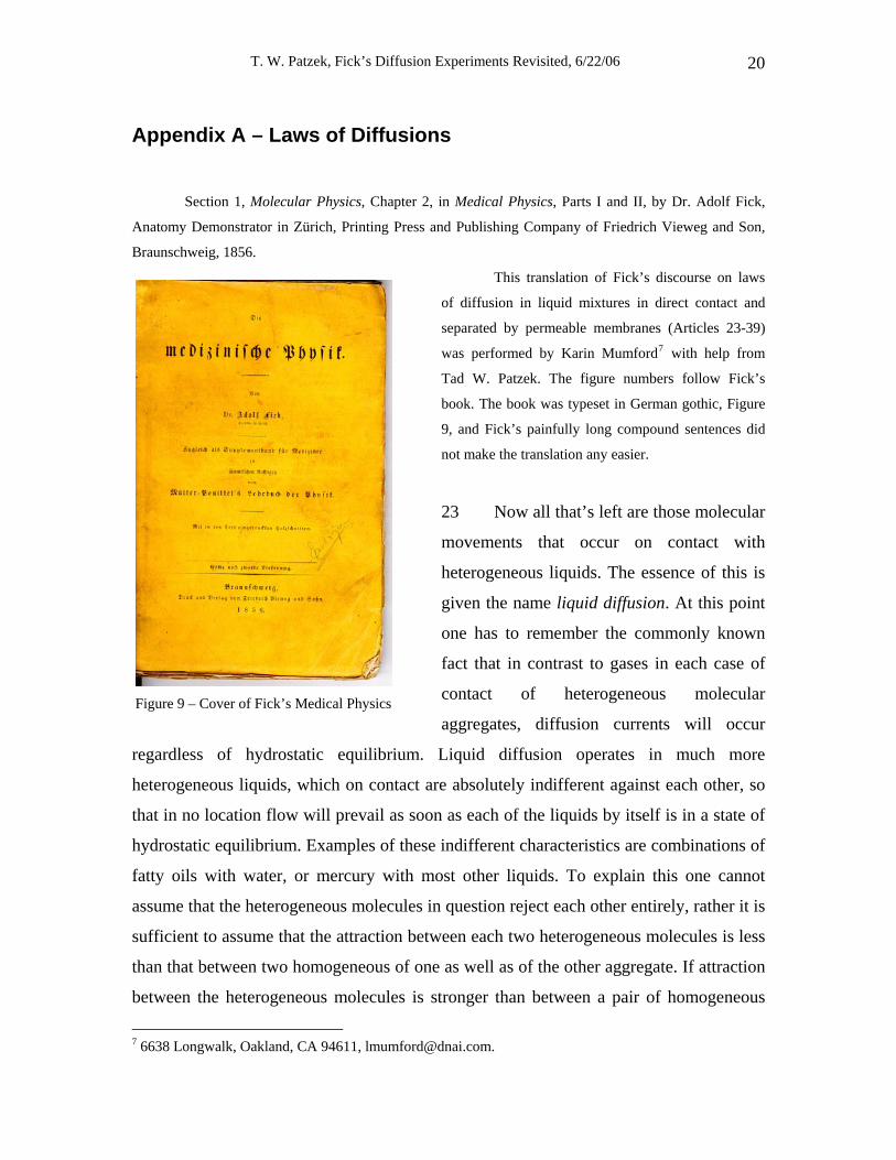
Section 1, Molecular Physics, Chapter 2, in Medical Physics, Parts I and II, by Dr. Adolf Fick,
Anatomy Demonstrator in Zürich, Printing Press and Publishing Company of Friedrich Vieweg and Son,
Braunschweig, 1856.
This translation of Fick’s discourse on laws
of diffusion in liquid mixtures in direct contact and
separated by permeable membranes (Articles 23-39)
was performed by Karin Mumford7 with help from
Tad W. Patzek. The figure numbers follow Fick’s
book. The book was typeset in German gothic, Figure
9, and Fick’s painfully long compound sentences did
not make the translation any easier.
Figure 9 – Cover of Fick’s Medical Physics
23 Now all that’s left are those molecular
movements that occur on contact with
heterogeneous liquids. The essence of this is
given the name liquid diffusion. At this point
one has to remember the commonly known
fact that in contrast to gases in each case of
contact of heterogeneous molecular
aggregates, diffusion currents will occur
regardless of hydrostatic equilibrium. Liquid diffusion operates in much more
heterogeneous liquids, which on contact are absolutely indifferent against each other, so
that in no location flow will prevail as soon as each of the liquids by itself is in a state of
hydrostatic equilibrium. Examples of these indifferent characteristics are combinations of
fatty oils with water, or mercury with most other liquids. To explain this one cannot
assume that the heterogeneous molecules in question reject each other entirely, rather it is
sufficient to assume that the attraction between each two heterogeneous molecules is less
than that between two homogeneous of one as well as of the other aggregate. If attraction
between the heterogeneous molecules is stronger than between a pair of homogeneous
7 6638 Longwalk, Oakland, CA 94611, [email protected].
T. W. Patzek, Fick’s Diffusion Experiments Revisited, 6/22/06 21
molecules, a molecular movement happens immediately at the interface, which develops
the diffusion current in a manner analogous to the gas process. Therefore, both processes
have in common that none of them comes to rest and attains final equilibrium until a
uniform equilibrium distribution is produced in the entire space that is occupied by both
diffusing substances, meaning until in each part of this space the same condition is
obtained for each of the substances.
24 In the currently still inadequate understanding of the structure of molecules, it
would be useless to try to demonstrate this course of events. We have to restrict ourselves
to just demonstrating here the known laws from our experience. Until now, from all
possible cases, only the ones where the touching liquid solutions of the same solid in the
same solvent, which only differed in their concentrations, were subject to a specific test.
This is the reason for us to start this case with the governing law, but not without
mentioning immediately that other cases with a probability bordering certainty are
subject to the same law, if one only interprets or modifies terms of their mathematical
description. To avoid unnecessary notation and at the same time deal with fixed concepts,
we will simply name the dissolved solid salt and the solvent water. The governing law for
the spreading of salt in a water mass is, to say it very briefly, the same as the one that
rules the spreading of heat in a heat-conducting body, on which Fourier based his famous
mathematical theory of heat, and that was extended by Ohm, as we know with great
success, to the flow of electricity in a conductor. Avoiding the shorthand language of
mathematical analysis, we must express the same as follows. One has to think of two
very thin horizontal solvent layers on top of each other, the lower one contains more salt
and its concentration is = k; in the top one we will assume the lesser concentration k ′ . If
now the separation of both layers is = d, all these quantities will somehow retain the same
values during a certain time interval ϑ . The diffusion current, caused by the
heterogeneity (concentration difference) between both layers during the imagined time
interval, conveys a quantity of salt through the unit area of the dividing surface from the
concentrated lower layer to the thinner upper one that is k kCd
ϑ′− . Here C is a quantity
depending on the chemical nature of the relevant salt and the temperature alone, and
T. W. Patzek, Fick’s Diffusion Experiments Revisited, 6/22/06 22
therefore for the present consideration it is considered constant. If Q were the total
surface area of both layers, the total amount of salt delivered to the upper would be =
A
C
M
P
m
B
N
QA
C
M
P
m
B
N
Q Fig. 7.
. k kC Qd
ϑ′− . At the same time, a water mass will be added from the upper layer to the
bottom layer, which occupies the same volume so that the volumes of both layers
together will not be altered during the process. The special assumption of horizontal
layers with constant concentration was necessary to make, because only in this case a
hydrostatic equilibrium remains in the liquid mass. It also had to be assumed, as we did
just now, that the change of the concentration from one horizontal layer to the other one
only takes place if the upper layer is more diluted than the lower layer. Only then,
meaning that always when a less dense layer rests upon a heavier one, the hydrostatic
equilibrium is stabilized. Hydrostatic equilibrium must also hold in the liquid mass if the
diffusion current shall be achieved untroubled by hydrodynamic currents8. One can
derive through integration of the just formulated law that directly represents the
elementary process, how the concentrations in a finite mass will change after elapse of a
finite time, if initially they were distributed in a given manner. By comparing the thus
achieved results with the observational facts, one can recognize the accuracy or
inaccuracy of the assumed governing law.
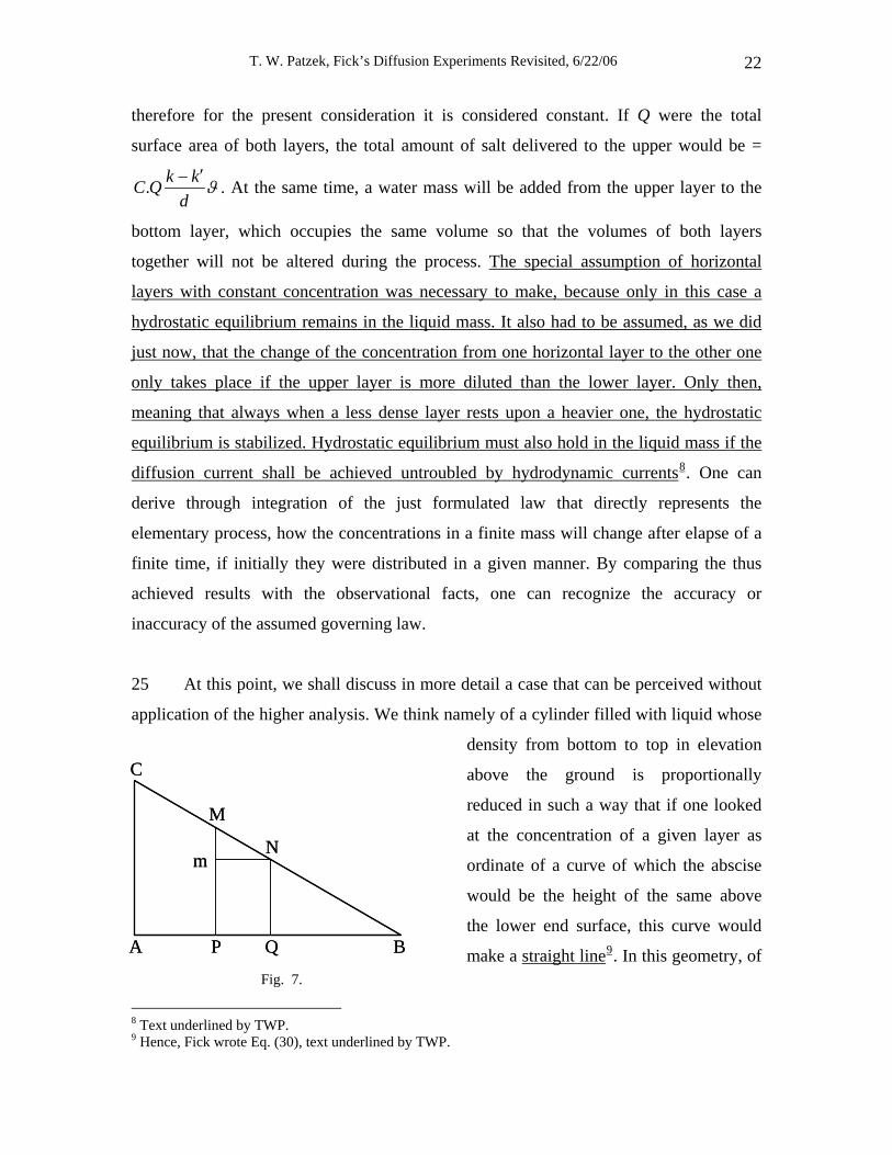
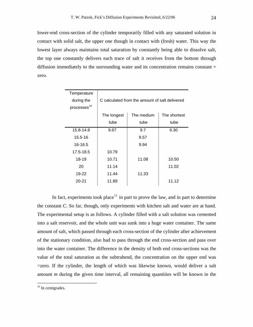
25 At this point, we shall discuss in more detail a case that can be perceived without
application of the higher analysis. We think namely of a cylinder filled with liquid whose
density from bottom to top in elevation
above the ground is proportionally
reduced in such a way that if one looked
at the concentration of a given layer as
ordinate of a curve of which the abscise
would be the height of the same above
the lower end surface, this curve would
make a straight line9. In this geometry, of
8 Text underlined by TWP. 9 Hence, Fick wrote Eq. (30), text underlined by TWP.
T. W. Patzek, Fick’s Diffusion Experiments Revisited, 6/22/06 23
course, the given concentration difference of two arbitrarily chosen layers is always
proportional to their distance, and the constant proportion of these two quantities can
namely be expressed through the proportion of the concentration difference between the
lower- and upper-end cross-section to the length of the whole cylinder. Figure 7 further
makes this assertion graphically clear. It means namely, AB is the length of the whole
cylinder and CB is a line, the ordinates of which denote the concentrations of the layers,
so that for example over a distance AP from the lower end cross-section the concentration
PM occurs. At Q, in comparison, the concentration QN is located. By looking at the
figure, one recognizes immediately that PM-QN or Mm has a constant proportion to the
distance of the layers PQ or mN. This distance is arbitrary, and specifically the latter
proportion is the same as the proportion of the difference of the concentration A (AC)
and B (zero is the assumed value of the liquid concentration at the upper end of the
cylinder) to the full length of the cylinder, therefore = ACAB
. The same ratio has to hold
between the infinitely small differences of concentrations in two immediately adjacent
layers at the just as infinitely small distance from each other. One may take the same
proportion at whichever section of the cylinder one chooses. As to how from this
proportion the salt and water exchange between consecutive layers depends on the
assumed governing law. This exchange is just as intense in all parts of the cylinder; that
means that each layer receives as much salt from the previous one during a given small
time interval as it distributes to the following one. Thus, the concentration (in each layer)
remains the same. If therefore the concentration AC of the lower-end cross-section and
the zero concentration of the upper end during a finite time interval could be kept
constant by any means, the concentration in all of the cylinder would remain constant
during the entire time. This way a stationary diffusion current is formed, which moves the
same amount of salt from bottom to top in each time instant through all cross-sections,
which according to our law has to be . ACC QAB
= . In due time, the stationary distribution
of the concentration in the cylinder evolves, it could have been in the beginning or
otherwise, one only needs to keep the concentration of the two end cross-sections
constant. This condition can be accomplished easily in an experiment. One keeps the
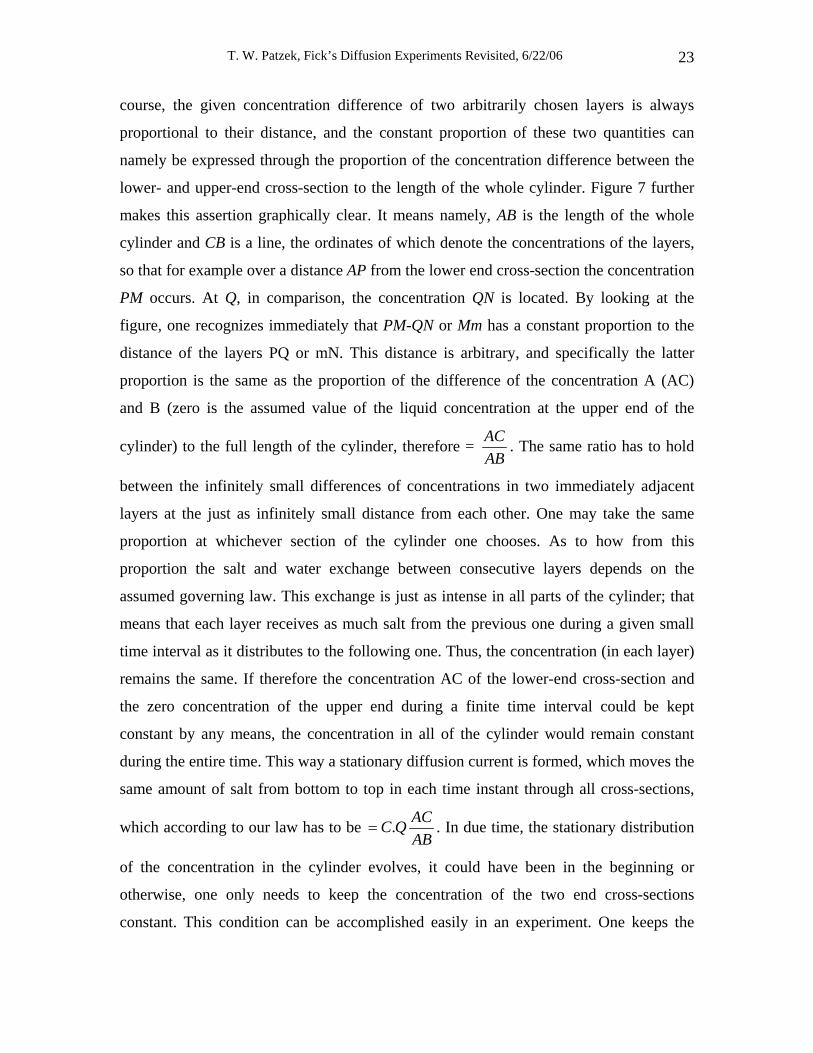
T. W. Patzek, Fick’s Diffusion Experiments Revisited, 6/22/06 24
lower-end cross-section of the cylinder temporarily filled with any saturated solution in
contact with solid salt, the upper one though in contact with (fresh) water. This way the
lowest layer always maintains total saturation by constantly being able to dissolve salt,
the top one constantly delivers each trace of salt it receives from the bottom through
diffusion immediately to the surrounding water and its concentration remains constant =
zero.
Temperature
during the
processes10
C calculated from the amount of salt delivered
The longest
tube
The medium
tube
The shortest
tube
15.8-14.8 9.67 9.7 9.30
15.5-16 9.57
16-16.5 9.94
17.5-18.5 10.79
18-19 10.71 11.08 10.50
20 11.14 11.02
19-22 11.44 11.33
20-21 11.89 11.12
In fact, experiments took place11 in part to prove the law, and in part to determine
the constant C. So far, though, only experiments with kitchen salt and water are at hand.
The experimental setup is as follows. A cylinder filled with a salt solution was cemented
into a salt reservoir, and the whole unit was sunk into a huge water container. The same
amount of salt, which passed through each cross-section of the cylinder after achievement
of the stationary condition, also had to pass through the end cross-section and pass over
into the water container. The difference in the density of both end cross-sections was the
value of the total saturation as the subtrahend, the concentration on the upper end was
=zero. If the cylinder, the length of which was likewise known, would deliver a salt
amount m during the given time interval, all remaining quantities will be known in the
10 In centigrades.
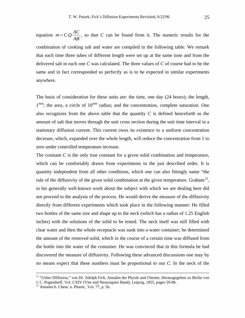
T. W. Patzek, Fick’s Diffusion Experiments Revisited, 6/22/06 25
equation . ACm C QAB
= , so that C can be found from it. The numeric results for the
combination of cooking salt and water are compiled in the following table. We remark
that each time three tubes of different length were set up at the same time and from the
delivered salt in each one C was calculated. The three values of C of course had to be the
same and in fact corresponded so perfectly as is to be expected in similar experiments
anywhere.
The basis of consideration for these units are: the time, one day (24 hours); the length,
1mm; the area, a circle of 10mm radius; and the concentration, complete saturation. One
also recognizes from the above table that the quantity C is defined henceforth as the
amount of salt that moves through the unit cross section during the unit time interval in a
stationary diffusion current. This current owes its existence to a uniform concentration
decrease, which, expanded over the whole length, will reduce the concentration from 1 to
zero under controlled temperature increase.
The constant C is the only true constant for a given solid combination and temperature,
which can be comfortably drawn from experiments in the just described order. It is
quantity independent from all other conditions, which one can also fittingly name “the
rule of the diffusivity of the given solid combination at the given temperature. Graham12,
in his generally well-known work about the subject with which we are dealing here did
not proceed to the analysis of the process. He would derive the measure of the diffusivity
directly from different experiments which took place in the following manner: He filled
two bottles of the same size and shape up to the neck (which has a radius of 1.25 English
inches) with the solutions of the solid to be tested. The neck itself was still filled with
clear water and then the whole receptacle was sunk into a water container; he determined
the amount of the removed solid, which in the course of a certain time was diffused from
the bottle into the water of the container. He was convinced that in this formula he had
discovered the measure of diffusivity. Following these advanced discussions one may by
no means expect that these numbers must be proportional to our C. In the neck of the
11 “Ueber Diffusion,” von Dr. Adolph Fick, Annalen der Physik und Chemie, Herausgegeben zu Berlin von J. C. Pogendorff, Vol. CXIV (Vier und Neunzigster Band), Leipzig, 1855, pages 59-86. 12 Annalen b. Chem. u. Pharm., Vol. 77, p. 56.
T. W. Patzek, Fick’s Diffusion Experiments Revisited, 6/22/06 26
bottle, a stationary diffusion current obviously does not develop, instead a process that
would be very difficult to discuss analytically. Nevertheless, these numbers are very
interesting whilst they at least grow simultaneously with the diffusivity, though not
proportionally, so that in Graham’s experiments a solid described by a larger number is
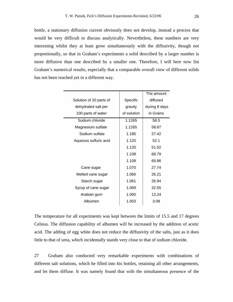
more diffusive than one described by a smaller one. Therefore, I will here now list
Graham’s numerical results, especially that a comparable overall view of different solids
has not been reached yet in a different way.
Solution of 20 parts of
dehydrated salt per
100 parts of water
Specific
gravity
of solution
The amount
diffused
during 8 days
in Grains
Sodium chloride 1.1265 58.5
Magnesium sulfate 1.1265 58.87
Sodium sulfate 1.185 27.42
Aqueous sulfuric acid 1.120 52.1
1.120 51.02
1.108 68.79
1.108 69.86
Cane sugar 1.070 27.74
Melted cane sugar 1.066 26.21
Starch sugar 1.061 26.94
Syrup of cane sugar 1.069 32.55
Arabian gum 1.060 13.24
Albumen 1.053 3.08
The temperature for all experiments was kept between the limits of 15.5 and 17 degrees
Celsius. The diffusion capability of albumen will be increased by the addition of acetic
acid. The adding of egg white does not reduce the diffusivity of the salts, just as it does
little to that of urea, which incidentally stands very close to that of sodium chloride.
27 Graham also conducted very remarkable experiments with combinations of
different salt solutions, which he filled into his bottles, retaining all other arrangements,
and let them diffuse. It was namely found that with the simultaneous presence of the
T. W. Patzek, Fick’s Diffusion Experiments Revisited, 6/22/06 27
other salt the diffusivity of the less soluble one became reduced. If bi-sulfuric acid potash
was filled to the bottle, not only this salt diffused out but also still free sulfuric acid, so
that therefore a part of this salt decomposed through the diffusion. Under these
circumstances, alum will be partly decomposed just as well, whilst more sulfuric acid
potash diffuses into the surrounding water than alum is built up by the simultaneously
diffusing sulfuric acid aluminum oxide. If Graham mixed sulfuric acid potash (in a very
diluted solution to not develop immediate concentration gradient), potassium chloride or
sodium chloride with calcium water and let the mixture diffuse against calcium water, the
freed alkali would diffuse and the acid would combine with the calcium, which would
precipitate if it was in sulfuric acid.
28 It also still seems to follow from Graham’s experiments that weak diffusion
currents can cross through each other without any disturbance; because it was found that
the diffusion of a 4-percent solution of sodium carbonate took place in the same manner
whether the surrounding liquid was pure water or a 4-percent solution of sodium chloride.
In addition, with several other different combinations of two salts, the same behavior was
observed.
29 The equilibration of heterogeneous liquids still also takes place, just alike the
gases, if they are separated by a porous partition wall of suitable composition, and with it
still occur very strange phenomena, which are known under the names of “endosmose13”
and “exosmose.” Without a doubt (the membrane) is the last reason for the equilibration
or the driving forces are here the same as in the simpler case of diffusion without a
membrane, only the effect is modified through the physical conditions of the liquid
molecules in the membrane. Therefore, above all, the attention has to be directed to these
if the reason is to discover the diffusion of liquids through membranes. That means one
has mainly to examine the way in which the liquids penetrate into those bodies, which
used as a partition wall can cause diffusion. Actually, the idea that a substance penetrates
13 The general term osmose (now osmosis) was introduced in 1854 by a British chemist, Thomas Graham. Here we shall use the modern term endosmosis, which is synonymous with motion through, passage, transmission; permeation; penetration, interpenetration; infiltration; endosmose, exosmose (obs); endosmosis (Chem) (Roget’s Thesaurus, Project Gutenberg, http://promo.net/pg/).
T. W. Patzek, Fick’s Diffusion Experiments Revisited, 6/22/06 28
into a space that is occupied by another substance cannot create any problems for us. We
assume from the atomic picture that each space occupied by an ever so dense substance
still leaves enough empty space to grant room for the atoms of another substance, which
will store themselves among the atoms of the first one. The penetration of a liquid into
certain solids, known by the name of “imbibition,” can also be thought of in a
considerably different way though. One can, 1) imagine the molecules of the imbibed
liquid are among themselves in the uniform molecular interstices of the solid body
distributed in the same manner. Were this opinion correct, then one might understandably
assume very radical differences between the constitution of “imbibable” and not
imbibable bodies; nevertheless, the same chemical substance (i.e., clay) can now have the
one and then the other characteristic depending on the mechanical formation of its small
(not smallest) particles. Admittedly, the imbibition of a piece of porous clay may still be
different in nature from that in a piece of coagulated protein. The difference shows itself
immediately if one changes the expression and says “swelling” instead of “imbibition.”
From a piece of clay, one cannot say that it swells. 2) It also can be thought that a body
capable to imbibe is similar to a network or a spongy tissue that besides the molecular
interstices also has other gaps that in mechanical sense stand far apart from the
interstices, namely much surpassing them in size. These gaps, one could think then, fill
themselves during the swelling with the imbibed liquid; meanwhile, no atom penetrates
into the space between the molecules that constitute the solid part of the network. This
idea offers the immense formal convenience that, if one takes it as a basis of the
explanation of the swelling appearances as well as the one of the diffusion through
separating walls, one becomes independent of each molecular hypothesis.
In fact, most of the researchers in these fields have more or less explicitly adopted the
just discussed second theory. By the way, it is still to consider that these two theories do
not exclude each other. In particular, Ludwig tends to connect them when he states14: “As
much as we find ourselves in the dark about the special kind of fusion (of the solid
substance and the imbibed liquid particles), we may yet still assert that in most of the
swollen substances the absorbed liquids partly are present in larger pores, which are
14 Lehrbuch der Physiologie, Vol. I, p 60.
T. W. Patzek, Fick’s Diffusion Experiments Revisited, 6/22/06 29
existing between more or less large piles of molecules, but partly are nestling between the
molecules themselves.”
30 The appearance of the swelling itself is now essentially that a substance capable
of it absorbs a certain quantity from the surrounding liquid in the course of a more or less
long time. When this happens, the process reaches equilibrium, whilst no other liquid
molecule penetrates into it, may by the way, as much or as little liquid be in store.
Through the comparison of the amount of the solid substance and the maximum absorbed
liquid (or in the equilibrium after completion of the process), one obtains the swelling
ratio. It (this ratio) obviously depends on the nature of the solid body as well as the
liquid, so that the same solid body can absorb different amounts of different liquids, and
that different amounts of the same liquid penetrate into different solids. Besides that, the
swelling ratio varies also with temperature. No extended quantitative series of
experiments are available yet on all these aspects.
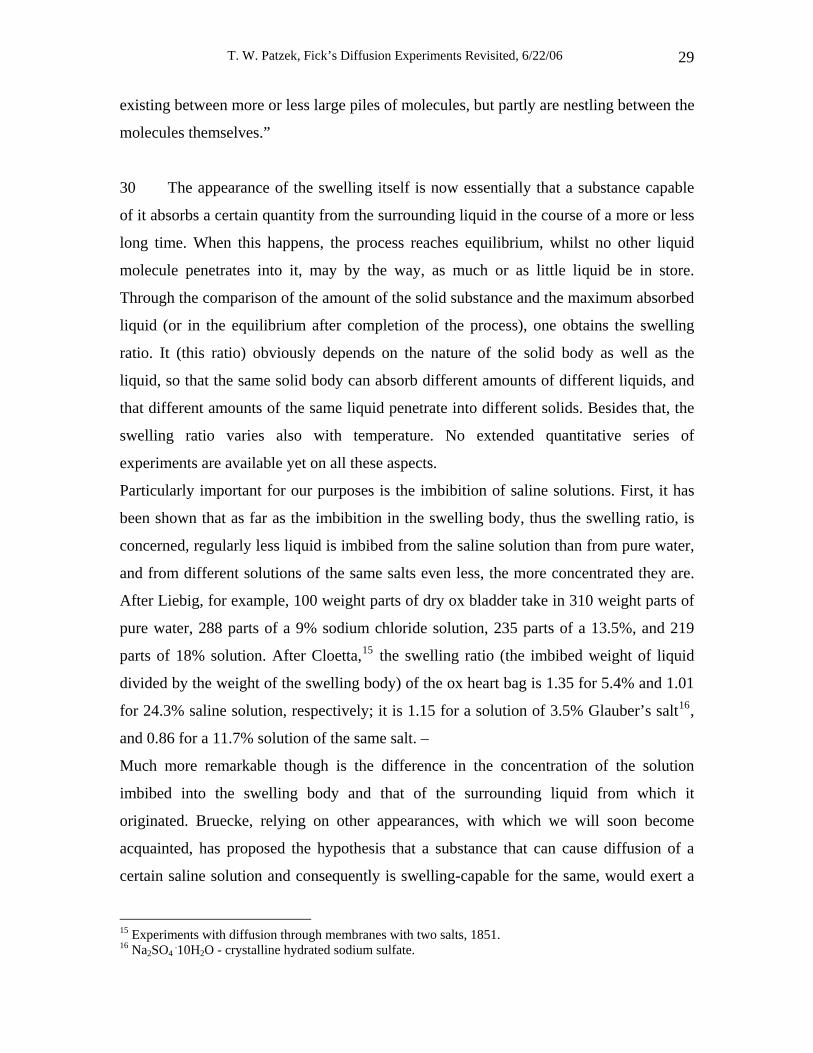
Particularly important for our purposes is the imbibition of saline solutions. First, it has
been shown that as far as the imbibition in the swelling body, thus the swelling ratio, is
concerned, regularly less liquid is imbibed from the saline solution than from pure water,
and from different solutions of the same salts even less, the more concentrated they are.
After Liebig, for example, 100 weight parts of dry ox bladder take in 310 weight parts of
pure water, 288 parts of a 9% sodium chloride solution, 235 parts of a 13.5%, and 219
parts of 18% solution. After Cloetta,15 the swelling ratio (the imbibed weight of liquid
divided by the weight of the swelling body) of the ox heart bag is 1.35 for 5.4% and 1.01
for 24.3% saline solution, respectively; it is 1.15 for a solution of 3.5% Glauber’s salt16,
and 0.86 for a 11.7% solution of the same salt. –
Much more remarkable though is the difference in the concentration of the solution
imbibed into the swelling body and that of the surrounding liquid from which it
originated. Bruecke, relying on other appearances, with which we will soon become
acquainted, has proposed the hypothesis that a substance that can cause diffusion of a
certain saline solution and consequently is swelling-capable for the same, would exert a
15 Experiments with diffusion through membranes with two salts, 1851. 16 Na2SO4
.10H2O - crystalline hydrated sodium sulfate.
T. W. Patzek, Fick’s Diffusion Experiments Revisited, 6/22/06 30
larger attraction towards the molecules of water than towards those of the dissolved salt.
If this assumption were correct, in each of the pores in which the imbibed liquid is
contained, there would be a less concentrated solution against the walls than in the center,
whilst the predominant attraction of the wall molecules against the water simply in the
proximity of the same has to draw together more water. Ludwig, based on this thought,
and also considering that even in the most central part of the pore in any case no larger
concentration could occur than in the surrounding liquid, assumed that the concentration
in all of the imbibed liquid should be lower than the one in the surrounding liquid from
which the imbibed one is taken. It had to be an average result of the lower concentrations
in the wall layers and the higher ones in the center layers, the last of which can at best
equal the concentration of the surrounding liquid. One therefore understands in one word
as the concentration on the imbibed liquid the figure, which expresses the proportion of
the imbibed salt amount to the total imbibed liquid mass, regardless of how water and salt
are distributed in the pores of the solid body. Ludwig saw himself not deceived by his
theory but confirmed it through compelling experiments. If he namely put an ox bladder
in a 7.2% solution of Glauber’s salt, it imbibed a liquid that contained only 4.4% salt. Did
he put the same substance in a 19% kitchen salt solution, it so imbibed a 16.5% solution
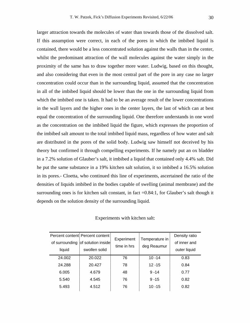
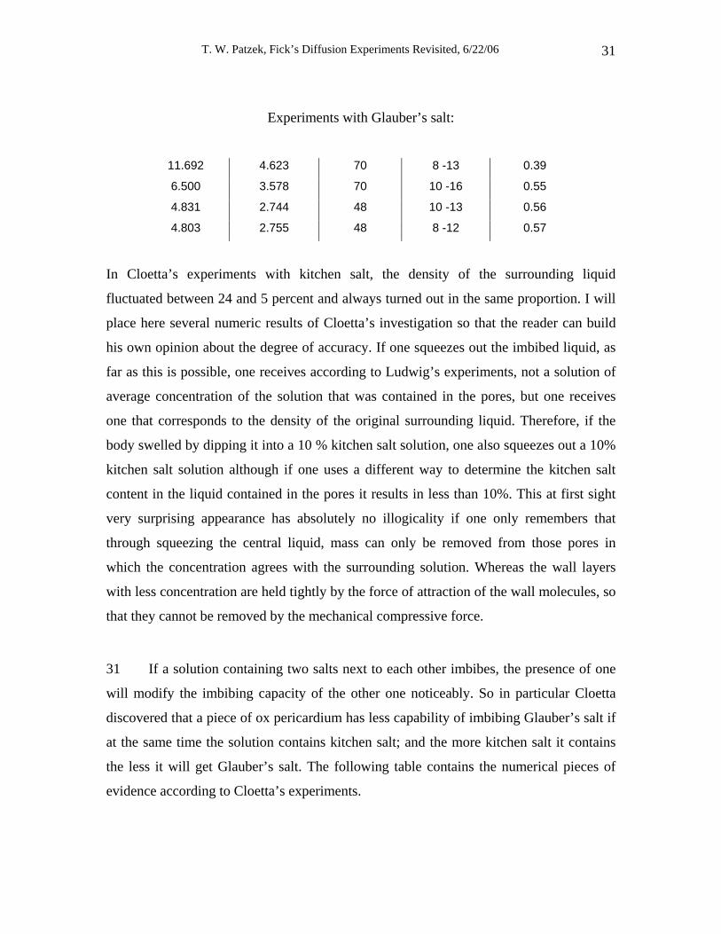
in its pores.- Cloetta, who continued this line of experiments, ascertained the ratio of the
densities of liquids imbibed in the bodies capable of swelling (animal membrane) and the
surrounding ones is for kitchen salt constant, in fact =0.84:1, for Glauber’s salt though it
depends on the solution density of the surrounding liquid.
Experiments with kitchen salt:
Percent content
of surrounding
liquid
Percent content
of solution inside
swollen solid
Experiment
time in hrs
Temperature in
deg Reaumur
Density ratio
of inner and
outer liquid
24.002 20.022 76 10 -14 0.83
24.288 20.427 78 12 -15 0.84
6.005 4.679 48 9 -14 0.77
5.540 4.545 76 9 -15 0.82
5.493 4.512 76 10 -15 0.82
T. W. Patzek, Fick’s Diffusion Experiments Revisited, 6/22/06 31
Experiments with Glauber’s salt:
11.692 4.623 70 8 -13 0.39
6.500 3.578 70 10 -16 0.55
4.831 2.744 48 10 -13 0.56
4.803 2.755 48 8 -12 0.57
In Cloetta’s experiments with kitchen salt, the density of the surrounding liquid
fluctuated between 24 and 5 percent and always turned out in the same proportion. I will
place here several numeric results of Cloetta’s investigation so that the reader can build
his own opinion about the degree of accuracy. If one squeezes out the imbibed liquid, as
far as this is possible, one receives according to Ludwig’s experiments, not a solution of
average concentration of the solution that was contained in the pores, but one receives
one that corresponds to the density of the original surrounding liquid. Therefore, if the
body swelled by dipping it into a 10 % kitchen salt solution, one also squeezes out a 10%
kitchen salt solution although if one uses a different way to determine the kitchen salt
content in the liquid contained in the pores it results in less than 10%. This at first sight
very surprising appearance has absolutely no illogicality if one only remembers that
through squeezing the central liquid, mass can only be removed from those pores in
which the concentration agrees with the surrounding solution. Whereas the wall layers
with less concentration are held tightly by the force of attraction of the wall molecules, so
that they cannot be removed by the mechanical compressive force.
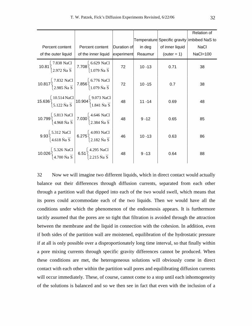
31 If a solution containing two salts next to each other imbibes, the presence of one
will modify the imbibing capacity of the other one noticeably. So in particular Cloetta
discovered that a piece of ox pericardium has less capability of imbibing Glauber’s salt if
at the same time the solution contains kitchen salt; and the more kitchen salt it contains
the less it will get Glauber’s salt. The following table contains the numerical pieces of
evidence according to Cloetta’s experiments.
T. W. Patzek, Fick’s Diffusion Experiments Revisited, 6/22/06 32
Percent content
of the outer liquid
Percent content
of the inner liquid
Duration of
experiment
Temperature
in deg
Reaumur
Specific gravity
of inner liquid
(outer = 1)
Relation of
imbibed NaS to
NaCl
NaCl=100
10.81 7.838 NaCl
2.972 Na S⎧⎨⎩
7.7086.629 NaCl
1.079 Na S⎧⎨⎩
72 10 -13 0.71 38
10.817 7.832 NaCl
2.985 Na S⎧⎨⎩
7.8566.776 NaCl
1.079 Na S⎧⎨⎩
72 10 -15 0.7 38
15.636 10.514 NaCl
5.122 Na S⎧⎨⎩
9.073 NaCl
1.841 Na S⎧⎨⎩
10.904 48 11 -14 0.69 48
10.799 5.813 NaCl
4.968 Na S⎧⎨⎩
7.0304.646 NaCl
2.384 Na S⎧⎨⎩
48 9 -12 0.65 85
9.93 5.312 NaCl
4.618 Na S⎧⎨⎩
6.2754.093 NaCl
2.182 Na S⎧⎨⎩
46 10 -13 0.63 86
10.026 5.326 NaCl
4.700 Na S⎧⎨⎩
6.51 4.295 NaCl
2.215 Na S⎧⎨⎩
48 9 -13 0.64 88
32 Now we will imagine two different liquids, which in direct contact would actually
balance out their differences through diffusion currents, separated from each other
through a partition wall that dipped into each of the two would swell, which means that
its pores could accommodate each of the two liquids. Then we would have all the
conditions under which the phenomenon of the endosmosis appears. It is furthermore
tacitly assumed that the pores are so tight that filtration is avoided through the attraction
between the membrane and the liquid in connection with the cohesion. In addition, even
if both sides of the partition wall are moistened, equilibration of the hydrostatic pressure
if at all is only possible over a disproportionately long time interval, so that finally within
a pore mixing currents through specific gravity differences cannot be produced. When
these conditions are met, the heterogeneous solutions will obviously come in direct
contact with each other within the partition wall pores and equilibrating diffusion currents
will occur immediately. These, of course, cannot come to a stop until each inhomogeneity
of the solutions is balanced and so we then see in fact that even with the inclusion of a
T. W. Patzek, Fick’s Diffusion Experiments Revisited, 6/22/06 33
partition wall between the two solutions the process will not end until all differences are
balanced out. During the process, though, fundamental modifications will be caused by
the existence of the partition wall. The important difference between the free diffusion
and the diffusion through partition walls is mainly because in the former the equal
volumes of the same substances are exchanged between two consecutive layers without
any difficulty, so that two equally strong currents in opposite directions are constantly
moving. In the latter, as a rule, both currents are not equally strong so that after some
time the volume on one side of the partition wall has become larger and on the other side
it has become smaller. A theory of the endosmosis has therefore first to be based on
explaining how the modification of the diffusion current can be created by the presence
of the partition wall. Bruecke carried out the first experiment in this direction, which is
already based on the aforementioned idea of the distribution of removed substances in the
pores of a body capable of swelling. By going into that in more detail now, it has to be
remarked beforehand, that here again we can only rely on the case where solutions of the
same salt of different density balance their differences through diffusion. The case is that
different mixtures of originally liquid masses (for example alcohol and water) diffuse in
one another. However, without hesitation, one can go back to the case that a salt in
solution is to be regarded as a liquid itself; its molecules are undoubtfully just as easy to
rearrange as the ones of a certain amount of alcohol distributed in water. It therefore
actually will be a shortcut expression when we talk about salt and water. If now, in fact,
the material of the partition wall has a stronger force of attraction to the water than to the
salt, and as a result of that a wall layer of pure water surrounds a central liquid thread
within the pores, which can adopt the density of the surrounding solution, the latter one
will cause a diffusion current the same way as in the pores which we have imagined
previously (see #25). That will distribute as much salt to one side as water to the other
side, whereas salt will never be able to penetrate into the wall layer, which can be brought
into motion by the attraction of the salt solutions with which it is in touch on both sides.
From the side of the concentrated solution, however, works an obviously stronger
attraction than from the other side, as here in the same area more attracting salt molecules
are facing it. Through the continuing currents, the dilute layer at the wall therefore will be
in the process of moving towards the concentrated solution, by replenishing itself
T. W. Patzek, Fick’s Diffusion Experiments Revisited, 6/22/06 34
constantly from the less concentrated one. Thus, to the amount of water, reaching through
the central thread the concentrated solution (which is the same as the amount of salt
traveling to the other side), an additional amount of water is added to the concentrated
solution through the peripheral layer for which no salt equivalent travels to the other side.
More water therefore has to travel each time from the more dilute solution to the denser
one than salt travels in the opposite direction. The volume of the concentrated solution
has to grow through the endosmosis. In fact, the success has been observed regularly. In
one case, Bruecke was able to substantiate this theoretical analysis by an unambiguous
experiment. Turpentine oil has a substantially stronger attraction to glass than tree oil as
it forces out completely the latter from a glass surface; therefore a wall layer of turpentine
oil and a central layer of a mixture of both liquids will be found in a glass capillary if
both can force their way into it. Bruecke manufactured such a capillary surface, which on
one side bordered turpentine oil and on the other side tree oil, and discovered according
to the theory that more turpentine oil diffused through the capillary to the tree oil than
tree oil in the opposite direction.
α α′
β β ′
a′a
b′b
α α′
β β ′
a′a
b′b Fig. 8.
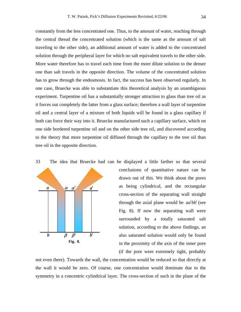
33 The idea that Bruecke had can be displayed a little farther so that several
conclusions of quantitative nature can be
drawn out of this. We think about the pores
as being cylindrical, and the rectangular
cross-section of the separating wall straight
through the axial plane would be (see
Fig. 8). If now the separating wall were
surrounded by a totally saturated salt
solution, according to the above findings, an
also saturated solution would only be found
in the proximity of the axis of the inner pore
(if the pore were extremely tight, probably
not even there). Towards the wall, the concentration would be reduced so that directly at
the wall it would be zero. Of course, one concentration would dominate due to the
symmetry in a concentric cylindrical layer. The cross-section of such in the plane of the
aa bb′ ′
T. W. Patzek, Fick’s Diffusion Experiments Revisited, 6/22/06 35
figure should be, e.g., αβ and α β′ ′ . The saturated solution beneath the separating wall
(thought as being horizontal) would now be replaced with pure water, diffusion would
start, and we could observe what must happen in particular in the cylindrical volume with
the cross-section αβ and α β′ ′ . At its lower end, the concentration is kept at the zero
level through constant contact with the water. At its upper end, though, the concentration
maintains the highest possible level through the contact with the saturated solution.
Immediately the stationary concentration distribution occurs in this space. The
concentration will grow in proportion to the height above the lower end area ( ββ ′). This
distribution of the concentration is indicated in the figure by the hatching. Due to the
smallness of this volume, stationary condition occurs almost immediately; thus, we can
restrict ourselves to its consideration. The concentration distribution now necessitates a
stationary diffusion current that moves just as much salt to the bottom as water to the top.
One should even be able to calculate the amounts following the above principles (see 26)
if the dimensions of the small volume and the maximum possible concentration in it were
known. Now, though, the water passing to the top demands a special consideration as
well. If the concentration in the small volume (what yet in general has to be
presupposed), on which we now have our eyes, has to be lower by a finite amount than
the absolute saturation, then a density jump will occur at α and α′ from the possible
maximum in the small volume to the absolute saturation above the separation wall. This
jump would cause an almost infinitely strong diffusion current on the spot, which means
almost infinitely large amounts of salt would be driven into the pores and just as large
amounts of water would be expelled. Let us suppose for a moment that this has actually
happened. The salt amounts could not penetrate because the highest concentration in this
particular area already exists at the upper end; they must somehow slip off sidewise.
Larger amounts of water though can be delivered from the bottom than the diffusion
current, already thought of as established in the cylindrical volume, delivers. A certain
water amount is in a way simultaneously being drawn through. This changes the solution
density, whilst the water distributes itself generally in the upper liquid, up to a certain
distance noticeable from the upper pore opening. In this way, water creates an upward
extending conically widening zone (its two cross-sections are shown in simplification in
Figure 8 above α and α′ ), in which the concentration grows from bottom to top up to the
T. W. Patzek, Fick’s Diffusion Experiments Revisited, 6/22/06 36
total saturation of the upper solution. Immediately, also here a stationary condition comes
into effect and causes a diffusion current of the same strength, which brings just as much
water to the top as can be distributed in the same time from the upper end of the imagined
volume into the reservoir of saturated solution without altering the concentration.
Because obviously the imagined zone would extend itself upwards (and through that the
intensity of the diffusion current would be reduced), as soon as more water climbed up in
this way, the concentration at the upper end of the zone could still be altered. On the
other hand, if less water went up, a jump in the concentration increase would occur at
some point, which immediately would cause an infinitely strong diffusion current and
this way again absorb the relevant water amount.
34 It is now apparent that through all those cylindrical elementary layers, which are
so close to the pore wall that totally saturated solution can no longer exist within them,
more water moves to one side than salt moves to other side. As now in a tighter pore
proportionally more parts are lying closer to the wall than in a larger one, considerably
more of water will be flowing in a tighter pore than in a wider one. One can hardly hope
to strongly substantiate this assertion through experiment, as one will hardly find two
separation walls that only distinguish themselves from each other by the width of the
pores. In any case, though, the following fact speaks for the just established assertion.
One has obviously some reason to assume that in the glassy colloidal membrane the pores
are unproportionally tighter than in one produced from animal connective tissue (heart
pericardium or bladder), so that all other differences against this one are only
insignificantly effective. However, it is shown that in fact with a colloidal separation
wall, the quantity of water that diffuses towards the concentrated solution is much larger
than with an animal bladder. Whilst with the bladder wall approximately 3 to 6 times as
much water moves into the solution as salt into the water, approximately 20 times as
much water moves through a colloidal separation wall as salt. In most of my experiments
only traces of salt had moved through the colloid, while substantial water quantities made
it through in the opposite direction.
According to the aforementioned idea, the excess of the water above the salt diffusing in
the opposite direction must still grow with the increasing mobility of the particles in the
T. W. Patzek, Fick’s Diffusion Experiments Revisited, 6/22/06 37
saturated solution above the membrane. The amount of absorbed water, which could
spread itself in the reservoir without alteration of the saturation, will be even larger the
easier movable the particles are. To prove this theory, I mixed solid particles with the
upper solution, which interfered with the mobility; received a positive result though,
while the proportion of the diffusing salt and water amounts was not changed.
35 Let us now imagine that instead of the pure water, a solution of the same salt is
located underneath the membrane. Above it there is a completely saturated solution at a
certain density c. Counting from the pore wall a number of cylindrical elementary layers
will immediately inactive; namely all those in which no higher concentration than that c
is possible. Naturally they fill themselves with a uniformly saturated solution, each one
with possibly the most concentrated, and on both their ends the absorbing power will be,
proportionally to the difference, between the concentration in the solution contained in it
and the respective solutions above and under it. As the upper solution is totally saturated,
the difference at the upper end and consequently the absorbency is higher, that is why
now only water moves from bottom to top through all these characterized elementary
layers. The more central layers in which a larger concentration than c is possible are
making way for a bilateral diffusion current which will produce itself in the afore
described manner even though in less intensity. As in doing this, to the contrary of the
first described case, some elementary layers have become passive (dormant) for the salt
movement, the surplus of the continuing water flow has to grow. If c were larger than the
possible maximum of concentration in the central liquid thread of the pore, the
endosmotic current would become unilateral and now only water would be able to move
from the thinner solution to the thicker one. In fact, I found out that 11.05 times as much,
in a different experiment even 17.05 times as much, water as salt went through a
membrane, if the same separated absolutely saturated kitchen salt solution from 22 %
one. Only 5 or 6 times as much water as salt went through if the membrane separated the
saturated kitchen salt solution from pure water.
(Other pieces of evidence in the following table.)
T. W. Patzek, Fick’s Diffusion Experiments Revisited, 6/22/06 38
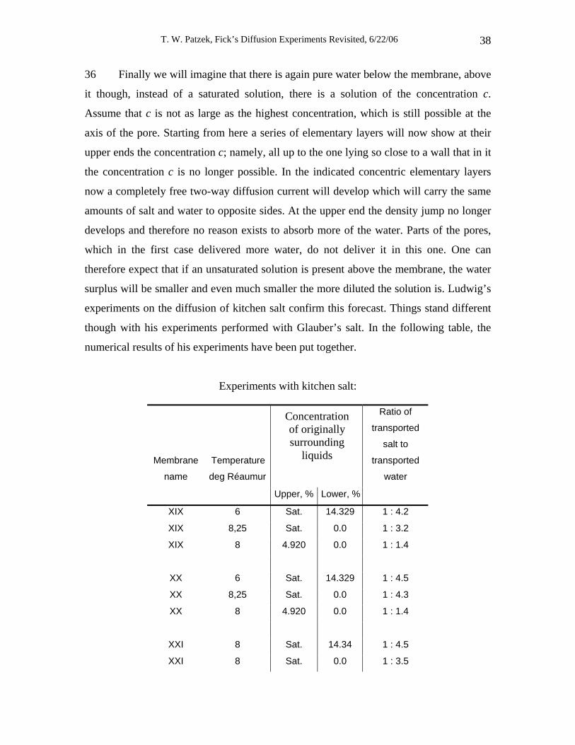
36 Finally we will imagine that there is again pure water below the membrane, above
it though, instead of a saturated solution, there is a solution of the concentration c.
Assume that c is not as large as the highest concentration, which is still possible at the
axis of the pore. Starting from here a series of elementary layers will now show at their
upper ends the concentration c; namely, all up to the one lying so close to a wall that in it
the concentration c is no longer possible. In the indicated concentric elementary layers
now a completely free two-way diffusion current will develop which will carry the same
amounts of salt and water to opposite sides. At the upper end the density jump no longer
develops and therefore no reason exists to absorb more of the water. Parts of the pores,
which in the first case delivered more water, do not deliver it in this one. One can
therefore expect that if an unsaturated solution is present above the membrane, the water
surplus will be smaller and even much smaller the more diluted the solution is. Ludwig’s
experiments on the diffusion of kitchen salt confirm this forecast. Things stand different
though with his experiments performed with Glauber’s salt. In the following table, the
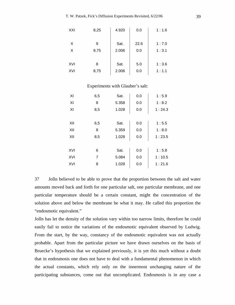
numerical results of his experiments have been put together.
Experiments with kitchen salt:
Membrane
name
Temperature
deg Réaumur
Ratio of
transported
salt to
transported
water
Upper, % Lower, %
XIX 6 Sat. 14.329 1 : 4.2
XIX 8,25 Sat. 0.0 1 : 3.2
XIX 8 4.920 0.0 1 : 1.4
XX 6 Sat. 14.329 1 : 4.5
XX 8,25 Sat. 0.0 1 : 4.3
XX 8 4.920 0.0 1 : 1.4
XXI 8 Sat. 14.34 1 : 4.5
XXI 8 Sat. 0.0 1 : 3.5
Concentration of originally surrounding
liquids
T. W. Patzek, Fick’s Diffusion Experiments Revisited, 6/22/06 39
XXI 8,25 4.920 0.0 1 : 1.6
X 9 Sat. 22.6 1 : 7.0
X 9,75 2.006 0.0 1 : 3.1
XVI 8 Sat. 5.0 1 : 3.6
XVI 8,75 2.006 0.0 1 : 1.1
Experiments with Glauber’s salt:
XI 6,5 Sat. 0.0 1 : 5.9
XI 8 5.358 0.0 1 : 8.2
XI 8,5 1.028 0.0 1 : 24.3
XII 6,5 Sat. 0.0 1 : 5.5
XII 8 5.359 0.0 1 : 8.0
XII 8,5 1.028 0.0 1 : 23.5
XVI 6 Sat. 0.0 1 : 5.8
XVI 7 5.084 0.0 1 : 10.5
XVI 8 1.028 0.0 1 : 21.6
37 Jolln believed to be able to prove that the proportion between the salt and water
amounts moved back and forth for one particular salt, one particular membrane, and one
particular temperature should be a certain constant, might the concentration of the
solution above and below the membrane be what it may. He called this proportion the
“endosmotic equivalent.”
Jolln has let the density of the solution vary within too narrow limits, therefore he could
easily fail to notice the variations of the endosmotic equivalent observed by Ludwig.
From the start, by the way, constancy of the endosmotic equivalent was not actually
probable. Apart from the particular picture we have drawn ourselves on the basis of
Bruecke’s hypothesis that we explained previously, it is yet this much without a doubt
that in endosmosis one does not have to deal with a fundamental phenomenon in which
the actual constants, which rely only on the innermost unchanging nature of the
participating substances, come out that uncomplicated. Endosmosis is in any case a
T. W. Patzek, Fick’s Diffusion Experiments Revisited, 6/22/06 40
course of events fundamentally modified much more through complicated conditions,
through the fundamental strength of the matter, though in last instance mechanically
caused like all others.
I have noticed that for one particular membrane the equivalent came out differently if I
brought saturated kitchen salt solution above and pure water underneath it than if I
poured saturated kitchen salt solution underneath and pure water over the membrane. In
the last case, the endosmosis equivalent was smaller and more salt went through during
the time unit than in the first case. Whether the density plays a role in this case or
whether the different sides of the membrane which were facing the water were the actual
cause, I do not dare to decide after my not adequately numerous experiments. It is known
that already Cima and Matteucci have observed phenomena that favor the last
interpretation.
38 Very important (especially for the organic process) are the diffusions that occur
when solution mixtures take the place of simple solutions. Theoretically, one can hardly
suspect anything about this object. Contrary to that, though, we have an exact and
extensive experimental investigation from Cloetta on the diffusion of mixtures of kitchen
salt and Glauber’s salt solution. This investigation has resulted in the following laws:
First, the diffusion equivalent for each of these two salts is, if it diffuses as the mixture,
just as large as if it separately diffuses through the same membrane under the same
circumstances (particularly therefore in the same solution density). The deviations from
this law in the different experiments are insignificant. If for example n and were the
endosmosic equivalents of the two salts for a certain membrane and concentration, and if
it were found in an experiment with the mixture that during any given time the amount a
of the first salt, and the amount b of the second salt moved across. Then, for the first one
a water amount =na, and for the second one a water amount =nb must have moved
across. Therefore the equivalent of the mixture =
n′
na n ba b
′++
should result from it. Thus this
quotient should express the proportion of the entire water amount moved in this
experiment counter currently to the simultaneously moved entire salt amount.
T. W. Patzek, Fick’s Diffusion Experiments Revisited, 6/22/06 41
Furthermore, it produced also certain relations between the diffusion velocity of the
different salt in itself and in a mixture. If one talks about diffusion velocity, for the
moment one must distinguish between the salt and the water current. The velocity of the
first would be measurable in each single case by the salt amount that moved through the
surface unit of the membrane during a given time. The velocity of the water current
would evidently find its measure in the related water amount moved to the opposite side.
During experiments with each of the two salts separately, it has become obvious that the
salt current for kitchen salt “ceteris paribus” has approximately twice the velocity as the
one for Glauber’s salt. The velocity of the water current is for both salts approximately
the same. It now became clear that within the mixture the velocity of the salt current
remained unchanged while that of Glauber’s salt was reduced. The velocity of the total
salt current was therefore larger than the one of a mere kitchen salt current, nevertheless
it not quite reached the value of the sum of the velocities of a kitchen salt current and a
Glauber’s salt current. The water current occurs for both salts in the mixture also with the
same velocity; understandably, though, the sum of each of the two speeds in itself cannot
combine to the velocity of the total water current because the diffusion velocity of the
Glauber’s salt is reduced in the mixture. When in this manner the diffusions of the two
mixed salts are independent of each other, so of course the salt endowed with a higher
velocity (or larger diffusion current against water) will remove itself from the container,
leaving behind the other one. From these conclusions can be founded about occurrences
in the animal body, about which one should read the quoted treatise by Cloetta.
39 In the chronological evolution of the diffusion phenomena, only very few
sentences can be expressed with certainty. Furthermore it is plausible that the
equilibration of chemical differences of two liquid masses must take place in a shorter
time frame when these masses are contacting each other directly than if they were
separated by a porous separation wall. The wall must due to the necessary tightness of the
pores, offer delayed resistance to the currents, which cause the equilibration. It can also
be asserted with the same evidence that everything else being equal, the time required for
equilibration increases with the thickness of the separation wall (length of the pores). –
Furthermore, the equilibration time depends on the size of the endosmosic equivalent. In
T. W. Patzek, Fick’s Diffusion Experiments Revisited, 6/22/06 42
fact, the equilibration happens even faster, the smaller the value of the endosmosic
equivalent is (same velocity of the water current presupposed), in other words the more
its value approaches unity. If, for example, the equivalent is very large then this means
that the water current dominates the opposite salt current by far and will therefore quickly
dilute the thicker solution. But the reversed current will hardly thicken the thinner
solution; while this would be the case in a more similar measure if the equivalent would
not differ so much from unity, i.e., if the strength of both currents would not differ so
much. – Furthermore, as illuminated from our consideration about the nature of the
phenomena (but, apart from this, also would be concluded from every other theoretical
idea) and already determined through older experiments (Vierordt17): The liquid amounts
exchanged in the same time frame are larger, everything else set equal, the larger is the
chemical difference of the masses separated by the membrane. With application of water
on one and salt solution on the other side, the transported mass will grow with the salt
amount in the solution. Different salts contained in a solution mixture equilibrate
themselves with pure water in almost the same amount of time as if they were taken
separately with water. The equilibration period of the already less diffusive salt seems to
become larger by mixing it with the other one.
17 In the article “Endosmosis” in the Dictionary of Physiology (Handwörtenbuch der Physiologie).
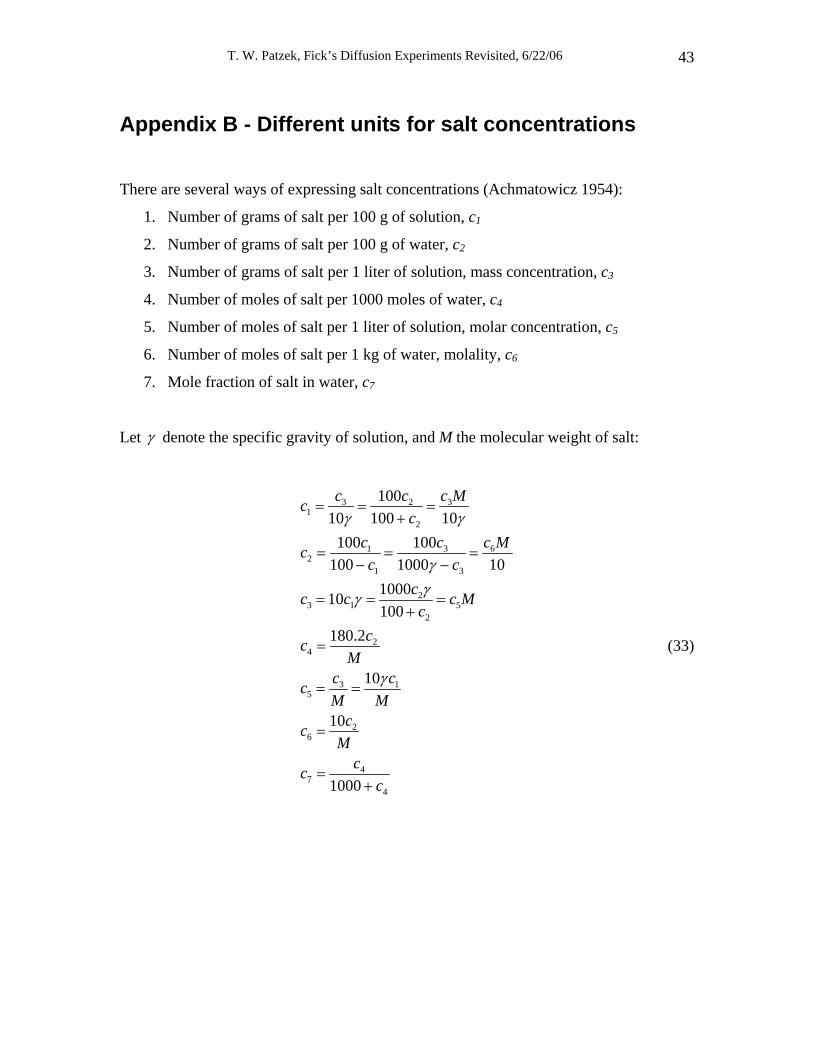
T. W. Patzek, Fick’s Diffusion Experiments Revisited, 6/22/06 43
Appendix B - Different units for salt concentrations
There are several ways of expressing salt concentrations (Achmatowicz 1954):
1. Number of grams of salt per 100 g of solution, c1
2. Number of grams of salt per 100 g of water, c2
3. Number of grams of salt per 1 liter of solution, mass concentration, c3
4. Number of moles of salt per 1000 moles of water, c4
5. Number of moles of salt per 1 liter of solution, molar concentration, c5
6. Number of moles of salt per 1 kg of water, molality, c6
7. Mole fraction of salt in water, c7
Let γ denote the specific gravity of solution, and M the molecular weight of salt:
3 2 31
2
1 32
1 3
23 1 5
2
24
3 15
26
47
4
10010 100 10
100 100100 1000 10
100010100
180.2
10
10
1000
c c c Mcc
c ccc c
cc c c Mc
ccM
c ccM M
ccM
ccc
γ γ
γγγ
γ
= = =+
= = =− −
= = =+
=
= =
=
=+
6c M
(33)
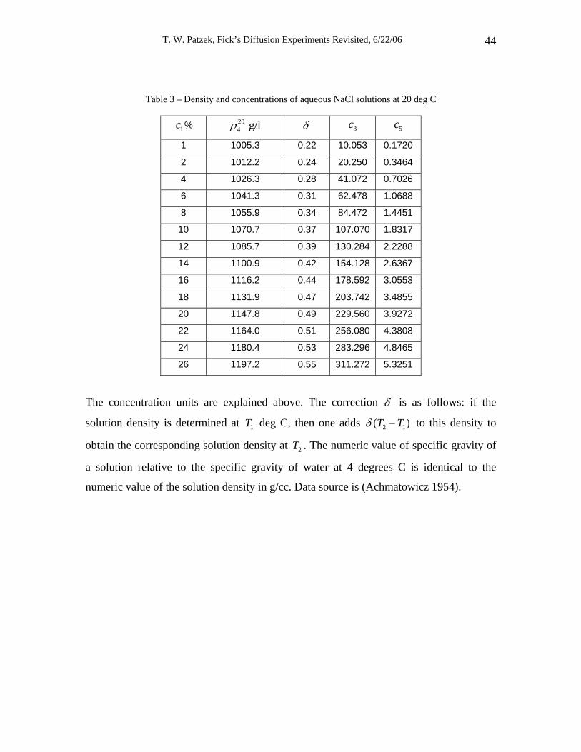
T. W. Patzek, Fick’s Diffusion Experiments Revisited, 6/22/06 44
Table 3 – Density and concentrations of aqueous NaCl solutions at 20 deg C
1c % 204 g/lρ δ 3c 5c
1 1005.3 0.22 10.053 0.1720
2 1012.2 0.24 20.250 0.3464
4 1026.3 0.28 41.072 0.7026
6 1041.3 0.31 62.478 1.0688
8 1055.9 0.34 84.472 1.4451
10 1070.7 0.37 107.070 1.8317
12 1085.7 0.39 130.284 2.2288
14 1100.9 0.42 154.128 2.6367
16 1116.2 0.44 178.592 3.0553
18 1131.9 0.47 203.742 3.4855
20 1147.8 0.49 229.560 3.9272
22 1164.0 0.51 256.080 4.3808
24 1180.4 0.53 283.296 4.8465
26 1197.2 0.55 311.272 5.3251
The concentration units are explained above. The correction δ is as follows: if the
solution density is determined at deg C, then one adds 1T 2 1(T T )δ − to this density to
obtain the corresponding solution density at . The numeric value of specific gravity of
a solution relative to the specific gravity of water at 4 degrees C is identical to the
numeric value of the solution density in g/cc. Data source is (Achmatowicz 1954).
2T