Fiber tractography using machine learning

Peter F. Neher a,*, Marc-Alexandre Cot!e b, Jean-Christophe Houde b, Maxime Descoteaux b,Klaus H. Maier-Hein a

a Medical Image Computing (MIC), German Cancer Research Center (DKFZ), Heidelberg, Germanyb Sherbrooke Connectivity Imaging Laboratory (SCIL), Computer Science Department, Universit!e de Sherbrooke, Sherbrooke, Qu!ebec, Canada

A R T I C L E I N F O

Keywords:Fiber tractographyMachine learningDiffusion-weighted imagingConnectomics

A B S T R A C T

We present a fiber tractography approach based on a random forest classification and voting process, guiding eachstep of the streamline progression by directly processing raw diffusion-weighted signal intensities. For comparisonto the state-of-the-art, i.e. tractography pipelines that rely on mathematical modeling, we performed a quanti-tative and qualitative evaluation with multiple phantom and in vivo experiments, including a comparison to the 96submissions of the ISMRM tractography challenge 2015. The results demonstrate the vast potential of machinelearning for fiber tractography.

1. Introduction

Fiber tractography on the basis of diffusion-weighted magneticresonance imaging (DW-MRI) has been a research topic for almost 20years. A vast spectrum of tractography algorithms has been presentedover the last years ranging from local deterministic approaches (Basser,1998; Chao et al., 2008; Lazar et al., 2003; Mori et al., 1999; Tournieret al., 2012) through probabilistic methods (Behrens et al., 2007; Bermanet al., 2008; Descoteaux et al., 2009; Friman et al., 2006; Vorburger et al.,2013; Zhang et al., 2013) to global tractography (Aganj et al., 2011;Daducci et al., 2015; Fillard et al., 2009; Jbabdi et al., 2007; Lemkaddemet al., 2014; Mangin et al., 2013; Reisert et al., 2011). To infer infor-mation about the complex microstructure of brain tissue and to optimallyexploit the acquisition dependent signal characteristics of diffusion-weighted images, tractography algorithms employ mathematicalmodels calculated from the diffusion-weighted signal. Prominent exam-ples include the diffusion tensor (Basser et al., 1994), multi tensor models(Kreher et al., 2005; Malcolm et al., 2010), spherical deconvolution(Alexander, 2005; Jeurissen et al., 2014; Schultz et al., 2010; Tournieret al., 2007), persistent angular structures (Jansons and Alexander,2003), Q-ball modeling (Aganj et al., 2009; Descoteaux et al., 2007) aswell as a large variety of multi-compartment models (Assaf et al., 2008;Assaf and Basser, 2005; Panagiotaki et al., 2012; Sotiropoulos et al.,2012; Zhang et al., 2012). To obtain such a model representation ofcertain local tissue properties, the corresponding inverse problem has tobe solved using the measured signal. Depending on the model, this

imposes different constraints on the data quality and acquisitionsequence, such as a minimum number of diffusion-weighting gradientsand a high signal to noise ratio (SNR). Usually, the more expressive amodel is, the more demanding is its calculation and the higher are therequirements for the signal. Choosing the optimal model is not a trivialproblem. Oversimplified modeling can, for example, hamper the abilityto resolve crossing fiber situations. Modeling approaches make variousassumptions about signal and tissue properties that are highly variableacross subjects, locations in the brain and acquisition schemes. This issuehas been discussed extensively and there is still no solution that isoptimal in all situations (Daducci et al., 2014; Farquharson et al., 2013;Jbabdi and Johansen-Berg, 2011; Neher et al., 2015a; Nimsky, 2014).Furthermore, depending on the model and the dataset, a certain numberof tractography parameters, such as a termination criterion, e.g. on thebasis of a threshold on the fractional anisotropy (FA), have to be adjustedmanually, which requires expert knowledge.

In the context of signal modeling, initial studies have successfullyshown the potential of machine learning techniques, e.g. for the tasks ofimage quality transfer and tissue micro-structure analysis (Alexanderet al., 2017; Golkov et al., 2016; Nedjati-Gilani et al., 2017; Reisert et al.,2017) and to estimate the number of distinct fiber clusters per voxel(Schultz, 2012). These methods avoid or alleviate some of the issues thatcome with the usage of diffusion-signal models.

Here, we present the first approach to fiber tractography based onmachine learning, which has several advantages: There is no need toexplicitly solve the inverse problem to obtain a representation of the

* Corresponding author. Im Neuenheimer Feld 280, 69120 Heidelberg, Germany.E-mail addresses: p.neher@dkfz.de (P.F. Neher), marc-alexandre.cote@usherbrooke.ca (M.-A. Cot!e), jean-christophe.houde@usherbrooke.ca (J.-C. Houde), m.descoteaux@

usherbrooke.ca (M. Descoteaux), k.maier-hein@dkfz.de (K.H. Maier-Hein).

Contents lists available at ScienceDirect

NeuroImage

journal homepage: www.elsevier .com/locate/neuroimage

http://dx.doi.org/10.1016/j.neuroimage.2017.07.028Received 31 January 2017; Received in revised form 13 May 2017; Accepted 14 July 2017Available online 15 July 20171053-8119/© 2017 Elsevier Inc. All rights reserved.

NeuroImage 158 (2017) 417–429

diffusion propagator or the tissue microstructure from the diffusion-weighted signal. Also, classical modeling approaches often strugglewith artifacts that are not included in the mathematical model, such asnoise and distortions, while a machine learning based approach can, to acertain extent, deal with such signal imperfections by learning them fromthe training data. While the desired information has of course to beencoded in the signal, there are no general restrictions on the type ofimage acquisition, e.g. regarding the number of diffusion-weightinggradients or the b-value. This enables straight-forward optimization ofthe method to a specific acquisition scheme. Machine learning also en-ables seamless integration of additional information into the tractog-raphy process, such as other image contrasts or the previous streamlinedirection. Furthermore, the distinction between white matter and non-white matter tissue is directly learned from the training data. Thismeans that additional white matter mask images or model derivedthresholds, such as on the FA or on the magnitude of the peaks deter-mined by the model, are not necessary to constrain the tractography.Additionally, in classical streamline tractography, the decision about thenext direction of the streamline progression is typically based solely onthe signal information at the current streamline position. Some ap-proaches have been presented that use neighborhood information todisentangle asymmetric fiber patterns such as curving and fanning fiberstructures (Bastiani et al., 2016; Rowe et al., 2013; Savadjiev et al.,2008). The probabilistic nature of our approach directly enables themeaningful integration of the information obtained from multiple signalsamples in the local neighborhood, guiding each step of the streamlineprogression. Similar to the aforementioned approaches, this enables thedisentangling of asymmetric fiber configurations. The focus in this workis, in contrast to these previous works, to enable a better-informed de-cision about whether to terminate or proceed the fiber progression usingthe neighborhood information.

This work is based on the preliminary results and methods presentedat MICCAI 2015 (Neher et al., 2015b). Here, we introduce new types ofclassification features and training data. The evaluation of our methodwas extended to the data and results from the ISMRM tractographychallenge 2015, including 96 tractography methods for comparison,including an in-depth analysis of the individual components of the pre-sented method. Furthermore, we extensively assessed the capabilities ofour method to generalize from in vivo to in vivo, in vivo to in silico and insilico to in vivo data. In our experiments, we show that the method per-forms as good as or better than the state-of-the-art and generalizes well tounseen datasets.

2. Materials and methods

Standard streamline tractography approaches reconstruct a fiber byiteratively extending the fiber in a direction depending on the currentposition. The directional information is usually inferred from a signalmodel at the respective location, such as the diffusion tensor (DT), fiberorientation distribution functions (fODF) or diffusion orientation distri-bution functions (dODF). The method presented in this work also itera-tively extends the current fiber, but in contrast to standard streamlineapproaches the determination of the next progression direction relies ona different concept:

1. Instead of mathematically modeling the signal, the presented methodemploys a random forest classifier working on the raw diffusion-weighted image values to obtain information about local tissueproperties, such as tissue type (white matter or not white-matter) andfiber direction (Section 2.1). The classifier learns the relationshipbetween the last fiber direction, the local image data and the nextfiber direction.

2. To progress or possibly terminate a streamline, not only the imageinformation at the current location but also at several sampling pointsdistributed in the neighborhood are considered. The final decision on

the next action is then based on a voting process among the individualclassification results at these sampling points (Section 2.2).

2.1. Learning fiber directions using random forest classification

2.1.1. Classification featuresWe evaluated two types of input features for the random forest clas-

sifier: raw signal intensities as well as the voxel-wise coefficients of thecorresponding spherical harmonics fit of the diffusion-weighted signal. Inboth cases, multiple b-values can be handled by concatenating the featurevectors of the individual b-shells. For the first case, the signal is resam-pled to 100 directions equally distributed over the hemisphere usingspherical harmonics, to become independent of the gradient scheme usedto acquire the data. In addition to the diffusion-weighted signal features,the normalized previous streamline direction is added to the list ofclassification features, thus enabling the method to better overcomeambiguous situations by taking its progression history into account. Eachsignal feature is used twice for training, one time in conjunction with thedirectional feature and a second time with a zero-vector instead of thedirection feature to enable valid classifications at streamline seed pointswhere no previous direction is available. To render the learning andtractography process invariant to image rotations, the fiber directions arerotated using the inverse of the image rotation matrix before being usedas training or classification feature.

We furthermore investigated the effect of adding features such as T1signal values or scalar indices derived from the diffusion-weighted signal,such as the generalized fractional anisotropy (GFA) (Tuch, 2004). Toobtain image values at arbitrary positions, the image voxels are inter-polated trilinearly.

2.1.2. Reference directionsTo train the classifier, reference fiber tracts corresponding to the

respective diffusion-weighted image are necessary. The tangent fiberdirections of the reference tractogram are discretized, i.e. assigned to the,in terms of angular deviation, nearest of 100 possible target directions vi(1 ! i ! 100) distributed over the hemisphere. Each of these directionscorresponds to a label that is learned by the classifier.

In our experiments, we explore two variants of obtaining thesereference tracts. (1) We use a previously performed standard tractog-raphy to obtain the reference tracts. The impact of the tractography al-gorithm choice on the presented approach was systematically evaluatedin our experiments. While this approach introduces a dependency of thetraining step on the quality of the reference tractogram, we performfurther experiments (2) with simulated datasets and the correspondingknown ground truth tracts for training. Multiple variations of trainingand test data are explored to analyze this aspect of our method.

2.1.3. Classifier outputThe classifier produces a probability PðviÞ for each of the 100 target

directions vi as well as a non-fiber probability Pnonfib.

2.1.4. Classifier implementationWe used the VIGRA random forest implementation (https://ukoethe.

github.io/vigra/) included in the medical imaging interaction toolkitMITK (Nolden et al., 2013).

2.2. Streamline progression using neighborhood sampling

The primary goal of using neighborhood information to determine thenext progression direction or a fiber termination is to avoid a prematuretermination of the streamline. The neighborhood sampling and votingprocess described in this section stabilizes the streamline progression bymaking it less sensitive to noise and local signal ambiguities. Further-more, it enables the streamline to deflect off white matter boundariesthat run relatively parallel to the streamline and that could otherwise

P.F. Neher et al. NeuroImage 158 (2017) 417–429

418

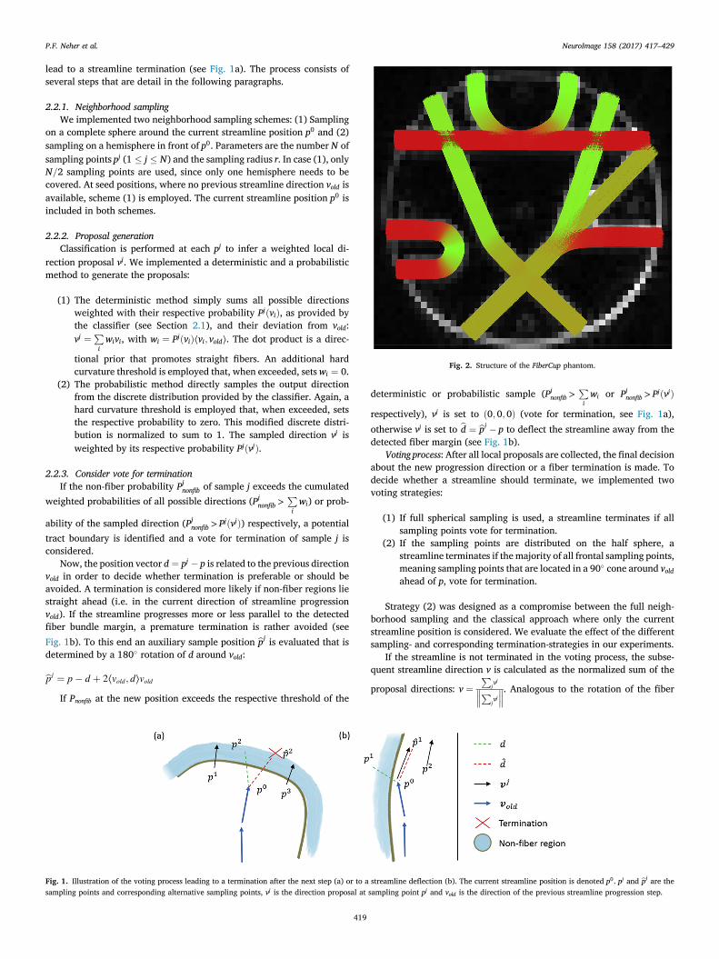
lead to a streamline termination (see Fig. 1a). The process consists ofseveral steps that are detail in the following paragraphs.

2.2.1. Neighborhood samplingWe implemented two neighborhood sampling schemes: (1) Sampling

on a complete sphere around the current streamline position p0 and (2)sampling on a hemisphere in front of p0. Parameters are the number N ofsampling points pj (1 ! j ! N) and the sampling radius r. In case (1), onlyN=2 sampling points are used, since only one hemisphere needs to becovered. At seed positions, where no previous streamline direction vold isavailable, scheme (1) is employed. The current streamline position p0 isincluded in both schemes.

2.2.2. Proposal generationClassification is performed at each pj to infer a weighted local di-

rection proposal vj. We implemented a deterministic and a probabilisticmethod to generate the proposals:

(1) The deterministic method simply sums all possible directionsweighted with their respective probability PjðviÞ, as provided bythe classifier (see Section 2.1), and their deviation from vold:vj ¼

Piwivi, with wi ¼ PjðviÞ⟨vi; vold⟩. The dot product is a direc-

tional prior that promotes straight fibers. An additional hardcurvature threshold is employed that, when exceeded, sets wi ¼ 0.

(2) The probabilistic method directly samples the output directionfrom the discrete distribution provided by the classifier. Again, ahard curvature threshold is employed that, when exceeded, setsthe respective probability to zero. This modified discrete distri-bution is normalized to sum to 1. The sampled direction vj isweighted by its respective probability PjðvjÞ.

2.2.3. Consider vote for terminationIf the non-fiber probability Pjnonfib of sample j exceeds the cumulated

weighted probabilities of all possible directions (Pjnonfib >Piwi) or prob-

ability of the sampled direction (Pjnonfib >PjðvjÞ) respectively, a potentialtract boundary is identified and a vote for termination of sample j isconsidered.

Now, the position vector d ¼ pj % p is related to the previous directionvold in order to decide whether termination is preferable or should beavoided. A termination is considered more likely if non-fiber regions liestraight ahead (i.e. in the current direction of streamline progressionvold). If the streamline progresses more or less parallel to the detectedfiber bundle margin, a premature termination is rather avoided (seeFig. 1b). To this end an auxiliary sample position bpj is evaluated that isdetermined by a 180& rotation of d around vold:

bpj ¼ p% d þ 2⟨vold; d⟩vold

If Pnonfib at the new position exceeds the respective threshold of the

deterministic or probabilistic sample (Pjnonfib >

Piwi or Pj

nonfib >PjðvjÞ

respectively), vj is set to ð0;0; 0Þ (vote for termination, see Fig. 1a),otherwise vj is set to bd ¼ bpj % p to deflect the streamline away from thedetected fiber margin (see Fig. 1b).

Voting process: After all local proposals are collected, the final decisionabout the new progression direction or a fiber termination is made. Todecide whether a streamline should terminate, we implemented twovoting strategies:

(1) If full spherical sampling is used, a streamline terminates if allsampling points vote for termination.

(2) If the sampling points are distributed on the half sphere, astreamline terminates if the majority of all frontal sampling points,meaning sampling points that are located in a 90& cone around voldahead of p, vote for termination.

Strategy (2) was designed as a compromise between the full neigh-borhood sampling and the classical approach where only the currentstreamline position is considered. We evaluate the effect of the differentsampling- and corresponding termination-strategies in our experiments.

If the streamline is not terminated in the voting process, the subse-quent streamline direction v is calculated as the normalized sum of the

proposal directions: v ¼P

jvj!!!

Pjvj!!!. Analogous to the rotation of the fiber

Fig. 1. Illustration of the voting process leading to a termination after the next step (a) or to a streamline deflection (b). The current streamline position is denoted p0. pj and bpj are thesampling points and corresponding alternative sampling points, vj is the direction proposal at sampling point pj and vold is the direction of the previous streamline progression step.

Fig. 2. Structure of the FiberCup phantom.

P.F. Neher et al. NeuroImage 158 (2017) 417–429

419

directions that are used as input features for the classifier (see Section2.1), the output direction v is multiplied with the original image rotationmatrix to obtain alignment with the image.

2.3. Experiments

We performed four types of experiments to evaluate our approach.

2.3.1. Experiment 1To determine the optimal choice of the tractography algorithm used

to create the training data for our approach and to obtain an initialevaluation of its performance, we used a simulated replication of theFiberCup phantom (see Fig. 2) (Fillard et al., 2011). The dataset wassimulated using the Fiberfox simulation tool (Neher et al., 2014) with thefollowing parameters: 30 gradient directions, a b-value 1000 s mm%2,3 mm isotropic voxels and a signal-to-noise ratio of about 40. The moti-vation for this choice of parameters was to create a challenging datasetthat is also comparable to a clinical acquisition in terms of acquisitionparameters. Tractography was performed with 12 combinations of thefollowing openly available tractography and local modeling techniques(see Table 1 for corresponding toolkits):

( Tractography algorithms:( Deterministic streamline tractography (DET)( Fiber assignment by continuous tracking (FACT)( Tensor deflection tractography (TEND)( Probabilistic streamline tractography (PROB)( Global Gibbs tractography

( Local modeling techniques:( Single-Tensor model (DT)( Two-Tensor model (DT-2)( Constrained spherical deconvolution (CSD)( Constant solid angle Q-ball (CSA)

The presented approach was trained individually with each of the 12benchmark methods. Based on the results of this analysis, the mostpromising algorithm was chosen to obtain the training tractogram for allfurther experiments (Atrain).

To quantify the performance of the methods, the following metricsfrom the Tractometer evaluation protocol (Cot!e et al., 2013) wereanalyzed: the fraction of no connections (NC), valid connections (VC),invalid connections (IC) and bundle overlap (OL), as well as an additionalmeasure for the local angular error (AE) (Neher et al., 2015a).

Seeding was performed homogeneously within the image. No white-matter mask was used to constrain the tractography. All tractographyalgorithms were run with their default parametrization. Only the stop-ping criteria (FA and ODF peak thresholds) were manually adjusted toobtain plausible results (FA threshold 0.15, peak threshold for CSA 0.085and peak threshold for CSD 0.15).

The presented method was run with N ¼ 50 sampling points, a stepsize of 0.5⋅f (f is the minimal voxel size in mm), full spherical samplingwith r ¼ 0.25⋅f, a minimum fiber length of 20 mm, a maximum fiberlength of 200mm, and a hard curvature threshold at a maximum angle of45& between two steps or a maximum directional standard deviation of30& over the last centimeter. The values for step size and angularthresholds are typical for streamline based fiber tractography approachesand were not optimized.

The number of sampling points and the sampling distance weredetermined empirically. The number of sampling points yields stableresults above a certain threshold (~30 samples). A much denser samplingthan the 50 points used in this experiment mainly increases the compu-tational load without yielding new information. The sampling distancewas chosen based on the following rational: a very large sampling dis-tance leads to an underestimation of the tracts, since the streamlines arepushed away too far from the white matter boundaries. A very smallsampling distance on the other hand leads to a vanishing of the sampling

effect since the information at the individual sampling points convergesto the information at the current streamline position. Therefore, a sam-pling distance r between 0.25⋅f and 0.75⋅f, depending on the voxel size(see Experiment 4), is a reasonable choice.

The classifier was trained using 30 trees, a maximum tree depth of 50and a Gini splitting criterion (Breiman, 1996). The forest parametersyielded stable results in a broad range (cf. Experiment 1 and Experiment 3)and increasing them further would mainly impact the computational costof the method and increase the risk of overfitting. The training data wassampled equidistantly (0.5⋅f) along the input tractogram fibers as well ason 50 randomly placed points in each non-fiber voxel. These values werechosen to obtain as many training samples as possible with the givenmemory. In general, more training data is always better. One advantageof random forests in this context is their low variance, i.e. error due tosensitivity to changes in the training data, which is favorable for gener-alizing to unseen data and also for robustness against changes in theparameters described above (Caruana and Niculescu-Mizil, 2006). Asclassification features we used the raw diffusion-weighted signal values,resampled to 100 directions equally distributed over the hemisphereusing spherical harmonics (see Section 2.1).

2.3.2. Experiment 2The in vivo performance of our approach in comparison to the 12

methods described in Experiment 1was qualitatively evaluated on basis ofreconstructions of the corticospinal tract (CST) and by an analysis of thespatial distribution of fiber end points. The dataset was acquired using 81gradient directions, a b-value 3000 s mm%2 and 2.5 mm isotropic voxels.All methods were run with their default parameterization, which is thesame as in Experiment 1. In contrast to Experiment 1, no manual adjust-ment of FA and ODF peak thresholds was necessary in vivo. As in Exper-iment 1, the interpolated raw signal values were used as input features forthe classifier. To obtain the training reference for the in vivo dataset, weused the tractography method determined in Experiment 1 (Atrain) with itsdefault parameterization.

2.3.3. Experiment 3In this experiment, we assessed the performance of the presented

method using the ISMRM tractography challenge 2015 data (Maier-Heinet al., 2016) (www.tractometer.org/ismrm_2015_challenge/). Theground truth fiber bundles mimic the shape and complexity of 25 wellknown in vivo fiber bundles (see Fig. 3). The diffusion-weighted datasetwas simulated with 32 gradient directions, a b-value 1000 s mm%2 and2 mm isotropic voxels.

This experiment enabled us to compare our approach to all 96 orig-inal submissions of the tractography challenge comprising a large varietyof tractography pipelines with different pre-processing, local recon-struction, tractography, and post-processing algorithms.

As preprocessing step, the dataset was denoised and corrected fordistortions using MRtrix (dwidenoise & dwipreproc, http://www.mrtrix.org/).

The random forest classifier was trained using all combinations of thefollowing parameters, resulting in a total of 8 trained classifiers:

( Classification features:1. Interpolated raw signal values2. Spherical harmonics coefficients (order 6)

( Additional features:1. No additional features2. T1 signal and GFA

( Training tractograms:1. Ground truth fibers (GTtrainÞ used to simulate the phantom image2. Tractogram obtained using the method Atrain

To reduce the computational load and since the parameters yieldedstable results across a broad range, the maximum tree depth was reducedto 25 and the number of sampling points N during tracking was reduced

P.F. Neher et al. NeuroImage 158 (2017) 417–429

420

to 30. To obtain balanced classes, the number of non-fiber samples waschosen automatically to match the number of fiber samples.

The tractography process is influenced by several components,namely the classifier, the neighborhood sampling and the voting strategy,as well as the direction proposal. To disentangle the effects of the indi-vidual components, tractographywas performedwith all combinations ofthe 8 trained classifiers and the different options for the sampling strat-egy and actual tractography:

( Sampling strategies:1. No neighborhood sampling. Only the prediction of the classifier at

the current streamline position is taken into account. This enablesto discern the contributions of the classifier vs. the contribution ofthe neighborhood sampling and voting mechanism.

2. Hemispherical sampling with majority voting (see 2.2, votingstrategy (2)).

3. Full spherical sampling (see 2.2, voting strategy (1)).( Direction proposal type (see Section 2.2):1. Deterministic2. Probabilistic

Furthermore, we repeated the same experiments with classical di-rection proposal strategies instead of the random forest classification:(1) The voxel-wise peak directions calculated using CSD (deterministictractography only) and (2) the voxel-wise CSD fODFs (deterministic andprobabilistic tractography). CSD was performed using MRtrix and trac-tography using MITK. As termination criterion for these experiments weused a peak magnitude and CSA-Q-ball GFA threshold of 0.1 respec-tively (Aganj et al., 2009). Comparing the classification based approachto these classical approaches enables a more in-depth analysis of thecontribution of the random forest classifier to the results. All experi-ments were run with 1 and 3 seed points per voxel. The step size andsampling distance of 0.5⋅f, r ¼ 0.25⋅f was kept at the same values as inExperiment 1 and 2.

The same evaluation metrics as presented in the original challengewere analyzed for all 16 tractograms using the official challenge evalu-ation pipeline: valid bundles (VB), invalid bundles (IB), valid connections(VC), bundle overlap (OL) and bundle overreach (OR).

2.3.4. Experiment 4Our final experiments aim at evaluating the generalization capability

of the presented method using in vivo and in silico data:As in vivo data we used five datasets of the Human Connectome

Project (HCP) (Van Essen et al., 2013, 2012; Van Essen and Ugurbil,2012) for training and five other HCP datasets for testing (HCPtrain[Subject IDs: 984472, 979984, 978578, 994273, 987983] and HCPtest[Subject IDs: 992774, 991267, 983773, 965771, 965367]). The HCPdatasets are acquired using 270 gradient directions, three b-values(1000 s mm%2, 2000 s mm%2, 3000 s mm%2) and 1:25 mm isotr-opic voxels.

As in silico data for this experiment, we employed the ISMRM trac-tography challenge phantom already used in Experiment 3. Since thephantom and the HCP datasets were acquired with different imagingsequences, they feature different image contrasts. Therefore, the phan-tom dataset was normalized to feature the same signal mean and stan-dard deviation across all weighted volumes inside the white matter as theHCP datasets. To ensure comparability with the results obtained on the insilico data, which only features a b-value of b ¼ 1000 s mm%2, we alsolimited the following in vivo experiments to a b-value of 1000 s mm%2 fortraining and tractography.

Three types of generalization were tested:

(1) In vivo → in vivo: In this part of the experiment, we trained ourmethod using HCPtrain and evaluated its performance on the un-seen datasets ofHCPtest. Training was performed usingmulti-tissueCSD (Jeurissen et al., 2014) deterministic tractography as Atrain,about 12 million samples per dataset and spherical harmonicscoefficients as classification features. Since the HCP datasetsfeature a much higher resolution compared to the datasets used inthe other experiments, tractography on HCPtest was performedusing an increased sampling distance (0.7⋅f) and step size (1.0*f).Streamlines were seeded five times in every brain voxel andproposals were generated deterministically using the hemispher-ical sampling scheme. Evaluation was performed qualitatively bymanually extracting the corticospinal tract (CST), cingulum (Cg)and fornix (Fx) from each of the five test results and a successivevisual inspection of the tracts.

Fig. 3. Illustration of the phantom generation process (a) and its constituent 25 fiber bundles (b). For details about the ISMRM tractography challenge 2015 and the phantom, please referto (Maier-Hein et al., 2016) and the challenge homepage www.tractometer.org/ismrm_2015_challenge/.

P.F. Neher et al. NeuroImage 158 (2017) 417–429

421

(2) In vivo → in silico: In this part of the experiment, we trained ourmethod using HCPtrain and evaluated its performance on theunseen phantom dataset already used in Experiment 3. The sametractography parameterization (deterministic, 3 seed points) asin Experiment 3 and the same classifier already employed inpart (1) were used. The resulting tractogram was evaluatedquantitatively using the same measures already described inExperiment 3.

(3) In silico → in vivo: In this part of the experiment, we trained ourmethod on the phantom dataset and the corresponding groundtruth fibers introduced in Experiment 3 and tested it on the five invivo HCPtest datasets. As in (1) and (2), the b ¼ 1000 s mm%2 shellsof HCPtest datasets were used to calculate the features for ourmethod. Evaluation and tractography was performed analogousto (1).

3. Results

3.1. Experiment 1

The best results on the phantom image were obtained using the CSDDET tractography (Tournier et al., 2012, 2007) for training ourapproach (Atrain ¼ CSD DET). With this configuration, the presentedapproach outperformed all benchmark methods in four out of the fivemetrics (see Table 1). Only 3% of the tracts terminated prematurely.Furthermore, the presented approach yielded the highest percentage ofvalid connections (93%), the highest bundle overlap (94%) and thelowest local angular error (4%). All 7 valid bundles in the phantomwere reconstructed successfully. Also, the percentage of invalid con-nections (4%) is rather low compared to the majority of benchmarkalgorithms (rank 4 out of 13). When varying the method that was usedfor training, the percentage of prematurely ending fibers and validconnections yielded by the presented approach improved on average by56% and 36% respectively as compared to the benchmark tractograms.The average percentage of invalid connections, however, was increasedby 21%.

3.2. Experiment 2

Based on the results of Experiment 1, the CSD DET tractography wasused as training method Atrain for the in vivo experiments. In vivo, ourapproach successfully reconstructed a whole brain tractogram includingchallenging regions such as the crossing between the corpus callosum,the CST and the superior longitudinal fasciculus. Our method wasfurthermore able to reconstruct parts of the CST that other approachesoften missed (e.g. lateral projections of the CST in Fig. 4b). In comparisonto the benchmark algorithms, most of the fibers reconstructed by the

presented approach correctly terminated in the cortex (see Fig. 4a).

3.3. Experiment 3

The following paragraphs describe the performance of the presentedmethod with respect to its individual components and elucidate specificaspects of the results. We focus on the performance of the deterministicproposal generation in conjunction with training the classifier using theclassical CSD streamline tractogram Atrain, if not stated otherwise. Theresults of the probabilistic proposal generation and the training usingthe ground truth tracts GTtrain are analyzed separately in the respectiveparagraphs. All results were tested for significance using a significancelevel of α ¼ 0:05 (Bonferroni corrected α ¼ 0:05

45 ≈0:00111), if notstated otherwise.

General observations and comparison to the original challenge sub-missions: The presented approach is the only method that was able toreconstruct all 25 valid bundles. Interestingly, it was able to outperformits training tractogram Atrain with respect to most metrics (see Fig. 5).Compared to the mean scores over all 96 benchmark submissions, theproposed approach performed better in terms of overlap (þ18.9%), validbundles (þ2.9), valid connections (þ7.5%) and invalid bundles (%0.7),albeit the latter two improvements were not statistically significant. Theoverreach on the other hand was increased by 11%. Significance testswere performed with a Mann-Whitney U-test.

Table 2 shows how many of the originally submitting teams could beoutperformed with respect to the team-mean of the respective score (nottested for significance due to a partially very small number of sub-missions per team). The scores show that our approach consistentlyoutperformed more than half of the challenge teams. In case of the VBscore, all 20 teams could be outperformed.

Classification vs. CSD based tractography: This paragraph presentsthe results of the proposed classification based approach compared toclassical CSD based proposal generation. On average over all samplingschemes, the classification based approach outperformed classical sam-pling with respect to the valid connections (þ16.1%) and the validbundles (þ1.1). Significance tests were performed with a Mann-WhitneyU-test. Statistically not significant changes were observed for the bundleoverlap (þ3.6%), the overreach (þ3.4%) and the number of invalidbundles (þ7). The remaining results of this paragraph were not tested forsignificance due to the low number of samples in the individual groups.Table 3 shows the score differences between the two approaches, indi-vidually calculated for each sampling scheme to disentangle the effects ofthe respective component. For all schemes, valid bundles, valid connec-tions and bundle overlap were improved using the classification basedapproach. On the other hand, the number of invalid bundles and theoverreach were increased. While out of the classical methods, the peakbased approach performed best in terms of valid connections (58%) andvalid bundles (23.5), it was still outperformed by the classification basedapproach (61.1% and 24.25 respectively).

Neighborhood sampling: Surprisingly, the neighborhood samplingonly had a very little effect on the scores. Using hemispherical samplingand voting, the only significant score change was an increased percent-age of valid connections (þ0.7%). Using full spherical sampling, the validconnections score was decreased by 2.6% while overlap and overreachwere increased by 2.3% and 3.5% respectively. Significance tests wereperformed with a paired t-test.

Probabilistic vs. deterministic proposal generation: To compare theresults between the probabilistic and deterministic proposal generation,only the pipelines without neighborhood sampling were analyzed toisolate the effect of the probabilistic sampling. Furthermore, usingneighborhood sampling in conjunction with probabilistic sampling issomewhat counterproductive, since the sampling process generates aweighted average of the proposals, which counteracts the probabilisticnature of the proposal generation. The deterministic approach yielded amuch higher valid connections rate (þ14.6%), while the overreach was

Table 1Results of Experiment 1. The best scores per metric are highlighted bold. The toolkits usedto obtain the 12 reference tractograms are 1MITK Diffusion (www.mitk.org/wiki/DiffusionImaging), 2Camino (camino.cs.ucl.ac.uk/) and 3MRtrix (www.mrtrix.org, v0.2).

Model Type NC VC IC OL AE

DT1 DET1 60% 25% 15% 21% 5&

DT1 FACT1 62% 23% 14% 24% 6&

DT1 TEND1 84% 8% 8% 21% 10&

DT2 PROB2 57% 23% 20% 27% 8&

DT1 Global1 82% 10% 8% 42% 12&

CSA1 DET3 24% 67% 9% 70% 8&

CSA1 PROB3 91% 5% 4% 83% 18&

CSA1 Global1 81% 14% 5% 74% 13&

DT-22 DET2 60% 37% 3% 58% 6&

CSD3 DET3 21% 78% 1% 86% 4&

CSD3 PROB3 66% 28% 7% 93% 4&

CSD3 Global1 81% 17% 2% 72% 12&

– Proposed 3% 93% 4% 94% 4&

P.F. Neher et al. NeuroImage 158 (2017) 417–429

422

lower using the probabilistic approach (%4.4%). Significance tests wereperformed with a paired t-test. The approaches showed no significantdifferences in the other scores.

Training data: In this paragraph, we analyzed the effect of the usedtraining data (Atrain or GTtrain). As expected, the presented method per-forms clearly better when using the GTtrain tracts as training data ascompared to the training tractogram obtained with Atrain (see Fig. 5).

Especially the valid connections (þ14.5%), bundle overlap (þ15.7%)and bundle overreach (%5.7%) were distinctly improved using GTtrain.Significance tests were performed with a paired t-test.

Effect of the different diffusion-weighted features: Using sphericalharmonics coefficients instead of the raw signal values as classificationfeatures resulted in consistently but only slightly higher valid connectionrates (þ2.3%) and a higher overlap (þ3%). Significance tests were

Fig. 4. Results on the in vivo Experiment 2. (a) Shows the max-normalized voxel-wise number of fiber endpoints, maximum intensity projected over 20 sagittal slices. (b) Shows thecorticospinal tracts obtained with all 13 algorithms. The green bars schematically depict the inclusion regions used for all whole brain tractograms to extract the respective CST.

P.F. Neher et al. NeuroImage 158 (2017) 417–429

423

performed with a paired t-test.Effect of additional features: The differences are very small and

consistent effects could only be detected when training on the groundtruth, where inclusion of T1 and GFA features lead to a slight increase ofvalid connections (þ1.3%), a higher overlap (þ0.7%) and a loweroverreach (%2.6%). Significance tests were performed with a pairedt-test.

Effect of the varying number of seed points: Using a larger number ofseed points resulted in a higher bundle overlap (þ6.6%), while at thesame time increasing the overreach (þ5.2%) and the number of invalidbundles (þ9.5). Significance tests were performed with a paired t-test.

3.4. Experiment 4

Overall, the presented approach was able to generalize well to unseendatasets. The following paragraphs describe the individual results of thethree parts of this experiment.

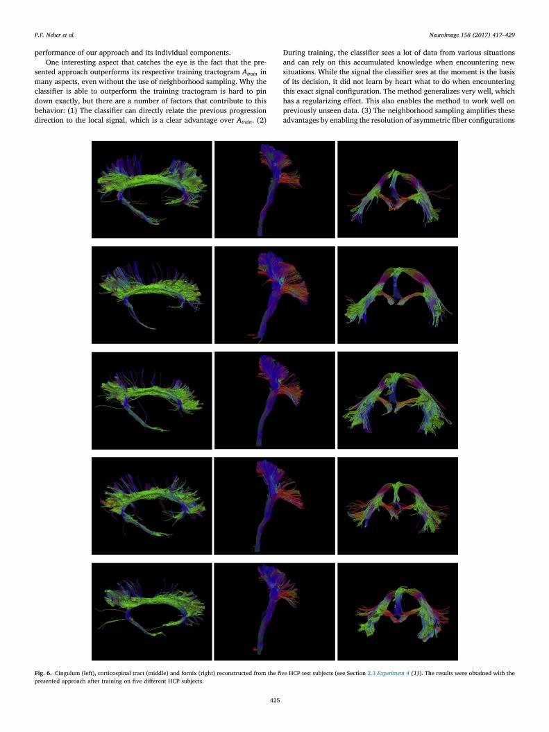
(1) In vivo → in vivo: Fig. 6 shows the tracts extracted from the fiveHCP test tractograms. All tracts were reconstructed successfully,which demonstrates that the classification based approach iscapable of generalization to unseen datasets.

(2) In vivo → in silico: The method trained on five HCP datasets wasable to reconstruct 23/25 valid bundles in the ISMRM tractog-raphy challenge phantom, while reconstructing 94 invalid bun-dles. Further scores were a fraction of valid connections of 52%, abundle overlap of 59% and a bundle overreach of 37%, which iscomparable to the results of Experiment 3, where the approach wasdirectly trained on the phantom dataset.

(3) In silico→ in vivo: As in (1), the approach trained on simulated datawas able to reconstruct the 3 tracts of interest in all five unseen invivo test datasets (see Fig. 7).

Fig. 8 shows a comparison between the results of classical CSD trac-tography (MRtrix) and the results of Experiment 4 (3). The classicalstreamline method had more difficulties to reconstruct the three tracts tothe full extent and struggled with prematurely ending fibers.

4. Discussion and conclusion

We presented a random-forest classification-based approach to fibertractography using neighborhood information that guides each step ofthe streamline progression. The presented approach is the first to utilizemachine learning for fiber tractography. The method systematically ex-ploits the diffusion-weighted signal not only locally but also in theneighborhood of the current streamline position.

We thoroughly evaluated the performance of the presented method incomparison to over 100 state-of-the-art tractography pipelines on simu-lated phantom datasets as well as in vivo.

In the in vivo experiments (Experiment 2), our approach yielded verygood results in reconstructing difficult tracts (e.g. the lateral projectionsof the CST) and a much lower number of fibers ending prematurely insidethe brain. As expected, tensor based approaches had difficulties indetecting the lateral projections of the CST. However, even the bench-mark method that performed best in the phantom experiments (Atrain ¼CSD DET) was unable to detect these projection fibers. The benchmarkmethods that showed a relatively high sensitivity in this region(CSA þ CSD PROB and DT-2 DET) displayed a very low specificity in thephantom experiments (Experiment 1) as well as with respect to the in vivoend-point distribution. In contrast, the presented algorithm showed aconstantly high sensitivity and specificity.

The quantitative analysis on the ISMRM tractography challengephantom dataset (Experiment 3) yielded various valuable insights into the

Table 2The table shows how many of the original challenge teams could be outperformed by thepresented approach with respect to the team-mean score.

Score VB IB VC OL OR

Number of outperformed teams 20 11 13 18 15

Table 3The table shows the score differences between classical CSD based and the proposedclassification based approach. The rows show the differences of the mean scores withrespect to the sampling scheme.

Score VB IB VC OL OR

No neighborhood sampling þ0.9 þ8.8 þ21% þ3% þ4%Frontal neighborhood sampling þ1.1 þ6.6 þ15% þ3% þ2%Full neighborhood sampling þ1.2 þ5.7 þ12% þ4% þ4%

Fig. 5. Scores of the 16 new tractograms obtained using the presented method (color) in comparison to the original challenge submissions (gray). The tractograms in Team 21 (green x)were obtained using Atrain to generate the training reference and the tractograms in Team 22 (blue, þ) with the ground truth tracts GTtrain as training reference. The scores of trainingtractogram Atrain itself are shown for comparison (red, star). For reasons of clarity, only the results obtained with the frontal neighborhood sampling scheme are shown.

P.F. Neher et al. NeuroImage 158 (2017) 417–429

424

performance of our approach and its individual components.One interesting aspect that catches the eye is the fact that the pre-

sented approach outperforms its respective training tractogram Atrain inmany aspects, even without the use of neighborhood sampling. Why theclassifier is able to outperform the training tractogram is hard to pindown exactly, but there are a number of factors that contribute to thisbehavior: (1) The classifier can directly relate the previous progressiondirection to the local signal, which is a clear advantage over Atrain. (2)

During training, the classifier sees a lot of data from various situationsand can rely on this accumulated knowledge when encountering newsituations. While the signal the classifier sees at the moment is the basisof its decision, it did not learn by heart what to do when encounteringthis exact signal configuration. The method generalizes very well, whichhas a regularizing effect. This also enables the method to work well onpreviously unseen data. (3) The neighborhood sampling amplifies theseadvantages by enabling the resolution of asymmetric fiber configurations

Fig. 6. Cingulum (left), corticospinal tract (middle) and fornix (right) reconstructed from the five HCP test subjects (see Section 2.3 Experiment 4 (1)). The results were obtained with thepresented approach after training on five different HCP subjects.

P.F. Neher et al. NeuroImage 158 (2017) 417–429

425

and a better informed decision about whether to terminate or proceedwith the streamline progression. In general, the presented approachyields one of the best performances in terms of valid connections andvalid bindles, while keeping a high overlap/overreach ratio.

Our evaluation further showed that the good performance of thepresented approach is mainly attributable to the random forest classifierand only to a very small degree to the neighborhood sampling process,particularly in Experiment 3. The reasons for the good performance of the

classifier are already discussed in the previous paragraph. Our resultshow that the neighborhood sampling mainly affects the distribution offiber endpoints, but does not necessarily increase the number of validconnections. While the effect of the neighborhood sampling was onlyanalyzed systematically in case of the more complex 3D phantom used inExperiment 3, it is likely that the effect is stronger in case of the muchsimpler 2D phantom (Experiment 1). The sampling basically keeps thefibers alive as long as possible, which is more likely to have a positive

Fig. 7. Cingulum (left), corticospinal tract (middle) and fornix (right) reconstructed from the five HCP test subjects (see Section 2.3, Experiment 4 (3)). The results were obtained with thepresented approach after training on the ISMRM tractography challenge phantom.

P.F. Neher et al. NeuroImage 158 (2017) 417–429

426

effect in case of a simple phantom with well-defined and easier torecognize bundle endpoint regions. Unsurprisingly, the probabilisticproposal generation yielded much lower valid connection scores.Nevertheless, this approach may be useful in conjunction with higherorder integration methods or approaches that exploit and quantify thelocal uncertainty, e.g. to yield probabilistic connectivity maps.

The capability of the presented approach to generalize to unseendatasets was successfully demonstrated in Experiment 4. We showed thatgeneralization is possible between different in vivo images acquired withthe same MR sequence as well as between in vivo images and simulateddatasets (in both directions). The latter experiment, generalizing fromsimulated datasets to in vivo, is especially important, since it enables us totrain on datasets with known ground truth. This eliminates the biasintroduced by training on tracts obtained with a conventional tractog-raphy method. We could also show that we can yield better results, interms of tract-completeness, with this approach as compared to theclassical approach used to generate the training data, albeit only quali-tatively. Nevertheless, the clearly observable differences in the tracto-grams obtained in Experiment 4 (1) and (3) (compare Figs. 6 and 7)emphasize the impact of the training data on the resulting tractogram, asalready shown in Experiment 3. Since we did not perform any sophisti-cated domain adaptation besides normalizing the image contrast, this isan expected phenomenon. Furthermore, the phantom and the in vivodatasets have quite different structural properties, e.g. the phantomcontains much more non-fiber regions since it only includes 25 majorfiber bundles.

While the presented results are promising, there are still some chal-lenges to address. Further work is necessary to quantify and improve theperformance of the presented approach when training on simulateddatasets. One important aspects in this regard is the simulation of furtherdatasets to obtain more comprehensive training data with respect toimage contrast and fiber structure. Another aspect where methodologicalimprovements are definitely possible is the currently employed naïveapproach to generalize between the simulated and in vivo domain, usingapproaches of unsupervised domain adaptation and transfer learning(G€otz et al., 2014; Heimann et al., 2014; Long et al., 2016, 2014;McKeough et al., 2013; Pan and Yang, 2010; Sener et al., 2016). This alsoincludes the possibility to generalize to images acquired with differentsettings such as b-value and number of shells. Initial experiments alreadyshowed a relatively good generalizability between b-values using only a

simple image contrast normalization. In the context of multiple b-shells,it would also be interesting to evaluate feature sets other than sphericalharmonics coefficients that are more suitable for multiple shells. Anotherchallenge is the still high number of invalid bundles, which is a knownissue of current fiber tractography approaches (Maier-Hein et al., 2016).This is a challenge the whole fiber tractography community is facing andthat does not have a simple solution. However, it seems promising toincorporate as much additional knowledge in the tractography process aspossible, for which machine learning based approaches seem to be wellsuited. Interesting candidates would be functional MRI data or priorknowledge in form of cortical parcellations. An extension of the pre-sented method to directly include a distinction between different non-white matter tissue types, such as gray matter and corticospinal fluid,seems promising to further improve the decision on where to terminatethe fiber progression. This includes addressing further interesting aspectsof the fiber termination such as orthogonality to and uniform coverage ofthe gray-white-matter interface. We are also planning to analyze how theprocess of including neighborhood information can be improved further,e.g. by applying patch-based classification at the sampling positions inorder to include more context information into the individual proposals.Before implementing the voting process presented in this work, we dis-cussed the possibility to jointly process of the feature vectors of allsampling positions using one classifier. We ultimately decided againstthis for one main reason. With the presented approach we have a bettercontrol about how the neighborhood information is incorporated into thedecision process. It would be difficult to provide suitable training datathat could teach the classifier our intended behavior of avoiding pre-maturely ending streamlines. Nevertheless, a combination of both ap-proaches, patch based classification and sample voting, seems promisingand will be investigated in the future. In this context we are also testingother variations of the sampling and voting strategy to improve thatcould improve the results. Another issue that we are currently investi-gating is the handling of image rotations that are not accounted for in theimage rotation matrix. We are currently looking into the possibility ofaugmenting the training data with random rotations. This would enablethe classifier to handle images with arbitrary rotations equally well, but itwould also increase the training effort. A more straight-forward alter-native is the alignment of the respective rotated test image with thetraining data using a standard rigid registration technique.

The source-code of all methods presented in this work is available

Fig. 8. Comparison between the results obtained on subject 992774 using classical deterministic CSD streamline tractography (bottom row) and the proposed approach (top row). Theclassical streamline tractogram was obtained with the same method and parameterization as the training tractograms of Experiment 4 (1).

P.F. Neher et al. NeuroImage 158 (2017) 417–429

427

open-source and integrated into the Medical Imaging Interaction Toolkit(MITK) (Fritzsche et al., 2012; Nolden et al., 2013). The datasets used inExperiment 1 and 2 are available for download at www.nitrc.org/projects/diffusion-data/. The dataset used in Experiment 3 as well asmany other resources regarding the ISMRM tractography challenge areavailable at www.tractometer.org/ismrm_2015_challenge/. The HCPdatasets used in Experiment 4 are available on www.humanconnectome.org/data/.

Acknowledgments

Data were provided in part by the Human Connectome Project, WU-Minn Consortium (Principal Investigators: David Van Essen and KamilUgurbil; 1U54MH091657) funded by the 16 NIH Institutes and Centersthat support the NIH Blueprint for Neuroscience Research; and by theMcDonnell Center for Systems Neuroscience at Washington University.

This work was supported by the Collaborative Research Center (SFB/TRR 125 Cognition-Guided Surgery) of the German Research Foundation(DFG) grant number INST 35/1120-1, DFG grant MA 6340/10-1 and DFGgrant MA 6340/12-1.

References

Aganj, I., Lenglet, C., Jahanshad, N., Yacoub, E., Harel, N., Thompson, P.M., Sapiro, G.,2011. A Hough transform global probabilistic approach to multiple-subject diffusionMRI tractography. Med. Image Anal. 15, 414–425.

Aganj, I., Lenglet, C., Sapiro, G., 2009. ODF reconstruction in q-ball imaging with solidangle consideration. In: IEEE International Symposium on Biomedical Imaging: fromNano to Macro, pp. 1398–1401.

Alexander, D.C., 2005. Maximum entropy spherical deconvolution for diffusion MRI. In:Biennial International Conference on Information Processing in Medical Imaging.Springer, pp. 76–87.

Alexander, D.C., Zikic, D., Ghosh, A., Tanno, R., Wottschel, V., Zhang, J., Kaden, E.,Dyrby, T.B., Sotiropoulos, S.N., Zhang, H., others, 2017. Image quality transfer andapplications in diffusion MRI. Neuroimage 152, 283–298.

Assaf, Y., Basser, P.J., 2005. Composite hindered and restricted model of diffusion(CHARMED) MR imaging of the human brain. Neuroimage 27, 48–58.

Assaf, Y., Blumenfeld-Katzir, T., Yovel, Y., Basser, P.J., 2008. AxCaliber: a method formeasuring axon diameter distribution from diffusion MRI. Magn. Reson. Med. 59,1347–1354.

Basser, P.J., 1998. Fiber-tractography via diffusion tensor MRI. In: Proc. InternationalSociety for Magnetic Resonance in Medicine.

Basser, P.J., Mattiello, J., Ihan, D.L.B., 1994. Estimation of the effective self-diffusiontensor from the NMR spin echo. J. Magn. Reson. B 103, 247–254.

Bastiani, M., Cottaar, M., Dikranian, K., Sotiropoulos, S.N., 2016. Improved tractographyby modelling sub-voxel fibre patterns using asymmetric fibre orientationdistributions. In: Proc. Int. Soc. Magn. Reson. Med. Presented at the ISMRM. ISMRM.

Behrens, T.E.J., Berg, H.J., Jbabdi, S., Rushworth, M.F.S., Woolrich, M.W., 2007.Probabilistic diffusion tractography with multiple fibre orientations: what can wegain? Neuroimage 34, 144–155.

Berman, J.I., Chung, S., Mukherjee, P., Hess, C.P., Han, E.T., Henry, R.G., 2008.Probabilistic streamline q-ball tractography using the residual bootstrap. Neuroimage39, 215–222.

Breiman, L., 1996. Technical note: some properties of splitting criteria. Mach. Learn 24,41–47.

Caruana, R., Niculescu-Mizil, A., 2006. An empirical comparison of supervised learningalgorithms. In: Proceedings of the 23rd International Conference on MachineLearning. ACM, pp. 161–168.

Chao, Y.-P., Chen, J.-H., Cho, K.-H., Yeh, C.-H., Chou, K.-H., Lin, C.-P., 2008. A multiplestreamline approach to high angular resolution diffusion tractography. Med. Eng.Phys. 30, 989–996.

Cot!e, M.-A., Girard, G., Bor!e, A., Garyfallidis, E., Houde, J.-C., Descoteaux, M., 2013.Tractometer: towards validation of tractography pipelines. Med. Image Anal. 17,844–857.

Daducci, A., Canales-Rodrõ, E.J., Descoteaux, M., Garyfallidis, E., Gur, Y., Lin, Y.-C.,Mani, M., Merlet, S., Paquette, M., Ramirez-Manzanares, A., others, 2014.Quantitative comparison of reconstruction methods for intra-voxel fiber recoveryfrom diffusion MRI. IEEE Trans. Med. Imaging 33, 384–399.

Daducci, A., Dal Palù, A., Lemkaddem, A., Thiran, J.-P., 2015. COMMIT: convexoptimization modeling for microstructure informed tractography. IEEE Trans. Med.Imaging 34, 246–257.

Descoteaux, M., Angelino, E., Fitzgibbons, S., Deriche, R., 2007. Regularized, fast, androbust analytical Q-ball imaging. Magn. Reson. Med. 58, 497–510.

Descoteaux, M., Deriche, R., Knosche, T.R., Anwander, A., 2009. Deterministic andprobabilistic tractography based on complex fibre orientation distributions. IEEETrans. Med. Imaging 28, 269–286.

Farquharson, S., Tournier, J.-D., Calamante, F., Fabinyi, G., Schneider-Kolsky, M.,Jackson, G.D., Connelly, A., 2013. White matter fiber tractography: why we need tomove beyond DTI: clinical article. J. Neurosurg. 118, 1367–1377.

Fillard, P., Descoteaux, M., Goh, A., Gouttard, S., Jeurissen, B., Malcolm, J., Ramirez-Manzanares, A., Reisert, M., Sakaie, K., Tensaouti, F., Yo, T., Mangin, J.-F.,Poupon, C., 2011. Quantitative evaluation of 10 tractography algorithms on arealistic diffusion MR phantom. Neuroimage 56, 220–234.

Fillard, P., Poupon, C., Mangin, J.-F., 2009. A novel global tractography algorithm basedon an adaptive spin glass model. In: International Conference on Medical ImageComputing and Computer-assisted Intervention. Springer, pp. 927–934.

Friman, O., Farneback, G., Westin, C.-F., 2006. A Bayesian approach for stochastic whitematter tractography. IEEE Trans. Med. Imaging 25, 965–978.

Fritzsche, K.H., Neher, P.F., Reicht, I., van Bruggen, T., Goch, C., Reisert, M., Nolden, M.,Zelzer, S., Meinzer, H.-P., Stieltjes, B., others, 2012. MITK diffusion imaging. MethodsInf. Med. 51, 441.

Golkov, V., Dosovitskiy, A., Sperl, J.I., Menzel, M.I., Czisch, M., S€amann, P., Brox, T.,Cremers, D., 2016. Q-space deep learning: twelve-fold shorter and model-freediffusion MRI scans. IEEE Trans. Med. Imaging 35, 1344–1351.

G€otz, Michael, Weber, Christian, Stieltjes, Bram, Maier-Hein, K.H., 2014. Learning fromsmall amounts of labeled data in a brain tumor classification task. In: SecondWorkshop on Transfer and Multi-task Learning: Theory Meets Practice, NeuralInformation Processing Systems (NIPS). Montreal, Canada.

Heimann, T., Mountney, P., John, M., Ionasec, R., 2014. Real-time ultrasound transducerlocalization in fluoroscopy images by transfer learning from synthetic training data.Med. Image Anal. 18, 1320–1328.

Jansons, K.M., Alexander, D.C., 2003. Persistent angular structure: new insights fromdiffusion magnetic resonance imaging data. Inverse Probl. 19, 1031.

Jbabdi, S., Johansen-Berg, H., 2011. Tractography: where do we go from here? BrainConnect. 1, 169–183.

Jbabdi, S., Woolrich, M.W., Andersson, J.L.R., Behrens, T.E.J., 2007. A Bayesianframework for global tractography. Neuroimage 37, 116–129.

Jeurissen, B., Tournier, J.-D., Dhollander, T., Connelly, A., Sijbers, J., 2014. Multi-tissueconstrained spherical deconvolution for improved analysis of multi-shell diffusionMRI data. NeuroImage 103, 411–426.

Kreher, B.W., Schneider, J.F., Mader, I., Martin, E., Hennig, J., Il’Yasov, K.A., 2005.Multitensor approach for analysis and tracking of complex fiber configurations.Magn. Reson. Med. 54, 1216–1225.

Lazar, M., Weinstein, D.M., Tsuruda, J.S., Hasan, K.M., Arfanakis, K.,Meyerand, M.E., Badie, B., Rowley, H.A., Haughton, V., Field, A., others, 2003.White matter tractography using diffusion tensor deflection. Hum. Brain Mapp.18, 306–321.

Lemkaddem, A., Ski€oldebrand, D., Dal Palú, A., Thiran, J.-P., Daducci, A., 2014. Globaltractography with embedded anatomical priors for quantitative connectivity analysis.Front. Neurol. 5.

Long, M., Wang, J., Ding, G., Pan, S.J., Philip, S.Y., 2014. Adaptation regularization: ageneral framework for transfer learning. IEEE Trans. Knowl. Data Eng. 26,1076–1089.

Long, M., Wang, J., Jordan, M.I., 2016. Unsupervised Domain Adaptation with ResidualTransfer Networks. ArXiv160204433 Cs.

Maier-Hein, K., Neher, P., Houde, J.-C., Cote, M.-A., Garyfallidis, E., Zhong, J.,Chamberland, M., Yeh, F.-C., Lin, Y.C., Ji, Q., others, 2016. Tractography-basedconnectomes are dominated by false-positive connections. bioRxiv 084137.

Malcolm, J.G., Shenton, M.E., Rathi, Y., 2010. Filtered multitensor tractography. IEEETrans. Med. Imaging 29, 1664–1675.

Mangin, J.-F., Fillard, P., Cointepas, Y., Bihan, D.L., Frouin, V., Poupon, C., 2013. Towardglobal tractography. Neuroimage 80, 290–296.

McKeough, A., Lupart, J.L., Marini, A., 2013. Teaching for Transfer: FosteringGeneralization in Learning. Routledge.

Mori, S., Crain, B.J., Chacko, V.P., Van Zijl, P., 1999. Three-dimensional tracking ofaxonal projections in the brain by magnetic resonance imaging. Ann. Neurol. 45,265–269.

Nedjati-Gilani, G.L., Schneider, T., Hall, M.G., Cawley, N., Hill, I., Ciccarelli, O.,Drobnjak, I., Wheeler-Kingshott, C.A.G., Alexander, D.C., 2017. Machine learningbased compartment models with permeability for white matter microstructureimaging. Neuroimage 150, 119–135.

Neher, P.F., Descoteaux, M., Houde, J.-C., Stieltjes, B., Maier-Hein, K.H., 2015a. Strengthsand weaknesses of state of the art fiber tractography pipelines–A comprehensive in-vivo and phantom evaluation study using Tractometer. Med. Image Anal. 26,287–305.

Neher, P.F., G€otz, M., Norajitra, T., Weber, C., Maier-Hein, K.H., 2015b. A machinelearning based approach to fiber tractography. In: Proceedings of InternationalSociety of Magnetic Resonance in Medicine.

Neher, P.F., Laun, F.B., Stieltjes, B., Maier-Hein, K.H., 2014. Fiberfox: facilitating thecreation of realistic white matter software phantoms. Magn. Reson. Med. 72,1460–1470.

Nimsky, C., 2014. Fiber tracking—we should move beyond diffusion tensor imaging.World Neurosurg. 82, 35–36.

Nolden, M., Zelzer, S., Seitel, A., Wald, D., Müller, M., Franz, A.M., Maleike, D.,Fangerau, M., Baumhauer, M., Maier-Hein, L., others, 2013. The medical imaginginteraction toolkit: challenges and advances. Int. J. Comput. Assist. Radiol. Surg. 8,607–620.

Pan, S.J., Yang, Q., 2010. A survey on transfer learning. Knowl. Data Eng. IEEE Trans. On.22, 1345–1359.

Panagiotaki, E., Schneider, T., Siow, B., Hall, M.G., Lythgoe, M.F., Alexander, D.C., 2012.Compartment models of the diffusion MR signal in brain white matter: a taxonomyand comparison. Neuroimage 59, 2241–2254.

Reisert, M., Kellner, E., Dhital, B., Hennig, J., Kiselev, V.G., 2017. Disentangling microfrom mesostructure by diffusion MRI: a Bayesian approach. NeuroImage 147,964–975.

P.F. Neher et al. NeuroImage 158 (2017) 417–429

428

Reisert, M., Mader, I., Anastasopoulos, C., Weigel, M., Schnell, S., Kiselev, V., 2011.Global fiber reconstruction becomes practical. Neuroimage 54, 955–962.

Rowe, M., Zhang, H.G., Oxtoby, N., Alexander, D.C., 2013. Beyond crossing fibers:tractography exploiting sub-voxel fibre dispersion and neighbourhood structure. Inf.Process. Med. Imaging Proc. Conf. 23, 402–413.

Savadjiev, P., Campbell, J.S., Descoteaux, M., Deriche, R., Pike, G.B., Siddiqi, K., 2008.Labeling of ambiguous subvoxel fibre bundle configurations in high angularresolution diffusion MRI. Neuroimage 41, 58–68.

Schultz, T., 2012. Learning a reliable estimate of the number of fiber directions indiffusion MRI. In: International Conference on Medical Image Computing andComputer-assisted Intervention. Springer, pp. 493–500.

Schultz, T., Westin, C.-F., Kindlmann, G., 2010. Multi-diffusion-tensor fitting viaspherical deconvolution: a unifying framework. In: International Conference onMedical Image Computing and Computer-assisted Intervention. Springer,pp. 674–681.

Sener, O., Song, H.O., Saxena, A., Savarese, S., 2016. Learning transferrablerepresentations for unsupervised domain adaptation. In: Advances in NeuralInformation Processing Systems, pp. 2110–2118.

Sotiropoulos, S.N., Behrens, T.E., Jbabdi, S., 2012. Ball and rackets: inferring fiberfanning from diffusion-weighted MRI. NeuroImage 60, 1412–1425.

Tournier, J.D., Calamante, F., Connelly, A., 2012. MRtrix: diffusion tractography incrossing fiber regions. Int. J. Imaging Syst. Technol. 22, 53–66.

Tournier, J.D., Calamante, F., Connelly, A., 2007. Robust determination of the fibreorientation distribution in diffusion MRI: non-negativity constrained super-resolvedspherical deconvolution. Neuroimage 35, 1459–1472.

Tuch, D.S., 2004. Q-ball imaging. Magn. Reson Med. 52, 1358–1372.Van Essen, D.C., Smith, S.M., Barch, D.M., Behrens, T.E., Yacoub, E., Ugurbil, K.,

Consortium, W.-M.H., others, 2013. The WU-Minn human connectome project: anoverview. Neuroimage 80, 62–79.

Van Essen, D.C., Ugurbil, K., 2012. The future of the human connectome. Neuroimage 62,1299–1310.

Van Essen, D.C., Ugurbil, K., Auerbach, E., Barch, D., Behrens, T.E.J., Bucholz, R.,Chang, A., Chen, L., Corbetta, M., Curtiss, S.W., Della Penna, S., Feinberg, D.,Glasser, M.F., Harel, N., Heath, A.C., Larson-Prior, L., Marcus, D., Michalareas, G.,Moeller, S., Oostenveld, R., Petersen, S.E., Prior, F., Schlaggar, B.L., Smith, S.M.,Snyder, A.Z., Xu, J., Yacoub, E., 2012. The Human Connectome Project: a dataacquisition perspective. Neuroimage 62, 2222–2231.

Vorburger, R.S., Reischauer, C., Boesiger, P., 2013. BootGraph: probabilistic fibertractography using bootstrap algorithms and graph theory. Neuroimage 66, 426–435.

Zhang, H., Schneider, T., Wheeler-Kingshott, C.A., Alexander, D.C., 2012. NODDI:practical in vivo neurite orientation dispersion and density imaging of the humanbrain. Neuroimage 61, 1000–1016.

Zhang, M., Sakaie, K.E., Jones, S.E., 2013. Logical foundations and fast implementation ofprobabilistic tractography. IEEE Trans. Med. Imaging 32, 1397–1410.

P.F. Neher et al. NeuroImage 158 (2017) 417–429

429