FIBER-OPTIC PRESSURE SENSOR FOR TIME-OF-FLIGHT ...arc.uta.edu/publications/td_files/Jagadevan_uta_2502M_10737.pdf · The University of Texas at Arlington, ... utilizing intensity

FIBER-OPTIC PRESSURE SENSOR FOR TIME-OF-FLIGHT

MEASUREMENTS IN A SHOCK WAVE

by

KARTHIKEYAN JAGADEVAN

Presented to the Faculty of the Graduate School of

The University of Texas at Arlington in Partial Fulfillment

of the Requirements

for the Degree of

MASTER OF SCIENCE IN AEROSPACE ENGINEERING

THE UNIVERSITY OF TEXAS AT ARLINGTON

August 2010

Copyright c© by Karthikeyan Jagadevan 2010

All Rights Reserved

To my mom, dad, sisters, friends and professors.

ACKNOWLEDGEMENTS

I would like to thank my research supervisor and professor, Dr. Frank Lu, for

supporting me throughout my masters program, for being the driving force behind

my work and allowing me to work at my pace, and for his understanding. I would also

like to thank Dr. Haying Huang for providing useful suggestions and modifications

that are required, I am grateful to her for allowing me to work in her lab to complete

my initial testing of the experiments. I would also like to thank Dr. Nader Hozhabri

for helping me with valuable information in order to proceed in the right direction to

complete my graduate studies. I would also like to thank Dr. Donald Wilson and Dr.

Wen Chan for their guidance as graduate advisors.

I would like to thank my friend Manjunath Shenoy for helping me at Dr. Haiy-

ing Huang’s laboratory to set up the experiments and for helping me in operating

them. I would like to thank my colleague Dr. Philip K. Panicker for supporting me

during my graduate studies. He was always ready to help me. I would like to thank

Prashaanth Ravindran for helping with LATEX to write my thesis. I would also like

to thank Adam Pierce, V. V. Suneel Jinnala, Hari Narayanan Nagarajan, Eric M.

Braun and Richard R. Mitchell for their help and support during my research at the

Aerodynamics Research Center. I would like to thank Alex Alphonse and Kermit

Beird for helping in machining the parts. I would also like to thank Manda machines

for helping me with the parts. I would also like to thank my friends Abhilash R.

Menon, Jitesh Cherrukkadu Parambil, and Bharathkrishnan Muralidharan and Pra-

jwal Shetty for their support and motivation that they provided during the stay at

UTA.

iv

I would like to thank all my friends and professors who made my life at UTA

fruitful and fun. Nonetheless, I would like to thank my parents and sisters being with

me during hard times and constantly encouraging me to reach new heights. I am

always grateful to everyone who helped and supported me.

May 28, 2010

v

ABSTRACT

FIBER-OPTIC PRESSURE SENSOR FOR TIME-OF-FLIGHT

MEASUREMENTS IN A SHOCK WAVE

Karthikeyan Jagadevan, M.S.

The University of Texas at Arlington, 2010

Supervising Professor: Frank K Lu

Fiber-optic sensors are widely employed to detect pressures and temperatures

precisely. In particular, MEMS-based fiber-optic sensors are immune to electromag-

netic interference but may have limitations at high temperatures as encountered in

combustors. To ensure high-temperature survivability, such sensors may be bonded

anodically. This project explains the development of a fiber-optic pressure sensor

utilizing intensity based principle whereby a fused silica optical window was glued to

the tungsten carbide enclosure. The development was estimated to determine high

pressures of up to at least 3.5 MPa (507 psi). The sensor is designed to capture

the pressure pulse and the time-of-flight (TOF) of a propagating detonation wave for

implementation shock tubes.

Time-of-flight is critically important in detonation studies as it relates directly

to the detonation wave velocity. Generally, the TOF is obtained by discrete sensors

separated by a distance of at least a few cm. Thus, the propagation velocity, is strictly

the average over that distance, thereby introducing a certain uncertainty. In order to

obtain a point measurement, the separation distance between the sensors should be

vi

kept as short as possible. Advances in MEMS and electro-optics have made it possible

to devise such an integrated TOF sensor together with high-speed data acquisition.

vii

TABLE OF CONTENTS

ACKNOWLEDGEMENTS . . . . . . . . . . . . . . . . . . . . . . . . . . . . iv

ABSTRACT . . . . . . . . . . . . . . . . . . . . . . . . . . . . . . . . . . . . vi

LIST OF FIGURES . . . . . . . . . . . . . . . . . . . . . . . . . . . . . . . . x

LIST OF TABLES . . . . . . . . . . . . . . . . . . . . . . . . . . . . . . . . . xi

Chapter Page

1. INTRODUCTION . . . . . . . . . . . . . . . . . . . . . . . . . . . . . . . 1

1.1 Introduction . . . . . . . . . . . . . . . . . . . . . . . . . . . . . . . . 1

2. PRESSURE SENSOR DESIGN AND FABRICATION . . . . . . . . . . . 4

2.1 Time-of-Flight . . . . . . . . . . . . . . . . . . . . . . . . . . . . . . . 4

2.2 Conventional and Advanced MEMS Micromachining . . . . . . . . . 5

2.3 Design and Development . . . . . . . . . . . . . . . . . . . . . . . . . 6

2.4 Diaphragm . . . . . . . . . . . . . . . . . . . . . . . . . . . . . . . . 9

2.4.1 Types of Diaphragm Materials Examined . . . . . . . . . . . . 9

2.5 Nano Fabrication . . . . . . . . . . . . . . . . . . . . . . . . . . . . . 12

2.6 Fiber Optics . . . . . . . . . . . . . . . . . . . . . . . . . . . . . . . . 12

3. CALCULATIONS AND DERIVATIONS . . . . . . . . . . . . . . . . . . . 14

3.1 Thin Plate Theory . . . . . . . . . . . . . . . . . . . . . . . . . . . . 14

3.2 Diaphragm Design Calculations . . . . . . . . . . . . . . . . . . . . . 16

3.2.1 Manual Calculations . . . . . . . . . . . . . . . . . . . . . . . 16

3.2.2 ANSYS Results . . . . . . . . . . . . . . . . . . . . . . . . . . 20

3.3 Fiber Optic Placement . . . . . . . . . . . . . . . . . . . . . . . . . . 20

4. RESULTS AND DISCUSSION . . . . . . . . . . . . . . . . . . . . . . . . 22

viii

4.1 Calibration . . . . . . . . . . . . . . . . . . . . . . . . . . . . . . . . 22

4.1.1 Setup . . . . . . . . . . . . . . . . . . . . . . . . . . . . . . . 22

4.1.2 Operation . . . . . . . . . . . . . . . . . . . . . . . . . . . . . 22

4.1.3 Calibration Results and Discussion . . . . . . . . . . . . . . . 25

5. CONCLUSION AND RECOMMENDATIONS . . . . . . . . . . . . . . . . 34

5.1 Conclusion . . . . . . . . . . . . . . . . . . . . . . . . . . . . . . . . . 34

5.2 Recommendations . . . . . . . . . . . . . . . . . . . . . . . . . . . . . 35

5.2.1 Diaphragm thickness . . . . . . . . . . . . . . . . . . . . . . . 35

5.2.2 Higher pressure . . . . . . . . . . . . . . . . . . . . . . . . . . 35

5.2.3 Placement of diaphragm . . . . . . . . . . . . . . . . . . . . . 35

5.2.4 Fiber protection . . . . . . . . . . . . . . . . . . . . . . . . . . 36

Appendix

A. PCB PRESSURE TRANSDUCER CHARACTERISTICS . . . . . . . . . 37

B. LASER SOURCE AND PHOTODETECTOR . . . . . . . . . . . . . . . . 40

REFERENCES . . . . . . . . . . . . . . . . . . . . . . . . . . . . . . . . . . . 44

BIOGRAPHICAL STATEMENT . . . . . . . . . . . . . . . . . . . . . . . . . 48

ix

LIST OF FIGURES

Figure Page

1.1 Fabry–Perot interferometry principle . . . . . . . . . . . . . . . . . . 2

2.1 Time-of-flight concept . . . . . . . . . . . . . . . . . . . . . . . . . . . 4

2.2 Dynamic pressure sensor [1] . . . . . . . . . . . . . . . . . . . . . . . 7

2.3 Water jacket [2] . . . . . . . . . . . . . . . . . . . . . . . . . . . . . . 7

2.4 Schematic of FOPS . . . . . . . . . . . . . . . . . . . . . . . . . . . . 8

2.5 3D model (a) Bottom view (b) Front view . . . . . . . . . . . . . . . 10

2.6 Polished bare fibers (a) Without light (b) With IR light . . . . . . . . 13

3.1 Motor position . . . . . . . . . . . . . . . . . . . . . . . . . . . . . . . 21

4.1 Calibration setup (a) View 1 (b) View 2 . . . . . . . . . . . . . . . . . 23

4.2 Unassembled sensors (a) Close view (b) Comparison with a penny . . 24

4.3 Pressure calibration tests Set 1 (a) Test 1(b) Test 2 (c) Test 3 . . . . 27

4.4 Voltage readings from Labview (a) 50 secs (b) 0.5 secs(c) 0 to 5 secs (d) Variations after 5 secs when pressure is applied . . . 28

4.5 Pressure Calibration Tests Set 2 (a) Test 1 (b) Test 2 . . . . . . . . . 30

4.6 Pressure Calibration Tests Cycles (a) Cycle 1(b) Cycle 2 (c) Cycle 3 (d) Cycle 4 (e) Cycle 5 . . . . . . . . . . . . . 31

4.7 Aluminum diaphragm with increasing pressure one way . . . . . . . . 32

4.8 Aluminum diaphragm pressure cycling (a) Cycle 1(b) Cycle 2 (c) Cycle 3 . . . . . . . . . . . . . . . . . . . . . . . . . . . 33

x

LIST OF TABLES

Table Page

2.1 Comparison between the properties of diamond and cubic zirconia . . 11

3.1 Calculated thickness from assumed deflection for cubic zirconia . . . . 17

3.2 Diaphragm thickness and deflection for fused silica . . . . . . . . . . . 18

3.3 Diaphragm thickness and deflection forAluminum . . . . . . . . . . . 19

xi

CHAPTER 1

INTRODUCTION

1.1 Introduction

Time of flight (TOF) is an important parameter in the study of propagating

shocks and detonation waves. For example, in a pulse detonation engine, TOF analy-

sis shows that the wave accelerates during deflagaration-to-detonation before stabiliz-

ing at Chapman–Jouguet levels in the detonation tube [3]. Obtaining the TOF from

two transducers spaced apart produces a certain level of uncertainty per [4, 5], which

shows the importance of achieving a point measurement. What is needed is a device

that can measure a propagating pressure disturbance from the propagating shock or

wave at two consecutive points which are as close as possible. Though there are nu-

merous pressure sensing devices that can be used in harsh environments [6, 7, 8, 9],

a couple of miniature pressure sensors separated closely is required for the time-of-

flight measurement. Advancements in MEMS technology [10, 11] and development in

electronics facilitate the development of micro sensors with fast rise and fall time. In

addition, a fast responding photodetector can be chosen in order to obtain the fast

moving detonation wave velocity [12].

Optical fibers can also be considered in miniaturizing optical sensors. In this

sensor design, an intensity based method is employed along with fiber optics to de-

termine the deflection of a diaphragm which is related to the pressure of the wave.

The optical principle is based on the Fabry–Perot interferometry principle [13] ex-

cept that there are no interference patterns involved. Multi-mode fibers are used to

receive the reflected light; hence the name modified Fabry–Perot method or inten-

1

2

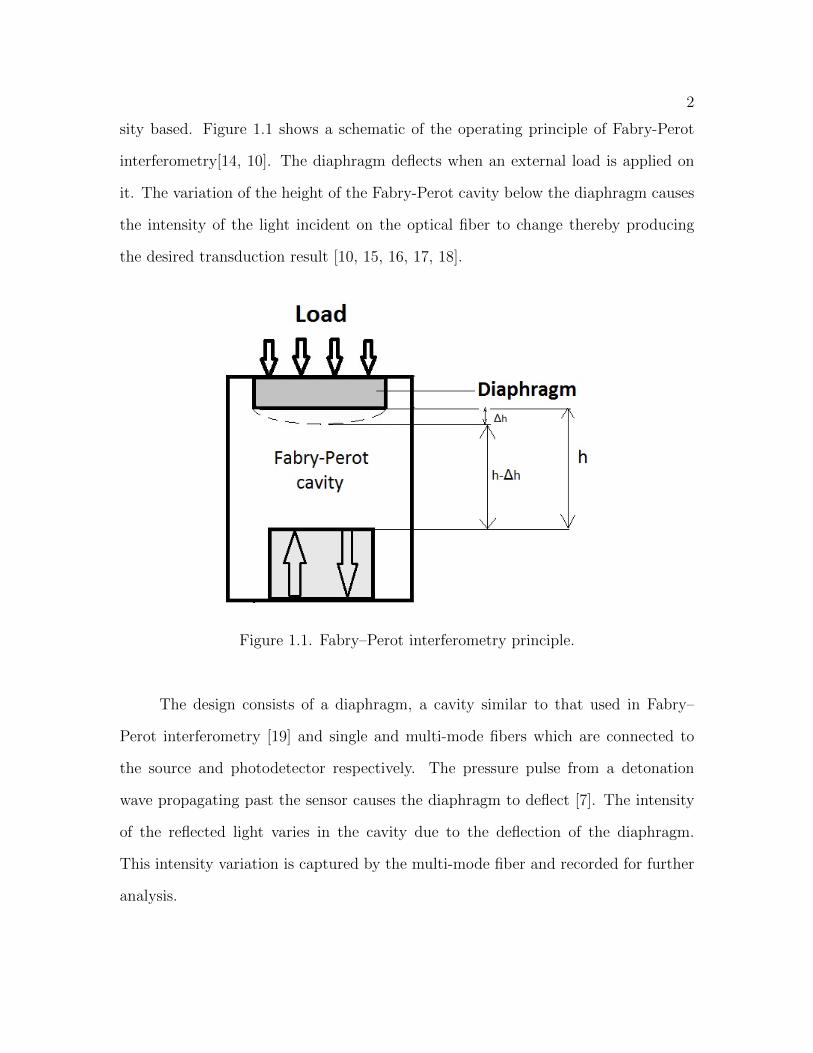
sity based. Figure 1.1 shows a schematic of the operating principle of Fabry-Perot

interferometry[14, 10]. The diaphragm deflects when an external load is applied on

it. The variation of the height of the Fabry-Perot cavity below the diaphragm causes

the intensity of the light incident on the optical fiber to change thereby producing

the desired transduction result [10, 15, 16, 17, 18].

Figure 1.1. Fabry–Perot interferometry principle.

The design consists of a diaphragm, a cavity similar to that used in Fabry–

Perot interferometry [19] and single and multi-mode fibers which are connected to

the source and photodetector respectively. The pressure pulse from a detonation

wave propagating past the sensor causes the diaphragm to deflect [7]. The intensity

of the reflected light varies in the cavity due to the deflection of the diaphragm.

This intensity variation is captured by the multi-mode fiber and recorded for further

analysis.

3

In the intensity-based method, single mode and multi-mode fibers were used

to send the incident light and receive the reflected light respectively. The deflections

produced due to the pressure are related to the reflection of the light from the di-

aphragm to the the multi-mode fiber. Optical power received through the multi-mode

fiber is converted to voltage in the photodetector and is observed in the oscilloscope.

We will discuss the design, development, calculations, calibration and testing,

and results and recommendations of the transducer in further chapters.

CHAPTER 2

PRESSURE SENSOR DESIGN AND FABRICATION

Pressure is an important parameter to be measured in detonation studies. Var-

ious types of pressure transducers can be used for this purpose.

2.1 Time-of-Flight

According to [20], time-of-flight values and their uncertainty estimates are im-

portant parameters in characterizing propagating shock and detonation processes. In

the classical time-of-flight method, the propagating disturbances pass through two

sensors placed in series and the time of propagation can then be estimated. Though

the TOF method seems to be simple, there is a certain level of uncertainity involved

in it. Further, more sophisticated methods may be used to determine the propagation

delay and to yield an uncertanity estimate.

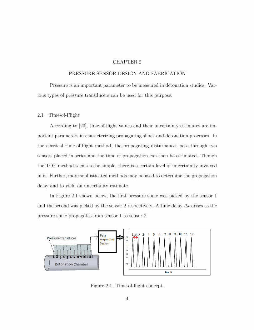
In Figure 2.1 shown below, the first pressure spike was picked by the sensor 1

and the second was picked by the sensor 2 respectively. A time delay ∆t arises as the

pressure spike propagates from sensor 1 to sensor 2.

Figure 2.1. Time-of-flight concept.

4

5

The TOF τ ≡ ∆t is obtained by placing the sensors 1 and 2 at a certain distance

ζ, thus, propagation velocity,

u =ζ

τ(2.1)

which is strictly the average over that distance, thereby introducing a certain un-

certainty. The sensors should be kept as close as possible for a point measurement,

hence reducing the level of uncertainty.

2.2 Conventional and Advanced MEMS Micromachining

Conventional micromachining follows the usual techniques of using the me-

chanical machining tools such as lathes, drills and other machining equipment. The

proposed sensor design requires machinig of stainless steel and tungsten carbide tubes

in order to assemble the parts as explained later in this chapter. The tungsten carbide

tube needed a step to be machined in the top to allow a diaphragm to be properly

seated. The electrical discharge machining technique [21] was used for this purpose,

drilling a concentric hole through a tungsten carbide rod of length 70 mm and for

creating a step of 1 mm diameter with a depth of 150 µm at the tip of the tungsten

carbide.

Advanced MEMS techniques [22] like etching uses silicon wafers and other ma-

terials to fabricate the sensors, there were different methods and models implemented

for fabrication. The size of the sensors can be miniaturized with the help these micro

and nanofabrication technology.

Conventional microfabrication techniques were used to design the sensor in-

stead of advanced MEMS techniques though the latter are more precise because the

design was intended to be subsequently improved for temperature and flame front

determination in the future. So a transparent diaphragm is required. Moreover, it

6

was determined that silicon nitride can be used as a substrate to glue a transparent

optical window like glass, sapphire, diamond or cubic zirconia but was not possible

because of the bonding properties of silicon nitride. So an optical window bonded to

micro-sized tungsten carbide and stainless steel tubes with fiber optics was designed

conventionally.

2.3 Design and Development

PCB pressure sensors [1], such as the model 111A24A, Figure 2.2, have been

used to measure the pressure in the detonation experiments. However, these pressure

transducers were placed at a certain distance from each other so that the propagation

time is the average over that distance. In other words, the measurement is not a point

measurement. A further, smaller source of error arises due to the large size of such

sensors. A pressure sensor that is very small is required. Such a miniature sensor was

designed so that two of them can be placed side-by-side in a housing with the same

dimensions as a conventional pressure transducer housing. The diameter of a single

PCB transducer is 5mm whereas the two micro pressure sensors were each 1.5 mm in

diameter so that both of them can be housed in the 5 mm diameter housing of the

PCB transducer. Electrical connections also can introduce small time delays due to

the presence of stray capacitance. Thus, optical transmission using optical fibers was

considered.

Another feature of the proposed design is its robustness and durability. Since

it is protected by enclosures, it can withstand high temperatures and pressures. A

water jacket [2] as shown in Figure 2.3 for which specifications are provided in the

Appendix A that is available for PCB Model 111A24 [1] can be used.

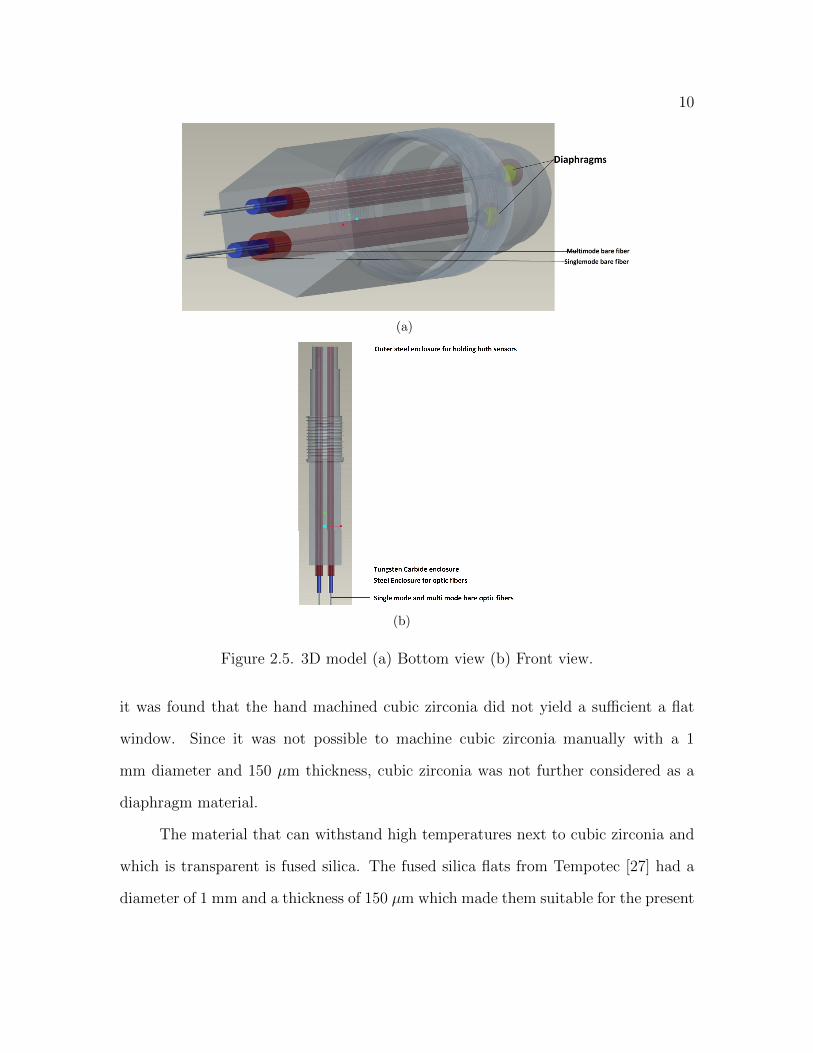
Figure 2.4 shows that the sensor consisted of a diaphragm in tungsten carbide

enclosures that were encased in an outer steel enclosure. This outer steel enclosure

7

Figure 2.2. Dynamic pressure sensor [1].

Figure 2.3. Water jacket [2].

was threaded to a water jacket (not shown). Different diaphragms were chosen in

order to get the expected pressure results in the shock tube. The diaphragm was

glued to the outer steel enclosure using high-temperature zirconia glue [23] and using

5-minute epoxy. The two steel tubes containing separately a single mode and a multi-

mode optical fiber were encased in another larger steel tube. A cavity was formed

by placing the tubes at a distance from the diaphragms. Two single-mode fibers

were coupled to a 1 × 2 splitter [24] and were connected to the laser source using

FC/PC connectors [24]. Similarly, the multi-mode fibers were connected to a 2 × 1

combiner [24] to a photodetector [12]. The light reflected from diaphragm traveled

8

in the multi-mode fibers and was sensed by the photodetector connected to a digital

storage oscilloscope for further analysis.

Figure 2.4. Schematic of FOPS.

The schematics were designed in Pro/E for the purpose of machining. Single

mode and multi-mode bare fibers with 9/125 µm and 50/125 µm as core diameters

respectively [25] were inserted in a hypodermic steel tube of dimensions 0.821 mm

9

O.D. and 0.250 mm I.D. Bare fibers are inserted in the hypodermic steel tubes and

are glued using epoxy to avoid the breakage of fibers in the tube and to avoid ir-

regularities in heights. The tips of the bare fibers are polished using various grits

to attain maximum transmittance and receiving of light. Hypodermic steel tube is

further inserted in another steel enclosure of O.D. 1.5 mm and I.D. 0.8211 mm. The

diaphragm is finally glued on the steel enclosure which has 0.150 mm depth and 1 mm

diameter on the top. The holes were drilled using wire EDM technology by Applegate

[21]. 3D model of the complete assembly with two sensors and diaphragm designed

in Pro/E is shown in Figure 2.5(b) and Figure 2.5(a).

2.4 Diaphragm

This transducer outputs pressure from mechanical deflections that occurs in

the diaphragm due to the applied load [26]. The diaphragm was chosen according

to temperature, rigidity, hardness and transparency for upgrading it to temperature

measurement in future. Calculations with which the diaphragm was chosen are ex-

plained in the later chapter.

2.4.1 Types of Diaphragm Materials Examined

Since the sensor is designed to use at high temperatures and pressures, diamond

was initially chosen because of the properties that it possesses. Considering cost as

the factor, diamond was not used instead cubic zirconia was chosen since its properties

were very similar to diamond.

Cubic zirconia (CZ) is mostly used in jewelry to replace diamonds. CZ material

was sourced from India which was in diamond shape and it was machined using a

grinder in the Material Science Engineering Department at University of Texas at

Arlington and polished using a polisher. The surface was verified using SEM but

10

(a)

(b)

Figure 2.5. 3D model (a) Bottom view (b) Front view.

it was found that the hand machined cubic zirconia did not yield a sufficient a flat

window. Since it was not possible to machine cubic zirconia manually with a 1

mm diameter and 150 µm thickness, cubic zirconia was not further considered as a

diaphragm material.

The material that can withstand high temperatures next to cubic zirconia and

which is transparent is fused silica. The fused silica flats from Tempotec [27] had a

diameter of 1 mm and a thickness of 150 µm which made them suitable for the present

11

Table 2.1. Comparison between the properties of diamond and cubic zirconia

Properties Diamond Cubic ZirconiaHardness 10,000 kg mm−2 1300 kg mm−2

Strength, tensile >1.2 GPa 900 MPaStrength, compressive >110 GPa -

Density 3520 kg m−3 5680 kg m−3

Young’s modulus 1.22 GPa 200 GPaPoisson’s ratio 0.2 -

Thermal expansion coefficient 0.0000011 K−1 10.3 10−6 K−1

Thermal conductivity 20.0 W cm−1 K−1 2 W cm−1 K−1

purpose. The flat was glued to the outer steel enclosure using high-temperature

zirconia glue. When compared to the dimensions of the diaphragm and the tungsten

carbide tube, the cubic zirconia glue that was used was thicker when applied by hand

and it covered the hole completely hence rendering the diaphragm useless. We needed

a sophisticated device to apply the glue carefully along the circumference of the step

provided at the top of the tube. Due to the constraint of funds, we were not able

to use micro robotics to apply the glue. Also, the diaphragm was not deflecting and

producing the expected results. The diaphragm may have been rigid along the corners

due to excess glue or the diaphragm may have been thicker for such pressures and it

did not deflect exactly as it was expected according to calculations.

Since the deflections were not satisfactory with cubic zirconia and fused silica

between 0 and 600 psi, aluminum was next considered used as the diaphragm material

with a thickness of 100 µm. Aluminum kitchen foil of that thickness was cut and glued

using the 5-minute epoxy [28] and dried. Even after using aluminum, deflections were

not as expected most likely due to applying the glue by hand.

12

2.5 Nano Fabrication

Conventional methods were not satisfactory, so advanced micro and nano fab-

rication were tried to solve the problem. As we know, these technologies are used to

fabricate micro devices using silicon as the main ingredient. Though there are many

nanofabrication techniques, most of them are for silicon and extending them to other

materials is not an easy process.

The material in question is tungsten carbide [22, 29] which is conductive. There-

fore, it appears that a diaphragm can be electroplated onto the sensing head but only

if the hole through the center can be temporarily blocked by a filler. Existing fa-

cilities are not able to perform this operation either by electroplating or by using a

microrobot to place a diaphragm or by growing a crystal diaphragm.

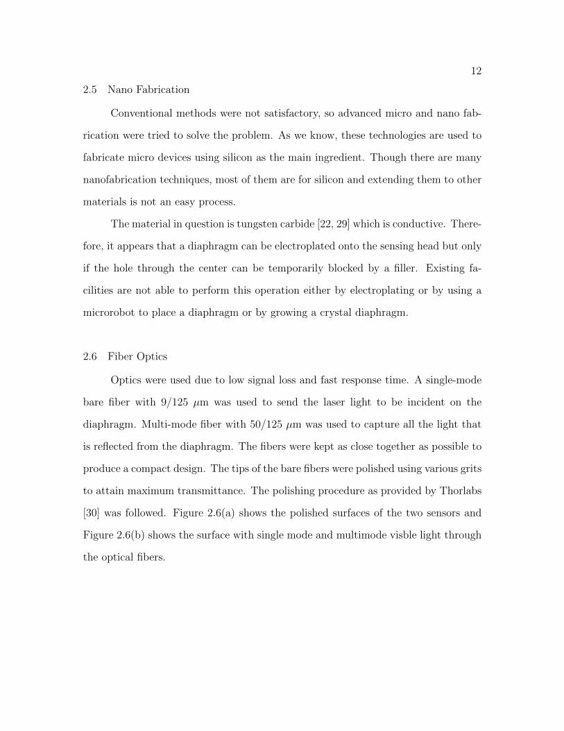
2.6 Fiber Optics

Optics were used due to low signal loss and fast response time. A single-mode

bare fiber with 9/125 µm was used to send the laser light to be incident on the

diaphragm. Multi-mode fiber with 50/125 µm was used to capture all the light that

is reflected from the diaphragm. The fibers were kept as close together as possible to

produce a compact design. The tips of the bare fibers were polished using various grits

to attain maximum transmittance. The polishing procedure as provided by Thorlabs

[30] was followed. Figure 2.6(a) shows the polished surfaces of the two sensors and

Figure 2.6(b) shows the surface with single mode and multimode visble light through

the optical fibers.

13

(a)

(b)

Figure 2.6. Polished bare fibers (a) Without light (b) With IR light.

CHAPTER 3

CALCULATIONS AND DERIVATIONS

3.1 Thin Plate Theory

According to [31], the following conditions are summarized from [32] for a true

membrane:

1. The boundaries are free from transverse shear forces and moments. Loads

applied to the boundaries must lie in planes tangent to the middle surface.

2. The normal displacements and rotations at the edges are unconstrained, that

is, these edges can displace freely in the direction of the normal to the middle

surface.

3. A membrane must have a smoothly varying, continuous surface.

4. The components of the surface and edge loads must also be smooth and con-

tinuous functions of the coordinates.

It was further shown that there are two more characterizations arrived from the

above basic assumptions and they are:

1. Membranes do not have any flexural rigidity and therefore cannot resist any

bending loads.

2. Membranes can only sustain tensile loads. Their inability to sustain compressive

loads leads to wrinkling.

The von Karman large deflection equations for thin plates were given as

14

15

∂4Φ

∂x4+ 2

∂4Φ

∂x2∂y2+∂4Φ

∂y4= Eh

[(∂2w

∂x∂y

)2

− ∂2w∂2w

∂x2∂y2

](3.1)

∂4w

∂x4+ 2

∂4w

∂x2∂y2+∂4w

∂y4=

1

D

(p+

∂2Φ∂2w

∂y2∂x2+∂2Φ∂2w

∂x2∂y2− 2

∂2Φ

∂x∂y

∂2w

∂x∂y

)(3.2)

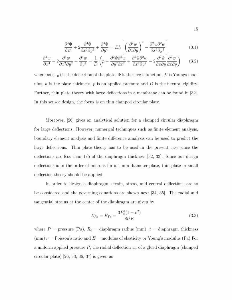
where w(x, y) is the deflection of the plate, Φ is the stress function, E is Youngs mod-

ulus, h is the plate thickness, p is an applied pressure and D is the flexural rigidity.

Further, thin plate theory with large deflections in a membrane can be found in [32].

In this sensor design, the focus is on thin clamped circular plate.

Moreover, [26] gives an analytical solution for a clamped circular diaphragm

for large deflections. However, numerical techniques such as finite element analysis,

boundary element analysis and finite difference amalysis can be used to predict the

large deflections. Thin plate theory has to be used in the present case since the

deflections are less than 1/5 of the diaphragm thickness [32, 33]. Since our design

deflections is in the order of microns for a 1 mm diameter plate, thin plate or small

deflection theory should be applied.

In order to design a diaphragm, strain, stress, and central deflections are to

be considered and the governing equations are shown next [34, 35]. The radial and

tangential strains at the center of the diaphragm are given by

ERc = ETc =3P 2

0 (1− ν2)8t2E

(3.3)

where P = pressure (Pa), R0 = diaphragm radius (mm), t = diaphragm thickness

(mm) ν = Poisson’s ratio and E = modulus of elasticity or Young’s modulus (Pa) For

a uniform applied pressure P , the radial deflection wr of a glued diaphragm (clamped

circular plate) [26, 33, 36, 37] is given as

16

wr = wc

[1−

(r

R0

)2]2

(3.4)

where r is the radial coordinate, R0 is the radius of the diaphragm and D is the

flexural rigidity, which is a measure of stiffness [26, 31, 33], given by

D =Et3

12(1− ν2)(3.5)

Also, [33, 34] give the following equation to calculate the maximum center

deflection

wc =PR4

0(1− ν2)64D

=3PR4

0(1− ν2)16t3E

(3.6)

Since the diaphragm is clamped, r = 0, and the central deflection of the diaphragm

is given by

W =3PR4

0(1− ν2)16t3E

(3.7)

and the sensitivity Yc of the diaphragm is given by [38]

Yc =3(1− ν2)

16t3E(3.8)

The sensitivity of the diaphragm can be increased by increasing the radius of the

diaphragm and by decreasing the thickness [18].

3.2 Diaphragm Design Calculations

3.2.1 Manual Calculations

The thickness of the diaphragm has to be determined in order to design a

diaphragm that gives a maximum deflection without being broken. The required

thickness for the diaphragm was calculated from the above equations for various

deflections. The appropriate thickness was obtained by substituting the properties of

various materials in the above equations and by assuming the required deflections for

different materials depending on the maximum reflection of light that will give the

17

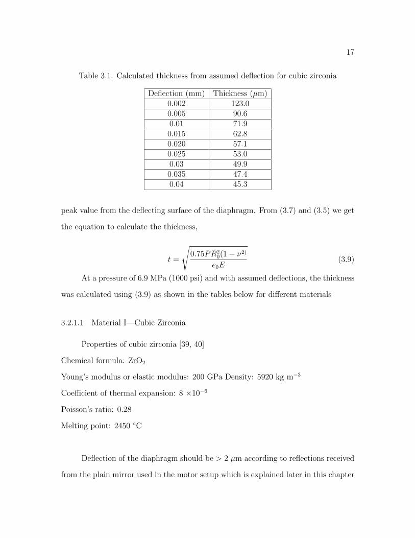
Table 3.1. Calculated thickness from assumed deflection for cubic zirconia

Deflection (mm) Thickness (µm)0.002 123.00.005 90.60.01 71.90.015 62.80.020 57.10.025 53.00.03 49.90.035 47.40.04 45.3

peak value from the deflecting surface of the diaphragm. From (3.7) and (3.5) we get

the equation to calculate the thickness,

t =

√0.75PR2

0(1− ν2)e0E

(3.9)

At a pressure of 6.9 MPa (1000 psi) and with assumed deflections, the thickness

was calculated using (3.9) as shown in the tables below for different materials

3.2.1.1 Material I—Cubic Zirconia

Properties of cubic zirconia [39, 40]

Chemical formula: ZrO2

Young’s modulus or elastic modulus: 200 GPa Density: 5920 kg m−3

Coefficient of thermal expansion: 8 ×10−6

Poisson’s ratio: 0.28

Melting point: 2450 C

Deflection of the diaphragm should be > 2 µm according to reflections received

from the plain mirror used in the motor setup which is explained later in this chapter

18

Table 3.2. Diaphragm thickness and deflection for fused silica


and also [41] shows that the deflection should be at least one-third of the diaphragm

thickness. Approximately 100 µm was chosen which is more than the calculated

deflection as diaphragm thickness with a diameter of 1 mm so that there is a prominent

deflection of the diaphragm without any fracture.

3.2.1.2 Material II—Fused Silica

Since machining of CZ was not precise, SiO2 was also considered as a diaphragm

material.

Properties of fused silica [39, 40]

Chemical formula: SiO2

Young’s modulus or elastic modulus: 73 GPa

Density: 2200 kg m−3

Coefficient of thermal expansion: 0.55 ×10−6



19

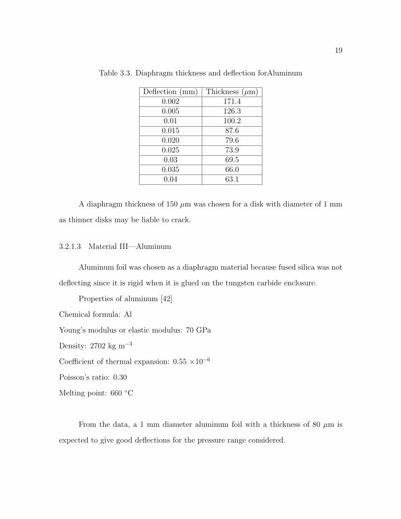
Table 3.3. Diaphragm thickness and deflection forAluminum


A diaphragm thickness of 150 µm was chosen for a disk with diameter of 1 mm

as thinner disks may be liable to crack.

3.2.1.3 Material III—Aluminum

Aluminum foil was chosen as a diaphragm material because fused silica was not

deflecting since it is rigid when it is glued on the tungsten carbide enclosure.

Properties of aluminum [42]

Chemical formula: Al

Young’s modulus or elastic modulus: 70 GPa

Density: 2702 kg m−3

Coefficient of thermal expansion: 0.55 ×10−6



From the data, a 1 mm diameter aluminum foil with a thickness of 80 µm is

expected to give good deflections for the pressure range considered.

20

3.2.2 ANSYS Results

A three-dimensional model of the sensor was developed in ANSYS workbench,

meshed and, for structural and thermal analyses were ran in it.

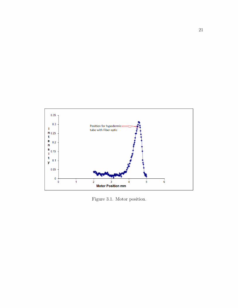
3.3 Fiber Optic Placement

The hypodermic steel tubes which house the single and multi-mode fibers were

inserted in the tungsten carbide enclosure as discussed earlier and they were fixed

at a particular distance where the multi-mode fibers received the maximum output

from the reflecting diaphragm. The exact position was determined by using the

motor setup available at the Advanced Sensor Technology Laboratory (ASTL) of the

Mechanical and Aerospace Engineering Department. The graph in Figure 3.1 below

shows a steady rise and fall of the points as the fiber tip moves with respect to the

motor. The photodetector reads the values from the multi-mode fiber as the motor

moves the fiber.1

After achieving the maximum intensity from the diaphragm, the fibers with the

hypodermic tubing were placed at the position as shown in Figure 3.1 which is lesser

than the peak reflecting point so that the diaphragm deflection will give a rise as the

diaphragm deflection moves closer to the peak value.

1The data acquisition program was written by Dr. Haiying Huang.

21

Figure 3.1. Motor position.

CHAPTER 4

RESULTS AND DISCUSSION

4.1 Calibration

Calibration plays an important role in deciding the various characteristics and

parameters for any device.

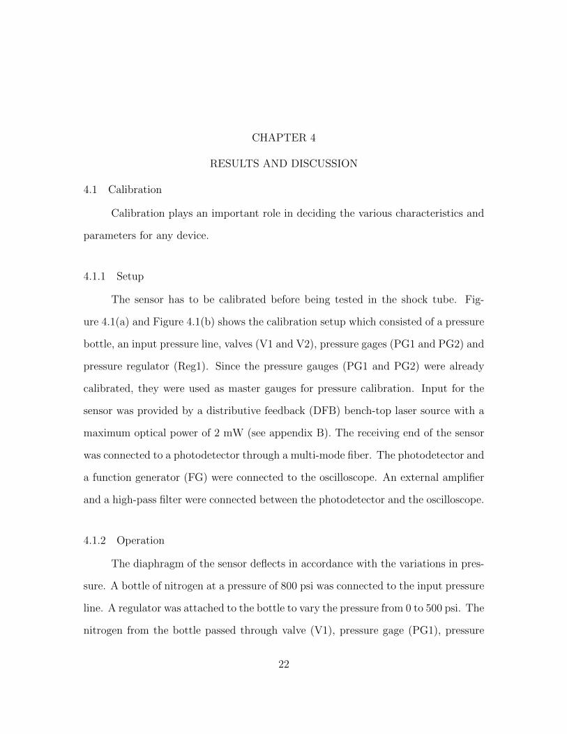
4.1.1 Setup

The sensor has to be calibrated before being tested in the shock tube. Fig-

ure 4.1(a) and Figure 4.1(b) shows the calibration setup which consisted of a pressure

bottle, an input pressure line, valves (V1 and V2), pressure gages (PG1 and PG2) and

pressure regulator (Reg1). Since the pressure gauges (PG1 and PG2) were already

calibrated, they were used as master gauges for pressure calibration. Input for the

sensor was provided by a distributive feedback (DFB) bench-top laser source with a

maximum optical power of 2 mW (see appendix B). The receiving end of the sensor

was connected to a photodetector through a multi-mode fiber. The photodetector and

a function generator (FG) were connected to the oscilloscope. An external amplifier

and a high-pass filter were connected between the photodetector and the oscilloscope.

4.1.2 Operation

The diaphragm of the sensor deflects in accordance with the variations in pres-

sure. A bottle of nitrogen at a pressure of 800 psi was connected to the input pressure

line. A regulator was attached to the bottle to vary the pressure from 0 to 500 psi. The

nitrogen from the bottle passed through valve (V1), pressure gage (PG1), pressure

22

23

(a)

(b)

Figure 4.1. Calibration setup (a) View 1 (b) View 2.

regulator (REG), pressure gage (PG2) and valve (V2) respectively before reaching the

diaphragm. Since the regulator in the bottle was not accurate, regulator (REG) was

used. The changes in pressure were compared with both the regulators and matched.

Also, the accuracy and preciseness of the reference devices (master gauges) played a

major role in calibrating the pressure sensor.

The pressure was released from the bottle and the regulator which was con-

nected to it was varied in steps of 50 psi. The valve (V1) was then opened, causing

the regulated pressure from the bottle to pass through PG1 to REG. The pressure

24

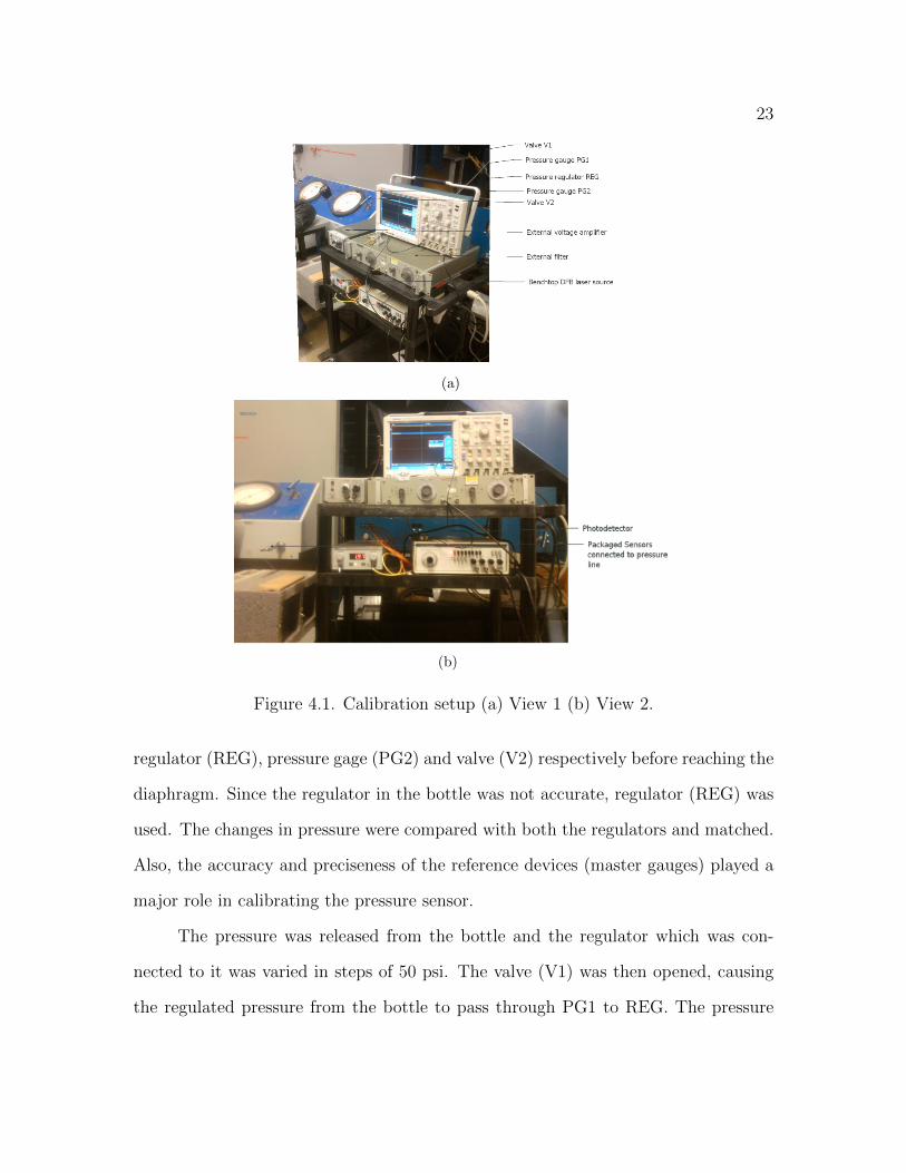
(a)

(b)

Figure 4.2. Unassembled sensors (a) Close view (b) Comparison with a penny.

regulator (REG) was adjusted in order to vary the pressure precisely. The pressure

then flowed through PG2; valve V2 was opened and the sensor detected the pressure

reading. Pressure readings in PG1 and PG2 were noted down respectively. The di-

aphragm consequently deflected according to the varying pressure noted in PG2. The

25

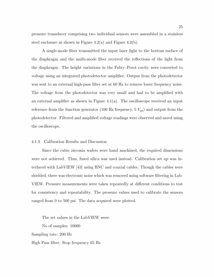
pressure transducer comprising two individual sensors were assembled in a stainless

steel enclosure as shown in Figure 4.2(a) and Figure 4.2(b).

A single-mode fiber transmitted the input laser light to the bottom surface of

the diaphragm and the multi-mode fiber received the reflections of the light from

the diaphragm. The height variations in the Fabry–Perot cavity were converted to

voltage using an integrated photodetector–amplifier. Output from the photodetector

was sent to an external high-pass filter set at 60 Hz to remove lower frequency noise.

The voltage from the photodetector was very small and had to be amplified with

an external amplifier as shown in Figure 4.1(a). The oscilloscope received an input

reference from the function generator (100 Hz frequency, 5 Vpp) and output from the

photodetector. Filtered and amplified voltage readings were observed and saved using

the oscilloscope.

4.1.3 Calibration Results and Discussion

Since the cubic zirconia wafers were hand machined, the required dimensions

were not achieved. Thus, fused silica was used instead. Calibration set up was in-

terfaced with LabVIEW [43] using BNC and coaxial cables. Though the cables were

shielded, there was electronic noise which was removed using software filtering in Lab-

VIEW. Pressure measurements were taken repeatedly at different conditions to test

for consistency and repeatability. The pressure values used to calibrate the sensors

ranged from 0 to 500 psi. The data acquired were plotted.

The set values in the LabVIEW were:

No of samples: 10000

Sampling rate: 200 Hz

High Pass filter: Stop frequency 65 Hz

26

Function Gen: 100 Hz

Acquisition time: 50 s

Applied pressure: 0 to 410 psi

Voltage amplification: ×100

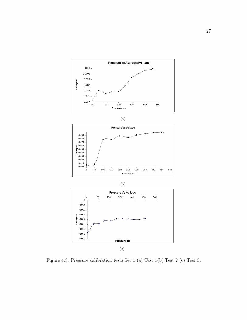
Figure 4.3(a) shows the plot between pressure and voltage. For a particular

pressure reading, the voltage was averaged over time. A steadily increasing curve was

observed with a voltage of 9.9 mV at 460 psi. In Figure 4.3(b), the voltage rose when

there was an increase in pressure from 0 psi but the increase was slow. The maximum

pressure threshold at which the sensor can operate was unknown and the maximum

pressure delivered from the pressure bottle was only 460 psi. Though there was a

steadily increasing curve, it was not linear. Similarly, Figure 4.3(c) shows that the

voltage increased gradually. The external voltage amplifier had a phase shift which

resulted in negative values of voltage.

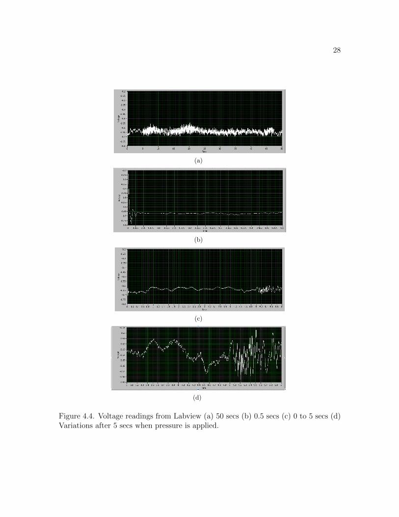
The readings obtained from LabVIEW were as shown in Figure 4.4. For pres-

sure values ranging from 0 to 500 psi, voltage readings were obtained using LabVIEW

and plotted as shown in Figure 4.4(a). Figure 4.4(b) shows the interval from 0 to 0.5

s. At 0.01 s, a sharp spike was observed, implying the sensing of laser signals by the

system though there were no deflections. The output in Figure 4.4(c) shows that from

0 to 0.5 s, the voltage had a steady value of approximately −0.675 V corresponding

to 0 psi. When the pressure value increased, there was a shift in the voltage value to

approximately −0.62 V. This trend continued till the 5 s mark, beyond which there

were rapid fluctuations with increase in pressure. Figure 4.4(d) shows a close up view

of the variations with pressures.

27

(a)

(b)

(c)

Figure 4.3. Pressure calibration tests Set 1 (a) Test 1(b) Test 2 (c) Test 3.

28

(a)

(b)

(c)

(d)

Figure 4.4. Voltage readings from Labview (a) 50 secs (b) 0.5 secs (c) 0 to 5 secs (d)Variations after 5 secs when pressure is applied.

29

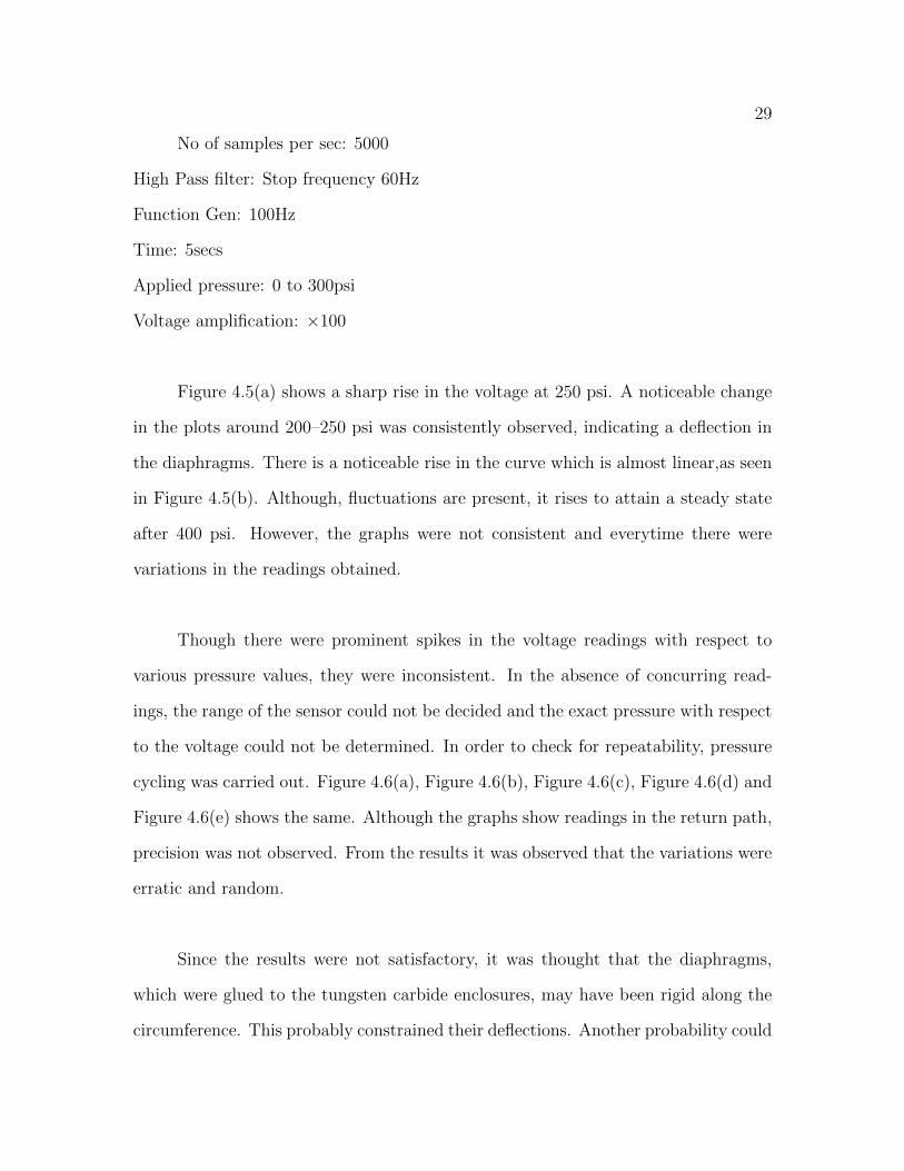
No of samples per sec: 5000

High Pass filter: Stop frequency 60Hz

Function Gen: 100Hz

Time: 5secs

Applied pressure: 0 to 300psi

Voltage amplification: ×100

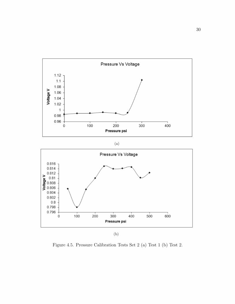
Figure 4.5(a) shows a sharp rise in the voltage at 250 psi. A noticeable change

in the plots around 200–250 psi was consistently observed, indicating a deflection in

the diaphragms. There is a noticeable rise in the curve which is almost linear,as seen

in Figure 4.5(b). Although, fluctuations are present, it rises to attain a steady state

after 400 psi. However, the graphs were not consistent and everytime there were

variations in the readings obtained.

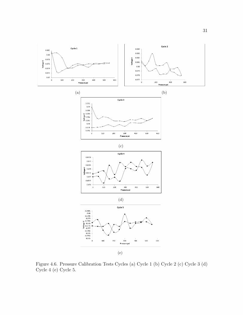
Though there were prominent spikes in the voltage readings with respect to

various pressure values, they were inconsistent. In the absence of concurring read-

ings, the range of the sensor could not be decided and the exact pressure with respect

to the voltage could not be determined. In order to check for repeatability, pressure

cycling was carried out. Figure 4.6(a), Figure 4.6(b), Figure 4.6(c), Figure 4.6(d) and

Figure 4.6(e) shows the same. Although the graphs show readings in the return path,

precision was not observed. From the results it was observed that the variations were

erratic and random.

Since the results were not satisfactory, it was thought that the diaphragms,

which were glued to the tungsten carbide enclosures, may have been rigid along the

circumference. This probably constrained their deflections. Another probability could

30

(a)

(b)

Figure 4.5. Pressure Calibration Tests Set 2 (a) Test 1 (b) Test 2.

31

(a) (b)

(c)

(d)

(e)

Figure 4.6. Pressure Calibration Tests Cycles (a) Cycle 1 (b) Cycle 2 (c) Cycle 3 (d)Cycle 4 (e) Cycle 5.

32

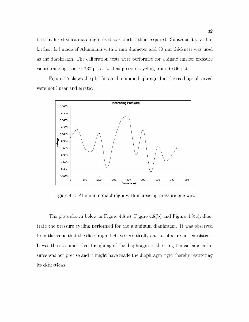
be that fused silica diaphragm used was thicker than required. Subsequently, a thin

kitchen foil made of Aluminum with 1 mm diameter and 80 µm thickness was used

as the diaphragm. The calibration tests were performed for a single run for pressure

values ranging from 0–730 psi as well as pressure cycling from 0–600 psi.

Figure 4.7 shows the plot for an aluminum diaphragm but the readings observed

were not linear and erratic.

Figure 4.7. Aluminum diaphragm with increasing pressure one way.

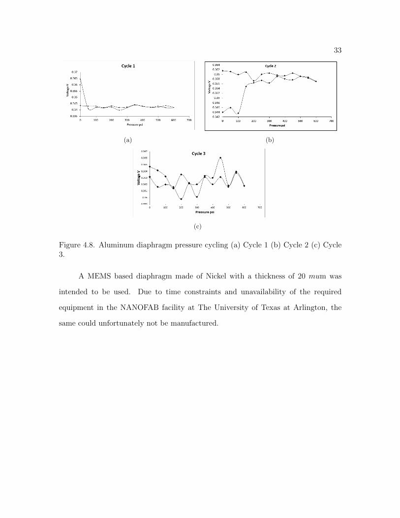
The plots shown below in Figure 4.8(a), Figure 4.8(b) and Figure 4.8(c), illus-

trate the pressure cycling performed for the aluminum diaphragm. It was observed

from the same that the diaphragm behaves erratically and results are not consistent.

It was thus assumed that the gluing of the diaphragm to the tungsten carbide enclo-

sures was not precise and it might have made the diaphragm rigid thereby restricting

its deflections.

33

(a) (b)

(c)

Figure 4.8. Aluminum diaphragm pressure cycling (a) Cycle 1 (b) Cycle 2 (c) Cycle3.

A MEMS based diaphragm made of Nickel with a thickness of 20 mum was

intended to be used. Due to time constraints and unavailability of the required

equipment in the NANOFAB facility at The University of Texas at Arlington, the

same could unfortunately not be manufactured.

CHAPTER 5

CONCLUSION AND RECOMMENDATIONS

5.1 Conclusion

A sensor was developed to determine the pressures and time-of-flight in a shock

tube. High temperature materials and a transparent diaphragm were chosen so that

the sensor can be further used for temperature measurements. The sensor was initially

modelled with a transparent cubic zirconia as the diaphragm material. But cubic

zirconia was not used due to the limitations of machining. Fused silica and aluminum

were next tried as diaphragms. From the results, it was clear that the diaphragmswere

deflecting with respect to pressure, but placement of the diaphragm required more

accuracy and precision than was available. The diaphragm was manually glued on

to the tungsten carbide enclosures whereas more sophisticated equipment is required.

A micro-robotic hand connected to a computer to view a magnified image of the

micro sensor can be used to apply the appropriate amount of glue and to place the

diaphragm. The sensors were not tested in the shock tube because they have to be

calibrated before being tested in the shock tube. The sensors were only tested in the

calibration setup. The results shows that there were definite changes in the voltages

when load was applied on the diaphragm; however, they were not consistent and

repeatable.

34

35

5.2 Recommendations

5.2.1 Diaphragm thickness

From the calculations, it was assumed that the fused silica thickness should be

≈ 150 µm to withstand high pressures in harsh environments. It can be observed

from the results that the deflections were very minimal due to the rigidity of the

diaphragm. In order to obtain the expected results, diaphragm thickness should be

between 50 µm and 75 µm depending upon the material used.

5.2.2 Higher pressure

The pressure used for calculation is 2000 psi and the diaphragm was designed

accordingly with respect to the maximum load that can be applied arising from the

expected pressures that can develop in detonation and shock tubes. But the maximum

pressure that was available in the pressure bottle was 700psi. Moreover, due to lack

of time and funding, many sensors were not able to be designed. Thus, there were

limitations on the testing to the available pressure range to avoid damage to the

sensor.

5.2.3 Placement of diaphragm

The diaphragm can be placed using micro robotic hands on top of the tung-

sten carbide enclosure. This may avoid the rigidity along the circumference since the

placement will be precise on the step provided on the enclosure. The diaphragm can

also be redesigned with a larger diameter (1.3 mm instead of 1 mm) which can be

placed on top of the enclosure instead of placing it on the step. Glue used to attach

the diaphragm to the enclosure plays a major role because it may cause rigidity which

restricts the deflection. So the glue has to be applied carefully using the micro robotic

36

hands such that it doesn’t overflow along the corners.

5.2.4 Fiber protection

The bare fibers used in the steel tubes are very fragile and tend to break often

while working. So extra care has to be taken to protect them in order to avoid re

working on the bare fibers polishing and assembling.

APPENDIX A

PCB PRESSURE TRANSDUCER CHARACTERISTICS

37

38

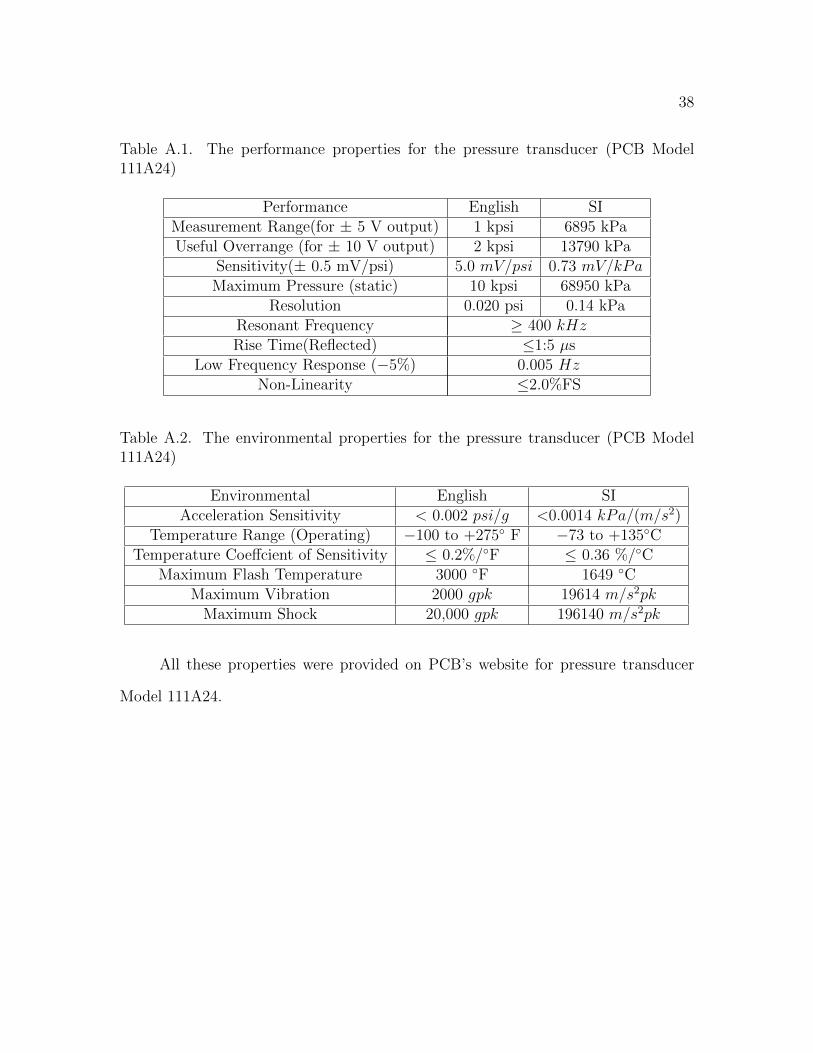
Table A.1. The performance properties for the pressure transducer (PCB Model111A24)

Performance English SIMeasurement Range(for ± 5 V output) 1 kpsi 6895 kPaUseful Overrange (for ± 10 V output) 2 kpsi 13790 kPa

Sensitivity(± 0.5 mV/psi) 5.0 mV/psi 0.73 mV/kPaMaximum Pressure (static) 10 kpsi 68950 kPa

Resolution 0.020 psi 0.14 kPaResonant Frequency ≥ 400 kHzRise Time(Reflected) ≤1:5 µs

Low Frequency Response (−5%) 0.005 HzNon-Linearity ≤2.0%FS

Table A.2. The environmental properties for the pressure transducer (PCB Model111A24)

Environmental English SIAcceleration Sensitivity < 0.002 psi/g <0.0014 kPa/(m/s2)

Temperature Range (Operating) −100 to +275 F −73 to +135CTemperature Coeffcient of Sensitivity ≤ 0.2%/F ≤ 0.36 %/C

Maximum Flash Temperature 3000 F 1649 CMaximum Vibration 2000 gpk 19614 m/s2pk

Maximum Shock 20,000 gpk 196140 m/s2pk

All these properties were provided on PCB’s website for pressure transducer

Model 111A24.

39

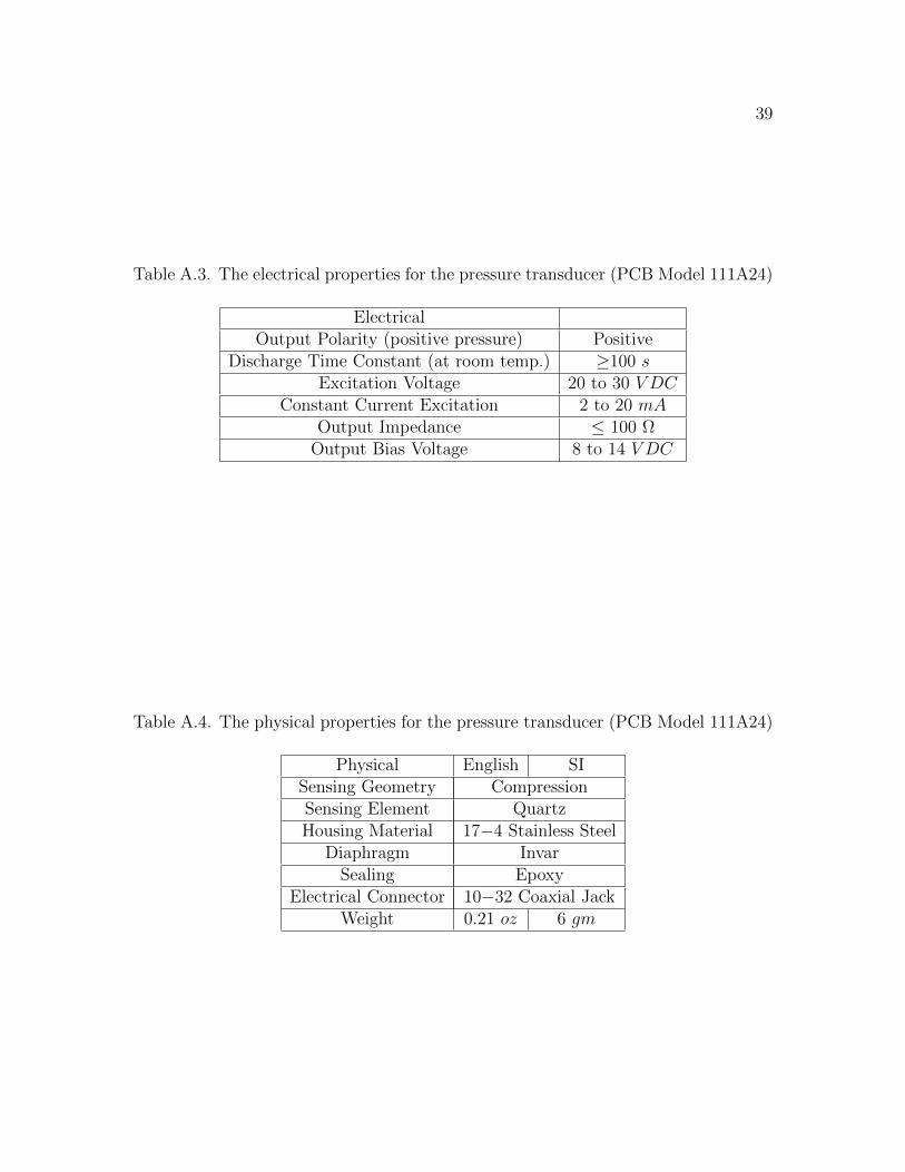
Table A.3. The electrical properties for the pressure transducer (PCB Model 111A24)

ElectricalOutput Polarity (positive pressure) Positive

Discharge Time Constant (at room temp.) ≥100 sExcitation Voltage 20 to 30 V DC

Constant Current Excitation 2 to 20 mAOutput Impedance ≤ 100 Ω

Output Bias Voltage 8 to 14 V DC

Table A.4. The physical properties for the pressure transducer (PCB Model 111A24)

Physical English SISensing Geometry CompressionSensing Element QuartzHousing Material 17−4 Stainless Steel

Diaphragm InvarSealing Epoxy

Electrical Connector 10−32 Coaxial JackWeight 0.21 oz 6 gm

APPENDIX B

LASER SOURCE AND PHOTODETECTOR

40

41

B.1 DFB Laser Source

All these properties were provided on Thorlab’s website for S3FC1550 - DFB

fiber coupled laser source 1550nm.

B.1.1 Description

The Thorlabs Fiber Coupled Laser Sources provide easy coupling and simple

control of laser diode driven fiber optics. These laser sources are available in two

versions, Fabry-Perot and Distributed Feed Back (DFB). The Fabry-Perot version

comes in five available wavelength choices from 635 nm to 1550 nm with standard

single mode fiber or polarization maintaining fiber output. The DFB version comes

equipped with a thermo-electric cooler to stabilize the output wavelength, and a 40

dB optical isolator to eliminate frequency jitter due to back-reflections. The DFB is

available in 1310 nm and 1550 nm wavelengths.

B.2 Photodetector

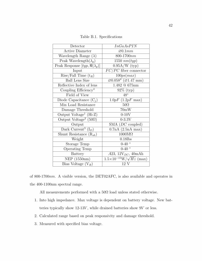
All these properties were provided on Thorlab’s website for DET01CFC - Fiber

Input InGaAs Photodetector.

B.2.1 Description

The DET01CFC is a ready-to-use, high-speed InGaAs photodetector for use

with FC/PC connectorized fiber optic cables in NIR optical systems. The unit comes

with an FC/PC bulkhead connector, detector, and 12V bias battery enclosed in a

compact aluminum housing. The FC/PC connector provides easy coupling to fiber-

based light sources. The output uses an SMA jack to minimize size and maximize

frequency response. The bandwidth is 2GHz and will operate over the spectral range

42

Table B.1. Specifications

Detector InGaAsPINActive Diameter ∅0.1mm

Wavelength Range (λ) 800-1700nmPeak Wavelength(λp) 1550 nm(typ)

Peak Response [typ,<(λp)] 0.95A/W (typ)Input FC/PC fiber connector

Rise/Fall Time (tR) 100ps(max)Ball Lens Size ∅0.058′′ (∅1.47 mm)

Reflective Index of lens 1.482 @ 675nmCoupling Efficiency4 92% (typ)

Field of View 48

Diode Capacitance (Cj) 1.0pF (1.2pF max)Min Load Resistance 50ΩDamage Threshold 70mW

Output Voltage1 (Hi-Z) 0-10VOutput Voltage2 (50Ω) 0-3.3V

Output SMA (DC coupled)Dark Current3 (ID) 0.7nA (2.5nA max)

Shunt Resistance (Rsh) 1000MΩWeight 0.18lbs

Storage Temp 0-40

Operating Temp 0-40

Battery A23, 12VDC , 40mAh

NEP (1550nm) 1.5×10−15W/√Hz (max)

Bias Voltage (VR) 12 V

of 800-1700nm. A visible version, the DET02AFC, is also available and operates in

the 400-1100nm spectral range.

All measurements performed with a 50Ω load unless stated otherwise.

1. Into high impedance. Max voltage is dependent on battery voltage. New bat-

teries typically show 12-13V , while drained batteries show 9V or less.

2. Calculated range based on peak responsivity and damage threshold.

3. Measured with specified bias voltage.

43

4. 92% into both single and multi-mode fibers over the full spectral response of

detector.

REFERENCES

[1] Model 111a24 spec sheet. [Online]. Available: http://www.pcb.com

[2] Model 064b02 spec sheet. [Online]. Available: http://www.pcb.com

[3] F. R. Schauer, C. L. Miser, K. C. Tucker, R. P. Bradley, and J. L. Hoke, “Det-

onation initiation of hydrocarbon-air mixtures in a pulsed detonation engine,”

43rd AIAA Aerospace Sciences Meeting, pp. 1–10, January 2005.

[4] F. K. Lu, A. A. Ortiz, J. M. Li, C. H. Kim, and K. M. Chung, “Detection of shock

and detonation wave propagation by cross correlation,” Mechanical Systems and

Signal Processing, vol. 23, no. 4, pp. 1098–111, 2009.

[5] ——, “Determining shock and detonation wave propagation time using wavelet

methods,” 39th AIAA Fluid Dynamics Conference, pp. 1–15, 2009.

[6] W. N. MacPherson, J. M. Kilpatrick, J. S. Barton, and J. D. Jones, “Miniature

fiber optic pressure sensor for turbomachinery applications,” American Institute

of Physics, vol. 70, pp. 1868–1874, 1999.

[7] W. N. MacPherson, M. J. Gander, J. S. Barton, J. D. Jones, C. L. Owen, A. J.

Watson, and R. M. Allen, “Blast-pressure measurements with a high-bandwidth

fibre optic pressure sensor,” Measurement Science and Technology, vol. 11, pp.

95–102, 2000.

[8] R. A. Pinnock, “Optically pressure and temperature sensors for aerospace appli-

cations,” Sensor Review, vol. 18, pp. 32–38, 1998.

[9] J. Zhou, S. Dasgupta, H. Kobayashi, H. E. Jackson, and J. T. Boyd, “Opti-

cally interrogated mems pressure sensors for propulsion applications,” Society of

Photo-Optical Instrumentation Engineers, vol. 40-4, pp. 598–604, April 2001.

44

45

[10] W. Pulliam and P. Russler, “High-temperature, high bandwidth, fiber-optic,

mems pressure sensor technology for turbine engine component testing,” 47th

IIS, pp. 1–10, 2001.

[11] S. Watson, W. N. MacPherson, J. S. Barton, J. D. C. Jones, A. Tyas, A. V.

Pichugin, A. Hindle, W. Parkes, C. Dunare, and T. Stevenson, “Investigation of

shock waves in explosive blasts using fibre optic pressure sensors,” Measurement

Science and Technology, vol. 17, pp. 1337–1342, 2006.

[12] Thorlabs.com - det10c high-speed ingaas detector, 700-1800 nm, 10 ns rise time.

[13] K. Betzler, “Fabry-perot interferometer,” Universit at Osnabruck, 2002.

[14] J. M. Kilpatrick, W. N. MacPherson, J. S. Barton, J. D. C. Jones, D. R.

Buttsworth, T. V. Jones, K. S. Chana, and S. J. Anderson, “Measurement of

unsteady gas temperature with optical fibre fabry-perot microsensors,” Mea-

surement Science and Technology, vol. 13, pp. 706–712, 2002.

[15] Y. Kim and D. P. Neikirk, “Micromachined fabry-perot cavity pressure trans-

ducer,” IEEE Photonics Technology Letters, vol. 7-12.

[16] A. Mendez, T. F. Morse, and K. A. Ramsey, “Mcromachined fabry-perot inter-

ferometer with corrugated silicon diaphragm for fiber optic sensing applications,”

Integrated Optics and Microstructures, vol. 1793, pp. 170–182, 1992.

[17] X. Wang, B. Li, O. L. Russo, H. T. Roman, K. K. Chin, and K. R. Farmer,

“Diaphragm design guidelines and an optical pressure sensor based on mems

technique,” Microelectronics Journal, vol. 37, pp. 50–56, 2005.

[18] M. Li, M. Wang, and H. Li, “Optical mems pressure sensor based on fabry-perot

interferometry,” Optics express, vol. 14, pp. 1497–1504, 20 February 2006.

[19] D. C. Abeysinghe, S. Dasgupta, J. T. Boyd, and H. E. Jackson, “A novel mems

pressure sensor fabricated on an optical fiber,” IEEE photonics technology letters,

vol. 13, pp. 993–995, September 2001.

46

[20] A. A. Ortiz, “Development of spectral and wavelet time-of-flight methods for

propagating shock and detonation waves,” Master’s thesis, The University of

Texas at Arlington, December 2008.

[21] Wire edm, sinker edm, edm hole driling services, applegate edm. [Online].

Available: http://www.applegateedm.com

[22] Material: Tungsten carbide (wc), bulk. [Online]. Available:

https://www.memsnet.org

[23] Aremco: High temperature adhesives, ceramics, potting compounds,

sealants, screen printers, dicing saws, furnaces. [Online]. Available:

http://www.aremco.com

[24] Oequest - components - passive components - polarization maintaining (pm)

couplers/splitters - pm fused couplers - 1x2 1550nm pm fused fiber coupler.

[Online]. Available: http://www.oequest.com

[25] Fiber optic patch cables. [Online]. Available: http://www.cablesondemand.com

[26] W. P. Eaton, F. Bitsie, J. H. Smith, and D. W. Plummer, “A new analytical

solution for diaphragm deflection and its application to a surface-micromachined

pressure sensor,” Modeling and Simulation of Microsystems, 1999.

[27] Optical windows. [Online]. Available: http://www.tempotec.com

[28] Thorlabs.com - g14250 5-minute epoxy, general purpose - two part. [Online].

Available: http://www.thorlabs.com

[29] Tungsten carbide information - provided by insaco inc, 215-536-3500. [Online].

Available: http://www.insaco.com

[30] Thorlabs.com - fiber polishing supplies. [Online]. Available:

http://www.thorlabs.com

[31] E. J. Ruggiero, “Modeling and control of spider satellite components,” Ph.D.

dissertation, Virginia Tech, year =.

47

[32] E. Ventsel and T. Krauthammer, Thin plates and shells: theory, analysis, and

applications. Marcel Dekker Inc., July 2001.

[33] S. Timoshenko and S. Woinosky-Kreiger, Theory of plates and shells. McGraw

Hill Classic, 1987.

[34] http://home.davidson.com.au/products/strain/mg/technology/technotes/tn510.pdf.

[Online]. Available: www.measurementsgroup.com

[35] efunda: Plate calculator – clamped circular plate with uniformly distributed

loading. [Online]. Available: http://www.efunda.com

[36] W. Parkes, V. Djakov, J. S. Barton, S. W. W. N. MacPherson, J. T. M. Steven-

son, and C. C. Dunare, “Design and fabrication of dielectric diaphragm pressure

sensors for applications to shock wave measurement in air,” Journal of Microme-

chanics and Microengineering, vol. 17, pp. 1334–1342, 2007.

[37] Evaluation of glued-diaphragm fibre optic pressure sensors in a shock tube, vol. 16,

2007.

[38] J. Xu, X. Wang, K. L.Cooper, and A. Wang, “Miniature all-silica fiber optic

pressure and acoustic sensors,” Optics Letters, vol. 30, 2005.

[39] Materials properties. [Online]. Available: http://accuratus.com

[40] Cubic zirconia information - provided by insaco inc, 215-536-3500. [Online].

Available: http://www.insaco.com

[41] R. S. Figliola and D. E. Beasley, Theory and design for mechanical

measurements. Hoboken, N.J.: John Wiley, 2006. [Online]. Available: 4.1.1

Publisher description http://www.loc.gov

[42] Periodic table of elements: Aluminum - al (environmentalchemistry.com).

[Online]. Available: http://environmentalchemistry.com

[43] Ni labview - the software that powers virtual instrumentation - national

instruments. [Online]. Available: http://www.ni.com

BIOGRAPHICAL STATEMENT

Karthikeyan Jagadevan was born in Chennai, Tamil Nadu, India in 28th Septem-

ber 1983.

He joined Bachelor of Engineering in Instrumentation and Control Engineering

in 2001 at SRM Engineering College affiliated to Anna University and fulfilled his

wish of learning an advanced technology. He received his B.E. degree fromAnna

University, Chennai, India, in 2005. He then worked as a software engineer with

Accenture services, Chennai, India. The desire for his passion with aerospace made

him pursue Master of Science degree Aerospace Engineering with The University of

Texas at Arlington.

48

Documents

FIBER-OPTIC PRESSURE SENSOR FOR TIME-OF-FLIGHT ...arc.uta.edu/publications/td_files/Jagadevan_uta_2502M_10737.pdf · The University of Texas at Arlington, ... utilizing intensity