Fiber Deep Networks and The Lessons Learned From The Field

© 2017 SCTE-ISBE and NCTA. All rights reserved.

Fiber Deep Networks and The Lessons Learned

From The Field

A Technical Paper prepared for SCTE/ISBE by

Todd Loeffelholz VP Product Management Alpha Technologies Inc.

3767 Alpha Way, Bellingham, WA 360-392-2172

[email protected]

© 2017 SCTE-ISBE and NCTA. All rights reserved. 2

Table of Contents Title Page Number Introduction ________________________________________________________________________ 3

Fiber Deep Networks _________________________________________________________________ 3

Fiber Deep Serving Groups ____________________________________________________________ 4 1. Distributed Powering ____________________________________________________________ 5 2. Centralized Powering ____________________________________________________________ 5

Remote PHY _______________________________________________________________________ 6

To Fiber or Not to Fiber? ______________________________________________________________ 7 1. FTTH – FDH + Hardened Drop Terminal _____________________________________________ 7 2. Fiber Deep: N+3 N+0 ________________________________________________________ 10

Conclusion ________________________________________________________________________ 13

Abbreviations ______________________________________________________________________ 14

Bibliography & References ___________________________________________________________ 14

List of Figures

Title Page Number Figure 1 - Residential Layout 8

Figure 2 - FTTH Residential Layout 9

Figure 3 - N+3 Network 11

Figure 4 - N+0 Network 12

List of Tables Title Page Number Table 1 - FTTH Total Cost 10


Introduction Fiber Deep architectures are becoming a natural next step in the evolution of the HFC network. As the need for bandwidth continues to grow, fiber will continue to be pushed deeper into the network. The constant expansion of fiber has already been witnessed in both telephony and cellular networks. The movement from DSL to ADSL and ultimately to VDSL2+ had the same goal - drive fiber closer to the customer and improve bandwidth at the customer premise. The same can be also said for the evolution of wireless networks. As the networks have upgraded from 1G to 4G, it has been about getting fiber closer to the customer and improving the amount of data available to watch the latest sports game or facetime with a friend. The world is fixated on data, and fiber is a medium which can help meet the demands of today and into the foreseeable future. The key is balancing the cost of deploying fiber against the demand for bandwidth.

As we look at how to balance the cost of deployment, a key factor to be considered is the amount of bandwidth available. The differentiating factor of the HFC network over competitive technologies is the wonderful coaxial cable. The natural form of the coaxial cable provides strong shielding of interfering signals from the center conductor which transmits both video and data. This shielding is a key differentiator which allows the coax to transmit significantly more data over the same distance versus a traditional twisted pair network. As can be seen in the current DOCSIS 3.1 technology, the HFC architecture using a coaxial last milehas the ability to provide up to 10 Gbps using today’s spectrum defined for DOCSIS 3.1. Today, due to spectrum allocation of video and data, capacity available is 1-2 Gbps. . In comparison, the latest deployable twisted pair technology G.FAST is capable of delivering only 800 Mbit/s over 300 feet. As can be seen, the coax cable has a significant amount of bandwidth available which makes it an excellent medium for the last mile.

With this in mind, the next focus is on minimizing deployment costs of new technologies. To do this effectively, a fiber deep architecture effectively utilizes the current last mile while providing higher bandwidths and a significant amount of additional network benefits.

Fiber Deep Networks A Fiber Deep Network typically refers to an HFC network which has had all line amplifiers removed and fiber nodes are therefore close to a customer’s premises. The general term for this type of network is N+0 (Node plus Zero Amplifiers). Typically, a fiber deep node will serve between 50 and 128 homes.

In a typical network migration, fiber nodes are split as the capacity of the node reaches its limit. The capacity can be referring to either upstream or downstream data bandwidth. A general rule of thumb is to split a node when either the upstream or downstream capacity reaches 80% of the total available capacity. This provides the necessary time to attain the proper permits and get the work scheduled before the node reaches full capacity before customers notice congestion.


So why go all the way to N+0 instead of adding fiber nodes and removing amplifiers as the bandwidth requires? The primary reason is to design a network which is easily upgradeable to next generation technologies. As a network is slowly upgraded over time (node splitting), the new network which emerges becomes less optimally segmented and potentially is not easily upgraded to next generation technology due to a mix of evolving technologies and legacy networks solutions coexisting in adjacent sections of the network. When a network is properly designed to N+0, the fiber deep nodes can be strategically placed to be within specified distances of all homes. Designs are generally optimized for maximum reach from the fewest nodes for economic reasons, and a good general rule is that nodes will be 1000 feet of the furthest home that is being served. This allows an upgrade path to Remote PHY, DOCSIS 3.1 full duplex, and potentially FTTH for customers looking interested in fiber connectivity and speeds.

Another benefit of making the leap to a fiber deep network is simplification of operational procedures and practices. For large networks, an entire city can be upgraded within a year. Once the new network is in place, all maintenance procedures and operational practices will be consistent within that city and typically within a serving area of a regional office. Technicians will enjoy not needing to learn how to maintain five different versions of the same fiber deep node which will also reduce errors in the field, will not need to maintain amplifiers, and have less distribution cable.

Probably the most important benefit will be a strong increase in customer satisfaction. Based on current bandwidth calculations, a properly deployed fiber deep network will provide enough bandwidth for the next 7-10 years for 90% of households passed. For the 10% that still require more bandwidth, upgrade paths to Remote PHY and FTTH are available.

Fiber Deep Serving Groups The challenging nature of today’s HFC network lies in the wide variety of architectures which exist. Even today small isolated sections which are Node + 10 Amplifiers (N+10) can still be found. These areas are rare but they do still exist and compound the challenge of upgrading a network. Over the years, most operators have been working aggressively to bring their networks into an N+3 or N+4 state. In the most bandwidth-congested areas, an N+2 network may exist to provide higher bandwidth services. As mentioned previously, a strength to a focused fiber deep strategy is converging all of these different network types into a single uniform architecture.

So where does one start? Most operators tend to start with homes passed by a node as the base criteria. Today’s networks tend to pass 500 – 2500 homes per node. The goal for a fiber deep network should be between 50 and 128 homes passed per node. The 128 is typically used as a maximum due to its alignment with both RFoG equipment and FTTH OLT equipment. A typical OLT port support 32 homes thus 4 OLT ports will support up to 128 homes. Similar in a RFOG environment, 128 homes is the maximum amount of homes which a single RFOG transmitter can support. Once a range for the number of homes passed has been decided, new serving groups can be overlaid onto the existing architecture and a single node placed within each of those serving groups. The goal will be to center the node as much as possible with the serving group while still utilizing as much of the existing coax as possible. Installation of new coax should be considered as a secondary option due to the additional cost associated with the installation. Existing amplifiers will be removed and replaced with a shunt to allow power to pass through but not RF. Once the new serving groups are overlaid, the power plant needs to be redesigned to support both the installation of the higher powered nodes plus the removal of the amplifiers.


An operator has basically two options to upgrading their power network. The first option is to redesign the power grid to optimize energy losses and reduce power loss within the coax. The second option is to maintain existing power supply locations and drive power from these locations to the new fiber deep nodes. Let’s take a look at both of these options individually.

1. Distributed Powering There have been a few trials performed over the past two years focused on many factors of a fiber deep network; however, one of the main focuses of the trials has been the final location of the power supplies. The initial theory was to redistribute the power supplies to minimize loss of power in the network and to redesign the network to maximize power efficiency. Due to the excess of power added to the network back when circuit switch telephony was a hot topic, a typical power supply runs today between 50% and 60% of its maximum capacity. Even with a 20% safety factor designed in, there is a significant amount of power available to be used.

The second variable in the equation is the reduction of power as the network transitions from an amplifier rich network to a node rich network. To demonstrate this, a N+3 network today will typically have seven amplifiers cascaded from a single leg of a node. Most nodes today have four output ports which equates to 28 amplifiers downstream of a node. Using 35 watts as typical power draw for an amplifier, the power draw on this amplifier segment is roughly 980 watts. Adding the 60 watts for the node give a total of 1040 watts for the node plus the amplifiers. Assuming that a N+3 network will require six fiber deep nodes at 140 watts per node, the new power load of the fiber deep network will be 840 watts. Theoretically, there is 200 watts of left over power.

A quick initial look at powering shows that theoretically it makes sense to redistribute the power and optimize the network at the same time.

2. Centralized Powering So, why are we discussing maintain the power supply locations and not moving them to better optimize the network? As is normally the case, theoretical and practical do not always match. The key to the challenge is the practicality of moving power supply locations. Unfortunately, the same old problems continue to haunt today’s network expansions primarily with the main problem being the permitting of new sites. It is not even the cost which becomes the major issue. Based on the trials performed, the biggest factor was the timing of getting the new permits and scheduling the work. With one of the trials, delays in permitting cost typically three to six months of delay. The delays became so significant that work was cancelled until after permits could be acquired which then put another delay into the overall schedule as work to install equipment and do the fiber deep upgrade was not scheduled until the permits were obtained.

This became such an issue that one major operator put moving the power supply as the absolute last option when designing a fiber deep network. Deploying 23 Ohm power feeder cable is considered a better option over moving power supply locations.

When considering powering of the new fiber deep nodes, it is generally a good idea to use a 140 Watts as the new load of the fiber deep node. If there is not enough power initially available, there are a few options to provide the additional power to the node. The first thing to consider is pulling power from an adjacent section of the network if there is additional power available. A secondary option would be to


increase the diameter of the cable to .875” to reduce resistance in the hardline cable. A third option would be to increase the capacity of the power supply available. For example, 15 Amp power supplies can be upgraded to 18 Amp power supplies. 18 Amp power supplies can be upgraded to 24 Amp power supplies with 240VAC feeds.

In a nutshell, the key lesson learned over the past two years of fiber deep trials and network expansion is that it is more important to maintain the existing power supply locations to meeting network upgrade timelines and budget.

Remote PHY The trials are just starting today for Remote PHY upgrades. As is normally the case, the next architecture upgrade is right on the heel of the current technology. The nice thing about Remote PHY is that it fits nicely as the next step for fiber deep. Fiber deep reduces the home passed per node. Remote PHY takes the next step and moves the PHY chip from the CMTS to the node. This has multiple advantages which include both the headend and the performance of the plant. For the headend, there is a significant reduction in space over current and prior technologies freeing up valuable space for new services. For the node, it has a significant impact on available bandwidth, transmission speeds, and architecture flexibility. With new services like small cells, there is still debate today around current architectures with DOCSIS 3.0 technologies having the speed and latency requirements to support 5G wireless networks. The benefit which Remote PHY provides is 10GbE connectivity which enables the possibility of edge computing/ processing happening in the node which could help deliver on low latency requirements. A combination of Remote PHY and DOCSIS 3.1 technology provides a network which has all of the benefits of real-estate, backhaul, and backup powering to be a strategic advantage in new and emerging business to business technologies.

So what are the challenges to Remote PHY in the outside plant? Today, the key challenge is with heat dissipation especially in ground level deployments. The current generation of node enclosures are designed to support 60 Watt loads. The new generation of Remote PHY nodes can be loading the network with up to 180 Watts. Initial testing has shown that a standard node enclosure does not perform well with a 180 Watt load installed inside of it. Testing results have shown that internal temperatures of the node can reach higher than 170º F on a sunny day with 90º F ambient temperatures. Newer generation of node enclosures are designed to support the higher loads and provide more airflow to keep the node cool. It is critical to perform a testing regime which mimics the extreme conditions for the intended network to prevent unexpected infant mortality conditions.

Over the years, many operators have created rules around never putting anything on the network which could potentially pull more than 150 Watts. This was done to protect the integrity of the network and reduce unexpected issues in the field. Due to the number of instances in the past of large loads taking down a portion of the network that these rules were put in place. Now, the latest generation of Remote PHY nodes is forcing us to rethink these rules.

So, how are large loads better managed? There are a few key items to be considered when understanding the impact of a large load on the network. Remember one of the first equations taught when taking any type of electronics course: “P=VI” Power is equal to the voltage times the current. This equation is extremely important to understand the impact of the larger load on the network. Assuming that the voltage right at the power supply is 90V will allow us to quickly calculate that the current draw of a 180 Watt load right at the power supply is 2A. Unfortunately, the loads are not typically placed right at a


power supply. Now, we have moved further out into the network to a spot where it would be ideal to place a node. If the voltage at this location is 60 Volts, the new current draw will be 3 Amps. But wait, is it really 60 volts anymore? Unfortunately, placing the load on the network has increased the current draw through the coax cable. Now it is time to apply Ohms law: “V=IR” For this example, the resistant of the coax cable is assumed to be 2 Ohms. The original current in the cable is 6 Amps. Therefore, the original voltage drop across the cable is 12 Volts. Now with the new load, the current increases to 7 Amps and the voltage drop becomes 14 Volts. If the voltage at the node location was original 60V, it will now be 58V. The impact of adding a large node can ripple through out a network. The further away from a power supply the load is applied to the network, the bigger the affect that the load will have. If the impact is too far away, a network can be destabilized and crash.

To maintain a healthy network when building a fiber deep network, there are a few key lessons to take into consideration. The first lesson is to plan for the larger 180 Watt Remote PHY nodes but design the network for the 140 Watt fiber deep nodes. When possible, attempt to future proof the network to simplify the deployment of Remote PHY nodes. Always maintain a minimum 50 VAC at the fiber deep node to reduce the impact of the load onto the network. Fiber deep network upgrades do not typically have a major impact on the amount of power used by the network. Individual sections can vary widely depending on the condition of the current network. There have been upgrades where power supplies were decommissioned and upgrades which require more power. To date, there did not appear to be a strong correlation as to why some network upgrades required additional power supplies and some did not. As deployments continue, a correlation may emerge.

To Fiber or Not to Fiber? For the past fifteen years, there has always been one looming question out there. Does it make sense to skip right to the end state and put fiber all the way to the residence? Even after all of the advancements in fiber deployments, it is still a tough question to answer today. The cost of deploying fiber has come down significantly since Verizon jumped in two feet first but has it come down enough to make it the first choice for all applications? To help answer this question, the first step will be to look at a cost comparison between upgrading a current HFC network to fiber deep versus jumping straight to FTTH. Then follow on with a discussion between the two deployment types.

1. FTTH – FDH + Hardened Drop Terminal There are many ways to build a fiber-to-the-home (FTTH) network and to keep it simple, the most common type of network deployed in the US has been chosen. In this model, fiber is run from the headend via a fiber ring into a neighborhood. The fiber ring uses a branch splice terminal to tap off up to 48 fibers which feed a 288 fiber FDH. 18 of the 48 fibers are used to feed splitters, the remainder are used for point-to-point connections. The FDH cabinet can feed up to 36 hardened drop terminals (8 fiber ports per terminal). Smaller hardened drop terminals (HDTs) can be used, however, 8 fiber terminals were used for this model. The last connection to the home is a single pre-connectorized fiber drop. These are used between the home and the HDT. There are a few key reasons why this network type has been chosen.

1. This has been the predominant network type chosen by most large telco and cable operators 2. This network type typically has the lowest total cost of ownership. This is primarily due to the

fact that general contractors can install the drop cable minimizing the use of fiber splicing technicians

3. The multiple connection points within the network provides easy access for trouble shooting.


4. Future upgrades are easier to implement due to the fiber optic splitters and customer connection points co-located within the FDH cabinet

With all of the positives, there are a couple of drawbacks to consider.

1. The FDH cabinets tend to be large due to the number of splitters and end user connection points. 2. The up-front cost of the deployment is typically higher

The model is generic in nature and should only be used as a reference point. It is built around a perfectly laid out housing addition which has four homes per block and all laid out in a perfect grid style pattern. This is done to make lengths of fibers and drops easier to calculate. The goal of the model is not to have a perfect cost but to have a comparison which can be used to assess the two network styles. As the geography of the residential neighborhood gets more complex, the assumption is that the cost will increase for both types of networks in a similar fashion.

Figure 1 - Residential Layout

For the FTTH model, two factors need to be taken into consideration: the cost to “pass” a house and the cost to “connect” a house. When investigating the total cost to deploy a network, it is very important to make an assumption on the percent of homes which will be connecting to the network. Based on this percent, different network types should be considered. For example, if there is a very low connection rate expected, then a heavier spliced network should be considered. The additional cost to connect a home will be small compared to the cost of deploying a network. For a more typical expected connection percentage (>35%), the cost to connect a house becomes the more significant factor and will drive an overall lower TCO. Especially if there is a medium to high churn rate, then simplifying the connection to the home is critical to keeping ongoing cost lower.

When purchasing a FTTH network, it important to fully understand the way the network was built. To keep initial costs lower, companies will build a network which uses splicing as a way to connect


customers. This becomes a burden for the operator who manages the network and is required to turn customers on and off.

There are four areas of cost which the model is focused on. The first is the material cost to pass 5000 homes. The second is the labor cost to install the materials for the 5000 homes. The third is the material cost to connect a single home and the final is the labor cost to connect the home.

The following figure shows how the FDH and HDTs are laid out for the 288 homes. The yellow rectangles represent houses and the black lines represent roads.

Figure 2 - FTTH Residential Layout

The total cost to pass 5000 homes is as follows: Material Cost: $310,000 Labor Cost: $650,000 Total Cost: $960,000

~$192 per home passed


The material cost to connect a home includes the hardened drop cable, the home fiber patch cord, the ONU, and the demarcation box at the side of the house. The labor includes the cost to install a drop aerially to the house, the installation of the demarcation box, the splice to connect the two cables plus an hour of support for the installation of the ONU.

The total cost to connect a home is as follows: Material Cost: $162 Labor Cost: $185 Total Cost: $347

The following table highlights the total cost to connect 5000 homes based on the projected percent of homes connected.

Table 1 - FTTH Total Cost % Total Cost % Total Cost 5 $1,042,062 55 $1,910,062 10 $1,128,862 60 $1,996,862 15 $1,215,662 65 $2,083,662 20 $1,302,462 70 $2,170,462 25 $1,389,262 75 $2,257,262 30 $1,476,062 80 $2,344,062 35 $1,562,862 85 $2,430,862 40 $1,649,662 90 $2,517,662 45 $1,736,462 95 $2,604,462 50 $1,823,262 100 $2,691,262

Based on a FDH with 8 fiber HDT, it would cost $1.82 million to pass 5000 homes and connect 50% of those homes (~$365 per home passed).

2. Fiber Deep: N+3 N+0 Now for comparison, a “typical” HFC N+3 network is converted to N+0 by pushing fiber further into the network by eliminating all amplifiers and utilizing DWDM splitters at the original node location to support the addition of new nodes downstream of the original node location.

The following figure represents a simplified N+3 network. A single node is supporting a network of amplifiers which provide service to 288 homes. Each active supports 16 homes via four drop terminals.


Figure 3 - N+3 Network

To move to a fiber deep network, the initial node is replaced with a DWDM splitter and typically 12 fiber or 24 fiber cable is laid between the old node location and the new fiber deep locations. To keep the model simple, individual fibers from the original node site were placed to the new fiber deep locations. In practice, a 24 fiber cable may be placed with four to six fibers dropping at each new node location. If properly done, this would reduce the cost of deploying fiber to the new locations.

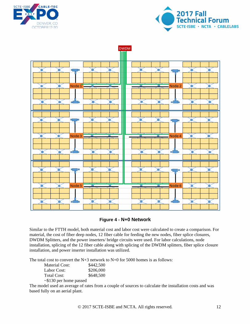
Figure 4 below shows the new layout of the N+0 network. The 20 amplifiers from the N+3 network have been removed and replaced with 6 fiber deep nodes. The model assumes that power supply locations are not moved and five power bridging circuits are utilized to move power from one line to another when needed within the 288 home serving group. The new N+0 network has 48 homes passed per fiber deep node.


Figure 4 - N+0 Network

Similar to the FTTH model, both material cost and labor cost were calculated to create a comparison. For material, the cost of fiber deep nodes, 12 fiber cable for feeding the new nodes, fiber splice closures, DWDM Splitters, and the power inserters/ bridge circuits were used. For labor calculations, node installation, splicing of the 12 fiber cable along with splicing of the DWDM splitters, fiber splice closure installation, and power inserter installation was utilized.

The total cost to convert the N+3 network to N+0 for 5000 homes is as follows: Material Cost: $442,500 Labor Cost: $206,000 Total Cost: $648,500 ~$130 per home passed

The model used an average of rates from a couple of sources to calculate the installation costs and was based fully on an aerial plant.


The question is now whether or not it is worth doing a one-time cost of $1.5 million to get to a full fiber network or invest $650 thousand to upgrade the current network. There are a few more factors which should be looked at when deciding if it is worth going fiber deep or FTTH.

A new growing focus on business-to-business services is driving a strong interest with the power, backhaul, and real-estate provided by the HFC network. Traditionally, the power requirements of the nodes and amplifiers was the primary reason to invest in a reliable powering network. Today, B2B activities like Small Cells, WiFi, IoT, Security & Surveillance (SWISS) are taking advantage of the HFC network in a whole new fashion. Over the past five years, a number of operators have been adding WiFi access points to their networks to create a stickier environment which allows their customers to always utilize their network. There has also been a new demand for IoT networks which allow machine to machine connections to happen across large areas with a single unit coverage. Connections of all kinds will be required to create a ubiquitous network across a geography and right now the HFC network is in a great position to take advantage of these new service requirements.

When strictly discussing a fiber deep network, the total power used will typically be less than the power required today. When doing a fiber deep upgrade, it is important to consider SWISS type of initiatives, these initiatives will drive a higher demand of the network with some of the current small cell opportunities being in the range of 300 – 400 watts at a single location. It is important to not reduce powering locations within the network when doing upgrades and redesigns. Power is a critical component which will differentiate the HFC network from the traditional telco network.

Conclusion Financially, it makes sense to continue the upgrade of the HFC network to fiber deep. The bandwidth and flexibility which a fiber deep network provides is second to none in the world. With DOCSIS 3.1 upgrades, the practical viability of the HFC network is solid for the foreseeable future. Planning ahead while deploying a Fiber Deep network will enable an operator to have enough spare fiber for fiber-to-the-radio, fiber-to-the-home and additional new services. The coax cable is such a simple and wonderful design which will continue to separate the HFC network from the traditional telco network. This network will be the future for both residential broadband as well as new services such as small cells, WiFi, IoT and Security & Surveillance. These type of services will fuel the industry for many years to come.


Abbreviations N+0 Node plus zero amplifiers N+3 Node plus three amplifiers HFC hybrid fiber-coax DWDM Dense Wavelength Division Multiplexing B2B Business to Business SWISS Small Cell, WiFi, IoT, Security & Surveillance SCTE Society of Cable Telecommunications Engineers DOCSIS Data Over Cable Service Interface Specification HDT Hardened Drop Terminal FDH Fiber Distribution Hub FTTH Fiber to the Home P Power V Voltage R Resistance I Current 10 GbE 10 Gigabit Ethernet

Bibliography & References Giving HFC a Green Thumb; John Ulm / Zoran Maricevic, Arris Corporation

Documents

Fiber Deep Networks and The Lessons Learned From The Field