DETERMINATION OF USABLE RESIDUAL ASPHALT BINDER IN RAP

Prepared By

Imad L. Al-Qadi Samuel H. Carpenter

Geoff Roberts Hasan Ozer

Qazi Aurangzeb University of Illinois at Urbana-Champaign

Mostafa Elseifi

Louisiana State University

James Trepanier Illinois Department of Transportation

Research Report ICT-09-031

ICT-R27-11 Determination of Usable Residual Asphalt Binder in RAP

Illinois Center for Transportation

January 2009

CIVIL ENGINEERING STUDIES Illinois Center for Transportation Series No. 09-031

UILU-ENG-2009-2001 ISSN: 0197-9191

i

TECHNICAL REPORT DOCUMENTATION PAGE 1. Report No. FHWA-ICT-09-031

2. Government Accession No. 3. Recipient's Catalog No.

4. Title and Subtitle Determination of Usable Residual Asphalt Binder in RAP

5. Report Date January 2009

6. Performing Organization Code

8. Performing Organization Report N o. 7. Author(s) Imad L. Al-Qadi, Samuel H. Carpenter, Geoffrey L. Roberts, Hasan Ozer, Qazi Aurangzeb, Mostafa A. Elseifi, and James Trepanier

ICT-09-031 UILU-ENG-2009-2001

University of Illinois at Urbana-Champaign Department of Civil and Environmental Engineering 205 North Mathews Ave, MC 250 Urbana, Illinois 61801

10. Work Unit ( TRAIS)

11. Contract or Grant No. ICT-R27-11 13. Type of Report and Period Covered

12. Sponsoring Agency Name and Address Illinois Department of Transportation Bureau of Material and Physical Research 126 East Ash Street Springfield, IL 62704

14. Sponsoring Agency Code

15. Supplementary Notes Study was conducted in cooperation with the U.S. Department of Transportation, Federal Highway Administration

16. Abstract For current recycled mix designs, the Illinois Department of Transportation (IDOT) assumes 100% contribution of

working binder from Recycled Asphalt Pavement (RAP) materials when added to Hot Mix Asphalt (HMA). However, it is unclear if this assumption is correct and whether some binder may potentially be acting as “black rock,” and not participating in the blending process with the new binder. Furthermore, it is also unclear whether binder modifications should be considered in the mix design for recycled HMA. The goal of this research was to determine if the current IDOT mix design practice required modification with respect to the use of RAP.

A set of mixtures was prepared using RAP in accordance with current practice. Additional sets were prepared using recovered binder and recovered aggregate to simulate the effect of RAP binder blending with virgin binder. Mixes containing 0, 20, and 40%RAP were prepared and the dynamic modulus testing results of these mixtures were compared to illustrate the effect of RAP on HMA. Tests on recovered, virgin, and blended binders were also conducted using the Dynamic Shear rheometer (DSR).

This study found that up to 20% RAP in HMA does not require a change in binder grade. However, at 40% RAP in HMA, a binder grade bump at high temperature and possibly at low temperature is needed; more tests are required to verify the need for low temperature binder grade bumping. In addition, this study recommends RAP fractionation in the preparation of laboratory specimens.

17. Key Words Recycled Asphalt Pavement (RAP), Working Binder, Dynamic Modulus

18. Distribution Statement No restrictions. This document is available to the public through the National Technical Information Service, Springfield, Virginia 22161.

19. Security Classif. (of this report) Unclassified

20. Security Classif. (of this page) Unclassified

21. No. of Pages

22. Price

ii

ACKNOWLEDGMENT, DISCLAIMER, MANUFACTURERS’ NAMES

This publication is based on the results of ICT-R27-11, Determination of Usable Residual Asphalt Binder in RAP. ICT-R27-11 was conducted in cooperation with the Illinois Center for Transportation; the Illinois Department of Transportation, Division of Highways; and the U.S. Department of Transportation, Federal Highway Administration.

The contents of this report reflect the view of the authors, who are responsible for the facts and the accuracy of the data presented herein. The contents do not necessarily reflect the official views or policies of the Illinois Center for Transportation, the Illinois Department of Transportation, or the Federal Highway Administration. This report does not constitute a standard, specification, or regulation.

Trademark or manufacturers’ names appear in this report only because they are considered essential to the object of this document and do not constitute an endorsement of product by the Federal Highway Administration, the Illinois Department of Transportation, or the Illinois Center for Transportation.

The input from the members of the Technical Review Panel (TRP) was extremely useful in the completion of this project and the interpretation of the results. The authors are grateful for their support. Members of the Technical Review Panel are the following: Marvin Traylor, Illinois Asphalt Pavement Association Melvin Kirchler, Illinois Department of Transportation William Pine, Heritage Research Laura Shanley, Illinois Department of Transportation Tim Murphy, Murphy Pavement Technology Derek Parish, Illinois Department of Transportation Tom Zehr, Illinois Department of Transportation Amy Schutzbach, Illinois Department of Transportation Steve Gillen, Illinois Tollway

iii

EXECUTIVE SUMMARY For current recycled mix designs, the Illinois Department of Transportation

(IDOT) assumes 100% contribution of working binder from Recycled Asphalt Pavement (RAP) materials when added to Hot Mix Asphalt (HMA) mixes. However, it is unclear if this assumption is correct and whether some binder may potentially be acting as “black rock” and not participating in a blending process with the new binder. Furthermore, it is also unclear whether binder modifications should be considered in mix design for recycled HMA. The goal of this research was to determine if the current IDOT mix design practice required modification with respect to the use of RAP.

An innovative test program was developed to determine the amount of working binder occurring in HMA mixes containing RAP. A set of mixtures for testing purposes was prepared using RAP in a normal recycling manner. Additional sets were also prepared using recovered binder and recovered aggregate to simulate the effect of RAP binder blending with virgin binder. Blends of 0, 20, and 40 percent were prepared and the dynamic modulus of these mixtures was compared to illustrate the effect of RAP blending percentages. Tests on recovered, virgin, and blended binders were also conducted using the Dynamic Shear rheometer (DSR).

Limited fracture testing was conducted to determine how RAP percentages affect the thermal cracking properties of the HMA. Finally, scanning election microscopy (SEM) was performed to determine if the blending effects of the virgin and RAP binder could be observed after the mixing process.

The dynamic modulus measurements did not provide a clear indication of the amount of working binder in RAP. This was due to selective absorption effects and changing aggregate structure which obscured the effect of the stiff binder. However, it was determined that from a mix design standpoint, the addition of RAP did not require any additional binder to achieve densities similar to HMA containing no RAP. The dynamic modulus testing showed that the stiff binder effect could be offset by modification of the binder grade.

The limited fracture energy testing at low temperatures found that the presence of RAP decreased the fracture energy of the HMA samples and thus indicated a lower thermal cracking resistance. The fracture testing also showed that the modification of binder type did not offset the RAP effect as was seen in the dynamic modulus testing. Finally, the SEM method was not able to visually identify binder blending locations, but a promising method was developed for future work.

This study recommends RAP fractionation in the preparation of laboratory specimens . When up to 20% RAP is used in HMA, binder grade does not need to be changed. The total amount of binder in the RAP should be considered as part of the binder content. The use of a PG 58-28 binder instead of a PG 64-22 binder, also known as “double bumping,” with 40% RAP content in HMA appeared to increase the level of binder blending. The addition of a softer binder allowed for the mixes to offset the increase in stiffness due to the presence of 40% RAP in the HMA. This study found that up to 20% RAP in HMA does not require a change in binder grade. However, at 40% RAP in HMA, double bumping the binder grade appears to be needed. Although preliminary tests suggested the potential need for low temperature binder grade bumping, more tests are required to verify that.

iv

CONTENTS TECHNICAL REPORT DOCUMENTATION PAGE .......................................................... i ACKNOWLEDGMENT, DISCLAIMER, MANUFACTURERS’ NAMES ........................... ii EXECUTIVE SUMMARY ................................................................................................. iii CHAPTER 1 INTRODUCTION ......................................................................................... 1 

1. 1 BACKGROUND ..................................................................................................... 1 1. 2 RESEARCH OBJECTIVES .................................................................................... 2 1. 3 RESEARCH METHODOLOGY AND SCOPE ........................................................ 2 

CHAPTER 2 EXPERIMENTAL PROGRAM ..................................................................... 4 2. 1 MATERIALS ........................................................................................................... 4 

2.1.1 Binder and Aggregate Recovery ...................................................................... 5 2.1.2 Rotovapor Extraction Method ........................................................................... 6 

2. 3 SPECIMEN SETS .................................................................................................. 8 2. 4 SPECIMEN PREPARATION .................................................................................. 9 

2.4.1 Laboratory Blending and RAP .......................................................................... 9 2.4.2 Mixture Design ............................................................................................... 10 

2.4.2.1 Aggregate Blend and Gradation .............................................................. 11 2.4.2.2 Mixture Design and Volumetrics .............................................................. 12 2.4.2.3 Blended Gradation Check ....................................................................... 14 2.4.2.4 Test Specimens ....................................................................................... 17 

2. 5 SPECIMEN CHARACTERIZATION ..................................................................... 17 2.5.1 Dynamic Modulus Testing .............................................................................. 17 2.5.2 Stripping Evaluation ....................................................................................... 19 2.5.3 Environmental Scanning Electron Microscope Approach .............................. 19 2.5.4 Fracture Characterization ............................................................................... 20 

CHAPTER 3 RESULTS AND ANALYSIS ...................................................................... 22 3. 1 DYNAMIC MODULUS TEST RESULTS .............................................................. 22 

3.1.1 District 1 HMA with 20% RAP Scenario ......................................................... 22 3.1.2 District 1 Mix with 40% RAP scenario ............................................................ 24 3.1.3 Comparison of District 1- 0, 20, and 40% RAP Cases ................................... 26 3.1.4 Statistics and Goodness of Dynamic Modulus Data ...................................... 27 3.1.5 District 4 Mix 20% RAP Scenario ................................................................... 27 3.1.6 District 4 Mix with 40% RAP Scenario............................................................ 30 3.1.7 Comparison of District 4 HMA with 0, 20, and 40% RAP ............................... 31 3.1.8 Statistics of HMA Dynamic Modulus Data (District 4) .................................... 33 3.1.9 Comparison of Mixes Prepared with PG58-28 and PG64-22 ......................... 33 3.1.10 Statistical Analysis of HMA Dynamic Modulus Results ................................ 35 3.1.11 Application of Hirsch Model to RAP Mixture Volumetrics. ........................... 39 

3. 2 RESIDUAL BINDER EVALUATION ..................................................................... 41 3. 3 EVALUATION OF STRIPPING SUSCEPTIBILITY .............................................. 43 3. 4 RAP PARTICLE-MASTIC BONDING AND BLENDING: ESEM ANALYSIS ........ 46 3. 5 FRACTURE ENERGY ANALYSIS ....................................................................... 55 

CHAPTER 4 SUMMARY AND CONCLUSIONS ............................................................ 59 

v

CHAPTER 5 RECOMMENDATIONS ............................................................................. 62 REFERENCES ................................................................................................................ 63 APPENDIX A BATCHING EXAMPLES FOR MIXES WITH RAP ................................ A-1 APPENDIX B MIXTURE DESIGN ................................................................................ A-6 APPENDIX C COMPLEX MODULUS TEST DATA STATISTICS ............................. A-17 APPENDIX D MOISTURE SUSCEPTIBILITY TESTING DATA ................................ A-28 

1

CHAPTER 1 INTRODUCTION 1. 1 BACKGROUND In recent years the use of reclaimed asphalt pavement (RAP) in new hot-mix asphalt (HMA) pavement construction has become more widespread. The use of RAP is desirable to both contactors and agencies due to the recognized cost savings in a recycling operation. Cost savings increase as higher RAP percentages are being used. However, physical changes due to the addition of high RAP percentages can pose a challenging mix design problem and significantly affect the HMA performance. One potential physical change between a virgin HMA pavement and a HMA pavement containing RAP materials is the modulus increase of the latter. The increased modulus is mainly due to the effect of the RAP’s binder. The increased dynamic modulus may be affected by the increased amount of RAP material passing the #200 sieve. The binder in RAP materials is significantly stiffer than the binder in virgin HMA (Kemp and Predoehl 1981). In addition to the standard aging during construction and normal service life, the binder tends to exhibit an increase in modulus when the pavement is excessively damaged, especially due to cracking, because of the relatively higher exposure to the environment (Smiljanic et al. 1993). Once a pavement is reclaimed, RAP aging continues during the stockpiling process due to air exposure and further oxidation (McMillian and Palsat 1985). As part of this study, a literature review was published in March 2007 as Reclaimed Asphalt Pavement – A Literature Review (Al-Qadi et al. 2007), (www.ict.uiuc.edu). Once a specific RAP material is selected for use in HMA, the effect of high stiffness binder on HMA properties must also be taken into account. The designer must first determine the amount of RAP materials to be used in the HMA. It has been found that low percentages of RAP in the mix (up to 20% by mix total weight) had little to no effect on the blend of virgin and RAP binder (Kennedy et al. 1998). However, when an intermediate or high amount of RAP is used, the effect of the RAP binder on the mix properties becomes significant and ultimately may even require changing the grade of the binder added to the mix. To determine the effect of the RAP binder on the overall mix binder properties, it is crucial to first determine the amount of blending that occurs between the RAP and virgin binder. Assuming that full blending occurs, it becomes necessary to modify the PG grade of the virgin binder to account for the possibility of high RAP binder stiffness; especially at higher RAP percentages. However, if no blending occurs, (i.e. the binder is behaving as a “black rock”), it is unnecessary for the designer to alter the PG grade of the virgin binder; hence, there is no “credit” for the RAP binder. This behavior would require the designer to add more virgin binder in order to achieve a proper mix design, ultimately decreasing the cost effectiveness of the recycling operation.

Currently, the Illinois Department of Transportation (IDOT) assumes that full blending occurs. Depending on the actual amount of blending in the mix versus the assumed amount, the resultant mix could differ compared to that of HMA with virgin materials. This would result from using the wrong PG grade or too little/much asphalt binder in the mix, and poor quality HMA may be produced. Thus, an accurate determination of the binder blending is required to ensure quality pavements containing RAP materials. Previous research has investigated the amount of blending that occurs between RAP and virgin binder. The NCHRP 9-12 study (McDaniel et al., 2000) found that at 10% RAP, the black rock (0% blending), total blending (100%), and actual practice were not significantly different. Conversely, when mixes contain 40% RAP, the black rock case was significantly different from the actual practice and total blending case. This indicates that

2

partial blending of binder occurs and may need to be accounted for when 40% RAP is used. Some degree of blending is likely occurring in mixes with 10% RAP; but the effect is not as significant because of the low binder amount. Hence, no special considerations are needed for mixes with 10% RAP.

A study conducted by Huang et al. (2005) found that when heated RAP was mixed with only virgin aggregates and no virgin binder was added, 11% mixing occurred only due to mechanical mixing. However, this study only used RAP material that passed the No. 4 sieve, and virgin materials retained on the No. 4 sieve. It should also be noted that the study allowed for longer than standard mixing time and above standard temperatures as well. These conditions make it unlikely that 11% blending can be assumed. In the same study, Huang et al. (2005) investigated the amount of blending that occurred with RAP during mixing with virgin binder and aggregates. Extractions were performed on the mixed materials and it was found that the binder at the outer edges of the RAP material was softer than the binder closer to the aggregates. This indicates that blending begins at the outer edges of the RAP particles and moves inward, but because of time and condition dependency, blending was not even and thus incomplete.

It is evident that complete binder blending may not occur; but the actual binder blending is not known either. One approach that may be useful in investigating the amount of RAP’s binder blending is capturing images of the mix using the Scanning Electron Microscope (SEM). The SEM allows the evaluation of the mixture structure at the micro-level, which may provide indications of binder blending mechanisms. Therefore, the SEM was used in the study to investigate the surface morphology of HMA. The use of the SEM may depict a visible difference between the RAP and virgin binders. The SEM images may be firstly used to observe if blending is occurring and secondly to determine if interactions may occur at a microscopic level between virgin and RAP materials. 1. 2 RESEARCH OBJECTIVES The objective of this research was to demonstrate the ability to characterize the amount of binder contribution of RAP materials during the mixing process. The desired outcome of the research was to develop a procedure to determine the amount of blending occurring in a recycled mix that could be readily implemented into the mix design procedure. In addition, the research project would define the effect of RAP on HMA properties. 1. 3 RESEARCH METHODOLOGY AND SCOPE In order to determine the amount of working RAP binder in a mix and the contribution of RAP to overall mixture behavior, an experimental program was developed. The experimental program was designed to allow the amount of working RAP binder to be easily determined by comparing mixes containing normally added RAP to those specifically prepared with a prescribed amount of working stiff RAP binder combined with the virgin binder. The HMA dynamic modulus was then used to evaluate the effect of blending.

In this study, mixtures containing 0, 20%, and 40% RAP added to the HMA were considered. Six different job mix formulae (JMF) were designed for the various blends of RAP. These mixes were prepared in accordance with the current IDOT specifications using aggregates from two IDOT districts and two RAP sources, each at 0%, 20% and 40% content in the HMA. Specimens, prepared with recovered RAP materials (binder and aggregate) to evaluate the effect of stiff binder/virgin binder combinations, were compared to actual practice mixtures. The HMA designs with 20% and 40% RAP included four various sets of specimens whereas the HMA design with 0% RAP had only one set of specimens:

3

• Set 1 - Actual RAP used with the assumption of 100% binder mobilization (current IDOT assumption)

• Set 2 - Recovered aggregates and no recovered binder used to replicate 0% binder mobilization (black rock assumption)

• Set 3 - Recovered aggregates and recovered binder used to replicate 50% binder mobilization

• Set 4 - Recovered aggregates and recovered binder used to replicate 100% binder mobilization

Of the four sets, only the first set used actual RAP materials. The remaining three sets, treated as specimens for comparison, used recovered aggregates and binders utilizing an extraction process. These sets were designed to simulate various scenarios of precisely controlled blending of recovered RAP binder and virgin binder. The sets were used for comparison with actual practice mixes where the amount of working binder is unknown.

The first aim of the research was to investigate the effect of RAP on the mixture design process, involving mixing and compaction. The impact of RAP on this process has important practical implications. The current practice of increased amounts of RAP in the mixtures raises many questions regarding the batching and mixing processes. Residual or working binder evaluation is of utmost importance because the current practice assumes 100% working binder for mix design purposes. This research study focused on the mix design with special attention to the working binder assumption. The effect of increasing RAP on the mix design procedure was also investigated. The same procedures were conducted on the materials provided by both districts with their different JMFs in order to verify the consistency of the findings.

The second aspect of the experimental methodology involved dynamic modulus tests to differentiate between the stiffness of various mixtures. The HMA dynamic modulus test, using repeated compressive loads on cylindrical specimens, is currently used to determine HMA modulus for design and research purposes. It provides a suitable testing and analysis environment to investigate the effect of mixture components at various temperatures and frequencies. It was thought that the stiffening effect of RAP binder would be manifested clearly in the dynamic modulus results. Dynamic modulus testing results would allow differentiation between specimens prepared with precisely controlled blends of RAP binder and virgin binder and those prepared in accordance with actual practice (unknown blending).

In addition to the HMA dynamic modulus testing, binder complex shear modulus was also examined. The complex shear modulus, G*, of the virgin, recovered, and blended binders were determined using a Dynamic Shear Rheometer (DSR). Extracted binders from the RAP sources used in this study were tested as well as blends with virgin PG 64-22 binder at 20% and 40% RAP binder. Virgin PG 64-22 grade binder was also tested to provide baseline data for comparisons of binder properties.

The amount of blending and interaction between the RAP and virgin materials was examined using a SEM at the microscopic level with the intent of showing the interaction of virgin and RAP materials. There are currently two types of SEM used: conventional SEM and environmental SEM (ESEM). The primary difference is that the conventional SEM requires a completely desiccated sample, a high working vacuum, and a metal coating for non-conductive specimens (such as HMA), while an ESEM can be used in “wet mode” to allow a non-conducting hydrated specimen to be placed directly into the instrument without additional preparation. However, if the observed non-conducting specimen is large, the resolution obtained from ESEM may not be as high as that obtained from conventional SEM. The image of the SEM or ESEM is from the surface or near surface since various energy

4

level electron beams can penetrate different depths depending on specimen type. Moreover, the resolution of the SEM or ESEM is dependent upon the combination of accelerating voltage, spot size, vapor pressure (when ESEM is used), and working distance.

Limited fracture energy tests of the evaluated HMA were conducted. The fracture energy tests were conducted to investigate the cause of “cracking” observed in SEM images. The results of fracture energy tests can provide a general idea about the effects of RAP on the thermal cracking potential of the tested HMA. The fracture energy was measured using both the Direct Compact Tension (DCT) test and the Semi Circular Bending (SCB) test. The tests were conducted using the one material source with 0%, 20%, and 40% RAP.

The final HMA characteristic evaluated was the stripping potential of HMA. This allows the determination of the effect of RAP on the HMA stripping susceptibility either positively or negatively. The striping potential was measured in accordance with the Illinois modified AASHTO T-283-02 test.

The experimental program is presented in section 2, while the test analysis and results are presented in section 3. The summary and conclusions of this study can be found in section 4. Section 5 contains the recommendations that result from this study.

CHAPTER 2 EXPERIMENTAL PROGRAM

The materials used in this investigation were provided by IDOT. Two aggregate types and two RAP sources were utilized in the study. The virgin aggregates were collected from sources from Districts 1 and 4. The binder used in this project was collected from one source by District 1. Two binder grades, PG 64-22 and PG 58-28, were used in this study. The PG 58-28 grade binder was used for mixing with selected HMA specimens containing 40% RAP to illustrate the impact of “double grade bumping” of the binder when a high percentage of RAP is used. Double grade bumping as defined here is accomplished by reducing both the high and low temperature grades available in the Performance Graded (PG) Binder System. 2. 1 MATERIALS

Five aggregate sizes were obtained from District 1: 032CM16, 038FM20, 037FM02, 004MF01, and 017CM16. Four sizes were obtained from Thornton; while the 037FM02 was obtained from Edwardsburg. The 017CM16 served as the RAP material; while the other aggregates were virgin materials. The primary rock present in the RAP material was dolomite. Four aggregates were collected from District 4: 032CM13, 038FM21, 037FM01, and 017CM13. The 004MF01, provided by District 1, was also used in the District 4 mixes due to the difficulty of obtaining this aggregate. 032CM13 and 038FM21 materials were collected from the Riverstone Group Inc. source; 037FM01 was collected from the Otter Creek S & G source; and 017CM13, the RAP source, was obtained from W.L. Miller. All of the aggregates from all sources were fractionated prior to mixing. The virgin aggregate and RAP materials were fractionated in an effort to ensure the quality control of specimen preparation. The District 4 RAP materials required processing in order to break down the agglomerations that were found in the materials provided.

The asphalt binder provided from District 1 was used in both District 1 and District 4 specimen preparations. The source of this binder was BP Amoco in Whiting, IN. The binder grades, as provided, are PG 64-22 and PG 58-28.

5

Aggregate bulk specific gravities, Gsb, were determined for each RAP fraction by IDOT’s Bureau of Materials and Physical Research. Asphalt extractions were performed on each fraction of the RAP to determine the asphalt content of that fraction. These extractions were performed using the reflux method, while the rotovapor method was used for the extraction of binder and reclaiming aggregates that were used for mixing specimen sets. Average asphalt contents were determined from weighted averages of the fractioned aggregate weights. A summary of the asphalt content of each fraction is presented in Figure 1. This graph also shows the average asphalt content considered in the mix designs of the HMA containing RAP. 2.1.1 Binder and Aggregate Recovery The testing program requires combining RAP and new aggregates to achieve RAP binder blending percentages of 0, 50, and 100. To obtain these blending percentages, the binder was extracted from the RAP materials in accordance with the procedure outlined in the SHRP Extraction Method AASHTO TP2. The products of the extraction process were clean recovered aggregates and clean recovered binder. This extraction method was chosen because it is reported to cause minimal aging to the recovered binder during the extraction process. Therefore, the process should not have a significant impact on the measured HMA dynamic modulus values. A detailed overview of the extraction process can be found in Section 2.1.2. Although this extraction process can also be used to determine the asphalt content of the mix, the asphalt contents as obtained by IDOT laboratories, using the reflux method, were used for HMA design.

0.0

1.0

2.0

3.0

4.0

5.0

6.0

7.0

8.0

>4.75 4.75-2.36 2.36-0.6 <0.6

RA

P A

C (%

)

Sieve size (mm)

RAP Residual Binder %

District 1 District 4

District 1 Avg RAP AC = 4.7 %District 4 Avg RAP AC = 5.1 %

Figure 1. Asphalt contents of RAP fractions.

6

Figure 2. Rotovapor extraction apparatus. 2.1.2 Rotovapor Extraction Method The AASHTO TP2 standard for binder extraction and recovery was followed. This standard uses a rotovapor extraction process. Other common methods include reflux or abson extraction. The rotovapor extraction apparatus was assembled at the Advanced Transportation Research and Engineering Laboratory (ATREL), where all extractions were conducted. Figure 2 illustrates the extraction apparatus; while Figure 3 shows a sample being centrifuged to remove fines during the recovery process.

Figure 3. Placing asphalt/solvent solution into centrifuge to remove fines.

The current standard does not cover certain issues related to successfully recovering the binder and aggregate for reuse, such as how to remove the recovered binder from the flask, so that it can be used in the HMA preparation process later. After the recovered binder had been centrifuged to remove fine materials, it was heated to 345 °F (174 °C)to remove all solvent and then nitrogen coated for 30 min, in accordance with the standard. The collection flask was then removed and placed into the oven. The flask was inverted to allow the binder to run out and into a binder tin, as shown in Figure 4. The recovered binder was placed into the oven at a temperature of 302 °F (150 °C) for 15 min and the temperature was then raised to 347 °F (175 °C) for an additional 10 min. After the

7

combined 25 min, the flask and collected recovered binder were removed from the oven. The time and temperature of the removal of the recovered binder were chosen to allow for the maximum amount of binder to be collected while keeping additional binder aging to a minimum.

Figure 4. Binder draining from collection flask in oven.

The project researchers developed the following method to preserve as much of the original gradation and quality of the recovered aggregate materials as possible. Once the extraction vessel was drained of the last solvent wash, the extraction vessel was disassembled and the clean recovered aggregates were placed into an enamel coated pan. The vessel was then allowed to air dry and the components of the vessel were then brushed clean with a soft bristled paint brush, as can been seen in Figure 5. This process prevents pan rusting and keeps the aggregates clean. During the extraction vessel cleaning, water was used to wash the internal surfaces, which left the aggregates covered with water in the pan.

Figure 5. Brushing the extraction vessel clean of fine material.

The desire to preserve the amount of fines in the recovered aggregates led to a two step process: The first step was to remove fines from the filter. This was done by removing the filter from the extraction setup and placing it in the oven at 248 °F (120 °C) for a period

8

of approximately 2 hrs in order to dry the filter of extraction solvent. Once the filter was dry, it was removed from the oven. The filter was then opened and the fines from the filter were placed with the rest of the recovered aggregates. Care was taken as to ensure that no plastic shavings from the filter fell into the recovered aggregates. After the outside of the filter was removed, the filter itself was tapped with a hammer to free as many fines as possible from the filter paper. The collected fines were then added to the other recovered aggregates. The second step to preserve the fines was to clean the flasks of any fines that settled during the extraction process. Generally the only flask that contained any fines was the first flask in the setup. The fines were removed by cleaning the flask with extraction solvent and pouring the solution into the pan containing the recovered aggregates. As a result of the cleaning process, the recovered aggregates and fines were immersed in water. The recovered aggregates were placed in the oven overnight at a temperature of 176 °F (80 °C) to dry. The next day the aggregates were removed from the oven and covered with alcohol. The addition of alcohol to the recovered aggregates removed any residual solvents that may have soaked into the aggregates during the procedure. Water was once again added to the recovered aggregates to ensure an equal covering of all of the aggregates. The recovered aggregates were once again placed in the oven overnight at 176 °F (80 °C) to allow the aggregates to dry. Figure 6 shows the RAP materials and the recovered aggregates after extraction.

Figure 6. RAP material before (left) and after (right) extraction.

After the recovered aggregates were placed in the oven overnight for the second time, they were collected and fractionated. Once the recovered aggregates were put through this recovery process they were handled similarly to the other aggregates. 2. 3 SPECIMEN SETS Specimens were prepared with different RAP contents to allow investigation of the amount of residual binder blending, or working, from RAP particles. The proportion of residual binder and virgin binder in HMA is expected to affect mixture volumetrics and mechanical properties. In order to quantify this effect, mixtures with 0, 20, and 40% RAP materials were designed. In addition to the specimens with varying percentages of RAP, control specimens were also prepared using recovered RAP materials (aggregate and binder). The control specimens were prepared with various ratios of recovered RAP binder

9

to virgin binder. This would isolate the recovered RAP binder variable in a mixture and allowed investigating the effect of recovered RAP binder on complex modulus. The same procedure was repeated using District 4 materials. In total six job mix formulae (JMF) were prepared.

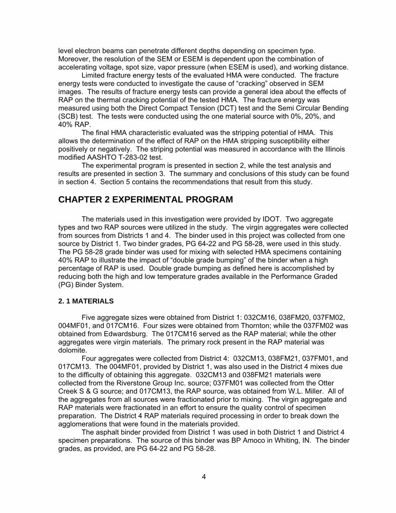
Table 1 shows District 1 specimen sets. Specimen sets used in this project can be grouped into two categories. The first are JMF with actual RAP and virgin materials (aggregate and binder) and the second set are JMF with recovered aggregates and binder from RAP materials in addition to virgin aggregates and binder. The first group of specimens (Set 1) is actual practice specimens and included only virgin materials and stockpile RAP materials. Working binder in this set is unknown and has yet to be determined. The second group (Sets 2, 3, and 4) are the control specimens and are further divided into three categories that provide various blending ratios of virgin and residual binders. The difference among these three specimen sets is the proportion of recovered RAP binder to total binder content of the mix. These specimens were designed to simulate the presence of varying proportions of mobilized RAP binder in an actual HMA with RAP materials. For example, Set 2 represents a 0% working binder scenario where RAP binder is not “working” as binder in the mix. Set 4 represents a scenario where 100% RAP binder is blended with virgin binder to produce a composite binder in the mixture. The same sets were also repeated with the materials obtained from District 4 in Illinois. The specifics of laboratory mixture preparation with RAP are discussed in more detail in the following sections.

Table 1. Mixture Sets Used in the Study RAP

% Specimen ID Binder RAP to Total binder (%) Notes

0 D1-SET 1-00 Virgin NA

20

D1-SET 1-20 Virgin Unknown Actual field practice

D1-SET 2-20 Virgin 0 0% working binder

D1-SET 3-20 Virgin and recovered 8 50% working

binder

D1-SET 4-20 Virgin and recovered 16 100% working

binder

40

D1-SET 1-40 Virgin Unknown Actual field practice

D1-SET 2-40 Virgin 0 0% working binder

D1-SET 3-40 Virgin and recovered 16 50% working

binder

D1-SET 4-40 Virgin and recovered 32 100% working

binder

2. 4 SPECIMEN PREPARATION 2.4.1 Laboratory Blending and RAP Unlike other virgin materials in a mixture, RAP aggregates contain binder; some amount of which needs to be considered in binder content calculations. Field practice assumes 100% of RAP binder is working in the HMA to form a composite binder blend. However, it is unlikely that the RAP binder absorbed into the pores will be released to mix with virgin binder, and then be reabsorbed by aggregates. It is more likely that the majority

10

of effective RAP binder is the portion that mixes with the virgin binder. Because no existing procedure measures absorbed binder, the current IDOT assumption, 100% RAP binder is working in the mix, was adopted in this study. Based on the amount of working binder in the RAP and the proportion of RAP in the mixture, one can calculate the virgin binder needs to be added to the mixture for a given optimum binder content. An example of mixture calculations is given in APPENDIX A to illustrate the proportion of residual and virgin binder for each set of mixtures. RAP stockpiles have inherent variability since they can be obtained from different pavement layers and/or multiple source locations. They can be also contaminated with fabrics, joint sealants, and grids. This inherent variability and contamination can have detrimental effects if mixture preparation with RAP is not handled carefully. Another source of variability can come from agglomeration of RAP particles to each other. In addition, residual binder content of different sizes of RAP can vary significantly.

To address these variability issues, the research followed the practice of fractionating the RAP. This procedure requires separating the RAP aggregates into various sizes. This process can be difficult because RAP particles are usually agglomerated. Heating (no more than 1000F) is required to break down the agglomerates before fractionating. The gradation obtained from this process is called an “apparent gradation” and is very different than the gradation of the recovered aggregates. The following steps were applied to RAP during this process:

1. Scoop out representative samples from each bag; 2. Take the weight of the sample; 3. Heat in the oven at 100 °F (37.8 °C) no more than 2 hrs; 4. Break down agglomerates (some may remain); 5. Fractionate the material into various sizes (+12.5 mm, +9.5 mm, +4.75 mm, +2.36

mm, +0.600 mm, and -0.600 mm); 6. Reheat +9.5 mm material if there is any; 7. Break down agglomerates again; 8. Sieve again and add the materials obtained in this step to those obtained in Step 5; 9. Record retained aggregates on each sieve and calculate their percentages (this is

the apparent gradation); 10. Repeat Steps 1 to 9 for at least three representative samples to determine the

average apparent gradation. This procedure is repeated to generate as much material as is needed for each sieve

size. Apparent gradation of Districts 1 and 4 RAP is shown in Table 2. The gradation analysis presented in Table 2 is an average of eight samples. A comparison of recovered aggregate gradation is also shown in the table. The increased amount of the larger fractions and decreased fines, as indicated by the apparent gradation, compared to the recovered aggregate gradation suggested that fine material (smaller than 2.36 mm) remained on the surface of the larger RAP aggregates (larger than 2.36 mm). This is an important observation that can affect mixture aggregate structure if these fine particles are not released during the mechanical mixing process. Apparent gradation can be used in batching materials, but should not be used for a job mix formula calculation. 2.4.2 Mixture Design Six JMF’s were prepared with varying percentages (0, 20, and 40%) of RAP using both Districts 1 and 4 materials. The IDOT gyratory mixture design procedure was followed to prepare the mix formulae. Optimum binder content and other volumetric properties were determined for each mix design. The mixture formula is an N50 mixture design with 4.0%

11

air voids. Set 1 mixture designs were prepared with virgin materials (aggregate and binder) and RAP aggregates (see Table 1).

Table 2. Apparent Gradation of Districts 1 and 4 RAP Aggregates Fraction

(mm) DISTRICT 1APPARENT

GRADATION (% Retained)

DISTRICT 1RECOVERED AGGREGATE (% Retained)

DISTRICT 4APPARENT

GRADATION (% Retained)

DISTRICT 4RECOVERED AGGREGATE (% Retained)

+9.5 0 0 4.7 1.2 +4.75 34.7 26.5 40.8 27.4+2.36 26.0 24.2 25.9 24.1

+0.600 24.9 23.3 21.9 17.8-0.600 14.3 26.0 6.7 30.1

Studying the material behavior during the mixture design is a critical step in

developing an understanding of RAP behavior during the mixing process. Mixtures with varying blend percentages were prepared using the two material sources. This allows examining the impact of varying RAP percentages on the volumetric properties of mixtures, and particularly the optimum binder content. It is also crucial to know how much of the RAP binder is working in order to properly adjust the amount of virgin binder that needs to be added. Current IDOT practice for RAP mixtures assumes 100% working RAP binder. The validity of this assumption was also investigated by preparing similar mixtures with varying RAP amounts and similar aggregate gradations. The aggregate gradations used in this research were similar; except for the amount of fines passing the # 200 sieve. For HMA with the District 1 material, the amount passing the #200 sieve were as follows: 4.5%, 5.8%, and 7.1% for mixes with 0%, 20%, and 40% RAP, respectively. Similarly, for mixes with District 4 materials, the percent passing the # 200 sieve were as follows: 2.9%, 4.1%, and 6.0% for the mixes with 0%, 20%, and 40% RAP, respectively. Detailed information regarding the mixture design is described herein. 2.4.2.1 Aggregate Blend and Gradation

Design gradations were chosen so that a comparable aggregate structure was obtained with each design excluding the amount of material passing the #200 sieve as was explained above. Figure 7 shows design aggregate gradation for HMA with 0, 20, and 40% RAP using District 1 materials. Figure 8 shows design aggregate gradation for 0, 20, and 40% RAP using District 4 materials. These aggregate gradation charts show that the target aggregate structure is very close for gradations with varying RAP percentage contents. An example of RAP contribution to an aggregate batch is given in Table 3.

12

0

10

20

30

40

50

60

70

80

90

100

Sieve mm (0.45 power)

Perc

enta

ge p

assin

g

0.07

5

0.30

0.15

50.0

0

25.0

0

19.0

0

9.50

12.5

0

37.5

0

0.60

1.18

4.75

2.36

20 % RAP DESIGN

40% RAP DESIGN

0 % RAP DESIGN

40.020.00.0RAP

1.51.51.5Filler

9.011.918.0FM02

9.515.923.0FM20

40.050.757.5CM16

RAP 40 % Blend (%)

RAP 20 % Blend (%)

RAP 0 % Blend (%)

Material

40.020.00.0RAP

1.51.51.5Filler

9.011.918.0FM02

9.515.923.0FM20

40.050.757.5CM16

RAP 40 % Blend (%)

RAP 20 % Blend (%)

RAP 0 % Blend (%)

Material

Figure 7. District 1 0, 20, and 40 % RAP blend gradation.

0

10

20

30

40

50

60

70

80

90

100

Sieve mm (0.45 power)

Perc

enta

ge p

assin

g

0.07

5

0.30

0.15

50.0

0

25.0

0

19.0

0

9.50

12.5

0

37.5

0

0.60

1.18

4.75

2.36

RAP 40 %DESIGN

RAP 20 %DESIGN

RAP 0 %DESIGN

1.50.08.021.569.0

RAP 0 % Blend (%)

40.020.0RAP

1.01.0Filler

4.09.0FM01

5.010.0FM21

50.060.0CM13

RAP 40 % Blend (%)

RAP 20 % Blend (%)

Material

1.50.08.021.569.0

RAP 0 % Blend (%)

40.020.0RAP

1.01.0Filler

4.09.0FM01

5.010.0FM21

50.060.0CM13

RAP 40 % Blend (%)

RAP 20 % Blend (%)

Material

Figure 8. District 4 aggregate gradation for HMA with 0, 20, and 40% RAP.

2.4.2.2 Mixture Design and Volumetrics

Optimum binder content of each HMA design was obtained from a volumetric analysis at various trial binder contents. The binder content that yields required air voids (4.0% at 50 gyrations) was selected to be the optimum binder content. The optimum binder content was physically measured in accordance with AASHTO T166. The binder content for HMA with RAP includes the existing RAP binder. Figure 9 shows the density curves with number of gyrations for Districts 1 and 4 mixtures with RAP.

13

72

76

80

84

88

92

96

100

1 10 100# of Gyrations

% G

mm

AC = 5.8 % AC = 5.4%

Optimum AC = 5.65 %

Ndesign = 50

4% air voids

< 89 @ Ninitial OK!

Ninitial = 672

76

80

84

88

92

96

100

1 10 100# of Gyrations

% G

mm

AC = 6.0 % AC = 5.5% AC = 5.0%

Optimum AC = 5.7% %

Ndesign = 50

4% air voids

< 89 @ Ninitial OK!

Ninitial = 6

D1-20% RAP D1-40% RAP

72

76

80

84

88

92

96

100

1 10 100# of Gyrations

% G

mm

AC = 6.0 % AC = 5.5% AC = 5.0% AC = 4.5%

Optimum AC = 6.0%

Ndesign = 50

4% air voids

< 89 @ Ninitial OK!

Ninitial = 6

72

76

80

84

88

92

96

100

1 10 100# of Gyrations

% G

mm

AC = 6.0 % AC = 5.5% AC = 5.0%

Optimum AC = 6.0 %

Ndesign = 50

4% air voids

< 89 @ Ninitial OK!

Ninitial = 6

D4-20% RAP D4-40% RAP

Figure 9. Optimum binder content determination for Districts 1 and 4 HMA with RAP.

A summary of each mixture design is shown in Tables 4 and 5 for Districts 1 and 4

materials, respectively (details and statistics of the samples prepared for the designs are presented in APPENDIX B). The volumetric calculations of mixes with RAP were performed based on the bulk specific gravity (Gsb) of RAP aggregates. Typical values approved by IDOT were used for Districts 1 and 4 RAP aggregates (2.660 and 2.630, respectively). The use of an accurate bulk specific gravity of the RAP for VMA calculations is crucial. Substituting effective specific gravity (Gse) for the Gsb will result in overestimating combined bulk specific gravity and thus an overestimation of VMA (Murphy, 2008). As shown in Tables 4 and 5, optimum binder content does not vary significantly with increasing RAP content. This result provides insight into the mechanism mixing and compaction process when RAP material is present. It is important to recall that 100% working RAP binder was assumed in the mix design process. Thus, it can be concluded that the 100% working binder hypothesis is acceptable from a mix design point of view since equivalent compactability was achieved regardless of RAP content. While it cannot be stated that 100% blending is occurring, the RAP binder still contributes to filling voids. In addition, a potential lubricating effect of RAP materials could facilitate compaction and lessen the need for additional binder. The VMA values of the mixes with 40% RAP using both Districts 1 and 4 materials were below the VMA minimum requirement by 0.3%.

14

Table 3. RAP Contribution to Aggregate Batch Having 20% District 1 RAP in the Mix Batch weight (g) 4700 RAP weight (g) 940

Fractions Used % of Total RAP Weight Fraction (g)+4.75 mm 34.7 327 +2.36 mm 26.0 244 +0.600 mm 24.9 234 -0.600 mm 14.3 135 Total 100 940

Table 4. District 1 Mixture Design with Various RAP Percentages

Optimum

AC (%)

Total needed binder

(g)*

Virgin binder

(g)

Recovered binder

(g)

Gmb @ optimum

AC

Gmm @ optimum

AC

VMA @ optimum

AC 0 % RAP 5.9 294 294 0 2.398 2.502 15.1

20 % RAP 5.7 281 237 0 2.397 2.496 15.040 % RAP 5.65 276 188 0 2.421 2.519 14.1

20 % Recovered Aggregate

5.7 284

284 (Set 2)

0 (Set 2)

2.395 2.499 15.1 262 (Set 3)

22 (Set 3)

240 (Set 4)

44 (Set 4)

40 % Recovered Aggregate

5.55 276

276 (Set 2)

0 (Set 2)

2.410 2.505 14.4 232 (Set 3)

44 (Set 3)

188 (Set 4)

88 (Set 4)

* Total binder content for a 4,700 g aggregate batch (Total binder = Virgin binder + % 100 of RAP binder)

2.4.2.3 Blended Gradation Check

Using RAP materials in HMA can cause significant variability due to differences in batching (apparent gradation) and gradation used in design, as was depicted in Table 2. It is important to check actual blend gradation against the design blend. Several design specimens were randomly selected and burned in the ignition oven in order to reclaim the aggregates. Washed aggregate gradation was then performed on these materials. Figure 10 shows the comparison of the design blend and actual sample blend for the District 1 mix with 20% RAP. Similarly, Figure 11 shows the comparison of the design blend and actual sample blend for the District 1 mix with 40% RAP. Figures 12 and 13 demonstrate the comparison of the design and actual sample blend for District 4 mixes with 20% and 40% RAP, respectively. The design and actual blends are in good agreement, which justifies the specimen preparation approach followed in this study. The variation in gradations, shown in Figures 10 and 11, could be related to the degradation of the coarse aggregate in the mix.

15

Table 5. District 4 Mixture Design with Various RAP Percentages

Optimum AC (%)

Total needed binder

(g)*

Virgin binder

(g)

Recovered binder

(g)

Gmb @ optimum

AC

Gmm @ optimum

AC

VMA @ optimum

AC 0 % RAP 5.9 295 295 0 2.429 2.524 13.7

20 % RAP 6.0 297 249 0 2.409 2.508 14.140 % RAP 6.0 294 198 0 2.406 2.506 14.2

20 % Recovered Aggregate

5.9 295

295 (Set 2)

0 (Set 2)

2.394 2.496 14.6 271 (Set 3)

24 (Set 3)

247 (Set 4)

48 (Set 4)

40 % Recovered Aggregate

5.9 295

295 (Set 2)

0 (Set 2)

2.391 2.490 14.6 247 (Set 3)

48 (Set 3)

199 (Set 4)

96 (Set 4)

* Total binder content for a 4,700 g aggregate batch (Total binder = Virgin binder + % 100 of RAP binder)

0

10

20

30

40

50

60

70

80

90

100

Sieve mm (0.45 power)

Perc

enta

ge p

assin

g

0.07

5

0.30

0.15

50.0

0

25.0

0

19.0

0

9.50

12.5

0

37.5

0

0.60

1.18

4.75

2.36

20 % RAP DESIGN

IGNITION SAMPLE

5.820.438.257.4

RAP 20 (%passing)

6.6No.200

22.0No.30

40.5No.8

60.5No.4

Ignition (%passing)

Sieve #

5.820.438.257.4

RAP 20 (%passing)

6.6No.200

22.0No.30

40.5No.8

60.5No.4

Ignition (%passing)

Sieve #

Figure 10. Blend check of District 1 design with 20% RAP.

16

0

10

20

30

40

50

60

70

80

90

100

Sieve mm (0.45 power)

Perc

enta

ge p

assin

g

0.07

5

0.30

0.15

50.0

0

25.0

0

19.0

0

9.50

12.5

0

37.5

0

0.60

1.18

4.75

2.36

40 % RAP DESIGN

IGNITION SAMPLE

7.122.039.259.4

RAP 40 (%passing)

5.1No.200

24.1No.30

42.8No.8

63.7No.4

Ignition (%passing)

Sieve #

7.122.039.259.4

RAP 40 (%passing)

5.1No.200

24.1No.30

42.8No.8

63.7No.4

Ignition (%passing)

Sieve #

Figure 11. Blend check of District 1 design with 40% RAP.

0

10

20

30

40

50

60

70

80

90

100

Sieve mm (0.45 power)

Perc

enta

ge p

assin

g

0.07

5

0.30

0.15

50.0

0

25.0

0

19.0

0

9.50

12.5

0

37.5

0

0.60

1.18

4.75

2.36

20 % RAP DESIGN

IGNITIONSAMPLE 4.1

18.333.358.9

RAP 40 (%passing)

2.7No.200

18.5No.30

35.9No.8

61.6No.4

Ignition (%passing)

Sieve #

4.118.333.358.9

RAP 40 (%passing)

2.7No.200

18.5No.30

35.9No.8

61.6No.4

Ignition (%passing)

Sieve #

Figure 12. Blend check of District 4 design with 20% RAP.

17

0

10

20

30

40

50

60

70

80

90

100

Sieve mm (0.45 power)

Perc

enta

ge p

assin

g

0.07

5

0.30

0.15

50.0

0

25.0

0

19.0

0

9.50

12.5

0

37.5

0

0.60

1.18

4.75

2.36

40 % RAP DESIGN

IGNITIONSAMPLE

6.0

18.7

33.0

59.5

RAP 40 (%passing)

3.6No.200

17.4No.30

35.8No.8

62.6No.4

Ignition (%passing)

Sieve #

6.0

18.7

33.0

59.5

RAP 40 (%passing)

3.6No.200

17.4No.30

35.8No.8

62.6No.4

Ignition (%passing)

Sieve #

Figure 13. Blend check of District 4 design with 40 % RAP . 2.4.2.4 Test Specimens

Once the design was finalized for each mixture type, gyratory test specimens were prepared at 4.0 % air voids. The specimens were compacted to 50 gyrations and air voids were controlled by adjusting mixture weight. The specimens were cored and sawed to the proper diameter and length for dynamic modulus testing following compaction. 2. 5 SPECIMEN CHARACTERIZATION 2.5.1 Dynamic Modulus Testing

Dynamic modulus testing was performed on each specimen set. Because the residual binder is aged, the effect of the residual binder is expected to increase the modulus of binder mastic; hence, the modulus of the composite mixture will increase as well. The specimen sets introduced in the preceding sections were designed to investigate the effect of stiff RAP binder on dynamic modulus and determine the working binder in RAP. Specimens were prepared using Districts 1 and 4 materials with 20 and 40% RAP blends. Specimen identification used in this report is illustrated in the following.

Di-SETj-AA where i: District 1 or 4 j: Specimen sets 1, 2, 3, and 4 AA: 00, 20 or 40% RAP EX: D1-SET1-20 is District 1, SET 1 (field practice), and 20% RAP D4-SET1-00 is District 4, SET 1 (field practice), and 0% RAP

18

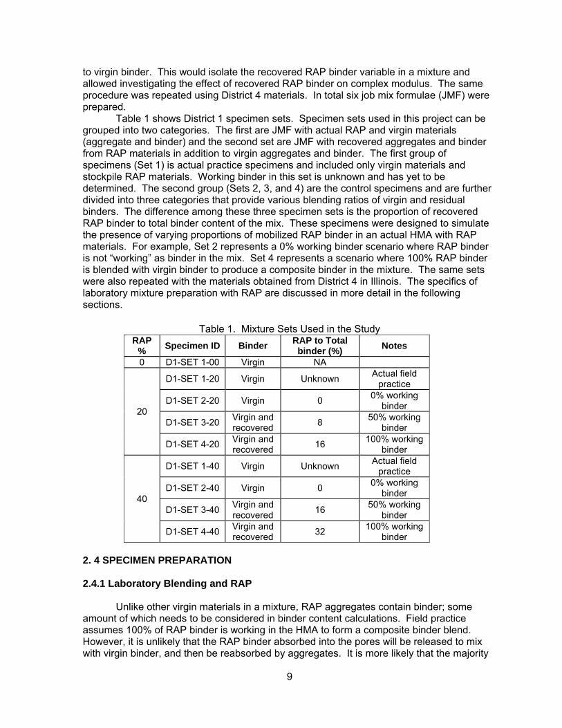
The following testing parameters were used in this study. An additional low frequency (0.01 Hz), not called for in the AASHTO procedure was added to the testing sequence to investigate the effect of binder which is more pronounced at low frequencies. A summary of the testing suite can be found in Table 6.

Table 6. Dynamic Modulus Testing Suite

Test Temperature (0C)

Frequency (Hz)

Load Amplitude

(kN)

Contact Load (kN)

-10 25, 10, 5, 1, 0.5, 0.1, and 0.01 7 0.3

4 25, 10, 5, 1, 0.5, 0.1, and 0.01 6 0.2

20 25, 10, 5, 1, 0.5, 0.1, and 0.01 2 0.1

Testing began at the lowest temperature and highest frequency. The total number of

loading cycles is shown in Table 7. The analysis software based on AASHTO TP 62-03 collects only the recordings from the last 10 cycles and then fits a sinusoid curve to the load and deformation data.

Table 7. Number of Cycles for Test Sequence

Frequency (Hz)

Number of cycles

25 20010 2005 1001 20

0.5 150.1 15

0.01 11

Phase angle and dynamic moduli are calculated at each frequency using the following formulas:

( )*

**

ε

σω =E and ( ) σε θθωθ −= (1)

where: θ(ω) = Phase angle between applied stress and strain for frequency ω,

degrees |E*(ω)| = Dynamic modulus for frequency ω, kPa (psi)

εθ = Average phase angle for all strain transducers, degrees θσ = Stress phase angle, degrees |σ*| = Stress magnitude, kPa (psi)

*ε = Average strain magnitude

19

2.5.2 Stripping Evaluation

The moisture susceptibility of RAP mixtures was also evaluated. Illinois modified AASHTO T 283-02 was followed to determine resistance of HMA with RAP to moisture induced damage. The procedure followed during this study is as follows:

1. Preparation of compacted specimens at 7% air voids (+/- 0.5%), 6 in (150 mm)

diameter, and 95 +/- 5 mm 3.75 +/- 0.20 in thick. 2. Specimens were grouped into dry and conditioned sets. 3. Conditioned specimens were saturated to 70-80%. 4. Conditioned specimens were placed in water bath at 140 °F (60 °C) for 24 hrs. 5. Following the 24 hr conditioning, specimens were placed in a water bath at 77 °F

(25 °C) for 2 hrs. 6. Conditioned specimens were tested at 77 °F (25 °C) to determine their indirect

tensile strength. 7. Visual stripping inspection was conducted. 8. Dry specimens were tested for indirect tensile strength after 2 hrs conditioning at 77

°F (25 °C).

Figure 14 illustrates the sample preparation path from saturation to 70-80% through conditioning, and finally testing.

Figure 14. Moisture susceptibility procedure for conditioned specimens after saturation.

2.5.3 Environmental Scanning Electron Microscope Approach

The electron microscope, Philips XL30 ESEM-FEG, used in this study was a dual function SEM. It can operate as both a conventional SEM or ESEM. Although metal coating is not required in the ESEM, both coated and uncoated specimens were examined to determine resolution enhancement. The following conditions were used in the experiment. The chamber pressure of 1 tor water vapor, 5 and 7.5 kV accelerating voltage,

20

spot size of 3 and 4, and working distance (WD) of 7.5 were used when the specimen was observed in the wet mode (ESEM). The chamber pressure of 1.3×10-4 tor, 20 kV accelerating voltage, spot size of 4 and WD of 10 were used for SEM. The images were stored as 1,290×968 pixel TIFF files. Sample preparation started by coring a 25 mm specimen from the 100 mm core obtained from a gyratory specimen. To obtain a 3 mm deep specimen, the sample was cut through its depth. The sample was then cleaned and dried at 104 °F (40 °C) in the oven. A spot of interest was then marked on the 25 mm specimen and was magnified repetitively using ESEM and SEM to reveal different surface features of the specimen. A photo summary of this process is shown in Figure 15.

The spots of interest were determined by visual observation of the specimen. The researchers observed the cross section of the samples and noticed that certain particles appeared discolored with respect to the remaining particles. These were assumed to be the RAP particles since the discolored particles occurred at approximately the same frequency as the percentage of RAP added to the mix. These discolored particles were then assumed to be RAP, and the particle-mastic interface was investigated with the SEM.

Figure 15. Sample preparation and capture of high-resolution images using scanning

electron microscopy. 2.5.4 Fracture Characterization Fracture energy characterization of the HMA with RAP is necessary to illustrate the potential for low temperature cracking. Two fracture tests were selected to determine the fracture energy of the mixes in this study. The SCB test and DCT test were used for HMA fracture energy characterization. Figures 16 through 18 show the specimens tested in the SCB and DCT.

For the DCT, test specimens are easily prepared from standard 6in gyratory specimens. Preparation of the DCT test specimens was in accordance of the ASTM 7313 standard. Three replicates of each mix were tested at 10.4 °F (-12 °C) and 32°F (0 °C). Preparation of the SCB specimens was in accordance with the approach outlined by Li (2005). As with the DCT testing, the SCB testing was conducted at 10.4 °F (-12 °C) and 32 °F (0 °C.) Three test replicates of each HMA with RAP content and testing temperature were performed. Table 8 illustrates the test matrix used for the fracture testing utilizing both the DCT and SCB testing. The numbers in Table 8 are the number of replicate tests run.

21

Semi Circular Beam-SCB Disc Compact Tension-DCT

Figure 16. SCB and DCT test specimens.

The fracture tests were both crack mouth opening displacement (CMOD) controlled.

The loading rate of the test was 0.7 mm/min CMOD displacement for the SCB test, and 0.1 mm/min for the DCT. These loading rates are typical of the loading rates used in the respective tests. The fracture energy for both testing methods was determined by calculating the area under the load vs. CMOD curve. These calculations were performed in MATLAB.

Figure 17. SCB test.

22

Figure 18. DCT test.

Table 8. Fracture Energy Evaluation Test Matrix

Temperature (°C) RAP (0%) RAP (20%) RAP (40%) Total0 3 3 3 9

-12 3 3 3 9Total 6 6 6 18

CHAPTER 3 RESULTS AND ANALYSIS 3. 1 DYNAMIC MODULUS TEST RESULTS

Dynamic modulus tests were performed on the gyratory compacted specimens

prepared at the target 4.0% air voids. The results are presented in the form of master curves at a reference temperature of 68 °F (20 °C). 3.1.1 District 1 HMA with 20% RAP Scenario

The specimen volumetric properties are presented in Table 9 including air voids,

VMA, and VFA of each specimen. As expected significant changes in air voids, VMA and VFA were observed after cutting and coring specimens. The results in Table 9, show some variation in VMA values. It is believed that these variations do not significantly affect the dynamic modulus results in a manner that would affect the comparisons between the various specimen sets.

Dynamic modulus test results are reported as master curves, shown in Figure 19. Master curves were constructed using time-temperature superposition with the reference temperature of 68 °F (20°C). As illustrated in the figure, there is no significant difference between the results of all four specimen sets. Recall that Sets 2, 3, and 4 were prepared with recovered aggregates and binder. The proportion of recovered RAP binder to total binder content is 0, 8, and 16% for Sets 2, 3, and 4, respectively. The stiff binder effect should be most observable in the results of Sets 2, 3, and 4. However, insignificant differences exist between the HMA dynamic moduli at this percentage of RAP in the mix. Hence, it is concluded that the addition of 20% RAP to a mixture does not significantly alter the mixture dynamic modulus.

Table 9. District 1 Mix with 20% RAP

23

Air Voids VMA VFA Air Voids VMA VFAD1-SET1-20-1 4.4 15.4 71.6 3.4 14.5 76.8D1-SET1-20-2 4.3 15.3 71.7 3.1 14.3 78.0D1-SET1-20-3 4.6 15.6 70.5 3.4 14.5 76.4Average 4.4 15.4 71.3 3.3 14.4 77.1D1-SET2-20-1 4.3 15.2 71.5 3.4 14.4 76.6D1-SET2-20-2 4.3 15.2 71.8 3.4 14.4 76.4D1-SET2-20-3 4.3 15.3 72.0 3.2 14.3 77.7Average 4.3 15.2 71.8 3.3 14.4 76.9D1-SET3-20-1 4.8 15.6 69.3 3.3 14.3 77.1D1-SET3-20-2 4.4 15.3 71.3 3.2 14.2 77.5D1-SET3-20-3 4.5 15.4 70.7 3.2 14.2 77.7Average 4.6 15.4 70.4 3.2 14.2 77.4D1-SET4-20-1 4.8 15.6 69.3 3.4 14.4 76.3D1-SET4-20-2 4.4 15.3 71.3 3.1 14.1 78.3D1-SET4-20-3 4.7 15.5 69.9 3.3 14.3 77.2Average 4.6 15.5 70.2 3.2 14.3 77.3

Before cutting & coring After cutting & coring

1E+2

1E+3

1E+4

1E-1 1E+1 1E+3 1E+5 1E+7Reduced frequency (Hz)

Com

plex

Mod

ulus

(ksi

)

D1-SET1-20D1-SET2-20D1-SET3-20D1-SET4-20

Figure 19. District 1 mix with 20% RAP master curves.

Similarly, phase angle master curves were constructed. Figure 20 presents the phase angle master curve for the four specimen sets. Similar to modulus results, phase angle results do not exhibit significant differences between the four mixes at this percentage of RAP. The differences between the mixtures are within the experimental variations.

24

0

10

20

30

40

1E-2 1E+0 1E+2 1E+4 1E+6Reduced Frequency (Hz)

Phas

e An

gle

(deg

rees

)

D1-SET1-20D1-SET2-20D1-SET3-20D1-SET4-20

Figure 20. District 1 mix with 20% RAP phase angle.

3.1.2 District 1 Mix with 40% RAP scenario

Table 10 presents the volumetric characteristics of the specimens prepared with 40%

RAP. For these test sets, only two specimens were tested. The resulting coefficient of variation was low (under 10%), hence, testing a third specimen was deemed unnecessary. As in the case of mixes with 20% RAP, some variations in the VMA results exist. These variations are considered acceptable and may not bias the outcome.

Table 10. District 1 Mix with 40% RAP

Before cutting & coring After cutting & coringAir Voids VMA VFA Air Voids VMA VFA

D1-SET1-40-1 4.2 14.4 70.9 2.8 13.2 78.6D1-SET1-40-2 3.5 13.8 74.5 2.5 12.8 80.8

Average 3.9 14.1 72.7 2.6 13.0 79.7D1-SET2-40-1 4.1 14.7 72.3 2.8 13.5 79.5D1-SET2-40-2 3.6 14.3 74.6 2.7 13.5 79.9

Average 3.8 14.5 73.4 2.7 13.5 79.7D1-SET3-40-1 3.8 14.4 73.9 3.3 13.5 75.6D1-SET3-40-2 3.4 14.1 75.8 2.9 13.1 78.1

Average 3.6 14.2 74.9 3.1 13.3 76.9D1-SET4-40-1 3.5 14.2 75.3 3.1 13.3 76.9D1-SET4-40-2 3.5 14.1 75.5 2.9 13.2 77.7

Average 3.5 14.2 75.4 3.0 13.2 77.3

Figure 21 presents the master curves for each set of specimens prepared with 40% RAP. As the proportion of RAP binder increases among Sets 2, 3, and 4, the modulus also increases. This effect of the RAP binder is more pronounced at high temperature and low

25

frequency. The stiff RAP binder effect is likely driving the majority of the differences observed in the dynamic modulus results. The differences observed in the mixes having 40% RAP are believed to be occurring in the mixes with 20% RAP, but the effect is so small that it is masked by experimental variability. Set 1, which was prepared with actual field RAP materials and virgin materials (binder and aggregate), has a significantly higher modulus than the other sets. For the assumption of 100% working RAP binder to be valid, Sets 1 and 4 should have performed similarly if stiff RAP binder was the only variable contributing to the dynamic modulus of mixtures with RAP.

The unexpected results could be due to the variations in aggregate selective absorption of binder between the two sets. Selective absorption is a process in which the lighter fractions of the asphalt binder are absorbed into the aggregates. In the case of a fresh mix, binder on the aggregate surface will not have enough time to be sufficiently absorbed; hence, the effective binder is not as stiff. On the other hand, RAP particles already have a stiff layer of binder that may be strongly bonded to the aggregate and better absorbed into the aggregate over the service years.

The change in total effective binder, and aggregate gradation as well as the incomplete binder blending affected the HMA dynamic modulus results. This may explain the increase in the dynamic modulus of Set 1 specimens compared to Sets 2, 3, and 4 specimens in addition to the stiff RAP binder effect.

Phase angle variation is presented in Figure 22. Similar trends, as were observed in the dynamic modulus data, between Set 1 and other Sets were noted. Set 1 exhibits a less viscous response due to the possible presence of aged binder or less working binder in the mix. Sets 2, 3, and 4 reveal the effects of stiff binder; there were insignificant differences in aggregate structure and volumetric characteristics between the three Sets’ specimens. The amount of RAP binder with respect to total binder is 0, 16% and 32% for Sets 2, 3, and 4, respectively. The effect of increasing the amount of stiff binder is clearly manifested in the phase angle results; especially in the intermediate and low frequency ranges. Again, Set 1 specimens show lower phase angle values compared to other sets.

1E+02

1E+03

1E+04

1E-02 1E+00 1E+02 1E+04 1E+06

Reduced frequency (Hz)

Com

plex

Mod

ulus

(ksi

)

D1-SET1-40

D1-SET2-40

D1-SET3-40

D1-SET4-40

Figure 21. District 1 mix with 40% RAP master curves.

26

0

10

20

30

40

1E-2 1E+0 1E+2 1E+4 1E+6Reduced Frequency (Hz)

Pha

se A

ngle

(deg

rees

)

D1-SET1-40D1-SET2-40D1-SET3-40D1-SET4-40

Figure 22. District 1 mix with 40% RAP phase angle.

3.1.3 Comparison of District 1- 0, 20, and 40% RAP Cases

To assess the effect of increased percentage of RAP with respect to a mixture

without RAP, specimens containing no RAP materials were prepared. Dynamic moduli of specimen sets prepared with 0, 20, and 40% RAP are presented in Figure 23. As the RAP percentage in the mix increases, the dynamic modulus increases. Similar observations can be made with phase angle comparisons. Phase angle results are shown in Figure 24. As RAP percentage increases in the mix, phase angle decreases; demonstrating the effect of stiff RAP binder, change in HMA volumetric properties, namely VMA differences, and aggregate structure, such as the increase in fines in the mixes with RAP.

1E+02

1E+03

1E+04

1E-02 1E+00 1E+02 1E+04 1E+06Reduced Frequency (Hz)

Com

plex

Mod

ulus

(ksi

)

D1-00-SET1

D1-20-SET1

D1-40-SET1

Figure 23. Dynamic modulus comparison of Set1 specimens with 0, 20, and 40% RAP.

27

0

10

20

30

40

1E-2 1E+0 1E+2 1E+4 1E+6Reduced Frequency (Hz)

Phas

e A

ngle

(deg

rees

) D1-SET1-00D1-SET1-20D1-SET1-40

Figure 24. Phase angle comparison of Set1 specimens with 0, 20, and 40% RAP.

3.1.4 Statistics and Goodness of Dynamic Modulus Data

Repeatability and statistical analyses were conducted on the dynamic modulus and

phase angle results. Each specimen set (Sets 1, 2, 3, and 4) master curve was constructed from a minimum of two replicates. Table 11 shows the standard deviation and coefficient of variation of dynamic modulus and phase angle results for District 1 specimens. Standard deviations and coefficients of variation for the tests at various frequencies (25, 10, 5, 1, 0.5, 0.1, and 0.01 Hz) were averaged to obtain a single value for each temperature. The coefficient of variation for the dynamic modulus and phase angle is generally less than 10%. This suggests that data reported herein exhibits good level of repeatability. A complete list of dynamic modulus test data statistics can be found in APPENDIX C. 3.1.5 District 4 Mix 20% RAP Scenario

District 4 materials were prepared similar to those of District 1. The objective of using

different materials and mix design was to check for consistency in the findings. Not only the materials but also the mix design changed between the two District materials. The same comparisons which were made with the District 1 results were also made with the District 4 results. Volumetric properties of each specimen are shown in Table 12.

The HMA dynamic modulus master curves for specimens’ Sets 1, 2, 3, and 4 are presented in Figure 25. The dynamic modulus results for HMA specimens with 20% RAP for District 4 are similar to those of District 1 specimens. Again, this indicates that the effect of RAP at this particular blending level is insignificant. Sets 2, 3, and 4 specimens were the control sets and contained 0, 8, and 16% stiff RAP binder (with respect to the total binder in the mix). On the other hand, Set 1 was prepared with actual RAP materials. Similar to the findings from District 1 materials and mixture design, the modulus results at this percentage of RAP do not display significant differences.

28

Table 11. District 1 Dynamic Modulus and Phase Angle Statistics

Temp (°C) STDEV (ksi) COVAR STDEV (deg) COVAR-10 30.7 0.9 0.3 4.64 57.1 2.8 0.4 1.720 19.5 3.7 1.1 6.6-10 164.0 4.2 1.2 19.44 106.4 4.5 0.6 6.020 125.9 12.8 0.7 5.7-10 658.1 17.3 0.5 5.84 261.2 5.9 0.7 4.420 99.3 5.4 0.4 1.8-10 175.5 5.9 2.2 23.54 68.2 2.9 0.4 3.820 33.6 4.3 0.5 2.2-10 109.0 2.8 0.3 4.74 36.6 2.1 0.9 5.420 56.9 7.1 1.0 4.1-10 101.9 3.7 0.2 2.84 139.9 5.0 0.5 5.020 102.7 7.6 0.3 1.8-10 296.8 9.7 0.2 1.84 341.1 6.4 0.3 2.820 80.4 5.3 1.0 3.9-10 48.8 1.5 0.1 1.34 248.5 12.0 0.4 1.520 91.5 4.3 1.0 4.5-10 174.6 5.2 0.1 0.84 96.0 4.7 0.0 1.520 65.8 6.4 0.1 1.3-10420

D1-SET3-40

D1-SET4-40

D1-SET1-40 w/ PG58-28 No statistics exist for this set. Only one good specimen.

D1-SET3-20

D1-SET4-20

D1-SET1-40

D1-SET2-40

Phase Angle

D1-SET1-00

D1-SET1-20

D1-SET2-20

Complex Modulus

29

Table 12. District 4 HMA with 20% RAP

Air Voids VMA VFA Air Voids VMA VFAD4-SET1-20-1 5.0 15.0 66.8 3.9 14.1 72.2D4-SET1-20-2 4.4 14.7 70.1 3.3 13.7 76.1D4-SET1-20-3 4.8 15.0 68.1 3.9 14.2 72.5D4-SET1-20-4 4.7 14.9 68.7 3.7 14.0 73.8Average 4.7 14.9 68.4 3.7 14.0 73.6D4-SET2-20-1 4.8 15.3 68.3 3.5 14.1 74.9D4-SET2-20-2 3.9 14.4 73.2 2.7 13.4 79.8D4-SET2-20-3Average 4.3 14.8 70.8 2.6 13.3 80.3D4-SET3-20-1 3.8 14.3 73.6 2.6 13.3 80.3D4-SET3-20-2 3.9 14.4 73.1 2.8 13.4 79.4D4-SET3-20-3Average 3.8 14.4 73.4 2.7 13.4 79.9D4-SET4-20-1 3.6 14.1 74.8 2.5 13.2 81.0D4-SET4-20-2 3.6 14.2 74.6 2.5 13.2 81.2D4-SET4-20-3Average 3.6 14.1 74.7 2.5 13.2 81.1

Before cutting & coring After cutting & coring

1E+2

1E+3

1E+4

1E-2 1E+0 1E+2 1E+4 1E+6Reduced frequency (Hz)

Com

plex

Mod

ulus

(ksi

)

D4-SET1-20D4-SET2-20D4-SET3-20D4-SET4-20

Figure 25. District 4 HMA with 20% RAP dynamic modulus master curves.

The phase angle master curves for Sets 1, 2, 3, and 4 are presented in Figure 26.

Similar to phase angle results from District 1 specimens, at 20% RAP, phase angle master curves do not exhibit noticeable effects due to the RAP inclusion in the mix. Variations in the data are within experimental variability. The dynamic modulus and phase angle master curves of HMA with 20% RAP support the findings from the testing of District 1 specimens at the same level of RAP in HMA.

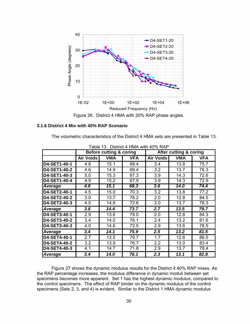
30

0

10

20

30

40

1E-02 1E+00 1E+02 1E+04 1E+06Reduced Frequency (Hz)

Pha

se A

ngle

(deg

rees

)

D4-SET1-20D4-SET2-20D4-SET3-20D4-SET4-20

Figure 26. District 4 HMA with 20% RAP phase angles.

3.1.6 District 4 Mix with 40% RAP Scenario

The volumetric characteristics of the District 4 HMA sets are presented in Table 13.

Table 13. District 4 HMA with 40% RAP

Air Voids VMA VFA Air Voids VMA VFAD4-SET1-40-1 4.8 15.1 68.4 3.4 13.8 75.7D4-SET1-40-2 4.6 14.9 69.4 3.2 13.7 76.3D4-SET1-40-3 5.0 15.3 67.3 3.9 14.3 72.6D4-SET1-40-4 4.9 15.2 67.9 3.9 14.3 72.9Average 4.8 15.1 68.3 3.6 14.0 74.4D4-SET2-40-1 4.5 15.0 70.3 3.2 13.8 77.2D4-SET2-40-2 3.0 13.7 78.2 2.0 12.8 84.5D4-SET2-40-3 4.0 14.6 72.6 3.0 13.7 78.3Average 3.8 14.4 73.7 2.7 13.5 79.7D4-SET3-40-1 2.9 13.6 79.0 2.0 12.8 84.3D4-SET3-40-2 3.4 14.0 76.1 2.4 13.2 81.6D4-SET3-40-3 4.0 14.6 72.5 2.9 13.6 78.5Average 3.4 14.1 75.9 2.5 13.2 81.5D4-SET4-40-1 2.7 13.5 79.7 1.7 12.6 86.5D4-SET4-40-2 3.2 13.9 76.7 2.2 13.0 83.4D4-SET4-40-3 4.1 14.7 71.8 2.9 13.7 78.4Average 3.4 14.0 76.1 2.3 13.1 82.8

Before cutting & coring After cutting & coring

Figure 27 shows the dynamic modulus results for the District 4 40% RAP mixes. As the RAP percentage increases, the modulus difference in dynamic moduli between set specimens becomes more apparent. Set 1 has the highest dynamic modulus, compared to the control specimens. The effect of RAP binder on the dynamic modulus of the control specimens (Sets 2, 3, and 4) is evident. Similar to the District 1 HMA dynamic modulus

31

results, the high HMA dynamic modulus of Set 1 specimens suggests the possible presence of factors other than RAP content affecting the results. These factors may include changes in aggregate structure with special considerations given to the fines content of the mix, variation in degree of working binder, and volumetric characteristics as well as the selective absorption of binder into aggregate over time.

1E+02

1E+03

1E+04

1E-02 1E+00 1E+02 1E+04 1E+06Reduced frequency (Hz)

Com

plex

Mod

ulus

(ksi

)

D4-SET1-40D4-SET2-40D4-SET3-40D4-SET4-40

Figure 27. District 4 HMA with 40% RAP dynamic modulus master curves.

Similar observations are apparent from phase angle comparisons as well. Figure 28

contains phase angle plots. As the percentage of RAP increases from 20 to 40%, the phase angle master curves begin to separate from one another, which relates to the effect of RAP in the mix. Among the control specimens, Set 4 has the lowest phase angle compared to Set 2 and 3. This is an indication of the stiff binder effect since all other variables were held constant in these specimen sets. On the other hand, the phase angle of Set 1 is the lowest. Similar arguments can be made for the reduction in phase angle of Set 1 in terms of the potential changes in a mix with RAP addition. The viscous component of an HMA sample is binder and mastic. In a Set 1 specimen, depending on the mechanism present in RAP mixing, the mastic properties can change significantly. If RAP is not releasing binder to the mix, the fines are remaining bonded to the surface of the RAP during the mixing process. This lack of fines alters the viscous properties of the mastic and volume fraction of binder in the final mix. This may explain why the phase angle of Set 1 is lower than the others.

3.1.7 Comparison of District 4 HMA with 0, 20, and 40% RAP

Figure 29 presents a comparison of dynamic modulus curves for HMA with 0, 20, and 40% RAP. The increase in dynamic modulus between the 20 to 40% RAP content is significant; whereas HMA specimens with 20% RAP do not exhibit significant difference in dynamic modulus from that of specimens without RAP.

32

0

10

20

30

40

1E-02 1E+00 1E+02 1E+04 1E+06Reduced Frequency (Hz)

Pha

se A

ngle

(deg

rees

)

D4-SET1-40D4-SET2-40D4-SET3-40D4-SET4-40

Figure 28. District 4 HMA with 40% RAP phase angles.

1E+2

1E+3

1E+4

1E-2 1E+0 1E+2 1E+4 1E+6Reduced Frequency (Hz)

Com

plex

Mod

ulus

(ksi

)

D4-00-SET1

D4-20-SET1

D4-40-SET1

Figure 29. Dynamic modulus comparison of District 4 Set 1 HMA with 0, 20, and 40% RAP. Figure 30 presents phase angle master curves for District 4 material, actual practice RAP percentages. As opposed to HMA dynamic modulus results, the phase angle results of 0 and 20% RAP specimens are now distinguishable. As the RAP percentage increases to 40%, the phase angle decreases further. It has to be noted that the variation in phase angle results is generally high and may mask the effect of RAP on phase angle results; particularly at high temperatures and low frequencies.

33

0

10

20

30

40

1E-2 1E+0 1E+2 1E+4 1E+6Reduced Frequency (Hz)

Phas

e A

ngle

(deg

rees

)

D4-SET1-00D4-SET1-20D4-SET1-40

Figure 30. Phase angle comparison of 0, 20, and 40% District 4 Set 1 specimens.

3.1.8 Statistics of HMA Dynamic Modulus Data (District 4)

Standard deviation and coefficient of variation of HMA phase angle and dynamic modulus data are shown in Table 14. Similar to District 1 results, the statistics for District 4’s HMA demonstrate a good level of repeatability, even for actual practice specimens (Set 1) where RAP mixtures can show a high coefficient of variation.

3.1.9 Comparison of Mixes Prepared with PG58-28 and PG64-22

The bumping of a binder grade, that is, lowering both the low and high temperature

grade, called “double bumping”, of HMA containing RAP is required for mixtures having more than 20% RAP as standard practice. The objective is to compensate for the additional stiffness or brittleness of the mixture, which results from the stiff RAP binder by softening the virgin binder. To examine bumping effects, new sets of HMA specimens with 40% RAP were prepared with PG 58-28 binder and tested for HMA dynamic modulus. The results were compared to the results obtained from the same set of specimens with standard binder (PG 64-22) and also to the specimen set with no RAP. Figure 31 shows this comparison for District 1 mixes. Reduction in dynamic modulus values due to the use of double bumping binder is apparent.

34

Table 14. Statistics of Phase Angle and Dynamic Modulus Measurements (District 4)

Temp (°C) STDEV (ksi) COVAR STDEV (deg) COVAR-10 223.3 6.3 0.4 5.44 48.9 3.0 0.3 3.020 20.9 3.7 1.1 3.9-10 89.3 3.1 0.6 7.34 110.4 6.6 0.5 3.020 38.1 6.7 0.7 2.9-10 58.6 2.4 0.3 2.64 75.8 6.0 0.9 3.020 24.9 4.7 0.8 2.9-10 111.2 4.2 0.1 2.64 21.4 1.1 0.1 3.020 26.4 4.5 0.2 2.9-10420-10 427.0 12.0 0.3 4.04 209.1 10.3 0.3 2.020 66.1 6.6 4.3 16.2-10 203.3 7.2 1.0 11.54 219.2 15.2 0.5 2.020 53.8 10.7 0.8 16.2-10 46.6 1.4 0.4 11.54 51.7 3.9 1.0 2.020 11.0 2.5 0.2 16.2-10 253.9 8.6 0.7 9.54 205.7 12.3 0.6 8.020 81.7 11.0 0.9 12.5-10 46.6 1.4 1.1 9.44 51.7 3.9 0.2 1.020 11.0 2.5 0.5 2.1

D4-SET3-40

D4-SET4-40

D4-SET1-40 w/ PG58-28

D4-SET2-20

D4-SET1-40

D4-SET2-40

D4-SET3-20

Complex Modulus Phase Angle

No statistics exist for this set. Only one good specimen.D4-SET4-20

D4-SET1-00

D4-SET1-20

1E+2

1E+3

1E+4

1E-2 1E+0 1E+2 1E+4 1E+6

Com

plex

Mod

ulus

(ks

i)

Reduced frequency (Hz)

D1-SET1-40 w/ PG58-28D1-SET1-00 w/ PG64-22D1-SET1-40 w/ PG64-22

Figure 31. HMA dynamic modulus comparison when PG 58-28 binder is used (District 1

design).

35

The effect of softer binder grade on District 4 HMA dynamic modulus results is shown in Figure 32. The dynamic moduli of actual practice specimens (with 40% RAP) prepared with standard binder (PG 64-22) and softer binder (PG 58-28) and HMA without RAP are compared in this figure. These results are consistent with the findings from District 1 tests. Softer binder significantly reduced the HMA dynamic modulus. It can be concluded that bumping the binder grade may have the potential to reduce brittleness and premature cracking problems in HMA with high RAP. However, this observation must be supported by fracture and/or fatigue tests. Bumping the low temperature grade may reduce the modulus at intermediate temperatures as well. This effect can clearly be noted in the District 4 HMA results (Figure 32). From the dynamic modulus results, one can conclude that high temperature bumping significantly affected the stiffness of the mix. However, the effect on performance resulting from bumping the low temperature grade cannot be isolated by the dynamic modulus test. As would be expected, no conclusions could be made on the effect of low temperature bumping on the mix stiffness from the available dynamic modulus result analyses.

1E+2

1E+3

1E+4

1E-2 1E+0 1E+2 1E+4 1E+6Reduced frequency (Hz)

Com

plex

Mod

ulus

(ksi

)

D4-SET1-40 w/ PG58-28

D4-SET1-00 w/ PG64-22

D4-SET1-40 w/ PG64-22

Figure 32. HMA dynamic modulus comparison when PG 58-28 binder is used (District 4

design). 3.1.10 Statistical Analysis of HMA Dynamic Modulus Results

In order to establish the test repeatability and the effect of various RAP percentages, a statistical analysis was conducted for the dynamic modulus test results. The first step was to verify the test repeatability. The same analysis procedure is used to examine the effect of the different RAP percentages. It can also be used to test between different sets of mixture.

First, a model shown in equation 1 was used to fit the dynamic modulus data. It was assumed that the dynamic modulus, G*, is a function of frequency, f, and a dummy variable, D.

Log(G)=a+b*D+c*Log(f) (1) where,

G = dynamic modulus;

36

D = dummy variable (=0 for G from specimen 1 group; =1 for G from specimen 2 group; =2 for G from specimen 3 group); f = frequency; and a, b, c = fitted regression coefficients.

The regression analysis with 95% confidence level was then performed on the selected data sets. The null hypothesis is b=0 which means that there is no significant difference between the selected data sets. An example data set for the repeatability of the 0% case from District 4 between two specimens is given below in Table 15. The data were reorganized as shown in Table 16 and a dummy variable D was assigned as 0 and 1 for each data set. Table 17 shows the strength of the data correlation to the model. The R2 value of 0.954 suggests a strong correlation between the measured data with model. Table 18 shows the inference of the model coefficients. The test statistics (t stat) or the p-values of the coefficient b were used to determine whether two sets of measured data are statistically the same. As shown in Table 18, at the 5% level, the coefficient b is insignificantly different from zero since the p-value is greater than 0.05. If the b=0, there is no statistical difference between the two data sets.

Table 15. Dynamic Modulus of Two Replicate Specimens with no RAP (District 4)

Specimen 1 Specimen 2 Red. F (Hz) G (ksi) Red. F (Hz) G (ksi)

0.010 145.499 0.010 157.0940.100 263.782 0.100 277.9530.500 425.264 0.500 446.1891.000 524.735 0.794 558.7761.585 576.060 1.000 549.6475.000 827.347 5.000 861.717

10.000 992.540 7.943 975.28915.849 1034.586 10.000 1035.27725.000 1243.355 25.000 1301.35979.261 1452.456 39.724 1371.149

158.489 1655.507 79.433 1570.972316.228 1918.662 100.000 1810.367792.447 2159.479 397.164 2065.831

1584.893 2394.729 794.328 2310.9103162.278 2737.256 1000.000 2540.1853962.249 2725.185 1985.829 2660.720

15814.551 3330.011 5001.000 3058.77531622.777 3590.093 10000.000 3271.010

158113.883 4144.552 50000.000 3750.503316227.766 4390.748 100000.000 3952.806

The summarized regression analyses of all Districts 1 and 4 data sets are presented

in Tables 19 and 20, respectively. While checking for test repeatability, it was found that, generally, the test had very good repeatability because the p-values are all greater than 0.05. However, Set 1 mix with 20% had a value of 0.05.

37

Table 16. Data for Fitting the Statistical Model Log (G) D Log (f) Log (G) D Log (f) 2.163 0 -2 2.196 1 -2 2.421 0 -1 2.444 1 -1 2.629 0 -0.301 2.65 1 -0.301 2.72 0 0 2.747 1 -0.1 2.76 0 0.2 2.74 1 0

2.918 0 0.699 2.935 1 0.699 2.997 0 1 2.989 1 0.9 3.015 0 1.2 3.015 1 1 3.095 0 1.398 3.114 1 1.398 3.162 0 1.899 3.137 1 1.599 3.219 0 2.2 3.196 1 1.9 3.283 0 2.5 3.258 1 2 3.334 0 2.899 3.315 1 2.599 3.379 0 3.2 3.364 1 2.9 3.437 0 3.5 3.405 1 3 3.435 0 3.598 3.425 1 3.298 3.522 0 4.199 3.486 1 3.699 3.555 0 4.5 3.515 1 4 3.617 0 5.199 3.574 1 4.699 3.643 0 5.5 3.597 1 5 3.675 0 5.898 3.629 1 5.398

Table 17. Measures of the Strength of Association of the Model

Regression Statistics Multiple R 0.9767R2 0.9540Adjusted R2 0.9516Standard Error 0.0887Observations 42

Table 18. Inferences about the Individual Coefficients of the Model

Coefficients Standard Error t stat P-value a 2.725 0.024 112.201 0.000 b 0.039 0.027 1.405 0.168 c 0.189 0.007 28.443 0.000

The results show that for District 1 materials, at a 95% confidence level, there is a

statistically significant difference between when 0% and 20% and also between 0% and 40% RAP in the mix. In addition, at 20% RAP, the results also show that there is a statistically significant difference between each mix set. This contradicts the findings reported in NCHRP 9-12, which suggests low percentages of RAP such as 20% do not significantly affect the HMA stiffness (McDaniel 2000). The significant difference between actual practice and other sets could be explained as the relative amount of working binder being different due to incomplete blending and differences in the aging of the binder in the various RAP materials used. The same observation was found, but more pronounced, when the 40% RAP was used due to the presence of stiffer binder. For HMA with 40% RAP, the effect of increased fine content and lower VMA become more pronounced, hence, may contribute to the increase in the HMA dynamic modulus..

38

Statistical analysis of dynamic modulus results for the HMA with District 4 materials showed that mixes with 20% RAP were not significantly different than those for mixes with no RAP. However, dynamic moduli of the mixes with 40% RAP were significantly different than those of mixes with no RAP. The only District 4 test which did not have good repeatability was the Set 2 mixture with 40% RAP. The difference in RAP effect on HMA between the districts could be due to the difference in the RAP binder stiffness of each District.

Table 19. p-value of Coefficient b for District 1 0%

Set 1 20% Set 1

20% Set 2

20% Set 3

20% Set 4

40% Set 1

40% Set 2

40% Set 3

40% Set 4

0% Set 1 0.394 0.001 5.8E-06

20% Set 1 0.050 0.004 0.050 0.014

20% Set 2 0.655

20% Set 3 0.914

20% Set 4 0.444

40% Set 1 0.346 0.001 0.003 0.001

40% Set 2 0.015

40% Set 3 0.095

40% Set 4 0.260

Table 20. p-value of Coefficient b for District 4

0% Set 1

20% Set 1

20% Set 2

20% Set 3

20% Set 4

40% Set 1

40% Set 2

40% Set 3

40% Set 4

0% Set 1 0.168 0.966 4.1E-05

20% Set 1 0.552 0.550 0.570 0.842

20% Set 2 0.144

20% Set 3 0.950

20% Set 4 0.599

40% Set 1 0.574 1.2E-04 4.0E-05 0.038

40% Set 2 0.018

40% Set 3 0.998

40% Set 4 0.017

39

3.1.11 Application of Hirsch Model to RAP Mixture Volumetrics. Some of the major factors that can cause the difference in dynamic modulus values between Set 1 and other sets with recovered aggregates are related to volumetric characteristics, binder stiffness, selective absorption, and aggregate gradation. A combination of all four factors can also influence mixture behavior. The Hirsch model allows these factors to be studied in the model to evaluate their individual impact on the resulting dynamic modulus of the HMA. It is apparent from the magnitude of the dynamic modulus increase when RAP was added that the change in binder stiffness only may not explain the magnitude of the difference.

The extent of the binder stiffness effect can be determined from a comparison between Sets 2, 3, and 4; where all variables were held constant, except binder stiffness. Sets 2, 3, and 4 mixtures were designed with similar aggregate gradations with the same RAP content. However, aggregate gradation of the actual practice specimens, Set 1, can deviate from target gradation if RAP is not dispersing fines similar to Sets 2, 3 and 4. Additionally, the batching aggregate gradation may be skewed as Set 1 is using actual practice RAP and the other mixes are using recovered aggregate. Volumetric characteristics can be quantified by air voids, VMA, or VFA. VMA involves information about both air voids and binder volume fraction. The average VMA of each specimen tested for dynamic modulus is shown in Figure 33. The VMA of Set 1 was calculated based on the assumption of 100% working binder. There are minor variations in specimen VMA that can be related to specimen preparation process. Therefore, it is safe to compare the dynamic modulus values of these specimens.

10

12

14

16

18

SET1 SET2 SET3 SET4

VM

A (%

)

D1-20% RAPD1-40% RAP20% Design40% Design

10.0

12.0

14.0

16.0

18.0

SET1 SET2 SET3 SET4

VMA

(%)

D4-20 % RAPD4-40 % RAP20 % Design40 % Design

Figure 33. Specimen’s VMA variation (Districts 1 and 4).

VMA is believed to influence the overall HMA behavior. Hence, accurate calculation

of VMA, especially with high RAP mixes, is essential. The relatively high dynamic modulus of actual practice specimens could not be explained by the increase in RAP binder stiffness only. It was apparent that an additional mechanism may be contributing to that increase. One of these mechanisms could be the changes in HMA volumetric characteristics when RAP was added as compared to using recovered aggregates. Figure 33 presents VMA values for each specimen set. Calculating VMA for HMA without RAP is straightforward, VMA is the volume ratio of the sum of effective binder and air voids to the total volume of the mix. However, the calculated effective binder can be ambiguous. When RAP is used, it is unclear how much RAP binder is working effectively in the mix. If RAP binder does not blend with additional virgin binder, the volume of effective binder decreases. In addition, the presence of RAP binder affects the mixing and the compaction processes, and hence, the overall mixture stiffness. These hypothetical volumetric relationships are shown in Figure 34.

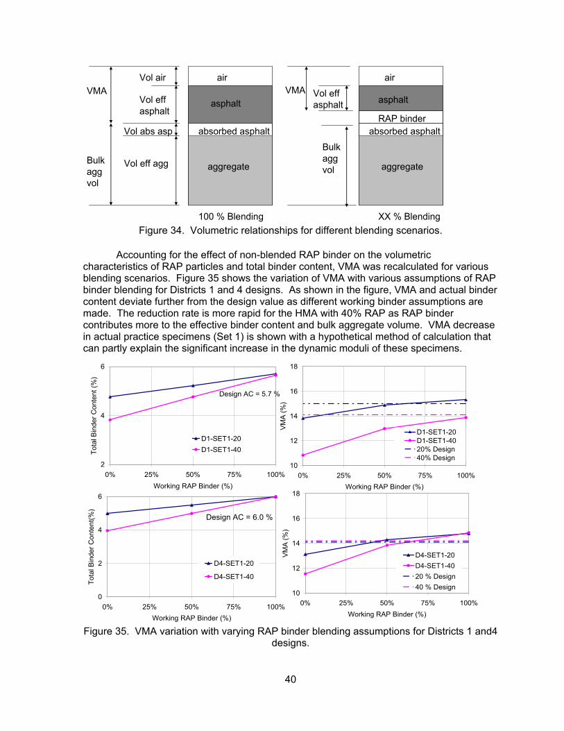
40

aggregate

absorbed asphalt

asphalt

air

Vol effasphalt

Vol air

Vol abs asp

Vol eff agg

VMA

aggregate

absorbed asphalt

asphalt

air

RAP binder

100 % Blending

Bulk aggvol

Bulk aggvol

Vol effasphalt

VMA

XX % Blending Figure 34. Volumetric relationships for different blending scenarios.

Accounting for the effect of non-blended RAP binder on the volumetric characteristics of RAP particles and total binder content, VMA was recalculated for various blending scenarios. Figure 35 shows the variation of VMA with various assumptions of RAP binder blending for Districts 1 and 4 designs. As shown in the figure, VMA and actual binder content deviate further from the design value as different working binder assumptions are made. The reduction rate is more rapid for the HMA with 40% RAP as RAP binder contributes more to the effective binder content and bulk aggregate volume. VMA decrease in actual practice specimens (Set 1) is shown with a hypothetical method of calculation that can partly explain the significant increase in the dynamic moduli of these specimens.

2

4

6

0% 25% 50% 75% 100%Working RAP Binder (%)

Tota

l Bin

der C

onte

nt (%

)

D1-SET1-20D1-SET1-40

Design AC = 5.7 %

10

12

14

16

18

0% 25% 50% 75% 100%Working RAP Binder (%)

VM

A (%

)

D1-SET1-20D1-SET1-4020% Design40% Design

10

12

14

16

18

0% 25% 50% 75% 100%Working RAP Binder (%)

VM

A (%

)

D4-SET1-20D4-SET1-4020 % Design40 % Design

0

2

4

6

0% 25% 50% 75% 100%Working RAP Binder (%)

Tota

l Bin

der C

onte

nt(%

)

D4-SET1-20

D4-SET1-40

Design AC = 6.0 %

Figure 35. VMA variation with varying RAP binder blending assumptions for Districts 1 and4

designs.

41

3. 2 RESIDUAL BINDER EVALUATION In addition to the HMA dynamic modulus measurements, the complex modulus of the binder itself was also measured. The binder modulus values were compared to the modulus values of the HMA dynamic modulus specimens using the Hirsch model. The binder characterization was conducted at the North Central States SuperPave Center at Purdue University. The binders blends that were prepared represented the various binder blending conditions that are assumed to occur during mixing in this research. The binders tested include the following: PG 64-22 binder, which represents the black rock or 0% blending case; binders recovered utilizing the rotovapor extraction process; binders from both Districts 1 and 4 RAP sources; and blended binders. The recovered Districts 1 and 4 binders were blended at 20% and 40% with PG 64-22 binder. The blending at 20% and 40% are not directly comparable to the amount of binder actually present in the mix. In order to resolve this issue, the 20% and 40% values were averaged to create a 30% blend which is closer to the amount of stiff RAP binder assumed to be working in a 40% RAP mix. The PG 64-22 binder, 20% and 40% blended District 1 binder, and 20% and 40% blended District 4 binder were also aged using the rolling thin film oven (RTFO) prior to testing. The non-blended recovered binders were not aged using the RTFO. The complex moduli of the RTFO aged binders represent that in the HMA after mixing, short term aging, and compaction. Binder complex modulus testing was conducted in accordance with the following testing suite: Testing temperature ranges from 60.8 °F (16°C) to 147.2 °F (64°C) at 10.8 °F (6°C) increments; and testing frequency ranges from 0.1 Hz to 27.3 Hz at the following frequency values, 0.1, 0.2, 0.4, 0.8, 1.6, 3.2, 6.4, 13, and 27.3 Hz. Figure 36 shows the complex shear modulus master curves for original PG 64-22 (subjected to RTFO aging) and RAP binder blends. To supplement the data collected on the 20% and 40% RAP binder blends, a curve representing a 30% blend data was interpolated by averaging the 20% and 40% binder blend data. The 30% RAP binder blend is closer to the actual percentage of RAP binder in a 40% RAP mixture. From the master curves, RAP binder blends are much stiffer than PG 64-22 for both Districts’ binders. The effect of increasing the RAP binder is evident in the case of District 1 RAP binder; whereas for the District 4’s RAP, the 20% and 40% RAP binder blends did not show a significant difference in complex modulus. This may raise a question as to the compatibility between District 4 recovered binder and the PG 64-22 binder that may affect the resulting homogeneity in the binder.

1

10

100

1000

0.001 0.1 10 1000Reduced Frequency, Hz

G*,

psi

PG64-22 Original RTFO20% Blend30% Blend40 % Blend

District 1

1

10

100

1000

0.001 0.1 10 1000Reduced Frequency, Hz

G*,

psi

PG64-22 Original RTFO20% Blend30% Blend40 % Blend

District 4

1

10

100

1000

0.001 0.1 10 1000Reduced Frequency, Hz

G*,

psi

PG64-22 Original RTFO20% Blend30% Blend40 % Blend

District 1

1

10

100

1000

0.001 0.1 10 1000Reduced Frequency, Hz

G*,

psi

PG64-22 Original RTFO20% Blend30% Blend40 % Blend

District 4

Figure 36. Complex modulus of PG 64-22 and RAP binder blends (20, 30, and 40%).

42

The measured binder complex shear moduli may be compared to the backcalculated values from the HMA dynamic moduli. There are numerous techniques to perform backcalculation, one of which is the Hirsch model. The Hirsch model is the simplest micromechanical model relying on law of mixtures and is commonly used for HMA modulus predictions. It is based on series and parallel configurations of different states of materials in a composite material such as HMA. These materials, or states, in our case, are aggregate, binder, and voids. The attractiveness of this method comes not only from its simplicity; but also consideration of very commonly and easily measured HMA volumetric parameters such as VMA and VFA. The final form of the Hirsch model for HMA is given in equations 2 and 3. The objective is to determine the binder shear modulus for the HMA modulus measured at each frequency and temperature; VMA and VFA are known. Details of the model development and use in HMA are described in the work by Christensen et al. (2003).

1]*||3000,200,4

100/1)[1(

)000,10

(|*|3)100/1(000,200,4[|*|

−

××+

−−+

××+−=

binderc

bindercmix

GVFAVMAVMAP

VMAVFAGVMAPE (2)

58.0

58.0

)|*|3(650

)|*|320(

VMAGVFA

VMAGVFA

Pbinder

binder

c ××+

××+

= (3)

where,

|E*| = mixture compressive dynamic modulus (ksi)

|G*| = binder shear complex modulus (psi)

Pc = Aggregate contact volume.

Backcalculation was performed using HMA dynamic moduli obtained for Districts 1 and 4 specimens with 40% RAP only. The effect of RAP binder is expected to be more pronounced at this percentage of RAP. Backcalculated binder moduli for Sets 1, 2, 3, and 4 are presented in Figure 37 for Districts 1 and 4. In addition to backcalculated values, measured binder shear modulus values were also plotted in the same figure as solid data points. Due to problems encountered during DSR testing, only four measured data points were selected. The authors believe that the DSR values measured at frequencies greater than 1Hz were not accurate due to device capacity limitations. Within the valid data range, a match between measured and backcalculated binder moduli were sought. As seen in the figures, there is a good match for District 1 blends for PG 64-22 and Set 2, and 30% binder blend and Set 4 pairs. Sets 2 and 4 were the control specimens with 0 and 30% RAP binder. However, District 4 blends exhibited a poor match between the measured and backcalculated modulus values The Hirsch model is not overly sensitive to VMA variations. A 1% variation in VMA did not significantly alter the backcalculation results.

43

1E+0

1E+2

1E+4

1E+6

1E-3 1E+0 1E+3 1E+6Reduced Frequency (Hz)

Bac

kcal

cula

ted

Bin

der M

odul

us

|G*|

(psi

)

D1-40-SET1D1-40-SET2D1-40-SET3D1-40-SET4PG 64-2230 % Binder blend

1E+0

1E+2

1E+4

1E+6

1E-3 1E+0 1E+3 1E+6Reduced Frequency (Hz)

Bac

kcal

cula

ted

Bin

der M

odul

us

|G*|

(psi

)

D4-40-SET1D4-40-SET2D4-40-SET3D4-40-SET4PG 64-22% 30 Binder blend

District 1 District 4

1E+0

1E+2

1E+4

1E+6

1E-3 1E+0 1E+3 1E+6Reduced Frequency (Hz)

Bac

kcal

cula

ted

Bin

der M

odul

us

|G*|

(psi

)

D1-40-SET1D1-40-SET2D1-40-SET3D1-40-SET4PG 64-2230 % Binder blend

1E+0

1E+2

1E+4

1E+6

1E-3 1E+0 1E+3 1E+6Reduced Frequency (Hz)

Bac

kcal

cula

ted

Bin

der M

odul

us

|G*|

(psi

)

D4-40-SET1D4-40-SET2D4-40-SET3D4-40-SET4PG 64-22% 30 Binder blend

District 1 District 4

Figure 37. Comparison of backcalculated and measured binder modulus.

It is worthwhile to note some of the shortcomings of the Hirsch model when it is used for the purpose of this study, which is evaluating the complex shear modulus of RAP and virgin materials. Firstly, although it has been shown to provide good matches to E* data, it is the simplest micromechanical model available. Secondly, and most importantly, the calculation of two of the three parameters used in the model, VMA and VFA, is ambiguous for HMA containing RAP; the percent of blending and percent of “black rock” binder are unknown. Finally, the model makes an assumption for the calculation of compressive (or extensional) modulus from shear modulus using linear elastic theory and a constant Poisson’s ratio. In the formula, the extensional modulus is replaced by 3x|G*|; assuming a Poisson’s ratio of 0.5 (for incompressible materials). This assumption, used for linear elastic materials, may not necessarily be true for binder. A linear elastic relationship may not necessarily hold for time dependent materials such as HMA and binder. This could induce some error into the Hirsch model calculation; however the level of error is not known. For these reasons, and the possible compatibility issue with the District 4 binder, the reliability of the Hirsch model calculation is unknown. It cannot be supported that the District 1 match, which supports complete binder blending, is a more accurate representation than the District 4 data, which indicates the original PG 64-22 to be stiffer than the binder in the HMA. This is not possible unless there are binder compatibility issues, which are beyond the scope of this research. For these reasons, the modulus backcalculations using the Hirsch model cannot indicate with any certainty what blending was achieved in the HMA. 3. 3 EVALUATION OF STRIPPING SUSCEPTIBILITY

Stripping resistance of the HMA containing RAP (specimen Set 1 only) was evaluated in accordance with the Illinois modified AASHTO T 283-02 specifications. Indirect tensile strength of dry and conditioned specimens was measured and a visual stripping inspection was conducted on cracked specimens. Figure 38 depicts the extent of stripping on some of the dry and conditioned specimens.

44

Figure 38. Fractured dry and conditioned specimens illustrating the extent of stripping.

A summary of tensile strength ratio and the stripping rating of specimens tested in

this study is given in Table 21. The results show that the HMA specimens tested in this study exhibited moderate to severe stripping potential. This resulted in significant tensile strength reduction of conditioned specimens. This effect is more pronounced with District 1 materials.

The stripping rating of dry and conditioned specimens indicates the relative amount of stripping occurring in HMA specimens. The stripping scale is between 1 and 3; where 1 indicates no stripping or slight stripping, 2 indicates moderate stripping, and 3 indicates severe stripping. The fine and coarse aggregates in the stripping samples were evaluated separately and results were reported for both portions of the mix.

Table 21. Tensile Strength Ratio (TSR) and Stripping Rating of HMA containing RAP Specimen SET Tensile Strength

Ratio (TSR) Dry Stripping Rating

(fine/coarse) Conditioned

Stripping Rating (fine/coarse)

D1-SET1-00 59.3 1/1 2/3D1-SET1-20 73.3 1/1 2/3D1-SET1-40 67.6 1/1 2/2D4-SET1-00 75.8 1/1 2/3D4-SET1-20 83.2 1/1 2/3D4-SET1-40 80.7 1/1 2/2

Figure 39 shows the tensile strength of dry and conditioned specimens tested at

room temperature. It was noted that the tensile strength of both dry and conditioned specimens increase as a function of RAP percentage. As was previously discussed with the dynamic modulus results, this increase can be attributed to several factors. One of these factors would be the HMA strength gain due to the presence of aged binder. As the percentage of aged binder increases, strength increases. Although aggregate gradation may have an effect on indirect tensile strength results as HMA with RAP could be coarser; it is well documented that indirect tensile strength test depends significantly on the binder

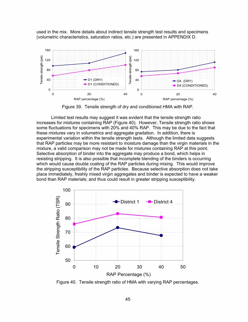
45

used in the mix. More details about indirect tensile strength test results and specimens (volumetric characteristics, saturation ratios, etc.) are presented in APPENDIX D.

Figure 39. Tensile strength of dry and conditioned HMA with RAP.

Limited test results may suggest it was evident that the tensile strength ratio

increases for mixtures containing RAP (Figure 40). However, Tensile strength ratio shows some fluctuations for specimens with 20% and 40% RAP. This may be due to the fact that these mixtures vary in volumetrics and aggregate gradation. In addition, there is experimental variation within the tensile strength tests. Although the limited data suggests that RAP particles may be more resistant to moisture damage than the virgin materials in the mixture, a valid comparison may not be made for mixtures containing RAP at this point. Selective absorption of binder into the aggregate may produce a bond, which helps in resisting stripping. It is also possible that incomplete blending of the binders is occurring which would cause double coating of the RAP particles during mixing. This would improve the stripping susceptibility of the RAP particles. Because selective absorption does not take place immediately, freshly mixed virgin aggregates and binder is expected to have a weaker bond than RAP materials; and thus could result in greater stripping susceptibility.

50

60

70

80

90

100

0 10 20 30 40 50RAP Percentage (%)

Tens

ile S

treng

th R

atio

(TS

R)

District 1 District 4

Figure 40. Tensile strength ratio of HMA with varying RAP percentages.

0

40

80

120

160

0 20 40RAP percentage (%)

Tens

ile s

treng

th (p

si)

D4 (DRY)D4 (CONDITIONED)

0

40

80

120

160

0 20 40RAP percentage (%)

Tens

ile s

treng

th (p

si)

D1 (DRY)D1 (CONDITIONED)

46

3. 4 RAP PARTICLE-MASTIC BONDING AND BLENDING: ESEM ANALYSIS As part of the investigation of working binder, electron microscopy was utilized to determine the mechanisms visibly occurring with the mixing of RAP binder and virgin binder. The first step in determining the mechanisms of binder mixing was to determine the binder film thickness on aggregate particles. Next, further SEM images were studied to investigate if the virgin and RAP binder could be uniquely identified.

To investigate the binder film thickness within the HMA composite system, the images were captured at a low magnification and at subsequently higher levels of magnification. Figures 41a through c show the images obtained using the wet mode of ESM (ESEM). Figure 41a presents an image of a 1.2mm by 1mm area. The darker color represents the asphalt binder and the lighter color represents the aggregate. As shown in the figure, a mastic strip was surrounded by two larger size aggregates. The image was further zoomed in to a 300μm to 250μm area, Figure 41 b, in the center of the mastic strip. This shows that the mastic was composed of binder and different sizes of fine material. Figure 41c shows further zooming into the image to a 60μm by 50μm area. The scale bar present in the image represents the length of 10μm, which is the theoretical film thickness. However, there is no clear boundary between binder and fines. The bright color that appears in the figure is due to overcharging by the electron beam on the specimen. This typically occurs when the highly accelerated voltage electron beam scans over the non-conducting sample.

Although the image obtained from the ESEM reveals that the HMA is a composite material composed of larger size aggregate and mastic, there is no direct evidence to show the material structure between fines and binder. To further investigate the microstructure between fines and binder requires higher quality images that ESEM could not produce. Therefore, the same specimen was coated with a thin 4nm film of gold-palladium to create a conductive surface. This metal layer is thin enough that all the micro-texture at the surface of HMA is preserved and observed under the conventional SEM.

(a) (b) (c)

Figure 41. SEM images showing surface morphology. When the microscope is operated at high vacuum mode, two types of electrons

which produce different images of the sample can be collected. The two electron imaging methods are secondary electron (SE) and backscattered electron (BSE) imaging. The secondary electron image is most useful for examining surface structure and gives the best image resolution. Depending on the initial size of the primary beam and other conditions such as the composition of the sample, accelerating voltage, position of specimen relative to the detector, a SE signal can resolve surface structures to the order of 10nm or finer. This signal will show the topographical image of the specimen. Additionally, the BSE image arises due to different atomic numbers within a material. That is, if a sample is composed of

47

two or more different elements with significantly different atomic numbers, it will produce an image that shows differential contrast of the elements despite a uniform topology. Elements that are of a higher atomic number will produce more backscattered electrons and will therefore appear brighter than other elements with smaller atomic numbers. Using the advantages of these two types of images, it is possible to perform a better investigation of the microstructure of HMA samples.

An illustration showing both types of images can be found in Figure 42. Figure 42a shows the SE image of the HMA surface morphology. The image shows a darker binder strip embedded between two larger aggregate which exhibit a lighter color; and air voids can be observed. Figure 42b presents a BSE image. This image reveals even more detail of the composition of the specimen structure. This increased detail is due to the fact that the binder is composed of hydrocarbons. The aggregates are composed of calcium, silicon, magnesium, etc., which have a larger atomic number compared to binder elements which is manifested as a different brightness. The air voids have a small atomic number as well, which also appear differently from the binder and aggregate. Therefore, the aggregate appears as the lightest color in the image, the binder shows darker color, and the air voids show the darkest color. However, because air voids and binder are both shown in black, in backscattered images sometimes the edge of air voids cannot be distinguished from the binder. If one combines both secondary and backscattered electron images, the air voids and binder can easily be differentiated.

Figure 43 presents the microstructure image of HMA specimen using conventional SEM. The secondary and backscattered electron images are presented side by side from low to high magnification. Figures 43a, c, e, and g show the image of SE evolution from low magnification (2400μm by 1800μm) to high magnification (48μm by 36μm). In addition, BSE images (Figure 43b, d, f, and h) were also presented. From both image types, it clearly shows that up to the resolution of 10μm, the morphology of HMA still presents a combination of aggregate and mastic. Furthermore, the lens was focused to the right side of the image in Figure 43h where the density of fines was higher and further magnified to investigate the film thickness of the HMA. This result shows the current film thickness assumption is not accurate to assess the true film thickness in the HMA composite system.

(a) (b)

Figure 42. Image of HMA surface.

48

(a) (b)

(c) (d)

(e) (f)

49

(g) (h)

Figure 43. Image of HMA surface binder film.

Figure 44 shows the resolution from 5μm up to 500nm, the images at 5μm start showing a clear two phase structure. Again, the images on the left are SE and those on the right are BSE. The fines were shown as a substrate embedded in the binder matrix. The benefit of using BSE detector is clear at such a small scale. In Figure 44b, more fine particles were revealed than images taken using SE in Figure 44a. From these two figures, it appears that there is no direct contact between the fine particles. With further zooming into the area where two fine particles appear to have direct contact, Figures 44c and d, the two fine particles actually do not have direct contact. The film thickness which was assumed in the aforementioned work can now be calculated. The distance between two particles is less than or equal to 2μm. This value is five times less than the theoretical calculation, unless the size of filler is defined and considered as part of the mastic.

From the SEM procedures, the meaning of “film thickness” can be discussed in terms of what is seen in the mixtures. If film thickness is defined as the binder between any aggregates then the film thickness would be 2μm. However, if the film thickness is defined as the binder between any two particles retained on a specific sieve the film thickness value becomes a moving target. If the second definition is applied to film thickness then a completely different value is obtained. An alternative to film thickness is to rename what has classically been referred to as film thickness. As has been shown in the SEM images the distance of the theoretical value of film thickness contains fine materials. Thus it may be wiser to refer to this as a ‘mastic thickness’ while reserving the term film thickness for the binder between the two fine particles.

Microscopy images were initially captured and evaluated to determine the amount of blending occurring between RAP particles and the virgin binder added to the mix. The amount of blending was not observable in the SEM images. Once it was deemed not possible to determine the blending from the initial SEM images, an alternative SEM method was investigated to determine if this method was promising for future work in identifying the film thickness of the coated aggregate, determining aggregate absorption/ binder penetration depth, and verifying the virgin/ aged binder intermixing phenomena.

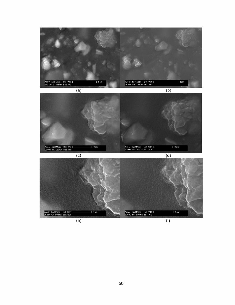
50

(a) (b)

(c) (d)

(e) (f)

51

(g) (h)

Figure 44. Image of HMA surface at high resolution.

To detect binder blending, Lee et al. (1983) used trace amounts of titanium incorporated with an AR-2000 paving grade asphalt binder before mixing with RAP material. The resulting SEM image and the corresponding Energy Dispersive X-Ray Spectroscopy (EDS) scan showed a clear interlayer of virgin binder and aged asphalt. It was concluded that the method had significant potential for verifying the micro scale interaction between virgin binder and RAP material.

The rationale of using SEM to study bitumen-aggregate interface relies on the different elements which constitute asphalt binder and aggregate. As the electron beam of the SEM is scanned across the sample surface, it generates X-ray fluorescence from the atoms in its path. The energy of each X-ray photon is characteristic of the element which produced it. The EDS microanalysis system collects the X-rays, sorts and plots them by energy, and automatically identifies and labels the elements responsible for the peaks in this energy distribution. The EDS data are typically compared with computer-generated standards to produce a full quantitative analysis showing the sample composition. Therefore, if the chemical composition of the asphalt and aggregate are known, the EDS can be used to map those elements and determine the configuration of asphalt and aggregate. Some representative petroleum elemental analysis is presented in Table 22 (Plancher et al. 1976). It shows that the major component of the asphalt binder is carbon. Table 23 shows the typical chemical composition of sandstone and limestone. The main composition of sandstone and limestone are silicon (Si) and calcium (Ca), respectively. The data output from the EDS analysis plots the original spectrum showing the number of X-rays collected at each energy level. Maps of element distributions over the areas of interest and quantitative composition tables can also be provided as necessary.

As part of a preliminary study, two aggregate types (limestone and sandstone) and a PG 64-22 virgin binder were investigated. The virgin binder and virgin aggregate were first heated to 155°C for one hr. Then, the aggregate was thoroughly mixed with heated binder. The coated aggregates were then placed on a steel sieve and allowed to drip the excess binder in the oven for an additional two hrs. The coated aggregates were then held at room temperature for 24 hrs to allow adhesion and binder absorption into aggregate. After 24 hrs, the coated aggregates were placed in liquid nitrogen, cooled, and then cut to expose the interface at the perimeter of the specimen. Figures 45a and b show the SEM image of sandstone in BSE and SE mode, respectively. Figure 45a clearly shows the binder absorption into the pores of the sandstone. The X-Ray analysis using EDS was employed to closely investigate these regions and map the chemical elements. As shown in Figure

52

46, the silicon and carbon element distribution was detected and the results were mapped with original SE image and shown in Figure 47.

Table 22. Elemental Analysis of Representative Petroleum Asphalts Element Mexican Ark-La. Boscam Calif. Carbon (%) 83.77 85.78 82.90 86.77

Hydrogen (%) 9.91 10.19 10.45 10.94

Nitrogen (%) 0.28 0.26 0.78 1.10

Sulfur (%) 5.25 3.41 5.43 0.99

Oxygen (%) 0.77 0.36 0.29 0.20 Vanadium (ppm) 180.0 7.0 1380.0 4.0 Nickel (ppm) 22.0 0.4 109.0 6.0

Table 23. Chemical Composition of Sandstone and Limestone

Sandstone Limestone Chemical Composition (%) Chemical Composition (%)

SiO2 93-94 CaCO3 97.30

Fe2O3 1.5-1.6 MgCO3 0.40

Al2O3 1.4-1.5 Al2O3 0.50

Na2O & Kro 1.0-1.2 SiO2 1.70

CaO 0.8-0.9 MgO 0.2-0.25 Loss On Ignition (LOI) 1.0-1.2%

(a) (b) Figure 45. SEM view of PG 64-22 absorption into sandstone in (a) BSE mode and (b) in SE

mode.

53

(a) (b) Figure 46. EDS x-ray scan of PG 64-22 coated sandstone cross-section (a) silicon element

distribution and (b) carbon element distribution.

(a) (b)

Figure 47. Mapping EDS element distribution results on the SE image for sandstone (a) silicon element distribution and (b) carbon element distribution.

The same observation was performed with coated limestone. In this case, a much

denser structure was observed in the limestone compared to that of sandstone. No distinct absorption phenomenon was observed. Figure 48 shows the asphalt binder coating the outside aggregate surface. The EDS analysis, Figures 49 and 50, shows the distribution of carbon and calcium in the area of interest. From the EDS data plot, the carbon elements mainly concentrate at the upper part of the picture (asphalt film) and calcium elements have a high concentration in the lower part of the picture (limestone). In Figure 50a, some carbon elements were detected at the bottom part of the specimen and this could be caused by the absorption of the binder. Alternatively the limestone used in the study has minor carbon compound that was also measured by the EDS and appears as “noise” in the measurements. The carbon in the limestone makes it difficult to accurately determine the absorption depth. This technique has potential to detect the film thickness outside the aggregate.

54

Figure 48. SEM view of PG 64-22 absorption into limestone in SE mode.

(a) (b) Figure 49. EDS x-ray scan of PG 64-22 coated limestone cross-section (a) silicon element

distribution and (b) carbon element distribution.

(a) (b)

Figure 50. Mapping EDS element distribution SE image for limestone (a) silicon element distribution and (b) carbon element distribution.

55

3. 5 FRACTURE ENERGY ANALYSIS In addition to the dynamic modulus testing, fracture tests were performed to investigate the RAP effect on HMA low temperature behavior. The fracture energy testing results can be used to characterize the thermal cracking characteristics of the mix. Only District 1 materials were tested for fracture energy. The fracture energy was first tested with the SCB test due to the more fundamental nature of the test compared to the DCT test. The effect of double bumping was only investigated using the SCB test. It was found that as the RAP content in the HMA increases, the fracture energy of the mix decreases. Although some variations in VMA and percent passing the #200 sieve exist between various mixtures tested herein. However, these variations were not significant enough to alter the comparative findings of the fracture energy analysis. This finding was in agreement with the work reported by Li, et al. (2008). A summary of the PG 64-22 SCB results is presented in Table 24.

Table 24. SCB Fracture Energy Results (PG 64-22)

Temperature (°C)

RAP (%)

Fracture Energy (J/m2)

Average Fracture Energy (J/m2)

Binder RAP/Total (%)

0

0 1925.4

1620.5 0 15161420.1

20 1202.6

1243.0 16 1283.41199.6

40 702.8

750.2 32 797.6762.5

-12

0 805.7

986.2 0 1036.31116.6

20 795.7

915.7 16 895.51055.9

40 892

651.6 32 635.2427.7

Graphs comparing the average values of the load (kN) vs. CMOD (mm) for the SCB

tests are presented in Figures 51 and 52 for 0°C and -12°C, respectively. These graphs indicate a noticeable difference in the fracture energy depending on the RAP content of the mix. Therefore, the effect of double bumping the binder grade to offset the lack of fracture energy was investigated.

56

0

0.5

1

1.5

2

2.5

3

3.5

0 1 2 3 4CMOD (mm)

Forc

e (k

N)

RAP-00 PG64-22RAP-20 PG64-22RAP-40 PG64-22

Temperature = 0 °C

Figure 51. Average load vs. CMOD curves for 0 °C SCB test.

0

0.5

1

1.5

2

2.5

3

3.5

0 0.5 1 1.5 2 2.5CMOD (mm)

Forc

e (k

N)

RAP-00 PG64-22RAP-20 PG64-22RAP-40 PG64-22

Temperature = -12 °C

Figure 52. Average load vs. CMOD curves for -12 °C SCB test.

In addition to the SCB tests, DCT tests were conducted to check the consistency of

the results. Similar trends were observed between the two fracture test methods. Table 25 presents the DCT fracture energy results. The average fracture energy results of the DCT testing were slightly higher than those of the SCB tests at 0°C. However, the results were slightly lower at -12°C. The average Load vs. CMOD curves for the 0°C and -12°C DCT tests are presented in Figures 53 and 54, respectively.

Since the test results are comparable and follow the same trends, the effect of RAP on HMA is evident. However, due to the limited number of specimens tested, conducting an extensive fracture energy testing is recommended.

57

Table 25. DCT Fracture Energy Results (PG 64-22)

Temperature (°C)

RAP (%)

Fracture Energy(J/m2)

Average Fracture Energy (J/m2)

Binder RAP/Total (%)

0

0 1631.2 1639.8 0 1648.4

20 1009.5

1332.5 16 15141474

40 781.9

843.4 32 767.9980.4

-12

0 551.1

596.7 0 600.9638.2

20 588.5

532.5 16 576.3432.6

40 449.3

437.7 32 432.1431.7

0

0.5

1

1.5

2

2.5

3

3.5

4

0 2 4 6 8CMOD (mm)

Forc

e (k

N)

RAP-00 PG64-22RAP-20 PG64-22RAP-40 PG64-22

Temperature = 0 °C

Figure 53. Average load vs. CMOD curves for DCT testing at 0°C.

The effect of double bumping on fracture energy was also studied. The double

bumping investigation was conducted using only SCB specimens. Greater fracture energy values were observed in the specimens containing PG 58-28 than in the specimens containing PG 64-22, Table 26. These results are expected as the softer PG 58-28 binder allows the HMA specimen to distort more (or to provide for greater flexibility to absorb more energy thus reducing crack occurrence.) under loading; hence, absorbing more energy during crack propagation.

58

0

0.5

1

1.5

2

2.5

3

3.5

4

0 1 2 3 4CMOD (mm)

Forc

e (k

N)

RAP-00 PG64-22RAP-20 PG64-22RAP-40 PG64-22

Temperature = -12 °C

Figure 54. Average load vs. CMOD curves for DCT testing at -12°C.

Table 26. SCB Fracture Energy Results (PG 58-28)

Temperature (°C)

RAP (%)

Fracture Energy (J/m2)

Average Fracture Energy (J/m2)

Binder RAP/Total (%)

0

0 2581.3

2845.3 0 2344.52530

20 2063.5

1787.7 16 1490.31809.4

40 1466.7

1364.7 32 1541.41086.1

-12

0 878.6

1097.7 0 1071.91342.7

20 899.5

988.2 16 1038.51026.5

40 686.9

638.8 32 522.2707.2

To compare the fracture energy results between HMA with PG 64-22 binder to that

with PG 58-28 binder using 40% RAP in the mix, the effect of double bumping can be determined. At testing temperatures, -12 °C and 0 °C, the HMA specimens with PG 58-28 and 40% RAP exhibited lower fracture energy than the HMA specimens with PG 64-22 and 0% RAP. Table 27 presents the average SCB fracture energies. The results indicate that double bumping offsets the impact of RAP at 0 °C; the SCB fracture energy was 1365 J/m2, for 40% RAP, which is higher than the fracture energy of mixes with 20% RAP and

59

unbumped binder (1243 J/m2). However, the impact of double bumping was not as effective at the lower temperature of -12 °C where one would anticipate greater thermal cracking susceptibility. Below glassy transition temperature (Tg) the viscoelastic nature of the binder is minimized and the binder becomes brittle. This should not imply that the low temperature binder grade should or should not be changed. Before any strong conclusions or design recommendations can be made, more extensive fracture testing is recommended. The testing may require fracture testing of specimens prepared with a PG 58-22 binder in order to determine if double bumping or only single bumping is needed. Additionally, testing at lower temperatures such as -30, and -24 °C will also be beneficial to determining if double bumping is required.

Table 27. SCB Fracture Energy Comparison

Temperature (°C)

RAP (%)

Average Fracture Energy PG 64-22

Samples (J/m2)

Average Fracture Energy PG 58-28

Samples (J/m2)

Binder RAP/Total (%)

0

0 1620.5 2845.3 0

20 1243.0 1787.7 16

40 750.2 1364.7 32

-12

0 986.2 1097.7 0

20 915.7 988.2 16

40 651.6 638.8 32

CHAPTER 4 SUMMARY AND CONCLUSIONS

The main objective of this research was to investigate procedures that had the potential to indicate the amount of working binder contributed by RAP to HMA during mixing. To accomplish this, six various mixture formulas were prepared according to current practice for two RAP sources at 0, 20, and 40% RAP in the HMA. One set of samples was prepared in accordance with current mix design practice. Three sets of samples, prepared with recovered RAP materials (binder and aggregate) and virgin materials, were designed to represent differing amounts of working binder in the RAP. No RAP materials were used in stockpile form in these control samples. The proportion of recovered RAP binder in the control samples was adjusted in an attempt to simulate the effect produced when the RAP used in an actual practice mix provided different amounts of working RAP binder in a mixture. The control samples were mixed with recovered RAP binder at 0, 50, and 100% working RAP binder blends. These three values represent the variation from the “black

60

rock” case where 0% of the RAP binder is released from the RAP to combine with the virgin binder, to the completely working case where 100% of the effective RAP binder combines with the added virgin binder. The mix design procedure produced an important and practical outcome that provides insight into the consideration of working binder in RAP. None of the mix designs with RAP, specifically the HMA with 40% RAP mix designs, required additional total binder content (RAP binder plus virgin binder added) to achieve the same density of HMA with no RAP. The asphalt binder content of the virgin HMA design was reproduced for the HMA with RAP. If the RAP binder was not working, the total asphalt content would have significantly increased with higher amounts of RAP in the HMA. The fact that the total asphalt content did not significantly increase indicates that the RAP binder was combined with the virgin binder to a very high extent.

The dynamic modulus test was selected to investigate the amount of working binder in the HMA. It was felt that comparisons of the dynamic modulus results between the actual practice mix and those of the control samples with a known amount of working binder would provide comparative results. Such results would show which blending assumption most closely matched actual practice.

The dynamic modulus results clearly show a consistent RAP effect. As the percentage of RAP increases, dynamic modulus values increase. These results are consistent for all materials and job mix formulae used in this research study. However, comparison of the individual results for the four different mixture sets did not produce definitive indication as to the working binder quantitatively. The generally held belief is that modulus increases as RAP percentages increase because of the increased amount of RAP’s aged binder that blends with the virgin binder being added. The dynamic modulus values for HMA with 20% RAP did not change significantly, which indicated that the RAP binder has little effect on mixture properties at this low percentage of RAP.

Given that the mix design considerations indicate a rather near complete blending of the effective RAP binder, it would be expected that the dynamic modulus values from actual practice would match the values obtained from the 100% working binder samples. If less than complete blending were occurring, the dynamic modulus of actual practice specimens would be less stiff than those of specimens having 100% working binder. However, the test results consistently showed that the dynamic modulus values for the specimens with 100% working binder were significantly lower than those of actual practice specimens.

The VMA of all mixes either meets the IDOT minimum requirement, or is at most 0.3% below the minimum requirement. In addition, there was variation in the amount of material passing the # 200 sieve. Although the passing #200 and VMA can have an effect on the HMA dynamic modulus, fracture energy, and moisture susceptibility results, however, these variations may not affect the overall behavior trend of the mixes.

The causes for the actual practice mixtures to have higher dynamic modulus values than those of the control specimens could include the following:

• Although the JMF aggregate gradation is similar for all sample sets, actual aggregate structure may not be the same for all mixes. Design blends are prepared with a tacit assumption that RAP binder is fully released during the mixing process. Variations will result from differing amounts of fines being released with various amounts of blending of the RAP binder. If complete blending does not occur, the aggregate structure will be altered significantly in favor of larger fractions.

• The differing amounts of fines released during blending will alter the mastic properties of the binder in the final mixture.

61

• Alterations in volumetric characteristics resulting from differing VMA calculations when various amounts of binder blend with the virgin binder, i.e. the relative amount of black rock changes.

• The asphalt-aggregate interface is not well-defined. This produces an asphalt material at this interface that is significantly stiffer than the remaining binder due to selective absorption of components of the binder into the aggregate. This selective absorption changes the aggregate binder interaction over time and forms a stiff layer of binder on the aggregate surface. This composite binder structure on the aggregate surface increases the mixture modulus. The HMA with aged RAP already contains this stiff binder layer at the aggregate surface, a condition not present in the control specimens.

The current practice that assumes100% working binder is considered acceptable; but may not be explicitly supported utilizing the data collected herein. However, it is clear that 100% of the RAP binder is not working because of the absorbed binder portion.

In addition to the HMA dynamic modulus, the binder shear complex modulus was tested. A comparison of blended binders’ complex shear modulus, G*, prepared using recovered and virgin binder illustrated that the blended binder stiffness increased when aged RAP binder percent increased. Increasing District 1 RAP binder in the blend (20 and 40% blends) showed consistent increase in the G* of the blended binder with respect to the standard PG64-22 binder. On the other hand, 20 and 40% blends of District 4 RAP binder did not show significant difference in the G* values. This raises a question as to the compatibility between District 4 recovered binder and the PG 64-22 binder combination; incompatibility may have prevented homogeneous blending. This could alter the interpretation of the dynamic modulus E* test data for the HMA; however, the exact nature is not known. The comparison between the binder backcalculated and measured G* values showed a good match for District 1 HMA with 40% RAP; suggesting nearly complete blending. However, the contradictory data for District 4 HMA does not allow a conclusion to be drawn at this time.

The stripping of the HMA containing RAP was determined in accordance with the IDOT procedures. Visual inspection of the specimens that failed in indirect tension testing was also conducted. The tensile strength ratio (TSR) of the specimens was calculated to determine the stripping susceptibility. The TSR increased as the amount of RAP in HMA increased when compared to HMA with no RAP. There appears to be some variations in the TSR results for the mixes with 20 and 40% RAP. These variations could be related to testing as well as the low number of valid tested specimens. Moisture susceptibility test results suggest that mixes containing RAP are less susceptible to moisture damage than virgin HMA. The District 4 materials had greater TSR values than those of District 1 materials. The reduction in stripping potential of HMA with RAP may be attributed to the strong binder-aggregate bonds of RAP materials that formed over time.

While the testing conducted here showed that increased RAP percentages in HMA reduce stripping potential, the two HMA with RAP investigated in this study should not be accepted as being indicative for all HMA with RAP. If the RAP source used in mixing had stripping problems prior to recycling, the stripping properties may not be improved. One might expect the mix to be more likely to strip although this has not been investigated in this study.

The amount of blending occurring between virgin and RAP binders was evaluated using SEM images. The film thickness was found to be significantly less than the theoretically calculated film thickness if film thickness is defined as the binder thickness between any two aggregate particles. Hence, an accurate definition of binder film thickness is needed. This method could not accurately determine the amount of binder blending. An

62

alternative method was performed to further investigate binder blending, ESM and EDS. This method showed promising results, and a further investigation will likely determine the binder blending.

The increasing stiffness of HMA as the amount of RAP increases results in an increased brittleness of the HMA which may lead to low temperature cracking. The HMA with RAP were tested using SCB and DCT fracture tests to determine the fracture energy of HMA with RAP. The fracture energy is related to the development of thermal cracking in the field. Preliminary results showed that as RAP content increases, fracture energy decreases and the mix becomes more susceptible to low-temperature cracking. Double bumping the binder grade had a positive effect on fracture energy results.

The research outcome supports the following conclusions: • While data suggests complete blending is not occurring, an accurate

determination of actual blending percentages could not be obtained. However, a high percentage of blending can be interpreted from the various testing results.

• The current mix design for HMA with RAP that assumes 100% working binder may be considered acceptable.

• Fractionation of RAP stockpiles into four fractions for mix designs of laboratory prepared specimens produced excellent quality control.

• Dynamic modulus testing, E*, on the HMA with RAP is not sufficient to differentiate binder blending impact.

• The HMA with 20% RAP did not indicate the need for changing the virgin binder grade to achieve similar dynamic modulus of HMA with no RAP. However, the fracture energy did show an increase in potential thermal cracking in these mixtures.

• At 40% RAP in HMA, double bumping the binder grade appears to be needed. Although preliminary tests suggested the potential need for low temperature binder grade bumping, more tests are required to verify that.

• The Hirsch model may not be appropriate to backcalculate binder complex shear modulus from HMA with RAP because of the complex nature of HMA with RAP. Binder compatibility could produce a four phase system rather than the three phase system assumed in the model development.

CHAPTER 5 RECOMMENDATIONS

Based upon the findings of this study, the following points summarize the recommendations for practical applications and future research:

• Fractionating RAP into four sizes for laboratory mix design allowed preparation of repeatable laboratory specimens. Field practice using fractionated RAP in order to avoid potential non homogenous gradations due to stockpiling and agglomeration of RAP particles has been recommended by IDOT for years and should be performed for quality control in the field. Studies into the degree of fractionation and the impact on quality control should be undertaken.

• No change in current mix design procedures for high RAP mixtures is supported by this study. However, mixes containing high RAP require special attention to ensure minimum VMA is met and the aggregate gradation is not significantly altered by the addition of fines associated with RAP materials.

63

• The dynamic modulus may not be an appropriate test to examine performance differences in HMA arising from binder effects due to its reliance on compressive aggregate to aggregate contact which minimizes binder effects.

• Further study into SEM imaging using the EDS technique is recommended to verify the potential ability of the systems to provide visual indications of RAP and virgin binder blending.

• Preliminary study showed that RAP may increase HMA susceptibility to low-temperature cracking. However, a more thorough investigation into grade bumping and the impact on low-temperature thermal cracking should be undertaken.

• An extensive performance testing program is recommended to investigate fatigue cracking, rutting, and thermal cracking for HMA with high RAP percentages. Analyzing distress related parameters should consider mixtures that meet VMA requirements and those that are 1% below current minimum VMA threshold.

• A testing program is recommended to investigate the effect of compaction temperature on mixes containing high RAP percentages.

REFERENCES Al-Qadi, I. L., M. Elseifi, S. H. Carpenter, Reclaimed Asphalt Pavement – A Literature Review. FHWA-ICT-07-001. Illinois Center for Transportation, University of Illinois at Urbana-Champaign, Urbana, IL, 2007. Christensen, D. W., T. K. Pellinen, and R. F. Bonaquist, “Hirsch Model for Estimating the Modulus of Asphalt Concrete.” Proceedings of the Association of Asphalt Paving Technologists, Vol. 72, 2003, pp. 97-121. Huang, B., G. Li, D. Vukosavljevic, X. Shu, X., and B. K. Egan, “Laboratory Investigation of Mixing Hot-Mix Asphalt with Reclaimed Asphalt Pavement,” Transportation Research Record: Journal of the Transportation Research Board, No. 1929, Washington, D.C., 2005, pp. 37-45. Kemp, G. R. and N. H. Predoehl, “A Comparison of Field and Laboratory Environments on Asphalt Durability,” Proceedings of the Association of Asphalt Paving Technologists, Vol. 50, 1981, pp. 492-537. Kennedy, T. W., W. O. Tam, and M. Solaimanian, “Optimizing Use of Reclaimed Asphalt Pavement with the SuperPave System,” Journal of the Association of Asphalt Paving Technologists, Vol. 67, 1998, pp. 311-333. Lee, T. C., R. L. Terrel, and J. P. Mahoney, “Test for Efficiency of Mixing of Recycled Asphalt Paving Material,” Transportation Research Record: Journal of the Transportation Research Board, No. 911, Washington D.C., 1983, pp. 51-60. Li, X., Investigation of the Fracture Resistance of Asphalt Mixtures at Low Temperature with a Semi Circular Bend (SCB) Test. Ph.D. Thesis, University of Minnesota, August 2005. McDaniel, R. S., H. Soleymani, R. M. Anderson, P. Turner, and R. Peterson, Recommended Use of Reclaimed Asphalt Pavement in the SuperPave Mixture Design Method, NCHRP Final Report (9-12), TRB, Washington, D.C., 2000.

64

McMillan, C., and D. Palsat, “Alberta’s Experience in Asphalt Recycling,” Proceedings of the Canadian Technical Asphalt Association, Vol. 30, 1985, pp. 148-167. Murphy, T. Personal Communication. 2008. Plancher, H., E. L. Green, and J. C. Petersen. “Reduction of Oxidative Hardening of Asphalts by Treatment with Hydrated Lime—A Mechanistic Study,” Proceedings of Association of Asphalt Paving Technologists, Vol. 45, 1976, pp.1-24. Smiljanic, M., J. Stefanovic, H.-J. Neumann, I. Rahimaian, and J. Jovanovic, “Aging of Asphalt on Paved Roads ― Characterization of Asphalt Extracted from the Wearing Courses of the Belgrade-Nis Highway,” Journal of Erdol and Kohl, Vol. 46, No. 6, Hamburg, Germany, 1993.

APPENDIX A BATCHING EXAMPLES FOR MIXES WITH RAP

A-2

SET 1 (ACTUAL PRACTICE 100 % BLENDING CASE)

This mixture set assumes 100 % residual binder mobilization from RAP aggregates. Mixture preparation step for this set is shown with the following example of 4700 g sample size.

Table A-1. SET1 Batching Example

Design AC % 5.7AC in RAP % 4.7Sample Size 4700 g

Total Mix % Agg % Weight (g)CM16 50.7 51.2 2383FM20 15.9 16.1 747FM02 11.9 12.0 559RAP 20.0 19.2 940MFM 1.5 1.5 71total 100.0 100.0 4700

STEP 1Determine AC and Agg weight in RAP

AC 940*4.7/100 = 44 gAgg 940-9.4 = 896 g

STEP 2Determine new aggregate batch size

2383+747+559+940+71 = 4656 g

STEP 3Determine total AC content

4656/(1-5.7/100)-4656 = 281 g

STEP 4Determine virgin AC to add

281-44 = 237 g

STEP 5Total mix

4656+281 = 4937 g

SET 1-ACTUAL PRACTICE (100 % BLENDING)

A-3

SET 2 (BLACK ROCK 0 % BLENDING CASE)

This mixture set uses recovered RAP aggregates in addition to virgin aggregates and binder. Since we assume no blending occurs, there is no need for recovered binder. Blending example is as follows;

Table A-2. SET2 Batching Example

Design AC % 5.7AC in RAP % 0Sample Size 4700 g

Total Mix % Agg % Weight (g)CM16 50.7 50.7 2383FM20 15.9 15.9 747FM02 11.9 11.9 559RAP 20.0 20.0 940MFM 1.5 1.5 71total 100.0 100.0 4700

STEP 1Determine AC and Agg weight in RAP

AC 940*0.0/100 = 0 g

STEP 2Determine new batch size

2383+747+559+940+71 = 4700 g

STEP 3Determine total AC content

4700/(1-5.7/100)-4700 = 284 g

STEP 4Determine virgin and recovered AC to add

Virgin 284-0 = 284 gRecovered 0 g

STEP 5Total mix

4700+284 = 4984 g

SET 2-BLACK ROCK (0 % BLENDING)

A-4

SET 3 (BLACK ROCK 50 % BLENDING CASE)

Table A-3. SET3 Batching Example

Design AC % 5.7AC in RAP % 4.7Sample Size 4700 g

Total Mix % Agg % Weight (gr)CM16 50.7 50.7 2383FM20 15.9 15.9 747FM02 11.9 11.9 559RAP 20.0 20.0 940MFM 1.5 1.5 71total 100.0 100.0 1000

STEP 1Determine equivalent recovered AC

AC 940*2.35/100 = 22 g

STEP 2Determine batch size (no change this due to recovered RAP)

2383+747+559+940+71 = 4700 g

STEP 3Determine total AC content

4700/(1-5.7/100)-4700 = 284 g

STEP 4Determine virgin and recovered AC to add

Virgin 284-22 = 262 gRecovered 22 g

STEP 5Total mix

4700+284 = 4984 g

SET 3-BLACK ROCK (50 % BLENDING)

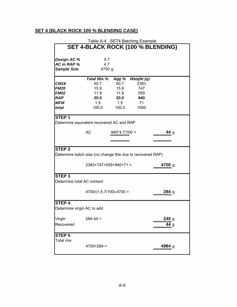
A-5

SET 4 (BLACK ROCK 100 % BLENDING CASE)

Table A-4. SET4 Batching Example

Design AC % 5.7AC in RAP % 4.7Sample Size 4700 g

Total Mix % Agg % Weight (g)CM16 50.7 50.7 2383FM20 15.9 15.9 747FM02 11.9 11.9 559RAP 20.0 20.0 940MFM 1.5 1.5 71total 100.0 100.0 1000

STEP 1Determine equivalent recovered AC and RAP

AC 940*4.7/100 = 44 g

STEP 2Determine batch size (no change this due to recovered RAP)

2383+747+559+940+71 = 4700 g

STEP 3Determine total AC content

4700/(1-5.7/100)-4700 = 284 g

STEP 4Determine virgin AC to add

Virgin 284-44 = 240 gRecovered 44 g

STEP 5Total mix

4700+284 = 4984 g

SET 4-BLACK ROCK (100 % BLENDING)

A-6

APPENDIX B MIXTURE DESIGN

A-7

Table A-5. District 1 RAP 0% Job Mix Formula DISTRICT 1-RAP 0 % DESIGN

Design Number District 1 RAP 0 %Agg No CM16 FM20 FM02 MFM RAP

4.7 % ACAgg Blend % 57.5 23.0 18.0 1.5 0.0 100.0 total

Gsb2 inches 2 inches 50.00 100.0 100.0 100.0 100.0 100.0 100.0 CM16 2.664

1 1/2 inches 1 1/2 inches 37.50 100.0 100.0 100.0 100.0 100.0 100.0 FM20 2.6701 inch 1 inch 25.00 100.0 100.0 100.0 100.0 100.0 100.0 FM02 2.597

3/4 inch 3/4 inch 19.00 100.0 100.0 100.0 100.0 100.0 100.0 Filler 2.9001/2 inch 1/2 inch 12.50 100.0 100.0 100.0 100.0 100.0 100.0 RAP 2.6603/8 inch 3/8 inch 9.50 97.0 100.0 100.0 100.0 98.0 98.3 Blend 2.656

No. 4 No. 4 4.75 29.0 97.0 97.0 100.0 71.0 57.9No. 8 No. 8 2.36 8.0 81.0 85.0 100.0 48.0 40.0

No. 16 No. 16 1.18 4.0 50.0 65.0 100.0 36.0 27.0No. 30 No. 30 0.60 4.0 31.0 53.0 100.0 28.0 20.5No. 50 No. 50 0.30 4.0 19.0 20.0 100.0 21.0 11.8No. 100 No. 100 0.15 4.0 10.0 5.0 95.0 13.0 6.9No. 200 No. 200 0.075 3.4 4.0 1.5 90.0 9.7 4.5

2.664 2.670 2.597 2.900 2.6602.790 2.766 2.681 2.900

Data for N-Design =50 Min 15 65-78Trial Batch # AC % (MIX) Gmb Gmm VMA VTM VFA Vbulk(cm3) Veff (cm3) Gse Gsb Pbe Pba DP

1 5.7 2.396 2.510 14.9 4.5 70 1761.0 1702.1 2.748 2.656 4.5 1.3 0.82 5.9 2.398 2.502 15.0 4.1 72 1756.1 1697.5 2.748 2.656 4.7 1.3 0.83

Data for N-Initial =6Trial Batch # AC % (MIX) Gmb Gmm VMA VTM VFA %Gmm

1 5.7 2.155 2.510 23.5 14.1 40 85.92 5.9 2.206 2.502 21.9 11.8 46 88.23

Design AC Design AC % Gmb Gmm VMA VTM VFA5.9 2.398 2.502 15.0 4.1 72

Stockpile 2 (%)

Stockpile 3 (%)

Stockpile 4 (%)

Stockpile 5 (%) Blend (%)

Bulk Specific GravityApparent Specific Gravity

Sieve Size (No.) Sieve Size (No.)

Sieve Size (mm)

Stockpile 1 (%)

A-8

Table A-6. District 1 RAP 20% Job Mix Formula

DISTRICT 1-RAP 20 % DESIGNDesign Number District 1 RAP 20 %Agg No CM16 FM20 FM02 MFM RAP

4.7 % ACAgg Blend % 51.2 16.1 12.0 1.5 19.2 100.0 total

Gsb2 inches 2 inches 50.0 100.0 100.0 100.0 100.0 100.0 100.0 CM16 2.664

1 1/2 inches 1 1/2 inches 37.5 100.0 100.0 100.0 100.0 100.0 100.0 FM20 2.6701 inch 1 inch 25.0 100.0 100.0 100.0 100.0 100.0 100.0 FM02 2.597

3/4 inch 3/4 inch 19.0 100.0 100.0 100.0 100.0 100.0 100.0 Filler 2.9001/2 inch 1/2 inch 12.5 100.0 100.0 100.0 100.0 100.0 100.0 RAP 2.6603/8 inch 3/8 inch 9.5 97.0 100.0 100.0 100.0 98.0 98.1 Blend 2.659

No. 4 No. 4 4.8 29.0 97.0 97.0 100.0 71.0 57.4No. 8 No. 8 2.4 8.0 81.0 85.0 100.0 48.0 38.2

No. 16 No. 16 1.2 4.0 50.0 65.0 100.0 36.0 26.4No. 30 No. 30 0.6 4.0 31.0 53.0 100.0 28.0 20.4No. 50 No. 50 0.3 4.0 19.0 20.0 100.0 21.0 13.1

No. 100 No. 100 0.2 4.0 10.0 5.0 95.0 13.0 8.2No. 200 No. 200 0.1 3.4 4.0 1.5 90.0 9.7 5.8

2.664 2.670 2.597 2.900 2.660 2.659

Data for N-Design =50 Min 15 65-78Trial Batch # AC % (MIX) Gmb Gmm VMA VTM VFA Vbulk(cm3) Veff (cm3) Gse Gsb Pbe Pba DP

1 5.0 2.368 2.525 15.4 6.2 60 1668.3 1622.7 2.734 2.659 4.0 1.1 1.22 5.5 2.386 2.505 15.2 4.8 69 1667.9 1623.1 2.733 2.659 4.5 1.0 1.13 6.0 2.415 2.482 14.6 2.7 82 1660.8 1619.2 2.727 2.659 5.1 1.0 1.0

Data for N-Initial =6Trial Batch # AC % (MIX) Gmb Gmm VMA VTM VFA %Gmm

1 5.0 2.157 2.525 23.0 14.6 36 85.42 5.5 2.169 2.505 22.9 13.4 42 86.63 6.0 2.194 2.482 22.5 11.6 48 88.4

Design AC Design AC % Gmb Gmm VMA VTM VFA5.7 2.397 2.496 15.0 3.9 74

REC AGG 5.7 2.395 2.499 15.1 4.2 72

Stockpile 3 (%)

Stockpile 4 (%)

Stockpile 5 (%) Blend (%)

Bulk Specific GravityApparent Specific Gravity

Sieve Size (No.) Sieve Size (No.)

Sieve Size (mm)

Stockpile 1 (%)

Stockpile 2 (%)

A-9

Figure A-1. Optimum AC content determination for District 1 20 % RAP design

70

75

80

85

90

95

100

1 10 100# of Gyrations

% G

mm

AC = 6.0 % AC = 5.5% AC = 5.0%

Optimum AC = 5.7 %

Ndesign = 50

4% air voids

< 89 @ Ninitial OK!

Ninitial = 6

A-10

Table A-7. District 1 RAP 40% Job Mix Formula DISTRICT 1-RAP 40 % DESIGN

Design Number District 1 RAP 40 %Agg No CM16 FM20 FM02 MFM CM16 (RAP)

4.7 % ACAgg Blend % 40.8 9.7 9.2 1.5 38.9 100.0 total

Gsb2 inches 2 inches 50.0 100.0 100.0 100.0 100.0 100.0 100.0 CM16 2.664

1 1/2 inches 1 1/2 inches 37.5 100.0 100.0 100.0 100.0 100.0 100.0 FM20 2.6701 inch 1 inch 25.0 100.0 100.0 100.0 100.0 100.0 100.0 FM02 2.597

3/4 inch 3/4 inch 19.0 100.0 100.0 100.0 100.0 100.0 100.0 Filler 2.9001/2 inch 1/2 inch 12.5 100.0 100.0 100.0 100.0 100.0 100.0 RAP 2.6603/8 inch 3/8 inch 9.5 97.0 100.0 100.0 100.0 98.0 98.0 Blend 2.660

No. 4 No. 4 4.8 29.0 97.0 97.0 100.0 71.0 59.4No. 8 No. 8 2.4 8.0 81.0 85.0 100.0 48.0 39.2

No. 16 No. 16 1.2 4.0 50.0 65.0 100.0 36.0 28.1No. 30 No. 30 0.6 4.0 31.0 53.0 100.0 28.0 22.0No. 50 No. 50 0.3 4.0 19.0 20.0 100.0 21.0 15.1No. 100 No. 100 0.2 4.0 10.0 5.0 95.0 13.0 9.6No. 200 No. 200 0.1 3.4 4.0 1.5 90.0 9.7 7.1

2.664 2.670 2.597 2.900 2.660 2.660

Data for N-Design =50 Min 15 65-78Trial Batch # AC % (MIX) Gmb Gmm VMA VTM VFA Vbulk(cm3) Veff (cm3) Gse Gsb Pbe Pba DP

1 5.8 2.429 2.508 14.0 3.1 77 1727.2 1670.1 2.751 2.660 4.6 1.3 1.22 5.4 2.408 2.535 14.4 5.0 65 1727.5 1661.8 2.765 2.660 4.0 1.5 1.3

3 (REC AGG) 5.4 2.386 2.511 15.2 5.0 67 1726.2 1678.9 2.735 2.660 4.4 1.1 1.34 (REC AGG) 5.6 2.418 2.503 14.2 3.4 76 1721.7 1674.5 2.735 2.660 4.6 1.1 1.3

Data for N-Initial =6Trial Batch # AC % (MIX) Gmb Gmm VMA VTM VFA %Gmm

1 5.8 2.215 2.508 21.6 11.7 46 88.32 5.4 2.151 2.535 23.5 15.1 36 84.9

3 (REC AGG) 5.4 2.139 2.511 23.9 14.8 38 85.24 (REC AGG) 5.6 2.169 2.503 23.0 13.4 42 86.6

Design AC Design AC % Gmb Gmm VMA VTM VFA5.6 2.418 2.521 14.2 4.1 715.65 2.421 2.519 14.1 3.9 72

RECOVERED AGG 5.6 2.418 2.503 14.2 3.4 76RECOVERED AGG 5.55 2.410 2.505 14.4 3.8 74

Stockpile 5 (%) Blend (%)

Bulk Specific GravityApparent Specific Gravity

Sieve Size (No.) Sieve Size (No.)

Sieve Size (mm)

Stockpile 1 (%)

Stockpile 2 (%)

Stockpile 3 (%)

Stockpile 4 (%)

OPT AC = 5.65 % OPT AC (REC AGG) = 5.55 %

A-11

70

75

80

85

90

95

100

1 10 100

# of Gyrations

% G

mm

AC = 5.8 % AC = 5.4%

Optimum AC = 5.65 %

Ndesign = 50

4% air voids

< 89 @ Ninitial OK!

Ninitial = 6

Figure A-1. Optimum AC determination for District 1 40 % RAP mixture design

A-12

Table A-8. District 4 RAP 0% Job Mix Formula

DISTRICT 4-RAP 0 % DESIGNDesign Number District 4 RAP 0 %Agg No CM13 FM21 FM01 MFM CM13 (RAP)

5.1 % ACAgg Blend % 69.0 21.5 8.0 1.5 0.0 100.0 total

Gsb2 inches 2 inches 50.0 100.0 100.0 100.0 100.0 100.0 100.0 CM13 2.627

1 1/2 inches 1 1/2 inches 37.5 100.0 100.0 100.0 100.0 100.0 100.0 FM21 2.7131 inch 1 inch 25.0 100.0 100.0 100.0 100.0 100.0 100.0 FM01 2.614

3/4 inch 3/4 inch 19.0 100.0 100.0 100.0 100.0 100.0 100.0 Filler 2.9001/2 inch 1/2 inch 12.5 99.0 100.0 100.0 100.0 100.0 99.3 RAP 2.6303/8 inch 3/8 inch 9.5 88.3 100.0 100.0 100.0 98.8 91.9 Blend 2.648

No. 4 No. 4 4.8 41.1 100.0 96.3 100.0 72.6 59.1No. 8 No. 8 2.4 8.7 91.6 91.4 100.0 48.6 34.5

No. 16 No. 16 1.2 1.2 71.8 85.4 100.0 37.4 24.6No. 30 No. 30 0.6 0.6 51.9 62.0 100.0 30.8 18.0No. 50 No. 50 0.3 0.5 35.1 9.7 100.0 23.8 10.2

No. 100 No. 100 0.2 0.4 20.1 0.9 95.0 14.9 6.1No. 200 No. 200 0.1 0.4 6.2 0.2 90.0 11.6 3.0

2.627 2.713 2.614 2.900 2.630 2.648

Data for N-Design =50 Min 15 65-78Trial Batch # AC % (MIX) Gmb Gmm VMA VTM VFA Vbulk(cm3) Veff (cm3) Gse Gsb Pbe Pba DP

1 5.9 2.429 2.524 13.7 3.8 72 1765.7 1683.5 2.777 2.648 4.2 1.8 0.5234

Data for N-Initial =6Trial Batch # AC % (MIX) Gmb Gmm VMA VTM VFA %Gmm

1 5.9 2.219 2.524 21.1 12.1 43 87.9234

Design AC Design AC % Gmb Gmm VMA VTM VFA5.9 2.429 2.524 13.7 3.8 72

Stockpile 5 (%) Blend (%)

Bulk Specific GravityApparent Specific Gravity

Sieve Size (No.) Sieve Size (No.)

Sieve Size (mm)

Stockpile 1 (%)

Stockpile 2 (%)

Stockpile 3 (%)

Stockpile 4 (%)

A-13

Table A-9. District 4 RAP 20% Job Mix Formula DISTRICT 4-RAP 20 % DESIGN

Design Number District 4 RAP 20 %Agg No CM13 FM21 FM01 MFM CM13 (RAP)

5.1 % ACAgg Blend % 60.6 10.1 9.1 1.0 19.2 100.0 total

Gsb2 inches 2 inches 50.0 100.0 100.0 100.0 100.0 100.0 100.0 CM13 2.627

1 1/2 inches 1 1/2 inches 37.5 100.0 100.0 100.0 100.0 100.0 100.0 FM21 2.7131 inch 1 inch 25.0 100.0 100.0 100.0 100.0 100.0 100.0 FM01 2.614

3/4 inch 3/4 inch 19.0 100.0 100.0 100.0 100.0 100.0 100.0 Filler 2.9001/2 inch 1/2 inch 12.5 99.0 100.0 100.0 100.0 100.0 99.4 RAP 2.6303/8 inch 3/8 inch 9.5 88.3 100.0 100.0 100.0 98.8 92.8 Blend 2.637

No. 4 No. 4 4.8 41.1 100.0 96.3 100.0 72.6 58.9No. 8 No. 8 2.4 8.7 91.6 91.4 100.0 48.6 33.3

No. 16 No. 16 1.2 1.2 71.8 85.4 100.0 37.4 24.1No. 30 No. 30 0.6 0.6 51.9 62.0 100.0 30.8 18.3No. 50 No. 50 0.3 0.5 35.1 9.7 100.0 23.8 10.4

No. 100 No. 100 0.2 0.4 20.1 0.9 95.0 14.9 6.3No. 200 No. 200 0.1 0.4 6.2 0.2 90.0 11.6 4.1

2.627 2.713 2.614 2.900 2.630 2.637

Data for N-Design =50 Min 15 65-78Trial Batch # AC % (MIX) Gmb Gmm VMA VTM VFA Vbulk(cm3) Veff (cm3) Gse Gsb Pbe Pba DP

1 6.0 2.409 2.504 14.1 3.8 73 1748.7 1673.6 2.756 2.637 6.0 1.7 0.72 5.5 2.380 2.523 14.7 5.7 62 1751.7 1676.6 2.755 2.637 5.5 1.7 0.73 5.0 2.375 2.546 14.4 6.7 54 1758.1 1680.2 2.760 2.637 5.0 1.7 0.84 4.5 2.350 2.566 14.9 8.4 44 1758.6 1680.7 2.760 2.637 4.5 1.7 0.9

Data for N-Initial =6Trial Batch # AC % (MIX) Gmb Gmm VMA VTM VFA %Gmm

1 6.0 2.203 2.504 21.5 12.0 44 88.02 5.5 2.127 2.523 23.8 15.7 34 84.33 5.0 2.125 2.546 23.4 16.5 30 83.54 4.5 2.111 2.566 23.6 17.7 25 82.3

Design AC Design AC % Gmb Gmm VMA VTM VFA5.9 2.404 2.508 14.2 4.1 716.0 2.409 2.504 14.1 3.8 73

REC AGG 5.9 2.394 2.496 14.6 4.1 72

Stockpile 5 (%) Blend (%)

Bulk Specific GravityApparent Specific Gravity

Sieve Size (No.) Sieve Size (No.) Sieve Size (mm)

Stockpile 1 (%)

Stockpile 2 (%)

Stockpile 3 (%)

Stockpile 4 (%)

OPT AC = 6.0 % OPT AC (REC AGG) = 5.9 %

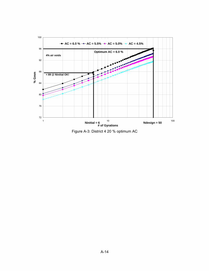
A-14

72

76

80

84

88

92

96

100

1 10 100

# of Gyrations

% G

mm

AC = 6.0 % AC = 5.5% AC = 5.0% AC = 4.5%

Optimum AC = 6.0 %

Ndesign = 50

4% air voids

< 89 @ Ninitial OK!

Ninitial = 6

Figure A-3: District 4 20 % optimum AC

A-15

Table A-10. District 4 RAP 40% Job Mix Formula DISTRICT 4-RAP 40 % DESIGN

Design Number District 4 RAP 40 %Agg No CM13 FM21 FM01 MFM CM13 (RAP)

5.1 % ACAgg Blend % 51.0 5.1 4.1 1.0 38.8 100.0 total

Gsb2 inches 2 inches 50.0 100.0 100.0 100.0 100.0 100.0 100.0 CM13 2.627

1 1/2 inches 1 1/2 inches 37.5 100.0 100.0 100.0 100.0 100.0 100.0 FM21 2.7131 inch 1 inch 25.0 100.0 100.0 100.0 100.0 100.0 100.0 FM01 2.614

3/4 inch 3/4 inch 19.0 100.0 100.0 100.0 100.0 100.0 100.0 Filler 2.9001/2 inch 1/2 inch 12.5 99.0 100.0 100.0 100.0 100.0 99.5 RAP 2.6303/8 inch 3/8 inch 9.5 88.3 100.0 100.0 100.0 98.8 93.7 Blend 2.634

No. 4 No. 4 4.8 41.1 100.0 96.3 100.0 72.6 59.5No. 8 No. 8 2.4 8.7 91.6 91.4 100.0 48.6 33.0

No. 16 No. 16 1.2 1.2 71.8 85.4 100.0 37.4 23.6No. 30 No. 30 0.6 0.6 51.9 62.0 100.0 30.8 18.7No. 50 No. 50 0.3 0.5 35.1 9.7 100.0 23.8 12.9

No. 100 No. 100 0.2 0.4 20.1 0.9 95.0 14.9 8.2No. 200 No. 200 0.1 0.4 6.2 0.2 90.0 11.6 6.0

2.627 2.713 2.614 2.900 2.630 2.634

Data for N-Design =50 Min 15 65-78Trial Batch # AC % (MIX) Gmb Gmm VMA VTM VFA Vbulk(cm3) Veff (cm3) Gse Gsb Pbe Pba DP

1 6.0 2.406 2.499 14.2 3.7 73.6 1734.2 1661.5 2.750 2.634 4.5 1.6 1.02 5.5 2.393 2.524 14.2 5.2 63.3 1738.5 1661.5 2.756 2.634 3.9 1.7 1.13 5.0 2.373 2.552 14.4 7.0 51.3 1744.1 1660.5 2.767 2.634 3.2 1.9 1.2

4 (REC AGG) 5.8 2.397 2.510 14.3 4.5 68.7 1749.4 1677.0 2.748 2.634 4.1 1.6 1.0

Data for N-Initial =6Trial Batch # AC % (MIX) Gmb Gmm VMA VTM VFA %Gmm

1 6.0 2.192 2.499 21.8 12.3 44 87.72 5.5 2.123 2.524 23.9 15.9 33 84.13 5.0 2.106 2.552 24.0 17.5 27 82.5

4 (REC AGG) 5.8 2.149 2.510 23.2 14.4 38 85.6

Design AC Design AC % Gmb Gmm VMA VTM VFA5.9 2.402 2.506 14.2 4.2 716.0 2.406 2.499 14.2 3.7 74

REC AGG 5.8 2.397 2.515 14.3 4.7 67REC AGG 5.9 2.391 2.490 14.6 4.0 73

Stockpile 5 (%) Blend (%)

Bulk Specific GravityApparent Specific Gravity

Sieve Size (No.) Sieve Size (No.)

Sieve Size (mm)

Stockpile 1 (%)

Stockpile 2 (%)

Stockpile 3 (%)

Stockpile 4 (%)

OPT AC = 6.0 % OPT AC (REC AGG) = 5.9 %

A-16

70

75

80

85

90

95

100

1 10 100

# of Gyrations

% G

mm

AC = 6.0 % AC = 5.5% AC = 5.0%

Optimum AC = 6.0 %

Ndesign = 50

4% air voids

< 89 @ Ninitial OK!

Ninitial = 6

Figure A-4: District 4 40% RAP optimum AC

A-17

APPENDIX C COMPLEX MODULUS TEST DATA STATISTICS

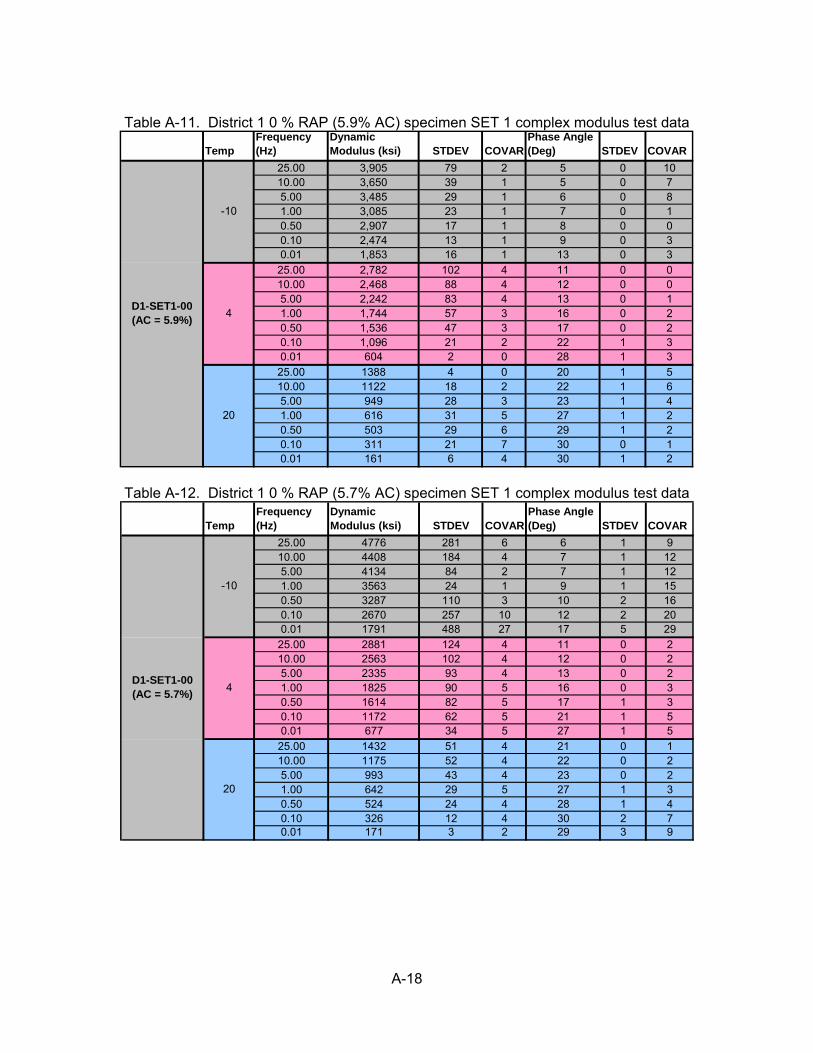
A-18

Table A-11. District 1 0 % RAP (5.9% AC) specimen SET 1 complex modulus test data

TempFrequency (Hz)

Dynamic Modulus (ksi) STDEV COVAR

Phase Angle (Deg) STDEV COVAR

25.00 3,905 79 2 5 0 1010.00 3,650 39 1 5 0 75.00 3,485 29 1 6 0 81.00 3,085 23 1 7 0 10.50 2,907 17 1 8 0 00.10 2,474 13 1 9 0 30.01 1,853 16 1 13 0 325.00 2,782 102 4 11 0 010.00 2,468 88 4 12 0 05.00 2,242 83 4 13 0 11.00 1,744 57 3 16 0 20.50 1,536 47 3 17 0 20.10 1,096 21 2 22 1 30.01 604 2 0 28 1 325.00 1388 4 0 20 1 510.00 1122 18 2 22 1 65.00 949 28 3 23 1 41.00 616 31 5 27 1 20.50 503 29 6 29 1 20.10 311 21 7 30 0 10.01 161 6 4 30 1 2

20

D1-SET1-00 (AC = 5.9%)

-10

4

Table A-12. District 1 0 % RAP (5.7% AC) specimen SET 1 complex modulus test data

TempFrequency (Hz)

Dynamic Modulus (ksi) STDEV COVAR

Phase Angle (Deg) STDEV COVAR

25.00 4776 281 6 6 1 910.00 4408 184 4 7 1 125.00 4134 84 2 7 1 121.00 3563 24 1 9 1 150.50 3287 110 3 10 2 160.10 2670 257 10 12 2 200.01 1791 488 27 17 5 2925.00 2881 124 4 11 0 210.00 2563 102 4 12 0 25.00 2335 93 4 13 0 21.00 1825 90 5 16 0 30.50 1614 82 5 17 1 30.10 1172 62 5 21 1 50.01 677 34 5 27 1 525.00 1432 51 4 21 0 110.00 1175 52 4 22 0 25.00 993 43 4 23 0 21.00 642 29 5 27 1 30.50 524 24 4 28 1 40.10 326 12 4 30 2 70.01 171 3 2 29 3 9

-10

4D1-SET1-00 (AC = 5.7%)

20

A-19

Table A-13. District 1 20 % RAP specimen SET 1 case complex modulus test data

Specimen Id Temp Frequency (Hz)Dynamic Modulus (ksi) STDEV COVAR

Phase Angle (Deg) STDEV COVAR

25.00 5,141 184 4 4 2 4310.00 4,778 209 4 5 2 315.00 4,572 176 4 6 1 211.00 4,058 143 4 7 1 110.50 3,824 138 4 8 1 100.10 3,273 143 4 9 1 100.01 2,499 156 6 13 1 1025.00 3,460 178 5 9 2 1810.00 3,122 135 4 10 1 115.00 2,878 123 4 11 1 71.00 2,331 103 4 13 0 20.50 2,097 94 4 15 0 20.10 1,580 73 5 18 0 20.01 942 38 4 24 0 125.00 1741 187 11 19 1 410.00 1421 166 12 20 1 45.00 1207 147 12 21 1 41.00 801 106 13 25 1 30.50 657 90 14 27 1 30.10 400 60 15 30 0 10.01 No Data

-10

4

20

D1-SET1-20

A-20

Table A-14. District 1 20 % RAP specimen SET 2 case complex modulus test data

Specimen Id Temp Frequency (Hz)Dynamic Modulus (ksi) STDEV COVAR

Phase Angle (Deg) STDEV COVAR

25.00 4,744 869 18 6 1 1410.00 4,481 790 18 6 1 95.00 4,287 751 18 6 1 91.00 3,823 667 17 7 0 30.50 3,612 624 17 8 0 30.10 3,103 533 17 9 0 50.01 2,378 373 16 12 1 425.00 3,195 363 11 9 1 1310.00 2,888 344 12 10 1 55.00 2,657 324 12 11 0 31.00 2,138 272 13 14 0 30.50 1,916 245 13 15 0 30.10 1,428 172 12 18 1 30.01 846 108 0 24 0 125.00 1606 184 11 19 0 210.00 1322 150 11 20 0 25.00 1130 126 11 21 0 21.00 752 87 12 25 0 20.50 619 70 11 26 0 10.10 387 53 14 29 0 10.01 199 26 13 29 1 3

20

-10

4D1-SET2-20

Table A-15. District 1 20 % RAP specimen SET 3 case complex modulus test data

Specimen Id Temp Frequency (Hz)Dynamic Modulus (ksi) STDEV COVAR

Phase Angle (Deg) STDEV COVAR

25.00 5,005 51 1 6 1 2110.00 4,667 41 1 6 1 205.00 4,431 32 1 7 2 261.00 3,875 158 4 9 2 250.50 3,626 219 6 9 2 250.10 3,036 333 11 11 3 260.01 2,231 394 18 15 3 2225.00 3,578 116 3 11 0 310.00 3,169 95 3 12 0 45.00 2,842 109 4 13 0 11.00 2,232 48 2 15 0 30.50 1,955 47 2 17 0 30.10 1,374 43 3 21 0 20.01 747 20 3 28 0 225.00 1655 48 3 20 1 410.00 1334 58 4 21 1 35.00 1127 50 4 23 1 31.00 730 28 4 27 1 30.50 594 24 4 28 1 20.10 361 16 4 30 0 10.01 181 11 6 31 0 0

D1-SET3-20

-10

4

20

A-21

Table A-16. District 1 20 % RAP specimen SET 4 case complex modulus test data

Specimen Id Temp Frequency (Hz)Dynamic Modulus (ksi) STDEV COVAR

Phase Angle (Deg) STDEV COVAR

25.00 4,913 157 3 5 1 1010.00 4,668 128 3 6 0 55.00 4,448 126 3 6 0 51.00 3,933 111 3 8 0 30.50 3,696 105 3 8 0 30.10 3,147 81 3 10 1 60.01 2,342 54 2 14 0 125.00 3,247 41 1 10 2 1710.00 2,894 43 1 11 1 95.00 2,638 37 1 12 0 41.00 2,076 36 2 15 0 20.50 1,837 35 2 17 0 20.10 1,331 31 2 21 0 20.01 747 32 4 28 1 325.00 1688 90 5 21 1 710.00 1365 85 6 21 1 45.00 1152 76 7 23 1 41.00 751 54 7 27 1 40.50 612 46 8 28 1 40.10 373 30 8 31 1 30.01 185 16 9 32 1 3

D1-SET4-20

-10

4

20

Table A-17. District 1 40 % RAP specimen SET 1 case complex modulus test data

Temp Frequency (Hz)Dynamic Modulus (ksi) STDEV COVAR

Phase Angle (Deg) STDEV COVAR

25.00 5,331 301 6 5 0 610.00 4,973 216 4 5 0 55.00 4,765 196 4 6 0 21.00 4,285 162 4 7 0 20.50 4,067 144 4 7 0 10.10 3,541 101 3 8 0 10.01 2,777 38 1 11 0 3

25.00 3,897 187 5 8 1 1210.00 3,555 186 5 9 1 85.00 3,305 181 5 9 1 61.00 2,741 152 6 11 0 30.50 2,499 132 5 12 0 30.10 1,930 98 5 16 0 10.01 1,198 42 4 22 1 3

25.00 2121 170 8 16 0 210.00 1773 142 8 17 0 05.00 1542 116 8 19 0 11.00 1078 81 8 23 0 10.50 902 64 7 24 0 10.10 575 43 7 28 0 10.01 283 22 8 32 1 2

-10

4

20

D1-SET1-40

A-22

Table A-18. District 1 40 % RAP specimen SET 2 case complex modulus test data

Specimen Id Temp Frequency (Hz)Dynamic Modulus (ksi) STDEV COVAR

Phase Angle (Deg) STDEV COVAR

25.00 3,934 368 9 6 0 110.00 3,727 352 9 6 0 15.00 3,560 339 10 7 0 11.00 3,134 293 9 8 0 10.50 2,943 275 9 9 0 20.10 2,488 241 10 11 0 40.01 1,852 209 11 15 1 6

25.00 2,996 526 18 11 0 210.00 2,674 465 17 12 0 35.00 2,438 422 17 13 0 31.00 1,906 340 18 16 1 40.50 1,682 302 18 17 1 40.10 1,209 217 18 21 1 30.01 674 116 17 28 0 2

25.00 1546 81 5 20 1 710.00 1251 126 10 23 1 45.00 1049 118 11 24 1 31.00 672 90 13 29 1 30.50 545 77 14 30 1 20.10 331 49 15 31 1 30.01 167 23 14 31 1 4

-10

4D1-SET2-40

20

Table A-19. District 1 40 % RAP specimen SET 3 case complex modulus test data

Specimen Id Temp Frequency (Hz)Dynamic Modulus (ksi) STDEV COVAR

Phase Angle (Deg) STDEV COVAR

25.00 4,247 117 3 6 0 010.00 4,025 63 2 6 0 15.00 3,858 40 1 6 0 11.00 3,427 23 1 8 0 00.50 3,236 10 0 8 0 10.10 2,778 30 1 10 0 20.01 2,107 59 3 14 0 3

25.00 3,379 329 10 10 0 110.00 2,989 315 11 10 0 15.00 2,719 298 11 11 0 11.00 2,149 258 12 14 0 30.50 1,901 242 13 16 0 30.10 1,369 187 14 20 1 30.01 763 110 14 27 1 3

25.00 1565 167 11 19 2 1310.00 1271 134 11 21 1 65.00 1070 114 11 23 1 41.00 694 86 12 27 0 20.50 564 74 13 28 0 10.10 340 46 13 31 0 10.01 171 20 12 30 1 4

D1-SET3-40

-10

4

20

A-23

Table 20. District 1 40 % RAP specimen SET 4 case complex modulus test data

Specimen Id Temp Frequency (Hz)Dynamic Modulus (ksi) STDEV COVAR

Phase Angle (Deg) STDEV COVAR

25.00 4,244 199 5 6 0 510.00 4,034 185 5 6 0 45.00 3,868 185 5 6 0 21.00 3,470 173 5 7 0 10.50 3,291 172 5 8 0 10.10 2,858 164 6 9 0 10.01 2,227 143 6 13 0 1

25.00 2,841 177 6 6 0 110.00 2,570 138 5 6 0 15.00 2,375 119 5 6 0 11.00 1,923 87 5 7 0 10.50 1,735 74 4 8 0 20.10 1,312 47 4 9 0 30.01 795 30 4 13 0 2

25.00 1689 150 9 6 0 110.00 1414 106 7 6 0 25.00 1219 81 7 6 0 21.00 828 51 6 7 0 10.50 687 41 6 8 0 20.10 433 22 5 9 0 10.01 218 10 4 13 0 0

D1-SET4-40

-10

4

20

Table A-21. District 4 0 % RAP specimen SET 1 case complex modulus test data

TempFrequency (Hz)

Dynamic Modulus (ksi) STDEV COVAR

Phase Angle (Deg) STDEV COVAR

25.00 4,494 342 8 6 1 1610.00 4,172 310 7 6 0 45.00 3,948 279 7 7 1 111.00 3,431 226 7 8 0 20.50 3,194 192 6 9 0 10.10 2,639 139 5 11 0 30.01 1,865 77 4 15 0 125.00 2,725 46 2 12 1 610.00 2,395 59 2 13 0 35.00 2,159 66 3 14 0 21.00 1,656 60 4 17 0 10.50 1,452 57 4 19 0 10.10 1,035 42 4 23 0 00.01 576 12 2 28 0 125.00 1243 41 3 22 0 210.00 993 30 3 23 0 25.00 827 24 3 25 1 41.00 525 18 3 28 2 70.50 425 15 3 29 2 60.10 264 10 4 28 1 50.01 145 8 6 24 1 2

-10

4

20

D4-SET1-00

A-24

Table A-22. District 4 20 % RAP specimen SET 1 case complex modulus test data

TempFrequency (Hz)

Dynamic Modulus (ksi) STDEV COVAR

Phase Angle (Deg) STDEV COVAR

25.00 3,882 115 3 5 0 910.00 3,627 83 2 6 0 55.00 3,466 86 2 6 0 51.00 3,064 71 2 8 1 70.50 2,889 75 3 8 1 80.10 2,467 85 3 10 1 80.01 1,855 109 6 14 1 925.00 2,638 168 6 11 1 510.00 2,330 150 6 12 0 45.00 2,106 136 6 13 0 31.00 1,634 113 7 16 0 30.50 1,437 101 7 18 0 30.10 1,025 72 7 22 0 20.01 564 33 6 29 0 125.00 1277 48 4 21 1 410.00 1043 51 5 22 1 45.00 883 48 5 23 1 31.00 570 44 8 27 1 30.50 465 38 8 29 1 20.10 285 26 9 31 0 10.01 147 11 8 30 1 3

-10

4

20

D4-SET1-20

Table A-23. District 4 20 % RAP specimen SET 2 case complex modulus test data

Specimen Id TempFrequency (Hz)

Dynamic Modulus (ksi) STDEV COVAR

Phase Angle (Deg) STDEV COVAR

25.00 3,302 85 3 8 0 310.00 3,067 67 2 8 0 25.00 2,894 66 2 9 0 21.00 2,462 65 3 11 0 20.50 2,279 61 3 12 0 20.10 1,847 41 2 14 0 20.01 1,268 26 2 20 1 525.00 2,401 121 5 14 1 510.00 2,052 93 5 15 1 65.00 1,812 81 4 16 1 51.00 1,325 77 6 20 1 50.50 1,134 70 6 22 1 50.10 759 55 7 26 1 40.01 396 33 8 32 1 225.00 1205 50 4 23 1 410.00 948 34 4 24 1 55.00 780 28 4 26 1 41.00 482 22 5 29 1 30.50 387 19 5 30 1 30.10 233 14 6 30 0 10.01 127 8 7 26 0 1

-10

4D4-SET2-20

20

A-25

Table A-24. District 4 20 % RAP specimen SET 3 case complex modulus test data

Specimen Id TempFrequency (Hz)

Dynamic Modulus (ksi) STDEV COVAR

Phase Angle (Deg) STDEV COVAR

25.00 3,551 129 4 7 0 110.00 3,318 126 4 7 0 05.00 3,137 125 4 8 0 01.00 2,710 118 4 10 0 10.50 2,523 113 4 10 0 10.10 2,086 96 5 13 0 10.01 1,493 72 5 17 0 025.00 2,558 69 3 13 0 410.00 2,270 32 1 14 0 15.00 2,051 21 1 15 0 11.00 1,552 12 1 18 0 00.50 1,353 5 0 20 0 00.10 944 4 0 24 0 00.01 495 6 1 31 0 025.00 1207 50 4 23 1 210.00 969 37 4 24 0 15.00 811 35 4 25 0 11.00 514 23 5 29 0 10.50 417 20 5 30 0 00.10 253 13 5 31 0 00.01 136 6 4 28 0 1

D4-SET3-20

-10

4

20

Table A-25. District 4 40 % RAP specimen SET 1 case complex modulus test data

TempFrequency (Hz)

Dynamic Modulus (ksi) STDEV COVAR

Phase Angle (Deg) STDEV COVAR

25.00 4,385 593 14 6 0 310.00 4,125 549 13 6 0 35.00 3,946 517 13 6 0 41.00 3,510 418 12 7 0 40.50 3,314 380 11 8 0 40.10 2,857 303 11 9 0 50.01 2,215 230 10 12 1 525.00 3,006 294 10 11 0 210.00 2,683 284 11 11 0 25.00 2,472 267 11 12 0 21.00 1,984 214 11 14 0 20.50 1,783 193 11 15 0 20.10 1,335 139 10 19 0 20.01 792 72 9 25 1 325.00 1664 148 9 19 3 1410.00 1402 105 7 20 3 145.00 1221 80 7 21 2 111.00 854 49 6 31 13 430.50 718 39 5 27 4 160.10 466 24 5 29 3 100.01 240 17 7 31 2 6

-10

4

20

D4-SET1-40

A-26

Table A-26. District 4 40 % RAP specimen SET 2 case complex modulus test data

Specimen Id TempFrequency (Hz)

Dynamic Modulus (ksi) STDEV COVAR

Phase Angle (Deg) STDEV COVAR

25.00 3,916 226 6 6 1 1910.00 3,653 243 7 7 1 175.00 3,448 241 7 7 1 121.00 2,961 205 7 9 1 90.50 2,741 198 7 10 1 90.10 2,220 182 8 13 1 80.01 1,511 128 8 18 1 6

25.00 2,328 404 17 14 1 510.00 2,011 323 16 15 1 45.00 1,787 276 15 16 1 41.00 1,311 208 16 20 1 40.50 1,123 172 15 22 1 30.10 753 102 14 26 1 20.01 388 48 13 32 0 0

25.00 1128 100 9 24 1 510.00 880 78 9 25 1 35.00 724 68 9 26 1 31.00 442 48 11 30 1 30.50 352 42 12 31 1 30.10 211 27 13 31 0 00.01 113 14 12 27 1 3

-10

4D4-SET2-40

20

Table A-27. District 4 40 % RAP specimen SET 3 case complex modulus test data

Specimen Id TempFrequency (Hz)

Dynamic Modulus (ksi) STDEV COVAR

Phase Angle (Deg) STDEV COVAR

25.00 3,919 80 2 7 0 010.00 3,654 69 2 8 0 15.00 3,457 64 2 8 0 21.00 2,978 48 2 10 0 50.50 2,770 39 1 10 1 50.10 2,282 23 1 13 1 60.01 1,617 3 0 17 1 4

25.00 2,642 39 1 13 1 610.00 2,316 48 2 13 1 75.00 2,080 53 3 15 1 71.00 1,571 68 4 18 1 70.50 1,364 67 5 20 1 70.10 939 58 6 24 1 50.01 491 30 6 31 0 1

25.00 1299 6 0 22 0 010.00 1045 12 1 23 0 15.00 873 17 2 24 0 01.00 550 14 3 28 0 00.50 444 13 3 29 0 00.10 268 9 3 30 0 10.01 139 7 5 29 0 1

D4-SET3-40

-10

4

20

A-27

Table A-28. District 4 40 % RAP specimen SET 4 case complex modulus test data

Specimen Id TempFrequency (Hz)

Dynamic Modulus (ksi) STDEV COVAR

Phase Angle (Deg) STDEV COVAR

25.00 3,833 317 8 5 1 2210.00 3,627 287 8 6 1 115.00 3,470 272 8 7 1 111.00 3,070 243 8 8 0 50.50 2,899 232 8 8 1 60.10 2,488 219 9 10 0 30.01 1,869 208 11 13 1 8

25.00 2,634 259 10 6 0 410.00 2,367 263 11 6 0 75.00 2,165 253 12 6 1 91.00 1,712 219 13 7 1 110.50 1,526 203 13 8 1 110.10 1,122 158 14 9 1 90.01 646 85 13 13 1 5

25.00 1462 130 9 6 1 1210.00 1212 121 10 6 0 85.00 1034 109 11 6 1 131.00 690 79 11 7 1 180.50 569 67 12 8 1 180.10 356 43 12 9 1 120.01 182 22 12 13 1 6

D4-SET4-40

-10

4

20

Table A-29. District 4 40 % RAP specimen SET 1 (w/ PG58-28) case complex modulus

test data

Specimen Id TempFrequency (Hz)

Dynamic Modulus (ksi) STDEV COVAR

Phase Angle (Deg) STDEV COVAR

25.00 2,902 80 2 8 1 710.00 2,653 69 2 9 1 125.00 2,475 64 2 10 1 111.00 2,068 48 2 12 1 110.50 1,897 39 1 12 1 100.10 1,516 23 1 15 1 80.01 1,068 3 0 20 1 6

25.00 2,199 39 1 13 0 010.00 1,940 48 2 13 0 15.00 1,757 53 3 14 0 11.00 1,351 68 4 17 0 20.50 1,189 67 5 18 0 20.10 856 58 6 22 0 10.01 492 30 6 28 0 0

25.00 1078 6 0 22 1 310.00 883 12 1 22 1 35.00 747 17 2 24 1 21.00 488 14 3 27 0 10.50 401 13 3 28 0 10.10 256 9 3 29 0 10.01 140 7 5 29 1 3

D4-SET1-40 PG 58-28

-10

4

20

A-28

APPENDIX D MOISTURE SUSCEPTIBILITY TESTING DATA

A-29

Table A-30. District 1 Specimens Moisture Damage Study Specimen Volumetrics and IDT Strength Results [1] [2] [3] [2]X[3]/100 [5] [5]-[1] [6] [7] [8] [9]

Mdry (g)Volume (cm3) VMA VFA Air Voids %

Air Voids (cm3) SSD (g)

Absorbed Water (cm3) Saturation %

Thickness (mm)

Max Load (lbs)

Tensile Strength (psi) Notes

D1-00-1 3838 1647 17.3 58.7 7.1 118 95.9 3397 97.0

D1-00-2 3836 1650 17.5 57.8 7.4 122 3930 94 77.4 96.0 1914 54.6

D1-00-3 3849 1647 17.0 59.7 6.9 113 95.7 3353 95.9

D1-00-4 3849 1636 16.5 62.1 6.2 102 3931 81.6 79.9 95.1 2211 63.7 outflier

D1-00-5 3840 1644 17.1 59.4 6.9 114 3926 86.5 75.7 95.4 2086 59.9

D1-00-6 3844 1631 16.3 62.8 6.1 99 94.8 3456 99.8 outflier

TSR 59.3

D1-20-1 3821 1645 18.1 61.8 6.9 114 3906 84.1 73.8 95.9 2763 78.9

D1-20-2 3815 1651 18.6 59.9 7.5 123 96.5 3823 108.5

D1-20-3 3820 1656 18.7 59.5 7.6 125 96.7 3850 109.0

D1-20-4 3816 1649 18.4 60.5 7.3 120 96.4 3699 105.1

D1-20-5 3804 1653 18.9 58.7 7.8 129 3896 91.7 71.0 96.7 2307 65.3 outflier

D1-20-6 3823 1658 18.7 59.3 7.6 126 3910 86.8 68.7 96.9 2468 69.7 outflier

TSR 73.3

D1-40-1 3844 1654 18.6 58.2 7.8 128 96.1 4441 126.5 outflier

D1-40-2 3846 1632 17.5 62.8 6.5 106 96.3 5252 149.4

D1-40-3 3855 1646 17.9 60.8 7.0 115 3934 79.1 68.5 96.0 3752 107.0 outflier

D1-40-4 3850 1645 18.0 60.5 7.1 117 3932 82 70.1 96.0 3599 102.7

D1-40-5 3853 1646 18.0 60.6 7.1 116 3937 83.7 71.9 95.9 3454 98.6

D1-40-6 3846 1640 17.8 61.3 6.9 113 96.0 5187 147.9

TSR 67.7

A-30

Table A-31. District 4 Specimens Moisture Damage Study Specimen Volumetrics and IDT Strength Results [1] [2] [3] [2]X[3]/100 [5] [5]-[1] [6] [7] [8] [9]

Mdry (g)Volume (cm3) VMA VFA Air Voids %

Air Voids (cm3) SSD (g)

Absorbed Water (cm3) Saturation %

Thickness (mm)

Max Load (lbs)

Tensile Strength (psi) Notes

D4-00-1 3852 1648 16.9 56.2 7.4 122 95.9 2420 69.1

D4-00-2 3851 1632 16.2 59.5 6.5 107 3930 79.1 74.0 95.4 1745 50.1

D4-00-3 3855 1644 16.7 57.3 7.1 117 3945 89.8 76.9 96.0 2003 57.1

D4-00-4 3849 1632 16.2 59.4 6.6 107 95.2 2691 77.4

D4-00-5 3851 1626 15.8 60.9 6.2 101 95.0 2774 80.0 outflier

D4-00-6 3847 1630 16.1 59.6 6.5 106 3927 80 75.3 95.1 2061 59.3

TSR 75.8

D4-20-1 3809 1643 17.9 58.6 7.4 121 3903 94.1 77.6 96.1 2317 66.0

D4-20-2 3812 1644 17.8 58.7 7.4 121 96.0 2833 80.8

D4-20-3 3799 1604 16.1 66.3 5.4 87 93.9 3475 101.3 outflier

D4-20-4 3815 1631 17.2 61.5 6.6 108 3897 81.7 75.9 95.4 2387 68.5

D4-20-5 3813 1652 18.2 57.1 7.8 129 3912 99.7 77.1 96.1 1845 52.6 outflier

D4-20-6 3813 1658 18.5 56.0 8.1 135 96.2 2803 79.8 outflier

TSR 83.2

D4-40-1 3798 1644 18.6 59.3 7.6 124 96.0 3715 106.0 outflier

D4-40-2 3806 1630 17.7 62.8 6.6 107 96.0 3927 112.0

D4-40-3 3804 1631 17.8 62.5 6.7 109 3884 79.9 73.4 95.5 3237 92.8

D4-40-4 3810 1624 17.3 64.5 6.2 100 95.1 3998 115.1 outlier

D4-40-5 3806 1634 17.9 62.0 6.8 111 3887 81.5 73.3 96.0 3028 86.4

D4-40-6 3798 1628 17.8 62.6 6.7 108 3879 80.4 74.2 95.2 3199 92.0TSR 80.7