FFT-based Gradient Sparsification for the Distributed

FFT-based Gradient Sparsification for the Distributed Trainingof Deep Neural Networks

Linnan Wang

Brown University

Providence, RI, USA

Wei Wu

Los Alamos National Laboratory

Los Alamos, NM, USA

Junyu Zhang

University of Minnesota, Twin Cities

Minneapolis, MN, USA

Hang Liu

Stevens Institute of Technology

Hoboken, NJ, USA

George Bosilca

University of Tennessee

Knoxville, TN, USA

Maurice Herlihy

Brown University

Providence, RI, USA

Rodrigo Fonseca

Brown University

Providence, RI, USA

ABSTRACTThe performance and efficiency of distributed training of Deep Neu-

ral Networks (DNN) highly depend on the performance of gradient

averaging among participating processes, a step bound by com-

munication costs. There are two major approaches to reduce com-

munication overhead: overlap communications with computations

(lossless), or reduce communications (lossy). The lossless solution

works well for linear neural architectures, e.g. VGG, AlexNet, but

more recent networks such as ResNet and Inception limit the op-

portunity for such overlapping. Therefore, approaches that reduce

the amount of data (lossy) become more suitable. In this paper, we

present a novel, explainable lossy method that sparsifies gradients

in the frequency domain, in addition to a new range-based float

point representation to quantize and further compress gradients.

These dynamic techniques strike a balance between compression

ratio, accuracy, and computational overhead, and are optimized to

maximize performance in heterogeneous environments.

Unlike existing works that strive for a higher compression ratio,

we stress the robustness of our methods, and provide guidance to

recover accuracy from failures. To achieve this, we prove how the

FFT sparsification affects the convergence and accuracy, and show

that our method is guaranteed to converge using a diminishing θ in

training. Reducing θ can also be used to recover accuracy from the

failure. Compared to STOA lossy methods, e.g., QSGD, TernGrad,

and Top-k sparsification, our approach incurs less approximation

error, thereby better in both the wall-time and accuracy. On an 8

GPUs, InfiniBand interconnected cluster, our techniques effectively

accelerate AlexNet training up to 2.26x to the baseline of no com-

pression, and 1.31x to QSGD, 1.25x to Terngrad and 1.47x to Top-K

sparsification.

ACMacknowledges that this contributionwas authored or co-authored by an employee,

contractor, or affiliate of the United States government. As such, the United States

government retains a nonexclusive, royalty-free right to publish or reproduce this

article, or to allow others to do so, for government purposes only.

HPDC ’20, June 23–26, 2020, Stockholm, Sweden© 2020 Association for Computing Machinery.

ACM ISBN 978-1-4503-7052-3/20/06. . . $15.00

https://doi.org/10.1145/3369583.3392681

CCS CONCEPTS•Computer systems organization→Neural networks; Het-

erogeneous (hybrid) systems; • Theory of computation → Datacompression; Machine learning theory.KEYWORDS

Neural Networks,Machine Learning, FFT, Gradient Compression,

Loosy Gradients

ACM Reference Format:Linnan Wang, Wei Wu, Junyu Zhang, Hang Liu, George Bosilca, Maurice

Herlihy, and Rodrigo Fonseca. 2020. FFT-based Gradient Sparsification for

the Distributed Training of Deep Neural Networks. In Proceedings of the29th International Symposium on High-Performance Parallel and DistributedComputing (HPDC ’20), June 23–26, 2020, Stockholm, Sweden. ACM, New

York, NY, USA, 12 pages. https://doi.org/10.1145/3369583.3392681

1 INTRODUCTIONParameter Server (PS) and allreduce-style communications are two

core parallelization strategies for distributed DNN training. In an

iteration, each worker produces a gradient, and both paralleliza-

tion strategies rely on the communication network to average the

gradients across all workers. The gradient size of current DNNs is

at the scale of 102MB, and, even with the state-of-the-art networks

such as Infiniband, repeatedly transferring such a large volume

of messages over millions of iterations is prohibitively expensive.

Furthermore, the tremendous improvement in GPU computing and

memory speeds (e.g., the latest NVIDIA TESLA V100 GPU features

a peak performance of 14 TFlops on single-precision and memory

bandwidth of 900 GB/s with HBM2) further underscores communi-

cation as a bottleneck.

Recently, several methods have shown that training can be done

with a lossy gradient due to the iterative nature of Stochastic Gra-

dient Descent (SGD). It opens up new opportunities to alleviate the

communication overhead by aggressively compressing gradients.

One approach to compress the gradients is quantization. For ex-ample, Terngrad [29] maps a gradient into [-1, 0, 1], and QSGD [4]

stochastically quantizes gradients onto a uniformly discretized set

larger than that of Terngrad. Such coarse approximation not only in-

curs large errors between the actual and quantized gradients as we

demonstrate in Figure 15 [QSGD, TernGrad], but also fails to exploit

Session: Distributed Learning HPDC ’20, June 23–26, 2020, Stockholm, Sweden

113

https://doi.org/10.1145/3369583.3392681

https://doi.org/10.1145/3369583.3392681

the bit efficiency in the quantization (Figure 7). Another approach

to gradient compression, sparsification, only keeps the top-k largestgradients [2, 5, 14]. Similarly, Top-k loses a significant amount of

actual gradients around zeros to achieve a high compression ratio

(Figure 15, [Top-k]). In summary, existing lossy methods greatly

drop gradients, incur large approximation errors (Figure 15e), lead-

ing to the deterioration of the final accuracy (Table 2). To avoid

compromising the convergence speed, both quantization and spar-sification must limit the compression ratio, leading to sub-optimal

improvement of the end-to-end training wall time.

In this paper, we propose a gradient compression framework

that takes advantages of both sparsi f ication and quantization with

two novel components, FFT-based sparsification, and a range-based

quantization. FFT-based sparsification allows removing the redun-

dant information, while preserving the most relevant information

(Figure 15 [FFT]). As a result, FFT incurs fewer errors in approxi-

mating the actual gradients (Figure 15e), thereby better in accuracy

than QSGD, TernGrad, and Top-K (Table 2). We treat the gradient

as a 1D signal, and drop near-zero coefficients in the frequency do-

main, after an FFT. Deleting some frequency components after the

FFT introduces magnitude errors, but the signal maintains its dis-

tribution (Figure 5). As a result, the sparsification in the frequency

domain can achieve the same compression ratio as in the spatial

domain but preserving more relevant information.

To further improve the end-to-end training wall time, we in-

troduce a new range-based variable precision floating point repre-

sentation to quantize and compress the gradient frequencies after

sparsification. Most importantly, unlike the uniform quantization

used in existing approaches, the precision of representable floats in

our method can be adjusted to follow the distribution of the original

gradients (Figure 9). The novel range-based design allows us to fully

exploit the precision given limited bits so that the approximation

error can be further reduced. By combining sparsification and quan-tization, our framework delivers a higher compression ratio than

the single method, resulting in shorter end-to-end training wall

time than QSGD, Terngrad, and Top-k.

Lastly, our compression framework is highly efficient and scal-

able. The primitive algorithms in our compression scheme, such

as FFT, top-k select, and precision conversions, are efficiently par-

allelizable and thus GPU-friendly. We resort to existing highly

optimized GPU libraries such as cuFFT, Thrust, and bucketSelect

[3], while we propose a simple yet efficient packing algorithm to

transform sparse gradients into a dense representation. Minimizing

the computational cost of the compression is crucial for high-speed

networks, such as Infiniband networks, as we analyzed in Figure 10.

Specifically, the contributions of this paper are as follows:

• a novel FFT-based, tunable gradient sparsification that retains

the original gradient distribution.

• a novel range-based variable precision floating-point that allo-

cates precision according to the gradient distribution.

• a analytic model to guide people when to enable compression

and how to set a compression ratio according to hardware spec-

ifications.

• the convergence proof of our methods, and its guidance in se-

lecting a compression ratio θ , to ensure the convergence, or

reduce θ to recover the accuracy. To the best of our knowledge,

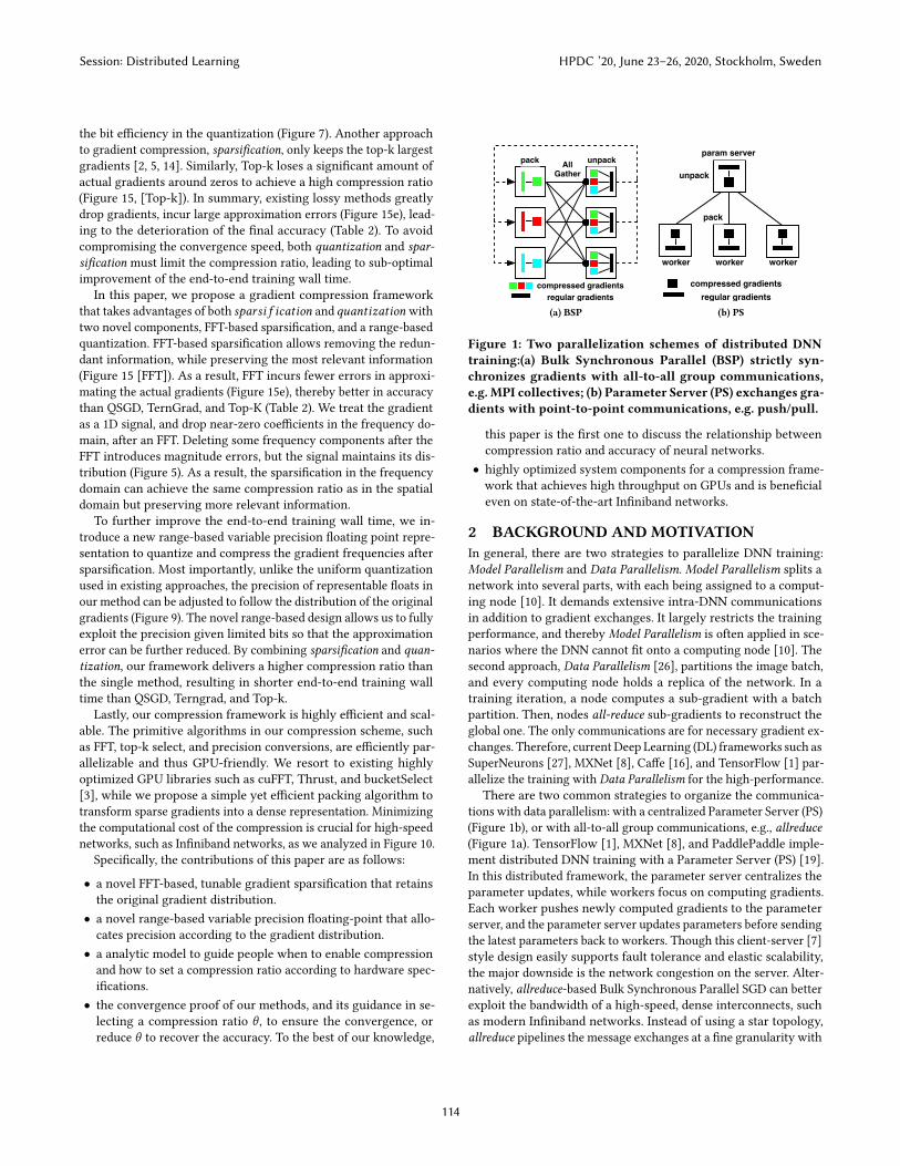
(a) BSP (b) PS

Figure 1: Two parallelization schemes of distributed DNNtraining:(a) Bulk Synchronous Parallel (BSP) strictly syn-chronizes gradients with all-to-all group communications,e.g. MPI collectives; (b) Parameter Server (PS) exchanges gra-dients with point-to-point communications, e.g. push/pull.

this paper is the first one to discuss the relationship between

compression ratio and accuracy of neural networks.

• highly optimized system components for a compression frame-

work that achieves high throughput on GPUs and is beneficial

even on state-of-the-art Infiniband networks.

2 BACKGROUND AND MOTIVATIONIn general, there are two strategies to parallelize DNN training:

Model Parallelism and Data Parallelism. Model Parallelism splits a

network into several parts, with each being assigned to a comput-

ing node [10]. It demands extensive intra-DNN communications

in addition to gradient exchanges. It largely restricts the training

performance, and thereby Model Parallelism is often applied in sce-

narios where the DNN cannot fit onto a computing node [10]. The

second approach, Data Parallelism [26], partitions the image batch,

and every computing node holds a replica of the network. In a

training iteration, a node computes a sub-gradient with a batch

partition. Then, nodes all-reduce sub-gradients to reconstruct the

global one. The only communications are for necessary gradient ex-

changes. Therefore, current Deep Learning (DL) frameworks such as

SuperNeurons [27], MXNet [8], Caffe [16], and TensorFlow [1] par-

allelize the training with Data Parallelism for the high-performance.

There are two common strategies to organize the communica-

tions with data parallelism: with a centralized Parameter Server (PS)

(Figure 1b), or with all-to-all group communications, e.g., allreduce(Figure 1a). TensorFlow [1], MXNet [8], and PaddlePaddle imple-

ment distributed DNN training with a Parameter Server (PS) [19].

In this distributed framework, the parameter server centralizes the

parameter updates, while workers focus on computing gradients.

Each worker pushes newly computed gradients to the parameter

server, and the parameter server updates parameters before sending

the latest parameters back to workers. Though this client-server [7]

style design easily supports fault tolerance and elastic scalability,

the major downside is the network congestion on the server. Alter-

natively, allreduce-based Bulk Synchronous Parallel SGD can better

exploit the bandwidth of a high-speed, dense interconnects, such

as modern Infiniband networks. Instead of using a star topology,

allreduce pipelines the message exchanges at a fine granularity with


114

0 2 4 6ith layer

10 − 4

10 − 3

10 − 2

10 − 1

late

ncy

inse

cond

s

comm

compt

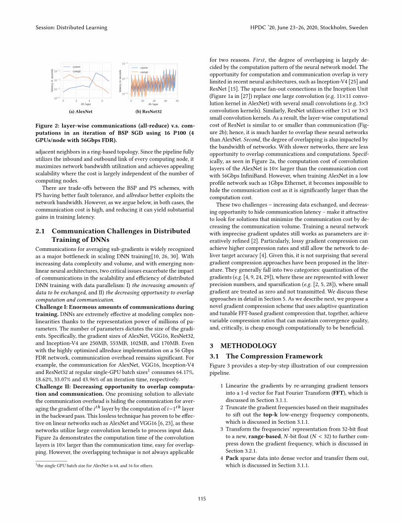
(a) AlexNet

0 20 40 60 80ith layer

10 − 4

10 − 3

10 − 2

late

ncy

inse

cond

s

comm

compt

(b) ResNet32

Figure 2: layer-wise communications (all-reduce) v.s. com-putations in an iteration of BSP SGD using 16 P100 (4GPUs/node with 56Gbps FDR).

adjacent neighbors in a ring-based topology. Since the pipeline fully

utilizes the inbound and outbound link of every computing node, it

maximizes network bandwidth utilization and achieves appealing

scalability where the cost is largely independent of the number of

computing nodes.

There are trade-offs between the BSP and PS schemes, with

PS having better fault tolerance, and allreduce better exploits thenetwork bandwidth. However, as we argue below, in both cases, the

communication cost is high, and reducing it can yield substantial

gains in training latency.

2.1 Communication Challenges in DistributedTraining of DNNs

Communications for averaging sub-gradients is widely recognized

as a major bottleneck in scaling DNN training[10, 26, 30]. With

increasing data complexity and volume, and with emerging non-

linear neural architectures, two critical issues exacerbate the impact

of communications in the scalability and efficiency of distributed

DNN training with data parallelism: I) the increasing amounts ofdata to be exchanged, and II) the decreasing opportunity to overlapcomputation and communication.Challenge I: Enormous amounts of communications duringtraining. DNNs are extremely effective at modeling complex non-

linearities thanks to the representation power of millions of pa-

rameters. The number of parameters dictates the size of the gradi-

ents. Specifically, the gradient sizes of AlexNet, VGG16, ResNet32,

and Inception-V4 are 250MB, 553MB, 102MB, and 170MB. Even

with the highly optimized allreduce implementation on a 56 Gbps

FDR network, communication overhead remains significant. For

example, the communication for AlexNet, VGG16, Inception-V4

and ResNet32 at regular single-GPU batch sizes1consumes 64.17%,

18.62%, 33.07% and 43.96% of an iteration time, respectively.

Challenge II: Decreasing opportunity to overlap computa-tion and communication. One promising solution to alleviate

the communication overhead is hiding the communication for aver-

aging the gradient of the ith layer by the computation of i−1th

layer

in the backward pass. This lossless technique has proven to be effec-

tive on linear networks such as AlexNet and VGG16 [6, 23], as these

networks utilize large convolution kernels to process input data.

Figure 2a demonstrates the computation time of the convolution

layers is 10× larger than the communication time, easy for overlap-

ping. However, the overlapping technique is not always applicable

1the single GPU batch size for AlexNet is 64, and 16 for others.

for two reasons. First , the degree of overlapping is largely de-

cided by the computation pattern of the neural network model. The

opportunity for computation and communication overlap is very

limited in recent neural architectures, such as Inception-V4 [25] and

ResNet [15]. The sparse fan-out connections in the Inception Unit

(Figure 1a in [27]) replace one large convolution (e.g. 11×11 convo-lution kernel in AlexNet) with several small convolutions (e.g. 3×3convolution kernels). Similarly, ResNet utilizes either 1×1 or 3×3small convolution kernels. As a result, the layer-wise computational

cost of ResNet is similar to or smaller than communication (Fig-

ure 2b); hence, it is much harder to overlap these neural networks

than AlexNet. Second , the degree of overlapping is also impacted by

the bandwidth of networks. With slower networks, there are less

opportunity to overlap communications and computations. Specif-

ically, as seen in Figure 2a, the computation cost of convolution

layers of the AlexNet is 10× larger than the communication cost

with 56Gbps InfiniBand. However, when training AlexNet in a low

profile network such as 1Gbps Ethernet, it becomes impossible to

hide the communication cost as it is significantly larger than the

computation cost.

These two challenges – increasing data exchanged, and decreas-

ing opportunity to hide communication latency – make it attractive

to look for solutions that minimize the communication cost by de-

creasing the communication volume. Training a neural network

with imprecise gradient updates still works as parameters are it-

eratively refined [2]. Particularly, lossy gradient compression can

achieve higher compression rates and still allow the network to de-

liver target accuracy [4]. Given this, it is not surprising that several

gradient compression approaches have been proposed in the liter-

ature. They generally fall into two categories: quantization of the

gradients (e.g. [4, 9, 24, 29]), where these are represented with lowerprecision numbers, and sparsification (e.g. [2, 5, 28]), where small

gradient are treated as zero and not transmitted. We discuss these

approaches in detail in Section 5. As we describe next, we propose a

novel gradient compression scheme that uses adaptive quantization

and tunable FFT-based gradient compression that, together, achieve

variable compression ratios that can maintain convergence quality,

and, critically, is cheap enough computationally to be beneficial.

3 METHODOLOGY3.1 The Compression FrameworkFigure 3 provides a step-by-step illustration of our compression

pipeline.

1 Linearize the gradients by re-arranging gradient tensors

into a 1-d vector for Fast Fourier Transform (FFT), which is

discussed in Section 3.1.1.

2 Truncate the gradient frequencies based on their magnitudes

to sift out the top-k low-energy frequency components,

which is discussed in Section 3.1.1.

3 Transform the frequencies’ representation from 32-bit float

to a new, range-based, N -bit float (N < 32) to further com-

press down the gradient frequency, which is discussed in

Section 3.2.1.

4 Pack sparse data into dense vector and transfer them out,

which is discussed in Section 3.1.1.


115

!" !#

!$ !%!" !# !$ !%

!"#$%&"'$()*&%("$#+,

&&' '()*+,-.-/01(2

&$+%"#

&$-./$

34/+ 542!-*64,-7894201:401(2

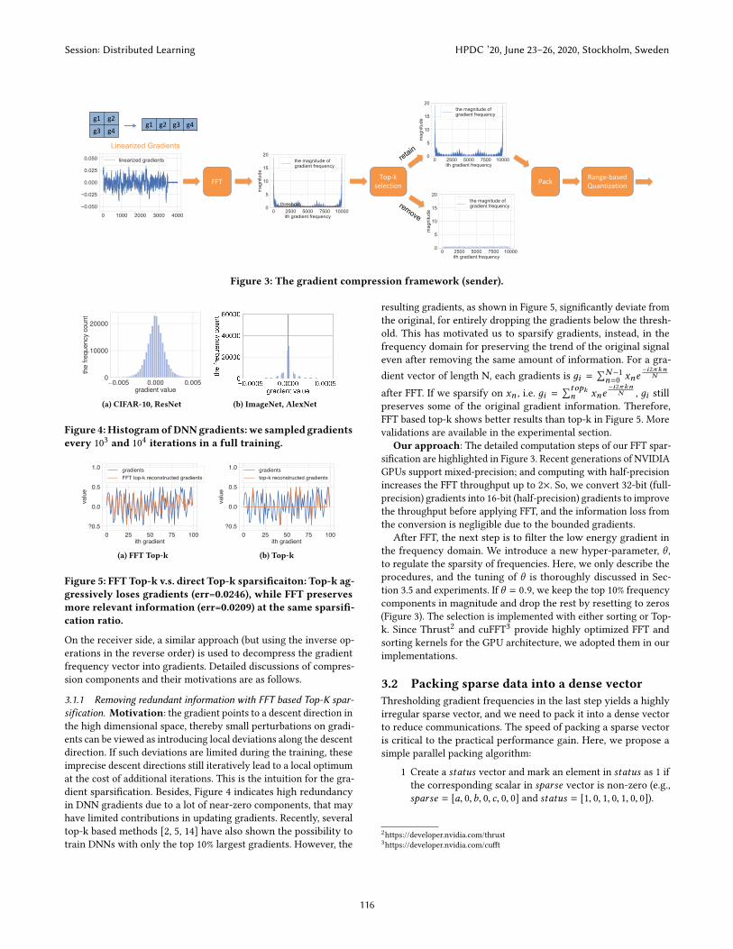
Figure 3: The gradient compression framework (sender).

− 0.005 0.000 0.005gradient value

0

10000

20000

the

frequ

ency

coun

t

(a) CIFAR-10, ResNet (b) ImageNet, AlexNet

Figure 4:HistogramofDNNgradients: we sampled gradientsevery 10

3 and 104 iterations in a full training.

0 25 50 75 100ith gradient

?0.5

0.0

0.5

1.0

valu

e

gradientsFFT top-k reconstructed gradients

(a) FFT Top-k

0 25 50 75 100ith gradient

?0.5

0.0

0.5

1.0

valu

e

gradientstop-k reconstructed gradients

(b) Top-k

Figure 5: FFT Top-k v.s. direct Top-k sparsificaiton: Top-k ag-gressively loses gradients (err=0.0246), while FFT preservesmore relevant information (err=0.0209) at the same sparsifi-cation ratio.

On the receiver side, a similar approach (but using the inverse op-

erations in the reverse order) is used to decompress the gradient

frequency vector into gradients. Detailed discussions of compres-

sion components and their motivations are as follows.

3.1.1 Removing redundant information with FFT based Top-K spar-sification. Motivation: the gradient points to a descent direction inthe high dimensional space, thereby small perturbations on gradi-

ents can be viewed as introducing local deviations along the descent

direction. If such deviations are limited during the training, these

imprecise descent directions still iteratively lead to a local optimum

at the cost of additional iterations. This is the intuition for the gra-

dient sparsification. Besides, Figure 4 indicates high redundancy

in DNN gradients due to a lot of near-zero components, that may

have limited contributions in updating gradients. Recently, several

top-k based methods [2, 5, 14] have also shown the possibility to

train DNNs with only the top 10% largest gradients. However, the

resulting gradients, as shown in Figure 5, significantly deviate from

the original, for entirely dropping the gradients below the thresh-

old. This has motivated us to sparsify gradients, instead, in the

frequency domain for preserving the trend of the original signal

even after removing the same amount of information. For a gra-

dient vector of length N, each gradients is дi =∑N−1

n=0xne

−i2πknN

after FFT. If we sparsify on xn , i.e. дi =∑topkn xne

−i2πknN , дi still

preserves some of the original gradient information. Therefore,

FFT based top-k shows better results than top-k in Figure 5. More

validations are available in the experimental section.

Our approach: The detailed computation steps of our FFT spar-

sification are highlighted in Figure 3. Recent generations of NVIDIA

GPUs support mixed-precision; and computing with half-precision

increases the FFT throughput up to 2×. So, we convert 32-bit (full-precision) gradients into 16-bit (half-precision) gradients to improve

the throughput before applying FFT, and the information loss from

the conversion is negligible due to the bounded gradients.

After FFT, the next step is to filter the low energy gradient in

the frequency domain. We introduce a new hyper-parameter, θ ,to regulate the sparsity of frequencies. Here, we only describe the

procedures, and the tuning of θ is thoroughly discussed in Sec-

tion 3.5 and experiments. If θ = 0.9, we keep the top 10% frequency

components in magnitude and drop the rest by resetting to zeros

(Figure 3). The selection is implemented with either sorting or Top-

k. Since Thrust2and cuFFT

3provide highly optimized FFT and

sorting kernels for the GPU architecture, we adopted them in our

implementations.

3.2 Packing sparse data into a dense vectorThresholding gradient frequencies in the last step yields a highly

irregular sparse vector, and we need to pack it into a dense vector

to reduce communications. The speed of packing a sparse vector

is critical to the practical performance gain. Here, we propose a

simple parallel packing algorithm:

1 Create a status vector and mark an element in status as 1 ifthe corresponding scalar in sparse vector is non-zero (e.g.,

sparse = [a, 0,b, 0, c, 0, 0] and status = [1, 0, 1, 0, 1, 0, 0]).

2https://developer.nvidia.com/thrust

3https://developer.nvidia.com/cufft


116

https://developer.nvidia.com/thrust

https://developer.nvidia.com/cufft

0 25 50 75 100 125 150(total message)/(compressed gradients)

0.000

0.005

0.010

0.015to

tal c

omm

cos

t in

seco

nds

0.97

0.98

0.99

1.00

stat

us/(t

otal

mes

sage

)

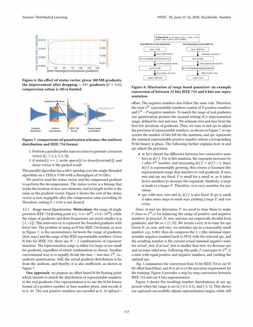
Figure 6: the effect of status vector: given 100 MB gradients,the improvement after dropping > 95% gradients (θ = 0.05,compression ration is 20) is limited.

Uniform quantization

IEEE-754 format

Range based quantization

Gradient distribution

wasted bit efficiency wasted bit efficiency wasted bit efficiency wasted bit efficiency wasted bit efficiency wasted bit efficiency min

max

range

Adjusted by m

Adjusted by m

Figure 7: comparisons of quantization schemes: the uniformdistribution and IEEE 754 format.

2 Perform a parallel prefix-sum on status to generate a locationvector ([1, 1, 2, 2, 3, 3, 3]).

3 if status[i] == 1, write sparse[i] to dense[location[i]], anddense vector is the packed result.

This parallel algorithm has a 689× speedup over the single-threaded

algorithm on a TESLA V100 with a throughput of 34 GB/s.

We need to send the status vector and the compressed gradient

to perform the decompression. The status vector is a bitmap that

tracks the location of non-zero elements, and its length in bits is the

same as the gradient vector. Figure 6 shows the cost of the status

vector is non-negligible after the compression ratio exceeding 20.

Therefore, setting θ < 0.05 is not desired.

3.2.1 Range based Quantization. Motivation: the range of singleprecision IEEE-754 floating point is [−3.4 ∗ 10

38,+3.4 ∗ 1038], while

the range of gradients and their frequencies are much smaller (e.g.

[-1, +1]). This motivates us to represent the bounded gradients with

fewer bits. The problem of using an N bits IEEE 754 format, as seen

in Figure 7, is the inconsistency between the range of gradients

[min,max] and the range of the IEEE representable numbers. Given

N bits for IEEE 754, there are N − 2 combinations of exponent-

mantissa. The representation range is either too large or too small

for gradients, regardless of which combinations to choose. Another

conventional way is to equally divide themax −min into 2N, i.e.,

uniform quantization. Still, the actual gradient distribution is far

from the uniform, and thereby it is also inefficient, as shown in

Figure 7.

Our approach: we propose an offset-based N-bit floating point,

which intends to match the distribution of representable numbers

to the real gradients. Our representation is to use the N-bit binary

format of a positive number as base number pbase , and encode it

to 0...01. The rest positive numbers are encoded as 0...01 (pbase) +

Configurations: m = 3; max = 2; min = -2; eps = 0.125pbase = eps >> (23-3) = 001111100000

input = 0.256

00111110100000110001001001101111

001111101000

output = 00001001

input = 00001001

output = 0.25

001111101000

00111110100000000000000000000000

Dec to IEEE-754 Bin

cut off the rightmost 20 bits

minus pbase, and add 1

add pbase, and minus 1

fill the rightmost 20 bits with 0

IEEE-754 Bin to Dec

32-bit IEEE-754 to 8-bit offset-based 8-bit offset-based to 32-bit IEEE-754

Figure 8: Illustration of range based quantizer: an exampleconversion of between 32 bits IEEE 754 and 8 bits our repre-sentation.

offset. The negative numbers also follow the same rule. Therefore,

the total 2N

representable numbers consist of P positive numbers

and 2N −P negative numbers. To match the range of real gradients,

our quantization permits the manual setting of a representation

range, defined bymin andmax . We estimatemin andmax from the

first few iterations of gradients. Then, we tunem and eps to adjust

the precision of representable numbers, as shown in Figure 7.m rep-

resents the number of bits left for the mantissa, and eps representsthe minimal representable positive number whose corresponding

N-bit binary is pbase . The following further explains howm and

eps adjust the precision:

• m: let’s denote the difference between two consecutive num-

bers as di f f . Form bits mantissa, the exponent increases by

1 after 2m

number, and increasing di f f = di f f ∗ 2. Since

di f f is exponentially growing, this creates a Gaussian like

representation range that matches to real gradients. Ifmax ,min and eps are fixed, P is small for a smallm, as it takes

fewer numbers to increase the exponent. Similarly, a large

m leads to a larger P . Therefore,m is very sensitive for pre-

cision.

• eps : withmax ,min andm, di f f is also fixed. If eps is small,

it takes more steps to reachmax yielding a large P ; and vice

versa.

Since m and eps determine P , we need to tune them to make

P close to 2N /2 for balancing the range of positive and negative

numbers. In practice, N ,min, andmax are empirically decided from

gradients, and them ∈ [1,N ]. We iterate everym to tune for eps.

Given N ,m,min, andmax , we initialize eps as a reasonably small

number, e.g., 0.002, then de-compress the 1..1 (the minimal repre-

sentable negative number) back to FP32 with the selected eps , andthe resulting number is the current actual minimal negative num-

ber actual_min; if actual_min is smaller thanmin, we decrease eps ,and increase otherwise. Following this path, P converges to 2

N /2,

a state with equal positive and negative numbers, and yielding the

optimal eps .Alg. 1 summarizes the conversion from 32-bit IEEE 754 to our N-

bit offset based float, and N is set w.r.t the precision requirement for

the training. Figure 8 provides a step-by-step conversion between

IEEE 754 and our 8 bits representation.

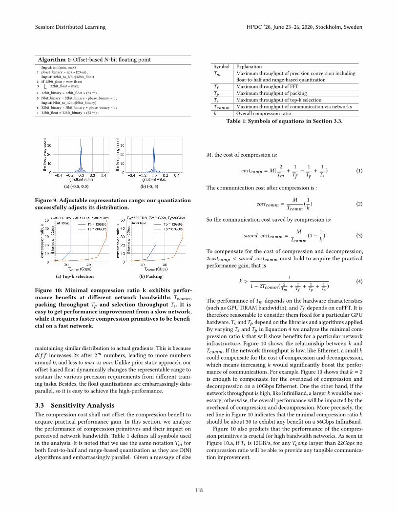
Figure 9 shows the resulting number distributions of our ap-

proach when the range is set to [-0.5, 0.5], and [-5, 5]. This shows

our approach successfully adjusts representation ranges, while still


117

Algorithm 1: Offset-based N -bit floating point

Input: init(min, max)

1 pbase_binary = eps » (23-m) ;

Input: 32bit_to_Nbit(32bit_float)2 if 32bit_float > max then3 32bit_float = max;

4 32bit_binary = 32bit_float » (23-m) ;

5 Nbit_binary = 32bit_binary - pbase_binary + 1 ;

Input: Nbit_to_32bit(Nbit_binary)6 32bit_binary = Nbit_binary + pbase_binary - 1 ;

7 32bit_float = 32bit_binary « (23-m) ;

(a) (-0.5, 0.5) (b) (-5, 5)

Figure 9: Adjustable representation range: our quantizationsuccessfully adjusts its distribution.

(a) Top-k selection (b) Packing

Figure 10: Minimal compression ratio k exhibits perfor-mance benefits at different network bandwidths Tcomm ,packing throughput Tp and selection throughput Ts . It iseasy to get performance improvement from a slow network,while it requires faster compression primitives to be benefi-cial on a fast network.

maintaining similar distribution to actual gradients. This is because

di f f increases 2x after 2m

numbers, leading to more numbers

around 0, and less tomax ormin. Unlike prior static approach, ouroffset based float dynamically changes the representable range to

sustain the various precision requirements from different train-

ing tasks. Besides, the float quantizations are embarrassingly data-

parallel, so it is easy to achieve the high-performance.

3.3 Sensitivity AnalysisThe compression cost shall not offset the compression benefit to

acquire practical performance gain. In this section, we analyze

the performance of compression primitives and their impact on

perceived network bandwidth. Table 1 defines all symbols used

in the analysis. It is noted that we use the same notation Tm for

both float-to-half and range-based quantization as they are O(N)

algorithms and embarrassingly parallel. Given a message of size

Symbol Explanation

Tm Maximum throughput of precision conversion including

float-to-half and range-based quantization

Tf Maximum throughput of FFT

Tp Maximum throughput of packing

Ts Maximum throughput of top-k selection

Tcomm Maximum throughput of communication via networks

k Overall compression ratio

Table 1: Symbols of equations in Section 3.3.

M , the cost of compression is:

costcomp = M( 2

Tm+

1

Tf+

1

Tp+

1

Ts) (1)

The communication cost after compression is :

costcomm =M

Tcomm( 1

k) (2)

So the communication cost saved by compression is:

saved_costcomm =M

Tcomm(1 − 1

k) (3)

To compensate for the cost of compression and decompression,

2costcomp < saved_costcomm must hold to acquire the practical

performance gain, that is

k >1

1 − 2Tcomm ( 2

Tm +1

Tf+ 1

Tp +1

Ts )(4)

The performance of Tm depends on the hardware characteristics

(such as GPU DRAM bandwidth), and Tf depends on cuFFT. It is

therefore reasonable to consider them fixed for a particular GPU

hardware.Ts andTp depend on the libraries and algorithms applied.

By varying Ts and Tp in Equation 4 we analyze the minimal com-

pression ratio k that will show benefits for a particular network

infrastructure. Figure 10 shows the relationship between k and

Tcomm . If the network throughput is low, like Ethernet, a small kcould compensate for the cost of compression and decompression,

which means increasing k would significantly boost the perfor-

mance of communications. For example, Figure 10 shows that k = 2

is enough to compensate for the overhead of compression and

decompression on a 10Gbps Ethernet. One the other hand, if the

network throughput is high, like InfiniBand, a largerk would be nec-

essary; otherwise, the overall performance will be impacted by the

overhead of compression and decompression. More precisely, the

red line in Figure 10 indicates that the minimal compression ratio kshould be about 30 to exhibit any benefit on a 56Gbps InfiniBand.

Figure 10 also predicts that the performance of the compres-

sion primitives is crucial for high bandwidth networks. As seen in

Figure 10.a, if Ts is 12GB/s, for any Tcomp larger than 22Gbps nocompression ratio will be able to provide any tangible communica-

tion improvement.


118

3.4 Convergence AnalysisIn order to analyse the convergence of our proposed technique we

formulate the DNN training as:

min

xf (x) :=

1

N

N∑i=1

fi (x), (5)

where fi is the loss of one data sample to a network. For non-convex

optimization, it is sufficient to prove the convergence by showing

∥∇f (xt )∥2 ≤ ϵ as t → ∞, where ϵ is a small constant and t is theiteration. The condition indicates the function converges to the

neighborhood of a stationary point. Before stating the theorem, we

need to introduce the notion of Lipschitz continuity. f (x) is smooth

and non-convex, and ∇f are L-Lipschitz continuous. Namely,

∥∇f (x) − ∇f (y)∥ ≤ L∥x − y∥.

For any x,y,

f (y) ≤ f (x) + ⟨∇f (x),y − x⟩ +L

2

∥x − y∥2.

Assumption 3.1. Suppose j is a uniform random sample from{1, ...,N }, then we make the following bounded variance assumption:

E[∥∇fj (x) − ∇f (x)∥2] ≤ σ 2, for any x .

This is a standard assumption widely adopted in the SGD con-

vergence proof [21] [13]. It holds if the gradient is bounded.

Assumption 3.2. In the data-parallel training, the gradient ofeach iteration is v̄ = 1

p∑p

1vi ; p is the number of processes, and

vi is the gradient from the ith process. Let’s denote θ ∈ [0, 1] tocontrol the percentage of information loss in the compression functionv̂i = T (vi , θ ) that does quant(FFT-sparsification(vi )), so ¯v̂ =

∑p1v̂i .

We assume there exists a α such that:

∥v̄ − ¯v̂ ∥ ≤ α ∥v̄ ∥.

So, v̂ only loses a small amount of information with respect to

v̄ , and the update from the sparsified gradient is within a bounded

error range of true gradient update. It is a necessary condition for

deriving the upper bound.

With our compression techniques, one SGD update becomes:

xt+1 = xt − ηt (1

P

p∑1

v̂i ) = xt − ηt ¯v̂t . (6)

Then, we have the following lemma for one step:

Lemma 3.3. Assume ηt ≤ 1

4L , θ2

t ≤ 1

4. Then

ηt4

E[∥∇f (xt )∥2] ≤ E[f (xt )] − E[f (xt+1)] + (Lηt + θ2

t )ηtσ

2

2bt. (7)

Please check the supplemental material for the proof of this

lemma. Summing over (7) for K iterations, we get:∑K−1

t=0ηtE[ ∥∇f (x t ) ∥2]≤4(f (x 0)−f (xK ))+

∑K−1

t=1(Lηt+θ 2

t )2ηt σ 2

bt. (8)

Next, we present the convergence theorem.

Theorem 3.4. If we choose a fixed learning rate, ηt = η; a fixeddropout ratio in the sparsification function, θt = θ ; and a fixed mini-batch size, bt = b; then the following holds:

min0≤t≤K−1 E[ ∥∇f (x t ) ∥2]≤4(f (x0)−f (xK−1))

K +(Lη+θ 2)2ησ 2

b .

Proof. min0≤t ≤K−1 E[∥∇f (xt )∥2] ≤ 1

K∑K−1

t=0ηtE[∥∇f (xt )∥2], as

∥∇f (xt )∥2 ≥ 0. By (8), we get the theorem. □

Theorem 3.5. If we apply the diminishing stepsize, ηt , satisfying∑∞t=0

ηt = ∞,∑∞t=0

η2

t < ∞, our compression algorithm guaranteesconvergence with a diminishing drop-out ratio, θt , if θ2

t = Lηt .

Proof. If we randomly choose the output, xout , from {x0, ..., xK−1},

with probabilityηt∑K−1

t=0ηt

for xt , then we have:

E[∥∇f (xout )∥2] =

∑K−1

t=0ηtE[ ∥∇f (x t ) ∥2]∑K−1

t=0ηt

(9)

≤4(f (x 0)−f (x ∗)∑K−1

t=0ηt

+

∑K−1

t=0(Lηt+θ 2

t )2ηtσ2

b∑K−1

t=0ηt

. (10)

Note that

∑K−1

t=0ηt → ∞, while∑K−1

t=0(Lηt + θ

2

t )2ηtσ2 =

∑K−1

t=04Lη2

tσ2 < ∞,

and we have E[∥∇f (xout )∥2] → 0. □

4 EVALUATIONOur experiments consist of two parts to assess the proposed tech-

niques. First, we validate the convergence theory and its assump-

tions with AlexNet on ImageNet and ResNet32 on CIFAR10, which

sufficiently cover typical workloads in traditional linear and re-

cent non-linear neural architectures, and also provide coverage

on two widely used datasets. Then, we show that the FFT-based

method demonstrates better convergence and faster compression

than other state-of-the-art compression methods such as QSGD [4],

TernGrad [29], Top-k sparsification [5, 20], as our techniques incur

fewer approximation errors, while still delivering a competitive

compression ratio for using both sparsification and quantization.

Parallelization scheme: we choose BSP for parallelization for

its simplicity in the theoretical analysis: BSP follows strict syn-

chronizations, allowing us to better observe the effects of gradient

compression toward the convergence by iterations.

Implementation: we implemented our approach, losses SGD(no

compression), QSGD, Top-K, and TernGrad in a C++ DL framework,

SuperNeurons [27]; We used the allgather collective from NVIDIA

NCCL2 to exchange compressed gradients since existing communi-

cation libraries lack the support for sparse all-reduce (Figure 1a).

Even though SGD usually uses allreduce instead of allgather as

it does not have compression; for a fair comparison, we applied

allgather for all algorithms to demonstrate the algorithmic benefit

of our FFT compression. Every GPU has a copy of global gradients

for updating parameters after all-gather local gradients. Parame-

ters need to be synchronized after multiple iterations to eliminate

the precision errors, and here we broadcast parameters every 10

iterations. It is noticed that we did not adopt communication and

computation overlapping strategy as it could be another optimiza-

tion method orthogonal to compression, and is not in the scope of

this paper.

Training setup: The single GPU batch is set to 128 and 64

for ResNet32 and AlexNet, respectively. The momentum for both

networks is set to 0.9. The learning rate for Resnet32 is 0.01 at epochs

∈ [0, 130], and 0.001 afterwards; the learning rate for AlexNet is 0.01

at epochs ∈ [0, 30], 0.001 at epochs ∈ [30, 60], and 0.0001 afterwards.


119

0 10 20 30#GPUs

0

1

2

3

4

late

ncy/

seco

nds

all-gather AlexNet, 250MBcompute

(a) AlexNet

0 10 20 30#GPUs

0.00

0.05

0.10

0.15

0.20

0.25

late

ncy/

seco

nds

all-gather ResNet32, 6MBcompute

(b) ResNet32

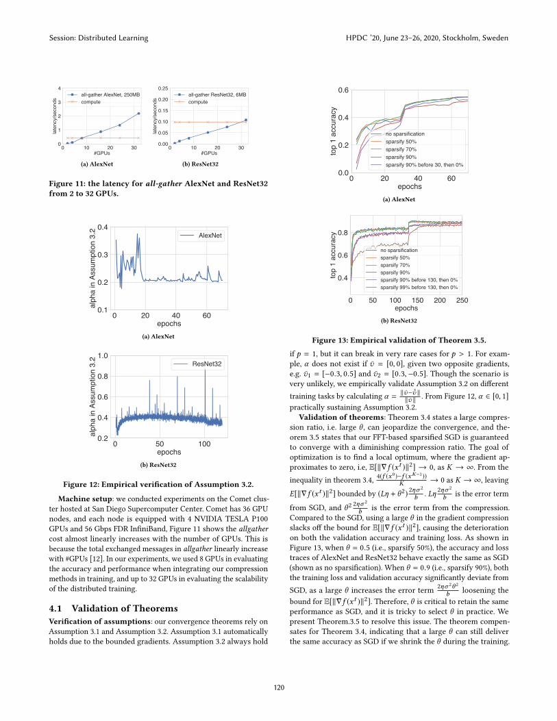
Figure 11: the latency for all-gather AlexNet and ResNet32from 2 to 32 GPUs.

0 20 40 60epochs

0.1

0.2

0.3

0.4

alph

a in

Ass

umpt

ion

3.2

AlexNet

(a) AlexNet

0 50 100epochs

0.2

0.4

0.6

0.8

1.0

alph

a in

Ass

umpt

ion

3.2

ResNet32

(b) ResNet32

Figure 12: Empirical verification of Assumption 3.2.

Machine setup: we conducted experiments on the Comet clus-

ter hosted at San Diego Supercomputer Center. Comet has 36 GPU

nodes, and each node is equipped with 4 NVIDIA TESLA P100

GPUs and 56 Gbps FDR InfiniBand, Figure 11 shows the allgathercost almost linearly increases with the number of GPUs. This is

because the total exchanged messages in allgather linearly increase

with #GPUs [12]. In our experiments, we used 8 GPUs in evaluating

the accuracy and performance when integrating our compression

methods in training, and up to 32 GPUs in evaluating the scalability

of the distributed training.

4.1 Validation of TheoremsVerification of assumptions: our convergence theorems rely on

Assumption 3.1 and Assumption 3.2. Assumption 3.1 automatically

holds due to the bounded gradients. Assumption 3.2 always hold

0 20 40 60epochs

0.0

0.2

0.4

0.6

top

1 ac

cura

cy

no sparsificationsparsify 50%sparsify 70%sparsify 90%sparsify 90% before 30, then 0%

(a) AlexNet

0 50 100 150 200 250epochs

0.4

0.6

0.8

top

1 ac

cura

cy

no sparsificationsparsify 50%sparsify 70%sparsify 90%sparsify 90% before 130, then 0%sparsify 99% before 130, then 0%

(b) ResNet32

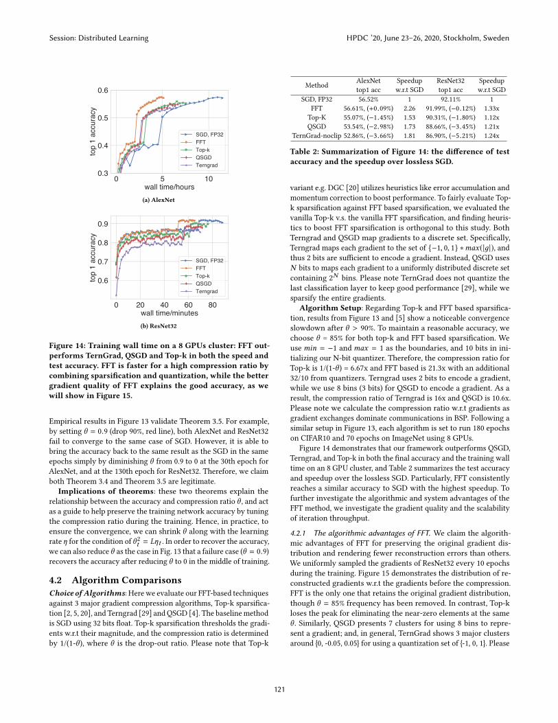
Figure 13: Empirical validation of Theorem 3.5.

if p = 1, but it can break in very rare cases for p > 1. For exam-

ple, α does not exist if v̄ = [0, 0], given two opposite gradients,

e.g. v̄1 = [−0.3, 0.5] and v̄2 = [0.3,−0.5]. Though the scenario is

very unlikely, we empirically validate Assumption 3.2 on different

training tasks by calculating α = ‖v̄− ¯v̂ ‖‖v̄ ‖ . From Figure 12, α ∈ [0, 1]

practically sustaining Assumption 3.2.

Validation of theorems: Theorem 3.4 states a large compres-

sion ratio, i.e. large θ , can jeopardize the convergence, and the-

orem 3.5 states that our FFT-based sparsified SGD is guaranteed

to converge with a diminishing compression ratio. The goal of

optimization is to find a local optimum, where the gradient ap-

proximates to zero, i.e, E[‖∇f (xt )‖2] → 0, as K → ∞. From the

inequality in theorem 3.4,4(f (x 0)−f (xK−1))

K → 0 as K → ∞, leaving

E[‖∇f (xt )‖2] bounded by (Lη + θ2) 2ησ 2

b . Lη2ησ 2

b is the error term

from SGD, and θ2 2ησ 2

b is the error term from the compression.

Compared to the SGD, using a large θ in the gradient compression

slacks off the bound for E[‖∇f (xt )‖2], causing the deterioration

on both the validation accuracy and training loss. As shown in

Figure 13, when θ = 0.5 (i.e., sparsify 50%), the accuracy and loss

traces of AlexNet and ResNet32 behave exactly the same as SGD

(shown as no sparsification). When θ = 0.9 (i.e., sparsify 90%), both

the training loss and validation accuracy significantly deviate from

SGD, as a large θ increases the error term2ησ 2θ 2

b loosening the

bound for E[‖∇f (xt )‖2]. Therefore, θ is critical to retain the same

performance as SGD, and it is tricky to select θ in practice. We

present Theorem.3.5 to resolve this issue. The theorem compen-

sates for Theorem 3.4, indicating that a large θ can still deliver

the same accuracy as SGD if we shrink the θ during the training.


120

0 5 10wall time/hours

0.3

0.4

0.5

0.6to

p 1

accu

racy

SGD, FP32FFTTop-kQSGDTerngrad

(a) AlexNet

0 20 40 60 80wall time/minutes

0.6

0.7

0.8

0.9

top

1 ac

cura

cy

SGD, FP32FFTTop-kQSGDTerngrad

(b) ResNet32

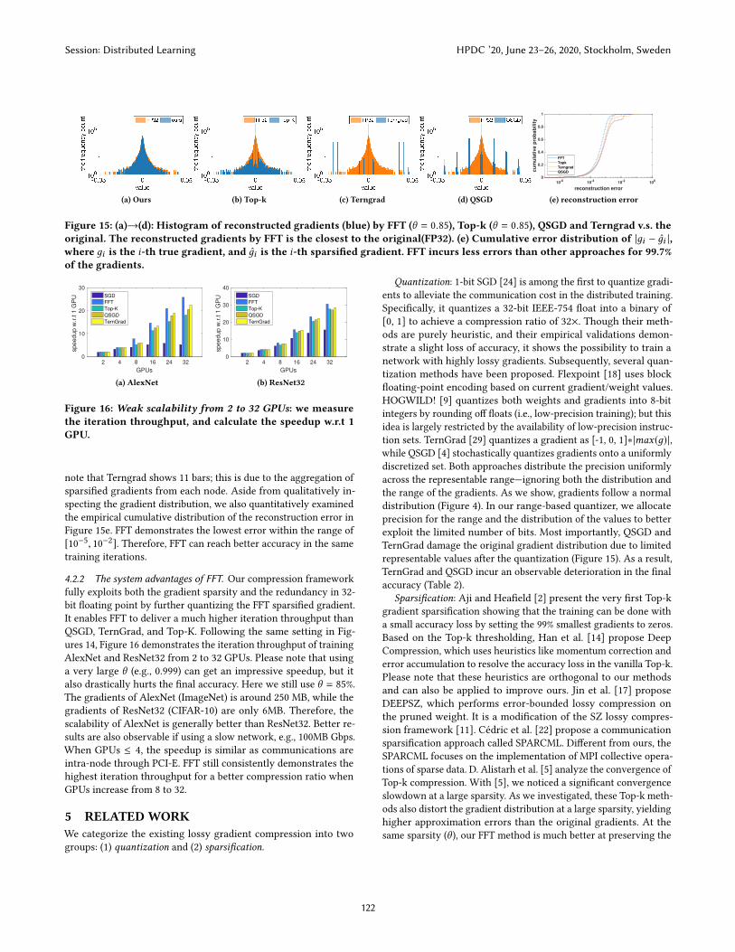
Figure 14: Training wall time on a 8 GPUs cluster: FFT out-performs TernGrad, QSGD and Top-k in both the speed andtest accuracy. FFT is faster for a high compression ratio bycombining sparsification and quantization, while the bettergradient quality of FFT explains the good accuracy, as wewill show in Figure 15.

Empirical results in Figure 13 validate Theorem 3.5. For example,

by setting θ = 0.9 (drop 90%, red line), both AlexNet and ResNet32

fail to converge to the same case of SGD. However, it is able to

bring the accuracy back to the same result as the SGD in the same

epochs simply by diminishing θ from 0.9 to 0 at the 30th epoch for

AlexNet, and at the 130th epoch for ResNet32. Therefore, we claim

both Theorem 3.4 and Theorem 3.5 are legitimate.

Implications of theorems: these two theorems explain the

relationship between the accuracy and compression ratio θ , and actas a guide to help preserve the training network accuracy by tuning

the compression ratio during the training. Hence, in practice, to

ensure the convergence, we can shrink θ along with the learning

rate η for the condition of θ2

t = Lηt . In order to recover the accuracy,we can also reduce θ as the case in Fig. 13 that a failure case (θ = 0.9)

recovers the accuracy after reducing θ to 0 in the middle of training.

4.2 Algorithm ComparisonsChoice of Algorithms: Here we evaluate our FFT-based techniquesagainst 3 major gradient compression algorithms, Top-k sparsifica-

tion [2, 5, 20], and Terngrad [29] andQSGD [4]. The baselinemethod

is SGD using 32 bits float. Top-k sparsification thresholds the gradi-

ents w.r.t their magnitude, and the compression ratio is determined

by 1/(1-θ ), where θ is the drop-out ratio. Please note that Top-k

Method

AlexNet

top1 acc

Speedup

w.r.t SGD

ResNet32

top1 acc

Speedup

w.r.t SGD

SGD, FP32 56.52% 1 92.11% 1

FFT 56.61%, (+0.09%) 2.26 91.99%, (−0.12%) 1.33x

Top-K 55.07%, (−1.45%) 1.53 90.31%, (−1.80%) 1.12x

QSGD 53.54%, (−2.98%) 1.73 88.66%, (−3.45%) 1.21x

TernGrad-noclip 52.86%, (−3.66%) 1.81 86.90%, (−5.21%) 1.24x

Table 2: Summarization of Figure 14: the difference of testaccuracy and the speedup over lossless SGD.

variant e.g. DGC [20] utilizes heuristics like error accumulation and

momentum correction to boost performance. To fairly evaluate Top-

k sparsification against FFT based sparsification, we evaluated the

vanilla Top-k v.s. the vanilla FFT sparsification, and finding heuris-

tics to boost FFT sparsification is orthogonal to this study. Both

Terngrad and QSGD map gradients to a discrete set. Specifically,

Terngrad maps each gradient to the set of {−1, 0, 1} ∗max(|д |), andthus 2 bits are sufficient to encode a gradient. Instead, QSGD uses

N bits to maps each gradient to a uniformly distributed discrete set

containing 2N

bins. Please note TernGrad does not quantize the

last classification layer to keep good performance [29], while we

sparsify the entire gradients.

Algorithm Setup: Regarding Top-k and FFT based sparsifica-

tion, results from Figure 13 and [5] show a noticeable convergence

slowdown after θ > 90%. To maintain a reasonable accuracy, we

choose θ = 85% for both top-k and FFT based sparsification. We

usemin = −1 andmax = 1 as the boundaries, and 10 bits in ini-

tializing our N-bit quantizer. Therefore, the compression ratio for

Top-k is 1/(1-θ ) = 6.67x and FFT based is 21.3x with an additional

32/10 from quantizers. Terngrad uses 2 bits to encode a gradient,

while we use 8 bins (3 bits) for QSGD to encode a gradient. As a

result, the compression ratio of Terngrad is 16x and QSGD is 10.6x.

Please note we calculate the compression ratio w.r.t gradients as

gradient exchanges dominate communications in BSP. Following a

similar setup in Figure 13, each algorithm is set to run 180 epochs

on CIFAR10 and 70 epochs on ImageNet using 8 GPUs.

Figure 14 demonstrates that our framework outperforms QSGD,

Terngrad, and Top-k in both the final accuracy and the training wall

time on an 8 GPU cluster, and Table 2 summarizes the test accuracy

and speedup over the lossless SGD. Particularly, FFT consistently

reaches a similar accuracy to SGD with the highest speedup. To

further investigate the algorithmic and system advantages of the

FFT method, we investigate the gradient quality and the scalability

of iteration throughput.

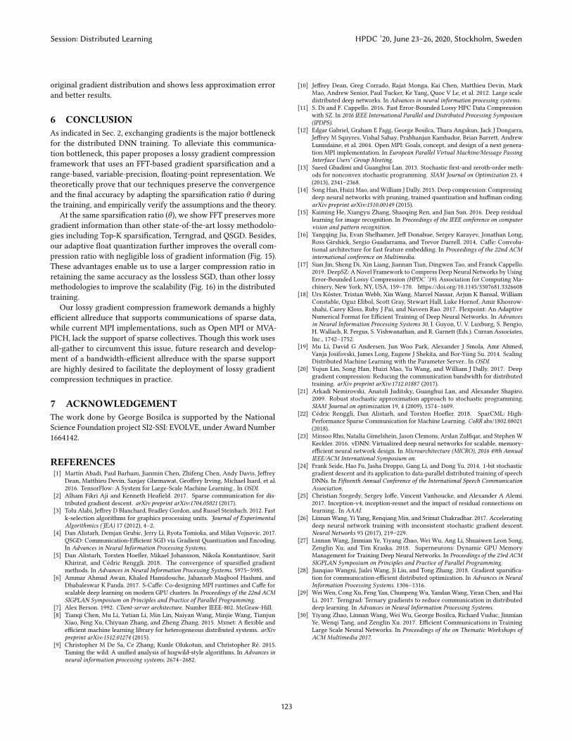
4.2.1 The algorithmic advantages of FFT. We claim the algorith-

mic advantages of FFT for preserving the original gradient dis-

tribution and rendering fewer reconstruction errors than others.

We uniformly sampled the gradients of ResNet32 every 10 epochs

during the training. Figure 15 demonstrates the distribution of re-

constructed gradients w.r.t the gradients before the compression.

FFT is the only one that retains the original gradient distribution,

though θ = 85% frequency has been removed. In contrast, Top-k

loses the peak for eliminating the near-zero elements at the same

θ . Similarly, QSGD presents 7 clusters for using 8 bins to repre-

sent a gradient; and, in general, TernGrad shows 3 major clusters

around {0, -0.05, 0.05} for using a quantization set of {-1, 0, 1}. Please


121

(a) Ours (b) Top-k (c) Terngrad (d) QSGD

10-6

10-4

10-2

100

reconstruction error

0

0.2

0.4

0.6

0.8

1

cu

mu

lati

ve p

rob

ab

ilit

y

FFT

Topk

Terngrad

QSGD

(e) reconstruction error

Figure 15: (a)→(d): Histogram of reconstructed gradients (blue) by FFT (θ = 0.85), Top-k (θ = 0.85), QSGD and Terngrad v.s. theoriginal. The reconstructed gradients by FFT is the closest to the original(FP32). (e) Cumulative error distribution of |дi − д̂i |,where дi is the i-th true gradient, and д̂i is the i-th sparsified gradient. FFT incurs less errors than other approaches for 99.7%of the gradients.

2 4 8 16 24 32

GPUs

0

10

20

30

speedup w

.r.t 1

GP

U SGD

FFT

Top-K

QSGD

TernGrad

(a) AlexNet

2 4 8 16 24 32

GPUs

0

10

20

30

40

speedup w

.r.t 1

GP

U SGD

FFT

Top-K

QSGD

TernGrad

(b) ResNet32

Figure 16: Weak scalability from 2 to 32 GPUs: we measurethe iteration throughput, and calculate the speedup w.r.t 1GPU.

note that Terngrad shows 11 bars; this is due to the aggregation of

sparsified gradients from each node. Aside from qualitatively in-

specting the gradient distribution, we also quantitatively examined

the empirical cumulative distribution of the reconstruction error in

Figure 15e. FFT demonstrates the lowest error within the range of

[10−5, 10

−2]. Therefore, FFT can reach better accuracy in the same

training iterations.

4.2.2 The system advantages of FFT. Our compression framework

fully exploits both the gradient sparsity and the redundancy in 32-

bit floating point by further quantizing the FFT sparsified gradient.

It enables FFT to deliver a much higher iteration throughput than

QSGD, TernGrad, and Top-K. Following the same setting in Fig-

ures 14, Figure 16 demonstrates the iteration throughput of training

AlexNet and ResNet32 from 2 to 32 GPUs. Please note that using

a very large θ (e.g., 0.999) can get an impressive speedup, but it

also drastically hurts the final accuracy. Here we still use θ = 85%.

The gradients of AlexNet (ImageNet) is around 250 MB, while the

gradients of ResNet32 (CIFAR-10) are only 6MB. Therefore, the

scalability of AlexNet is generally better than ResNet32. Better re-

sults are also observable if using a slow network, e.g., 100MB Gbps.

When GPUs ≤ 4, the speedup is similar as communications are

intra-node through PCI-E. FFT still consistently demonstrates the

highest iteration throughput for a better compression ratio when

GPUs increase from 8 to 32.

5 RELATEDWORKWe categorize the existing lossy gradient compression into two

groups: (1) quantization and (2) sparsification.

Quantization: 1-bit SGD [24] is among the first to quantize gradi-

ents to alleviate the communication cost in the distributed training.

Specifically, it quantizes a 32-bit IEEE-754 float into a binary of

[0, 1] to achieve a compression ratio of 32×. Though their meth-

ods are purely heuristic, and their empirical validations demon-

strate a slight loss of accuracy, it shows the possibility to train a

network with highly lossy gradients. Subsequently, several quan-

tization methods have been proposed. Flexpoint [18] uses block

floating-point encoding based on current gradient/weight values.

HOGWILD! [9] quantizes both weights and gradients into 8-bit

integers by rounding off floats (i.e., low-precision training); but this

idea is largely restricted by the availability of low-precision instruc-

tion sets. TernGrad [29] quantizes a gradient as [-1, 0, 1]∗|max(д)|,while QSGD [4] stochastically quantizes gradients onto a uniformly

discretized set. Both approaches distribute the precision uniformly

across the representable range—ignoring both the distribution and

the range of the gradients. As we show, gradients follow a normal

distribution (Figure 4). In our range-based quantizer, we allocate

precision for the range and the distribution of the values to better

exploit the limited number of bits. Most importantly, QSGD and

TernGrad damage the original gradient distribution due to limited

representable values after the quantization (Figure 15). As a result,

TernGrad and QSGD incur an observable deterioration in the final

accuracy (Table 2).

Sparsification: Aji and Heafield [2] present the very first Top-k

gradient sparsification showing that the training can be done with

a small accuracy loss by setting the 99% smallest gradients to zeros.

Based on the Top-k thresholding, Han et al. [14] propose Deep

Compression, which uses heuristics like momentum correction and

error accumulation to resolve the accuracy loss in the vanilla Top-k.

Please note that these heuristics are orthogonal to our methods

and can also be applied to improve ours. Jin et al. [17] propose

DEEPSZ, which performs error-bounded lossy compression on

the pruned weight. It is a modification of the SZ lossy compres-

sion framework [11]. Cédric et al. [22] propose a communication

sparsification approach called SPARCML. Different from ours, the

SPARCML focuses on the implementation of MPI collective opera-

tions of sparse data. D. Alistarh et al. [5] analyze the convergence of

Top-k compression. With [5], we noticed a significant convergence

slowdown at a large sparsity. As we investigated, these Top-k meth-

ods also distort the gradient distribution at a large sparsity, yielding

higher approximation errors than the original gradients. At the

same sparsity (θ ), our FFT method is much better at preserving the


122

original gradient distribution and shows less approximation error

and better results.

6 CONCLUSIONAs indicated in Sec. 2, exchanging gradients is the major bottleneck

for the distributed DNN training. To alleviate this communica-

tion bottleneck, this paper proposes a lossy gradient compression

framework that uses an FFT-based gradient sparsification and a

range-based, variable-precision, floating-point representation. We

theoretically prove that our techniques preserve the convergence

and the final accuracy by adapting the sparsification ratio θ during

the training, and empirically verify the assumptions and the theory.

At the same sparsification ratio (θ ), we show FFT preserves more

gradient information than other state-of-the-art lossy methodolo-

gies including Top-K sparsification, Terngrad, and QSGD. Besides,

our adaptive float quantization further improves the overall com-

pression ratio with negligible loss of gradient information (Fig. 15).

These advantages enable us to use a larger compression ratio in

retaining the same accuracy as the lossless SGD, than other lossy

methodologies to improve the scalability (Fig. 16) in the distributed

training.

Our lossy gradient compression framework demands a highly

efficient allreduce that supports communications of sparse data,

while current MPI implementations, such as Open MPI or MVA-

PICH, lack the support of sparse collectives. Though this work uses

all-gather to circumvent this issue, future research and develop-

ment of a bandwidth-efficient allreduce with the sparse support

are highly desired to facilitate the deployment of lossy gradient

compression techniques in practice.

7 ACKNOWLEDGEMENTThe work done by George Bosilca is supported by the National

Science Foundation project SI2-SSI: EVOLVE, under Award Number

1664142.

REFERENCES[1] Martín Abadi, Paul Barham, Jianmin Chen, Zhifeng Chen, Andy Davis, Jeffrey

Dean, Matthieu Devin, Sanjay Ghemawat, Geoffrey Irving, Michael Isard, et al.

2016. TensorFlow: A System for Large-Scale Machine Learning.. In OSDI.[2] Alham Fikri Aji and Kenneth Heafield. 2017. Sparse communication for dis-

tributed gradient descent. arXiv preprint arXiv:1704.05021 (2017).[3] Tolu Alabi, Jeffrey D Blanchard, Bradley Gordon, and Russel Steinbach. 2012. Fast

k-selection algorithms for graphics processing units. Journal of ExperimentalAlgorithmics (JEA) 17 (2012), 4–2.

[4] Dan Alistarh, Demjan Grubic, Jerry Li, Ryota Tomioka, and Milan Vojnovic. 2017.

QSGD: Communication-Efficient SGD via Gradient Quantization and Encoding.

In Advances in Neural Information Processing Systems.[5] Dan Alistarh, Torsten Hoefler, Mikael Johansson, Nikola Konstantinov, Sarit

Khirirat, and Cédric Renggli. 2018. The convergence of sparsified gradient

methods. In Advances in Neural Information Processing Systems. 5975–5985.[6] Ammar Ahmad Awan, Khaled Hamidouche, Jahanzeb Maqbool Hashmi, and

Dhabaleswar K Panda. 2017. S-Caffe: Co-designing MPI runtimes and Caffe for

scalable deep learning on modern GPU clusters. In Proceedings of the 22nd ACMSIGPLAN Symposium on Principles and Practice of Parallel Programming.

[7] Alex Berson. 1992. Client-server architecture. Number IEEE-802. McGraw-Hill.

[8] Tianqi Chen, Mu Li, Yutian Li, Min Lin, Naiyan Wang, Minjie Wang, Tianjun

Xiao, Bing Xu, Chiyuan Zhang, and Zheng Zhang. 2015. Mxnet: A flexible and

efficient machine learning library for heterogeneous distributed systems. arXivpreprint arXiv:1512.01274 (2015).

[9] Christopher M De Sa, Ce Zhang, Kunle Olukotun, and Christopher Ré. 2015.

Taming the wild: A unified analysis of hogwild-style algorithms. In Advances inneural information processing systems. 2674–2682.

[10] Jeffrey Dean, Greg Corrado, Rajat Monga, Kai Chen, Matthieu Devin, Mark

Mao, Andrew Senior, Paul Tucker, Ke Yang, Quoc V Le, et al. 2012. Large scale

distributed deep networks. In Advances in neural information processing systems.[11] S. Di and F. Cappello. 2016. Fast Error-Bounded Lossy HPC Data Compression

with SZ. In 2016 IEEE International Parallel and Distributed Processing Symposium(IPDPS).

[12] Edgar Gabriel, Graham E Fagg, George Bosilca, Thara Angskun, Jack J Dongarra,

Jeffrey M Squyres, Vishal Sahay, Prabhanjan Kambadur, Brian Barrett, Andrew

Lumsdaine, et al. 2004. Open MPI: Goals, concept, and design of a next genera-

tion MPI implementation. In European Parallel Virtual Machine/Message PassingInterface Users’ Group Meeting.

[13] Saeed Ghadimi and Guanghui Lan. 2013. Stochastic first-and zeroth-order meth-

ods for nonconvex stochastic programming. SIAM Journal on Optimization 23, 4

(2013), 2341–2368.

[14] Song Han, Huizi Mao, andWilliam J Dally. 2015. Deep compression: Compressing

deep neural networks with pruning, trained quantization and huffman coding.

arXiv preprint arXiv:1510.00149 (2015).[15] Kaiming He, Xiangyu Zhang, Shaoqing Ren, and Jian Sun. 2016. Deep residual

learning for image recognition. In Proceedings of the IEEE conference on computervision and pattern recognition.

[16] Yangqing Jia, Evan Shelhamer, Jeff Donahue, Sergey Karayev, Jonathan Long,

Ross Girshick, Sergio Guadarrama, and Trevor Darrell. 2014. Caffe: Convolu-

tional architecture for fast feature embedding. In Proceedings of the 22nd ACMinternational conference on Multimedia.

[17] Sian Jin, Sheng Di, Xin Liang, Jiannan Tian, Dingwen Tao, and Franck Cappello.

2019. DeepSZ: A Novel Framework to Compress Deep Neural Networks by Using

Error-Bounded Lossy Compression (HPDC ’19). Association for Computing Ma-

chinery, New York, NY, USA, 159–170. https://doi.org/10.1145/3307681.3326608

[18] Urs Köster, Tristan Webb, Xin Wang, Marcel Nassar, Arjun K Bansal, William

Constable, Oguz Elibol, Scott Gray, Stewart Hall, Luke Hornof, Amir Khosrow-

shahi, Carey Kloss, Ruby J Pai, and Naveen Rao. 2017. Flexpoint: An Adaptive

Numerical Format for Efficient Training of Deep Neural Networks. In Advancesin Neural Information Processing Systems 30, I. Guyon, U. V. Luxburg, S. Bengio,H. Wallach, R. Fergus, S. Vishwanathan, and R. Garnett (Eds.). Curran Associates,

Inc., 1742–1752.

[19] Mu Li, David G Andersen, Jun Woo Park, Alexander J Smola, Amr Ahmed,

Vanja Josifovski, James Long, Eugene J Shekita, and Bor-Yiing Su. 2014. Scaling

Distributed Machine Learning with the Parameter Server.. In OSDI.[20] Yujun Lin, Song Han, Huizi Mao, Yu Wang, and William J Dally. 2017. Deep

gradient compression: Reducing the communication bandwidth for distributed

training. arXiv preprint arXiv:1712.01887 (2017).

[21] Arkadi Nemirovski, Anatoli Juditsky, Guanghui Lan, and Alexander Shapiro.

2009. Robust stochastic approximation approach to stochastic programming.

SIAM Journal on optimization 19, 4 (2009), 1574–1609.

[22] Cédric Renggli, Dan Alistarh, and Torsten Hoefler. 2018. SparCML: High-

Performance Sparse Communication for Machine Learning. CoRR abs/1802.08021

(2018).

[23] Minsoo Rhu, Natalia Gimelshein, Jason Clemons, Arslan Zulfiqar, and Stephen W

Keckler. 2016. vDNN: Virtualized deep neural networks for scalable, memory-

efficient neural network design. In Microarchitecture (MICRO), 2016 49th AnnualIEEE/ACM International Symposium on.

[24] Frank Seide, Hao Fu, Jasha Droppo, Gang Li, and Dong Yu. 2014. 1-bit stochastic

gradient descent and its application to data-parallel distributed training of speech

DNNs. In Fifteenth Annual Conference of the International Speech CommunicationAssociation.

[25] Christian Szegedy, Sergey Ioffe, Vincent Vanhoucke, and Alexander A Alemi.

2017. Inception-v4, inception-resnet and the impact of residual connections on

learning.. In AAAI.[26] LinnanWang, Yi Yang, Renqiang Min, and Srimat Chakradhar. 2017. Accelerating

deep neural network training with inconsistent stochastic gradient descent.

Neural Networks 93 (2017), 219–229.[27] Linnan Wang, Jinmian Ye, Yiyang Zhao, Wei Wu, Ang Li, Shuaiwen Leon Song,

Zenglin Xu, and Tim Kraska. 2018. Superneurons: Dynamic GPU Memory

Management for Training Deep Neural Networks. In Proceedings of the 23rd ACMSIGPLAN Symposium on Principles and Practice of Parallel Programming.

[28] Jianqiao Wangni, Jialei Wang, Ji Liu, and Tong Zhang. 2018. Gradient sparsifica-

tion for communication-efficient distributed optimization. In Advances in NeuralInformation Processing Systems. 1306–1316.

[29] Wei Wen, Cong Xu, Feng Yan, ChunpengWu, YandanWang, Yiran Chen, and Hai

Li. 2017. Terngrad: Ternary gradients to reduce communication in distributed

deep learning. In Advances in Neural Information Processing Systems.[30] Yiyang Zhao, Linnan Wang, Wei Wu, George Bosilca, Richard Vuduc, Jinmian

Ye, Wenqi Tang, and Zenglin Xu. 2017. Efficient Communications in Training

Large Scale Neural Networks. In Proceedings of the on Thematic Workshops ofACM Multimedia 2017.


123

https://doi.org/10.1145/3307681.3326608

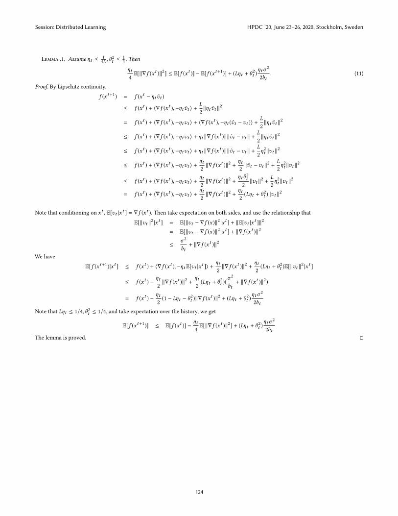
Lemma .1. Assume ηt ≤ 1

4L , θ2

t ≤ 1

4. Then

ηt4

E[∥∇f (xt )∥2] ≤ E[f (xt )] − E[f (xt+1)] + (Lηt + θ2

t )ηtσ

2

2bt. (11)

Proof. By Lipschitz continuity,

f (xt+1) = f (xt − ηt v̂t )

≤ f (xt ) + ⟨∇f (xt ),−ηt v̂t ⟩ +L

2

∥ηt v̂t ∥2

= f (xt ) + ⟨∇f (xt ),−ηtvt ⟩ + ⟨∇f (xt ),−ηt (v̂t −vt )⟩ +L

2

∥ηt v̂t ∥2

≤ f (xt ) + ⟨∇f (xt ),−ηtvt ⟩ + ηt ∥∇f (xt )∥∥v̂t −vt ∥ +L

2

∥ηt v̂t ∥2

≤ f (xt ) + ⟨∇f (xt ),−ηtvt ⟩ + ηt ∥∇f (xt )∥∥v̂t −vt ∥ +L

2

η2

t ∥vt ∥2

≤ f (xt ) + ⟨∇f (xt ),−ηtvt ⟩ +ηt2

∥∇f (xt )∥2 +ηt2

∥v̂t −vt ∥2 +

L

2

η2

t ∥vt ∥2

≤ f (xt ) + ⟨∇f (xt ),−ηtvt ⟩ +ηt2

∥∇f (xt )∥2 +ηtθ

2

t2

∥vt ∥2 +

L

2

η2

t ∥vt ∥2

= f (xt ) + ⟨∇f (xt ),−ηtvt ⟩ +ηt2

∥∇f (xt )∥2 +ηt2

(Lηt + θ2

t )∥vt ∥2

Note that conditioning on xt , E[vt |xt ] = ∇f (xt ). Then take expectation on both sides, and use the relationship that

E[∥vt ∥2 |xt ] = E[∥vt − ∇f (x)∥2 |xt ] + ∥E[vt |x

t ]∥2

= E[∥vt − ∇f (x)∥2 |xt ] + ∥∇f (xt )∥2

≤σ 2

bt+ ∥∇f (xt )∥2

We have

E[f (xt+1)|xt ] ≤ f (xt ) + ⟨∇f (xt ),−ηtE[vt |xt ]⟩ +

ηt2

∥∇f (xt )∥2 +ηt2

(Lηt + θ2

t )E[∥vt ∥2 |xt ]

≤ f (xt ) −ηt2

∥∇f (xt )∥2 +ηt2

(Lηt + θ2

t )(σ 2

bt+ ∥∇f (xt )∥2)

= f (xt ) −ηt2

(1 − Lηt − θ2

t )∥∇f (xt )∥2 + (Lηt + θ2

t )ηtσ

2

2bt

Note that Lηt ≤ 1/4, θ2

t ≤ 1/4, and take expectation over the history, we get

E[f (xt+1)] ≤ E[f (xt )] −ηt4

E[∥∇f (xt )∥2] + (Lηt + θ2

t )ηtσ

2

2btThe lemma is proved. □


124

Documents

FFT-based Gradient Sparsification for the Distributed