Embed Size (px)
Citation preview

Fast Finite Shearlet Transform: a tutorial
Soren Hauser∗
February 8, 2012
Contents
1 Introduction 1
2 Shearlet transform 32.1 Some functions and their properties . . . . . . . . . . . . . . . . . . . . . . . . 32.2 The continuous shearlet transform . . . . . . . . . . . . . . . . . . . . . . . . . 82.3 Shearlets on the cone . . . . . . . . . . . . . . . . . . . . . . . . . . . . . . . . . 92.4 Scaling function . . . . . . . . . . . . . . . . . . . . . . . . . . . . . . . . . . . . 12
3 Computation of the shearlet transform 133.1 Finite discrete shearlets . . . . . . . . . . . . . . . . . . . . . . . . . . . . . . . 143.2 A discrete shearlet frame . . . . . . . . . . . . . . . . . . . . . . . . . . . . . . . 163.3 Inversion of the shearlet transform . . . . . . . . . . . . . . . . . . . . . . . . . 203.4 Smooth shearlets . . . . . . . . . . . . . . . . . . . . . . . . . . . . . . . . . . . 213.5 Implementation details . . . . . . . . . . . . . . . . . . . . . . . . . . . . . . . . 26
3.5.1 Indexing . . . . . . . . . . . . . . . . . . . . . . . . . . . . . . . . . . . . 263.5.2 Computation of spectra . . . . . . . . . . . . . . . . . . . . . . . . . . . 27
3.6 Short documentation . . . . . . . . . . . . . . . . . . . . . . . . . . . . . . . . . 293.7 Download & Installation . . . . . . . . . . . . . . . . . . . . . . . . . . . . . . . 303.8 Performance . . . . . . . . . . . . . . . . . . . . . . . . . . . . . . . . . . . . . . 313.9 Remarks . . . . . . . . . . . . . . . . . . . . . . . . . . . . . . . . . . . . . . . . 32
1 Introduction
In recent years, much effort has been spent to design directional representation systems forimages such as curvelets [1], ridgelets [2] and shearlets [10] and corresponding transforms(this list is not complete). Among these transforms, the shearlet transform stands out sinceit stems from a square-integrable group representation [4] and has the corresponding useful
∗University of Kaiserslautern, Dept. of Mathematics, Kaiserslautern, Germany, [email protected]
1

mathematical properties. Moreover, similarly as wavelets are related to Besov spaces via atomicdecompositions, shearlets correspond to certain function spaces, the so-called shearlet coorbitspaces [5]. In addition shearlets provide an optimally sparse approximation in the class ofpiecewise smooth functions with C2 singularity curves, i.e.,
‖f − fN‖2L2≤ CN−2(logN)3 as N →∞,
where fN is the nonlinear shearlet approximation of a function f from this class obtained bytaking the N largest shearlet coefficients in absolute value.
Shearlets have been applied to a wide field of image processing tasks, see, e.g., [7, 11, 12, 17].In [9] the authors showed how the directional information encoded by the shearlet transformcan be used in image segmentation. Fig 1 illustrates the directional information in the shearletcoefficients. To this end, we introduced a simple discrete shearlet transform which translatesthe shearlets over the full grid at each scale and for each direction. Using the FFT thistransform can be still realized in a fast way. This tutorial explains the details behind theMatlab-implementation of the transform and shows how to apply the transform. The softwareis available for free under the GPL-license at
http://www.mathematik.uni-kl.de/~haeuser/FFST/
In analogy with other transforms we named the software FFST – Fast Finite Shearlet Transform.The package provides a fast implementation of the finite (discrete) shearlet transform.
(a) Forms with different edge ori-entations
(b) Shearlet coefficientsfor a = 1
64and s = −1
(c) Sum of shearlet coefficientsfor a = 1
64for all s
Figure 1: Shearlet coefficients can detect edges with different orientations.
This tutorial is organized as follows: In Section 2 we introduce the continuous shearlet trans-form and prove the properties of the involved shearlets. We follow in Section 3 the path viathe continuous shearlet transform, its counterpart on cones and finally its discretization on thefull grid to obtain the translation invariant discrete shearlet transform. This is different toother implementations as, e.g., in ShearLab1, see [16]. Our discrete shearlet transform can beefficiently computed by the fast Fourier transform (FFT). The discrete shearlets constitute aParseval frame of the finite Euclidean space such that the inversion of the shearlet transform
1http://www.shearlab.org
2
can be simply done by applying the adjoint transform. The second part of the section coversthe implementation and installation details and provides some performance measures.
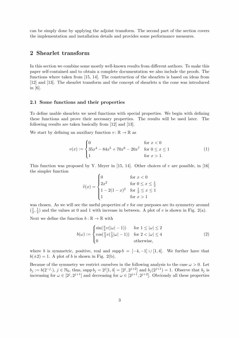
2 Shearlet transform
In this section we combine some mostly well-known results from different authors. To make thispaper self-contained and to obtain a complete documentation we also include the proofs. Thefunctions where taken from [15, 14]. The construction of the shearlets is based on ideas from[12] and [13]. The shearlet transform and the concept of shearlets n the cone was introducedin [6].
2.1 Some functions and their properties
To define usable shearlets we need functions with special properties. We begin with definingthese functions and prove their necessary properties. The results will be used later. Thefollowing results are taken basically from [12] and [13].
We start by defining an auxiliary function v : R→ R as
v(x) :=
0 for x < 0
35x4 − 84x5 + 70x6 − 20x7 for 0 ≤ x ≤ 1
1 for x > 1.
(1)
This function was proposed by Y. Meyer in [15, 14]. Other choices of v are possible, in [16]the simpler function
v(x) =
0 for x < 0
2x2 for 0 ≤ x ≤ 12
1− 2(1− x)2 for 12 ≤ x ≤ 1
1 for x > 1
was chosen. As we will see the useful properties of v for our purposes are its symmetry around(1
2 ,12) and the values at 0 and 1 with increase in between. A plot of v is shown in Fig. 2(a).
Next we define the function b : R→ R with
b(ω) :=
sin(π2 v(|ω| − 1)) for 1 ≤ |ω| ≤ 2
cos(π2 v(12 |ω| − 1)) for 2 < |ω| ≤ 4
0 otherwise,
(2)
where b is symmetric, positive, real and supp b = [−4,−1] ∪ [1, 4]. We further have thatb(±2) = 1. A plot of b is shown in Fig. 2(b).
Because of the symmetry we restrict ourselves in the following analysis to the case ω > 0. Letbj := b(2−j ·), j ∈ N0, thus, supp bj = 2j [1, 4] = [2j , 2j+2] and bj(2
j+1) = 1. Observe that bj isincreasing for ω ∈ [2j , 2j+1] and decreasing for ω ∈ [2j+1, 2j+2]. Obviously all these properties
3

−0.5 0 0.5 1 1.5
0
0.2
0.4
0.6
0.8
1
(a) v(x)
−5 −4 −3 −2 −1 0 1 2 3 4 5
0
0.2
0.4
0.6
0.8
1
(b) solid: b(ω), dashed: b(2ω)
Figure 2: The two auxiliary functions v in (1) and b in (2)
carry over to b2j . These facts are illustrated in the following diagram where stands for theincreasing function and for decreasing function.
ω 2j 2j+1 2j+2 2j+3
bj 0 1 0bj+1 0 1 0
For j1 6= j2 the overlap between the support of b2j1 and b2j2 is empty except for |j1−j2| = 1. Thus,
for b2j and b2j+1 we have that supp b2j ∩ supp b2j+1 = [2j+1, 2j+2]. In this interval b2j is decreasing
with b2j = cos2(π2 v(2−j
2 |ω|−1)) and b2j+1 is increasing with b2j+1 = sin2(π2 v(2−(j+1)|ω|−1)). Weget for their sum in this interval
b2j (ω) + b2j+1(ω) = cos2(π
2v(2−j−1|ω| − 1)
)+ sin2
(π2v(2−j−1|ω| − 1)
)= 1.
Hence, we can summarize
(b2j + b2j+1)(ω) =
b2j for ω < 2j+1
1 for 2j+1 ≤ ω ≤ 2j+2
b2j+1 for ω > 2j+2.
Consequently, we have the following lemma
Lemma 2.1. For bj defined as above, the relations
∞∑j=−1
b2j (ω) =
∞∑j=−1
b2(2−jω) = 1 for |ω| ≥ 1
and
∞∑j=−1
b2j (ω) =
0 for |ω| ≤ 1
2
sin2(π2 v(2ω − 1)
)for 1
2 < |ω| < 1
1 for |ω| ≥ 1
(3)
hold true.
4

Proof. In each interval [2j+1, 2j+2] only bj and bj+1, j ≥ −1, are not equal to zero. Thus, it issufficient to prove that b2j + b2j+1 ≡ 1 in this interval. We get that
(b2j + b2j+1)(ω) = b2(2−jω︸ ︷︷ ︸∈ 2−j [2j+1, 2j+2] = [2, 4]
) + b2(2−j−1ω︸ ︷︷ ︸∈ 2−j−1[2j+1, 2j+2] = [1, 2]
)
= cos2
(π
2v(
1
2· 2−jω − 1)
)+ sin2
(π2v(2−j−1ω − 1)
)= cos2
(π2v(2−j−1ω − 1)
)+ sin2
(π2v(2−j−1ω − 1)
)= 1.
The second relation follows by straightforward computation.
Recall that the Fourier transform F : L2(R2)→ L2(R2) and the inverse transform are definedby
Ff(ω) = f(ω):=
∫R2
f(t)e−2πi〈ω,t〉dt,
F−1f(ω) = f(t) =
∫R2
f(ω)e2πi〈ω,t〉dω.
Now we define the function ψ1 : R→ R via its Fourier transform as
ψ1(ω) :=√b2(2ω) + b2(ω). (4)
Fig. 3(a) shows the function. The following theorem states an important property of ψ1.
Theorem 2.2. The above defined function ψ1 has supp ψ1 = [−4,−12 ] ∪ [1
2 , 4] and fulfills∑j≥0
|ψ1(2−2jω)|2 = 1 for |ω| > 1.
Proof. The assumption on the support follows from the definition of b. For the sum we have
∑j≥0
|ψ1(2−2jω)|2 =∞∑j=0
b2(2 · 2−2jω) + b2(2−2jω)
=
∞∑j=0
b2(2−2j+1ω) + b2(2−2jω),
where −2j + 1 ∈ +1,−1,−3, . . . (odd) and −2j ∈ 0,−2,−4, . . . (even). Thus, by Lemma2.1, we get
∑j≥0
|ψ1(2−2jω)|2 =∞∑
j=−1
b2(2−jω)
= 1.
5

By (3) we have that
∑j≥0
|ψ1(2−2jω)|2 =
0 for |ω| ≤ 1
2
sin2(π2 v(2ω − 1)
)for 1
2 < |ω| < 1
1 for |ω| ≥ 1.
(5)
Next we define a second function ψ2 : R→ R – again in the Fourier domain – by
ψ2(ω) :=
√v(1 + ω) for ω ≤ 0√v(1− ω) for ω > 0.
(6)
The function ψ2 is shown in Fig. 3(b). Before stating a theorem about the properties of ψ2 weneed the following two auxiliary lemmas. Recall that a function f : R→ R is point symmetric
−5 −4 −3 −2 −1 0 1 2 3 4 5
0
0.2
0.4
0.6
0.8
1
(a) ψ1
−1.5 −1 −0.5 0 0.5 1 1.5
0
0.2
0.4
0.6
0.8
1
(b) ψ2
Figure 3: The functions ψ1 in (4) and ψ2 in (6)
with respect to (a, b) if and only if
f(a+ x)− b = −f(a− x) + b ∀ x ∈ R.
With the substitution x+ a→ x this is equivalent to
f(x) + f(2a− x) = 2b ∀ x ∈ R.
Thus, for a function symmetric to (0.5, 0.5) we have that f(x) + f(1− x) = 1.
Lemma 2.3. The function v in (1) is symmetric with respect to (0.5, 0.5), i.e., v(x)+v(1−x) =1 ∀ x ∈ R.
Proof. The symmetry is obvious for x < 0 and x > 1. It remains to prove the symmetry for
6

0 ≤ x ≤ 1, we have
v(x) + v(1− x)
= 35x4 − 84x5 + 70x6 − 20x7 + 35(1− x)4 − 84(1− x)5 + 70(1− x)6 − 20(1− x)7
= 35x4 − 84x5 + 70x6 − 20x7
+ 35
4∑k=0
(4
k
)(−x)k − 84
5∑k=0
(5
k
)(−x)k + 70
6∑k=0
(6
k
)(−x)k − 20
7∑k=0
(7
k
)(−x)k
= 1.
Note that ψ2 is axially symmetric to the y-axis.
Lemma 2.4. The function ψ2 fulfills
ψ22(ω − 1) + ψ2
2(ω) + ψ22(ω + 1) = 1 for |ω| ≤ 1.
Proof. We have that
ψ22(ω) =
v(1 + ω) for ω ≤ 0
v(1− ω) for ω > 0.
Consequently we get for 0 ≤ ω ≤ 1 that
ψ22(ω − 1) + ψ2
2(ω) + ψ22(ω + 1) = v(1 + ω − 1) + v(1− ω) + v(1− ω − 1)
= v(ω) + v(1− ω) + v(−ω)︸ ︷︷ ︸=0
= 1,
and similarly we obtain for −1 ≤ ω < 0 that
ψ22(ω − 1) + ψ2
2(ω) + ψ22(ω + 1) = v(1 + ω − 1) + v(1− ω) + v(1− ω − 1)
= v(−|ω|)︸ ︷︷ ︸=0
+v(1− |ω|) + v(|ω|)
= 1.
As can be seen in the proof the sum reduces in both cases to two (different) summands, inparticular
1 = ψ22(ω − 1) + ψ2
2(ω) + ψ22(ω + 1) =
ψ2
2(ω − 1) + ψ22(ω) for 0 ≤ ω ≤ 1
ψ22(ω) + ψ2
2(ω + 1) for − 1 ≤ ω < 0.
With these lemmas we can prove the following theorem.
7

Theorem 2.5. The function ψ2 defined in (6) fulfills
2j∑k=−2j
|ψ2(k + 2jω)|2 = 1 for |ω| ≤ 1, j ≥ 0. (7)
Proof. With ω := 2jω the assertion in (7) becomes
2j∑k=−2j
|ψ2(k + ω)|2 = 1 for |ω| ≤ 2j , j ≥ 0.
For a fixed (but arbitrary) ω? ∈ [−2j , 2j ] ⊂ R we need that −1 ≤ ω?+k ≤ 1 for ψ2(ω?+k) 6= 0since supp ψ2 = [−1, 1]. Thus, for ω? ∈ Z, only the summands for k ∈ −ω?−1,−ω?,−ω?+1do not vanish. But for k = −ω? ± 1 we have that ω? + k = ±1 and ψ2(±1) = 0. In this casethe entire sum reduces to one summand k = −ω? such that
2j∑k=−2j
|ψ2(k + ω?)|2 = |ψ2(−ω? + ω?)|2 = |ψ2(0)|2 = 1.
If ω? 6∈ Z and ω? > 0 the only nonzero summands appear for k ∈ bω?c, bω?c− 1. Thus, with0 < r+ := ω? − bω?c < 1, we get
2j∑k=−2j
|ψ2(k + ω?)|2 = |ψ2(−bω?c+ ω?)|2 + |ψ2(−bω?c − 1 + ω?)|2 = |ψ2(r+)|2 + |ψ2(1− r+)|2
which is equal to 1 by Lemma 2.4. Analogously we obtain for ω? 6∈ Z, ω? < 0 that the remainingnonzero summands are those for k ∈ dω?e, dω?e+ 1. With −1 < r− := dω?e+ω? < 0 we get
2j∑k=−2j
|ψ2(k + ω?)|2 = |ψ2(dω?e+ ω?)|2 + |ψ2(dω?e+ 1 + ω?)|2 = |ψ2(r−)|2 + |ψ2(1 + r−)|2.
By Lemma 2.4 and since ψ2(x) = ψ2(−x), we finally obtain
|ψ2(r−)|2 + |ψ2(1 + r−)|2 = |ψ2(|r−|)|2 + |ψ2(1− |r−|)|2 = 1.
2.2 The continuous shearlet transform
For the shearlet transform we need a scaling (or dilation) matrix Aa and a shear matrix Ssdefined by
Aa =
(a 00√a
), a ∈ R+, Ss =
(1 s0 1
), s ∈ R.
8
The shearlets ψa,s,t emerge by dilation, shearing and translation of a function ψ ∈ L2(R2) asfollows
ψa,s,t(x) :=a−34ψ(A−1
a S−1s (x− t)) (8)
=a−34ψ
((1a − s
a0 1√
a
)(x− t)
).
We assume that ψ can be written as ψ(ω1, ω2) = ψ1(ω1)ψ2(ω2ω1
). Consequently, we obtain forthe Fourier transform
ψa,s,t(ω) = a−34ψ
((1a − s
a0 1√
a
)(· − t)
)(ω)
= a−34 e−2πi〈ω,t〉ψ
((1a − s
a0 1√
a
)·)
(ω)
= a−34 e−2πi〈ω,t〉(a−
32 )−1ψ
((a 0s√a√a
)ω
)= a
34 e−2πi〈ω,t〉ψ
(aω1,
√a(sω1 + ω2)
)= a
34 e−2πi〈ω,t〉ψ1 (aω1) ψ2
(a−
12
(ω2
ω1+ s
)).
The shearlet transform SHψ(f) of a function f ∈ L2(R) can now be defined as follows
SHψ(f)(a, s, t) :=〈f, ψa,s,t〉=〈f , ψa,s,t〉
=
∫R2
f(ω)ψa,s,t(ω)dω
=a34
∫R2
f(ω)ψ1(aω1)ψ2
(a−
12
(ω2
ω1+ s
))e2πi〈ω,t〉dω
=a34F−1
(f(ω)ψ1(aω1)ψ2
(a−
12
(ω2
ω1+ s
)))(t).
The same formula can be derived by interpreting the shearlet transform as a convolution withthe function ψa,s(x) = ψ(−A−1
a S−1s x) and using the convolution theorem.
The shearlet transform is invertible if the function ψ fulfills the admissibility property∫R2
|ψ(ω1, ω2)|2|ω1|2
dω1dω2 <∞.
2.3 Shearlets on the cone
Up to now we have nothing said about the support of our shearlet ψ. We use band-limitedshearlets, thus, we have compact support in the Fourier domain. In the previous section weassumed that ψ(ω1, ω2) = ψ1(ω1)ψ2(ω2
ω1), where we now define ψ1 and ψ2 as in (4) and (6)
9

respectively. With the results shown for ψ1 with |ω1| ≥ 12 and ψ2 for |ω| < 1, i.e., |ω2| < |ω1|,
it is natural to define the area
Ch := (ω1, ω2) ∈ R2 : |ω1| ≥1
2, |ω2| < |ω1|.
We will refer to this set as the horizontal cone (see Fig. 4). Analogously we define the verticalcone as
Cv := (ω1, ω2) ∈ R2 : |ω2| ≥1
2, |ω2| > |ω1|.
To cover all R2 we define two more sets
C× := (ω1, ω2) ∈ R2 : |ω1| ≥1
2, |ω2| ≥
1
2, |ω1| = |ω2|,
C0 := (ω1, ω2) ∈ R2 : |ω1| < 1, |ω2| < 1,
where C× is the “intersection” (or the seam lines) of the two cones and C0 is the “low frequency”part. Altogether R2 = Ch ∪ Cv ∪ C× ∪ C0 with an overlapping domain
C := (−1, 1)2 \ (−1
2,1
2)2. (9)
Ch
Ch
Cv
Cv
C0
C×C×
12 1
Figure 4: The sets Ch, Cv, C× and C0
Obviously the shearlet ψ defined above is perfectly suited for the horizontal cone. For each setCκ, κ ∈ h, v,×, we define a characteristic function χCκ(ω) which is equal to 1 for ω ∈ Cκ and0 for ω 6∈ Cκ. We need these characteristic functions as cut-off functions at the seam lines. Weset
ψh(ω1, ω2) := ψ(ω1, ω2) = ψ1(ω1)ψ2
(ω2
ω1
)χCh . (10)
10

For the non-dilated and non-sheared ψh the cut-off function has no effect since the support ofψh is completely contained in Ch. But after the dilation and shearing we have
supp ψa,s,0 ⊆
(ω1, ω2) :1
2a≤ |ω1| ≤
4
a,
∣∣∣∣s+ω2
ω1
∣∣∣∣ ≤ √a .The question arises for which a and s this set remains a subset of the horizontal cone. Fora > 1 we have that ω1 ≤ 1
2 is in supp ψa,s,0 but not in Ch. Thus, we can restrict ourselves toa ≤ 1.
Having a fixed, the second condition for supp ψa,s,0 becomes
−√a ≤ s+ω1
ω2≤√a,
−√a− s ≤ ω1
ω2≤√a− s. (11)
Since∣∣∣ω1ω2
∣∣∣ ≤ 1 we have for the right condition√a− s ≤ 1 and for the left condition −√a− s ≥
−1, hence, we can conclude−1 +
√a ≤ s ≤ 1−√a.
For such s we have supp ψa,s,0 ⊆ Ch, in particular the indicator function is not needed for theses (with respective a). One might ask for which s (depending on a) the indicator function cutsoff only parts of the function, i.e., supp ψa,s,0 ∩ Ch 6= ∅. We take again (11) but now we do not
use a condition to guarantee that∣∣∣ω1ω2
∣∣∣ < 1 but rather ask for a condition that allows∣∣∣ω1ω2
∣∣∣ < 1.
Thus, the right bound√a − s should be larger than −1 and the left bound −√a − s should
be smaller than 1. Consequently, we obtain
−1−√a ≤ s ≤ 1 +√a.
Summing up, we have for |s| ≤ 1−√a that supp ψa,s,0 ⊆ Ch. For 1−√a < |s| < 1 +√a parts
of supp ψa,s,0 are also in Cv, which are cut off. For |s| > 1+√a the whole shearlet is set to zero
by the characteristic function. If we get back to the definition of ψa,s,0 we see that the vertical
range is determined by ψ2. By definition ψ2 is axially symmetric with respect to the y-axis, inother words the “center” of ψ2 is taken for the argument equal to zero, i.e., a−
12 (ω1ω2
+s) = 0. It
follows that for |s| = 1 the center of ψa,s,0 is at the seam-lines. Thus, for |s| = 1 approximatelyone half of the shearlet is cut off whereas the other part remains. For larger s more would becut. Consequently, we restrict ourselves to |s| ≤ 1.
Analogously the shearlet for the vertical cone can be defined, where the roles of ω1 and ω2 areinterchanged, i.e.,
ψv(ω1, ω2) := ψ(ω2, ω1) = ψ1(ω2)ψ2
(ω1
ω2
)χCv . (12)
All the results from above apply to this setting. For (ω1, ω2) ∈ C×, i.e., |ω1| = |ω2|, bothdefinitions coincide and we define
ψ×(ω1, ω2) := ψ(ω1, ω2)χC× . (13)
The shearlets ψh, ψv (and ψ×) are called shearlets on the cone. This concept was introducedin [10].
We have functions to cover three of the four parts of R2. The remaining part C0 will be handledwith a scaling function which is presented in the next section.
11

2.4 Scaling function
For the center part C0 (or low-frequency part) we define another set of functions. To this end,we need the following so-called “mother”-scaling function
ϕ(ω) :=
1 for |ω| ≤ 1
2
cos(π2 v(2|ω| − 1)) for 12 < |ω| < 1
0 otherwise.
The full scaling function φ can then be defined as follows
φ(ω1, ω2) :=
ϕ(ω1) for |ω1| < 1, |ω2| ≤ |ω1|ϕ(ω2) for |ω2| < 1, |ω1| < |ω2|
(14)
=
1 for |ω1| ≤ 1
2 , |ω2| ≤ 12
cos(π2 v(2|ω1| − 1)) for 12 < |ω1| < 1, |ω2| ≤ |ω1|
cos(π2 v(2|ω2| − 1)) for 12 < |ω2| < 1, |ω1| < |ω2|
0 otherwise.
The decay of the scaling function φ (respectively ϕ) is chosen to match perfectly with theincrease of ψ1. For |ω| ∈ [1
2 , 1] we have by (5), that
|ψ1(ω)|2 + |ϕ(ω)|2 = sin2(π
2v(2|ω| − 1)
)+ cos2
(π2v(2|ω| − 1)
)= 1. (15)
Remark 2.6. Observe that in our setting it seems not to be useful to define the scaling functionas a simple tensor product, namely
Φ(ω) :=ϕ(ω1)ϕ(ω2)
=
1 for |ω1| ≤ 12 , |ω2| ≤ 1
2
cos(π2 v(2|ω1| − 1)) for 12 < |ω1| < 1, |ω2| ≤ 1
2
cos(π2 v(2|ω2| − 1)) for 12 < |ω2| < 1, |ω1| ≤ 1
2
cos(π2 v(2|ω1| − 1)) cos(π2 v(2|ω2| − 1)) for 12 < |ω1| ≤ 1, 1
2 < |ω2| ≤ 1
0 otherwise.
(16)
Fig. 5 shows the difference between both scaling functions. Obviously, the first scaling functionaligns much better with the cones. Recently in [8] a new shearlet construction was introducedwhich is based on the scaling function in (16). We discuss the new construction in Section 3.4.
Remark 2.7. On the other hand it is possible to rewrite the definition of the original φ as ashearlet-like tensor product. We obtain a horizontal scaling function φh and a vertical scalingfunction φv as follows
φh(ω1, ω2) := ϕ(ω1)ϕ
(ω2
2ω1
)and φv(ω1, ω2) := ϕ(ω2)ϕ
(ω1
2ω2
),
where
ϕ
(ω2
2ω1
)=
1 for |ω2| ≤ |ω1|cos(π2 v(∣∣∣ω2
ω1
∣∣∣− 1))
for |ω1| < |ω2| < 2|ω1|0 otherwise.
12

−1.5 −1 −0.5 0 0.5 1 1.5−1.5
−1
−0.5
0
0.5
1
1.5
(a) φ(ω)
−1.5 −1 −0.5 0 0.5 1 1.5−1.5
−1
−0.5
0
0.5
1
1.5
(b) Φ(ω)
Figure 5: The different scaling functions in (14) and (16).
Thus, ϕ( ω22ω1
) is a continuous extension of the characteristic function of the horizontal cone
Ch.
We setφa,s,t(x) = φt(x) = φ(x− t).
Note that there is neither scaling nor shearing for the scaling function, only a translation.Thus, the index “a, s, t” from the shearlet ψ reduces to “t”. We further obtain
φt(ω) = e−2πi〈ω,t〉φ(ω).
The transform can be obtained similar as before, namely
SHφ(f)(a, s, t) = 〈f, φt〉.
3 Computation of the shearlet transform
In the following, we consider digital images as functions sampled on the grid (m1M , m2
N ) :(m1,m2) ∈ I with I := (m1,m2) : m1 = 0, . . . ,M − 1, m2 = 0, . . . N − 1.The discrete shearlet transform is basically known, but in contrast to the existing literature wepresent here a fully discrete setting. That is, we do not only discretize the involved parametersa, s and t but also consider only a finite number of discrete translations t. Additionally, oursetting discretizes the translation parameter t on a rectangular grid and independent of thedilation and shearing parameter. See Section 3.9 for further remarks on this topic.
13

3.1 Finite discrete shearlets
Let j0 := b12 log2Nc be the number of considered scales. To obtain a discrete shearlet trans-
form, we discretize the scaling, shear and translation parameters as
aj := 2−2j =1
4j, j = 0, . . . , j0 − 1,
sj,k := k2−j , −2j ≤ k ≤ 2j ,
tm :=(m1
M,m2
N
), m ∈ I. (17)
With these notations our shearlets becomes ψj,k,m(x) := ψaj ,sj,k,tm(x) = ψ(A−1aj S
−1sj,k
(x− tm)).
Observe that compared to the continuous shearlets defined in (8) we omit the factor a−34 . In
the Fourier domain we obtain
ψj,k,m(ω) = ψ(ATajS
Tsj,k
ω)e−2πi〈ω,tm〉 = ψ1
(4−jω1
)ψ2
(2jω2
ω1+ k
)e−2πi〈ω,(m1/M
m2/N)〉, ω ∈ Ω,
where Ω :=
(ω1, ω2) : ω1 = −⌊M2
⌋, . . . ,
⌈M2
⌉− 1, ω2 = −
⌊N2
⌋, . . . ,
⌈N2
⌉− 1.
(a) Shearlet in Fourier domainfor a = 1
4and s = − 1
2
(b) Same shearlet in time domain (zoomed)
Figure 6: Shearlet in Fourier and time domain.
By definition we have a ≤ 1 and |s| ≤ 1. Therefore we see that we have a cut off due to thecone boundaries only for |k| = 2j where |s| = 1. For both cones we have for |s| = 1 two “half”shearlets with a gap at the seam line. None of the shearlets are defined on the seam line C×.To obtain “full” shearlets at the seam lines we “glue” the three parts together, thus, we definefor |k| = 2j a sum of shearlets
ψh×vj,k,m := ψhj,k,m + ψvj,k,m + ψ×j,k,m.
14

We define the discrete shearlet transform as
SH(f)(κ, j, k,m) :=
〈f, φm〉 for κ = 0,
〈f, ψκj,k,m〉 for κ ∈ h, v,〈f, ψh×vj,k,m〉 for κ = ×, |k| = 2j .
where j = 0, . . . , j0 − 1, −2j + 1 ≤ k ≤ 2j − 1 and m ∈ I if not stated in another way. Theshearlet transform can be efficiently realized by applying the fft2 and its inverse ifft2 whichcompute the following discrete Fourier transforms with O(N2 logN) arithmetic operations:
f(ω) =∑m∈I
f(m)e−2πi
⟨ω,(m1/M
m2/N)⟩
=∑m∈I
f(m)e−2πi(ω1m1M
+ω2m2N ), ω ∈ Ω,
f(m) =1
MN
∑ω∈Ω
f(ω)e2πi⟨ω,(m1/M
m2/N)⟩
=1
MN
∑ω∈Ω
f(ω)e2πi(ω1m1M
+ω2m2N ), m ∈ I.
We have the Plancherel formula
〈f, g〉 =1
MN〈f , g〉.
Thus, the discrete shearlet transform can be computed for κ = h as follows (observe that ψ isreal):
SH(f)(h, j, k,m) = 〈f, ψhj,k,m〉 =1
MN〈f , ψhj,k,m〉
=1
MN
∑ω∈Ω
e−2πi〈ω,(m1/M
m2/N)〉ψ(4−jω1, 4−jkω1 + 2−jω2)f(ω1, ω2)
=1
MN
∑ω∈Ω
ψ(4−jω1, 4−jkω1 + 2−jω2)f(ω1, ω2)e
2πi⟨ω,(m1/M
m2/N)⟩.
With gj,k(ω) := ψ(4−jω1, 4−jkω1 + 2−jω2)f(ω1, ω2) this can be rewritten as
SH(f)(h, j, k,m) =1
MN
∑ω∈Ω
gj,k(ω)e2πi⟨ω,(m1/M
m2/N)⟩.
Since gj,k(ω) ∈ CM×N the shearlet transform can be computed as an inverse FFT of gj,k, thus
SH(f)(h, j, k,m) = ifft2(gj,k)
= ifft2(ψ(4−jω1, 4−jkω1 + 2−jω2)f(ω1, ω2)). (18)
For the vertical cone, i.e., κ = v, we obtain
SH(f)(v, j, k,m) = ifft2(ψ(4−jω2, 4−jkω2 + 2−jω1)f(ω1, ω2)) (19)
and for the seam line part with |k| = 2j we use the “glued” shearlets and obtain
SH(f)ψh×v(j, k,m) = ifft2(ψh×v(4−jω1, 4−jkω1 + 2−jω2)f(ω1, ω2)). (20)
15

Finally for the low-pass with g0(ω1, ω2) := φ(ω1, ω2)f(ω1, ω2) the transform can be obtainedsimilar as before, namely
SHφ(f)(m) = 〈f, φm〉
=1
MN〈f , φm〉
=1
MN
∑ω∈Ω
e−2πi〈ω,(m1/M
m2/N)〉φ(ω1, ω2)f(ω1, ω2)
=1
MN
∑ω∈Ω
e+2πi〈ω,(m1/M
m2/N)〉φ(ω1, ω2)f(ω1, ω2)
=1
MN
∑ω∈Ω
e+2πi〈ω,(m1/M
m2/N)〉g0(ω)
= ifft2(g0)
= ifft2(φ(ω1, ω2)f(ω1, ω2)). (21)
The complete shearlet transform is the combination of (18) to (21). We summarize
SH(f)(κ, j, k,m) =
ifft2(φ(ω1, ω2)f(ω1, ω2)) for κ = 0
ifft2(ψ(4−jω1, 4−jkω1 + 2−jω2)f(ω1, ω2)) for κ = h, |k| ≤ 2j − 1
ifft2(ψ(4−jω2, 4−jkω2 + 2−jω1)f(ω1, ω2)) for κ = v, |k| ≤ 2j − 1
ifft2(ψh×v(4−jω1, 4−jkω1 + 2−jω2)f(ω1, ω2)) for κ 6= 0, |k| = 2j .
(22)
3.2 A discrete shearlet frame
In view of the inverse shearlet transform we prove that our discrete shearlets constitute aParseval frame of the finite Euclidean space L2(I). Recall that for a Hilbert spaceH a sequenceuj : j ∈ J is a frame if and only if constants 0 < A ≤ B <∞ exists such that
A‖f‖2 ≤∑j∈J|〈f, uj〉|2 ≤ B‖f‖2 for all f ∈ H.
The frame is called tight if A = B and a Parseval frame if A = B = 1. Thus, for Parsevalframes we have that
‖f‖2 =∑j∈J|〈f, uj〉|2 for all f ∈ H
which is equivalent to the reconstruction formula
f =∑j∈J〈f, uj〉uj for all f ∈ H.
Further details on frames can be found in [3] and [14]. In the n-dimensional Euclidean spacewe can arrange the frame elements uj , j = 1, . . . , n ≥ n as rows of a matrix U . Then we haveindeed a frame if U has full rank and a Parseval frame if and only if UTU = In. Note that
16

UUT = In is only true if the frame is an orthonormal basis. The Parseval frame transform andits inverse read
(〈f, uj〉)nj=1 = Uf and f = UT(〈f, uj〉)nj=1.
By the following theorem our shearlets provide such a convenient system.
Theorem 3.1. The discrete shearlet system
ψhj,k,m(ω) : j = 0, . . . , j0 − 1,−2j + 1 ≤ k ≤ 2j − 1,m ∈ I∪ ψvj,k,m(ω) : j = 0, . . . , j0 − 1,−2j + 1 ≤ k ≤ 2j − 1,m ∈ I∪ ψh×vj,k,m(ω) : j = 0, . . . , j0 − 1, |k| = 2j ,m ∈ I∪ φm(ω) : m ∈ I
provides a Parseval frame for L2(I).
Proof. We have to show that
‖f‖2 =∑
κ∈h,v
j0−1∑j=0
2j−1∑k=−2j+1
∑m∈I|〈f, ψκj,k,m〉|2 +
j0−1∑j=0
∑k=±2j
∑m∈I|〈f, ψh×vj,k,m〉|2 +
∑m∈I|〈f, φm〉|2 =: C.
Since ‖f‖2F = 1MN ‖f‖2F (Parsevals formula, ‖·‖ denotes the Frobenius norm, i.e., ‖·‖F =
‖vec(·)‖2) it is sufficient to show that C is equal to 1MN ‖f‖2F .
By (18) we know that
〈f, ψhj,k,m〉 =1
MN
∑ω∈Ω
e2πi〈ω,(m1/M
m2/N)〉gj,k(ω) = gj,k(m).
We further obtain ∑m∈I|〈f, ψhj,k,m〉|2 =
∑m∈I|gj,k(m)|2 = ‖gj,k‖2F .
Consequently, with Parsevals formula
‖gj,k‖2F =1
MN‖gj,k‖2F =
1
MN
∑ω∈Ω
|gj,k(ω)|2
=1
MN
∑ω∈Ω
|ψ(4−jω1, 4−jkω1 + 2−jω2)f(ω1, ω2)|2
=1
MN
∑ω∈Ω
|ψ(4−jω1, 4−jkω1 + 2−jω2)|2|f(ω1, ω2)|2.
Analogously we obtain for the vertical part∑m∈I|〈f, ψvj,k,m〉|2 =
1
MN
∑ω∈Ω
|ψ(4−jω2, 4−jkω2 + 2−jω1)|2|f(ω1, ω2)|2.
17

Using these results we can conclude for the seam-line part∑m∈I|〈f, ψh×vj,k,m〉|2 =
1
MN
∑ω∈Ω
|ψ(4−jω1, 4−jkω1 + 2−jω2)|2|f(ω1, ω2)|2χCh
+1
MN
∑ω∈Ω
|ψ(4−jω2, 4−jkω2 + 2−jω1)|2|f(ω1, ω2)|2χCv
+1
MN
∑ω∈Ω
|ψ(4−jω1, 4−jkω1 + 2−jω2)|2|f(ω1, ω2)|2χC× .
For the remaining low-pass part we get similarly∑m∈I|〈f, φm〉|2 =
1
MN
∑m∈I|〈f , φm〉|2
=1
MN
∑m∈I
∣∣∑ω∈Ω
φm(ω)f(ω)∣∣2
=1
MN
∑m∈Ω
∣∣∑ω∈Ω
e2πi〈ω,(m1/M
m2/N)〉φ(ω1, ω2)f(ω1, ω2)
∣∣2with g0(ω) := φ(ω1, ω2)f(ω1, ω2)
=∑m∈I
∣∣ 1
MN
∑ω∈Ω
e2πi〈ω,(m1/M
m2/N)〉g0(ω)
∣∣2=∑m∈I|g0(m)|2 = ‖g0‖2F =
1
MN‖g0‖2
=1
MN
∑ω∈Ω
|φ(ω1, ω2)f(ω1, ω2)|2
=1
MN
∑ω∈Ω
|φ(ω1, ω2)|2|f(ω1, ω2)|2.
18
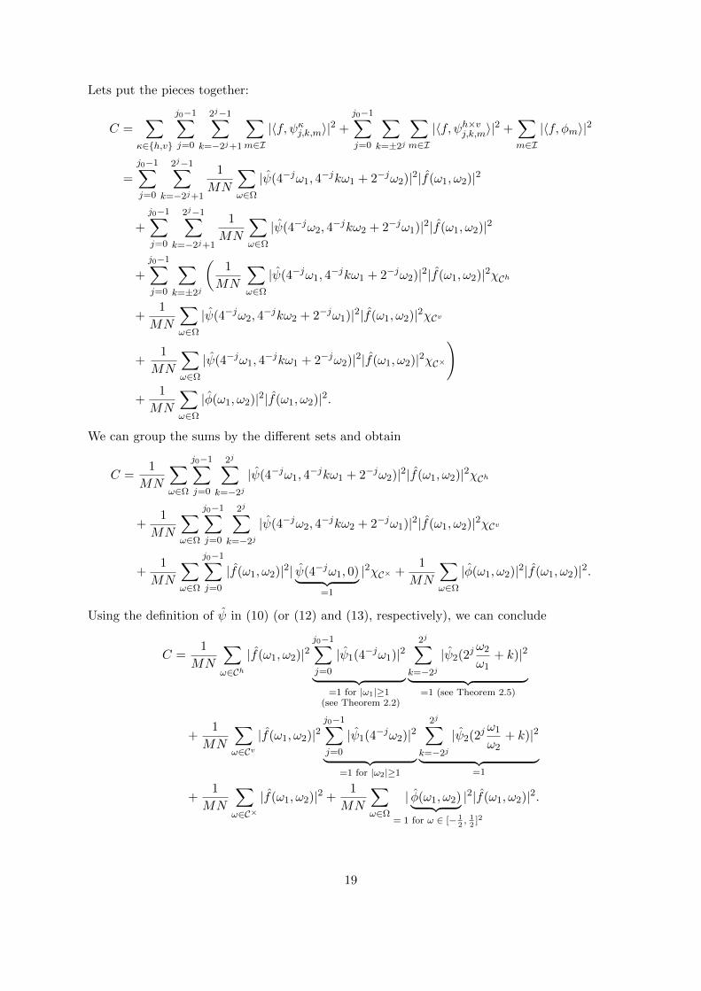
Lets put the pieces together:
C =∑
κ∈h,v
j0−1∑j=0
2j−1∑k=−2j+1
∑m∈I|〈f, ψκj,k,m〉|2 +
j0−1∑j=0
∑k=±2j
∑m∈I|〈f, ψh×vj,k,m〉|2 +
∑m∈I|〈f, φm〉|2
=
j0−1∑j=0
2j−1∑k=−2j+1
1
MN
∑ω∈Ω
|ψ(4−jω1, 4−jkω1 + 2−jω2)|2|f(ω1, ω2)|2
+
j0−1∑j=0
2j−1∑k=−2j+1
1
MN
∑ω∈Ω
|ψ(4−jω2, 4−jkω2 + 2−jω1)|2|f(ω1, ω2)|2
+
j0−1∑j=0
∑k=±2j
(1
MN
∑ω∈Ω
|ψ(4−jω1, 4−jkω1 + 2−jω2)|2|f(ω1, ω2)|2χCh
+1
MN
∑ω∈Ω
|ψ(4−jω2, 4−jkω2 + 2−jω1)|2|f(ω1, ω2)|2χCv
+1
MN
∑ω∈Ω
|ψ(4−jω1, 4−jkω1 + 2−jω2)|2|f(ω1, ω2)|2χC×
)
+1
MN
∑ω∈Ω
|φ(ω1, ω2)|2|f(ω1, ω2)|2.
We can group the sums by the different sets and obtain
C =1
MN
∑ω∈Ω
j0−1∑j=0
2j∑k=−2j
|ψ(4−jω1, 4−jkω1 + 2−jω2)|2|f(ω1, ω2)|2χCh
+1
MN
∑ω∈Ω
j0−1∑j=0
2j∑k=−2j
|ψ(4−jω2, 4−jkω2 + 2−jω1)|2|f(ω1, ω2)|2χCv
+1
MN
∑ω∈Ω
j0−1∑j=0
|f(ω1, ω2)|2| ψ(4−jω1, 0)︸ ︷︷ ︸=1
|2χC× +1
MN
∑ω∈Ω
|φ(ω1, ω2)|2|f(ω1, ω2)|2.
Using the definition of ψ in (10) (or (12) and (13), respectively), we can conclude
C =1
MN
∑ω∈Ch
|f(ω1, ω2)|2j0−1∑j=0
|ψ1(4−jω1)|2︸ ︷︷ ︸=1 for |ω1|≥1
(see Theorem 2.2)
2j∑k=−2j
|ψ2(2jω2
ω1+ k)|2︸ ︷︷ ︸
=1 (see Theorem 2.5)
+1
MN
∑ω∈Cv
|f(ω1, ω2)|2j0−1∑j=0
|ψ1(4−jω2)|2︸ ︷︷ ︸=1 for |ω2|≥1
2j∑k=−2j
|ψ2(2jω1
ω2+ k)|2︸ ︷︷ ︸
=1
+1
MN
∑ω∈C×
|f(ω1, ω2)|2 +1
MN
∑ω∈Ω
| φ(ω1, ω2)︸ ︷︷ ︸= 1 for ω ∈ [− 1
2, 12
]2
|2|f(ω1, ω2)|2.
19

With the properties of ψ1 and ψ2 (see Theorems 2.2 and 2.5) we obtain two sums, one for theoverlapping domain C (see (9)) and one for the remaining part
C =1
MN
∑ω∈Ω\C
|f(ω1, ω2)|2+∑ω∈C
|f(ω1, ω2)|2j0−1∑
j=0
|ψ1(4−jω1)|2 +
j0−1∑j=0
|ψ1(4−jω2)|2 + |φ(ω1, ω2)|2
where we can split up the second sum as
C =1
MN
∑ω∈Ω\C
|f(ω1, ω2)|2
+1
MN
∑ω∈Ch∩C
|f(ω1, ω2)|2 sin2(π
2v(2|ω1| − 1)
)+
1
MN
∑ω∈Cv∩C
|f(ω1, ω2)|2 sin2(π
2v(2|ω2| − 1)
)+
1
MN
∑ω∈Ch∩C
|f(ω1, ω2)|2 cos2(π
2v(2|ω1| − 1)
)+
1
MN
∑ω∈Cv∩C
|f(ω1, ω2)|2 cos2(π
2v(2|ω2| − 1)
)using the overlap (see (15)) we can continue
C =1
MN
∑ω∈Ω\C
|f(ω1, ω2)|2
+1
MN
∑ω∈Ch∩C
|f(ω1, ω2)|2(
sin2(π
2v(2|ω1| − 1)
)+ cos2
(π2v(2|ω1| − 1)
))︸ ︷︷ ︸
=1 (see (15))
+1
MN
∑ω∈Cv∩C
|f(ω1, ω2)|2(
sin2(π
2v(2|ω2| − 1)
)+ cos2
(π2v(2|ω2| − 1)
))︸ ︷︷ ︸
=1 (see (15))
.
Finally, we obtain
C =1
MN
∑ω∈Ω
|f(ω1, ω2)|2 =1
MN‖f‖2F = ‖f‖2F .
3.3 Inversion of the shearlet transform
Having the discrete Parseval frame the inversion of the shearlet transform is straightforward:multiply each coefficient with the respective shearlet and sum over all involved parameters. Asan inversion formula we obtain
f =∑
κ∈h,v
j0−1∑j=0
2j−1∑k=−2j+1
∑m∈I〈f, ψκj,k,m〉ψκj,k,m +
j0−1∑j=0
∑k=±2j
∑m∈I〈f, ψh×vj,k,m〉ψh×vj,k,m +
∑m∈I〈f, φm〉φm.
The actual computation of f from given coefficients c(κ, j, k,m) is done in the Fourier domain.Due to the linearity of the Fourier transform we get
f =∑
κ∈h,v
j0−1∑j=0
2j−1∑k=−2j+1
∑m∈I〈f, ψκj,k,m〉ψκj,k,m +
j0−1∑j=0
∑k=±2j
∑m∈I〈f, ψh×vj,k,m〉ψh×vj,k,m +
∑m∈I〈f, φm〉φm.
20

We take a closer look at the part for the horizontal cone where we have
f(ω)χCh =
j0−1∑j=0
2j−1∑k=−2j+1
∑m∈I〈f, ψj,k,m〉ψhj,k,m(ω)
=
j0−1∑j=0
2j−1∑k=−2j+1
∑m∈I
c(h, j, k,m)e−2πi〈ω,(m1/M
m2/N)〉ψ(4−jω1, 4
jkω1 + 2−jω2).
The inner sum can be interpreted as a two-dimensional discrete Fourier transform and can becomputed with a FFT and we can write
f(ω)χCh =
j0−1∑j=0
2j−1∑k=−2j+1
fft2(c(h, j, k, ·))(ω1, ω2)ψ(4−jω1, 4jkω1 + 2−jω2).
Hence, f can be computed by simple multiplications of the Fourier-transformed shearlet co-efficients with the dilated and sheared spectra of ψ and afterwards summing over all “parts”,scales j and all shears k, respectively. In detail we have
f(ω1, ω2) =fft2(c(0, ·))φ(ω1, ω2)
+
j0−1∑j=0
2j−1∑k=−2j+1
fft2(c(h, j, k, ·))ψ(4−jω1, 4−jkω1 + 2−jω2)
+
j0−1∑j=0
2j−1∑k=−2j+1
fft2(c(v, j, k, ·))ψ(4−jω2, 4−jkω2 + 2−jω1)
+
j0−1∑j=0
∑k=±2j
fft2(c(h× v, j, k, ·))ψ(4−jω1, 4−jkω1 + 2−jω2).
(23)
Finally we get f itself by an iFFT of f
f = ifft2(f).
3.4 Smooth shearlets
In many theoretical and some practical purposes one needs smooth shearlets in the Fourierdomain because such shearlets provide well-localized shearlets in time domain. Recently, in[8] a new shearlet construction was proposed that provides smooth shearlets for all scales aand respective shears s. Our shearlets are smooth for all scales and for all shears |s| 6= 1.The “diagonal” shearlets ψh×v are continuous by construction but they are not smooth. Fig7(a) illustrates this. Obviously our construction is not smooth in points on the diagonal. Thenew construction circumvents this with “round” corners. To this end, we get back to thetwo different scaling functions which we discussed in Section 2.4. While we chose the scalingfunction matching our cone-construction the new construction is based on the tensor-product
21
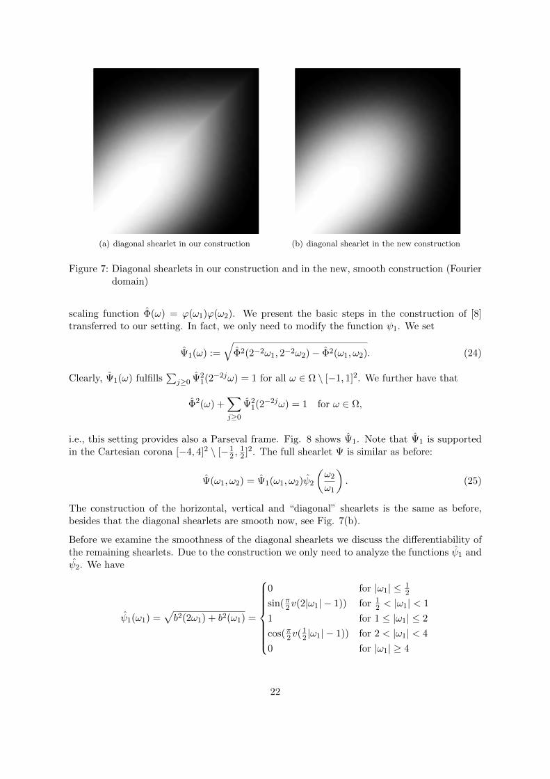
(a) diagonal shearlet in our construction (b) diagonal shearlet in the new construction
Figure 7: Diagonal shearlets in our construction and in the new, smooth construction (Fourierdomain)
scaling function Φ(ω) = ϕ(ω1)ϕ(ω2). We present the basic steps in the construction of [8]transferred to our setting. In fact, we only need to modify the function ψ1. We set
Ψ1(ω) :=
√Φ2(2−2ω1, 2−2ω2)− Φ2(ω1, ω2). (24)
Clearly, Ψ1(ω) fulfills∑
j≥0 Ψ21(2−2jω) = 1 for all ω ∈ Ω \ [−1, 1]2. We further have that
Φ2(ω) +∑j≥0
Ψ21(2−2jω) = 1 for ω ∈ Ω,
i.e., this setting provides also a Parseval frame. Fig. 8 shows Ψ1. Note that Ψ1 is supportedin the Cartesian corona [−4, 4]2 \ [−1
2 ,12 ]2. The full shearlet Ψ is similar as before:
Ψ(ω1, ω2) = Ψ1(ω1, ω2)ψ2
(ω2
ω1
). (25)
The construction of the horizontal, vertical and “diagonal” shearlets is the same as before,besides that the diagonal shearlets are smooth now, see Fig. 7(b).
Before we examine the smoothness of the diagonal shearlets we discuss the differentiability ofthe remaining shearlets. Due to the construction we only need to analyze the functions ψ1 andψ2. We have
ψ1(ω1) =√b2(2ω1) + b2(ω1) =
0 for |ω1| ≤ 12
sin(π2 v(2|ω1| − 1)) for 12 < |ω1| < 1
1 for 1 ≤ |ω1| ≤ 2
cos(π2 v(12 |ω1| − 1)) for 2 < |ω1| < 4
0 for |ω1| ≥ 4
22

Figure 8: The new function Ψ1 in (24)
and with straight forward differentiation
ψ′1(ω1) =
0 for |ω1| ≤ 12
πv(2|ω1| − 1)v′(2|ω1| − 1) cos(π2 v(2|ω1| − 1)) for 12 < |ω1| < 1
0 for 1 ≤ |ω1| ≤ 2
−π2 v(1
2 |ω1| − 1)v′(12 |ω1| − 1) sin(π2 v(1
2 |ω1| − 1)) for 2 < |ω1| < 4
0 for |ω1| ≥ 4.
The derivative is continuous if and only if the values at the critical points 12 , 1, 2, 4 coincide (for
symmetry reasons we can restrict ourselves to the positive range). We have that v(2 · 12 − 1) =
v(0) = 0 (even v′(0) = 0) and v′(2 · 1 − 1) = v′(1) = 0 and further v(12 · 2 − 1) = v(0) = 0
and v′(12 · 4 − 1) = v′(1) = 0. Consequently, ψ′1 is continuous and in particular ψ1 ∈ C1. By
induction we see that ψ(n)1 ∈ Cn if and only if v(n)(0) = 0 and v(n)(1) = 0, n ≥ 1.
For our v in (1) we have v(3)(1) = 0 but v(4)(1) 6= 0, i.e., ψ1 ∈ C3.
Similarly, we obtain for ψ2 that
∂ψ2
∂ω1(ω1, ω2) =
−ω2
ω21v′(1 + ω2
ω1) 1
2√v(1+
ω1ω2
)for ω2
ω1≤ 0
ω2
ω21v′(1− ω2
ω1) 1
2√v(1−ω1
ω2)
for ω2ω1> 0,
where we see that we need v′(0) = 0 for the derivative to exist. Thus, the shearlet ψ is Cn ifv(n)(0) = v(n)(1) = 0. This is also valid for the dilated and sheared shearlet ψhj,k,m (and ψvj,k,m)
for |k| 6= 2j . We take a closer look at the diagonal shearlet for k = −2j where we have
ψh×vj,−2j ,m
(ω) =
ψhj,−2j ,m
(ω), for ω ∈ Chψvj,−2j ,m
(ω), for ω ∈ Cvψ×j,−2j ,m
(ω), for ω ∈ C×.
23

Naturally, ψh×vj,−2j ,m
is smooth for ω ∈ Ch and ω ∈ Cv. Additionally, ψh×vj,−2j ,m
(ω) is continuous at
the seam lines, but not differentiable there since we have for the partial derivatives of ψhj,−2j ,m
and ψvj,−2j ,m
(ω) that
∂ψhj,−2j ,m
∂ω1(ω) = ψ2(2j(
ω2
ω1− 1))e−
2πiN
(ω1m1+ω2m2) · 2−2j ∂ψ1
∂ω1(2−2jω1)
+ ψ1(2−2jω1)e−2πiN
(ω1m1+ω2m2)(−2jω2
ω21
)∂ψ2
∂ω1(2j(
ω2
ω1− 1))
+ ψ1(2−2jω1)ψ2(2j(ω2
ω1− 1))(−2πi
Nm1)e−
2πiN
(ω1m1+ω2m2)
and
∂ψvj,−2j ,m
∂ω1(ω) = ψ1(2−2jω2)
(e−
2πiN
(ω1m1+ω2m2)(2j
ω2)∂ψ2
∂ω1(2j(
ω1
ω2− 1))
+ ψ2(2j(ω1
ω2− 1))(−2πi
Nm1)e−
2πiN
(ω1m1+ω2m2)
).
For ω1 = ω2 we obtain
∂ψhj,−2j ,m
∂ω1(ω1, ω1) = e−
2πiNω1(m1+m2) ·
(ψ2(0)︸ ︷︷ ︸
=1
2−2j ∂ψ1
∂ω1(2−2jω1)
− ψ1(2−2jω1)(2j
ω1)∂ψ2
∂ω1(0)︸ ︷︷ ︸
=0
−ψ1(2−2jω1) ψ2(0)︸ ︷︷ ︸=1
(2πi
Nm1)
)
= e−2πiNω1(m1+m2) ·
(2−2j ∂ψ1
∂ω1(2−2jω1)− (
2πi
Nm1)ψ1(2−2jω1)
)and
∂ψvj,−2j ,m
∂ω1(ω1, ω1) = e−
2πiNω1(m1+m2) ·
(ψ1(2−2jω1)(
2j
ω1)∂ψ2
∂ω1(0)︸ ︷︷ ︸
=0
−ψ1(2−2jω1) ψ2(0)︸ ︷︷ ︸=1
(2πi
Nm1)
)
= e−2πiNω1(m1+m2) ·
(−(
2πi
Nm1)ψ1(2−2jω1)
).
Obviously, both derivatives do not coincide, thus, our shearlet construction is not smooth forthe diagonal shearlets. If we get back to the new construction we obtain for the both partialderivatives
∂Ψhj,−2j ,m
∂ω1(ω) = 2−2j ∂Ψ1
∂ω1(2−2jω)ψ2(2j(
ω2
ω1− 1))e−
2πiN
(ω1m1+ω2m2)
− 2jω2
ω21
Ψ1(2−2jω)∂ψ2
∂ω1(2j(
ω2
ω1− 1))e−
2πiN
(ω1m1+ω2m2)
− 2πi
Nm1Ψ1(2−2jω)ψ2(2j(
ω2
ω1− 1))e−
2πiN
(ω1m1+ω2m2)
24

and
∂Ψvj,−2j ,m
∂ω1(ω) = 2−2j ∂Ψ1
∂ω1(2−2jω)ψ2(2j(
ω1
ω2− 1))e−
2πiN
(ω1m1+ω2m2)
+ (2j
ω2)Ψ1(2−2jω)
∂ψ2
∂ω1(2j(
ω1
ω2− 1))e−
2πiN
(ω1m1+ω2m2)
− 2πi
Nm1Ψ1(2−2jω)ψ2(2j(
ω1
ω2− 1))e−
2πiN
(ω1m1+ω2m2).
With ω1 = ω2 we obtain further
∂Ψhj,−2j ,m
∂ω1(ω1, ω1) = 2−2j ∂Ψ1
∂ω1(2−2jω1, 2
−2jω1) ψ2(0)︸ ︷︷ ︸=1
e−2πiNω1(m1+m2)
− 2jω2
ω21
Ψ1(2−2jω1, 2−2jω1)
∂ψ2
∂ω1(0)︸ ︷︷ ︸
=0
e−2πiNω1(m1+m2)
− 2πi
Nm1Ψ1(2−2jω1, 2
−2jω1) ψ2(0)︸ ︷︷ ︸=1
e−2πiNω1(m1+m2)
and
∂Ψvj,−2j ,m
∂ω1(ω1, ω1) = 2−2j ∂Ψ1
∂ω1(2−2jω1, 2
−2jω1) ψ2(0)︸ ︷︷ ︸=1
e−2πiNω1(m1+m2)
+ (2j
ω2)Ψ1(2−2jω1, 2
−2jω1)∂ψ2
∂ω1(0)︸ ︷︷ ︸
=0
e−2πiNω1(m1+m2)
− 2πi
Nm1Ψ1(2−2jω1, 2
−2jω1) ψ2(0)︸ ︷︷ ︸=1
e−2πiNω1(m1+m2).
It can be easily seen that both derivatives coincide if and only if ∂ψ2
∂ω1(0) = 0 since then the
second term vanishes. The same result is obtained for partial derivative with respect to ω2.Consequently, the new construction is smooth everywhere.
Remark 3.2. As we have seen the smoothness of the shearlets depends strongly on the smooth-ness of the function v. The v we have used was constructed to provide shearlets in C3. Thefirst three derivatives at 0 and 1 should be equal to zero, i.e., v′(x) = c · x3(x − 1)3. Withv(1) = 1 and straight forward integration one obtain c = −140 and the function v as in (1).
Higher grades of smoothness can easily be obtained by creating a new v by setting v′(x) =c · xk(x− 1)k. These shearlets would be in Ck.
Note that due to our discretization t = m we have a unique handling of both the horizontaland the vertical cone and do not have to make any adjustments for the diagonal shearlets, incontrast to the discretization t = AajSsjkm where you have different discretizations for t in
25

the horizontal and in the vertical cone. Consequently, some adjustments have to be made forthe diagonal shearlets.
Smooth shearlets are well-located in time. To show the difference we present in Fig. 9(a) the“old” shearlet in the time domain and in comparison in Fig. 9(b) the new construction in thetime domain. The non-smooth construction is slightly worse located. The shearlet coefficients
(a) diagonal shearlet in our construction, timedomain
(b) diagonal shearlet in the new construction,time domain
Figure 9: diagonal shearlets in our construction and in the new, smooth construction (Timedomain)
of, e.g., a diagonal line only show marginal differences such that for practical applications it isirrelevant which construction is used.
3.5 Implementation details
The implementation of the shearlet transform follows very closely the details described here.As we see in (22) and (23) for both directions of the transform the spectra of ψ and φ areneeded for all scales j and all shears s on “all” sets. We precompute these spectra to use themfor both directions.
Up to now our implementation only supports quadratic images, i.e., M = N (see Remark 3.4for a short discussion on this topic).
3.5.1 Indexing
To reduce the number of parameters we introduce one index i which replaces the parameters κ,j and k. We set i = 1 for the low-pass part. We continue with the lowest frequency band, i.e.,j = 0. The different “cones” and shear parameters represent the different “directions” of theshearlet. For illustration we reduce the shearlet to a line which is rotated counter-clockwisearound the center and assign the index i accordingly. In each frequency band we start in the
26

horizontal position, i.e., κ = h and k = 0, and increase i by one. For each k = −1, . . . ,−2j + 1we continue increasing the index by one. The line is now almost in a 45 angle (or a line withslope 1). The next index is assigned to the combined shearlet “h× v” at the seam line whichcovers the “diagonal” for k = −2j . We continue in the vertical cone for k = −2j +1, . . . , 2j−1.Next is again the combined shearlet for k = 2j . With decreasing shear, i.e., k = 2j , . . . , 1, wefinish the indexing for this frequency-band and continue with the next one.
Summarizing we have always one index for the low-pass part. In each frequency band we have 2indices (or shearlets) for the diagonals (k = ±2j). In each cone we have 1+2·(2j−1) = 2j+1−1shearlets. For the scale j we have 2 · (2j+1 − 1) + 2 = 2j+2 shearlets. The following table liststhe number of shearlets for each j.
low-pass j = 0 j = 1 j = 2 · · ·1 4 8 16 · · ·
With a maximum scale j0 − 1 the number of all indices η is
η = 1 +
j0−1∑j=0
2j+2 = 1 + 4
j0−1∑j=0
2j = 1 + 4 · (2j0 − 1) = 2j0+2 − 3. (26)
For each index the spectrum is computed on a grid of size N × N . We store all indices in athree-dimensional matrix of size N ×N × η. The first both components refer to the ω2 and ω1
coordinates and the third component is the respective index. Consequently, an image f of sizeN ×N is oversampled to an image of size N ×N × η. In particular we have an oversamplingfactor of η. The following table lists η for j0 = 1, . . . , 4.
j0 1 2 3 4 · · ·η 5 13 29 61 · · ·
Note that j0 is the number of scales, the highest scale parameter j is always j0 − 1, i.e., wehave the scale parameters 0, . . . , j0 − 1. The function helper/shearletScaleShear providesvarious possibilities to compute the index i from a and s or from j and k and vice versa. Seedocumentation inside the file for more information.
3.5.2 Computation of spectra
We compute the spectra ψj,k,m as discrete versions of the continuous functions, i.e., we computethe values on a finite discrete lattice Ξ of size N ×N . With the functions defined as in (4) and(6) we may not take Ξ = Ω as this would destroy the frame property. The question is how tochoose X (such that Ξ ∈ [−X,X)N×N ) or the distance ∆ between to grid points, respectively.
The use of Theorem 2.2 in the proof of Theorem 3.1 was not completely correct. We havethat supp ψ1(ω) = [1
2 , 4] = [2−1, 22] and ψ1 = 1 for ω ∈ [1, 2] = [20, 21]. For the scaled
27

version we further have supp ψ1(2−2jω) = [22j−1, 22j+2] and ψ1(2−2jω) = 1 for ω ∈ [22j , 22j+1].Consequently, we can conclude
j0−1∑j=0
|ψ1(2−2jω)|2 =
0 for |ω| ≤ 12
sin2(π2 v(2ω − 1)
)for 1
2 < |ω| < 1
1 for 1 ≤ |ω| ≤ 22(j0−1)+1
cos2(π2 v(2−2j0−1ω − 1)
)for 22(j0−1)+1 < |ω| < 22(j0−1)+2
0 for |ω| ≥ 22(j0−1)+2.
We see that the sum is equal to 1 for a wide range of ω. As we have seen the part for |ω| < 1where the sum increases from 0 to 1 matches with the decreasing part of the scaling function(see (15)). But we also have a decay for |ω| > 22(j0−1)+1 where there is no compensation to 1since there are no higher scales. Keeping this decay would violate the frame property.
Consequently, X must be less or equal than 22(j0−1)+1 = 22j0−1 which implies the decay to be“outside” the image. We set X = 22j0−1. Additionally, if we get back to the lowest scale it isreasonable to set ∆ ≤ 1 since otherwise there would be to less grid points in supp ψ1.
To compute the grid and the spectra we assume that N = 2n + 1 is odd. We then have asymmetric grid around 0, hence, we have n grid points in the negative range and n grid pointsin the positive range and one grid point at 0. If N is given even we increase it by 1. Aftercomputing grid and spectra we neglect the last row and column to retain the original imagesize. Having n = N−1
2 grid points for the positive range and the maximal distance betweentwo grid points ∆ = 1 we get
X = 22j0−1 =N − 1
2=⇒ j0 =
1
2log2(N − 1).
Since j0 is the (scalar!) number of scales, we set for the number of scales (as used above)j0 := b1
2 log2(N)c. In the following table we list the number of scales for all image sizesN = 4 . . . , 1024
N 4, . . . , 15 16, . . . , 63 64, . . . , 255 256, . . . , 1023 1024
j0 1 2 3 4 5.
With j0 fixed we can compute the second parameter ∆. As we have seen the highest value inthe grid should be X = 22j0−1. For an odd N the grid ranges from [−X,X] and for an evengrid we have the range [−X,X) = [−X,X−∆]. We assume again an odd N , thus, the interval[−X,X] should be divided in N grid points including the bounds −X and X what leads toN − 1 subintervals and
∆ =2 ·XN − 1
=2 · 22j0−1
N − 1=
22j0
N − 1.
Where ∆ = 1 if N = 22j0 + 1 and ∆ > 14 , i.e., 1
4 < ∆ ≤ 1. Thus, for the same number of scaleswe obtain a better resolution with increasing image size.
It seems a little awkward to discretize f and ψ on different lattices. However, with thisauxiliary construction the definition and properties of the shearlet ψ is much more convenient.Additionally the shearlets are now independent of the parameter ∆ (or other grid properties).Anyway, to circumvent the imperfection with two lattices we can now formerly also discretizeψ(∆ω) on Ω instead of ψ(ω) on Ξ and obtain the same spectra.
28

Remark 3.3. The spectra depend strongly on the image size. In particular, if we reduce theimage size a bit but still have the same number of scales the resolution of the different frequencybands varies. This may be not wanted for comparison issues. To circumvent this one couldchose the grid according to the highest image size (for the respective number of scales) and dropthe boundaries for smaller images. This would however lead to a very small high frequency bandfor smaller images. In our current implementation this frequency band is as large as possible.
Remark 3.4. The theoretical results shown are valid for both square images and rectangularimages, i.e., we have I and Ω of size M×N . However, our implementation only supports squareimages. For the extension to rectangular images some questions remain. The first questionis what the “diagonal” in a discrete rectangular setting is, i.e., the “diagonal” shearlets haveto be handled carefully. More tricky is the question how to handle the different sizes in theboth directions with respect to the size of the grid especially if M N (or M N) andthe number of scales. Possible are an equispaced grid in both directions and thus less scalesin one direction or the same number of scales but a non-equispaced grid what would lead torectangular frequency bands. Depending on the application both seems useful. We hope toimplement rectangular shearlets in a future version of the software.
3.6 Short documentation
Every file contained in the package is commented, see there for details on the arguments andreturn values. Thus, we only want to comment on the two important functions.
The transform for an image A∈ CN×N is called with the following command
[ST ,Psi] = shearletTransformSpect(A,numOfScales ,shearlet_spect
,shearlet_arg)
where numOfscales, shearlet_spect and shearlet_arg are optional arguments. If only A isgiven the number of scales j0 is computed from the size of A, i.e., j0 = b1
2 log2(N)c and theshearlet with (4) and (6) is used. On the other hand numOfScales can be used two-fold. Ifgiven as a scalar value it simply states the number of scales to consider. On the other handwe can provide precomputed shearlet spectra which are then used for the computation of thetransform. Observe that the shearlet spectra only depend on the size of the image and thenumber of scales, thus, they are cached and reused if the function is called with an imageof same size again. The variable ST contains the shearlet coefficients as a three-dimensionalmatrix of size N ×N × η with the third dimension ordered as described in section 3.5.1. Psi
is of same size and contains the respective shearlet spectra ψκj,k,0.
With the parameters shearlet_spect and shearlet_arg other shearlets can be used to com-pute the spectra. Included in the software is the ’meyerShearletSpect’ as default shearlet(based on (4) and (6)) and ’meyerNewShearletSpect’ for the new smooth construction (see(25)). The parameter shearlet_arg is not used in both cases.
The application of other shearlet spectra is very straight forward. One the one hand onecan simply compute them externally in the matrix Psi and provide them as the parameternumOfScales. On the other hand it is possible to provide an own function ’myShearletSpect’(with arbitrary name) with the function head
29
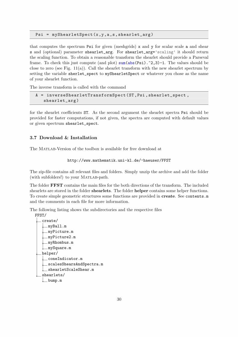
Psi = myShearletSpect(x,y,a,s,shearlet_arg)
that computes the spectrum Psi for given (meshgrids) x and y for scalar scale a and shears and (optional) parameter shearlet_arg. For shearlet_arg=’scaling’ it should returnthe scaling function. To obtain a reasonable transform the shearlet should provide a Parsevalframe. To check this just compute (and plot) sum(abs(Psi).^2,3)-1. The values should beclose to zero (see Fig. 11(a)). Call the shearlet transform with the new shearlet spectrum bysetting the variable sherlet_spect to myShearletSpect or whatever you chose as the nameof your shearlet function.
The inverse transform is called with the command
A = inverseShearletTransformSpect(ST,Psi ,shearlet_spect ,
shearlet_arg)
for the shearlet coefficients ST. As the second argument the shearlet spectra Psi should beprovided for faster computations, if not given, the spectra are computed with default valuesor given spectrum shearlet_spect.
3.7 Download & Installation
The Matlab-Version of the toolbox is available for free download at
http://www.mathematik.uni-kl.de/~haeuser/FFST
The zip-file contains all relevant files and folders. Simply unzip the archive and add the folder(with subfolders!) to your Matlab-path.
The folder FFST contains the main files for the both directions of the transform. The includedshearlets are stored in the folder shearlets. The folder helper contains some helper functions.To create simple geometric structures some functions are provided in create. See contents.m
and the comments in each file for more information.
The following listing shows the subdirectories and the respective filesFFST/
create/
myBall.m
myPicture.m
myPicture2.m
myRhombus.m
mySquare.m
helper/
coneIndicator.m
scalesShearsAndSpectra.m
shearletScaleShear.m
shearlets/
bump.m
30

meyeraux.m
meyerNewShearletSpect.m
meyerScaling.m
meyerScalingSpect.m
meyerShearletSpect.m
meyerWavelet.m
inverseShearletTransformSpect.m
shearletTransformSpect.m
If everything is installed correctly run simple_example for testing. The result should look likeFig. 10.
original image shearlet coefficients
shearlet reconstructed image
Figure 10: Result of script simple_example.
3.8 Performance
To evaluate the performance and the exactness of our implementation we present the followingfigures. In Fig. 11(a) we investigate the numerical tightness of the frame. The figure showsthe difference between the square sum of the shearlets and 1, i.e.,
∑κ∈h,v
j0−1∑j=0
2j∑k=−2j
|ψκj,k,0|2 +
j0−1∑j=0
∑k=±2j
|ψh×vj,k,0|2 + |φ0|2 − 1
The biggest deviation is about 8 · 10−15 which is 40 times the machine precision. The secondfigure Fig. 11(b) shows the difference between the original image and the back transformedimage of a random image, i.e., the exactness of the forward and backwards transform. Herethe biggest difference is about 2 · 10−15 or approximately 10 times the machine precision.Surprisingly this is even better than the tightness of the used frame.Next we want to compare the speed of our implementation for different image sizes N × Nfor N = 2i with i = 5, . . . , 10. In the first run all the spectra are computed, thus, this run
31

−8
−6
−4
−2
0
2
4
6
8
x 10−15
(a) frame tightness
−1.5
−1
−0.5
0
0.5
1
1.5
2
x 10−15
(b) transform exactness
Figure 11: Comparison of frame tightness and the exactness of the transform
takes significantly longer than the second and all following runs. The different run times areshown in Fig. 12 with logarithmic scale. To get reasonable results we take the average timeover 5 “first” runs (with deleting the cache, solid line) and 5 “second runs” (dashed line). Thedotted line shows the time needed for the inverse shearlet transform. Since no spectra have tobe computed here the time is approximately the same as for the second runs of the transformself. We compare the runtimes with ShearLab2, the only so far publicly available shearletimplementation. The dash-dotted line in Fig. 12 shows that ShearLab is slightly slower thenour implementation (in the first run). Observe that no time could be measured for N = 1024with ShearLab. In our implementation it is possible to compute the shearlet transform forarbitrary image sizes, whereas in ShearLab the transform is only possible for given image sizes.All tests were performed on an Intel i7 870 (Quad Core, each 2.93 GHz) with 8 GB RAM onUbuntu 10.04 with Matlab R2011b (64-bit).
3.9 Remarks
1. In [16] and the respective implementation ShearLab a pseudo-polar Fourier transformis used to implement a discrete (or digital) shearlet transform. For the scale a andthe shear s the same discretization is used. But for the translation t the authors settj,k,m := AajSsj,km where we in contrast simply set tm := m (see (17)). Thus, theirdiscrete shearlet becomes
ˆψj,k,m(ω) = ψ(AajS
Tsj,k
ω)e−2πi〈ω,AajSsj,km〉 = ψ(AajSTsj,k
ω)e−2πi〈ST
sj,kAajω,m〉.
Since the operation STsj,k
Aajω would destroy the pseudo-polar grid a “slight” adjustmentis made and the exponential term is replaced by
e−2πi〈(θS−T
sj,k)STsj,k
Aajω,m〉
2http://www.shearlab.org
32

32 64 128 256 512 10240.001
0.01
0.1
1
10
100
seco
nds
image size N
Figure 12: run times for different image sizes, “first run” (solid), “second” run (dashed), inverse(dotted), ShearLab (dashed-dotted, no time for N = 1024).
with θ : R \ 0 × R→ R× R and θ(x, y) = (x, yx) such that
e−2πi〈(θS−T
sj,k)STsj,k
Aajω,m〉 = e−2πi
⟨(ajω1,
√ajω2ω1
),m⟩.
With this adjustment the last step of the shearlet transform can be obtained with astandard inverse fast Fourier transform (similar as in our implementation). Unfortunatelythis is no longer related to translations of the shearlets in the time domain.
2. We are aware of our larger oversampling factor in comparison with, e.g., ShearLab. Hav-ing 4 scales we obtain 61 images of the same size as the original image. But sinceshearlets are designed to detect edges in images we like to avoid any down-sampling andkeep translation invariance. A possibility to reduce the memory usage would be to usethe compact support of the shearlets in the frequency domain and only compute themon a “relevant” region. But we then would also have to store the position and size ofeach region what decreases the memory savings and would make the implementation alot more complicated.
Acknowledgement
The author thanks Tomas Sauer (University of Gießen) for his support at the beginning of thisproject.
33

References
[1] E. Candes, L. Demanet, D. Donoho, and L. Ying. Fast discrete curvelet transforms.Multiscale Modeling Simulation, 5(3), 2006.
[2] E. J. Candes and D. L. Donoho. Ridgelets: a key to higher-dimensional intermittency?Philosophical Transactions of the London Royal Society, 357:2495–2509, 1999.
[3] O. Christensen. An Introduction to Frames and Riesz Bases. Birkhauser, 2003.
[4] S. Dahlke, G. Kutyniok, P. Maass, C. Sagiv, H.-G. Stark, and G. Teschke. The uncertaintyprinciple associated with the continuous shearlet transform. International Journal onWavelets Multiresolution and Information Processing, 6:157–181, 2008.
[5] S. Dahlke, G. Kutyniok, G. Steidl, and G. Teschke. Shearlet coorbit spaces and associatedbanach frames. Applied and Computational Harmonic Analysis, 27(2):195–214, 2009.
[6] K. Guo, G. Kutyniok, and D. Labate. Sparse multidimensional representations usinganisotropic dilation und shear operators. Wavelets und Splines (Athens, GA, 2005), G.Chen und M. J. Lai, eds., Nashboro Press, Nashville, TN, pages 189–201, 2006.
[7] K. Guo and D. Labate. Characterization and analysis of edges using the continuousshearlet transform. SIAM Journal on Imaging Sciences, 2(3):959–986, 2009.
[8] K. Guo and D. Labate. The construction of smooth parseval frames of shearlets. 2011.
[9] S. Hauser and G. Steidl. Convex multilabel segmentation with shearlet regularization.Preprint University of Kaiserslautern, 2011.
[10] G. Kutyniok, K. Guo, and D. Labate. Sparse multidimensional representations usinganisotropic dilation and shear operators. Wavelets und Splines (Athens, GA, 2005), G.Chen und MJ Lai, eds., Nashboro Press, Nashville, TN, pages 189–201, 2006.
[11] G. Kutyniok and W. Lim. Image separation using wavelets and shearlets. Curves andSurfaces (Avignon, France, 2010), Lecture Notes in Computer Science, to appear.
[12] D. Labate, G. Easley, and W. Lim. Sparse directional image representations using thediscrete shearlet transform. Applied and Computational Harmonic Analysis, 25(1):25–46,2008.
[13] W. Lim, G. Kutyniok, and X. Zhuang. Digital shearlet transforms. Shearlets: MultiscaleAnalysis for Multivariate Data, to appear.
[14] S. Mallat. A Wavelet Tour of Signal Processing: The Sparse Way. Academic Press, 2008.
[15] Y. Meyer. Oscillating Patterns in Image Processing and Nonlinear Evolution Equations,volume 22. AMS, Providence, 2001.
[16] M. Shahram, G. Kutyniok, and X. Zhuang. Shearlab: A rational design of a digitalparabolic scaling algorithm. submitted.
[17] S. Yi, D. Labate, G. Easley, and H. Krim. A shearlet approach to edge analysis anddetection. Image Processing, IEEE Transactions on, 18(5):929–941, 2009.
34