Embed Size (px)
Citation preview
SCHOOL OF ENGINEERING OF THE UNIVERSITY OF PORTO
FEUP
Estimation of the glottal pulse
from speech or singing voice
Sandra de Oliveira Dias
Master’s Thesis submitted in partial fulfillment of the requirements for
the degree of Master in Biomedical Engineering
Supervisor: Prof. Dr. Aníbal João de Sousa Ferreira
July, 2012

© Sandra de Oliveira Dias, 2012

ESTIMATION OF THE GLOTTAL PULSE
FROM SPEECH OR SINGING VOICE
Sandra de Oliveira Dias
Mathematics Education Degree by University of Minho (2003)
Supervisor: Prof. Dr. Aníbal João de Sousa Ferreira
Assistant Professor of the Department of Electrical and Computer Engineering
School of Engineering of the University of Porto


v
Abstract
The human speech production system is, briefly, the result of the convolution between the
excitation signal, the glottal pulse, and the impulse response resulting from the transfer
function of the vocal tract. This model of voice production is often referred to in the literature
as a source-filter model, where the source represents the flow of the air leaving the lungs and
passing through the glottis (space between the vocal folds), and the filter representing the
resonances of the vocal tract and lip/nostrils radiation.
The estimation of the shape of the glottal pulse from the speech signal is of significant
importance in many fields and applications, since the most important features of speech
related to voice quality, vocal effort and speech disorders, for example, are mainly due to the
voice source. Unfortunately, the glottal flow waveform which is at the origin of the glottal
pulse, is a very difficult signal to measure directly and non-invasively.
Several methods for estimating the glottal pulse have been proposed over the last few
decades, but there is not yet a complete and automatic algorithm which performs reliably.
Most of the developed methods are based on an approach called inverse filtering. The inverse
filtering approach represents a deconvolution process, i.e., it seeks to obtain the source signal
by applying the inverse of the vocal tract transfer function to the output speech signal. Despite
the simplicity of the concept, the inverse filtering procedure is complex because the output
signal may include noise and it is not straightforward to accurately model the characteristics of
the vocal tract filter.
In this dissertation we discuss a new glottal pulse prototype and a robust frequency-domain
approach for glottal source estimation that uses a phase-related feature based on the
Normalized Relative Delays (NRDs) of the harmonics. This model is applied to several speech
signals (synthetic and real), and the results of the estimation of the glottal pulse are compared
with the ones obtained using other state-of-the-art methods.
Key words: glottal pulse, glottal model, estimation of the glottal pulse, inverse filtering,
integration in the frequency-domain, Normalized Relative Delays (NRDs), frequency-domain
glottal source estimation.
vi
Resumo
O processo de produção humana de voz é, resumidamente, o resultado da convolução entre o
sinal de excitação, o impulso glótico, e a resposta impulsiva resultante da função de
transferência do trato vocal. Este modelo de produção de voz é frequentemente referido na
literatura como um modelo fonte-filtro, em que a fonte representa o fluxo de ar que sai dos
pulmões e passa pela glote (espaço entre as pregas vocais), e o filtro representa as
ressonâncias do trato vocal e a radiação labial/nasal.
Estimar a forma do impulso glótico a partir do sinal de voz é de importância significativa em
diversas áreas e aplicações, uma vez que as características de voz relacionadas, por exemplo,
com a qualidade da voz, esforço vocal e distúrbios da voz, devem-se, principalmente, ao fluxo
glotal. No entanto, este fluxo é um sinal difícil de determinar de forma direta e não invasiva.
Ao longo das últimas décadas foram desenvolvidos vários métodos para estimar o impulso
glótico mas ainda não existe um algoritmo completo e automático. A maioria dos métodos
desenvolvidos baseia-se num processo designado por filtragem inversa. A filtragem inversa
representa, portanto, a desconvolução, ou seja, procura obter o sinal de entrada aplicando o
inverso da função de transferência do trato vocal ao sinal de saída. Apesar da simplicidade do
conceito, o processo de filtragem inversa não é simples uma vez que o sinal de saída pode
incluir ruído e não é simples modelar com precisão as características do filtro do trato vocal.
Nesta dissertação apresentamos um novo protótipo de impulso glótico e um método robusto
de estimação da fonte glótica, no domínio das frequências, que usa uma característica de fase
baseada nos Atrasos Relativos Normalizados (NRDs) dos harmónicos. Este modelo é aplicado a
diversos sinais de voz (sintéticos e reais), e os resultados obtidos da estimação do impulso
glótico são comparados com os obtidos usando outros métodos analisados no estado da arte.
Palavras chave: impulso glótico, modelos de impulso glótico, estimação do impulso glótico,
filtragem inversa, integração no domínio das frequências, Atrasos Relativos Normalizados
(NRDs), estimação do impulso glótico no domínio das frequências.

vii
Acknowledgements
“A mind without instruction can no more
bear fruit than a field, however fertile, without cultivation.”
(Cicero).
This thesis would not be possible without the support of many persons to whom I would like to
thank.
First of all, I would like to express my deep and sincerest gratitude to my supervisor, Professor
Aníbal Ferreira, for the opportunity to do my master’s thesis on this important and interesting
topic, and for his endless support, patience, motivation, encouragement and guidance during
this study. His professional knowledge, contagious enthusiasm and faith in me were very
important and gave me the strength to conclude this work. It was not always easy to be out of
my comfort zone, but it was a challenge and an opportunity to grow and learn. Thank you!
I am also grateful to Ricardo Sousa for his time and help, and to Dr. José Seabra and the
volunteers who collaborated in an experimental procedure implemented in this work.
I would like to show my gratitude to all my friends, for walking with me in all days of my life
and making easier this journey. For both help and friendship, I am especially thankful to
Leonor.
A special thanks to Filipe, for his love and care, my breath of life.
My final words go to my family. Thank you for the unconditional support, guidance and love
through all my life, especially while I was working on this project. In particular, to my nieces,
Sara, Eva and Inês, for being my sunshine every day and always kept smiling even when I had
to work and could not play with them.
Thank you one and all who directly or indirectly had an influence in this work.


Contents
List of Figures ............................................................................................................................ xi
List of Tables ............................................................................................................................. xv
Notations ................................................................................................................................. xvi
Acronyms ................................................................................................................................ xvii
Usual Expressions .................................................................................................................. xviii
1. Introduction .................................................................................................................... 1
1.1. Overview........................................................................................................................... 1
1.2. Objectives ......................................................................................................................... 3
1.3. Structure of the Dissertation ............................................................................................ 4
2. Human Speech Production System ................................................................................... 6
2.1. Introduction ...................................................................................................................... 7
2.2. Anatomy and Physiology of the Voice Organ ................................................................... 7
2.3. Glottal Flow .................................................................................................................... 10
2.3.1. Electroglottography ........................................................................................... 12
2.3.2. Imaging Techniques ........................................................................................... 14
2.4. Summary ........................................................................................................................ 17
3. Models of Voice Production ........................................................................................... 18
3.1. Introduction .................................................................................................................... 19
3.2. Source-Filter Model ........................................................................................................ 19
3.3. Extraction of Characteristics from a Speech Signal ........................................................ 24
3.3.1. Linear Predictive Coding (LPC) Method ............................................................. 27
3.3.2. Discrete All-Pole Modelling (DAP) ..................................................................... 30
3.3.3. Mel-Frequency Cepstral Coefficients (MFCC) Method ...................................... 32
3.3.3.1. Cepstral Analysis ................................................................................... 32
3.3.3.2. Mel scale ............................................................................................... 33
3.3.3.3. MFCC calculation process ..................................................................... 34
3.4. Glottal Pulse Models ...................................................................................................... 35
3.5. Summary ........................................................................................................................ 44
4. Glottal Pulse Estimation - State of the art ....................................................................... 45
4.1. Introduction .................................................................................................................... 46
4.2. Glottal Pulse Parameterization ...................................................................................... 47
4.2.1. Time-Domain Methods ...................................................................................... 47
4.2.2. Frequency-Domain Methods ............................................................................. 50
4.2.3. Model-Based Methods ...................................................................................... 51
4.3. Inverse Filtering Techniques ........................................................................................... 51
4.3.1. Iterative Adaptive Inverse Filtering (IAIF/PSIAIF) .............................................. 52
4.3.2. Javkin et al. Method .......................................................................................... 56
4.4. Zeros of the Z-Transform (ZZT) and Complex Cepstrum (CC) ........................................ 59
4.5. Evaluation of the Estimation of the Glottal FLow .......................................................... 64
4.6. Brief Relative Performance Comparison ........................................................................ 65
4.7. Summary ........................................................................................................................ 71
5. Frequency-domain approach to Glottal Source Estimation .............................................. 72
5.1. Introduction .................................................................................................................... 73
5.2. General Overview and Approach ................................................................................... 74
5.2.1. Signal Integration in the Frequency Domain ..................................................... 76
5.2.2. Normalized Relative Delay Concept .................................................................. 78
5.3. Physiological Signal Acquisition for Source and Filter Modelling ................................... 82
5.4. Glottal Source Estimation in the Frequency Domain ..................................................... 85
5.4.1. Hybrid LF-Rosenberg Glottal Source Model ...................................................... 90
5.4.2. Glottal Source Estimation Approach ................................................................. 93
5.5. Testing the New Approach to Glottal Source Estimation ............................................... 95
5.5.1. Tests with Synthetic Speech Signals .................................................................. 96
5.5.2. Tests with Real Speech Signals ........................................................................ 100
5.5.3. Conclusions ...................................................................................................... 106
5.6. Summary ...................................................................................................................... 107
6. Conclusion ................................................................................................................... 109
6.1. Overview....................................................................................................................... 110
6.2. Future Directions .......................................................................................................... 111
Appendix A – FUNDAMENTALS OF DIGITAL SIGNAL PROCESSING .................................................... 112
Appendix B – DATA ANALYSIS ............................................................................................... 116
Bibliography .................................................................................................................... 118

xi
List of Figures
Figure 2.1 Human speech production mechanism. ............................................................ 8
Figure 2.2 Top view of the larynx, showing the positions of the vocal folds. ..................... 9
Figure 2.3 Speech signals: (a)–voiced speech signal; (b)–unvoiced speech signal. .......... 10
Figure 2.4 Glottal phases. ................................................................................................ 11
Figure 2.5 EGG measurement setting. .............................................................................. 12
Figure 2.6 Schematic representation of a single cycle of vocal fold vibration viewed
coronally and superiorly, and an EGG of a normal phonation. ....................... 13
Figure 2.7 Electroglottogram of a normal phonation of a male subject. ......................... 13
Figure 2.8 Video laryngoscopy. ........................................................................................ 14
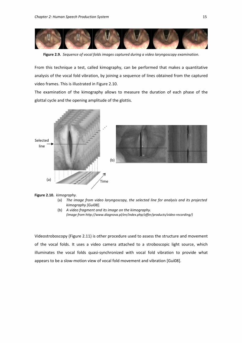
Figure 2.9 Sequence of vocal folds images captured during a video laryngoscopic
examination. ................................................................................................... 15
Figure 2.10 Kimography. .................................................................................................... 15
Figure 2.11 Videostroboscopy. ........................................................................................... 16
Figure 2.12 Fundamental principle of videostroboscopy. ................................................... 16
Figure 3.1 Schematic illustration of the generation of voice sounds. ............................... 20
Figure 3.2 Block diagram of the source-filter model. ....................................................... 21
Figure 3.3 Schematic view of voice production models. .................................................. 22
Figure 3.4 General discrete-time model of speech production and its physiologic
correspondence. .............................................................................................. 23
Figure 3.5 Source-filter model. ......................................................................................... 23
Figure 3.6 Illustrations of speech sounds. ........................................................................ 25
Figure 3.7 Illustration of the LPC method. ....................................................................... 29
Figure 3.8 FFT magnitude spectrum of a male vowel /a/ and the all-pole spectrum
of the DAP method together with the LP method. ........................................... 31
Figure 3.9 The Mel scale. .................................................................................................. 34
Figure 3.10 Block diagram of the MFCC calculation process. ............................................ 35
Figure 3.11 Main scheme of the glottal pulse used by most of glottal models. ................ 36

xii
Figure 3.12 Glottal pulse models. ....................................................................................... 43
Figure 4.1 Schematic spectra of the speech production system and the
corresponding inverse filtering process. ......................................................... 46
Figure 4.2 Three periods of a sound-pressure waveform and the respective glottal
flow and its derivative. .................................................................................... 48
Figure 4.3 Flow magnitude spectrum. ............................................................................. 50
Figure 4.4 Speech production model used in IAIF. ............................................................ 52
Figure 4.5 The bock diagram of the IAIF method for estimation of the glottal
excitation from the speech signal. .................................................................. 53
Figure 4.6 The graphical user interface and the signal view of Aparat. . ......................... 54
Figure 4.7 The spectra view in Aparat of a speech signal, the calculated glottal flow
and the used vocal tract filter, and parameters computed from the
estimated glottal flow. .................................................................................... 55
Figure 4.8 Block diagram of the main steps of the PSIAIF method. .................................. 55
Figure 4.9 Inverse filtering model by Murphy [Mur08]. ................................................... 56
Figure 4.10 Inverse Filter interface. .................................................................................... 58
Figure 4.11 Syntheziser interface. ...................................................................................... 58
Figure 4.12 Sky interface. ................................................................................................... 59
Figure 4.13 Illustration of the source-filter modelling for one period, in which the
Glottal Closing Instant (GCI) allows the separation of glottal open and
glottal closed phases. ...................................................................................... 59
Figure 4.14 The model of speech production used on ZZT. ................................................. 60
Figure 4.15 The ZZT of a speech signal. ............................................................................. 61
Figure 4.16 Example of decomposition on a real speech segment using Causal and
Anticausal decomposition. ............................................................................... 61
Figure 4.17 Block diagram of the ZZT decomposition algorithm. ...................................... 62
Figure 4.18 Effect of a sharp CGI-centered windowing on a two-period long speech
frame. .............................................................................................................. 63
Figure 4.19 Glottal flow estimations of a synthetic vowel /a/ using the LF model. ........... 67
Figure 4.20 Glottal flow estimations of a female vowel /a/. ............................................. 68
Figure 4.21 Glottal flow estimations of a male vowel /a/. ................................................ 69

xiii
Figure 4.22 Glottal flow estimations of a female vowel /i/. .............................................. 70
Figure 5.1 Initial idea for analysis by synthesis approach to filter/source fine-
tuning. ............................................................................................................. 75
Figure 5.2 Analysis-synthesis processing framework. ...................................................... 76
Figure 5.3 Time representation of the derivative of the LF glottal waveforms
without noise and with white noise at 9 dB SNR, and the corresponding
output results of a first-order time-domain integrator and of a
frequency-domain integrator. ......................................................................... 78
Figure 5.4 Illustration of the relative delay d between a harmonic of a fundamental
frequency sinusoid, whose delay to a time reference is 1n , and the
fundamental frequency sinusoid, whose delay to a time reference is 0n . ...... 80
Figure 5.5 Algorithm implementing the estimation of the NRD parameters and
overall time shift (n0) of the waveform. ......................................................... 81
Figure 5.6 Time representation, the corresponding magnitude spectrum and NRD
representation of the LF and the Rosenberg glottal flow models. ................... 81
Figure 5.7 Laryngoscopic exam and voice signal acquisition. ........................................... 83
Figure 5.8 Time-aligned speech signals for vowel /i/ by a male subject: the signal
captured near the vocal folds and the signal captured outside the
mouth. . ............................................................................................................ 85
Figure 5.9 Waveform for vowel /i/ by a male subject, the corresponding magnitude
spectrum where harmonics are depicted and the NRD representation of
the signal captured near the glottis and the signal captured outside the
mouth. . ........................................................................................................... 86
Figure 5.10 Magnitude spectrum, where the harmonics are depicted, of the
waveform of the LF and Rosenberg glottal models. ....................................... 86
Figure 5.11 Normalized magnitude of the first 24 harmonics of the LF glottal pulse
model, and the 30 harmonics of the Rosenberg model and the reference
line with - 12 db/octave slope. ......................................................................... 87
Figure 5.12 Unwrapped NRDs of time-aligned signals frames captured “inside” and
“outside” the mouth and the corresponding linear regression models. .......... 88
Figure 5.13 Unwrapped NRDs of the LF and Rosenberg glottal pulse models, and the
corresponding linear regression models. .......................................................... 91
Figure 5.14 Normalized magnitude of the first 24 harmonics pertaining to the LF
glottal pulse model, the Rosenberg model and a hybrid model. .................... 92
Figure 5.15 Time representation of the LF model, Rosenberg model and hybrid

xiv
glottal pulse model, and the corresponding derivatives. ................................ 92
Figure 5.16 Glottal source estimation algorithm. .............................................................. 94
Figure 5.17 Illustration of the glottal source estimation. .................................................. 94
Figure 5.18 Glottal flow estimations of a male synthetic vowel /a/ using the LF
model. ............................................................................................................. 98
Figure 5.19 Glottal flow estimations of a male synthetic vowel /i/ using the LF
model. .............................................................................................................. 98
Figure 5.20 Glottal flow estimations of a female synthetic vowel /a/ using the LF
model. .............................................................................................................. 99
Figure 5.21 Glottal flow estimations of a female synthetic vowel /i/ using the LF
model. ............................................................................................................. 99
Figure 5.22 Glottal flow estimations of a female vowel /a/. ........................................... 102
Figure 5.23 Glottal flow estimations of a male vowel /a/. ............................................... 102
Figure 5.24 Glottal flow estimations of a female vowel /i/. ............................................ 103
Figure 5.25 Glottal flow estimations of a singing signal of a male voice. ........................ 103
Figure 5.26 Glottal flow estimations of a female vowel /a/ from our data base
(subject SF). .................................................................................................... 104
Figure 5.27 Glottal flow estimations of a female vowel /i/ from our data base
(subject SD). ................................................................................................... 104
Figure 5.28 Glottal flow estimations of a female vowel /i/ from our data base
(subject SF). ..................................................................................................... 105
Figure 5.29 Glottal flow estimations of a male vowel /a/ from our data base (subject
RT). ................................................................................................................. 105
Figure 5.30 Glottal flow estimations of a male vowel /i/ from our data base (subject
RT). ................................................................................................................. 106
Figure A.1 ZZT representation of a signal in cartesian and polar coordinates. .............. 115

xv
List of Tables
Table 5.1. Characterization of the volunteer subjects. ...................................................... 84
Table 5.2. Average and Standard Deviation of the spectral decay of the source
harmonics, in dB/octave, as a function of gender and vowel. ........................ 87
Table 5.3 Average and Standard Deviation of the slope of the linear regression
models corresponding to the unwrapped NRDs of the source signals, as
a function of gender and vowel. ..................................................................... 89
Table 5.4. Average and Standard Deviation of the slope of the linear regression
models corresponding to the unwrapped NRDs of the signals captured
outside the mouth, as a function of gender and vowel. ................................. 89
Table 5.5. Average and Standard Deviation of the difference, in modulus, between
the slopes of the linear regression models that fit the unwrapped NRDs
of the signals captured near the vocal folds and outside the mouth, as a
function of gender and vowel. ........................................................................ 90
Table 5.6. SNR values for the glottal source estimations of synthetic speech signals,
using IAIF method and our glottal source estimation approach. ................... 97
Table 5.7. SNR values for the glottal source estimations using IAIF method and our
glottal source estimation approach. .............................................................. 97
Table B.1 Spectral decay of the source harmonics, in dB/octave, Average and
Standard Deviation, as a function of vowel per subject. ............................... 116
Table B.2 Linear Regression Models of the unwrapped NRDs of the time-aligned
acoustics signals. ........................................................................................... 117

xvi
Notations
sf : Sampling frequency of a discrete signal.
F0 or 0f : Fundamental frequency in Hz of a periodic signal.
0 01/T f= : Fundamental period.
( )x t : Continuous signal with respect to time t.
[ ]x n : Discrete signal with respect to sample n.
( ) ( )x t y t∗ : Convolution between ( )x t and ( )y t .
vA : Peak amplitude of the glottal pulse.
mα : Asymmetry coefficient of the glottal pulse.
ceps : Smooth magnitude of the spectral envelope based on the spectral peaks of the
harmonics of the voiced speech signal.
dif : Difference between the magnitude of the spectral peaks of the voiced speech
signal and the magnitude of the interpolation of the spectral envelope.
Fm : Magnitude of the (vocal tract) filter.
HMm : Magnitude of the spectral peaks of the hybrid LF - Rosenberg glottal model.
Sm : Magnitude of the spectral peaks of the harmonics of the speech signal.
Gnrd : Normalized Relative Delay (NRD) coefficients of the source signal.
Fnrd : Normalized Relative Delay (NRD) coefficients of the (vocal tract) filter.
Snrd : Normalized Relative Delay (NRD) coefficients of the speech signal.
.slope difNRD
:
Difference between the slope of the Normalized Relative Delays (NRDs) of the
speech signal and the slope of the NRDs of the source signal.
pT : Opening glottal phase length.
lT : Closing glottal phase length.
T : Total length of the glottal cycle.
ct : Duration of the period of the glottal flow waveform ( 0 01 /ct T f= = ).
pt : Time of the maximum of the glottal pulse.
et : Time of the minimum of the time-derivative of the glottal pulse.
at : Return phase duration.

xvii
Acronyms
AQ Amplitude Quotient
AR AutoRegressive
CALM Causal-Anticausal Linear Model
CC Complex Cepstrum
ClQ Closing Quotient
DAP Discrete All-Pole Modelling
DCT Discrete Cosine Transform
DFT Discrete Fourier Transform
DTFT The Discrete Time Fourier Transform
EGG ElectroGlottoGraphy
FFT Fast Fourier Transform
GCI Glottal Closing Instant
GOI Glottal Opening Instant
H1-H2 Difference of the first two harmonics on the decibel scale
HRF Harmonic Richness Factor
IAIF Iterative Adaptive Inverse Filtering
IDFT Inverse of the Discrete Fourier Transform
LF Liljencrants-Fant glottal model
LFRd
Transformed-LF glottal model
LP Linear Prediction
LPC Linear Predictive Coding
MFCC Mel Frequency Cepstrum Coefficients
NAQ Normalized Amplitude Quotient
NRD Normalized Relative Delay
Odd-DFT Odd-frequency Discrete Fourier Transform
OQ Open Quotient
PSIAIF Pitch Synchronous Iterative Adaptive Inverse Filtering
SNR Signal to Noise Ratio
SQ Speed Quotient
VTF Vocal Tract Filter
ZZT Zeros of the Z-Transform

xviii
Usual Expressions
Analysis/synthesis method
A method that entirely models an observed signal by choosing a combination of its parameters, originating a reconstructed signal which is as close as possible to the observed signal.
Formant A resonant frequency of the vocal tract.
Glottal flow or Glottal source The airflow velocity waveform that comes out of the glottis and enters the vocal tract.
Glottal model A mathematical model of the glottal pulse.
Glottal pulse The shape of the glottal source in a single period,
corresponding to a puff of air at the glottis. Frequently is referred to as glottal flow or glottal source.
Normalized Relative Delay
(NRD)
Relative delay difference between a harmonic and the fundamental frequency sinusoid, divided by the period of the sinusoid.
Pitch The perceptual measure of the fundamental frequency of a sound.
Quasi-periodic A particular case of aperiodicity waveform where the deviation from periodicity is very small.
Spectral analysis Analysis of a signal by the amplitude, frequency and phase of its component sinusoids.
Source-filter theory
Theory that describes the human voice production process as source signal, representing the glottal airflow, which is modulated by a transfer (filter) function determined by the shape of the vocal tract.
Unvoiced sound Sound produced without the vibrations of the vocal folds (they simply remain open).
Voiced sound Sound produced by the vibrations of the vocal folds.
Chapter 1
INTRODUCTION
"Nothing so surely reveals the character
of a person as his voice."
(Benjamin Disraeli)
Contents
1.1. OVERVIEW ........................................................................................................................... 1
1.2. OBJECTIVES .......................................................................................................................... 3
1.3. STRUCTURE OF THE DOCUMENT ............................................................................................... 4
1.1. OVERVIEW
Voice is one of the most important instruments of human communication and it is such a
complex phenomenon that, despite being investigated over the years in different areas as
engineering, medicine and singing, not all of its attributes seem to be known.
As sound identity of human beings, the voice reflects individual characteristics such as age,
sex, race, social status, personal characteristics and even emotional state. It is maybe in the
nuances and inflections of the voice that lies the expressive power of human language.
Claudius Galen, a Greek second century physician, physiologist and philosopher, studied the
voice production and believed that voice was the mirror of the soul1.
Voice is the unique signal generated by the human vocal apparatus and is perceived as the
sounds originated from a flow of air from the lungs, which causes the vocal folds to vibrate,
and that are subsequently modified by the vocal tract. Very briefly, voice is the result of a
balance between two forces: the force of the air leaving the lungs and the muscle strength of
the larynx, where the vocal folds are located. As a physical phenomenon, voice is defined as a
1 In http://www.acsu.buffalo.edu/~duchan/new_history/ancient_history/galen.html

Chapter 1: Introduction 2
complex sound, whose voiced regions, i.e., those resulting from a vibration of the vocal folds,
consist of a fundamental frequency and a large number of harmonics [Sun87].
Several mathematical models have been proposed over the years both to model the voice
production system or to estimate the flow of air passing through the glottis (i.e., the space
between the vocal folds) (e.g. [JBM87], [BDA+05], [Alk95]), called the glottal flow or glottal
source2. Most models of the voice production system presume that voice is the result of an
excitation signal, consisting in the voice source, and that is modulated by a transfer (filter)
function determined by the shape of the vocal tract. This model is often referred to as the
"source-filter model of speech production” (e.g. [Fan60], [JBM87], [Air08b], [Mag05]).
According to Fant’s source-filter theory, the glottal flow and the transfer function of the vocal
tract are linearly separable from the speech signal [Fan60]. Specifically, using a technique
called inverse filtering, it is possible to cancel the spectral effects of the vocal tract and lip and
nostrils radiation on a speech signal and, then, to estimate the glottal source, i.e, the
waveform produced at the glottis. Separation between source and filter is one of the most
difficult challenges in speech processing, since neither the glottal or the vocal contributions are
observable in the speech waveform.
The importance of the estimation of the glottal source is well established in speech science,
providing insight into the voice signal, which is of potential benefit in many application areas
such as speech coding, synthesis or re-synthesis, speaker identification, the non-invasive
assessment of laryngeal aspects of voice quality and the study of pathological voices (since
perturbations on the glottal flow component are considered to be one of the main sources of
speech disorders), the vocal perception of emotions, and the extraction of musically relevant
phonation parameters for biofeedback purposes. However, it is difficult to observe the glottal
behaviour from the speech signal and the concealed location of the vocal folds makes rather
difficult the direct observation and measurement of their vibration, which implies intrusive
techniques. This motivates the development of computational procedures for the estimation
of the glottal source directly from the speech signal.
Most approaches for estimating the glottal source are time-domain based. Nevertheless, there
are several advantages on the spectral approach to voice source estimation when compared to
time-domain methods, including the possibility to control spectral magnitude and phase
independently, and to characterize the spectral profile of the noise so as to minimize its
impact.
2 Some authors consider the glottal source as the derivative of the glottal pulse. However, as it will be
assumed in this dissertation, the most common definition of the glottal source is as the sound wave propagated from the glottis into the vocal tract.

Chapter 1: Introduction 3
The goal of this thesis is to present a new glottal pulse prototype and a glottal source
estimation algorithm that comprises frequency-domain signal analysis and synthesis, and relies
on an accurate spectral magnitude modelling of the harmonics of the speech signal. In
particular, a new feature is used that is based on the Normalized Relative Delays (NRDs) of the
spectral harmonics.
This new approach results from accurate sinusoidal/harmonic analysis and synthesis of two
concomitant acoustic signals for vowels /a/ and /i/: the glottal source signal captured near the
vocal folds, and the corresponding voiced signal outside the mouth. The experimental
procedure in which these signals were captured will be described and the obtained data will be
studied in two main parts. Firstly, the magnitude and the group delay of the glottal source
signal will be analysed and, based on the results, we propose a new glottal source model
combining features of two reference glottal models - the Liljencrants-Fant and the Rosenberg
models. Secondly, the same analysis is made using the signals captured outside the mouth and
from the results of the two-time-aligned signals, we attempt to synthesize the glottal pulse
using the estimation of the NRDs and the magnitude of the spectral peaks of the voice source.
To validate the proposed approach, the results of the estimation of the glottal pulse will be
critically compared and discussed with the ones obtained using representative state-of-the-art
methods, highlighting the advantages of a spectral approach.
Although the estimation of the glottal source has been extensively studied over the last
decades, it is very likely that it will continue to be an open topic over the next few years, which
shows both its importance and complexity.
1.2. OBJECTIVES
Many inverse filtering methods and processes of estimation of the glottal pulse were
developed over the last years, but a fully automatic procedure is not yet available and, as it
was stated before, the estimation of the glottal source is important in many application areas
which justifies the motivation of this work.
The main purpose of this thesis is to present a new frequency-domain algorithm to glottal
source estimation, highlighting the advantages of a spectral approach and the potential of a
new phase-related feature based on the Normalized Relative Delays (NRDs) of the harmonics.
Chapter 1: Introduction 4
With this work we hope to contribute to the development of non-invasive procedures of
estimation of the glottal pulse and to enhance scientific knowledge about the glottal pulse and
speech analysis.
1.3. STRUCTURE OF THE DISSERTATION
Chapter 2, “Human speech production system”, presents the analysis of the anatomy and
physiology of the organ of voice, and the three systems that integrate the voice organ (the
breathing apparatus, the vocal folds and the vocal tract) are briefly described.
Chapter 3, “Models of voice production”, gives an overview of the fundamental source-filter
theory of speech production and its usual simplifications and hypothesis. Also, different
methods of extraction of characteristics from speech signals and several glottal waveform
models are summarized as well as their respective mathematical details.
Chapter 4, “Estimation of the glottal flow: state of the art”, describes several techniques of
estimation of the glottal flow that are representative of the state of art, namely inverse
filtering methods. A brief evaluation of those methods using synthetic and real speech signals
is presented and the corresponding results of the estimation of the glottal pulse are discussed
and compared.
Chapter 5, “Frequency-domain approach to glottal source estimation”, presents a new
approach and algorithm for the estimation of the glottal source signal, which is implemented
in the frequency domain and is based on the results of an experimental procedure from which
the data set of our work was obtained.
This process of the estimation of the glottal pulse is applied to several speech signals (synthetic
and real) and the obtained results are critically compared to the ones obtained using other
procedures that are representative of the state of the art. This chapter also reviews the
Normalized Relative Delay (NRD) concept and demonstrates how to accurately implement
signal integration in the frequency domain.

Chapter 1: Introduction 5
Chapter 6, “Conclusions”, summarizes the main results obtained in the context of this
dissertation, relates them to the findings of the previous research and adds remarks and
possible directions for future research.

Chapter 2
HUMAN SPEECH PRODUCTION SYSTEM
Contents
2.1. INTRODUCTION ..................................................................................................................... 7
2.2. ANATOMY AND PHYSIOLOGY OF THE VOICE ORGAN .................................................................... 7
2.3. GLOTTAL FLOW .................................................................................................................. 10
2.3.1. ELECTROGLOTTOGRAPHY .................................................................................................. 12
2.3.2. IMAGING TECHNIQUES ...................................................................................................... 14
2.4. SUMMARY ......................................................................................................................... 17

Chapter 2: Human Speech Production System 7
2.1. INTRODUCTION
An understanding of the human speech production system is essential in the context of our
research.
This chapter begins with a brief anatomic and physiologic study of the voice organ and a
description of the speech production process. A particular emphasis is placed on the glottal
source signal and associated phases.
2.2. ANATOMY AND PHYSIOLOGY OF THE VOICE ORGAN
The voice organ, also called phonetic system, consists of three different systems: the breathing
apparatus, the vocal folds and the vocal tract. Figure 2.1 illustrates the human voice
production mechanism.
The lungs or respiratory organs, are spongy structures with numerous wells that provide a
large surface area for gas exchange with the blood. They are located in the chest, which is
separated from the abdominal cavity by the diaphragm. The latter, together with the
intercostal muscles, promote respiratory movements [KG00].
On expiration, the diaphragm and intercostal muscles relax causing a decrease in the volume
of the thorax and hence the increase of pressure in the chest pushes the air out of the lungs.
This causes an increase in subglottal pressure that forces the opening of the vocal folds, an
end-point of which is found at the site of the Adam’s Apple (i.e., at the midpoint of the larynx).
As air rushes through the vocal folds, these may start to vibrate, opening and closing, in
alternation, the passage of air flow. Thus, the air flow causes a series of short pulses of air,
which increases the supraglottal pressure, and then, the suction phenomenon known as the
Bernoulli effect is observed. This effect, due to the decrease of the pressure across the
constriction aperture (i.e., the glottis), sucks the folds back together, and the subglottal
pressure increases again, so that the vocal folds open giving rise to a new pulse of air [Sun87].
This phonation process has a fundamental frequency directly related to the frequency of the
vibration of the vocal folds, as it will be explained below. The phonation from the larynx then
enters the various chambers of the vocal tract: the pharynx, the nasal cavity and the oral
cavity. The pharynx is the chamber stemming the length of the throat from the larynx to the

Chapter 2: Human Speech Production System 8
oral cavity. The position of the velum, a piece of tissue that makes up the back of the roof of
the mouth, determines the access to the nasal cavity [Cin08]. For the production of certain
phonemes, the velum can be raised or lowered to prevent or to allow acoustic coupling
between the nasal and oral cavities. The tongue and lips, in combination with the lower jaw,
are called the articulators and act to provide varying degrees of constriction at different
locations, helping to change the “filter” and, therefore, the produced sound [Gol00].
Thus, according to this theory, the sustained vibration of the vocal folds is described as the
balance between three aspects: the lung pressure, the Bernoulli principle and the elastic
restoring force of the vocal fold tissue. However, according to recent studies, together with the
Bernoulli forces, there must be also an asymmetrical driving force that is exerted on the folds
and that changes with the direction of their velocity, supplying the vocal fold tissue with more
energy – without which the vibrations would dissipate too readily. The Bernoulli force, along
with the asymmetrical force at the glottis due to the mucosal wave as well as the closed and
open phase of the folds, is now considered to be the sustaining model for vocal fold vibration
[Mur08].
The vocal folds are the most important functional components of the voice organ, because
they function as a generator of voiced sounds (explained below). They are covered by a
Figure 2.1. Human speech production mechanism (adapted from [Pul05]).
1- Nasal cavity
2- Hard palate
3- Alveolar ridge
4- Soft palate (velum)
5- Tongue tip
6- Dorsum
7- Uvula
8- Radix
9- Pharynx
10- Epiglottis
11- False vocal folds
12- Vocal folds
13- Larynx
14- Esophagus
15- Trachea
16- Lungs
17- Diaphragm
16
17

Chapter 2: Human Speech Production System 9
mucous membrane and the space between them is given the name of glottis, an end-point of
which is found at the site of the Adam’s Apple. Images of the human glottis are shown in
Figure 2.2.
The length of the vocal folds varies: in a newborn it is approximately 3 mm, and increases to
−9 13mm and −15 20 mm in adult female and male, respectively [Sun87]. This length is what
defines the frequency of vibration of the vocal folds, called the fundamental frequency (or
pitch). Because frequency is inversely proportional to length, the values of the fundamental
frequency of female voices are higher than those of male voices. For female voices, the values
of the fundamental frequency are close to 220 Hz while for male voices are around 110 Hz
[Per09]. So, when a tenor sings a note with a fundamental frequency of 330 Hz, this means
that his vocal folds open and close 330 times per second.
Arytenoid cartilages control the movement of the vocal folds, separating them, in the case of
breathing, and joining them and tightening them to produce a voiced sound emission. The
action of the cartilage joining the vocal folds is known as adduction and the opposite action
(i.e., separating the vocal folds) is abduction. It is the combination of adduction and abduction
actions, when performed at certain frequencies, that cause the production of a sound wave
and that is then propagated towards the lip opening.
The sounds produced as a result of the vibration of the vocal folds are called voiced sounds,
and the sounds produced without vibration of the latter (the vocal folds remain open only and
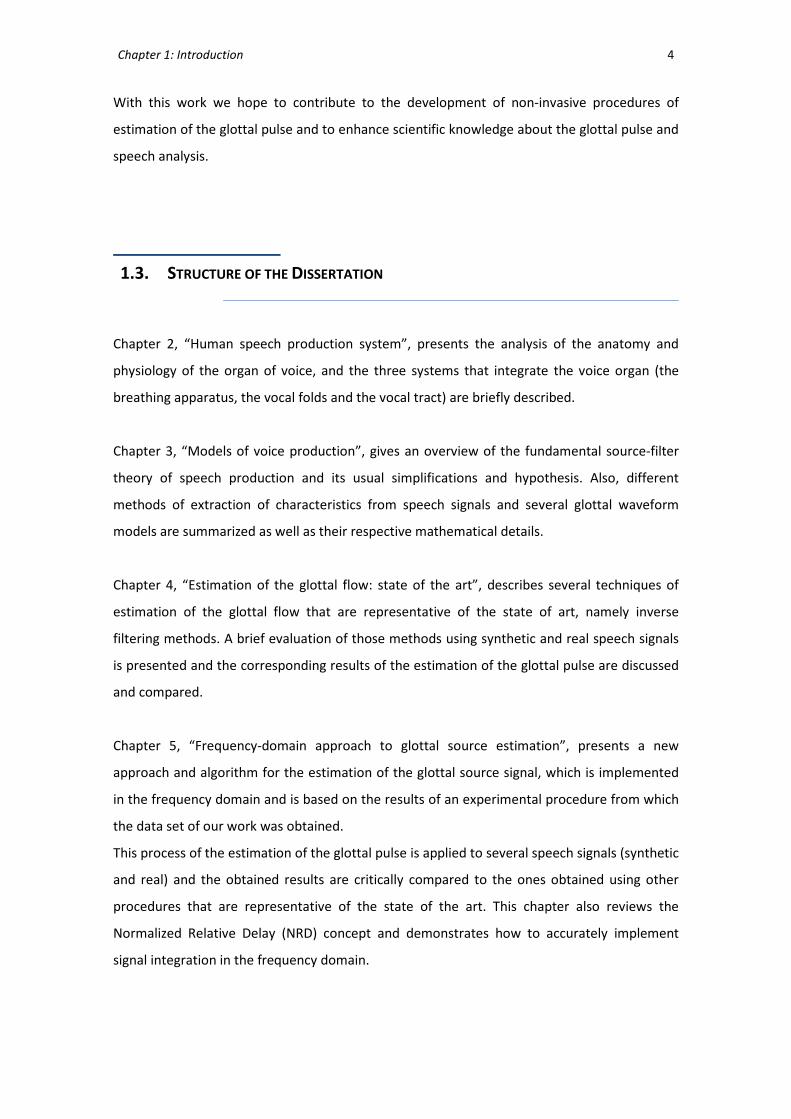
the glottal excitation is noisy) are referred to as unvoiced [Per09]. In Figure 2.3, one can see a
voiced and an unvoiced segment of speech signals. These signals are better analysed in section
3.3, from the signal synthesis point of view.
The tube formed by the larynx, the pharynx, and the oral and nasal cavities, is called the vocal
tract, so it can be defined as the space downstream the glottis that ends with the mouth cavity
or the nostrils [Kob02]. The individual morphology determines it length but in adult males, the
Figure 2.2. Top view of the larynx, showing the positions of the vocal folds.
(a) – open vocal folds; (b) – closed vocal folds.
12 2
34
65
5
6 55
2 2
1- Glottis
2- Vocal folds
3- Epiglottis
4- Anterior commissure
5- Arytenoid cartilages
6- Posterior commissure (a)
0
(b)
Chapter 2: Human Speech Production System 10
vocal tract length is about 17 – 20 cm and 3 cm of diameter. Children and adult females have
shorter vocal tracts [Sun87].
It is known that the longer the vocal tract, the lower the formant frequencies. This knowledge
is very useful to singers: if they want to sing a lower note, they have to increase the vocal tract,
for example, projecting the lips or lowering the larynx.
When the vocal folds vibrate and form pressure pulses near the glottis (which, in turn, are
propagated towards the vocal and nasal openings), the energy of the frequencies of the
excitation is altered as these travel trough the vocal tract [Gol00]. Consequently, the sound
produced is shaped by the resonant cavities above the glottal source and, therefore, the vocal
tract is responsible for changing acoustically the voice source.
2.3. GLOTTAL FLOW
According to the anatomy and physiology of speech production, the glottal flow is the airflow
velocity waveform that comes out of the glottis and enters the vocal tract, also called the
glottal source. The shape of the glottal source waveform in a single period is denoted by glottal
pulse. It should be noted that it is very common to find in several research texts the use of the
terms glottal flow, glottal source and glottal pulse interchangeably. However, Murphy [Mur08]
states that the glottal flow and the glottal pulse represent the airflow that passes through the
glottis and that the glottal source is the glottal pressure wave or, in some cases, the glottal
aperture, i.e., the derivative of the glottal pulse.
Nevertheless, in this dissertation we will use the most common definitions, considering that
they do not compromise the understanding and development of a rigorous study.
(a) (b)
0 200 400 600 800 1000-0.4
-0.2
0
0.2
0.4
Time (ms)
Amplitude
0 200 400 600 800 1000-0.1
-0.05
0
0.05
0.1
0.15
Time (ms)
Amplitude
Figure 2.3. Speech signals: (a) – voiced speech signal; (b) – unvoiced speech signal.

Chapter 2: Human Speech Production System 11
As the vocal folds open and close the glottis at identical intervals, the frequency of the sound
generated is equal to the frequency of vibration of the vocal folds [Sun87]. Each cycle consists
of four glottal phases, as it can be seen in Figure 2.4: closed, opening, opened and closing (or
return).
Typically, when the folds are in a closed position, the flow begins slowly, builds up to a
maximum, and then quickly decreases to zero when the vocal folds abruptly shut [Kaf08].
However, studies have indicated that total closure of the glottis is an idealistic assumption and
that the majority of the individuals exhibit some sort of glottal leakage during the assumed
closed phase [Cin08]. Still, most of the glottal models (chapter 4) assume that the source has
zero flow during the closed phase of the glottal cycle.
The time interval during which the vocal folds are closed and no flow occurs is referred to as
the glottal closed phase. The next phase, during which there is nonzero flow and up to the
maximum of the airflow velocity is called the glottal opening phase, and the time interval from
the maximum to the time of glottal closure is referred to as the closing or return phase.
Many factors can influence the rate at which the vocal folds oscillate through a closed, open
and return cycle, such as the vocal folds muscle tension, the vocal fold mass and the air
pressure below the glottis [Kaf08].
Due to the location of the larynx, the glottal flow cannot be measured directly, but there are
some medical procedures that allow the observation of the larynx and the vocal fold vibration.
These techniques can be divided into two categories. First, electrical and electromagnetical
glottography extract specific features of the vocal fold vibration related to the changing
electrical properties of the human tissue. Second, imaging techniques are based on visual
analysis of larynx by observing the vocal folds using a mirror [Air08b].
Figure 2.4. Glottal phases (adapted from [San09]).
closed opening open closing closed
Tension Adduction
+ Lungs
pressure
Air
flo
w
(faster)
time
Chapter 2: Human Speech Production System 12
Glottal inverse filtering, which will be explored in chapter 4, is also a technique used to
estimate the airflow through the glottis without requiring any medical procedure and using
only computational procedures.
2.3.1. ELECTROGLOTTOGRAPHY
Electroglottography (EGG), a very common technique used both in voice research and clinical
work, is a non-invasive method for examination of the vocal fold vibration [Air08b]. However,
EGG involves contact with the skin and even physical pressure, and some specialists consider
this to be an invasive technique.
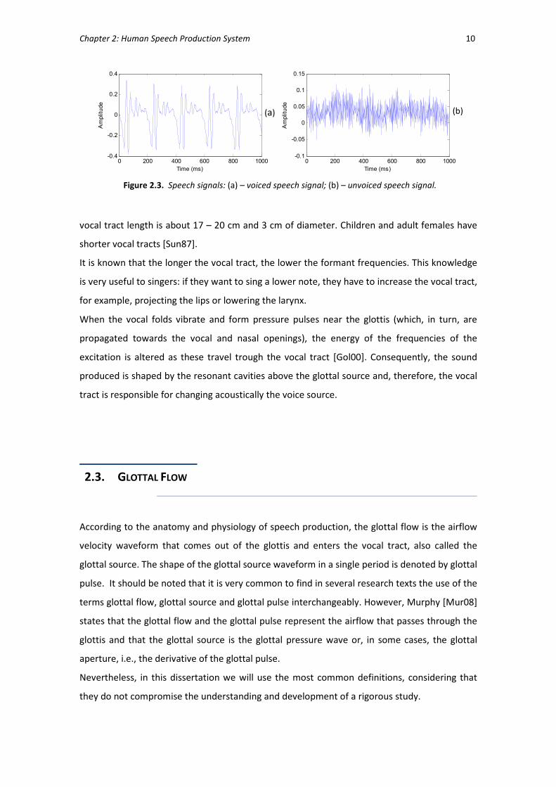
EGG is based on the fact that human tissues are conductors of electric current [Hen09], giving
a variable resistance to electric current, whereas air is a particularly poor conductor. It
measures the contact area of the vocal folds by placing one electrode on each side of the
thyroid cartilage, as it can be seen in Figure 2.5.
The conductivity of the vocal fold tissue is larger than that of the air within the laryngeal cavity
and the glottis, which makes that the impedance between the electrodes varies in step with
the vocal fold vibration [Air08b]. A high-pass filter (with cut-off frequency between 5 and 40
Hz) removes the low frequency noise components, mainly due to the movement of the larynx
during phonation, the blood flow in arteries and veins of the neck, and the contractions of
laryngeal muscles [Hen01].
The resulting electroglottographic signal, the electroglottogram, allows to analyse the vocal
folds movement and to identify the glottal phases (see Figure 2.6).
Figure 2.5. EGG measurement setting.
Electrodes have been placed on the subject’s skin and a band has been adjusted around the
neck to hold the electrodes in place. The electroglottograph (Glottal Enterprises MC2-1) is on
the right on top of the oscilloscope [Pul05].
Chapter 2: Human Speech Production System 13
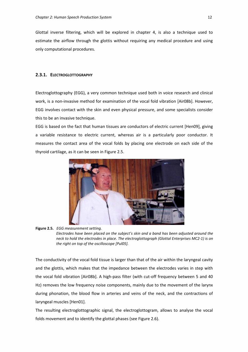
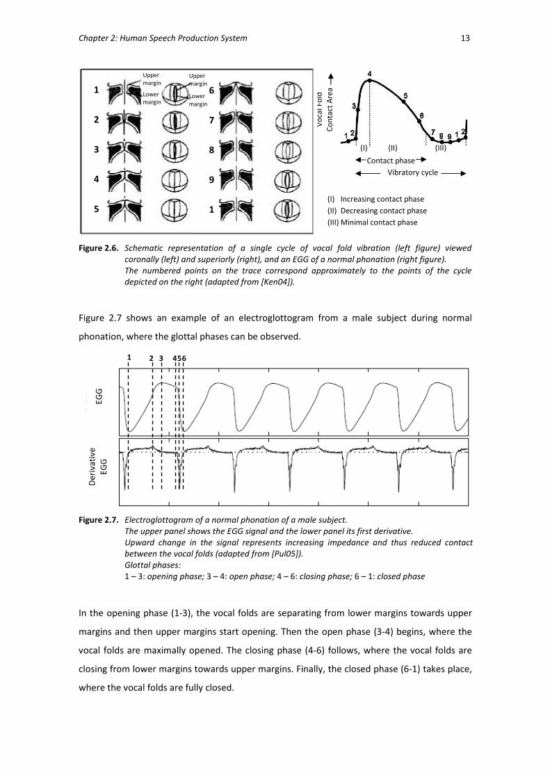
Figure 2.7 shows an example of an electroglottogram from a male subject during normal
phonation, where the glottal phases can be observed.
In the opening phase (1-3), the vocal folds are separating from lower margins towards upper
margins and then upper margins start opening. Then the open phase (3-4) begins, where the
vocal folds are maximally opened. The closing phase (4-6) follows, where the vocal folds are
closing from lower margins towards upper margins. Finally, the closed phase (6-1) takes place,
where the vocal folds are fully closed.
Figure 2.7. Electroglottogram of a normal phonation of a male subject. The upper panel shows the EGG signal and the lower panel its first derivative.
Upward change in the signal represents increasing impedance and thus reduced contact
between the vocal folds (adapted from [Pul05]).
Glottal phases:
1 – 3: opening phase; 3 – 4: open phase; 4 – 6: closing phase; 6 – 1: closed phase
EGG
D
eriv
ativ
e
EGG
1 2 3 4 5 6
Figure 2.6. Schematic representation of a single cycle of vocal fold vibration (left figure) viewed
coronally (left) and superiorly (right), and an EGG of a normal phonation (right figure).
The numbered points on the trace correspond approximately to the points of the cycle
depicted on the right (adapted from [Ken04]).
Contact phase
(I) (II) (III)
Vibratory cycle
Vo
cal F
old
Co
nta
ct A
rea
(I) Increasing contact phase
(II) Decreasing contact phase
(III) Minimal contact phase
1
2
3
4
5
6
7
8
9
1
Upper margin
Lower margin
Upper margin
Lower margin

Chapter 2: Human Speech Production System 14
Despite its relative simplicity, the EGG allows the investigation of the vocal fold vibration
during phonation and a measurement of the glottal activity, independently of the supraglottic
system. However, many authors argue that the EGG signal does not allow an exact
determination of the instants of closure and glottal opening, and some prefer to analyse the
derivative of the signal EGG [Pul05]. This signal is often studied because it allows to visualize
the changes in the tilt of the signal: if the derivative is negative in a given instant, it means that
the EGG signal is decreasing at that instant, which corresponds to the closing phase; if the
derivative is positive, than the EGG signal is increasing, which denotes the opening phase;
otherwise, the derivative is equal to zero, meaning either the open phase (maximum) or the
closed phase.
Nathalie Henrich [Hen01] regarded the peaks of the derivative of the EGG signal as reliable
indicators of glottal opening and closing instants defined by reference to the glottal air flow.
But this kind of approach is unreliable because often such peaks are imprecise or absent, or
double peaks may occur [Pul05]. Also, the EGG signals denote the area of contact of the vocal
folds and thus do not represent directly the glottal airflow pulse shape.
2.3.2. IMAGING TECHNIQUES
Video laryngoscopy (Figure 2.8) consists of a video camera attached to a laryngoscope so that
images (Figure 2.9) and sounds of the larynx and vocal folds can be simultaneously recorded
and later analysed [Gui08].
Figure 2.8. Video laryngoscopy.
Chapter 2: Human Speech Production System 15
From this technique a test, called kimography, can be performed that makes a quantitative
analysis of the vocal fold vibration, by joining a sequence of lines obtained from the captured
video frames. This is illustrated in Figure 2.10.
The examination of the kimography allows to measure the duration of each phase of the
glottal cycle and the opening amplitude of the glottis.
Videostroboscopy (Figure 2.11) is other procedure used to assess the structure and movement
of the vocal folds. It uses a video camera attached to a stroboscopic light source, which
illuminates the vocal folds quasi-synchronized with vocal fold vibration to provide what
appears to be a slow-motion view of vocal fold movement and vibration [Gui08].
Figure 2.9. Sequence of vocal folds images captured during a video laryngoscopy examination.
(a)
(b)
Figure 2.10. kimography.
(a) The image from video laryngoscopy, the selected line for analysis and its projected
kimography [Gui08].
(b) A video fragment and its image on the kimography. (Image from http://www.diagnova.pl/en/index.php/offer/products/video-recording/)
Time
Selected
line

Chapter 2: Human Speech Production System 16
Illustration of the fundamental principle of videostroboscopy is shown in Figure 2.12.
By enabling the vocal folds to be viewed both in slow motion and at standstill, assessment of
amplitude and glottic closure is enhanced using the videostrobocopy procedure [WB87].
Despite the fact that these techniques allow the analysis of the glottal source, they can
interfere with normal phonation behaviour. Also, the logistic requirements of these techniques
(equipment and health professionals for video laryngoscopy and videostroboscopy), the
invasive nature of the procedures and the time required make these techniques not practical
and, therefore, unattractive for the estimation of the glottal source.
The estimation of the glottal pulse directly from the speech signal seems to be much more
attractive, due to the relative simplicity and non-invasiveness of the process, which explains,
somehow, the numerous studies done in this area in recent decades.
Figure 2.12. Fundamental principle of videostroboscopy.
Flashes of light are fired one time each frame of video at a given moment (above). The
images captured from each frame are combined to create an artificial cycle (below)
[Gui08].
(Image from http://www.uwec.edu/Maps/bldgtour/hss/index.htm
Figure 2.11. Videostroboscopy

Chapter 2: Human Speech Production System 17
2.4. SUMMARY
In this chapter an overview is given of the anatomy and physiology of the voice organ, and the
human speech production process.
Also, the four phases of the glottal cycle are presented as well as different medical procedures
that allow the observation of the larynx and the vocal fold vibration. In general, these
procedures are uncomfortable for the speaker and interfere with normal phonation behaviour,
which makes more attractive and motivates the development of techniques that estimate the
glottal pulse directly from the speech signal.

Chapter 3
MODELS OF VOICE PRODUCTION
Contents
3.1. INTRODUCTION ................................................................................................................... 19
3.2. SOURCE-FILTER MODEL ....................................................................................................... 19
3.3. EXTRACTION OF CHARACTERISTICS FROM A SPEECH SIGNAL ....................................................... 24
3.3.1. LINEAR PREDICTIVE CODING (LPC) METHOD ............................................................................ 27
3.3.2. DISCRETE ALL-POLE MODELLING (DAP) .................................................................................. 30
3.3.3. MEL-FREQUENCY CEPSTRAL COEFFICIENTS (MFCC) METHOD ..................................................... 32
3.3.3.1. Cepstral Analysis .............................................................................................. 32
3.3.3.2. Mel Scale .......................................................................................................... 33
3.3.3.3. MFCC calculation process................................................................................. 34
3.4. GLOTTAL PULSE MODELS ..................................................................................................... 35
3.5. SUMMARY ......................................................................................................................... 44

Chapter 3: Models of Voice Production 19
3.1. INTRODUCTION
Any sound, given the physical nature of sound waves, requires an energy source, an oscillator
and a medium to travel trough. In the human body system, these are represented by the lungs,
the vocal folds and the vocal tract, respectively. From the action of the lungs, the vocal folds
vibrate as an oscillating force and, together with the resonant cavities of the vocal tract, mouth
and nose, this force creates the sound waves required for voice [Mur08]. Thus, this is the basis
of any model of voice production, as the source-filter model, that will be presented and
analysed in this chapter. Also, different methods of extraction of characteristics from speech
signals and glottal waveform models are described and their respective mathematical details
are presented.
3.2. SOURCE-FILTER MODEL
The voice organ, as a generator of sounds, has three major units: a power supply (the lungs),
an oscillator (the vocal folds) and a resonator (the vocal tract) [Sun77].
As it was explained in the previous chapter, when the vocal folds are closed and an airstream
arises from the lungs, the pressure below the glottis forces the vocal folds apart: the air
passing between the folds generates a Bernoulli force that, along with the mechanical
properties of the folds (and the asymmetrical force), almost immediately closes the glottis. The
pressure differential builds up again, forcing the vocal folds apart again. This cycle of opening
and closing the glottis feeds a train of air pulses into the vocal tract and produces a rapidly
oscillating air pressure in the vocal tract: in other words, a sound [Sun77]. During this process,
an entire family of spectrum tones is generated, called partials, where the lowest tone is
known as the fundamental and the others as overtones.
The vocal tract has four or five important resonances, called formants, that shape the initial
sound wave, setting frequency amplitudes and formant features, which define the quality and
vowel type when the wave is perceived audibly [Mur08].
The glottal source spectrum is filtered by the vocal tract and since the partials have different
frequencies, the vocal tract treats them in different ways: the partials closest to a formant

Chapter 3: Models of Voice Production 20
frequency reach higher amplitudes than neighbouring partials [Sun87]. This is illustrated in
Figure 3.1.
Many models for voice production system are based on Fant’s source-filter theory: the voice is
the result of the convolution between the excitation source and the filter system, i.e., the
source represents the air flow at the vocal folds and the filter represents the resonances of the
vocal tract which change over time [Fan60]. For voiced speech, the excitation is a periodic
series of pulses, whereas for unvoiced speech, the excitation has the properties for random
noise [Kaf10]. Thus, the source is the creation of the puffs of air at the glottis (glottal pulses)
generating the sound wave (glottal source), which propagates through the vocal tract, and that
is then filtered by varying shapes and cavities encountered therein and radiated by the lips
[Mur08]. This model is, then, a simplification of the intricate relationship between the glottal
source, the vocal tract and the lip/nostrils radiation, usually simply referred as lip radiation.
Figure 3.2 illustrates this simple model.
Figure 3.1. Schematic illustration of the generation of voice sounds (adapted from [Sun77], [Sun87]).
Lungs
(power supply)
Vibrating Vocal Folds (oscillator)
Vocal Tract (Resonator)
airstream
voice source
output sound
Time
Velum
Vocal folds
Trachea
Lungs
Glottal source spectrum
Frequency
Frequency
Glottal source waveform
Tran
sglo
ttal
air
flo
w
Leve
l Le
vel
Leve
l
Frequency
Radiated
spectrum
Vocal
Tract
Vocal tract sound transfer curve
formants

Chapter 3: Models of Voice Production 21
This model has two strong assumptions:
1. the source and the filter are separated and independent systems ;
2. in time domain, voice production can be represented by means of a convolution of its
elements (i.e., the glottal source, the vocal tract filter and lip radiation) [Deg10].
The first assumption implies that the glottal source is equal to the glottal flow, which in reality,
is not perfectly valid, because a source-tract interaction exists and the glottal flow is actually
dependent in some degree of the variations of the vocal tract impedance. Yet, the source-filter
model has been used in this dissertation, since the underlying assumptions can be considered
sufficient for most cases of interest which explains for example that it is widely used in speech
processing systems [Pul05].
This model is a simplification of the physiology and acoustic model of voice production and the
scheme in Figure 3.3 emphasizes the links between these elements. According to Gilles
Degottex ([Deg10]), the author of the scheme, the articulators are in blue, the passive
structures are in grey and the glottis, which is acoustically active, is in orange like the vocal
folds.
On the left of Figure 3.3 is a synthesis of the physiology of the voice production system,
described in the previous chapter.
In the center, an acoustical model is presented, in which the impedance of the vocal apparatus
is represented by area sections and their physical properties all along the structures. The
impedance of the larynx is mainly defined by the glottal area, which is an implicit variable
influenced by the imposed mechanical properties of the vocal folds [Deg10].
On the right of Figure 3.3, the source-filter model is depicted: the speech signal is the result of
a glottal flow filtered by the vocal tract cavities and radiated by the lips and nostrils.
The source-filter model is, as it was explained, a simplification of the discrete-time model of
speech production, represented in Figure 3.4.
The mathematical framework of the classic source-filter model of speech production model
can be expressed as follows:
[ ] [ ] [ ] [ ]s n g n v n l n= ∗ ∗ (1)
Speech Excitation
Source
Vocal Tract
Filter
Lip
radiation
Figure 3.2. Block diagram of the source-filter model.

Chapter 3: Models of Voice Production 22
where [ ]s n is the output signal, i.e., the speech signal, [ ]g n is the excitation source signal,
[ ]v n is the impulse response of the vocal tract and [ ]l n is the lip/nostrils radiation. This is
illustrated in Figure 3.5.
Figure 3.3. Schematic view of voice production models [Deg10].
Envi
ron
men
t V
oca
l T
ract
La
ryn
x S
ub
glo
tta
l st
ruct
ure
Physiology Acoustic model Source-filter model
Acoustic signal
Radiation
Vocal tract filter
Glottal source
Acoustic signal
Nostrils radiation Lip/nostrils
Nasal-tract area
function
Buccal-tract area
function
Pharynx area function
Subglottal pressure
Glottal flow
Glottal Area
Nostrils Lips
Nasal
Cavity
Buccal
Cavity
Pharynx
Epig
lott
is
Ton
gue
Jaw
Vocal folds Glottis
Ventricular folds
Left lung
Right lung
Trac
hea
Velum Uvula
Par
anas
al
si
nu
ses
Pir
ifo
rm
sin
use
s

Chapter 3: Models of Voice Production 23
In Z-domain, equation (1) can be written as:
( ) ( ) ( ) ( )S z G z V z L z= (2)
where ( )G z is the Z transform of the acoustic excitation at the glottis level. The resonances
and anti-resonances of the vocal tract are combined into a single filter ( )V z , termed Vocal
Tract Filter (VTF) and the lip and nostrils radiation are combined into a single filter ( )L z ,
termed radiation. Therefore, the glottal inverse filtering requires solving the equation:
( )( )
( ) ( )
S zG z
V z L z=
(3)
∗ ∗ =
Impulse train Vocal tract filter response Differential glottal flow signal Speech signal
Tim
e-d
om
ain
sig
nal
Figure 3.5. Source-filter model: the speech signal as a result of the convolution between the excitation
source signal, the impulse response of the vocal tract and the lip/nostrils radiation.
Figure 3.4. General discrete-time model of speech production and its physiologic correspondence
(adapted from [HAH01] and [Gol00]).
Impulse train
generator
Glottal pulse
model
Random noise
generator
Vocal tract
model
Radiation
model
Speech
Pitch period
Gain for voice source
Gain for noise source
Voiced/unvoiced switch

Chapter 3: Models of Voice Production 24
that is, to determine the glottal waveform, the influence of the vocal tract and the lip/nostrils
radiation must be removed. In the case of a voiced speech signal, the glottal waveform
presents a typical periodic shape as previously shown in Figure 2.4.
Usually, the VTF is modelled as an p-order all-pole filter:
where the poles correspond to resonances of the vocal tract filter and, therefore, to the
formant frequencies of the vocal tract [Mur08].
The lip/nostrils radiation imposes a high pass filter approximated by a first order time-domain
derivative [Mur08], meaning that the derivative of the glottal flow is the effective excitation of
the vocal tract. Therefore:
1( ) 1L z zα −= − (5)
where α is the lip/nostrils radiation coefficient, which value is close to (but less than) 1
[JBM87]. Usually, α is a value between 0.95 and 0.99 in order that the zero lies inside the unit
circle in the z plane.
This equation can be written as [JBM87]:
0
1( )
.N
k k
k
L z
zα −
=
≈
∑
(6)
where N is theoretically infinite but in practice finite because 1α < . This result suggests that
the effect of a zero may be approximated by a sufficiently large number of poles.
Although in the literature, most often, these three processing stages are implemented in the
discrete-time domain, the spectral approach to voice source modelling has a number of
advantages, as it will be discussed in this dissertation.
3.3. EXTRACTION OF CHARACTERISTICS FROM A SPEECH SIGNAL
Speech signals can be classified into voiced and unvoiced. This classification is fundamental in
signal analysis, since each type has a different kind of excitation in the synthesis of the signal.
1
1( )
1P
i
i
i
V z
b z−
=
=−∑
(4)

Chapter 3: Models of Voice Production 25
Voiced speech signals are those that are generated as a result of the vibration of vocal folds,
for example, all the vowels that we pronounce. These signals have an important feature: a well
defined periodicity.
Unvoiced speech signals, such as “s”, “p”, “z” or “ch”, are generated by the passage of air at
high speed through the vocal tract while the glottis is partially open. These kind of signals have
almost no periodicity.
Figure 3.6 shows the speech analysis of voiced and unvoiced speech signals. Plots (a) and (b)
illustrate the corresponding speech waveforms, the plots below, (c) and (d), illustrate the
corresponding spectrograms, i.e., a time-varying spectral representation of the energy
distribution reflecting to the resonances of the vocal tract, and plots (e) and (f), the
corresponding magnitude spectra.
(a)
(b)
(c)
(d)
0 2000 4000 6000 8000 100000
50
100
150
Frequency (Hz) →
Magnitude (dB) →
(e)
0 2000 4000 6000 8000 100000
50
100
150
Frequency (Hz) →
Magnitude (dB) →
(f)
Figure 3.6. Illustrations of speech sounds.
(a): the speech waveform of the voiced sound of the vowels “a e i o u”, uttered by a female
subject; (c): the corresponding spectrogram; (e): the magnitude spectrum pertaining to a
segment of vowel /a/ where the harmonics are depicted;
(b): the speech waveform of the unvoiced sound “z”; (d): the corresponding spectrogram; (f): the magnitude spectrum pertaining to a short segment of that unvoiced sound.

Chapter 3: Models of Voice Production 26
From these illustrations it is possible to observe that the unvoiced speech signal (plot (b)) is
characterized by a non-periodic nature and its spectrum (plot (d)) has more energy in the high
frequency region. On the other hand, the spectrum of the voiced speech signal (plot(c)) has
more energy in low frequency region.
Speech signals are non stationary signals, i.e., over time their main attributes and, in particular,
their waveform, are constantly being changed. The mathematical tools used in signal
processing typically require that these signals remain time invariant so that its characteristics
can be conveniently analysed. If a speech signal is divided into short enough segments
(approximately between 10 and 30 ms), these "new" signals of short duration can be
considered almost stationary since, throughout this duration, the phonatory articulators
movements are sufficiently reduced and slow. Thus, the transfer function associated to the
vocal tract shape remains fixed (or nearly fixed) and the acoustic characteristics of the "new"
signal can be considered virtually time invariant.
Therefore, in order to extract features from a voice signal it is first necessary to perform a
segmentation of the signal into segments of sufficiently short duration. This segmentation is
achieved by applying a sliding window (e.g., Hanning, Hamming, Sine or Blackman3) to the
complete voice signal, i.e., the segmentation of the speech signal is made by multiplying the
window with the voice segment. Each one of these segments is called a frame and can be
expressed as:
[ ] [ ] [ ]m mx n x n w n= (7)
where [ ]x n is the speech signal and [ ]m
w n is the window function, which is zero everywhere
except in a small region.
The short-time Fourier (DTFT) representation for frame m is defined as:
( ) [ ] [ ] [ ] .j j n j n
m m m
n n
X e x n e w n x n eω ω ω+∞ +∞
− −
=−∞ =−∞
= =∑ ∑ (8)
There are several methods to extract features from a voice signal, and some will be analysed:
Linear Predictive Coding (LPC), Mel-Frequency Cepstral Coefficients (MFCC) and Discrete All-
Pole Modelling (DAP).
3 See mathematical details in the Appendix A.

Chapter 3: Models of Voice Production 27
3.3.1. LINEAR PREDICTIVE CODING (LPC) METHOD
Linear Predictive Coding (LPC) is a mathematical technique introduced in the sixties that may
be applied to time series data and was used, primarily, as a direct proposal to modelling the
voice spectral envelope in digital form [Mur08]. Given a speech signal, LPC assumes that a
current sample can be determined by a weighted linear combination of a certain number of
past previous samples. This method is widely used because it is fast and simple, and effective
ways exist of estimating the main parameters, or coefficients, of the predition filter [HAH01].
The most common representation of linear prediction (LP) is:
1
[ ] [ ]N
i
i
y n a x n i=
= −∑ (9)
where [ ]y n is the linear prediction of a signal [ ]x n , and ia , for 1i = to N , are the prediction
coefficients. N is the predictor order, which is usually in the range of 8 to 14, with 10 being the
most common for coding applications. The choice of the prediction order determines the
number of poles that result in the designed filter and is essentially determined by the sampling
rate. Equation (9) is sometimes referred to as an autoregressive (AR) model. The difference
between the actual sample and the predicted sample is called the residual error or the
prediction error, and is given as:
[ ] [ ] [ ]e n x n y n= − (10)
and from equation (9), one obtains:
1
[ ] [ ] [ ] [ ] [ ].N
i
i
e n x n y n x n a x n i=
= − = − −∑ (11)
The aim of LPC analysis is getting the most suited coefficients such that the residue is as small
as possible. Their estimation is termed linear predictive analysis, and the most common choice
for the optimization of these coefficients is the criterion of minimizing the square error
function given by:
[ ]2
1 12
0 0 1
[ ] [ ] [ ] .L L N
i
n n i
E e n x n a x n i− −
= = =
= = − −
∑ ∑ ∑ (12)
This function can be minimized by imposing:
0 , 1,..., .i
Ei N
a
∂= =
∂
(13)
From this equation, one obtains:

Chapter 3: Models of Voice Production 28
1
0
[ ]2 [ ]. 0L
n i
e ne n
a
−
=
∂= ⇔ ∂
∑ (14)
( )1
0
2 [ ]. [ ] 0L
n
e n x n i−
=
⇔ − − = ∑ (15)
1
0 1
2 [ ] [ ] [ ] 0L N
k
n k
x n a x n k x n i−
= =
⇔ − − − − =
∑ ∑ (16)
[ ]1 1
0 0 1
2 [ ]. [ ] [ ]. [ ] 0L L N
k
n n k
x n x n i a x n k x n i− −
= = =
⇔ − − − − − =
∑ ∑∑ (17)
1 1
1 0 0
[ ]. [ ] [ ]. [ ].N L L
k
k n n
a x n k x n i x n x n i− −
= = =
⇔ − − = −∑ ∑ ∑ (18)
This last equation leads to the normal equations for linear prediction [Cin08].
Thus, the result of LPC analysis is a set of coefficients ia , for 1i = to N , that can be computed
using the autocorrelation or covariance methods [Cin08], and the error signal [ ]e n , which is as
small as possible in the least squares sense, represents the difference between the predicted
signal and the original signal.
Figure 3.7 illustrates the LPC method: after windowing the segment of the speech signal,
shown in plot (a), from a spectral standpoint, linear prediction attempts to match the power
spectrum of the signal [ ]x n to the predicted filter given by the coefficients ia , as it is observed
in plot (b), where it is also possible to identify some vocal tract resonances, i.e., the formants,
denoted F1 to F4. By inverse filtering, the LPC residual is obtained, displayed in plot (c), and
then the amplitude spectrum of the residual signal, represented in plot (d). In this last plot, it is
possible to observe that the amplitude spectrum is almost flat, which denotes that the effects
of the vocal tract resonances have been removed [Dru11].
In Z-Transform domain, equation (11) is equivalent to:
1
( ) ( ) 1 ( ) ( )N
i
i
i
E z X z a z X z A z−
=
= − =
∑ (19)
where ( )A z is the Z-Transform model of the ‘whitening’ filter, ( )E z is the Z-Transform of the
prediction error and ( )X z is the Z-Transform of the speech signal.
Usually, ( )A z is referred to as the LPC analysis filter and 1
( )A z , an all-pole filter, as the
synthesis filter.

Chapter 3: Models of Voice Production 29
Defining the power spectrum ( )P ω of the signal [ ]x n as
then, from equation (19), one has:
( )( )( )
2
2.
j
j
E eP
A e
ω
ωω = (21)
If the prediction filter is effective, the prediction error is white noise, which means its power
spectral density is flat. As a consequence, the signal spectrum ( )P ω is approximated by the
all-pole model spectrum ( )P ωɶ of the estimated filter. Assuming that the noise is white, then
2 2( )E z σ= and
( )( )
2
2j
PA e ω
σω =ɶ
(22)
where 2σ is the error energy. From equations (21) and (22), one can conclude that the more
“flat” the residual power spectrum is, the better approximation is obtained ( )( )2 2jE e ω σ≈ .
Defining the total error as the infinite sum
( )2
2 1( ) ( )
2
j
n
n
a e a E e d
πω
π
ε ωπ
+∞
=−∞ −
= =∑ ∫ (23)
where ne is the prediction error, given by equation (10), and combining equations (21) and
(22), equation (23) reduces to:
( ) ( )2
jP X e ωω = (20)
Figure 3.7. Illustration of the LPC method. (a): the speech signal (thin line) and the applied window (solid
line); (b): the magnitude spectrum (thin line) and the corresponding LPC spectral envelope
(solid line), where the four first formants (F1 to F4) are depicted; (c): the LPC residual
obtained by inverse filtering; (d): the magnitude spectrum of the residual signal [Dru11].
M
agn
itu
de
dB
)
M
agn
itu
de
(dB
)
A
mp
litu
de
A
mp
litu
de
Time (s) Frequency (Hz)
(a) (b)
(c) (d)

Chapter 3: Models of Voice Production 30
( ) ( )2
2 21 1 ( )( ) ( ) .
ˆ2 2 2 ( )
j j Pa E e d P A e d d
P
π π πω ω
π π π
σ ωε ω ω ω ω
π π π ω− − −
= = =∫ ∫ ∫ (24)
Analysing equation (24), one can conclude that, if a small region of the spectrum is considered,
the error can be minimized and a better fit is obtained when ˆ( ) ( )P Pω ω> , because
ˆ( ) / ( )P Pω ω is small [Mag05].
One disadvantage of this method is that for discrete spectrum, the LPC error measure
possesses an error cancelation property, which means that the contributions to the error when
ˆ( ) ( )P Pω ω> cancel those when ˆ( ) ( )P Pω ω< . Thus, an envelope can be selected rather the
only one which passes through all the spectral points [JM91]. Also, the optimal order is difficult
to determine and the iterative procedure is rather slow [Dru11].
The LPC model has other limitations as: it assumes an all-pole spectrum, it is naturally adapted
to accurately model resonances (or pole effects) rather than anti-resonances (or zero effects).
However nasalized vowels, involving the lowering of the velum within the vocal tract and the
radiation of speech sounds through the nose, can create zeros in the spectrum [Mur08]. On
the other hand, consonants produced with a continuous airflow through a vocal tract
constriction, called fricative sounds, also introduce anti-resonances into the spectrum. Another
disadvantage of this procedure is that LPC is especially problematic for high pitched harmonic
sounds [Dru11]. In this case, the ‘harmonic locking effect’ effect is typically observed because
pole locations are tied to the frequency of the harmonics of voiced speech signal.
3.3.2. DISCRETE ALL-POLE MODELLING (DAP)
In 1991, El-Jaroudi and Makhoul [JM91] proposed a new method for parametric modelling of
spectral envelopes, called the Discrete All-Pole (DAP) modelling. The main purpose of the DAP
method is to fit the all-pole model using only the finite set of spectral locations that are related
to the harmonic positions of the fundamental. Figure 3.8 shows an example of a spectral
envelope given by DAP and LP.
This method uses the discrete Itakura-Saito error measure and the optimization criterion is
derived in the frequency domain.
The Itakura-Saito error measure is given by [JM91]:

Chapter 3: Models of Voice Production 31
1
( ) ( )1ln 1
ˆ ˆ( ) ( )
Nm m
IS
m m m
P PE
N P P
ω ωω ω=
= − −
∑ (25)
where ( )m
P ω and ˆ ( )mP ω are the given discrete spectrum and the all-pole spectrum,
respectively, defined at N frequency points. This error reaches the minimum only when
model spectrum coincide on all discrete points.
According to El-Jaroudi and Makhoul [JM91], the minimum error is obtained when
1
( )11.
ˆ ( )
Nm
m m
P
N P
ωω=
=∑ (26)
Thus, from equation (25):
1/
1
min 1/1
1
ˆ( )( )1
ln lnˆ( )
( )
NN
mNmm
IS NN
m m
mm
PP
EN P
P
ωωω
ω
=
=
=
= − =
Π∑
Π (27)
and one can conclude that the minimum error is equal to the logarithm of the ratio of the
geometric means of the model spectrum and the original spectrum.
Alku et al. [AVV02] stated that the DAP allows a better estimation of the formants of the vocal
tract, particularly the F1, and decreases the amount of formant ripple in the estimated glottal
flows. Also, it seems to be more accurate for high-pitched voices than the LPC method.
Figure 3.8. FFT magnitude spectrum of a male vowel /a/ (thin line) and the all-pole spectrum of the DAP
method (thick line) together with the LP method (dashed line). For the sake of clarity, the
magnitude levels of the prediction model have been lifted 10 dB [Mag05].
MA
gnit
ud
e (d
B)
Frequency (Hz)

Chapter 3: Models of Voice Production 32
3.3.3. MEL-FREQUENCY CEPSTRAL COEFFICIENTS (MFCC) METHOD
Mel-Frequency Cepstral Coefficients (MFCC) method is based on feature extraction of speech
signal from its cepstrum, changed according to the Mel scale, a scale that seeks to replicate the
human auditory perception.
3.3.3.1. Cepstral Analysis
In the frequency domain, the convolution between the two components of the signal, the
excitation source signal [ ]g n , and the impulse response of the vocal tract [ ]v n , is transformed
into a product:
[ ] [ ] ( ). ( ).g n v n G Vω ω∗ ⇔ (28)
Applying the logarithm operator to the signal, it yields:
Thus, the resulting signal is a linear combination between the two components.
Applying the inverse of the Fourier transform to the resulting signal from equation (29), the
signal will be represented in a new domain, called the cepstral domain. In this domain, it is
possible that the two components of the signal, the excitation and the impulse response of the
vocal tract, are linearly combined and separated from each other. Thus, representing the
speech signal in the cepstrum, it is possible to select specific components of the latter,
applying a linear filter to remove unwanted parts. Applying a reverse Fourier transform to the
preserved components of the cepstrum, allows to reconstruct the desired components in the
spectral domain.
The cepstral domain can be divided into real cepstrum and complex cepstrum. The difference
between them is that, in the former case, the phase information of the speech signal is lost,
i.e., any signal is minimum phase. In the latter, the cepstral coefficients have real part and
imaginary part and, thus, the phase information is preserved.
The real cepstrum and the complex cepstrum of a signal [ ]x n are given, respectively, by
[Gol00]:
( ) ( ) ( )log ( ). ( ) log ( ) log ( ) .G V G Gω ω ω ω= + (29)
( )1[ ] ln
2
j j nc n X e e d
πω ω
π
ωπ −
= ∫ (30)

Chapter 3: Models of Voice Production 33
and
( )1ˆ[ ] ln .
2
j j nx n X e e d
πω ω
π
ωπ −
= ∫ (31)
In this equation, the complex logarithm is used and can be written as:
( ) ( ) ( ) ( )ˆ ln lnj j jX e X e X e jω ω ω θ ω= = + (32)
and the phase ( )θ ω is given by:
( ) ( )arg .jX e ωθ ω = (33)
From equations (30) and (31) it is simple to conclude that if the signal [ ]x n is real, both the
real cepstrum and the complex cepstrum are real signals and homomorphic transformations,
i.e., they convert a convolution into a sum. Thus, if [ ]x n is a speech signal, then the real
cepstrum and the complex cepstrum can be written as the sum of the excitation and the vocal
tract filter.
3.3.3.2. Mel scale
Several studies state that the correlation between the human perception of the fundamental
frequency of a sound and its real value is not linear (e.g. [CL09; Cua07]). The perceived
frequency by human people is known as pitch. In 1940, Stevens and Volkman developed a
scale, called the Mel scale, that seeks to approach the characteristics of sensitivity of human
hearing [Gol00].
“Mel” is a unit of measure of perceived pitch or frequency of a tone, defined as:
1127ln 1700
mel
ff
= +
(34)
where f is the actual frequency in Hz.
Figure 3.9 shows the Mel scale. As it can be seen, this scale has almost a linear frequency
behaviour below 1000 Hz and a logarithmic behaviour above 1000 Hz.

Chapter 3: Models of Voice Production 34
Some experiments in human perception have shown that frequencies of a complex sound
within a certain bandwidth of some nominal frequency cannot be individually identified unless
one of the components of this sound falls outside the bandwidth [Cua07]. This bandwidth is
known as critical bandwidth and its width varies with the frequency.
3.3.3.3. MFCC calculation process
In the MFCC analysis, the first steps are the pre-emphasis and the segmentation of the speech
signal, typically using the Hamming window with 50% overlapping. The next processing step is
the Fast Fourier Transform (FFT), which converts each frame of N samples from the time
domain into the frequency domain. Then, the amplitude of the FFT is obtained
and is filtered through triangular windows to approximate the Mel frequency scale. A cepstral
analysis follows from a minimum frequency of 0 Hz to the maximum frequency of half of the
sampling frequency. In the final step, the cepstral coefficients are extracted, applying the
logarithm function to the different frames of the spectrum and then using the Discrete Cosine
Transform (DCT)4.
A block diagram of the MFCC calculation process is represented in Figure 3.10.
According to Jankowski et al. [JVL95], the MFCC analysis provides superior noise robustness in
comparison with linear prediction-based feature extraction techniques.
4 See Appendix A for mathematical details.
Figure 3.9. The Mel scale.
0 1000 2000 3000 4000 5000 6000 7000 8000 9000 100000
500
1000
1500
2000
2500
3000
3500
Frequency (Hz)
Pitch (mels)

Chapter 3: Models of Voice Production 35
3.4. GLOTTAL PULSE MODELS
The importance of the analysis of the glottal flow is very well established in different areas but
it was stated before that the medical procedures that allow the observation of the vocal fold
vibration are uncomfortable for the speaker and interfere with normal phonation behaviour.
The estimation of the glottal flow from a speech signal (called inverse filtering) has been a
challenge over the last decades and, as a consequence, several glottal models have been
proposed to define one period of the glottal flow analytically. In this section, some of these
models will be described.
Although the glottal models do not use the same number of parameters or the same name for
similar parameters, which makes it rather difficult to understand the differences and
similarities among models, all share some common features, as stated by Doval and
d’Alessandro [DA99], because:
• the glottal flow is always positive or null;
• the glottal flow is quasi-periodic;
• the glottal flow is a continuous function of time;
• on a single period, the glottal flow is bell-shaped: it starts increasing, then decreasing and
finally null;
• the glottal flow is a differentiable function of time, except in some instants as the glottal
closing instant (GCI) and the glottal opening instant (GOI);
• the glottal opening phase is longer than the glottal closure phase.
Despite the fact that most of the glottal models consider these assumptions, as it was
previously mentioned, studies have shown that the majority of the individuals reveal a glottal
Figure 3.10. Block diagram of the MFCC calculation process.
Logarithm DCT
y Hamming
Window
FFT
abs (y2)
Pre-
emphasis
Power
Spectrum
FFT
Cepstral
coefficients
using DCT
Linear to Mel frequency transformation using
triangular filters
Speech Signal
MFCC

Chapter 3: Models of Voice Production 36
leakage during the closed phase and, therefore, the glottal flow is not completely null during
that phase [Deg10].
According to the general properties of the glottal flow expressed above, the existing models
use mainly a set of time instants, as it is shown in Figure 3.11:
:ct duration of the period (
0 01 /
ct T f= = );
:pt time of the maximum of the pulse. This maximum is termed the voicing amplitude vA ;
:et time of the minimum of the time-derivative;
:at the return phase duration.
Most of glottal pulse models, if not all, show an asymmetry that gives more importance to the
right part of the flow [DAH03]. Some of these models have a time-based parameter, the
asymmetry coefficient, denoted by m
α , that regulates this asymmetry. This is a dimensionless
glottal flow parameter defined as the ratio between the flow rise time and the open time. It is
equivalent to the speed quotient (SQ), i.e., the ratio of the opening phase duration to the
closing phase duration, as shown by the following relationship:
.1
m
SQ
SQα =
+
(35)
This parameter was introduced by Doval and d’Alessandro to simplify the equations of glottal
flow models [HSA+03]. Another advantage of using the asymmetry coefficient instead of the
speed quotient is that the values of this parameter are more easily understandable: m
α ranges
between 0 and 1 (which corresponds to 0 SQ< < ∞ ), with typical values between 0.5 ( 2SQ = )
and 0.8 ( 4SQ = ). For 0.5m
α < ( 1SQ < ), the glottal pulse is skewed to the left, for 0.5m
α = , is
symmetric, and for 0.5m
α > , the glottal pulse is skewed to the right.
De
riv
ati
ve
glo
tta
l fl
ow
G
lott
al
flo
w
opening phase
opening instant
Opened phase Closed phase
closing instant closing
phase 0ct T=
et at pt
vA
E
Figure 3.11. Main scheme of the glottal pulse used by most of glottal models [Hen01].
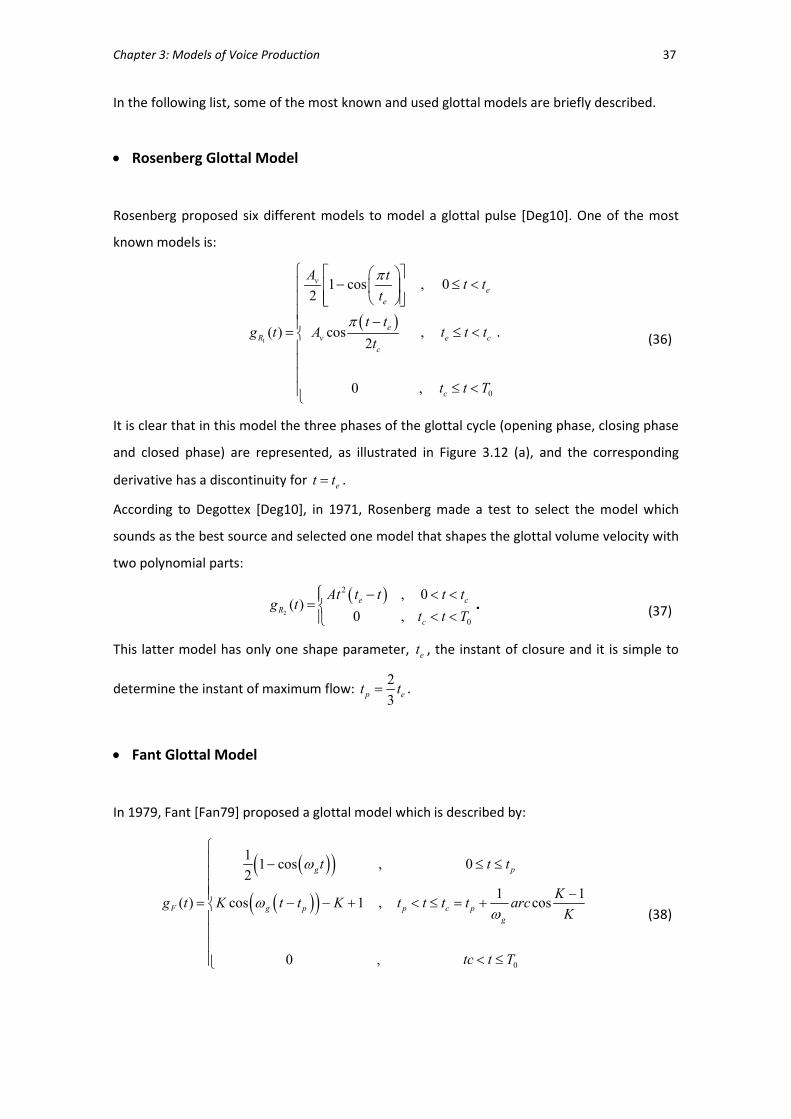
Chapter 3: Models of Voice Production 37
In the following list, some of the most known and used glottal models are briefly described.
• Rosenberg Glottal Model
Rosenberg proposed six different models to model a glottal pulse [Deg10]. One of the most
known models is:
( )1
0
1 cos , 02
( ) cos ,2
0 ,
− ≤ <
−
= ≤ <
≤ <
ve
e
e
R v e c
c
c
A tt t
t
t tg t A t t t
t
t t T
π
π. (36)
It is clear that in this model the three phases of the glottal cycle (opening phase, closing phase
and closed phase) are represented, as illustrated in Figure 3.12 (a), and the corresponding
derivative has a discontinuity for =e
t t .
According to Degottex [Deg10], in 1971, Rosenberg made a test to select the model which
sounds as the best source and selected one model that shapes the glottal volume velocity with
two polynomial parts:
( )2
2
0
, 0( )
0 ,
e c
R
c
At t t t tg t
t t T
− < <=
< <. (37)
This latter model has only one shape parameter, et , the instant of closure and it is simple to
determine the instant of maximum flow: 2
3p et t= .
• Fant Glottal Model
In 1979, Fant [Fan79] proposed a glottal model which is described by:
( )( )
( )( )
0
11 cos , 0
2
1 1( ) cos 1 , cos
0 ,
g p
F g p p c p
g
t t t
Kg t K t t K t t t t arc
K
tc t T
ω
ωω
− ≤ ≤ −
= − − + < ≤ = +
< ≤
(38)

Chapter 3: Models of Voice Production 38
where /g ptω π= and K is a parameter that controls the slope of the descending branch.
According to this model, if 0.5K = the pulse is symmetric.
This model of glottal flow is illustrated in Figure 3.12 (b).
• Liljencrants-Fant Glottal Model (LF Model)
Liljencrants and Fant [FLL85] suggested a model for the derivative of the glottal flow, called the
LF model. This is a five parameter model that, together with the length of the glottal cycle,
determines uniquely the pulse shape.
The LF model is described by the following equations:
( )( ) ( )( )
0
0
sin , 0
' ( ),
− − − −
≤ ≤
= − − < ≤ =
e c e
t
g e
LF t t t tee c
a
E e w t t t
g t Ee e t t t T
t
α
β β
β
(39)
where,
• 0E is a scale factor necessary to achieve area balance;
• eE is the amplitude of the negative maximum;
• Cα π= , where C controls the exponentially growing sinusoid;
• 2g g
w Fπ= is the frequency of the sinusoid , where 1
2g
p
Ft
= ;
• β is a decay constant for the recovery phase of the exponential.
The parameters α and β can be calculated from equation (39) by imposing:
( )'LF e eg t E= (40)
and the energy balance,
0
0' ( ) 0
T
LFg t =∫ . (41)
The LF model is, thus, a piecewise function, consisting of two parts. The first part models the
glottal flow derivative from the instant of glottal opening to the instant of the maximum
negative extreme and corresponds to the opening phase. The second segment characterizes
the closure phase. In addition to these two equations, the model is governed by the principle
of area balance, meaning that the integral of the function over the entire period must be equal
to zero [Cin08]. In Figure 3.12 (c) the LF-model is represented as well as the derivative of the

Chapter 3: Models of Voice Production 39
glottal flow, where it is apparent that the timing instants of the LF model have a
correspondence with the behaviour of the vocal folds.
This model seems to be the preferred glottal model by many researchers (e.g. [Boz05],
[Hen01], [CRR+07]), because of its ability to accommodate a wide range of natural variation.
Also, several studies have shown that the LF model is superior to other models when the
objective is to model natural speech [Cin08]. However, its use in speech synthesizers is limited
because of its computational complexity, since it involves solving a nonlinear equation (41)
[Vel98].
• Transformed-LF (LFRd
): a particular parameterization of the LF model
In 1995, Fant proposed an alternative model, called the LFRd model, which is a particular
parameterization of the LF model. In this model, the curve is parameterized by only one shape
parameter Rd . The author has shown that this parameter allows to better describing voice
qualities using a single value.
The t parameters can be expressed in a normalized form, known as R parameters:
• 0 0
/e
R t T= ;
• ( )0 / 2g pR T t= ;
• ( ) /k e p pR t t t= − ;
• 0
/a aR t T= .
From several measurements of the R parameters on various speakers having different types of
phonation, the following statistical regression has been proposed:
( )( )( )1 / 0.11 0.5 1.2 / 4 .k k g aRd R R R R= + + (42)
Figure 3.12 (e) illustrates some examples of the LFRd model for different Rd values.
From this parameter, the parameters can be predicted as follows [Deg10]:
( )( )
( )( )( )
1 4.8 /100
22.4 11.8 /100
1 / 4 0.11 / 0.5 1.2 /
ap
kp
gp kp ap kp
R Rd
R Rd
R Rd R R R
= − +
= +
= + − .
(43)
According to Fant [Fan95], Rd takes a value between 0.3 and 2.7.
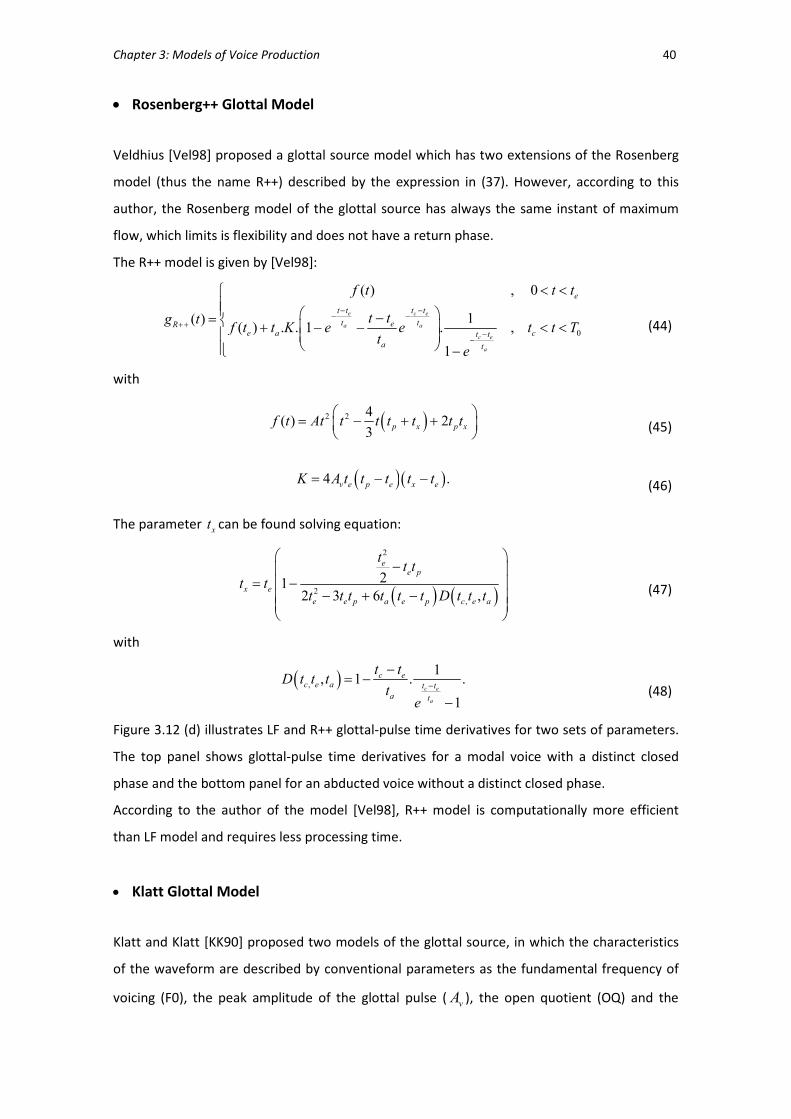
Chapter 3: Models of Voice Production 40
• Rosenberg++ Glottal Model
Veldhius [Vel98] proposed a glottal source model which has two extensions of the Rosenberg
model (thus the name R++) described by the expression in (37). However, according to this
author, the Rosenberg model of the glottal source has always the same instant of maximum
flow, which limits is flexibility and does not have a return phase.
The R++ model is given by [Vel98]:
0
( ) , 0
1( )( ) . . 1 . ,
1
e c e
a a
c e
a
e
t t t t
t teRe a ct t
a t
f t t t
t tg tf t t K e e t t T
te
− −− −
++−
−
< < −= + − − < <
−
(44)
with
( )2 2 4( ) 2
3p x p xf t At t t t t t t
= − + +
(45)
( )( )4 .v e p e x eK A t t t t t= − − (46)
The parameter xt can be found solving equation:
( ) ( )
2
2
,
212 3 6 ,
ee p
x e
e e p a e p c e a
tt t
t tt t t t t t D t t t
−
= − − + −
(47)
with
( ),
1, 1 . .
1
c e
a
c ec e a t t
a t
t tD t t t
te
−
−= −
−
(48)
Figure 3.12 (d) illustrates LF and R++ glottal-pulse time derivatives for two sets of parameters.
The top panel shows glottal-pulse time derivatives for a modal voice with a distinct closed
phase and the bottom panel for an abducted voice without a distinct closed phase.
According to the author of the model [Vel98], R++ model is computationally more efficient
than LF model and requires less processing time.
• Klatt Glottal Model
Klatt and Klatt [KK90] proposed two models of the glottal source, in which the characteristics
of the waveform are described by conventional parameters as the fundamental frequency of
voicing (F0), the peak amplitude of the glottal pulse (vA ), the open quotient (OQ) and the

Chapter 3: Models of Voice Production 41
spectral tilt or the spectral change associated with “corner rounding” in which closure is
nonsimultaneous along the length of the vocal folds. The open quotient corresponds to the
ratio of the open phase duration to the total duration (i.e, the period) of the glottal cycle.
One of the models is a slightly modified version of the LF model allowing to consider
turbulence noise generation at the glottis. Thus, a cutoff frequency is specified below which
the source consists of harmonics, and above which the source is flat-spectrum noise.
The other proposed model, known as the KLGLOTT88 model, or the Klatt model, synthesizes
the glottal pulse in the same way as the Rosenberg model described by the analytical
expression (37).
Figure 3.12 (f) illustrates the derivative glottal wave of the Klatt model.
The derivative of the glottal flow model is given by:
2
0
0 0
2 3 , 0 . .' ( )
0 , . . .
s
K s s
s s
t ta b t T OQ f
g t f f
T OQ f t T f
− ≤ ≤ =
< ≤
(49)
where
2
0
27
4 .
vA
aOQ T
= (50)
0
3 2
27.
4 .
vAbOQ T
= (51)
In this model the closed phase of the glottal cycle (i.e., the derivative is zero) is clearly visible,
as it can be seen in Figure 3.12 (f).
• Causal-Anticausal Linear Model (CALM)
This model, proposed by Doval, d’Alessandro and Henrich [DAH03] and referred to as CALM
model, is totally described in the spectral domain, based on the assumption that the glottal
flow can be considered as the impulse response of a linear filter.
The authors showed that glottal flow characteristics contribute to the speech signal spectrum
with two components: the glottal formant (frequency of the maximum on the spectrum of the
time-derivative of the glottal pulse) and spectral tilt [Boz05]. The latter is linked, in this model,
to the causal part of the model glottal closure and it is related, in terms of spectra, to the
position of the single causal pole of the model. The glottal formant corresponds to the
anticausal part of the glottal model and to the pair of poles outside the unit circle.
This model is defined by two filters. The first anti-causal filter is given by:

Chapter 3: Models of Voice Production 42
1
2
1 2
( )1
A
b zH z
a z a z=
+ +
(52)
with
( )/
1 2 cos /p sa f
p sa e b f−= − (53)
2 /
2p sa f
a e−= (54)
( )2
/
1 3sin /p sa f
p s
p
b E e b fb
π −= (55)
( )0. tanp
m
aOQT
ππα
= − (56)
0
..
pbOQT
π=
(57)
The second causal filter is equivalent to the low-pass filter of the KLGLOTT88 model, used to
control the spectral tilt at high frequencies [Deg10].
The anti-causal pole pair, as it can be concluded from the equations above, does not depend
on the time-parameters and the causal real pole is independent of the parameters OQ and
mα .
This approach, that will be explored in the next chapter, implies that it is possible to obtain an
estimation of the voice source parameters without any inverse filtering procedure, only
requiring a process to separate the causal and the anticausal parts of the speech signal.

Chapter 3: Models of Voice Production 43
Figure 3.12. Glottal pulse models:
(a) The Rosenberg model. In blue is represented the glottal pulse defined by the model
(36) and in red glottal pulse defined by the model (37).
(b) Fant model, proposed in 1979.
(c) The LF model (upper panel) and the corresponding derivative (lower panel).
(d) R++ (solid lines) and LF (dashed lines) glottal pulse time derivatives [Vel98].
(e) LFRd
model for different Rd values [Deg10].
(f) Klatt derivative glottal pulse model.
Am
plit
ud
e
0 10 20 30 40 50 60 70 80
Time
0
Am
plit
ud
e
Time
Am
plit
ud
e
Time
Am
plit
ud
e
Time
k=0.5
k=1
k=2
k=4
0
Time
Am
plit
ud
e
Am
plit
ud
e
0
Time
Rd=0,3 Rd=1 Rd=2,7
Am
plit
ud
e
Am
plit
ud
e
Am
plit
ud
e
0 0 0
Time Time Time
(a)
(c)
(b)
(d)
(e)
(f)
Time
-10
-5
0
5
-15
Am
plit
ud
e 0

Chapter 3: Models of Voice Production 44
3.5. SUMMARY
This chapter has focused on Fant’s source-filter theory of speech production, according to
which the human voice is the result of the convolution between the excitation source signal,
that represents the glottal flow, the impulse response of the vocal tract filter and the lip
radiation. The mathematical details of this process and some methods to extract features from
a voice signal, specifically the LPC, DAP and MFCC methods, were presented and analysed. It
was concluded that despite the fact that the LPC method is widely used because it is fast and
simple, it has some limitations, namely the difficulty in the determination of the optimal order,
the iterative procedure is rather slow and it is especially problematic for high pitched harmonic
sounds. This last limitation turns the DAP method more attractive than LPC, since it is more
accurate for high-pitched voices and also in the estimation of the formants of the vocal tract,
particularly the F1. The MFCC method provides superior noise robustness in comparison with
linear prediction-based feature extraction techniques.
Also, within this chapter different glottal flow models were presented that are representative
of the state of the art, as well as their respective mathematic details. Most of these glottal
flow models are implemented in the time domain and although they do not use the same
number or the same parameters, all have in common some features, namely the signal of the
glottal flow (always positive or null) and the glottal flow derivative, for one single period, starts
positive, then negative and finally null, which means that the glottal flow starts increasing,
then decreasing and, in the last, it is null.

Chapter 4
GLOTTAL PULSE ESTIMATION - STATE OF THE ART
Contents
4.1. INTRODUCTION ................................................................................................................... 46
4.2. GLOTTAL PULSE PARAMETERIZATION ..................................................................................... 47
4.2.1. TIME DOMAIN METHODS ...................................................................................................... 47
4.2.2. FREQUENCY-DOMAIN METHODS ............................................................................................. 50
4.2.3. MODEL-BASED METHODS...................................................................................................... 51
4.3. INVERSE FILTERING TECHNIQUES ........................................................................................... 51
4.3.1. ITERATIVE ADAPTIVE INVERSE FILTERING (IAIF/PSIAIF) ............................................................. 52
4.3.2. JAVKIN ET AL. METHOD ........................................................................................................ 56
4.4. ZEROS OF THE Z-TRANSFORM (ZZT) AND COMPLEX CEPSTRUM (CC) .......................................... 59
4.5. EVALUATION OF THE ESTIMATION OF THE GLOTTAL FLOW ......................................................... 64
4.6. BRIEF RELATIVE PERFORMANCE COMPARISON .......................................................................... 65
4.7. SUMMARY ......................................................................................................................... 71
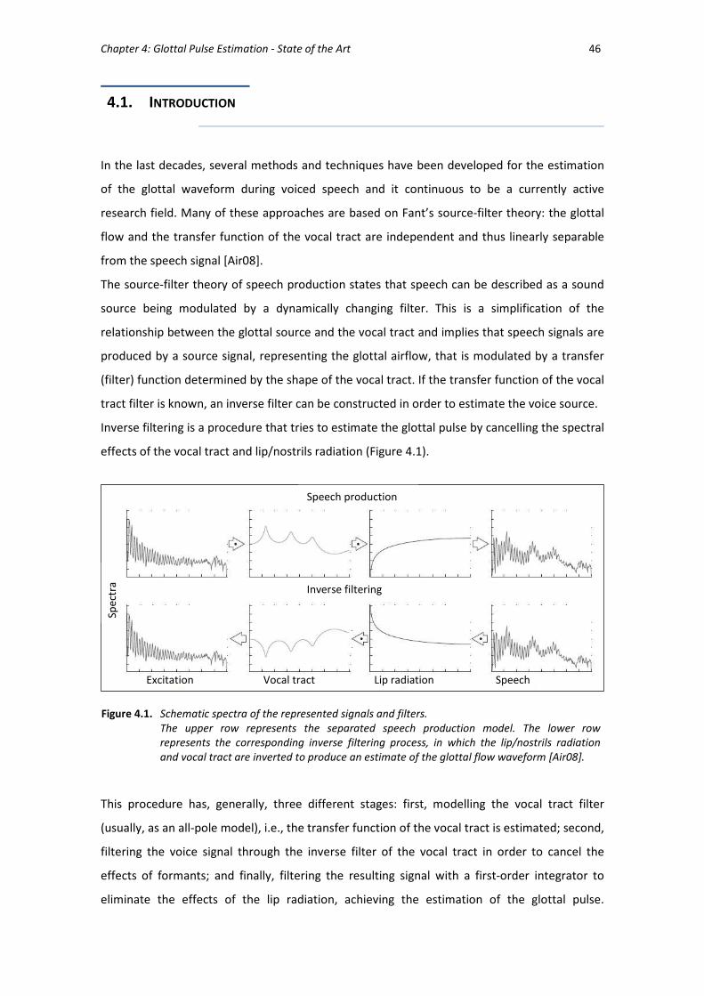
Chapter 4: Glottal Pulse Estimation - State of the Art 46
4.1. INTRODUCTION
In the last decades, several methods and techniques have been developed for the estimation
of the glottal waveform during voiced speech and it continuous to be a currently active
research field. Many of these approaches are based on Fant’s source-filter theory: the glottal
flow and the transfer function of the vocal tract are independent and thus linearly separable
from the speech signal [Air08].
The source-filter theory of speech production states that speech can be described as a sound
source being modulated by a dynamically changing filter. This is a simplification of the
relationship between the glottal source and the vocal tract and implies that speech signals are
produced by a source signal, representing the glottal airflow, that is modulated by a transfer
(filter) function determined by the shape of the vocal tract. If the transfer function of the vocal
tract filter is known, an inverse filter can be constructed in order to estimate the voice source.
Inverse filtering is a procedure that tries to estimate the glottal pulse by cancelling the spectral
effects of the vocal tract and lip/nostrils radiation (Figure 4.1).
This procedure has, generally, three different stages: first, modelling the vocal tract filter
(usually, as an all-pole model), i.e., the transfer function of the vocal tract is estimated; second,
filtering the voice signal through the inverse filter of the vocal tract in order to cancel the
effects of formants; and finally, filtering the resulting signal with a first-order integrator to
eliminate the effects of the lip radiation, achieving the estimation of the glottal pulse.
Figure 4.1. Schematic spectra of the represented signals and filters. The upper row represents the separated speech production model. The lower row
represents the corresponding inverse filtering process, in which the lip/nostrils radiation
and vocal tract are inverted to produce an estimate of the glottal flow waveform [Air08].
Speech production
Inverse filtering
Excitation Vocal tract Lip radiation Speech
Spec
tra

Chapter 4: Glottal Pulse Estimation - State of the Art 47
Basically, the procedure involves extracting two signals, the volume velocity waveform at the
glottis, and the effect of the vocal tract filter, from a single source signal [Pul05]. If voice
production is described as a convolution between the glottal excitation and the vocal tract
filter, than inverse filtering can be understood as a deconvolution operation.
In the last years other glottal flow estimation techniques have been developed that are not
based on inverse filtering procedures.
In this chapter different glottal flow estimation processes, including inverse filtering
techniques, are reviewed. Also, some of these procedures will be implemented using speech
signals (real and synthetic) in order to analyse, compare and evaluate the corresponding
estimations of the glottal pulse.
4.2. GLOTTAL PULSE PARAMETERIZATION
The estimation of the glottal pulse has usually a final step consisting in the parameterization,
whose purpose is to determine quantitative features of the signal that characterize the glottal
wave and may quantify a perception parameter [Sou11]. The parameterization of the
estimated glottal pulse might be helpful to the interpretation of the data within the signal
[Cin08].
There are three main categories of parameterization methods of the glottal flow: time-domain,
frequency-domain and model-based methods [Air08a].
4.2.1. TIME-DOMAIN METHODS
The glottal cycle, as it was referred, can be divided to a few phases. Usually, in time-domain
methods, the critical time instants, as the instant of the glottal opening and the glottal closure,
are marked in the glottal flow pulse and the durations of the phases are measured. This is
illustrated in Figure 4.2. From these values some time-domain parameters can be obtained, as
the open quotient (OQ), the closing quotient (ClQ) and the speed quotient (SQ).

Chapter 4: Glottal Pulse Estimation - State of the Art 48
As mentioned in section 3.4, the open quotient, also sometimes referred to in the literature as
the glottal pulse width [Cin08], is defined as the ratio of the open phase duration to the total
duration of the glottal cycle. According to this definition, the open quotient is null for a sealed
larynx, and when turbulent air is travelling unhindered through the glottis, the open quotient
is 1. According to some authors, the open quotient of a normal phonation is a value between
0.4 and 0.8 [Cin08].
The closing quotient is the ratio of the closing phase duration to the glottal cycle duration and
due to abrupt closure of the vocal folds during phonation, usually this value is less than half of
the open quotient.
The speed quotient, also called the glottal pulse skewness, is the ratio of the opening phase
duration to the closing phase duration. This last value indicates the speed of glottal opening to
glottal closing and, if it is equal to 1, it means that the opening phase has the same duration as
the closing phase.
Denoting T the duration of the glottal cycle, pT the duration of the opening phase and lT the
duration of the closing phase, OQ, ClQ and SQ result as:
Figure 4.2. Three periods of a sound-pressure waveform and the respective glottal flow and its
derivative. The opening, closing and closed phases of the glottal flow waveform are
highlighted for clarity. The length of the glottal cycle is denoted by T, the length of the
opening phase by Tp, and the length of the closing phase by Tl (adapted from [Air08a]).
T
Tp Tl
time
Opening phase Closing phase
Closed phase
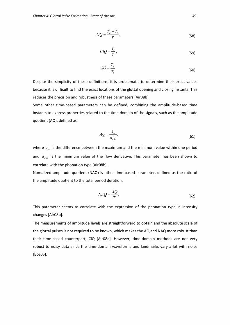
Chapter 4: Glottal Pulse Estimation - State of the Art 49
,p lT T
OQT
+= (58)
,lTClQT
= (59)
.p
l
TSQ
T= (60)
Despite the simplicity of these definitions, it is problematic to determine their exact values
because it is difficult to find the exact locations of the glottal opening and closing instants. This
reduces the precision and robustness of these parameters [Air08b].
Some other time-based parameters can be defined, combining the amplitude-based time
instants to express properties related to the time domain of the signals, such as the amplitude
quotient (AQ), defined as:
where acA is the difference between the maximum and the minimum value within one period
and mind is the minimum value of the flow derivative. This parameter has been shown to
correlate with the phonation type [Air08b].
Nomalized amplitude quotient (NAQ) is other time-based parameter, defined as the ratio of
the amplitude quotient to the total period duration:
This parameter seems to correlate with the expression of the phonation type in intensity
changes [Air08b].
The measurements of amplitude levels are straightforward to obtain and the absolute scale of
the glottal pulses is not required to be known, which makes the AQ and NAQ more robust than
their time-based counterpart, ClQ [Air08a]. However, time-domain methods are not very
robust to noisy data since the time-domain waveforms and landmarks vary a lot with noise
[Boz05].
min
.acAAQd
= (61)
.AQ
NAQT
= (62)

Chapter 4: Glottal Pulse Estimation - State of the Art 50
4.2.2. FREQUENCY-DOMAIN METHODS
Glottal flow parameterization is achieved in the frequency domain by taking measurements
from the power spectrum of the flow signal, as shown in Figure 4.3.
0 500 1000 1500 2000 25000
50
100
150
Frequency (Hz) →
Magnitude (dB) →
Some parameters have been proposed to facilitate parameterization of the spectra of the
glottal flow pulses, as the difference of the first and second harmonics decibels, denoted
by1 2
H H− , or 12
H∆ , and the harmonic richness factor (HRF):
2
1
kkH
HRFH
≥=∑
(63)
where k
H is the k th harmonic. This parameter is related to 1 2
H H− but tries to approximate
the spectral energy distribution from more than one higher harmonic [Air08b].
A trivial observation on these parameters is that they co-vary with the fundamental frequency.
When the fundamental frequency increases, the distance between the harmonics grows and,
thus, the value of 1 2
H H− increases while the value of HRF decreases.
Parabolic spectrum parameter (PSP) is another frequency-domain parameter used to improve
spectral parameterization, which fits a second-order polynomial to the flow spectrum to gain
an estimate of the spectral slope [Air08a].
There are several advantages on the spectral approach to voice source modelling, such as the
better description of the voice quality spectral parameters, the more efficient voice quality
modification and voice source parameter estimation [DAH03]. Frequency-domain methods
seem to be also more robust in handling both noisy and phase distorted data [Boz05].
However, there are few frequency-domain glottal source models discussed in the literature.
H2 H1
H3
H4 H5
Figure 4.3. Flow magnitude spectrum. The levels of the first five harmonics are depicted as H1 to H5.

Chapter 4: Glottal Pulse Estimation - State of the Art 51
4.2.3. MODEL-BASED METHODS
The model-based parameterization methods attempt to capture to general flow shape of the
glottal source with the finer subtleties of the vocal fold motion, using some mathematical
formula (as the glottal pulse models) that yields artificial waveforms similar to glottal flow
pulses and usually implemented in the time domain [Cin08].
4.3. INVERSE FILTERING TECHNIQUES
Inverse filtering has many applications in both research and clinical examination of voice
production, as it was stated above, but few voice inverse filtering software packages exist and
it is still a challenge to develop a complete and automatic inverse filtering method. Some of
the existing tools implement manual inverse filtering techniques, as DeCap, developed by
Svante Granqvist, and Waveview, developed by Glottal Enterprises. This latter software allows
to analyse both CV-mask (airflow) and microphone (radiated pressure) waveforms during
speech and singing. Also, Paul Milenkovich [Mil01] developed a time-frequency analysis
software, TF32, that is able of linear predictive inverse filtering, and Kreiman et al. [KGB06],
based on the inverse filtering method proposed by Javkin et al. [JBM87], developed an open-
source inverse filtering and analysis software, Inverse Filter and Sky. Another open-source
licence software package that implements glottal inverse filtering and several time-based
parameters of the voice source in a graphical user interface is HUT Voice Source Analysis and
Parametrization Toolkit (Aparat), develop by Airas et al. [APB+05]. This software is used in
Matlab environment and implements the inverse filtering algorithms Iterative Adaptive Inverse
Filtering (IAIF) and Pitch Synchronous Iterative Adaptive Inverse Filtering (PSIAIF). Also, in
Matlab, there is Voicebox5, a speech processing toolbox maintained and mostly written by
Mike Brookes, which includes inverse filtering routines but with no graphical user interface.
In this section some of the above mentioned techniques of inverse filtering and others will be
presented and analysed and some of the inverse filtering software applications will be used to
estimate the glottal pulse from speech signals.
5 Available at http://www.ee.ic.ac.uk/hp/staff/dmb/voicebox/voicebox.html

Chapter 4: Glottal Pulse Estimation - State of the Art 52
4.3.1. ITERATIVE ADAPTIVE INVERSE FILTERING (IAIF/PSIAIF)
The Iterative Adaptive Inverse Filtering (IAIF) is a semi-automatic inverse filtering method
proposed by Alku [Alk92]. The method uses a speech pressure signal as input and generates an
estimate of the corresponding glottal flow signal. This procedure has three fundamental parts:
analysis, inverse filtering and integration. The glottal contribution to the speech spectrum is
initially estimated using an iterative structure. This contribution is cancelled and, then, the
transfer function of the vocal tract is modelled. Finally, the glottal excitation is estimated by
cancelling the effects of the vocal tract (using inverse filtering) and lip radiation (by
integration). A scheme of speech production model used in this approach is presented in
Figure 4.4.
The algorithm has been changed from that described by Alku [Alk92] by replacing the
conventional linear predictive analysis (LPC) with the discrete all-pole modelling (DAP) method.
These modifications, by Alku et al. [APB+05], allow to reduce the bias due to the harmonic
structure of the speech spectrum in the formant frequency estimates. The block diagram of
the IAIF procedure is shown in Figure 4.5.
The method operates in two iterations: the first phase, which consists on the stages 1 to 6,
makes an estimation of the vocal tract function and applies inverse filtering to the signal with
that estimate, and generates an estimate of the glottal source which is used as input of the
second phase (stages 7 to 12) to achieve a more accurate estimate. A more detailed
description of each step is provided below [Pul05].
1. The input signal (speech signal) is first high-pass filtered using a linear-phase finite
impulse response (FIR) filter to remove disturbing low-frequency fluctuations. To avoid
filtering out relevant information, the cut-off frequency should be lower than the
fundamental frequency of the speech signal. The high-pass filtered signal is used as the
input of the next stages.
2. The output of the previous step is analysed by a first-order DAP and there is a first
estimate of the combined effect of the glottal flow and the lip radiation effect on the
speech spectrum.
Speech Glottal
excitation Vocal Tract
Lip
radiation
Figure 4.4. Speech production model used in IAIF.

Chapter 4: Glottal Pulse Estimation - State of the Art 53
3. The input signal is inverse filtered using the filter obtained in step 2. The spectral tilt
caused by the spectrum of the excitation signal and the lip radiation effect is removed.
4. A new analysis by DAP is calculated to obtain a model of the vocal tract transfer function.
The order p of the DAP analysis can be adjusted by the operator of the IAIF method and it
is related to the number of formants modelled in the relevant frequency band.
5. The input signal is inverse filtered using the inverse of the pth-order model from the
previous step.
6. Lip radiation is cancelled by integrating the output of the previous step. Then, a first
estimation of the glottal flow is obtained and completes the first phase of the procedure.
Figure 4.5. The bock diagram of the IAIF method for estimation of the glottal excitation g(n) from the
speech signal s(n) [APB+05].
1. Highpass
filtering
s(n)
2. DAP
(order 1)
3. inverse
filtering
4. DAP
(order p)
7. DAP
(order g)
8. inverse
filtering
10. DAP
(order r)
9. integration
5. inverse
filtering
11. inverse
filtering
6. integration 12. integration
g(n)

Chapter 4: Glottal Pulse Estimation - State of the Art 54
7. A gth-order analysis of the obtained glottal flow estimate is calculated and then the
second phase of the IAIF method. This gives a spectral model of the effect of glottal
excitation on the speech spectrum. The value of g is usually between 2 and 4.
8. The input signal is inverse filtered using the model of the excitation signal to eliminate the
glottal contribution.
9. The output of the previous step is integrated in order to cancel the lip radiation effect.
10. A new model of the vocal tract filter is formed by an rth order DAP analysis. The value of r
can be adjusted and it is usually set equal to the value of p in step 4.
11. The input signal is inverse filtered with the vocal tract model obtained in the step 10, in
order to remove the effect of the vocal tract.
12. The final estimate of the glottal flow is obtained, removing the lip radiation effect by
integrating the signal. This yields, finally, to the output of the IAIF method.
A toolkit for voice inverse filtering, Aparat, which is a Matlab implementation of the IAIF
method, was developed at the Laboratory of Acoustics and Audio Signal Processing at Helsinki
University of Technology. This software (Figure 4.6), available as open-source6, is an interface
for the semi-automatic IAIF inverse filtering algorithm. Also, allows to determine the time and
amplitude based parameters and to visualize the spectra of the speech signal, the estimated
glottal flow and the used vocal tract filter (Figure 4.7).
According to the authors, Aparat has been used successfully in several research projects.
However, the application of automatic inverse filtering has been problematic in high pitched
signals [APB+05].
6 Available at http://www.acoustics.hut.fi/software/aparat/
Figure 4.6. The graphical user interface and the signal view of Aparat.

Chapter 4: Glottal Pulse Estimation - State of the Art 55
Pitch Synchronous Iterative Adaptive Inverse Filtering (PSIAIF) is an inverse filtering method
based on IAIF. The glottal pulse is obtained by applying the IAIF method twice to the speech
signal. The output of the first IAIF procedure is used to calculate the fundamental period which
is important to calculate the new windowing, before applying IAIF again. The block diagram of
PSIAF procedure is shown in Figure 4.8.
Also based on IAIF is the method used by Murphy [Mur08], represented in Figure 4.9. The
process uses repeated paired lattices to eliminate the effects of the vocal tract and lip
radiation effects on the sound wave produced at the glottis.
The model operates as follows.
1. The input voice, s(n), is filtered using an inverse radiation model filter to eliminate the
effect of the lip radiation and produces a signal for the radiation compensated voice, sl(n).
2. A first estimation of the simple glottal pulse inverse function is obtained, which is used to
eliminate the behaviour of the glottal pulse on the radiation compensated voice. Then, a
trace for the deglottalised voice, sv(n), is produced.
Figure 4.7. The spectra view in Aparat of a speech signal, the calculated glottal flow and the used vocal
tract filter (left), and parameters computed from the estimated glottal flow.
0 1000 2000 3000 4000 5000 6000 7000 8000 9000 10000-60
-40
-20
0
20
40
Hz
dB
808 Hz, 21.2 dB 1199 Hz, 22.4 dB
2647 Hz, 8.5 dB 3546 Hz, 10.5 dB
4550 Hz, -1.9 dB
5398 Hz, -6.3 dB
6310 Hz, -16.9 dB
7119 Hz, -21.5 dB 9518 Hz, -21.7 dB
speech
tract filter
formants
flow
glottis filter
Figure 4.8. Block diagram of the main steps of the PSIAIF method.
s(n)
g(n)
1. Highpass
filtering 2. IAIF - 1
4. IAIF - 2
3. Pitch
syncronism

Chapter 4: Glottal Pulse Estimation - State of the Art 56
3. A model for the vocal tract is derived by inverse filtering sv(n) with lattice filters and
extracting the model of the vocal tract.
4. The vocal tract inverse model is applied to the radiation compensated voice, sl(n), and
generates a residual trace that contains information on the glottal pulse second
derivative, ug(n), which is related to the relative speed between each fold’s centre of
mass.
5. The glottal pulse is extracted and, by repeating step 2 and, then, steps 3 to 5, reliable
estimations for the glottal pulse second derivative and vocal tract function are made.
The author advocates that this method generates robust estimates for the voice signal
decompositions, which have been used for determining any unusual vibration patterns that
may be caused by pathological masses on the vocal folds or in their immediate environment.
This inverse filtering model is not free available and, therefore, it could not be tested for
glottal source estimations.
4.3.2. JAVKIN ET AL. METHOD
The first assumption of Javkin et al. [JBM87] is that speech waveforms are the product of both
the phonatory setting and the shape of the vocal tract, and if the effect of the vocal tract can
be subtracted from the speech waveform, then the glottal waveform can be examined without
requiring any invasive procedure.
ug(n)
Glottal pulse
2nd
derivative
De- glottalised
voice
sv(n)
Input voice
s(n)
Radiation compensated
voice
sl(n)
1. Inverse
radiation
model
2. Glottal pulse
inverse
model
4. Vocal tract
inverse
model
3. Vocal
tract
model
5. Glottal
pulse
model
Figure 4.9. Inverse filtering model by Murphy [Mur08].
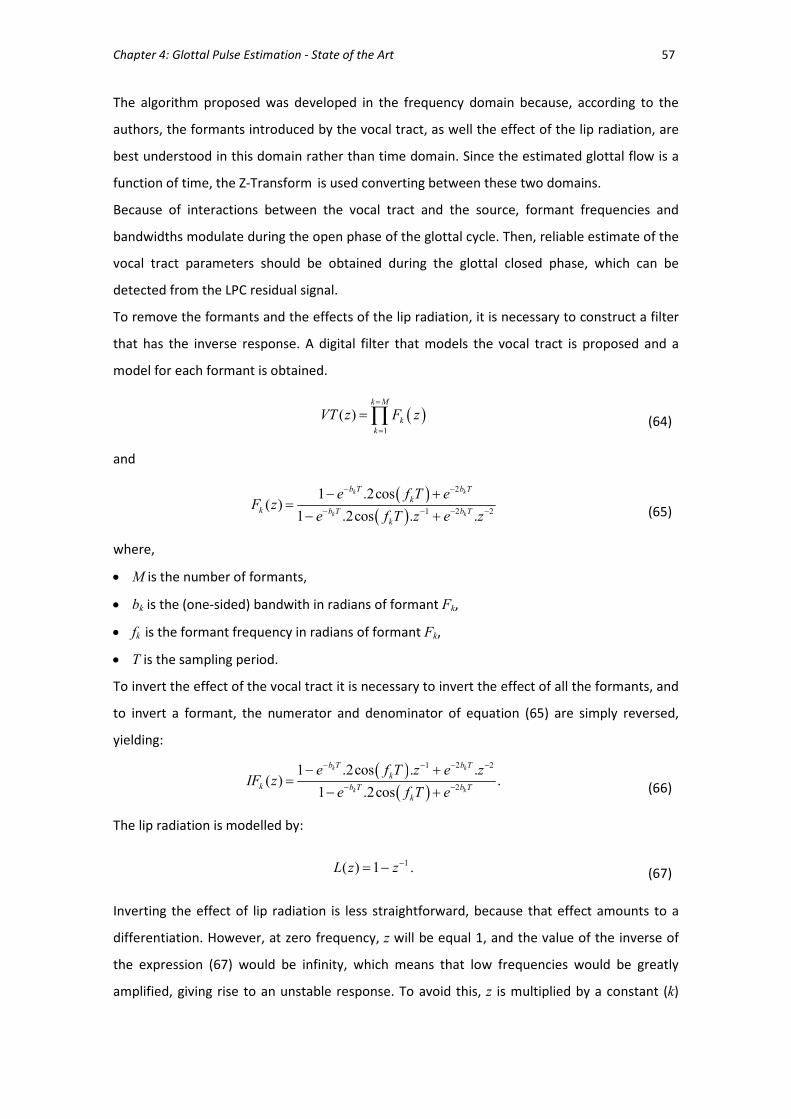
Chapter 4: Glottal Pulse Estimation - State of the Art 57
The algorithm proposed was developed in the frequency domain because, according to the
authors, the formants introduced by the vocal tract, as well the effect of the lip radiation, are
best understood in this domain rather than time domain. Since the estimated glottal flow is a
function of time, the Z-Transform is used converting between these two domains.
Because of interactions between the vocal tract and the source, formant frequencies and
bandwidths modulate during the open phase of the glottal cycle. Then, reliable estimate of the
vocal tract parameters should be obtained during the glottal closed phase, which can be
detected from the LPC residual signal.
To remove the formants and the effects of the lip radiation, it is necessary to construct a filter
that has the inverse response. A digital filter that models the vocal tract is proposed and a
model for each formant is obtained.
and
where,
• M is the number of formants,
• bk is the (one-sided) bandwith in radians of formant Fk,
• fk is the formant frequency in radians of formant Fk,
• T is the sampling period.
To invert the effect of the vocal tract it is necessary to invert the effect of all the formants, and
to invert a formant, the numerator and denominator of equation (65) are simply reversed,
yielding:
( )( )
21 2
2
1 .2cos . .( ) .
1 .2cos
k k
k k
b T b T
k
k b T b T
k
e f T z e zIF z
e f T e
− −− −
− −
− +=
− + (66)
The lip radiation is modelled by:
1( ) 1 .L z z−= − (67)
Inverting the effect of lip radiation is less straightforward, because that effect amounts to a
differentiation. However, at zero frequency, z will be equal 1, and the value of the inverse of
the expression (67) would be infinity, which means that low frequencies would be greatly
amplified, giving rise to an unstable response. To avoid this, z is multiplied by a constant (k)
( )1
( )k M
k
k
VT z F z=
=
=∏ (64)
( )( )
2
21 2
1 .2cos( )
1 .2cos . .
k k
k k
b T b T
k
k b T b T
k
e f T eF z
e f T z e z
− −
− −− −
− +=
− + (65)
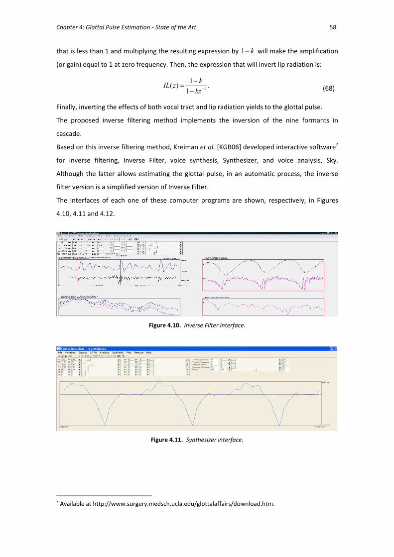
Chapter 4: Glottal Pulse Estimation - State of the Art 58
that is less than 1 and multiplying the resulting expression by 1 k− will make the amplification
(or gain) equal to 1 at zero frequency. Then, the expression that will invert lip radiation is:
1
1( ) .
1
kIL z
kz−−
=−
(68)
Finally, inverting the effects of both vocal tract and lip radiation yields to the glottal pulse.
The proposed inverse filtering method implements the inversion of the nine formants in
cascade.
Based on this inverse filtering method, Kreiman et al. [KGB06] developed interactive software7
for inverse filtering, Inverse Filter, voice synthesis, Synthesizer, and voice analysis, Sky.
Although the latter allows estimating the glottal pulse, in an automatic process, the inverse
filter version is a simplified version of Inverse Filter.
The interfaces of each one of these computer programs are shown, respectively, in Figures
4.10, 4.11 and 4.12.
Figure 4.10. Inverse Filter interface.
Figure 4.11. Synthesizer interface.
7 Available at http://www.surgery.medsch.ucla.edu/glottalaffairs/download.htm.
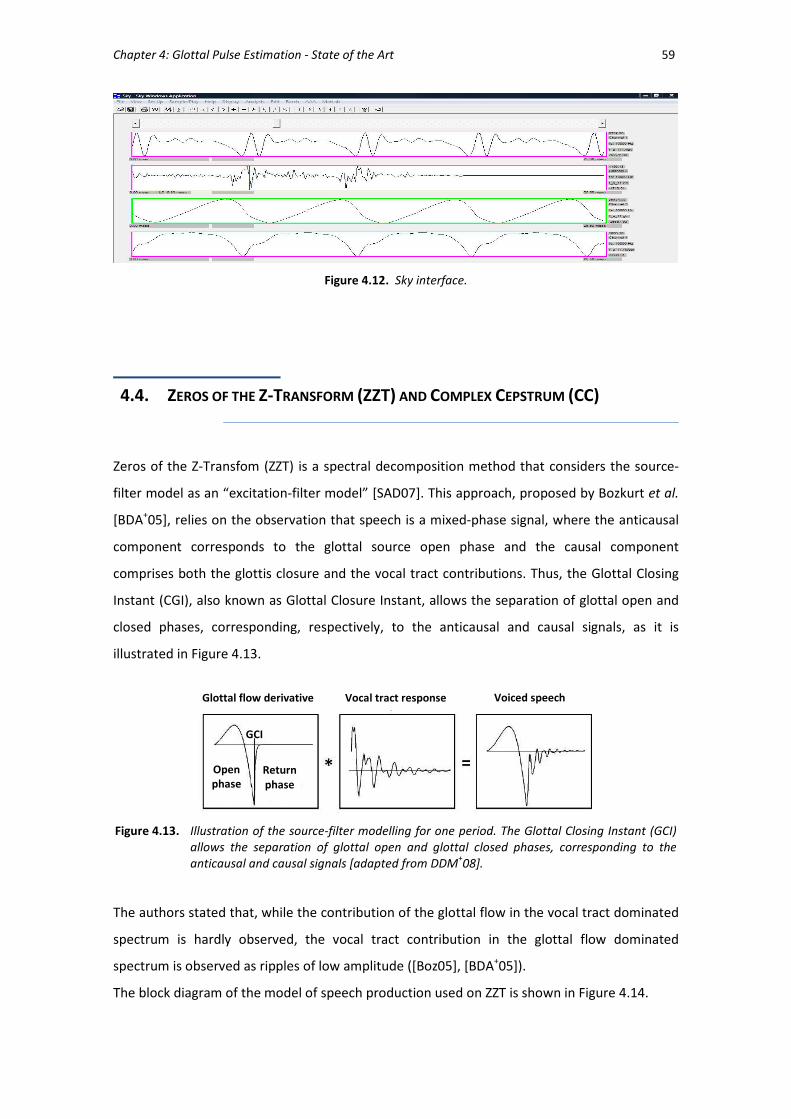
Chapter 4: Glottal Pulse Estimation - State of the Art 59
Figure 4.12. Sky interface.
4.4. ZEROS OF THE Z-TRANSFORM (ZZT) AND COMPLEX CEPSTRUM (CC)
Zeros of the Z-Transfom (ZZT) is a spectral decomposition method that considers the source-
filter model as an “excitation-filter model” [SAD07]. This approach, proposed by Bozkurt et al.
[BDA+05], relies on the observation that speech is a mixed-phase signal, where the anticausal
component corresponds to the glottal source open phase and the causal component
comprises both the glottis closure and the vocal tract contributions. Thus, the Glottal Closing
Instant (CGI), also known as Glottal Closure Instant, allows the separation of glottal open and
closed phases, corresponding, respectively, to the anticausal and causal signals, as it is
illustrated in Figure 4.13.
The authors stated that, while the contribution of the glottal flow in the vocal tract dominated
spectrum is hardly observed, the vocal tract contribution in the glottal flow dominated
spectrum is observed as ripples of low amplitude ([Boz05], [BDA+05]).
The block diagram of the model of speech production used on ZZT is shown in Figure 4.14.
Figure 4.13. Illustration of the source-filter modelling for one period. The Glottal Closing Instant (GCI)
allows the separation of glottal open and glottal closed phases, corresponding to the
anticausal and causal signals [adapted from DDM+08].
Glottal flow derivative Vocal tract response Voiced speech
Open
phase
Return
phase
GCI

Chapter 4: Glottal Pulse Estimation - State of the Art 60
ZZT it is a representation of the z-transform polynomial through its zeros (roots)8 and,
according to Bozkurt [Boz05], the set of ZZT of a speech signal is just the union of ZZT sets of
the three components: the impulse, the glottal flow and the vocal tract filter.
The ZZT pattern for the impulse train is a set of zeros on the unit circle (i.e., with modulus 1),
with a gap at each multiple of the fundamental frequency. For the differential glottal flow, the
ZZT pattern is an union of two sets of zeros: one inside the unit circle (i.e., with modulus lower
than 1), in which a gap can be seen, corresponding to the spectral tilt; other outside the unit
circle (i.e., with modulus greater than 1), showing a gap between the zero on the real axis and
the others, which corresponds to the glottal formant. Also, the glottal formant and the spectral
tilt can be seen on the spectrum representation, respectively, as a local maximum in the low-
frequency region and a global slope. The ZZT pattern for the vocal tract is a line of zeros inside
the unit circle, in which can be seen zero gaps, each one corresponding to a formant [BDA+04].
This is illustrated in Figure 4.15.
Before beginning the ZZT process, the glottal closure instants (GCI) of the speech signal have to
be detected and for each GCI synchronously windowed speech frame, the roots of the z-
transform are computed and separated in two subsets based on their modulus: the roots with
modulus greater than 1 (i.e., outside the unit circle) and the roots with modulus lower than 1
(i.e., inside the unit circle). According to this representation, the first subset of roots
corresponds to the anticausal part of the voice source and the other to the causal part of
source and vocal tract. Then, computing DFT for each of these groups, the corresponding
spectrum is obtained. Finally, using IDFT, the estimation of the glottal source and the vocal
tract filter are obtained. An example of this decomposition is shown in Figure 4.16.
A block diagram of the ZZT decomposition algorithm is shown in Figure 4.17.
8 See Appendix A for mathematical details.
Source-filter
model
Excitation-
filter model
Mixed causal-anticausal
linear part
(filter)
Non-linear part
(excitation)
Figure 4.14. The model of speech production used on ZZT.
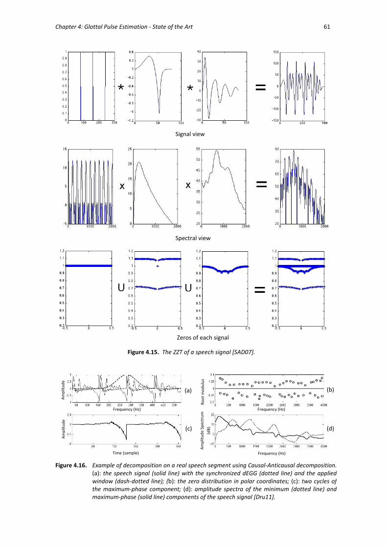
Chapter 4: Glottal Pulse Estimation - State of the Art 61
Figure 4.15. The ZZT of a speech signal [SAD07].
Signal view
Spectral view
Zeros of each signal
Frequency (Hz) Time (sample)
Am
plit
ud
e
Am
plit
ud
e
Am
plit
ud
e Sp
ectr
um
(dB
)
Ro
ot
mo
du
lus
(a) (b)
(d) (c)
Frequency (Hz) Frequency (Hz)
Figure 4.16. Example of decomposition on a real speech segment using Causal-Anticausal decomposition.
(a): the speech signal (solid line) with the synchronized dEGG (dotted line) and the applied
window (dash-dotted line); (b): the zero distribution in polar coordinates; (c): two cycles of
the maximum-phase component; (d): amplitude spectra of the minimum (dotted line) and
maximum-phase (solid line) components of the speech signal [Dru11].
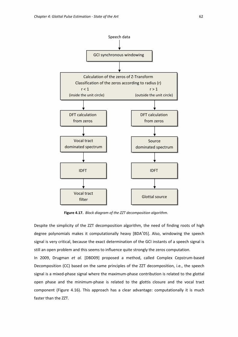
Chapter 4: Glottal Pulse Estimation - State of the Art 62
Despite the simplicity of the ZZT decomposition algorithm, the need of finding roots of high
degree polynomials makes it computationally heavy [BDA+05]. Also, windowing the speech
signal is very critical, because the exact determination of the GCI instants of a speech signal is
still an open problem and this seems to influence quite strongly the zeros computation.
In 2009, Drugman et al. [DBD09] proposed a method, called Complex Cepstrum-based
Decomposition (CC) based on the same principles of the ZZT decomposition, i.e., the speech
signal is a mixed-phase signal where the maximum-phase contribution is related to the glottal
open phase and the minimum-phase is related to the glottis closure and the vocal tract
component (Figure 4.16). This approach has a clear advantage: computationally it is much
faster than the ZZT.
Figure 4.17. Block diagram of the ZZT decomposition algorithm.
GCI synchronous windowing
Speech data
Calculation of the zeros of Z-Transform
Classification of the zeros according to radius (r)
r < 1 r > 1
(inside the unit circle) (outside the unit circle)
DFT calculation
from zeros
DFT calculation
from zeros
Vocal tract
dominated spectrum
Source
dominated spectrum
IDFT
IDFT
Vocal tract
filter
Glottal source

Chapter 4: Glottal Pulse Estimation - State of the Art 63
This decomposition is based on the fact that the complex cepstrum of an anticausal signal and
causal signal is zero for, respectively, all n positive and negative. Thus, if one considers only the
negative part of the CC, it is possible to estimate the glottal contribution.
According to the authors, a difficulty of CC implementation is the estimation of the phase
because requires an efficient phase unwrapping algorithm and the windowing is still a critical
issue in this approach.
In 2008, Thomas Drugman et al. [DDM+08] proposed a new approach for glottal source
estimation directly from the speech signal. This method uses the knowledge mentioned above,
that GCI marks the separation between the glottal open and closed phases, which correspond,
respectively, to the anticausal and causal signals. Thus, the causality and anticausality
dominated regions are delimitated by GCI and, according to the authors, the Anticausality
Dominated Region makes a good approximation of the glottal open phase, since the causal
contribution, i.e., the glottal source return phase and the vocal tract filter have almost no
contribution before GCI . This approach requires a GCI-centered and sharp window (typically a
Hanning-Poisson or Blackman window9), as it is illustrated in Figure 4.18.
9 See Appendix A for mathematic details.
GCI – centered
Sharp windowing
ACDR CDR
Figure 4.18. Effect of a sharp CGI-centered windowing on a two-period long speech frame. The
Anticausality Dominated Region (ACDR) approximates the glottal source open phase and
the Causality Dominated Region (CDR) the source return phase and the vocal tract filter
([DDM08]).

Chapter 4: Glottal Pulse Estimation - State of the Art 64
4.5. EVALUATION OF THE ESTIMATION OF THE GLOTTAL FLOW
Even though the estimation of the glottal flow is not a trivial process, the validation of the
method and the evaluation of the quality of the estimations, namely in real speech signals, is
other difficult problem since it is uncertain how the real shape of the glottal flow of real
speech signals looks like without using special equipment and invasive procedures [WM07].
In current literature, there are some researchers that make a qualitative evaluation of the
glottal flow waveform estimations based on some demonstrative pictures and compare them
with the original glottal flow when is known, as in synthetic signals (e.g., [Boz05], [Deg10]) or
with the ones obtained using other techniques and, thus, evaluate the quality of each
procedure. However, in this last case, for real speech signals, it is difficult to determine which
one is a better estimation. Also, it is difficult to know if the selected examples represent the
general behaviour of those methods.
In this evaluation process, some researchers analyse the quality of the estimated glottal flow
waveform using some parameters, as the glottal formant (e.g. [Dru11]), time-based
parameters, as NAQ and ClQ, (e.g., [Air08a], [Dru11]) and the harmonic richness factor (e.g.,
[DDM+08], [Kaf10], [Dru11]), or evaluate the quality of the algorithm used calculating the error
between the estimated glottal flow waveform and the input glottal waveform, when this latter
is known (e.g., [Sou11], [Dru11], [Deg10]) . In this case, it is common to determine the Signal to
Noise Ratio (SNR), given by [Sou11]:
( )
2
1
2
1
ˆ ( )10log
ˆ( ) ( )
N
n
N
n
g nSNR
g n g n
=
=
= −
∑∑
(69)
where ( )g n represents the ideal glottal pulse and ˆ ( )g n represents the glottal pulse
estimation, or the spectral distortion defined as [Dru11]:
( )2
20logˆ 2( )
G dSD
G
π
π
ω ωπω−
= ∫ (70)
where ( )G ω and ( )G ω correspond to the DTFT of the original glottal pulse and to the DTFT
of the estimated glottal pulse, respectively.

Chapter 4: Glottal Pulse Estimation - State of the Art 65
4.6. BRIEF RELATIVE PERFORMANCE COMPARISON
This section reports and discusses the results obtained using some of the previously described
methods in order to estimate the glottal pulse of selected speech signals, namely: the IAIF
method, which is built in the Aparat software; the Javkin et al. method, using Inverse Filter;
LPC inverse filtering, using TF32 software, and the ZZT and CC decompositions, using Matlab.
Concerning the latter two methods, the GCI-centered Blackman window was used and the GCI
instants were calculated using the Matlab function dypsa included in the Voicebox toolbox.
In this section, the evaluation of the estimations of the glottal pulse will be qualitative. The
determination of a quantitative parameter (such as the SNR) to better analyse the quality of
the estimated glottal flow waveforms, will be presented in the next chapter.
For this evaluation, four signals samples were selected, with normal phonation, in which one is
a synthetic signal:
• a signal of a male synthetic vowel /a/ with F0=110 Hz, generated using the Voicebox
Matlab toolbox and having the LF model as glottal impulse (Figure 4.19);
• a real signal of a female vowel /a/ with F0=161 Hz (Figure 4.20);
• a real signal of a male vowel /a/ with F0=102 Hz(Figure 4.21);
• a real signal of a female vowel /i/ with F0=186 Hz (Figure 4.22).
All speech signals were down-converted to 22050 Hz.
In each figure (from left to right) we show first the glottal flow waveform, for the synthetic
signal, or the speech waveform, for the real speech signals. Then estimates follow using IAIF,
LPC inverse filtering, Javkin et al. method and finally ZZT and CC decompositions, in which, as it
was mentioned above, the maximum-phase component corresponds to the glottal open phase
and the minimum-phase component corresponds both to the glottis closure and the vocal
tract influence.
Analysing Figure 4.19, since the glottal pulse reference is available, one can conclude that the
better estimations are the ones obtained using IAIF and the CC decomposition. However, only
in the estimations obtained using IAIF, the Javkin et al. method and LPC inverse filtering, it is
possible to denote the abrupt closure of the glottal pulse, often referred to in the literature. In
ZZT and CC decompositions, the glottal flow derivative waveforms do not denote what
corresponds to that, i.e., there is no abrupt decreasing on the negative amplitudes. Also, the
estimation performed by the ZZT decomposition, has almost no positive amplitudes and,

Chapter 4: Glottal Pulse Estimation - State of the Art 66
therefore, no opening glottal phase. These features may be caused by the GCI windowing issue
or, simply, by the computational procedures underlying the decompositions.
It is also possible to visualize in the estimation by IAIF that the glottal impulse has almost no
closed phase, contrarily to the real input glottal flow waveform.
Analysing the estimations of the glottal flow waveforms from real speech signals (Figures 4.20
to 4.22), as it was mentioned above, it is difficult to evaluate the quality of each estimation
since the real glottal pulse waveform is not known. Although, what seems to be common in
the approaches using IAIF, the Javkin et al. method and LPC inverse filtering, is the abrupt
closure as well as the asymmetric and bell-shape of the glottal pulses. Also, a ripple is visible in
the closed phase of the glottal flow using these methods. This is often assumed to illustrate
the non-zero air flow in the closed phase or the effect of the noise when the signal was
captured. Still, maybe it highlights that some part of the vocal tract filter contribution was not
removed and, therefore, the estimation of the glottal flow is not correctly achieved.
However, this closed phase is clearly visible on the estimations using the ZZT and CC
decompositions, because the derivative is approximate or equal to zero in some intervals.
Our results also show that the effectiveness of the ZZT and CC decompositions appears to be
similar, with a slight improvement in the latter in the case of the synthetic signal.

Chapter 4: Glottal Pulse Estimation - State of the Art 67
Figure 4.19. Glottal flow estimations of a male synthetic vowel /a/ using the LF model ( 0 110F Hz= ).
(a) Glottal flow waveform (left) and glottal flow derivative (right); (b) The glottal flow (top row) and derivative (bottom row) waveforms estimated by IAIF; (c) The glottal flow (top row) and derivative (bottom row) waveforms estimated by LPC
inverse filtering; (d) The glottal flow (top row) and derivative (bottom row) waveforms estimated by Javkin
et al method; (e) The estimation of the derivative of the glottal flow (maximum-phase component) and
vocal tract contribution (minimum-phase component) using the ZZT and CC
decompositions. The top panel represents the speech waveform and the applied
window.
(e)
(a)
Time
0 20 40 60 80 100-0.1
-0.05
0
0.05
0.1
Amplitude
Time
Derivative waveform
0 20 40 60 80 1000
0.5
1
Time
Amplitude
LF glottal model waveform
(b) (c) (d)

Chapter 4: Glottal Pulse Estimation - State of the Art 68
0 200 400 600 800 1000-0.4
-0.3
-0.2
-0.1
0
0.1
0.2
0.3
0.4
Time (ms)
Amplitude
0 1000 2000 3000 4000 5000 6000-0.5
0
0.5
1
0 20 40 60-1
0
1Maximum-phase component from ZZT
0 20 40 60 80-1
0
1Minimum-phase component from ZZT
0 20 40 60-1
0
1Maximum-phase component from CCD
0 20 40 60-1
0
1Minimum-phase component from CCD
Figure 4.20. Glottal flow estimations of a female vowel /a/.
(a) Waveform; (b) The glottal flow (top row) and derivative (bottom row) waveforms estimated by IAIF; (c) The glottal flow (top row) and derivative (bottom row) waveforms estimated by LPC
inverse filtering; (d) The glottal flow (top row) and derivative (bottom row) waveforms estimated by Javkin
et al method; (e) The estimation of the derivative of the glottal flow (maximum-phase component) and
vocal tract contribution (minimum-phase component) using the ZZT and CC
decompositions. The top panel represents the speech waveform and the applied
window.
(e)
(a)
(b) (c) (d)

Chapter 4: Glottal Pulse Estimation - State of the Art 69
0 200 400 600 800 1000-0.08
-0.06
-0.04
-0.02
0
0.02
0.04
0.06
0.08
Amplitude
Time (ms)
Figure 4.21. Glottal flow estimations of a male vowel /a/.
(a) Waveform; (b) The glottal flow (top row) and derivative (bottom row) waveforms estimated by IAIF; (c) The glottal flow (top row) and derivative (bottom row) waveforms estimated by LPC
inverse filtering; (d) The glottal flow (top row) and derivative (bottom row) waveforms estimated by Javkin
et al method; (e) The estimation of the derivative of the glottal flow (maximum-phase component) and
vocal tract contribution (minimum-phase component) using the ZZT and CC
decompositions. The top panel represents the speech waveform and the applied
window.
(e)
(a)
(b) (c) (d)

Chapter 4: Glottal Pulse Estimation - State of the Art 70
0 200 400 600 800 1000-0.25
-0.2
-0.15
-0.1
-0.05
0
0.05
0.1
0.15
0.2
Amplitude
Time (ms)
0 20 40 60 80-1
0
1Maximum-phase component from ZZT
0 20 40 60 80-1
0
1Minimum-phase component from ZZT
0 20 40 60 80-1
0
1Maximum-phase component from CCD
0 20 40 60 80-1
0
1Minimum-phase component from CCD
0 500 1000 1500 2000 2500 3000-0.5
0
0.5
1
Figure 4.22. Glottal flow estimations of a female vowel /i/.
(a) Waveform; (b) The glottal flow (top row) and derivative (bottom row) waveforms estimated by IAIF; (c) The glottal flow (top row) and derivative (bottom row) waveforms estimated by LPC
inverse filtering; (d) The glottal flow (top row) and derivative (bottom row) waveforms estimated by Javkin
et al method; (e) The estimation of the derivative of the glottal flow (maximum-phase component) and
vocal tract contribution (minimum-phase component) using the ZZT and CC
decompositions. The top panel represents the speech waveform and the applied
window.
(e)
(a)
(b) (c) (d)

Chapter 4: Glottal Pulse Estimation - State of the Art 71
4.7. SUMMARY
The focus of this chapter was laid on the mathematical description of different procedures of
estimation of the glottal pulse which included different inverse filtering techniques. Also, the
glottal pulse parameterization was reviewed as well as the evaluation of glottal flow
estimations.
Some of the analysed procedures and inverse filtering techniques were applied into four
signals (one synthetic and three real signals) in order to estimate the glottal flow and to
compare the results. The selected methods were: IAIF using the Aparat software, the Javkin et
al. method using Inverse Filter, LCP inverse filtering using TF32, and the ZZT and CC
decompositions. The IAIF and the ZZT and CC decompositions are automatic processes,
although these two latter are computationally very heavy, with a slight improvement in the
case of the CC decomposition. The problematic issue of windowing in these two processes (ZZT
and CC decompositions) was also clear: if the window applied to the segment of the voiced
speech signal is not appropriate, the correct estimation of the glottal source derivative
(maximum phase component) is compromised.
The estimations by ZZT and CC methods are very close to each other, but the latter
outperforms in the synthetic signal.
The results have shown that neither of these approaches is completely robust since the
estimations of the glottal flow for the synthetic signal were not very close to the original
waveform. However, for this signal, the IAIF and the CC decomposition seem to give the most
accurate estimations.
Regarding the real signals, some features of the glottal flow were mostly common: the
asymmetric and bell-shape of the glottal impulse, the abrupt closure and the quasi no-existing
glottal closed phase. Only in the ZZT and CC decompositions this last feature is clearly visible,
but the abrupt closure is not denoted.
As previously mentioned, the evaluation of these procedures will be complemented in the next
chapter.

Chapter 5
FREQUENCY-DOMAIN APPROACH TO GLOTTAL SOURCE ESTIMATION
Contents
5.1. INTRODUCTION ................................................................................................................... 73
5.2. GENERAL OVERVIEW AND APPROACH..................................................................................... 74
5.2.1. SIGNAL INTEGRATION IN THE FREQUENCY DOMAIN .................................................................... 76
5.2.2. NORMALIZED RELATIVE DELAY CONCEPT ................................................................................. 78
5.3. PSYSIOLOGICAL SIGNAL AQUISITION FOR SOURCE AND FILTER MODELLING .................................. 82
5.4. GLOTTAL SOURCE ESTIMATION IN THE FREQUENCY DOMAIN ..................................................... 85
5.4.1. HYBRID LF-ROSENBERG GLOTTAL SOURCE MODEL .................................................................... 90
5.4.2. GLOTTAL SOURCE ESTIMATION APPROACH ............................................................................... 93
5.5. TESTING THE NEW APPROACH TO GLOTTAL SOURCE ESTIMATION ............................................... 95
5.5.1. TESTS WITH SYNTHETIC SPEECH SIGNALS .................................................................................. 96
5.5.2. TESTS WITH REAL SPEECH SIGNALS ........................................................................................ 100
5.5.3. CONCLUSIONS .................................................................................................................. 106
5.6. SUMMARY ....................................................................................................................... 107

Chapter 5: Frequency-domain approach to glottal source estimation 73
5.1. INTRODUCTION
Over the last decades several procedures were developed in order to estimate the excitation
of voiced speech and most of them were implemented in the time domain. However,
frequency-domain methods seem to be more robust in handling both noisy and phase
distorted data [Boz05] and they also have a potential to provide a better description of the
voice quality spectral parameters, to implement more efficient voice quality modification, and
to perform voice source parameter estimation [DAH03].
In this chapter we present a new glottal source estimation approach that comprises frequency-
domain signal analysis and synthesis, and that relies on both accurate spectral magnitude
modelling and determination of the Normalized Relative Delays (NRDs) of the harmonics of the
speech signal. Therefore, the NRD concept is also reviewed here. Moreover, a new frequency-
domain model of the glottal excitation combining features of the LF and Rosenberg models is
devised.
Our approach also results from a set of experiments conducted with the collaboration of an
otorhinolaryngologist. A tiny and high-quality microphone was attached at the tip of a rigid
video laryngoscope, and was used as in a conventional laryngoscopy exam. An identical
microphone was put outside the mouth in order to record two time-aligned acoustic signals: a
glottal source signal captured as close as possible to the vocal folds, and the corresponding
voiced signal captured outside the mouth. The aim of capturing these signals was to model the
spectral magnitude and the group delay of the glottal source and the voiced signals,
corresponding to each one of the vowels /a/ and /i/. This clarification was essential to the
complete design of a new approach to glottal source estimation.
The proposed approach to glottal source estimation will be validated using several speech
signals (synthetic and real) and the results will be critically compared with the ones obtained
using others estimation processes representative of the state of the art: IAIF and CC
decomposition.
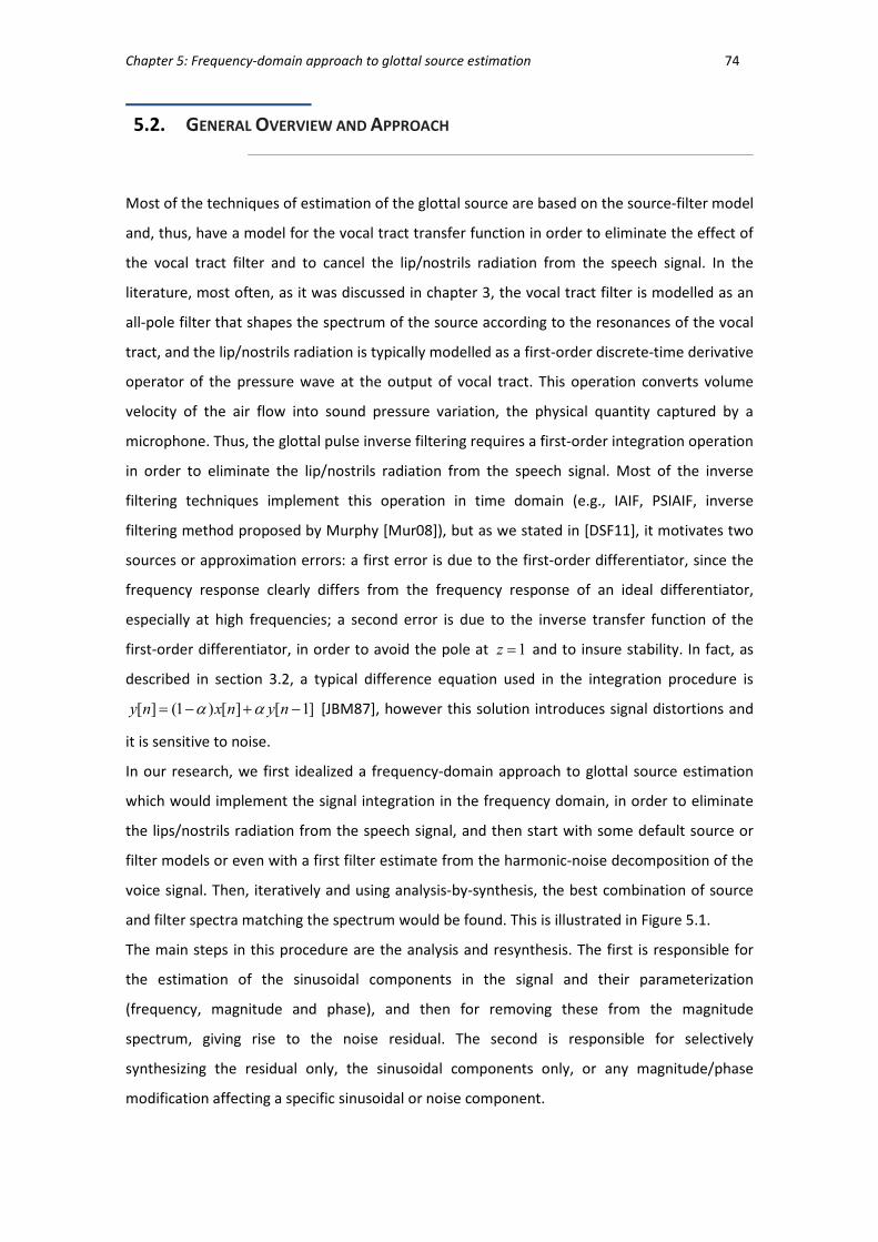
Chapter 5: Frequency-domain approach to glottal source estimation 74
5.2. GENERAL OVERVIEW AND APPROACH
Most of the techniques of estimation of the glottal source are based on the source-filter model
and, thus, have a model for the vocal tract transfer function in order to eliminate the effect of
the vocal tract filter and to cancel the lip/nostrils radiation from the speech signal. In the
literature, most often, as it was discussed in chapter 3, the vocal tract filter is modelled as an
all-pole filter that shapes the spectrum of the source according to the resonances of the vocal
tract, and the lip/nostrils radiation is typically modelled as a first-order discrete-time derivative
operator of the pressure wave at the output of vocal tract. This operation converts volume
velocity of the air flow into sound pressure variation, the physical quantity captured by a
microphone. Thus, the glottal pulse inverse filtering requires a first-order integration operation
in order to eliminate the lip/nostrils radiation from the speech signal. Most of the inverse
filtering techniques implement this operation in time domain (e.g., IAIF, PSIAIF, inverse
filtering method proposed by Murphy [Mur08]), but as we stated in [DSF11], it motivates two
sources or approximation errors: a first error is due to the first-order differentiator, since the
frequency response clearly differs from the frequency response of an ideal differentiator,
especially at high frequencies; a second error is due to the inverse transfer function of the
first-order differentiator, in order to avoid the pole at 1z = and to insure stability. In fact, as
described in section 3.2, a typical difference equation used in the integration procedure is
[ ] (1 ) [ ] [ 1]y n x n y nα α= − + − [JBM87], however this solution introduces signal distortions and
it is sensitive to noise.
In our research, we first idealized a frequency-domain approach to glottal source estimation
which would implement the signal integration in the frequency domain, in order to eliminate
the lips/nostrils radiation from the speech signal, and then start with some default source or
filter models or even with a first filter estimate from the harmonic-noise decomposition of the
voice signal. Then, iteratively and using analysis-by-synthesis, the best combination of source
and filter spectra matching the spectrum would be found. This is illustrated in Figure 5.1.
The main steps in this procedure are the analysis and resynthesis. The first is responsible for
the estimation of the sinusoidal components in the signal and their parameterization
(frequency, magnitude and phase), and then for removing these from the magnitude
spectrum, giving rise to the noise residual. The second is responsible for selectively
synthesizing the residual only, the sinusoidal components only, or any magnitude/phase
modification affecting a specific sinusoidal or noise component.

Chapter 5: Frequency-domain approach to glottal source estimation 75
However, with the development of our research, this glottal source estimation model was
reformulated and, in particular, does not implement the speech signal integration step, since it
is implicit in the procedure, as it will explained in the following sections.
Nevertheless, since the signal integration is common in most glottal source estimation
procedures and usually implemented in the time domain, we will review in the next section
that it possible and advantageous to implement this operation in the frequency domain
[DSF11].
Despite speech signals are strongly studied over the years, most often the phase information is
ignored. However, recent studies (e.g. [SF10], [BNG06], [Boz05], [Dru11], [MY11]) have shown
the importance and the pertinence of using this information in order, for example, to identify
the perceptual signature of a periodic sound, or to obtain a higher quality speech synthesis or
even to extract other speech features, as the Normalized Relative Delay (NRD). This feature
expresses the delay between the harmonics relative to the fundamental of a periodic signal
and denotes the phase contribution to the shape invariance of a periodic signal. The NRD
concept and its computation will be thoroughly described in section 5.2.2.
According to Sousa and Ferreira [SF10], the NRD feature can be used in identifying the
phonation type (pressed, normal and breathy), and also allows the analysis and synthesis of a
desired harmonic synchronization, independently of the overall time shift of the signal and of
its fundamental frequency. Therefore, NRDs, in addition to magnitude information, are also
powerful features because they allow to characterize completely the time waveform of a
speech signal, which is essential in the analysis-synthesis of our glottal source estimation
process. In fact, one of the main results of our research was that, for sustained vowels /a/ and
/i/, it is possible to estimate the NRDs corresponding to the glottal source signal using simply a
Figure 5.1. Initial idea for analysis by synthesis approach to filter/source fine-tuning.
Y
Voiced Speech estimate
filter/source
fine-tune filter/source
model
good approximation
to original spectrum?
N
source model
filter model
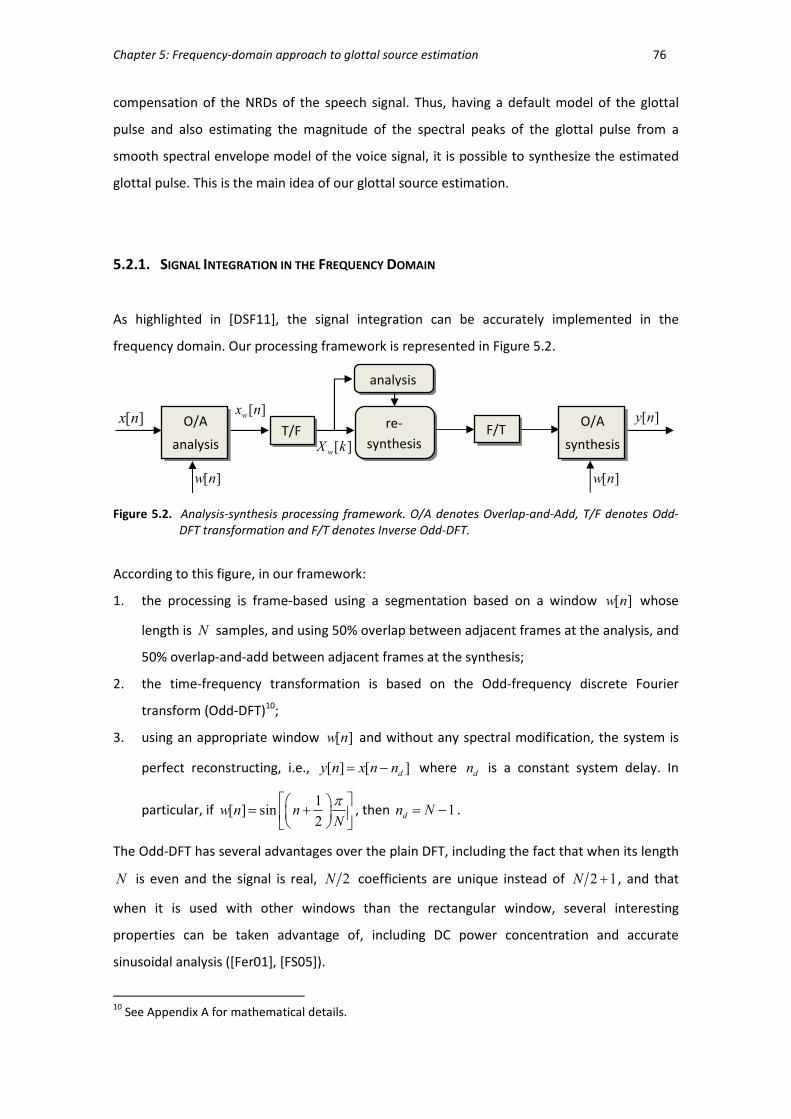
Chapter 5: Frequency-domain approach to glottal source estimation 76
compensation of the NRDs of the speech signal. Thus, having a default model of the glottal
pulse and also estimating the magnitude of the spectral peaks of the glottal pulse from a
smooth spectral envelope model of the voice signal, it is possible to synthesize the estimated
glottal pulse. This is the main idea of our glottal source estimation.
5.2.1. SIGNAL INTEGRATION IN THE FREQUENCY DOMAIN
As highlighted in [DSF11], the signal integration can be accurately implemented in the
frequency domain. Our processing framework is represented in Figure 5.2.
According to this figure, in our framework:
1. the processing is frame-based using a segmentation based on a window [ ]w n whose
length is N samples, and using 50% overlap between adjacent frames at the analysis, and
50% overlap-and-add between adjacent frames at the synthesis;
2. the time-frequency transformation is based on the Odd-frequency discrete Fourier
transform (Odd-DFT)10;
3. using an appropriate window [ ]w n and without any spectral modification, the system is
perfect reconstructing, i.e., [ ] [ ]d
y n x n n= − where dn is a constant system delay. In
particular, if 1
[ ] sin2
w n nN
π = +
, then 1dn N= − .
The Odd-DFT has several advantages over the plain DFT, including the fact that when its length
N is even and the signal is real, 2N coefficients are unique instead of 2 1N + , and that
when it is used with other windows than the rectangular window, several interesting
properties can be taken advantage of, including DC power concentration and accurate
sinusoidal analysis ([Fer01], [FS05]).
10
See Appendix A for mathematical details.
Figure 5.2. Analysis-synthesis processing framework. O/A denotes Overlap-and-Add, T/F denotes Odd-
DFT transformation and F/T denotes Inverse Odd-DFT.
[ ]wX k
O/A
analysis T/F
re-
synthesis
[ ]x n[ ]wx n
F/T O/A
synthesis
analysis
[ ]y n
[ ]w n [ ]w n

Chapter 5: Frequency-domain approach to glottal source estimation 77
Let us considerer a continuous signal ( )cx t and [ ]x n the signal obtained by sampling ( )cx t in
the time domain, i.e., ( )[ ] c sx n x nT= , where 1/s sT F= represents the sampling period, the
reciprocal of the sampling frequency sF .
In order to have the signal segmentation, as illustrated in Figure 5.2, a windowing step is
implemented. Therefore,
( ) ( )1[ ] [ ]. [ ]
2
F j j
wx n x n w n X e W eω ω
π= ←→ ∗ (71)
Taking the Odd-DFT of [ ]wx n , the time-frequency transformation is obtained:
[ ]2 11
2
0
[ ]N j k n
N
w w
n
X k x n e
π − − +
=
=∑ (72)
where N is the length of the transform. This implies that, for analysis and synthesis purposes,
the spectral information that we have access is discrete, i.e., for 0,1,..., 1:k N= −
Following the accurate estimation of the frequency, magnitude and phase of all the
identifiable sinusoids in the [ ]wX k spectrum [Fer01], resynthesis of these sinusoids can take
place with any desired modification, generating a new spectrum vector [ ]wX k . For example,
signal integration in the time domain is achieved by modifying [ ]wX k as:
[ ] ( )( )
,2 0.5 /
w
w
s
X kY k
jF k Nπ=
+ 0,1, ..., 1.k N= − (74)
In order to illustrate some of the pitfalls of the integration in time domain, we present in
Figure 5.3 a comparison between the integration in the time domain and in the frequency
domain of the LF derivative glottal pulse without noise and with white noise at 9 dB SNR. It is
clear that the output results of the integration implemented in the frequency domain
(according to the algorithm of Figure 5.2 and the modification defined by equation (74)) are
faithful reconstructions of the LF waveform. Furthermore, even when the input signal is a noisy
derivative of the LF glottal pulse, the output is still a correct reconstruction of that model. In
this last case, during the resynthesis, the high-frequency components of the derivative of the
glottal model disappear due to the noise, generating the artifacts that are visible on the closed
phase of the glottal model. Nevertheless, the noise has markedly less impact in this output
than in the one obtained using the time-domain integration according to
[ ] (1 ) [ ] [ 1]y n x n y nα α= − + − .
[ ] ( ) 2 1
2
.j
w wk
N
X k X e ωπ
ω = +
= (73)

Chapter 5: Frequency-domain approach to glottal source estimation 78
As discussed in detail in [DSF11], for both cases, the signal integrations implemented in the
frequency domain are significantly superior to the ones implemented in the time domain,
which highlight its advantages.
5.2.2. NORMALIZED RELATIVE DELAY CONCEPT
According to Bozkurt [Boz05], research developed during the last years showed that phase
plays an important role in speech perception, contrarily to early research which stated that the
human year is insensible to phase. Also, recent studies (e.g., [SF10], [SF11], [MY11]) have
shown that phase information from the speech signal has important applications in speech
analysis and synthesis. However, the phase spectrum is frequently ignored and there are few
studies that use this feature for parameter estimation purpose, when compared to amplitude
based parameter estimation methods.
As previously mentioned, in our framework phase-related features are used that are based on
the NRDs of the spectral harmonics of the glottal source. Therefore, the NRD concept is
explained here.
Let us admit a periodic signal [ ]x n consisting of L sinusoids harmonically related according to
a fundamental frequency 0
ω .
Therefore [SF10],
0 5 10 15-1
-0.5
0
0.5Amplitude
0 5 10 15-1
-0.5
0
0.5
Amplitude
Time (ms)
0 5 10 15
-2
0
2
4
Amplitude
0 5 10 15
-2
0
2
4
Amplitude
Time (ms)
0 5 10 15
0
0.5
1
Amplitude
0 5 10 15-0.4
-0.2
0
0.2
0.4
0.6
0.8
Amplitude
Time (ms)
Figure 5.3. Time representation of the derivative of the LF glottal waveforms without noise (top left
figure) and with white noise at 9 dB SNR (bottom left figure), and the corresponding output
results of a first-order time-domain integrator (center) and of a frequency-domain integrator
(right figure).
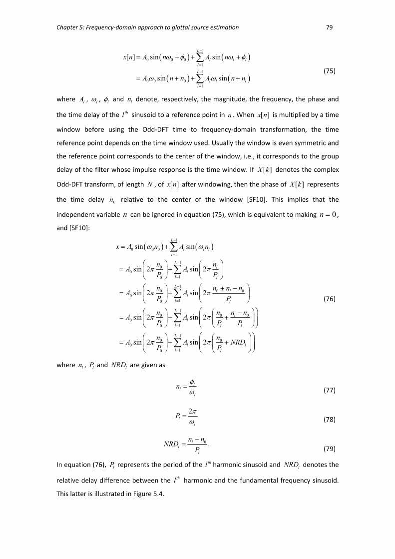
Chapter 5: Frequency-domain approach to glottal source estimation 79
( ) ( )
( ) ( )
1
0 0 0
1
1
0 0 0
1
[ ] sin sin
sin sin
L
l l l
l
L
l l l
l
x n A n A n
A n n A n n
ω φ ω φ
ω ω
−
=
−
=
= + + +
= + + +
∑
∑ (75)
where lA ,
lω ,
lφ and
ln denote, respectively, the magnitude, the frequency, the phase and
the time delay of the thl sinusoid to a reference point in n . When [ ]x n is multiplied by a time
window before using the Odd-DFT time to frequency-domain transformation, the time
reference point depends on the time window used. Usually the window is even symmetric and
the reference point corresponds to the center of the window, i.e., it corresponds to the group
delay of the filter whose impulse response is the time window. If [ ]X k denotes the complex
Odd-DFT transform, of length N , of [ ]x n after windowing, then the phase of [ ]X k represents
the time delay kn relative to the center of the window [SF10]. This implies that the
independent variable n can be ignored in equation (75), which is equivalent to making 0=n ,
and [SF10]:
( ) ( )1
0 0 0
1
10
0
10
10 0 0
0
10
10 0 0
0
10
00
0
sin sin
sin 2 sin 2
sin 2 sin 2
sin 2 sin 2
sin 2
L
l l l
l
Ll
l
l l
Ll
l
l l
Ll
l
l l l
l
x A n A n
n nA A
P P
n n n nA A
P P
n n n nA A
P P P
nA A
P
ω ω
π π
π π
π π
π
−
=
−
=
−
=
−
=
= +
= +
+ −= +
−= + +
= +
∑
∑
∑
∑
10
1
sin 2L
l
l l
nNRD
Pπ
−
=
+
∑
(76)
where ln ,
lP and
lNRD are given as
ll
l
nφω
= (77)
2l
l
Pπω
=
(78)
0 .ll
l
n nNRD
P
−=
(79)
In equation (76), lP represents the period of the thl harmonic sinusoid and
lNRD denotes the
relative delay difference between the thl harmonic and the fundamental frequency sinusoid.
This latter is illustrated in Figure 5.4.
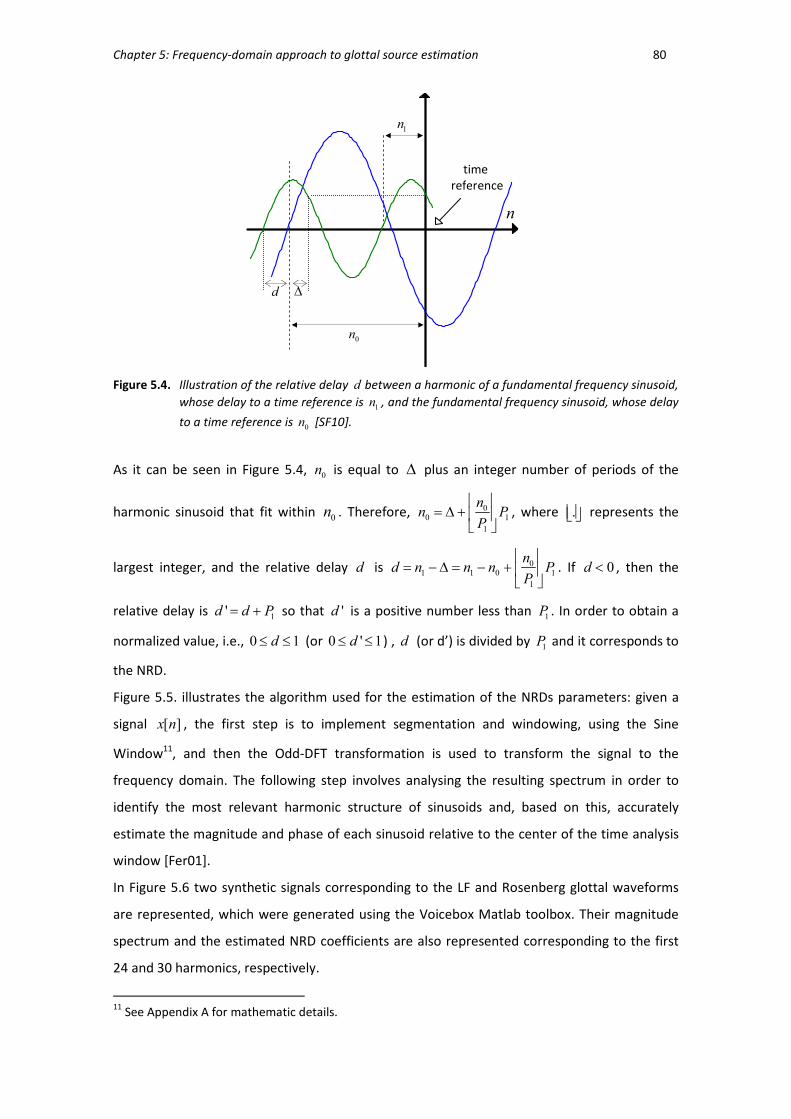
Chapter 5: Frequency-domain approach to glottal source estimation 80
As it can be seen in Figure 5.4, 0n is equal to ∆ plus an integer number of periods of the
harmonic sinusoid that fit within 0n . Therefore, 00 1
1
nn P
P
= ∆ +
, where . represents the
largest integer, and the relative delay d is 01 1 0 1
1
nd n n n P
P
= − ∆ = − +
. If 0d < , then the
relative delay is 1
'd d P= + so that 'd is a positive number less than 1P . In order to obtain a
normalized value, i.e., 0 1d≤ ≤ (or 0 ' 1d≤ ≤ ) , d (or d’) is divided by 1P and it corresponds to
the NRD.
Figure 5.5. illustrates the algorithm used for the estimation of the NRDs parameters: given a
signal [ ]x n , the first step is to implement segmentation and windowing, using the Sine
Window11, and then the Odd-DFT transformation is used to transform the signal to the
frequency domain. The following step involves analysing the resulting spectrum in order to
identify the most relevant harmonic structure of sinusoids and, based on this, accurately
estimate the magnitude and phase of each sinusoid relative to the center of the time analysis
window [Fer01].
In Figure 5.6 two synthetic signals corresponding to the LF and Rosenberg glottal waveforms
are represented, which were generated using the Voicebox Matlab toolbox. Their magnitude
spectrum and the estimated NRD coefficients are also represented corresponding to the first
24 and 30 harmonics, respectively.
11
See Appendix A for mathematic details.
Figure 5.4. Illustration of the relative delay d between a harmonic of a fundamental frequency sinusoid,
whose delay to a time reference is 1n , and the fundamental frequency sinusoid, whose delay
to a time reference is 0n [SF10].
n
∆
0n
d
1n
time reference

Chapter 5: Frequency-domain approach to glottal source estimation 81
It is clear, from Figure 5.6, that the NRD representation is regular and wrapped and the
unwrapping leads to a straight line, as it will shown below. Also, the first NRD coefficient is
always zero since it corresponds to the reference delay of the fundamental frequency.
Another important note is that, despite the similarities between the glottal flow waveforms
and the magnitude spectra of these two signals, the NRDs coefficients are clearly different
which suggests that the NRD possesses relevant information. In fact, Sousa and Ferreira [SF10]
state that NRD features are phase related only and correlate significantly with perceptual
information. Moreover, we have shown [DSF11] that it is possible to implant the magnitude
and NRD models on a periodic signal with the same fundamental frequency, since these two
features (the relative magnitude and NRDs between all relevant upper harmonics and the
fundamental frequency) completely define a wave prototype. Therefore, this procedure has
potentialities to contribute to an accurate glottal source estimation, which will be used in our
glottal source estimation process.
windowing and
Odd-DFT
accurate harmonic analysis
[ ]x n [ ]OX k
lφ
lPlω0n
lnlNRD
Figure 5.5. Algorithm implementing the estimation of the NRD parameters and overall time shift (0n ) of
the waveform [SF10].
Figure 5.6. (a) - Time representation of the LF glottal flow model (top row), its magnitude spectrum
(middle) and NRD representation (bottom row).
(b) - Time representation of the Rosenberg glottal flow model (top row), its magnitude
spectrum (middle) and NRD representation (bottom row).
(a)
0 5 10 15 20 250
0.5
1
Time (ms)Norm
alized Amplitude
0 1 2 3 4 5 6 70
50
100
150
Frequency (kHz)
Magnitude (dB)
0 5 10 15 20 25 300
0.5
1
Harmonic
Norm
aliz
ed D
elay
0 5 10 15 20 250
0.5
1
Time (ms)Norm
alized A
mplitude
0 1 2 3 4 5 6 70
50
100
150
Frequency (kHz)
Magnitude (dB)
0 5 10 15 20 25 300
0.5
1
Harmonic
Norm
aliz
ed D
elay
(b)
Chapter 5: Frequency-domain approach to glottal source estimation 82
5.3. PHYSIOLOGICAL SIGNAL ACQUISITION FOR SOURCE AND FILTER MODELLING
In order to accurately estimate the glottal source from a speech signal and since its
contribution is not directly observable in the speech waveform captured through a
microphone outside the mouth, we devised a technique, after consulting several specialists
concerning viability, feasibility, ethical and technical aspects, with the purpose to capture two
time-aligned acoustic signals: the source signal as close as possible to the vocal folds and the
corresponding voiced signal outside the mouth. That would allow us to characterize:
• the source signal, and compare the results with ideal (i.e., mathematical) existing models,
such as the LF and Rosenberg models, whose correspondence to physiological data is not
clear;
• the frequency response of the vocal tract filter, namely regarding the group delay.
Based on these characterizations, it would be possible to design a robust frequency-domain
approach for glottal source estimation, which is the main goal of our research. Also, we would
know how the real shape of the glottal flow looks like and that would allow us to evaluate the
quality of the estimation of the glottal source, and compare these estimations with the ones
obtained using other state-of-the-art glottal flow estimation methods, as discussed in chapter
4.
This experimental procedure was carefully planned and conducted with the collaboration of an
otorhinolaryngologist (ORL). We attached a tiny and high-quality microphone (of the ear-worn
type) at the tip of a rigid video laryngoscope and another similar microphone was used to
capture the signal outside the mouth. The literature recommendations about acquisition of
voice signals [Tiz94] were followed, namely the distance to the mouth of this latter
microphone was held constant, less than 10 cm (about 3 or 4 cm) and off-axis positioning (45o
to 90o from the mouth axis), as well as the equipment characteristics, as specified below.
The recording sessions took place during conventional video laryngoscopy examinations, in a
quiet room, and the ORL professional acted in order to capture the glottal source signal as
close as possible to the glottis, while insuring safety and ethical conditions for all volunteer
subjects. The acoustic signals were recorded simultaneously with an A/D interface and audio
recorder. Figure 5.7 illustrates the procedure and the equipment involved.
The equipment used in this experimental procedure was:
• a rigid video laryngoscope with 7 mm diameter and length of 180 mm (Xion);
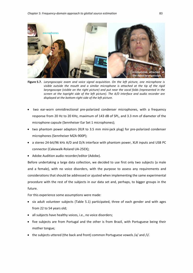
Chapter 5: Frequency-domain approach to glottal source estimation 83
• two ear-worn omnidirectional pre-polarized condenser microphones, with a frequency
response from 20 Hz to 20 KHz, maximum of 143 dB of SPL, and 3.3 mm of diameter of the
microphone capsule (Sennheiser Ear Set 1 microphones);
• two phantom power adaptors (XLR to 3.5 mm mini-jack plug) for pre-polarized condenser
microphones (Sennheiser MZA-900P);
• a stereo 24-bit/96 kHz A/D and D/A interface with phantom power, XLR inputs and USB PC
connector (Cakewalk-Roland UA-25EX);
• Adobe Audition audio recorder/editor (Adobe).
Before undertaking a large data collection, we decided to use first only two subjects (a male
and a female), with no voice disorders, with the purpose to assess any requirements and
considerations that should be addressed or ajusted when implementing the same experimental
procedure with the rest of the subjects in our data set and, perhaps, to bigger groups in the
future.
For this experience some assumptions were made:
• six adult volunteer subjects (Table 5.1) participated, three of each gender and with ages
from 22 to 54 years old;
• all subjects have healthy voices, i.e., no voice disorders;
• five subjects are from Portugal and the other is from Brazil, with Portuguese being their
mother tongue;
• the subjects uttered (the back and front) common Portuguese vowels /a/ and /i/.
Figure 5.7. Laryngoscopic exam and voice signal acquisition. On the left picture, one microphone is
visible outside the mouth and a similar microphone is attached at the tip of the rigid
laryngoscope (visible on the right picture) and put near the vocal folds (represented in the
screen at the topright side of the left picture). The A/D interface and audio recorder are
displayed at the bottom-right side of the left picture.
Figure 5.8.
microphones
microphone attached at
the video-laryngoscope
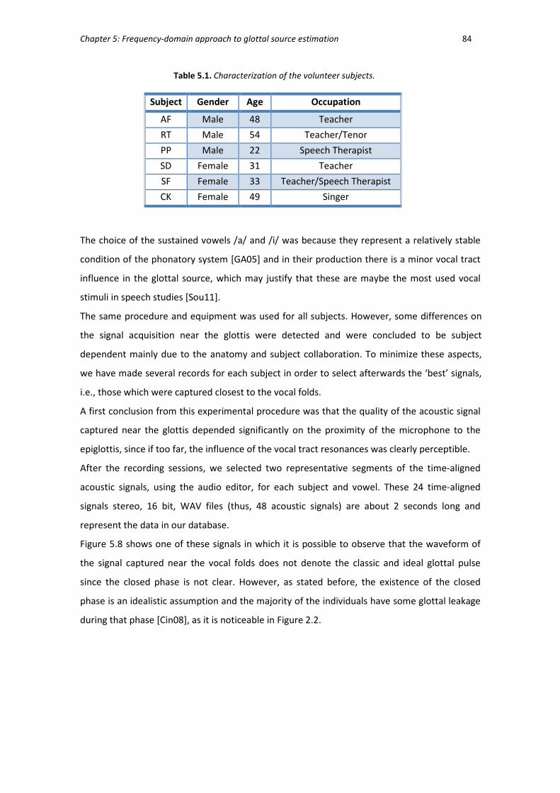
Chapter 5: Frequency-domain approach to glottal source estimation 84
The choice of the sustained vowels /a/ and /i/ was because they represent a relatively stable
condition of the phonatory system [GA05] and in their production there is a minor vocal tract
influence in the glottal source, which may justify that these are maybe the most used vocal
stimuli in speech studies [Sou11].
The same procedure and equipment was used for all subjects. However, some differences on
the signal acquisition near the glottis were detected and were concluded to be subject
dependent mainly due to the anatomy and subject collaboration. To minimize these aspects,
we have made several records for each subject in order to select afterwards the ‘best’ signals,
i.e., those which were captured closest to the vocal folds.
A first conclusion from this experimental procedure was that the quality of the acoustic signal
captured near the glottis depended significantly on the proximity of the microphone to the
epiglottis, since if too far, the influence of the vocal tract resonances was clearly perceptible.
After the recording sessions, we selected two representative segments of the time-aligned
acoustic signals, using the audio editor, for each subject and vowel. These 24 time-aligned
signals stereo, 16 bit, WAV files (thus, 48 acoustic signals) are about 2 seconds long and
represent the data in our database.
Figure 5.8 shows one of these signals in which it is possible to observe that the waveform of
the signal captured near the vocal folds does not denote the classic and ideal glottal pulse
since the closed phase is not clear. However, as stated before, the existence of the closed
phase is an idealistic assumption and the majority of the individuals have some glottal leakage
during that phase [Cin08], as it is noticeable in Figure 2.2.
Table 5.1. Characterization of the volunteer subjects.
Subject Gender Age Occupation
AF Male 48 Teacher
RT Male 54 Teacher/Tenor
PP Male 22 Speech Therapist
SD Female 31 Teacher
SF Female 33 Teacher/Speech Therapist
CK Female 49 Singer

Chapter 5: Frequency-domain approach to glottal source estimation 85
The original recording sampling frequency was 48000 Hz but the files were down-converted to
22050 Hz in order to facilitate subsequent processing, namely in terms of spectral analysis.
5.4. GLOTTAL SOURCE ESTIMATION IN THE FREQUENCY DOMAIN
In order to better analyse and synthesize the glottal source, for each one of the 24 acoustic
signals captured near the vocal folds, we characterized in detail the magnitude and NRDs of
the harmonics using the algorithm illustrated in Figure 5.5.
A first observation from the signals captured near the glottis was that the waveforms do not
correspond to the idealistic glottal pulse models (as the ones illustrated in Figure 3.12).
However, to our knowledge, there are no real experimental data of reference to sustain the
wave shape of the idealist glottal pulse models and, therefore, the correspondence to real
glottal source waveform is not clear.
Concerning magnitude, we found the magnitude of individual harmonics for each frame of the
source signal, as illustrated in Figure 5.9. The segmentation process was achieved by applying
Sine Window, with 1024N = samples, and using 50% overlap between adjacent frames at the
analysis, according to the framework illustrated in Figure 5.2. Then, for each vowel recorded
and speaker, we determined the average normalized magnitude (relative to the magnitude of
F0) of all detected harmonics. The following step was to obtain from this information the
corresponding Least Squares Regression model in the logarithmic scale with the purpose to
compare the resulting slope with the traditional -12 dB/octave reference. This slope reference
is usually considered in the literature as the natural decay of the glottal pulse spectrum
[Fan60]. In particular, according to [CRR+07], the LF model can be stylized in the spectral
Figure 5.8. Time-aligned speech signals for vowel /i/ by a male subject: the signal captured near the
vocal folds (top row) and the signal captured outside the mouth (bottom row).
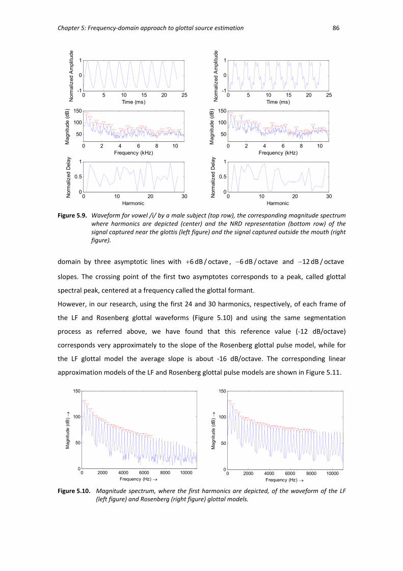
Chapter 5: Frequency-domain approach to glottal source estimation 86
domain by three asymptotic lines with 6 dB / octave+ , 6 dB / octave− and 12 dB / octave−
slopes. The crossing point of the first two asymptotes corresponds to a peak, called glottal
spectral peak, centered at a frequency called the glottal formant.
However, in our research, using the first 24 and 30 harmonics, respectively, of each frame of
the LF and Rosenberg glottal waveforms (Figure 5.10) and using the same segmentation
process as referred above, we have found that this reference value (-12 dB/octave)
corresponds very approximately to the slope of the Rosenberg glottal pulse model, while for
the LF glottal model the average slope is about -16 dB/octave. The corresponding linear
approximation models of the LF and Rosenberg glottal pulse models are shown in Figure 5.11.
0 2000 4000 6000 8000 100000
50
100
150
Frequency (Hz) →
Magnitude (dB) →
0 2000 4000 6000 8000 10000
0
50
100
150
Frequency (Hz) →
Magnitude (dB) →
Figure 5.10. Magnitude spectrum, where the first harmonics are depicted, of the waveform of the LF
(left figure) and Rosenberg (right figure) glottal models.
0 5 10 15 20 25-1
0
1
Time (ms)Norm
aliz
ed Amplitude
0 2 4 6 8 10
50
100
150
Frequency (kHz)
Magnitude (dB)
0 10 20 300
0.5
1
Harmonic
Norm
aliz
ed D
elay
0 5 10 15 20 25-1
0
1
Time (ms)Norm
aliz
ed Amplitude
0 2 4 6 8 10
50
100
150
Frequency (kHz)
Magnitude (dB)
0 10 20 300
0.5
1
Harmonic
Norm
aliz
ed D
elay
Figure 5.9. Waveform for vowel /i/ by a male subject (top row), the corresponding magnitude spectrum
where harmonics are depicted (center) and the NRD representation (bottom row) of the
signal captured near the glottis (left figure) and the signal captured outside the mouth (right
figure).

Chapter 5: Frequency-domain approach to glottal source estimation 87
Table 5.2 presents the spectral decay results of the acoustic signals captured near the vocal
folds according to gender and vowel. The results for each one of the 24 signals of our database
are presented in Table B.1 of Appendix B and have been obtained using on average 16
harmonics for vowel /a/ and 11 harmonics for vowel /i/. This difference highlights the fact that
vowel /i/ has an intrinsic pitch which is higher than that of vowel /a/.
Analysing these values it can be concluded that results per vowel are quite consistent between
genders, and the standard deviation reveals there are no strong differences among subjects of
the same gender. For both genders, the average slope for vowel /a/ is about -10 dB/octave
and, for vowel /i/, is approximately -14 dB/octave. Thus, comparing to the -12 dB/octave
reference, the average slope for vowel /a/ is lower, while the average slope for vowel /i/ falls
between the slope of the Rosenberg glottal model (-11,84 dB/octave) and that of the LF glottal
model (-16,43 dB/octave).
100
101
-55
-50
-45
-40
-35
-30
-25
-20
-15
-10
-5
0
Harmonic Index
Norm
alized Average M
agnitude (dB)
LF MODEL
ROS MODEL
-12 dB REF.
Figure 5.11. Normalized magnitude of the first 24 harmonics of the LF glottal pulse model (red dashed
line), and the 30 harmonics of the Rosenberg model (blue dashed line) and the reference
line with - 12 db/octave slope (black solid line).
Table 5.2. Average (AVG) and Standard Deviation (STDev) of the spectral decay of the source
harmonics, in dB/octave, as a function of gender and vowel.
AVG /a/ STDev /a/ AVG /i/ STDev /i/
Males -9,6443 2,3266 -13,7305 2,8674
Females -9,9334 3,3521 -13,6694 2,2575
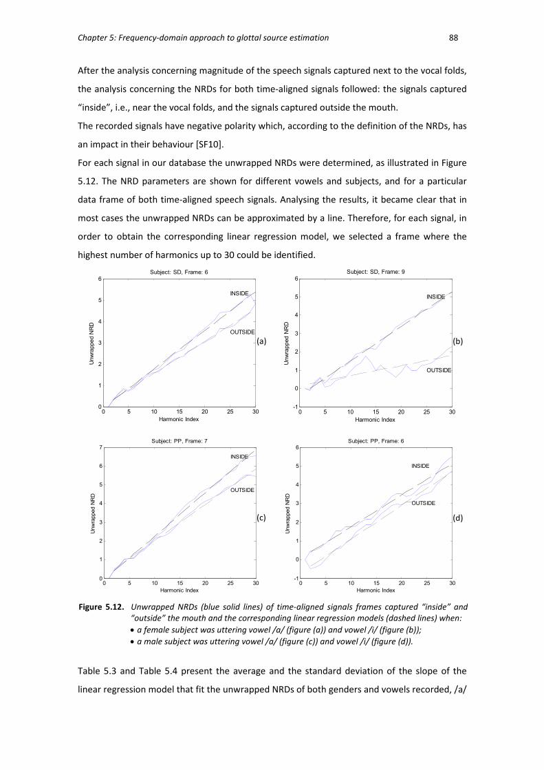
Chapter 5: Frequency-domain approach to glottal source estimation 88
After the analysis concerning magnitude of the speech signals captured next to the vocal folds,
the analysis concerning the NRDs for both time-aligned signals followed: the signals captured
“inside”, i.e., near the vocal folds, and the signals captured outside the mouth.
The recorded signals have negative polarity which, according to the definition of the NRDs, has
an impact in their behaviour [SF10].
For each signal in our database the unwrapped NRDs were determined, as illustrated in Figure
5.12. The NRD parameters are shown for different vowels and subjects, and for a particular
data frame of both time-aligned speech signals. Analysing the results, it became clear that in
most cases the unwrapped NRDs can be approximated by a line. Therefore, for each signal, in
order to obtain the corresponding linear regression model, we selected a frame where the
highest number of harmonics up to 30 could be identified.
Table 5.3 and Table 5.4 present the average and the standard deviation of the slope of the
linear regression model that fit the unwrapped NRDs of both genders and vowels recorded, /a/
Figure 5.12. Unwrapped NRDs (blue solid lines) of time-aligned signals frames captured “inside” and
“outside” the mouth and the corresponding linear regression models (dashed lines) when:
• a female subject was uttering vowel /a/ (figure (a)) and vowel /i/ (figure (b));
• a male subject was uttering vowel /a/ (figure (c)) and vowel /i/ (figure (d)).
0 5 10 15 20 25 300
1
2
3
4
5
6
7
Harmonic Index
Unwrapped NRD
Subject: PP, Frame: 7
INSIDE
OUTSIDE
0 5 10 15 20 25 30-1
0
1
2
3
4
5
6
Harmonic Index
Unwrapped NRD
Subject: PP, Frame: 6
INSIDE
OUTSIDE
0 5 10 15 20 25 30-1
0
1
2
3
4
5
6
Harmonic Index
Unwrapped N
RD
Subject: SD, Frame: 9
INSIDE
OUTSIDE
0 5 10 15 20 25 300
1
2
3
4
5
6
Harmonic Index
Unwrapped N
RD
Subject: SD, Frame: 6
OUTSIDE
INSIDE
(a) (b)
(c) (d)
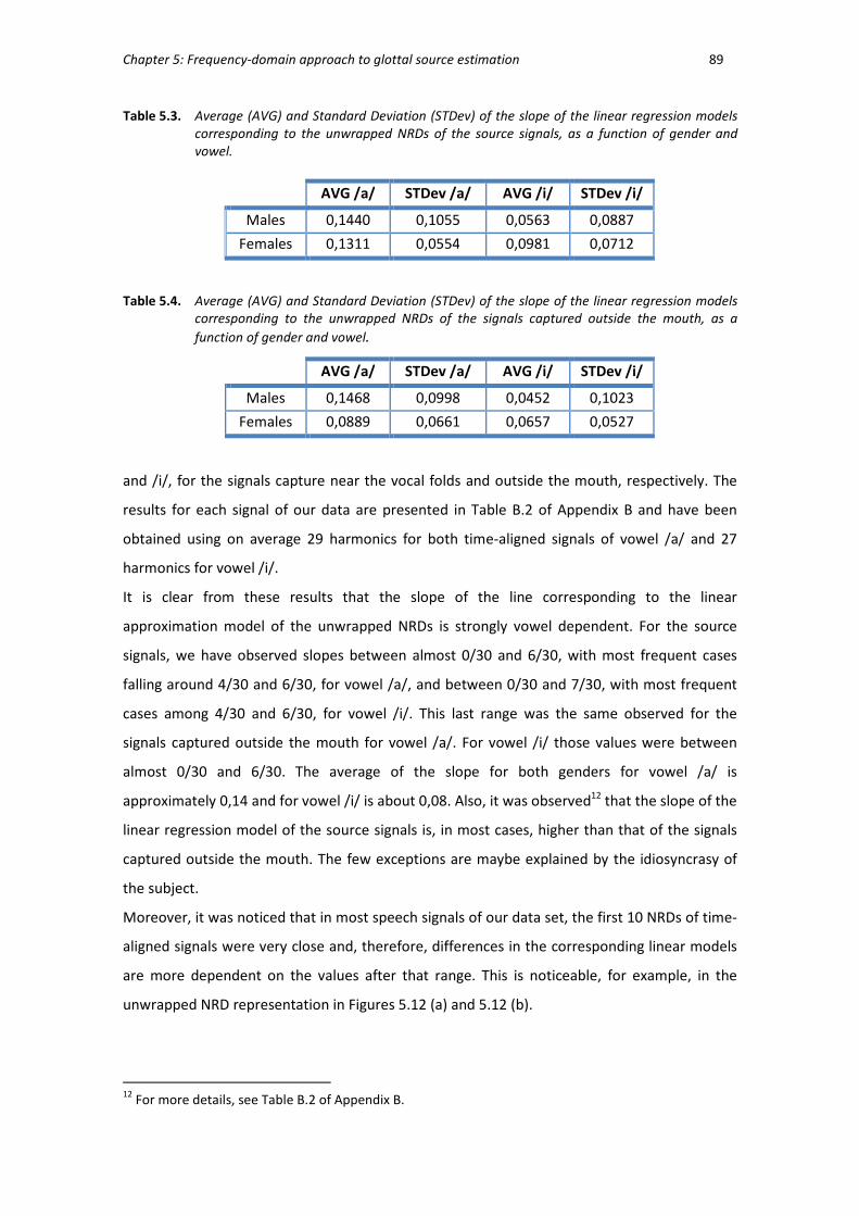
Chapter 5: Frequency-domain approach to glottal source estimation 89
and /i/, for the signals capture near the vocal folds and outside the mouth, respectively. The
results for each signal of our data are presented in Table B.2 of Appendix B and have been
obtained using on average 29 harmonics for both time-aligned signals of vowel /a/ and 27
harmonics for vowel /i/.
It is clear from these results that the slope of the line corresponding to the linear
approximation model of the unwrapped NRDs is strongly vowel dependent. For the source
signals, we have observed slopes between almost 0/30 and 6/30, with most frequent cases
falling around 4/30 and 6/30, for vowel /a/, and between 0/30 and 7/30, with most frequent
cases among 4/30 and 6/30, for vowel /i/. This last range was the same observed for the
signals captured outside the mouth for vowel /a/. For vowel /i/ those values were between
almost 0/30 and 6/30. The average of the slope for both genders for vowel /a/ is
approximately 0,14 and for vowel /i/ is about 0,08. Also, it was observed12 that the slope of the
linear regression model of the source signals is, in most cases, higher than that of the signals
captured outside the mouth. The few exceptions are maybe explained by the idiosyncrasy of
the subject.
Moreover, it was noticed that in most speech signals of our data set, the first 10 NRDs of time-
aligned signals were very close and, therefore, differences in the corresponding linear models
are more dependent on the values after that range. This is noticeable, for example, in the
unwrapped NRD representation in Figures 5.12 (a) and 5.12 (b).
12
For more details, see Table B.2 of Appendix B.
Table 5.4. Average (AVG) and Standard Deviation (STDev) of the slope of the linear regression models
corresponding to the unwrapped NRDs of the signals captured outside the mouth, as a
function of gender and vowel.
AVG /a/ STDev /a/ AVG /i/ STDev /i/
Males 0,1468 0,0998 0,0452 0,1023
Females 0,0889 0,0661 0,0657 0,0527
Table 5.3. Average (AVG) and Standard Deviation (STDev) of the slope of the linear regression models
corresponding to the unwrapped NRDs of the source signals, as a function of gender and
vowel.
AVG /a/ STDev /a/ AVG /i/ STDev /i/
Males 0,1440 0,1055 0,0563 0,0887
Females 0,1311 0,0554 0,0981 0,0712

Chapter 5: Frequency-domain approach to glottal source estimation 90
Analysing the difference, in modulus, between the slopes of the linear regression models
corresponding to the unwrapped NRDs of the signals captured near the vocal folds and outside
the mouth, it was observed that the values were between 0,02 and 0,06 for vowel /a/ and
between 0,01 and 0,14 for vowel /i/.
According to the results presented in Table 5.5, the average of these differences, for vowel /a/,
is about 0,04 for both genders and, for vowel /i/, is approximately 0,05 and 0,09 for male and
female, respectively. Therefore, the average of this latter difference, for both genders, is about
0,04 for vowel /a/ and 0,07 for vowel /i/.
5.4.1. HYBRID LF-ROSENBERG GLOTTAL SOURCE MODEL
Our glottal source estimation requires a default glottal model and, in order to find the one that
better matches our physiological data, we analysed two glottal source models of reference, LF
and Rosenberg.
Using the same procedure explained previously, the unwrapped NRDs coefficients as well as
the corresponding linear regression models were obtained for both glottal pulse models, as
illustrated in Figure 5.13. It can be observed that the slope of the linear regression model of
the LF glottal model is significantly higher than that of the Rosenberg model. In fact, the linear
approximation for the LF model is given by 0,0849 0,0511y x= + , where x represents the
index of the harmonic, for 2x ≥ , since by definition the NRD of F0 is always zero, and for the
Rosenberg model is given by 0,0090 0,2412y x= + .
However, according to the results presented in the previous section, neither of the two glottal
source models of reference – LF and Rosenberg – fits our data, and thus a new problem
aroused: which glottal pulse model should be used that better matches our physiological data?
The spectral decay of the LF model (about -16 dB/octave) is significantly higher than the
spectral decays obtained for vowels /a/ and /i/ in our data. On the other hand, the Rosenberg
Table 5.5. Average (AVG) and Standard Deviation (STDev) of the difference, in modulus, between the
slopes of the linear regression models that fit the unwrapped NRDs of the signals captured
near the vocal folds and outside the mouth, as a function of gender and vowel.
AVG /a/ STDev /a/ AVG /i/ STDev /i/
Males 0,0436 0,0063 0,0527 0,0463
Females 0,0422 0,0148 0,0868 0,0326

Chapter 5: Frequency-domain approach to glottal source estimation 91
model has a discontinuity in its derivative and, thus, is not a realistic model. Therefore, using
the normalized magnitude of the first 24 harmonics of each model, LF and Rosenberg, and the
corresponding unwrapped NRDs coefficients, we decided to devise a hybrid model. This model
was built using the average of the normalized spectral magnitudes of the harmonics of the LF
and Rosenberg glottal models and we have used different combinations of linear regressions in
order to build an NRD model. The smoothest result was obtained for the LF NRD model.
One advantage of this approach, as stated before, is that the normalized spectral magnitudes
and NRDs of the harmonics allow to thoroughly define a time waveform shape independently
of its fundamental frequency, time-shift or amplitude, which is essential for a glottal source
model.
Figure 5.14 illustrates the normalized spectral magnitude of the first 24 harmonics of all three
models: LF model, hybrid model and Rosenberg model. The time domain representation of
these glottal pulse models and its corresponding derivatives are shown in Figure 5.15. The
derivative signals were obtained in the frequency domain using the analysis-synthesis
processing framework illustrated in Figure 5.2. In particular, since the derivation in the time
domain corresponds to multiplying by jΩ in the frequency domain, before the synthesis we
shifted the phases of all harmonics by / 2π and scaled their magnitude by Ω at the exact
frequency of each harmonic sinusoid.
0 5 10 15 200
0.5
1
1.5
2
2.5
ROSENBERG MODEL
LF MODEL
Harmonic Index
Unwrapped NRD
Figure 5.13. Unwrapped NRDs of the LF and Rosenberg glottal pulse models (solid lines) and the
corresponding linear regression models (dashed lines).

Chapter 5: Frequency-domain approach to glottal source estimation 92
Figure 5.14. Normalized magnitude of the first 24 harmonics pertaining to the LF glottal pulse model
(red dashed line), the Rosenberg model (blue dash-dotted line) and a hybrid model (green
solid line).
Harmonic Index
Mag
nit
ud
e (d
B)
Figure 5.15. Time representation of the glottal pulse models (left figure) and the corresponding
derivative: LF (top), hybrid (center), and Rosenberg (bottom).
0 2 4 6 8 10 12 14 16 18 20 22
0
0.2
0.4
0.6
0.8
1
Norm
alized Amplitude
Time (ms)
LF
Hybrid
Rosenberg
0 2 4 6 8 10 12 14 16 18 20 22
-0.4
-0.2
0
0.2
0.4
0.6
Norm
alized Amplitude
Time (ms)
LF
Hybrid
Rosenberg

Chapter 5: Frequency-domain approach to glottal source estimation 93
It can be observed in Figure 5.15 that the hybrid model is smoother on the closing phase than
LF and Rosenberg models, but quite approaches the LF model and does not have the
discontinuity on the derivative signal, as the Rosenberg glottal model.
5.4.2. GLOTTAL SOURCE ESTIMATION APPROACH
According to previous sections, at this point we have:
• a new prototype of glottal pulse, whose magnitude model is hybrid of the LF and Rosenberg
glottal models, and whose NRD model matches that of the LF model;
• the spectrum of a sustained voiced signal captured outside the mouth, from which we
determined the magnitude and NRD coefficients from the spectral peaks;
• an estimation of the difference between the slope of the linear regression model of the
NRDs of the signals captured “inside” and “outside”, based on an experimental procedure
with real subjects.
Therefore, since the spectral magnitude information is independent of the phase information,
from which the NRDs are obtained, we developed the algorithm of estimation of the glottal
pulse represented in Figures 5.16 and 5.17.
This process consists of the following steps:
1. A smooth magnitude interpolation of the spectral envelope ( ceps ) is determined based
on the spectral peaks of the harmonics of the voiced speech signal (mS ), using the
Matlab function interp1. The smooth envelope is achieved by “short-pass liftering” the
output signal of interp1.
2. The difference ( dif ) between the magnitude of the spectral peaks and the magnitude of
the model resulted from step 1 ( ceps ) is estimated:
dif mS ceps= − . (80)
3. Based on the assumption that the unique requirement associated to the magnitude
frequency response of the (vocal tract) filter is smoothess, the spectral peaks of the
glottal source (mG ) are estimated by adding the difference obtained in step 2 to the
magnitude of the spectral peaks of the hybrid glottal model ( HMmG ):
HMmG mG dif= + . (81)
The magnitude of the filter (mF ) is, therefore, given as:

Chapter 5: Frequency-domain approach to glottal source estimation 94
.
HM
HM
HM
mF mS mG mS mG dif
mS mG mS ceps
ceps mG
= − = − −
= − − +
= −
(82)
4. The NRD coefficients of the voiced speech signal ( nrdS ) are computed and then the NRDs
of the source signal ( nrdG ) are estimated as follows:
. _slope difnrdG nrdS NRD h index= + × (83)
where .slope difNRD corresponds to the difference between the slope of the NRDs of the
speech signal and that of the source signal (mentioned in section 5.4), and _h index
corresponds to the harmonic index.
0 5 10
mG
+ =
Frequency Frequency Frequency
Mag
nit
ud
e
Mag
nit
ud
e
Mag
nit
ud
e
Figure 5.17. Illustration of the glottal source estimation.
0 5 10 0 5 10
nrdG nrdF+ =
nF0 nF0 nF0
NR
Ds
NR
Ds
NR
Ds
nrdS
mScepsmF
lifter order
NRD slope difference
Figure 5.16. Glottal source estimation algorithm.
Voiced Speech
estimate smooth spectral envelope
model ( ceps )
estimate magnitude of the spectral peaks of the glottal pulse
( )mG
estimate NRDs of “inside” speech signal
according to vowel
( )nrdG
synthesize
estimate of
the
glottal pulse compute NRDs of
the “outside” speech signal
( )nrdS

Chapter 5: Frequency-domain approach to glottal source estimation 95
5. Using the estimated NRDs (equation 83) and the magnitude of the spectral peaks
(equation 81), the glottal pulse is synthesized.
In step 1, the magnitude spectral envelope is estimated using the cepstral approach instead of
the popular LPC method because it better matches the poles and the zeros while the LPC
method insures a good match only to the poles.
5.5. TESTING THE NEW APPROACH TO GLOTTAL SOURCE ESTIMATION
In this section the new approach to glottal source estimation described previously is tested
with twelve speech signals including four synthetic and eight real (five from our data base),
and also one male singing signal. The results are evaluated and compared with the ones
obtained using two main state-of-the-art methods: IAIF and CC decomposition. These two
techniques were chosen not only because they are very popular in glottal source estimation
research, but also because they had better performances in the estimation of the glottal
source presented in chapter 4.
It should be noted that the CC decomposition only delivers the estimation of the glottal source
derivative (and the estimation of the vocal tract filter). Although we could implement the
integration step in order to achieve the glottal source signal, it would be a modification of the
result of the original procedure. Therefore, in this section the estimations of the glottal source
derivative using the CC decomposition will be presented, will be compared to the ones
obtained using IAIF (that are not necessarily results of reference) and will only be evaluated
qualitatively.
In order to assess the quality of the estimations, the evaluation of the estimations using IAIF
and our glottal source estimation approach will be complemented with an objective
quantitative measure: the Signal to Noise Ratio (SNR), defined by equation 69. This
measurement compares the signal and the noise resulting from the difference between the
estimated and the reference signal, and efficient glottal flow estimations are then reflected in
higher SNR values.
According to the definition of SNR, this value is only computed when the glottal source signal is
known, as it happens in the case of synthetic signals. On the other hand and concerning real
signals, we can not fully guarantee that the signals of our data base captured near the glottis
correspond to the correct glottal source. If fact, we have remarked that if captured far from

Chapter 5: Frequency-domain approach to glottal source estimation 96
the epiglottis, the influence of the vocal tract resonances becomes somehow noticeable. Thus,
the signals were chosen with the criterion of being captured as close as possible to the glottis.
We are however confident that the similarities of the waveforms for the majority of the
captured signals, as well as the similarities to classic and ideal glottal source models, except on
the closing and closed phases, enhance the validity of those signals as glottal source signals.
Furthermore, the ideal or analytical glottal source models are not sustained with real data and,
as previously mentioned, the existence of the closed phase seems to be an idealistic
assumption since during the closed phase the majority of the individuals have some glottal
leakage. Thus, according to these considerations, the SNR will be computed for nine signals
(four synthetic and five from our data base).
5.5.1. TESTS WITH SYNTHETIC SPEECH SIGNALS
Four synthetic signals will be used in order to compare and evaluate the estimations of the
glottal source: one of each gender, for vowels /a/ and /i/. These signals were generated using
the Voicebox Matlab toolbox and having the LF model as glottal impulse. The fundamental
frequency is 110 Hz and 300 Hz, for the male and the female synthetic signals, respectively.
Figures 5.1813 and 5.19 present the results for male signals and Figures 5.20 and 5.21 show the
results for female signals, for vowels /a/ and /i/, respectively. In each figure (from left to right)
we show first the LF flow waveform (top row) and the corresponding glottal flow derivative
(bottom row). Then, we first present the estimations performed by the state-of-the-art
methods – IAIF and CC decomposition – and, finally, the estimation using our glottal source
estimation.
The SNR values for the glottal source estimations using IAIF and our approach are presented in
Table 5.6.
Analysing all the estimations of the glottal pulse derivative using the CC decomposition, it is
clear that they approach the LF glottal pulse derivative, except from the minimum, where the
estimations are significantly smoother. This implies that the corresponding glottal pulses
would not have an abrupt closure as the LF glottal pulse. Also, it is noticeable that this
estimation method is less effective in the case of female signals, which corroborates that the
CC decomposition efficiency reduces significantly in high frequency signals [Dru11].
13
This synthetic signal corresponds to the signal shown in Figure 4.19.

Chapter 5: Frequency-domain approach to glottal source estimation 97
When comparing the estimations performed by CC decomposition to the glottal pulse
derivative estimations using IAIF, the differences are obvious, namely on the nonexistence of
ripples as in the results by IAIF, and the former method clearly outperforms in these signals.
The estimations of the glottal source using our proposed approach are close to the LF flow
waveform but, like the estimations using IAIF, do not denote the closed phase of the glottal
pulse.
While the glottal flow estimations performed by IAIF are relatively similar between vowels and
for the same gender, the results of our approach are significantly different for gender and
vowel. Nevertheless, some features are common: the abrupt closure, as in the LF glottal pulse,
and the asymmetric and bell-shape of the glottal pulses.
It can be also observed from Figures 5.20 and 5.21 that both estimation procedures
outperform in the female synthetic signals, which is emphasized by the corresponding SNR
values. These are interesting results since IAIF is usually less efficient on high frequency speech
signals.
Also, according to the SNR values from Table 5.6, the performance of our approach is more
effective in most test signals than the IAIF method, which highlights the robustness of our
glottal source estimation process.
Table 5.6. SNR values for the glottal source estimations of synthetic speech signals, using the IAIF
method and our glottal source estimation approach.
Male synthetic
vowel /a/
Male synthetic
vowel /i/
Female synthetic
vowel /a/
Female synthetic
vowel /i/
IAIF 6,3832 6,0905 9,7968 8,7182
Our approach 7,3010 8,7168 9,7475 8,8672

Chapter 5: Frequency-domain approach to glottal source estimation 98
(a)
0 50 1000
0.5
1
TimeAmplitude
0 50 100-0.1
0
0.1
Time
Amplitude
(b)
Am
plit
ud
e
Time
(c)
Am
plit
ud
e
0 10 20 30 40 50 60 70 80
(d)
Am
plit
ud
e
Time Time
Figure 5.18. Glottal flow estimation of a male synthetic vowel /a/ using the LF model.
(a) Glottal flow waveform (top) and glottal flow derivative (bottom) ( 0 110F Hz= );
(b) The glottal flow (top row) and derivative (bottom row) waveforms estimated by IAIF; (c) The glottal flow derivative estimation (maximum-phase component) using CC
decomposition; (d) The glottal flow waveform estimated by our glottal source estimation approach.
(a)
0 50 1000
0.5
1
Time
Amplitude
0 50 100-0.1
0
0.1
Time
Amplitude
(b)
Am
plit
ud
e
Time
(c)
Am
plit
ud
e
(d)
Am
plit
ud
e
0 100 200 300 400 500 600 700
Time Time
Figure 5.19. Glottal flow estimation of a male synthetic vowel /i/ using the LF model.
(a) Glottal flow waveform (top) and glottal flow derivative (bottom) ( 0 110F Hz= )
(b) The glottal flow (top row) and derivative (bottom row) waveforms estimated by IAIF; (c) The glottal flow derivative estimation (maximum-phase component) using CC
decomposition; (d) The glottal flow waveform estimated by our glottal source estimation approach.

Chapter 5: Frequency-domain approach to glottal source estimation 99
(a)
0 50 1000
0.5
1
TimeAmplitude
0 50 100-0.1
0
0.1
Time
Amplitude
(b) Am
plit
ud
e
Time
(c)
Am
plit
ud
e
(d)
Am
plit
ud
e
Time Time
Figure 5.20. Glottal flow estimation of a female synthetic vowel /a/ using the LF model.
(a) Glottal flow waveform (top) and glottal flow derivative (bottom) ( 0 300F Hz= );
(b) The glottal flow (top row) and derivative (bottom row) waveforms estimated by IAIF; (c) The glottal flow derivative estimation (maximum-phase component) using CC
decomposition; (d) The glottal flow waveform estimated by our glottal source estimation approach.
(a)
0 50 1000
0.5
1
Time
Amplitude
0 50 100-0.1
0
0.1
Time
Amplitude
(b) Am
plit
ud
e
Time
(c)
Am
plit
ud
e
(d)
Am
plit
ud
e
Time Time
Figure 5.21. Glottal flow estimation of a female synthetic vowel /i/ using the LF model.
(a) Glottal flow waveform (top) and glottal flow derivative (bottom) ( 0 300F Hz= )
(b) The glottal flow (top row) and derivative (bottom row) waveforms estimated by IAIF; (c) The glottal flow derivative estimation (maximum-phase component) using CC
decomposition; (d) The glottal flow waveform estimated by our glottal source estimation approach.

Chapter 5: Frequency-domain approach to glottal source estimation 100
5.5.2. TESTS WITH REAL SPEECH SIGNALS
In this section eight real speech signals and one male singing signal are used, with normal
phonation, in order to evaluate the quality of the glottal source estimations. Three of these
speech signals, illustrated in Figures 5.22 to 5.24, were also used in chapter 414, and the
remaining five signals are from our data base:
• a female vowel /a/ (subject SF) with F0=372 Hz (Figure 5.26);
• a female vowel /i/ (subject SD) with F0=489 Hz (Figure 5.27);
• a female vowel /i/ (subject SF) with F0=464 Hz (Figure 5.28);
• a male vowel /a/ (subject RT) with F0=261 Hz (Figure 5.29);
• a male vowel /i/ (subject RT) with F0=266 Hz (Figure 5.30).
An advantage of these latter signals is that, as explained above, a representation of the source
signal is known and, therefore, it is easy to evaluate the estimations provided by the different
techniques.
Following the same procedure of the previous section, in each figure (from left to right) we
first present the speech waveform, for the first three speech signals and for the singing signal,
or the signal captured near the glottis, for the five speech signals of our data set. The estimates
follow and are shown in the same order: IAIF, CC decomposition and our glottal source
estimation approach.
Due to the unavailability of the glottal source signals for the first three speech signals and for
the singing signal, it is more difficult to assess the quality of the estimations. Still, we will
compare the estimations performed by the different techniques between each other.
Analysing Figures 5.22 to 5.25, strong similarities between the glottal source estimations using
IAIF and our approach can be noted. While for the first two speech signals, the estimations
performed by these two methods show the classic asymmetry and bell-shape of the glottal
pulse, often referred to in the literature, the estimations for the third signal show a
modification on the closing phase. This modification is also present either in all signals of our
data captured near the glottis analysed here (as in most of our data base) and in all
corresponding estimations performed using our approach.
Concerning the estimations performed by CC decomposition for the same signals, they quite
approximate classic glottal pulse derivative models, except on the closing phase, however they
are significantly different from the estimations using IAIF, namely in the closed phase.
14
The signals are shown in Figures 4.20 to 4.22.

Chapter 5: Frequency-domain approach to glottal source estimation 101
It is interesting to notice, in particular, that the estimations performed by the three techniques
of the singing signal have similarities.
The analysis of the estimations performed by IAIF and our approach, related to the signals
from our data base, will be also assessed with the SNR values exhibited in Table 5.7.
According to Figures 5.26 to 5.30, it is clear that the glottal flow estimations resulted from our
approach are significantly identical to the waveforms of the corresponding signals captured
near the glottis and the SNR values enhance the quality of those estimations. For most of these
signals, the estimations performed by IAIF and our approach are close, with outperformance of
our approach, which is corroborated by the higher SNR values from Table 5.7.
It can also be noticed that the estimations by CC decomposition are quite consistent and,
despite the differences when compared to the glottal flow derivative waveforms estimated
using IAIF, the positive and negative parts are identical.
An important and common feature of most of these glottal flow estimations is the shape of the
waveform on the closing phase. This is noticeable in Figures 5.24, 5.26, 5.27, 5.28, 5.29 and
5.30, and, as mentioned above, it was clear in most of the signals of our data base captured
“inside”, i.e., near the vocal folds. This maybe highlights the fact that mathematical glottal
pulse models do not entirely correspond to realistic glottal pulses, namely on the closing and
closed phases.
The similarities between the glottal source estimations performed by our approach and the
corresponding glottal flow waveforms of the signals, as well as the higher SNR values
comparatively to the ones related to the IAIF performances, emphasize that our proposed
approach performs robust glottal source estimations and, therefore, confirm this new glottal
source estimation method as a promising technique.
Table 5.7. SNR values for the glottal source estimations using the IAIF method and our glottal source
estimation approach.
Female
vowel /a/
(subject SF)
Female
vowel /i/
(subject SD)
Female
vowel /i/
(subject SF)
Male vowel
/a/
(subject RT)
Male vowel
/i/
(subject RT)
IAIF 8,9982 9,5403 10,3138 9,6980 11,3175
Our approach 11,8187 15,8266 11,2107 14,6801 13,3643
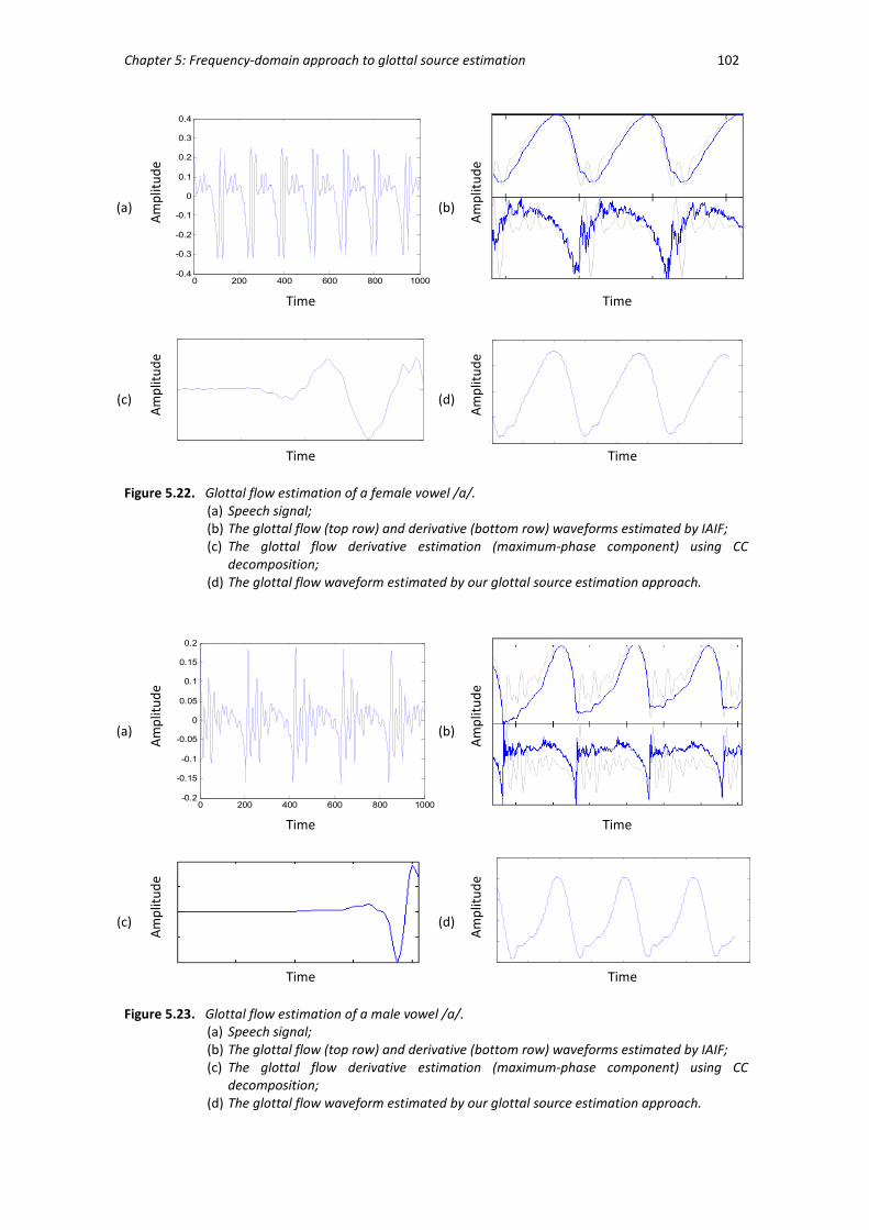
Chapter 5: Frequency-domain approach to glottal source estimation 102
(a)
Am
plit
ud
e
0 200 400 600 800 1000-0.4
-0.3
-0.2
-0.1
0
0.1
0.2
0.3
0.4
(b)
Am
plit
ud
e
Time Time
(c)
Am
plit
ud
e
0 20 40 60
(d)
Am
plit
ud
e
-0.2
-0.1
0
0.1
0.2
Time Time
Figure 5.22. Glottal flow estimation of a female vowel /a/.
(a) Speech signal; (b) The glottal flow (top row) and derivative (bottom row) waveforms estimated by IAIF; (c) The glottal flow derivative estimation (maximum-phase component) using CC
decomposition; (d) The glottal flow waveform estimated by our glottal source estimation approach.
(a)
Am
plit
ud
e
0 200 400 600 800 1000-0.2
-0.15
-0.1
-0.05
0
0.05
0.1
0.15
0.2
(b)
Am
plit
ud
e
Time Time
(c)
Am
plit
ud
e
(d)
Am
plit
ud
e
Time Time
Figure 5.23. Glottal flow estimation of a male vowel /a/.
(a) Speech signal; (b) The glottal flow (top row) and derivative (bottom row) waveforms estimated by IAIF; (c) The glottal flow derivative estimation (maximum-phase component) using CC
decomposition; (d) The glottal flow waveform estimated by our glottal source estimation approach.
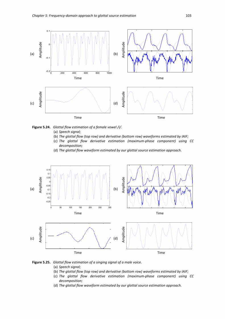
Chapter 5: Frequency-domain approach to glottal source estimation 103
(a)
Am
plit
ud
e
0 200 400 600 800 1000-0.2
-0.1
0
0.1
(b)
Am
plit
ud
e
Time Time
(c)
Am
plit
ud
e
0 20 40 60 80
(d)
Am
plit
ud
e
0 50 100 150 200
Time Time
Figure 5.24. Glottal flow estimation of a female vowel /i/.
(a) Speech signal; (b) The glottal flow (top row) and derivative (bottom row) waveforms estimated by IAIF; (c) The glottal flow derivative estimation (maximum-phase component) using CC
decomposition; (d) The glottal flow waveform estimated by our glottal source estimation approach.
(a)
Am
plit
ud
e
0 50 100 150 200 250 300
-0.25
-0.2
-0.15
-0.1
-0.05
0
0.05
0.1
0.15
(b)
Am
plit
ud
e
Time Time
(c)
Am
plit
ud
e
(d)
Am
plit
ud
e
Time Time
Figure 5.25. Glottal flow estimation of a singing signal of a male voice.
(a) Speech signal; (b) The glottal flow (top row) and derivative (bottom row) waveforms estimated by IAIF; (c) The glottal flow derivative estimation (maximum-phase component) using CC
decomposition; (d) The glottal flow waveform estimated by our glottal source estimation approach.
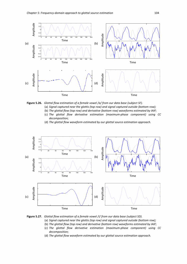
Chapter 5: Frequency-domain approach to glottal source estimation 104
(a)
Am
plit
ud
e
0 20 40 60 80 100 120 140 160 180 200-0.4
-0.2
0
0.2
0.4
(b)
Am
plit
ud
e
Time
Am
plit
ud
e
0 20 40 60 80 100 120 140 160 180 200
-0.4
-0.2
0
0.2
0.4
Time Time
(c)
Am
plit
ud
e
(d)
Am
plit
ud
e
Time Time
Figure 5.26. Glottal flow estimation of a female vowel /a/ from our data base (subject SF).
(a) Signal captured near the glottis (top row) and signal captured outside (bottom row); (b) The glottal flow (top row) and derivative (bottom row) waveforms estimated by IAIF; (c) The glottal flow derivative estimation (maximum-phase component) using CC
decomposition; (d) The glottal flow waveform estimated by our glottal source estimation approach.
(a)
Am
plit
ud
e
0 20 40 60 80 100 120 140-0.2
-0.1
0
0.1
0.2
(b)
Am
plit
ud
e
Time
Am
plit
ud
e
0 20 40 60 80 100 120 140-0.2
0
0.2
0.4
Time Time
(c)
Am
plit
ud
e
(d)
Am
plit
ud
e
0 50 100 150
Time Time
Figure 5.27. Glottal flow estimation of a female vowel /i/ from our data base (subject SD).
(a) Signal captured near the glottis (top row) and signal captured outside (bottom row); (b) The glottal flow (top row) and derivative (bottom row) waveforms estimated by IAIF; (c) The glottal flow derivative estimation (maximum-phase component) using CC
decomposition; (d) The glottal flow waveform estimated by our glottal source estimation approach.

Chapter 5: Frequency-domain approach to glottal source estimation 105
(a)
Am
plit
ud
e
0 20 40 60 80 100 120 140 160-0.4
-0.2
0
0.2
0.4
(b)
Am
plit
ud
e
Time
Am
plit
ud
e
0 20 40 60 80 100 120 140 160-0.4
-0.2
0
0.2
0.4
Time Time
(c)
Am
plit
ud
e
(d)
Am
plit
ud
e
Time Time
Figure 5.28. Glottal flow estimation of a female vowel /i/ from our data base (subject SF).
(a) Signal captured near the glottis (top row) and signal captured outside (bottom row); (b) The glottal flow (top row) and derivative (bottom row) waveforms estimated by IAIF; (c) The glottal flow derivative estimation (maximum-phase component) using CC
decomposition; (d) The glottal flow waveform estimated by our glottal source estimation approach.
(a)
Am
plit
ud
e
0 50 100 150 200 250-0.4
-0.2
0
0.2
0.4
(b)
Am
plit
ud
e
Time
Am
plit
ud
e
0 50 100 150 200 250-0.2
-0.1
0
0.1
0.2
Time Time
(c)
Am
plit
ud
e
(d)
Am
plit
ud
e
0 50 100 150 200 250
Time Time
Figure 5.29. Glottal flow estimation of a male vowel /a/ from our data base (subject RT).
(a) Signal captured near the glottis (top row) and signal captured outside (bottom row); (b) The glottal flow (top row) and derivative (bottom row) waveforms estimated by IAIF; (c) The glottal flow derivative estimation (maximum-phase component) using CC
decomposition; (d) The glottal flow waveform estimated by our glottal source estimation approach.

Chapter 5: Frequency-domain approach to glottal source estimation 106
(a)
Am
plit
ud
e
0 50 100 150 200 250-0.4
-0.2
0
0.2
0.4
(b)
Am
plit
ud
e
Time
Am
plit
ud
e
0 50 100 150 200 250-0.4
-0.2
0
0.2
0.4
Time Time
(c)
Am
plit
ud
e
(d)
Am
plit
ud
e
Time Time
Figure 5.30. Glottal flow estimation of a male vowel /i/ from our data base (subject RT)
(a) Signal captured near the glottis (top row) and signal captured outside (bottom row); (b) The glottal flow (top row) and derivative (bottom row) waveforms estimated by IAIF; (c) The glottal flow derivative estimation (maximum-phase component) using CC
decomposition; (d) The glottal flow waveform estimated by our glottal source estimation approach.
5.5.3. CONCLUSIONS
In the previous sections, our glottal source estimation approach was tested in several speech
signals, synthetic and real, with the purpose to evaluate its performance and to compare the
effectiveness of this procedure with two state-of-the-art glottal flow estimation techniques:
IAIF and CC decomposition.
It was clear that most of the glottal flow estimations performed by IAIF and our approach were
similar and revealed some particularities and common shapes, namely on the closing and
closed phases. These characteristics were also noticeable in most of the signals captured near
the glottis from our data set and maybe indicate that the real glottal pulse has not a bell-shape
as in the reference classic glottal flow models.
The results performed by CC decomposition do not allow substantial conclusions since this
method only gives the glottal source derivative estimation and, therefore, the estimations for
the real signals were only compared to the ones using IAIF. However, in the synthetic speech
tests, the effectiveness of the CC decomposition was rather higher than IAIF, although the
estimations were significantly smoother on the closing phase when compared to the reference
Chapter 5: Frequency-domain approach to glottal source estimation 107
LF glottal source derivative. In real speech tests, the results of this method were consistent and
revealed some particularities similar to the IAIF results.
Despite the fact that the glottal flow estimations by IAIF and our approach for the synthetic
speech signals have in general, an asymmetric and bell-shape, we observed that in the case of
real signals the results shown a common characteristic: a variation on the closing phase, also
noticeable in the majority of the signals of our data base captured near the glottis.
We also observed that the estimations of the glottal source using our approach were, in the
majority of the tests, similar to the ones delivered by IAIF, however our approach
outperformed this method which is corroborated by the higher SNR values.
Therefore, our glottal source estimation approach exhibits promising results, which motivates
the improvement in future developments of our initial approach illustrated in Figure 5.1.
5.6. SUMMARY
In this chapter a new glottal pulse estimation procedure, implemented in the frequency-
domain, was proposed based on an accurate spectral magnitude modelling and estimation of
the Normalized Relative Delays (NRDs) of the harmonics of the voiced signal.
This approach was developed using the results from accurate sinusoidal/harmonic analysis and
synthesis of two time aligned acoustic signals for vowels /a/ and /i/: the glottal source signal
captured near the glottis and the corresponding voiced signal captured outside the mouth. The
experimental procedure in which these signals were captured was thoroughly described.
The results of the data set analysis were presented, namely concerning the magnitude of the
spectral peaks and the NRDs of the harmonics, and a new hybrid glottal pulse prototype was
devised, combining features of two reference glottal models - the Liljencrants-Fant and the
Rosenberg models.
The performance of the new glottal source approach was assessed on several voiced signals,
synthetic and real, and the results look competitive taking into consideration results by other
reference algorithms, namely IAIF. Moreover, in almost all the tests where the glottal source
was known, our estimation approach led to the best results, as evidenced by higher SNR
values.
It was noticeable in most glottal source estimations and in the majority of the signals from our
data base captured near the glottis, a common shape that exhibits a variation on the closing

Chapter 5: Frequency-domain approach to glottal source estimation 108
phase. This maybe highlights that the real glottal pulse has not a bell-shape, often assumed in
the literature and as usually considered in classic glottal pulse models.
Despite the fact that our glottal source estimation approach does not implement the first
order integration step, common in most inverse filtering techniques in order to eliminate the
lip/nostrils radiation effect from the voiced signal and usually implemented in time domain, we
reviewed also in this chapter that this procedure can be accurately implemented in the
frequency domain avoiding some of the pitfalls of the integration in time domain.

Chapter 6
CONCLUSION
Contents
6.1. OVERVIEW ....................................................................................................................... 110
6.2. FUTURE DIRECTIONS ......................................................................................................... 111

Chapter 6: Conclusion 110
6.1. OVERVIEW
Over the years, the voice has been an important object of study in different areas but it still
remains an open field for investigation. In particular, the estimation of the glottal pulse from a
speech signal raised the interest of many researchers due to its great potential in speech
science. However, due to the concealed location of the vocal folds and, therefore, to the
difficulties on capturing directly and non-invasively the glottal source signal, computational
alternatives have been proposed over the years in order to accurately estimate the glottal
source directly from speech signals. Most of the glottal source estimation procedures are
based on the source-filter model and, thus, the glottal source is estimated by reversing the
voice production, i.e., the glottal source and the vocal tract filter are separated in order to
obtain the voice source generated at the glottis.
In this dissertation a new frequency-domain approach to glottal source estimation was
proposed, using a phase-related feature based on the Normalized Relative Delays (NRDs) of
the harmonics and an accurate determination of the magnitude of the spectral peaks of the
harmonics of the speech signal. From these values, the magnitude of the spectral peaks and
the NRDs corresponding to the glottal source are estimated and the glottal pulse is
synthesized, using a new hybrid model combining features of two reference glottal models -
the Liljencrants-Fant and Rosenberg - and that represents a better fit to our experimental data,
whose special acquisition was also described.
The performance of our approach has been evaluated and compared on a significant number
of speech signals, synthetic and real, using two representative state-of-the-art techniques for
the same purpose - IAIF and CC decomposition. For the synthetic signals and signals of our
data base, an objective measure (SNR) was used in order to assess the quality of the glottal
source estimations.
The results have shown that for synthetic signals, the estimations of our approach were similar
to the ones obtained by IAIF and the SNR values revealed that, in the majority of these signals,
our approach was more effective.
For real signals, our approach to glottal source estimation also exhibited better performance
when compared to other techniques. On the other hand, results also suggested that the glottal
pulse estimations do not have the bell-shape, usually assumed in the literature and common in
mathematical glottal pulse models, but revealed a variation on the closing phase. Also, the
closed phase was not perceptible in any glottal flow estimations. These results maybe suggest

Chapter 6: Conclusion 111
that idealistic glottal pulse models do not entirely correspond to real glottal pulse, namely on
the closing and closed phases.
Finally, it is important to emphasize the importance of phase features in speech analysis and
synthesis, namely the NRDs, and the promising results presented in this work corroborate that
our glottal source approach has a great potential in glottal source estimation. Therefore, this
dissertation work added an important contribution in this research direction.
6.2. FUTURE DIRECTIONS
In the following list, possible future direction of research are proposed.
• Capture time-aligned speech signals (the signal “inside” as close as possible to the glottis
and the signal outside the mouth), as implemented in this study, for a larger number of
subjects, with and without speech disorders, and not only for sustained vowels. This
would allow to better characterize the relation between the NRDs of the harmonics of the
voiced signal and the respective glottal source signal. Also, it would be interesting to use a
third signal, as the EGG, to improve the estimation.
• Implement an iterative procedure in the proposed algorithm for the estimation of the
glottal source in order to obtain even more accurate estimations.
• Explore the potential of the NRDS in the development of a robust algorithm for speaker
identification.
• Explore the potentialities of our approach in the independent manipulation of the spectral
magnitude and of the NRDs, characterizing the phase, in order to improve the naturalness
of synthetic speech and implant the sound signature of a specific speaker.

Appendix A 112
APPENDIX A – FUNDAMENTALS OF DIGITAL SIGNAL PROCESSING
• WINDOW FUNCTIONS
Blackman
2 2( ) 0.42 0.5cos 0.08cos ,0 1
1 1B
n nw n n N
N N
π π = + + ≤ ≤ − − −
Hamming
2( ) 0.54 0.46cos ,0 1
1HM
nw n n N
N
π = − ≤ ≤ − −
Hanning
2( ) 0.5 0.5cos ,0 1
1HN
nw n n N
N
π = − ≤ ≤ − −
Hanning-Poisson
2| |2
( ) 0.5 1 cos ,2
n
NHP
n Nw n e n
N
απ − = + ≤
Sin
1( ) sin ,0 1
2Sw n n n N
N
π = × + ≤ ≤ −
Triangular
2 1 1 1( ) ,
1 2 2 2T
N N Nw n n n
N
− − −= − − ≤ −

Appendix A 113
• DISCRETE TIME FOURIER TRANSFORM (DTFT)
The Fourier transform represents a signal in terms of complex exponentials (or sinusoids,
because ( ) ( )cos sinj ne n j nω ω ω− = − ).
The discrete time Fourier transform (DTFT) of a discrete signal [ ]x n is defined as:
( ) [ ]j j n
n
X e x n eω ω+∞
−
=−∞
= ∑ .
The inverse of the discrete time Fourier transform (IDTFT) is given by:
( )1[ ]
2
j j nx n X e e d
πω ω
π
ωπ −
= ∫ .
• DISCRETE FOURIER TRANSFORM (DFT)
The discrete Fourier transform (DFT) of a periodic signal [ ]x n , with period N, is defined as:
21
0
[ ] [ ]π− −
=
=∑N jkn
N
n
X k x n e
and the corresponding inverse (IDFT) is given by:
21
0
1[ ] [ ]
π−
=
= ∑N jkn
N
k
x n X k eN
.
• FAST FOURIER TRANSFORM (FFT)
The fast Fourier transform (FFT) of a signal produces exactly the same result as evaluating the
DFT definition directly but is much faster.
There are several algorithms of FFT, as the function fft.m in Matlab.
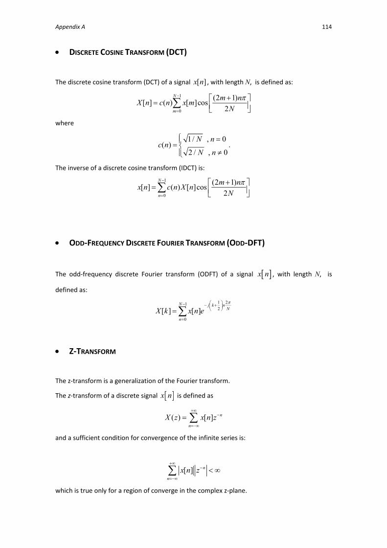
Appendix A 114
• DISCRETE COSINE TRANSFORM (DCT)
The discrete cosine transform (DCT) of a signal [ ]x n , with length N, is defined as:
1
0
(2 1)[ ] ( ) [ ]cos
2
π−
=
+ = ∑N
m
m nX n c n x m
N
where
1/ , 0( )
2 / , 0
N nc n
N n
==
≠.
The inverse of a discrete cosine transform (IDCT) is:
1
0
(2 1)[ ] ( ) [ ]cos
2
π−
=
+ = ∑N
n
m nx n c n X n
N
• ODD-FREQUENCY DISCRETE FOURIER TRANSFORM (ODD-DFT)
The odd-frequency discrete Fourier transform (ODFT) of a signal [ ]x n , with length N, is
defined as:
1 212
0
[ ] [ ]
π − − +
=
=∑N j k n
N
n
X k x n e
• Z-TRANSFORM
The z-transform is a generalization of the Fourier transform.
The z-transform of a discrete signal [ ]x n is defined as
( ) [ ] n
n
X z x n z+∞
−
=−∞
= ∑
and a sufficient condition for convergence of the infinite series is:
[ ] n
n
x n z+∞
−
=−∞
< ∞∑
which is true only for a region of converge in the complex z-plane.

Appendix A 115
The inverse z-transform is defined as:
[ ] 11( )
2
nx n X z z dzjπ
−= ∫
where the contour integral is evaluated on a closed contour, within the region of convergence
for z and enclosing the origin.
• ZEROS OF THE Z-TRANSFORM
For a serie of N samples ( )(0), (1), ..., ( 1)x x x N − taken from a discrete time signal ( )x n , the
zeros of z-transform (ZZT) representation is defined as set of roots (zeros), ( )1 2 1, , ..., NZ Z Z − of
the corresponding z-transform polynomial ( )X z :
( ) ( )11
1
0 1
( ) (0)NN
n N
n m
X z x n z x z z Zm−−
− − +
= =
= = −∑ ∏
considering that (0)x is non-zero.
Figure A1 shows an example of a ZZT representation of a signal.
Figure A.1. ZZT representation of a signal in (a) cartesian coordinates and
(b) polar coordinates [BDA+05].
Adapted from [Ort05], [HAH01], [Gol00] and [Boz05].

Appendix B 116
APPENDIX B – DATA ANALYSIS
Table B. 1. Spectral decay of the source harmonics, in dB/octave, Average (AVG) and Standard
Deviation (STDev), as a function of vowel per subject.
Subject Speech file Vowel Spectral decay AVG STDev
AF
AF_1_a_d /a/ -10,14 -8,80 1,89
AF_2_a_d /a/ -7,46
AF_1_i_d /i/ -16,43 -16,90 0,66
AF_2_i_d /i/ -17,36
RT
RT_1_a_d /a/ -12,03 -12,27 0,35
RT_2_a_d /a/ -12,52
RT_1_i_d /i/ -12,02 -12,99 1,38
RT_2_i_d /i/ -13,96
PP
PP_1_a_d /a/ -4,99 -7,86 4,05
PP_2_a_d /a/ -10,72
PP_1_i_d /i/ -11,41 -11,31 0,14
PP_2_i_d /i/ -11,21
SD
SD_1_a_d /a/ -5,20 -6,06 1,23
SD_2_a_d /a/ -6,93
SD_1_i_d /i/ -15,00 -14,44 0,79
SD_2_i_d /i/ -13,88
SF
SF_1_a_d /a/ -7,63 -11,94 6,10
SF_2_a_d /a/ -16,25
SF_1_i_d /i/ -15,12 -15,44 0,46
SF_2_i_d /i/ -15,76
CK
CK_1_a_d /a/ -12,55 -11,79 1,08
CK_2_a_d /a/ -11,03
CK_1_i_d /i/ -10,82 -11,13 0,43
CK_2_i_d /i/ -11,43

Appendix B 117
Table B.2. Linear Regression Models of the unwrapped NRDs of the time-aligned acoustics signals.
Subject Speech
file Vowel
Linear Regression Models
Signal “Inside” Signal “Outside”
AF
AF_1_a /a/ 0,2238 0,0534y x= − 0,1825 0,1595y x= +
AF_2_a /a/ 0,1883 0,4167y x= + 0,2381 0,0689y x= +
AF_1_i /i/ 0,0261 1,0575y x= − 0,1118 0,3822y x= − +
AF_2_i /i/ 0,01591 0,3962y x= − − 0,0521 0,3554y x= −
RT
RT_1_a /a/ 0,0305 1,3573y x= − + 0,0223 1,3314y x= +
RT_2_a /a/ 0,0600 0,7097y x= − 0,0192 0,6805y x= +
RT_1_i /i/ 0,0381 0,0803y x= − − 0,0078 0,8469y x= +
RT_2_i /i/ 0,0351 0,0207y x= + 0,0139 0,5292y x= +
PP
PP_1_a /a/ 0,1905 0,4204y x= + 0,2270 0,1061y x= +
PP_2_a /a/ 0,2316 0,07551y x= − 0,1915 0,1032y x= +
PP_1_i /i/ 0,1613 0,1656y x= + 0,1290 0,6859y x= +
PP_2_i /i/ 0,1694 0,0585y x= + 0,1802 0,7163y x= −
SD
SD_1_a /a/ 0,1734 0,0358y x= − 0,1445 0,0644y x= +
SD_2_a /a/ 0,1935 0,0076y x= + 0,1707 0,0782y x= +
SD_1_i /i/ 0,1885 0,3764y x= − 0,0545 0,1660y x= +
SD_2_i /i/ 0,1160 1,6171y x= − 0,0624 0,1611y x= −
SF
SF_1_a /a/ 0,1349 0,0432y x= − 0,0863 0,4515y x= +
SF_2_a /a/ 0,0730 0,2096y x= − 0,0345 0,6166y x= +
SF_1_i /i/ 0,0780 0,4522y x= + 0,0196 0,1176y x= −
SF_2_i /i/ 0,1331 0,0207y x= − 0,0217 0,2003y x= −
CK
CK_1_a /a/ 0,0560 1,0618y x= + 0,0054 1,4035y x= − +
CK_2_a /a/ 0,1558 0,0139y x= − 0,1030 0,2788y x= +
CK_1_i /i/ 0,0981 0,2047y x= − 0,1638 0,2437y x= −
CK_2_i /i/ 0,0253 0,8328y x= − + 0,0722 0,4273y x= +

BIBLIOGRAPHY
[Air08a] Matti Airas. TKK Aparat: An environment for voice inverse filtering and
parameterization. Logopedics Phoniatrics Vocology, 33(1), pp. 49-64, 2008.
[Air08b] Matti Airas. Methods and Studies of Laryngeal Voice Quality Analysis in Speech
Production. PhD thesis, Helsinki University of Techonolgy, Finland, 2008.
[Alk92] Paavo Alku. Glottal wave analysis with pitch synchronous iterative adaptive
inverse filtering. Speech Communication 11, pp. 109-118, 1992.
[AVV02] Paavo Alku, Juha Vinturri, and Erkki Vilkman. Measuring the effect of
fundamental frequency raising as a strategy for increasing vocal intensity in
soft, normal and loud phonation. Speech Communication 38, pp. 321-334, 2002.
[APB+05] M. Airas, H. Pulakka, T. Backström, and P. Alku. A Toolkit for Voice Inverse
Filtering and Parameterization. INTERSPEECH 2005, pp. 2145-2148, September
4-8, Lisbon, 2005.
[BDA+05] Baris Bozkurt, B. Doval, C. d’Alessandro, and T. Dutoit. Zeros of Z-Transform
representation with application to source-filter separation in speech. IEEE Signal
Processing Letters, vol. 12, nº 4, pp. 344-347, 2005.
[Boz05] Baris Bozkurt. Zeros of the z-transform (ZZT) representation and chirp group
delay processing for the analysis of source and filter characteristics of speech
signals. PhD thesis, Faculté Polytechinique de Mons, Belgium, 2005.
[BNG06] Mike Brookes, Patrick A. Naylor, and Jon Gudnason. A Quantitative Assessment
of Group Delay Methodsfor Identifying Glottal Closures in Voiced Speech. IEEE
Transactions on Speech and Audio Processing, vol.14, nº2, 2006.
[Cua07] Carlos Cuadros. Reconhecimento de voz e de locutor em ambientes ruidosos:
comparação das técnicas MFCC e ZPCA. Tese de Mestrado, Escola de
Engenharia da Universidade Federal Fluminense, Brasil, 2007.
[Cin08] Alan Ó Cinnéide. PhD Transfer Report. Institute of Technology, Dublin, March
2008.
[CL09] Shi-Huang Chen and Yu-Ren Luo. Speaker Verification Using MFCC and Support
Vector Machine. IMECS 2009, March 18 - 20, Hong Kong, 2009.
[CRR+07] J. Cabral, S. Renals, K. Richmond, and J. Yamagishi. Towards an Improved
Modelling of the Glottal Source in Statistical Parametric Speech Synthesis. ISCA
SSW6, 2007.
[DA99] Boris Doval and Cristophe d’Alessandro. The spectrum of glottal flow models.

Bibliography 119
Notes et documents LIMSI 99-07, 1999.
[DAH03] Boris Doval, Cristophe d’Alessandro, and Nathalie Henrich. The voice source as a
causal/anticausal linear filter. ISCA (VOQUAL), pp. 16-20, 2003.
[DBD09] Thomas Drugman, Baris Bozkurt, and Thierry Dutoit. Complex Cepstrum-based
Decomposition of Speech for Glottal Source Estimation. Interspeech, pp. 116-
119, 2009.
[Deg10] Gilles Degottex. Glottal source and vocal-tract separation. Estimation of glottal
parameters, voice transformation and synthesis using a glottal model. PhD
thesis, Université Paris, France, 2010.
[DDM+08] Thomas Drugman, Thomas Dubuisson et al. Glottal source estimation
robustness. A comparison of sensitivity of voice source estimation techniques. In
Proceedings of SIGMAP'2008, pp. 202-207, 2008.
[Dru11] Thomas Drugman. Advances in Glottal Analysis and its Apllications. PhD thesis,
Université Paris, France, 2010. University of Mons, Belgium, 2011.
[DSF11] Sandra Dias, Ricardo Sousa and Aníbal Ferreira. Glottal inverse filtering: a new
road-map and first results. AFEKA: Speech Processing Conference, Israel, June
2011.
[Fan60] Gunnar Fant. Acoustic Theory of Speech Production. Mouton, The Hague, 1960.
[Fan79] Gunnar Fant. Vocal-source analysis – a progress report. STL-QPSR, 20 (3-4): pp.
31-53, 1979.
[Fan95] Gunnar Fant. The LF-model revisited. Transformations and frequency analysis.
STL-QPSR, 36 (2-3): pp. 119-156, 1995.
[Fer01] Aníbal J. S. Ferreira. Combined Spectral envelope normalization and subtraction
of sinusoidal components in the ODFT and MDCT frequency domains. IEEE
Workshop on Applications of Signal Processing to Audio and Acoustics, pp. 51-
54, 2001.
[FS05] Aníbal Ferreira and Deepen Sinha. Accurate and robust frequency estimation in
the ODFT domain. IEEE Workshop on Applications of Signal Processing to Audio
and Acoustics, pp. 203-205, October 2005.
[FLL85] Gunnar Fant, Johan Liljencrants, and Qi-guaq Lin. A four parameter model of
glottal flow. STL-QPSR, 4, pp. 1-13, 1985.
[GA05] Isabel Guimarães and Evelyn Abberton. Fundamental frequency in speakers of
Portuguese for different voice samples. Journal of Voice, December, 2005.
[Gol00] Randy Goldberg. A pratical handbook of Speech Coders. CRC Press LLC, 2000.

Bibliography 120
[Gui08] Vinicius F. Guimarães. Estabilização de imagens para laringoscopia. Dissertação
de Mestrado, Instituto de Química de São Carlos da Universidade de São Paulo,
Brasil, 2008.
[Hen09] Luís Henrique. Acústica musical – 3ª edição. Fundação Calouste Gulbenkian,
Lisboa, 2009.
[Hen01] Nathalie Henrich. Etude de la source glottique en voix parlée et chantée:
modélisation et estimation, mesures acoustiques et électroglottographiques,
perception. PhD these, Université Paris, France, 2001.
[HAH01] Xuedong Huang, Alex Acero, and Hsiao-Wuen Hon. Spoken Language
Processing: a guide to theory, algorithm, and system development. Prentice-
Hall, New Jersey, 2001.
[HSA+03] N. Henrich, G. Sundin, D. Ambroise, et al. Just Noticeable Differences of Open
Quotient and Asymmetry Coefficient in Singing Voice. Journal of Voice, Vol. 17,
No. 4, pp. 481–494, 2003.
[JBM87] Hector Raul Javkin, Norma Antõnanzas-Barroso, and Ian Maddieson. Digital
Inverse Filtering for Linguistic Research. Journal of Speech and Hearing Research
30, pp. 122-129, 1987.
[JVL95] C. R. Jankowski, H. D. H. Vo, and R. P. Lippmann. A comparison of signal
processing front ends for automatic word recognition. IEEE Transactions on
Speech and Audio Processing, 4(3), pp. 251–266, 1995.
[JM91] A. El-Jaroudi and J. Makhoul. Discrete All-Pole Modelling. IEEE Transactions on
Signal Processing, 39(2), pp. 411-423, February 1991.
[Kaf08] George P. kafentzis. On the glottal flow derivative wavefom and its properties.
Bachelor’s Dissertation, University of Crete, Greece, 2008.
[Kaf10] George P. kafentzis. On the inverse filtering of speech. MsC thesis, University of
Crete, Greece, 2010.
[Ken04] Raymond D. Kent. The MIT Encyclopedia of Communication Disorders. The MIT
Press, Cambridge, 2004.
[KK90] Dennis Klatt and Laura Klatt. Analysis, synthesis, and perception of voice quality
variations among female and male talkers. Journal of the Acoustical Society of
America, 87, pp. 820-857, 1990.
[KG00] Kenneth C. Jones e Anthony J. Gaudin. Introdução à Biologia – 3ª edição.
Fundação Calouste Gulbenkian, Lisboa, 2000.
[KGB06] Jody Kreiman, Bruce R. Gerrat, and Norma Antõnanzas-Barroso. Analysis and

Bibliography 121
Synthesis of Pathological Voice Quality. Bureau of Glottal Affairs, LA, USA, 2006.
[Kob02] Malte Kob. Physical Modelling of the Singing Voice. PhD thesis, Technical
University Aachen, Germany, 2002.
[Lev05] Stephen E. Levinson. Mathematical Models for Speech Technology. John Wiley
& Sons, Ltd, England, 2005.
[Mag05] Carlo Magi. All-Pole Modelling of Speech: Mathematical Analysis Combined with
Objective and Subjective Evaluation of Seven Selected Methods. MsC thesis,
Helsinki University of Techonolgy, Finland, 2005.
[Mil01] Paul Milenkovic. TF32 User’s Manual. Madison, Milenkovic, 2001.
[Mur08] Katharine Murphy. Digital signal processing techniques for application in the
analysis of pathological voice and normophonic singing voice. PhD thesis,
Universidad Politécnica de Madrid, Spain, 2008.
[MY11] Hema A. Murthy and B. Yegnanarayana. Group delay functions and its
applications in speech technology. Indian Academy of Sciences, Vol. 36, Part 5,
pp. 745–782, October, 2011.
[Ort05] Manuel D. Ortigueira. Processamento Digital de Sinais. Fundação Calouste
Gulbenkian, 2005.
[Per09] Fernando Pereira. Comunicações Audiovisuais: Tecnologias, Normas e
Aplicações. Instituto Superior Técnico, Lisboa, 2009.
[Pul05] Hannu Pulakka. Analysis of Human Voice Production Using Inverse Filtering,
High-Speed Imaging, and Electroglottography. MsC thesis, Helsinki University of
Technology, Finland, 2005.
[SAD07] N. Sturmel, C. d’Alessandro and B. Doval. Comparative evaluation of the ZZT
and inverse filtering for voice source analysis. Scientific Report, 2007 (in
http://rs2007.limsi.fr/index.php/PS:Page_4, accessed 2011).
[San09] Ricardo Jorge Ferreira dos Santos. Avaliação de Pacientes com Paralisia
Unilateral das Pregas Vocais. Tese de Mestrado, Universidade de Aveiro,
Portugal, 2009.
[SF10] Ricardo Sousa and Aníbal Ferreira. Importance of the relative delay of glottal
source harmonics. AES 39th International Conference, Denmark, June, 2010.
[SF11] Ricardo Sousa and Aníbal Ferreira. Singing Voice Analysis Using Relative
Harmonic Delays. Interspeech, pp. 1997-2000, 2011.
[Sou11] Ricardo Sousa. Metodologias de Avaliação Percetiva e Acústica do Sinal de Voz
em Aplicações de Ensino do Canto e Diagnóstico/Reabilitação da Fala. Tese de
Bibliography 122
Doutoramento, FEUP, Portugal, 2011.
[She09] Christina Shewell. Voice Work: Art and Science in Changing Voices. Wiley-
Blackwell, 2009.
[Sun77] Johan Sundberg. The acoustics of the singing voice. Scientific American, 236(3),
p. 82-100, March, 1977.
[Sun87] Johan Sundberg. The science of singing voice. Northern Illinois University Press.
Dekalb, Illinois, 1987.
[Tiz94] I. Titze. Workshop on Acoustic Voice Analysis: Summary Statement. Iowa City,
IA: National Center for Voice and Speech, 1994.
[Vel98] Raymond Veldhuis. A computationally efficient alternative for the LF model and
its perceptual evaluation. Journal of Acoustical Society of America, 103, pp. 566-
571, 1998.
[WB87] Neil Weir and Isobel Bassett. Outpatient fibreoptic nasolaryngoscopy and
videostroboscopy. Journal of the Royal Society of Medicine, vol. 80, p. 299-300,
1987.
[WM05] Jacqueline Walker and Peter Murphy. Advanced Methods for Glottal Wave
Extraction. NOLISP 2005, LNAI 3817, pp. 139-149, Springer – Verlag, Berlin,
2005.
[WM07] Jacqueline Walker and Peter Murphy. A Review of Glottal Waveform Analysis.
WNSP 2005, LNCS 4391, pp. 1-21, Springer – Verlag, Berlin, 2007.