IEEE TRANSACTIONS ON BIOMEDICAL ENGINEERING, VOL. 45, NO. 1, JANUARY 1998 133

TABLE ICOMPARISON OF BSLM’ S WITH AND WITHOUT THE LUNGS

(a) (b)

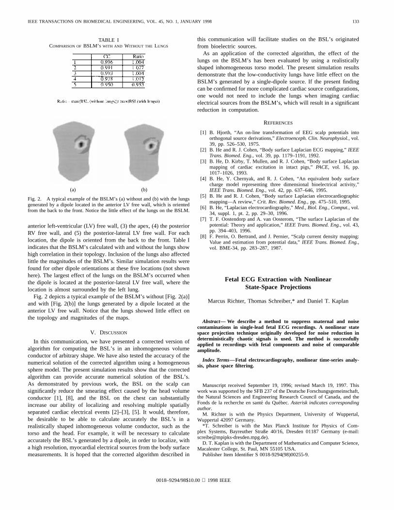
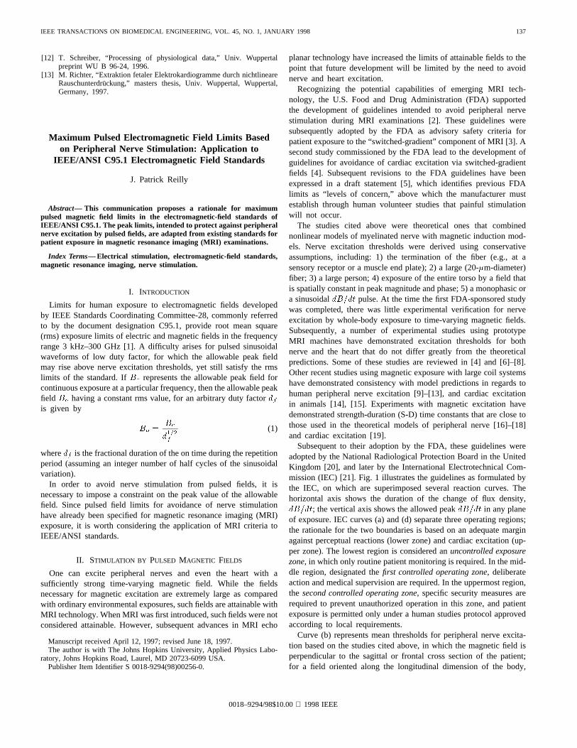
Fig. 2. A typical example of the BSLM’s (a) without and (b) with the lungsgenerated by a dipole located in the anterior LV free wall, which is orientedfrom the back to the front. Notice the little effect of the lungs on the BSLM.

anterior left-ventricular (LV) free wall, (3) the apex, (4) the posteriorRV free wall, and (5) the posterior-lateral LV free wall. For eachlocation, the dipole is oriented from the back to the front. Table Iindicates that the BSLM’s calculated with and without the lungs showhigh correlation in their topology. Inclusion of the lungs also affectedlittle the magnitudes of the BSLM’s. Similar simulation results werefound for other dipole orientations at these five locations (not shownhere). The largest effect of the lungs on the BSLM’s occurred whenthe dipole is located at the posterior-lateral LV free wall, where thelocation is almost surrounded by the left lung.

Fig. 2 depicts a typical example of the BSLM’s without [Fig. 2(a)]and with [Fig. 2(b)] the lungs generated by a dipole located at theanterior LV free wall. Notice that the lungs showed little effect onthe topology and magnitudes of the maps.

V. DISCUSSION

In this communication, we have presented a corrected version ofalgorithm for computing the BSL’s in an inhomogeneous volumeconductor of arbitrary shape. We have also tested the accuracy of thenumerical solution of the corrected algorithm using a homogeneoussphere model. The present simulation results show that the correctedalgorithm can provide accurate numerical solution of the BSL’s.As demonstrated by previous work, the BSL on the scalp cansignificantly reduce the smearing effect caused by the head volumeconductor [1], [8], and the BSL on the chest can substantiallyincrease our ability of localizing and resolving multiple spatiallyseparated cardiac electrical events [2]–[3], [5]. It would, therefore,be desirable to be able to calculate accurately the BSL’s in arealistically shaped inhomogeneous volume conductor, such as thetorso and the head. For example, it will be necessary to calculateaccurately the BSL’s generated by a dipole, in order to localize, witha high resolution, myocardial electrical sources from the body surfacemeasurements. It is hoped that the corrected algorithm described in

this communication will facilitate studies on the BSL’s originatedfrom bioelectric sources.

As an application of the corrected algorithm, the effect of thelungs on the BSLM’s has been evaluated by using a realisticallyshaped inhomogeneous torso model. The present simulation resultsdemonstrate that the low-conductivity lungs have little effect on theBSLM’s generated by a single-dipole source. If the present findingcan be confirmed for more complicated cardiac source configurations,one would not need to include the lungs when imaging cardiacelectrical sources from the BSLM’s, which will result in a significantreduction in computation.

REFERENCES

[1] B. Hjorth, “An on-line transformation of EEG scalp potentials intoorthogonal source derivations,”Electroenceph. Clin. Neurophysiol., vol.39, pp. 526–530, 1975.

[2] B. He and R. J. Cohen, “Body surface Laplacian ECG mapping,”IEEETrans. Biomed. Eng., vol. 39, pp. 1179–1191, 1992.

[3] B. He, D. Kirby, T. Mullen, and R. J. Cohen, “Body surface Laplacianmapping of cardiac excitation in intact pigs,”PACE, vol. 16, pp.1017–1026, 1993.

[4] B. He, Y. Chernyak, and R. J. Cohen, “An equivalent body surfacecharge model representing three dimensional bioelectrical activity,”IEEE Trans. Biomed. Eng., vol. 42, pp. 637–646, 1995.

[5] B. He and R. J. Cohen, “Body surface Laplacian electrocardiographicmapping—A review,”Crit. Rev. Biomed. Eng., pp. 475–510, 1995.

[6] B. He, “Laplacian electrocardiography,”Med., Biol. Eng., Comput., vol.34, suppl. 1, pt. 2, pp. 29–30, 1996.

[7] T. F. Oostendorp and A. van Oosterom, “The surface Laplacian of thepotential: Theory and application,”IEEE Trans. Biomed. Eng., vol. 43,pp. 394–403, 1996.

[8] F. Perrin, O. Bertrand, and J. Pernier, “Scalp current density mapping:Value and estimation from potential data,”IEEE Trans. Biomed. Eng.,vol. BME-34, pp. 283–287, 1987.

Fetal ECG Extraction with NonlinearState-Space Projections

Marcus Richter, Thomas Schreiber,* and Daniel T. Kaplan

Abstract—We describe a method to suppress maternal and noisecontaminations in single-lead fetal ECG recordings. A nonlinear statespace projection technique originally developed for noise reduction indeterministically chaotic signals is used. The method is successfullyapplied to recordings with fetal components and noise of comparableamplitude.

Index Terms—Fetal electrocardiography, nonlinear time-series analy-sis, phase space filtering.

Manuscript received September 19, 1996; revised March 19, 1997. Thiswork was supported by the SFB 237 of the Deutsche Forschungsgemeinschaft,the Natural Sciences and Engineering Research Council of Canada, and theFonds de la recherche en sante du Quebec.Asterisk indicates correspondingauthor.

M. Richter is with the Physics Department, University of Wuppertal,Wuppertal 42097 Germany.

*T. Schreiber is with the Max Planck Institute for Physics of Com-plex Systems, Bayreuther Straße 40/16, Dresden 01187 Germany (e-mail:screibe@mpipks-dresden.mpg.de).

D. T. Kaplan is with the Department of Mathematics and Computer Science,Macalester College, St. Paul, MN 55105 USA.

Publisher Item Identifier S 0018-9294(98)00255-9.

0018–9294/98$10.00 1998 IEEE

134 IEEE TRANSACTIONS ON BIOMEDICAL ENGINEERING, VOL. 45, NO. 1, JANUARY 1998

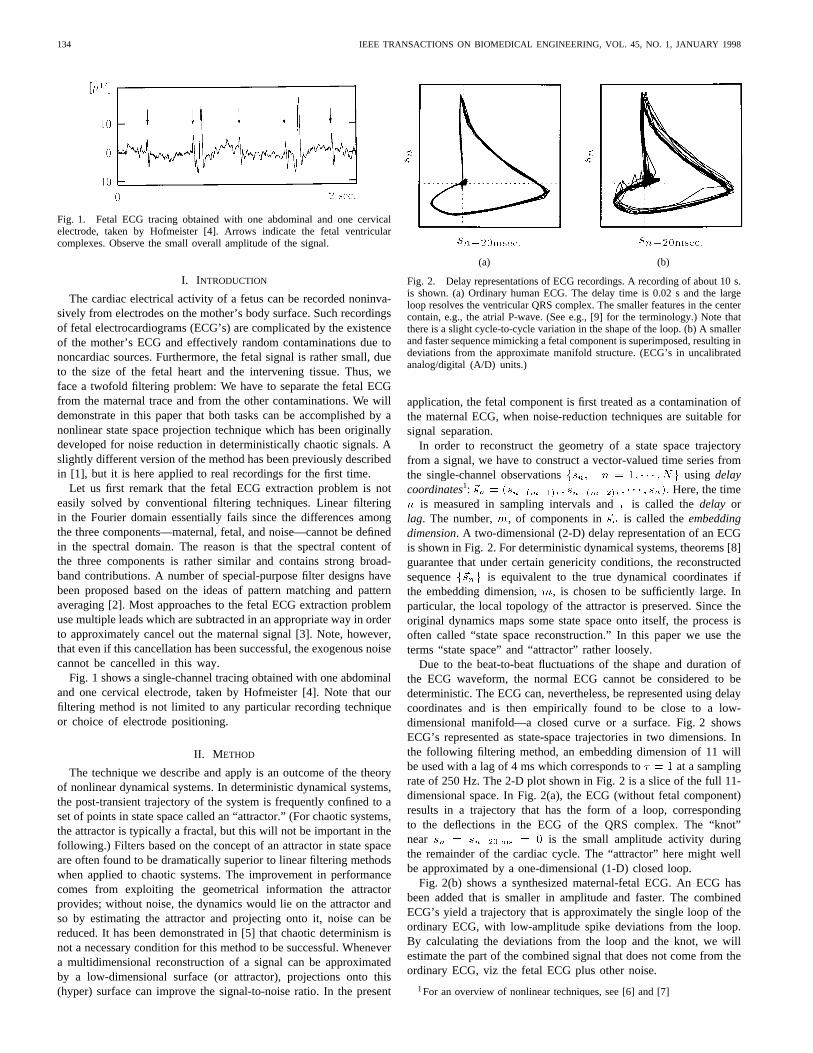
Fig. 1. Fetal ECG tracing obtained with one abdominal and one cervicalelectrode, taken by Hofmeister [4]. Arrows indicate the fetal ventricularcomplexes. Observe the small overall amplitude of the signal.

I. INTRODUCTION

The cardiac electrical activity of a fetus can be recorded noninva-sively from electrodes on the mother’s body surface. Such recordingsof fetal electrocardiograms (ECG’s) are complicated by the existenceof the mother’s ECG and effectively random contaminations due tononcardiac sources. Furthermore, the fetal signal is rather small, dueto the size of the fetal heart and the intervening tissue. Thus, weface a twofold filtering problem: We have to separate the fetal ECGfrom the maternal trace and from the other contaminations. We willdemonstrate in this paper that both tasks can be accomplished by anonlinear state space projection technique which has been originallydeveloped for noise reduction in deterministically chaotic signals. Aslightly different version of the method has been previously describedin [1], but it is here applied to real recordings for the first time.

Let us first remark that the fetal ECG extraction problem is noteasily solved by conventional filtering techniques. Linear filteringin the Fourier domain essentially fails since the differences amongthe three components—maternal, fetal, and noise—cannot be definedin the spectral domain. The reason is that the spectral content ofthe three components is rather similar and contains strong broad-band contributions. A number of special-purpose filter designs havebeen proposed based on the ideas of pattern matching and patternaveraging [2]. Most approaches to the fetal ECG extraction problemuse multiple leads which are subtracted in an appropriate way in orderto approximately cancel out the maternal signal [3]. Note, however,that even if this cancellation has been successful, the exogenous noisecannot be cancelled in this way.

Fig. 1 shows a single-channel tracing obtained with one abdominaland one cervical electrode, taken by Hofmeister [4]. Note that ourfiltering method is not limited to any particular recording techniqueor choice of electrode positioning.

II. M ETHOD

The technique we describe and apply is an outcome of the theoryof nonlinear dynamical systems. In deterministic dynamical systems,the post-transient trajectory of the system is frequently confined to aset of points in state space called an “attractor.” (For chaotic systems,the attractor is typically a fractal, but this will not be important in thefollowing.) Filters based on the concept of an attractor in state spaceare often found to be dramatically superior to linear filtering methodswhen applied to chaotic systems. The improvement in performancecomes from exploiting the geometrical information the attractorprovides; without noise, the dynamics would lie on the attractor andso by estimating the attractor and projecting onto it, noise can bereduced. It has been demonstrated in [5] that chaotic determinism isnot a necessary condition for this method to be successful. Whenevera multidimensional reconstruction of a signal can be approximatedby a low-dimensional surface (or attractor), projections onto this(hyper) surface can improve the signal-to-noise ratio. In the present

(a) (b)

Fig. 2. Delay representations of ECG recordings. A recording of about 10 s.is shown. (a) Ordinary human ECG. The delay time is 0.02 s and the largeloop resolves the ventricular QRS complex. The smaller features in the centercontain, e.g., the atrial P-wave. (See e.g., [9] for the terminology.) Note thatthere is a slight cycle-to-cycle variation in the shape of the loop. (b) A smallerand faster sequence mimicking a fetal component is superimposed, resulting indeviations from the approximate manifold structure. (ECG’s in uncalibratedanalog/digital (A/D) units.)

application, the fetal component is first treated as a contamination ofthe maternal ECG, when noise-reduction techniques are suitable forsignal separation.

In order to reconstruct the geometry of a state space trajectoryfrom a signal, we have to construct a vector-valued time series fromthe single-channel observationsfsn; n = 1; � � � ; Ng using delaycoordinates1: ~sn = (s

n�(m�1)� ; sn�(m�2)� ; � � � ; sn): Here, the timen is measured in sampling intervals and� is called thedelay orlag. The number,m, of components in~sn is called theembeddingdimension. A two-dimensional (2-D) delay representation of an ECGis shown in Fig. 2. For deterministic dynamical systems, theorems [8]guarantee that under certain genericity conditions, the reconstructedsequencef~sng is equivalent to the true dynamical coordinates ifthe embedding dimension,m, is chosen to be sufficiently large. Inparticular, the local topology of the attractor is preserved. Since theoriginal dynamics maps some state space onto itself, the process isoften called “state space reconstruction.” In this paper we use theterms “state space” and “attractor” rather loosely.

Due to the beat-to-beat fluctuations of the shape and duration ofthe ECG waveform, the normal ECG cannot be considered to bedeterministic. The ECG can, nevertheless, be represented using delaycoordinates and is then empirically found to be close to a low-dimensional manifold—a closed curve or a surface. Fig. 2 showsECG’s represented as state-space trajectories in two dimensions. Inthe following filtering method, an embedding dimension of 11 willbe used with a lag of 4 ms which corresponds to� = 1 at a samplingrate of 250 Hz. The 2-D plot shown in Fig. 2 is a slice of the full 11-dimensional space. In Fig. 2(a), the ECG (without fetal component)results in a trajectory that has the form of a loop, correspondingto the deflections in the ECG of the QRS complex. The “knot”near sn = sn�20 ms = 0 is the small amplitude activity duringthe remainder of the cardiac cycle. The “attractor” here might wellbe approximated by a one-dimensional (1-D) closed loop.

Fig. 2(b) shows a synthesized maternal-fetal ECG. An ECG hasbeen added that is smaller in amplitude and faster. The combinedECG’s yield a trajectory that is approximately the single loop of theordinary ECG, with low-amplitude spike deviations from the loop.By calculating the deviations from the loop and the knot, we willestimate the part of the combined signal that does not come from theordinary ECG, viz the fetal ECG plus other noise.

1For an overview of nonlinear techniques, see [6] and [7]

IEEE TRANSACTIONS ON BIOMEDICAL ENGINEERING, VOL. 45, NO. 1, JANUARY 1998 135

The noise reduction algorithm consists of three main steps.

1) Find a low-dimensional approximation to the “attractor” de-scribed by the trajectoryf~sng:

2) Project each point~sn in the trajectory orthogonally onto theapproximation to the attractor to produce a cleaned vector~sn

3) Convert the sequence of cleaned vectors~sn back into the scalartime domain to produce a cleaned time seriessn:

The algorithm was originally proposed in [10] and adapted to theECG case in [5]. See [11] for a review on nonlinear noise reductionfor chaotic time series. A technical description of the algorithm isfound in the [5] and [10]. A simpler, but equivalent, formulation isgiven in [12].

We approximate the “attractor” as a collection of locally linearmanifolds. For example, in Fig. 2, the loop can be approximated asa collection of short line segments; in this case the approximatingmanifold is 1-D. When the embedding dimensionm is larger thantwo, it can be appropriate to select locally linear manifolds withdimensionQ where 1 � Q<m: For Q = 2, for instance, themanifolds are locally planar.

To construct the manifold approximating the “attractor” near agiven point~sn, the following procedure is used.

1) Find all of the points that are within a distance� of ~sn inthe delay space. This set of nearby points is denotedU(n) =

f~sk: k~sk � ~snk<�g where k~sk � ~snk is the (max norm)distance between~sk and~sn:

2) Compute the local center of massh~si(n) = jU (n)j�1

�~s 2U~sn , where jU (n)j is the number of vectors in

U(n) and�~s 2Umeans summation over those vectors.

3) Compute the local weighted covariance matrix

C(n)

ij =

~s 2U

RRR ~sn � h~si(n)iRRR(~sn � h~si(n))

j

where[�]i denotes theith component of the vector in brackets.As discussed in [10], the weight matrixRRR is chosen to bediagonal withR11 andRmm large and all other diagonal entriesRii = 1:

4) Determine the orthonormal eigenvectors~cq and eigenvalues ofC(n)

ij using standard matrix techniques.2

5) A Q-dimensional manifold is then locally approximated bythoseQ eigenvectors with the largest eigenvalues. The pro-jected vector~sn is then given by

~sn = ~sn �RRR�1

Q

q=1

~cq~cq �RRR ~sn � h~si(n) :

In order to translatef~sng back into a scalar signal, we note that eachscalar measurementsn appears as a component inm embeddingvectors,~sn; � � � ; ~sn+m�1: The corrected scalar time-series valuessn are, thus, obtained by averaging the corresponding componentsof ~sn; � � � ; ~sn+m�1: This procedure may be seen as a local andanisotropic version of principal component projection.

After fixing � , the algorithm requires the choice of three importantparameters: the time(m � 1)� covered by a single delay vector~sn; the dimension of the local manifold projected on; the diameterof the neighborhoods used to form the linear approximations. Theneighborhood size determines a length scale in state space. We willuse these parameters to select the desired and undesired parts of therecording.

2The eigenvectors ofC(n)= A(n) � A(n)T can be computed in a

numerically more reliable way from the singular value decomposition ofA(n):

In order to limit the computational effort (A(n) has as many columns as thereare points inU(n)), we resort to standard matrix techniques.

Fig. 3. Fetal ECG extraction demonstrated on a longer (5 s) segment ofa recording with abdominal and cervical electrodes. First line: originalrecording. Second line: maternal ECG after projective filtering. Third line:difference of the first two lines, that is, deviations from the mother ECGas detected by the state space projection technique. This sequence containsboth fetal and noise contributions. Last line: Noise is further suppressed toenhance the fetal component.

III. RESULTS

First, we carried out extensive trials [13] to determine good param-eter settings. By inspecting the results, we found that usually aboutten dimensions are sufficient to separate the signals. Additional lagsincrease the accuracy only marginally, but increase the computationaleffort. We setm = 11: As suggested by Fig. 2, one can interpretthe phase space reconstruction of the ECG as a perturbed limitcycle which corresponds to a 2-D object. Therefore, we setQ = 2

to select the signal by the two largest components. Other choices(1 � Q � 4) gave slightly inferior results. Since we use the maxnorm to measure distances, the diameter of the neighborhoods� candirectly be obtained by visual inspection of the time series for therelevant length scales.

In the examples in Figs. 3 and 4, in the first filtering step thediameter of the neighborhoods is chosen to be 10�V which is largeenough in order to cover both the fetal signal and the noise. Thedifference between the input and the output of this filter containsfetal and noise disturbances of the maternal ECG. A second filter,for cleaning the extracted fetal ECG, is constructed with smallerneighborhoods of diameter 3�V. To improve the efficiency of thefilter, 60-Hz contaminations were removed by a notch filter and a low-frequency baseline drift was eliminated by using a 0.5-Hz highpassfilter. In general, systematic low-frequency fluctuations of the baselinecan hamper the effectiveness of the method, since points get spreadout in the reconstructed phase space. In the worst case, only veryfew neighbors would be identified and a reliable correction wouldbe impossible.

The signal-separation scheme adopted in this work differs some-what from that proposed in [5]. There, the filter was applied twiceto the measured sequence—once to select all contaminations with re-spect to the maternal signal and once to select the noise only—leavingthe sum of the maternal and fetal ECG’s. The difference of the twooutputs was taken as an estimate of the fetal signal. The recordingsavailable for the present study contain a noise contribution whichis at least comparable in root mean square (rms) amplitude to thefetal signal.3 Thus, the exclusive selection of the noise from the

3Most of the variance of the fetal signal is contained in the spike like QRScomplexes. Therefore in an ECG contaminated by a noise level of 100% (inthe rms sense) the spikes can still be identified by visual inspection.

136 IEEE TRANSACTIONS ON BIOMEDICAL ENGINEERING, VOL. 45, NO. 1, JANUARY 1998

Fig. 4. Result of the same procedure in a more difficult situation. The mater-nal and fetal heart rates are almost commensurate. Thus about every secondfetal beat coincides with the maternal QRS complex. In the reconstructedfetal ECG, the fetal spikes can still be seen, so that the heart rate can bedetermined reliably.

full recording is rather difficult. It proved to be a much more stableprocedure to first extract all contaminations from the maternal trace,and then subject the output—containing fetus and noise—to a secondsweep of the projective filter.

Since the local neighborhoods are set large enough to containthe peak-to-peak amplitude of the fetal ECG, the fetal componentis not recognized as part of the manifold structure, and, therefore,removed by the projections. This removed part of the sequence is,thus, identified to contain both fetal and noise contributions. It hasto be further cleaned. This can be done with the same state spaceprojection filtering approach; the parameters are now adjusted inorder to treat the fetal component as the signal and only the randomfluctuations as noise.

In principle, the formation of state space neighborhoods for eachdata point is quite computer-time intensive; the computation increasesas the square of the signal length. Since the neighborhoods arenot very small, fast neighbor-search algorithms do not help much.However, we do not needall available neighbors in order to constructthe linear approximations to the manifold in state space. Thus, weare content once we have found 200 neighbors for each point. Theresulting algorithm allows the calculation of the fetal ECG in realtime on a Pentium computer with 133 MHz.

IV. DISCUSSION

Although we do not offer here a quantitative comparison to previ-ous methods, the power of the method is apparent from Figs. 3 and4. Since the method provides a general-purpose filtering techniquethat may be applicable to other problems, we believe that the methodwill be of general interest outside the domain of the fetal ECG andfor practical fetal-ECG monitoring.

One may conjecture that the performance could be increasedby using a global nonlinear approach to account for the cardiacdynamics. Using radial basis functions, multivariate polynomials,and neural networks we found [13], however, that the deterministicapproximation is too crude to yield a global function fit which isstable enough for signal separation. Not only is the resulting fetalsignal of much poorer quality than that obtained by using local linearprojections, the trajectory adjustment procedure also turns out to bemore time consuming.

Inspecting the fetal ECG’s shown in Figs. 3 and 4, we find thefetal QRS complex to be the only structure of the fetal ECG that wecan recover at this noise level. Systematic studies with synthesizedmaternal-fetal ECG’s at different noise levels suggest that the noiseis the only limiting factor for the estimation of clinically relevantparameters, like the P-Q interval, from abdominal recordings. In

the low-noise limit, all details like P- and T-waves are faithfullyrecovered. Further details can be found in [13].

The filter mechanism proposed here uses the fact that beat-to-beat variations of the shape of the maternal ECG waveform areapproximately captured by a few degrees of freedom. Anomalousbehavior of the heart, with nonsystematic fluctuations of the ECGcycle, potentially poses a problem for the algorithm. Since the signalsare not identified by their timing, extrasystoles should be handledproperly.

The different approaches that have been developed for extractingthe fetal ECG from a single lead [2] are all nonlinear, reflectingthe difficulty of distinguishing the maternal ECG, fetal ECG, andnoise in the frequency domain. What has been lacking is a generalscheme for specifying nonlinear filters, analogous to the frequencydomain description used for linear filters. From what we know aboutthe physiological differences between the fetal and maternal ECG,it is an attractive concept to discriminate between the fetal andmaternal components in terms of amplitude and time scale. Thenatural language to implement such filtering procedures is in terms ofthe geometry in a reconstructed state space. Here, we have estimatedthe geometry of the maternal ECG using projections onto locallylinear surfaces which proves effective at filtering the fetal ECG fromthe measured signal.

ACKNOWLEDGMENT

The authors would like to thank J. F. Hofmeister and P. Saparinfor providing ECG recordings. They would also like to thank P.Grassberger and H. Kantz for their stimulating discussions.

REFERENCES

[1] T. Schreiber and D. T. Kaplan, “Signal separation by nonlinear projec-tions: The fetal electrocardiogram,”Phys. Rev. E., vol. 53, p. R4326,1996.

[2] J. R. Mazzeo, “Noninvasive fetal electrocardiography,”Med. Prog.through Technol., vol. 20, pp. 75–79, 1994; S. Abboud, A. Alaluf, S.Einav, and D. Sadeh, “Real-time abdominal fetal ECG recording using ahardware correlator,”Comput. Biol., Med., vol. 22, pp. 325–335, 1995;Y. Tal and S. Akselrod, “A new method for fetal ECG detection,”Comput., Biomed. Res., vol. 24, pp. 296–306, 1991.

[3] E. Cicinelli, A. Bartone, I. Carbonara, G. Incampo, M. Bachicchio,G. Ventura, S. Montanaro, and G. Aloisio, “Improved equipment forabdominal fetal electrocardiogram recording: description and clinicalevaluation,” Int. J. Biol., Med. Comput., vol. 35, pp. 193–205, 1994;D. Callaertset al., “Description of a real time system to extract thefetal electrocardiogram,”Clin. Phys. Physiol. Meas., vol. 10, suppl. B,pp. 7–10, 1989; D. Callaerts, B. DeMoor, J. Vanderville, W. Sansen,“Comparison of SVD methods to extract the fetal electrocardiograms,”Med., Biol. Eng., Comput., vol. 28, pp. 217–224, 1990.

[4] J. F Hofmeister, J. C. Slocumb, L. M. Kottmann, J. B. Picchiottino, andD. G. Ellis, “A noninvasive method for recording the electrical activityof the human uterusin vivo,” Biomed. Instrum. Technol., p. 391, Sept.1994.

[5] T. Schreiber and D. T. Kaplan, “Nonlinear noise reduction for electro-cardiograms,”CHAOS, vol. 6, pp. 87–92, 1996.

[6] D. Kaplan and L. Glass,Understanding Nonlinear Dynamics. NewYork: Springer-Verlag, 1995.

[7] H. Kantz and T. Schreiber,Nonlinear Time Series Analysis. Cam-bridge, U.K.: Cambridge Univ. Press, 1997.

[8] T. Sauer, J. Yorke, and M. Casdagli, “Embedology,”J. Stat. Phys., vol.65, p. 579, 1991.

[9] A. L. Goldberger and E. Goldberger,Clinical Electrocardiography. St.Louis, MO: Mosby, 1977.

[10] P. Grassberger, R. Hegger, H. Kantz, C. Schaffrath, and T. Schreiber,“On noise reduction methods for chaotic data,”CHAOS, vol. 3, p. 127,1993.

[11] E. J. Kostelich and T. Schreiber, “Noise reduction in chaotic time-seriesdata: A survey of common methods,”Phys. Rev. E, vol. 48, p. 1752,1993.

IEEE TRANSACTIONS ON BIOMEDICAL ENGINEERING, VOL. 45, NO. 1, JANUARY 1998 137

[12] T. Schreiber, “Processing of physiological data,” Univ. Wuppertalpreprint WU B 96-24, 1996.

[13] M. Richter, “Extraktion fetaler Elektrokardiogramme durch nichtlineareRauschunterdruckung,” masters thesis, Univ. Wuppertal, Wuppertal,Germany, 1997.

Maximum Pulsed Electromagnetic Field Limits Basedon Peripheral Nerve Stimulation: Application to

IEEE/ANSI C95.1 Electromagnetic Field Standards

J. Patrick Reilly

Abstract—This communication proposes a rationale for maximumpulsed magnetic field limits in the electromagnetic-field standards ofIEEE/ANSI C95.1. The peak limits, intended to protect against peripheralnerve excitation by pulsed fields, are adapted from existing standards forpatient exposure in magnetic resonance imaging (MRI) examinations.

Index Terms—Electrical stimulation, electromagnetic-field standards,magnetic resonance imaging, nerve stimulation.

I. INTRODUCTION

Limits for human exposure to electromagnetic fields developedby IEEE Standards Coordinating Committee-28, commonly referredto by the document designation C95.1, provide root mean square(rms) exposure limits of electric and magnetic fields in the frequencyrange 3 kHz–300 GHz [1]. A difficulty arises for pulsed sinusoidalwaveforms of low duty factor, for which the allowable peak fieldmay rise above nerve excitation thresholds, yet still satisfy the rmslimits of the standard. IfBc represents the allowable peak field forcontinuous exposure at a particular frequency, then the allowable peakfield Bo having a constant rms value, for an arbitrary duty factordfis given by

Bo =Bc

d1=2f

(1)

wheredf is the fractional duration of the on time during the repetitionperiod (assuming an integer number of half cycles of the sinusoidalvariation).

In order to avoid nerve stimulation from pulsed fields, it isnecessary to impose a constraint on the peak value of the allowablefield. Since pulsed field limits for avoidance of nerve stimulationhave already been specified for magnetic resonance imaging (MRI)exposure, it is worth considering the application of MRI criteria toIEEE/ANSI standards.

II. STIMULATION BY PULSED MAGNETIC FIELDS

One can excite peripheral nerves and even the heart with asufficiently strong time-varying magnetic field. While the fieldsnecessary for magnetic excitation are extremely large as comparedwith ordinary environmental exposures, such fields are attainable withMRI technology. When MRI was first introduced, such fields were notconsidered attainable. However, subsequent advances in MRI echo

Manuscript received April 12, 1997; revised June 18, 1997.The author is with The Johns Hopkins University, Applied Physics Labo-

ratory, Johns Hopkins Road, Laurel, MD 20723-6099 USA.Publisher Item Identifier S 0018-9294(98)00256-0.

planar technology have increased the limits of attainable fields to thepoint that future development will be limited by the need to avoidnerve and heart excitation.

Recognizing the potential capabilities of emerging MRI tech-nology, the U.S. Food and Drug Administration (FDA) supportedthe development of guidelines intended to avoid peripheral nervestimulation during MRI examinations [2]. These guidelines weresubsequently adopted by the FDA as advisory safety criteria forpatient exposure to the “switched-gradient” component of MRI [3]. Asecond study commissioned by the FDA lead to the development ofguidelines for avoidance of cardiac excitation via switched-gradientfields [4]. Subsequent revisions to the FDA guidelines have beenexpressed in a draft statement [5], which identifies previous FDAlimits as “levels of concern,” above which the manufacturer mustestablish through human volunteer studies that painful stimulationwill not occur.

The studies cited above were theoretical ones that combinednonlinear models of myelinated nerve with magnetic induction mod-els. Nerve excitation thresholds were derived using conservativeassumptions, including: 1) the termination of the fiber (e.g., at asensory receptor or a muscle end plate); 2) a large (20-�m-diameter)fiber; 3) a large person; 4) exposure of the entire torso by a field thatis spatially constant in peak magnitude and phase; 5) a monophasic ora sinusoidaldB=dt pulse. At the time the first FDA-sponsored studywas completed, there was little experimental verification for nerveexcitation by whole-body exposure to time-varying magnetic fields.Subsequently, a number of experimental studies using prototypeMRI machines have demonstrated excitation thresholds for bothnerve and the heart that do not differ greatly from the theoreticalpredictions. Some of these studies are reviewed in [4] and [6]–[8].Other recent studies using magnetic exposure with large coil systemshave demonstrated consistency with model predictions in regards tohuman peripheral nerve excitation [9]–[13], and cardiac excitationin animals [14], [15]. Experiments with magnetic excitation havedemonstrated strength-duration (S-D) time constants that are close tothose used in the theoretical models of peripheral nerve [16]–[18]and cardiac excitation [19].

Subsequent to their adoption by the FDA, these guidelines wereadopted by the National Radiological Protection Board in the UnitedKingdom [20], and later by the International Electrotechnical Com-mission (IEC) [21]. Fig. 1 illustrates the guidelines as formulated bythe IEC, on which are superimposed several reaction curves. Thehorizontal axis shows the duration of the change of flux density,dB=dt; the vertical axis shows the allowed peakdB=dt in any planeof exposure. IEC curves (a) and (d) separate three operating regions;the rationale for the two boundaries is based on an adequate marginagainst perceptual reactions (lower zone) and cardiac excitation (up-per zone). The lowest region is considered anuncontrolled exposurezone, in which only routine patient monitoring is required. In the mid-dle region, designated thefirst controlled operating zone, deliberateaction and medical supervision are required. In the uppermost region,the second controlled operating zone, specific security measures arerequired to prevent unauthorized operation in this zone, and patientexposure is permitted only under a human studies protocol approvedaccording to local requirements.

Curve (b) represents mean thresholds for peripheral nerve excita-tion based on the studies cited above, in which the magnetic field isperpendicular to the sagittal or frontal cross section of the patient;for a field oriented along the longitudinal dimension of the body,

0018–9294/98$10.00 1998 IEEE