Fertility, Education and Development:

Further Evidence from India∗

Jean Drèze Mamta MurthiCDE, Delhi School of Economics CHE, King’s College

Delhi 110 007 Cambridge CB2 1ST(e-mail: jean@cdedse.ernet.in) (e-mail: mm316@cam.ac.uk)

22 November, 1999

Abstract

There has been a significant decline in fertility in many parts of India since the early 1980s.This paper reexamines the determinants of fertility levels and fertility decline, using panel dataon Indian districts for 1981 and 1991. We find that women's education is the most importantfactor explaining fertility differences across the country and over time. Low levels of childmortality and son preference also contribute to lower fertility. By contrast, general indicatorsof modernization and development such as urbanization, poverty reduction and male literacybear no significant association with fertility. En passant, we probe a subject of muchconfusion - the relation between fertility decline and gender bias.

Keywords: fertility, demographic transition, female literacy, India

∗ We are grateful to Alaka Basu, Angus Deaton, P N Mari Bhat, Amartya Sen, S V Subramanian, and

seminar participants at Cambridge and Harvard for useful discussions. Mamta Murthi’s work was supportedby the John D and Catherine T MacArthur Foundation's network on Inequality and Poverty in BroaderPerspectives.

1

1 Introduction

India is in the midst of a significant demographic transition. In Kerala, a state well

known for its advanced social indicators, fertility is below the replacement level (2.1

children per woman). What is less well known is that substantial fertility decline is

taking place far beyond the boundaries of Kerala. For instance, fertility is also below

replacement level in Tamil Nadu, and Andhra Pradesh is only a couple of years away

from the same benchmark. The decline, however, is highly uneven: in the 1980s, for

instance, the total fertility rate declined by 25 percent in Punjab but virtually stagnated in

Bihar.

Aside from the intrinsic importance of understanding these patterns of fertility decline,

the diversity of the Indian experience is a valuable opportunity to reexamine various

interpretations of the fertility transition. India, it may be recalled, was one of the first

countries in the world to introduce a national family planning programme, in the 1950s.

In the early days, ‘population control’ (as it was then called) appeared to assume some

urgency, with world authorities such as Paul Ehrlich (1968) warning of the impending

‘population bomb’, and the spectre of famine hovering over India itself. Then came a

more gentle approach, stressing that ‘development is the best contraceptive’. Initially

this was taken to mean that economic growth would automatically reduce poverty and

slow down the growth of population. The notion of ‘development’, however, itself

underwent some revision as awareness grew that economic growth per se did not mean

a rapid improvement in the quality of life. Over time, the focus shifted from economic

growth to ‘social development’, with the latter calling for economic growth to be

supplemented with direct action in fields such as public health, elementary education and

social security. The emphasis on social development gained acceptance as a growing

body of empirical research substantiated the view that public action in these fields had

much to contribute both to better living conditions and to reducing population growth.

In recent years, however, doubts have been expressed about the effectiveness of the

social development approach. Attention has been drawn, for instance, to the successes

of Bangladesh and Tamil Nadu in achieving rapid fertility declines, allegedly without

2

abiding by the rules (at least not all the rules) of the social development book.

Disenchantment with the social development approach has prompted some to argue that

‘contraceptives are the best contraceptive’ after all. Renewed concern about the so-

called population explosion, notably from environmental lobbies, has further tilted the

balance in favour of energetic family planning programmes, Chinese-style if needed.1

The alarmist backlash has even taken concrete forms. Family planning messages, for

instance, now refer to ‘population control’ and a single-child norm (see Drèze, 1998),

and several Indian states have introduced laws barring parents of more than two children

from contesting local elections. Many other proposals in the same vein have been

floated.2

We shall argue that the Indian experience does not warrant this disenchantment with the

social development approach. India is not a model of social development by any means,

but it is making reasonable progress with fertility decline through non-authoritarian

methods. This progress owes a great deal to the improvement of female literacy and the

decline of child mortality, and much more can be achieved in that direction.

Experiments with authoritarian intervention, by contrast, have had disastrous results.

This is not to deny, of course, that more can and should be done in India in the field of

family planning. Indeed, providing convenient and informed access to contraception

(including non-terminal methods) is an essential component of the social development

approach, much neglected in India so far.

The relation between female education and fertility has a crucial bearing on this whole

debate. Indeed, female education plays a key role in the social development approach.

A large body of Indian and international evidence points to the role of rising female

education in lowering fertility.3 In recent years, however, challenging questions have

1 Among recent outbursts of alarmism is Lester Brown and Brian Halweil's widely-publicised

article ‘India Reaching 1 Billion on August 15: No Celebration Planned’ (International Herald Tribune,11 August 1999). The authors warn that India ‘risks falling into a demographic dark hole, one wherepopulation will begin to slow because death rates are rising’ – a bold prediction, considering thatfertility and mortality rates in India are steadily falling year after year.

2 See e.g. Singh (1999), who argues that the only solution to the population problem ‘is toclassify having more than two children as an act of sedition resulting in losing the right to universaladult franchise’.

3 On the international evidence, see Bulatao and Lee (1983), Cleland and Wilson (1987),

3

been raised about the nature and interpretation of the Indian evidence (Jeffery and Basu,

1996b). Several studies failed to find much evidence of a positive link between women's

education and ‘female autonomy’, casting doubt on one of the major pathways through

which the former was supposed to reduce fertility (see, e.g., Jeffery and Jeffery, 1996;

Vlassoff, 1996; and Visaria, 1996). Further, some studies - mainly at the village level -

report no significant correlation between female education and fertility. In these studies,

observed differences in fertility across groups or over time are attributed to other

factors, including reductions in infant mortality (Kolenda, 1998), family planning

programmes and the rising cost of children (Vlassoff, 1996), and different risk

environments (Jeffery and Jeffery, 1997). Without necessarily disputing the general

statistical association between female education and low fertility, this body of literature

asserts that the association is neither universal nor well-established, and that the process

through which female education influences fertility - if such a causal link exists at all -

remains far from clear (Jeffery and Basu, 1996b).

This paper is an attempt to move forward on these issues. It examines the determinants

of fertility in India in a multivariate framework, using a district-level panel data set

linking the two most recent Censuses, 1981 and 1991.4 A district is the basic unit of

administration and is the lowest level at which spatially disaggregated information on

fertility is available (there are over four hundred districts in India). The panel aspect of

the data allows us to control for district-specific effects which might otherwise produce

a spurious correlation between fertility and female literacy (or other explanatory

variables). Even after controlling for fixed effects, women's education emerges as the

most important factor explaining fertility differences across the country and over time.

Low levels of child mortality and son preference also contribute to lower fertility. By

contrast, general indicators of modernization and development such as urbanization,

United Nations (1987), Subbarao and Raney (1995), and Schultz (1997), among others. For studiesrelating to India, see Jain and Nag (1985, 1986), Sharma and Retherford (1990), Satia and Jejeebhoy(1991), Basu (1992), United Nations (1993), International Institute for Population Sciences (1995),Jejeebhoy (1995), Murthi, Guio and Drèze (1995), Government of India (1997), and Gandotra et al.(1998).

4 We hope that the use of panel data will help to address earlier doubts about the use of cross-section analysis in this context: ‘Populations live through time. But a disproportionate share of researchon [South Asia's] demographic evolution has relied upon the dual blunderbusses of cross-sectionalcensuses and surveys’ (Dyson, 1999, p.2).

4

poverty reduction and male literacy bear no significant association with fertility decline.

2 Issues and Hypotheses

2.1 Female education and fertility

Although much has been written on the subject of female education and fertility, there

appears to be some lack of clarity as to the pathways through which it operates.

Following our earlier work with Anne-Catherine Guio (see Murthi et al., 1995), we find

it useful to distinguish between the influence of female education on (i) desired family

size, (ii) the relationship between desired family size and planned number of births, and

(iii) women’s ability to achieve the planned number of births.

Female education can be expected to reduce desired family size for a number of reasons.

First, education raises the opportunity cost of women's time and, generally, opens up

greater opportunities for women that often conflict with repeated child-bearing. This

may lead educated women to want fewer children.5 Second, in a country such as India

where there is marked son preference, the education of women may reduce their

dependence on sons for social recognition or support in old age. This too may lead to

some reduction in desired family size, to the extent that large families are the

consequence of a desire for an adequate number of surviving sons. Third, educated

women may have higher aspirations for their children, combined with lower expectations

of them in terms of labour services. This may also reduce desired family size, especially

if there is a trade-off between the number of children and the time available for each

child.6 Fourth, educated women may be more receptive to modern social norms and

family planning campaigns. For example, according to the National Family Health

Survey (1992-3), less than 60 percent of illiterate women in India consider family

5 This is the argument most emphasized in family economics and originates from the work of

Leibenstein (1957) and Becker (1960). For extensions of this literature, see Schultz (1975) andRosenzweig and Stark (1997).

6 This is known as the quantity-quality trade-off in the family economics literature. Forempirical evidence from rural Maharashtra, see United Nations (1993).

5

planning messages in the media to be ‘acceptable’, compared with over 90 percent of

women who have completed high school education (International Institute for

Population Sciences, 1995, Table 6.28). The overall negative relation between female

education and desired family size is borne out in a wide range of studies.7

In addition to reducing desired family size, female education is likely to affect the

relationship between desired family size and planned number of births. In particular,

female education reduces infant and child mortality.8 Educated mothers thus need to

plan fewer births in order to achieve a given desired family size.

Finally, female education may assist in achieving the planned number of births, especially

by facilitating knowledge of and access to contraception and by enhancing women’s

bargaining power within the family. For example, the National Family Health Survey

(1992-3) found that six percent of illiterate women in India have no knowledge of any

contraceptive method, compared with less than half a percent of women who have

finished high school. Among those with some knowledge of contraception, 16 percent

of illiterate women did not know where to obtain it (the corresponding figure for women

with high school education was around 1 percent). Similarly, communication between

spouses regarding contraception was observed to increase with education: 71 percent of

women who completed high school had discussed family planning with their husbands

compared with 42 percent of illiterate women. Female education was also found to be

positively related to the use of contraception, with the biggest difference observed

between illiterate women and those with basic education (International Institute for

Population Sciences, 1995, Tables 6.2, 6.6 and 6.29,). These indicators suggest that

educated women not only have different fertility goals, but are also better able to

7 See e.g. International Institute for Population Sciences (1995), Table 7.8. The only contrary

evidence we are aware of appears in Vlassoff (1996), who observes no difference in desired fertilityamong women with different levels of schooling in rural Maharashtra. However, this is in a contextwhere desired fertility had fallen below 3 at all levels of education in the community surveyed. Inearlier work in the same region, Vlassoff (1980) found a clear association between desired number ofchildren and the education levels of adolescent girls.

8 The evidence is fairly strong. For India specifically, see Jain (1985), Nag (1989), Beenstockand Sturdy (1990), Bourne and Walker (1991), Satia and Jejeebhoy (1991), Basu (1992), InternationalInstitute for Population Sciences (1995), Murthi et al. (1995), Govindaswamy and Ramesh (1997),Jeffery and Jeffery (1997), Bhargava (1998) and Pandey et al. (1998).

6

translate their aspirations into reality.

Note that ‘female autonomy’ (a much-discussed issue in this context) is one of the

variables that potentially mediate the link between female education and fertility, for

instance by giving women greater control over their fertility.9 The relationship between

female education and autonomy is itself somewhat controversial. Some studies suggest

that the two are, in fact, poorly correlated.10 Much also depends on how one defines

female autonomy.11 These outstanding issues, however, have a limited bearing on the

overall relation between female education and fertility, since female autonomy (however

defined) is only one of the possible intervening variables. Thus, the doubts that have

been raised about the empowerment value of female education (Jeffery and Basu,

1996b) should not be casually extended to the relation between the latter and fertility.

That relation, as will be seen below, is very robust.

2.2 Other determinants of fertility

Many of the above arguments apply to men as well as women. Thus, improvements in

male education may also lower fertility. However, the impact of male education on

fertility is likely to be smaller than that of female education, because women bear the

primary responsibility for child-rearing. It is also possible, in principle, for male

education to matter more than female education, e.g. if fertility decisions are dominated

by men. However, this does not seem to be the case in practice. Indeed, most of the

studies that have investigated both effects support the hypothesis that female education

has a greater impact on fertility than male education.

9 See e.g., LeVine (1980), Cleland and Wilson (1987), Lindenbaum (1990), World Bank

(1991).10 See various contributions in Jeffery and Basu (1996a), particularly Jeffery and Jeffery

(1996), Visaria (1996) and Vlassoff (1996). For a different perspective, see The PROBE Team (1999).11 A range of indicators of female autonomy have been investigated. Examples are whether a

woman is consulted about the choice of her marriage partner, whether she forms a nuclear family aftermarriage or becomes part of her husband's joint family, whether she has control over a portion ofhousehold resources, whether she is free to take certain budgeting decisions, how often she visits herparental home, and whether she uses contraception.

7

The effect of income on fertility is harder to predict than that of education.12 At least

two basic issues are involved. First, income effects are likely to depend on whether

children are generally perceived as an economic burden or a productive asset. In the

literature on family economics in developed countries, the tendency has been to see

children as a consumption good, leading inter alia to a focus on the ‘cost of children’

and the ‘quantity-quality trade-off’. In this framework, higher incomes make children

more ‘affordable’, but negative income effects on fertility are also possible, e.g. if

parents substitute quality for quantity as income rises or if higher incomes are associated

with a higher opportunity cost of time. In developing countries, on the other hand,

children may be regarded as economic assets by some parents, e.g. because they are a

source of labour power and old-age security. This is likely to reinforce negative income

effects, as higher incomes reduce the economic dependence of parents on their children.

Indeed, the notion that children are economic assets effectively turns the ‘affordability’

argument (the main argument for positive income effects on fertility) on its head.

Second, income effects are not independent of the source of additional income (‘pure’

income effects are elusive in the real world). For instance, if higher incomes reflect high

adult wages, or a high participation of women in the labour force (both of which raise

the opportunity cost of time), the relationship between income and fertility is likely to be

negative. On the other hand, if higher incomes reflect higher endowments of productive

assets (such as land) that also raise the marginal product of child labour, they may be

associated with a higher demand for children.13 Unfortunately, available data do not

enable us to distinguish between different sources of income.

Access to public health services may also have a role to play in reducing fertility,

independently of education and income. Aside from direct effects through improved

access to contraception, public health services may reduce fertility by enhancing child

survival.14 However, these effects may be small where services are of poor quality, as

12 For useful discussions of income effects in the household demand framework, and reviews of

the empirical evidence, see Hotz et al. (1997) and Schultz (1997).13 Rosenzweig and Evenson (1977) present some evidence of this effect, with reference to land

ownership; see also Cain (1985), Nagarajan and Krishnamoorty (1992) and Säävälä (1996), and theliterature cited there.

14 Evidence on the relation between child survival and access to health services in India islimited as things stand. Using district-level data for 1981, Murthi et al. (1995) found that access to

8

applies in much of north India. Moreover, services delivered through heavy-handed

methods may prove counterproductive, as India’s sobering experience with compulsory

sterilisation illustrates.15

The role of urbanization has also been emphasized in the literature (e.g. Schultz, 1981,

1994). Urbanization is believed to reduce fertility because children are less likely to

contribute to household production and more difficult to supervise in an urban setting.

In so far as fertility decline is in part a ‘diffusion process’, it is also likely to proceed at

an accelerated pace in urban areas, where people have greater exposure to mass media

as well as wider opportunities to observe and discuss the lifestyles of other social

groups.

Diverse regional and cultural factors also affect fertility patterns in the Indian population

(see Sopher, 1980, Dyson and Moore, 1983, Basu, 1992, Maharatna, 1998a, and Mari

Bhat, 1998, among others). For instance, fertility rates tend to be somewhat higher

among Muslims than in other communities, though the extent to which this relationship

holds after controlling for various socio-economic disadvantages experienced by Indian

Muslims (e.g. lower incomes and literacy rates) is a matter of some debate.16 Tribal

populations have distinct kinship patterns and gender relations, including higher rates of

female labour force participation, which may encourage lower fertility. Similarly, the

higher status of women and weaker hold of patriarchy in the southern region of India are

believed to contribute to relatively low fertility rates.

In addition to these relatively familiar determinants of fertility, we shall examine the

possible role of ‘son preference’ in enhancing fertility. This concern arises from the

common-sense observation that desire for a specified number of sons often interferes

public health services reduces child mortality, but has no significant effect on fertility (preliminaryanalysis of 1991 data points to similar results). A later study by the World Bank (1998), based onNFHS data, found no effect of public health services on child mortality. Bhargava (1998), using NFHSdata for Uttar Pradesh, finds that family planning and immunization programmes do have a strongeffect on infant survival.

15 Compulsory methods were taken to a short-lived extreme during the Emergency (1975-77).Birth rates, which had been falling prior to the Emergency, stagnated for roughly ten years thereafter,before resuming their decline.

16 For an insightful discussion of this issue, see Jeffery and Jeffery (1997), chapter 6.

9

with the transition towards small-family norms, particularly in north India. To illustrate,

if the probability of a new-born child reaching adulthood is, say, 0.75 (a plausible value

for states such as Uttar Pradesh), a mother who wants the risk of ending up without an

adult son to be lower than 0.05 has to give birth to three sons; this would require six

births on average.17 By contrast, if sons and daughters are considered equally valuable

(so that the predicament to avoid is that of ending up with no adult son or daughter),

three births are enough. If the probability of survival to adulthood rises from 0.75 to

0.8, two births are enough. As this simple example illustrates, the interaction of son

preference and high child mortality is apt to have quite a dramatic effect on fertility

rates.

2.3 Endogenous factors

So far, we have focused on variables that might reasonably be expected to influence

fertility but not be influenced by it. Examples of variables which stand in a relation of

mutual interdependence with fertility (or are jointly determined) are infant mortality,

female labour force participation, and age at marriage. There are good reasons for

infant mortality to affect fertility. Parents may have more children than they ultimately

desire in anticipation of losing some (so-called ‘hoarding’ behavior). They may also

replace lost children. At the same time, high fertility itself is likely to raise infant

mortality, due to both biological and behavioural reasons.18 Likewise, higher female

labour force participation may both lead to and result from lower fertility.19 Age at

marriage and fertility are likely to be jointly determined by factors such as education and

17 For detailed simulations of this type, based on all-India data, see May and Heer (1968). On

the relation between son preference and fertility, see also Mutharayappa et al. (1997) and Arnold et al.(1998), and the literature cited there. Both studies suggest that son preference has a positive effect onfertility.

18 High fertility is associated with short birth spacing, and with bearing children at relativelyyoung or old ages, both of which increase the risk of infant mortality (see Wolpin, 1997, for a review ofthis literature). If high fertility is motivated by the desire for sons, it may go hand in hand with highmortality among unwanted girls. See Das Gupta (1987) for evidence of high mortality among higherbirth-order girls in Punjab.

19 The association between fertility and female labour force participation in India is discussedin Murthi et al. (1995).

10

culture.

When explanatory variables are influenced by the ‘dependent variable’ (in this case

fertility), or when both are influenced by the same unobserved variables, standard

estimators are biased and inconsistent. Unbiased estimation (e.g. using two-stage

techniques) is possible if adequate ‘instruments’ can be found for the endogenous

variables, but credible instruments are hard to find in this context. In the case of infant

mortality, for instance, this would require specifying an exogenous factor which affects

infant mortality but is not otherwise correlated with fertility. To avoid these difficulties,

this paper focuses mainly on reduced forms, in which we consider the effects of

variables that can reasonably be expected to be exogenous. The estimated coefficients

measure the total impact of each variable on fertility, without determining the relative

importance of different mechanisms through which the relevant variable operates. Thus,

for example, the female literacy variable picks up the total effect of female education,

including any impact it might have via reduced infant mortality, higher age at marriage,

and so on. While this procedure helps to remove the simultaneity bias, it means that we

remain uncertain as to the specific contribution of, say, declining infant mortality to

fertility reduction. In section 4, one attempt is made to identify this effect based on two-

stage estimation.

The possible endogeneity of ‘son preference’ (captured here by the ratio of female to

male child mortality) is also an issue. That issue is discussed in Appendix 1, where it is

shown that (1) the main conclusions of this paper are not sensitive to different

treatments of the son-preference indicator (including two-stage estimation), and (2) the

hypothesis of exogeneity of the son-preference indicator is difficult to reject, even if we

allow a large probability of type-1 error. Following on this, we treat the son-preference

indicator as an exogenous variable in the text, for clarity of exposition. Our

interpretation of the coefficient of this variable is conditional on the exogeneity

assumption, which appears to be plausible as things stand. The other conclusions are

quite robust with respect to different treatments of the son-preference indicator.

11

3 Statistical Analysis

3.1 Data

The dependent variable analyzed in this paper is the district-level total fertility rate

(henceforth TFR), available from Government of India (1997) for both 1981 and 1991.

The TFR is the sum of prevailing age-specific fertility rates (births per woman per year

in a given age group), derived from Census questions on births during the previous year

and number of children ever born. Thus, the TFR measures the number of children that

would be born to a woman during her lifetime if at each age she were to bear children in

accordance with the prevailing age-specific fertility rate. 20 District-level estimates of the

total fertility rate are not available for Censuses prior to 1981.

Note that the district is a useful unit of analysis in this context, considering the social

dimension of fertility change (which would be difficult to capture in household-level

analysis). To illustrate, the effect of rising education on fertility at the district level may

be larger than one would predict from cross-section estimates based on household data,

if education contributes to the spread of small-family norms not only among the

educated but throughout the community. Indeed, the importance of community effects

and motivational externalities is one possible reason why some micro-studies based on

comparisons between households within a specific community (e.g. Jeffery and Jeffery,

1997) have failed to find much evidence of a major effect of women’s education on

fertility.21

Turning to the explanatory variables (listed in Table 1 below), our indicator of female

20 For our purposes, the TFR is a more useful indicator of fertility than the crude birth rate

(births per 1,000 population), as the latter is not independent of the age distribution of the population.21 For further discussion of this point, see Sen (1999), pp. 218-9. Another possible reason is

12

education is literacy in the 15+ age group (‘adult female literacy’ for short), and

similarly with male education.22 Poverty is measured by the rural head-count index - the

proportion of the rural population below the poverty line.23 Urbanization refers to the

share of the population residing in urban areas. The shares of scheduled castes,

scheduled tribes and Muslims in the population are used as indicators of the social

composition of different districts. We use five dummy variables to identify regional

patterns: ‘South’ for (districts in) the states of Andhra Pradesh, Karnataka, Kerala and

Tamil Nadu, ‘East’ for Orissa and West Bengal, ‘West’ for Gujarat and Maharashtra,

‘North’ for Madhya Pradesh, Rajasthan and Uttar Pradesh, and ‘Bihar’ for Bihar.24 The

control region consists of Haryana and Punjab.

We use the ratio of female to male child mortality as an index of ‘son preference’. There

is indeed much evidence that son preference gets reflected in differential child mortality

rates between boys and girls. Alternative indices were also tried, including the female-

male ratio, lagged values of the female-male ratio, and the juvenile female-male ratio.

The results are much the same in each case. Note that we use the same son-preference

indicator for both 1981 and 1991; given the slow pace of change in this domain, short-

term variations in mortality ratios are unlikely to be useful measures of underlying

changes in son preference.

All the information is available from standard Census sources (see Table 1 for details).

The only exception is poverty. In India, poverty estimates are usually calculated from

National Sample Survey (NSS) data. The NSS sample frame rules out district-level

high standard errors, due to small sample sizes.22 In the absence of more detailed indicators of educational achievements, the terms ‘literacy’

and ‘education’ are used interchangeably in this paper. In principle, it would be useful to distinguishbetween different levels of education, and to take into account the quality of education.

23 The poverty line is the widely-used benchmark proposed by Dandekar and Rath (1971): Rs15 per capita per month at 1960-61 prices. The reason for focusing on rural poverty is that the relevantpoverty estimates for rural and urban areas combined are not available. Since we control for the level ofurbanization, and since rural and urban poverty are highly correlated, this is not a major concern.

24 We introduced a separate dummy variable for Bihar, which consistently turned out not toconform to predicted patterns for the northern or eastern regions. The fact that Bihar seems to stand ina category of its own as far as demographic indicators are concerned (in particular, it has surprisingly‘low’ mortality rates) has been noted earlier by demographers; see e.g. Dyson and Moore (1983) andDyson (1984).

13

poverty estimates, but it does permit the calculation of poverty indicators at the level of

NSS ‘divisions’.25 The latter are intermediate units between district and state. Every

state consists of several divisions (three to five of them in most cases), and each division

in turn is made up of several contiguous districts that are meant to be reasonably

homogeneous in agro-climatic and socio-economic terms. For each district, we use the

head-count index applying to the division where the district is situated as the relevant

poverty estimate. Since division-level poverty estimates are available only for specific

years (not including 1981 or 1991), we calculate estimates for the Census years by

interpolation.26 Further discussion of the procedure used to pool Census and NSS data

may be found in Murthi et al. (1999).

Using the division-level poverty estimate for each district within a particular division can

be justified on the grounds that the divisions are meant to be reasonably homogenous in

this respect. Thus poverty levels may not vary a great deal between districts within a

division. If they do vary, the coefficient of poverty remains unbiased (though there is

some loss of precision), but the coefficients of variables that are correlated with poverty

may be biased.27 We therefore examine the basic relationships at both the district and

the division level, where the division-level aggregates are constructed as population-

weighted averages of the district-level variables. The division-level regressions

(reported in the Appendix 2) are free of estimation bias, although there is some loss of

precision as the shift from district to division reduces the number of observations. As it

turns out, the division-level results are highly consistent with the district-level results.

25 The standard term is ‘region’, but we reserve the latter for other purposes, and use the ad

hoc term ‘division’ here to avoid confusion. The ‘divisions’ of this paper are the same as the ‘NSSregions’ of Murthi et al. (1995) and Drèze and Srinivasan (1996).

26 Division-level estimates are available from published sources only for 1963-64, 1972-73,1973-74, 1987-88, and 1993-94 (see Jain et al., 1988, Pal and Bhattacharya, 1989, Drèze andSrinivasan, 1996, and Dubey and Gangopadhyay, 1998). For 1981, we interpolate between 1972-73and 1987-88, and for 1991 we interpolate between 1987-88 and 1993-94.

27 The standard errors-in-variables result is that if one variable is measured with error, the OLSestimator of its coefficient is biased towards zero (see e.g. Greene, 1993). If a variable is replaced bygroup means (which involves a measurement error with a difference viz., the sum of errors is identicallyzero), the OLS estimator is unbiased and consistent, although there is some loss of efficiency.Estimates of other coefficients, however, may be biased if the measurement error is correlated withthese variables.

14

As Table 1 indicates, fertility fell by 0.7 (from 5.1 to 4.4 children per woman) between

1981 and 1991.28 During the same period, there was an increase in adult literacy, with

female literacy achieving a larger improvement but from a much lower base. In 1991,

adult female literacy was still as low as 30 percent, barely half of the corresponding

figure for men. Urbanization increased relatively slowly between 1981 and 1991. The

head-count index of poverty fell from 40.3 percent to 32.3 percent, and child mortality

(defined here as the probability of dying before age five) registered a major drop - from

157 to 106 per 1,000.

There is considerable cross-sectional variation in the data, as illustrated in Tables 2A and

2B which report state-specific means for India's 15 major states (those with a population

of more than 10 million). The total fertility rate ranged from 6.0 in Rajasthan to 3.4 in

Kerala in 1981, and from 5.4 in Uttar Pradesh to 2.6 in Kerala in 1991. Rates of fertility

decline have also been highly uneven. Compared to an all-India decline of about 14

percent over the reference period, fertility declined by over 20 percent in the states of

Kerala (3.4 to 2.6), Punjab (5.0 to 3.8), and Tamil Nadu (3.9 to 3.1). The large

proportionate reductions in Kerala and Tamil Nadu are all the more remarkable

considering that they were achieved from a relatively low base. Compared to these

reductions, fertility in the largest state, Uttar Pradesh, declined by less than 8 percent

(5.8 to 5.4), while in its eastern neighbour, Bihar, the decline was under 3 percent (5.2

to 5.0).

3.2 Estimation

Our main results pertain to panel data regressions of the form:

TFRdt = ád + â Xdt + ãt + ådt

28 The census-based fertility estimates used here are higher than the corresponding estimates

from the Sample Registration System (on this issue, see also Mari Bhat, 1998). Fortunately, the extentof overestimation seems to be relatively uniform; for instance, the correlation coefficient between SRS-based and census-based estimates of state-level fertility rates in 1991 is 0.968. Uniform overestimationdoes not matter much for our purposes.

15

where TFRdt is total fertility in district d at time t, ád is a district-specific effect, â is a

vector of coefficients, Xdt is a vector of explanatory variables, ãt is a time dummy, and ådt

is an error term. In this section we focus on a reduced-form equation, which excludes

child mortality (the latter is examined in section 4). Our explanatory variables are adult

female literacy, adult male literacy, poverty, urbanization, caste, tribe, religion, son

preference and regional location (see Table 1 for precise definitions). Our sample

consists of 326 districts, covering 14 of the 15 major states and over 96 percent of the

population. The missing major state is Assam, where no Census took place in 1981.29

We can think about the district-specific effects (ád) in two ways, as fixed-effects or as

random-effects. In the fixed-effects approach, the regression intercept is assumed to

vary across districts. Estimation is by OLS using a dummy variable for each district (or

rather, a suitable transformation to facilitate computation). In the random-effects

approach, the district-specific effect is modelled as an additional, time-invariant error

term for each district. The composite error term, ád + ådt , has a particular covariance

structure, allowing estimation by generalized least squares (GLS). The random-effects

approach has the advantage that it saves many degrees of freedom (using a dummy for

every district effectively halves the number of observations). Also, unlike the fixed-

effects approach, it does not preclude the inclusion of time-invariant variables such as

regional dummies. However, the random-effects approach assumes that the district-

specific random error is uncorrelated with the other explanatory variables, which may

not be the case. To check whether the random-effects approach is appropriate, we test

for the orthogonality of the random effects and the regressors using a test devised by

Hausman (1978). To perform all tests (including tests of significance and the Hausman

test) we use the robust Huber-White estimate of variance which allows for different

error variances across districts as well as serial correlation for given districts.

29 There were 326 districts in the 14 major states in 1981, rising to 362 districts in 1991 owing

to the partitioning of districts between the two Censuses (see Murthi et al. 1999 for details). Toconstruct the panel for 1981-91, we use the 1981 district map as an anchor and calculate the 1991 valueof a variable for a particular district as a population-weighted average over the relevant 1991 districts(in cases where the district was partitioned between 1981 and 1991).

16

3.3 Main Results

Table 3 presents our main results. We begin by considering the relationship in the

individual cross-sections. Column (1) reports estimates for 1981, and column (2) for

1991.

Looking at the first column of Table 3, we see that the explanatory variables account for

around three-fourths of the variation in fertility across districts in 1981. The coefficient

of female literacy is negative and highly significant. The coefficient of the son-

preference index is positive and significant, confirming that son preference enhances

fertility. By contrast, we find no significant relation between fertility levels and general

indicators of development and modernization such as the poverty index, male literacy,

and urbanization. The poverty index has a negative sign, contrary to the notion that

poverty is a cause of high fertility.30 Male literacy does not make any contribution to

fertility reduction, after controlling for female literacy. Among the caste and religion

variables, only the Muslim population share is significant, with a positive sign.31

Column (2) presents the corresponding estimates for 1991. Here we are able to explain

nearly four-fifths of the variation in fertility across districts. The results are very similar

to those obtained for 1981. Female literacy continues to be negative and highly

significant. Moreover, its effect is even larger in 1991 than in 1981. However, the

female literacy coefficients for 1981 and 1991 are, statistically speaking,

indistinguishable.

Next we pool the data, allowing for a different intercept in 1991 and district-specific

30 There may be some ‘positive feedback’ from fertility to poverty, in so far as high fertility

rates contribute to the incidence of poverty (especially when the latter is measured without taking intoaccount economies of scale in household consumption). This is likely to lead to an upward bias in thepoverty coefficient in the fertility regressions. The fact that the poverty coefficient is negative in spite ofthis possible upward bias casts further doubt on the hypothesis that poverty per se is a cause of highfertility.

31 In separate estimates (not presented here), we examine the role of access to medical facilitiesand find that it is not significantly associated with fertility levels.

17

effects. In column (3) we estimate a random-effects model and in column (4) a fixed-

effects model.32 Both models broadly confirm the cross-section findings. Under the

assumption that the district-specific effects are random, the results are very similar to the

cross-section results. When the district effects are taken as fixed as in column (4), the

coefficients are estimated with less precision (in general, the standard errors more than

double). This is because a great deal of the cross-section information is absorbed in the

district-specific dummies. However, even in this specification, female literacy remains

negative and highly significant. Apart from female literacy and the time dummy, none of

the other variables is significant at 5 percent. However, the large standard errors

suggest that the coefficients are not significantly different from the random-effects

estimates. This is confirmed by the Hausman test, which does not reject the null

hypothesis that the district-specific effects are orthogonal to the regressors. In other

words, we need not reject the random-effects model in favour of fixed-effects.

Taken together, these results yield a consistent picture of the relation between female

literacy and fertility. Female literacy is significantly associated with lower fertility, and

the size of the effect is also similar across the regressions. This effect is upheld even

when we allow for other factors, such as male literacy, poverty, urbanization, caste and

religion, and for unobserved district-specific influences on fertility. The continued

significance of female literacy in the fixed-effects model challenges the view that low

fertility and high female literacy are jointly driven by some common third factor (such as

the status of women), and that the observed correlation in the cross-section is in this

sense ‘spurious’.

It is worth reflecting on the possible reasons why we find no association between

fertility and poverty.33 This finding contrasts with the common notion that children are

32 Note that the son-preference index has to be excluded from the fixed-effects regression; this

is because this index, being time-invariant, is not linearly independent from the district dummies. Also,for ease of exposition we maintain the equality of coefficients across years. Alternative estimates, wherewe allow the coefficients to vary across years, are available from the authors on request. They do notalter the main arguments of the paper.

33 We note in passing that the bivariate correlation between poverty and fertility happens to bepositive and statistically significant in 1991. This contrast is a useful reminder of the potentiallymisleading nature of bivariate correlations in this context. The main reason why poor districts havehigher fertility rates seems to be that the same districts also have low literacy rates; after controlling for

18

typically seen as economic assets in poor households, and that poverty therefore

contributes to high fertility. Here, it is useful to distinguish between two different

reasons why parents might see children as economic assets. One is that children

(particularly sons) provide old-age security, the other is that they sometimes take part in

productive work. The latter reason might lead us to expect poverty to be an important

cause of high fertility.34 There is little evidence, however, that Indian parents see

children as economic assets in that particular sense; qualitative survey responses suggest

they tend to consider children as a short-term economic burden, made worthwhile first

and foremost by the prospect of security in old age.35 The latter motive, for its part,

may or may not be closely related to income levels. For one thing, concern for old-age

security is partly a desire to maintain one's acquired living standard in old age, rather

than some absolute level of living. For another, what is at stake is not just income

security, but also other material and psychological aspects of well-being that are

associated with being able to live with one's children in old age. These needs, again,

may or may not decline as income rises. Even then, one would still expect the old-age

security motive to have more influence on fertility at low levels of income, e.g. due to

restricted access to credit and other insurance mechanisms. But this relation need not be

strong, and the implied negative association between fertility and income could easily be

neutralised by positive income effects (relating in particular to the ‘affordability’

argument).

It is also possible that the absence of any significant association between fertility and

poverty in Table 3 reflects the lack of precision of our poverty indicators (the latter refer

to ‘divisions’ rather than districts, and are based on interpolations from reference years

other than 1981 and 1991). Further, the relationship between poverty and fertility may

that, the positive association between poverty and fertility no longer holds.34 This was a central theme of Mahmood Mamdani's (1973) classic debunking of the ‘myth of

population control’. Mamdani argued that the Khanna experiment with family planning in ruralPunjab in the late 1950s and early 1960s had failed because parents could not afford to dispense withchildren's labour power. The parents in question, however, took to family planning like ducks to watersoon after the publication of Mamdani's study, which now tends to be remembered as a damp squib.

35 Relevant evidence on this includes Vlassoff (1979), Cain (1986), Jejeebhoy and Kulkarni(1989), Säävälä (1996), Jeffery and Jeffery (1997), Drèze and Sharma (1998), among others. Note alsothat the productive value of children need not decline as income rises; land ownership, for instance,raises both.

19

be non-linear. There is scope for further research on this issue, based for instance on

various income proxies at the district level. Meanwhile, this study suggests that it would

be unwise to rely on income effects to reduce fertility levels on their own.

3.4 Regional effects

We now turn to regional effects. Table 4 presents the estimated coefficients of the

regional dummies, which were excluded from Table 3 for expositional clarity. The first

three columns present estimates corresponding to the first three columns of Table 3.

For obvious reasons no regional dummies were estimated in the fixed-effects

specification (column 4 in Table 3). Estimates in the last column of Table 4 will be

discussed further on.

As Table 4 indicates, regional location exerts a strong influence on fertility even after

controlling for other factors. In particular, fertility in south India is distinctly lower than

the control region (Haryana and Punjab), by around 0.4 children per woman. We

experimented with many variants of the baseline regressions to see whether the lower

fertility levels in the southern region could somehow be ‘accounted for’ by including

other explanatory variables or changing the functional form. However, the

distinctiveness of the southern region in this respect is a very robust pattern. Similarly,

fertility is distinctly higher in the northern region than in the control region (by about 0.5

children per woman), and the gap persists in alternative specifications. Fertility rates in

the east (Orissa and West Bengal) and west (Gujarat and Maharashtra) are fairly close to

the control region. The existence of these location specific effects in no way

compromises the effects of the other explanatory variables reported earlier.

3.5 Fertility decline and gender bias

We end this section with a short digression on the relation between our findings on son

preference and the striking thesis, advanced by Das Gupta and Mari Bhat (1995, 1997),

that ‘intensified gender bias’ in India is ‘a consequence of fertility decline’. In their

discussion of the relation between fertility decline and gender bias in child mortality, the

20

authors make a useful distinction between the ‘parity effect’ and the ‘intensification

effect’: ‘In societies characterized by a strong preference for sons, fertility decline has

two opposing effects on discrimination against girls. On one hand, there are fewer births

at higher parities where discrimination against girls is strongest, and this reduces

discrimination (the ‘parity’ effect). On the other hand, parity-specific discrimination

becomes more pronounced…, and makes for increased discrimination (the

intensification effect).’36 The parity effect is highly plausible, since female child

mortality in India rises sharply with birth parity, as we know inter alia from Monica Das

Gupta’s (1987) pioneering work on this subject. Das Gupta and Mari Bhat attempt to

establish not only the existence of an intensification effect, but also that in India this

effect outweighs the parity effect.

The evidence for this comes in two forms. First, the authors convincingly document the

spread of sex-selective abortion. The latter does make a contribution to fertility decline

and also has the effect of raising parity-specific discrimination (if we count abortion as a

form of ‘pre-natal mortality’, following Das Gupta and Mari Bhat). The relevance of

this observation, however, depends on the spread of sex-selective abortion itself being ‘a

consequence of fertility decline’; this has not been argued. With or without fertility

decline, one would expect the introduction of sex-selection technology in India to have

many takers. In any case, the spread of sex-selective abortion is a very minor channel of

fertility decline, as the authors themselves note. Evidence on sex-selective abortion,

therefore, has a limited bearing on the general relationship between gender bias and

fertility decline.

Second, using fertility and mortality data from the ‘Khanna re-study’ in Punjab (Das

Gupta, 1987), the authors present direct evidence of the intensification effect in this

particular case: parity-specific gender bias in child mortality is higher among women

with lower fertility. Further, this intensification effect is strong enough to induce an

overall negative association between fertility and gender bias (i.e. it outweighs the parity

effect). The sample, however, is small, and in the absence of statistical tests it is difficult

to assess the significance of this pattern, let alone its wider applicability.

36 Das Gupta and Mari Bhat (1997), p. 313.

21

Our own results indicate that in India as a whole, the association between fertility and

gender bias is firmly positive, rather than negative.37 In itself, this is not a conclusive

refutation of the claim that the intensification effect (such as it may be) dominates the

parity effect, since that claim is concerned with fertility decline over time rather than

with cross-section patterns. However, our findings do cast doubt on the argument used

by Das Gupta and Mari Bhat to substantiate their thesis.

Further research is needed to settle this issue. Meanwhile, there is little reason to fear an

intensification of gender bias in India as a consequence of fertility decline. Indeed, there

has been virtually no change in the ratio of female to male child mortality in India

between 1981 and 1991, a period of rapid fertility decline. Sex-selective abortion did

spread, but that is best seen as a social problem in its own right (linked primarily with

technological change) rather than as a consequence of fertility decline.

4 Fertility and child mortality

So far we have focused on reduced forms. In particular, we have discarded child

mortality from the list of independent variables to avoid simultaneity bias (see section

2.3). In this section we make an attempt to estimate the effect of child mortality on

fertility, and the extent to which this effect mediates the relation between fertility and

female literacy. Summary statistics on child mortality are given in Tables 1 and 2.

As explained earlier, the fact that fertility and child mortality are mutually interdependent

means that estimating the impact of one on the other is not straightforward. To remove

the simultaneity bias, we need an instrument for child mortality -- an exogenous variable

that is correlated with child mortality but is not otherwise associated with fertility. One

37 Das Gupta and Mari Bhat’s study raises the possibility of endogeneity of son preference in

the fertility regressions. Note, however, that their argument suggests a negative ‘feedback’ fromfertility to son preference; this reinforces the finding that son preference has a positive effect on fertility(since negative feedback suggests a downward bias in the coefficient of son preference). The possibleendogeneity of son prefrence is addressed in Appendix 1.

22

possible instrument is access to safe drinking water. Childhood diarrhoea is an

important cause of child mortality in India (International Institute for Population

Sciences, 1995). Aside from reflecting various household characteristics (such as

maternal education and income), childhood mortality is likely to be associated with the

quality of the household's environment, including its access to safe drinking water (see,

e.g., Rosenzweig and Wolpin, 1982). At the same time, there is no obvious reason why

access to safe drinking water should have an independent effect on fertility. Information

on access to safe drinking water in 1981 and 1991 is available from Government of India

(1994) and Government of India (1989), respectively, and is summarized in Tables 1 and

2.38 This variable is used to instrument child mortality in the regressions that follow.

Table 5 presents two-stage least squares (2SLS) estimates using panel data for 1981-

1991.39 For comparison purposes, column (1) reproduces the random-effects (GLS)

estimate of the reduced form, excluding child mortality (this is the same regression as in

Table 3, column 3). Column (2) includes child mortality as an additional regressor,

assuming it is exogenous. Column (3) instruments for child mortality, while column (4)

presents the first stage regression. Our primary interest is in column (3).

A comparison between columns (2) and (3) enables us to test whether child mortality is

exogenous (assuming safe drinking water to be a valid instrument).40 As it turns out, we

cannot reject the null hypothesis that child mortality is exogenous, ÷2(1)=0.02 (0.90).

Indeed, the GLS estimates in column (2) and the 2SLS estimates in column (3) are very

similar. Child mortality is found to have a positive and significant effect on fertility.

The size of the coefficient implies that a fall in child mortality of 50 per 1,000 (as

happened between 1981 and 1991) would reduce fertility by 0.2 children per woman.

Correspondingly, the inclusion of child mortality in the regression reduces the coefficient

of the 1991 time dummy, from 0.52 in column (1) to 0.35 in column (3). Controlling for

child mortality also reduces the coefficient of female literacy. The reduction, however,

38 The variable measures the proportion of households with access to drinking water supplied

from a tap, hand-pump or tube-well (as opposed to a river, canal or tank).39 On 2SLS estimation with panel data, see Hsiao (1986), chapter 5.40 The test, due to Hausman (1978), is similar to the test for random versus fixed effects

discussed earlier (see also Appendix 1).

23

is small (and not statistically significant), suggesting that the bulk of the effect of female

literacy on fertility is a ‘direct’ effect, rather than an indirect effect mediated by child

mortality.41

The other coefficients are largely unchanged. The regional dummies (reported in the

final column of Table 4) are much the same as before. The main difference is that

controlling for child mortality leads to a substantial narrowing of the fertility gap

between the northern region and the control region: about half of this gap is accounted

for by higher child mortality rates in the northern region. Another difference is that the

‘east’ dummy crosses the threshold of statistical significance.

The first-stage regression (Table 5, column 4) is of some interest on its own. None of

the variables have a counter-intuitive sign. Note that, much as with the fertility

regressions, general indicators of development such as the poverty index, male literacy

and urbanization turn out to have little explanatory power. Far more important are

variables that have a direct bearing on child health - in this case female literacy, son

preference and the availability of safe drinking water. The coefficient of drinking water

is quite large: improved access to drinking water alone accounts for more than one fifth

of the decline in child mortality between 1981 and 1991.

Using the coefficients in column 3 of Table 5, combined with information on sample

means (Table 1), we can tentatively assess the contribution of different factors to fertility

decline. As noted earlier, TFR declined by 0.7 births between 1981 and 1991. Taken

together, the improvement of female literacy and the decline of child mortality account

for a decline of 0.35 births. Other regression variables make a negligible contribution to

fertility decline, so that the balance of 0.35 births is accounted for by the time dummy.

5 Concluding remarks

41 By contrast, Schultz (1997) estimates that roughly half of the total effect of female education

on fertility operates via child mortality, on the basis of international data.

24

Several lessons emerge from the results presented in this paper. First, our findings

consolidate earlier evidence on the association between female literacy and fertility in

India. This link turns out to be extremely robust. In all the specifications we have

explored (only a few of which are reported in this paper), female literacy has a negative

and highly significant effect on the fertility rate. The fact that the coefficient of female

literacy is quite robust to the inclusion of other variables, as well as of district-level fixed

effects, suggests that the driving force behind it is a direct link between female education

and fertility, rather than the joint influence of unobserved variables on both. These

findings should help to dispel recent skepticism about the role of female education in

fertility decline. The estimates in column (3) of Table 3 suggest that an increase in

female literacy from its base level of 26 percent in 1981 to, say, 70 percent would

reduce the total fertility rate by 1.0 children per woman. This is very substantial,

considering for instance that the gap separating the current TFR in India (about 3.2)

from the replacement rate of 2.1 is of a similar order of magnitude. Of course, it would

be absurd to rely exclusively on female literacy to reach the replacement level (and even

the preceding simulation exercise involves strong assumptions about causality and

linearity). But the calculations do illustrate the crucial role of women's education in

reaching that goal. The fact that female education plays such a central role in fertility

decline is not surprising, given that women are the primary agents of change in this

context.

Second, the preceding analysis reinstates ‘son preference’ as an important determinant

of fertility levels. If parents value sons and daughters more or less equally, so that they

are satisfied with, say, two surviving children irrespective of their sex (rather than

wanting two sons), the pressure for repeated births is correspondingly lower. As

discussed in the text, the positive association found here between fertility and son

preference is difficult to reconcile with the view that fertility decline in India is a cause of

intensified gender bias. Contrary to that view, our findings suggest that fertility decline

and reduction of gender bias are highly compatible goals.

Third, the strong effects of female literacy, child survival and son preference on fertility

levels contrast with the tenuous correlation between the latter and various indicators of

overall development and modernisation such as male literacy, urbanization and even

25

poverty. None of these variables exert a statistically significant influence on fertility.

Fertility decline is not just a byproduct of unaimed development; it depends on

improving the specific conditions that are conducive to changed fertility goals, and that

help parents to realise these goals.

Much remains to be explained. In particular, it is important to unpack the time dummy,

which accounts for a large part of the decline in fertility between the two Censuses. We

have made a first step in that direction by attempting to estimate the effect of reductions

in child mortality on fertility. Although we regard our estimates as tentative, they

suggest that a reduction in child mortality of around 50 per 1,000 (as occurred between

the two Censuses) would reduce fertility by around 0.2 children per woman - about two

fifths of the effect initially imputed to the time dummy. As with the time dummy, the

regional dummies have strong effects that need to be unpacked. There is plenty of

scope for further research.

26

References

Arnold, F, M K Choe and T K Roy (1998), ‘Son Preference, the Family-buildingProcess and Child Mortality in India’, Population Studies, 52, 301-15.

Basu, Alaka (1992), Culture, the Status of Women, and Demographic Behavior(Oxford: Clarendon).

Bhargava, Alok (1998), ‘Family Planning, Gender Differences and Infant Mortality:Evidence from Uttar Pradesh (India)’, mimeo, Department of Economics,University of Houston.

Becker, Gary (1960), ‘An Economic Analysis of Fertility’, in National Bureau ofEconomic Research (1960), Demographic and Economic Change in DevelopedCountries (Princeton, NJ: Princeton University Press).

Beenstock, M and P Sturdy (1990), ‘The Determinants of Mortality in Regional India’,World Development, 18.

Bledsoe, C H, J B Casterline, J A Johnson-Kuhn and J G Haaga (eds.) (1999), CriticalPerspectives on Schooling and Fertility in the Developing World (Washington,DC: National Academy Press).

Bourne, K and G M Walker (1991), ‘The Differential Effect of Mother's Education onMortality of Boys and Girls in India’, Population Studies, 45.

Bulatao, R A and R D Lee (1983), ‘An Overview of Fertility Determinants inDeveloping Countries’, in Bulatao and Lee (eds.) (1983), Determinants ofFertility in Developing Countries (New York: Academic Press).

Cain, Mead (1985), ‘On the Relationship between Landholding and Fertility’,Population Studies, 39:5-15.

Cain, Mead (1986), ‘The Consequences of Reproductive Failure: Dependence, Mobility,and Mortality among the Elderly of Rural South Asia’, Population Studies, 40,375-88.

Cleland, J and C Wilson (1987), ‘Demand Theories of Fertility Decline: An IconoclasticView’, Population Studies, 41, 5-30.

Coale, A J and S C Watkins (1986), The Decline of Fertility in Europe (Princeton:Princeton University Press).

Dandekar, V M and N Rath (1971), Poverty in India (Bombay: Sameeksha Trust).

Das Gupta, Monica (1987), ‘Selective Discrimination against Female Children in RuralPunjab’, Population and Development Review, 13, 77-100.

27

Das Gupta, M, and P N Mari Bhat (1995), ‘Intensified Gender Bias in India: AConsequence of Fertility Decline’, Working Paper 95.02, Harvard Center forPopulation and Development Studies, Harvard University.

Das Gupta, M, and P N Mari Bhat (1997), ‘Fertility Decline and IncreasedManifestation of Sex Bias in India’, Population Studies, 51, 307-15.

Dasgupta, Partha (1993), An Inquiry into Well-Being and Destitution (Oxford:Clarendon Press).

Drèze, Jean (1998), ‘Two is Company, One is no Fun’, Times of India, 12 June.

Drèze, J and A Sen (1995), India: Economic Development and Social Opportunity(Oxford: Oxford University Press).

Drèze, J and N K Sharma (1998), ‘Palanpur: Population, Economy, Society’, inLanjouw, P and N H Stern (eds.) (1998), Economic Development in Palanpurover Five Decades (Oxford: Clarendon).

Drèze, J and P V Srinivasan (1996), ‘Poverty in India: Regional Estimates, 1987-88’,Discussion Paper No. 70, Development Economics Research Programme,STICERD, London School of Economics; revised version forthcoming inJournal of Quantitative Economics.

Dubey, A and S Gangopadhyay (1998), ‘Counting the Poor’, Sarvekshana AnalyticalReport Number 1, Department of Statistics, Government of India, New Delhi.

Dyson, Tim (1984), ‘India’s Regional Demography’, World Health Statistics Quarterly,37.

Dyson, Tim (1999), ‘Birth Rate Trends in India, Sri Lanka, Bangladesh and Pakistan’,mimeo, London School of Economics; forthcoming in Phillips, J F and Z ASathar (eds.), Comparative Perspectives on Fertility Transition in South Asia(Oxford: Clarendon)

Dyson, T and M Moore (1983), ‘On Kinship Structure, Female Autonomy, andDemographic Behavior in India’, Population and Development Review, 9, 35-60.

Ehrlich, Paul R. (1968), The Population Bomb (New York: Ballantine).

Fricke, T (1997), ‘The Uses of Culture in Demographic Research: A Continuing Placefor Community Studies’, Population and Development Review, 23, 825-32.

Gandotra, M M, R D Retherford, A Pandey, N Y Luther and V K Mishra (1998),‘Fertility in India’, NFHS Subject Reports Number 9, International Institute forPopulation Sciences, Mumbai.

28

Greene, William H (1993), Econometric Analysis, second edition (New Jersey: Prentice-Hall).

Government of India (1988), ‘Fertility in India: An Analysis of 1981 Census data’,Occasional Paper 13 of 1988, Demography Division, Office of the RegistrarGeneral, New Delhi.

Government of India (1989), ‘Census of India 1981, Household Literacy, DrinkingWater, Electricity and Toilet Facilities’, Occasional Paper No.1 of 1989, Officeof the Registrar General, New Delhi.

Government of India (1994), ‘Census of India 1991, Housing and Amenities, ADatabase on Housing and Amenities for Districts, Towns and Cities’, OccasionalPaper No. 5 of 1994, Office of the Registrar General, New Delhi.

Government of India (1997), ‘District Level Estimates of Fertility and Child Mortalityfor 1991 and their Interrelations with Other Variables’, Occasional Paper No. 1of 1997, Office of the Registrar General, New Delhi.

Govindaswamy, P and B M Ramesh (1997), ‘Maternal Education and the Utilization ofMaternal and Child Health Services in India’, NFHS Subject Reports Number 5,International Institute for Population Sciences, Mumbai.

Hausman, J A (1978), ‘Specification Tests in Econometrics’, Econometrica, 49, 1251-71.

Hotz, V J, J A Klerman and R J Willis (1997), ‘The Economics of Fertility in DevelopedCountries’, in Rosenzweig and Stark (1997).

Hsiao, Cheng (1986), Analysis of Panel Data (Cambridge: Cambridge UniversityPress).

International Institute for Population Sciences (1995), National Family Health Survey:India 1992-93 (Bombay: IIPS).

Jain, A K (1985), ‘Determinants of Regional Variations in Infant Mortality in RuralIndia’, Population Studies, 39.

Jain, A and M Nag (1985), ‘Female Primary Education and Fertility Reduction in India’,Working Paper No. 114, Centre for Policy Studies, Population Council, NewYork.

Jain, A and M Nag (1986), ‘The Importance of Female Primary Education for FertilityReduction in India’, Economic and Political Weekly, September 6.

Jain, L R, K Sundaram and S D Tendulkar (1988), ‘Dimensions of Rural Poverty: AnInter-Regional Profile’, Economic and Political Weekly, Special NumberNovember 1988.

29

Jeffery, P and R Jeffery (1996), ‘What's the Benefit of Being Educated: Women'sautonomy and Fertility Outcomes in Bijnor’, in Jeffery and Basu (1996a).

Jeffery, R and A Basu (eds.) (1996a), Girls' Schooling, Women's Autonomy, andFertility Change in South Asia (New Delhi: Sage).

Jeffery, R and A Basu (1996b), ‘Schooling as Contraception?’, in Jeffery and Basu(1996a).

Jeffery, R and P Jeffery (1997), Population, Gender and Politics: Demographic Changein Rural North India (Cambridge: Cambridge University Press).

Jejeebhoy, Shireen (1996), Women's Education, Autonomy, and ReproductiveBehaviour: Experience from Developing Countries (Oxford: Oxford UniversityPress).

Jejeebhoy, S and S Kulkarni (1989), ‘Demand for Children and ReproductiveMotivation: Empirical Observations from Maharashtra’, in Singh, S N, et al.(eds.) (1989), Population Transition in India (New Delhi: B.R. Publishing).

Kertzer, D (1997), ‘Qualitative and Quantitative Approaches to HistoricalDemography’, Population and Development Review, 23, 839-46.

Kolenda, Pauline (1998), ‘Fewer Deaths, Fewer Births: Decline of Child Mortality in aUP Village’, Manushi, 105, 5-13.

Nagarajan, R and S Krishnamoorty (1992), ‘Landholding and Fertility Relationship in aLow-Fertility Agricultural Community in Tamil Nadu’, in Bose, A and M KPremi (eds.) (1992), Population Transition in South Asia (Delhi: B.R.Publishing).

Kulkarni, S and M J Choe (1998), ‘Wanted and Unwanted Fertility in Selected States ofIndia’, NFHS Subject Reports Number 6, International Institute for PopulationSciences, Mumbai.

Leibenstein, H (1957), ‘Economic Backwardness and Economic Growth’ (New York:Wiley).

LeVine, R A (1980), ‘Influences of women's schooling on maternal behavior in theThird World’, Comparative Education Review, 24, 78-105.

Lindenbaum, Shirley (1990), ‘The Education of Women and the Mortality of Children inBangladesh’, in Swedlund, A.C., and Armelagos, G.J. (eds.), Disease inPopulations in Transition: Anthropological and Epidemiological Perspectives(New York: Bergin & Garvey).

Maharatna, Arup (1998a), ‘Fertility, Mortality and Gender Bias Among TribalPopulation: An Indian Perspective’, Working Paper Number 98.08, Harvard

30

Center for Population and Development Studies, Harvard University, CambridgeMA.

Maharatna, Arup (1998b), ‘On Tribal Fertility in the Late Nineteenth and EarlyTwentieth Century India’, Working Paper Number 98.01, Harvard Center forPopulation and Development Studies, Harvard University, Cambridge MA.

Mamdani, Mahmood (1973), The Myth of Population Control: Family, Caste and Classin an Indian Village (London: Monthly Review Press).

Mari Bhat, P N (1998), ‘Contours of Fertility Decline in India: An Analysis of District-level Trends from Two Recent Censuses’, in Martine, G, M Das Gupta and L CChen (eds.) (1998), Reproductive Change in India and Brazil (Delhi: OxfordUniversity Press).

May, D A, and D M Heer (1968), ‘Son Survivorship Motivation and Family Size inIndia: A Computer Simulation’, Population Studies, 22, 199-210.

Murthi, M, A Guio, and J Drèze (1995), ‘Mortality, Fertility, and Gender-Bias in India:A District-Level Analysis’, Population and Development Review, 21, 745-82.

Murthi, M, P V Srinivasan, and S V Subramanian (1999), ‘Linking the Indian Censuswith the National Sample Survey’, mimeo, Centre for History and Economics,King's College, Cambridge. Also available fromhttp://www.kings.cam.ac.uk/histecon/linking.htm.

Mutharayappa, R, M K Choe, F Arnold and T K Roy (1997), ‘Son Preference and ItsEffect on Fertility in India’, NFHS Subject Reports Number 3, InternationalInstitute for Population Sciences, Mumbai.

Nag, M (1989), ‘Political Awareness as a Factor in Accessibility of Health Services: ACase Study of Rural Kerala and West Bengal’, Economic and Political Weekly,February 25.

Pal, P and N Bhattacharya (1989), ‘On Areal Distribution of Poverty in Rural Indiaduring 1973-74’, Sankhya, 51 Series B Part 1, 225-262.

Pandey A, M K Choe, N Y Luther, D Sahu and J Chand (1998), ‘Infant and ChildMortality in India’, NFHS Subject Reports Number 11, International Institute forPopulation Sciences, Mumbai.

Rosenzweig, M R and R Evenson (1977), ‘Fertility, Schooling, and the EconomicContribution of Children in Rural India: An Econometric Analysis’,Econometrica, 45.

Rosenzweig, M R and O Stark (eds.) (1997), Handbook of Population and FamilyEconomics (Amsterdam: Elsevier Science B V).

Rosenzweig, M R and K Wolpin (1982), ‘Governmental Interventions and Household

31

Behavior in a Developing Country’, Journal of Development Economics, 10,209-225.

Säävälä, Minna (1996), ‘A Child is a Gift of God but How Will We Nourish Him? RuralFertility Decline in Coastal Andhra Pradesh, South India’, mimeo, Centre forAsian Studies, Amsterdam.

Satia, J K and S J Jejeebhoy (eds.) (1991), The Demographic Challenge: A Study ofFour Large Indian States (Delhi: Oxford University Press).

Schultz, T P (1981), Economics of Population (Reading, MA: Addison-Wesley).

Schultz, T P (1994), ‘Sources of Fertility Decline in Modern Economic Growth: IsAggregate Evidence on Demographic Transition Credible?’, mimeo, YaleUniversity.

Schultz, T P (1997), ‘Demand for Children in Low Income Countries’, in Rosenzweigand Stark (1997).

Schultz, T W (1975), Economics of the Family: Marriage, Children and HumanCapital Economics (Chicago and London: University of Chicago Press).

Sen, Amartya (1999), Development as Freedom (New York: Alfred A. Knopf).

Sharma, O P and R D Retherford (1990), ‘Effect of Female Literacy on Fertility inIndia’, Occasional Paper 1 of 1990, Office of the Registrar General, New Delhi.

Singh, Digvijay (1999), ‘Treason, not Reason: Six Billion and Still Growing’, Times ofIndia, 12 October.

Sopher, David (1980), An Exploration of India (London: Longman).

Subbarao, K and L Raney (1995), ‘Social Gains from Female Education: A Cross-National Study’, Economic Development and Cultural Change, 44, 105-28.

The PROBE Team (1999), Public Report on Basic Education in India (New Delhi:Oxford University Press).

United Nations (1987), ‘Fertility Behavior in the Context of Development: Evidencefrom the World Fertility Surveys’, United Nations, New York.

United Nations (1993), Women's Education and Fertility Behavior: A Case Study ofRural Maharashtra (New York: Department of Economic and SocialInformation and Policy Analysis, United Nations).

Visaria, Leela (1996), ‘Regional Variations in Female Autonomy and Fertility andContraception in India’, in Jeffery and Basu (1996a).

32

Vlassoff, Carol (1980), ‘Unmarried Adolescent Females in Rural India: A Study of theSocial Impact of Education’, Journal of Marriage and the Family, 42, 427-36.

Vlassoff, Carol (1996), ‘Against the Odds: The Changing Impact of Schooling onFemale Autonomy and Fertility in an Indian Village’, in Jeffery and Basu(1996a).

Vlassoff, Michael (1979), ‘Labour Demand and Economic Utility of Children: A CaseStudy in Rural India’, Population Studies, 33, 415-28.

Wolpin, Kenneth (1997), ‘Determinants and Consequences of the Mortality and Healthof Infants and Children’, in Rosenzweig and Stark (1997).

World Bank (1991), World Development Report 1991: The Challenge of Development(Oxford and New York: Oxford University Press).

World Bank (1998), Reducing Poverty in India: Options for More Effective PublicServices, (Washington, DC: World Bank).

Zachariah, K C and S I Rajan (eds.) (1997), Kerala's Demographic Transition:Determinants and Consequences (New Delhi: Sage).

33

Table 1: Variable Definitions and Sample MeansVariable name Definition 1981 1991

TFR Total Fertility Rate 5.1(0.9)

4.4(1.0)

Female 15+ literacy Proportion of women aged 15 and abovewho are literate (%)

22.2(15.2)

29.9(17.7)

Male 15+ literacy Proportion of men aged 15 and abovewho are literate (%)

52.3(14.3)

59.4(14.1)

Poverty Proportion of population below thepoverty line (%)

40.3(13.6)

32.3(13.8)

Urbanization Proportion of population resident in urbanareas (%)

20.5(15.1)

22.4(16.1)

Scheduled castes Proportion of scheduled castes in totalpopulation (%)

15.9(7.1)

16.7(7.2)

Scheduled tribes Proportion of scheduled tribes in totalpopulation (%)

8.9(15.2)

8.9(15.5)

Muslim Proportion of Muslims in total population 9.8(9.1)

10.7(10.1)

Son preferenceindex

Ratio of female to male child mortality,1981

1.07(0.13)

South dummy Dummy = 1 for districts in the states ofAndhra Pradesh, Karnataka, Kerala andTamil Nadu

0.21(0.41)

0.21(0.41)

North dummy Dummy = 1 for districts in the states ofMadhya Pradesh, Rajasthan and UttarPradesh

0.39(0.49)

0.37(0.48)

Bihar dummy Dummy=1 for districts in Bihar 0.10(0.29)

0.12(0.32)

East dummy Dummy = 1 for districts in Orissa andWest Bengal

0.09(0.28)

0.08(0.28)

West dummy Dummy = 1 for districts in Gujarat andMaharashtra

0.14(0.34)

0.13(0.34)

Child mortality Probability that a child will die beforereaching his or her fifth birthday (x 1000)

156.7(42.9)

106.3(36.7)

Access to drinkingwater

Proportion of households with access tosafe drinking water (%)

34.7(22.8)

59.8(22.4)

Sample size(no. of districts)

326 362

Notes: Means are unweighted. Standard deviations in parentheses.Sources: Government of India (1997), for TFR and child mortality. For poverty, see footnote 21. Theremaining variables are calculated from Census of India 1981, Social and Cultural Tables, Part IV-A;Census of India 1981, General Economic Tables, Part 3; Census of India 1981, Series 1, Paper 1 of1982, ‘Final Population Totals’; Census of India 1981, Primary Census Abstract, Part 2-B(i); Census ofIndia 1981, Series 1, Paper 4 of 1984, ‘Household Population by Religion of the Head of theHousehold’; Census of India 1991, Social and Cultural Tables, Part IV-B, Table C-3; Census of India1991, Primary Census Abstract, General Population, Part II B(i); and Government of India (1989,1994); Census of India 1991, Paper 1 of 1995, ‘Religion’.

34

Table 2A: Sample means and standard deviations for major states, 1981 and 1991

TFR Female 15+ literacy Male 15+ literacy Poverty Urbanization1981 1991 1981 1991 1981 1991 1981 1991 1981 1991

Andhra Pradesh 4.3(0.4)

3.6(0.4)

18.5(10.8)

25.5(11.4)

43.0(10.2)

49.5(9.0)

31.4(4.0)

19.5(2.7)

22.8(17.8)

26.1(18.3)

Assam n.a. 4.6(1.0)

n.a. 36.7(7.8)

n.a. 59.7(7.3)

n.a. 36.5(5.3)

n.a.. 10.3(7.1)

Bihar 5.2(0.4)

5.0(0.5)

12.8(4.6)

17.1(6.6)

44.8(7.8)

48.6(9.4)

54.8(2.3)

52.1(1.7)

11.7(10.4)

12.2(11.3)

Gujarat 4.8(0.6)

4.2(0.5)

31.1(10.9)

41.5(15.1)

60.0(10.9)

68.3(11.2)

34.3(11.1)

23.0(7.2)

26.4(16.0)

30.5(16.5)

Haryana 5.4(0.3)

4.3(0.5)

20.7(6.5)

31.3(8.3)

54.3(7.7)

64.2(8.3)

14.3(3.9)

16.0(3.7)

21.4(8.2)

23.8(9.2)

Karnataka 4.7(0.4)

3.8(0.6)

26.2(12.7)

35.9(13.6)

56.9(9.2)

62.3(10.1)

33.9(6.3)

25.3(8.9)

24.5(11.3)

26.1(15.1)

Kerala 3.4(0.9)

2.6(0.6)

69.5(10.5)

82.8(7.2)

84.1(10.6)

92.1(4.1)

41.5(5.6)

27.9(4.7)

15.4(11.3)

23.4(15.2)

Madhya Pradesh 5.6(0.8)

5.0(0.7)

15.2(8.1)

21.7(9.4)

46.4(11.2)

54.6(11.0)

43.5(8.5)

30.0(9.7)

19.6(15.2)

22.5(15.2)

Maharashtra 4.3(0.5)

3.8(0.5)

30.7(11.5)

40.2(13.1)

65.4(8.4)

71.0(8.1)

49.7(6.0)

40.4(11.5)

26.0(19.0)

27.5(19.4)

Orissa 4.8(0.5)

4.2(0.5)

18.3(9.2)

26.0(12.1)

54.3(15.3)

59.0(13.3)

63.2(13.0)

49.1(11.7)

11.6(6.7)

13.0(7.4)

Punjab 5.0(0.3)

3.8(0.3)

32.5(8.2)

42.8(10.0)

52.8(12.1)

61.2(10.1)

12.8(1.5)

9.4(2.9)

26.6(7.5)

27.9(8.9)

Rajasthan 6.0(0.4)

5.0(0.5)

11.0(4.7)

15.1(5.9)

40.9(8.7)

49.9(9.1)

37.2(15.2)

25.2(9.2)

19.3(10.2)

20.7(9.8)

Tamil Nadu 3.9(0.6)

3.1(0.4)

35.2(13.7)

43.7(12.7)

65.8(10.5)

70.1(8.7)

43.5(7.6)

35.3(9.9)

32.2(21.6)

33.4(19.9)

Uttar Pradesh 5.8(0.6)

5.4(0.6)

14.6(7.6)

21.3(9.7)

46.9(11.7)

55.1(11.8)

36.5(6.9)

30.6(11.6)

17.2(11.8)

19.1(14.8)

West Bengal 4.6(0.7)

3.9(0.6)

30.1(13.9)

38.7(14.6)

56.9(11.6)

64.3(11.3)

52.1(7.2)

40.6(6.1)

23.2(24.0)

25.0(24.1)

Notes: Means are unweighted. Standard deviations in parentheses. For sources, see Table 1.

35

Table 2B: Sample means and standard deviations for major states, 1981 and 1991 (continued)Scheduled castes Scheduled tribes Muslim Son pref

indexChild mortality Access to drinking

water1981 1991 1981 1991 1981 1991 1981 1981 1991 1981 1991

Andhra Pradesh 15.0(3.6)

15.9(3.7)

6.4(5.7)

6.8(5.9)

8.7(7.4)

9.0(8.0)

0.94(0.05)

142.6(21.4)

71.6(19.7)

25.7(14.6)

55.6(19.1)

Assam n.a. 7.3(3.7)

n.a. 16.8(17.5)

n.a. 25.9(21.4)

n.a. n.a. 117.0(23.1)

n.a. n.a.

Bihar 15.0(5.2)

15.1(5.3)

6.7(13.9)

6.1(12.7)

14.1(7.9)

14.6(8.4)

1.18(0.10)

141.8(17.9)

100.8(21.3)

38.5(21.0)

59.7(23.1)

Gujarat 6.9(2.9)

7.3(3.2)

17.6(25.9)

18.0(26.2)

8.1(4.3)

8.3(4.5)

1.07(0.09)

124.2(19.9)

93.8(18.1)

48.9(20.3)

66.8(17.5)

Haryana 18.9(3.3)

19.8(3.5)

0.0 0.0 4.5(8.9)

4.9(9.7)

1.22(0.08)

139.2(20.4)

86.1(15.2)

54.1(16.5)

73.5(15.6)

Karnataka 15.1(4.6)

16.6(4.9)

5.1(3.7)

4.8(3.6)

10.9(3.6)

11.4(3.9)

0.97(0.06)

150.9(37.3)

82.8(15.7)

30.6(10.7)

64.3(23.0)

Kerala 9.8(4.0)

9.8(3.7)

2.2(4.8)

2.3(4.5)

20.5(16.6)

21.7(17.2)

0.90(0.02)

80.9(19.2)

55.2(12.8)

12.0(8.3)

18.9(10.5)

Madhya Pradesh 14.9(5.7)

15.2(5.7)

21.1(20.1)

21.5(20.1)

5.3(4.2)

5.4(4.4)

1.06(0.11)

203.2(34.3)

157.4(28.6)

19.5(14.3)

53.1(18.4)

Maharashtra 7.3(3.6)

11.8(4.5)

9.9(10.0)

10.0(10.8)

8.7(3.5)

8.9(4.3)

0.98(0.04)

156.3(38.6)

90.3(24.6)

34.4(19.0)

63.5(16.3)

Orissa 14.2(3.6)

15.4(4.0)

27.7(20.2)

27.5(20.0)

1.2(1.3)

1.4(1.5)

0.96(0.04)

175.4(25.6)

145.4(17.2)

14.2(11.1)

38.1(11.7)

Punjab 26.7(4.3)

28.3(5.1)

0.0 0.0 1.0(1.7)

1.2(1.9)

1.12(0.06)

110.5(8.9)

81.4(18.2)

83.7(7.7)

92.1(4.4)

Rajasthan 16.6(5.4)

16.9(5.1)

13.8(18.3)

14.1(18.7)

7.6(4.3)

8.2(4.4)

1.12(0.12)

174.5(40.2)

120.8(26.1)

26.9(10.6)

59.0(11.6)

Tamil Nadu 17.7(5.4)

18.7(5.4)

1.1(1.1)

1.0(1.1)

5.3(2.1)

5.4(1.8)

0.98(0.08)

126.8(25.2)

71.5(14.2)

41.3(19.2)

61.3(15.9)

Uttar Pradesh 20.6(5.6)

21.0(5.6)

0.5(1.6)

0.4(1.3)

14.1(10.1)

15.3(10.8)

1.19(0.12)

185.0(34.3)

126.4(28.8)

34.2(21.9)

62.0(20.3)

West Bengal 22.9(10.6)

24.6(10.8)

7.2(6.7)

7.0(6.5)

21.1(15.3)

22.9(15.7)

1.01(0.05)

122.9(35.1)

95.1(25.8)

61.9(25.5)

75.6(21.0)

Notes: Means are unweighted. Standard deviations in parentheses. For sources, see Table 1.

36

Table 3: Fertility in India: Main Results(Dependent variable: TFR)

1981: OLS 1991: OLS Panel 1981-91:GLS-RE OLS-FE

(1) (2) (3) (4)Constant 3.338**

(8.28)2.760**(6.04)

3.343**(9.18)

-

Female 15+ literacy -0.019**(4.32)

-0.025**(6.66)

-0.022**(7.37)

-0.022**(2.80)

Male 15+ literacy 0.0001(0.02)

0.004(0.87)

0.001(0.24)

-0.005(0.68)

Poverty -0.005(1.50)

0.002(0.99)

-0.001(0.68)

-0.001(0.15)

Urbanization -0.003(1.18)

-0.002(1.51)

-0.002(1.53)

0.003(0.33)

Scheduled castes 0.005(1.03)

0.001(0.13)

0.003(0.78)

0.002(0.17)

Scheduled tribes 0.002(0.84)

0.004(1.26)

0.002(0.99)

-0.038*(1.71)

Muslim 0.016**(4.98)

0.021**(6.76)

0.019**(7.39)

0.053*(1.81)

Son preferenceindex

1.98**(5.98)

1.66**(5.19)

1.83**(6.49)

-

1991 time dummy - - -0.52**(13.48)

-0.50**(5.96)

Regional dummies yes(see Table 4)

yes(see Table 4)

yes(see Table 4)

no

Adjusted R2 0.73 0.79 0.94F(p-value)

64.3(0.00)

116.0(0.00)

76.09(0.00)

Pseudo-R2 0.77Wald, ÷2 (12)(p-value)

2503.0(0.00)

Sample size 326 326 652 652GLS vs. FE, ÷2 (8)(p-value)

8.4(0.39)

* significant at 10 percent level ** significant at 5 percent level

Notes: 1. Absolute t-ratios in parentheses. All standard errors are robust.2. The F- and Wald-tests are tests of the joint hypothesis that all coefficients (except theconstant term) equal zero; the Hausman test (GLS vs. FE) is a test of random versus fixedeffects.

37

Table 4: Fertility in India: Regional Effects

1981: OLS 1991: OLS Panel 1981-91:GLS-RE 2SLS-RE

(1) (2) (3) (4)Other variables asin:

Table 3 (1) Table 3 (2) Table 3 (3) Table 5 (3)

South dummy -0.43**(3.38)

-0.42**(3.59)

-0.45**(4.48)

-0.46**(4.07)

North dummy 0.45**(3.91)

0.52**(5.06)

0.47**(6.04)

0.28*(1.94)

Bihar dummy -0.21(1.21)

0.17(1.14)

-0.03(0.26)

0.002(0.14)

East dummy -0.16(0.82)

-0.24(1.63)

-0.22(1.64)

-0.30**(2.13)

West dummy -0.17(1.17)

0.03(0.27)

-0.08(0.80)

-0.15(1.18)

* significant at 10 percent level ** significant at 5 percent level

Note: This table should be read as a continuation of Table 3 (columns 1, 2, 3) and Table 5(column 3). It gives regression coefficients and absolute t-ratios of regional dummies in therelevant regressions. All standard errors are robust.

38

Table 5: Fertility and Child Mortality(IV Estimation, based on 1981-91 panel)

Dependent variable:TFR TFR TFR Child mortality

(GLS-RE) (GLS-RE) (2SLS-RE) (GLS-RE)(1) (2) (3) (4)

Constant 3.343**(9.18)

2.764**(7.99)

2.830**(6.14)

150.481**(21.41)

Female 15+ literacy -0.022**(7.37)

-0.020**(7.19)

-0.020**(6.50)

-0.529**(3.02)

Male 15+ literacy 0.001(0.24)

0.002(0.75)

0.002(0.68)

-0.291(1.42)

Poverty -0.001(0.68)

-0.004(1.62)

-0.002(0.91)

0.173(1.45)

Urbanization -0.002(1.53)

-0.001(0.55)

-0.001(0.49)

-0.078(0.81)

Scheduled castes 0.003(0.78)

0.002(0.56)

0.002(0.61)

0.223(0.93)

Scheduled tribes 0.002(0.99)

0.002(0.92)

0.002(0.95)

0.021(0.17)

Muslim 0.019**(7.39)

0.020**(8.20)

0.020**(7.42)

0.070(0.49)

Son preferenceindex

1.83**(6.49)

1.68**(6.32)

1.70**(6.56)

27.51*(1.85)

1991 time dummy -0.52**(13.48)

-0.33**(6.74)

-0.35**(3.37)

-30.53**(12.93)

Child mortality - 0.005**(6.21)

0.004*(1.73)

-

Access to drinkingwater

- - - -0.461**(7.10)

Regional dummies yes(see Table 4)

yes yes(see Table 4)

yes

Pseudo- R2 0.77 0.80 0.78 0.70Wald - ÷2

(p-value)2503.0(0.00)

2834.9(0.00)

1918.4(0.00)

2432.7(0.00)

Sample size 652 652 652 652

* significant at 10 percent level ** significant at 5 percent level

Notes: 1. Absolute t-ratios in parentheses. All standard errors are robust.2. The Wald (÷2) test is a test of the joint hypothesis that all coefficients (except theconstant term) equal zero.

- - 39

Appendix 1

This appendix explores alternative treatments of the son-preference indicator, bearing in mindthe possibility of a "feedback" from fertility to son preference (e.g. due to the "parity effect"),as well as the possibility that both might be jointly determined by unobserved variables. Thefirst table below focuses on the cross-section regressions for 1981. The first column omits theson-preference indicator; in that sense, it is a "reduced form" equation (see section 2.3). In thesecond column, son preference is included on the assumption that it is an exogenous variable,as in the text. That regression is the same as in Table 3, column 1. In the third column, the1901 female-male ratio is used as an instrument for son preference, and the equation isestimated by two-stage least squares. The fourth column presents the first-regression, whereson preference is the dependent variable.

The rationale for using the 1901 female-male ratio as an instrument for son preference is thatthe latter has deep historical roots (relating inter alia to kinship systems and regional cultures),and must have manifested itself in female-male ratios at that time. Areas of strong sonpreference, such as north-west India, already had low female-male ratios in 1901. On the otherhand, there have been profound changes in fertility patterns between 1901 and 1981, so thatthe female-male ratio in 1901 is unlikely to have a direct relation with fertility in 1981.

As the first table below indicates, the main results are robust with respect to differenttreatments of the son-preference variable. The only notable variation is that, when sonpreference is omitted (column 1), the poverty variable crosses the threshold of significance,with a negative sign as in Tables 3 and 5. This is of no consequence for the main conclusionsof this paper. Also, there is no ground for rejecting the hypothesis that son preference isexogenous, even if we allow a large probability of type-1 error (F(1,311)=0.45, p-value=0.50).42

The second table presents the corresponding regressions for 1991. Once again, the patterns ofinterest are robust with respect to different treatments of the son-preference variable. In thiscase, it is even harder to reject the hypothesis of exogeneity of son preference (F(1,311)=0.01,p-value=0.91).

The first-stage regressions (last column in both tables) are worth noting in passing. We findno support for the common view that son preference is particularly high among Muslims (onthis myth, see also Drèze and Sen, 1995, chapter 7). On the other hand, son preference doesseem to be relatively low among scheduled tribes, in line with earlier studies. Femaleeducation tends to reduce the gender bias in child mortality, contrary to some earlier analyses(for further discussion, see Murthi et al., 1995). As with mortality and fertility, generalindicators of development and modernisation are not associated with any improvement (i.e.decline) in the extent of gender bias. The positive coefficient of male literacy is bestinterpreted as an indication that gender biases in mortality and education are correlated. 42 The test (Hausman, 1978) effectively consists of using the residuals of the first-stage regression as anadditional right-hand side variable in the second-stage regression, and rejecting exogeneity if the coefficient ofthis variable is significant. If there is a strong feedback effect from fertility to son preference, we would indeedexpect the “mistakes” involved in predicting the latter from the 1901 female-male ratio to be correlated withcurrent fertility.

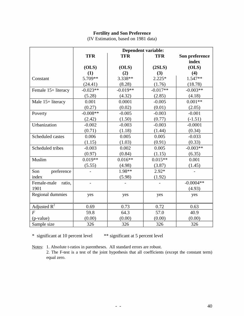
- - 40

Fertility and Son Preference(IV Estimation, based on 1981 data)

Dependent variable:TFR TFR TFR Son preference

index(OLS) (OLS) (2SLS) (OLS)

(1) (2) (3) (4)Constant 5.709**

(24.41)3.338**(8.28)

2.225*(1.76)

1.547**(18.78)

Female 15+ literacy -0.023**(5.28)

-0.019**(4.32)

-0.017**(2.85)

-0.003**(4.18)

Male 15+ literacy 0.001(0.27)

0.0001(0.02)

-0.005(0.01)

0.001**(2.05)

Poverty -0.008**(2.42)

-0.005(1.50)

-0.003(0.77)

-0.001(-1.51)

Urbanization -0.002(0.71)

-0.003(1.18)

-0.003(1.44)

-0.0001(0.34)

Scheduled castes 0.006(1.15)

0.005(1.03)

0.005(0.91)

-0.033(0.33)

Scheduled tribes -0.003(0.97)

0.002(0.84)

0.005(1.15)

-0.003**(6.35)

Muslim 0.019**(5.55)

0.016**(4.98)

0.015**(3.87)

0.001(1.45)

Son preferenceindex

- 1.98**(5.98)

2.92*(1.92)

-

Female-male ratio,1901

- - - -0.0004**(4.93)

Regional dummies yes yes yes yes

Adjusted R2 0.69 0.73 0.72 0.63F(p-value)

59.8(0.00)

64.3(0.00)

57.0(0.00)

40.9(0.00)

Sample size 326 326 326 326

* significant at 10 percent level ** significant at 5 percent level

Notes: 1. Absolute t-ratios in parentheses. All standard errors are robust.2. The F-test is a test of the joint hypothesis that all coefficients (except the constant term)equal zero.

- - 41

Fertility and Son Preference(IV Estimation, based on 1991 data)

Dependent variable:TFR TFR TFR Son preference

index(OLS) (OLS) (2SLS) (OLS)

(1) (2) (3) (4)Constant 4.756**

(19.87)2.760**(6.04)

2.630**(2.20)

1.580**(18.80)

Female 15+ literacy -0.029**(7.22)

-0.025**(6.66)

-0.024**(5.72)

-0.003**(4.09)

Male 15+ literacy 0.005(1.10)

0.004(0.87)

0.004(0.84)

0.002**(2.16)

Poverty 0.002(0.69)

0.002(0.99)

0.002(1.01)

0.001(0.79)

Urbanization -0.002(0.96)

-0.002(1.51)

-0.003(1.42)

-0.0002(0.43)

Scheduled castes -0.0003(0.07)

0.001(0.13)

0.001(0.14)

-0.001(1.31)

Scheduled tribes -0.002(0.70)

0.004(1.26)

0.004(0.90)

-0.003**(7.53)

Muslim 0.023**(7.08)

0.021**(6.76)

0.021**(6.57)

0.001(1.06)

Son preferenceindex

- 1.66**(5.19)

1.76*(1.82)

-

Female-male ratio,1901

- - - -0.0004**(5.39)

Regional dummies yes yes(see Table 4)

yes yes

Adjusted R2 0.77 0.79 0.79 0.61F(p-value)

113.0(0.00)

116.0(0.00)

111.0(0.00)

40.7(0.00)

Sample size 326 326 326 326

* significant at 10 percent level ** significant at 5 percent level

Notes: 1. Absolute t-ratios in parentheses. All standard errors are robust.2. The F-test is a test of the joint hypothesis that all coefficients (except the constant term)equal zero.

- - 42

Appendix 2

Fertility in India: Main Results using Divisions as the Basic Units(Dependent variable: TFR)

1981: OLS 1991: OLS Panel 1981-91:GLS-RE OLS-FE

(1) (2) (3) (4)

Constant 3.342**(3.626)

2.201**(2.72)

3.210**(4.54)

-

Female 15+ literacy -0.023(1.62)

-0.032**(4.75)

-0.026**(3.22)

-0.032*(1.69)

Male 15+ literacy 0.002(0.17)

0.015*(1.95)

0.006(0.70)

-0.011(0.49)

Poverty -0.006(1.02)

-0.001(0.22)

-0.003(0.96)

0.001(0.12)

Urbanization -0.005(0.82)

-0.004(1.25)

-0.005(1.31)

0.020(1.08)

Scheduled castes -0.178(1.22)

-0.007(0.85)

-0.001(1.05)

0.019(0.77)

Scheduled tribes 3.8e-05(0.01)

0.007(0.90)

0.002(0.31)

-0.061**(2.40)

Muslim 0.015*(1.78)

0.022**(4.36)

0.017**(3.35)

-0.004(0.10)

Son preferenceindex

2.51**(3.38)

1.97**(3.82)

2.15**(4.13)

-

1991 time dummy - - -0.58**(7.76)

-0.47**(3.09)

Regional dummies yes yes yes no

Adjusted R2 0.84 0.92 0.83 0.95F(p-value)

20.5(0.00)

44.5(0.00)

27.6(0.00)

Pseudo-R2

Wald, ÷2 1293.2(0.00)

Sample size 48 48 96 96GLS vs. FE, ÷2 (8)(p-value)

15.1(0.06)

Notes: See Table 3. In this table, the unit of observation is the ‘division’ rather than the district (seesection 3.1). The division-level values of each variable were calculated as a population-weightedaverage of the relevant district-level values.