Fertility after China’s More-than-One-Child Policy · Fertility after China’s More-than-One-Child Policy ... document that the One-Child Policy caused only a minor fraction of

$Page 1: Fertility after China’s More-than-One-Child Policy · Fertility after China’s More-than-One-Child Policy ... document that the One-Child Policy caused only a minor fraction of$
Fertility after China’s More-than-One-Child Policy⇤

Jorge Luis GarcıaThe University of Chicago

November 27, 2017

[link to most recent version]

Abstract

The One-Child Policy is often incorrectly perceived as an authoritarian mandate of

fertility limits by a centralized government. In reality, the policy was incentive-based.

Every woman and her partner were allowed to have more than one child—if they

paid a price. In this paper, I construct a novel dataset combining fertility histories

with individually tailored policy-dictated prices. Exploiting price variation across each

woman’s life cycle and across demographic groups and provinces, I document that the

policy diminished average completed fertility by 0.3 children per woman; 0.6 when the

first child was a girl and virtually zero when the first child was a boy. The policy

generated 18% of the observed decrease in average completed fertility from 1979 to

2000. Institutional changes in the organization of agriculture and factors describing

economic growth are more important than the policy in explaining the decrease. I

show that the e↵ect of the policy remained stable from 2000 to 2010 and argue that

the introduction of a nationally uniform Two-Child Policy in 2015 will have little e↵ect

on fertility.

⇤PhD Candidate in Economics. I am very grateful to James J. Heckman for his committed mentoring andto Stephane Bonhomme and Alessandra Voena for their insightful and patient feedback. I thank AmandaBlock, Jacob Eyferth, Manasi Deshpande, Lancelot Henry de Frahan, Ganesh Karapakula, Magne Mogstad,Sidharth Moktan, Casey Mulligan, Nancy Qian, and Anna L. Zi↵ for useful comments.

http://www.jorgeluisgarcia.com/job-market-paper/

I. Introduction

In 1979, the Chinese government liberalized the economy and introduced market principles

through a series of economic reforms. Agricultural production transitioned from collective-

based to household-based, the economy opened to foreign investment, and permissions for

entrepreneurship and private businesses were granted. The introduction of the One-Child

Policy was also based on market principles. It allowed every woman and her partner to have

more than one child—if they paid a price. This contrasts with the common perception of

the policy as an authoritarian imposition of fertility limits by a centralized government. I

document that the One-Child Policy caused only a minor fraction of the decrease in fertility

observed after 1979, despite having a robust and statistically significant negative average

e↵ect on completed fertility.

The challenge in analyzing the impact of the One-Child Policy is isolating the e↵ect of the

policy from a decreasing trend in fertility driven by other factors, especially a rising oppor-

tunity cost of children due to wage growth, but also an increase in education, an increase

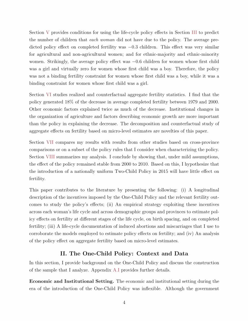
in housing prices, and reforms to agricultural production. Some analysts argue that the de-

crease in fertility is a direct result of these factors rather than an outcome of the One-Child

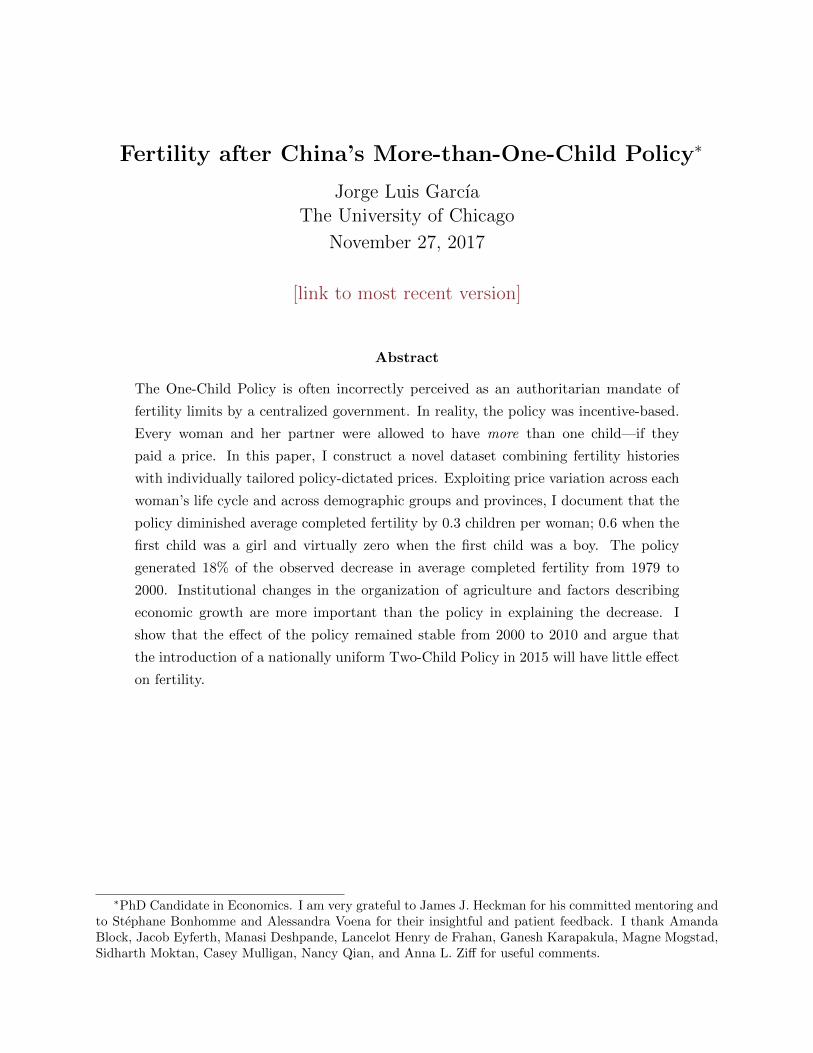
Policy (e.g., Sen, 2015; Whyte et al., 2015). Based on evidence like that in Figure 1, they

observe that after 1979 fertility continued to decrease smoothly not only in China but in

neighboring countries.1 Others contend that the draconian nature of the policy in fact drove

most of the decrease in fertility, and claim that the policy prevented up to 400 million births.

Feng and Cai (2010) discuss this and related estimates.

Methodological problems with these arguments prevent a definitive conclusion and are im-

portant to resolve. The policy operated on an unprecedented scale, potentially a↵ecting the

fertility outcomes of approximately 500 million women between 1979 and 2010.2 Numerous

studies in economics take as given the policy’s e↵ect on family size to study phenomena such

as the quantity-quality trade-o↵, the e↵ect of expected fertility on education, or sex selection

at birth.3 The belief that the policy had a sizable e↵ect on aggregate fertility is the basis

for drawing strong conclusions, both in academic and popular circles. For example, The

Economist claims that the One-Child Policy was the fourth main cause of the accumulated

reduction in carbon emissions up to 2013.4 Analyzing the policy provides a lesson regarding

1An issue with the fertility comparison across neighboring countries over time is that these countries wereactually at di↵erent stages of economic development during each point of time. Figure A.1 plots fertility asa function of GDP per capita. Countries with similar development share similar fertility rates.

2See Section II for details on this approximation.3See Zhang (2017) for a recent survey.4In “Curbing Climate Change: The Deepest Cuts” (The Economist, 2014).

1

the e↵ectiveness of family-planning policies in the presence of economic growth. This is

especially salient for developing countries facing demographic transitions.5

Figure 1: Average Number of Children for Women between Age 15 and 45

What was Driven by the Trend? ⇓

What was Driven by the Policy? ⇓

1.5

2.5

3.5

4.5

Ave

rage N

um

ber

of C

hild

ren

Wom

en A

ge 1

5 to 4

5

1960 1965 1970 1975 1979 1985 1990 1995 2000 2005 2010Year

China South Korea Taiwan Japan

Note: This figure displays the average number of children born to women with birth years between 1925and 1972 and between age 15 and 45 during the calendar year indicated in the abscissa.Sources: Author’s calculations using data from the China Health and Retirement Longitudinal Study(National School of Development, 2017), the Korean Longitudinal Study of Aging (Employment InformationService, 2017), the Taiwan Social Change Survey (Institute for Social Change, 2013), and the Japan GeneralSocial Survey (Tanioka et al., 2006).

This paper analyzes the One-Child Policy relying on the construction of a new dataset that

integrates multiple sources of household-, township-, and province-level information with

historical documents on the policy’s implementation. I generate a longitudinal, nationally

representative dataset that describes, for the first time in the Chinese context, the onset

of fertility, birth spacing, completed fertility, induced abortions, miscarriages, the economic

5Recent arguments assert that population control policies were a fundamental component in the globaldecline in fertility rates in the last 50 years (De Silva and Tenreyro, 2017). Other arguments suggest thatthe opportunity cost of raising children and the increasing demand for human capital is a main driver ofdemographic transitions (Galor, 2012).

2

environment in which fertility and related decisions were made, and the specific policy rules

that each woman faced during each year of her fertility history.

The One-Child Policy did not mandate uniform one-child families. Instead, it set rules that

dictated the price associated with having more than one child. Women faced a two-part

tari↵. Every woman was allowed to have one child without a penalty, but having additional

children imposed a fine proportional to the household’s labor income. The rules of the policy

generated de facto variation in the values of the fine across each woman’s life cycle and across

demographic groups and provinces.

Incentives varied across provinces and time. Exemptions to the fines were granted according

to characteristics related to ethnicity, sex of the first child, scarcity of males in the extended

family, and the risks associated with jobs in which women and their spouses worked.6 Across

provinces, a total of 17 exemptions were applied after the enactment of the policy. Evidence

from auxiliary sources and my empirical analysis establish that the fines were plausibly ex-

ogenous from the perspective of women and that women did not anticipate future fines when

deciding current fertility levels.

I empirically characterize the policy and fertility outcomes in an individual-level, longitudi-

nal setting. This allows me to conduct an economic analysis of the e↵ect of the One-Child

Policy on the decrease in fertility between 1979 and 2010 exploiting plausibly exogenous

variation.

The analysis unfolds as follows. Section II provides the economic and institutional context,

discusses the details of my data construction, and formally describes the policy variation

that I exploit.

Section III uses di↵erence-in-di↵erences to estimate the policy e↵ect on the number of chil-

dren at di↵erent stages of the life cycle. The analysis accounts for potentially endogenous

determinants of fertility (e.g., education, migration opportunities, household labor income).

I document that the policy e↵ect is robust to accounting for these determinants and to a

variety of functional form assumptions. Section IV complements this analysis by document-

ing that the policy e↵ects over the life cycle operated through delaying birth spacing rather

than through delaying the onset of fertility.

6The fines and the exemptions were determined by local family-planning o�cials in each province. Theirperformance was evaluated by the central government. The evaluation was based on the evolution of concreteaggregate fertility statistics. Scharping (2003) documents the bureaucratic implementation of the policy ingreat detail.

3

Section V provides conditions for using the life-cycle policy e↵ects in Section III to predict

the number of children that each woman did not have due to the policy. The average pre-

dicted policy e↵ect on completed fertility was �0.3 children. This e↵ect was very similar

for agricultural and non-agricultural women; and for ethnic-majority and ethnic-minority

women. Strikingly, the average policy e↵ect was �0.6 children for women whose first child

was a girl and virtually zero for women whose first child was a boy. Therefore, the policy

was not a binding fertility constraint for women whose first child was a boy, while it was a

binding constraint for women whose first child was a girl.

Section VI studies realized and counterfactual aggregate fertility statistics. I find that the

policy generated 18% of the decrease in average completed fertility between 1979 and 2000.

Other economic factors explained twice as much of the decrease. Institutional changes in

the organization of agriculture and factors describing economic growth are more important

than the policy in explaining the decrease. The decomposition and counterfactual study of

aggregate e↵ects on fertility based on micro-level estimates are novelties of this paper.

Section VII compares my results with results from other studies based on cross-province

comparisons or on a subset of the policy rules that I consider when characterizing the policy.

Section VIII summarizes my analysis. I conclude by showing that, under mild assumptions,

the e↵ect of the policy remained stable from 2000 to 2010. Based on this, I hypothesize that

the introduction of a nationally uniform Two-Child Policy in 2015 will have little e↵ect on

fertility.

This paper contributes to the literature by presenting the following: (i) A longitudinal

description of the incentives imposed by the One-Child Policy and the relevant fertility out-

comes to study the policy’s e↵ects; (ii) An empirical strategy exploiting these incentives

across each woman’s life cycle and across demographic groups and provinces to estimate pol-

icy e↵ects on fertility at di↵erent stages of the life cycle, on birth spacing, and on completed

fertility; (iii) A life-cycle documentation of induced abortions and miscarriages that I use to

corroborate the models employed to estimate policy e↵ects on fertility; and (iv) An analysis

of the policy e↵ect on aggregate fertility based on micro-level estimates.

II. The One-Child Policy: Context and Data

In this section, I provide background on the One-Child Policy and discuss the construction

of the sample that I analyze. Appendix A.I provides further details.

Economic and Institutional Setting. The economic and institutional setting during the

era of the introduction of the One-Child Policy was inflexible. Although the government

4

implemented market principles through a series of reforms, it had great control over eco-

nomic decisions. This justifies the use of variables describing the policy and the economic

environment in which women made fertility decisions as plausibly exogenous (from their

perspective). I further develop arguments for this in Section III.

Chinese authorities exerted control over households’ economic activities. In agricultural

jobs, the legacy of the collective production system and an extensive bureaucracy for grain

procurement made it possible for the government to monitor household labor income. In

non-agricultural jobs, employment was provided by the government through state-owned

enterprises for a large fraction of the population, making it possible to implement taxation

in the form of wage deductions (Whyte and Parish, 1985; Tang and Parish, 2000).

The institutional setting further controlled the economic lives of individuals. During the

period of my analysis, the hukou (residency) dictated the location in which a person could

live and assigned her either an agricultural or a non-agricultural status.7 Until 2000, indi-

viduals with non-agricultural hukou also belonged to a danwei (work unit). Membership to

a danwei granted permanent employment and dictated total labor income—including access

to food, health care, pensions and benefits, children’s education, and housing (Naughton,

2007), according to statutes of the central government. Most individuals remained in their

danwei for life (Lu and Perry, 1997). After the liberalization of the economy, production

activities began to change as a response to aggregate demand. Despite this, the danwei

system continued to regulate individuals’ economic lives.

Individuals with agricultural hukou mostly worked as farmers in collective systems until

1984. The collective to which they belonged dictated labor income through a point sys-

tem. Individuals earned points per day worked and received basic in-kind payments. At the

end of the harvest year, the government procured the grain, the surplus was sold at fixed

prices, and the money was divided according to days worked (net of household-level fines

and taxes). Between 1978 and 1984, the agricultural system was reformed. The land was di-

vided as part of a contract between the collective and households. The contract also dictated

grain prices. Because this system kept centralized control of the grain prices, it controlled

household labor income (Cai, 2003). Agricultural activities gradually lost importance and

individuals became part of town and village enterprises or other centralized activities, which

regulated the economic life of individuals in a similar fashion as the danwei (Naughton, 2007).

7Despite the location for residing being dictated by the hukou, massive migration occurred during themid-1990s. I explain how my analysis accounts for migration as a potential determinant of fertility inSection III.

5

Policy Evolution and Bureaucratic Implementation. After establishing the People’s

Republic of China in 1949, Mao Zedong encouraged population growth. Birth control, which

would reduce the size of the workforce, was condemned and imports of contraceptives were

banned. After unfettered population growth, the government launched family-planning cam-

paigns, encouraging the use of contraception, the delay of marriage, and the formation of

relatively small families (Powell, 2012). Before 1979, specific limits were suggested and not

enforced.

In 1979, the government announced the One-Child Policy at the federal level. The mandate

placed local authorities in charge of timing and implementation of the policy. Local authori-

ties were incentivized to implement the policy because their e↵ectiveness in curbing fertility

factored into their job evaluations. Failing to e↵ectively implement the policy could even

result in disa�liation from the communist party (Scharping, 2003). An example evaluation

sheet based on local aggregate fertility and citizens’ knowledge of the policy is in Table A.6.

Local authorities also faced opposition to the policy from citizens (Hardee-Cleaveland and

Banister, 1988). Arguably, the trade-o↵ between conforming to national policy and mitigat-

ing social discontent at the local level, together with the contemporaneous economic reforms

that introduced market principles, led o�cials to design the policy as a set of incentives

dictating the price of having more than one child, instead of an uncompromising imposition

of one-child families.8

The family-planning policies preceding the One-Child Policy established a bureaucracy for

population control. Upon getting pregnant, each woman had to register her new child in-

dependently of her parity beginning in the early 1960s. After the enactment of the policy,

permits for having a first child were generally granted. Permits for having a second or a

third child had a price. Permits for having a fourth child and beyond were generally denied,

although some were granted.9 The price per permit (fine) was a proportional tax on labor

income, usually placed on the woman and her partner for the first 14 years of the new child’s

life.

8Greenhalgh and Winckler (2005) provide examples that support this hypothesis. For instance, in 1989,Li Peng addressed provincial governors stating that: “To achieve substantial compliance, policy must besupplemented with more detailed management by objectives . . . . Targets should be evaluative.” Anotherargument against a strict limit was that relatively small families would be economically damaged by theinability to have more than one child or that minorities would become underpopulated. The president of theChinese Population Associated discussed this in 1984 (Xu, 1984).

9Given the size of China’s population, registering every single birth and collecting fines suggests the needfor an immense bureaucracy. In fact, birth-planning expenditures grew from virtually 0 to 40 billion USD(2016) from 1970 to 1995. Employment in Birth-Planning Commissions grew from less than 5, 000 in 1970to almost 400, 000 employees in 1994 (Scharping, 2003).

6

The fines were the main nation-wide policy instrument (Scharping, 2003). I estimate the

number of women potentially a↵ected by the policy to be 504.3 million. To do so, I use the

1982, 1990, and 2000 census waves (Minnesota Population Center, 2017). I include women

who were between 15 and 45 years old for at least one year between 1979 and 2010. Fertility

data between 2010 and 2015 are still incomplete.

Quantification of the Policy. When women wanted to have more than one child, they

committed, together with their partners, to pay a fine through a contract with the gov-

ernment. Exemptions to the fines were granted on an individual- and year-specific basis.10

Empirically, I construct the household-level fines as follows. I first empirically determine

a baseline fine, which varied across provinces and time. I then set the fine to zero when

women qualified for an exemption. The criteria qualifying women for exemptions varied

across provinces and time. These criteria can be grouped into four categories: ethnicity, sex

of the first child, scarcity of males in the extended family, and the risk associated with the

parents’ jobs. The exact details are in Tables A.1 to A.4. The fines and exemptions were

tied to each woman’s hukou. The hukou was (and remains) basically impossible to change.

For the baseline fine, I use the quantification of the fines in Ebenstein (2010b), which is in

terms of province- and year-specific average household labor income. For example, he calcu-

lates that in 1980 in the province of Guangdong the present value of the fine was 1.21 years

of household labor income. The calculation uses the deduction (proportional tax imposed by

the policy) of 10% of yearly household labor income to be paid for 14 years with province-

and year-specific data on household labor income, demographic information from the China

Health and Nutrition Study (CHNS) (Carolina Population Center and the National Institute

for Nutrition and Health, 2009), and a 2% discount rate.11

The deduction of 10% was set by the current state of the policy in that year. When permits

were assigned, contracts were signed with the government based on the current deduction

10Scharping (2003) collates the historical documents that allow for a quantification of both the exemptionsand the fines. These come from a variety of sources made available by the federal government and province-level Birth Planning Commissions in charge of implementing the policy. The calculations in Ebenstein(2010a), which I use for the quantification of the fines, also rely on the historical documents in Scharping(2003).

11In this calculation, Ebenstein (2010b) considers the relative exposure of the population to the policy.The calculation also accounts for urban-rural di↵erences in the fines, and other di↵erences within provinces.The final fine that he reports (1.21 years of household labor income in this example) is the weighted averageof the fines reported in Scharping (2003) for di↵erent population groups, where the weights correspond to therelative density of the households exposed to the di↵erent fines. The calculations are available in Ebenstein(2010a). They produce a pattern of geographic variation similar to that of Baochang et al. (2007), who useprefecture-level, restricted access information on the enforcement of the policy.

7

and the number of years in which the deduction would take place. Once a contract was

signed, it was not revised when future deductions changed as part of the policy variation.

When entering the contract, households had perfect certainty of both the percentage de-

ducted from household labor income and the number of years in which the deduction would

occur. The present value of the fine is calculated based on the exact number of years in

which household labor income was deducted.

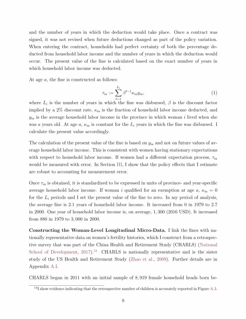
At age a, the fine is constructed as follows:

⌧ia :=LiX

`=1

�`�1iayia, (1)

where Li is the number of years in which the fine was disbursed, � is the discount factor

implied by a 2% discount rate, ia is the fraction of household labor income deducted, and

yia is the average household labor income in the province in which woman i lived when she

was a years old. At age a, ia is constant for the Li years in which the fine was disbursed. I

calculate the present value accordingly.

The calculation of the present value of the fine is based on yia and not on future values of av-

erage household labor income. This is consistent with women having stationary expectations

with respect to household labor income. If women had a di↵erent expectation process, ⌧ia

would be measured with error. In Section III, I show that the policy e↵ects that I estimate

are robust to accounting for measurement error.

Once ⌧ia is obtained, it is standardized to be expressed in units of province- and year-specific

average household labor income. If woman i qualified for an exemption at age a, ia = 0

for the Li periods and I set the present value of the fine to zero. In my period of analysis,

the average fine is 2.1 years of household labor income. It increased from 0 in 1979 to 2.7

in 2000. One year of household labor income is, on average, 1, 300 (2016 USD). It increased

from 880 in 1979 to 3, 000 in 2000.

Constructing the Woman-Level Longitudinal Micro-Data. I link the fines with na-

tionally representative data on women’s fertility histories, which I construct from a retrospec-

tive survey that was part of the China Health and Retirement Study (CHARLS) (National

School of Development, 2017).12 CHARLS is nationally representative and is the sister

study of the US Health and Retirement Study (Zhao et al., 2009). Further details are in

Appendix A.I.

CHARLS began in 2011 with an initial sample of 8, 919 female household heads born be-

12I show evidence indicating that the retrospective number of children is accurately reported in Figure A.3.

8

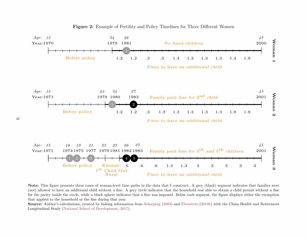
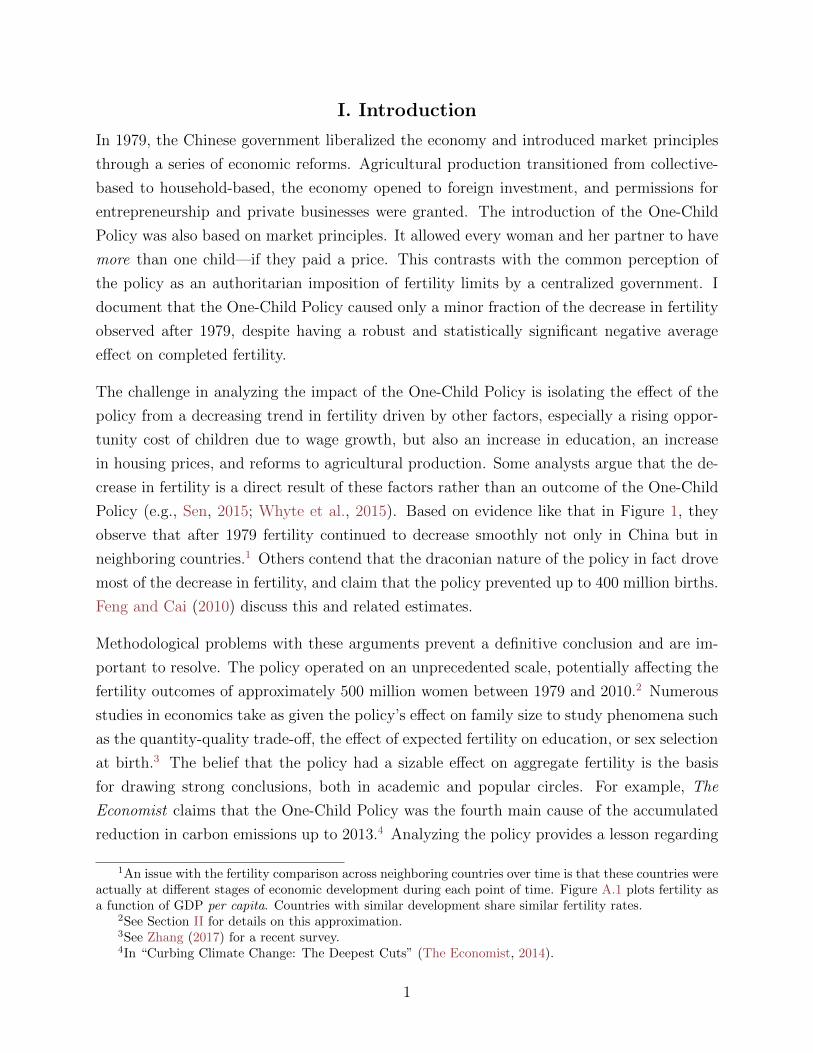
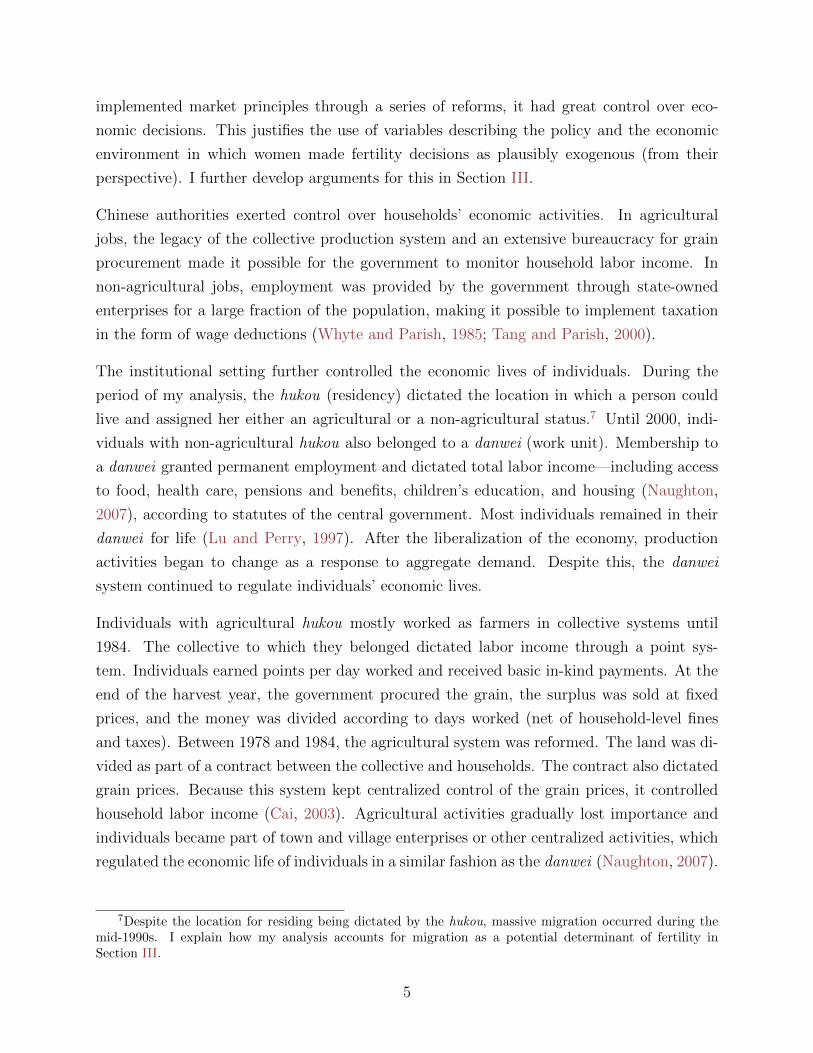
Figure 2: Example of Fertility and Policy Timelines for Three Di↵erent Women

Wom

an

1

Age:

Year:

1970

15

2000

45

1979

24

Before policy

Fines to have an additional child

1

1981

26

1.2 1.2 .3 .3 1.3 1.3 1.3 1.3 1.3 1.9

No fined children

Wom

an

2

Age:

Year:

1971

15

2001

45

1979

23

Family paid fine for 2

nd

child

Before policy


1

1980

24

2

1983

27

1.2 1.2 .3 1.3 1.3 1.3 1.3 1.3 1.9 1.9

Wom

an

3

Age:

Year:

1971

15

2001

45

1979

23

Before policy


1981

25

Exempt:

1

st

Child Girl

Rural

1

1974

18

2

1975

19

3

1977

21

4

1982

26

5

1983

27

Family paid fine for 4

th

and 5

th

children

.6 .6 .6 1.3 1.3 3 3 3 3 3

Note: This figure presents three cases of woman-level time paths in the data that I construct. A grey (black) segment indicates that families were(not) allowed to have an additional child without a fine. A grey circle indicates that the household was able to obtain a child permit without a finefor the parity inside the circle, while a black sphere indicates that a fine was imposed. Below each segment, the figure displays either the exemptionthat applied to the household or the fine during that year.Source: Author’s calculations, created by linking information from Scharping (2003) and Ebenstein (2010b) with the China Health and RetirementLongitudinal Study (National School of Development, 2017).

9

tween 1925 and 1972. I analyze fertility between 1970 and 2000 using this sample. My main

analysis stops at 2000 because precise details on policy implementation are only available

from 1979 to 2000. When analyzing fertility over the life cycle, I include women who were

between 15 and 45 during my period of analysis. When analyzing completed fertility, I follow

accepted conventions and assume that women complete fertility at age 40. This limits the

cohorts for which I observe completed fertility to those born between 1925 and 1960, for

which the initial sample size is 7, 247. Additional cohorts born between 1961 and 1972 total

1, 780 women. Analyzing them provides information on the e↵ect of the policy on completed

fertility between 2001 and 2010.

For each woman in the sample, I characterize each year of her fertility history (i.e., each year

between age 15 and 45) with the total number of children (dead or alive), the total number

of miscarriages and induced abortions, and the fines that she faced.

To complement these data, I construct and match a dataset characterizing the economic

environment in which the women in the sample made fertility decisions. This construction

combines two sources: province- and year-specific data from Chinese Statistical Yearbooks

available in China Data Center (2017) and township- and year-specific data based on retro-

spective surveys of community leaders available in CHARLS. Table A.7 provides a full list of

the measures. I aggregate each economic category into the factors listed in Table 1. I stack

these factors into a vector denoted by Zia.

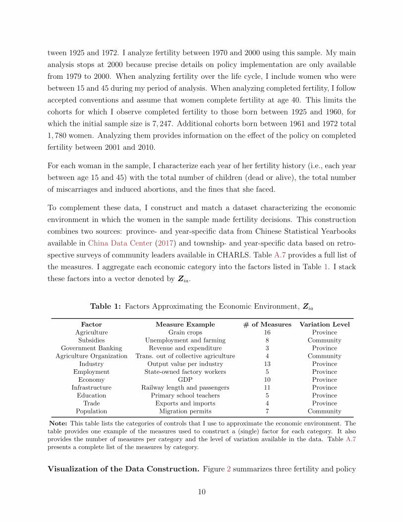
Table 1: Factors Approximating the Economic Environment, Zia

Factor Measure Example # of Measures Variation LevelAgriculture Grain crops 16 ProvinceSubsidies Unemployment and farming 8 Community

Government Banking Revenue and expenditure 3 ProvinceAgriculture Organization Trans. out of collective agriculture 4 Community

Industry Output value per industry 13 ProvinceEmployment State-owned factory workers 5 ProvinceEconomy GDP 10 Province

Infrastructure Railway length and passengers 11 ProvinceEducation Primary school teachers 5 ProvinceTrade Exports and imports 4 Province

Population Migration permits 7 Community

Note: This table lists the categories of controls that I use to approximate the economic environment. Thetable provides one example of the measures used to construct a (single) factor for each category. It alsoprovides the number of measures per category and the level of variation available in the data. Table A.7presents a complete list of the measures by category.

Visualization of the Data Construction. Figure 2 summarizes three fertility and policy

10

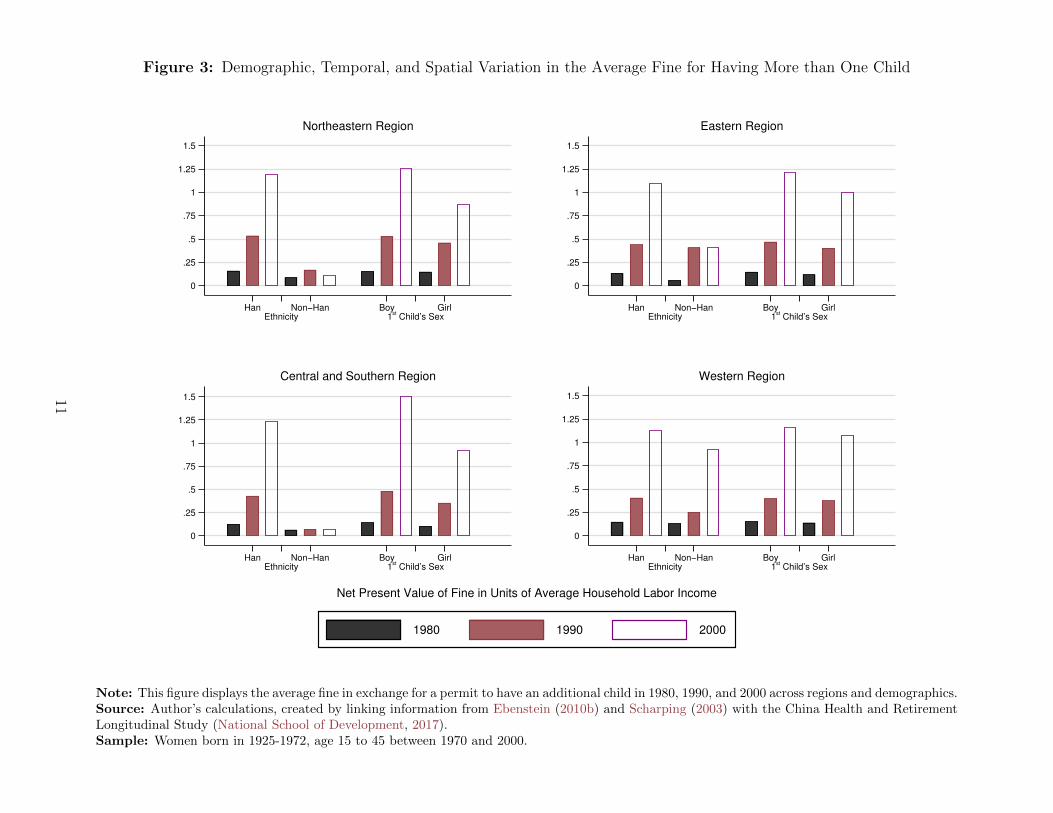
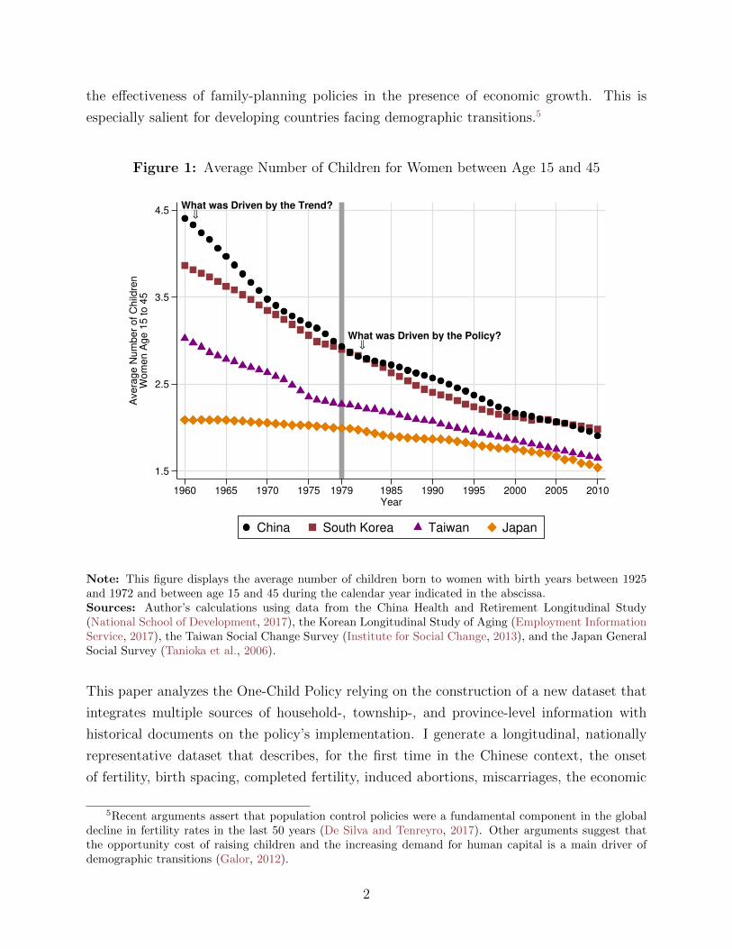
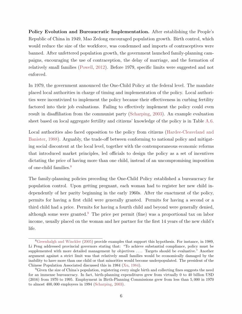
Figure 3: Demographic, Temporal, and Spatial Variation in the Average Fine for Having More than One Child

0

.25

.5

.75

1

1.25

1.5

Han Ethnicity

Non−Han Boy 1

st Child’s Sex

Girl

Northeastern Region

0

.25

.5

.75

1

1.25

1.5

Han Ethnicity

Non−Han Boy 1

st Child’s Sex

Girl

Eastern Region

0

.25

.5

.75

1

1.25

1.5

Han Ethnicity

Non−Han Boy 1

st Child’s Sex

Girl

Central and Southern Region

0

.25

.5

.75

1

1.25

1.5

Han

EthnicityNon−Han Boy

1st Child’s Sex

Girl

Western Region

Net Present Value of Fine in Units of Average Household Labor Income

1980 1990 2000

Note: This figure displays the average fine in exchange for a permit to have an additional child in 1980, 1990, and 2000 across regions and demographics.Source: Author’s calculations, created by linking information from Ebenstein (2010b) and Scharping (2003) with the China Health and RetirementLongitudinal Study (National School of Development, 2017).Sample: Women born in 1925-1972, age 15 to 45 between 1970 and 2000.

11

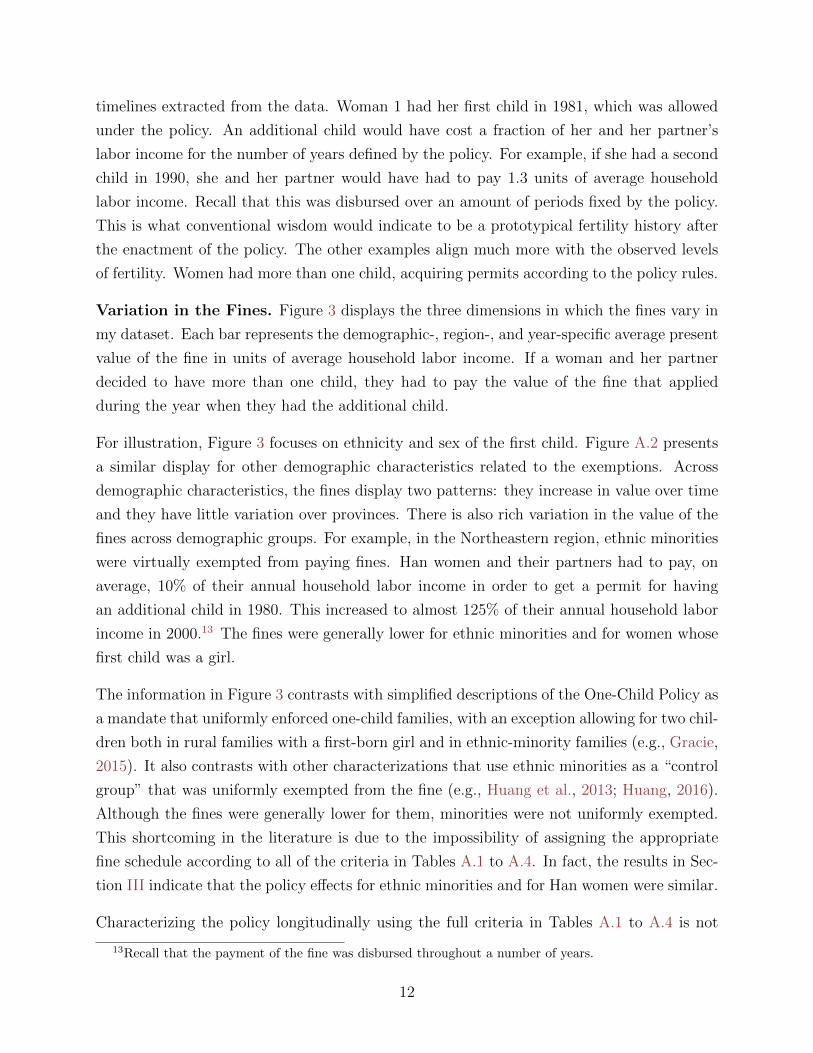
timelines extracted from the data. Woman 1 had her first child in 1981, which was allowed

under the policy. An additional child would have cost a fraction of her and her partner’s

labor income for the number of years defined by the policy. For example, if she had a second

child in 1990, she and her partner would have had to pay 1.3 units of average household

labor income. Recall that this was disbursed over an amount of periods fixed by the policy.

This is what conventional wisdom would indicate to be a prototypical fertility history after

the enactment of the policy. The other examples align much more with the observed levels

of fertility. Women had more than one child, acquiring permits according to the policy rules.

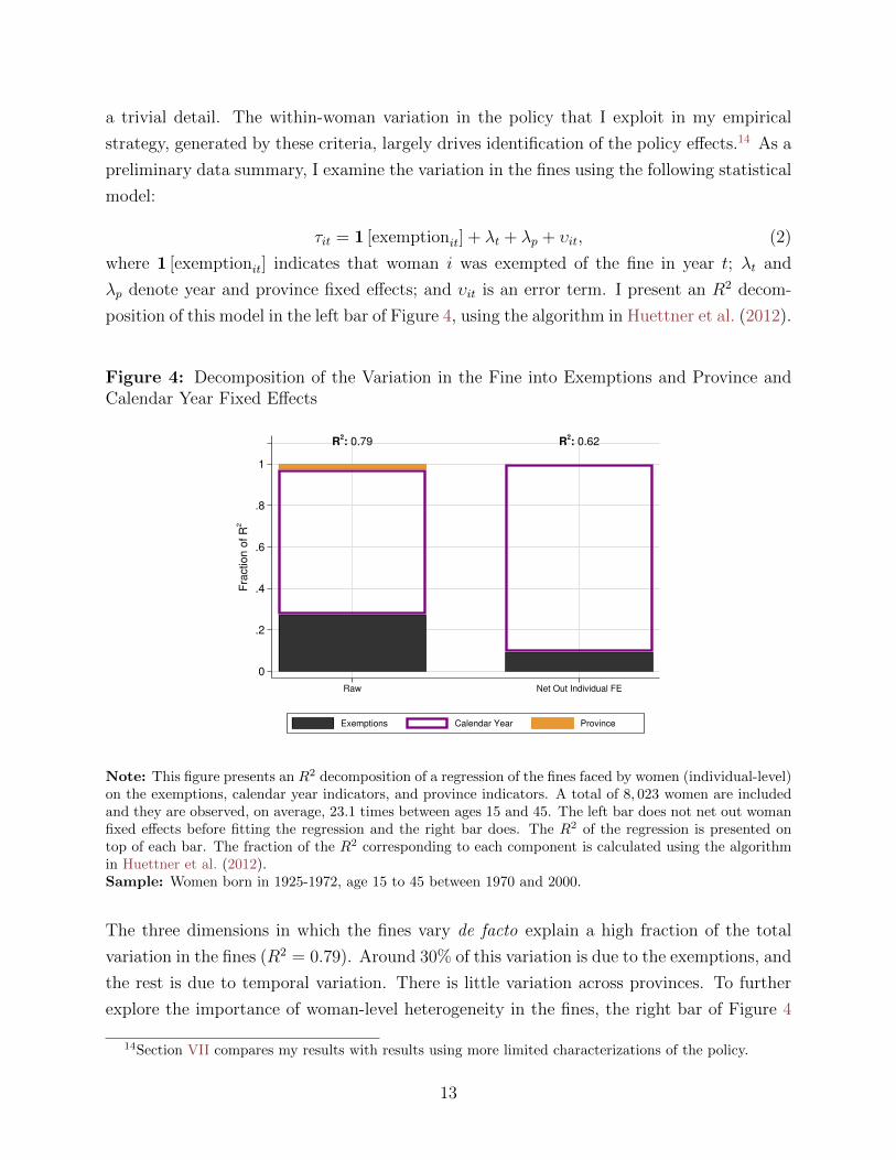
Variation in the Fines. Figure 3 displays the three dimensions in which the fines vary in

my dataset. Each bar represents the demographic-, region-, and year-specific average present

value of the fine in units of average household labor income. If a woman and her partner

decided to have more than one child, they had to pay the value of the fine that applied

during the year when they had the additional child.

For illustration, Figure 3 focuses on ethnicity and sex of the first child. Figure A.2 presents

a similar display for other demographic characteristics related to the exemptions. Across

demographic characteristics, the fines display two patterns: they increase in value over time

and they have little variation over provinces. There is also rich variation in the value of the

fines across demographic groups. For example, in the Northeastern region, ethnic minorities

were virtually exempted from paying fines. Han women and their partners had to pay, on

average, 10% of their annual household labor income in order to get a permit for having

an additional child in 1980. This increased to almost 125% of their annual household labor

income in 2000.13 The fines were generally lower for ethnic minorities and for women whose

first child was a girl.

The information in Figure 3 contrasts with simplified descriptions of the One-Child Policy as

a mandate that uniformly enforced one-child families, with an exception allowing for two chil-

dren both in rural families with a first-born girl and in ethnic-minority families (e.g., Gracie,

2015). It also contrasts with other characterizations that use ethnic minorities as a “control

group” that was uniformly exempted from the fine (e.g., Huang et al., 2013; Huang, 2016).

Although the fines were generally lower for them, minorities were not uniformly exempted.

This shortcoming in the literature is due to the impossibility of assigning the appropriate

fine schedule according to all of the criteria in Tables A.1 to A.4. In fact, the results in Sec-

tion III indicate that the policy e↵ects for ethnic minorities and for Han women were similar.

Characterizing the policy longitudinally using the full criteria in Tables A.1 to A.4 is not

13Recall that the payment of the fine was disbursed throughout a number of years.

12

a trivial detail. The within-woman variation in the policy that I exploit in my empirical

strategy, generated by these criteria, largely drives identification of the policy e↵ects.14 As a

preliminary data summary, I examine the variation in the fines using the following statistical

model:

⌧it = 1 [exemptionit] + �t + �p + �it, (2)

where 1 [exemptionit] indicates that woman i was exempted of the fine in year t; �t and

�p denote year and province fixed e↵ects; and �it is an error term. I present an R2 decom-

position of this model in the left bar of Figure 4, using the algorithm in Huettner et al. (2012).

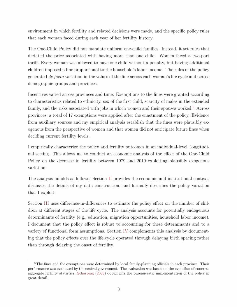
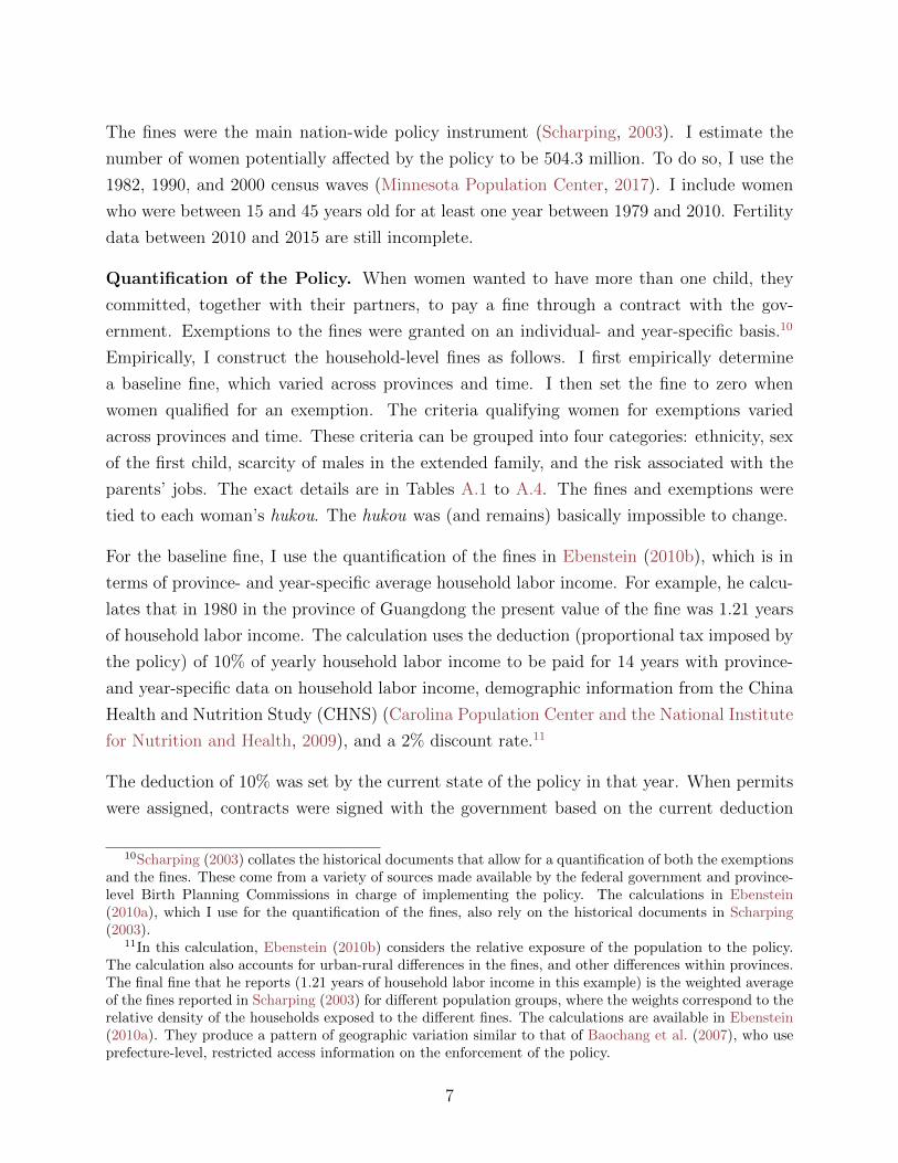
Figure 4: Decomposition of the Variation in the Fine into Exemptions and Province andCalendar Year Fixed E↵ects

R2: 0.79 R

2: 0.62

0

.2

.4

.6

.8

1

Fra

ctio

n o

f R

2

Raw Net Out Individual FE

Exemptions Calendar Year Province

Note: This figure presents an R2 decomposition of a regression of the fines faced by women (individual-level)on the exemptions, calendar year indicators, and province indicators. A total of 8, 023 women are includedand they are observed, on average, 23.1 times between ages 15 and 45. The left bar does not net out womanfixed e↵ects before fitting the regression and the right bar does. The R2 of the regression is presented ontop of each bar. The fraction of the R2 corresponding to each component is calculated using the algorithmin Huettner et al. (2012).Sample: Women born in 1925-1972, age 15 to 45 between 1970 and 2000.

The three dimensions in which the fines vary de facto explain a high fraction of the total

variation in the fines (R2 = 0.79). Around 30% of this variation is due to the exemptions, and

the rest is due to temporal variation. There is little variation across provinces. To further

explore the importance of woman-level heterogeneity in the fines, the right bar of Figure 4

14Section VII compares my results with results using more limited characterizations of the policy.

13

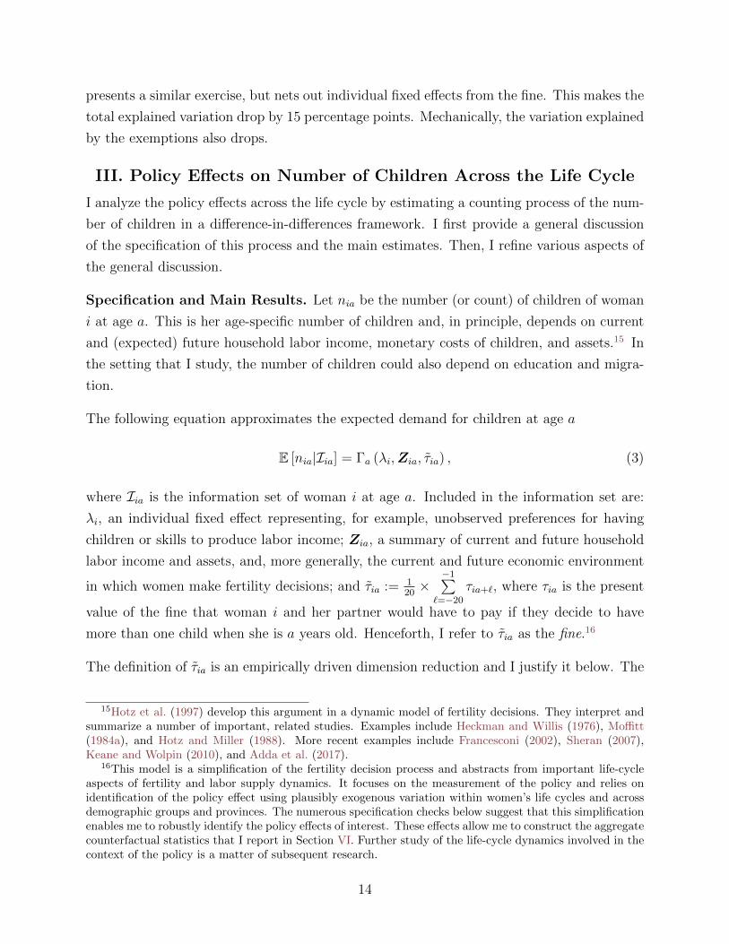
presents a similar exercise, but nets out individual fixed e↵ects from the fine. This makes the

total explained variation drop by 15 percentage points. Mechanically, the variation explained

by the exemptions also drops.

III. Policy E↵ects on Number of Children Across the Life Cycle

I analyze the policy e↵ects across the life cycle by estimating a counting process of the num-

ber of children in a di↵erence-in-di↵erences framework. I first provide a general discussion

of the specification of this process and the main estimates. Then, I refine various aspects of

the general discussion.

Specification and Main Results. Let nia be the number (or count) of children of woman

i at age a. This is her age-specific number of children and, in principle, depends on current

and (expected) future household labor income, monetary costs of children, and assets.15 In

the setting that I study, the number of children could also depend on education and migra-

tion.

The following equation approximates the expected demand for children at age a

E [nia|Iia] = �a (�i,Zia, ⌧ia) , (3)

where Iia is the information set of woman i at age a. Included in the information set are:

�i, an individual fixed e↵ect representing, for example, unobserved preferences for having

children or skills to produce labor income; Zia, a summary of current and future household

labor income and assets, and, more generally, the current and future economic environment

in which women make fertility decisions; and ⌧ia :=120 ⇥

�1P`=�20

⌧ia+`, where ⌧ia is the present

value of the fine that woman i and her partner would have to pay if they decide to have

more than one child when she is a years old. Henceforth, I refer to ⌧ia as the fine.16

The definition of ⌧ia is an empirically driven dimension reduction and I justify it below. The

15Hotz et al. (1997) develop this argument in a dynamic model of fertility decisions. They interpret andsummarize a number of important, related studies. Examples include Heckman and Willis (1976), Mo�tt(1984a), and Hotz and Miller (1988). More recent examples include Francesconi (2002), Sheran (2007),Keane and Wolpin (2010), and Adda et al. (2017).

16This model is a simplification of the fertility decision process and abstracts from important life-cycleaspects of fertility and labor supply dynamics. It focuses on the measurement of the policy and relies onidentification of the policy e↵ect using plausibly exogenous variation within women’s life cycles and acrossdemographic groups and provinces. The numerous specification checks below suggest that this simplificationenables me to robustly identify the policy e↵ects of interest. These e↵ects allow me to construct the aggregatecounterfactual statistics that I report in Section VI. Further study of the life-cycle dynamics involved in thecontext of the policy is a matter of subsequent research.

14

fine is a device that I use to approximate the intensity of the policy. Relying on this as

a measure of the policy is consistent with the information up to 20 years before a being

relevant. Below, I empirically test that future information is irrelevant when measuring the

intensity of the policy and interpret this as a methodological advantage.

Policy rules induced variation in ⌧ia. As described in Section II, these rules were set by

birth-planning o�cials according to their own interests. Changes to these rules were intro-

duced over time after the enactment of the policy, according to province of residence and

demographic characteristics. Within a province and a demographic group, a policy change

introduced variation in ⌧ia for women at di↵erent life-cycle stages. Observing the province-

and demographic-specific fine during each stage of each woman’s life cycle and accounting for

�i and the economic environment justifies the exogeneity of this variation. Within-woman

variation across the life cycle identifies the policy e↵ects. I elaborate on this argument and

discuss further evidence of exogeneity below.

Table 1 lists the factors that I use to approximateZia, together with examples of the measures

that I use to construct them. In 1979, in addition to the One-Child Policy, the government

enacted a series of policies that implemented market principles and increased the opportunity

cost of children. Below, I discuss the relationship between the variables in Zia and fertility.

In summary, industrial activities, education, trade and foreign investment, and economic

growth are negative determinants of fertility and increased after 1979. The change between

1979 and 1984 in the organization of agricultural production from collective- to household-

based also reduced fertility.

Both employment and income were set by governmental rules, migration was only possible

through temporary permits granted by the government, and the final level of education,

which was the compulsory level for most women, was set before fertility decisions began (see

Figure A.4).17 The variation in Zia was driven by policies and prices fixed by the government.

Within each woman’s life cycle, province- or community-level variation in Zia is a plausibly

exogenous shifter of economic decisions that occur simultaneously to fertility decisions (e.g.,

education, migration, and labor supply).

The institutional setting also indicates that ⌧ia was the main cost associated with having

children apart from the opportunity cost. Health and education services were provided by

17Migration might have determined the opportunity cost of children. Migration was mostly within-ruralor within-urban areas and was regulated by temporary permits (Chan, 2001; Au and Henderson, 2006). Toaccount for the potential e↵ects of migration, I include the volume of the community-level yearly provisionof individual migration permits in Zia. De Brauw and Giles (2016) and Pan (2017) use versions of thisvariation as exogenous shifters of the cost of migration.

15

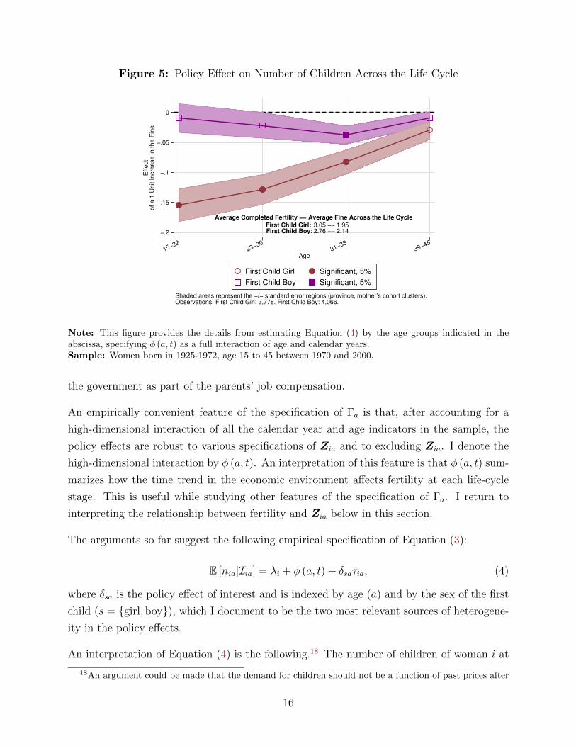
Figure 5: Policy E↵ect on Number of Children Across the Life Cycle

Average Completed Fertility −− Average Fine Across the Life Cycle First Child Girl: First Child Boy:

3.05 −− 1.95 2.76 −− 2.14

0

−.05

−.1

−.15

−.2

Eff

ect

of

a 1

Un

it In

cre

ase

in t

he

Fin

e

15−2223−30

31−3839−45

Age

First Child Girl Significant, 5%

First Child Boy Significant, 5%

Shaded areas represent the +/− standard error regions (province, mother’s cohort clusters).Observations. First Child Girl: 3,778. First Child Boy: 4,066.

Note: This figure provides the details from estimating Equation (4) by the age groups indicated in theabscissa, specifying � (a, t) as a full interaction of age and calendar years.Sample: Women born in 1925-1972, age 15 to 45 between 1970 and 2000.

the government as part of the parents’ job compensation.

An empirically convenient feature of the specification of �a is that, after accounting for a

high-dimensional interaction of all the calendar year and age indicators in the sample, the

policy e↵ects are robust to various specifications of Zia and to excluding Zia. I denote the

high-dimensional interaction by � (a, t). An interpretation of this feature is that � (a, t) sum-

marizes how the time trend in the economic environment a↵ects fertility at each life-cycle

stage. This is useful while studying other features of the specification of �a. I return to

interpreting the relationship between fertility and Zia below in this section.

The arguments so far suggest the following empirical specification of Equation (3):

E [nia|Iia] = �i + � (a, t) + �sa⌧ia, (4)

where �sa is the policy e↵ect of interest and is indexed by age (a) and by the sex of the first

child (s = {girl, boy}), which I document to be the two most relevant sources of heterogene-

ity in the policy e↵ects.

An interpretation of Equation (4) is the following.18 The number of children of woman i at

18An argument could be made that the demand for children should not be a function of past prices after

16

age a in calendar year t is given by the population average � (a, t) plus her individual-specific

preference shifter �i (e.g., desired total number of children). An increase of one unit in the

fine at age a shifts the number of children by an average of �sa. Recall that the fine is in

units of province- and year-specific average household labor income.19

Figure 5 summarizes the results from estimating Equation (4).20 The e↵ect is weak for

women whose first child was a boy. For women whose first child was a girl, �sa decreases in

magnitude across the life cycle. At earlier ages, the policy e↵ect is stronger because women

are most fecund and more resource constrained. These two factors diminish in importance

as the life cycle evolves and �sa tends towards zero after age 38.21

Figure 5 indicates that the policy was not binding for women whose first child was a boy.

For women whose first child was a girl, the policy imposes a restriction. This is consistent

with a stark preference in China for having a male child (Li and Wu, 2011). Women whose

first child was a girl were restricted by the policy if they wanted to have additional children

to increase their likelihood of having a boy. This supports the interpretation of �as as the

average intertemporal e↵ect of the fine on the treated population.

Specification of ⌧ia. As a methodological simplification, suppose that the object of in-

terest is the average policy e↵ect across the life cycle, �sa = �. This allows me to use

data-demanding methods to assess the specification of �a beyond heterogeneity in �.22

I summarize the policy through the average fine from 20 years to 1 year before the age-a

number of children is realized. I test whether this is a good summary by comparing the

conditioning on the number of children in previous periods (e.g., when separating women by gender of thefirst child). Previous fines, however, could still influence the demand for children by, for example, providinginformation on what the expectation on future fines should be.

19Mo�tt (1984b) and Hotz et al. (1997) argue that estimating Equation (4) using standard panel datamodels is problematic because nia is a limited dependent variable. In Figure A.7, however, I show thatthe variables that are relevant when identifying �sa, the residual number of children and the residual fine,are continuously and approximately normally distributed. The residuals are the respective variables netof individual and calendar year times age (all possible interactions between calendar years and ages) fixede↵ects.

20The di↵erence in the initial sample size that I report in Section II (8, 919) and the final sample sizefor my analysis (8, 023) is due to item non-response. I document the di↵erence in observed characteristicsbetween the initial and final samples in Appendix A.I and show that standard weighting procedures to assessitem non-response have little impact on my estimates in Table A.8.

21Figure A.8 provides a visual display of the variation identifying the policy e↵ect for each age group inFigure 5. For each age group, there is a negative relationship between the residual number of children andthe residual fine. The residuals are the respective variables net of individual and all possible interactionsbetween calendar year and age fixed e↵ects.

22This does not mean that ⌧ia does not a↵ect fertility at di↵erent ages. Instead, it means that ⌧ia a↵ectsthe policy in the same way across ages. � could be interpreted as the average policy e↵ect across the lifecycle.

17

following models:

E[nia|Iia] = �i + � (a, t) + �⌧ia (5)

E[nia|Iia] = �i + � (a, t) +10X

`=�20

�`⌧ia+`. (6)

The models in Equations (5) and (6) are equivalent under the following null hypotheses:

H10 : [��20, . . . , ��1] =

1

20� ⇥ 10

H20 : [�0, . . . , �10] = 00. (7)

I cannot reject the model in Equation (5) when the model in Equation (6) is the alternative

(see Figure A.5 for a visual display of the tests). The F -statistic associated with H10 is 0.09

(p-value = 1.00, N = 8, 023). Not rejecting H10 allows me to focus on one interpretable

measure of the policy, ⌧ia.

An alternative to measure the policy’s intensity is to interpret ⌧ia�20, . . . , ⌧ia�1 as noisy mea-

sures of the policy’s intensity and construct a factor based on these measures. A factor would

not restrict the weights of each measure as the average does; instead, it would estimate the

weights. Figure A.6 shows that the results are closely aligned when using the factor and

when using ⌧ia. This is not surprising given that I fail to reject H10 .

The F -statistic associated with H20 is 0.02 (p-value = 1.00, N = 8, 023). Not rejecting H2

0

is evidence of non-anticipatory behavior with respect to the fine. The formulation of this

hypothesis in Equation (6) could be refined. For a woman who is age 15, up to 30 fines could

be relevant throughout the period of her life cycle that I analyze. For a woman who is age

40, only 5 fines could be relevant. I impose H10 and estimate the following models:

Ages 15 to 22 : E[nia|Iia] = �i + � (a, t) + �⌧ia +30X

`=0

�`⌧ia+`


`=0

�`⌧ia+`


`=0

�`⌧ia+`


`=0

�`⌧ia+`, (8)

which test the relevance of future fines up to when the youngest woman in the age group is

18

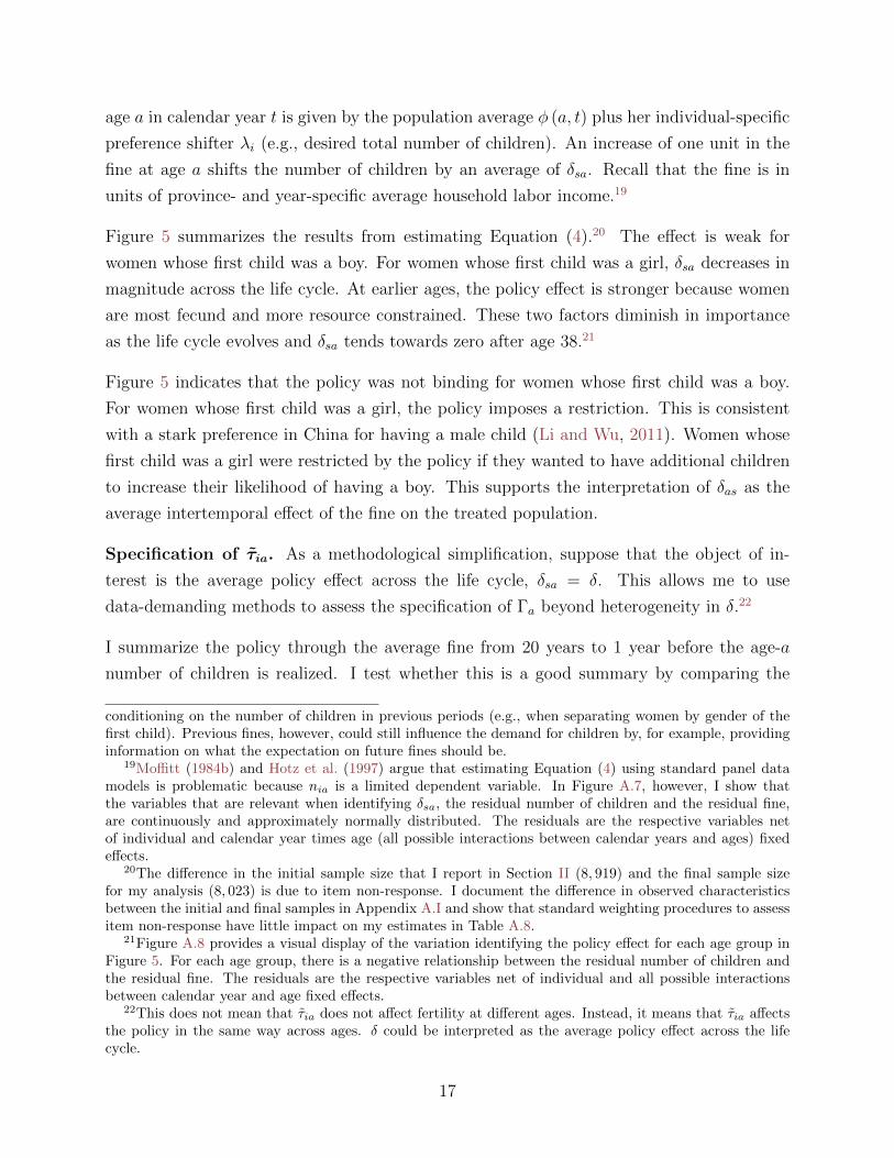
45 years old. Figure 6 displays the coe�cients on future fines �` for the relevant ` in each

age group. There is consistent evidence of non-anticipatory behavior across age groups.

Non-Anticipatory Behavior with Respect to the Fine. Anticipatory behavior is prob-

lematic if, by choosing to have one child at age a, a woman was also deciding the fine that she

would face in future periods. Anticipatory behavior would also complicate formally defining

Equation (4) as a counting process (Yashin and Arjas, 1988).23

There are two economic interpretations of the evidence on non-anticipatory behavior. First,

it could be that the demand for children is such that women do not account for future prices

when deciding current fertility perhaps due to ignorance of the trajectory of future prices.

Second, it could be that women have stationary expectations about the fine, i.e., they take

the current fine as a valid prediction of the future fines.

Figure 6: E↵ect of Future Fines on Current Number of Children

0

0

0

0

Co

eff

icie

nt

on

Fu

ture

Fin

e

0 6 14 22 30

Years After Current Fertility

15−22 23−30 31−38 39−45

Shaded areas represent the 95% confidence interval (province, mother’s cohort clusters).

Note: This figure provides estimates of the coe�cients on realized future fines in Equation (8). Theestimation specifies � (a, t) as a full interaction of age and calendar year indicators. Standard errors areclustered at province, mother’s cohort level.Sample: Women born in 1925-1972, age 15 to 45 between 1970 and 2000.

In either scenario, the fact that current fertility is not a function of future fines is consistent

23In the language of event history analysis, a concern would arise because the fine would be an internalcovariate. See Cortese and Andersen (2010) for a recent discussion.

19

with women not predicting the future fines when planning their fertility. They do not plan

future prices, but rather experience them as surprises shifting them from their desired total

number of children. If that is the case, the evidence in Figure 6 allows me to interpret my

methodology as an event study where previous but not future values of the policy have an

e↵ect on the outcome of interest.

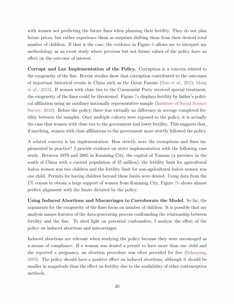
Corrupt and Lax Implementation of the Policy. Corruption is a concern related to

the exogeneity of the fine. Recent studies show that corruption contributed to the outcomes

of important historical events in China such as the Great Famine (Sun et al., 2013; Meng

et al., 2015). If women with close ties to the Communist Party received special treatment,

the exogeneity of the fines could be threatened. Figure 7a displays fertility by father’s politi-

cal a�liation using an auxiliary nationally representative sample (Institute of Social Science

Survey, 2010). Before the policy, there was virtually no di↵erence in average completed fer-

tility between the samples. Once multiple cohorts were exposed to the policy, it is actually

the case that women with close ties to the government had lower fertility. This suggests that,

if anything, women with close a�liations to the government more strictly followed the policy.

A related concern is lax implementation: How strictly were the exemptions and fines im-

plemented in practice? I provide evidence on strict implementation with the following case

study. Between 1979 and 2005 in Kunming City, the capital of Yunnan (a province in the

south of China with a current population of 45 million), the fertility limit for agricultural

hukou women was two children and the fertility limit for non-agricultural hukou women was

one child. Permits for having children beyond these limits were denied. Using data from the

1% census to obtain a large support of women from Kunming City, Figure 7b shows almost

perfect alignment with the limits dictated by the policy.

Using Induced Abortions and Miscarriages to Corroborate the Model. So far, the

arguments for the exogeneity of the fines focus on number of children. It is possible that my

analysis misses features of the data-generating process confounding the relationship between

fertility and the fine. To shed light on potential confounders, I analyze the e↵ect of the

policy on induced abortions and miscarriages.

Induced abortions are relevant when studying the policy because they were encouraged as

a means of compliance. If a woman was denied a permit to have more than one child and

she reported a pregnancy, an abortion procedure was often provided for free (Scharping,

2003). The policy should have a positive e↵ect on induced abortions, although it should be

smaller in magnitude than the e↵ect on fertility due to the availability of other contraception

methods.

20

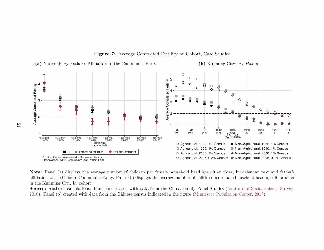
Figure 7: Average Completed Fertility by Cohort, Case Studies

(a) National: By Father’s A�liation to the Communist Party

1

2

3

4

Ave

rage C

om

ple

ted F

ert

ility

1940−1943(39−36)

1944−1947(35−32)

1948−1950(31−29)

1951−1952(28−27)

1953−1954(26−25)

1955−1956(24−23)

1957−1959(22−20)

1960−1962(19−17)

Birth Year(Age in 1979)

All Father: No Affiliation Father: Communist

Point estimates are centered in the +/− s.e. bands.Observations. All: 32,478. Communist Father: 4,104.

(b) Kunming City: By Hukou

1

2

3

4

5

Ave

rage C

om

ple

ted F

ert

ility

1930(49)

1934(45)

1938(41)

1942(37)

1946(33)

1950(29)

1954(25)

1958(21)

1962(17)


Agricultural. 1982, 1% Census Non−Agricultural. 1982, 1% Census



Agricultural. 2005, 0.2% Census Non−Agricultural. 2005, 0.2% Census

Note: Panel (a) displays the average number of children per female household head age 40 or older, by calendar year and father’sa�liation to the Chinese Communist Party. Panel (b) displays the average number of children per female household head age 40 or olderin the Kunming City, by cohort.Source: Author’s calculations. Panel (a) created with data from the China Family Panel Studies (Institute of Social Science Survey,2010). Panel (b) created with data from the Chinese census indicated in the figure (Minnesota Population Center, 2017).

21

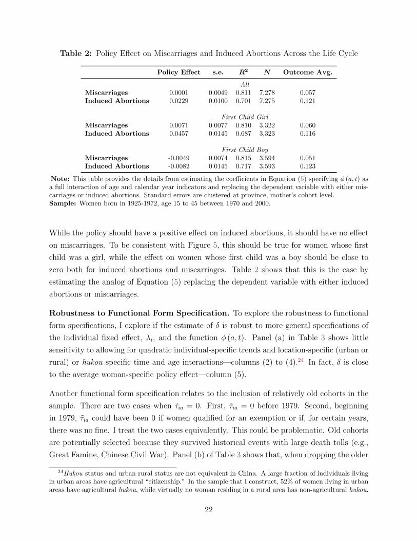
Table 2: Policy E↵ect on Miscarriages and Induced Abortions Across the Life Cycle

Policy E↵ect s.e. R2 N Outcome Avg.

AllMiscarriages 0.0001 0.0049 0.811 7,278 0.057Induced Abortions 0.0229 0.0100 0.701 7,275 0.121

First Child GirlMiscarriages 0.0071 0.0077 0.810 3,322 0.060Induced Abortions 0.0457 0.0145 0.687 3,323 0.116

First Child BoyMiscarriages -0.0049 0.0074 0.815 3,594 0.051Induced Abortions -0.0082 0.0145 0.717 3,593 0.123

Note: This table provides the details from estimating the coe�cients in Equation (5) specifying � (a, t) asa full interaction of age and calendar year indicators and replacing the dependent variable with either mis-carriages or induced abortions. Standard errors are clustered at province, mother’s cohort level.Sample: Women born in 1925-1972, age 15 to 45 between 1970 and 2000.

While the policy should have a positive e↵ect on induced abortions, it should have no e↵ect

on miscarriages. To be consistent with Figure 5, this should be true for women whose first

child was a girl, while the e↵ect on women whose first child was a boy should be close to

zero both for induced abortions and miscarriages. Table 2 shows that this is the case by

estimating the analog of Equation (5) replacing the dependent variable with either induced

abortions or miscarriages.

Robustness to Functional Form Specification. To explore the robustness to functional

form specifications, I explore if the estimate of � is robust to more general specifications of

the individual fixed e↵ect, �i, and the function � (a, t). Panel (a) in Table 3 shows little

sensitivity to allowing for quadratic individual-specific trends and location-specific (urban or

rural) or hukou-specific time and age interactions—columns (2) to (4).24 In fact, � is close

to the average woman-specific policy e↵ect—column (5).

Another functional form specification relates to the inclusion of relatively old cohorts in the

sample. There are two cases when ⌧ia = 0. First, ⌧ia = 0 before 1979. Second, beginning

in 1979, ⌧ia could have been 0 if women qualified for an exemption or if, for certain years,

there was no fine. I treat the two cases equivalently. This could be problematic. Old cohorts

are potentially selected because they survived historical events with large death tolls (e.g.,

Great Famine, Chinese Civil War). Panel (b) of Table 3 shows that, when dropping the older

24Hukou status and urban-rural status are not equivalent in China. A large fraction of individuals livingin urban areas have agricultural “citizenship.” In the sample that I construct, 52% of women living in urbanareas have agricultural hukou, while virtually no woman residing in a rural area has non-agricultural hukou.

22

Table 3: Policy E↵ect on Number of Children Across the Life Cycle, Robustness

(1) (2) (3) (4) (5)

Panel (a) Woman Fixed E↵ect Specification

Additively + Quadratic + Hukou + Rural Woman-SpecificSeparable Age Trends Age/Year Age/Year E↵ect(Baseline) FE FE (Mean)

� -0.205 -0.256 -0.242 -0.249 -0.175(0.029) (0.173) (0.172) (0.174) (0.047)

R2 0.884 0.959 0.959 0.959 0.931N 8,023 8,023 7,966 8,023 8,023

Panel (b) Birth Cohort Sample

1925-1972 1930-1972 1935-1972 1945-1972 1955-1972(Baseline)

� -0.205 -0.205 -0.205 -0.202 -0.201(0.029) (0.029) (0.029) (0.029) (0.033)

R2 0.884 0.884 0.879 0.854 0.809N 8,023 7,905 7,622 6,465 3,850

Panel (c) Standard Error Specification

Province*Birth Homos- Woman Province Birth CohortCohort Clusters cedastic Clusters Custers Clusters(Baseline)

� -0.205 -0.205 -0.205 -0.205 -0.205(0.029) (0.007) (0.024) (0.074) (0.026)

# Clusters 1,067 185,118 8,023 27 47

Panel (d) Accounting for the Economic Environment (Zia)

None Current Current +3 Current +1 Current +3(Baseline) Lags Lag/Lead Lags/Leads

� -0.205 -0.230 -0.239 -0.252 -0.267(0.029) (0.027) (0.026) (0.028) (0.031)

R2 0.884 0.887 0.893 0.892 0.896N 8,023 7,962 7,927 7,954 7,927

Note: Panel (a) provides results from estimating the coe�cients in Equation (5) (baseline) exploring vari-ous specification for the woman fixed e↵ect. Panel (b) provides the results from estimating the coe�cients inEquation (5) specifying � (a, t) as a full interaction of age and calendar year indicators for the birth cohortsindicated in the columns. Panel (c) replicates the baseline with di↵erent specifications for estimating stan-dard errors. Panel (d) replicates the baseline including di↵erent specifications to account for the economicenvironment (Zia). Standard errors clustered at province, mother’s cohort level (unless otherwise specified)are in parentheses.Sample: Women born in 1925-1972 (unless otherwise specified), age 15 to 45 between 1970 and 2000.

23

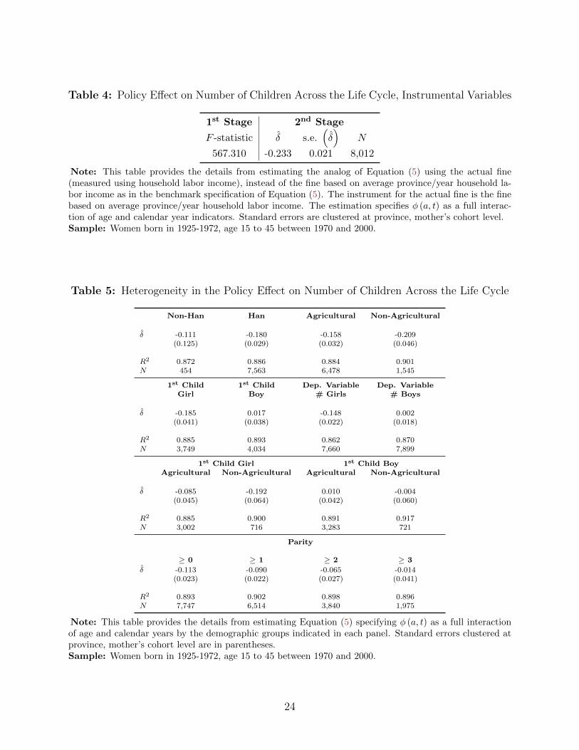
Table 4: Policy E↵ect on Number of Children Across the Life Cycle, Instrumental Variables

1st Stage 2nd Stage

F -statistic � s.e.⇣�⌘

N

567.310 -0.233 0.021 8,012

Note: This table provides the details from estimating the analog of Equation (5) using the actual fine(measured using household labor income), instead of the fine based on average province/year household la-bor income as in the benchmark specification of Equation (5). The instrument for the actual fine is the finebased on average province/year household labor income. The estimation specifies � (a, t) as a full interac-tion of age and calendar year indicators. Standard errors are clustered at province, mother’s cohort level.Sample: Women born in 1925-1972, age 15 to 45 between 1970 and 2000.

Table 5: Heterogeneity in the Policy E↵ect on Number of Children Across the Life Cycle

Non-Han Han Agricultural Non-Agricultural

� -0.111 -0.180 -0.158 -0.209(0.125) (0.029) (0.032) (0.046)

R2 0.872 0.886 0.884 0.901N 454 7,563 6,478 1,545

1st Child 1st Child Dep. Variable Dep. VariableGirl Boy # Girls # Boys

� -0.185 0.017 -0.148 0.002(0.041) (0.038) (0.022) (0.018)

R2 0.885 0.893 0.862 0.870N 3,749 4,034 7,660 7,899

1st Child Girl 1st Child BoyAgricultural Non-Agricultural Agricultural Non-Agricultural

� -0.085 -0.192 0.010 -0.004(0.045) (0.064) (0.042) (0.060)

R2 0.885 0.900 0.891 0.917N 3,002 716 3,283 721

Parity

� 0 � 1 � 2 � 3

� -0.113 -0.090 -0.065 -0.014(0.023) (0.022) (0.027) (0.041)

R2 0.893 0.902 0.898 0.896N 7,747 6,514 3,840 1,975

Note: This table provides the details from estimating Equation (5) specifying � (a, t) as a full interactionof age and calendar years by the demographic groups indicated in each panel. Standard errors clustered atprovince, mother’s cohort level are in parentheses.Sample: Women born in 1925-1972, age 15 to 45 between 1970 and 2000.

24

cohorts, the results remain virtually identical. This is sensible because identification relies

on within-woman policy variation and not on relatively old “pure controls” never exposed

to the policy.

Estimation of standard errors also requires a specification decision. It requires specification

of the correlation structure of the panel observations. Panel (c) of Table 3 shows that the

estimate of � remains significant at the 95% level when allowing for woman, province, birth-

cohort, and province times birth-cohort correlation structures.

Measuring the Fine Using Household- and Year-Specific Labor Income. Through-

out this section, I measure the fine in terms of average province- and year-specific household

labor income. An alternative is to use actual household labor income. Even if actual house-

hold labor income is exogenous, it is potentially measured with error, especially given the

institutional framework in China where in-kind transfers were included in total labor income.

I construct household labor income and obtain a fine based on actual household labor in-

come, ˜⌧ia. I provide details of these constructions in Appendix A.I. I use ⌧ia as an instrument

for ˜⌧ia to obtain an instrumental-variable estimate of �. Table 4 shows that the results are

closely aligned to the baseline in Table 3.

Other Dimensions of Heterogeneity. The main sources of heterogeneity in the policy

e↵ect are maternal age and sex of the first child. Table 5 provides a summary of these and

other sources of heterogeneity. Despite the common use of ethnic minorities as a “control

group” that was not exposed to the policy, Figure 3 documents that, in some regions, ethnic

minorities did face sizable fines for having more than one child. Table 5 shows that the

policy had a negative e↵ect on the fertility of ethnic minorities, although the small sample

of these women does not allow for precise inference.

Similarly, previous studies argue that women from agricultural hukou faced a less restrictive

policy. It is actually the case that the e↵ects across hukou types are similar. The di↵erence

in the policy e↵ect by sex of the first child persists across hukou types. Finally, the e↵ects

are strongest at lower parities. This is not surprising because the decline in fertility driven

by economic factors, which I explain in Section VI, indicates that the policy was not binding

at higher-order parities.

Fertility and the Economic Environment. Panel (d) of Table 3 shows that, once I

condition on calendar year and age e↵ects, the policy e↵ect is robust to accounting for the

economic environment. This includes various specifications to condition on the information

in Zia. To directly assess the relationship between fertility and these categories, Figure 8

25

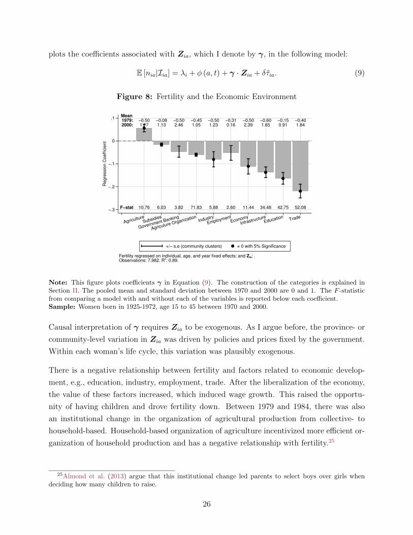
plots the coe�cients associated with Zia, which I denote by �, in the following model:

E [nia|Iia] = �i + � (a, t) + � ·Zia + �⌧ia. (9)

Figure 8: Fertility and the Economic Environment

Mean

1979:

2000:

F−stat

−0.50 −0.08 −0.50 −0.45 −0.50 −0.31 −0.50 −0.60 −0.15 −0.401.17 1.13 2.46 1.05 1.23 0.16 2.39 1.65 0.91 1.84

10.76 6.03 3.82 71.83 5.88 2.60 11.44 34.48 42.75 52.08

.1

0

−.1

−.2

−.3

Re

gre

ssio

n C

oe

ffic

ien

t

Agriculture

Subsidies

Government Banking

Agriculure OrganizationIndustry

EmploymentEconomy

InfrastructureEducation

Trade

+/− s.e (community clusters) ≠ 0 with 5% Significance

Fertility regressed on individual, age, and year fixed effects; and Zia; .Observations: 7,982. R

2: 0.89.

Note: This figure plots coe�cients � in Equation (9). The construction of the categories is explained inSection II. The pooled mean and standard deviation between 1970 and 2000 are 0 and 1. The F -statisticfrom comparing a model with and without each of the variables is reported below each coe�cient.Sample: Women born in 1925-1972, age 15 to 45 between 1970 and 2000.

Causal interpretation of � requires Zia to be exogenous. As I argue before, the province- or

community-level variation in Zia was driven by policies and prices fixed by the government.

Within each woman’s life cycle, this variation was plausibly exogenous.

There is a negative relationship between fertility and factors related to economic develop-

ment, e.g., education, industry, employment, trade. After the liberalization of the economy,

the value of these factors increased, which induced wage growth. This raised the opportu-

nity of having children and drove fertility down. Between 1979 and 1984, there was also

an institutional change in the organization of agricultural production from collective- to

household-based. Household-based organization of agriculture incentivized more e�cient or-

ganization of household production and has a negative relationship with fertility.25

25Almond et al. (2013) argue that this institutional change led parents to select boys over girls whendeciding how many children to raise.

26

Another factor, housing prices, which have steadily increased in China (Zhang and Fung,

2006), could have negatively a↵ected family size.26 The data availability does not allow me

to measure housing prices during my period of analysis. The infrastructure factor could be

interpreted as an approximation of housing prices, given that it is measured by construction

of urban infrastructure. There is a stark negative relationship between this factor and

fertility, and the factor increased between 1979 and 2000.

IV. Policy E↵ects on the Onset of Fertility and Birth Spacing

The analysis in Section III approximates a stochastic counting process. The rate or the in-

tensity of this process is the hazard of having a child at each birth spell (Aalen et al., 2001).

I complement the analysis in Section III by identifying and estimating the parameters that

describe the hazards at each birth spell. This allows me to analyze life-cycle fertility through

the onset of fertility and birth spacing.

I follow Heckman and Walker (1990) and model the birth process as follows. Woman i

becomes viable for pregnancy at age a = 15. As before, nia and Iia denote her number

of children and her information set when she is a years old. She can give up to P births

and her birth spells, conditional on the age-relevant information set, are A1, . . . , AP . If the

conditional birth spells are absolutely continuous and women have no anticipatory behavior,

a conditional hazard characterizes the spells (Yashin and Arjas, 1988). Dropping individual

indices for brevity and denoting the parity as an argument of the age, the conditional hazard

of giving birth j at age a(j � 1) and spell duration ↵j is:

hj

�↵j|I(a(j�1)+↵j)

�(10)

and has an associated survival function

Sj

�↵j|I(a(j�1)+↵j)

�:= hj

�↵j|I(a(j�1)+↵j)

�

= exp

2

4�↵jZ

15

hj

�u|I(a(j�1)+↵j)

�du

3

5 . (11)

This model allows me to study the onset of fertility. For example, the probability of the

onset of fertility for a woman who becomes at risk of pregnancy at age a = 15 is:

1� Pr�A1 > ↵1|I(a(0)+↵1)

�= 1� S1

�↵1|I(a(0)+↵1)

�. (12)

The onset of fertility happens at age A1 := a1 and the woman arrives at the following state

26Dettling and Kearney (2014) document the negative e↵ect of housing prices on fertility.

27

in her birth process: na1 = 1.

This model also allows me to study birth spacing. For example, the probability of giving

birth during the jth spell is

1� Pr�Aj > ↵j|I(a(j�1)+↵j)

�= 1� Sj

�↵j|I(a(j�1)+↵j)

�, (13)

where Aj := Aj � Aj�1, i.e., the spell between birth j � 1 and birth j.

By assumption, birth spells terminate at rate hj

�↵j|I(a(j�1)+↵j)

�. Thus, careful specification

of I(a(j�1)+↵j) is important. Because the counting process in Section III and the hazard are

intrinsically linked, I specify the information set similarly, relying on age and calendar year

controls. In Table A.9, I document the robustness to functional form assumptions when

specifying these controls and controls for the economic environment. Given the particular

interest in di↵erent birth spells, I also allow for parity-specific hazard drifts and for parity-

specific fine e↵ects.

As in Section III, it is necessary to account for woman-level unobserved heterogeneity. This

allows me to rely on within-woman policy variation to identify the parameters of inter-

est. I index unobserved heterogeneity at the woman level by a scalar random variable, !,

with age-invariant conditional distribution function F (!) and with support ⌦. This hetero-

geneity is part of I(a(j�1)+↵j). In a slight abuse of notation, I make explicit the dependence

of this dimension as an additional argument in the conditional hazard, hj

�↵j|I(a(j�1)+↵j),!

�.

For empirical purposes, I specify hj (·|·) as follows:

hj

�↵j|I(a(j�1)+↵j),!

�= exp

2

4�0j +

KjX

k=1

�kj

↵⇣kjj � 1

⇣kj

!+X�j + fj!

3

5 , (14)

whereX are time-varying characteristics (e.g., the fine, age, and calendar year indicators and

controls to account for the economic environment). I assume that the hazard model is Weibull

(Kj = 1, ⇣1j = 0), and find little sensitivity when exploring alternative models in Table A.9,

which is consistent with Heckman and Walker (1990). This model allows for unobserved

heterogeneity correlated within each woman; fj allows for birth-spell-specific dependence on

this heterogeneity. I provide specification and estimation details in Appendix A.III.27

Two important results from Section III remain. First, the hazard does not change when

27This accounts for unobserved heterogeneity by allowing for a random e↵ect that is correlated acrossbirth spells. The random e↵ect, !, is regulated across birth spells by fj . The model in Section III accountsfor heterogeneity through a fixed e↵ect across the life cycle, �i.

28

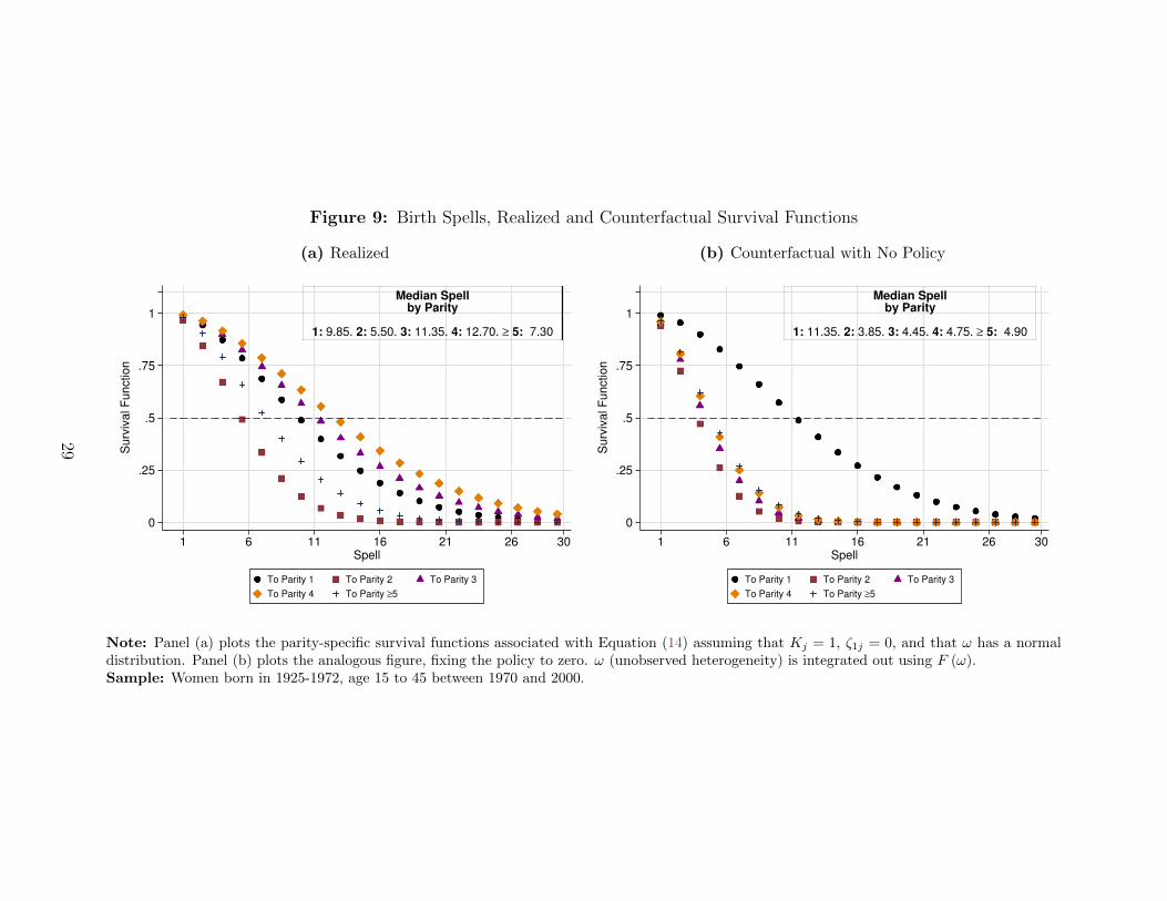
Figure 9: Birth Spells, Realized and Counterfactual Survival Functions

(a) Realized

Median Spellby Parity

1: 9.85. 2: 5.50. 3: 11.35. 4: 12.70. ≥ 5: 7.30

0

.25

.5

.75

1

Surv

ival F

unct

ion

1 6 11 16 21 26 30Spell

To Parity 1 To Parity 2 To Parity 3

To Parity 4 To Parity ≥5

(b) Counterfactual with No Policy


1: 11.35. 2: 3.85. 3: 4.45. 4: 4.75. ≥ 5: 4.90

0

.25

.5

.75

1

Surv

ival F

unct

ion

1 6 11 16 21 26 30Spell



Note: Panel (a) plots the parity-specific survival functions associated with Equation (14) assuming that Kj = 1, ⇣1j = 0, and that ! has a normaldistribution. Panel (b) plots the analogous figure, fixing the policy to zero. ! (unobserved heterogeneity) is integrated out using F (!).Sample: Women born in 1925-1972, age 15 to 45 between 1970 and 2000.

29

including variables describing the economic environment. That is, once age, calendar year,

and woman-level e↵ects are accounted for, the hazard remains invariant to the inclusion of

variables describing the economy in the conditioning set. Second, future fines have no e↵ect

on the current period’s hazard (consistent with the necessary condition of no anticipatory

behavior to describe the spells using hazards).

A statistic of interest is the e↵ect of the fine on the median number of periods to the onset of

fertility and subsequent births. This is of interest both as realized and in the counterfactual

scenario in which the fine is fixed to zero. More generally, the entire survival function is of

interest.

One way to analyze the survival function is to integrate out unobserved heterogeneity, !. In

doing so, the composition of ! does not vary across parity-specific spells, but the hazard rate

does consider the di↵erent e↵ects that unobserved heterogeneity has across di↵erent spells.

At each spell, the e↵ect is regulated by the parameter fj. Alternatively, it is possible to fix

the value of ! to a specific value of ⌦ (e.g., the mean). I present results integrating out ! in

Figure 9 and present results fixing ! to a specific value in Figure A.9. The qualitative and

quantitative features of both exercises are very similar.

The results indicate that the policy accelerated the onset of fertility by a median of 1.5 years.

An interpretation consistent with the results in Section III is the following. Having children

earlier allows a woman to learn the sex of her first child early in her fertility history. If

she has a girl, she has a longer period of time to plan the birth of a second child given the

restrictions of the policy, i.e., to plan how to face these restrictions. Some women pay the

fine to have a second child while some women do not have a second child. This prolongs

the median spacing between the first and the second child. Spacing between higher order

parities is similarly prolonged.

V. Policy E↵ects on Completed Fertility

Section III documents that the policy e↵ects on the number of children throughout the life

cycle were negative. Section IV documents that the policy operated by prolonging birth

spacing. In this section, I document to what extent these e↵ects diminished completed fer-

tility. The goal is to predict the number of children that each woman did not have due to the

policy. This is of interest in itself and also allows me to compute counterfactual aggregate

fertility statistics.

In Equation (4), the benchmark model that I use to estimate life-cycle policy e↵ects, the

prediction associated with the policy at age a is �sa⌧ia. The prediction at age a conditions

30

on Iia, the information set woman i had when she was a years old. �i :=P45

a=15 �sa⌧ia is the

sum of predictions across ages and represents the reduction in her completed fertility caused

by the policy.28

If the only reduction in fertility came through the fine, �i measures the departure of com-

pleted fertility from the baseline scenario without the policy. If the policy had an additional

e↵ect on the intercept, denoted by �0, �i measures the departure of completed fertility from

the baseline scenario with the policy. An economic interpretation of �0 is that it represents

a fixed cost imposed by the policy in addition to the fine. As long as the object of interest

is the change in completed fertility due to the fine, which was the main policy instrument,

it is irrelevant what �i is a departure of. When analyzing a counterfactual scenario with

no policy, it is necessary to predict the departure from the baseline with no policy, i.e., to

consider the reduction in fertility given by �0 +�i.

This poses the additional challenge of identifying �0. Tackling this challenge requires sep-

arating the constant in � (a, t) from �0. As an example, consider parameterizing � (a, t)

using a set of age indicators, �A (a), and a second-degree polynomial of the calendar years,

�T (t) := '0 + '1t+ '2t2.29

Equation (4) becomes

E[nia|Iia] = �i + �A (a) + '0 + '1t+ '2t2| {z }:=�(a,t)

+�0 + �sa⌧ia

= '0 + �0| {z }constant

+�i + �A (a) + '1t+ '2t2 + �sa⌧ia. (15)

The challenge is to separately identify '0 and �0. I do so by constructing an auxiliary sample

of communities not a↵ected by the policy. This allows me to verify that the policy had no

intercept e↵ect (�0 = 0), although it had a slope e↵ect (�sa < 0).

I construct an auxiliary sample of women whose communities began to implement the policy

after 2000, which is after my period of analysis.30 Figure 10a shows evidence that �sa = 0

28This estimate is a sum of predictions across the life cycle (a level), not a derivative like the policy e↵ectsestimated in Section III. Heckman et al. (2006) discuss identification in levels in a general policy evaluationsetting. Identification in levels and identification at infinity are related concepts, where an auxiliary sampleis useful to identify the intercepts that are necessary when constructing levels (Heckman, 1990).

29Figure A.11 shows that this parameterization has a minimal impact on the estimate of �. �A (a) couldalso have an intercept. The very low levels of fertility between ages 15 and 20 make plausible the assumptionthat there is no intercept associated with age.

30I obtain this information through a survey of community leaders in CHARLS asking when the One-ChildPolicy began to be locally implemented.

31

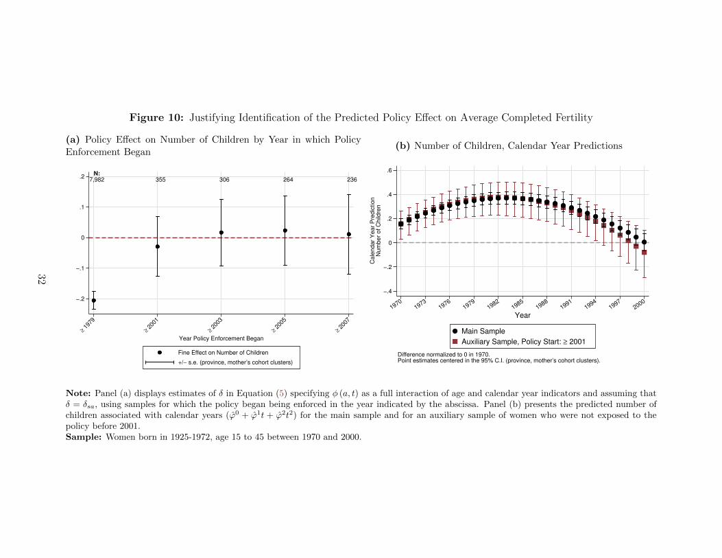
Figure 10: Justifying Identification of the Predicted Policy E↵ect on Average Completed Fertility

(a) Policy E↵ect on Number of Children by Year in which PolicyEnforcement Began

N:

7,982 355 306 264 236

−.2

−.1

0

.1

.2

≥ 1

979

≥ 2

001

≥ 2

003

≥ 2

005

≥ 2

007

Year Policy Enforcement Began

Fine Effect on Number of Children

+/− s.e. (province, mother’s cohort clusters)

(b) Number of Children, Calendar Year Predictions

−.4

−.2

0

.2

.4

.6

Cale

ndar

Year

Pre

dic

tion

Num

ber

of C

hild

ren

19701973

19761979

19821985

19881991

19941997

2000

Year

Main Sample

Auxiliary Sample, Policy Start: ≥ 2001

Difference normalized to 0 in 1970.Point estimates centered in the 95% C.I. (province, mother’s cohort clusters).

Note: Panel (a) displays estimates of � in Equation (5) specifying � (a, t) as a full interaction of age and calendar year indicators and assuming that� = �sa, using samples for which the policy began being enforced in the year indicated by the abscissa. Panel (b) presents the predicted number ofchildren associated with calendar years ('0 + '1t + '2t2) for the main sample and for an auxiliary sample of women who were not exposed to thepolicy before 2001.Sample: Women born in 1925-1972, age 15 to 45 between 1970 and 2000.

32

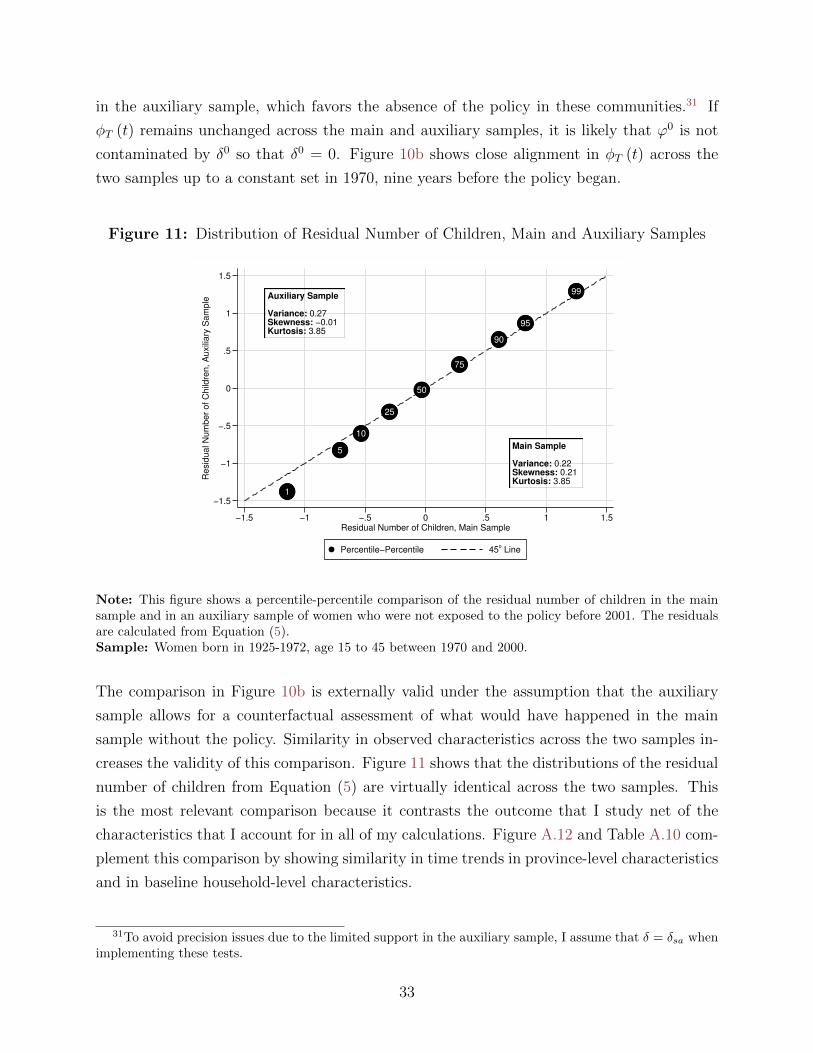
in the auxiliary sample, which favors the absence of the policy in these communities.31 If

�T (t) remains unchanged across the main and auxiliary samples, it is likely that '0 is not

contaminated by �0 so that �0 = 0. Figure 10b shows close alignment in �T (t) across the

two samples up to a constant set in 1970, nine years before the policy began.

Figure 11: Distribution of Residual Number of Children, Main and Auxiliary Samples

1

5

10

25

50

75

90

95

99Auxiliary Sample Variance: 0.27Skewness: −0.01Kurtosis: 3.85

Main Sample Variance: 0.22Skewness: 0.21Kurtosis: 3.85

−1.5

−1

−.5

0

.5

1

1.5

Re

sid

ua

l Nu

mb

er

of

Ch

ildre

n,

Au

xilia

ry S

am

ple

−1.5 −1 −.5 0 .5 1 1.5Residual Number of Children, Main Sample

Percentile−Percentile 45o Line

Note: This figure shows a percentile-percentile comparison of the residual number of children in the mainsample and in an auxiliary sample of women who were not exposed to the policy before 2001. The residualsare calculated from Equation (5).Sample: Women born in 1925-1972, age 15 to 45 between 1970 and 2000.

The comparison in Figure 10b is externally valid under the assumption that the auxiliary

sample allows for a counterfactual assessment of what would have happened in the main

sample without the policy. Similarity in observed characteristics across the two samples in-

creases the validity of this comparison. Figure 11 shows that the distributions of the residual

number of children from Equation (5) are virtually identical across the two samples. This

is the most relevant comparison because it contrasts the outcome that I study net of the

characteristics that I account for in all of my calculations. Figure A.12 and Table A.10 com-

plement this comparison by showing similarity in time trends in province-level characteristics

and in baseline household-level characteristics.

31To avoid precision issues due to the limited support in the auxiliary sample, I assume that � = �sa whenimplementing these tests.

33

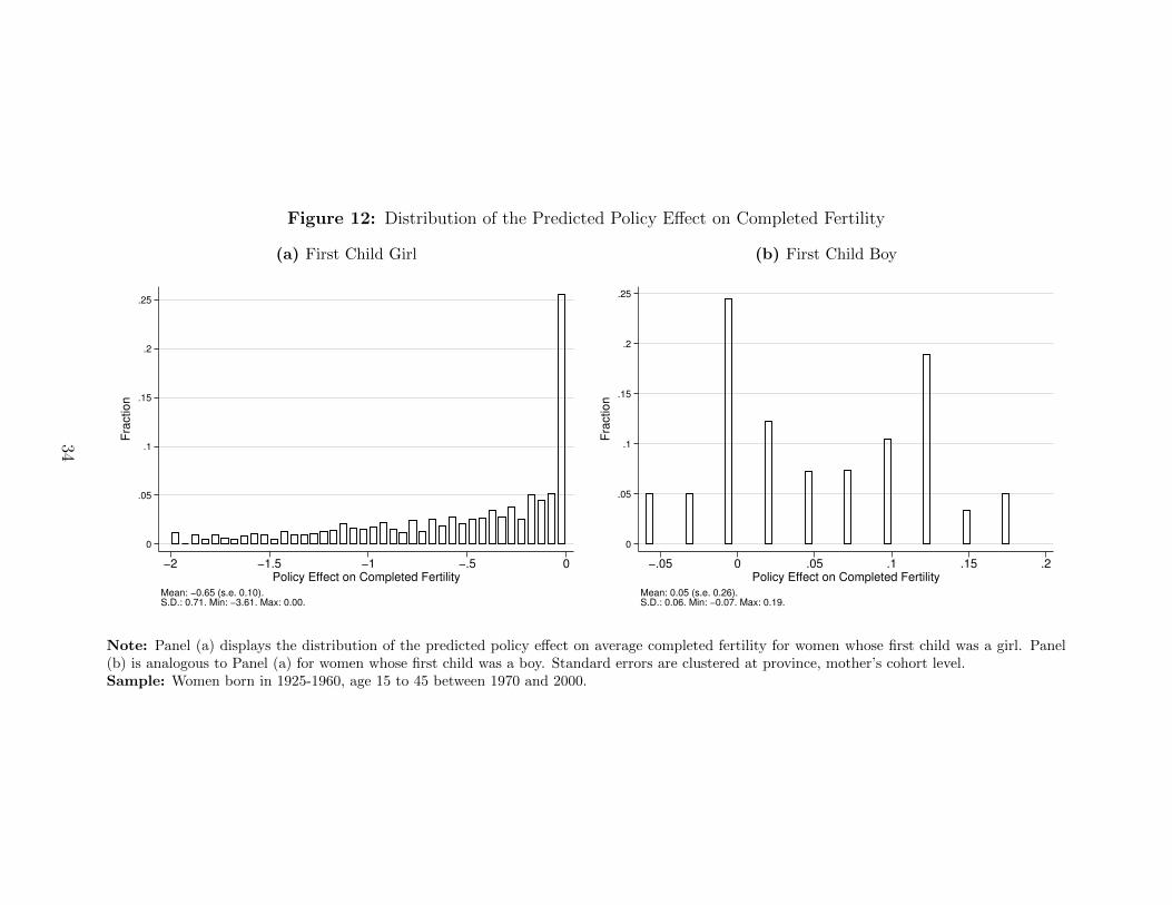
Figure 12: Distribution of the Predicted Policy E↵ect on Completed Fertility

(a) First Child Girl

0

.05

.1

.15

.2

.25

Fra

ctio

n

−2 −1.5 −1 −.5 0Policy Effect on Completed Fertility

Mean: −0.65 (s.e. 0.10).S.D.: 0.71. Min: −3.61. Max: 0.00.

(b) First Child Boy

0

.05

.1

.15

.2

.25

Fra

ctio

n

−.05 0 .05 .1 .15 .2Policy Effect on Completed Fertility

Mean: 0.05 (s.e. 0.26).S.D.: 0.06. Min: −0.07. Max: 0.19.

Note: Panel (a) displays the distribution of the predicted policy e↵ect on average completed fertility for women whose first child was a girl. Panel(b) is analogous to Panel (a) for women whose first child was a boy. Standard errors are clustered at province, mother’s cohort level.Sample: Women born in 1925-1960, age 15 to 45 between 1970 and 2000.

34

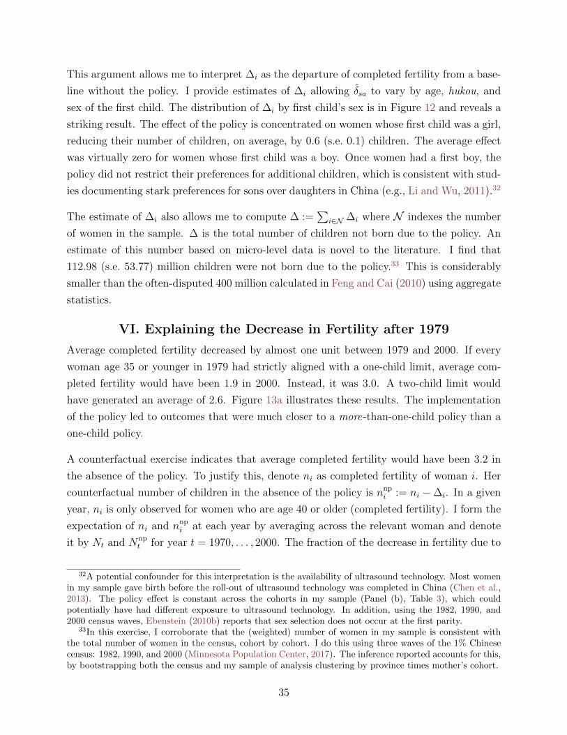
This argument allows me to interpret �i as the departure of completed fertility from a base-

line without the policy. I provide estimates of �i allowing �sa to vary by age, hukou, and

sex of the first child. The distribution of �i by first child’s sex is in Figure 12 and reveals a

striking result. The e↵ect of the policy is concentrated on women whose first child was a girl,

reducing their number of children, on average, by 0.6 (s.e. 0.1) children. The average e↵ect

was virtually zero for women whose first child was a boy. Once women had a first boy, the

policy did not restrict their preferences for additional children, which is consistent with stud-

ies documenting stark preferences for sons over daughters in China (e.g., Li and Wu, 2011).32

The estimate of �i also allows me to compute � :=P

i2N �i where N indexes the number

of women in the sample. � is the total number of children not born due to the policy. An

estimate of this number based on micro-level data is novel to the literature. I find that

112.98 (s.e. 53.77) million children were not born due to the policy.33 This is considerably

smaller than the often-disputed 400 million calculated in Feng and Cai (2010) using aggregate

statistics.

VI. Explaining the Decrease in Fertility after 1979

Average completed fertility decreased by almost one unit between 1979 and 2000. If every

woman age 35 or younger in 1979 had strictly aligned with a one-child limit, average com-

pleted fertility would have been 1.9 in 2000. Instead, it was 3.0. A two-child limit would

have generated an average of 2.6. Figure 13a illustrates these results. The implementation

of the policy led to outcomes that were much closer to a more-than-one-child policy than a

one-child policy.

A counterfactual exercise indicates that average completed fertility would have been 3.2 in

the absence of the policy. To justify this, denote ni as completed fertility of woman i. Her

counterfactual number of children in the absence of the policy is nnpi := ni ��i. In a given

year, ni is only observed for women who are age 40 or older (completed fertility). I form the

expectation of ni and nnpi at each year by averaging across the relevant woman and denote

it by Nt and Nnpt for year t = 1970, . . . , 2000. The fraction of the decrease in fertility due to

32A potential confounder for this interpretation is the availability of ultrasound technology. Most womenin my sample gave birth before the roll-out of ultrasound technology was completed in China (Chen et al.,2013). The policy e↵ect is constant across the cohorts in my sample (Panel (b), Table 3), which couldpotentially have had di↵erent exposure to ultrasound technology. In addition, using the 1982, 1990, and2000 census waves, Ebenstein (2010b) reports that sex selection does not occur at the first parity.

33In this exercise, I corroborate that the (weighted) number of women in my sample is consistent withthe total number of women in the census, cohort by cohort. I do this using three waves of the 1% Chinesecensus: 1982, 1990, and 2000 (Minnesota Population Center, 2017). The inference reported accounts for this,by bootstrapping both the census and my sample of analysis clustering by province times mother’s cohort.

35

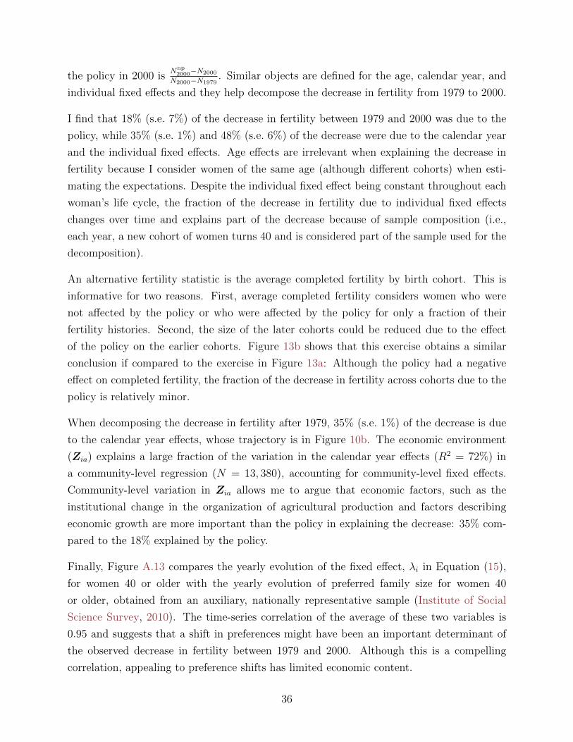
the policy in 2000 is Nnp2000�N2000

N2000�N1979. Similar objects are defined for the age, calendar year, and

individual fixed e↵ects and they help decompose the decrease in fertility from 1979 to 2000.

I find that 18% (s.e. 7%) of the decrease in fertility between 1979 and 2000 was due to the

policy, while 35% (s.e. 1%) and 48% (s.e. 6%) of the decrease were due to the calendar year

and the individual fixed e↵ects. Age e↵ects are irrelevant when explaining the decrease in

fertility because I consider women of the same age (although di↵erent cohorts) when esti-

mating the expectations. Despite the individual fixed e↵ect being constant throughout each

woman’s life cycle, the fraction of the decrease in fertility due to individual fixed e↵ects

changes over time and explains part of the decrease because of sample composition (i.e.,

each year, a new cohort of women turns 40 and is considered part of the sample used for the

decomposition).

An alternative fertility statistic is the average completed fertility by birth cohort. This is

informative for two reasons. First, average completed fertility considers women who were

not a↵ected by the policy or who were a↵ected by the policy for only a fraction of their

fertility histories. Second, the size of the later cohorts could be reduced due to the e↵ect

of the policy on the earlier cohorts. Figure 13b shows that this exercise obtains a similar

conclusion if compared to the exercise in Figure 13a: Although the policy had a negative

e↵ect on completed fertility, the fraction of the decrease in fertility across cohorts due to the

policy is relatively minor.

When decomposing the decrease in fertility after 1979, 35% (s.e. 1%) of the decrease is due

to the calendar year e↵ects, whose trajectory is in Figure 10b. The economic environment

(Zia) explains a large fraction of the variation in the calendar year e↵ects (R2 = 72%) in

a community-level regression (N = 13, 380), accounting for community-level fixed e↵ects.

Community-level variation in Zia allows me to argue that economic factors, such as the

institutional change in the organization of agricultural production and factors describing

economic growth are more important than the policy in explaining the decrease: 35% com-

pared to the 18% explained by the policy.

Finally, Figure A.13 compares the yearly evolution of the fixed e↵ect, �i in Equation (15),

for women 40 or older with the yearly evolution of preferred family size for women 40

or older, obtained from an auxiliary, nationally representative sample (Institute of Social

Science Survey, 2010). The time-series correlation of the average of these two variables is

0.95 and suggests that a shift in preferences might have been an important determinant of

the observed decrease in fertility between 1979 and 2000. Although this is a compelling

correlation, appealing to preference shifts has limited economic content.

36

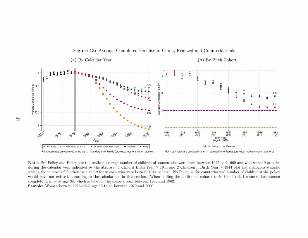
Figure 13: Average Completed Fertility in China, Realized and Counterfactuals

(a) By Calendar Year

3.0

3.3

1.9

2.6

2

2.5

3

3.5

4

Ave

rage C

om

ple

ted F

ert

ility

19701975

19791983

19871991

19952000

Year

Pre−Policy 1 Child if Birth Year ≥ 1944 2 Children if Birth Year ≥ 1944 No Policy Policy

Point estimates are centered in the the +/− standard error bands (province, mother’s cohort clusters).

(b) By Birth Cohort

2.2

2.8

1

2

3

4

Ave

rage C

om

ple

ted F

ert

ility

1934(45)

1938(41)

1942(37)

1946(33)

1950(29)

1954(25)

1958(21)

1962(17)


No Policy Realized

Point estimates are centered in the +/− standard error bands (province, mother’s cohort clusters).

Note: Pre-Policy and Policy are the realized average number of children of women who were born between 1925 and 1960 and who were 40 or olderduring the calendar year indicated by the abscissa. 1 Child if Birth Year � 1944 and 2 Children if Birth Year � 1944 plot the analogous statisticsetting the number of children to 1 and 2 for women who were born in 1944 or later. No Policy is the counterfactual number of children if the policywould have not existed, according to the calculations in this section. When adding the additional cohorts to in Panel (b), I assume that womencomplete fertility at age 38, which is true for the cohorts born between 1960 and 1962.Sample: Women born in 1925-1962, age 15 to 45 between 1970 and 2000.

37

VII. Comparison to Previous Literature

The quantitatively precise characterization of fertility outcomes and the incentives imposed

by the One-Child Policy in a longitudinal setting is a major contribution of this paper. It

allows me to exploit a novel empirical strategy leveraging variation within women and across

demographic groups, provinces, and time to estimate policy e↵ects on the number of children

at di↵erent stages of the life cycle, on birth spacing, and on completed fertility. A life-cycle

analysis of induced abortions and miscarriages allows me to corroborate the models that I

use when estimating policy e↵ects. In the context of the One-Child Policy, estimates using

longitudinal outcomes and variation are novel.

Two previous studies provide benchmarks for comparison. Ebenstein (2010b) uses variation

in the fines across provinces and time to study sex selection at birth. The strategy in Eben-

stein (2010b) is a benchmark for subsequent studies on the consequences of the One-Child

Policy on various household outcomes (e.g., education, age of marriage, intergenerational ed-

ucation).34 Ebenstein (2010b) does not exploit individual-level variation because his strategy

uses repeated cross sections from di↵erent census waves. Qian (2009) uses variation across

provinces and time in only one of the many policy exemptions that I discuss in Section II.

Qian (2009) studies whether the policy had an intergenerational e↵ect on children’s educa-

tion. She does not use variation in the fines.

None of the studies in Zhang (2017) provide conditions for identifying the average policy

e↵ect on completed fertility in levels using micro-level data. As I discuss above, using micro-

level data allows me both to describe the distribution of the number of children that women

did not have and to quantify the total number of children not born due to the policy. To

investigate the empirical advantage of the variation that I exploit, I compare my results on

average completed fertility to results using other strategies.35

I first explore a result constructing the fine without the exemptions in column (1). As Fig-

ure 4 describes, the exemptions are a fundamental component of the variation in the fine.

Without them, the policy e↵ect on average completed fertility is a positive and noisy number

that is hard to interpret. I then explore constructing the fine only using the exemption based

34The survey in Zhang (2017) reveals that the strategy in Ebenstein (2010b) is the standard in thisliterature.

35The results in Table 6 also allow for comparison with literature evaluating the e↵ect of monetaryincentives on fertility. Examples include an evaluation of a per-child lump sum subsidy in Canada (Milligan,2005); a lump sum subsidy for 3rd or higher order births in Israel (Cohen et al., 2013); and a per-child lumpsum subsidy granted as part of the tax system in France (Laroque and Salanie, 2014) and in Germany (Haanand Wrohlich, 2011). I compare the results in these papers with my results in Table A.11. Chinese familieswere the most sensitive to economic incentives.

38

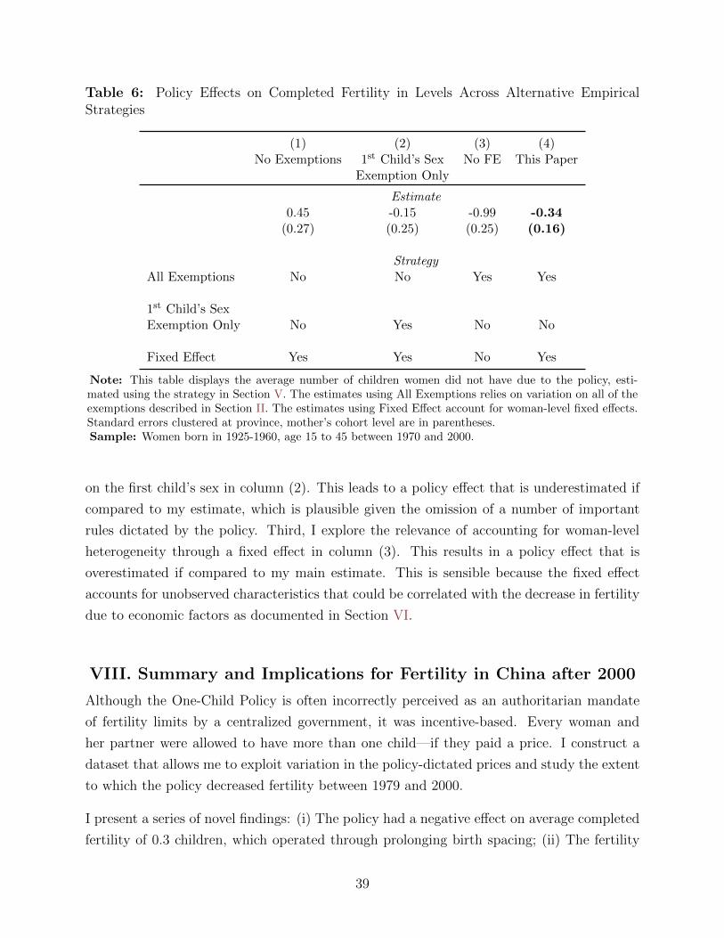
Table 6: Policy E↵ects on Completed Fertility in Levels Across Alternative EmpiricalStrategies

(1) (2) (3) (4)No Exemptions 1st Child’s Sex No FE This Paper

Exemption Only

Estimate0.45 -0.15 -0.99 -0.34(0.27) (0.25) (0.25) (0.16)

StrategyAll Exemptions No No Yes Yes

1st Child’s SexExemption Only No Yes No No

Fixed E↵ect Yes Yes No Yes

Note: This table displays the average number of children women did not have due to the policy, esti-mated using the strategy in Section V. The estimates using All Exemptions relies on variation on all of theexemptions described in Section II. The estimates using Fixed E↵ect account for woman-level fixed e↵ects.Standard errors clustered at province, mother’s cohort level are in parentheses.Sample: Women born in 1925-1960, age 15 to 45 between 1970 and 2000.

on the first child’s sex in column (2). This leads to a policy e↵ect that is underestimated if

compared to my estimate, which is plausible given the omission of a number of important

rules dictated by the policy. Third, I explore the relevance of accounting for woman-level

heterogeneity through a fixed e↵ect in column (3). This results in a policy e↵ect that is

overestimated if compared to my main estimate. This is sensible because the fixed e↵ect

accounts for unobserved characteristics that could be correlated with the decrease in fertility

due to economic factors as documented in Section VI.

VIII. Summary and Implications for Fertility in China after 2000

Although the One-Child Policy is often incorrectly perceived as an authoritarian mandate

of fertility limits by a centralized government, it was incentive-based. Every woman and

her partner were allowed to have more than one child—if they paid a price. I construct a

dataset that allows me to exploit variation in the policy-dictated prices and study the extent

to which the policy decreased fertility between 1979 and 2000.

I present a series of novel findings: (i) The policy had a negative e↵ect on average completed

fertility of 0.3 children, which operated through prolonging birth spacing; (ii) The fertility

39

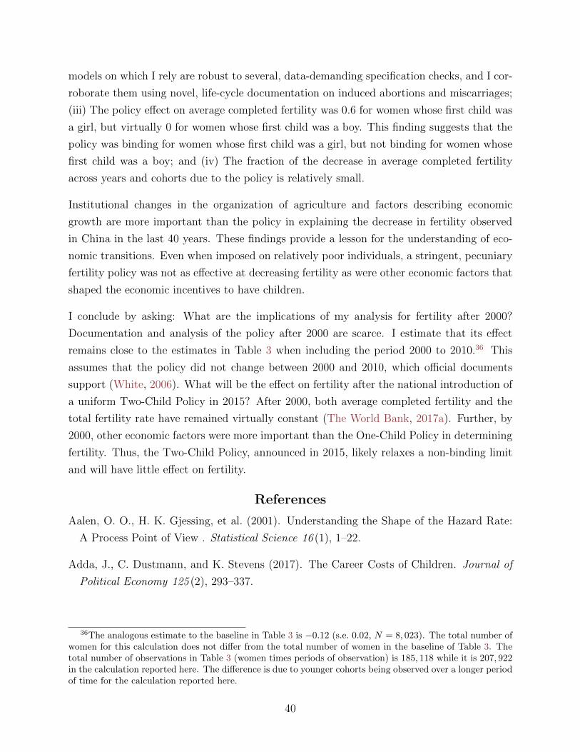
models on which I rely are robust to several, data-demanding specification checks, and I cor-

roborate them using novel, life-cycle documentation on induced abortions and miscarriages;

(iii) The policy e↵ect on average completed fertility was 0.6 for women whose first child was

a girl, but virtually 0 for women whose first child was a boy. This finding suggests that the

policy was binding for women whose first child was a girl, but not binding for women whose

first child was a boy; and (iv) The fraction of the decrease in average completed fertility

across years and cohorts due to the policy is relatively small.

Institutional changes in the organization of agriculture and factors describing economic

growth are more important than the policy in explaining the decrease in fertility observed

in China in the last 40 years. These findings provide a lesson for the understanding of eco-

nomic transitions. Even when imposed on relatively poor individuals, a stringent, pecuniary

fertility policy was not as e↵ective at decreasing fertility as were other economic factors that

shaped the economic incentives to have children.

I conclude by asking: What are the implications of my analysis for fertility after 2000?

Documentation and analysis of the policy after 2000 are scarce. I estimate that its e↵ect

remains close to the estimates in Table 3 when including the period 2000 to 2010.36 This

assumes that the policy did not change between 2000 and 2010, which o�cial documents

support (White, 2006). What will be the e↵ect on fertility after the national introduction of

a uniform Two-Child Policy in 2015? After 2000, both average completed fertility and the

total fertility rate have remained virtually constant (The World Bank, 2017a). Further, by

2000, other economic factors were more important than the One-Child Policy in determining

fertility. Thus, the Two-Child Policy, announced in 2015, likely relaxes a non-binding limit

and will have little e↵ect on fertility.

References

Aalen, O. O., H. K. Gjessing, et al. (2001). Understanding the Shape of the Hazard Rate:

A Process Point of View . Statistical Science 16 (1), 1–22.

Adda, J., C. Dustmann, and K. Stevens (2017). The Career Costs of Children. Journal of

Political Economy 125 (2), 293–337.

36The analogous estimate to the baseline in Table 3 is �0.12 (s.e. 0.02, N = 8, 023). The total number ofwomen for this calculation does not di↵er from the total number of women in the baseline of Table 3. Thetotal number of observations in Table 3 (women times periods of observation) is 185, 118 while it is 207, 922in the calculation reported here. The di↵erence is due to younger cohorts being observed over a longer periodof time for the calculation reported here.

40

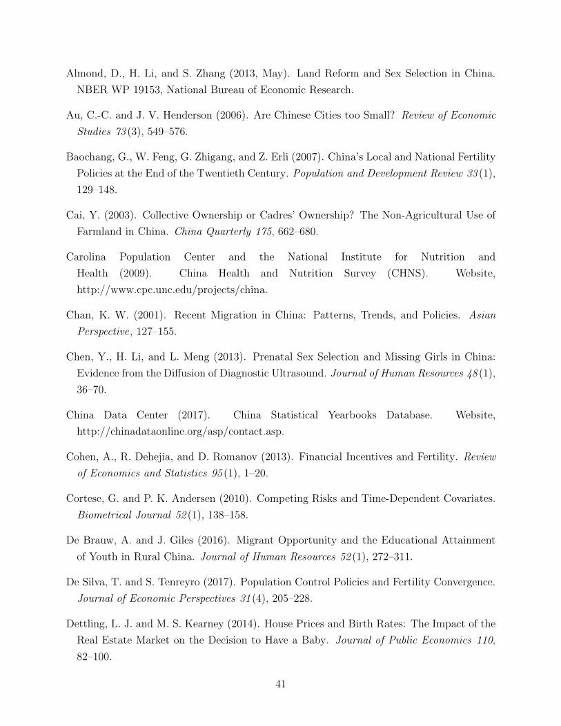
Almond, D., H. Li, and S. Zhang (2013, May). Land Reform and Sex Selection in China.

NBER WP 19153, National Bureau of Economic Research.

Au, C.-C. and J. V. Henderson (2006). Are Chinese Cities too Small? Review of Economic

Studies 73 (3), 549–576.

Baochang, G., W. Feng, G. Zhigang, and Z. Erli (2007). China’s Local and National Fertility

Policies at the End of the Twentieth Century. Population and Development Review 33 (1),

129–148.

Cai, Y. (2003). Collective Ownership or Cadres’ Ownership? The Non-Agricultural Use of

Farmland in China. China Quarterly 175, 662–680.

Carolina Population Center and the National Institute for Nutrition and

Health (2009). China Health and Nutrition Survey (CHNS). Website,

http://www.cpc.unc.edu/projects/china.

Chan, K. W. (2001). Recent Migration in China: Patterns, Trends, and Policies. Asian

Perspective, 127–155.

Chen, Y., H. Li, and L. Meng (2013). Prenatal Sex Selection and Missing Girls in China:

Evidence from the Di↵usion of Diagnostic Ultrasound. Journal of Human Resources 48 (1),

36–70.

China Data Center (2017). China Statistical Yearbooks Database. Website,

http://chinadataonline.org/asp/contact.asp.

Cohen, A., R. Dehejia, and D. Romanov (2013). Financial Incentives and Fertility. Review

of Economics and Statistics 95 (1), 1–20.

Cortese, G. and P. K. Andersen (2010). Competing Risks and Time-Dependent Covariates.

Biometrical Journal 52 (1), 138–158.

De Brauw, A. and J. Giles (2016). Migrant Opportunity and the Educational Attainment

of Youth in Rural China. Journal of Human Resources 52 (1), 272–311.

De Silva, T. and S. Tenreyro (2017). Population Control Policies and Fertility Convergence.

Journal of Economic Perspectives 31 (4), 205–228.

Dettling, L. J. and M. S. Kearney (2014). House Prices and Birth Rates: The Impact of the

Real Estate Market on the Decision to Have a Baby. Journal of Public Economics 110,

82–100.

41

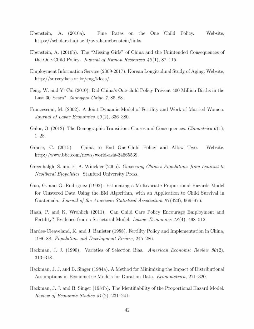
Ebenstein, A. (2010a). Fine Rates on the One Child Policy. Website,

https://scholars.huji.ac.il/avrahamebenstein/links.

Ebenstein, A. (2010b). The “Missing Girls” of China and the Unintended Consequences of

the One-Child Policy. Journal of Human Resources 45 (1), 87–115.

Employment Information Service (2009-2017). Korean Longitudinal Study of Aging. Website,

http://survey.keis.or.kr/eng/klosa/.

Feng, W. and Y. Cai (2010). Did China’s One-child Policy Prevent 400 Million Births in the

Last 30 Years? Zhongguo Gaige 7, 85–88.

Francesconi, M. (2002). A Joint Dynamic Model of Fertility and Work of Married Women.

Journal of Labor Economics 20 (2), 336–380.

Galor, O. (2012). The Demographic Transition: Causes and Consequences. Cliometrica 6 (1),

1–28.

Gracie, C. (2015). China to End One-Child Policy and Allow Two. Website,

http://www.bbc.com/news/world-asia-34665539.

Greenhalgh, S. and E. A. Winckler (2005). Governing China’s Population: from Leninist to

Neoliberal Biopolitics. Stanford University Press.

Guo, G. and G. Rodriguez (1992). Estimating a Multivariate Proportional Hazards Model

for Clustered Data Using the EM Algorithm, with an Application to Child Survival in

Guatemala. Journal of the American Statistical Association 87 (420), 969–976.

Haan, P. and K. Wrohlich (2011). Can Child Care Policy Encourage Employment and

Fertility? Evidence from a Structural Model. Labour Economics 18 (4), 498–512.

Hardee-Cleaveland, K. and J. Banister (1988). Fertility Policy and Implementation in China,

1986-88. Population and Development Review , 245–286.

Heckman, J. J. (1990). Varieties of Selection Bias. American Economic Review 80 (2),

313–318.

Heckman, J. J. and B. Singer (1984a). A Method for Minimizing the Impact of Distributional

Assumptions in Econometric Models for Duration Data. Econometrica, 271–320.

Heckman, J. J. and B. Singer (1984b). The Identifiability of the Proportional Hazard Model.

Review of Economic Studies 51 (2), 231–241.

42

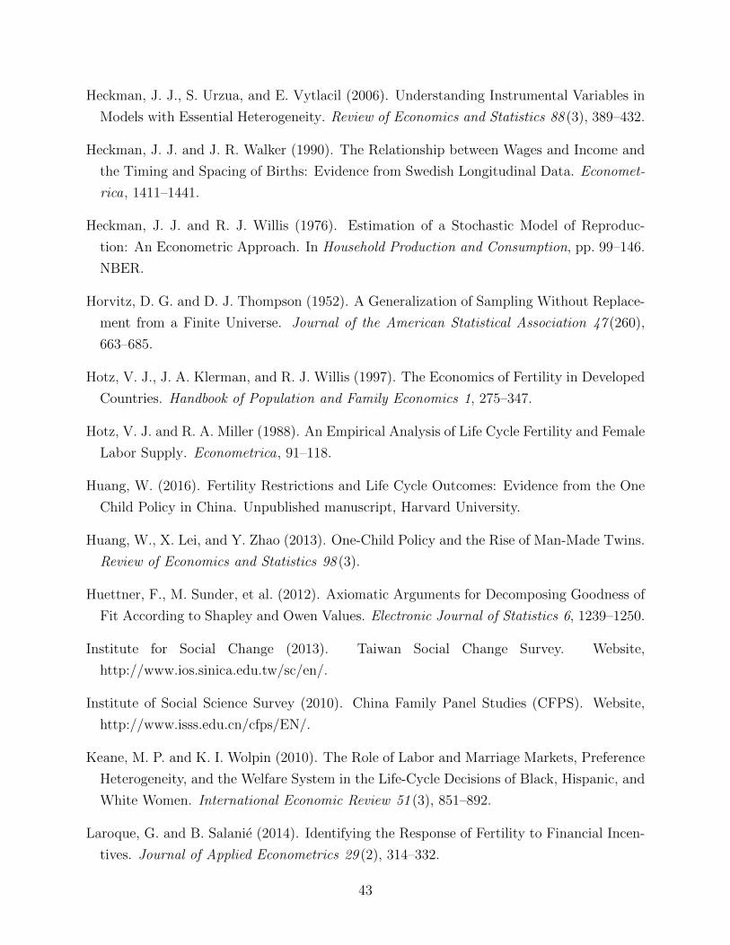
Heckman, J. J., S. Urzua, and E. Vytlacil (2006). Understanding Instrumental Variables in

Models with Essential Heterogeneity. Review of Economics and Statistics 88 (3), 389–432.

Heckman, J. J. and J. R. Walker (1990). The Relationship between Wages and Income and

the Timing and Spacing of Births: Evidence from Swedish Longitudinal Data. Economet-

rica, 1411–1441.

Heckman, J. J. and R. J. Willis (1976). Estimation of a Stochastic Model of Reproduc-

tion: An Econometric Approach. In Household Production and Consumption, pp. 99–146.

NBER.

Horvitz, D. G. and D. J. Thompson (1952). A Generalization of Sampling Without Replace-

ment from a Finite Universe. Journal of the American Statistical Association 47 (260),

663–685.

Hotz, V. J., J. A. Klerman, and R. J. Willis (1997). The Economics of Fertility in Developed

Countries. Handbook of Population and Family Economics 1, 275–347.

Hotz, V. J. and R. A. Miller (1988). An Empirical Analysis of Life Cycle Fertility and Female

Labor Supply. Econometrica, 91–118.

Huang, W. (2016). Fertility Restrictions and Life Cycle Outcomes: Evidence from the One

Child Policy in China. Unpublished manuscript, Harvard University.

Huang, W., X. Lei, and Y. Zhao (2013). One-Child Policy and the Rise of Man-Made Twins.

Review of Economics and Statistics 98 (3).

Huettner, F., M. Sunder, et al. (2012). Axiomatic Arguments for Decomposing Goodness of

Fit According to Shapley and Owen Values. Electronic Journal of Statistics 6, 1239–1250.

Institute for Social Change (2013). Taiwan Social Change Survey. Website,

http://www.ios.sinica.edu.tw/sc/en/.

Institute of Social Science Survey (2010). China Family Panel Studies (CFPS). Website,

http://www.isss.edu.cn/cfps/EN/.

Keane, M. P. and K. I. Wolpin (2010). The Role of Labor and Marriage Markets, Preference

Heterogeneity, and the Welfare System in the Life-Cycle Decisions of Black, Hispanic, and

White Women. International Economic Review 51 (3), 851–892.

Laroque, G. and B. Salanie (2014). Identifying the Response of Fertility to Financial Incen-

tives. Journal of Applied Econometrics 29 (2), 314–332.

43

Li, L. and X. Wu (2011). Gender of Children, Bargaining Power, and Intra-household

Resource Allocation in China. Journal of Human Resources 46 (2), 295–316.

Li Jinfeng (1992). Jihua Shengyu Guanli. The Administration of Birth Planning.

Lu, X. and E. J. Perry (1997). Danwei: The Changing Chinese Workplace in Historical and

Comparative Perspective. Me Sharpe.

Meng, X., N. Qian, and P. Yared (2015). The Institutional Causes of China’s Great Famine,

1959–1961. Review of Economic Studies 82 (4), 1568–1611.

Milligan, K. (2005). Subsidizing the Stork: New Evidence on Tax Incentives and Fertility.

Review of Economics and Statistics 87 (3), 539–555.

Minnesota Population Center (2017). Integrated Public Use Microdata Series, International

Varsion 6.5 [dataset]. Website, http://doi.org/10.18128/D020.V6.5.

Mo�tt, R. (1984a). Profiles of Fertility, Labour Supply and Wages of Married Women: A

Complete Life Cycle Model. Review of Economic Studies 51 (2), 263–278.

Mo�tt, R. (1984b). The Estimation of Fertility Equations on Panel Data. Journal of Human

Resources , 22–34.

National School of Development (2009-2017). China Health and Retirement Longitudinal

Study (CHARLS). Website, http://charls.pku.edu.cn/en.

Naughton, B. (2007). The Chinese Economy: Transitions and Growth. MIT Press.

Pan, Y. (2017). The Impact of Removing Selective Migration Restrictions on Education

Evidence from China. Journal of Human Resources 52 (3), 859–885.

Powell, T. M. (2012). The Negative Impact of the One-Child Policy on the Chinese Society

as it Related to Parental Support and the Aging of the Population. Georgetown University,

Thesis.

Qian, N. (2009, May). Quantity-Quality and the One Child Policy: The Only-Child Dis-

advantage in School Enrollment in Rural China. NBER WP 14973, National Bureau of

Economic Research.

Scharping, T. (2003). Birth Control in China 1949-2000: Population policy and Demographic

Development. London, Routledge.

44

Sen, A. (2015). Women’s Progress Outdid China’s One-Child-Policy. Website,

http://www.nytimes.com/2015/11/02/opinion/.

Sheran, M. (2007). The Career and Family Choices of Women: A Dynamic Analysis of Labor

Force Participation, Schooling, Marriage, and Fertility Decisions. Review of Economic

Dynamics 10 (3), 367–399.

Sun, X., T. J. Warner, D. L. Yang, and M. Liu (2013). Patterns of Authority and Governance

in Rural China: Who’s in charge? Why? Journal of Contemporary China 22 (83), 733–

754.

Tang, W. and W. L. Parish (2000). Chinese Urban Life under Reform: The Changing Social

Contract. Cambridge University Press.

Tanioka, I., N. Iwai, M. Nitta, and T. Yasuda (2006). Japan General Social Survey. Website,

https://doi.org/10.3886/ICPSR25181.v1.

The Economist (2014). Curbing Climate Change: The Deepest Cuts. Website,

https://www.economist.com/news/briefing/.

The World Bank (2017a). Fertility Rate, Total (Birth per Woman). Website,

http://data.worldbank.org/indicator/.

The World Bank (2017b). GDP per capita (constant 2010 US$). Website,

http://data.worldbank.org/indicator/.

White, T. (2006). China’s Longest Campaign: Birth Planning in the People’s Republic,

1949-2005. Cornell University Press.

Whyte, M. K., W. Feng, and Y. Cai (2015). Challenging Myths about China’s One-Child

Policy. China Journal (74), 144–159.

Whyte, M. K. and W. L. Parish (1985). Urban Life in Contemporary China. University of

Chicago Press.

Xu, D. (1984). China’s Population Policy and Family Planning Work. Population and

Economy 2, 8–9.

Yashin, A. and E. Arjas (1988). A Note on Random Intensities and Conditional Survival

Functions. Journal of Applied Probability 25 (3), 630–635.

Zhang, G. and H.-G. Fung (2006). On the Imbalance between the Real Estate Market and

the Stock Markets in China. Chinese Economy 39 (2), 26–39.

45

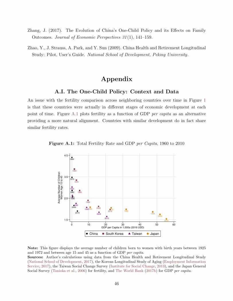
Zhang, J. (2017). The Evolution of China’s One-Child Policy and its E↵ects on Family

Outcomes. Journal of Economic Perspectives 31 (1), 141–159.

Zhao, Y., J. Strauss, A. Park, and Y. Sun (2009). China Health and Retirement Longitudinal

Study: Pilot, User’s Guide. National School of Development, Peking University .

Appendix

A.I. The One-Child Policy: Context and Data

An issue with the fertility comparison across neighboring countries over time in Figure 1

is that these countries were actually in di↵erent stages of economic development at each

point of time. Figure A.1 plots fertility as a function of GDP per capita as an alternative

providing a more natural alignment. Countries with similar development do in fact share

similar fertility rates.

Figure A.1: Total Fertility Rate and GDP per Capita, 1960 to 2010

1960

1970

1980

1990

2000

2010

1960

1970

1980

1990

2000

2010

1960 19701980

1990

2000

2010

1960

1970

1980

1990

2000

20101.5

2.5

3.5

4.5

Ave

rag

e N

um

be

r o

f C

hild

ren

Wo

me

n A

ge

15

to

45

0 10 20 30 40 50 60GDP per Capita in 1,000s (2016 USD)

China South Korea Taiwan Japan

Note: This figure displays the average number of children born to women with birth years between 1925and 1972 and between age 15 and 45 as a function of GDP per capita.Sources: Author’s calculations using data from the China Health and Retirement Longitudinal Study(National School of Development, 2017), the Korean Longitudinal Study of Aging (Employment InformationService, 2017), the Taiwan Social Change Survey (Institute for Social Change, 2013), and the Japan GeneralSocial Survey (Tanioka et al., 2006) for fertility, and The World Bank (2017b) for GDP per capita.

46

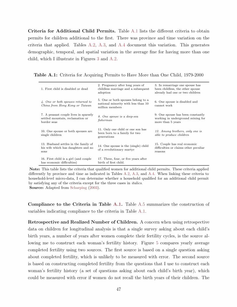
Criteria for Additional Child Permits. Table A.1 lists the di↵erent criteria to obtain

permits for children additional to the first. There was province and time variation on the

criteria that applied. Tables A.2, A.3, and A.4 document this variation. This generates

demographic, temporal, and spatial variation in the average fine for having more than one

child, which I illustrate in Figures 3 and A.2.

Table A.1: Criteria for Acquiring Permits to Have More than One Child, 1979-2000

1. First child is disabled or dead2. Pregnancy after long years ofchildless marriage and a subsequentadoption

3. In remarriage one spouse hasbeen childless, the other spousealready had one or two children

4. One or both spouses returned toChina from Hong Kong or Taiwan

5. One or both spouses belong to anational minority with less than 10million members

6. One spouse is disabled andcannot work

7. A peasant couple lives in sparselysettled mountain, reclamation orborder seas

8. One spouse is a deep-seafisherman

9. One spouse has been constantlyworking in underground mining formore than 5 years

10. One spouse or both spouses aresingle children

11. Only one child or one son hasbeen born to a family for twogenerations

12. Among brothers, only one isable to produce children

13. Husband settles in the family ofhis wife which has daughters and nosons

14. One spouse is the (single) childof a revolutionary martyr

15. Couple has real economicdi�culties or claims other peculiarreasons

16. First child is a girl (and couplehas economic di�culties)

17. Three, four, or five years afterbirth of first child.

Note: This table lists the criteria that qualified women for additional child permits. These criteria applieddi↵erently by province and time as indicated in Tables A.2, A.3, and A.4. When linking these criteria tohousehold-level micro-data, I can determine whether a household qualified for an additional child permitby satisfying any of the criteria except for the three cases in italics.Source: Adapted from Scharping (2003).

Compliance to the Criteria in Table A.1. Table A.5 summarizes the construction of

variables indicating compliance to the criteria in Table A.1.

Retrospective and Realized Number of Children. A concern when using retrospective

data on children for longitudinal analysis is that a single survey asking about each child’s

birth years, a number of years after women complete their fertility cycles, is the source al-

lowing me to construct each woman’s fertility history. Figure 5 compares yearly average

completed fertility using two sources. The first source is based on a single question asking

about completed fertility, which is unlikely to be measured with error. The second source

is based on constructing completed fertility from the questions that I use to construct each

woman’s fertility history (a set of questions asking about each child’s birth year), which

could be measured with error if women do not recall the birth years of their children. The

47

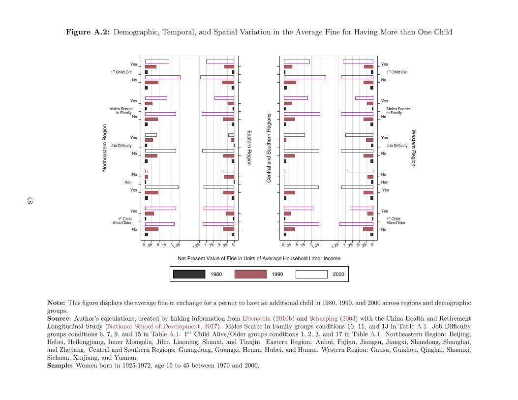
Figure A.2: Demographic, Temporal, and Spatial Variation in the Average Fine for Having More than One Child

Ea

stern

Re

gio

n

No

1st Child

Alive/Older

Yes

Yes

Han

No

No

Job Diffculty

Yes

No

Males Scarce in Family

Yes

No

1st Child Girl

Yes

No

rth

ea

ste

rn R

eg

ion

0 .25 .5 .75 11.25

1.25 1 .75 .5 .25 0

No

1st Child

Alive/Older

Yes

Yes

Han

No

No

Job Diffculty

Yes

No

Males Scarce in Family

Yes

No

1st Child Girl

Yes

We

stern

Re

gio

n

Ce

ntr

al a

nd

So

uth

ern

Re

gio

ns

0 .25 .5 .75 11.25

1.25 1 .75 .5 .25 0

Net Present Value of Fine in Units of Average Household Labor Income

1980 1990 2000

Note: This figure displays the average fine in exchange for a permit to have an additional child in 1980, 1990, and 2000 across regions and demographicgroups.Source: Author’s calculations, created by linking information from Ebenstein (2010b) and Scharping (2003) with the China Health and RetirementLongitudinal Study (National School of Development, 2017). Males Scarce in Family groups conditions 10, 11, and 13 in Table A.1. Job Di�cultygroups conditions 6, 7, 9, and 15 in Table A.1. 1st Child Alive/Older groups conditions 1, 2, 3, and 17 in Table A.1. Northeastern Region: Beijing,Hebei, Heilongjiang, Inner Mongolia, Jilin, Liaoning, Shanxi, and Tianjin. Eastern Region: Anhui, Fujian, Jiangsu, Jiangxi, Shandong, Shanghai,and Zhejiang. Central and Southern Regions: Guangdong, Guangxi, Henan, Hubei, and Hunan. Western Region: Gansu, Guizhou, Qinghai, Shaanxi,Sichuan, Xinjiang, and Yunnan.Sample: Women born in 1925-1972, age 15 to 45 between 1970 and 2000.

48

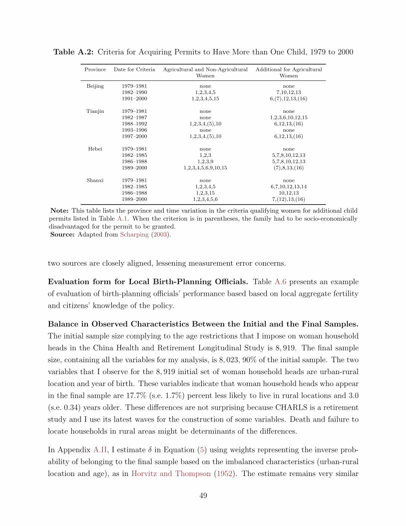
Table A.2: Criteria for Acquiring Permits to Have More than One Child, 1979 to 2000

Province Date for Criteria Agricultural and Non-Agricultural Additional for AgriculturalWomen Women

Beijing 1979–1981 none none1982–1990 1,2,3,4,5 7,10,12,131991–2000 1,2,3,4,5,15 6,(7),12,13,(16)

Tianjin 1979–1981 none none1982–1987 none 1,2,3,6,10,12,151988–1992 1,2,3,4,(5),10 6,12,13,(16)1993–1996 none none1997–2000 1,2,3,4,(5),10 6,12,13,(16)

Hebei 1979–1981 none none1982–1985 1,2,3 5,7,8,10,12,131986–1988 1,2,3,9 5,7,8,10,12,131989–2000 1,2,3,4,5,6,9,10,15 (7),8,13,(16)

Shanxi 1979–1981 none none1982–1985 1,2,3,4,5 6,7,10,12,13,141986–1988 1,2,3,15 10,12,131989–2000 1,2,3,4,5,6 7,(12),13,(16)

Note: This table lists the province and time variation in the criteria qualifying women for additional childpermits listed in Table A.1. When the criterion is in parentheses, the family had to be socio-economicallydisadvantaged for the permit to be granted.Source: Adapted from Scharping (2003).

two sources are closely aligned, lessening measurement error concerns.

Evaluation form for Local Birth-Planning O�cials. Table A.6 presents an example

of evaluation of birth-planning o�cials’ performance based based on local aggregate fertility

and citizens’ knowledge of the policy.

Balance in Observed Characteristics Between the Initial and the Final Samples.

The initial sample size complying to the age restrictions that I impose on woman household

heads in the China Health and Retirement Longitudinal Study is 8, 919. The final sample

size, containing all the variables for my analysis, is 8, 023, 90% of the initial sample. The two

variables that I observe for the 8, 919 initial set of woman household heads are urban-rural

location and year of birth. These variables indicate that woman household heads who appear

in the final sample are 17.7% (s.e. 1.7%) percent less likely to live in rural locations and 3.0

(s.e. 0.34) years older. These di↵erences are not surprising because CHARLS is a retirement

study and I use its latest waves for the construction of some variables. Death and failure to

locate households in rural areas might be determinants of the di↵erences.

In Appendix A.II, I estimate � in Equation (5) using weights representing the inverse prob-

ability of belonging to the final sample based on the imbalanced characteristics (urban-rural

location and age), as in Horvitz and Thompson (1952). The estimate remains very similar

49

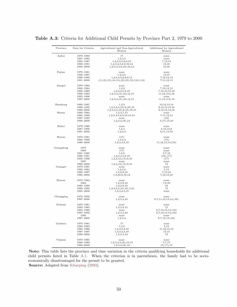
Table A.3: Criteria for Additional Child Permits by Province Part 2, 1979 to 2000

Province Date for Criteria Agricultural and Non-Agricultural Additional for AgriculturalWomen Women

Anhui 1979–1980 17 none1981–1983 1,2,3,5 none1984–1987 1,2,3,4,5,6,9,10 7,12,131988–1991 1,2,3,4,5,6,9,10,12 13,161992–2000 1,2,3,4,5,6,(9),10,12 13,16

Fujian 1979–1981 none none1982–1987 1,2,3,5 13,151988–1990 1,2,3,4,5,6,8,9,14 7,10,12,131991–2000 (1),(2),(3),(4),(5),(6),(8),(9),(10),(14) 7,11,12,13

Jiangxi 1979–1982 none none1983–1984 1,2,3 7,10,12,131985–1989 1,2,3,4,5,9,10 7,10,12,13,161990–1994 1,2,3,4,(5),(9),14,15 11,12,(13),161995–1996 none none1997–2000 1,2,3,4,(5),(9),14,15 11,12,(13),16

Shandong 1982–1987 1,2,3 10,12,13,141988–1995 1,2,3,4,5,(6),8,(9),15 8,12,13,14,161996–2000 1,2,3,4,5,(6),8,(9),10,15 8,12,13,14,16

Henan 1982–1984 1,2,3,7,12 none1985–1986 1,2,3,4,5,6,9,10,14,15 7,11,12,131987–1989 none (16)1990–2000 1,2,3,4,(9),14 5,(7),13,16

Hubei 1979–1986 none none1987–1990 1,2,4 6,10,13,61991–2000 1,2,3,4 6,11,13,16

Hunan 1979–1981 (17) none1982–1988 1,2,3,4 (15)1989–2000 1,2,3,4,5,10 11,12,13,14,(16)

Guangdong 1979 none none1980 (17) none

1981–1985 1,8,9 3,7,161986–1991 1,2,3,4,5,9,10 (16),(17)1992–1996 1,2,3,(4),(5),9,10 (17)

1997 none none1998–2000 1,2,3,(4),(5),9,10 16

Guangxi 1979–1981 none none1982–1984 1,2,3,6 5,151985–1987 1,5,6,9,10 7,13,161988–2000 1,2,35,6,19,14 7,12,13,16

Hainan 1979–1983 none none1984 1,2,3,9,10 7,8,16

1985–1988 1,2,3,9,19 161989–1994 1,2,3,4,5,(6),(9),(14) 151995–2000 1,2,3,4,5,15 none

Chongqing 1979–1996 none none1997–2000 1,2,3,4,10 6,7,11,12,13,14,(16)

Sichuan 1979–1981 none none1982–1983 1,2,3,4,15 151984–1986 none 6,7,12,13,14,(16)1987–1992 1,2,3,4,10 6,7,12,13,14,(16)

1993 none none1997–2000 1,2,3,4 6,7,12,13,(16)

Guizhou 1979–1981 17 none1982–1983 1,2,3 5,151984–1986 1,2,3,5,6,10 11,12,13,151987–1997 1,2,3,4,5,10 13,151998–2000 1,2,3,4,10 13

Yunnan 1979–1985 none none1986–1989 1,2,3,4,5,(6),10,13 5,7,171990–2000 1,2,3,4,(6),10 (5),(7),15

Note: This table lists the province and time variation in the criteria qualifying households for additionalchild permits listed in Table A.1. When the criterion is in parentheses, the family had to be socio-economically disadvantaged for the permit to be granted.Source: Adapted from Scharping (2003).

50

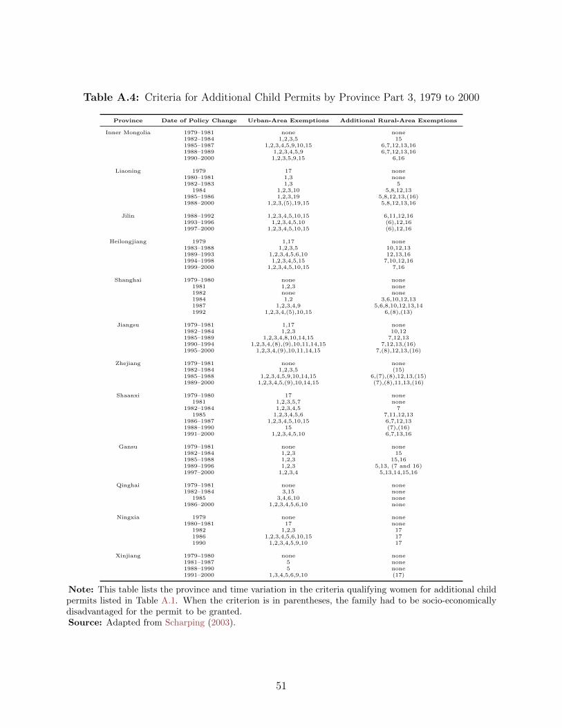
Table A.4: Criteria for Additional Child Permits by Province Part 3, 1979 to 2000

Province Date of Policy Change Urban-Area Exemptions Additional Rural-Area Exemptions

Inner Mongolia 1979–1981 none none1982–1984 1,2,3,5 151985–1987 1,2,3,4,5,9,10,15 6,7,12,13,161988–1989 1,2,3,4,5,9 6,7,12,13,161990–2000 1,2,3,5,9,15 6,16

Liaoning 1979 17 none1980–1981 1,3 none1982–1983 1,3 5

1984 1,2,3,10 5,8,12,131985–1986 1,2,3,19 5,8,12,13,(16)1988–2000 1,2,3,(5),19,15 5,8,12,13,16

Jilin 1988–1992 1,2,3,4,5,10,15 6,11,12,161993–1996 1,2,3,4,5,10 (6),12,161997–2000 1,2,3,4,5,10,15 (6),12,16

Heilongjiang 1979 1,17 none1983–1988 1,2,3,5 10,12,131989–1993 1,2,3,4,5,6,10 12,13,161994–1998 1,2,3,4,5,15 7,10,12,161999–2000 1,2,3,4,5,10,15 7,16

Shanghai 1979–1980 none none1981 1,2,3 none1982 none none1984 1,2 3,6,10,12,131987 1,2,3,4,9 5,6,8,10,12,13,141992 1,2,3,4,(5),10,15 6,(8),(13)

Jiangsu 1979–1981 1,17 none1982–1984 1,2,3 10,121985–1989 1,2,3,4,8,10,14,15 7,12,131990–1994 1,2,3,4,(8),(9),10,11,14,15 7,12,13,(16)1995–2000 1,2,3,4,(9),10,11,14,15 7,(8),12,13,(16)

Zhejiang 1979–1981 none none1982–1984 1,2,3,5 (15)1985–1988 1,2,3,4,5,9,10,14,15 6,(7),(8),12,13,(15)1989–2000 1,2,3,4,5,(9),10,14,15 (7),(8),11,13,(16)

Shaanxi 1979–1980 17 none1981 1,2,3,5,7 none

1982–1984 1,2,3,4,5 71985 1,2,3,4,5,6 7,11,12,13

1986–1987 1,2,3,4,5,10,15 6,7,12,131988–1990 15 (7),(16)1991–2000 1,2,3,4,5,10 6,7,13,16

Gansu 1979–1981 none none1982–1984 1,2,3 151985–1988 1,2,3 15,161989–1996 1,2,3 5,13, (7 and 16)1997–2000 1,2,3,4 5,13,14,15,16

Qinghai 1979–1981 none none1982–1984 3,15 none

1985 3,4,6,10 none1986–2000 1,2,3,4,5,6,10 none

Ningxia 1979 none none1980–1981 17 none

1982 1,2,3 171986 1,2,3,4,5,6,10,15 171990 1,2,3,4,5,9,10 17

Xinjiang 1979–1980 none none1981–1987 5 none1988–1990 5 none1991–2000 1,3,4,5,6,9,10 (17)

Note: This table lists the province and time variation in the criteria qualifying women for additional childpermits listed in Table A.1. When the criterion is in parentheses, the family had to be socio-economicallydisadvantaged for the permit to be granted.Source: Adapted from Scharping (2003).

51

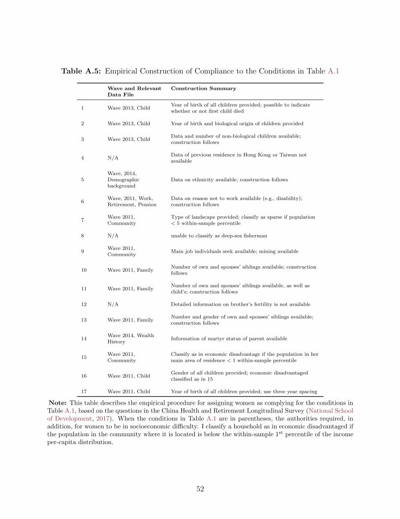
Table A.5: Empirical Construction of Compliance to the Conditions in Table A.1

Wave and Relevant Construction SummaryData File

1 Wave 2013, ChildYear of birth of all children provided; possible to indicatewhether or not first child died

2 Wave 2013, Child Year of birth and biological origin of children provided

3 Wave 2013, ChildData and number of non-biological children available;construction follows

4 N/AData of previous residence in Hong Kong or Taiwan notavailable

5Wave, 2014,Demographicbackground

Data on ethnicity available; construction follows

6Wave, 2011, Work,Retirement, Pension

Data on reason not to work available (e.g., disability);construction follows

7Wave 2011,Community

Type of landscape provided; classify as sparse if population< 5 within-sample percentile

8 N/A unable to classify as deep-sea fisherman


Main job individuals seek available; mining available

10 Wave 2011, FamilyNumber of own and spouses’ siblings available; constructionfollows

11 Wave 2011, FamilyNumber of own and spouses’ siblings available, as well aschild’s; construction follows

12 N/A Detailed information on brother’s fertility is not available

13 Wave 2011, FamilyNumber and gender of own and spouses’ siblings available;construction follows

14Wave 2014, WealthHistory

Information of martyr status of parent available


Classify as in economic disadvantage if the population in hermain area of residence < 1 within-sample percentile

16 Wave 2011, ChildGender of all children provided; economic disadvantagedclassified as in 15

17 Wave 2011, Child Year of birth of all children provided; use three year spacing

Note: This table describes the empirical procedure for assigning women as complying for the conditions inTable A.1, based on the questions in the China Health and Retirement Longitudinal Survey (National Schoolof Development, 2017). When the conditions in Table A.1 are in parentheses, the authorities required, inaddition, for women to be in socioeconomic di�culty. I classify a household as in economic disadvantaged ifthe population in the community where it is located is below the within-sample 1st percentile of the incomeper-capita distribution.

52

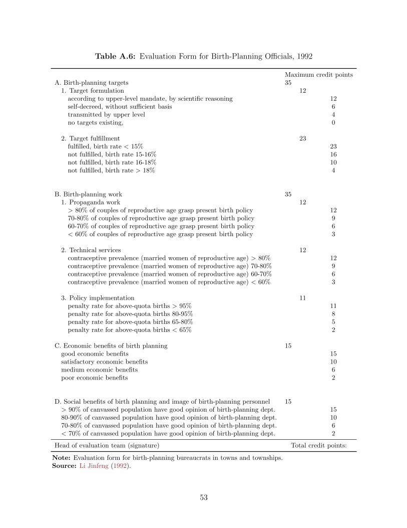
Table A.6: Evaluation Form for Birth-Planning O�cials, 1992

Maximum credit pointsA. Birth-planning targets 35

1. Target formulation 12according to upper-level mandate, by scientific reasoning 12self-decreed, without su�cient basis 6transmitted by upper level 4no targets existing, 0

2. Target fulfillment 23fulfilled, birth rate < 15% 23not fulfilled, birth rate 15-16% 16not fulfilled, birth rate 16-18% 10not fulfilled, birth rate > 18% 4

B. Birth-planning work 351. Propaganda work 12> 80% of couples of reproductive age grasp present birth policy 1270-80% of couples of reproductive age grasp present birth policy 960-70% of couples of reproductive age grasp present birth policy 6< 60% of couples of reproductive age grasp present birth policy 3

2. Technical services 12contraceptive prevalence (married women of reproductive age) > 80% 12contraceptive prevalence (married women of reproductive age) 70-80% 9contraceptive prevalence (married women of reproductive age) 60-70% 6contraceptive prevalence (married women of reproductive age) < 60% 3

3. Policy implementation 11penalty rate for above-quota births > 95% 11penalty rate for above-quota births 80-95% 8penalty rate for above-quota births 65-80% 5penalty rate for above-quota births < 65% 2

C. Economic benefits of birth planning 15good economic benefits 15satisfactory economic benefits 10medium economic benefits 6poor economic benefits 2

D. Social benefits of birth planning and image of birth-planning personnel 15> 90% of canvassed population have good opinion of birth-planning dept. 1580-90% of canvassed population have good opinion of birth-planning dept. 1070-80% of canvassed population have good opinion of birth-planning dept. 6< 70% of canvassed population have good opinion of birth-planning dept. 2

Head of evaluation team (signature) Total credit points:

Note: Evaluation form for birth-planning bureaucrats in towns and townships.Source: Li Jinfeng (1992).

53

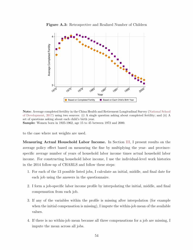
Figure A.3: Retrospective and Realized Number of Children

3

4

Ave

rag

e C

om

ple

ted

Fe

rtili

ty

19701975

19791983

19871991

19952000

Year

Based on Completed Fertility Based on Each Child’s Birth Year

Note: Average completed fertility in the China Health and Retirement Longitudinal Survey (National Schoolof Development, 2017) using two sources: (i) A single question asking about completed fertility; and (ii) Aset of questions asking about each child’s birth year.Sample: Women born in 1925-1962, age 15 to 45 between 1972 and 2000.

to the case where not weights are used.

Measuring Actual Household Labor Income. In Section III, I present results on the

average policy e↵ect based on measuring the fine by multiplying the year- and province-

specific average number of years of household labor income times actual household labor

income. For constructing household labor income, I use the individual-level work histories

in the 2014 follow-up of CHARLS and follow these steps:

1. For each of the 13 possible listed jobs, I calculate an initial, middle, and final date for

each job using the answers in the questionnaire.

2. I form a job-specific labor income profile by interpolating the initial, middle, and final

compensation from each job.

3. If any of the variables within the profile is missing after interpolation (for example

when the initial compensation is missing), I impute the within-job mean of the available

values.

4. If there is no within-job mean because all three compensations for a job are missing, I

impute the mean across all jobs.

54

5. I sum the woman and male households heads incomes and convert the values to 2016

USD dollars, by using the 2000 Chinese price index and the (2016) exchange rate

between the yuan and the dollar.

6. If the household labor income is missing, I impute the province- and year-specific gross

domestic product, by agricultural status. I calculate this using statistical yearbooks

available in China Data Center (2017).When presenting results using this construction, the standard errors are bootstrapped and

clustered as indicated when the result is presented. Each bootstrap procedure repeats the

steps above, to account for the sampling error that comes from constructing the measure.

Individuals who worked in collective agricultural systems had, roughly, the following pay-

ment system: (i) For each day of work, they received a number of points; (ii) The points

were counted along a year; (iii) At the end of the harvest year, the government carried on

the procurement of grains and compensated the collective; and (iv) Dividends were split

according to the accumulated working points. Throughout the year, the workers were com-

pensated in-kind with food, transportation, medical services, etc. For each job, I observe

both the points and how much the realized monetary value of the points was. I also observe

the monetary value individuals assigned to in kind compensation. I sum both the monetary

value of the points and the in-kind compensation. Recall that the estimation strategy that

I employ when using this variable accounts for measurement error.

Measuring Fines Using Observed Household Labor Income. I construct a quantifi-

cation of the fine based on observed household-specific labor income as follows. When the

calculation in Ebenstein (2010b) indicates that the province- and year-specific fine is 1 unit,

then I assign the corresponding individual a unit of her household-specific labor income as

a fine. I proceed similarly for other values of the fine.

Accounting for the Economic Environment. Table A.7 complements Table 1 in Sec-

tion II by listing the full set of measures that I use to describe each category in the economy.

An important component of the economic environment is education. Figure A.4 describes the

level of completed education by cohort in the sample that I analyze. Most women achieve the

final level of education that is dictated and provided by the government, which is generally

completed before age 15 (see Naughton (2007) for details).

A.II. Policy E↵ects on Number of Children Across the Life Cycle

IPW. The sample satisfying my age and cohort requirements in CHARLS contains 8, 919

women. After restricting the sample to women for whom I observe all of the variables for

55

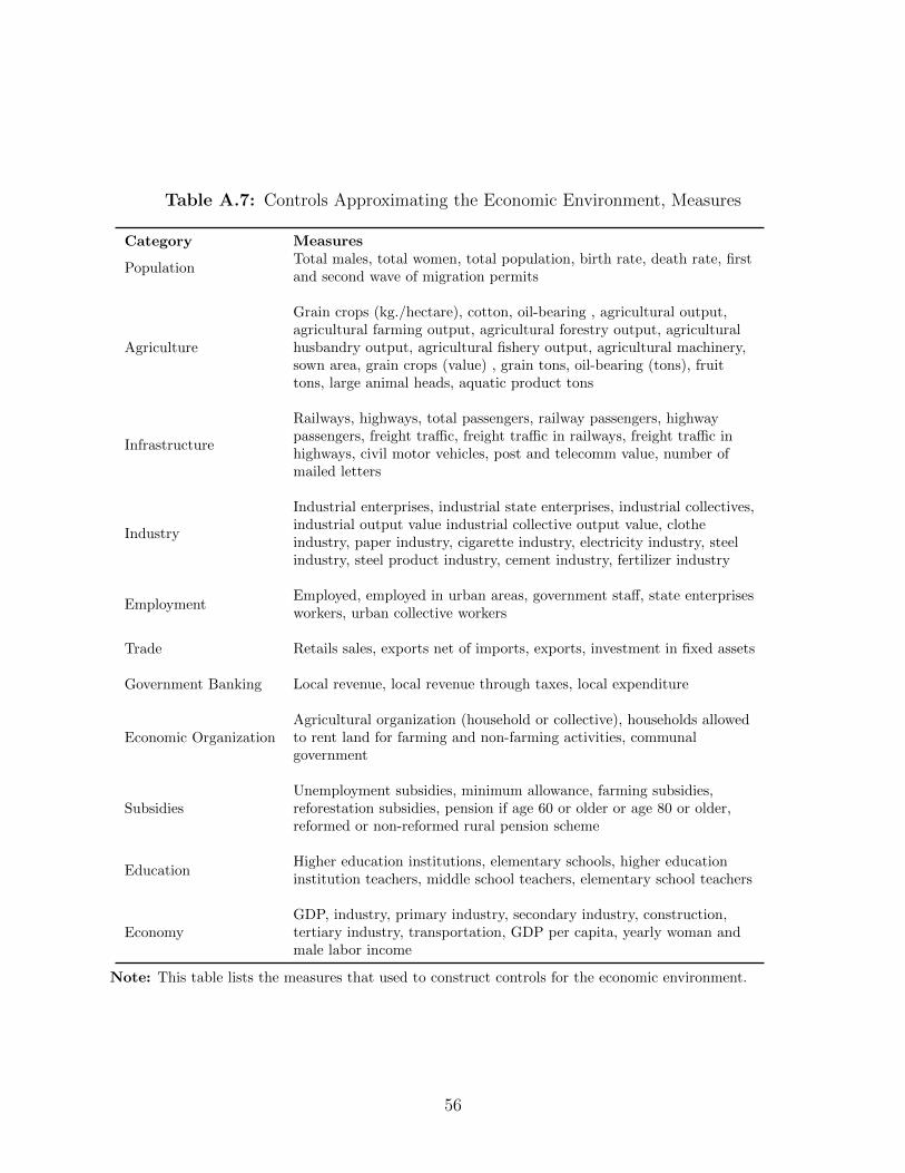
Table A.7: Controls Approximating the Economic Environment, Measures

Category Measures

PopulationTotal males, total women, total population, birth rate, death rate, firstand second wave of migration permits

Agriculture

Grain crops (kg./hectare), cotton, oil-bearing , agricultural output,agricultural farming output, agricultural forestry output, agriculturalhusbandry output, agricultural fishery output, agricultural machinery,sown area, grain crops (value) , grain tons, oil-bearing (tons), fruittons, large animal heads, aquatic product tons

Infrastructure

Railways, highways, total passengers, railway passengers, highwaypassengers, freight tra�c, freight tra�c in railways, freight tra�c inhighways, civil motor vehicles, post and telecomm value, number ofmailed letters

Industry

Industrial enterprises, industrial state enterprises, industrial collectives,industrial output value industrial collective output value, clotheindustry, paper industry, cigarette industry, electricity industry, steelindustry, steel product industry, cement industry, fertilizer industry

EmploymentEmployed, employed in urban areas, government sta↵, state enterprisesworkers, urban collective workers

Trade Retails sales, exports net of imports, exports, investment in fixed assets

Government Banking Local revenue, local revenue through taxes, local expenditure

Economic OrganizationAgricultural organization (household or collective), households allowedto rent land for farming and non-farming activities, communalgovernment

SubsidiesUnemployment subsidies, minimum allowance, farming subsidies,reforestation subsidies, pension if age 60 or older or age 80 or older,reformed or non-reformed rural pension scheme

EducationHigher education institutions, elementary schools, higher educationinstitution teachers, middle school teachers, elementary school teachers

EconomyGDP, industry, primary industry, secondary industry, construction,tertiary industry, transportation, GDP per capita, yearly woman andmale labor income

Note: This table lists the measures that used to construct controls for the economic environment.

56

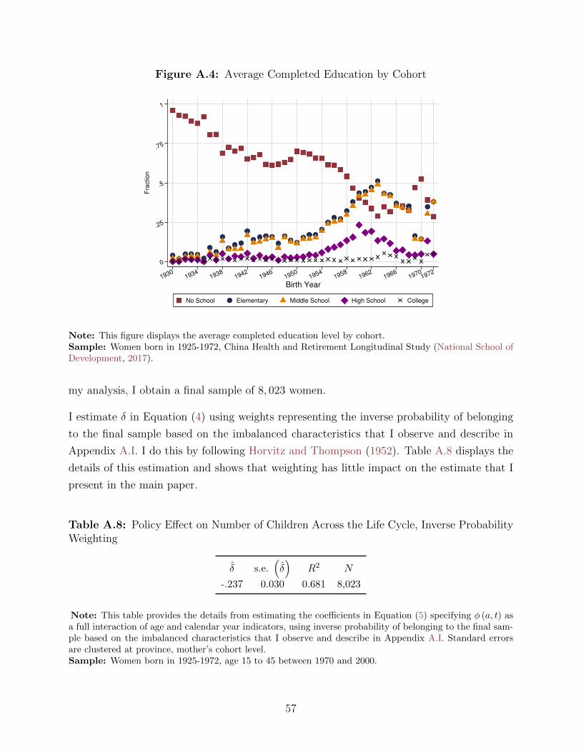
Figure A.4: Average Completed Education by Cohort

1

.75

.5

.25

0

Fra

ctio

n

19301934

19381942

19461950

19541958

19621966

19701972

Birth Year

No School Elementary Middle School High School College

Note: This figure displays the average completed education level by cohort.Sample: Women born in 1925-1972, China Health and Retirement Longitudinal Study (National School ofDevelopment, 2017).

my analysis, I obtain a final sample of 8, 023 women.

I estimate � in Equation (4) using weights representing the inverse probability of belonging

to the final sample based on the imbalanced characteristics that I observe and describe in

Appendix A.I. I do this by following Horvitz and Thompson (1952). Table A.8 displays the

details of this estimation and shows that weighting has little impact on the estimate that I

present in the main paper.

Table A.8: Policy E↵ect on Number of Children Across the Life Cycle, Inverse ProbabilityWeighting

� s.e.⇣�⌘

R2 N

-.237 0.030 0.681 8,023

Note: This table provides the details from estimating the coe�cients in Equation (5) specifying � (a, t) asa full interaction of age and calendar year indicators, using inverse probability of belonging to the final sam-ple based on the imbalanced characteristics that I observe and describe in Appendix A.I. Standard errorsare clustered at province, mother’s cohort level.Sample: Women born in 1925-1972, age 15 to 45 between 1970 and 2000.

57

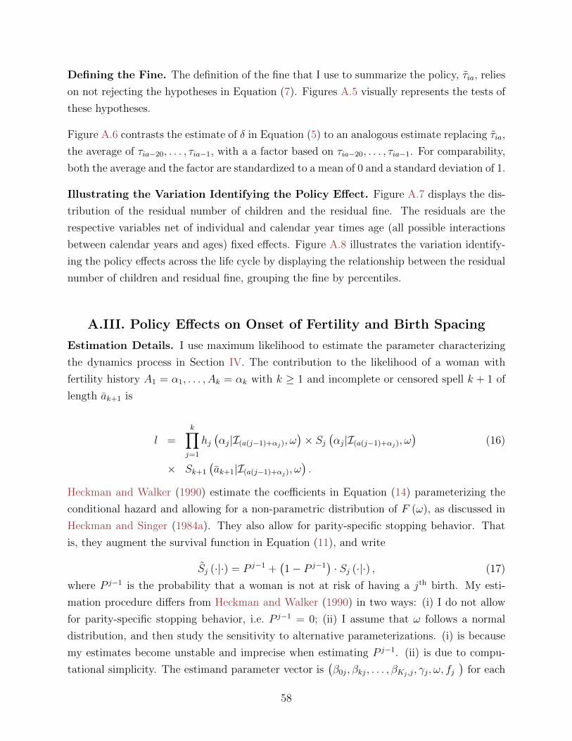
Defining the Fine. The definition of the fine that I use to summarize the policy, ⌧ia, relies

on not rejecting the hypotheses in Equation (7). Figures A.5 visually represents the tests of

these hypotheses.

Figure A.6 contrasts the estimate of � in Equation (5) to an analogous estimate replacing ⌧ia,

the average of ⌧ia�20, . . . , ⌧ia�1, with a a factor based on ⌧ia�20, . . . , ⌧ia�1. For comparability,

both the average and the factor are standardized to a mean of 0 and a standard deviation of 1.

Illustrating the Variation Identifying the Policy E↵ect. Figure A.7 displays the dis-

tribution of the residual number of children and the residual fine. The residuals are the

respective variables net of individual and calendar year times age (all possible interactions

between calendar years and ages) fixed e↵ects. Figure A.8 illustrates the variation identify-

ing the policy e↵ects across the life cycle by displaying the relationship between the residual

number of children and residual fine, grouping the fine by percentiles.

A.III. Policy E↵ects on Onset of Fertility and Birth Spacing

Estimation Details. I use maximum likelihood to estimate the parameter characterizing

the dynamics process in Section IV. The contribution to the likelihood of a woman with

fertility history A1 = ↵1, . . . , Ak = ↵k with k � 1 and incomplete or censored spell k + 1 of

length ak+1 is

l =kY

j=1

hj

�↵j|I(a(j�1)+↵j),!

�⇥ Sj

�↵j|I(a(j�1)+↵j),!

�(16)

⇥ Sk+1

�ak+1|I(a(j�1)+↵j),!

�.

Heckman and Walker (1990) estimate the coe�cients in Equation (14) parameterizing the

conditional hazard and allowing for a non-parametric distribution of F (!), as discussed in

Heckman and Singer (1984a). They also allow for parity-specific stopping behavior. That

is, they augment the survival function in Equation (11), and write

Sj (·|·) = P j�1 +�1� P j�1

�· Sj (·|·) , (17)

where P j�1 is the probability that a woman is not at risk of having a jth birth. My esti-

mation procedure di↵ers from Heckman and Walker (1990) in two ways: (i) I do not allow

for parity-specific stopping behavior, i.e. P j�1 = 0; (ii) I assume that ! follows a normal

distribution, and then study the sensitivity to alternative parameterizations. (i) is because

my estimates become unstable and imprecise when estimating P j�1. (ii) is due to compu-

tational simplicity. The estimand parameter vector is��0j, �kj, . . . , �Kj ,j, �j,!, fj

�for each

58

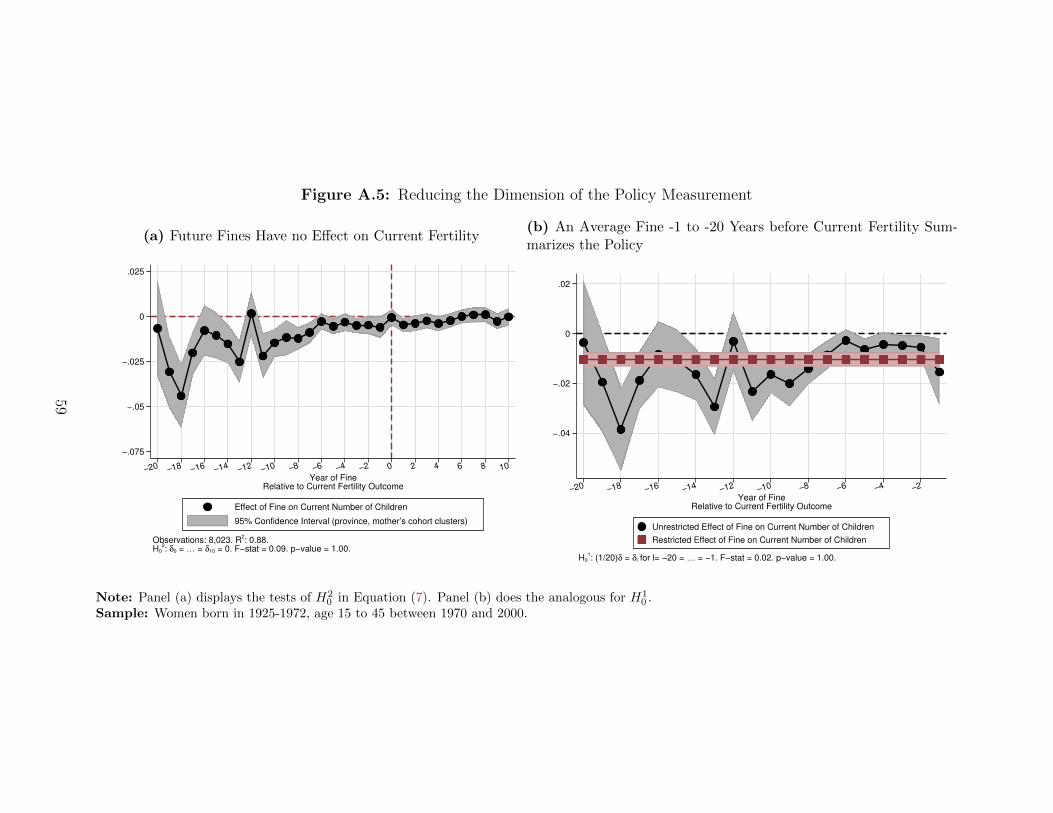
Figure A.5: Reducing the Dimension of the Policy Measurement

(a) Future Fines Have no E↵ect on Current Fertility

.025

0

−.025

−.05

−.075

−20 −18 −16 −14 −12 −10 −8 −6 −4 −2 0 2 4 6 8 10

Year of FineRelative to Current Fertility Outcome

Effect of Fine on Current Number of Children

95% Confidence Interval (province, mother’s cohort clusters)

Observations: 8,023. R2: 0.88.

H02: δ0 = … = δ10 = 0. F−stat = 0.09. p−value = 1.00.

(b) An Average Fine -1 to -20 Years before Current Fertility Sum-marizes the Policy

.02

0

−.02

−.04

−20 −18 −16 −14 −12 −10 −8 −6 −4 −2

Year of FineRelative to Current Fertility Outcome

Unrestricted Effect of Fine on Current Number of Children

Restricted Effect of Fine on Current Number of Children

H01: (1/20)δ = δl for l= −20 = … = −1. F−stat = 0.02. p−value = 1.00.

Note: Panel (a) displays the tests of H20 in Equation (7). Panel (b) does the analogous for H1

0 .Sample: Women born in 1925-1972, age 15 to 45 between 1970 and 2000.

59

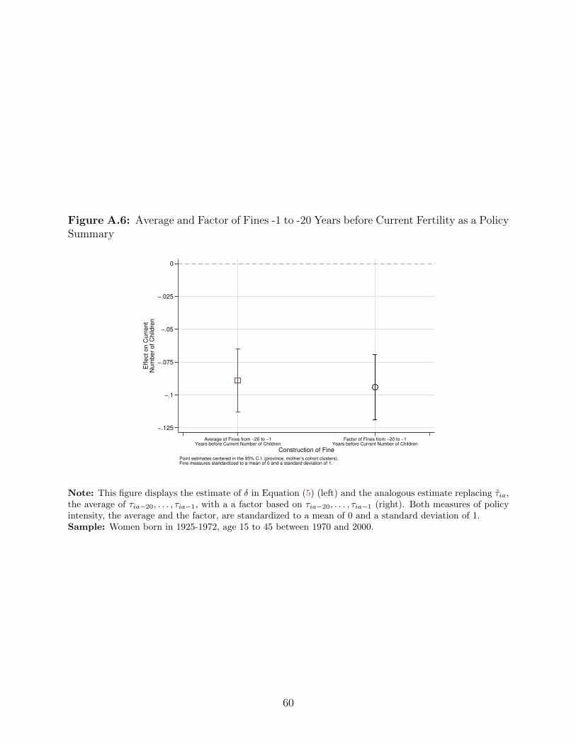
Figure A.6: Average and Factor of Fines -1 to -20 Years before Current Fertility as a PolicySummary

0

−.025

−.05

−.075

−.1

−.125

Eff

ect

on

Cu

rre

nt

Nu

mb

er

of

Ch

ildre

n

Average of Fines from −20 to −1Years before Current Number of Children

Factor of Fines from −20 to −1Years before Current Number of Children

Construction of Fine

Point estimates centered in the 95% C.I. (province, mother’s cohort clusters).Fine measures standardized to a mean of 0 and a standard deviation of 1.

Note: This figure displays the estimate of � in Equation (5) (left) and the analogous estimate replacing ⌧ia,the average of ⌧ia�20, . . . , ⌧ia�1, with a a factor based on ⌧ia�20, . . . , ⌧ia�1 (right). Both measures of policyintensity, the average and the factor, are standardized to a mean of 0 and a standard deviation of 1.Sample: Women born in 1925-1972, age 15 to 45 between 1970 and 2000.

60

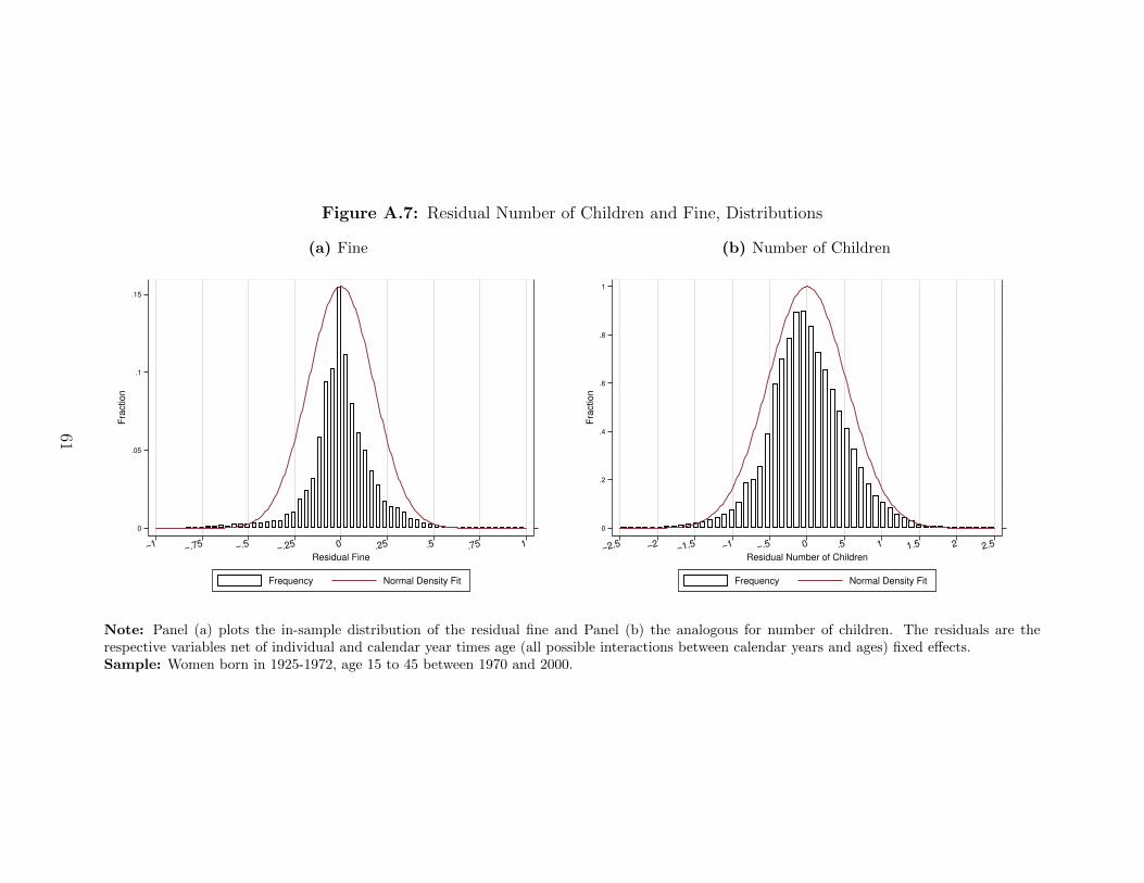
Figure A.7: Residual Number of Children and Fine, Distributions

(a) Fine

0

.05

.1

.15

Fra

ctio

n

−1 −.75 −.5 −.25 0 .25 .5 .75 1

Residual Fine

Frequency Normal Density Fit

(b) Number of Children

0

.2

.4

.6

.8

1

Fra

ctio

n

−2.5 −2 −1.5 −1 −.5 0 .5 1 1.5 2 2.5

Residual Number of Children

Frequency Normal Density Fit

Note: Panel (a) plots the in-sample distribution of the residual fine and Panel (b) the analogous for number of children. The residuals are therespective variables net of individual and calendar year times age (all possible interactions between calendar years and ages) fixed e↵ects.Sample: Women born in 1925-1972, age 15 to 45 between 1970 and 2000.

61

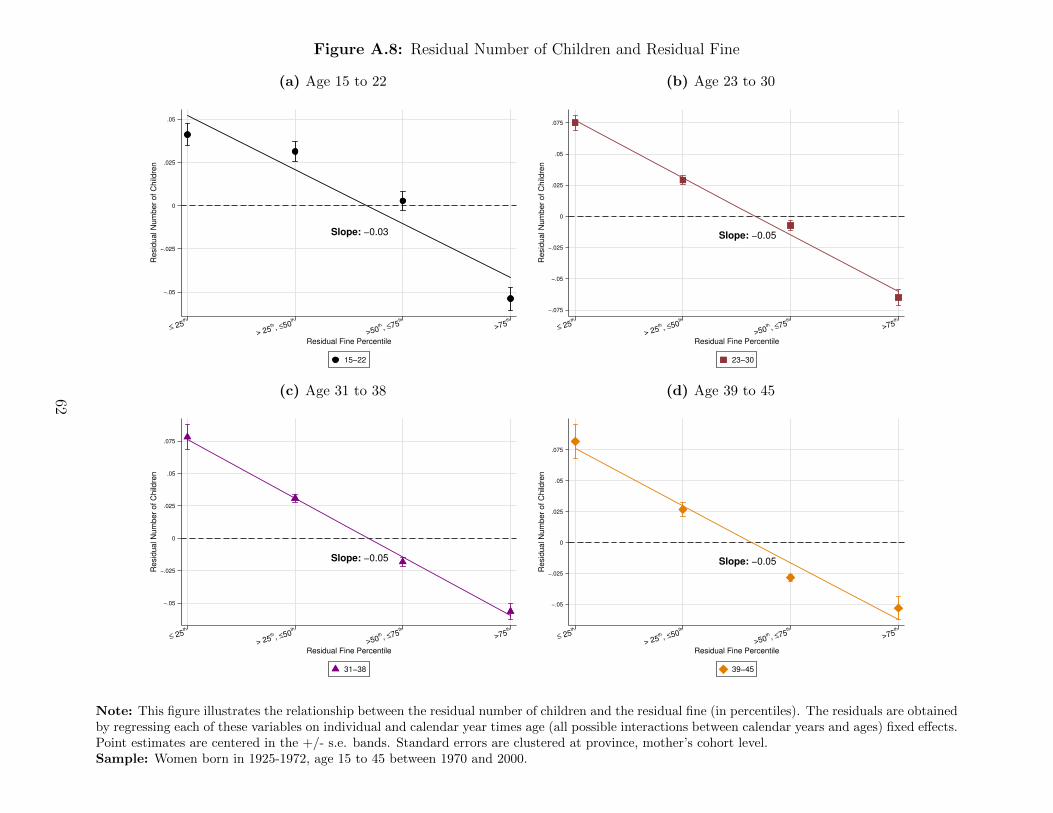
Figure A.8: Residual Number of Children and Residual Fine

(a) Age 15 to 22

Slope: −0.03

−.05

−.025

0

.025

.05

Re

sid

ua

l N

um

be

r o

f C

hild

ren

≤ 25th

> 25th , ≤50

th

>50th , ≤75

th

>75th

Residual Fine Percentile

15−22

(b) Age 23 to 30

Slope: −0.05

−.075

−.05

−.025

0

.025

.05

.075

Re

sid

ua

l N

um

be

r o

f C

hild

ren

≤ 25th

> 25th , ≤50

th

>50th , ≤75

th

>75th


23−30

(c) Age 31 to 38

Slope: −0.05

−.05

−.025

0

.025

.05

.075

Re

sid

ua

l N

um

be

r o

f C

hild

ren

≤ 25th

> 25th , ≤50

th

>50th , ≤75

th

>75th


31−38

(d) Age 39 to 45

Slope: −0.05

−.05

−.025

0

.025

.05

.075

Re

sid

ua

l N

um

be

r o

f C

hild

ren

≤ 25th

> 25th , ≤50

th

>50th , ≤75

th

>75th


39−45

Note: This figure illustrates the relationship between the residual number of children and the residual fine (in percentiles). The residuals are obtainedby regressing each of these variables on individual and calendar year times age (all possible interactions between calendar years and ages) fixed e↵ects.Point estimates are centered in the +/- s.e. bands. Standard errors are clustered at province, mother’s cohort level.Sample: Women born in 1925-1972, age 15 to 45 between 1970 and 2000.

62

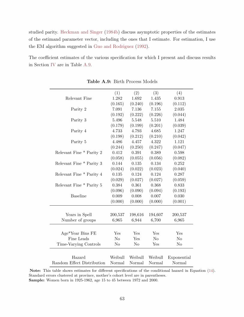
studied parity. Heckman and Singer (1984b) discuss asymptotic properties of the estimates

of the estimand parameter vector, including the ones that I estimate. For estimation, I use

the EM algorithm suggested in Guo and Rodriguez (1992).

The coe�cient estimates of the various specification for which I present and discuss results

in Section IV are in Table A.9.

Table A.9: Birth Process Models

(1) (2) (3) (4)Relevant Fine 1.282 1.692 1.435 0.913

(0.165) (0.240) (0.196) (0.112)Parity 2 7.091 7.136 7.155 2.035

(0.192) (0.222) (0.226) (0.044)Parity 3 5.496 5.548 5.510 1.484

(0.179) (0.199) (0.201) (0.039)Parity 4 4.733 4.793 4.685 1.247

(0.198) (0.212) (0.210) (0.042)Parity 5 4.486 4.457 4.322 1.121

(0.244) (0.250) (0.247) (0.047)Relevant Fine * Parity 2 0.412 0.391 0.389 0.598




(0.096) (0.090) (0.094) (0.193)Baseline 0.009 0.008 0.007 0.030

(0.000) (0.000) (0.000) (0.001)

Years in Spell 200,537 198,616 194,607 200,537Number of groups 6,965 6,944 6,700 6,965

Age*Year Bins FE Yes Yes Yes YesFine Leads No Yes No No

Time-Varying Controls No No Yes No

Hazard Weibull Weibull Weibull ExponentialRandom E↵ect Distribution Normal Normal Normal Normal

Note: This table shows estimates for di↵erent specifications of the conditional hazard in Equation (14).Standard errors clustered at province, mother’s cohort level are in parentheses.Sample: Women born in 1925-1962, age 15 to 45 between 1972 and 2000.

63

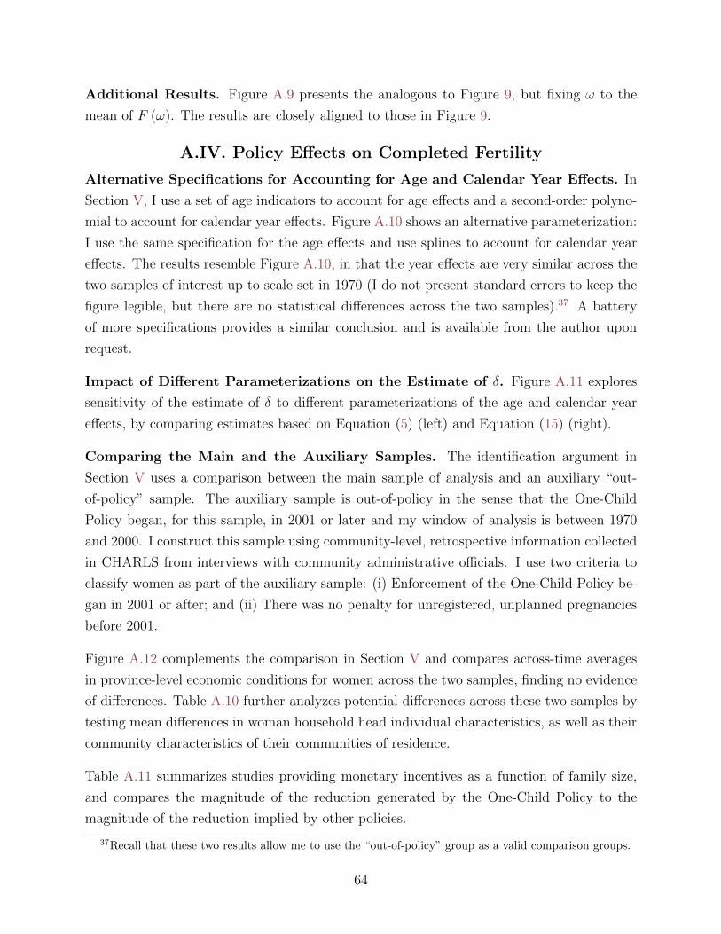
Additional Results. Figure A.9 presents the analogous to Figure 9, but fixing ! to the

mean of F (!). The results are closely aligned to those in Figure 9.

A.IV. Policy E↵ects on Completed Fertility

Alternative Specifications for Accounting for Age and Calendar Year E↵ects. In

Section V, I use a set of age indicators to account for age e↵ects and a second-order polyno-

mial to account for calendar year e↵ects. Figure A.10 shows an alternative parameterization:

I use the same specification for the age e↵ects and use splines to account for calendar year

e↵ects. The results resemble Figure A.10, in that the year e↵ects are very similar across the

two samples of interest up to scale set in 1970 (I do not present standard errors to keep the

figure legible, but there are no statistical di↵erences across the two samples).37 A battery

of more specifications provides a similar conclusion and is available from the author upon

request.

Impact of Di↵erent Parameterizations on the Estimate of �. Figure A.11 explores

sensitivity of the estimate of � to di↵erent parameterizations of the age and calendar year

e↵ects, by comparing estimates based on Equation (5) (left) and Equation (15) (right).

Comparing the Main and the Auxiliary Samples. The identification argument in

Section V uses a comparison between the main sample of analysis and an auxiliary “out-

of-policy” sample. The auxiliary sample is out-of-policy in the sense that the One-Child

Policy began, for this sample, in 2001 or later and my window of analysis is between 1970

and 2000. I construct this sample using community-level, retrospective information collected

in CHARLS from interviews with community administrative o�cials. I use two criteria to

classify women as part of the auxiliary sample: (i) Enforcement of the One-Child Policy be-

gan in 2001 or after; and (ii) There was no penalty for unregistered, unplanned pregnancies

before 2001.

Figure A.12 complements the comparison in Section V and compares across-time averages

in province-level economic conditions for women across the two samples, finding no evidence

of di↵erences. Table A.10 further analyzes potential di↵erences across these two samples by

testing mean di↵erences in woman household head individual characteristics, as well as their

community characteristics of their communities of residence.

Table A.11 summarizes studies providing monetary incentives as a function of family size,

and compares the magnitude of the reduction generated by the One-Child Policy to the

magnitude of the reduction implied by other policies.

37Recall that these two results allow me to use the “out-of-policy” group as a valid comparison groups.

64

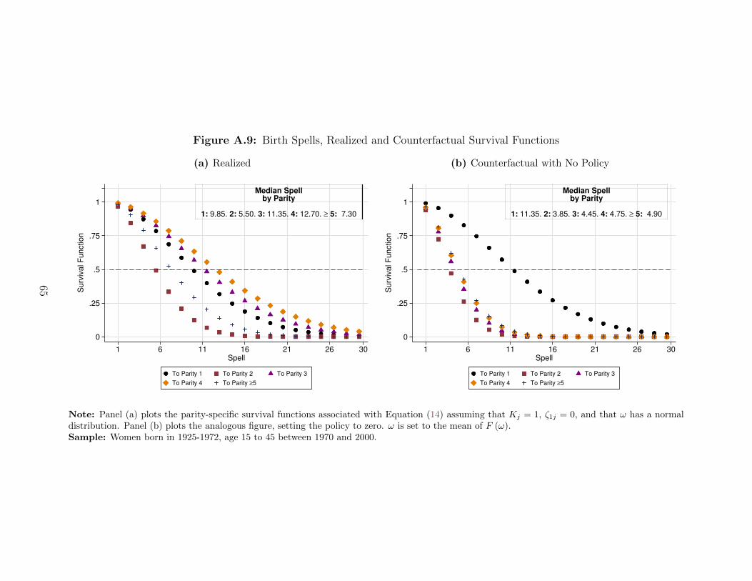
Figure A.9: Birth Spells, Realized and Counterfactual Survival Functions

(a) Realized


1: 9.85. 2: 5.50. 3: 11.35. 4: 12.70. ≥ 5: 7.30

0

.25

.5

.75

1

Surv

ival F

unct

ion

1 6 11 16 21 26 30Spell



(b) Counterfactual with No Policy


1: 11.35. 2: 3.85. 3: 4.45. 4: 4.75. ≥ 5: 4.90

0

.25

.5

.75

1

Surv

ival F

unct

ion

1 6 11 16 21 26 30Spell



Note: Panel (a) plots the parity-specific survival functions associated with Equation (14) assuming that Kj = 1, ⇣1j = 0, and that ! has a normaldistribution. Panel (b) plots the analogous figure, setting the policy to zero. ! is set to the mean of F (!).Sample: Women born in 1925-1972, age 15 to 45 between 1970 and 2000.

65

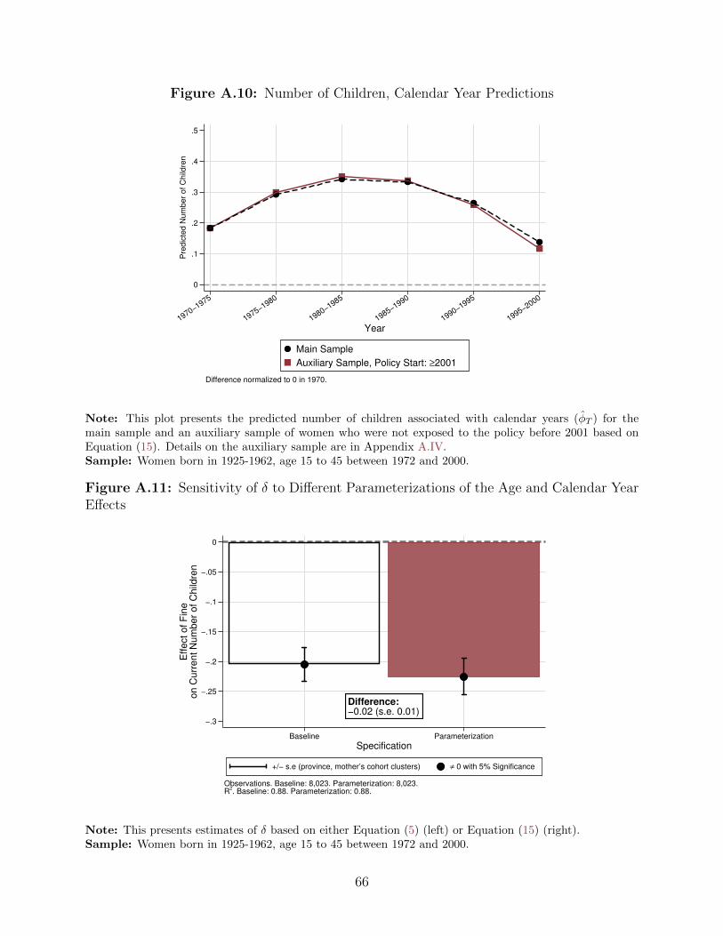
Figure A.10: Number of Children, Calendar Year Predictions

0

.1

.2

.3

.4

.5

Pre

dic

ted

Nu

mb

er

of

Ch

ildre

n

1970−1975

1975−1980

1980−1985

1985−1990

1990−1995

1995−2000

Year

Main Sample

Auxiliary Sample, Policy Start: ≥2001

Difference normalized to 0 in 1970.

Note: This plot presents the predicted number of children associated with calendar years (�T ) for themain sample and an auxiliary sample of women who were not exposed to the policy before 2001 based onEquation (15). Details on the auxiliary sample are in Appendix A.IV.Sample: Women born in 1925-1962, age 15 to 45 between 1972 and 2000.

Figure A.11: Sensitivity of � to Di↵erent Parameterizations of the Age and Calendar YearE↵ects

Difference:−0.02 (s.e. 0.01)

0

−.05

−.1

−.15

−.2

−.25

−.3

Eff

ect

of

Fin

eo

n C

urr

en

t N

um

be

r o

f C

hild

ren

Baseline Parameterization

Specification

+/− s.e (province, mother’s cohort clusters) ≠ 0 with 5% Significance

Observations. Baseline: 8,023. Parameterization: 8,023.R

2. Baseline: 0.88. Parameterization: 0.88.

Note: This presents estimates of � based on either Equation (5) (left) or Equation (15) (right).Sample: Women born in 1925-1962, age 15 to 45 between 1972 and 2000.

66

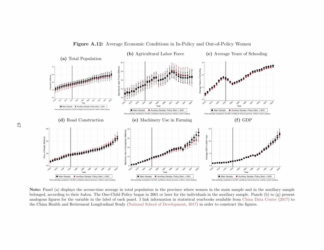
Figure A.12: Average Economic Conditions in In-Policy and Out-of-Policy Women

(a) Total Population

30

40

50

60

70

Po

pu

latio

n (

Mill

ion

s)

19701973

19761979

19821985

19881991

19941997

2000

Year

Main Sample Auxiliary Sample, Policy Start: ≥ 2001

Point estimates cenetered in the 95% confidence interval (province, mother’s cohort clusters).

(b) Agricultural Labor Force

12

14

16

18

20

Ag

ricu

ltura

l La

bo

r F

orc

e (

Mill

ion

s)

19701973

19761979

19821985

19881991

19941997

2000

Year



(c) Average Years of Schooling

2

4

6

8

Ave

rag

e Y

ea

rs o

f S

cho

olin

g

19701973

19761979

19821985

19881991

19941997

2000

Year



(d) Road Construction

20

40

60

80

Km

s. o

f R

oa

ds

(Mill

ion

s)

19701973

19761979

19821985

19881991

19941997

2000

Year



(e) Machinery Use in Farming

0

10

20

30

40

Ma

chin

ery

Use

in H

ors

ep

ow

er

(Mill

ion

s)

19701973

19761979

19821985

19881991

19941997

2000

Year



(f) GDP

0

5

10

15

Ave

rag

e G

DP

in 2

00

0 Y

ua

n

19701973

19761979

19821985

19881991

19941997

2000

Year



Note: Panel (a) displays the across-time average in total population in the province where women in the main sample and in the auxiliary samplebelonged, according to their hukou. The One-Child Policy began in 2001 or later for the individuals in the auxiliary sample. Panels (b) to (g) presentanalogous figures for the variable in the label of each panel. I link information in statistical yearbooks available from China Data Center (2017) tothe China Health and Retirement Longitudinal Study (National School of Development, 2017) in order to construct the figures.

67

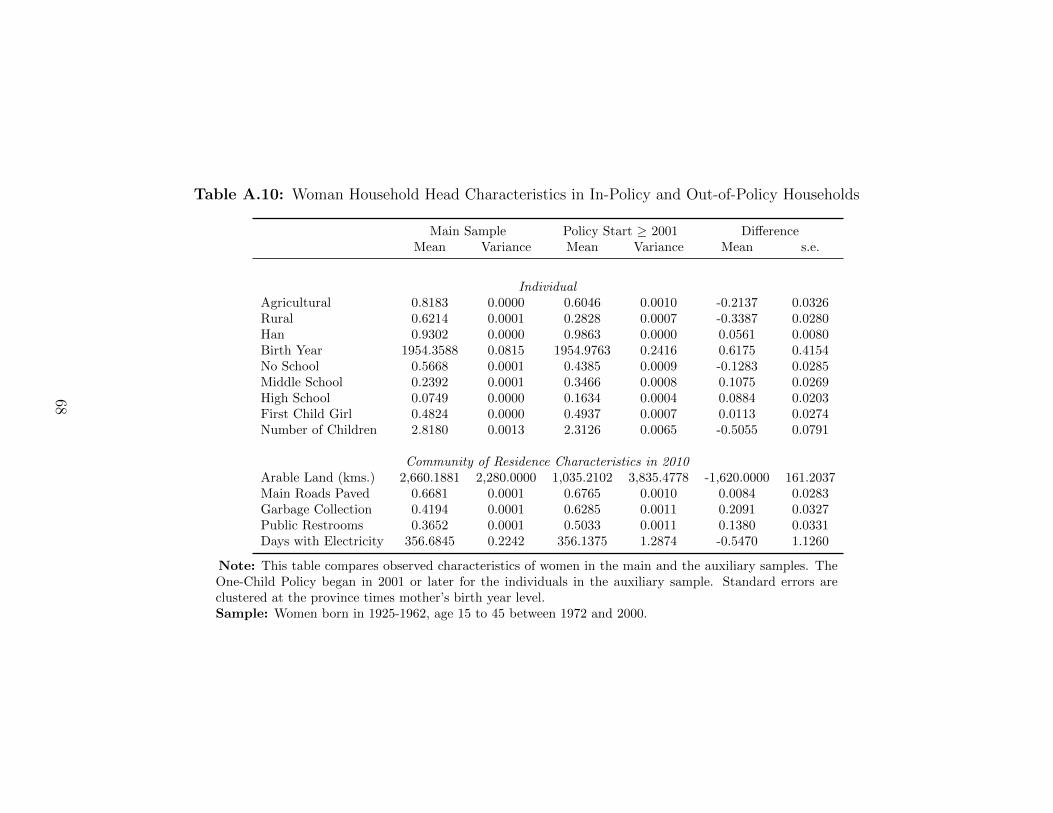
Table A.10: Woman Household Head Characteristics in In-Policy and Out-of-Policy Households

Main Sample Policy Start � 2001 Di↵erenceMean Variance Mean Variance Mean s.e.

IndividualAgricultural 0.8183 0.0000 0.6046 0.0010 -0.2137 0.0326Rural 0.6214 0.0001 0.2828 0.0007 -0.3387 0.0280Han 0.9302 0.0000 0.9863 0.0000 0.0561 0.0080Birth Year 1954.3588 0.0815 1954.9763 0.2416 0.6175 0.4154No School 0.5668 0.0001 0.4385 0.0009 -0.1283 0.0285Middle School 0.2392 0.0001 0.3466 0.0008 0.1075 0.0269High School 0.0749 0.0000 0.1634 0.0004 0.0884 0.0203First Child Girl 0.4824 0.0000 0.4937 0.0007 0.0113 0.0274Number of Children 2.8180 0.0013 2.3126 0.0065 -0.5055 0.0791

Community of Residence Characteristics in 2010Arable Land (kms.) 2,660.1881 2,280.0000 1,035.2102 3,835.4778 -1,620.0000 161.2037Main Roads Paved 0.6681 0.0001 0.6765 0.0010 0.0084 0.0283Garbage Collection 0.4194 0.0001 0.6285 0.0011 0.2091 0.0327Public Restrooms 0.3652 0.0001 0.5033 0.0011 0.1380 0.0331Days with Electricity 356.6845 0.2242 356.1375 1.2874 -0.5470 1.1260

Note: This table compares observed characteristics of women in the main and the auxiliary samples. TheOne-Child Policy began in 2001 or later for the individuals in the auxiliary sample. Standard errors areclustered at the province times mother’s birth year level.Sample: Women born in 1925-1962, age 15 to 45 between 1972 and 2000.

68

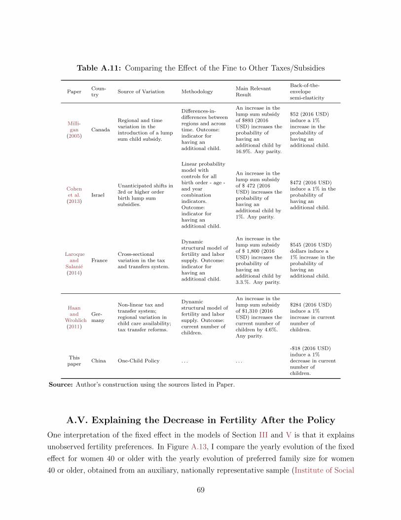
Table A.11: Comparing the E↵ect of the Fine to Other Taxes/Subsidies

PaperCoun-try

Source of Variation MethodologyMain RelevantResult

Back-of-the-envelopesemi-elasticity

Milli-gan

(2005)Canada

Regional and timevariation in theintroduction of a lumpsum child subsidy.

Di↵erences-in-di↵erences betweenregions and acrosstime. Outcome:indicator forhaving anadditional child.

An increase in thelump sum subsidyof $893 (2016USD) increases theprobability ofhaving anadditional child by16.9%. Any parity.

$52 (2016 USD)induce a 1%increase in theprobability ofhaving anadditional child.

Cohenet al.(2013)

Israel

Unanticipated shifts in3rd or higher orderbirth lump sumsubsidies.

Linear probabilitymodel withcontrols for allbirth order - age -and yearcombinationindicators.Outcome:indicator forhaving anadditional child.

An increase in thelump sum subsidyof $ 472 (2016USD) increases theprobability ofhaving anadditional child by1%. Any parity.

$472 (2016 USD)induce a 1% in theprobability ofhaving anadditional child.

Laroqueand

Salanie(2014)

FranceCross-sectionalvariation in the taxand transfers system.

Dynamicstructural model offertility and laborsupply. Outcome:indicator forhaving anadditional child.

An increase in thelump sum subsidyof $ 1,800 (2016USD) increases theprobability ofhaving anadditional child by3.3.%. Any parity.

$545 (2016 USD)dollars induce a1% increase in theprobability ofhaving anadditional child.

Haanand

Wrohlich(2011)

Ger-many

Non-linear tax andtransfer system;regional variation inchild care availability;tax transfer reforms.

Dynamicstructural model offertility and laborsupply. Outcome:current number ofchildren.

An increase in thelump sum subsidyof $1,310 (2016USD) increases thecurrent number ofchildren by 4.6%.Any parity.

$284 (2016 USD)induce a 1%increase in currentnumber ofchildren.

Thispaper

China One-Child Policy . . . . . .

-$18 (2016 USD)induce a 1%decrease in currentnumber ofchildren.

Source: Author’s construction using the sources listed in Paper.

A.V. Explaining the Decrease in Fertility After the Policy

One interpretation of the fixed e↵ect in the models of Section III and V is that it explains

unobserved fertility preferences. In Figure A.13, I compare the yearly evolution of the fixed

e↵ect for women 40 or older with the yearly evolution of preferred family size for women

40 or older, obtained from an auxiliary, nationally representative sample (Institute of Social

69

Science Survey, 2010). The time-series correlation of the average of these two variables is

striking. Although this is a compelling correlation, preference shifts are of limited economic

content, and explaining the residual remains a subject for future research.

Figure A.13: Fixed E↵ects and the Ideal Number of Children

Time Series Correlation: 0.95

−.5

−.25

0

.25

Ave

rag

e f

or

Fe

ma

les

40

or

Old

er

19701975

19791983

19871991

19952000

Year

Ideal Number of Children Fixed Effect

1970 levels normalized to zero.Observations. Ideal Number of Children: 4,559. Female Fixed Effect: 8,133.

Note: Fixed e↵ects estimated from Equation (15) for women 40 or older and ideal or preferrednumber of children for women 40 or older obtained in Institute of Social Science Survey (2010).Both the fixed e↵ects and the ideal number of children consider women born between 1925 and 1960.

70

Documents

Fertility after China’s More-than-One-Child Policy · Fertility after China’s More-than-One-Child Policy ... document that the One-Child Policy caused only a minor fraction of