Embed Size (px)
Citation preview
International Macroeconomic Impacts on the Brazilian Economy: a note*
Fernando de Holanda Barbosa Filho
Samuel de Abreu Pessôa
1 - Introduction
The impact of international macroeconomic policies on the Brazilian economy
was evident in the subprime crisis period and its aftermath. The Brazilian economy
faced a new economic environment with a lower growth rate in the developed world
that changed relative prices, generating terms of trade gains that favored the services
sector in comparison with industry. As a consequence, despite lower GDP growth the
labor market continues to flourish (services are labor intensive but have lower
productivity in Brazil).
In the years following the crisis the Brazilian economy observed lower interest
rates, a real exchange appreciation and a loosening of fiscal policy that reduced the
primary surplus (that maintained debt sustainability) and increased its vulnerability.
In this context, the impact of the tapering process on the Brazilian economy is an
important topic that must be addressed in order to avoid/reduce its possible negative
impacts in Brazil.
This note is organized in 5 sections including this introduction. The immediate
post crisis and its effects on Brazil are reported in section 2. Section 3 shows the
Quantitative Easing and Tapering effects on Brazil. Section 4 presents a Growth
decomposition analysis and the fiscal policy shift after 2008. Section 5 summarizes the
findings of this note.
2 – The Immediate post-Crisis Period
The Brazilian economy was doing well like many other countries before the
subprime crisis. Brazilian GDP growth rate accelerated from 2002 until 2008. The
average growth rate was 2.3% in the FHC government and increased to 3.4% between
2002 and 2006 and to 4.5% in the 2006-2010 period, during the Lula government.
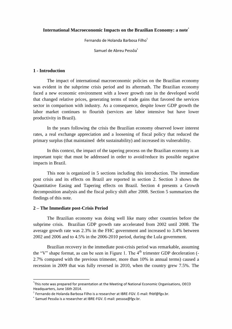
Brazilian recovery in the immediate post-crisis period was remarkable, assuming
the “V” shape format, as can be seen in Figure 1. The 4th
trimester GDP deceleration (-
2.7% compared with the previous trimester, more than 10% in annual terms) caused a
recession in 2009 that was fully reversed in 2010, when the country grew 7.5%. The
*This note was prepared for presentation at the Meeting of National Economic Organisations, OECD
Headquarters, June 16th 2014. Fernando de Holanda Barbosa Filho is a researcher at IBRE-FGV. E-mail: [email protected]. Samuel Pessôa is a researcher at IBRE-FGV. E-mail: [email protected].
combination of expansionary monetary and fiscal policy helped the quick recovery in an
election year.
Source: IBGE.
Despite the fast 2010 economic recovery, the Brazilian economy suffered some
permanent effects, especially due to relative price changes caused by weak world
economic growth.
2.1 – Terms of Trade
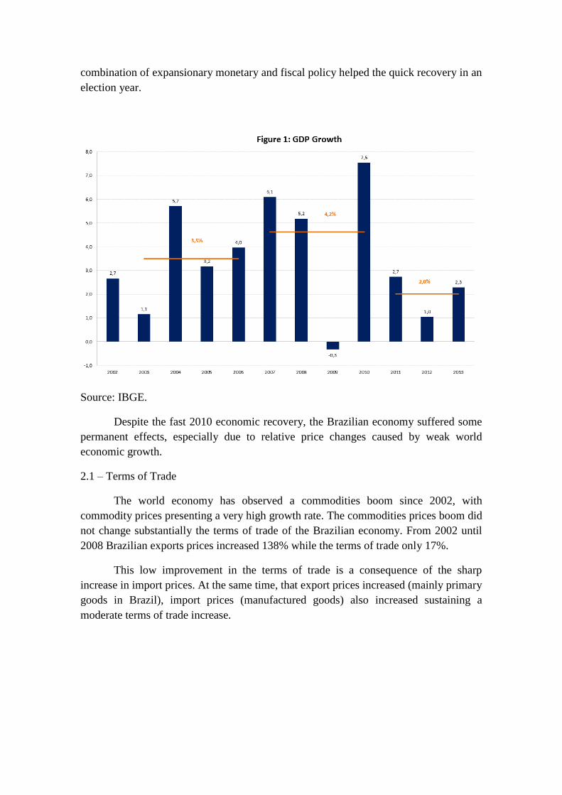
The world economy has observed a commodities boom since 2002, with
commodity prices presenting a very high growth rate. The commodities prices boom did
not change substantially the terms of trade of the Brazilian economy. From 2002 until
2008 Brazilian exports prices increased 138% while the terms of trade only 17%.
This low improvement in the terms of trade is a consequence of the sharp
increase in import prices. At the same time, that export prices increased (mainly primary
goods in Brazil), import prices (manufactured goods) also increased sustaining a
moderate terms of trade increase.
Source: Funcex.
The high imported goods prices were signaling a high world demand for
manufactured goods. This tendency changed after the 2008 crisis caused a demand drop
on the developed economies reducing the demand for manufactured goods and therefore
increasing Brazilian terms of trade.
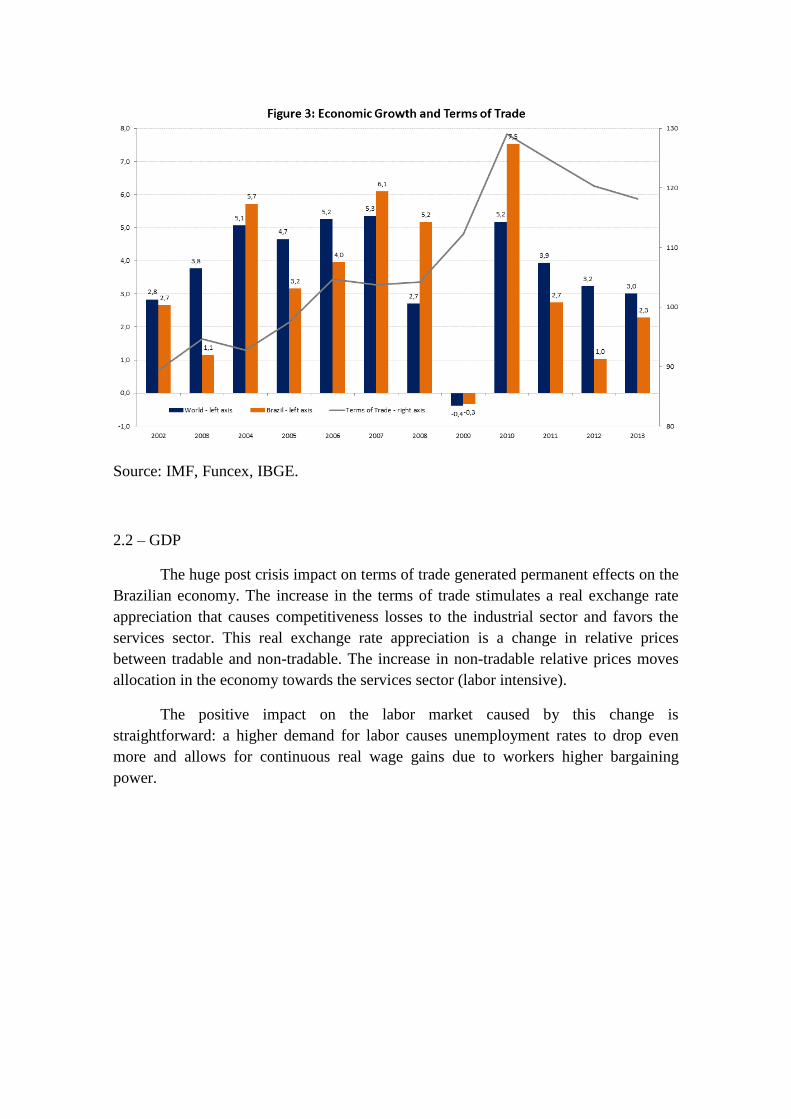
Figure 3 shows the GDP growth rate in Brazil and in the world together with the
terms of trade evolution. The terms of trade increased sharply in Brazil after the crisis
but then its trend was reduced after 2010. However, the level remains much higher than
that of 2008.
80
100
120
140
160
180
200
220
240
260
280
jan
/02
mai
/02
set/
02
jan
/03
mai
/03
set/
03
jan
/04
mai
/04
set/
04
jan
/05
mai
/05
set/
05
jan
/06
mai
/06
set/
06
jan
/07
mai
/07
set/
07
jan
/08
mai
/08
set/
08
jan
/09
mai
/09
set/
09
jan
/10
mai
/10
set/
10
jan
/11
mai
/11
set/
11
jan
/12
mai
/12
set/
12
jan
/13
mai
/13
set/
13
jan
/14
FIgure 2: Brazlian Terms of Trade and its components
Exports Prices
Imports Prices
Terms of Trade
Source: IMF, Funcex, IBGE.
2.2 – GDP
The huge post crisis impact on terms of trade generated permanent effects on the
Brazilian economy. The increase in the terms of trade stimulates a real exchange rate
appreciation that causes competitiveness losses to the industrial sector and favors the
services sector. This real exchange rate appreciation is a change in relative prices
between tradable and non-tradable. The increase in non-tradable relative prices moves
allocation in the economy towards the services sector (labor intensive).
The positive impact on the labor market caused by this change is
straightforward: a higher demand for labor causes unemployment rates to drop even
more and allows for continuous real wage gains due to workers higher bargaining
power.
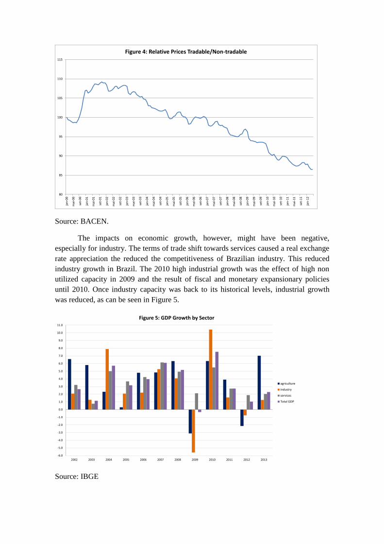
Source: BACEN.
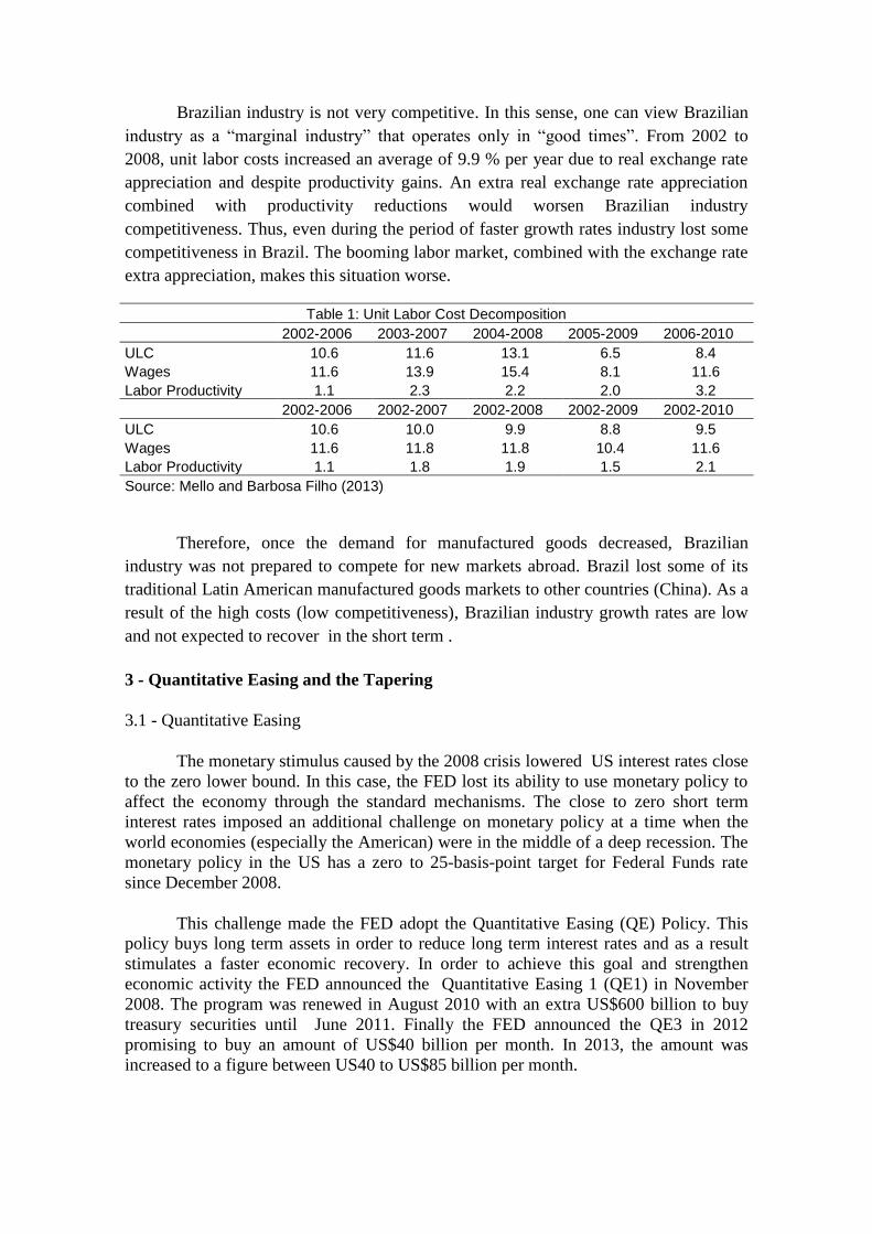
The impacts on economic growth, however, might have been negative,
especially for industry. The terms of trade shift towards services caused a real exchange
rate appreciation the reduced the competitiveness of Brazilian industry. This reduced
industry growth in Brazil. The 2010 high industrial growth was the effect of high non
utilized capacity in 2009 and the result of fiscal and monetary expansionary policies
until 2010. Once industry capacity was back to its historical levels, industrial growth
was reduced, as can be seen in Figure 5.
Source: IBGE
80
85
90
95
100
105
110
115
jan
-00
mai
-00
set-
00
jan
-01
mai
-01
set-
01
jan
-02
mai
-02
set-
02
jan
-03
mai
-03
set-
03
jan
-04
mai
-04
set-
04
jan
-05
mai
-05
set-
05
jan
-06
mai
-06
set-
06
jan
-07
mai
-07
set-
07
jan
-08
mai
-08
set-
08
jan
-09
mai
-09
set-
09
jan
-10
mai
-10
set-
10
jan
-11
mai
-11
set-
11
jan
-12
Figure 4: Relative Prices Tradable/Non-tradable
-6.0
-5.0
-4.0
-3.0
-2.0
-1.0
0.0
1.0
2.0
3.0
4.0
5.0
6.0
7.0
8.0
9.0
10.0
11.0
2002 2003 2004 2005 2006 2007 2008 2009 2010 2011 2012 2013
Figure 5: GDP Growth by Sector
agriculture
industry
services
Total GDP
Brazilian industry is not very competitive. In this sense, one can view Brazilian
industry as a “marginal industry” that operates only in “good times”. From 2002 to
2008, unit labor costs increased an average of 9.9 % per year due to real exchange rate
appreciation and despite productivity gains. An extra real exchange rate appreciation
combined with productivity reductions would worsen Brazilian industry
competitiveness. Thus, even during the period of faster growth rates industry lost some
competitiveness in Brazil. The booming labor market, combined with the exchange rate
extra appreciation, makes this situation worse.
Table 1: Unit Labor Cost Decomposition
2002-2006 2003-2007 2004-2008 2005-2009 2006-2010
ULC 10.6 11.6 13.1 6.5 8.4
Wages 11.6 13.9 15.4 8.1 11.6
Labor Productivity 1.1 2.3 2.2 2.0 3.2
2002-2006 2002-2007 2002-2008 2002-2009 2002-2010
ULC 10.6 10.0 9.9 8.8 9.5
Wages 11.6 11.8 11.8 10.4 11.6
Labor Productivity 1.1 1.8 1.9 1.5 2.1
Source: Mello and Barbosa Filho (2013)
Therefore, once the demand for manufactured goods decreased, Brazilian
industry was not prepared to compete for new markets abroad. Brazil lost some of its
traditional Latin American manufactured goods markets to other countries (China). As a
result of the high costs (low competitiveness), Brazilian industry growth rates are low
and not expected to recover in the short term .
3 - Quantitative Easing and the Tapering
3.1 - Quantitative Easing
The monetary stimulus caused by the 2008 crisis lowered US interest rates close
to the zero lower bound. In this case, the FED lost its ability to use monetary policy to
affect the economy through the standard mechanisms. The close to zero short term
interest rates imposed an additional challenge on monetary policy at a time when the
world economies (especially the American) were in the middle of a deep recession. The
monetary policy in the US has a zero to 25-basis-point target for Federal Funds rate
since December 2008.
This challenge made the FED adopt the Quantitative Easing (QE) Policy. This
policy buys long term assets in order to reduce long term interest rates and as a result
stimulates a faster economic recovery. In order to achieve this goal and strengthen
economic activity the FED announced the Quantitative Easing 1 (QE1) in November
2008. The program was renewed in August 2010 with an extra US$600 billion to buy
treasury securities until June 2011. Finally the FED announced the QE3 in 2012
promising to buy an amount of US$40 billion per month. In 2013, the amount was
increased to a figure between US40 to US$85 billion per month.
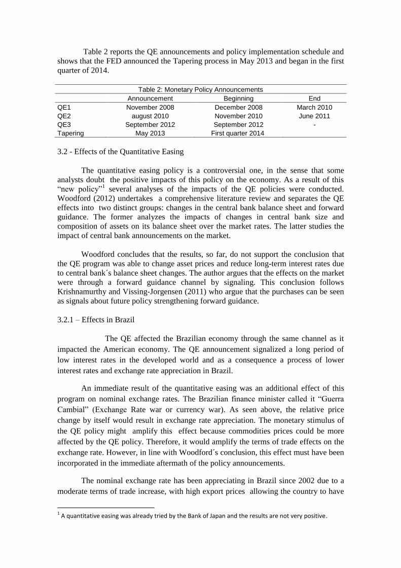
Table 2 reports the QE announcements and policy implementation schedule and
shows that the FED announced the Tapering process in May 2013 and began in the first
quarter of 2014.
Table 2: Monetary Policy Announcements
Announcement Beginning End
QE1 November 2008 December 2008 March 2010
QE2 august 2010 November 2010 June 2011
QE3 September 2012 September 2012 -
Tapering May 2013 First quarter 2014
3.2 - Effects of the Quantitative Easing
The quantitative easing policy is a controversial one, in the sense that some
analysts doubt the positive impacts of this policy on the economy. As a result of this
“new policy”1 several analyses of the impacts of the QE policies were conducted.
Woodford (2012) undertakes a comprehensive literature review and separates the QE
effects into two distinct groups: changes in the central bank balance sheet and forward
guidance. The former analyzes the impacts of changes in central bank size and
composition of assets on its balance sheet over the market rates. The latter studies the
impact of central bank announcements on the market.
Woodford concludes that the results, so far, do not support the conclusion that
the QE program was able to change asset prices and reduce long-term interest rates due
to central bank´s balance sheet changes. The author argues that the effects on the market
were through a forward guidance channel by signaling. This conclusion follows
Krishnamurthy and Vissing-Jorgensen (2011) who argue that the purchases can be seen
as signals about future policy strengthening forward guidance.
3.2.1 – Effects in Brazil
The QE affected the Brazilian economy through the same channel as it
impacted the American economy. The QE announcement signalized a long period of
low interest rates in the developed world and as a consequence a process of lower
interest rates and exchange rate appreciation in Brazil.
An immediate result of the quantitative easing was an additional effect of this
program on nominal exchange rates. The Brazilian finance minister called it “Guerra
Cambial” (Exchange Rate war or currency war). As seen above, the relative price
change by itself would result in exchange rate appreciation. The monetary stimulus of
the QE policy might amplify this effect because commodities prices could be more
affected by the QE policy. Therefore, it would amplify the terms of trade effects on the
exchange rate. However, in line with Woodford´s conclusion, this effect must have been
incorporated in the immediate aftermath of the policy announcements.
The nominal exchange rate has been appreciating in Brazil since 2002 due to a
moderate terms of trade increase, with high export prices allowing the country to have
1 A quantitative easing was already tried by the Bank of Japan and the results are not very positive.

strong trade surpluses. During the crises the flexible exchange rate regime protected the
country from external negative shock through a huge depreciation2. Despite the different
conditions in the world economy (lower trade surplus), the exchange rate appreciated
again in response to lower US interest rates turning the Brazilian economy more
attractive to capital due to its better recovery perspectives. The real exchange rate
continued to appreciate until July 2011.
Source: BACEN.
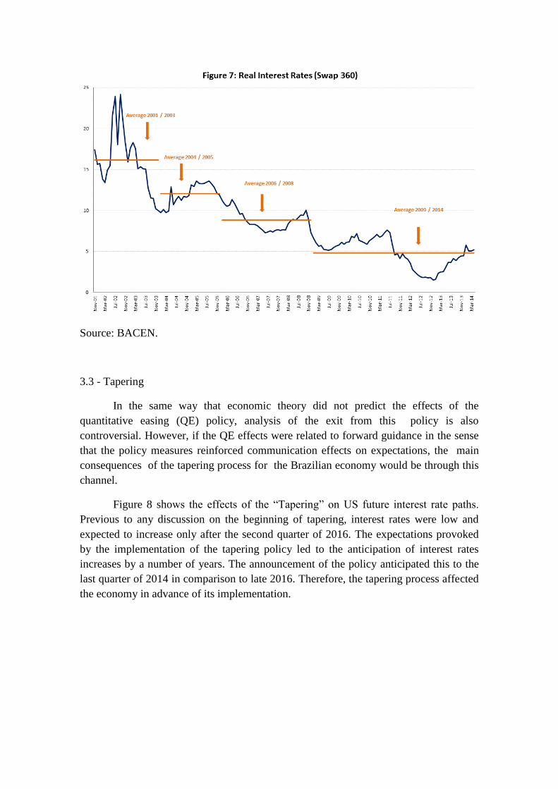
The lower interest rates in the US allowed a reduction in Brazilian interest rates3.
This monetary phenomena can be seen in Figure 8. The real interest rates in Brazil had
been dropping gradually for long time, a clear indication of institutional improvement.
The US sharp interest rates reduction allowed Brazil´s Central Bank to reduce sharply
its interest rates.
The real interest rate reduction was deeper than it should have been and caused
inflation to increase in Brazil. This extra drop was not a consequence of international
monetary policy but a Brazilian monetary policy mistake that put the interest rates
below its neutral level.
2 Blanco, Barbosa Filho and Pessôa (2011).
3 Brazil is a small open economy. Therefore, US lower interest rates allowed a reduction in Brazilian
interest rates (Selic).
Source: BACEN.
3.3 - Tapering
In the same way that economic theory did not predict the effects of the
quantitative easing (QE) policy, analysis of the exit from this policy is also
controversial. However, if the QE effects were related to forward guidance in the sense
that the policy measures reinforced communication effects on expectations, the main
consequences of the tapering process for the Brazilian economy would be through this
channel.
Figure 8 shows the effects of the “Tapering” on US future interest rate paths.
Previous to any discussion on the beginning of tapering, interest rates were low and
expected to increase only after the second quarter of 2016. The expectations provoked
by the implementation of the tapering policy led to the anticipation of interest rates
increases by a number of years. The announcement of the policy anticipated this to the
last quarter of 2014 in comparison to late 2016. Therefore, the tapering process affected
the economy in advance of its implementation.
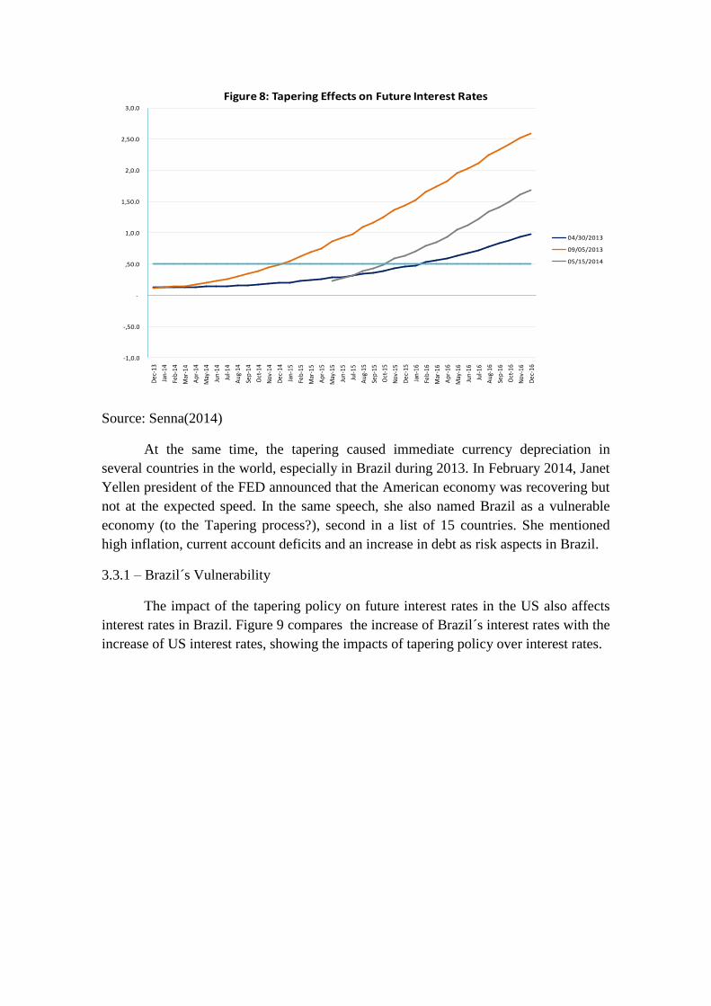
Source: Senna(2014)
At the same time, the tapering caused immediate currency depreciation in
several countries in the world, especially in Brazil during 2013. In February 2014, Janet
Yellen president of the FED announced that the American economy was recovering but
not at the expected speed. In the same speech, she also named Brazil as a vulnerable
economy (to the Tapering process?), second in a list of 15 countries. She mentioned
high inflation, current account deficits and an increase in debt as risk aspects in Brazil.
3.3.1 – Brazil´s Vulnerability
The impact of the tapering policy on future interest rates in the US also affects
interest rates in Brazil. Figure 9 compares the increase of Brazil´s interest rates with the
increase of US interest rates, showing the impacts of tapering policy over interest rates.
-1,0.0
-,50.0
-
,50.0
1,0.0
1,50.0
2,0.0
2,50.0
3,0.0
Dec
-13
Jan-
14
Feb-
14
Mar
-14
Apr
-14
May
-14
Jun-
14
Jul-1
4
Aug
-14
Sep-
14
Oct
-14
Nov
-14
Dec
-14
Jan-
15
Feb-
15
Mar
-15
Apr
-15
May
-15
Jun-
15
Jul-1
5
Aug
-15
Sep-
15
Oct
-15
Nov
-15
Dec
-15
Jan-
16
Feb-
16
Mar
-16
Apr
-16
May
-16
Jun-
16
Jul-1
6
Aug
-16
Sep-
16
Oct
-16
Nov
-16
Dec
-16
Figure 8: Tapering Effects on Future Interest Rates
04/30/2013
09/05/2013
05/15/2014
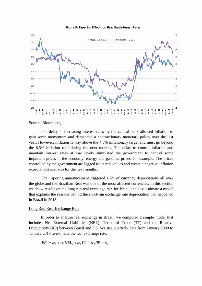
Source: Bloomberg.
The delay in increasing interest rates by the central bank allowed inflation to
gain some momentum and demanded a contractionary monetary policy over the last
year. However, inflation is way above the 4.5% inflationary target and must go beyond
the 6.5% inflation roof during the next months. The delay to control inflation and
maintain interest rates at low levels stimulated the government to control some
important prices in the economy: energy and gasoline prices, for example. The prices
controlled by the government are lagged to its real values and create a negative inflation
expectations scenario for the next months.
The Tapering announcement triggered a lot of currency depreciations all over
the globe and the Brazilian Real was one of the most affected currencies. In this section
we show results on the long-run real exchange rate for Brazil and also estimate a model
that explains the reasons behind the short-run exchange rate depreciation that happened
in Brazil in 2013.
Long Run Real Exchange Rate
In order to analyze real exchange in Brazil, we computed a simple model that
includes Net External Liabilities (NEL), Terms of Trade (TT) and the Relative
Productivity (RP) between Brazil and US. We use quarterly data from January 1980 to
January 2013 to estimate the real exchange rate.
ttttt RPTTNELER 3210

The estimation results show the expected relation among the Exchange rates and
the selected variables. On the one hand, an increase in net external liabilities and
relative productivity causes exchange rate depreciation. On the other hand, an increase
in the terms of trade generates an exchange rate appreciation.
Table 3: Results of the Regression
Constant -0.982**
NEL 0.061*
TT -0,011*
RP 0,154*
R2 0,90
* Significant at 5% level. ** Significant at 10% level.
The Figure 10 shows the graph that compares the actual real exchange rate with
the one forecasted by the model.
The long-run real exchange rate predicted that the BRL should depreciate in the
near future as a result of changes in fiscal conditions and terms of trade, especially the
former, as can be seen in Figure11. The Fiscal Policy change caused a huge
deterioration on NEL, which causes an exchange rate depreciation.

Source: Bloomberg.
Short Run Exchange Rate
Nominal exchange rates depreciated in many countries after the Tapering policy
was expected to be adopted in the beginning of 2014. Therefore, we estimated a model
to explain the reasons for the BRL to devaluate much more than other currencies . In
order to do this we computed the exchange rate depreciation of several currencies from
May 2013 until September 2013, the period of the BRL sharp depreciation. We use data
from the Bloomberg for 18 countries4on several variables
5. We estimated three different
models: one that included Public Debt (PD) and Basic Interest Rates (BIR), the second
that includes a combination of the PD and BIR, the service debt and the third that
contains debt service (DS) and primary exports to China (PEC) The selected model has
a combination of two variables: gross public debt and interest rates and the primary
exports to China (PEC), as below:
tt PECDSe 20122201210
The model fit improves with the product of these variables that is a proxy for the
debt service. The model explains 67 percent of total data variation (R2=0.67). We also
add a variable that relates the importance of primary exports to the Chinese economy,
and the model provided an R2 equal to 0.86, as can be seen in Table 4.
4 Australia, Brazil, Canada, Chile, Colombia, India, Indonesia, Malaysia, Mexico, New Zealand, Norway,
Peru, Russia, South Africa, South Korea, Taiwan, Thailand and Turkey. 5 2012 GDP growth rates, 2012 inflation, public deficit, 2012 trade currency account deficit, 2013 first
quarterly interest rates, 2012 GDP debt ratio, international reserves, long and short term external debt.
70
90
110
130
150
170
190
2100
1/0
3/2
00
8
01
/06
/20
08
01
/09
/20
08
01
/12
/20
08
01
/03
/20
09
01
/06
/20
09
01
/09
/20
09
01
/12
/20
09
01
/03
/20
10
01
/06
/20
10
01
/09
/20
10
01
/12
/20
10
01
/03
/20
11
01
/06
/20
11
01
/09
/20
11
01
/12
/20
11
01
/03
/20
12
01
/06
/20
12
01
/09
/20
12
01
/12
/20
12
01
/03
/20
13
01
/06
/20
13
01
/09
/20
13
01
/12
/20
13
01
/03
/20
14
01
/06
/20
14
01
/09
/20
14
01
/12
/20
14
01
/03
/20
15
01
/06
/20
15
01
/09
/20
15
01
/12
/20
15
01
/03
/20
16
01
/06
/20
16
01
/09
/20
16
01
/12
/20
16
01
/03
/20
17
01
/06
/20
17
01
/09
/20
17
01
/12
/20
17
01
/03
/20
18
01
/06
/20
18
01
/09
/20
18
01
/12
/20
18
Figure 11: Evolution of TT, RP and NEL
Terms of Trade (TT)
Relative Productivity (RP)
Net External Liabilities (NEL)
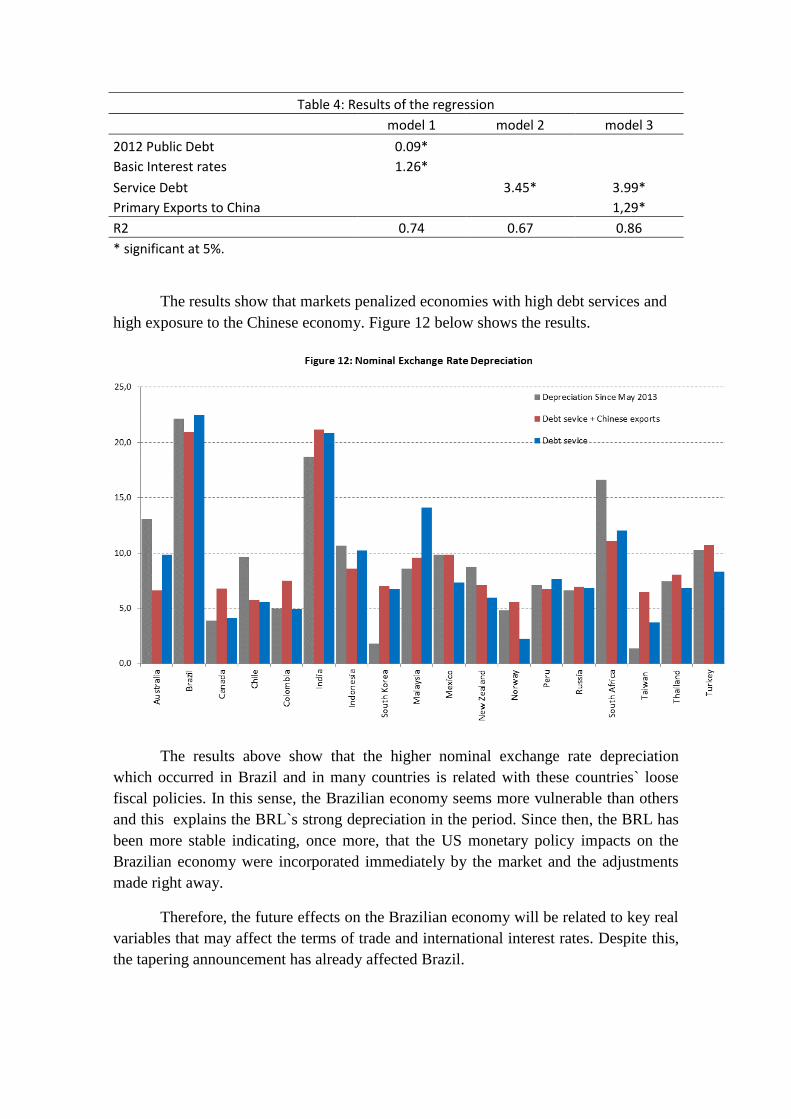
Table 4: Results of the regression
model 1 model 2 model 3
2012 Public Debt 0.09* Basic Interest rates 1.26* Service Debt 3.45* 3.99*
Primary Exports to China 1,29*
R2 0.74 0.67 0.86
* significant at 5%.
The results show that markets penalized economies with high debt services and
high exposure to the Chinese economy. Figure 12 below shows the results.
The results above show that the higher nominal exchange rate depreciation
which occurred in Brazil and in many countries is related with these countries` loose
fiscal policies. In this sense, the Brazilian economy seems more vulnerable than others
and this explains the BRL`s strong depreciation in the period. Since then, the BRL has
been more stable indicating, once more, that the US monetary policy impacts on the
Brazilian economy were incorporated immediately by the market and the adjustments
made right away.
Therefore, the future effects on the Brazilian economy will be related to key real
variables that may affect the terms of trade and international interest rates. Despite this,
the tapering announcement has already affected Brazil.
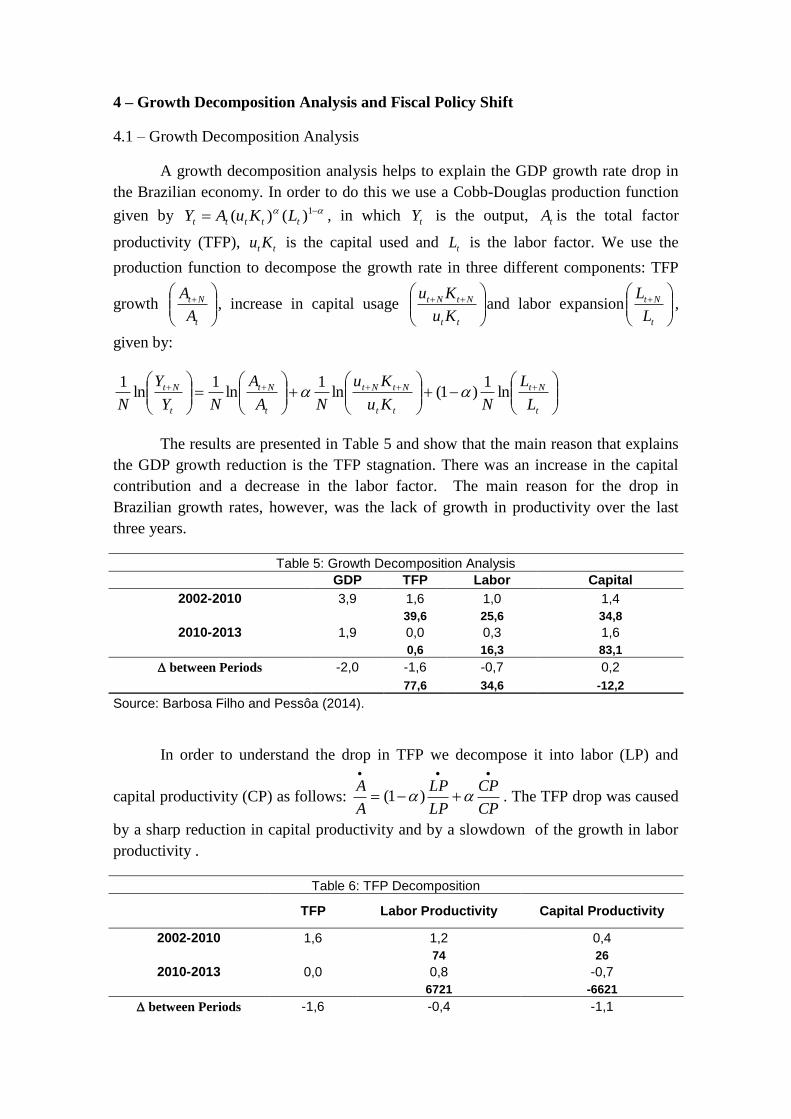
4 – Growth Decomposition Analysis and Fiscal Policy Shift
4.1 – Growth Decomposition Analysis
A growth decomposition analysis helps to explain the GDP growth rate drop in
the Brazilian economy. In order to do this we use a Cobb-Douglas production function
given by 1)()( ttttt LKuAY , in which tY is the output, tA is the total factor
productivity (TFP), tt Ku is the capital used and tL is the labor factor. We use the
production function to decompose the growth rate in three different components: TFP
growth
t
Nt
A
A, increase in capital usage
tt
NtNt
Ku
Kuand labor expansion
t
Nt
L
L,
given by:
t
Nt
tt
NtNt
t
Nt
t
Nt
L
L
NKu
Ku
NA
A
NY
Y
Nln
1)1(ln
1ln
1ln
1
The results are presented in Table 5 and show that the main reason that explains
the GDP growth reduction is the TFP stagnation. There was an increase in the capital
contribution and a decrease in the labor factor. The main reason for the drop in
Brazilian growth rates, however, was the lack of growth in productivity over the last
three years.
Table 5: Growth Decomposition Analysis
GDP TFP Labor Capital
2002-2010 3,9 1,6 1,0 1,4
39,6 25,6 34,8
2010-2013 1,9 0,0 0,3 1,6
0,6 16,3 83,1
between Periods -2,0 -1,6 -0,7 0,2
77,6 34,6 -12,2
Source: Barbosa Filho and Pessôa (2014).
In order to understand the drop in TFP we decompose it into labor (LP) and
capital productivity (CP) as follows: CP
CP
LP
LP
A
A
)1( . The TFP drop was caused
by a sharp reduction in capital productivity and by a slowdown of the growth in labor
productivity .
Table 6: TFP Decomposition
TFP Labor Productivity Capital Productivity
2002-2010 1,6 1,2 0,4
74 26
2010-2013 0,0 0,8 -0,7
6721 -6621
between Periods -1,6 -0,4 -1,1
26,3 73,7
Source: Barbosa Filho and Pessôa (2014).
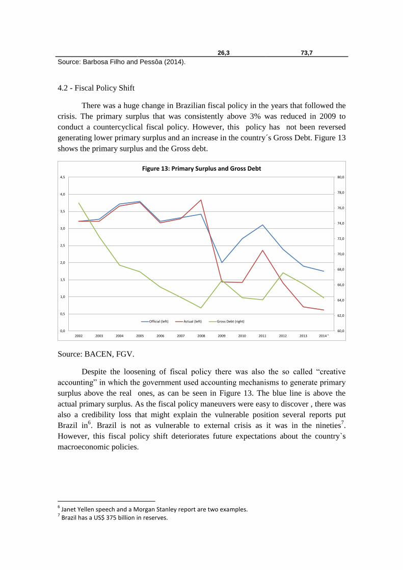
4.2 - Fiscal Policy Shift
There was a huge change in Brazilian fiscal policy in the years that followed the
crisis. The primary surplus that was consistently above 3% was reduced in 2009 to
conduct a countercyclical fiscal policy. However, this policy has not been reversed
generating lower primary surplus and an increase in the country´s Gross Debt. Figure 13
shows the primary surplus and the Gross debt.
Source: BACEN, FGV.
Despite the loosening of fiscal policy there was also the so called “creative
accounting” in which the government used accounting mechanisms to generate primary
surplus above the real ones, as can be seen in Figure 13. The blue line is above the
actual primary surplus. As the fiscal policy maneuvers were easy to discover , there was
also a credibility loss that might explain the vulnerable position several reports put
Brazil in6. Brazil is not as vulnerable to external crisis as it was in the nineties
7.
However, this fiscal policy shift deteriorates future expectations about the country`s
macroeconomic policies.
6 Janet Yellen speech and a Morgan Stanley report are two examples.
7 Brazil has a US$ 375 billion in reserves.
60,0
62,0
64,0
66,0
68,0
70,0
72,0
74,0
76,0
78,0
80,0
0,0
0,5
1,0
1,5
2,0
2,5
3,0
3,5
4,0
4,5
2002 2003 2004 2005 2006 2007 2008 2009 2010 2011 2012 2013 2014 ¹
Figure 13: Primary Surplus and Gross Debt
Official (left) Actual (left) Gross Debt (right)
5 – Conclusion
Brazil is a small open economy and as such is affected by American economic
development and its economic policies. The 2008 crisis caused a deceleration of
developed economies that decreased manufactured goods prices. At the same time, the
prices of primary goods recovered sooner than manufactured prices. This generated
huge terms of trade gains for the Brazilian economy and results in exchange rate
appreciation that shifted resource allocation from industry to the service sector. This
new resource allocation resulted in a slower GDP growth in Brazil due to the lower
value added services with low productivity growth.
The set of QE policies seemed to have little impact on Brazil. First the effects
should be limited to the timing of the policy announcement as the major effects of such
policies occur through expectations. The real exchange rate drop is a result of a weaker
world economy and not caused by the QE policy. The QE policy may have amplified
the term of trade channel effect on Brazil if it caused commodities prices to increase
even more. But the qualitative effect was already in place.
The Tapering process already affected the Brazilian economy. At the time of its
announcement, the BRL depreciated and has been stable since then. The Tapering
caused a reallocation of world portfolio towards the US direction and away from Brazil
and other developing countries resulting in BRL depreciation.
The Tapering process signals a stronger American economy that will not need
extra monetary policy stimulus. This stronger world economy will likely have an impact
on Brazil changing, once more, its terms of trade and domestic relative prices.
References
Barbosa Filho, Fernando and Pessôa, Samuel (2014). “Desaceleração Recente da
Economia”, Mimeo.
Blanco, Fernando; Barbosa Filho, Fernando and Pessôa, Samuel (2011). Brazil:
Resilience in the Face of a Global Crisis. In Mustapha Nabli : The Great Recession and
developing Countries. The World Bank.
Krishnamurthy , A. and A. Vissing-Jorgensen (2011). “The Effects of Quantitative
Easing on Interest Rates: Channels and Implications for Policy”, Brookings Papers on
Economic Activity 2011(2): 215-265.
Mello, P and Barbosa Filho, F. (2013). “O Custo Unitário do Trabalho no Brasil:
Evolução Agregada e Regional”, Mimeo.
Senna, J. J (2014). “Seminário de Conjuntura do IBRE: 2º Trimestre de 2014”,
presented in the IBRE Brazilian Current Trends seminar.
Woodford, M. (2012).Methods of policy Accommodation at the Interest-Rate Lower
Bound.