JHEP02(2011)068

Published for SISSA by Springer

Received: December 21, 2010

Accepted: February 7, 2011

Published: February 15, 2011

Fermions and D = 11 supergravity on squashed

Sasaki-Einstein manifolds

Ibrahima Bah,a Alberto Faraggi,a Juan I. Jottar,b Robert G. Leighb and

Leopoldo A. Pando Zayasa

aMichigan Center for Theoretical Physics, Randall Laboratory of Physics, University of Michigan,

Ann Arbor, MI 48109, U.S.A.bDepartment of Physics, University of Illinois,

1110 W. Green Street, Urbana, IL 61801, U.S.A.

E-mail: ibbah@umich.edu, faraggi@umich.edu, jjottar2@illinois.edu,

rgleigh@illinois.edu, lpandoz@umich.edu

Abstract: We discuss the dimensional reduction of fermionic modes in a recently found

class of consistent truncations of D = 11 supergravity compactified on squashed seven-

dimensional Sasaki-Einstein manifolds. Such reductions are of interest, for example, in

that they have (2 + 1)-dimensional holographic duals, and the fermionic content and their

interactions with charged scalars are an important aspect of their applications. We derive

the lower-dimensional equations of motion for the fermions and exhibit their couplings

to the various bosonic modes present in the truncations under consideration, which most

notably include charged scalar and form fields. We demonstrate that our results are con-

sistent with the expected supersymmetric structure of the lower dimensional theory, and

apply them to a specific example which is relevant to the study of (2 + 1)-dimensional

holographic superconductors.

Keywords: Holography and condensed matter physics (AdS/CMT), Gauge-gravity cor-

respondence, AdS-CFT Correspondence

ArXiv ePrint: 1008.1423

c© SISSA 2011 doi:10.1007/JHEP02(2011)068

JHEP02(2011)068

Contents

1 Introduction 1

2 D = 11 supergravity on squashed Sasaki-Einstein manifolds 4

2.1 The bosonic ansatz 4

2.2 The gravitino ansatz 6

3 Four-dimensional equations of motion and effective action 8

3.1 Reduction of covariant derivatives 8

3.2 Reduction of fluxes 9

3.3 Field redefinitions and diagonalization 10

3.4 Effective d = 4 action 11

4 N = 2 supersymmetry 13

5 Examples 16

5.1 Minimal gauged supergravity 16

5.2 Fermions coupled to the holographic superconductor 17

6 Conclusions 19

A Conventions and useful formulae 20

A.1 Conventions for forms and Hodge duality 20

A.2 Elfbein and spin connection 20

A.3 Fluxes 21

A.4 Clifford algebra 22

A.5 Charge conjugation conventions 23

B More on SU(3) singlets 23

C d = 4 equations of motion 24

1 Introduction

Over the last decade, the gauge/gravity correspondence [1–4] has generated an unprece-

dented interest in the construction of new classes of supergravity solutions. The initial

efforts were naturally directed at the construction of supergravity backgrounds dual to

gauge theories displaying confinement and chiral symmetry breaking [5, 6]. More recently,

the search for supergravity backgrounds describing systems that might be relevant for con-

densed matter physics has considerably expanded our knowledge of classical gravity and su-

pergravity solutions. These include hairy black holes relevant for a holographic description

– 1 –

JHEP02(2011)068

of superfluidity [7–9], and both extremal and non-extremal solutions with non-relativistic

asymptotic symmetry groups (see, for example, [10–14]).

Since we are usually interested in lower-dimensional physics, the ability to reduce ten

or eleven-dimensional supergravity solutions is central. However, only in a few cases can

one explicitly construct the full non-linear Kaluza-Klein (KK) spectrum. In the context

of eleven-dimensional supergravity, one of the few such examples where the full supersym-

metric spectrum of the lower-dimensional theory was worked out at the non-linear level is

the reduction of D = 11 supergravity on S4 obtained in [15, 16]. In other cases, the best

that can be done is to work with a “consistent truncation” where only a few low-energy

modes are taken into account. In this context, by a consistent truncation we mean that any

solution of the lower-dimensional effective theory can be uplifted to a solution of the higher

dimensional theory. Typically, the intuitive way of thinking about consistent truncations

includes the assumption that there is a separation of energy scales that allows one to keep

only the “light” fields emerging from the compactification, in such a way that they do not

source the tower of “heavy” modes they have decoupled from. Often another principle

at work in consistent reductions involves the truncation to chargeless modes when such

charges can be defined from the isometries of the compactification manifold; for example,

this is the argument behind the consistency of compactifications on tori, where the massless

fields carry no charge under the U(1)n gauge symmetry.

The kind of solutions we are interested in in this paper have as precursors some nat-

ural generalizations of Freund-Rubin solutions [17] of the form AdS4 × SE7 in D = 11

supergravity, where SE7 denotes a seven-dimensional Sasaki-Einstein manifold. In [18],

solutions of D = 11 supergravity of this form were shown to have a consistent reduction

to minimal N = 2 gauged supergravity in four dimensions. Furthermore, a conjecture was

put forward in [18], asserting that for any supersymmetric solution of D = 10 or D = 11

supergravity that consists of a warped product of AdSd+1 with a Riemannian manifold

M , there is a consistent KK truncation on M resulting in a gauged supergravity theory

in (d + 1)-dimensions.1 This is a non-trivial statement, since consistent truncations of

supergravity theories are hard to come by, even in the cases where the internal manifold

is a sphere. While these consistent truncations to massless modes are difficult to con-

struct, the reductions including a finite number of charged (massive) modes were believed

to be, in most cases, necessarily inconsistent. In this light, the results of [12–14] had a

quite interesting by-product: while searching for solutions of Type IIB supergravity with

non-relativistic asymptotic symmetry groups, consistent five-dimensional truncations in-

cluding massive bosonic modes were constructed. In particular, massive scalars arise from

the breathing and squashing modes in the internal manifold, which is then a “deformed”

Sasaki-Einstein space, generalizing the case of breathing and squashing modes on spheres

that had been studied in [19, 20] (see [21], also). The corresponding truncations including

massive modes in D = 11 supergravity on squashed SE7 manifolds were then discussed

in [22], and we will use them as the starting point for our work.

1In the context of holography, the corresponding lower-dimensional modes are dual to the supercurrent

multiplet of the d-dimensional dual CFT.

– 2 –

JHEP02(2011)068

While the supergravity truncations we have mentioned above are interesting in their

own right, they serve the dual purpose of providing an arena for testing and exploring

the ideas of gauge/gravity duality, and in particular its applications to the description of

strongly-coupled condensed matter systems. In fact, even though the initial holographic

models of superfluids [7–9] and non-relativistic theories [10, 11] were of a phenomenolog-

ical (“bottom-up”) nature, it soon became apparent that it was desirable to provide a

stringy (“top-down”) description of these systems. Indeed, a description in terms of ten or

eleven-dimensional supergravity backgrounds sheds light on the existence of a consistent

UV completion of the lower-dimensional effective bulk theories, while fixing various pa-

rameters that appear to be arbitrary in the bottom-up constructions. An important step

in this direction was taken in [23, 24], where a (2 + 1)-dimensional holographic supercon-

ductor was embedded in M-theory, the relevant feature being the presence of a complex

(charged) bulk scalar field supporting the dual field theory condensate for sufficiently low

temperatures of the background black hole solution, with the conformal dimensions of the

dual operator matching those of the original examples [8, 9]. At the same time, a model

for a (3 + 1)-dimensional holographic superconductor embedded in Type IIB string theory

was constructed in [25].

Some of the Type IIB truncations have been recently brought into the limelight again,

and a more complete and formal treatment of the reduction has been reported. In partic-

ular, consistent N = 4 truncations of Type IIB supergravity on squashed Sasaki-Einstein

manifolds including massive modes have been studied in [26] and [27], while [28] also ex-

tended previous truncations to gauged N = 2 five-dimensional supergravity to include the

full bosonic sector coupled to massive modes up to the second KK level. Similarly, [29]

studied holographic aspects of such reductions as well as the properties of solutions of the

type AdS4 ×R× SE5. Issues of stability of vacua have been considered in ref. [30].

It is important to realize that, with the exception of [15, 16], all of the work on con-

sistent truncations that we have mentioned so far discussed the reduction of the bosonic

modes only,2 in the hope that the consistency of the truncation of the fermionic sec-

tor is ensured by the supersymmetry of the higher-dimensional theory. In fact, this has

been rigorously proven to hold in certain simple cases involving compactifications on a

sphere [31, 32]. However, from the point of view of applications to gauge/gravity dual-

ity, it is important to know the precise form of the couplings between the various bosonic

fields and their fermionic partners, inasmuch as this knowledge would allow one to address

relevant questions such as the nature of fermionic correlators in the presence of supercon-

ducting condensates, that rely on how the fermionic operators of the dual theory couple to

scalars. A related problem involving a superfluid p-wave transition was studied in [35], in

the context of (3+1)-dimensional supersymmetric field theories dual to probe D5-branes

in AdS5 × S5. In the case of the (2 + 1)-dimensional field theories which concern us here,

some of these issues have been discussed in a bottom-up framework in [33, 34]. We note

in particular though that in the presence of scalar excitations, the d = 4 gravitino will mix

2In some cases (see [18, 21], for example), fermions were considered to the extent that the lower-

dimensional solutions preserving supersymmetry were shown to uplift to higher-dimensional solutions which

also preserve supersymmetry.

– 3 –

JHEP02(2011)068

with any other fermions (beyond the linearized approximation). The goal of the present

paper is to set the stage for addressing these questions in a more systematic top-down fash-

ion, by explicitly reducing the fermionic sector of the truncations of D = 11 supergravity

constructed in [22–24].

This paper is organized as follows. In section 2 we briefly review some aspects of

the truncations of D = 11 supergravity constructed in [22–24] and the extension of the

bosonic ansatz to include the gravitino. In section 3 we present our main result: the four-

dimensional equations of motion for the fermion modes, and the corresponding effective

four-dimensional action functional in terms of diagonal fields. In section 4 we reduce the

supersymmetry variation of the gravitino, and elucidate the supersymmetric structure of

the four-dimensional theory by considering how the fermions fit into the supermultiplets

of gauged N = 2 supergravity in four dimensions. Thus, we explain how the reduction

is embedded in the general scheme of ref. [36]. In section 5 we apply our results to two

further truncations of interest: the minimal gauged supergravity theory in four dimensions,

and the dual [23, 24] of the (2+ 1)-dimensional holographic superconductor. In particular,

we briefly discuss the possibility of further truncating the fermionic sector which would

be necessary to obtain a simpler theory of fermionic operators coupled to superconducting

condensates. We conclude in section 6. Various conventions and useful expressions have

been collected in the appendices.

2 D = 11 supergravity on squashed Sasaki-Einstein manifolds

In this section we briefly review the ansatz for the bosonic fields in the consistent trunca-

tions of [22–24], and discuss the extension of this ansatz to include the gravitino.

2.1 The bosonic ansatz

The Kaluza-Klein metric ansatz in the truncations of interest is given by [22]

ds211 = e−6U(x)−V (x)ds2E(M) + e2U(x)ds2(Y ) + e2V (x)(

η +A(x))2, (2.1)

where M is an arbitrary “external” four-dimensional manifold, with coordinates denoted

generically by x and four-dimensional Einstein-frame metric ds2E(M), and Y is an “in-

ternal” six-dimensional Kahler-Einstein manifold (henceforth referred to as “KE base”)

coordinatized by y and possessing Kahler form J . The one-form A is defined in T ∗M and

η ≡ dχ+A(y), where A is an element of T ∗Y satisfying dA ≡ F = 2J . For a fixed point in

the external manifold, the compact coordinate χ parameterizes the fiber of a U(1) bundle

over Y , and the seven-dimensional internal manifold spanned by (y, χ) is then a squashed

Sasaki-Einstein manifold, with the breathing and squashing modes parameterized by the

scalars U(x) and V (x).3 In addition to the metric, the bosonic content of D = 11 super-

gravity includes a 4-form flux F4; the rationale behind the corresponding ansatz is the idea

3In particular, U − V is the squashing mode, describing the squashing of the U(1) fiber with respect to

the KE base, while the breathing mode 6U +V modifies the overall volume of the internal manifold. When

U = V = 0, the internal manifold becomes a seven-dimensional Sasaki-Einstein manifold SE7.

– 4 –

JHEP02(2011)068

that the consistency of the dimensional reduction is a result of truncating the KK tower to

include fields that transform as singlets only under the structure group of the U(1) bundle

over the KE base, which in this case corresponds to SU(3). As we will discuss below, this

prescription allows for an interesting spectrum in the lower dimensional theory, inasmuch

as the SU(3) singlets include fields that are charged under the U(1) isometry generated

by ∂χ. The globally defined Kahler 2-form J = dA/2 and the holomorphic (3, 0)-form Σ

that define the Kahler and complex structures, respectively, on the KE base Y are SU(3)-

invariant and can be used in the reduction of F4 to four dimensions. The U(1)-bundle over

Y is such that they satisfy4

Σ ∧Σ∗ = −4i

3J3 , and dΣ = 4iA ∧ Σ . (2.2)

More precisely, as will be clear from the discussion to follow below, the relevant charged

form Ω on the total space of the bundle that should enter the ansatz for F4 is given by

Ω ≡ e4iχΣ , (2.3)

and satisfies

dΩ = 4iη ∧Ω . (2.4)

The ansatz for F4 is then [22]

F4 = f vol4 +H3 ∧ (η +A) +H2 ∧ J + dh ∧ J ∧ (η +A) + 2hJ2

+

[

X(η +A) ∧Ω− i

4(dX − 4iAX) ∧ Ω + c.c.

]

, (2.5)

where, as follows from the equations of motion, f = 6e6W (ǫ+h2 + 13 |X|2), with ǫ = ±1 and

W (x) ≡ −3U(x)−V (x)/2, a notation we will use often.5 All the fields other than (η, J,Ω)

are defined on Λ∗T ∗M . The matter fields X and h are scalars, while H2 and H3 are 2-form

and 3-form field strengths, respectively. In terms of a 1-form potential B1 and a 2-form

potential B2, the field strengths can be written H3 = dB2 and H2 = dB1 + 2B2 + hF ,

and it is then easy to verify that the Bianchi identity dF4 = 0 is satisfied. As pointed

out in [22–24], when ǫ = +1 the dimensionally reduced theory admits a vacuum solution

with vanishing matter fields, which uplifts to an AdS4 × SE7 eleven-dimensional solution.

On the other hand, by reversing the orientation in the compact manifold (i.e. ǫ = −1) the

corresponding vacuum is a “skew-whiffed” AdS4 × SE7 solution, which generically does

not preserve any supersymmetries, but is nevertheless perturbatively stable [37].

4Our conventions for the various form fields are discussed in appendix A.5The normalization of the charged scalar X is related to the one in [22] by X =

√3χ. Here, we reserve

the notation χ for the fiber coordinate.

– 5 –

JHEP02(2011)068

2.2 The gravitino ansatz

Quite generally, we would like to decompose the gravitino using a separation of variables

ansatz of the form

ψa(x, y, χ) =∑

I

ψIa(x)⊗ ηI(y, χ) (2.6)

ψα(x, y, χ) =∑

I

λI(x)⊗ ηIα(y, χ) (2.7)

ψf (x, y, χ) =∑

I

ϕI(x)⊗ ηIf (y, χ) . (2.8)

The relevant point to understand is how precisely to project to SU(3) singlets, appropriate

to the consistent truncation. The first step is to understand how SU(3) acts on the spinors,

which is explored fully in appendix B.

As we have discussed, the seven-dimensional internal space is the total space of a U(1)

bundle over a KE base Y . In general, the base is not spin, and therefore spinors do not

necessarily exist globally on the base. However, it is always possible to define a Spinc

bundle globally on Y (see [38], for example), and our “spinors” will then be sections of this

bundle. The corresponding U(1) generator is proportional to ∂χ, and hence ∇α −Aα∂χ is

the gauge connection on the Spinc bundle, where ∇α is the covariant derivative on Y . Of

central importance to us in the reduction to SU(3) invariants are the gauge-covariantly-

constant spinors, which can be defined on any Kahler manifold [39] and thus satisfy in the

present context

(∇α −Aα∂χ)ε(y, χ) = 0 , (2.9)

where

ε(y, χ) = ε(y)eieχ (2.10)

for fixed “charge” e. Their existence is independent of the metric on the total space of

the bundle. Thus, in our discussion, solutions to (2.9) are supposed to exist, and indeed

as we will see shortly they must exist in numbers sufficient to give N = 2 supersymmetric

structure in d = 4.

Our next task is to determine the values of the charge e occurring in (2.10). We will

do so for a general KE manifold Y of real dimension db. Following [40, 41], we start by

examining the integrability condition6

[∇β,∇α]ε =1

4(Rδγ)βαΓδγε . (2.11)

The key feature is that internal gauge curvature is equal to the Kahler form, F = 2J .

Given the assumption (2.10) that ∇αε = ieAαε, we find

[∇β,∇α]ε = −ieFαβε = −2ieJαβ , (2.12)

and hence1

4(Rδγ)βαJ

βαΓδγε = −2ieJαβJβαε = 2iedb ε . (2.13)

6Our Clifford algebra conventions are detailed in appendix A.

– 6 –

JHEP02(2011)068

Since Y is an Einstein manifold, the Ricci form satisfies

Ric =1

4(Rδγ)βαJ

βαeδ ∧ eγ = (db + 2)J , (2.14)

and we then conclude

Qε ≡ −iJαβΓαβε =4edbdb + 2

ε . (2.15)

In other words, the matrix Q = −iJαβΓαβ on the left is (up to normalization) the U(1)

charge operator.7 It has maximum eigenvalues ±db, and the corresponding spinors have

charge

e = ±db + 2

4. (2.16)

These two spinors are charge conjugates of one another, and we will henceforth denote them

by ε±. By definition, they satisfy F/ ε± = iQε± = ±idb ε±, where F/ ≡ (1/2)FαβΓαβ. As

discussed in appendix B, the spinors with maximal Q-charge are in fact the singlets under

the structure group, and we will use them to build the reduction ansatz for the gravitino.

In the case at hand db = 6, the structure group is SU(3), and ε+ and ε− transform in the

4 and 4 of Spin(6) ≃ SU(4), respectively, so they have opposite six-dimensional chirality:

γ7ε± = ±ε± . (2.17)

Incidentally, we can now understand why it is that Ω = e4iχΣ enters the 4-form

flux ansatz: defining 6Σ = 13!ΣαβγΓ

αβγ , we can compute [Q, 6Σ ] = 126Σ . This means

that Σ carries charge eΣ = 4. Since the Q charge is realized in the spinors through

their χ-dependence, for the holomorphic form we are lead to define Ω = e4iχΣ, with Σ

given by (A.18).

We are now in position to write the reduction ansatz for the gravitino. Taking into

account the eleven-dimensional Majorana condition on the gravitino, and dropping all the

SU(3) representations other than the singlets, we take

Ψα(x, y, χ) = λ(x)⊗ γα ε+(y)e2iχ (2.18)

Ψα(x, y, χ) = −λc(x)⊗ γα ε−(y)e−2iχ (2.19)

Ψf (x, y, χ) = ϕ(x)⊗ ε+(y)e2iχ + ϕc(x)⊗ ε−(y)e−2iχ (2.20)

Ψa(x, y, χ) = ψa(x)⊗ ε+(y)e2iχ + ψc

a(x)⊗ ε−(y)e−2iχ , (2.21)

where ϕ, λ and ψa are four-dimensional Dirac spinors on M , the superscript c denotes

charge conjugation,8 and we have used the complex basis introduced in A.3 for the KE

base directions (α, α = 1, 2, 3). Notice that all of these modes are annihilated by the

gauge-covariant derivative on Y . Equations (2.18)–(2.21) provide the starting point for the

dimensional reduction of the D = 11 supergravity equations of motion down to d = 4.

7This is explored further in appendix B, in terms of the gravitino states.8Our charge conjugation conventions are summarized in section A.5.

– 7 –

JHEP02(2011)068

3 Four-dimensional equations of motion and effective action

The D = 11 equation of motion for the gravitino is

ΓABCDBΨC +1

4

1

4!

[

ΓADEFGCFDEFG + 12ΓDEFACDE]

ΨC = 0 . (3.1)

In this paper, we will consider only effects linear in the fermion fields in the equations

of motion. Consequently, we will not derive the four-fermion (current-current) couplings

that are certainly present in the 4-d Lagrangian. These can be obtained using the same

methods that we will develop here, and it would be interesting to do so, as they might be

relevant for holographic applications. In section 4, we will show that all of our results fit

into the expected d = 4 N = 2 gauged supergravity, and so the four fermion terms could

also be derived by evaluating the known expressions.

The spin connection and our conventions for the Clifford algebra and the various form

fields can be found in appendix A. Below, we write down the effective four-dimensional

equations of motion for the fermion modes λ,ϕ, ψa on M (and their charge conjugates). We

then perform a field redefinition in order to write the kinetic terms in diagonal form, and

present our main result: the effective four-dimensional action functional for the diagonal

fermion fields. The equations of motion that follow from this action have been written

explicitly in appendix C.

3.1 Reduction of covariant derivatives

We make use of the gravitino ansatz discussed in section 2.2 to reduce the eleven-

dimensional covariant derivatives. In what follows, we will project the various expressions

to the terms proportional to the positive chirality spinor ε+, and drop the overall factor

e2iχ. The ε−e−2iχ contributions are the charge conjugates of the expressions that we will

write and thus can be easily resurrected.

Reducing the component in the direction of the fiber, ΓfABDAΨB, and denoting the

resulting expression by Lf , we get

eWLf =

[

γabDa +1

2(∂bW ) + γb∂/(V + 3U) + 3ieW+V−2Uγ5γ

b − 1

4eV−WFdaγ

abγdγ5

]

ψb

+ 6

[

D/+1

2∂/(W + U − V ) +

1

2eV−WF/ γ5 +

3i

2eW+V−2Uγ5

]

γ5λ

+(

eV−WF/ + 6ieW+V−2U)

ϕ , (3.2)

where we have defined the four-dimensional gauge-covariant derivative Da = ∇a − 2iAa.

Similarly, for the piece coming from the a-component ΓaABDAΨB, which we denote by

– 8 –

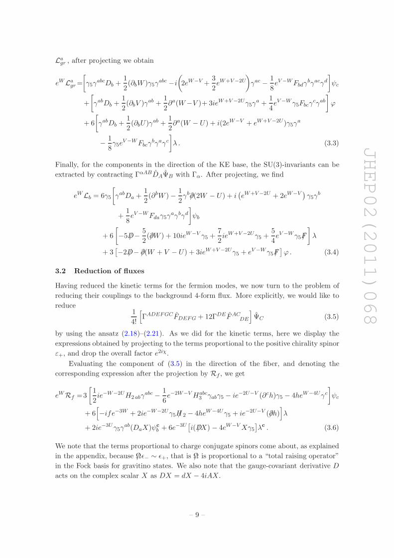
JHEP02(2011)068

Lagr , after projecting we obtain

eWLagr=[

γ5γabcDb +

1

2(∂bW )γ5γ

abc −i(

2eW−V +3

2eW+V−2U

)

γac − 1

8eV−WFbdγ

bγacγd]

ψc

+

[

γabDb +1

2(∂bV )γab +

1

2∂a(W−V )+ 3ieW+V −2Uγ5γ

a +1

4eV −Wγ5Fbcγ

cγab]

ϕ

+ 6

[

γabDb +1

2(∂bU)γab +

1

2∂a(W − U) + i(2eW−V + eW+V−2U )γ5γ

a

− 1

8γ5e

V−WFbcγbγaγc

]

λ . (3.3)

Finally, for the components in the direction of the KE base, the SU(3)-invariants can be

extracted by contracting ΓαABDAΨB with Γα. After projecting, we find

eWLb = 6γ5

[

γabDa +1

2(∂bW )− 1

2γb∂/(2W − U) + i

(

eW+V−2U + 2eW−V)

γ5γb

+1

8eV−WFdaγ5γ

aγbγd]

ψb

+ 6

[

−5D/− 5

2(∂/W ) + 10ieW−V γ5 +

7

2ieW+V−2Uγ5 +

5

4eV −Wγ5F/

]

λ

+ 3[

−2D/− ∂/(W + V − U) + 3ieW+V−2Uγ5 + eV−Wγ5F/]

ϕ . (3.4)

3.2 Reduction of fluxes

Having reduced the kinetic terms for the fermion modes, we now turn to the problem of

reducing their couplings to the background 4-form flux. More explicitly, we would like to

reduce1

4!

[

ΓADEFGCFDEFG + 12ΓDEFACDE

]

ΨC (3.5)

by using the ansatz (2.18)–(2.21). As we did for the kinetic terms, here we display the

expressions obtained by projecting to the terms proportional to the positive chirality spinor

ε+, and drop the overall factor e2iχ.

Evaluating the component of (3.5) in the direction of the fiber, and denoting the

corresponding expression after the projection by Rf , we get

eWRf =3

[

1

2ie−W−2UH2 abγ

abc − 1

6e−2W−VHabc

3 γabγ5 − ie−2U−V (∂ch)γ5 − 4heW−4Uγc]

ψc

+ 6[

−ife−3W + 2ie−W−2Uγ5H/ 2 − 4heW−4Uγ5 + ie−2U−V (∂/h)]

λ

+ 2ie−3Uγ5γab(DaX)ψc

b + 6e−3U[

i(D/X) − 4eW−VXγ5

]

λc . (3.6)

We note that the terms proportional to charge conjugate spinors come about, as explained

in the appendix, because Ω/ ǫ− ∼ ǫ+, that is Ω/ is proportional to a “total raising operator”

in the Fock basis for gravitino states. We also note that the gauge-covariant derivative D

acts on the complex scalar X as DX = dX − 4iAX.

– 9 –

JHEP02(2011)068

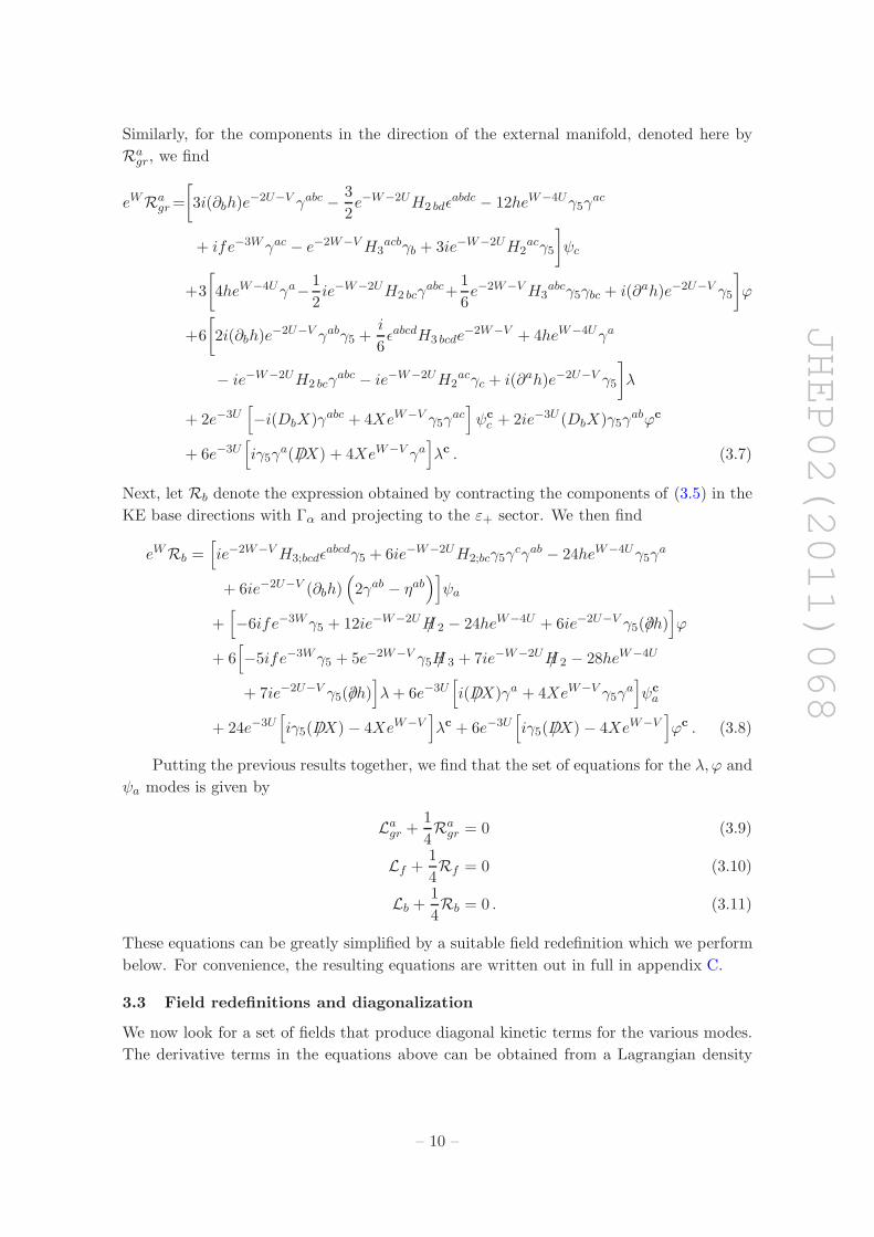
Similarly, for the components in the direction of the external manifold, denoted here by

Ragr, we find

eWRagr=[

3i(∂bh)e−2U−V γabc − 3

2e−W−2UH2 bdǫ

abdc − 12heW−4Uγ5γac

+ ife−3W γac − e−2W−VH3acbγb + 3ie−W−2UH2

acγ5

]

ψc

+3

[

4heW−4Uγa− 1

2ie−W−2UH2 bcγ

abc+1

6e−2W−VH3

abcγ5γbc + i(∂ah)e−2U−V γ5

]

ϕ

+6

[

2i(∂bh)e−2U−V γabγ5 +

i

6ǫabcdH3 bcde

−2W−V + 4heW−4Uγa

− ie−W−2UH2 bcγabc − ie−W−2UH2

acγc + i(∂ah)e−2U−V γ5

]

λ

+ 2e−3U[

−i(DbX)γabc + 4XeW−V γ5γac

]

ψc

c + 2ie−3U (DbX)γ5γabϕc

+ 6e−3U[

iγ5γa(D/X) + 4XeW−V γa

]

λc . (3.7)

Next, let Rb denote the expression obtained by contracting the components of (3.5) in the

KE base directions with Γα and projecting to the ε+ sector. We then find

eWRb =[

ie−2W−VH3;bcdǫabcdγ5 + 6ie−W−2UH2;bcγ5γ

cγab − 24heW−4Uγ5γa

+ 6ie−2U−V (∂bh)(

2γab − ηab)]

ψa

+[

−6ife−3Wγ5 + 12ie−W−2UH/ 2 − 24heW−4U + 6ie−2U−V γ5(∂/h)]

ϕ

+ 6[

−5ife−3W γ5 + 5e−2W−V γ5H/ 3 + 7ie−W−2UH/ 2 − 28heW−4U

+ 7ie−2U−V γ5(∂/h)]

λ+ 6e−3U[

i(D/X)γa + 4XeW−V γ5γa]

ψc

a

+ 24e−3U[

iγ5(D/X) − 4XeW−V]

λc + 6e−3U[

iγ5(D/X) − 4XeW−V]

ϕc . (3.8)

Putting the previous results together, we find that the set of equations for the λ,ϕ and

ψa modes is given by

Lagr +1

4Ragr = 0 (3.9)

Lf +1

4Rf = 0 (3.10)

Lb +1

4Rb = 0 . (3.11)

These equations can be greatly simplified by a suitable field redefinition which we perform

below. For convenience, the resulting equations are written out in full in appendix C.

3.3 Field redefinitions and diagonalization

We now look for a set of fields that produce diagonal kinetic terms for the various modes.

The derivative terms in the equations above can be obtained from a Lagrangian density

– 10 –

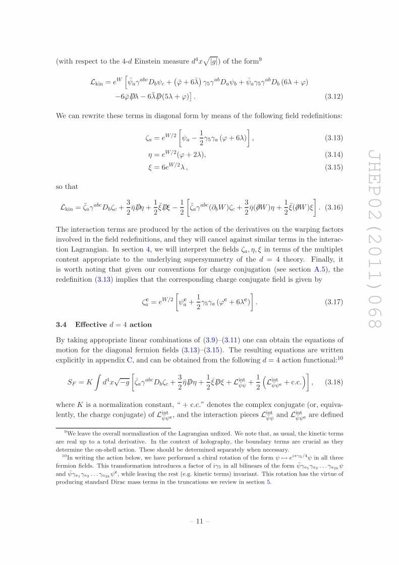
JHEP02(2011)068

(with respect to the 4-d Einstein measure d4x√

|g|) of the form9

Lkin = eW[

ψaγabcDbψc +

(

ϕ+ 6λ)

γ5γabDaψb + ψaγ5γ

abDb (6λ+ ϕ)

−6ϕD/λ− 6λD/ (5λ+ ϕ)]

. (3.12)

We can rewrite these terms in diagonal form by means of the following field redefinitions:

ζa = eW/2[

ψa −1

2γ5γa (ϕ+ 6λ)

]

, (3.13)

η = eW/2(ϕ+ 2λ), (3.14)

ξ = 6eW/2λ , (3.15)

so that

Lkin = ζaγabcDbζc +

3

2ηD/η +

1

2ξD/ξ − 1

2

[

ζaγabc(∂bW )ζc +

3

2η(∂/W )η +

1

2ξ(∂/W )ξ

]

. (3.16)

The interaction terms are produced by the action of the derivatives on the warping factors

involved in the field redefinitions, and they will cancel against similar terms in the interac-

tion Lagrangian. In section 4, we will interpret the fields ζa, η, ξ in terms of the multiplet

content appropriate to the underlying supersymmetry of the d = 4 theory. Finally, it

is worth noting that given our conventions for charge conjugation (see section A.5), the

redefinition (3.13) implies that the corresponding charge conjugate field is given by

ζca = eW/2[

ψc

a +1

2γ5γa (ϕc + 6λc)

]

. (3.17)

3.4 Effective d = 4 action

By taking appropriate linear combinations of (3.9)–(3.11) one can obtain the equations of

motion for the diagonal fermion fields (3.13)–(3.15). The resulting equations are written

explicitly in appendix C, and can be obtained from the following d = 4 action functional:10

SF = K

∫

d4x√−g

[

ζaγabcDbζc +

3

2ηD/ η +

1

2ξD/ ξ + Lint

ψψ +1

2

(

Lintψψc

+ c.c.)

]

, (3.18)

where K is a normalization constant, “ + c.c.” denotes the complex conjugate (or, equiva-

lently, the charge conjugate) of Lintψψc

, and the interaction pieces Lintψψ

and Lintψψc

are defined

9We leave the overall normalization of the Lagrangian unfixed. We note that, as usual, the kinetic terms

are real up to a total derivative. In the context of holography, the boundary terms are crucial as they

determine the on-shell action. These should be determined separately when necessary.10In writing the action below, we have performed a chiral rotation of the form ψ 7→ eiπγ5/4ψ in all three

fermion fields. This transformation introduces a factor of iγ5 in all bilinears of the form ψγa1γa2

. . . γa2kψ

and ψγa1γa2

. . . γa2kψc, while leaving the rest (e.g. kinetic terms) invariant. This rotation has the virtue of

producing standard Dirac mass terms in the truncations we review in section 5.

– 11 –

JHEP02(2011)068

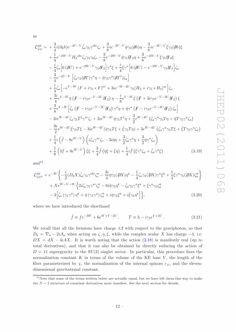
as

Lintψψ = +

3

4i(∂bh)e

−2U−V ζaγ5γabcζc +

3

8ie−2U−V ηγ5(∂/h)η −

3

8ie−2U−V ξγ5(∂/h)ξ

+1

4e−2W−VH3

abcζaγ5γbζc −3

8e−2W−V ηγ5H/ 3η +

3

8e−2W−V ξγ5H/ 3ξ

− i

4ζa

[

6 (∂/U) + e−2W−V γ5H/ 3

]

γaξ +i

4ξγa

[

6 (∂/U)− e−2W−V γ5H/ 3

]

ζa

− 3

4e−2U−V

[

ζaγ5(∂/T )γaη − ηγ5γa(∂/T †)ζa

]

+i

4ζa

[

−eV−W (F + iγ5 ∗ F )ac + 3ie−W−2Uγ5(H2 + iγ5 ∗H2)ac

]

ζc

+3i

4eV−W η

(

F/ − iγ5e−V−2UH/ 2

)

η − i

8eV−W ξ

(

F/ + 3iγ5e−V−2UH/ 2

)

ξ

+3

8eV−W

[

ζa(

F/ − iγ5e−V−2UH/ 2

)

γaη + ηγa(

F/ − iγ5e−V−2UH/ 2

)

ζa

]

− 3ieW−4U ζaγ5T†γacζc + 3ieW−4U ηγ5T

†η +3

2eW−4U

(

ζaγaγ5Tη + ηT γ5γ

aζa)

− 9i

2eW−4U ξγ5Tξ − 3ieW−4U (ηγ5Tξ + ξγ5Tη) + 3eW−4U

(

ζaγaγ5Tξ + ξT γ5γ

aζa)

+1

4i(

f − 8eW−V)

(

iζaγacζc − 3iηη +

3

2ζaγ

aη +3

2ηγaζa

)

+1

8

(

3f + 8eW−V)

ξξ +3

4f

(

ηξ + ξη)

+1

4if

(

ξγaζa + ζaγaξ

)

(3.19)

and11

Lintψψc

= e−3U

− i2(DbX)ζaγ5γ

abcζcc −3i

4ηγ5(D/X)ηc − 1

4ζaγ5(D/X)γaξc +

1

4ξγaγ5(D/X)ζca

+XeW−V−3U

2iζaγ5γacζcc − 6iηγ5η

c − ζaγ5γaξc + ξγaγ5ζ

c

a

− 3[

ζa (γ5γa) ηc + η (γ5γ

a) ζca + iηγ5ξc + iξγ5η

c

]

, (3.20)

where we have introduced the shorthand

f ≡ fe−3W + 6eW+V−2U , T ≡ h− iγ5eV+2U . (3.21)

We recall that all the fermions have charge ±2 with respect to the graviphoton, so that

Da = ∇a − 2iAa when acting on ζ, η, ξ, while the complex scalar X has charge −4, i.e.

DX = dX − 4iAX. It is worth noting that the action (3.18) is manifestly real (up to

total derivatives), and that it can also be obtained by directly reducing the action of

D = 11 supergravity to the SU(3) singlet sector. In particular, this procedure fixes the

normalization constant K in terms of the volume of the KE base Y , the length of the

fiber parameterized by χ, the normalization of the internal spinors ε±, and the eleven-

dimensional gravitational constant.

11Note that some of the terms written below are actually equal, but we have left them this way to make

the N = 2 structure of covariant derivatives more manifest. See the next section for details.

– 12 –

JHEP02(2011)068

4 N = 2 supersymmetry

To interpret this action further, we consider how the fields fit into supermultiplets of

gauged N = 2 supergravity in four dimensions, ignoring the possibility of supersymmetry

enhancement for special compactifications. Using the same techniques as above, we can

reduce the 11-d supersymmetry variations of the fermionic fields.12 These take the form

δΨA = DAΘ +1

12

1

4!(ΓA

BCDE − 8δBAΓCDE)ΘFBCDE . (4.1)

We are interested only in the Grassmann parameters that are SU(3) invariant, and it proves

convenient to then write

Θ = eW/2θ ⊗ ε+e2iχ + eW/2θc ⊗ ε−e−2iχ . (4.2)

Here, θ is a 4-d Dirac spinor. By making appropriate projections on (4.1) to terms of

definite charge, one obtains the variations of the fields ϕ, λ, ψa. Performing then the change

of variables (3.13)–(3.15), we arrive at the variations

δη = −1

4eV−W

(

F/ − ie−2U−V γ5H/ 2

)

θ +i

2e−2U−V (∂/T )θ

−eW−4UTγ5θ −1

4i(

f − 8eW−V)

θ − 2eW−3U−VXγ5θc (4.3)

δξ = 3γ5(∂/U)θ − 1

2e6UH/ 3θ −

1

2e−3U i(D/X)θc

−1

2ifθ + 6eW−4UT †γ5θ − 2XeW−V−3Uγ5θ

c (4.4)

δζa =

(

Da −3

4i(∂ah)e

−2U−V γ5 +1

8eV−W γ5

(

F/ − 3ie−V −2Uγ5H/ 2

)

γa

)

θ

+

(

1

8i(

f − 8eW−V)

γ5 +3

2TeW−4U

)

γaθ +1

8e−2W−V γ5 [γa,H/ 3] θ

−XeW−3U−V γaθc +

1

2e−3Uγ5(iDaX)θc . (4.5)

Now, according to [22], there is a single vector multiplet that contains the scalar

τ = h + ieV+2U (in this notation, T = τP− + τP+, where P± = 12(1 ± γ5)), and there is

universal hypermultiplet containing ρ = 4e6U , the pseudoscalar dual to H3 and X. The

gravity multiplet contains the gravitino ζa while the vector multiplet and hypermultiplet

each contains a Dirac spinor. Examining then the first lines of the variations (4.3) and (4.4)

written above which contain derivatives of bosonic fields, we can identify the gauginos with

η and the hyperinos with ξ.

In the N = 2 literature, one usually finds things written in terms of Weyl spinors. For

a generic spinor Ψ, we could write

Ψ1 = P+Ψ, Ψ2 = P+Ψc (4.6)

12In what follows we keep only the terms linear in fermions.

– 13 –

JHEP02(2011)068

and we then have Ψc

2 = P−Ψ and Ψc

1 = P−Ψc. To be specific, let us consider the gaugino

variation. It is convenient to first write the charge conjugate equation

δηc = −1

4eV −W

(

F/ − ie−2U−V γ5H/ 2

)

θc − i

2e−2U−V (∂/T )θc

+eW−4UTγ5θc +

1

4i(

f − 8eW−V)

θc + 2eW−3U−VX∗γ5θ (4.7)

and doing the chiral projection, we then obtain

δη1 = +i

2e−2U−V (∂/τ)θc1 −

1

4eV−W

(

F/ − ie−2U−VH/ 2

)

θ1

−eW−4U τ θ1 −1

4i(

f − 8eW−V)

θ1 − 2eW−3U−VXθ2 (4.8)

δη2 = − i2e−2U−V (∂/τ)θc2 −

1

4eV−W

(

F/ − ie−2U−VH/ 2

)

θ2

+eW−4U τ θ2 +1

4i(

f − 8eW−V)

θ2 + 2eW−3U−VX∗θ1 . (4.9)

With a minor change of notation, these expressions can be understood as those that are

obtained from working out this specific case of ref. [36]. (Details of the bosonic sector of

this have also recently appeared in ref. [30]). Indeed, we have worked through the details

of deriving the 4-d action using the results of [36]; we will not show this calculation in full

here, but just point out the geometric features. The field content is usually presented after

dualizing H2 and H3 [24]13

H(2) =1

4h2 + e4U+2V

(

2h(H(2) + h2F (2))− e2U+V ∗ (H(2) + h2F (2)))

(4.12)

H(3) = −1

4e−12U ∗ [Dσ + JX ] (4.13)

where Da = da + 6(B1 − ǫA1), H2 = dB1, JX = i(X∗DX − DX∗X), ρ = 4e6U and

σ = 4a. The hypermultiplet contains the scalars X,σ, ρ, while the vector multiplet

contains τ = h + ieV+2U . The scalars of the hypermultiplet coordinatize a quaternionic

space HM ≃ SO(4, 1)/SO(4) with metric

ds2H =1

ρ2dρ2 +

1

4ρ2[dσ − i (XdX∗ −X∗dX)]2 +

1

ρ2dXdX∗ . (4.14)

The vector multiplet scalars coordinatize a special Kahler manifold SM with Kahler po-

tential

KV = − logi(τ − τ)3

2. (4.15)

13It’s convenient to note that these imply

H/ 2 =h+ T

|h+ τ |2 (H/ 2 + h2F/ ) (4.10)

ie6Uγ5H/ 3 =1

ρ[D/σ + J/ X ] . (4.11)

– 14 –

JHEP02(2011)068

On SM there is a line bundle L with c1(L) = i2π ∂∂KV = 3i

8π1

(Imτ)2. Each of the fermions

is a section of L1/2, with Hermitian connection θ = ∂KV . In the local coordinates τ, τ ,

we have θ = − 32iImτ dτ . Associated naturally to the line bundle is a U(1) bundle with

connection Q = Imθ = 32dReτImτ . Given τ = h + ieV+2U , this gives Q = 3

2e−V−2Udh. The

gaugino is also a section of TSM; the Levi-Civita connection on SM is Γ ≡ Γτ τ = iImτ dτ =

ie−V −2Udh− d(V + 2U).

Because of the quaternionic structure, HM possesses three complex structures J α :

THM → THM that satisfy the quaternion algebra J αJ β = −δαβ1 + ǫαβγJ γ . Corre-

spondingly, there is a triplet of Kahler forms KαH , which we regard as SU(2) Lie algebra

valued. Required by N = 2 supersymmetry, there is a principal SU(2)-bundle SU over HMwith connection such that the hyper-Kahler form is covariantly closed; the curvature of the

principal bundle is proportional to the hyper-Kahler form. It follows that the Levi-Civita

connection of HM has holonomy contained in SU(2)⊗Sp(2,R). The fermions are sections

of these bundles as follows:

• gravitino: L1/2 × SU

• gaugino: L1/2 × T SM× SU

• hyperino: L1/2 × T HM× SU−1

In the last line, one means that the hyperino is a section of the vector bundle obtained by

deleting the SU(2) part of the holonomy group on HM.

The connections on SU and THM×SU−1 are evaluated in terms of the hypermultiplet

scalars, and one finds the following results, following a translation into Dirac notation. The

gravitino covariant derivative reads

Dbζc = Dbζc −3i

4e−2U−V (∂bh)γ5ζc −

i

4e6U (∗H3)bζc +

i

2e−3U (DbX)γ5ζ

c

c , (4.16)

which leads to

γabcDbζc = γabcDbζc +3i

4e−2U−V (∂bh)γ5γ

abcζc +1

4e6UHabc

3 γ5γbζc

− i

2e−3U (DbX)γ5γ

abcζcc . (4.17)

The gaugino covariant derivative is

Daη = Daη −i

4e−(2U+V )(∂ah)γ5η −

i

4e6U (∗H3)aη +

i

2e−3U (DaX)γ5η

c , (4.18)

giving

D/ η = D/η +i

4e−(2U+V )γ5(∂/h)η −

1

4e6Uγ5H/ 3η −

i

2e−3Uγ5(D/X)ηc . (4.19)

Finally, the hyperino is a section of THM×SU−1. The covariant derivative is then

Daξ = Daξ +3i

4e−(2U+V )(∂ah)γ5ξ +

3i

4e6U (∗H3)aξ . (4.20)

– 15 –

JHEP02(2011)068

Equivalently,

D/ ξ = D/ξ − 3i

4e−(2U+V )γ5(∂/h)ξ +

3

4e6Uγ5H/ 3ξ . (4.21)

We recognize the pieces of these covariant derivatives in the action given above. Indeed,

the action takes the form

Skin = K

∫

d4x√−g

[

ζaγabcDbζc +

3

2ηD/ η +

1

2ξD/ ξ + · · ·

]

. (4.22)

In comparing to the first few lines of (3.19) and (3.20), one can see these covariant deriva-

tives forming. The remaining couplings to F and H2 and to the scalars can also be derived

from the N = 2 geometric structure, but we will not give further details here.

5 Examples

In this section we compare the general effective four-dimensional action to various holo-

graphic fermion systems that have been considered in the literature, and look for appro-

priate further (consistent) truncations of the fermionic sector. We focus mainly on two

relevant further truncations, namely, the minimal gauged N = 2 supergravity theory, and

the model of [23, 24], which provided an embedding of the holographic superconductor [8, 9]

into M-theory.

5.1 Minimal gauged supergravity

As discussed in [22], a possible further truncation entails taking

U = V = W = H3 = h = X = 0, f = 6ǫ , H2 = −ǫ ∗ F (i.e. iγ5H/ 2 = ǫF/ ) , (5.1)

which sets all the massive fields to zero, leaving the N = 2 gravity multiplet only. The

corresponding equations for the bosonic fields can be derived from the Einstein-Maxwell

action

SB = KB

∫

d4x√−g (R− FµνFµν + 24) . (5.2)

The simplest fermionic content that one can consider is a charged massive bulk Dirac

fermion minimally coupled to gravity and the gauge field (see for example [34, 42–45]).

In our context, this truncation has an AdS4 vacuum solution which uplifts to a su-

persymmetric AdS4 × SE7 solution in D = 11. These solutions are thought of as being

dual to three-dimensional SCFTs with N = 2 supersymmetry (in principle). In this trun-

cation, we note that for ǫ = +1, the variations (4.3)–(4.4) of η and ξ are both zero, and

ζa decouples from η, ξ. Consequently, it is consistent to set η = ξ = 0 (as we did for their

superpartners) in this case, and we then obtain the effective d = 4 action (3.18) for the

gravity supermultiplet

S = SB +K

∫

d4x√−g

[

ζaγabcDbζc − iζa

[

(F + iγ5 ∗ F )ac + 2iγac]

ζc

]

. (5.3)

– 16 –

JHEP02(2011)068

We note that this gives the expected couplings between the gravitino and the gravipho-

ton14 [46, 47] (see [48] also).

If ǫ = −1, supersymmety is broken, and we wish to consider other truncations of the

fermionic sector. It appears that there are no non-trivial consistent truncations in this

case — if we choose to set the gravitino to zero for example, its equation of motion gives

a constraint on η and ξ that appears to have no non-trivial solutions. To see this, we note

the action contains the interaction terms (as usual neglecting 4-fermion couplings)

Lintψψ = 5ζaγ

acζc −9

2i(

ζaγaη + ηγaζa

)

− 3i(

ζaγaξ + ξγaζa

)

+i

2ζa

[

(F + iγ5 ∗ F )ac]

ζc +3

4

[

ζaF/ γaη + ηγaF/ ζa

]

− 9ηη − 7

2ξξ − 3(ηξ + ξη) +

3i

2ηF/ η +

i

4ξF/ ξ . (5.4)

5.2 Fermions coupled to the holographic superconductor

We now consider truncations appropriate to holographic superconductors. We note that

the general model contains the charged boson X, of charge twice the charge of the fermion

fields. This is one of the basic features of the model considered in [33], which studied

charged fermions coupled to the holographic superconductor. It is interesting to see how

the couplings used there appear in the top-down model.

Refs. [23, 24] considered the following truncation of the bosonic sector

h = 0 , e6U = 1− 1

4|X|2 , V = −2U (= W ), H2 = ∗F ,

H3 =i

4e−12U ∗ (X∗DX −XDX∗) , ǫ = −1 , f = 6e−12U

(

−1 +|X|2

3

)

, (5.5)

where DX = dX − 4iAX as before. As pointed out in [23, 24], in order to set h = 0 we

need to impose F ∧ F = 0 by hand, and thus the truncation (even before considering the

fermions) is not consistent. While this restriction allows for black hole solutions carrying

electric or magnetic charge only, it excludes solutions of the dyonic type. This theory

also has an AdS4 vacuum solution (with X = 0 and f = −6), which uplifts to a skew-

whiffed AdS4 × SE7 solution in D = 11. In general, these solutions do not preserve any

supersymmetries (an exception being the case where SE7 = S7).

The d = 4 effective action (3.18) for this truncation is given by

SF = K

∫

d4x√−g

[

ζaγabcDbζc +

3

2ηD/ η +

1

2ξD/ ξ + Lint

ψψ +1

2

(

Lintψψc

+ c.c.)

]

, (5.6)

14One can use the identity F bdγ[bγacγd] = Fbdγ

bdac + 2F ac = iFbdγ5ǫbdac + 2F ac to rewrite the coupling

of the gravitino to the field-strength in the somewhat more familiar form ∼ F bdζaγ[bγacγd]ζc .

– 17 –

JHEP02(2011)068

where now

e6ULintψψ=

1

2ζa

[

(

1− |X|2

4

)

i (F + iγ5 ∗ F )ac − 2(

|X|2 − 5)

γac − 1

8

(

X∗←→DbX)

γbac

]

ζc

+3

4η

[

−4(

3− |X|2)

+1

8

(

X∗←→D/ X

)

+ 2

(

1− |X|2

4

)

iF/

]

η

+3

8ξ

[

−4

3

(

7− |X|2)

+2

3

(

1− |X|2

4

)

iF/ − 1

4

(

X∗←→D/ X

)

]

ξ

+3

4ζa

[

2i(

|X|2− 3)

+

(

1− |X|2

4

)

F/

]

γaη +3

4ηγa

[

2i(

|X|2− 3)

+

(

1− |X|2

4

)

F/

]

ζa

+i

2ζa

[

(

|X|2 − 6)

+1

4X∗(D/X)

]

γaξ +i

2ξγa

[

(

|X|2 − 6)

− 1

4X(D/X)∗

]

ζa

− 3

2η

(

2− |X|2)

ξ − 3

2ξ(

2− |X|2)

η (5.7)

and

e3ULintψψc

=i

2ζaγ5

[

−(DbX)γabc + 4Xγac]

ζcc −3i

4ηγ5 (D/X + 8X) ηc

− 1

4ζaγ5 (D/X + 4X) γaξc − 1

4ξγ5γ

a (D/X + 4X) ζca

− 3X[

ζa (γ5γa) ηc + η (γ5γ

a) ζca + iηγ5ξc + iξγ5η

c

]

. (5.8)

In order to compare to phenomenologically motivated models, such as the holographic

superconductor models, it is instructive to expand in powers of the complex scalar X, it

being natural to organize the action by engineering dimension. Since 4-fermi couplings

are dimension 6 or higher, we will here keep all terms up to and including dimension five.

Doing so we obtain

Lintψψ ≃

1

2iζa

[

(F + iγ5 ∗ F )ac − 10iγac]

ζc +3

2iη (6i+ F/ ) η

+1

4iξ (14i+ F/ ) ξ +

3

4ζa (−6i+ F/ ) γaη +

3

4ηγa (−6i+ F/ ) ζa

− 3(

ηξ + ξη + iζaγaξ + iξγaζa

)

− 1

4i|X|2

[

iζaγacζc −

3

2

(

ζaγaη + ηγaζa

)

+(

ζaγaξ + ξγaζa

)

]

+3

4|X|2

[

ηη − 1

2ξξ +

(

ηξ + ξη)

]

, (5.9)

and

Lintψψc≃ 1

2iζaγ5

[

− (DbX)γabc + 4Xγac]

ζcc −3

4iηγ5 (D/X + 8X) ηc

− 1

4ζaγ5 (D/X + 4X) γaξc − 1

4ξγ5γ

a (D/X + 4X) ζca

− 3X(

ζaγ5γaηc + ηγ5γ

aζca + iηγ5ξc + iξγ5η

c)

. (5.10)

– 18 –

JHEP02(2011)068

Note that we have the same basic couplings as in [33]: we have Majorana couplings between

the doubly-charged boson X and spin-1/2 fermions. The model is significantly more com-

plicated for several reasons. First, we have kept here several species of spin-1/2 fermions,

and they are also coupled to the gravitino. An exploration of this model holographically, or

a further truncation of the model, would be of interest. We also note that there are generic

terms of the form ψγ5D/Xψc. These could also be of interest holographically; first in the

presence of a boundary chemical potential for A, such a coupling looks similar to the other

Majorana coupling near the boundary. But it also would presumably be the most impor-

tant coupling in non-homogeneous boundary configurations (such as would correspond to

spin-wave, nematic order, etc.). We also note that there are generically the “Pauli terms”,

involving dipole couplings of the fermions to the gauge field strength, which could have

important effects in electric or magnetic backgrounds.

It is clear that dropping all of the fermions is a consistent truncation, at least as

consistent as the bosonic truncation. It is also apparently possible to keep all of the

fermions, although the h equation of motion will now give a condition including terms

non-linear in fermions. It would be interesting to find other truncations of the fermion

content. For example, can one reduce, say, to a single species of charged fermion, including

the elimination of the gravitino?. If such a truncation exists, it is non-trivial.

6 Conclusions

In this paper, we have explicitly worked out the form of the fermionic action obtained from

a consistent truncation of 11-d supergravity on warped Sasaki-Einstein 7-manifolds, which

should be thought of as the total space of a Spinc bundle over a Kahler-Einstein base. The

consistent truncation is obtained by restricting to SU(3)-invariant excitations. We have

checked that the resulting theory is consistent with what is expected from N = 2 gauged

supergravity in four dimensions, in the case where there is a single vector multiplet and a

single hypermultiplet.

This work is relevant to the recent literature on holographic duals of three-dimensional

strongly-coupled field theories, particularly to those in which fermions play a central role in

the dynamics, such as in superconductors. The theory does contain interesting couplings

of the Majorana type, similar to those considered in the literature, as well as some new

ones. We have briefly considered several further truncations that are closer to bottom-up

models that have been discussed in the literature. Generally, we have found that it is

difficult to find truncations of the fermionic sector. In particular, the gravitino is typically

coupled to the other fermion fields. As a result, in holographic studies, we expect to see

a spin-3/2 operator in the dual theory (the boundary supercurrents, in supersymmetric

cases), and given appropriate asymptotic bosonic configurations, this operator would mix

with other fermionic operators. We have not done an exhaustive job of studying this

decoupling problem however, and it would be of interest to do so and to consider a variety

of holographic applications.

– 19 –

JHEP02(2011)068

Acknowledgments

It is a pleasure to thank Riccardo Argurio, Jim Liu, Phil Szepietowski and Diana Vaman for

helpful conversations. J.I.J. and R.G.L. are thankful to the Michigan Center for Theoretical

Physics (MCTP) for their hospitality during different stages of this project. We have been

informed by J. Sonner of an ongoing collaboration with J. Gauntlett and D. Waldram

that has some overlap with the work presented here. R.G.L. is supported by DOE grant

FG02-91-ER40709. J.I.J. and A.T.F. are supported by Fulbright-CONICYT fellowships,

and I.B. by a University of Michigan Rackham Science Award. L.P.Z and I.B. are partially

supported by DOE grant DE-FG02-95ER40899.

A Conventions and useful formulae

In this appendix we introduce the various conventions used in the body of the paper, and

collect some useful results.

A.1 Conventions for forms and Hodge duality

We normalize all the (real) form fields according to

ω = ωa1...ap ea1 ⊗ ea2 · · · ⊗ eap

=1

p!ωa1...ap e

a1 ∧ · · · ∧ eap . (A.1)

In d spacetime dimensions, the Hodge dual acts on the basis of forms as

∗ (ea1 ∧ · · · ∧ eap) =1

(d− p)!ǫb1...bd−p

a1...ap eb1 ∧ · · · ∧ ebd−p , (A.2)

where ǫb1...bd−pa1...ap are the components of the Levi-Civita tensor. Equivalently, for the

components of the Hodge dual ∗ω of a p-form ω we have

(∗ω)a1...ad−p=

1

p!ǫa1...ad−p

b1...bpωb1...bp . (A.3)

In the (3 + 1)-dimensional external manifold M we adopt the convention ǫ0123 = +1 for

the components of the Levi-Civita tensor in the orthonormal frame.

A.2 Elfbein and spin connection

As discussed in section 2, the Kaluza-Klein metric ansatz of [22] is given by

ds211 = e2W (x)ds2E(M) + e2U(x)ds2(Y ) + e2V (x)(

dχ+A(y) +A(x))2, (A.4)

where W (x) = −3U(x) − V (x)/2 as in the body of the paper. We now introduce the

eleven-dimensional orthonormal frame eM . Denoting by a, b, . . . the tangent indices to M ,

– 20 –

JHEP02(2011)068

by α, β, . . . the tangent indices to the KE base Y , and by f the index associated with the

U(1) fiber direction χ, our choice of elfbein reads

ea = eW ea (A.5)

eα = eUeα (A.6)

ef = eV(

dχ+A(y) +A(x))

, (A.7)

where ea and eα are orthonormal frames for M and Y , respectively. The dual basis is then

ea = e−W(

ea −Aa∂χ)

(A.8)

eα = e−U(

eα −Aα∂χ)

(A.9)

ef = e−V ∂χ . (A.10)

Denoting by ωab the spin connection associated with ds2(M) and by ωαβ the spin connec-

tion appropriate to ds2(Y ), for the eleven-dimensional spin connection ωMN we find

ωαa = eU−W (∂aU)eα (A.11)

ωfa = eV−W

[

1

2Fabe

b + (∂aV )(

dχ+A+A)

]

(A.12)

ωfα = eV−U 1

2Fαβeβ (A.13)

ωab = ωab − 2ηac∂[cWηb]ded − 1

2e2(V −W )F ab

(

dχ+A+A)

(A.14)

ωαβ = ωαβ −1

2e2(V −U)Fαβ

(

dχ+A+A)

, (A.15)

where ηab is the flat metric in (3 + 1) dimensions, F ≡ dA and F ≡ dA = 2J , J being the

Kahler form on Y .

A.3 Fluxes

The ansatz (2.5) for the 4-form flux F4, reproduced here for convenience, is [22]

F4 = f vol4 +H3 ∧ (η +A) +H2 ∧ J + dh ∧ J ∧ (η +A) + 2hJ2

+

[

X(η +A) ∧Ω− i

4(dX − 4iAX) ∧ Ω + c.c.

]

. (A.16)

We will often use a complex basis on T ∗Y . If y denote real coordinates on Y , we define

z1 ≡ 12 (y1+iy2), z1 ≡ 1

2

(

y1 − iy2)

, and similarly for z2, z2, z3, z3. With this normalization,

the Kahler form J and the holomorphic (3,0)-form Σ are given by

J = 2i∑

α=1,2,3

eα ∧ eα (A.17)

Σ =8

3!ǫαβγ e

α ∧ eβ ∧ eγ , (A.18)

– 21 –

JHEP02(2011)068

where we have chosen ǫ123 = +1. Similarly, the forms on the external manifold can be

written

vol4 =1

4!ǫabcd e

a ∧ eb ∧ ec ∧ ed (A.19)

H2 =1

2!H2 ab e

a ∧ eb (A.20)

H3 =1

3!H3 abc e

a ∧ eb ∧ ec . (A.21)

The components of F4 with respect to the eleven-dimensional frame eM are then (in the

real basis for T ∗Y )

Fabcf = e−3W−VH3abc (A.22)

Faαβf = e−W−2U−V (∂ah)Jαβ (A.23)

Ffαβγ = Xe−3U−V Ωαβγ + c.c. (A.24)

Fabcd = fe−4W ǫabcd (A.25)

Fabαβ = e−2W−2UJαβH2ab (A.26)

Fαβγδ = 4he−4U (JαβJγδ − JαγJβδ + JαδJβγ) (A.27)

Faαβγ = − i4(DaX)e−3U−WΩαβγ + c.c. (A.28)

A.4 Clifford algebra

We choose the following basis for the D = 11 Clifford algebra:

Γa = γa ⊗ 18 (A.29)

Γα = γ5 ⊗ γα (A.30)

Γf = γ5 ⊗ γ7 (A.31)

where the γa are a basis for Cℓ(3, 1) with γ5 = iγ0γ1γ2γ3 and the γα are a basis for

Cℓ(6) with γ7 = i∏

α γα. These dimensions are such that we can define Majorana spinors

in each case. In D = 11, we take Γ0 to be anti-Hermitian and the rest Hermitian. This

means that γ0 is anti-Hermitian, while γa(a 6= 0), γ5, γ7 and γα are Hermitian. We also

have γ25 = 1 and γ2

7 = 1. In the standard basis, the γa, γ5 are 4 × 4 matrices while the

γα, γ7 are 8× 8 matrices. It will also be convenient to define

Γ7 =∏

α

Γα = 14 ⊗ γ7 (A.32)

Γ5 =∏

a

Γa = γ5 ⊗ 18 . (A.33)

Some useful identities involving the Cℓ(3, 1) gamma matrices include

ǫabcd = −iγ5γabcd , ǫabcdγa = iγ5γbcd , ǫabcdγ

cd = 2iγ5γab , ǫabcdγbcd = 6iγ5γa . (A.34)

– 22 –

JHEP02(2011)068

A.5 Charge conjugation conventions

In d = 4 dimensions with signature (−,+,+,+) we can define unitary intertwiners B4 and

C4 (the charge conjugation matrix), unique up to a phase, satisfying

B4γaB†4 = γ∗a BT

4 = B4 (A.35)

B4γ5B†4 = −γ∗5 B∗

4B4 = 1 , (A.36)

and

C4γaC†4 = −γTa CT4 = −C4 (A.37)

C4γ5C†4 = γT5 C4 = BT

4 γ0 = B4γ0 . (A.38)

If ψ is any spinor, its charge conjugate ψc is then defined as

ψc = B−14 ψ∗ = B†

4ψ∗ = γ0C

†4ψ

∗ . (A.39)

In (3+1) dimensions one can define Majorana spinors. By definition, a spinor ψ is Majorana

if ψ = ψc. Notice that in (3+1) dimensions this condition relates opposite chirality spinors.

Similarly, we can define the charge conjugates of a spinor Ψ in (10+1) dimensions and a

spinor η in 7 Euclidean dimensions as

Ψc = B−111 Ψ∗ , where B11ΓMB

−111 = Γ∗

M , (A.40)

ηc = B−17 η∗ , where B7γαB

−17 = −γ∗α . (A.41)

Defining ψc in the (3+1)-dimensional space M by using the intertwiner B4 defined above,

(as opposed to using an intertwiner B4− satisfying B4−γaB†4− = −γ∗a and BT

4− = −B4−),

ensures that the charge conjugation operation acts uniformly in all the 11 directions, with

B11 = B4 ⊗B7 . (A.42)

B More on SU(3) singlets

The crucial feature of the truncations we are examining is that we retain only singlets

under the structure group of the internal manifold. To further understand the structure in

play in the reduction of the fermionic degrees of freedom, we consider the corresponding

problem on gravitino states.

In the complex basis, the Γ matrices act as raising and lowering operators on the states.

The raising operators transform as a 3 of SU(3) and the lowering operators as a 3. Using

complex notation, we write Γ1 = 12

[

Γ1 + iΓ2]

, etc. where the matrix on the left-hand side

is understood to be defined in the complex basis and those on the right are in the real

basis. We then see that Γα and Γα satisfy Heisenberg algebras, and we can associate Fock

spaces to each pair. Then, P1 = Γ1Γ1 is a projector, and we are led to define the set of

projection operators (we are using complex indices, so α = 1, 2, 3)

Pα = ΓαΓα, Pα = ΓαΓα (no sum) (B.1)

– 23 –

JHEP02(2011)068

and “charge” operators15

Qα = Γαα (no sum) (B.2)

Since a spinor can be thought of in the corresponding Fock space representation as∣

∣± 12 ,±1

2 ,±12

⟩

, with the ±12 being eigenvalues of Qα, the SU(3) singlets are those spinors

that satisfy

Qαε± = ±1

2ε±, ∀ α (B.3)

The six other states are in non-trivial representations of SU(3). Note that Γ7 =∏

α 2Qα,

so the positive (negative) chirality spinor has an even (odd) number of minus signs, and

Γ7 is the “volume form” (the product of all the signs). The (c-)spinors are in the 4 + 4 of

Spin(6) ≃ SU(4), with the two conjugate representations corresponding to the two chiral

spinors. We can now appreciate the significance of the operator Q that we encountered

in section 2: it is (up to normalization) the “total charge operator” Q = 2∑

α 2Qα. It is

clear that it is the SU(3) singlets that have maximum charge Q = ±6, where the sign is

correlated with the chirality. The other spinor states are in 3 and 3 and have Q-charges ∓2.

We then find that the ordinary spinor consists of |1, 6〉+, |3,−2〉+, |3, 2〉−, |1,−6〉−,where the subscript on the ket indicates the γ7-chirality. In the weight language, the |1, 6〉+corresponds to

∣

∣

12 ,

12 ,

12

⟩

and the |1,−6〉− corresponds to∣

∣− 12 ,−1

2 ,−12

⟩

, and it is clear from

the construction that they are related by charge conjugation.

As described in the body of the paper, we focus on the SU(3) singlet spinors, and

consequently discard all but the internal spinors

ε(y, χ) = ε±(y)e±2iχ . (B.4)

Notice that ε± are not only γ7-chiral, but they satisfy the projections

Pαε+ = 0, Pαε− = 0, ∀α (B.5)

Finally, the gravitino states can be thought of as the spin-1/2 spinor tensored with

|3, 4〉 ⊕ |3,−4〉 (i.e. the representations corresponding to the raising/lowering operators).

Thus, the gravitino states transform as |3, 10〉, |1, 6〉, |8, 6〉, |3, 2〉, |6, 2〉, |3,−2〉 and their

conjugates. This totals 48 states, which is the right counting.

C d = 4 equations of motion

Here we explicitly collect the equations of motion for the diagonal fermion fields ζa, η and

ξ. To this end we define the following linear combinations

Laζ ≡ e3W2 γ5Lagr Raζ ≡ e

3W2 γ5Ragr (C.1)

Lη ≡ e3W2

(

2

3γ5Lf +

1

3γaLagr

)

Rη ≡ e3W2

(

2

3γ5Rf +

1

3γaRagr

)

(C.2)

Lξ ≡2

3e

3W2

(

1

2Lb − γ5Lf + γaLagr

)

Rξ ≡2

3e

3W2

(

1

2Rb − γ5Rf + γaRagr

)

, (C.3)

where Lf ,Lagr,Lb and Rf ,Ragr,Rb are given in section 3. After performing the chiral

15Note that Γ1,Γ2, Q1 can be identified as the generators Jx, Jy , Jz of the spin-1/2 representation of an

SU(2) subgroup, and similarly for Γ3,Γ4, Q2, etc.

– 24 –

JHEP02(2011)068

rotation of the fermion fields described in section 3, the equations of motion then read

0 = Laζ +1

4Raζ (C.4)

= γabcDbζc +1

4

[

−ieV−W (F + iγ5 ∗ F )ac − 12ieW−4Uγ5(h+ iγ5eV+2U )γac

+ 3i(∂bh)e−2U−V γ5γ

abc − 3e−W−2Uγ5 (H2 + iγ5 ∗H2)ac

−(

fe−3W + 6eW+V−2U − 8eW−V)

γac + e−2W−VH3abcγ5γb

]

ζc

+3

8

[

i(

fe−3W + 6eW+V−2U − 8eW−V)

+ eV−W(

F/ − iγ5e−V−2UH/ 2

)

− 4eW−4Uγ5

(

h+ iγ5eV+2U

)

− 2e−2U−V γ5∂/(

h− iγ5eV+2U

)]

γaη

+1

4

[

i(

fe−3W + 6eW+V−2U)

− 12eW−4Uγ5

(

h+ iγ5eV+2U

)

− 6i (∂/U)

− ie−2W−V γ5H/ 3

]

γaξ +i

2γ5

[

−(DbX)e−3Uγabc + 4XeW−3U−V γac]

ζcc

− 1

4γ5

[

e−3U (D/X)γa + 4XeW−3U−V γa]

ξc − 3XeW−3U−V γ5γaηc , (C.5)

0 = Lη +1

4Rη

= D/η +

[

1

2

(

fe−3W + 6eW+V−2U − 8eW−V)

− 1

4e−2W−V γ5H/ 3 +

i

4e−2U−V γ5(∂/h)

+i

2eV−W

(

F/ − iγ5e−V−2UH/ 2

)

+ 2ieW−4Uγ5

(

h+ iγ5eV+2U

)

]

η

+1

4

[

i(

fe−3W + 6eW+V−2U − 8eW−V)

+ 4eW−4Uγ5

(

h− iγ5eV +2U

)]

γbζb

+1

4γb

[

eV−W(

F/ − iγ5e−V−2UH/ 2

)

− 2e−2U−V γ5∂/(

h+ iγ5eV+2U

)]

ζb

+1

2

[(

fe−3W + 6eW+V−2U)

− 4iγ5eW−4U

(

h− iγ5eV+2U

)]

ξ

− i

2γ5

[

e−3U (D/X) + 8XeW−3U−V]

ηc +(

−2ieW−3U−VX)

γ5ξc

+(

−2XeW−3U−V γ5γc)

ζcc , (C.6)

and

0 = Lξ +1

4Rξ

= D/ξ +3

4

[

8

3eW−V +

(

fe−3W + 6eW+V−2U)

− i

3eV−W

(

F/ + 3iγ5e−V−2UH/ 2

)

+ e−2W−V γ5H/ 3 − 12ieW−4Uγ5

(

h− iγ5eV+2U

)

− ie−2U−V γ5(∂/h)

]

ξ

+1

2

[

iγ5γae−2W−VH/ 3 + 6iγa (∂/U) + iγa

(

fe−3W + 6eW+V−2U)

+ 12eW−4Uγ5

(

h− iγ5eV+2U

)

γa]

ζa

+3

2

[(

fe−3W + 6eW+V−2U)

− 4ieW−4Uγ5

(

h− iγ5eV+2U

)]

η

− e−3U

2γ5γ

a[

(D/X) + 4XeW−V]

ζca − 6iXeW−3U−V γ5ηc . (C.7)

– 25 –

JHEP02(2011)068

We recall that all the fermions have charge ±2 with respect to the graviphoton, so that

Da = ∇a − 2iAa when acting on ζ, η, ξ, while the complex scalar X has charge −4, i.e.

DX = dX − 4iAX. Naturally, the equations of motion for the charge conjugate fields

ζca , ηc, ξc can be obtained by taking the complex conjugate of the equations above and

using the rules given in section A.5. Alternatively, the above equations can be obtained

directly by taking functional derivatives of the effective action (3.18).

References

[1] J.M. Maldacena, The large-N limit of superconformal field theories and supergravity,

Int. J. Theor. Phys. 38 (1999) 1113 [Adv. Theor. Math. Phys. 2 (1998) 231]

[hep-th/9711200] [SPIRES].

[2] S.S. Gubser, I.R. Klebanov and A.M. Polyakov, Gauge theory correlators from non-critical

string theory, Phys. Lett. B 428 (1998) 105 [hep-th/9802109] [SPIRES].

[3] E. Witten, Anti-de Sitter space and holography, Adv. Theor. Math. Phys. 2 (1998) 253

[hep-th/9802150] [SPIRES].

[4] O. Aharony, S.S. Gubser, J.M. Maldacena, H. Ooguri and Y. Oz, Large-N field theories,

string theory and gravity, Phys. Rept. 323 (2000) 183 [hep-th/9905111] [SPIRES].

[5] I.R. Klebanov and M.J. Strassler, Supergravity and a confining gauge theory: Duality

cascades and χSB-resolution of naked singularities, JHEP 08 (2000) 052 [hep-th/0007191]

[SPIRES].

[6] J.M. Maldacena and C. Nunez, Towards the large-N limit of pure N = 1 super Yang-Mills,

Phys. Rev. Lett. 86 (2001) 588 [hep-th/0008001] [SPIRES].

[7] S.S. Gubser, Breaking an Abelian gauge symmetry near a black hole horizon,

Phys. Rev. D 78 (2008) 065034 [arXiv:0801.2977] [SPIRES].

[8] S.A. Hartnoll, C.P. Herzog and G.T. Horowitz, Building a Holographic Superconductor,

Phys. Rev. Lett. 101 (2008) 031601 [arXiv:0803.3295] [SPIRES].

[9] S.A. Hartnoll, C.P. Herzog and G.T. Horowitz, Holographic Superconductors,

JHEP 12 (2008) 015 [arXiv:0810.1563] [SPIRES].

[10] D.T. Son, Toward an AdS/cold atoms correspondence: a geometric realization of the

Schroedinger symmetry, Phys. Rev. D 78 (2008) 046003 [arXiv:0804.3972] [SPIRES].

[11] K. Balasubramanian and J. McGreevy, Gravity duals for non-relativistic CFTs,

Phys. Rev. Lett. 101 (2008) 061601 [arXiv:0804.4053] [SPIRES].

[12] J. Maldacena, D. Martelli and Y. Tachikawa, Comments on string theory backgrounds with

non-relativistic conformal symmetry, JHEP 10 (2008) 072 [arXiv:0807.1100] [SPIRES].

[13] C.P. Herzog, M. Rangamani and S.F. Ross, Heating up Galilean holography,

JHEP 11 (2008) 080 [arXiv:0807.1099] [SPIRES].

[14] A. Adams, K. Balasubramanian and J. McGreevy, Hot Spacetimes for Cold Atoms,

JHEP 11 (2008) 059 [arXiv:0807.1111] [SPIRES].

[15] H. Nastase, D. Vaman and P. van Nieuwenhuizen, Consistent nonlinear K K reduction of 11d

supergravity on AdS7 × S4 and self-duality in odd dimensions, Phys. Lett. B 469 (1999) 96

[hep-th/9905075] [SPIRES].

– 26 –

JHEP02(2011)068

[16] H. Nastase, D. Vaman and P. van Nieuwenhuizen, Consistency of the AdS7 × S4 reduction

and the origin of self-duality in odd dimensions, Nucl. Phys. B 581 (2000) 179

[hep-th/9911238] [SPIRES].

[17] P.G.O. Freund and M.A. Rubin, Dynamics of Dimensional Reduction,

Phys. Lett. B 97 (1980) 233 [SPIRES].

[18] J.P. Gauntlett and O. Varela, Consistent Kaluza-Klein Reductions for General

Supersymmetric AdS Solutions, Phys. Rev. D 76 (2007) 126007 [arXiv:0707.2315]

[SPIRES].

[19] M.S. Bremer, M.J. Duff, H. Lu, C.N. Pope and K.S. Stelle, Instanton cosmology and domain

walls from M-theory and string theory, Nucl. Phys. B 543 (1999) 321 [hep-th/9807051]

[SPIRES].

[20] J.T. Liu and H. Sati, Breathing mode compactifications and supersymmetry of the

brane-world, Nucl. Phys. B 605 (2001) 116 [hep-th/0009184] [SPIRES].

[21] A. Buchel and J.T. Liu, Gauged supergravity from type IIB string theory on Y(p,q)

manifolds, Nucl. Phys. B 771 (2007) 93 [hep-th/0608002] [SPIRES].

[22] J.P. Gauntlett, S. Kim, O. Varela and D. Waldram, Consistent supersymmetric Kaluza–Klein

truncations with massive modes, JHEP 04 (2009) 102 [arXiv:0901.0676] [SPIRES].

[23] J.P. Gauntlett, J. Sonner and T. Wiseman, Holographic superconductivity in M-theory,

Phys. Rev. Lett. 103 (2009) 151601 [arXiv:0907.3796] [SPIRES].

[24] J.P. Gauntlett, J. Sonner and T. Wiseman, Quantum Criticality and Holographic

Superconductors in M-theory, JHEP 02 (2010) 060 [arXiv:0912.0512] [SPIRES].

[25] S.S. Gubser, C.P. Herzog, S.S. Pufu and T. Tesileanu, Superconductors from Superstrings,

Phys. Rev. Lett. 103 (2009) 141601 [arXiv:0907.3510] [SPIRES].

[26] D. Cassani, G. Dall’Agata and A.F. Faedo, Type IIB supergravity on squashed

Sasaki-Einstein manifolds, JHEP 05 (2010) 094 [arXiv:1003.4283] [SPIRES].

[27] J.P. Gauntlett and O. Varela, Universal Kaluza-Klein reductions of type IIB to N = 4

supergravity in five dimensions, JHEP 06 (2010) 081 [arXiv:1003.5642] [SPIRES].

[28] J.T. Liu, P. Szepietowski and Z. Zhao, Consistent massive truncations of IIB supergravity on

Sasaki-Einstein manifolds, Phys. Rev. D 81 (2010) 124028 [arXiv:1003.5374] [SPIRES].

[29] K. Skenderis, M. Taylor and D. Tsimpis, A consistent truncation of IIB supergravity on

manifolds admitting a Sasaki-Einstein structure, JHEP 06 (2010) 025 [arXiv:1003.5657]

[SPIRES].

[30] N. Bobev, N. Halmagyi, K. Pilch and N.P. Warner, Supergravity Instabilities of

Non-Supersymmetric Quantum Critical Points, Class. Quant. Grav. 27 (2010) 235013

[arXiv:1006.2546] [SPIRES].

[31] C.N. Pope and K.S. Stelle, Zilch Currents, Supersymmetry And Kaluza-Klein Consistency,

Phys. Lett. B 198 (1987) 151 [SPIRES].

[32] M. Cvetic, H. Lu and C.N. Pope, Consistent Kaluza-Klein sphere reductions,

Phys. Rev. D 62 (2000) 064028 [hep-th/0003286] [SPIRES].

[33] T. Faulkner, G.T. Horowitz, J. McGreevy, M.M. Roberts and D. Vegh, Photoemission

’experiments’ on holographic superconductors, JHEP 03 (2010) 121 [arXiv:0911.3402]

[SPIRES].

– 27 –

JHEP02(2011)068

[34] S.S. Gubser, F.D. Rocha and P. Talavera, Normalizable fermion modes in a holographic

superconductor, JHEP 10 (2010) 087 [arXiv:0911.3632] [SPIRES].

[35] M. Ammon, J. Erdmenger, M. Kaminski and A. O’Bannon, Fermionic Operator Mixing in

Holographic p-wave Superfluids, JHEP 05 (2010) 053 [arXiv:1003.1134] [SPIRES].

[36] L. Andrianopoli et al., N = 2 supergravity and N = 2 super Yang-Mills theory on general

scalar manifolds: Symplectic covariance, gaugings and the momentum map,

J. Geom. Phys. 23 (1997) 111 [hep-th/9605032] [SPIRES].

[37] M.J. Duff, B.E.W. Nilsson and C.N. Pope, The Criterion For Vacuum Stability In

Kaluza-Klein Supergravity, Phys. Lett. B 139 (1984) 154 [SPIRES].

[38] D. Martelli, J. Sparks and S.-T. Yau, Sasaki-Einstein manifolds and volume minimisation,

Commun. Math. Phys. 280 (2008) 611 [hep-th/0603021] [SPIRES].

[39] N. Hitchin, Harmonic spinors, Adv. Math. 14 (1974) 1.

[40] C.N. Pope and N.P. Warner, Two new classes of compactifications of d = 11 supergravity ,

Class. Quant. Grav. 2 (1985) L1 [SPIRES].

[41] G.W. Gibbons, S.A. Hartnoll and C.N. Pope, Bohm and Einstein-Sasaki metrics, black holes

and cosmological event horizons, Phys. Rev. D 67 (2003) 084024 [hep-th/0208031]

[SPIRES].

[42] H. Liu, J. McGreevy and D. Vegh, Non-Fermi liquids from holography, arXiv:0903.2477

[SPIRES].

[43] T. Faulkner, H. Liu, J. McGreevy and D. Vegh, Emergent quantum criticality, Fermi

surfaces and AdS2, arXiv:0907.2694 [SPIRES].

[44] J.-W. Chen, Y.-J. Kao and W.-Y. Wen, Peak-Dip-Hump from Holographic Superconductivity,

Phys. Rev. D 82 (2010) 026007 [arXiv:0911.2821] [SPIRES].

[45] S.S. Gubser, F.D. Rocha and A. Yarom, Fermion correlators in non-abelian holographic

superconductors, JHEP 11 (2010) 085 [arXiv:1002.4416] [SPIRES].

[46] D.Z. Freedman and A.K. Das, Gauge Internal Symmetry in Extended Supergravity,

Nucl. Phys. B 120 (1977) 221 [SPIRES].

[47] E.S. Fradkin and M.A. Vasiliev, Model of Supergravity with Minimal Electromagnetic

Interaction, Lebedev Institute preprint, LEBEDEV-76-197 [SPIRES].

[48] L.J. Romans, Supersymmetric, cold and lukewarm black holes in cosmological

Einstein-Maxwell theory, Nucl. Phys. B 383 (1992) 395 [hep-th/9203018] [SPIRES].

– 28 –