Embed Size (px)
Citation preview

Fermionic walkers driven out of equilibrium
Simon Andreys1 Alain Joye1 Renaud Raquepas1,2
1. Univ. Grenoble Alpes 2. McGill UniversityCNRS, Institut Fourier Dept. of Mathematics and Statistics
F-38 000 Grenoble 1005–805 rue Sherbrooke OuestFrance Montreal (Quebec) H3A 0B9, Canada
Abstract
We consider a discrete-time non-Hamiltonian dynamics of a quantum systemconsisting of a finite sample locally coupled to several bi-infinite reservoirs of fermionswith a translation symmetry. In this setup, we compute the asymptotic state, meanfluxes of fermions into the different reservoirs, as well as the mean entropy produc-tion rate of the dynamics. Formulas are explicitly expanded to leading order in thestrength of the coupling to the reservoirs.
1 Introduction
1.1 Motivation
The mathematical description of the long time dynamics of many-body quantum systemscoupled to several infinite reservoirs, and of the transport properties of non-equilibriumsteady states they give rise to, is a long standing problem in quantum statistical mechan-ics, see e.g. [AJP06], [JOPP11]. To achieve a better understanding of those importantconceptual issues, many efforts have been devoted to the construction and analysis ofmodels in various contexts or regimes. Following Jaksic and Pillet [JP01, JP02], themain objectives for these models considered in the framework of open quantum systemsare to establish the validity of the laws of thermodynamics, to derive the positivity ofthe entropy production rate and to analyse its fluctuations. It is desirable too to graspmodel dependent salient features of the corresponding non-equilibrium steady states andcurrents they induce between the reservoirs. See the following papers for a non exhaus-tive list of works dedicated to those questions in different contexts and regimes: [Spo78,SL78, DdRM08, JPW14], [AJPP06, AJPP07, JOPP11] [Rue00, Rue01, AP03, JLP13],[BJM06, BJM14, HJPR17, HJPR18, BJPP18, And20, BB20], [MMS07b, MMS07a],...In these works, the quantum dynamics of these systems derives from their Hamiltonians.
The last two decades have seen the emergence of a class of non-Hamiltonian modelsthat proves efficient in modelling the quantum dynamics of complex systems, namelyquantum walks. A quantum walk (QW for short) arises as a unitary operator defined ona Hilbert space with basis elements associated to the vertices of an infinite graph, matrixelements coupling vertices of the graph a finite distance away from each other only.The QW discrete time dynamics implemented by iteration of the unitary operator hasfinite speed of propagation, and yields a dynamical system easily amenable to numericalinvestigation. By contrast to the models mentioned above, there is no Hamiltonian
1

with natural physical meaning attached to a QW. It was demonstrated over the yearsthat QW provide useful approximations in various physical contexts and regimes, seee.g. [CC88, KFC+09, SVA+13, ZKG+10, SAM+19, WM13, TMT20]. Furthermore,QW play an important role in quantum computing [AAKV01, Kem03, San08, Por13],and they are also considered a quantum counterparts of classical random walks [Gud08,Kon08, APSS12]; see also the reviews [VA12, ABJ15].
Given the versatility of QW and the wide range of physical situations they modeland claims regarding different notions of quantum transport [KAG12, MNSJ20], it isnatural to investigate their collective dynamical behaviour within the framework of openquantum systems when considered as indistinguishable quantum particles (quantumwalkers) interacting with reservoirs. The first steps in this direction were performed inthe work [HJ17] and its generalisation [Raq20]. They analyse the discrete time dynamicsof an ensemble of fermionic QW on a finite sample, exchanging particles with an infinitereservoir of quasifree QW, and establish a form of return to equilibrium of the system.From a different perspective, these efforts can be viewed as an extension to discrete-timedynamics of a program which has mainly been carried out in Hamiltonian continuous-time settings.
Building up on [HJ17, Raq20], our aim is twofold. First we generalize the frameworkto the genuinely out of equilibrium situation in which the fermionic QW on the finitesample interact with several different quasifree QW reservoirs. Second, we analyse theonset of a non-equilibrium steady state in the sample and reservoirs, the developmentof related particle currents between the reservoirs, and establish strict positivity of theentropy production rate, in keeping with the program above. This closely parallels thework [AJPP07] on a Hamiltonian continuous-time model called the “electronic blackbox”.
More precisely, each reservoir consists in noninteracting fermionic QW on a bi-infinitelattice, forced to hop to their left at discrete times. Hence the reservoirs free dynamicsis the second quantization of a shift operator S, while the free dynamics on the finitesample is the second quantization of an arbitrary one-particle unitary matrix W . Theinteraction between the sample and each reservoir is given at the one-particle level bya unitary operator exchanging particles at specific sites of the sample and the reservoir,whose intensity is monitored by some coupling constant α. The overall discrete dynamicsis defined by one step of interaction, one step of free evolution, one step of interaction,one step of free evolution and so on. Considering an initial state ρ(0) given by a productof quasifree states in each reservoir defined by a translation invariant symbol T (two-point function), and an arbitrary (even) state ρS(0) in the sample, we determine theevolved state ρ(t) for all time t ∈ N.
Under mild assumptions, we prove that ρ(t) converges as t → ∞ to a quasifreestate, irrespective of the initial state in the sample, which allows us to determine thereduced asymptotic states in the sample and in the reservoirs. We extend the resultsof [HJ17, Raq20] to our multi-reservoir setup by showing that the reduced asymptoticstates in the sample is also a quasifree non-equilibrium state whose symbol ∆∞ is fullyparametrized by T , W and the coupling terms. Then, we turn to the flux into thedifferent reservoirs and determine the steady state quantum mechanical expectationvalue of the flux observables, or QW currents. We establish the validity of the firstlaw of thermodynamics under very general conditions, and describe the conditions onthe initial state ρ(0) that induce nontrivial currents between the reservoirs. AssumingρS(0) is quasifree as well and considering the entropy production rate σ(t) defined interms the relative entropy between the symbols for the quasifree states at time 0 and t,
2

we prove that the asymptotic entropy production rate σ+ = limt→∞ σ(t) exists and wecharacterize its strict positivity as a function of the initial state T of the reservoirs,the dynamics W in the sample and the couplings. Finally, we express the asymptoticentropy production rate σ+ in terms of the asymptotic currents between the reservoirsthrough the sample.
1.2 Illustration
For concreteness, let us illustrate our main results in the case of an environment com-posed of two reservoirs. We consider that the Hilbert space of the environment is thefermionic second quantization of the space `2(Z)⊗C2 with a basis δl : l ∈ Z of `2(Z)and a basis ψL, ψR for C2. Heuristically `2(Z)⊗ψL supports the one-particle spacea reservoir situated to the left of the sample and `2(Z) ⊗ ψR the one-particle spacea reservoir situated to the right of the sample. The Hilbert space of the sample is thefermionic second quantization of HS, a finite-dimensional space, so that the full one-particle space representing the sample and the environment is Htot = `2(Z)⊗C2 ⊕HS.The free evolution of the sample is defined by a fixed one-particle unitary operator Won HS, while that of the reservoirs is described by the one-particle shift operator on`2(Z):
Sδl = δl−1.
To make the sample interact with the environment, we fix two orthonormal vectors φL
and φR of HS, representing the position of the sample which are in contact respectivelywith the left and the right reservoir, and we suppose that walkers in the sample whichare in the state φL [resp. φR] can jump to the left reservoir [resp. the right reservoir],at the position indexed by zero in the environment. For a given coupling strength α, wedescribe the interaction by the one-particle unitary operator
eiα((δ0⊗ψL)φ∗L+(δ0⊗ψR)φ∗R+h.c.),
where(δ0 ⊗ ψL)φ∗L : η ⊗ ψ ⊕ ϕ 7→ 〈φL, ϕ〉 δ0 ⊗ ψL ⊕ 0
for all η ∈ `2(Z), ψ ∈ C2, ϕ ∈ HS, and similarly for the index R. Here “h.c.” standsfor hermitian conjugate, i.e. adjoint. Eventually, each step of the overall evolution isrepresented by the fermionic second quantization of the unitary operator
U =((S ⊗ 1)⊕W
)eiα((δ0⊗ψL)φ∗L+(δ0⊗ψR)φ∗R+h.c.) .
Suppose that, at the level of Fock spaces, the left [resp. right] reservoir is initially aquasifree state with translation invariant symbol that has sufficiently regular Fouriertransform fL [resp. fR] defined on [0, 2π] and the sample is initially in an arbitraryeven state. Then, under some generic assumptions on W , the total system relaxes to aquasifree state whose zeroth order approximation in α depends only on W , fL and fR
and not on the initial state on the sample. Moreover, a steady current of particlessettles across the sample. Assuming that W has only simple eigenvalues λ1, ..., λn withnormalized eigenvectors χ1, ..., χn we can express the current into the right reservoir inthe limit α→ 0 as
JR = α2n∑i=1
| 〈χi, φR〉 |2| 〈χi, φL〉 |2
| 〈χi, φR〉 |2 + | 〈χi, φL〉 |2(fL(−i log λi)− fR(−i log λi)) +O(α4),
3
l = 0
l = −1
l = 1
l = 2
S
JL
Figure 1: The setup we are using to illustrate our results: walkers in a sample S con-sisting of a cycle with 8 vertices can hop to and from two environments, one on the leftand one on the right. Walkers at sites with a positive index l in the environment cannothave interacted with the sample yet.
while the current JL into the right reservoir is such that JL + JR = 0. If fL (θ) > fR (θ)for all θ ∈ R then the current is necessarily directed from the left to the right. However,if the function fR and fL cannot be compared on the unit circle, then we may choose thesign of the current JR by tuning the eigenvalues of W . This last property occurs whenconsidering for example the one-particle free dynamics W of a coined spin-1
2 quantumwalk on the sample provided by a cycle with an even number n of vertices sketched inFigure 1.
With a basis xν ⊗ eτ : ν = 0, 1, . . . , n − 1; τ = −1,+1 of HS = `2(0, 1, . . . , n −1)⊗C2, an oft-studied model for the one-particle dynamics is given by the unitary
W := W1W2
where
W1 :=n−1∑ν=0
∑τ=±1
xν+τ ⊗ eτ 〈xν ⊗ eτ , · 〉
is a spin-dependent shift and
W2 :=
n−1∑ν=0
xνx∗ν ⊗ Cν
encodes the rotation of a possibly position-dependent coin. In the special case where
Cν =
(eiβ cosϕ sinϕ− sinϕ e−iβ cosϕ
)for some real parameters β, ϕ ∈ (0, 1
2π) independent of ν, the spectrum of W is easilyshown to be contained in eiu : ϕ ≤ ±u ≤ π − ϕ and is simple if β /∈ (2π/n)Z.
Before each step of the free walk, spin-up walkers located at sites 0 or 12n of the
ring can be exchanged with those of the left or the right reservoirs. That means the
4

ϕ
R
1iR
θ
fR(θ)
fL(θ)
spW
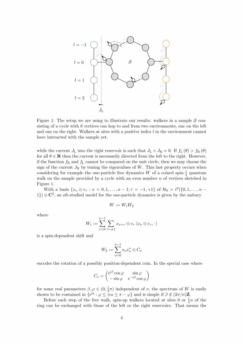
Figure 2: Still in the setup of Figure 1, with ϕ = 13π and β = 0.1, the spectrum of W (on
the left, in red online) lies in closed cones of opening π − 2ϕ about the imaginary axis.The corresponding arguments are values of θ for which fL(θ) > fR(θ) (on the right).Multiplying W by a phase of i amounts to a rotation by quarter turn of the spectrum onthe left and to a horizontal shift for the arguments on the right, leading to the oppositeinequality.
interaction term above has
φL = x0 ⊗ e+1, φR = xn/2 ⊗ e+1.
Moreover, the eigenvectors of W being explicitly computable, the current into theright reservoir eventually takes the form
JR = α2∑
λi∈spW
sin2(2ϕ)| sinϕ− 1 + λi2|2
4(fL(−i log λi)− fR(−i log λi)) +O(α4).
Therefore, if the parameter ϕ is small and fL > fR holds on open neighbourhoods ofπ/2 and −π/2 while fL < fR on open neighbourhoods of 0 and π, one gets that JR > 0for small couplings. Considering iW instead of W for the same reservoirs yields JR < 0for small couplings; see Figure 2. The change of sign can equivalently be obtained byadding an appropriate common phase to the free dynamics of each reservoir — whichis analogous to the change of sign that can occur by shifting the chemical potential inHamiltonian systems for which the Landauer–Buttiker formula is valid.
1.3 Structure of the paper
The paper is organized as follows: The next section is devoted to the description ofour quantum dynamical system in a fairly general abstract framework. The long timeasymptotic state is determined in Section 3, together with its restrictions to the sampleand the reservoirs. Section 4 analyses the properties of the steady state currents ofparticles across the sample, while the study of the entropy production rate is conductedin Section 5. Eventually, the small coupling regime is analyzed in Section 6, and thepaper closes with the proofs of certain results.
5

Acknowledgements The research of the authors is partially supported by the FrenchNational Agency through the grant NonStops (ANR-17-CE40-0006). The research ofS. A. is supported by the French National Research Agency in the framework of the “In-vestissements d’avenir” program (ANR-15-IDEX-02). The research of R. R. is partiallyfunded by the National Sciences and Engineering Research Council of Canada. The au-thors would like to thank the anonymous referees for their comments, which improvedthe quality of the presentation.
2 The setup
2.1 The spaces and one-particle dynamics
Let HS be a finite-dimensional Hilbert space. Throughout the paper, our terminologyimplicitly relies on the assumption that HS is the appropriate Hilbert space for thedescription of a quantum walker on a finite graph, sometimes referred to as a sample.An evolution for a quantum walker on a slight extension of this sample could be encodedin a unitary operator Z on a Hilbert space of the form HB⊕HS where HB is the Hilbertspace associated the extension. With respect to this direct sum decomposition, theblocks of Z, say
Z =
(C ZBS
ZSB M
), (1)
should satisfy C∗C + Z∗SBZSB = 1, C∗ZBS + Z∗SBM = 0,Z∗BSC +M∗ZSB = 0, Z∗BSZBS +M∗M = 1,
(2)
for the identity Z∗Z = 1 to hold (and similarly for ZZ∗ = 1). The off-diagonalblocks ZBS and ZSB describe the coupling between the sample and its extension andthe bock M is thought of as an effective perturbation of a unitary W on HS.
The Hilbert spaceHtot := (`2(Z)⊗HB)⊕HS
for some finite-dimensional Hilbert space HB is instead suitable for the description ofsituations where the sample is interacting with an infinite environment which has acertain translation-invariant structure. Let us construct a single-particle unitary opera-tor U on Htot such that powers of U can be interpreted as successive interactions of thetype encoded in Z with different blocks of this infinite environment.
Let (δl)l∈Z be the canonical basis of `2(Z) and let
S : `2(Z)→ `2(Z)
δl 7→ δl−1
be the shift operator and U : HB → HB be an arbitrary unitary operator. We set
U :=
((S ⊗ U)(P⊥0 ⊗ 1 + P0 ⊗ C) Sδ0 ⊗ UZBS
δ∗0 ⊗ ZSB M
), (3)
onHtot where P0 : `2(Z)→ `2(Z) is the orthogonal projector on the span of δ0 and P⊥0 :=1−P0. Here, δ0 ∈ `2(Z) is identified with a linear operator from C to `2(Z), so that e.g.δ0⊗ZBS can indeed be considered as an operator from HS ' C⊗HS to `2(Z)⊗HB. Theunitary operator U is quite natural to consider: it acts as the unitary operator Z on the
6

space δ0 ⊗HB ⊕HS ' HB ⊕HS and then as the free evolution S ⊗U on `2(Z)⊗HB;see Section 6 for the discussion of the explicit link with the Introduction.
We make the following assumptions on the effective dynamics in the sample whichwas previously discussed in [HJ17, Raq20] in important examples.
Assumption (Sp) The spectrum of M is contained in the interior of the unit disk.
2.2 The initial state in Fock space
To describe the evolution of a varying number of fermionic walkers in the system weconsider observables in the canonical anticommutation algebra CAR(Htot) representedon the fermionic Fock space Γ−(Htot).
The fermionic Fock space space Γ−(Htot) is unitarily equivalent to the tensor prod-uct Γ−(`2(Z)⊗HB)⊗ Γ−(HS) of Fock spaces through a map E such that
Ea∗(v ⊕ w)E−1 = a∗(v)⊗ 1 + (−1)dΓ(1) ⊗ a∗(w)
for all v ∈ `2(Z)⊗HB and w ∈ HS. This map associates quasifree states on CAR(Htot)with a symbol of the form T ⊕∆ for some suitable T : `2(Z)⊗HB → `2(Z)⊗HB and ∆ :HS → HS with the product of the corresponding quasifree states on CAR(`2(Z) ⊗HB) and CAR(HS) respectively. We refer the reader to [AJPP06, §5.1,6.3] for a morethorough discussion.
We recall that ωT is a gauge-invariant quasifree state on CAR(`2(Z) ⊗ HB) withsymbol 0 ≤ T ≤ 1 if
ωT[a∗(vn) · · · a∗(v1)a(u1) · · · a(um)
]= δn,m det[〈ui, T vj〉]
for all choices of v1, . . . , vn, u1, . . . , vm ∈ `2(Z)⊗HB, where a∗ and a are the usual Fockspace creation and annihilation operators — and similarly for other spaces. We refer thereader to [DFP08] for the basic theory of such states.
We will always make either of the following two assumptions on the initial state of thesystem, the second being technically more convenient and allowing simpler expressionsfor quantities of interest:
Assumption (IC) The initial state of the joint system is of the form
ρ(0) = E−1(ωT ⊗ ρS)E
where ρS is an even state on the algebra CAR(HS) and ωT is a gauge-invariantquasifree state on the algebra CAR(`2(Z)⊗HB) with symbol T : `2(Z) ⊗ HB →`2(Z) ⊗ HB, 0 ≤ T ≤ 1 such that
[T, S ⊗ U ] = 0.
In addition, we assume that∑l∈Z|l|‖(δ∗0 ⊗ 1)T (δl ⊗ 1)‖ <∞.
Assumption (IC+) The initial state of the joint system is as in (IC) with ρS alsoquasifree, with a symbol ∆ : HS → HS; equivalently, the initial state is a quasifreestate with a density of the form T ⊕∆. Moreover, it is bounded away from 0 and 1in the sense that there exists ε > 0 such that ε1 ≤ T ≤ (1− ε)1.
7

We also suppose that
Assumption (Bl) There exists a family ΠknBk=1 of orthogonal projections summing
to the identity on HB such that
[U,Πk] = 0,
and[T,1⊗Πk] = 0
for each k = 1, . . . , nB.
Note that Assumption (Bl) technically always holds with nB = 1 and Π1 = 1, but isthought of as a separation of the environment into nB different bi-infinite reservoirsof fermions, with their own dynamics, which only interact through the sample. Also,the case with rank Πk = 1 for each k will allow more explicit computations of someimportant quantities.
In terms of the linear operators
Tn,m := (δ∗n ⊗ 1)T (δm ⊗ 1) (4)
on HB, referred to as blocks, the commutation assumption in (IC) becomes the require-ment that
Tn,m = U−nT0,m−nUn. (5)
for all n,m ∈ Z.
2.3 Relation to repeated interaction systems
To clarify the place of our model in the zoo of discrete-time quantum dynamics, wecomment on its relation to repeated interaction systems (ris). This subsection can beskipped on a first reading. Consider the effective one-step dynamics in the sample
Λ1(ρ) := trΓ−(`2(Z)⊗HB)[Γ(U∗)(ωT ⊗ ρ)Γ(U)],
starting with an initial state as in Assumption (IC+). A straightforward computationmaking use of the Bogolyubov relation shows that Λ1(ρ) is a quasifree state with symbol
∆1 = M∆M∗ + ZSBT0,0Z∗SB.
Repeatedly applying the map Λ1, say t times to obtain a quasifree state with symbol
∆tRIS = M t∆(M∗)t +
t−1∑m=0
MmZSBT0,0Z∗SB(M∗)m,
is an instance of a ris, as noted in the single reservoir setups of [HJ17, Raq20]. Onecan show that this ris picture coincides precisely with what happens at the level ofthe sample in the setup of Subsections 2.1 and 2.2 if Tn,m = 0 whenever n 6= m. Forexample, compare our setup with Z = exp[−iτ(kE ⊕ kS + λv)] for some one-particleselfadjoints operators kE, kS and v and compare the resulting dynamics on Fock spaceto the content of Section II of [BJM14] using the exponential law for fermions.
However, in general, the effective dynamics in the sample
Λt(ρ) := trΓ−(`2(Z)⊗HB)[Γ(U∗)t(ωT ⊗ ρ)Γ(U)t]
8

need not enjoy the semigroup property Λt+t′ = ΛtΛt′ . Indeed, we will see in Remark 3.5below that, under Assumption (IC+), Λt(ρ) is a quasifree state with density
∆t = M t∆(M∗)t +t−1∑m=0
t−1∑n=0
MmZSBT0,m−nUn−mZ∗SB(M∗)n.
The difference between ∆tRIS obtained in the ris scenario and our general ∆t amounts to
the terms with n 6= m in the latter, which generically do not cancel out. More generally,tracing out at steps that are multiples of a number τ ≥ 2 for which T0,m = 0 for m > τ ,a similar computation shows that the dynamics differs from the original one by termswith no particular structure for cancellation.
On the other hand, the fact that we obtain our dynamics from the second quanti-zation of a one-body operator imposes a conservation law which rules out certain risscenarios where nontrivial entropy production rates arise from interaction with a singlereservoir; see e.g. the discussions surrounding Lemma 6.5 in [HJPR17] and Section 3.4in [BB20].
3 Mixing
We present several results on the large-time behaviour of the system. While explicitformulae using the canonical relations in Fock space have proved to be useful in [HJ17,Raq20], we here focus on a scattering approach to the problem. We set
Y0 := C (6)
andYm := ZBSM
m−1ZSB (7)
for m ≥ 1. Heuristically, Ym encodes what happens to the wave function of a fermionfrom a reservoir which enters the sample, spends m− 1 more time steps there and thenexits the sample.
3.1 Scattering and the asymptotic state
It is straightforward to check by induction that
Ut −∑
n6=0,...,t−1
δn−tδ∗n ⊗ U t ⊕ 0
=
(∑t−1l=0
∑t−l−1m=0 δl−t+mδ
∗l ⊗ U t−l−mYmU l
∑t−1m=0 δ−t+m ⊗ U t−mZBSM
m∑t−1m=0 δ
∗t−m−1 ⊗MmZSBU
t−m−1 M t
). (8)
for all t ≥ 0. As is customary, we investigate the behaviour of Ut for large t throughMøller-like operators. Multiplying (8) by (S ⊗ U ⊕ 1)−t on the right and performing areindexation to eliminate explicit occurrences of t in the summand for the double sum,we find
Ut(S ⊗ U ⊕ 1)−t −∑
n6=−t,...,−1
δnδ∗n ⊗ 1⊕ 0
=
(∑t−1m=0
∑t−ml=1 δ−lδ
∗−m−l ⊗ U lYmU−m−l
∑t−1m=0 δ−t+m ⊗ U t−mZBSM
m∑t−1m=0 δ
∗−m−1 ⊗MmZSBU
−m−1 M t
)(9)
9

for t ≥ 0. Multiplying the adjoint of (8) by (S ⊗ U ⊕ 1)t on the right and performing areindexation, we find a similar formula for U−t(S ⊗ U ⊕ 1)t with t ≥ 0.
Under Assumption (Sp), it is thus easy to see from the matrix elements that thelimits
Ω±U := w-limt→∓∞
Ut(S ⊗ U ⊕ 1)−t (10)
exist and are given by the explicit expressions
Ω−U =
(∑n≥0 δnδ
∗n ⊗ 1 0
0 0
)+∑m≥0
(∑l≥1 δ−lδ
∗−m−l ⊗ U lYmU−m−l 0
δ∗−m−1 ⊗MmZSBU−m−1 0
)(11)
and
Ω+U =
(∑n′≤−1 δn′δ
∗n′ ⊗ 1 0
0 0
)+∑m′≥0
(∑l′≥m′ δl′−m′δ
∗l′ ⊗ Um
′−l′Y ∗m′Ul′ 0
δ∗m′ ⊗ (M∗)m′Z∗BSU
m′ 0
). (12)
Note that we have not yet projected onto `2(Z) ⊗ HB, i.e. the subspace associated tothe absolutely continuous spectrum of (S ⊗ U ⊕ 1), but have used the weak operatortopology. As expected, strong convergence holds on the appropriate subspace; the proofof the following proposition concerning Ω−U is postponed to Section 7. While not neededin what follows, an analogue result holds for Ω+
U .
Proposition 3.1. Suppose that Assumption (Sp) holds. Then, both
s-limt→∞
Ut(S ⊗ U ⊕ 1)−t(1⊗ 1⊕ 0) = Ω−U (1⊗ 1⊕ 0)
ands-limt→∞
(Ut(S ⊗ U ⊕ 1)−t)∗ = (Ω−U )∗.
The scattering matrix
YU := (1⊗ 1⊕ 0)(Ω+U )∗Ω−U (1⊗ 1⊕ 0)
on `2(Z)⊗HB will also frequently appear in the sequel. The following lemma makes itsstructure more explicit. A direct proof that YU is unitary is given in the next section.
Lemma 3.2. Under Assumption (Sp),
YU =∑m≥0
∑l∈Z
δlδ∗l−m ⊗ U−lYmU l−m. (13)
Proof. We expand
(1⊗ 1⊕ 0)(Ω+U )∗Ω−U (1⊗ 1⊕ 0)
=∑m≥0
∑l≥1
δ−lδ∗−m−l ⊗ U lYmU−m−l +
∑m′≥0
∑l′≥m′
δl′δ∗l′−m′ ⊗ U−l
′Ym′U
−m′+l′
+∑m′≥0
∑m≥0
δm′δ∗−m−1 ⊗ U−m
′ZBSM
m′MmZSBU−m−1.
Rewriting the double sum on the last line in terms of Ym′′ with m′′ = m+m′ yields thedesired formula.
10

We use a subscript U on some of the objects introduced in this section because it isat times convenient to factor out the contribution from the unitary U and then considerthe special case U = 1. For example,
Ω−U =
(∑m∈Z
Pm ⊗ Um ⊕ 1
)∗Ω−1
(∑n∈Z
Pn ⊗ Un ⊕ 1
)and
YU =( ∑m∈Z
Pm ⊗ Um)∗
Y1
(∑n∈Z
Pn ⊗ Un). (14)
In view of this factorization, we introduce a modification of T which absorbs part of thefree dynamics in the environment:
Ξ :=
(∑n∈Z
Pn ⊗ Un)T
(∑m∈Z
Pm ⊗ Um)∗, (15)
so thatΞ =
∑n,m∈Z
δnδ∗m ⊗ Ξm−n,
whereΞn := T0,nU
−n.
Note that Ξ is selfadjoint and commutes with S ⊗ 1 and 1⊗Πk, k = 1, . . . , nB.
Proposition 3.3. Under Assumptions (IC) and (Sp), the limit
ρ(∞)[A] := limt→∞
ρ(0)[Γ(U)−tAΓ(U)t] (16)
exists for all A ∈ CAR(Htot) and defines a quasifree state with symbol
T∞tot := Ω−U (T ⊕ 0)(Ω−U )∗. (17)
Proof. To prove the proposition it suffices to show that
limt→∞
ρ(0)
[Γ(U∗)t
( N∏h=1
a(Vh))∗( N ′∏
h′=1
a(V ′h′))
Γ(U)t
]= δN,N ′ det[〈V ′h′ , T∞totVh〉]Nh,h′=1
for an arbitrary choice of N,N ′ ≥ 0 and V1, . . . , VN , V′
1 , . . . , V′N ′ ∈ Htot. Because T
commutes with S ⊗ U , we have
ρ(0)[A] = ρ(0)[Γ(S ⊗ U ⊕ 1)tAΓ(S∗ ⊗ U∗ ⊕ 1)t
]for all A ∈ CAR(Htot) and the Bogolyubov relation gives that the identity to be shownis equivalent to
limt→∞
ρ(0)
[( N∏h=1
a((Ω(t)U )∗Vh)
)∗ N ′∏h′=1
a((Ω(t)U )∗V ′h′)
]= δN,N ′ det[〈V ′h′ , T∞totVh〉]Nh,h′=1, (18)
whereΩ
(t)U := Ut(S ⊗ U ⊕ 1)−t.
11

First note thatlimt→∞‖(Ω(t)
U )∗Vh − (1⊗ 1⊕ 0)(Ω(t)U )∗Vh‖ = 0
for each h = 1, . . . , N by Proposition 3.1, and similarly with primes. Hence, by continu-ity of the fermionic creation and annihilation operators as functions from (Htot, ‖ · ‖)to (B(Γ−(Htot)), ‖ · ‖), the limit in (18) will exist if and only if the limit
limt→∞
ωT
[( N∏h=1
a((1⊗ 1⊕ 0)(Ω(t)U )∗Vh)
)∗ N ′∏h′=1
a((1⊗ 1⊕ 0)(Ω(t)U )∗V ′h′)
]exists, in which case they will coincide. In particular, we may as well assume that theinitial state ρS(0) is quasifree with vanishing symbol.
Under this extra assumption, the state ρ(t) is quasifree for all t ∈ N and has symbolTtot(t):
ρ(0)
[( N∏h=1
a((Ω(t)U )∗Vh)
)∗ N ′∏h′=1
a((Ω(t)U )∗V ′h′)
]= δN,N ′ det[〈V ′h′ , Ttot(t)Vh〉]Nh,h′=1,
where
Ttot(t) = Ω(t)U (T ⊕ 0)(Ω
(t)U )∗.
Therefore, we will be done if we can show that Ttot(t) converges weakly to the proposedlimit T∞tot. But this is easily deduced from Proposition 3.1.
We are now in a position to get the symbol of the restriction of the state to thesample, i.e.
∆∞ := (0⊕ 1)T∞tot(0⊕ 1). (19)
Proposition 3.4. Suppose that Assumptions (Sp) and (IC) hold and let
Ψ(X) :=∞∑k=0
MkX(M∗)k
for X : HS → HS. Then,
∆∞ = Ψ(G+G∗),
where
G := 12ZSBΞ0Z
∗SB +
∞∑l=1
M lZSBΞlZ∗SB.
Proof. Since,
(0⊕ 1)Ω−U (1⊕ 0) =∞∑m=0
δ∗−m−1⊗MmZSBU−m−1
by Proposition 3.1, (19) gives
∆∞ =
∞∑m,n=0
MmZSBU−m−1T−m−1,−n−1U
n+1Z∗SB(M∗)n
=∞∑
m,n=0
MmZSBΞm−nZ∗SB(M∗)n
using T−m−1,−n−1 = Um+1Ξm−nU−n−1. Splitting the contributions with m − n > 0,
m−n = 0 and m−n < 0 and reindexing with l = |m−n| gives the proposed formula.
12

Remark 3.5. If Assumption (IC+) holds, the symbol of the restriction to the sampleat time t reads
∆t = M t∆(M∗)t +t−1∑m=0
t−1∑n=0
MmZSBT0,m−nUn−mZ∗SB(M∗)n.
We now turn our attention to the block
T∞E := (1⊗ 1⊕ 0)T∞tot(1⊗ 1⊕ 0)
of Ttot corresponding to the environment. As a direct consequence of Proposition 3.1,we have the following corollary.
Corollary 3.6. Suppose that Assumption (Sp) holds and let ρ(0) be an initial stateon Γ−(Htot) as in Assumption (IC). Then,
δ∗nT∞E δm =
U−n
(∑l,l′≥0 YlΞl−l′+m−nY
∗l′
)Um n < 0,m < 0,
U−n(∑
l≥0 YlΞl+m−n
)Um n < 0,m ≥ 0,
U−nΞm−nUm n ≥ 0,m ≥ 0.
(20)
In particular, δ∗nT∞E δm = δ∗nTδm for n,m ≥ 0.
Note that the asymptotic symbol T∞E need not commute with S ⊗ U ; blocks corre-sponding to positions having already interacted (negative indices) are given a differentexpression than those corresponding to position which have not yet interacted. This isinherent to our choice of dynamics in the environment, which prevents the effects of theinteraction taking place at the site zero to affect the state at locations that have not yetbeen in contact with the sample. We will come back to this point in the next subsection.
3.2 Fourier representation
Many of the expressions call for a representation in Fourier space that we will take advan-tage of in what follows. We introduce the unitary map F : `2(Z)⊗HB → L2([0, 2π];HB)as follows: for ψ =
∑l∈Z δl ⊗ ψl with
∑l∈Z ‖ψl‖2 <∞ and θ ∈ [0, 2π], we set
(Fψ)(θ) :=∑l∈Z
e−ilθψl.
In practice, we will more often use the notation
ψ := Fψ.
Let R : `2(Z)⊗HB → `2(Z)⊗HB have the form
R =∑n,m∈Z
δnδ∗m ⊗Rm−n (21)
for some norm-summable sequence (Rl)l∈Z of operators on HB — hereafter referred toas Fourier coefficients —, so that ‖R‖ ≤
∑l∈Z ‖Rl‖. Then,
(FRψ)(θ) =((FRF−1)(Fψ)
)(θ) = R(θ)ψ(θ),
13

where R : L2([0, 2π];HB)→ L2([0, 2π];HB) is the multiplication operator by
R(θ) :=∑l∈Z
eilθRl.
Also note that R is selfadjoint if and only if R−l = R∗l for each l ∈ Z, in which case R(θ)is selfadjoint for all θ ∈ [0, 2π].
We will make use of this representation for Ξ:
Ξ(θ) =∑l∈Z
eilθΞl.
Recall That Ξ is of the form (21) by construction (under Assumption (IC)), with blocks
Ξm−n = UnTn,mU−m. (22)
Then, with
Y(θ) :=∑l≥0
e−ilθYl
(note the sign of ilθ), we set
Ξ∞(θ) := Y(θ)Ξ(θ)Y(θ)∗.
Equivalently, Ξ∞(θ) is the Fourier representation of an operator Ξ∞ of the form (21)with blocks
Ξ∞m =∑l,l′≥0
YlΞl−l′+mY∗l′ (23)
for all m ∈ Z. To see this, integrate Y(θ)Ξ(θ)Y(θ)∗ against 12π e−imθ to find the m-th
block.Note that combining (20) and (23) gives
Ξ∞m−n = Unδ∗nT∞E δmU
−m (24)
if n < 0 and m < 0. In other words, Ξ∞ is translation invariant, but as far as blocksthat have been affected by the interaction with the sample, Ξ∞ is to T∞E as Ξ is to T ;compare (24) to (22). Note that T∞E = T implies Ξ∞ = Ξ; the converse implicationfails.
Lemma 3.7. The operator YU is unitary.
Proof. In view of (14) and (15), it suffices to prove the lemma with U = 1. Let
Y(θ) :=∑l≥0
e−ilθYl
be as in the previous discussion; it is clear that it suffices to show that Y(θ) is unitaryfor all θ ∈ R. Given the definitions Y0 := C and Yl := ZBSM
l−1ZSB for l ≥ 1, theoperator Y(θ) can be expressed in terms of resolvents of M :
Y(θ) = C +∑l≥0
e−iθe−ilθZBSMlZSB = C − ZBS(M − eiθ)−1ZSB (25)
an expression which is well defined for all θ ∈ R under Assumption (Sp). The operatorsinvolved correspond to the block representation (1) of the unitary operator Z. Unitarityof Y is given by the next lemma and the present lemma follows.
14

Lemma 3.8. Let Z be a unitary operator with block decomposition Z = ( a bc d ) withrespect to an orthogonal direct sum decomposition of a finite-dimensional Hilbert space.Then, for all η ∈ R, the bounded operator s(η) := a− b(d− eiη)−1c is a unitary operatoron the first subspace in the decomposition.
Proof. Simply expand the expression s(η)s(η)∗ and make use of the relation satisfiedby a, b, c and d as a consequence of unitarity of Z as well as of the identity d(d−eiη)−1 =1 + eiη(d− eiη)−1.
4 Fluxes of particles
We associate to a bounded selfadjoint operator X : HB → HB the flux
ΦX = dΓ(U∗(1⊗X ⊕ 0)U− 1⊗X ⊕ 0).
Using the block form of U, and assuming [X,U ] = 0, one can check that
U∗(1⊗X ⊕ 0)U− 1⊗X ⊕ 0 =
(−P0 ⊗X + P0 ⊗ C∗XC δ0 ⊗ C∗XZBS
δ∗0 ⊗ Z∗BSXC Z∗BSXZBS
)is trace class. The interest of such quantities is best seen through the case of particlefluxes between the different parts of the environment, hereafter referred to as reservoirs,whose definition requires the structure in Assumption (Bl). Such a structure is evidentlypresent in the special case discussed in the introduction. Formally, the (infinite) numberof fermions in the reservoir `2(Z) ⊗ ΠkHB is given by the observable dΓ(1 ⊗ Πk ⊕ 0),where [Πk, U ] = 0, and the number of fermions that enter this reservoir in one time stepis given by the observable
Φk ≡ ΦΠk= Γ(U∗) dΓ(1⊗Πk ⊕ 0)Γ(U)− dΓ(1⊗Πk ⊕ 0)
on Γ−(Htot).Back to the general observable X such that [X,U ] = 0, we know from Section 3.1 that
the asymptotic state of the full system, denoted ρ(∞), is quasifree with symbol T∞tot =Ω−U (T ⊕ 0)(Ω−U )∗ if ρ(0) satisfies Assumption (IC). Hence, the steady-state expectationvalue of the flux ΦX , or current, is given by
JX := ρ(∞)[ΦX ]
= trHtot [T∞totU∗(1⊗X ⊕ 0)U− 1⊗X ⊕ 0].
(26)
Using the decomposition
T∞tot =
(T∞E T∞ES
T∞SE ∆∞
), (27)
we get
JX = tr`2(Z)⊗HB(T∞E (P0 ⊗ (CXC∗ −X)) + T∞ES(δ∗0 ⊗ Z∗BSXC))
+ trHS(T∞SE(δ0 ⊗ C∗XZBS + ∆∞Z∗BSXZBS).
(28)
This expression serves as a basis for obtaining more transparent expressions.
Proposition 4.1. Under Assumptions (IC) and (Sp), if X : HB → HB is a boundedobservable such that [X,U ] = 0, then
JX = tr
[X
ˆ 2π
0(Y(θ)Ξ(θ)Y∗(θ)− Ξ(θ))
dθ
2π
].
15

Proof sketch. We consider the case U = 1 to lighten the notation. Use cyclicity of thetrace to rewrite the trace over HS as a trace over `2(Z)⊗HB. Then, expand the formulaefor T∞E , T∞ES, T∞SE and ∆∞. The part on `2(Z) is restricted to the span of δ0 and weare left with a trace on HB. Rewrite this trace gathering all occurrences of Ym definedby (6)–(7):
JX = trHB
[X
( ∑n,m≥0
YnΞn−mY∗m − Ξ0
)]. (29)
Conclude using the identity (23).
For the currents Jk ≡ JΠkassociated to the projectors Πk, k = 1, . . . , nB, we imme-
diately get the two following consequences.
Corollary 4.2. Under Assumptions (IC), (Sp) and (Bl), we have
nB∑k=1
Jk = 0.
More precisely, for each k = 1, . . . , nB,
Jk =∑k′ 6=k
ˆtr[Y∗(θ)ΠkY(θ)Πk′Ξ(θ)]− tr[Y∗(θ)Πk′Y(θ)ΠkΞ(θ)]
dθ
2π
and, with the additional assumption that each ΠknBk=1 has rank one,
Jk =
ˆ ∑k′ 6=k
Ck,k′(θ)(fk′(θ)− fk(θ))dθ
2π, (30)
where fk(θ) := tr[ΠkΞ(θ)] and Ck,k′(θ) := tr[Y∗(θ)ΠkY(θ)Πk′ ] are nonnegative, andsatisfy
nB∑k′=1
Ck,k′(θ) =
nB∑k=1
Ck,k′(θ) = 1.
Remark 4.3. Formula (30) in the case where each Πk has rank one implies in particularthat if one of the functions fk : θ 7→ tr[ΠkΞ(θ)] satisfies fk(θ) ≥ fk′(θ) for all k′ 6= k,then the flux of particles is necessarily going out of the k-th reservoir (i.e. Jk ≤ 0).
Remark 4.4. We may think of the Ck′,k(θ) as some effective conductance at frequency θ.This is similar to the Landauer–Buttiker formula presented in [AJPP07] (Corollary 4.2),with the following differences: the context in [AJPP07] is in continuous time and notin discrete time, and the free dynamics on the reservoir number k is generated by someHamiltonian hk instead of the shift S. The flux of some observable q is then expressedas a sum of integrals over spac(hk) ∩ spac(hk′), where spac(hk′) is the absolutely contin-uous spectrum of the Hamiltonian hk′ of another reservoir, while in our expression weintegrate over the spectrum of S, i.e. the unit circle.
Proof of Corollary 4.2. We have Jk = JΠk, which by Proposition 4.1 gives
Jk =
ˆ 2π
0tr[ΠkY(θ)Ξ(θ)Y∗(θ)−ΠkΞ(θ)
]dθ2π.
16

Since∑nB
k′=1 Πk′ = 1 and Y(θ) is unitary for all θ, we have∑nB
k=1 Jk = 0. Now byassumption (Bl) we have Ξ =
∑nBk′=1 Πk′ΞΠk′ =
∑nBk′=1 Πk′Ξ hence
Jk =
ˆ 2π
0tr[ nB∑k′=1
ΠkY(θ)Πk′Ξ(θ)Y∗(θ)−ΠkΞ(θ)]dθ
2π
and by the properties of Πk and Y(θ) we have
tr[ΠkΞ(θ)
]=
nB∑k′=1
tr[Y∗(θ)Πk′Y(θ)ΠkΞ(θ)
].
This proves that Jk =∑
k′ 6=k Ak,k′ − Ak′,k for Ak′,k = tr[Y∗(θ)ΠkY(θ)Πk′Ξ(θ)]. More-over, in the case where the Πk are of rank one, we have
ΠkΞ(θ) = ΠkΞ(θ)Πk = tr[ΠkΞ(θ)] Πk
and, restoring the summation to all indices,∑k′
tr[Y∗(θ)Πk′Y(θ)Πk
]= tr[Πk] =
∑k′
tr[Y(θ)Πk′Y
∗(θ)Πk
],
which gives the second formula for Jk and the summation property of Ck,k′(θ).
5 Entropy production
Since nontrivial asymptotic currents can develop between the reservoirs of the systemat hand, we expect that the total system genuinely settles into a nonequilibrium steadystate. Another key signature of such states is the nontrivial entropy production ratethey give rise to. We prove here the existence and strict positivity of the asymptoticentropy production rate related to the convergence towards the nonequilibrium steadystate. More precisely, we work under Assumption (IC+) and provide a convergenceresult for the quantity
σ(t) := t−1(S[Ttot(t)|Ttot(0)] + S[1− Ttot(t)|1− Ttot(0)]
), (31)
where Ttot(t) := Ω(t)U (T ⊕∆)(Ω
(t)U )∗ and
S[X|Y ] := tr[X(logX − log Y )]
for any trace-class operators X and Y with ε ≤ X,Y ≤ 1 − ε on some commonHilbert space. This definition is motivated by a formula for the relative entropy be-tween quasifree states which is well established for finite-dimensional systems [DFP08,
§IV.B] and the observation that Ω(t)U is a finite-rank perturbation of the identity. It will
also be a posteriori justified by the relation to fluxes established in Corollary 5.3.The following theorem states that the entropy production rate converges to the
integral of the relative entropies of matrices related to the initial and asymptotic statesof the environment introduced in Section 3.2. Its proof is postponed to Section 8.
17

Theorem 5.1. Under Assumption (IC+), Ttot(t) − Ttot(0) has finite rank and σ(t)in (31) is well defined for all t ∈ N. If, in addition, Assumption (Sp) holds, then thelimit
σ+ := limt→∞
σ(t)
exists and is given by
σ+ =
ˆ 2π
0S[Y(θ)Ξ(θ)Y∗(θ)
∣∣Ξ(θ)] dθ
2π+
ˆ 2π
0S[1− Y(θ)Ξ(θ)Y∗(θ)
∣∣1− Ξ(θ)] dθ
2π. (32)
Moreover, σ+ ≥ 0 with equality if and only if Ξ(θ) = Y(θ)Ξ(θ)Y∗(θ) for Lebesgue-almostall θ ∈ [0, 2π].
Remark 5.2. Recall that θ 7→ Y(θ)Ξ(θ)Y∗(θ) is the Fourier transform of a translation-invariant operator Ξ∞ which, up to the transformation which relates Ξ to T , shares itsblocks with T∞E .
The following reformulation of the result is closer to typical formulations in termsof currents and thermodynamic potentials (see for example Equation (17) in [JPW14]),albeit frequency-wise. It can be compared to Corollary 4.3 of [AJPP07]; see also Re-mark 4.3.
Corollary 5.3. Suppose that Assumptions (IC+), (Sp) and (Bl) hold with the projec-tors Π1, . . . ,ΠnB having rank one. Then we have the identity
σ+ =
nB∑k=1
ˆ 2π
0µk(θ)k(θ)
dθ
2π, (33)
where
µk(θ) := log1− fk(θ)fk(θ)
and k(θ) denotes the integrand of the expression (30) for the k-th flux of particles.
Remark 5.4. In the case where each fk is constant in θ, the formula simplifies to
σ+ =
nB∑k=1
nB∑k′=1
µk(fk′ − fk)ˆCk,k′(θ)
dθ
2π
=
nB∑k=1
nB∑k′=1
µk(fk′ − fk)∑l≥0
tr[Y ∗l ΠkYlΠk′ ].
At this stage, the picture of entropy production is still short of a study of thestatistical fluctuations in measurement processes of physical observable properly relatedto the “information-theoretical” notion of entropy production; see e.g. [JOPP11, §4.4.5].
6 Discussion for small coupling strength
In order to investigate the regime where the interaction between the sample and itsenvironment is weak, we will consider a special case where the unitary operator Z onHB ⊕HS is of the form
Z =
(1 00 W
)exp
[−iα
(0 A∗
A 0
)]18

for some unitary operator W : HS → HS which represents the free evolution on thesample, some bounded operator A : HB → HS which couples sites of the sample and sitesof the environment, and some coupling strength α ∈ R. Computing the exponential, weobtain
C = cos(α√A∗A) ZBS = −iA∗
sin(α√AA∗)√
AA∗
ZSB = −iWsin(α
√AA∗)√
AA∗A M = W cos(α
√AA∗).
In this particular setup, we can give a more tractable condition for the Assumption (Sp)to hold true as well as more explicit formulas as the coupling strength α tends to 0.
Proposition 6.1. Let us consider M(α) := W cos(α√AA∗) for α ∈ R, and write
V ⊆ HS the range of A. Then, there exists αA > 0 depending on A only such that thefollowing properties are equivalent:
1. The spectrum of M(α) is contained in the interior of the unit disc for all α ∈(−αA, αA),
2. The subspace V is contained in no strict subspace of HS which is stable by W ,
3. We havespan
i=0,...,dimHS
W iV = HS,
The equivalence between the second and third property is well known and onlyincluded because of its relation to linear control theory, where it is called the Kalmancondition.
Proof. Let µii≥0 be the (nonnegative) eigenvalues of√AA∗ and let pii≥0 be the
corresponding spectral projectors. We include 0 as µ0, possibly at the cost of having p0 =0. Choose αA > 0 small enough that |αµi| < π whenever |α| < αA. Then, with νi :=cos(αµi), we have
cos(α√AA∗) = p0 +
l∑i=1
νipi.
Note that p0 is the orthogonal projection onto the kernel of√AA∗, which coincides with
the orthogonal complement of V.If the first property is not satisfied, then there exists a normalized eigenvector φ
of M(α) with eigenvalue λ with |λ| ≥ 1 for some α ∈ (−αA, αA). Then,
|λ|2 = 〈M(α)φ,M(α)φ〉 = 〈φ, p0φ〉+∑i≥1
ν2i 〈φ, piφ〉
and since∑
i≥0 〈φ, piφ〉 = 1 this implies that |λ|2 = 1, p0φ = φ and∑
i≥1 piφ = 0.Then, φ is in the orthogonal complement of V and is also an eigenvector of W since
λφ = M(α)φ = W
(p0 +
∑i≥1
νipi
)φ = Wφ.
We conclude that V is contained in the orthogonal complement of the span of φ, whichis stable by W since φ is an eigenvector of W . Thus the second property is not satisfied.
19

Conversely, if the second property is not satisfied, then there exists an eigenvector φof W in the orthogonal complement of V. Then, φ is clearly an eigenvector of M(α)with eigenvalue on the unit circle for all α, which implies in particular that the firstproperty is not satisfied.
In order to carry some usual procedures from perturbation theory, we will need asemisimplicity and regularity assumption on the spectral decompostion of the family ofoperators M(α) analytic in the coupling strength α.
Assumption (12Sim) There exists a punctured neighbourhood Ω of 0 in C such that
the eigenvalues of M(α) are semisimple for all α ∈ Ω and there is a decomposition
M(α) =∑j∈I
λj(α)Qj(α) (34)
with scalar functions λj : Ω 7→ C and projection-valued functions Qj : Ω→ B(HS)which are analytic for each j in a finite set I. Moreover, we assume that 0 is aremovable singularity of all functions Qj and λj .
Note that Qj(α) need not be selfadjoint. Also note that W = M(0) may havedegenerate eigenvalues which split as α moves away from 0. With λ1, . . . , λr the distincteigenvalues of W and Q1, . . . , Qr the associated orthogonal projectors, we may write I =⋃ri=1 Ii with λj(0) = λi if and only if j ∈ Ii. Then, Qi =
∑j∈Ii Qj(0) and λjj∈Ii
is called the λi-group in the terminology of Kato. The Assumption (12Sim) is more
general than the following simplicity assumption, which is already rather generic froma topological point of view and sometimes easier to verify.
Assumption (Sim) Each eigenvalue λi of W is simple in the sense that the associatedspectral projector Qi is of the form χiχ
∗i for some unit vector χi ∈ HS.
One interesting advantage of Assumption (12Sim) over (Sim) is that it can be inferred
from a simple condition on AA∗, thanks to the following lemma.
Lemma 6.2. If κ−1AA∗ is an orthogonal projection for some nonzero κ ∈ R, thenAssumption (1
2Sim) is satisfied.
Proof. Analytically extend M(α) to the complex plane and consider the set C := α ∈C : | cos(ακ)| = 1. Then, M(α) is unitary for α ∈ C. It can be shown that C containsnontrivial curves and hence has at least one accumulation point. The lemma thus followsfrom Theorem 1.10 in [Kat95, §II.1.6].
Now that we have clarified our assumptions, we can proceed to give the limitingbehaviour of the formula for the reduced asymptotic symbol in the sample in Proposi-tion 3.4 and for the asymptotic currents in Corollary 4.2 as α→ 0.
Lemma 6.3. If Assumption (12Sim) is satisfied then for all α ∈ Ω, a complex neigh-
bourhood of the origin, we have λj(α) = λj(−α) and Qi(α) = Qi(−α).
Proof. With N(α) = W∑+∞
n=0(−α)n
(2n)! (A∗A)n, we have M(α) = N(α2) for any α ∈ Ω,
and, for 0 < α ∈ Ω, N(α) =∑
j∈I λj(√α)Qj(
√α) ≡
∑j∈I µj(α)Pj(α). By perturbation
theory, [Kat95, §II.1], the eigenvalues and eigenprojectors of N(α), µj(α) and Pj(α),admit analytic extensions in Ω\0 given by Laurent series in α1/dj , dj ∈ N∗. Theorem
20

1.9 in [Kat95, §II.1], implies dj = 1, since otherwise ‖Pj(α)‖ = ‖Qj(√α)‖ diverges as
α → 0, contradicting (12Sim.). Thus, µj and Pj are analytic in Ω and λj(α) = µj(α
2)and Qj(α) = Pj(α
2) for all α ∈ Ω.
Theorem 6.4. Suppose that Assumption (Sp) holds for all α ∈ Ω ∩R, that Assump-tions (IC) and (1
2Sim) hold. Then, the symbol ∆∞α in Proposition 3.4, which dependson the coupling strength α, admits an expansion
∆∞α =r∑i=1
∑j,j′∈Ii
2
cj + cj′Qj(0)AΞ(−i log λi)A
∗Qj′(0) +O(α2)
wherecj := tr[Qj(0)AA∗] > 0.
Before we proceed with the proof, let us remark that the appearance of a logarithmis due to the fact that we have defined our Fourier representation on the interval ratherthan on the unit circle. By periodicity of Ξ and the fact that λi is on the unit circle,the choice of logarithm is irrelevant.
Proof of Theorem 6.4. By Proposition 6.1, Assumption (Sp) implies that the imageof AA∗ is contained in no nontrivial subspace which is stable by W . Hence, cj :=tr[Qj(0)AA∗] > 0 for each j. Since M(α) = W (1− 1
2α2AA∗) +O(α4), Lemma 6.3 and
standard perturbation theory give
j ∈ Ii ⇒ λj(α) = λi(1− 12α
2cj) +O(α4). (35)
Claim. The map Ψ introduced in Proposition 3.4 is such that
α2Ψ(X) =r∑i=1
∑j,j′∈Ii
2
cj + c′jQj(0)XQj′(0) +O(α2)
for any linear map X on HS.
Accepting this claim, we need only note that
ZSB = −iWsin(α
√AA∗)√
AA∗A = −iαWA+O(α3)
and the summability condition in Assumption (IC) imply that the map G appearing inProposition 3.4 has the expansion
G = α2
(1
2WAΞ0A
∗W ∗ +
∞∑k=1
W k+1AΞkA∗W ∗
)+O(α4)
to conclude the proof.
Proof of Claim. Inserting the spectral decomposition (34) ofM in Assumption (12Sim)
in the definition of Ψ(X) :=∑∞
m=0MmX(M∗)m yields
Ψ(X) =∑j,j′∈I
∞∑m=0
λj(α)mλj′(α)mQj(α)XQj′(α)∗
=∑j,j′∈I
1
1− λj(α)λj′(α)Qj(α)XQj′(α)∗.
21

Since W is unitary we have Qj(0)∗ = Qj(0) and λj′(0) = λj′(0)−1. If λj(0) 6=λj′(0), the expansion (35) gives
1
1− λj(α)λj′(α)=
1
1− λj(0)λj′(0)−1+O(α2)
This leaves the terms for which λj(0) = λj′(0) (i.e. j, j′ ∈ Ii for some i), for whichwe have
λj(α)λj′(α) = 1− 12α
2(cj + cj′) +O(α4).
by (35). Hence,α2
1− λj(α)λj′(α)=
2
cj + cj′+O(α2)
whenever j, j′ ∈ Ii for some common i.
And the Claim yields the Theorem.
Proposition 6.5. Suppose that Assumption (Sp) for all α ∈ Ω ∩R and that Assump-tions (IC), (Bl) and (1
2Sim) hold. Then, with Jk as in Corollary 4.2 depending on α,we have
Jk = α2 tr(ΠkD) +O(α4), (36)
as Ω 3 α→ 0, where
D =r∑
h=1
(−A∗QhAΞ(−i log λh) +
∑j,j′∈Ih
2
cj + cj′A∗Qj(0)AΞ(−i log λh)A∗Qj′(0)A
).
Proof. The starting point is the expression (29) for Jk.
Y0 = C = cos(α√A∗A) = I − α2
2A∗A+O(α4)
Yl = ZBSMl−1ZSB = −α2A∗M l−1WA+O(α4‖M l−1‖),
where M l−1 = M(α)l−1 is such that ‖M(α)l−1‖ is uniformly bounded in l > 0 andα ∈ Ω ∩R. Thus, using Equation (29) we have
Jk = trHB
[Πk
(− α2
2(A∗AΞ0 + Ξ0A
∗A)
++∞∑l=1
YlΞlC + C+∞∑l=1
Ξ−lY∗l +
∑l,l′>0
YlΞl−l′Y∗l′
)]+O(α4).
(37)
Let us estimate the first sum, making use of Assumptions (IC) and (12Sim)
+∞∑l=1
YlΞlC = −α2+∞∑l=1
∑j∈I
A∗Qj(α)WAλj(α)l−1Ξl +O(α4)
= −α2∑j∈I
1
λj(α)A∗Qj(α)WA
(+∞∑l=1
λj(α)lΞl
)+O(α4) .
22

Thanks to Ξ∗l = Ξ−l, we have Ξ(θ) = F (θ) + F (θ)∗ = 2 Re(F (θ)), where
F (θ) =1
2Ξ0 +
∑l≥1
eilθΞl.
Now, 1λj(α)Qj(α)W = Qj(0)+O(α), and F is differentiable (since
∑k∈Z |k|‖Ξk‖ < +∞)
so F (−i log λj(α)) = F (−i log λh) + O(α) where h is such that j ∈ Ih. Taking intoaccount the identity
∑j∈I Qj(0) = 1, and repeating the argument for the second sum,
we get
α2
2(A∗AΞ0 + Ξ0A
∗A)−+∞∑l=1
YlΞlC − C+∞∑l=1
Ξ−lY∗l
= α2r∑
h=1
2 Re(A∗QhAF (−i log λh)) +O(α4).
The only thing left is the double sum. We consider the cases where l = l′, l < l′ andl > l′ separately to write
∑l,l′>0
YlΞl−l′Y∗l′ =
+∞∑l=1
YlΞ0Y∗l + 2 Re
(∑d>0
∑l>0
Yl+dΞdY∗l
).
Writing M =∑
j∈I λj(α)Qj(α) and performing the summations as in the proof ofTheorem 6.4, we obtain
+∞∑l=1
YlΞ0Y∗l =
∑j,j′∈I
1
1− λj(α)λj′(α)ZBSQj(α)ZSBΞ0Z
∗SBQj′(α)∗Z∗BS .
We also saw in the proof of Theorem 6.4 that as α→ 0
α2
1− λj(α)λj′(α)=
2
(cj+cj′ )+O(α2) if λj(0) = λj′(0)
O(α2) if λj(0) 6= λj′(0)
and since ZSB = −iαWA+O(α3) and ZBS = −iαA∗ +O(α3) we obtain
+∞∑l=1
YlΞ0Y∗l = α2
r∑h=1
∑j,j′∈Ih
2
cj + cj′A∗Qj(0)AΞ0A
∗Qj′(0)A+O(α4) .
Similarly, using the differentiability of z 7→∑
d>0 zdΞd we have
∑d>0
∑l>0
Yl+dΞdY∗l = α2
r∑h=1
∑j,j′∈Ih
2
cj + cj′A∗Qj(0)A
(∑d>0
λdhΞd
)A∗Qj′(0)A+O(α4) .
Adding up all the previous estimates we get for the order-α2 term in parentheses in (37)
r∑h=1
2 Re
−A∗QhAF (−i log λh) +
∑j,j′∈Ih
2
cj + cj′A∗Qj(0)AF (−i log λh)A∗Qj′(0)A
.
Finally, the relation [Πk, F (θ)] = 0 and the cyclicity of the trace in the definition of thecurrent proves the proposition.
23

For the remainder of the section, we fix
A =
nB∑k=1
φkψ∗k (38)
for an orthonormal basis (ψk)nBk=1 of HB and an orthonormal family (φk)
nBk=1 in HS, and
assume that
T (θ) =
nB∑k=1
fk(θ)ψkψ∗k
for some scalar functions fk : [0, 2π]→ [0, 1]. This corresponds to the situation from theintroduction. Note that AA∗ being an orthogonal projector on HS, Lemma 6.2 applies.
The following proposition expresses, to leading order in the coupling parameter α,the currents as a sum of the contributions from channels corresponding to the eigenval-ues λii∈I associated to normalized eigenvectors χii∈I of W , each expressed in termsof a simple star-shaped linear circuit.
Proposition 6.6. Suppose that Assumption (Sp) holds for all α ∈ Ω ∩ R and thatAssumptions (IC) and (Sim) are satisfied in the setup described above. Then the sym-bol ∆∞α admits an expansion
∆∞α =r∑i=1
nB∑k=1
| 〈χi, φk〉 |2∑nBk′=1 | 〈χi, φk′〉 |2
fk(−i log λi)χiχ∗i +O(α2)
and the k-th current admits an expansion
Jk = α2∑i∈I
J(2)k,i +O(α4)
where
J(2)k,i =
∑k′
| 〈φk, χi〉 |2| 〈φk′ , χi〉 |2∑nBk′′=1 | 〈φk′′ , χi〉 |2
(fk′(−i log λi)− fk(−i log λi)
). (39)
Equivalently, the last equation states that the currents J (2)k,i
nbk=1 are the solutions to
the classical Kirchhoff problem in Figure 3 with voltage sources fk(−i log λi)nBk=1 and
resistors | 〈φk, χi〉 |−2nBk=1.
Note that the sign of the currents is not completely determined by the propertiesof the initial state of the different reservoirs. While this phenomenon is not specific toour model, formulas such as (39) may allow one to explore its relation to the differentphases and properties of the walk on the sample. In keeping with the illustration of theintroduction, consider HB = C2, with orthonormal basis ψ1, ψ2 and note that if thefunctions f1 and f2 in the decomposition
T (θ) = f1(θ)ψ1ψ∗1 + f2(θ)ψ2ψ
∗2
of T : `2(Z) ×C2 → `2(Z) ×C2 are such that neither f1 ≥ f2 or f1 ≤ f2 everywhere,then we can construct a unitary one-particle dynamics W→ : HS → HS in the sampleand a bounded operator A→ : C2 → HS of the form (38) such that J1 > 0 for allnonzero α ∈ Ω sufficiently small, as well as a unitary dynamics W← : HS → HS in thesample and a bounded operator A← : C2 → HS of the form (38) such that J1 < 0 for allnonzero α ∈ Ω sufficiently small. Indeed, we can choose W to have simple eigenvalues
24

−+
f1(−i log λi)
J(2)1,i
| 〈φ1, χi〉 |−2
−+
f2(−i log λi)
J(2)2,i
| 〈φ2, χi〉 |−2
−+
f3(−i log λi)
J(2)3,i
| 〈φ3, χi〉 |−2
−+
fnB(−i log λi)
J(2)nB,i
| 〈φnB, χi〉 |−2
. . .
. . .
Figure 3: The currents (J(2)k,i )nb
k=1 in Proposition 6.6 are the steady-state solutions to
a linear circuit with voltage sources (fk(−i log λi))nbk=1 and resistors (| 〈φk, χi〉 |−2)nB
k=1.Such a circuit is associated to each eigenvalue λi of W .
associated to eigenvectors (χi)i∈I such that 〈χi, φk〉 6= 0 for both k = 1 and k = 2.Then, by (39), choosing the eigenvalues in z ∈ S1 : f1(−i log z) < f2(−i log z) [resp.f1(−i log z) > f2(−i log z)] gives J1 > 0 [resp. J1 < 0] for α small enough.
Remark 6.7. In case fk(θ) ≡ fk for all k, Proposition 6.6 and Corollary 5.3 providethe following small coupling expression of the entropy production rate
σ+ = α2nB∑k=1
nB∑k′=1
µk(fk′ − fk)∑i∈I
| 〈φk, χi〉 |2| 〈φk′ , χi〉 |2∑nBk′′=1 | 〈φk′′ , χi〉 |2
+O(α4)
Setting C(2)k,k′ :=
∑i∈I|〈φk,χi〉|2|〈φk′ ,χi〉|2∑nB
k′′=1|〈φk′′ ,χi〉|2
> 0, we have C(2)k,k′ = C
(2)k′,k,
∑k C
(2)k,k′ = 1 and
σ+ =α2
2
∑k 6=k′
(µk − µ′k)(fk′ − fk)C(2)k,k′ +O(α4).
where the leading term is zero if and only if the summand vanishes for all pairs k 6= k′.
Because C(2)k,k′ > 0 and because the function (0, 1) 3 f 7→ log((1 − f)/f) defining µ is
strictly decreasing, this is in turn equivalent to fk = fk′ for each pair (k, k′).
7 Proof of Proposition 3.1
The following lemma is straightforward, but we give a proof for lack of convenientreference. It can alternatively be shown to be a consequence of the Riemann–Lebesguelemma.
Lemma 7.1. Let x = (xn)∞n=0 and y = (yn)∞n=0 be two square-summable sequences.Then,
limt→∞
t∑n=0
|xnyt−n| = 0.
25

Proof. We consider t even for notational simplicity. In this case,
t∑n=0
|xnyt−n| ≤t/2∑d=0
|xt/2+dyt/2−d|+t/2∑d=1
|xt/2−dyt/2+d|
≤( t/2∑d=0
|xt/2+d|2) 1
2( t/2∑d=0
|yt/2−d|2) 1
2
+
( t/2−1∑d=1
|xt/2−d|2) 1
2( t/2∑d=1
|yt/2+d|2) 1
2
≤( ∞∑m=t/2
|xm|2) 1
2
‖y‖`2 + ‖x‖`2( ∞∑m=(t/2)+1
|ym|2) 1
2
.
Hence, the result follows from square summability.
Proof of Proposition 3.1. The selfadjoint term being subtracted on the left-hand sideof (9) obviously converges strongly to
∑n≥0 δnδ
∗n ⊗ 1 ⊕ 0 as t → ∞. The only explicit
t-dependence in summands on the right-hand side of (9) is in the upper-right block,but the adjoint of this contribution vanishes strongly as t → ∞. To see this, combineLemma 7.1 with the estimate∥∥∥∥ t−1∑
m=0
(δ∗−t+m ⊗ (M∗)mZ∗BSUm−t)v
∥∥∥∥ ≤ t∑n=1
‖M t−n‖‖(δ∗−n ⊗ 1)v‖
keeping in mind that the facts that v ∈ `2(Z) ⊗ HB and that Assumption (Sp) holdsimply respectively that
∑m≥0 ‖Mm‖2 <∞ and
∑n≥0 ‖(δ∗−n ⊗ 1)v‖2 <∞.
Thus, in order to prove the proposition, it is sufficient to show the strong conver-gences
s-limt→∞
t−1∑m=0
t−m∑l=1
ULB−m,l =∑m≥0
∑l≥1
ULB−m,l, s-limt→∞
t−1∑m=0
LLB−m =∑m≥0
LLB−m,
where ULB−m,l and LLB−m are respectively the summands in the upper-left and lowerleft-block on the right-hand side of (9).
For the upper-left block, we will make use of the shorthand
Tt := (m, l) : 0 ≤ m ≤ t− 1; 1 ≤ l ≤ t−m.
We want to show that the sequence of partial sums is Cauchy for the strong topology.To this end, consider v ∈ `2(Z)⊗HB and natural numbers 0 < t < u and note that∥∥∥∥ ∑
(m,l)∈Tu
ULB−m,lv −∑
(m,l)∈Tt
ULB−m,lv
∥∥∥∥2
≤∑j
∑(m,l)/∈Tt
‖Ym‖2 |aj,−m−l|2
where j ranges over the finite index set for the orthonormal basis φjj of HB and(aj,l′)j,l′ are the coefficients of v in the corresponding basis of `2(Z)⊗HB. If (m, l) /∈ Tt,then n := m+ l ≥ t. Hence, the square summability of aj,l′s and the Yms implies that
∑(m,l)/∈Tt
‖Ym‖2 |aj,−m−l|2 ≤∞∑n=t
|aj,−n|2∞∑m=0
‖Ym‖2
converges to 0 as t→∞ for each of the (finitely many) indices j.
26

For the lower left-block, note that, for 0 < t < u,∥∥∥∥ u−1∑m=0
LLB−m −t−1∑m=0
LLB−m
∥∥∥∥ ≤ ∞∑m=t
‖LLB−m‖,
with‖LLB−m‖ = ‖δ∗−m−1 ⊗MmZSBU
−m−1‖ ≤ ‖Mm‖.
Again because the sequence (‖Ym‖)m≥1 is summable, the sequence of partial sums isCauchy in the uniform operator topology.
8 Proof of Theorem 5.1
We will make use of the following technical lemma.
Lemma 8.1. If ε ≤ T ≤ (1 − ε)1 for some ε > 0 and Ω is a unitary operator suchthat Ω− 1 is trace class, then
tr[ΩTΩ∗(log(ΩTΩ∗)− log T )] = tr[(T − ΩTΩ∗) log T ] <∞.
Proof. Let Θ be the trace-class operator such that Ω = 1 + Θ. Then,
ΩTΩ∗(log(ΩTΩ∗)− log T ) = (1 + Θ)T log T (1 + Θ∗)− (1 + Θ)T (1 + Θ∗) log T
= ΘT log T + T log TΘ∗ + ΘT log TΘ∗
−ΘT log T − TΘ∗ log T −ΘTΘ∗ log T.
On the other hand,
(T − ΩTΩ∗) log T = (1 + Θ∗)(1 + Θ)T log T − (1 + Θ)T (1 + Θ∗) log T
= Θ∗T log T + ΘT log T + Θ∗ΘT log T
−ΘT log T − TΘ∗ log T −ΘTΘ∗ log T.
All terms are trace class in each right-hand side since T and log T are bounded. Hence,using linearity and cyclicity of the trace and the fact that [T, log T ] = 0, we get
tr[ΩTΩ∗(log(ΩTΩ∗)− log T )] = tr[(Θ∗ΘT −ΘTΘ∗) log T ]
= tr[(T − ΩTΩ∗) log T ].
Let us recall that we are looking at the relative entropy between the quasifree statesassociated to the symbols Ttot and Ttot(t) = Ω(t)TtotΩ
∗(t) — we have dropped someindices for readability — assuming that Ttot has the block diagonal form
Ttot =
(TE 00 TS
).
We also decompose the unitary
Ω(t) =
(ΩE(t) ΩES(t)ΩSE(t) ΩS(t)
).
We observe also that (9) yields for any t,
Ut(S ⊗ U ⊕ 1)−t =
(∑m∈Z
Pm ⊗ Um ⊕ 1
)∗Ut1(S ⊗ 1⊕ 1)−t
(∑m∈Z
Pm ⊗ Um ⊕ 1
),
27

where U1 is obtained from U by setting U = 1. Since the relative entropies in thedefinition of σ(t) are invariant under simultaneous unitary transformation of both theirarguments, we can consider Ω(t) for U = 1 above and consider that TE absorbs U asdescribed in (15).
It easy to see from the results of Subsection 3.1 that ΩES(t), ΩSE(t) and ΩS(t) havetheir rank bounded by dimHS, uniformly in t ≥ 0.
Let us introduce
Yt :=
t−1∑l=0
t−l∑m=1
δ−mδ∗−m−l ⊗ Yl. (40)
Then, rankYt ≤ tdimHS and Proposition 3.1 gives ΩE(t) − 1E = −P[−t,−1] ⊗ 1 + Yt.Hence, Lemma 8.1 applies and
σ(t) = t−1 tr[(Ttot − Ω(t)TtotΩ∗(t)) log Ttot] + [Ttot 7→ 1− Ttot], (41)
where “ + [Ttot 7→ 1 − Ttot]” means to we add the same term with 1 − Ttot insteadof Ttot. We will show how to deal with the first of the two traces, the other one beingsimilar. The term log Ttot being bounded, we consider the following representation ofits multiplier
Ω(t)TtotΩ∗(t)− Ttot
=
(ΩE(t)TEΩ∗E(t) + ΩESTSΩ∗ES(t)− TE ΩE(t)TEΩ∗SE(t) + ΩES(t)TSΩ∗S(t)
ΩSE(t)TEΩ∗E(t) + ΩS(t)TSΩ∗ES(t) ΩSE(t)TEΩ∗SE(t) + ΩS(t)TSΩ∗S(t)− TS
).
Note that the rank of the lower-right block is bounded by dimHS and hence cannotcontribute to the limit of (41). The same is true for each term in which TS appears.Hence, provided that the limit exists, we must have
σ+ = limt→∞
t−1 tr[(TE − Ω(t)TEΩ∗(t)) log TE] + [TE 7→ 1− TE]. (42)
Proposition 3.1 yields
ΩE(t)TEΩ∗E(t)− TE = (P⊥[−t,−1] ⊗ 1)TE(P⊥[−t,−1] ⊗ 1)− TE
+ YtTE(1E − P[−t,−1] ⊗ 1) + (1E − P[−t,−1] ⊗ 1)TEY∗t + YtTEY
∗t ,
where the operator on the second line has finite rank since Yt does. The first line of theright hand side above writes
(P⊥[−t,−1] ⊗ 1)TE(P⊥[−t,−1] ⊗ 1)− TE = (P[−t,−1] ⊗ 1)TE(P[−t,−1] ⊗ 1)
− TE(P[−t,−1] ⊗ 1)− (P[−t,−1] ⊗ 1)TE, (43)
where P[−t,−1] has rank t, so that altogether, each term in this composition of Ω(t)TEΩ∗(t)−TE has finite rank of order t.
Let us now spell out what is left of the (first) trace in (42) dropping the tensoredidentities for readability:
tr[TEP[−t,−1] log(TE)] + tr[P[−t,−1]TEP⊥[−t,−1] log(TE)]
− tr[YtTEP⊥[−t,−1] log(TE) + h.c.]− tr[YtTEY
∗t log(TE)].
We have used yet again cyclicity of the trace, as well as the identity
Yt = P[−t,−1]YtP[−t,−1]
28

following immediately from the definition.By invariance under translations and selfadjointness, the matrix-valued sequences,
(Gil)l∈Z, i = 0, 1, 2, defined by
〈φ′, G0l φ〉 = 〈δm ⊗ φ′, TE log TE(δm+l ⊗ φ)〉 ,
〈φ′, G1l φ〉 = 〈δm ⊗ φ′, TE(δm+l ⊗ φ)〉 ,
〈φ′, G2l φ〉 = 〈δm ⊗ φ′, log TE(δm+l ⊗ φ)〉 ,
do not depend on the choice of m and satisfy (Gil)∗ = Gi−l. Because TE log TE is a
bounded operator,‖TE log TE(δ0 ⊗ φ)‖2 ≤ ‖TE log TE‖2‖φ‖2
is finite for all φ ∈ HB. Noting that
d∑j=1
‖TE log TE(δ0 ⊗ φj)‖2 = lim supn→∞
d∑j=1
‖(P[−n,n] ⊗ 1)TE log TE(δ0 ⊗ φj)‖2
= lim supn→∞
n∑l=−n
d∑j,j′=1
〈TE log TE(δ0 ⊗ φj),
(δ−lδ∗−l ⊗ φj′φ∗j′)TE log TE(δ0 ⊗ φj)〉
= lim supn→∞
n∑l=−n
tr[(G0l )∗G0
l ]
for any orthonormal basis (φj)dj=1, it follows that
‖|G0|‖2 :=∑l∈Z
tr[(G0l )∗G0
l ] ≤ d‖TE log TE‖2 <∞.
Similarly, ‖|G1‖|, ‖|G2‖| < ∞. It is then easy to show using the Holder inequality fortrace norms and the decay of the sequence (‖Yl‖)∞l=1 that the following three boundshold ∑
n∈Z| tr[GinG
j−n]| ≤ ‖|Gi|‖‖|Gj |‖ <∞, (44)
∞∑l=0
∑n∈Z| tr[YlGil+nG
j−n]| ≤
∞∑l=0
‖Yl‖‖|Gi|‖‖|Gj |‖ <∞, (45)
∞∑l,l′=0
∞∑n∈Z| tr[YlGin−l′+lYl′G
j−n]| ≤
∞∑l,l′=0
‖Yl‖‖Yl′‖‖|Gi|‖‖|Gj |‖ <∞. (46)
The Fourier transforms are defined accordingly,
Gi(θ) :=∑l∈Z
eilθGil,
and satisfyG0 = G1G2. (47)
29

Lemma 8.2. Under the hypotheses of Theorem 5.1,
t−1 tr[P[−t,−1]TE log(TE)] =
ˆ 2π
0tr[Ξ(θ) log Ξ(θ)]
dθ
2π
for all t > 0, with Ξ the Fourier of transform of Ξ according to the conventions ofSection 3.2.
Proof. On one hand, we have
ˆ 2π
0tr[Ξ(θ) log Ξ(θ)]
dθ
2π=
ˆ 2π
0tr[G0(θ)]
dθ
2π= tr[G0
0]. (48)
On the other hand, we have
tr[P[−t,−1]TE log(TE)] =t∑
n=1
∑l,m∈Z
δ∗−nδmδ∗m+lδ−n tr[G0
l ]
=
t∑n=1
∑l∈Z
δ∗−n+lδ−n tr[G0l ] = t tr[G0
0],
hence the equality.
Lemma 8.3. Under the ongoing hypotheses,
limt→+∞
t−1 tr[P[−t,−1]TEP⊥[−t,−1] log(TE)] = 0.
Proof. In view of Lemma 8.2 and the definition of P⊥[−t,−1], the claim will be proved ifwe can show that
limt→+∞
t−1 tr[P[−t,−1]TEP[−t,−1] log(TE)] =
ˆ 2π
0tr[Ξ(θ) log Ξ(θ)]
dθ
2π.
We have
tr[P[−t,−1]TEP[−t,−1] log(TE)]
=
t∑n,n′=1
∑l,l′,m,m′∈Z
δ∗−nδmδ∗m+lδ−n′δ
∗−n′δm′δ
∗m′+l′δ−n tr[G1
lG2l′ ]
=t∑
n,n′=1
∑l,l′∈Z
δ∗−n+lδ−n′δ∗−n′+l′δ−n tr[G1
lG2l′ ]
=t−1∑
l′′=−t+1
mint− l′′, t+ l′′ tr[G1l′′G
2−l′′ ].
Here, mint−l′′, t+l′′ is the number of pairs (n, n′) between 1 and t satisfying n−n′ = l′′.Thus, in view of (47) and (48), the rest
rt :=
∣∣∣∣t−1 tr[P[−t,−1]TEP[−t,−1] log(TE)]−ˆ 2π
0tr[Ξ(θ) log Ξ(θ)]
dθ
2π
∣∣∣∣30

satisfies
rt ≤∑l∈Z
min
1, |l|t
∣∣tr(G1lG
2−l)∣∣ .
Given the absolute convergence expressed in equation (44) it is easily deduced thatrt → 0 as t→∞.
Lemma 8.4. Under the ongoing hypotheses,
limt→∞
t−1 tr[YtTEP⊥[−t,−1] log(TE)] = 0.
Proof. We have
tr[YtTE log(TE)] =∑n∈Z
t−1∑l=0
t−l∑m=1
∑m′,l′∈Z
δ∗nδ−mδ∗−m−lδm′δ
∗m′+l′δn tr[YlG
0l′ ]
=
t−1∑l=0
(t− l) tr[YlG0l ],
while (similarly)
tr[YtTEP[−t,−1] log(TE)]
=
t−1∑l=0
t−l∑m=1
−1∑m′=−t
tr[YlG1(m′+m)+lG
2−(m′+m)]
=t−1∑l=0
t−l−1∑n=1−t
mint− l − n, t− l, t+ n tr[YlG1n+lG
2−n].
Here, mint − l − n, t − l, t + n is the cardinality of the set of pairs (m,m′) withinthe prescribed intervals such that m′ + m = n. In view of (47) and (45), botht−1 tr[YtTE log(TE)] and t−1 tr[YtTEP[−t,−1] log(TE)] converge to the (absolutely con-vergent) sum
∞∑l=0
∑n∈Z
tr[YlG1n+lG
2−n].
The lemma follows by taking the difference.
Lemma 8.5. Under the ongoing hypotheses,
limt→∞
t−1 tr[YtTEY∗t log(TE)] =
ˆ 2π
0tr[Y(θ)Ξ(θ)Y∗(θ) log(Ξ(θ))]
dθ
2π.
Proof. We have
ˆ 2π
0tr[Y(θ)Ξ(θ)Y∗(θ) log(Ξ(θ))]
dθ
2π=
ˆ 2π
0
∑l,l′≥0
∑m,m′∈Z
tr[YlG1mY∗l′G
2m′ ]e
i(m+m′−l+l′)θ dθ
2π
=∑l,l′≥0
∑m∈Z
tr[YlG1mYl′G
2l−l′−m].
31

On the other hand,
tr[YtTEY∗t log(TE)] =
t−1∑l,l′=0
t−l∑m=1
t−l′∑m′=1
tr[YlG1m−m′+l−l′Y
∗l′G
2m′−m]
=
t−1∑l,l′=0
t−l−1∑n=−t+l′+1
mint− l − n, t− l, t− l′, t− l′ + n
tr[YlG1n+l−l′Y
∗l′G
2−n]
where we performed the change of variables n = m −m′ and mint − l − n, t − l, t −l′, t− l′+ n is the cardinality of the set of pairs (m,m′) within the prescribed intervalssuch that m−m′ = n. Thus the rest in the statement of the lemma is
rt ≤∞∑
l,l′=0
∑n∈Z
cl,l′,n,t∣∣ tr[YlG1
n+l−l′Y∗l′G
2−n]∣∣
where 1 ≥ |cl,l′,n,t| → 0 as t → ∞ for fixed l, l′ and n. Hence, absolute convergence inequation (46) yields that the rest rt → 0 as t→∞, and hence the lemma.
References
[AAKV01] D. Aharonov, A. Ambainis, J. Kempe, and U. Vazirani. Quantum walks ongraphs. In Proceedings of the thirty-third annual ACM symposium on Theoryof computing, pages 50–59. ACM, 2001.
[ABJ15] J. Asch, O. Bourget, and A. Joye. Spectral stability of unitary networkmodels. Rev. Math. Phys., 27(07):1530004, 2015.
[AJP06] S. Attal, A. Joye, and C.-A. Pillet, editors. Open quantum systems. III Re-cent developments, volume 1882 of Lecture Notes in Mathematics. Springer-Verlag, 2006. Lecture notes from the Summer School held in Grenoble, June16–July 4, 2003.
[AJPP06] W. Aschbacher, V. Jaksic, Y. Pautrat, and C.-A. Pillet. Topics in non-equilibrium quantum statistical mechanics. In Open quantum systems. III,pages 1–66. Springer-Verlag, Berlin, 2006.
[AJPP07] W. Aschbacher, V. Jaksic, Y. Pautrat, and C.-A. Pillet. Transport propertiesof quasi-free fermions. J. Math. Phys, 48(3):032101, 2007.
[And20] S. Andreys. Repeated interaction processes in the continuous-time limit,applied to quadratic fermionic systems. Ann. Henri Poincare, 21(1):115–154, 2020.
[AP03] W. H. Aschbacher and C.-A. Pillet. Non-equilibrium steady states of theXY chain. J. Stat. Phys, 112:1153–1175, 2003.
[APSS12] S. Attal, F. Petruccione, C. Sabot, and I. Sinayskiy. Open quantum randomwalks. J. Stat. Phys., 147(4):832–852, 2012.
32

[BB20] J.-F. Bougron and L. Bruneau. Linear response theory and entropicfluctuations in repeated interaction quantum systems. arXiv preprintarXiv:2002.10989, 2020.
[BJM06] L. Bruneau, A. Joye, and M. Merkli. Asymptotics of repeated interactionquantum systems. J. Funct. Anal., 239(1):310–344, 2006.
[BJM14] L. Bruneau, A. Joye, and M. Merkli. Repeated interactions in open quantumsystems. J. Math. Phys, 55(7):075204, 2014.
[BJPP18] T. Benoist, V. Jaksic, Y. Pautrat, and C.-A. Pillet. On entropy production ofrepeated quantum measurements i. general theory. Commun. Math. Phys.,357(1):77–123, 2018.
[CC88] J. T. Chalker and P. D. Coddington. Percolation, quantum tunnelling andthe integer Hall effect. J. Phys. C: Solid State Phys., 21(14):2665, 1988.
[DdRM08] J. Derezinski, W. de Roeck, and C. Maes. Fluctuations of quantum currentsand unravelings of master equations. J. Stat. Phys., 131(2):341–356, 2008.
[DFP08] B. Dierckx, M. Fannes, and M. Pogorzelska. Fermionic quasifree states andmaps in information theory. J. Math. Phys., 49(3):032109, 2008.
[Gud08] S. Gudder. Quantum Markov chains. J. Math. Phys., 49(7):072105, 2008.
[HJ17] E. Hamza and A. Joye. Thermalization of fermionic quantum walkers. J.Stat. Phys., 166(6):1365–1392, 2017.
[HJPR17] E. P. Hanson, A. Joye, Y. Pautrat, and R. Raquepas. Landauer’s principle inrepeated interaction systems. Commun. Math. Phys., 349(1):285–327, 2017.
[HJPR18] E. P. Hanson, A. Joye, Y. Pautrat, and R. Raquepas. Landauer’s princi-ple for trajectories of repeated interaction systems. Ann. Henri Poincare,19(7):1939–1991, 2018.
[JLP13] V. Jaksic, B. Landon, and C.-A. Pillet. Entropic fluctuations in xy chainsand reflectionless jacobi matrices. Ann. Henri Poincare, 14(7):1775–1800,2013.
[JOPP11] V. Jaksic, Y. Ogata, Y. Pautrat, and C.-A. Pillet. Entropic fluctuations inquantum statistical mechanics an introduction. In J. Frohlich, M. Salmhofer,V. Mastropietro, W. De Roeck, and L. F. Cugliandolo, editors, QuantumTheory from Small to Large Scales, volume 95 of Lecture Notes of the LesHouches Summer School, pages 213–410. Oxford University Press, 2011.
[JP01] V. Jaksic and C.-A. Pillet. On entropy production in quantum statisticalmechanics. Commun. Math. Phys., 217(2):285–293, 2001.
[JP02] V. Jaksic and C.-A. Pillet. Mathematical theory of non-equilibrium quantumstatistical mechanics. J. Stat. Phys., 108(5-6):787–829, 2002.
[JPW14] V. Jaksic, C.-A. Pillet, and M. Westrich. Entropic fluctuations of quantumdynamical semigroups. J. Stat. Phys., 154(1-2):153–187, 2014.
33

[KAG12] I. Kassal and A. Aspuru-Guzik. Environment-assisted quantum transportin ordered systems. New J. Phys., 14(5):053041, 2012.
[Kat95] T. Kato. Perturbation theory for linear operators, volume 132 of Grundlehrender mathematischen Wissenschaften. Springer, second edition, 1995.
[Kem03] J. Kempe. Quantum random walks: an introductory overview. Contemp.Phys., 44(4):307–327, 2003.
[KFC+09] M. Karski, L. Forster, J.-M. Choi, A. Steffen, W. Alt, D. Meschede, andA. Widera. Quantum walk in position space with single optically trappedatoms. Science, 325(5937):174–177, 2009.
[Kon08] N. Konno. Quantum walks. In Quantum potential theory, pages 309–452.Springer, 2008.
[MMS07a] M. Merkli, M. Muck, and I. Sigal. Instability of equilibrium states for coupledheat reservoirs at different temperatures. J. Funct. Anal., 243(1):87–120,2007.
[MMS07b] M. Merkli, M. Muck, and I. M. Sigal. Theory of non-equilibrium stationarystates as a theory of resonances. Ann. Henri Poincare, 8(8):1539–1593, 2007.
[MNSJ20] J. Mares, J. Novotny, M. Stefanak, and I. Jex. Counterintuitive role ofgeometry in transport by quantum walks. Phys. Rev. A, 101(3):032113,2020.
[Por13] R. Portugal. Quantum walks and search algorithms. Springer Science &Business Media, 2013.
[Raq20] R. Raquepas. On fermionic walkers interacting with a correlated structuredenvironment. Lett. Math. Phys., 110(1):121–145, 2020.
[Rue00] D. Ruelle. Natural nonequilibrium states in quantum statistical mechanics.J. Stat. Phys., 98(1-2):57–75, 2000.
[Rue01] D. Ruelle. Entropy production in quantum spin systems. Commun. Math.Phys., 224(1):3–16, 2001.
[SAM+19] M. Sajid, J. K. Asboth, D. Meschede, R. F. Werner, and A. Alberti. Creatinganomalous floquet chern insulators with magnetic quantum walks. Phys.Rev. B, 99:214303, 2019.
[San08] M. Santha. Quantum walk based search algorithms. In International Con-ference on Theory and Applications of Models of Computation, pages 31–46.Springer, 2008.
[SL78] H. Spohn and J. L. Lebowitz. Irreversible thermodynamics for quantumsystems weakly coupled to thermal reservoirs. Adv. Chem. Phys., 38:109–142, 1978.
[Spo78] H. Spohn. Entropy production for quantum dynamical semigroups. J. Math.Phys., 19(5):1227–1230, 1978.
34

[SVA+13] N. Spagnolo, C. Vitelli, L. Aparo, P. Mataloni, F. Sciarrino, A. Crespi,R. Ramponi, and R. Osellame. Three-photon bosonic coalescence in anintegrated tritter. Nature Commun., 4(1):1–6, 2013.
[TMT20] M. Tamura, T. Mukaiyama, and K. Toyoda. Quantum walks of a phonon intrapped ions. Phys. Rev. Lett., 124:200501, 2020.
[VA12] S. E. Venegas-Andraca. Quantum walks: a comprehensive review. QuantumInf. Process., 11(5):1015–1106, 2012.
[WM13] J. Wang and K. Manouchehri. Physical implementation of quantum walks.Springer, 2013.
[ZKG+10] F. Zahringer, G. Kirchmair, R. Gerritsma, E. Solano, R. Blatt, and C. Roos.Realization of a quantum walk with one and two trapped ions. Phys. Rev.Lett., 104(10):100503, 2010.
35