Embed Size (px)
Citation preview

CSA Short Course: Property and Cooler Considerations for Cryogenic
Systems
Sunday, July 21 2019; CEC-ICMC 2019 at Hartford CT
Thermal contact resistance
R.C. Dhuley
FERMILAB-SLIDES-19-042-TD
This manuscript has been authored by Fermi Research Alliance, LLC under Contract No. DE-AC02-07CH11359 with the U.S. Department of Energy, Office of Science, Office of High Energy Physics.
6/19/20192 Dhuley | Thermal contact resistance
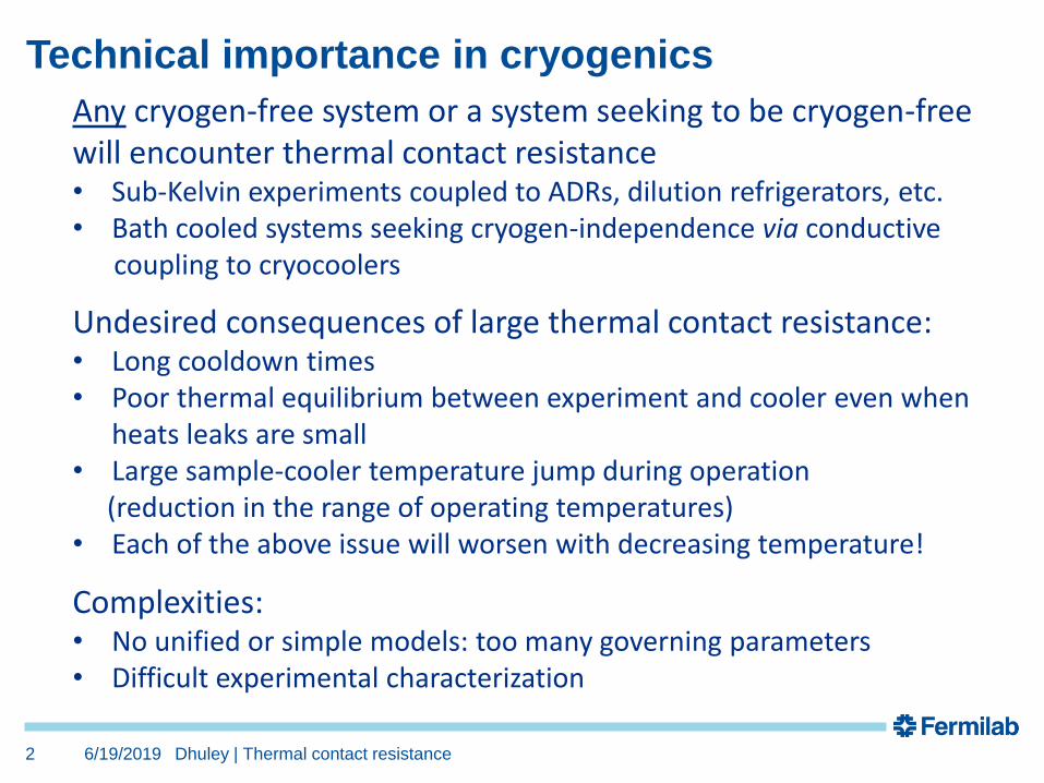
Technical importance in cryogenics
Any cryogen-free system or a system seeking to be cryogen-freewill encounter thermal contact resistance• Sub-Kelvin experiments coupled to ADRs, dilution refrigerators, etc.• Bath cooled systems seeking cryogen-independence via conductive
coupling to cryocoolers
Undesired consequences of large thermal contact resistance:• Long cooldown times• Poor thermal equilibrium between experiment and cooler even when
heats leaks are small• Large sample-cooler temperature jump during operation
(reduction in the range of operating temperatures)• Each of the above issue will worsen with decreasing temperature!
Complexities:• No unified or simple models: too many governing parameters• Difficult experimental characterization
6/19/20193 Dhuley | Thermal contact resistance
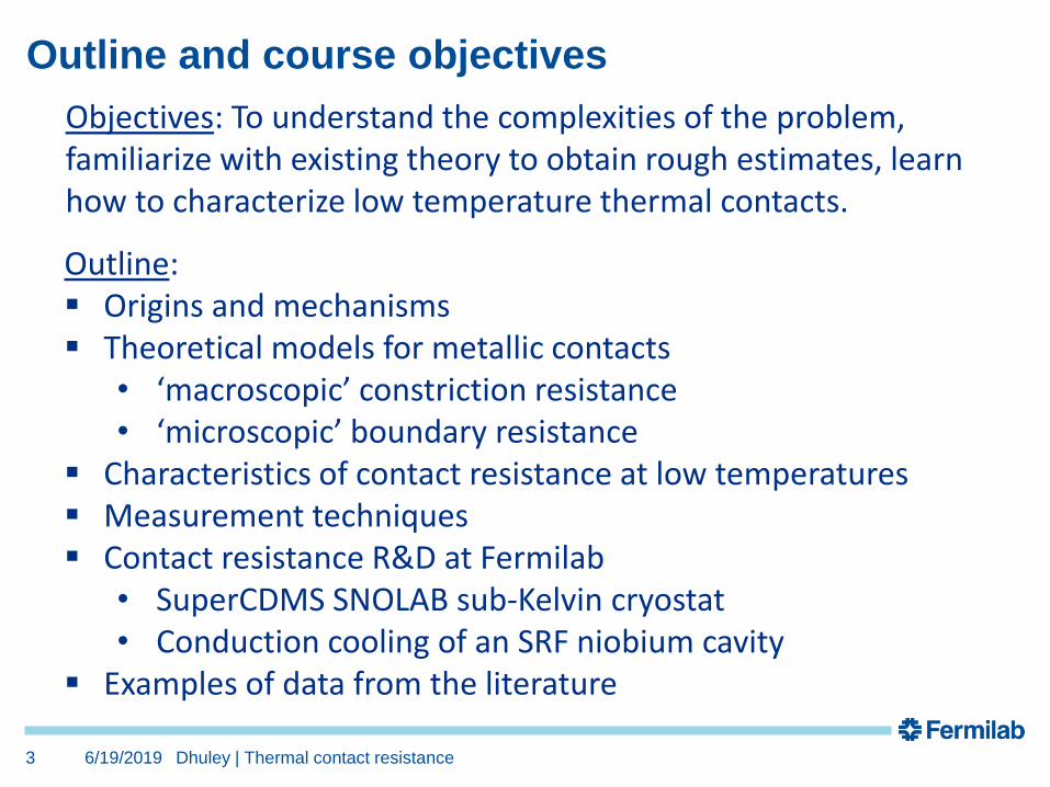
Outline and course objectives
Outline:▪ Origins and mechanisms▪ Theoretical models for metallic contacts
• ‘macroscopic’ constriction resistance• ‘microscopic’ boundary resistance
▪ Characteristics of contact resistance at low temperatures▪ Measurement techniques▪ Contact resistance R&D at Fermilab
• SuperCDMS SNOLAB sub-Kelvin cryostat• Conduction cooling of an SRF niobium cavity
▪ Examples of data from the literature
Objectives: To understand the complexities of the problem, familiarize with existing theory to obtain rough estimates, learn how to characterize low temperature thermal contacts.
6/19/20194 Dhuley | Thermal contact resistance
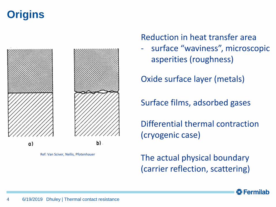
Origins
Ref: Van Sciver, Nellis, Pfotenhauer
Reduction in heat transfer area- surface “waviness”, microscopic
asperities (roughness)
Oxide surface layer (metals)
Surface films, adsorbed gases
Differential thermal contraction(cryogenic case)
The actual physical boundary(carrier reflection, scattering)

6/19/20195 Dhuley | Thermal contact resistance
Contact heat transfer mechanisms
• Conduction through actual solid-solid contact spots (spot or constriction resistance)- important for cryogenic applications
• Conduction through interstitial medium, example air (gap resistance)- neglected if fluid is absent (eg. vacuum in cryogenic systems)
• Radiation- small unless T or ΔT are is large (not significant at low T)
Ref: Madhusudhana
6/19/20196 Dhuley | Thermal contact resistance
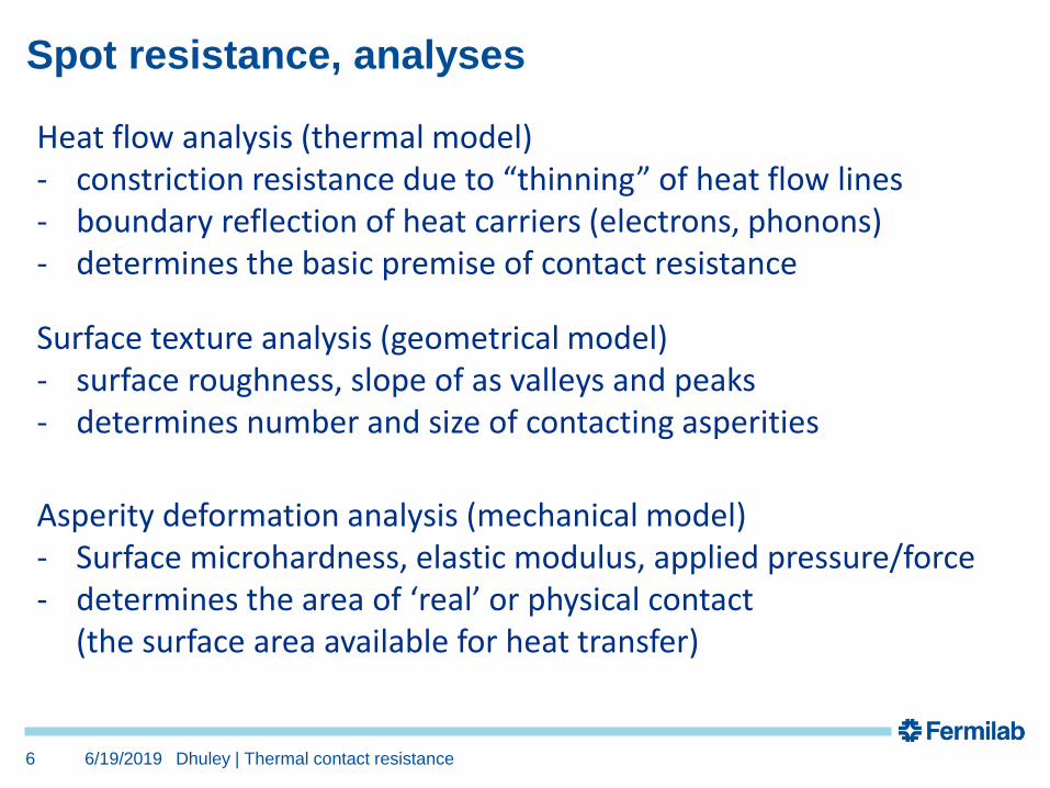
Spot resistance, analyses
Heat flow analysis (thermal model)- constriction resistance due to “thinning” of heat flow lines- boundary reflection of heat carriers (electrons, phonons)- determines the basic premise of contact resistance
Surface texture analysis (geometrical model)- surface roughness, slope of as valleys and peaks- determines number and size of contacting asperities
Asperity deformation analysis (mechanical model)- Surface microhardness, elastic modulus, applied pressure/force- determines the area of ‘real’ or physical contact
(the surface area available for heat transfer)
6/19/20197 Dhuley | Thermal contact resistance
Ref: Prasher and Phelan
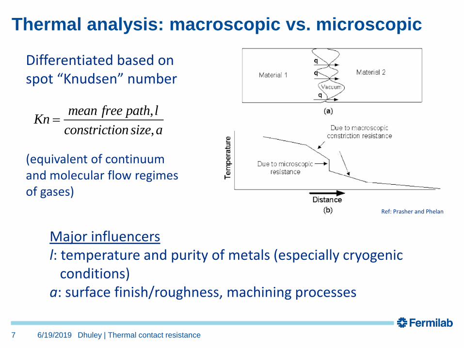
Thermal analysis: macroscopic vs. microscopic
Differentiated based on spot “Knudsen” number
,
,
mean free path lKn
constriction size a=
Major influencersl: temperature and purity of metals (especially cryogenic
conditions)a: surface finish/roughness, machining processes
(equivalent of continuum and molecular flow regimes of gases)
6/19/20198 Dhuley | Thermal contact resistance
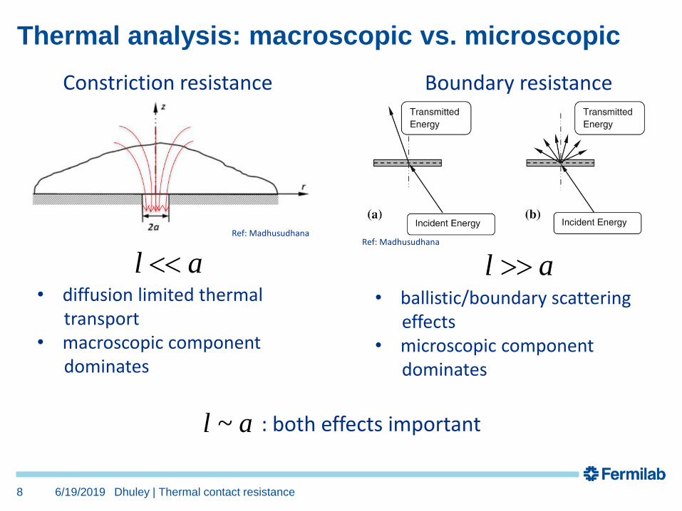
Thermal analysis: macroscopic vs. microscopic
: both effects important~l a
l a• diffusion limited thermal
transport• macroscopic component
dominates
Constriction resistance
Ref: Madhusudhana
l a• ballistic/boundary scattering
effects• microscopic component
dominates
Boundary resistance
Ref: Madhusudhana
6/19/20199 Dhuley | Thermal contact resistance
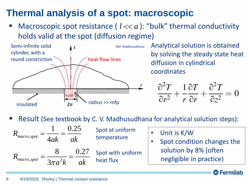
Thermal analysis of a spot: macroscopic
▪ Macroscopic spot resistance ( ): “bulk” thermal conductivity holds valid at the spot (diffusion regime)
l a
Analytical solution is obtained by solving the steady state heat diffusion in cylindrical coordinates
▪ Result (See textbook by C. V. Madhusudhana for analytical solution steps):
,
1 0.25
4macro spotR
ak ak= =
, 2
8 0.27
3macro spotR
a k ak= =
Spot at uniform temperature
Spot with uniform heat flux
• Unit is K/W• Spot condition changes the
solution by 8% (often negligible in practice)
insulated
Semi-infinite solidcylinder, with a round constriction
radius >> mfp
heat flow lines
Ref: Madhusudhana
6/19/201910 Dhuley | Thermal contact resistance
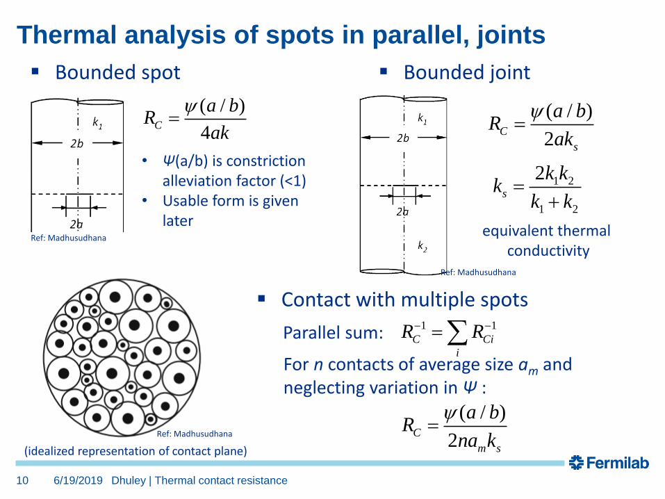
Thermal analysis of spots in parallel, joints
( / )
4C
a bR
ak
=
• Ψ(a/b) is constriction alleviation factor (<1)
• Usable form is given later
▪ Bounded spot
Ref: Madhusudhana
▪ Contact with multiple spots
(idealized representation of contact plane)
1 1
C Ci
i
R R− −=Parallel sum:
( / )
2C
m s
a bR
na k
=
For n contacts of average size am and neglecting variation in Ψ :
Ref: Madhusudhana
▪ Bounded joint
1 2
1 2
2s
k kk
k k=
+
equivalent thermal conductivity
( / )
2C
s
a bR
ak
=
Ref: Madhusudhana
6/19/2019 Dhuley | Thermal contact resistance11
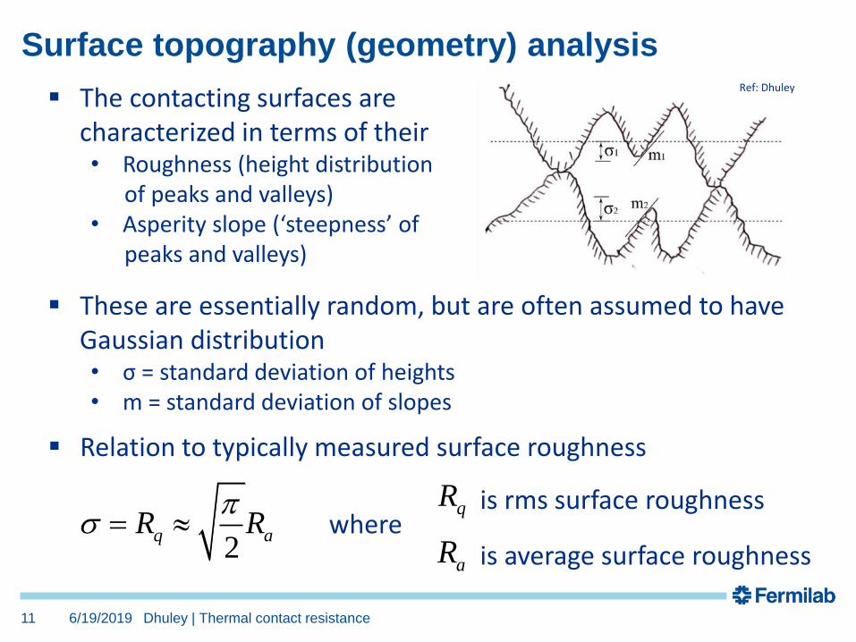
▪ The contacting surfaces are characterized in terms of their • Roughness (height distribution
of peaks and valleys)• Asperity slope (‘steepness’ of
peaks and valleys)
▪ These are essentially random, but are often assumed to haveGaussian distribution• σ = standard deviation of heights• m = standard deviation of slopes
▪ Relation to typically measured surface roughness
2q aR R
= where
qR
aR
is rms surface roughness
is average surface roughness
Surface topography (geometry) analysisRef: Dhuley
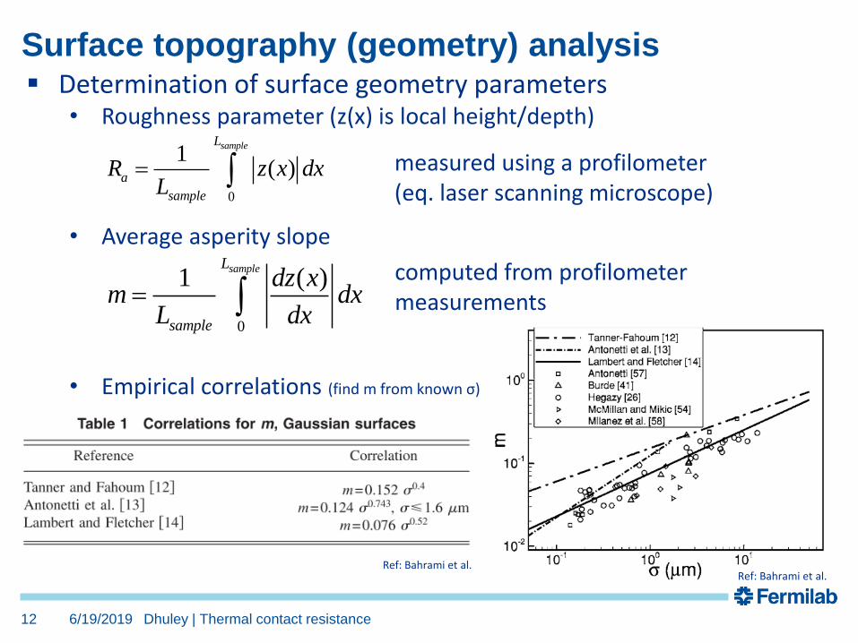
Surface topography (geometry) analysis
6/19/2019 Dhuley | Thermal contact resistance12
▪ Determination of surface geometry parameters • Roughness parameter (z(x) is local height/depth)
• Average asperity slope
• Empirical correlations (find m from known σ)
0
1( )
sampleL
a
sample
R z x dxL
=
0
1 ( )sampleL
sample
dz xm dx
L dx=
measured using a profilometer(eq. laser scanning microscope)
computed from profilometermeasurements
Ref: Bahrami et al.Ref: Bahrami et al.
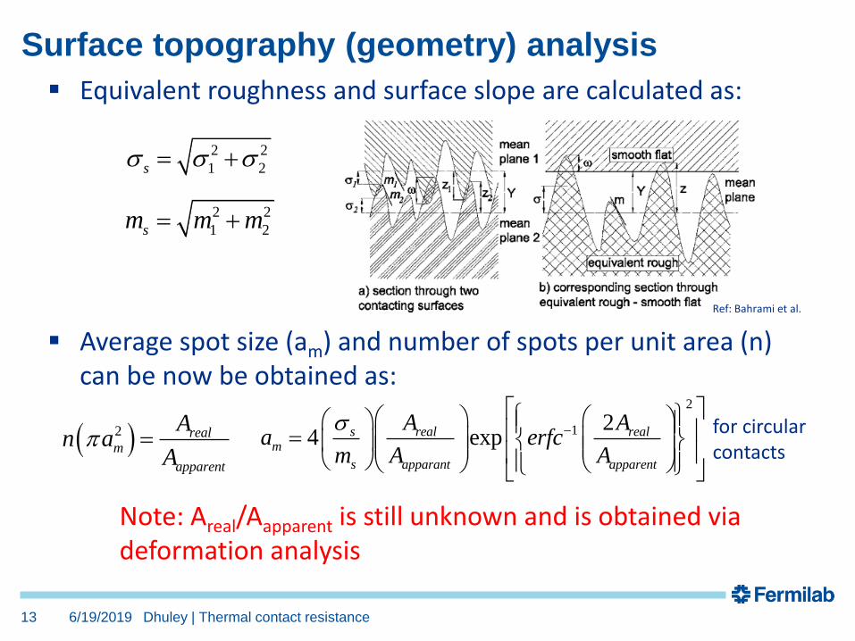
6/19/2019 Dhuley | Thermal contact resistance13
Note: Areal/Aapparent is still unknown and is obtained via deformation analysis
▪ Average spot size (am) and number of spots per unit area (n) can be now be obtained as:
2
1 24 exps real real
m
s apparant apparent
A Aa erfc
m A A
−
=
( )2 realm
apparent
An a
A =
for circular contacts
Surface topography (geometry) analysis
▪ Equivalent roughness and surface slope are calculated as:
2 2
1 2s = +
2 2
1 2sm m m= +
Ref: Bahrami et al.
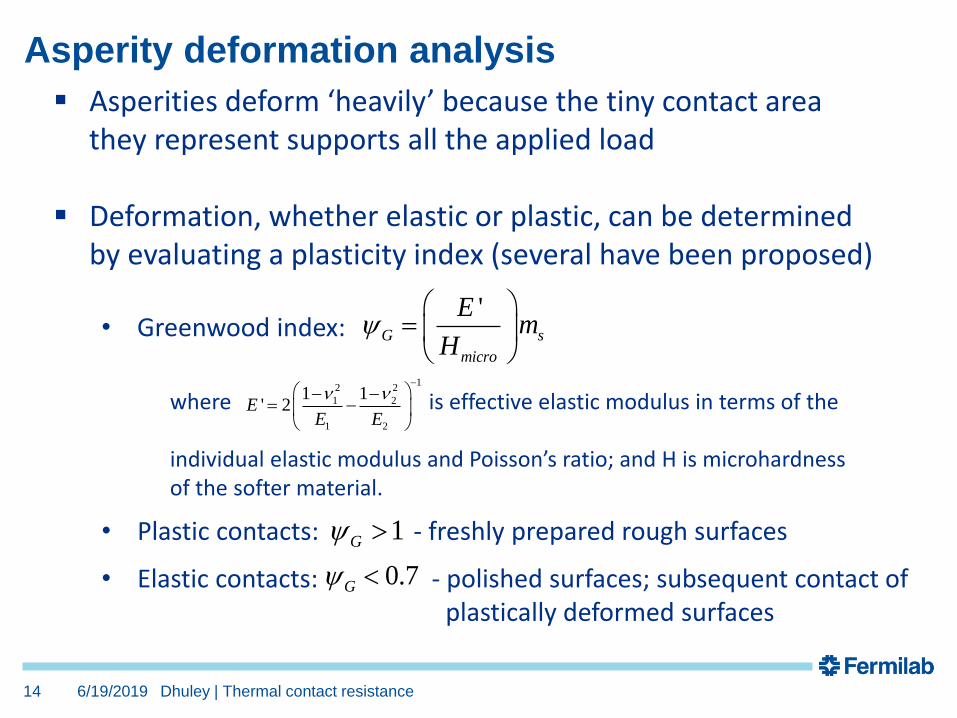
Asperity deformation analysis
6/19/2019 Dhuley | Thermal contact resistance14
▪ Asperities deform ‘heavily’ because the tiny contact areathey represent supports all the applied load
▪ Deformation, whether elastic or plastic, can be determined by evaluating a plasticity index (several have been proposed)
• Greenwood index:
12 2
1 2
1 2
1 1' 2E
E E
−
− −= −
where is effective elastic modulus in terms of the
individual elastic modulus and Poisson’s ratio; and H is microhardness of the softer material.
• Plastic contacts: - freshly prepared rough surfaces1G
• Elastic contacts: - polished surfaces; subsequent contact ofplastically deformed surfaces
0.7G
'G s
micro
Em
H
=
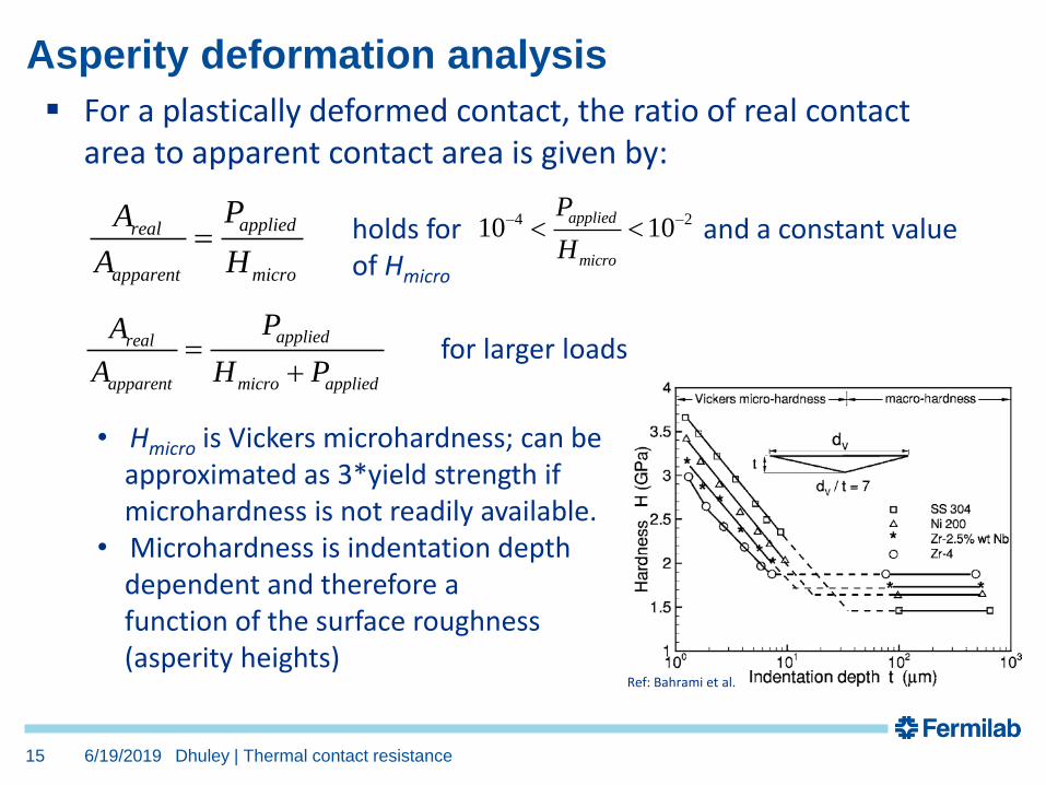
▪ For a plastically deformed contact, the ratio of real contact area to apparent contact area is given by:
• Hmicro is Vickers microhardness; can be approximated as 3*yield strength if microhardness is not readily available.
• Microhardness is indentation depth dependent and therefore a function of the surface roughness (asperity heights)
Asperity deformation analysis
6/19/2019 Dhuley | Thermal contact resistance15
appliedreal
apparent micro
PA
A H=
4 210 10applied
micro
P
H
− − holds for and a constant valueof Hmicro
appliedreal
apparent micro applied
PA
A H P=
+for larger loads
Ref: Bahrami et al.
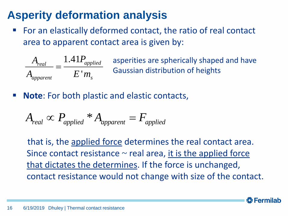
▪ For an elastically deformed contact, the ratio of real contact area to apparent contact area is given by:
Asperity deformation analysis
6/19/2019 Dhuley | Thermal contact resistance16
1.41
'
appliedreal
apparent s
PA
A E m=
asperities are spherically shaped and haveGaussian distribution of heights
▪ Note: For both plastic and elastic contacts,
that is, the applied force determines the real contact area. Since contact resistance ~ real area, it is the applied forcethat dictates the determines. If the force is unchanged, contact resistance would not change with size of the contact.
*real applied apparent appliedA P A F =
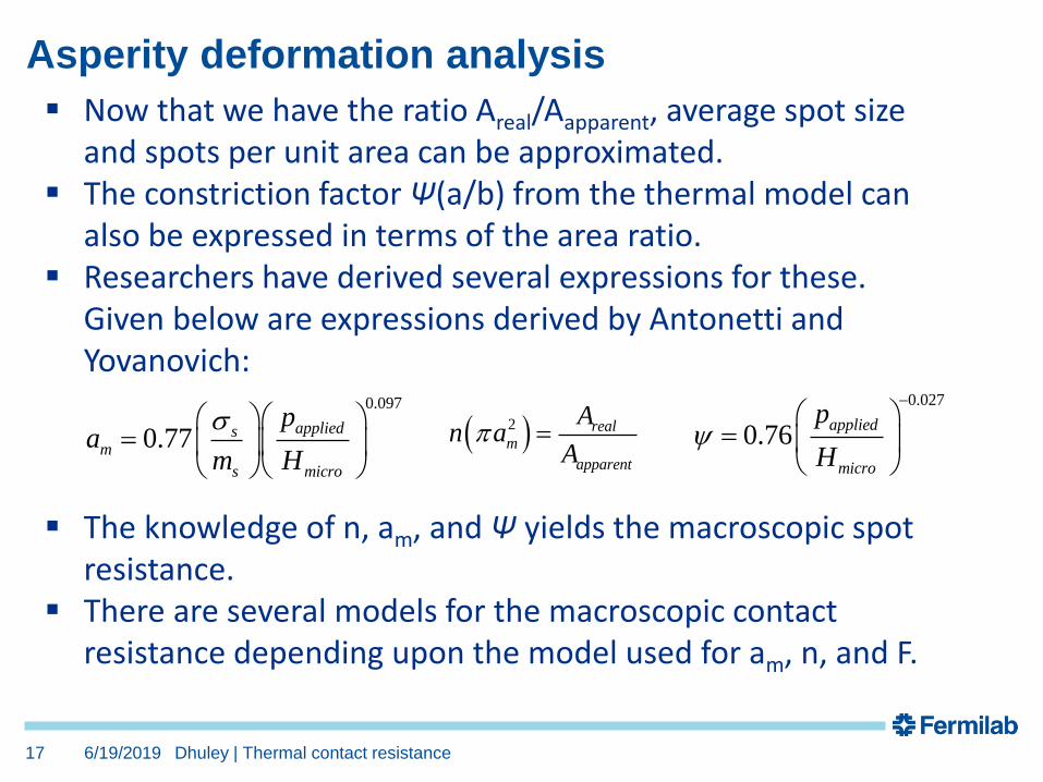
▪ Now that we have the ratio Areal/Aapparent, average spot size and spots per unit area can be approximated.
▪ The constriction factor Ψ(a/b) from the thermal model can also be expressed in terms of the area ratio.
▪ Researchers have derived several expressions for these. Given below are expressions derived by Antonetti and Yovanovich:
▪ The knowledge of n, am, and Ψ yields the macroscopic spot resistance.
▪ There are several models for the macroscopic contact resistance depending upon the model used for am, n, and F.
Asperity deformation analysis
6/19/2019 Dhuley | Thermal contact resistance17
0.097
0.77applieds
m
s micro
pa
m H
=
( )2 real
m
apparent
An a
A =
0.027
0.76applied
micro
p
H
−
=

Macroscopic contact thermal resistance
6/19/2019 Dhuley | Thermal contact resistance18
▪ For flat, conforming contacts with plastic deformation, the expression for contact resistance has the form:
▪ See review paper by Lambert and Fletcher for more models,range of validity, etc. (https://arc.aiaa.org/doi/10.2514/2.6221)
K*m2/W, expressed in terms of the apparent contact area; usable for 10-4 < papplied/Hmicro < 10-2
1 1B
appliedsC
s s micro
pR
A m k H
−
=
Macroscopic contact thermal resistance
6/19/2019 Dhuley | Thermal contact resistance19
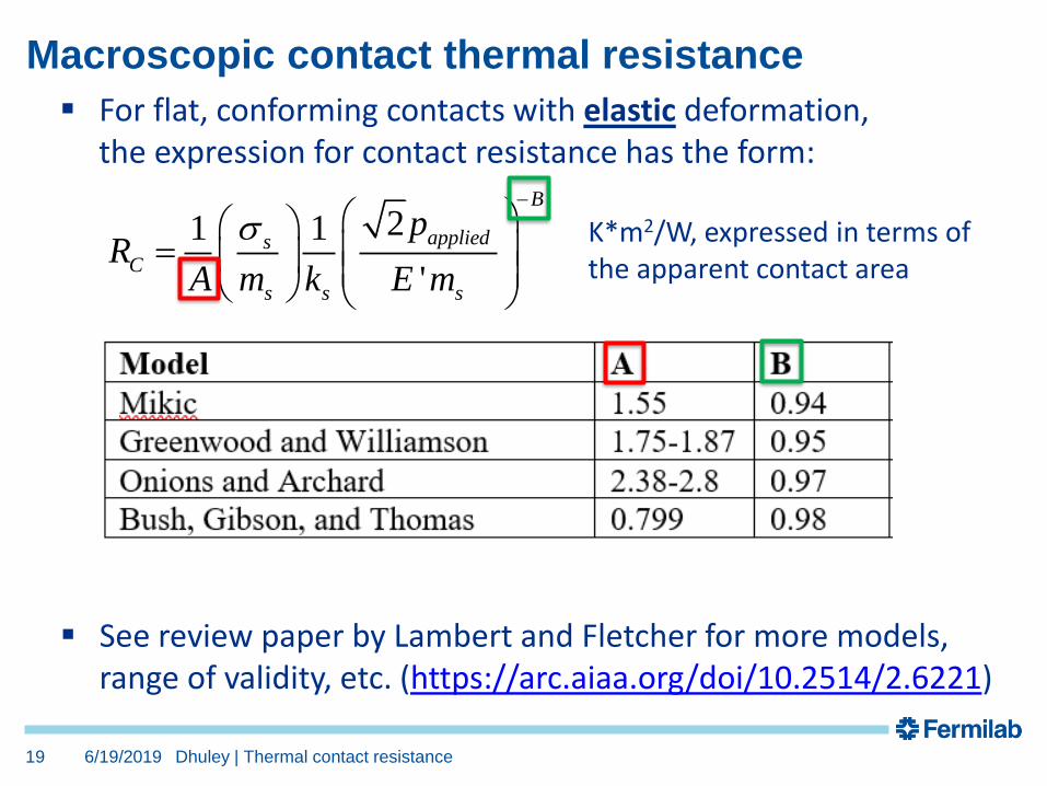
▪ For flat, conforming contacts with elastic deformation, the expression for contact resistance has the form:
▪ See review paper by Lambert and Fletcher for more models,range of validity, etc. (https://arc.aiaa.org/doi/10.2514/2.6221)
K*m2/W, expressed in terms of the apparent contact area
21 1
'
B
appliedsC
s s s
pR
A m k E m
−
=
6/19/201920 Dhuley | Thermal contact resistance
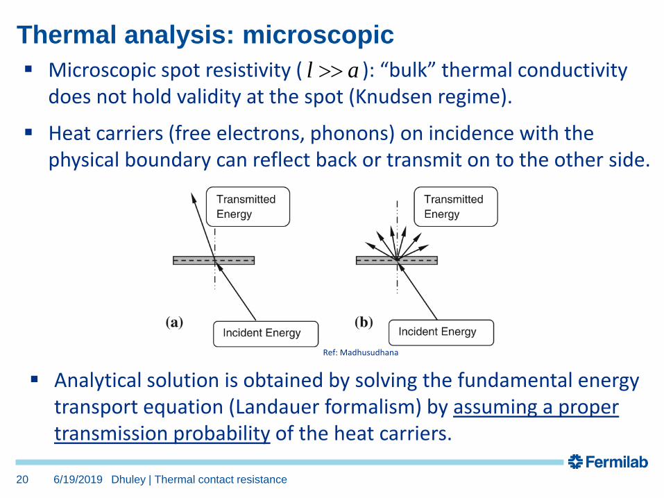
Thermal analysis: microscopic
▪ Microscopic spot resistivity ( ): “bulk” thermal conductivity does not hold validity at the spot (Knudsen regime).
▪ Analytical solution is obtained by solving the fundamental energy transport equation (Landauer formalism) by assuming a proper transmission probability of the heat carriers.
l a
▪ Heat carriers (free electrons, phonons) on incidence with thephysical boundary can reflect back or transmit on to the other side.
Ref: Madhusudhana
6/19/201921 Dhuley | Thermal contact resistance
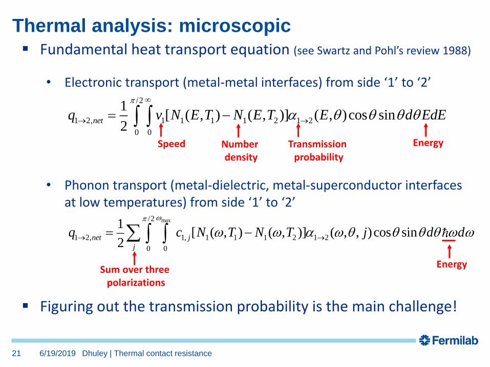
Thermal analysis: microscopic
▪ Fundamental heat transport equation (see Swartz and Pohl’s review 1988)
• Electronic transport (metal-metal interfaces) from side ‘1’ to ‘2’
• Phonon transport (metal-dielectric, metal-superconductor interfaces at low temperatures) from side ‘1’ to ‘2’
▪ Figuring out the transmission probability is the main challenge!
max/2
1 2, 1, 1 1 1 2 1 2
0 0
1[ ( , ) ( , )] ( , , )cos sin
2net j
j
q c N T N T j d d
→ →= −
/2
1 2, 1 1 1 1 2 1 2
0 0
1[ ( , ) ( , )] ( , )cos sin
2netq v N E T N E T E d EdE
→ →= − Speed Number
densityTransmission
probability
Energy
Sum over three polarizations
Energy
6/19/201922 Dhuley | Thermal contact resistance
Thermal analysis: microscopic
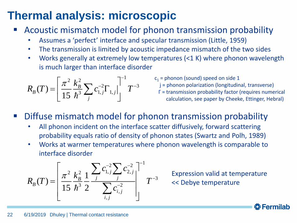
▪ Acoustic mismatch model for phonon transmission probability• Assumes a ‘perfect’ interface and specular transmission (Little, 1959)• The transmission is limited by acoustic impedance mismatch of the two sides• Works generally at extremely low temperatures (<1 K) where phonon wavelength
is much larger than interface disorder
c1 = phonon (sound) speed on side 1j = phonon polarization (longitudinal, transverse)Γ = transmission probability factor (requires numerical
calculation, see paper by Cheeke, Ettinger, Hebral)
▪ Diffuse mismatch model for phonon transmission probability• All phonon incident on the interface scatter diffusively, forward scattering
probability equals ratio of density of phonon states (Swartz and Polh, 1989)• Works at warmer temperatures where phonon wavelength is comparable to
interface disorder
Expression valid at temperature << Debye temperature
122
2 3
1, 1,3( )
15
BB j j
j
kR T c T
−
− −
=
12 2
1, 2,223
3 2
,
,
1( )
15 2
j j
j jBB
i j
i j
c ck
R T Tc
−− −
−
−
=
6/19/201923 Dhuley | Thermal contact resistance
Thermal analysis: microscopic
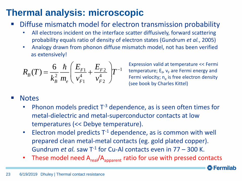
▪ Diffuse mismatch model for electron transmission probability• All electrons incident on the interface scatter diffusively, forward scattering
probability equals ratio of density of electron states (Gundrum et al., 2005)• Analogy drawn from phonon diffuse mismatch model, not has been verified
as extensively!
Expression valid at temperature << Fermi temperature; EF, vF are Fermi energy and Fermi velocity; ne is free electron density (see book by Charles Kittel)
▪ Notes• Phonon models predict T-3 dependence, as is seen often times for
metal-dielectric and metal-superconductor contacts at low temperatures (<< Debye temperature).
• Electron model predicts T-1 dependence, as is common with well prepared clean metal-metal contacts (eg. gold plated copper). Gundrum et al. saw T-1 for Cu-Al contacts even in 77 – 300 K.
• These model need Areal/Aapparent ratio for use with pressed contacts
11 2
2 4 4
1 2
6( ) F F
B
B e F F
E ER T T
k m v v
− = +

6/19/2019 Dhuley | Thermal contact resistance24
▪ Metal-metal contacts
= (Areal/Aapparent)-1
1
11 2
2 4 4
1 2
1 1 6( )
B
applied applieds F FB
s s micro B e F F micro
p pE ER T T
A m k H k m v v H
− −
− = + +
▪ Metal-dielectric, metal-superconductor contacts1
2 211, 2,22
3
3 2
,
,
1 1 1( )
15 2
B j j
applied j j applieds BB
s s micro i j micro
i j
c cp pk
R T TA m k H c H
−− −
− −
−
−
= +
A simple model for pressed contacts
▪ The contacts are assumed to be flat and conforming

Common observations at low temperature (LHe)
6/19/2019 Dhuley | Thermal contact resistance25
▪ Weideman Franz law analogy for contacts
, 1
,
0
C elec
C thermal
RR T
L
−=
▪ Dependence on temperature1
CR T −
2
CR T −
2 1n
CR T − −
3
CR T −
: pure or lightly oxidized metallic contacts (oxide<<deBroglie λelectron)
: oxidized metallic contacts (deBroglie λelectron<<oxide<<λphonon)
: contact with a superconductor (T<<Tcrit)
: practical metallic contacts (limited exposure to oxygen)
L0 is theoretical Lorenz number (=2.44x10⁻⁸ WΩ/K2)
• at lower temperature since is constant
1
,C thermalR T −
,C elecR
• Gives an upper bound of thermal contact resistanceas an additional heat transfer channel (phonon) can be present. Ref: Van Sciver,
Nellis, Pfotenhauer
Measurement techniques
6/19/2019 Dhuley | Thermal contact resistance26
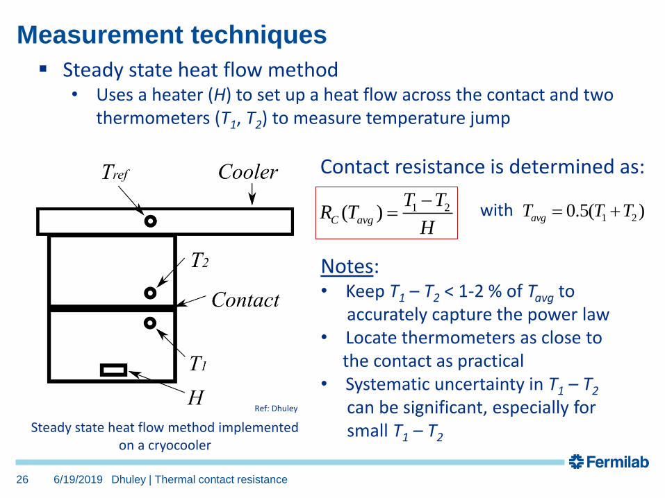
▪ Steady state heat flow method• Uses a heater (H) to set up a heat flow across the contact and two
thermometers (T1, T2) to measure temperature jump
Contact resistance is determined as:
1 2( )C avg
T TR T
H
−= 1 20.5( )avgT T T= +with
Notes:• Keep T1 – T2 < 1-2 % of Tavg to
accurately capture the power law• Locate thermometers as close to
the contact as practical• Systematic uncertainty in T1 – T2
can be significant, especially for small T1 – T2
Steady state heat flow method implemented on a cryocooler
Ref: Dhuley
Measurement techniques
6/19/2019 Dhuley | Thermal contact resistance27
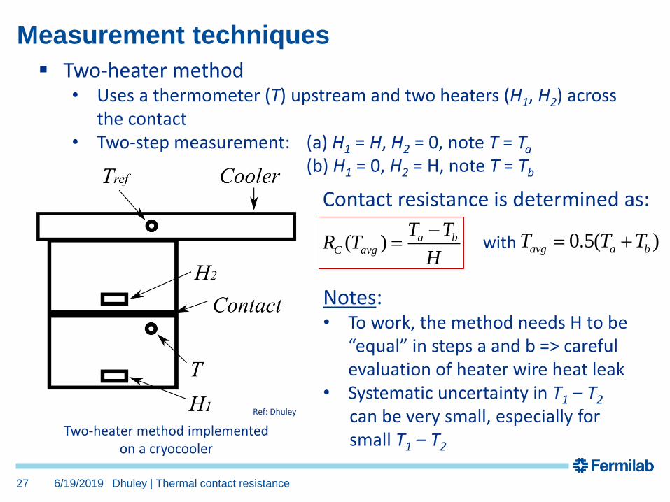
▪ Two-heater method• Uses a thermometer (T) upstream and two heaters (H1, H2) across
the contact• Two-step measurement: (a) H1 = H, H2 = 0, note T = Ta
(b) H1 = 0, H2 = H, note T = Tb
Contact resistance is determined as:
Notes:• To work, the method needs H to be
“equal” in steps a and b => careful evaluation of heater wire heat leak
• Systematic uncertainty in T1 – T2
can be very small, especially for small T1 – T2
( ) a bC avg
T TR T
H
−= 0.5( )avg a bT T T= +with
Two-heater method implemented on a cryocooler
Ref: Dhuley
Measurement techniques
6/19/2019 Dhuley | Thermal contact resistance28
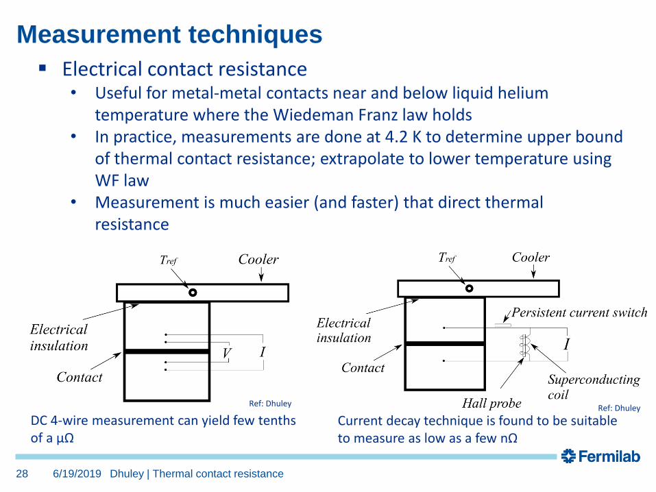
▪ Electrical contact resistance• Useful for metal-metal contacts near and below liquid helium
temperature where the Wiedeman Franz law holds• In practice, measurements are done at 4.2 K to determine upper bound
of thermal contact resistance; extrapolate to lower temperature using WF law
• Measurement is much easier (and faster) that direct thermal resistance
DC 4-wire measurement can yield few tenths of a µΩ
Ref: Dhuley
Current decay technique is found to be suitable to measure as low as a few nΩ
Ref: Dhuley
Example: SuperCDMS SNOLAB cryostat
6/19/2019 Dhuley | Thermal contact resistance29
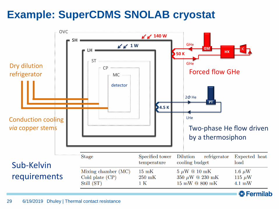
detector
Dry dilution refrigerator
Conduction cooling via copper stems
Sub-Kelvin requirements
6/19/2019 Dhuley | Thermal contact resistance30
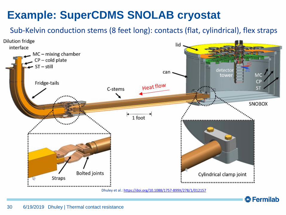
Example: SuperCDMS SNOLAB cryostat
Sub-Kelvin conduction stems (8 feet long): contacts (flat, cylindrical), flex straps
Dhuley et al.: https://doi.org/10.1088/1757-899X/278/1/012157
Conduction stem: Flat and cylindrical joints
6/19/2019 Dhuley | Thermal contact resistance31
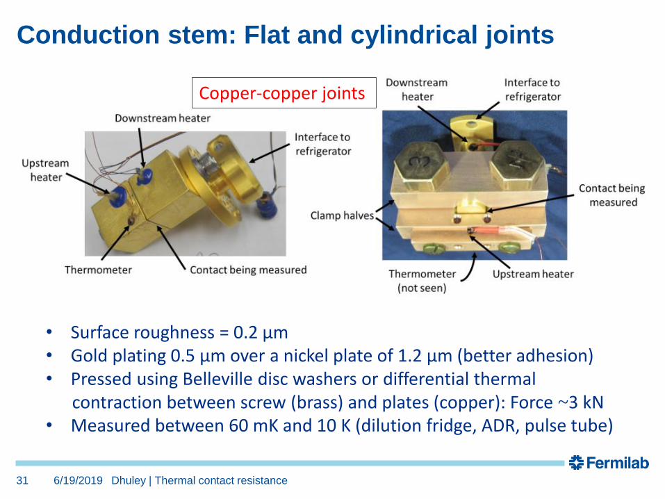
• Surface roughness = 0.2 µm• Gold plating 0.5 µm over a nickel plate of 1.2 µm (better adhesion)• Pressed using Belleville disc washers or differential thermal
contraction between screw (brass) and plates (copper): Force ~3 kN• Measured between 60 mK and 10 K (dilution fridge, ADR, pulse tube)
Copper-copper joints
6/19/2019 Dhuley | Thermal contact resistance32
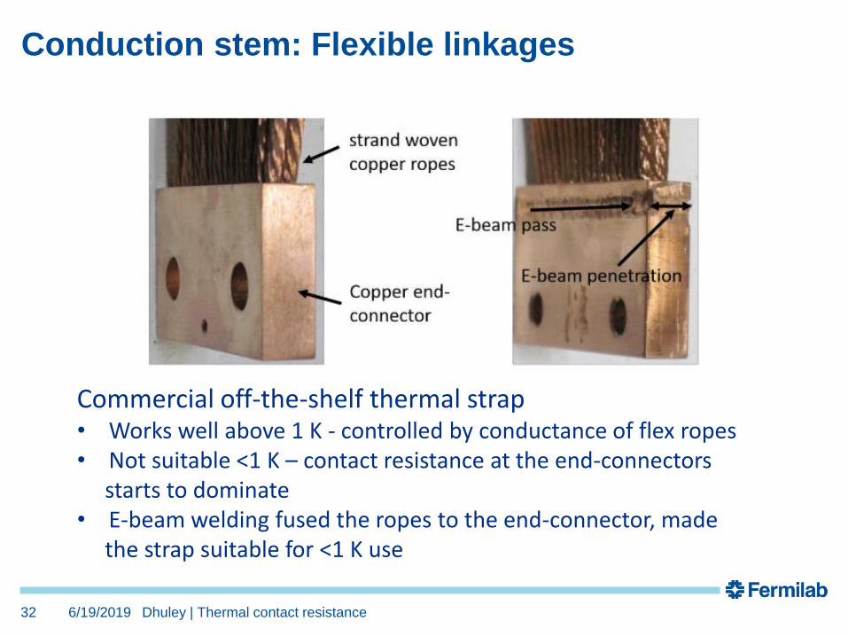
Conduction stem: Flexible linkages
Commercial off-the-shelf thermal strap• Works well above 1 K - controlled by conductance of flex ropes• Not suitable <1 K – contact resistance at the end-connectors
starts to dominate• E-beam welding fused the ropes to the end-connector, made
the strap suitable for <1 K use
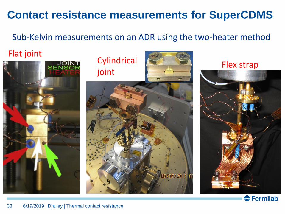
Contact resistance measurements for SuperCDMS
6/19/2019 Dhuley | Thermal contact resistance33
Flat jointCylindrical joint
Flex strap
Sub-Kelvin measurements on an ADR using the two-heater method

Results: conductance vs. temperature
6/19/2019 Dhuley | Thermal contact resistance34
Flat and cylindrical contacts Flex straps
~T2
• Gold plated contacts produced nearly ~T1 conductance
• Pressed straps yielded ~T2 below1 K (ropes/end connector may have carried copper oxide during swaging)
• Welding fused the ropes with end-connector, and produced ~T1
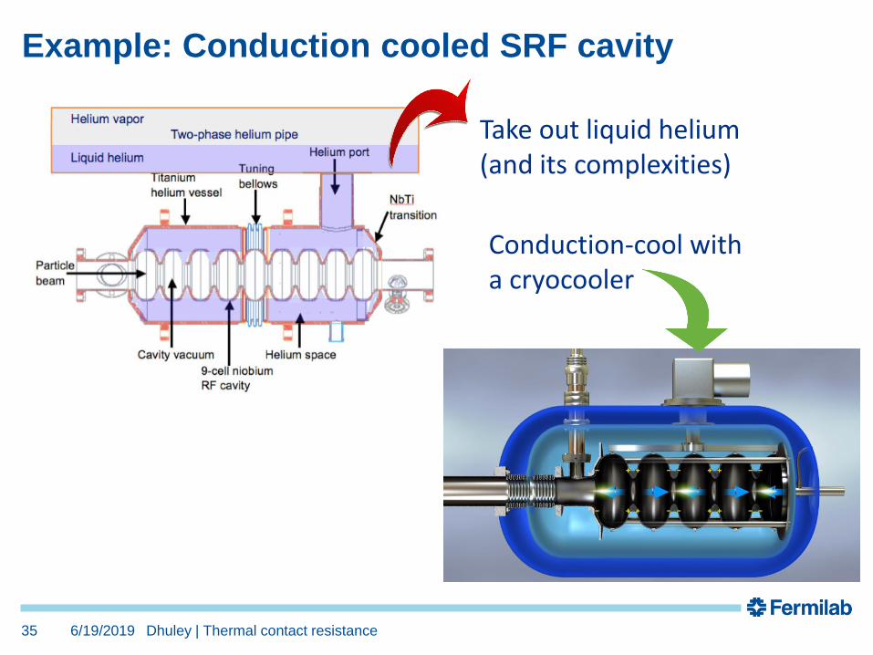
Example: Conduction cooled SRF cavity
6/19/2019 Dhuley | Thermal contact resistance35
Take out liquid helium(and its complexities)
Conduction-cool with a cryocooler
6/19/2019 Dhuley | Thermal contact resistance36
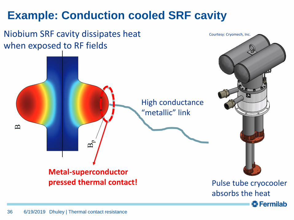
Niobium SRF cavity dissipates heat when exposed to RF fields
High conductance “metallic” link
Example: Conduction cooled SRF cavity
Metal-superconductor pressed thermal contact! Pulse tube cryocooler
absorbs the heat
Courtesy: Cryomech, Inc.
6/19/2019 Dhuley | Thermal contact resistance37
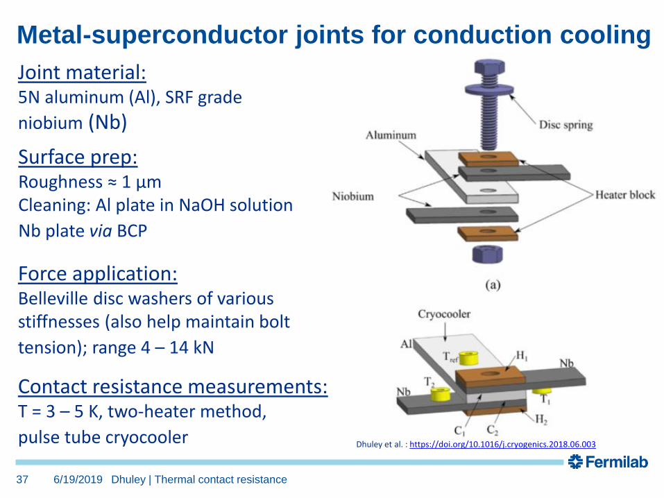
Metal-superconductor joints for conduction cooling
Joint material:5N aluminum (Al), SRF grade
niobium (Nb)
Surface prep:Roughness ≈ 1 µmCleaning: Al plate in NaOH solution
Nb plate via BCP
Force application:Belleville disc washers of variousstiffnesses (also help maintain bolt
tension); range 4 – 14 kN
Contact resistance measurements:T = 3 – 5 K, two-heater method,
pulse tube cryocooler Dhuley et al. : https://doi.org/10.1016/j.cryogenics.2018.06.003
6/19/2019 Dhuley | Thermal contact resistance38
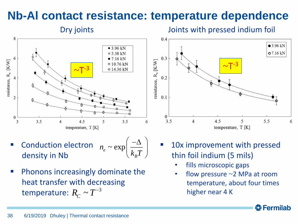
Dry joints
~T-3
Nb-Al contact resistance: temperature dependence
~T-3
Joints with pressed indium foil
~ expe
B
nk T
−
▪ Conduction electron density in Nb
▪ Phonons increasingly dominate theheat transfer with decreasingtemperature: 3~CR T −
▪ 10x improvement with pressed thin foil indium (5 mils) • fills microscopic gaps• flow pressure ~2 MPa at room
temperature, about four times higher near 4 K
6/19/2019 Dhuley | Thermal contact resistance39
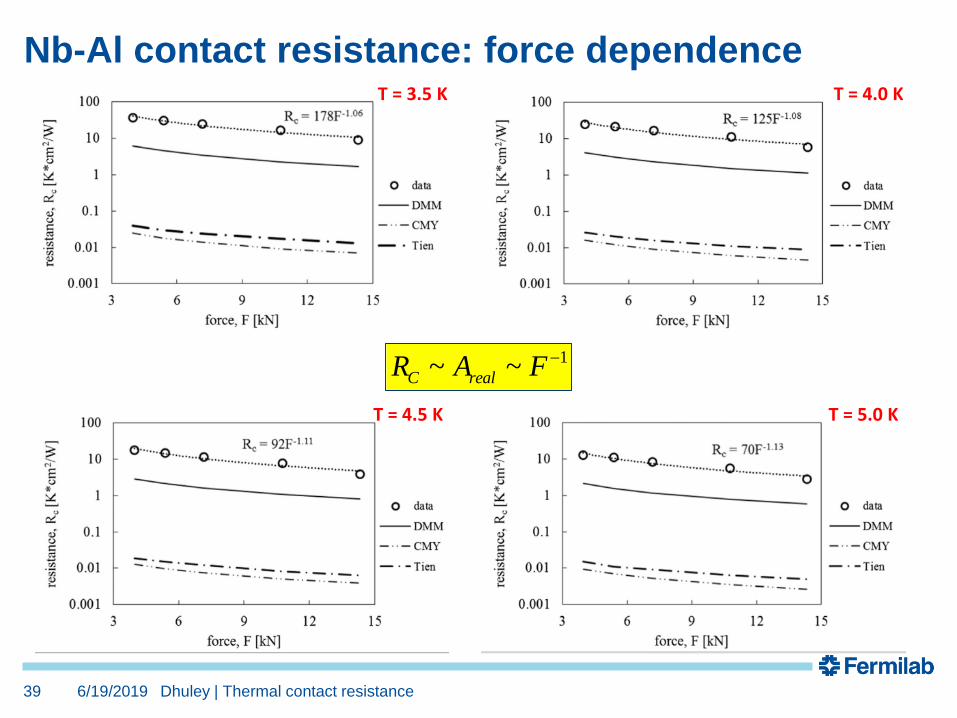
Nb-Al contact resistance: force dependenceT = 3.5 K
T = 4.5 K
T = 4.0 K
T = 5.0 K
1~ ~C realR A F −
6/19/2019 Dhuley | Thermal contact resistance40
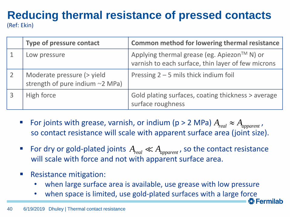
Reducing thermal resistance of pressed contacts
Type of pressure contact Common method for lowering thermal resistance
1 Low pressure Applying thermal grease (eg. ApiezonTM N) or varnish to each surface, thin layer of few microns
2 Moderate pressure (> yield strength of pure indium ~2 MPa)
Pressing 2 – 5 mils thick indium foil
3 High force Gold plating surfaces, coating thickness > average surface roughness
▪ For joints with grease, varnish, or indium (p > 2 MPa) , so contact resistance will scale with apparent surface area (joint size).
real apparentA A
▪ For dry or gold-plated joints , so the contact resistancewill scale with force and not with apparent surface area.
real apparentA A
▪ Resistance mitigation:• when large surface area is available, use grease with low pressure• when space is limited, use gold-plated surfaces with a large force
(Ref: Ekin)

6/19/2019 Dhuley | Thermal contact resistance41
Reducing resistance across pressed contacts
Dissimilar metals
Belleville disc spring
Copper plates
Bronze bolts
Some methods of applying force
Copper fingers
Nylonring
Boughton et al.: http://dx.doi.org/10.1063/1.1721058Bintley et al.: http://doi.org/10.1016/j.cryogenics.2007.04.004

6/19/2019 Dhuley | Thermal contact resistance42
Examples of data from literature
(From Ekin)

Examples of data from literature
6/19/2019 Dhuley | Thermal contact resistance43
(From Van Sciver, Nilles, and Pfotenhauer)
Examples of data from literature
6/19/2019 Dhuley | Thermal contact resistance44
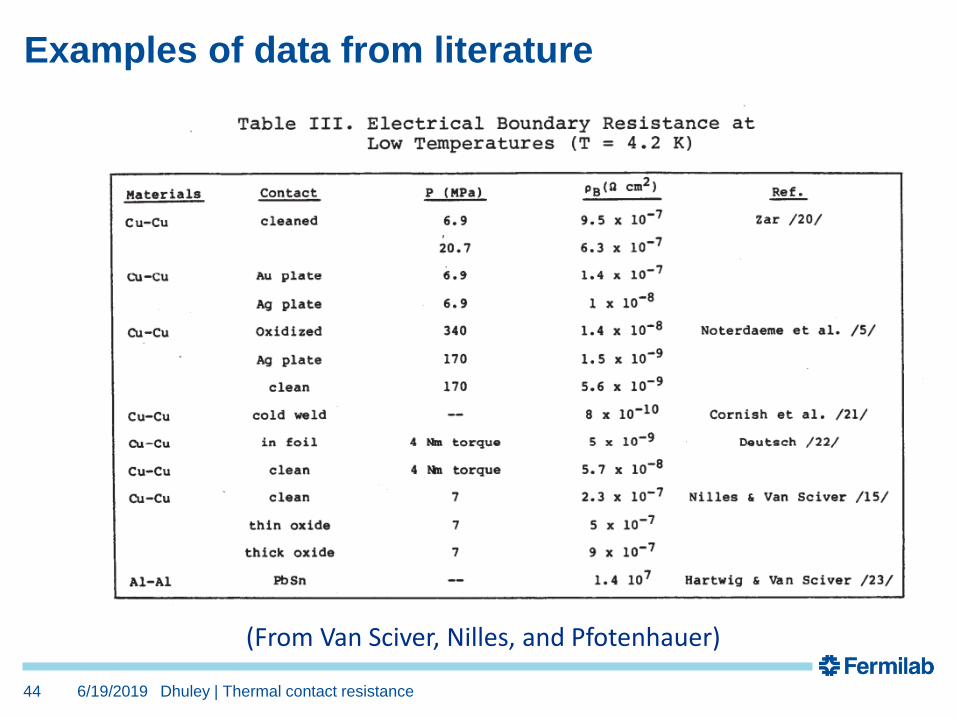
(From Van Sciver, Nilles, and Pfotenhauer)
Examples of data from literature
6/19/2019 Dhuley | Thermal contact resistance45
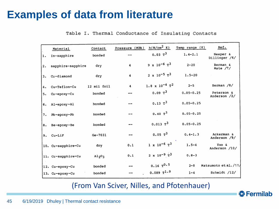
(From Van Sciver, Nilles, and Pfotenhauer)

Examples of data from literature
6/19/2019 Dhuley | Thermal contact resistance46
(From Mamiya et al.)
Examples of data from literature
6/19/2019 Dhuley | Thermal contact resistance47
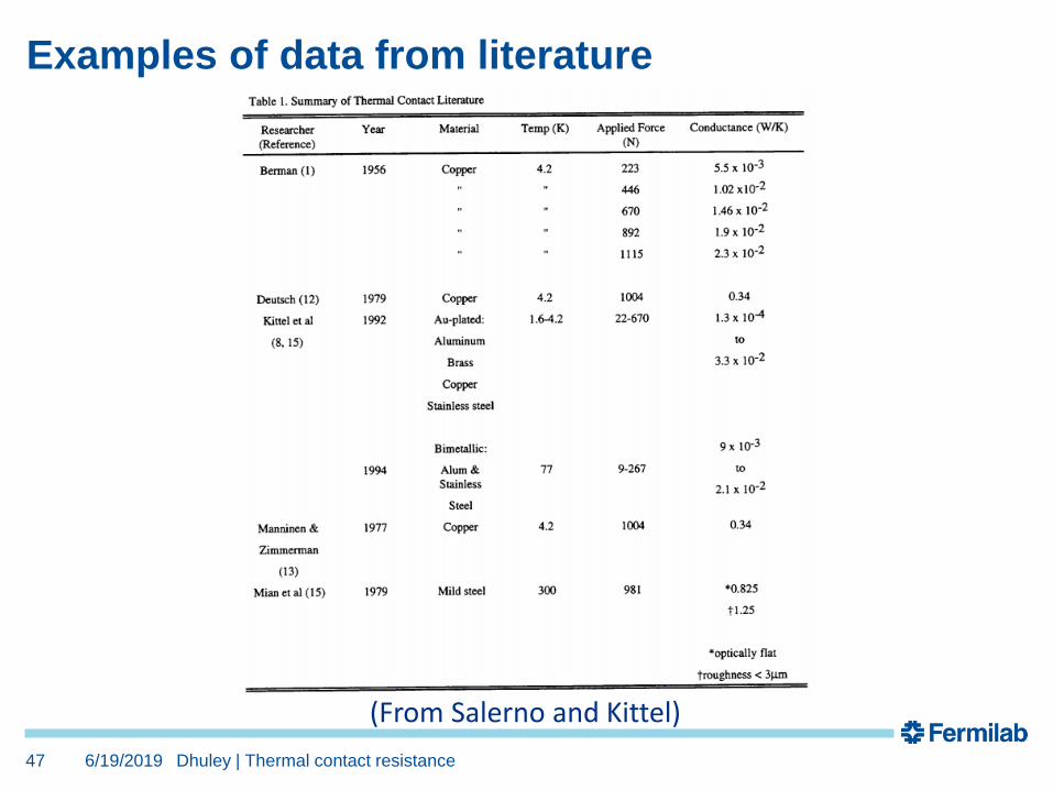
(From Salerno and Kittel)

Examples of data from literature
6/19/2019 Dhuley | Thermal contact resistance48
(From Salerno and Kittel)

6/19/201949 Dhuley | Thermal contact resistance
Useful references
Overview of boundary resistance models• Little: https://doi.org/10.1139/p59-037• Swartz and Pohl: https://doi.org/10.1103/RevModPhys.61.605• Gundrum et al.: https://doi.org/10.1103/PhysRevB.72.245426• Prasher and Phelan: https://doi.org/10.1063/1.2353704
Data at cryogenic temperatures (reviews)• Salerno and Kittel: NASA NTRS 19970026086• Mamiya et al.: https://doi.org/10.1063/1.1139684• Van Sciver, Nilles, Pfotenhauer: Proc. SCW 1984• Gmelin et al.: https://doi.org/10.1088/0022-3727/32/6/004• Ekin: http://dx.doi.org/10.1093/acprof:oso/9780198570547.001.0001• Dhuley:
Overview of constriction resistance models• Madhusudhana: https://www.springer.com/us/book/9783319012759• Lambert and Fletcher: https://dx.doi.org/10.2514/2.6221• Bahrami et al.: http://dx.doi.org/10.1115/1.2110231
6/19/201950 Dhuley | Thermal contact resistance
6/19/201951 Dhuley | Thermal contact resistance
This document has been authored by Fermi Research Alliance, LLC under Contract No. DE-AC02-07CH11359 with the U.S. Department of Energy, Office of Science, Office of High Energy Physics.