Embed Size (px)
DESCRIPTION
AS
Citation preview
Technical Report CHL-97-12July 1997
FEMWATER : A Three-Dimensional Finite ElementComputer Model for Simulating Density-DependentFlow and Transport in Variably Saturated Media
by Hsin-Chi J. Lin, David R. Richards and Cary A. Talbot
U.S. Army Corps of EngineersWaterways Experiment Station3909 Halls Ferry RoadVicksburg, MS 39180-6199
Gour-Tsyh Yeh, Jing-Ru Cheng, Hwai-Ping Cheng
Department of Civil and Environmental EngineeringPennsylvania State UniversityUniversity Park, PA 16802
Norman L. Jones
Department of Civil EngineeringEngineering Computer Graphics LaboratoryBrigham Young University368 CBProvo, UT 84602
Approved for public release; distribution is unlimited

vii
Contents
Preface ............................................................................................................... viii
1 Introduction .......................................................................................................1
Purpose ...............................................................................................................1FEMWATER Origins.........................................................................................1Formulation of FEMWATER ............................................................................2
Governing equations for flow ........................................................................2Governing equations for transport .................................................................6
2 Running FEMWATER ...................................................................................11
File Organization..............................................................................................11Super File .........................................................................................................11Card Style Format ............................................................................................12Other Files ........................................................................................................13
3 Meshes ..............................................................................................................14
Introduction ......................................................................................................14Elements Supported..........................................................................................14Geometry File Format ......................................................................................14Mesh Generation Guidelines............................................................................17
4 Analysis Options..............................................................................................21
Introduction ......................................................................................................21File Format .......................................................................................................21Run Option Parameters ....................................................................................21
Type of simulation (OP1).............................................................................21Solver options (OP2)....................................................................................23Weighting factor options (OP3) ...................................................................25Sorption options (OP4) ................................................................................26Preconditioned conjugate gradient method (OP5) .......................................27
Iteration Parameters..........................................................................................28Flow simulation (IP1) ..................................................................................28Transport simulation (IP2) ...........................................................................29
viii
Coupled simulation (IP3) .............................................................................30Particle Tracking Parameters ...........................................................................31Time Control Parameters .................................................................................32
Maximum simulation time (TC1) ................................................................32Time-step interval (TC2) .............................................................................32The XY Series format (XY1).......................................................................33
Output Control Parameters...............................................................................34Print interval (OC1) .....................................................................................35Print options (OC2)......................................................................................35Save interval (OC3)......................................................................................36Save options (OC4) ......................................................................................37
5 Material Properties .........................................................................................40
Introduction ......................................................................................................40File Format .......................................................................................................40Fluid Properties ................................................................................................40
Density, viscosity and compressibility of fresh water and acceleration ofgravity (MP3) ...............................................................................................41Concentration dependence coefficients (MP4)............................................42
Soil Properties ..................................................................................................42Hydraulic conductivity (MP1, MP2) ...........................................................43Dispersion/diffusion coefficients (MP5) .....................................................48Soil properties for unsaturated zone (SP1) ..................................................50
6 Boundary Conditions ......................................................................................55
Introduction ......................................................................................................55Choosing Appropriate Boundary Conditions...................................................55File Format .......................................................................................................56Element Faces ..................................................................................................56Point Sources/Sinks (PS)..................................................................................57Dirichlet Boundary Conditions (DB) ...............................................................59Flux Boundary Conditions (CB) ......................................................................60Gradient Flux Boundary Conditions (NB) .......................................................62Variable Boundary Conditions (RS) ................................................................64
7 Initial Conditions.............................................................................................69
Introduction ......................................................................................................69Types of Initial Conditions...............................................................................69Cold Starts ........................................................................................................69
Steady state versus transient ........................................................................70Required values............................................................................................70Convergence.................................................................................................71
Hot Starts..........................................................................................................71
vii
Hot start time................................................................................................72Required values............................................................................................72File format....................................................................................................72
Flow Solutions..................................................................................................73Summary of Initial Condition Requirements ...................................................73Model File Input...............................................................................................74
Start type (ICS) ............................................................................................74Hot start time (ICT)......................................................................................75Constant or variable concentration (ICC) ....................................................75Constant or variable head (ICH) ..................................................................76Initial condition file format (ICF) ................................................................76
Super File Input ................................................................................................77
8 Sample Applications........................................................................................79
Problem 1: Steady-State Wellhead Protection ................................................79Problem 2: Transient Confined Disposal ........................................................80Problem 3: Transient Groundwater Remediation............................................81Problem 4: Transient Non-point Chemical Spill.............................................82Problem 5: Transient Salinity Intrusion ..........................................................83
References ...........................................................................................................85
Appendix A Mathematical Formulation ..........................................................89
Governing Equations for Flow.........................................................................89Governing Equations for Transport..................................................................98
Appendix B Numerical Formulation ..............................................................107
Introduction ....................................................................................................107Numerical Approximation of the Flow Equations .........................................109
Spatial discretization with the Galerkin finite element method.................109Base and weighting functions ....................................................................112Numerical integration.................................................................................112Mass lumping option..................................................................................116Finite difference approximation in time.....................................................117Numerical implementation of boundary conditions...................................118Solution of the matrix equations ................................................................120
Transport Equation.........................................................................................122Spatial discretization with the weighted residual finite element method ..122Base and weighting functions ....................................................................126Numerical integration.................................................................................127Mass lumping option..................................................................................129
viii
Finite difference approximation in time ....................................................129Numerical implementation of boundary conditions...................................131Solution of the matrix equations ................................................................134
Appendix C Output File Formats...................................................................135
Introduction ....................................................................................................135Data Set Files .................................................................................................135Text Data Set File Format ..............................................................................136Binary Data Set File Format...........................................................................139
List of Figures
Figure 1 Super file format . . . . . . . . . . . . . . . . . . . . . . . . . . . . . . . . . . 11
Figure 2 The element types supported by FEMWATER . . . . . . . . . . 15
Figure 3 Geometry file format . . . . . . . . . . . . . . . . . . . . . . . . . . . . . . . 15
Figure 4 The analysis option cards in the model file . . . . . . . . . . . . . . 22
Figure 5 The material properties cards in the model file . . . . . . . . . . . 40
Figure 6 The boundary condition cards in the model file . . . . . . . . . . . 54
Figure 7 Numbering scheme for element faces . . . . . . . . . . . . . . . . . . 55
Figure 8 The initial condition cards in the model file . . . . . . . . . . . . . . 72
Figure 9 The initial condition cards in the super file . . . . . . . . . . . . . . 75
Figure 10 Wellhead protection application showing numericalmodel mesh and assigned boundary conditions . . . . . . . . . . . 78
Figure 11 Confined disposal facility application showing numericalmodel mesh and assigned boundary conditions . . . . . . . . . . 79
Figure 12 Groundwater remediation application showing numericalmodel mesh and assigned boundary conditions . . . . . . . . . . 80
Figure 13 Chemical spill application showing numerical model meshand assigned boundary conditions . . . . . . . . . . . . . . . . . . . . . 81
vii
Figure 14 Transient salinity intrusion application showing numericalmodel mesh and assigned boundary conditions . . . . . . . . . . . 82
Figure B1 A hexahedral element in local coordinates . . . . . . . . . . . . . . 111
Figure B2 A surface area and its imbedded local coordinates . . . . . . . . 113
Figure B3 Weighting factor along a line element . . . . . . . . . . . . . . . . . 124
Figure B4 Upstream weighting factors along 12 sides of a hexahedralelement . . . . . . . . . . . . . . . . . . . . . . . . . . . . . . . . . . . . . . . . 126
Figure C1 Text data set file format . . . . . . . . . . . . . . . . . . . . . . . . . . . . 134
List of Tables
Table 1 Input Files . . . . . . . . . . . . . . . . . . . . . . . . . . . . . . . . . . . . . . . . 12
Table 2 Output Files . . . . . . . . . . . . . . . . . . . . . . . . . . . . . . . . . . . . . . . 12
Table 3 Time-Step Interval Specification . . . . . . . . . . . . . . . . . . . . . . 33
Table 4 Resulting Time-Step Lengths . . . . . . . . . . . . . . . . . . . . . . . . . 33
Table 5 Representative Soil Parameters . . . . . . . . . . . . . . . . . . . . . . . 52
Table 6 Initial Condition Requirements . . . . . . . . . . . . . . . . . . . . . . . 72
viii
Preface
This report on a three-dimensional finite element computer model forsimulating density-driven flow and transport in variably saturated media wasprepared for the U.S. Army Environmental Center and the Athens EcosystemResearch Division, Office of Research and Development, U.S. EnvironmentalProtection Agency.
The study was conducted in the Hydraulics Laboratory (HL) of the U.S.Army Engineer Waterways Experiment Station (WES) from 1994 to 1995 underthe direction of Messrs. F. A. Herrmann, Jr., Director, HL; R. A. Sager, AssistantDirector, HL; and William D. Martin, Chief, Hydrosciences Division, (HD) HL.
The report was prepared by Dr. Hsin-Chi J. Lin, Watershed Systems Group,Hydro-Science Division; Mr. David R. Richards and Mr. Cary A. Talbot,Groundwater Systems Group, Hydro-Science Division; Drs. Gour-Tsyh Yeh,Jing-Ru Cheng, and Hwai-Ping Cheng, Pennsylvania State University,University Park, PA; and Dr. Norman L. Jones, Brigham Young University,Provo, UT.
This report is being published by the WES Coastal and HydraulicsLaboratory (CHL). The CHL was formed in October 1996 with the merger ofthe WES Coastal Engineering Research Center and Hydraulics Laboratory.Dr. James R. Houston is the Director of the CHL and Messrs. Richard A. Sagerand Charles C. Calhoun, Jr., are Assistant Directors.
At the time of publication of this report, Director of WES was Dr. Robert W.Whalin. Commander was COL Bruce K. Howard, EN.
Chapter 1 Introduction 1
1 Introduction
Purpose
The purpose of this report is to provide a complete set of documentation forthe FEMWATER groundwater model. The intended users of the manual willhave a wide range of technical experience and have widely different needs thatthe model and documentation will fulfill. While it is impossible to address allneeds in the body of one document, this report has been written to provide usefulinformation for all users. Sophisticated users will find descriptions of thenumerical techniques and a complete set of governing equations that form thetheoretical basis of the model. The casual user will find examples of severaltypes of problems that it is hoped will include their type of application. Withlittle effort the casual modeler will be able to follow the examples provided andspend little time with problem setup.
FEMWATER Origins
In the early 1990’s, the Athens Laboratory of the U.S. EnvironmentalProtection Agency (AERL) and the U.S. Army Engineer Waterways ExperimentStation (WES) conducted independent evaluations of a wide variety ofgroundwater models to determine which existing groundwater models could beadopted for use in their in-house applications. AERL was interested in adoptinga three-dimensional (3-D) variably saturated model for wellhead protection usethat could model irregular geometries. WES was interested in the samecapabilities but for the purposes of conducting groundwater remediation studiesat contaminated Department of Defense sites and for salinity intrusionapplications in U.S. Army Corps of Engineers navigation projects. Theindependent evaluations by both agencies resulted in the selection of the3DFEMWATER (Yeh 1987b) and 3DLEWASTE (Yeh 1990) models for futuredevelopment and implementation within their agencies. Once it became knownto the agencies that they had similar interests and research responsibilities, acooperative research agreement was reached and work began on a singlegroundwater modeling system to support both agencies. FEMWATER is thename of the developed model.
2 Chapter 1 Introduction
FEMWATER is a modern implementation of the two older models,3DFEMWATER (flow) and 3DLEWASTE (transport). FEMWATER wasformed by combining the two codes into a single coupled flow and transportmodel. The 3DFEMWATER and 3DLEWASTE models were originally writtenby Dr. Gour-Tsyh (George) Yeh at Pennsylvania State University whileFEMWATER was written as a collaborative effort between Dr. Yeh and Dr.Hsin-Chi (Jerry) Lin at WES.
The improvements implemented in FEMWATER are numerous. First, theentire program structure was changed to allow its integration into theDepartment of Defense Groundwater Modeling System (GMS). The GMScontains a state-of-the-art graphical user environment that allows efficient modelsetup and visualization (Engineering Computer Graphics Laboratory (ECGL)1996). This was a particularly onerous task in the older implementation of themodel since it suffered from the common limitations of older FORTRAN codes.Second, a series of new solvers were added to replace the previously used blockiterative solver. The new solvers allow an arbitrary node numbering scheme thatallows easier graphical user interface connections and still enjoy improvedcomputational efficiency. Third, density-driven (salinity) transport capabilitywas added to allow salinity intrusion studies in coastal aquifers. This requiredthe coupling of flow and transport within a common model which is the lastmajor improvement. Previous versions separated the flow and transportcalculations.
Formulation of FEMWATER
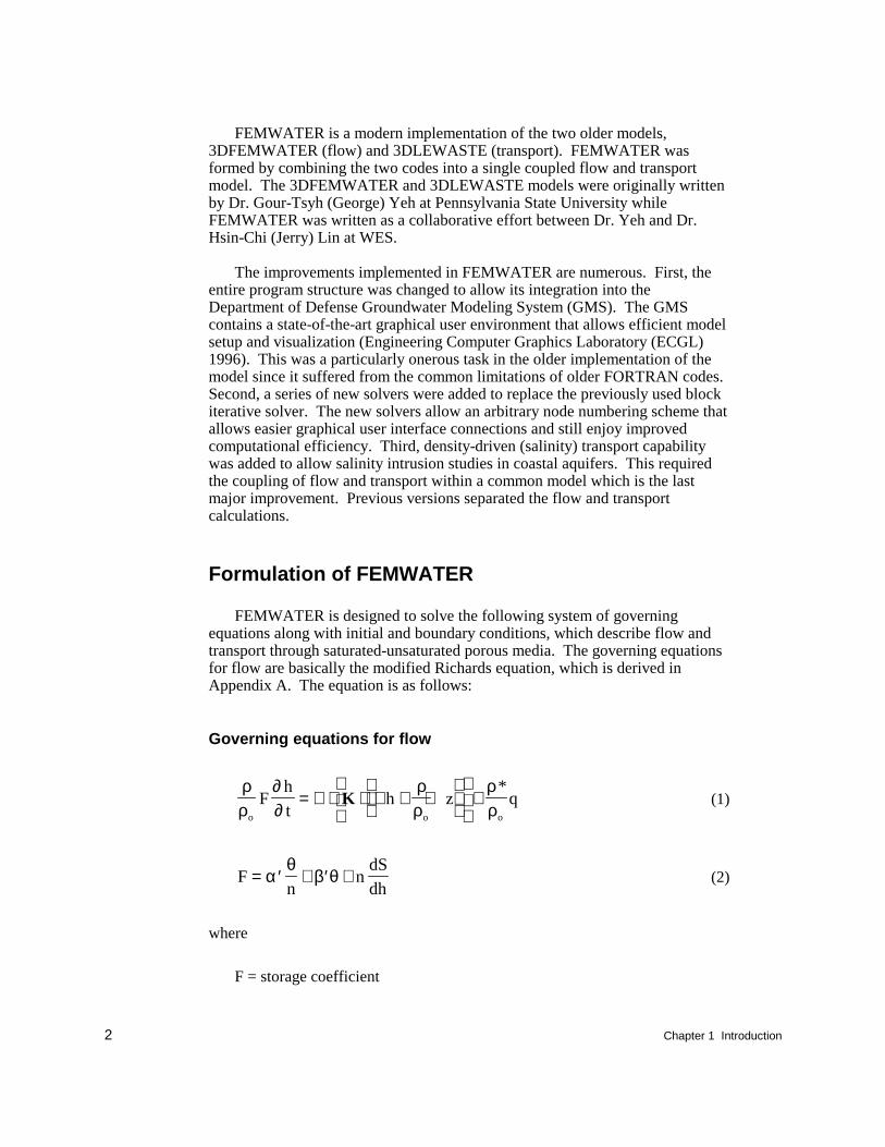
FEMWATER is designed to solve the following system of governingequations along with initial and boundary conditions, which describe flow andtransport through saturated-unsaturated porous media. The governing equationsfor flow are basically the modified Richards equation, which is derived inAppendix A. The equation is as follows:
Governing equations for flow
ρρ
∂∂
ρρ
ρρo o o
Fh
th z q= ∇ ⋅ ⋅ ∇ + ∇
+K
*(1)
Fn
ndSdh
= ′ + ′ +αθ
β θ (2)
where
F = storage coefficient
Chapter 1 Introduction 3
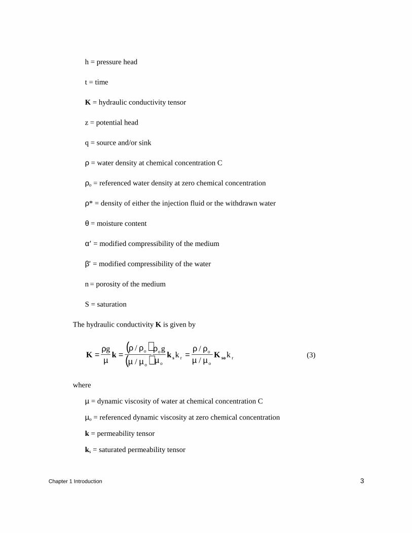
h = pressure head
t = time
K = hydraulic conductivity tensor
z = potential head
q = source and/or sink
ρ = water density at chemical concentration C
ρo = referenced water density at zero chemical concentration
ρ* = density of either the injection fluid or the withdrawn water
θ = moisture content
α′ = modified compressibility of the medium
β′ = modified compressibility of the water
n = porosity of the medium
S = saturation
The hydraulic conductivity K is given by
( )( )K k k Ks so= = =
ρµ
ρ ρ
µ µρµ
ρ ρµ µ
g gk k
o
o
o
or
o
or
/
/
/
/(3)
where
µ = dynamic viscosity of water at chemical concentration C
µo = referenced dynamic viscosity at zero chemical concentration
k = permeability tensor
ks = saturated permeability tensor
4 Chapter 1 Introduction
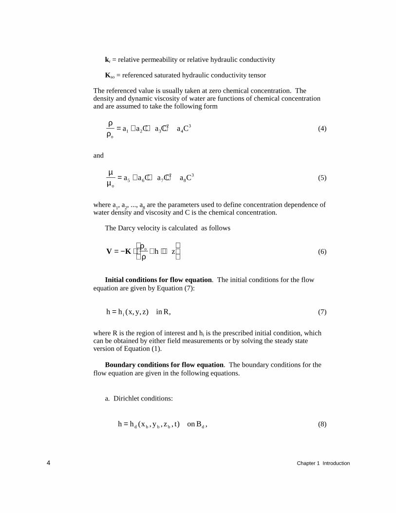
kr = relative permeability or relative hydraulic conductivity
Kso = referenced saturated hydraulic conductivity tensor
The referenced value is usually taken at zero chemical concentration. Thedensity and dynamic viscosity of water are functions of chemical concentrationand are assumed to take the following form
ρρo
a a C a C a C= + + +1 2 32
43 (4)
and
µµo
a a C a C a C= + + +5 6 72
83 (5)
where a1, a2, ..., a8 are the parameters used to define concentration dependence ofwater density and viscosity and C is the chemical concentration.
The Darcy velocity is calculated as follows
V K= − ⋅ ∇ + ∇
ρρ
o h z (6)
Initial conditions for flow equation. The initial conditions for the flowequation are given by Equation (7):
h h x y z in Ri= ( , , ) , (7)
where R is the region of interest and hi is the prescribed initial condition, whichcan be obtained by either field measurements or by solving the steady stateversion of Equation (1).
Boundary conditions for flow equation. The boundary conditions for theflow equation are given in the following equations.
a. Dirichlet conditions:
h h x y z t on Bd b b b d= ( , , , ) , (8)
Chapter 1 Introduction 5
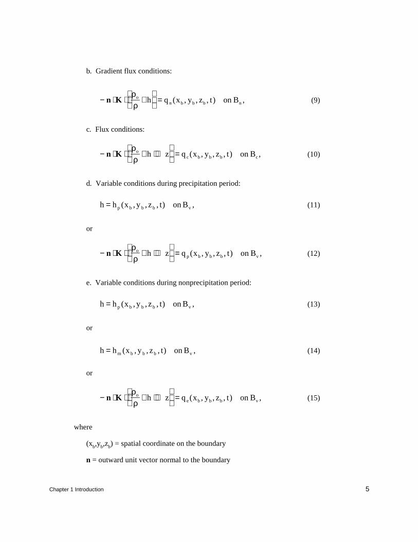
b. Gradient flux conditions:
− ⋅ ⋅ ∇
=n K
ρρ
on b b b nh q x y z t on B( , , , ) , (9)
c. Flux conditions:
− ⋅ ⋅ ∇ + ∇
=n K
ρρ
oc b b b ch z q x y z t on B( , , , ) , (10)
d. Variable conditions during precipitation period:
h h x y z t on Bp b b b v= ( , , , ) , (11)
or
− ⋅ ⋅ ∇ + ∇
=n K
ρρ
op b b b vh z q x y z t on B( , , , ) , (12)
e. Variable conditions during nonprecipitation period:
h h x y z t on Bp b b b v= ( , , , ) , (13)
or
h h x y z t on Bm b b b v= ( , , , ) , (14)
or
− ⋅ ⋅ ∇ + ∇
=n K
ρρ
oe b b b vh z q x y z t on B( , , , ) , (15)
where
(xb,yb,zb) = spatial coordinate on the boundary
n = outward unit vector normal to the boundary
6 Chapter 1 Introduction
hd = Dirichlet functional value
qn = Gradient flux value
qc = Flux value
Bd = Dirichlet boundary
Bn = Gradient flux boundary
Bc = Flux boundary
Bv = variable boundary
hp = ponding depth
qp = throughfall of precipitation on the variable boundary
hm = minimum pressure on the variable boundary
qe = evaporation rate on the variable boundary
Only one of Equations (11)-(15) is used at any point on the variableboundary at any time.
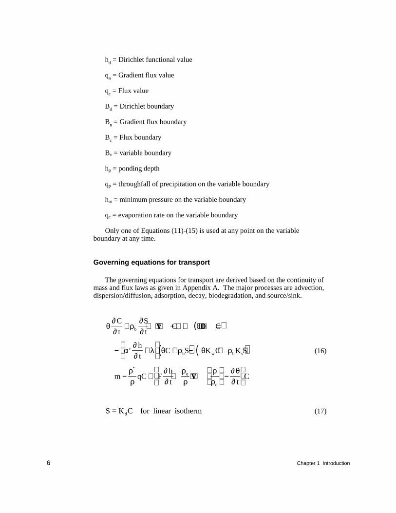
Governing equations for transport
The governing equations for transport are derived based on the continuity ofmass and flux laws as given in Appendix A. The major processes are advection,dispersion/diffusion, adsorption, decay, biodegradation, and source/sink.
( )
( ) ( )
θ∂∂
ρ∂∂
θ
α∂∂
λ θ ρ θ ρ
ρρ
∂∂
ρρ
ρρ
∂θ∂
C
t
S
tC C
h
tC S K C K S
m qC Fh
t tC
b
b w b s
o
o
+ + ⋅ ∇ − ∇ ⋅ ⋅ ∇ =
− ′ +
+ − + +
− + + ⋅ ∇
−
∗
V D
V
(16)
S K Cd= for linear isotherm (17)
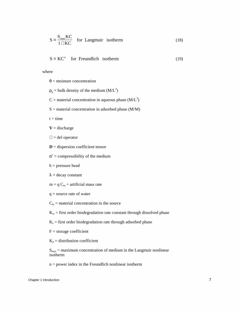
Chapter 1 Introduction 7
SS KC
KC=
+max
1for Langmuir isotherm (18)
S KCn= for Freundlich isotherm (19)
where
θ = moisture concentration
ρb = bulk density of the medium (M/L3)
C = material concentration in aqueous phase (M/L3)
S = material concentration in adsorbed phase (M/M)
t = time
V = discharge
∇ = del operator
D = dispersion coefficient tensor
α′ = compressibility of the medium
h = pressure head
λ = decay constant
m = q Cin = artificial mass rate
q = source rate of water
Cin = material concentration in the source
Kw = first order biodegradation rate constant through dissolved phase
Ks = first order biodegradation rate through adsorbed phase
F = storage coefficient
Kd = distribution coefficient
Smax = maximum concentration of medium in the Langmuir nonlinearisotherm
n = power index in the Freundlich nonlinear isotherm
8 Chapter 1 Introduction
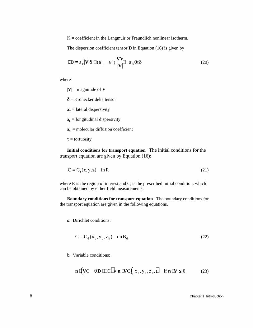
K = coefficient in the Langmuir or Freundlich nonlinear isotherm.
The dispersion coefficient tensor D in Equation (16) is given by
θ θτD VVVV
= + − +a a a aT L T mδ δ( ) (20)
where
|V| = magnitude of V
δ = Kronecker delta tensor
aT = lateral dispersivity
aL = longitudinal dispersivity
am = molecular diffusion coefficient
τ = tortuosity
Initial conditions for transport equation. The initial conditions for thetransport equation are given by Equation (16):
C C x y z in Ri= ( , , ) (21)
where R is the region of interest and Ci is the prescribed initial condition, whichcan be obtained by either field measurements.
Boundary conditions for transport equation. The boundary conditions forthe transport equation are given in the following equations.
a. Dirichlet conditions:
C C x y z on Bd b b b d= ( , , ) (22)
b. Variable conditions:
( ) ( )n V D n V n V⋅ − ⋅ ∇ = ⋅ ⋅ ≤C C C x y z t ifv b b bθ , , , 0 (23)
Chapter 1 Introduction 9
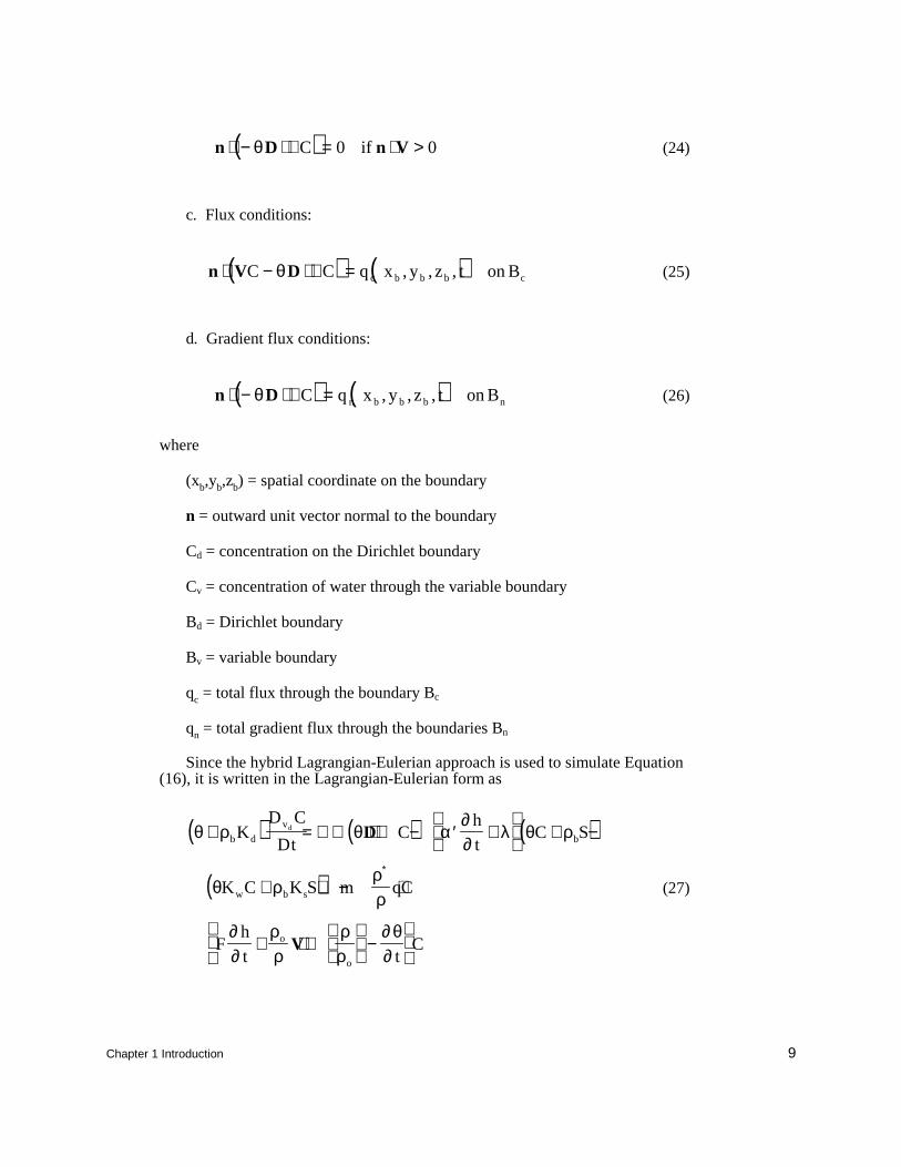
( )n D n V⋅ − ⋅ ∇ = ⋅ >θ C if0 0 (24)
c. Flux conditions:
( ) ( )n V D⋅ − ⋅ ∇ =C C q x y z t on Bc b b b cθ , , , (25)
d. Gradient flux conditions:
( ) ( )n D⋅ − ⋅ ∇ =θ C q x y z t on Bn b b b n, , , (26)
where
(xb,yb,zb) = spatial coordinate on the boundary
n = outward unit vector normal to the boundary
Cd = concentration on the Dirichlet boundary
Cv = concentration of water through the variable boundary
Bd = Dirichlet boundary
Bv = variable boundary
qc = total flux through the boundary Bc
qn = total gradient flux through the boundaries Bn
Since the hybrid Lagrangian-Eulerian approach is used to simulate Equation(16), it is written in the Lagrangian-Eulerian form as
( ) ( ) ( )
( )
θ ρ θ α∂∂
λ θ ρ
θ ρρρ
∂∂
ρρ
ρρ
∂ θ∂
+ = ∇ ⋅ ⋅ ∇ − ′ +
+ −
+ + − +
+ ⋅ ∇
−
∗
b d
v
b
w b s
o
o
KD C
DtC
ht
C S
K C K S m qC
Fh
t tC
d D
V
(27)
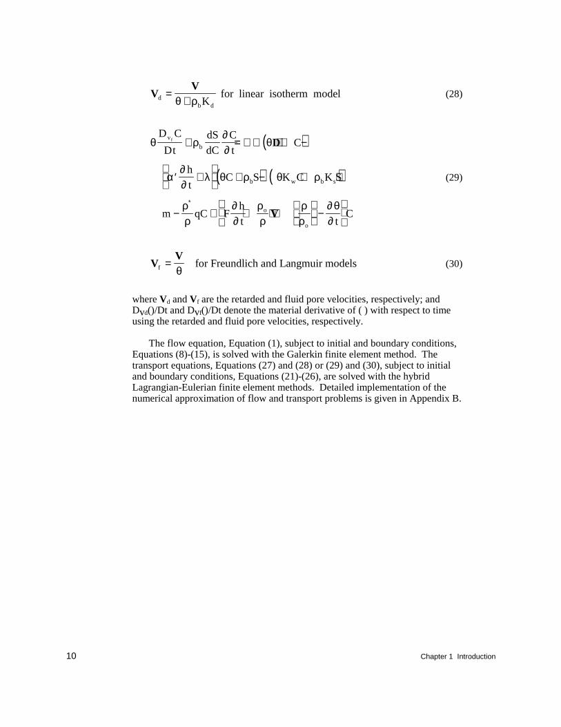
10 Chapter 1 Introduction
VV
db dK
=+θ ρ
for linear isotherm model (28)
( )
( ) ( )
θ ρ∂∂
θ
α∂∂
λ θ ρ θ ρ
ρρ
∂∂
ρρ
ρρ
∂ θ∂
D C
Dt
dS
dC
C
tC
h
tC S K C K S
m qC Fh
t tC
v
b
b w b s
o
o
f + = ∇ ⋅ ⋅ ∇ −
′ +
+ − + +
− + + ⋅ ∇
−
∗
D
V
(29)
VV
f =θ
for Freundlich and Langmuir models (30)
where Vd and Vf are the retarded and fluid pore velocities, respectively; andDvd()/Dt and Dvf()/Dt denote the material derivative of ( ) with respect to timeusing the retarded and fluid pore velocities, respectively.
The flow equation, Equation (1), subject to initial and boundary conditions,Equations (8)-(15), is solved with the Galerkin finite element method. Thetransport equations, Equations (27) and (28) or (29) and (30), subject to initialand boundary conditions, Equations (21)-(26), are solved with the hybridLagrangian-Eulerian finite element methods. Detailed implementation of thenumerical approximation of flow and transport problems is given in Appendix B.
Chapter 2 Running FEMWATER 11
2 Running FEMWATER
File Organization
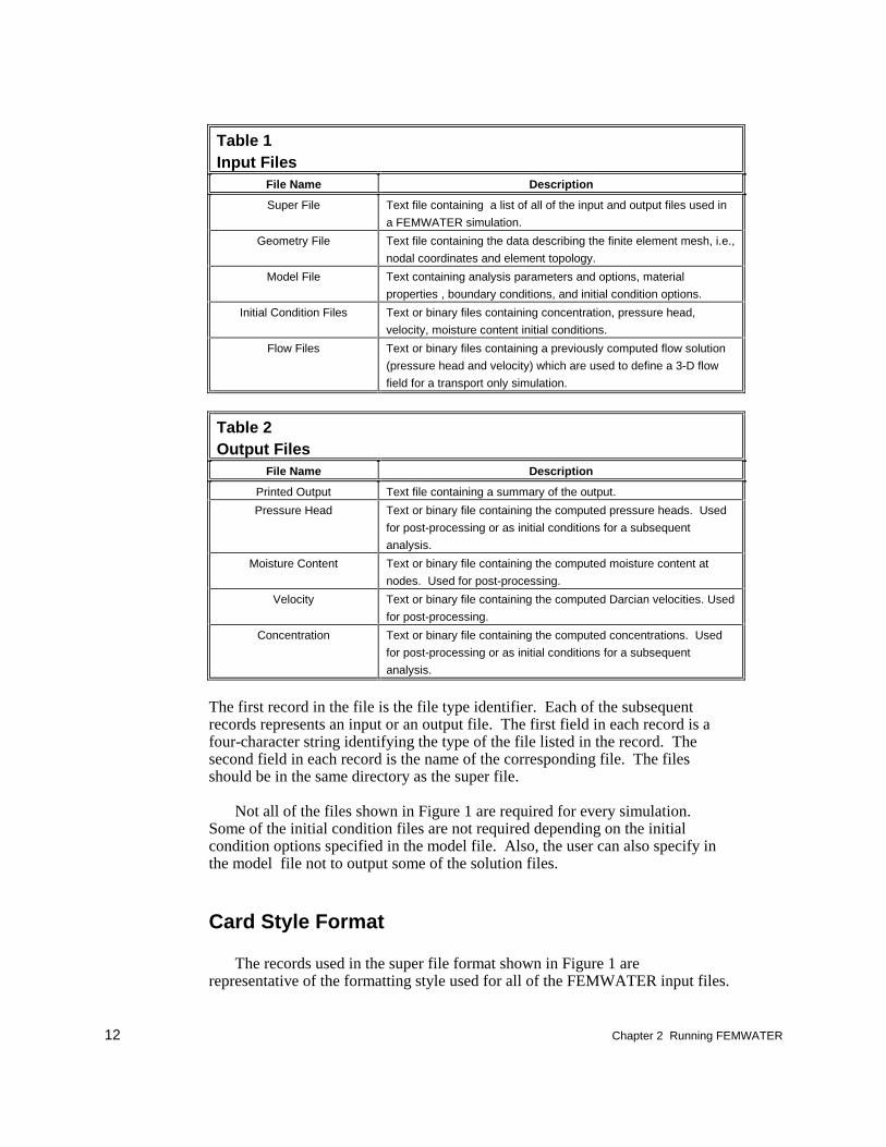
FEMWATER was designed to be operated in batch mode. The input forFEMWATER is organized into a set of input files. The output fromFEMWATER is a combination of screen and file output. A summary of theinput and output files is shown in Table 1 and Table 2.
Super File
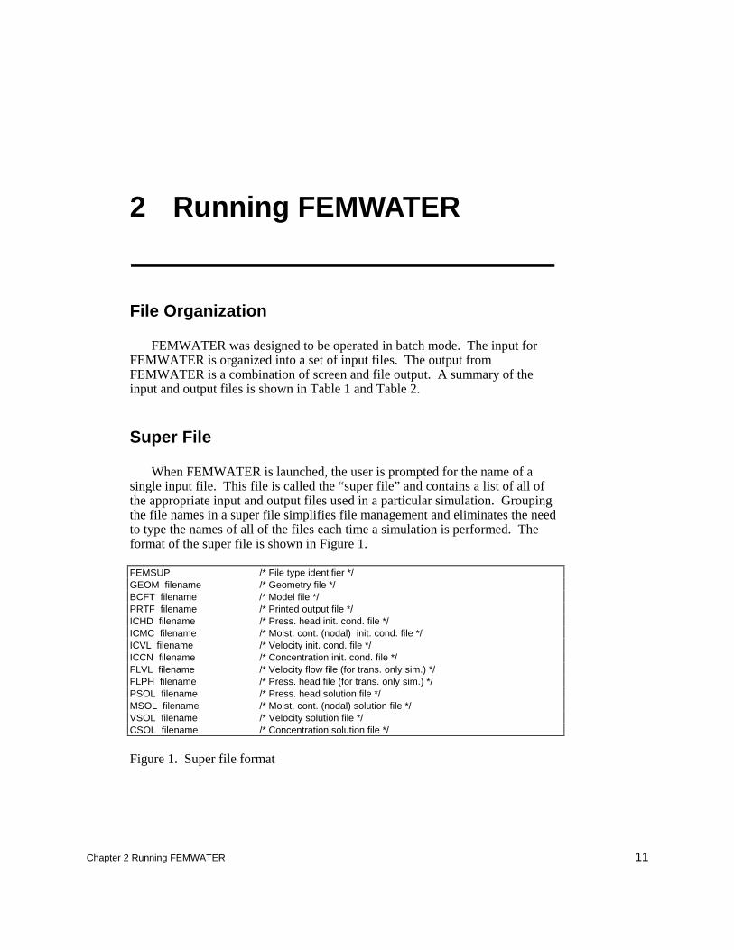
When FEMWATER is launched, the user is prompted for the name of asingle input file. This file is called the “super file” and contains a list of all ofthe appropriate input and output files used in a particular simulation. Groupingthe file names in a super file simplifies file management and eliminates the needto type the names of all of the files each time a simulation is performed. Theformat of the super file is shown in Figure 1.
FEMSUP /* File type identifier */GEOM filename /* Geometry file */BCFT filename /* Model file */PRTF filename /* Printed output file */ICHD filename /* Press. head init. cond. file */ICMC filename /* Moist. cont. (nodal) init. cond. file */ICVL filename /* Velocity init. cond. file */ICCN filename /* Concentration init. cond. file */FLVL filename /* Velocity flow file (for trans. only sim.) */FLPH filename /* Press. head file (for trans. only sim.) */PSOL filename /* Press. head solution file */MSOL filename /* Moist. cont. (nodal) solution file */VSOL filename /* Velocity solution file */CSOL filename /* Concentration solution file */
Figure 1. Super file format
12 Chapter 2 Running FEMWATER
Table 1Input Files
File Name Description
Super File Text file containing a list of all of the input and output files used in
a FEMWATER simulation.
Geometry File Text file containing the data describing the finite element mesh, i.e.,
nodal coordinates and element topology.
Model File Text containing analysis parameters and options, material
properties , boundary conditions, and initial condition options.
Initial Condition Files Text or binary files containing concentration, pressure head,
velocity, moisture content initial conditions.
Flow Files Text or binary files containing a previously computed flow solution
(pressure head and velocity) which are used to define a 3-D flow
field for a transport only simulation.
Table 2Output Files
File Name Description
Printed Output Text file containing a summary of the output.
Pressure Head Text or binary file containing the computed pressure heads. Used
for post-processing or as initial conditions for a subsequent
analysis.
Moisture Content Text or binary file containing the computed moisture content at
nodes. Used for post-processing.
Velocity Text or binary file containing the computed Darcian velocities. Used
for post-processing.
Concentration Text or binary file containing the computed concentrations. Used
for post-processing or as initial conditions for a subsequent
analysis.
The first record in the file is the file type identifier. Each of the subsequentrecords represents an input or an output file. The first field in each record is afour-character string identifying the type of the file listed in the record. Thesecond field in each record is the name of the corresponding file. The filesshould be in the same directory as the super file.
Not all of the files shown in Figure 1 are required for every simulation.Some of the initial condition files are not required depending on the initialcondition options specified in the model file. Also, the user can also specify inthe model file not to output some of the solution files.
Card Style Format
The records used in the super file format shown in Figure 1 arerepresentative of the formatting style used for all of the FEMWATER input files.
Chapter 2 Running FEMWATER 13
This format is often referred to as the “card style” format. With this format, thecomponents of the file are grouped into logical groups called “cards.” Typically,each card is a single line or record; however, some cards extend to multiplelines. The first component of each card is a short name that serves as the cardidentifier. The remaining fields on the line contain the information associatedwith the card. In some cases, such as lists, a card can use multiple lines. All ofthe cards are assumed to be free-format.
Several advantages are associated with the card type approach to formattingfiles:
a. Card identifiers make the file easier to read. Each input line has a label,which helps to identify the data on the line.
b. The card names are useful as text strings for searching in a large file.All input lines of a particular type can be located quickly in a large inputfile.
c. Cards allow the data to be input in any order in many cases; i.e., theorder that the cards appear in the file is usually not important.
d. Cards make it easy to modify a file format. New data can be includedsimply by defining a new card type. If the new card is optional (which istypically the case for new cards) old files are still compatible. If an oldcard type is no longer used, the card can simply be ignored withoutcausing input errors.
Other Files
Each of the files listed in the super file are described in more detail insubsequent chapters. The geometry file is described in Chapter 3, the contents ofthe model file are described in Chapters 3, 4, 5, and 6, the initial condition filesare described in Chapter 7, and the solution files are described in Appendix C.
14 Chapter 3 Meshes
3 Meshes
Introduction
The computational discretization utilized by FEMWATER is a three-dimensional finite element mesh. The volumetric domain to be modeled byFEMWATER must be idealized and discretized into hexahedra, prisms, and/ortetrahedra. Elements are typically grouped into zones representing differentstratigraphic units. Each element is assigned a material ID representing the zoneto which the elements belongs. When constructing a mesh, care should be takento ensure that elements do not cross or straddle stratigraphic boundaries.
Elements Supported
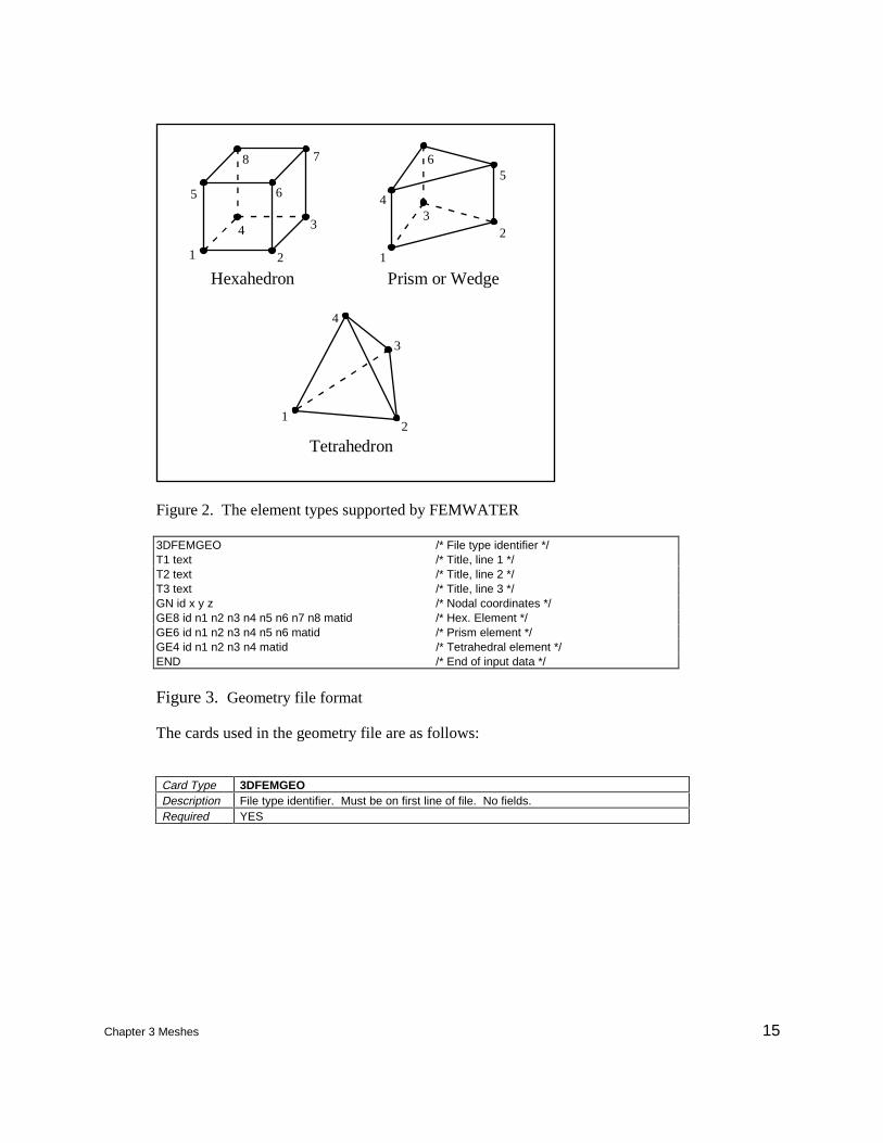
The types of elements supported by FEMWATER are shown in Figure 2.Each of the elements are linear; quadratic elements are not supported. Althoughall three element types are supported, tetrahedra do not perform as well as theother types and should be avoided if possible. The numbering sequence shownin Figure 2 should be used when describing the elements in the geometry file.
Geometry File Format
The coordinates of the mesh nodes and the element topology are input toFEMWATER through the geometry file. The format of the geometry file isshown in Figure 3.
Chapter 3 Meshes 15
12
3
4
Tetrahedron
1
23
4
56
Prism or Wedge
1 2
34
5 6
78
Hexahedron
Figure 2. The element types supported by FEMWATER
3DFEMGEO /* File type identifier */T1 text /* Title, line 1 */T2 text /* Title, line 2 */T3 text /* Title, line 3 */GN id x y z /* Nodal coordinates */GE8 id n1 n2 n3 n4 n5 n6 n7 n8 matid /* Hex. Element */GE6 id n1 n2 n3 n4 n5 n6 matid /* Prism element */GE4 id n1 n2 n3 n4 matid /* Tetrahedral element */END /* End of input data */
Figure 3. Geometry file format
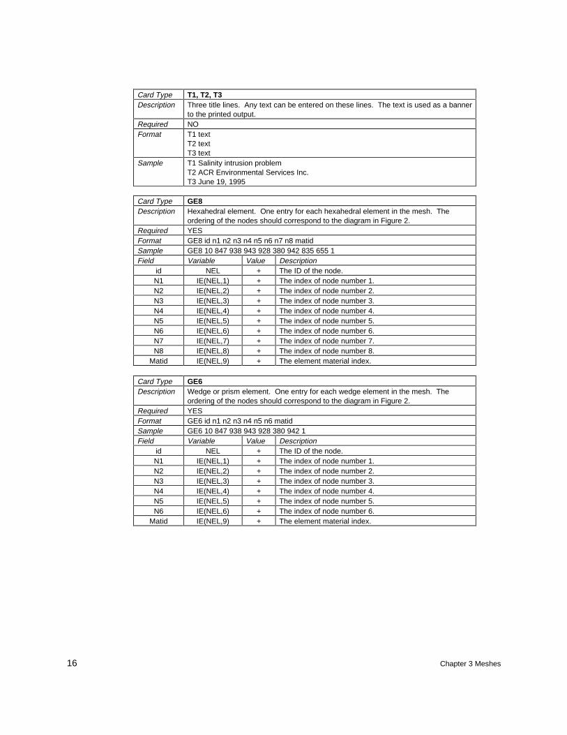
The cards used in the geometry file are as follows:
Card Type 3DFEMGEODescription File type identifier. Must be on first line of file. No fields.Required YES
16 Chapter 3 Meshes
Card Type T1, T2, T3Description Three title lines. Any text can be entered on these lines. The text is used as a banner
to the printed output.Required NOFormat T1 text
T2 textT3 text
Sample T1 Salinity intrusion problemT2 ACR Environmental Services Inc.T3 June 19, 1995
Card Type GE8Description Hexahedral element. One entry for each hexahedral element in the mesh. The
ordering of the nodes should correspond to the diagram in Figure 2.Required YESFormat GE8 id n1 n2 n3 n4 n5 n6 n7 n8 matidSample GE8 10 847 938 943 928 380 942 835 655 1Field Variable Value Description
id NEL + The ID of the node.N1 IE(NEL,1) + The index of node number 1.N2 IE(NEL,2) + The index of node number 2.N3 IE(NEL,3) + The index of node number 3.N4 IE(NEL,4) + The index of node number 4.N5 IE(NEL,5) + The index of node number 5.N6 IE(NEL,6) + The index of node number 6.N7 IE(NEL,7) + The index of node number 7.N8 IE(NEL,8) + The index of node number 8.
Matid IE(NEL,9) + The element material index.
Card Type GE6Description Wedge or prism element. One entry for each wedge element in the mesh. The
ordering of the nodes should correspond to the diagram in Figure 2.Required YESFormat GE6 id n1 n2 n3 n4 n5 n6 matidSample GE6 10 847 938 943 928 380 942 1Field Variable Value Description
id NEL + The ID of the node.N1 IE(NEL,1) + The index of node number 1.N2 IE(NEL,2) + The index of node number 2.N3 IE(NEL,3) + The index of node number 3.N4 IE(NEL,4) + The index of node number 4.N5 IE(NEL,5) + The index of node number 5.N6 IE(NEL,6) + The index of node number 6.
Matid IE(NEL,9) + The element material index.
Chapter 3 Meshes 17
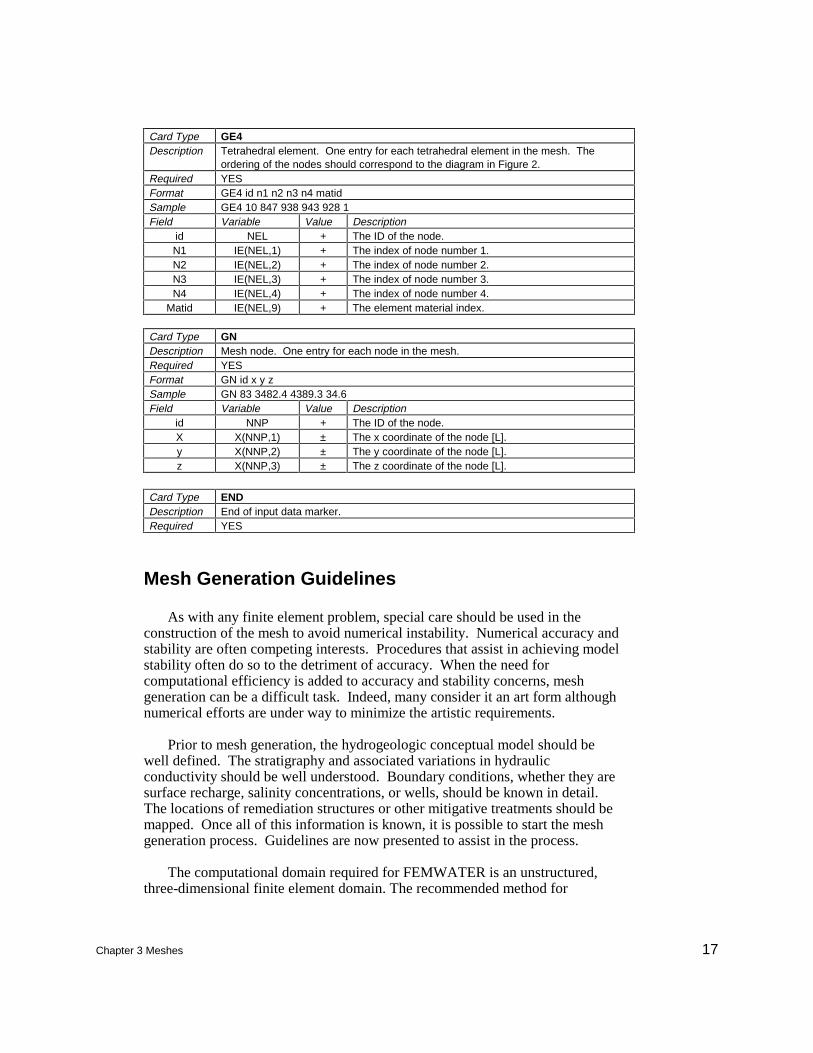
Card Type GE4Description Tetrahedral element. One entry for each tetrahedral element in the mesh. The
ordering of the nodes should correspond to the diagram in Figure 2.Required YESFormat GE4 id n1 n2 n3 n4 matidSample GE4 10 847 938 943 928 1Field Variable Value Description
id NEL + The ID of the node.N1 IE(NEL,1) + The index of node number 1.N2 IE(NEL,2) + The index of node number 2.N3 IE(NEL,3) + The index of node number 3.N4 IE(NEL,4) + The index of node number 4.
Matid IE(NEL,9) + The element material index.
Card Type GNDescription Mesh node. One entry for each node in the mesh.Required YESFormat GN id x y zSample GN 83 3482.4 4389.3 34.6Field Variable Value Description
id NNP + The ID of the node.X X(NNP,1) ± The x coordinate of the node [L].y X(NNP,2) ± The y coordinate of the node [L].z X(NNP,3) ± The z coordinate of the node [L].
Card Type ENDDescription End of input data marker.Required YES
Mesh Generation Guidelines
As with any finite element problem, special care should be used in theconstruction of the mesh to avoid numerical instability. Numerical accuracy andstability are often competing interests. Procedures that assist in achieving modelstability often do so to the detriment of accuracy. When the need forcomputational efficiency is added to accuracy and stability concerns, meshgeneration can be a difficult task. Indeed, many consider it an art form althoughnumerical efforts are under way to minimize the artistic requirements.
Prior to mesh generation, the hydrogeologic conceptual model should bewell defined. The stratigraphy and associated variations in hydraulicconductivity should be well understood. Boundary conditions, whether they aresurface recharge, salinity concentrations, or wells, should be known in detail.The locations of remediation structures or other mitigative treatments should bemapped. Once all of this information is known, it is possible to start the meshgeneration process. Guidelines are now presented to assist in the process.
The computational domain required for FEMWATER is an unstructured,three-dimensional finite element domain. The recommended method for
18 Chapter 3 Meshes
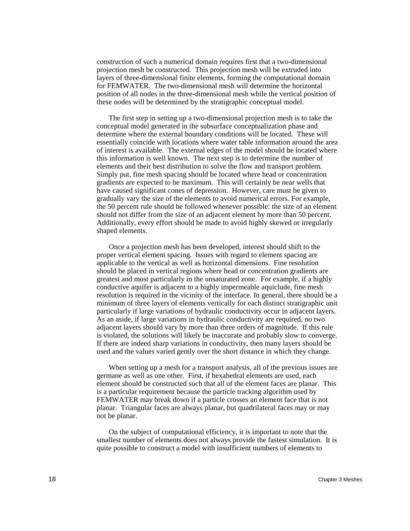
construction of such a numerical domain requires first that a two-dimensionalprojection mesh be constructed. This projection mesh will be extruded intolayers of three-dimensional finite elements, forming the computational domainfor FEMWATER. The two-dimensional mesh will determine the horizontalposition of all nodes in the three-dimensional mesh while the vertical position ofthese nodes will be determined by the stratigraphic conceptual model.
The first step in setting up a two-dimensional projection mesh is to take theconceptual model generated in the subsurface conceptualization phase anddetermine where the external boundary conditions will be located. These willessentially coincide with locations where water table information around the areaof interest is available. The external edges of the model should be located wherethis information is well known. The next step is to determine the number ofelements and their best distribution to solve the flow and transport problem.Simply put, fine mesh spacing should be located where head or concentrationgradients are expected to be maximum. This will certainly be near wells thathave caused significant cones of depression. However, care must be given togradually vary the size of the elements to avoid numerical errors. For example,the 50 percent rule should be followed whenever possible: the size of an elementshould not differ from the size of an adjacent element by more than 50 percent.Additionally, every effort should be made to avoid highly skewed or irregularlyshaped elements.
Once a projection mesh has been developed, interest should shift to theproper vertical element spacing. Issues with regard to element spacing areapplicable to the vertical as well as horizontal dimensions. Fine resolutionshould be placed in vertical regions where head or concentration gradients aregreatest and most particularly in the unsaturated zone. For example, if a highlyconductive aquifer is adjacent to a highly impermeable aquiclude, fine meshresolution is required in the vicinity of the interface. In general, there should be aminimum of three layers of elements vertically for each distinct stratigraphic unitparticularly if large variations of hydraulic conductivity occur in adjacent layers.As an aside, if large variations in hydraulic conductivity are required, no twoadjacent layers should vary by more than three orders of magnitude. If this ruleis violated, the solutions will likely be inaccurate and probably slow to converge.If there are indeed sharp variations in conductivity, then many layers should beused and the values varied gently over the short distance in which they change.
When setting up a mesh for a transport analysis, all of the previous issues aregermane as well as one other. First, if hexahedral elements are used, eachelement should be constructed such that all of the element faces are planar. Thisis a particular requirement because the particle tracking algorithm used byFEMWATER may break down if a particle crosses an element face that is notplanar. Triangular faces are always planar, but quadrilateral faces may or maynot be planar.
On the subject of computational efficiency, it is important to note that thesmallest number of elements does not always provide the fastest simulation. It isquite possible to construct a model with insufficient numbers of elements to

Chapter 3 Meshes 19
characterize the problem adequately, thereby creating a simulation that is slow toconverge. In short, fewer elements will be used in the calculation, but greaternumbers of iterations will be required. In general, if sufficient numbers ofelements are used, fewer iterations will be required to converge on a solution. Itis better to use large numbers of elements for few iterations to get accurateanswers than to use few elements for many iterations to get inaccurate andpossibly divergent answers.

Chapter 4 Analysis Options 21
4 Analysis Options
Introduction
One of the primary FEMWATER input files is the model file, which consistsof analysis options, material properties, boundary, and initial conditions. Thefirst of these groups, the analysis options, are described in this Chapter. Thematerial properties are described in Chapter 5, the boundary conditions aredescribed in Chapter 6, and the initial conditions are described in Chapter 7.
File Format
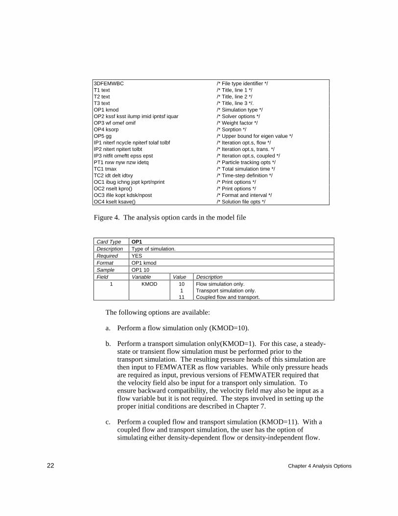
The set of cards in the model file corresponding to analysis options is shownin Figure 4. The file type identifier and the title cards are similar to thecorresponding cards found in the geometry file and described in Chapter 0. Eachof the remaining cards is described in more detail in the following sections.
Run Option Parameters
The run option parameters designated on cards OP1, OP2, OP3, OP4, andOP5 include options for specifying the type of simulation, the solver, relaxationparameters, and sorption options.
Type of simulation (OP1)
The OP1 card is used to specify the type of simulation to be performed byFEMWATER. The parameter KMOD indicates the type of simulation to beconducted.
22 Chapter 4 Analysis Options
3DFEMWBC /* File type identifier */T1 text /* Title, line 1 */T2 text /* Title, line 2 */T3 text /* Title, line 3 */.OP1 kmod /* Simulation type */OP2 kssf ksst ilump imid ipntsf iquar /* Solver options */OP3 wf omef omif /* Weight factor */OP4 ksorp /* Sorption */OP5 gg /* Upper bound for eigen value */IP1 niterf ncycle npiterf tolaf tolbf /* Iteration opt.s, flow */IP2 nitert npitert tolbt /* Iteration opt.s, trans. */IP3 nitfit omeftt epss epst /* Iteration opt.s, coupled */PT1 nxw nyw nzw idetq /* Particle tracking opts */TC1 tmax /* Total simulation time */TC2 idt delt idtxy /* Time-step definition */OC1 ibug ichng jopt kprt/nprint /* Print options */OC2 nselt kpro() /* Print options */OC3 ifile kopt kdsk/npost /* Format and interval */OC4 kselt ksave() /* Solution file opts */
Figure 4. The analysis option cards in the model file
Card Type OP1Description Type of simulation.Required YESFormat OP1 kmodSample OP1 10Field Variable Value Description
1 KMOD 101
11
Flow simulation only.Transport simulation only.Coupled flow and transport.
The following options are available:
a. Perform a flow simulation only (KMOD=10).
b. Perform a transport simulation only(KMOD=1). For this case, a steady-state or transient flow simulation must be performed prior to thetransport simulation. The resulting pressure heads of this simulation arethen input to FEMWATER as flow variables. While only pressure headsare required as input, previous versions of FEMWATER required thatthe velocity field also be input for a transport only simulation. Toensure backward compatibility, the velocity field may also be input as aflow variable but it is not required. The steps involved in setting up theproper initial conditions are described in Chapter 7.
c. Perform a coupled flow and transport simulation (KMOD=11). With acoupled flow and transport simulation, the user has the option ofsimulating either density-dependent flow or density-independent flow.
Chapter 4 Analysis Options 23
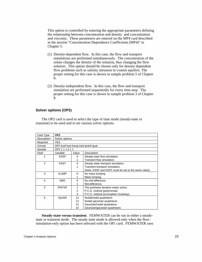
This option is controlled by entering the appropriate parameters definingthe relationship between concentration and density and concentrationand viscosity. These parameters are entered on the MP4 card describedin the section “Concentration Dependence Coefficients (MP4)” inChapter 5.
(1) Density-dependent flow. In this case, the flow and transportsimulations are performed simultaneously. The concentration of thesolute changes the density of the solution, thus changing the flowsolution. This option should be chosen only for density dependentflow problems such as salinity intrusion in coastal aquifers. Theproper setting for this case is shown in sample problem 5 of Chapter8.
(2) Density-independent flow. In this case, the flow and transportsimulation are performed sequentially for every time-step. Theproper setting for this case is shown in sample problem 3 of Chapter8.
Solver options (OP2)
The OP2 card is used to select the type of time mode (steady-state ortransient) to be used and to set various solver options.
Card Type OP2Description Solver options.Required YESFormat OP2 kssf ksst ilump imid ipntsf iquarSample OP2 1 1 1 0 1 1Field Variable Value Description
1 KSSF 01
Steady-state flow simulation.Transient flow simulation.
2 KSST 01
Steady-state transport simulation.Transient transport simulation.(Note: KSSF and KSST must be set to the same value)
3 ILUMP 01
No mass lumping.Mass lumping.
4 IMID 01
No mid-difference.Mid-difference.
5 IPNTSF 123
The pointwise iterative matrix solver.P.C.G. method (polynomial).P.C.G. method (incomplete Cholesky).
6 IQUAR 11122122
Nodal/nodal quadrature.Nodal/ gaussian quadrature.Gaussian/nodal quadrature.Gaussian/gaussian quadrature.
Steady-state versus transient. FEMWATER can be run in either a steady-state or transient mode. The steady state mode is allowed only when the flow-simulation-only option has been selected with the OP1 card. FEMWATER uses
24 Chapter 4 Analysis Options
the Lagrangian-Eulerian finite element method to solve the transport equation.Therefore, the steady-state mode of transport simulation is not allowed in thisoption. The transient mode must be used when a transport simulation is beingperformed.
Mass lumping (ILUMP). This parameter indicates whether or not the massmatrix is to be lumped. With lumping (ILUMP=1), the solution is less accuratebut potentially more stable. For saturated-unsaturated flow computations, or ifnegative concentrations or oscillating solutions occur, this parameter should beset to 1. If the computations are quite stable, particularly in largely saturatedflow simulations, the parameter should be set to zero.
Mid-difference (IMID). This parameter indicates if the mid-differencemethod should be used in both the flow and transport computations. If IMID =1,the mid-difference method is used. Setting IMID=1 is reserved for researchpurposes so IMID=0 is the preferred setting.
Solver Selection (IPNTSF). The following three solvers are provided inFEMWATER:
a. Pointwise iterative matrix solver. The pointwise iterative matrix solveremploys the basic successive iterative method to solve the matrixequation, including the Gauss-Seidel method, successiveunderrelaxation, and successive overrelaxation. When the resultingmatrix is diagonally dominant, the pointwise iterative solver provides aconvergent solution. This solver is preferred because it is more robustthan the other two solvers. However, when the speed of convergence istoo slow, one may wish to choose one of the other two solvers.
b. Preconditioned conjugate gradient method (polynomial). This solveremploys the conjugate gradient method to solve the matrix equation. Ituses a polynomial as a preconditioner. This matrix solver provides aconvergent solution when the resulting matrix is symmetric positivedefinite (SPD). Theoretically, the convergence speed is faster than thepointwise iterative solver. This solver should be used only when thepointwise iterative solver is too slow.
c. Preconditioned conjugate gradient method (incomplete Choleski). Thissolver employs the conjugate gradient method using the incompleteCholeski decomposition as the preconditioner. A convergent solution isprovided when the matrix is SPD. However, when the matrix is slightlynon-symmetric, the solver could also give convergent solutions. Itsspeed of convergence is theoretically faster than the pointwise iterativesolver and is comparable to the polynomial preconditioned conjugategradient method. This solver should be used only when the pointwiseiterative solver is too slow. This solver is generally but not alwayspreferred over the polynomial preconditioned conjugate gradientmethod.
Chapter 4 Analysis Options 25
Quadrature selection (IQUAR). This parameter is an indicator of the typeof quadrature used in the numerical integration. The following four quadratureoptions are provided:
a. Nodal/nodal quadrature. Nodal quadrature is used for surface andelement integration.
b. Nodal/gaussian quadrature. Nodal quadrature is used for surfaceintegration, and gaussian quadrature is used for element integration.
c. Gaussian/nodal quadrature. Gaussian quadrature is used for surfaceintegration, and nodal quadrature is used for element integration.
d. Gaussian/gaussian quadrature. Gaussian quadrature is used for bothsurface and element integration.
Gaussian/gaussian quadrature yields the most accurate solution and shouldbe used as the default value. However, this option may provide oscillations ordivergence in highly nonlinear problems. When this occurs, the user should tryto use the nodal/nodal quadrature. Once these options have been usedunsuccessfully, the remaining options can be tried.
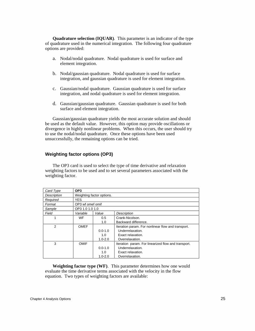
Weighting factor options (OP3)
The OP3 card is used to select the type of time derivative and relaxationweighting factors to be used and to set several parameters associated with theweighting factor.
Card Type OP3Description Weighting factor options.Required YESFormat OP3 wf omef omifSample OP3 1.0 1.0 1.0Field Variable Value Description
1 WF 0.51.0
Crank-Nicolson.Backward difference.
2 OMEF0.0-1.0
1.01.0-2.0
Iteration param. For nonlinear flow and transport. Underrelaxation. Exact relaxation. Overrelaxation.
3 OMIF0.0-1.0
1.01.0-2.0
Iteration param. For linearized flow and transport. Underrelaxation. Exact relaxation. Overrelaxation.
Weighting factor type (WF). This parameter determines how one wouldevaluate the time derivative terms associated with the velocity in the flowequation. Two types of weighting factors are available:
26 Chapter 4 Analysis Options
a. Crank-Nicolson central (WF=0.5). When new time derivatives aredetermined by averaging the previous time derivative and an estimatedtime derivative, the process is called Crank-Nicolson central weighting.
b. Backward difference (WF=1.0). When the time derivatives areevaluated only at the new time, the process is called backward differenceweighting.
A value of WF equal to 1.0 (an implicit numerical scheme) should be usedfor most practical problems. Setting WF equal to 0.5 is normally done forresearch purposes to assess the accuracy of the Crank-Nicolson scheme.
Relaxation parameter for solving nonlinear flow and transportequations (OMEF). When the flow and transport equations are nonlinear, anestimate of the pressure head and the concentration is needed to compose thematrix equation. There are three options to estimate the pressure head andconcentration based on previous guesses and newly obtained values:underrelaxation, exact relaxation, and overrelaxation. OMEF is a weightingfactor that is applied to the newly obtained values, and a weighting factor of 1.0minus OMEF is applied to the previous guesses. For underrelaxation, a value ofOMEF between 0.0 and 1.0 is used for the newly obtained values. For exactrelaxation OMEF is set equal to 1.0 and the newly obtained values are used asthe new guesses. For overrelaxation, a value of OMEF between 1.0 and 2.0 isused for the newly obtained values.
Normally OMEF should be set to 1.0. If the convergence history showssigns of oscillation, then a value of 0.5 should be used. If the convergencehistory shows a monotonic decrease but at a very slow rate, then it should be setto between 1.7 and 1.9.
Relaxation parameter for solving linearized flow and transportequations (OMIF). In order to solve the linearized matrix equations using theiteration method, an estimate of the solution is needed prior to taking the nextiteration. There are three options to estimate the solution based on previousguesses and the newly obtained solution: underrelaxation, exact relaxation, andoverrelaxation. This is accomplished with an OMIF weighting factor that issimilar to the OMEF factor described in the previous section.
Normally OMIF should be set to 1.0. If the convergence history shows signsof oscillation, then a value of 0.5 should be used. If the convergence historyshows a monotonic decrease but at a very slow rate, then it should be set tobetween 1.7 and 1.9.
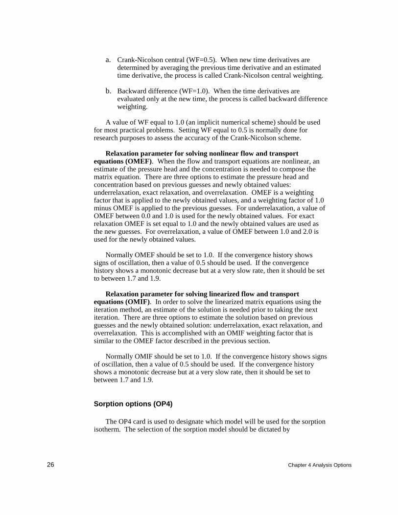
Sorption options (OP4)
The OP4 card is used to designate which model will be used for the sorptionisotherm. The selection of the sorption model should be dictated by
Chapter 4 Analysis Options 27
experimental evidence, and it depends highly on the type of chemicals andsubsurface media.
Card Type OP4Description Sorption options.Required YESFormat OP4 ksorpSample OP4 1Field Variable Value Description
1 KSORP 123
Linear isotherm.Freundlich isotherm.Langmuir isotherm.
The following three models are available for modeling the sorption isotherm:
a. Linear. A linear isotherm is used for the adsorption model. For salinityintrusion simulations, a linear model is sufficient.
b. Freundlich. A nonlinear isotherm (Freundlich isotherm) is used for theadsorption model.
c. Langmuir. A nonlinear isotherm (Langmuir isotherm) is used for theadsorption model.
Although the Freundlich isotherm option can be used to simulate a linearisotherm by setting the value of the exponent (n = 1), it is recommended that thelinear isotherm be simulated by using only the linear isotherm option. This isbecause the linear isotherm option makes use of retarded seepage velocities,which result in a more accurate solution for the particle tracking scheme than thepore velocities used in conjunction with the nonlinear adsorption models.Sorption constants for the different isotherm options are entered on the MP5 carddiscussed in Chapter 5.
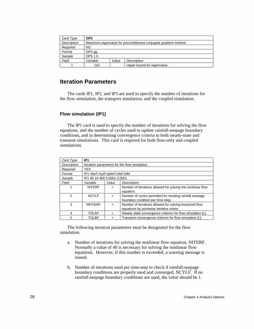
Preconditioned conjugate gradient method (OP5)
The OP5 card is used to provide an estimator for GG in the preconditionedconjugate gradient method. If the OP5 card is not present in the input, GG is notread but will be computed by the solver itself. If the OP5 card is present, GG isread and it will be the upper bound of the maximum eigenvalue of the coefficientmatrix using the preconditioned conjugate gradient method. The default value is1.0.
28 Chapter 4 Analysis Options
Card Type OP5Description Maximum eigenvalue for preconditioned conjugate gradient method.Required NOFormat OP5 ggSample OP5 1.0Field Variable Value Description
1 GG Upper bound for eigenvalue.
Iteration Parameters
The cards IP1, IP2, and IP3 are used to specify the number of iterations forthe flow simulation, the transport simulation, and the coupled simulation.
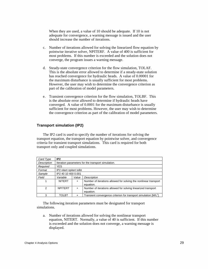
Flow simulation (IP1)
The IP1 card is used to specify the number of iterations for solving the flowequations, and the number of cycles used to update rainfall-seepage boundaryconditions, and in determining convergence criteria in both steady-state andtransient simulations. This card is required for both flow-only and coupledsimulations.
Card Type IP1Description Iteration parameters for the flow simulation.Required YESFormat IP1 niterf ncylf npiterf tolaf tolbfSample IP1 40 10 400 0.0001 0.0001Field Variable Value Description
1 NITERF + Number of iterations allowed for solving the nonlinear flowequation.
2 NCYLF + Number of cycles permitted for iterating rainfall seepageboundary condition per time-step.
3 NPITERF + Number of iterations allowed for solving linearized flowequations by pointwise iterative solver.
4 TOLAF + Steady state convergence criterion for flow simulation [L].5 TOLBF + Transient convergence criterion for flow simulation [L].
The following iteration parameters must be designated for the flowsimulation.
a. Number of iterations for solving the nonlinear flow equation, NITERF.Normally a value of 40 is necessary for solving the nonlinear flowequations. However, if this number is exceeded, a warning message isissued.
b. Number of iterations used per time-step to check if rainfall-seepageboundary conditions are properly used and converged, NCYLF. If norainfall-seepage boundary conditions are used, the value should be 1.
Chapter 4 Analysis Options 29
When they are used, a value of 10 should be adequate. If 10 is notadequate for convergence, a warning message is issued and the usershould increase the number of iterations.
c. Number of iterations allowed for solving the linearized flow equation bypointwise iterative solver, NPITERF. A value of 400 is sufficient formost problems. If this number is exceeded and the solution does notconverge, the program issues a warning message.
d. Steady-state convergence criterion for the flow simulation, TOLAF.This is the absolute error allowed to determine if a steady-state solutionhas reached convergence for hydraulic heads. A value of 0.00001 forthe maximum disturbance is usually sufficient for most problems.However, the user may wish to determine the convergence criterion aspart of the calibration of model parameters.
e. Transient convergence criterion for the flow simulation, TOLBF. Thisis the absolute error allowed to determine if hydraulic heads haveconverged. A value of 0.0001 for the maximum disturbance is usuallysufficient for most problems. However, the user may wish to determinethe convergence criterion as part of the calibration of model parameters.
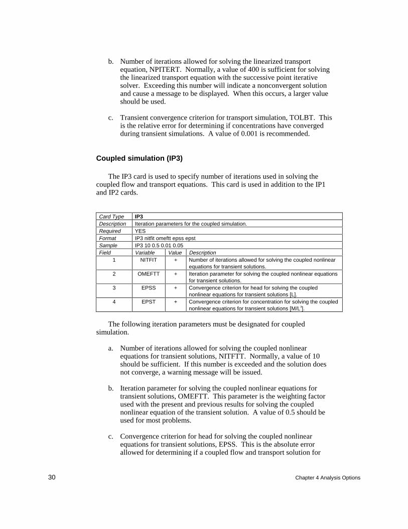
Transport simulation (IP2)
The IP2 card is used to specify the number of iterations for solving thetransport equation, the transport equation by pointwise solver, and convergencecriteria for transient transport simulations. This card is required for bothtransport only and coupled simulations.
Card Type IP2Description Iteration parameters for the transport simulation.Required YESFormat IP2 nitert npitert tolbtSample IP2 40 10 400 0.001Field Variable Value Description
1 NITERT + Number of iterations allowed for solving the nonlinear transportequation.
2 NPITERT + Number of iterations allowed for solving linearized transportequation.
3 TOLBT + Transient convergence criterion for transport simulation [M/L3].
The following iteration parameters must be designated for transportsimulations.
a. Number of iterations allowed for solving the nonlinear transportequation, NITERT. Normally, a value of 40 is sufficient. If this numberis exceeded and the solution does not converge, a warning message isdisplayed.
30 Chapter 4 Analysis Options
b. Number of iterations allowed for solving the linearized transportequation, NPITERT. Normally, a value of 400 is sufficient for solvingthe linearized transport equation with the successive point iterativesolver. Exceeding this number will indicate a nonconvergent solutionand cause a message to be displayed. When this occurs, a larger valueshould be used.
c. Transient convergence criterion for transport simulation, TOLBT. Thisis the relative error for determining if concentrations have convergedduring transient simulations. A value of 0.001 is recommended.
Coupled simulation (IP3)
The IP3 card is used to specify number of iterations used in solving thecoupled flow and transport equations. This card is used in addition to the IP1and IP2 cards.
Card Type IP3Description Iteration parameters for the coupled simulation.Required YESFormat IP3 nitfit omeftt epss epstSample IP3 10 0.5 0.01 0.05Field Variable Value Description
1 NITFIT + Number of iterations allowed for solving the coupled nonlinearequations for transient solutions.
2 OMEFTT + Iteration parameter for solving the coupled nonlinear equationsfor transient solutions.
3 EPSS + Convergence criterion for head for solving the couplednonlinear equations for transient solutions [L].
4 EPST + Convergence criterion for concentration for solving the couplednonlinear equations for transient solutions [M/L3].
The following iteration parameters must be designated for coupledsimulation.
a. Number of iterations allowed for solving the coupled nonlinearequations for transient solutions, NITFTT. Normally, a value of 10should be sufficient. If this number is exceeded and the solution doesnot converge, a warning message will be issued.
b. Iteration parameter for solving the coupled nonlinear equations fortransient solutions, OMEFTT. This parameter is the weighting factorused with the present and previous results for solving the couplednonlinear equation of the transient solution. A value of 0.5 should beused for most problems.
c. Convergence criterion for head for solving the coupled nonlinearequations for transient solutions, EPSS. This is the absolute errorallowed for determining if a coupled flow and transport solution for
Chapter 4 Analysis Options 31
hydraulic head has converged. A value of 0.01 for the maximumdisturbance should be sufficient.
d. Convergence criterion for concentration for solving the couplednonlinear equations for transient solutions, EPST. This is the relativeerror allowed for determining if a coupled flow and transport solutionfor concentration has converged. A value of 0.05 for the maximumdisturbance should be sufficient.
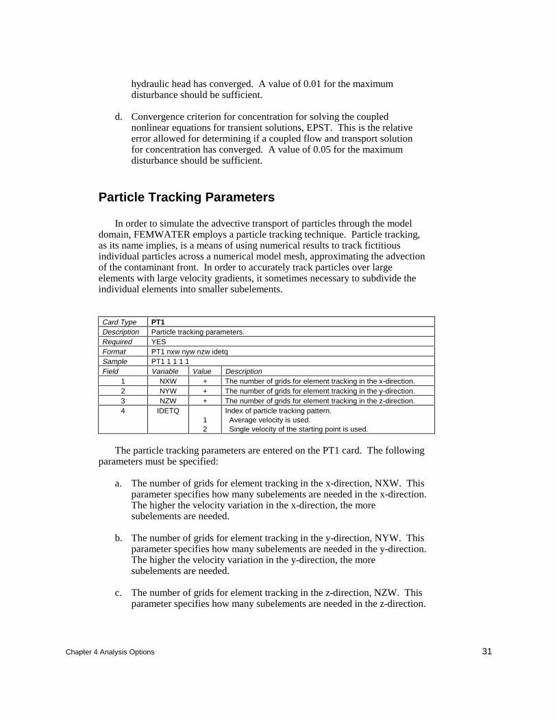
Particle Tracking Parameters
In order to simulate the advective transport of particles through the modeldomain, FEMWATER employs a particle tracking technique. Particle tracking,as its name implies, is a means of using numerical results to track fictitiousindividual particles across a numerical model mesh, approximating the advectionof the contaminant front. In order to accurately track particles over largeelements with large velocity gradients, it sometimes necessary to subdivide theindividual elements into smaller subelements.
Card Type PT1Description Particle tracking parameters.Required YESFormat PT1 nxw nyw nzw idetqSample PT1 1 1 1 1Field Variable Value Description
1 NXW + The number of grids for element tracking in the x-direction.2 NYW + The number of grids for element tracking in the y-direction.3 NZW + The number of grids for element tracking in the z-direction.4 IDETQ
12
Index of particle tracking pattern. Average velocity is used. Single velocity of the starting point is used.
The particle tracking parameters are entered on the PT1 card. The followingparameters must be specified:
a. The number of grids for element tracking in the x-direction, NXW. Thisparameter specifies how many subelements are needed in the x-direction.The higher the velocity variation in the x-direction, the moresubelements are needed.
b. The number of grids for element tracking in the y-direction, NYW. Thisparameter specifies how many subelements are needed in the y-direction.The higher the velocity variation in the y-direction, the moresubelements are needed.
c. The number of grids for element tracking in the z-direction, NZW. Thisparameter specifies how many subelements are needed in the z-direction.
32 Chapter 4 Analysis Options
The higher the velocity variation in the z-direction, the moresubelements are needed.
d. The particle tracking pattern, IDETQ. Two options are available:
(1) Average velocity is used (IDETQ=1). The use of average velocity ismore accurate, and it requires fewer subelements.
(2) Single velocity of the starting point is used (IDETQ=2). This optionshould be used when the velocity pattern is so complicated that theuse of the average velocity would fail to locate a fictitious particle.It should be used when a quick tracking is needed.
Time Control Parameters
The TC1 and TC2 cards are used to specify the total simulation time and thetime-step interval.
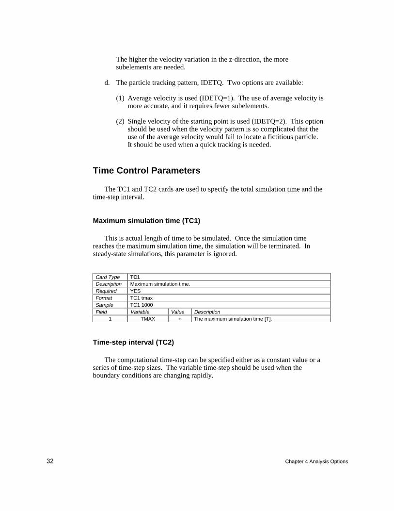
Maximum simulation time (TC1)
This is actual length of time to be simulated. Once the simulation timereaches the maximum simulation time, the simulation will be terminated. Insteady-state simulations, this parameter is ignored.
Card Type TC1Description Maximum simulation time.Required YESFormat TC1 tmaxSample TC1 1000Field Variable Value Description
1 TMAX + The maximum simulation time [T].
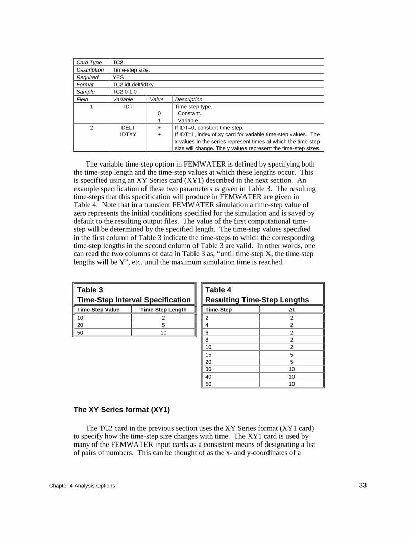
Time-step interval (TC2)
The computational time-step can be specified either as a constant value or aseries of time-step sizes. The variable time-step should be used when theboundary conditions are changing rapidly.
Chapter 4 Analysis Options 33
Card Type TC2Description Time-step size.Required YESFormat TC2 idt delt/idtxySample TC2 0 1.0Field Variable Value Description
1 IDT01
Time-step type. Constant. Variable.
2 DELTIDTXY
++
If IDT=0, constant time-step.If IDT=1, index of xy card for variable time-step values. Thex values in the series represent times at which the time-stepsize will change. The y values represent the time-step sizes.
The variable time-step option in FEMWATER is defined by specifying boththe time-step length and the time-step values at which these lengths occur. Thisis specified using an XY Series card (XY1) described in the next section. Anexample specification of these two parameters is given in Table 3. The resultingtime-steps that this specification will produce in FEMWATER are given inTable 4. Note that in a transient FEMWATER simulation a time-step value ofzero represents the initial conditions specified for the simulation and is saved bydefault to the resulting output files. The value of the first computational time-step will be determined by the specified length. The time-step values specifiedin the first column of Table 3 indicate the time-steps to which the correspondingtime-step lengths in the second column of Table 3 are valid. In other words, onecan read the two columns of data in Table 3 as, “until time-step X, the time-steplengths will be Y”, etc. until the maximum simulation time is reached.
Table 3Time-Step Interval SpecificationTime-Step Value Time-Step Length
10 220 550 10
Table 4Resulting Time-Step LengthsTime-Step ∆t
2 24 26 28 210 215 520 530 1040 1050 10
The XY Series format (XY1)
The TC2 card in the previous section uses the XY Series format (XY1 card)to specify how the time-step size changes with time. The XY1 card is used bymany of the FEMWATER input cards as a consistent means of designating a listof pairs of numbers. This can be thought of as the x- and y-coordinates of a
34 Chapter 4 Analysis Options
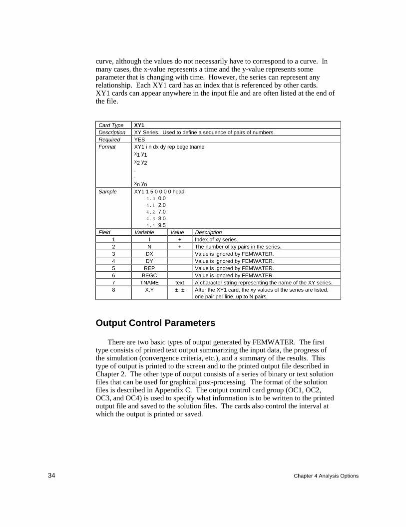
curve, although the values do not necessarily have to correspond to a curve. Inmany cases, the x-value represents a time and the y-value represents someparameter that is changing with time. However, the series can represent anyrelationship. Each XY1 card has an index that is referenced by other cards.XY1 cards can appear anywhere in the input file and are often listed at the end ofthe file.
Card Type XY1Description XY Series. Used to define a sequence of pairs of numbers.Required YESFormat XY1 i n dx dy rep begc tname
x1 y1x2 y2..xn yn
Sample XY1 1 5 0 0 0 0 head4.0 0.04.1 2.04.2 7.04.3 8.04.4 9.5
Field Variable Value Description1 I + Index of xy series.2 N + The number of xy pairs in the series.3 DX Value is ignored by FEMWATER.4 DY Value is ignored by FEMWATER.5 REP Value is ignored by FEMWATER.6 BEGC Value is ignored by FEMWATER.7 TNAME text A character string representing the name of the XY series.8 X,Y ±, ± After the XY1 card, the xy values of the series are listed,
one pair per line, up to N pairs.
Output Control Parameters
There are two basic types of output generated by FEMWATER. The firsttype consists of printed text output summarizing the input data, the progress ofthe simulation (convergence criteria, etc.), and a summary of the results. Thistype of output is printed to the screen and to the printed output file described inChapter 2. The other type of output consists of a series of binary or text solutionfiles that can be used for graphical post-processing. The format of the solutionfiles is described in Appendix C. The output control card group (OC1, OC2,OC3, and OC4) is used to specify what information is to be written to the printedoutput file and saved to the solution files. The cards also control the interval atwhich the output is printed or saved.
Chapter 4 Analysis Options 35
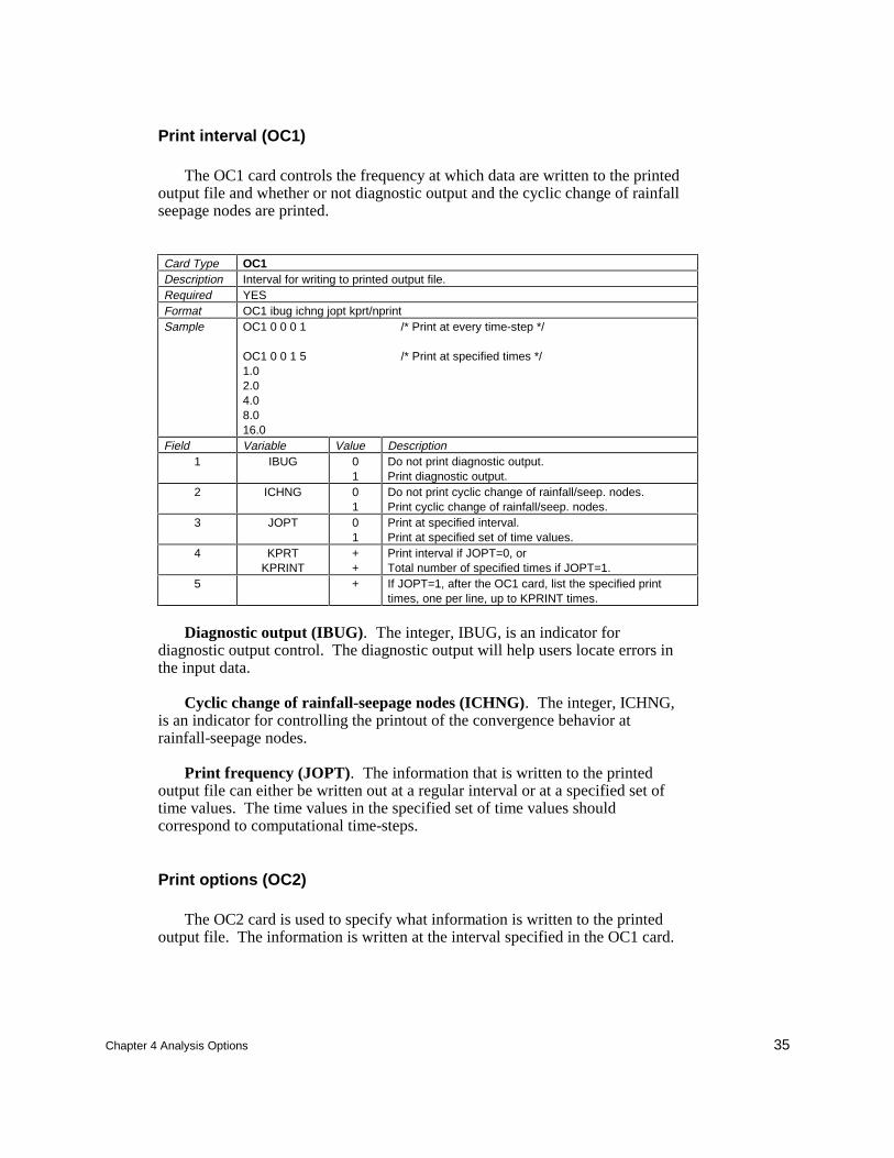
Print interval (OC1)
The OC1 card controls the frequency at which data are written to the printedoutput file and whether or not diagnostic output and the cyclic change of rainfallseepage nodes are printed.
Card Type OC1Description Interval for writing to printed output file.Required YESFormat OC1 ibug ichng jopt kprt/nprintSample OC1 0 0 0 1 /* Print at every time-step */
OC1 0 0 1 5 /* Print at specified times */1.02.04.08.016.0
Field Variable Value Description1 IBUG 0
1Do not print diagnostic output.Print diagnostic output.
2 ICHNG 01
Do not print cyclic change of rainfall/seep. nodes.Print cyclic change of rainfall/seep. nodes.
3 JOPT 01
Print at specified interval.Print at specified set of time values.
4 KPRTKPRINT
++
Print interval if JOPT=0, orTotal number of specified times if JOPT=1.
5 + If JOPT=1, after the OC1 card, list the specified printtimes, one per line, up to KPRINT times.
Diagnostic output (IBUG). The integer, IBUG, is an indicator fordiagnostic output control. The diagnostic output will help users locate errors inthe input data.
Cyclic change of rainfall-seepage nodes (ICHNG). The integer, ICHNG,is an indicator for controlling the printout of the convergence behavior atrainfall-seepage nodes.
Print frequency (JOPT). The information that is written to the printedoutput file can either be written out at a regular interval or at a specified set oftime values. The time values in the specified set of time values shouldcorrespond to computational time-steps.
Print options (OC2)
The OC2 card is used to specify what information is written to the printedoutput file. The information is written at the interval specified in the OC1 card.
36 Chapter 4 Analysis Options
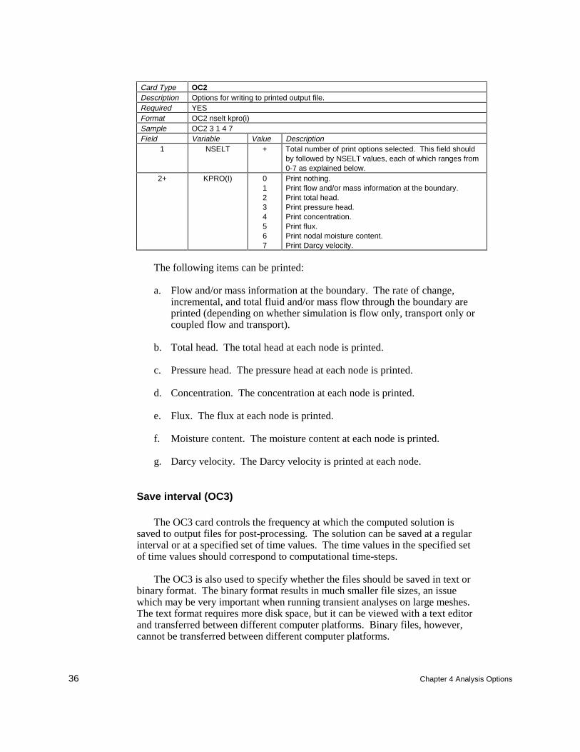
Card Type OC2Description Options for writing to printed output file.Required YESFormat OC2 nselt kpro(i)Sample OC2 3 1 4 7Field Variable Value Description
1 NSELT + Total number of print options selected. This field shouldby followed by NSELT values, each of which ranges from0-7 as explained below.
2+ KPRO(I) 01234567
Print nothing.Print flow and/or mass information at the boundary.Print total head.Print pressure head.Print concentration.Print flux.Print nodal moisture content.Print Darcy velocity.
The following items can be printed:
a. Flow and/or mass information at the boundary. The rate of change,incremental, and total fluid and/or mass flow through the boundary areprinted (depending on whether simulation is flow only, transport only orcoupled flow and transport).
b. Total head. The total head at each node is printed.
c. Pressure head. The pressure head at each node is printed.
d. Concentration. The concentration at each node is printed.
e. Flux. The flux at each node is printed.
f. Moisture content. The moisture content at each node is printed.
g. Darcy velocity. The Darcy velocity is printed at each node.
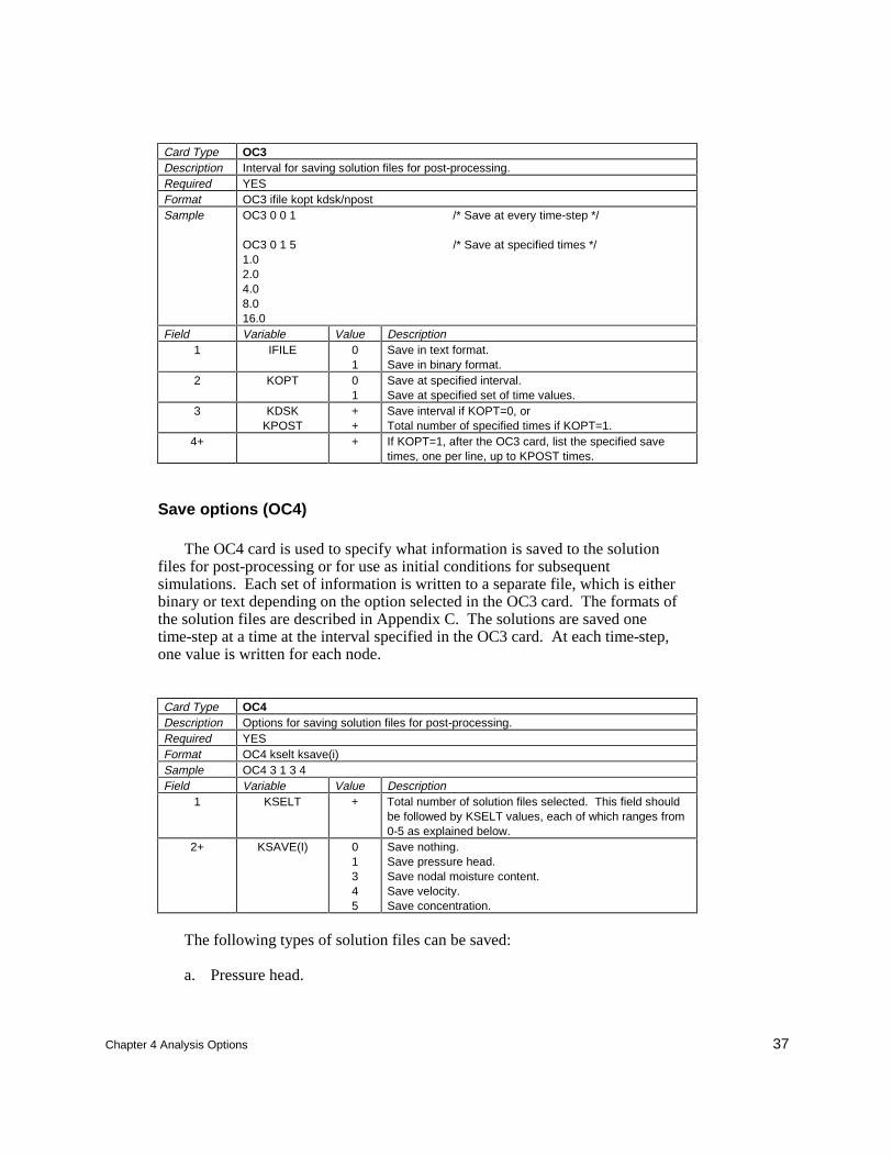
Save interval (OC3)
The OC3 card controls the frequency at which the computed solution issaved to output files for post-processing. The solution can be saved at a regularinterval or at a specified set of time values. The time values in the specified setof time values should correspond to computational time-steps.
The OC3 is also used to specify whether the files should be saved in text orbinary format. The binary format results in much smaller file sizes, an issuewhich may be very important when running transient analyses on large meshes.The text format requires more disk space, but it can be viewed with a text editorand transferred between different computer platforms. Binary files, however,cannot be transferred between different computer platforms.
Chapter 4 Analysis Options 37
Card Type OC3Description Interval for saving solution files for post-processing.Required YESFormat OC3 ifile kopt kdsk/npostSample OC3 0 0 1 /* Save at every time-step */
OC3 0 1 5 /* Save at specified times */1.02.04.08.016.0
Field Variable Value Description1 IFILE 0
1Save in text format.Save in binary format.
2 KOPT 01
Save at specified interval.Save at specified set of time values.
3 KDSKKPOST
++
Save interval if KOPT=0, orTotal number of specified times if KOPT=1.
4+ + If KOPT=1, after the OC3 card, list the specified savetimes, one per line, up to KPOST times.
Save options (OC4)
The OC4 card is used to specify what information is saved to the solutionfiles for post-processing or for use as initial conditions for subsequentsimulations. Each set of information is written to a separate file, which is eitherbinary or text depending on the option selected in the OC3 card. The formats ofthe solution files are described in Appendix C. The solutions are saved onetime-step at a time at the interval specified in the OC3 card. At each time-step,one value is written for each node.
Card Type OC4Description Options for saving solution files for post-processing.Required YESFormat OC4 kselt ksave(i)Sample OC4 3 1 3 4Field Variable Value Description
1 KSELT + Total number of solution files selected. This field shouldbe followed by KSELT values, each of which ranges from0-5 as explained below.
2+ KSAVE(I) 01345
Save nothing.Save pressure head.Save nodal moisture content.Save velocity.Save concentration.
The following types of solution files can be saved:
a. Pressure head.

38 Chapter 4 Analysis Options
b. Nodal moisture content computed at nodes as an average of surroundingelements.
c. Darcy velocity.
d. Concentration.

40 Chapter 5 Material Properties
5 Material Properties
Introduction
The second of the four primary groups of information in the model file is thematerial properties. The material properties include fluid properties and soilproperties. One set of fluid properties is defined for the entire mesh, and one setof soil properties is defined for each of the soil or aquifer types referenced by theelement material ID’s.
File Format
The set of cards in the model file corresponding to material properties isshown in Figure 5.
.MP1 kcp /* Cond. Or perm. Flag*/MP2 i kxx kxy kz kxy kxz kyz alpha por /* Cond. Or perm. Values */MP3 rho visc grav betap /* Dens. And visc. Of water */MP4 a1 a2 a3 a4 a5 a6 a7 a8 /* Dens. And visc. Coeff.s */MP5 I k gamma al at am t decay n deckw decks /* Disp./diffusion coeff.s */SP1 I ihm ihc ihw /* Soil prop.For unsat. zone */.
Figure 5. The material properties cards in the model file
Fluid Properties
The fluid property cards input to the model file are used to specify thedensity, the viscosity and the compressibility of fluid, and the acceleration ofgravity. The acceleration of gravity is not a fluid property, but it is input on thesame line as the density and viscosity for convenience. Specifying theacceleration of gravity allows the user to use any desired units for the fluidproperties, soil properties, and all other parameters input to FEMWATER. Allparameters should be consistent with the units of the specified acceleration of
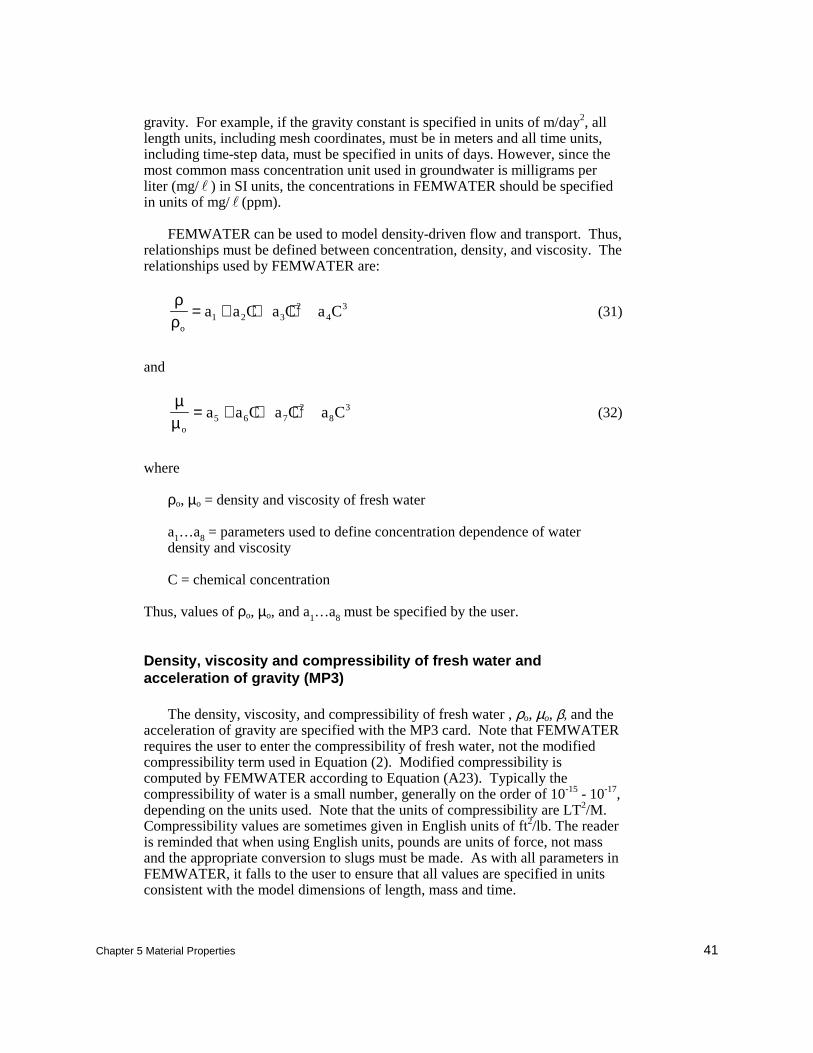
Chapter 5 Material Properties 41
gravity. For example, if the gravity constant is specified in units of m/day2, alllength units, including mesh coordinates, must be in meters and all time units,including time-step data, must be specified in units of days. However, since themost common mass concentration unit used in groundwater is milligrams perliter (mg/ l ) in SI units, the concentrations in FEMWATER should be specifiedin units of mg/ l (ppm).
FEMWATER can be used to model density-driven flow and transport. Thus,relationships must be defined between concentration, density, and viscosity. Therelationships used by FEMWATER are:
ρρo
a a C a C a C= + + +1 2 32
43 (31)
and
µµo
a a C a C a C= + + +5 6 72
83 (32)
where
ρo, µo = density and viscosity of fresh water
a1…a8 = parameters used to define concentration dependence of waterdensity and viscosity
C = chemical concentration
Thus, values of ρo, µo, and a1…a8 must be specified by the user.
Density, viscosity and compressibility of fresh water andacceleration of gravity (MP3)
The density, viscosity, and compressibility of fresh water , ρo, µo, β, and theacceleration of gravity are specified with the MP3 card. Note that FEMWATERrequires the user to enter the compressibility of fresh water, not the modifiedcompressibility term used in Equation (2). Modified compressibility iscomputed by FEMWATER according to Equation (A23). Typically thecompressibility of water is a small number, generally on the order of 10-15 - 10-17,depending on the units used. Note that the units of compressibility are LT2/M.Compressibility values are sometimes given in English units of ft2/lb. The readeris reminded that when using English units, pounds are units of force, not massand the appropriate conversion to slugs must be made. As with all parameters inFEMWATER, it falls to the user to ensure that all values are specified in unitsconsistent with the model dimensions of length, mass and time.
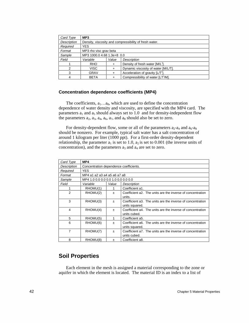
42 Chapter 5 Material Properties
Card Type MP3Description Density, viscosity and compressibility of fresh water.Required YESFormat MP3 rho visc grav betaSample MP3 1000.0 4.68 1.3e+8 0.0Field Variable Value Description
1 RHO + Density of fresh water [M/L3].2 VISC + Dynamic viscosity of water [M/L/T].3 GRAV + Acceleration of gravity [L/T2].4 BETA + Compressibility of water [LT2/M].
Concentration dependence coefficients (MP4)
The coefficients, a1…a8, which are used to define the concentrationdependence of water density and viscosity, are specified with the MP4 card. Theparameters a1 and a5 should always set to 1.0 and for density-independent flowthe parameters a2, a3, a4, a6, a7, and a8 should also be set to zero.
For density-dependent flow, some or all of the parameters a2-a4 and a6-a8
should be nonzero. For example, typical salt water has a salt concentration ofaround 1 kilogram per liter (1000 ppt). For a first-order density-dependentrelationship, the parameter a1 is set to 1.0, a2 is set to 0.001 (the inverse units ofconcentration), and the parameters a3 and a4 are set to zero.
Card Type MP4Description Concentration dependence coefficients.Required YESFormat MP4 a1 a2 a3 a4 a5 a6 a7 a8Sample MP4 1.0 0.0 0.0 0.0 1.0 0.0 0.0 0.0Field Variable Value Description
1 RHOMU(1) 1 Coefficient a1.2 RHOMU(2) ± Coefficient a2. The units are the inverse of concentration
units.3 RHOMU(3) ± Coefficient a3. The units are the inverse of concentration
units squared.4 RHOMU(4) ± Coefficient a4. The units are the inverse of concentration
units cubed.5 RHOMU(5) 1 Coefficient a5.6 RHOMU(6) ± Coefficient a6. The units are the inverse of concentration
units squared.7 RHOMU(7) ± Coefficient a7. The units are the inverse of concentration
units cubed.8 RHOMU(8) ± Coefficient a8.
Soil Properties
Each element in the mesh is assigned a material corresponding to the zone oraquifer in which the element is located. The material ID is an index to a list of
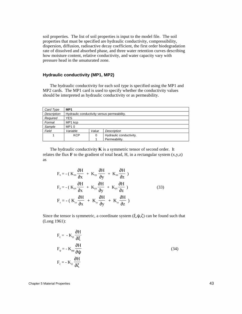
Chapter 5 Material Properties 43
soil properties. The list of soil properties is input to the model file. The soilproperties that must be specified are hydraulic conductivity, compressibility,dispersion, diffusion, radioactive decay coefficient, the first order biodegradationrate of dissolved and absorbed phase, and three water retention curves describinghow moisture content, relative conductivity, and water capacity vary withpressure head in the unsaturated zone.
Hydraulic conductivity (MP1, MP2)
The hydraulic conductivity for each soil type is specified using the MP1 andMP2 cards. The MP1 card is used to specify whether the conductivity valuesshould be interpreted as hydraulic conductivity or as permeability.
Card Type MP1Description Hydraulic conductivity versus permeability.Required YESFormat MP1 kcpSample MP1 0Field Variable Value Description
1 KCP 01
Hydraulic conductivity.Permeability.
The hydraulic conductivity K is a symmetric tensor of second order. Itrelates the flux F to the gradient of total head, H, in a rectangular system (x,y,z)as
Fx = - ( Kxx
∂∂Hx
+ Kxy
∂∂Hy
+ Kxz
∂∂Hz
)
Fy = - ( Kyx
∂∂Hx
+ Kyy
∂∂Hy
+ Kyz
∂∂Hz
) (33)
Fz = - ( Kzx
∂∂Hx
+ Kzy
∂∂Hy
+ Kzz
∂∂Hz
)
Since the tensor is symmetric, a coordinate system (ξ,ψ,ζ) can be found such that(Long 1961):
Fξ = - Kξξ
∂∂ξH
Fψ = - Kψψ
∂∂ψH
(34)
Fζ = - Kζζ
∂∂ζH
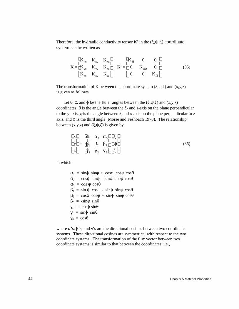
44 Chapter 5 Material Properties
Therefore, the hydraulic conductivity tensor K′ in the (ξ,ψ,ζ) coordinatesystem can be written as
K =
K K K
K K K
K K K
xx xy xz
yx yy yz
zx zy zz
K′ =
K
K
K
ξξ
ψψ
ζζ
0 0
0 0
0 0
(35)
The transformation of K between the coordinate system (ξ,ψ,ζ) and (x,y,z)is given as follows.
Let θ, φ, and ϕ be the Euler angles between the (ξ,ψ,ζ) and (x,y,z)coordinates: θ is the angle between the ζ- and z-axis on the plane perpendicularto the y-axis, φ is the angle between ξ and x-axis on the plane perpendicular to z-axis, and ϕ is the third angle (Morse and Feshbach 1978). The relationshipbetween (x,y,z) and (ξ,ψ,ζ) is given by
x
y
z
=
αβγ
1
1
1
αβγ
2
2
2
αβγ
3
3
3
ξψζ
(36)
in which
α1 = sinϕ sinφ + cosϕ cosφ cosθα2 = cosϕ sinφ - sinϕ cosφ cosθα3 = cos φ cosθβ1 = sin ϕ cosφ - sinϕ sinφ cosθβ2 = cosϕ cosφ + sinϕ sinφ cosθβ3 = -sinφ sinθγ1 = -cosϕ sinθγ2 = sinϕ sinθγ3 = cosθ
where α’s, β’s, and γ’s are the directional cosines between two coordinatesystems. These directional cosines are symmetrical with respect to the twocoordinate systems. The transformation of the flux vector between twocoordinate systems is similar to that between the coordinates, i.e.,
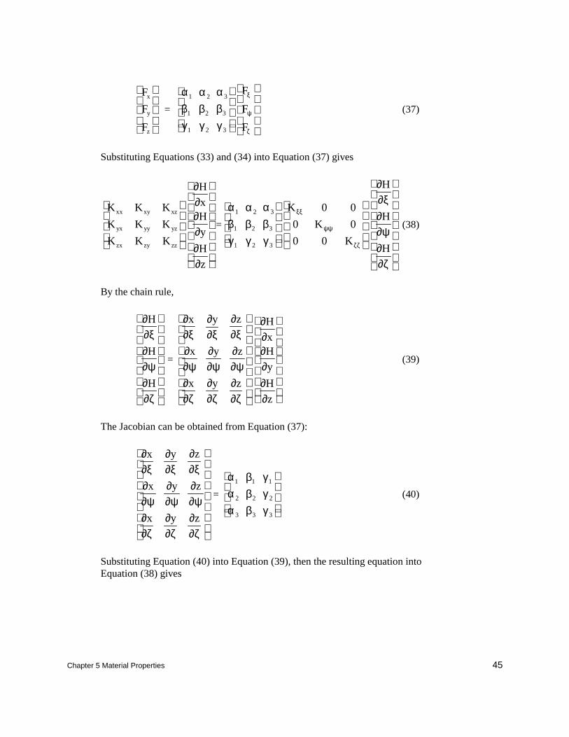
Chapter 5 Material Properties 45
F
F
F
x
y
z
=
αβγ
1
1
1
αβγ
2
2
2
αβγ
3
3
3
F
F
F
ξ
ψ
ζ
(37)
Substituting Equations (33) and (34) into Equation (37) gives
K K K
K K K
K K K
xx xy xz
yx yy yz
zx zy zz
∂∂∂∂∂∂
H
xH
y
H
z
=
αβγ
1
1
1
αβγ
2
2
2
αβγ
3
3
3
K
K
K
ξξ
ψψ
ζζ
0 0
0 0
0 0
∂∂ξ∂∂ψ∂∂ζ
H
H
H
(38)
By the chain rule,
∂∂ξ∂∂ψ∂∂ζ
H
H
H
=
∂∂ξ∂∂ψ∂∂ζ
x
x
x
∂∂ξ∂∂ψ∂∂ζ
y
y
y
∂∂ξ∂∂ψ∂∂ζ
z
z
z
∂∂∂∂∂∂
H
xH
y
H
z
(39)
The Jacobian can be obtained from Equation (37):
∂∂ξ∂∂ψ∂∂ζ
x
x
x
∂∂ξ∂∂ψ∂∂ζ
y
y
y
∂∂ξ∂∂ψ∂∂ζ
z
z
z
=
ααα
1
2
3
βββ
1
2
3
γγγ
1
2
3
(40)
Substituting Equation (40) into Equation (39), then the resulting equation intoEquation (38) gives
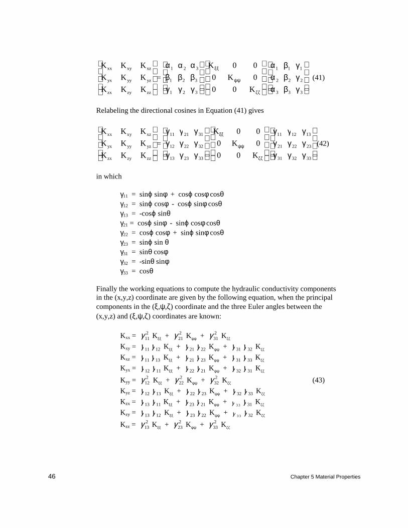
46 Chapter 5 Material Properties
K K K
K K K
K K K
xx xy xz
yx yy yz
zx zy zz
=
αβγ
1
1
1
αβγ
2
2
2
αβγ
3
3
3
K 0 0
0 K 0
0 0 K
ξξ
ψψ
ζζ
ααα
1
2
3
βββ
1
2
3
γγγ
1
2
3
(41)
Relabeling the directional cosines in Equation (41) gives
Kxx xy xz
yx yy yz
zx zy zz
K K
K K K
K K K
=
γγγ
11
12
13
γγγ
21
22
23
γγγ
31
32
33
K 0 0
0 K 0
0 0 K
ξξ
ψψ
ζζ
γγγ
11
21
31
γγγ
12
22
32
γγγ
13
23
33
(42)
in which
γ11 = sinϕ sinφ + cosϕ cosφ cosθγ12 = sinϕ cosφ - cosϕ sinφ cosθγ13 = -cosϕ sinθγ21 = cosϕ sinφ - sinϕ cosφ cosθγ22 = cosϕ cosφ + sinϕ sinφ cosθγ23 = sinϕ sin θγ31 = sinθ cosφγ32 = -sinθ sinφγ33 = cosθ
Finally the working equations to compute the hydraulic conductivity componentsin the (x,y,z) coordinate are given by the following equation, when the principalcomponents in the (ξ,ψ,ζ) coordinate and the three Euler angles between the(x,y,z) and (ξ,ψ,ζ) coordinates are known:
Kxx = γ 112 Kξξ + γ 21
2 Kψψ + γ 312 Kζζ
Kxy = γ 11 γ 12 Kξξ + γ 21 γ 22 Kψψ + γ 31 γ 32 Kζζ
Kxz = γ 11 γ 13 Kξξ + γ 21 γ 23 Kψψ + γ 31 γ 33 Kζζ
Kyx = γ 12 γ 11 Kξξ + γ 22 γ 21 Kψψ + γ 32 γ 31 Kζζ
Kyy = γ 122 Kξξ + γ 22
2 Kψψ + γ 322 Kζζ (43)
Kyz = γ 12 γ 13 Kξξ + γ 22 γ 23 Kψψ + γ 32 γ 33 Kζζ
Kzx = γ 13 γ 11 Kξξ + γ 23 γ 21 Kψψ + γ 3 3γ 31 Kζζ
Kzy = γ 13 γ 12 Kξξ + γ 23 γ 22 Kψψ + γ 3 3γ 32 Kζζ
Kzz = γ 132 Kξξ + γ 23
2 Kψψ + γ 332 Kζζ
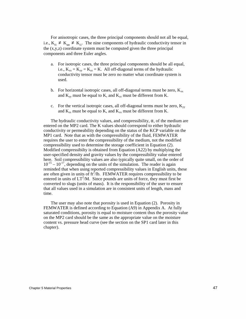
Chapter 5 Material Properties 47
For anisotropic cases, the three principal components should not all be equal,i.e., Kξξ ≠ Kψψ ≠ Kζζ. The nine components of hydraulic conductivity tensor inthe (x,y,z) coordinate system must be computed given the three principalcomponents and three Euler angles.
a. For isotropic cases, the three principal components should be all equal,i.e., Kxx = Kyy = Kzz = K. All off-diagonal terms of the hydraulicconductivity tensor must be zero no matter what coordinate system isused.
b. For horizontal isotropic cases, all off-diagonal terms must be zero, Kxx
and Kyy must be equal to K, and Kzz must be different from K.
c. For the vertical isotropic cases, all off-diagonal terms must be zero, Kyy
and Kzz must be equal to K, and Kxx must be different from K.
The hydraulic conductivity values, and compressibility, α, of the medium areentered on the MP2 card. The K values should correspond to either hydraulicconductivity or permeability depending on the status of the KCP variable on theMP1 card. Note that as with the compressibility of the fluid, FEMWATERrequires the user to enter the compressibility of the medium, not the modifiedcompressibility used to determine the storage coefficient in Equation (2).Modified compressibilty is obtained from Equation (A22) by multiplying theuser-specified density and gravity values by the compressibility value enteredhere. Soil compressibility values are also typically quite small, on the order of10-15 – 10-17, depending on the units of the simulation. The reader is againreminded that when using reported compressibility values in English units, theseare often given in units of ft2/lb. FEMWATER requires compressibility to beentered in units of LT2/M. Since pounds are units of force, they must first beconverted to slugs (units of mass). It is the responsibility of the user to ensurethat all values used in a simulation are in consistent units of length, mass andtime.
The user may also note that porosity is used in Equation (2). Porosity inFEMWATER is defined according to Equation (A9) in Appendix A. At fullysaturated conditions, porosity is equal to moisture content thus the porosity valueon the MP2 card should be the same as the appropriate value on the moisturecontent vs. pressure head curve (see the section on the SP1 card later in thischapter).
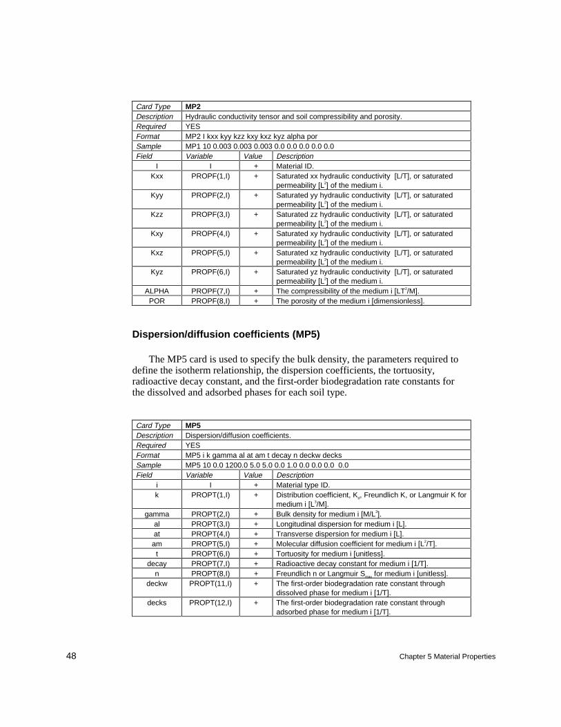
48 Chapter 5 Material Properties
Card Type MP2Description Hydraulic conductivity tensor and soil compressibility and porosity.Required YESFormat MP2 I kxx kyy kzz kxy kxz kyz alpha porSample MP1 10 0.003 0.003 0.003 0.0 0.0 0.0 0.0 0.0Field Variable Value Description
I I + Material ID.Kxx PROPF(1,I) + Saturated xx hydraulic conductivity [L/T], or saturated
permeability [L2] of the medium i.Kyy PROPF(2,I) + Saturated yy hydraulic conductivity [L/T], or saturated
permeability [L2] of the medium i.Kzz PROPF(3,I) + Saturated zz hydraulic conductivity [L/T], or saturated
permeability [L2] of the medium i.Kxy PROPF(4,I) + Saturated xy hydraulic conductivity [L/T], or saturated
permeability [L2] of the medium i.Kxz PROPF(5,I) + Saturated xz hydraulic conductivity [L/T], or saturated
permeability [L2] of the medium i.Kyz PROPF(6,I) + Saturated yz hydraulic conductivity [L/T], or saturated
permeability [L2] of the medium i.ALPHA PROPF(7,I) + The compressibility of the medium i [LT2/M].
POR PROPF(8,I) + The porosity of the medium i [dimensionless].
Dispersion/diffusion coefficients (MP5)
The MP5 card is used to specify the bulk density, the parameters required todefine the isotherm relationship, the dispersion coefficients, the tortuosity,radioactive decay constant, and the first-order biodegradation rate constants forthe dissolved and adsorbed phases for each soil type.
Card Type MP5Description Dispersion/diffusion coefficients.Required YESFormat MP5 i k gamma al at am t decay n deckw decksSample MP5 10 0.0 1200.0 5.0 5.0 0.0 1.0 0.0 0.0 0.0 0.0Field Variable Value Description
i I + Material type ID.k PROPT(1,I) + Distribution coefficient, Kd, Freundlich K, or Langmuir K for
medium i [L3/M].gamma PROPT(2,I) + Bulk density for medium i [M/L3].
al PROPT(3,I) + Longitudinal dispersion for medium i [L].at PROPT(4,I) + Transverse dispersion for medium i [L].am PROPT(5,I) + Molecular diffusion coefficient for medium i [L2/T].t PROPT(6,I) + Tortuosity for medium i [unitless].
decay PROPT(7,I) + Radioactive decay constant for medium i [1/T].n PROPT(8,I) + Freundlich n or Langmuir Smax for medium i [unitless].
deckw PROPT(11,I) + The first-order biodegradation rate constant throughdissolved phase for medium i [1/T].
decks PROPT(12,I) + The first-order biodegradation rate constant throughadsorbed phase for medium i [1/T].
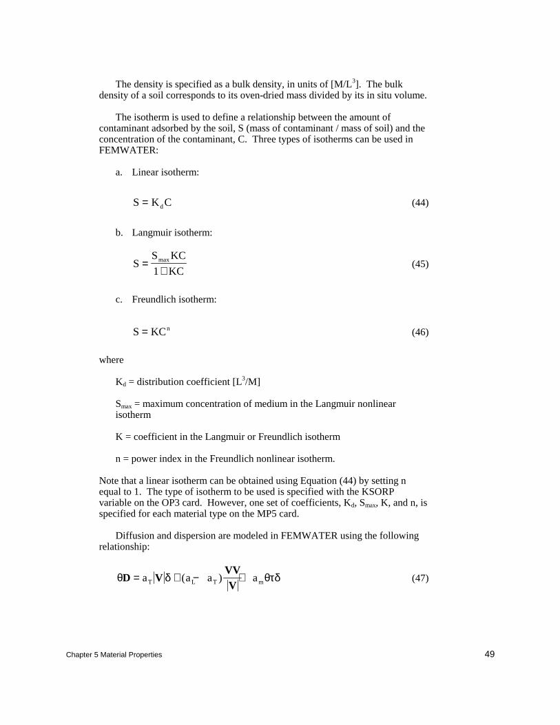
Chapter 5 Material Properties 49
The density is specified as a bulk density, in units of [M/L3]. The bulkdensity of a soil corresponds to its oven-dried mass divided by its in situ volume.
The isotherm is used to define a relationship between the amount ofcontaminant adsorbed by the soil, S (mass of contaminant / mass of soil) and theconcentration of the contaminant, C. Three types of isotherms can be used inFEMWATER:
a. Linear isotherm:
S K Cd= (44)
b. Langmuir isotherm:
SS KC
KC=
+max
1(45)
c. Freundlich isotherm:
S KCn= (46)
where
Kd = distribution coefficient [L3/M]
Smax = maximum concentration of medium in the Langmuir nonlinearisotherm
K = coefficient in the Langmuir or Freundlich isotherm
n = power index in the Freundlich nonlinear isotherm.
Note that a linear isotherm can be obtained using Equation (44) by setting nequal to 1. The type of isotherm to be used is specified with the KSORPvariable on the OP3 card. However, one set of coefficients, Kd, Smax, K, and n, isspecified for each material type on the MP5 card.
Diffusion and dispersion are modeled in FEMWATER using the followingrelationship:
θ θτD VVVV
= + − +a a a aT L T mδ δ( ) (47)
50 Chapter 5 Material Properties
where
θ = moisture content
D = dispersion coefficient tensor
aT = transverse dispersion [L]
δ = Kronecker delta tensor
|V| = the magnitude of the Darcy velocity V [L/T]
aL = longitudinal dispersion [L]
am = molecular diffusion coefficient [L2/T]
τ = tortuosity
Thus, the parameters, aT, aL, am, and t must be specified by the user. They can beobtained by experiment or literature review.
A radioactive decay constant, λ [1/T], may be specified for each material ifthe contaminant decays according to radioactive decay behavior. First-orderbiodegredation of the contaminant can also be simulated by enteringbiodegradation constants for both the dissolved and adsorbed phases of thecontaminant in each material.
Soil properties for unsaturated zone (SP1)
The final set of parameters that must be specified for each medium is asequence of three curves defining how the moisture content, relativeconductivity, and water capacity vary as a function of pressure head in theunsaturated zone.
Card Type SP1Description Soil properties for unsaturated zone.Required YESFormat SP1 i ihm, ihc, ihwSample SP1 10 3 4 5Field Variable Value Description
1 I + Material type index.2 IHM(I) + Index of moisture content versus pressure head XY series.3 IHC(I) + Index of relative conductivity versus pressure head XY series.4 IHW(I) + Index of water capacity versus pressure head XY series.
Relative conductivity. The governing equation for flow of water through avariably saturated porous medium has effective hydraulic conductivity and
Chapter 5 Material Properties 51
storage terms. The effective hydraulic conductivity can be rewritten as theproduct of nonlinear and constant terms in the form:
( )K h K Kr S= (48)
where Kr is the relative conductivity, ranging in value from 0.0 to 1.0, and KS isthe saturated hydraulic conductivity. The change of relative hydraulicconductivity is caused by changes in moisture content, resulting in thepreferential movement of water through certain pathways, due to the influence ofcapillary forces. As the soil becomes less saturated, the flow of water becomesrestricted to the pore sequences of smaller radii. This results in a reduction inthe spatially averaged effective hydraulic conductivity.
Moisture content. Moisture content in the unsaturated zone is a function ofthe pressure head. The more negative the pressure head, the lower the moisturecontent. The curve defining the relationship between moisture content andpressure head should vary between the saturated moisture content, θs, and theresidual moisture content, θr. The saturated moisture content is equal to theporosity of the medium since all of the void space is filled with fluid and asmentioned previously, FEMWATER uses this value in all calculations whereporosity is required. Under unsaturated conditions, however, some of the voidspace is filled with air; thus, the moisture content is less than the medium’sporosity. The residual moisture content represents the amount of water thatcannot be removed from a soil by gravity drainage (even under large suctionpressure) because it adheres to the grains of the soil.
Water capacity. The water capacity curve is equal to the slope of themoisture content versus pressure head curve. Although this curve could bedetermined automatically by FEMWATER from the moisture content curve, it isinput by the user to avoid errors resulting from the approximate piecewise linearnature of the moisture content curve.
Generating the curves. Ideally, the relative conductivity, moisture content,and water capacity curves are determined directly by performing a series of testson the soils involved in the study. However, in many cases they can beapproximated using a set of measured or approximated constants and a set ofempirical relationships. For example, one option for generating the curves is touse the van Genuchten functions (van Genuchten 1980):
( )[ ]Kr e e= − −θ θ γ γ0 5 12
1 1. / (49)
and
( )[ ]θ α β γ
e h= +−
1 for h < 0 (50)
52 Chapter 5 Material Properties
θe = 1 for h ≥ 0 (51)
where
( )θ θ θ θ θw r e s r= + − (52)
γβ
= −11
(53)
and
θw = moisture content (dimensionless)
θe = effective moisture content (dimensionless)
θ s = saturation moisture content (dimensionless)
θ r = residual moisture content (dimensionless)
β γ, = soil-specific exponents (dimensionless)
α = soil-specific coefficient (1/L)
Table 5 lists a set of saturated and residual moisture contents and the vanGenuchten α and β terms for a variety of common soil types. When applying theα term, care should be taken to convert it to the proper units.
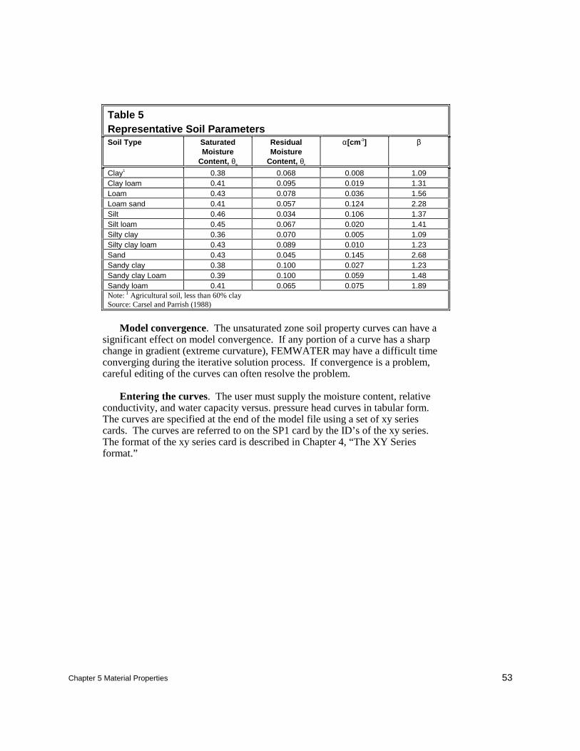
Chapter 5 Material Properties 53
Table 5Representative Soil ParametersSoil Type Saturated
MoistureContent, θs
ResidualMoisture
Content, θr
α[cm-1] β
Clay1 0.38 0.068 0.008 1.09Clay loam 0.41 0.095 0.019 1.31Loam 0.43 0.078 0.036 1.56Loam sand 0.41 0.057 0.124 2.28Silt 0.46 0.034 0.106 1.37Silt loam 0.45 0.067 0.020 1.41Silty clay 0.36 0.070 0.005 1.09Silty clay loam 0.43 0.089 0.010 1.23Sand 0.43 0.045 0.145 2.68Sandy clay 0.38 0.100 0.027 1.23Sandy clay Loam 0.39 0.100 0.059 1.48Sandy loam 0.41 0.065 0.075 1.89Note: 1 Agricultural soil, less than 60% claySource: Carsel and Parrish (1988)
Model convergence. The unsaturated zone soil property curves can have asignificant effect on model convergence. If any portion of a curve has a sharpchange in gradient (extreme curvature), FEMWATER may have a difficult timeconverging during the iterative solution process. If convergence is a problem,careful editing of the curves can often resolve the problem.
Entering the curves. The user must supply the moisture content, relativeconductivity, and water capacity versus. pressure head curves in tabular form.The curves are specified at the end of the model file using a set of xy seriescards. The curves are referred to on the SP1 card by the ID’s of the xy series.The format of the xy series card is described in Chapter 4, “The XY Seriesformat.”

Chapter 6 Boundary Conditions 55
6 Boundary Conditions
Introduction
The boundary conditions supported by FEMWATER include point sourcesand sinks1 , Dirichlet (specified head), flux, flux gradient, and variableboundaries (rainfall/evaporation and seepage). In each case, the prescribedvalues can be either constant or vary with time. Not assigning boundaryconditions to a mesh boundary is equivalent to a no-flux boundary in a flowsimulation or to a no-diffusion flux boundary in a transport simulation.
Choosing Appropriate Boundary Conditions
FEMWATER offers the user several types of boundary conditions in anattempt to cover the range of valid boundary conditions that can be encounteredin finite element groundwater modeling. Some confusion over which boundaryconditions are appropriate for various situations will undoubtedly occur. Thefollowing discussion is intended to help in choosing appropriate boundaryconditions in FEMWATER simulations.
The most common boundary condition used in groundwater modeling is thespecified head (Dirichlet) boundary condition. If heads are known at a givenlocation over the length of the simulation, this is the most appropriate boundarycondition to use.
As a general rule, the variable boundary condition should be used whenmodeling rainfall and evaporation. This boundary condition is the most robustbecause it allows FEMWATER the freedom to change the boundary condition toa specified head boundary condition for both over- and undersaturatedconditions (see the discussion of this boundary condition later in this chapter).This feature is especially applicable in transient simulations where the watertable may fluctuate over the simulation time span.
1 Point sources/sinks are technically not boundary conditions. However, they are included in thischapter for convenience.
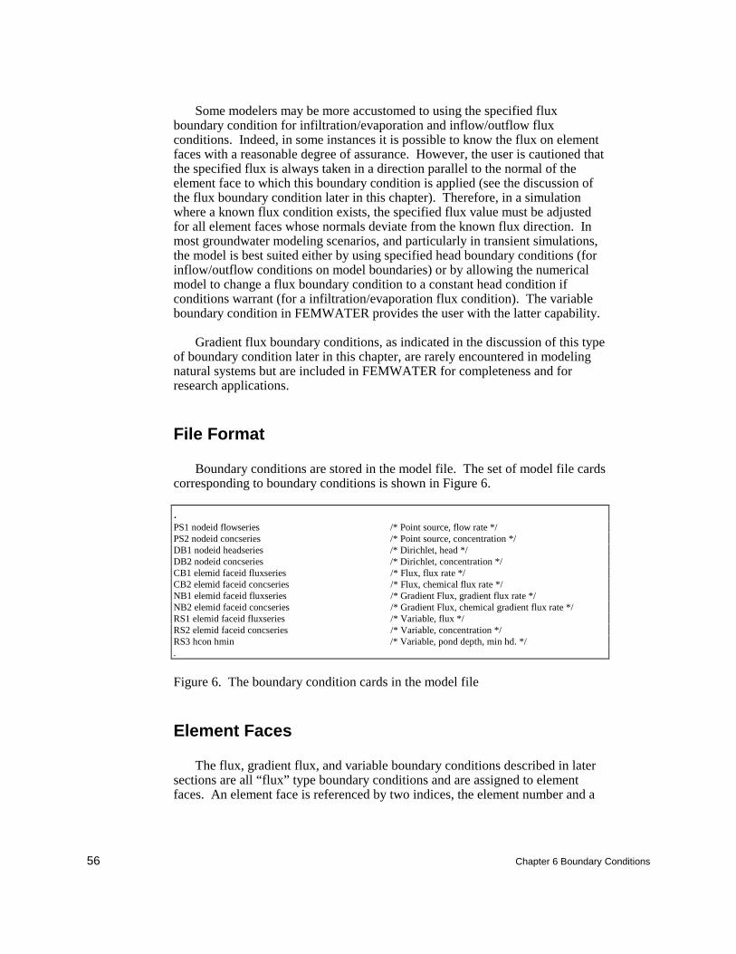
56 Chapter 6 Boundary Conditions
Some modelers may be more accustomed to using the specified fluxboundary condition for infiltration/evaporation and inflow/outflow fluxconditions. Indeed, in some instances it is possible to know the flux on elementfaces with a reasonable degree of assurance. However, the user is cautioned thatthe specified flux is always taken in a direction parallel to the normal of theelement face to which this boundary condition is applied (see the discussion ofthe flux boundary condition later in this chapter). Therefore, in a simulationwhere a known flux condition exists, the specified flux value must be adjustedfor all element faces whose normals deviate from the known flux direction. Inmost groundwater modeling scenarios, and particularly in transient simulations,the model is best suited either by using specified head boundary conditions (forinflow/outflow conditions on model boundaries) or by allowing the numericalmodel to change a flux boundary condition to a constant head condition ifconditions warrant (for a infiltration/evaporation flux condition). The variableboundary condition in FEMWATER provides the user with the latter capability.
Gradient flux boundary conditions, as indicated in the discussion of this typeof boundary condition later in this chapter, are rarely encountered in modelingnatural systems but are included in FEMWATER for completeness and forresearch applications.
File Format
Boundary conditions are stored in the model file. The set of model file cardscorresponding to boundary conditions is shown in Figure 6.
.PS1 nodeid flowseries /* Point source, flow rate */PS2 nodeid concseries /* Point source, concentration */DB1 nodeid headseries /* Dirichlet, head */DB2 nodeid concseries /* Dirichlet, concentration */CB1 elemid faceid fluxseries /* Flux, flux rate */CB2 elemid faceid concseries /* Flux, chemical flux rate */NB1 elemid faceid fluxseries /* Gradient Flux, gradient flux rate */NB2 elemid faceid concseries /* Gradient Flux, chemical gradient flux rate */RS1 elemid faceid fluxseries /* Variable, flux */RS2 elemid faceid concseries /* Variable, concentration */RS3 hcon hmin /* Variable, pond depth, min hd. */.
Figure 6. The boundary condition cards in the model file
Element Faces
The flux, gradient flux, and variable boundary conditions described in latersections are all “flux” type boundary conditions and are assigned to elementfaces. An element face is referenced by two indices, the element number and a
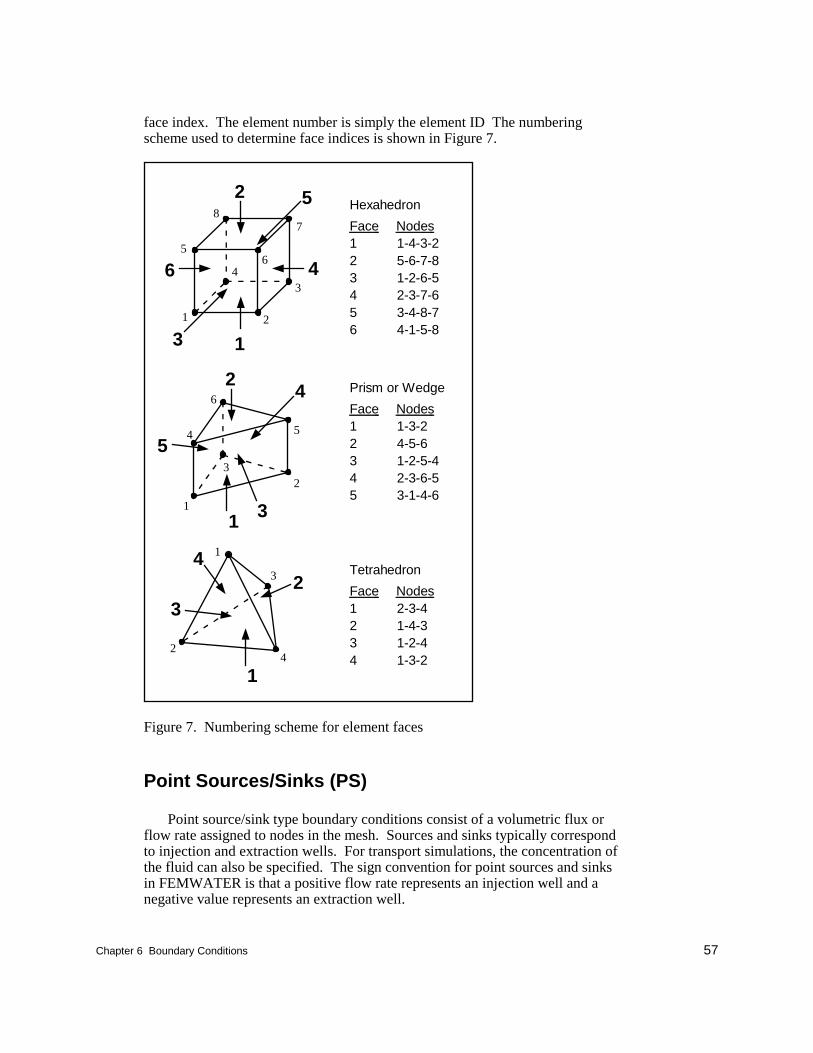
Chapter 6 Boundary Conditions 57
face index. The element number is simply the element ID The numberingscheme used to determine face indices is shown in Figure 7.
24
3
1
1
24
3
1
23
4 5
6
24
5
3
1 2
34
56
78
6
1
2
3
5
4
Hexahedron
Face Nodes 1 1-4-3-22 5-6-7-83 1-2-6-54 2-3-7-65 3-4-8-76 4-1-5-8
Prism or Wedge
Face Nodes 1 1-3-22 4-5-63 1-2-5-44 2-3-6-55 3-1-4-6
Tetrahedron
Face Nodes 1 2-3-42 1-4-33 1-2-44 1-3-2
1
Figure 7. Numbering scheme for element faces
Point Sources/Sinks (PS)
Point source/sink type boundary conditions consist of a volumetric flux orflow rate assigned to nodes in the mesh. Sources and sinks typically correspondto injection and extraction wells. For transport simulations, the concentration ofthe fluid can also be specified. The sign convention for point sources and sinksin FEMWATER is that a positive flow rate represents an injection well and anegative value represents an extraction well.
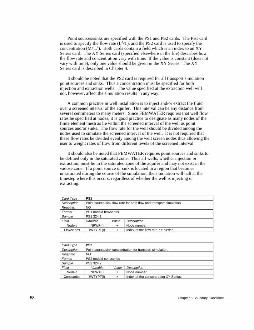
58 Chapter 6 Boundary Conditions
Point sources/sinks are specified with the PS1 and PS2 cards. The PS1 cardis used to specify the flow rate (L3/T), and the PS2 card is used to specify theconcentration (M/ L3). Both cards contain a field which is an index to an XYSeries card. The XY Series card (specified elsewhere in the file) describes howthe flow rate and concentration vary with time. If the value is constant (does notvary with time), only one value should be given in the XY Series. The XYSeries card is described in Chapter 4.
It should be noted that the PS2 card is required for all transport simulationpoint sources and sinks. Thus a concentration must be specified for bothinjection and extraction wells. The value specified at the extraction well willnot, however, affect the simulation results in any way.
A common practice in well installation is to inject and/or extract the fluidover a screened interval of the aquifer. This interval can be any distance fromseveral centimeters to many meters. Since FEMWATER requires that well flowrates be specified at nodes, it is good practice to designate as many nodes of thefinite element mesh as lie within the screened interval of the well as pointsources and/or sinks. The flow rate for the well should be divided among thenodes used to simulate the screened interval of the well. It is not required thatthese flow rates be divided evenly among the well screen nodes thus allowing theuser to weight rates of flow from different levels of the screened interval.
It should also be noted that FEMWATER requires point sources and sinks tobe defined only in the saturated zone. Thus all wells, whether injection orextraction, must lie in the saturated zone of the aquifer and may not exist in thevadose zone. If a point source or sink is located in a region that becomesunsaturated during the course of the simulation, the simulation will halt at thetimestep where this occurs, regardless of whether the well is injecting orextracting.
Card Type PS1Description Point source/sink flow rate for both flow and transport simulation.Required NOFormat PS1 nodeid flowseriesSample PS1 324 1Field Variable Value Description
Nodeid NPWF(I) + Node number.Flowseries IWTYPF(I) + Index of the flow rate XY Series.
Card Type PS2Description Point source/sink concentration for transport simulation.Required NOFormat PS2 nodeid concseriesSample PS2 324 2Field Variable Value Description
Nodeid NPWT(I) + Node number.Concseries IWTYPT(I) + Index of the concentration XY Series.
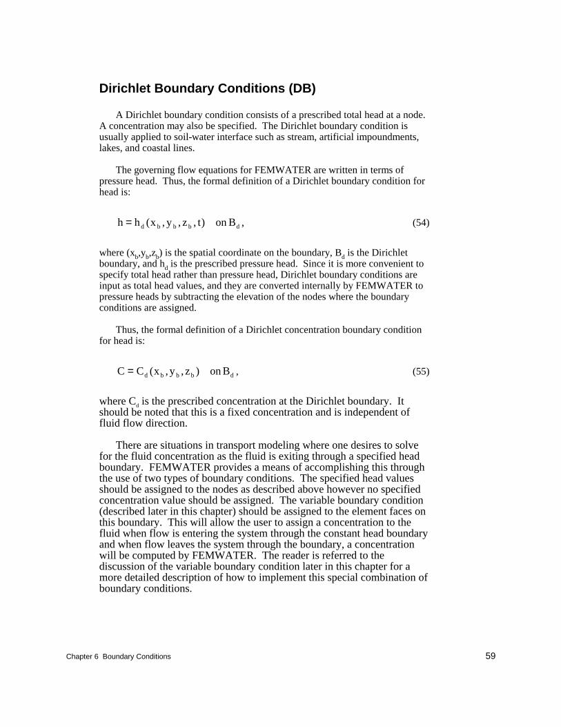
Chapter 6 Boundary Conditions 59
Dirichlet Boundary Conditions (DB)
A Dirichlet boundary condition consists of a prescribed total head at a node.A concentration may also be specified. The Dirichlet boundary condition isusually applied to soil-water interface such as stream, artificial impoundments,lakes, and coastal lines.
The governing flow equations for FEMWATER are written in terms ofpressure head. Thus, the formal definition of a Dirichlet boundary condition forhead is:
h h x y z t on Bd b b b d= ( , , , ) , (54)
where (xb,yb,zb) is the spatial coordinate on the boundary, Bd is the Dirichletboundary, and hd is the prescribed pressure head. Since it is more convenient tospecify total head rather than pressure head, Dirichlet boundary conditions areinput as total head values, and they are converted internally by FEMWATER topressure heads by subtracting the elevation of the nodes where the boundaryconditions are assigned.
Thus, the formal definition of a Dirichlet concentration boundary conditionfor head is:
C C x y z on Bd b b b d= ( , , ) , (55)
where Cd is the prescribed concentration at the Dirichlet boundary. Itshould be noted that this is a fixed concentration and is independent offluid flow direction.
There are situations in transport modeling where one desires to solvefor the fluid concentration as the fluid is exiting through a specified headboundary. FEMWATER provides a means of accomplishing this throughthe use of two types of boundary conditions. The specified head valuesshould be assigned to the nodes as described above however no specifiedconcentration value should be assigned. The variable boundary condition(described later in this chapter) should be assigned to the element faces onthis boundary. This will allow the user to assign a concentration to thefluid when flow is entering the system through the constant head boundaryand when flow leaves the system through the boundary, a concentrationwill be computed by FEMWATER. The reader is referred to thediscussion of the variable boundary condition later in this chapter for amore detailed description of how to implement this special combination ofboundary conditions.
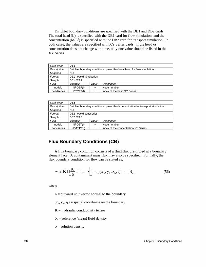
60 Chapter 6 Boundary Conditions
Dirichlet boundary conditions are specified with the DB1 and DB2 cards.The total head (L) is specified with the DB1 card for flow simulation, and theconcentration (M/L3) is specified with the DB2 card for transport simulation. Inboth cases, the values are specified with XY Series cards. If the head orconcentration does not change with time, only one value should be listed in theXY Series.
Card Type DB1Description Dirichlet boundary conditions, prescribed total head for flow simulation.Required NOFormat DB1 nodeid headseriesSample DB1 324 2Field Variable Value Description
nodeid NPDBF(I) + Node number.headseries IDTYPF(I) + Index of the head XY Series.
Card Type DB2Description Dirichlet boundary conditions, prescribed concentration for transport simulation.Required NOFormat DB2 nodeid concseriesSample DB2 324 3Field Variable Value Description
nodeid NPDBT(I) + Node number.concseries JDTYPT(I) + Index of the concentration XY Series.
Flux Boundary Conditions (CB)
A flux boundary condition consists of a fluid flux prescribed at a boundaryelement face. A contaminant mass flux may also be specified. Formally, theflux boundary condition for flow can be stated as:
− ⋅ ⋅ ∇ + ∇
=n K
ρρ
oc b b b ch z q x y z t on B( , , , ) , (56)
where
n = outward unit vector normal to the boundary
(xb, yb, zb) = spatial coordinate on the boundary
K = hydraulic conductivity tensor
ρo = reference (clean) fluid density
ρ = solution density
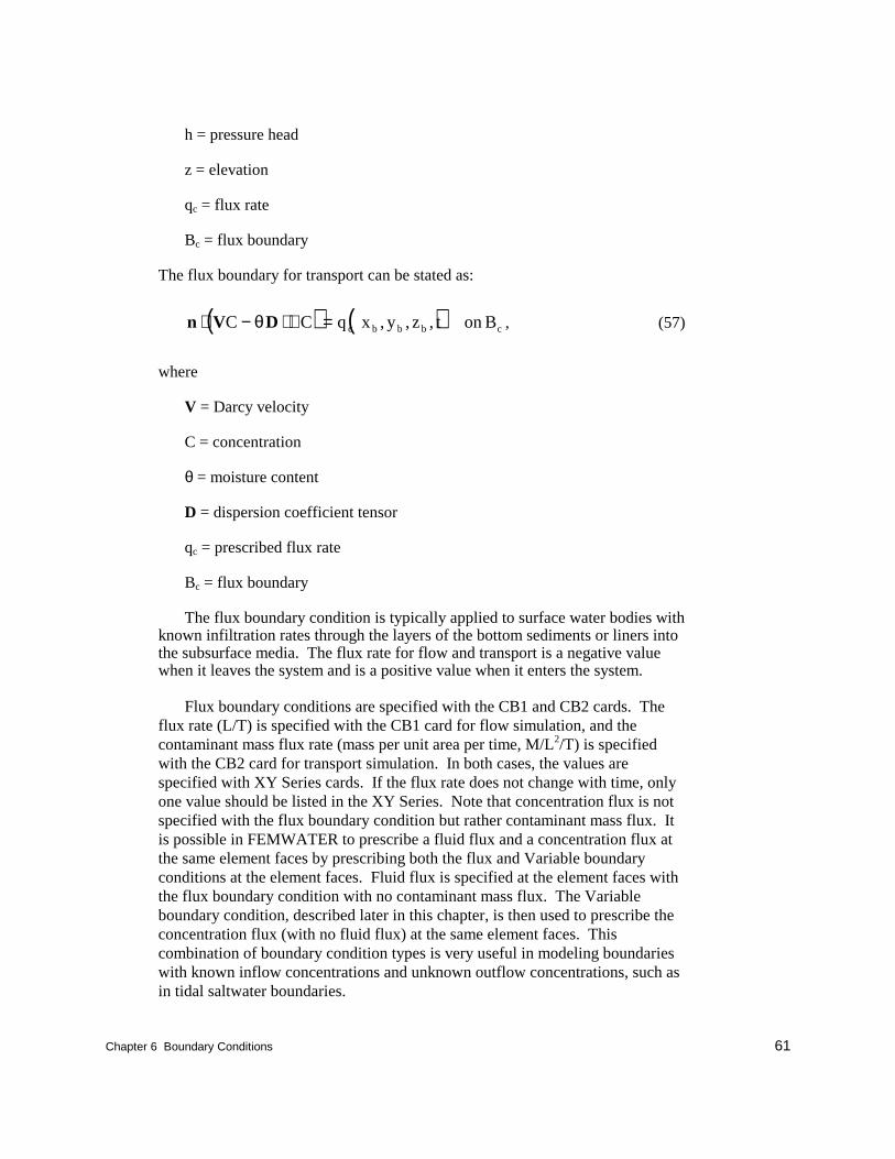
Chapter 6 Boundary Conditions 61
h = pressure head
z = elevation
qc = flux rate
Bc = flux boundary
The flux boundary for transport can be stated as:
( ) ( )n V D⋅ − ⋅ ∇ =C C q x y z t on Bc b b b cθ , , , , (57)
where
V = Darcy velocity
C = concentration
θ = moisture content
D = dispersion coefficient tensor
qc = prescribed flux rate
Bc = flux boundary
The flux boundary condition is typically applied to surface water bodies withknown infiltration rates through the layers of the bottom sediments or liners intothe subsurface media. The flux rate for flow and transport is a negative valuewhen it leaves the system and is a positive value when it enters the system.
Flux boundary conditions are specified with the CB1 and CB2 cards. Theflux rate (L/T) is specified with the CB1 card for flow simulation, and thecontaminant mass flux rate (mass per unit area per time, M/L2/T) is specifiedwith the CB2 card for transport simulation. In both cases, the values arespecified with XY Series cards. If the flux rate does not change with time, onlyone value should be listed in the XY Series. Note that concentration flux is notspecified with the flux boundary condition but rather contaminant mass flux. Itis possible in FEMWATER to prescribe a fluid flux and a concentration flux atthe same element faces by prescribing both the flux and Variable boundaryconditions at the element faces. Fluid flux is specified at the element faces withthe flux boundary condition with no contaminant mass flux. The Variableboundary condition, described later in this chapter, is then used to prescribe theconcentration flux (with no fluid flux) at the same element faces. Thiscombination of boundary condition types is very useful in modeling boundarieswith known inflow concentrations and unknown outflow concentrations, such asin tidal saltwater boundaries.
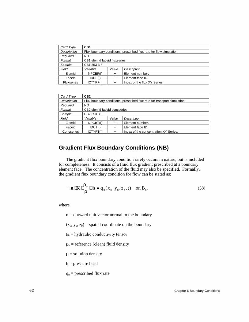
62 Chapter 6 Boundary Conditions
Card Type CB1Description Flux boundary conditions, prescribed flux rate for flow simulation.Required NOFormat CB1 elemid faceid fluxseriesSample CB1 353 3 8Field Variable Value Description
Elemid NPCBF(I) + Element number.Faceid IDCF(I) + Element face ID.
Fluxseries ICTYPF(I) + Index of the flux XY Series.
Card Type CB2Description Flux boundary conditions, prescribed flux rate for transport simulation.Required NOFormat CB2 elemid faceid concseriesSample CB2 353 3 9Field Variable Value Description
Elemid NPCBT(I) + Element number.Faceid IDCT(I) + Element face ID.
Concseries ICTYPT(I) + Index of the concentration XY Series.
Gradient Flux Boundary Conditions (NB)
The gradient flux boundary condition rarely occurs in nature, but is includedfor completeness. It consists of a fluid flux gradient prescribed at a boundaryelement face. The concentration of the fluid may also be specified. Formally,the gradient flux boundary condition for flow can be stated as:
− ⋅ ⋅ ∇ =n Kρρ
on b b b nh q x y z t on B( , , , ) , (58)
where
n = outward unit vector normal to the boundary
(xb, yb, zb) = spatial coordinate on the boundary
K = hydraulic conductivity tensor
ρo = reference (clean) fluid density
ρ = solution density
h = pressure head
qn = prescribed flux rate
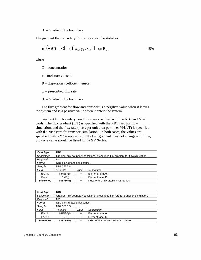
Chapter 6 Boundary Conditions 63
Bn = Gradient flux boundary
The gradient flux boundary for transport can be stated as:
( ) ( )n D⋅ − ⋅ ∇ =θ C q x y z t on Bn b b b n, , , , (59)
where
C = concentration
θ = moisture content
D = dispersion coefficient tensor
qn = prescribed flux rate
Bn = Gradient flux boundary
The flux gradient for flow and transport is a negative value when it leavesthe system and is a positive value when it enters the system.
Gradient flux boundary conditions are specified with the NB1 and NB2cards. The flux gradient (L/T) is specified with the NB1 card for flowsimulation, and the flux rate (mass per unit area per time, M/L2/T) is specifiedwith the NB2 card for transport simulation. In both cases, the values arespecified with XY Series cards. If the flux gradient does not change with time,only one value should be listed in the XY Series.
Card Type NB1Description Gradient flux boundary conditions, prescribed flux gradient for flow simulation.Required NOFormat NB1 elemid faceid fluxseriesSample NB1 353 3 8Field Variable Value Description
Elemid NPNBF(I) + Element number.Faceid IDNF(I) + Element face ID.
Fluxseries INTYPF(I) + Index of the flux gradient XY Series.
Card Type NB2Description Gradient flux boundary conditions, prescribed flux rate for transport simulation.Required NOFormat NB2 elemid faceid fluxseriesSample NB2 353 3 9Field Variable Value Description
Elemid NPNBT(I) + Element number.Faceid IDNT(I) + Element face ID.
Fluxseries INTYPT(I) + Index of the concentration XY Series.
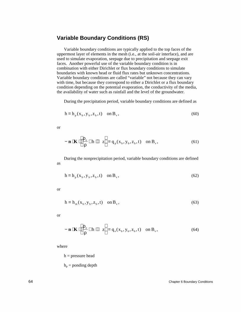
64 Chapter 6 Boundary Conditions
Variable Boundary Conditions (RS)
Variable boundary conditions are typically applied to the top faces of theuppermost layer of elements in the mesh (i.e., at the soil-air interface), and areused to simulate evaporation, seepage due to precipitation and seepage exitfaces. Another powerful use of the variable boundary condition is incombination with either Dirichlet or flux boundary conditions to simulateboundaries with known head or fluid flux rates but unknown concentrations.Variable boundary conditions are called “variable” not because they can varywith time, but because they correspond to either a Dirichlet or a flux boundarycondition depending on the potential evaporation, the conductivity of the media,the availability of water such as rainfall and the level of the groundwater.
During the precipitation period, variable boundary conditions are defined as
h h x y z t on Bp b b b v= ( , , , ) , (60)
or
− ⋅ ⋅ ∇ + ∇
=n K
ρρ
op b b b vh z q x y z t on B( , , , ) , (61)
During the nonprecipitation period, variable boundary conditions are definedas
h h x y z t on Bp b b b v= ( , , , ) , (62)
or
h h x y z t on Bm b b b v= ( , , , ) , (63)
or
− ⋅ ⋅ ∇ + ∇
=n K
ρρ
oe b b b vh z q x y z t on B( , , , ) , (64)
where
h = pressure head
hp = ponding depth
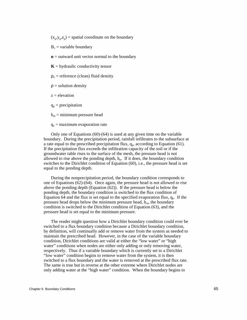
Chapter 6 Boundary Conditions 65
(xb,yb,zb) = spatial coordinate on the boundary
Bv = variable boundary
n = outward unit vector normal to the boundary
K = hydraulic conductivity tensor
ρo = reference (clean) fluid density
ρ = solution density
z = elevation
qp = precipitation
hm = minimum pressure head
qe = maximum evaporation rate
Only one of Equations (60)-(64) is used at any given time on the variableboundary. During the precipitation period, rainfall infiltrates to the subsurface ata rate equal to the prescribed precipitation flux, qp, according to Equation (61).If the precipitation flux exceeds the infiltration capacity of the soil or if thegroundwater table rises to the surface of the mesh, the pressure head is notallowed to rise above the ponding depth, hp. If it does, the boundary conditionswitches to the Dirichlet condition of Equation (60), i.e., the pressure head is setequal to the ponding depth.
During the nonprecipitation period, the boundary condition corresponds toone of Equations (62)-(64). Once again, the pressure head is not allowed to riseabove the ponding depth (Equation (62)). If the pressure head is below theponding depth, the boundary condition is switched to the flux condition ofEquation 64 and the flux is set equal to the specified evaporation flux, qe. If thepressure head drops below the minimum pressure head, hm, the boundarycondition is switched to the Dirichlet condition of Equation (63), and thepressure head is set equal to the minimum pressure.
The reader might question how a Dirichlet boundary condition could ever beswitched to a flux boundary condition because a Dirichlet boundary condition,by definition, will continually add or remove water from the system as needed tomaintain the prescribed head. However, in the case of the variable boundarycondition, Dirichlet conditions are valid at either the “low water” or “highwater” conditions when nodes are either only adding or only removing water,respectively. Thus if a variable boundary which is currently set to a Dirichlet“low water” condition begins to remove water from the system, it is thenswitched to a flux boundary and the water is removed at the prescribed flux rate.The same is true but in reverse at the other extreme where Dirichlet nodes areonly adding water at the “high water” condition. When the boundary begins to
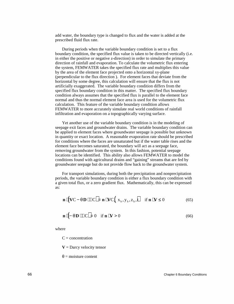
66 Chapter 6 Boundary Conditions
add water, the boundary type is changed to flux and the water is added at theprescribed fluid flux rate.
During periods when the variable boundary condition is set to a fluxboundary condition, the specified flux value is taken to be directed vertically (i.e.in either the positive or negative z-direction) in order to simulate the primarydirection of rainfall and evaporation. To calculate the volumetric flux enteringthe system, FEMWATER takes the specified flux rate and multiplies this valueby the area of the element face projected onto a horizontal xy-plane(perpendicular to the flux direction ). For element faces that deviate from thehorizontal by some degree, this calculation will ensure that the flux is notartificially exaggerated. The variable boundary condition differs from thespecified flux boundary condition in this matter. The specified flux boundarycondition always assumes that the specified flux is parallel to the element facenormal and thus the normal element face area is used for the volumetric fluxcalculation. This feature of the variable boundary condition allowsFEMWATER to more accurately simulate real world conditions of rainfallinfiltration and evaporation on a topographically varying surface.
Yet another use of the variable boundary condition is in the modeling ofseepage exit faces and groundwater drains. The variable boundary condition canbe applied to element faces where groundwater seepage is possible but unknownin quantity or exact location. A reasonable evaporation rate should be prescribedfor conditions where the faces are unsaturated but if the water table rises and theelement face becomes saturated, the boundary will act as a seepage face,removing groundwater from the system. In this fashion, potential seepagelocations can be identified. This ability also allows FEMWATER to model theconditions found with agricultural drains and “gaining” streams that are fed bygroundwater seepage but do not provide flow back to the groundwater system.
For transport simulations, during both the precipitation and nonprecipitationperiods, the variable boundary condition is either a flux boundary condition witha given total flux, or a zero gradient flux. Mathematically, this can be expressedas:
( ) ( )n V D n V n V⋅ − ⋅ ∇ = ⋅ ⋅ ≤C C C x y z t ifv b b bθ , , , 0 (65)
( )n D n V⋅ − ⋅ ∇ = ⋅ >θ C if0 0 (66)
where
C = concentration
V = Darcy velocity tensor
θ = moisture content
Chapter 6 Boundary Conditions 67
D = dispersion coefficient tensor
Cv = concentration at the variable boundary
If the flow direction through the boundary is into the region, the fluxcondition of Equation (65) governs and the concentration in the incoming fluid isequal to the prescribed concentration Cv. If the flow direction through theboundary is out of the region, the gradient flux condition of Equation (66)governs, meaning that the concentration of the outgoing fluid is whatever it wasbefore it left the region.
The behavior of the variable boundary condition in transport simulationsprovides a powerful tool in modeling conditions where fluid head or fluxconditions are known but concentration flux is unknown. As mentioned in boththe Dirichlet and flux boundary condition sections, it is possible to assign eitherDirichlet or flux conditions at a boundary for the fluid, leaving the concentrationunassigned for these types. Then, by assigning a variable type boundarycondition for the concentration, the user is able to specify the concentration ofthe fluid when flow is entering the system but have FEMWATER calculate theconcentration of the fluid when flow is leaving the system.
Variable boundary conditions are defined by specifying the minimumpressure head, hm, the ponding depth, hp, the flux rates qp and qe, and theconcentration, Cv. The minimum pressure head and the ponding depth arespecified on the RS3 card. Only one RS3 card is entered in the model file thusthe minimum pressure head, hm, and the ponding depth, hp are global values forthe entire simulation. The specified minimum pressure head and ponding depthare used for all element faces where a variable boundary condition is specified.
The flux rates (L/T) for precipitation and evaporation, qp and qe, are bothspecified on the RS1 card as an index to a single XY Series. The values in theseries that are positive are treated as precipitation flux, and the values that arenegative are interpreted as evaporation flux. Thus, cycles of rainfall/evaporationcan be designated on one curve by varying the curve in the XY Series frompositive to negative and vice versa.
The concentration (M/L3) is entered on the RS2 card as an index to an XYseries. The ponding depth (L) and the minimum pressure head (L) are bothspecified on the RS3 card.
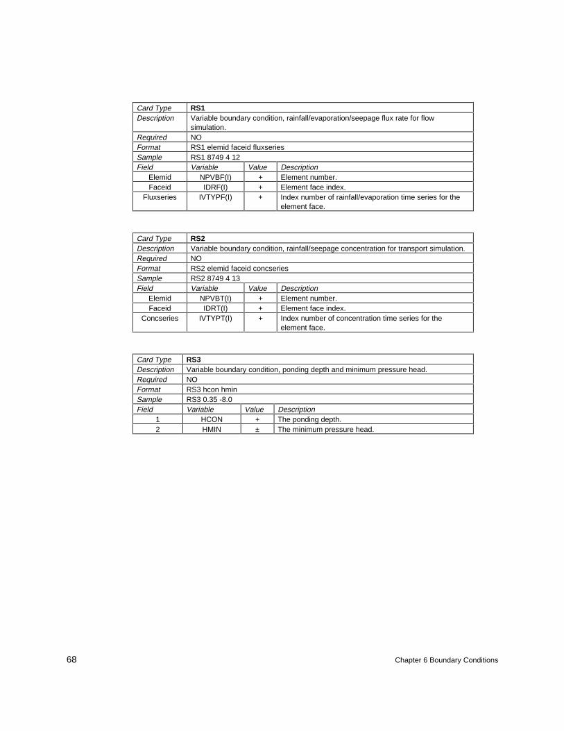
68 Chapter 6 Boundary Conditions
Card Type RS1Description Variable boundary condition, rainfall/evaporation/seepage flux rate for flow
simulation.Required NOFormat RS1 elemid faceid fluxseriesSample RS1 8749 4 12Field Variable Value Description
Elemid NPVBF(I) + Element number.Faceid IDRF(I) + Element face index.
Fluxseries IVTYPF(I) + Index number of rainfall/evaporation time series for theelement face.
Card Type RS2Description Variable boundary condition, rainfall/seepage concentration for transport simulation.Required NOFormat RS2 elemid faceid concseriesSample RS2 8749 4 13Field Variable Value Description
Elemid NPVBT(I) + Element number.Faceid IDRT(I) + Element face index.
Concseries IVTYPT(I) + Index number of concentration time series for theelement face.
Card Type RS3Description Variable boundary condition, ponding depth and minimum pressure head.Required NOFormat RS3 hcon hminSample RS3 0.35 -8.0Field Variable Value Description
1 HCON + The ponding depth.2 HMIN ± The minimum pressure head.
Chapter 7 Initial Conditions 69
7 Initial Conditions
Introduction
Whenever a FEMWATER analysis is performed, a set of initial conditionsmust be defined. Initial conditions define the initial status of the pressure headand concentration. Which initial conditions are required for a particular problemdepends on the type of simulation that is being performed. The rules, options,and formats for defining initial conditions for FEMWATER are described in thischapter.
Types of Initial Conditions
Three types of initial conditions are possible for a FEMWATER simulation:cold starts, hot starts, and flow solutions. Cold starts are used to establish a setof initial values at the beginning of a steady-state or transient simulation. Hotstarts are used to continue a previous run of FEMWATER without having tostart over from a cold start. Flow solutions are used to define the flow field thatis necessary when performing a transport-only simulation (as opposed to coupledflow and transport).
Cold Starts
FEMWATER uses an iterative method to find a solution to flow andtransport problems. An iterative approach involves starting with an initialestimate of heads and concentrations and utilizing an iterative solver to graduallymodify the initial values until they converge to a set of values that satisfy theunderlying governing equations. Using an initial estimate of values is called acold start.
70 Chapter 7 Initial Conditions
Steady state versus transient
Cold starts must be specified regardless of whether the simulation is steady-state or transient. However, the approach taken to define the cold start may varydepending on whether the simulation is steady state or transient. If an initialcondition is chosen with values that are closer to the final solution, thesimulation will converge with fewer iterations (resulting in a much shorterexecution time). Because of the non-linear nature of unsaturated zonecalculations, the solution to the flow equation is often non-unique. Various setsof initial condition values chosen for a simulation can result in differentconverged solutions for the same set of boundary conditions, especially if theinitial conditions used in each simulation vary significantly from each other.Special care should be taken to ensure that reasonable estimates of groundwaterconditions are used as initial conditions for FEMWATER simulations.
With a transient simulation, the specification of the initial condition becomesmore critical. In this case, the initial condition should represent the actual stateof the aquifer at the beginning of the simulation period. In order for thesimulation to be accurate, the initial condition must be compatible with thespecified boundary conditions and stresses. For example, suppose that thetransient effect of a new injection/extraction well system on an aquifer is to besimulated. If an incompatible initial condition is used, the response of theaquifer in the early part of the simulation will be due in part to the wells and inpart to an adjustment of the aquifer that is required to make the heads andconcentrations compatible with the other stresses and boundary conditions.Therefore, it is often best to first perform a steady state simulation with theboundary conditions that will not change during the transient simulation, andthen use the solution to this simulation as the initial condition for the transientsimulation. For this example, this would involve first running a steady-statesimulation with all of the boundary conditions except for the injection andextraction wells. The solution to this simulation would then be used as the initialcondition for the transient simulation, and the response of the aquifer would bedue solely to the added stresses from the injection and extraction wells.
In the case of concentration, a steady-state simulation is often not applicablesince transport seldom achieves steady-state conditions. In many cases, theinitial condition will correspond to an existing plume that has been characterizedvia three-dimensional interpolation from measurements at scattered locations.
Required values
If a flow-only simulation is performed, a set of pressure heads is required forthe cold start initial condition. If a transport-only simulation is performed, a setof concentrations is required (in addition to the flow solution as explainedbelow). If a coupled flow and transport simulation is being performed, a set ofheads and a set of concentrations are both required.
Chapter 7 Initial Conditions 71
The set of pressure head values required for a cold start simulation can be anestimate based on a level pool or an interpolated set of pressure heads based onmeasured values at discrete locations. However, another option is to use theresult of a previous FEMWATER simulation as the initial condition pressureheads. This technique is often called “hot starting” a simulation. FEMWATERhas a hot start feature that is slightly different and only applies to transient runswhich is described in the next section. If a simulation is approachingconvergence but the maximum number of iterations specified on the IP1 card isreached before convergence is achieved, FEMWATER will write out theunconverged pressure head file and terminate. This file can then be used as theinitial condition file for the next simulation, effectively starting the simulationwhere it stopped in the previous run. This technique is useful in choosing initialconditions for a plan condition and a converged solution for the base conditionhas already been computed in a previous simulation.
Another useful application of this technique is called “spinning up” a model.As mentioned in the previous section, if the cold start initial condition differsgreatly from the final solution, the stresses due to the boundary conditions maycause FEMWATER to oscillate and have difficulty converging. One solution tothis problem is to select a better cold start. Another solution is to start with a setof boundary conditions that are more compatible with the specified cold start andcompute a solution. The boundary conditions are then modified slightly and thesolution from the first simulation is used as the initial condition for the secondsimulation. This process is repeated and the boundary conditions are graduallychanged until they correspond to the desired values.
Convergence
The values chosen for a cold start can have a significant impact onconvergence. If the selected cold start differs greatly from the convergedsolution, i.e., is highly incompatible with the model stresses, FEMWATER mayhave difficulty converging. The quickest and most robust solution is achievedwhen cold start values are as close to the converged solution as possible.
Hot Starts
Since FEMWATER is a nonlinear, finite element model, solutions canrequire extensive computation time even for moderately sized meshes,particularly when a transient simulation involving numerous time-steps is beingperformed. During a modeling study, it is not uncommon to encounter situationswhere the solution progresses well to a certain point in time and then diverges or“blows up.” This situation can often be solved by decreasing the time-step sizenear the point in time where the solution degraded. In such cases, it is oftenuseful to be able to restart the simulation at some point just before the problemoccurred rather than starting over from the beginning. In order to do this, the“hot start” type of initial condition is required.
72 Chapter 7 Initial Conditions
Hot start time
A hot start consists of a set of files representing a transient solution ofpressure head, moisture content (optional), velocity (optional), and concentrationand a hot start time. FEMWATER reads the transient solution file(s) and locatesthe set(s) of values at the time-step matching the hot start time. The appropriatevalues are then loaded into FEMWATER as initial conditions and the simulationis restarted. Moisture content and velocity files are not required byFEMWATER to hot start a simulation. However, if a stopped simulationwherein moisture content or velocity files were output is hot started and the userspecifies the velocity and/or moisture content file(s) as input to the simulation,the new solutions from the hot started simulation will be appended to thevelocity and moisture content files from the previous simulation.
When the initial or original simulation is performed, time-variant boundaryconditions are typically defined on a time scale whose beginning corresponds tothe start time of the simulation. When a hot start is performed, it is notnecessary to redefine time-variant boundary conditions so that they are definedfrom a point corresponding to the beginning of the new start time. FEMWATERuses the specified hot start time and automatically interpolates the time-variantboundary conditions to the correct beginning time.
Required values
The solution files necessary for a hot start depend on the type of simulation.If a flow-only simulation is being performed, pressure head is required. If atransport-only simulation is being performed, concentration is required (As in alltransport-only simulations, a flow solution for the entire simulation time isrequired but this is not specified as a hot start input parameter). If a coupledflow and transport simulation is being performed, pressure head andconcentration are required. The velocity and nodal moisture content files areused for post-processing and are only required as input if the user wishes to havethe new simulation solutions appended to the previous simulation solution filesas described above. If the user desires to have the flow and/or concentrationvalues from a hot start simulation appended to the simulation results of aprevious simulation, the same file name for the initial condition and output filesshould be specified in the super file. See the section titled “Super File Input” atthe end of this chapter for the super file input specifications.
File format
The files used for hot starts correspond to the data set solution files outputby FEMWATER for post-processing. These files consist of solutions organizedby time-step and are sequential lists of scalar or vector values, with one valuelisted per node. The nodal values are used for post-processing. The output
Chapter 7 Initial Conditions 73
control options which control data set output are described in the section “Saveinterval (OC3).” The formats of the data set files are described in Appendix C.
Flow Solutions
A third type of initial condition is required when a transport-only simulationis being performed. A transport-only simulation uses a previously computedflow solution (steady-state or transient) to define the three-dimensional flowfield required to properly model the contaminant migration. The flow solutionconsists of two options: pressure head or velocity and pressure head written todata set files. When the first option is used, the needed velocity and moisturecontent for transport simulation are computed from the pressure head. When thesecond option is used, the needed moisture content is computed from thepressure head and velocity is read directly from the velocity file. Thus, whenrunning the flow simulation, care should be taken to ensure that the properoptions are selected for solution output (see “Save options (OC4)”).
The flow solution for a transport-only simulation is used in combination witheither a cold start or a hot start. With a cold start, a set of initial concentrationvalues is provided for concentration in addition to the steady-state or transientflow solution. With a hot start, a transient concentration solution and a hot starttime are provided in addition to the flow solution.
Summary of Initial Condition Requirements
It can sometimes be confusing to determine which combination of initialconditions is required for a particular situation. The sets of initial conditionsrequired for all possible scenarios are shown in Table 6. The X’s in the lowerright corner of the table indicate which sets of values are required. For example,for a cold start with a coupled flow and transport simulation, pressure head andconcentration must be specified.
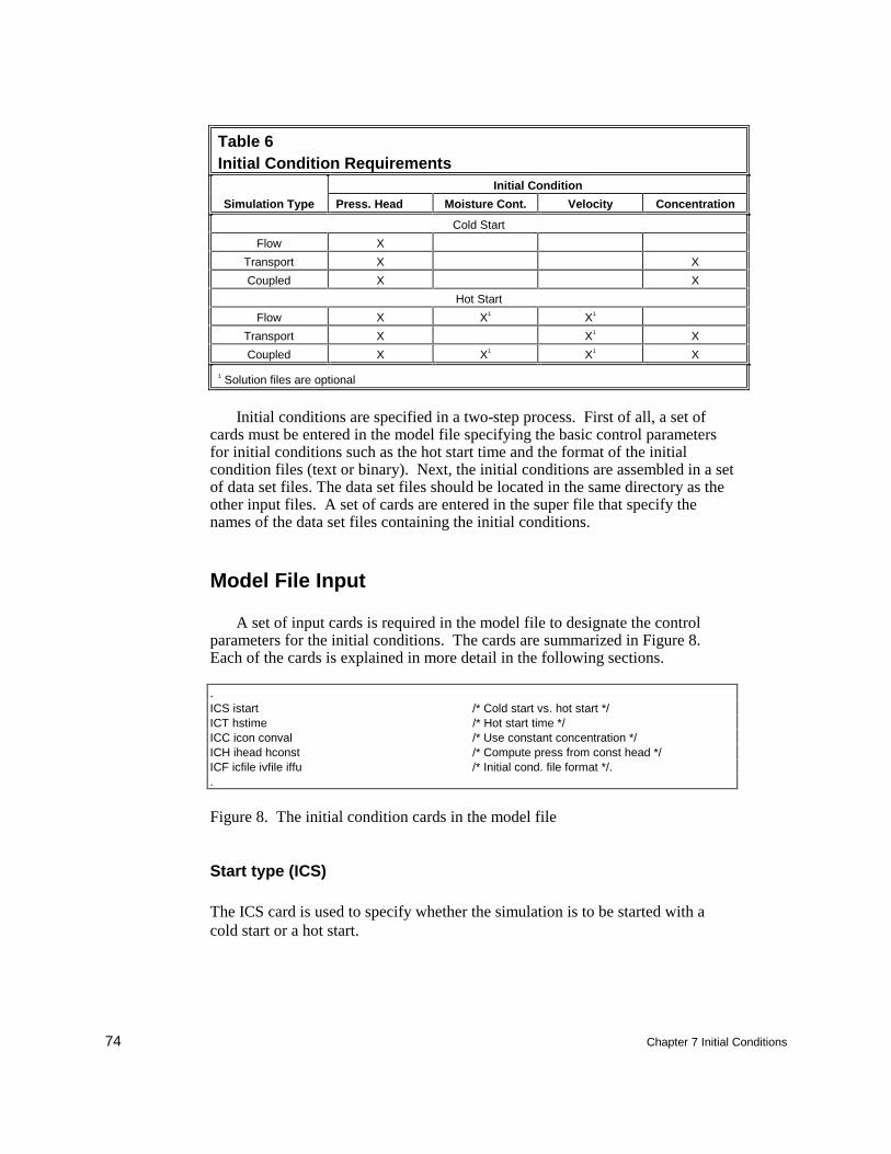
74 Chapter 7 Initial Conditions
Table 6Initial Condition Requirements
Initial Condition
Simulation Type Press. Head Moisture Cont. Velocity Concentration
Cold Start
Flow X
Transport X X
Coupled X X
Hot Start
Flow X X1 X1
Transport X X1 X
Coupled X X1 X1 X
1 Solution files are optional
Initial conditions are specified in a two-step process. First of all, a set ofcards must be entered in the model file specifying the basic control parametersfor initial conditions such as the hot start time and the format of the initialcondition files (text or binary). Next, the initial conditions are assembled in a setof data set files. The data set files should be located in the same directory as theother input files. A set of cards are entered in the super file that specify thenames of the data set files containing the initial conditions.
Model File Input
A set of input cards is required in the model file to designate the controlparameters for the initial conditions. The cards are summarized in Figure 8.Each of the cards is explained in more detail in the following sections.
.ICS istart /* Cold start vs. hot start */ICT hstime /* Hot start time */ICC icon conval /* Use constant concentration */ICH ihead hconst /* Compute press from const head */ICF icfile ivfile iffu /* Initial cond. file format */..
Figure 8. The initial condition cards in the model file
Start type (ICS)
The ICS card is used to specify whether the simulation is to be started with acold start or a hot start.
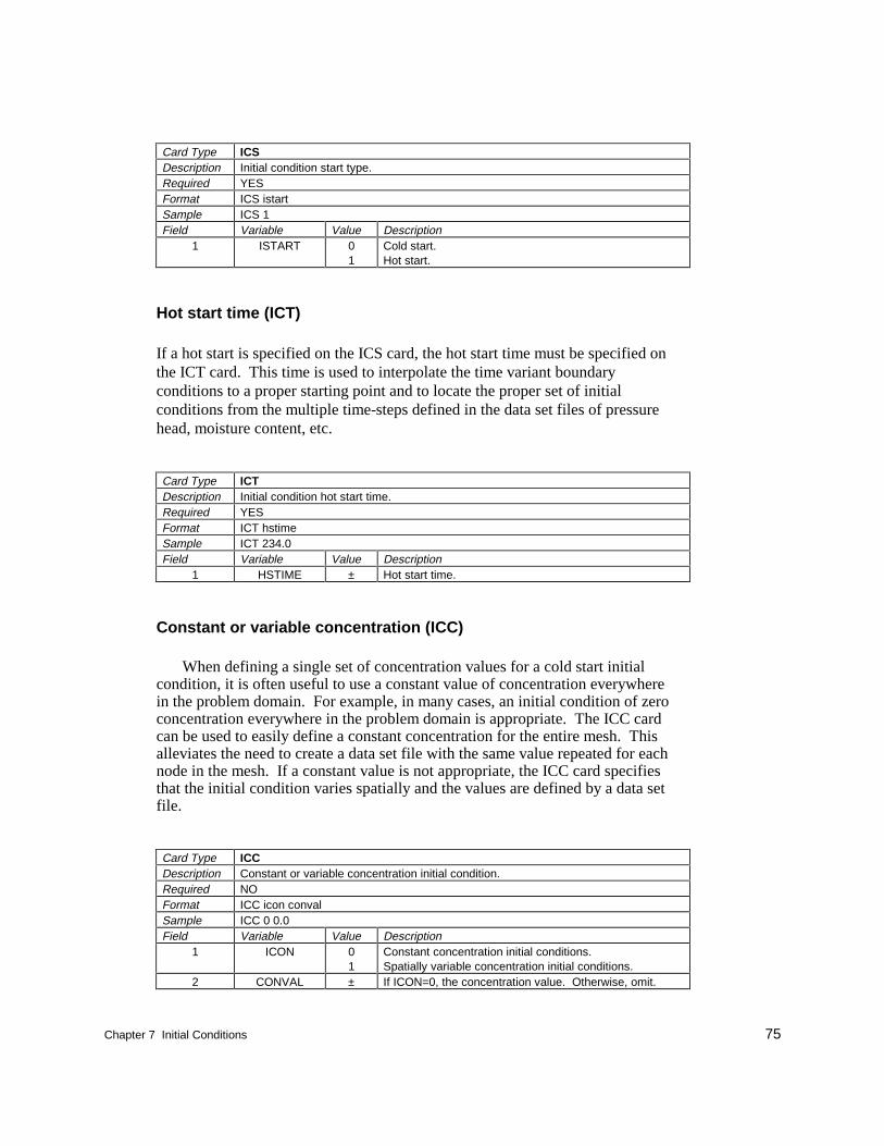
Chapter 7 Initial Conditions 75
Card Type ICSDescription Initial condition start type.Required YESFormat ICS istartSample ICS 1Field Variable Value Description
1 ISTART 01
Cold start.Hot start.
Hot start time (ICT)
If a hot start is specified on the ICS card, the hot start time must be specified onthe ICT card. This time is used to interpolate the time variant boundaryconditions to a proper starting point and to locate the proper set of initialconditions from the multiple time-steps defined in the data set files of pressurehead, moisture content, etc.
Card Type ICTDescription Initial condition hot start time.Required YESFormat ICT hstimeSample ICT 234.0Field Variable Value Description
1 HSTIME ± Hot start time.
Constant or variable concentration (ICC)
When defining a single set of concentration values for a cold start initialcondition, it is often useful to use a constant value of concentration everywherein the problem domain. For example, in many cases, an initial condition of zeroconcentration everywhere in the problem domain is appropriate. The ICC cardcan be used to easily define a constant concentration for the entire mesh. Thisalleviates the need to create a data set file with the same value repeated for eachnode in the mesh. If a constant value is not appropriate, the ICC card specifiesthat the initial condition varies spatially and the values are defined by a data setfile.
Card Type ICCDescription Constant or variable concentration initial condition.Required NOFormat ICC icon convalSample ICC 0 0.0Field Variable Value Description
1 ICON 01
Constant concentration initial conditions.Spatially variable concentration initial conditions.
2 CONVAL ± If ICON=0, the concentration value. Otherwise, omit.
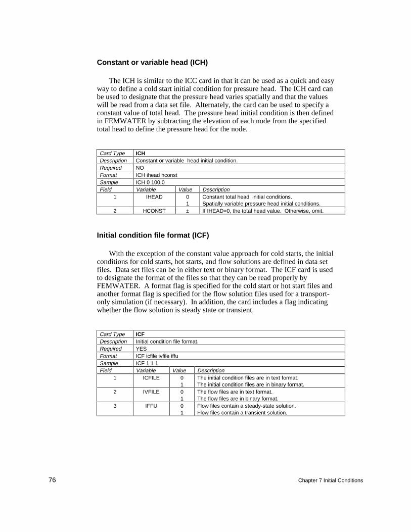
76 Chapter 7 Initial Conditions
Constant or variable head (ICH)
The ICH is similar to the ICC card in that it can be used as a quick and easyway to define a cold start initial condition for pressure head. The ICH card canbe used to designate that the pressure head varies spatially and that the valueswill be read from a data set file. Alternately, the card can be used to specify aconstant value of total head. The pressure head initial condition is then definedin FEMWATER by subtracting the elevation of each node from the specifiedtotal head to define the pressure head for the node.
Card Type ICHDescription Constant or variable head initial condition.Required NOFormat ICH ihead hconstSample ICH 0 100.0Field Variable Value Description
1 IHEAD 01
Constant total head initial conditions.Spatially variable pressure head initial conditions.
2 HCONST ± If IHEAD=0, the total head value. Otherwise, omit.
Initial condition file format (ICF)
With the exception of the constant value approach for cold starts, the initialconditions for cold starts, hot starts, and flow solutions are defined in data setfiles. Data set files can be in either text or binary format. The ICF card is usedto designate the format of the files so that they can be read properly byFEMWATER. A format flag is specified for the cold start or hot start files andanother format flag is specified for the flow solution files used for a transport-only simulation (if necessary). In addition, the card includes a flag indicatingwhether the flow solution is steady state or transient.
Card Type ICFDescription Initial condition file format.Required YESFormat ICF icfile ivfile iffuSample ICF 1 1 1Field Variable Value Description
1 ICFILE 01
The initial condition files are in text format.The initial condition files are in binary format.
2 IVFILE 01
The flow files are in text format.The flow files are in binary format.
3 IFFU 01
Flow files contain a steady-state solution.Flow files contain a transient solution.
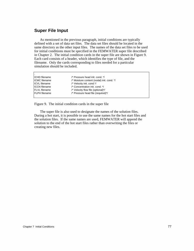
Chapter 7 Initial Conditions 77
Super File Input
As mentioned in the previous paragraph, initial conditions are typicallydefined with a set of data set files. The data set files should be located in thesame directory as the other input files. The names of the data set files to be usedfor initial conditions must be specified in the FEMWATER super file describedin Chapter 2. The initial condition cards in the super file are shown in Figure 9.Each card consists of a header, which identifies the type of file, and thefilename. Only the cards corresponding to files needed for a particularsimulation should be included.
.ICHD filename /* Pressure head init. cond. */ICMC filename /* Moisture content (nodal) init. cond. */ICVL filename /* Velocity init. cond.*/ICCN filename /* Concentration init. cond. */FLVL filename /* Velocity flow file (optional)*/FLPH filename /* Pressure head file (required)*/.
Figure 9. The initial condition cards in the super file
The super file is also used to designate the names of the solution files.During a hot start, it is possible to use the same names for the hot start files andthe solution files. If the same names are used, FEMWATER will append thesolution to the end of the hot start files rather than overwriting the files orcreating new files.

Chapter 8 Sample Applications 79
8 Sample Applications
The purpose of this section is to provide typical examples of FEMWATERapplications after which one might pattern new applications. Five examples areprovided that demonstrate different capabilities of FEMWATER. Eachdiscusses boundary and initial condition specification. The input files associatedwith these examples are distributed with the FEMWATER executable and can befound in the “examples” directory.
Problem 1: Steady-State Wellhead Protection
The initial support for developing FEMWATER within the GMS wasprovided by the AERL to advance the state of the art and provide practice indoing wellhead protection studies. As a result, of the technologies accepted bythe U.S. Environmental Protection Agency (EPA) to do wellhead protectionstudies, FEMWATER and GMS provide the most rigorous modeling tools.Several of these studies have been completed within the Department of Defenseand many more are in the planning phase.
The provided example illustrates how to use FEMWATER to conduct asteady-flow simulation for a wellhead protection problem. The left and rightsides of the model are bounded by freshwater head boundary conditions (Figure10). The front and back of the model are groundwater divides represented by no-flux boundary conditions. The bottom of the model is an impervious stratumthat does not allow significant amounts of water to leave the model. This iscommonly located at aquicludes or deep aquitards. The pressure head isassumed to be hydrostatic throughout the model with water table initialconditions assumed to be a constant 12.0 m. The following boundary conditionsare given: constant head of 12.0 m on the left side of the model, 13.0 m on theright side of the model, and no flux on the front and back of the model.Seventeen pumping wells are located in the top layer of coarse sand near themiddle of the region. The pumping rate of the wells is a constant 0.25 m3/hr.One of the wells could be increased to determine the effect on the other wells.The head tolerance is 0.001 m. The pointwise iterative solver is used to solvethe matrix equations. The computational mesh consists of 4,000 elements and3,507 nodes.
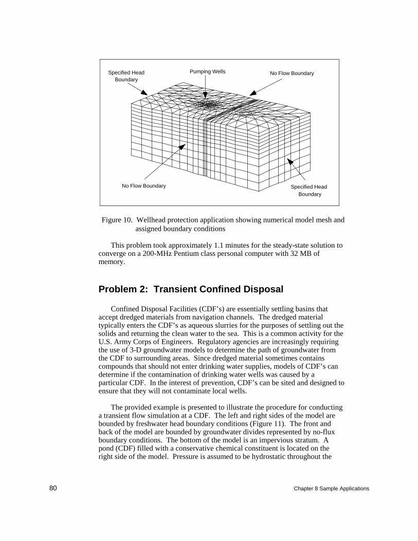
80 Chapter 8 Sample Applications
No Flow BoundaryPumping WellsSpecified HeadBoundary
Specified HeadBoundary
No Flow Boundary
Figure 10. Wellhead protection application showing numerical model mesh andassigned boundary conditions
This problem took approximately 1.1 minutes for the steady-state solution toconverge on a 200-MHz Pentium class personal computer with 32 MB ofmemory.
Problem 2: Transient Confined Disposal
Confined Disposal Facilities (CDF’s) are essentially settling basins thataccept dredged materials from navigation channels. The dredged materialtypically enters the CDF’s as aqueous slurries for the purposes of settling out thesolids and returning the clean water to the sea. This is a common activity for theU.S. Army Corps of Engineers. Regulatory agencies are increasingly requiringthe use of 3-D groundwater models to determine the path of groundwater fromthe CDF to surrounding areas. Since dredged material sometimes containscompounds that should not enter drinking water supplies, models of CDF’s candetermine if the contamination of drinking water wells was caused by aparticular CDF. In the interest of prevention, CDF’s can be sited and designed toensure that they will not contaminate local wells.
The provided example is presented to illustrate the procedure for conductinga transient flow simulation at a CDF. The left and right sides of the model arebounded by freshwater head boundary conditions (Figure 11). The front andback of the model are bounded by groundwater divides represented by no-fluxboundary conditions. The bottom of the model is an impervious stratum. Apond (CDF) filled with a conservative chemical constituent is located on theright side of the model. Pressure is assumed to be hydrostatic throughout the
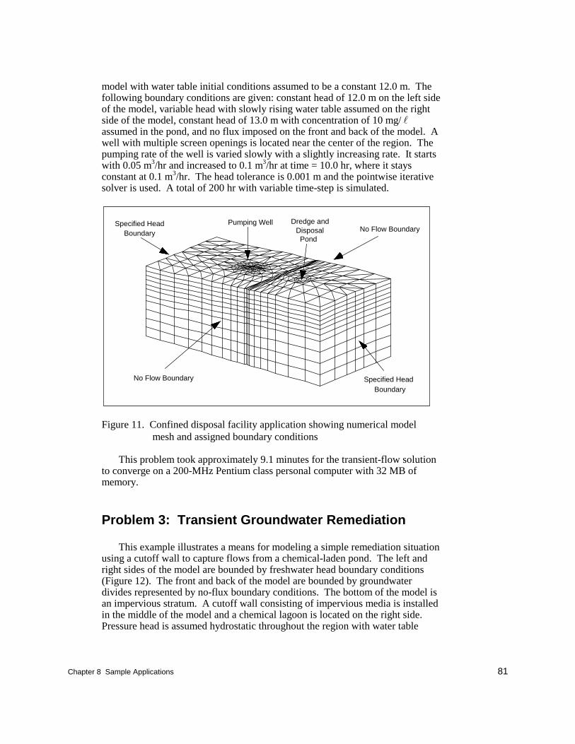
Chapter 8 Sample Applications 81
model with water table initial conditions assumed to be a constant 12.0 m. Thefollowing boundary conditions are given: constant head of 12.0 m on the left sideof the model, variable head with slowly rising water table assumed on the rightside of the model, constant head of 13.0 m with concentration of 10 mg/ lassumed in the pond, and no flux imposed on the front and back of the model. Awell with multiple screen openings is located near the center of the region. Thepumping rate of the well is varied slowly with a slightly increasing rate. It startswith 0.05 m3/hr and increased to 0.1 m3/hr at time = 10.0 hr, where it staysconstant at 0.1 m3/hr. The head tolerance is 0.001 m and the pointwise iterativesolver is used. A total of 200 hr with variable time-step is simulated.
PondDisposal
Dredge andNo Flow Boundary
Pumping WellSpecified HeadBoundary
Specified HeadBoundary
No Flow Boundary
Figure 11. Confined disposal facility application showing numerical modelmesh and assigned boundary conditions
This problem took approximately 9.1 minutes for the transient-flow solutionto converge on a 200-MHz Pentium class personal computer with 32 MB ofmemory.
Problem 3: Transient Groundwater Remediation
This example illustrates a means for modeling a simple remediation situationusing a cutoff wall to capture flows from a chemical-laden pond. The left andright sides of the model are bounded by freshwater head boundary conditions(Figure 12). The front and back of the model are bounded by groundwaterdivides represented by no-flux boundary conditions. The bottom of the model isan impervious stratum. A cutoff wall consisting of impervious media is installedin the middle of the model and a chemical lagoon is located on the right side.Pressure head is assumed hydrostatic throughout the region with water table
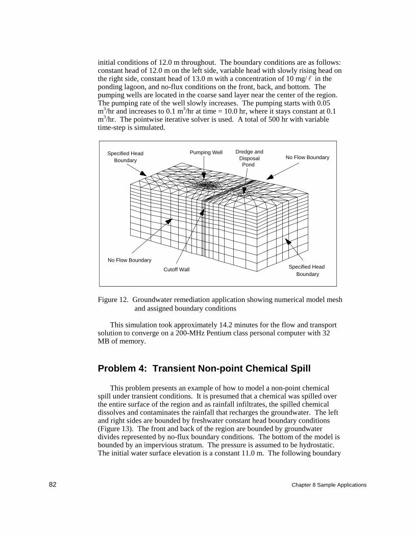
82 Chapter 8 Sample Applications
initial conditions of 12.0 m throughout. The boundary conditions are as follows:constant head of 12.0 m on the left side, variable head with slowly rising head onthe right side, constant head of 13.0 m with a concentration of 10 mg/ l in theponding lagoon, and no-flux conditions on the front, back, and bottom. Thepumping wells are located in the coarse sand layer near the center of the region.The pumping rate of the well slowly increases. The pumping starts with 0.05m3/hr and increases to 0.1 m3/hr at time = 10.0 hr, where it stays constant at 0.1m3/hr. The pointwise iterative solver is used. A total of 500 hr with variabletime-step is simulated.
Cutoff Wall
PondDisposal
Dredge andNo Flow Boundary
Pumping WellSpecified HeadBoundary
Specified HeadBoundary
No Flow Boundary
Figure 12. Groundwater remediation application showing numerical model meshand assigned boundary conditions
This simulation took approximately 14.2 minutes for the flow and transportsolution to converge on a 200-MHz Pentium class personal computer with 32MB of memory.
Problem 4: Transient Non-point Chemical Spill
This problem presents an example of how to model a non-point chemicalspill under transient conditions. It is presumed that a chemical was spilled overthe entire surface of the region and as rainfall infiltrates, the spilled chemicaldissolves and contaminates the rainfall that recharges the groundwater. The leftand right sides are bounded by freshwater constant head boundary conditions(Figure 13). The front and back of the region are bounded by groundwaterdivides represented by no-flux boundary conditions. The bottom of the model isbounded by an impervious stratum. The pressure is assumed to be hydrostatic.The initial water surface elevation is a constant 11.0 m. The following boundary
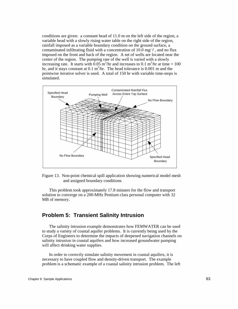
Chapter 8 Sample Applications 83
conditions are given: a constant head of 11.0 m on the left side of the region, avariable head with a slowly rising water table on the right side of the region,rainfall imposed as a variable boundary condition on the ground surface, acontaminated infiltrating fluid with a concentration of 10.0 mg/ l , and no fluximposed on the front and back of the region. A set of wells are located near thecenter of the region. The pumping rate of the well is varied with a slowlyincreasing rate. It starts with 0.05 m3/hr and increases to 0.1 m3/hr at time = 100hr, and it stays constant at 0.1 m3/hr. The head tolerance is 0.001 m and thepointwise iterative solver is used. A total of 150 hr with variable time-steps issimulated.
Across Entire Top SurfaceContaminated Rainfall Flux
No Flow Boundary
Pumping WellSpecified Head
Boundary
Specified HeadBoundary
No Flow Boundary
Figure 13. Non-point chemical spill application showing numerical model meshand assigned boundary conditions
This problem took approximately 17.8 minutes for the flow and transportsolution to converge on a 200-MHz Pentium class personal computer with 32MB of memory.
Problem 5: Transient Salinity Intrusion
The salinity intrusion example demonstrates how FEMWATER can be usedto study a variety of coastal aquifer problems. It is currently being used by theCorps of Engineers to determine the impacts of deepened navigation channels onsalinity intrusion in coastal aquifers and how increased groundwater pumpingwill affect drinking water supplies.
In order to correctly simulate salinity movement in coastal aquifers, it isnecessary to have coupled flow and density-driven transport. The exampleproblem is a schematic example of a coastal salinity intrusion problem. The left
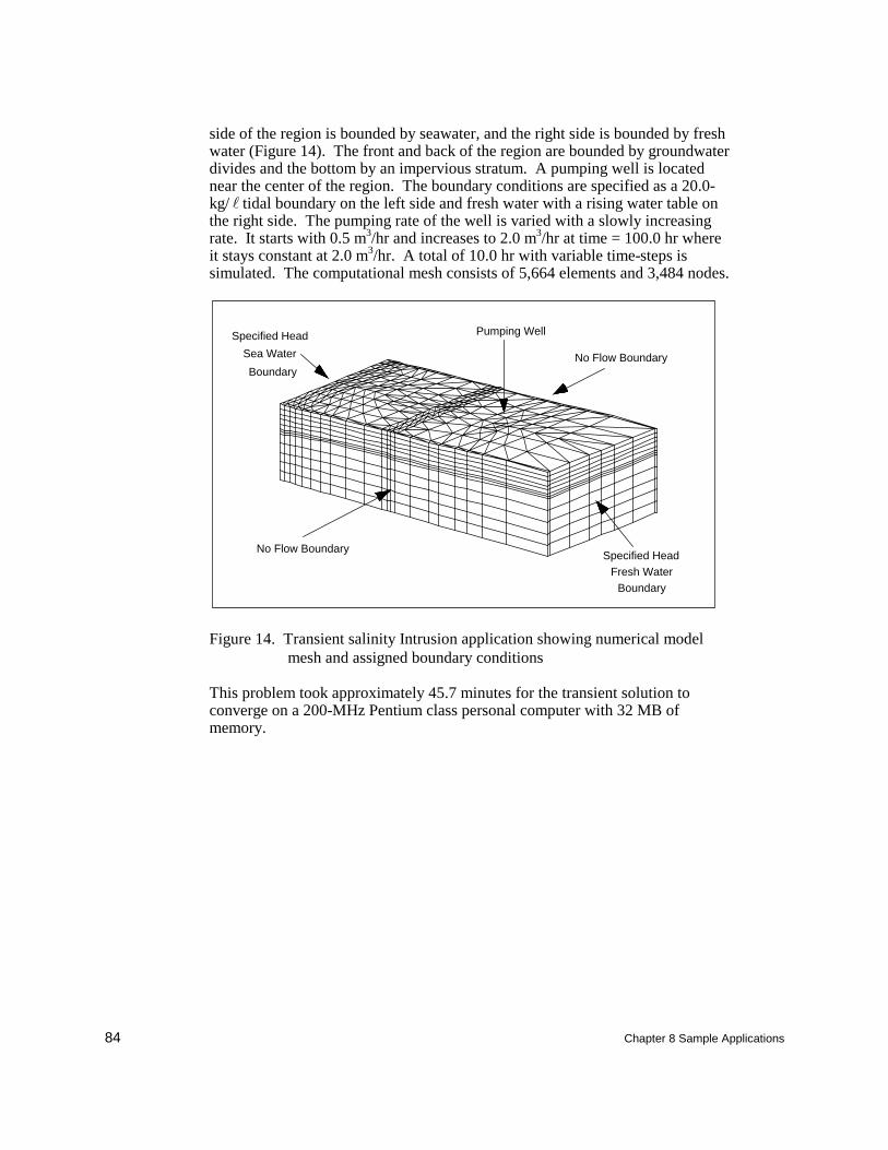
84 Chapter 8 Sample Applications
side of the region is bounded by seawater, and the right side is bounded by freshwater (Figure 14). The front and back of the region are bounded by groundwaterdivides and the bottom by an impervious stratum. A pumping well is locatednear the center of the region. The boundary conditions are specified as a 20.0-kg/ l tidal boundary on the left side and fresh water with a rising water table onthe right side. The pumping rate of the well is varied with a slowly increasingrate. It starts with 0.5 m3/hr and increases to 2.0 m3/hr at time = 100.0 hr whereit stays constant at 2.0 m3/hr. A total of 10.0 hr with variable time-steps issimulated. The computational mesh consists of 5,664 elements and 3,484 nodes.
No Flow Boundary
Pumping WellSpecified Head
Sea Water
Boundary
Specified HeadFresh Water
Boundary
No Flow Boundary
Figure 14. Transient salinity Intrusion application showing numerical modelmesh and assigned boundary conditions
This problem took approximately 45.7 minutes for the transient solution toconverge on a 200-MHz Pentium class personal computer with 32 MB ofmemory.
References 85
References
Carsel, R. F., and Parrish, R. S. (1988). “Developing joint probabilitydistributions of soil-water retention characteristics,” Water ResourcesResearch 24(5),755-769.
Clough, R. W. (1971). “Analysis of structural vibrations and dynamicresponse.” Recent advances in matrix methods of structural analysis anddesign: Proceedings, United States-Japan Seminar on Matrix Methods ofStructural Analysis and Design. R. H. Gallagher, Y. Yamada, and J. T. Oden,ed., University of Alabama Press, Huntsville, AL.
Engineering Computer Graphics Laboratory (1996). The Department ofDefense Groundwater Modeling System Reference Manual. Brigham YoungUniversity, Provo, UT.
Freeze, R. A. (1972a). “Role of subsurface flow in generating surface runoff: 1.Base flow contribution to channel flow,” Water Resources Research 8, 609-623.
Freeze, R. A. (1972b). “Role of subsurface flow in generating surface runoff: 2.Upstream source areas,” Water Resources Research 8, 609-623.
Frind, E. O. (1982). “Simulation of long-term transient density-dependenttransport in groundwater,” Advances in Water Resources 5(2), 73-88.
Galeati, G., Gambolati, G., and Neuman, S. P. (1992). “Coupled and partiallycoupled Eulerian-Langrangian model of freshwater-seawater mixing,” WaterResources Research 28(1), 149-165.
Istok, J. D. (1989). Groundwater modeling by the finite element method.American Geophysical Union, Washington, DC.
Long, R. R. (1961). Mechanics of solids and fluids. Prentice-Hall, EnglewoodCliffs, NJ.
Morse, P. M., and Feshbach, H. (1978). Methods of theoretical physics.
86 References
McGraw-Hill, New York.
Nguyen, V. V., Gray, W. G., Pinder, G. F., Botha, J. F., and Crefar, D. A. (1982).“A theoretical investigation on the transport of chemicals in reactive porousmedia,” Water Resources Research 18(4), 1149-1156.
Owczarek, J. A. (1964). Fundamentals of gas dynamics. InternationalTextbook, Scranton, PA.
van Genuchten, M. T. (1980). “A closed-form equation for predicting thehydraulic conductivity of unsaturated soils,” Soil Sci. Soc. J. 44, 892-898.
Wang, J. D., and Conner, J. J. (1975). “Mathematical modeling of near-coastalcirculation,” Report No. MITSG 75-13, Massachusetts Institute ofTechnology, Cambridge, MA, 1975.
Yeh, G. T. (1985). “Comparison of successive iteration and direct methods tofinite element equations of aquifer contaminant transport,” Water ResourceRes.21(3), 272-280.
Yeh, G. T. (1987a). “FEMWATER: A finite element model of water flowthrough saturated-unsaturated porous media, First Revision,” ORNL-5567/R1, Oak Ridge National Laboratory, Oak Ridge, TN.
Yeh, G. T. (1987b). “3DFEMWATER: A three-dimensional finite elementmodel of water flow through saturated-unsaturated media,” ORNL-6368, OakRidge National Laboratory, Oak Ridge, TN.
Yeh, G. T. (1990). “3DLEWASTE: A hybrid Lagrangian-Eulerian finite elementmodel of waste transport through saturated-unsaturated media,” PSUTechnical Report, Department of Civil Engineering, The Pennsylvania StateUniversity, University Park, PA.
Yeh, G. T. (1991). “Class notes: CE597D: Computational subsurface hydrologyPart I,” Fall semester 1991, The Pennsylvania State University, UniversityPark, PA.
Yeh, G. T. (1992). “Class notes: CE597C: Computational subsurface hydrologyPart II,” Spring semester 1992, The Pennsylvania State University, UniversityPark, PA.
Yeh, G. T., and Tripathi, V. S. (1987). “Strategies in modeling transport ofreactive multi-chemical components.” Groundwater and the environment:Proceedings, International Groundwater Conference. Faculty of Engineeringand Faculty of Physical and Applied Science, Universitti KebangsaanMalaysis, Kuala Lampur, Malaysia, E26-E36.

References 87
Yeh, G. T., and Ward, D. S. (1981). “FEMWASTE: A finite element model oftransport through saturated-unsaturated porous media,” ORNL-5601, OakRidge National Laboratory, Oak Ridge, TN.
Yeh, G. T., and Ward, D. S. (1980). “FEMWASTE: A finite element model ofwater flow through saturated-unsaturated porous media,” ORNL-5567, OakRidge National Laboratory, Oak Ridge, TN.

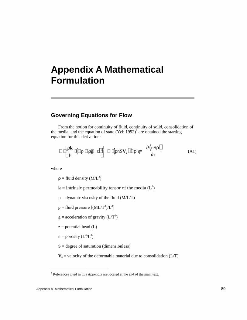
Appendix A Mathematical Formulation 89
Appendix A MathematicalFormulation
Governing Equations for Flow
From the notion for continuity of fluid, continuity of solid, consolidation ofthe media, and the equation of state (Yeh 1992)1 are obtained the startingequation for this derivation:
( ) ( ) ( )∇ ⋅ ⋅ ∇ + ∇
− ∇ ⋅ + =∗ρ
µρ ρ ρ
∂ ρ∂
kVsp g z nS q
nS
t(A1)
where
ρ = fluid density (M/L3)
k = intrinsic permeability tensor of the media (L2)
µ = dynamic viscosity of the fluid (M/L/T)
p = fluid pressure [(ML/T2)/L2]
g = acceleration of gravity (L/T2)
z = potential head (L)
n = porosity (L3/L3)
S = degree of saturation (dimensionless)
Vs = velocity of the deformable material due to consolidation (L/T)
1 References cited in this Appendix are located at the end of the main text.
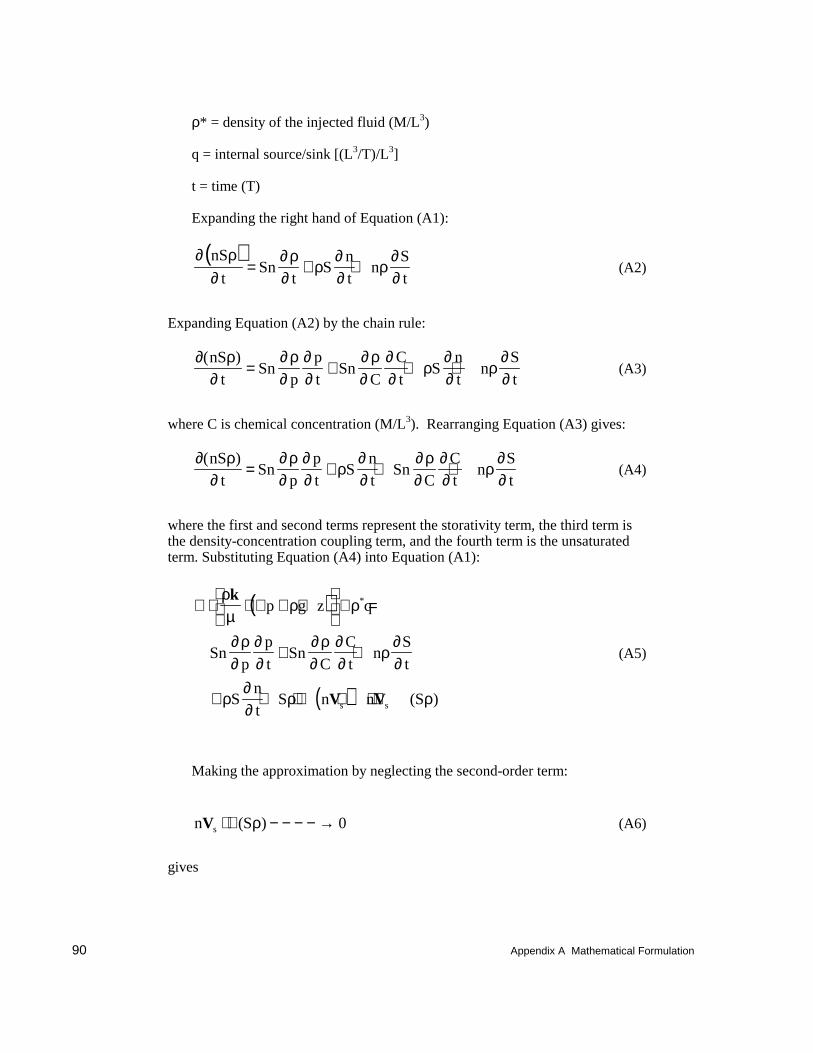
90 Appendix A Mathematical Formulation
ρ* = density of the injected fluid (M/L3)
q = internal source/sink [(L3/T)/L3]
t = time (T)
Expanding the right hand of Equation (A1):
( )∂ ρ∂
∂ρ∂
ρ∂∂
ρ∂∂
nS
tSn
tS
nt
nSt
= + + (A2)
Expanding Equation (A2) by the chain rule:
∂ ρ∂
∂ ρ∂
∂∂
∂ ρ∂
∂∂
ρ∂∂
ρ∂∂
( )nSt
Snp
p
tSn
C
C
tS
n
tn
S
t= + + + (A3)
where C is chemical concentration (M/L3). Rearranging Equation (A3) gives:
∂ ρ∂
∂ρ∂
∂∂
ρ∂∂
∂ρ∂
∂∂
ρ∂∂
( )nSt
Snp
pt
Snt
SnC
Ct
nSt
= + + + (A4)
where the first and second terms represent the storativity term, the third term isthe density-concentration coupling term, and the fourth term is the unsaturatedterm. Substituting Equation (A4) into Equation (A1):
( )
( )
∇ ⋅ ⋅ ∇ + ∇
+ =
+ +
+ + ⋅ + ⋅ ∇
ρµ
ρ ρ
∂ρ∂
∂∂
∂ρ∂
∂∂
ρ∂∂
ρ∂∂
ρ∇ ρ
k
V V
p g z q
Snp
p
tSn
C
C
tn
S
t
Sn
tS n ns s
*
(S )
(A5)
Making the approximation by neglecting the second-order term:
n sV ⋅ ∇ − − − − →(S )ρ 0 (A6)
gives
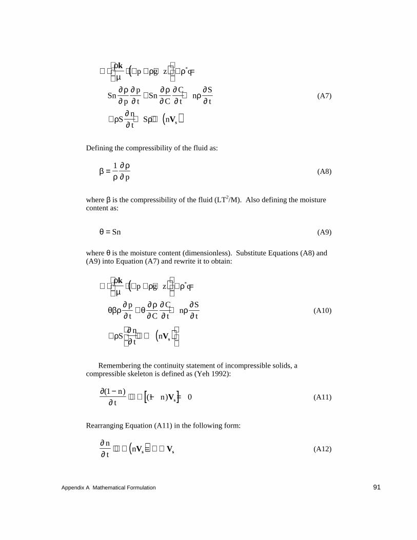
Appendix A Mathematical Formulation 91
( )
( )
∇ ⋅ ⋅ ∇ + ∇
+ =
+ +
+ + ⋅
ρµ
ρ ρ
∂ ρ∂
∂∂
∂ ρ∂
∂∂
ρ∂∂
ρ∂∂
ρ∇
k
Vs
p g z q
Snp
p
tSn
C
C
tn
S
t
Sn
tS n
*
(A7)
Defining the compressibility of the fluid as:
βρ
∂ ρ∂
=1
p(A8)
where β is the compressibility of the fluid (LT2/M). Also defining the moisturecontent as:
θ = Sn (A9)
where θ is the moisture content (dimensionless). Substitute Equations (A8) and(A9) into Equation (A7) and rewrite it to obtain:
( )
( )
∇ ⋅ ⋅ ∇ + ∇
+ =
+ +
+ + ∇ ⋅
ρµ
ρ ρ
θβρ∂∂
θ∂ρ∂
∂∂
ρ∂∂
ρ∂∂
k
Vs
p g z q
pt C
Ct
nSt
Sn
tn
*
(A10)
Remembering the continuity statement of incompressible solids, acompressible skeleton is defined as (Yeh 1992):
[ ]∂∂
( )( )
11 0
−+ ∇ ⋅ − =
nt
n Vs (A11)
Rearranging Equation (A11) in the following form:
( )∂∂
n
tn+ ∇ ⋅ = ∇ ⋅V Vss (A12)
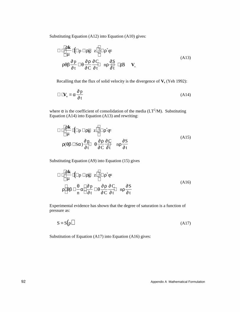
92 Appendix A Mathematical Formulation
Substituting Equation (A12) into Equation (A10) gives:
( )∇ ⋅ ⋅ ∇ + ∇
+ =
+ + + ∇ ⋅
ρµ
ρ ρ
ρθβ∂∂
θ∂ ρ∂
∂∂
ρ∂∂
ρ
k
V
p g z q
p
t C
C
tn
S
tS s
*
(A13)
Recalling that the flux of solid velocity is the divergence of Vs (Yeh 1992):
∇ ⋅ =Vs α∂∂
pt
(A14)
where α is the coefficient of consolidation of the media (LT2/M). SubstitutingEquation (A14) into Equation (A13) and rewriting:
( )∇ ⋅ ⋅ ∇ + ∇
+ =
+ + +
ρµ
ρ ρ
ρ θβ α∂∂
θ∂ρ∂
∂∂
ρ∂∂
kp g z q
Sp
t C
C
tn
S
t
*
( )
(A15)
Substituting Equation (A9) into Equation (15) gives
( )∇ ⋅ ⋅ ∇ + ∇
+ =
+
+ +
ρµ
ρ ρ
ρ θβθ
α∂∂
θ∂ ρ∂
∂∂
ρ∂∂
kp g z q
n
p
t C
C
tn
S
t
*
(A16)
Experimental evidence has shown that the degree of saturation is a function ofpressure as:
( )S S p= (A17)
Substitution of Equation (A17) into Equation (A16) gives:
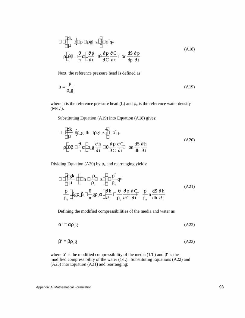
Appendix A Mathematical Formulation 93
( )∇ ⋅ ⋅ ∇ + ∇
+ =
+
+ +
ρµ
ρ ρ
ρ θβθ
α∂∂
θ∂ρ∂
∂∂
ρ∂∂
kp g z q
n
p
t C
C
tn
dS
dp
p
t
*
(A18)
Next, the reference pressure head is defined as:
hpgo
=ρ
(A19)
where h is the reference pressure head (L) and ρo is the reference water density(M/L3).
Substituting Equation (A19) into Equation (A18) gives:
( )∇ ⋅ ⋅ ∇ + ∇
+ =
+
+ +
ρµ
ρ ρ ρ
ρ θβθ
α ρ∂∂
θ∂ρ∂
∂∂
ρ∂∂
ko
o
g h g z q
ng
h
t C
C
tn
dS
dh
h
t
*
(A20)
Dividing Equation (A20) by ρo and rearranging yields:
∇ ⋅ ⋅ ∇ + ∇
+ =
+
+ +
∗ρµ
ρρ
ρρ
ρρ
θ ρ βθ
ρ α∂∂
θρ
∂ ρ∂
∂∂
ρρ
∂∂
gh z q
gn
gh
t C
C
tn
dS
dh
h
t
o o
oo o
o o
k
(A21)
Defining the modified compressibilities of the media and water as
′ =α αρog (A22)
′ =β βρog (A23)
where α′ is the modified compressibility of the media (1/L) and β′ is themodified compressibility of the water (1/L). Substituting Equations (A22) and(A23) into Equation (A21) and rearranging:
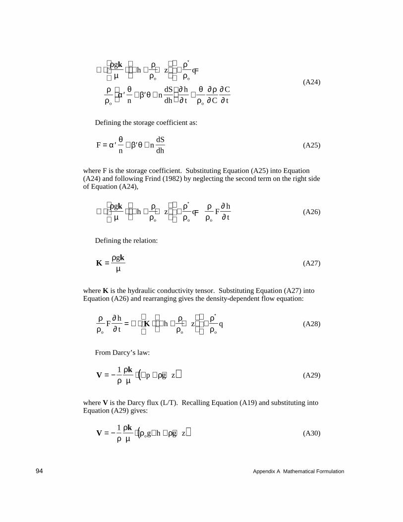
94 Appendix A Mathematical Formulation
∇ ⋅ ⋅ ∇ + ∇
+ =
′ + ′ +
+
∗ρµ
ρρ
ρρ
ρρ
αθ
β θ∂∂
θρ
∂ρ∂
∂∂
gh z q
nn
dS
dh
h
t C
C
t
o o
o o
k
(A24)
Defining the storage coefficient as:
Fn
ndSdh
= ′ + ′ +αθ
β θ (A25)
where F is the storage coefficient. Substituting Equation (A25) into Equation(A24) and following Frind (1982) by neglecting the second term on the right sideof Equation (A24),
∇ ⋅ ⋅ ∇ + ∇
+ =
∗ρµ
ρρ
ρρ
ρρ
∂∂
gh z q F
h
to o o
k(A26)
Defining the relation:
Kk
=ρ
µg
(A27)
where K is the hydraulic conductivity tensor. Substituting Equation (A27) intoEquation (A26) and rearranging gives the density-dependent flow equation:
ρρ
∂∂
ρρ
ρρo o o
Fh
th z q= ∇ ⋅ ⋅ ∇ + ∇
+
∗
K (A28)
From Darcy’s law:
( )Vk
= − ⋅ ∇ + ∇1ρ
ρµ
ρp g z (A29)
where V is the Darcy flux (L/T). Recalling Equation (A19) and substituting intoEquation (A29) gives:
( )Vk
= − ⋅ ∇ + ∇1ρ
ρµ
ρ ρog h g z (A30)
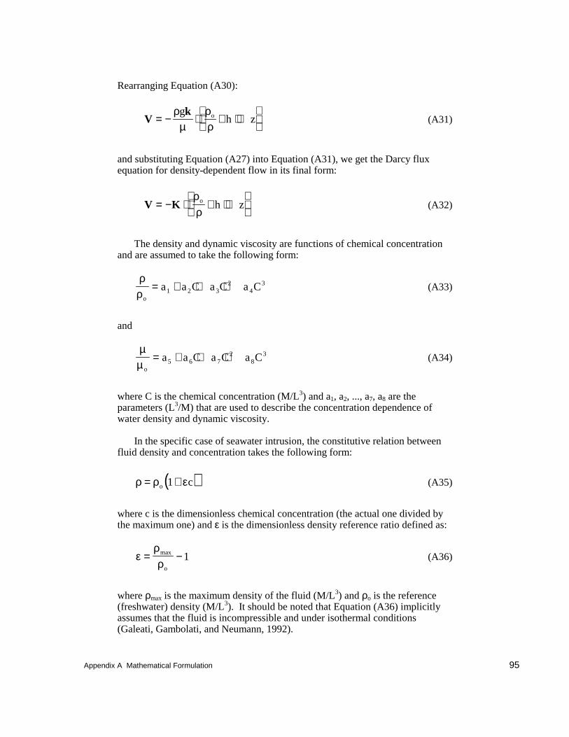
Appendix A Mathematical Formulation 95
Rearranging Equation (A30):
Vk
= − ⋅ ∇ + ∇
ρµ
ρρ
gh zo (A31)
and substituting Equation (A27) into Equation (A31), we get the Darcy fluxequation for density-dependent flow in its final form:
V K= − ⋅ ∇ + ∇
ρρ
o h z (A32)
The density and dynamic viscosity are functions of chemical concentrationand are assumed to take the following form:
ρρo
a a C a C a C= + + +1 2 32
43 (A33)
and
µµ o
a a C a C a C= + + +5 6 72
83 (A34)
where C is the chemical concentration (M/L3) and a1, a2, ..., a7, a8 are theparameters (L3/M) that are used to describe the concentration dependence ofwater density and dynamic viscosity.
In the specific case of seawater intrusion, the constitutive relation betweenfluid density and concentration takes the following form:
( )ρ ρ ε= +o c1 (A35)
where c is the dimensionless chemical concentration (the actual one divided bythe maximum one) and ε is the dimensionless density reference ratio defined as:
ερρ
= −max
o
1 (A36)
where ρmax is the maximum density of the fluid (M/L3) and ρo is the reference(freshwater) density (M/L3). It should be noted that Equation (A36) implicitlyassumes that the fluid is incompressible and under isothermal conditions(Galeati, Gambolati, and Neumann, 1992).
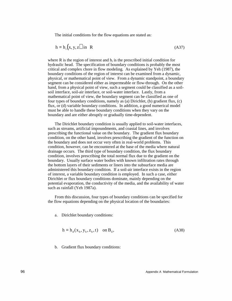
96 Appendix A Mathematical Formulation
The initial conditions for the flow equations are stated as:
( )h h x y z in Ri= , , (A37)
where R is the region of interest and hi is the prescribed initial condition forhydraulic head. The specification of boundary conditions is probably the mostcritical and complex chore in flow modeling. As explained by Yeh (1987), theboundary conditions of the region of interest can be examined from a dynamic,physical, or mathematical point of view. From a dynamic standpoint, a boundarysegment can be considered either as impermeable or flow-through. On the otherhand, from a physical point of view, such a segment could be classified as a soil-soil interface, soil-air interface, or soil-water interface. Lastly, from amathematical point of view, the boundary segment can be classified as one offour types of boundary conditions, namely as (a) Dirichlet, (b) gradient flux, (c)flux, or (d) variable boundary conditions. In addition, a good numerical modelmust be able to handle these boundary conditions when they vary on theboundary and are either abruptly or gradually time-dependent.
The Dirichlet boundary condition is usually applied to soil-water interfaces,such as streams, artificial impoundments, and coastal lines, and involvesprescribing the functional value on the boundary. The gradient flux boundarycondition, on the other hand, involves prescribing the gradient of the function onthe boundary and does not occur very often in real-world problems. Thiscondition, however, can be encountered at the base of the media where naturaldrainage occurs. The third type of boundary condition, the flux boundarycondition, involves prescribing the total normal flux due to the gradient on theboundary. Usually surface water bodies with known infiltration rates throughthe bottom layers of their sediments or liners into the subsurface media areadministered this boundary condition. If a soil-air interface exists in the regionof interest, a variable boundary condition is employed. In such a case, eitherDirichlet or flux boundary conditions dominate, mainly depending on thepotential evaporation, the conductivity of the media, and the availability of watersuch as rainfall (Yeh 1987a).
From this discussion, four types of boundary conditions can be specified forthe flow equations depending on the physical location of the boundaries:
a. Dirichlet boundary conditions:
h h x y z t on Bd b b b d= ( , , , ) , (A38)
b. Gradient flux boundary conditions:
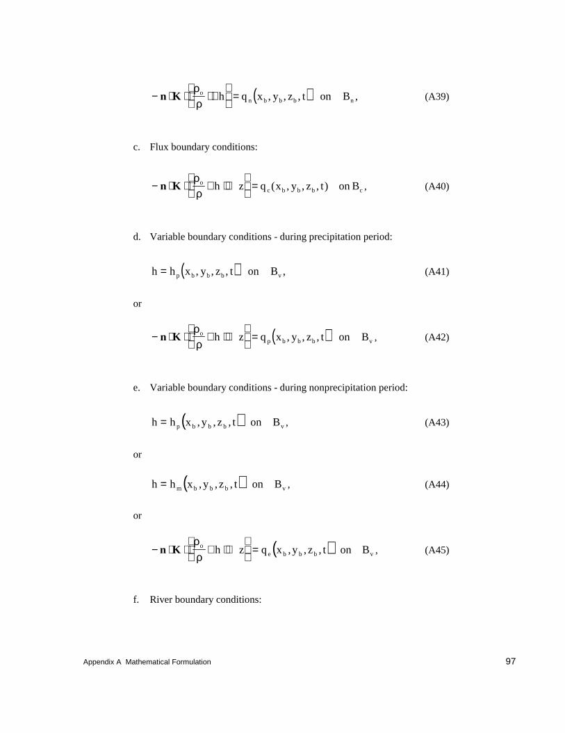
Appendix A Mathematical Formulation 97
( )− ⋅ ⋅ ⋅ ∇
=n K
ρρ
on b b b nh q x y z t on B, , , , (A39)
c. Flux boundary conditions:
− ⋅ ⋅ ∇ + ∇
=n K
ρρ
oc b b b ch z q x y z t on B( , , , ) , (A40)
d. Variable boundary conditions - during precipitation period:
( )h h x y z t on Bp b b b v= , , , , (A41)
or
( )− ⋅ ⋅ ∇ + ∇
=n K
ρρ
op b b b vh z q x y z t on B, , , , (A42)
e. Variable boundary conditions - during nonprecipitation period:
( )h h x y z t on Bp b b b v= , , , , (A43)
or
( )h h x y z t on Bm b b b v= , , , , (A44)
or
( )− ⋅ ⋅ ∇ + ∇
=n K
ρρ
oe b b b vh z q x y z t on B, , , , (A45)
f. River boundary conditions:
98 Appendix A Mathematical Formulation
( )− ⋅ ⋅ ∇ + ∇
= − −n K
ρρ
o R
RR rh z
K
bh h on B , (A46)
where
n = outward unit vector normal to the boundary
(xb, yb, zb) = spatial coordinate on the boundary
hd = Dirichlet functional value
qh = Gradient flux value
qc = Flux value
Bd = Dirichlet boundary
Bn = Gradient flux boundary
Bc = Flux boundary
Bv = variable boundary
hp = ponding depth on the variable boundary
qp = throughfall of precipitation on the variable boundary
hm = minimum pressure on the variable boundary
qe = evaporation rate (potential evaporation) on the variable boundary
KR = hydraulic conductivity of the river bottom sediment layer
bR = thickness of the river bottom sediment layer
hR = depth of the river bottom measured from the river surface.
Note that only one of Equations (A41)-(A45) is utilized at any point on thevariable boundary at any time.
Governing Equations for Transport
The governing equations for material transport through groundwater systemsare derived based on the laws of continuity of mass and flux. The majorprocesses that are included are advection, dispersion/diffusion, decay,adsorption, biodegradation through both liquid and solid phases, the
Appendix A Mathematical Formulation 99
compressibility of media, as well as source(s)/sink(s). Let C be the dissolvedconcentration and S be the adsorbed concentration. The governing equation ofthe spatial-temporal distribution of dissolved concentrations can be obtained byapplying this principle of mass balance in integral form as follows:
( ) ( )
( )
( )
D
DtC S dv n C d
d K C K S dv
C S dv m dv
bv
w b sv
bv v
θ ρ θ
θ ρ
λ θ ρ
+ = − ⋅
− ⋅ − +
− + +
∫ ∫
∫ ∫
∫ ∫
V
n J
fs Γ
ΓΓ
Γ
(A47)
where
v = material volume containing constant amount of media (L3)
C = dissolved concentration (M/L3)
S = adsorbed concentration (M/M)
ρb = bulk density of the medium (M/L3)
Γ = surface enclosing the material volume v (L2)
n = outward unit vector normal to the surface G
Vfs = fluid velocity relative to the solid (L/T)
J = surface flux with respect to fluid velocity V fs [(M/T)/L2]
Kw = first-order biodegradation rate constant through dissolved phase (1/T)
Ks = first-order biodegradation rate constant through adsorbed phase (1/T)
λ = decay constant (1/T)
m = external source/sink rate per medium volume [(M/L3)/T]
By the Reynolds transport theorem (Owczarek 1964), Equation (A47) can bewritten as
( ) ( )[ ] ( )
( ) ( )
∂ θ ρ∂
θ ρ θ
θ ρ λ θ ρ
C S
tdv C S d C d
d K C K S dv C S dv m dv
bb
v
w b sv
bv v
++ ⋅ + + ⋅ =
− ⋅ − + − + +
∫ ∫∫
∫ ∫ ∫ ∫
n V n V
n J
s fsΓ Γ
ΓΓ Γ
Γ
(A48)
100 Appendix A Mathematical Formulation
where Vs is the velocity of the solid. The fluid velocity relative to the solid Vfs
and Darcy velocity V are related to each other by
V Vfs= θ (A49)
Applying the Gaussian divergence theorem to Equation (A48) and using thefact that v is arbitrary, one can obtain the following continuity in differentialform:
( ) ( )[ ] ( )
( ) ( )
∂ θ ρ∂
θ ρ
θ ρ λ θ ρ
C S
tC S
K C K S C S m
sb
w b s b
++ ∇ ⋅ + + ∇ ⋅ = −∇ ⋅
− + − + +
V VC Js(A50)
The second term of Equation (A50) can be expressed as
( )[ ] ( ) ( )∇ ⋅ + = ∇ + ⋅ + + ∇ ⋅V V Vs s sθ ρ θ ρ θ ρC S C S C Sb b b (A51)
The first term on the right side of Equation (A51) is the product of two smallvectors and will be neglected. If all the displacement of the medium is assumedto be vertical (e.g., vertical consolidation), the solid velocity becomes
∇ ⋅ =Vs α∂∂
pt
(A52)
The surface flux J has been postulated to be proportional to the gradient of C(Nguyen et al. 1982) as
J D= − ⋅ ∇θ C (A53)
( )θ θτD V VV V= + − +a a a aT L T mδ δ/ (A54)
where
aT = transverse diffusivity (L)
δ = Kronecker delta tensor
|V| = magnitude of the Darcy velocity V (L/T)
aL = longitudinal diffusivity (L)
Appendix A Mathematical Formulation 101
am = molecular diffusion coefficient (L2/T)
τ = tortuosity
Substitution of Equations (A51) through (A54) into Equation (A50) yields
( ) ( ) ( )
( ) ( )
∂ θ ρ∂
θ
α∂∂
λ θ ρ θ ρ
C S
tC C
pt
C S K C K S m
b
b w b s
++ ∇ ⋅ − ∇ ⋅ ⋅ ∇ =
− +
+ − + +
V D
(A55)
Equation (A55) is simply the statement of mass balance over a differentialvolume. The first term represents the rate of mass accumulation, the secondterm represents the net rate of mass flux due to advection, the third term is thenet mass flux due to dispersion and diffusion, the fourth term is the rate of massproduction and reduction due to consolidation and radioactive decay, the fifthterm is the degradation rate due to microbial transformation through aqueous andadsorbed phases, and the last term is a source/sink term corresponding toartificial injection and or withdrawal.
Equation (A55) is written in conservative form. Using the advective form issometimes more appropriate, especially if the finite element method is used tosimulate the chemical transport equation. More importantly, an advective formof the transport equations allows one to use the mixed Lagrangian-Eulerianapproach, which can better solve advection-dominant transport problems (Yehand Tripathi 1987). Therefore, an advective form of the transport equation isderived by expanding the advection term and using the continuity equation forwater flow. The water flow equation can be rewritten in the following form:
ρρ
∂∂
ρρ
ρρ
ρρ
ρρ
ρρ
o o o
o o o
Fh
tq
q
= −∇ ⋅
+ =
− ∇ ⋅ − ⋅ ∇
+
∗
∗
V
V V
(A56)
which is conservation of fluid mass. Substituting Equation (A56) into (A55) andperforming the necessary manipulation gives
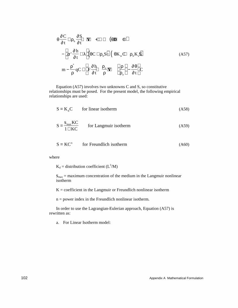
102 Appendix A Mathematical Formulation
( )
( ) ( )
θ∂∂
ρ∂∂
θ
α∂∂
λ θ ρ θ ρ
ρρ
∂∂
ρρ
ρρ
∂θ∂
C
t
S
tC C
h
tC S K C K S
m qC Fh
t tC
b
b w b s
o
o
+ + ⋅ ∇ − ∇ ⋅ ⋅ ∇ =
− ′ +
+ − + +
− + + ⋅ ∇
−
∗
V D
V
(A57)
Equation (A57) involves two unknowns C and S, so constitutiverelationships must be posed. For the present model, the following empiricalrelationships are used:
S K C for linear isothermd= (A58)
SKCKC
for Langmuir isotherm=+
smax
1(A59)
S KC for Freundlich isothermn= (A60)
where
Kd = distribution coefficient (L3/M)
smax = maximum concentration of the medium in the Langmuir nonlinearisotherm
K = coefficient in the Langmuir or Freundlich nonlinear isotherm
n = power index in the Freundlich nonlinear isotherm.
In order to use the Lagrangian-Eulerian approach, Equation (A57) isrewritten as:
a. For Linear Isotherm model:
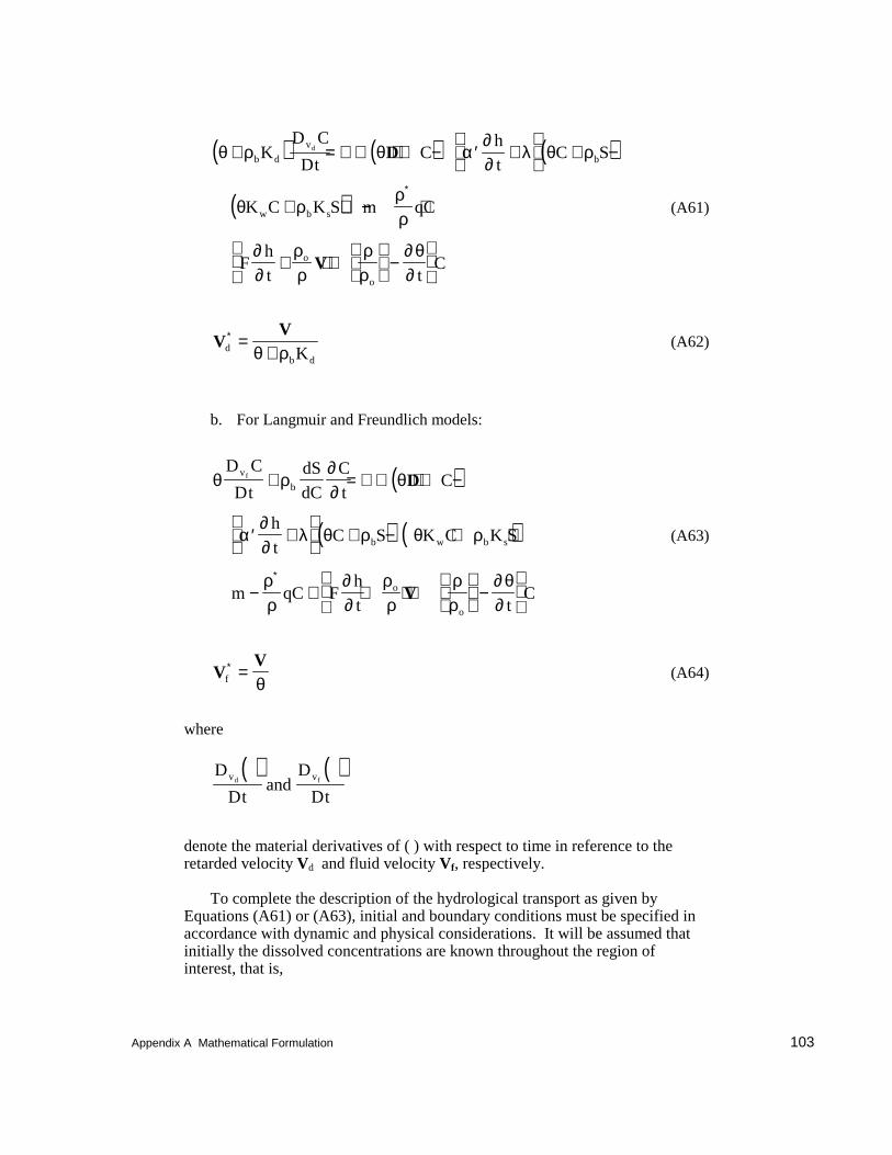
Appendix A Mathematical Formulation 103
( ) ( ) ( )
( )
θ ρ θ α∂∂
λ θ ρ
θ ρρρ
∂∂
ρρ
ρρ
∂ θ∂
+ = ∇ ⋅ ⋅ ∇ − ′ +
+ −
+ + − +
+ ⋅ ∇
−
∗
b d
v
b
w b s
o
o
KD C
DtC
ht
C S
K C K S m qC
Fh
t tC
d D
V
(A61)
VV
db dK
∗ =+θ ρ
(A62)
b. For Langmuir and Freundlich models:
( )
( ) ( )
θ ρ∂∂
θ
α∂∂
λ θ ρ θ ρ
ρρ
∂∂
ρρ
ρρ
∂ θ∂
D C
Dt
dS
dC
C
tC
h
tC S K C K S
m qC Fh
t tC
v
b
b w b s
o
o
f + = ∇ ⋅ ⋅ ∇ −
′ +
+ − + +
− + + ⋅ ∇
−
∗
D
V
(A63)
VV
f∗ =
θ(A64)
where
( ) ( )D
Dt
D
Dtv vd fand
denote the material derivatives of ( ) with respect to time in reference to theretarded velocity Vd and fluid velocity Vf, respectively.
To complete the description of the hydrological transport as given byEquations (A61) or (A63), initial and boundary conditions must be specified inaccordance with dynamic and physical considerations. It will be assumed thatinitially the dissolved concentrations are known throughout the region ofinterest, that is,
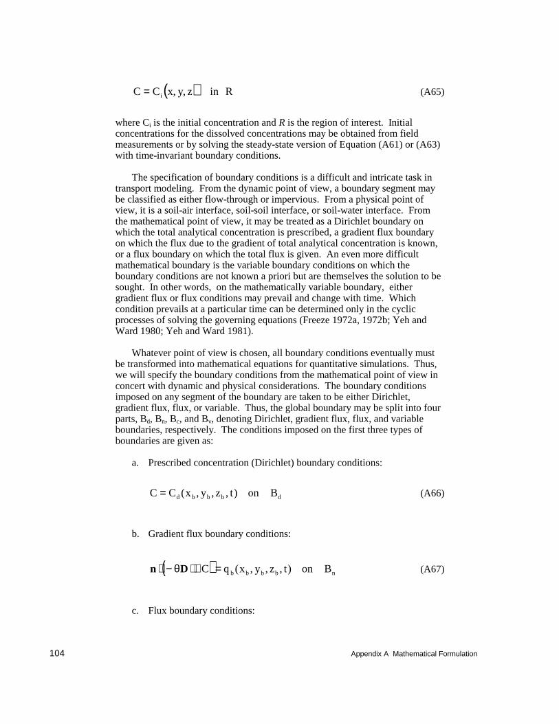
104 Appendix A Mathematical Formulation
( )C C x y z in Ri= , , (A65)
where Ci is the initial concentration and R is the region of interest. Initialconcentrations for the dissolved concentrations may be obtained from fieldmeasurements or by solving the steady-state version of Equation (A61) or (A63)with time-invariant boundary conditions.
The specification of boundary conditions is a difficult and intricate task intransport modeling. From the dynamic point of view, a boundary segment maybe classified as either flow-through or impervious. From a physical point ofview, it is a soil-air interface, soil-soil interface, or soil-water interface. Fromthe mathematical point of view, it may be treated as a Dirichlet boundary onwhich the total analytical concentration is prescribed, a gradient flux boundaryon which the flux due to the gradient of total analytical concentration is known,or a flux boundary on which the total flux is given. An even more difficultmathematical boundary is the variable boundary conditions on which theboundary conditions are not known a priori but are themselves the solution to besought. In other words, on the mathematically variable boundary, eithergradient flux or flux conditions may prevail and change with time. Whichcondition prevails at a particular time can be determined only in the cyclicprocesses of solving the governing equations (Freeze 1972a, 1972b; Yeh andWard 1980; Yeh and Ward 1981).
Whatever point of view is chosen, all boundary conditions eventually mustbe transformed into mathematical equations for quantitative simulations. Thus,we will specify the boundary conditions from the mathematical point of view inconcert with dynamic and physical considerations. The boundary conditionsimposed on any segment of the boundary are taken to be either Dirichlet,gradient flux, flux, or variable. Thus, the global boundary may be split into fourparts, Bd, Bn, Bc, and Bv, denoting Dirichlet, gradient flux, flux, and variableboundaries, respectively. The conditions imposed on the first three types ofboundaries are given as:
a. Prescribed concentration (Dirichlet) boundary conditions:
C C x y z t on Bd b b b d= ( , , , ) (A66)
b. Gradient flux boundary conditions:
( )n D⋅ − ⋅ ∇ =θ C q x y z t on Bb b b b n( , , , ) (A67)
c. Flux boundary conditions:
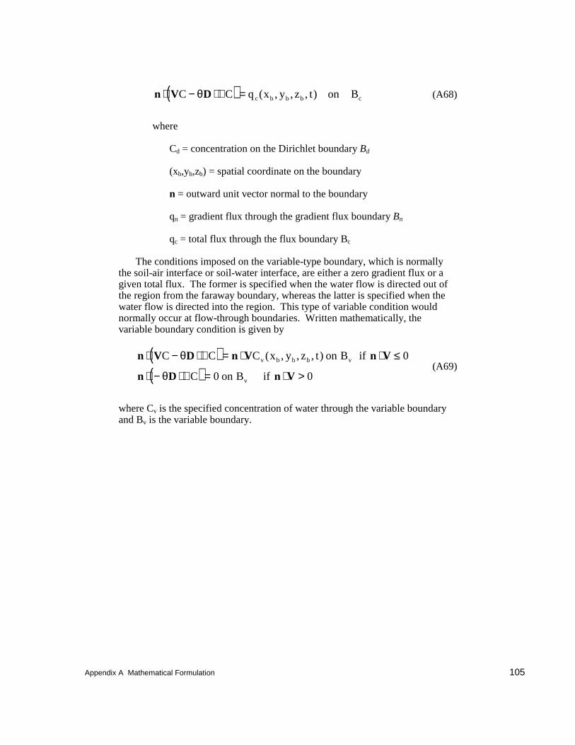
Appendix A Mathematical Formulation 105
( )n V D⋅ − ⋅ ∇ =C C q x y z t on Bc b b b cθ ( , , , ) (A68)
where
Cd = concentration on the Dirichlet boundary Bd
(xb,yb,zb) = spatial coordinate on the boundary
n = outward unit vector normal to the boundary
qn = gradient flux through the gradient flux boundary Bn
qc = total flux through the flux boundary Bc
The conditions imposed on the variable-type boundary, which is normallythe soil-air interface or soil-water interface, are either a zero gradient flux or agiven total flux. The former is specified when the water flow is directed out ofthe region from the faraway boundary, whereas the latter is specified when thewater flow is directed into the region. This type of variable condition wouldnormally occur at flow-through boundaries. Written mathematically, thevariable boundary condition is given by
( )( )
n V D n V n V
n D n V
⋅ − ⋅ ∇ = ⋅ ⋅ ≤
⋅ − ⋅ ∇ = ⋅ >
C C C x y z t on B if
C on B if
v b b b v
v
θ
θ
( , , , ) 0
0 0(A69)
where Cv is the specified concentration of water through the variable boundaryand Bv is the variable boundary.

Appendix B Numerical Formulation 107
Appendix B NumericalFormulation
Introduction
The initial-boundary value problem described by the governing equations ofthe flow and transport modules of FEMWATER along with the boundaryconditions cannot, in general, be solved analytically using applied mathematics.Hence, in order to solve these sets of governing equations, numerical methodsare the only mathematical tools capable of handling this task. Although there aremany different numerical approximation methods capable of reducing partialdifferential equations to simpler systems of algebraic equations, there are onlytwo numerical methods that are most common and that can be employed to solvethe most basic form of the governing equations. These are the finite differenceand finite element methods.
The basic difference between the finite difference and finite elementmethods is that the finite element method is based upon approximating thefunction, while the finite difference method is founded upon approximating thederivatives of the function. Therefore, the finite difference method producessolutions only at discrete points, while the finite element method yields spatiallycontinuous solutions.
Also, the finite element method offers numerous advantages over the finitedifference method:
a. Anisotropy and heterogeneity of aquifers are easily taken care of.
b. Formulation of special formulae to incorporate irregular boundaries isunnecessary.
c. Computer storage and computational time can sometimes be savedbecause often fewer nodal points are needed to portray the region ofinterest to the same level of accuracy.
108 Appendix B Numerical Formulation
d. Irregular grids for handling different levels of spatial discretization indifferent sections of the region of interest can be incorporated.
e. The integral formulation used in this method permits the flux types ofthe boundary conditions to come about naturally (Yeh 1987).
Thus, the finite element method is used in this model. The theoreticalbackground as well as numerical procedures of this method can be found in anygood finite element method book, such as Istok (1989), and therefore will not bedescribed here. A brief summary of the numerical procedure for applying thefinite element method can be found in Yeh (1987).
The flow module of FEMWATER includes three options for solving thefinite element equations. In other words, there are three iteration methods forsolving the linearized matrix equations: successive point iteration, polynomialpreconditioned conjugate gradient, and incomplete Cholesky preconditionedconjugate gradient. Direct elimination methods are not used in this reportbecause they are impractical in dealing with large three-dimensional problems.Because the Newton-Raphson method will yield a nonsymmetric matrix, thePicard method is used to linearize the matrix equation.
To handle a large variety of possible problems, the flow module forFEMWATER contains 12 optional numerical schemes. Specifically, the mixtureof schemes includes the combinations of (a) the three options for solving theresulting matrix equation as mentioned in the previous paragraph, (b) twooptions (lumping and consistent) for handling the mass matrix resulting from thestorage term, and (c) two options (time-weighted difference and middifference)for approximating the time derivatives. The theoretical background for (b) and(c) may also be found in any respectable matrix computation book and in Yeh(1991).
The transport module for FEMWATER also includes these 16 options, plusmore. While the Galerkin finite element method is used in the flow module, anoption of two conventional finite element methods (Galerkin and upstreamweighting) or the alternative option of a hybrid Lagrangian-Eulerian finiteelement method is provided in the transport module. The main differencebetween the two conventional finite element methods is that while the Galerkinfinite element method uses the base functions as the weighting functions, theupstream weighting finite element method uses weighting functions differentfrom the base functions. The advantages of using the upstream weighting finiteelement method over the Galerkin finite element method become apparent whenthe advection terms in the transport governing equation are equally important tothe dispersion terms (Yeh and Ward 1981). More details of the twoconventional finite element methods may be found in Yeh and Ward (1981).
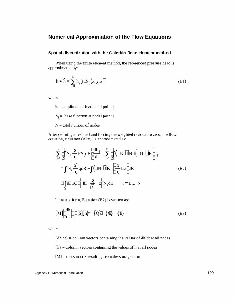
Appendix B Numerical Formulation 109
Numerical Approximation of the Flow Equations
Spatial discretization with the Galerkin finite element method
When using the finite element method, the referenced pressure head isapproximated by:
( ) ( )h h h t N x y zjj
N
j≈ ==
∑$ , ,1
(B1)
where
hj = amplitude of h at nodal point j
Nj = base function at nodal point j
N = total number of nodes
After defining a residual and forcing the weighted residual to zero, the flowequation, Equation (A28), is approximated as:
( ) ( )
( )
N FN dRdh
dtN N dR h
N qdR N z dR
h z N dB i N
io
jR
j
j
N
i jR
jj
N
ioR
iR o
B oi
ρρ
ρρ
ρρ
ρρ
∫∑ ∫∑
∫ ∫
∫
+ ∇ ⋅ ⋅ ∇
= − ∇ ⋅ ⋅ ∇
+ ⋅ ⋅ ∇ + ∇
=
= =
∗
1 1
1
K
K
n K ,...,
(B2)
In matrix form, Equation (B2) is written as:
[ ] [ ]{ } { } { } { }Mdh
dtS h Q G B
+ = + + (B3)
where
{dh/dt} = column vectors containing the values of dh/dt at all nodes
{h} = column vectors containing the values of h at all nodes
[M] = mass matrix resulting from the storage term
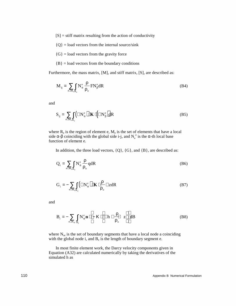
110 Appendix B Numerical Formulation
[S] = stiff matrix resulting from the action of conductivity
{Q} = load vectors from the internal source/sink
{G} = load vectors from the gravity force
{B} = load vectors from the boundary conditions
Furthermore, the mass matrix, [M], and stiff matrix, [S], are described as:
M N FN dRije
Re M o
e
ee
= ∫∑∈
α βρρ
(B4)
and
( ) ( )S N N dRije
Re M
e
ee
= ∇ ⋅ ⋅ ∇∫∑∈
α βK (B5)
where Re is the region of element e, Me is the set of elements that have a localside α-β coinciding with the global side i-j, and Nα
e is the α-th local basefunction of element e.
In addition, the three load vectors, {Q}, {G}, and {B}, are described as:
Q N qdRie
Re M oee
= ∫∑∈
αρρ
(B6)
( )G N zdRie
Re M oee
= − ∇ ⋅ ⋅ ∇∫∑∈
αρρ
K (B7)
and
B N h z dBie
oBe Nese
= − ⋅ − ⋅ ∇ + ∇
∫∑
∈α
ρρ
n Κ (B8)
where Nse is the set of boundary segments that have a local node a coincidingwith the global node i, and Be is the length of boundary segment e.
In most finite element work, the Darcy velocity components given inEquation (A32) are calculated numerically by taking the derivatives of thesimulated h as
Appendix B Numerical Formulation 111
( )V K= − ⋅ ∇ + ∇
=∑ρ
ρo
j jj
N
N h z1
(B9)
This formulation results in a velocity field that is not continuous at elementboundaries and nodal points if the variation of h is other than linear or constant.The alternative approach would be to apply the Galerkin finite element methodto Equation (A32); thus one obtains
[ ]{ } { }T V Dx x= (B10)
[ ]{ } { }T V Dy y= (B11)
[ ]{ } { }T V Dz z= (B12)
where the matrix [T] and the load vectors {Dx}, {Dy}, and {Dz} are given by
T N N dRije e
Re Mee
= ∫∑∈
α β (B13)
D N h z dBxie o
Re Mee
= − ⋅ ⋅ ∇ + ∇
∫∑∈
αρρ
i K (B14)
D N h z dByie o
Re Mee
= − ⋅ ⋅ ∇ + ∇
∫∑∈
αρρ
j K (B15)
D N h z dBzie o
Re Mee
= − ⋅ ⋅ ∇ + ∇
∫∑∈
αρρ
k K (B16)
where Vx, Vy, and Vz are the Darcy velocity components along the x-, y-, and z-directions, respectively; and i, j, and k are the unit vectors along the x-, y-, and z-coordinates, respectively.
The reduction of the partial differential equation (Equation (A28)) to the setof ordinary differential equations (Equation (B3)) simplifies the evaluation ofintegrals on the right side of Equations (B4) through (B8) for every element forboundary surface e. The major tasks that remain to be done are the specificationof base and weighting functions and the performance of integration to yield the
112 Appendix B Numerical Formulation
element matrices. Linear hexahedral elements are employed in thisdocumentation.
Base and weighting functions
The construction of base functions for hexahedral elements is bestaccomplished using the local coordinates (ξ,η,ζ). In the local coordinates, theoriginal hexahedral element is mapped into a cubic whose corners are located atξ = ±1, η = ±1, and ζ = ±1 as shown in Figure B1.
For trilinear hexahedral elements, the eight base functions are obtained bytaking the tensor product of the three base functions of the linear line elements as
( ) ( )( )( )N ii i i iξ η ζ ξξ ηη ζζ, , , , , ...,= + + + =18
1 1 1 1 2 8 (B17)
Because the Galerkin finite element method is used to solve the flow equations,the set of eight weighting functions is taken as the same set of eight basefunctions.
Numerical integration
To complete the reduction of the partial differential equation (Equation(B3)) to the ordinary differential equation (Equation (B3)), one has to evaluatethe integrals on the right sides of Equations (B4)-(B8) for every element to yieldthe element mass matrix [Me] and the stiff element matrix [S
e] as well as the
element gravity column vector {Ge}, the source/sink column vector {Q
e}, and the
boundary column vector {Be} as
M N FN dRe e
o
e
Re
αβ α βρρ
= ∫ (B18)
( ) ( )S N N dRe e e
Re
αβ α β= ∇ ⋅ ⋅ ∇∫ K (B19)
Q N qdRe e
oRe
α αρρ
=∗
∫ (B20)
( )G N zdRe e
R oe
α αρρ
= − ∇ ⋅ ⋅ ∇∫ K (B21)
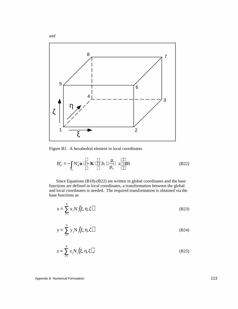
Appendix B Numerical Formulation 113
and
1
78
3
2
4
65
ζη
ξ
Figure B1. A hexahedral element in local coordinates
B N h z dBe e
oBe
α αρρ
= − ⋅ − ⋅ ∇ + ∇
∫ n K (B22)
Since Equations (B18)-(B22) are written in global coordinates and the basefunctions are defined in local coordinates, a transformation between the globaland local coordinates is needed. The required transformation is obtained via thebase functions as
( )x x Nj jj
==∑ ξ η ζ, ,
1
8
(B23)
( )y y Nj jj
==∑ ξ η ζ, ,
1
8
(B24)
( )z z Nj jj
==∑ ξ η ζ, ,
1
8
, (B25)
114 Appendix B Numerical Formulation
Because the coordinate transformation uses the base functions, the element istermed an “isoparametric” element.
Using the transformation in Equations (B23)-(B25), differentiation of thebase function with respect to the global coordinate can be changed todifferentiation with respect to the local coordinate by
[ ]
[ ] [ ] [ ]
∂∂
∂∂
∂∂
∂∂ ξ
∂∂ η
∂∂ζ
∂∂ ξ
∂∂ ξ
∂∂ ξ
∂∂ η
∂∂ η
∂∂ η
∂∂ζ
∂∂ζ
∂∂ζ
N
xN
yN
z
J
N
N
N
J
x y z
x y z
x y z
J Inverse of J
i
i
i
i
i
i
=
=
=
−
−
1
1
(B26)
where [J] is the Jacobian of the transformation and J = |[J]|. In the mean time, adifferential volume written in the local coordinate becomes
dR Jd d de∫ ∫∫∫=
−−−
ξ η ζ1
1
1
1
1
1
(B27)
With Equations (B26) and (B27), all the integrals in Equations (B18)-(B21) canbe reduced to the following form
( )f Jd d dξ η ζ ξ η ζ, ,−−−∫∫∫1
1
1
1
1
1
(B28)
the integration of which can easily be carried out with a 2 × 2 × 2 = 8 pointGaussian quadrature. The surface integration of Equation (B22) in three-dimensional space is not as straightforward as in two-dimensional space. Thisintegration requires further elaboration. Any surface integral of a continuousfunction F(x,y,z) specified on the surface S (Figure B2) can be reduced to thearea integration. Let I represent the surface integral:
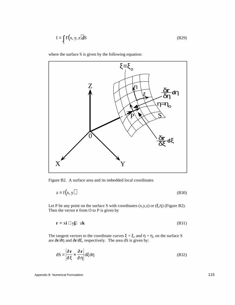
Appendix B Numerical Formulation 115
( )I F x y z dSS
= ∫ , , (B29)
where the surface S is given by the following equation:
ξ=ξο
δrδη dη
η=ηο
δrδξ dξ
ξη
P
Z
YX
0
S
Figure B2. A surface area and its imbedded local coordinates
( )z f x y= , (B30)
Let P be any point on the surface S with coordinates (x,y,z) or (ξ,η) (Figure B2).Then the vector r from O to P is given by
r i j k= + +x y z (B31)
The tangent vectors to the coordinate curves ξ = ξo and η = ηo on the surface Sare ∂r/∂η and ∂r/∂ξ, respectively. The area dS is given by:
dS d d= ×∂∂ ξ
∂∂ η
ξ ηr r
(B32)
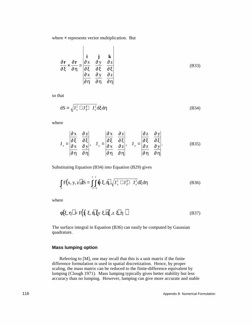
116 Appendix B Numerical Formulation
where × represents vector multiplication. But
∂∂ ξ
∂∂ η
∂∂ ξ
∂∂ ξ
∂∂ ξ
∂∂ η
∂∂ η
∂∂ η
r ri j k
× =x y z
x y z
(B33)
so that
dS J J J d dx y z= + +2 2 2 ξ η (B34)
where
J
x y
x y J
x z
x z J
z y
z yz y x= = =
∂∂ ξ
∂∂ ξ
∂∂ η
∂∂ η
∂∂ ξ
∂∂ ξ
∂∂ η
∂∂ η
∂∂ ξ
∂∂ ξ
∂∂ η
∂∂ η
, , . (B35)
Substituting Equation (B34) into Equation (B29) gives
( ) ( )F x y z dS J J J d dS
x y z, , ,= + +−−∫∫∫ φ ξ η ξ η1
1
1
12 2 2 (B36)
where
( ) ( ) ( ) ( )( )φ ξ η ξ η ξ η ξ η, , , , , ,= F x y z (B37)
The surface integral in Equation (B36) can easily be computed by Gaussianquadrature.
Mass lumping option
Referring to [M], one may recall that this is a unit matrix if the finitedifference formulation is used in spatial discretization. Hence, by properscaling, the mass matrix can be reduced to the finite-difference equivalent bylumping (Clough 1971). Mass lumping typically gives better stability but lessaccuracy than no lumping. However, lumping can give more accurate and stable
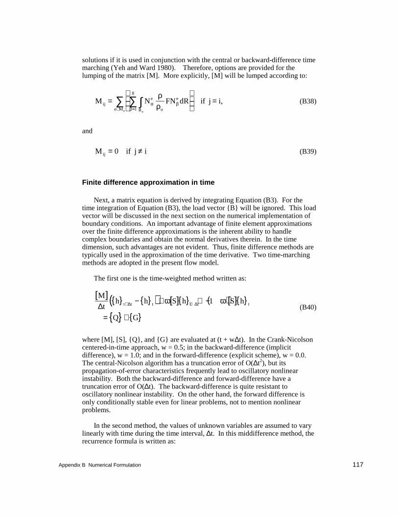
Appendix B Numerical Formulation 117
solutions if it is used in conjunction with the central or backward-difference timemarching (Yeh and Ward 1980). Therefore, options are provided for thelumping of the matrix [M]. More explicitly, [M] will be lumped according to:
M N FN dR if j i,ije
o
e
Re Mee
=
=∫∑∑
=∈α β
β
ρρ1
8
(B38)
and
M if j iij = ≠0 (B39)
Finite difference approximation in time
Next, a matrix equation is derived by integrating Equation (B3). For thetime integration of Equation (B3), the load vector {B} will be ignored. This loadvector will be discussed in the next section on the numerical implementation ofboundary conditions. An important advantage of finite element approximationsover the finite difference approximations is the inherent ability to handlecomplex boundaries and obtain the normal derivatives therein. In the timedimension, such advantages are not evident. Thus, finite difference methods aretypically used in the approximation of the time derivative. Two time-marchingmethods are adopted in the present flow model.
The first one is the time-weighted method written as:
[ ] { } { }( ) [ ]{ } ( )[ ]{ }
{ } { }
M
th h S h S h
Q G
t t t t t t∆ ∆ ∆+ +− + + −
= +
ω ω1(B40)
where [M], [S], {Q}, and {G} are evaluated at (t + w∆t). In the Crank-Nicolsoncentered-in-time approach, w = 0.5; in the backward-difference (implicitdifference), w = 1.0; and in the forward-difference (explicit scheme), w = 0.0.The central-Nicolson algorithm has a truncation error of O(∆t2), but itspropagation-of-error characteristics frequently lead to oscillatory nonlinearinstability. Both the backward-difference and forward-difference have atruncation error of O(∆t). The backward-difference is quite resistant tooscillatory nonlinear instability. On the other hand, the forward difference isonly conditionally stable even for linear problems, not to mention nonlinearproblems.
In the second method, the values of unknown variables are assumed to varylinearly with time during the time interval, ∆t. In this middifference method, therecurrence formula is written as:
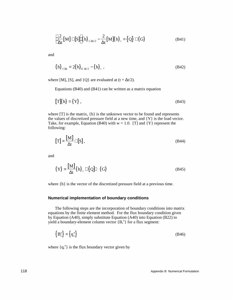
118 Appendix B Numerical Formulation
[ ] [ ] { } [ ]{ } { } { }2 22∆ ∆∆t
M S ht
M h Q Gt t t+
− = ++ / (B41)
and
{ } { } { }h h ht t t t t+ += −∆ ∆2 2/ , (B42)
where [M], [S], and {Q} are evaluated at (t + ∆t/2).
Equations (B40) and (B41) can be written as a matrix equation
[ ]{ } { }T h Y= , (B43)
where [T] is the matrix, {h} is the unknown vector to be found and representsthe values of discretized pressure field at a new time, and {Y} is the load vector.Take, for example, Equation (B40) with w = 1.0. [T] and {Y} represent thefollowing:
[ ] [ ] [ ]TM
tS= +
∆, (B44)
and
{ } [ ]{ } { } { }YM
th Q Gt= + +
∆(B45)
where {h} is the vector of the discretized pressure field at a previous time.
Numerical implementation of boundary conditions
The following steps are the incorporation of boundary conditions into matrixequations by the finite element method. For the flux boundary condition givenby Equation (A40), simply substitute Equation (A40) into Equation (B22) toyield a boundary-element column vector {Bc
e} for a flux segment:
{ } { }B qce
ce= (B46)
where {qce} is the flux boundary vector given by
Appendix B Numerical Formulation 119
q N q dBce e
oc
Be
α αρρ
α= − =∫ , , ...,1 4 (B47)
The flux boundary vector represents the normal fluxes through the two nodalpoints of the segment Be on Bc. For the gradient flux boundary condition givenby Equation (A39), substitute Equation (A39) into Equation (B22) to yield aboundary-element column vector {Bn
e} for a gradient flux segment:
{ } { }B qne
ne= (B48)
where {qnae} is the gradient flux boundary flux vector given by:
{ }q N n K z N q dBne e
o
en
Be
α α αρρ
α= ⋅ ⋅ ∇ −
=∫ ; ,...,1 4 (B49)
which is independent of pressure head.
The implementation of variable-type boundary conditions is more involved.During the iteration of boundary conditions on the variable boundary, one ofEquations (A41) through (A45) is used at a node. If either Equation (A42) or(A45) is used, substitute it into Equation (B22) to yield a boundary elementcolumn vector {Bv
e} for a variable boundary segment:
{ } { }B qve
ve= (B50)
where {qve} is the variable boundary flux given by:
q N q dB or
q N q dB
ve e
op
B
ve e
oe
B
e
e
α α
α α
ρρ
ρρ
α
= −
= − =
∫
∫
,
; , ...,1 4(B51)
Assembling over all gradient flux, flux, and variable boundary segments yieldsthe global boundary column vector {B} as:
{ } { }B q= (B52)
in which
120 Appendix B Numerical Formulation
{ } { } { } { }q q q qne
e Nce
e Nve
e Nne ce ve
= + +∈ ∈ ∈∑ ∑ ∑ (B53)
where Nne, Nce, and Nve are the number of gradient flux boundary segments, fluxboundary segments, and variable boundary segments with flux conditionsimposed on them, respectively. The boundary flux {B} given by Equations(B52) and (B53) should be added to the right side of Equation (B43).
For the river boundary condition given by Equation (A46), simply substituteEquation (A46) into Equation (B22) to yield a boundary-element column vector{BR
e} and boundary matrix [BRe] for a river boundary segment:
{ } { } [ ] [ ]B q and B bRe
re
Re
re= = (B54)
where {qre} and {br
e} are the contribution of the flux boundary to the right andleft sides of the matrix equation, respectively. They are given by
q NK
bh dB and
b NK
bN dB
re e
o
R
RR
B
re e
o
R
R
e
B
e
e
α α
αβ α β
ρρ
α
ρρ
α β
= =
= = =
∫
∫
, , ...,
, , ..., , , ...,
1 4
1 4 1 4(B55)
At nodes where Dirichlet boundary conditions are applied, an identityequation is generated for each node and included in the matrices of Equation(B43). The Dirichlet nodes include the nodes on the Dirichlet boundary and thenodes on the variable boundary to which either Equation (A41), (A43), or (A44)is applied.
After time discretization of Equation (B3) and incorporation of boundaryconditions, the following matrix equation is obtained
[ ]{ } { }C h R= (B56)
where [C] is the coefficient matrix and {R} is the known vector of the right side.For the saturated-unsaturated flow simulation, [C] is a highly nonlinear functionof the pressure head {h}.
Solution of the matrix equations
Equation (B56) is in general a banded sparse matrix equation. It may besolved numerically by either direct or iteration methods. In direct methods, a
Appendix B Numerical Formulation 121
single solution operation sequence is performed. This would result in an exactsolution except for round-off error. In this method, one is concerned with theefficiency and magnitude of round-off error associated with the sequence ofoperations. On the other hand, in an iterative method, one attempts to find asolution by a process of successive approximations. This involves making aninitial guess, then improving the guess by some iterative process until an errorcriterion is obtained. Therefore, in this technique, one must be concerned withconvergence, and the rate of convergence. The round-off errors tend to be self-corrected.
For practical purposes, the advantages of direct methods are as follows: (a)the efficient computation when the bandwidth of the matrix [C] is small, and (b)the fact that no convergence problem is encountered when the matrix equation islinear or small convergence problems when the mass equation is nonlinear. Thedisadvantages of direct methods are the excessive requirements on CPU storageand CPU time when a large number of nodes is needed for discretization. On theother hand, the advantages of iterative methods are the efficiencies in terms ofCPU storage and CPU time when large problems are encountered. Theirdisadvantages are the requirements that the matrix [C] must be well conditionedto guarantee a convergent solution. For three-dimensional problems, thebandwidth of the matrix is usually large; thus the direction solution method isnot practical. Only iterative methods are implemented in FEMWATER. Fouriteration methods are used in solving the linearized matrix equation: (a) blockiteration, (b) successive point iteration, (c) polynomial preconditioned conjugategradient method, and (d) incomplete Cholesky preconditioned conjugate gradientmethod.
The matrix equation, Equation (B56), is nonlinear because both thehydraulic conductivity and the water capacity are functions of the pressure headh. To solve the nonlinear matrix equation, two approaches can be taken: (a) thePicard method and (b) the Newton-Raphson method. The Newton-Raphsonmethod has a second order of convergent rate and is very robust. However, theNewton-Raphson method would destroy the symmetrical property of thecoefficient matrix resulting from the finite element approximation. As a resultthe solution of the linearized matrix equation requires extra care. Many of theiterative methods will not give a convergent solution for the nonsymmetriclinearized matrix equation. Thus, the Picard method is used in this report tosolve the nonlinear problems.
In the Picard method, an initial estimate is made of the unknown {h}. Usingthis estimate, the coefficient matrix [C] is then computed and the linearizedmatrix equation solved using linear algebra. The new estimate is now obtainedby the weighted average of the new solution and the previous estimate:
{ } { } ( ){ }h h hk k+ = + −1 1ω ω , (B57)
where
122 Appendix B Numerical Formulation
{hk+1} = new estimate
{hk} = previous estimate
{h} = new solution
ω = iteration parameter
The procedure is repeated until the new solution {h} is within a tolerance error.If ω is greater than or equal to 0 but is less than 1, the iteration isunderrelaxation. If ω = 1, the method is the exact relaxation. If ω is greater than1 but less than or equal to 2, the iteration is termed overrelaxation. Theunderrelaxation should be used to overcome cases of non-convergence or slowconvergence rates due to fluctuations rather than due to “divergent”computations. Overrelaxation should be used to speed up the convergence ratewhen it decreases monotonically.
In summary, there are sixteen optional numerical schemes here to deal with awide range of problems. These are the combinations of (a) two ways of treatingthe mass matrix (lumping and no-lumping); (b) two ways of approximating thetime derivatives (time-weighting and middifference), and (c) four ways ofsolving the linearized matrix equation.
Transport Equation
Spatial discretization with the weighted residual finite elementmethod
Let Cj be approximated by a finite element interpolation as
( ) ( )C C C t N x y zj jj
N
≈ ==∑$ , ,
1
(B58)
Substituting Equation (B58) into Equations (A57), (A61), and (A63), and forcinga weighted residual to zero gives the following ordinary differential equations:
a. For the conventional finite element approach:
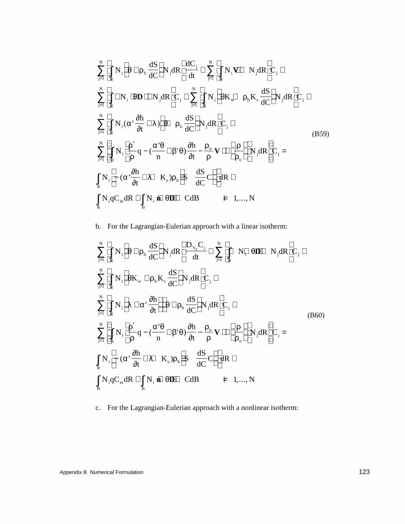
Appendix B Numerical Formulation 123
NdSdC
N dRdC
dtN N dR C
N N dR C N K KdS
dCN dR C
Nh
t
dS
dCN dR
i b jR
j
j
N
iR
j jj
N
iR
j jj
N
i w b s jR
jj
N
i b jR
θ ρ
θ θ ρ
α∂∂
λ θ ρ
+
+ ⋅ ∇
+
∇ ⋅ ⋅ ∇
+ +
+
′ + +
∫∑ ∫∑
∫∑ ∫∑
∫
= =
= =
1 1
1 1
V
D
( )
+
−′
+ ′ − ⋅ ∇
=
− + + −
+
+ ⋅ ⋅ ∇ =
=
∗
=
∑
∫∑
∫
∫ ∫
C
N qn
h
tN dR C
Nh
tK S
dS
dCC dR
N qC dR N CdB i N
jj
N
io
oRj j
j
N
iR
s b
iR
in iB
1
1
1
ρρ
α θβ θ
∂∂
ρρ
ρρ
α∂∂
λ ρ
θ
( )
( ’ )
,...,
V
n D
(B59)
b. For the Lagrangian-Eulerian approach with a linear isotherm:
NdSdC
N dRD C
dtN N dR C
N K KdS
dCN dR C
Nh
t
dS
dCN dR C
N
i b jR
V j
j
N
iR
j jj
N
i w b s jR
jj
N
i b jR
jj
N
i
dθ ρ θ
θ ρ
λ α∂∂
θ ρ
ρρ
+
+ ∇ ⋅ ⋅ ∇
+
+
+
+ ′
+
+
∫∑ ∫∑
∫∑
∫∑
= =
=
=
∗
1 1
1
1
D
qn
h
tN dR C
Nh
tK S
dS
dCC dR
N qC dR N CdB i N
o
oRj j
j
N
iR
s b
iR
in iB
−′
+ ′ − ⋅ ∇
=
− ′ + + −
+
+ ⋅ ⋅ ∇ =
∫∑
∫
∫ ∫
=( )
( )
,...,
α θβ θ
∂∂
ρρ
ρρ
α∂∂
λ ρ
θ
V
n D
1
1
(B60)
c. For the Lagrangian-Eulerian approach with a nonlinear isotherm:
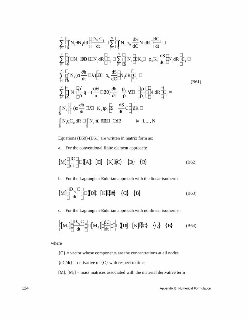
124 Appendix B Numerical Formulation
N N dRD C
dtN
dSdC
N dRdC
dt
N N dR C N K KdS
dCN dR C
Nh
t
dS
dCN dR C
i jR
V j
j
N
iR
b j
j
j
N
iR
j jj
N
i w b s jR
jj
N
i b jR
j
fθ ρ
θ θ ρ
α∂∂
λ θ ρ
∫∑ ∫∑
∫∑ ∫∑
∫
+
+
∇ ⋅ ⋅ ∇
+ +
+
+ +
= =
= =
1 1
1 1
D
( )j
N
io
oRj j
j
N
iR
s b
iR
in iB
N qn
h
tN dR C
Nh
tK S
dS
dCC dR
N qC dR N CdB i N
=
∗
=
∑
∫∑
∫
∫ ∫
+
− + − ⋅ ∇
=
− + + −
+
+ ⋅ ⋅ ∇ =
1
1
1
ρρ
αθβθ
∂∂
ρρ
ρρ
α∂∂
λ ρ
θ
( )
( )
,...,
V
n D
(B61)
Equations (B59)-(B61) are written in matrix form as:
a. For the conventional finite element approach:
[ ] [ ] [ ] [ ]( ){ } { } { }MdC
dtA D K C Q B
+ + + = + (B62)
b. For the Lagrangian-Eulerian approach with the linear isotherm:
[ ] [ ] [ ]( ){ } { } { }MD C
dtD K C Q B
Vd
+ + = + (B63)
c. For the Lagrangian-Eulerian approach with nonlinear isotherms:
[ ] [ ] [ ] [ ]( ){ } { } { }MD C
dtM
dC
dtD K C Q B
Vf
1 2
+
+ + = + (B64)
where
{C} = vector whose components are the concentrations at all nodes
{dC/dt} = derivative of {C} with respect to time
[M], [M1] = mass matrices associated with the material derivative term
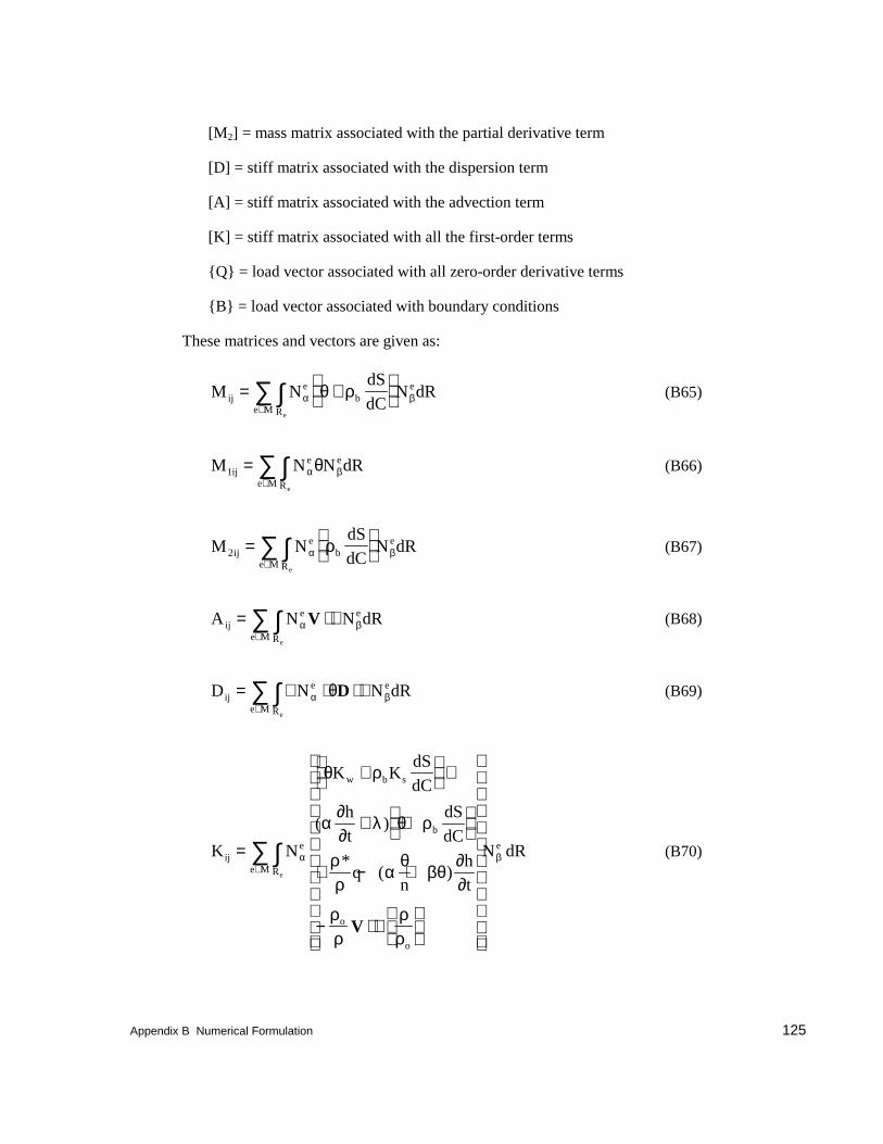
Appendix B Numerical Formulation 125
[M2] = mass matrix associated with the partial derivative term
[D] = stiff matrix associated with the dispersion term
[A] = stiff matrix associated with the advection term
[K] = stiff matrix associated with all the first-order terms
{Q} = load vector associated with all zero-order derivative terms
{B} = load vector associated with boundary conditions
These matrices and vectors are given as:
M NdS
dCN dRij
eb
Re M
e
e
= +
∫∑
∈α βθ ρ (B65)
M N N dRije
Re M
e
e
1 = ∫∑∈
α βθ (B66)
M NdS
dCN dRij
eb
Re M
e
e
2 =
∫∑
∈α βρ (B67)
A N N dRije
Re M
e
e
= ⋅ ∇∫∑∈
α βV (B68)
D N N dRije
Re M
e
e
= ∇ ⋅ ⋅ ∇∫∑∈
α βθD (B69)
K N
K KdS
dC
h
t
dS
dC
qn
ht
N dRije
w b s
b
o
o
R
e
e Me
=
+
+
+ +
+ − +
− ⋅ ∇
∫∑∈
α β
θ ρ
α∂∂
λ θ ρ
ρρ
αθ
βθ∂∂
ρρ
ρρ
( )
*( )
V
(B70)
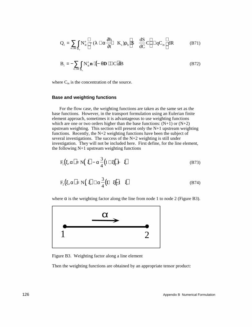
126 Appendix B Numerical Formulation
Q Nht
K SdSdC
C qC dRie
s b inRe M
e
= − + + −
+
∫∑
∈α λ α
∂∂
ρ( ) (B71)
( )B N C dBie
Be Me
= − ⋅ − ⋅ ∇∫∑∈
α θn D (B72)
where Cin is the concentration of the source.
Base and weighting functions
For the flow case, the weighting functions are taken as the same set as thebase functions. However, in the transport formulation using an Eulerian finiteelement approach, sometimes it is advantageous to use weighting functionswhich are one or two orders higher than the base functions: (N+1) or (N+2)upstream weighting. This section will present only the N+1 upstream weightingfunctions. Recently, the N+2 weighting functions have been the subject ofseveral investigations. The success of the N+2 weighting is still underinvestigation. They will not be included here. First define, for the line element,the following N+1 upstream weighting functions
( ) ( ) ( )( )F N1 1
34
1 1ξ α ξ α ξ ξ, = − + − (B73)
( ) ( ) ( )( )F N2 2
34
1 1ξ α ξ α ξ ξ, = + + − (B74)
where α is the weighting factor along the line from node 1 to node 2 (Figure B3).
α
1 2
Figure B3. Weighting factor along a line element
Then the weighting functions are obtained by an appropriate tensor product:
Appendix B Numerical Formulation 127
( ) ( ) ( )W F F F1 1 1 1 1 1 1= ξ α η β ζ γ, , , (B75)
( ) ( ) ( )W F F F2 2 1 1 2 1 2= ξ α η β ζ γ, , , (B76)
( ) ( ) ( )W F F F3 2 2 2 2 1 4= ξ α η β ζ γ, , , (B77)
( ) ( ) ( )W F F F4 1 2 2 1 1 3= ξ α η β ζ γ, , , (B78)
( ) ( ) ( )W F F F5 1 3 1 3 2 1= ξ α η β ζ γ, , , (B79)
( ) ( ) ( )W F F F6 2 3 1 4 2 2= ξ α η β ζ γ, , , (B80)
( ) ( ) ( )W F F F7 2 4 2 4 2 4= ξ α η β ζ γ, , , (B81)
( ) ( ) ( )W F F F8 1 4 2 3 2 3= ξ α η β ζ γ, , , (B82)
where α’s, β’s, and γ’s are the weighting factors along the side given in FigureB4.
Numerical integration
To reduce the partial differential equations, Equations (A57), (A61), and(A63) to ordinary differential equations, Equations (B62)-(B64), one has toevaluate the integrals on the right sides of Equations (B65)-(B72) for everyelement to yield the element mass matrices [Me], [M 1
e], and [M2e] and the stiff
element matrices [Ae], [De], and [Ke] as well as the source/sink column vector{Q e} and the boundary column vector {Be} as:
M NdS
dCN dRe e
bR
e
e
αβ α βθ ρ= +
∫ (B83)
M N N dRe e
R
e
e
1αβ α βθ= ∫ (B84)
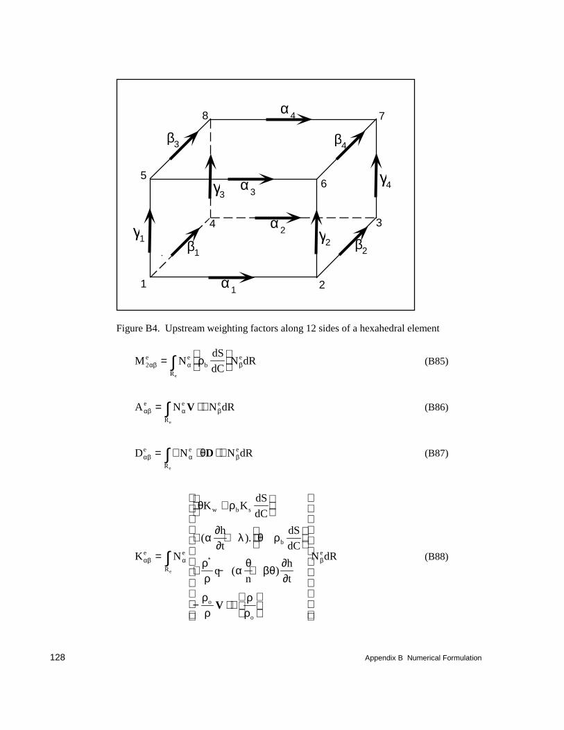
128 Appendix B Numerical Formulation
1
78
3
2
4
65
α4
α3
α2
α1
β3
β1
β4
β2
γ1 γ2
γ4γ3
Figure B4. Upstream weighting factors along 12 sides of a hexahedral element
M NdS
dCN dRe e
bR
e
e
2αβ α βρ=
∫ (B85)
A N N dRe e
R
e
e
αβ α β= ⋅ ∇∫ V (B86)
D N N dRe e
R
e
e
αβ α βθ= ∇ ⋅ ⋅ ∇∫ D (B87)
K N
K KdS
dC
h
t
dS
dC
qn
h
t
N dRe e
w b s
b
o
o
R
e
e
αβ α β
θ ρ
α∂∂
λ θ ρ
ρρ
αθ
βθ∂∂
ρρ
ρρ
=
+
+ + +
+ − +
− ⋅ ∇
∗∫( ).
( )
V
(B88)
Appendix B Numerical Formulation 129
Q Nht
K SdSdC
C qC dRe es b in
Re
α α λ α∂∂
ρ= − + + −
+
∫ ( ) (B89)
( )B N C dBe e
Be
α α θ= − ⋅ − ⋅ ∇∫ n D (B90)
Following the procedures presented in the section “Numerical integration,”Equations (B83)-(B90) are first transformed in terms of local coordinates. Thenthe resulting equations are integrated with Gaussian quadrature. Thetransformation between the global and local coordinates is given by Equations(B23)-(B25) resulting in isoparametric elements. The surface integration fromthe boundary conditions also follows that presented in “Numerical integration.”
Mass lumping option
As with the solution of the flow equations, a consistent mass matrix or masslumping option can be used when the Eulerian approach is used. Although aconsistent mass matrix option can be used when the hybrid Lagrangian-Eulerianapproach is taken, a mass lumping scheme is more appropriate and easier toimplement.
Finite difference approximation in time
When the Eulerian approach is taken in approximating the governingequations, either time-weighted difference or middifference can be used as in thesection “Finite difference approximation in time.” However, when theLagrangian-Eulerian approach is taken, the time integration is different from theflow problem. Although there is still a choice of time-weighted difference ormiddifference, the time-weighted difference scheme is preferred. In thefollowing, the time integration for the Lagrangian-Eulerian approach isdemonstrated. As in the time integration of the flow equations, the boundaryload vector will be ignored in the time integration of the transport equations inthis section. This load vector will be discussed in the next section.
In the Lagrangian-Eulerian approach, Equations (B63) and (B64) areintegrated along the characteristic lines. First Equation (B63) will be integratedfor the linear isotherm case. Then Equation (B64) will be integrated fornonlinear isotherms. The time-weighted integration of Equation (B63) yields
[ ] { } { }( ) [ ] [ ]( ){ }( ) [ ] [ ]( ){ } { }
MC C D K C
D K C Q
n n
∆τ+ ∗ +
∗
− + + +
− + =
1 1
1
ω
ω(B91)
130 Appendix B Numerical Formulation
where ∆τ is the time-step size (the determination of ∆τ will be explained later),{Cn+1} is the concentration vector containing the concentration at all nodes at thenew time n+1, and {C*} is the Lagrangian concentration vector. The Lagrangianconcentration {C*} is computed by the backward method of characteristics asfollows.
( ) ( )
x x V
x
i i d
i
∗+
∗ ∗
= −
=
∫∑
dt
C C t N
t
t t
i j jj
∆
(B92)
where xi* (the Lagrangian point) is the location of a fictitious particle originatingat time t and arriving at the node xi at time t + ∆t. Ci(t) is the concentration valueat node j at time t and Nj(xi*) is the interpolation function associated with node jevaluated at the Lagrangian point xi*. If xi* is located in the interior of theregion of interest, ∆τ in Equation (B91) is defined as
∆τ ∆= t (B93)
If ∆x* is located outside the region of interest, a ∆τ(xi*) as a function of xi* mustbe found such that
( )x x Vi i d
xi
∗+
= −
∗
∫ dtt
t ∆τ
(B94)
will be located on the boundary. Thus, it can be seen that ∆τ is less than or equalto ∆t.
For the nonlinear isotherm case, Equation (B64) can be integrated to yield
[ ] [ ] { } [ ] [ ]( ){ }
[ ]{ } [ ]{ } ( ) [ ] [ ]( ){ } { }
M M
tC D K C
MC
M
tC D K C Q
n n
n
1 2 1 1
1 2 1
∆τ ∆
∆τ ∆
+
+ + =
+
− − + +
+ +
∗ ∗
ω
ω
(B95)
The computation of ∆t and the Lagrangian concentrations C* in Equation (B95)follows Equations (B92)-(B94) but with Vd replaced by Vf.
Appendix B Numerical Formulation 131
Numerical implementation of boundary conditions
To incorporate the boundary conditions, the right side of Equation (B90)must be evaluated for every boundary face Be to yield the load vector {Be}:
( )B N C dBe e
Be
α α θ α= − ⋅ − ⋅ ∇ =∫ n D , ,...,1 4 (B96)
For the gradient flux boundary condition given by Equation (A67), simplysubstitute Equation (A67) into Equation (B90) to yield a boundary-elementcolumn vector {Bn
e} for a gradient flux face:
{ } { }B qne
ne= (B97)
where {qne} is the gradient flux boundary flux vector given by
q N q dBne e
BN
e
α α α= − =∫ , ,...,1 4 (B98)
This gradient flux boundary flux vector represents the normal fluxes through thetwo nodal points of the face Be on Bn.
For the flux boundary condition given by Equation (A68), Equation (B90)may be rewritten in the following form:
( )B N C C dB N CdBe e
B
e
Be e
α α αθ α= − ⋅ − ⋅ ∇ + ⋅ =∫ ∫n V D n V , ,...,1 4 (B99)
The concentration on the boundary segment Be can be approximated by
C C Ne==
∑ β ββ 1
4
(B100)
Substituting Equations (A68) and (B100) into Equation (B99) gives a boundary-element column vector {Bc
e} for a flux face:
{ } { } [ ]{ }B q V Cce
ce
ce= + (B101)
in which the flux boundary vector {qce} and the flux boundary matrix [Vc
e] fromthe normal velocity component are given by
132 Appendix B Numerical Formulation
{ }q N q dB
V N N dB and
ce e
cB
ce e
b
e
e
e
α α
αβ α β
α
α β
= − =
= ⋅ = =
∫
∫
, , ...,
, ,..., , ...,
1 4
1 4 1 4n V(B102)
Faces on which the variable boundary conditions are imposed are the flow-through boundaries on which the flow direction is not known a priori. When theflow is directed into the region, flux boundary conditions will be used. Theboundary element column vector {Bv
e} for a variable boundary segment can beobtained similarly to {Bc
e}:
{ } { } [ ]{ }B q V Cve
ve
ve= + (B103)
in which the variable boundary flux vector {qve} and the variable boundary
matrix [VVe] from the normal velocity component are given by:
{ } ( )q N C dB
V N N dB and
ve e
inB
ve e
b
e
e
e
α α
αβ α β
α
α β
= − ⋅ =
= ⋅ = =
∫
∫
n V
n V
, ,...,
, ,..., ,...,
1 4
1 4 1 4(B104)
where Cin is the total dissolved concentration of the incoming fluid. When theflow is directed out from the region, both {qv
e} and [VVe] are set equal to 0.
Assembling over all gradient flux, flux, and variable boundary segments, theglobal boundary column vector {B} is obtained as:
{ } { } [ ]{ }B q V C= + (B105)
in which
{ } { } { } { }[ ] { } { }
q q q q
V V V
ne
e Nce
e Nve
e N
ce
e Nve
e N
ne ce ve
ce ve
= + +
= +∈ ∈ ∈
∈ ∈
∑ ∑ ∑
∑ ∑(B106)
where Nne, Nce, and Nve are the number of gradient flux, flux, and variableboundary segments, respectively.
At nodes where Dirichlet boundary conditions are applied, an identityequation is generated for each node and included in the matrices of Equation
Appendix B Numerical Formulation 133
(B91) for the case of linear isotherms or Equation (B95) for the case of nonlinearisotherms. The detailed method of applying this type of boundary condition canbe found in Wang and Connor (1975).
Boundary conditions need to be implemented in the computation of theLagrangian concentrations {C*}. Gradient flux boundary conditions arenormally applied to the boundary when flow is directed out from the region ofinterest. On the gradient flux boundary, the backtracking would locate xi* in theinterior of the domain; hence the Lagrangian concentration at the ith gradientflux boundary node is simply computed via interpolation. On the Dirichletboundary nodes, the Lagrangian concentration is simply set to the specifiedvalue.
On the variable boundary, boundary conditions need not be implemented ifthe flow is directed out from the region. If the flow is directed into the region,the concentration of incoming fluid is specified. An intermediate concentrationC** is calculated according to
C
N V C dB
N V dBi
i n in
B
i n
B
v
v
∗∗ =−
−
∫
∫, (B107)
where Ci** is the concentration due to the boundary source at the boundary nodei, Vn is the normal vertically integrated Darcy’s velocity, and Cin is theconcentration of the incoming fluid.
Flux boundary conditions are normally applied to the boundary where flowis directed into the region, where the material flux of incoming fluid is specified.The intermediate concentration is thus calculated according to
C
N q dB
N V dBi
i cB
i nB
c
c
∗∗ =∫
∫, (B108)
where Ci** is the concentration due to flux fluxes at the boundary node i, Vn isthe normal Darcy’s velocity, and qc is the flux of the incoming fluid.
The Lagrangian concentration is obtained by using the value Ci** and Cin
(the concentration at previous time-step) as follows:
134 Appendix B Numerical Formulation
( )C
N N C dB N K N C dB
N K dBlinear isothermi
i j j i b d j jn
Bj
N
Bj
N
i b dB
∗
∗∗
===+
+
∫∑∫∑
∫
θ ρ
θ ρ11
(B109)
C C for the nonlinear isothermi i∗ ∗∗= (B110)
Solution of the matrix equations
Because the Lagrangian-Eulerian approach results in a symmetric positivedefinite matrix, the system of algebraic equations can be solved by any of thefour options: block iteration, successive point iteration, polynomialpreconditioned conjugate gradient, and incomplete Cholesky preconditionedconjugate gradient methods. For the Eulerian approach, however, the blockiteration and successive point iteration methods are the preferred choice forsolving the matrix equation. When the advection transport is dominant, the twobasic iteration methods with underrelaxation are very effective in reducing thenumber of iterations required for a convergent solution (Yeh 1985).
Appendix C Output File Formats 135
Appendix C Output FileFormats
Introduction
The output from FEMWATER consists of a printed output file and a numberof solution files. The printed output file is a text file listing a summary of theinput, iteration and convergence data, and solution summaries. The solutionfiles are used for post-processing or as initial conditions for subsequent runs.The content and format of the solution files are described in this appendix.
There are four solution files that can be output from FEMWATER: pressurehead, velocity, moisture content (nodal), and concentration. All of the files canbe output in either binary or text format. The options for selecting which filesare to be output and which format is used are specified on the OC4 card in themodel file (see section, “Save options (OC4),” in main text).
Data Set Files
The pressure head, moisture content (nodal), concentration, and velocityfiles are all written using the standard Department of Defense GroundwaterModeling System (GMS) data set file format. The data set file formats are twoof the standard file formats used by the GMS. Multiple data sets, including bothscalar and vector, can be included in one file. However, the data set files usedby FEMWATER for input and output are assumed to contain one data set perfile.
With the scalar data sets, one scalar value is listed per node, in sequentialorder based on the node ID’s. If the data set is transient, a complete set of scalarvalues is listed for each time-step. With vector data sets, the x-, y-, and z-components of the vector (velocity in this case) are listed on a node by nodebasis.
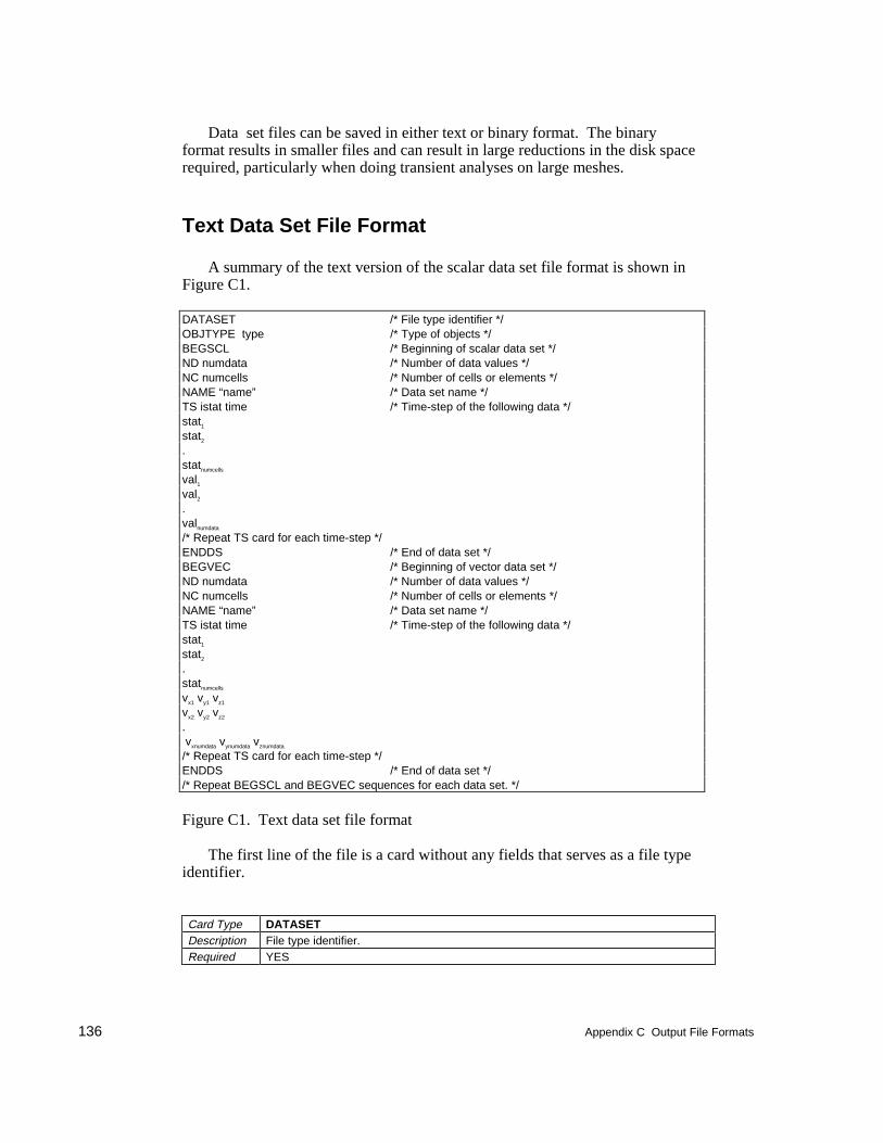
136 Appendix C Output File Formats
Data set files can be saved in either text or binary format. The binaryformat results in smaller files and can result in large reductions in the disk spacerequired, particularly when doing transient analyses on large meshes.
Text Data Set File Format
A summary of the text version of the scalar data set file format is shown inFigure C1.
DATASET /* File type identifier */OBJTYPE type /* Type of objects */BEGSCL /* Beginning of scalar data set */ND numdata /* Number of data values */NC numcells /* Number of cells or elements */NAME “name” /* Data set name */TS istat time /* Time-step of the following data */stat1
stat2
.statnumcells
val1val2.valnumdata
/* Repeat TS card for each time-step */ENDDS /* End of data set */BEGVEC /* Beginning of vector data set */ND numdata /* Number of data values */NC numcells /* Number of cells or elements */NAME “name” /* Data set name */TS istat time /* Time-step of the following data */stat1
stat2
.statnumcells
vx1 vy1 vz1
vx2 vy2 vz2
. vxnumdata vynumdata vznumdata
/* Repeat TS card for each time-step */ENDDS /* End of data set *//* Repeat BEGSCL and BEGVEC sequences for each data set. */
Figure C1. Text data set file format
The first line of the file is a card without any fields that serves as a file typeidentifier.
Card Type DATASETDescription File type identifier.Required YES
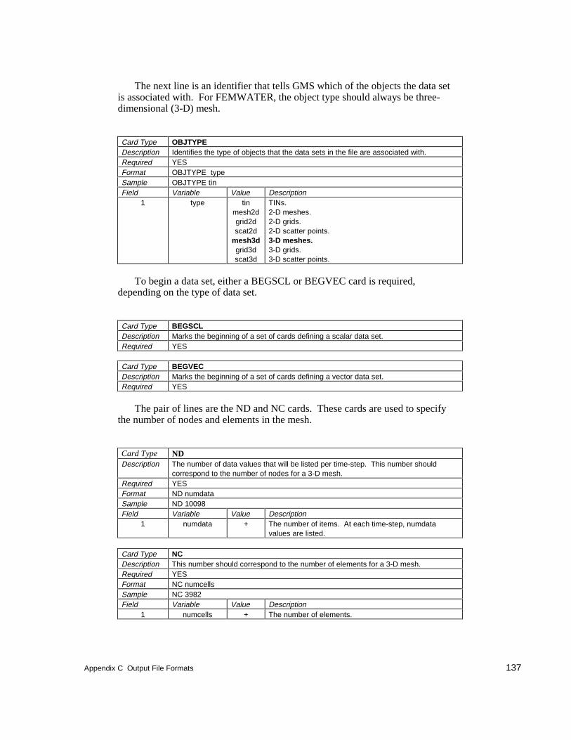
Appendix C Output File Formats 137
The next line is an identifier that tells GMS which of the objects the data setis associated with. For FEMWATER, the object type should always be three-dimensional (3-D) mesh.
Card Type OBJTYPEDescription Identifies the type of objects that the data sets in the file are associated with.Required YESFormat OBJTYPE typeSample OBJTYPE tinField Variable Value Description
1 type tinmesh2dgrid2dscat2d
mesh3dgrid3dscat3d
TINs.2-D meshes.2-D grids.2-D scatter points.3-D meshes.3-D grids.3-D scatter points.
To begin a data set, either a BEGSCL or BEGVEC card is required,depending on the type of data set.
Card Type BEGSCLDescription Marks the beginning of a set of cards defining a scalar data set.Required YES
Card Type BEGVECDescription Marks the beginning of a set of cards defining a vector data set.Required YES
The pair of lines are the ND and NC cards. These cards are used to specifythe number of nodes and elements in the mesh.
Card Type NDDescription The number of data values that will be listed per time-step. This number should
correspond to the number of nodes for a 3-D mesh.Required YESFormat ND numdataSample ND 10098Field Variable Value Description
1 numdata + The number of items. At each time-step, numdatavalues are listed.
Card Type NCDescription This number should correspond to the number of elements for a 3-D mesh.Required YESFormat NC numcellsSample NC 3982Field Variable Value Description
1 numcells + The number of elements.
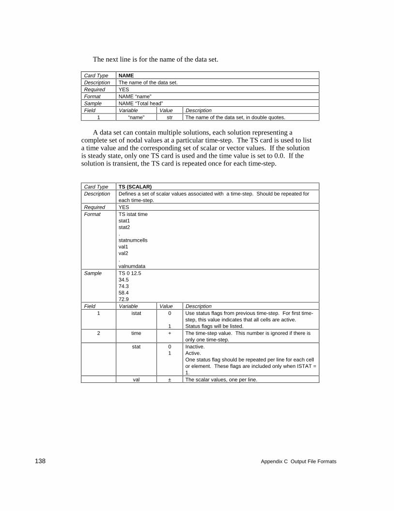
138 Appendix C Output File Formats
The next line is for the name of the data set.
Card Type NAMEDescription The name of the data set.Required YESFormat NAME “name”Sample NAME “Total head”Field Variable Value Description
1 “name” str The name of the data set, in double quotes.
A data set can contain multiple solutions, each solution representing acomplete set of nodal values at a particular time-step. The TS card is used to lista time value and the corresponding set of scalar or vector values. If the solutionis steady state, only one TS card is used and the time value is set to 0.0. If thesolution is transient, the TS card is repeated once for each time-step.
Card Type TS (SCALAR)Description Defines a set of scalar values associated with a time-step. Should be repeated for
each time-step.Required YESFormat TS istat time
stat1stat2.statnumcellsval1val2.valnumdata
Sample TS 0 12.534.574.358.472.9
Field Variable Value Description1 istat 0
1
Use status flags from previous time-step. For first time-step, this value indicates that all cells are active.Status flags will be listed.
2 time + The time-step value. This number is ignored if there isonly one time-step.
stat 01
Inactive.Active.One status flag should be repeated per line for each cellor element. These flags are included only when ISTAT =1.
val ± The scalar values, one per line.
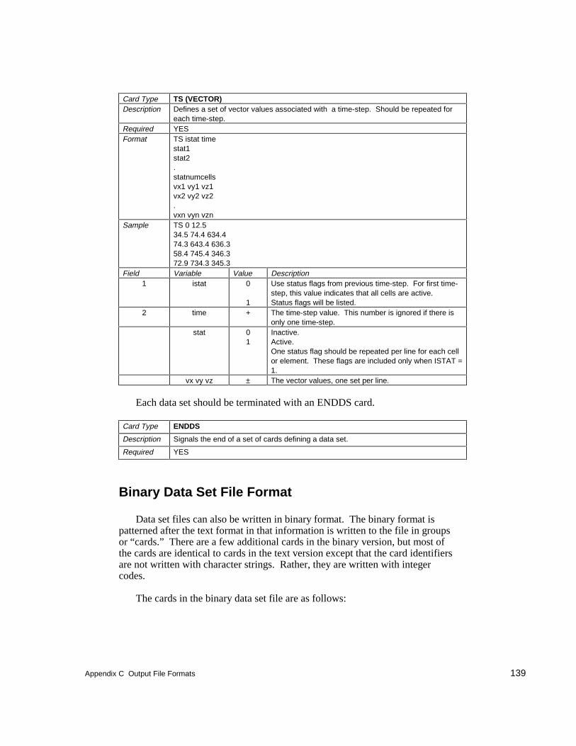
Appendix C Output File Formats 139
Card Type TS (VECTOR)Description Defines a set of vector values associated with a time-step. Should be repeated for
each time-step.Required YESFormat TS istat time
stat1stat2.statnumcellsvx1 vy1 vz1vx2 vy2 vz2.vxn vyn vzn
Sample TS 0 12.534.5 74.4 634.474.3 643.4 636.358.4 745.4 346.372.9 734.3 345.3
Field Variable Value Description1 istat 0
1
Use status flags from previous time-step. For first time-step, this value indicates that all cells are active.Status flags will be listed.
2 time + The time-step value. This number is ignored if there isonly one time-step.
stat 01
Inactive.Active.One status flag should be repeated per line for each cellor element. These flags are included only when ISTAT =1.
vx vy vz ± The vector values, one set per line.
Each data set should be terminated with an ENDDS card.
Card Type ENDDS
Description Signals the end of a set of cards defining a data set.
Required YES
Binary Data Set File Format
Data set files can also be written in binary format. The binary format ispatterned after the text format in that information is written to the file in groupsor “cards.” There are a few additional cards in the binary version, but most ofthe cards are identical to cards in the text version except that the card identifiersare not written with character strings. Rather, they are written with integercodes.
The cards in the binary data set file are as follows:
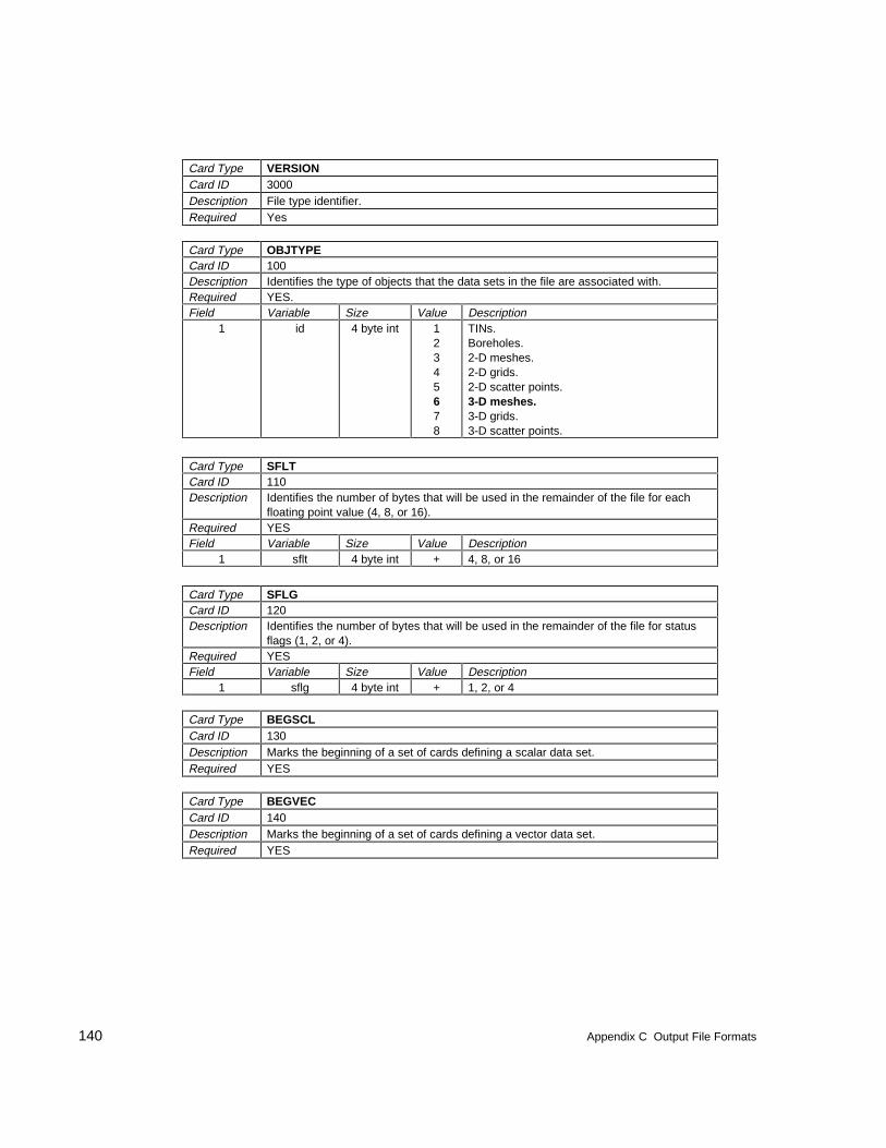
140 Appendix C Output File Formats
Card Type VERSIONCard ID 3000Description File type identifier.Required Yes
Card Type OBJTYPECard ID 100Description Identifies the type of objects that the data sets in the file are associated with.Required YES.Field Variable Size Value Description
1 id 4 byte int 12345678
TINs.Boreholes.2-D meshes.2-D grids.2-D scatter points.3-D meshes.3-D grids.3-D scatter points.
Card Type SFLTCard ID 110Description Identifies the number of bytes that will be used in the remainder of the file for each
floating point value (4, 8, or 16).Required YESField Variable Size Value Description
1 sflt 4 byte int + 4, 8, or 16
Card Type SFLGCard ID 120Description Identifies the number of bytes that will be used in the remainder of the file for status
flags (1, 2, or 4).Required YESField Variable Size Value Description
1 sflg 4 byte int + 1, 2, or 4
Card Type BEGSCLCard ID 130Description Marks the beginning of a set of cards defining a scalar data set.Required YES
Card Type BEGVECCard ID 140Description Marks the beginning of a set of cards defining a vector data set.Required YES
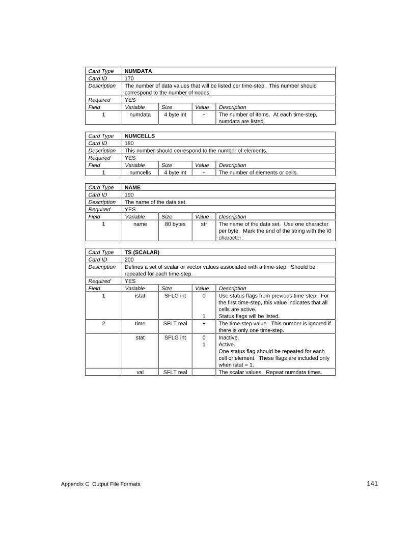
Appendix C Output File Formats 141
Card Type NUMDATACard ID 170Description The number of data values that will be listed per time-step. This number should
correspond to the number of nodes.Required YESField Variable Size Value Description
1 numdata 4 byte int + The number of items. At each time-step,numdata are listed.
Card Type NUMCELLSCard ID 180Description This number should correspond to the number of elements.Required YESField Variable Size Value Description
1 numcells 4 byte int + The number of elements or cells.
Card Type NAMECard ID 190Description The name of the data set.Required YESField Variable Size Value Description
1 name 80 bytes str The name of the data set. Use one characterper byte. Mark the end of the string with the \0character.
Card Type TS (SCALAR)Card ID 200Description Defines a set of scalar or vector values associated with a time-step. Should be
repeated for each time-step.Required YESField Variable Size Value Description
1 istat SFLG int 0
1
Use status flags from previous time-step. Forthe first time-step, this value indicates that allcells are active.Status flags will be listed.
2 time SFLT real + The time-step value. This number is ignored ifthere is only one time-step.
stat SFLG int 01
Inactive.Active.One status flag should be repeated for eachcell or element. These flags are included onlywhen istat = 1.
val SFLT real The scalar values. Repeat numdata times.
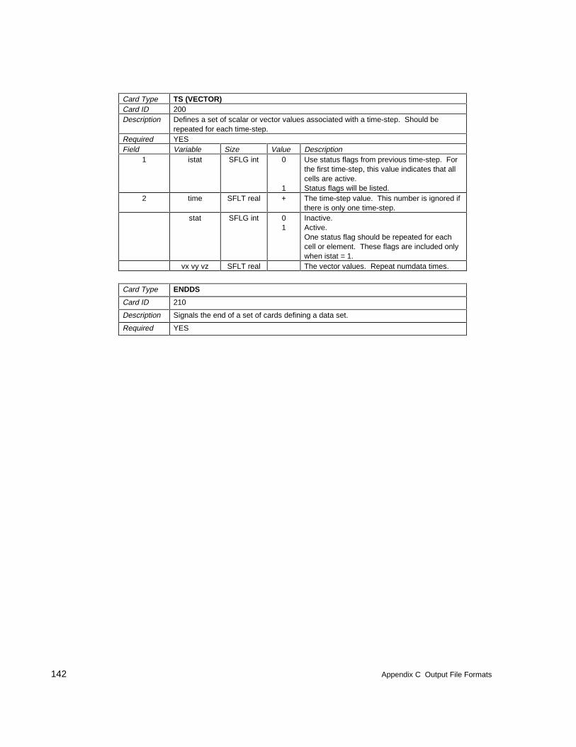
142 Appendix C Output File Formats
Card Type TS (VECTOR)Card ID 200Description Defines a set of scalar or vector values associated with a time-step. Should be
repeated for each time-step.Required YESField Variable Size Value Description
1 istat SFLG int 0
1
Use status flags from previous time-step. Forthe first time-step, this value indicates that allcells are active.Status flags will be listed.
2 time SFLT real + The time-step value. This number is ignored ifthere is only one time-step.
stat SFLG int 01
Inactive.Active.One status flag should be repeated for eachcell or element. These flags are included onlywhen istat = 1.
vx vy vz SFLT real The vector values. Repeat numdata times.
Card Type ENDDS
Card ID 210
Description Signals the end of a set of cards defining a data set.
Required YES

Appendix C Output File Formats 143


