p-FEMs in biomechanics: Bones and Arteries

Zohar Yosibash

Department of Mechanical Engineering, Ben-Gurion University of the Negev,

Beer-Sheva, Israel

Abstract

The p-version of the finite element method (p-FEM) is extended to problemsin the field of biomechanics: the mechanical response of bones and arteries.These problems are extremely challenging, partly because the constitutivemodels governing these materials are very complex and have not been in-vestigated by sufficiently rigorous methods. Furthermore, these biologicalstructures have a complex geometrical description (substructures with highaspect ratios), undergo finite deformations (arteries), are anisotropic andalmost incompressible (arteries). The intrinsic verification capabilities andhigh convergence rates demonstrated for linear problems are being exploitedand enhanced here, so that validation of the results can be easily conductedby comparison to experimental observations.

In the first part of the paper we present p-FE models for patient-specificfemurs generated semi-automatically from quantitative computed tomogra-phy (qCT) scans with inhomogeneous linear elastic material assigned directlyfrom the qCT scan. The FE results are being verified and thereafter validatedon a cohort of 17 fresh-frozen femurs which were defrosted, qCT-scanned, andtested in an in-vitro setting.

The complex combined passive-active mechanical response of human ar-teries is considered in the second part and the enhancement of p-FEMs tothese non-linear problems is detailed. We apply a new ‘p-prediction’ al-gorithm in the iterative scheme and demonstrate the efficiency of p-FEMscompared to traditional commercial h-FEMs as Abaqus (in respect of bothdegrees of freedom and CPU times). The influence of the active response isshown to be crucial if a realistic mechanical response of an artery is sought.

Email address: zohary@bgu.ac.il (Zohar Yosibash)

Preprint submitted to CMAME September 14, 2012

Keywords: Femurs, Arteries, Hyperelasticity, p-FEM

1. Introduction

The p-version of the finite element method (p-FEMs), known for threedecades already, has several advantages that make its use for linear ellipticproblems attractive: the boundary’s domain is represented accurately us-ing blending-functions, it converges exponentially for smooth solutions, thefinite element mesh is kept constant while only the polynomial degree isincreased so that elements are larger, may be far more distorted and havelarge aspect ratios [1], and is not prone to locking for nearly incompress-ible materials. These methods have been extended to non-linear problems,first for plasticity [2, 3], and thereafter to isotropic hyperelasticity [4] and tonearly-incompressible hyperelasticity [5].

The intrinsic verification capabilities and high convergence rates of thep-FEMs are extremely important for analysts that aim at validating mathe-matical models of biomechanical structures such as femurs and arteries. Forarteries, this is because the suggested constitutive models at the tissue levelare of high mathematical complexity and to determine the coefficients in thesemodels, FE approximations are compared to experimental observations. Forfemurs, several biomechanical constitutive models at the tissue-level are sug-gested (formulated based on experiments on small tissue-specimens takenfrom a whole organ), none of which agreed by the scientific community tobest represent the “reality”. Therefore, the most appropriate tissue-levelmodel used in the FE analysis of the entire femur is usually sought by com-parison to experimental observations, namely, by a validation process. Thevalidation process can only be conducted after the numerical results havebeen verified, i.e. the numerical error has been quantified. Here, extensionsto p-FEMs are addressed to exploit their advantages when solving problemsin the field of biomechanics. We first address the mechanical response of apatient-specific human femur, which is well described by an inhomogeneousanisotropic linear elastic model.

Simulations of human femurs by classical h-FEMs started in the early 90’sby Keyak and coworkers [6]. In these methods the inhomogeneous distribu-tion of material properties was usually attained by assigning constant distinctvalues to distinct elements (see e.g. [7] and references therein), thus the ma-terial properties become mesh dependent. Furthermore, the bone’s surface

2

was approximated by piecewise flat tessellation or piecewise parabolic tes-sellation, introducing un-smoothness of the surface and inaccuracies in thesurface strains. Among the vast literature addressing h-FE simulations of thefemur, the recent ones that present results which are closest to experimentalobservations are [8, 9].

Combining p-FEMs with quantitative computer tomography (qCT) scansfor an individual, a systematic method is presented that generates an accu-rate description of femur’s geometry, creates a p-FE mesh and determinesthe inhomogeneous material properties. Micro-mechanical approaches canbe used to assign orthotropic properties to the whole organ [10, 11, 12], butunder simplified loading conditions an isotropic assumption is sufficient towell describe the mechanical response. In this case, the Young’s modulusE is determined by empirical relationships to a densitometric measure, andthe “best” relationship found to well represent the whole-organ mechanicalresponse is determined based on comparison to experimental observations(the validation process). A solution at increasing polynomial degrees enablesan easy verification (both boundary and material properties are smooth soan exponential convergence is obtained), assuring that the numerical errorsare bounded by a specified tolerance. Finally, the FE results are comparedagainst all measurable data (strains and displacements) recorded during sim-plified in-vitro tests on a variety of femurs (with a wide spread in age, genderand weight) for validation. Here, a systematic V&V process, involving thelargest set (so far considered) of seventeen human fresh-frozen femurs, is con-sidered. The verified p-FEMs results where then used for validation purposes;both strains and displacements results were compared to experimental obser-vations, such that twelve of these experiments were performed by a differentgroup so a “blind” non-biased comparison was obtained [13].

Unlike bone mechanics, which is governed by the linear theory of elastic-ity, arteries undergo finite-deformations, are nearly-incompressible, containfamilies of collagen fibers in different directions, are constructed by two dis-tinct and different thin layers and in addition contain muscle cells that addan active response along their directions. The p-FEM based on the dis-placement formulation has been shown to be efficient in the framework offinite-deformations for isotropic hyperelastic materials [4, 14] and that it islocking free for nearly-incompressible hyperelastic materials [5, 15] thus it isexpected to be especially attractive for modeling arteries.

The fibers reinforced hyperelastic constitutive model (manifested in a

3

strain energy density function, SEDF) by Holzapfel et. al [16, 17] is com-plemented by a “compressible” part divided by a bulk modulus becauseit describes a compressible deformation becoming increasingly more incom-pressible as the bulk modulus tends to ∞ (see for details [18]). The activeresponse is added to the passive SEDF, derived in [15] based on [19]. A newiterative algorithm, named “p-prediction”, is introduced that accelerates con-siderably the Newton-Raphson method when combined with p-FEMs. Thep-FE formulation for anisotropic hyperelastic nearly incompressible ”artery-like” domains is described and its advantages over conventional FEMs aredemonstrated both when considering degrees of freedom and CPU. Artery-like structures are investigated and the effect of the activation level is demon-strated, showing that the predicted passive-active mechanical response is asobserved in experiments.

To demonstrate the advantages of p-FEMs and their systematic use forverification and validation in the field of biomechanics, we construct themanuscript as follows: In section 2 patient-specific p-FE analyses of the fe-mur are presented. We concentrate our attention on the generation of FEmodels from qCT scans and emphasize the discrete representation of the ma-terial data in CT scans and their influence on the numerical results. We alsoshow a systematic V&V process where the verified FE results obtained bya specific constitutive model are compared to a large set of experiments forvalidation purposes. Thereafter we address artery simulations in section 3starting by introducing notations, then discuss the constitutive model andweak formulation followed by the discretization in the context of p-FEMs.A simple example problem with an analytical solution is solved by the p-FEimplementation to verify the accuracy and efficiency compared to a commoncommercial h-FE code, Abaqus [20], and thereafter an artery-like cylindricaldomain under internal pressure is addressed to investigate the passive-activeresponse when considering collagen and smooth-muscle-cell fibers. We con-clude with a summary and conclusions in section 4.

2. p-FE analysis of the femur

The generation of CT-based FE models starts with qCT image segmen-tation that separates the bone region from the remainder of the image basedon the Hounsfield Units (HU). To distinguish between the cortical and tra-becular regions we associate voxel values of HU> 600 (ρash > 0.6 g/cm3) to

4

the cortical bone and values of HU≤ 600 to the trabecular bone. Exteriorand interior boundaries are traced and arrays are generated, each represent-ing different boundaries of a given slice. These arrays are manipulated bya 3-D smoothing algorithm that generates smooth raw data arrays. Thesmooth edges, using cubic spline interpolation, are read into the CAD pack-age SolidWorks-2010 (SolidWorks Corporation, MA, USA) and manipulatedto generate a surface representation of the femur and subsequently a solidmodel. Large curved patches representing the surfaces are generated, whichare essential in order to allow the automatic p-mesh generator to producecurved-face elements which are not necessary small. The resulting 3D solidis imported into the p-FE StressCheck1 code. An auto-mesher is thereafterapplied that generates tetrahedral high-order elements having curved faces,following exactly the domain’s geometry. The entire algorithm (qCT to FE)is schematically illustrated in Figure 1.

Remark 1. The numerical error associated with the use of tetrahedron p-elements, compared to hexahedral p-elements, was investigated and was con-firmed to be of the same order of accuracy when the polynomial degree isincreased [21]. The “overly stiff” behavior of tetrahedral h-elements does notoccur for p-FEs.

2.1. Assigning isotropic material properties to the finite elements

The next step is to assign inhomogeneous material properties to the finiteelements, associated with the density at each point within the bone. Sincethe material properties are given at distinct “grid” points, at the centerof the qCT voxels, we demonstrate here on a benchmark problem that fora reasonably “dense grid” an excellent approximation is obtained as if thematerial properties would had been available as an analytic function.

2.1.1. A benchmark problem to quantify the influence of E-data provided at

discrete points

Consider a sphere determined by

Ω =

(r, ϕ, θ)

∣

∣

∣

∣

r < 5, ϕ < π, θ < 2π

1StressCheck is trademark of Engineering Software Research and Development, Inc, St.Louis, MO, USA.

5

CT

Num.

HU

EQM

Ash

),,( zyxE

g. Material g. Material

evaluationevaluation

slicesa. CTc. Smooth

boundaries

b. Boundaries

identification

d1. Points

cloud

d2. Splines

through points

f. p-FE mesh e. Surface

through splines

Figure 1: Schematic flowchart describing the generation of the p-FE model from qCTscans. a - Typical CT-slice, b. - Contour identification, c. - Smoothing boundary points,d1. - Points cloud representing the bone surface. d2. - Close splines for all slices, e. -Bone surface, f. - p-FE mesh and g. - Material evaluation from CT data. (Figure from[12].)

where r =√

x2 + y2 + z2, with a boundary ∂Ω defined by r = 5 (see Figure2). The center of the sphere is at (x, y, z) = (0, 0, 0).Traction boundary conditions: On the part of the boundary ∂ΩT defined byr = 5 ∩ z > 4 pressure boundary conditions tn = −1/∂ΩT are prescribed.On ∂ΩT0 defined by r = 5∩ −4 < z < 4 traction free boundary conditionsare prescribed.Clamped boundary conditions: On the part of the boundary ∂Ωu definedby r = 5 ∩ z < −4 clamped boundary conditions are prescribed u =(ux, uy, uz)

T = 0.Material properties: Consider an inhomogeneous isotropic material with Young’smodulus E being provided analytically:

E = 100 ×[

1 + sin(rπ/10) + exp(r2/10)

]

+ 100x+ 100y. (1)

This expression is a good representation of a bone-like structure which has alow Young’s modulus in the middle, that becomes higher towards the surface.

6

The last two terms in (1) ensure that the material properties do not havea spherical symmetry. To represent a CT-like scan of such a sphere, theanalytical expression is evaluated at voxels with increasing resolution. Threeresolutions denoted as 50 Cells, 100 Cells and 150 Cells resemble a CT scanin a bounding box of dimensions 11× 11× 11 so that −5.5 ≥ x, y, z ≥ 5.5.This box containing the sphere is divided into 50× 50× 50, 100× 100× 100and 150×150×150 voxels and E according to (1) is computed in the middleof each voxel within the sphere. These discrete values are provided in theFE analysis, and are typical of the resolutions in CT-scans. In all cases thePoisson’s ratio is kept constant ν = 0.3. The domain was discretized by 128p-FEs (tetrahedrons, pentahedrons and hexahedrons) as shown in Figure 2with the boundary conditions and E distribution.

Figure 2: Left - FE mesh and BCs. Right - Inhomogeneous Young’s modulus at a slice atx = 0.

The total potential energy, the displacement in the z direction at theapex (uz(0, 0, 5)), and the maximum negative average principal strain ε3 at100 points along the surface curve between z = 4 to z = 4.75 shown in Figure3 for polynomial degrees p = 1 to 8 are summarized in Table 1.

The relative error as percentage in the potential energy compared to p = 8FE solution with the “analytic E” is presented in Figure 4.

The convergence in energy norm for increasing p values is rather slow.This is because the solution at the circular edge r = 5∪z = −4, which is thecurve where a sharp transition in boundary conditions occurs (from clamped

7

Figure 3: The edge along which ε3 is extracted and then averaged.

Figure 4: Relative error as percentage in potential energy compared to the FE analysiswith analytical E at p = 8.

8

Table 1: FE results for the sphere problem: p-level, DOFs, potential energy, uz(0, 0, 5)and average ε3 for the E given at 50,100,150 CT-like cells and the analytic E.

Total Potential Energy uz

p DOF 50 Cells 100 Cells 150 Cells Analytic 50 Cells 100 Cells 150 Cells Analytic1 315 -1.435E-4 -1.431E-4 -1.430E-4 -1.429E-4 -3.833E-4 -3.822E-4 -3.818E-4 -3.817E-42 1302 -1.727E-4 -1.721E-4 -1.720E-4 -1.719E-4 -4.310E-4 -4.302E-4 -4.296E-4 -4.296E-43 2601 -1.755E-4 -1.750E-4 -1.748E-4 -1.747E-4 -4.341E-4 -4.337E-4 -4.331E-4 -4.330E-44 5004 -1.771E-4 -1.765E-4 -1.764E-4 -1.763E-4 -4.379E-4 -4.369E-4 -4.362E-4 -4.362E-45 8775 -1.790E-4 -1.784E-4 -1.782E-4 -1.781E-4 -4.415E-4 -4.404E-4 -4.399E-4 -4.398E-46 14298 -1.799E-4 -1.794E-4 -1.792E-4 -1.791E-4 -4.433E-4 -4.425E-4 -4.418E-4 -4.418E-47 21957 -1.806E-4 -1.800E-4 -1.798E-4 -1.797E-4 -4.446E-4 -4.439E-4 -4.431E-4 -4.431E-48 32136 -1.811E-4 -1.805E-4 -1.802E-4 -1.802E-4 -4.458E-4 -4.447E-4 -4.441E-4 -4.441E-4

Average ε3

p DOF 50 Cells 100 Cells 150 Cells Analytic1 315 -2.166E-5 -1.756E-5 -2.166E-5 -2.150E-52 1302 -2.141E-5 -2.029E-5 -2.141E-5 -2.132E-53 2601 -2.139E-5 -2.077E-5 -2.139E-5 -2.125E-54 5004 -2.130E-5 -2.143E-5 -2.130E-5 -2.124E-55 8775 -2.119E-5 -2.150E-5 -2.119E-5 -2.124E-56 14298 -2.135E-5 -2.164E-5 -2.135E-5 -2.135E-57 21957 -2.129E-5 -2.172E-5 -2.129E-5 -2.139E-58 32136 -2.130E-5 -2.179E-5 -2.130E-5 -2.143E-5

to traction free), is singular, i.e. the stresses tend to infinity. A remedy to thisdeterioration in the convergence rate may be achieved in the framework ofp-FEMs, if a mesh refinement in geometric progression towards the singularcircular edge is enforced (see [1]). Nevertheless, for comparison purposesbetween the analytic E and voxelized E the slow convergence should not posea problem. One is interested whether the voxelized E description representswell the analytic E. The presented benchmark problem demonstrates wellthat the CT-like E values provide an approximation, comparable in qualityto the material properties being specified by analytic functions. In Figure 4a fast convergence in potential energy is observed (when comparing the thevoxelized results to the analytical ones).

2.1.2. E in a patient-specific femur determined by empirical correlation

Many empirical relations between Young’s modulus and bone density,with a constant Poisson’s ratio were suggested, see e.g. [22, 23, 24, 25, 26].In [21, 27] we found that p-FE analyses with the relationships in [24] (thecortical connections are based on [25]) provide the closest results to in-vitro

9

experiments on the proximal femur:

ρEQM = 10−3 (a×HU − b) [g/cm3] (2)

ρash = (1.22 × ρEQM + 0.0523) [g/cm3] (3)

ECort = 10200 × ρ2.01ash [MPa] ρash > 0.6 (4)

ETrab = 5307 × ρash + 469 [MPa] 0.27 < ρash ≤ 0.6 (5)

ETrab = 33900 × ρ2.20ash [MPa] ρash ≤ 0.27 (6)

where ρEQM is the equivalent mineral density, ρash is the ash density, ECort, ETrab

are the Young’s modulii in the cortical and trabecular regions and the pa-rameters a and b are determined by K2HPO4 phantoms placed around thefemur in the CT-scan. Constant Poisson ratio ν = 0.3 was assigned to theentire bone. According to a sensitivity analysis in [28, 21] the influence of νon the results is very small.

Determination of E(x, y, z) at each integration point (Gauss points), inthe FE model is performed as follows. First a moving average algorithm isapplied to average the HU data in each voxel based on a pre-defined cubicvolume of 3 × 3 × 3 mm3 surrounding it (cubic volumes of 27,125,343 mm3

showed similar results in [28]). HU averaged data is subsequently convertedto an equivalent mineral density ρEQM by (2) which is determined by thecalibration phantom - see for details [29, 28]. E at every Gauss point isassigned the value of the closest available point in the qCT file. The numberof Gauss points was 512 for tetrahedral and 2744 for hexahedral elements,independent of the p-level.

2.1.3. Verification of p-FE results and sensitivity analyses.

p-FE results are verified so to ensure that the numerical error is under aspecific tolerance. To this end, the polynomial degree over the elements isincreased until the relative error in energy norm is small, and the strains atthe points of interest converge. Such a verification, for example for a femurdenoted FF3, when increasing p from 1 to 5 is presented in Figure 5.

The solid model of the femur was partitioned such that the number offinite elements was between 3500 to 4500 elements (∼ 150, 000 degrees offreedom (DOFs) at p = 4 and ∼ 300, 000 DOFs at p = 5).

Sensitivity studies:

To ensure the reliability of the FE analyses sensitivity studies were per-formed to ensure that the obtained results are not too sensitive. a) Poisson

10

Figure 5: Convergence in energy norm, head displacement and ǫzz at a representativepoint of interest in FF3. (Figure from [27].)

ratios ν = 0.01, 0.1, 0.3, 0.4 were applied to the femur, as in [23, 30, 28], b)The distal face of the femur residing in PMMA in in-vitro experiments waseither clamped or modeled as attached to a distributed spring. c) Strainsat strain-gauge locations were checked at ±5 offset orientations. d) Strainswere computed either as averaged over an element or as maximum or mini-mum values.

2.2. Validation by comparison to in-vitro experiments

Biomechanical experiments on seventeen fresh-frozen human cadaver fe-murs were conducted to validate the FEA. Experiments on five femurs (de-noted FF1-FF5) were performed in-house, and six pairs of femurs (denoted by1 to 6) were tested by another research institute with results unknown untilthe analyses were completed to avoid any bias. Table 2 summarizes the dataon femurs and CT scan resolutions. Within one day of defrosting and per-forming CT measurements, experiments were conducted to mimic a simplestance position configuration in which the femurs were loaded through theirhead while inclined at different inclination angles (0, 7, 15 and 20 degrees) asshown in Figure 6. We measured the vertical and horizontal displacements

11

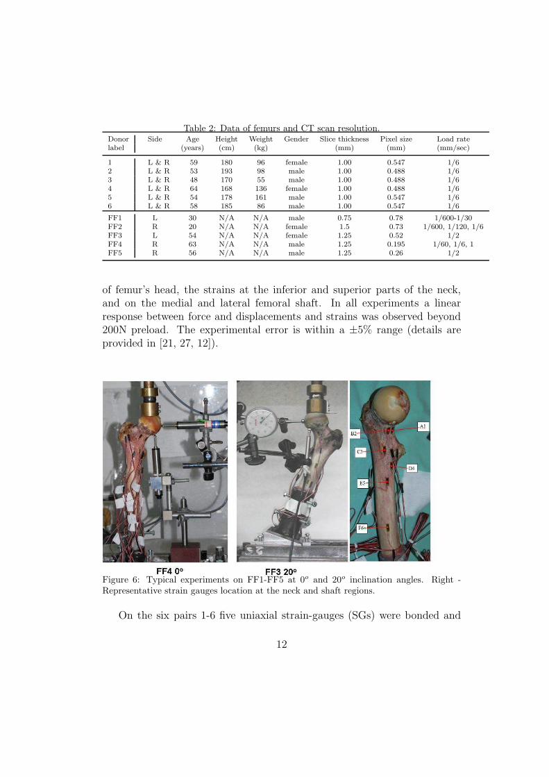
Table 2: Data of femurs and CT scan resolution.Donor Side Age Height Weight Gender Slice thickness Pixel size Load ratelabel (years) (cm) (kg) (mm) (mm) (mm/sec)

1 L & R 59 180 96 female 1.00 0.547 1/62 L & R 53 193 98 male 1.00 0.488 1/63 L & R 48 170 55 male 1.00 0.488 1/64 L & R 64 168 136 female 1.00 0.488 1/65 L & R 54 178 161 male 1.00 0.547 1/66 L & R 58 185 86 male 1.00 0.547 1/6

FF1 L 30 N/A N/A male 0.75 0.78 1/600-1/30FF2 R 20 N/A N/A female 1.5 0.73 1/600, 1/120, 1/6FF3 L 54 N/A N/A female 1.25 0.52 1/2FF4 R 63 N/A N/A male 1.25 0.195 1/60, 1/6, 1FF5 R 56 N/A N/A male 1.25 0.26 1/2

of femur’s head, the strains at the inferior and superior parts of the neck,and on the medial and lateral femoral shaft. In all experiments a linearresponse between force and displacements and strains was observed beyond200N preload. The experimental error is within a ±5% range (details areprovided in [21, 27, 12]).

Figure 6: Typical experiments on FF1-FF5 at 0o and 20o inclination angles. Right -Representative strain gauges location at the neck and shaft regions.

On the six pairs 1-6 five uniaxial strain-gauges (SGs) were bonded and

12

Figure 7: (a-left) Sketch of the frontal plane of an embedded and instrumented left femur.The adapter applied the load by the testing machine to the specimen. The proximalembedding (hidden in adapter) builds a ball-joint with the adapter. Strain gauges (SG1-SG5) are applied to specific anatomic sites. SG1 - located at the middle of the superiorneck. SG2 - located opposite to SG1 at the inferior neck. SG3 - located next to the mostprominent part of the lesser trochanter. SG4 - located 100mm distally to SG3 at themedial side of the shaft. SG5 - located opposite to SG4 at the lateral side of the shaft.(b-right) Experimental setup with the optical markers on an instrumented left femur andits corresponding deformed (magnified) FE model (Figure from [13].)

optical markers were distributed over the femur, the adapter of the testingmachine, and the cardan joint, see Figure 7. The distal end of each femurwas potted with casting resin in an aluminum case that fitted into a cardanjoint so that the line of force went through the center of the femoral head andthe center of the epicondyles. The femoral head was potted in a hemisphereof casting resin that fitted the proximal adapter of the test setup (Fig. 7b).The mean values of strains were calculated to be used for the later com-parison with the FEA. The total displacements utot =

√

u2x + u2

y + u2z of the

optical markers on the bone surface were also calculated. Details on theseexperiments were provided in [13].

The verified FE analyses that mimic the in-vitro experiments are usedfor validation purposes, i.e. to ensure that these indeed represent the biome-

13

chanical response. For each FE analysis the strains at the location of thestrain-gauges (SGs) were averaged over a small area representing the areaover which the gauge or the SG measured the strains. Because uni-axialSGs were used in our experiments, we considered the FE-strain componentin the direction coinciding with the SG direction (in most cases the SGs arealigned along the principal strain directions). A total of 102 displacementsand 161 strains on the 17 femurs were used to assess the validity of the p-FEsimulations. In Figure 8 the pooled FE strains and displacements are com-pared to the experimental observations - this comparison is demonstratedby a linear regression plot, inspecting the slope, intersection and R2 of thelinear regression between the experimental observations and FE predictions.

Remark 2. Note that for twelve of the seventeen femurs a blind comparisonwas performed, i.e. the group that performed the experiments did not knowthe FE results, and vice-versa, the experimental results were not known bythe group that performed the analysis.

−1500 −1000 −500 0 500 1000 1500

−1500

−1000

−500

0

500

1000

1500

EXP

FE

A

Strain [µε]Displacement [µm]Linear

FE =0.961⋅EXP−22R2 =0.965

Figure 8: Comparison of the computed strains + and displacements to the experimentalobservations normalized to 1000 N load.

14

One may observe the unprecedented match between the predicted and mea-sured data for femurs under stance position loading: the slope and R2 of thelinear regression are very close to 1. The strains prediction is highly accurate,but not less important, the displacements are also well predicted.

Based on the results of validation experiments no reasons were found toreject or modify the mathematical model, so that the FE results may bealso utilized to investigate the internal state of strains within the femur. Forexample, Figure 9 shows the maximum (tensile) and minimum (compression)principal strains at a cutting plane within FF5.

Figure 9: Principle maximum strains (left) and minimum strains (right) at a cutting planein the middle of FF5, loaded at 7o.

The presented p-FEMs based on patient-specific qCT-scans are semiau-tomatic procedures requiring less than three hours from qCT-scan to theverified results on a PC. The ability to keep numerical errors under controlenables to focus the attention on the idealization errors. The validation ofthe FE-results was performed by comparing FE extracted strains and dis-placements to measured data on 17 fresh-frozen femurs. This comparisondemonstrated an excellent agreement, better than previous works reportedin the literature (comparison of displacements is not reported in studies byother authors, to the best of our knowledge).

Thanks to the double-blinded validation on 12 of the 17 femurs [13], thisvalidation process is also bias-free. The V&V process outlined herein laysthe foundation for the extension of the study to prediction of fractures in

15

pathological cases as osteoporotic bones. Once the strains and displacementsare shown to be well computed in the femur, these can be used so to determinethe predictability of different failure laws. This of course calls for a newvalidation process along the lines outlined herein.

The successful use of p-FEMs in biomechanical problems governed bylinear elasticity and the systematic use of a V&V methodology are expectedto be more pronounced when the equations are non-linear, as the governingequations describing the mechanical response of arteries. In the next sectionthe application of p-FEMs for simulating artery’s mechanical response isaddressed and verified towards its validation by experimental observations.

3. p-FEMs for arteries

The constitutive models for arteries are based on fiber reinforced, nearly-incompressible hyperelasticity, involving finite deformations, as detailed inAppendix A. Because both passive and active responses are of major im-portance for the mechanical response of the artery tissue, we consider astrain-energy density function (SEDF) of the form:

Ψtissue = Ψpassive + Ψactive (7)

The passive SEDF (see (A.4) and (A.6) in the Appendix) represents anisotropic nearly-incompressible hyperelastic matrix with two families of fiberswhich depends on the invariants of the right Cauchy-Green tensor C and twounit direction vectors along collagen fiber directions M 0, and M 1. For exam-ple, using the Cartesian coordinate system in Figure 10, the fibers directionsareM 0 = (sin βM ,− cosβM

Y√Y 2+Z2 , cosβM

Z√Y 2+Z2 )

T ,

M 1 = (− sin βM ,− cosβMY√

Y 2+Z2 , cosβMZ√

Y 2+Z2 )T . The active SEDF Ψactive

depends on the concentration level of a vasoconstrictor, the stretch ratio anda unit direction vector along the smooth muscle cells, given in (A.10).

3.1. Weak formulation and discretization by p-FEMs

Having determined the SEDFs, we choose to formulate a weak formula-tion in the reference configuration, neglecting inertia terms (also denoted bythe Total-Lagrange formulation), see e.g. [31]. This is a Newton-Raphsoniterative scheme in which the displacements are assumed to be known at a

16

Figure 10: Coordinate system in a typical artery. (Figure from [18].)

given instance, U (k), so that when applying an additional load increment,one is interested in the associated displacement increment denoted by ∆U .Once ∆U is computed a new displacement vector is generated

U (k+1) = U (k) + ∆U , (8)

and the iterative scheme continues until convergence.

Having U (k), the associated deformation gradient may be computed F (k) def=

I + ∂U(k)

∂X. The linearized system to be solved is [31, p.148]:

Find ∆U ∈ E(Ω0) such that ∀Q ∈ E(Ω0)

1

4

∫

Ω0

[

∂Q

∂X· F (k) + F (k) · ∂Q

∂X

]

: C(k) :

[

∂∆U

∂X· F (k) + F (k) · ∂∆U

∂X

]

dΩ0

+

∫

Ω0

S(U (k)) :

(

∂∆U

∂X· ∂Q∂X

)

dΩ0 +DG(∆U ,Q)

=

∫

∂Ω0

T (N) · QdΓ0 +G(Q)

−1

2

∫

Ω0

S(U (k)) :

[(

∂Q

∂X

)

· F (k) +(

F (k))

· ∂Q∂X

]

dΩ0 (9)

17

with T (N) = FS ·N being the traction applied on the reference configurationboundary. The second Piola-Kirchhoff stress tensor and fourth order tangenttensor are obtained from the SEDF:

Sdef= 2

∂Ψ

∂C, C

def= 2

∂S

∂C(10)

S = Spassive + Sactive = 2∂Ψpassive

∂C+ 2

∂Ψactive

∂C, (11)

C = Cpassive + Cactive = 2∂Spassive

∂C+ 2

∂Sactive

∂C(12)

The terms DG(∆U ,Q) and G(Q) are to be added if pressure (follower loads)are considered, see equations (49) and (53) in [14].

Remark 3. In our in-house p-FEM implementation C is computed at eachiteration step, unlike the modified Newton methods in which C is computedonly once for each load increment or once every several equilibrium iterations.

3.1.1. p-FEM implementation

The weak form (9) is discretized using a space of hierarchical polynomials(shape functions) Ni(ξ, η, ζ) on the standard hexahedral element (see [32]).The sought (trial) vector ∆U is represented by an unknown 3n × 1 vector∆U as follows:

∆U =

N1 · · ·Nn 0 · · ·0 0 · · ·00 · · ·0 N1 · · ·Nn 0 · · ·00 · · ·0 0 · · ·0 N1 · · ·Nn

∆Udef= [N ]∆U (13)

whereas Qdef= [N ]Q is the test vector. Using blending mapping functions

Γ(ξ, η, ζ) from the standard element to the physical element [1], an exact ge-

ometry description of the faces and edges of the physical element is obtained:

X =

XYZ

=

Γ1(ξ, η, ζ)Γ2(ξ, η, ζ)Γ3(ξ, η, ζ)

, [J ] =

∂Γ1

∂ξ∂Γ2

∂ξ∂Γ3

∂ξ∂Γ1

∂η∂Γ2

∂η∂Γ3

∂η∂Γ1

∂ζ∂Γ2

∂ζ∂Γ3

∂ζ

(14)

Derivatives of the shape functions in the standard element are computed by:

∂Ni

∂X=

∂Ni

∂X∂Ni

∂Y∂Ni

∂Z

= [J ]−1

∂Ni

∂ξ∂Ni

∂η∂Ni

∂ζ

(15)

18

Remark 4. It is important to realize that the use of the Total-Lagrangeformulation does not require to update the FE mesh, and hence the Jacobian[J ] is determined once, relative to the material (undeformed) configuration.The updates from one iteration to the next are performed by updating theintegrand terms due to the update of the displacements (8).

By using (15) with (13) and (14) the discretized form of (9), to be solved ateach iteration step, is obtained:

[

KTangent]

∆U = rob (16)

The tangent stiffness matrix, [KTangent], consists three parts [KTangent] =[KInt,Mat

T +KInt,GeoT +KFollower

T ] [31] with the third term (see [14, eq. (53)])only considered in cases of follower loads.The out-of-balance vector, rob consists also three parts rob = rExt +rFollwer−rInt with rFollwer (given in [14, eq. (49)]) only considered in case of followerloads.

The explicit expressions for the computation of rob and [KTangent] arepresented in [18]. Both rob and [KTangent] are computed at each iteration andthe iterative process continues until the relative difference in each element

of the “out-of-balance” vector,∣

∣

∣r

ob(k)i − r

ob(k−1)i

∣

∣

∣/∣

∣

∣r

ob(k)i

∣

∣

∣, is smaller than a

given tolerance, ǫ = 10−6.

Remark 5. The matrices [KInt,Mat] and [KInt,Geo] are symmetric [31] whereas[KFollower] in general is not [31]. Therefore the bi-conjugate gradient method[33] is utilized for inverting [KTangent] and solving (16).

3.1.2. Acceleration of the iterative scheme by “p-prediction”

The Newton-Raphson iterative scheme requires an initial guess in thevicinity of the solution, and the closer this guess is to the exact solution,the faster is the convergence (the number of iterations are smaller). It iscommon therefore, in most FE implementation to introduce an additionalloop by dividing the total load into several load steps, so that the iterationson U (k) start at each load step with an initial solution being the solution atthe previous load step.

The p-FE inherent hierarchical basis of the shape functions allows a simpleand novel acceleration of the iterative scheme by predicting the initial guess

19

U (0) for a higher p-level using the converged solution already available at alower p-level. This ”p-prediction” method requires load steps only for p = 1with an “usual” Newton-Raphson iterative scheme. For p ≥ 2 the convergedsolution at p− 1 is used as the ”initial guess” to the iterative scheme. Thisresults in a very fast convergence, noticed to be obtained within one loadstep in all numerical tests. Numerical experiments using the standard and“p-prediction” methods show a speedup factor of at least 20 in CPU. For anearly-incompressible material, the p-FEMs are locking-free only for p-levels4 and above [5], therefore the first initial solution to be applied with the“p-prediction” method is at p = 4.

3.2. Verification of the p-FE implementation

To verify our in-house numerical implementation and to compare its effi-ciency to classical h-FEMs, we first consider a benchmark problems for whichan analytical solution was provided for a hyperelastic material in [18]. Con-

sider the cube defined by Ω =

(X, Y, Z)

∣

∣

∣

∣

0 < X < 2, 0 < Y < 2, 1 <

Z < 3

shown in Figure 11 with the constitutive model given by the SEDF

Ψ = Ψisoch + Ψvol in (A.4). We apply the following boundary conditions on

F1

F2

F3

F4

F5

F6

X Y

Z

Figure 11: Domain and p-FE mesh for the cube problem and h-FE mesh used by Abaqus.

20

the six faces F1 − F6:

U = 0 on F1

tX = 0, tY = −[

23c1

(

Z− 13 − Z

23

)

+ 2D1

(

Z −√Z

)]

, tZ = 0 on F2

tX = 23c1

(

Z− 13 − Z

23

)

+ 2D1

(

Z −√Z

)

, tY = 0, tZ = 0 on F3

tX = 0, tY = 23c1

(

Z− 13 − Z

23

)

+ 2D1

(

Z −√Z

)

, tZ = 0 on F4

tX = −[

23c1

(

Z− 13 − Z

23

)

+ 2D1

(

Z −√Z

)]

, tY = 0, tZ = 0 on F5

tX = 0, tY = 0, tZ = 89c13

16 + 2

D1

(√3 − 1

)

on F6,

and the body forces:

(fX , fY , fZ) =

(

0, 0, −10

9c1Z

− 73 +

2

9c1Z

− 43 − 1

D1Z

)

.

Under these boundary conditions the exact solution is (notice that the solu-tion is analytic because the domain is such that 1 < Z):

x = X, y = Y, z =1

3

(

2Z32 + 1

)

or in terms of displacements: UX = UY = 0, UZ = 13

(

2Z32 + 1

)

− Z

The material properties chosen are c1 = 0.027 MPa and D1 = 30 MPa−1.The “cube problem” was solved by the p-FEM with eight uniform hexahe-dral elements and for comparison also by the h-FE commercial code Abaqus6.8 EF with 8-node hexahedral elements and an automatic load step control(the conventional “displacement formulation elements” were used in Abaqusbecause the deformation is clearly compressible). Structured meshes of hex-ahedral elements are used for all analyses on arteries reported here. A directsolver was used for both codes, and computations performed on a singleprocessor (no parallelization was applied).

The convergence pattern is shown in Figure 12 by monitoring the relativeerror in energy norm, defined as:

||e(U)||(%) =

√

∫

ΩΨ(C)dΩ

FE−

∫

ΩΨ(C)dΩ

Exact∫

ΩΨ(C)dΩ

Exact

× 100

21

replacem

en

Figure 12: Relative error in energy norm as a function of DOFs (left) and CPU with andwithout the p-prediction algorithm (right) for the cube problem (number of load steps andaverage number of equilibrium iterations shown in brackets).

One may observe that the p-FEM is orders of magnitude faster in termsof DOFs compared to its h-FEM counterpart, and at least one to two ordersof magnitude faster in terms of computational times.

Similar problems with an analytical solution for the verification of the p-FE implementation of the passive and active response are provided in [18, 15].

3.3. The active-passive response of an artery-like tube

The coupled passive-active mechanical response (7) of an artery-like do-main made of two layers, media and adventitia, is investigated. The innerand outer diameter and media thickness is estimated from an in-vivo studyof the abdominal aorta, having Din = 10 mm, Dout = 12.6 mm, hmedia =0.866 mm, hadventitia/hmedia = 2/3, and length of L = 20 mm. The tubeis clamped at both ends and loaded by an internal physiological pressure ofP = 13.33 kPa (100 mmHg).

Collagen fibers are orientated at the angles ±βM with respect to thecircumferential direction and SMCs are wrapped in the media only in a cir-cumferential direction (pitch angle βMF = 0). Very little SMCs exist in theadventitia [34] so its mechanical response is purely passive. The material pa-rameters for the passive and active response are given in Table 3. Because foreach fiber at an angle βM with respect to the circumferential direction, thereis a fiber at an angle −βM , and because the SMCs fibers are aligned along the

22

circumferential direction, circumferential symmetry is obtained (the ”fibers”are not modeled, but only their homogenized contribution, so at each pointthere are 2 fibers at ±βM ). Therefore only one eighth of the domain isdiscretized. Ten circular hexahedral elements graded towards the clampedboundary with symmetric boundary conditions are considered as shown inFigure 13.

Figure 13: Mesh and boundary conditions for an artery-like structure with SMCs andcollagen fibers.

Table 3: Material parameters fitted to a slightly compressible passive-active SEDF usedin the FEA.

c1 D1 k1 k2 βM λ0 λ1 λm m EC50 Smax

[MPa] [MPa−1] [MPa] [0] [mol/liter] [kPa]media 0.012 1.5 0.1 450 ±44 0.4 2.1 1.25 1 0.00075 222adventitia 0.003 1.5 0.07 60 ±47 / / / / / /

The value of D1 in this example problem was chosen to be 1.5 [MPa−1]that although results in a relative volume change is about ∆V/V ≈ 0.8%,still allows the use of the displacement formulation even for the h-versionwithout the locking effect.

Since an analytical solution is unavailable for such a problem we computeda “benchmark” solution using 50 p-elements at p = 8 and 50% activation(basal tone), corresponding to a concentration value of [A] = 7.5 × 10−4.By using this solution as the reference solution, we plot in Figure 14 theestimated relative error in energy norm as a function of DOFs and CPU forp-and h-FEMs (we used the in-house p-FE code having blending mapping sowith p = 1 and uniformly refine the mesh).

For comparison, if the same problem is solved with D1 = 0.15 [MPa−1]instead (the material becomes progressively more incompressible), resulting

23

101

102

103

104

105

10−5

10−4

10−3

10−2

10−1

100

||e(U

)|| [

%]

h−FEMp−FEMP=1 (20,3)

P=2(1,3)

P=3 (1,3)

P=4 (1,3)P=5 (1,3)

P=7 (1,3)P=6 (1,3)

P=8 (1,3)

32 (20,3)

256 (20,3)

1536 (20,3)

3200 (20,3)

6250(20,3)

10800(20,3)

replacem

en

DOF

100

101

102

103

104

10−5

10−4

10−3

10−2

10−1

100

||e(U

)|| [

%]

CPU (seconds)

Figure 14: Estimated relative error in energy norm as a function of DOFs (left) and CPUwith the p-prediction algorithm (right) for the bi-layer artery (number of load steps andaverage number of equilibrium iterations shown in brackets).

in a relative volume change of ∆V/V ≈ 0.075%, then the displacement for-mulation of the h-FEM experience locking as shown in Figure 15. Comparingto Figure 14 one may observe that the p-FEM convergence is almost unaf-fected whereas the h-FEM convergence considerably deteriorates. In such

101

102

103

104

105

10−3

10−2

10−1

100

101

||e(U

)||[%

]

h−FEM (p=1)p−FEM

P=1

P=6

P=7

P=8

P=2

P=3

P=4

P=5

DOF

Figure 15: Estimated relative error in energy norm as a function of DOFs for the bi-layerartery with D1 = 0.15 [MPa−1].

cases, it is well known that the hybrid formulation should be used for h-FEMs. A comparison between the performance of the p-FE implementationand the hybrid (mixed) formulation available in the commercial code Abaqusfor a nearly incompressible artery-like structure is given in Appendix B.

24

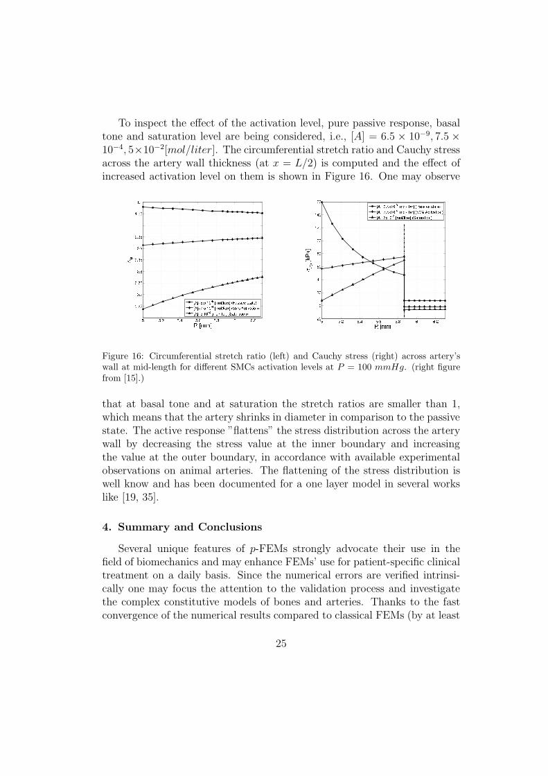
To inspect the effect of the activation level, pure passive response, basaltone and saturation level are being considered, i.e., [A] = 6.5 × 10−9, 7.5 ×10−4, 5×10−2[mol/liter]. The circumferential stretch ratio and Cauchy stressacross the artery wall thickness (at x = L/2) is computed and the effect ofincreased activation level on them is shown in Figure 16. One may observe

Figure 16: Circumferential stretch ratio (left) and Cauchy stress (right) across artery’swall at mid-length for different SMCs activation levels at P = 100 mmHg. (right figurefrom [15].)

that at basal tone and at saturation the stretch ratios are smaller than 1,which means that the artery shrinks in diameter in comparison to the passivestate. The active response ”flattens” the stress distribution across the arterywall by decreasing the stress value at the inner boundary and increasingthe value at the outer boundary, in accordance with available experimentalobservations on animal arteries. The flattening of the stress distribution iswell know and has been documented for a one layer model in several workslike [19, 35].

4. Summary and Conclusions

Several unique features of p-FEMs strongly advocate their use in thefield of biomechanics and may enhance FEMs’ use for patient-specific clinicaltreatment on a daily basis. Since the numerical errors are verified intrinsi-cally one may focus the attention to the validation process and investigatethe complex constitutive models of bones and arteries. Thanks to the fastconvergence of the numerical results compared to classical FEMs (by at least

25

one order of magnitude faster in computational time), and the possible use ofdistorted FE meshes that may contain elements with high aspect ratios, it iseasier to construct models and thus investigate more complex mathematicaldescriptions of the human organs.

For any patient-specific human femur, being an inhomogeneous elastic or-gan, the complete work-flow that may predict its mechanical response underloading has been developed, verified and tested by in-vitro experimentation,and to the author’s opinion is ready for in-vivo clinical trials in an attemptto be used on a daily clinical basis.

The use of p-FEMs has been extended here to thin-layers, anisotropic,hyperelastic materials that may represent human arteries by strain-energy-density-functions which include both active and passive parts. p-FEMs weredemonstrated for the first time (to the author’s knowledge) to be ordersof magnitude faster than h-FEMs both in respect to DOFs and CPU forthese non-linear problems. Since not many experimental observations areavailable on arterial human tissues, we concentrated our attention on theverification procedures and the efficiency of p-FEMs when applied to artery-like structured made of thin layers. Similarly to the investigation of thehuman femur, these capabilities will be combined in the future with a patient-specific model generation of arteries and a set of in-vitro experiments to havea verified and validated method.

AcknowledgementsThe author thanks two of his graduate students, Mr. Nir Trabelsi and

Mr. Elad Priel for their assistance in preparing this manuscript. Four figuresin this manuscript and Appendix B are from their PhD dissertation.

The author gratefully acknowledges the support of the Technische Uni-versitat Munchen Institute for Advanced Study, funded by the German Ex-cellence Initiative, and the Chief Scientist Office of the Ministry of Health,Israel, for their financial support for the research on bones.

Appendix A. Constitutive equations for arteries

Let us define the deformation gradient F = Grad ϕ(X, t)= ∂ϕk(X1, X2, X3, t)/∂XKgi ⊗ GK , where x = ϕ(X, t) defines the place-ment of the point X at time t. XK , k = 1, 2, 3, are the material (reference)(curvilinear) coordinates, gi are the tangent and GK the gradient vectorsin the current and the reference configuration. Usually, the displacement

26

vector U(X, t)def= (UX , UY , UZ)T is introduced, i.e. x = X + U(X, t), and

with this notation F = I + Grad U(X, t). We interchange X1, X2, X3

with X, Y, Z when appropriate for the Cartesian coordinate system. Ageneral strain-energy density function (SEDF) for an isotropic hyperelas-tic material with two families of fibers used to model the passive responseis denoted by, ψpassive(C,M 0,M1) = Ψpassive(IC, IIC, IIIC, IVC,VIC), fol-lowing [16]. It depends on the invariants of the right Cauchy-Green tensorC = F T F = (I + GradU)T (I + GradU), and the two unit direction vectorsalong collagen fiber directions M 0, and M 1.

The invariants of the Cauchy-Green tensor are

IC = trC, IIC =1

2((trC)2 − trC2), IIIC = det C = (det F )2 def

= J2,

(A.1)where trC symbolizes the trace operator and the invariants that representstretch in the fiber directions are

IVC = M 0 · C · M 0, VIC = M 1 · C · M 1, (A.2)

We consider a strain-energy density function composed of three parts formodeling the passive response, an isochoric isotropic and a volumetric isotropicNeo-Hookean parts representing the elastic matrix, and a transversely isotropicpart representing the collagen fibers in the artery wall

Ψpassive = [Ψisoch(IC, IIIC) + Ψvol(IIIC)] + Ψfibers(IVC,VIC), (A.3)

The isochoric isotropic and volumetric isotropic parts are represented by anearly incompressible Neo-Hookean SEDF:

Ψisoch = c1(ICIII−1/3C

− 3), Ψvol =1

D1(III

1/2C

− 1)2 (A.4)

c1 and D1 are constants related to the shear modulus µ and to the bulkmodulus κ

c1 =µ

2, D1 =

2

κ. (A.5)

The transversely isotropic part for modelling the collagen fiber contributionis [16]:

Ψfibers =k1

2k2

[

exp[

k2 (IVC − 1)2] − 1]

(A.6)

+k1

2k2

[

exp[

k2 (VIC − 1)2] − 1]

, IVC,VIC ≥ 1

27

To model the active response we construct a SEDF based on [19]. The firstPiola-Kirchhoff stress component due to smooth muscle cells (SMCs) contrac-tion was found to be proportional to the concentration of the vasoconstrictor[A], as well as the stretch ratio in the SMCs-fibers direction MMF , denotedby λf :

P activeff = S([A])f(λf) (A.7)

where S([A]) is the tension-dose relationship and f(λf) is the tension-stretchrelation. The tension-dose relationship is usually available from ring-tests,as given in [36], so that:

S([A]) = Smax[A]m

[A]m + ECm50

(A.8)

where m is the slope parameter, Smax the maximum value of contraction andEC50 being the concentration at which 50% of maximum generated tension isobtained. In Figure A.17 a representative tension-dose relation is presented.Figure A.17 shows that under a vasoconstrictor threshold concentration no

Figure A.17: Representative tension-dose relation using EC50 = 0.000015 [mol/liter],m =1 taken from [36] and Smax = 100 kPa taken from [19].

induced active response is generated and on the other end the active responsereaches a saturation level beyond a given vasoconstrictor concentration.

The tension-stretch relation is adopted from the work in [19]:

f(λf) =

[

1 −(

λm−λf

λm−λ0

)2]

, λ1 > λf > λ0

0, Otherwise(A.9)

28

with λm being the stretch at which maximum contraction is possible and λ0

and λ1 = λ0 +2(λm−λ0) being the minimum and maximum stretch at whichcontraction can be generated. Using (A.8), (A.9) and (A.7), and defining thedirection of the SMCs before deformation by MMF (with a correspondingangle βSMC) we may obtain an expression for the active SEDF Ψactive:

Ψactive =

Smax[A]m

[A]m+ECm50

[

(λm−√

IVMFC

)3

3(λm−λ0)2+

√

IVMFC

]

, λ21 > IVMF

C> λ2

0

0, Otherwise

(A.10)The dependency of Ψactive on IVMF

Cassures that the active stress is in the

SMCs direction only with zero components perpendicular to it.

Appendix B. An almost incompressible artery: p-FEA comparedto Abaqus hybrid(mixed) h-FEA

In this appendix the performance of the “displacement formulation” ofthe p-FEM for a nearly incompressible artery is compared to the hybridformulation used in Abaqus for an incompressible artery. Because only the“incompressible” passive implementation is available in Abaqus (same formu-lation as in (A.4) and (A.6)) we use it for the simulation of a LAD coronaryartery. The material parameters for (A.5) and (A.6) were fitted by Gasseret al. [37] to experimental data on the human LAD coronary artery re-ported by Carmines et al. [38] and are summarized (with each layer’s radii)in Table B.4 In the p-FE analysis a value of D1 = 0.01 MPa−1 was used

Table B.4: Material parameters fitted to a LAD human coronary arteries according to[37].

Layer c1[kPa] k1[kPa] k2 ±βM [deg] Rin[mm] Rout[mm]Media 27 0.64 3.54 10 3.3170 3.8103

Adventitia 2.7 5.1 15.4 40 3.8103 4.0570

to ensure that J − 1 = VV

≈ 0.001%. The artery was modeled as a tubeof length L = 20 mm, clamped at both ends and loaded by an internalpressure of P = 13.3 kPa(100 mmHg). Due to problem’s symmetry, aneight of the tube was modeled with symmetry boundary conditions appliedas shown in Figure B.18. The “benchmark” solution was obtained using agraded mesh model with 100 hexahedral elements (see Figure B.18) having at

29

Figure B.18: Left - p-FE mesh used in our analyses. Middle - refined p-FE mesh used forthe benchmark solution. Right - Boundary conditions and locations at which data wasextracted.

p = 8 54720 DOFs. The problem was also solved using hybrid(mixed) h-FEelements (the commercial code Abaqus 6.8 EF). An example of the meshesused for Abaqus analysis are shown in Figure B.19. The elements have amaximum aspect ratio of 1:4 thus a large number of elements are obtainedfor thin layered structures such as the artery wall. Eight-noded hexahedral

Figure B.19: The h-FE mesh (used by Abaqus).

hybrid elements were used due to the incompressibility constraint (20-nodedquadratic hexahedral elements were also tested showing same efficiency asthe 8-noded ones) and an automatic load step control was utilized in thenon-linear iterative scheme. Convergence in relative error in strain energyfor the “benchmark” solution is shown in Figure B.20.

30

Figure B.20: Relative error in energy norm (average number of equilibrium iterationsshown in brackets).

In Figures B.21 and B.22 the convergence of the radial displacement andcircumferential stress at point A and B are presented. The convergence ratesof the p-FEMs with respect to DOFs and CPU are much faster comparedto their h-FEM counterparts. This is especially important when modelinga general artery constructed from multiple thin layers. In Figure B.23 anexample of the circumferential stress plot obtained for ABAQUS (28650 el-ements) and by p-FEMs (10 elements with p = 4) is shown. The ”mesh”in the figure is the visualization mesh. Due to the slow convergence rate ofthe h-FEM if one would conduct a standard convergence test of the stressthe results may be misleading. Comparing the circumferential stress at pointB for a mesh of 15840 elements (point 6 in Figure B.22) to a finer mesh of21000 elements (point 7 in Figure B.22) one obtains a difference of 0.89%which seems to be within less than < 1% when in fact the actual error forthe 15840 element mesh is ≈ 6%.

31

Figure B.21: Relative error in radial displacement ur and circumferential stress σθθat pointA.

Figure B.22: Relative error in radial displacement ur and circumferential stress σθθ atpoint B.

32

Figure B.23: Left - Mesh used for computations Abaqus (Top) and our p-FE code (Bot-tom). Right - Circumferential stress σθθ plot for bi-layered artery Abaqus (Top) and ourp-FE code (Bottom).

33

References

[1] B. A. Szabo, I. Babuska, Finite Element Analysis, John Wiley & Sons,New York, 1991.

[2] S. M. Holzer, Z. Yosibash, The p-version of the finite element method inincremental elasto-plastic analysis, Int. Jour. Numer. Meth. Engrg. 39(1996) 1859–1878.

[3] A. Duster, E. Rank, A p-version finite element approach for two-and three-dimensional problems of the J2 flow theory with non-linearisotropic hardening, Int. Jour. Numer. Meth. Engrg. 53 (2002) 49–63.

[4] A. Duster, S. Hartmann, E. Rank, p-FEM applied to finite isotropichyperelastic bodies, Computer Meth. Appl. Mech. Engrg. 192 (2003)5147–5166.

[5] U. Heisserer, S. Hartmann, A. Duster, Z. Yosibash, On volumetriclocking-free behavior of p-version finite elements under finite deforma-tions, Communications Numer. Meth. Engrg. 24 (11) (2008) 1019–1032.

[6] J. H. Keyak, J. M. Meagher, H. B. Skinner, J. C. D. Mote, Automatedthree-dimensional finite element modelling of bone: A new method,ASME Jour. Biomech. Eng. 12 (1990) 389–397.

[7] F. Taddei, E. Schileo, B. Helgason, L. Cristofolini, M. Viceconti, Thematerial mapping strategy influences the accuracy of CT-based finiteelement models of bones: An evaluation against experimental measure-ments, Med. Eng. Phys. 29 (9) (2007) 973–979.

[8] E. Schileo, E. DallAra, F. Taddei, A. Malandrino, T. Schotkamp,M. Baleani, M. Viceconti, An accurate estimation of bone densityimproves the accuracy of subject-specific finite element models, Jour.Biomech. 41 (2008) 2483–2491.

[9] U. Pise, A. Bhatt, R. Srivastava, R. Warkedkar, A B-spline based hetero-geneous modeling and analysis of proximal femur with graded element,Jour. Biomech. 42 (2009) 1981 – 1988.

[10] C. Hellmich, C. Kober, B. Erdmann, Micromechanics-based conversionof CT data into anisotropic elasticity tensors, applied to FE simulationsof a mandible, Annals of Biomedical Engineering 36 (2008) 108–122.

34

[11] Z. Yosibash, N. Trabelsi, C. Hellmich, Subject-specific p-FE analysis ofthe proximal femur utilizing micromechanics based material properties,Int. Jour. Multiscale Computational Engineering 6 (5) (2008) 483–498.

[12] N. Trabelsi, Z. Yosibash, Patient-specific FE analyses of the proximalfemur with orthotropic material properties validated by experiments,ASME Jour. Biomech. Eng. 155 (2011) 061001–1 – 061001–11.

[13] N. Trabelsi, Z. Yosibash, C. Wutte, R. Augat, S. Eberle, Patient-specificfinite element analysis of the human femur - a double-blinded biome-chanical validation, Jour. Biomech. 44 (2011) 1666 – 1672.

[14] Z. Yosibash, S. Hartmann, U. Heisserer, A. Duester, E. Rank, M. Szanto,Axisymmetric pressure boundary loading for finite deformation analysisusing p-FEM, Computer Meth. Appl. Mech. Engrg. 196 (2007) 12611277.

[15] Z. Yosibash, E. Priel, Artery active mechanical response: High orderfinite element implementation and investigation, Computer Meth. Appl.Mech. Engrg. 237 - 240 (2012) 51 – 66.

[16] G. Holzapfel, T. Gasser, R. Ogden, A new constitutive framework forarterial wall mechanics and a comparative study of material models,Jour. Elasticity 61 (2000) 1–48.

[17] G. Holzapfel, R. Ogden, Constitutive modelling of arteries, Proc. R. Soc.A 466 (2010) 15511597.

[18] Z. Yosibash, E. Priel, p-FEMs for hyperelastic anisotropic nearly in-compressible materials under finite deformations with applications toarteries simulation, Int. Jour. Numer. Meth. Engrg. 88 (2011) 1152–1174.

[19] A. Rachev, K. Hayashi, Theoretical study of the effects of vascularsmooth muscle contraction on strain and stress distributions in arteries,Annals of Biomedical Engineering 27 (4) (1999) 459–468.

[20] K. Hibbitt, S. Inc., ABAQUS manual version 6.82EF, 2009.

[21] Z. Yosibash, N. Trabelsi, C. Milgrom, Reliable simulations of the hu-man proximal femur by high-order finite element analysis validated byexperimental observations, Jour. Biomech. 40 (2007) 3688–3699.

35

[22] D. Carter, W. Hayes, The compressive behavior of bone as a two-phaseporous structure, Jour. Bone Joint Surg. 59 (1977) 954–962.

[23] D. D. Cody, F. J. Hou, G. W. Divine, D. P. Fyhrie, Short term in vivostudy of proximal femoral finite element modeling, Annals BiomedicalEng. 28 (2000) 408–414.

[24] J. Keyak, Y. Falkinstein, Comparison of in situ and in vitro CT scan-based finite element model predictions of proximal femoral fracture load,Med. Eng. Phys. 25 (2003) 781–787.

[25] T. S. Keller, Predicting the compressive mechanical behavior of bone,Jour. Biomech. 27 (1994) 1159–1168.

[26] E. F. Morgan, H. H. Bayraktar, T. M. Keaveny, Trabecular bonemodulus-density relationships depend on anatomic site, Jour. Biomech.36 (2003) 897–904.

[27] N. Trabelsi, Z. Yosibash, C. Milgrom, Validation of subject-specific au-tomated p-FE analysis of the proximal femur, Jour. Biomech. 42 (2009)234–241.

[28] Z. Yosibash, R. Padan, L. Joscowicz, C. Milgrom, A CT-based high-order finite element analysis of the human proximal femur compared toin-vitro experiments, ASME Jour. Biomech. Eng. 129 (3) (2007) 297–309.

[29] C. Cann, Quantitative CT for determination of bone mineral density:A review, Radiology 166 (1988) 509–522.

[30] F. Taddei, L. Cristofolini, S. Martelli, H. Gill, M. Viceconti, Subject-specific finite element models of long bones: An in vitro evaluation ofthe overall accuracy, Jour. Biomech. 39 (2006) 2457–2467.

[31] J. Bonet, R. Wood, Nonlinear continuum mechanics for finite elementanalysis, Cambridge university press, USA, 1997.

[32] A. Duster, High order finite elements for three dimensional, thin-wallednonlinear continua, Ph.D. thesis, Technische Universitat Munchen, Mu-nich, Germany (2001).

36

[33] W. Press, B. Flannery, S. Teukolsky, W. Vetterling, Numerical Recipes:The art of scientific computing, Cambridge University Press, 1986.

[34] B. Levy, A. Tedgui, Biology of the arterial wall, Kluwer Academic Pub-lishers, 1999.

[35] H. Wagner, J. Humphrey, Differential passive and active biaxial mechan-ical behavior of muscular and elastic arteries: Basilar versus commoncarotid, Jour. Biomech. Eng. 133, article number: 051009.

[36] P. Chamiot-Clerc, X. Copie, J. Renaud, M. Safer, X. Girerd, Compar-ative reactivity amd mechanical properties of human isolated internalmammary and radial arteries, Cardiovascular Resrearch 37 (1998) 811–819.

[37] T. Gasser, C. Schulz-Bauer, G. Holzapfel, A three dimensional finiteelement model for arterial clamping, Jour. Biomech. Eng. 124 (2002)355–363.

[38] D. Carmines, J. McElhaney, R. Stack, A piecewise non-linear elasticstress-expression of human and pig coronary arteries tested in-vitro,Jour. Biomech. 24 (1991) 899–906.

37