Embed Size (px)
Citation preview

Feedback Systems
An Introduction for Scientists and Engineers
Karl Johan AströmRichard M. Murray
Version v2.10c (March 4, 2010)
This is the electronic edition ofFeedback Systemsand is availablefrom http://www.cds.caltech.edu/∼murray/amwiki. Hardcovereditions may be purchased from Princeton Univeristy Press,http://press.princeton.edu/titles/8701.html.
This manuscript is for personal use only and may not bereproduced, in whole or in part, without written consent from thepublisher (see http://press.princeton.edu/permissions.html).
PRINCETON UNIVERSITY PRESS
PRINCETON AND OXFORD

Copyright ©2008 by Princeton University Press
Published by Princeton University Press41 William Street, Princeton, New Jersey 08540
In the United Kingdom: Princeton University Press6 Oxford Street, Woodstock, Oxfordshire OX20 1TW
All Rights Reserved
Library of Congress Cataloging-in-Publication DataÅström, Karl J. (Karl Johan), 1934-
Feedback systems : an introduction for scientists and engineers / Karl JohanÅström and Richard M. Murrayp. cm.
Includes bibliographical references and index.ISBN-13: 978-0-691-13576-2 (alk. paper)ISBN-10: 0-691-13576-2 (alk. paper)1. Feedback control systems. I. Murray, Richard M., 1963-. II. Title.
TJ216.A78 2008629.8′3–dc22 2007061033
British Library Cataloging-in-Publication Data is available
This book has been composed in LATEX
The publisher would like to acknowledge the authors of this volume for providingthe camera-ready copy from which this book was printed.
Printed on acid-free paper.∞
press.princeton.edu
Printed in the United States of America
10 9 8 7 6 5 4 3

iii
This version ofFeedback Systemsis the electronic edition of the text. Revisionhistory:
• Version 2.10c (4 Mar 2010): third printing, with corrections
• Version 2.10b (22 Feb 2009): second printing, with corrections
• Version 2.10a (2 Dec 2008): electronic edition. Correctedall errata listed oncompanion web site (multiple changes)
• Version 2.9d (30 Jan 2008): first printing
A full list of changes made in each revision is available on the companion web site:
http://www.cds.caltech.edu/∼murray/amwiki


Contents
Preface ix
Chapter 1. Introduction 1
1.1 What Is Feedback? 11.2 What Is Control? 31.3 Feedback Examples 51.4 Feedback Properties 171.5 Simple Forms of Feedback 231.6 Further Reading 25
Exercises 25
Chapter 2. System Modeling 27
2.1 Modeling Concepts 272.2 State Space Models 342.3 Modeling Methodology 442.4 Modeling Examples 512.5 Further Reading 61
Exercises 61
Chapter 3. Examples 65
3.1 Cruise Control 653.2 Bicycle Dynamics 693.3 Operational Amplifier Circuits 713.4 Computing Systems and Networks 753.5 Atomic Force Microscopy 813.6 Drug Administration 853.7 Population Dynamics 89
Exercises 91
Chapter 4. Dynamic Behavior 95
4.1 Solving Differential Equations 954.2 Qualitative Analysis 984.3 Stability 1024.4 Lyapunov Stability Analysis 1104.5 Parametric and Nonlocal Behavior 120

vi CONTENTS
4.6 Further Reading 126Exercises 126
Chapter 5. Linear Systems 131
5.1 Basic Definitions 1315.2 The Matrix Exponential 1365.3 Input/Output Response 1455.4 Linearization 1585.5 Further Reading 163
Exercises 164
Chapter 6. State Feedback 167
6.1 Reachability 1676.2 Stabilization by State Feedback 1756.3 State Feedback Design 1836.4 Integral Action 1956.5 Further Reading 197
Exercises 198
Chapter 7. Output Feedback 201
7.1 Observability 2017.2 State Estimation 2067.3 Control Using Estimated State 2117.4 Kalman Filtering 2157.5 A General Controller Structure 2197.6 Further Reading 226
Exercises 226
Chapter 8. Transfer Functions 229
8.1 Frequency Domain Modeling 2298.2 Derivation of the Transfer Function 2318.3 Block Diagrams and Transfer Functions 2428.4 The Bode Plot 2508.5 Laplace Transforms 2598.6 Further Reading 262
Exercises 262
Chapter 9. Frequency Domain Analysis 267
9.1 The Loop Transfer Function 2679.2 The Nyquist Criterion 2709.3 Stability Margins 2789.4 Bode’s Relations and Minimum Phase Systems 2839.5 Generalized Notions of Gain and Phase 2859.6 Further Reading 290

CONTENTS vii
Exercises 290
Chapter 10. PID Control 293
10.1 Basic Control Functions 29310.2 Simple Controllers for Complex Systems 29810.3 PID Tuning 30210.4 Integrator Windup 30610.5 Implementation 30810.6 Further Reading 312
Exercises 313
Chapter 11. Frequency Domain Design 315
11.1 Sensitivity Functions 31511.2 Feedforward Design 31911.3 Performance Specifications 32211.4 Feedback Design via Loop Shaping 32611.5 Fundamental Limitations 33111.6 Design Example 34011.7 Further Reading 343
Exercises 344
Chapter 12. Robust Performance 347
12.1 Modeling Uncertainty 34712.2 Stability in the Presence of Uncertainty 35212.3 Performance in the Presence of Uncertainty 35812.4 Robust Pole Placement 36112.5 Design for Robust Performance 36912.6 Further Reading 374
Exercises 374
Bibliography 377
Index 387


Preface
This book provides an introduction to the basic principles and tools for the designand analysis of feedback systems. It is intended to serve a diverse audience ofscientists and engineers who are interested in understanding and utilizing feedbackin physical, biological, information and social systems. We have attempted to keepthe mathematical prerequisites to a minimum while being careful not to sacrificerigor in the process. We have also attempted to make use of examples from a varietyof disciplines, illustrating the generality of many of the tools while at the same timeshowing how they can be applied in specific application domains.
A major goal of this book is to present a concise and insightful view of thecurrent knowledge in feedback and control systems. The field ofcontrol startedby teaching everything that was known at the time and, as new knowledge wasacquired, additional courses were developed to cover new techniques. A conse-quence of this evolution is that introductory courses have remained the same formany years, and it is often necessary to take many individualcourses in order toobtain a good perspective on the field. In developing this book, we have attemptedto condense the current knowledge by emphasizing fundamental concepts. We be-lieve that it is important to understand why feedback is useful, to know the languageand basic mathematics of control and to grasp the key paradigms that have beendeveloped over the past half century. It is also important tobe able to solve simplefeedback problems using back-of-the-envelope techniques, to recognize fundamen-tal limitations and difficult control problems and to have a feel for available designmethods.
This book was originally developed for use in an experimentalcourse at Caltechinvolving students from a wide set of backgrounds. The coursewas offered toundergraduates at the junior and senior levels in traditional engineering disciplines,as well as first- and second-year graduate students in engineering and science. Thislatter group included graduate students in biology, computer science and physics.Over the course of several years, the text has been classroomtested at Caltech andat Lund University, and the feedback from many students and colleagues has beenincorporated to help improve the readability and accessibility of the material.
Because of its intended audience, this book is organized in aslightly unusualfashion compared to many other books on feedback and control. In particular, weintroduce a number of concepts in the text that are normally reserved for second-year courses on control and hence often not available to students who are notcontrol systems majors. This has been done at the expense of certain traditionaltopics, which we felt that the astute student could learn independently and are often

x PREFACE
explored through the exercises. Examples of topics that we have included are non-linear dynamics, Lyapunov stability analysis, the matrix exponential, reachabilityand observability, and fundamental limits of performance and robustness. Topicsthat we have deemphasized include root locus techniques, lead/lag compensationand detailed rules for generating Bode and Nyquist plots by hand.
Several features of the book are designed to facilitate its dual function as a basicengineering text and as an introduction for researchers in natural, information andsocial sciences. The bulk of the material is intended to be used regardless of theaudience and covers the core principles and tools in the analysis and design offeedback systems. Advanced sections, marked by the “dangerous bend” symbol�shown here, contain material that requires a slightly more technical background,of the sort that would be expected of senior undergraduates in engineering. A fewsections are marked by two dangerous bend symbols and are intended for readerswith more specialized backgrounds, identified at the beginning of the section. Tolimit the length of the text, several standard results and extensions are given in theexercises, with appropriate hints toward their solutions.
To further augment the printed material contained here, a companion web sitehas been developed and is available from the publisher’s webpage:
http://www.cds.caltech.edu/∼murray/amwiki
The web site contains a database of frequently asked questions, supplemental exam-ples and exercises, and lecture material for courses based on this text. The material isorganized by chapter and includes a summary of the major points in the text as wellas links to external resources. The web site also contains thesource code for manyexamples in the book, as well as utilities to implement the techniques described inthe text. Most of the code was originally written using MATLAB M-files but wasalso tested with LabView MathScript to ensure compatibility with both packages.Many files can also be run using other scripting languages suchas Octave, SciLab,SysQuake and Xmath.
The first half of the book focuses almost exclusively on state space controlsystems. We begin in Chapter 2 with a description of modelingof physical, biolog-ical and information systems using ordinary differential equations and differenceequations. Chapter 3 presents a number of examples in some detail, primarily as areference for problems that will be used throughout the text. Following this, Chap-ter 4 looks at the dynamic behavior of models, including definitions of stabilityand more complicated nonlinear behavior. We provide advanced sections in thischapter on Lyapunov stability analysis because we find that itis useful in a broadarray of applications and is frequently a topic that is not introduced until later inone’s studies.
The remaining three chapters of the first half of the book focus on linear systems,beginning with a description of input/output behavior in Chapter 5. In Chapter 6,we formally introduce feedback systems by demonstrating how state space controllaws can be designed. This is followed in Chapter 7 by materialon output feed-back and estimators. Chapters 6 and 7 introduce the key concepts of reachability

PREFACE xi
and observability, which give tremendous insight into the choice of actuators andsensors, whether for engineered or natural systems.
The second half of the book presents material that is often considered to befrom the field of “classical control.” This includes the transfer function, introducedin Chapter 8, which is a fundamental tool for understanding feedback systems.Using transfer functions, one can begin to analyze the stability of feedback systemsusing frequency domain analysis, including the ability to reason about the closedloop behavior of a system from its open loop characteristics. This is the subject ofChapter 9, which revolves around the Nyquist stability criterion.
In Chapters 10 and 11, we again look at the design problem, focusing firston proportional-integral-derivative (PID) controllers and then on the more generalprocess of loop shaping. PID control is by far the most common design techniquein control systems and a useful tool for any student. The chapter on frequencydomain design introduces many of the ideas of modern controltheory, includingthe sensitivity function. In Chapter 12, we combine the results from the second halfof the book to analyze some of the fundamental trade-offs between robustness andperformance. This is also a key chapter illustrating the power of the techniques thathave been developed and serving as an introduction for more advanced studies.
The book is designed for use in a 10- to 15-week course in feedback systemsthat provides many of the key concepts needed in a variety of disciplines. For a10-week course, Chapters 1–2, 4–6 and 8–11 can each be covered in a week’s time,with the omission of some topics from the final chapters. A moreleisurely course,spread out over 14–15 weeks, could cover the entire book, with 2 weeks on modeling(Chapters 2 and 3)—particularly for students without much background in ordinarydifferential equations—and 2 weeks on robust performance (Chapter 12).
The mathematical prerequisites for the book are modest and inkeeping withour goal of providing an introduction that serves a broad audience. We assumefamiliarity with the basic tools of linear algebra, including matrices, vectors andeigenvalues. These are typically covered in a sophomore-level course on the sub-ject, and the textbooks by Apostol [Apo69], Arnold [Arn87] and Strang [Str88]can serve as good references. Similarly, we assume basic knowledge of differentialequations, including the concepts of homogeneous and particular solutions for lin-ear ordinary differential equations in one variable. Apostol [Apo69] and Boyce andDiPrima [BD04] cover this material well. Finally, we also makeuse of complexnumbers and functions and, in some of the advanced sections,more detailed con-cepts in complex variables that are typically covered in a junior-level engineering orphysics course in mathematical methods. Apostol [Apo67] orStewart [Ste02] canbe used for the basic material, with Ahlfors [Ahl66], Marsden and Hoffman [MH98]or Saff and Snider [SS02] being good references for the more advanced material.We have chosen not to include appendices summarizing these various topics sincethere are a number of good books available.
One additional choice that we felt was important was the decision not to relyon a knowledge of Laplace transforms in the book. While their use is by far themost common approach to teaching feedback systems in engineering, many stu-

xii PREFACE
dents in the natural and information sciences may lack the necessary mathematicalbackground. Since Laplace transforms are not required in any essential way, wehave included them only in an advanced section intended to tie things togetherfor students with that background. Of course, we make tremendous use oftransferfunctions, which we introduce through the notion of response to exponential inputs,an approach we feel is more accessible to a broad array of scientists and engineers.For classes in which students have already had Laplace transforms, it should bequite natural to build on this background in the appropriatesections of the text.
Acknowledgments
The authors would like to thank the many people who helped during the preparationof this book. The idea for writing this book came in part from a report on futuredirections in control [Mur03] to which Stephen Boyd, Roger Brockett, John Doyleand Gunter Stein were major contributors. Kristi Morgansen and Hideo Mabuchihelped teach early versions of the course at Caltech on whichmuch of the text isbased, and Steve Waydo served as the head TA for the course taught at Caltech in2003–2004 and provided numerous comments and corrections.Charlotta Johns-son and Anton Cervin taught from early versions of the manuscript in Lund in2003–2007 and gave very useful feedback. Other colleagues and students who pro-vided feedback and advice include Leif Andersson, John Carson, K. Mani Chandy,Michel Charpentier, Domitilla Del Vecchio, Kate Galloway,Per Hagander, ToivoHenningsson Perby, Joseph Hellerstein, George Hines, Tore Hägglund, Cole Lep-ine, Anders Rantzer, Anders Robertsson, Dawn Tilbury and Francisco Zabala. Thereviewers for Princeton University Press and Tom Robbins at NIPress also providedvaluable comments that significantly improved the organization, layout and focusof the book. Our editor, Vickie Kearn, was a great source of encouragement and helpthroughout the publishing process. Finally, we would like tothank Caltech, LundUniversity and the University of California at Santa Barbarafor providing manyresources, stimulating colleagues and students, and pleasant working environmentsthat greatly aided in the writing of this book.
Karl Johan Åström Richard M. MurrayLund, Sweden Pasadena, CaliforniaSanta Barbara, California

Chapter OneIntroduction
Feedback is a central feature of life. The process of feedback governshow we grow, respondto stress and challenge, and regulate factors such as body temperature,blood pressure andcholesterol level. The mechanisms operate at every level, from the interaction of proteins incells to the interaction of organisms in complex ecologies.
M. B. Hoagland and B. Dodson,The Way Life Works, 1995 [HD95].
In this chapter we provide an introduction to the basic concept of feedbackandthe related engineering discipline ofcontrol. We focus on both historical and currentexamples, with the intention of providing the context for current tools in feedbackand control. Much of the material in this chapter is adapted from [Mur03], andthe authors gratefully acknowledge the contributions of Roger Brockett and GunterStein to portions of this chapter.
1.1 What Is Feedback?
A dynamical systemis a system whose behavior changes over time, often in responseto external stimulation or forcing. The termfeedbackrefers to a situation in whichtwo (or more) dynamical systems are connected together suchthat each systeminfluences the other and their dynamics are thus strongly coupled. Simple causalreasoning about a feedback system is difficult because the firstsystem influencesthe second and the second system influences the first, leading toa circular argument.This makes reasoning based on cause and effect tricky, and it is necessary to analyzethe system as a whole. A consequence of this is that the behavior of feedback systemsis often counterintuitive, and it is therefore necessary toresort to formal methodsto understand them.
Figure 1.1 illustrates in block diagram form the idea of feedback. We often use
uSystem 2System 1
y
(a) Closed loop
ySystem 2System 1
ur
(b) Open loop
Figure 1.1: Open and closed loop systems. (a) The output of system 1 is used as the input ofsystem 2, and the output of system 2 becomes the input of system 1, creating a closed loopsystem. (b) The interconnection between system 2 and system 1 is removed, and the systemis said to be open loop.

2 CHAPTER 1. INTRODUCTION
Figure 1.2: The centrifugal governor and the steam engine. The centrifugal governor on theleft consists of a set of flyballs that spread apart as the speed of the engine increases. Thesteam engine on the right uses a centrifugal governor (above and to theleft of the flywheel)to regulate its speed. (Credit: Machine a Vapeur Horizontale de Philip Taylor[1828].)
the termsopen loopandclosed loopwhen referring to such systems. A systemis said to be a closed loop system if the systems are interconnected in a cycle, asshown in Figure 1.1a. If we break the interconnection, we refer to the configurationas an open loop system, as shown in Figure 1.1b.
As the quote at the beginning of this chapter illustrates, a major source of exam-ples of feedback systems is biology. Biological systems make use of feedback in anextraordinary number of ways, on scales ranging from molecules to cells to organ-isms to ecosystems. One example is the regulation of glucosein the bloodstreamthrough the production of insulin and glucagon by the pancreas. The body attemptsto maintain a constant concentration of glucose, which is used by the body’s cellsto produce energy. When glucose levels rise (after eating a meal, for example), thehormone insulin is released and causes the body to store excess glucose in the liver.When glucose levels are low, the pancreas secretes the hormone glucagon, whichhas the opposite effect. Referring to Figure 1.1, we can view the liver as system 1and the pancreas as system 2. The output from the liver is the glucose concentrationin the blood, and the output from the pancreas is the amount ofinsulin or glucagonproduced. The interplay between insulin and glucagon secretions throughout theday helps to keep the blood-glucose concentration constant, at about 90 mg per100 mL of blood.
An early engineering example of a feedback system is a centrifugal governor,in which the shaft of a steam engine is connected to a flyball mechanism that isitself connected to the throttle of the steam engine, as illustrated in Figure 1.2. Thesystem is designed so that as the speed of the engine increases (perhaps because of alessening of the load on the engine), the flyballs spread apartand a linkage causes thethrottle on the steam engine to be closed. This in turn slows down the engine, whichcauses the flyballs to come back together. We can model this system as a closedloop system by taking system 1 as the steam engine and system 2as the governor.

1.2. WHAT IS CONTROL? 3
When properly designed, the flyball governor maintains a constant speed of theengine, roughly independent of the loading conditions. The centrifugal governorwas an enabler of the successful Watt steam engine, which fueled the industrialrevolution.
Feedback has many interesting properties that can be exploited in designingsystems. As in the case of glucose regulation or the flyball governor, feedback canmake a system resilient toward external influences. It can also be used to create linearbehavior out of nonlinear components, a common approach in electronics. Moregenerally, feedback allows a system to be insensitive both to external disturbancesand to variations in its individual elements.
Feedback has potential disadvantages as well. It can create dynamic instabilitiesin a system, causing oscillations or even runaway behavior.Another drawback,especially in engineering systems, is that feedback can introduce unwanted sensornoise into the system, requiring careful filtering of signals. It is for these reasonsthat a substantial portion of the study of feedback systems is devoted to developingan understanding of dynamics and a mastery of techniques in dynamical systems.
Feedback systems are ubiquitous in both natural and engineered systems. Con-trol systems maintain the environment, lighting and power in our buildings andfactories; they regulate the operation of our cars, consumer electronics and manu-facturing processes; they enable our transportation and communications systems;and they are critical elements in our military and space systems. For the most partthey are hidden from view, buried within the code of embeddedmicroprocessors,executing their functions accurately and reliably. Feedback has also made it pos-sible to increase dramatically the precision of instruments such as atomic forcemicroscopes (AFMs) and telescopes.
In nature, homeostasis in biological systems maintains thermal, chemical andbiological conditions through feedback. At the other end ofthe size scale, globalclimate dynamics depend on the feedback interactions between the atmosphere, theoceans, the land and the sun. Ecosystems are filled with examples of feedback dueto the complex interactions between animal and plant life. Even the dynamics ofeconomies are based on the feedback between individuals andcorporations throughmarkets and the exchange of goods and services.
1.2 What Is Control?
The termcontrol has many meanings and often varies between communities. Inthis book, we define control to be the use of algorithms and feedback in engineeredsystems. Thus, control includes such examples as feedback loops in electronic am-plifiers, setpoint controllers in chemical and materials processing, “fly-by-wire”systems on aircraft and even router protocols that control traffic flow on the Inter-net. Emerging applications include high-confidence softwaresystems, autonomousvehicles and robots, real-time resource management systems and biologically en-gineered systems. At its core, control is aninformationscience and includes theuse of information in both analog and digital representations.

4 CHAPTER 1. INTRODUCTION
Controller
System Sensors
Filter
Clock
operator input
D/A Computer A/D
noiseexternal disturbancesnoise
66Output
Process
Actuators
Figure 1.3: Components of a computer-controlled system. The upper dashed box representsthe process dynamics, which include the sensors and actuators in additionto the dynamicalsystem being controlled. Noise and external disturbances can perturb the dynamics of theprocess. The controller is shown in the lower dashed box. It consists ofa filter and analog-to-digital (A/D) and digital-to-analog (D/A) converters, as well as a computerthat implementsthe control algorithm. A system clock controls the operation of the controller, synchronizingthe A/D, D/A and computing processes. The operator input is also fed to thecomputer as anexternal input.
A modern controller senses the operation of a system, compares it against thedesired behavior, computes corrective actions based on a model of the system’sresponse to external inputs and actuates the system to effect the desired change.This basicfeedback loopof sensing, computation and actuation is the central con-cept in control. The key issues in designing control logic areensuring that thedynamics of the closed loop system are stable (bounded disturbances give boundederrors) and that they have additional desired behavior (good disturbance attenua-tion, fast responsiveness to changes in operating point, etc). These properties areestablished using a variety of modeling and analysis techniques that capture theessential dynamics of the system and permit the explorationof possible behaviorsin the presence of uncertainty, noise and component failure.
A typical example of a control system is shown in Figure 1.3. Thebasic elementsof sensing, computation and actuation are clearly seen. In modern control systems,computation is typically implemented on a digital computer, requiring the use ofanalog-to-digital (A/D) and digital-to-analog (D/A) converters. Uncertainty entersthe system through noise in sensing and actuation subsystems, external disturbancesthat affect the underlying system operation and uncertain dynamics in the system(parameter errors, unmodeled effects, etc). The algorithm that computes the controlaction as a function of the sensor values is often called acontrol law. The systemcan be influenced externally by an operator who introducescommand signalstothe system.

1.3. FEEDBACK EXAMPLES 5
Control engineering relies on and shares tools from physics(dynamics andmodeling), computer science (information and software) and operations research(optimization, probability theory and game theory), but itis also different fromthese subjects in both insights and approach.
Perhaps the strongest area of overlap between control and other disciplines is inthe modeling of physical systems, which is common across allareas of engineeringand science. One of the fundamental differences between control-oriented mod-eling and modeling in other disciplines is the way in which interactions betweensubsystems are represented. Control relies on a type of input/output modeling thatallows many new insights into the behavior of systems, such as disturbance attenu-ation and stable interconnection. Model reduction, where asimpler (lower-fidelity)description of the dynamics is derived from a high-fidelity model, is also naturallydescribed in an input/output framework. Perhaps most importantly, modeling in acontrol context allows the design ofrobustinterconnections between subsystems,a feature that is crucial in the operation of all large engineered systems.
Control is also closely associated with computer science since virtually all mod-ern control algorithms for engineering systems are implemented in software. How-ever, control algorithms and software can be very differentfrom traditional com-puter software because of the central role of the dynamics ofthe system and thereal-time nature of the implementation.
1.3 Feedback Examples
Feedback has many interesting and useful properties. It makes it possible to designprecise systems from imprecise components and to make relevant quantities in asystem change in a prescribed fashion. An unstable system can be stabilized usingfeedback, and the effects of external disturbances can be reduced. Feedback alsooffers new degrees of freedom to a designer by exploiting sensing, actuation andcomputation. In this section we survey some of the importantapplications andtrends for feedback in the world around us.
Early Technological Examples
The proliferation of control in engineered systems occurredprimarily in the latterhalf of the 20th century. There are some important exceptions, such as the centrifugalgovernor described earlier and the thermostat (Figure 1.4a), designed at the turn ofthe century to regulate the temperature of buildings.
The thermostat, in particular, is a simple example of feedback control that every-one is familiar with. The device measures the temperature in abuilding, comparesthat temperature to a desired setpoint and uses thefeedback errorbetween the twoto operate the heating plant, e.g., to turn heat on when the temperature is too lowand to turn it off when the temperature is too high. This explanation captures theessence of feedback, but it is a bit too simple even for a basicdevice such as thethermostat. Because lags and delays exist in the heating plant and sensor, a good

6 CHAPTER 1. INTRODUCTION
(a) Honeywell thermostat, 1953
Movementopens
throttle
Electromagnet
ReversibleMotor
Latch
GovernorContacts
Speed-Adjustment
Knob
LatchingButton
Speed-ometer
FlyballGovernor
AdjustmentSpring
LoadSpring Accelerator
Pedal
(b) Chrysler cruise control, 1958
Figure 1.4: Early control devices. (a) Honeywell T87 thermostat originally introduced in1953. The thermostat controls whether a heater is turned on by comparing the current tem-perature in a room to a desired value that is set using a dial. (b) Chrysler cruise control systemintroduced in the 1958 Chrysler Imperial [Row58]. A centrifugal governor is used to detectthe speed of the vehicle and actuate the throttle. The reference speed is specified through anadjustment spring. (Left figure courtesy of Honeywell International,Inc.)
thermostat does a bit of anticipation, turning the heater off before the error actuallychanges sign. This avoids excessive temperature swings and cycling of the heatingplant. This interplay between the dynamics of the process andthe operation of thecontroller is a key element in modern control systems design.
There are many other control system examples that have developed over theyears with progressively increasing levels of sophistication. An early system withbroad public exposure was thecruise controloption introduced on automobiles in1958 (see Figure 1.4b). Cruise control illustrates the dynamic behavior of closedloop feedback systems in action—the slowdown error as the system climbs a grade,the gradual reduction of that error due to integral action inthe controller, the smallovershoot at the top of the climb, etc. Later control systems on automobiles suchas emission controls and fuel-metering systems have achieved major reductions ofpollutants and increases in fuel economy.
Power Generation and Transmission
Access to electrical power has been one of the major drivers of technologicalprogress in modern society. Much of the early development ofcontrol was drivenby the generation and distribution of electrical power. Control is mission criticalfor power systems, and there are many control loops in individual power stations.Control is also important for the operation of the whole power network since itis difficult to store energy and it is thus necessary to match production to con-sumption. Power management is a straightforward regulationproblem for a systemwith one generator and one power consumer, but it is more difficult in a highlydistributed system with many generators and long distancesbetween consumptionand generation. Power demand can change rapidly in an unpredictable manner and

1.3. FEEDBACK EXAMPLES 7
Figure 1.5: A small portion of the European power network. By 2008 European powersuppliers will operate a single interconnected network covering a region from the Arctic tothe Mediterranean and from the Atlantic to the Urals. In 2004 the installed power was morethan 700 GW (7× 10¹¹ W). (Source: UCTE [www.ucte.org])
combining generators and consumers into large networks makes it possible to shareloads among many suppliers and to average consumption amongmany customers.Large transcontinental and transnational power systems have therefore been built,such as the one show in Figure 1.5.
Most electricity is distributed by alternating current (AC) because the transmis-sion voltage can be changed with small power losses using transformers. Alternatingcurrent generators can deliver power only if the generatorsare synchronized to thevoltage variations in the network. This means that the rotorsof all generators in anetwork must be synchronized. To achieve this with local decentralized controllersand a small amount of interaction is a challenging problem. Sporadic low-frequencyoscillations between distant regions have been observed when regional power gridshave been interconnected [KW05].
Safety and reliability are major concerns in power systems. There may be dis-turbances due to trees falling down on power lines, lightning or equipment failures.There are sophisticated control systems that attempt to keepthe system operatingeven when there are large disturbances. The control actions can be to reduce volt-age, to break up the net into subnets or to switch off lines andpower users. Thesesafety systems are an essential element of power distribution systems, but in spiteof all precautions there are occasionally failures in largepower systems. The powersystem is thus a nice example of a complicated distributed system where control isexecuted on many levels and in many different ways.

8 CHAPTER 1. INTRODUCTION
(a) F/A-18 “Hornet” (b) X-45 UCAV
Figure 1.6:Military aerospace systems. (a) The F/A-18 aircraft is one of the first productionmilitary fighters to use “fly-by-wire” technology. (b) The X-45 (UCAV) unmanned aerialvehicle is capable of autonomous flight, using inertial measurement sensors and the globalpositioning system (GPS) to monitor its position relative to a desired trajectory.(Photographscourtesy of NASA Dryden Flight Research Center.)
Aerospace and Transportation
In aerospace, control has been a key technological capability tracing back to thebeginning of the 20th century. Indeed, the Wright brothers are correctly famousnot for demonstrating simply powered flight butcontrolledpowered flight. Theirearly Wright Flyer incorporated moving control surfaces (vertical fins and canards)and warpable wings that allowed the pilot to regulate the aircraft’s flight. In fact,the aircraft itself was not stable, so continuous pilot corrections were mandatory.This early example of controlled flight was followed by a fascinating success storyof continuous improvements in flight control technology, culminating in the high-performance, highly reliable automatic flight control systems we see in moderncommercial and military aircraft today (Figure 1.6).
Similar success stories for control technology have occurred in many otherapplication areas. Early World War II bombsights and fire control servo systemshave evolved into today’s highly accurate radar-guided guns and precision-guidedweapons. Early failure-prone space missions have evolved into routine launch oper-ations, manned landings on the moon, permanently manned space stations, roboticvehicles roving Mars, orbiting vehicles at the outer planets and a host of commer-cial and military satellites serving various surveillance, communication, navigationand earth observation needs. Cars have advanced from manually tuned mechani-cal/pneumatic technology to computer-controlled operation of all major functions,including fuel injection, emission control, cruise control, braking and cabin com-fort.
Current research in aerospace and transportation systems is investigating theapplication of feedback to higher levels of decision making, including logical regu-lation of operating modes, vehicle configurations, payload configurations and healthstatus. These have historically been performed by human operators, but today that

1.3. FEEDBACK EXAMPLES 9
Figure 1.7:Materials processing. Modern materials are processed under carefully controlledconditions, using reactors such as the metal organic chemical vapor deposition (MOCVD)reactor shown on the left, which was for manufacturing superconducting thin films. Usinglithography, chemical etching, vapor deposition and other techniques, complex devices canbe built, such as the IBM cell processor shown on the right. (MOCVD imagecourtesy of BobKee. IBM cell processor photograph courtesy Tom Way, IBM Corporation; unauthorized usenot permitted.)
boundary is moving and control systems are increasingly taking on these functions.Another dramatic trend on the horizon is the use of large collections of distributedentities with local computation, global communication connections, little regularityimposed by the laws of physics and no possibility of imposingcentralized controlactions. Examples of this trend include the national airspace management problem,automated highway and traffic management and command and control for futurebattlefields.
Materials and Processing
The chemical industry is responsible for the remarkable progress in developingnew materials that are key to our modern society. In additionto the continuing needto improve product quality, several other factors in the process control industryare drivers for the use of control. Environmental statutes continue to place stricterlimitations on the production of pollutants, forcing the use of sophisticated pollutioncontrol devices. Environmental safety considerations haveled to the design ofsmaller storage capacities to diminish the risk of major chemical leakage, requiringtighter control on upstream processes and, in some cases, supply chains. And largeincreases in energy costs have encouraged engineers to design plants that are highlyintegrated, coupling many processes that used to operate independently. All of thesetrends increase the complexity of these processes and the performance requirementsfor the control systems, making control system design increasingly challenging.Some examples of materials-processing technology are shownin Figure 1.7.
As in many other application areas, new sensor technology iscreating newopportunities for control. Online sensors—including laser backscattering, videomicroscopy and ultraviolet, infrared and Raman spectroscopy—are becoming more

10 CHAPTER 1. INTRODUCTION
Electrode
Glass Pipette
Ion Channel
Cell Membrane
ControllerI -
+
∆vr∆v
ve
vi
Figure 1.8:The voltage clamp method for measuring ion currents in cells using feedback. Apipet is used to place an electrode in a cell (left and middle) and maintain the potential of thecell at a fixed level. The internal voltage in the cell isvi , and the voltage of the external fluidis ve. The feedback system (right) controls the currentI into the cell so that the voltage dropacross the cell membrane1v = vi − ve is equal to its reference value1vr . The currentI isthen equal to the ion current.
robust and less expensive and are appearing in more manufacturing processes. Manyof these sensors are already being used by current process control systems, butmore sophisticated signal-processing and control techniques are needed to use moreeffectively the real-time information provided by these sensors. Control engineersalso contribute to the design of even better sensors, which are still needed, forexample, in the microelectronics industry. As elsewhere, the challenge is makinguse of the large amounts of data provided by these new sensorsin an effectivemanner. In addition, a control-oriented approach to modeling the essential physicsof the underlying processes is required to understand the fundamental limits onobservability of the internal state through sensor data.
Instrumentation
The measurement of physical variables is of prime interest inscience and engineer-ing. Consider, for example, an accelerometer, where early instruments consisted ofa mass suspended on a spring with a deflection sensor. The precision of such aninstrument depends critically on accurate calibration of the spring and the sensor.There is also a design compromise because a weak spring gives high sensitivity butlow bandwidth.
A different way of measuring acceleration is to useforce feedback. The springis replaced by a voice coil that is controlled so that the massremains at a constantposition. The acceleration is proportional to the current through the voice coil. Insuch an instrument, the precision depends entirely on the calibration of the voice coiland does not depend on the sensor, which is used only as the feedback signal. Thesensitivity/bandwidth compromise is also avoided. This wayof using feedback hasbeen applied to many different engineering fields and has resulted in instrumentswith dramatically improved performance. Force feedback isalso used in hapticdevices for manual control.
Another important application of feedback is in instrumentation for biologicalsystems. Feedback is widely used to measure ion currents in cells using a devicecalled avoltage clamp, which is illustrated in Figure 1.8. Hodgkin and Huxley usedthe voltage clamp to investigate propagation of action potentials in the axon of the

1.3. FEEDBACK EXAMPLES 11
giant squid. In 1963 they shared the Nobel Prize in Medicine with Eccles for “theirdiscoveries concerning the ionic mechanisms involved in excitation and inhibitionin the peripheral and central portions of the nerve cell membrane.” A refinement ofthe voltage clamp called apatch clampmade it possible to measure exactly when asingle ion channel is opened or closed. This was developed by Neher and Sakmann,who received the 1991 Nobel Prize in Medicine “for their discoveries concerningthe function of single ion channels in cells.”
There are many other interesting and useful applications of feedback in scien-tific instruments. The development of the mass spectrometer isan early example.In a 1935 paper, Nier observed that the deflection of ions depends on both themagnetic and the electric fields [Nie35]. Instead of keeping both fields constant,Nier let the magnetic field fluctuate and the electric field was controlled to keep theratio between the fields constant. Feedback was implemented using vacuum tubeamplifiers. This scheme was crucial for the development of massspectroscopy.
The Dutch engineer van der Meer invented a clever way to use feedback tomaintain a good-quality high-density beam in a particle accelerator [MPTvdM80].The idea is to sense particle displacement at one point in the accelerator and applya correcting signal at another point. This scheme, calledstochastic cooling, wasawarded the Nobel Prize in Physics in 1984. The method was essential for thesuccessful experiments at CERN where the existence of the particles W and Zassociated with the weak force was first demonstrated.
The 1986 Nobel Prize in Physics—awarded to Binnig and Rohrer fortheir designof the scanning tunneling microscope—is another example ofan innovative use offeedback. The key idea is to move a narrow tip on a cantilever beam across a surfaceand to register the forces on the tip [BR86]. The deflection of the tip is measuredusing tunneling. The tunneling current is used by a feedback system to control theposition of the cantilever base so that the tunneling current is constant, an exampleof force feedback. The accuracy is so high that individual atoms can be registered.A map of the atoms is obtained by moving the base of the cantilever horizontally.The performance of the control system is directly reflected in the image quality andscanning speed. This example is described in additional detail in Chapter 3.
Robotics and Intelligent Machines
The goal of cybernetic engineering, already articulated in the 1940s and even before,has been to implement systems capable of exhibiting highly flexible or “intelligent”responses to changing circumstances. In 1948 the MIT mathematician NorbertWiener gave a widely read account of cybernetics [Wie48]. A more mathematicaltreatment of the elements of engineering cybernetics was presented by H. S. Tsienin 1954, driven by problems related to the control of missiles [Tsi54]. Together,these works and others of that time form much of the intellectual basis for modernwork in robotics and control.
Two accomplishments that demonstrate the successes of the field are the MarsExploratory Rovers and entertainment robots such as the Sony AIBO, shown inFigure 1.9. The two Mars Exploratory Rovers, launched by the JetPropulsion

12 CHAPTER 1. INTRODUCTION
Figure 1.9:Robotic systems. (a) Spirit, one of the two Mars Exploratory Rovers that landed onMars in January 2004. (b) The Sony AIBO Entertainment Robot, one ofthe first entertainmentrobots to be mass-marketed. Both robots make use of feedback between sensors, actuators andcomputation to function in unknown environments. (Photographs courtesy of Jet PropulsionLaboratory and Sony Electronics, Inc.)
Laboratory (JPL), maneuvered on the surface of Mars for more than 4 years startingin January 2004 and sent back pictures and measurements of their environment. TheSony AIBO robot debuted in June 1999 and was the first “entertainment” robot to bemass-marketed by a major international corporation. It wasparticularly noteworthybecause of its use of artificial intelligence (AI) technologies that allowed it to act inresponse to external stimulation and its own judgment. This higher level of feedbackis a key element in robotics, where issues such as obstacle avoidance, goal seeking,learning and autonomy are prevalent.
Despite the enormous progress in robotics over the last half-century, in manyways the field is still in its infancy. Today’s robots still exhibit simple behaviorscompared with humans, and their ability to locomote, interpret complex sensoryinputs, perform higher-level reasoning and cooperate together in teams is limited.Indeed, much of Wiener’s vision for robotics and intelligent machines remainsunrealized. While advances are needed in many fields to achieve this vision—including advances in sensing, actuation and energy storage—the opportunity tocombine the advances of the AI community in planning, adaptation and learningwith the techniques in the control community for modeling, analysis and design offeedback systems presents a renewed path for progress.
Networks and Computing Systems
Control of networks is a large research area spanning many topics, including con-gestion control, routing, data caching and power management. Several features ofthese control problems make them very challenging. The dominant feature is theextremely large scale of the system; the Internet is probably the largest feedbackcontrol system humans have ever built. Another is the decentralized nature of thecontrol problem: decisions must be made quickly and based only on local informa-

1.3. FEEDBACK EXAMPLES 13
The Internet
Request
Reply
Request
Reply
Request
Reply
Tier 1 Tier 2 Tier 3
Clients
(a) Multitiered Internet services (b) Individual server
Figure 1.10:A multitier system for services on the Internet. In the complete system shownschematically in (a), users request information from a set of computers (tier 1), which in turncollect information from other computers (tiers 2 and 3). The individualserver shown in (b)has a set of reference parameters set by a (human) system operator, with feedback used tomaintain the operation of the system in the presence of uncertainty. (Basedon Hellerstein etal. [HDPT04].)
tion. Stability is complicated by the presence of varying time lags, as informationabout the network state can be observed or relayed to controllers only after a delay,and the effect of a local control action can be felt throughout the network only aftersubstantial delay. Uncertainty and variation in the network, through network topol-ogy, transmission channel characteristics, traffic demand and available resources,may change constantly and unpredictably. Other complicating issues are the diversetraffic characteristics—in terms of arrival statistics at both the packet and flow timescales—and the different requirements for quality of service that the network mustsupport.
Related to the control of networks is control of the servers that sit on these net-works. Computers are key components of the systems of routers, web servers anddatabase servers used for communication, electronic commerce, advertising andinformation storage. While hardware costs for computing have decreased dramati-cally, the cost of operating these systems has increased because of the difficulty inmanaging and maintaining these complex interconnected systems. The situation issimilar to the early phases of process control when feedbackwas first introduced tocontrol industrial processes. As in process control, thereare interesting possibili-ties for increasing performance and decreasing costs by applying feedback. Severalpromising uses of feedback in the operation of computer systems are described inthe book by Hellerstein et al. [HDPT04].
A typical example of a multilayer system for e-commerce is shown in Fig-ure 1.10a. The system has several tiers of servers. The edge server accepts incom-ing requests and routes them to the HTTP server tier where they are parsed anddistributed to the application servers. The processing for different requests can varywidely, and the application servers may also access external servers managed byother organizations.
Control of an individual server in a layer is illustrated in Figure 1.10b. A quan-tity representing the quality of service or cost of operation—such as response time,throughput, service rate or memory usage—is measured in thecomputer. The con-trol variables might represent incoming messages accepted, priorities in the oper-

14 CHAPTER 1. INTRODUCTION
ating system or memory allocation. The feedback loop then attempts to maintainquality-of-service variables within a target range of values.
Economics
The economy is a large, dynamical system with many actors: governments, orga-nizations, companies and individuals. Governments control the economy throughlaws and taxes, the central banks by setting interest rates and companies by settingprices and making investments. Individuals control the economy through purchases,savings and investments. Many efforts have been made to model the system bothat the macro level and at the micro level, but this modeling isdifficult because thesystem is strongly influenced by the behaviors of the different actors in the system.
Keynes [Key36] developed a simple model to understand relations among grossnational product, investment, consumption and governmentspending. One of Keynes’observations was that under certain conditions, e.g., during the 1930s depression,an increase in the investment of government spending could lead to a larger increasein the gross national product. This idea was used by several governments to try toalleviate the depression. Keynes’ ideas can be captured by asimple model that isdiscussed in Exercise 2.4.
A perspective on the modeling and control of economic systems can be obtainedfrom the work of some economists who have received the Sveriges Riksbank Prizein Economics in Memory of Alfred Nobel, popularly called the Nobel Prize inEconomics. Paul A. Samuelson received the prize in 1970 for “the scientific workthrough which he has developed static and dynamic economic theory and activelycontributed to raising the level of analysis in economic science.” Lawrence Kleinreceived the prize in 1980 for the development of large dynamical models withmany parameters that were fitted to historical data [KG55], e.g., a model of theU.S. economy in the period 1929–1952. Other researchers havemodeled othercountries and other periods. In 1997 Myron Scholes shared theprize with RobertMerton for a new method to determine the value of derivatives. A key ingredient wasa dynamic model of the variation of stock prices that is widely used by banks andinvestment companies. In 2004 Finn E. Kydland and Edward C. Prestcott sharedthe economics prize “for their contributions to dynamic macroeconomics: the timeconsistency of economic policy and the driving forces behind business cycles,” atopic that is clearly related to dynamics and control.
One of the reasons why it is difficult to model economic systemsis that thereare no conservation laws. A typical example is that the valueof a company asexpressed by its stock can change rapidly and erratically. There are, however, someareas with conservation laws that permit accurate modeling. One example is theflow of products from a manufacturer to a retailer as illustrated in Figure 1.11. Theproducts are physical quantities that obey a conservation law, and the system can bemodeled by accounting for the number of products in the different inventories. Thereare considerable economic benefits in controlling supply chains so that productsare available to customers while minimizing products that are in storage. The realproblems are more complicated than indicated in the figure because there may be

1.3. FEEDBACK EXAMPLES 15
Factory Warehouse Distributors
ConsumersAdvertisement
Retailers
Figure 1.11: Supply chain dynamics (after Forrester [For61]). Products flow from the pro-ducer to the customer through distributors and retailers as indicated by the solid lines. Thereare typically many factories and warehouses and even more distributorsand retailers. Multiplefeedback loops are present as each agent tries to maintain the proper inventory level.
many different products, there may be different factories that are geographicallydistributed and the factories may require raw material or subassemblies.
Control of supply chains was proposed by Forrester in 1961 [For61] and is nowgrowing in importance. Considerable economic benefits can beobtained by usingmodels to minimize inventories. Their use accelerated dramatically when infor-mation technology was applied to predict sales, keep track of products and enablejust-in-time manufacturing. Supply chain management has contributed significantlyto the growing success of global distributors.
Advertising on the Internet is an emerging application of control. With network-based advertising it is easy to measure the effect of different marketing strategiesquickly. The response of customers can then be modeled, and feedback strategiescan be developed.
Feedback in Nature
Many problems in the natural sciences involve understanding aggregate behaviorin complex large-scale systems. This behavior emerges from the interaction of amultitude of simpler systems with intricate patterns of information flow. Repre-sentative examples can be found in fields ranging from embryology to seismology.Researchers who specialize in the study of specific complex systems often developan intuitive emphasis on analyzing the role of feedback (or interconnection) infacilitating and stabilizing aggregate behavior.
While sophisticated theories have been developed by domainexperts for theanalysis of various complex systems, the development of a rigorous methodologythat can discover and exploit common features and essentialmathematical structureis just beginning to emerge. Advances in science and technology are creating a newunderstanding of the underlying dynamics and the importance of feedback in a widevariety of natural and technological systems. We briefly highlight three applicationareas here.
Biological Systems.A major theme currently of interest to the biology commu-

16 CHAPTER 1. INTRODUCTION
Figure 1.12: The wiring diagram of the growth-signaling circuitry of the mammaliancell [HW00]. The major pathways that are thought to play a role in cancerare indicatedin the diagram. Lines represent interactions between genes and proteinsin the cell. Linesending in arrowheads indicate activation of the given gene or pathway; lines ending in aT-shaped head indicate repression. (Used with permission of Elsevier Ltd. and the authors.)
nity is the science of reverse (and eventually forward) engineering of biologicalcontrol networks such as the one shown in Figure 1.12. There area wide varietyof biological phenomena that provide a rich source of examples of control, includ-ing gene regulation and signal transduction; hormonal, immunological and cardio-vascular feedback mechanisms; muscular control and locomotion; active sensing,vision and proprioception; attention and consciousness; and population dynamicsand epidemics. Each of these (and many more) provide opportunities to figure outwhat works, how it works, and what we can do to affect it.
One interesting feature of biological systems is the frequent use of positive feed-back to shape the dynamics of the system. Positive feedback can be used to createswitchlike behavior through autoregulation of a gene, and to create oscillations suchas those present in the cell cycle, central pattern generators or circadian rhythm.
Ecosystems.In contrast to individual cells and organisms, emergent propertiesof aggregations and ecosystems inherently reflect selectionmechanisms that act onmultiple levels, and primarily on scales well below that of the system as a whole.Because ecosystems are complex, multiscale dynamical systems, they provide abroad range of new challenges for the modeling and analysis of feedback systems.Recent experience in applying tools from control and dynamical systems to bacterialnetworks suggests that much of the complexity of these networks is due to thepresence of multiple layers of feedback loops that provide robust functionality

1.4. FEEDBACK PROPERTIES 17
to the individual cell. Yet in other instances, events at thecell level benefit thecolony at the expense of the individual. Systems level analysis can be applied toecosystems with the goal of understanding the robustness ofsuch systems and theextent to which decisions and events affecting individual species contribute to therobustness and/or fragility of the ecosystem as a whole.
Environmental Science.It is now indisputable that human activities have alteredthe environment on a global scale. Problems of enormous complexity challengeresearchers in this area, and first among these is to understand the feedback sys-tems that operate on the global scale. One of the challenges in developing such anunderstanding is the multiscale nature of the problem, withdetailed understandingof the dynamics of microscale phenomena such as microbiological organisms be-ing a necessary component of understanding global phenomena, such as the carboncycle.
1.4 Feedback Properties
Feedback is a powerful idea which, as we have seen, is used extensively in naturaland technological systems. The principle of feedback is simple: base correctingactions on the difference between desired and actual performance. In engineering,feedback has been rediscovered and patented many times in many different contexts.The use of feedback has often resulted in vast improvements insystem capability,and these improvements have sometimes been revolutionary,as discussed above.The reason for this is that feedback has some truly remarkableproperties. In thissection we will discuss some of the properties of feedback that can be understoodintuitively. This intuition will be formalized in subsequent chapters.
Robustness to Uncertainty
One of the key uses of feedback is to provide robustness to uncertainty. By mea-suring the difference between the sensed value of a regulated signal and its desiredvalue, we can supply a corrective action. If the system undergoes some change thataffects the regulated signal, then we sense this change and try to force the systemback to the desired operating point. This is precisely the effect that Watt exploitedin his use of the centrifugal governor on steam engines.
As an example of this principle, consider the simple feedback system shown inFigure 1.13. In this system, the speed of a vehicle is controlled by adjusting theamount of gas flowing to the engine. Simpleproportional-integral(PI) feedbackis used to make the amount of gas depend on both the error between the currentand the desired speed and the integral of that error. The plot on the right showsthe results of this feedback for a step change in the desired speed and a variety ofdifferent masses for the car, which might result from havinga different number ofpassengers or towing a trailer. Notice that independent of the mass (which varies bya factor of 3!), the steady-state speed of the vehicle alwaysapproaches the desiredspeed and achieves that speed within approximately 5 s. Thus the performance of

18 CHAPTER 1. INTRODUCTION
Compute
ActuateThrottle
SenseSpeed
0 5 10
25
30
Spe
ed[m
/s]
Time [s]
m
Figure 1.13:A feedback system for controlling the speed of a vehicle. In the block diagramon the left, the speed of the vehicle is measured and compared to the desired speed within the“Compute” block. Based on the difference in the actual and desired speeds, the throttle (orbrake) is used to modify the force applied to the vehicle by the engine, drivetrain and wheels.The figure on the right shows the response of the control system to a commanded change inspeed from 25 m/s to 30 m/s. The three different curves correspondto differing masses of thevehicle, between 1000 and 3000 kg, demonstrating the robustness of theclosed loop systemto a very large change in the vehicle characteristics.
the system is robust with respect to this uncertainty.Another early example of the use of feedback to provide robustness is the nega-
tive feedback amplifier. When telephone communications weredeveloped, ampli-fiers were used to compensate for signal attenuation in long lines. A vacuum tubewas a component that could be used to build amplifiers. Distortion caused by thenonlinear characteristics of the tube amplifier together with amplifier drift wereobstacles that prevented the development of line amplifiers for a long time. A ma-jor breakthrough was the invention of the feedback amplifier in 1927 by Harold S.Black, an electrical engineer at Bell Telephone Laboratories. Black usednegativefeedback, which reduces the gain but makes the amplifier insensitive tovariationsin tube characteristics. This invention made it possible to build stable amplifierswith linear characteristics despite the nonlinearities ofthe vacuum tube amplifier.
Design of Dynamics
Another use of feedback is to change the dynamics of a system.Through feed-back, we can alter the behavior of a system to meet the needs ofan application:systems that are unstable can be stabilized, systems that are sluggish can be maderesponsive and systems that have drifting operating pointscan be held constant.Control theory provides a rich collection of techniques to analyze the stability anddynamic response of complex systems and to place bounds on the behavior of suchsystems by analyzing the gains of linear and nonlinear operators that describe theircomponents.
An example of the use of control in the design of dynamics comes from the areaof flight control. The following quote, from a lecture presented by Wilbur Wrightto the Western Society of Engineers in 1901 [McF53], illustrates the role of controlin the development of the airplane:
Men already know how to construct wings or airplanes, which whendriven through the air at sufficient speed, will not only sustain the

1.4. FEEDBACK PROPERTIES 19
Figure 1.14: Aircraft autopilot system. The Sperry autopilot (left) contained a set offourgyros coupled to a set of air valves that controlled the wing surfaces. The 1912 Curtiss usedan autopilot to stabilize the roll, pitch and yaw of the aircraft and was able to maintain levelflight as a mechanic walked on the wing (right) [Hug93].
weight of the wings themselves, but also that of the engine, and ofthe engineer as well. Men also know how to build engines and screwsof sufficient lightness and power to drive these planes at sustainingspeed ... Inability to balance and steer still confronts students of theflying problem ... When this one feature has been worked out, theage of flying will have arrived, for all other difficulties are ofminorimportance.
The Wright brothers thus realized that control was a key issueto enable flight.They resolved the compromise between stability and maneuverability by buildingan airplane, the Wright Flyer, that was unstable but maneuverable. The Flyer hada rudder in the front of the airplane, which made the plane very maneuverable. Adisadvantage was the necessity for the pilot to keep adjusting the rudder to fly theplane: if the pilot let go of the stick, the plane would crash.Other early aviatorstried to build stable airplanes. These would have been easierto fly, but because oftheir poor maneuverability they could not be brought up intothe air. By using theirinsight and skillful experiments the Wright brothers made the first successful flightat Kitty Hawk in 1903.
Since it was quite tiresome to fly an unstable aircraft, there was strong motiva-tion to find a mechanism that would stabilize an aircraft. Such adevice, invented bySperry, was based on the concept of feedback. Sperry used a gyro-stabilized pendu-lum to provide an indication of the vertical. He then arranged a feedback mechanismthat would pull the stick to make the plane go up if it was pointing down, and viceversa. The Sperry autopilot was the first use of feedback in aeronautical engineer-ing, and Sperry won a prize in a competition for the safest airplane in Paris in 1914.Figure 1.14 shows the Curtiss seaplane and the Sperry autopilot. The autopilot isa good example of how feedback can be used to stabilize an unstable system andhence “design the dynamics” of the aircraft.

20 CHAPTER 1. INTRODUCTION
One of the other advantages of designing the dynamics of a device is that itallows for increased modularity in the overall system design. By using feedbackto create a system whose response matches a desired profile, wecan hide thecomplexity and variability that may be present inside a subsystem. This allows usto create more complex systems by not having to simultaneously tune the responsesof a large number of interacting components. This was one of the advantages ofBlack’s use of negative feedback in vacuum tube amplifiers: the resulting devicehad a well-defined linear input/output response that did not depend on the individualcharacteristics of the vacuum tubes being used.
Higher Levels of Automation
A major trend in the use of feedback is its application to higher levels of situationalawareness and decision making. This includes not only traditional logical branch-ing based on system conditions but also optimization, adaptation, learning and evenhigher levels of abstract reasoning. These problems are in the domain of the arti-ficial intelligence community, with an increasing role of dynamics, robustness andinterconnection in many applications.
One of the interesting areas of research in higher levels of decision is autonomouscontrol of cars. Early experiments with autonomous driving were performed byErnst Dickmanns, who in the 1980s equipped cars with cameras and other sen-sors [Dic07]. In 1994 his group demonstrated autonomous driving with human su-pervision on a highway near Paris and in 1995 one of his cars drove autonomously(with human supervision) from Munich to Copenhagen at speeds of up to 175km/hour. The car was able to overtake other vehicles and change lanes automati-cally.
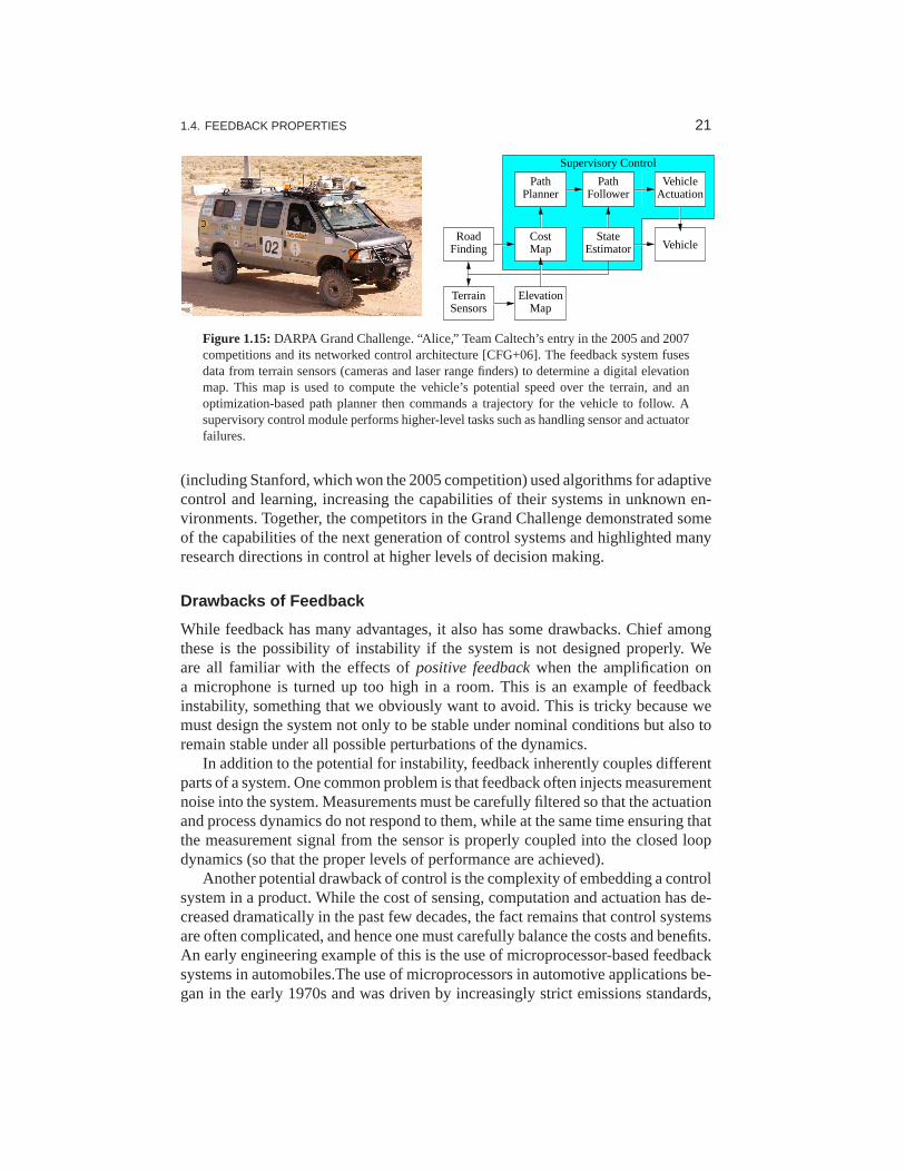
This application area has been recently explored through theDARPA GrandChallenge, a series of competitions sponsored by the U.S. government to build ve-hicles that can autonomously drive themselves in desert andurban environments.Caltech competed in the 2005 and 2007 Grand Challenges usinga modified Ford E-350 offroad van nicknamed “Alice.” It was fully automated, including electronicallycontrolled steering, throttle, brakes, transmission and ignition. Its sensing systemsincluded multiple video cameras scanning at 10–30 Hz, several laser ranging unitsscanning at 10 Hz and an inertial navigation package capableof providing positionand orientation estimates at 5 ms temporal resolution. Computational resources in-cluded 12 high-speed servers connected together through a 1-Gb/s Ethernet switch.The vehicle is shown in Figure 1.15, along with a block diagram of its controlarchitecture.
The software and hardware infrastructure that was developedenabled the ve-hicle to traverse long distances at substantial speeds. In testing, Alice drove itselfmore than 500 km in the Mojave Desert of California, with the ability to follow dirtroads and trails (if present) and avoid obstacles along the path. Speeds of more than50 km/h were obtained in the fully autonomous mode. Substantial tuning of the al-gorithms was done during desert testing, in part because of the lack of systems-leveldesign tools for systems of this level of complexity. Other competitors in the race
1.4. FEEDBACK PROPERTIES 21
Road
SensorsTerrain
FollowerPath
StateEstimator
PlannerPath
Supervisory Control
MapElevation
MapCost
Vehicle
VehicleActuation
Finding
Figure 1.15:DARPA Grand Challenge. “Alice,” Team Caltech’s entry in the 2005 and 2007competitions and its networked control architecture [CFG+06]. The feedback system fusesdata from terrain sensors (cameras and laser range finders) to determine a digital elevationmap. This map is used to compute the vehicle’s potential speed over the terrain, and anoptimization-based path planner then commands a trajectory for the vehicleto follow. Asupervisory control module performs higher-level tasks such as handling sensor and actuatorfailures.
(including Stanford, which won the 2005 competition) used algorithms for adaptivecontrol and learning, increasing the capabilities of theirsystems in unknown en-vironments. Together, the competitors in the Grand Challenge demonstrated someof the capabilities of the next generation of control systems and highlighted manyresearch directions in control at higher levels of decisionmaking.
Drawbacks of Feedback
While feedback has many advantages, it also has some drawbacks. Chief amongthese is the possibility of instability if the system is not designed properly. Weare all familiar with the effects ofpositive feedbackwhen the amplification ona microphone is turned up too high in a room. This is an example of feedbackinstability, something that we obviously want to avoid. Thisis tricky because wemust design the system not only to be stable under nominal conditions but also toremain stable under all possible perturbations of the dynamics.
In addition to the potential for instability, feedback inherently couples differentparts of a system. One common problem is that feedback often injects measurementnoise into the system. Measurements must be carefully filtered so that the actuationand process dynamics do not respond to them, while at the sametime ensuring thatthe measurement signal from the sensor is properly coupled into the closed loopdynamics (so that the proper levels of performance are achieved).
Another potential drawback of control is the complexity of embedding a controlsystem in a product. While the cost of sensing, computation and actuation has de-creased dramatically in the past few decades, the fact remains that control systemsare often complicated, and hence one must carefully balancethe costs and benefits.An early engineering example of this is the use of microprocessor-based feedbacksystems in automobiles.The use of microprocessors in automotive applications be-gan in the early 1970s and was driven by increasingly strict emissions standards,

22 CHAPTER 1. INTRODUCTION
which could be met only through electronic controls. Early systems were expensiveand failed more often than desired, leading to frequent customer dissatisfaction. Itwas only through aggressive improvements in technology that the performance,reliability and cost of these systems allowed them to be usedin a transparent fash-ion. Even today, the complexity of these systems is such that it is difficult for anindividual car owner to fix problems.
Feedforward
Feedback is reactive: there must be an error before corrective actions are taken.However, in some circumstances it is possible to measure a disturbance before itenters the system, and this information can then be used to take corrective actionbefore the disturbance has influenced the system. The effect ofthe disturbance isthus reduced by measuring it and generating a control signalthat counteracts it.This way of controlling a system is calledfeedforward. Feedforward is particularlyuseful in shaping the response to command signals because command signals arealways available. Since feedforward attempts to match two signals, it requires goodprocess models; otherwise the corrections may have the wrong size or may be badlytimed.
The ideas of feedback and feedforward are very general and appear in many dif-ferent fields. In economics, feedback and feedforward are analogous to a market-based economy versus a planned economy. In business, a feedforward strategycorresponds to running a company based on extensive strategic planning, while afeedback strategy corresponds to a reactive approach. In biology, feedforward hasbeen suggested as an essential element for motion control inhumans that is tunedduring training. Experience indicates that it is often advantageous to combine feed-back and feedforward, and the correct balance requires insight and understandingof their respective properties.
Positive Feedback
In most of this text, we will consider the role ofnegative feedback, in which weattempt to regulate the system by reacting to disturbances in a way that decreasesthe effect of those disturbances. In some systems, particularly biological systems,positive feedbackcan play an important role. In a system with positive feedback,the increase in some variable or signal leads to a situation in which that quantityis further increased through its dynamics. This has a destabilizing effect and isusually accompanied by a saturation that limits the growth of the quantity. Althoughoften considered undesirable, this behavior is used in biological (and engineering)systems to obtain a very fast response to a condition or signal.
One example of the use of positive feedback is to create switching behavior,in which a system maintains a given state until some input crosses a threshold.Hysteresis is often present so that noisy inputs near the threshold do not cause thesystem to jitter. This type of behavior is calledbistability and is often associatedwith memory devices.

1.5. SIMPLE FORMS OF FEEDBACK 23
u
e
(a) On-off control
u
e
(b) Dead zone
u
e
(c) Hysteresis
Figure 1.16: Input/output characteristics of on-off controllers. Each plot shows theinput onthe horizontal axis and the corresponding output on the vertical axis. Ideal on-off control isshown in (a), with modifications for a dead zone (b) or hysteresis (c). Note that for on-offcontrol with hysteresis, the output depends on the value of past inputs.
1.5 Simple Forms of Feedback
The idea of feedback to make corrective actions based on the difference betweenthe desired and the actual values of a quantity can be implemented in many differentways. The benefits of feedback can be obtained by very simple feedback laws suchas on-off control, proportional control and proportional-integral-derivative control.In this section we provide a brief preview of some of the topics that will be studiedmore formally in the remainder of the text.
On-Off Control
A simple feedback mechanism can be described as follows:
u ={
umax if e> 0
umin if e< 0,(1.1)
where thecontrol error e= r − y is the difference between the reference signal (orcommand signal)r and the output of the systemy andu is the actuation command.Figure 1.16a shows the relation between error and control. This control law impliesthat maximum corrective action is always used.
The feedback in equation (1.1) is calledon-off control. One of its chief advan-tages is that it is simple and there are no parameters to choose. On-off control oftensucceeds in keeping the process variable close to the reference, such as the use ofa simple thermostat to maintain the temperature of a room. Ittypically results ina system where the controlled variables oscillate, which isoften acceptable if theoscillation is sufficiently small.
Notice that in equation (1.1) the control variable is not defined when the erroris zero. It is common to make modifications by introducing either a dead zone orhysteresis (see Figure 1.16b and 1.16c).
PID Control
The reason why on-off control often gives rise to oscillations is that the systemoverreacts since a small change in the error makes the actuated variable change overthe full range. This effect is avoided inproportional control, where the characteristic

24 CHAPTER 1. INTRODUCTION
of the controller is proportional to the control error for small errors. This can beachieved with the control law
u =
umax if e ≥ emax
kpe if emin < e< emax
umin if e ≤ emin,
(1.2)
wherekp is the controller gain,emin = umin/kp andemax = umax/kp. The interval(emin,emax) is called theproportional bandbecause the behavior of the controlleris linear when the error is in this interval:
u = kp(r − y) = kpe if emin ≤ e ≤ emax. (1.3)
While a vast improvement over on-off control, proportionalcontrol has the draw-back that the process variable often deviates from its reference value. In particular,if some level of control signal is required for the system to maintain a desired value,then we must havee 6= 0 in order to generate the requisite input.
This can be avoided by making the control action proportionalto the integral ofthe error:
u(t) = ki
∫ t
0e(τ )dτ. (1.4)
This control form is calledintegral control, andki is the integral gain. It can beshown through simple arguments that a controller with integral action has zerosteady-state error (Exercise 1.5). The catch is that there maynot always be a steadystate because the system may be oscillating.
An additional refinement is to provide the controller with an anticipative abil-ity by using a prediction of the error. A simple prediction isgiven by the linearextrapolation
e(t + Td) ≈ e(t)+ Tdde(t)
dt,
which predicts the errorTd time units ahead. Combining proportional, integral andderivative control, we obtain a controller that can be expressed mathematically as
u(t) = kpe(t)+ ki
∫ t
0e(τ )dτ + kd
de(t)
dt. (1.5)
The control action is thus a sum of three terms: the past as represented by theintegral of the error, the present as represented by the proportional term and thefuture as represented by a linear extrapolation of the error(the derivative term).This form of feedback is called aproportional-integral-derivative (PID) controllerand its action is illustrated in Figure 1.17.
A PID controller is very useful and is capable of solving a widerange of con-trol problems. More than 95% of all industrial control problems are solved byPID control, although many of these controllers are actuallyproportional-integral(PI) controllersbecause derivative action is often not included [DM02]. There arealso more advanced controllers, which differ from PID controllers by using moresophisticated methods for prediction.

1.6. FURTHER READING 25
Present
FuturePast
t t + TdTime
Error
Figure 1.17: Action of a PID controller. At timet , the proportional term depends on theinstantaneous value of the error. The integral portion of the feedback isbased on the integralof the error up to timet (shaded portion). The derivative term provides an estimate of thegrowth or decay of the error over time by looking at the rate of change ofthe error.Td
represents the approximate amount of time in which the error is projected forward (see text).
1.6 Further Reading
The material in this section draws heavily from the report of the Panel on FutureDirections on Control, Dynamics and Systems [Mur03]. Severaladditional papersand reports have highlighted the successes of control [NS99]and new vistas incontrol [Bro00, Kum01, Wis07]. The early development of control is describedby Mayr [May70] and in the books by Bennett [Ben79, Ben93], which cover theperiod 1800–1955. A fascinating examination of some of the early history of con-trol in the United States has been written by Mindell [Min02].A popular bookthat describes many control concepts across a wide range of disciplines isOut ofControl by Kelly [Kel94]. There are many textbooks available that describe con-trol systems in the context of specific disciplines. For engineers, the textbooks byFranklin, Powell and Emami-Naeini [FPEN05], Dorf and Bishop [DB04], Kuo andGolnaraghi [KG02] and Seborg, Edgar and Mellichamp [SEM04] are widely used.More mathematically oriented treatments of control theoryinclude Sontag [Son98]and Lewis [Lew03]. The book by Hellerstein et al. [HDPT04] provides a descriptionof the use of feedback control in computing systems. A numberof books look at therole of dynamics and feedback in biological systems, including Milhorn [Mil66](now out of print), J. D. Murray [Mur04] and Ellner and Guckenheimer [EG05].The book by Fradkov [Fra07] and the tutorial article by Bechhoefer [Bec05] covermany specific topics of interest to the physics community.
Exercises
1.1(Eye motion) Perform the following experiment and explain your results: Hold-ing your head still, move one of your hands left and right in front of your face,following it with your eyes. Record how quickly you can move your hand beforeyou begin to lose track of it. Now hold your hand still and shake your head left toright, once again recording how quickly you can move before losing track of your
26 CHAPTER 1. INTRODUCTION
hand.
1.2 Identify five feedback systems that you encounter in your everyday environ-ment. For each system, identify the sensing mechanism, actuation mechanism andcontrol law. Describe the uncertainty with respect to whichthe feedback systemprovides robustness and/or the dynamics that are changed through the use of feed-back.
1.3(Balance systems) Balance yourself on one foot with your eyes closed for 15 s.Using Figure 1.3 as a guide, describe the control system responsible for keeping youfrom falling down. Note that the “controller” will differ from that in the diagram(unless you are an android reading this in the far future).
1.4(Cruise control) Download the MATLAB code used to produce simulations forthe cruise control system in Figure 1.13 from the companion web site. Using trialand error, change the parameters of the control law so that the overshoot in speedis not more than 1 m/s for a vehicle with massm = 1000 kg.
1.5(Integral action) We say that a system with a constant input reaches steady stateif the output of the system approaches a constant value as time increases. Show thata controller with integral action, such as those given in equations (1.4) and (1.5),gives zero error if the closed loop system reaches steady state.
1.6 Search the web and pick an article in the popular press about a feedback andcontrol system. Describe the feedback system using the terminology given in thearticle. In particular, identify the control system and describe (a) the underlyingprocess or system being controlled, along with the (b) sensor, (c) actuator and (d)computational element. If the some of the information is notavailable in the article,indicate this and take a guess at what might have been used.

Chapter TwoSystem Modeling
... I asked Fermi whether he was not impressed by the agreement between our calculatednumbers and his measured numbers. He replied, “How many arbitraryparameters did you usefor your calculations?” I thought for a moment about our cut-off procedures and said, “Four.”He said, “I remember my friend Johnny von Neumann used to say, with four parameters I canfit an elephant, and with five I can make him wiggle his trunk.”
Freeman Dyson on describing the predictions of his model for meson-proton scattering toEnrico Fermi in 1953 [Dys04].
A model is a precise representation of a system’s dynamics used to answer ques-tions via analysis and simulation. The model we choose depends on the questionswe wish to answer, and so there may be multiple models for a single dynamical sys-tem, with different levels of fidelity depending on the phenomena of interest. In thischapter we provide an introduction to the concept of modeling and present somebasic material on two specific methods commonly used in feedback and controlsystems: differential equations and difference equations.
2.1 Modeling Concepts
A modelis a mathematical representation of a physical, biologicalor informationsystem. Models allow us to reason about a system and make predictions abouthow a system will behave. In this text, we will mainly be interested in models ofdynamical systems describing the input/output behavior ofsystems, and we willoften work in “state space” form.
Roughly speaking, a dynamical system is one in which the effects of actionsdo not occur immediately. For example, the velocity of a car does not changeimmediately when the gas pedal is pushed nor does the temperature in a room riseinstantaneously when a heater is switched on. Similarly, a headache does not vanishright after an aspirin is taken, requiring time for it to takeeffect. In business systems,increased funding for a development project does not increase revenues in the shortterm, although it may do so in the long term (if it was a good investment). Allof these are examples of dynamical systems, in which the behavior of the systemevolves with time.
In the remainder of this section we provide an overview of some of the keyconcepts in modeling. The mathematical details introduced here are explored morefully in the remainder of the chapter.

28 CHAPTER 2. SYSTEM MODELING
c (q)
q
m
k
Figure 2.1:Spring–mass system with nonlinear damping. The position of the mass is denotedby q, with q = 0 corresponding to the rest position of the spring. The forces on the mass aregenerated by a linear spring with spring constantk and a damper with force dependent on thevelocity q.
The Heritage of Mechanics
The study of dynamics originated in attempts to describe planetary motion. Thebasis was detailed observations of the planets by Tycho Brahe and the results ofKepler, who found empirically that the orbits of the planetscould be well describedby ellipses. Newton embarked on an ambitious program to try to explain why theplanets move in ellipses, and he found that the motion could be explained by hislaw of gravitation and the formula stating that force equalsmass times acceleration.In the process he also invented calculus and differential equations.
One of the triumphs of Newton’s mechanics was the observation that the motionof the planets could be predicted based on the current positions and velocities ofall planets. It was not necessary to know the past motion. Thestateof a dynamicalsystem is a collection of variables that completely characterizes the motion of asystem for the purpose of predicting future motion. For a system of planets thestate is simply the positions and the velocities of the planets. We call the set of allpossible states thestate space.
A common class of mathematical models for dynamical systemsis ordinarydifferential equations (ODEs). In mechanics, one of the simplest such differentialequations is that of a spring–mass system with damping:
mq + c(q)+ kq = 0. (2.1)
This system is illustrated in Figure 2.1. The variableq ∈ R represents the positionof the massm with respect to its rest position. We use the notationq to denote thederivative ofq with respect to time (i.e., the velocity of the mass) andq to representthe second derivative (acceleration). The spring is assumedto satisfy Hooke’s law,which says that the force is proportional to the displacement. The friction element(damper) is taken as a nonlinear functionc(q), which can model effects such asstiction and viscous drag. The positionq and velocityq represent the instantaneousstate of the system. We say that this system is asecond-order systemsince thedynamics depend on the first two derivatives ofq.
The evolution of the position and velocity can be described using either a timeplot or a phase portrait, both of which are shown in Figure 2.2.The time plot, on

2.1. MODELING CONCEPTS 29
0 5 10 15−2
−1
0
1
2
Time t [s]
Pos
ition
q[m
],ve
loci
tyq
[m/s
]
PositionVelocity
−1 −0.5 0 0.5 1−1
−0.5
0
0.5
1
Positionq [m]
Velo
city
q[m
/s]
Figure 2.2: Illustration of a state model. A state model gives the rate of change of the stateas a function of the state. The plot on the left shows the evolution of the state as a function oftime. The plot on the right shows the evolution of the states relative to each other, with thevelocity of the state denoted by arrows.
the left, shows the values of the individual states as a function of time. Thephaseportrait, on the right, shows thevector fieldfor the system, which gives the statevelocity (represented as an arrow) at every point in the state space. In addition,we have superimposed the traces of some of the states from different conditions.The phase portrait gives a strong intuitive representation of the equation as a vectorfield or a flow. While systems of second order (two states) can be represented inthis way, unfortunately it is difficult to visualize equations of higher order usingthis approach.
The differential equation (2.1) is called anautonomoussystem because thereare no external influences. Such a model is natural for use in celestial mechanicsbecause it is difficult to influence the motion of the planets. Inmany examples, itis useful to model the effects of external disturbances or controlled forces on thesystem. One way to capture this is to replace equation (2.1) by
mq + c(q)+ kq = u, (2.2)
whereu represents the effect of external inputs. The model (2.2) is called aforcedor controlled differential equation. It implies that the rate of change of the statecan be influenced by the inputu(t). Adding the input makes the model richer andallows new questions to be posed. For example, we can examinewhat influenceexternal disturbances have on the trajectories of a system.Or, in the case wherethe input variable is something that can be modulated in a controlled way, we cananalyze whether it is possible to “steer” the system from onepoint in the state spaceto another through proper choice of the input.
The Heritage of Electrical Engineering
A different view of dynamics emerged from electrical engineering, where the designof electronic amplifiers led to a focus on input/output behavior. A system wasconsidered a device that transforms inputs to outputs, as illustrated in Figure 2.3.Conceptually an input/output model can be viewed as a giant table of inputs and

30 CHAPTER 2. SYSTEM MODELING
7+v
–v
vos adj
(+)
(–)
InputsOutput3
2
6
4
Q9
Q1 Q2
Q3 Q4
Q7
Q5
R1 R12
R8
R7 R9
R10
R11R2
Q6Q22
Q17
Q16
Q1830pF
Q15
Q14
Q20
Q8
SystemInput Output
Figure 2.3: Illustration of the input/output view of a dynamical system. The figure on theleft shows a detailed circuit diagram for an electronic amplifier; the one onthe right is itsrepresentation as a block diagram.
outputs. Given an input signalu(t) over some interval of time, the model shouldproduce the resulting outputy(t).
The input/output framework is used in many engineering disciplines since itallows us to decompose a system into individual components connected throughtheir inputs and outputs. Thus, we can take a complicated system such as a radioor a television and break it down into manageable pieces suchas the receiver,demodulator, amplifier and speakers. Each of these pieces has aset of inputs andoutputs and, through proper design, these components can beinterconnected toform the entire system.
The input/output view is particularly useful for the specialclass oflinear time-invariant systems. This term will be defined more carefully later in this chapter,butroughly speaking a system is linear if the superposition (addition) of two inputsyields an output that is the sum of the outputs that would correspond to individualinputs being applied separately. A system is time-invariant if the output responsefor a given input does not depend on when that input is applied.
Many electrical engineering systems can be modeled by linear time-invariantsystems, and hence a large number of tools have been developed to analyze them.One such tool is thestep response, which describes the relationship between aninput that changes from zero to a constant value abruptly (a step input) and thecorresponding output. As we shall see later in the text, the step response is veryuseful in characterizing the performance of a dynamical system, and it is often usedto specify the desired dynamics. A sample step response is shown in Figure 2.4a.
Another way to describe a linear time-invariant system is torepresent it by itsresponse to sinusoidal input signals. This is called thefrequency response, and arich, powerful theory with many concepts and strong, usefulresults has emerged.The results are based on the theory of complex variables and Laplace transforms.The basic idea behind frequency response is that we can completely characterizethe behavior of a system by its steady-state response to sinusoidal inputs. Roughly

2.1. MODELING CONCEPTS 31
0 10 20 300
1
2
3
4
Time
Inpu
t, ou
tput
InputOutput
(a) Step response
10−4
10−2
100
Gai
n
10−1
100
101
102
−270
−180
−90
0
Pha
se [d
eg]
Frequency
(b) Frequency response
Figure 2.4: Input/output response of a linear system. The step response (a) shows the outputof the system due to an input that changes from 0 to 1 at timet = 5 s. The frequencyresponse (b) shows the amplitude gain and phase change due to a sinusoidal input at differentfrequencies.
speaking, this is done by decomposing any arbitrary signal into a linear combi-nation of sinusoids (e.g., by using the Fourier transform) and then using linearityto compute the output by combining the response to the individual frequencies. Asample frequency response is shown in Figure 2.4b.
The input/output view lends itself naturally to experimental determination ofsystem dynamics, where a system is characterized by recording its response toparticular inputs, e.g., a step or a set of sinusoids over a range of frequencies.
The Control View
When control theory emerged as a discipline in the 1940s, theapproach to dy-namics was strongly influenced by the electrical engineering(input/output) view.A second wave of developments in control, starting in the late 1950s, was inspiredby mechanics, where the state space perspective was used. Theemergence of spaceflight is a typical example, where precise control of the orbitof a spacecraft isessential. These two points of view gradually merged into what is today the statespace representation of input/output systems.
The development of state space models involved modifying themodels frommechanics to include external actuators and sensors and utilizing more generalforms of equations. In control, the model given by equation (2.2) was replaced by
dx
dt= f (x,u), y = h(x,u), (2.3)
wherex is a vector of state variables,u is a vector of control signals andy is avector of measurements. The termdx/dt represents the derivative ofx with respectto time, now considered a vector, andf andh are (possibly nonlinear) mappings oftheir arguments to vectors of the appropriate dimension. For mechanical systems,the state consists of the position and velocity of the system, so thatx = (q, q) in thecase of a damped spring–mass system. Note that in the controlformulation we model

32 CHAPTER 2. SYSTEM MODELING
dynamics as first-order differential equations, but we will see that this can capturethe dynamics of higher-order differential equations by appropriate definition of thestate and the mapsf andh.
Adding inputs and outputs has increased the richness of the classical problemsand led to many new concepts. For example, it is natural to askif possible statesxcan be reached with the proper choice ofu (reachability) and if the measurementycontains enough information to reconstruct the state (observability). These topicswill be addressed in greater detail in Chapters 6 and 7.
A final development in building the control point of view was the emergence ofdisturbances and model uncertainty as critical elements inthe theory. The simpleway of modeling disturbances as deterministic signals likesteps and sinusoids hasthe drawback that such signals cannot be predicted precisely. A more realistic ap-proach is to model disturbances as random signals. This viewpoint gives a naturalconnection between prediction and control. The dual views ofinput/output repre-sentations and state space representations are particularly useful when modelinguncertainty since state models are convenient to describe anominal model but un-certainties are easier to describe using input/output models (often via a frequencyresponse description). Uncertainty will be a constant theme throughout the text andwill be studied in particular detail in Chapter 12.
An interesting observation in the design of control systemsis that feedbacksystems can often be analyzed and designed based on comparatively simple models.The reason for this is the inherent robustness of feedback systems. However, otheruses of models may require more complexity and more accuracy. One example isfeedforward control strategies, where one uses a model to precompute the inputsthat cause the system to respond in a certain way. Another area is system validation,where one wishes to verify that the detailed response of the system performs as itwas designed. Because of these different uses of models, it is common to use ahierarchy of models having different complexity and fidelity.
Multidomain Modeling�
Modeling is an essential element of many disciplines, but traditions and methodsfrom individual disciplines can differ from each other, as illustrated by the previousdiscussion of mechanical and electrical engineering. A difficulty in systems engi-neering is that it is frequently necessary to deal with heterogeneous systems frommany different domains, including chemical, electrical, mechanical and informa-tion systems.
To model such multidomain systems, we start by partitioninga system intosmaller subsystems. Each subsystem is represented by balance equations for mass,energy and momentum, or by appropriate descriptions of information processingin the subsystem. The behavior at the interfaces is captured by describing how thevariables of the subsystem behave when the subsystems are interconnected. Theseinterfaces act by constraining variables within the individual subsystems to be equal(such as mass, energy or momentum fluxes). The complete model isthen obtainedby combining the descriptions of the subsystems and the interfaces.

2.1. MODELING CONCEPTS 33
Using this methodology it is possible to build up libraries of subsystems thatcorrespond to physical, chemical and informational components. The proceduremimics the engineering approach where systems are built from subsystems that arethemselves built from smaller components. As experience isgained, the componentsand their interfaces can be standardized and collected in model libraries. In practice,it takes several iterations to obtain a good library that canbe reused for manyapplications.
State models or ordinary differential equations are not suitable for component-based modeling of this form because states may disappear when components areconnected. This implies that the internal description of a component may changewhen it is connected to other components. As an illustrationwe consider two ca-pacitors in an electrical circuit. Each capacitor has a statecorresponding to thevoltage across the capacitors, but one of the states will disappear if the capacitorsare connected in parallel. A similar situation happens withtwo rotating inertias,each of which is individually modeled using the angle of rotation and the angularvelocity. Two states will disappear when the inertias are joined by a rigid shaft.
This difficulty can be avoided by replacing differential equations bydifferentialalgebraic equations, which have the form
F(z, z) = 0,
wherez ∈ Rn. A simple special case is
x = f (x, y), g(x, y) = 0, (2.4)
wherez = (x, y) and F = (x − f (x, y), g(x, y)). The key property is that thederivativez is not given explicitly and there may be pure algebraic relations betweenthe components of the vectorz.
The model (2.4) captures the examples of the parallel capacitors and the linkedrotating inertias. For example, when two capacitors are connected, we simply addthe algebraic equation expressing that the voltages acrossthe capacitors are thesame.
Modelica is a language that has been developed to support component-basedmodeling. Differential algebraic equations are used as thebasic description, andobject-oriented programming is used to structure the models. Modelica is used tomodel the dynamics of technical systems in domains such as mechanical, electri-cal, thermal, hydraulic, thermofluid and control subsystems. Modelica is intendedto serve as a standard format so that models arising in different domains can beexchanged between tools and users. A large set of free and commercial Modelicacomponent libraries are available and are used by a growing number of peoplein industry, research and academia. For further information about Modelica, seehttp://www.modelica.org or Tiller [Til01].

34 CHAPTER 2. SYSTEM MODELING
2.2 State Space Models
In this section we introduce the two primary forms of models that we use in thistext: differential equations and difference equations. Both make use of the notionsof state, inputs, outputs and dynamics to describe the behavior of a system.
Ordinary Differential Equations
The state of a system is a collection of variables that summarize the past of asystem for the purpose of predicting the future. For a physical system the state iscomposed of the variables required to account for storage ofmass, momentum andenergy. A key issue in modeling is to decide how accurately this storage has to berepresented. The state variables are gathered in a vectorx ∈ R
n called thestatevector. The control variables are represented by another vectoru ∈ R
p, and themeasured signal by the vectory ∈ R
q. A system can then be represented by thedifferential equation
dx
dt= f (x,u), y = h(x,u), (2.5)
where f : Rn × R
p → Rn andh : R
n × Rp → R
q are smooth mappings. We calla model of this form astate space model.
The dimension of the state vector is called theorder of the system. The sys-tem (2.5) is calledtime-invariantbecause the functionsf andh do not dependexplicitly on timet ; there are more general time-varying systems where the func-tions do depend on time. The model consists of two functions: the function f givesthe rate of change of the state vector as a function of statex and controlu, and thefunctionh gives the measured values as functions of statex and controlu.
A system is called alinear state space system if the functionsf andh are linearin x andu. A linear state space system can thus be represented by
dx
dt= Ax + Bu, y = Cx + Du, (2.6)
whereA, B, C andD are constant matrices. Such a system is said to belinear andtime-invariant, or LTI for short. The matrixA is called thedynamics matrix, thematrix B is called thecontrol matrix, the matrixC is called thesensor matrixandthe matrixD is called thedirect term. Frequently systems will not have a directterm, indicating that the control signal does not influence the output directly.
A different form of linear differential equations, generalizing the second-orderdynamics from mechanics, is an equation of the form
dny
dtn+ a1
dn−1y
dtn−1+ · · · + any = u, (2.7)
wheret is the independent (time) variable,y(t) is the dependent (output) variableandu(t) is the input. The notationdky/dtk is used to denote thekth derivativeof y with respect tot , sometimes also written asy(k). The controlled differentialequation (2.7) is said to be annth-order system. This system can be converted into

2.2. STATE SPACE MODELS 35
state space form by defining
x =
x1
x2...
xn−1
xn
=
dn−1y/dtn−1
dn−2y/dtn−2
...
dy/dty
,
and the state space equations become
d
dt
x1
x2...
xn−1
xn
=
−a1x1 − · · · − anxn
x1...
xn−2
xn−1
+
u0...
00
, y = xn.
With the appropriate definitions ofA, B, C andD, this equation is in linear statespace form.
An even more general system is obtained by letting the outputbe a linear com-bination of the states of the system, i.e.,
y = b1x1 + b2x2 + · · · + bnxn + du.
This system can be modeled in state space as
d
dt
x1
x2
x3...
xn
=
−a1 −a2 . . . −an−1 −an
1 0 . . . 0 00 1 0 0...
. . ....
0 0 1 0
x +
100...
0
u,
y =b1 b2 . . . bn
x + du.
(2.8)
This particular form of a linear state space system is calledreachable canonicalformand will be studied in more detail in later chapters.
Example 2.1 Balance systemsAn example of a type of system that can be modeled using ordinary differentialequations is the class ofbalance systems. A balance system is a mechanical systemin which the center of mass is balanced above a pivot point. Some common examplesof balance systems are shown in Figure 2.5. The Segway® Personal Transporter(Figure 2.5a) uses a motorized platform to stabilize a personstanding on top ofit. When the rider leans forward, the transportation devicepropels itself along theground but maintains its upright position. Another exampleis a rocket (Figure 2.5b),in which a gimbaled nozzle at the bottom of the rocket is used to stabilize the bodyof the rocket above it. Other examples of balance systems include humans or otheranimals standing upright or a person balancing a stick on their hand.

36 CHAPTER 2. SYSTEM MODELING
(a) Segway (b) Saturn rocket
MF
p
θm
l
(c) Cart–pendulum system
Figure 2.5: Balance systems. (a) Segway Personal Transporter, (b) Saturn rocket and (c)inverted pendulum on a cart. Each of these examples uses forces at thebottom of the systemto keep it upright.
Balance systems are a generalization of the spring–mass system we saw earlier.We can write the dynamics for a mechanical system in the general form
M(q)q + C(q, q)+ K (q) = B(q)u,
whereM(q) is the inertia matrix for the system,C(q, q) represents the Coriolisforces as well as the damping,K (q) gives the forces due to potential energy andB(q) describes how the external applied forces couple into the dynamics. Thespecific form of the equations can be derived using Newtonian mechanics. Notethat each of the terms depends on the configuration of the system q and that theseterms are often nonlinear in the configuration variables.
Figure 2.5c shows a simplified diagram for a balance system consisting of aninverted pendulum on a cart. To model this system, we choose state variables thatrepresent the position and velocity of the base of the system, p and p, and the angleand angular rate of the structure above the base,θ and θ . We let F represent theforce applied at the base of the system, assumed to be in the horizontal direction(aligned withp), and choose the position and angle of the system as outputs.Withthis set of definitions, the dynamics of the system can be computed using Newtonianmechanics and have the form
(M + m) −ml cosθ
−ml cosθ (J + ml2)
pθ
+
cp + ml sinθ θ2
γ θ − mglsinθ
=
F
0
, (2.9)
whereM is the mass of the base,m andJ are the mass and moment of inertia of thesystem to be balanced,l is the distance from the base to the center of mass of thebalanced body,c andγ are coefficients of viscous friction andg is the accelerationdue to gravity.
We can rewrite the dynamics of the system in state space form by defining thestate asx = (p, θ, p, θ ), the input asu = F and the output asy = (p, θ). If we

2.2. STATE SPACE MODELS 37
define the total mass and total inertia as
Mt = M + m, Jt = J + ml2,
the equations of motion then become
d
dt
pθ
pθ
=
pθ
−mlsθ θ2 + mg(ml2/Jt)sθcθ − cp − γ lmcθ θ + u
Mt − m(ml2/Jt)c2θ
−ml2sθcθ θ2 + Mt glsθ − clcθ p − γ (Mt/m)θ + lcθu
Jt(Mt/m)− m(lcθ )2
,
y =pθ
,
where we have used the shorthandcθ = cosθ andsθ = sinθ .In many cases, the angleθ will be very close to 0, and hence we can use the
approximations sinθ ≈ θ and cosθ ≈ 1. Furthermore, ifθ is small, we canignore quadratic and higher terms inθ . Substituting these approximations into ourequations, we see that we are left with alinear state space equation
d
dt
pθ
pθ
=
0 0 1 00 0 0 1
0 m2l 2g/µ −cJt/µ −γ Jt lm/µ
0 Mtmgl/µ −clm/µ −γMt/µ
pθ
pθ
+
00
Jt/µ
lm/µ
u,
y =1 0 0 0
0 1 0 0
x,
whereµ = Mt Jt − m2l 2. ∇
Example 2.2 Inverted pendulumA variation of the previous example is one in which the location of the basep doesnot need to be controlled. This happens, for example, if we areinterested only instabilizing a rocket’s upright orientation without worrying about the location ofbase of the rocket. The dynamics of this simplified system are given by
d
dt
θθ
=
θmgl
Jtsinθ − γ
Jtθ + l
Jtcosθ u
, y = θ, (2.10)
whereγ is the coefficient of rotational friction,Jt = J + ml2 andu is the forceapplied at the base. This system is referred to as aninverted pendulum. ∇
Difference Equations
In some circumstances, it is more natural to describe the evolution of a system atdiscrete instants of time rather than continuously in time.If we refer to each of

38 CHAPTER 2. SYSTEM MODELING
these times by an integerk = 0,1,2, . . . , then we can ask how the state of thesystem changes for eachk. Just as in the case of differential equations, we definethe state to be those sets of variables that summarize the past of the system for thepurpose of predicting its future. Systems described in this manner are referred toasdiscrete-time systems.
The evolution of a discrete-time system can be written in the form
x[k + 1] = f (x[k],u[k]), y[k] = h(x[k],u[k]), (2.11)
wherex[k] ∈ Rn is the state of the system at timek (an integer),u[k] ∈ R
p isthe input andy[k] ∈ R
q is the output. As before,f andh are smooth mappings ofthe appropriate dimension. We call equation (2.11) adifference equationsince ittells us howx[k + 1] differs fromx[k]. The statex[k] can be either a scalar- or avector-valued quantity; in the case of the latter we writex j [k] for the value of thej th state at timek.
Just as in the case of differential equations, it is often thecase that the equationsare linear in the state and input, in which case we can describe the system by
x[k + 1] = Ax[k] + Bu[k], y[k] = Cx[k] + Du[k].
As before, we refer to the matricesA, B,C andD as the dynamics matrix, the controlmatrix, the sensor matrix and the direct term. The solution ofa linear differenceequation with initial conditionx[0] and inputu[0], . . . ,u[T ] is given by
x[k] = Akx0 +k−1∑
j =0
Ak− j −1Bu[ j ],
y[k] = C Akx0 +k−1∑
j =0
C Ak− j −1Bu[ j ] + Du[k],
k > 0. (2.12)
Difference equations are also useful as an approximation ofdifferential equa-tions, as we will show later.
Example 2.3 Predator–preyAs an example of a discrete-time system, consider a simple model for a predator–prey system. The predator–prey problem refers to an ecological system in whichwe have two species, one of which feeds on the other. This type of system hasbeen studied for decades and is known to exhibit interestingdynamics. Figure 2.6shows a historical record taken over 90 years for a population of lynxes versus apopulation of hares [Mac37]. As can been seen from the graph,the annual recordsof the populations of each species are oscillatory in nature.
A simple model for this situation can be constructed using a discrete-time modelby keeping track of the rate of births and deaths of each species. LettingH representthe population of hares andL represent the population of lynxes, we can describethe state in terms of the populations at discrete periods of time. Lettingk be the

2.2. STATE SPACE MODELS 39
1845
160
140
120
100
80
60
40
20
1855 1865 1875 1885 1895
Hare
Lynx
1905 1915 1925 1935
Figure 2.6: Predator versus prey. The photograph on the left shows a Canadian lynx anda snowshoe hare, the lynx’s primary prey. The graph on the right shows the populations ofhares and lynxes between 1845 and 1935 in a section of the Canadian Rockies [Mac37]. Thedata were collected on an annual basis over a period of 90 years. (Photograph copyright Tomand Pat Leeson.)
discrete-time index (e.g., the month number), we can write
H [k + 1] = H [k] + br (u)H [k] − aL[k]H [k],
L[k + 1] = L[k] + cL[k]H [k] − d f L[k],(2.13)
wherebr (u) is the hare birth rate per unit period and as a function of the foodsupplyu, d f is the lynx mortality rate anda andc are the interaction coefficients.The interaction termaL[k]H [k] models the rate of predation, which is assumedto be proportional to the rate at which predators and prey meet and is hence givenby the product of the population sizes. The interaction termcL[k]H [k] in thelynx dynamics has a similar form and represents the rate of growth of the lynxpopulation. This model makes many simplifying assumptions—such as the factthat hares decrease in number only through predation by lynxes—but it often issufficient to answer basic questions about the system.
To illustrate the use of this system, we can compute the number of lynxes andhares at each time point from some initial population. This isdone by starting withx[0] = (H0, L0) and then using equation (2.13) to compute the populations inthe following period. By iterating this procedure, we can generate the populationover time. The output of this process for a specific choice of parameters and initialconditions is shown in Figure 2.7. While the details of the simulation are differentfrom the experimental data (to be expected given the simplicity of our assumptions),we see qualitatively similar trends and hence we can use the model to help explorethe dynamics of the system. ∇
Example 2.4 E-mail serverThe IBM Lotus server is an collaborative software system that administers users’e-mail, documents and notes. Client machines interact withend users to provideaccess to data and applications. The server also handles other administrative tasks.In the early development of the system it was observed that the performance waspoor when the central processing unit (CPU) was overloaded because of too manyservice requests, and mechanisms to control the load were therefore introduced.
The interaction between the client and the server is in the form of remote pro-

40 CHAPTER 2. SYSTEM MODELING
1850 1860 1870 1880 1890 1900 1910 19200
50
100
150
200
250
Year
Pop
ulat
ion
Hares Lynxes
Figure 2.7:Discrete-time simulation of the predator–prey model (2.13). Using the parametersa = c = 0.014,br (u) = 0.6 andd = 0.7 in equation (2.13), the period and magnitude of thelynx and hare population cycles approximately match the data in Figure 2.6.
cedure calls (RPCs). The server maintains a log of statistics of completed requests.The total number of requests being served, calledRIS (RPCs in server), is alsomeasured. The load on the server is controlled by a parameter calledMaxUsers,which sets the total number of client connections to the server. This parameter iscontrolled by the system administrator. The server can be regarded as a dynami-cal system withMaxUsers as the input andRIS as the output. The relationshipbetween input and output was first investigated by exploring the steady-state per-formance and was found to be linear.
In [HDPT04] a dynamic model in the form of a first-order difference equationis used to capture the dynamic behavior of this system. Usingsystem identificationtechniques, they construct a model of the form
y[k + 1] = ay[k] + bu[k],
whereu = MaxUsers − MaxUsers and y = RIS − RIS. The parametersa = 0.43 andb = 0.47 are parameters that describe the dynamics of the systemaround the operating point, andMaxUsers = 165 andRIS = 135 represent thenominal operating point of the system. The number of requestswas averaged overa sampling period of 60 s. ∇
Simulation and Analysis
State space models can be used to answer many questions. One ofthe most common,as we have seen in the previous examples, involves predicting the evolution of thesystem state from a given initial condition. While for simple models this can bedone in closed form, more often it is accomplished through computer simulation.One can also use state space models to analyze the overall behavior of the systemwithout making direct use of simulation.
Consider again the damped spring–mass system from Section 2.1, but this timewith an external force applied, as shown in Figure 2.8. We wishto predict themotion of the system for a periodic forcing function, with a given initial condition,and determine the amplitude, frequency and decay rate of theresulting motion.

2.2. STATE SPACE MODELS 41
q
m
k
u(t) = A sin tω
c
Figure 2.8: A driven spring–mass system with damping. Here we use a linear dampingelement with coefficient of viscous frictionc. The mass is driven with a sinusoidal force ofamplitudeA.
We choose to model the system with a linear ordinary differential equation.Using Hooke’s law to model the spring and assuming that the damper exerts a forcethat is proportional to the velocity of the system, we have
mq + cq + kq = u, (2.14)
wherem is the mass,q is the displacement of the mass,c is the coefficient ofviscous friction,k is the spring constant andu is the applied force. In state spaceform, usingx = (q, q) as the state and choosingy = q as the output, we have
dx
dt=
x2
− c
mx2 − k
mx1 + u
m
, y = x1.
We see that this is a linear second-order differential equation with one inputu andone outputy.
We now wish to compute the response of the system to an input ofthe formu = Asinωt . Although it is possible to solve for the response analytically, weinstead make use of a computational approach that does not rely on the specificform of this system. Consider the general state space system
dx
dt= f (x,u).
Given the statex at time t , we can approximate the value of the state at a shorttimeh > 0 later by assuming that the rate of change off (x,u) is constant over theintervalt to t + h. This gives
x(t + h) = x(t)+ h f (x(t),u(t)). (2.15)
Iterating this equation, we can thus solve forx as a function of time. This approxi-mation is known as Euler integration and is in fact a difference equation if we lethrepresent the time increment and writex[k] = x(kh). Although modern simulationtools such as MATLAB and Mathematica use more accurate methodsthan Eulerintegration, they still have some of the same basic trade-offs.
Returning to our specific example, Figure 2.9 shows the resultsof computingx(t) using equation (2.15), along with the analytical computation. We see that as

42 CHAPTER 2. SYSTEM MODELING
0 5 10 15 20 25 30 35 40 45 50−2
−1
0
1
2
Time t [sec]
Pos
ition
q [m
]
h = 1h = 0.5h = 0.1analytical
Figure 2.9: Simulation of the forced spring–mass system with different simulation timeconstants. The dashed line represents the analytical solution. The solid lines represent theapproximate solution via the method of Euler integration, using decreasing step sizes.
h gets smaller, the computed solution converges to the exact solution. The formof the solution is also worth noticing: after an initial transient, the system settlesinto a periodic motion. The portion of the response after the transient is called thesteady-state responseto the input.
In addition to generating simulations, models can also be used to answer othertypes of questions. Two that are central to the methods described in this text concernthe stability of an equilibrium point and the input/output frequency response. Weillustrate these two computations through the examples below and return to thegeneral computations in later chapters.
Returning to the damped spring–mass system, the equations of motion with noinput forcing are given by
dx
dt=
x2
− c
mx2 − k
mx1
, (2.16)
wherex1 is the position of the mass (relative to the rest position) and x2 is itsvelocity. We wish to show that if the initial state of the system is away from therest position, the system will return to the rest position eventually (we will laterdefine this situation to mean that the rest position isasymptotically stable). Whilewe could heuristically show this by simulating many, many initial conditions, weseek instead to prove that this is true forany initial condition.
To do so, we construct a functionV : Rn → R that maps the system state to a
positive real number. For mechanical systems, a convenientchoice is the energy ofthe system,
V(x) = 1
2kx2
1 + 1
2mx2
2. (2.17)
If we look at the time derivative of the energy function, we see that
dV
dt= kx1x1 + mx2x2 = kx1x2 + mx2(−
c
mx2 − k
mx1) = −cx2
2,
which is always either negative or zero. HenceV(x(t)) is never increasing and,

2.2. STATE SPACE MODELS 43
using a bit of analysis that we will see formally later, the individual states mustremain bounded.
If we wish to show that the states eventually return to the origin, we must usea slightly more detailed analysis. Intuitively, we can reason as follows: supposethat for some period of time,V(x(t)) stops decreasing. Then it must be true thatV(x(t)) = 0, which in turn implies thatx2(t) = 0 for that same period. In thatcase,x2(t) = 0, and we can substitute into the second line of equation (2.16) toobtain
0 = x2 = − c
mx2 − k
mx1 = k
mx1.
Thus we must have thatx1 also equals zero, and so the only time thatV(x(t)) canstop decreasing is if the state is at the origin (and hence this system is at its restposition). Since we know thatV(x(t)) is never increasing (becauseV ≤ 0), wetherefore conclude that the origin is stable (forany initial condition).
This type of analysis, called Lyapunov stability analysis, is considered in detailin Chapter 4. It shows some of the power of using models for theanalysis of systemproperties.
Another type of analysis that we can perform with models is tocompute theoutput of a system to a sinusoidal input. We again consider the spring–mass system,but this time keeping the input and leaving the system in its original form:
mq + cq + kq = u. (2.18)
We wish to understand how the system responds to a sinusoidalinput of the form
u(t) = Asinωt.
We will see how to do this analytically in Chapter 6, but for now we make use ofsimulations to compute the answer.
We first begin with the observation that ifq(t) is the solution to equation (2.18)with inputu(t), then applying an input 2u(t)will give a solution 2q(t) (this is easilyverified by substitution). Hence it suffices to look at an input with unit magnitude,A = 1. A second observation, which we will prove in Chapter 5, is that the long-term response of the system to a sinusoidal input is itself a sinusoid at the samefrequency, and so the output has the form
q(t) = g(ω) sin(ωt + ϕ(ω)),
whereg(ω) is called thegainof the system andϕ(ω) is called thephase(or phaseoffset).
To compute the frequency response numerically, we can simulate the systemat a set of frequenciesω1, . . . , ωN and plot the gain and phase at each of thesefrequencies. An example of this type of computation is shownin Figure 2.10.

44 CHAPTER 2. SYSTEM MODELING
0 10 20 30 40 50−4
−2
0
2
4
Out
puty
Time [s]10
−110
010
110
−2
10−1
100
101
Gai
n(lo
gsc
ale)
Frequency [rad/sec] (log scale)
Figure 2.10: A frequency response (gain only) computed by measuring the response ofindividual sinusoids. The figure on the left shows the response of the system as a function oftime to a number of different unit magnitude inputs (at different frequencies). The figure onthe right shows this same data in a different way, with the magnitude of the response plottedas a function of the input frequency. The filled circles correspond to theparticular frequenciesshown in the time responses.
2.3 Modeling Methodology
To deal with large, complex systems, it is useful to have different representationsof the system that capture the essential features and hide irrelevant details. In allbranches of science and engineering it is common practice touse some graphicaldescription of systems, calledschematic diagrams. They can range from stylisticpictures to drastically simplified standard symbols. These pictures make it possibleto get an overall view of the system and to identify the individual components.Examples of such diagrams are shown in Figure 2.11. Schematic diagrams are usefulbecause they give an overall picture of a system, showing different subprocesses andtheir interconnection and indicating variables that can bemanipulated and signalsthat can be measured.
Block Diagrams
A special graphical representation called ablock diagramhas been developed incontrol engineering. The purpose of a block diagram is to emphasize the informationflow and to hide details of the system. In a block diagram, different process elementsare shown as boxes, and each box has inputs denoted by lines with arrows pointingtoward the box and outputs denoted by lines with arrows goingout of the box.The inputs denote the variables that influence a process, and the outputs denotethe signals that we are interested in or signals that influenceother subsystems.Block diagrams can also be organized in hierarchies, where individual blocks maythemselves contain more detailed block diagrams.
Figure 2.12 shows some of the notation that we use for block diagrams. Signalsare represented as lines, with arrows to indicate inputs andoutputs. The first diagramis the representation for a summation of two signals. An input/output response isrepresented as a rectangle with the system name (or mathematical description) in

2.3. MODELING METHODOLOGY 45
1
3
5
2
Buscoding
Bussymbol
Generatorsymbol
Transformersymbol
Tie lineconnecting withneighbor system
Line symbol
Load symbol
6
4
(a) Power electronics
–150
glnAp2 glnG
NRI NRI-P
glnKp lacl
Lacl
0° 0°
(b) Cell biology
LC
LC
AT
AC
D
B
V
L
AC
AT
(c) Process control
t5t6
t3
t4
t1
p1
(ready tosend)
(bufferin use)
(bufferin use)
(input)(output) (ready toreceive)
(consume)
(ack. sent)(receiveack.)
Process A Process B
(ack.received)
(produce)(received)
(sendack.)
(waitingfor ack.)
p3
p8
p6
p4p5
p2
p7
(d) Networking
Figure 2.11:Schematic diagrams for different disciplines. Each diagram is used to illustratethe dynamics of a feedback system: (a) electrical schematics for a power system [Kun93], (b)a biological circuit diagram for a synthetic clock circuit [ASMN03], (c) aprocess diagram fora distillation column [SEM04] and (d) a Petri net description of a communication protocol.
u1 u1 + u2
u2
6
(a) Summing junction
kkuu
(b) Gain block
sat(u)u
(c) Saturation
u f (u)
(d) Nonlinear map
∫u
∫ t
0u(t)dt
(e) Integrator
Systemu y
(f) Input/output system
Figure 2.12:Standard block diagram elements. The arrows indicate the the inputs and outputsof each element, with the mathematical operation corresponding to the blocked labeled at theoutput. The system block (f) represents the full input/output response of a dynamical system.

46 CHAPTER 2. SYSTEM MODELING
Wind
66
Ref (a) SensoryMotorSystem
(b) WingAero-
dynamics
(c) BodyDynamics
(d) DragAero-
dynamics
(e) VisionSystem
−1
Figure 2.13:A block diagram representation of the flight control system for an insectflyingagainst the wind. The mechanical portion of the model consists of the rigid-body dynamicsof the fly, the drag due to flying through the air and the forces generated by the wings. Themotion of the body causes the visual environment of the fly to change, and this informationis then used to control the motion of the wings (through the sensory motor system), closingthe loop.
the block. Two special cases are a proportional gain, which scales the input bya multiplicative factor, and an integrator, which outputs the integral of the inputsignal.
Figure 2.13 illustrates the use of a block diagram, in this case for modeling theflight response of a fly. The flight dynamics of an insect are incredibly intricate,involving careful coordination of the muscles within the fly to maintain stable flightin response to external stimuli. One known characteristic of flies is their ability tofly upwind by making use of the optical flow in their compound eyesas a feedbackmechanism. Roughly speaking, the fly controls its orientation so that the point ofcontraction of the visual field is centered in its visual field.
To understand this complex behavior, we can decompose the overall dynamicsof the system into a series of interconnected subsystems (orblocks). Referring toFigure 2.13, we can model the insect navigation system through an interconnectionof five blocks. The sensory motor system (a) takes the information from the visualsystem (e) and generates muscle commands that attempt to steer the fly so that thepoint of contraction is centered. These muscle commands are converted into forcesthrough the flapping of the wings (b) and the resulting aerodynamic forces that areproduced. The forces from the wings are combined with the dragon the fly (d) toproduce a net force on the body of the fly. The wind velocity enters through thedrag aerodynamics. Finally, the body dynamics (c) describe how the fly translatesand rotates as a function of the net forces that are applied toit. The insect position,speed and orientation are fed back to the drag aerodynamics and vision systemblocks as inputs.
Each of the blocks in the diagram can itself be a complicated subsystem. Forexample, the visual system of a fruit fly consists of two complicated compound eyes(with about 700 elements per eye), and the sensory motor system has about 200,000

2.3. MODELING METHODOLOGY 47
neurons that are used to process information. A more detailed block diagram ofthe insect flight control system would show the interconnections between theseelements, but here we have used one block to represent how themotion of the flyaffects the output of the visual system, and a second block torepresent how the visualfield is processed by the fly’s brain to generate muscle commands. The choice of thelevel of detail of the blocks and what elements to separate into different blocks oftendepends on experience and the questions that one wants to answer using the model.One of the powerful features of block diagrams is their ability to hide informationabout the details of a system that may not be needed to gain an understanding ofthe essential dynamics of the system.
Modeling from Experiments
Since control systems are provided with sensors and actuators, it is also possible toobtain models of system dynamics from experiments on the process. The modelsare restricted to input/output models since only these signals are accessible toexperiments, but modeling from experiments can also be combined with modelingfrom physics through the use of feedback and interconnection.
A simple way to determine a system’s dynamics is to observe the response to astep change in the control signal. Such an experiment begins by setting the controlsignal to a constant value; then when steady state is established, the control signal ischanged quickly to a new level and the output is observed. The experiment gives thestep response of the system, and the shape of the response gives useful informationabout the dynamics. It immediately gives an indication of the response time, and ittells if the system is oscillatory or if the response is monotone.
Example 2.5 Spring–mass systemConsider the spring–mass system from Section 2.1, whose dynamics are given by
mq + cq + kq = u. (2.19)
We wish to determine the constantsm, c andk by measuring the response of thesystem to a step input of magnitudeF0.
We will show in Chapter 6 that whenc2 < 4km, the step response for thissystem from the rest configuration is given by
q(t) = F0
k
(1 − exp
(− ct
2m
)sin(ωdt + ϕ)
),
ωd =√
4km− c2
2m,
ϕ = tan−1(√
4km− c2).
From the form of the solution, we see that the form of the response is determinedby the parameters of the system. Hence, by measuring certainfeatures of the stepresponse we can determine the parameter values.
Figure 2.14 shows the response of the system to a step of magnitudeF0 = 20N, along with some measurements. We start by noting that the steady-state position
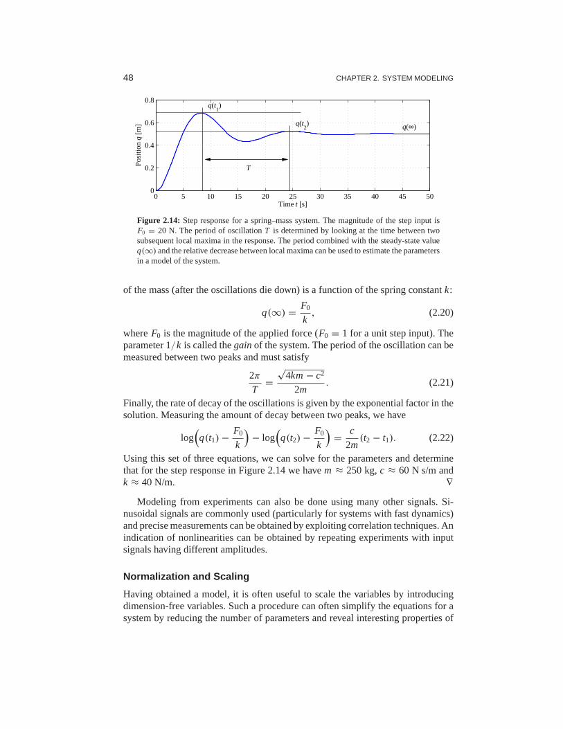
48 CHAPTER 2. SYSTEM MODELING
0 5 10 15 20 25 30 35 40 45 500
0.2
0.4
0.6
0.8
Time t [s]
Pos
ition
q [m
]
q(t1)
q(t2) q(∞)
T
Figure 2.14: Step response for a spring–mass system. The magnitude of the step input isF0 = 20 N. The period of oscillationT is determined by looking at the time between twosubsequent local maxima in the response. The period combined with the steady-state valueq(∞) and the relative decrease between local maxima can be used to estimate theparametersin a model of the system.
of the mass (after the oscillations die down) is a function ofthe spring constantk:
q(∞) = F0
k, (2.20)
whereF0 is the magnitude of the applied force (F0 = 1 for a unit step input). Theparameter 1/k is called thegainof the system. The period of the oscillation can bemeasured between two peaks and must satisfy
2π
T=
√4km− c2
2m. (2.21)
Finally, the rate of decay of the oscillations is given by the exponential factor in thesolution. Measuring the amount of decay between two peaks, we have
log(q(t1)− F0
k
)− log
(q(t2)− F0
k
)= c
2m(t2 − t1). (2.22)
Using this set of three equations, we can solve for the parameters and determinethat for the step response in Figure 2.14 we havem ≈ 250 kg,c ≈ 60 N s/m andk ≈ 40 N/m. ∇
Modeling from experiments can also be done using many other signals. Si-nusoidal signals are commonly used (particularly for systems with fast dynamics)and precise measurements can be obtained by exploiting correlation techniques. Anindication of nonlinearities can be obtained by repeating experiments with inputsignals having different amplitudes.
Normalization and Scaling
Having obtained a model, it is often useful to scale the variables by introducingdimension-free variables. Such a procedure can often simplify the equations for asystem by reducing the number of parameters and reveal interesting properties of

2.3. MODELING METHODOLOGY 49
the model. Scaling can also improve the numerical conditioning of the model toallow faster and more accurate simulations.
The procedure of scaling is straightforward: choose units for each indepen-dent variable and introduce new variables by dividing the variables by the chosennormalization unit. We illustrate the procedure with two examples.
Example 2.6 Spring–mass systemConsider again the spring–mass system introduced earlier.Neglecting the damping,the system is described by
mq + kq = u.
The model has two parametersm and k. To normalize the model we introducedimension-free variablesx = q/ l andτ = ω0t , whereω0 =
√k/m andl is the
chosen length scale. We scale force bymlω20 and introducev = u/(mlω2
0). Thescaled equation then becomes
d2x
dτ 2= d2q/ l
d(ω0t)2= 1
mlω20
(−kq + u) = −x + v,
which is the normalized undamped spring–mass system. Notice that the normalizedmodel has no parameters, while the original model had two parametersm andk.Introducing the scaled, dimension-free state variablesz1 = x = q/ l and z2 =dx/dτ = q/(lω0), the model can be written as
d
dt
z1
z2
=
0 1
−1 0
z1
z2
+
0v
.
This simple linear equation describes the dynamics of any spring–mass system,independent of the particular parameters, and hence gives us insight into the fun-damental dynamics of this oscillatory system. To recover the physical frequency ofoscillation or its magnitude, we must invert the scaling we have applied. ∇
Example 2.7 Balance systemConsider the balance system described in Section 2.1. Neglecting damping byputtingc = 0 andγ = 0 in equation (2.9), the model can be written as
(M + m)d2q
dt2− ml cosθ
d2θ
dt2+ ml sinθ
(dq
dt
)2 = F,
−ml cosθd2q
dt2+ (J + ml2)
d2θ
dt2− mglsinθ = 0.
Letω0 =√
mgl/(J + ml2), choose the length scale asl , let the time scale be 1/ω0,choose the force scale as(M + m)lω2
0 and introduce the scaled variablesτ = ω0t ,x = q/ l andu = F/((M + m)lω2
0). The equations then become
d2x
dτ 2− α cosθ
d2θ
dτ 2+ α sinθ
(dθ
dτ
)2= u, −β cosθ
d2x
dτ 2+ d2θ
dτ 2− sinθ = 0,
whereα = m/(M +m) andβ = ml2/(J +ml2). Notice that the original model hasfive parametersm, M , J, l andg but the normalized model has only two parameters

50 CHAPTER 2. SYSTEM MODELING
10−2
100
102
10−2
100
102
Input u
Out
put y
(a) Static uncertainty
101
102
103
10−1
100
101
Frequency
Am
plitu
de
(b) Uncertainty lemon
1
6u y
M
(c) Model uncertainty
Figure 2.15: Characterization of model uncertainty. Uncertainty of a static system is illus-trated in (a), where the solid line indicates the nominal input/output relationshipand thedashed lines indicate the range of possible uncertainty. The uncertainty lemon [GPD59] in(b) is one way to capture uncertainty in dynamical systems emphasizing that a model is validonly in some amplitude and frequency ranges. In (c) a model is represented by a nominalmodelM and another model1 representing the uncertainty analogous to the representationof parameter uncertainty.
α andβ. If M ≫ m andml2 ≫ J, we getα ≈ 0 andβ ≈ 1 and the model can beapproximated by
d2x
dτ 2= u,
d2θ
dτ 2− sinθ = u cosθ.
The model can be interpreted as a mass combined with an inverted pendulum drivenby the same input. ∇
Model Uncertainty
Reducing uncertainty is one of the main reasons for using feedback, and it is there-fore important to characterize uncertainty. When making measurements, there is agood tradition to assign both a nominal value and a measure ofuncertainty. It isuseful to apply the same principle to modeling, but unfortunately it is often difficultto express the uncertainty of a model quantitatively.
For a static system whose input/output relation can be characterized by a func-tion, uncertainty can be expressed by an uncertainty band asillustrated in Fig-ure 2.15a. At low signal levels there are uncertainties due to sensor resolution,friction and quantization. Some models for queuing systems or cells are based onaverages that exhibit significant variations for small populations. At large signallevels there are saturations or even system failures. The signal ranges where a modelis reasonably accurate vary dramatically between applications, but it is rare to findmodels that are accurate for signal ranges larger than 104.
Characterization of the uncertainty of a dynamic model is much more difficult.We can try to capture uncertainties by assigning uncertainties to parameters of themodel, but this is often not sufficient. There may be errors due to phenomena thathave been neglected, e.g., small time delays. In control theultimate test is how wella control system based on the model performs, and time delayscan be important.There is also a frequency aspect. There are slow phenomena, such as aging, that

2.4. MODELING EXAMPLES 51
can cause changes or drift in the systems. There are also high-frequency effects: aresistor will no longer be a pure resistance at very high frequencies, and a beamhas stiffness and will exhibit additional dynamics when subject to high-frequencyexcitation. Theuncertainty lemon[GPD59] shown in Figure 2.15b is one way toconceptualize the uncertainty of a system. It illustrates that a model is valid only incertain amplitude and frequency ranges.
We will introduce some formal tools for representing uncertainty in Chapter 12using figures such as Figure 2.15c. These tools make use of the concept of a transferfunction, which describes the frequency response of an input/output system. Fornow, we simply note that one should always be careful to recognize the limits ofa model and not to make use of models outside their range of applicability. Forexample, one can describe the uncertainty lemon and then check to make sure thatsignals remain in this region. In early analog computing, a system was simulatedusing operational amplifiers, and it was customary to give alarms when certainsignal levels were exceeded. Similar features can be included in digital simulation.
2.4 Modeling Examples
In this section we introduce additional examples that illustrate some of the differenttypes of systems for which one can develop differential equation and differenceequation models. These examples are specifically chosen from arange of differentfields to highlight the broad variety of systems to which feedback and controlconcepts can be applied. A more detailed set of applicationsthat serve as runningexamples throughout the text are given in the next chapter.
Motion Control Systems
Motion control systems involve the use of computation and feedback to control themovement of a mechanical system. Motion control systems range from nanopo-sitioning systems (atomic force microscopes, adaptive optics), to control systemsfor the read/write heads in a disk drive of a CD player, to manufacturing systems(transfer machines and industrial robots), to automotive control systems (antilockbrakes, suspension control, traction control), to air and space flight control systems(airplanes, satellites, rockets and planetary rovers).
Example 2.8 Vehicle steering—the bicycle modelA common problem in motion control is to control the trajectory of a vehiclethrough an actuator that causes a change in the orientation.A steering wheel on anautomobile and the front wheel of a bicycle are two examples,but similar dynamicsoccur in the steering of ships or control of the pitch dynamics of an aircraft. In manycases, we can understand the basic behavior of these systemsthrough the use of asimple model that captures the basic kinematics of the system.
Consider a vehicle with two wheels as shown in Figure 2.16. Forthe purpose ofsteering we are interested in a model that describes how the velocity of the vehicle

52 CHAPTER 2. SYSTEM MODELING
ab
α δv
y
x
α
α
δ
δ
O
Figure 2.16:Vehicle steering dynamics. The left figure shows an overhead view of avehiclewith four wheels. The wheel base isb and the center of mass at a distancea forward of therear wheels. By approximating the motion of the front and rear pairs of wheels by a singlefront wheel and a single rear wheel, we obtain an abstraction called thebicycle model, shownon the right. The steering angle isδ and the velocity at the center of mass has the angleα
relative the length axis of the vehicle. The position of the vehicle is given by(x, y) and theorientation (heading) byθ .
depends on the steering angleδ. To be specific, consider the velocityv at the centerof mass, a distancea from the rear wheel, and letb be the wheel base, as shownin Figure 2.16. Letx andy be the coordinates of the center of mass,θ the headingangle andα the angle between the velocity vectorv and the centerline of the vehicle.Sinceb = ra tanδ anda = ra tanα, it follows that tanα = (a/b) tanδ and we getthe following relation betweenα and the steering angleδ:
α(δ) = arctan(a tanδ
b
). (2.23)
Assume that the wheels are rolling without slip and that the velocity of the rearwheel isv0. The vehicle speed at its center of mass isv = v0/ cosα, and we findthat the motion of this point is given by
dx
dt= v cos(α + θ) = v0
cos(α + θ)
cosα,
dy
dt= v sin(α + θ) = v0
sin(α + θ)
cosα.
(2.24)
To see how the angleθ is influenced by the steering angle, we observe from Fig-ure 2.16 that the vehicle rotates with the angular velocityv0/ra around the pointO. Hence
dθ
dt= v0
ra= v0
btanδ. (2.25)
Equations (2.23)–(2.25) can be used to model an automobile under the assump-tions that there is no slip between the wheels and the road andthat the two frontwheels can be approximated by a single wheel at the center of the car. The as-sumption of no slip can be relaxed by adding an extra state variable, giving a morerealistic model. Such a model also describes the steering dynamics of ships as well

2.4. MODELING EXAMPLES 53
(a) Harrier “jump jet”
r
x
y
θ
F1
F2
(b) Simplified model
Figure 2.17: Vectored thrust aircraft. The Harrier AV-8B military aircraft (a) redirects itsengine thrust downward so that it can “hover” above the ground. Some air from the engineis diverted to the wing tips to be used for maneuvering. As shown in (b), thenet thrust onthe aircraft can be decomposed into a horizontal forceF1 and a vertical forceF2 acting at adistancer from the center of mass.
as the pitch dynamics of aircraft and missiles. It is also possible to choose coor-dinates so that the reference point is at the rear wheels (corresponding to settingα = 0), a model often referred to as theDubins car[Dub57].
Figure 2.16 represents the situation when the vehicle moves forward and hasfront-wheel steering. The case when the vehicle reverses is obtained by changingthe sign of the velocity, which is equivalent to a vehicle with rear-wheel steering.
∇
Example 2.9 Vectored thrust aircraftConsider the motion of vectored thrust aircraft, such as theHarrier “jump jet”shown Figure 2.17a. The Harrier is capable of vertical takeoffby redirecting itsthrust downward and through the use of smaller maneuvering thrusters located onits wings. A simplified model of the Harrier is shown in Figure 2.17b, where wefocus on the motion of the vehicle in a vertical plane throughthe wings of theaircraft. We resolve the forces generated by the main downward thruster and themaneuvering thrusters as a pair of forcesF1 andF2 acting at a distancer below theaircraft (determined by the geometry of the thrusters).
Let (x, y, θ) denote the position and orientation of the center of mass of theaircraft. Letmbe the mass of the vehicle,J the moment of inertia,g the gravitationalconstant andc the damping coefficient. Then the equations of motion for the vehicleare given by
mx = F1 cosθ − F2 sinθ − cx,
my = F1 sinθ + F2 cosθ − mg− cy,
Jθ = r F1.
(2.26)
It is convenient to redefine the inputs so that the origin is an equilibrium point of the

54 CHAPTER 2. SYSTEM MODELING
message queue
incoming outgoingmessages
x
µλ
messages
Figure 2.18:Schematic diagram of a queuing system. Messages arrive at rateλ and are storedin a queue. Messages are processed and removed from the queue atrateµ. The average sizeof the queue is given byx ∈ R.
system with zero input. Lettingu1 = F1 andu2 = F2 − mg, the equations become
mx = −mgsinθ − cx + u1 cosθ − u2 sinθ,
my = mg(cosθ − 1)− cy + u1 sinθ + u2 cosθ,
Jθ = ru1.
(2.27)
These equations describe the motion of the vehicle as a set of three coupled second-order differential equations. ∇
Information Systems
Information systems range from communication systems likethe Internet to soft-ware systems that manipulate data or manage enterprisewideresources. Feedbackis present in all these systems, and designing strategies for routing, flow control andbuffer management is a typical problem. Many results in queuing theory emergedfrom design of telecommunication systems and later from development of the In-ternet and computer communication systems [BG87, Kle75, Sch87]. Managementof queues to avoid congestion is a central problem and we willtherefore start bydiscussing the modeling of queuing systems.
Example 2.10 Queuing systemsA schematic picture of a simple queue is shown in Figure 2.18. Requests arriveand are then queued and processed. There can be large variations in arrival ratesand service rates, and the queue length builds up when the arrival rate is largerthan the service rate. When the queue becomes too large, service is denied usingan admission control policy.
The system can be modeled in many different ways. One way is to model eachincoming request, which leads to an event-based model wherethe state is an integerthat represents the queue length. The queue changes when a request arrives or arequest is serviced. The statistics of arrival and servicingare typically modeled asrandom processes. In many cases it is possible to determine statistics of quantitieslike queue length and service time, but the computations canbe quite complicated.
A significant simplification can be obtained by using aflow model. Insteadof keeping track of each request we instead view service and requests as flows,similar to what is done when replacing molecules by a continuum when analyzing

2.4. MODELING EXAMPLES 55
0 0.5 10
50
100
Service rate excess λ/µmax
Que
ue le
ngth
x e
(a) Steady-state queue size
0 20 40 60 800
10
20
Time [s]
Que
ue le
ngth
xe
(b) Overload condition
Figure 2.19:Queuing dynamics. (a) The steady-state queue length as a function ofλ/µmax.(b) The behavior of the queue length when there is a temporary overloadin the system. Thesolid line shows a realization of an event-based simulation, and the dashed line shows thebehavior of the flow model (2.29).
fluids. Assuming that the average queue lengthx is a continuous variable and thatarrivals and services are flows with ratesλ andµ, the system can be modeled bythe first-order differential equation
dx
dt= λ− µ = λ− µmax f (x), x ≥ 0, (2.28)
whereµmax is the maximum service rate andf (x) is a number between 0 and 1that describes the effective service rate as a function of the queue length.
It is natural to assume that the effective service rate depends on the queue lengthbecause larger queues require more resources. In steady state we havef (x) =λ/µmax, and we assume that the queue length goes to zero whenλ/µmaxgoes to zeroand that it goes to infinity whenλ/µmax goes to 1. This implies thatf (0) = 0 andthat f (∞) = 1. In addition, if we assume that the effective service rate deterioratesmonotonically with queue length, then the functionf (x) is monotone and concave.A simple function that satisfies the basic requirements isf (x) = x/(1+ x), whichgives the model
dx
dt= λ− µmax
x
x + 1. (2.29)
This model was proposed by Agnew [Agn76]. It can be shown that if arrival andservice processes are Poisson processes, the average queue length is given by equa-tion (2.29) and that equation (2.29) is a good approximationeven for short queuelengths; see Tipper [TS90].
To explore the properties of the model (2.29) we will first investigate the equi-librium value of the queue length when the arrival rateλ is constant. Setting thederivativedx/dt to zero in equation (2.29) and solving forx, we find that the queuelengthx approaches the steady-state value
xe = λ
µmax − λ. (2.30)
Figure 2.19a shows the steady-state queue length as a function of λ/µmax, theeffective service rate excess. Notice that the queue lengthincreases rapidly asλ
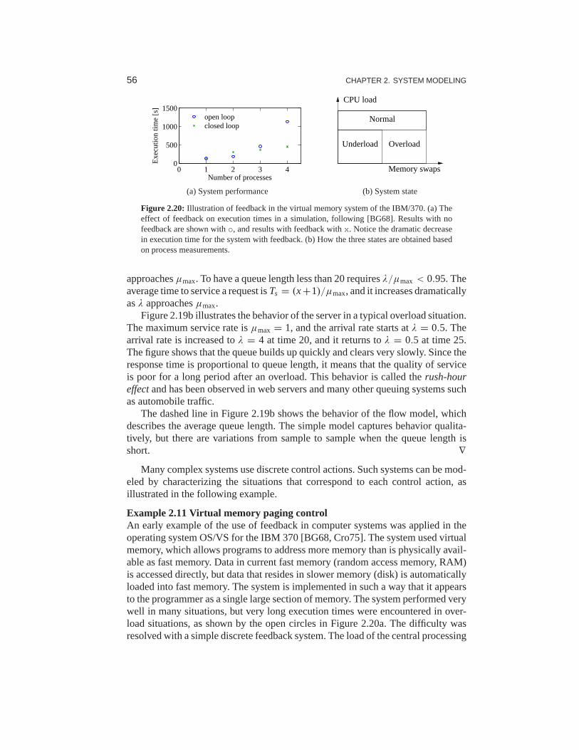
56 CHAPTER 2. SYSTEM MODELING
0 1 2 3 40
500
1000
1500
Number of processes
Exe
cutio
n tim
e [s
]
open loopclosed loop
(a) System performance
Normal
CPU load
Memory swaps
Underload Overload
(b) System state
Figure 2.20: Illustration of feedback in the virtual memory system of the IBM/370. (a) Theeffect of feedback on execution times in a simulation, following [BG68]. Results with nofeedback are shown witho, and results with feedback withx. Notice the dramatic decreasein execution time for the system with feedback. (b) How the three states are obtained basedon process measurements.
approachesµmax. To have a queue length less than 20 requiresλ/µmax< 0.95. Theaverage time to service a request isTs = (x+1)/µmax, and it increases dramaticallyasλ approachesµmax.
Figure 2.19b illustrates the behavior of the server in a typical overload situation.The maximum service rate isµmax = 1, and the arrival rate starts atλ = 0.5. Thearrival rate is increased toλ = 4 at time 20, and it returns toλ = 0.5 at time 25.The figure shows that the queue builds up quickly and clears veryslowly. Since theresponse time is proportional to queue length, it means thatthe quality of serviceis poor for a long period after an overload. This behavior is called therush-houreffectand has been observed in web servers and many other queuing systems suchas automobile traffic.
The dashed line in Figure 2.19b shows the behavior of the flow model, whichdescribes the average queue length. The simple model captures behavior qualita-tively, but there are variations from sample to sample when the queue length isshort. ∇
Many complex systems use discrete control actions. Such systems can be mod-eled by characterizing the situations that correspond to each control action, asillustrated in the following example.
Example 2.11 Virtual memory paging controlAn early example of the use of feedback in computer systems was applied in theoperating system OS/VS for the IBM 370 [BG68, Cro75]. The system used virtualmemory, which allows programs to address more memory than isphysically avail-able as fast memory. Data in current fast memory (random access memory, RAM)is accessed directly, but data that resides in slower memory(disk) is automaticallyloaded into fast memory. The system is implemented in such a way that it appearsto the programmer as a single large section of memory. The system performed verywell in many situations, but very long execution times were encountered in over-load situations, as shown by the open circles in Figure 2.20a.The difficulty wasresolved with a simple discrete feedback system. The load of the central processing

2.4. MODELING EXAMPLES 57
4
5 2 31
(a) Sensor network
0 10 20 30 4010
20
30
40
Iteration
Age
nt s
tate
s x i
(b) Consensus convergence
Figure 2.21: Consensus protocols for sensor networks. (a) A simple sensor network withfive nodes. In this network, node 1 communicates with node 2 and node 2 communicateswith nodes 1, 3, 4, 5, etc. (b) A simulation demonstrating the convergenceof the consensusprotocol (2.31) to the average value of the initial conditions.
unit (CPU) was measured together with the number of page swapsbetween fastmemory and slow memory. The operating region was classified as being in one ofthree states: normal, underload or overload. The normal state is characterized byhigh CPU activity, the underload state is characterized by low CPU activity and fewpage replacements, the overload state has moderate to low CPUload but many pagereplacements; see Figure 2.20b. The boundaries between the regions and the timefor measuring the load were determined from simulations using typical loads. Thecontrol strategy was to do nothing in the normal load condition, to exclude a processfrom memory in the overload condition and to allow a new process or a previouslyexcluded process in the underload condition. The crosses in Figure 2.20a show theeffectiveness of the simple feedback system in simulated loads. Similar principlesare used in many other situations, e.g., in fast, on-chip cache memory. ∇
Example 2.12 Consensus protocols in sensor networksSensor networks are used in a variety of applications where wewant to collectand aggregate information over a region of space using multiple sensors that areconnected together via a communications network. Examples include monitoringenvironmental conditions in a geographical area (or insidea building), monitoringthe movement of animals or vehicles and monitoring the resource loading acrossa group of computers. In many sensor networks the computational resources aredistributed along with the sensors, and it can be important for the set of distributedagents to reach a consensus about a certain property, such asthe average temperaturein a region or the average computational load among a set of computers.
We model the connectivity of the sensor network using a graph, with nodescorresponding to the sensors and edges corresponding to theexistence of a directcommunications link between two nodes. We use the notationN i to represent theset of neighbors of a nodei . For example, in the network shown in Figure 2.21aN2 = {1,3,4,5} andN3 = {2,4}.
To solve the consensus problem, letxi be the state of thei th sensor, correspond-ing to that sensor’s estimate of the average value that we aretrying to compute. Weinitialize the state to the value of the quantity measured bythe individual sensor.

58 CHAPTER 2. SYSTEM MODELING
The consensus protocol (algorithm) can now be realized as a local update law
xi [k + 1] = xi [k] + γ∑
j ∈Ni
(x j [k] − xi [k]). (2.31)
This protocol attempts to compute the average by updating thelocal state of eachagent based on the value of its neighbors. The combined dynamics of all agents canbe written in the form
x[k + 1] = x[k] − γ (D − A)x[k], (2.32)
where A is the adjacency matrix andD is a diagonal matrix with entries corre-sponding to the number of neighbors of each node. The constantγ describes therate at which the estimate of the average is updated based on information fromneighboring nodes. The matrixL := D − A is called theLaplacianof the graph.
The equilibrium points of equation (2.32) are the set of states such thatxe[k +1] = xe[k]. It can be shown thatxe = (α, α, . . . , α) is an equilibrium state for thesystem, corresponding to each sensor having an identical estimateα for the average.Furthermore, we can show thatα is indeed the average value of the initial states.Since there can be cycles in the graph, it is possible that the state of the systemcould enter into an infinite loop and never converge to the desired consensus state.A formal analysis requires tools that will be introduced later in the text, but it canbe shown that for any connected graph we can always find aγ such that the statesof the individual agents converge to the average. A simulation demonstrating thisproperty is shown in Figure 2.21b. ∇
Biological Systems
Biological systems provide perhaps the richest source of feedback and control ex-amples. The basic problem of homeostasis, in which a quantitysuch as temperatureor blood sugar level is regulated to a fixed value, is but one of the many types of com-plex feedback interactions that can occur in molecular machines, cells, organismsand ecosystems.
Example 2.13 Transcriptional regulationTranscription is the process by which messenger RNA (mRNA) is generated from asegment of DNA. The promoter region of a gene allows transcription to be controlledby the presence of other proteins, which bind to the promoterregion and eitherrepress or activate RNA polymerase, the enzyme that produces an mRNA transcriptfrom DNA. The mRNA is then translated into a protein accordingto its nucleotidesequence. This process is illustrated in Figure 2.22.
A simple model of the transcriptional regulation process isthrough the useof a Hill function [dJ02, Mur04]. Consider the regulation ofa protein A with aconcentration given bypa and a corresponding mRNA concentrationma. Let Bbe a second protein with concentrationpb that represses the production of proteinA through transcriptional regulation. The resulting dynamics of pa andma can be

2.4. MODELING EXAMPLES 59
RNApolymerase
DNA
Polypeptide
mRNA
RibosomeTranscription
Translation
Figure 2.22:Biological circuitry. The cell on the left is a bovine pulmonary cell, stained sothat the nucleus, actin and chromatin are visible. The figure on the right gives an overviewof the process by which proteins in the cell are made. RNA is transcribed from DNA by anRNA polymerase enzyme. The RNA is then translated into a protein by an organelle calleda ribosome.
written asdma
dt= αab
1 + kabpnabb
+ αa0 − γama,dpa
dt= βama − δa pa, (2.33)
whereαab+αa0 is the unregulated transcription rate,γa represents the rate of degra-dation of mRNA,αab, kab andnab are parameters that describe how B represses A,βa represents the rate of production of the protein from its corresponding mRNAandδa represents the rate of degradation of the protein A. The parameterαa0 de-scribes the “leakiness” of the promoter, andnab is called the Hill coefficient andrelates to the cooperativity of the promoter.
A similar model can be used when a protein activates the production of anotherprotein rather than repressing it. In this case, the equations have the form
dma
dt= αabkabpnab
b
1 + kabpnabb
+ αa0 − γama,dpa
dt= βama − δa pa, (2.34)
where the variables are the same as described previously. Note that in the case ofthe activator, ifpb is zero, then the production rate isαa0 (versusαab + αa0 for therepressor). Aspb gets large, the first term in the expression forma approaches 1and the transcription rate becomesαab + αa0 (versusαa0 for the repressor). Thuswe see that the activator and repressor act in opposite fashion from each other.
As an example of how these models can be used, we consider the model of a“repressilator,” originally due to Elowitz and Leibler [EL00].The repressilator isa synthetic circuit in which three proteins each repress another in a cycle. This isshown schematically in Figure 2.23a, where the three proteins are TetR,λcI andLacI. The basic idea of the repressilator is that if TetR is present, then it repressesthe production ofλcI. If λcI is absent, then LacI is produced (at the unregulatedtranscription rate), which in turn represses TetR. Once TetR is repressed, thenλcI isno longer repressed, and so on. If the dynamics of the circuitare designed properly,the resulting protein concentrations will oscillate.
We can model this system using three copies of equation (2.33), with A andB replaced by the appropriate combination of TetR, cI and LacI. The state of the

60 CHAPTER 2. SYSTEM MODELING
ampR
SC101
origin
PLtetO1
cI-lite
PR
lacI-lite
PLlacO1
tetR-lite
TetR
LacI cI
(a) Repressilator plasmid
0 100 200 3000
1000
2000
3000
4000
5000
Time t [min]
Pro
tein
s pe
r ce
ll
cI lacI tetR
(b) Repressilator simulation
Figure 2.23: The repressilator genetic regulatory network. (a) A schematic diagram of therepressilator, showing the layout of the genes in the plasmid that holds the circuit as well asthe circuit diagram (center). (b) A simulation of a simple model for the repressilator, showingthe oscillation of the individual protein concentrations. (Figure courtesy M. Elowitz.)
system is then given byx = (mTetR, pTetR,mcI, pcI,mLacI, pLacI). Figure 2.23bshows the traces of the three protein concentrations for parametersn = 2,α = 0.5,k = 6.25× 10⁻⁴, α0 = 5 × 10⁻⁴, γ = 5.8 × 10⁻³, β = 0.12 andδ = 1.2 × 10⁻³
with initial conditionsx(0) = (1,0,0,200,0,0) (following [EL00]). ∇
Example 2.14 Wave propagation in neuronal networksThe dynamics of the membrane potential in a cell are a fundamental mechanismin understanding signaling in cells, particularly in neurons and muscle cells. TheHodgkin–Huxley equations give a simple model for studying propagation waves innetworks of neurons. The model for a single neuron has the form
CdV
dt= −INa − IK − I leak + I input,
whereV is the membrane potential,C is the capacitance,INa andIK are the currentcaused by the transport of sodium and potassium across the cell membrane,I leak
is a leakage current andI input is the external stimulation of the cell. Each currentobeys Ohm’s law, i.e.,
I = g(V − E),
whereg is the conductance andE is the equilibrium voltage. The equilibriumvoltage is given by Nernst’s law,
E = RT
nFlog
ce
ci,
whereR is Boltzmann’s constant,T is the absolute temperature,F is Faraday’s con-stant,n is the charge (or valence) of the ion andci andce are the ion concentrationsinside the cell and in the external fluid. At 20◦C we haveRT/F = 20 mV.
The Hodgkin–Huxley model was originally developed as a meansto predict thequantitative behavior of the squid giant axon [HH52]. Hodgkin and Huxley sharedthe 1963 Nobel Prize in Physiology (along with J. C. Eccles) for analysis of the

2.5. FURTHER READING 61
electrical and chemical events in nerve cell discharges. Thevoltage clamp describedin Section 1.3 was a key element in Hodgkin and Huxley’s experiments. ∇
2.5 Further Reading
Modeling is ubiquitous in engineering and science and has a long history in appliedmathematics. For example, the Fourier series was introduced by Fourier when hemodeled heat conduction in solids [Fou07]. Models of dynamics have been de-veloped in many different fields, including mechanics [Arn78, Gol53], heat con-duction [CJ59], fluids [BRS60], vehicles [Abk69, Bla91, Ell94], robotics [MLS94,SV89], circuits [Gui63], power systems [Kun93], acoustics [Ber54] and microme-chanical systems [Sen01]. Control theory requires modelingfrom many differ-ent domains, and most control theory texts contain several chapters on modelingusing ordinary differential equations and difference equations (see, for example,[FPEN05]). A classic book on the modeling of physical systems, especially me-chanical, electrical and thermofluid systems, is Cannon [Can03]. The book byAris [Ari94] is highly original and has a detailed discussion of the use of dimension-free variables. Two of the authors’ favorite books on modeling of biological systemsare J. D. Murray [Mur04] and Wilson [Wil99].
Exercises
2.1 (Chain of integrators form) Consider the linear ordinary differential equa-tion (2.7). Show that by choosing a state space representation with x1 = y, thedynamics can be written as
A =
0 1 0
0. . .
. . . 00 · · · 0 1
−an −an−1 −a1
, B =
00...
1
, C =
1 . . . 0 0
.
This canonical form is called thechain of integratorsform.
2.2(Inverted pendulum) Use the equations of motion for a balance system to derivea dynamic model for the inverted pendulum described in Example 2.2 and verifythat for smallθ the dynamics are approximated by equation (2.10).
2.3 (Disrete-time dynamics) Consider the following discrete-time system
x[k + 1] = Ax[k] + Bu[k], y[k] = Cx[k],
where
x =x1
x2
, A =
a11 a12
0 a22
, B =
0
1
, C =
1 0
.

62 CHAPTER 2. SYSTEM MODELING
In this problem, we will explore some of the properties of this discrete-time systemas a function of the parameters, the initial conditions and the inputs.
(a) For the case whena12 = 0 andu = 0, give a closed form expression for theoutput of the system.
(b) A discrete system is inequilibriumwhenx[k + 1] = x[k] for all k. Let u = rbe a constant input and compute the resulting equilibrium point for the system.Show that if|ai i | < 1 for all i , all initial conditions give solutions that converge tothe equilibrium point.
(c) Write a computer program to plot the output of the system in response to a unitstep input,u[k] = 1, k ≥ 0. Plot the response of your system withx[0] = 0 andAgiven bya11 = 0.5, a12 = 1 anda22 = 0.25.
2.4 (Keynesian economics) Keynes’ simple model for an economy is given by
Y[k] = C[k] + I [k] + G[k],
whereY, C, I andG are gross national product (GNP), consumption, investmentand government expenditure for yeark. Consumption and investment are modeledby difference equations of the form
C[k + 1] = aY[k], I [k + 1] = b(C[k + 1] − C[k]),
wherea andbare parameters. The first equation implies that consumption increaseswith GNP but that the effect is delayed. The second equation implies that investmentis proportional to the rate of change of consumption.
Show that the equilibrium value of the GNP is given by
Ye = 1
1 − a(Ie + Ge),
where the parameter 1/(1 − a) is the Keynes multiplier (the gain fromI or G toY). With a = 0.25 an increase of government expenditure will result in a fourfoldincrease of GNP. Also show that the model can be written as thefollowing discrete-time state model:
C[k + 1]I [k + 1]
=
a a
ab− b ab
C[k]
I [k]
+
a
ab
G[k],
Y[k] = C[k] + I [k] + G[k].
2.5(Least squares system identification) Consider a nonlinear differential equation�that can be written in the form
dx
dt=
M∑
i =1
αi fi (x),
where fi (x) are known nonlinear functions andαi are unknown, but constant,parameters. Suppose that we have measurements (or estimates) of the full statex

EXERCISES 63
at time instantst1, t2, . . . , tN , with N > M . Show that the parametersαi can bedetermined by finding the least squares solution to a linear equation of the form
Hα = b,
whereα ∈ RM is the vector of all parameters andH ∈ R
N×M andb ∈ RN are
appropriately defined.
2.6(Normalized oscillator dynamics) Consider a damped spring–mass system withdynamics
mq + cq + kq = F.
Let ω0 =√
k/m be the natural frequency andζ = c/(2√
km) be the dampingratio.
(a) Show that by rescaling the equations, we can write the dynamics in the form
q + 2ζω0q + ω20q = ω2
0u, (2.35)
whereu = F/k. This form of the dynamics is that of a linear oscillator with naturalfrequencyω0 and damping ratioζ .
(b) Show that the system can be further normalized and writtenin the form
dz1
dτ= z2,
dz2
dτ= −z1 − 2ζz2 + v. (2.36)
The essential dynamics of the system are governed by a single damping parameterζ . TheQ-valuedefined asQ = 1/2ζ is sometimes used instead ofζ .
2.7(Electric generator) An electric generator connected to a strong power grid canbe modeled by a momentum balance for the rotor of the generator:
Jd2ϕ
dt2= Pm − Pe = Pm − EV
Xsinϕ,
whereJ is the effective moment of inertia of the generator,ϕ the angle of rotation,Pm the mechanical power that drives the generator,Pe is the active electrical power,E the generator voltage,V the grid voltage andX the reactance of the line. Assumingthat the line dynamics are much faster than the rotor dynamics, Pe = V I =(EV/X) sinϕ, whereI is the current component in phase with the voltageE andϕis the phase angle between voltagesE andV . Show that the dynamics of the electricgenerator has a normalized form that is similar to the dynamics of a pendulum withforcing at the pivot.
2.8 (Admission control for a queue) Consider the queuing systemdescribed inExample 2.10. The long delays created by temporary overloads can be reduced byrejecting requests when the queue gets large. This allows requests that are acceptedto be serviced quickly and requests that cannot be accommodated to receive arejection quickly so that they can try another server. Consider an admission controlsystem described by
dx
dt= λu − µmax
x
x + 1, u = sat(0,1)(k(r − x)), (2.37)

64 CHAPTER 2. SYSTEM MODELING
where the controller is a simple proportional control with saturation (sat(a,b) isdefined by equation (3.9)) andr is the desired (reference) queue length. Use asimulation to show that this controller reduces the rush-hour effect and explainhow the choice ofr affects the system dynamics.
2.9 (Biological switch) A genetic switch can be formed by connecting two repres-sors together in a cycle as shown below.
u1
A
B
u2B
u2
u1
A
Using the models from Example 2.13—assuming that the parameters are the samefor both genes and that the mRNA concentrations reach steadystate quickly—showthat the dynamics can be written in normalized coordinates as
dz1
dτ= µ
1 + zn2
− z1 − v1,dz2
dτ= µ
1 + zn1
− z2 − v2, (2.38)
wherez1 andz2 are scaled versions of the protein concentrations and the time scalehas also been changed. Show thatµ ≈ 200 using the parameters in Example 2.13,and use simulations to demonstrate the switch-like behavior of the system.
2.10(Motor drive) Consider a system consisting of a motor driving two masses thatare connected by a torsional spring, as shown in the diagram below.
MotorI
J1
1
1
J2
ω
ϕ 2ϕ
2ω
This system can represent a motor with a flexible shaft that drives a load. Assumingthat the motor delivers a torque that is proportional to the current, the dynamics ofthe system can be described by the equations
J1d2ϕ1
dt2+ c
(dϕ1
dt− dϕ2
dt
)+ k(ϕ1 − ϕ2) = kI I ,
J2d2ϕ2
dt2+ c
(dϕ2
dt− dϕ1
dt
)+ k(ϕ2 − ϕ1) = Td.
(2.39)
Similar equations are obtained for a robot with flexible arms and for the arms ofDVD and optical disk drives.
Derive a state space model for the system by introducing the (normalized)state variablesx1 = ϕ1, x2 = ϕ2, x3 = ω1/ω0, andx4 = ω2/ω0, whereω0 =√
k(J1 + J2)/(J1J2) is the undamped natural frequency of the system when thecontrol signal is zero.

Chapter ThreeExamples
... Don’t apply any model until you understand the simplifying assumptions on which it isbased, and you can test their validity. Catch phrase: use only as directed. Don’t limit yourselfto a single model: More than one model may be useful for understanding different aspects ofthe same phenomenon. Catch phrase: legalize polygamy.”
Saul Golomb, “Mathematical Models—Uses and Limitations,” 1970 [Gol70].
In this chapter we present a collection of examples spanningmany differentfields of science and engineering. These examples will be used throughout thetext and in exercises to illustrate different concepts. First-time readers may wish tofocus on only a few examples with which they have had the most prior experience orinsight to understand the concepts of state, input, output and dynamics in a familiarsetting.
3.1 Cruise Control
The cruise control system of a car is a common feedback system encountered ineveryday life. The system attempts to maintain a constant velocity in the presenceof disturbances primarily caused by changes in the slope of aroad. The controllercompensates for these unknowns by measuring the speed of thecar and adjustingthe throttle appropriately.
To model the system we start with the block diagram in Figure 3.1. Let v bethe speed of the car andvr the desired (reference) speed. The controller, whichtypically is of the proportional-integral (PI) type described briefly in Chapter 1,receives the signalsv andvr and generates a control signalu that is sent to anactuator that controls the throttle position. The throttle in turn controls the torqueT delivered by the engine, which is transmitted through the gears and the wheels,generating a forceF that moves the car. There are disturbance forcesFd due tovariations in the slope of the road, the rolling resistance and aerodynamic forces.The cruise controller also has a human–machine interface that allows the driverto set and modify the desired speed. There are also functions that disconnect thecruise control when the brake is touched.
The system has many individual components—actuator, engine, transmission,wheels and car body—and a detailed model can be very complicated. In spite ofthis, the model required to design the cruise controller canbe quite simple.
To develop a mathematical model we start with a force balancefor the car body.Let v be the speed of the car,m the total mass (including passengers),F the forcegenerated by the contact of the wheels with the road, andFd the disturbance force

66 CHAPTER 3. EXAMPLES
Gears &
Actuator
vr
Controller
BodyThrottle &
Engine
Fd
v
cancelresume/accelset/decelon/off
Driver
Interface
T F
u
Wheels
Figure 3.1: Block diagram of a cruise control system for an automobile. The throttle-controlled engine generates a torqueT that is transmitted to the ground through the gearboxand wheels. Combined with the external forces from the environment, such as aerodynamicdrag and gravitational forces on hills, the net force causes the car to move. The velocityof the carv is measured by a control system that adjusts the throttle through an actuationmechanism. A driver interface allows the system to be turned on and off and the referencespeedvr to be established.
due to gravity, friction and aerodynamic drag. The equation of motion of the car issimply
mdv
dt= F − Fd. (3.1)
The forceF is generated by the engine, whose torque is proportional to the rateof fuel injection, which is itself proportional to a controlsignal 0≤ u ≤ 1 thatcontrols the throttle position. The torque also depends on engine speedω. A simplerepresentation of the torque at full throttle is given by thetorque curve
T(ω) = Tm
(1 − β
(ω
ωm− 1
)2), (3.2)
where the maximum torqueTm is obtained at engine speedωm. Typical parametersare Tm = 190 Nm,ωm = 420 rad/s (about 4000 RPM) andβ = 0.4. Let n bethe gear ratio andr the wheel radius. The engine speed is related to the velocitythrough the expression
ω = n
rv =: αnv,
and the driving force can be written as
F = nu
rT(ω) = αnuT(αnv).
Typical values ofαn for gears 1 through 5 areα1 = 40,α2 = 25,α3 = 16,α4 = 12andα5 = 10. The inverse ofαn has a physical interpretation as theeffective wheelradius. Figure 3.2 shows the torque as a function of engine speed and vehicle speed.The figure shows that the effect of the gear is to “flatten” the torque curve so thatan almost full torque can be obtained almost over the whole speed range.
The disturbance forceFd has three major components:Fg, the forces due to

3.1. CRUISE CONTROL 67
0 200 400 600100
120
140
160
180
200
Angular velocity ω [rad/s]
Tor
que T
[Nm
]
0 20 40 60100
120
140
160
180
200
n=1 n=2 n=3 n=4
n=5
Velocity v [m/s]
Tor
que T
[Nm
]
Figure 3.2: Torque curves for typical car engine. The graph on the left shows thetorquegenerated by the engine as a function of the angular velocity of the engine,while the curveon the right shows torque as a function of car speed for different gears.
gravity; Fr , the forces due to rolling friction; andFa, the aerodynamic drag. Lettingthe slope of the road beθ , gravity gives the forceFg = mgsinθ , as illustrated inFigure 3.3a, whereg = 9.8 m/s2 is the gravitational constant. A simple model ofrolling friction is
Fr = mgCr sgn(v),
whereCr is the coefficient of rolling friction and sgn(v) is the sign ofv (±1) orzero if v = 0. A typical value for the coefficient of rolling friction isCr = 0.01.Finally, the aerodynamic drag is proportional to the square of the speed:
Fa = 1
2ρCd Av2,
whereρ is the density of air,Cd is the shape-dependent aerodynamic drag coefficientandA is the frontal area of the car. Typical parameters areρ = 1.3 kg/m3,Cd = 0.32andA = 2.4 m2.
Summarizing, we find that the car can be modeled by
mdv
dt= αnuT(αnv)− mgCr sgn(v)− 1
2ρCd Av2 − mgsinθ, (3.3)
where the functionT is given by equation (3.2). The model (3.3) is a dynamicalsystem of first order. The state is the car velocityv, which is also the output. Theinput is the signalu that controls the throttle position, and the disturbance istheforceFd, which depends on the slope of the road. The system is nonlinear becauseof the torque curve, the gravity term and the nonlinear character of rolling frictionand aerodynamic drag. There can also be variations in the parameters; e.g., the massof the car depends on the number of passengers and the load being carried in thecar.
We add to this model a feedback controller that attempts to regulate the speedof the car in the presence of disturbances. We shall use a proportional-integral

68 CHAPTER 3. EXAMPLES
gF
mg
F
θ
(a) Effect of gravitational forces
0 10 20 3019
20
Time t [s]
Vel
ocity
v [m
/s]
0 10 20 300
1
Time t [s]
Thr
ottle
u
(b) Closed loop response
Figure 3.3: Car with cruise control encountering a sloping road. A schematic diagramisshown in (a), and (b) shows the response in speed and throttle when a slope of 4◦ is encoun-tered. The hill is modeled as a net change of 4◦ in hill angleθ , with a linear change in theangle betweent = 5 andt = 6. The PI controller has proportional gain iskp = 0.5, and theintegral gain iski = 0.1.
controller, which has the form
u(t) = kpe(t)+ ki
∫ t
0e(τ )dτ.
This controller can itself be realized as an input/output dynamical system by defin-ing a controller statez and implementing the differential equation
dz
dt= vr − v, u = kp(vr − v)+ ki z, (3.4)
wherevr is the desired (reference) speed. As discussed briefly in Section 1.5, theintegrator (represented by the statez) ensures that in steady state the error will bedriven to zero, even when there are disturbances or modelingerrors. (The design ofPI controllers is the subject of Chapter 10.) Figure 3.3b showsthe response of theclosed loop system, consisting of equations (3.3) and (3.4), when it encounters ahill. The figure shows that even if the hill is so steep that the throttle changes from0.17 to almost full throttle, the largest speed error is lessthan 1 m/s, and the desiredvelocity is recovered after 20 s.
Many approximations were made when deriving the model (3.3). It may seemsurprising that such a seemingly complicated system can be described by the simplemodel (3.3). It is important to make sure that we restrict ouruse of the model tothe uncertainty lemon conceptualized in Figure 2.15b. The model is not valid forvery rapid changes of the throttle because we have ignored the details of the enginedynamics, neither is it valid for very slow changes because the properties of theengine will change over the years. Nevertheless the model isvery useful for thedesign of a cruise control system. As we shall see in later chapters, the reason forthis is the inherent robustness of feedback systems: even ifthe model is not perfectlyaccurate, we can use it to design a controller and make use of the feedback in the

3.2. BICYCLE DYNAMICS 69
cancel
StandbyOff
Cruise
Hold
on
off
off
off
set
brake resume
Figure 3.4: Finite state machine for cruise control system. The figure on the left showssome typical buttons used to control the system. The controller can be in one of four modes,corresponding to the nodes in the diagram on the right. Transition between the modes iscontrolled by pressing one of the five buttons on the cruise control interface: on, off, set,resume or cancel.
controller to manage the uncertainty in the system.The cruise control system also has a human–machine interfacethat allows the
driver to communicate with the system. There are many different ways to implementthis system; one version is illustrated in Figure 3.4. The system has four buttons:on-off, set/decelerate, resume/accelerate and cancel. Theoperation of the systemis governed by a finite state machine that controls the modes ofthe PI controllerand the reference generator. Implementation of controllers and reference generatorswill be discussed more fully in Chapter 10.
The use of control in automotive systems goes well beyond the simple cruisecontrol system described here. Applications include emissions control, tractioncontrol, power control (especially in hybrid vehicles) andadaptive cruise control.Many automotive applications are discussed in detail in thebook by Kiencke andNielsen [KN00] and in the survey papers by Powers et al. [BP96, PN00].
3.2 Bicycle Dynamics
The bicycle is an interesting dynamical system with the feature that one of its keyproperties is due to a feedback mechanism that is created by the design of the frontfork. A detailed model of a bicycle is complex because the system has many degreesof freedom and the geometry is complicated. However, a greatdeal of insight canbe obtained from simple models.
To derive the equations of motion we assume that the bicycle rolls on the hor-izontal xy plane. Introduce a coordinate system that is fixed to the bicycle withthe ξ -axis through the contact points of the wheels with the ground, theη-axishorizontal and theζ -axis vertical, as shown in Figure 3.5. Letv0 be the velocity ofthe bicycle at the rear wheel,b the wheel base,ϕ the tilt angle andδ the steeringangle. The coordinate system rotates around the pointO with the angular veloc-ity ω = v0δ/b, and an observer fixed to the bicycle experiences forces due tothemotion of the coordinate system.
The tilting motion of the bicycle is similar to an inverted pendulum, as shown in
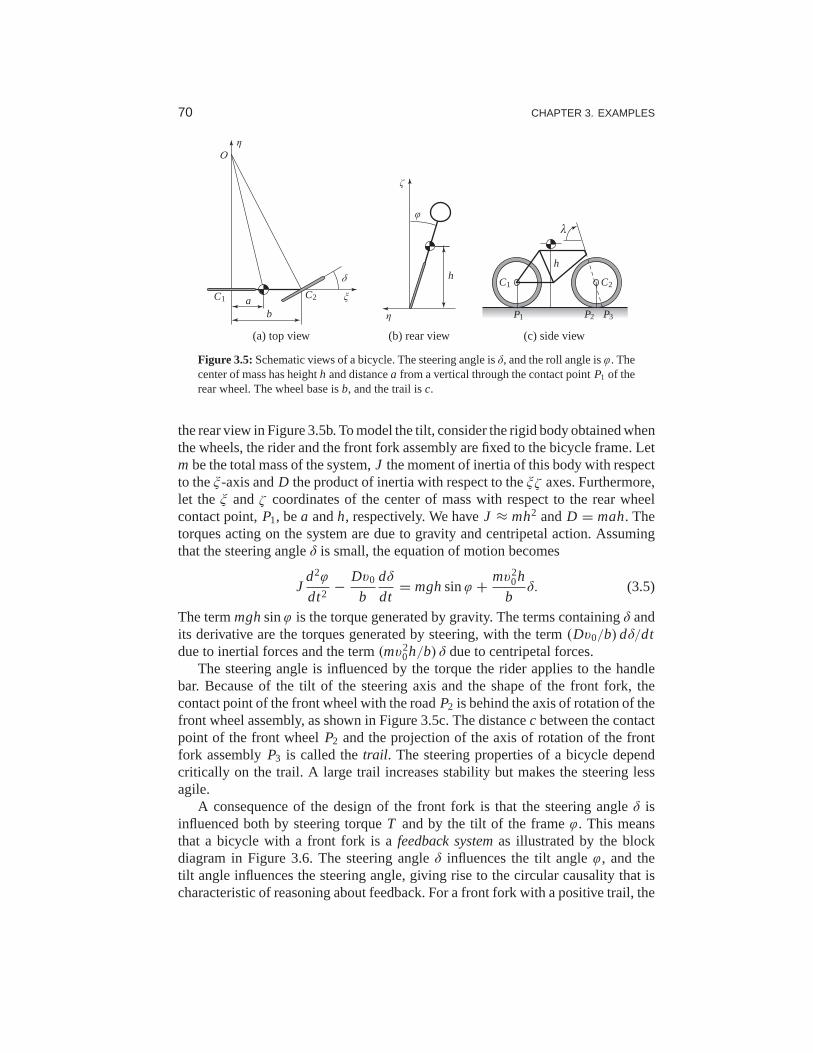
70 CHAPTER 3. EXAMPLES
ξ
η
ab
δ
O
C1 C2
(a) top view
η
ζ
h
ϕ
(b) rear view
λ
h
C1 C2
P1 P2 P3
(c) side view
Figure 3.5:Schematic views of a bicycle. The steering angle isδ, and the roll angle isϕ. Thecenter of mass has heighth and distancea from a vertical through the contact pointP1 of therear wheel. The wheel base isb, and the trail isc.
the rear view in Figure 3.5b. To model the tilt, consider the rigid body obtained whenthe wheels, the rider and the front fork assembly are fixed to the bicycle frame. Letm be the total mass of the system,J the moment of inertia of this body with respectto theξ -axis andD the product of inertia with respect to theξζ axes. Furthermore,let theξ andζ coordinates of the center of mass with respect to the rear wheelcontact point,P1, bea andh, respectively. We haveJ ≈ mh2 andD = mah. Thetorques acting on the system are due to gravity and centripetal action. Assumingthat the steering angleδ is small, the equation of motion becomes
Jd2ϕ
dt2− Dv0
b
dδ
dt= mghsinϕ + mv2
0h
bδ. (3.5)
The termmghsinϕ is the torque generated by gravity. The terms containingδ andits derivative are the torques generated by steering, with the term(Dv0/b)dδ/dtdue to inertial forces and the term(mv2
0h/b) δ due to centripetal forces.The steering angle is influenced by the torque the rider appliesto the handle
bar. Because of the tilt of the steering axis and the shape of the front fork, thecontact point of the front wheel with the roadP2 is behind the axis of rotation of thefront wheel assembly, as shown in Figure 3.5c. The distancec between the contactpoint of the front wheelP2 and the projection of the axis of rotation of the frontfork assemblyP3 is called thetrail . The steering properties of a bicycle dependcritically on the trail. A large trail increases stability but makes the steering lessagile.
A consequence of the design of the front fork is that the steering angleδ isinfluenced both by steering torqueT and by the tilt of the frameϕ. This meansthat a bicycle with a front fork is afeedback systemas illustrated by the blockdiagram in Figure 3.6. The steering angleδ influences the tilt angleϕ, and thetilt angle influences the steering angle, giving rise to the circular causality that ischaracteristic of reasoning about feedback. For a front fork with a positive trail, the

3.3. OPERATIONAL AMPLIFIER CIRCUITS 71
ϕFrontFork
Tδ
Frame
Figure 3.6: Block diagram of a bicycle with a front fork. The steering torque applied tothehandlebars isT , the roll angle isϕ and the steering angle isδ. Notice that the front forkcreates a feedback from the roll angleϕ to the steering angleδ that under certain conditionscan stabilize the system.
bicycle will steer into the lean, creating a centrifugal force that attempts to diminishthe lean. Under certain conditions, the feedback can actually stabilize the bicycle.A crude empirical model is obtained by assuming that the block B can be modeledas the static system
δ = k1T − k2ϕ. (3.6)
This model neglects the dynamics of the front fork, the tire–road interaction andthe fact that the parameters depend on the velocity. A more accurate model, calledtheWhipple model, is obtained using the rigid-body dynamics of the front forkandthe frame. Assuming small angles, this model becomes
M
ϕδ
+ Cv0
ϕδ
+ (K0 + K2v
20)
ϕδ
=
0
T
, (3.7)
where the elements of the 2×2 matricesM , C, K0 andK2 depend on the geometryand the mass distribution of the bicycle. Note that this has aform somewhat similarto that of the spring–mass system introduced in Chapter 2 andthe balance system inExample 2.1. Even this more complex model is inaccurate because the interactionbetween the tire and the road is neglected; taking this into account requires twoadditional state variables. Again, the uncertainty lemon in Figure 2.15b provides aframework for understanding the validity of the model underthese assumptions.
Interesting presentations on the development of the bicycle are given in thebooks by D. Wilson [Wil04] and Herlihy [Her04]. The model (3.7) was presentedin a paper by Whipple in 1899 [Whi99]. More details on bicyclemodeling are givenin the paper [ÅKL05], which has many references.
3.3 Operational Amplifier Circuits
An operational amplifier (op amp) is a modern implementation of Black’s feedbackamplifier. It is a universal component that is widely used for instrumentation, con-trol and communication. It is also a key element in analog computing. Schematicdiagrams of the operational amplifier are shown in Figure 3.7. The amplifier has oneinverting input (v−), one noninverting input (v+) and one output (vout). There arealso connections for the supply voltages,e− ande+, and a zero adjustment (offsetnull). A simple model is obtained by assuming that the input currentsi− andi+ are
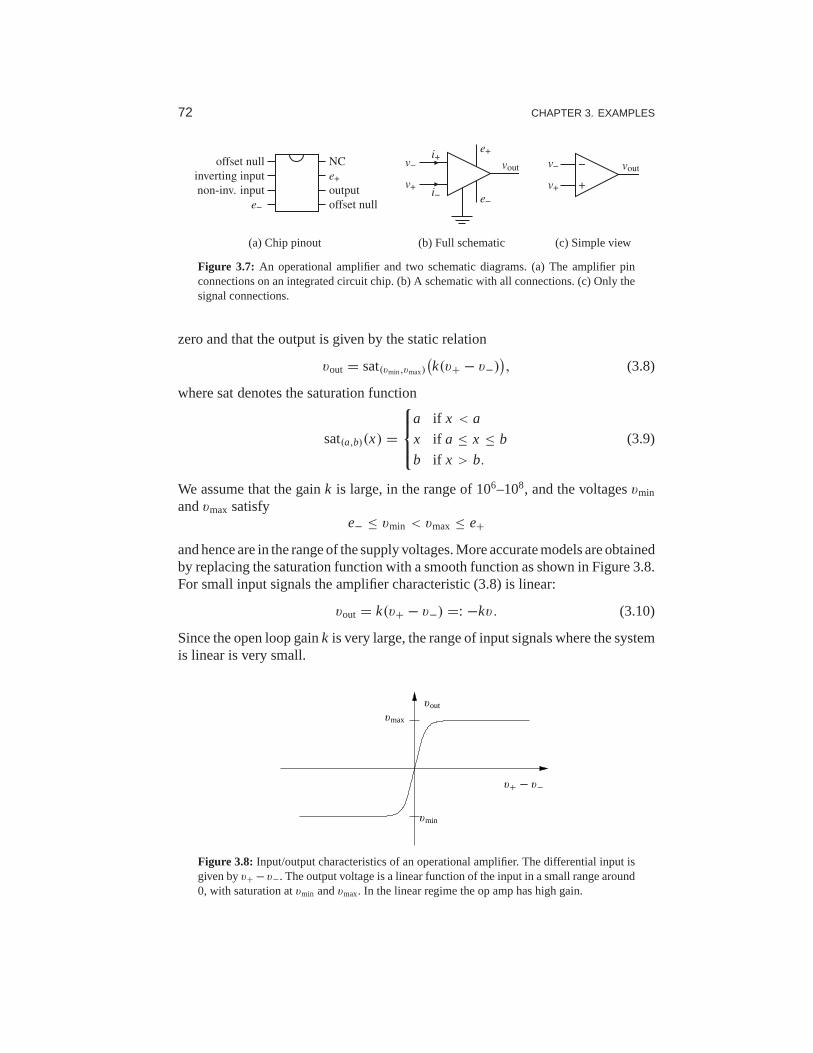
72 CHAPTER 3. EXAMPLES
e−
NC
e+
output
offset null
offset null
inverting input
non-inv. input
(a) Chip pinout
voutv−
v+e−
e+i+
i−
(b) Full schematic
−
v+
v− vout
+
(c) Simple view
Figure 3.7: An operational amplifier and two schematic diagrams. (a) The amplifier pinconnections on an integrated circuit chip. (b) A schematic with all connections. (c) Only thesignal connections.
zero and that the output is given by the static relation
vout = sat(vmin,vmax)
(k(v+ − v−)
), (3.8)
where sat denotes the saturation function
sat(a,b)(x) =
a if x < a
x if a ≤ x ≤ b
b if x > b.
(3.9)
We assume that the gaink is large, in the range of 106–108, and the voltagesvmin
andvmax satisfye− ≤ vmin < vmax ≤ e+
and hence are in the range of the supply voltages. More accurate models are obtainedby replacing the saturation function with a smooth functionas shown in Figure 3.8.For small input signals the amplifier characteristic (3.8) islinear:
vout = k(v+ − v−) =: −kv. (3.10)
Since the open loop gaink is very large, the range of input signals where the systemis linear is very small.
vmin
vout
v+ − v−
vmax
Figure 3.8: Input/output characteristics of an operational amplifier. The differential input isgiven byv+ − v−. The output voltage is a linear function of the input in a small range around0, with saturation atvmin andvmax. In the linear regime the op amp has high gain.

3.3. OPERATIONAL AMPLIFIER CIRCUITS 73
v −
+v1
v2
R1 R2
i0
replacements
(a) Amplifier circuit
v2R1
R1 + R2
e vR2
R1
v1−k6
(b) Block diagram
Figure 3.9: Stable amplifier using an op amp. The circuit (a) uses negative feedback aroundan operational amplifier and has a corresponding block diagram (b). The resistorsR1 andR2
determine the gain of the amplifier.
A simple amplifier is obtained by arranging feedback around the basic opera-tional amplifier as shown in Figure 3.9a. To model the feedback amplifier in thelinear range, we assume that the currenti0 = i− + i+ is zero and that the gain ofthe amplifier is so large that the voltagev = v− − v+ is also zero. It follows fromOhm’s law that the currents through resistorsR1 andR2 are given by
v1
R1= − v2
R2,
and hence the closed loop gain of the amplifier is
v2
v1= −kcl, where kcl = R2
R1. (3.11)
A more accurate model is obtained by continuing to neglect the currenti0 butassuming that the voltagev is small but not negligible. The current balance is then
v1 − v
R1= v − v2
R2. (3.12)
Assuming that the amplifier operates in the linear range and using equation (3.10),the gain of the closed loop system becomes
kcl = −v2
v1= R2
R1
k R1
R1 + R2 + k R1(3.13)
If the open loop gaink of the operational amplifier is large, the closed loop gainkcl is the same as in the simple model given by equation (3.11). Notice that theclosed loop gain depends only on the passive components and that variations inkhave only a marginal effect on the closed loop gain. For example if k = 106 andR2/R1 = 100, a variation ofk by 100% gives only a variation of 0.01% in the closedloop gain. The drastic reduction in sensitivity is a nice illustration of how feedbackcan be used to make precise systems from uncertain components. In this particularcase, feedback is used to trade high gain and low robustness for low gain and highrobustness. Equation (3.13) was the formula that inspired Black when he inventedthe feedback amplifier [Bla34] (see the quote at the beginningof Chapter 12).
It is instructive to develop a block diagram for the feedbackamplifier in Fig-ure 3.9a. To do this we will represent the pure amplifier with inputv and outputv2

74 CHAPTER 3. EXAMPLES
v −
+v1
v2
R1 R C2
i0
Figure 3.10:Circuit diagram of a PI controller obtained by feedback around an operationalamplifier. The capacitorC is used to store charge and represents the integral of the input.
as one block. To complete the block diagram, we must describehowv depends onv1 andv2. Solving equation (3.12) forv gives
v = R2
R1 + R2v1 + R1
R1 + R2v2 = R1
R1 + R2
(R2
R1v1 + v2
),
and we obtain the block diagram shown in Figure 3.9b. The diagram clearly showsthat the system has feedback and that the gain fromv2 to v is R1/(R1 + R2), whichcan also be read from the circuit diagram in Figure 3.9a. If theloop is stable andthe gain of the amplifier is large, it follows that the errore is small, and we find thatv2 = −(R2/R1)v1. Notice that the resistorR1 appears in two blocks in the blockdiagram. This situation is typical in electrical circuits, and it is one reason whyblock diagrams are not always well suited for some types of physical modeling.
The simple model of the amplifier given by equation (3.10) provides qualitativeinsight, but it neglects the fact that the amplifier is a dynamical system. A morerealistic model is
dvout
dt= −avout − bv. (3.14)
The parameterb that has dimensions of frequency and is called thegain-bandwidthproductof the amplifier. Whether a more complicated model is used depends onthe questions to be answered and the required size of the uncertainty lemon. Themodel (3.14) is still not valid for very high or very low frequencies since driftcauses deviations at low frequencies and there are additional dynamics that appearat frequencies close tob. The model is also not valid for large signals—an upperlimit is given by the voltage of the power supply, typically in the range of 5–10 V—neither is it valid for very low signals because of electrical noise. These effects canbe added, if needed, but increase the complexity of the analysis.
The operational amplifier is very versatile, and many different systems can bebuilt by combining it with resistors and capacitors. In fact, any linear system canbe implemented by combining operational amplifiers with resistors and capacitors.Exercise 3.5 shows how a second-order oscillator is implemented, and Figure 3.10shows the circuit diagram for an analog proportional-integral controller. To developa simple model for the circuit we assume that the currenti0 is zero and that the openloop gaink is so large that the input voltagev is negligible. The currenti throughthe capacitor isi = Cdvc/dt, wherevc is the voltage across the capacitor. Since

3.4. COMPUTING SYSTEMS AND NETWORKS 75
the same current goes through the resistorR1, we get
i = v1
R1= C
dvc
dt,
which implies that
vc(t) = 1
C
∫i (t)dt = 1
R1C
∫ t
0v1(τ )dτ.
The output voltage is thus given by
v2(t) = −R2i − vc = − R2
R1v1(t)− 1
R1C
∫ t
0v1(τ )dτ,
which is the input/output relation for a PI controller.
The development of operational amplifiers was pioneered by Philbrick [Lun05,Phi48], and their usage is described in many textbooks (e.g.,[CD75]). Good infor-mation is also available from suppliers [Jun02, Man02].
3.4 Computing Systems and Networks
The application of feedback to computing systems follows thesame principles asthe control of physical systems, but the types of measurements and control inputsthat can be used are somewhat different. Measurements (sensors) are typicallyrelated to resource utilization in the computing system or network and can includequantities such as the processor load, memory usage or network bandwidth. Controlvariables (actuators) typically involve setting limits onthe resources available to aprocess. This might be done by controlling the amount of memory, disk space ortime that a process can consume, turning on or off processing, delaying availabilityof a resource or rejecting incoming requests to a server process. Process modelingfor networked computing systems is also challenging, and empirical models basedon measurements are often used when a first-principles model is not available.
Web Server Control
Web servers respond to requests from the Internet and provide information in theform of web pages. Modern web servers start multiple processes to respond torequests, with each process assigned to a single source until no further requests arereceived from that source for a predefined period of time. Processes that are idlebecome part of a pool that can be used to respond to new requests. To provide afast response to web requests, it is important that the web server processes do notoverload the server’s computational capabilities or exhaust its memory. Since otherprocesses may be running on the server, the amount of available processing powerand memory is uncertain, and feedback can be used to provide good performancein the presence of this uncertainty.

76 CHAPTER 3. EXAMPLES
Idle
Busy
Client Servers
dataoutgoing
queueaccept
requestsincoming
−1
Wait
Memory usage
KeepAlive
MaxClients
Processor load
Control
Ref
−1
Figure 3.11:Feedback control of a web server. Connection requests arrive on an input queue,where they are sent to a server process. A finite state machine keeps track of the state of theindividual server processes and responds to requests. A control algorithm can modify theserver’s operation by controlling parameters that affect its behavior,such as the maximumnumber of requests that can be serviced at a single time (MaxClients) or the amount oftime that a connection can remain idle before it is dropped (KeepAlive).
Figure 3.11 illustrates the use of feedback to modulate the operation of anApache web server. The web server operates by placing incoming connection re-quests on a queue and then starting a subprocess to handle requests for each acceptedconnection. This subprocess responds to requests from a given connection as theycome in, alternating between aBusy state and aWait state. (Keeping the sub-process active between requests is known as thepersistenceof the connection andprovides a substantial reduction in latency to requests formultiple pieces of infor-mation from a single site.) If no requests are received for a sufficiently long periodof time, controlled by theKeepAlive parameter, then the connection is droppedand the subprocess enters anIdle state, where it can be assigned another connec-tion. A maximum ofMaxClients simultaneous requests will be served, with theremainder remaining on the incoming request queue.
The parameters that control the server represent a trade-offbetween perfor-mance (how quickly requests receive a response) and resource usage (the amountof processing power and memory used by the server). Increasing theMaxClientsparameter allows connection requests to be pulled off of thequeue more quicklybut increases the amount of processing power and memory usage that is required.Increasing theKeepAlive timeout means that individual connections can remainidle for a longer period of time, which decreases the processing load on the machinebut increases the size of the queue (and hence the amount of time required for a userto initiate a connection). Successful operation of a busy server requires a properchoice of these parameters, often based on trial and error.
To model the dynamics of this system in more detail, we createa discrete-timemodel with states given by the average processor loadxcpu and the percentagememory usagexmem. The inputs to the system are taken as the maximum numberof clientsumc and the keep-alive timeuka. If we assume a linear model around the

3.4. COMPUTING SYSTEMS AND NETWORKS 77
equilibrium point, the dynamics can be written as xcpu[k + 1]
xmem[k + 1]
=
A11 A12
A21 A22
xcpu[k]
xmem[k]
+
B11 B12
B21 B22
uka[k]
umc[k]
, (3.15)
where the coefficients of theAandB matrices can be determined based on empiricalmeasurements or detailed modeling of the web server’s processing and memoryusage. Using system identification, Diao et al. [DGH+02, HDPT04] identified thelinearized dynamics as
A = 0.54 −0.11
−0.026 0.63
, B =
−85 4.4
−2.5 2.8
× 10−4,
where the system was linearized about the equilibrium point
xcpu = 0.58, uka = 11 s, xmem = 0.55, umc = 600.
This model shows the basic characteristics that were described above. Lookingfirst at theB matrix, we see that increasing theKeepAlive timeout (first columnof the B matrix) decreases both the processor usage and the memory usage sincethere is more persistence in connections and hence the server spends a longer timewaiting for a connection to close rather than taking on a new active connection. TheMaxClientsconnection increases both the processing and memory requirements.Note that the largest effect on the processor load is theKeepAlive timeout.The A matrix tells us how the processor and memory usage evolve in aregion ofthe state space near the equilibrium point. The diagonal terms describe how theindividual resources return to equilibrium after a transient increase or decrease.The off-diagonal terms show that there is coupling between the two resources, sothat a change in one could cause a later change in the other.
Although this model is very simple, we will see in later examples that it canbe used to modify the parameters controlling the server in real time and providerobustness with respect to uncertainties in the load on the machine. Similar types ofmechanisms have been used for other types of servers. It is important to rememberthe assumptions on the model and their role in determining when the model is valid.In particular, since we have chosen to use average quantities over a given sampletime, the model will not provide an accurate representationfor high-frequencyphenomena.
Congestion Control
The Internet was created to obtain a large, highly decentralized, efficient and ex-pandable communication system. The system consists of a large number of inter-connected gateways. A message is split into several packetswhich are transmittedover different paths in the network, and the packages are rejoined to recover themessage at the receiver. An acknowledgment (“ack”) messageis sent back to thesender when a packet is received. The operation of the system is governed by asimple but powerful decentralized control structure that has evolved over time.

78 CHAPTER 3. EXAMPLES
Sources
Sou
rces
Router RouterLink
Receiver
ack
Link
Link
(a) Block diagram
10−2
100
102
104
0
0.2
0.4
0.6
0.8
1
1/(2ρ2N2) (log scale)
ρb e
(b) Operating point
Figure 3.12: Internet congestion control. (a) Source computers send information torouters,which forward the information to other routers that eventually connect to the receiving com-puter. When a packet is received, an acknowledgment packet is sent back through the routers(not shown). The routers buffer information received from the sources and send the dataacross the outgoing link. (b) The equilibrium buffer sizebe for a set ofN identical computerssending packets through a single router with drop probabilityρ.
The system has two control mechanisms calledprotocols: the TransmissionControl Protocol (TCP) for end-to-end network communication and the InternetProtocol (IP) for routing packets and for host-to-gateway or gateway-to-gatewaycommunication. The current protocols evolved after some spectacular congestioncollapses occurred in the mid 1980s, when throughput unexpectedly could drop bya factor of 1000 [Jac95]. The control mechanism in TCP is based on conservingthe number of packets in the loop from the sender to the receiver and back to thesender. The sending rate is increased exponentially when there is no congestion,and it is dropped to a low level when there is congestion.
To derive an overall model for congestion control, we model three separateelements of the system: the rate at which packets are sent by individual sources(computers), the dynamics of the queues in the links (routers) and the admissioncontrol mechanism for the queues. Figure 3.12a is a block diagram of the system.
The current source control mechanism on the Internet is a protocol knownas TCP/Reno [LPD02]. This protocol operates by sending packets toa receiverand waiting to receive an acknowledgment from the receiver that the packet hasarrived. If no acknowledgment is sent within a certain timeout period, the packetis retransmitted. To avoid waiting for the acknowledgment before sending the nextpacket, Reno transmits multiple packets up to a fixedwindow around the latestpacket that has been acknowledged. If the window length is chosen properly, packetsat the beginning of the window will be acknowledged before the source transmitspackets at the end of the window, allowing the computer to continuously streampackets at a high rate.
To determine the size of the window to use, TCP/Reno uses a feedback mech-anism in which (roughly speaking) the window size is increased by 1 every time apacket is acknowledged and the window size is cut in half whenpackets are lost.This mechanism allows a dynamic adjustment of the window sizein which each
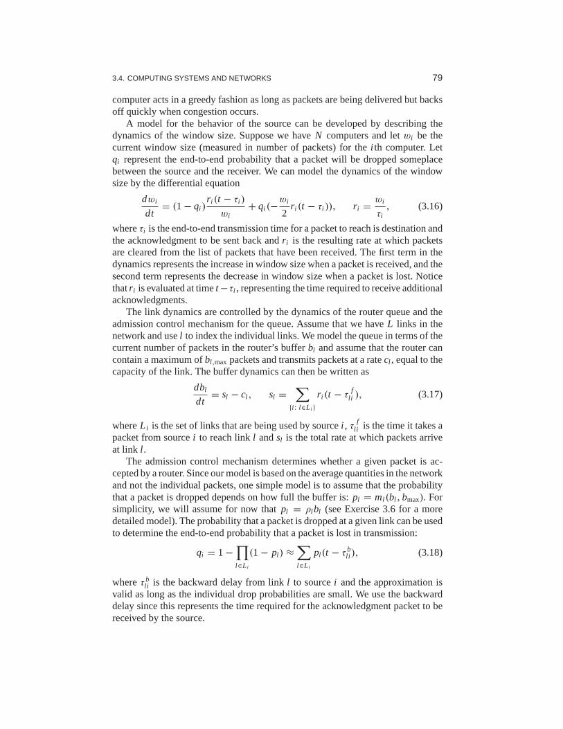
3.4. COMPUTING SYSTEMS AND NETWORKS 79
computer acts in a greedy fashion as long as packets are beingdelivered but backsoff quickly when congestion occurs.
A model for the behavior of the source can be developed by describing thedynamics of the window size. Suppose we haveN computers and letwi be thecurrent window size (measured in number of packets) for thei th computer. Letqi represent the end-to-end probability that a packet will be dropped someplacebetween the source and the receiver. We can model the dynamics of the windowsize by the differential equation
dwi
dt= (1 − qi )
r i (t − τi )
wi+ qi (−
wi
2r i (t − τi )), r i = wi
τi, (3.16)
whereτi is the end-to-end transmission time for a packet to reach is destination andthe acknowledgment to be sent back andr i is the resulting rate at which packetsare cleared from the list of packets that have been received.The first term in thedynamics represents the increase in window size when a packet is received, and thesecond term represents the decrease in window size when a packet is lost. Noticethatr i is evaluated at timet −τi , representing the time required to receive additionalacknowledgments.
The link dynamics are controlled by the dynamics of the routerqueue and theadmission control mechanism for the queue. Assume that we have L links in thenetwork and usel to index the individual links. We model the queue in terms of thecurrent number of packets in the router’s bufferbl and assume that the router cancontain a maximum ofbl ,max packets and transmits packets at a ratecl , equal to thecapacity of the link. The buffer dynamics can then be written as
dbl
dt= sl − cl , sl =
∑
{i : l∈L i }r i (t − τ
fli ), (3.17)
whereL i is the set of links that are being used by sourcei , τ fli is the time it takes a
packet from sourcei to reach linkl andsl is the total rate at which packets arriveat link l .
The admission control mechanism determines whether a given packet is ac-cepted by a router. Since our model is based on the average quantities in the networkand not the individual packets, one simple model is to assumethat the probabilitythat a packet is dropped depends on how full the buffer is:pl = ml (bl ,bmax). Forsimplicity, we will assume for now thatpl = ρl bl (see Exercise 3.6 for a moredetailed model). The probability that a packet is dropped at agiven link can be usedto determine the end-to-end probability that a packet is lost in transmission:
qi = 1 −∏
l∈L i
(1 − pl ) ≈∑
l∈L i
pl (t − τ bli ), (3.18)
whereτ bli is the backward delay from linkl to sourcei and the approximation is
valid as long as the individual drop probabilities are small. We use the backwarddelay since this represents the time required for the acknowledgment packet to bereceived by the source.

80 CHAPTER 3. EXAMPLES
Together, equations (3.16), (3.17) and (3.18) represent a model of congestioncontrol dynamics. We can obtain substantial insight by considering a special casein which we haveN identical sources and 1 link. In addition, we assume for themoment that the forward and backward time delays can be ignored, in which casethe dynamics can be reduced to the form
dwi
dt= 1
τ− ρc(2 + w2
i )
2,
db
dt=
N∑
i =1
wi
τ− c, τ = b
c, (3.19)
wherewi ∈ R, i = 1, . . . , N, are the window sizes for the sources of data,b ∈ R isthe current buffer size of the router,ρ controls the rate at which packets are droppedandc is the capacity of the link connecting the router to the computers. The variableτ represents the amount of time required for a packet to be processed by a router,based on the size of the buffer and the capacity of the link. Substitutingτ into theequations, we write the state space dynamics as
dwi
dt= c
b− ρc
(1 + w2
i
2
),
db
dt=
N∑
i =1
cwi
b− c. (3.20)
More sophisticated models can be found in [HMTG00, LPD02].The nominal operating point for the system can be found by settingwi = b = 0:
0 = c
b− ρc
(1 + w2
i
2
), 0 =
N∑
i =1
cwi
b− c.
Exploiting the fact that all of the source dynamics are identical, it follows that allof thewi should be the same, and it can be shown that there is a unique equilibriumsatisfying the equations
wi,e = be
N= cτe
N,
1
2ρ2N2(ρbe)
3 + (ρbe)− 1 = 0. (3.21)
The solution for the second equation is a bit messy but can easily be determined nu-merically. A plot of its solution as a function of 1/(2ρ2N2) is shown in Figure 3.12b.We also note that at equilibrium we have the following additional equalities:
τe = be
c= Nwe
c, qe = N pe = Nρbe, re = we
τe. (3.22)
Figure 3.13 shows a simulation of 60 sources communicating across a singlelink, with 20 sources dropping out att = 500 ms and the remaining sources in-creasing their rates (window sizes) to compensate. Note that the buffer size andwindow sizes automatically adjust to match the capacity of the link.
A comprehensive treatment of computer networks is given in the textbook byTannenbaum [Tan96]. A good presentation of the ideas behindthe control prin-ciples for the Internet is given by one of its designers, Van Jacobson, in [Jac95].F. Kelly [Kel85] presents an early effort on the analysis of the system. The book

3.5. ATOMIC FORCE MICROSCOPY 81
Router
Sou
rces
...
Link
Link
ack
Receiver
0 200 400 600 800 10000
5
10
15
20
Time t [ms]
Sta
tes w
i [pkt
s/m
s], b
[pkt
s]
b
w1−w
60
w1−w
40
Figure 3.13:Internet congestion control forN identical sources across a single link. As shownon the left, multiple sources attempt to communicate through a router acrossa single link. An“ack” packet sent by the receiver acknowledges that the message was received; otherwise themessage packet is resent and the sending rate is slowed down at the source. The simulationon the right is for 60 sources starting random rates, with 20 sources dropping out att = 500ms. The buffer size is shown at the top, and the individual source ratesfor 6 of the sourcesare shown at the bottom.
by Hellerstein et al. [HDPT04] gives many examples of the use offeedback incomputer systems.
3.5 Atomic Force Microscopy
The 1986 Nobel Prize in Physics was shared by Gerd Binnig and Heinrich Rohrerfor their design of thescanning tunneling microscope. The idea of the instrumentis to bring an atomically sharp tip so close to a conducting surface that tunnelingoccurs. An image is obtained by traversing the tip across thesample and measuringthe tunneling current as a function of tip position. This invention has stimulatedthe development of a family of instruments that permit visualization of surfacestructure at the nanometer scale, including theatomic force microscope(AFM),where a sample is probed by a tip on a cantilever. An AFM can operate in twomodes. Intapping modethe cantilever is vibrated, and the amplitude of vibrationis controlled by feedback. Incontact modethe cantilever is in contact with thesample, and its bending is controlled by feedback. In both cases control is actuatedby a piezo element that controls the vertical position of thecantilever base (or thesample). The control system has a direct influence on picture quality and scanningrate.
A schematic picture of an atomic force microscope is shown inFigure 3.14a. Amicrocantilever with a tip having a radius of the order of 10 nm is placed close tothe sample. The tip can be moved vertically and horizontally using a piezoelectricscanner. It is clamped to the sample surface by attractive van der Waals forces andrepulsive Pauli forces. The cantilever tilt depends on the topography of the surfaceand the position of the cantilever base, which is controlledby the piezo element.

82 CHAPTER 3. EXAMPLES
Amplifier Amplifier
Sample
Cantilever
x,y z
LaserPhotodiode
Controller
Piezodrive
Deflection reference
Sweepgenerator
(a) Schematic diagram (b) AFM image of DNA
Figure 3.14:Atomic force microscope. (a) A schematic diagram of an atomic force micro-scope, consisting of a piezo drive that scans the sample under the AFM tip. A laser reflects offof the cantilever and is used to measure the detection of the tip through a feedback controller.(b) An AFM image of strands of DNA. (Image courtesy Veeco Instruments.)
The tilt is measured by sensing the deflection of the laser beam using a photodiode.The signal from the photodiode is amplified and sent to a controller that drivesthe amplifier for the vertical position of the cantilever. By controlling the piezoelement so that the deflection of the cantilever is constant, the signal driving thevertical deflection of the piezo element is a measure of the atomic forces betweenthe cantilever tip and the atoms of the sample. An image of thesurface is obtainedby scanning the cantilever along the sample. The resolution makes it possible tosee the structure of the sample on the atomic scale, as illustrated in Figure 3.14b,which shows an AFM image of DNA.
The horizontal motion of an AFM is typically modeled as a spring–mass systemwith low damping. The vertical motion is more complicated. Tomodel the system,we start with the block diagram shown in Figure 3.15. Signals that are easily acces-sible are the input voltageu to the power amplifier that drives the piezo element,the voltagev applied to the piezo element and the output voltagey of the signal
v
Cantilever
ComputerDA
u AD
ϕ
y
z
Deflection reference
amplifierSignal
photodiodeLaser &
Sample topography
amplifierPower
elementPiezo
Figure 3.15: Block diagram of the system for vertical positioning of the cantilever for anatomic force microscope in contact mode. The control system attempts to keep the can-tilever deflection equal to its reference value. Cantilever deflection is measured, amplifiedand converted to a digital signal, then compared with its reference value. Acorrecting signal isgenerated by the computer, converted to analog form, amplified and sent to the piezo element.

3.5. ATOMIC FORCE MICROSCOPY 83
u
y
Vp
(a) Step response
Piezo crystal
z1 z2
m1
m2
(b) Mechanical model
Figure 3.16: Modeling of an atomic force microscope. (a) A measured step response. Thetop curve shows the voltageu applied to the drive amplifier (50 mV/div), the middle curveis the outputVp of the power amplifier (500 mV/div) and the bottom curve is the outputyof the signal amplifier (500 mV/div). The time scale is 25µs/div. Data have been suppliedby Georg Schitter. (b) A simple mechanical model for the vertical positioner and the piezocrystal.
amplifier for the photodiode. The controller is a PI controller implemented by acomputer, which is connected to the system by analog-to-digital (A/D) and digital-to-analog (D/A) converters. The deflection of the cantileverϕ is also shown in thefigure. The desired reference value for the deflection is an inputto the computer.
There are several different configurations that have different dynamics. Here wewill discuss a high-performance system from [SÅD+07] where the cantilever baseis positioned vertically using a piezo stack. We begin the modeling with a simpleexperiment on the system. Figure 3.16a shows a step response of a scanner from theinput voltageu to the power amplifier to the output voltagey of the signal amplifierfor the photodiode. This experiment captures the dynamics ofthe chain of blocksfrom u to y in the block diagram in Figure 3.15. Figure 3.16a shows that thesystemresponds quickly but that there is a poorly damped oscillatory mode with a periodof about 35 µs. A primary task of the modeling is to understandthe origin of theoscillatory behavior. To do so we will explore the system in more detail.
The natural frequency of the clamped cantilever is typicallyseveral hundredkilohertz, which is much higher than the observed oscillation of about 30 kHz. Asa first approximation we will model it as a static system. Since the deflections aresmall, we can assume that the bendingϕ of the cantilever is proportional to thedifference in height between the cantilever tip at the probeand the piezo scanner. Amore accurate model can be obtained by modeling the cantilever as a spring–masssystem of the type discussed in Chapter 2.
Figure 3.16a also shows that the response of the power amplifieris fast. Thephotodiode and the signal amplifier also have fast responses and can thus be mod-eled as static systems. The remaining block is a piezo system with suspension. Aschematic mechanical representation of the vertical motion of the scanner is shownin Figure 3.16b. We will model the system as two masses separated by an ideal

84 CHAPTER 3. EXAMPLES
piezo element. The massm1 is half of the piezo system, and the massm2 is theother half of the piezo system plus the mass of the support.
A simple model is obtained by assuming that the piezo crystalgenerates a forceF between the masses and that there is a dampingc in the spring. Let the positionsof the center of the masses bez1 andz2. A momentum balance gives the followingmodel for the system:
m1d2z1
dt2= F, m2
d2z2
dt2= −c2
dz2
dt− k2z2 − F.
Let the elongation of the piezo elementl = z1 − z2 be the control variable andthe heightz1 of the cantilever base be the output. Eliminating the variable F inequations (3.23) and substitutingz1 − l for z2 gives the model
(m1 + m2)d2z1
dt2+ c2
dz1
dt+ k2z1 = m2 f racd2ldt2 + c2
dl
dt+ k2l . (3.23)
Summarizing, we find that a simple model of the system is obtained by modelingthe piezo by (3.23) and all the other blocks by static models.Introducing the linearequationsl = k3u andy = k4z1, we now have a complete model relating the outputy to the control signalu. A more accurate model can be obtained by introducing thedynamics of the cantilever and the power amplifier. As in the previous examples,the concept of the uncertainty lemon in Figure 2.15b providesa framework fordescribing the uncertainty: the model will be accurate up tothe frequencies of thefastest modeled modes and over a range of motion in which linearized stiffnessmodels can be used.
The experimental results in Figure 3.16a can be explained qualitatively as fol-lows. When a voltage is applied to the piezo, it expands byl0, the massm1 movesup and the massm2 moves down instantaneously. The system settles after a poorlydamped oscillation.
It is highly desirable to design a control system for the vertical motion so that itresponds quickly with little oscillation. The instrument designer has several choices:to accept the oscillation and have a slow response time, to design a control systemthat can damp the oscillations or to redesign the mechanics to give resonances ofhigher frequency. The last two alternatives give a faster response and faster imaging.
Since the dynamic behavior of the system changes with the properties of thesample, it is necessary to tune the feedback loop. In simple systems this is currentlydone manually by adjusting parameters of a PI controller. There are interestingpossibilities for making AFM systems easier to use by introducing automatic tuningand adaptation.
The book by Sarid [Sar91] gives a broad coverage of atomic force microscopes.The interaction of atoms close to surfaces is fundamental to solid state physics, seeKittel [Kit95]. The model discussed in this section is based on Schitter [Sch01].

3.6. DRUG ADMINISTRATION 85
Chemicalinactivation“fixation”
etc.Subcutis
etc.
Blood circulation
Tissue boundaries
Dose N0
k1 k4 k2 k3
k5
Figure 3.17: Abstraction used to compartmentalize the body for the purpose of describingdrug distribution (based on Teorell [Teo37]). The body is abstracted by a number of com-partments with perfect mixing, and the complex transport processes are approximated byassuming that the flow is proportional to the concentration differences in the compartments.The constantski parameterize the rates of flow between different compartments.
3.6 Drug Administration
The phrase “Take two pills three times a day” is a recommendation with which weare all familiar. Behind this recommendation is a solution of an open loop controlproblem. The key issue is to make sure that the concentration of a medicine ina part of the body is sufficiently high to be effective but not sohigh that it willcause undesirable side effects. The control action is quantized,take two pills, andsampled,every 8 hours. The prescriptions are based on simple models captured inempirical tables, and the dose is based on the age and weight of the patient.
Drug administration is a control problem. To solve it we mustunderstand howa drug spreads in the body after it is administered. This topic, calledpharmacoki-netics, is now a discipline of its own, and the models used are calledcompartmentmodels. They go back to the 1920s when Widmark modeled the propagation of alco-hol in the body [WT24]. Compartment models are now important for the screeningof all drugs used by humans. The schematic diagram in Figure 3.17 illustrates theidea of a compartment model. The body is viewed as a number of compartmentslike blood plasma, kidney, liver and tissues that are separated by membranes. It isassumed that there is perfect mixing so that the drug concentration is constant ineach compartment. The complex transport processes are approximated by assumingthat the flow rates between the compartments are proportionalto the concentrationdifferences in the compartments.
To describe the effect of a drug it is necessary to know both its concentrationand how it influences the body. The relation between concentration c and its effecte is typically nonlinear. A simple model is
e = c
c0 + cemax. (3.24)
The effect is linear for low concentrations, and it saturatesat high concentrations.The relation can also be dynamic, and it is then calledpharmacodynamics.
86 CHAPTER 3. EXAMPLES
Compartment Models
The simplest dynamic model for drug administration is obtained by assuming thatthe drug is evenly distributed in a single compartment afterit has been administeredand that the drug is removed at a rate proportional to the concentration. The com-partments behave like stirred tanks with perfect mixing. Letc be the concentration,V the volume andq the outflow rate. Converting the description of the system intodifferential equations gives the model
Vdc
dt= −qc, c ≥ 0. (3.25)
This equation has the solutionc(t) = c0e−qt/V = c0e−kt, which shows that theconcentration decays exponentially with the time constantT = V/q after an injec-tion. The input is introduced implicitly as an initial condition in the model (3.25).More generally, the way the input enters the model depends onhow the drug isadministered. For example, the input can be represented as amass flow into thecompartment where the drug is injected. A pill that is dissolved can also be inter-preted as an input in terms of a mass flow rate.
The model (3.25) is called a aone-compartment modelor asingle-pool model.The parameterq/V is called the elimination rate constant. This simple model isoften used to model the concentration in the blood plasma. Bymeasuring the con-centration at a few times, the initial concentration can be obtained by extrapolation.If the total amount of injected substance is known, the volume V can then be de-termined asV = m/c0; this volume is called theapparent volume of distribution.This volume is larger than the real volume if the concentration in the plasma islower than in other parts of the body. The model (3.25) is very simple, and thereare large individual variations in the parameters. The parametersV andq are oftennormalized by dividing by the weight of the person. Typical parameters for aspirinareV = 0.2 L/kg andq = 0.01(L/h)/kg. These numbers can be compared witha blood volume of 0.07 L/kg, a plasma volume of 0.05 L/kg, an intracellular fluidvolume of 0.4 L/kg and an outflow of 0.0015 L/ min /kg.
The simple one-compartment model captures the gross behavior of drug distri-bution, but it is based on many simplifications. Improved models can be obtained byconsidering the body as composed of several compartments. Examples of such sys-tems are shown in Figure 3.18, where the compartments are represented as circlesand the flows by arrows.
Modeling will be illustrated using the two-compartment model in Figure 3.18a.We assume that there is perfect mixing in each compartment and that the transportbetween the compartments is driven by concentration differences. We further as-sume that a drug with concentrationc0 is injected in compartment 1 at a volumeflow rate ofu and that the concentration in compartment 2 is the output. Letc1 andc2 be the concentrations of the drug in the compartments and letV1 andV2 be the

3.6. DRUG ADMINISTRATION 87
k2
V1
k0
b0
u
V2
k1
(a) Two compartment model
u1
V4V6
k64
k46
V1V3
k31
k13
V5
k54
k45
u4
V2
k21
k12
k03
k06 k05
k02
b4
b1
(b) Thyroid hormone model
Figure 3.18: Schematic diagrams of compartment models. (a) A simple two-compartmentmodel. Each compartment is labeled by its volume, and arrows indicate the flow of chemicalinto, out of and between compartments. (b) A system with six compartmentsused to studythe metabolism of thyroid hormone [God83]. The notationki j denotes the transport fromcompartmentj to compartmenti .
volumes of the compartments. The mass balances for the compartments are
V1dc1
dt= q(c2 − c1)− q0c1 + c0u, c1 ≥ 0,
V2dc2
dt= q(c1 − c2), c2 ≥ 0,
y = c2.
(3.26)
Introducing the variablesk0 = q0/V1, k1 = q/V1, k2 = q/V2 andb0 = c0/V1 andusing matrix notation, the model can be written as
dc
dt=−k0 − k1 k1
k2 −k2
c +
b0
0
u, y =
0 1
c. (3.27)
Comparing this model with its graphical representation in Figure 3.18a, we findthat the mathematical representation (3.27) can be writtenby inspection.
It should also be emphasized that simple compartment modelssuch as the one inequation (3.27) have a limited range of validity. Low-frequency limits exist becausethe human body changes with time, and since the compartment model uses averageconcentrations, they will not accurately represent rapid changes. There are alsononlinear effects that influence transportation between thecompartments.
Compartment models are widely used in medicine, engineering and environ-mental science. An interesting property of these systems isthat variables like con-centration and mass are always positive. An essential difficulty in compartmentmodeling is deciding how to divide a complex system into compartments. Com-partment models can also be nonlinear, as illustrated in thenext section.
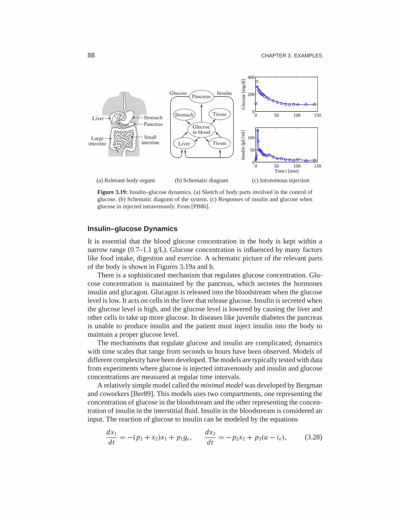
88 CHAPTER 3. EXAMPLES
Liver
Largeintestine
Stomach
Pancreas
Smallintestine
(a) Relevant body organs
InsulinPancreas
Liver Tissue
Stomach Tissue
Glucose
Glucosein blood
(b) Schematic diagram
0 50 100 1500
200
400
Glu
cose
[mg/
dl]
0 50 100 1500
50
100
Time t [min]
Insu
lin [µ
U/m
l]
(c) Intravenous injection
Figure 3.19: Insulin–glucose dynamics. (a) Sketch of body parts involved in the control ofglucose. (b) Schematic diagram of the system. (c) Responses of insulinand glucose whenglucose in injected intravenously. From [PB86].
Insulin–glucose Dynamics
It is essential that the blood glucose concentration in the body is kept within anarrow range (0.7–1.1 g/L). Glucose concentration is influenced by many factorslike food intake, digestion and exercise. A schematic picture of the relevant partsof the body is shown in Figures 3.19a and b.
There is a sophisticated mechanism that regulates glucose concentration. Glu-cose concentration is maintained by the pancreas, which secretes the hormonesinsulin and glucagon. Glucagon is released into the bloodstream when the glucoselevel is low. It acts on cells in the liver that release glucose. Insulin is secreted whenthe glucose level is high, and the glucose level is lowered bycausing the liver andother cells to take up more glucose. In diseases like juvenile diabetes the pancreasis unable to produce insulin and the patient must inject insulin into the body tomaintain a proper glucose level.
The mechanisms that regulate glucose and insulin are complicated; dynamicswith time scales that range from seconds to hours have been observed. Models ofdifferent complexity have been developed. The models are typically tested with datafrom experiments where glucose is injected intravenously and insulin and glucoseconcentrations are measured at regular time intervals.
A relatively simple model called theminimal modelwas developed by Bergmanand coworkers [Ber89]. This models uses two compartments, one representing theconcentration of glucose in the bloodstream and the other representing the concen-tration of insulin in the interstitial fluid. Insulin in the bloodstream is considered aninput. The reaction of glucose to insulin can be modeled by theequations
dx1
dt= −(p1 + x2)x1 + p1ge,
dx2
dt= −p2x2 + p3(u − ie), (3.28)

3.7. POPULATION DYNAMICS 89
wherege andie represent the equilibrium values of glucose and insulin,x1 is theconcentration of glucose andx2 is proportional to the concentration of interstitialinsulin. Notice the presence of the termx2x1 in the first equation. Also noticethat the model does not capture the complete feedback loop because it does notdescribe how the pancreas reacts to the glucose. Figure 3.19cshows a fit of themodel to a test on a normal person where glucose was injected intravenously attime t = 0. The glucose concentration rises rapidly, and the pancreasrespondswith a rapid spikelike injection of insulin. The glucose and insulin levels thengradually approach the equilibrium values.
Models of the type in equation (3.28) and more complicated models having manycompartments have been developed and fitted to experimental data. A difficulty inmodeling is that there are significant variations in model parameters over time andfor different patients. For example, the parameterp1 in equation (3.28) has beenreported to vary with an order of magnitude for healthy individuals. The modelshave been used for diagnosis and to develop schemes for the treatment of personswith diseases. Attempts to develop a fully automatic artificial pancreas have beenhampered by the lack of reliable sensors.
The papers by Widmark and Tandberg [WT24] and Teorell [Teo37] are classicsin pharmacokinetics, which is now an established discipline with many textbooks[Dos68, Jac72, GP82]. Because of its medical importance, pharmacokinetics isnow an essential component of drug development. The book by Riggs [Rig63] is agood source for the modeling of physiological systems, and amore mathematicaltreatment is given in [KS01]. Compartment models are discussed in [God83]. Theproblem of determining rate coefficients from experimental data is discussed in[BÅ70] and [God83]. There are many publications on the insulin–glucose model.The minimal model is discussed in [CT84, Ber89] and more recentreferences are[MLK06, FCF+06].
3.7 Population Dynamics
Population growth is a complex dynamic process that involvesthe interaction of oneor more species with their environment and the larger ecosystem. The dynamics ofpopulation groups are interesting and important in many different areas of social andenvironmental policy. There are examples where new species have been introducedinto new habitats, sometimes with disastrous results. Therehave also been attemptsto control population growth both through incentives and through legislation. Inthis section we describe some of the models that can be used tounderstand howpopulations evolve with time and as a function of their environments.
Logistic Growth Model
Let x be the population of a species at timet . A simple model is to assume that thebirth rates and mortality rates are proportional to the total population. This gives

90 CHAPTER 3. EXAMPLES
the linear model
dx
dt= bx − dx = (b − d)x = r x, x ≥ 0, (3.29)
where birth rateb and mortality rated are parameters. The model gives an expo-nential increase ifb > d or an exponential decrease ifb < d. A more realisticmodel is to assume that the birth rate decreases when the population is large. Thefollowing modification of the model (3.29) has this property:
dx
dt= r x(1 − x
k), x ≥ 0, (3.30)
wherek is thecarrying capacityof the environment. The model (3.30) is called thelogistic growth model.
Predator–Prey Models
A more sophisticated model of population dynamics includesthe effects of compet-ing populations, where one species may feed on another. This situation, referred toas thepredator–prey problem, was introduced in Example 2.3, where we developeda discrete-time model that captured some of the features of historical records oflynx and hare populations.
In this section, we replace the difference equation model used there with a moresophisticated differential equation model. LetH(t) represent the number of hares(prey) and letL(t) represent the number of lynxes (predator). The dynamics of thesystem are modeled as
d H
dt= r H
(1 − H
k
)− aH L
c + H, H ≥ 0,
dL
dt= b
aH L
c + H− dL, L ≥ 0.
(3.31)
In the first equation,r represents the growth rate of the hares,k represents themaximum population of the hares (in the absence of lynxes),a represents theinteraction term that describes how the hares are diminished as a function of thelynx population andc controls the prey consumption rate for low hare population.In the second equation,b represents the growth coefficient of the lynxes anddrepresents the mortality rate of the lynxes. Note that the hare dynamics include aterm that resembles the logistic growth model (3.30).
Of particular interest are the values at which the population values remain con-stant, calledequilibrium points. The equilibrium points for this system can bedetermined by setting the right-hand side of the above equations to zero. LettingHe andLe represent the equilibrium state, from the second equation we have
Le = 0 or H∗e = cd
ab− d. (3.32)
Substituting this into the first equation, we have that forLe = 0 eitherHe = 0 or

EXERCISES 91
0 10 20 30 40 50 60 700
20
40
60
80
100
Time t [years]
Pop
ulat
ion
HareLynx
0 50 1000
20
40
60
80
100
Hares
Lynx
es
Figure 3.20:Simulation of the predator–prey system. The figure on the left shows a simulationof the two populations as a function of time. The figure on the right shows thepopulationsplotted against each other, starting from different values of the population. The oscillation seenin both figures is an example of alimit cycle. The parameter values used for the simulationsarea = 3.2, b = 0.6, c = 50,d = 0.56,k = 125 andr = 1.6.
He = k. For Le 6= 0, we obtain
L∗e = r He(c + He)
aHe
(1 − He
k
)= bcr(abk− cd − dk)
(ab− d)2k. (3.33)
Thus, we have three possible equilibrium pointsxe = (Le, He):
xe =0
0
, xe =
k
0
, xe =
H∗
eL∗
e
,
whereH∗e andL∗
e are given in equations (3.32) and (3.33). Note that the equilib-rium populations may be negative for some parameter values,corresponding to anonachievable equilibrium point.
Figure 3.20 shows a simulation of the dynamics starting from aset of popu-lation values near the nonzero equilibrium values. We see that for this choice ofparameters, the simulation predicts an oscillatory population count for each species,reminiscent of the data shown in Figure 2.6.
Volume I of the two-volume set by J. D. Murray [Mur04] give a broad coverageof population dynamics.
Exercises
3.1 (Cruise control) Consider the cruise control example described in Section 3.1.Build a simulation that re-creates the response to a hill shown in Figure 3.3b andshow the effects of increasing and decreasing the mass of thecar by 25%. Redesignthe controller (using trial and error is fine) so that it returns to within 1% of thedesired speed within 3 s of encountering the beginning of thehill.

92 CHAPTER 3. EXAMPLES
3.2 (Bicycle dynamics) Show that the dynamics of a bicycle frame given by equa-tion (3.5) can be approximated in state space form as
d
dt
x1
x2
=
0 1
mgh/J 0
x1
x2
+
Dv0/(bJ)
mv20h/(bJ)
u,
y =1 0
x,
where the inputu is the steering angleδ and the outputy is the tilt angleϕ. Whatdo the statesx1 andx2 represent?
3.3 (Bicycle steering) Combine the bicycle model given by equation (3.5) and themodel for steering kinematics in Example 2.8 to obtain a modelthat describes thepath of the center of mass of the bicycle.
3.4 (Operational amplifier circuit) Consider the op amp circuit shown below.
−
+v1 vo
v3
v2
RaR1
R2
C2
C1
Rb
Show that the dynamics can be written in state space form as
dx
dt=
− 1
R1C1− 1
RaC10
Rb
Ra
1
R2C2− 1
R2C2
x +
1
R1C1
0
u, y =0 1
x,
whereu = v1 andy = v3. (Hint: Usev2 andv3 as your state variables.)
3.5(Operational amplifier oscillator) The op amp circuit shown below is an imple-mentation of an oscillator.
−
+
−
+
−
+ v1v3v2
R1R3R2
R4C2 C1
Show that the dynamics can be written in state space form as
dx
dt=
0R4
R1R3C1
− 1
R2C20
x,
where the state variables represent the voltages across thecapacitorsx1 = v1 andx2 = v2.

EXERCISES 93
3.6 (Congestion control using RED [LPW+02]) A number of improvements canbe made to the model for Internet congestion control presented in Section 3.4.To ensure that the router’s buffer size remains positive, wecan modify the bufferdynamics to satisfy
dbl
dt={
sl − cl bl > 0
sat(0,∞)(sl − cl ) bl = 0.
In addition, we can model the drop probability of a packet based on how close weare to the buffer limits, a mechanism known as random early detection (RED):
pl = ml (al ) =
0 al (t) ≤ blowerl
ρl r i (t)− ρl blowerl blower
l < al (t) < bupperl
ηl r i (t)− (1 − 2bupperl ) bupper
l ≤ al (t) < 2bupperl
1 al (t) ≥ 2bupperl ,
dal
dt= −αl cl (al − bl ),
whereαl , bupperl , blower
l and pupperl are parameters for the RED protocol.
Using the model above, write a simulation for the system and find a set ofparameter values for which there is a stable equilibrium point and a set for whichthe system exhibits oscillatory solutions. The following sets of parameters shouldbe explored:
N = 20,30, . . . ,60, blowerl = 40 pkts, ρl = 0.1,
c = 8,9, . . . ,15 pkts/ms, bupperl = 540 pkts, αl = 10−4,
τ = 55,60, . . . ,100 ms.
3.7 (Atomic force microscope with piezo tube) A schematic diagram of an AFMwhere the vertical scanner is a piezo tube with preloading isshown below.
m1
k1
m2
c1
k2 c2
F
F
Show that the dynamics can be written as
(m1 + m2)d2z1
dt2+ (c1 + c2)
dz1
dt+ (k1 + k2)z1 = m2
d2l
dt2+ c2
dl
dt+ k2l .
Are there parameter values that make the dynamics particularly simple?

94 CHAPTER 3. EXAMPLES
3.8 (Drug administration) The metabolism of alcohol in the body can be modeledby the nonlinear compartment model
Vbdcb
dt= q(cl − cb)+ qi v , Vl
dcl
dt= q(cb − cl )− qmax
cl
c0 + cl+ qgi ,
whereVb = 48 L andVl = 0.6 L are the apparent volumes of distribution ofbody water and liver water,cb andcl are the concentrations of alcohol in the com-partments,qi v andqgi are the injection rates for intravenous and gastrointestinalintake,q = 1.5 L/min is the total hepatic blood flow,qmax = 2.75 mmol/min andc0 = 0.1 mmol/L. Simulate the system and compute the concentrationin the bloodfor oral and intravenous doses of 12 g and 40 g of alcohol.
3.9 (Population dynamics) Consider the model for logistic growth given by equa-tion (3.30). Show that the maximum growth rate occurs when thesize of the pop-ulation is half of the steady-state value.
3.10 (Fisheries management) The dynamics of a commercial fishery canbe de-scribed by the following simple model:
dx
dt= f (x)− h(x,u), y = bh(x,u)− cu
wherex is the total biomass,f (x) = r x(1− x/k) is the growth rate andh(x,u) =axu is the harvesting rate. The outputy is the rate of revenue, and the parametersa,b andc are constants representing the price of fish and the cost of fishing. Show thatthere is an equilibrium where the steady-state biomass isxe = c/(ab). Comparewith the situation when the biomass is regulated to a constant value and find themaximum sustainable return in that case.

Chapter FourDynamic Behavior
It Don’t Mean a Thing If It Ain’t Got That Swing.
Duke Ellington (1899–1974)
In this chapter we present a broad discussion of the behaviorof dynamical sys-tems focused on systems modeled by nonlinear differential equations. This allowsus to consider equilibrium points, stability, limit cyclesand other key concepts inunderstanding dynamic behavior. We also introduce some methods for analyzingthe global behavior of solutions.
4.1 Solving Differential Equations
In the last two chapters we saw that one of the methods of modeling dynamicalsystems is through the use of ordinary differential equations (ODEs). A state space,input/output system has the form
dx
dt= f (x,u), y = h(x,u), (4.1)
wherex = (x1, . . . , xn) ∈ Rn is the state,u ∈ R
p is the input andy ∈ Rq is
the output. The smooth mapsf : Rn × R
p → Rn and h : R
n × Rp → R
q
represent the dynamics and measurements for the system. In general, they can benonlinear functions of their arguments. We will sometimes focus on single-input,single-output (SISO) systems, for whichp = q = 1.
We begin by investigating systems in which the input has beenset to a functionof the state,u = α(x). This is one of the simplest types of feedback, in which thesystem regulates its own behavior. The differential equations in this case become
dx
dt= f (x, α(x)) =: F(x). (4.2)
To understand the dynamic behavior of this system, we need toanalyze thefeatures of the solutions of equation (4.2). While in some simple situations we canwrite down the solutions in analytical form, often we must rely on computationalapproaches. We begin by describing the class of solutions for this problem.
We say thatx(t) is a solution of the differential equation (4.2) on the timeintervalt0 ∈ R to t f ∈ R if
dx(t)
dt= F(x(t)) for all t0 < t < t f .

96 CHAPTER 4. DYNAMIC BEHAVIOR
A given differential equation may have many solutions. We will most often beinterested in theinitial value problem, wherex(t) is prescribed at a given timet0 ∈ R and we wish to find a solution valid for allfuturetime t > t0.
We say thatx(t) is a solution of the differential equation (4.2) with initial valuex0 ∈ R
n at t0 ∈ R if
x(t0) = x0 anddx(t)
dt= F(x(t)) for all t0 < t < t f .
For most differential equations we will encounter, there isauniquesolution that isdefined fort0 < t < t f . The solution may be defined for all timet > t0, in whichcase we taket f = ∞. Because we will primarily be interested in solutions of theinitial value problem for ODEs, we will usually refer to this simply as the solutionof an ODE.
We will typically assume thatt0 is equal to 0. In the case whenF is independentof time (as in equation (4.2)), we can do so without loss of generality by choosinga new independent (time) variable,τ = t − t0 (Exercise 4.1).
Example 4.1 Damped oscillatorConsider a damped linear oscillator with dynamics of the form
q + 2ζω0q + ω20q = 0,
whereq is the displacement of the oscillator from its rest position. These dynamicsare equivalent to those of a spring–mass system, as shown in Exercise 2.6. Weassume thatζ < 1, corresponding to a lightly damped system (the reason for thisparticular choice will become clear later). We can rewrite this in state space formby settingx1 = q andx2 = q/ω0, giving
dx1
dt= ω0x2,
dx2
dt= −ω0x1 − 2ζω0x2.
In vector form, the right-hand side can be written as
F(x) = ω0x2
−ω0x1 − 2ζω0x2
.
The solution to the initial value problem can be written in a number of differentways and will be explored in more detail in Chapter 5. Here we simply assert thatthe solution can be written as
x1(t) = e−ζω0t
(x10 cosωdt + 1
ωd(ω0ζ x10 + x20) sinωdt
),
x2(t) = e−ζω0t
(x20 cosωdt − 1
ωd(ω2
0x10 + ω0ζ x20) sinωdt
),
wherex0 = (x10, x20) is the initial condition andωd = ω0
√1 − ζ 2. This solution
can be verified by substituting it into the differential equation. We see that thesolution is explicitly dependent on the initial condition,and it can be shown thatthis solution is unique. A plot of the initial condition response is shown in Figure 4.1.

4.1. SOLVING DIFFERENTIAL EQUATIONS 97
0 2 4 6 8 10 12 14 16 18 20−1
−0.5
0
0.5
1
Time t [s]
Sta
tes x
1, x2
x
1x
2
Figure 4.1: Response of the damped oscillator to the initial conditionx0 = (1,0). Thesolution is unique for the given initial conditions and consists of an oscillatorysolution foreach state, with an exponentially decaying magnitude.
We note that this form of the solution holds only for 0< ζ < 1, corresponding toan “underdamped” oscillator. ∇
�Without imposing some mathematical conditions on the function F , the differ-
ential equation (4.2) may not have a solution for allt , and there is no guarantee thatthe solution is unique. We illustrate these possibilities with two examples.
Example 4.2 Finite escape timeLet x ∈ R and consider the differential equation
dx
dt= x2 (4.3)
with the initial conditionx(0) = 1. By differentiation we can verify that the function
x(t) = 1
1 − t
satisfies the differential equation and that it also satisfies the initial condition. Agraph of the solution is given in Figure 4.2a; notice that the solution goes to infinityas t goes to 1. We say that this system hasfinite escape time. Thus the solutionexists only in the time interval 0≤ t < 1. ∇
Example 4.3 Nonunique solutionLet x ∈ R and consider the differential equation
dx
dt= 2
√x (4.4)
with initial conditionx(0) = 0. We can show that the function
x(t) ={
0 if 0 ≤ t ≤ a
(t − a)2 if t > a
satisfies the differential equation for all values of the parametera ≥ 0. To see this,

98 CHAPTER 4. DYNAMIC BEHAVIOR
0 0.5 1 1.50
50
100
Time t
Sta
tex
(a) Finite escape time
0 2 4 6 8 100
50
100
Time t
Sta
tex a
(b) Nonunique solutions
Figure 4.2:Existence and uniqueness of solutions. Equation (4.3) has a solution onlyfor timet < 1, at which point the solution goes to∞, as shown in (a). Equation (4.4) is an exampleof a system with many solutions, as shown in (b). For each value ofa, we get a differentsolution starting from the same initial condition.
we differentiatex(t) to obtain
dx
dt={
0 if 0 ≤ t ≤ a
2(t − a) if t > a,
and hencex = 2√
x for all t ≥ 0 with x(0) = 0. A graph of some of the possiblesolutions is given in Figure 4.2b. Notice that in this case there are many solutionsto the differential equation. ∇
These simple examples show that there may be difficulties even with simpledifferential equations. Existence and uniqueness can be guaranteed by requiringthat the functionF have the property that for some fixedc ∈ R,
‖F(x)− F(y)‖ < c‖x − y‖ for all x, y,
which is calledLipschitz continuity. A sufficient condition for a function to beLipschitz is that the Jacobian∂F/∂x is uniformly bounded for allx. The difficultyin Example 4.2 is that the derivative∂F/∂x becomes large for largex, and thedifficulty in Example 4.3 is that the derivative∂F/∂x is infinite at the origin.
4.2 Qualitative Analysis
The qualitative behavior of nonlinear systems is important in understanding some ofthe key concepts of stability in nonlinear dynamics. We willfocus on an importantclass of systems known as planar dynamical systems. These systems have two statevariablesx ∈ R
2, allowing their solutions to be plotted in the(x1, x2) plane. Thebasic concepts that we describe hold more generally and can be used to understanddynamical behavior in higher dimensions.
Phase Portraits
A convenient way to understand the behavior of dynamical systems with statex ∈ R
2 is to plot the phase portrait of the system, briefly introducedin Chapter 2.

4.2. QUALITATIVE ANALYSIS 99
−1 −0.5 0 0.5 1−1
−0.5
0
0.5
1
x1
x2
(a) Vector field
−1 −0.5 0 0.5 1−1
−0.5
0
0.5
1
x1
x2
(b) Phase portrait
Figure 4.3: Phase portraits. (a) This plot shows the vector field for a planar dynamicalsystem. Each arrow shows the velocity at that point in the state space. (b)This plot includesthe solutions (sometimes called streamlines) from different initial conditions, with the vectorfield superimposed.
We start by introducing the concept of avector field. For a system of ordinarydifferential equations
dx
dt= F(x),
the right-hand side of the differential equation defines at every x ∈ Rn a velocity
F(x) ∈ Rn. This velocity tells us howx changes and can be represented as a vector
F(x) ∈ Rn.
For planar dynamical systems, each state corresponds to a point in the plane andF(x) is a vector representing the velocity of that state. We can plot these vectorson a grid of points in the plane and obtain a visual image of thedynamics of thesystem, as shown in Figure 4.3a. The points where the velocities are zero are ofparticular interest since they define stationary points of the flow: if we start at sucha state, we stay at that state.
A phase portraitis constructed by plotting the flow of the vector field corre-sponding to the planar dynamical system. That is, for a set of initial conditions, weplot the solution of the differential equation in the planeR
2. This corresponds tofollowing the arrows at each point in the phase plane and drawing the resulting tra-jectory. By plotting the solutions for several different initial conditions, we obtaina phase portrait, as show in Figure 4.3b. Phase portraits are also sometimes calledphase plane diagrams.
Phase portraits give insight into the dynamics of the system by showing thesolutions plotted in the (two-dimensional) state space of the system. For example,we can see whether all trajectories tend to a single point as time increases or whetherthere are more complicated behaviors. In the example in Figure 4.3, correspondingto a damped oscillator, the solutions approach the origin for all initial conditions.This is consistent with our simulation in Figure 4.1, but it allows us to infer thebehavior for all initial conditions rather than a single initial condition. However,the phase portrait does not readily tell us the rate of changeof the states (although

100 CHAPTER 4. DYNAMIC BEHAVIOR
(a)
u
θ
m
l
(b)
0−2
−1
0
1
2
x1
x2
−2π −π π 2π
(c)
Figure 4.4: Equilibrium points for an inverted pendulum. An inverted pendulum is a modelfor a class of balance systems in which we wish to keep a system upright, such as a rocket (a).Using a simplified model of an inverted pendulum (b), we can develop a phase portrait thatshows the dynamics of the system (c). The system has multiple equilibrium points, markedby the solid dots along thex2 = 0 line.
this can be inferred from the lengths of the arrows in the vector field plot).
Equilibrium Points and Limit Cycles
An equilibrium pointof a dynamical system represents a stationary condition forthe dynamics. We say that a statexe is an equilibrium point for a dynamical system
dx
dt= F(x)
if F(xe) = 0. If a dynamical system has an initial conditionx(0) = xe, then it willstay at the equilibrium point:x(t) = xe for all t ≥ 0, where we have takent0 = 0.
Equilibrium points are one of the most important features of adynamical sys-tem since they define the states corresponding to constant operating conditions. Adynamical system can have zero, one or more equilibrium points.
Example 4.4 Inverted pendulumConsider the inverted pendulum in Figure 4.4, which is a part of the balance systemwe considered in Chapter 2. The inverted pendulum is a simplified version of theproblem of stabilizing a rocket: by applying forces at the base of the rocket, weseek to keep the rocket stabilized in the upright position. The state variables arethe angleθ = x1 and the angular velocitydθ/dt = x2, the control variable is theaccelerationu of the pivot and the output is the angleθ .
For simplicity we assume thatmgl/Jt = 1 andml/Jt = 1, so that the dynamics(equation (2.10)) become
dx
dt= x2
sinx1 − cx2 + u cosx1
. (4.5)
This is a nonlinear time-invariant system of second order. This same set of equa-tions can also be obtained by appropriate normalization of the system dynamics asillustrated in Example 2.7.

4.2. QUALITATIVE ANALYSIS 101
−1 0 1−1.5
−1
−0.5
0
0.5
1
1.5
x1
x2
(a)
0 10 20 30−2
−1
0
1
2
Time t
x 1, x2
x
1x
2
(b)
Figure 4.5: Phase portrait and time domain simulation for a system with a limit cycle. Thephase portrait (a) shows the states of the solution plotted for different initial conditions. Thelimit cycle corresponds to a closed loop trajectory. The simulation (b) shows a single solutionplotted as a function of time, with the limit cycle corresponding to a steady oscillation offixed amplitude.
We consider the open loop dynamics by settingu = 0. The equilibrium pointsfor the system are given by
xe =±nπ
0
,
wheren = 0,1,2, . . . . The equilibrium points forn even correspond to the pendu-lum pointing up and those forn odd correspond to the pendulum hanging down. Aphase portrait for this system (without corrective inputs)is shown in Figure 4.4c.The phase portrait shows−2π ≤ x1 ≤ 2π , so five of the equilibrium points areshown. ∇
Nonlinear systems can exhibit rich behavior. Apart from equilibria they can alsoexhibit stationary periodic solutions. This is of great practical value in generatingsinusoidally varying voltages in power systems or in generating periodic signals foranimal locomotion. A simple example is given in Exercise 4.12, which shows thecircuit diagram for an electronic oscillator. A normalizedmodel of the oscillator isgiven by the equation
dx1
dt= x2 + x1(1 − x2
1 − x22),
dx2
dt= −x1 + x2(1 − x2
1 − x22). (4.6)
The phase portrait and time domain solutions are given in Figure 4.5. The figureshows that the solutions in the phase plane converge to a circular trajectory. In thetime domain this corresponds to an oscillatory solution. Mathematically the circleis called alimit cycle. More formally, we call an isolated solutionx(t) a limit cycleof periodT > 0 if x(t + T) = x(t) for all t ∈ R.
There are methods for determining limit cycles for second-order systems, but forgeneral higher-order systems we have to resort to computational analysis. Computeralgorithms find limit cycles by searching for periodic trajectories in state space that

102 CHAPTER 4. DYNAMIC BEHAVIOR
0 1 2 3 4 5 60
2
4
Sta
tex
Time t
Figure 4.6: Illustration of Lyapunov’s concept of a stable solution. The solution representedby the solid line is stable if we can guarantee that all solutions remain within a tubeof diameterǫ by choosing initial conditions sufficiently close the solution.
satisfy the dynamics of the system. In many situations, stable limit cycles can befound by simulating the system with different initial conditions.
4.3 Stability
The stability of a solution determines whether or not solutions nearby the solutionremain close, get closer or move further away. We now give a formal definition ofstability and describe tests for determining whether a solution is stable.
Definitions
Let x(t ; a) be a solution to the differential equation with initial condition a. Asolution isstableif other solutions that start neara stay close tox(t ; a). Formally,we say that the solutionx(t ; a) is stable if for allǫ > 0, there exists aδ > 0 suchthat
‖b − a‖ < δ =⇒ ‖x(t ; b)− x(t ; a)‖ < ǫ for all t > 0.
Note that this definition does not imply thatx(t ; b) approachesx(t ; a) as timeincreases but just that it stays nearby. Furthermore, the value ofδ may depend onǫ, so that if we wish to stay very close to the solution, we may have to start very,very close (δ ≪ ǫ). This type of stability, which is illustrated in Figure 4.6, is alsocalledstability in the sense of Lyapunov. If a solution is stable in this sense and thetrajectories do not converge, we say that the solution isneutrally stable.
An important special case is when the solutionx(t ; a) = xe is an equilibriumsolution. Instead of saying that the solution is stable, we simply say that the equi-librium point is stable. An example of a neutrally stable equilibrium point is shownin Figure 4.7. From the phase portrait, we see that if we start near the equilibriumpoint, then we stay near the equilibrium point. Indeed, for this example, given anyǫ that defines the range of possible initial conditions, we can simply chooseδ = ǫ
to satisfy the definition of stability since the trajectoriesare perfect circles.A solutionx(t ; a) isasymptotically stableif it is stable in the sense of Lyapunov
and alsox(t ; b) → x(t ; a) ast → ∞ for b sufficiently close toa. This correspondsto the case where all nearby trajectories converge to the stable solution for large time.Figure 4.8 shows an example of an asymptotically stable equilibrium point. Note
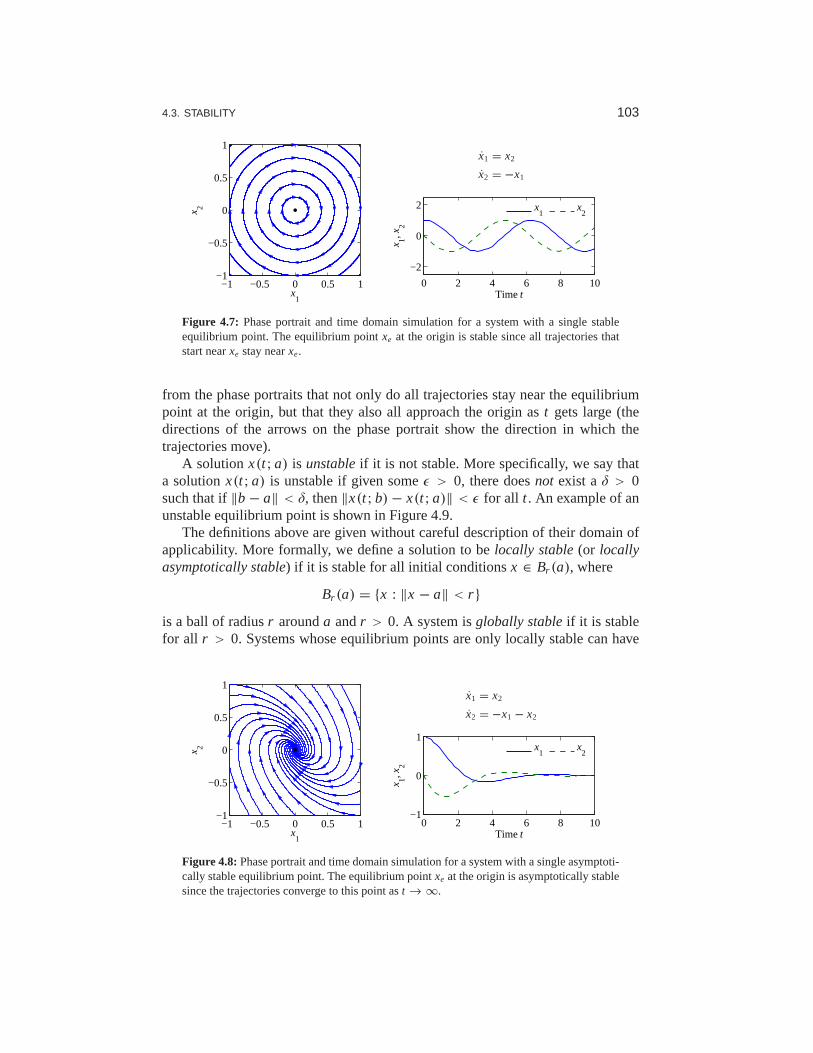
4.3. STABILITY 103
−1 −0.5 0 0.5 1−1
−0.5
0
0.5
1
x1
x 2
x1 = x2
x2 = −x1
0 2 4 6 8 10
−2
0
2
Time t
x 1, x2
x
1x
2
Figure 4.7: Phase portrait and time domain simulation for a system with a single stableequilibrium point. The equilibrium pointxe at the origin is stable since all trajectories thatstart nearxe stay nearxe.
from the phase portraits that not only do all trajectories stay near the equilibriumpoint at the origin, but that they also all approach the origin ast gets large (thedirections of the arrows on the phase portrait show the direction in which thetrajectories move).
A solution x(t ; a) is unstableif it is not stable. More specifically, we say thata solutionx(t ; a) is unstable if given someǫ > 0, there doesnot exist aδ > 0such that if‖b − a‖ < δ, then‖x(t ; b)− x(t ; a)‖ < ǫ for all t . An example of anunstable equilibrium point is shown in Figure 4.9.
The definitions above are given without careful description oftheir domain ofapplicability. More formally, we define a solution to belocally stable(or locallyasymptotically stable) if it is stable for all initial conditionsx ∈ Br (a), where
Br (a) = {x : ‖x − a‖ < r }
is a ball of radiusr arounda andr > 0. A system isglobally stableif it is stablefor all r > 0. Systems whose equilibrium points are only locally stable can have
−1 −0.5 0 0.5 1−1
−0.5
0
0.5
1
x1
x 2
x1 = x2
x2 = −x1 − x2
0 2 4 6 8 10−1
0
1
Time t
x 1, x2
x
1x
2
Figure 4.8: Phase portrait and time domain simulation for a system with a single asymptoti-cally stable equilibrium point. The equilibrium pointxe at the origin is asymptotically stablesince the trajectories converge to this point ast → ∞.

104 CHAPTER 4. DYNAMIC BEHAVIOR
−1 −0.5 0 0.5 1−1
−0.5
0
0.5
1
x1
x 2
x1 = 2x1 − x2
x2 = −x1 + 2x2
0 1 2 3−100
0
100
Time t
x 1, x2
x
1
x2
Figure 4.9: Phase portrait and time domain simulation for a system with a single unstableequilibrium point. The equilibrium pointxe at the origin is unstable since not all trajectoriesthat start nearxe stay nearxe. The sample trajectory on the right shows that the trajectoriesvery quickly depart from zero.
interesting behavior away from equilibrium points, as we explore in the next section.For planar dynamical systems, equilibrium points have beenassigned names
based on their stability type. An asymptotically stable equilibrium point is calleda sink or sometimes anattractor. An unstable equilibrium point can be either asource, if all trajectories lead away from the equilibrium point, or a saddle, ifsome trajectories lead to the equilibrium point and others move away (this is thesituation pictured in Figure 4.9). Finally, an equilibrium point that is stable but notasymptotically stable (i.e., neutrally stable, such as theone in Figure 4.7) is calledacenter.
Example 4.5 Congestion controlThe model for congestion control in a network consisting ofN identical computersconnected to a single router, introduced in Section 3.4, is given by
dw
dt= c
b− ρc
(1 + w2
2
),
db
dt= N
wc
b− c,
wherew is the window size andb is the buffer size of the router. Phase portraits areshown in Figure 4.10 for two different sets of parameter values. In each case we seethat the system converges to an equilibrium point in which the buffer is below itsfull capacity of 500 packets. The equilibrium size of the buffer represents a balancebetween the transmission rates for the sources and the capacity of the link. We seefrom the phase portraits that the equilibrium points are asymptotically stable sinceall initial conditions result in trajectories that converge to these points. ∇
Stability of Linear Systems
A linear dynamical system has the form
dx
dt= Ax, x(0) = x0, (4.7)

4.3. STABILITY 105
0 2 4 6 8 100
100
200
300
400
500
Window size, w [pkts]
Buf
fer
size
, b [p
kts]
(a)ρ = 2 × 10⁻⁴, c = 10 pkts/ms
0 2 4 6 8 100
100
200
300
400
500
Window size, w [pkts]
Buf
fer
size
, b [p
kts]
(b) ρ = 4 × 10⁻⁴, c = 20 pkts/ms
Figure 4.10:Phase portraits for a congestion control protocol running withN = 60 identicalsource computers. The equilibrium values correspond to a fixed windowat the source, whichresults in a steady-state buffer size and corresponding transmission rate. A faster link (b) usesa smaller buffer size since it can handle packets at a higher rate.
where A ∈ Rn×n is a square matrix, corresponding to the dynamics matrix of a
linear control system (2.6). For a linear system, the stability of the equilibrium atthe origin can be determined from the eigenvalues of the matrix A:
λ(A) = {s ∈ C : det(s I − A) = 0}.The polynomial det(s I − A) is thecharacteristic polynomialand the eigenvaluesare its roots. We use the notationλ j for the j th eigenvalue ofA, so thatλ j ∈ λ(A).In generalλ can be complex-valued, although ifA is real-valued, then for anyeigenvalueλ, its complex conjugateλ∗ will also be an eigenvalue. The origin isalways an equilibrium for a linear system. Since the stability of a linear systemdepends only on the matrixA, we find that stability is a property of the system. Fora linear system we can therefore talk about the stability of the system rather thanthe stability of a particular solution or equilibrium point.
The easiest class of linear systems to analyze are those whosesystem matricesare in diagonal form. In this case, the dynamics have the form
dx
dt=
λ1 0λ2
. . .
0 λn
x. (4.8)
It is easy to see that the state trajectories for this system are independent of eachother, so that we can write the solution in terms ofn individual systemsx j = λ j x j .Each of these scalar solutions is of the form
x j (t) = eλ j t x(0).
We see that the equilibrium pointxe = 0 is stable ifλ j ≤ 0 and asymptoticallystable ifλ j < 0.

106 CHAPTER 4. DYNAMIC BEHAVIOR
Another simple case is when the dynamics are in the block diagonal form
dx
dt=
σ1 ω1 0 0−ω1 σ1 0 0
0 0. . .
......
0 0 σm ωm
0 0 −ωm σm
x.
In this case, the eigenvalues can be shown to beλ j = σ j ± iω j . We once again canseparate the state trajectories into independent solutions for each pair of states, andthe solutions are of the form
x2 j −1(t) = eσ j t(x2 j −1(0) cosω j t + x2 j (0) sinω j t
),
x2 j (t) = eσ j t(−x2 j −1(0) sinω j t + x2 j (0) cosω j t
),
where j = 1,2, . . . ,m. We see that this system is asymptotically stable if and onlyif σ j = Reλ j < 0. It is also possible to combine real and complex eigenvalues in(block) diagonal form, resulting in a mixture of solutions of the two types.
Very few systems are in one of the diagonal forms above, but some systemscan be transformed into these forms via coordinate transformations. One such classof systems is those for which the dynamics matrix has distinct (nonrepeating)eigenvalues. In this case there is a matrixT ∈ R
n×n such that the matrixT AT−1
is in (block) diagonal form, with the block diagonal elements corresponding tothe eigenvalues of the original matrixA (see Exercise 4.14). If we choose newcoordinatesz = T x, then
dz
dt= Tx = T Ax = T AT−1z
and the linear system has a (block) diagonal dynamics matrix. Furthermore, theeigenvalues of the transformed system are the same as the original system sinceif v is an eigenvector ofA, thenw = Tv can be shown to be an eigenvector ofT AT−1. We can reason about the stability of the original system by noting thatx(t) = T−1z(t), and so if the transformed system is stable (or asymptoticallystable), then the original system has the same type of stability.
This analysis shows that for linear systems with distinct eigenvalues, the stabilityof the system can be completely determined by examining the real part of theeigenvalues of the dynamics matrix. For more general systems, we make use of thefollowing theorem, proved in the next chapter:
Theorem 4.1(Stability of a linear system). The system
dx
dt= Ax
is asymptotically stable if and only if all eigenvalues of A all have a strictly negativereal part and is unstable if any eigenvalue of A has a strictlypositive real part.
Example 4.6 Compartment modelConsider the two-compartment module for drug delivery introduced in Section 3.6.

4.3. STABILITY 107
Using concentrations as state variables and denoting the state vector byx, the systemdynamics are given by
dx
dt=−k0 − k1 k1
k2 −k2
x +
b0
0
u, y =
0 1
x,
where the inputu is the rate of injection of a drug into compartment 1 and theconcentration of the drug in compartment 2 is the measured output y. We wish todesign a feedback control law that maintains a constant output given byy = yd.
We choose an output feedback control law of the form
u = −k(y − yd)+ ud,
whereud is the rate of injection required to maintain the desired concentration andk is a feedback gain that should be chosen such that the closed loop system is stable.Substituting the control law into the system, we obtain
dx
dt=−k0 − k1 k1 − b0k
k2 −k2
x +
b0
0
(ud + kyd) =: Ax + Bue,
y =0 1
x =: Cx.
The equilibrium concentrationxe ∈ R2 is given byxe = −A−1Bue and
ye = −C A−1Bue = b0k2
k0k2 + b0k2k(ud + kyd).
Choosingud such thatye = yd provides the constant rate of injection required tomaintain the desired output. We can now shift coordinates toplace the equilibriumpoint at the origin, which yields (after some algebra)
dz
dt=−k0 − k1 k1 − b0k
k2 −k2
z,
wherez = x − xe. We can now apply the results of Theorem 4.1 to determine thestability of the system. The eigenvalues of the system are given by the roots of thecharacteristic polynomial
λ(s) = s2 + (k0 + k1 + k2)s + (k0k2 + b0k2k).
While the specific form of the roots is messy, it can be shown that the roots are posi-tive as long as the linear term and the constant term are both positive (Exercise 4.16).Hence the system is stable for anyk > 0. ∇
Stability Analysis via Linear Approximation
An important feature of differential equations is that it isoften possible to determinethe local stability of an equilibrium point by approximating the system by a linearsystem. The following example illustrates the basic idea.

108 CHAPTER 4. DYNAMIC BEHAVIOR
Example 4.7 Inverted pendulumConsider again an inverted pendulum whose open loop dynamics are given by
dx
dt= x2
sinx1 − γ x2
,
where we have defined the state asx = (θ, θ). We first consider the equilibriumpoint atx = (0,0), corresponding to the straight-up position. If we assume that theangleθ = x1 remains small, then we can replace sinx1 with x1 and cosx1 with 1,which gives the approximate system
dx
dt= x2
x1 − γ x2
=
0 1
1 −γ
x. (4.9)
Intuitively, this system should behave similarly to the more complicated modelas long asx1 is small. In particular, it can be verified that the equilibrium point(0,0) is unstable by plotting the phase portrait or computing the eigenvalues of thedynamics matrix in equation (4.9)
We can also approximate the system around the stable equilibrium point atx = (π,0). In this case we have to expand sinx1 and cosx1 aroundx1 = π ,according to the expansions
sin(π + θ) = − sinθ ≈ −θ, cos(π + θ) = − cos(θ) ≈ −1.
If we definez1 = x1 − π andz2 = x2, the resulting approximate dynamics aregiven by
dz
dt= z2
−z1 − γ z2
=
0 1
−1 −γ
z. (4.10)
Note thatz = (0,0) is the equilibrium point for this system and that it has the samebasic form as the dynamics shown in Figure 4.8. Figure 4.11 shows the phase por-traits for the original system and the approximate system around the correspondingequilibrium points. Note that they are very similar, although not exactly the same.It can be shown that if a linear approximation has either asymptotically stable orunstable equilibrium points, then the local stability of the original system must bethe same (Theorem 4.3). ∇
More generally, suppose that we have a nonlinear system
dx
dt= F(x)
that has an equilibrium point atxe. Computing the Taylor series expansion of thevector field, we can write
dx
dt= F(xe)+ ∂F
∂x
∣∣∣∣xe
(x − xe)+ higher-order terms in(x − xe).
SinceF(xe) = 0, we can approximate the system by choosing a new state variable

4.3. STABILITY 109
−2
−1
0
1
2
x1
x2
0 π/2 π 2π3π/2
(a) Nonlinear model
−2
−1
0
1
2
z1
z2
−π −π/2 0 π/2 π
(b) Linear approximation
Figure 4.11:Comparison between the phase portraits for the full nonlinear systems (a) andits linear approximation around the origin (b). Notice that near the equilibriumpoint at thecenter of the plots, the phase portraits (and hence the dynamics) are almost identical.
z = x − xe and writing
dz
dt= Az, where A = ∂F
∂x
∣∣∣∣xe
. (4.11)
We call the system (4.11) thelinear approximationof the original nonlinear systemor thelinearizationat xe.
The fact that a linear model can be used to study the behavior ofa nonlinearsystem near an equilibrium point is a powerful one. Indeed, we can take this evenfurther and use a local linear approximation of a nonlinear system to design a feed-back law that keeps the system near its equilibrium point (design of dynamics).Thus, feedback can be used to make sure that solutions remain close to the equi-librium point, which in turn ensures that the linear approximation used to stabilizeit is valid.
Linear approximations can also be used to understand the stability of nonequi-librium solutions, as illustrated by the following example.
Example 4.8 Stable limit cycleConsider the system given by equation (4.6),
dx1
dt= x2 + x1(1 − x2
1 − x22),
dx2
dt= −x1 + x2(1 − x2
1 − x22),
whose phase portrait is shown in Figure 4.5. The differential equation has a periodicsolution
x1(t) = x1(0) cost + x2(0) sint, (4.12)
with x21(0)+ x2
2(0) = 1.To explore the stability of this solution, we introduce polar coordinatesr and
ϕ, which are related to the state variablesx1 andx2 by
x1 = r cosϕ, x2 = r sinϕ.

110 CHAPTER 4. DYNAMIC BEHAVIOR
Differentiation gives the following linear equations forr andϕ:
x1 = r cosϕ − r ϕ sinϕ, x2 = r sinϕ + r ϕ cosϕ.
Solving this linear system forr andϕ gives, after some calculation,
dr
dt= r (1 − r 2),
dϕ
dt= −1.
Notice that the equations are decoupled; hence we can analyze the stability of eachstate separately.
The equation forr has three equilibria:r = 0, r = 1 andr = −1 (not realiz-able sincer must be positive). We can analyze the stability of these equilibria bylinearizing the radial dynamics withF(r ) = r (1 − r 2). The corresponding lineardynamics are given by
dr
dt= ∂F
∂r
∣∣∣∣re
r = (1 − 3r 2e)r, re = 0, 1,
where we have abused notation and usedr to represent the deviation from theequilibrium point. It follows from the sign of(1 − 3r 2
e) that the equilibriumr = 0is unstable and the equilibriumr = 1 is asymptotically stable. Thus for any initialconditionr > 0 the solution goes tor = 1 as time goes to infinity, but if the systemstarts withr = 0, it will remain at the equilibrium for all times. This implies thatall solutions to the original system that do not start atx1 = x2 = 0 will approachthe circlex2
1 + x22 = 1 as time increases.
To show the stability of the full solution (4.12), we must investigate the behaviorof neighboring solutions with different initial conditions. We have already shownthat the radiusr will approach that of the solution (4.12) as long asr (0) > 0. Theequation for the angleϕ can be integrated analytically to giveϕ(t) = −t + ϕ(0),which shows that solutions starting at different anglesϕ will neither converge nordiverge. Thus, the unit circle isattracting, but the solution (4.12) is only stable, notasymptotically stable. The behavior of the system is illustrated by the simulationin Figure 4.12. Notice that the solutions approach the circlerapidly, but that thereis a constant phase shift between the solutions. ∇
4.4 Lyapunov Stability Analysis�
We now return to the study of the full nonlinear system
dx
dt= F(x), x ∈ R
n. (4.13)
Having defined when a solution for a nonlinear dynamical system is stable, wecan now ask how to prove that a given solution is stable, asymptotically stableor unstable. For physical systems, one can often argue aboutstability based ondissipation of energy. The generalization of that techniqueto arbitrary dynamicalsystems is based on the use of Lyapunov functions in place of energy.

4.4. LYAPUNOV STABILITY ANALYSIS 111
−1 0 1 2
−1
−0.5
0
0.5
1
1.5
2
x1
x20 5 10 15 20
−1
0
1
2
0 5 10 15 20−1
0
1
2
x1
x2
Time t
Figure 4.12:Solution curves for a stable limit cycle. The phase portrait on the left shows thatthe trajectory for the system rapidly converges to the stable limit cycle. The starting pointsfor the trajectories are marked by circles in the phase portrait. The time domain plots on theright show that the states do not converge to the solution but instead maintaina constant phaseerror.
In this section we will describe techniques for determiningthe stability of so-lutions for a nonlinear system (4.13). We will generally be interested in stabilityof equilibrium points, and it will be convenient to assume that xe = 0 is the equi-librium point of interest. (If not, rewrite the equations ina new set of coordinatesz = x − xe.)
Lyapunov Functions
A Lyapunov function V: Rn → R is an energy-like function that can be used to
determine the stability of a system. Roughly speaking, if wecan find a nonnegativefunction that always decreases along trajectories of the system, we can concludethat the minimum of the function is a stable equilibrium point (locally).
To describe this more formally, we start with a few definitions. We say that acontinuous functionV is positive definiteif V(x) > 0 for all x 6= 0 andV(0) = 0.Similarly, a function isnegative definiteif V(x) < 0 for all x 6= 0 andV(0) = 0.We say that a functionV is positive semidefiniteif V(x) ≥ 0 for all x, but V(x)can be zero at points other than justx = 0.
To illustrate the difference between a positive definite function and a positivesemidefinite function, suppose thatx ∈ R
2 and let
V1(x) = x21, V2(x) = x2
1 + x22.
Both V1 andV2 are always nonnegative. However, it is possible forV1 to be zeroeven if x 6= 0. Specifically, if we setx = (0, c), wherec ∈ R is any nonzeronumber, thenV1(x) = 0. On the other hand,V2(x) = 0 if and only if x = (0,0).ThusV1 is positive semidefinite andV2 is positive definite.
We can now characterize the stability of an equilibrium point xe = 0 for thesystem (4.13).
Theorem 4.2(Lyapunov stability theorem). Let V be a nonnegative function on

112 CHAPTER 4. DYNAMIC BEHAVIOR
dxdt
∂V∂x
V(x) = c2V(x) = c1 < c2
Figure 4.13: Geometric illustration of Lyapunov’s stability theorem. The closed contoursrepresent the level sets of the Lyapunov functionV(x) = c. If dx/dt points inward to thesesets at all points along the contour, then the trajectories of the system will always causeV(x)to decrease along the trajectory.
Rn and let V represent the time derivative of V along trajectories of the system
dynamics(4.13):
V = ∂V
∂x
dx
dt= ∂V
∂xF(x).
Let Br = Br (0) be a ball of radius r around the origin. If there exists r> 0 suchthat V is positive definite andV is negative semidefinite for all x∈ Br , then x= 0is locally stable in the sense of Lyapunov. If V is positive definite andV is negativedefinite in Br , then x= 0 is locally asymptotically stable.
If V satisfies one of the conditions above, we say thatV is a (local)Lyapunovfunction for the system. These results have a nice geometric interpretation. Thelevel curves for a positive definite function are the curves defined byV(x) = c,c > 0, and for eachc this gives a closed contour, as shown in Figure 4.13. Thecondition thatV(x) is negative simply means that the vector field points towardlower-level contours. This means that the trajectories moveto smaller and smallervalues ofV and if V is negative definite thenx must approach 0.
Example 4.9 Scalar nonlinear systemConsider the scalar nonlinear system
dx
dt= 2
1 + x− x.
This system has equilibrium points atx = 1 andx = −2. We consider the equilib-rium point atx = 1 and rewrite the dynamics usingz = x − 1:
dz
dt= 2
2 + z− z − 1,
which has an equilibrium point atz = 0. Now consider the candidate Lyapunovfunction
V(z) = 1
2z2,

4.4. LYAPUNOV STABILITY ANALYSIS 113
which is globally positive definite. The derivative ofV along trajectories of thesystem is given by
V(z) = zz = 2z
2 + z− z2 − z.
If we restrict our analysis to an intervalBr , wherer < 2, then 2+ z > 0 and wecan multiply through by 2+ z to obtain
2z − (z2 + z)(2 + z) = −z3 − 3z2 = −z2(z + 3) < 0, z ∈ Br , r < 2.
It follows that V(z) < 0 for all z ∈ Br , z 6= 0, and hence the equilibrium pointxe = 1 is locally asymptotically stable. ∇
A slightly more complicated situation occurs ifV is negative semidefinite. Inthis case it is possible thatV(x) = 0 whenx 6= 0, and hencex could stop decreasingin value. The following example illustrates this case.
Example 4.10 Hanging pendulumA normalized model for a hanging pendulum is
dx1
dt= x2,
dx2
dt= − sinx1,
wherex1 is the angle between the pendulum and the vertical, with positive x1
corresponding to counterclockwise rotation. The equation has an equilibriumx1 =x2 = 0, which corresponds to the pendulum hanging straight down.To explore thestability of this equilibrium we choose the total energy as aLyapunov function:
V(x) = 1 − cosx1 + 1
2x2
2 ≈ 1
2x2
1 + 1
2x2
2.
The Taylor series approximation shows that the function is positive definite forsmallx. The time derivative ofV(x) is
V = x1 sinx1 + x2x2 = x2 sinx1 − x2 sinx1 = 0.
Since this function is positive semidefinite, it follows from Lyapunov’s theorem thatthe equilibrium is stable but not necessarily asymptotically stable. When perturbed,the pendulum actually moves in a trajectory that corresponds to constant energy.∇
Lyapunov functions are not always easy to find, and they are notunique. In manycases energy functions can be used as a starting point, as wasdone in Example 4.10.It turns out that Lyapunov functions can always be found for any stable system (un-der certain conditions), and hence one knows that if a systemis stable, a Lyapunovfunction exists (and vice versa). Recent results using sum-of-squares methods haveprovided systematic approaches for finding Lyapunov systems[PPP02]. Sum-of-squares techniques can be applied to a broad variety of systems, including systemswhose dynamics are described by polynomial equations, as well as hybrid systems,which can have different models for different regions of state space.
For a linear dynamical system of the form
dx
dt= Ax,

114 CHAPTER 4. DYNAMIC BEHAVIOR
it is possible to construct Lyapunov functions in a systematic manner. To do so, weconsider quadratic functions of the form
V(x) = xT Px,
whereP ∈ Rn×n is a symmetric matrix (P = PT ). The condition thatV be positive
definite is equivalent to the condition thatP be apositive definite matrix:
xT Px > 0, for all x 6= 0,
which we write asP > 0. It can be shown that ifP is symmetric, thenP is positivedefinite if and only if all of its eigenvalues are real and positive.
Given a candidate Lyapunov functionV(x) = xT Px, we can now compute itsderivative along flows of the system:
V = ∂V
∂x
dx
dt= xT (AT P + P A)x =: −xT Qx.
The requirement thatV be negative definite (for asymptotic stability) becomes acondition that the matrixQ be positive definite. Thus, to find a Lyapunov functionfor a linear system it is sufficient to choose aQ > 0 and solve theLyapunovequation:
AT P + P A = −Q. (4.14)
This is a linear equation in the entries ofP, and hence it can be solved usinglinear algebra. It can be shown that the equation always has asolution if all of theeigenvalues of the matrixA are in the left half-plane. Moreover, the solutionP ispositive definite ifQ is positive definite. It is thus always possible to find a quadraticLyapunov function for a stable linear system. We will defer aproof of this untilChapter 5, where more tools for analysis of linear systems will be developed.
Knowing that we have a direct method to find Lyapunov functionsfor linearsystems, we can now investigate the stability of nonlinear systems. Consider thesystem
dx
dt= F(x) =: Ax + F(x), (4.15)
whereF(0) = 0 andF(x) contains terms that are second order and higher in theelements ofx. The functionAx is an approximation ofF(x) near the origin, and wecan determine the Lyapunov function for the linear approximation and investigate ifit is also a Lyapunov function for the full nonlinear system.The following exampleillustrates the approach.
Example 4.11 Genetic switchConsider the dynamics of a set of repressors connected together in a cycle, asshown in Figure 4.14a. The normalized dynamics for this systemwere given inExercise 2.9:
dz1
dτ= µ
1 + zn2
− z1,dz2
dτ= µ
1 + zn1
− z2, (4.16)
wherez1 and z2 are scaled versions of the protein concentrations,n andµ are

4.4. LYAPUNOV STABILITY ANALYSIS 115
u2
A BA
u1
(a) Circuit diagram
0 1 2 3 4 50
1
2
3
4
5
z1, f (z2)
z1, f (z1)
z 2,
f(z 1)
z2, f (z2)
(b) Equilibrium points
Figure 4.14:Stability of a genetic switch. The circuit diagram in (a) represents two proteinsthat are each repressing the production of the other. The inputsu1 andu2 interfere with thisrepression, allowing the circuit dynamics to be modified. The equilibrium points for thiscircuit can be determined by the intersection of the two curves shown in (b).
parameters that describe the interconnection between the genes and we have set theexternal inputsu1 andu2 to zero.
The equilibrium points for the system are found by equating the time derivativesto zero. We define
f (u) = µ
1 + un, f ′(u) = d f
du= −µnun−1
(1 + un)2,
and the equilibrium points are defined as the solutions of the equations
z1 = f (z2), z2 = f (z1).
If we plot the curves(z1, f (z1)) and( f (z2), z2) on a graph, then these equationswill have a solution when the curves intersect, as shown in Figure 4.14b. Becauseof the shape of the curves, it can be shown that there will always be three solutions:one atz1e = z2e, one withz1e < z2e and one withz1e > z2e. If µ ≫ 1, then we canshow that the solutions are given approximately by
z1e ≈ µ, z2e ≈ 1
µn−1; z1e = z2e; z1e ≈ 1
µn−1, z2e ≈ µ. (4.17)
To check the stability of the system, we writef (u) in terms of its Taylor seriesexpansion aboutue:
f (u) = f (ue)+ f ′(ue) ·(u − ue)+ 1
2f ′′(ue) ·(u − ue)
2 + higher-order terms,
where f ′ represents the first derivative of the function, andf ′′ the second. Usingthese approximations, the dynamics can then be written as
dw
dt= −1 f ′(z2e)
f ′(z1e) −1
w + F(w),

116 CHAPTER 4. DYNAMIC BEHAVIOR
wherew = z−ze is the shifted state andF(w) represents quadratic and higher-orderterms.
We now use equation (4.14) to search for a Lyapunov function.ChoosingQ = Iand lettingP ∈ R
2×2 have elementspi j , we search for a solution of the equation−1 f ′
2f ′1 −1
p11 p12
p12 p22
+
p11 p12
p12 p22
−1 f ′
1f ′2 −1
=
−1 0
0 −1
,
where f ′1 = f ′(z1e) and f ′
2 = f ′(z2e). Note that we have setp21 = p12 to forcePto be symmetric. Multiplying out the matrices, we obtain
−2p11 + 2 f ′
2 p12 p11 f ′1 − 2p12 + p22 f ′
2p11 f ′
1 − 2p12 + p22 f ′2 −2p22 + 2 f ′
1 p12
=
−1 0
0 −1
,
which is a set oflinear equations for the unknownspi j . We can solve these linearequations to obtain
p11 = − f ′1
2 − f ′2 f ′
1 + 2
4( f ′1 f ′
2 − 1), p12 = − f ′
1 + f ′2
4( f ′1 f ′
2 − 1), p22 = − f ′
22 − f ′
1 f ′2 + 2
4( f ′1 f ′
2 − 1).
To check thatV(w) = wT Pw is a Lyapunov function, we must verify thatV(w) ispositive definite function or equivalently thatP > 0. SinceP is a 2× 2 symmetricmatrix, it has two real eigenvaluesλ1 andλ2 that satisfy
λ1 + λ2 = trace(P), λ1 ·λ2 = det(P).
In order forP to be positive definite we must have thatλ1 andλ2 are positive, andwe thus require that
trace(P) = f ′1
2−2 f ′2 f ′
1+ f ′2
2 + 4
4−4 f ′1 f ′
2
> 0, det(P) = f ′1
2−2 f ′2 f ′
1+ f ′2
2+4
16− 16 f ′1 f ′
2
> 0.
We see that trace(P) = 4 det(P) and the numerator of the expressions is just( f1 − f2)
2 + 4 > 0, so it suffices to check the sign of 1− f ′1 f ′
2. In particular, forP to be positive definite, we require that
f ′(z1e) f ′(z2e) < 1.
We can now make use of the expressions forf ′ defined earlier and evaluate atthe approximate locations of the equilibrium points derived in equation (4.17). Forthe equilibrium points wherez1e 6= z2e, we can show that
f ′(z1e) f ′(z2e) ≈ f ′(µ) f ′(1
µn−1) = −µnµn−1
(1 + µn)2·−µnµ−(n−1)2
1 + µ−n(n−1)≈ n2µ−n2+n.
Usingn = 2 andµ ≈ 200 from Exercise 2.9, we see thatf ′(z1e) f ′(z2e) ≪ 1 andhenceP is a positive definite. This implies thatV is a positive definite function andhence a potential Lyapunov function for the system.
To determine if the system (4.16) is stable, we now computeV at the equilibrium

4.4. LYAPUNOV STABILITY ANALYSIS 117
0 1 2 3 4 50
1
2
3
4
5
Protein A [scaled]
Pro
tein
B [s
cale
d]
0 5 10 15 20 250
1
2
3
4
5
Time t [scaled]
Pro
tein
con
cent
ratio
ns [s
cale
d]
z1 (A) z2 (B)
Figure 4.15:Dynamics of a genetic switch. The phase portrait on the left shows that theswitchhas three equilibrium points, corresponding to protein A having a concentration greater than,equal to or less than protein B. The equilibrium point with equal protein concentrations isunstable, but the other equilibrium points are stable. The simulation on the right shows thetime response of the system starting from two different initial conditions. The initial portion ofthe curve corresponds to initial concentrationsz(0) = (1,5) and converges to the equilibriumwherez1e < z2e. At time t = 10, the concentrations are perturbed by+2 in z1 and−2 in z2,moving the state into the region of the state space whose solutions converge tothe equilibriumpoint wherez2e < z1e.
point. By construction,
V = wT(P A+ ATP)w + FT(w)Pw + wTPF(w)
= −wTw + FT(w)Pw + wTPF(w).
Since all terms inF are quadratic or higher order inw, it follows that FT(w)PwandwTPF(w) consist of terms that are at least third order inw. Therefore ifwis sufficiently close to zero, then the cubic and higher-orderterms will be smallerthan the quadratic terms. Hence, sufficiently close tow = 0, V is negative definite,allowing us to conclude that these equilibrium points are both stable.
Figure 4.15 shows the phase portrait and time traces for a system withµ = 4,illustrating the bistable nature of the system. When the initial condition starts witha concentration of protein B greater than that of A, the solution converges to theequilibrium point at (approximately)(1/µn−1, µ). If A is greater than B, then itgoes to(µ,1/µn−1). The equilibrium point withz1e = z2e is unstable. ∇
More generally, we can investigate what the linear approximation tells aboutthe stability of a solution to a nonlinear equation. The following theorem gives apartial answer for the case of stability of an equilibrium point.
Theorem 4.3. Consider the dynamical system(4.15)with F(0) = 0 and F suchthat lim ‖F(x)‖/‖x‖ → 0 as‖x‖ → 0. If the real parts of all eigenvalues of A arestrictly less than zero, then xe = 0 is a locally asymptotically stable equilibriumpoint of equation(4.15).
This theorem implies that asymptotic stability of the linearapproximation im-plieslocalasymptotic stability of the original nonlinear system. The theorem is very

118 CHAPTER 4. DYNAMIC BEHAVIOR
important for control because it implies that stabilization of a linear approximationof a nonlinear system results in a stable equilibrium for thenonlinear system. Theproof of this theorem follows the technique used in Example 4.11. A formal proofcan be found in [Kha01].
Krasovski–Lasalle Invariance Principle��
For general nonlinear systems, especially those in symbolic form, it can be difficultto find a positive definite functionV whose derivative is strictly negative definite.The Krasovski–Lasalle theorem enables us to conclude the asymptotic stability ofan equilibrium point under less restrictive conditions, namely, in the case whereVis negative semidefinite, which is often easier to construct.However, it applies onlyto time-invariant or periodic systems. This section makes use of some additionalconcepts from dynamical systems; see Hahn [Hah67] or Khalil[Kha01] for a moredetailed description.
We will deal with the time-invariant case and begin by introducing a few moredefinitions. We denote the solution trajectories of the time-invariant system
dx
dt= F(x) (4.18)
asx(t ; a), which is the solution of equation (4.18) at timet starting froma att0 = 0.Theω limit setof a trajectoryx(t ; a) is the set of all pointsz ∈ R
n such that thereexists a strictly increasing sequence of timestn such thatx(tn; a) → z asn → ∞.A set M ⊂ R
n is said to be aninvariant setif for all b ∈ M , we havex(t ; b) ∈ Mfor all t ≥ 0. It can be proved that theω limit set of every trajectory is closed andinvariant. We may now state the Krasovski–Lasalle principle.
Theorem 4.4(Krasovski–Lasalle principle). Let V : Rn → R be a locally positive
definite function such that on the compact set�r = {x ∈ Rn : V(x) ≤ r } we have
V(x) ≤ 0. DefineS = {x ∈ �r : V(x) = 0}.
As t → ∞, the trajectory tends to the largest invariant set inside S;i.e., itsω limitset is contained inside the largest invariant set in S. In particular, if S contains noinvariant sets other than x= 0, then 0 is asymptotically stable.
Proofs are given in [Kra63] and [LaS60].Lyapunov functions can often be used to design stabilizing controllers, as is
illustrated by the following example, which also illustrates how the Krasovski–Lasalle principle can be applied.
Example 4.12 Inverted pendulumFollowing the analysis in Example 2.7, an inverted pendulum can be described bythe following normalized model:
dx1
dt= x2,
dx2
dt= sinx1 + u cosx1, (4.19)

4.4. LYAPUNOV STABILITY ANALYSIS 119
u
θ
m
l
(a) Physical system
−4
−2
0
2
4
x1
x2
−2π −π 0 π 2π
(b) Phase portrait
θ
θ
(c) Manifold view
Figure 4.16: Stabilized inverted pendulum. A control law applies a forceu at the bottomof the pendulum to stabilize the inverted position (a). The phase portrait (b)shows thatthe equilibrium point corresponding to the vertical position is stabilized. The shaded regionindicates the set of initial conditions that converge to the origin. The ellipse corresponds to alevel set of a Lyapunov functionV(x) for whichV(x) > 0 andV(x) < 0 for all points insidethe ellipse. This can be used as an estimate of the region of attraction of the equilibrium point.The actual dynamics of the system evolve on a manifold (c).
wherex1 is the angular deviation from the upright position andu is the (scaled)acceleration of the pivot, as shown in Figure 4.16a. The systemhas an equilib-rium at x1 = x2 = 0, which corresponds to the pendulum standing upright. Thisequilibrium is unstable.
To find a stabilizing controller we consider the following candidate for a Lya-punov function:
V(x) = (cosx1 − 1)+ a(1 − cos2 x1)+ 1
2x2
2 ≈(a − 1
2
)x2
1 + 1
2x2
2.
The Taylor series expansion shows that the function is positive definite near theorigin if a > 0.5. The time derivative ofV(x) is
V = −x1 sinx1 + 2ax1 sinx1 cosx1 + x2x2 = x2(u + 2a sinx1) cosx1.
Choosing the feedback law
u = −2a sinx1 − x2 cosx1
givesV = −x2
2 cos2 x1.
It follows from Lyapunov’s theorem that the equilibrium is locally stable. However,since the function is only negative semidefinite, we cannot conclude asymptoticstability using Theorem 4.2. However, note thatV = 0 implies thatx2 = 0 orx1 = π/2 ± nπ .
If we restrict our analysis to a small neighborhood of the origin�r , r ≪ π/2,then we can define
S = {(x1, x2) ∈ �r : x2 = 0}

120 CHAPTER 4. DYNAMIC BEHAVIOR
and we can compute the largest invariant set insideS. For a trajectory to remainin this set we must havex2 = 0 for all t and hencex2(t) = 0 as well. Using thedynamics of the system (4.19), we see thatx2(t) = 0 andx2(t) = 0 impliesx1(t) =0 as well. Hence the largest invariant set insideS is (x1, x2) = 0, and we can use theKrasovski–Lasalle principle to conclude that the origin is locally asymptoticallystable. A phase portrait of the closed loop system is shown inFigure 4.16b.
In the analysis and the phase portrait, we have treated the angle of the pendulumθ = x1 as a real number. In fact,θ is an angle withθ = 2π equivalent toθ = 0.Hence the dynamics of the system actually evolves on amanifold(smooth surface)as shown in Figure 4.16c. Analysis of nonlinear dynamical systems on manifoldsis more complicated, but uses many of the same basic ideas presented here. ∇
4.5 Parametric and Nonlocal Behavior�
Most of the tools that we have explored are focused on the local behavior of afixed system near an equilibrium point. In this section we briefly introduce someconcepts regarding the global behavior of nonlinear systems and the dependenceof a system’s behavior on parameters in the system model.
Regions of Attraction
To get some insight into the behavior of a nonlinear system wecan start by findingthe equilibrium points. We can then proceed to analyze the local behavior aroundthe equilibria. The behavior of a system near an equilibrium point is called thelocalbehavior of the system.
The solutions of the system can be very different far away froman equilibriumpoint. This is seen, for example, in the stabilized pendulum in Example 4.12. Theinverted equilibrium point is stable, with small oscillations that eventually convergeto the origin. But far away from this equilibrium point thereare trajectories thatconverge to other equilibrium points or even cases in which the pendulum swingsaround the top multiple times, giving very long oscillations that are topologicallydifferent from those near the origin.
To better understand the dynamics of the system, we can examine the set of allinitial conditions that converge to a given asymptoticallystable equilibrium point.This set is called theregion of attractionfor the equilibrium point. An exampleis shown by the shaded region of the phase portrait in Figure 4.16b. In general,computing regions of attraction is difficult. However, even if we cannot determinethe region of attraction, we can often obtain patches aroundthe stable equilibriathat are attracting. This gives partial information about the behavior of the system.
One method for approximating the region of attraction is through the use ofLyapunov functions. Suppose thatV is a local Lyapunov function for a systemaround an equilibrium pointx0. Let�r be a set on whichV(x) has a value less thanr ,
�r = {x ∈ Rn : V(x) ≤ r },

4.5. PARAMETRIC AND NONLOCAL BEHAVIOR 121
and suppose thatV(x) ≤ 0 for all x ∈ �r , with equality only at the equilibriumpoint x0. Then�r is inside the region of attraction of the equilibrium point.Sincethis approximation depends on the Lyapunov function and thechoice of Lyapunovfunction is not unique, it can sometimes be a very conservative estimate.
It is sometimes the case that we can find a Lyapunov functionV such thatV ispositive definite andV is negative (semi-) definite for allx ∈ R
n. In many instancesit can then be shown that the region of attraction for the equilibrium point is theentire state space, and the equilibrium point is said to begloballystable.
Example 4.13 Stabilized inverted pendulumConsider again the stabilized inverted pendulum from Example 4.12. The Lyapunovfunction for the system was
V(x) = (cosx1 − 1)+ a(1 − cos2 x1)+ 1
2x2
2,
and V was negative semidefinite for allx and nonzero whenx1 6= ±π/2. Hencefor any x such that|x2| < π/2, V(x) > 0 will be inside the invariant set definedby the level curves ofV(x). One of these level sets is shown in Figure 4.16b.∇
Bifurcations
Another important property of nonlinear systems is how their behavior changes asthe parameters governing the dynamics change. We can study this in the contextof models by exploring how the location of equilibrium points, their stability, theirregions of attraction and other dynamic phenomena, such as limit cycles, vary basedon the values of the parameters in the model.
Consider a differential equation of the form
dx
dt= F(x, µ), x ∈ R
n, µ ∈ Rk, (4.20)
wherex is the state andµ is a set of parameters that describe the family of equations.The equilibrium solutions satisfy
F(x, µ) = 0,
and asµ is varied, the corresponding solutionsxe(µ) can also vary. We say that thesystem (4.20) has abifurcationatµ = µ∗ if the behavior of the system changesqualitatively atµ∗. This can occur either because of a change in stability type orachange in the number of solutions at a given value ofµ.
Example 4.14 Predator–preyConsider the predator–prey system described in Section 3.7.The dynamics of thesystem are given by
d H
dt= r H
(1 − H
k
)− aH L
c + H,
dL
dt= b
aH L
c + H− dL, (4.21)
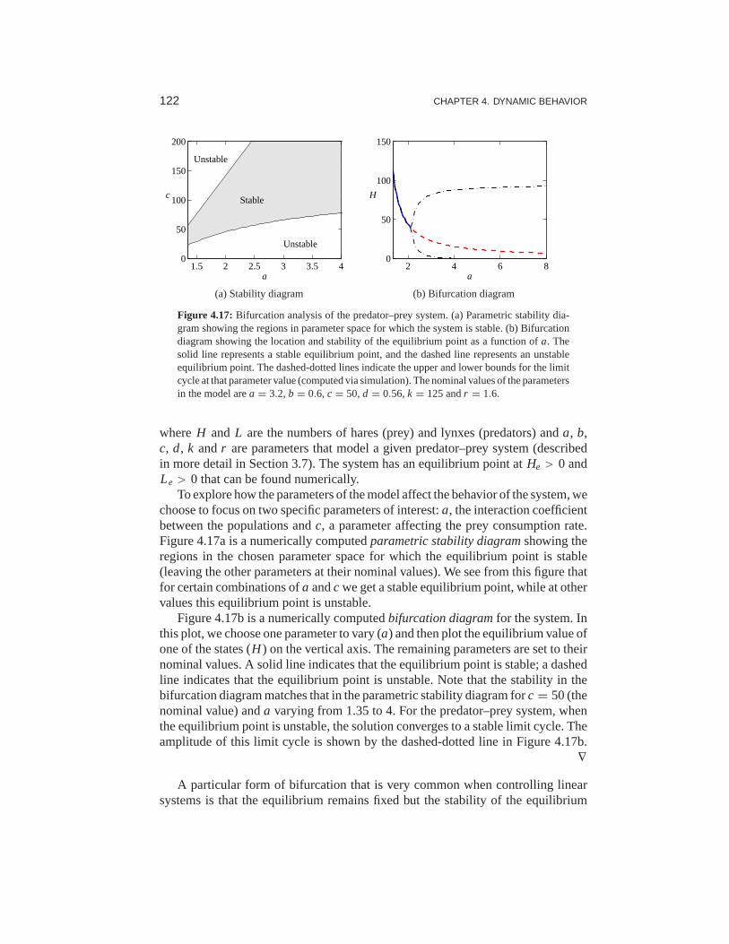
122 CHAPTER 4. DYNAMIC BEHAVIOR
1.5 2 2.5 3 3.5 40
50
100
150
200
a
c
Unstable
Stable
Unstable
(a) Stability diagram
2 4 6 80
50
100
150
a
H
(b) Bifurcation diagram
Figure 4.17: Bifurcation analysis of the predator–prey system. (a) Parametric stabilitydia-gram showing the regions in parameter space for which the system is stable. (b) Bifurcationdiagram showing the location and stability of the equilibrium point as a function of a. Thesolid line represents a stable equilibrium point, and the dashed line represents an unstableequilibrium point. The dashed-dotted lines indicate the upper and lower bounds for the limitcycle at that parameter value (computed via simulation). The nominal values of the parametersin the model area = 3.2, b = 0.6, c = 50,d = 0.56,k = 125 andr = 1.6.
whereH andL are the numbers of hares (prey) and lynxes (predators) anda, b,c, d, k andr are parameters that model a given predator–prey system (describedin more detail in Section 3.7). The system has an equilibrium point at He > 0 andLe > 0 that can be found numerically.
To explore how the parameters of the model affect the behavior of the system, wechoose to focus on two specific parameters of interest:a, the interaction coefficientbetween the populations andc, a parameter affecting the prey consumption rate.Figure 4.17a is a numerically computedparametric stability diagramshowing theregions in the chosen parameter space for which the equilibrium point is stable(leaving the other parameters at their nominal values). We see from this figure thatfor certain combinations ofa andc we get a stable equilibrium point, while at othervalues this equilibrium point is unstable.
Figure 4.17b is a numerically computedbifurcation diagramfor the system. Inthis plot, we choose one parameter to vary (a) and then plot the equilibrium value ofone of the states (H ) on the vertical axis. The remaining parameters are set to theirnominal values. A solid line indicates that the equilibriumpoint is stable; a dashedline indicates that the equilibrium point is unstable. Notethat the stability in thebifurcation diagram matches that in the parametric stability diagram forc = 50 (thenominal value) anda varying from 1.35 to 4. For the predator–prey system, whenthe equilibrium point is unstable, the solution converges to a stable limit cycle. Theamplitude of this limit cycle is shown by the dashed-dotted line in Figure 4.17b.
∇
A particular form of bifurcation that is very common when controlling linearsystems is that the equilibrium remains fixed but the stability of the equilibrium

4.5. PARAMETRIC AND NONLOCAL BEHAVIOR 123
−10 0 10−15
−10
−5
0
5
10
15
Unstable
Sta
ble
Uns
tabl
e
Velocity v [m/s]
Reλ
(a) Stability diagram
−10 0 10−10
−5
0
5
10
V = 6.1
V = 6.1
←V V→
Reλ
Imλ
(b) Root locus diagram
Figure 4.18:Stability plots for a bicycle moving at constant velocity. The plot in (a) showsthe real part of the system eigenvalues as a function of the bicycle velocityv. The system isstable when all eigenvalues have negative real part (shaded region). The plot in (b) shows thelocus of eigenvalues on the complex plane as the velocityv is varied and gives a differentview of the stability of the system. This type of plot is called aroot locus diagram.
changes as the parameters are varied. In such a case it is revealing to plot the eigen-values of the system as a function of the parameters. Such plots are calledrootlocus diagramsbecause they give the locus of the eigenvalues when parameterschange. Bifurcations occur when parameter values are such that there are eigenval-ues with zero real part. Computing environments such LabVIEW,MATLAB andMathematica have tools for plotting root loci.
Example 4.15 Root locus diagram for a bicycle modelConsider the linear bicycle model given by equation (3.7) inSection 3.2. Introducingthe state variablesx1 = ϕ, x2 = δ, x3 = ϕ andx4 = δ and setting the steeringtorqueT = 0, the equations can be written as
dx
dt=
0 I
−M−1(K0 + K2v20) −M−1Cv0
x =: Ax,
whereI is a 2× 2 identity matrix andv0 is the velocity of the bicycle. Figure 4.18ashows the real parts of the eigenvalues as a function of velocity. Figure 4.18bshows the dependence of the eigenvalues ofA on the velocityv0. The figures showthat the bicycle is unstable for low velocities because two eigenvalues are in theright half-plane. As the velocity increases, these eigenvalues move into the lefthalf-plane, indicating that the bicycle becomes self-stabilizing. As the velocity isincreased further, there is an eigenvalue close to the origin that moves into the righthalf-plane, making the bicycle unstable again. However, this eigenvalue is smalland so it can easily be stabilized by a rider. Figure 4.18a shows that the bicycle isself-stabilizing for velocities between 6 and 10 m/s. ∇
Parametric stability diagrams and bifurcation diagrams can provide valuableinsights into the dynamics of a nonlinear system. It is usually necessary to carefullychoose the parameters that one plots, including combining the natural parameters

124 CHAPTER 4. DYNAMIC BEHAVIOR
Internal
MicrophoneMicrophone
External
(a)
Exterior microphone
Controller Filter
−
6
w
n
S
e
a, b
Parameters
Head-phone
Interiormicro-phone
(b)
Figure 4.19:Headphones with noise cancellation. Noise is sensed by the exterior microphone(a) and sent to a filter in such a way that it cancels the noise that penetratesthe head phone(b). The filter parametersa andb are adjusted by the controller.S represents the input signalto the headphones.
of the system to eliminate extra parameters when possible. Computer programssuch asAUTO, LOCBIF andXPPAUT provide numerical algorithms for producingstability and bifurcation diagrams.
Design of Nonlinear Dynamics Using Feedback
In most of the text we will rely on linear approximations to design feedback lawsthat stabilize an equilibrium point and provide a desired level of performance.However, for some classes of problems the feedback controller must be nonlinear toaccomplish its function. By making use of Lyapunov functions we can often designa nonlinear control law that provides stable behavior, as wesaw in Example 4.12.
One way to systematically design a nonlinear controller is to begin with acandidate Lyapunov functionV(x) and a control systemx = f (x,u). We saythat V(x) is acontrol Lyapunov functionif for every x there exists au such thatV(x) = ∂V
∂x f (x,u) < 0. In this case, it may be possible to find a functionα(x)such thatu = α(x) stabilizes the system. The following example illustrates theapproach.
Example 4.16 Noise cancellationNoise cancellation is used in consumer electronics and in industrial systems toreduce the effects of noise and vibrations. The idea is to locally reduce the effect ofnoise by generating opposing signals. A pair of headphones with noise cancellationsuch as those shown in Figure 4.19a is a typical example. A schematic diagram ofthe system is shown in Figure 4.19b. The system has two microphones, one outsidethe headphones that picks up exterior noisen and another inside the headphones thatpicks up the signale, which is a combination of the desired signal and the externalnoise that penetrates the headphone. The signal from the exterior microphone isfiltered and sent to the headphones in such a way that it cancelsthe external noise

4.5. PARAMETRIC AND NONLOCAL BEHAVIOR 125
that penetrates into the headphones. The parameters of the filter are adjusted by afeedback mechanism to make the noise signal in the internal microphone as smallas possible. The feedback is inherently nonlinear because itacts by changing theparameters of the filter.
To analyze the system we assume for simplicity that the propagation of externalnoise into the headphones is modeled by a first-order dynamical system describedby
dz
dt= a0z + b0n, (4.22)
wherez is the sound level and the parametersa0 < 0 andb0 are not known. Assumethat the filter is a dynamical system of the same type:
dw
dt= aw + bn.
We wish to find a controller that updatesa and b so that they converge to the(unknown) parametersa0 andb0. Introducex1 = e = w − z, x2 = a − a0 andx3 = b − b0; then
dx1
dt= a0(w − z)+ (a − a0)w + (b − b0)n = a0x1 + x2w + x3n. (4.23)
We will achieve noise cancellation if we can find a feedback lawfor changing theparametersa andb so that the errore goes to zero. To do this we choose
V(x1, x2, x3) = 1
2
(αx2
1 + x22 + x2
3
)
as a candidate Lyapunov function for (4.23). The derivative of V is
V = αx1x1 + x2x2 + x3x3 = αa0x21 + x2(x2 + αwx1)+ x3(x3 + αnx1).
Choosing
x2 = −αwx1 = −αwe, x3 = −αnx1 = −αne, (4.24)
we find thatV = αa0x21 < 0, and it follows that the quadratic function will decrease
as long ase = x1 = w − z 6= 0. The nonlinear feedback (4.24) thus attempts tochange the parameters so that the error between the signal and the noise is small.Notice that feedback law (4.24) does not use the model (4.22)explicitly.
A simulation of the system is shown in Figure 4.20. In the simulation we haverepresented the signal as a pure sinusoid and the noise as broad band noise. Thefigure shows the dramatic improvement with noise cancellation. The sinusoidalsignal is not visible without noise cancellation. The filter parameters change quicklyfrom their initial valuesa = b = 0. Filters of higher order with more coefficientsare used in practice. ∇

126 CHAPTER 4. DYNAMIC BEHAVIOR
0 50 100 150 200
−5
0
5
0 50 100 150 200
−5
0
5
0 50 100 150 200−1
−0.5
0
0 50 100 150 2000
0.5
1
No
canc
ella
tion
Can
cella
tion
a
b
Time t [s]Time t [s]
Figure 4.20:Simulation of noise cancellation. The top left figure shows the headphone signalwithout noise cancellation, and the bottom left figure shows the signal with noise cancellation.The right figures show the parametersa andb of the filter.
4.6 Further Reading
The field of dynamical systems has a rich literature that characterizes the possi-ble features of dynamical systems and describes how parametric changes in thedynamics can lead to topological changes in behavior. Readable introductions todynamical systems are given by Strogatz [Str94] and the highlyillustrated text byAbraham and Shaw [AS82]. More technical treatments include Andronov, Vitt andKhaikin [AVK87], Guckenheimer and Holmes [GH83] and Wiggins [Wig90]. Forstudents with a strong interest in mechanics, the texts by Arnold [Arn87] and Mars-den and Ratiu [MR94] provide an elegant approach using toolsfrom differentialgeometry. Finally, good treatments of dynamical systems methods in biology aregiven by Wilson [Wil99] and Ellner and Guckenheimer [EG05]. There is a large lit-erature on Lyapunov stability theory, including the classic texts by Malkin [Mal59],Hahn [Hah67] and Krasovski [Kra63]. We highly recommend thecomprehensivetreatment by Khalil [Kha01].
Exercises
4.1 (Time-invariant systems) Show that if we have a solution of the differentialequation (4.1) given byx(t)with initial conditionx(t0) = x0, thenx(τ ) = x(t − t0)is a solution of the differential equation
dx
dτ= F(x)
with initial condition x(0) = x0, whereτ = t − t0.
4.2 (Flow in a tank) A cylindrical tank has cross sectionA m2, effective outletareaa m2 and inflowqin m3/s. An energy balance shows that the outlet velocity is

EXERCISES 127
v =√
2gh m/s, whereg m/s2 is the acceleration of gravity andh is the distancebetween the outlet and the water level in the tank (in meters). Show that the systemcan be modeled by
dh
dt= − a
A
√2gh − 1
Aqin, qout = a
√2gh.
Use the parametersA = 0.2,a = 0.01. Simulate the system when the inflow is zeroand the initial level ish = 0.2. Do you expect any difficulties in the simulation?
4.3 (Cruise control) Consider the cruise control system described in Section 3.1.Generate a phase portrait for the closed loop system on flat ground (θ = 0), in thirdgear, using a PI controller (withkp = 0.5 andki = 0.1), m = 1000 kg and desiredspeed 20 m/s. Your system model should include the effects ofsaturating the inputbetween 0 and 1.
4.4 (Lyapunov functions) Consider the second-order system
dx1
dt= −ax1,
dx2
dt= −bx1 − cx2,
wherea,b, c > 0. Investigate whether the functions
V1(x) = 1
2x2
1 + 1
2x2
2, V2(x) = 1
2x2
1 + 1
2(x2 + b
c − ax1)
2
are Lyapunov functions for the system and give any conditions that must hold.
4.5 (Damped spring–mass system) Consider a damped spring–masssystem with �dynamics
mq + cq + kq = 0.
A natural candidate for a Lyapunov function is the total energy of the system, givenby
V = 1
2mq2 + 1
2kq2.
Use the Krasovski–Lasalle theorem to show that the system is asymptotically stable.
4.6 (Electric generator) The following simple model for an electric generator con-nected to a strong power grid was given in Exercise 2.7:
Jd2ϕ
dt2= Pm − Pe = Pm − EV
Xsinϕ.
The parameter
a = Pmax
Pm= EV
X Pm(4.25)
is the ratio between the maximum deliverable powerPmax = EV/X and the me-chanical powerPm.
(a) Considera as a bifurcation parameter and discuss how the equilibria dependona.

128 CHAPTER 4. DYNAMIC BEHAVIOR
(b) For a > 1, show that there is a center atϕ0 = arcsin(1/a) and a saddle atϕ = π − ϕ0.
(c) Show that ifPm/J = 1 there is a solution through the saddle that satisfies
1
2
(dϕ
dt
)2− ϕ + ϕ0 − a cosϕ −
√a2 − 1 = 0. (4.26)
Use simulation to show that the stability region is the interior of the area enclosedby this solution. Investigate what happens if the system is in equilibrium with avalue ofa that is slightly larger than 1 anda suddenly decreases, corresponding tothe reactance of the line suddenly increasing.
4.7(Lyapunov equation) Show that Lyapunov equation (4.14) always has a solutionif all of the eigenvalues ofA are in the left half-plane. (Hint: Use the fact that theLyapunov equation is linear inP and start with the case whereA has distincteigenvalues.)
4.8(Congestion control) Consider the congestion control problem described in Sec-tion 3.4. Confirm that the equilibrium point for the system is given by equation (3.21)and compute the stability of this equilibrium point using a linear approximation.
4.9 (Swinging up a pendulum) Consider the inverted pendulum, discussed in Ex-ample 4.4, that is described by
θ = sinθ + u cosθ,
whereθ is the angle between the pendulum and the vertical and the control signalu is the acceleration of the pivot. Using the energy function
V(θ, θ ) = cosθ − 1 + 1
2θ2,
show that the state feedbacku = k(V0 − V)θ cosθ causes the pendulum to “swingup” to the upright position.
4.10(Root locus diagram) Consider the linear system
dx
dt=0 1
0 −3
x +
−1
4
u, y =
1 0
x,
with the feedbacku = −ky. Plot the location of the eigenvalues as a function theparameterk.
4.11(Discrete-time Lyapunov function) Consider a nonlinear discrete-time system�with dynamicsx[k + 1] = f (x[k]) and equilibrium pointxe = 0. Suppose thereexists a smooth, positive definite functionV : R
n → R such thatV( f (x))−V(x) <0 for x 6= 0 and V(0) = 0. Show thatxe = 0 is (locally) asymptotically stable.
4.12 (Operational amplifier oscillator) An op amp circuit for an oscillator wasshown in Exercise 3.5. The oscillatory solution for that linear circuit was stablebut not asymptotically stable. A schematic of a modified circuit that has nonlinearelements is shown in the figure below.

EXERCISES 129
v1
v3v2 v1
v2
v1
v2
2v0
2
2
R1R
R
R R
R R R
3R2
R22 R4C2
a e
R11
a e
a e
C1
−
+
−
+
−
+
−
+
−
+
The modification is obtained by making a feedback around each operational am-plifier that has capacitors using multipliers. The signalae = v2
1 + v22 − v2
0 is theamplitude error. Show that the system is modeled by
dv1
dt= R4
R1R3C1v2 + 1
R11C1v1(v
20 − v2
1 − v22),
dv2
dt= − 1
R2C2v1 + 1
R22C2v2(v
20 − v2
1 − v22).
Show that the circuit gives an oscillation with a stable limitcycle with amplitudev0. (Hint: Use the results of Example 4.8.)
4.13(Self-activating genetic circuit) Consider the dynamics ofa genetic circuit thatimplementsself-activation: the protein produced by the gene is an activator for theprotein, thus stimulating its own production through positive feedback. Using themodels presented in Example 2.13, the dynamics for the systemcan be written as
dm
dt= αp2
1 + kp2+ α0 − γm,
dp
dt= βm − δp, (4.27)
for p,m ≥ 0. Find the equilibrium points for the system and analyze the localstability of each using Lyapunov analysis.
4.14 (Diagonal systems) LetA ∈ Rn×n be a square matrix with real eigenvalues
λ1, . . . , λn and corresponding eigenvectorsv1, . . . , vn.
(a) Show that if the eigenvalues are distinct (λi 6= λ j for i 6= j ), thenvi 6= v j fori 6= j .
(b) Show that the eigenvectors form a basis forRn so that any vectorx can be
written asx =∑αi vi for αi ∈ R.
(c) Let T =v1 v2 . . . vn
and show thatT−1AT is a diagonal matrix of
the form (4.8).

130 CHAPTER 4. DYNAMIC BEHAVIOR
(d) Show that if some of theλi are complex numbers, thenA can be written as
A =
31 0. . .
0 3k
where 3i = λ ∈ R or 3i = σ ω
−ω σ
.
in an appropriate set of coordinates.
This form of the dynamics of a linear system is often referred to asmodal form.
4.15(Furuta pendulum) The Furuta pendulum, an inverted pendulum ona rotatingarm, is shown to the left in the figure below.
θ
ϕ
m
z
y
xl
r
0 5 10 15 20−1
−0.5
0
0.5
1
Angular velocityω
Pen
dulu
man
gleθ/π
Consider the situation when the pendulum arm is spinning with constant rate. Thesystem has multiple equilibrium points that depend on the angular velocityω, asshown in the bifurcation diagram on the right.
The equations of motion for the system are given by
Jpθ − Jpω20 sinθ cosθ − mpgl sinθ = 0,
whereJp is the moment of inertia of the pendulum with respect to its pivot, mp isthe pendulum mass,l is the distance between the pivot and the center of mass ofthe pendulum andω0 is the the rate of rotation of the arm.
(a) Determine the equilibria for the system and the condition(s) for stability of eachequilibrium point (in terms ofω0).
(b) Consider the angular velocity as a bifurcation parameter and verify the bifur-cation diagram given above. This is an example of apitchfork bifurcation.
4.16 (Routh-Hurwitz criterion) Consider a linear differentialequation with thecharacteristic polynomial
λ(s) = s2 + a1s + a2, λ(s) = s3 + a1s2 + a2s + a3.
Show that the system is asymptotically stable if and only if all the coefficientsai
are positive and ifa1a2 > a3. This is a special case of a more general set of criteriaknown as the Routh-Hurwitz criterion.

Chapter FiveLinear Systems
Few physical elements display truly linear characteristics. For example therelation betweenforce on a spring and displacement of the spring is always nonlinear to some degree. Therelation between current through a resistor and voltage drop across it also deviates from astraight-line relation. However, if in each case the relation isreasonablylinear, then it willbe found that the system behavior will be very close to that obtained by assuming an ideal,linear physical element, and the analytical simplification is so enormous thatwe make linearassumptions wherever we can possibly do so in good conscience.
Robert H. Cannon,Dynamics of Physical Systems, 1967 [Can03].
In Chapters 2–4 we considered the construction and analysisof differentialequation models for dynamical systems. In this chapter we specialize our results tothe case of linear, time-invariant input/output systems. Two central concepts are thematrix exponential and the convolution equation, through which we can completelycharacterize the behavior of a linear system. We also describe some properties ofthe input/output response and show how to approximate a nonlinear system by alinear one.
5.1 Basic Definitions
We have seen several instances of linear differential equations in the examples in theprevious chapters, including the spring–mass system (damped oscillator) and theoperational amplifier in the presence of small (nonsaturating) input signals. Moregenerally, many dynamical systems can be modeled accurately by linear differentialequations. Electrical circuits are one example of a broad class of systems for whichlinear models can be used effectively. Linear models are alsobroadly applicable inmechanical engineering, for example, as models of small deviations from equilibriain solid and fluid mechanics. Signal-processing systems, including digital filters ofthe sort used in CD and MP3 players, are another source of good examples, althoughthese are often best modeled in discrete time (as described in more detail in theexercises).
In many cases, wecreatesystems with a linear input/output response throughthe use of feedback. Indeed, it was the desire for linear behavior that led HaroldS. Black to the invention of the negative feedback amplifier. Almost all modernsignal processing systems, whether analog or digital, use feedback to produce linearor near-linear input/output characteristics. For these systems, it is often useful torepresent the input/output characteristics as linear, ignoring the internal detailsrequired to get that linear response.

132 CHAPTER 5. LINEAR SYSTEMS
For other systems nonlinearities cannot be ignored, especially if one cares aboutthe global behavior of the system. The predator–prey problemis one example ofthis: to capture the oscillatory behavior of the interdependent populations we mustinclude the nonlinear coupling terms. Other examples include switching behaviorand generating periodic motion for locomotion. However, ifwe care about whathappens near an equilibrium point, it often suffices to approximate the nonlineardynamics by their local linearization, as we already explored briefly in Section 4.3.The linearization is essentially an approximation of the nonlinear dynamics aroundthe desired operating point.
Linearity
We now proceed to define linearity of input/output systems more formally. Considera state space system of the form
dx
dt= f (x,u), y = h(x,u), (5.1)
wherex ∈ Rn, u ∈ R
p andy ∈ Rq. As in the previous chapters, we will usually
restrict ourselves to the single-input, single-output case by takingp = q = 1. Wealso assume that all functions are smooth and that for a reasonable class of inputs(e.g., piecewise continuous functions of time) the solutions of equation (5.1) existfor all time.
It will be convenient to assume that the originx = 0, u = 0 is an equilibriumpoint for this system (x = 0) and thath(0,0) = 0. Indeed, we can do so withoutloss of generality. To see this, suppose that(xe,ue) 6= (0,0) is an equilibrium pointof the system with outputye = h(xe,ue). Then we can define a new set of states,inputs and outputs,
x = x − xe, u = u − ue, y = y − ye,
and rewrite the equations of motion in terms of these variables:
d
dtx = f (x + xe, u + ue) =: f (x, u),
y = h(x + xe, u + ue)− ye =: h(x, u).
In the new set of variables, the origin is an equilibrium point with output 0, andhence we can carry out our analysis in this set of variables. Once we have obtainedour answers in this new set of variables, we simply “translate” them back to theoriginal coordinates usingx = x + xe, u = u + ue andy = y + ye.
Returning to the original equations (5.1), now assuming without loss of gener-ality that the origin is the equilibrium point of interest, we write the outputy(t)corresponding to the initial conditionx(0) = x0 and inputu(t) asy(t ; x0,u). Usingthis notation, a system is said to be alinear input/output systemif the following

5.1. BASIC DEFINITIONS 133
0 20 40 60−2
0
2
Hom
ogen
eous Input u
0 20 40 60−2
0
2
0 20 40 60−2
0
2Output y
0 20 40 60−2
0
2
Par
ticul
ar
0 20 40 60−2
0
2
0 20 40 60−2
0
2
0 20 40 60−2
0
2
Com
plet
e
Time t [sec]0 20 40 60
−2
0
2
Time t [sec]0 20 40 60
−2
0
2
Time t [sec]
Statex1, x2
Figure 5.1: Superposition of homogeneous and particular solutions. The first row shows theinput, state and output corresponding to the initial condition response. Thesecond row showsthe same variables corresponding to zero initial condition but nonzero input. The third rowis the complete solution, which is the sum of the two individual solutions.
conditions are satisfied:
(i) y(t ; αx1 + βx2,0) = αy(t ; x1,0)+ βy(t ; x2,0),
(ii) y(t ; αx0, δu) = αy(t ; x0,0)+ δy(t ; 0,u),
(iii) y(t ; 0, δu1 + γu2) = δy(t ; 0,u1)+ γ y(t ; 0,u2).
(5.2)
Thus, we define a system to be linear if the outputs are jointly linear in the initialcondition response(u = 0) and the forced response(x(0) = 0). Property (iii) is astatement of theprinciple of superposition: the response of a linear system to thesum of two inputsu1 andu2 is the sum of the outputsy1 andy2 corresponding tothe individual inputs.
The general form of a linear state space system is
dx
dt= Ax + Bu, y = Cx + Du, (5.3)
whereA ∈ Rn×n, B ∈ R
n×p, C ∈ Rq×n and D ∈ R
q×p. In the special case of asingle-input, single-output system,B is a column vector,C is a row vector andDis scalar. Equation (5.3) is a system of linear first-order differential equations withinputu, statex and outputy. It is easy to show that given solutionsx1(t) andx2(t)for this set of equations, they satisfy the linearity conditions.
We definexh(t) to be the solution with zero input (thehomogeneous solution)and the solutionxp(t) to be the solution with zero initial condition (aparticularsolution). Figure 5.1 illustrates how these two individual solutionscan be superim-posed to form the complete solution.

134 CHAPTER 5. LINEAR SYSTEMS
It is also possible to show that if a finite-dimensional dynamical system isinput/output linear in the sense we have described, it can always be representedby a state space equation of the form (5.3) through an appropriate choice of statevariables. In Section 5.2 we will give an explicit solution ofequation (5.3), but weillustrate the basic form through a simple example.
Example 5.1 Scalar systemConsider the first-order differential equation
dx
dt= ax + u, y = x,
with x(0) = x0. Letu1 = Asinω1t andu2 = B cosω2t . The homogeneous solutionis xh(t) = eatx0, and two particular solutions withx(0) = 0 are
xp1(t) = −A−ω1eat + ω1 cosω1t + a sinω1t
a2 + ω21
,
xp2(t) = Baeat − a cosω2t + ω2 sinω2t
a2 + ω22
.
Suppose that we now choosex(0) = αx0 andu = u1 + u2. Then the resultingsolution is the weighted sum of the individual solutions:
x(t) = eat
(αx0 + Aω1
a2 + ω21
+ Ba
a2 + ω22
)
− Aω1 cosω1t + a sinω1t
a2 + ω21
+ B−a cosω2t + ω2 sinω2t
a2 + ω22
.
(5.4)
To see this, substitute equation (5.4) into the differential equation. Thus, the prop-erties of a linear system are satisfied. ∇
Time Invariance
Time invarianceis an important concept that is used to describe a system whoseproperties do not change with time. More precisely, for a time-invariant system ifthe inputu(t) gives outputy(t), then if we shift the time at which the input is appliedby a constant amounta, u(t + a) gives the outputy(t + a). Systems that are linearand time-invariant, often calledLTI systems, have the interesting property that theirresponse to an arbitrary input is completely characterizedby their response to stepinputs or their response to short “impulses.”
To explore the consequences of time invariance, we first compute the responseto a piecewise constant input. Assume that the system is initially at rest and considerthe piecewise constant input shown in Figure 5.2a. The input has jumps at timestk,and its values after the jumps areu(tk). The input can be viewed as a combinationof steps: the first step at timet0 has amplitudeu(t0), the second step at timet1 hasamplitudeu(t1)− u(t0), etc.
Assuming that the system is initially at an equilibrium point (so that the initialcondition response is zero), the response to the input can beobtained by superim-

5.1. BASIC DEFINITIONS 135
0 2 4 6 80
0.2
0.4
0.6
0.8
1
Time (sec)
Inpu
t (u)
u(t0)
u(t1)
u(t1)−u(t0)
(a) Piecewise constant input
0 5 10 15
−0.5
0
0.5
1
Time (sec)
Out
put (
y)
CompleteSteps
(b) Output response
Figure 5.2: Response to piecewise constant inputs. A piecewise constant signal canbe rep-resented as a sum of step signals (a), and the resulting output is the sum ofthe individualoutputs (b).
posing the responses to a combination of step inputs. LetH(t) be the response toa unit step applied at time 0. The response to the first step is then H(t − t0)u(t0),the response to the second step isH(t − t1)
(u(t1) − u(t0)
), and we find that the
complete response is given by
y(t) = H(t − t0)u(t0)+ H(t − t1)(u(t1)− u(t0)
)+ · · ·
=(H(t − t0)− H(t − t1)
)u(t0)+
(H(t − t1)− H(t − t2)
)u(t1)+ · · ·
=tn<t∑
n=0
∞(H(t − tn)− H(t − tn+1)
)u(tn)
=tn<t∑
n=0
H(t − tn)− H(t − tn+1)
tn+1 − tnu(tn)
(tn+1 − tn
).
An example of this computation is shown in Figure 5.2b.The response to a continuous input signal is obtained by taking the limit as
tn+1 − tn → 0, which gives
y(t) =∫ t
0H ′(t − τ)u(τ )dτ, (5.5)
whereH ′ is the derivative of the step response, also called theimpulse response.The response of a linear time-invariant system to any input can thus be computedfrom the step response. Notice that the output depends only on the input since weassumed the system was initially at rest,x(0) = 0. We will derive equation (5.5)in a slightly different way in the Section 5.3.
136 CHAPTER 5. LINEAR SYSTEMS
5.2 The Matrix Exponential
Equation (5.5) shows that the output of a linear system can be written as an integralover the inputsu(t). In this section and the next we derive a more general versionof this formula, which includes nonzero initial conditions. We begin by exploringthe initial condition response using the matrix exponential.
Initial Condition Response
Although we have shown that the solution of a linear set of differential equationsdefines a linear input/output system, we have not fully computed the solution of thesystem. We begin by considering the homogeneous response corresponding to thesystem
dx
dt= Ax. (5.6)
For thescalardifferential equation
dx
dt= ax, x ∈ R, a ∈ R,
the solution is given by the exponential
x(t) = eatx(0).
We wish to generalize this to the vector case, whereA becomes a matrix. We definethematrix exponentialas the infinite series
eX = I + X + 1
2X2 + 1
3!X3 + · · · =
∞∑
k=0
1
k!Xk, (5.7)
whereX ∈ Rn×n is a square matrix andI is then × n identity matrix. We make
use of the notation
X0 = I , X2 = X X, Xn = Xn−1X,
which defines what we mean by the “power” of a matrix. Equation (5.7) is easy toremember since it is just the Taylor series for the scalar exponential, applied to thematrix X. It can be shown that the series in equation (5.7) converges for any matrixX ∈ R
n×n in the same way that the normal exponential is defined for any scalara ∈ R.
ReplacingX in equation (5.7) byAt, wheret ∈ R, we find that
eAt = I + At + 1
2A2t2 + 1
3!A3t3 + · · · =
∞∑
k=0
1
k!Aktk,
and differentiating this expression with respect tot gives
d
dteAt = A + A2t + 1
2A3t2 + · · · = A
∞∑
k=0
1
k!Aktk = AeAt. (5.8)

5.2. THE MATRIX EXPONENTIAL 137
Multiplying by x(0) from the right, we find thatx(t) = eAtx(0) is the solutionto the differential equation (5.6) with initial conditionx(0). We summarize thisimportant result as a proposition.
Proposition 5.1. The solution to the homogeneous system of differential equa-tions(5.6) is given by
x(t) = eAtx(0).
Notice that the form of the solution is exactly the same as forscalar equations,but we must put the vectorx(0) on the right of the matrixeAt.
The form of the solution immediately allows us to see that the solution is linearin the initial condition. In particular, ifxh1(t) is the solution to equation (5.6) withinitial conditionx(0) = x01 andxh2(t) with initial conditionx(0) = x02, then thesolution with initial conditionx(0) = αx01 + βx02 is given by
x(t) = eAt(αx01 + βx02
)=(αeAtx01 + βeAtx02) = αxh1(t)+ βxh2(t).
Similarly, we see that the corresponding output is given by
y(t) = Cx(t) = αyh1(t)+ βyh2(t),
whereyh1(t) andyh2(t) are the outputs corresponding toxh1(t) andxh2(t).We illustrate computation of the matrix exponential by two examples.
Example 5.2 Double integratorA very simple linear system that is useful in understanding basic concepts is thesecond-order system given by
q = u, y = q.
This system is called adouble integratorbecause the inputu is integrated twice todetermine the outputy.
In state space form, we writex = (q, q) and
dx
dt=0 1
0 0
x +
0
1
u.
The dynamics matrix of a double integrator is
A =0 1
0 0
,
and we find by direct calculation thatA2 = 0 and hence
eAt =1 t
0 1
.
Thus the homogeneous solution (u = 0) for the double integrator is given by
x(t) =1 t
0 1
x1(0)
x2(0)
=
x1(0)+ t x2(0)
x2(0)
,
y(t) = x1(0)+ t x2(0). ∇

138 CHAPTER 5. LINEAR SYSTEMS
Example 5.3 Undamped oscillatorA simple model for an oscillator, such as the spring–mass system with zero damping,is
q + ω20q = u.
Putting the system into state space form, the dynamics matrixfor this system canbe written as
A = 0 ω0
−ω0 0
and eAt =
cosω0t sinω0t
− sinω0t cosω0t
.
This expression foreAt can be verified by differentiation:
d
dteAt =
−ω0 sinω0t ω0 cosω0t
−ω0 cosω0t −ω0 sinω0t
= 0 ω0
−ω0 0
cosω0t sinω0t
− sinω0t cosω0t
= AeAt.
The solution is then given by
x(t) = eAtx(0) = cosω0t sinω0t
− sinω0t cosω0t
x1(0)
x2(0)
.
If the system has damping,
q + 2ζω0q + ω20q = u,
the solution is more complicated, but the matrix exponential can be shown to be
e−ω0ζ t
ζeiωdt − ζe−iωdt
2√ζ 2 − 1
+ eiωdt + e−iωdt
2
eiωdt − e−iωdt
2√ζ 2 − 1
e−iωdt − eiωdt
2√ζ 2 − 1
ζe−iωdt − ζeiωdt
2√ζ 2 − 1
+ eiωdt + e−iωdt
2
,
whereωd = ω0
√ζ 2 − 1. Note thatωd and
√ζ 2 − 1 can be either real or complex,
but the combinations of terms will always yield a real value for the entries in thematrix exponential. ∇
An important class of linear systems are those that can be converted into diagonalform. Suppose that we are given a system
dx
dt= Ax
such that all the eigenvalues ofA are distinct. It can be shown (Exercise 4.14) thatwe can find an invertible matrixT such thatT AT−1 is diagonal. If we choose a setof coordinatesz = T x, then in the new coordinates the dynamics become
dz
dt= T
dx
dt= T Ax = T AT−1z.
By construction ofT , this system will be diagonal.

5.2. THE MATRIX EXPONENTIAL 139
Now consider a diagonal matrixA and the correspondingkth power of At,which is also diagonal:
A =
λ1 0λ2
. . .
0 λn
, (At)k =
λk1tk 0
λk2tk
. . .
0 λkntk
,
It follows from the series expansion that the matrix exponential is given by
eAt =
eλ1t 0eλ2t
. . .
0 eλnt
.
A similar expansion can be done in the case where the eigenvalues are complex,using a block diagonal matrix, similar to what was done in Section 4.3.
Jordan Form�
Some matrices with equal eigenvalues cannot be transformed to diagonal form. Theycan, however, be transformed to a closely related form, called theJordan form, inwhich the dynamics matrix has the eigenvalues along the diagonal. When there areequal eigenvalues, there may be 1’s appearing in the superdiagonal indicating thatthere is coupling between the states.
More specifically, we define a matrix to be in Jordan form if it canbe writtenas
J =
J1 0 . . . 0 00 J2 0 0 0...
. . .. . .
...
0 0 Jk−1 00 0 . . . 0 Jk
, where Ji =
λi 1 0 . . . 00 λi 1 0...
. . .. . .
...
0 0 λi 10 0 . . . 0 λi
.
(5.9)Each matrixJi is called aJordan block, andλi for that block corresponds to aneigenvalue ofJ. A first-order Jordan block can be represented as a system consistingof an integrator with feedbackλ. A Jordan block of higher order can be representedas series connections of such systems, as illustrated in Figure 5.3.
Theorem 5.2(Jordan decomposition). Any matrix A∈ Rn×n can be transformed
into Jordan form with the eigenvalues of A determiningλi in the Jordan form.
Proof. See any standard text on linear algebra, such as Strang [Str88].The specialcase where the eigenvalues are distinct is examined in Exercise 4.14.
Converting a matrix into Jordan form can be complicated, although MATLABcan do this conversion for numerical matrices using thejordan function. Thestructure of the resulting Jordan form is particularly interesting since there is no

140 CHAPTER 5. LINEAR SYSTEMS
x2∫
λ
x16
∫
λ
x1 ∫
λ
x26 6
∫
λ
x2∫
λ
x1 ∫
λ
Figure 5.3:Representations of linear systems where the dynamics matrices are Jordan blocks.A first-order Jordan block can be represented as an integrator with feedbackλ, as shown onthe left. Second- and third-order Jordan blocks can be represented as series connections ofintegrators with feedback, as shown on the right.
requirement that the individualλi ’s be unique, and hence for a given eigenvalue wecan have one or more Jordan blocks of different sizes.
Once a matrix is in Jordan form, the exponential of the matrixcan be computedin terms of the Jordan blocks:
eJ =
eJ1 0 . . . 0
0 eJ2...
.... . . 0
0 . . . 0 eJk .
. (5.10)
This follows from the block diagonal form ofJ. The exponentials of the Jordanblocks can in turn be written as
eJi t =
1 t t2
2! . . . tn−1
(n−1)!
0 1 t . . . tn−2
(n−2)!... 1
. . ....
. . . t0 . . . 0 1
eλi t . (5.11)
When there are multiple eigenvalues, the invariant subspaces associated witheach eigenvalue correspond to the Jordan blocks of the matrix A. Note thatλmay becomplex, in which case the transformationT that converts a matrix into Jordan formwill also be complex. Whenλ has a nonzero imaginary component, the solutionswill have oscillatory components since
eσ+iωt = eσ t(cosωt + i sinωt).
We can now use these results to prove Theorem 4.1, which statesthat the equilibriumpoint xe = 0 of a linear system is asymptotically stable if and only if Reλi < 0.
Proof of Theorem 4.1.Let T ∈ Cn×n be an invertible matrix that transformsA into
Jordan form,J = T AT−1. Using coordinatesz = T x, we can write the solutionz(t) as
z(t) = eJ tz(0).

5.2. THE MATRIX EXPONENTIAL 141
Since any solutionx(t) can be written in terms of a solutionz(t)with z(0) = T x(0),it follows that it is sufficient to prove the theorem in the transformed coordinates.
The solutionz(t) can be written in terms of the elements of the matrix exponen-tial. From equation (5.11) these elements all decay to zero for arbitraryz(0) if andonly if Reλi < 0. Furthermore, if anyλi has positive real part, then there exists aninitial conditionz(0) such that the corresponding solution increases without bound.Since we can scale this initial condition to be arbitrarily small, it follows that theequilibrium point is unstable if any eigenvalue has positive real part.
The existence of a canonical form allows us to prove many properties of linearsystems by changing to a set of coordinates in which theA matrix is in Jordan form.We illustrate this in the following proposition, which follows along the same linesas the proof of Theorem 4.1.
Proposition 5.3. Suppose that the system
dx
dt= Ax
has no eigenvalues with strictly positive real part and one or more eigenvalueswith zero real part. Then the system is stable if and only if theJordan blockscorresponding to each eigenvalue with zero real part are scalar (1 × 1) blocks.
Proof. See Exercise 5.6b.
The following example illustrates the use of the Jordan form.
Example 5.4 Linear model of a vectored thrust aircraftConsider the dynamics of a vectored thrust aircraft such as that described in Exam-ple 2.9. Suppose that we chooseu1 = u2 = 0 so that the dynamics of the systembecome
dz
dt=
z4
z5
z6
−g sinz3 − cm z4
−g(cosz3 − 1)− cm z5
0
, (5.12)
wherez = (x, y, θ, x, y, θ ). The equilibrium points for the system are given bysetting the velocitiesx, y and θ to zero and choosing the remaining variables tosatisfy
−g sinz3,e = 0
−g(cosz3,e − 1) = 0=⇒ z3,e = θe = 0.
This corresponds to the upright orientation for the aircraft. Note thatxe andye arenot specified. This is because we can translate the system to a new (upright) positionand still obtain an equilibrium point.

142 CHAPTER 5. LINEAR SYSTEMS
(a) Mode 1 (b) Mode 2
Figure 5.4: Modes of vibration for a system consisting of two masses connected by springs.In (a) the masses move left and right in synchronization in (b) they movetoward or againsteach other.
To compute the stability of the equilibrium point, we compute the linearizationusing equation (4.11):
A = ∂F
∂z
∣∣∣∣ze
=
0 0 0 1 0 00 0 0 0 1 00 0 0 0 0 10 0 −g −c/m 0 00 0 0 0 −c/m 00 0 0 0 0 0
.
The eigenvalues of the system can be computed as
λ(A) = {0,0,0,0,−c/m,−c/m}.We see that the linearized system is not asymptotically stable since not all of theeigenvalues have strictly negative real part.
To determine whether the system is stable in the sense of Lyapunov, we mustmake use of the Jordan form. It can be shown that the Jordan form of A is given by
J =
0 0 0 0 0 00 0 1 0 0 00 0 0 1 0 00 0 0 0 0 00 0 0 0 −c/m 00 0 0 0 0 −c/m
.
Since the second Jordan block has eigenvalue 0 and is not a simple eigenvalue, thelinearization is unstable. ∇
Eigenvalues and Modes
The eigenvalues and eigenvectors of a system provide a description of the types ofbehavior the system can exhibit. For oscillatory systems, the termmodeis oftenused to describe the vibration patterns that can occur. Figure 5.4 illustrates themodes for a system consisting of two masses connected by springs. One pattern iswhen both masses oscillate left and right in unison, and another is when the massesmove toward and away from each other.
The initial condition response of a linear system can be written in terms of amatrix exponential involving the dynamics matrixA. The properties of the matrixA
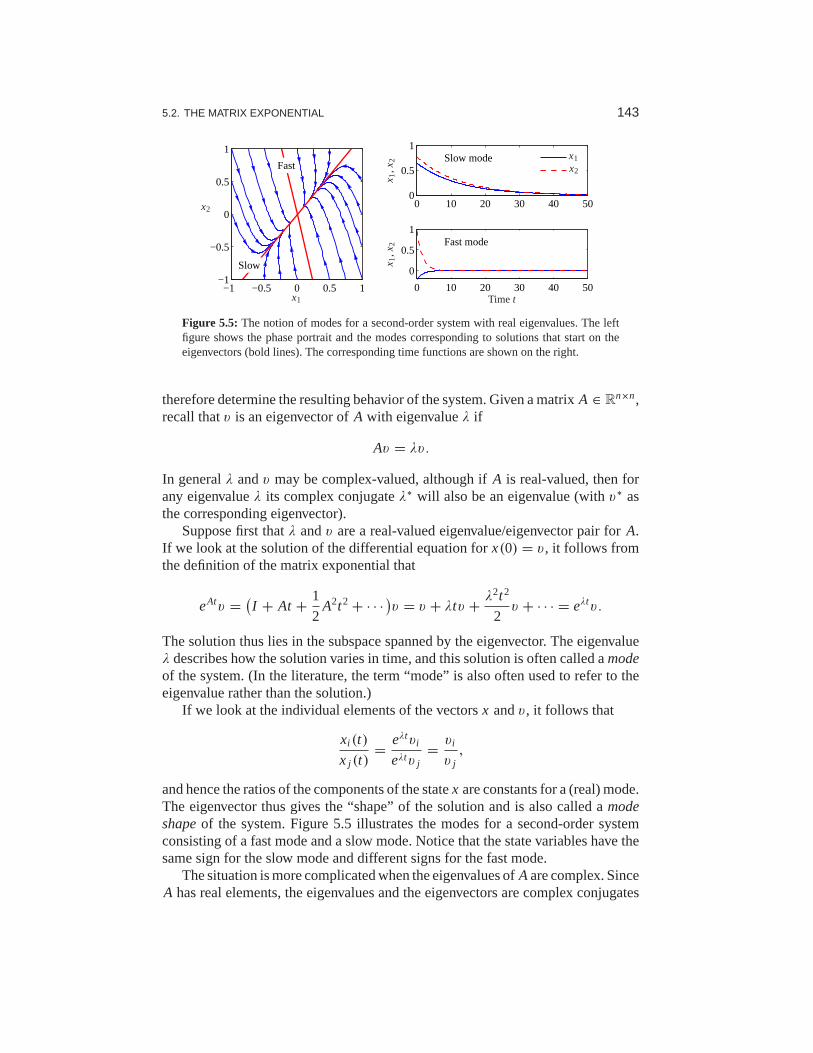
5.2. THE MATRIX EXPONENTIAL 143
−1 −0.5 0 0.5 1−1
−0.5
0
0.5
1
Fast
Slow
x1
x20 10 20 30 40 50
0
0.5
1Slow mode
0 10 20 30 40 50
0
0.5
1Fast mode
x 1,x
2x 1
,x2 x1
x2
Time t
Figure 5.5: The notion of modes for a second-order system with real eigenvalues.The leftfigure shows the phase portrait and the modes corresponding to solutions that start on theeigenvectors (bold lines). The corresponding time functions are shownon the right.
therefore determine the resulting behavior of the system. Given a matrixA ∈ Rn×n,
recall thatv is an eigenvector ofA with eigenvalueλ if
Av = λv.
In generalλ andv may be complex-valued, although ifA is real-valued, then forany eigenvalueλ its complex conjugateλ∗ will also be an eigenvalue (withv∗ asthe corresponding eigenvector).
Suppose first thatλ andv are a real-valued eigenvalue/eigenvector pair forA.If we look at the solution of the differential equation forx(0) = v, it follows fromthe definition of the matrix exponential that
eAtv =(I + At + 1
2A2t2 + · · ·
)v = v + λtv + λ2t2
2v + · · · = eλtv.
The solution thus lies in the subspace spanned by the eigenvector. The eigenvalueλ describes how the solution varies in time, and this solutionis often called amodeof the system. (In the literature, the term “mode” is also often used to refer to theeigenvalue rather than the solution.)
If we look at the individual elements of the vectorsx andv, it follows that
xi (t)
x j (t)= eλtvi
eλtv j= vi
v j,
and hence the ratios of the components of the statex are constants for a (real) mode.The eigenvector thus gives the “shape” of the solution and is also called amodeshapeof the system. Figure 5.5 illustrates the modes for a second-order systemconsisting of a fast mode and a slow mode. Notice that the state variables have thesame sign for the slow mode and different signs for the fast mode.
The situation is more complicated when the eigenvalues ofAare complex. SinceA has real elements, the eigenvalues and the eigenvectors arecomplex conjugates

144 CHAPTER 5. LINEAR SYSTEMS
λ = σ ± iω andv = u ± iw, which implies that
u = v + v∗
2, w = v − v∗
2i.
Making use of the matrix exponential, we have
eAtv = eλt(u + iw) = eσ t((u cosωt − w sinωt)+ i (u sinωt + w cosωt)
),
from which it follows that
eAtu = 1
2
(eAtv + eAtv∗
)= ueσ t cosωt − weσ t sinωt,
eAtw = 1
2i
(eAtv − eAtv∗
)= ueσ t sinωt + weσ t cosωt .
A solution with initial conditions in the subspace spanned by the real partu andimaginary partw of the eigenvector will thus remain in that subspace. The solutionwill be a logarithmic spiral characterized byσ andω. We again call the solutioncorresponding toλ a mode of the system, andv the mode shape.
If a matrix A hasn distinct eigenvaluesλ1, . . . , λn, then the initial conditionresponse can be written as a linear combination of the modes.To see this, supposefor simplicity that we have all real eigenvalues with corresponding unit eigenvectorsv1, . . . , vn. From linear algebra, these eigenvectors are linearly independent, andwe can write the initial conditionx(0) as
x(0) = α1v1 + α2v2 + · · · + αnvn.
Using linearity, the initial condition response can be written as
x(t) = α1eλ1tv1 + α2eλ2tv2 + · · · + αneλntvn.
Thus, the response is a linear combination of the modes of the system, with theamplitude of the individual modes growing or decaying aseλi t . The case for distinctcomplex eigenvalues follows similarly (the case for nondistinct eigenvalues is moresubtle and requires making use of the Jordan form discussed in the previous section).
Example 5.5 Coupled spring–mass systemConsider the spring–mass system shown in Figure 5.4, but withthe addition ofdampers on each mass. The equations of motion of the system are
mq1 = −2kq1 − cq1 + kq2, mq2 = kq1 − 2kq2 − cq2.
In state space form, we define the state to bex = (q1,q2, q1, q2), and we can rewritethe equations as
dx
dt=
0 0 1 00 0 0 1
−2k
m
k
m− c
m0
k
m−2k
m0 − c
m
x.

5.3. INPUT/OUTPUT RESPONSE 145
We now define a transformationz = T x that puts this system into a simpler form.Let z1 = 1
2(q1 + q2), z2 = z1, z3 = 12(q1 − q2) andz4 = z3, so that
z = T x = 1
2
1 1 0 00 0 1 11 −1 0 00 0 1 −1
x.
In the new coordinates, the dynamics become
dz
dt=
0 1 0 0
− k
m− c
m0 0
0 0 0 1
0 0 −3k
m− c
m
z,
and we see that the system is in block diagonal (ormodal) form.In the z coordinates, the statesz1 andz2 parameterize one mode with eigen-
valuesλ ≈ c/(2√
km) ± i√
k/m, and the statesz3 and z4 another mode withλ ≈ c/(2
√3km) ± i
√3k/m. From the form of the transformationT we see that
these modes correspond exactly to the modes in Figure 5.4, in whichq1 andq2 moveeither toward or against each other. The real and imaginary parts of the eigenvaluesgive the decay ratesσ and frequenciesω for each mode. ∇
5.3 Input/Output Response
In the previous section we saw how to compute the initial condition response usingthe matrix exponential. In this section we derive the convolution equation, whichincludes the inputs and outputs as well.
The Convolution Equation
We return to the general input/output case in equation (5.3), repeated here:
dx
dt= Ax + Bu, y = Cx + Du. (5.13)
Using the matrix exponential, the solution to equation (5.13) can be written asfollows.
Theorem 5.4. The solution to the linear differential equation(5.13)is given by
x(t) = eAtx(0)+∫ t
0eA(t−τ)Bu(τ )dτ. (5.14)
Proof. To prove this, we differentiate both sides and use the property (5.8) of thematrix exponential. This gives
dx
dt= AeAtx(0)+
∫ t
0AeA(t−τ)Bu(τ )dτ + Bu(t) = Ax + Bu,

146 CHAPTER 5. LINEAR SYSTEMS
0 2 4 6 8 100
0.5
1
1.5
u
Time t(a) Pulse and impulse functions
0 10 20 30 400
0.5
1
t
y
Pulse responsesImpulse response
(b) Pulse and impulse responses
Figure 5.6: Pulse response and impulse response. (a) The rectangles show pulses of width5, 2.5 and 0.8, each with total area equal to 1. The arrow denotes an impulseδ(t) definedby equation (5.17). The corresponding pulse responses for a linearsystem with eigenvaluesλ = {−0.08,−0.62} are shown in (b) as dashed lines. The solid line is the true impulseresponse, which is well approximated by a pulse of duration 0.8.
which proves the result. Notice that the calculation is essentially the same as forproving the result for a first-order equation.
It follows from equations (5.13) and (5.14) that the input/output relation for alinear system is given by
y(t) = CeAtx(0)+∫ t
0CeA(t−τ)Bu(τ )dτ + Du(t). (5.15)
It is easy to see from this equation that the output is jointlylinear in both theinitial conditions and the input, which follows from the linearity of matrix/vectormultiplication and integration.
Equation (5.15) is called theconvolution equation, and it represents the generalform of the solution of a system of coupled linear differential equations. We seeimmediately that the dynamics of the system, as characterized by the matrixA, playa critical role in both the stability and performance of the system. Indeed, the matrixexponential describesbothwhat happens when we perturb the initial condition andhow the system responds to inputs.
Another interpretation of the convolution equation can be given using the concept�of the impulse responseof a system. Consider the application of an input signalu(t) given by the following equation:
u(t) = pǫ(t) =
0 t < 0
1/ǫ 0 ≤ t < ǫ
0 t ≥ ǫ.
(5.16)
This signal is apulseof durationǫ and amplitude 1/ǫ, as illustrated in Figure 5.6a.We define animpulseδ(t) to be the limit of this signal asǫ → 0:
δ(t) = limǫ→0
pǫ(t). (5.17)

5.3. INPUT/OUTPUT RESPONSE 147
This signal, sometimes called adelta function,is not physically achievable butprovides a convenient abstraction in understanding the response of a system. Notethat the integral of an impulse is 1:
∫ t
0δ(τ )dτ =
∫ t
0limǫ→0
pǫ(t)dτ = limǫ→0
∫ t
0pǫ(t)dτ
= limǫ→0
∫ ǫ
01/ǫ dτ = 1 t > 0.
In particular, the integral of an impulse over an arbitrarily short period of time isidentically 1.
We define theimpulse responseof a systemh(t) to be the output correspondingto having an impulse as its input:
h(t) =∫ t
0CeA(t−τ)Bδ(τ )dτ = CeAt B, (5.18)
where the second equality follows from the fact thatδ(t) is zero everywhere exceptthe origin and its integral is identically 1. We can now writethe convolution equationin terms of the initial condition response, the convolutionof the impulse responseand the input signal, and the direct term:
y(t) = CeAtx(0)+∫ t
0h(t − τ)u(τ )dτ + Du(t). (5.19)
One interpretation of this equation, explored in Exercise 5.2, is that the responseof the linear system is the superposition of the response to an infinite set of shiftedimpulses whose magnitudes are given by the inputu(t). This is essentially theargument used in analyzing Figure 5.2 and deriving equation (5.5). Note that thesecond term in equation (5.19) is identical to equation (5.5), and it can be shown thatthe impulse response is formally equivalent to the derivative of the step response.
The use of pulses as approximations of the impulse function also provides amechanism for identifying the dynamics of a system from data. Figure 5.6b showsthe pulse responses of a system for different pulse widths. Notice that the pulseresponses approach the impulse response as the pulse width goes to zero. As ageneral rule, if the fastest eigenvalue of a stable system has real part−σmax, then apulse of lengthǫ will provide a good estimate of the impulse response ifǫσmax ≪ 1.Note that for Figure 5.6, a pulse width ofǫ = 1 s givesǫσmax = 0.62 and the pulseresponse is already close to the impulse response.
Coordinate Invariance
The components of the input vectoru and the output vectory are given by the choseninputs and outputs of a model, but the state variables dependon the coordinate framechosen to represent the state. This choice of coordinates affects the values of thematricesA, B andC that are used in the model. (The direct termD is not affectedsince it maps inputs to outputs.) We now investigate some of the consequences ofchanging coordinate systems.

148 CHAPTER 5. LINEAR SYSTEMS
m m
k k
u(t) = sin tωk
c c
q1 q2
Figure 5.7:Coupled spring mass system. Each mass is connected to two springs with stiffnessk and a viscous damper with damping coefficientc. The mass on the right is drive through aspring connected to a sinusoidally varying attachment.
Introduce new coordinatesz by the transformationz = T x, whereT is aninvertible matrix. It follows from equation (5.3) that
dz
dt= T(Ax + Bu) = T AT−1z + T Bu =: Az+ Bu,
y = Cx + Du = CT−1z + Du =: Cz+ Du.
The transformed system has the same form as equation (5.3), but the matricesA,B andC are different:
A = T AT−1, B = T B, C = CT−1. (5.20)
There are often special choices of coordinate systems that allow us to see a particularproperty of the system, hence coordinate transformations can be used to gain newinsight into the dynamics.
We can also compare the solution of the system in transformedcoordinates tothat in the original state coordinates. We make use of an important property of theexponential map,
eT ST−1 = T eST−1,
which can be verified by substitution in the definition of the matrix exponential.Using this property, it is easy to show that
x(t) = T−1z(t) = T−1eAtT x(0)+ T−1∫ t
0eA(t−τ) Bu(τ )dτ.
From this form of the equation, we see that if it is possible to transformA intoa form A for which the matrix exponential is easy to compute, we can use thatcomputation to solve the general convolution equation for the untransformed statex by simple matrix multiplications. This technique is illustrated in the followingexample.
Example 5.6 Coupled spring–mass systemConsider the coupled spring–mass system shown in Figure 5.7.The input to thissystem is the sinusoidal motion of the end of the rightmost spring, and the outputis the position of each mass,q1 andq2. The equations of motion are given by
mq1 = −2kq1 − cq1 + kq2, mq2 = kq1 − 2kq2 − cq2 + ku.

5.3. INPUT/OUTPUT RESPONSE 149
In state space form, we define the state to bex = (q1,q2, q1, q2), and we can rewritethe equations as
dx
dt=
0 0 1 00 0 0 1
−2k
m
k
m− c
m0
k
m−2k
m0 − c
m
x +
00
0
k
m
u.
This is a coupled set of four differential equations and is quite complicated to solvein analytical form.
The dynamics matrix is the same as in Example 5.5, and we can use the coor-dinate transformation defined there to put the system in modalform:
dz
dt=
0 1 0 0
− k
m− c
m0 0
0 0 0 1
0 0 −3k
m− c
m
z +
0k
2m0
− k
2m
u.
Note that the resulting matrix equations are block diagonaland hence decoupled.We can solve for the solutions by computing the solutions of two sets of second-order systems represented by the states(z1, z2) and(z3, z4). Indeed, the functionalform of each set of equations is identical to that of a single spring–mass system.(The explicit solution is derived in Section 6.3.)
Once we have solved the two sets of independent second-orderequations, wecan recover the dynamics in the original coordinates by inverting the state transfor-mation and writingx = T−1z. We can also determine the stability of the systemby looking at the stability of the independent second-ordersystems. ∇
Steady-State Response
Given a linear input/output system
dx
dt= Ax + Bu, y = Cx + Du, (5.21)
the general form of the solution to equation (5.21) is given by the convolutionequation:
y(t) = CeAtx(0)+∫ t
0CeA(t−τ)Bu(τ )dτ + Du(t).
We see from the form of this equation that the solution consists of an initial conditionresponse and an input response.
The input response, corresponding to the last two terms in theequation above,itself consists of two components—thetransient responseand thesteady-state
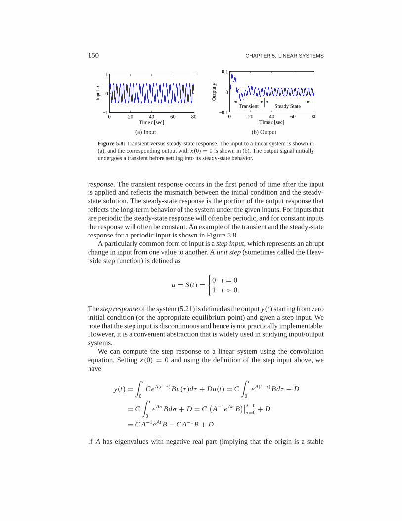
150 CHAPTER 5. LINEAR SYSTEMS
0 20 40 60 80−1
0
1
Time t [sec]
Inpu
t u
(a) Input
0 20 40 60 80−0.1
0
0.1
Transient Steady State
Time t [sec]
Out
put y
(b) Output
Figure 5.8: Transient versus steady-state response. The input to a linear system isshown in(a), and the corresponding output withx(0) = 0 is shown in (b). The output signal initiallyundergoes a transient before settling into its steady-state behavior.
response. The transient response occurs in the first period of time afterthe inputis applied and reflects the mismatch between the initial condition and the steady-state solution. The steady-state response is the portion of the output response thatreflects the long-term behavior of the system under the given inputs. For inputs thatare periodic the steady-state response will often be periodic, and for constant inputsthe response will often be constant. An example of the transient and the steady-stateresponse for a periodic input is shown in Figure 5.8.
A particularly common form of input is astep input, which represents an abruptchange in input from one value to another. Aunit step(sometimes called the Heav-iside step function) is defined as
u = S(t) ={
0 t = 0
1 t > 0.
Thestep responseof the system (5.21) is defined as the outputy(t)starting from zeroinitial condition (or the appropriate equilibrium point) and given a step input. Wenote that the step input is discontinuous and hence is not practically implementable.However, it is a convenient abstraction that is widely used in studying input/outputsystems.
We can compute the step response to a linear system using the convolutionequation. Settingx(0) = 0 and using the definition of the step input above, wehave
y(t) =∫ t
0CeA(t−τ)Bu(τ )dτ + Du(t) = C
∫ t
0eA(t−τ)Bdτ + D
= C∫ t
0eAσ Bdσ + D = C
(A−1eAσ B
)∣∣σ=t
σ=0 + D
= C A−1eAt B − C A−1B + D.
If A has eigenvalues with negative real part (implying that the origin is a stable

5.3. INPUT/OUTPUT RESPONSE 151
0 5 10 15 20 25 300
0.5
1
1.5
2
Time [sec]
Out
put
Rise timeTr
Settling timeTs
OvershootMp
Steady-state valueyss
Figure 5.9: Sample step response. The rise time, overshoot, settling time and steady-statevalue give the key performance properties of the signal.
equilibrium point in the absence of any input), then we can rewrite the solution as
y(t) = C A−1eAt B︸ ︷︷ ︸transient
+ D − C A−1B︸ ︷︷ ︸steady-state
, t > 0. (5.22)
The first term is the transient response and decays to zero ast → ∞. The secondterm is the steady-state response and represents the value of the output for largetime.
A sample step response is shown in Figure 5.9. Several terms areused whenreferring to a step response. Thesteady-state value yss of a step response is thefinal level of the output, assuming it converges. Therise time Tr is the amount oftime required for the signal to go from 10% of its final value to 90% of its finalvalue. It is possible to define other limits as well, but in thisbook we shall use thesepercentages unless otherwise indicated. Theovershoot Mp is the percentage of thefinal value by which the signal initially rises above the final value. This usuallyassumes that future values of the signal do not overshoot thefinal value by morethan this initial transient, otherwise the term can be ambiguous. Finally, thesettlingtime Ts is the amount of time required for the signal to stay within 2%of its finalvalue for all future times. The settling time is also sometimes defined as reaching 1%or 5% of the final value (see Exercise 5.7). In general these performance measurescan depend on the amplitude of the input step, but for linear systems the last threequantities defined above are independent of the size of the step.
Example 5.7 Compartment modelConsider the compartment model illustrated in Figure 5.10 and described in moredetail in Section 3.6. Assume that a drug is administered by constant infusion incompartmentV1 and that the drug has its effect in compartmentV2. To assess howquickly the concentration in the compartment reaches steady state we compute thestep response, which is shown in Figure 5.10b. The step response is quite slow,with a settling time of 39 min. It is possible to obtain the steady-state concentrationmuch faster by having a faster injection rate initially, as shown in Figure 5.10c.The response of the system in this case can be computed by combining two step

152 CHAPTER 5. LINEAR SYSTEMS
k2
V1
k0
b0
u
V2
k1
(a) Schematic
0 20 400
1
2
0 20 400
0.2
0.4
Time t [min]
Inpu
t dos
age
Con
cent
ratio
nC2
(b) Step input
0 20 400
1
2
0 20 400
0.2
0.4
Time t [min]
Inpu
t dos
age
Con
cent
ratio
nC2
(c) Pulse input
Figure 5.10:Response of a compartment model to a constant drug infusion. A simplediagramof the system is shown in (a). The step response (b) shows the rate of concentration buildupin compartment 2. In (c) a pulse of initial concentration is used to speed upthe response.
responses (Exercise 5.3). ∇
Another common input signal to a linear system is a sinusoid (or a combinationof sinusoids). Thefrequency responseof an input/output system measures the way inwhich the system responds to a sinusoidal excitation on one of its inputs. As we havealready seen for scalar systems, the particular solution associated with a sinusoidalexcitation is itself a sinusoid at the same frequency. Hencewe can compare themagnitude and phase of the output sinusoid to the input. Moregenerally, if a systemhas a sinusoidal output response at the same frequency as theinput forcing, we canspeak of the frequency response of the system.
To see this in more detail, we must evaluate the convolution equation (5.15) foru = cosωt . This turns out to be a very messy calculation, but we can make use ofthe fact that the system is linear to simplify the derivation. In particular, we notethat
cosωt = 1
2
(eiωt + e−iωt
).
Since the system is linear, it suffices to compute the response of the system to thecomplex inputu(t) = est and we can then reconstruct the input to a sinusoid byaveraging the responses corresponding tos = iω ands = −iω.
Applying the convolution equation to the inputu = est we have
y(t) = CeAtx(0)+∫ t
0CeA(t−τ)Besτdτ + Dest
= CeAtx(0)+ CeAt∫ t
0e(s I−A)τ Bdτ + Dest.
If we assume that none of the eigenvalues ofA are equal tos = ±iω, then the

5.3. INPUT/OUTPUT RESPONSE 153
matrixs I − A is invertible, and we can write
y(t) = CeAtx(0)+ CeAt((s I − A)−1e(s I−A)τ B
)∣∣∣t
0+ Dest
= CeAtx(0)+ CeAt(s I − A)−1(e(s I−A)t − I
)B + Dest
= CeAtx(0)+ C(s I − A)−1estB − CeAt(s I − A)−1B + Dest,
and we obtain
y(t) = CeAt(
x(0)− (s I − A)−1B)
︸ ︷︷ ︸transient
+(C(s I − A)−1B + D
)est
︸ ︷︷ ︸steady-state
. (5.23)
Notice that once again the solution consists of both a transient component and asteady-state component. The transient component decays to zero if the system isasymptotically stable and the steady-state component is proportional to the (com-plex) inputu = est.
We can simplify the form of the solution slightly further by rewriting the steady-state response as
yss(t) = Mei θest = Me(st+i θ),
whereMei θ = C(s I − A)−1B + D (5.24)
andM andθ represent the magnitude and phase of the complex numberC(s I −A)−1B + D. Whens = iω, we say thatM is thegain andθ is thephaseof thesystem at a given forcing frequencyω. Using linearity and combining the solutionsfor s = +iω ands = −iω, we can show that if we have an inputu = Au sin(ωt+ψ)and an outputy = Ay sin(ωt + ϕ), then
gain(ω) = Ay
Au= M, phase(ω) = ϕ − ψ = θ.
The steady-state solution for a sinusoidu = cosωt is now given by
yss(t) = M cos(ωt + θ).
If the phaseθ is positive, we say that the outputleadsthe input, otherwise we sayit lagsthe input.
A sample sinusoidal response is illustrated in Figure 5.11a.The dashed lineshows the input sinusoid, which has amplitude 1. The output sinusoid is shown as asolid line and has a different amplitude plus a shifted phase. The gain is the ratio ofthe amplitudes of the sinusoids, which can be determined by measuring the heightof the peaks. The phase is determined by comparing the ratio ofthe time betweenzero crossings of the input and output to the overall period of the sinusoid:
θ = −2π ·1T
T.

154 CHAPTER 5. LINEAR SYSTEMS
0 5 10 15 20−2
−1
0
1
2
Time [sec]
Inpu
t, ou
tput
Input Output
Au
Ay
1T
T
(a) Input/output response
10−3
10−1
101
Gai
n
0.5 5−270
−180
−90
0
Pha
se [d
eg]
Frequency [rad/s]
(b) Frequency response
Figure 5.11:Response of a linear system to a sinusoid. (a) A sinusoidal input of magnitudeAu (dashed) gives a sinusoidal output of magnitudeAy (solid), delayed by1T seconds. (b)Frequency response, showing gain and phase. The gain is given by the ratio of the outputamplitude to the input amplitude,M = Ay/Au. The phase lag is given byθ = −2π1T/T ;it is negative for the case shown because the output lags the input.
A convenient way to view the frequency response is to plot howthe gain andphase in equation (5.24) depend onω (throughs = iω). Figure 5.11b shows anexample of this type of representation.
Example 5.8 Active band-pass filterConsider the op amp circuit shown in Figure 5.12a. We can derive the dynamics ofthe system by writing thenodal equations, which state that the sum of the currentsat any node must be zero. Assuming thatv− = v+ = 0, as we did in Section 3.3,we have
0 = v1 − v2
R1− C1
dv2
dt, 0 = C1
dv2
dt+ v3
R2+ C2
dv3
dt.
Choosingv2 andv3 as our states and using these equations, we obtain
dv2
dt= v1 − v2
R1C1,
dv3
dt= −v3
R2C2− v1 − v2
R1C2.
Rewriting these in linear state space form, we obtain
dx
dt=
− 1
R1C10
1
R1C2− 1
R2C2
x +
1
R1C1
−1
R1C2
u, y =0 1
x, (5.25)
wherex = (v2, v3), u = v1 andy = v3.The frequency response for the system can be computed using equation (5.24):
Mej θ = C(s I − A)−1B + D = − R2
R1
R1C1s
(1 + R1C1s)(1 + R2C2s), s = iω.
The magnitude and phase are plotted in Figure 5.12b forR1 = 100�, R2 = 5 k�and C1 = C2 = 100 µF. We see that the circuit passes through signals with

5.3. INPUT/OUTPUT RESPONSE 155
−
+v1
v3
R1 C1
C2
R2
v2
(a) Circuit diagram
10−1
100
Gai
n
10−1
100
101
102
103
−360−270−180−90
0
Pha
se [d
eg]
Frequency [rad/s]
(b) Frequency response
Figure 5.12:Active band-pass filter. The circuit diagram (a) shows an op amp with twoRCfilters arranged to provide a band-pass filter. The plot in (b) shows the gain and phase of thefilter as a function of frequency. Note that the phase starts at -90◦ due to the negative gain ofthe operational amplifier.
frequencies at about 10 rad/s, but attenuates frequencies below 5 rad/s and above50 rad/s. At 0.1 rad/s the input signal is attenuated by 20× (0.05). This type ofcircuit is called aband-pass filtersince it passes through signals in the band offrequencies between 5 and 50 rad/s. ∇
As in the case of the step response, a number of standard properties are definedfor frequency responses. The gain of a system atω = 0 is called thezero frequencygainand corresponds to the ratio between a constant input and thesteady output:
M0 = −C A−1B + D.
The zero frequency gain is well defined only ifA is invertible (and, in particular, ifit does not have eigenvalues at 0). It is also important to note that the zero frequencygain is a relevant quantity only when a system is stable aboutthe correspondingequilibrium point. So, if we apply a constant inputu = r , then the correspondingequilibrium pointxe = −A−1Br must be stable in order to talk about the zerofrequency gain. (In electrical engineering, the zero frequency gain is often calledtheDC gain. DC stands for direct current and reflects the common separation ofsignals in electrical engineering into a direct current (zero frequency) term and analternating current (AC) term.)
Thebandwidthωb of a system is the frequency range over which the gain hasdecreased by no more than a factor of 1/
√2 from its reference value. For systems
with nonzero, finite zero frequency gain, the bandwidth is thefrequency wherethe gain has decreased by 1/
√2 from the zero frequency gain. For systems that
attenuate low frequencies but pass through high frequencies, the reference gainis taken as the high-frequency gain. For a system such as the band-pass filter inExample 5.8, bandwidth is defined as the range of frequencies where the gain islarger than 1/
√2 of the gain at the center of the band. (For Example 5.8 this would
give a bandwidth of approximately 50 rad/s.)

156 CHAPTER 5. LINEAR SYSTEMS
Amplifier Amplifier
Sample
Cantilever
x,y z
LaserPhotodiode
Controller
Piezodrive
Deflection reference
Sweepgenerator
(a) AFM block diagram
10−1
101
Gai
n
104
105
106
107
−180
−90
0
Pha
se [d
eg]
Frequency [rad/s]
Mr1Mr2
ω=ωr1 ω=ωr2
(b) Frequency response
Figure 5.13:AFM frequency response. (a) A block diagram for the vertical dynamics of anatomic force microscope in contact mode. The plot in (b) shows the gain and phase for thepiezo stack. The response contains two frequency peaks at resonances of the system, alongwith an antiresonance atω = 268 krad/s. The combination of a resonant peak followed byan antiresonance is common for systems with multiple lightly damped modes.
Another important property of the frequency response is theresonant peakMr , the largest value of the frequency response, and thepeak frequencyωmr, thefrequency where the maximum occurs. These two properties describe the frequencyof the sinusoidal input that produces the largest possible output and the gain at thefrequency.
Example 5.9 Atomic force microscope in contact modeConsider the model for the vertical dynamics of the atomic force microscope incontact mode, discussed in Section 3.5. The basic dynamics aregiven by equa-tion (3.23). The piezo stack can be modeled by a second-order system with un-damped natural frequencyω3 and damping ratioζ3. The dynamics are then de-scribed by the linear system
dx
dt=
0 1 0 0−k2/(m1 + m2) −c2/(m1 + m2) 1/m2 0
0 0 0 ω3
0 0 −ω3 −2ζ3ω3
x +
000ω3
u,
y = m2
m1 + m2
m1k2
m1 + m2
m1c2
m1 + m21 0
x,
where the input signal is the drive signal to the amplifier and the output is the elon-gation of the piezo. The frequency response of the system is shown in Figure 5.13b.The zero frequency gain of the system isM0 = 1. There are two resonant poles withpeaksMr 1 = 2.12 atωmr1 = 238 krad/s andMr 2 = 4.29 atωmr2 = 746 krad/s.The bandwidth of the system, defined as the lowest frequency where the gain is√
2 less than the zero frequency gain, isωb = 292 krad/s. There is also a dip inthe gainMd = 0.556 forωmd = 268 krad/s. This dip, called anantiresonance, isassociated with a dip in the phase and limits the performancewhen the system iscontrolled by simple controllers, as we will see in Chapter 10. ∇

5.3. INPUT/OUTPUT RESPONSE 157
Sampling
It is often convenient to use both differential and difference equations in modelingand control. For linear systems it is straightforward to transform from one to theother. Consider the general linear system described by equation (5.13) and assumethat the control signal is constant over a sampling intervalof constant lengthh. Itfollows from equation (5.14) of Theorem 5.4 that
x(t + h) = eAhx(t)+∫ t+h
teA(t+h−τ)Bu(k)dτ = 8x(t)+ Ŵu(t), (5.26)
where we have assumed that the discontinuous control signalis continuous fromthe right. The behavior of the system at the sampling timest = kh is described bythe difference equation
x[k + 1] = 8x[k] + Ŵu[k], y[k] = Cx[k] + Du[k]. (5.27)
Notice that the difference equation (5.27) is an exact representation of the behaviorof the system at the sampling instants. Similar expressions can also be obtained ifthe control signal is linear over the sampling interval.
The transformation from (5.26) to (5.27) is calledsampling. The relations be-tween the system matrices in the continuous and sampled representations are asfollows:
8 = eAh, Ŵ =(∫ h
0eAs ds
)B; A = 1
hlog8, B =
(∫ h
0eAs ds
)−1Ŵ.
(5.28)Notice that ifA is invertible, we have
Ŵ = A−1(eAh − I
)B.
All continuous-time systems can be sampled to obtain a discrete-time version,but there are discrete-time systems that do not have a continuous-time equivalent.The precise condition is that the matrix8 cannot have real eigenvalues on thenegative real axis.
Example 5.10 IBM Lotus serverIn Example 2.4 we described how the dynamics of an IBM Lotus server wereobtained as the discrete-time system
y[k + 1] = ay[k] + bu[k],
wherea = 0.43, b = 0.47 and the sampling period ish = 60 s. A differentialequation model is needed if we would like to design control systems based oncontinuous-time theory. Such a model is obtained by applyingequation (5.28);hence
A = loga
h= −0.0141, B =
(∫ h
0eAt dt
)−1b = 0.0116,
and we find that the difference equation can be interpreted as asampled version of

158 CHAPTER 5. LINEAR SYSTEMS
the ordinary differential equation
dx
dt= −0.0141x + 0.0116u.
∇
5.4 Linearization
As described at the beginning of the chapter, a common sourceof linear systemmodels is through the approximation of a nonlinear system bya linear one. Theseapproximations are aimed at studying the local behavior of asystem, where thenonlinear effects are expected to be small. In this section we discuss how to locallyapproximate a system by its linearization and what can be said about the approxi-mation in terms of stability. We begin with an illustration of the basic concept usingthe cruise control example from Chapter 3.
Example 5.11 Cruise controlThe dynamics for the cruise control system were derived in Section 3.1 and havethe form
mdv
dt= αnuT(αnv)− mgCr sgn(v)− 1
2ρCv Av2 − mgsinθ, (5.29)
where the first term on the right-hand side of the equation is the force generatedby the engine and the remaining three terms are the rolling friction, aerodynamicdrag and gravitational disturbance force. There is an equilibrium (ve,ue) when theforce applied by the engine balances the disturbance forces.
To explore the behavior of the system near the equilibrium wewill linearize thesystem. A Taylor series expansion of equation (5.29) aroundthe equilibrium gives
d(v − ve)
dt= a(v − ve)− bg(θ − θe)+ b(u − ue)+ higher order terms, (5.30)
where
a = ueα2nT ′(αnve)− ρCv Ave
m, bg = g cosθe, b = αnT(αnve)
m. (5.31)
Notice that the term corresponding to rolling friction disappears ifv 6= 0. For a carin fourth gear withve = 25 m/s,θe = 0 and the numerical values for the car fromSection 3.1, the equilibrium value for the throttle isue = 0.1687 and the parametersarea = −0.0101,b = 1.32 andc = 9.8. This linear model describes how smallperturbations in the velocity about the nominal speed evolve in time.
Figure 5.14 shows a simulation of a cruise controller with linear and nonlinearmodels; the differences between the linear and nonlinear models are small, andhence the linearized model provides a reasonable approximation. ∇

5.4. LINEARIZATION 159
gF
mg
F
θ
0 10 20 30
19
19.5
20
20.5
Vel
ocity
v [m
/s]
NonlinearLinear
0 10 20 300
0.5
1
Time t [s]
Thr
ottle
u
Figure 5.14:Simulated response of a vehicle with PI cruise control as it climbs a hill with aslope of 4◦. The solid line is the simulation based on a nonlinear model, and the dashed lineshows the corresponding simulation using a linear model. The controller gains arekp = 0.5andki = 0.1.
Jacobian Linearization Around an Equilibrium Point
To proceed more formally, consider a single-input, single-output nonlinear system
dx
dt= f (x,u), x ∈ R
n,u ∈ R,
y = h(x,u), y ∈ R,
(5.32)
with an equilibrium point atx = xe, u = ue. Without loss of generality we canassume thatxe = 0 andue = 0, although initially we will consider the general caseto make the shift of coordinates explicit.
To study thelocal behavior of the system around the equilibrium point(xe,ue),we suppose thatx − xe andu − ue are both small, so that nonlinear perturbationsaround this equilibrium point can be ignored compared with the (lower-order) linearterms. This is roughly the same type of argument that is used when we do small-angle approximations, replacing sinθ with θ and cosθ with 1 for θ near zero.
As we did in Chapter 4, we define a new set of state variablesz, as well as inputsv and outputsw:
z = x − xe, v = u − ue, w = y − h(xe,ue).
These variables are all close to zero when we are near the equilibrium point, and soin these variables the nonlinear terms can be thought of as the higher-order terms ina Taylor series expansion of the relevant vector fields (assuming for now that theseexist).
Formally, theJacobian linearizationof the nonlinear system (5.32) is
dz
dt= Az+ Bv, w = Cz+ Dv, (5.33)
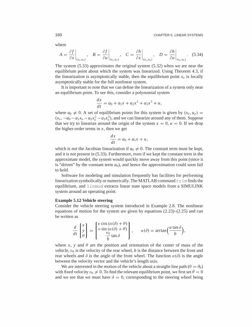
160 CHAPTER 5. LINEAR SYSTEMS
where
A = ∂ f
∂x
∣∣∣∣(xe,ue)
, B = ∂ f
∂u
∣∣∣∣(xe,ue)
, C = ∂h
∂x
∣∣∣∣(xe,ue)
, D = ∂h
∂u
∣∣∣∣(xe,ue)
. (5.34)
The system (5.33) approximates the original system (5.32) when we are near theequilibrium point about which the system was linearized. Using Theorem 4.3, ifthe linearization is asymptotically stable, then the equilibrium point xe is locallyasymptotically stable for the full nonlinear system.
It is important to note that we can define the linearization of asystem only nearan equilibrium point. To see this, consider a polynomial system
dx
dt= a0 + a1x + a2x2 + a3x3 + u,
wherea0 6= 0. A set of equilibrium points for this system is given by(xe,ue) =(xe,−a0 −a1xe−a2x2
e −a3x3e), and we can linearize around any of them. Suppose
that we try to linearize around the origin of the systemx = 0, u = 0. If we dropthe higher-order terms inx, then we get
dx
dt= a0 + a1x + u,
which isnot the Jacobian linearization ifa0 6= 0. The constant term must be kept,and it is not present in (5.33). Furthermore, even if we kept the constant term in theapproximate model, the system would quickly move away from this point (since itis “driven” by the constant terma0), and hence the approximation could soon failto hold.
Software for modeling and simulation frequently has facilities for performinglinearization symbolically or numerically. The MATLAB commandtrim finds theequilibrium, andlinmod extracts linear state space models from a SIMULINKsystem around an operating point.
Example 5.12 Vehicle steeringConsider the vehicle steering system introduced in Example 2.8. The nonlinearequations of motion for the system are given by equations (2.23)–(2.25) and canbe written as
d
dt
xyθ
=
v cos(α(δ)+ θ)
v sin(α(δ)+ θ)v0
btanδ
, α(δ) = arctan
(a tanδ
b
),
wherex, y and θ are the position and orientation of the center of mass of thevehicle,v0 is the velocity of the rear wheel,b is the distance between the front andrear wheels andδ is the angle of the front wheel. The functionα(δ) is the anglebetween the velocity vector and the vehicle’s length axis.
We are interested in the motion of the vehicle about a straight-line path (θ = θ0)with fixed velocityv0 6= 0. To find the relevant equilibrium point, we first setθ = 0and we see that we must haveδ = 0, corresponding to the steering wheel being

5.4. LINEARIZATION 161
straight. This also yieldsα = 0. Looking at the first two equations in the dynamics,we see that the motion in thexy direction is by definitionnot at equilibrium sinceξ2 + η2 = v2
0 6= 0. Therefore we cannot formally linearize the full model.Suppose instead that we are concerned with the lateral deviation of the vehicle
from a straight line. For simplicity, we letθe = 0, which corresponds to drivingalong thex axis. We can then focus on the equations of motion in they andθdirections. With some abuse of notation we introduce the state x = (y, θ) andu = δ. The system is then in standard form with
f (x,u) =
v sin(α(u)+ x2)
v0
btanu
, α(u) = arctan
(a tanu
b
), h(x,u) = x1.
The equilibrium point of interest is given byx = (0,0) andu = 0. To compute thelinearized model around this equilibrium point, we make useof the formulas (5.34).A straightforward calculation yields
A = ∂ f
∂x
∣∣∣∣ x=0u=0
=0 v0
0 0
, B = ∂ f
∂u
∣∣∣∣ x=0u=0
=av0/bv0/b
,
C = ∂h
∂x
∣∣∣∣ x=0u=0
=1 0
, D = ∂h
∂u
∣∣∣∣ x=0u=0
= 0,
and the linearized system
dx
dt= Ax + Bu, y = Cx + Du (5.35)
thus provides an approximation to the original nonlinear dynamics.The linearized model can be simplified further by introducing normalized vari-
ables, as discussed in Section 2.3. For this system, we choosethe wheel basebas the length unit and the unit as the time required to travel awheel base. Thenormalized state is thusz = (x1/b, x2), and the new time variable isτ = v0t/b.The model (5.35) then becomes
dz
dτ=z2 + γu
u
=
0 1
0 0
z +
γ1
u, y =
1 0
z, (5.36)
whereγ = a/b. The normalized linear model for vehicle steering with nonslippingwheels is thus a linear system with only one parameter. ∇
Feedback Linearization
Another type of linearization is the use of feedback to convert the dynamics of anonlinear system into those of a linear one. We illustrate the basic idea with anexample.
Example 5.13 Cruise controlConsider again the cruise control system from Example 5.11, whose dynamics are

162 CHAPTER 5. LINEAR SYSTEMS
e uLinearController
−1
6
vα(x,v)
y
ProcessNonlinear
Linearized dynamics
r
Figure 5.15:Feedback linearization. A nonlinear feedback of the formu = α(x, v) is usedto modify the dynamics of a nonlinear process so that the response fromthe inputv to theoutputy is linear. A linear controller can then be used to regulate the system’s dynamics.
given in equation (5.29):
mdv
dt= αnuT(αnv)− mgCr sgn(v)− 1
2ρCd Av2 − mgsinθ.
If we chooseu as a feedback law of the form
u = 1
αnT(αnv)
(u′ + mgCr sgn(v)+ 1
2ρCv Av2
), (5.37)
then the resulting dynamics become
mdv
dt= u′ + d, (5.38)
whered = −mgsinθ is the disturbance force due the slope of the road. If wenow define a feedback law foru′ (such as a proportional-integral-derivative [PID]controller), we can use equation (5.37) to compute the final input that should becommanded.
Equation (5.38) is a linear differential equation. We have essentially “inverted”the nonlinearity through the use of the feedback law (5.37).This requires that wehave an accurate measurement of the vehicle velocityv as well as an accuratemodel of the torque characteristics of the engine, gear ratios, drag and frictioncharacteristics and mass of the car. While such a model is notgenerally available(remembering that the parameter values can change), if we design a good feedbacklaw for u′, then we can achieve robustness to these uncertainties. ∇
More generally, we say that a system of the form
dx
dt= f (x,u), y = h(x),
is feedback linearizableif we can find a control lawu = α(x, v) such that theresulting closed loop system is input/output linear with input v and outputy, asshown in Figure 5.15. To fully characterize such systems is beyond the scope ofthis text, but we note that in addition to changes in the input, the general theory alsoallows for (nonlinear) changes in the states that are used todescribe the system,keeping only the input and output variables fixed. More details of this process canbe found in the textbooks by Isidori [Isi95] and Khalil [Kha01].

5.5. FURTHER READING 163
One case that comes up relatively frequently, and is hence worth special mention,�is the set of mechanical systems of the form
M(q)q + C(q, q) = B(q)u.
Here q ∈ Rn is the configuration of the mechanical system,M(q) ∈ R
n×n isthe configuration-dependent inertia matrix,C(q, q) ∈ R
n represents the Coriolisforces and additional nonlinear forces (such as stiffness and friction) andB(q) ∈R
n×p is the input matrix. Ifp = n, then we have the same number of inputs andconfiguration variables, and if we further have thatB(q) is an invertible matrix forall configurationsq, then we can choose
u = B−1(q)(M(q)v − C(q, q)
). (5.39)
The resulting dynamics become
M(q)q = M(q)v =⇒ q = v,
which is a linear system. We can now use the tools of linear system theory toanalyze and design control laws for the linearized system, remembering to applyequation (5.39) to obtain the actual input that will be applied to the system.
This type of control is common in robotics, where it goes by thename ofcomputed torque, and in aircraft flight control, where it is calleddynamic inver-sion. Some modeling tools like Modelica can generate the code for the inversemodel automatically. One caution is that feedback linearization can often cancelout beneficial terms in the natural dynamics, and hence it mustbe used with care.Extensions that do not require complete cancellation of nonlinearities are discussedin Khalil [Kha01] and Krstic et al. [KKK95].
5.5 Further Reading
The majority of the material in this chapter is classical and can be found in mostbooks on dynamics and control theory, including early workson control such asJames, Nichols and Phillips [JNP47] and more recent textbookssuch as Dorf andBishop [DB04], Franklin, Powell and Emami-Naeini [FPEN05] and Ogata [Oga01].An excellent presentation of linear systems based on the matrix exponential isgiven in the book by Brockett [Bro70], a more comprehensive treatment is given byRugh [Rug95] and an elegant mathematical treatment is givenin Sontag [Son98].Material on feedback linearization can be found in books on nonlinear control theorysuch as Isidori [Isi95] and Khalil [Kha01]. The idea of characterizing dynamics byconsidering the responses to step inputs is due to Heaviside, he also introduced anoperator calculus to analyze linear systems. The unit step istherefore also calledtheHeaviside step function. Analysis of linear systems was simplified significantly,but Heaviside’s work was heavily criticized because of lackof mathematical rigor,as described in the biography by Nahin [Nah88]. The difficulties were cleared uplater by the mathematician Laurent Schwartz who developeddistribution theoryin the late 1940s. In engineering, linear systems have traditionally been analyzed
164 CHAPTER 5. LINEAR SYSTEMS
using Laplace transforms as described in Gardner and Barnes [GB42]. Use ofthe matrix exponential started with developments of control theory in the 1960s,strongly stimulated by a textbook by Zadeh and Desoer [ZD63]. Use of matrixtechniques expanded rapidly when the powerful methods of numeric linear algebrawere packaged in programs like LabVIEW, MATLAB and Mathematica.
Exercises
5.1 (Response to the derivative of a signal) Show that ify(t) is the output of alinear system corresponding to inputu(t), then the output corresponding to aninput u(t) is given by y(t). (Hint: Use the definition of the derivative:y(t) =limǫ→0
(y(t + ǫ)− y(t)
)/ǫ.)
5.2(Impulse response and convolution) Show that a signalu(t) can be decomposed�in terms of the impulse functionδ(t) as
u(t) =∫ t
0δ(t − τ)u(τ )dτ
and use this decomposition plus the principle of superposition to show that theresponse of a linear system to an inputu(t) (assuming a zero initial condition) canbe written as
y(t) =∫ t
0h(t − τ)u(τ )dτ,
whereh(t) is the impulse response of the system.
5.3 (Pulse response for a compartment model) Consider the compartment modelgiven in Example 5.7. Compute the step response for the systemand compare itwith Figure 5.10b. Use the principle of superposition to compute the response tothe 5 s pulse input shown in Figure 5.10c. Use the parameter valuesk0 = 0.1,k1 = 0.1, k2 = 0.5 andb0 = 1.5.
5.4(Matrix exponential for second-order system) Assume thatζ < 1 and letωd =ω0
√1 − ζ 2. Show that
exp
−ζω0 ωd
−ωd −ζω0
t =
e−ζω0t cosωdt e−ζω0t sinωdt
−e−ζω0t sinωdt e−ζω0t cosωdt
.
5.5(Lyapunov function for a linear system) Consider a linear systemx = Ax withReλ j < 0 for all eigenvaluesλ j of the matrixA. Show that the matrix
P =∫ ∞
0eAT τ QeAτ dτ
defines a Lyapunov function of the formV(x) = xT Px.
5.6(Nondiagonal Jordan form) Consider a linear system with a Jordan form that isnon-diagonal.

EXERCISES 165
(a) Prove Proposition 5.3 by showing that if the system contains a real eigenvalueλ = 0 with a nontrivial Jordan block, then there exists an initial condition with asolution that grows in time.
(b) Extend this argument to the case of complex eigenvalues with Reλ = 0 by �using the block Jordan form
Ji =
0 ω 1 0−ω 0 0 10 0 0 ω
0 0 −ω 0
.
5.7 (Rise time for a first-order system) Consider a first-order system of the form
τdx
dt= −x + u, y = x.
We say that the parameterτ is thetime constantfor the system since the zero inputsystem approaches the origin ase−t/τ . For a first-order system of this form, showthat the rise time for a step response of the system is approximately 2τ , and that1%, 2%, and 5% settling times approximately corresponds to 4.6τ , 4τ and 3τ .
5.8 (Discrete-time systems) Consider a linear discrete-time system of the form
x[k + 1] = Ax[k] + Bu[k], y[k] = Cx[k] + Du[k].
(a) Show that the general form of the output of a discrete-timelinear system isgiven by the discrete-time convolution equation:
y[k] = C Akx[0] +k−1∑
j =0
C Ak− j −1Bu[ j ] + Du[k].
(b) Show that a discrete-time linear system is asymptotically stable if and only ifall the eigenvalues ofA have a magnitude strictly less than 1.
(c) Let u[k] = sin(ωk) represent an oscillatory input with frequencyω < π (toavoid “aliasing”). Show that the steady-state component of the response has gainM and phaseθ , where
Mei θ = C(eiω I − A)−1B + D.
(d) Show that if we have a nonlinear discrete-time system
x[k] = f (x[k],u[k]), x[k] ∈ Rn, u ∈ R,
y[k] = h(x[k],u[k]), y ∈ R,
then we can linearize the system around an equilibrium point(xe,ue) by definingthe matricesA, B, C andD as in equation (5.34).

166 CHAPTER 5. LINEAR SYSTEMS
5.9 (Keynesian economics) Consider the following simple Keynesian macroeco-nomic model in the form of a linear discrete-time system discussed in Exercise 5.8:
C[t + 1]
I [t + 1]
=
a a
ab− b ab
C[t ]
I [t ]
+
a
ab
G[t ],
Y[t ] = C[t ] + I [t ] + G[t ].
Determine the eigenvalues of the dynamics matrix. When are the magnitudes ofthe eigenvalues less than 1? Assume that the system is in equilibrium with constantvalues capital spendingC, investmentI and government expenditureG. Explorewhat happens when government expenditure increases by 10%.Use the valuesa = 0.25 andb = 0.5.
5.10 Consider a scalar system
dx
dt= 1 − x3 + u.
Compute the equilibrium points for the unforced system (u = 0) and use a Taylorseries expansion around the equilibrium point to compute the linearization. Verifythat this agrees with the linearization in equation (5.33).
5.11(Transcriptional regulation) Consider the dynamics of a genetic circuit that im-plementsself-repression: the protein produced by a gene is a repressor for that gene,thus restricting its own production. Using the models presented in Example 2.13,the dynamics for the system can be written as
dm
dt= α
1 + kp2+ α0 − γm − u,
dp
dt= βm − δp, (5.40)
whereu is a disturbance term that affects RNA transcription andm, p ≥ 0. Findthe equilibrium points for the system and use the linearizeddynamics around eachequilibrium point to determine the local stability of the equilibrium point and thestep response of the system to a disturbance.

Chapter SixState Feedback
Intuitively, the state may be regarded as a kind of information storage or memory or accumula-tion of past causes. We must, of course, demand that the set of internal states6 be sufficientlyrich to carry all information about the past history of6 to predict the effect of the past uponthe future. We do not insist, however, that the state is theleastsuch information although thisis often a convenient assumption.
R. E. Kalman, P. L. Falb and M. A. Arbib,Topics in Mathematical System Theory, 1969 [KFA69].
This chapter describes how the feedback of a system’s state can be used to shapethe local behavior of a system. The concept of reachability isintroduced and usedto investigate how to design the dynamics of a system throughassignment of itseigenvalues. In particular, it will be shown that under certain conditions it is possibleto assign the system eigenvalues arbitrarily by appropriate feedback of the systemstate.
6.1 Reachability
One of the fundamental properties of a control system is whatset of points in thestate space can be reached through the choice of a control input. It turns out that theproperty of reachability is also fundamental in understanding the extent to whichfeedback can be used to design the dynamics of a system.
Definition of Reachability
We begin by disregarding the output measurements of the system and focusing onthe evolution of the state, given by
dx
dt= Ax + Bu, (6.1)
wherex ∈ Rn, u ∈ R, A is ann × n matrix andB a column vector. A fundamental
question is whether it is possible to find control signals so that any point in the statespace can be reached through some choice of input. To study this, we define thereachable setR(x0,≤ T) as the set of all pointsx f such that there exists an inputu(t), 0 ≤ t ≤ T that steers the system fromx(0) = x0 to x(T) = x f , as illustratedin Figure 6.1a.
Definition 6.1 (Reachability). A linear system isreachableif for any x0, x f ∈ Rn
there exists aT > 0 andu : [0, T ] → R such that the corresponding solutionsatisfiesx(0) = x0 andx(T) = x f .

168 CHAPTER 6. STATE FEEDBACK
x(T)
x0R(x0,≤ T)
(a) Reachable set
E
(b) Reachability through control
Figure 6.1:The reachable set for a control system. The setR(x0,≤ T) shown in (a) is the setof points reachable fromx0 in time less thanT . The phase portrait in (b) shows the dynamicsfor a double integrator, with the natural dynamics drawn as horizontal arrows and the controlinputs drawn as vertical arrows. The set of achievable equilibrium pointsis thex axis. Bysetting the control inputs as a function of the state, it is possible to steer the system to theorigin, as shown on the sample path.
The definition of reachability addresses whether it is possible to reach all pointsin the state space in atransientfashion. In many applications, the set of points thatwe are most interested in reaching is the set of equilibrium points of the system(since we can remain at those points once we get there). The setof all possibleequilibria for constant controls is given by
E = {xe : Axe + Bue = 0 for someue ∈ R}.This means that possible equilibria lie in a one- (or possiblyhigher) dimensionalsubspace. If the matrixA is invertible, this subspace is spanned byA−1B.
The following example provides some insight into the possibilities.
Example 6.1 Double integratorConsider a linear system consisting of a double integrator whose dynamics aregiven by
dx1
dt= x2,
dx2
dt= u.
Figure 6.1b shows a phase portrait of the system. The open loop dynamics (u = 0)are shown as horizontal arrows pointed to the right forx2 > 0 and to the left forx2 < 0. The control input is represented by a double-headed arrow in the verticaldirection, corresponding to our ability to set the value ofx2. The set of equilibriumpointsE corresponds to thex1 axis, withue = 0.
Suppose first that we wish to reach the origin from an initial condition (a,0).We can directly move the state up and down in the phase plane, but we must relyon the natural dynamics to control the motion to the left and right. If a > 0, wecan move the origin by first settingu < 0, which will causex2 to become negative.Oncex2 < 0, the value ofx1 will begin to decrease and we will move to the left.After a while, we can setu2 to be positive, movingx2 back toward zero and slowingthe motion in thex1 direction. If we bringx2 > 0, we can move the system state inthe opposite direction.

6.1. REACHABILITY 169
Figure 6.1b shows a sample trajectory bringing the system to the origin. Notethat if we steer the system to an equilibrium point, it is possible to remain thereindefinitely (sincex1 = 0 whenx2 = 0), but if we go to any other point in the statespace, we can pass through the point only in a transient fashion. ∇
To find general conditions under which a linear system is reachable, we willfirst give a heuristic argument based on formal calculations with impulse functions.We note that if we can reach all points in the state space through some choice ofinput, then we can also reach all equilibrium points.
Testing for Reachability
When the initial state is zero, the response of the system to an inputu(t) is givenby
x(t) =∫ t
0eA(t−τ)Bu(τ )dτ. (6.2)
If we choose the input to be a impulse functionδ(t) as defined in Section 5.3, thestate becomes
xδ =∫ t
0eA(t−τ)Bδ(τ )dτ = dxS
dt= eAt B.
(Note that the state changes instantaneously in response tothe impulse.) We canfind the response to the derivative of an impulse function by taking the derivativeof the impulse response (Exercise 5.1):
xδ = dxδdt
= AeAt B.
Continuing this process and using the linearity of the system, the input
u(t) = α1δ(t)+ α2δ(t)+ α3δ(t)+ · · · + αnδ(n−1)(t)
gives the state
x(t) = α1eAt B + α2AeAt B + α3A2eAt B + · · · + αn An−1eAt B.
Taking the limit ast goes to zero through positive values, we get
limt→0+
x(t) = α1B + α2AB + α3A2B + · · · + αn An−1B.
On the right is a linear combination of the columns of the matrix
Wr =B AB · · · An−1B
. (6.3)
To reach an arbitrary point in the state space, we thus require that there aren linearindependent columns of the matrixWr . The matrixWr is called thereachabilitymatrix.
An input consisting of a sum of impulse functions and their derivatives is a veryviolent signal. To see that an arbitrary point can be reachedwith smoother signals

170 CHAPTER 6. STATE FEEDBACK
we can make use of the convolution equation. Assuming that the initial conditionis zero, the state of a linear system is given by
x(t) =∫ t
0eA(t−τ)Bu(τ )dτ =
∫ t
0eAτ Bu(t − τ)dτ.
It follows from the theory of matrix functions, specifically the Cayley–Hamiltontheorem (see Exercise 6.10), that
eAτ = I α0(τ )+ Aα1(τ )+ · · · + An−1αn−1(τ ),
whereαi (τ ) are scalar functions, and we find that
x(t) = B∫ t
0α0(τ )u(t − τ)dτ + AB
∫ t
0α1(τ )u(t − τ)dτ
+ · · · + An−1B∫ t
0αn−1(τ )u(t − τ)dτ.
Again we observe that the right-hand side is a linear combination of the columnsof the reachability matrixWr given by equation (6.3). This basic approach leads tothe following theorem.
Theorem 6.1(Reachability rank condition). A linear system is reachable if andonly if the reachability matrix Wr is invertible.
The formal proof of this theorem is beyond the scope of this text but followsalong the lines of the sketch above and can be found in most books on linearcontrol theory, such as Callier and Desoer [CD91] or Lewis [Lew03]. We illustratethe concept of reachability with the following example.
Example 6.2 Balance systemConsider the balance system introduced in Example 2.1 and shown in Figure 6.2.Recall that this system is a model for a class of examples in which the center of massis balanced above a pivot point. One example is the Segway Personal Transportershown in Figure 6.2a, about which a natural question to ask is whether we can movefrom one stationary point to another by appropriate application of forces throughthe wheels.
The nonlinear equations of motion for the system are given in equation (2.9)and repeated here:
(M + m) p − ml cosθ θ = −cp − ml sinθ θ2 + F,
(J + ml2)θ − ml cosθ p = −γ θ + mglsinθ.(6.4)
For simplicity, we takec = γ = 0. Linearizing around the equilibrium pointxe = (p,0,0,0), the dynamics matrix and the control matrix are
A =
0 0 1 00 0 0 1
0 m2l 2g/µ 0 0
0 Mtmgl/µ 0 0
, B =
00
Jt/µ
lm/µ
,

6.1. REACHABILITY 171
(a) Segway
MF
p
θm
l
(b) Cart-pendulum system
Figure 6.2:Balance system. The Segway Personal Transporter shown in (a) is anexample ofa balance system that uses torque applied to the wheels to keep the rider upright. A simplifieddiagram for a balance system is shown in (b). The system consists of a massm on a rod oflengthl connected by a pivot to a cart with massM .
whereµ = Mt Jt − m2l 2, Mt = M +m andJt = J +ml2. The reachability matrixis
Wr =
0 Jt/µ 0 gl3m3/µ2
0 lm/µ 0 gl2m2(m + M)/µ2
Jt/µ 0 gl3m3/µ2 0
lm/µ 0 gl2m2(m + M)/µ2 0
. (6.5)
The determinant of this matrix is
det(Wr ) = g2l 4m4
(µ)46= 0,
and we can conclude that the system is reachable. This impliesthat we can movethe system from any initial state to any final state and, in particular, that we canalways find an input to bring the system from an initial state toan equilibrium point.
∇
It is useful to have an intuitive understanding of the mechanisms that make asystem unreachable. An example of such a system is given in Figure 6.3. Thesystem consists of two identical systems with the same input. Clearly, we cannotseparately cause the first and the second systems to do something different sincethey have the same input. Hence we cannot reach arbitrary states, and so the systemis not reachable (Exercise 6.3).
More subtle mechanisms for nonreachability can also occur.For example, ifthere is a linear combination of states that always remains constant, then the systemis not reachable. To see this, suppose that there exists a rowvectorH such that
0 = d
dtHx = H(Ax + Bu), for all u.

172 CHAPTER 6. STATE FEEDBACK
MF
1
p
θ 2θm m
l l S
S
Figure 6.3:An unreachable system. The cart–pendulum system shown on the left has a singleinput that affects two pendula of equal length and mass. Since the forces affecting the twopendula are the same and their dynamics are identical, it is not possible to arbitrarily controlthe state of the system. The figure on the right is a block diagram representation of thissituation.
ThenH is in the left null space of bothA andB and it follows that
HWr = HB AB · · · An−1B
= 0.
Hence the reachability matrix is not full rank. In this case,if we have an initialconditionx0 and we wish to reach a statex f for which Hx0 6= Hx f , then sinceHx(t) is constant, no inputu can move fromx0 to x f .
Reachable Canonical Form
As we have already seen in previous chapters, it is often convenient to changecoordinates and write the dynamics of the system in the transformed coordinatesz = T x. One application of a change of coordinates is to convert a system into acanonical form in which it is easy to perform certain types ofanalysis.
A linear state space system is inreachable canonical formif its dynamics aregiven by
dz
dt=
−a1 −a2 −a3 . . . −an
1 0 0 . . . 00 1 0 . . . 0...
. . .. . .
...
0 1 0
z +
100...
0
u,
y =b1 b2 b3 . . . bn
z + du.
(6.6)
A block diagram for a system in reachable canonical form is shown in Figure 6.4.We see that the coefficients that appear in theA andB matrices show up directlyin the block diagram. Furthermore, the output of the system isa simple linearcombination of the outputs of the integration blocks.
The characteristic polynomial for a system in reachable canonical form is given

6.1. REACHABILITY 173
zn−1∫
a1
6
6
b1
−1
∫u
6
a2
6
. . .
. . .
. . .
b2
∫z1 z2
6
d
6
6
an−1 an
bnbn−1
∫
y6
zn
Figure 6.4: Block diagram for a system in reachable canonical form. The individual statesof the system are represented by a chain of integrators whose input depends on the weightedvalues of the states. The output is given by an appropriate combination ofthe system inputand other states.
by
λ(s) = sn + a1sn−1 + · · · + an−1s + an. (6.7)
The reachability matrix also has a relatively simple structure:
Wr =B AB . . . An−1B
=
1 −a1 a21 − a2 · · · ∗
0 1 −a1 · · · ∗...
.... . .
. . ....
0 0 0 1 ∗0 0 0 · · · 1
,
where∗ indicates a possibly nonzero term. This matrix is full rank since no col-umn can be written as a linear combination of the others because of the triangularstructure of the matrix.
We now consider the problem of changing coordinates such that the dynamicsof a system can be written in reachable canonical form. LetA, B represent thedynamics of a given system andA, B be the dynamics in reachable canonical form.Suppose that we wish to transform the original system into reachable canonicalform using a coordinate transformationz = T x. As shown in the last chapter, thedynamics matrix and the control matrix for the transformed system are
A = T AT−1, B = T B.
The reachability matrix for the transformed system then becomes
Wr =B AB · · · An−1B
.

174 CHAPTER 6. STATE FEEDBACK
Transforming each element individually, we have
AB = T AT−1T B = T AB,
A2B = (T AT−1)2T B = T AT−1T AT−1T B = T A2B,...
An B = T AnB,
and hence the reachability matrix for the transformed system is
Wr = TB AB · · · An−1B
= T Wr . (6.8)
SinceWr is invertible, we can thus solve for the transformationT that takes thesystem into reachable canonical form:
T = Wr W−1r .
The following example illustrates the approach.
Example 6.3 Transformation to reachable formConsider a simple two-dimensional system of the form
dx
dt= α ω
−ω α
x +
0
1
u.
We wish to find the transformation that converts the system into reachable canonicalform:
A =−a1 −a2
1 0
, B =
1
0
.
The coefficientsa1 anda2 can be determined from the characteristic polynomialfor the original system:
λ(s) = det(s I − A) = s2 − 2αs + (α2 + ω2) =⇒a1 = −2α,
a2 = α2 + ω2.
The reachability matrix for each system is
Wr =0 ω
1 α
, Wr =
1 −a1
0 1
.
The transformationT becomes
T = Wr W−1r =
−(a1 + α)/ω 1
1/ω 0
=
α/ω 1
1/ω 0
,
and hence the coordinatesz1
z2
= T x =
αx1/ω + x2
x1/ω
put the system in reachable canonical form. ∇
We summarize the results of this section in the following theorem.

6.2. STABILIZATION BY STATE FEEDBACK 175
Controller
yu
6 6krrx = Ax + Bu
y = Cx + Du
Processd
−Kx
Figure 6.5: A feedback control system with state feedback. The controller uses the systemstatex and the reference inputr to command the process through its inputu. We modeldisturbances via the additive inputd.
Theorem 6.2 (Reachable canonical form). Let A and B be the dynamics andcontrol matrices for a reachable system. Then there exists a transformation z= T xsuch that in the transformed coordinates the dynamics and control matrices are inreachable canonical form(6.6)and the characteristic polynomial for A is given by
det(s I − A) = sn + a1sn−1 + · · · + an−1s + an.
One important implication of this theorem is that for any reachable system, wecan assume without loss of generality that the coordinates are chosen such that thesystem is in reachable canonical form. This is particularly useful for proofs, as weshall see later in this chapter. However, for high-order systems, small changes inthe coefficientsai can give large changes in the eigenvalues. Hence, the reachablecanonical form is not always well conditioned and must be used with some care.
6.2 Stabilization by State Feedback
The state of a dynamical system is a collection of variables that permits predictionof the future development of a system. We now explore the ideaof designingthe dynamics of a system through feedback of the state. We will assume that thesystem to be controlled is described by a linear state model and has a single input(for simplicity). The feedback control law will be developedstep by step using asingle idea: the positioning of closed loop eigenvalues in desired locations.
State Space Controller Structure
Figure 6.5 is a diagram of a typical control system using statefeedback. The fullsystem consists of the process dynamics, which we take to be linear, the controllerelementsK andkr , the reference input (or command signal)r and process distur-bancesd. The goal of the feedback controller is to regulate the outputof the systemy such that it tracks the reference input in the presence of disturbances and alsouncertainty in the process dynamics.
An important element of the control design is the performance specification.The simplest performance specification is that of stability: in the absence of any

176 CHAPTER 6. STATE FEEDBACK
disturbances, we would like the equilibrium point of the system to be asymptoticallystable. More sophisticated performance specifications typically involve giving de-sired properties of the step or frequency response of the system, such as specifyingthe desired rise time, overshoot and settling time of the step response. Finally, weare often concerned with the disturbance attenuation properties of the system: towhat extent can we experience disturbance inputsd and still hold the outputy nearthe desired value?
Consider a system described by the linear differential equation
dx
dt= Ax + Bu, y = Cx + Du, (6.9)
where we have ignored the disturbance signald for now. Our goal is to drive theoutput y to a given reference valuer and hold it there. Notice that it may not bepossible to maintain all equilibria; see Exercise 6.8.
We begin by assuming that all components of the state vector are measured.Since the state at timet contains all the information necessary to predict the futurebehavior of the system, the most general time-invariant control law is a function ofthe state and the reference input:
u = α(x, r ).
If the feedback is restricted to be linear, it can be written as
u = −K x + kr r, (6.10)
wherer is the reference value, assumed for now to be a constant.This control law corresponds to the structure shown in Figure 6.5. The negative
sign is a convention to indicate that negative feedback is the normal situation. Theclosed loop system obtained when the feedback (6.10) is applied to the system (6.9)is given by
dx
dt= (A − BK)x + Bkr r. (6.11)
We attempt to determine the feedback gainK so that the closed loop system hasthe characteristic polynomial
p(s) = sn + p1sn−1 + · · · + pn−1s + pn. (6.12)
This control problem is called theeigenvalue assignment problemorpole placementproblem(we will define poles more formally in Chapter 8).
Note thatkr does not affect the stability of the system (which is determined bythe eigenvalues ofA− BK) but does affect the steady-state solution. In particular,the equilibrium point and steady-state output for the closed loop system are givenby
xe = −(A − BK)−1Bkr r, ye = Cxe + Due,
hencekr should be chosen such thatye = r (the desired output value). Sincekr isa scalar, we can easily solve to show that ifD = 0 (the most common case),
kr = −1/(C(A − BK)−1B
). (6.13)

6.2. STABILIZATION BY STATE FEEDBACK 177
Notice thatkr is exactly the inverse of the zero frequency gain of the closed loopsystem. The solution forD 6= 0 is left as an exercise.
Using the gainsK andkr , we are thus able to design the dynamics of the closedloop system to satisfy our goal. To illustrate how to construct such a state feedbackcontrol law, we begin with a few examples that provide some basic intuition andinsights.
Example 6.4 Vehicle steeringIn Example 5.12 we derived a normalized linear model for vehicle steering. Thedynamics describing the lateral deviation were given by
A =0 1
0 0
, B =
γ1
,
C =1 0
, D = 0.
The reachability matrix for the system is thus
Wr =B AB
=
γ 1
1 0
.
The system is reachable since detWr = −1 6= 0.We now want to design a controller that stabilizes the dynamics and tracks a
given reference valuer of the lateral position of the vehicle. To do this we introducethe feedback
u = −K x + kr r = −k1x1 − k2x2 + kr r,
and the closed loop system becomes
dx
dt= (A − BK)x + Bkr r =
−γ k1 1 − γ k2
−k1 −k2
x +
γ kr
kr
r,
y = Cx + Du =1 0
x.
(6.14)
The closed loop system has the characteristic polynomial
det(s I − A + BK) = det
s + γ k1 γ k2 − 1
k1 s + k2
= s2 + (γ k1 + k2)s + k1.
Suppose that we would like to use feedback to design the dynamics of the systemto have the characteristic polynomial
p(s) = s2 + 2ζcωcs + ω2c.
Comparing this polynomial with the characteristic polynomial of the closed loopsystem, we see that the feedback gains should be chosen as
k1 = ω2c, k2 = 2ζcωc − γω2
c.
Equation (6.13) giveskr = k1 = ω2c, and the control law can be written as
u = k1(r − x1)− k2x2 = ω2c(r − x1)− (2ζcωc − γω2
c)x2.

178 CHAPTER 6. STATE FEEDBACK
0 2 4 6 8 100
0.5
1
0 2 4 6 8 10
0
2
4
Late
ralp
ositi
ony/
b
Normalized timev0t
Ste
erin
gan
gleδ
[rad
]
ωc
ωc
(a) Step response for varyingωc
0 2 4 6 8 100
0.5
1
0 2 4 6 8 10−0.5
0
0.5
1
Late
ralp
ositi
ony/
b
Normalized timev0t
Ste
erin
gan
gleδ
[rad
]
ζc
ζc
(b) Step response for varyingζc
Figure 6.6: State feedback control of a steering system. Step responses obtained with con-trollers designed withζc = 0.7 andωc = 0.5, 1 and 2 [rad/s] are shown in (a). Notice thatresponse speed increases with increasingωc, but that largeωc also give large initial controlactions. Step responses obtained with a controller designed withωc = 1 andζc = 0.5, 0.7and 1 are shown in (b).
The step responses for the closed loop system for different values of the designparameters are shown in Figure 6.6. The effect ofωc is shown in Figure 6.6a, whichshows that the response speed increases with increasingωc. The responses forωc = 0.5 and 1 have reasonable overshoot. The settling time is about 15 car lengthsfor ωc = 0.5 (beyond the end of the plot) and decreases to about 6 car lengths forωc = 1. The control signalδ is large initially and goes to zero as time increasesbecause the closed loop dynamics have an integrator. The initial value of the controlsignal isu(0) = kr = ω2
cr , and thus the achievable response time is limited by theavailable actuator signal. Notice in particular the dramatic increase in control signalwhenωc changes from 1 to 2. The effect ofζc is shown in Figure 6.6b. The responsespeed and the overshoot increase with decreasing damping. Using these plots, weconclude that reasonable values of the design parameters are to haveωc in the rangeof 0.5 to 1 andζc ≈ 0.7. ∇
The example of the vehicle steering system illustrates how state feedback canbe used to set the eigenvalues of a closed loop system to arbitrary values.
State Feedback for Systems in Reachable Canonical Form
The reachable canonical form has the property that the parameters of the system arethe coefficients of the characteristic polynomial. It is therefore natural to considersystems in this form when solving the eigenvalue assignmentproblem.

6.2. STABILIZATION BY STATE FEEDBACK 179
Consider a system in reachable canonical form, i.e,
dz
dt= Az+ Bu =
−a1 −a2 −a3 . . . −an
1 0 0 . . . 00 1 0 . . . 0...
. . .. . .
...
0 1 0
z +
10...
00
u
y = Cz =b1 b2 · · · bn
z.
(6.15)
It follows from(6.7) that the open loop system has the characteristic polynomial
det(s I − A) = sn + a1sn−1 + · · · + an−1s + an.
Before making a formal analysis we can gain some insight by investigating theblock diagram of the system shown in Figure 6.4. The characteristic polynomial isgiven by the parametersak in the figure. Notice that the parameterak can be changedby feedback from statezk to the inputu. It is thus straightforward to change thecoefficients of the characteristic polynomial by state feedback.
Returning to equations, introducing the control law
u = −K z + kr r = −k1z1 − k2z2 − · · · − knzn + kr r, (6.16)
the closed loop system becomes
dz
dt=
−a1 − k1 −a2 − k2 −a3 − k3 . . . −an − kn
1 0 0 . . . 00 1 0 . . . 0...
. . .. . .
...
0 1 0
z +
kr
00...
0
r,
y =bn · · · b2 b1
z.
(6.17)The feedback changes the elements of the first row of theA matrix, which corre-sponds to the parameters of the characteristic polynomial.The closed loop systemthus has the characteristic polynomial
sn + (al + k1)sn−1 + (a2 + k2)s
n−2 + · · · + (an−1 + kn−1)s + an + kn.
Requiring this polynomial to be equal to the desired closed loop polynomial
p(s) = sn + p1sn−1 + · · · + pn−1s + pn,
we find that the controller gains should be chosen as
k1 = p1 − a1, k2 = p2 − a2, . . . kn = pn − an.
This feedback simply replaces the parametersai in the system (6.15) bypi . Thefeedback gain for a system in reachable canonical form is thus
K =p1 − a1 p2 − a2 · · · pn − an
. (6.18)
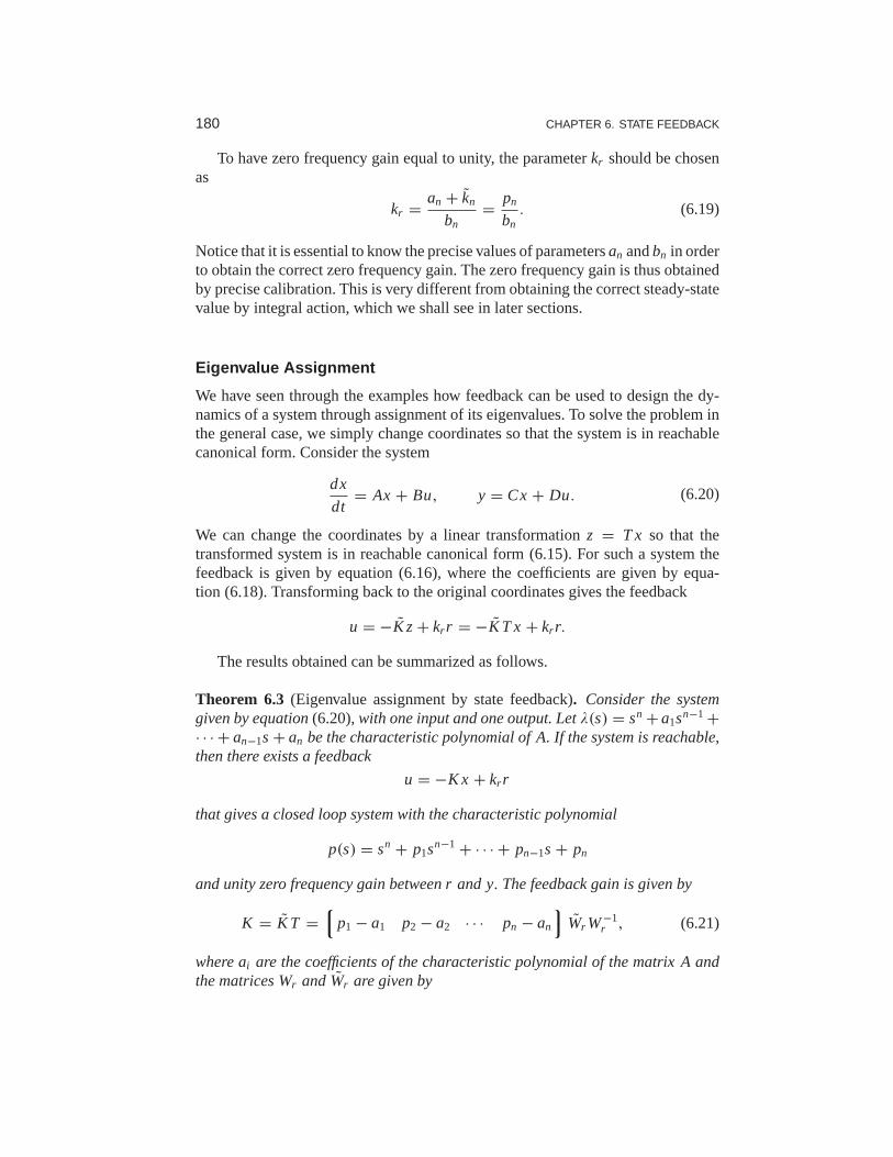
180 CHAPTER 6. STATE FEEDBACK
To have zero frequency gain equal to unity, the parameterkr should be chosenas
kr = an + kn
bn= pn
bn. (6.19)
Notice that it is essential to know the precise values of parametersan andbn in orderto obtain the correct zero frequency gain. The zero frequencygain is thus obtainedby precise calibration. This is very different from obtaining the correct steady-statevalue by integral action, which we shall see in later sections.
Eigenvalue Assignment
We have seen through the examples how feedback can be used to design the dy-namics of a system through assignment of its eigenvalues. Tosolve the problem inthe general case, we simply change coordinates so that the system is in reachablecanonical form. Consider the system
dx
dt= Ax + Bu, y = Cx + Du. (6.20)
We can change the coordinates by a linear transformationz = T x so that thetransformed system is in reachable canonical form (6.15). For such a system thefeedback is given by equation (6.16), where the coefficients are given by equa-tion (6.18). Transforming back to the original coordinatesgives the feedback
u = −K z + kr r = −K T x + kr r.
The results obtained can be summarized as follows.
Theorem 6.3 (Eigenvalue assignment by state feedback). Consider the systemgiven by equation(6.20), with one input and one output. Letλ(s) = sn + a1sn−1 +· · · + an−1s + an be the characteristic polynomial of A. If the system is reachable,then there exists a feedback
u = −K x + kr r
that gives a closed loop system with the characteristic polynomial
p(s) = sn + p1sn−1 + · · · + pn−1s + pn
and unity zero frequency gain between r and y. The feedback gain is given by
K = K T =p1 − a1 p2 − a2 · · · pn − an
Wr W−1
r , (6.21)
where ai are the coefficients of the characteristic polynomial of thematrix A andthe matrices Wr andWr are given by

6.2. STABILIZATION BY STATE FEEDBACK 181
Wr =B AB · · · An−1B
, Wr =
1 a1 a2 · · · an−1
0 1 a1 · · · an−2...
. . .. . .
...
0 0 · · · 1 a1
0 0 0 · · · 1
−1
.
The reference gain is given by
kr = −1/(C(A − BK)−1B
).
For simple problems, the eigenvalue assignment problem canbe solved byintroducing the elementski of K as unknown variables. We then compute thecharacteristic polynomial
λ(s) = det(s I − A + BK)
and equate coefficients of equal powers ofs to the coefficients of the desired char-acteristic polynomial
p(s) = sn + p1sn−1 + · · · + pn−1s + pn.
This gives a system of linear equations to determineki . The equations can alwaysbe solved if the system is reachable, exactly as we did in Example 6.4.
Equation (6.21), which is called Ackermann’s formula [Ack72, Ack85], canbe used for numeric computations. It is implemented in the MATLAB functionacker. The MATLAB function place is preferable for systems of high orderbecause it is better conditioned numerically.
Example 6.5 Predator–preyConsider the problem of regulating the population of an ecosystem by modulatingthe food supply. We use the predator–prey model introduced in Section 3.7. Thedynamics for the system are given by
d H
dt= (r + u)H
(1 − H
k
)− aH L
c + H, H ≥ 0,
dL
dt= b
aH L
c + H− dL, L ≥ 0.
We choose the following nominal parameters for the system, which correspond tothe values used in previous simulations:
a = 3.2, b = 0.6, c = 50,
d = 0.56, k = 125 r = 1.6.
We take the parameterr , corresponding to the growth rate for hares, as the input tothe system, which we might modulate by controlling a food source for the hares.This is reflected in our model by the term(r + u) in the first equation. We choosethe number of lynxes as the output of our system.
To control this system, we first linearize the system around the equilibriumpoint of the system(He, Le), which can be determined numerically to bexe ≈

182 CHAPTER 6. STATE FEEDBACK
(20.6,29.5). This yields a linear dynamical system
d
dt
z1
z2
=
0.13 −0.93
0.57 0
z1
z2
+
17.2
0
v, w =
0 1
z1
z2
,
wherez1 = L − Le, z2 = H − He andv = u. It is easy to check that the systemis reachable around the equilibrium(z, v) = (0,0), and hence we can assign theeigenvalues of the system using state feedback.
Determining the eigenvalues of the closed loop system requires balancing theability to modulate the input against the natural dynamics of the system. This canbe done by the process of trial and error or by using some of themore systematictechniques discussed in the remainder of the text. For now, we simply choose thedesired closed loop eigenvalues to be atλ = {−0.1,−0.2}. We can then solve forthe feedback gains using the techniques described earlier,which results in
K =0.025 −0.052
.
Finally, we solve for the reference gainkr , using equation (6.13) to obtainkr =0.002.
Putting these steps together, our control law becomes
v = −K z + kr r.
In order to implement the control law, we must rewrite it using the original coordi-nates for the system, yielding
u = ue − K (x − xe)+ kr (r − ye)
=0.025 −0.052
H − 20.6
L − 29.5
+ 0.002(r − 29.5).
This rule tells us how much we should modulaterh as a function of the currentnumber of lynxes and hares in the ecosystem. Figure 6.7a showsa simulation ofthe resulting closed loop system using the parameters definedabove and startingwith an initial population of 15 hares and 20 lynxes. Note that the system quicklystabilizes the population of lynxes at the reference value (L = 30). A phase portraitof the system is given in Figure 6.7b, showing how other initial conditions convergeto the stabilized equilibrium population. Notice that the dynamics are very differentfrom the natural dynamics (shown in Figure 3.20). ∇
The results of this section show that we can use state feedbackto design thedynamics of a system, under the strong assumption that we canmeasure all of thestates. We shall address the availability of the states in the next chapter, when weconsider output feedback and state estimation. In addition, Theorem 6.3, whichstates that the eigenvalues can be assigned to arbitrary locations, is also highlyidealized and assumes that the dynamics of the process are known to high precision.The robustness of state feedback combined with state estimators is considered inChapter 12 after we have developed the requisite tools.

6.3. STATE FEEDBACK DESIGN 183
0 20 40 60 80 1000
20
40
60
80
Time (years)
Pop
ulat
ion
HareLynx
(a) Initial condition response
0 50 1000
20
40
60
80
100
Hares
Lynx
es
(b) Phase portrait
Figure 6.7: Simulation results for the controlled predator–prey system. The populationoflynxes and hares as a function of time is shown in (a), and a phase portrait for the controlledsystem is shown in (b). Feedback is used to make the population stable atHe = 20.6 andLe = 20.
6.3 State Feedback Design
The location of the eigenvalues determines the behavior of the closed loop dynam-ics, and hence where we place the eigenvalues is the main design decision to bemade. As with all other feedback design problems, there are trade-offs among themagnitude of the control inputs, the robustness of the system to perturbations andthe closed loop performance of the system. In this section weexamine some ofthese trade-offs starting with the special case of second-order systems.
Second-Order Systems
One class of systems that occurs frequently in the analysis and design of feedbacksystems is second-order linear differential equations. Because of their ubiquitousnature, it is useful to apply the concepts of this chapter to that specific class ofsystems and build more intuition about the relationship between stability and per-formance.
The canonical second-order system is a differential equation of the form
q + 2ζω0q + ω20q = kω2
0u, y = q. (6.22)
In state space form, this system can be represented as
dx
dt= 0 ω0
−ω0 −2ζω0
x +
0
kω0
u, y =
1 0
x. (6.23)
The eigenvalues of this system are given by
λ = −ζω0 ±√ω2
0(ζ2 − 1),
and we see that the origin is a stable equilibrium point ifω0 > 0 andζ > 0. Notethat the eigenvalues are complex ifζ < 1 and real otherwise. Equations (6.22)

184 CHAPTER 6. STATE FEEDBACK
and (6.23) can be used to describe many second-order systems, including dampedoscillators, active filters and flexible structures, as shown in the examples below.
The form of the solution depends on the value ofζ , which is referred to as thedamping ratiofor the system. Ifζ > 1, we say that the system isoverdamped, andthe natural response (u = 0) of the system is given by
y(t) = βx10 + x20
β − αe−αt − αx10 + x20
β − αe−βt ,
whereα = ω0(ζ +√ζ 2 − 1) andβ = ω0(ζ −
√ζ 2 − 1). We see that the response
consists of the sum of two exponentially decaying signals. If ζ = 1, then the systemis critically dampedand solution becomes
y(t) = e−ζω0t(x10 + (x20 + ζω0x10)t
).
Note that this is still asymptotically stable as long asω0 > 0, although the secondterm in the solution is increasing with time (but more slowlythan the decayingexponential that is multiplying it).
Finally, if 0 < ζ < 1, then the solution is oscillatory and equation (6.22) is saidto beunderdamped. The parameterω0 is referred to as thenatural frequencyof thesystem, stemming from the fact that for smallζ , the eigenvalues of the system areapproximatelyλ = −ζω0 ± jω0. The natural response of the system is given by
y(t) = e−ζω0t
(x10 cosωdt +
(ζω0
ωdx10 + 1
ωdx20
)sinωdt
),
whereωd = ω0
√1 − ζ 2 is called thedamped frequency. For ζ ≪ 1, ωd ≈ ω0
defines the oscillation frequency of the solution andζ gives the damping rate relativetoω0.
Because of the simple form of a second-order system, it is possible to solvefor the step and frequency responses in analytical form. The solution for the stepresponse depends on the magnitude ofζ :
y(t) = k
(1 − e−ζω0t cosωdt − ζ√
1 − ζ 2e−ζω0t sinωdt
), ζ < 1;
y(t) = k(1 − e−ω0t(1 + ω0t)
), ζ = 1;
y(t) = k
(1 − 1
2
(ζ√ζ 2−1
+ 1)e−ω0t (ζ−
√ζ 2−1)
+1
2
(ζ√ζ 2−1
− 1)e−ω0t (ζ+
√ζ 2−1)
), ζ > 1,
(6.24)
where we have takenx(0) = 0. Note that for the lightly damped case (ζ < 1) wehave an oscillatory solution at frequencyωd.
Step responses of systems withk = 1 and different values ofζ are shown inFigure 6.8. The shape of the response is determined byζ , and the speed of theresponse is determined byω0 (included in the time axis scaling): the response isfaster ifω0 is larger.

6.3. STATE FEEDBACK DESIGN 185
Re
Im
ζ = 0ζ = 0.4ζ = 0.7
ζ = 1
ζ = 1.2
(a) Eigenvalues
0 5 10 150
0.5
1
1.5
2
Normalized timeω0t
y
ζ
(b) Step responses
Figure 6.8: Step response for a second-order system. Normalized step responsesh for thesystem (6.23) forζ = 0, 0.4, 0.7, 1 and 1.2. As the damping ratio is increased, the rise timeof the system gets longer, but there is less overshoot. The horizontal axis is in scaled unitsω0t ; higher values ofω0 result in a faster response (rise time and settling time).
In addition to the explicit form of the solution, we can also compute the propertiesof the step response that were defined in Section 5.3. For example, to compute themaximum overshoot for an underdamped system, we rewrite theoutput as
y(t) = k
(1 − 1√
1 − ζ 2e−ζω0t sin(ωdt + ϕ)
), (6.25)
whereϕ = arccosζ . The maximum overshoot will occur at the first time in whichthe derivative ofy is zero, which can be shown to be
Mp = e−πζ/√
1−ζ 2.
Similar computations can be done for the other characteristics of a step response.Table 6.1 summarizes the calculations.
The frequency response for a second-order system can also be computed ex-
Table 6.1:Properties of the step response for a second-order system with 0< ζ < 1.
Property Value ζ = 0.5 ζ = 1/√
2 ζ = 1
Steady-state value k k k k
Rise time Tr = 1/ω0 ·eϕ/ tanϕ 1.8/ω0 2.2/ω0 2.7/ω0
Overshoot Mp = e−πζ/√
1−ζ2 16% 4% 0%
Settling time (2%) Ts ≈ 4/ζω0 8.0/ω0 5.9/ω0 5.8/ω0

186 CHAPTER 6. STATE FEEDBACK
Re
Im ζ ≈ 0ζ = 0.08
ζ = 0.2ζ = 0.5
ζ = 1
(a) Eigenvalues
10−2
100
102
Gai
n
10−1
100
101
−180
−90
0
Pha
se [d
eg]
Normalized frequencyω/ω0
ζ
ζ
(b) Frequency responses
Figure 6.9:Frequency response of a second-order system (6.23). (a) Eigenvalues as a functionof ζ . (b) Frequency response as a function ofζ . The upper curve shows the gain ratioM , andthe lower curve shows the phase shiftθ . For smallζ there is a large peak in the magnitude ofthe frequency response and a rapid change in phase centered atω = ω0. As ζ is increased,the magnitude of the peak drops and the phase changes more smoothly between 0◦ and -180◦.
plicitly and is given by
Mej θ = kω20
(iω)2 + 2ζω0(iω)+ ω20
= kω20
ω20 − ω2 + 2i ζω0ω
.
A graphical illustration of the frequency response is givenin Figure 6.9. Notice theresonant peak that increases with decreasingζ . The peak is often characterized byis Q-value, defined asQ = 1/2ζ . The properties of the frequency response for asecond-order system are summarized in Table 6.2.
Example 6.6 Drug administrationTo illustrate the use of these formulas, consider the two-compartment model fordrug administration, described in Section 3.6. The dynamics of the system are
dc
dt=−k0 − k1 k1
k2 −k2
c +
b0
0
u, y =
0 1
x,
wherec1 andc2 are the concentrations of the drug in each compartment,ki , i =0, . . . ,2 andb0 are parameters of the system,u is the flow rate of the drug into
Table 6.2:Properties of the frequency response for a second-order system with 0< ζ < 1.
Property Value ζ = 0.1 ζ = 0.5 ζ = 1/√
2
Zero frequency gain M0 k k k
Bandwidth ωb 1.54ω0 1.27ω0 ω0
Resonant peak gain Mr 1.54k 1.27k k
Resonant frequency ωmr ω0 0.707ω0 0

6.3. STATE FEEDBACK DESIGN 187
0 5 10 15 20 25 30 35 40 45 500
0.5
1
1.5
State feedbackPulses
0 5 10 15 20 25 30 35 40 45 500
0.2
0.4
0.6
Inpu
t dos
age
Con
cent
ratio
n,C2
Time t [min]
Time t [min]
Figure 6.10:Open loop versus closed loop drug administration. Comparison between drugadministration using a sequence of doses versus continuously monitoringthe concentrationsand adjusting the dosage continuously. In each case, the concentration is(approximately)maintained at the desired level, but the closed loop system has substantially less variabilityin drug concentration.
compartment 1 andy is the concentration of the drug in compartment 2. We assumethat we can measure the concentrations of the drug in each compartment, and wewould like to design a feedback law to maintain the output at agiven referencevaluer .
We chooseζ = 0.9 to minimize the overshoot and choose the rise time to beTr = 10 min. Using the formulas in Table 6.1, this gives a value forω0 = 0.22.We can now compute the gain to place the eigenvalues at this location. Settingu = −K x + kr r , the closed loop eigenvalues for the system satisfy
λ(s) = −0.198± 0.0959i .
Choosingk1 = −0.2027 andk2 = 0.2005 gives the desired closed loop behavior.Equation (6.13) gives the reference gainkr = 0.0645. The response of the con-troller is shown in Figure 6.10 and compared with an open loop strategy involvingadministering periodic doses of the drug. ∇
Higher-Order Systems
Our emphasis so far has considered only second-order systems. For higher-ordersystems, eigenvalue assignment is considerably more difficult, especially whentrying to account for the many trade-offs that are present ina feedback design.
One of the other reasons why second-order systems play such an importantrole in feedback systems is that even for more complicated systems the response isoften characterized by thedominant eigenvalues. To define these more precisely,consider a system with eigenvaluesλ j , j = 1, . . . ,n. We define thedamping ratio

188 CHAPTER 6. STATE FEEDBACK
for a complex eigenvalueλ to be
ζ = −Reλ
|λ| .
We say that a complex conjugate pair of eigenvaluesλ, λ∗ is adominant pairif ithas the lowest damping ratio compared with all other eigenvalues of the system.
Assuming that a system is stable, the dominant pair of eigenvalues tends to bethe most important element of the response. To see this, assume that we have asystem in Jordan form with a simple Jordan block corresponding to the dominantpair of eigenvalues:
dz
dt=
λ
λ∗
J2. . .
Jk
z + Bu, y = Cz.
(Note that the statez may be complex because of the Jordan transformation.) Theresponse of the system will be a linear combination of the responses from eachof the individual Jordan subsystems. As we see from Figure 6.8, for ζ < 1 thesubsystem with the slowest response is precisely the one with the smallest dampingratio. Hence, when we add the responses from each of the individual subsystems,it is the dominant pair of eigenvalues that will be the primary factor after the initialtransients due to the other terms in the solution die out. While this simple analysisdoes not always hold (e.g., if some nondominant terms have larger coefficientsbecause of the particular form of the system), it is often thecase that the dominanteigenvalues determine the (step) response of the system.
The only formal requirement for eigenvalue assignment is that the system bereachable. In practice there are many other constraints because the selection ofeigenvalues has a strong effect on the magnitude and rate of change of the controlsignal. Large eigenvalues will in general require large control signals as well asfast changes of the signals. The capability of the actuators will therefore imposeconstraints on the possible location of closed loop eigenvalues. These issues willbe discussed in depth in Chapters 11 and 12.
We illustrate some of the main ideas using the balance systemas an example.
Example 6.7 Balance systemConsider the problem of stabilizing a balance system, whosedynamics were givenin Example 6.2. The dynamics are given by
A =
0 0 1 00 0 0 1
0 m2l 2g/µ −cJt/µ −γ Jt lm/µ
0 Mtmgl/µ −clm/µ −γMt/µ
, B =
00
Jt/µ
lm/µ
,
whereMt = M + m, Jt = J + ml2, µ = Mt Jt − m2l 2 and we have leftc andγ

6.3. STATE FEEDBACK DESIGN 189
nonzero. We use the following parameters for the system (corresponding roughlyto a human being balanced on a stabilizing cart):
M = 10 kg, m = 80 kg, c = 0.1 N s/m,
J = 100 kg m2/s2, l = 1 m, γ = 0.01 N m s,g = 9.8 m/s2.
The eigenvalues of the open loop dynamics are given byλ ≈ 0,4.7,−1.9±2.7i .We have verified already in Example 6.2 that the system is reachable, and hencewe can use state feedback to stabilize the system and providea desired level ofperformance.
To decide where to place the closed loop eigenvalues, we notethat the closedloop dynamics will roughly consist of two components: a set of fast dynamicsthat stabilize the pendulum in the inverted position and a set of slower dynamicsthat control the position of the cart. For the fast dynamics,we look to the naturalperiod of the pendulum (in the hanging-down position), which is given byω0 =√
mgl/(J + ml2) ≈ 2.1 rad/s. To provide a fast response we choose a damping ratioof ζ = 0.5 and try to place the first pair of eigenvalues atλ1,2 ≈ −ζω0 ± ω0 ≈−1 ± 2i , where we have used the approximation that
√1 − ζ 2 ≈ 1. For the slow
dynamics, we choose the damping ratio to be 0.7 to provide a small overshoot andchoose the natural frequency to be 0.5 to give a rise time of approximately 5 s. Thisgives eigenvaluesλ3,4 = −0.35± 0.35i .
The controller consists of a feedback on the state and a feedforward gain for thereference input. The feedback gain is given by
K =−15.6 1730 −50.1 443
,
which can be computed using Theorem 6.3 or using the MATLABplace com-mand. The feedforward gain iskr = −1/(C(A − BK)−1B) = −15.5. The stepresponse for the resulting controller (applied to the linearized system) is given inFigure 6.11a. While the step response gives the desired characteristics, the inputrequired (bottom left) is excessively large, almost three times the force of gravityat its peak.
To provide a more realistic response, we can redesign the controller to haveslower dynamics. We see that the peak of the input force occurs on the fast time scale,and hence we choose to slow this down by a factor of 3, leaving the damping ratiounchanged. We also slow down the second set of eigenvalues, with the intuition thatwe should move the position of the cart more slowly than we stabilize the pendulumdynamics. Leaving the damping ratio for the slow dynamics unchanged at 0.7 andchanging the frequency to 1 (corresponding to a rise time of approximately 10 s),the desired eigenvalues become
λ = {−0.33± 0.66i, −0.18± 0.18i }.The performance of the resulting controller is shown in Figure6.11b. ∇
As we see from this example, it can be difficult to determine where to placethe eigenvalues using state feedback. This is one of the principal limitations of this

190 CHAPTER 6. STATE FEEDBACK
0 5 10 15
0
1
2
0 5 10 15−10
0
10
20
30
Pos
ition
p[m
]
Time t [s]
Inpu
tfor
ceF
[N]
(a)λ1,2 = −1 ± 2i
0 10 20 30 40
0
1
2
0 10 20 30 40−10
0
10
20
30
Pos
ition
p[m
]
Time t [s]
Inpu
tfor
ceF
[N]
(b) λ1,2 = −0.33± 0.66i
Figure 6.11: State feedback control of a balance system. The step response of a controllerdesigned to give fast performance is shown in (a). Although the response characteristics(top left) look very good, the input magnitude (bottom left) is very large. A less aggressivecontroller is shown in (b). Here the response time is slowed down, but the input magnitudeis much more reasonable. Both step responses are applied to the linearized dynamics.
approach, especially for systems of higher dimension. Optimal control techniques,such as the linear quadratic regulator problem discussed next, are one approachthat is available. One can also focus on the frequency response for performing thedesign, which is the subject of Chapters 8–12.
Linear Quadratic Regulators�
As an alternative to selecting the closed loop eigenvalue locations to accomplish acertain objective, the gains for a state feedback controller can instead be chosen isby attempting to optimize a cost function. This can be particularly useful in helpingbalance the performance of the system with the magnitude of the inputs requiredto achieve that level of performance.
The infinite horizon, linear quadratic regulator (LQR) problemis one of themost common optimal control problems. Given a multi-input linear system
dx
dt= Ax + Bu, x ∈ R
n, u ∈ Rp,
we attempt to minimize the quadratic cost function
J =∫ ∞
0
(xT Qxx + uT Quu
)dt, (6.26)
whereQx ≥ 0 andQu > 0 are symmetric, positive (semi-) definite matrices ofthe appropriate dimensions. This cost function represents atrade-off between thedistance of the state from the origin and the cost of the control input. By choosing

6.3. STATE FEEDBACK DESIGN 191
the matricesQx andQu, we can balance the rate of convergence of the solutionswith the cost of the control.
The solution to the LQR problem is given by a linear control law of the form
u = −Q−1u BT Px,
whereP ∈ Rn×n is a positive definite, symmetric matrix that satisfies the equation
P A+ AT P − P BQ−1u BT P + Qx = 0. (6.27)
Equation (6.27) is called thealgebraic Riccati equationand can be solved numer-ically (e.g., using thelqr command in MATLAB).
One of the key questions in LQR design is how to choose the weights Qx andQu. To guarantee that a solution exists, we must haveQx ≥ 0 andQu > 0. Inaddition, there are certain “observability” conditions onQx that limit its choice.Here we assumeQx > 0 to ensure that solutions to the algebraic Riccati equationalways exist.
To choose specific values for the cost function weightsQx andQu, we must useour knowledge of the system we are trying to control. A particularly simple choiceis to use diagonal weights
Qx =
q1 0. . .
0 qn
, Qu =
ρ1 0. . .
0 ρn
.
For this choice ofQx andQu, the individual diagonal elements describe how mucheach state and input (squared) should contribute to the overall cost. Hence, wecan take states that should remain small and attach higher weight values to them.Similarly, we can penalize an input versus the states and other inputs through choiceof the corresponding input weightρ.
Example 6.8 Vectored thrust aircraftConsider the original dynamics of the system (2.26), written in state space form as
dz
dt=
z4
z5
z6
−g sinθ − cm z4
−g cosθ − cm z5
0
+
000
1m cosθ F1 − 1
m sinθ F2
1m sinθ F1 + 1
m cosθ F2
rJ F1
(see Example 5.4). The system parameters arem = 4 kg, J = 0.0475 kg m2,r = 0.25 m,g = 9.8 m/s2, c = 0.05 N s/m, which corresponds to a scaled modelof the system. The equilibrium point for the system is given byF1 = 0, F2 = mgandze = (xe, ye,0,0,0,0). To derive the linearized model near an equilibrium

192 CHAPTER 6. STATE FEEDBACK
point, we compute the linearization according to equation (5.34):
A =
0 0 0 1 0 00 0 0 0 1 00 0 0 0 0 10 0 −g −c/m 0 00 0 0 0 −c/m 00 0 0 0 0 0
, B =
0 00 00 0
1/m 00 1/m
r/J 0
,
C =1 0 0 0 0 0
0 1 0 0 0 0
, D =
0 0
0 0
.
Letting z = z − ze andv = u − ue, the linearized system is given by
dz
dt= Az+ Bv, y = Cx.
It can be verified that the system is reachable.To compute a linear quadratic regulator for the system, we write the cost function
asJ =
∫ ∞
0(zT Qzz + vT Qvv )dt,
wherez = z−ze andv = u−ue represent the local coordinates around the desiredequilibrium point(ze,ue). We begin with diagonal matrices for the state and inputcosts:
Qz =
1 0 0 0 0 00 1 0 0 0 00 0 1 0 0 00 0 0 1 0 00 0 0 0 1 00 0 0 0 0 1
, Qv =1 0
0 1
.
This gives a control law of the formv = −K z, which can then be used to derivethe control law in terms of the original variables:
u = v + ue = −K (z − ze)+ ue.
As computed in Example 5.4, the equilibrium points haveue = (0,mg) andze =(xe, ye,0,0,0,0). The response of the controller to a step change in the desiredposition is shown in Figure 6.12a. The response can be tuned by adjusting theweights in the LQR cost. Figure 6.12b shows the response in thex direction fordifferent choices of the weightρ. ∇
Linear quadratic regulators can also be designed for discrete-time systems, asillustrated by the following example.
Example 6.9 Web server controlConsider the web server example given in Section 3.4, where a discrete-time modelfor the system was given. We wish to design a control law that sets the serverparameters so that the average server processor load is maintained at a desired

6.3. STATE FEEDBACK DESIGN 193
0 2 4 6 8 100
0.5
1
Time t [s]
Pos
ition
x,y
[m]
xy
(a) Step response inx andy
0 2 4 6 8 100
0.5
1
Time t [s]
Pos
ition
x[m
]
ρ
(b) Effect of control weightρ
Figure 6.12:Step response for a vectored thrust aircraft. The plot in (a) shows thex andypositions of the aircraft when it is commanded to move 1 m in each direction.In (b) thexmotion is shown for control weightsρ = 1, 102, 104. A higher weight of the input term inthe cost function causes a more sluggish response.
level. Since other processes may be running on the server, theweb server mustadjust its parameters in response to changes in the load.
A block diagram for the control system is shown in Figure 6.13.We focus onthe special case where we wish to control only the processor load using both theKeepAlive andMaxClients parameters. We also include a “disturbance” onthe measured load that represents the use of the processing cycles by other processesrunning on the server. The system has the same basic structureas the generic controlsystem in Figure 6.5, with the variation that the disturbanceenters after the processdynamics.
The dynamics of the system are given by a set of difference equations of theform
x[k + 1] = Ax[k] + Bu[k], ycpu[k] = Ccpux[k] + dcpu[k],
wherex = (xcpu, xmem) is the state,u = (uka,umc) is the input,dcpu is the processingload from other processes on the computer andycpu is the total processor load.
We choose our controller to be a state feedback controller ofthe form
u = −K
ycpu
xmem
+ kr rcpu,
Feedback
6
rcpu u6
d
yη
Precompensation Controller
kr
eC
−1
Server
P
Figure 6.13: Feedback control of a web server. The controller sets the values of thewebserver parameters based on the difference between the nominal parameters (determined bykr r ) and the current loadycpu. The disturbanced represents the load due to other processesrunning on the server. Note that the measurement is taken after the disturbance so that wemeasure the total load on the server.

194 CHAPTER 6. STATE FEEDBACK
wherercpu is the desired processor load. Note that we have used the measuredprocessor loadycpu instead of the state to ensure that we adjust the system operationbased on the actual load. (This modification is necessary because of the nonstandardway in which the disturbance enters the process dynamics.)
The feedback gain matrixK can be chosen by any of the methods described inthis chapter. Here we use a linear quadratic regulator, withthe cost function givenby
Qx =5 0
0 1
, Qu =
1/502 0
0 1/10002
.
The cost function for the stateQx is chosen so that we place more emphasis onthe processor load versus the memory use. The cost function for the inputsQu
is chosen so as to normalize the two inputs, with aKeepAlive timeout of 50 shaving the same weight as aMaxClients value of 1000. These values are squaredsince the cost associated with the inputs is given byuT Quu. Using the dynamicsin Section 3.4 and thedlqr command in MATLAB, the resulting gains become
K =−22.3 10.1
382.7 77.7
.
As in the case of a continuous-time control system, the reference gainkr ischosen to yield the desired equilibrium point for the system. Settingx[k + 1] =x[k] = xe, the steady-state equilibrium point and output for a given reference inputr are given by
xe = (A − BK)xe + Bkr r, ye = Cxe.
This is a matrix differential equation in whichkr is a column vector that sets thetwo inputs values based on the desired reference. If we take the desired output tobe of the formye = (r,0), then we must solve
1
0
= C(A − BK − I )−1Bkr .
Solving this equation forkr , we obtain
kr =((
C(A − BK − I )−1B))−1
1
0
=
49.3
539.5
.
The dynamics of the closed loop system are illustrated in Figure 6.14. We applya change in load ofdcpu = 0.3 at timet = 10 s, forcing the controller to adjustthe operation of the server to attempt to maintain the desired load at 0.57. Notethat both theKeepAlive andMaxClients parameters are adjusted. Althoughthe load is decreased, it remains approximately 0.2 above the desired steady state.(Better results can be obtained using the techniques of the next section.) ∇

6.4. INTEGRAL ACTION 195
0 20 40 600.4
0.6
0.8
1
x cpu,x m
em
xcpu xmem
Time k [ms]
(a) System state
0 20 40 600
10
20
30
40
50
0 20 40 600
300
600
900
1200
1500
ka (l) mc (r)KeepAlive
MaxClients
Time k [ms]
(b) System inputs
Figure 6.14:Web server with LQR control. The plot in (a) shows the state of the system undera change in external load applied atk = 10 ms. The corresponding web server parameters(system inputs) are shown in (b). The controller is able to reduce the effect of the disturbanceby approximately 40%.
6.4 Integral Action
Controllers based on state feedback achieve the correct steady-state response tocommand signals by careful calibration of the gainkr . However, one of the primaryuses of feedback is to allow good performance in the presenceof uncertainty,and hence requiring that we have anexactmodel of the process is undesirable. Analternative to calibration is to make use of integral feedback, in which the controlleruses an integrator to provide zero steady-state error. The basic concept of integralfeedback was given in Section 1.5 and in Section 3.1; here we provide a morecomplete description and analysis.
The basic approach in integral feedback is to create a state within the controllerthat computes the integral of the error signal, which is thenused as a feedback term.We do this by augmenting the description of the system with a new statez:
d
dt
x
z
=
Ax + Bu
y − r
=
Ax + Bu
Cx − r
. (6.28)
The statez is seen to be the integral of the difference between the the actual outputy and desired outputr . Note that if we find a compensator that stabilizes the system,then we will necessarily havez = 0 in steady state and hencey = r in steady state.
Given the augmented system, we design a state space controller in the usualfashion, with a control law of the form
u = −K x − ki z + kr r, (6.29)
whereK is the usual state feedback term,ki is the integral term andkr is used toset the nominal input for the desired steady state. The resulting equilibrium pointfor the system is given as
xe = −(A − BK)−1B(kr r − ki ze).
Note that the value ofze is not specified but rather will automatically settle to thevalue that makesz = y − r = 0, which implies that at equilibrium the output willequal the reference value. This holds independently of the specific values ofA,

196 CHAPTER 6. STATE FEEDBACK
B andK as long as the system is stable (which can be done through appropriatechoice ofK andki ).
The final compensator is given by
u = −K x − ki z + kr r,dz
dt= y − r,
where we have now included the dynamics of the integrator as part of the specifica-tion of the controller. This type of compensator is known as adynamic compensatorsince it has its own internal dynamics. The following exampleillustrates the basicapproach.
Example 6.10 Cruise controlConsider the cruise control example introduced in Section 3.1 and considered fur-ther in Example 5.11. The linearized dynamics of the process around an equilibriumpoint ve, ue are given by
dx
dt= ax − bgθ + bw, y = v = x + ve,
wherex = v−ve,w = u−ue, m is the mass of the car andθ is the angle of the road.The constanta depends on the throttle characteristic and is given in Example 5.11.
If we augment the system with an integrator, the process dynamics become
dx
dt= ax − bgθ + bw,
dz
dt= y − vr = ve + x − vr ,
or, in state space form,
d
dt
x
z
=
a 0
1 0
x
z
+
b
0
u +
−bg
0
θ +
0ve − vr
.
Note that when the system is at equilibrium, we have thatz = 0, which impliesthat the vehicle speedv = ve + x should be equal to the desired reference speedvr . Our controller will be of the form
dz
dt= y − vr , u = −kpx − ki z + kr vr ,
and the gainskp, ki andkr will be chosen to stabilize the system and provide thecorrect input for the reference speed.
Assume that we wish to design the closed loop system to have the characteristicpolynomial
λ(s) = s2 + a1s + a2.
Setting the disturbanceθ = 0, the characteristic polynomial of the closed loopsystem is given by
det(s I − (A − BK)
)= s2 + (bkp − a)s + bki ,
and hence we set
kp = a1 + a
b, ki = a2
b, kr = −1/
(C(A − BK)−1B
)= a
b.
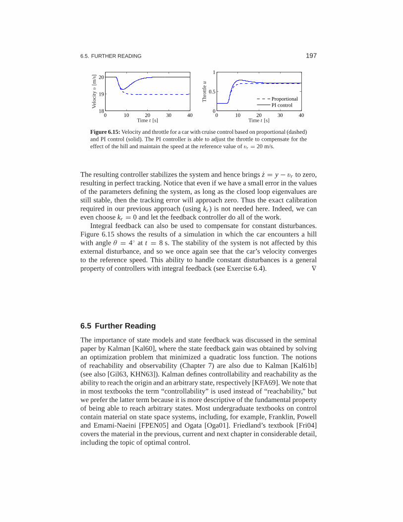
6.5. FURTHER READING 197
0 10 20 30 4018
19
20
0 10 20 30 400
0.5
1
ProportionalPI control
Time t [s]Time t [s]
Velo
cityv
[m/s
]
Thr
ottle
u
Figure 6.15:Velocity and throttle for a car with cruise control based on proportional (dashed)and PI control (solid). The PI controller is able to adjust the throttle to compensate for theeffect of the hill and maintain the speed at the reference value ofvr = 20 m/s.
The resulting controller stabilizes the system and hence bringsz = y − vr to zero,resulting in perfect tracking. Notice that even if we have a small error in the valuesof the parameters defining the system, as long as the closed loop eigenvalues arestill stable, then the tracking error will approach zero. Thus the exact calibrationrequired in our previous approach (usingkr ) is not needed here. Indeed, we caneven choosekr = 0 and let the feedback controller do all of the work.
Integral feedback can also be used to compensate for constant disturbances.Figure 6.15 shows the results of a simulation in which the car encounters a hillwith angleθ = 4◦ at t = 8 s. The stability of the system is not affected by thisexternal disturbance, and so we once again see that the car’svelocity convergesto the reference speed. This ability to handle constant disturbances is a generalproperty of controllers with integral feedback (see Exercise 6.4). ∇
6.5 Further Reading
The importance of state models and state feedback was discussed in the seminalpaper by Kalman [Kal60], where the state feedback gain was obtained by solvingan optimization problem that minimized a quadratic loss function. The notionsof reachability and observability (Chapter 7) are also due to Kalman [Kal61b](see also [Gil63, KHN63]). Kalman defines controllability and reachability as theability to reach the origin and an arbitrary state, respectively [KFA69]. We note thatin most textbooks the term “controllability” is used instead of “reachability,” butwe prefer the latter term because it is more descriptive of the fundamental propertyof being able to reach arbitrary states. Most undergraduatetextbooks on controlcontain material on state space systems, including, for example, Franklin, Powelland Emami-Naeini [FPEN05] and Ogata [Oga01]. Friedland’s textbook [Fri04]covers the material in the previous, current and next chapter in considerable detail,including the topic of optimal control.

198 CHAPTER 6. STATE FEEDBACK
Exercises
6.1 (Double integrator) Consider the double integrator. Find a piecewise constantcontrol strategy that drives the system from the origin to the statex = (1,1).
6.2(Reachability from nonzero initial state) Extend the argument in Section 6.1 toshow that if a system is reachable from an initial state of zero, it is reachable froma nonzero initial state.
6.3 (Unreachable systems) Consider the system shown in Figure 6.3. Write thedynamics of the two systems as
dx
dt= Ax + Bu,
dz
dt= Az+ Bu.
If x andz have the same initial condition, they will always have the same stateregardless of the input that is applied. Show that this violates the definition ofreachability and further show that the reachability matrixWr is not full rank.
6.4(Integral feedback for rejecting constant disturbances) Consider a linear systemof the form
dx
dt= Ax + Bu + Fd, y = Cx
whereu is a scalar andd is a disturbance that enters the system through a disturbancevectorF ∈ R
n. Assume that the matrixA is invertible and the zero frequency gainC A−1B is nonzero. Show that integral feedback can be used to compensate for aconstant disturbance by giving zero steady-state output error even whend 6= 0.
6.5(Rear-steered bicycle) A simple model for a bicycle was given by equation (3.5)in Section 3.2. A model for a bicycle with rear-wheel steeringis obtained by re-versing the sign of the velocity in the model. Determine the conditions under whichthis systems is reachable and explain any situations in which the system is notreachable.
6.6 (Characteristic polynomial for reachable canonical form)Show that the char-acteristic polynomial for a system in reachable canonical form is given by equa-tion (6.7) and that
dnzk
dtn+ a1
dn−1zk
dtn−1+ · · · + an−1
dzk
dt+ anzk = dn−ku
dtn−k,
wherezk is thekth state.
6.7(Reachability matrix for reachable canonical form) Consider a system in reach-able canonical form. Show that the inverse of the reachability matrix is given by
W−1r =
1 a1 a2 · · · an
0 1 a1 · · · an−1
0 0 1. . .
......
. . . a1
0 0 0 · · · 1
.

EXERCISES 199
6.8 (Non-maintainable equilibria) Consider the normalized model of a pendulumon a cart
d2x
dt2= u,
d2θ
dt2= −θ + u,
wherex is cart position andθ is pendulum angle. Can the angleθ = θ0 for θ0 6= 0be maintained?
6.9 (Eigenvalue assignment for unreachable system) Consider the system
dx
dt=0 1
0 0
x +
1
0
u, y =
1 0
x,
with the control lawu = −k1x1 − k2x2 + kr r.
Show that eigenvalues of the system cannot be assigned to arbitrary values.
6.10 (Cayley–Hamilton theorem) LetA ∈ Rn×n be a matrix with characteristic
polynomialλ(s) = det(s I − A) = sn + a1sn−1 + · · · + an−1s + an. Assume thatthe matrixA can be diagonalized and show that it satisfies
λ(A) = An + a1An−1 + · · · + an−1A + an I = 0,
Use the result to show thatAk, k ≥ n, can be rewritten in terms of powers ofA oforder less thann.
6.11 (Motor drive) Consider the normalized model of the motor drive in Exer-cise 2.10. Using the following normalized parameters,
J1 = 10/9, J2 = 10, c = 0.1, k = 1, kI = 1,
verify that the eigenvalues of the open loop system are 0,0,−0.05± i . Design astate feedback that gives a closed loop system with eigenvalues−2,−1 and−1± i .This choice implies that the oscillatory eigenvalues will bewell damped and thatthe eigenvalues at the origin are replaced by eigenvalues onthe negative real axis.Simulate the responses of the closed loop system to step changes in the commandsignal forθ2 and a step change in a disturbance torque on the second rotor.
6.12(Whipple bicycle model) Consider the Whipple bicycle modelgiven by equa-tion (3.7) in Section 3.2. Using the parameters from the companion web site, themodel is unstable at the velocityv = 5 m/s and the open loop eigenvalues are -1.84,-14.29 and 1.30± 4.60i . Find the gains of a controller that stabilizes the bicycleand gives closed loop eigenvalues at -2, -10 and−1 ± i . Simulate the response ofthe system to a step change in the steering reference of 0.002rad.

200 CHAPTER 6. STATE FEEDBACK
6.13(Atomic force microscope) Consider the model of an AFM in contact modegiven in Example 5.9:
dx
dt=
0 1 0 0−k2/(m1 + m2) −c2/(m1 + m2) 1/m2 0
0 0 0 ω3
0 0 −ω3 −2ζ3ω3
x +
000ω3
u,
y = m2
m1 + m2
m1k2
m1 + m2
m1c2
m1 + m21 0
x.
Use the MATLAB scriptafm_data.m from the companion web site to generate thesystem matrices.
(a) Compute the reachability matrix of the system and numerically determine itsrank. Scale the model by using milliseconds instead of seconds as time units. Repeatthe calculation of the reachability matrix and its rank.
(b) Find a state feedback controller that gives a closed loop system with complexpoles having damping ratio 0.707. Use the scaled model for the computations.
(c) Compute state feedback gains using linear quadratic control. Experiment byusing different weights. Compute the gains forq1 = q2 = 0,q3 = q4 = 1 andρ1 = 0.1 and explain the result. Chooseq1 = q2 = q3 = q4 = 1 and explore whathappens to the feedback gains and closed loop eigenvalues when you changeρ1.Use the scaled system for this computation.
6.14 Consider the second-order system
d2y
dt2+ 0.5
dy
dt+ y = a
du
dt+ u.
Let the initial conditions be zero.
(a) Show that the initial slope of the unit step response isa. Discuss what it meanswhena < 0.
(b) Show that there are points on the unit step response that are invariant witha.Discuss qualitatively the effect of the parametera on the solution.
(c) Simulate the system and explore the effect ofa on the rise time and overshoot.
6.15(Bryson’s rule) Bryson and Ho [BH75] have suggested the following methodfor choosing the matricesQx and Qu in equation (6.26). Start by choosingQx
and Qu as diagonal matrices whose elements are the inverses of the squares ofthe maxima of the corresponding variables. Then modify the elements to obtain acompromise among response time, damping and control effort. Apply this methodto the motor drive in Exercise 6.11. Assume that the largest values of theϕ1 andϕ2 are 1, the largest values ofϕ1 andϕ2 are 2 and the largest control signal is 10.Simulate the closed loop system forϕ2(0) = 1 and all other states are initialized to0. Explore the effects of different values of the diagonal elements forQx andQu.

Chapter SevenOutput Feedback
One may separate the problem of physical realization into two stages: computation of the“best approximation”x(t1) of the state from knowledge of y(t) for t ≤ t1 and computation ofu(t1) givenx(t1).
R. E. Kalman, “Contributions to the Theory of Optimal Control,” 1960 [Kal60].
In this chapter we show how to use output feedback to modify the dynamicsof the system through the use of observers. We introduce the concept of observ-ability and show that if a system is observable, it is possible to recover the statefrom measurements of the inputs and outputs to the system. Wethen show how todesign a controller with feedback from the observer state. An important concept isthe separation principle quoted above, which is also proved. The structure of thecontrollers derived in this chapter is quite general and is obtained by many otherdesign methods.
7.1 Observability
In Section 6.2 of the previous chapter it was shown that it is possible to find astate feedback law that gives desired closed loop eigenvalues provided that thesystem is reachable and that all the states are measured. Formany situations, itis highly unrealistic to assume that all the states are measured. In this section weinvestigate how the state can be estimated by using a mathematical model and afew measurements. It will be shown that computation of the states can be carriedout by a dynamical system called anobserver.
Definition of Observability
Consider a system described by a set of differential equations
dx
dt= Ax + Bu, y = Cx + Du, (7.1)
wherex ∈ Rn is the state,u ∈ R
p the input andy ∈ Rq the measured output. We
wish to estimate the state of the system from its inputs and outputs, as illustratedin Figure 7.1. In some situations we will assume that there is only one measuredsignal, i.e., that the signaly is a scalar and thatC is a (row) vector. This signal maybe corrupted by noisen, although we shall start by considering the noise-free case.We write x for the state estimate given by the observer.

202 CHAPTER 7. OUTPUT FEEDBACK
u6
n
Observerx
Process
x = Ax + Bu
y = Cx + Du
y
Figure 7.1: Block diagram for an observer. The observer uses the process measurementy(possibly corrupted by noisen) and the inputu to estimate the current state of the process,denotedx.
Definition 7.1 (Observability). A linear system isobservableif for any T > 0 it ispossible to determine the state of the systemx(T) through measurements ofy(t)andu(t) on the interval [0, T ].
The definition above holds for nonlinear systems as well, and the results dis-cussed here have extensions to the nonlinear case.
The problem of observability is one that has many important applications, evenoutside feedback systems. If a system is observable, then there are no “hidden” dy-namics inside it; we can understand everything that is goingon through observation(over time) of the inputs and outputs. As we shall see, the problem of observabilityis of significant practical interest because it will determine if a set of sensors issufficient for controlling a system. Sensors combined with a mathematical modelcan also be viewed as a “virtual sensor” that gives information about variables thatare not measured directly. The process of reconciling signals from many sensorswith mathematical models is also calledsensor fusion.
Testing for Observability
When discussing reachability in the last chapter, we neglected the output and fo-cused on the state. Similarly, it is convenient here to initially neglect the input andfocus on the autonomous system
dx
dt= Ax, y = Cx. (7.2)
We wish to understand when it is possible to determine the state from observationsof the output.
The output itself gives the projection of the state on vectorsthat are rows of thematrixC. The observability problem can immediately be solved if the matrix C isinvertible. If the matrix is not invertible, we can take derivatives of the output toobtain
dy
dt= C
dx
dt= C Ax.
From the derivative of the output we thus get the projection ofthe state on vectors

7.1. OBSERVABILITY 203
that are rows of the matrixC A. Proceeding in this way, we get
y
y
y...
y(n−1)
=
CC AC A2
...
C An−1
x. (7.3)
We thus find that the state can be determined if theobservability matrix
Wo =
CC AC A2
...
C An−1
(7.4)
hasn independent rows. It turns out that we need not consider any derivatives higherthann−1 (this is an application of the Cayley–Hamilton theorem [Exercise 6.10]).
The calculation can easily be extended to systems with inputs. The state is thengiven by a linear combination of inputs and outputs and theirhigher derivatives.The observability criterion is unchanged. We leave this caseas an exercise for thereader.
In practice, differentiation of the output can give large errors when there ismeasurement noise, and therefore the method sketched aboveis not particularlypractical. We will address this issue in more detail in the next section, but for nowwe have the following basic result.
Theorem 7.1(Observability rank condition). A linear system of the form(7.1) isobservable if and only if the observability matrix Wo is full rank.
Proof. The sufficiency of the observability rank condition follows from the analysis�above. To prove necessity, suppose that the system is observable butWo is not fullrank. Letv ∈ R
n, v 6= 0, be a vector in the null space ofWo, so thatWov = 0. Ifwe letx(0) = v be the initial condition for the system and chooseu = 0, then theoutput is given byy(t) = CeAtv. SinceeAt can be written as a power series inAand sinceAn and higher powers can be rewritten in terms of lower powers ofA (bythe Cayley–Hamilton theorem), it follows that the output will be identically zero(the reader should fill in the missing steps if this is not clear). However, if both theinput and output of the system are 0, then a valid estimate of the state isx = 0 forall time, which is clearly incorrect sincex(0) = v 6= 0. Hence by contradiction wemust have thatWo is full rank if the system is observable.
Example 7.1 Compartment modelConsider the two-compartment model in Figure 3.18a, but assume that the concen-tration in the first compartment can be measured. The system is described by the

204 CHAPTER 7. OUTPUT FEEDBACK
S
6
S
−
+v1 v2
R2
−
+
R1
R2R1
C2
C2
R3
R3
Figure 7.2:An unobservable system. Two identical subsystems have outputs that add togetherto form the overall system output. The individual states of the subsystem cannot be determinedsince the contributions of each to the output are not distinguishable. The circuit diagram onthe right is an example of such a system.
linear system
dc
dt=−k0 − k1 k1
k2 −k2
c +
b0
0
u, y =
1 0
x.
The first compartment represents the drug concentration in theblood plasma, andthe second compartment the drug concentration in the tissuewhere it is active. Todetermine if it is possible to find the concentration in the tissue compartment froma measurement of blood plasma, we investigate the observability of the system byforming the observability matrix
Wo = C
C A
=
1 0
−k0 − k1 k1
.
The rows are linearly independent ifk1 6= 0, and under this condition it is thuspossible to determine the concentration of the drug in the active compartment frommeasurements of the drug concentration in the blood. ∇
It is useful to have an understanding of the mechanisms that make a systemunobservable. Such a system is shown in Figure 7.2. The system iscomposed oftwo identical systems whose outputs are added. It seems intuitively clear that it is notpossible to deduce the states from the output since we cannotdeduce the individualoutput contributions from the sum. This can also be seen formally (Exercise 7.2).
Observable Canonical Form
As in the case of reachability, certain canonical forms willbe useful in studying ob-servability. A linear single-input, single-output state space system is inobservable

7.1. OBSERVABILITY 205
z1y
a1
∫
b1
66
. . .
. . .
an−1
∫
bn−1
6
. . .
a2
∫
b2
6
an
u
∫
bn
6
d
−1
zn zn−1 z2
Figure 7.3:Block diagram of a system in observable canonical form. The states of the systemare represented by individual integrators whose inputs are a weighted combination of the nextintegrator in the chain, the first state (rightmost integrator) and the system input. The outputis a combination of the first state and the input.
canonical formif its dynamics are given by
dz
dt=
−a1 1 0 · · · 0−a2 0 1 0...
. . .
−an−1 0 0 1−an 0 0 · · · 0
z +
b1
b2...
bn−1
bn
u,
y =1 0 0 · · · 0
z + Du.
The definition can be extended to systems with many inputs; the only difference isthat the vector multiplyingu is replaced by a matrix.
Figure 7.3 is a block diagram for a system in observable canonical form. Asin the case of reachable canonical form, we see that the coefficients in the systemdescription appear directly in the block diagram. The characteristic polynomial fora system in observable canonical form is
λ(s) = sn + a1sn−1 + · · · + an−1s + an. (7.5)
It is possible to reason about the observability of a system in observable canonicalform by studying the block diagram. If the inputu and the outputy are available,the statez1 can clearly be computed. Differentiatingz1, we obtain the input to theintegrator that generatesz1, and we can now obtainz2 = z1+a1z1−b1u. Proceedingin this way, we can compute all states. The computation will, however, require thatthe signals be differentiated.
To check observability more formally, we compute the observability matrix for

206 CHAPTER 7. OUTPUT FEEDBACK
a system in observable canonical form, which is given by
Wo =
1 0 0 . . . 0−a1 1 0 . . . 0
−a21 − a1a2 −a1 1 0...
.... . .
...
∗ ∗ . . . 1
,
where * represents an entry whose exact value is not important. The rows of thismatrix are linearly independent (since it is lower triangular), and henceWo isfull rank. A straightforward but tedious calculation showsthat the inverse of theobservability matrix has a simple form given by
W−1o =
1 0 0 · · · 0a1 1 0 · · · 0a2 a1 1 · · · 0...
.... . .
...
an−1 an−2 an−3 · · · 1
.
As in the case of reachability, it turns out that if a system isobservable then therealways exists a transformationT that converts the system into observable canonicalform. This is useful for proofs since it lets us assume that a system is in observablecanonical form without any loss of generality. The observable canonical form maybe poorly conditioned numerically.
7.2 State Estimation
Having defined the concept of observability, we now return to the question ofhow to construct an observer for a system. We will look for observers that can berepresented as a linear dynamical system that takes the inputs and outputs of thesystem we are observing and produces an estimate of the system’s state. That is,we wish to construct a dynamical system of the form
dx
dt= Fx + Gu + Hy,
whereu and y are the input and output of the original system andx ∈ Rn is an
estimate of the state with the property thatx(t) → x(t) ast → ∞.
The Observer
We consider the system in equation (7.1) withD set to zero to simplify the expo-sition:
dx
dt= Ax + Bu, y = Cx. (7.6)

7.2. STATE ESTIMATION 207
We can attempt to determine the state simply by simulating the equations with thecorrect input. An estimate of the state is then given by
dx
dt= Ax + Bu. (7.7)
To find the properties of this estimate, introduce the estimation errorx = x − x. Itfollows from equations (7.6) and (7.7) that
dx
dt= Ax.
If matrix A has all its eigenvalues in the left half-plane, the errorx will go to zero,and hence equation (7.7) is a dynamical system whose output converges to the stateof the system (7.6).
The observer given by equation (7.7) uses only the process inputu; the measuredsignal does not appear in the equation. We must also require that the system be stable,and essentially our estimator converges because the state of both the observer andthe estimator are going zero. This is not very useful in a control design context sincewe want to have our estimate converge quickly to a nonzero state so that we canmake use of it in our controller. We will therefore attempt tomodify the observerso that the output is used and its convergence properties canbe designed to be fastrelative to the system’s dynamics. This version will also work for unstable systems.
Consider the observer
dx
dt= Ax + Bu + L(y − Cx). (7.8)
This can be considered as a generalization of equation (7.7).Feedback from themeasured output is provided by adding the termL(y−Cx), which is proportional tothe difference between the observed output and the output predicted by the observer.It follows from equations (7.6) and (7.8) that
dx
dt= (A − LC)x.
If the matrix L can be chosen in such a way that the matrixA − LC has eigen-values with negative real parts, the errorx will go to zero. The convergence rate isdetermined by an appropriate selection of the eigenvalues.
Notice the similarity between the problems of finding a state feedback andfinding the observer. State feedback design by eigenvalue assignment is equivalentto finding a matrixK so thatA− BK has given eigenvalues. Designing an observerwith prescribed eigenvalues is equivalent to finding a matrixL so thatA− LC hasgiven eigenvalues. Since the eigenvalues of a matrix and its transpose are the samewe can establish the following equivalences:
A ↔ AT , B ↔ CT , K ↔ LT , Wr ↔ WTo .
The observer design problem is thedualof the state feedback design problem. Usingthe results of Theorem 6.3, we get the following theorem on observer design.

208 CHAPTER 7. OUTPUT FEEDBACK
Theorem 7.2(Observer design by eigenvalue assignment). Consider the systemgiven by
dx
dt= Ax + Bu, y = Cx, (7.9)
with one input and one output. Letλ(s) = sn + a1sn−1 + · · · + an−1s + an be thecharacteristic polynomial for A. If the system is observable, then the dynamicalsystem
dx
dt= Ax + Bu + L(y − Cx) (7.10)
is an observer for the system, with L chosen as
L = W−1o Wo
p1 − a1
p2 − a2...
pn − an
(7.11)
and the matrices Wo andWo given by
Wo =
CC A...
C An−1
, Wo =
1 0 0 · · · 0 0a1 1 0 · · · 0 0a2 a1 1 0 0...
.... . .
...
an−2 an−3 an−4 1 0an−1 an−2 an−3 . . . a1 1
−1
.
The resulting observer errorx = x − x is governed by a differential equationhaving the characteristic polynomial
p(s) = sn + p1sn−1 + · · · + pn.
The dynamical system (7.10) is called anobserverfor (the states of) the sys-tem (7.9) because it will generate an approximation of the states of the system fromits inputs and outputs. This form of an observer is a much more useful form thanthe one given by pure differentiation in equation (7.3).
Example 7.2 Compartment modelConsider the compartment model in Example 7.1, which is characterized by thematrices
A =−k0 − k1 k1
k2 −k2
, B =
b0
0
, C =
1 0
.
The observability matrix was computed in Example 7.1, where weconcluded thatthe system was observable ifk1 6= 0. The dynamics matrix has the characteristicpolynomial
λ(s) = det
s + k0 + k1 −k1
−k2 s + k2
= s2 + (k0 + k1 + k2)s + k0k2.
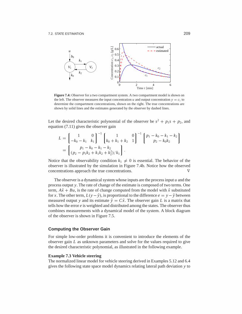
7.2. STATE ESTIMATION 209
k2
V1
k0
b0
u
V2
k1
0 2 4 60
0.1
0.2
0.3
0.4
0.5
0.6
actualestimated
Con
cent
ratio
nc1,c
2[g
/L]
Time t [min]
c1
c2
Figure 7.4:Observer for a two compartment system. A two compartment model is shown onthe left. The observer measures the input concentrationu and output concentrationy = c1 todetermine the compartment concentrations, shown on the right. The true concentrations areshown by solid lines and the estimates generated by the observer by dashed lines.
Let the desired characteristic polynomial of the observer bes2 + p1s + p2, andequation (7.11) gives the observer gain
L = 1 0
−k0 − k1 k1
−1 1 0k0 + k1 + k2 1
−1p1 − k0 − k1 − k2
p2 − k0k2
= p1 − k0 − k1 − k2
(p2 − p1k2 + k1k2 + k22)/k1
.
Notice that the observability conditionk1 6= 0 is essential. The behavior of theobserver is illustrated by the simulation in Figure 7.4b. Notice how the observedconcentrations approach the true concentrations. ∇
The observer is a dynamical system whose inputs are the process inputu and theprocess outputy. The rate of change of the estimate is composed of two terms. Oneterm, Ax + Bu, is the rate of change computed from the model withx substitutedfor x. The other term,L(y− y), is proportional to the differencee = y− y betweenmeasured outputy and its estimatey = Cx. The observer gainL is a matrix thattells how the errore is weighted and distributed among the states. The observer thuscombines measurements with a dynamical model of the system.A block diagramof the observer is shown in Figure 7.5.
Computing the Observer Gain
For simple low-order problems it is convenient to introducethe elements of theobserver gainL as unknown parameters and solve for the values required to givethe desired characteristic polynomial, as illustrated in the following example.
Example 7.3 Vehicle steeringThe normalized linear model for vehicle steering derived in Examples 5.12 and 6.4gives the following state space model dynamics relating lateral path deviationy to

210 CHAPTER 7. OUTPUT FEEDBACK
˙x6
6
x
x
y
y
u
L −1
B∫
C
A
Figure 7.5: Block diagram of the observer. The observer takes the signalsy andu as inputsand produces an estimatex. Notice that the observer contains a copy of the process modelthat is driven byy − y through the observer gainL.
steering angleu:
dx
dt=0 1
0 0
x +
γ1
u, y =
1 0
x. (7.12)
Recall that the statex1 represents the lateral path deviation and thatx2 representsthe turning rate. We will now derive an observer that uses thesystem model todetermine the turning rate from the measured path deviation.
The observability matrix is
Wo =1 0
0 1
,
i.e., the identity matrix. The system is thus observable, andthe eigenvalue assign-ment problem can be solved. We have
A − LC =−l1 1
−l2 0
,
which has the characteristic polynomial
det(s I − A + LC) = det
s + l1 −1
l2 s
= s2 + l1s + l2.
Assuming that we want to have an observer with the characteristic polynomial
s2 + p1s + p2 = s2 + 2ζoωos + ω2o,
the observer gains should be chosen as
l1 = p1 = 2ζoωo, l2 = p2 = ω2o.
The observer is then
dx
dt= Ax + Bu + L(y − Cx) =
0 1
0 0
x +
γ1
u +
l1
l2
(y − x1).

7.3. CONTROL USING ESTIMATED STATE 211
0 10 20 300
5
10
15
20
25
30
x [m]
y[m
] 0 2 4 60
2
4
6
ActEst
0 2 4 6
0
0.2
0.4
0 2 4 6−1
0
1
2
0 2 4 60
0.5
1
x 1,x
1x 2
,x2
x 1−
x 1x 2
−x 2
Normalized timetNormalized timet
Figure 7.6:Simulation of an observer for a vehicle driving on a curvy road (left). The observerhas an initial velocity error. The plots on the middle show the lateral deviationx1, the lateralvelocityx2 by solid lines and their estimatesx1 andx2 by dashed lines. The plots on the rightshow the estimation errors.
A simulation of the observer for a vehicle driving on a curvy road is simulated inFigure 7.6. The vehicle length is the time unit in the normalized model. The figureshows that the observer error settles in about 3 vehicle lengths. ∇
For systems of high order we have to use numerical calculations. The dualitybetween the design of a state feedback and the design of an observer means that thecomputer algorithms for state feedback can also be used for the observer design;we simply use the transpose of the dynamics matrix and the output matrix. TheMATLAB commandacker, which essentially is a direct implementation of thecalculations given in Theorem 7.2, can be used for systems with one output. TheMATLAB commandplace can be used for systems with many outputs. It is alsobetter conditioned numerically.
7.3 Control Using Estimated State
In this section we will consider a state space system of the form
dx
dt= Ax + Bu, y = Cx. (7.13)
Notice that we have assumed that there is no direct term in thesystem (D = 0).This is often a realistic assumption. The presence of a direct term in combinationwith a controller having proportional action creates an algebraic loop, which willbe discussed in Section 8.3. The problem can be solved even if there is a directterm, but the calculations are more complicated.
We wish to design a feedback controller for the system where only the outputis measured. As before, we will assume thatu andy are scalars. We also assumethat the system is reachable and observable. In Chapter 6 we found a feedback ofthe form
u = −K x + kr r

212 CHAPTER 7. OUTPUT FEEDBACK
for the case that all states could be measured, and in Section 7.2 we developed anobserver that can generate estimates of the statex based on inputs and outputs. Inthis section we will combine the ideas of these sections to finda feedback that givesdesired closed loop eigenvalues for systems where only outputs are available forfeedback.
If all states are not measurable, it seems reasonable to try the feedback
u = −K x + kr r, (7.14)
wherex is the output of an observer of the state, i.e.,
dx
dt= Ax + Bu + L(y − Cx). (7.15)
Since the system (7.13) and the observer (7.15) are both of state dimensionn, theclosed loop system has state dimension 2n with state (x, x). The evolution of thestates is described by equations (7.13)–(7.15). To analyzethe closed loop system,the state variablex is replaced by
x = x − x. (7.16)
Subtraction of equation (7.15) from equation (7.13) gives
dx
dt= Ax − Ax − L(Cx − Cx) = Ax − LCx = (A − LC)x.
Returning to the process dynamics, introducingu from equation (7.14) intoequation (7.13) and using equation (7.16) to eliminatex gives
dx
dt= Ax + Bu = Ax − BKx + Bkr r = Ax − BK(x − x)+ Bkr r
= (A − BK)x + BKx + Bkr r.
The closed loop system is thus governed by
d
dt
x
x
=
A − BK BK
0 A − LC
x
x
+
Bkr
0
r. (7.17)
Notice that the statex, representing the observer error, is not affected by the refer-ence signalr . This is desirable since we do not want the reference signal togenerateobserver errors.
Since the dynamics matrix is block diagonal, we find that the characteristicpolynomial of the closed loop system is
λ(s) = det(s I − A + BK) det(s I − A + LC).
This polynomial is a product of two terms: the characteristicpolynomial of theclosed loop system obtained with state feedback and the characteristic polyno-mial of the observer error. The feedback (7.14) that was motivated heuristicallythus provides a neat solution to the eigenvalue assignment problem. The result issummarized as follows.

7.3. CONTROL USING ESTIMATED STATE 213
−y
6x
6
6
6y
Process
Observer
x
B
A
∫C
L
B∫
−C
A
Controller
ukr
−K
r
e
x
˙x
Figure 7.7: Block diagram of an observer-based control system. The observeruses the mea-sured outputy and the inputu to construct an estimate of the state. This estimate is usedby a state feedback controller to generate the corrective input. The controller consists of theobserver and the state feedback; the observer is identical to that in Figure 7.5.
Theorem 7.3(Eigenvalue assignment by output feedback). Consider the system
dx
dt= Ax + Bu, y = Cx.
The controller described by
dx
dt= Ax + Bu + L(y − Cx) = (A − BK − LC)x + Ly,
u = −K x + kr r
gives a closed loop system with the characteristic polynomial
λ(s) = det(s I − A + BK)det(s I − A + LC).
This polynomial can be assigned arbitrary roots if the systemis reachable andobservable.
The controller has a strong intuitive appeal: it can be thought of as being com-posed of two parts, one state feedback and one observer. The dynamics of thecontroller are generated by the observer. The feedback gainK can be computed asif all state variables can be measured, and it depends on onlyA andB. The observergainL depends on onlyA andC. The property that the eigenvalue assignment foroutput feedback can be separated into an eigenvalue assignment for a state feedbackand an observer is called theseparation principle.
A block diagram of the controller is shown in Figure 7.7. Notice that the con-

214 CHAPTER 7. OUTPUT FEEDBACK
0 5 10 15−2
0
2
4
6
8
State feedbackOutput feedbackReference
x 1,x
1
Normalized timet
0 5 10 15−1
0
1
0 5 10 15−1
0
1
x 2,x
2u,u
sfb
Normalized timet
Figure 7.8: Simulation of a vehicle driving on a curvy road with a controller based onstate feedback and an observer. The left plot shows the lane boundaries (dotted), the vehicleposition (solid) and its estimate (dashed), the upper right plot shows the velocity (solid) andits estimate (dashed), and the lower right plot shows the control signal using state feedback(solid) and the control signal using the estimated state (dashed).
troller contains a dynamical model of the plant. This is called the internal modelprinciple: the controller contains a model of the process being controlled.
Example 7.4 Vehicle steeringConsider again the normalized linear model for vehicle steering in Example 6.4.The dynamics relating the steering angleu to the lateral path deviationy is given bythe state space model (7.12). Combining the state feedback derived in Example 6.4with the observer determined in Example 7.3, we find that the controller is givenby
dx
dt= Ax + Bu + L(y − Cx) =
0 1
0 0
x +
γ1
u +
l1
l2
(y − x1),
u = −K x + kr r = k1(r − x1)− k2x2.
Elimination of the variableu gives
dx
dt= (A − BK − LC)x + Ly + Bkr r
=−l1 − γ k1 1 − γ k2
−k1 − l2 −k2
x +
l1
l2
y +
γ1
k1r.
The controller is a dynamical system of second order, with twoinputsy andr andone outputu. Figure 7.8 shows a simulation of the system when the vehicle is drivenalong a curvy road. Since we are using a normalized model, the length unit is thevehicle length and the time unit is the time it takes to travelone vehicle length. Theestimator is initialized with all states equal to zero but the real system has an initialvelocity of 0.5. The figures show that the estimates converge quickly to their truevalues. The vehicle tracks the desired path, which is in the middle of the road, butthere are errors because the road is irregular. The tracking error can be improvedby introducing feedforward (Section 7.5). ∇

7.4. KALMAN FILTERING 215
7.4 Kalman Filtering ��
One of the principal uses of observers in practice is to estimate the state of asystem in the presence ofnoisymeasurements. We have not yet treated noise in ouranalysis, and a full treatment of stochastic dynamical systems is beyond the scopeof this text. In this section, we present a brief introduction to the use of stochasticsystems analysis for constructing observers. We work primarily in discrete time toavoid some of the complications associated with continuous-time random processesand to keep the mathematical prerequisites to a minimum. Thissection assumesbasic knowledge of random variables and stochastic processes; see Kumar andVaraiya [KV86] or Åström [Åst06] for the required material.
Consider a discrete-time linear system with dynamics
x[k + 1] = Ax[k] + Bu[k] + Fv[k], y[k] = Cx[k] + w[k], (7.18)
wherev[k] andw[k] are Gaussian white noise processes satisfying
E{v[k]} = 0, E{w[k]} = 0,
E{v[k]vT [ j ]} ={
0 k 6= j
Rv k = j,E{w[k]wT [ j ]} =
{0 k 6= j
Rw k = j,
E{v[k]wT [ j ]} = 0.
(7.19)
E{v[k]} represents the expected value ofv[k] and E{v[k]vT [ j ]} the correlationmatrix. The matricesRv and Rw are the covariance matrices for the process dis-turbancev and measurement noisew. We assume that the initial condition is alsomodeled as a Gaussian random variable with
E{x[0]} = x0, E{x[0]xT [0]} = P0. (7.20)
We would like to find an estimatex[k] that minimizes the mean square errorE{(x[k] − x[k])(x[k] − x[k])T } given the measurements{y(τ ) : 0 ≤ τ ≤ t}. Weconsider an observer in the same basic form as derived previously:
x[k + 1] = Ax[k] + Bu[k] + L[k](y[k] − Cx[k]). (7.21)
The following theorem summarizes the main result.
Theorem 7.4 (Kalman, 1961). Consider a random process x[k] with dynamicsgiven by equation(7.18)and noise processes and initial conditions described byequations(7.19)and (7.20). The observer gain L that minimizes the mean squareerror is given by
L[k] = AP[k]CT (Rw + C P[k]CT )−1,
where
P[k + 1] = (A − LC)P[k](A − LC)T + F RvFT + L RwLT
P0 = E{x[0]xT [0]}.(7.22)
Before we prove this result, we reflect on its form and function. First, notethat the Kalman filter has the form of arecursivefilter: given mean square error

216 CHAPTER 7. OUTPUT FEEDBACK
P[k] = E{(x[k]− x[k])(x[k]− x[k])T } at timek, we can compute how the estimateand errorchange. Thus we do not need to keep track of old values of the output.Furthermore, the Kalman filter gives the estimatex[k] and the error covarianceP[k], so we can see how reliable the estimate is. It can also be shown that theKalman filter extracts the maximum possible information about output data. If weform the residual between the measured output and the estimated output,
e[k] = y[k] − Cx[k],
we can show that for the Kalman filter the correlation matrix is
Re( j, k) = E{e[ j ]eT [k]} = W[k]δ jk, δ jk ={
1 j = k
0 j 6= k.
In other words, the error is a white noise process, so there isno remaining dynamicinformation content in the error.
The Kalman filter is extremely versatile and can be used even if the process,noise or disturbances are nonstationary. When the system isstationary andif P[k]converges, then the observer gain is constant:
L = APCT (Rw + C PCT ),
whereP satisfies
P = AP AT + F RvFT − APCT(Rw + C PCT
)−1C P AT .
We see that the optimal gain depends on both the process noiseand the measurementnoise, but in a nontrivial way. Like the use of LQR to choose state feedback gains,the Kalman filter permits a systematic derivation of the observer gains given adescription of the noise processes. The solution for the constant gain case is solvedby thedlqe command in MATLAB.
Proof of theorem.We wish to minimize the mean square of the errorE{(x[k] −x[k])(x[k] − x[k])T }. We will define this quantity asP[k] and then show that itsatisfies the recursion given in equation (7.22). By definition,
P[k + 1] = E{(x[k + 1] − x[k + 1])(x[k + 1] − x[k + 1])T }= (A − LC)P[k](A − LC)T + F RvFT + L RwLT
= AP[k] AT + F RvFT − AP[k]CT LT − LC P[k] AT
+ L(Rw + C P[k]CT )LT .
Letting Rǫ = (Rw + C P[k]CT ), we have
P[k + 1] = AP[k] AT + F RvFT − AP[k]CT LT − LC P[k] AT + L RǫLT
= AP[k] AT + F RvFT +(L− AP[k]CT R−1
ǫ
)Rǫ(L− AP[k]CT R−1
ǫ
)T
− AP[k]CT R−1ǫ C PT [k] AT .
To minimize this expression, we chooseL = AP[k]CT R−1ǫ , and the theorem is
proved.

7.4. KALMAN FILTERING 217
The Kalman filter can also be applied to continuous-time stochastic processes.The mathematical derivation of this result requires more sophisticated tools, butthe final form of the estimator is relatively straightforward.
Consider a continuous stochastic system
dx
dt= Ax + Bu + Fv, E{v(s)vT(t)} = Rv(t)δ(t − s),
y = Cx + w, E{w(s)wT(t)} = Rw(t)δ(t − s),
whereδ(τ ) is the unit impulse function. Assume that the disturbancev and noisew are zero mean and Gaussian (but not necessarily stationary):
pdf(v) = 1n√
2π√
detRve− 1
2vT R−1
v v , pdf(w) = 1n√
2π√
detRwe− 1
2wT R−1
w w.
We wish to find the estimatex(t) that minimizes the mean square errorE{(x(t)−x(t))(x(t)− x(t))T } given{y(τ ) : 0 ≤ τ ≤ t}.
Theorem 7.5(Kalman–Bucy, 1961). The optimal estimator has the form of a linearobserver
dx
dt= Ax + Bu + L(y − Cx),
where L(t) = P(t)CT R−1w and P(t) = E{(x(t)− x(t))(x(t)− x(t))T } and satisfies
d P
dt= AP + P AT − PCT R−1
w (t)C P + F Rv(t)FT , P[0] = E{x[0]xT [0]}.
As in the discrete case, when the system is stationary and ifP(t) converges, theobserver gain is constant:
L = PCT R−1w where AP + P AT − PCT R−1
w C P + F RvFT = 0.
The second equation is thealgebraic Riccati equation.
Example 7.5 Vectored thrust aircraftWe consider the lateral dynamics of the system, consisting of the subsystems whosestates are given byz = (x, θ, x, θ ). To design a Kalman filter for the system, wemust include a description of the process disturbances and the sensor noise. Wethus augment the system to have the form
dz
dt= Az+ Bu + Fv, y = Cz+ w,
whereF represents the structure of the disturbances (including the effects of non-linearities that we have ignored in the linearization),w represents the disturbancesource (modeled as zero mean, Gaussian white noise) andv represents that mea-surement noise (also zero mean, Gaussian and white).
For this example, we chooseF as the identity matrix and choose disturbancesvi ,i = 1, . . . ,n, to be independent disturbances with covariance given byRi i = 0.1,Ri j = 0, i 6= j . The sensor noise is a single random variable which we model as

218 CHAPTER 7. OUTPUT FEEDBACK
0 0.5 1 1.5 2−0.4
−0.3
−0.2
−0.1
0
0.1
Time t [s]
Sta
tesz
i[m
ixed
units
]
xθxd
θd
(a) Position measurement only
0 0.5 1 1.5 2−0.4
−0.3
−0.2
−0.1
0
0.1
Time t [s]
Sta
tesz
i[m
ixed
units
]
xθxd
θd
(b) Position and orientation
Figure 7.9: Kalman filter design for a vectored thrust aircraft. In the first design (a) onlythe lateral position of the aircraft is measured. Adding a direct measurement of the rollangle produces a much better observer (b). The initial condition for bothsimulations is(0.1,0.0175, 0.01, 0).
having covarianceRw = 10−4. Using the same parameters as before, the resultingKalman gain is given by
L =
37.0−46.9185
−31.6
.
The performance of the estimator is shown in Figure 7.9a. We seethat while theestimator converges to the system state, it contains significant overshoot in the stateestimate, which can lead to poor performance in a closed loopsetting.
To improve the performance of the estimator, we explore the impact of adding anew output measurement. Suppose that instead of measuring just the output positionx, we also measure the orientation of the aircraftθ . The output becomes
y =1 0 0 0
0 1 0 0
z +
w1
w2
,
and if we assume thatw1 andw2 are independent noise sources each with covarianceRwi = 10−4, then the optimal estimator gain matrix becomes
L =
32.6 −0.150−0.150 32.6
32.7 −9.79−0.0033 31.6
.
These gains provide good immunity to noise and high performance, as illustratedin Figure 7.9b. ∇

7.5. A GENERAL CONTROLLER STRUCTURE 219
x
6
ufb6
y6
ηνe StateFeedback
xd
r
Generation
Trajectory
uff
uProcess
d n
6
−1 Observer
Figure 7.10:Block diagram of a controller based on a structure with two degrees of freedomwhich combines feedback and feedforward. The controller consists of a trajectory generator,state feedback and an observer. The trajectory generation subsystemcomputes a feedforwardcommanduff along with the desired statexd. The state feedback controller uses the estimatedstate and desired state to compute a corrective inputufb.
7.5 A General Controller Structure
State estimators and state feedback are important components of a controller. Inthis section, we will add feedforward to arrive at a general controller structure thatappears in many places in control theory and is the heart of most modern controlsystems. We will also briefly sketch how computers can be used to implement acontroller based on output feedback.
Feedforward
In this chapter and the previous one we have emphasized feedback as a mechanismfor minimizing tracking error; reference values were introduced simply by addingthem to the state feedback through a gainkr . A more sophisticated way of doingthis is shown by the block diagram in Figure 7.10, where the controller consists ofthree parts: an observer that computes estimates of the states based on a model andmeasured process inputs and outputs, a state feedback, and atrajectory generatorthat generates the desired behavior of all statesxd and a feedforward signaluff .Under the ideal conditions of no disturbances and no modeling errors the signaluff
generates the desired behaviorxd when applied to the process. The signalxd can begenerated by a system that gives the desired response of the state. To generate thethe signaluff , we must also have a model of the inverse of the process dynamics.
To get some insight into the behavior of the system, we assumethat there areno disturbances and that the system is in equilibrium with a constant referencesignal and with the observer statex equal to the process statex. When the referencesignal is changed, the signalsuff andxd will change. The observer tracks the stateperfectly because the initial state was correct. The estimated statex is thus equal tothe desired statexd, and the feedback signalufb = L(xd − x) will also be zero. Allaction is thus created by the signals from the trajectory generator. If there are somedisturbances or some modeling errors, the feedback signal will attempt to correctthe situation.
This controller is said to havetwo degrees of freedombecause the responses

220 CHAPTER 7. OUTPUT FEEDBACK
to command signals and disturbances are decoupled. Disturbance responses aregoverned by the observer and the state feedback, while the response to commandsignals is governed by the trajectory generator (feedforward).
For an analytic description we start with the full nonlineardynamics of theprocess
dx
dt= f (x,u), y = h(x,u). (7.23)
Assume that the trajectory generator is able to compute a desired trajectory(xd,uff )
that satisfies the dynamics (7.23) and satisfiesr = h(xd,uff ). To design the con-troller, we construct the error system. Letz = x − xd andv = u − uff and computethe dynamics for the error:
z = x − xd = f (x,u)− f (xd,uff )
= f (z + xd, v + uff )− f (xd,uff ) =: F(z, v, xd(t),uff (t)).
In general, this system is time-varying. Note thatz = −e in Figure 7.10 due to theconvention of using negative feedback in the block diagram.
For trajectory tracking, we can assume thate is small (if our controller is doinga good job), and so we can linearize aroundz = 0:
dz
dt≈ A(t)z + B(t)v, A(t) = ∂F
∂z
∣∣∣∣(xd(t),uff (t))
, B(t) = ∂F
∂v
∣∣∣∣(xd(t),uff (t)
.
It is often the case thatA(t) and B(t) depend only onxd, in which case it isconvenient to writeA(t) = A(xd) andB(t) = B(xd).
Assume now thatxd anduff are either constant or slowly varying (with respectto the performance criterion). This allows us to consider just the (constant) linearsystem given by(A(xd), B(xd)). If we design a state feedback controllerK (xd) foreachxd, then we can regulate the system using the feedback
v = −K (xd)z.
Substituting back the definitions ofe andv, our controller becomes
u = −K (xd)(x − xd)+ uff .
This form of controller is called again scheduledlinear controller withfeedforwarduff .
Finally, we consider the observer. The full nonlinear dynamics can be used forthe prediction portion of the observer and the linearized system for the correctionterm:
dx
dt= f (x,u)+ L(x)(y − h(x,u)),
where L(x) is the observer gain obtained by linearizing the system around thecurrently estimated state. This form of the observer is knownas anextended Kalmanfilter and has proved to be a very effective means of estimating the state of a nonlinearsystem.

7.5. A GENERAL CONTROLLER STRUCTURE 221
x0, y0
x f , y f
(a) Overhead view
0 1 2 3 4−5
0
5
0 1 2 3 4−0.5
0
0.5
y[m
]δ
[rad
]
Time t [s]
(b) Position and steering
Figure 7.11:Trajectory generation for changing lanes. We wish to change from the left laneto the right lane over a distance of 30 m in 4 s. The planned trajectory in thexyplane is shownin (a) and the lateral positiony and the steering angleδ over the maneuver time interval areshown in (b).
.
There are many ways to generate the feedforward signal, and there are also manydifferent ways to compute the feedback gainK and the observer gainL. Note thatonce again the internal model principle applies: the controller contains a model ofthe system to be controlled through the observer.
Example 7.6 Vehicle steeringTo illustrate how we can use a two degree-of-freedom design to improve the per-formance of the system, consider the problem of steering a car to change lanes ona road, as illustrated in Figure 7.11a.
We use the non-normalized form of the dynamics, where were derived in Exam-ple 2.8. Using the center of the rear wheels as the reference (α = 0), the dynamicscan be written as
dx
dt= cosθv,
dy
dt= sinθv,
dθ
dt= v
btanδ,
wherev is the forward velocity of the vehicle andδ is the steering angle. To generatea trajectory for the system, we note that we can solve for the states and inputs ofthe system givenx, y by solving the following sets of equations:
x = v cosθ, x = v cosθ − vθ sinθ,
y = v sinθ, y = v sinθ + vθ cosθ,
θ = (v/b) tanδ.
(7.24)
This set of five equations has five unknowns (θ , θ , v, v andδ) that can be solvedusing trigonometry and linear algebra. It follows that we can compute a feasibletrajectory for the system given any pathx(t), y(t). (This special property of a systemis known asdifferential flatness[FLMR92, FLMR95].)
To find a trajectory from an initial state(x0, y0, θ0) to a final state(x f , y f , θ f )

222 CHAPTER 7. OUTPUT FEEDBACK
at a timeT , we look for a pathx(t), y(t) that satisfies
x(0) = x0, x(T) = x f ,
y(0) = y0, y(T) = y f ,
x(0) sinθ0 − y(0) cosθ0 = 0, x(T) sinθ f − y(T) cosθ f = 0,
y(0) sinθ0 + x(0) cosθ0 = v0, y(T) sinθ f + x(T) cosθ f = v f .
(7.25)
One such trajectory can be found by choosingx(t) andy(t) to have the form
xd(t) = α0 + α1t + α2t2 + α3t3, yd(t) = β0 + β1t + β2t2 + β3t
3.
Substituting these equations into equation (7.25), we are left with a set of linearequations that can be solved forαi , βi , i = 0,1,2,3. This gives a feasible trajectoryfor the system by using equation (7.24) to solve forθd, vd andδd.
Figure 7.11b shows a sample trajectory generated by a set of higher-order equa-tions that also set the initial and final steering angle to zero. Notice that the feedfor-ward input is quite different from 0, allowing the controller to command a steeringangle that executes the turn in the absence of errors. ∇
Kalman’s Decomposition of a Linear System�
In this chapter and the previous one we have seen that two fundamental propertiesof a linear input/output system are reachability and observability. It turns out thatthese two properties can be used to classify the dynamics of asystem. The keyresult is Kalman’s decomposition theorem, which says that alinear system can bedivided into four subsystems:6ro which is reachable and observable,6r o which isreachable but not observable,6ro which is not reachable but is observable and6r o
which is neither reachable nor observable.We will first consider this in the special case of systems wherethe matrixA has
distinct eigenvalues. In this case we can find a set of coordinates such that theAmatrix is diagonal and, with some additional reordering of the states, the systemcan be written as
dx
dt=
Aro 0 0 00 Ar o 0 00 0 Aro 00 0 0 Ar o
x +
Bro
Br o
00
u,
y =Cro 0 Cro 0
x + Du.
(7.26)
All statesxk such thatBk 6= 0 are reachable, and all states such thatCk 6= 0 areobservable. If we set the initial state to zero (or equivalently look at the steady-stateresponse ifA is stable), the states given byxro andxr o will be zero andxr o doesnot affect the output. Hence the outputy can be determined from the system
dxro
dt= Aroxro + Brou, y = Croxro + Du.

7.5. A GENERAL CONTROLLER STRUCTURE 223
u+6ro
6ro
6r o
6r o
y
(a) Distinct eigenvalues
u+6ro
6ro
6r o
6r o
y
(b) General case
Figure 7.12: Kalman’s decomposition of a linear system. The decomposition in (a) is fora system with distinct eigenvalues and the one in (b) is the general case. The system isbroken into four subsystems, representing the various combinations ofreachable and observ-able states. The input/output relationship only depends on the subset of states that are bothreachable and observable.
Thus from the input/output point of view, it is only the reachable and observabledynamics that matter. A block diagram of the system illustrating this property isgiven in Figure 7.12a.
The general case of the Kalman decomposition is more complicated and re-quires some additional linear algebra; see the original paper by Kalman, Ho andNarendra [KHN63]. The key result is that the state space can still be decomposedinto four parts, but there will be additional coupling so that the equations have theform
dx
dt=
Aro 0 ∗ 0∗ Ar o ∗ ∗0 0 Aro 00 0 ∗ Ar o
x +
Bro
Br o
00
u,
y =Cro 0 Cro 0
x,
(7.27)
where∗ denotes block matrices of appropriate dimensions. The input/output re-sponse of the system is given by
dxro
dt= Aroxro + Brou, y = Croxro + Du, (7.28)
which are the dynamics of the reachable and observable subsystem6ro. A blockdiagram of the system is shown in Figure 7.12b.
The following example illustrates Kalman’s decomposition.
Example 7.7 System and controller with feedback from observer statesConsider the system
dx
dt= Ax + Bu, y = Cx.
The following controller, based on feedback from the observer state, was given in

224 CHAPTER 7. OUTPUT FEEDBACK
Theorem 7.3:
dx
dt= Ax + Bu + L(y − Cx), u = −K x + kr r.
Introducing the statesx andx = x − x, the closed loop system can be written as
d
dt
x
x
=
A − BK BK
0 A − LC
x
x
+
Bkr
0
r, y =
C 0
x,
which is a Kalman decomposition like the one shown in Figure 7.12b with onlytwo subsystems6ro and6ro. The subsystem6ro, with statex, is reachable andobservable, and the subsystem6ro, with statex, is not reachable but observable.It is natural that the statex is not reachable from the reference signalr because itwould not make sense to design a system where changes in the command signalcould generate observer errors. The relationship between the referencer and theoutputy is given by
dx
dt= (A − BK)x + Bkr r, y = Cx,
which is the same relationship as for a system with full statefeedback. ∇
Computer Implementation
The controllers obtained so far have been described by ordinary differential equa-tions. They can be implemented directly using analog components, whether elec-tronic circuits, hydraulic valves or other physical devices. Since in modern engi-neering applications most controllers are implemented using computers, we willbriefly discuss how this can be done.
A computer-controlled system typically operates periodically: every cycle, sig-nals from the sensors are sampled and converted to digital form by the A/D converter,the control signal is computed and the resulting output is converted to analog formfor the actuators, as shown in Figure 7.13. To illustrate the main principles of howto implement feedback in this environment, we consider the controller describedby equations (7.14) and (7.15), i.e.,
dx
dt= Ax + Bu + L(y − Cx), u = −K x + kr r.
The second equation consists only of additions and multiplications and can thusbe implemented directly on a computer. The first equation can beimplemented byapproximating the derivative by a difference
dx
dt≈ x(tk+1)− x(tk)
h= Ax(tk)+ Bu(tk)+ L
(y(tk)− Cx(tk)
),
wheretk are the sampling instants andh = tk+1−tk is the sampling period. Rewritingthe equation to isolatex(tk+1), we get the difference equation
x(tk+1) = x(tk)+ h(Ax(tk)+ Bu(tk)+ L
(y(tk)− Cx(tk)
)). (7.29)

7.5. A GENERAL CONTROLLER STRUCTURE 225
Controller
System Sensors
Filter
Clock
operator input
D/A Computer A/D
noiseexternal disturbancesnoise
66Output
Process
Actuators
Figure 7.13:Components of a computer-controlled system. The controller consists ofanalog-to-digital (A/D) and digital-to-analog (D/A) converters, as well as a computer that implementsthe control algorithm. A system clock controls the operation of the controller, synchronizingthe A/D, D/A and computing processes. The operator input is also fed to thecomputer as anexternal input.
The calculation of the estimated state at timetk+1 requires only addition and mul-tiplication and can easily be done by a computer. A section ofpseudocode for theprogram that performs this calculation is
% Control algorithm - main loopr = adin(ch1) % read referencey = adin(ch2) % get process outputu = K*(xd - xhat) + uff % compute control variabledaout(ch1, u) % set analog outputxhat = xhat + h*(A*x+B*u+L*(y-C*x)) % update state estimate
The program runs periodically at a fixed rateh. Notice that the number ofcomputations between reading the analog input and setting the analog output hasbeen minimized by updating the state after the analog outputhas been set. Theprogram has an array of statesxhat that represents the state estimate. The choiceof sampling period requires some care.
There are more sophisticated ways of approximating a differential equation by adifference equation. If the control signal is constant between the sampling instants,it is possible to obtain exact equations; see [ÅW97].
There are several practical issues that also must be dealt with. For example, itis necessary to filter measured signals before they are sampled so that the filteredsignal has little frequency content abovefs/2, wherefs is the sampling frequency.This avoids a phenomena knows asaliasing. If controllers with integral action areused, it is also necessary to provide protection so that the integral does not becometoo large when the actuator saturates. This issue, calledintegrator windup, is studiedin more detail in Chapter 10. Care must also be taken so that parameter changes do

226 CHAPTER 7. OUTPUT FEEDBACK
not cause disturbances.
7.6 Further Reading
The notion of observability is due to Kalman [Kal61b] and, combined with the dualnotion of reachability, it was a major stepping stone towardestablishing state spacecontrol theory beginning in the 1960s. The observer first appeared as the Kalmanfilter, in the paper by Kalman [Kal61a] on the discrete-time case and Kalman andBucy [KB61] on the continuous-time case. Kalman also conjectured that the con-troller for output feedback could be obtained by combining astate feedback withan observer; see the quote in the beginning of this chapter. This result was formallyproved by Josep and Tou [JT61] and Gunckel and Franklin [GF71]. The combinedresult is known as the linear quadratic Gaussian control theory; a compact treat-ment is given in the books by Anderson and Moore [AM90] and Åström [Åst06].Much later it was shown that solutions to robust control problems also had a sim-ilar structure but with different ways of computing observer and state feedbackgains [DGKF89]. The general controller structure discussed in Section 7.5, whichcombines feedback and feedforward, was described by Horowitz in 1963 [Hor63].The particular form in Figure 7.10 appeared in [ÅW97], which also treats digitalimplementation of the controller. The hypothesis that motion control in humansis based on a combination of feedback and feedforward was proposed by Ito in1970 [Ito70].
Exercises
7.1(Coordinate transformations) Consider a system under a coordinate transforma-tion z = T x, whereT ∈ R
n×n is an invertible matrix. Show that the observabilitymatrix for the transformed system is given byWo = WoT−1 and hence observabilityis independent of the choice of coordinates.
7.2 Show that the system depicted in Figure 7.2 is not observable.
7.3 (Observable canonical form) Show that if a system is observable, then thereexists a change of coordinatesz = T x that puts the transformed system into ob-servable canonical form.
7.4(Bicycle dynamics) The linearized model for a bicycle is given in equation (3.5),which has the form
Jd2ϕ
dt2− Dv0
b
dδ
dt= mghϕ + mv2
0h
bδ,
whereϕ is the tilt of the bicycle andδ is the steering angle. Give conditions underwhich the system is observable and explain any special situations where it losesobservability.

EXERCISES 227
7.5 (Integral action) The model (7.1) assumes that the inputu = 0 corresponds tox = 0. In practice, it is very difficult to know the value of the control signal thatgives a precise value of the state or the output because this would require a perfectlycalibrated system. One way to avoid this assumption is to assume that the model isgiven by
dx
dt= Ax + B(u + u0), y = Cx + Du,
whereu0 is an unknown constant that can be modeled asdu0/dt = 0. Consideru0 as an additional state variable and derive a controller based on feedback fromthe observed state. Show that the controller has integral action and that it does notrequire a perfectly calibrated system.
7.6 (Vectored thrust aircraft) The lateral dynamics of the vectored thrust aircraft�example described in Example 6.8 can be obtained by considering the motiondescribed by the statesz = (x, θ, x, θ ). Construct an estimator for these dynamicsby setting the eigenvalues of the observer into aButterworth patternwith λbw =−3.83± 9.24i , −9.24± 3.83i . Using this estimator combined with the state spacecontroller computed in Example 6.8, plot the step response ofthe closed loopsystem.
7.7 (Uniqueness of observers) Show that the design of an observerby eigenvalueassignment is unique for single-output systems. Constructexamples that show thatthe problem is not necessarily unique for systems with many outputs.
7.8 (Observers using differentiation) Consider the linear system (7.2), and assumethat the observability matrixWo is invertible. Show that
x = W−1o
y y y · · · y(n−1)
T
is an observer. Show that it has the advantage of giving the state instantaneouslybut that it also has some severe practical drawbacks.
7.9 (Observer for Teorell’s compartment model) Teorell’s compartment model,�shown in Figure 3.17, has the following state space representation:
dx
dt=
−k1 0 0 0 0k1 −k2 − k4 0 k3 00 k4 0 0 00 k2 0 −k3 − k5 00 0 0 k5 0
x +
10000
u,
where representative parameters arek1 = 0.02, k2 = 0.1, k3 = 0.05, k4 = k5 =0.005. The concentration of a drug that is active in compartment5 is measured inthe bloodstream (compartment 2). Determine the compartments that are observablefrom measurement of concentration in the bloodstream and design an estimatorfor these concentrations base on eigenvalue assignment. Choose the closed loopeigenvalues−0.03,−0.05 and−0.1. Simulate the system when the input is a pulseinjection.

228 CHAPTER 7. OUTPUT FEEDBACK
7.10(Observer design for motor drive) Consider the normalized model of the motordrive in Exercise 2.10 where the open loop system has the eigenvalues 0,0,−0.05±i . A state feedback that gave a closed loop system with eigenvalues in−2, −1 and−1 ± i was designed in Exercise 6.11. Design an observer for the system that haseigenvalues−4, −2 and−2 ± 2i . Combine the observer with the state feedbackfrom Exercise 6.11 to obtain an output feedback and simulate the complete system.
7.11(Feedforward design for motor drive) Consider the normalized model of themotor drive in Exercise 2.10. Design the dynamics of the blocklabeled “trajectorygeneration” in Figure 7.10 so that the dynamics relating the outputη to the referencesignalr has the dynamics
d3ym
dt3+ am1
d2ym
dt2+ am2
dym
dt+ am3ym = am3r, (7.30)
with parametersam1 = 2.5ωm,am2 = 2.5ω2m andam3 = ω3
m. Discuss how the largestvalue of the feedforward signal for a unit step in the commandsignal depends onωm.
7.12(Whipple bicycle model) Consider the Whipple bicycle modelgiven by equa-tion (3.7) in Section 3.2. A state feedback for the system was designed in Exer-cise 6.12. Design an observer and an output feedback for the system.
7.13(Discrete-time random walk) Suppose that we wish to estimatethe position�of a particle that is undergoing a random walk in one dimension (i.e., along a line).We model the position of the particle as
x[k + 1] = x[k] + u[k],
wherex is the position of the particle andu is a white noise processes withE{u[i ]} =0 andE{u[i ] u[ j ]} = Ruδ(i − j ). We assume that we can measurex subject toadditive, zero-mean, Gaussian white noise with covariance1.
(a) Compute the expected value and covariance of the particle as a function ofk.
(b) Construct a Kalman filter to estimate the position of the particle given thenoisy measurements of its position. Compute the steady-state expected value andcovariance of the error of your estimate.
(c) Suppose thatE{u[0]} = µ 6= 0 but is otherwise unchanged. How would youranswers to parts (a) and (b) change?
7.14(Kalman decomposition) Consider a linear system characterized by the matri-ces
A =
−2 1 −1 21 −3 0 21 1 −4 20 1 −1 −1
, B =
2221
, C =
0 1 −1 0
, D = 0.
Construct a Kalman decomposition for the system. (Hint: Tryto diagonalize.)

Chapter EightTransfer Functions
The typical regulator system can frequently be described, in essentials, by differential equationsof no more than perhaps the second, third or fourth order. …In contrast, the order of the setof differential equations describing the typical negative feedback amplifierused in telephonyis likely to be very much greater. As a matter of idle curiosity, I once countedto find out whatthe order of the set of equations in an amplifier I had just designed would have been, if I hadworked with the differential equations directly. It turned out to be 55.
Henrik Bode, 1960 [Bod60].
This chapter introduces the concept of thetransfer function, which is a compactdescription of the input/output relation for a linear system. Combining transferfunctions with block diagrams gives a powerful method for dealing with complexlinear systems. The relationship between transfer functions and other descriptionsof system dynamics is also discussed.
8.1 Frequency Domain Modeling
Figure 8.1 is a block diagram for a typical control system, consisting of a process tobe controlled and a controller that combines feedback and feedforward. We saw inthe previous two chapters how to analyze and design such systems using state spacedescriptions of the blocks. As mentioned in Chapter 2, an alternative approach isto focus on the input/output characteristics of the system.Since it is the inputs andoutputs that are used to connect the systems, one could expect that this point of
Controller
6
d
6
n
yν η6
Processdynamics
Pu
Reference Feedbackshaping controller
Fe
C
−1
r
Figure 8.1: A block diagram for a feedback control system. The reference signal r is fedthrough a reference shaping block, which produces the signal that willbe tracked. The errorbetween this signal and the output is fed to a controller, which produces theinput to theprocess. Disturbances and noise are included as external signals at the input and output ofthe process dynamics.

230 CHAPTER 8. TRANSFER FUNCTIONS
view would allow an understanding of the overall behavior ofthe system. Transferfunctions are the main tool in implementing this point of view for linear systems.
The basic idea of the transfer function comes from looking at the frequencyresponse of a system. Suppose that we have an input signal thatis periodic. Thenwe can decompose this signal into the sum of a set of sines and cosines,
u(t) =∞∑
k=0
ak sin(kωt)+ bk cos(kωt),
whereω is the fundamental frequency of the periodic input. Each of the terms in thisinput generates a corresponding sinusoidal output (in steady state), with possiblyshifted magnitude and phase. The gain and phase at each frequency are determinedby the frequency response given in equation (5.24):
G(s) = C(s I − A)−1B + D, (8.1)
where we sets = i (kω) for eachk = 1, . . . ,∞ and i =√
−1. If we know thesteady-state frequency responseG(s), we can thus compute the response to any(periodic) signal using superposition.
The transfer function generalizes this notion to allow a broader class of inputsignals besides periodic ones. As we shall see in the next section, the transferfunction represents the response of the system to anexponential input, u = est.It turns out that the form of the transfer function is precisely the same as that ofequation (8.1). This should not be surprising since we derived equation (8.1) bywriting sinusoids as sums of complex exponentials. Formally, the transfer functionis the ratio of the Laplace transforms of output and input, although one does nothave to understand the details of Laplace transforms in orderto make use of transferfunctions.
Modeling a system through its response to sinusoidal and exponential signals isknown asfrequency domain modeling. This terminology stems from the fact thatwe represent the dynamics of the system in terms of the generalized frequencysrather than the time domain variablet . The transfer function provides a completerepresentation of a linear system in the frequency domain.
The power of transfer functions is that they provide a particularly convenientrepresentation in manipulating and analyzing complex linear feedback systems. Aswe shall see, there are many graphical representations of transfer functions thatcapture interesting properties of the underlying dynamics. Transfer functions alsomake it possible to express the changes in a system because ofmodeling error, whichis essential when considering sensitivity to process variations of the sort discussedin Chapter 12. More specifically, using transfer functions, it is possible to analyzewhat happens when dynamic models are approximated by staticmodels or whenhigh-order models are approximated by low-order models. One consequence is thatwe can introduce concepts that express the degree of stability of a system.
While many of the concepts for state space modeling and analysis apply di-rectly to nonlinear systems, frequency domain analysis applies primarily to linearsystems. The notions of gain and phase can be generalized to nonlinear systems

8.2. DERIVATION OF THE TRANSFER FUNCTION 231
and, in particular, propagation of sinusoidal signals through a nonlinear systemcan approximately be captured by an analog of the frequency response called thedescribing function. These extensions of frequency response will be discussed inSection 9.5.
8.2 Derivation of the Transfer Function
As we have seen in previous chapters, the input/output dynamics of a linear sys-tem have two components: the initial condition response andthe forced response.In addition, we can speak of the transient properties of the system and its steady-state response to an input. The transfer function focuses on the steady-state forcedresponse to a given input and provides a mapping between inputs and their corre-sponding outputs. In this section, we will derive the transfer function in terms ofthe exponential response of a linear system.
Transmission of Exponential Signals
To formally compute the transfer function of a system, we will make use of a specialtype of signal, called anexponential signal,of the formest, wheres = σ + iω isa complex number. Exponential signals play an important rolein linear systems.They appear in the solution of differential equations and in the impulse responseof linear systems, and many signals can be represented as exponentials or sums ofexponentials. For example, a constant signal is simplyeαt with α = 0. Dampedsine and cosine signals can be represented by
e(σ+iω)t = eσ teiωt = eσ t(cosωt + i sinωt),
whereσ < 0 determines the decay rate. Figure 8.2 gives examples of signals thatcan be represented by complex exponentials; many other signals can be representedby linear combinations of these signals. As in the case of sinusoidal signals, we willallow complex-valued signals in the derivation that follows, although in practicewe always add together combinations of signals that result in real-valued functions.
To investigate how a linear system responds to an exponential input u(t) = est
we consider the state space system
dx
dt= Ax + Bu, y = Cx + Du. (8.2)
Let the input signal beu(t) = est and assume thats 6= λ j (A), j = 1, . . . ,n, whereλ j (A) is the j th eigenvalue ofA. The state is then given by
x(t) = eAtx(0)+∫ t
0eA(t−τ)Besτ dτ = eAtx(0)+ eAt
∫ t
0e(s I−A)τ B dτ.
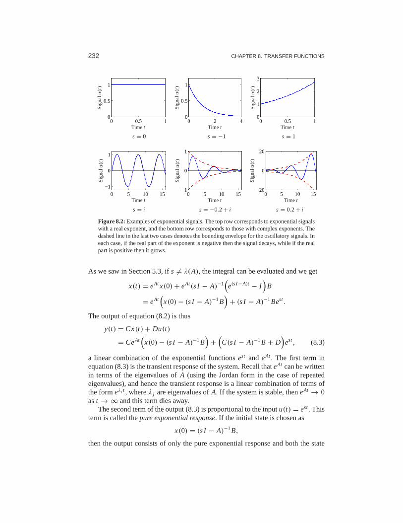
232 CHAPTER 8. TRANSFER FUNCTIONS
0 0.5 10
0.5
1
Time t
Sig
nalu(t)
s = 0
0 2 40
0.5
1
Time t
Sig
nalu(t)
s = −1
0 0.5 10
1
2
3
Time t
Sig
nalu(t)
s = 1
0 5 10 15−1
0
1
Time t
Sig
nalu(t)
s = i
0 5 10 15−1
0
1
Time t
Sig
nalu(t)
s = −0.2 + i
0 5 10 15−20
0
20
Time t
Sig
nalu(t)
s = 0.2 + i
Figure 8.2:Examples of exponential signals. The top row corresponds to exponential signalswith a real exponent, and the bottom row corresponds to those with complexexponents. Thedashed line in the last two cases denotes the bounding envelope for the oscillatory signals. Ineach case, if the real part of the exponent is negative then the signal decays, while if the realpart is positive then it grows.
As we saw in Section 5.3, ifs 6= λ(A), the integral can be evaluated and we get
x(t) = eAtx(0)+ eAt(s I − A)−1(e(s I−A)t − I
)B
= eAt(
x(0)− (s I − A)−1B)
+ (s I − A)−1Best.
The output of equation (8.2) is thus
y(t) = Cx(t)+ Du(t)
= CeAt(
x(0)− (s I − A)−1B)
+(C(s I − A)−1B + D
)est, (8.3)
a linear combination of the exponential functionsest and eAt. The first term inequation (8.3) is the transient response of the system. Recall that eAt can be writtenin terms of the eigenvalues ofA (using the Jordan form in the case of repeatedeigenvalues), and hence the transient response is a linear combination of terms ofthe formeλ j t , whereλ j are eigenvalues ofA. If the system is stable, theneAt → 0ast → ∞ and this term dies away.
The second term of the output (8.3) is proportional to the input u(t) = est. Thisterm is called thepure exponential response. If the initial state is chosen as
x(0) = (s I − A)−1B,
then the output consists of only the pure exponential response and both the state

8.2. DERIVATION OF THE TRANSFER FUNCTION 233
and the output are proportional to the input:
x(t) = (s I − A)−1Best = (s I − A)−1Bu(t),
y(t) =(C(s I − A)−1B + D
)est =
(C(s I − A)−1B + D
)u(t).
This is also the output we see in steady state, when the transients represented bythe first term in equation (8.3) have died out. The map from the input to the output,
Gyu(s) = C(s I − A)−1B + D, (8.4)
is thetransfer functionfrom u to y for the system (8.2), and we can writey(t) =Gyu(s)u(t) for the case thatu(t) = est. Compare with the definition of frequencyresponse given by equation (5.24).
An important point in the derivation of the transfer function is the fact thatwe have restricteds so thats 6= λ j (A), the eigenvalues ofA. At those values ofs, we see that the response of the system is singular (sinces I − A will fail tobe invertible). Ifs = λ j (A), the response of the system to the exponential inputu = eλ j t is y = p(t)eλ j t , wherep(t) is a polynomial of degree less than or equalto the multiplicity of the eigenvalueλ j (see Exercise 8.2).
Example 8.1 Damped oscillatorConsider the response of a damped linear oscillator, whose state space dynamicswere studied in Section 6.3:
dx
dt= 0 ω0
−ω0 −2ζω0
x +
0
kω0
u, y =
1 0
x. (8.5)
This system is stable ifζ > 0, and so we can look at the steady-state response toan inputu = est,
Gyu(s) = C(s I − A)−1B =1 0
s −ω0
ω0 s + 2ζω0
−1 0kω0
=1 0
(
1
s2 + 2ζω0s + ω20
s ω0
−ω0 s + 2ζω0
) 0
kω0
= kω20
s2 + 2ζω0s + ω20
.
(8.6)
To compute the steady-state response to a step function, we set s = 0 and we seethat
u = 1 =⇒ y = Gyu(0)u = k.
If we wish to compute the steady-state response to a sinusoid, we write
u = sinωt = 1
2
(ie−iωt − ieiωt
),
y = 1
2
(iG yu(−iω)e−iωt − iG yu(iω)e
iωt).

234 CHAPTER 8. TRANSFER FUNCTIONS
We can now writeG(iω) in terms of its magnitude and phase,
G(iω) = kω20
s2 + 2ζω0s + ω20
= Mei θ ,
where the magnitude (or gain)M and phaseθ are given by
M = kω20√
(ω20 − ω2)2 + (2ζω0ω)2
,sinθ
cosθ= −2ζω0ω
ω20 − ω2
.
We can also make use of the fact thatG(−iω) is given by its complex conjugateG∗(iω), and it follows thatG(−iω) = Me−i θ . Substituting these expressions intoour output equation, we obtain
y = 1
2
(i (Me−i θ )e−iωt − i (Mei θ )eiωt
)
= M ·1
2
(ie−i (ωt+θ) − iei (ωt+θ)) = M sin(ωt + θ).
The responses to other signals can be computed by writing the input as an appro-priate combination of exponential responses and using linearity. ∇
Coordinate Changes
The matricesA, B andC in equation (8.2) depend on the choice of coordinatesystem for the states. Since the transfer function relates input to outputs, it shouldbe invariant to coordinate changes in the state space. To show this, consider themodel (8.2) and introduce new coordinatesz by the transformationz = T x, whereT is a nonsingular matrix. The system is then described by
dz
dt= T(Ax + Bu) = T AT−1z + T Bu =: Az+ Bu,
y = Cx + Du = CT−1z + Du =: Cz+ Du.
This system has the same form as equation (8.2), but the matricesA, B andC aredifferent:
A = T AT−1, B = T B, C = CT−1. (8.7)
Computing the transfer function of the transformed model, we get
G(s) = C(s I − A)−1B + D = CT−1(s I − T AT−1)−1T B + D
= C(T−1(s I − T AT−1)T
)−1B + D = C(s I − A)−1B + D = G(s),
which is identical to the transfer function (8.4) computed from the system descrip-tion (8.2). The transfer function is thus invariant to changes of the coordinates inthe state space.
Another property of the transfer function is that it corresponds to the portion of the�state space dynamics that is both reachable and observable.In particular, if we make

8.2. DERIVATION OF THE TRANSFER FUNCTION 235
use of the Kalman decomposition (Section 7.5), then the transfer function dependsonly on the dynamics in the reachable and observable subspace6ro (Exercise 8.7).
Transfer Functions for Linear Systems
Consider a linear input/output system described by the controlled differential equa-tion
dny
dtn+ a1
dn−1y
dtn−1+ · · · + any = b0
dmu
dtm+ b1
dm−1u
dtm−1+ · · · + bmu, (8.8)
whereu is the input andy is the output. This type of description arises in manyapplications, as described briefly in Section 2.2; bicycle dynamics and AFM mod-eling are two specific examples. Note that here we have generalized our previoussystem description to allow both the input and its derivatives to appear.
To determine the transfer function of the system (8.8), let the input beu(t) = est.Since the system is linear, there is an output of the system that is also an exponentialfunction y(t) = y0est. Inserting the signals into equation (8.8), we find
(sn + a1sn−1 + · · · + an)y0est = (b0sm + b1s
m−1 · · · + bm)e−st,
and the response of the system can be completely described bytwo polynomials
a(s) = sn + a1sn−1 + · · · + an, b(s) = b0sm + b1s
m−1 + · · · + bm.(8.9)
The polynomiala(s) is the characteristic polynomial of the ordinary differentialequation. Ifa(s) 6= 0, it follows that
y(t) = y0est = b(s)
a(s)est. (8.10)
The transfer function of the system (8.8) is thus the rationalfunction
G(s) = b(s)
a(s), (8.11)
where the polynomialsa(s) andb(s) are given by equation (8.9). Notice that thetransfer function for the system (8.8) can be obtained by inspection since the co-efficients ofa(s) andb(s) are precisely the coefficients of the derivatives ofu andy. The order of the transfer function is defined as the order of the denominatorpolynomial.
Equations (8.8)–(8.11) can be used to compute the transfer functions of manysimple ordinary differential equations. Table 8.1 gives some of the more com-mon forms. The first five of these follow directly from the analysis above. For theproportional-integral-derivative (PID) controller, we make use of the fact that theintegral of an exponential input is given by(1/s)est.
The last entry in Table 8.1 is for a pure time delay, in which theoutput is identicalto the input at an earlier time. Time delays appear in many systems: typical examplesare delays in nerve propagation, communication and mass transport. A system with

236 CHAPTER 8. TRANSFER FUNCTIONS
Table 8.1:Transfer functions for some common ordinary differential equations.
Type ODE Transfer Function
Integrator y = u1
sDifferentiator y = u s
First-order system y + ay = u1
s + a
Double integrator y = u1
s2
Damped oscillator y + 2ζω0 y + ω20y = u
1
s2 + 2ζω0s + ω20
PID controller y = kpu + kdu + ki
∫u kp + kds + ki
s
Time delay y(t) = u(t − τ) e−τs
a time delay has the input/output relation
y(t) = u(t − τ). (8.12)
As before, let the input beu(t) = est. Assuming that there is an output of the formy(t) = y0est and inserting into equation (8.12), we get
y(t) = y0est = es(t−τ) = e−sτest = e−sτu(t).
The transfer function of a time delay is thusG(s) = e−sτ , which is not a rationalfunction but is analytic except at infinity. (A complex function isanalyticin a regionif it has no singularities in the region.)
Example 8.2 Electrical circuit elementsModeling of electrical circuits is a common use of transfer functions. Consider, forexample, a resistor modeled by Ohm’s lawV = I R, whereV is the voltage acrossthe resister,I is the current through the resistor andR is the resistance value. Ifwe consider current to be the input and voltage to be the output, the resistor hasthe transfer functionZ(s) = R. Z(s) is also called theimpedanceof the circuitelement.
Next we consider an inductor whose input/output characteristic is given by
Ld I
dt= V.
Letting the current beI (t) = est, we find that the voltage isV(t) = Lsest and thetransfer function of an inductor is thusZ(s) = Ls. A capacitor is characterized by
CdV
dt= I ,

8.2. DERIVATION OF THE TRANSFER FUNCTION 237
−
+v1
v2
R1 R2
100
102
104
106
108
100
102
104
106
Gai
n
Frequencyω [rad/s]
Figure 8.3:Stable amplifier based on negative feedback around an operational amplifier. Theblock diagram on the left shows a typical amplifier with low-frequency gainR2/R1. If wemodel the dynamic response of the op amp asG(s) = ak/(s + a), then the gain falls off atfrequencyω = aR1k/R2, as shown in the gain curves on the right. The frequency responseis computed fork = 107, a = 10 rad/s,R2 =106 �, andR1 = 1, 102, 104 and 106 �.
and a similar analysis gives a transfer function from current to voltage ofZ(s) =1/(Cs). Using transfer functions, complex electrical circuits can be analyzed alge-braically by using the complex impedanceZ(s) just as one would use the resistancevalue in a resistor network. ∇
Example 8.3 Operational amplifier circuitTo further illustrate the use of exponential signals, we consider the operationalamplifier circuit introduced in Section 3.3 and reproduced in Figure 8.3a. Themodel introduced in Section 3.3 is a simplification because thelinear behavior of theamplifier was modeled as a constant gain. In reality there are significant dynamicsin the amplifier, and the static modelvout = −kv (equation (3.10)) should thereforebe replaced by a dynamic model. In the linear range of the amplifier, we can modelthe operational amplifier as having a steady-state frequencyresponse
vout
v= − ak
s + a=: −G(s). (8.13)
This response corresponds to a first-order system with time constant 1/a. Theparameterk is called theopen loop gain, and the productak is called thegain-bandwidth product; typical values for these parameters arek = 107 andak = 107–109 rad/s.
Since all of the elements of the circuit are modeled as being linear, if we drivethe inputv1 with an exponential signalest, then in steady state all signals will beexponentials of the same form. This allows us to manipulate the equations describingthe system in an algebraic fashion. Hence we can write
v1 − v
R1= v − v2
R2and v2 = −G(s)v, (8.14)
using the fact that the current into the amplifier is very small, as we did in Section 3.3.Eliminatingv between these equations gives the following transfer function of thesystem
v2
v1= −R2G(s)
R1 + R2 + R1G(s)= −R2ak
R1ak + (R1 + R2)(s + a).

238 CHAPTER 8. TRANSFER FUNCTIONS
The low-frequency gain is obtained by settings = 0, hence
Gv2v1(0) = −k R2
(k + 1)R1 + R2≈ − R2
R1,
which is the result given by (3.11) in Section 3.3. The bandwidth of the amplifiercircuit is
ωb = aR1(k + 1)+ R2
R1 + R2≈ a
R1k
R2,
where the approximation holds forR2/R1 ≫ 1. The gain of the closed loop systemdrops off at high frequencies asR2k/(ω(R1 + R2)). The frequency response of thetransfer function is shown in Figure 8.3b fork = 107, a = 10 rad/s,R2 = 106 �
andR1 = 1, 102, 104 and 106 �.Note that in solving this example, we bypassed explicitly writing the signals as
v = v0est and instead worked directly withv, assuming it was an exponential. Thisshortcut is handy in solving problems of this sort and when manipulating blockdiagrams. A comparison with Section 3.3, where we made the same calculationwhenG(s) was a constant, shows analysis of systems using transfer functions isas easy as using static systems. The calculations are the sameif the resistancesR1
andR2 are replaced by impedances, as discussed in Example 8.2. ∇
Although we have focused thus far on ordinary differential equations, transfer func-�tions can also be used for other types of linear systems. We illustrate this via anexample of a transfer function for a partial differential equation.
Example 8.4 Heat propagationConsider the problem of one-dimensional heat propagation in a semi-infinite metalrod. Assume that the input is the temperature at one end and that the output is thetemperature at a point along the rod. Letθ(x, t) be the temperature at positionxand timet . With a proper choice of length scales and units, heat propagation isdescribed by the partial differential equation
∂θ
∂t= ∂2θ
∂2x, (8.15)
and the point of interest can be assumed to havex = 1. The boundary conditionfor the partial differential equation is
θ(0, t) = u(t).
To determine the transfer function we choose the input asu(t) = est. Assume thatthere is a solution to the partial differential equation of the formθ(x, t) = ψ(x)est
and insert this into equation (8.15) to obtain
sψ(x) = d2ψ
dx2,
with boundary conditionψ(0) = est. This ordinary differential equation (with
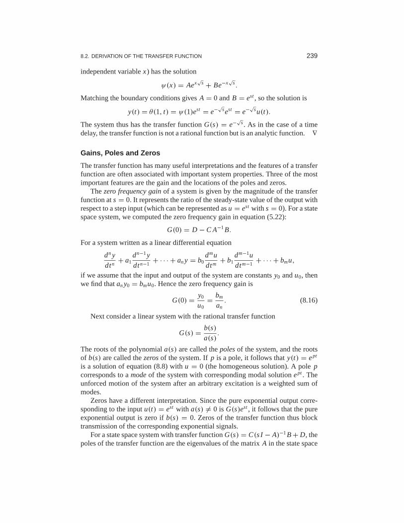
8.2. DERIVATION OF THE TRANSFER FUNCTION 239
independent variablex) has the solution
ψ(x) = Aex√
s + Be−x√
s.
Matching the boundary conditions givesA = 0 andB = est, so the solution is
y(t) = θ(1, t) = ψ(1)est = e−√sest = e−√
su(t).
The system thus has the transfer functionG(s) = e−√s. As in the case of a time
delay, the transfer function is not a rational function but is an analytic function. ∇
Gains, Poles and Zeros
The transfer function has many useful interpretations and the features of a transferfunction are often associated with important system properties. Three of the mostimportant features are the gain and the locations of the poles and zeros.
Thezero frequency gainof a system is given by the magnitude of the transferfunction ats = 0. It represents the ratio of the steady-state value of the output withrespect to a step input (which can be represented asu = est with s = 0). For a statespace system, we computed the zero frequency gain in equation (5.22):
G(0) = D − C A−1B.
For a system written as a linear differential equation
dny
dtn+ a1
dn−1y
dtn−1+ · · · + any = b0
dmu
dtm+ b1
dm−1u
dtm−1+ · · · + bmu,
if we assume that the input and output of the system are constants y0 andu0, thenwe find thatany0 = bmu0. Hence the zero frequency gain is
G(0) = y0
u0= bm
an. (8.16)
Next consider a linear system with the rational transfer function
G(s) = b(s)
a(s).
The roots of the polynomiala(s) are called thepolesof the system, and the rootsof b(s) are called thezerosof the system. Ifp is a pole, it follows thaty(t) = ept
is a solution of equation (8.8) withu = 0 (the homogeneous solution). A polepcorresponds to amodeof the system with corresponding modal solutionept. Theunforced motion of the system after an arbitrary excitationis a weighted sum ofmodes.
Zeros have a different interpretation. Since the pure exponential output corre-sponding to the inputu(t) = est with a(s) 6= 0 is G(s)est, it follows that the pureexponential output is zero ifb(s) = 0. Zeros of the transfer function thus blocktransmission of the corresponding exponential signals.
For a state space system with transfer functionG(s) = C(s I − A)−1B+ D, thepoles of the transfer function are the eigenvalues of the matrix A in the state space

240 CHAPTER 8. TRANSFER FUNCTIONS
−6 −4 −2 2
−2
2
Re
Im
Figure 8.4:A pole zero diagram for a transfer function with zeros at−5 and−1 and poles at−3 and−2±2 j . The circles represent the locations of the zeros, and the crosses the locationsof the poles. A complete characterization requires we also specify the gainof the system.
model. One easy way to see this is to notice that the value ofG(s) is unboundedwhens is an eigenvalue of a system since this is precisely the set ofpoints wherethe characteristic polynomialλ(s) = det(s I − A) = 0 (and hences I − A isnoninvertible). It follows that the poles of a state space system depend only on thematrix A, which represents the intrinsic dynamics of the system. We say that atransfer function is stable if all of its poles have negativereal part.
To find the zeros of a state space system, we observe that the zeros are complexnumberss such that the inputu(t) = u0est gives zero output. Inserting the pureexponential responsex(t) = x0est andy(t) = 0 in equation (8.2) gives
sestx0 = Ax0est + Bu0est 0 = Cestx0 + Destu0,
which can be written asA − s I B
C D
x0
u0
est = 0.
This equation has a solution with nonzerox0, u0 only if the matrix on the left doesnot have full rank. The zeros are thus the valuess such that the matrix
A − s I B
C D
(8.17)
loses rank.Since the zeros depend onA, B, C and D, they therefore depend on how the
inputs and outputs are coupled to the states. Notice in particular that if the matrixB has full row rank, then the matrix in equation (8.17) hasn linearly independentrows for all values ofs. Similarly there aren linearly independent columns if thematrixC has full column rank. This implies that systems where the matrix B or Cis square and full rank do not have zeros. In particular it means that a system hasno zeros if it is fully actuated (each state can be controlledindependently) or if thefull state is measured.
A convenient way to view the poles and zeros of a transfer function is througha pole zero diagram, as shown in Figure 8.4. In this diagram, each pole is markedwith a cross, and each zero with a circle. If there are multiple poles or zeros at a

8.2. DERIVATION OF THE TRANSFER FUNCTION 241
MF
p
θm
l
(a) Cart–pendulum system
−4 −2 2 4−1
1
Re
Im
(b) Pole zero diagram forHθF
−4 −2 2 4−1
1
Re
Im
(c) Pole zero diagram forHpF
Figure 8.5: Poles and zeros for a balance system. The balance system (a) can be modeledaround its vertical equilibrium point by a fourth order linear system. The poles and zeros forthe transfer functionsHθF andHpF are shown in (b) and (c), respectively.
fixed location, these are often indicated with overlapping crosses or circles (or otherannotations). Poles in the left half-plane correspond to stable modes of the system,and poles in the right half-plane correspond to unstable modes. We thus call a polein the left-half plane astable poleand a pole in the right-half plane anunstablepole. A similar terminology is used for zeros, even though the zeros do not directlyrelated to stability or instability of the system. Notice that the gain must also begiven to have a complete description of the transfer function.
Example 8.5 Balance systemConsider the dynamics for a balance system, shown in Figure 8.5. The transfer func-tion for a balance system can be derived directly from the second-order equations,given in Example 2.1:
Mtd2 p
dt2− ml
d2θ
dt2cosθ + c
dp
dt+ ml sinθ
(dθdt
)2 = F,
−ml cosθd2 p
dt2+ Jt
d2θ
dt2− mglsinθ + γ θ = 0.
If we assume thatθ andθ are small, we can approximate this nonlinear system bya set of linear second-order differential equations,
Mtd2 p
dt2− ml
d2θ
dt2+ c
dp
dt= F,
−mld2 p
dt2+ Jt
d2θ
dt2+ γ
dθ
dt− mglθ = 0.

242 CHAPTER 8. TRANSFER FUNCTIONS
If we let F be an exponential signal, the resulting response satisfies
Mts2 p − mls2 θ + cs p= F,
Jts2 θ − mls2 p + γ sθ − mglθ = 0,
where all signals are exponential signals. The resulting transfer functions for theposition of the cart and the orientation of the pendulum are given by solving forpandθ in terms ofF to obtain
HθF = mls
(Mt Jt − m2l 2)s4 + (γMt + cJt)s2 + (cγ − Mtmgl)s − mglc,
HpF = Jts2 + γ s − mgl
(Mt Jt − m2l 2)s4 + (γMt + cJt)s3 + (cγ − Mtmgl)s2 − mglcs,
where each of the coefficients is positive. The pole zero diagrams for these twotransfer functions are shown in Figure 8.5 using the parameters from Example 6.7.
If we assume the damping is small and setc = 0 andγ = 0, we obtain
HθF = ml
(Mt Jt − m2l 2)s2 − Mtmgl,
HpF = Jts2 − mgl
s2((Mt Jt − m2l 2)s2 − Mtmgl
) .
This gives nonzero poles and zeros at
p = ±√
mglMt
Mt Jt − m2l 2≈ ±2.68, z = ±
√mgl
Jt≈ ±2.09.
We see that these are quite close to the pole and zero locations in Figure 8.5. ∇
8.3 Block Diagrams and Transfer Functions
The combination of block diagrams and transfer functions is apowerful way torepresent control systems. Transfer functions relating different signals in the systemcan be derived by purely algebraic manipulations of the transfer functions of theblocks usingblock diagram algebra. To show how this can be done, we will beginwith simple combinations of systems.
Consider a system that is a cascade combination of systems with the transferfunctionsG1(s) andG2(s), as shown in Figure 8.6a. Let the input of the systembeu = est. The pure exponential output of the first block is the exponential signalG1u, which is also the input to the second system. The pure exponential output ofthe second system is
y = G2(G1u) = (G2G1)u.
The transfer function of the series connection is thusG = G2G1, i.e., the productof the transfer functions. The order of the individual transfer functions is due tothe fact that we place the input signal on the right-hand sideof this expression,

8.3. BLOCK DIAGRAMS AND TRANSFER FUNCTIONS 243
G1 G2
u y
(a) Gyu = G2G1
G2
6u y
G1
(b) Gyu = G1 + G2
−G2
6eu y
G1
(c) Gyu = G1
1 + G1G2
Figure 8.6: Interconnections of linear systems. Series (a), parallel (b) and feedback (c) con-nections are shown. The transfer functions for the composite systems can be derived byalgebraic manipulations assuming exponential functions for all signals.
hence we first multiply byG1 and then byG2. Unfortunately, this has the oppositeordering from the diagrams that we use, where we typically have the signal flowfrom left to right, so one needs to be careful. The ordering is important if eitherG1
or G2 is a vector-valued transfer function, as we shall see in someexamples.Consider next a parallel connection of systems with the transfer functionsG1
andG2, as shown in Figure 8.6b. Lettingu = est be the input to the system, thepure exponential output of the first system is theny1 = G1u and the output of thesecond system isy2 = G2u. The pure exponential output of the parallel connectionis thus
y = G1u + G2u = (G1 + G2)u,
and the transfer function for a parallel connection isG = G1 + G2.Finally, consider a feedback connection of systems with the transfer functions
G1 andG2, as shown in Figure 8.6c. Letu = est be the input to the system,y bethe pure exponential output, ande be the pure exponential part of the intermediatesignal given by the sum ofu and the output of the second block. Writing the relationsfor the different blocks and the summation unit, we find
y = G1e, e = u − G2y.
Elimination ofe gives
y = G1(u − G2y) =⇒ (1 + G1G2)y = G1u =⇒ y = G1
1 + G1G2u.
The transfer function of the feedback connection is thus
G = G1
1 + G1G2.
These three basic interconnections can be used as the basis for computing transferfunctions for more complicated systems.

244 CHAPTER 8. TRANSFER FUNCTIONS
ν6 6
d
6
n
ye u ηF(s)
rC(s) P(s)
−1
Figure 8.7: Block diagram of a feedback system. The inputs to the system are the referencesignalr , the process disturbanced and the measurement noisen. The remaining signals inthe system can all be chosen as possible outputs, and transfer functionscan be used to relatethe system inputs to the other labeled signals.
Control System Transfer Functions
Consider the system in Figure 8.7, which was given at the beginning of the chapter.The system has three blocks representing a processP, a feedback controllerCand a feedforward controllerF . Together,C andF define thecontrol law for thesystem. There are three external signals: the reference (or command signal)r , theload disturbanced and the measurement noisen. A typical problem is to find outhow the errore is related to the signalsr , d andn.
To derive the relevant transfer functions we assume that allsignals are expo-nential signals, drop the arguments of signals and transferfunctions and trace thesignals around the loop. We begin with the signal in which we are interested, in thiscase the control errore, given by
e = Fr − y.
The signaly is the sum ofn andη, whereη is the output of the process:
y = n + η, η = P(d + u), u = Ce.
Combining these equations gives
e = Fr − y = Fr − (n + η) = Fr −(n + P(d + u)
)
= Fr −(n + P(d + Ce)
),
and hencee = Fr − n − Pd − PCe.
Finally, solving this equation fore gives
e = F
1 + PCr − 1
1 + PCn − P
1 + PCd = Gerr + Genn + Gedd, (8.18)
and the error is thus the sum of three terms, depending on the referencer , themeasurement noisen and the load disturbanced. The functions
Ger = F
1 + PC, Gen = −1
1 + PC, Ged = −P
1 + PC(8.19)
are transfer functions from referencer , noisen and disturbanced to the errore.

8.3. BLOCK DIAGRAMS AND TRANSFER FUNCTIONS 245
(c)
(b)
F PCr e
6
−1
Fr
PC1+PC
y
PC F1+PC
yr
y
(a)
Figure 8.8:Example of block diagram algebra. The results from multiplying the process andcontroller transfer functions (from Figure 8.7) are shown in (a). Replacing the feedback loopwith its transfer function equivalent yields (b), and finally multiplying the two remainingblocks gives the reference to output representation in (c).
We can also derive transfer functions by manipulating the block diagrams di-rectly, as illustrated in Figure 8.8. Suppose we wish to compute the transfer functionbetween the referencer and the outputy. We begin by combining the process andcontroller blocks in Figure 8.7 to obtain the diagram in Figure8.8a. We can noweliminate the feedback loop using the algebra for a feedbackinterconnection (Fig-ure 8.8b) and then use the series interconnection rule to obtain
Gyr = PC F
1 + PC. (8.20)
Similar manipulations can be used to obtain the other transfer functions (Exer-cise 8.8).
The derivation illustrates an effective way to manipulate the equations to obtainthe relations between inputs and outputs in a feedback system. The general idea isto start with the signal of interest and to trace signals around the feedback loop untilcoming back to the signal we started with. With some practice, equations (8.18)and (8.19) can be written directly by inspection of the blockdiagram. Notice, forexample, that all terms in equation (8.19) have the same denominators and that thenumerators are the blocks that one passes through when goingdirectly from inputto output (ignoring the feedback). This type of rule can be used to compute transferfunctions by inspection, although for systems with multiple feedback loops it canbe tricky to compute them without writing down the algebra explicitly.
Example 8.6 Vehicle steeringConsider the linearized model for vehicle steering introduced in Example 5.12. InExamples 6.4 and 7.3 we designed a state feedback compensatorand state esti-mator for the system. A block diagram for the resulting control system is given inFigure 8.9. Note that we have split the estimator into two components,Gxu(s) andGx y(s), corresponding to its inputsu andy. The controller can be described as thesum of two (open loop) transfer functions
u = Guy(s)y + Gur (s)r.
The first transfer function,Guy(s), describes the feedback term and the second,Gur (s), describes the feedforward term. We call theseopen looptransfer functions

246 CHAPTER 8. TRANSFER FUNCTIONS
y(t)
r (t)
Controller
6
KGxu Gx y
−1 6
P(s)u yr
kr
Estimator
x
Figure 8.9: Block diagram for a steering control system. The control system is designed tomaintain the lateral position of the vehicle along a reference curve (left). The structure of thecontrol system is shown on the right as a block diagram of transfer functions. The estimatorconsists of two components that compute the estimated statex from the combination of theinput u and outputy of the process. The estimated state is fed through a state feedbackcontroller and combined with a reference gain to obtain the commanded steering angleu.
because they represent the relationships between the signals without consideringthe dynamics of the process (e.g., removingP(s) from the system description). Toderive these functions, we compute the transfer functions for each block and thenuse block diagram algebra.
We begin with the estimator, which takesu and y as its inputs and producesan estimatex. The dynamics for this process were derived in Example 7.3 and aregiven by
dx
dt= (A − LC)x + Ly + Bu,
x =(s I − (A − LC)
)−1B︸ ︷︷ ︸
Gxu
u +(s I − (A − LC)
)−1L︸ ︷︷ ︸
Gx y
y.
Using the expressions forA, B, C andL from Example 7.3, we obtain
Gxu(s) =
γ s + 1
s2 + l1s + l2
s + l1 − γ l2s2 + l1s + l2
, Gx y(s) =
l1s + l2s2 + l1s + l2
l2s
s2 + l1s + l2
,
wherel1 and l2 are the observer gains andγ is the scaled position of the centerof mass from the rear wheels. The controller was a state feedback compensator,which can be viewed as a constant, multi-input, single-output transfer function ofthe formu = −K x.
We can now proceed to compute the transfer function for the overall controlsystem. Using block diagram algebra, we have
Guy(s) = −K Gx y(s)
1 + K Gxu(s)= − s(k1l1 + k2l2)+ k1l2
s2 + s(γ k1 + k2 + l1)+ k1 + l2 + k2l1 − γ k2l2
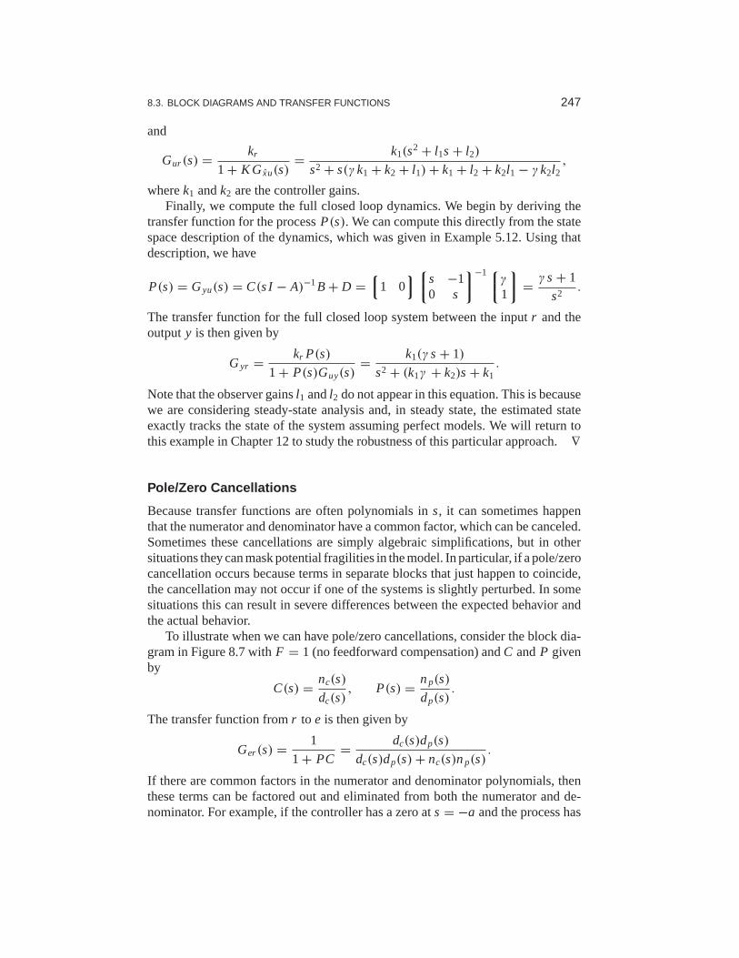
8.3. BLOCK DIAGRAMS AND TRANSFER FUNCTIONS 247
and
Gur (s) = kr
1 + K Gxu(s)= k1(s2 + l1s + l2)
s2 + s(γ k1 + k2 + l1)+ k1 + l2 + k2l1 − γ k2l2,
wherek1 andk2 are the controller gains.Finally, we compute the full closed loop dynamics. We begin byderiving the
transfer function for the processP(s). We can compute this directly from the statespace description of the dynamics, which was given in Example5.12. Using thatdescription, we have
P(s) = Gyu(s) = C(s I − A)−1B + D =1 0
s −1
0 s
−1γ1
= γ s + 1
s2.
The transfer function for the full closed loop system betweenthe inputr and theoutputy is then given by
Gyr = kr P(s)
1 + P(s)Guy(s)= k1(γ s + 1)
s2 + (k1γ + k2)s + k1.
Note that the observer gainsl1 andl2 do not appear in this equation. This is becausewe are considering steady-state analysis and, in steady state, the estimated stateexactly tracks the state of the system assuming perfect models. We will return tothis example in Chapter 12 to study the robustness of this particular approach. ∇
Pole/Zero Cancellations
Because transfer functions are often polynomials ins, it can sometimes happenthat the numerator and denominator have a common factor, which can be canceled.Sometimes these cancellations are simply algebraic simplifications, but in othersituations they can mask potential fragilities in the model. In particular, if a pole/zerocancellation occurs because terms in separate blocks that just happen to coincide,the cancellation may not occur if one of the systems is slightly perturbed. In somesituations this can result in severe differences between the expected behavior andthe actual behavior.
To illustrate when we can have pole/zero cancellations, consider the block dia-gram in Figure 8.7 withF = 1 (no feedforward compensation) andC andP givenby
C(s) = nc(s)
dc(s), P(s) = np(s)
dp(s).
The transfer function fromr to e is then given by
Ger(s) = 1
1 + PC= dc(s)dp(s)
dc(s)dp(s)+ nc(s)np(s).
If there are common factors in the numerator and denominatorpolynomials, thenthese terms can be factored out and eliminated from both the numerator and de-nominator. For example, if the controller has a zero ats = −a and the process has

248 CHAPTER 8. TRANSFER FUNCTIONS
a pole ats = −a, then we will have
Ger(s) =(s + a)dc(s)d′
p(s)
(s + a)dc(s)d′p(s)+ (s + a)n′
c(s)np(s)=
dc(s)d′p(s)
dc(s)d′p(s)+ n′
c(s)np(s),
wheren′c(s) and d′
p(s) represent the relevant polynomials with the terms + afactored out. In the case whena < 0 (so that the zero or pole is in the righthalf-plane), we see that there is no impact on the transfer functionGer.
Suppose instead that we compute the transfer function fromd to e, which repre-sents the effect of a disturbance on the error between the reference and the output.This transfer function is given by
Ged(s) = − dc(s)np(s)
(s + a)dc(s)d′p(s)+ (s + a)n′
c(s)np(s).
Notice that ifa < 0, then the pole is in the right half-plane and the transfer functionGed is unstable. Hence, even though the transfer function fromr to eappears to beokay (assuming a perfect pole/zero cancellation), the transfer function fromd to ecan exhibit unbounded behavior. This unwanted behavior is typical of anunstablepole/zero cancellation.
It turns out that the cancellation of a pole with a zero can also be understood interms of the state space representation of the systems. Reachability or observabilityis lost when there are cancellations of poles and zeros (Exercise 8.11). A conse-quence is that the transfer function represents the dynamics only in the reachableand observable subspace of a system (see Section 7.5).
Example 8.7 Cruise controlThe input/output response from throttle to velocity for the linearized model for acar has the transfer functionG(s) = b/(s−a), a < 0. A simple (but not necessarilygood) way to design a PI controller is to choose the parametersof the PI controllerso that the controller zero ats = −ki /kp cancels the process pole ats = a. Thetransfer function from reference to velocity isGvr (s) = bkp/(s+bkp), and controldesign is simply a matter of choosing the gainkp. The closed loop system dynamicsare of first order with the time constant 1/bkp.
Figure 8.10 shows the velocity error when the car encounters an increase in theroad slope. A comparison with the controller used in Figure 3.3b (reproduced indashed curves) shows that the controller based on pole/zerocancellation has verypoor performance. The velocity error is larger, and it takes along time to settle.
Notice that the control signal remains practically constant after t = 15 even ifthe error is large after that time. To understand what happens we will analyze thesystem. The parameters of the system area = −0.0101 andb = 1.32, and thecontroller parameters arekp = 0.5 andki = 0.0051. The closed loop time constantis 1/(bkp) = 2.5 s, and we would expect that the error would settle in about10 s(4 time constants). The transfer functions from road slope tovelocity and control

8.3. BLOCK DIAGRAMS AND TRANSFER FUNCTIONS 249
0 10 20 30 4018
19
20
Time t [s]
Velo
cityv
[m/s
]
0 10 20 30 400
0.2
0.4
0.6
Time t [s]
Thr
ottle
ki = 0.0051ki = 0.5
Figure 8.10: Car with PI cruise control encountering a sloping road. The velocity error isshown on the left and the throttle is shown on the right. Results with a PI controller withkp = 0.5 andki = 0.0051, where the process poles = −0.0101, is shown by solid lines, anda controller withkp = 0.5 andki = 0.5 is shown by dashed lines. Compare with Figure 3.3b.
signals are
Gv θ (s) = bgkps
(s − a)(s + bkp), Gu θ (s) = bkp
s + bkp.
Notice that the canceled modes = a = −0.0101 appears inGvθ but not inGuθ .The reason why the control signal remains constant is that thecontroller has a zeroats = −0.0101, which cancels the slowly decaying process mode. Notice that theerror would diverge if the canceled pole was unstable. ∇
The lesson we can learn from this example is that it is a bad ideato try tocancel unstable or slow process poles. A more detailed discussion of pole/zerocancellations is given in Section 12.4.
Algebraic Loops
When analyzing or simulating a system described by a block diagram, it is necessaryto form the differential equations that describe the complete system. In many casesthe equations can be obtained by combining the differentialequations that describeeach subsystem and substituting variables. This simple procedure cannot be usedwhen there are closed loops of subsystems that all have a direct connection betweeninputs and outputs, known as analgebraic loop.
To see what can happen, consider a system with two blocks, a first-order non-linear system,
dx
dt= f (x,u), y = h(x), (8.21)
and a proportional controller described byu = −ky. There is no direct term sincethe functionh does not depend onu. In that case we can obtain the equation for theclosed loop system simply by replacingu by −ky in (8.21) to give
dx
dt= f (x,−ky), y = h(x).
Such a procedure can easily be automated using simple formulamanipulation.
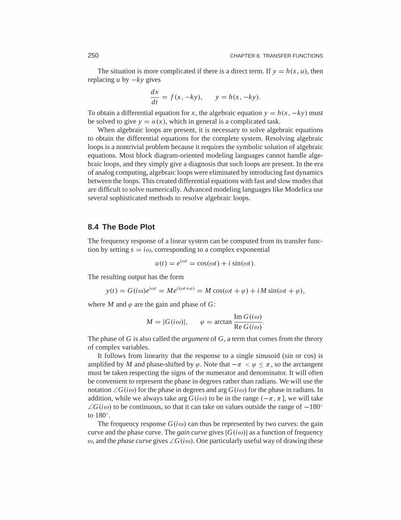
250 CHAPTER 8. TRANSFER FUNCTIONS
The situation is more complicated if there is a direct term. Ify = h(x,u), thenreplacingu by −ky gives
dx
dt= f (x,−ky), y = h(x,−ky).
To obtain a differential equation forx, the algebraic equationy = h(x,−ky)mustbe solved to givey = α(x), which in general is a complicated task.
When algebraic loops are present, it is necessary to solve algebraic equationsto obtain the differential equations for the complete system. Resolving algebraicloops is a nontrivial problem because it requires the symbolic solution of algebraicequations. Most block diagram-oriented modeling languages cannot handle alge-braic loops, and they simply give a diagnosis that such loopsare present. In the eraof analog computing, algebraic loops were eliminated by introducing fast dynamicsbetween the loops. This created differential equations withfast and slow modes thatare difficult to solve numerically. Advanced modeling languages like Modelica useseveral sophisticated methods to resolve algebraic loops.
8.4 The Bode Plot
The frequency response of a linear system can be computed fromits transfer func-tion by settings = iω, corresponding to a complex exponential
u(t) = eiωt = cos(ωt)+ i sin(ωt).
The resulting output has the form
y(t) = G(iω)eiωt = Mei (ωt+ϕ) = M cos(ωt + ϕ)+ i M sin(ωt + ϕ),
whereM andϕ are the gain and phase ofG:
M = |G(iω)|, ϕ = arctanIm G(iω)
ReG(iω).
The phase ofG is also called theargumentof G, a term that comes from the theoryof complex variables.
It follows from linearity that the response to a single sinusoid (sin or cos) isamplified byM and phase-shifted byϕ. Note that−π < ϕ ≤ π , so the arctangentmust be taken respecting the signs of the numerator and denominator. It will oftenbe convenient to represent the phase in degrees rather than radians. We will use thenotation∠G(iω) for the phase in degrees and argG(iω) for the phase in radians. Inaddition, while we always take argG(iω) to be in the range(−π, π ], we will take∠G(iω) to be continuous, so that it can take on values outside the range of−180◦
to 180◦.The frequency responseG(iω) can thus be represented by two curves: the gain
curve and the phase curve. Thegain curvegives|G(iω)| as a function of frequencyω, and thephase curvegives∠G(iω). One particularly useful way of drawing these

8.4. THE BODE PLOT 251
101
102
103
104
10−2
10−1
100
101
102
−90
0
90
ActualApprox
Frequencyω [rad/s]
|G(iω)|
∠G(iω)
[deg
]
Figure 8.11: Bode plot of the transfer functionC(s) = 20+ 10/s + 10s corresponding toan ideal PID controller. The top plot is the gain curve and the bottom plot is thephase curve.The dashed lines show straight-line approximations of the gain curve and the correspondingphase curve.
curves is to use a log/log scale for the gain plot and a log/linear scale for the phaseplot. This type of plot is called aBode plotand is shown in Figure 8.11.
Sketching and Interpreting Bode Plots
Part of the popularity of Bode plots is that they are easy to sketch and interpret.Since the frequency scale is logarithmic, they cover the behavior of a linear systemover a wide frequency range.
Consider a transfer function that is a rational function of the form
G(s) = b1(s)b2(s)
a1(s)a2(s).
We have
log |G(s)| = log |b1(s)| + log |b2(s)| − log |a1(s)| − log |a2(s)|,
and hence we can compute the gain curve by simply adding and subtracting gainscorresponding to terms in the numerator and denominator. Similarly,
∠G(s) = ∠b1(s)+ ∠b2(s)− ∠a1(s)− ∠a2(s),
and so the phase curve can be determined in an analogous fashion. Since a polyno-mial can be written as a product of terms of the type
k, s, s + a, s2 + 2ζω0s + ω20,
it suffices to be able to sketch Bode diagrams for these terms. The Bode plot of acomplex system is then obtained by adding the gains and phases of the terms.

252 CHAPTER 8. TRANSFER FUNCTIONS
10−2
100
102
10−1
100
101
−180
0
180
Frequencyω [rad/s]
|G(iω)|
∠G(iω)
[deg
]
1
1
s−1
s−1
s−2
s−2
10−2
100
102
10−1
100
101
−180
0
180
Frequencyω [rad/s]
|G(iω)|
∠G(iω)
[deg
] s2
s2
s
s
1
1
Figure 8.12: Bode plots of the transfer functionsG(s) = sk for k = −2,−1, 0, 1, 2. On alog-log scale, the gain curve is a straight line with slopek. Using a log-linear scale, the phasecurves for the transfer functions are constants, with phase equal to 90◦ × k
.
The simplest term in a transfer function is one of the formsk, wherek > 0 ifthe term appears in the numerator andk < 0 if the term is in the denominator. Thegain and phase of the term are given by
log |G(iω)| = k logω, ∠G(iω) = 90k.
The gain curve is thus a straight line with slopek, and the phase curve is a constantat 90◦×k. The case whenk = 1 corresponds to a differentiator and has slope 1 withphase 90◦. The case whenk = −1 corresponds to an integrator and has slope−1with phase−90◦. Bode plots of the various powers ofk are shown in Figure 8.12.
Consider next the transfer function of a first-order system, given by
G(s) = a
s + a.
We have
|G(s)| = |a||s + a| , ∠G(s) = ∠(a)− ∠(s + a),
and hence
log |G(iω)| = loga − 1
2log(ω2 + a2), ∠G(iω) = −180
πarctan
ω
a.
The Bode plot is shown in Figure 8.13a, with the magnitude normalized by the zerofrequency gain. Both the gain curve and the phase curve can beapproximated by

8.4. THE BODE PLOT 253
−180
−90
0
ExactApprox
Frequencyω [rad/s]
|G(iω)|
∠G(iω)
[deg
]
10−2
100
102
a 10a 100aa/10a/100
(a) First-order system
−180
−90
0
ExactApprox
Frequencyω [rad/s]
|G(iω)|
∠G(iω)
[deg
]
10−2
100
102
ω0 10ω0 100ω0ω0/10ω0/100
ζ
ζ
(b) Second-order system
Figure 8.13:Bode plots for first- and second-order systems. (a) The first-ordersystemG(s) =a/(s + a) can be approximated by asymptotic curves (dashed) in both the gain and thefrequency, with the breakpoint in the gain curve atω = a and the phase decreasing by 90◦
over a factor of 100 in frequency. (b) The second-order systemG(s) = ω20/(s
2+2ζω0s+ω20)
has a peak at frequencya and then a slope of−2 beyond the peak; the phase decreases from0◦ to−180◦. The height of the peak and the rate of change of phase depending on the dampingratio ζ (ζ = 0.02, 0.1, 0.2, 0.5 and 1.0 shown).
the following straight lines
log |G(iω)| ≈{
0 if ω < a
loga − logω if ω > a,
∠G(iω) ≈
0 if ω < a/10
−45− 45(logω − loga) a/10< ω < 10a
−90 if ω > 10a.
The approximate gain curve consists of a horizontal line up tofrequencyω = a,called thebreakpointor corner frequency, after which the curve is a line of slope−1 (on a log-log scale). The phase curve is zero up to frequencya/10 and thendecreases linearly by 45◦/decade up to frequency 10a, at which point it remainsconstant at 90◦. Notice that a first-order system behaves like a constant for lowfrequencies and like an integrator for high frequencies; compare with the Bode plotin Figure 8.12.
Finally, consider the transfer function for a second-order system,
G(s) = ω20
s2 + 2ω0ζs + ω20
,

254 CHAPTER 8. TRANSFER FUNCTIONS
for which we have
log |G(iω)| = 2 logω0 − 1
2log
(ω4 + 2ω2
0ω2(2ζ 2 − 1)+ ω4
0
),
∠G(iω) = −180
πarctan
2ζω0ω
ω20 − ω2
.
The gain curve has an asymptote with zero slope forω ≪ ω0. For large val-ues ofω the gain curve has an asymptote with slope−2. The largest gainQ =maxω |G(iω)| ≈ 1/(2ζ ), called theQ-value, is obtained forω ≈ ω0. The phaseis zero for low frequencies and approaches 180◦ for large frequencies. The curvescan be approximated with the following piecewise linear expressions
log |G(iω)| ≈{
0 if ω ≪ ω0
2 logω0 − 2 logω if ω ≫ ω0,
∠G(iω) ≈{
0 if ω ≪ ω0
−180 ifω ≫ ω0.
The Bode plot is shown in Figure 8.13b. Note that the asymptoticapproximation ispoor nearω = ω0 and that the Bode plot depends strongly onζ near this frequency.
Given the Bode plots of the basic functions, we can now sketchthe frequencyresponse for a more general system. The following example illustrates the basicidea.
Example 8.8 Asymptotic approximation for a transfer functionConsider the transfer function given by
G(s) = k(s + b)
(s + a)(s2 + 2ζω0s + ω20), a ≪ b ≪ ω0.
The Bode plot for this transfer function appears in Figure 8.14, with the completetransfer function shown as a solid line and the asymptotic approximation shown asa dashed line.
We begin with the gain curve. At low frequency, the magnitudeis given by
G(0) = kb
aω20
.
When we reachω = a, the effect of the pole begins and the gain decreases withslope−1. At ω = b, the zero comes into play and we increase the slope by 1,leaving the asymptote with net slope 0. This slope is used until the effect of thesecond-order pole is seen atω = ω0, at which point the asymptote changes to slope−2. We see that the gain curve is fairly accurate except in the region of the peakdue to the second-order pole (since for this caseζ is reasonably small).
The phase curve is more complicated since the effect of the phase stretchesout much further. The effect of the pole begins atω = a/10, at which point wechange from phase 0 to a slope of−45◦/decade. The zero begins to affect thephase atω = b/10, producing a flat section in the phase. Atω = 10a the phase

8.4. THE BODE PLOT 255
10−2
100
102
10−2
10−1
100
101
102
−180
−90
0
ExactApprox
|G(iω)|
∠G(iω)
[deg
]
Frequencyω [rad/s]
ω = a ω = b ω = ω0
ω = a/10 ω = b/10 ω = 10a
ω = 10b
Figure 8.14:Asymptotic approximation to a Bode plot. The thin line is the Bode plot for thetransfer functionG(s) = k(s + b)/(s + a)(s2 + 2ζω0s + ω2
0), wherea ≪ b ≪ ω0. Eachsegment in the gain and phase curves represents a separate portion ofthe approximation,where either a pole or a zero begins to have effect. Each segment of theapproximation is astraight line between these points at a slope given by the rules for computing the effects ofpoles and zeros.
contributions from the pole end, and we are left with a slope of +45◦/decade (fromthe zero). At the location of the second-order pole,s ≈ iω0, we get a jump in phaseof −180◦. Finally, atω = 10b the phase contributions of the zero end, and we areleft with a phase of−180 degrees. We see that the straight-line approximation forthe phase is not as accurate as it was for the gain curve, but itdoes capture the basicfeatures of the phase changes as a function of frequency. ∇
The Bode plot gives a quick overview of a system. Since any signal can bedecomposed into a sum of sinusoids, it is possible to visualize the behavior of asystem for different frequency ranges. The system can be viewed as a filter that canchange the amplitude (and phase) of the input signals according to the frequencyresponse. For example, if there are frequency ranges where the gain curve hasconstant slope and the phase is close to zero, the action of the system for signalswith these frequencies can be interpreted as a pure gain. Similarly, for frequencieswhere the slope is +1 and the phase close to 90◦, the action of the system can beinterpreted as a differentiator, as shown in Figure 8.12.
Three common types of frequency responses are shown in Figure 8.15. Thesystem in Figure 8.15a is called alow-pass filterbecause the gain is constant forlow frequencies and drops for high frequencies. Notice thatthe phase is zero forlow frequencies and−180◦ for high frequencies. The systems in Figure 8.15b andc are called aband-pass filterandhigh-pass filterfor similar reasons.
To illustrate how different system behaviors can be read from the Bode plotswe consider the band-pass filter in Figure 8.15b. For frequencies aroundω = ω0,the signal is passed through with no change in gain. However,for frequencies well

256 CHAPTER 8. TRANSFER FUNCTIONS
10−2
10−1
100
−180
0
180
Frequencyω [rad/s]
|G(iω)|
∠G(iω)
ω0 100ω0ω0/100
10−2
10−1
100
−180
0
180
Frequencyω [rad/s]
|G(iω)|
∠G(iω)
ω0 100ω0ω0/100
10−2
10−1
100
−180
0
180
Frequencyω [rad/s]
|G(iω)|
∠G(iω)
ω0 100ω0ω0/100
G(s) = ω20
s2 + 2ζω0s + ω20
(a) Low-pass filter
G(s) = 2ζω0s
s2 + 2ζω0s + ω20
(b) Band-pass filter
G(s) = s2
s2 + 2ζω0s + ω20
(c) High-pass filter
Figure 8.15:Bode plots for low-pass, band-pass and high-pass filters. The top plotsare thegain curves and the bottom plots are the phase curves. Each system passes frequencies in adifferent range and attenuates frequencies outside of that range.
below or well aboveω0, the signal is attenuated. The phase of the signal is alsoaffected by the filter, as shown in the phase curve. For frequencies belowω0/100there is a phase lead of 90◦, and for frequencies above 100ω0 there is a phase lagof 90◦. These actions correspond to differentiation and integration of the signal inthese frequency ranges.
Example 8.9 Transcriptional regulationConsider a genetic circuit consisting of a single gene. We wish to study the responseof the protein concentration to fluctuations in the mRNA dynamics. We considertwo cases: aconstitutive promoter(no regulation) and self-repression (negativefeedback), illustrated in Figure 8.16. The dynamics of the system are given by
dm
dt= α(p)− γm − u,
dp
dt= βm − δp,
whereu is a disturbance term that affects mRNA transcription.For the case of no feedback we haveα(p) = α0, and the system has an equi-
librium point atme = α0/γ , pe = βα0/(δγ ). The transfer function fromv to p isgiven by
Golpv(s) = −β
(s + γ )(s + δ).
For the case of negative regulation, we have
α(p) = α1
1 + kpn+ α0,
and the equilibrium points satisfy
me = δ
βpe,
α
1 + kpne
+ α0 = γme = γ δ
βpe.

8.4. THE BODE PLOT 257
A
RNAP
(a) Open loop
RNAP
A
(b) Negative feedback
10−4
10−3
10−2
10−2
10−1
100
open loopnegative feedback
|Gpv(iω)|
Frequencyω [rad/s]
(c) Frequency response
Figure 8.16: Noise attenuation in a genetic circuit. The open loop system (a) consists of aconstitutive promoter, while the closed loop circuit (b) is self-regulated withnegative feedback(repressor). The frequency response for each circuit is shown in(c).
The resulting transfer function is given by
Gclpv(s) = β
(s + γ )(s + δ)+ βσ, σ = nα1kpn−1
e
(1 + kpne)
2.
Figure 8.16c shows the frequency response for the two circuits. We see that thefeedback circuit attenuates the response of the system to disturbances with low-frequency content but slightly amplifies disturbances at high frequency (comparedto the open loop system). Notice that these curves are very similar to the frequencyresponse curves for the op amp shown in Figure 8.3b. ∇
Transfer Functions from Experiments
The transfer function of a system provides a summary of the input/output responseand is very useful for analysis and design. However, modeling from first principlescan be difficult and time-consuming. Fortunately, we can often build an input/outputmodel for a given application by directly measuring the frequency response andfitting a transfer function to it. To do so, we perturb the inputto the system using asinusoidal signal at a fixed frequency. When steady state is reached, the amplituderatio and the phase lag give the frequency response for the excitation frequency. Thecomplete frequency response is obtained by sweeping over a range of frequencies.
By using correlation techniques it is possible to determinethe frequency re-sponse very accurately, and an analytic transfer function can be obtained from thefrequency response by curve fitting. The success of this approach has led to in-struments and software that automate this process, calledspectrum analyzers. Weillustrate the basic concept through two examples.
Example 8.10 Atomic force microscopeTo illustrate the utility of spectrum analysis, we considerthe dynamics of the atomicforce microscope, introduced in Section 3.5. Experimental determination of the

258 CHAPTER 8. TRANSFER FUNCTIONS
10−1
100
101
102
102
103
104
−270
−180
−90
0
MeasuredModel
|G|
∠G
[deg
]
Frequencyf [Hz]
Figure 8.17: Frequency response of a preloaded piezoelectric drive for an atomicforcemicroscope. The Bode plot shows the response of the measured transfer function (solid) andthe fitted transfer function (dashed).
frequency response is particularly attractive for this system because its dynamics arevery fast and hence experiments can be done quickly. A typical example is given inFigure 8.17, which shows an experimentally determined frequency response (solidline). In this case the frequency response was obtained in less than a second. Thetransfer function
G(s) = kω22ω
23ω
25(s
2 + 2ζ1ω1s + ω21)(s
2 + 2ζ4ω4s + ω24)e
−sτ
ω21ω
24(s
2 + 2ζ2ω2s + ω22)(s
2 + 2ζ3ω3s + ω23)(s
2 + 2ζ5ω5s + ω25),
with ωk = 2π fk and f1 = 2.42 kHz,ζ1 = 0.03, f2 = 2.55 kHz,ζ2 = 0.03, f3 =6.45 kHz,ζ3 = 0.042, f4 = 8.25 kHz,ζ4 = 0.025, f5 = 9.3 kHz,ζ5 = 0.032,τ = 10−4 s andk = 5, was fit to the data (dashed line). The frequencies associatedwith the zeros are located where the gain curve has minima, and the frequenciesassociated with the poles are located where the gain curve has local maxima. Therelative damping ratios are adjusted to give a good fit to maxima and minima. Whena good fit to the gain curve is obtained, the time delay is adjusted to give a good fit tothe phase curve. The piezo drive is preloaded, and a simple model of its dynamics isderived in Exercise 3.7. The pole at 2.42 kHz corresponds to thetrampoline modederived in the exercise; the other resonances are higher modes.
∇
Example 8.11 Pupillary light reflex dynamicsThe human eye is an organ that is easily accessible for experiments. It has a controlsystem that adjusts the pupil opening to regulate the light intensity at the retina.
This control system was explored extensively by Stark in the 1960s [Sta68].To determine the dynamics, light intensity on the eye was varied sinusoidally andthe pupil opening was measured. A fundamental difficulty is that the closed loopsystem is insensitive to internal system parameters, so analysis of a closed loop

8.5. LAPLACE TRANSFORMS 259
(a) Closed loop (b) Open loop (c) High gain
Figure 8.18:Light stimulation of the eye. In (a) the light beam is so large that it always coversthe whole pupil, giving closed loop dynamics. In (b) the light is focused intoa beam whichis so narrow that it is not influenced by the pupil opening, giving open loop dynamics. In (c)the light beam is focused on the edge of the pupil opening, which has the effect of increasingthe gain of the system since small changes in the pupil opening have a largeeffect on theamount of light entering the eye. From Stark [Sta68].
system thus gives little information about the internal properties of the system. Starkused a clever experimental technique that allowed him to investigate both open andclosed loop dynamics. He excited the system by varying the intensity of a light beamfocused on the eye and measured pupil area, as illustrated inFigure 8.18. By usinga wide light beam that covers the whole pupil, the measurement gives the closedloop dynamics. The open loop dynamics were obtained by using anarrow beam,which is small enough that it is not influenced by the pupil opening. The result ofone experiment for determining open loop dynamics is given in Figure 8.19. Fittinga transfer function to the gain curve gives a good fit forG(s) = 0.17/(1+ 0.08s)3.This curve gives a poor fit to the phase curve as shown by the dashed curve inFigure 8.19. The fit to the phase curve is improved by adding a timedelay, whichleaves the gain curve unchanged while substantially modifying the phase curve.The final fit gives the model
G(s) = 0.17
(1 + 0.08s)3e−0.2s.
The Bode plot of this is shown with solid curves in Figure 8.19. Modeling of thepupillary reflex from first principles is discussed in detail in[KS01]. ∇
Notice that for both the AFM drive and pupillary dynamics it isnot easy toderive appropriate models from first principles. In practice, it is often fruitful to usea combination of analytical modeling and experimental identification of parameters.Experimental determination of frequency response is less attractive for systems withslow dynamics because the experiment takes a long time.
8.5 Laplace Transforms �
Transfer functions are conventionally introduced using Laplace transforms, and inthis section we derive the transfer function using this formalism. We assume basicfamiliarity with Laplace transforms; students who are not familiar with them cansafely skip this section. A good reference for the mathematical material in this

260 CHAPTER 8. TRANSFER FUNCTIONS
0 5 1510 2010
20
30
Pu
pil
are
a(m
m2)
Time (s)
10
20
30
Lig
ht
Flu
x(m
lm)
0.010.02
0.050.10.2
2 5 10 20−360
−180
0
MeasuredModel
Model w/out delay
Frequencyω [rad/s]
|G(iω)|
∠G(iω)
[deg
]
Figure 8.19: Sample curves from an open loop frequency response of the eye (left) and aBode plot for the open loop dynamics (right). The solid curve shows a fitof the data using athird-order transfer function with time delay. The dashed curve in the Bode plot is the phaseof the system without time delay, showing that the delay is needed to properlycapture thephase. (Figure redrawn from the data of Stark [Sta68].)
section is the classic book by Widder [Wid41].Traditionally, Laplace transforms were used to compute responses of linear sys-
tems to different stimuli. Today we can easily generate the responses using com-puters. Only a few elementary properties are needed for basic control applications.There is, however, a beautiful theory for Laplace transforms that makes it possibleto use many powerful tools from the theory of functions of a complex variable toget deep insights into the behavior of systems.
Consider a functionf (t), f : R+ → R, that is integrable and grows no faster
thanes0t for some finites0 ∈ R and larget . The Laplace transform mapsf to afunction F = L f : C → C of a complex variable. It is defined by
F(s) =∫ ∞
0e−st f (t)dt, Res> s0. (8.22)
The transform has some properties that makes it well suited todeal with linearsystems.
First we observe that the transform is linear because
L(a f + bg) =∫ ∞
0e−st(a f (t)+ bg(t))dt
= a∫ ∞
0e−st f (t)dt + b
∫ ∞
0e−stg(t)dt = aL f + bLg.
(8.23)
Next we calculate the Laplace transform of the derivative of afunction. We have
Ld f
dt=∫ ∞
0e−st f ′(t)dt = e−st f (t)
∣∣∣∞
0+ s
∫ ∞
0e−st f (t)dt = − f (0)+ sL f,
where the second equality is obtained using integration by parts. We thus obtain
Ld f
dt= sL f − f (0) = sF(s)− f (0). (8.24)

8.5. LAPLACE TRANSFORMS 261
This formula is particularly simple if the initial conditions are zero because it followsthat differentiation of a function corresponds to multiplication of the transform bys.
Since differentiation corresponds to multiplication bys, we can expect thatintegration corresponds to division bys. This is true, as can be seen by calculatingthe Laplace transform of an integral. Using integration by parts, we get
L
∫ t
0f (τ )dτ =
∫ ∞
0
(e−st
∫ t
0f (τ )dτ
)dt
= −e−st
s
∫ t
0f (τ )dτ
∣∣∣∞
0+∫ ∞
0
e−sτ
sf (τ )dτ = 1
s
∫ ∞
0e−sτ f (τ )dτ,
hence
L
∫ t
0f (τ )dτ = 1
sL f = 1
sF(s). (8.25)
Next consider a linear time-invariant system with zero initial state. We saw inSection 5.3 that the relation between the inputu and the outputy is given by theconvolution integral
y(t) =∫ ∞
0h(t − τ)u(τ )dτ,
whereh(t) is the impulse response for the system. Taking the Laplace transform ofthis expression, we have
Y(s) =∫ ∞
0e−sty(t)dt =
∫ ∞
0e−st
∫ ∞
0h(t − τ)u(τ )dτ dt
=∫ ∞
0
∫ t
0e−s(t−τ)e−sτh(t − τ)u(τ )dτ dt
=∫ ∞
0e−sτu(τ )dτ
∫ ∞
0e−sth(t)dt = H(s)U (s).
Thus, the input/output response is given byY(s) = H(s)U (s), whereH , U andY are the Laplace transforms ofh, u and y. The system theoretic interpretationis that the Laplace transform of the output of a linear system is a product of twoterms, the Laplace transform of the inputU (s) and the Laplace transform of theimpulse response of the systemH(s). A mathematical interpretation is that theLaplace transform of a convolution is the product of the transforms of the functionsthat are convolved. The fact that the formulaY(s) = H(s)U (s) is much simplerthan a convolution is one reason why Laplace transforms have become popular inengineering.
We can also use the Laplace transform to derive the transfer function for a statespace system. Consider, for example, a linear state space system described by
dx
dt= Ax + Bu, y = Cx + Du.
Taking Laplace transformsunder the assumption that all initial values are zero

262 CHAPTER 8. TRANSFER FUNCTIONS
givessX(s) = AX(s)+ BU(s) Y(s) = C X(s)+ DU (s).
Elimination of X(s) gives
Y(s) =(C(s I − A)−1B + D
)U (s). (8.26)
The transfer function isG(s) = C(s I − A)−1B+ D (compare with equation (8.4)).
8.6 Further Reading
The idea of characterizing a linear system by its steady-state response to sinusoidswas introduced by Fourier in his investigation of heat conduction in solids [Fou07].Much later, it was used by the electrical engineer Steinmetz who introduced theiω method for analyzing electrical circuits. Transfer functions were introduced viathe Laplace transform by Gardner Barnes [GB42], who also usedthem to calcu-late the response of linear systems. The Laplace transform wasvery important inthe early phase of control because it made it possible to find transients via tables(see, e.g., [JNP47]). Combined with block diagrams, transfer functions and Laplacetransforms provided powerful techniques for dealing with complex systems. Cal-culation of responses based on Laplace transforms is less important today, whenresponses of linear systems can easily be generated using computers. There aremany excellent books on the use of Laplace transforms and transfer functions formodeling and analysis of linear input/output systems. Traditional texts on controlsuch as [DB04], [FPEN05] and [Oga01] are representative examples. Pole/zerocancellation was one of the mysteries of early control theory. It is clear that com-mon factors can be canceled in a rational function, but cancellations have systemtheoretical consequences that were not clearly understooduntil Kalman’s decom-position of a linear system was introduced [KHN63]. In the following chapters, wewill use transfer functions extensively to analyze stability and to describe modeluncertainty.
Exercises
8.1 Let G(s) be the transfer function for a linear system. Show that if we ap-ply an inputu(t) = Asin(ωt), then the steady-state output is given byy(t) =|G(iω)|Asin(ωt + argG(iω)). (Hint: Start by showing that the real part of a com-plex number is a linear operation and then use this fact.)
8.2 Consider the systemdx
dt= ax + u.
Compute the exponential response of the system and use this to derive the transferfunction fromu to y. Show that whens = a, a pole of the transfer function, theresponse to the exponential inputu(t) = est is x(t) = eatx(0)+ teat.

EXERCISES 263
8.3 (Inverted pendulum) A model for an inverted pendulum was introduced inExample 2.2. Neglecting damping and linearizing the pendulum around the uprightposition gives a linear system characterized by the matrices
A = 0 1
mgl/Jt 0
, B =
0
1/Jt
, C =
1 0
, D = 0.
Determine the transfer function of the system.
8.4(Solutions corresponding to poles and zeros) Consider the differential equation
dny
dtn+ a1
dn−1y
dtn−1+ · · · + any = b1
dn−1u
dtn−1+ b2
dn−2u
dtn−2+ · · · + bnu.
(a) Letλ be a root of the characteristic polynomial
sn + a1sn−1 + · · · + an = 0.
Show that ifu(t) = 0, the differential equation has the solutiony(t) = eλt .
(b) Letκ be a zero of the polynomial
b(s) = b1sn−1 + b2sn−2 + · · · + bn.
Show that if the input isu(t) = eκt , then there is a solution to the differentialequation that is identically zero.
8.5 (Operational amplifier) Consider the operational amplifier introduced in Sec-tion 3.3 and analyzed in Example 8.3. A PI controller can be constructed using anop amp by replacing the resistorR2 with a resistor and capacitor in series, as shownin Figure 3.10. The resulting transfer function of the circuitis given by
G(s) = −(
R2 + 1
Cs
)·
(kCs
(k R1C + R2C)s + 1
),
wherek is the gain of the op amp,R1 andR2 are the resistances in the compensationnetwork andC is the capacitance.
(a) Sketch the Bode plot for the system under the assumption that k ≫ R2 > R1.You should label the key features in your plot, including thegain and phase at lowfrequency, the slopes of the gain curve, the frequencies at which the gain changesslope, etc.
(b) Suppose now that we include some dynamics in the amplifier, as outlined inExample 8.1. This would involve replacing the gaink with the transfer function
H(s) = k
1 + sT.
Compute the resulting transfer function for the system (i.e., replacek with H(s))and find the poles and zeros assuming the following parameter values
R2
R1= 100, k = 106, R2C = 1, T = 0.01.

264 CHAPTER 8. TRANSFER FUNCTIONS
(c) Sketch the Bode plot for the transfer function in part (b) using straight lineapproximations and compare this to the exact plot of the transfer function (usingMATLAB). Make sure to label the important features in your plot.
8.6(Transfer function for state space system) Consider the linear state space system
dx
dt= Ax + Bu, y = Cx.
Show that the transfer function is
G(s) = b1sn−1 + b2sn−2 + · · · + bn
sn + a1sn−1 + · · · + an,
where
b1=C B, b2=C AB+a1C B, . . . , bn =C An−1B+a1C An−1B+· · ·+an−1C B
andλ(s) = sn + a1sn−1 + · · · + an is the characteristic polynomial forA.
8.7 (Kalman decomposition) Show that the transfer function of a system depends�only on the dynamics in the reachable and observable subspace of the Kalmandecomposition. (Hint: Consider the representation given by equation (7.27).)
8.8 Using block diagram algebra, show that the transfer functions fromd to y andn to y in Figure 8.7 are given by
Gyd = P
1 + PCGyn = 1
1 + PC.
8.9 (Bode plot for a simple zero) Show that the Bode plot for transfer functionG(s) = (s + a)/a can be approximated by
log |G(iω)| ≈{
0 if ω < a
logω − loga if ω > a,
∠G(iω) ≈
0 if ω < a/10
45+ 45(logω − loga) a/10< ω < 10a
90 if ω > 10a.
8.10 (Vectored thrust aircraft) Consider the lateral dynamics of a vectored thrustaircraft as described in Example 2.9. Show that the dynamics can be describedusing the following block diagram:
1
ms2 + cs
θ−mg 6
νu1
r
Js2x
Use this block diagram to compute the transfer functions from u1 to θ andx andshow that they satisfy
Hθu1 = r
Js2, Hxu1 = Js2 − mgr
Js2(ms2 + cs).

EXERCISES 265
8.11 (Common poles) Consider a closed loop system of the form of Figure 8.7, �with F = 1 andP andC having a pole/zero cancellation. Show that if each systemis written in state space form, the resulting closed loop system is not reachable andnot observable.
8.12(Congestion control) Consider the congestion control model described in Sec-tion 3.4. Letw represent the individual window size for a set ofN identical sources,q represent the end-to-end probability of a dropped packet,b represent the numberof packets in the router’s buffer andp represent the probability that that a packet isdropped by the router. We writew = Nw to represent the total number of packetsbeing received from allN sources. Show that the linearized model can be describedby the transfer functions
Gbw(s) = e−τ f s
τes + e−τ f s, Gwq(s) = − N
qe(τes + qewe), Gpb(s) = ρ,
where(we,be) is the equilibrium point for the system,τe is the steady-state round-trip time andτ f is the forward propagation time.
8.13(Inverted pendulum with PD control) Consider the normalizedinverted pen-dulum system, whose transfer function is given byP(s) = 1/(s2 − 1) (Exer-cise 8.3). A proportional-derivative control law for this system has transfer func-tion C(s) = kp + kds (see Table 8.1). Suppose that we chooseC(s) = α(s − 1).Compute the closed loop dynamics and show that the system hasgood tracking ofreference signals but does not have good disturbance rejection properties.
8.14(Vehicle suspension [HB90]) Active and passive damping areused in cars togive a smooth ride on a bumpy road. A schematic diagram of a carwith a dampingsystem in shown in the figure below.
(Porter Class I race car driven by Todd Cuffaro)
xb
xw
xr
F +
-
Σ
F
Body
Actuator
Wheel
This model is called aquarter car model, and the car is approximated with twomasses, one representing one fourth of the car body and the other a wheel. Theactuator exerts a forceF between the wheel and the body based on feedback fromthe distance between the body and the center of the wheel (therattle space).
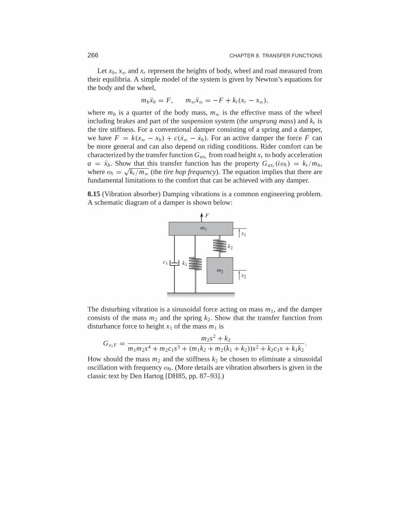
266 CHAPTER 8. TRANSFER FUNCTIONS
Let xb, xw andxr represent the heights of body, wheel and road measured fromtheir equilibria. A simple model of the system is given by Newton’s equations forthe body and the wheel,
mbxb = F, mw xw = −F + kt(xr − xw),
wheremb is a quarter of the body mass,mw is the effective mass of the wheelincluding brakes and part of the suspension system (theunsprung mass) andkt isthe tire stiffness. For a conventional damper consisting ofa spring and a damper,we haveF = k(xw − xb) + c(xw − xb). For an active damper the forceF canbe more general and can also depend on riding conditions. Rider comfort can becharacterized by the transfer functionGaxr from road heightxr to body accelerationa = xb. Show that this transfer function has the propertyGaxr (iωt) = kt/mb,whereωt =
√kt/mw (the tire hop frequency). The equation implies that there are
fundamental limitations to the comfort that can be achievedwith any damper.
8.15(Vibration absorber) Damping vibrations is a common engineering problem.A schematic diagram of a damper is shown below:
m1
k1
m2
c1
k2
F
x1
x2
The disturbing vibration is a sinusoidal force acting on massm1, and the damperconsists of the massm2 and the springk2. Show that the transfer function fromdisturbance force to heightx1 of the massm1 is
Gx1F = m2s2 + k2
m1m2s4 + m2c1s3 + (m1k2 + m2(k1 + k2))s2 + k2c1s + k1k2.
How should the massm2 and the stiffnessk2 be chosen to eliminate a sinusoidaloscillation with frequencyω0. (More details are vibration absorbers is given in theclassic text by Den Hartog [DH85, pp. 87–93].)

Chapter NineFrequency Domain Analysis
Mr. Black proposed a negative feedback repeater and proved by tests that it possessed theadvantages which he had predicted for it. In particular, its gain was constant to a high degree,and it was linear enough so that spurious signals caused by the interactionof the variouschannels could be kept within permissible limits. For best results the feedback factorµβ hadto be numerically much larger than unity. The possibility of stability with a feedback factorlarger than unity was puzzling.
Harry Nyquist, “The Regeneration Theory,” 1956 [Nyq56].
In this chapter we study how the stability and robustness of closed loop systemscan be determined by investigating how sinusoidal signals of different frequenciespropagate around the feedback loop. This technique allows usto reason aboutthe closed loop behavior of a system through the frequency domain properties ofthe open loop transfer function. The Nyquist stability theorem is a key result thatprovides a way to analyze stability and introduce measures of degrees of stability.
9.1 The Loop Transfer Function
Determining the stability of systems interconnected by feedback can be tricky be-cause each system influences the other, leading to potentially circular reasoning.Indeed, as the quote from Nyquist above illustrates, the behavior of feedback sys-tems can often be puzzling. However, using the mathematicalframework of transferfunctions provides an elegant way to reason about such systems, which we callloopanalysis.
The basic idea of loop analysis is to trace how a sinusoidal signal propagates inthe feedback loop and explore the resulting stability by investigating if the prop-agated signal grows or decays. This is easy to do because the transmission ofsinusoidal signals through a linear dynamical system is characterized by the fre-quency response of the system. The key result is the Nyquist stability theorem,which provides a great deal of insight regarding the stability of a system. Unlikeproving stability with Lyapunov functions, studied in Chapter 4, the Nyquist crite-rion allows us to determine more than just whether a system isstable or unstable.It provides a measure of the degree of stability through the definition of stabilitymargins. The Nyquist theorem also indicates how an unstable system should bechanged to make it stable, which we shall study in detail in Chapters 10–12.
Consider the system in Figure 9.1a. The traditional way to determine if the closedloop system is stable is to investigate if the closed loop characteristic polynomialhas all its roots in the left half-plane. If the process and the controller have rational

268 CHAPTER 9. FREQUENCY DOMAIN ANALYSIS
−1
6
r e uP(s)
yC(s)
(a)
L(s)
−1
AB
(b)
Figure 9.1: The loop transfer function. The stability of the feedback system (a) can bedetermined by tracing signals around the loop. LettingL = PC represent the loop transferfunction, we break the loop in (b) and ask whether a signal injected at the point A has thesame magnitude and phase when it reaches point B.
transfer functionsP(s) = np(s)/dp(s) andC(s) = nc(s)/dc(s), then the closedloop system has the transfer function
Gyr (s) = PC
1 + PC= np(s)nc(s)
dp(s)dc(s)+ np(s)nc(s),
and the characteristic polynomial is
λ(s) = dp(s)dc(s)+ np(s)nc(s).
To check stability, we simply compute the roots of the characteristic polynomialand verify that they each have negative real part. This approach is straightforwardbut it gives little guidance for design: it is not easy to tellhow the controller shouldbe modified to make an unstable system stable.
Nyquist’s idea was to investigate conditions under which oscillations can occurin a feedback loop. To study this, we introduce theloop transfer function L(s) =P(s)C(s), which is the transfer function obtained by breaking the feedback loop,as shown in Figure 9.1b. The loop transfer function is simply the transfer functionfrom the input at position A to the output at position B multiplied by−1 (to accountfor the usual convention of negative feedback).
We will first determine conditions for having a periodic oscillation in the loop.Assume that a sinusoid of frequencyω0 is injected at point A. In steady state thesignal at point B will also be a sinusoid with the frequencyω0. It seems reasonablethat an oscillation can be maintained if the signal at B has the same amplitude andphase as the injected signal because we can then disconnect the injected signal andconnect A to B. Tracing signals around the loop, we find that thesignals at A andB are identical if
L(iω0) = −1, (9.1)
which then provides a condition for maintaining an oscillation. The key idea ofthe Nyquist stability criterion is to understand when this can happen in a generalsetting. As we shall see, this basic argument becomes more subtle when the looptransfer function has poles in the right half-plane.
Example 9.1 Operational amplifier circuitConsider the op amp circuit in Figure 9.2a, whereZ1 andZ2 are the transfer func-

9.1. THE LOOP TRANSFER FUNCTION 269
−
+v
v2
Z
I
1 Z2
v1
(a) Amplifier circuit
v2Z1
Z1 + Z2
e vZ2
Z1
v1 −G(s)6
(b) Block diagram
Figure 9.2: Loop transfer function for an op amp. The op amp circuit (a) has a nominaltransfer functionv2/v1 = Z2(s)/Z1(s), whereZ1 and Z2 are the impedances of the circuitelements. The system can be represented by its block diagram (b), where we now include theop amp dynamicsG(s). The loop transfer function isL = Z1G/(Z1 + Z2).
tions of the feedback elements from voltage to current. Thereis feedback becausevoltagev2 is related to voltagev through the transfer function−G describing the opamp dynamics and voltagev is related to voltagev2 through the transfer functionZ1/(Z1 + Z2). The loop transfer function is thus
L = GZ1
Z1 + Z2. (9.2)
Assuming that the currentI is zero, the current through the elementsZ1 andZ2 isthe same, which implies
v1 − v
Z1= v − v2
Z2.
Solving forv gives
v = Z2v1 + Z1v2
Z1 + Z2= Z2v1 − Z1Gv
Z1 + Z2= Z2
Z1
L
Gv1 − Lv.
Sincev2 = −Gv the input/output relation for the circuit becomes
Gv2v1 = − Z2
Z1
L
1 + L.
A block diagram is shown in Figure 9.2b. It follows from (9.1) that the conditionfor oscillation of the op amp circuit is
L(iω) = Z1(iω)G(iω)
Z1(iω)+ Z2(iω)= −1 (9.3)
∇
One of the powerful concepts embedded in Nyquist’s approachto stability anal-ysis is that it allows us to study the stability of the feedback system by looking atproperties of the loop transfer function. The advantage of doing this is that it iseasy to see how the controller should be chosen to obtain a desired loop transferfunction. For example, if we change the gain of the controller, the loop transferfunction will be scaled accordingly. A simple way to stabilize an unstable system isthen to reduce the gain so that the−1 point is avoided. Another way is to introduce

270 CHAPTER 9. FREQUENCY DOMAIN ANALYSIS
Re
Im
r
R
Ŵ
(a) Nyquist D contour
Re
Im
L(iω)
−1
(b) Nyquist plot
Figure 9.3: The Nyquist contourŴ and the Nyquist plot. The Nyquist contour (a) enclosesthe right half-plane, with a small semicircle around any poles ofL(s) on the imaginary axis(illustrated here at the origin) and an arc at infinity, represented byR → ∞. The Nyquistplot (b) is the image of the loop transfer functionL(s) whens traversesŴ in the clockwisedirection. The solid line corresponds toω > 0, and the dashed line toω < 0. The gain andphase at the frequencyω are g = |L(iω)| andϕ = ∠L(iω). The curve is generated forL(s) = 1.4e−s/(s + 1)2.
a controller with the property that it bends the loop transfer function away from thecritical point, as we shall see in the next section. Different ways to do this, calledloop shaping, will be developed and will be discussed in Chapter 11.
9.2 The Nyquist Criterion
In this section we present Nyquist’s criterion for determining the stability of afeedback system through analysis of the loop transfer function. We begin by intro-ducing a convenient graphical tool, the Nyquist plot, and show how it can be usedto ascertain stability.
The Nyquist Plot
We saw in the last chapter that the dynamics of a linear systemcan be representedby its frequency response and graphically illustrated by a Bode plot. To study thestability of a system, we will make use of a different representation of the frequencyresponse called aNyquist plot. The Nyquist plot of the loop transfer functionL(s)is formed by tracings ∈ C around the Nyquist “D contour,” consisting of theimaginary axis combined with an arc at infinity connecting theendpoints of theimaginary axis. The contour, denoted asŴ ∈ C, is illustrated in Figure 9.3a. Theimage ofL(s) whens traversesŴ gives a closed curve in the complex plane and isreferred to as the Nyquist plot forL(s), as shown in Figure 9.3b. Note that if thetransfer functionL(s) goes to zero ass gets large (the usual case), then the portionof the contour “at infinity” maps to the origin. Furthermore, the portion of the plotcorresponding toω < 0 is the mirror image of the portion withω > 0.

9.2. THE NYQUIST CRITERION 271
There is a subtlety in the Nyquist plot when the loop transfer function has poleson the imaginary axis because the gain is infinite at the poles.To solve this problem,we modify the contourŴ to include small deviations that avoid any poles on theimaginary axis, as illustrated in Figure 9.3a (assuming a pole of L(s) at the origin).The deviation consists of a small semicircle to the right of the imaginary axis polelocation.
The condition for oscillation given in equation (9.1) implies that the Nyquistplot of the loop transfer function go through the pointL = −1, which is calledthecritical point. Let ωc represent a frequency at which∠L(iωc) = 180◦, corre-sponding to the Nyquist curve crossing the negative real axis. Intuitively it seemsreasonable that the system is stable if|L(iωc)| < 1, which means that the criticalpoint−1 is on the left-hand side of the Nyquist curve, as indicated in Figure 9.3b.This means that the signal at point B will have smaller amplitude than the injectedsignal. This is essentially true, but there are several subtleties that require a propermathematical analysis to clear up. We defer the details for now and state the Nyquistcondition for the special case whereL(s) is a stable transfer function.
Theorem 9.1(Simplified Nyquist criterion). Let L(s) be the loop transfer functionfor a negative feedback system (as shown in Figure 9.1a) and assume that L hasno poles in the closed right half-plane (Res ≥ 0) except for single poles on theimaginary axis. Then the closed loop system is stable if and only if the closedcontour given by� = {L(iω) : −∞ < ω < ∞} ⊂ C has no net encirclements ofthe critical point s= −1.
The following conceptual procedure can be used to determine that there areno encirclements. Fix a pin at the critical points = −1, orthogonal to the plane.Attach a string with one end at the critical point and the other on the Nyquist plot.Let the end of the string attached to the Nyquist curve traverse the whole curve.There are no encirclements if the string does not wind up on thepin when the curveis encircled.
Example 9.2 Third-order systemConsider a third-order transfer function
L(s) = 1
(s + a)3.
To compute the Nyquist plot we start by evaluating points on the imaginary axiss = iω, which yields
L(iω) = 1
(iω + a)3= (a − iω)3
(a2 + ω2)3= a3 − 3aω2
(a2 + ω2)3+ i
ω3 − 3a2ω
(a2 + ω2)3.
This is plotted in the complex plane in Figure 9.4, with the points corresponding toω > 0 drawn as a solid line andω < 0 as a dashed line. Notice that these curvesare mirror images of each other.
To complete the Nyquist plot, we computeL(s) for s on the outer arc of the

272 CHAPTER 9. FREQUENCY DOMAIN ANALYSIS
−1 1 3 5
−2
2
ReL(iω)
Im L(iω)
Figure 9.4: Nyquist plot for a third-order transfer function. The Nyquist plot consists of atrace of the loop transfer functionL(s) = 1/(s + a)3. The solid line represents the portionof the transfer function along the positive imaginary axis, and the dashedline the negativeimaginary axis. The outer arc of the D contour maps to the origin.
Nyquist D contour. This arc has the forms = Rei θ for R → ∞. This gives
L(Rei θ ) = 1
(Rei θ + a)3→ 0 as R → ∞.
Thus the outer arc of theD contour maps to the origin on the Nyquist plot. ∇
An alternative to computing the Nyquist plot explicitly is to determine the plotfrom the frequency response (Bode plot), which gives the Nyquist curve fors = iω,ω > 0. We start by plottingG(iω) from ω = 0 toω = ∞, which can be read offfrom the magnitude and phase of the transfer function. We then plot G(Rei θ ) withθ ∈ [−π/2, π/2] andR → ∞, which almost always maps to zero. The remainingparts of the plot can be determined by taking the mirror imageof the curve thus far(normally plotted using a dashed line). The plot can then be labeled with arrowscorresponding to a clockwise traversal around the D contour(the same direction inwhich the first portion of the curve was plotted).
Example 9.3 Third-order system with a pole at the originConsider the transfer function
L(s) = k
s(s + 1)2,
where the gain has the nominal valuek = 1. The Bode plot is shown in Figure 9.5a.The system has a single pole ats = 0 and a double pole ats = −1. The gain curveof the Bode plot thus has the slope−1 for low frequencies, and at the double poles = 1 the slope changes to−3. For smalls we haveL ≈ k/s, which means that thelow-frequency asymptote intersects the unit gain line atω = k. The phase curvestarts at−90◦ for low frequencies, it is−180◦ at the breakpointω = 1 and it is−270◦ at high frequencies.
Having obtained the Bode plot, we can now sketch the Nyquist plot, shownin Figure 9.5b. It starts with a phase of−90◦ for low frequencies, intersects thenegative real axis at the breakpointω = 1 whereL(i ) = 0.5 and goes to zero along

9.2. THE NYQUIST CRITERION 273
10−2
100
10−1
100
101
−270
−180
−90
|L(iω)|
∠L(iω)
Frequencyω [rad/s]
(a) Bode plot
−1
ReL(iω)
Im L(iω)
(b) Nyquist plot
Figure 9.5:Sketching Nyquist and Bode plots. The loop transfer function isL(s) = 1/(s(s+1)2). The large semicircle is the map of the small semicircle of theŴ contour around the poleat the origin. The closed loop is stable because the Nyquist curve does not encircle the criticalpoint. The point where the phase is−180◦ is marked with a circle in the Bode plot.
the imaginary axis for high frequencies. The small half-circle of theŴ contour atthe origin is mapped on a large circle enclosing the right half-plane. The Nyquistcurve does not encircle the critical point, and it follows from the simplified Nyquisttheorem that the closed loop is stable. SinceL(i ) = −k/2, we find the systembecomes unstable if the gain is increased tok = 2 or beyond. ∇
The Nyquist criterion does not require that|L(iωc)| < 1 for allωc correspondingto a crossing of the negative real axis. Rather, it says that the number of encirclementsmust be zero, allowing for the possibility that the Nyquist curve could cross thenegative real axis and cross back at magnitudes greater than1. The fact that itwas possible to have high feedback gains surprised the earlydesigners of feedbackamplifiers, as mentioned in the quote in the beginning of this chapter.
One advantage of the Nyquist criterion is that it tells us howa system is in-fluenced by changes of the controller parameters. For example, it is very easy tovisualize what happens when the gain is changed since this just scales the Nyquistcurve.
Example 9.4 Congestion controlConsider the Internet congestion control system describedin Section 3.4. Supposewe haveN identical sources and a disturbanced representing an external datasource, as shown in Figure 9.6a. We letw represent the individual window size fora source,q represent the end-to-end probability of a dropped packet,b representthe number of packets in the router’s buffer andp represent the probability that thata packet is dropped by the router. We writew for the total number of packets beingreceived from allN sources. We also include a time delay between the router andthe senders, representing the time delays between the sender and receiver.
To analyze the stability of the system, we use the transfer functions computed

274 CHAPTER 9. FREQUENCY DOMAIN ANALYSIS
Gbw(s)6
Linkdelay delay
Link
dGpb(s)
bw
e−τ f s
TCPw q
p
RouterAdmission
Control
Gwq(s)N
e−τbs−0.5
ReL(iω)
Im L(iω)
Figure 9.6: Internet congestion control. A set ofN sources using TCP/Reno send messagesthrough a single router with admission control (left). Link delays are included for the forwardand backward directions. The Nyquist plot for the loop transfer function is shown on theright.
in Exercise 8.12:
Gbw(s) = 1
τes + e−τ f s, Gwq(s) = − 1
qe(τes + qewe), Gpb(s) = ρ,
where(we,be) is the equilibrium point for the system,N is the number of sources,τe is the steady-state round-trip time andτ f is the forward propagation time. We useGbw to represent the transfer function with the forward time delay removed sincethis is accounted for as a separate block in Figure 9.6a. Similarly, Gwq = Gwq/Nsince we have pulled out the multiplierN as a separate block as well.
The loop transfer function is given by
L(s) = ρ ·N
τes + e−τ f s·
1
qe(τes + qewe)e−τes.
Using the fact thatqe ≈ 2N/w2e = 2N3/(τec)2 andwe = be/N = τec/N from
equation (3.22), we can show that
L(s) = ρ ·N
τes + e−τ f s·
c3τ 3e
2N3(cτ 2e s + 2N2)
e−τes.
Note that we have chosen the sign ofL(s) to use the same sign convention as inFigure 9.1b. The exponential term representing the time delaygives significantphase aboveω = 1/τe, and the gain at the crossover frequency will determinestability.
To check stability, we require that the gain be sufficiently small at crossover. Ifwe assume that the pole due to the queue dynamics is sufficiently fast that the TCPdynamics are dominant, the gain at the crossover frequencyωc is given by
|L(iωc)| = ρ · N ·c3τ 3
e
2N3cτ 2eωc
= ρc2τe
2Nωc.
Using the Nyquist criterion, the closed loop system will be unstable if this quantity

9.2. THE NYQUIST CRITERION 275
−200
ReL(iω)
Im L(iω)
−1
ReL(iω)
Im L(iω)
Figure 9.7:Nyquist curve for the loop transfer functionL(s) = 3(s+1)2
s(s+6)2. The plot on the right
is an enlargement of the box around the origin of the plot on the left. The Nyquist curveintersections the negative real axis twice but has no net encirclements of−1.
is greater than 1. In particular, for a fixed time delay, the system will becomeunstable as the link capacityc is increased. This indicates that the TCP protocolmay not be scalable to high-capacity networks, as pointed out by Low et al. [LPD02].Exercise 9.7 provides some ideas of how this might be overcome. ∇
Conditional Stability
Normally, we find that unstable systems can be stabilized simply by reducing theloop gain. There are, however, situations where a system can be stabilized byincreasing the gain. This was first encountered by electrical engineers in the designof feedback amplifiers, who coined the termconditional stability. The problem wasactually a strong motivation for Nyquist to develop his theory. We will illustrate byan example.
Example 9.5 Third-order systemConsider a feedback system with the loop transfer function
L(s) = 3(s + 6)2
s(s + 1)2. (9.4)
The Nyquist plot of the loop transfer function is shown in Figure 9.7. Notice that theNyquist curve intersects the negative real axis twice. The first intersection occurs atL = −12 forω = 2, and the second atL = −4.5 forω = 3. The intuitive argumentbased on signal tracing around the loop in Figure 9.1b is strongly misleading in thiscase. Injection of a sinusoid with frequency 2 rad/s and amplitude 1 at A gives, insteady state, an oscillation at B that is in phase with the input and has amplitude12. Intuitively it is seems unlikely that closing of the loopwill result in a stablesystem. However, it follows from Nyquist’s stability criterion that the system isstable because there are no net encirclements of the critical point. Note, however,that if we decreasethe gain, then we can get an encirclement, implying that thegain must be sufficiently large for stability. ∇

276 CHAPTER 9. FREQUENCY DOMAIN ANALYSIS
General Nyquist Criterion
Theorem 9.1 requires thatL(s) have no poles in the closed right half-plane. Insome situations this is not the case and a more general resultis required. Nyquistoriginally considered this general case, which we summarize as a theorem.
Theorem 9.2(Nyquist’s stability theorem). Consider a closed loop system with theloop transfer function L(s) that has P poles in the region enclosed by the Nyquistcontour. Let N be the net number of clockwise encirclements of−1 by L(s) when sencircles the Nyquist contourŴ in the clockwise direction. The closed loop systemthen has Z= N + P poles in the right half-plane.
The full Nyquist criterion states that ifL(s) hasP poles in the right half-plane,then the Nyquist curve forL(s) should haveP counterclockwise encirclements of−1 (so thatN = −P). In particular, thisrequiresthat |L(iωc)| > 1 for someωc
corresponding to a crossing of the negative real axis. Care has to be taken to get theright sign of the encirclements. The Nyquist contour has to betraversed clockwise,which means thatω moves from−∞ to ∞ andN is positive if the Nyquist curvewinds clockwise. If the Nyquist curve winds counterclockwise, thenN will benegative (the desired case ifP 6= 0).
As in the case of the simplified Nyquist criterion, we use smallsemicircles ofradiusr to avoid any poles on the imaginary axis. By lettingr → 0, we can useTheorem 9.2 to reason about stability. Note that the image of the small semicirclesgenerates a section of the Nyquist curve whose magnitude approaches infinity,requiring care in computing the winding number. When plotting Nyquist curves onthe computer, one must be careful to see that such poles are properly handled, andoften one must sketch those portions of the Nyquist plot by hand, being careful toloop the right way around the poles.
Example 9.6 Stabilized inverted pendulumThe linearized dynamics of a normalized inverted pendulum can be represented bythe transfer functionP(s) = 1/(s2−1), where the input is acceleration of the pivotand the output is the pendulum angleθ , as shown in Figure 9.8 (Exercise 8.3). Weattempt to stabilize the pendulum with a proportional-derivative (PD) controllerhaving the transfer functionC(s) = k(s + 2). The loop transfer function is
L(s) = k(s + 2)
s2 − 1.
The Nyquist plot of the loop transfer function is shown in Figure 9.8b. We haveL(0) = −2k andL(∞) = 0. If k > 0.5, the Nyquist curve encircles the criticalpoint s = −1 in the counterclockwise direction when the Nyquist contour γ isencircled in the clockwise direction. The number of encirclements is thusN = −1.Since the loop transfer function has one pole in the right half-plane (P = 1), wefind thatZ = N + P = 0 and the system is thus stable fork > 0.5. If k < 0.5, thereis no encirclement and the closed loop will have one pole in the right half-plane.
∇

9.2. THE NYQUIST CRITERION 277
u
θ
m
l
(a) Inverted pendulum
−1
ReL(iω)
Im L(iω)
(b) Nyquist plot
Figure 9.8: PD control of an inverted pendulum. (a) The system consists of a mass that isbalanced by applying a force at the pivot point. A proportional-derivative controller withtransfer functionC(s) = k(s + 2) is used to commandu based onθ . (b) A Nyquist plot ofthe loop transfer function for gaink = 1. There is one counterclockwise encirclement of thecritical point, givingN = −1 clockwise encirclements.
Derivation of Nyquist’s Stability Theorem�
We will now prove the Nyquist stability theorem for a generalloop transfer functionL(s). This requires some results from the theory of complex variables, for whichthe reader can consult Ahlfors [Ahl66]. Since some precisionis needed in statingNyquist’s criterion properly, we will use a more mathematical style of presenta-tion. We also follow the mathematical convention of counting encirclements in thecounterclockwise direction for the remainder of this section. The key result is thefollowing theorem about functions of complex variables.
Theorem 9.3(Principle of variation of the argument). Let D be a closed regionin the complex plane and letŴ be the boundary of the region. Assume the functionf : C → C is analytic in D and onŴ, except at a finite number of poles and zeros.Then thewinding numberwn is given by
wn = 1
2π1Ŵ arg f (z) = 1
2π i
∫
Ŵ
f ′(z)
f (z)dz = Z − P,
where1Ŵ is the net variation in the angle when z traverses the contourŴ in thecounterclockwise direction, Z is the number of zeros in D andP is the number ofpoles in D. Poles and zeros of multiplicity m are counted m times.
Proof. Assume thatz = a is a zero of multiplicitym. In the neighborhood ofz = awe have
f (z) = (z − a)mg(z),
where the functiong is analytic and different from zero. The ratio of the derivativeof f to itself is then given by
f ′(z)
f (z)= m
z − a+ g′(z)
g(z),
and the second term is analytic atz = a. The function f ′/ f thus has a single pole

278 CHAPTER 9. FREQUENCY DOMAIN ANALYSIS
at z = a with the residuem. The sum of the residues at the zeros of the function isZ. Similarly, we find that the sum of the residues for the poles is−P, and hence
Z − P = 1
2π i
∫
Ŵ
f ′(z)
f (z)dz = 1
2π i
∫
Ŵ
d
dzlog f (z)dz = 1
2π i1Ŵ log f (z),
where1Ŵ again denotes the variation along the contourŴ. We have
log f (z) = log | f (z)| + i arg f (z),
and since the variation of| f (z)| around a closed contour is zero it follows that
1Ŵ log f (z) = i1Ŵ arg f (z),
and the theorem is proved.
This theorem is useful in determining the number of poles and zeros of a functionof complex variables in a given region. By choosing an appropriate closed regionD with boundaryŴ, we can determine the difference between the number of polesand zeros through computation of the winding number.
Theorem 9.3 can be used to prove Nyquist’s stability theorem by choosingŴ asthe Nyquist contour shown in Figure 9.3a, which encloses the right half-plane. Toconstruct the contour, we start with part of the imaginary axis − j R ≤ s ≤ j R anda semicircle to the right with radiusR. If the function f has poles on the imaginaryaxis, we introduce small semicircles with radiir to the right of the poles as shownin the figure. The Nyquist contour is obtained by lettingR → ∞ and r → 0.Note thatŴ has orientationoppositethat shown in Figure 9.3a. (The convention inengineering is to traverse the Nyquist contour in the clockwise direction since thiscorresponds to moving upwards along the imaginary axis, which makes it easy tosketch the Nyquist contour from a Bode plot.)
To see how we use the principle of variation of the argument tocompute stability,consider a closed loop system with the loop transfer function L(s). The closed looppoles of the system are the zeros of the functionf (s) = 1+L(s). To find the numberof zeros in the right half-plane, we investigate the windingnumber of the functionf (s) = 1 + L(s) ass moves along the Nyquist contourŴ in thecounterclockwisedirection. The winding number can conveniently be determined from the Nyquistplot. A direct application of Theorem 9.3 gives the Nyquist criterion, taking careto flip the orientation. Since the image of 1+ L(s) is a shifted version ofL(s),we usually state the Nyquist criterion as net encirclementsof the−1 point by theimage ofL(s).
9.3 Stability Margins
In practice it is not enough that a system is stable. There mustalso be some marginsof stability that describe how stable the system is and its robustness to perturbations.There are many ways to express this, but one of the most common is the use of gainand phase margins, inspired by Nyquist’s stability criterion. The key idea is that it

9.3. STABILITY MARGINS 279
ReL(iω)
Im L(iω)
−1
ϕm
sm
−1/gm
(a) Nyquist plot
10−1
100
101
10−1
100
101
−180
−150
−120
−90
Frequencyω [rad/s]
|L(iω)|
∠L(iω)
log10 gm
ϕm
(b) Bode plot
Figure 9.9:Stability margins. The gain margingm and phase marginϕm are shown on the theNyquist plot (a) and the Bode plot (b). The gain margin corresponds tothe smallest increasein gain that creates an encirclement, and the phase margin is the smallest change in phasethat creates an encirclement. The Nyquist plot also shows the stability margin sm, which isthe shortest distance to the critical point−1.
is easy to plot the loop transfer functionL(s). An increase in controller gain simplyexpands the Nyquist plot radially. An increase in the phase of the controller twiststhe Nyquist plot. Hence from the Nyquist plot we can easily pick off the amount ofgain or phase that can be added without causing the system to become unstable.
Formally, thegain margin gm of a system is defined as the smallest amount thatthe open loop gain can be increased before the closed loop system goes unstable. Fora system whose phase decreases monotonically as a function of frequency startingat 0◦, the gain margin can be computed based on the smallest frequency where thephase of the loop transfer functionL(s) is −180◦. Letωpc represent this frequency,called thephase crossover frequency. Then the gain margin for the system is givenby
gm = 1
|L(iωpc)|. (9.5)
Similarly, thephase marginis the amount of phase lag required to reach the stabilitylimit. Letωgc be thegain crossover frequency, the smallest frequency where the looptransfer functionL(s) has unit magnitude. Then for a system with monotonicallydecreasing gain, the phase margin is given by
ϕm = π + argL(iωgc). (9.6)
These margins have simple geometric interpretations on the Nyquist diagram ofthe loop transfer function, as shown in Figure 9.9a, where we have plotted the portionof the curve corresponding toω > 0. The gain margin is given by the inverse ofthe distance to the nearest point between−1 and 0 where the loop transfer functioncrosses the negative real axis. The phase margin is given by the smallest angle onthe unit circle between−1 and the loop transfer function. When the gain or phaseis monotonic, this geometric interpretation agrees with the formulas above.

280 CHAPTER 9. FREQUENCY DOMAIN ANALYSIS
−1
ReL(iω)
Im L(iω)
10−3
10−1
101
10−1
100
101
−270
−180
−90
0
|L(iω)|
∠L(iω)
Frequencyω [rad/s]
Figure 9.10: Stability margins for a third-order transfer function. The Nyquist plot ontheleft allows the gain, phase and stability margins to be determined by measuring the distancesof relevant features. The gain and phase margins can also be read off of the Bode plot on theright.
A drawback with gain and phase margins is that it is necessaryto give both ofthem in order to guarantee that the Nyquist curve is not closeto the critical point.An alternative way to express margins is by a single number, thestability marginsm, which is the shortest distance from the Nyquist curve to thecritical point. Thisnumber is related to disturbance attenuation, as will be discussed in Section 11.3.
For many systems, the gain and phase margins can be determined from the Bodeplot of the loop transfer function. To find the gain margin we first find the phasecrossover frequencyωpc where the phase is−180◦. The gain margin is the inverseof the gain at that frequency. To determine the phase margin we first determine thegain crossover frequencyωgc, i.e., the frequency where the gain of the loop transferfunction is 1. The phase margin is the phase of the loop transfer function at thatfrequency plus 180◦. Figure 9.9b illustrates how the margins are found in the Bodeplot of the loop transfer function. Note that the Bode plot interpretation of the gainand phase margins can be incorrect if there are multiple frequencies at which thegain is equal to 1 or the phase is equal to−180◦.
Example 9.7 Third-order systemConsider a loop transfer functionL(s) = 3/(s + 1)3. The Nyquist and Bode plotsare shown in Figure 9.10. To compute the gain, phase and stability margins, we canuse the Nyquist plot shown in Figure 9.10. This yields the following values:
gm = 2.67, ϕm = 41.7◦, sm = 0.464.
The gain and phase margins can also be determined from the Bodeplot. ∇
The gain and phase margins are classical robustness measuresthat have beenused for a long time in control system design. The gain margin is well defined if theNyquist curve intersects the negative real axis once. Analogously, the phase marginis well defined if the Nyquist curve intersects the unit circleat only one point. Othermore general robustness measures will be introduced in Chapter 12.

9.3. STABILITY MARGINS 281
ReL(iω)
Im L(iω)
(a)
10−1
101
10−1
100
−180
−90
Frequencyω [rad/s]
|L(iω)|
∠L(iω)
(b)
0 50 100 1500
0.5
1
1.5
Time t [s]
Out
puty
(c)
Figure 9.11:System with good gain and phase margins but a poor stability margin. Nyquist(a) and Bode (b) plots of the loop transfer function and step response (c) for a system withgood gain and phase margins but with a poor stability margin. The Nyquist plot shows on theportion of the curve corresponding toω > 0.
Even if both the gain and phase margins are reasonable, the system may stillnot be robust, as is illustrated by the following example.
Example 9.8 Good gain and phase margins but poor stability marginsConsider a system with the loop transfer function
L(s) = 0.38(s2 + 0.1s + 0.55)
s(s + 1)(s2 + 0.06s + 0.5).
A numerical calculation gives the gain margin asgm = 266, and the phase marginis 70◦. These values indicate that the system is robust, but the Nyquist curve isstill close to the critical point, as shown in Figure 9.11. The stability margin issm = 0.27, which is very low. The closed loop system has two resonant modes, onewith damping ratioζ = 0.81 and the other withζ = 0.014. The step response ofthe system is highly oscillatory, as shown in Figure 9.11c. ∇
The stability margin cannot easily be found from the Bode plotof the looptransfer function. There are, however, other Bode plots thatwill give sm; these willbe discussed in Chapter 12. In general, it is best to use the Nyquist plot to checkstability since this provides more complete information than the Bode plot.
When designing feedback systems, it will often be useful to define the robustnessof the system using gain, phase and stability margins. These numbers tell us howmuch the system can vary from our nominal model and still be stable. Reasonablevalues of the margins are phase marginϕm = 30◦–60◦, gain margingm = 2–5 andstability marginsm = 0.5–0.8.
There are also other stability measures, such as thedelay margin, which is thesmallest time delay required to make the system unstable. For loop transfer functionsthat decay quickly, the delay margin is closely related to the phase margin, but forsystems where the gain curve of the loop transfer function has several peaks at highfrequencies, the delay margin is a more relevant measure.

282 CHAPTER 9. FREQUENCY DOMAIN ANALYSIS
−1
ReL(iω)
Im L(iω)
10−2
100
10−2
100
102
−270
−180
−90
Normalized frequencyω/ω0
|L(iω)|
∠L(iω)
Figure 9.12:Nyquist and Bode plots of the loop transfer function for the AFM system (9.7)with an integral controller. The frequency in the Bode plot is normalized bya. The parametersareζ = 0.01 andki = 0.008.
Example 9.9 Nanopositioning system for an atomic force microscopeConsider the system for horizontal positioning of the sample in an atomic forcemicroscope. The system has oscillatory dynamics, and a simple model is a spring–mass system with low damping. The normalized transfer function is given by
P(s) = ω20
s2 + 2ζω0s + ω20
, (9.7)
where the damping ratio typically is a very small number, e.g., ζ = 0.1.We will start with a controller that has only integral action. The resulting loop
transfer function is
L(s) = kiω20
s(s2 + 2ζω0s + ω20),
whereki is the gain of the controller. Nyquist and Bode plots of the loop transferfunction are shown in Figure 9.12. Notice that the part of the Nyquist curve that isclose to the critical point−1 is approximately circular.
From the Bode plot in Figure 9.12b, we see that the phase crossover frequencyis ωpc = a, which will be independent of the gainki . Evaluating the loop transferfunction at this frequency, we haveL(iω0) = −ki /(2ζω0), which means that thegain margin isgm = 1−ki /(2ζω0). To have a desired gain margin ofgm the integralgain should be chosen as
ki = 2ω0ζ(1 − gm).
Figure 9.12 shows Nyquist and Bode plots for the system with gain margingm =1.67 and stability marginsm = 0.597. The gain curve in the Bode plot is almosta straight line for low frequencies and has a resonant peak atω = ω0. The gaincrossover frequency is approximately equal toki . The phase decreases monotoni-cally from−90◦ to−270◦: it is equal to−180◦ atω = ω0. The curve can be shiftedvertically by changingki : increasingki shifts the gain curve upward and increasesthe gain crossover frequency. Since the phase is−180◦ at the resonant peak, it isnecessary that the peak not touch the line|L(iω)| = 1. ∇

9.4. BODE’S RELATIONS AND MINIMUM PHASE SYSTEMS 283
9.4 Bode’s Relations and Minimum Phase Systems
An analysis of Bode plots reveals that there appears to be a relation between thegain curve and the phase curve. Consider, for example, the Bode plots for thedifferentiator and the integrator (shown in Figure 8.12). For the differentiator theslope is+1 and the phase is a constantπ/2 radians. For the integrator the slope is−1 and the phase is−π/2. For the first-order systemG(s) = s+ a, the amplitudecurve has the slope 0 for small frequencies and the slope+1 for high frequencies,and the phase is 0 for low frequencies andπ/2 for high frequencies.
Bode investigated the relations between the curves for systems with no polesand zeros in the right half-plane. He found that the phase wasuniquely given bythe shape of the gain curve, and vice versa:
argG(iω0) = π
2
∫ ∞
0f (ω)
d log |G(iω)|d logω
d logω ≈ π
2
d log |G(iω)|d logω
, (9.8)
where f is the weighting kernel
f (ω) = 2
π2log
∣∣∣ω + ω0
ω − ω0
∣∣∣.
The phase curve is thus a weighted average of the derivative ofthe gain curve. Ifthe gain curve has constant slopen, the phase curve has constant valuenπ/2.
Bode’s relations (9.8) hold for systems that do not have poles and zeros in theright half-plane. Such systems are calledminimum phase systemsbecause systemswith poles and zeros in the right half-plane have a larger phase lag. The distinctionis important in practice because minimum phase systems are easier to control thansystems with a larger phase lag. We will now give a few examples of nonminimumphase transfer functions.
The transfer function of a time delay ofτ units isG(s) = e−sτ . This transferfunction has unit gain|G(iω)| = 1, and the phase is argG(iω) = −ωτ . Thecorresponding minimum phase system with unit gain has the transfer functionG(s) = 1. The time delay thus has an additional phase lag ofωτ . Notice that thephase lag increases linearly with frequency. Figure 9.13a shows the Bode plot ofthe transfer function. (Because we use a log scale for frequency, the phase falls offexponentially in the plot.)
Consider a system with the transfer functionG(s) = (a − s)/(a + s) witha > 0, which has a zeros = a in the right half-plane. The transfer functionhas unit gain|G(iω)| = 1, and the phase is argG(iω) = −2 arctan(ω/a). Thecorresponding minimum phase system with unit gain has the transfer functionG(s) = 1. Figure 9.13b shows the Bode plot of the transfer function. Asimilaranalysis of the transfer functionG(s) = (s + a)/s − a) with a > 0, which has apole in the right half-plane, shows that its phase is argG(iω) = −2 arctan(a/ω).The Bode plot is shown in Figure 9.13c.
The presence of poles and zeros in the right half-plane imposes severe limitationson the achievable performance. Dynamics of this type shouldbe avoided by redesignof the system whenever possible. While the poles are intrinsic properties of the
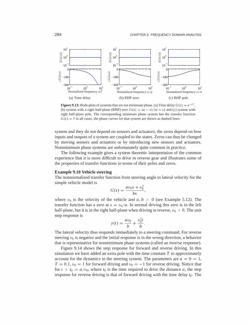
284 CHAPTER 9. FREQUENCY DOMAIN ANALYSIS
10−1
100
101
10−1
100
101
−360
−180
0
Normalized frequencyωT
|G(iω)|
∠G(iω)
(a) Time delay
10−1
100
101
10−1
100
101
−360
−180
0
Normalized frequencyω/a
|G(iω)|
∠G(iω)
(b) RHP zero
10−1
100
101
10−1
100
101
−360
−180
0
Normalized frequencyω/a
|G(iω)|
∠G(iω)
(c) RHP pole
Figure 9.13:Bode plots of systems that are not minimum phase. (a) Time delayG(s) = e−sT,(b) system with a right half-plane (RHP) zeroG(s) = (a − s)/(a + s) and (c) system withright half-plane pole. The corresponding minimum phase system has thetransfer functionG(s) = 1 in all cases, the phase curves for that system are shown as dashed lines.
system and they do not depend on sensors and actuators, the zeros depend on howinputs and outputs of a system are coupled to the states. Zeroscan thus be changedby moving sensors and actuators or by introducing new sensors and actuators.Nonminimum phase systems are unfortunately quite common inpractice.
The following example gives a system theoretic interpretation of the commonexperience that it is more difficult to drive in reverse gear and illustrates some ofthe properties of transfer functions in terms of their polesand zeros.
Example 9.10 Vehicle steeringThe nonnormalized transfer function from steering angle to lateral velocity for thesimple vehicle model is
G(s) = av0s + v20
bs,
wherev0 is the velocity of the vehicle anda,b > 0 (see Example 5.12). Thetransfer function has a zero ats = v0/a. In normal driving this zero is in the lefthalf-plane, but it is in the right half-plane when driving inreverse,v0 < 0. The unitstep response is
y(t) = av0
b+ v2
0t
b.
The lateral velocity thus responds immediately to a steeringcommand. For reversesteeringv0 is negative and the initial response is in the wrong direction, a behaviorthat is representative for nonminimum phase systems (called aninverse response).
Figure 9.14 shows the step response for forward and reverse driving. In thissimulation we have added an extra pole with the time constantT to approximatelyaccount for the dynamics in the steering system. The parameters area = b = 1,T = 0.1, v0 = 1 for forward driving andv0 = −1 for reverse driving. Notice thatfor t > t0 = a/v0, wheret0 is the time required to drive the distancea, the stepresponse for reverse driving is that of forward driving withthe time delayt0. The

9.5. GENERALIZED NOTIONS OF GAIN AND PHASE 285
0 1 2 3 4−1
0
1
2
3
4
5
FowardReverse
Time t [s]
Late
ralv
eloc
ityy
[m/s
]
(a) Step response
10−1
100
101
10−1
100
101
−180
−90
0
Frequencyω [rad/s]
|G(iω)|
∠G(iω)
(b) Frequency response
Figure 9.14:Vehicle steering for driving in reverse. (a) Step responses from steering angle tolateral translation for a simple kinematics model when driving forward (dashed) and reverse(solid). With rear-wheel steering the center of mass first moves in the wrong direction andthat the overall response with rear-wheel steering is significantly delayed compared with thatfor front-wheel steering. (b) Frequency response for driving forward (dashed) and reverse(solid). Notice that the gain curves are identical, but the phase curve fordriving in reversehas nonminimum phase.
position of the zerov0/a depends on the location of the sensor. In our calculationwe have assumed that the sensor is at the center of mass. The zero in the transferfunction disappears if the sensor is located at the rear wheel. The difficulty withzeros in the right half-plane can thus be visualized by a thought experiment wherewe drive a car in forward and reverse and observe the lateral position through ahole in the floor of the car. ∇
9.5 Generalized Notions of Gain and Phase�
A key idea in frequency domain analysis is to trace the behavior of sinusoidalsignals through a system. The concepts of gain and phase represented by the transferfunction are strongly intuitive because they describe amplitude and phase relationsbetween input and output. In this section we will see how to extend the conceptsof gain and phase to more general systems, including some nonlinear systems. Wewill also show that there are analogs of Nyquist’s stabilitycriterion if signals areapproximately sinusoidal.
System Gain
We begin by considering the case of a static linear systemy = Au, whereA isa matrix whose elements are complex numbers. The matrix does not have to besquare. Let the inputs and outputs be vectors whose elements are complex numbersand use the Euclidean norm
‖u‖ =√6|ui |2. (9.9)
286 CHAPTER 9. FREQUENCY DOMAIN ANALYSIS
The norm of the output is‖y‖2 = u∗ A∗ Au,
where∗ denotes the complex conjugate transpose. The matrixA∗ A is symmetricand positive semidefinite, and the right-hand side is a quadratic form. The squareroot of eigenvalues of the matrixA∗ A are all real, and we have
‖y‖2 ≤ λmax(A∗ A)‖u‖2.
The gain of the system can then be defined as the maximum ratio of the output tothe input over all possible inputs:
γ = maxu
‖y‖‖u‖ =
√λmax(A∗ A). (9.10)
The square root of the eigenvalues of the matrixA∗ A are called thesingular valuesof the matrixA, and the largest singular value is denotedσ (A).
To generalize this to the case of an input/output dynamical system, we needto think of the inputs and outputs not as vectors of real numbers but as vectors ofsignals. For simplicity, consider first the case of scalar signals andlet the signalspaceL2 be square-integrable functions with the norm
‖u‖2 =√∫ ∞
0|u|2(τ )dτ .
This definition can be generalized to vector signals by replacing the absolute valuewith the vector norm (9.9). We can now formally define the gain of a system takinginputsu ∈ L2 and producing outputsy ∈ L2 as
γ = supu∈L2
‖y‖‖u‖ , (9.11)
where sup is thesupremum,defined as the smallest number that is larger than itsargument. The reason for using the supremum is that the maximum may not bedefined foru ∈ L2. This definition of the system gain is quite general and can evenbe used for some classes of nonlinear systems, though one needs to be careful abouthow initial conditions and global nonlinearities are handled.
The norm (9.11) has some nice properties in the case of linear systems. Inparticular, given a single-input, single-output stable linear system with transferfunctionG(s), it can be shown that the norm of the system is given by
γ = supω
|G(iω)| =: ‖G‖∞. (9.12)
In other words, the gain of the system corresponds to the peakvalue of the frequencyresponse. This corresponds to our intuition that an input produces the largest outputwhen we are at the resonant frequencies of the system.‖G‖∞ is called theinfinitynormof the transfer functionG(s).
This notion of gain can be generalized to the multi-input, multi-output case aswell. For a linear multivariable system with a real rationaltransfer function matrix

9.5. GENERALIZED NOTIONS OF GAIN AND PHASE 287
H2
6 H1
Figure 9.15:A feedback connection of two general nonlinear systemsH1 andH2. The stabilityof the system can be explored using the small gain theorem.
G(s) we can define the gain as
γ = ‖G‖∞ = supωσ (G(iω)). (9.13)
Thus we can combine the idea of the gain of a matrix with the ideaof the gain of alinear system by looking at the maximum singular value over all frequencies.
Small Gain and Passivity
For linear systems it follows from Nyquist’s theorem that the closed loop is stableif the gain of the loop transfer function is less than 1 for allfrequencies. This resultcan be extended to a larger class of systems by using the concept of the system gaindefined in equation (9.11).
Theorem 9.4 (Small gain theorem). Consider the closed loop system shown inFigure 9.15, where H1 and H2 are stable systems and the signal spaces are properlydefined. Let the gains of the systems H1 and H2 beγ1 andγ2. Then the closed loopsystem is input/output stable ifγ1γ2 < 1, and the gain of the closed loop system is
γ = γ1
1 − γ1γ2.
Notice that if systemsH1 andH2 are linear, it follows from the Nyquist stabilitytheorem that the closed loop is stable because ifγ1γ2 < 1, the Nyquist curve isalways inside the unit circle. The small gain theorem is thus an extension of theNyquist stability theorem.
Although we have focused on linear systems, the small gain theorem also holdsfor nonlinear input/output systems. The definition of gain in equation (9.11) holdsfor nonlinear systems as well, with some care needed in handling the initial condi-tion.
The main limitation of the small gain theorem is that it does not consider thephasing of signals around the loop, so it can be very conservative. To define thenotion of phase we require that there be a scalar product. Forsquare-integrablefunctions this can be defined as
〈u, y〉 =∫ ∞
0u(τ )y(τ )dτ.
The phaseϕ between two signals can now be defined as
〈u, y〉 = ‖u‖‖y‖ cos(ϕ).

288 CHAPTER 9. FREQUENCY DOMAIN ANALYSIS
L(s)
−N( ·)
AB
(a) Block diagram
Re
Im
−1/N(a)
G(iω)
(b) Nyquist plot
Figure 9.16:Describing function analysis. A feedback connection between a static nonlin-earity and a linear system is shown in (a). The linear system is characterized by its transferfunction L(s), which depends on frequency, and the nonlinearity by its describing functionN(a), which depends on the amplitudea of its input. The Nyquist plot ofL(iω) and the plotof the−1/N(a) are shown in (b). The intersection of the curves represents a possible limitcycle.
Systems where the phase between inputs and outputs is 90◦ or less for all inputsare calledpassive systems. It follows from the Nyquist stability theorem that aclosed loop linear system is stable if the phase of the loop transfer function isbetween−π andπ . This result can be extended to nonlinear systems as well. It iscalled thepassivity theoremand is closely related to the small gain theorem. SeeKhalil [Kha01] for a more detailed description.
Additional applications of the small gain theorem and its application to robuststability are given in Chapter 12.
Describing Functions�
For special nonlinear systems like the one shown in Figure 9.16a, which consistsof a feedback connection between a linear system and a staticnonlinearity, it ispossible to obtain a generalization of Nyquist’s stabilitycriterion based on the ideaof describing functions. Following the approach of the Nyquist stability condition,we will investigate the conditions for maintaining an oscillation in the system. Ifthe linear subsystem has low-pass character, its output is approximately sinusoidaleven if its input is highly irregular. The condition for oscillation can then be foundby exploring the propagation of a sinusoid that correspondsto the first harmonic.
To carry out this analysis, we have to analyze how a sinusoidal signal propa-gates through a static nonlinear system. In particular we investigate how the firstharmonic of the output of the nonlinearity is related to its (sinusoidal) input. LettingF represent the nonlinear function, we expandF(eiωt) in terms of its harmonics:
F(aeiωt) =∞∑
n=0
Mn(a)ei (nωt+ϕn(a)),
whereMn(a) andϕn(a) represent the gain and phase of thenth harmonic, whichdepend on the input amplitude since the functionF is nonlinear. We define the

9.5. GENERALIZED NOTIONS OF GAIN AND PHASE 289
y
u
c
b
(a)0 5 10 15 20
−4
−2
0
2
4
6
In Out 1st har.
(b)
Re
Im
(c)
Figure 9.17:Describing function analysis for a relay with hysteresis. The input/output relationof the hysteresis is shown in (a) and the input with amplitudea = 2, the output and its firstharmonic are shown in (b). The Nyquist plots of the transfer functionL(s) = (s + 1)−4 andthe negative of the inverse describing function for the relay withb = 3 andc = 1 are shownin (c).
describing function to be the complex gain of the first harmonic:
N(a) = M1(a)eiϕn(a). (9.14)
The function can also be computed by assuming that the input isa sinusoid andusing the first term in the Fourier series of the resulting output.
Arguing as we did when deriving Nyquist’s stability criterion, we find that anoscillation can be maintained if
L(iω)N(a) = −1. (9.15)
This equation means that if we inject a sinusoid at A in Figure 9.16, the same signalwill appear at B and an oscillation can be maintained by connecting the points.Equation (9.15) gives two conditions for finding the frequencyω of the oscillationand its amplitudea: the phase must be 180◦, and the magnitude must be unity. Aconvenient way to solve the equation is to plotL(iω) and−1/N(a) on the samediagram as shown in Figure 9.16b. The diagram is similar to the Nyquist plot wherethe critical point−1 is replaced by the curve−1/N(a) anda ranges from 0 to∞.
It is possible to define describing functions for types of inputs other than si-nusoids. Describing function analysis is a simple method, but it is approximatebecause it assumes that higher harmonics can be neglected. Excellent treatments ofdescribing function techniques can be found in the texts by Atherton [Ath75] andGraham and McRuer [GM61].
Example 9.11 Relay with hysteresisConsider a linear system with a nonlinearity consisting of arelay with hysteresis.The output has amplitudeb and the relay switches when the input is±c, as shown inFigure 9.17a. Assuming that the input isu = a sin(ωt), we find that the output is zeroif a ≤ c, and ifa > c, the output is a square wave with amplitudeb that switches attimesωt = arcsin(c/a)+nπ . The first harmonic is theny(t) = (4b/π) sin(ωt−α),where sinα = c/a. Fora > c the describing function and its inverse are
N(a) = 4b
aπ
(√1 − c2
a2− i
c
a
),
1
N(a)= π
√a2 − c2
4b+ i
πc
4b,

290 CHAPTER 9. FREQUENCY DOMAIN ANALYSIS
where the inverse is obtained after simple calculations. Figure 9.17b shows theresponse of the relay to a sinusoidal input with the first harmonic of the outputshown as a dashed line. Describing function analysis is illustrated in Figure 9.17c,which shows the Nyquist plot of the transfer functionL(s) = 2/(s + 1)4 (dashedline) and the negative inverse describing function of a relay with b = 1 andc = 0.5.The curves intersect fora = 1 andω = 0.77 rad/s, indicating the amplitude andfrequency for a possible oscillation if the process and the relay are connected in aa feedback loop. ∇
9.6 Further Reading
Nyquist’s original paper giving his now famous stability criterion was published intheBell Systems Technical Journalin 1932 [Nyq32]. More accessible versions arefound in the book [BK64], which also includes other interesting early papers oncontrol. Nyquist’s paper is also reprinted in an IEEE collection of seminal papers oncontrol [Bas01]. Nyquist used+1 as the critical point, but Bode changed it to−1,which is now the standard notation. Interesting perspectives on early developmentsare given by Black [Bla77], Bode [Bod60] and Bennett [Ben93]. Nyquist did a directcalculation based on his insight into the propagation of sinusoidal signals throughsystems; he did not use results from the theory of complex functions. The ideathat a short proof can be given by using the principle of variation of the argumentis presented in the delightful book by MacColl [Mac45]. Bodemade extensiveuse of complex function theory in his book [Bod45], which laid the foundationfor frequency response analysis where the notion of minimumphase was treated indetail. A good source for complex function theory is the classic by Ahlfors [Ahl66].Frequency response analysis was a key element in the emergence of control theoryas described in the early texts by James et al. [JNP47], Brown and Campbell [BC48]and Oldenburger [Old56], and it became one of the cornerstones of early controltheory. Frequency response methods underwent a resurgence when robust controlemerged in the 1980s, as will be discussed in Chapter 12.
Exercises
9.1 (Operational amplifier) Consider an op amp circuit withZ1 = Z2 that givesa closed loop system with nominally unit gain. Let the transfer function of theoperational amplifier be
G(s) = ka1a2
(s + a)(s + a1)(s + a2),
wherea1,a2 ≫ a. Show that the condition for oscillation isk < a1 + a2 andcompute the gain margin of the system. Hint: Assumea = 0.
9.2 (Atomic force microscope) The dynamics of the tapping mode ofan atomicforce microscope are dominated by the damping of the cantilever vibrations andthe system that averages the vibrations. Modeling the cantilever as a spring–mass

EXERCISES 291
system with low damping, we find that the amplitude of the vibrations decays asexp(−ζωt), whereζ is the damping ratio andω is the undamped natural frequencyof the cantilever. The cantilever dynamics can thus be modeled by the transferfunction
G(s) = a
s + a,
wherea = ζω0. The averaging process can be modeled by the input/output relation
y(t) = 1
τ
∫ t
t−τu(v)dv,
where the averaging time is a multiplen of the period of the oscillation 2π/ω. Thedynamics of the piezo scanner can be neglected in the first approximation becausethey are typically much faster thana. A simple model for the complete system isthus given by the transfer function
P(s) = a(1 − e−sτ )
sτ(s + a).
Plot the Nyquist curve of the system and determine the gain of aproportionalcontroller that brings the system to the boundary of stability.
9.3 (Heat conduction) A simple model for heat conduction in a solid is given bythe transfer function
P(s) = ke−√s.
Sketch the Nyquist plot of the system. Determine the frequency where the phase ofthe process is−180◦ and the gain at that frequency. Show that the gain required tobring the system to the stability boundary isk = eπ .
9.4 (Vectored thrust aircraft) Consider the state space controller designed for the�vectored thrust aircraft in Examples 6.8 and 7.5. The controller consists of twocomponents: an optimal estimator to compute the state of thesystem from the outputand a state feedback compensator that computes the input given the (estimated)state. Compute the loop transfer function for the system anddetermine the gain,phase and stability margins for the closed loop dynamics.
9.5 (Vehicle steering) Consider the linearized model for vehicle steering with acontroller based on state feedback discussed in Example 7.4.The transfer functionsfor the process and controller are given by
P(s) = γ s + 1
s2, C(s) = s(k1l1 + k2l2)+ k1l2
s2 + s(γ k1 + k2 + l1)+ k1 + l2 + k2l1 − γ k2l2,
as computed in Example 8.6. Let the process parameter beγ = 0.5 and assumethat the state feedback gains arek1 = 1 andk2 = 0.914 and that the observer gainsarel1 = 2.828 andl2 = 4. Compute the stability margins numerically.
9.6 (Stability margins for second-order systems) A process whose dynamics isdescribed by a double integrator is controlled by an ideal PD controller with the

292 CHAPTER 9. FREQUENCY DOMAIN ANALYSIS
transfer functionC(s) = kds + kp, where the gains arekd = 2ζω0 andkp = ω20.
Calculate and plot the gain, phase and stability margins as afunctionζ .
9.7 (Congestion control in overload conditions) A strongly simplified flow modelof a TCP loop under overload conditions is given by the loop transfer function
L(s) = k
se−sτ ,
where the queuing dynamics are modeled by an integrator, theTCP window controlis a time delayτ and the controller is simply a proportional controller. A majordifficulty is that the time delay may change significantly during the operation ofthe system. Show that if we can measure the time delay, it is possible to choose again that gives a stability margin ofsn ≥ 0.6 for all time delaysτ .
9.8 (Bode’s formula) Consider Bode’s formula (9.8) for the relation between gainand phase for a transfer function that has all its singularities in the left half-plane.Plot the weighting function and make an assessment of the frequencies where theapproximation argG ≈ (π/2)d log |G|/d logω is valid.
9.9 (Padé approximation to a time delay) Consider the transfer functions
G1(s) = e−sτ , G2(s) = e−sτ ≈ 1 − sτ/2
1 + sτ/2. (9.16)
Show that the minimum phase properties of the transfer functions are similar forfrequenciesω < 1/τ . A long time delayτ is thus equivalent to a small right half-plane zero. The approximation (9.16) is called a first-orderPadé approximation.
9.10(Inverse response) Consider a system whose input/output response is modeledby G(s) = 6(−s + 1)/(s2 + 5s + 6), which has a zero in the right half-plane.Compute the step response for the system, and show that the output goes in thewrong direction initially, which is also referred to as aninverse response. Comparethe response to a minimum phase system by replacing the zero at s = 1 with a zeroats = −1.
9.11(Describing function analysis) . Consider the system with the block diagramshown on the left below.
−1
6
r e uP(s)
yR( ·)
y
u
c
b
The blockR is a relay with hysteresis whose input/output response is shown on theright and the process transfer function isP(s) = e−sτ/s. Use describing functionanalysis to determine frequency and amplitude of possible limit cycles. Simulatethe system and compare with the results of the describing function analysis.

Chapter TenPID Control
Based on a survey of over eleven thousand controllers in the refining, chemicals and pulp andpaper industries, 97% of regulatory controllers utilize PID feedback.
L. Desborough and R. Miller, 2002 [DM02].
This chapter treats the basic properties of proportional-integral-derivative (PID)control and the methods for choosing the parameters of the controllers. We alsoanalyze the effects of actuator saturation and time delay, two important features ofmany feedback systems, and describe methods for compensating for these effects.Finally, we will discuss the implementation of PID controllers as an example ofhow to implement feedback control systems using analog or digital computation.
10.1 Basic Control Functions
PID control, which was introduced in Section 1.5 and has been used in severalexamples, is by far the most common way of using feedback in engineering systems.It appears in simple devices and in large factories with thousands of controllers.PID controllers appear in many different forms: as stand-alone controllers, as partof hierarchical, distributed control systems and built into embedded components.Most PID controllers do not use derivative action, so they should strictly speakingbe called PI controllers; we will, however, use PID as a genericterm for this classof controller. There is also growing evidence that PID controlappears in biologicalsystems [YHSD00].
Block diagrams of closed loop systems with PID controllers are shown in Fig-ure 10.1. The control signalu for the system in Figure 10.1a is formed entirely fromthe errore; there is no feedforward term (which would correspond tokr r in the statefeedback case). A common alternative in which proportionaland derivative actiondo not act on the reference is shown in Figure 10.1b; combinations of the schemeswill be discussed in Section 10.5. The command signalr is called the referencesignal in regulation problems, or thesetpointin the literature of PID control. Theinput/output relation for an ideal PID controller with errorfeedback is
u = kpe+ ki
∫ t
0e(τ )dτ + kd
de
dt= kp
(e+ 1
Ti
∫ t
0e(τ )dτ + Td
de
dt
). (10.1)
The control action is thus the sum of three terms: proportional feedback, the integralterm and derivative action. For this reason PID controllers were originally calledthree-term controllers. The controller parameters are the proportional gainkp, the

294 CHAPTER 10. PID CONTROL
Controller
kp
kds
ki /s
6
−1
e6
r uP(s)
y
(a) PID using error feedback
Controller
kp
kds
ki /s6
6u
r
yP(s)
−1
(b) PID using two degrees of freedom
Figure 10.1: Block diagrams of closed loop systems with ideal PID controllers. Both con-trollers have one output, the control signalu. The controller in (a), which is based on errorfeedback, has one input, the control errore = r − y. For this controller proportional, integraland derivative action acts on the errore = r − y. The two degree-of-freedom controller in(b) has two inputs, the referencer and the process outputy. Integral action acts on the error,but proportional and derivative action act on the process outputy.
integral gainki and the derivative gainkd. The time constantsTi and Td, calledintegral time (constant) and derivative time (constant), are sometimes used insteadof the integral and derivative gains.
The controller (10.1) represents an idealized controller. It is a useful abstractionfor understanding the PID controller, but several modifications must be made toobtain a controller that is practically useful. Before discussing these practical issueswe will develop some intuition about PID control.
We start by considering pure proportional feedback. Figure 10.2a shows theresponses of the process output to a unit step in the reference value for a system withpure proportional control at different gain settings. In the absence of a feedforwardterm, the output never reaches the reference, and hence we are left with nonzerosteady-state error. Letting the process and the controller have transfer functionsP(s) andC(s), the transfer function from reference to output is
Gyr = PC
1 + PC, (10.2)
and thus the steady-state error for a unit step is
1 − Gyr (0) = 1
1 + kpP(0).
For the system in Figure 10.2a with gainskp = 1, 2 and 5, the steady-state erroris 0.5, 0.33 and 0.17. The error decreases with increasing gain, but the system alsobecomes more oscillatory. Notice in the figure that the initial value of the controlsignal equals the controller gain.
To avoid having a steady-state error, the proportional termcan be changed to
u(t) = kpe(t)+ uff , (10.3)
whereuff is a feedforward term that is adjusted to give the desired steady-state
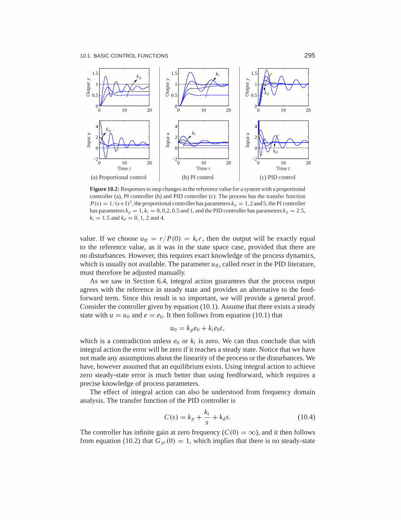
10.1. BASIC CONTROL FUNCTIONS 295
0 10 200
0.5
1
1.5
0 10 20−2
0
2
4
Time t
Out
puty
Inpu
tu
kp
kp
(a) Proportional control
0 10 200
0.5
1
1.5
0 10 20−2
0
2
4
Time tO
utpu
tyIn
putu ki
ki
(b) PI control
0 10 200
0.5
1
1.5
0 10 20−2
0
2
4
Time t
Out
puty
Inpu
tu
kd
kd
(c) PID control
Figure 10.2:Responses to step changes in the reference value for a system with a proportionalcontroller (a), PI controller (b) and PID controller (c). The process has the transfer functionP(s) = 1/(s+1)3, the proportional controller has parameterskp = 1, 2 and 5, the PI controllerhas parameterskp = 1,ki = 0, 0.2, 0.5 and 1, and the PID controller has parameterskp = 2.5,ki = 1.5 andkd = 0, 1, 2 and 4.
value. If we chooseuff = r/P(0) = kr r , then the output will be exactly equalto the reference value, as it was in the state space case, provided that there areno disturbances. However, this requires exact knowledge ofthe process dynamics,which is usually not available. The parameteruff , calledresetin the PID literature,must therefore be adjusted manually.
As we saw in Section 6.4, integral action guarantees that the process outputagrees with the reference in steady state and provides an alternative to the feed-forward term. Since this result is so important, we will provide a general proof.Consider the controller given by equation (10.1). Assume that there exists a steadystate withu = u0 ande = e0. It then follows from equation (10.1) that
u0 = kpe0 + ki e0t,
which is a contradiction unlesse0 or ki is zero. We can thus conclude that withintegral action the error will be zero if it reaches a steady state. Notice that we havenot made any assumptions about the linearity of the process or the disturbances. Wehave, however assumed that an equilibrium exists. Using integral action to achievezero steady-state error is much better than using feedforward, which requires aprecise knowledge of process parameters.
The effect of integral action can also be understood from frequency domainanalysis. The transfer function of the PID controller is
C(s) = kp + ki
s+ kds. (10.4)
The controller has infinite gain at zero frequency (C(0) = ∞), and it then followsfrom equation (10.2) thatGyr (0) = 1, which implies that there is no steady-state

296 CHAPTER 10. PID CONTROL
1
1 + sTi
6kp
e u
(a) Automatic reset
u6kp
e
−1
1 + sTd
(b) Proportional-derivative
Figure 10.3: Implementation of PI and PD controllers. The block diagram in (a) shows howintegral action is implemented usingpositive feedbackwith a first-order system, sometimescalled automatic reset. The block diagram in (b) shows how derivative action can be imple-mented by taking differences between a static system and a first-order system.
error for a step input.Integral action can also be viewed as a method for generatingthe feedforward
termuff in the proportional controller (10.3) automatically. One way to do this isshown in Figure 10.3a, where the controller output is low-pass-filtered and fed backwith positive gain. This implementation, calledautomatic reset, was one of the earlyinventions of integral control. The transfer function of thesystem in Figure 10.3ais obtained by block diagram algebra; we have
Gue = kp1 + sTi
sTi= kp + kp
sTi,
which is the transfer function for a PI controller.The properties of integral action are illustrated in Figure 10.2b for a step input.
The proportional gain is constant,kp = 1, and the integral gains areki = 0, 0.2, 0.5and 1. The caseki = 0 corresponds to pure proportional control, with a steady-stateerror of 50%. The steady-state error is eliminated when integral gain action is used.The response creeps slowly toward the reference for small values ofki and goesfaster for larger integral gains, but the system also becomes more oscillatory.
The integral gainki is a useful measure for attenuation of load disturbances.Consider a closed loop system under PID control and assume that the system isstable and initially at rest with all signals being zero. Apply a unit step disturbance atthe process input. After a transient the process output goesto zero and the controlleroutput settles at a value that compensates for the disturbance. It follows from (10.1)that
u(∞) = ki
∫ ∞
0e(t)dt.
The integrated error is thus inversely proportional to the integral gainki . The integralgain is thus a measure of the effectiveness of disturbance attenuation. A large gainki attenuates disturbances effectively, but too large a gain gives oscillatory behavior,poor robustness and possibly instability.
We now return to the general PID controller and consider the effect of thederivative termkd. Recall that the original motivation for derivative feedback wasto provide predictive or anticipatory action. Notice that the combination of the

10.1. BASIC CONTROL FUNCTIONS 297
proportional and the derivative terms can be written as
u = kpe+ kdde
dt= kp
(e+ Td
de
dt
)= kpep,
whereep(t) can be interpreted as a prediction of the error at timet + Td by linearextrapolation. The prediction timeTd = kd/kp is the derivative time constant ofthe controller.
Derivative action can be implemented by taking the difference between the signaland its low-pass filtered version as shown in Figure 10.3b. The transfer functionfor the system is
Gue(s) = kp
(1 − 1
1 + sTd
)= kp
sTd
1 + sTd. (10.5)
The system thus has the transfer functionG(s) = sTd/(1 + sTd), which approxi-mates a derivative for low frequencies (|s| < Td).
Figure 10.2c illustrates the effect of derivative action: the system is oscillatorywhen no derivative action is used, and it becomes more dampedas the derivativegain is increased. Performance deteriorates if the derivative gain is too high. Whenthe input is a step, the controller output generated by the derivative term will bean impulse. This is clearly visible in Figure 10.2c. The impulsecan be avoided byusing the controller configuration shown in Figure 10.1b.
Although PID control was developed in the context of engineering applications,it also appears in nature. Disturbance attenuation by feedback in biological sys-tems is often calledadaptation. A typical example is the pupillary reflex discussedin Example 8.11, where it is said that the eye adapts to changing light intensity.Analogously, feedback with integral action is called perfect adaptation [YHSD00].In biological systems proportional, integral and derivative action is generated bycombining subsystems with dynamical behavior similarly towhat is done in en-gineering systems. For example, PI action can be generated bythe interaction ofseveral hormones [ESGK02].
Example 10.1 PD action in the retinaThe response of cone photoreceptors in the retina is an example where proportionaland derivative action is generated by a combination of conesand horizontal cells.The cones are the primary receptors stimulated by light, which in turn stimulate thehorizontal cells, and the horizontal cells give inhibitory(negative) feedback to thecones. A schematic diagram of the system is shown in Figure 10.4a. The systemcan be modeled by ordinary differential equations by representing neuron signalsas continuous variables representing the average pulse rate. In [Wil99] it is shownthat the system can be represented by the differential equations
dx1
dt= 1
Tc(−x1 − kx2 + u),
dx2
dt= 1
Th(x1 − x2),
whereu is the light intensity andx1 andx2 are the average pulse rates from the conesand the horizontal cells. A block diagram of the system is shown in Figure 10.4b.

298 CHAPTER 10. PID CONTROL
C
H
(a)
1
1 + sTc6
u x1
−k
1 + sTh
(b)
0 0.2 0.40
0.2
0.4
0.6
Con
epu
lse
ratey
Time t [s]
(c)
Figure 10.4: Schematic diagram of cone photoreceptors (C) and horizontal cells (H)inthe retina. In the schematic diagram in (a), excitatory feedback is indicatedby arrows andinhibitory feedback by circles. A block diagram is shown in (b) and the stepresponse in (c).
The step response of the system shown in Figure 10.4c shows thatthe system hasa large initial response followed by a lower, constant steady-state response typicalof proportional and derivative action. The parameters used in the simulation arek = 4, Tc = 0.025 andTh = 0.08. ∇
10.2 Simple Controllers for Complex Systems
Many of the design methods discussed in previous chapters have the property thatthe complexity of the controller is directly reflected by the complexity of the model.When designing controllers by output feedback in Chapter 7,we found for single-input, single-output systems that the order of the controller was the same as the orderof the model, possibly one order higher if integral action was required. Applyingsimilar design methods for PID control will require that we have low-order modelsof the processes to be able to easily analyze the results.
Low-order models can be obtained from first principles. Any stable systemcan be modeled by a static system if its inputs are sufficientlyslow. Similarly afirst-order model is sufficient if the storage of mass, momentumor energy can becaptured by only one variable; typical examples are the velocity of a car on a road,angular velocity of a stiff rotational system, the level in atank and the concentrationin a volume with good mixing. System dynamics are of second order if the storageof mass, energy and momentum can be captured by two state variables; typicalexamples are the position of a car on the road, the stabilization of stiff satellites,the levels in two connected tanks and two-compartment models. A wide range oftechniques for model reduction are also available. In this chapter we will focus ondesign techniques where we simplify the models to capture the essential propertiesthat are needed for PID design.
We begin by analyzing the case of integral control. A stable system can becontrolled by an integral controller provided that the requirements on the closedloop system are modest. To design the controller we assume that the transfer functionof the process is a constantK = P(0). The loop transfer function under integralcontrol then becomesKki /s, and the closed loop characteristic polynomial is simply
10.2. SIMPLE CONTROLLERS FOR COMPLEX SYSTEMS 299
s+ Kki . Specifying performance by the desired time constantTcl of the closed loopsystem, we find that the integral gain is given by
ki = 1/(Tcl P(0)).
The analysis requires thatTcl be sufficiently large that the process transfer functioncan be approximated by a constant.
For systems that are not well represented by a constant gain,we can obtaina better approximation by using the Taylor series expansionof the loop transferfunction:
L(s) = ki P(s)
s≈ ki (P(0)+ s P′(0))
s= ki P
′(0)+ ki P(0)
s.
Choosingki P′(0) = −0.5 gives a system with good robustness, as will be discussedin Section 12.5. The controller gain is then given by
ki = − 1
2P′(0), (10.6)
and the expected closed loop time constant isTcl ≈ −2P′(0)/P(0).
Example 10.2 Integral control of AFM in tapping modeA simplified model of the dynamics of the vertical motion of an atomic forcemicroscope in tapping mode was discussed in Exercise 9.2. The transfer functionfor the system dynamics is
P(s) = a(1 − e−sτ )
sτ(s + a),
wherea = ζω0, τ = 2πn/ω0 and the gain has been normalized to 1. We haveP(0) = 1 andP′(0) = −τ/2 − 1/a, and it follows from (10.6) that the integralgain can be chosen aski = a/(2 + aτ). Nyquist and Bode plots for the resultingloop transfer function are shown in Figure 10.5. ∇
A first-order system has the transfer function
P(s) = b
s + a.
With a PI controller the closed loop system has the characteristic polynomial
s(s + a)+ bkps + bki s = s2 + (a + bkp)s + bki .
The closed loop poles can thus be assigned arbitrary values byproper choice ofthe controller gains. Requiring that the closed loop systemhave the characteristicpolynomial
p(s) = s2 + a1s + a22,
we find that the controller parameters are
kp = a1 − a
b, ki = a2
b. (10.7)

300 CHAPTER 10. PID CONTROL
Im L(iω)
ReL(iω)
(a) Nyquist plot
10−4
10−2
100
102
10−2
10−1
100
101
102
−360−270−180−90
0
|L(iω)|
∠L(iω)
Frequencyω [rad/s]
(b) Bode plot
Figure 10.5: Integral control for AFM in tapping mode. An integral controller is designedbased on the slope of the process transfer function at 0. The controllergives good robustnessproperties based on a very simple analysis.
If we require a response of the closed loop system that is slower than that of the openloop system, a reasonable choice isa1 = a + α anda2 = αa. If a response fasterthan that of the open loop system is required, it is reasonable to choosea1 = 2ζω0
anda2 = ω20, whereω0 andζ are undamped natural frequency and damping ratio
of the dominant mode. These choices have significant impact on the robustness ofthe system and will be discussed in Section 12.4. An upper limit to ω0 is given bythe validity of the model. Large values ofω0 will require fast control actions, andactuators may saturate if the value is too large. A first-ordermodel is unlikely torepresent the true dynamics for high frequencies. We illustrate the design by anexample.
Example 10.3 Cruise control using PI feedbackConsider the problem of maintaining the speed of a car as it goes up a hill. InExample 5.14 we found that there was little difference between the linear andnonlinear models when investigating PI control, provided that the throttle did notreach the saturation limits. A simple linear model of a car was given in Example 5.11:
d(v − ve)
dt= −a(v − ve)+ b(u − ue)− gθ, (10.8)
wherev is the velocity of the car,u is the input from the engine andθ is the slopeof the hill. The parameters werea = 0.0101,b = 1.3203,g = 9.8, ve = 20 andue = 0.1616. This model will be used to find suitable parameters of a vehicle speedcontroller. The transfer function from throttle to velocityis a first-order system.Since the open loop dynamics is so slow, it is natural to specify a faster closed loopsystem by requiring that the closed loop system be of second-order with dampingratioζ and undamped natural frequencyω0. The controller gains are given by (10.7).
Figure 10.6 shows the velocity and the throttle for a car that initially moveson a horizontal road and encounters a hill with a slope of 4◦ at time t = 6 s. Todesign a PI controller we chooseζ = 1 to obtain a response without overshoot, as

10.2. SIMPLE CONTROLLERS FOR COMPLEX SYSTEMS 301
0 10 20 30 40−2
−1
0
0 10 20 30 400
0.2
0.4
0.6
0.8
Time t [s]
v−v
e[m
/s]
u−
ue
ζ
ζ
(a)ω0 = 0.5, ζ = 0.5, 1, 2
0 10 20 30 40−2
−1
0
0 10 20 30 400
0.2
0.4
0.6
0.8
Time t [s]
v−v
e[m
/s]
u−
ue
ω0
ω0
(b) ζ = 1,ω0 = 0.2, 0.5, 1
Figure 10.6: Cruise control using PI feedback. The step responses for the errorand inputillustrate the effect of parametersζ = 1 andω0 on the response of a car with cruise control.A change in road slope from 0◦ to 4◦ is applied betweent = 5 and 6 s. (a) Responses forω0 = 0.5 andζ = 0.5, 1 and 2. Choosingζ = 1 gives no overshoot. (b) Responses forζ = 1andω0 = 0.2, 0.5 and 1.0.
shown in Figure 10.6a. The choice ofω0 is a compromise between response speedand control actions: a large value gives a fast response, butit requires fast controlaction. The trade-off is is illustrated in Figure 10.6b. The largest velocity errordecreases with increasingω0, but the control signal also changes more rapidly. Inthe simple model (10.8) it was assumed that the force responds instantaneously tothrottle commands. For rapid changes there may be additional dynamics that haveto be accounted for. There are also physical limitations to the rate of change of theforce, which also restricts the admissible value ofω0. A reasonable choice ofω0
is in the range 0.5–1.0. Notice in Figure 10.6 that even withω0 = 0.2 the largestvelocity error is only 1 m/s. ∇
A PI controller can also be used for a process with second-order dynamics, butthere will be restrictions on the possible locations of the closed loop poles. Using aPID controller, it is possible to control a system of second order in such a way thatthe closed loop poles have arbitrary locations; see Exercise10.2.
Instead of finding a low-order model and designing controllers for them, wecan also use a high-order model and attempt to place only a fewdominant poles.An integral controller has one parameter, and it is possibleto position one pole.Consider a process with the transfer functionP(s). The loop transfer function withan integral controller isL(s) = ki P(s)/s. The roots of the closed loop characteristicpolynomial are the roots ofs + ki P(s) = 0. Requiring thats = −a be a root, wefind that the controller gain should be chosen as
ki = a
P(−a). (10.9)
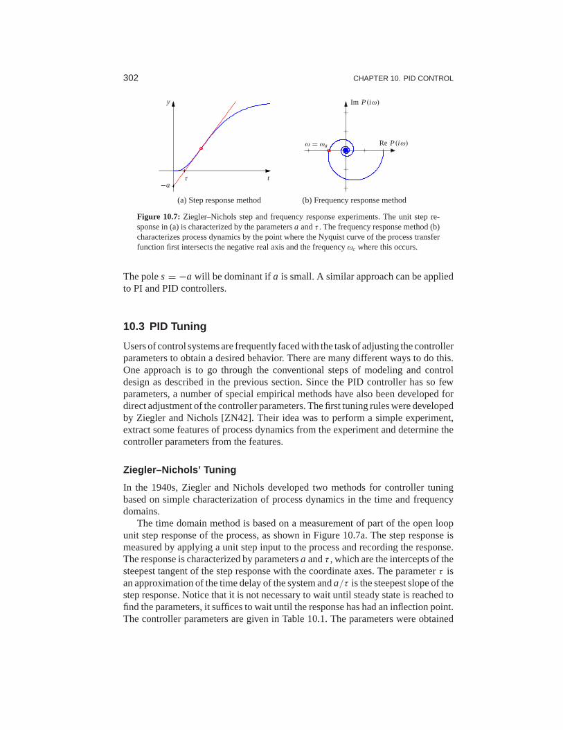
302 CHAPTER 10. PID CONTROL
tτ
y
−a
(a) Step response method
Re P(iω)
Im P(iω)
ω = ωa
(b) Frequency response method
Figure 10.7: Ziegler–Nichols step and frequency response experiments. The unit step re-sponse in (a) is characterized by the parametersa andτ . The frequency response method (b)characterizes process dynamics by the point where the Nyquist curveof the process transferfunction first intersects the negative real axis and the frequencyωc where this occurs.
The poles = −a will be dominant ifa is small. A similar approach can be appliedto PI and PID controllers.
10.3 PID Tuning
Users of control systems are frequently faced with the task of adjusting the controllerparameters to obtain a desired behavior. There are many different ways to do this.One approach is to go through the conventional steps of modeling and controldesign as described in the previous section. Since the PID controller has so fewparameters, a number of special empirical methods have alsobeen developed fordirect adjustment of the controller parameters. The first tuning rules were developedby Ziegler and Nichols [ZN42]. Their idea was to perform a simpleexperiment,extract some features of process dynamics from the experiment and determine thecontroller parameters from the features.
Ziegler–Nichols’ Tuning
In the 1940s, Ziegler and Nichols developed two methods for controller tuningbased on simple characterization of process dynamics in thetime and frequencydomains.
The time domain method is based on a measurement of part of the open loopunit step response of the process, as shown in Figure 10.7a. Thestep response ismeasured by applying a unit step input to the process and recording the response.The response is characterized by parametersa andτ , which are the intercepts of thesteepest tangent of the step response with the coordinate axes. The parameterτ isan approximation of the time delay of the system anda/τ is the steepest slope of thestep response. Notice that it is not necessary to wait until steady state is reached tofind the parameters, it suffices to wait until the response has had an inflection point.The controller parameters are given in Table 10.1. The parameters were obtained

10.3. PID TUNING 303
Table 10.1:Ziegler–Nichols tuning rules. (a) The step response methods give the parametersin terms of the intercepta and the apparent time delayτ . (b) The frequency response methodgives controller parameters in terms ofcritical gain kc andcritical period Tc.
Type kp Ti Td
P 1/a
PI 0.9/a 3τ
PID 1.2/a 2τ 0.5τ
(a) Step response method
Type kp Ti Td
P 0.5kc
PI 0.4kc 0.8Tc
PID 0.6kc 0.5Tc 0.125Tc
(b) Frequency response method
by extensive simulation of a range of representative processes. A controller wastuned manually for each process, and an attempt was then madeto correlate thecontroller parameters witha andτ .
In the frequency domain method, a controller is connected tothe process, theintegral and derivative gains are set to zero and the proportional gain is increaseduntil the system starts to oscillate. The critical value of the proportional gainkc
is observed together with the period of oscillationTc. It follows from Nyquist’sstability criterion that the loop transfer functionL = kcP(s) intersects the criticalpoint at the frequencyωc = 2π/Tc. The experiment thus gives the point on theNyquist curve of the process transfer function where the phase lag is 180◦, asshown in Figure 10.7b.
The Ziegler–Nichols methods had a huge impact when they were introducedin the 1940s. The rules were simple to use and gave initial conditions for manualtuning. The ideas were adopted by manufacturers of controllers for routine use. TheZiegler–Nichols tuning rules unfortunately have two severedrawbacks: too littleprocess information is used, and the closed loop systems that are obtained lackrobustness.
The step response method can be improved significantly by characterizing theunit step response by parametersK , τ andT in the model
P(s) = K
1 + sTe−τs. (10.10)
The parameters can be obtained by fitting the model to a measuredstep response.Notice that the experiment takes a longer time than the experiment in Figure 10.7abecause to determineK it is necessary to wait until the steady state has been reached.Also notice that the intercepta in the Ziegler–Nichols rule is given bya = K τ/T .
The frequency response method can be improved by measuring more points onthe Nyquist curve, e.g., the zero frequency gainK or the point where the processhas a 90◦ phase lag. This latter point can be obtained by connecting an integralcontroller and increasing its gain until the system reachesthe stability limit. Theexperiment can also be automated by using relay feedback, aswill be discussedlater in this section.
There are many versions of improved tuning rules. As an illustration we give

304 CHAPTER 10. PID CONTROL
Re
Im
ProcessZeigler−NicholsModified ZN
(a)
0 2 4 6 8 100
0.5
1
1.5
Ziegler−NicholsModified ZN
0 2 4 6 8 100
5
10
15
Normalized timeat
Dis
plac
emen
tyC
ontr
olu
(b)
Figure 10.8: PI control of an AFM in tapping mode. Nyquist plots (a) and step responses(b) for PI control of the vertical motion of an atomic force microscope intapping mode. Theaveraging parameter isn = 20. Results with Ziegler–Nichols tuning are shown by dashedlines, and modified Ziegler–Nichols tuning is shown by solid lines. The Nyquist plot of theprocess transfer function is shown by dotted lines.
the following rules for PI control, based on [ÅH05]:
kp = 0.15τ + 0.35T
K τ
(0.9T
K τ
), ki = 0.46τ + 0.02T
K τ 2
(0.3T
K τ 2
),
kp = 0.22kc − 0.07
K
(0.4kc
), ki = 0.16kc
Tc+ 0.62
K Tc
(0.5kc
Tc
).
(10.11)
The values for the Ziegler–Nichols rule are given in parentheses. Notice that theimproved formulas typically give lower controller gains than the Ziegler–Nicholsmethod. The integral gain is higher for systems where the dynamics are delay-dominated,τ ≫ T .
Example 10.4 Atomic force microscope in tapping modeA simplified model of the dynamics of the vertical motion of an atomic forcemicroscope in tapping mode was discussed in Example 10.2. The transfer functionis normalized by choosing 1/a as the time unit. The normalized transfer functionis
P(s) = 1 − e−sTn
sTn(s + 1),
whereTn = 2nπa/ω0 = 2nπζ . The Nyquist plot of the transfer function is shownin Figure 10.8a forz = 0.002 andn = 20. The leftmost intersection of the Nyquistcurve with the real axis occurs at Res = −0.0461 forω = 13.1. The critical gainis thuskc = 21.7 and the critical period isTc = 0.48. Using the Ziegler–Nicholstuning rule, we find the parameterskp = 8.87 andki = 22.6 (Ti = 0.384) fora PI controller. With this controller the stability margin issm = 0.31, which isquite small. The step response of the controller is shown in Figure 10.8. Notice inparticular that there is a large overshoot in the control signal.
The modified Ziegler–Nichols rule (10.11) gives the controllerparametersk =

10.3. PID TUNING 305
G(s)6
r ye u
−1
(a) Relay feedback
0 10 20 30−1
0
1
2
u y
u,
y
Time [s]
(b) Oscillatory response
Figure 10.9:Block diagram of a process with relay feedback (a) and typical signals (b). Theprocess outputy is a solid line, and the relay outputu is a dashed line. Notice that the signalsu andy have opposite phases.
3.47 andki = 8.73 (Ti = 0.459) and the stability margin becomessm = 0.61. Thestep response with this controller is shown in Figure 10.8. A comparison of theresponses obtained with the original Ziegler–Nichols rule shows that the overshoothas been reduced. Notice that the control signal reaches itssteady-state value almostinstantaneously. It follows from Example 10.2 that a pure integral controller hasthe normalized gainki = 1/(2 + Tn) = 0.44. Comparing this with the gains of aPI controller, we can conclude that a PI controller gives much better performancethan a pure integral controller. ∇
Relay Feedback
The Ziegler–Nichols frequency response method increases thegain of a proportionalcontroller until oscillation to determine the critical gain kc and the correspondingcritical periodTc or, equivalently, the point where the Nyquist curve intersects thenegative real axis. One way to obtain this information automatically is to connectthe process in a feedback loop with a nonlinear element having a relay function asshown in Figure 10.9a. For many systems there will then be an oscillation, as shownin Figure 10.9b, where the relay outputu is a square wave and the process outputy is close to a sinusoid. Moreover the input and the output are out of phase, whichmeans that the system oscillates with the critical periodTc, where the process hasa phase lag of 180◦. Notice that an oscillation with constant period is establishedquickly.
The critical period is simply the period of the oscillation. To determine thecritical gain we expand the square wave relay output in a Fourier series. Noticein the figure that the process output is practically sinusoidal because the processattenuates higher harmonics effectively. It is then sufficient to consider only thefirst harmonic component of the input. Lettingd be the relay amplitude, the firstharmonic of the square wave input has amplitude 4d/π . If a is the amplitudeof the process output, the process gain at the critical frequencyωc = 2π/Tc is|P(iωc)| = πa/(4d) and the critical gain is
Kc = 4d
aπ. (10.12)

306 CHAPTER 10. PID CONTROL
Having obtained the critical gainKc and the critical periodTc, the controller pa-rameters can then be determined using the Ziegler–Nichols rules. Improved tuningcan be obtained by fitting a model to the data obtained from the relay experiment.
The relay experiment can be automated. Since the amplitude of the oscillationis proportional to the relay output, it is easy to control it by adjusting the relayoutput.Automatic tuningbased on relay feedback is used in many commercial PIDcontrollers. Tuning is accomplished simply by pushing a button that activates relayfeedback. The relay amplitude is automatically adjusted to keep the oscillationssufficiently small, and the relay feedback is switched to a PID controller as soon asthe tuning is finished.
10.4 Integrator Windup
Many aspects of a control system can be understood from linear models. There are,however, some nonlinear phenomena that must be taken into account. These aretypically limitations in the actuators: a motor has limitedspeed, a valve cannot bemore than fully opened or fully closed, etc. For a system thatoperates over a widerange of conditions, it may happen that the control variablereaches the actuatorlimits. When this happens, the feedback loop is broken and the system runs inopen loop because the actuator remains at its limit independently of the processoutput as long as the actuator remains saturated. The integral term will also buildup since the error is typically nonzero. The integral term andthe controller outputmay then become very large. The control signal will then remain saturated evenwhen the error changes, and it may take a long time before the integrator and thecontroller output come inside the saturation range. The consequence is that thereare large transients. This situation is referred to asintegrator windup, illustrated inthe following example.
Example 10.5 Cruise controlThe windup effect is illustrated in Figure 10.10a, which showswhat happens whena car encounters a hill that is so steep (6◦) that the throttle saturates when the cruisecontroller attempts to maintain speed. When encountering the slope at timet = 5,the velocity decreases and the throttle increases to generate more torque. However,the torque required is so large that the throttle saturates.The error decreases slowlybecause the torque generated by the engine is just a little larger than the torquerequired to compensate for gravity. The error is large and theintegral continues tobuild up until the error reaches zero at time 30, but the controller output is still largerthan the saturation limit and the actuator remains saturated. The integral term startsto decrease, and at time 45 and the velocity settles quickly to the desired value.Notice that it takes considerable time before the controller output comes into therange where it does not saturate, resulting in a large overshoot. ∇
There are many methods to avoid windup. One method is illustrated in Fig-ure 10.11: the system has an extra feedback path that is generated by measuringthe actual actuator output, or the output of a mathematical model of the saturating

10.4. INTEGRATOR WINDUP 307
0 20 40 6018
19
20
21
0 20 40 600
1
2
CommandedApplied
Velo
city
[m/s
]T
hrot
tle
Time t [s]
(a) Windup
0 20 40 6018
19
20
21
0 20 40 600
1
2
CommandedApplied
Velo
city
[m/s
]T
hrot
tle
Time t [s]
(b) Anti-windup
Figure 10.10:Simulation of PI cruise control with windup (a) and anti-windup (b). The figureshows the speedv and the throttleu for a car that encounters a slope that is so steep thatthe throttle saturates. The controller output is a dashed line. The controller parameters arekp = 0.5 andki = 0.1. The anti-windup compensator eliminates the overshoot by preventingthe error for building up in the integral term of the controller.
actuator, and forming an error signales as the difference between the output ofthe controllerv and the actuator outputu. The signales is fed to the input of theintegrator through gainkt . The signales is zero when there is no saturation and theextra feedback loop has no effect on the system. When the actuator saturates, thesignales is fed back to the integrator in such a way thates goes toward zero. Thisimplies that controller output is kept close to the saturation limit. The controlleroutput will then change as soon as the error changes sign and integral windup isavoided.
The rate at which the controller output is reset is governed bythe feedbackgainkt ; a large value ofkt gives a short reset time. The parameterkt cannot be toolarge because measurement noise can then cause an undesirable reset. A reasonablechoice is to choosekt as a fraction of 1/Ti . We illustrate how integral windup canbe avoided by investigating the cruise control system.
Example 10.6 Cruise control with anti-windupFigure 10.10b shows what happens when a controller with anti-windup is appliedto the system simulated in Figure 10.10a. Because of the feedback from the actuatormodel, the output of the integrator is quickly reset to a value such that the controlleroutput is at the saturation limit. The behavior is drastically different from that inFigure 10.10a and the large overshoot is avoided. The trackinggain iskt = 2 in thesimulation. ∇

308 CHAPTER 10. PID CONTROL
11+sTf
6
y
66
ν u
+−
e = r − y
−y
es
Actuator
ki1s
kt
P(s)kp
kds
Figure 10.11: PID controller with a filtered derivative and anti-windup. The input to theintegrator (1/s) consists of the error term plus a “reset” based on input saturation. If theactuator is not saturated, thenes = u − ν, otherwisees will decrease the integrator input toprevent windup.
10.5 Implementation
There are many practical issues that have to be considered when implementing PIDcontrollers. They have been developed over time based on practical experience. Inthis section we consider some of the most common. Similar considerations alsoapply to other types of controllers.
Filtering the Derivative
A drawback with derivative action is that an ideal derivative has high gain forhigh-frequency signals. This means that high-frequency measurement noise willgenerate large variations in the control signal. The effect of measurement noise maybe reduced by replacing the termkds by kds/(1 + sTf ), which can be interpretedas an ideal derivative of a low-pass filtered signal. For smalls the transfer functionis approximatelykds and for larges it is equal tokd/T f . The approximation actsas a derivative for low-frequency signals and as a constant gain for high-frequencysignals. The filtering time is chosen asT f = (kd/k)/N, with N in the range 2–20.Filtering is obtained automatically if the derivative is implemented by taking thedifference between the signal and its filtered version as shown in Figure 10.3b (seeequation (10.5)).
Instead of filtering just the derivative, it is also possible to use an ideal controllerand filter the measured signal. The transfer function of such a controller with a filteris then
C(s) = kp
(1 + 1
sTi+ sTd
)1
1 + sTf + (sTf )2/2, (10.13)
where a second-order filter is used.

10.5. IMPLEMENTATION 309
Setpoint Weighting
Figure 10.1 shows two configurations of a PID controller. The system in Fig-ure 10.1a has a controller witherror feedbackwhere proportional, integral andderivative action acts on the error. In the simulation of PID controllers in Fig-ure 10.2c there is a large initial peak in the control signal,which is caused by thederivative of the reference signal. The peak can be avoided byusing the controllerin Figure 10.1b, where proportional and derivative action acts only on the processoutput. An intermediate form is given by
u = kp(βr − y
)+ ki
∫ ∞
0
(r (τ )− y(τ )
)dτ + kd
(γ
dr
dt− dy
dt
), (10.14)
where the proportional and derivative actions act on fractionsβ andγ of the refer-ence. Integral action has to act on the error to make sure thatthe error goes to zeroin steady state. The closed loop systems obtained for different values ofβ andγrespond to load disturbances and measurement noise in the same way. The responseto reference signals is different because it depends on the values ofβ andγ , whichare calledreference weightsor setpoint weights. We illustrate the effect of setpointweighting by an example.
Example 10.7 Cruise control with setpoint weightingConsider the PI controller for the cruise control system derived in Example 10.3.Figure 10.12 shows the effect of setpoint weighting on the response of the systemto a reference signal. Withβ = 1 (error feedback) there is an overshoot in velocityand the control signal (throttle) is initially close to the saturation limit. There is noovershoot withβ = 0 and the control signal is much smaller, clearly a much betterdrive comfort. The frequency responses gives another view ofthe same effect. Theparameterβ is typically in the range 0–1, andγ is normally zero to avoid largetransients in the control signal when the reference is changed. ∇
The controller given by equation (10.14) is a special case of the general controllerstructure having two degrees of freedom, which was discussed in Section 7.5.
Implementation Based on Operational Amplifiers
PID controllers have been implemented in different technologies. Figure 10.13shows how PI and PID controllers can be implemented by feedbackaround opera-tional amplifiers.
To show that the circuit in Figure 10.13b is a PID controller we will use theapproximate relation between the input voltagee and the output voltageu of theoperational amplifier derived in Example 8.3,
u = − Z2
Z1e.
In this equationZ1 is the impedance between the negative input of the amplifier andthe input voltagee, andZ2 is the impedance between the zero input of the amplifier

310 CHAPTER 10. PID CONTROL
0 5 10 1520
20.5
21
0 5 10 150
0.2
0.4
0.6
0.8
Thr
ottle
uS
peedv
[m/s
]
Time t [s]
β
β
(a) Step response
10−1
100
101
10−2
10−1
100
10−1
100
101
10−2
10−1
100
Frequencyω [rad/s]
|Gvr(iω)|
|Gu
r(iω)|
β
β
(b) Frequency responses
Figure 10.12:Time and frequency responses for PI cruise control with setpoint weighting.Step responses are shown in (a), and the gain curves of the frequency responses in (b). Thecontroller gains arekp = 0.74 andki = 0.19. The setpoint weights areβ = 0, 0.5 and 1, andγ = 0.
and the output voltageu. The impedances are given by
Z1(s) = R1
1 + R1C1s, Z2(s) = R2 + 1
C2s,
and we find the following relation between the input voltageeand the output voltageu:
u = − Z2
Z1e = − R2
R1
(1 + R1C1s)(1 + R2C2s)
R2C2se.
This is the input/output relation for a PID controller of the form (10.1) with param-eters
kp = R2
R1, Ti = R2C1, Td = R1C1.
−
+
R1 R C2 2
e
u
(a) PI controller
−
+
R1 R C2 2
C1
e
u
(b) PID controller
Figure 10.13:Schematic diagrams for PI and PID controllers using op amps. The circuit in(a) uses a capacitor in the feedback path to store the integral of the error. The circuit in (b)adds a filter on the input to provide derivative action.

10.5. IMPLEMENTATION 311
The corresponding results for a PI controller are obtained by settingC1 = 0 (re-moving the capacitor).
Computer Implementation
In this section we briefly describe how a PID controller may be implemented usinga computer. The computer typically operates periodically, with signals from thesensors sampled and converted to digital form by the A/D converter, and the controlsignal computed and then converted to analog form for the actuators. The sequenceof operation is as follows:
1. Wait for clock interrupt
2. Read input from sensor
3. Compute control signal
4. Send output to the actuator
5. Update controller variables
6. Repeat
Notice that an output is sent to the actuators as soon as it is available. The timedelay is minimized by making the calculations in step 3 as short as possible andperforming all updates after the output is commanded. This simple way of reducingthe latency is, unfortunately, seldom used in commercial systems.
As an illustration we consider the PID controller in Figure 10.11, which hasa filtered derivative, setpoint weighting and protection against integral windup.The controller is a continuous-time dynamical system. To implement it using acomputer, the continuous-time system has to be approximated by a discrete-timesystem.
A block diagram of a PID controller with anti-windup is shown in Figure 10.11.The signalv is the sum of the proportional, integral and derivative terms, and thecontroller output isu = sat(v), where sat is the saturation function that models theactuator. The proportional termkp(βr − y) is implemented simply by replacing thecontinuous variables with their sampled versions. Hence
P(tk) = kp (βr (tk)− y(tk)) , (10.15)
where{tk} denotes the sampling instants, i.e., the times when the computer readsits input. We leth represent the sampling time, so thattk+1 = tk + h. The integralterm is obtained by approximating the integral with a sum,
I (tk+1) = I (tk)+ ki h e(tk)+ h
Tt
(sat(v)− v
), (10.16)
whereTt = h/kt represents the anti-windup term. The filtered derivative termDis given by the differential equation
T fd D
dt+ D = −kd y.
Approximating the derivative with a backward difference gives
T fD(tk)− D(tk−1)
h+ D(tk) = −kd
y(tk)− y(tk−1)
h,

312 CHAPTER 10. PID CONTROL
which can be rewritten as
D(tk) = T f
T f + hD(tk−1)− kd
T f + h(y(tk)− y(tk−1)) . (10.17)
The advantage of using a backward difference is that the parameterT f /(T f + h)is nonnegative and less than 1 for allh > 0, which guarantees that the differenceequation is stable. Reorganizing equations (10.15)–(10.17), the PID controller canbe described by the following pseudocode:
% Precompute controller coefficientsbi=ki*had=Tf/(Tf+h)bd=kd/(Tf+h)br=h/Tt
% Control algorithm - main loopwhile (running) {
r=adin(ch1) % read setpoint from ch1y=adin(ch2) % read process variable from ch2P=kp*(b*r-y) % compute proportional partD=ad*D-bd*(y-yold) % update derivative partv=P+I+D % compute temporary outputu=sat(v,ulow,uhigh) % simulate actuator saturationdaout(ch1) % set analog output ch1I=I+bi*(r-y)+br*(u-v) % update integralyold=y % update old process outputsleep(h) % wait until next update interval
}
Precomputation of the coefficientsbi, ad, bd andbr saves computer time inthe main loop. These calculations have to be done only when controller parametersare changed. The main loop is executed once every sampling period. The programhas three states:yold, I, andD. One state variable can be eliminated at the costof less readable code. The latency between reading the analoginput and settingthe analog output consists of four multiplications, four additions and evaluationof thesat function. All computations can be done using fixed-point calculationsif necessary. Notice that the code computes the filtered derivative of the processoutput and that it has setpoint weighting and anti-windup protection.
10.6 Further Reading
The history of PID control is very rich and stretches back to thebeginning of thefoundation of control theory. Very readable treatments aregiven by Bennett [Ben79,Ben93] and Mindel [Min02]. The Ziegler–Nichols rules for tuning PID controllers,first presented in 1942 [ZN42], were developed based on extensive experimentswith pneumatic simulators and Vannevar Bush’s differential analyzer at MIT. Aninteresting view of the development of the Ziegler–Nichols rules is given in aninterview with Ziegler [Bli90]. An industrial perspective on PID control is given

EXERCISES 313
in [Bia95], [Shi96] and [YH91] and in the paper [DM02] cited inthe beginningof this chapter. A comprehensive presentation of PID controlis given in [ÅH05].Interactive learning tools for PID control can be downloadedfrom http://www.calerga.com/contrib.
Exercises
10.1(Ideal PID controllers) Consider the systems represented bythe block diagramsin Figure 10.1. Assume that the process has the transfer function P(s) = b/(s+a)and show that the transfer functions fromr to y are
(a) Gyr (s) = bkds2 + bkps + bki
(1 + bkd)s2 + (a + bkp)s + bki,
(b) Gyr (s) = bki
(1 + bkd)s2 + (a + bkp)s + bki.
Pick some parameters and compare the step responses of the systems.
10.2 Consider a second-order process with the transfer function
P(s) = b
s2 + a1s + a2.
The closed loop system with a PI controller is a third-order system. Show that it ispossible to position the closed loop poles as long as the sum of the poles is−a1. Giveequations for the parameters that give the closed loop characteristic polynomial
(s + α0)(s2 + 2ζ0ω0s + ω2
0).
10.3 Consider a system with the transfer functionP(s) = (s + 1)−2. Find anintegral controller that gives a closed loop pole ats = −a and determine the valueof a that maximizes the integral gain. Determine the other polesof the system andjudge if the pole can be considered dominant. Compare with the value of the integralgain given by equation (10.6).
10.4 (Ziegler–Nichols tuning) Consider a system with transfer function P(s) =e−s/s. Determine the parameters of P, PI and PID controllers using Ziegler–Nicholsstep and frequency response methods. Compare the parametervalues obtained bythe different rules and discuss the results.
10.5 (Vehicle steering) Design a proportional-integral controller for the vehiclesteering system that gives the closed loop characteristic polynomial
s3 + 2ω0s2 + 2ω0s + ω30.
10.6 (Congestion control) A simplified flow model for TCP transmission is de-rived in [HMTG00, LPD02]. The linearized dynamics are modeled bythe transfer

314 CHAPTER 10. PID CONTROL
functionGqp(s) = b
(s + a1)(s + a2)e−sτe,
which describes the dynamics relating the expected queue lengthq to the expectedpacket dropp. The parameters are given bya1 = 2N2/(cτ 2
e ), a2 = 1/τe andb = c2/(2N). The parameterc is the bottleneck capacity,N is the number ofsources feeding the link andτe is the round-trip delay time. Use the parametervaluesN = 75 sources,C = 1250 packets/s andτe = 0.15 and find the parametersof a PI controller using one of the Ziegler–Nichols rules and the correspondingimproved rule. Simulate the responses of the closed loop systems obtained with thePI controllers.
10.7(Motor drive) Consider the model of the motor drive in Exercise 2.10. Developan approximate second-order model of the system and use it todesign an ideal PDcontroller that gives a closed loop system with eigenvaluesin ζω0 ± iω0
√1 − ζ 2.
Add low-pass filtering as shown in equation (10.13) and explore how largeω0 canbe made while maintaining a good stability margin. Simulate the closed loop systemwith the chosen controller and compare the results with the controller based on statefeedback in Exercise 6.11.
10.8 Consider the system in Exercise 10.7 investigate what happens if the second-order filtering of the derivative is replace by a first-order filter.
10.9 (Tuning rules) Apply the Ziegler–Nichols and the modified tuning rules todesign PI controllers for systems with the transfer functions
P1 = e−s
s, P2 = e−s
s + 1, P3 = e−s.
Compute the stability margins and explore any patterns.
10.10(Windup and anti-windup) Consider a PI controller of the formC(s) = 1+1/sfor a process with input that saturates when|u| > 1, and whose linear dynamics aregiven by the transfer functionP(s) = 1/s. Simulate the response of the system tostep changes in the reference signal of magnitude 1, 2 and 3. Repeat the simulationwhen the windup protection scheme in Figure 10.11 is used.
10.11 (Windup protection by conditional integration) Many methods have beenproposed to avoid integrator windup. One method calledconditional integrationis to update the integral only when the error is sufficiently small. To illustrate thismethod we consider a system with PI control described by
dx1
dt= u, u = satu0(kpe+ ki x2),
dx2
dt={
e if |e| < e0
0 if |e| ≥ e0,
wheree = r − x. Plot the phase portrait of the system for the parameter valueskp = 1, ki = 1, u0 = 1 ande0 = 1 and discuss the properties of the system.The example illustrates the difficulties of introducing ad hocnonlinearities withoutcareful analysis.

Chapter ElevenFrequency Domain Design
Sensitivity improvements in one frequency range must be paid for with sensitivity deteriorationsin another frequency range, and the price is higher if the plant is open-loop unstable. Thisapplies to every controller, no matter how it was designed.
Gunter Stein in the inaugural IEEE Bode Lecture, 1989 [Ste03].
In this chapter we continue to explore the use of frequency domain techniqueswith a focus on the design of feedback systems. We begin with amore thoroughdescription of the performance specifications for control systems and then introducethe concept of “loop shaping” as a mechanism for designing controllers in thefrequency domain. We also introduce some fundamental limitations to performancefor systems with time delays and right half-plane poles and zeros.
11.1 Sensitivity Functions
In the previous chapter, we considered the use of proportional-integral-derivative(PID) feedback as a mechanism for designing a feedback controller for a givenprocess. In this chapter we will expand our approach to include a richer repertoireof tools for shaping the frequency response of the closed loop system.
One of the key ideas in this chapter is that we can design the behavior of theclosed loop system by focusing on the open loop transfer function. This sameapproach was used in studying stability using the Nyquist criterion: we plotted theNyquist plot for theopenloop transfer function to determine the stability of theclosedloop system. From a design perspective, the use of loop analysis tools is verypowerful: since the loop transfer function isL = PC, if we can specify the desiredperformance in terms of properties ofL, we can directly see the impact of changesin the controllerC. This is much easier, for example, than trying to reason directlyabout the tracking response of the closed loop system, whosetransfer function isgiven byGyr = PC/(1 + PC).
We will start by investigating some key properties of the feedback loop. Ablock diagram of a basic feedback loop is shown in Figure 11.1.The system loop iscomposed of two components: the process and the controller.The controller itselfhas two blocks: the feedback blockC and the feedforward blockF . There are twodisturbances acting on the process, the load disturbanced and the measurementnoisen. The load disturbance represents disturbances that drive the process awayfrom its desired behavior, while the measurement noise represents disturbances thatcorrupt information about the process given by the sensors.In the figure, the load

316 CHAPTER 11. FREQUENCY DOMAIN DESIGN
−1
6
e6
d
6
n
yν ηur
Controller Process
y
F(s) C(s) P(s)
Figure 11.1: Block diagram of a basic feedback loop with two degrees of freedom. Thecontroller has a feedback blockC and a feedforward blockF . The external signals are thereference signalr , the load disturbanced and the measurement noisen. The process outputis η, and the control signal isu.
disturbance is assumed to act on the process input. This is a simplification sincedisturbances often enter the process in many different ways, but it allows us tostreamline the presentation without significant loss of generality.
The process outputη is the real variable that we want to control. Control is basedon the measured signaly, where the measurements are corrupted by measurementnoisen. The process is influenced by the controller via the control variable u.The process is thus a system with three inputs—the control variable u, the loaddisturbanced and the measurement noisen—and one output—the measured signaly. The controller is a system with two inputs and one output. The inputs are themeasured signaly and the reference signalr , and the output is the control signalu. Note that the control signalu is an input to the process and the output of thecontroller, and that the measured signaly is the output of the process and an inputto the controller.
The feedback loop in Figure 11.1 is influenced by three external signals, thereferencer , the load disturbanced and the measurement noisen. Any of the re-maining signals can be of interest in controller design, depending on the particularapplication. Since the system is linear, the relations between the inputs and the in-teresting signals can be expressed in terms of the transfer functions. The followingrelations are obtained from the block diagram in Figure 11.1:
yη
ν
ue
=
PC F
1 + PC
P
1 + PC
1
1 + PCPC F
1 + PC
P
1 + PC
−PC
1 + PCC F
1 + PC
1
1 + PC
−C
1 + PCC F
1 + PC
−PC
1 + PC
−C
1 + PCF
1 + PC
−P
1 + PC
−1
1 + PC
rdn
. (11.1)
In addition, we can write the transfer function for the errorbetween the reference

11.1. SENSITIVITY FUNCTIONS 317
r and the outputη (not an explicit signal in the diagram), which satisfies
ǫ = r − η =(1 − PC F
1 + PC
)r + −P
1 + PCd + PC
1 + PCn.
There are several interesting conclusions we can draw from these equations. Firstwe can observe that several transfer functions are the same and that the majority ofthe relations are given by the following set of six transfer functions, which we calltheGang of Six:
T F = PC F
1 + PC, T = PC
1 + PC, PS= P
1 + PC,
C FS= C F
1 + PC, CS= C
1 + PC, S = 1
1 + PC.
(11.2)
The transfer functions in the first column give the response of the process outputand control signal to the reference signal. The second columngives the responseof the control variable to the load disturbance and the noise, and the final columngives the response of the process output to those two inputs.Notice that only fourtransfer functions are required to describe how the system reacts to load disturbancesand measurement noise, and that two additional transfer functions are required todescribe how the system responds to reference signals.
The linear behavior of the system is determined by the six transfer functionsin equation (11.2), and specifications can be expressed in terms of these transferfunctions. The special case whenF = 1 is called a system with (pure) error feed-back. In this case all control actions are based on feedback from the error only andthe system is completely characterized by four transfer functions, namely, the fourrightmost transfer functions in equation (11.2), which have specific names:
S = 1
1 + PCsensitivityfunction
PS= P
1 + PC
loadsensitivityfunction
T = PC
1 + PC
complementarysensitivityfunction
CS= C
1 + PC
noisesensitivityfunction
(11.3)
These transfer functions and their equivalent systems are called theGang of Four.The load sensitivity function is sometimes called the input sensitivity function andthe noise sensitivity function is sometimes called the output sensitivity function.These transfer functions have many interesting properties that will be discussedin detail in the rest of the chapter. Good insight into these properties is essentialin understanding the performance of feedback systems for the purposes of bothanalysis and design.
Analyzing the Gang of Six, we find that the feedback controllerC influencesthe effects of load disturbances and measurement noise. Notice that measurementnoise enters the process via the feedback. In Section 12.2 it will be shown thatthe controller influences the sensitivity of the closed loop to process variations.

318 CHAPTER 11. FREQUENCY DOMAIN DESIGN
P
zw
C
yu
Figure 11.2: A more general representation of a feedback system. The process input urepresents the control signal, which can be manipulated, and the process inputw representsother signals that influence the process. The process outputy is the vector of measuredvariables andz are other signals of interest.
The feedforward partF of the controller influences only the response to commandsignals.
In Chapter 9 we focused on the loop transfer function, and we found that itsproperties gave useful insights into the properties of a system. To make a properassessment of a feedback system it is necessary to consider the properties of all thetransfer functions (11.2) in the Gang of Six or the Gang of Four, as illustrated inthe following example.
Example 11.1 The loop transfer function gives only limited insightConsider a process with the transfer functionP(s) = 1/(s − a) controlled by a PIcontroller with error feedback having the transfer function C(s) = k(s−a)/s. Theloop transfer function isL = k/s, and the sensitivity functions are
T = PC
1 + PC= k
s + k, PS= P
1 + PC= s
(s − a)(s + k),
CS= C
1 + PC= k(s − a)
s + k, S = 1
1 + PC= s
s + k.
Notice that the factors− a is canceled when computing the loop transfer functionand that this factor also does not appear in the sensitivity function or the comple-mentary sensitivity function. However, cancellation of the factor is very serious ifa > 0 since the transfer functionPSrelating load disturbances to process output isthen unstable. In particular, a small disturbanced can lead to an unbounded output,which is clearly not desirable. ∇
The system in Figure 11.1 represents a special case because it is assumed thatthe load disturbance enters at the process input and that themeasured output is thesum of the process variable and the measurement noise. Disturbances can enter inmany different ways, and the sensors may have dynamics. A more abstract wayto capture the general case is shown in Figure 11.2, which has only two blocksrepresenting the process (P) and the controller (C). The process has two inputs,the control signalu and a vector of disturbancesw, and two outputs, the measuredsignaly and a vector of signalsz that is used to specify performance. The systemin Figure 11.1 can be captured by choosingw = (d,n) andz = (η, ν,e, ǫ). Theprocess transfer functionP is a 4× 3 matrix, and the controller transfer functionCis a 1× 2 matrix; compare with Exercise 11.3.

11.2. FEEDFORWARD DESIGN 319
uff
6
e6 6
ν ηP1(s)
Fd(s)Fu(s) 6
ufbFm(s) C(s)
−1
r
P2(s)yym
ufr ufd
y
d
Figure 11.3: Block diagram of a system with feedforward compensation for improvedre-sponse to reference signals and measured disturbances (2 DOF system). Three feedforwardelements are present:Fm(s) sets the desired output value,Fu(s) generates the feedforwardcommandufr andFd(s) attempts to cancel disturbances.
Processes with multiple inputs and outputs can also be considered by regardinguandy as vectors. Representations at these higher levels of abstraction are useful forthe development of theory because they make it possible to focus on fundamentalsand to solve general problems with a wide range of applications. However, caremust be exercised to maintain the coupling to the real-worldcontrol problems weintend to solve.
11.2 Feedforward Design
Most of our analysis and design tools up to this point have focused on the role offeedback and its effect on the dynamics of the system. Feedforward is a simple andpowerful technique that complements feedback. It can be used both to improve theresponse to reference signals and to reduce the effect of measurable disturbances.Feedforward compensation admits perfect elimination of disturbances, but it ismuch more sensitive to process variations than feedback compensation. A generalscheme for feedforward was discussed in Section 7.5 using Figure 7.10. A simpleform of feedforward for PID controllers was discussed in Section 10.5. The con-troller in Figure 11.1 also has a feedforward block to improveresponse to commandsignals. An alternative version of feedforward is shown in Figure 11.3, which wewill use in this section to understand some of the trade-offsbetween feedforwardand feedback.
Controllers with two degrees of freedom (feedforward and feedback) have theadvantage that the response to reference signals can be designed independently ofthe design for disturbance attenuation and robustness. We will first consider theresponse to reference signals, and we will therefore initially assume that the loaddisturbanced is zero. LetFm represent the ideal response of the system to referencesignals. The feedforward compensator is characterized by the transfer functionsFu
andFm. When the reference is changed, the transfer functionFu generates the signalufr , which is chosen to give the desired output when applied as input to the process.Under ideal conditions the outputy is then equal toym, the error signal is zero and

320 CHAPTER 11. FREQUENCY DOMAIN DESIGN
there will be no feedback action. If there are disturbances or modeling errors, thesignalsym andy will differ. The feedback then attempts to bring the error to zero.
To make a formal analysis, we compute the transfer function from referenceinput to process output:
Gyr (s) = P(C Fm + Fu)
1 + PC= Fm + P Fu − Fm
1 + PC, (11.4)
whereP = P2P1. The first term represents the desired transfer function. The secondterm can be made small in two ways. Feedforward compensation can be used tomakeP Fu − Fm small, or feedback compensation can be used to make 1+ PClarge. Perfect feedforward compensation is obtained by choosing
Fu = Fm
P. (11.5)
Design of feedforward using transfer functions is thus a very simple task. Noticethat the feedforward compensatorFu contains an inverse model of the processdynamics.
Feedback and feedforward have different properties. Feedforward action is ob-tained by matching two transfer functions, requiring precise knowledge of the pro-cess dynamics, while feedback attempts to make the error small by dividing it bya large quantity. For a controller having integral action, the loop gain is large forlow frequencies, and it is thus sufficient to make sure that thecondition for idealfeedforward holds at higher frequencies. This is easier thantrying to satisfy thecondition (11.5) for all frequencies.
We will now consider reduction of the effects of the load disturbanced in Fig-ure 11.3 by feedforward control. We assume that the disturbance signal is measuredand that the disturbance enters the process dynamics in a known way (captured byP1 andP2). The effect of the disturbance can be reduced by feeding the measuredsignal through a dynamical system with the transfer function Fd. Assuming thatthe referencer is zero, we can use block diagram algebra to find that the transferfunction from the disturbance to the process output is
Gyd = P2(1 + Fd P1)
1 + PC, (11.6)
whereP = P1P2. The effect of the disturbance can be reduced by making 1+ Fd P1
small (feedforward) or by making 1+ PC large (feedback). Perfect compensationis obtained by choosing
Fd = −P−11 , (11.7)
requiring inversion of the transfer functionP1.As in the case of reference tracking, disturbance attenuation can be accomplished
by combining feedback and feedforward control. Since low-frequency disturbancescan be eliminated by feedback, we require the use of feedforward only for high-frequency disturbances, and the transfer functionFd in equation (11.7) can then becomputed using an approximation ofP1 for high frequencies.

11.2. FEEDFORWARD DESIGN 321
(a) Overhead view
0 2 4 6 8 10−5
0
5
0 2 4 6 8 10−1
0
1
y[m
]δ
[rad
]
Normalized timet
(b) Position and steering
Figure 11.4:Feedforward control for vehicle steering. The plot on the left shows the trajectorygenerated by the controller for changing lanes. The plots on the right show the lateral deviationy (top) and the steering angleδ (bottom) for a smooth lane change control using feedforward(based on the linearized model).
Equations (11.5) and (11.7) give analytic expressions for the feedforward com-pensator. To obtain a transfer function that can be implemented without difficultieswe require that the feedforward compensator be stable and that it does not requiredifferentiation. Therefore there may be constraints on possible choices of the de-sired responseFm, and approximations are needed if the process has zeros in theright half-plane or time delays.
Example 11.2 Vehicle steeringA linearized model for vehicle steering was given in Example 6.4. The normalizedtransfer function from steering angleδ to lateral deviationy is P(s) = (γ s+1)/s2.For a lane transfer system we would like to have a nice response without overshoot,and we therefore choose the desired response asFm(s) = a2/(s + a)2, where theresponse speed or aggressiveness of the steering is governed by the parametera.Equation (11.5) gives
Fu = Fm
P= a2s2
(γ s + 1)(s + a)2,
which is a stable transfer function as long asγ > 0. Figure 11.4 shows the responsesof the system fora = 0.5. The figure shows that a lane change is accomplishedin about 10 vehicle lengths with smooth steering angles. The largest steering angleis slightly larger than 0.1 rad (6◦). Using the scaled variables, the curve showinglateral deviations (y as a function oft) can also be interpreted as the vehicle path(y as a function ofx) with the vehicle length as the length unit. ∇
A major advantage of controllers with two degrees of freedomthat combinefeedback and feedforward is that the control design problemcan be split in two parts.The feedback controllerC can be designed to give good robustness and effectivedisturbance attenuation, and the feedforward part can be designed independentlyto give the desired response to command signals.

322 CHAPTER 11. FREQUENCY DOMAIN DESIGN
11.3 Performance Specifications
A key element of the control design process is how we specify the desired per-formance of the system. It is also important for users to understand performancespecifications so that they know what to ask for and how to test asystem. Specifi-cations are often given in terms of robustness to process variations and responsesto reference signals and disturbances. They can be given in terms of both time andfrequency responses. Specifications for the step response to reference signals weregiven in Figure 5.9 in Section 5.3 and in Section 6.3. Robustnessspecificationsbased on frequency domain concepts were provided in Section 9.3 and will be con-sidered further in Chapter 12. The specifications discussed previously were basedon the loop transfer function. Since we found in Section 11.1 that a single transferfunction did not always characterize the properties of the closed loop completely,we will give a more complete discussion of specifications in this section, based onthe full Gang of Six.
The transfer function gives a good characterization of the linear behavior of asystem. To provide specifications it is desirable to capture the characteristic prop-erties of a system with a few parameters. Common features fortime responses areovershoot, rise time and settling time, as shown in Figure 5.9. Common features offrequency responses are resonant peak, peak frequency, gain crossover frequencyand bandwidth. Aresonant peakis a maximum of the gain, and the peak frequencyis the corresponding frequency. Thegain crossover frequencyis the frequencywhere the open loop gain is equal one. Thebandwidthis defined as the frequencyrange where the closed loop gain is 1/
√2 of the low-frequency gain (low-pass),
mid-frequency gain (band-pass) or high-frequency gain (high-pass). There are inter-esting relations between specifications in the time and frequency domains. Roughlyspeaking, the behavior of time responses for short times is related to the behaviorof frequency responses at high frequencies, and vice versa.The precise relationsare not trivial to derive.
Response to Reference Signals
Consider the basic feedback loop in Figure 11.1. The response to reference signalsis described by the transfer functionsGyr = PC F/(1+ PC) andGur = C F/(1+PC) (F = 1 for systems with error feedback). Notice that it is useful to considerboth the response of the output and that of the control signal. In particular, thecontrol signal response allows us to judge the magnitude andrate of the controlsignal required to obtain the output response.
Example 11.3 Third-order systemConsider a process with the transfer functionP(s) = (s+ 1)−3 and a PI controllerwith error feedback having the gainskp = 0.6 andki = 0.5. The responses areillustrated in Figure 11.5. The solid lines show results for a proportional-integral (PI)controller with error feedback. The dashed lines show results for a controller withfeedforward designed to give the transfer functionGyr = (0.5s + 1)−3. Lookingat the time responses, we find that the controller with feedforward gives a faster

11.3. PERFORMANCE SPECIFICATIONS 323
0 5 10 15 20 250
0.5
1
1.5
Error feedbackWith feedforward
0 5 10 15 20 250
5
10
Out
puty
Inpu
tu
Time t [s]
(a) Step responses
10−1
100
101
10−1
100
10−1
100
101
10−1
100
101
|Gyr(iω)|
|Gu
r(iω)|
Frequencyω [rad/s]
(b) Frequency responses
Figure 11.5:Reference signal responses. The responses in process outputy and control signalu to a unit step in the reference signalr are shown in (a), and the gain curves ofGyr andGur
are shown in (b). Results with PI control with error feedback are shownby solid lines, andthe dashed lines show results for a controller with a feedforward compensator.
response with no overshoot. However, much larger control signals are required toobtain the fast response. The largest value of the control signal is 8, compared to 1.2for the regular PI controller. The controller with feedforward has a larger bandwidth(marked with◦) and no resonant peak. The transfer functionGur also has highergain at high frequencies. ∇
Response to Load Disturbances and Measurement Noise
A simple criterion for disturbance attenuation is to compare the output of the closedloop system in Figure 11.1 with the output of the corresponding open loop systemobtained by settingC = 0. If we let the disturbances for the open and closed loopsystems be identical, the output of the closed loop system isthen obtained simplyby passing the open loop output through a system with the transfer functionS.The sensitivity function tells how the variations in the output are influenced byfeedback (Exercise 11.7). Disturbances with frequencies such that|S(iω)| < 1 areattenuated, but disturbances with frequencies such that|S(iω)| > 1 are amplifiedby feedback. The maximum sensitivityMs, which occurs at the frequencyωms,is thus a measure of the largest amplification of the disturbances. The maximummagnitude of 1/(1 + L) is also the minimum of|1 + L|, which is precisely thestability marginsm defined in Section 9.3, so thatMs = 1/sm. The maximumsensitivity is therefore also a robustness measure.
If the sensitivity function is known, the potential improvements by feedbackcan be evaluated simply by recording a typical output and filtering it through thesensitivity function. A plot of the gain curve of the sensitivity function is a good wayto make an assessment of the disturbance attenuation. Since the sensitivity function

324 CHAPTER 11. FREQUENCY DOMAIN DESIGN
10−1
100
101
10−1
100
10−1
100
101
Frequencyω [rad/s]
|L(iω)|
|S(iω)|
(a) Gain curves
Re
Im
sm ωms
ωsc
−1
(b) Nyquist plot
Figure 11.6: Graphical interpretation of the sensitivity function. Gain curves of the looptransfer function and the sensitivity function (a) can be used to calculate the properties of thesensitivity function through the relationS = 1/(1+ L). The sensitivity crossover frequencyωsc and the frequencyωms where the sensitivity has its largest value are indicated in thesensitivity plot. The Nyquist plot (b) shows the same information in a different form. Allpoints inside the dashed circle have sensitivities greater than 1.
depends only on the loop transfer function, its properties can also be visualizedgraphically using the Nyquist plot of the loop transfer function. This is illustratedin Figure 11.6. The complex number 1+ L(iω) can be represented as the vectorfrom the point−1 to the pointL(iω) on the Nyquist curve. The sensitivity is thusless than 1 for all points outside a circle with radius 1 and center at−1. Disturbanceswith frequencies in this range are attenuated by the feedback.
The transfer functionGyd from load disturbanced to process outputy for thesystem in Figure 11.1 is
Gyd = P
1 + PC= PS= T
C. (11.8)
Since load disturbances typically have low frequencies, it is natural to focus on thebehavior of the transfer function at low frequencies. For a system withP(0) 6= 0and a controller with integral action, the controller gain goes to infinity for smallfrequencies and we have the following approximation for small s:
Gyd = T
C≈ 1
C≈ s
ki, (11.9)
whereki is the integral gain. Since the sensitivity functionS goes to 1 for larges,we have the approximationGyd ≈ P for high frequencies.
Measurement noise, which typically has high frequencies, generates rapid vari-ations in the control variable that are detrimental becausethey cause wear in manyactuators and can even saturate an actuator. It is thus important to keep variations inthe control signal due to measurement noise at reasonable levels—a typical require-ment is that the variations are only a fraction of the span of the control signal. Thevariations can be influenced by filtering and by proper design ofthe high-frequency

11.3. PERFORMANCE SPECIFICATIONS 325
0 5 10 15 20−0.2
0
0.2
0.4
10−1
100
101
10−2
10−1
100
Frequencyω [rad/s]
Time t [s]
Out
puty
|Gyd(iω)|
(a) Output load response
0 0.5 1 1.5 20
10
20
10−1
100
101
102
100
101
102
Frequencyω [rad/s]
Time t [s]
Inpu
tu|G
un(iω)|
(b) Input noise response
Figure 11.7:Disturbance responses. The time and frequency responses of process outputyto load disturbanced are shown in (a) and the responses of control signalu to measurementnoisen are shown in (b).
properties of the controller.The effects of measurement noise are captured by the transferfunction from the
measurement noise to the control signal,
−Gun = C
1 + PC= CS= T
P. (11.10)
The complementary sensitivity function is close to 1 for low frequencies (ω < ωgc),andGun can be approximated by−1/P. The sensitivity function is close to 1 forhigh frequencies (ω > ωgc), andGun can be approximated by−C.
Example 11.4 Third-order systemConsider a process with the transfer functionP(s) = (s+1)−3 and a proportional-integral-derivative (PID) controller with gainskp = 0.6, ki = 0.5 andkd = 2.0.We augment the controller using a second-order noise filter with T f = 0.1, so thatits transfer function is
C(s) = kds2 + kps + ki
s(s2T2f /2 + sTf + 1)
.
The system responses are illustrated in Figure 11.7. The response of the output toa step in the load disturbance in the top part of Figure 11.7a has a peak of 0.28 attime t = 2.73 s. The frequency response in Figure 11.7a shows that the gain has amaximum of 0.58 atω = 0.7 rad/s.
The response of the control signal to a step in measurement noise is shownin Figure 11.7b. The high-frequency roll-off of the transfer function Gun(iω) isdue to filtering; without it the gain curve in Figure 11.7b wouldcontinue to riseafter 20 rad/s. The step response has a peak of 13 att = 0.08 s. The frequency

326 CHAPTER 11. FREQUENCY DOMAIN DESIGN
response has its peak 20 atω = 14 rad/s. Notice that the peak occurs far abovethe peak of the response to load disturbances and far above the gain crossoverfrequencyωgc = 0.78 rad/s. An approximation derived in Exercise 11.9 givesmax|CS(iω)| ≈ kd/T f = 20, which occurs atω =
√2/Td = 14.1 rad/s. ∇
11.4 Feedback Design via Loop Shaping
One advantage of the Nyquist stability theorem is that it is based on the loop transferfunction, which is related to the controller transfer function throughL = PC. It isthus easy to see how the controller influences the loop transfer function. To makean unstable system stable we simply have to bend the Nyquist curve away from thecritical point.
This simple idea is the basis of several different design methods collectivelycalled loop shaping. These methods are based on choosing a compensator thatgives a loop transfer function with a desired shape. One possibility is to determinea loop transfer function that gives a closed loop system withthe desired propertiesand to compute the controller asC = L/P. Another is to start with the processtransfer function, change its gain and then add poles and zeros until the desiredshape is obtained. In this section we will explore differentloop-shaping methodsfor control law design.
Design Considerations
We will first discuss a suitable shape for the loop transfer function that gives goodperformance and good stability margins. Figure 11.8 shows a typical loop transferfunction. Good robustness requires good stability margins(or good gain and phasemargins), which imposes requirements on the loop transfer function around thecrossover frequenciesωpc andωgc. The gain ofL at low frequencies must be largein order to have good tracking of command signals and good attenuation of low-frequency disturbances. SinceS = 1/(1+ L), it follows that for frequencies where|L| > 101 disturbances will be attenuated by a factor of 100 and thetracking error isless than 1%. It is therefore desirable to have a large crossover frequency and a steep(negative) slope of the gain curve. The gain at low frequencies can be increased bya controller with integral action, which is also calledlag compensation. To avoidinjecting too much measurement noise into the system, the loop transfer functionshould have low gain at high frequencies, which is calledhigh-frequency roll-off.The choice of gain crossover frequency is a compromise among attenuation of loaddisturbances, injection of measurement noise and robustness.
Bode’s relations (see Section 9.4) impose restrictions on the shape of the looptransfer function. Equation (9.8) implies that the slope of the gain curve at gaincrossover cannot be too steep. If the gain curve has a constant slope, we have thefollowing relation between slopengc and phase marginϕm:
ngc = −2 + 2ϕm
π[rad]. (11.11)

11.4. FEEDBACK DESIGN VIA LOOP SHAPING 327
attenuation
High frequencymeasurement noise
Load disturbance
Robustnessωgc
log|L(iω)| lo
g|S(iω)|
log|T(iω)|
logωlogω
Figure 11.8:Gain curve and sensitivity functions for a typical loop transfer function.The ploton the left shows the gain curve and the plots on the right show the sensitivityfunction andcomplementary sensitivity function. The gain crossover frequencyωgc and the slopengc ofthe gain curve at crossover are important parameters that determine the robustness of closedloop systems. At low frequency, a large magnitude forL provides good load disturbancerejection and reference tracking, while at high frequency a small loop gain is used to avoidamplifying measurement noise.
This formula is a reasonable approximation when the gain curve does not deviate toomuch from a straight line. It follows from equation (11.11) that the phase margins30◦, 45◦ and 60◦ correspond to the slopes−5/3, −3/2 and−4/3.
Loop shaping is a trial-and-error procedure. We typically start with a Bode plotof the process transfer function. We then attempt to shape the loop transfer functionby changing the controller gain and adding poles and zeros tothe controller trans-fer function. Different performance specifications are evaluated for each controlleras we attempt to balance many different requirements by adjusting controller pa-rameters and complexity. Loop shaping is straightforward toapply to single-input,single-output systems. It can also be applied to systems with one input and manyoutputs by closing the loops one at a time starting with the innermost loop. The onlylimitation for minimum phase systems is that large phase leads and high controllergains may be required to obtain closed loop systems with a fast response. Manyspecific procedures are available: they all require experience, but they also givegood insight into the conflicting requirements. There are fundamental limitationsto what can be achieved for systems that are not minimum phase; they will bediscussed in the next section.
Lead and Lag Compensation
A simple way to do loop shaping is to start with the transfer function of the processand add simple compensators with the transfer function
C(s) = ks + a
s + b. (11.12)
The compensator is called alead compensatorif a < b, and alag compensatorifa > b. The PI controller is a special case of a lag compensator withb = 0, and

328 CHAPTER 11. FREQUENCY DOMAIN DESIGN
10−1
100
101
0
45
90
LeadPD
Frequencyω [rad/s]
|C(iω)|
∠C(iω)
a b
(a) Lead compensation,a < b
10−1
100
101
−90
−45
0
LagPI
Frequencyω [rad/s]
|C(iω)|
∠C(iω)
ab
(b) Lag compensation,b < a
Figure 11.9:Frequency response for lead and lag compensatorsC(s) = k(s+a)/(s+b). Leadcompensation (a) occurs whena < b and provides phase lead betweenω = a andω = b.Lag compensation (b) corresponds toa > b and provides low-frequency gain. PI control isa special case of lag compensation and PD control is a special case of lead compensation.PI/PD frequency responses are shown by dashed curves.
the ideal PD controller is a special case of a lead compensatorwith a = 0. Bodeplots of lead and lag compensators are shown in Figure 11.9. Lagcompensation,which increases the gain at low frequencies, is typically used to improve trackingperformance and disturbance attenuation at low frequencies. Compensators that aretailored to specific disturbances can be also designed, as shown in Exercise 11.10.Lead compensation is typically used to improve phase margin.The following ex-amples give illustrations.
Example 11.5 Atomic force microscope in tapping modeA simple model of the dynamics of the vertical motion of an atomic force micro-scope in tapping mode was given in Exercise 9.2. The transfer function for thesystem dynamics is
P(s) = a(1 − e−sτ )
sτ(s + a),
wherea = ζω0, τ = 2πn/ω0 and the gain has been normalized to 1. A Bode plotof this transfer function for the parametersa = 1 andτ − 0.25 is shown in dashedcurves in Figure 11.10a. To improve the attenuation of load disturbances we increasethe low-frequency gain by introducing an integral controller. The loop transferfunction then becomesL = ki P(s)/s, and we adjust the gain so that the phasemargin is zero, givingki = 8.3. Notice the increase of the gain at low frequencies.The Bode plot is shown by the dotted line in Figure 11.10a, wherethe critical pointis indicated by◦. To improve the phase margin we introduce proportional actionand we increase the proportional gainkp gradually until reasonable values of thesensitivities are obtained. The valuekp = 3.5 gives maximum sensitivityMs = 1.6and maximum complementary sensitivityMt = 1.3. The loop transfer function isshown in solid lines in Figure 11.10a. Notice the significant increase of the phase

11.4. FEEDBACK DESIGN VIA LOOP SHAPING 329
10−2
100
102
10−2
100
102
P(s)PIIntegral
10−2
100
102
−270
−180
−90
0
Freqω [rad/s]
|L(iω)|,
|P(iω)|
∠L(iω),
∠P(iω)
(a) Loop shaping
10−2
100
102
10−1
100
10−2
100
102
10−2
10−1
100
10−2
100
102
100
101
10−2
100
102
10−1
100
Freqω [rad/s]Freqω [rad/s]
|S(iω)|
|T(iω)|
|PS(
iω)|
|CS(
iω)|
(b) Gang of Four
Figure 11.10:Loop-shaping design of a controller for an atomic force microscope in tappingmode. (a) Bode plots of the process (dashed), the loop transfer function for an integralcontroller with critical gain (dotted) and a PI controller (solid) adjusted to give reasonablerobustness. (b) Gain curves for the Gang of Four for the system.
margin compared with the purely integral controller (dotted line).To evaluate the design we also compute the gain curves of the transfer functions
in the Gang of Four. They are shown in Figure 11.10b. The peaks of the sensitivitycurves are reasonable, and the plot ofPS shows that the largest value ofPS is0.3, which implies that the load disturbances are well attenuated. The plot ofCSshows that the largest controller gain is 6. The controller has a gain of 3.5 at highfrequencies, and hence we may consider adding high-frequency roll-off. ∇
A common problem in the design of feedback systems is that thephase marginis too small, and phaseleadmust then be added to the system. If we seta < b inequation (11.12), we add phase lead in the frequency range between the pole/zeropair (and extending approximately 10× in frequency in each direction). By appro-priately choosing the location of this phase lead, we can provide additional phasemargin at the gain crossover frequency.
Because the phase of a transfer function is related to the slope of the magnitude,increasing the phase requires increasing the gain of the loop transfer function overthe frequency range in which the lead compensation is applied. In Exercise 11.11it is shown that the gain increases exponentially with the amount of phase lead. Wecan also think of the lead compensator as changing the slope of the transfer functionand thus shaping the loop transfer function in the crossoverregion (although it canbe applied elsewhere as well).
Example 11.6 Roll control for a vectored thrust aircraftConsider the control of the roll of a vectored thrust aircraft such as the one illustratedin Figure 11.11. Following Exercise 8.10, we model the system with a second-order

330 CHAPTER 11. FREQUENCY DOMAIN DESIGN
r
x
y
θ
F1
F2
(a) Simplified model
Symbol Description Value
m Vehicle mass 4.0 kg
J Vehicle inertia,ϕ3 axis 0.0475 kg m2
r Force moment arm 25.0 cm
c Damping coefficient 0.05 kg m/s
g Gravitational constant 9.8 m/s2
(b) Parameter values
Figure 11.11:Roll control of a vectored thrust aircraft. (a) The roll angleθ is controlled byapplying maneuvering thrusters, resulting in a moment generated byFz. (b) The table liststhe parameter values for a laboratory version of the system.
transfer function of the formP(s) = r
Js2,
with the parameters given in Figure 11.11b. We take as our performance specifica-tion that we would like less than 1% error in steady state and less than 10% trackingerror up to 10 rad/s.
The open loop transfer function is shown in Figure 11.12a. To achieve ourperformance specification, we would like to have a gain of at least 10 at a frequencyof 10 rad/s, requiring the gain crossover frequency to be at ahigher frequency. Wesee from the loop shape that in order to achieve the desired performance we cannotsimply increase the gain since this would give a very low phase margin. Instead,we must increase the phase at the desired crossover frequency.
To accomplish this, we use a lead compensator (11.12) witha = 2 andb = 50.We then set the gain of the system to provide a large loop gain up to the desiredbandwidth, as shown in Figure 11.12b. We see that this system has a gain of greaterthan 10 at all frequencies up to 10 rad/s and that it has more than 60◦ of phasemargin. ∇
The action of a lead compensator is essentially the same as that of the derivativeportion of a PID controller. As described in Section 10.5, we often use a filter forthe derivative action of a PID controller to limit the high-frequency gain. This sameeffect is present in a lead compensator through the pole ats = b.
Equation (11.12) is a first-order compensator and can provide up to 90◦ of phaselead. Larger phase lead can be obtained by using a higher-order lead compensator(Exercise 11.11):
C(s) = k(s + a)n
(s + b)n, a < b.

11.5. FUNDAMENTAL LIMITATIONS 331
10−2
100
102
10−1
100
101
−180
−90
0
Frequencyω [rad/s]
|P(iω)|
∠P(iω)
(a) Process dynamics
10−3
100
103
10−1
100
101
102
103
−180
−90
0
Frequencyω [rad/s]
|L(iω)|
∠L(iω)
(b) Lead compensator
Figure 11.12:Control design for a vectored thrust aircraft using lead compensation. The Bodeplot for the open loop processP is shown in (a) and the loop transfer functionL = PC usinga lead compensator in (b). Note the phase lead in the crossover region nearω = 100 rad/s.
11.5 Fundamental Limitations
Although loop shaping gives us a great deal of flexibility in designing the closedloop response of a system, there are certain fundamental limits on what can beachieved. We consider here some of the primary performance limitations that canoccur because of difficult dynamics; additional limitationsrelated to robustness areconsidered in the next chapter.
Right Half-Plane Poles and Zeros and Time Delays
There are linear systems that are inherently difficult to control. The limitations arerelated to poles and zeros in the right half-plane and time delays. To explore thelimitations caused by poles and zeros in the right half-plane we factor the processtransfer function as
P(s) = Pmp(s)Pap(s), (11.13)
wherePmp is the minimum phase part andPap is the nonminimum phase part. Thefactorization is normalized so that|Pap(iω)| = 1, and the sign is chosen so thatPap
has negative phase. The transfer functionPap is called anall-pass systembecauseit has unit gain for all frequencies. Requiring that the phase margin beϕm, we get
argL(iωgc) = argPap(iωgc)+argPmp(iωgc)+argC(iωgc) ≥ −π+ϕm, (11.14)
whereC is the controller transfer function. Letngc be the slope of the gain curveat the crossover frequency. Since|Pap(iω)| = 1, it follows that
ngc = d log |L(iω)|d logω
∣∣∣∣ω=ωgc
= d log |Pmp(iω)C(iω)|d logω
∣∣∣∣ω=ωgc
.

332 CHAPTER 11. FREQUENCY DOMAIN DESIGN
Assuming that the slopengc is negative, it has to be larger than−2 for the systemto be stable. It follows from Bode’s relations, equation (9.8), that
argPmp(iω)+ argC(iω) ≈ ngcπ
2.
Combining this with equation (11.14) gives the following inequality for the allow-able phase lag of the all-pass part at the gain crossover frequency:
− argPap(iωgc) ≤ π − ϕm + ngcπ
2=: ϕl . (11.15)
This condition, which we call thegain crossover frequency inequality, shows that thegain crossover frequency must be chosen so that the phase lagof the nonminimumphase component is not too large. For systems with high robustness requirementswe may choose a phase margin of 60◦ (ϕm = π/3) and a slopengc = −1, whichgives an admissible phase lagϕl = π/6 = 0.52 rad (30◦). For systems where wecan accept a lower robustness we may choose a phase margin of 45◦ (ϕm = π/4) andthe slopengc = −1/2, which gives an admissible phase lagϕl = π/2 = 1.57 rad(90◦).
The crossover frequency inequality shows that nonminimum phase componentsimpose severe restrictions on possible crossover frequencies. It also means that thereare systems that cannot be controlled with sufficient stability margins. We illustratethe limitations in a number of commonly encountered situations.
Example 11.7 Zero in the right half-planeThe nonminimum phase part of the process transfer function for a system with aright half-plane zero is
Pap(s) = z − s
z + s,
wherez> 0. The phase lag of the nonminimum phase part is
− argPap(iω) = 2 arctanω
z.
Since the phase lag ofPap increases with frequency, the inequality (11.15) givesthe following bound on the crossover frequency:
ωgc < z tan(ϕ l/2). (11.16)
With ϕl = π/3 we getωgc < 0.6z. Slow right half-plane zeros (z small) thereforegive tighter restrictions on possible gain crossover frequencies than fast right half-plane zeros. ∇
Time delays also impose limitations similar to those given by zeros in the righthalf-plane. We can understand this intuitively from the Padé approximation
e−sτ ≈ 1 − 0.5sτ
1 + 0.5sτ= 2/τ − s
2/τ + s.
A long time delay is thus equivalent to a slow right half-plane zeroz = 2/τ .

11.5. FUNDAMENTAL LIMITATIONS 333
Example 11.8 Pole in the right half-planeThe nonminimum phase part of the transfer function for a system with a pole in theright half-plane is
Pap(s) = s + p
s − p,
wherep > 0. The phase lag of the nonminimum phase part is
− argPap(iω) = 2 arctanp
ω,
and the crossover frequency inequality becomes
ωgc >p
tan(ϕ l/2). (11.17)
Right half-plane poles thus require that the closed loop system have a sufficientlyhigh bandwidth. Withϕl = π/3 we getωgc > 1.7p. Fast right half-plane poles(p large) therefore give tighter restrictions on possible gain crossover frequenciesthan slow right half-plane poles. The control of unstable systems imposes minimumbandwidth requirements for process actuators and sensors. ∇
We will now consider systems with a right half-plane zerozand a right half-planepole p. If p = z, there will be an unstable subsystem that is neither reachable norobservable, and the system cannot be stabilized (see Section7.5). We can thereforeexpect that the system is difficult to control if the right half-plane pole and zero areclose. A straightforward way to use the crossover frequencyinequality is to plot thephase of the nonminimum phase factorPap of the process transfer function. Sucha plot, which can be incorporated in an ordinary Bode plot, will immediately showthe permissible gain crossover frequencies. An illustration is given in Figure 11.13,which shows the phase ofPap for systems with a right half-plane pole/zero pairand systems with a right half-plane pole and a time delay. If we require that thephase lagϕ l of the nonminimum phase factor be less than 90◦, we must require thatthe ratioz/p be larger than 6 or smaller than 1/6 for systems with right half-planepoles and zeros and that the productpτ be less than 0.3 for systems with a timedelay and a right half-plane pole. Notice the symmetry in theproblem forz > pand z < p: in either case the zeros and the poles must be sufficiently farapart(Exercise 11.12). Also notice that possible values of the gain crossover frequencyωgc are quite restricted.
Using the theory of functions of complex variables, it can beshown that forsystems with a right half-plane polep and a right half-plane zeroz (or a time delayτ ), any stabilizing controller gives sensitivity functionswith the property
supω
|S(iω)| ≥ p + z
|p − z| , supω
|T(iω)| ≥ epτ . (11.18)
This result is proven in Exercise 11.13.As the examples above show, right half-plane poles and zerossignificantly
limit the achievable performance of a system, hence one would like to avoid thesewhenever possible. The poles of a system depend on the intrinsic dynamics of the

334 CHAPTER 11. FREQUENCY DOMAIN DESIGN
10−2
100
102
−180
−90
0b=100
b=20
b=5
b=0.01
b=0.05
b=0.2
Frequencyω [rad/s]
∠P a
p(iω)
(a) RHP pole/zero pair
10−2
100
102
−180
−90
0τ=0.02
τ=0.1
τ=0.5
τ=1
Frequencyω [rad/s]
∠P a
p(iω)
(b) RHP pole and time delay
Figure 11.13:Example limitations due to the gain crossover frequency inequality. The figuresshow the phase lag of the all-pass factorPap as a function of frequency. Since the phase lagof Pap at the gain crossover frequency cannot be too large, it is necessaryto choose the gaincrossover frequency properly. All systems have a right half-planepole ats = 1. The systemin (a) has zeros ats = 2, 5, 20 and 100 (solid lines) and ats = 0.5, 0.2, 0.05 and 0.01 (dashedlines). The system in (b) has time delaysτ = 0.02 0.1, 0.5 and 1.
system and are given by the eigenvalues of the dynamics matrix Aof a linear system.Sensors and actuators have no effect on the poles; the only wayto change polesis to redesign the system. Notice that this does not imply that unstable systemsshould be avoided. Unstable system may actually have advantages; one example ishigh-performance supersonic aircraft.
The zeros of a system depend on how the sensors and actuators are coupled tothe states. The zeros depend on all the matricesA, B, C andD in a linear system.The zeros can thus be influenced by moving the sensors and actuators or by addingsensors and actuators. Notice that a fully actuated systemB = I does not have anyzeros.
Example 11.9 Balance systemAs an example of a system with both right half-plane poles andzeros, consider thebalance system with zero damping, whose dynamics are given by
HθF = ml
−(Mt Jt − m2l 2)s2 + mglMt,
HpF = −Jts2 + mgl
s2(−(Mt Jt − m2l 2)s2 + mglMt
) .
Assume that we want to stabilize the pendulum by using the cart position as themeasured signal. The transfer function from the input forceF to the cart positionp has poles{0,0,±
√mglMt/(Mt Jt − m2l 2)} and zeros{±
√mgl/Jt}. Using the
parameters in Example 6.7, the right half-plane pole is atp = 2.68 and the zero isat z = 2.09. Equation (11.18) then gives|S(iω)| ≥ 8, which shows that it is notpossible to control the system robustly.

11.5. FUNDAMENTAL LIMITATIONS 335
The right half-plane zero of the system can be eliminated by changing the outputof the system. For example, if we choose the output to correspond to a position at adistancer along the pendulum, we havey = p − r sinθ and the transfer functionfor the linearized output becomes
Hy,F = HpF − r HθF = (mlr − Jt)s2 + mgl
s2(−(Mt Jt − m2l 2)s2 + mglMt
) .
If we chooser sufficiently large, thenmlr − Jt > 0 and we eliminate the righthalf-plane zero, obtaining instead two pure imaginary zeros. The gain crossoverfrequency inequality is then based just on the right half-plane pole (Example 11.8).If our admissible phase lag for the nonminimum phase part isϕl = 45◦, then ourgain crossover must satisfy
ωgc >p
tan(ϕl/2)= 6.48 rad/s.
If the actuators have sufficiently high bandwidth, e.g., a factor of 10 aboveωgc orroughly 10 Hz, then we can provide robust tracking up to this frequency. ∇
Bode’s Integral Formula
In addition to providing adequate phase margin for robust stability, a typical controldesign will have to satisfy performance conditions on the sensitivity functions (Gangof Four). In particular, the sensitivity functionS = 1/(1 + PC) represents thedisturbance attenuation and also relates the tracking error e to the reference signal:we usually want the sensitivity to be small over the range of frequencies where wewant small tracking error and good disturbance attenuation. A basic problem is toinvestigate ifS can be made small over a large frequency range. We will start byinvestigating an example.
Example 11.10 System that admits small sensitivitiesConsider a closed loop system consisting of a first-order process and a proportionalcontroller. Let the loop transfer function be
L(s) = PC = k
s + 1,
where parameterk is the controller gain. The sensitivity function is
S(s) = s + 1
s + 1 + k
and we have
|S(iω)| =
√1 + ω2
1 + 2k + k2 + ω2.
This implies that|S(iω)| < 1 for all finite frequencies and that the sensitivity can bemade arbitrarily small for any finite frequency by makingk sufficiently large. ∇

336 CHAPTER 11. FREQUENCY DOMAIN DESIGN
The system in Example 11.10 is unfortunately an exception. The key featureof the system is that the Nyquist curve of the process is completely contained inthe right half-plane. Such systems are calledpassive, and their transfer functionsarepositive real. For typical control systems there are severe constraints on thesensitivity function. The following theorem, due to Bode, provides insights into thelimits of performance under feedback.
Theorem 11.1(Bode’s integral formula). Assume that the loop transfer functionL(s) of a feedback system goes to zero faster than1/s as s→ ∞, and let S(s)be the sensitivity function. If the loop transfer function has poles pk in the righthalf-plane, then the sensitivity function satisfies the following integral:
∫ ∞
0log |S(iω)| dω =
∫ ∞
0log
1
|1 + L(iω)| dω = π∑
pk. (11.19)
Equation (11.19) implies that there are fundamental limitations to what canbe achieved by control and that control design can be viewed as a redistributionof disturbance attenuation over different frequencies. Inparticular, this equationshows that if the sensitivity function is made smaller for some frequencies, it mustincrease at other frequencies so that the integral of log|S(iω)| remains constant.This means that if disturbance attenuation is improved in onefrequency range, itwill be worse in another, a property sometime referred to as thewaterbed effect. Italso follows that systems with open loop poles in the right half-plane have largeroverall sensitivity than stable systems.
Equation (11.19) can be regarded as aconservation law: if the loop transferfunction has no poles in the right half-plane, the equation simplifies to
∫ ∞
0log |S(iω)|dω = 0.
This formula can be given a nice geometric interpretation as illustrated in Fig-ure 11.14, which shows log|S(iω)| as a function ofω. The area over the horizontalaxis must be equal to the area under the axis when the frequency is plotted on alinear scale. Thus if we wish to make the sensitivity smaller up to some frequencyωsc, we must balance this by increased sensitivity aboveωsc. Control system designcan be viewed as trading the disturbance attenuation at somefrequencies for distur-bance amplification at other frequencies. Notice that the system in Example 11.10violates the condition that lims→∞ sL(s) = 0 and hence the integral formula doesnot apply.
There is result analogous to equation (11.19) for the complementary sensitivityfunction: ∫ ∞
0
log |T(iω)|ω2
dω = π∑ 1
zi, (11.20)
where the summation is over all right half-plane zeros. Notice that slow right half-plane zeros are worse than fast ones and that fast right half-plane poles are worsethan slow ones.

11.5. FUNDAMENTAL LIMITATIONS 337
0 1 2 3−3
−2
−1
0
1
Frequencyω [rad/s] (linear scale)
log
|S(iω)|
(a) Bode integral formula
10
0.1
1.0
Serious Design s.g
Log M
agnit
ude
Frequency0.0 0.5 1.0 1.5 2.0
(b) Control design process
Figure 11.14:Interpretation of thewaterbed effect. The function log|S(iω)| is plotted versusω in linear scales in (a). According to Bode’s integral formula (11.19), the area of log|S(iω)|above zero must be equal to the area below zero. Gunter Stein’s interpretation of design as atrade-off of sensitivities at different frequencies is shown in (b) (from [Ste03]).
Example 11.11 X-29 aircraftAs an example of the application of Bode’s integral formula,we present an anal-ysis of the control system for the X-29 aircraft (see Figure 11.15a), which has anunusual configuration of aerodynamic surfaces that are designed to enhance itsmaneuverability. This analysis was originally carried out by Gunter Stein in hisarticle “Respect the Unstable” [Ste03], which is also the source of the quote at thebeginning of this chapter.
To analyze this system, we make use of a small set of parameters that describethe key properties of the system. The X-29 has longitudinal dynamics that are verysimilar to inverted pendulum dynamics (Exercise 8.3) and, inparticular, have a pairof poles at approximatelyp = ±6 and a zero atz = 26. The actuators that stabilizethe pitch have a bandwidth ofωa = 40 rad/s and the desired bandwidth of the pitchcontrol loop isω1 = 3 rad/s. Since the ratio of the zero to the pole is only 4.3, wemay expect that it may be difficult to achieve the specifications.
(a) X-29 aircraft
1
Ms
ω1 ωa
|S(iω)|
Frequencyω [rad/s]
(b) Sensitivity analysis
Figure 11.15:X-29 flight control system. The aircraft makes use of forward swept wings anda set of canards on the fuselage to achieve high maneuverability (a). The desired sensitivityfor the closed loop system is shown in (b). We seek to use our control authority to shape thesensitivity curve so that we have low sensitivity (good performance) upto frequencyω1 bycreating higher sensitivity up to our actuator bandwidthωa.

338 CHAPTER 11. FREQUENCY DOMAIN DESIGN
To evaluate the achievable performance, we search for a control law such thatthe sensitivity function is small up to the desired bandwidth and not greater thanMs
beyond that frequency. Because of the Bode integral formula, we know thatMs mustbe greater than 1 at high frequencies to balance the small sensitivity at low frequency.We thus ask if we can find a controller that has the shape shown inFigure 11.15bwith the smallest value ofMs. Note that the sensitivity above the frequencyωa
is not specified since we have no actuator authority at that frequency. However,assuming that the process dynamics fall off at high frequency, the sensitivity athigh frequency will approach 1. Thus, we desire to design a closed loop systemthat has low sensitivity at frequencies belowω1 and sensitivity that is not too largebetweenω1 andωa.
From Bode’s integral formula, we know that whatever controller we choose,equation (11.19) must hold. We will assume that the sensitivity function is givenby
|S(iω)| ={ωMsω1
ω ≤ ω1
Ms ω1 ≤ ω ≤ ωa,
corresponding to Figure 11.15b. If we further assume that|L(s)| ≤ δ/ω2 for fre-quencies larger than the actuator bandwidth, Bode’s integral becomes
∫ ∞
0log |S(iω)| dω =
∫ ωa
0log |S(iω)| dω
=∫ ω1
0log
ωMs
ω1dω + (ωa − ω1) log Ms = πp.
Evaluation of the integral gives−ω1 + ωa log Ms = πp or
Ms = e(πp+ω1)/ωa .
This formula tells us what the achievable value ofMs will be for the given controlspecifications. In particular, usingp = 6, ω1 = 3 andωa = 40 rad/s, we findthat Ms = 1.75, which means that in the range of frequencies betweenω1 andωa,disturbances at the input to the process dynamics (such as wind) will be amplifiedby a factor of 1.75 in terms of their effect on the aircraft.
Another way to view these results is to compute the phase margin that corre-sponds to the given level of sensitivity. Since the peak sensitivity normally occursat or near the crossover frequency, we can compute the phase margin correspondingto Ms = 1.75. As shown in Exercise 11.14, the maximum achievable phase marginfor this system is approximately 35◦, which is below the usual design limit of 45◦
in aerospace systems. The zero ats = 26 limits the maximum gain crossover thecan be achieved. ∇
Derivation of Bode’s Formula�
We now derive Bode’s integral formula (Theorem 11.1). This is atechnical sectionthat requires some knowledge of the theory of complex variables, in particularcontour integration. Assume that the loop transfer function has distinct poles at

11.5. FUNDAMENTAL LIMITATIONS 339
γx+
x-
-
Res
Im s
iR
iR
Figure 11.16:Contour used to prove Bode’s theorem. For each right half-plane polewe createa path from the imaginary axis that encircles the pole as shown. To avoid clutter we haveshown only one of the paths that enclose one right half-plane.
s = pk in the right half-plane and thatL(s) goes to zero faster than 1/s for largevalues ofs.
Consider the integral of the logarithm of the sensitivity functionS(s) = 1/(1+L(s)) over the contour shown in Figure 11.16. The contour encloses the righthalf-plane except for the pointss = pk where the loop transfer functionL(s) =P(s)C(s) has poles and the sensitivity functionS(s) has zeros. The direction of thecontour is counterclockwise.
The integral of the log of the sensitivity function around this contour is givenby∫
Ŵ
log(S(s))ds =∫ −i R
i Rlog(S(s))ds+
∫
Rlog(S(s))ds+
∑
k
∫
γ
log(S(s))ds
= I1 + I2 + I3 = 0,
where R is a large semicircle on the right andγk is the contour starting on theimaginary axis ats = Im pk and a small circle enclosing the polepk. The integralis zero because the function logS(s) is analytic inside the contour. We have
I1 = −i∫ i R
−i Rlog(S(iω))dω = −2i
∫ i R
0log(|S(iω)|)dω
because the real part of logS(iω) is an even function and the imaginary part is anodd function. Furthermore we have
I2 =∫
Rlog(S(s))ds = −
∫
Rlog(1 + L(s))ds ≈ −
∫
RL(s)ds.
SinceL(s) goes to zero faster than 1/s for larges, the integral goes to zero whenthe radius of the circle goes to infinity.
Next we consider the integralI3. For this purpose we split the contour into threepartsX+, γ andX−, as indicated in Figure 11.16. We can then write the integral as
I3 =∫
X+
log S(s)ds+∫
γ
log S(s)ds+∫
X−log S(s)ds.

340 CHAPTER 11. FREQUENCY DOMAIN DESIGN
The contourγ is a small circle with radiusr around the polepk. The magnitude ofthe integrand is of the order logr , and the length of the path is 2πr . The integralthus goes to zero as the radiusr goes to zero. Furthermore, making use of the factthat X− is oriented oppositely fromX+, we have∫
X+
log S(s)ds+∫
X−
log S(s)ds =∫
X+
(log S(s)−log S(s − 2π i )
)ds = 2π Repk.
Since|S(s)| = |S(s − 2π i )|, we have
log S(s)− log S(s − 2π i ) = argS(s)− argS(s − 2π i ) = 2π i,
and we find thatI3 = 2π i
∑
k
Repk.
Letting the small circles go to zero and the large circle go to infinity and adding thecontributions from all right half-plane polespk gives
I1 + I2 + I3 = −2i∫ R
0log |S(iω)|dω + i
∑
k
2π Repk = 0.
Since complex poles appear as complex conjugate pairs,∑
k Repk =∑
k pk, whichgives Bode’s formula (11.19).
11.6 Design Example
In this section we present a detailed example that illustrates the main design tech-niques described in this chapter.
Example 11.12 Lateral control of a vectored thrust aircraftThe problem of controlling the motion of a vertical takeoff and landing (VTOL)aircraft was introduced in Example 2.9 and in Example 11.6, where we designed acontroller for the roll dynamics. We now wish to control the position of the aircraft,a problem that requires stabilization of both the attitude and the position.
To control the lateral dynamics of the vectored thrust aircraft, we make use of a“inner/outer” loop design methodology, as illustrated in Figure 11.17. This diagramshows the process dynamics and controller divided into two components: aninnerloop consisting of the roll dynamics and control and anouter loopconsisting ofthe lateral position dynamics and controller. This decomposition follows the blockdiagram representation of the dynamics given in Exercise 8.10.
The approach that we take is to design a controllerCi for the inner loop sothat the resulting closed loop systemHi provides fast and accurate control of theroll angle for the aircraft. We then design a controller for the lateral position thatuses the approximation that we can directly control the rollangle as an input tothe dynamics controlling the position. Under the assumption that the dynamics ofthe roll controller are fast relative to the desired bandwidth of the lateral positioncontrol, we can then combine the inner and outer loop controllers to get a single

11.6. DESIGN EXAMPLE 341
−mg66
r θd
Hi
Co
−1
ν6 Po
y
ui
θCi
−1
Pi
Figure 11.17: Inner/outer control design for a vectored thrust aircraft. The inner loop Hi
controls the roll angle of the aircraft using the vectored thrust. The outerloop controllerCo
commands the roll angle to regulate the lateral position. The process dynamics are decom-posed into inner loop (Pi ) and outer loop (Po) dynamics, which combine to form the fulldynamics for the aircraft.
.
controller for the entire system. As a performance specification for the entire system,we would like to have zero steady-state error in the lateral position, a bandwidth ofapproximately 1 rad/s and a phase margin of 45◦.
For the inner loop, we choose our design specification to provide the outer loopwith accurate and fast control of the roll. The inner loop dynamics are given by
Pi = Hθu1 = r
Js2 + cs.
We choose the desired bandwidth to be 10 rad/s (10 times that of the outer loop)and the low-frequency error to be no more than 5%. This specification is satisfiedusing the lead compensator of Example 11.6 designed previously, so we choose
Ci (s) = ks + a
s + b, a = 2, b = 50, k = 1.
The closed loop dynamics for the system satisfy
Hi = Ci
1 + Ci Pi− mg
Ci Pi
1 + Ci Pi= Ci (1 − mgPi )
1 + Ci Pi.
A plot of the magnitude of this transfer function is shown in Figure 11.18, and wesee thatHi ≈ −mg= 39.2 is a good approximation up to 10 rad/s.
To design the outer loop controller, we assume the inner looproll control isperfect, so that we can takeθd as the input to our lateral dynamics. Following thediagram shown in Exercise 8.10, the outer loop dynamics can bewritten as
P(s) = Hi (0)Po(s) = Hi (0)
ms2,
where we replaceHi (s) with Hi (0) to reflect our approximation that the inner loopwill eventually track our commanded input. Of course, this approximation may notbe valid, and so we must verify this when we complete our design.

342 CHAPTER 11. FREQUENCY DOMAIN DESIGN
dynamics
6 Co −mg Po
−1
Roll
(a) Outer loop approximation
101
102
103
100
101
102
103
0
90
180
|Hi(
iω)|
∠H
i(iω)
Frequencyω [rad/s]
(b) Actual roll dynamics
Figure 11.18: Outer loop control design for a vectored thrust aircraft. (a) The outerloopapproximates the roll dynamics as a state gain−mg. (b) The Bode plot for the roll dynamics,indicating that this approximation is accurate up to approximately 10 rad/s.
Our control goal is now to design a controller that gives zerosteady-state errorin x and has a bandwidth of 1 rad/s. The outer loop process dynamicsare given by asecond-order integrator, and we can again use a simple lead compensator to satisfythe specifications. We also choose the design such that the loop transfer functionfor the outer loop has|Lo| < 0.1 forω > 10 rad/s, so that theHi dynamics can beneglected. We choose the controller to be of the form
Co(s) = −kos + ao
s + bo,
with the negative sign to cancel the negative sign in the process dynamics. To find thelocation of the poles, we note that the phase lead flattens out at approximatelyb/10.We desire phase lead at crossover, and we desire the crossover atωgc = 1 rad/s, sothis givesbo = 10. To ensure that we have adequate phase lead, we must chooseao such thatbo/10< 10ao < bo, which implies thatao should be between 0.1 and1. We chooseao = 0.3. Finally, we need to set the gain of the system such that atcrossover the loop gain has magnitude 1. A simple calculation shows thatko = 2satisfies this objective. Thus, the final outer loop controller becomes
Co(s) = 0.8s + 0.3
s + 10.
Finally, we can combine the inner and outer loop controllers and verify thatthe system has the desired closed loop performance. The Bode and Nyquist plotscorresponding to Figure 11.17 with inner and outer loop controllers are shown inFigure 11.19, and we see that the specifications are satisfied. Inaddition, we showthe Gang of Four in Figure 11.20, and we see that the transfer functions between allinputs and outputs are reasonable. The sensitivity to load disturbancesPS is largeat low frequency because the controller does not have integral action.
The approach of splitting the dynamics into an inner and an outer loop is commonin many control applications and can lead to simpler designsfor complex systems.

11.7. FURTHER READING 343
10−5
10−1
103
10−4
10−2
100
102
−360−270−180−90
0
|L(iω)|
∠L(iω)
Frequencyω [rad/s]
(a) Bode plot
Re
Im
Re
Im
(b) Nyquist plot
Figure 11.19: Inner/outer loop controller for a vectored thrust aircraft. The Bode plot (a)and Nyquist plot (b) for the transfer function for the combined inner and outer loop transferfunctions are shown. The system has a phase margin of 68◦ and a gain margin of 6.2.
Indeed, for the aircraft dynamics studied in this example, it is very challenging todirectly design a controller from the lateral positionx to the inputu1. The use of theadditional measurement ofθ greatly simplifies the design because it can be brokenup into simpler pieces. ∇
11.7 Further Reading
Design by loop shaping was a key element in the early development of control, andsystematic design methods were developed; see James, Nichols and Phillips [JNP47],Chestnut and Mayer [CM51], Truxal [Tru55] and Thaler [Tha89].Loop shap-ing is also treated in standard textbooks such as Franklin, Powell and Emami-Naeini [FPEN05], Dorf and Bishop [DB04], Kuo and Golnaraghi [KG02] andOgata [Oga01]. Systems with two degrees of freedom were developed by Horowitz [Hor63],who also discussed the limitations of poles and zeros in the right half-plane. Funda-mental results on limitations are given in Bode [Bod45]; more recent presentationsare found in Goodwin, Graebe and Salgado [GGS01]. The treatmentin Section 11.5is based on [Åst00]. Much of the early work was based on the loop transfer function;the importance of the sensitivity functions appeared in connection with the devel-opment in the 1980s that resulted inH∞ design methods. A compact presentationis given in the texts by Doyle, Francis and Tannenbaum [DFT92] and Zhou, Doyleand Glover [ZDG96]. Loop shaping was integrated with the robust control theoryin McFarlane and Glover [MG90] and Vinnicombe [Vin01]. Comprehensive treat-ments of control system design are given in Maciejowski [Mac89] and Goodwin,Graebe and Salgado [GGS01].

344 CHAPTER 11. FREQUENCY DOMAIN DESIGN
10−2
100
102
10−5
10−3
10−1
101
10−2
100
102
10−5
10−2
101
10−2
100
102
10−5
10−3
10−1
101
10−2
100
102
10−4
10−2
100
|T(iω)|
|PS(
iω)|
|CS(
iω)|
|S(iω)|
Frequencyω [rad/s]Frequencyω [rad/s]
Frequencyω [rad/s]Frequencyω [rad/s]
Figure 11.20:Gang of Four for vectored thrust aircraft system.
Exercises
11.1 Consider the system in Figure 11.1. Give all signal pairs thatare related bythe transfer functions 1/(1+ PC), P/(1+ PC), C/(1+ PC) andPC/(1+ PC).
11.2 Consider the system in Example 11.1. Choose the parametersa = −1 andcompute the time and frequency responses for all the transfer functions in the Gangof Four for controllers withk = 0.2 andk = 5.
11.3(Equivalence of Figures 11.1 and 11.2) Consider the system in Figure 11.1 andlet the outputs of interest bez = (η, ν) and the major disturbances bew = (n,d).Show that the system can be represented by Figure 11.2 and give the matrix transferfunctionsP andC. Verify that the elements of the closed loop transfer function Hzw
are the Gang of Four.
11.4 Consider the spring–mass system given by (2.14), which has the transferfunction
P(s) = 1
ms2 + cs+ k.
Design a feedforward compensator that gives a response withcritical damping(ζ = 1).
11.5(Sensitivity of feedback and feedforward) Consider the system in Figure 11.1and letGyr be the transfer function relating the measured signaly to the referencer . Show that the sensitivities ofGyr with respect to the feedforward and feed-back transfer functionsF andC are given bydGyr/d F = C P/(1 + PC) anddGyr/dC = F P/(1 + PC)2 = Gyr L/C.
11.6(Equivalence of controllers with two degrees of freedom) Showthat the systemsin Figures 11.1 and 11.3 give the same responses to command signals ifFmC+Fu =C F.

EXERCISES 345
11.7(Disturbance attenuation) Consider the feedback system shown in Figure 11.1.Assume that the reference signal is constant. Letyol be the measured output whenthere is no feedback andycl be the output with feedback. Show thatYcl(s) =S(s)Yol(s), whereS is the sensitivity function.
11.8 (Disturbance reduction through feedback) Consider a problem in which anoutput variable has been measured to estimate the potentialfor disturbance attenu-ation by feedback. Suppose an analysis shows that it is possible to design a closedloop system with the sensitivity function
S(s) = s
s2 + s + 1.
Estimate the possible disturbance reduction when the measured disturbance is
y(t) = 5 sin(0.1 t)+ 3 sin(0.17t)+ 0.5 cos(0.9 t)+ 0.1 t.
11.9 Show that the effect of high frequency measurement noise on the controlsignal for the system in Example 11.4 can be approximated by
CS≈ C = kds
(sTf )2 /2 + sTf + 1,
and that the largest value of|CS(iω)| is kd/T f which occurs forω =√
2/T f .
11.10(Attenuation of low-frequency sinusoidal disturbances) Integral action elim-inates constant disturbances and reduces low-frequency disturbances because thecontroller gain is infinite at zero frequency. A similar idea can be used to reduce theeffects of sinusoidal disturbances of known frequencyω0 by using the controller
C(s) = kp + kss
s2 + 2ζω0s + ω20
.
This controller has the gainCs(iω) = kp+ks/(2ζ ) for the frequencyω0, which canbe large by choosing a small value ofζ . Assume that the process has the transferfunction P(s) = 1/s. Determine the Bode plot of the loop transfer function andsimulate the system. Compare the results with PI control.
11.11 Consider a lead compensator with the transfer function
Cn(s) =(s n
√k + a
s + a
)n,
which has zero frequency gainC(0) = 1 and high-frequency gainC(∞) = k.Show that the gain required to give a given phase leadϕ is
k =(1 + 2 tan2(ϕ/n)+ 2 tan(ϕ/n)
√1 + tan2(ϕ/n)
)n,
and that limn→∞
k = e2ϕ .

346 CHAPTER 11. FREQUENCY DOMAIN DESIGN
11.12 Consider a process with the loop transfer function
L(s) = kz − s
s − p,
with positivez and p. Show that the system is stable ifp/z < k < 1 or 1< k <p/z, and that the largest stability margin issm = |p − z|/(p + z) is obtained fork = 2p/(p + z). Determine the pole/zero ratios that gives the stability marginsm = 2/3.
11.13 Prove the inequalities given by equation (11.18). (Hint: Usethe maximum�modulus theorem.)
11.14(Phase margin formulas) Show that the relationship between the phase marginand the values of the sensitivity functions at gain crossover is given by
|S(iωgc)| = |T(iωgc)| = 1
2 sin(ϕm/2).
11.15(Stabilization of an inverted pendulum with visual feedback) Consider sta-bilization of an inverted pendulum based on visual feedbackusing a video camerawith a 50-Hz frame rate. Let the effective pendulum length bel . Assume that wewant the loop transfer function to have a slope ofngc = −1/2 at the crossoverfrequency. Use the gain crossover frequency inequality to determine the minimumlength of the pendulum that can be stabilized if we desire a phase margin of 45◦.
11.16 (Rear-steered bicycle) Consider the simple model of a bicycle in Equa-tion (3.5), which has one pole in the right half-plane. The model is also valid for abicycle with rear wheel steering, but the sign of the velocity is then reversed andthe system also has a zero in the right half-plane. Use the results of Exercise 11.12to give a condition on the physical parameters that admits a controller with thestability marginsm.
11.17Prove the formula (11.20) for the complementary sensitivity.�

Chapter TwelveRobust Performance
However, by building an amplifier whose gain is deliberately made, say 40 decibels higherthan necessary (10000 fold excess on energy basis), and then feedingthe output back on theinput in such a way as to throw away that excess gain, it has been found possible to effectextraordinary improvement in constancy of amplification and freedom from non-linearity.
Harold S. Black, “Stabilized Feedback Amplifiers,” 1934 [Bla34].
This chapter focuses on the analysis of robustness of feedback systems, a vasttopic for which we provide only an introduction to some of thekey concepts. Weconsider the stability and performance of systems whose process dynamics areuncertain and derive fundamental limits for robust stability and performance. Todo this we develop ways to describe uncertainty, both in the form of parametervariations and in the form of neglected dynamics. We also briefly mention somemethods for designing controllers to achieve robust performance.
12.1 Modeling Uncertainty
Harold Black’s quote above illustrates that one of the key uses of feedback is toprovide robustness to uncertainty (“constancy of amplification”). It is one of themost useful properties of feedback and is what makes it possible to design feedbacksystems based on strongly simplified models.
One form of uncertainty in dynamical systems isparametric uncertaintyinwhich the parameters describing the system are unknown. A typical example is thevariation of the mass of a car, which changes with the number of passengers and theweight of the baggage. When linearizing a nonlinear system,the parameters of thelinearized model also depend on the operating conditions. It is straightforward to in-vestigate the effects of parametric uncertainty simply by evaluating the performancecriteria for a range of parameters. Such a calculation reveals the consequences ofparameter variations. We illustrate by a simple example.
Example 12.1 Cruise controlThe cruise control problem was described in Section 3.1, and a PIcontroller wasdesigned in Example 10.3. To investigate the effect of parameter variations, we willchoose a controller designed for a nominal operating condition corresponding tomassm = 1600 kg, fourth gear (α = 12) and speedve = 25 m/s; the controllergains arekp = 0.72 andki = 0.18. Figure 12.1a shows the velocityv and thethrottleu when encountering a hill with a 3◦ slope with masses in the range 1600<m< 2000 kg, gear ratios 3–5 (α = 10, 12 and 16) and velocity 10≤ v ≤ 40 m/s.

348 CHAPTER 12. ROBUST PERFORMANCE
0 5 10 15 20−1
0
1
Time t [s]
Err
or e
0 5 10 15 200
1
2
Time t [s]
Inpu
t u
(a) Disturbance response
−1 −0.5
−0.5
0.5
Reλ
Im λ
(b) Closed loop eigenvalues
Figure 12.1: Responses of the cruise control system to a slope increase of 3◦ (a) and theeigenvalues of the closed loop system (b). Model parameters are swept over a wide range.
The simulations were done using models that were linearized around the differentoperating conditions. The figure shows that there are variations in the responsebut that they are quite reasonable. The largest velocity error is in the range of0.2–0.6 m/s, and the settling time is about 15 s. The control signal is marginallylarger than 1 in some cases, which implies that the throttle is fully open. A fullnonlinear simulation using a controller with windup protection is required if wewant to explore these cases in more detail. Figure 12.1b showsthe eigenvalues ofthe closed loop system for the different operating conditions. The figure shows thatthe closed loop system is well damped in all cases. ∇
This example indicates that at least as far as parametric variations are concerned,the design based on a simple nominal model will give satisfactory control. Theexample also indicates that a controller with fixed parameters can be used in allcases. Notice that we have not considered operating conditions in low gear and atlow speed, but cruise controllers are not typically used in these cases.
Unmodeled Dynamics
It is generally easy to investigate the effects of parametric variations. However,there are other uncertainties that also are important, as discussed at the end of Sec-tion 2.3. The simple model of the cruise control system captures only the dynamicsof the forward motion of the vehicle and the torque characteristics of the engineand transmission. It does not, for example, include a detailed model of the enginedynamics (whose combustion processes are extremely complex) or the slight delaysthat can occur in modern electronically controlled engines(as a result of the pro-cessing time of the embedded computers). These neglected mechanisms are calledunmodeled dynamics.
Unmodeled dynamics can be accounted for by developing a morecomplexmodel. Such models are commonly used for controller development, but substantialeffort is required to develop them. An alternative is to investigate if the closed loopsystem is sensitive to generic forms of unmodeled dynamics.The basic idea is to

12.1. MODELING UNCERTAINTY 349
P 6
1
P 6
δ
P6
1fb
Figure 12.2:Unmodeled dynamics in linear systems. Uncertainty can be represented usingadditive perturbations (left), multiplicative perturbations (middle) or feedback perturbations(right). The nominal system isP, and1, δ = 1/P and1fb represent unmodeled dynamics.
describe the unmodeled dynamics by including a transfer function in the systemdescription whose frequency response is bounded but otherwise unspecified. Forexample, we might model the engine dynamics in the cruise control example asa system that quickly provides the torque that is requested through the throttle,giving a small deviation from the simplified model, which assumed the torqueresponse was instantaneous. This technique can also be used in many instancesto model parameter variations, allowing a quite general approach to uncertaintymanagement.
In particular, we wish to explore if additional linear dynamics may cause dif-ficulties. A simple way is to assume that the transfer functionof the process isP(s)+1, whereP(s) is the nominal simplified transfer function and1 representsthe unmodeled dynamics in terms ofadditive uncertainty. Different representationsof uncertainty are shown in Figure 12.2.
When Are Two Systems Similar? The Vinnicombe Metric�
A fundamental issue in describing robustness is to determine when two systems areclose. Given such a characterization, we can then attempt todescribe robustnessaccording to how close the actual system must be to the model in order to stillachieve the desired levels of performance. This seemingly innocent problem isnot as simple as it may appear. A naive approach is to say that two systems areclose if their open loop responses are close. Even if this appears natural, there arecomplications, as illustrated by the following examples.
Example 12.2 Similar in open loop but large differences in closed loopThe systems with the transfer functions
P1(s) = k
s + 1, P2(s) = k
(s + 1)(sT + 1)2(12.1)
have very similar open loop responses for small values ofT , as illustrated in the topplot in Figure 12.3a, which is plotted forT = 0.025 andk = 100. The differencesbetween the step responses are barely noticeable in the figure. The step responseswith unit gain error feedback are shown in the bottom plot in Figure 12.3a. Noticethat one closed loop system is stable and the other one is unstable. ∇
Example 12.3 Different in open loop but similar in closed loop

350 CHAPTER 12. ROBUST PERFORMANCE
0 1 2 3 4 50
50
100Open loop
System 1System 2
0 0.1 0.2 0.3 0.4 0.5−1
0
1
2
3Closed loop
Time t
Out
puty
Out
puty
(a) Example 12.2
0 0.5 1 1.5 20
200
400
Open loop
System 1System 2
0 0.02 0.04 0.06 0.08 0.10
0.5
1
Closed loop
Time t
Out
puty
Out
puty
(b) Example 12.3
Figure 12.3:Determining when two systems are close. The plots in (a) show a situation whenthe open loop responses are almost identical, but the closed loop responses are very different.The processes are given by equation (12.1) withk = 100 andT = 0.025. The plots in (b)show the opposite situation: the systems are different in open loop but similar in closed loop.The processes are given by equation (12.2) withk = 100.
Consider the systems
P1(s) = k
s + 1, P2(s) = k
s − 1. (12.2)
The open loop responses are very different becauseP1 is stable andP2 is unstable,as shown in the top plot in Figure 12.3b. Closing a feedback loop with unit gainaround the systems, we find that the closed loop transfer functions are
T1(s) = k
s + k + 1, T2(s) = k
s + k − 1,
which are very close for largek, as shown in Figure 12.3b. ∇
These examples show that if our goal is to close a feedback loop, it may be verymisleading to compare the open loop responses of the system.
Inspired by these examples we introduce theVinnicombe metric, which is adistance measure that is appropriate for closed loop systems. Consider two systemswith the transfer functionsP1 andP2, and define
d(P1, P2) = supω
|P1(iω)− P2(iω)|√(1 + |P1(iω)|2)(1 + |P2(iω)|2)
, (12.3)
which is a metric with the property 0≤ d(P1, P2) ≤ 1. The numberd(P1, P2) canbe interpreted as the difference between the complementarysensitivity functionsfor the closed loop systems that are obtained with unit feedback aroundP1 andP2;see Exercise 12.3. The metric also has a nice geometric interpretation, as shown in

12.1. MODELING UNCERTAINTY 351
Re
Im
1−i
1−i
−i
Figure 12.4: Geometric interpretation ofd(P1, P2). At each frequency, the points on theNyquist curve forP1 (solid) andP2 (dashed) are projected onto a sphere of radius 1 sittingat the origin of the complex plane. The projection of the point 1− i is shown. The distancebetween the two systems is defined as the maximum distance between the projections ofP1(iω) and P2(iω) over all frequenciesω. The figure is plotted for the transfer functionsP1(s) = 2/(s + 1) andP2(s) = 2/(s − 1). (Diagram courtesy G. Vinnicombe.)
Figure 12.4, where the Nyquist plots ofP1 andP2 are projected onto a sphere withradius 1 at the origin of the complex plane (called theRiemann sphere). Points inthe complex plane are projected onto the sphere by a line through the point andthe north pole (Figure 12.4). The distanced(P1, P2) is the longest chordal distancebetween the projections ofP1(iω) andP2(iω). The distance is small whenP1 andP2 are small or large, but it emphasizes the behavior around thegain crossoverfrequency.
The distanced(P1, P2) has one drawback for the purpose of comparing thebehavior of systems under feedback. IfP2 is perturbed continuously fromP1 to P2,there can be intermediate transfer functionsP whered(P1, P) is 1 even ifd(P1, P2)
is small (see Exercise 12.4). To explore when this could happen, we observe that
1 − d2(P1, P) = (1 + P(iω)P1(−iω))(1 + P(−iω)P1(iω))
(1 + |P1(iω)|2)(1 + |P(iω)|2) .
The right-hand side is zero, and henced(P1, P) = 1 if 1 + P(iω)P1(−iω) = 0for someω. To explore when this could occur, we investigate the behavior of thefunction 1+P(s)P1(−s)whenP is perturbed fromP1 to P2. If the functionsf1(s) =1+P1(s)P1(−s)and f2(s) = 1+P2(s)P1(−s)do not have the same number of zerosin the right half-plane, there is an intermediateP such that 1+ P(iω)P1(−iω) = 0for someω. To exclude this case we introduce the setC as all pairs(P1, P2) suchthat the functionsf1 = 1+ P1(s)P1(−s) and f2 = 1+ P2(s)P1(−s) have the samenumber of zeros in the right half-plane.
TheVinnicombe metricor ν-gap metricis defined as
δν(P1, P2) ={
d(P1, P2), if (P1, P2) ∈ C
1, otherwise.(12.4)
Vinnicombe [Vin01] showed thatδν(P1, P2) is a metric, he gave strong robustnessresults based on the metric and he developed the theory for systems with many
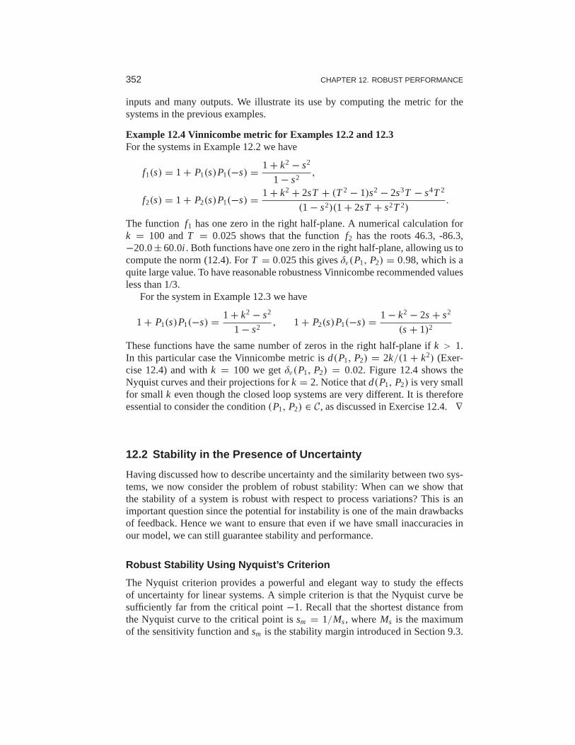
352 CHAPTER 12. ROBUST PERFORMANCE
inputs and many outputs. We illustrate its use by computing the metric for thesystems in the previous examples.
Example 12.4 Vinnicombe metric for Examples 12.2 and 12.3For the systems in Example 12.2 we have
f1(s) = 1 + P1(s)P1(−s) = 1 + k2 − s2
1 − s2,
f2(s) = 1 + P2(s)P1(−s) = 1 + k2 + 2sT + (T2 − 1)s2 − 2s3T − s4T2
(1 − s2)(1 + 2sT + s2T2).
The function f1 has one zero in the right half-plane. A numerical calculation fork = 100 andT = 0.025 shows that the functionf2 has the roots 46.3, -86.3,−20.0± 60.0i . Both functions have one zero in the right half-plane, allowing us tocompute the norm (12.4). ForT = 0.025 this givesδν(P1, P2) = 0.98, which is aquite large value. To have reasonable robustness Vinnicombe recommended valuesless than 1/3.
For the system in Example 12.3 we have
1 + P1(s)P1(−s) = 1 + k2 − s2
1 − s2, 1 + P2(s)P1(−s) = 1 − k2 − 2s + s2
(s + 1)2
These functions have the same number of zeros in the right half-plane if k > 1.In this particular case the Vinnicombe metric isd(P1, P2) = 2k/(1 + k2) (Exer-cise 12.4) and withk = 100 we getδν(P1, P2) = 0.02. Figure 12.4 shows theNyquist curves and their projections fork = 2. Notice thatd(P1, P2) is very smallfor smallk even though the closed loop systems are very different. It isthereforeessential to consider the condition(P1, P2) ∈ C, as discussed in Exercise 12.4.∇
12.2 Stability in the Presence of Uncertainty
Having discussed how to describe uncertainty and the similarity between two sys-tems, we now consider the problem of robust stability: When can we show thatthe stability of a system is robust with respect to process variations? This is animportant question since the potential for instability is one of the main drawbacksof feedback. Hence we want to ensure that even if we have smallinaccuracies inour model, we can still guarantee stability and performance.
Robust Stability Using Nyquist’s Criterion
The Nyquist criterion provides a powerful and elegant way to study the effectsof uncertainty for linear systems. A simple criterion is that the Nyquist curve besufficiently far from the critical point−1. Recall that the shortest distance fromthe Nyquist curve to the critical point issm = 1/Ms, whereMs is the maximumof the sensitivity function andsm is the stability margin introduced in Section 9.3.

12.2. STABILITY IN THE PRESENCE OF UNCERTAINTY 353
Re
Im
sm ωms
ωsc
−1
(a) Nyquist plot
Re
Im
−1
1+L
C1
(b) Additive uncertainty
Figure 12.5:Robust stability using the Nyquist criterion. (a) This plot shows that the shortestdistance to the critical pointsm is a robustness measure. (b) This plot shows the Nyquist curveof a nominal loop transfer function and its uncertainty caused by additiveprocess variations1.
The maximum sensitivityMs or the stability marginsm is thus a good robustnessmeasure, as illustrated in Figure 12.5a.
We will now derive explicit conditions for permissible process uncertainties.Consider a stable feedback system with a processP and a controllerC. If theprocess is changed fromP to P +1, the loop transfer function changes fromPCto PC + C1, as illustrated in Figure 12.5b. If we have a bound on the size of1 (represented by the dashed circle in the figure), then the system remains stableas long as the process variations never overlap the−1 point, since this leaves thenumber of encirclements of−1 unchanged.
Some additional assumptions are required for the analysis tohold. Most im-portantly, we require that the process perturbations1 be stable so that we do notintroduce any new right half-plane poles that would requireadditional encirclementsin the Nyquist criterion.
We will now compute an analytical bound on the allowable process disturbances.The distance from the critical point−1 to the loop transfer functionL is |1 + L|.This means that the perturbed Nyquist curve will not reach thecritical point−1provided that|C1| < |1 + L|, which implies
|1| <∣∣∣1 + PC
C
∣∣∣ or |δ| =∣∣∣1
P
∣∣∣ <1
|T | . (12.5)
This condition must be valid for all points on the Nyquist curve, i.e, pointwisefor all frequencies. The condition for robust stability can thus be written as
|δ(iω)| =∣∣∣1(iω)
P(iω)
∣∣∣ <1
|T(iω)| for all ω ≥ 0. (12.6)
Notice that the condition is conservative because it follows from Figure 12.5 thatthe critical perturbation is in the direction toward the critical point −1. Largerperturbations can be permitted in the other directions.
The condition in equation (12.6) allows us to reason about uncertainty without

354 CHAPTER 12. ROBUST PERFORMANCE
exact knowledge of the process perturbations. Namely, we can verify stability foranyuncertainty1 that satisfies the given bound. From an analysis perspective, thisgives us a measure of the robustness for a given design. Conversely, if we requirerobustness of a given level, we can attempt to choose our controller C such that thedesired level of robustness is available (by asking thatT be small) in the appropriatefrequency bands.
Equation (12.6) is one of the reasons why feedback systems work so well inpractice. The mathematical models used to design control systems are often simpli-fied, and the properties of a process may change during operation. Equation (12.6)implies that the closed loop system will at least be stable for substantial variationsin the process dynamics.
It follows from equation (12.6) that the variations can be large for those fre-quencies whereT is small and that smaller variations are allowed for frequencieswhereT is large. A conservative estimate of permissible process variations thatwill not cause instability is given by
|δ(iω)| =∣∣∣1(iω)
P(iω)
∣∣∣ <1
Mt,
whereMt is the largest value of the complementary sensitivity
Mt = supω
|T(iω)| =∥∥∥
PC
1 + PC
∥∥∥∞. (12.7)
The value ofMt is influenced by the design of the controller. For example, itis shown in Exercise 12.5 that ifMt = 2 then pure gain variations of 50% orpure phase variations of 30◦ are permitted without making the closed loop systemunstable.
Example 12.5 Cruise controlConsider the cruise control system discussed in Section 3.1.The model of the carin fourth gear at speed 25 m/s is
P(s) = 1.38
s + 0.0142,
and the controller is a PI controller with gainskp = 0.72 andki = 0.18. Fig-ure 12.6 plots the allowable size of the process uncertaintyusing the bound inequation (12.6). At low frequencies,T(0) = 1 and so the perturbations can be aslarge as the original process (|δ| = |1/P| < 1). The complementary sensitivityhas its maximumMt = 1.14 atωmt = 0.35, and hence this gives the minimumallowable process uncertainty, with|δ| < 0.87 or |1| < 3.47. Finally, at highfrequencies,T → 0 and hence the relative error can get very large. For example,atω = 5 we have|T(iω)| = 0.195, which means that the stability requirement is|δ| < 5.1. The analysis clearly indicates that the system has good robustness andthat the high-frequency properties of the transmission system are not important forthe design of the cruise controller.
Another illustration of the robustness of the system is given in the right diagram

12.2. STABILITY IN THE PRESENCE OF UNCERTAINTY 355
10−1
100
101
100
101
ReL(iω)
Im L(iω)
Frequencyω [rad/s]
Gai
n
1
T
P
T
Figure 12.6:Robustness for a cruise controller. On the left the maximum relative error 1/|T |(solid) and the absolute error|P|/|T | (dashed) for the process uncertainty1. The Nyquistcurve is shown on the right as a solid line. The dashed circles show permissible perturbationsin the process dynamics,|1| = |P|/|T |, at the frequenciesω = 0, 0.0142 and 0.05.
in Figure 12.6, which shows the Nyquist curve of the transfer function of theprocess and the uncertainty bounds1 = |P|/|T | for a few frequencies. Note thatthe controller can tolerate large amounts of uncertainty and still maintain stabilityof the closed loop. ∇
The situation illustrated in the previous example is typicalof many processes:moderately small uncertainties are required only around the gain crossover frequen-cies, but large uncertainties can be permitted at higher andlower frequencies. Aconsequence of this is that a simple model that describes theprocess dynamics wellaround the crossover frequency is often sufficient for design. Systems with manyresonant peaks are an exception to this rule because the process transfer functionfor such systems may have large gains for higher frequenciesalso, as shown forinstance in Example 9.9.
The robustness condition given by equation (12.6) can be given another inter-pretation by using the small gain theorem (Theorem 9.4). To apply the theoremwe start with block diagrams of a closed loop system with a perturbed process andmake a sequence of transformations of the block diagram thatisolate the blockrepresenting the uncertainty, as shown in Figure 12.7. The result is the two-blockinterconnection shown in Figure 12.7c, which has the loop transfer function
L = PC
1 + PC
1
P= Tδ.
Equation (12.6) implies that the largest loop gain is less than 1 and hence the systemis stable via the small gain theorem.
The small gain theorem can be used to check robust stability for uncertainty ina variety of other situations. Table 12.1 summarizes a few ofthe common cases;the proofs (all via the small gain theorem) are left as exercises.
The following example illustrates that it is possible to design systems that arerobust to parameter variations.

356 CHAPTER 12. ROBUST PERFORMANCE
P 66
1
−C
1P
6P
−C−PC1+PC
δ
Figure 12.7: Illustration of robustness to process perturbations. A system with additiveun-certainty (left) can be manipulated via block diagram algebra to one with multiplicativeuncertaintyδ = 1/P (center). Additional manipulations isolate the uncertainty in a mannerthat allows application of the small gain theorem (right)
Example 12.6 Bode’s ideal loop transfer functionA major problem in the design of electronic amplifiers is to obtain a closed loopsystem that is insensitive to changes in the gain of the electronic components.Bode found that the loop transfer functionL(s) = ks−n, with 1 ≤ n ≤ 5/3, wasan ideal loop transfer function. The gain curve of the Bode plot is a straight linewith slope−n and the phase is constant argL(iω) = −nπ/2. The phase marginis thusϕm = 90(2 − n)◦ for all values of the gaink and the stability margin issm = sinπ(1 − n/2). This exact transfer function cannot be realized with physicalcomponents, but it can be approximated over a given frequency range with a rationalfunction (Exercise 12.7). An operational amplifier circuit that has the approximatetransfer functionG(s) = k/(s+a) is a realization of Bode’s ideal transfer functionwith n = 1, as described in Example 8.3. Designers of operational amplifiers go togreat efforts to make the approximation valid over a wide frequency range. ∇
Youla Parameterization�
Since stability is such an essential property, it is useful tocharacterize all controllersthat stabilize a given process. Such a representation, whichis called aYoula pa-rameterization, is very useful when solving design problems because it makes itpossible to search over all stabilizing controllers without the need to test stabilityexplicitly.
We will first derive Youla’s parameterization for a stable process with a rationaltransfer functionP. A system with the complementary sensitivity functionT canbe obtained by feedforward control with the stable transferfunctionQ if T = P Q.
Table 12.1:Conditions for robust stability for different types of uncertainty
Process Uncertainty Type Robust Stability
P +1 Additive ‖CS1‖∞ < 1
P(1 + δ) Multiplicative ‖Tδ‖∞ < 1
P/(1 +1fb · P) Feedback ‖PS1fb‖∞ < 1

12.2. STABILITY IN THE PRESENCE OF UNCERTAINTY 357
Q
6
6
v
−1
−P
P
(a) Stable process
P66
6
v
−1
G0 F−10
Q B −A
(b) Unstable process
Figure 12.8:Youla parameterization. Block diagrams of Youla parameterizations for astablesystem (a) and an unstable system (b). Notice that the signalv is zero in steady state.
Notice thatT must have the same right half-plane zeros asP sinceQ is stable.Now assume that we want to implement the complementary transfer functionT byusing unit feedback with the controllerC. SinceT = PC/(1 + PC) = P Q, itfollows that the controller transfer function is
C = Q
1 − P Q. (12.8)
A straightforward calculation gives
S = 1 − P Q, PS= P(1 − P Q), CS= Q, T = P Q.
These transfer functions are all stable ifP andQ are stable and the controller givenby equation (12.8) is thus stabilizing. Indeed, it can be shown that all stabilizingcontrollers are in the form given by equation (12.8) for somechoice ofQ. Theparameterization is illustrated by the block diagrams in Figure 12.8a.
A similar characterization can be obtained for unstable systems. Consider aprocess with a rational transfer functionP(s) = a(s)/b(s), wherea(s) andb(s)are polynomials. By introducing a stable polynomialc(s), we can write
P(s) = a(s)
b(s)= A(s)
B(s),
whereA(s) = a(s)/c(s) andB(s) = b(s)/c(s) are stable rational functions. Simi-larly we introduce the controllerC0(s) = F0(s)/G0(s), whereF0(s) andG0(s) arestable rational functions. We have
S0 = AF0
AF0 + BG0, PS0 = BF0
AF0 + BG0,
C0S0 = AG0
AF0 + BG0, T0 = BG0
AF0 + BG0.
The controllerC0 is stabilizing if and only if the rational functionAF0 + BG0 doesnot have any zeros in the right half plane. LetQ be a stable rational function and

358 CHAPTER 12. ROBUST PERFORMANCE
P(s)6
e6
d
6
n
yν ηur
Controller Process
y
F(s)
−1
C(s)
Figure 12.9:Block diagram of a basic feedback loop. The external signals are the referencesignalr , the load disturbanced and the measurement noisen. The process output isy, andthe control signal isu. The processP may include unmodeled dynamics, such as additiveperturbations.
consider the controllerC = G0 + Q A
F0 − QB. (12.9)
The Gang of Four forP andC is
S = A(F0 − QB)
AF0 + BG0, PS= B(F0 − QB)
AF0 + BG0,
CS= A(G0 + Q A)
AF0 + BG0, T = B(G0 + Q A)
AF0 + BG0.
All these transfer functions are stable if the rational function AF0 + BG0 doesnot have any zeros in the right half plane and the controllerC given by (12.9) istherefore stabilizing for any stableQ. A block diagram of the closed loop systemwith the controllerC is shown in Figure 12.8b. Notice that the transfer functionQappears affinely in the expressions for the Gang of Four, whichis very useful if wewant to determine the transfer functionQ to obtain specific properties.
12.3 Performance in the Presence of Uncertainty
So far we have investigated the risk for instability and robustness to process un-certainty. We will now explore how responses to load disturbances, measurementnoise and reference signals are influenced by process variations. To do this we willanalyze the system in Figure 12.9, which is identical to the basic feedback loopanalyzed in Chapter 11.
Disturbance Attenuation
The sensitivity functionS gives a rough characterization of the effect of feedbackon disturbances, as was discussed in Section 11.3. A more detailed characterizationis given by the transfer function from load disturbances to process output:
Gyd = P
1 + PC= PS. (12.10)

12.3. PERFORMANCE IN THE PRESENCE OF UNCERTAINTY 359
Load disturbances typically have low frequencies, and it is therefore important thatthe transfer function be small for low frequencies. For processes with constantlow-frequency gain and a controller with integral action wehaveGyd ≈ s/ki . Theintegral gainki is thus a simple measure of the attenuation of load disturbances.
To find out how the transfer functionGyd is influenced by small variations inthe process transfer function we differentiate (12.10) with respect toP yielding
dGyd
d P= 1
(1 + PC)2= SP
P(1 + PC)= S
Gyd
P,
and it follows thatdGyd
Gyd= S
d P
P. (12.11)
The response to load disturbances is thus insensitive to process variations for fre-quencies where|S(iω)| is small, i.e., for frequencies where load disturbances areimportant.
A drawback with feedback is that the controller feeds measurement noise intothe system. In addition to the load disturbance rejection, it is thus also important thatthe control actions generated by measurement noise are not too large. It follows fromFigure 12.9 that the transfer functionGun from measurement noise to controlleroutput is given by
Gun = − C
1 + PC= − T
P. (12.12)
Since measurement noise typically has high frequencies, thetransfer functionGun
should not be too large for high frequencies. The loop transfer function PC istypically small for high frequencies, which implies thatGun ≈ C for large s. Toavoid injecting too much measurement noise it is therefore important thatC(s)be small for larges. This property is calledhigh-frequency roll-off. An exampleis filtering of the measured signal in a PID controller to reducethe injection ofmeasurement noise; see Section 10.5.
To determine how the transfer functionGun is influenced by small variations inthe process transfer, we differentiate equation (12.12):
dGun
d P= d
d P
(− C
1 + PC
)= C
(1 + PC)2C = T
Gun
P.
Rearranging the terms givesdGun
Gun= T
d P
P. (12.13)
Since the complementary sensitivity function is also small for high frequencies, wefind that process uncertainty has little influence on the transfer functionGun forfrequencies where measurements are important.

360 CHAPTER 12. ROBUST PERFORMANCE
−
+v
v
1
v2
R2R
G (s)
1
Rl
R2
R16 6−G(s)
v2
d
vR1
R1+R2
ev1
Figure 12.10:Operational amplifier with uncertain dynamics. The circuit on the left is mod-eled using the transfer functionG(s) to capture its dynamic properties and it has a load atthe output. The block diagram on the right shows the input/output relationships. The load isrepresented as a disturbanced applied at the output ofG(s).
Reference Signal Tracking
The transfer function from reference to output is given by
Gyr = PC F
1 + PC= T F, (12.14)
which contains the complementary sensitivity function. Tosee how variations inPaffect the performance of the system, we differentiate equation (12.14) with respectto the process transfer function:
dGyr
d P= C F
1 + PC− PC FC
(1 + PC)2= C F
(1 + PC)2= S
Gyr
P,
and it follows thatdGyr
Gyr= S
d P
P. (12.15)
The relative error in the closed loop transfer function thus equals the product ofthe sensitivity function and the relative error in the process. In particular, it followsfrom equation (12.15) that the relative error in the closed loop transfer function issmall when the sensitivity is small. This is one of the useful properties of feedback.
As in the last section, there are some mathematical assumptions that are re-quired for the analysis presented here to hold. As already stated, we require thatthe perturbations1 be small (as indicated by writingd P). Second, we require thatthe perturbations be stable, so that we do not introduce any new right half-planepoles that would require additional encirclements in the Nyquist criterion. Also, asbefore, this condition is conservative: it allows for any perturbation that satisfiesthe given bounds, while in practice the perturbations may bemore restricted.
Example 12.7 Operational amplifier circuitTo illustrate the use of these tools, consider the performance of an op amp-basedamplifier, as shown in Figure 12.10. We wish to analyze the performance of theamplifier in the presence of uncertainty in the dynamic response of the op amp andchanges in the loading on the output. We model the system using the block diagramin Figure 12.10b, which is based on the derivation in Example 9.1.
Consider first the effect of unknown dynamics for the operational amplifier. Ifwe model the dynamics of the op amp asv2 = −G(s)v, then the transfer function

12.4. ROBUST POLE PLACEMENT 361
for the overall circuit is given by
Gv2v1 = − R2
R1
G(s)
G(s)+ R2/R1 + 1.
We see that ifG(s) is large over the desired frequency range, then the closed loopsystem is very close to the ideal responseα = R2/R1. AssumingG(s) = b/(s+a),whereb is the gain-bandwidth product of the amplifier, as discussed in Example 8.3,the sensitivity function and the complementary sensitivity function become
S = s + a
s + a + αb, T = αb
s + a + αb.
The sensitivity function around the nominal values tells us how the tracking responseresponse varies as a function of process perturbations:
dGyr
Gyr= S
d P
P.
We see that for low frequencies, whereS is small, variations in the bandwidtha orthe gain-bandwidth productb will have relatively little effect on the performanceof the amplifier (under the assumption thatb is sufficiently large.
To model the effects of an unknown load, we consider the addition of a dis-turbance at the output of the system, as shown in Figure 12.10b. This disturbancerepresents changes in the output voltage due to loading effects. The transfer func-tion Gyd = S gives the response of the output to the load disturbance, andwe seethat if Sis small, then we are able to reject such disturbances. The sensitivity of Gyd
to perturbations in the process dynamics can be computed by taking the derivativeof Gyd with respect toP:
dGyd
d P= −C
(1 + PC)2= − T
PGyd =⇒ dGyd
Gyd= −T
d P
P.
Thus we see that the relative changes in the disturbance rejection are roughly thesame as the process perturbations at low frequency (whenT is approximately 1)and drop off at higher frequencies. However, it is importantto remember thatGyd
itself is small at low frequency, and so these variations in relative performance maynot be an issue in many applications. ∇
12.4 Robust Pole Placement
In Chapters 6 and 7 we saw how to design controllers by settingthe locations ofthe eigenvalues of the closed loop system. If we analyze the resulting system in thefrequency domain, the closed loop eigenvalues correspond to the poles of the closedloop transfer function and hence these methods are often referred to as design bypole placement.
State space design methods, like many methods developed for control systemdesign, do not explicitly take robustness into account. In such cases it is essential to

362 CHAPTER 12. ROBUST PERFORMANCE
ReL(iω)
Im L(iω)
10−3
10−1
101
103
10−1
100
101
102
103
−360
−270
−180
|L(iω)|
∠L(iω)
Frequencyω [rad/s]
Figure 12.11:Observer-based control of steering. The Nyquist plot (left) and Bode plot (right)of the loop transfer function for vehicle steering with a controller based onstate feedbackand an observer. The controller provides stable operation, but with very low gain and phasemargin.
always investigate the robustness because there are seemingly reasonable designsthat give controllers with poor robustness. We illustrate this by analyzing controllersdesigned by state feedback and observers. The closed loop poles can be assignedto arbitrary locations if the system is observable and reachable. However, if wewant to have a robust closed loop system, the poles and zeros of the process imposesevere restrictions on the location of the closed loop poles. Some examples are firstgiven; based on the analysis of these examples we then present design rules forrobust pole (eigenvalue) placement.
Slow Stable Process Zeros
We will first explore the effects of slow stable zeros, and we begin with a simpleexample.
Example 12.8 Vehicle steeringConsider the linearized model for vehicle steering in Example 8.6, which has thetransfer function
P(s) = 0.5s + 1
s2.
A controller based on state feedback was designed in Example 6.4, and state feed-back was combined with an observer in Example 7.4. The system simulated inFigure 7.8 has closed loop poles specified byωc = 0.3, ζc = 0.707,ωo = 7 andζo = 9. Assume that we want a faster closed loop system and chooseωc = 10,ζc = 0.707,ωo = 20 andζo = 0.707. Using the state representation in Example 7.3,a pole placement design gives state feedback gainsk1 = 100 andk2 = −35.86 andobserver gainsl1 = 28.28 andl2 = 400. The controller transfer function is
C(s) = −11516s + 40000
s2 + 42.4s + 6657.9.
Figure 12.11 shows Nyquist and Bode plots of the loop transferfunction. The

12.4. ROBUST POLE PLACEMENT 363
Nyquist plot indicates that the robustness is poor since theloop transfer function isvery close to the critical point−1. The phase margin is 7◦ and the stability marginis sm = 0.077. The poor robustness shows up in the Bode plot, where the gaincurve hovers around the value 1 and the phase curve is close to−180◦ for a widefrequency range. More insight is obtained by analyzing the sensitivity functions,shown by solid lines in Figure 12.12. The maximum sensitivities areMs = 13 andMt = 12, indicating that the system has poor robustness.
At first sight it is surprising that a controller where the nominal closed systemhas well damped poles and zeros is so sensitive to process variations. We have anindication that something is unusual because the controller has a zero ats = 3.5in the right half-plane. To understand what happens, we willinvestigate the reasonfor the peaks of the sensitivity functions.
Let the transfer functions of the process and the controller be
P(s) = np(s)
dp(s), C(s) = nc(s)
dc(s),
wherenp(s), nc(s), dp(s) anddc(s) are the numerator and denominator polynomi-als. The complementary sensitivity function is
T(s) = PC
1 + PC= np(s)nc(s)
dp(s)dc(s)+ np(s)np(s).
The poles ofT(s) are the poles of the closed loop system and the zeros are givenby the zeros of the process and controller. Sketching the gaincurve of the comple-mentary sensitivity function we find thatT(s) = 1 for low frequencies and that|T(iω)| starts to increase at its first zero, which is the process zero at s = −2. Itincreases further at the controller zero ats = 3.5, and it does not start to decreaseuntil the closed loop poles appear atωc = 10 andωo = 20. We can thus concludethat there will be a peak in the complementary sensitivity function. The magnitudeof the peak depends on the ratio of the zeros and the poles of the transfer function.
The peak of the complementary sensitivity function can be avoided by assigninga closed loop pole close to the slow process zero. We can achieve this by choosingωc = 10 andζc = 2.6, which gives closed loop poles ats = −2 ands = −50. Thecontroller transfer function then becomes
C(s) = 3628s + 40000
s2 + 80.28s + 156.56= 3628
s + 11.02
(s + 2)(s + 78.28).
The sensitivity functions are shown by dashed lines in Figure 12.12. The controllergives the maximum sensitivitiesMs = 1.34 andMt = 1.41, which give muchbetter robustness. Notice that the controller has a pole ats = −2 that cancels theslow process zero. The design can also be done simply by canceling the slow stableprocess zero and designing the controller for the simplified system. ∇
One lesson from the example is that it is necessary to choose closed loop polesthat are equal to or close to slow stable process zeros. Another lesson is that slowunstable process zeros impose limitations on the achievable bandwidth, as already

364 CHAPTER 12. ROBUST PERFORMANCE
100
102
10−2
100
100
102
10−2
100
OriginalImproved
|S(iω)|
|T(iω)|
Frequencyω [rad/s]Frequencyω [rad/s]
Figure 12.12:Sensitivity functions for observer-based control of vehicle steering.The com-plementary sensitivity function (left) and the sensitivity function (right) forthe original con-troller with ωc = 10, ζc = 0.707,ωo = 20, ζo = 0.707 (solid) and the improved controllerwith ωc = 10,ζc = 2.6 (dashed).
noted in Section 11.5.
Fast Stable Process Poles
The next example shows the effect of fast stable poles.
Example 12.9 Fast system polesConsider a PI controller for a first-order system, where the process and the controllerhave the transfer functionsP(s) = b/(s + a) andC(s) = kp + ki /s. The looptransfer function is
L(s) = b(kps + ki )
s(s + a),
and the closed loop characteristic polynomial is.
s(s + a)+ b(kps + ki ) = s2 + (a + bkp)s + ki b
If we specify the desired closed loop poles should be−p1 and−p2, we find thatthe controller parameters are given by
kp = p1 + p2 − a
b, ki = p1 p2
b.
The sensitivity functions are then
S(s) = s(s + a)
(s + p1)(s + p2), T(s) = (p1 + p2 − a)s + p1 p2
(s + p1)(s + p2).
Assume that the process pole−a is much more negative than the closed loop poles−p1 and−p2, say,p1 < p2 ≪ a. Notice that the proportional gain is negative andthat the controller has a zero in the right half-plane ifa > p1 + p2, an indicationthat the system has bad properties.
Next consider the sensitivity function, which is 1 for high frequencies. Movingfrom high to low frequencies, we find that the sensitivity increases at the process poles = −a. The sensitivity does not decrease until the closed loop poles are reached,resulting in a large sensitivity peak that is approximatelya/p2. The magnitude ofthe sensitivity function is shown in Figure 12.13 fora = b = 1, p1 = 0.05 andp2 = 0.2. Notice the high-sensitivity peak. For comparison we alsoshow the gain

12.4. ROBUST POLE PLACEMENT 365
10
−1
100
101
Exact Approx
Frequencyω [rad/s]
|S(iω)|
ap1 p2
10−2
100
Exact Approx
Frequencyω [rad/s]
|S(iω)|
a p1 p2
Figure 12.13: Gain curves for Bode plots of the sensitivity functionS for designs withp1 < p2 < a (left) anda < p1 < p2 (right). The solid lines are the true sensitivities, and thedashed lines are the asymptotes.
curve for the case when the closed loop poles (p1 = 5, p2 = 20) are faster than theprocess pole (a = 1).
The problem with poor robustness can be avoided by choosing one closed looppole equal to the process pole, i.e.,p2 = a. The controller gains then become
kp = p1
b, ki = ap1
l,
which means that the fast process pole is canceled by a controller zero. The looptransfer function and the sensitivity functions are
L(s) = bkp
s, S(s) = s
s + bkp, T(s) = bkp
s + bkp.
The maximum sensitivities are now less than 1 for all frequencies. Notice that thisis possible because the process transfer function goes to zero ass−1. ∇
Design Rules for Pole Placement
Based on the insight gained from the examples, it is now possible to obtain designrules that give designs with good robustness. Consider the expression (12.8) formaximum complementary sensitivity, repeated here:
Mt = supω
|T(iω)| =∥∥∥
PC
1 + PC
∥∥∥∞.
Letωgc be the desired gain crossover frequency. Assume that the process has zerosthat are slower thanωgc. The complementary sensitivity function is 1 for low fre-quencies, and it increases for frequencies close to the process zeros unless there is aclosed loop pole in the neighborhood. To avoid large values of the complementarysensitivity function we find that the closed loop system should therefore have polesclose to or equal to the slow stable zeros. This means that slowstable zeros shouldbe canceled by controller poles. Since unstable zeros cannotbe canceled, the pres-ence of slow unstable zeros means that achievable gain crossover frequency mustbe smaller than the slowest unstable process zero.
Now consider process poles that are faster than the desired gain crossover fre-

366 CHAPTER 12. ROBUST PERFORMANCE
quency. Consider the expression for the maximum of the sensitivity function:
Ms = supω
|S(iω)| =∥∥∥
1
1 + PC
∥∥∥∞.
The sensitivity function is 1 for high frequencies. Moving from high to low fre-quencies, the sensitivity function increases at the fast process poles. Large peakscan result unless there are closed loop poles close to the fast process poles. To avoidlarge peaks in the sensitivity the closed loop system shouldtherefore have polesthat match the fast process poles. This means that the controller should cancel thefast process poles by controller zeros. Since unstable modescannot be canceled,the presence of a fast unstable pole implies that the gain crossover frequency mustbe sufficiently large.
To summarize, we obtain the following simple rule for choosing closed looppoles: slow stable process zeros should be matched by slow closed loop poles, andfast stable process poles should be matched by fast closed loop poles. Slow unstableprocess zeros and fast unstable process poles impose severelimitations.
Example 12.10 Nanopositioning system for an atomic force microscopeA simple nanopositioner was explored in Example 9.9, where itwas shown thatthe system could be controlled using an integral controller. The performance ofthe closed loop was poor because the gain crossover frequency was limited toωgc = 2ζω0(1 − sm). It can be shown that little improvement is obtained by usinga PI controller. To achieve improved performance, we will therefore apply PIDcontrol. For a modest performance increase, we will use the design rule derived inExample 12.9 that fast stable process poles should be canceled by controller zeros.The controller transfer function should thus be chosen as
C(s) = kds2 + kps + ki
s= ki
s
s2 + 2ζs + a2
a2, (12.16)
which giveskp = 2ζki /a andkd = ki /a2.Figure 12.14 shows the gain curves for the Gang of Four for a system designed
with ki = 0.5. A comparison with Figure 9.12 shows that the bandwidth is increasedsignificantly fromωgc = 0.01 toωgc = ki = 0.5. Since the process pole is canceled,the system will, however, still be very sensitive to load disturbances with frequenciesclose to the resonant frequency. The gain curve ofCShas a dip or a notch at theresonant frequency, which implies that the controller gainis very low for frequenciesaround the resonance. The gain curve also shows that the system is very sensitiveto high-frequency noise. The system will likely be unusable because the gain goesto infinity for high frequencies.
The sensitivity to high frequency noise can be remedied by modifying the con-troller to be
C(s) = ki
s
s2 + 2ζas+ a2
a2(1 + sTf + (sTf )2/2), (12.17)
which has high-frequency roll-off. Selection of the constant T f for the filter is acompromise between attenuation of high-frequency measurement noise and ro-

12.4. ROBUST POLE PLACEMENT 367
10−2
100
102
10−2
100
10−2
100
102
10−2
100
10−2
100
102
10−2
100
10−2
100
102
10−2
100
Ideal PIDPID w/ filtering
Normalized frequencyω/aNormalized frequencyω/a
|T(iω)|
|S(iω)|
|PS(
iω)|
|CS(
iω)|
Figure 12.14: Nanopositioning system control via cancellation of the fast process pole.Gain plots for the Gang of Four for PID control with second-order filtering (12.17) areshown by solid lines, and the dashed lines show results for an ideal PID controller withoutfiltering (12.16).
bustness. A large value ofT f reduces the effects of sensor noise significantly, butit also reduces the stability margin. Since the gain crossover frequency withoutfiltering iski , a reasonable choice isTF = 0.2/T f , as shown by the solid curves inFigure 12.14. The plots of|CS(iω)| and|S(iω)| show that the sensitivity to high-frequency measurement noise is reduced dramatically at thecost of a marginalincrease of sensitivity. Notice that the poor attenuation of disturbances with fre-quencies close to the resonance is not visible in the sensitivity function because ofthe exact cancellation of poles and zeros.
The designs thus far have the drawback that load disturbanceswith frequenciesclose to the resonance are not attenuated. We will now consider a design that activelyattenuates the poorly damped modes. We start with an ideal PIDcontroller wherethe design can be done analytically, and we add high-frequency roll-off. The looptransfer function obtained with this controller is
L(s) = kds2 + kps + ki
s(s2 + 2ζas+ a2). (12.18)
The closed loop system is of third order, and its characteristic polynomial is
s3 + (kda2 + 2ζa)s2 + (kp + 1)a2s + ki a2. (12.19)
A general third-order polynomial can be parameterized as
s3 + (α0 + 2ζ )ω0s2 + (1 + 2α0ζ )ω20s + α0ω
30. (12.20)
The parametersα0 andζ give the relative configuration of the poles, and the pa-rameterω0 gives their magnitudes, and therefore also the bandwidth ofthe system.
The identification of coefficients of equal powers ofs with equation (12.19)

368 CHAPTER 12. ROBUST PERFORMANCE
10−2
100
102
10−2
100
10−2
100
102
10−4
10−2
100
10−2
100
102
100
102
10−2
100
102
10−2
100
Normalized frequencyω/aNormalized frequencyω/a
|T(iω)|
|S(iω)|
|PS(
iω)|
|CS(
iω)|
ω0 = aω0 = 2aω0 = 4a
Figure 12.15: Nanopositioner control using active damping. Gain curves for the GangofFour for PID control of the nanopositioner designed forω0 = a (dash-dotted), 2a (dashed),and 4a (solid). The controller has high-frequency roll-off and has been designed to giveactive damping of the oscillatory mode. The different curves correspond to different choicesof magnitudes of the poles, parameterized byω0 in equation (12.19).
gives a linear equation for the controller parameters, which has the solution
kp = (1 + 2α0ζ )ω20
a2− 1, ki = α0ω
30
a2, kd = (α0 + 2ζ )ω0
a2− 2ζa. (12.21)
To obtain a design with active damping, it is necessary that the closed loop band-width be at least as fast as the oscillatory modes. Adding high-frequency roll-off,the controller becomes
C(s) = kds2 + kps + k
s(1 + sTf + (sTf )2/2). (12.22)
The valueT f = Td/10 = 0.1kd/k is a good value for the filtering time constant.Figure 12.15 shows the gain curves of the Gang of Four for designs withζ =
0.707,α0 = 1 andω0 = a, 2a and 4a. The figure shows that the largest values ofthe sensitivity function and the complementary sensitivity function are small. Thegain curve forPSshows that the load disturbances are now well attenuated overthe whole frequency range, and attenuation increases with increasingω0. The gaincurve forCSshows that large control signals are required to provide active damping.The high gain ofCS for high frequencies also shows that low-noise sensors andactuators with a wide range are required. The largest gains for CS are 19, 103and 434 forω0 = a, 2a and 4a, respectively. There is clearly a trade-off betweendisturbance attenuation and controller gain. A comparisonof Figures 12.14 and12.15 illustrates the trade-offs between control action and disturbance attenuationfor the designs with cancellation of the fast process pole and active damping. ∇

12.5. DESIGN FOR ROBUST PERFORMANCE 369
12.5 Design for Robust Performance �
Control design is a rich problem where many factors have to betaken into account.Typical requirements are that load disturbances should be attenuated, the controllershould inject only a moderate amount of measurement noise, the output shouldfollow variations in the command signal well and the closed loop system should beinsensitive to process variations. For the system in Figure 12.9 these requirementscan be captured by specifications on the sensitivity functions S and T and thetransfer functionsGyd, Gun, Gyr andGur . Notice that it is necessary to considerat least six transfer functions, as discussed Section 11.1. The requirements aremutually conflicting, and it is necessary to make trade-offs.The attenuation of loaddisturbances will be improved if the bandwidth is increased, but so will the noiseinjection.
It is highly desirable to have design methods that can guarantee robust perfor-mance. Such design methods did not appear until the late 1980s. Many of thesedesign methods result in controllers having the same structure as the controllerbased on state feedback and an observer. In this section we provide a brief reviewof some of the techniques as a preview for those interested inmore specializedstudy.
Quantitative Feedback Theory
Quantitative feedback theory(QFT) is a graphical design method for robust loopshaping that was developed by I. M. Horowitz [Hor91]. The ideais to first determinea controller that gives a complementary sensitivity that isrobust to process variationsand then to shape the response to reference signals by feedforward. The idea isillustrated in Figure 12.16a, which shows the level curves ofthe complementarysensitivity functionT on a Nyquist plot. The complementary sensitivity function hasunit gain on the line ReL(iω) = −0.5. In the neighborhood of this line, significantvariations in process dynamics only give moderate changes in the complementarytransfer function. The dashed part of the figure corresponds tothe region 0.9 <|T(iω)| < 1.1. To use the design method, we represent the uncertainty foreachfrequency by a region and attempt to shape the loop transfer function so that thevariation in T is as small as possible. The design is often performed using theNichols chart shown in Figure 12.16b.
Linear Quadratic Control
One way to make the trade-off between the attenuation of loaddisturbances andthe injection of measurement noise is to design a controllerthat minimizes the lossfunction
J = 1
T
∫ T
0
(y2(t)+ ρu2(t)
)dt,
whereρ is a weighting parameter as discussed in Section 6.3. This lossfunctiongives a compromise between load disturbance attenuation and disturbance injec-tion because it balances control actions against deviations in the output. If all state

370 CHAPTER 12. ROBUST PERFORMANCE
−5 0 5
−4
−2
0
2
4
ReL(iω)
ImL(iω)
(a) Hall chart
−4 −3 −2 −1 0−1
0
1
2
3
argL(iω) [rad]
log|L(iω)|
(b) Nichols chart
Figure 12.16: Hall and Nichols charts. The Hall chart is a Nyquist plot with curves forconstant gain and phase of the complementary sensitivity functionT . The Nichols chartis the conformal map of the Hall chart under the transformationN = log L (with the scaleflipped). The dashed curve is the line where|T(iω)| = 1, and the shaded region correspondingto loop transfer functions whose complementary sensitivity changes by no more than±10%is shaded.
variables are measured, the controller is a state feedbacku = −K x and it has thesame form as the controller obtained by eigenvalue assignment (pole placement)in Section 6.2. However, the controller gain is obtained by solving an optimiza-tion problem. It has been shown that this controller is very robust. It has a phasemargin of at least 60◦ and an infinite gain margin. The controller is called alinearquadratic controlorLQ controlbecause the process model is linear and the criterionis quadratic.
When all state variables are not measured, the state can be reconstructed usingan observer, as discussed in Section 7.3. It is also possible to introduce processdisturbances and measurement noise explicitly in the modeland to reconstructthe states using a Kalman filter, as discussed briefly in Section 7.4. The Kalmanfilter has the same structure as the observer designed by eigenvalue assignment inSection 7.3, but the observer gainsL are now obtained by solving an optimizationproblem. The control law obtained by combining linear quadratic control with aKalman filter is calledlinear quadratic Gaussian controlor LQG control. TheKalman filter is optimal when the models for load disturbancesand measurementnoise are Gaussian.
It is interesting that the solution to the optimization problem leads to a controllerhaving the structure of a state feedback and an observer. The state feedback gainsdepend on the parameterρ, and the filter gains depend on the parameters in themodel that characterize process noise and measurement noise (see Section 7.4).There are efficient programs to compute these feedback and observer gains.
The nice robustness properties of state feedback are unfortunately lost when theobserver is added. It is possible to choose parameters that give closed loop systemswith poor robustness, similar to Example 12.8. We can thus conclude that there is a

12.5. DESIGN FOR ROBUST PERFORMANCE 371
uP
zw
C
yP6
6
d η
u ny
ν
−C
Figure 12.17:H∞ robust control formulation. The left figure shows a general representationof a control problem used in robust control. The inputu represents the control signal, the inputw represents the external influences on the system, the outputz is the generalized error and theoutputy is the measured signal. The right figure shows the special case of the basic feedbackloop in Figure 12.9 where the reference signal is zero. In this case we havew = (n, d) andz = (y,−u).
fundamental difference between using sensors for all states and reconstructing thestates using an observer.
H∞ Control�
Robust control design is often calledH∞ control for reasons that will be explainedshortly. The basic ideas are simple, but the details are complicated and we willtherefore just give the flavor of the results. A key idea is illustrated in Figure 12.17,where the closed loop system is represented by two blocks, the processP andthe controllerC as discussed in Section 11.1. The processP has two inputs, thecontrol signalu, which can be manipulated by the controller, and the generalizeddisturbancew, which represents all external influences, e.g., command signals anddisturbances. The process has two outputs, the generalized error z, which is a vectorof error signals representing the deviation of signals fromtheir desired values, andthe measured signaly, which can be used by the controller to computeu. For alinear system and a linear controller the closed loop systemcan be represented bythe linear system
z = H(P(s),C(s))w, (12.23)
which tells how the generalized errorz depends on the generalized disturbancesw. The control design problem is to find a controllerC such that the gain of thetransfer functionH is small even when the process has uncertainties. There are manydifferent ways to specify uncertainty and gain, giving riseto different designs. ThenamesH2 andH∞ control correspond to the norms‖H‖2 and‖H‖∞.
To illustrate the ideas we will consider a regulation problem for a system wherethe reference signal is assumed to be zero and the external signals are the loaddisturbanced and the measurement noisen, as shown in Figure 12.17b. The gener-alized input isw = (−n,d). (The negative sign ofn is not essential but is chosento obtain somewhat nicer equations.) The generalized error is chosen asz = (η, ν),whereη is the process output andν is the part of the load disturbance that is not

372 CHAPTER 12. ROBUST PERFORMANCE
compensated by the controller. The closed loop system is thusmodeled by
z = y
−u
=
1
1 + PC
P
1 + PCC
1 + PC
PC
1 + PC
n
d
= H(P,C)
n
d
, (12.24)
which is the same as equation (12.23). A straightforward calculation shows that
‖H(P,C))‖∞ = supω
√(1 + |P(iω)|2)(1 + |C(iω)|2)
|1 + P(iω)C(iω)| . (12.25)
There are numerical methods for finding a controller such that‖H(P,C)‖∞ <
γ , if such a controller exists. The best controller can then be found by iterating onγ . The calculations can be made by solvingalgebraic Riccatiequations, e.g., byusing the commandhinfsyn in MATLAB. The controller has the same order asthe process and the same structure as the controller based onstate feedback and anobserver; see Figure 7.7 and Theorem 7.3.
Notice that if we minimize‖H(P,C)‖∞, we make sure that the transfer func-tionsGyd = P/(1+ PC), representing the transmission of load disturbances to theoutput, andGun = −C/(1 + PC), representing how measurement noise is trans-mitted to the control signal, are small. Since the sensitivity and the complementarysensitivity functions are also elements ofH(P,C), we have also guaranteed thatthe sensitivities are less thanγ . The design methods thus balance performance androbustness.
There are strong robustness results associated with theH∞ controller. It followsfrom equations (12.4) and (12.25) that
‖H(P,C)‖∞ = 1
δν(P,−1/C). (12.26)
The inverse of‖H(P,C)‖∞ is thus equal to the Vinnicombe distance betweenP and−1/C and can therefore be interpreted as ageneralized stability margin. Comparethis with sm, which we defined as the shortest distance between the Nyquistcurveof the loop transfer function and the critical point−1. It also follows that if wefind a controllerC with ‖H(P,C)‖∞ < γ , then this controller will stabilize anyprocessP∗ such thatδν(P, P∗) < 1/γ .
Disturbance Weighting
Minimizing the gain‖H(P,C)‖∞ means that the gains of all individual signaltransmissions from disturbances to outputs are less thanγ for all frequencies ofthe input signals. The assumption that the disturbances are equally important andthat all frequencies are also equally important is not very realistic; recall that loaddisturbances typically have low frequencies and measurement noise is typicallydominated by high frequencies. It is straightforward to modify the problem so thatdisturbances of different frequencies are given differentemphasis, by introducing

12.5. DESIGN FOR ROBUST PERFORMANCE 373
P6
6
d
u
νd η
y n
W
−C
W6
6
ν
u
d ην
u y nW−1 −C
P SP6
6
d ν
u y
η
n−SC
Figure 12.18:Block diagrams of a system with disturbance weighting. The left figure providesa frequency weight on processes disturbances. Through block diagram manipulation, this canbe converted to the standard problem on the right.
a weighting filter on the load disturbance as shown in Figure 12.18. For example,low-frequency load disturbances will be enhanced by choosing W as a low-passfilter because the actual load disturbance isWd.
By using block diagram manipulation as shown in Figure 12.18,we find thatthe system with frequency weighting is equivalent to the system with no frequencyweighting in Figure 12.18 and the signals are related through
z =y
u
1
1 + SP SCSP
1 + SP SCSC
1 + SP SCSP SC
1 + SP SC
n
d
= H(SP, SC)w, (12.27)
where SP = PW and SC = W−1C. The problem of finding a controllerSC thatminimizes the gain ofH(SP, SC) is thus equivalent to the problem without distur-bance weighting; having obtainedSC, the controller for the original system is thenC = WSC. Notice that if we introduce the frequency weightingW = k/s, we willautomatically get a controller with integral action.
Limits of Robust Design
There is a limit to what can be achieved by robust design. In spite of the niceproperties of feedback, there are situations where the process variations are solarge that it is not possible to find a linear controller that gives a robust systemwith good performance. It is then necessary to use other types of controllers. Insome cases it is possible to measure a variable that is well correlated with theprocess variations. Controllers for different parameter values can then be designedand the corresponding controller can be chosen based on the measured signal.This type of control design is calledgain scheduling. The cruise controller is atypical example where the measured signal could be gear position and velocity. Gainscheduling is the common solution for high-performance aircraft where schedulingis done based on Mach number and dynamic pressure. When usinggain scheduling,it is important to make sure that switches between the controllers do not createundesirable transients (often referred to asbumpless transfer).
If it is not possible to measure variables related to the parameters,automatictuningandadaptive controlcan be used. In automatic tuning the process dynamicsare measured by perturbing the system, and a controller is then designed automat-

374 CHAPTER 12. ROBUST PERFORMANCE
ically. Automatic tuning requires that parameters remain constant, and it has beenwidely applied for PID control. It is a reasonable guess that in the future manycontrollers will have features for automatic tuning. If parameters are changing, itis possible to use adaptive methods where process dynamics are measured online.
12.6 Further Reading
The topic of robust control is a large one, with many articles and textbooks devotedto the subject. Robustness was a central issue in classical control as described inBode’s classical book [Bod45]. Robustness was deemphasized in the euphoria ofthe development of design methods based on optimization. Thestrong robustnessof controllers based on state feedback, shown by Anderson and Moore [AM90],contributed to the optimism. The poor robustness of output feedback was pointedout by Rosenbrock [RM71], Horowitz [Hor75] and Doyle [Doy78] and resultedin a renewed interest in robustness. A major step forward wasthe development ofdesign methods where robustness was explicitly taken into account, such as theseminal work of Zames [Zam81]. Robust control was originally developed usingpowerful results from the theory of complex variables, which gave controllers ofhigh order. A major breakthrough was made by Doyle, Glover, Khargonekar andFrancis [DGKF89], who showed that the solution to the problem could be obtainedusing Riccati equations and that a controller of low order could be found. This paperled to an extensive treatment ofH∞ control, including books by Francis [Fra87],McFarlane and Glover [MG90], Doyle, Francis and Tannenbaum [DFT92], Greenand Limebeer [GL95], Zhou, Doyle and Glover [ZDG96], Skogestand and Postleth-waite [SP05] and Vinnicombe [Vin01]. A major advantage of the theory is that itcombines much of the intuition from servomechanism theory with sound numericalalgorithms based on numerical linear algebra and optimization. The results havebeen extended to nonlinear systems by treating the design problem as a game wherethe disturbances are generated by an adversary, as described in the book by Basarand Bernhard [BB91]. Gain scheduling and adaptation are discussed in the bookby Åström and Wittenmark [ÅW08].
Exercises
12.1 Consider systems with the transfer functionsP1 = 1/(s + 1) and P2 =1/(s+ a). Show thatP1 can be changed continuously toP2 with bounded additiveand multiplicative uncertainty ifa > 0 but not ifa < 0. Also show that no restrictionona is required for feedback uncertainty.
12.2 Consider systems with the transfer functionsP1 = (s + 1)/(s + 1)2 andP2 = (s + a)/(s + 1)2. Show thatP1 can be changed continuously toP2 withbounded feedback uncertainty ifa > 0 but not if a < 0. Also show that norestriction ona is required for additive and multiplicative uncertainties.

EXERCISES 375
12.3(Difference in sensitivity functions) LetT(P,C) be the complementary sen-sitivity function for a system with processP and controllerC. Show that
T(P1,C)− T(P2,C) = (P1 − P2)C
(1 + P1C)(1 + P2C),
and derive a similar formula for the sensitivity function.
12.4 (The Riemann sphere) Consider systems with the transfer functions P1 = �k/(s + 1) andP2 = k/(s − 1). Show that
d(P1, P2) = 2k
1 + k2, δν(P1, P2) =
1, if k < 12k
1 + k2otherwise.
Use the Riemann sphere to show geometrically thatδν(P1, P2) = 1 if k < 1. (Hint:It is sufficient to evaluate the transfer function forω = 0.)
12.5(Stability margins) Consider a feedback loop with a process and a controllerhaving transfer functionsP andC. Assume that the maximum sensitivity isMs = 2.Show that the phase margin is at least 30◦ and that the closed loop system will bestable if the gain is changed by 50%.
12.6(Bode’s ideal loop transfer function) Make Bode and Nyquistplots of Bode’sideal loop transfer function. Show that the phase margin isϕm =180◦–90◦n andthat the stability margin issm = arcsinπ(1 − n/2).
12.7 Consider a process with the transfer functionP(s) = k/(s(s+1)), where thegain can vary between 0.1 and 10. A controller that is robust to these gain variationscan be obtained by finding a controller that gives the loop transfer functionL(s) =1/(s
√s). Suggest how the transfer function can be implemented by approximating
it by a rational function.
12.8 (Smith predictor) TheSmith predictor, a controller for systems with timedelays, is a special version of Figure 12.8a withP(s) = e−sτ P0(s) andC(s) =C0(s)/(1+C0(s)P(s)). The controllerC0(s) is designed to give good performancefor the processP0(s). Show that the sensitivity functions are
S(s) = 1 + (1 − e−sτ )P0(s)C0(s)
1 + P0(s)C0(s), T(s) = P0(s)C0(s)
1 + P0(s)C0(s)e−sτ .
12.9 (Ideal delay compensator) Consider a process whose dynamics are a puretime delay with transfer functionP(s) = e−s. The ideal delay compensator is acontroller with the transfer functionC(s) = 1/(1− e−s). Show that the sensitivityfunctions areT(s) = e−s andS(s) = 1 − e−s and that the closed loop system willbe unstable for arbitrarily small changes in the delay.
12.10(Vehicle steering) Consider the Nyquist curve in Figure 12.11. Explain whypart of the curve is approximately a circle. Derive a formulafor the center and theradius and compare with the actual Nyquist curve.

376 CHAPTER 12. ROBUST PERFORMANCE
12.11 Consider a process with the transfer function
P(s) = (3 + 3)(s + 200)
(s + 1)(s2 + 10s + 40)(s + 40).
Discuss suitable choices of closed loop poles for a design that gives dominant poleswith undamped natural frequency 1 and 10.
12.12(AFM nanopositioning system) Consider the design in Example 12.10 andexplore the effects of changing parametersα0 andζ0.
12.13(H∞ control) Consider the matrixH(P,C) in equation (12.24). Show thatit has the singular values
σ1 = 0, σ2 = σ = supω
√(1 + |P(iω)|2)(1 + |C(iω)|2)
|1 + P(iω)C(iω)| = ‖H(P,C))‖∞.
Also show thatσ = 1/dν(P,−1/C), which implies that 1/σ is a generalization ofthe closest distance of the Nyquist plot to the critical point.
12.14 Show that
δv(P,−1/C) = infω
|P(iω)+ 1/C(iω)|√(1 + |P(iω)|2)(1 + 1/|C(iω)|2)
= 1
‖H(P,C))‖∞.
12.15 Consider the system
dx
dt= Ax + Bu =
−1 0
1 0
x +
a − 1
1
u, y = Cx =
0 1
y.
Design a state feedback that gives det(s I−BK) = s2+2ζcωcs+ω2c, and an observer
with det(s I − LC) = s2 + 2ζoωos + ω2o and combine them using the separation
principle to get an output feedback. Choose the numerical valuesa = 1.5,ωc = 5,ζc = 0.6 andωo = 10,ζo = 0.6. Compute the eigenvalues of the perturbed systemwhen the process gain is increased by 2%. Also compute the loop transfer functionand the sensitivity functions. Is there a way to know beforehand that the systemwill be highly sensitive?
12.16(Robustness using the Nyquist criterion) Another view of robust performancecan be obtained through appeal to the Nyquist criterion. LetSmax(iω) represent adesired upper bound on our sensitivity function. Show that the system provides thislevel of performance subject to additive uncertainty1 if the following inequalityis satisfied:
|1 + L| = |1 + L + C1| > 1
|Smax(iω)|for all ω ≥ 0. (12.28)
Describe how to check this condition using a Nyquist plot.

Bibliography
[Abk69] M. A. Abkowitz. Stability and Motion Control of Ocean Vehicles. MIT Press, Cam-bridge, MA, 1969.
[Ack72] J. Ackermann. Der Entwurf linearer Regelungssysteme im Zustandsraum.Regelung-stechnik und Prozessdatenverarbeitung, 7:297–300, 1972.
[Ack85] J. Ackermann.Sampled-Data Control Systems. Springer, Berlin, 1985.
[Agn76] C. E. Agnew. Dynamic modeling and control of congestion-prone systems.OperationsResearch, 24(3):400–419, 1976.
[ÅH05] K. J. Åström and T. Hägglund.Advanced PID Control. ISA—The Instrumentation,Systems, and Automation Society, Research Triangle Park, NC, 2005.
[Ahl66] L. V. Ahlfors. Complex Analysis. McGraw-Hill, New York, 1966.
[ÅKL05] K. J. Åström, R. E. Klein, and A. Lennartsson. Bicycle dynamics and control.IEEEControl Systems Magazine, 25(4):26–47, 2005.
[AM90] B. D. O. Anderson and J. B. Moore.Optimal Control Linear Quadratic Methods.Prentice Hall, Englewood Cliffs, NJ, 1990. Republished by Dover Publications, 2007.
[Apo67] T. M. Apostol. Calculus,Vol. II: Multi-Variable Calculus and Linear Algebra withApplications. Wiley, New York, 1967.
[Apo69] T. M. Apostol.Calculus,Vol. I: One-Variable Calculus with an Introduction to LinearAlgebra. Wiley, New York, 1969.
[Ari94] R. Aris. Mathematical Modeling Techniques. Dover, New York, 1994. Originallypublished by Pitman, 1978.
[Arn78] V. I. Arnold. Mathematical Methods in Classical Mechanics. Springer, New York,1978.
[Arn87] V. I. Arnold. Ordinary Differential Equations. MIT Press, Cambridge, MA, 1987.10th printing 1998.
[AS82] R. H. Abraham and C. D. Shaw.Dynamics—The Geometry of Behavior,Part 1:Periodic Behavior. Aerial Press, Santa Cruz, CA, 1982.
[ASMN03] M. Atkinson, M. Savageau, J. Myers, and A. Ninfa. Development of genetic circuitryexhibiting toggle switch or oscillatory behavior inEscherichia coli. Cell, 113(5):597–607, 2003.
[Åst00] K. J. Åström. Limitations on control system performance.European Journal onControl, 6(1):2–20, 2000.
[Åst06] K. J. Åström. Introduction to Stochastic Control Theory. Dover, New York, 2006.Originally published by Academic Press, New York, 1970.
[Ath75] D. P. Atherton.Nonlinear Control Engineering. Van Nostrand, New York, 1975.
[AVK87] A. A. Andronov, A. A. Vitt, and S. E. Khaikin.Theory of Oscillators. Dover, NewYork, 1987.

378 BIBLIOGRAPHY
[ÅW97] K. J. Åström and B. Wittenmark.Computer-Control Systems: Theory and Design.Prentice Hall, Englewood Cliffs, NJ, 3rd edition, 1997.
[ÅW08] K. J. Åström and B. Wittenmark.Adaptive Control. Dover, New York, 2nd edition,2008. Originally published by Addison Wesley, 1995.
[BÅ70] R. Bellman and K. J. Åström. On structural identifiability.Mathematical Biosciences,7:329–339, 1970.
[Bas01] T. Basar, editor.Control Theory: Twenty-five Seminal Papers (1932–1981). IEEEPress, New York, 2001.
[BB91] T. Basar and P. Bernhard.H∞-Optimal Control and Related Minimax Design Prob-lems: A Dynamic Game Approach. Birkhauser, Boston, 1991.
[BC48] G. S. Brown and D. P. Campbell.Principles of Servomechanims. Wiley, New York,1948.
[BD04] W. E. Boyce and R. C. DiPrima.Elementary Differential Equations. Wiley, NewYork, 2004.
[Bec05] J. Bechhoefer. Feedback for physicists: A tutorial essay on control.Reviews of ModernPhysics, 77:783–836, 2005.
[Ben79] S. Bennett.A History of Control Engineering: 1800–1930. Peter Peregrinus, Steve-nage, 1979.
[Ben93] S. Bennett.A History of Control Engineering: 1930–1955. Peter Peregrinus, Steve-nage, 1993.
[Ber54] L. L. Beranek.Acoustics. McGraw-Hill, New York, 1954.
[Ber89] R. N. Bergman. Toward physiological understanding of glucose tolerance: Minimalmodel approach.Diabetes, 38:1512–1527, 1989.
[BG68] B. Brawn and F. Gustavson. Program behavior in a paging environment.Proceedingsof the AFIPS Fall Joint Computer Conference, pp. 1019–1032, 1968.
[BG87] D. Bertsekas and R. Gallager.Data Networks. Prentice Hall, Englewood Cliffs, 1987.
[BH75] A. E. Bryson, Jr. and Y.-C. Ho.Applied Optimal Control: Optimization, Estimation,and Control. Wiley, New York, 1975.
[Bia95] B. Bialkowski. Process control sample problems. In N. J. Sell,editor,Process ControlFundamentals for the Pulp & Paper Industry. Tappi Press, Norcross, GA, 1995.
[BK64] R. E. Bellman and R. Kalaba.Selected Papers on Mathematical Trends in ControlTheory. Dover, New York, 1964.
[Bla34] H. S. Black. Stabilized feedback amplifiers.Bell System Technical Journal, 13:1–2,1934.
[Bla77] H. S. Black. Inventing the negative feedback amplifier.IEEE Spectrum, pp. 55–60,1977.
[Bla91] J. H. Blakelock.Automatic Control of Aircraft and Missiles. Addison-Wesley, Cam-bridge, MA, 2nd edition, 1991.
[Bli90] G. Blickley. Modern control started with Ziegler-Nichols tuning.Control Engineering,37:72–75, 1990.
[Bod45] H. W. Bode.Network Analaysis and Feedback Amplifier Design. Van Nostrand, NewYork, 1945.
[Bod60] H. W. Bode. Feedback—The history of an idea. InSymposium on Active Networksand Feedback Systems. Polytechnic Institute of Brooklyn, New York, 1960. Reprintedin [BK64].

BIBLIOGRAPHY 379
[BP96] M. B. Barron and W. F. Powers. The role of electronic controlsfor future automotivemechatronic systems.IEEE Transactions on Mechatronics, 1(1):80–89, 1996.
[BR86] G. Binnig and H. Rohrer. Scanning tunneling microscopy.IBM Journal of Researchand Development, 30(4):355–369, 1986.
[Bro70] R. W. Brockett.Finite Dimensional Linear Systems. Wiley, New York, 1970.
[Bro00] R. W. Brockett. New issues in the mathematics of control. In B. Engquistand W. Schmid, editors,Mathematics Unlimited—2001 and Beyond, pp. 189–220.Springer-Verlag, Berlin, 2000.
[BRS60] J. F. Blackburn, G. Reethof, and J. L. Shearer.Fluid Power Control. MIT Press,Cambridge, MA, 1960.
[Can03] R. H. Cannon.Dynamics of Physical Systems. Dover, New York, 2003. Originallypublished by McGraw-Hill, 1967.
[CD75] R. F. Coughlin and F. F. Driscoll.Operational Amplifiers and Linear IntegratedCircuits. Prentice Hall, Englewood Cliffs, NJ, 6th edition, 1975.
[CD91] F. M. Callier and C. A. Desoer.Linear System Theory. Springer-Verlag, London,1991.
[CFG+06] L. B. Cremean, T. B. Foote, J. H. Gillula, G. H. Hines, D. Kogan, K. L. Kriechbaum,J. C. Lamb, J. Leibs, L. Lindzey, C. E. Rasmussen, A. D. Stewart, J.W. Burdick, andR. M. Murray. Alice: An information-rich autonomous vehicle for high-speed desertnavigation.Journal of Field Robotics, 23(9):777–810, 2006.
[CJ59] H. S. Carslaw and J. C. Jaeger.Conduction of Heat in Solids. Clarendon Press, Oxford,UK, 2nd edition, 1959.
[CM51] H. Chestnut and R. W. Mayer.Servomechanisms and Regulating System Design,Vol.1. Wiley, New York, 1951.
[Cro75] Crocus.Systemes d’Exploitation des Ordinateurs. Dunod, Paris, 1975.
[CT84] C. Cobelli and G. Toffolo. Model of glucose kinetics and their control by in-sulin, compartmental and non-compartmental approaches.Mathematical Biosciences,72(2):291–316, 1984.
[DB04] R. C. Dorf and R. H. Bishop.Modern Control Systems. Prentice Hall, Upper SaddleRiver, NJ, 10th edition, 2004.
[DFT92] J. C. Doyle, B. A. Francis, and A. R. Tannenbaum.Feedback Control Theory. Macmil-lan, New York, 1992.
[DGH+02] Y. Diao, N. Gandhi, J. L. Hellerstein, S. Parekh, and D. M. Tilbury. Using MIMO feed-back control to enforce policies for interrelated metrics with application to theApacheweb server. InProceedings of the IEEE/IFIP Network Operations and ManagementSymposium, pp. 219–234, 2002.
[DGKF89] J. C. Doyle, K. Glover, P. P. Khargonekar, and B. A. Francis. State-space solutionsto standardH2 andH∞ control problems.IEEE Transactions on Automatic Control,34(8):831–847, 1989.
[DH85] J. P. Den Hartog.Mechanical Vibrations. Dover, New York, 1985. Reprint of 4th ed.from 1956; 1st ed. published in 1934.
[Dic07] E. D. Dickmanns.Dynamic Vision for Perception and Control of Motion. Springer,Berlin, 2007.
[dJ02] H. de Jong. Modeling and simulation of genetic regulatory systems: A literaturereview. Journal of Computational Biology, 9:67–103, 2002.

380 BIBLIOGRAPHY
[DM02] L. Desborough and R. Miller. Increasing customer value of industrial control perfor-mance monitoring—Honeywell’s experience. InSixth International Conference onChemical Process Control. AIChE Symposium Series Number 326 (Vol. 98), 2002.
[Dos68] F. H. Dost.Grundlagen der Pharmakokinetik. Thieme Verlag, Stuttgart, 1968.
[Doy78] J. C. Doyle. Guaranteed margins for LQG regulators.IEEE Transactions on AutomaticControl, 23(4):756–757, 1978.
[Dub57] L. E. Dubins. On curves of minimal length with a constraint on average curvature,and with prescribed initial and terminal positions and tangents.American Journal ofMathematics, 79:497–516, 1957.
[Dys04] F. Dyson. A meeting with Enrico Fermi.Nature, 247(6972):297, 2004.
[EG05] S. P. Ellner and J. Guckenheimer.Dynamic Models in Biology. Princeton UniversityPress, Princeton, NJ, 2005.
[EL00] M. B. Elowitz and S. Leibler. A synthetic oscillatory network of transcriptional reg-ulators.Nature, 403(6767):335–338, 2000.
[Ell94] J. R. Ellis. Vehicle Handling Dynamics. Mechanical Engineering Publications, Lon-don, 1994.
[ESGK02] H. El-Samad, J. P. Goff, and M. Khammash. Calcium homeostasis and parturienthypocalcemia: An integral feedback perspective.Journal of Theoretical Biology,214:17–29, 2002.
[FCF+06] P. G. Fabietti, V. Canonico, M. O. Federici, M. Benedetti, and E. Sarti. Control orientedmodel of insulin and glucose dynamics in type 1 diabetes.Medical and BiologicalEngineering and Computing, 44:66–78, 2006.
[FLMR92] M. Fliess, J. Levine, P. Martin, and P. Rouchon. On differentially flat nonlinear systems.Comptes Rendus des Séances de l’Académie des Sciences,Serie I, 315:619–624, 1992.
[FLMR95] M. Fliess, J. Levine, P. Martin, and P. Rouchon. Flatness and defect of non-linear systems: Introductory theory and examples.International Journal of Control,61(6):1327–1361, 1995.
[For61] J. W. Forrester.Industrial Dynamics. MIT Press, Cambridge, MA, 1961.
[Fou07] J. B. J. Fourier. On the propagation of heat in solid bodies. Memoir, read before theClass of the Instut de France, 1807.
[FPEN05] G. F. Franklin, J. D. Powell, and A. Emami-Naeini.Feedback Control of DynamicSystems. Prentice Hall, Upper Saddle River, NJ, 5th edition, 2005.
[Fra87] B. A. Francis.A Course inH∞ Control. Springer-Verlag, Berlin, 1987.
[Fra07] A. Fradkov. Cybernetical Physics: From Control of Chaos to Quantum Control.Springer, Berlin, 2007.
[Fri04] B. Friedland.Control System Design: An Introduction to State Space Methods. Dover,New York, 2004.
[GB42] M. A. Gardner and J. L. Barnes.Transients in Linear Systems. Wiley, New York,1942.
[GF71] L. Gunkel and G. F. Franklin. A general solution for linear sampled data systems.IEEE Transactions on Automatic Control, AC-16:767–775, 1971.
[GGS01] G. C. Goodwin, S. F. Graebe, and M. E. Salgado.Control System Design. PrenticeHall, Upper Saddle River, NJ, 2001.
[GH83] J. Guckenheimer and P. Holmes.Nonlinear Oscillations, Dynamical Systems, andBifurcations of Vector Fields. Springer-Verlag, Berlin, 1983.

BIBLIOGRAPHY 381
[Gil63] E. Gilbert. Controllability and observability in multivariable control systems.SIAMJournal of Control, 1(1):128–151, 1963.
[GL95] M. Green and D. J. N. Limebeer.Linear Robust Control. Prentice Hall, EnglewoodCliffs, NJ, 1995.
[GM61] D. Graham and D. McRuer.Analysis of Nonlinear Control Systems. Wiley, New York,1961.
[God83] K. Godfrey.Compartment Models and Their Application. Academic Press, New York,1983.
[Gol53] H. Goldstein.Classical Mechanics. Addison-Wesley, Cambridge, MA, 1953.
[Gol70] S. W. Golomb. Mathematical models—Uses and limitations.Simulation, 4(14):197–198, 1970.
[GP82] M. Giobaldi and D. Perrier.Pharmacokinetics. Marcel Dekker, New York, 2nd edition,1982.
[GPD59] J. C. Gille, M. J. Pelegrin, and P. Decaulne.Feedback Control Systems; Analysis,Synthesis, and Design. McGraw-Hill, New York, 1959.
[Gui63] E. A. Guillemin. Theory of Linear Physical Systems. MIT Press, Cambridge, MA,1963.
[Hah67] W. Hahn.Stability of Motion. Springer, Berlin, 1967.
[HB90] J. K. Hedrick and T. Batsuen. Invariant properties of automobile suspensions. InPro-ceedigns of the Institution of Mechanical Engineers, volume 204, pp. 21–27, London,1990.
[HD95] M. B. Hoagland and B. Dodson.The Way Life Works. Times Books, New York, 1995.
[HDPT04] J. L. Hellerstein, Y. Diao, S. Parekh, and D. M. Tilbury.Feedback Control of ComputingSystems. Wiley, New York, 2004.
[Her04] D. V. Herlihy.Bicycle—The History. Yale University Press, New Haven, CT, 2004.
[HH52] A. L. Hodgkin and A. F. Huxley. A quantitative description of membrane currentand its application to conduction and excitation in nerve.Journal of Physiology,117(500–544), 1952.
[HMTG00] C. V. Hollot, V. Misra, D. Towsley, and W-B. Gong. A controltheoretic analysis ofRED. InProceedings of IEEE Infocom, pp. 1510–1519, 2000.
[Hor63] I. M. Horowitz. Synthesis of Feedback Systems. Academic Press, New York, 1963.
[Hor75] I. M. Horowitz. Superiority of transfer function over state-variable methods in linear,time-invariant feedback system design.IEEE Transactions on Automatic Control,AC-20(1):84–97, 1975.
[Hor91] I. M. Horowitz. Survey of quantitative feedback theory.International Journal ofControl, 53:255291, 1991.
[Hug93] T. P. Hughes.Elmer Sperry: Inventor and Engineer. John Hopkins University Press,Baltimore, MD, 1993.
[HW00] D. Hanahan and R. A. Weinberg. The hallmarks of cancer.Cell, 100:57–70, 2000.
[Isi95] A. Isidori. Nonlinear Control Systems. Springer-Verlag, Berlin, 3rd edition, 1995.
[Ito70] M. Ito. Neurophysiological aspects of the cerebellar motor system. InternationalJournal of Neurology, 7:162178, 1970.
[Jac72] J. A. Jacquez.Compartment Analysis in Biology and Medicine. Elsevier, Amsterdam,1972.

382 BIBLIOGRAPHY
[Jac95] V. Jacobson. Congestion avoidance and control.ACM SIGCOMM Computer Com-munication Review, 25:157–173, 1995.
[JNP47] H. James, N. Nichols, and R. Phillips.Theory of Servomechanisms. McGraw-Hill,New York, 1947.
[JT61] P. D. Joseph and J. T. Tou. On linear control theory.Transactions of the AIEE, 80(18),1961.
[Jun02] W. G. Jung, editor.Op Amp Applications. Analog Devices, Norwood, MA, 2002.
[Kal60] R. E. Kalman. Contributions to the theory of optimal control.Boletin de la SociedadMatématica Mexicana, 5:102–119, 1960.
[Kal61a] R. E. Kalman. New methods and results in linear prediction and filtering theory.Technical Report 61-1, Research Institute for Advanced Studies (RIAS), Baltimore,MD, February 1961.
[Kal61b] R. E. Kalman. On the general theory of control systems. InProceedings of theFirst IFAC Congress on Automatic Control, Moscow, 1960, volume 1, pp. 481–492.Butterworths, London, 1961.
[KB61] R. E. Kalman and R. S. Bucy. New results in linear filtering and prediction theory.Transactions of the ASME (Journal of Basic Engineering), 83 D:95–108, 1961.
[Kel85] F. P. Kelly. Stochastic models of computer communication.Journal of the RoyalStatistical Society, B47(3):379–395, 1985.
[Kel94] K. Kelly. Out of Control. Addison-Wesley, Reading, MA, 1994. Available at http://www.kk.org/outofcontrol.
[Key36] J. M. Keynes.The General Theory of Employment, Interest and Money. CambridgeUniverstiy Press, Cambridge, UK, 1936.
[KFA69] R. E. Kalman, P. L. Falb, and M. A. Arbib.Topics in Mathematical System Theory.McGraw-Hill, New York, 1969.
[KG55] L. R. Klein and A. S. Goldberger.An Econometric Model of the United States 1929–1952. North Holland, Amsterdam, 1955.
[KG02] B. C. Kuo and F. Golnaraghi.Automatic Control Systems. Wiley, New York, 8thedition, 2002.
[Kha01] H. K. Khalil. Nonlinear Systems. Macmillan, New York, 3rd edition, 2001.
[KHN63] R. E. Kalman, Y. Ho, and K. S. Narendra.Controllability of Linear Dynamical Systems,volume 1 ofContributions to Differential Equations. Wiley, New York, 1963.
[Kit95] C. Kittel. Introduction to Solid State Physics. Wiley, New York, 1995.
[KKK95] M. Krstic, I. Kanellakopoulos, and P. Kokotovic.Nonlinear and Adaptive ControlDesign. Wiley, 1995.
[Kle75] L. Kleinrock. Queuing Systems,Vols. I and II. Wiley-Interscience, New York, 2ndedition, 1975.
[KN00] U. Kiencke and L. Nielsen.Automotive Control Systems: For Engine, Driveline, andVehicle. Springer, Berlin, 2000.
[Kra63] N. N. Krasovski.Stability of Motion. Stanford University Press, Stanford, CA, 1963.
[KS01] J. Keener and J. Sneyd.Mathematical Physiology. Springer, New York, 2001.
[Kum01] P. R. Kumar. New technological vistas for systems and control: The example ofwireless networks.Control Systems Magazine, 21(1):24–37, 2001.
[Kun93] P. Kundur.Power System Stability and Control. McGraw-Hill, New York, 1993.

BIBLIOGRAPHY 383
[KV86] P. R. Kumar and P. Varaiya.Stochastic Systems: Estimation, Identification, and Adap-tive Control. Prentice Hall, Englewood Cliffs, NJ, 1986.
[KW05] M. Kurth and E. Welfonder. Oscillation behavior of the enlarged European powersystem under deregulated energy market conditions.Control Engineering Practice,13:1525–1536, 2005.
[LaS60] J. P. LaSalle. Some extensions of Lyapunov’s second method. IRE Transactions onCircuit Theory, CT-7(4):520–527, 1960.
[Lew03] A. D. Lewis. A mathematical approach to classical control. Technical report, QueensUniversity, Kingston, Ontario, 2003.
[LPD02] S. H. Low, F. Paganini, and J. C. Doyle. Internet congestioncontrol. IEEE ControlSystems Magazine, pp. 28–43, February 2002.
[LPW+02] S. H. Low, F. Paganini, J. Wang, S. Adlakha, and J. C. Doyle. Dynamics of TCP/REDand a scalable control. InProceedings of IEEE Infocom, pp. 239–248, 2002.
[Lun05] K. H. Lundberg. History of analog computing.IEEE Control Systems Magazine, pp.22–28, March 2005.
[Mac37] D. A. MacLulich. Fluctuations in the Numbers of the Varying Hare (Lepus ameri-canus). University of Toronto Press, 1937.
[Mac45] L.A. MacColl. Fundamental Theory of Servomechanims. Van Nostrand, Princeton,NJ, 1945. Dover reprint 1968.
[Mac89] J. M. Maciejowski.Multivariable Feedback Design. Addison Wesley, Reading, MA,1989.
[Mal59] J. G. Malkin.Theorie der Stabilität einer Bewegung. Oldenbourg, München, 1959.
[Man02] R. Mancini.Op Amps for Everyone. Texas Instruments, Houston. TX, 2002.
[May70] O. Mayr.The Origins of Feedback Control. MIT Press, Cambridge, MA, 1970.
[McF53] M. W. McFarland, editor.The Papers of Wilbur and Orville Wright. McGraw-Hill,New York, 1953.
[MG90] D. C. McFarlane and K. Glover.Robust Controller Design Using Normalized CoprimeFactor Plant Descriptions. Springer, New York, 1990.
[MH98] J. E. Marsden and M. J. Hoffmann.Basic Complex Analysis. W. H. Freeman, NewYork, 1998.
[Mil66] H. T. Milhorn. The Application of Control Theory to Physiological Systems. Saunders,Philadelphia, 1966.
[Min02] D. A. Mindel. Between Human and Machine: Feedback, Control, and ComputingBefore Cybernetics. Johns Hopkins University Press, Baltimore, MD, 2002.
[MLK06] A. Makroglou, J. Li, and Y. Kuang. Mathematical models and software tools forthe glucose-insulin regulatory system and diabetes: An overview.Applied NumericalMathematics, 56:559–573, 2006.
[MLS94] R. M. Murray, Z. Li, and S. S. Sastry.A Mathematical Introduction to Robotic Ma-nipulation. CRC Press, 1994.
[MPTvdM80] D. Möhl, G. Petrucci, L. Thorndahl, and S. van der Meer. Physics and technique ofstochastic cooling.Physics Reports, 58(2):73–102, 1980.
[MR94] J. E. Marsden and T. S. Ratiu.Introduction to Mechanics and Symmetry. Springer-Verlag, New York, 1994.
[Mur03] R. M. Murray, editor.Control in an Information Rich World: Report of the Panel onFuture Directions in Control, Dynamics and Systems. SIAM, Philadelphia, 2003.

384 BIBLIOGRAPHY
[Mur04] J. D. Murray.Mathematical Biology,Vols. I and II. Springer-Verlag, New York, 3rdedition, 2004.
[Nah88] P. J. Nahin.Oliver Heaviside: Sage in Solitude: The Life, Work and Times of anElectrical Genius of the Victorian Age. IEEE Press, New York, 1988.
[Nie35] A. O. Nier. Evidence for the existence of an isotope of potassiumof mass 40.PhysicalReview, 48:283–284, 1935.
[NS99] H. Nijmeijer and J. M. Schumacher. Four decades of mathematical system theory.In J. W. Polderman and H. L. Trentelman, editors,The Mathematics of Systems andControl: From Intelligent Control to Behavioral Systems, pp. 73–83. University ofGroningen, 1999.
[Nyq32] H. Nyquist. Regeneration theory.Bell System Technical Journal, 11:126–147, 1932.
[Nyq56] H. Nyquist. The regeneration theory. In R. Oldenburger, editor, Frequency Response,p. 3. MacMillan, New York, 1956.
[Oga01] K. Ogata.Modern Control Engineering. Prentice Hall, Upper Saddle River, NJ, 4thedition, 2001.
[Old56] R. Oldenburger, editor.Frequency Response. MacMillan, New York, 1956.
[PB86] G. Pacini and R. N. Bergman. A computer program to calculate insulin sensitivity andpancreatic responsivity from the frequently sampled intraveneous glucose tolerancetest.Computer Methods and Programs in Biomedicine, 23:113–122, 1986.
[Phi48] G. A. Philbrick. Designing industrial controllers by analog.Electronics, 21(6):108–111, 1948.
[PN00] W. F. Powers and P. R. Nicastri. Automotive vehicle control challenges in the 21stcentury.Control Engineering Practice, 8:605–618, 2000.
[PPP02] S. Prajna, A. Papachristodoulou, and P. A. Parrilo. SOSTOOLS: Sum of squaresoptimization toolbox for MATLAB, 2002. Available from http://www.cds.caltech.edu/sostools.
[Rig63] D. S. Riggs.The Mathematical Approach to Physiological Problems. MIT Press,Cambridge, MA, 1963.
[RM71] H. H. Rosenbrock and P. D. Moran. Good, bad or optimal?IEEE Transactions onAutomatic Control, AC-16(6):552–554, 1971.
[Row58] F. Rowsone, Jr. What it’s like to drive an auto-pilot car.Popular Science Monthly,April 1958. Available at http://www.imperialclub.com/ImFormativeArticles/1958AutoPilot.
[Rug95] W. J. Rugh.Linear System Theory. Prentice Hall, Englewood Cliffs, NJ, 2nd edition,1995.
[SÅD+07] G. Schitter, K. J. Åström, B. DeMartini, P. J. Thurner, K. L.Turner, and P. K. Hansma.Design and modeling of a high-speed AFM-scanner.IEEE Transactions on ControlSystem Technology, 15(5):906–915, 2007.
[Sar91] D. Sarid.Atomic Force Microscopy. Oxford University Press, Oxford, UK, 1991.
[Sas99] S. Sastry.Nonlinear Systems. Springer, New York, 1999.
[Sch87] M. Schwartz.Telecommunication Networks. Addison Wesley, Reading, MA, 1987.
[Sch01] G. Schitter. High performance feedback for fast scanningatomic force microscopes.Review of Scientific Instruments, 72(8):3320–3327, 2001.
[SEM04] D. E. Seborg, T. F. Edgar, and D. A. Mellichamp.Process Dynamics and Control.Wiley, Hoboken, NJ, 2nd edition, 2004.

BIBLIOGRAPHY 385
[Sen01] S. D. Senturia.Microsystem Design. Kluwer, Boston, MA, 2001.
[Shi96] F. G. Shinskey.Process-Control Systems. Application, Design, and Tuning. McGraw-Hill, New York, 4th edition, 1996.
[Son98] E. P. Sontag.Mathematical Control Theory: Deterministic Finite Dimensional Sys-tems. Springer, New York, 2nd edition, 1998.
[SP05] S. Skogestad and I Postlethwaite.Multivariable Feedback Control. Wiley, Hoboken,NJ, 2nd edition, 2005.
[SS02] E. B. Saff and A. D. Snider.Fundamentals of Complex Analysis with Applications toEngineering, Science and Mathematics. Prentice Hall, Englewood Cliffs, NJ, 2002.
[Sta68] L. Stark.Neurological Control Systems—Studies in Bioengineering. Plenum Press,New York, 1968.
[Ste02] J. Stewart.Calculus: Early Transcendentals. Brooks Cole, Pacific Grove, CA, 2002.
[Ste03] G. Stein. Respect the unstable.Control Systems Magazine, 23(4):12–25, 2003.
[Str88] G. Strang.Linear Algebra and Its Applications. Harcourt Brace Jovanovich, SanDiego, 3rd edition, 1988.
[Str94] S. H. Strogatz.Nonlinear Dynamics and Chaos, with Applications to Physics, Biology,Chemistry, and Engineering. Addison-Wesley, Reading, MA, 1994.
[SV89] M. W. Spong and M. Vidyasagar.Dynamics and Control of Robot Manipulators. JohnWiley, 1989.
[Tan96] A. S. Tannenbaum.Computer Networks. Prentice Hall, Upper Saddle River, NJ, 3rdedition, 1996.
[Teo37] T. Teorell. Kinetics of distribution of substances administered to the body, I and II.Archives Internationales de Pharmacodynamie et de Therapie, 57:205–240, 1937.
[Tha89] G. T. Thaler.Automatic Control Systems. West Publishing, St. Paul, MN, 1989.
[Til01] M. Tiller. Introduction to Physical Modeling with Modelica. Springer, Berlin, 2001.
[Tru55] J. G. Truxal.Automatic Feedback Control System Synthesis. McGraw-Hill, New York,1955.
[TS90] D. Tipper and M. K. Sundareshan. Numerical methods for modeling computer net-works under nonstationary conditions.IEEE Journal of Selected Areas in Communi-cations, 8(9):1682–1695, 1990.
[Tsi54] H. S. Tsien.Engineering Cybernetics. McGraw-Hill, New York, 1954.
[Vin01] G. Vinnicombe.Uncertainty and Feedback:H∞ Loop-Shaping and theν-Gap Metric.Imperial College Press, London, 2001.
[Whi99] F. J. W. Whipple. The stability of the motion of a bicycle.Quarterly Journal of Pureand Applied Mathematics, 30:312–348, 1899.
[Wid41] D. V. Widder.Laplace Transforms. Princeton University Press, Princeton, NJ, 1941.
[Wie48] N. Wiener.Cybernetics: Or Control and Communication in the Animal and the Ma-chine. Wiley, 1948.
[Wig90] S. Wiggins. Introduction to Applied Nonlinear Dynamical Systems and Chaos.Springer-Verlag, Berlin, 1990.
[Wil99] H. R. Wilson. Spikes, Decisions, and Actions: The Dynamical Foundations of Neuro-science. Oxford University Press, Oxford, UK, 1999.
[Wil04] D. G. Wilson. Bicycling Science. MIT Press, Cambridge, MA, 3rd edition, 2004.With contributions by Jim Papadopoulos.

386 BIBLIOGRAPHY
[Wis07] K. A. Wise. Guidance and control for military systems: Future challenges. InAIAAConference on Guidance, Navigation, and Control, 2007. AIAA Paper 2007-6867.
[WT24] E. P. M. Widmark and J. Tandberg. Über die Bedingungen fürdie Akkumulationindifferenter Narkotika.Biochemische Zeitung, 148:358–389, 1924.
[YH91] S. Yamamoto and I. Hashimoto. Present status and future needs: The view fromJapanese industry. In Y. Arkun and W. H. Ray, editors,Chemical Process Control—CPC IV, 1991.
[YHSD00] T.-M. Yi, Y. Huang, M. I. Simon, and J. Doyle. Robust perfect adaptation in bacterialchemotaxis through integral feedback control.PNAS, 97:4649–4653, 2000.
[Zam81] G. Zames. Feedback and optimal sensitivity: Model reference transformations, mul-tiplicative seminorms, and approximative inverse.IEEE Transactions on AutomaticControl, AC-26(2):301–320, 1981.
[ZD63] L. A. Zadeh and C. A. Desoer.Linear System Theory: the State Space Approach.McGraw-Hill, New York, 1963.
[ZDG96] J. C. Zhou, J. C. Doyle, and K. Glover.Robust and Optimal Control. Prentice Hall,Englewood Cliffs, NJ, 1996.
[ZN42] J. G. Ziegler and N. B. Nichols. Optimum settings for automatic controllers. Trans-actions of the ASME, 64:759–768, 1942.

Index
access control,seeadmissioncontrol
acknowledgment (ack) packet,77–79
activator, 16, 59, 129active filter, 154,see also
operational amplifieractuators, 4, 31, 51, 65, 81,
178, 224, 265, 284, 311,324, 333–335, 337
effect on zeros, 284, 334in computing systems, 75saturation, 50, 225, 300,
306–307, 311, 324A/D converters,see
analog-to-digitalconverters
adaptation, 297adaptive control, 21, 373, 374additive uncertainty, 349, 353,
356, 376admission control, 54, 63, 78,
79, 274advertising, 15aerospace systems, 8–9, 18,
338,see alsovectoredthrust aircraft; X-29aircraft
AFM, seeatomic forcemicroscope
aircraft,seeflight controlalcohol, metabolism of, 94algebraic loops, 211, 249–250aliasing, 225all-pass transfer function, 331alternating current (AC), 7,
155amplifier,seeoperational
amplifieramplitude ratio,seegainanalog computing, 51, 71, 250,
309
analog implementation,controllers, 74, 263,309–311
analog-to-digital converters, 4,83, 224, 225, 311
analytic function, 236anticipation, in controllers, 6,
24, 296,see alsoderivative action
antiresonance, 156anti-windup compensation,
306–307, 311, 312, 314Apache web server, 76,see
alsoweb server controlapparent volume of
distribution, 86, 94Arbib, M. A., 167argument, of a complex
number, 250arrival rate (queuing systems),
55artificial intelligence (AI), 12,
20asymptotes, in Bode plot, 253,
254asymptotic stability, 42,
102–106, 112, 114, 117,118, 120, 140
discrete-time systems, 165atmospheric dynamics,see
environmental scienceatomic force microscopes, 3,
51, 81–84contact mode, 81, 156, 199horizontal positioning, 282,
366system identification, 257tapping mode, 81, 290, 299,
304, 328with preloading, 93
attractor (equilibrium point),104
automatic reset, in PIDcontrol, 296
automatic tuning, 306, 373automotive control systems, 6,
21, 51, 69,see alsocruisecontrol; vehicle steering
autonomous differentialequation, 29,see alsotime-invariant systems
autonomous vehicles, 8, 20–21autopilot, 6, 19
balance systems, 35–37, 49,170, 188, 241, 334,seealsocart-pendulumsystem; invertedpendulum
band-pass filter, 154, 155, 255,256
bandwidth, 155, 186, 322, 333Bell Labs, 18, 290Bennett, S., 25, 290, 312bicycle dynamics, 69–71, 91,
123, 226Whipple model, 71
bicycle model, for vehiclesteering, 51–53
bicycledynamicsWhipple model, 199
bifurcations, 121–124, 130,see alsoroot locus plots
biological circuits, 16, 45,58–60, 129, 166, 256
genetic switch, 64, 114repressilator, 59–60
biological systems, 1–3, 10,15–16, 22, 25, 58–61,126, 293, 297,see alsobiological circuits; drugadministration; neuralsystems; populationdynamics
bistability, 22, 117

388 INDEX
Black, H. S., 18, 20, 71, 73,131, 267, 290, 347
block diagonal systems, 106,129, 139, 145, 149, 212
block diagram algebra, 242,245, 356
block diagrams, 1, 44–47, 238,242–247, 249
control system, 4, 229, 244,315
Kalman decomposition, 223observable canonical form,
205observer, 202, 210observer-based control
system, 213PID controllers, 293, 296,
311reachable canonical form,
172two degree-of-freedom
controller, 219, 316, 358Youla parameterization, 357
Bode, H., 229, 290, 343, 374Bode plots, 250–257, 283
asymptotic approximation,253, 254, 264
low-, band-, high-passfilters, 256
nonminimum phase systems,284
of rational function, 251sketching, 254
Bode’s ideal loop transferfunction, 356, 375
Bode’s integral formula,335–340
Bode’s relations, 283, 326Brahe, T., 28breakpoint, 253, 272Brockett, R. W., xii, 1, 163Bryson, A. E., 200bumpless transfer, 373Bush, V., 312
calibration, versus feedback,10, 180, 195, 197
Cannon, R. H., 61, 131capacitor, transfer function for,
236car,seeautomotive control
systems
carrying capacity, inpopulation models, 90
cart-pendulum system, 36,172,see alsobalancesystems
causal reasoning, 1, 70Cayley-Hamilton theorem,
170, 199, 203center (equilibrium point), 104centrifugal governor, 2, 3, 6, 17chain of integrators (normal
form), 61, 173characteristic polynomial, 105,
199, 235, 240for closed loop transfer
function, 268observable canonical form,
205output feedback controller,
212, 213reachable canonical form,
173, 175, 179, 198chemical systems, 9, 293,see
alsoprocess control;compartment models
chordal distance, 351Chrysler autopilot, 6circuits,seebiological circuits;
electrical circuitsclassical control, xi, 374closed loop, 1, 2, 4, 6, 162,
176, 183, 267, 268, 287,315
versus open loop, 2, 269,288, 315
command signals, 4, 22, 220,293,see alsoreferencesignal; setpoint
compartment models, 85–89,106, 151, 186, 203, 208,227
exercises, 164compensator,seecontrol lawcomplementary sensitivity
function, 317, 325, 336,350, 354, 356, 360, 365,369, 375
complexity, of controlsystems, 9, 21, 298
computed torque, 163computer implementation,
controllers, 224–226,
311–312computer science, relationship
to control, 5computer systems, control of,
12–14, 25, 39, 56, 57,75–81, 157,see alsoqueuing systems
conditional integration, 314conditional stability, 275congestion control, 12, 77–80,
104, 273, 292, 313,seealsoqueuing systems
router dynamics, 93consensus, 57control
definition of, 3–5early examples, 2, 5, 6, 8,
11, 18, 21, 25, 296fundamental limitations,
283, 331–340, 343, 363,366, 373–374
history of, 25, 312modeling for, 5, 31–32, 61,
347successes of, 8, 25system, 3, 175, 213, 219,
224, 229, 316, 318, 358using estimated state,
211–214, 370control error, 23, 244, 294control law, 4, 23, 24, 162,
176, 179, 244control Lyapunov function,
124control matrix, 34, 38control signal, 31, 157, 293controllability, 197,see also
reachabilitycontrolled differential
equation, 29, 34, 235convolution equation,
145–147, 149, 150, 170,261
discrete-time, 165coordinate transformations,
106, 147–149, 173, 226,234–235
to Jordan form, 139to observable canonical
form, 206to reachable canonical form,
174, 175

INDEX 389
Coriolis forces, 36, 163corner frequency, 253correlation matrix, 215, 216cost function, 190coupled spring-mass system,
142, 144, 148covariance matrix, 215critical gain, 303, 305critical period, 303, 305critical point, 271, 273, 279,
280, 289, 290, 303, 352,353, 372
critically damped oscillator,184
crossover frequency,seegaincrossover frequency;phase crossover frequency
crossover frequency inequality,seegain crossoverfrequency inequality
cruise control, 6, 17–18, 65–69Chrysler autopilot, 6control design, 196, 300, 309feedback linearization, 161integrator windup, 306, 307linearization, 158pole/zero cancellation, 248robustness, 17, 347, 348, 354
Curtiss seaplane, 19cybernetics, 11,see also
robotics
D/A converters,seedigital-to-analogconverters
damped frequency, 184damping, 28, 36, 41, 96, 265,
266damping ratio, 184, 185, 187,
188, 300DARPA Grand Challenge, 20,
21DC gain, 155,see alsozero
frequency gaindead zone, 23decision making, higher levels
of, 8, 12, 20delay,seetime delaydelay compensation, 292, 375delay margin, 281delta function,seeimpulse
function
derivative action, 24, 25, 293,296–298, 310, 330
filtering, 297, 308, 311, 312setpoint weighting, 309, 312time constant, 294versus lead compensator,
330describing functions, 288–290design of dynamics, 18–20,
109, 124–125, 131, 167,177, 182
diabetes,seeinsulin-glucosedynamics
diagonal systems, 105, 139Kalman decomposition for,
222transforming to, 106, 129,
138Dickmanns, E., 20difference equations, 34,
37–41, 61, 157, 224, 312differential algebraic
equations, 33,see alsoalgebraic loops
differential equations, 28,34–37, 95–98
controlled, 29, 133, 235equilibrium points, 100–101existence and uniqueness of
solutions, 96–98first-order, 32, 298isolated solution, 101periodic solutions, 101–102,
109qualitative analysis, 98–102second-order, 99, 183, 298solutions, 95, 96, 133, 137,
145, 263stability,seestabilitytransfer functions for, 236
differential flatness, 221digital control systems,see
computer implementation,controllers
digital-to-analog converters, 4,83, 224, 225, 311
dimension-free variables, 48,61
direct term, 34, 38, 147, 211,250
discrete control, 56discrete-time systems, 38, 61,
128, 157, 165, 311Kalman filter for, 215linear quadratic regulator
for, 192disk drives, 64disturbance attenuation, 4,
176, 323–324, 358–359design of controllers for,
319, 320, 326, 336, 345,369
fundamental limits, 336in biological systems, 257,
297integral gain as a measure
of, 296, 324, 359relationship to sensitivity
function, 323, 335, 345,358
disturbance weighting, 372disturbances, 4, 29, 32, 244,
248, 315, 318, 319generalized, 371random, 215
Dodson, B., 1dominant eigenvalues (poles),
187, 300, 301double integrator, 137, 168,
236Doyle, J. C., xii, 343, 374drug administration, 85–89,
94, 151, 186,see alsocompartment models
duality, 207, 211Dubins car, 53dynamic compensator, 196,
213dynamic inversion, 163dynamical systems, 1, 27, 95,
98, 126linear, 104, 131observer as a, 201state of, 175stochastic, 215uncertainty in, 347–349see alsodifferential
equationsdynamics matrix, 34, 38, 105,
142Dyson, F., 27
e-commerce, 13

390 INDEX
e-mail server, control of, 39,157
economic systems, 14–15, 22,62
ecosystems, 16–17, 89, 181,see alsopredator-preysystem
eigenvalue assignment, 176,178, 180–182, 188, 212,299, 313
by output feedback, 213for observer design, 208
eigenvalues, 105, 114, 123,142, 232
and Jordan form, 139–141,165
distinct, 128, 129, 138, 144,222
dominant, 187effect on dynamic behavior,
183, 185–187, 233for discrete-time systems,
165invariance under coordinate
transformation, 106relationship to modes,
142–145relationship to poles, 239relationship to stability, 117,
140, 141eigenvectors, 106, 129, 142,
143relationship to mode shape,
143electric power,seepower
systems (electric)electrical circuits, 33, 45, 74,
131, 236,see alsooperational amplifier
electrical engineering, 6–7,29–31, 155, 275
elephant, modeling of an, 27Elowitz, M. B., 59encirclement, 271,see also
Nyquist criterionentertainment robots, 11, 12environmental science, 3, 9, 17equilibrium points, 90, 100,
105, 132, 159, 168bifurcations of, 121discrete time, 62for closed loop system, 176,
195for planar systems, 104region of attraction,
119–121, 128stability, 102
error feedback, 5, 293, 294,309, 317
estimators,seeoservers387Euler integration, 41, 42exponential signals, 230–235,
239, 250extended Kalman filter, 220
F/A-18 aircraft, 8Falb, P. L., 167feedback, 1–3
as technology enabler, 3, 19drawbacks of, 3, 21, 308,
352, 359in biological systems, 1–3,
15–16, 25, 297,see alsobiological circuits
in engineered systems,seecontrol
in financial systems, 3in nature, 3, 15–17, 89positive,seepositive
feedbackproperties, 3, 5, 17–22, 315,
320, 347robustness through, 17versus feedforward, 22, 296,
320feedback connection, 243, 287,
288feedback controller, 244, 315feedback linearization,
161–163feedback loop, 4, 267, 315, 358feedback uncertainty, 349, 356feedforward, 22, 219–222,
244, 315, 319, 321Fermi, E., 27filters
active, 154for disturbance weighting,
373for measurement signals, 21,
225, 359see alsoband-pass filters;
high-filters; low-passfilters
financial systems,seeeconomic systems
finite escape time, 97finite state machine, 69, 76first-order systems, 134, 165,
236, 252, 253fisheries management, 94flatness,seedifferential
flatnessflight control, 8, 18, 19, 53,
163airspace management, 9F/A-18 aircraft, 8X-29 aircraft, 336X-45 aircraft, 8see alsovectored thrust
aircraftflow, of a vector field, 29, 99flow in a tank, 126flow model (queuing systems),
54, 292, 313flyball governor,see
centrifugal governorforce feedback, 10, 11forced response, 133, 231Forrester, J. W., 15Fourier, J. B. J., 61, 262frequency domain, 229–231,
267, 285, 315frequency response, 30, 43, 44,
152–157, 230, 290, 303,322
relationship to Bode plot,250
relationship to Nyquist plot,270, 272
second-order systems, 185,256
system identification using,257
fully actuated systems, 240fundamental limits,see
control: fundamentallimitations
Furuta pendulum, 130
gain, 24, 43, 72, 153, 154, 186,230, 234, 239, 250, 279,285–288, 347
H∞, 286, 287, 371observer,seeobserver gainof a system, 285

INDEX 391
reference, 195state feedback, 176, 177,
180, 195, 197zero frequency,seezero
frequency gainsee alsointegral gain
gain crossover frequency, 279,280, 322, 327, 332, 351,365
gain crossover frequencyinequality, 332, 334
gain curve (Bode plot),250–254, 283, 327
gain margin, 279–281from Bode plot, 280reasonable values, 281
gain scheduling, 220, 373gain-bandwidth product, 74,
237, 361Gang of Four, 317, 344, 358Gang of Six, 317, 322gene regulation, 16, 58, 59,
166, 256genetic switch, 64, 114, 115global behavior, 103, 120–124Glover, K., 343, 374glucose regulation,see
insulin-glucose dynamicsGolomb, S., 65governor,seecentrifugal
governor
H∞ control, 371–374, 376Harrier AV-8B aircraft, 53heat propagation, 238Heaviside, O., 163Heaviside step function, 150,
163Hellerstein, J. L., 13, 25, 81high-frequency roll-off, 326,
359, 366high-pass filter, 255, 256Hill function, 58Hoagland, M. B., 1Hodgkin-Huxley equations, 60homeostasis, 3, 58homogeneous solution, 133,
136, 137, 239Honeywell thermostat, 6Horowitz, I. M., 226, 343, 369,
374
human-machine interface, 65,69
hysteresis, 23, 289
identification,seesystemidentification
impedance, 236, 309implementation, controllers,
seeanalogimplementation; computerimplementation
impulse function, 146, 164,169
impulse response, 135, 146,147, 261
inductor, transfer function for,236
inertia matrix, 36, 163infinity norm, 286, 372information systems, 12,
54–58,see alsocongestion control; webserver control
initial condition, 96, 99, 102,132, 137, 144, 215
initial condition response, 133,136–139, 142, 144, 147,231
initial value problem, 96inner loop control, 340, 342input sensitivity function,see
load sensitivity functioninput/output models, 5, 29, 31,
132, 145–158, 229, 286,see alsofrequencyresponse; steady-stateresponse; step response
and transfer functions, 261and uncertainty, 51, 349from experiments, 257relationship to state space
models, 32, 95, 146steady-state response, 149transfer function for, 235
inputs, 29, 32insect flight control, 46–47instrumentation, 10–11, 71insulin-glucose dynamics, 2,
88–89integral action, 24–26,
195–198, 293, 295–296,298, 324
for bias compensation, 227setpoint weighting, 309, 312time constant, 294
integral gain, 24, 294, 296, 299integrator windup, 225,
306–307, 314conditional integration, 314
intelligent machines,seerobotics
internal model principle, 214,221
Internet, 12, 13, 75, 77, 80, 93,see alsocongestioncontrol
Internet Protocol (IP), 77invariant set, 118, 121inverse model, 162, 219, 320inverse response, 284, 292inverted pendulum, 37, 69,
100, 107, 118, 121, 128,130, 276, 337,see alsobalance systems
Jacobian linearization,159–161
Jordan form, 139–142, 164,188
Kalman, R. E., 167, 197, 201,223, 226
Kalman decomposition,222–224, 235, 262, 264
Kalman filter, 215–218, 226,370
extended, 220Kalman-Bucy filter, 217Kelly, F. P., 80Kepler, J., 28Keynes, J. M., 14Keynesian economic model,
62, 166Krasovski-Lasalle principle,
118
LabVIEW, 123, 164lag,seephase laglag compensation, 326–328Laplace transforms, xi,
259–262Laplacian matrix, 58Lasalle’s invariance principle,
seeKrasovski-Lasalleprinciple

392 INDEX
lead,seephase leadlead compensation, 327–330,
341, 345limit cycle, 91, 101, 109, 111,
122, 288, 289linear quadratic control,
190–194, 216, 226,369–371
linear systems, 30, 34, 74, 104,131–164, 222, 231, 235,262, 286
linear time-invariant systems,30, 34, 134, 261
linearity, 133, 250linearization, 109, 117, 132,
158–163, 220, 347Lipschitz continuity, 98load disturbances, 315, 359,
see alsodisturbancesload sensitivity function, 317local behavior, 103, 109, 117,
120, 159locally asymptotically stable,
103logistic growth model, 89, 90,
94loop analysis, 267, 315loop shaping, 270, 326–330,
343, 369design rules, 327fundamental limitations,
331–340see alsoBode’s loop transfer
functionloop transfer function,
267–270, 279, 280, 287,315, 318, 326, 329, 336,343,see alsoBode’s looptransfer function
Lotus Notes server,seee-mailserver
low-order models, 298low-pass filter, 255, 256, 308LQ control,seelinear
quadratic controlLTI systems,seelinear
time-invariant systemsLyapunov equation, 114, 128Lyapunov functions, 111–114,
120, 127, 164design of controllers using,
118, 124
existence of, 113Lyapunov stability analysis,
43, 110–120, 126discrete time, 128
manifold, 120margins,seestability marginsMars Exploratory Rovers, 11mass spectrometer, 11materials science, 9Mathematica, 41, 123, 164MATLAB, 26, 41, 123, 164,
200acker, 181, 211dlqe, 216dlqr, 194hinfsyn, 372jordan, 139linmod, 160lqr, 191place, 181, 189, 211trim, 160
matrix exponential, 136–139,143, 145, 163, 164
coordinate transformations,148
Jordan form, 140second-order systems, 138,
164maximum complementary
sensitivity, 354, 365maximum sensitivity, 323,
352, 366measured signals, 31, 32, 34,
95, 201, 213, 225, 316,318, 371
measurement noise, 4, 21, 201,203, 215, 217, 244, 308,315–317, 326, 359
response to, 324–326, 359mechanical systems, 31, 35,
42, 51, 61, 163mechanics, 28–29, 31, 126,
131minimal model
(insulin-glucose), 88, 89,see alsoinsulin-glucosedynamics
minimum phase, 283, 290, 331modal form, 130, 145, 149Modelica, 33modeling, 5, 27–33, 61, 65
control perspective, 31discrete control, 56discrete-time, 37–38,
157–158frequency domain, 229–231from experiments, 47–48model reduction, 5normalization and scaling,
48of uncertainty, 50–51simplified models, use of,
32, 298, 348, 354, 355software for, 33, 160, 163state space, 34–43uncertainty,seeuncertainty
modes, 142–144, 239relationship to poles, 241
motion control systems,51–54, 226
motors, electric, 64, 199, 228multi-input, multi-output
systems, 286, 318, 327,see alsoinput/outputmodels
multiplicative uncertainty, 349,356
nanopositioner (AFM), 282,366
natural frequency, 184, 300negative definite function, 111negative feedback, 18, 22, 73,
176, 267, 297Nernst’s law, 60networking, 12, 45, 80,see
alsocongestion controlneural systems, 11, 47, 60, 297neutral stability, 102–104Newton, I., 28Nichols, N. B., 163, 302, 343Nichols chart, 369, 370Nobel Prize, 11, 14, 60, 61, 81noise,seedisturbances;
measurement noisenoise attenuation, 257,
324–326noise cancellation, 124noise sensitivity function, 317nonlinear systems, 31, 95, 98,
101, 108, 110, 114,120–125, 202, 220,286–288

INDEX 393
linear approximation, 109,117, 159, 165, 347
system identification, 62nonminimum phase, 283, 284,
292, 331–333,see alsoinverse response
nonunique solutions (ODEs),97
normalized coordinates,48–50, 63, 161
norms, 285–286Nyquist, H., 267, 290Nyquist criterion, 271, 273,
276, 278, 287, 288, 303for robust stability, 352, 376
Nyquist D contour, 270, 276Nyquist plot, 270–271, 279,
303, 324, 370
observability, 32, 201–202,222, 226
rank condition, 203tests for, 202–203unobservable systems, 204,
222–223, 265observability matrix, 203, 205observable canonical form,
204, 205, 226observer gain, 207, 209–211,
213, 215–217observers, 201, 206–209, 217,
220block diagram, 202, 210see alsoKalman filter
ODEs,seedifferentialequations
Ohm’s law, 60, 73, 236on-off control, 23open loop, 1, 2, 72, 168, 245,
267, 306, 315, 323, 349open loop gain, 237, 279, 322operational amplifiers, 71–75,
237, 309, 356circuits, 92, 154, 268, 360dynamic model, 74, 237input/output characteristics,
72oscillator using, 92, 128static model, 72, 237
optimal control, 190, 215, 217,370
order, of a system, 34, 235
ordinary differential equations,seedifferential equations
oscillator dynamics, 92, 96,97, 138, 184, 233, 236
normal form, 63see alsonanopositioner
(AFM); spring-masssystem
outer loop control, 340–342output feedback, 211, 212,
226,see alsocontrol:using estimated state; loopshaping; PID control
output sensitivity function,seenoise sensitivity function
outputs,seemeasured signalsoverdamped oscillator, 184overshoot, 151, 176, 185, 322
Padé approximation, 292, 332paging control (computing), 56parallel connection, 243parametric stability diagram,
122, 123parametric uncertainty, 50, 347particle accelerator, 11particular solution, 133, 152,
see alsoforced responsepassive systems, 288, 336passivity theorem, 288patch clamp, 11PD control, 296, 328peak frequency, 156, 322pendulum dynamics, 113,see
also inverted pendulumperfect adaptation, 297performance, 76performance limitations, 331,
336, 365, 373due to right half-plane poles
and zeros, 283see alsocontrol:
fundamental limitationsperformance specifications,
151, 175, 315, 322–327,358,see alsoovershoot;maximum sensitivity;resonant peak; rise time;settling time
periodic solutions,seedifferential equations;limit cycles
persistence, of a webconnection, 76, 77
Petri net, 45pharmacokinetics, 85, 89,see
alsodrug administrationphase, 43, 153, 154, 186, 230,
234, 250, 288,see alsominimum phase;nonminimum phase
minimum vs. nonminimum,283
phase crossover frequency,279, 280
phase curve (Bode plot),250–252, 254
relationship to gain curve,283, 326
phase lag, 153, 154, 256, 283,332, 333
phase lead, 153, 256, 330, 345phase margin, 279, 280, 326,
329, 332, 346, 375from Bode plot, 280reasonable values, 281
phase portrait, 28, 29, 98–100,120
Philbrick, G. A., 75photoreceptors, 297physics, relationship to
control, 5PI control, 17, 24, 65, 68, 296,
301, 327, 328first-order system, 299, 364
PID control, 23–24, 235,293–313, 330
block diagram, 294, 296,308
computer implementation,311
ideal form, 293, 313implementation, 296,
308–312in biological systems, 297op amp implementation,
309–311tuning, 302–306see alsoderivative action;
integral actionpitchfork bifurcation, 130planar dynamical systems, 99,
104,see alsosecond-ordersystems

394 INDEX
pole placement, 176, 361,365–366,see alsoeigenvalue assignment
robust, 361pole zero diagram, 240pole/zero cancellations,
247–249, 265, 365, 366poles, 239, 241
dominant, 301,see alsodominant eigenvalues(poles)
fast stable, 364, 366pure imaginary, 270, 276relationship to eigenvalues,
239right half-plane, 241, 276,
283, 331, 333–334, 336,346, 366
population dynamics, 89–91,94,see alsopredator-preysystem
positive definite function, 111,112, 114, 118
positive definite matrix, 114,191
positive feedback, 16, 21–22,129, 296
positive real (transferfunction), 336
power of a matrix, 136power systems (electric), 6–7,
63, 101, 127predator-prey system, 38,
90–91, 121, 181prediction, in controllers, 24,
220, 296, 375,see alsoderivative action
prediction time, 297principle of the argument,see
variation of the argument,principle of
process control, 9, 10, 13, 45proportional control, 23, 24,
293,see alsoPID controlproportional, integral,
derivative control,seePIDcontrol
protocol,seecongestioncontrol; consensus
pulse signal, 146, 147, 187,seealso impulse function
pupil response, 258, 297
pure exponential response, 232
Q-value, 63, 186, 254quantitative feedback theory
(QFT), 369quarter car model, 265queuing systems, 54–56, 63
random process, 54, 215, 228reachability, 32, 167–175, 197,
222rank condition, 170tests for, 169unreachable systems, 171,
199, 222–223, 265reachability matrix, 169, 173reachable canonical form, 35,
172–175, 178, 180, 198reachable set, 167real-time systems, 5reference signal, 23, 175, 176,
229, 244, 293, 309, 317,319,see alsocommandsignals; setpoint
effect on observer error, 212,219, 224
response to, 322, 344tracking, 175, 219, 220, 326,
360reference weighting,see
setpoint weightingregion of attraction,see
equilibrium points:regions of attraction
regulator,seecontrol lawrelay feedback, 289, 305Reno (protocol),seeInternet;
congestion controlrepressilator, 59–60repressor, 16, 59, 64, 114, 166,
257reset, in PID control, 295, 296resonant frequency, 186, 286resonant peak, 156, 186, 322,
355resource usage, in computing
systems, 13, 55, 57, 75, 76response,seeinput/output
modelsretina, 297,see alsopupil
response
Riccati equation, 191, 217,372, 374
Riemann sphere, 351right half-plane poles and
zeros,seepoles: righthalf-plane; zeros: righthalf-plane
rise time, 151, 176, 185, 322robotics, 8, 11–12, 163robustness, 16–18, 322, 349,
374performance, 358–361,
369–374stability, 352–358using gain and phase
margin, 281, 326using maximum sensitivity,
323, 326, 353, 375, 376using pole placement,
361–368via gain and phase margin,
280see alsouncertainty
roll-off, seehigh-frequencyroll-off
root locus diagram, 123Routh-Hurwitz criterion, 130rush-hour effect, 56, 64
saddle (equilibrium point), 104sampling, 157, 224, 225, 311saturation function, 45, 72,
311,see alsoactuators:saturation
scaling,seenormalizedcoordinates
scanning tunnelingmicroscope, 11, 81
schematic diagrams, 44, 45, 71Schitter, G., 83, 84second-order systems, 28, 164,
183–187, 200, 253, 301Segway Personal Transporter,
35, 170self-activation, 129self-repression, 166, 256semidefinite function, 111sensitivity crossover
frequency, 324sensitivity function, 317, 324,
325, 327, 336, 352, 360,366

INDEX 395
and disturbance attenuation,323, 336, 345
sensor matrix, 34, 38sensor networks, 57sensors, 3, 4, 9, 202, 224, 284,
311, 315, 318, 333, 334,371
effect on zeros, 284, 334in computing systems, 75see alsomeasured signals
separation principle, 201, 213series connection, 242, 243service rate (queuing systems),
55setpoint, 293setpoint weighting, 309, 312settling time, 151, 165, 176,
185, 322similarity of two systems,
349–352simulation, 40–42, 51SIMULINK, 160single-input, single-output
(SISO) systems, 95, 132,133, 159, 204, 286
singular values, 286, 287, 376sink (equilibrium point), 104small gain theorem, 287–288,
355Smith predictor, 375software tools for control, xsolution (ODE),see
differential equations:solutions
Sony AIBO, 11, 12source (equilibrium point), 104spectrum analyzer, 257Sperry autopilot, 19spring-mass system, 28, 40,
42, 43, 82, 127coupled, 144, 148generalized, 35, 71identification, 47normalization, 49, 63see alsooscillator dynamics
stability, 3, 5, 18, 19, 42, 98,102–120
asymptotic stability, 102,106
conditional, 275in the sense of Lyapunov,
102
local versus global, 103,110, 120, 121
Lyapunov analysis,seeLyapunov stabilityanalysis
neutrally stable, 102, 104of a system, 105of equilibrium points, 42,
102, 104, 111, 117of feedback loop,see
Nyquist criterionof limit cycles, 109of linear systems, 104–107,
113, 140of solutions, 102, 110of transfer functions, 240robust,seerobust stabilityunstable solutions, 103using eigenvalues, 117, 140,
141using linear approximation,
107, 117, 160using Routh-Hurwitz
criterion, 130using state feedback,
175–194see alsobifurcations;
equilibrium pointsstability diagram,see
parametric stabilitydiagram
stability margin (quantity),280, 281, 323, 346, 353,372
reasonable values, 281stability margins (concept),
278–282, 291, 326stable pole, 241stable zero, 241Stark, L., 258state, of a dynamical system,
28, 31, 34state estimators,seeobserversstate feedback, 167–197, 207,
212, 219–221, 224–226,362, 370,see alsoeigenvalue assignment;linear quadratic control
state space, 28, 34–43, 175state vector, 34steady-state gain,seezero
frequency gain
steady-state response, 26, 42,149–157, 165, 176, 185,230, 231, 233, 257, 262
steam engines, 2, 17steering,seevehicle steeringStein, G., xii, 1, 315, 337step input, 30, 135, 150, 239,
302step response, 30, 31, 47, 48,
135, 147, 150, 151, 176,184, 185, 302
stochastic cooling, 11stochastic systems, 215, 217summing junction, 45superposition, 30, 133, 147,
164, 230supervisory control,see
decision making: higherlevels of
supply chains, 14, 15supremum (sup), 286switching behavior, 22, 64,
117, 373system identification, 47, 62,
257
tapping mode,seeatomicforce microscope
TCP/IP,seeInternet;congestion control
Teorell, T., 85, 89thermostat, 5, 6three-term controllers, 293,see
alsoPID controlthrust vectored aircraft,see
vectored thrust aircrafttime constant, first-order
system, 165time delay, 5, 13, 235, 236,
281, 283, 302, 311,332–334
compensation for, 375Padé approximation, 292,
332time plot, 28time-invariant systems, 30, 34,
126, 134–135tracking,seereference signal:
trackingtrail (bicycle dynamics), 70transcriptional regulation,see
gene regulation

396 INDEX
transfer functions, 229–262by inspection, 235derivation using exponential
signals, 231derivation using Laplace
transforms, 261for control systems, 244, 264for electrical circuits, 236for time delay, 235frequency response, 230,
250from experiments, 257irrational, 236, 239linear input/output systems,
231, 235, 264transient response, 42, 149,
151, 153, 168, 188, 231,232
Transmission Control Protocol(TCP), 77
transportation systems, 8Tsien, H. S., 11tuning rules, 314,see
Ziegler-Nichols tuningtwo degree-of-freedom
control, 219, 294, 319,321, 343, 344
uncertainty, 4, 17–18, 32,50–51, 195, 347–352
component or parametervariation, 4, 50, 347
disturbances and noise, 4,32, 175, 244, 315
unmodeled dynamics, 4, 50,348, 353
see alsoadditive uncertainty;feedback uncertainty;multiplicative uncertainty
uncertainty band, 50
uncertainty lemon, 50, 51, 68,74, 84
underdamped oscillator, 97,184, 185
unit step, 150unmodeled dynamics,see
uncertainty: unmodeleddynamics
unstable pole,seepoles: righthalf-plane
unstable pole/zerocancellation, 248
unstable solution, for adynamical system, 103,104, 106, 141, 241
unstable zero,seezeros: righthalf-plane
variation of the argument,principle of, 277, 290
vector field, 29, 99vectored thrust aircraft, 53–54,
141, 191, 217, 264, 329,340
vehicle steering, 51–53, 160,177, 209, 214, 221, 245,284, 291, 321, 362
ship dynamics, 51vehicle suspension, 265,see
alsocoupled spring-masssystem
vertical takeoff and landing,seevectored thrust aircraft
vibration absorber, 266Vinnicombe, G., 343, 351, 374Vinnicombe metric, 349–352,
372voltage clamp, 10, 61
waterbed effect, 336, 337
Watt governor,seecentrifugalgovernor
Watt steam engine, 3, 17web server control, 75–77, 192web site, companion, xWhipple, F. J. W., 71Wiener, N., 11, 12winding number, 277window size (TCP), 78, 80,
104windup,seeintegrator windupWright, W., 18Wright Flyer, 8, 19
X-29 aircraft, 336X-45 aircraft, 8
Youla parameterization,356–358
zero frequency gain, 155, 177,180, 186, 239
zeros, 239Bode plot for, 264effect of sensors and
actuators on, 284, 285,334
for a state space system, 240right half-plane, 241, 283,
331–334, 336, 346, 365signal-blocking property,
239slow stable, 362, 363, 365
Ziegler, J. G., 302, 312Ziegler-Nichols tuning,
302–305, 312frequency response, 303improved method, 303step response, 302