Feedback methods for inverse simulation of dynamic …eprints.gla.ac.uk/66825/1/66825.pdf · D.J. Murray-Smith Mathematical and Computer Modelling of Dynamical Systems 1 Feedback

Enlighten – Research publications by members of the University of Glasgow http://eprints.gla.ac.uk

Murray-Smith, D.J. (2011) Feedback methods for inverse simulation of dynamic models for engineering systems applications. Mathematical and Computer Modelling of Dynamical Systems, 17 (5). pp. 515-541. ISSN 1744-5051 http://eprints.gla.ac.uk/66825/ Deposited on: 11 July 2012

D.J. Murray-Smith

Mathematical and Computer Modelling of Dynamical Systems

1

Feedback Methods for Inverse Simulation of Dynamic Models for Engineering Systems Applications

David J. Murray-Smith* ,

School of Engineering, University of Glasgow, Glasgow, Scotland, United Kingdom.

ABSTRACT

Inverse simulation is a form of inverse modelling in which computer simulation methods are used to find the time histories of input variables that, for a given model, match a set of required output responses. Conventional inverse simulation methods for dynamic models are computationally intensive and can present difficulties for high-speed applications. This paper includes a review of established methods of inverse simulation, giving some emphasis to iterative techniques that were first developed for aeronautical applications. It goes on to discuss the application of a different approach which is based on feedback principles. This feedback method is suitable for a wide range of linear and nonlinear dynamic models and involves two distinct stages. The first stage involves design of a feedback loop around the given simulation model and, in the second stage, that closed-loop system is used for inversion of the model. Issues of robustness within closed-loop systems used in inverse simulation are not significant as there are no plant uncertainties or external disturbances. Thus the process is simpler than that required for the development of a control system of equivalent complexity. Engineering applications of this feedback approach to inverse simulation are described through case studies that put particular emphasis on nonlinear and multi-input multi-output models.

Keywords: inverse model, inverse simulation, feedback, aircraft, flight dynamics, coupled-tanks system, liquid-level control. Mathematics Subject Classification codes: 00A72; 34K29; 37M05; 49N45; 65L09; 68U20

*E-mail: [email protected]

D.J. Murray-Smith


2

1. Introduction An inverse dynamic model allows a time history of input variables to be found which will allow a given set of requirements in terms of output time histories to be satisfied. In some fields, such as environmental science, “inverse modelling” is a term used to describe the process of fitting a model to measurements or to field observations (essentially the process of system identification and parameter estimation) but that is not the meaning being used here. The significance of inverse models can be understood from an example. If one were to define a specific manoeuvre for an aircraft in terms of a series of positions in three dimensions (in an earth-based axis system) together with the corresponding times, inverse modelling techniques could be used to find the required control surface deflections and actuator movements to allow the aircraft to follow the given manoeuvre. If, for the given control surface and actuator characteristics, it is impossible to meet the requirements of this manoeuvre the inverse model could also provide information to allow design changes to be made that might allow the specifications to be met. Analytical methods, although applied successfully in some application areas, can present difficulties in the case of nonlinear dynamic models. A number of simulation techniques have been developed that can avoid the complexities of the available analytical approaches and the term “inverse simulation” is used within this paper to describe any process of inverse modelling based on simulation methods rather than analytical techniques. 1.1 Model inversion and the inverse simulation approach The example given above involving aircraft manoeuvres is typical of how inverse models and inverse simulations are used in engineering system design. The inverse approach provides a different view of the dynamics of a given system and can lead to distinctly different forms of investigation compared with conventional modelling and simulation. Although this has relevance for many dynamic problems and in system design, especially where actuator and other limits are important, inverse methods have proved to be particularly useful for investigations involving systems in which a human operator has a central role. Examples include piloting of fixed-wing aircraft and helicopters, crane operation, ship steering and similar man-machine control tasks. Military fixed-wing aircraft and helicopter applications stimulated much early research on inverse modelling and simulation techniques since handling-qualities are of vital importance in these vehicles and inverse methods have been shown to provide important additional insight (see, e.g., [1],[2]). Other applications of inverse modelling and inverse simulation have been reported in robotics and, more generally, in mechatronics applications and vehicle power-line models (see, e.g., [3]). Although analytical techniques are of limited importance for practical applications involving nonlinear models, they are widely used for the inversion of linear models. For example, linear inverse models are commonly used in feed-forward control systems and analytical methods can provide useful information about the structure of inverse models and possible errors in inverse solutions. For single-input single-output linear models, a transfer function can be inverted directly, provided we ensure that the inverse model is realisable. In other words, since poles and zeros of the given transfer function are interchanged in the inverse, additional factors may be needed in the

D.J. Murray-Smith


3

denominator of the inverted transfer function to ensure that the number of poles is at least as great as the number of zeros. These additional poles (termed “propering” poles by Bucholz and von Grünhagen [4], [5]) must lie in the s-plane at points that are far away from the poles and zeros of the given transfer function. In the case of multi-input multi-output linear models inversion is also possible through simple analysis, but practical application may present difficulties depending on the structure of the system model. Some details of methods of inversion for linear systems based on state-space descriptions may be found in published work of Brockett [6], Dorato [7] and Hirschorn [8]. These analytical approaches to model inversion have been further developed by a number of researchers including Isidori [9], Hunt and Meyer [10] and Zou and Devasia [11], especially for applications involving the design of control systems. Some of these approaches are applied to nonlinear models through methods involving transformation of the nonlinear descriptions to linear and controllable models using a nonlinear state feedback control law. Such techniques can involve concepts from differential geometry that are unfamiliar to most design engineers, as are other relevant mathematical techniques, such as regularisation theory. However, these analytical methods, although successful in some application areas involving automatic control problems, have not been applied widely in other fields. Methods based on the numerical solution of differential algebraic equations are also of interest (see, e.g., [12]) but do not appear, so far, to have been applied routinely to large and complex models of the type that arise in many design applications. In Section 2 of the paper there is a brief review of established methods of inverse simulation, giving emphasis to some widely-used iterative techniques developed initially for applications involving fixed-wing aircraft and helicopters. Section 3 provides an outline of methods for inverse simulation that are based on the use of feedback system principles involving proportional control. That section also goes on to present a systematic approach that can be applied in the more general case (allowing other feedback structures to be used if appropriate) and includes an example involving a third-order single-input single-output linear model. Section 4 describes the successful application of feedback principles to a single-input single-output nonlinear model of a fixed wing aircraft, while Section 5 presents a multi-input multi-output case study involving a nonlinear model of two coupled tanks of liquid. Section 6 provides some final discussion of the findings from the applications and presents conclusions. 2. Established methods of inverse simulation A number of inverse simulation methods have been developed for applications involving nonlinear mathematical models and have been applied widely because they avoid the mathematical complexities of analytical methods of model inversion. Different methods have been developed in different application areas, such as fixed-wing aircraft and helicopter applications, road vehicle propulsion system applications and robotics. Although some application areas, such as vehicle drive-line modelling, have involved work on inverse simulation tools that are quasi-static rather than fully dynamic, the motivation in terms of the use of the tools in design optimisation and analysis has been essentially the same as in the other areas. Most of the established dynamic inverse simulation methods involve iterative techniques and there are two broad classes of approach that have been widely adopted – so-called “integration-based” and “differentiation-based” methods which both originated in fixed-wing aircraft and helicopter applications.

D.J. Murray-Smith


4

The most widely-used approach is the integration-based methodology. This involves repeated solution of a conventional forward simulation model to find the input needed to match the required output using gradient information. Hess, Gao and Wang [13] published an account of research on this type of approach in 1991 and similar methods have been described by Thomson and Bradley and their colleagues (see e.g., [14], [2], [1]). In the context of the aeronautical applications, for which the methods were initially developed, the first step involves discretising a specified manoeuvre using a sampling period T that is relatively long compared with the integration step length for forward simulation. In the approach of Hess, Gao and Wang [13] an estimate is made at each time point of the amplitude of the step displacement needed in each input to move the vehicle to the next point in the time history. The resulting position is calculated and the error between the actual and required outputs is found. An iterative procedure then minimises the error and thus the time history of inputs is found that will move the vehicle to the required position. The fundamental assumption in the integration-based method is that the inputs are constant over the time interval T. Clearly, the requirement that the output matches the required output can then be satisfied only at exact multiples of the time step T.

Although this technique is computationally demanding in that it requires repeated simulation runs, it uses the forward model of the system within an iterative loop and there is flexibility in terms of the form of the model. No major reorganisation of the program is required to accommodate changes in the structure of the model. Thus any conventional forward model can be incorporated within the appropriate iterative loop to provide an inverse simulation. This gradient-based iterative approach to inverse simulation has been applied widely in the context of fixed-wing aircraft and helicopter applications and, more recently, in some marine engineering applications (e.g., [14], [15], [16]). The gradient-based approach conventionally used in the integration-based method involves application of the Newton-Raphson algorithm. Search-based optimisation approaches such as the Nelder-Mead algorithm have also been applied and have been found to provide useful solutions in cases where the Newton-Raphson algorithm fails to converge (see, e.g., [16], [17], [18]). Additional published iterative techniques involving the integration-based approach include an approach based on sensitivity analysis [19] and some other optimisation-based techniques (see, e.g., [20]). With currently-available personal computers these iterative integration-based methods are, unfortunately, inappropriate for some real-time and other high-speed applications, or for other problems such as design optimisation which necessitate the repeated generation of inverse solutions. A two time-scale approach to inverse simulation was developed by Avanzini and de Matteis [21], [22]. It involves partitioning the state variables into two sub-vectors on physical grounds. This is also an integration-based approach. It is interesting to note that, in the context of the integration-based methods outlined above, inverse simulation has a close link with concepts of nonlinear model predictive control that have been developed in recent years within the automatic control community (see, e.g., [23], [24]). Both the inverse simulation and model predictive control problems involve the development of algorithms to force a nonlinear dynamic system to follow a prescribed trajectory. In model predictive control a model is used to predict future plant outputs based on past and current values of outputs and proposed future control inputs. Control actions are calculated as a control sequence based on optimisation of an objective function in the presence of constraints. The future output is estimated from the model for a pre-determined time horizon involving a number of sample periods.

D.J. Murray-Smith


5

The procedure is repeated at each sampling instant but only the first control sequence calculated at each time step is applied. The most obvious difference between the two approaches is that while inverse simulation involves determining the complete time history of the inputs that have to be applied to a given model in order to ensure that a given output time history is followed, the aim of model predictive control is to ensure accurate control of the plant in the presence of external disturbances, measurement noise and plant uncertainties. Similarities clearly exist at the algorithmic level but the objectives and applications of the two techniques are significantly different. Until relatively recently, there has been little meaningful cross-fertilisation of ideas, experience or expertise between the two communities. However, the idea of the “receding horizon”, which is of fundamental importance in model predictive control, has been incorporated recently into inverse simulation and a new approach involving a “predictive inverse simulation algorithm” has been applied successfully to problems of helicopter flight control in aggressive manoeuvring flight [25]. In this method, whenever inverse simulation shows that a physical limit of the vehicle is to be exceeded over some prediction horizon, a “decision tree” algorithm is used to find a new control strategy that avoids the limit being exceeded. This approach thus involves a hybrid inverse method which is based on conventional inverse simulation, predictive control and decision tree methods. The “differentiation” approach, mentioned above, involves transformation of the given differential equations into a set of finite difference equations by replacing time derivatives of state variables by equivalent finite difference approximations. These methods were developed in the specific context of practical problems of helicopter and fixed-wing aircraft flight mechanics. Much of the initial work on this was by Thomson in the middle and late 1980s (see, e.g., [26], [27]) and related to helicopter applications. About the same time Kato and Suguira [28] applied a similar method to a fixed-wing aircraft problem. Although also implemented in an iterative fashion, the differentiation-based approach provides an alternative to the integration-based methodology and has some possible advantages. For example, it has been found that the iterative differentiation-based approach of Thomson and Bradley [27] is inherently faster than the integration-based methods and may therefore be more appropriate for some applications. However, it has not proved as popular as the integration-based approach since changes within the model tend to lead to significant changes within the inverse simulation program, unlike the approach using integration where the simulation model is separate and self-contained.

An entirely different approach has been suggested by Buchholz and von Grünhagen ([4], [5]) who have pointed out that feedback principles provide an alternative and potentially very fast approach to inverse modelling of linear and nonlinear dynamic systems. It should be noted that this principle was used very successfully for many years for the generation of inverse functions on analog computers (using electronic hardware within a feedback loop) and there is relevant information available on this type of approach to be found within the simulation literature from the period between the 1950s and 1980s. For example, feedback pathways applied to analog multiplier hardware can be used to generate units to carry out a division operation. Feedback principles can also be used in the generation of inverse functions from conventional analog function generators (see e.g., [29], [30]). Known problems that may be encountered in applying inversion methods such as these, as implemented on general purpose analog computer hardware, include issues of instability. Dynamic performance limitations are also important in applying these methods, especially for applications requiring high speeds of solution. Essentially, the feedback approach to inverse simulation involves the design and implementation of a closed-loop system around the forward model for which the inverse solution is required. The desired form of output is used as the reference input for this closed-loop system and the exact

D.J. Murray-Smith


6

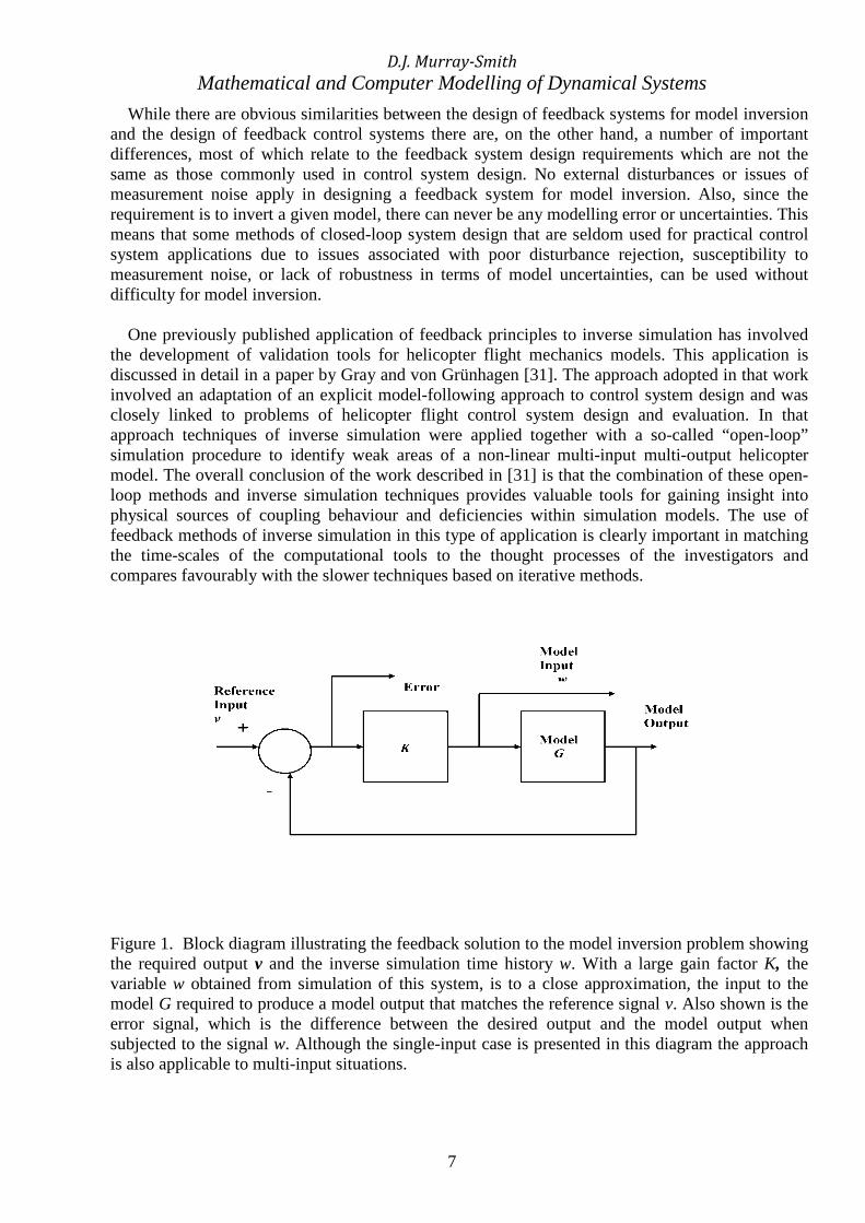
inverse solution can, if the feedback system is ideal, be found from the signal generated at the input to the model. The approach is closely linked to methods for the design of model-following control systems. In the case of inverse simulation the required output is generated using a reference model and the feedback structure provides the means for generating the inverse solution. This paper provides an account of recent research involving the further development and application of the feedback approach to inverse simulation for linear and nonlinear problems. Issues that are addressed include the generalisation of the approach to avoid some of the limitations that may arise when using high-gain proportional feedback. An important aspect of this generalised approach is the use made of control system analysis tools to guide the user in the selection of the feedback structure and the values of feedback controller parameters. The carefully selected case studies that are presented involve physically-based nonlinear single-input and multi-input multi-output models of practical engineering systems. The work provides a useful extension to the earlier published work of Buchholz and von Grünhagen [4]. 3. Model inversion using feedback system properties 3.1 Use of feedback involving proportional control The use of feedback to generate an inverse solution is based on the properties of closed-loop systems. For a linear time-invariant single-input single-output system with transfer function G(s) the block diagram shown in Figure 1 provides a general basis for this approach to model inversion. For the single-input single-output case with a simple gain factor K in cascade with the model G(s), the transfer function relating the variable W(s) to the input V(s) in Figure 1 is given by:

)(1)(

)(

sKG

K

sV

sW

+= (1)

)(1

1

sGK

+= (2)

For the case where K is very large this gives:

)(

1

)(

)(

sGsV

sW ≈ (3)

Thus the inverse model for G may be found by applying high-gain feedback around the model itself. The input to G in that feedback structure forms the output of the inverse model. It should be noted that the order of both the numerator and the denominator of the closed loop transfer function is the same as the order of the denominator of G. The number of poles in the inverse model is thus always the same as the number of zeros and there is no issue of realisability associated with an excess of zeros. The variable v in this representation is therefore the form of output that we require from the model while w is the input to the model (under open-loop conditions) that will produce this model output.

D.J. Murray-Smith


7

While there are obvious similarities between the design of feedback systems for model inversion and the design of feedback control systems there are, on the other hand, a number of important differences, most of which relate to the feedback system design requirements which are not the same as those commonly used in control system design. No external disturbances or issues of measurement noise apply in designing a feedback system for model inversion. Also, since the requirement is to invert a given model, there can never be any modelling error or uncertainties. This means that some methods of closed-loop system design that are seldom used for practical control system applications due to issues associated with poor disturbance rejection, susceptibility to measurement noise, or lack of robustness in terms of model uncertainties, can be used without difficulty for model inversion. One previously published application of feedback principles to inverse simulation has involved the development of validation tools for helicopter flight mechanics models. This application is discussed in detail in a paper by Gray and von Grünhagen [31]. The approach adopted in that work involved an adaptation of an explicit model-following approach to control system design and was closely linked to problems of helicopter flight control system design and evaluation. In that approach techniques of inverse simulation were applied together with a so-called “open-loop” simulation procedure to identify weak areas of a non-linear multi-input multi-output helicopter model. The overall conclusion of the work described in [31] is that the combination of these open-loop methods and inverse simulation techniques provides valuable tools for gaining insight into physical sources of coupling behaviour and deficiencies within simulation models. The use of feedback methods of inverse simulation in this type of application is clearly important in matching the time-scales of the computational tools to the thought processes of the investigators and compares favourably with the slower techniques based on iterative methods.

Figure 1. Block diagram illustrating the feedback solution to the model inversion problem showing the required output v and the inverse simulation time history w. With a large gain factor K, the variable w obtained from simulation of this system, is to a close approximation, the input to the model G required to produce a model output that matches the reference signal v. Also shown is the error signal, which is the difference between the desired output and the model output when subjected to the signal w. Although the single-input case is presented in this diagram the approach is also applicable to multi-input situations.

D.J. Murray-Smith


8

3.2 The general case of feedback-based model inversion While simple proportional high-gain feedback provides acceptable solutions in many cases and has provided the basis for much previous work in this field [4],[5], the principle of feedback-based model inversion applies also to other forms of feedback structure and the approach is not limited to proportional control methods. For example, steady-state errors in the inverse model that can arise with proportional control may be eliminated by the introduction of proportional plus integral feedback, although this may introduce additional stability problems. Classical feedback systems analysis techniques can provide useful insight in the case of low-order linear models and can allow a sensible choice of controller to be made. For nonlinear models, computer-based analysis of linearised descriptions can be very useful in investigating possible limitations of a high-gain proportional control approach and the possible merits of other forms of control structure. For complex nonlinear models computer-based analysis is usually followed by preliminary simulation runs to fine-tune feedback gain values prior to using the inverse simulation in the intended application. This applies not only to linear single-input single-output models but also to multi-input multi-output models and to nonlinear models. 3.3 The general case for single-input single-output linearised models. With proportional control the feedback system has the simple form shown in Figure 1 and if the gain factor K is replaced by a transfer function K(s), as for example in the case of proportional plus integral control, the principles outlined above for the implementation of inverse simulation by feedback methods still apply. In this more general case Equation (2) has the form:

and the requirement for effective inverse simulation is that the magnitude of 1/K(s) should be small compared with the magnitude of G(s) over the frequency range of interest for the intended application of the inverse. Investigation of the feedback system can be carried out using frequency-domain analysis methods based on Bode plots while root locus plots can be used subsequently to determine how the dynamics of the closed loop system change with variation of selected parameters of K(s). Values of the adjustable parameters can then be found that ensure that poles of the inverse simulation model lie at points in the s-plane that are close to the positions of the zeros of the forward model. The behaviour of any branches of the root locus that tend towards infinity in the s-plane as the gain factor becomes large can also be established and their effect on the properties of the inverse simulation can then be understood. The feedback approach to inverse simulation may be considered as involving two distinct stages. This applies to both the linear and nonlinear cases but the importance of the two stages is more obvious in the case of applications involving nonlinear models.

(4) )(

)(

11

)(

)(

sGsK

sV

sW

+=

D.J. Murray-Smith


9

In the first stage of the inversion process the closed-loop system is designed, by whatever method is appropriate, and parameters are then adjusted so that the feedback system meets specific requirements in terms of the response to simple inputs such as a step or impulse. If a linearised description of the model is used in the initial design, the performance of the closed-loop system must be checked through simulation for other operating conditions, preferably using the full nonlinear model. Any limitations should be corrected or noted for the application stage. In the second stage, the use of a feedback system for model inversion is similar to a model-following type of control system where the outputs of the model are forced to follow time histories generated by a reference model. The input variables for the model within the closed- loop system are then the inputs necessary to achieve the required outputs. It is recommended that the differences between the reference inputs (which represents the time histories to be followed by the model output variables) and the actual model outputs should be monitored continuously and that quantitative measures of these differences (such as the integral of the squared error) should be generated and recorded along with the time histories of model inputs (which are the required outputs of the inverse simulation) as shown in Figure 1.

3.3.1 An example involving a third-order system model The use of simulation combined with the feedback approach for a single-input single-output system model can best be illustrated through an example. This involves a simple single-input single-output system (SISO) model that has been used in previous investigations [16], [17], [18] involving the conventional integration-based iterative approach to inverse simulation. The state-space model for the system has the following form:

��

where

(5)

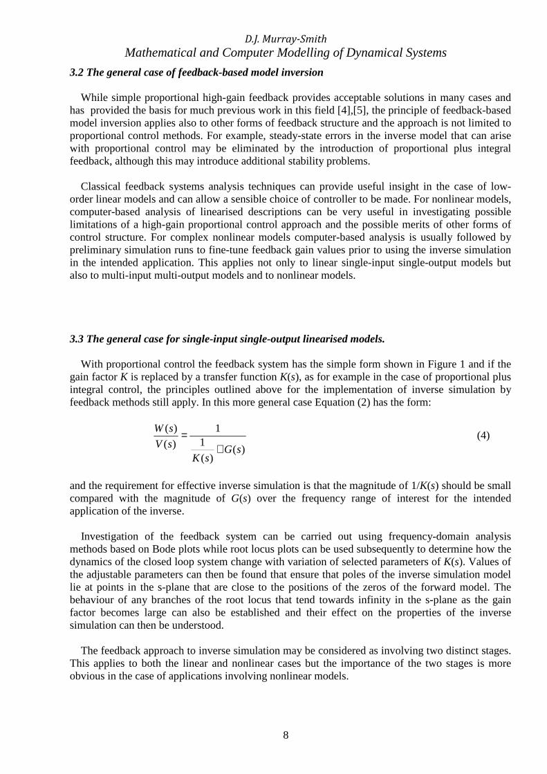
Analysis shows that the system has three poles (at s = -1.000, s = -2.000 and s = -3.000) and one pair of complex transmission zeros (at s = -0.5000 ± j7.0534). For this s-plane pattern of poles and zeros it is reasonable to define the range of frequencies of interest for this model as, at most, zero to 30 rad./s.. Being a single-input single-output system, there is only one feedback loop. Figure 2 shows the root-locus diagram for the closed-loop system for simple proportional feedback. It is clear, as would be expected, that as the gain factor is increased two of the poles of the closed-loop system move towards the positions of the zeros of the forward model, although there is an range of intermediate values of gain which leads to two closed-loop poles that lie in the right half of the s-plane and would produce an unstable inverse. Values of the gain factor used for the inverse simulation must therefore be chosen to be significantly larger than this critical range. A third closed-loop pole

[ ] 0 , 001 ,

69

5

1

,

6116

100

010

==

−=

−−−= DCBA

D.J. Murray-Smith


10

moves off along the negative real axis and for large gain values this produces a very fast transient mode which can be neglected.

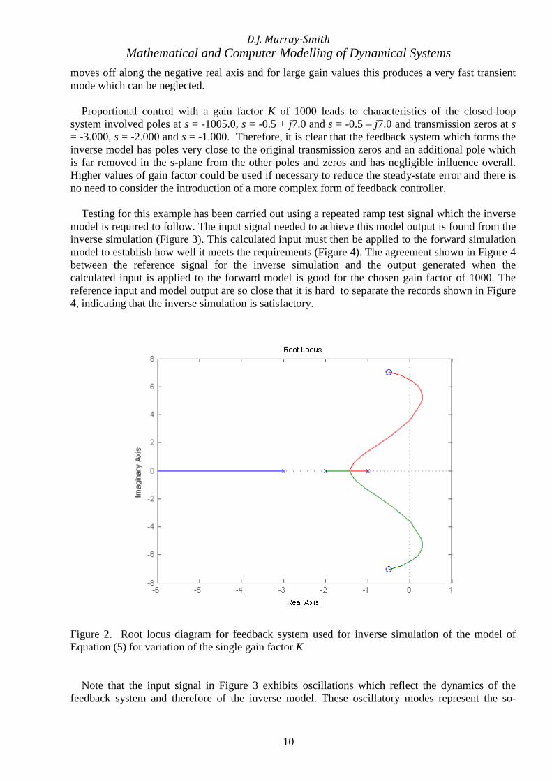
Proportional control with a gain factor K of 1000 leads to characteristics of the closed-loop system involved poles at s = -1005.0, s = -0.5 + j7.0 and s = -0.5 – j7.0 and transmission zeros at s = -3.000, s = -2.000 and s = -1.000. Therefore, it is clear that the feedback system which forms the inverse model has poles very close to the original transmission zeros and an additional pole which is far removed in the s-plane from the other poles and zeros and has negligible influence overall. Higher values of gain factor could be used if necessary to reduce the steady-state error and there is no need to consider the introduction of a more complex form of feedback controller. Testing for this example has been carried out using a repeated ramp test signal which the inverse model is required to follow. The input signal needed to achieve this model output is found from the inverse simulation (Figure 3). This calculated input must then be applied to the forward simulation model to establish how well it meets the requirements (Figure 4). The agreement shown in Figure 4 between the reference signal for the inverse simulation and the output generated when the calculated input is applied to the forward model is good for the chosen gain factor of 1000. The reference input and model output are so close that it is hard to separate the records shown in Figure 4, indicating that the inverse simulation is satisfactory.

Figure 2. Root locus diagram for feedback system used for inverse simulation of the model of Equation (5) for variation of the single gain factor K Note that the input signal in Figure 3 exhibits oscillations which reflect the dynamics of the feedback system and therefore of the inverse model. These oscillatory modes represent the so-

D.J. Murray-Smith


11

called “constraint oscillation” phenomenon which has been discussed extensively in connection with iterative approaches to inverse simulation [1], [16]. Such oscillatory effects have also been found when inverse modelling techniques based on analytical methods have been applied [17]. As already mentioned, this example provides an interesting comparison with previous work involving the application of the integration-based iterative type of approach to inverse simulation and results obtained for this same problem using such methods are discussed at greater length in [16].

Figure 3. Input time history found from inverse simulation of the SISO model using a gain factor K of 1000.

D.J. Murray-Smith


12

Figure 4. Reference signal applied to the inverse simulation of the SISO linear model (dashed line) together with the output resulting from application of the input found from the inverse simulation process (continuous line) for a gain factor K of 1000. These results were obtained using the lsim function in MATLAB®.

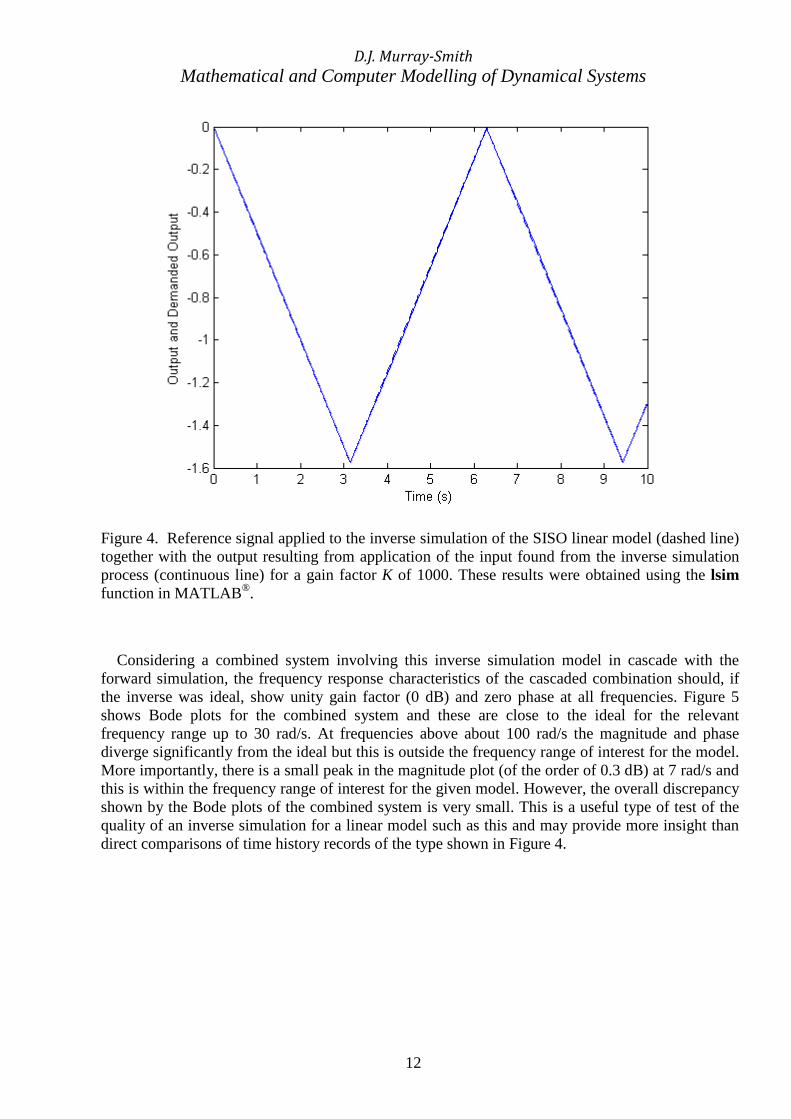
Considering a combined system involving this inverse simulation model in cascade with the forward simulation, the frequency response characteristics of the cascaded combination should, if the inverse was ideal, show unity gain factor (0 dB) and zero phase at all frequencies. Figure 5 shows Bode plots for the combined system and these are close to the ideal for the relevant frequency range up to 30 rad/s. At frequencies above about 100 rad/s the magnitude and phase diverge significantly from the ideal but this is outside the frequency range of interest for the model. More importantly, there is a small peak in the magnitude plot (of the order of 0.3 dB) at 7 rad/s and this is within the frequency range of interest for the given model. However, the overall discrepancy shown by the Bode plots of the combined system is very small. This is a useful type of test of the quality of an inverse simulation for a linear model such as this and may provide more insight than direct comparisons of time history records of the type shown in Figure 4.

D.J. Murray-Smith


13

Figure 5. Bode plot for the combined system involving the inverse simulation model based on feedback principles and the given forward model, connected in series.

4. Feedback principles applied to inverse simulation of single-input single-output nonlinear dynamic models The significance of the two-stage nature of the process for inverse-simulation becomes clear when nonlinear applications are considered. The feedback loop design process is really quite separate from the inverse simulation application stage. This is best illustrated using an example, which in this case involves an aeronautical engineering application. 4.1 Application to a nonlinear dynamic model of a fixed-wing aircraft The model involved in this application represents the longitudinal dynamics of an HS125 business jet (now known as the Hawker-Raytheon 800 series). This model has also been used in previous investigations [17], [18], [19] involving the conventional integration-based iterative approach to inverse simulation. The flight condition considered is level flight at 120 knots at sea level. The equations of motion in terms of the response to control inputs are as follows:

�� = ��

� �sinΘ (6)

�� QU� �

��g cos (7)

D.J. Murray-Smith


14

�� !

"## (8)

Θ� � Q (9)

&'� � �cos Θ� Wsin Θ (10)

+'� = �sin Θ� Wcos Θ (11)

where U is the forward velocity (m/s), W is the heave velocity (m/s), Q is the pitch rate (rad/s), is the pitch angle (rad), XE are ZE are the positions of the aircraft in the direction of the x and z axes respectively in the earth-fixed frame of reference. A change of the elevator angle ,- (rad) from the trim value changes the external forces X and Z (N) and the external moment M (Nm). These external forces and moments are obtained from the following equations:

& = . / cos 0 � 1 sin 0 (12)

+ = 1 cos 0 / sin 0 (13)

2 = 23 � .45 (14) Here the aerodynamic loads L, D and MA are given by:

1 =6

789:

7;<= (15)

/ =6

789:

7;<> (16)

23 =6

789:

7;?@<! (17)

where

<= = <=A � <=B0 � <=C-,- (18)

<> = <>A � <>B0 � <>BB07 (19)

<! = <!A � <!B0 � <!C-,- � <!D EF@

GH (20)

The angle of attack, α, is given by the equation:

D.J. Murray-Smith


15

tan 0 =K

L (21)

These equations and symbols are widely used in aircraft models and details of the derivation of a general model for longitudinal motion of a fixed wing aircraft such as this may be found in many textbooks (e.g. [32], [33], [34]). Parameters for the HS125 model are as follows [35]: m = 7484.4 kg (mass), Iyy= 84309 kgm2 (moment of inertia), S = 32.8 m2 (wing area) ?@ = 2.29 m (mean chord), hT = 0.378 m (thrustline above the x-axis, which in trimmed flight is fixed in the aircraft in the direction of motion), ρ = 1.225 kg/m3 (air density), CD0 = 0.177, CDα = 0.232, CDαα = 1.393, CL0 = 0.895, CLα = 5.01, CLδe = 0.722, CM0 = -0.046, CMα = -1.087, CMδe = -1.88, CMq = -7.055, T = 13878 N (thrust), and g = 9.81 m/s2 (gravitational constant).

The equations can be solved simultaneously for the six state variables in response to the elevator input. Appropriate initial conditions must be applied and these normally involve a trimmed equilibrium flight state. For the given forward velocity the following set of values applies: Ue = 61.8682 m/s, We = 0.8501 m/s, Qe=0 rad/s, Θ- = 0.01374 rad, δee = -0.01659 rad, XEe=0 m and ZEe=0 m. Here the subscript e indicates that these are values for the trimmed equilibrium flight state. The Equations (6) to (21) can be solved simultaneously for the six state variables (U, W, Q, M, XE, ZE) in response to elevator inputs δe. The elevator input feeds into lift and pitching moment equations and subsequently into expressions for the external forces and moments which appear as X, Z and M in Equations (6), (7) and (8). A change of δe from its trim value leads to changes of the external forces and moments and thus to changes in the state variables. Linearised equations of motion may be derived from Equations (6) to (21) using standard methods (e.g., [ 33], [34]) and, for the state variables � � N� O P QR5 and input u = δe, these equations are as follows [35]:

��

where A=S 0.05718 0.12433 0 0.30512 0.8651 61.87 0.0015040 0.036750 0.545481 9.81000 Z and B = S0.10194 7.4188 3.92750 Z (12)

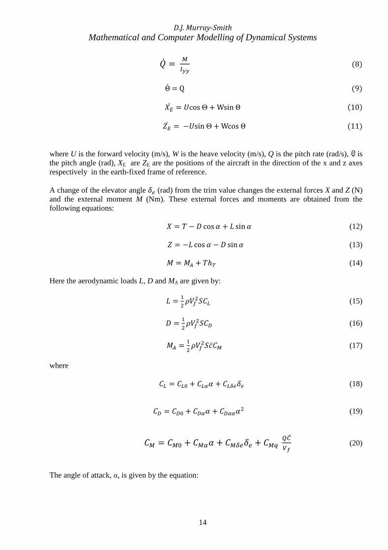
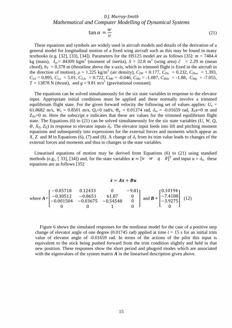
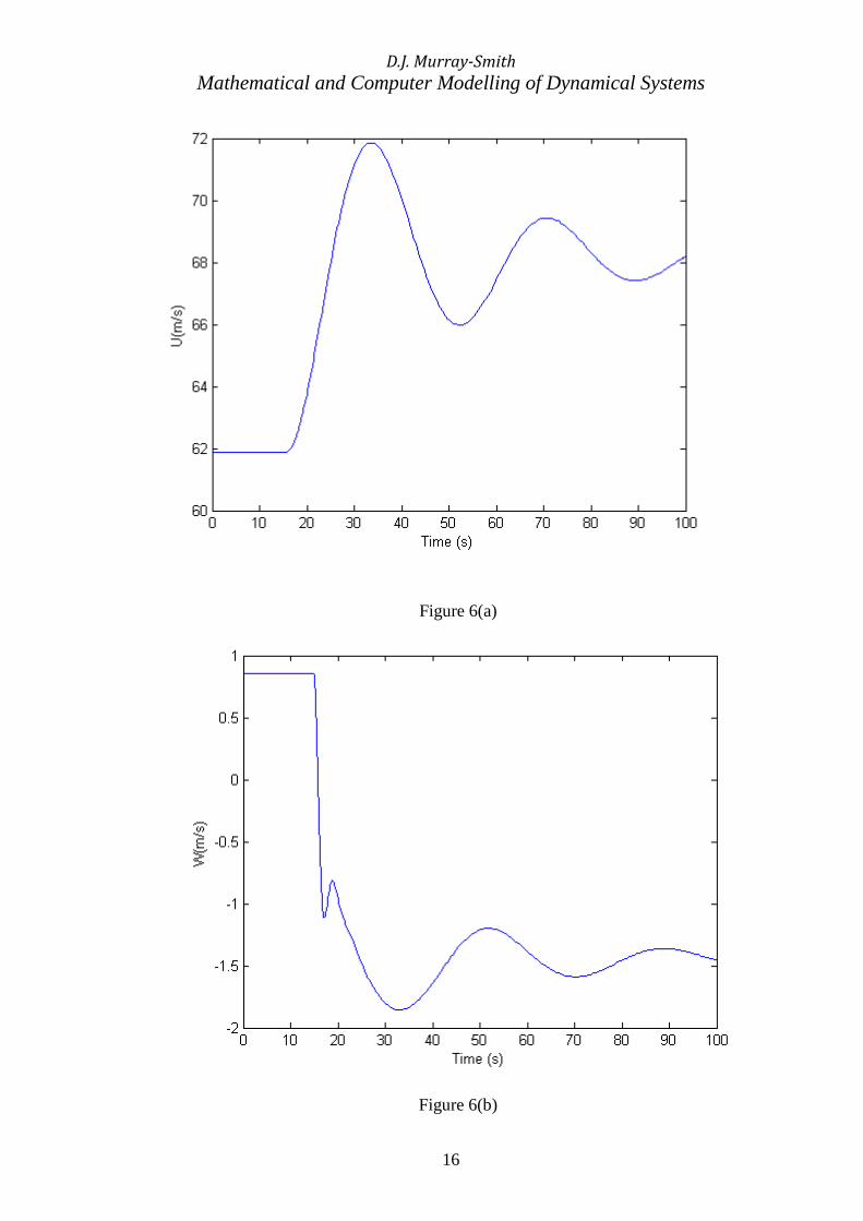
Figure 6 shows the simulated responses for the nonlinear model for the case of a positive step change of elevator angle of one degree (0.01745 rad) applied at time t = 15 s for an initial trim value of elevator angle of -0.01659 rad. In terms of the actions of the pilot this input is equivalent to the stick being pushed forward from the trim condition slightly and held in that new position. These responses show the short period and phugoid modes which are associated with the eigenvalues of the system matrix A in the linearised description given above.

D.J. Murray-Smith


16

Figure 6(a)

Figure 6(b)

D.J. Murray-Smith


17

Figure 6(c)

Figure 6(d)

D.J. Murray-Smith


18

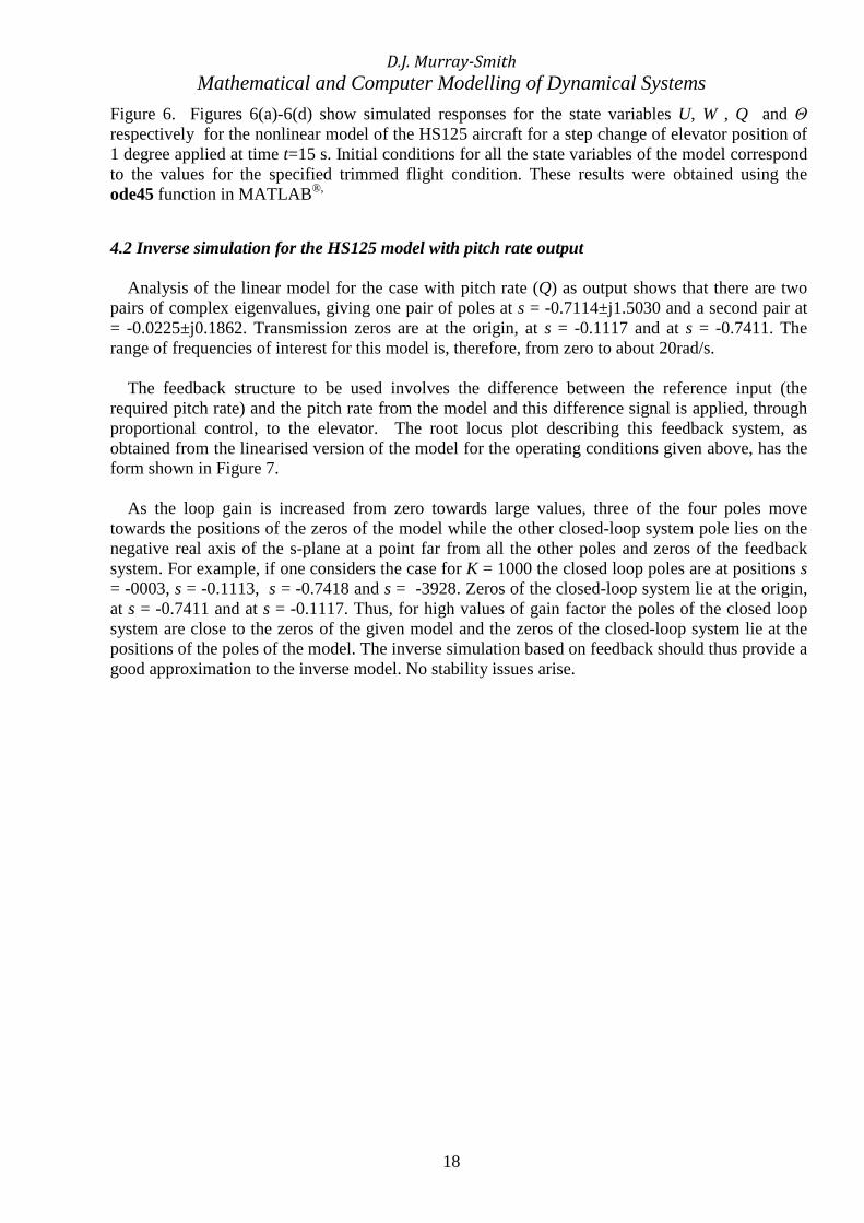
Figure 6. Figures 6(a)-6(d) show simulated responses for the state variables U, W , Q and Θ respectively for the nonlinear model of the HS125 aircraft for a step change of elevator position of 1 degree applied at time t=15 s. Initial conditions for all the state variables of the model correspond to the values for the specified trimmed flight condition. These results were obtained using the ode45 function in MATLAB®, 4.2 Inverse simulation for the HS125 model with pitch rate output Analysis of the linear model for the case with pitch rate (Q) as output shows that there are two pairs of complex eigenvalues, giving one pair of poles at s = -0.7114±j1.5030 and a second pair at = -0.0225±j0.1862. Transmission zeros are at the origin, at s = -0.1117 and at s = -0.7411. The range of frequencies of interest for this model is, therefore, from zero to about 20rad/s. The feedback structure to be used involves the difference between the reference input (the required pitch rate) and the pitch rate from the model and this difference signal is applied, through proportional control, to the elevator. The root locus plot describing this feedback system, as obtained from the linearised version of the model for the operating conditions given above, has the form shown in Figure 7. As the loop gain is increased from zero towards large values, three of the four poles move towards the positions of the zeros of the model while the other closed-loop system pole lies on the negative real axis of the s-plane at a point far from all the other poles and zeros of the feedback system. For example, if one considers the case for K = 1000 the closed loop poles are at positions s = -0003, s = -0.1113, s = -0.7418 and s = -3928. Zeros of the closed-loop system lie at the origin, at s = -0.7411 and at s = -0.1117. Thus, for high values of gain factor the poles of the closed loop system are close to the zeros of the given model and the zeros of the closed-loop system lie at the positions of the poles of the model. The inverse simulation based on feedback should thus provide a good approximation to the inverse model. No stability issues arise.

D.J. Murray-Smith


19

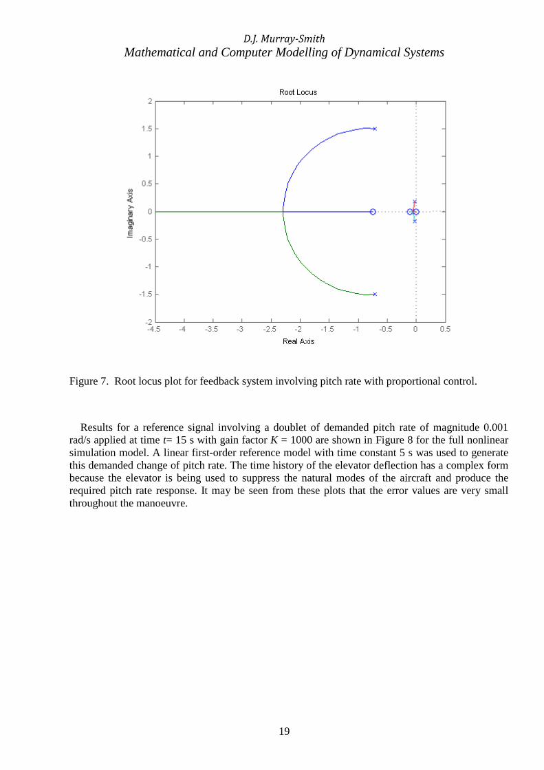
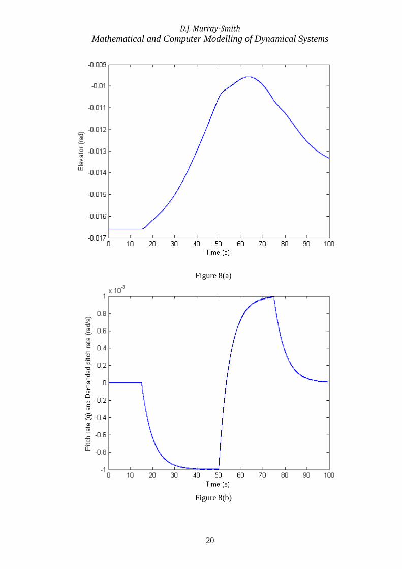
Figure 7. Root locus plot for feedback system involving pitch rate with proportional control. Results for a reference signal involving a doublet of demanded pitch rate of magnitude 0.001 rad/s applied at time t= 15 s with gain factor K = 1000 are shown in Figure 8 for the full nonlinear simulation model. A linear first-order reference model with time constant 5 s was used to generate this demanded change of pitch rate. The time history of the elevator deflection has a complex form because the elevator is being used to suppress the natural modes of the aircraft and produce the required pitch rate response. It may be seen from these plots that the error values are very small throughout the manoeuvre.

D.J. Murray-Smith


20

Figure 8(a)

Figure 8(b)

D.J. Murray-Smith


21

Figure 8(c)

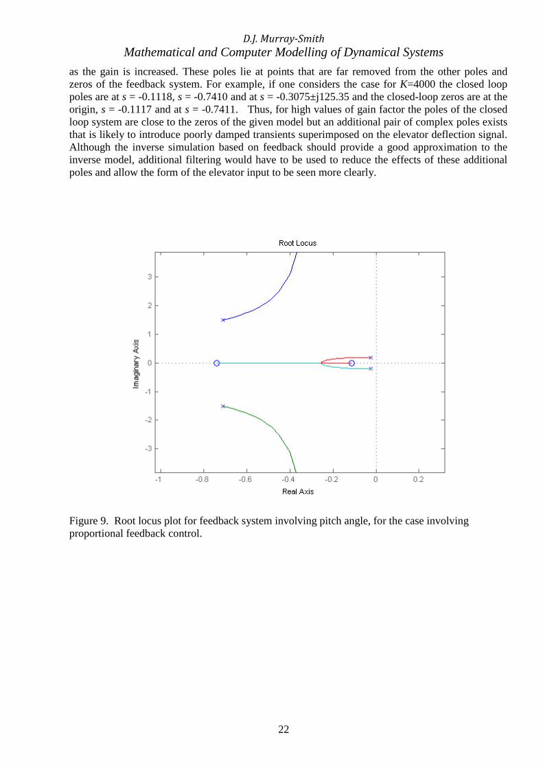
Figure 8. The record in Figure 8(a) shows the elevator deflection obtained from inverse simulation for a specific demanded pitch rate time history. The second plot, Figure 8(b), shows the reference input (dashed line) together with the corresponding pitch rate time output obtained from the forward model (continuous line) for that elevator input. The third plot, Figure 8(c), shows the error between the reference input and the model pitch rate resulting from the application of that input. These results were obtained using the ode45 function in MATLAB® using the full nonlinear simulation model of the aircraft. 4.3 Inverse simulation for the HS125 model with pitch attitude as output Analysis of the linear model for this case shows that there are once again two pairs of complex poles, one pair at s = -0.0225±j0.1862 and a second pair at s = -0.7114±j1.5030. There are only two transmission zeros and these are at s = -0.7412 and at s = -0.1117. As in the previous case the frequency range of interest is from zero to approximately 20 rad/s.. If Θ (pitch angle) is chosen as the output variable the feedback structure must involve the difference between the reference input (the required pitch) and the pitch value obtained from the HS125 model. This difference signal is used for generation of the required elevator deflection. Using proportional control, the root locus plot describing the feedback system, as obtained from the linearised version of the model for the operating conditions given above, has the form shown in Figure 9. As the loop gain is increased from zero towards large values, two of the four poles of this model move towards the positions of the zeros while the other two complex poles remain complex in form

D.J. Murray-Smith


22

as the gain is increased. These poles lie at points that are far removed from the other poles and zeros of the feedback system. For example, if one considers the case for K=4000 the closed loop poles are at s = -0.1118, s = -0.7410 and at s = -0.3075±j125.35 and the closed-loop zeros are at the origin, s = -0.1117 and at s = -0.7411. Thus, for high values of gain factor the poles of the closed loop system are close to the zeros of the given model but an additional pair of complex poles exists that is likely to introduce poorly damped transients superimposed on the elevator deflection signal. Although the inverse simulation based on feedback should provide a good approximation to the inverse model, additional filtering would have to be used to reduce the effects of these additional poles and allow the form of the elevator input to be seen more clearly.

Figure 9. Root locus plot for feedback system involving pitch angle, for the case involving proportional feedback control.

D.J. Murray-Smith


23

Figure 10(a)

Figure 10(b)

D.J. Murray-Smith


24

Figure 10(c)

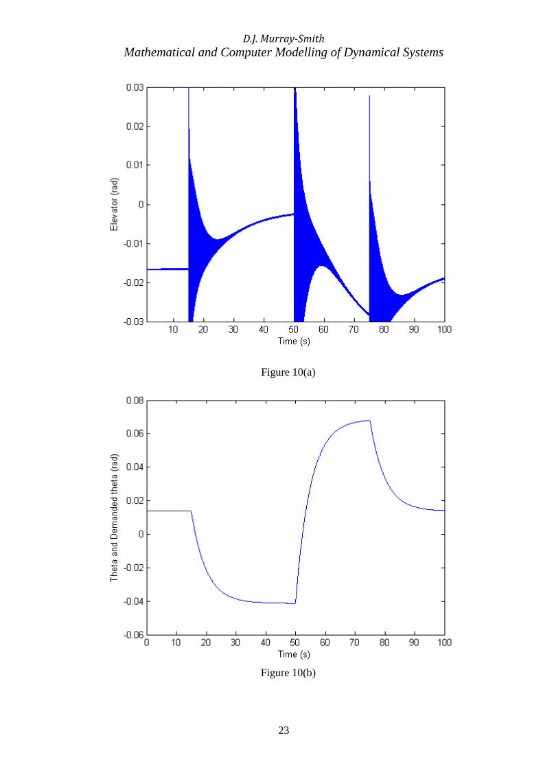
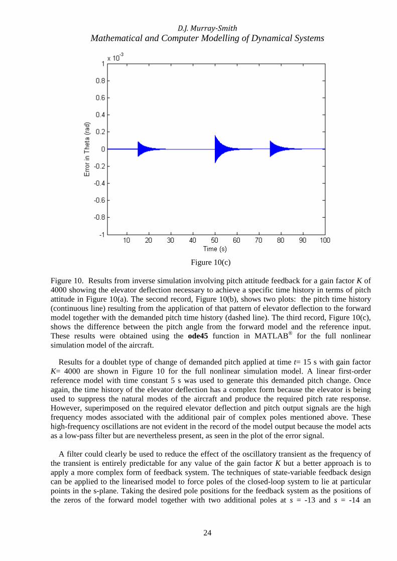
Figure 10. Results from inverse simulation involving pitch attitude feedback for a gain factor K of 4000 showing the elevator deflection necessary to achieve a specific time history in terms of pitch attitude in Figure 10(a). The second record, Figure 10(b), shows two plots: the pitch time history (continuous line) resulting from the application of that pattern of elevator deflection to the forward model together with the demanded pitch time history (dashed line). The third record, Figure 10(c), shows the difference between the pitch angle from the forward model and the reference input. These results were obtained using the ode45 function in MATLAB® for the full nonlinear simulation model of the aircraft. Results for a doublet type of change of demanded pitch applied at time t= 15 s with gain factor K= 4000 are shown in Figure 10 for the full nonlinear simulation model. A linear first-order reference model with time constant 5 s was used to generate this demanded pitch change. Once again, the time history of the elevator deflection has a complex form because the elevator is being used to suppress the natural modes of the aircraft and produce the required pitch rate response. However, superimposed on the required elevator deflection and pitch output signals are the high frequency modes associated with the additional pair of complex poles mentioned above. These high-frequency oscillations are not evident in the record of the model output because the model acts as a low-pass filter but are nevertheless present, as seen in the plot of the error signal. A filter could clearly be used to reduce the effect of the oscillatory transient as the frequency of the transient is entirely predictable for any value of the gain factor K but a better approach is to apply a more complex form of feedback system. The techniques of state-variable feedback design can be applied to the linearised model to force poles of the closed-loop system to lie at particular points in the s-plane. Taking the desired pole positions for the feedback system as the positions of the zeros of the forward model together with two additional poles at s = -13 and s = -14 an

D.J. Murray-Smith


25

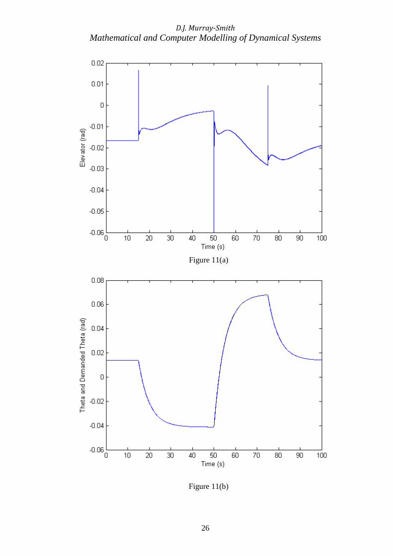
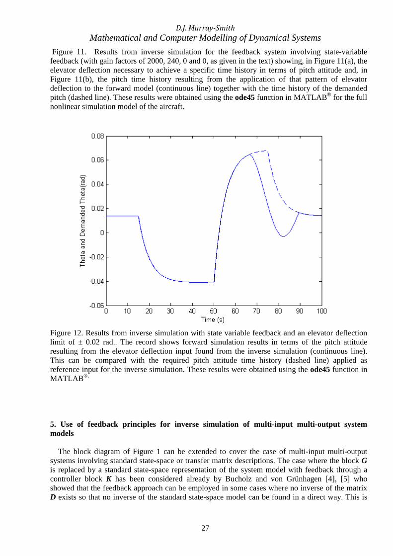
appropriate state-variable feedback structure can be found without difficulty using, for example, the place function within the MATLAB® Control Systems Toolbox [36]. Although this solution is satisfactory it involves a gain factor of about 55 in the main feedback loop involving Θ and this gives rise to a steady-state error. This performance can be improved substantially using a method of feedback system tuning involving controller parameter sensitivity measures [37] to ensure that the steady state error is negligible. Results are shown in Figure 11 for the case involving state variable feedback with gain factors for the negative feedback paths from Θ, Q, W and U of 2000, 240, 0 and 0 respectively. There is no high frequency oscillatory mode present and the error between the desired output and model output is negligible. In this case the poles of the closed-loop system are at the origin, at s= -0.1117, s = -0.74102, s = -16.96 and s= -926.3. Thus, as required, three of the poles of the feedback system lie at or very close to the positions of the zeros of the model and all other poles are well removed from the area of the s-plane that is of interest. The positions of the zeros are, of course, unaltered by the addition of the feedback loops. Applications of this inverse simulation have included investigation of the limitations of the aircraft in terms of the effect on manoeuvrability of the elevator and associated actuators. The effects of elevator deflection and rate limits can be investigated directly using the inverse simulation results. The time history of the pitch angle or pitch rate variables for a demanded manoeuvre are applied to the inverse simulation and the required elevator movement immediately indicates whether or not the manoeuvre can be performed. For example it can be seen in the elevator deflection time history of Figure 11 that the required manoeuvre involves elevator deflections between about -0.06 rad and 0.016 rad, although for much of the time the elevator deflection remains within the range -0.028 rad and -0.004 rad. If the largest allowable elevator deflection is set to be ± 0.02 rad in the forward model and the inverse simulation is repeated (with the same gain factor values in the feedback pathways as used previously) the results obtained are as shown in Figure 12. The error between the desired pitch and the pitch output obtained from the forward model shows very clearly that the required manoeuvre cannot be performed. The necessary elevator deflection would exceed the limiting value in the negative direction for a significant time.

D.J. Murray-Smith


26

Figure 11(a)

Figure 11(b)

D.J. Murray-Smith


27

Figure 11. Results from inverse simulation for the feedback system involving state-variable feedback (with gain factors of 2000, 240, 0 and 0, as given in the text) showing, in Figure 11(a), the elevator deflection necessary to achieve a specific time history in terms of pitch attitude and, in Figure 11(b), the pitch time history resulting from the application of that pattern of elevator deflection to the forward model (continuous line) together with the time history of the demanded pitch (dashed line). These results were obtained using the ode45 function in MATLAB® for the full nonlinear simulation model of the aircraft.

Figure 12. Results from inverse simulation with state variable feedback and an elevator deflection limit of ± 0.02 rad.. The record shows forward simulation results in terms of the pitch attitude resulting from the elevator deflection input found from the inverse simulation (continuous line). This can be compared with the required pitch attitude time history (dashed line) applied as reference input for the inverse simulation. These results were obtained using the ode45 function in MATLAB ®, 5. Use of feedback principles for inverse simulation of multi-input multi-output system models The block diagram of Figure 1 can be extended to cover the case of multi-input multi-output systems involving standard state-space or transfer matrix descriptions. The case where the block G is replaced by a standard state-space representation of the system model with feedback through a controller block K has been considered already by Bucholz and von Grünhagen [4], [5] who showed that the feedback approach can be employed in some cases where no inverse of the matrix D exists so that no inverse of the standard state-space model can be found in a direct way. This is

D.J. Murray-Smith


28

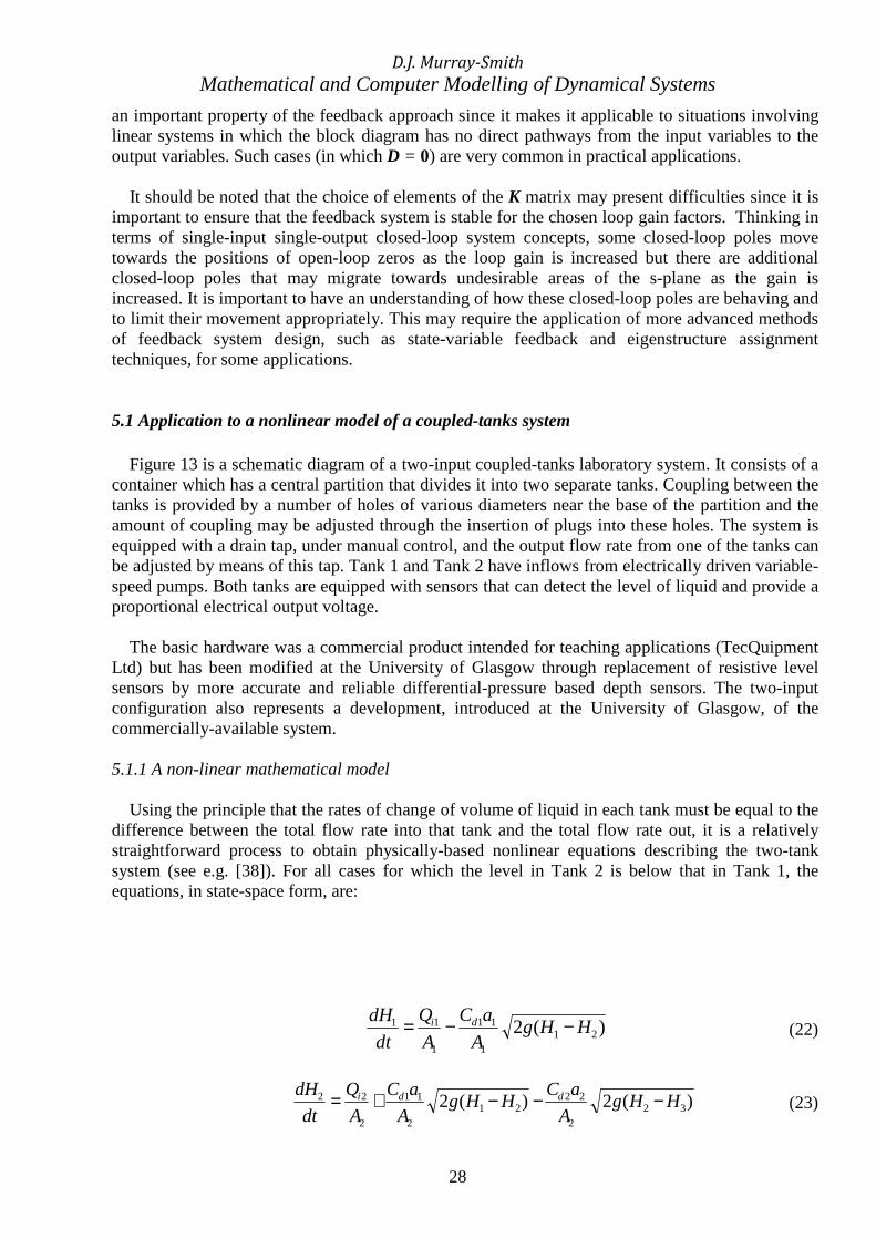
an important property of the feedback approach since it makes it applicable to situations involving linear systems in which the block diagram has no direct pathways from the input variables to the output variables. Such cases (in which D = 0) are very common in practical applications. It should be noted that the choice of elements of the K matrix may present difficulties since it is important to ensure that the feedback system is stable for the chosen loop gain factors. Thinking in terms of single-input single-output closed-loop system concepts, some closed-loop poles move towards the positions of open-loop zeros as the loop gain is increased but there are additional closed-loop poles that may migrate towards undesirable areas of the s-plane as the gain is increased. It is important to have an understanding of how these closed-loop poles are behaving and to limit their movement appropriately. This may require the application of more advanced methods of feedback system design, such as state-variable feedback and eigenstructure assignment techniques, for some applications. 5.1 Application to a nonlinear model of a coupled-tanks system Figure 13 is a schematic diagram of a two-input coupled-tanks laboratory system. It consists of a container which has a central partition that divides it into two separate tanks. Coupling between the tanks is provided by a number of holes of various diameters near the base of the partition and the amount of coupling may be adjusted through the insertion of plugs into these holes. The system is equipped with a drain tap, under manual control, and the output flow rate from one of the tanks can be adjusted by means of this tap. Tank 1 and Tank 2 have inflows from electrically driven variable-speed pumps. Both tanks are equipped with sensors that can detect the level of liquid and provide a proportional electrical output voltage. The basic hardware was a commercial product intended for teaching applications (TecQuipment Ltd) but has been modified at the University of Glasgow through replacement of resistive level sensors by more accurate and reliable differential-pressure based depth sensors. The two-input configuration also represents a development, introduced at the University of Glasgow, of the commercially-available system. 5.1.1 A non-linear mathematical model Using the principle that the rates of change of volume of liquid in each tank must be equal to the difference between the total flow rate into that tank and the total flow rate out, it is a relatively straightforward process to obtain physically-based nonlinear equations describing the two-tank system (see e.g. [38]). For all cases for which the level in Tank 2 is below that in Tank 1, the equations, in state-space form, are:

)(2 211

11

1

11 HHgA

aC

A

Q

dt

dH di −−= (22)

)(2)(2 322

2221

2

11

2

22 HHgA

aCHHg

A

aC

A

Q

dt

dH ddi −−−+= (23)

D.J. Murray-Smith


29

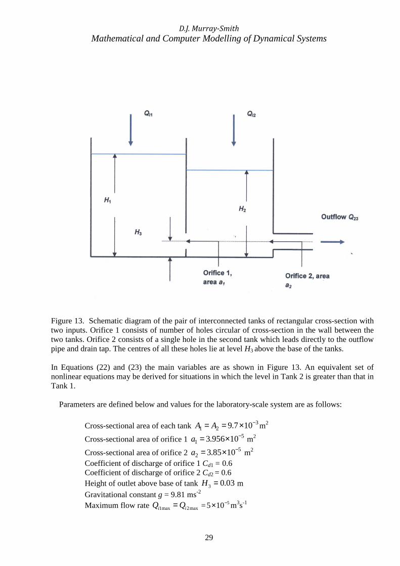
Figure 13. Schematic diagram of the pair of interconnected tanks of rectangular cross-section with two inputs. Orifice 1 consists of number of holes circular of cross-section in the wall between the two tanks. Orifice 2 consists of a single hole in the second tank which leads directly to the outflow pipe and drain tap. The centres of all these holes lie at level H3 above the base of the tanks. In Equations (22) and (23) the main variables are as shown in Figure 13. An equivalent set of nonlinear equations may be derived for situations in which the level in Tank 2 is greater than that in Tank 1. Parameters are defined below and values for the laboratory-scale system are as follows:

Cross-sectional area of each tank 321 107.9 −×== AA m2

Cross-sectional area of orifice 1 51 10956.3 −×=a m2

Cross-sectional area of orifice 2 52 1085.3 −×=a m2

Coefficient of discharge of orifice 1 Cd1 = 0.6 Coefficient of discharge of orifice 2 Cd2 = 0.6 Height of outlet above base of tank 03.03 =H m

Gravitational constant g = 9.81 ms-2 Maximum flow rate max2max1 ii QQ = = 5105 −× m3s-1

D.J. Murray-Smith


30

Maximum liquid level 3.0max2max1 == HH m

Further first-order linear ordinary differential equations have been introduced to describe the dynamics of the pumps. Instead of describing each pump simply by constants Gp1 and Gp2, the relationship between the electrical voltage at the pump inputs ve1(t) and ve2(t) and the flow rates Qi1(t) and Qi2(t) provided by the pumps takes the form:

11

11

11e

pi

pi vT

GQ

T

G

dt

dQ+−= (24)

and

22

22

2

22e

pi

pi vT

GQ

T

G

dt

dQ+−= (25)

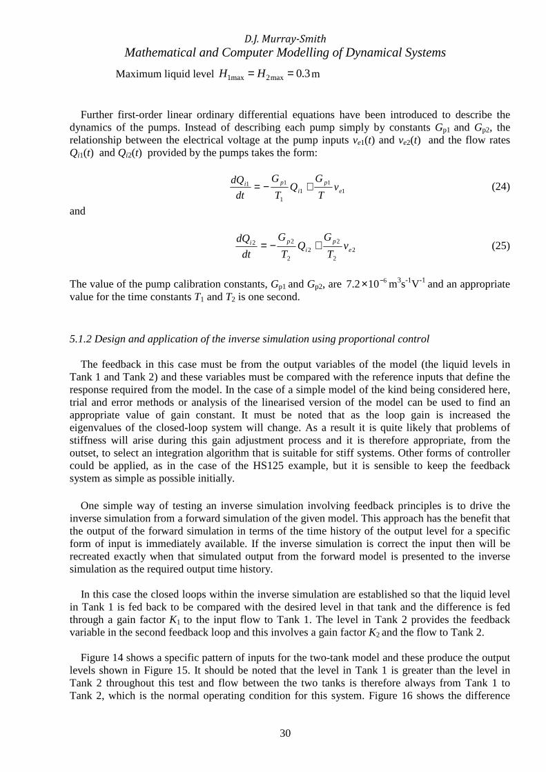
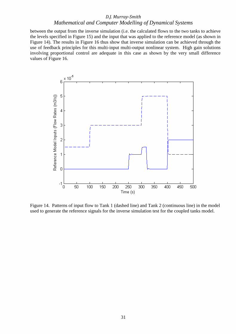
The value of the pump calibration constants, Gp1 and Gp2, are 6102.7 −× m3s-1V-1 and an appropriate value for the time constants T1 and T2 is one second. 5.1.2 Design and application of the inverse simulation using proportional control The feedback in this case must be from the output variables of the model (the liquid levels in Tank 1 and Tank 2) and these variables must be compared with the reference inputs that define the response required from the model. In the case of a simple model of the kind being considered here, trial and error methods or analysis of the linearised version of the model can be used to find an appropriate value of gain constant. It must be noted that as the loop gain is increased the eigenvalues of the closed-loop system will change. As a result it is quite likely that problems of stiffness will arise during this gain adjustment process and it is therefore appropriate, from the outset, to select an integration algorithm that is suitable for stiff systems. Other forms of controller could be applied, as in the case of the HS125 example, but it is sensible to keep the feedback system as simple as possible initially. One simple way of testing an inverse simulation involving feedback principles is to drive the inverse simulation from a forward simulation of the given model. This approach has the benefit that the output of the forward simulation in terms of the time history of the output level for a specific form of input is immediately available. If the inverse simulation is correct the input then will be recreated exactly when that simulated output from the forward model is presented to the inverse simulation as the required output time history. In this case the closed loops within the inverse simulation are established so that the liquid level in Tank 1 is fed back to be compared with the desired level in that tank and the difference is fed through a gain factor K1 to the input flow to Tank 1. The level in Tank 2 provides the feedback variable in the second feedback loop and this involves a gain factor K2 and the flow to Tank 2. Figure 14 shows a specific pattern of inputs for the two-tank model and these produce the output levels shown in Figure 15. It should be noted that the level in Tank 1 is greater than the level in Tank 2 throughout this test and flow between the two tanks is therefore always from Tank 1 to Tank 2, which is the normal operating condition for this system. Figure 16 shows the difference

D.J. Murray-Smith


31

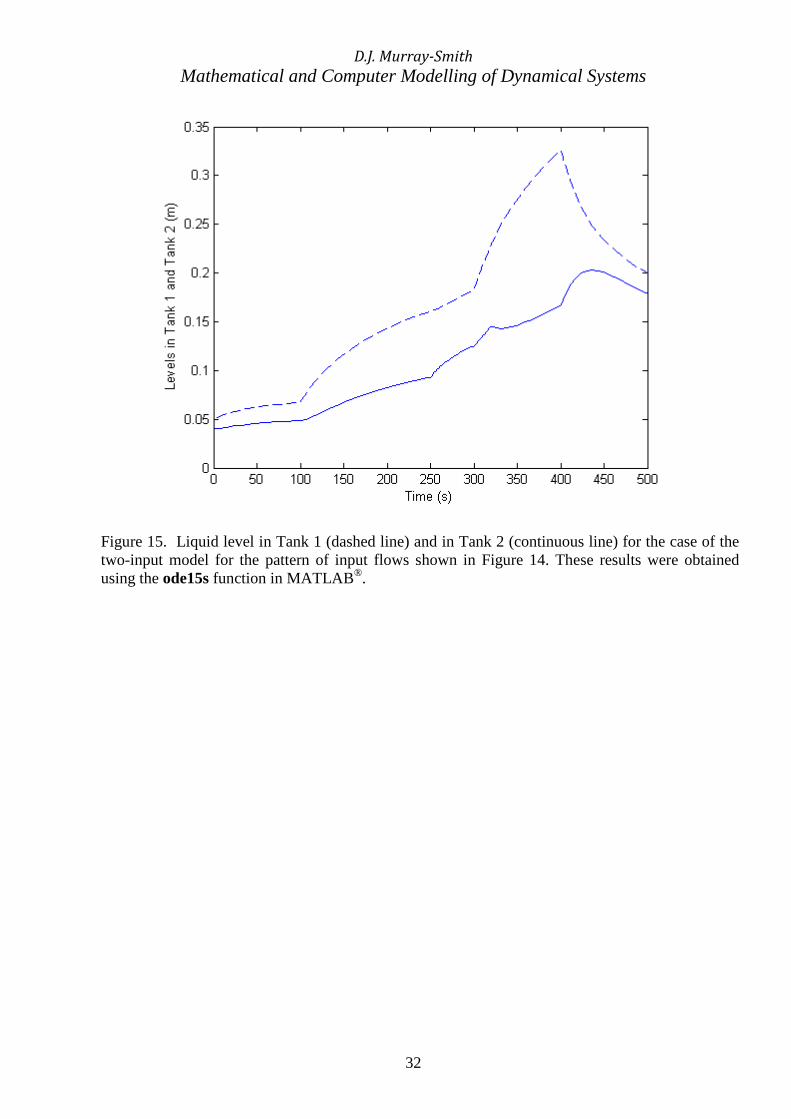
between the output from the inverse simulation (i.e. the calculated flows to the two tanks to achieve the levels specified in Figure 15) and the input that was applied to the reference model (as shown in Figure 14). The results in Figure 16 thus show that inverse simulation can be achieved through the use of feedback principles for this multi-input multi-output nonlinear system. High gain solutions involving proportional control are adequate in this case as shown by the very small difference values of Figure 16.

Figure 14. Patterns of input flow to Tank 1 (dashed line) and Tank 2 (continuous line) in the model used to generate the reference signals for the inverse simulation test for the coupled tanks model.

D.J. Murray-Smith


32

Figure 15. Liquid level in Tank 1 (dashed line) and in Tank 2 (continuous line) for the case of the two-input model for the pattern of input flows shown in Figure 14. These results were obtained using the ode15s function in MATLAB®.

D.J. Murray-Smith


33

Figure 16. Difference between input flows to the tanks found from inverse simulation and equivalent quantities applied to the reference model. The difference for the case of the input to Tank 1 is shown by the dashed line and for the input to Tank 2 by the continuous line. The gain factors K1 and K2 used in the inverse simulation in this case were both 20,000. These results were obtained using the ode15s function in MATLAB®. One application of the inverse simulation in this case is investigation of demanded patterns of level change that would take the two pumps beyond their maximum flow rate limits. This is similar to the investigation of the effect of elevator deflection limits on possible aircraft manoeuvres that was discussed in Section 4.3. In this coupled-tanks example information is immediately available from the inverse simulation results and this could, for any demanded pattern of level changes, be used to highlight situations in which the necessary inflow flow rates exceeded their limits. A second use of this inverse simulation has been as an additional tool for investigation of the limitations of the nonlinear two-tank model given in Equations (22) to (25) through driving the inverse simulation using input-flow and output-level data recorded experimentally from the equipment. New insight regarding aspects of the system model, and especially the modelling of the discharge from the second tank has come from this use of inverse simulation methods as part of this experimentally-based model validation study. 6. Discussion and conclusions

Several different cases have been considered in this paper. Starting with single-input single-output systems, an approach based on feedback methods has been presented and applied to a

D.J. Murray-Smith


34

number of linear and nonlinear examples. In principle, any closed-loop system design method can be applied in developing a feedback system for inverse simulation, provided it leads to solutions that involve relatively high loop-gains over the frequency range that is important for intended application of the model. In general, this involves selection of an appropriate feedback structure, often using linear analysis methods and subsequent tuning of feedback parameter values for the application involving the full nonlinear model. From the applications considered it is clear that inverse simulation methods can provide a form of insight for engineering investigations that is different from the understanding that comes from conventional modelling and simulation studies. Viewing the system in terms of the inputs that are needed to achieve a defined pattern of outputs provides the investigator with information that is potentially important in engineering design. It is believed that this understanding would not be so readily obtained using traditional modelling and simulation tools. The feedback approach to inverse simulation, described and applied in this paper, is an important alternative to the more widely-used iterative methods. One very important point about the feedback approach, that does not appear to have been highlighted previously, is that the problem of designing a feedback system for an inverse model is, generally, much less difficult than that of designing a feedback system for a control system application involving a model of similar complexity. Questions of response to external disturbances, insensitivity to measurement noise and robustness in terms of model uncertainties are all irrelevant in the inverse simulation case since disturbances and measurement noise are not present. The model is also completely known so there are no issues of robustness (other than numerical robustness). There may well be uncertainties within the model when compared with the corresponding real system but, for the purposes of inverting a given model, no uncertainty exists. Relatively simple methods of feedback system design involving high-gain solutions and state-variable feedback can therefore be considered for the model inversion application. Although problems of numerical stiffness can arise with the feedback approach to inverse simulation this need not create major difficulties, for most applications, if an appropriate choice of numerical integration algorithm is made. Errors in the inverse simulation procedure depend on the dynamics of the closed-loop system and thus on the form of feedback controller used. The number of possible inverse simulation models is infinite as there is no limit to the possible number of designs for the feedback loop. Analysis of the forward model does, however, provide useful information about eigenvalues and transmission zeros for the closed-loop system and this can provide valuable insight in assessing the inverse model. Experience gained from the case studies suggests that, with a careful choice of integration method and integration step size, computation times can often be achieved that are similar to the computation time for a conventional forward simulation for the same model. This contrasts with the integration-based approach described in Section 2, which clearly involves a number of forward simulation runs. Generation of the inverse solution by that iterative method may therefore take significantly longer than the time for a single forward simulation run, depending on the number of runs required for convergence of the algorithm. It should also be noted that the integration-based method requires choosing of an interval T over which inputs are constant. Selection of that interval generally involves a trial-and-error process, especially in the case of nonlinear models. This means

D.J. Murray-Smith


35

that a number of attempts may have to be made before an acceptable inverse simulation solution is achieved using that approach. In some cases the closed-loop system in the feedback-based approach may have an execution time that is noticeably greater than the time for the forward simulation because of the fact that the integration step size required for the model with feedback is significantly smaller than the integration step size for the forward model. This is due to the fact that the introduction of feedback with high gain factors can give closed-loop system poles that lie far from the poles of the forward model, thus making the equations for the feedback system stiffer than those of the model itself. The feedback approach therefore requires careful choice of integration method and step size, but selection of these this is a familiar task for all involved in system modelling and simulation activities. In making comparisons between the feedback-based approach and other methods, the trade-off between the additional complications of a one-off feedback system design for the model being inverted and the possible benefits, such as improvements in computational speed and overall efficiency, are perhaps as important as the time for a single inverse simulation run. This is clearly very dependent on the application and is an issue that requires further quantitative investigation. However, from the qualitative evidence from the case studies presented here, it is clear that there may be advantages in using the feedback approach, rather than the established methods, for some real-time applications and for applications involving repeated inverse simulation runs, such as in design optimisation. Earlier published work on this topic put particular emphasis on linear models and feedback involving proportional control techniques. The main objective in the work described in this paper has been to generalise the approach, including the use (where necessary) of other forms of feedback, such as state-variable feedback, which may avoid some of the limitations that arise with simple proportional feedback control. The current work also puts more emphasis on nonlinear models of the kind that are likely to arise in engineering design applications. Thus, from the experience gained with the examples considered in this paper, it can be concluded that the feedback-based approach provides a useful method of inverse simulation. For applications involving nonlinear dynamic models this is, therefore, an appropriate and useful approach to be considered, alongside the more established methods of inverse simulation and model inversion.

Acknowledgements The author wishes to thank the US Office of Naval Research for the funding that supports the work described in this paper through awards to California State University, Chico and associated sub-contracts placed by California State University, Chico at the University of Glasgow. The author also wishes to thank Dr R.E. Crosbie of the Department of Electrical and Computer Engineering, California State University, Chico, for the support and continuing interest that he has shown in this research. In addition the author acknowledges many useful discussions on inverse simulation methods with Dr Douglas Thomson of the School of Engineering, University of Glasgow and Dr Linghai Lu, formerly at the University of Glasgow, who is now with the School of Engineering, University of Liverpool. References

D.J. Murray-Smith


36

[1] D. Thomson and R. Bradley, Inverse simulation as a tool for flight dynamics research- Principles and applications, Progress in Aerospace Sciences 42 (2006), pp. 174-210. [2] D.J. Murray-Smith, The inverse simulation approach: a focused review of methods and applications, Mathematics and Computers in Simulation 53 (2000), pp. 239-247. [3] A. Fröberg, Extending the Inverse Vehicle Propulsion Simulation Concept – To Improve Simulation Performance. Linköping Studies in Science and Technology, Thesis No. 1181, Department of Electrical Engineering, Linköpings universitet, SE-581 83 Linköping, Sweden, 2005. [4] J.J. Buchholz and W. von Grünhagen, Inversion Impossible? Technical Report, University of Applied Sciences Bremen, Germany, September 2004. [5] J.J. Buchholz, and W. von Grünhagen, Inversion dynamischer Systeme mit Matlab. Technical Report, University of Applied Sciences Bremen, Germany, August 2005. [6] R. Brockett, Poles, zeros and feedback: state space interpretation, IEEE Transactions on Automatic Control AC-10 (1963), pp. 129-135. [7] P. Dorato, On the inverse of linear dynamical systems, IEEE Transactions on Systems Science and Cybernetics SSC-5 (1) (1969), pp. 43-48. [8] R.M. Hirschorn, Invertibility of multivariable nonlinear control systems, AIAA J. Guidance, Control and Dynamics, 24 (1979), pp. 855-865. [9] I. Isidori, Nonlinear Control Systems: An Introduction. 2nd Ed., Springer, Berlin, Germany, 1989. [10] L.R. Hunt and G. Meyer, Stable inversion for nonlinear systems, Automatica 33 (8) (1997), pp. 1549-1554. [11] Q. Zou and S. Devasia, Preview-based inversion of nonlinear nonminimum-phase systems: VTOL example, Automatica 43 (1) (2007), pp. 117-127. [12] M. Thümme, G. Looye, M. Kurze, M. Otter and J. Bals, Nonlinear inverse models for control, In G. Schmitz, Editor, Proceedings of the 4th International Modelica Conference, Hamburg, Germany, March 7-8, 2005, pp. 267-279. [13] R.A. Hess, C. Gao and S.H. Wang, A generalized technique for inverse simulation applied to aircraft maneuvers. AIAA J. Guidance Control and Dynamics 14 (5) (1991), pp. 920-926. [14] D.G. Thomson and R. Bradley, The principles and practical application of helicopter inverse simulation. Simulation Practice and Theory 6 (1998), pp. 47-70. [15] D.G. Thomson, N. Talbot, C. Taylor, R. Bradley and R. Ablett, An investigation of piloting strategies for engine failures during take-off from offshore platforms, Aeronaut. J. 99 (981) (1995), pp. 15-25. [16] L. Lu, D.J. Murray-Smith and D.G. Thomson, Issues of numerical accuracy and stability in inverse simulation. Simulation Modelling Practice and Theory 16 (2008), pp. 1350-1364. [17] L. Lu, Advances in Inverse Modelling and Inverse Simulation for System Engineering and Control Applications, PhD Dissertation, Faculty of Engineering, University of Glasgow, 2007. [18] L. Lu, Inverse Modelling and Inverse Simulation for Engineering Applications, Lap Lambert Academic Publishing, Saarbrücken, Germany, 2010. [19] L. Lu, D.J. Murray-Smith and D.G. Thomson, Sensitivity analysis method for inverse simulation application, AIAA J. Guidance, Control and Dynamics 30 (1) (2007), pp. 114-121. [20] R. Celi, Optimisation based inverse simulation of a helicopter slalom maneuver, AIAA J. Guidance, Control and Dynamics 23 (2000), pp. 289-297. [21] G. Avanzini and G. de Matteis., Two timescale integration method for inverse simulation, AIAA J. Guidance, Control and Dynamics 24 (2) (2001), pp. 330-339. [22] G. Avanzini and G. de Matteis, Two timescale inverse simulation of a helicopter model, AIAA J. Guidance, Control and Dynamics 22 (3) (1999), pp. 395-401. [23] J.M. Maciejowski, Predictive Control with Constraints, Prentice Hall, London, UK, 2001.

D.J. Murray-Smith


37

[24] E.F. Camacho and C. Bordons, Model Predictive Control, 2nd Edition, Springer, London, UK, 2004. [25] M. Bagiev, D.G. Thomson, D.Anderson and D. Murray-Smith, Hybrid inverse methods for helicopters in aggressive manoeuvring flight, In, Proceedings ACA’2007, 17th IFAC Symposium on Automatic Control in Aerospace, June 25-29 2007, Toulouse, France, IFAC, 2007. [26] D.G. Thomson and R. Bradley, Development and verification of an algorithm for helicopter inverse simulation, Vertica 14 (2) (1990), pp. 185-200. [27] D.G. Thomson and R. Bradley, Recent developments in the calculation of inverse solutions of the helicopter equations of motion, In Proceedings UK Simulation Council Conference, University College of North Wales, 9-11 September 1987, UKSC, Ghent, Belgium, 1987, pp. 227-234. [28] O. Kato and I. Suguira, An interpretation of airplane motion and control as an inverse problem, AIAA J. Guidance Control and Dynamics 9 (2) (1986), pp. 198-204. [29] R.W. Williams, Analogue Computation, Heywood, London, UK, 1961, p 215 [30] A.S. Charlesworth and J.R. Fletcher, Systematic Analogue Computer Programming, Pitman, London, UK, 1967, pp. 117-118. [31] G.J. Gray and W. von Grünhagen, An investigation of open-loop and inverse simulation as nonlinear model validation tools for helicopter flight mechanics, Mathematical and Computer Modelling of Dynamical Systems 4 (1998), pp. 32-57. [32] L.V. Schmidt, Introduction to Aircraft Flight Dynamics, AIAA, Reston, Virginia, USA, 1998. [33] D. McReur, I. Ashkenas and D. Graham, Aircraft Dynamics and Automatic Control, Princeton University Press, Princeton, NJ, USA, 1973. [34] D. McLean, Automatic Flight Control Systems, Prentice Hall, London, 1990. [35] D. Thomson, Flight Dynamics 4 Notes-Section 1: Mathematical Modelling and Simulation of Fixed Wing Aircraft, Department of Aerospace Engineering, University of Glasgow. [36] Anonymous, MATLAB® Control Systems Toolbox User’s Guide, The Mathworks Inc, Natick, MA, USA, 1996. [37] D.J. Murray-Smith, J. Kocijan, and Mingrui Gong, A signal convolution method for estimation of controller parameter sensitivity functions for tuning of feedback control systems by an iterative process, Control Engineering Practice 11 (2003), pp. 1087-1094. [38] M. Gong and D.J. Murray-Smith, A practical exercise in simulation model validation, Mathematical and Computer Modelling of Dynamical Systems 4 (1) (1998), pp. 100-117.

Documents

Feedback methods for inverse simulation of dynamic …eprints.gla.ac.uk/66825/1/66825.pdf · D.J. Murray-Smith Mathematical and Computer Modelling of Dynamical Systems 1 Feedback