Embed Size (px)
Citation preview
1
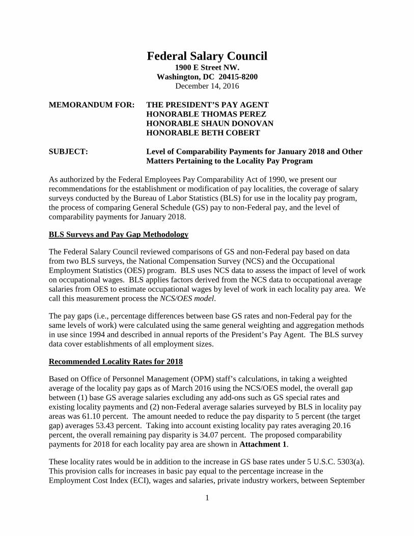
Federal Salary Council 1900 E Street NW.
Washington, DC 20415-8200 December 14, 2016
MEMORANDUM FOR: THE PRESIDENT’S PAY AGENT HONORABLE THOMAS PEREZ HONORABLE SHAUN DONOVAN HONORABLE BETH COBERT
SUBJECT: Level of Comparability Payments for January 2018 and Other
Matters Pertaining to the Locality Pay Program As authorized by the Federal Employees Pay Comparability Act of 1990, we present our recommendations for the establishment or modification of pay localities, the coverage of salary surveys conducted by the Bureau of Labor Statistics (BLS) for use in the locality pay program, the process of comparing General Schedule (GS) pay to non-Federal pay, and the level of comparability payments for January 2018.
BLS Surveys and Pay Gap Methodology
The Federal Salary Council reviewed comparisons of GS and non-Federal pay based on data from two BLS surveys, the National Compensation Survey (NCS) and the Occupational Employment Statistics (OES) program. BLS uses NCS data to assess the impact of level of work on occupational wages. BLS applies factors derived from the NCS data to occupational average salaries from OES to estimate occupational wages by level of work in each locality pay area. We call this measurement process the NCS/OES model.
The pay gaps (i.e., percentage differences between base GS rates and non-Federal pay for the same levels of work) were calculated using the same general weighting and aggregation methods in use since 1994 and described in annual reports of the President’s Pay Agent. The BLS survey data cover establishments of all employment sizes.
Recommended Locality Rates for 2018
Based on Office of Personnel Management (OPM) staff’s calculations, in taking a weighted average of the locality pay gaps as of March 2016 using the NCS/OES model, the overall gap between (1) base GS average salaries excluding any add-ons such as GS special rates and existing locality payments and (2) non-Federal average salaries surveyed by BLS in locality pay areas was 61.10 percent. The amount needed to reduce the pay disparity to 5 percent (the target gap) averages 53.43 percent. Taking into account existing locality pay rates averaging 20.16 percent, the overall remaining pay disparity is 34.07 percent. The proposed comparability payments for 2018 for each locality pay area are shown in Attachment 1.
These locality rates would be in addition to the increase in GS base rates under 5 U.S.C. 5303(a). This provision calls for increases in basic pay equal to the percentage increase in the Employment Cost Index (ECI), wages and salaries, private industry workers, between September
2
2015 and September 2016, less half a percentage point. The ECI increased 2.4 percent in September 2016, so the base GS increase in 2018 would be 1.9 percent.
In our recommendations for 2017 locality pay, we recommended that Burlington, VT, and Virginia Beach, VA, be established as new locality pay areas. (Like the 13 locality pay areas established as new locality pay areas in January 2016, Burlington and Virginia Beach both had pay gaps significantly exceeding that for the “Rest of U.S.” locality pay area over an extended period.) Accordingly, this report includes recommended locality pay rates for Burlington and Virginia Beach. We urge the Pay Agent to begin the regulatory process to establish Burlington and Virginia Beach as new locality pay areas.
Terms Used in Referring to Composition of Locality Pay Areas
These recommendations will cover several issues related to the definition of locality pay areas. In discussion of these issues, the terms basic locality pay area and area of application will be used. By way of review, locality pay areas consist of (1) a main metropolitan area forming the basic locality pay area and, where criteria recommended by the Council and approved by the Pay Agent are met, (2) areas of application. Areas of application are locations that are adjacent to the basic locality pay area and meet approved criteria for inclusion in the locality pay area.
Updated Commuting Patterns Data for Calculating Employment Interchange Rates
Since January 2014, our recommendations for establishing areas of application have been based on employment interchange rates calculated using commuting patterns data collected by the U.S. Census Bureau between 2006 and 2010 as part of the American Community Survey. (The “employment interchange rate”—also referred to as the “commuting rate” in some past Council documents—is the sum of (1) the percentage of employed residents of the area under consideration who work in the basic locality pay area and (2) the percentage of the employment in the area under consideration that is accounted for by workers who reside in the basic locality pay area. The employment interchange rate is calculated by including all workers in assessed locations, not just Federal employees.) The Census Bureau has issued updated commuting patterns data collected between 2009 and 2013 as part of the American Community Survey. The commuting patterns data presented in these recommendations are updated accordingly, and we recommend the updated commuting patterns be used in the locality pay program.
In applying criteria approved by the Pay Agent for areas of application, we found that the single-county location McKinley County, NM, qualifies as an area of application to the Albuquerque locality pay area. It is adjacent to the Albuquerque basic locality pay area and has 1,550 GS employees and a 7.88 percent employment interchange rate with the basic locality pay area. Under current criteria, for an adjacent single county an employment interchange rate of 7.5 percent or more and GS employment of 400 or more qualify the single county as an area of application. Accordingly, we recommend that McKinley County, NM, be included in the Albuquerque locality pay area as an area of application.
Updated Definitions of Metropolitan Areas
Metropolitan areas defined by the Office of Management and Budget (OMB) are the basis of locality pay area boundaries and are also considered in the evaluation of “Rest of U.S.” locations
3
as potential areas of application to locality pay areas. In July 2015, OMB made minor updates to its definitions of metropolitan areas, which are detailed in OMB Bulletin 15-01. The current regulations defining locality pay areas provide that basic locality pay areas—
• Will include the same locations as those included in the combined statistical areas (CSAs) and metropolitan statistical areas (MSAs) defined in OMB Bulletin 13-01 and comprising each basic locality pay area; and
• Will include any locations subsequently added to the applicable MSA or CSA by OMB.
Considering the provision in the regulations, we recommend that the updated definitions of CSAs and MSAs be used for analytic purposes in the locality pay program.
Monitoring of Pay Gaps in “Rest of U.S.” Metropolitan Areas
We continue to monitor pay gaps for “Rest of U.S.” metropolitan areas that have 2,500 or more GS employees and for which BLS is able to produce NCS/OES salary estimates. We refer to such “Rest of U.S.” areas as “research areas.”
Recommending Birmingham, AL, and San Antonio, TX, as New Locality Pay Areas
We are now monitoring pay gaps in 45 research areas. We studied pay gaps for these areas, compared to the “Rest of U.S.” pay gap, over a 3-year period (2014-2016). Over that period, the pay gaps for the Birmingham, AL, and San Antonio, TX, research areas exceeded that for the “Rest of U.S.” locality pay area by more than 10 percentage points on average.
Since the pay gap for the Birmingham and San Antonio research areas both significantly exceeded the “Rest of U.S.” pay gap over the 3-year period studied (2014-2016), we recommend that those two areas be established as separate locality pay areas in 2018.
Defining Locality Pay Areas
A brief history of Council recommendations on the establishment of locality pay area boundaries can be found in our January 23, 2014, recommendations on the locality pay program. Those recommendations and other Council materials can be found posted on the OPM website at http://www.opm.gov/policy-data-oversight/pay-leave/pay-systems/general-schedule/#url=Federal-Salary-Council.
For this set of Council recommendations, we are focused on the following issues with respect to defining locality pay areas:
• Regarding new locality pay areas, as discussed above—
o Urging the Pay Agent to begin the regulatory process to establish Burlington, VT, and Virginia Beach, VA, as new locality pay areas, and
o Recommending Birmingham, AL, and San Antonio, TX, for establishment as new locality pay areas, as discussed above.
4
• Evaluating areas in the vicinity of locality pay areas, including— o Eliminating the GS employment criterion and adjusting commuting criteria,
o Evaluation of multi-county micropolitan statistical areas in the vicinity of locality pay areas, and
o Criteria for evaluating single-county locations adjacent to multiple locality pay areas.
Evaluating Areas in the Vicinity of Locality Pay Areas
Some of our recommendations this year are resubmissions of recommendations for evaluating areas in the vicinity of locality pay areas, which the Pay Agent has not approved. We continue to believe these recommendations are based on sound compensation analysis, and we urge the Pay Agent to reconsider its views on them.
Current Criteria
Our current criteria for adding adjacent Core-Based Statistical Areas (CBSAs) or counties to locality pay areas are:
• For a multi-county CBSA adjacent to a basic locality pay area: 1,500 or more GS employees and an employment interchange rate with the basic locality pay area of at least 7.5 percent.
• For a single county that is not part of a multi-county, non-micropolitan CBSA and is adjacent to a basic locality pay area: 400 or more GS employees and an employment interchange rate with the basic locality pay area of at least 7.5 percent.
We also have criteria for evaluating individual Federal facilities with portions in more than one locality pay area:
• For Federal facilities that cross locality pay area boundaries: To be included in an adjacent locality pay area, the whole facility must have at least 500 GS employees, with the majority of those employees in the higher-paying locality pay area, or that portion of a Federal facility outside of a higher-paying locality pay area must have at least 750 GS employees, the duty stations of the majority of those employees must be within 10 miles of the separate locality pay area, and a significant number of those employees must commute to work from the higher-paying locality pay area.
As we recommended last year, the Council recommends leaving the criteria for Federal facilities unchanged but recommends the changes discussed below to the criteria for evaluating “Rest of U.S.” locations that are adjacent to separate locality pay areas.
Eliminating the GS Employment Criterion and Adjusting Commuting Criteria
For the last several years, the Council has recommended that the GS employment criterion be eliminated because GS employment is not an indicator of linkages among labor markets or other economic linkages among areas. Even though the Pay Agent has rejected this recommendation
5
for the past several years, the Council continues to believe defining areas of application based solely on commuting patterns is the more proper methodology. Accordingly, this year we resubmit our recommendation to eliminate the GS employment criterion.
As stated in our November 2014 recommendations, the Council has examined the economic literature on local labor markets and concludes that GS employment is not a useful criterion for establishing local labor markets.
Since the 1950s, labor economists (e.g., Wilcock and Sobel 1958; Tolbert and Sizer 1987; Casado-Diaz and Coombes 2011) have agreed on a definition of labor markets similar to that currently used by BLS. BLS (2014) describes labor markets as “an economically integrated geographic area within which individuals can reside and find employment within a reasonable distance or can readily change employment without changing their place of residence” (p. iii). Further, BLS (2014) notes that “Regardless of population size, commuting flows are an indication of the degree of integration of labor markets among counties; commutation data show the extent that workers have been willing and able to commute to other counties” (p. 168). Economists generally agree with the BLS position. For example, Casado-Diaz and Coombes (2011) note that “one crucial advantage of commuting data as the basis for definitions of [local labor market areas] is that the ‘friction of distance’ which restricts people’s patterns of movement causes most of the strongest interactions to be between nearby areas” (p. 13). See Attachment 3, which list sources considered in assessing the relevance of the GS employment criterion.
Accordingly, we again recommend that the employment interchange measure for “Rest of U.S.” counties not in a metropolitan statistical area (MSA) or combined statistical area (CSA) be increased from 7.5 percent to 20 percent, thus indicating an even stronger economic linkage among areas.
Since adjacent CBSAs are more likely to have employment opportunities in the CBSA and thus less commuting to the pay area, the criterion for CBSAs should remain at 7.5 percent for both multi-county CBSAs and single-county, non-micropolitan CBSAs.
Our recommended criteria for evaluating CBSAs or counties that are adjacent to the main locality pay area, i.e. the OMB-defined metropolitan area on which the locality pay area is based, are as follows:
• For a CBSA (includes single-county CBSAs other than single-county micropolitan areas) adjacent to a basic locality pay area: an employment interchange rate with the basic locality pay area of at least 7.5 percent.
• For a county that is not part of a CBSA or comprises a single-county micropolitan area and is adjacent to a basic locality pay area: an employment interchange rate with the basic locality pay area of at least 20 percent.
Alternative in the Event the Pay Agent Retains the GS Employment Criterion
We hope the Pay Agent will take a fresh look at the sound reasoning behind our recommendation to eliminate the GS employment criterion, and approve that recommendation. However, for
6
2018 we are offering an additional recommendation regarding the GS employment criterion. If the Pay Agent continues to use GS employment in deciding whether an adjacent “Rest of U.S.” location should be added to a separate locality pay area, we recommend reducing the required GS employment where there are very high levels of employment interchange between a “Rest of U.S.” location and a basic locality pay area. Specifically, regarding “Rest of U.S.” locations adjacent to basic locality pay areas, we recommend that—
• For adjacent “Rest of U.S.” locations with an employment interchange rate of at least 20 percent but less than 30 percent, the GS employment criterion be reduced to 100 GS employees; and
• For adjacent “Rest of U.S.” locations with employment interchange rates greater than or equal to 30 percent, the GS employment criterion be set at some level below 100—and preferably completely eliminated.
Employment interchange rates for some “Rest of U.S.” locations are very high. A number of locations have employment interchange rates of more than 50 percent—much higher than the 7.5 percent employment interchange rate the Pay Agent now combines with GS employment to qualify “Rest of U.S.” areas as areas of application.
Micropolitan Areas
We continue to believe it is appropriate to treat multi-county micropolitan statistical areas the same as multi-county metropolitan statistical areas in evaluating locations in the vicinity of locality pay areas, so we are resubmitting our December 2015 recommendation on multi-county micropolitan areas.
As noted in our December 2015 recommendations, historically there has been some controversy about the use of micropolitan statistical areas for locality pay. Micropolitan areas are CBSAs where the largest population center has between 10,000 and 49,999 residents. The Pay Agent concluded it would not use micropolitan areas in the locality pay program except when included in a CSA with one or more MSAs—micropolitan areas are too small with too little economic activity to be considered separately. The Council, on the other hand, recommended in 2003 that micropolitan statistical areas be used if part of any CSA, whether or not an MSA was included. For example, under the Council’s view, the Claremont, NH-VT, CSA—a four-county CSA in 2003 composed of two micropolitan areas, would have been considered as a unit. Under the Pay Agent’s view, the Claremont area would not have been considered as a unit but rather evaluated as four separate counties.
In February 2013, presumably due to increased commuting among the components, OMB redelineated the Claremont, NH-VT CSA into a single four-county, stand-alone micropolitan area. Under the Council’s earlier recommendation on micropolitan areas discussed above, the Claremont area would no longer qualify to be considered as a unit because the same four counties are no longer combined as a CSA but rather into a single micropolitan area. To avoid this incongruous result, the Council changed its earlier position to recognize multi-county micropolitan areas, not just those in CSAs, while continuing to evaluate single-county micropolitan areas as single counties. The Council recommended to the Pay Agent that multi-county micropolitan statistical areas be treated the same as multi-county metropolitan statistical
7
areas in the locality pay program. The Pay Agent did not approve that recommendation.
We urge the Pay Agent to reconsider its views on micropolitan statistical areas and approve our recommendation to treat multi-county micropolitan statistical areas the same as multi-county metropolitan statistical areas in evaluating locations in the vicinity of locality pay areas.
Completely or Almost Completely Surrounded “Rest of U.S.” Locations
The Council has previously recommended that “Rest of U.S.” locations completely surrounded by higher-paying locality pay areas be added to the pay area with which such locations have the highest commuting, and that partially surrounded areas be evaluated by the Pay Agent on a case-by-case basis. The Pay Agent has agreed that a single-county “Rest of U.S.” location completely surrounded by higher-paying locality pay areas should be added to the adjacent locality pay area with which the county has the highest level of commuting.
Regarding partially surrounded areas, while below we resubmit our November 2014 recommendations for single-county locations bordered by multiple locality pay areas, which addresses some partially surrounded locations, we still believe it is unclear at what point being bordered by higher-paying areas constitutes a problem. Hence, the Council continues to believe that the Pay Agent should evaluate additional partially surrounded locations on a case-by-case basis.
Special Recommendation for San Luis Obispo County, CA
There is one partially surrounded “Rest of U.S.” location for which we have decided to make a special recommendation. San Luis Obispo County, CA, is bordered to the north by the San Jose locality pay area, bordered to the south and east by the Los Angeles locality pay area, and bordered to the west by the Pacific Ocean. More than 99 percent of its land boundary is bordered by the Los Angeles and San Jose locality pay areas.
Because practically all of San Luis Obispo County’s land boundary is bordered by the Los Angeles and San Jose locality pay areas, we believe the county should be treated as a surrounded “Rest of U.S.” location. Specifically, as a county surrounded by two locality pay areas, San Luis Obispo should be added to the Los Angeles locality pay area, with which it has the highest employment interchange rate. We recommend the Pay Agent make that change during the regulatory process establishing Burlington, VT, and Virginia Beach, VA, as new locality pay areas—a change we recommended in our recommendations for locality pay in 2017.
While we believe that San Luis Obispo County should be treated as a completely surrounded location, it is less clear what additional recommendations should be made for other partially surrounded locations beyond our recommendations below for single-county locations bordered by multiple locality pay areas. We believe a comprehensive Council Working Group study of partially surrounded locations should precede any new recommendations for such locations.
Evaluating Single-County Locations Adjacent to Multiple Locality Pay Areas
We first recommended adding criteria for evaluating single-county “Rest of U.S.” locations that border multiple locality pay areas in our November 2014 recommendations. The Pay Agent, in
8
its report on locality pay in 2016, said it could see the logic of that recommendation in the context of the Council’s recommendation to eliminate the GS employment criterion (which the Pay Agent did not approve). Accordingly, since we are resubmitting our recommendation to eliminate the GS employment criterion, we are also resubmitting our recommendation regarding single-county locations adjacent to multiple locality pay areas. That recommendation is explained again below.
Our other recommendations presented so far would result in some single-county locations remaining in the “Rest of U.S.” locality pay area while being adjacent to multiple separate locality pay areas. When mapped with our other recommendations for defining locality pay areas, such “Rest of U.S.” locations often appear surrounded, or nearly surrounded, by higher-paying locality pay areas. We believe that, without some remedy, Federal employers in such locations could have staffing problems caused by higher locality pay nearby, so we are making a recommendation to evaluate such locations for possible inclusion in one of the separate locality pay areas they border:
• For single counties adjacent to multiple locality pay areas and not qualifying under our other proposed criteria—
o For a county comprising a single-county CBSA other than a micropolitan area, the sum of commuting rates to the separate basic locality pay areas must be greater than or equal to 7.5 percent.
o For a county that either is not in any CBSA or comprises a single-county micropolitan statistical area, the sum of commuting rates to the separate basic locality pay areas must be greater than or equal to 20 percent.
Under this recommendation, counties with the required sum of commuting rates would be covered by the adjacent separate locality pay area with which the single county location has the highest level of commuting. The locations that would be added to separate locality pay areas under this recommendation, if our other recommendations are approved, are shown in Attachment 7.
Impact of Applying Recommended Criteria for Evaluating Adjacent “Rest of U.S.” Areas
Proposed new areas of application are shown in Attachments 4-7. Regarding those attachments—
• Attachment 4 shows multi-county MSAs, CSAs, and micropolitan areas qualifying as areas of application under the proposed CBSA criteria;
• Attachment 5 shows single-county CBSAs qualifying as areas of application under the proposed CBSA criteria (single-county metropolitan statistical areas, not micropolitan areas, with an employment interchange rate of 7.5 percent or more);
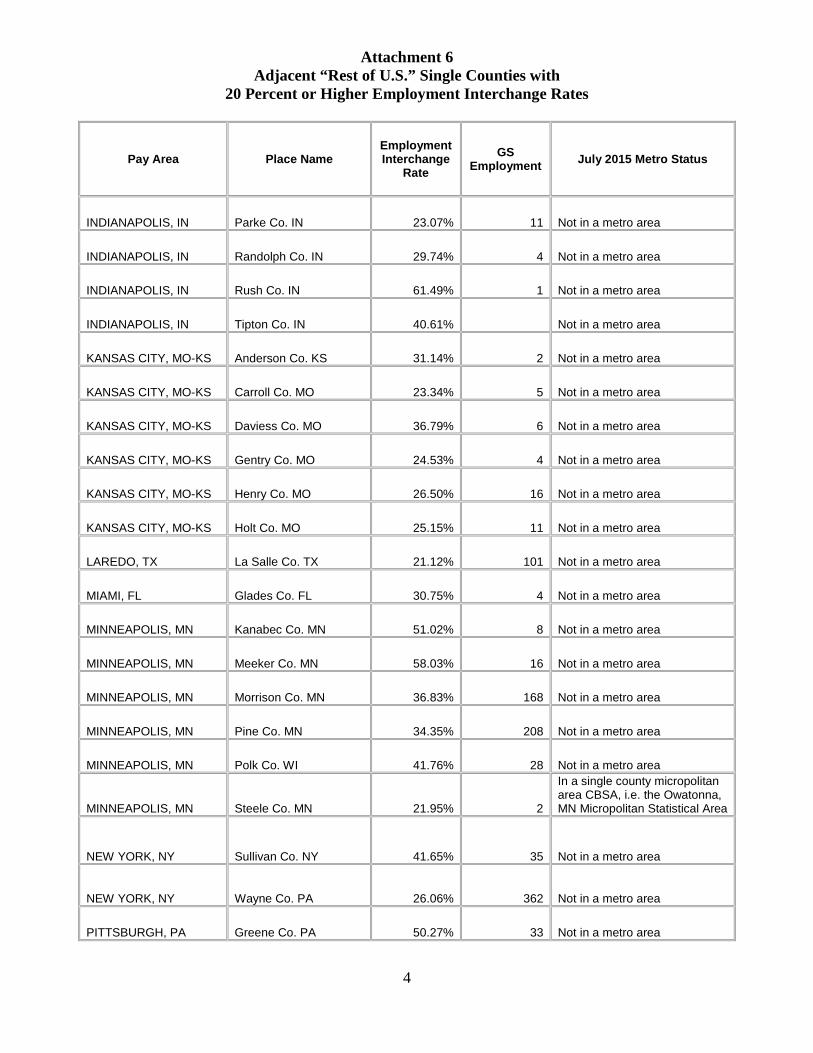
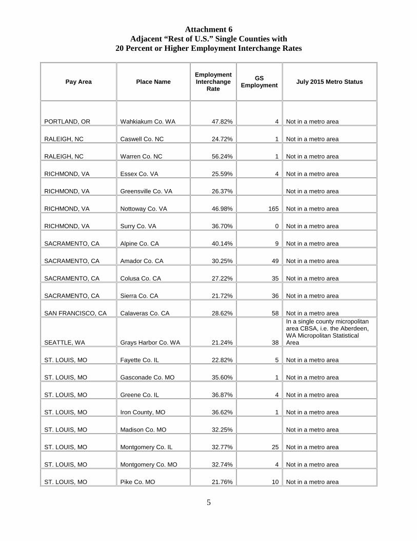
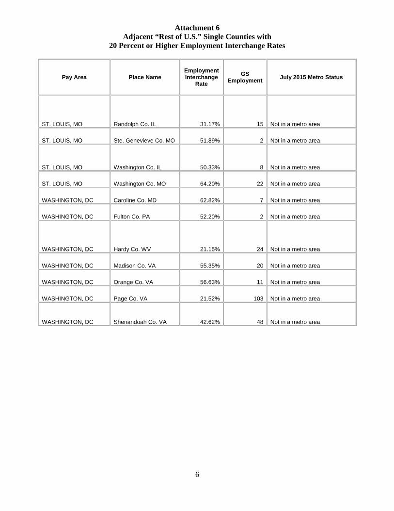
• Attachment 6 shows counties qualifying as areas of application under the proposed criteria for adjacent counties that are not part of a CBSA or comprise a single-county micropolitan area; and
• Attachment 7 shows counties qualifying as areas of application under the proposed
9
criteria for single-county locations adjacent to multiple locality pay areas and not qualifying under other criteria as areas of application.
Under these recommendations, locality pay area coverage would change for about 13,251 GS employees who are now in the “Rest of U.S.” locality pay area and would be covered, under our proposed Council recommendations, by separate locality pay areas.
Requests to be Included in Higher-Paying Locality Pay Areas
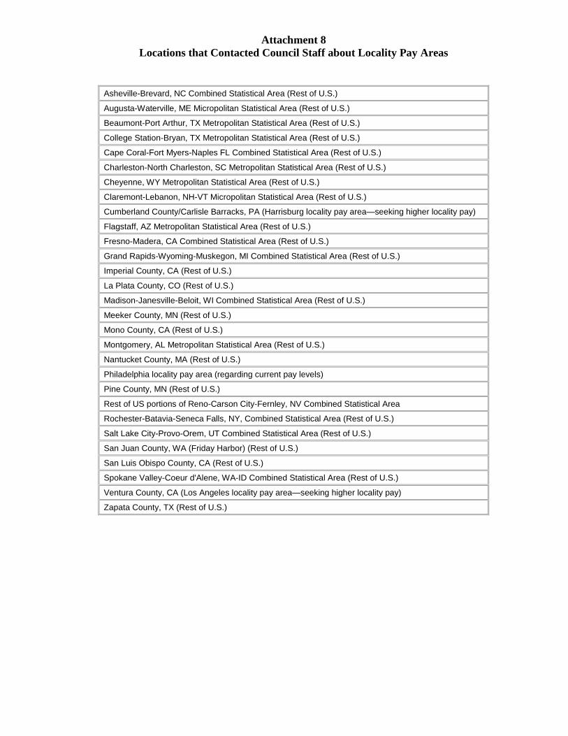
Federal Salary Council staff had contacts from employees in 29 locations since the November 6, 2016, Council meeting. Most of these are “Rest of U.S.” areas requesting that the areas be included in new or existing locality pay areas separate from the “Rest of U.S.” locality pay area. These areas are listed in the table in Attachment 8.
In addition to simple contacts, we also received more detailed inquiries or petitions from groups or employees in some “Rest of U.S.” locations. For example, we received detailed written materials from groups or employees in Charleston, SC; Cumberland County, PA; Imperial County, CA; Montgomery, AL; Nantucket, MA; Pine County, MN; Reno, NV; San Juan, WA; and San Luis Obispo, CA.
Some of the areas that contacted Federal Salary Council staff would benefit from our other recommendations. For others that do not meet our criteria, the Council recommends that OPM continue to encourage agencies to use other pay flexibilities such as recruitment, retention, and relocation payments, and special salary rates to ease any staffing problems in these areas.
Summary of Major Recommendations
In summary, our major recommendations for 2018 include the following:
• We recommend using the 2018 locality rates shown in Attachment 1.
• We urge the Pay Agent to begin the regulatory process to establish Burlington, VT, and Virginia Beach, VA, as new locality pay areas as soon as possible.
• We recommend establishing Birmingham, AL, and San Antonio, TX, as separate locality pay areas.
• We recommend modifying the qualifying criteria for new areas of application as stated above.
By direction of the Council:
SIGNED Stephen E. Condrey, Ph.D. Chairman
Attachments
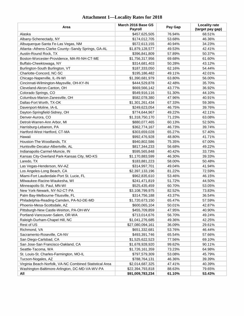
Attachment 1—Locality Rates for 2018
Area March 2016 Base GS Payroll Pay Gap Locality rate
(target pay gap) Alaska $457,625,505 76.94% 68.51% Albany-Schenectady, NY $174,012,705 53.68% 46.36% Albuquerque-Santa Fe-Las Vegas, NM $572,613,155 40.94% 34.23% Atlanta--Athens-Clarke County--Sandy Springs, GA-AL $1,879,128,577 49.53% 42.41% Austin-Round Rock, TX $396,841,809 57.89% 50.37% Boston-Worcester-Providence, MA-RI-NH-CT-ME $1,756,317,956 69.68% 61.60% Buffalo-Cheektowaga, NY $314,681,403 50.28% 43.12% Burlington-South Burlington, VT $187,333,050 62.16% 54.44% Charlotte-Concord, NC-SC $195,186,482 49.11% 42.01% Chicago-Naperville, IL-IN-WI $1,390,681,979 63.80% 56.00% Cincinnati-Wilmington-Maysville, OH-KY-IN $444,529,878 42.48% 35.70% Cleveland-Akron-Canton, OH $669,566,142 43.77% 36.92% Colorado Springs, CO $549,916,116 51.30% 44.10% Columbus-Marion-Zanesville, OH $582,078,380 47.96% 40.91% Dallas-Fort Worth, TX-OK $1,301,261,434 67.33% 59.36% Davenport-Moline, IA-IL $249,623,054 46.75% 39.76% Dayton-Springfield-Sidney, OH $774,644,967 49.22% 42.11% Denver-Aurora, CO $1,318,750,170 71.23% 63.08% Detroit-Warren-Ann Arbor, MI $880,077,465 60.13% 52.50% Harrisburg-Lebanon, PA $362,774,167 46.73% 39.74% Hartford-West Hartford, CT-MA $303,659,028 65.27% 57.40% Hawaii $992,476,928 48.80% 41.71% Houston-The Woodlands, TX $940,802,586 75.35% 67.00% Huntsville-Decatur-Albertville, AL $817,344,233 56.68% 49.22% Indianapolis-Carmel-Muncie, IN $595,565,848 40.42% 33.73% Kansas City-Overland Park-Kansas City, MO-KS $1,170,883,599 46.30% 39.33% Laredo, TX $183,881,223 58.00% 50.48% Las Vegas-Henderson, NV-AZ $314,997,701 49.04% 41.94% Los Angeles-Long Beach, CA $2,397,133,196 81.22% 72.59% Miami-Fort Lauderdale-Port St. Lucie, FL $962,835,610 53.46% 46.15% Milwaukee-Racine-Waukesha, WI $241,471,819 51.72% 44.50% Minneapolis-St. Paul, MN-WI $525,435,459 60.70% 53.05% New York-Newark, NY-NJ-CT-PA $3,108,799,975 82.52% 73.83% Palm Bay-Melbourne-Titusville, FL $314,756,188 43.37% 36.54% Philadelphia-Reading-Camden, PA-NJ-DE-MD $1,720,673,150 65.47% 57.59% Phoenix-Mesa-Scottsdale, AZ $600,065,104 50.01% 42.87% Pittsburgh-New Castle-Weirton, PA-OH-WV $455,709,859 47.95% 40.90% Portland-Vancouver-Salem, OR-WA $713,014,676 56.70% 49.24% Raleigh-Durham-Chapel Hill, NC $1,041,276,685 49.36% 42.25% Rest of US $27,080,094,161 36.09% 29.61% Richmond, VA $651,332,681 53.76% 46.44% Sacramento-Roseville, CA-NV $493,391,746 65.54% 57.66% San Diego-Carlsbad, CA $1,525,622,523 77.56% 69.10% San Jose-San Francisco-Oakland, CA $1,678,928,920 99.62% 90.11% Seattle-Tacoma, WA $1,726,161,359 73.23% 64.98% St. Louis-St. Charles-Farmington, MO-IL $797,579,309 53.08% 45.79% Tucson-Nogales, AZ $788,764,131 46.36% 39.39% Virginia Beach-Norfolk, VA-NC Combined Statistical Area $2,014,687,325 47.41% 40.39% Washington-Baltimore-Arlington, DC-MD-VA-WV-PA $22,394,793,818 88.63% 79.65% All $91,009,783,234 61.10% 53.43%
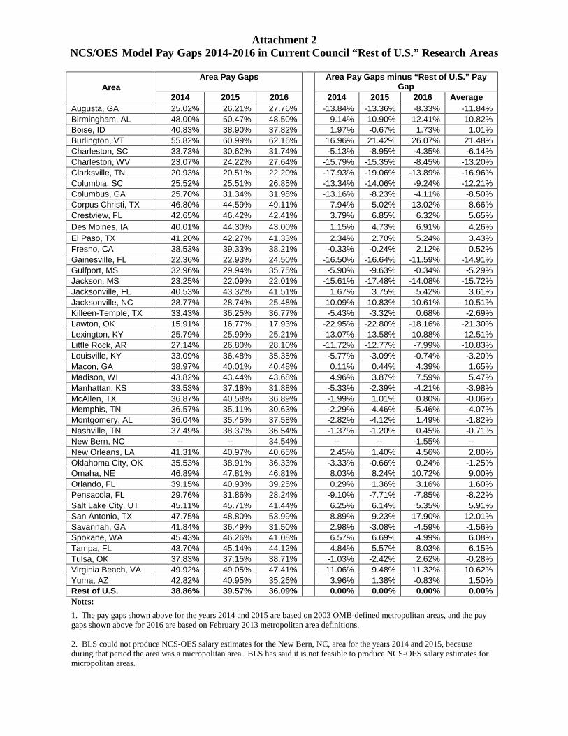
Attachment 2 NCS/OES Model Pay Gaps 2014-2016 in Current Council “Rest of U.S.” Research Areas
Area Area Pay Gaps Area Pay Gaps minus “Rest of U.S.” Pay
Gap 2014 2015 2016 2014 2015 2016 Average
Augusta, GA 25.02% 26.21% 27.76% -13.84% -13.36% -8.33% -11.84% Birmingham, AL 48.00% 50.47% 48.50% 9.14% 10.90% 12.41% 10.82% Boise, ID 40.83% 38.90% 37.82% 1.97% -0.67% 1.73% 1.01% Burlington, VT 55.82% 60.99% 62.16% 16.96% 21.42% 26.07% 21.48% Charleston, SC 33.73% 30.62% 31.74% -5.13% -8.95% -4.35% -6.14% Charleston, WV 23.07% 24.22% 27.64% -15.79% -15.35% -8.45% -13.20% Clarksville, TN 20.93% 20.51% 22.20% -17.93% -19.06% -13.89% -16.96% Columbia, SC 25.52% 25.51% 26.85% -13.34% -14.06% -9.24% -12.21% Columbus, GA 25.70% 31.34% 31.98% -13.16% -8.23% -4.11% -8.50% Corpus Christi, TX 46.80% 44.59% 49.11% 7.94% 5.02% 13.02% 8.66% Crestview, FL 42.65% 46.42% 42.41% 3.79% 6.85% 6.32% 5.65% Des Moines, IA 40.01% 44.30% 43.00% 1.15% 4.73% 6.91% 4.26% El Paso, TX 41.20% 42.27% 41.33% 2.34% 2.70% 5.24% 3.43% Fresno, CA 38.53% 39.33% 38.21% -0.33% -0.24% 2.12% 0.52% Gainesville, FL 22.36% 22.93% 24.50% -16.50% -16.64% -11.59% -14.91% Gulfport, MS 32.96% 29.94% 35.75% -5.90% -9.63% -0.34% -5.29% Jackson, MS 23.25% 22.09% 22.01% -15.61% -17.48% -14.08% -15.72% Jacksonville, FL 40.53% 43.32% 41.51% 1.67% 3.75% 5.42% 3.61% Jacksonville, NC 28.77% 28.74% 25.48% -10.09% -10.83% -10.61% -10.51% Killeen-Temple, TX 33.43% 36.25% 36.77% -5.43% -3.32% 0.68% -2.69% Lawton, OK 15.91% 16.77% 17.93% -22.95% -22.80% -18.16% -21.30% Lexington, KY 25.79% 25.99% 25.21% -13.07% -13.58% -10.88% -12.51% Little Rock, AR 27.14% 26.80% 28.10% -11.72% -12.77% -7.99% -10.83% Louisville, KY 33.09% 36.48% 35.35% -5.77% -3.09% -0.74% -3.20% Macon, GA 38.97% 40.01% 40.48% 0.11% 0.44% 4.39% 1.65% Madison, WI 43.82% 43.44% 43.68% 4.96% 3.87% 7.59% 5.47% Manhattan, KS 33.53% 37.18% 31.88% -5.33% -2.39% -4.21% -3.98% McAllen, TX 36.87% 40.58% 36.89% -1.99% 1.01% 0.80% -0.06% Memphis, TN 36.57% 35.11% 30.63% -2.29% -4.46% -5.46% -4.07% Montgomery, AL 36.04% 35.45% 37.58% -2.82% -4.12% 1.49% -1.82% Nashville, TN 37.49% 38.37% 36.54% -1.37% -1.20% 0.45% -0.71% New Bern, NC -- -- 34.54% -- -- -1.55% -- New Orleans, LA 41.31% 40.97% 40.65% 2.45% 1.40% 4.56% 2.80% Oklahoma City, OK 35.53% 38.91% 36.33% -3.33% -0.66% 0.24% -1.25% Omaha, NE 46.89% 47.81% 46.81% 8.03% 8.24% 10.72% 9.00% Orlando, FL 39.15% 40.93% 39.25% 0.29% 1.36% 3.16% 1.60% Pensacola, FL 29.76% 31.86% 28.24% -9.10% -7.71% -7.85% -8.22% Salt Lake City, UT 45.11% 45.71% 41.44% 6.25% 6.14% 5.35% 5.91% San Antonio, TX 47.75% 48.80% 53.99% 8.89% 9.23% 17.90% 12.01% Savannah, GA 41.84% 36.49% 31.50% 2.98% -3.08% -4.59% -1.56% Spokane, WA 45.43% 46.26% 41.08% 6.57% 6.69% 4.99% 6.08% Tampa, FL 43.70% 45.14% 44.12% 4.84% 5.57% 8.03% 6.15% Tulsa, OK 37.83% 37.15% 38.71% -1.03% -2.42% 2.62% -0.28% Virginia Beach, VA 49.92% 49.05% 47.41% 11.06% 9.48% 11.32% 10.62% Yuma, AZ 42.82% 40.95% 35.26% 3.96% 1.38% -0.83% 1.50% Rest of U.S. 38.86% 39.57% 36.09% 0.00% 0.00% 0.00% 0.00% Notes: 1. The pay gaps shown above for the years 2014 and 2015 are based on 2003 OMB-defined metropolitan areas, and the pay gaps shown above for 2016 are based on February 2013 metropolitan area definitions. 2. BLS could not produce NCS-OES salary estimates for the New Bern, NC, area for the years 2014 and 2015, because during that period the area was a micropolitan area. BLS has said it is not feasible to produce NCS-OES salary estimates for micropolitan areas.
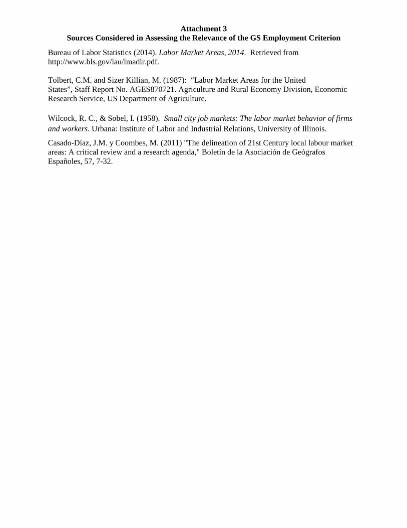
Attachment 3 Sources Considered in Assessing the Relevance of the GS Employment Criterion
Bureau of Labor Statistics (2014). Labor Market Areas, 2014. Retrieved from http://www.bls.gov/lau/lmadir.pdf. Tolbert, C.M. and Sizer Killian, M. (1987): “Labor Market Areas for the United States”, Staff Report No. AGES870721. Agriculture and Rural Economy Division, Economic Research Service, US Department of Agriculture.
Wilcock, R. C., & Sobel, I. (1958). Small city job markets: The labor market behavior of firms and workers. Urbana: Institute of Labor and Industrial Relations, University of Illinois.
Casado-Díaz, J.M. y Coombes, M. (2011) "The delineation of 21st Century local labour market areas: A critical review and a research agenda," Boletín de la Asociación de Geógrafos Españoles, 57, 7-32.
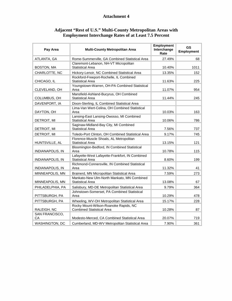
Attachment 4
Adjacent “Rest of U.S.” Multi-County Metropolitan Areas with Employment Interchange Rates of at Least 7.5 Percent
Pay Area Multi-County Metropolitan Area Employment Interchange
Rate GS
Employment
ATLANTA, GA Rome-Summerville, GA Combined Statistical Area 27.49% 68
BOSTON, MA Claremont-Lebanon, NH-VT Micropolitan Statistical Area 10.40% 1011
CHARLOTTE, NC Hickory-Lenoir, NC Combined Statistical Area 13.35% 152
CHICAGO, IL Rockford-Freeport-Rochelle, IL Combined Statistical Area 11.63% 225
CLEVELAND, OH Youngstown-Warren, OH-PA Combined Statistical Area 11.07% 954
COLUMBUS, OH Mansfield-Ashland-Bucyrus, OH Combined Statistical Area 11.44% 245
DAVENPORT, IA Dixon-Sterling, IL Combined Statistical Area
DAYTON, OH Lima-Van Wert-Celina, OH Combined Statistical Area 10.03% 163
DETROIT, MI Lansing-East Lansing-Owosso, MI Combined Statistical Area 10.06% 786
DETROIT, MI Saginaw-Midland-Bay City, MI Combined Statistical Area 7.56% 737
DETROIT, MI Toledo-Port Clinton, OH Combined Statistical Area 9.17% 745
HUNTSVILLE, AL Florence-Muscle Shoals, AL Metropolitan Statistical Area 13.15% 121
INDIANAPOLIS, IN Bloomington-Bedford, IN Combined Statistical Area 10.78% 115
INDIANAPOLIS, IN Lafayette-West Lafayette-Frankfort, IN Combined Statistical Area 8.60% 199
INDIANAPOLIS, IN Richmond-Connersville, IN Combined Statistical Area 11.32% 41
MINNEAPOLIS, MN Brainerd, MN Micropolitan Statistical Area 7.59% 273
MINNEAPOLIS, MN Mankato-New Ulm-North Mankato, MN Combined Statistical Area 13.08% 67
PHILADELPHIA, PA Salisbury, MD-DE Metropolitan Statistical Area 9.79% 364
PITTSBURGH, PA Johnstown-Somerset, PA Combined Statistical Area 10.29% 478
PITTSBURGH, PA Wheeling, WV-OH Metropolitan Statistical Area 15.17% 228
RALEIGH, NC Rocky Mount-Wilson-Roanoke Rapids, NC Combined Statistical Area 10.28% 87
SAN FRANCISCO, CA Modesto-Merced, CA Combined Statistical Area 20.07% 719 WASHINGTON, DC Cumberland, MD-WV Metropolitan Statistical Area 7.90% 361
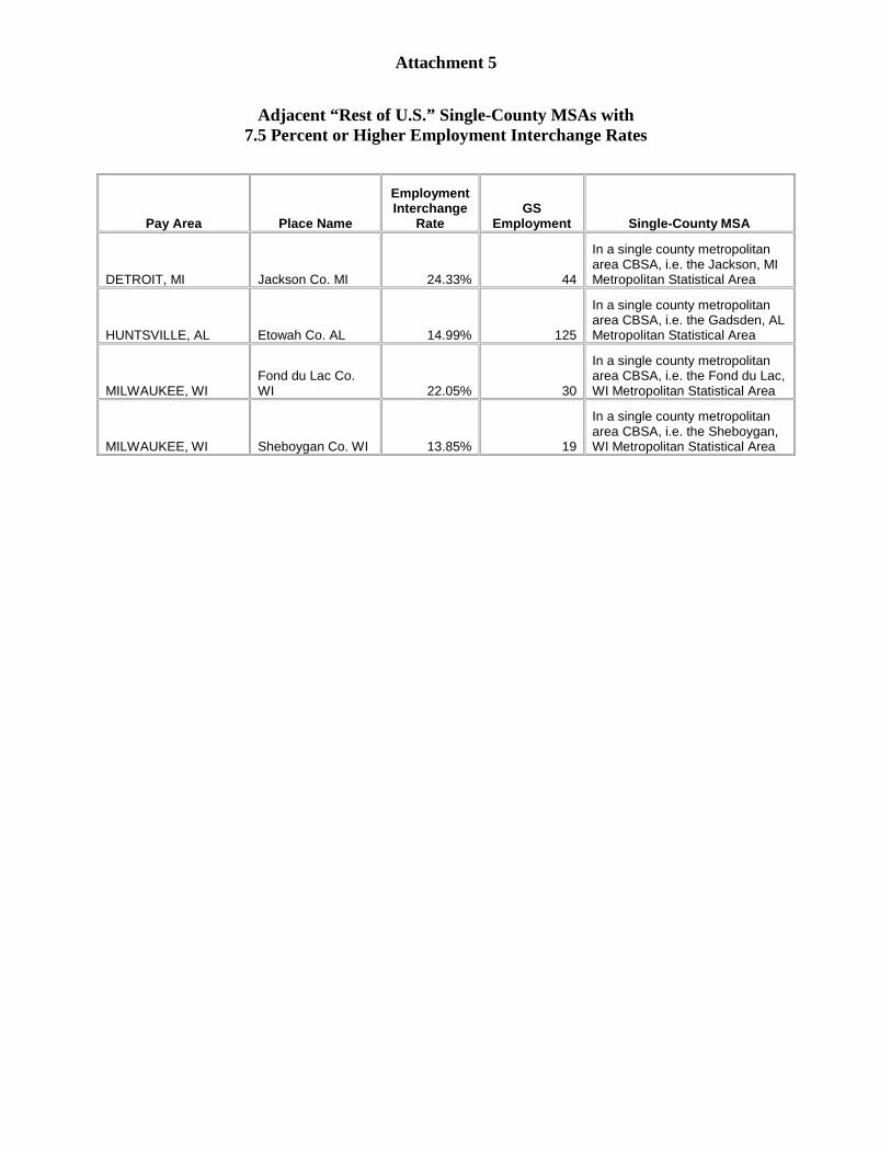
Attachment 5
Adjacent “Rest of U.S.” Single-County MSAs with 7.5 Percent or Higher Employment Interchange Rates
Pay Area Place Name
Employment Interchange
Rate GS
Employment Single-County MSA
DETROIT, MI Jackson Co. MI 24.33% 44
In a single county metropolitan area CBSA, i.e. the Jackson, MI Metropolitan Statistical Area
HUNTSVILLE, AL Etowah Co. AL 14.99% 125
In a single county metropolitan area CBSA, i.e. the Gadsden, AL Metropolitan Statistical Area
MILWAUKEE, WI Fond du Lac Co. WI 22.05% 30
In a single county metropolitan area CBSA, i.e. the Fond du Lac, WI Metropolitan Statistical Area
MILWAUKEE, WI Sheboygan Co. WI 13.85% 19
In a single county metropolitan area CBSA, i.e. the Sheboygan, WI Metropolitan Statistical Area
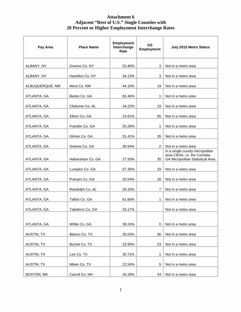
Attachment 6 Adjacent “Rest of U.S.” Single Counties with
20 Percent or Higher Employment Interchange Rates
1
Pay Area Place Name Employment Interchange
Rate GS
Employment July 2015 Metro Status
ALBANY, NY Greene Co. NY 53.46% 3 Not in a metro area
ALBANY, NY Hamilton Co. NY 34.13% 3 Not in a metro area
ALBUQUERQUE, NM Mora Co. NM 44.10% 19 Not in a metro area
ATLANTA, GA Banks Co. GA 82.46% 1 Not in a metro area
ATLANTA, GA Cleburne Co. AL 34.22% 19 Not in a metro area
ATLANTA, GA Elbert Co. GA 23.61% 55 Not in a metro area
ATLANTA, GA Franklin Co. GA 25.29% 1 Not in a metro area
ATLANTA, GA Gilmer Co. GA 31.41% 35 Not in a metro area
ATLANTA, GA Greene Co. GA 39.54% 2 Not in a metro area
ATLANTA, GA Habersham Co. GA 27.93% 35
In a single county micropolitan area CBSA, i.e. the Cornelia, GA Micropolitan Statistical Area
ATLANTA, GA Lumpkin Co. GA 67.35% 33 Not in a metro area
ATLANTA, GA Putnam Co. GA 33.54% 26 Not in a metro area
ATLANTA, GA Randolph Co. AL 29.16% 7 Not in a metro area
ATLANTA, GA Talbot Co. GA 61.66% 1 Not in a metro area
ATLANTA, GA Taliaferro Co. GA 33.17% Not in a metro area
ATLANTA, GA White Co. GA 39.24% 0 Not in a metro area
AUSTIN, TX Blanco Co. TX 26.03% 36 Not in a metro area
AUSTIN, TX Burnet Co. TX 23.90% 23 Not in a metro area
AUSTIN, TX Lee Co. TX 30.71% 1 Not in a metro area
AUSTIN, TX Milam Co. TX 22.54% 5 Not in a metro area
BOSTON, MA Carroll Co. NH 26.28% 44 Not in a metro area
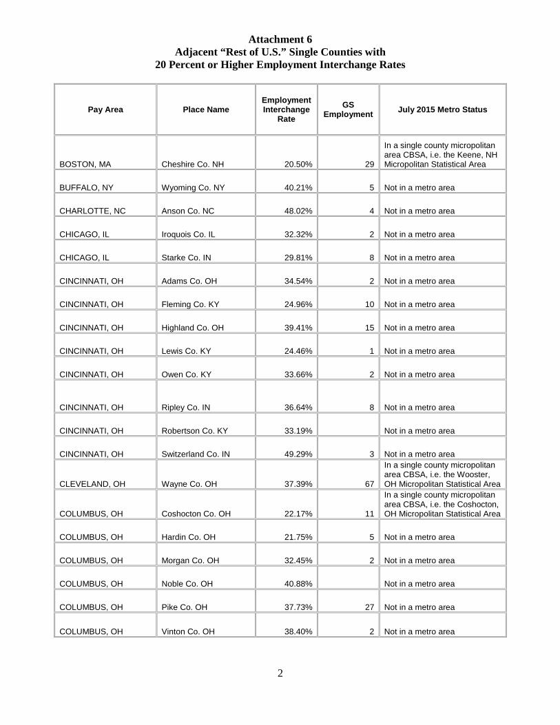
Attachment 6 Adjacent “Rest of U.S.” Single Counties with
20 Percent or Higher Employment Interchange Rates
2
Pay Area Place Name Employment Interchange
Rate GS
Employment July 2015 Metro Status
BOSTON, MA Cheshire Co. NH 20.50% 29
In a single county micropolitan area CBSA, i.e. the Keene, NH Micropolitan Statistical Area
BUFFALO, NY Wyoming Co. NY 40.21% 5 Not in a metro area
CHARLOTTE, NC Anson Co. NC 48.02% 4 Not in a metro area
CHICAGO, IL Iroquois Co. IL 32.32% 2 Not in a metro area
CHICAGO, IL Starke Co. IN 29.81% 8 Not in a metro area
CINCINNATI, OH Adams Co. OH 34.54% 2 Not in a metro area
CINCINNATI, OH Fleming Co. KY 24.96% 10 Not in a metro area
CINCINNATI, OH Highland Co. OH 39.41% 15 Not in a metro area
CINCINNATI, OH Lewis Co. KY 24.46% 1 Not in a metro area
CINCINNATI, OH Owen Co. KY 33.66% 2 Not in a metro area
CINCINNATI, OH Ripley Co. IN 36.64% 8 Not in a metro area
CINCINNATI, OH Robertson Co. KY 33.19% Not in a metro area
CINCINNATI, OH Switzerland Co. IN 49.29% 3 Not in a metro area
CLEVELAND, OH Wayne Co. OH 37.39% 67
In a single county micropolitan area CBSA, i.e. the Wooster, OH Micropolitan Statistical Area
COLUMBUS, OH Coshocton Co. OH 22.17% 11
In a single county micropolitan area CBSA, i.e. the Coshocton, OH Micropolitan Statistical Area
COLUMBUS, OH Hardin Co. OH 21.75% 5 Not in a metro area
COLUMBUS, OH Morgan Co. OH 32.45% 2 Not in a metro area
COLUMBUS, OH Noble Co. OH 40.88% Not in a metro area
COLUMBUS, OH Pike Co. OH 37.73% 27 Not in a metro area
COLUMBUS, OH Vinton Co. OH 38.40% 2 Not in a metro area
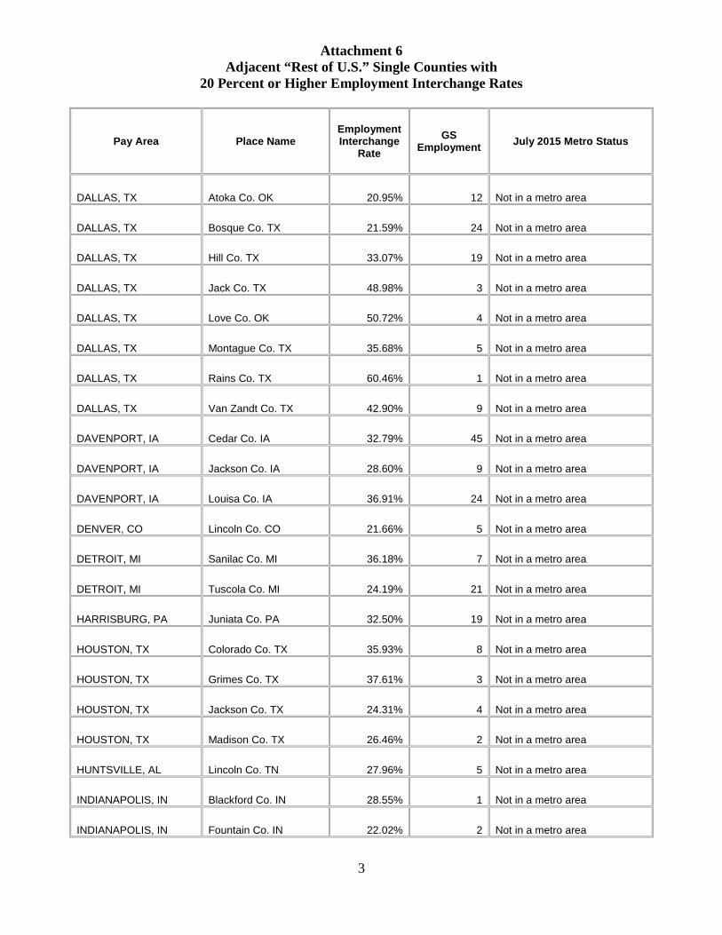
Attachment 6 Adjacent “Rest of U.S.” Single Counties with
20 Percent or Higher Employment Interchange Rates
3
Pay Area Place Name Employment Interchange
Rate GS
Employment July 2015 Metro Status
DALLAS, TX Atoka Co. OK 20.95% 12 Not in a metro area
DALLAS, TX Bosque Co. TX 21.59% 24 Not in a metro area
DALLAS, TX Hill Co. TX 33.07% 19 Not in a metro area
DALLAS, TX Jack Co. TX 48.98% 3 Not in a metro area
DALLAS, TX Love Co. OK 50.72% 4 Not in a metro area
DALLAS, TX Montague Co. TX 35.68% 5 Not in a metro area
DALLAS, TX Rains Co. TX 60.46% 1 Not in a metro area
DALLAS, TX Van Zandt Co. TX 42.90% 9 Not in a metro area
DAVENPORT, IA Cedar Co. IA 32.79% 45 Not in a metro area
DAVENPORT, IA Jackson Co. IA 28.60% 9 Not in a metro area
DAVENPORT, IA Louisa Co. IA 36.91% 24 Not in a metro area
DENVER, CO Lincoln Co. CO 21.66% 5 Not in a metro area
DETROIT, MI Sanilac Co. MI 36.18% 7 Not in a metro area
DETROIT, MI Tuscola Co. MI 24.19% 21 Not in a metro area
HARRISBURG, PA Juniata Co. PA 32.50% 19 Not in a metro area
HOUSTON, TX Colorado Co. TX 35.93% 8 Not in a metro area
HOUSTON, TX Grimes Co. TX 37.61% 3 Not in a metro area
HOUSTON, TX Jackson Co. TX 24.31% 4 Not in a metro area
HOUSTON, TX Madison Co. TX 26.46% 2 Not in a metro area
HUNTSVILLE, AL Lincoln Co. TN 27.96% 5 Not in a metro area
INDIANAPOLIS, IN Blackford Co. IN 28.55% 1 Not in a metro area
INDIANAPOLIS, IN Fountain Co. IN 22.02% 2 Not in a metro area
Attachment 6 Adjacent “Rest of U.S.” Single Counties with
20 Percent or Higher Employment Interchange Rates
4
Pay Area Place Name Employment Interchange
Rate GS
Employment July 2015 Metro Status
INDIANAPOLIS, IN Parke Co. IN 23.07% 11 Not in a metro area
INDIANAPOLIS, IN Randolph Co. IN 29.74% 4 Not in a metro area
INDIANAPOLIS, IN Rush Co. IN 61.49% 1 Not in a metro area
INDIANAPOLIS, IN Tipton Co. IN 40.61% Not in a metro area
KANSAS CITY, MO-KS Anderson Co. KS 31.14% 2 Not in a metro area
KANSAS CITY, MO-KS Carroll Co. MO 23.34% 5 Not in a metro area
KANSAS CITY, MO-KS Daviess Co. MO 36.79% 6 Not in a metro area
KANSAS CITY, MO-KS Gentry Co. MO 24.53% 4 Not in a metro area
KANSAS CITY, MO-KS Henry Co. MO 26.50% 16 Not in a metro area
KANSAS CITY, MO-KS Holt Co. MO 25.15% 11 Not in a metro area
LAREDO, TX La Salle Co. TX 21.12% 101 Not in a metro area
MIAMI, FL Glades Co. FL 30.75% 4 Not in a metro area
MINNEAPOLIS, MN Kanabec Co. MN 51.02% 8 Not in a metro area
MINNEAPOLIS, MN Meeker Co. MN 58.03% 16 Not in a metro area
MINNEAPOLIS, MN Morrison Co. MN 36.83% 168 Not in a metro area
MINNEAPOLIS, MN Pine Co. MN 34.35% 208 Not in a metro area
MINNEAPOLIS, MN Polk Co. WI 41.76% 28 Not in a metro area
MINNEAPOLIS, MN Steele Co. MN 21.95% 2
In a single county micropolitan area CBSA, i.e. the Owatonna, MN Micropolitan Statistical Area
NEW YORK, NY Sullivan Co. NY 41.65% 35 Not in a metro area
NEW YORK, NY Wayne Co. PA 26.06% 362 Not in a metro area
PITTSBURGH, PA Greene Co. PA 50.27% 33 Not in a metro area
Attachment 6 Adjacent “Rest of U.S.” Single Counties with
20 Percent or Higher Employment Interchange Rates
5
Pay Area Place Name Employment Interchange
Rate GS
Employment July 2015 Metro Status
PORTLAND, OR Wahkiakum Co. WA 47.82% 4 Not in a metro area
RALEIGH, NC Caswell Co. NC 24.72% 1 Not in a metro area
RALEIGH, NC Warren Co. NC 56.24% 1 Not in a metro area
RICHMOND, VA Essex Co. VA 25.59% 4 Not in a metro area
RICHMOND, VA Greensville Co. VA 26.37% Not in a metro area
RICHMOND, VA Nottoway Co. VA 46.98% 165 Not in a metro area
RICHMOND, VA Surry Co. VA 36.70% 0 Not in a metro area
SACRAMENTO, CA Alpine Co. CA 40.14% 9 Not in a metro area
SACRAMENTO, CA Amador Co. CA 30.25% 49 Not in a metro area
SACRAMENTO, CA Colusa Co. CA 27.22% 35 Not in a metro area
SACRAMENTO, CA Sierra Co. CA 21.72% 36 Not in a metro area
SAN FRANCISCO, CA Calaveras Co. CA 28.62% 58 Not in a metro area
SEATTLE, WA Grays Harbor Co. WA 21.24% 38
In a single county micropolitan area CBSA, i.e. the Aberdeen, WA Micropolitan Statistical Area
ST. LOUIS, MO Fayette Co. IL 22.82% 5 Not in a metro area
ST. LOUIS, MO Gasconade Co. MO 35.60% 1 Not in a metro area
ST. LOUIS, MO Greene Co. IL 36.87% 4 Not in a metro area
ST. LOUIS, MO Iron County, MO 36.62% 1 Not in a metro area
ST. LOUIS, MO Madison Co. MO 32.25% Not in a metro area
ST. LOUIS, MO Montgomery Co. IL 32.77% 25 Not in a metro area
ST. LOUIS, MO Montgomery Co. MO 32.74% 4 Not in a metro area
ST. LOUIS, MO Pike Co. MO 21.76% 10 Not in a metro area
Attachment 6 Adjacent “Rest of U.S.” Single Counties with
20 Percent or Higher Employment Interchange Rates
6
Pay Area Place Name Employment Interchange
Rate GS
Employment July 2015 Metro Status
ST. LOUIS, MO Randolph Co. IL 31.17% 15 Not in a metro area
ST. LOUIS, MO Ste. Genevieve Co. MO 51.89% 2 Not in a metro area
ST. LOUIS, MO Washington Co. IL 50.33% 8 Not in a metro area
ST. LOUIS, MO Washington Co. MO 64.20% 22 Not in a metro area
WASHINGTON, DC Caroline Co. MD 62.82% 7 Not in a metro area
WASHINGTON, DC Fulton Co. PA 52.20% 2 Not in a metro area
WASHINGTON, DC Hardy Co. WV 21.15% 24 Not in a metro area
WASHINGTON, DC Madison Co. VA 55.35% 20 Not in a metro area
WASHINGTON, DC Orange Co. VA 56.63% 11 Not in a metro area
WASHINGTON, DC Page Co. VA 21.52% 103 Not in a metro area
WASHINGTON, DC Shenandoah Co. VA 42.62% 48 Not in a metro area
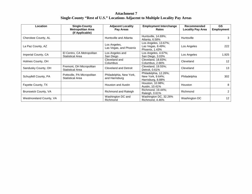
Attachment 7 Single-County “Rest of U.S.” Locations Adjacent to Multiple Locality Pay Areas
Location Single-County Metropolitan Area
(If Applicable)
Adjacent Locality Pay Areas
Employment Interchange Rates
Recommended Locality Pay Area
GS Employment
Cherokee County, AL Huntsville and Atlanta Huntsville, 14.69%; Atlanta, 6.58% Huntsville 3
La Paz County, AZ Los Angeles, Las Vegas, and Phoenix
Los Angeles, 13.67%; Las Vegas, 8.49%; Phoenix, 1.43%
Los Angeles 222
Imperial County, CA El Centro, CA Metropolitan Statistical Area
Los Angeles and San Diego
Los Angeles, 4.67%; San Diego, 3.03% Los Angeles 1,925
Holmes County, OH Cleveland and Columbus
Cleveland, 18.83%; Columbus, 2.66% Cleveland 12
Sandusky County, OH Fremont, OH Micropolitan Statistical Area Cleveland and Detroit Cleveland, 19.55%;
Detroit, 0.61% Cleveland 13
Schuylkill County, PA Pottsville, PA Micropolitan Statistical Area
Philadelphia, New York, and Harrisburg
Philadelphia, 12.26%; New York, 9.64%; Harrisburg, 8.88%
Philadelphia 302
Fayette County, TX Houston and Austin Houston, 10.98%; Austin, 10.41% Houston 8
Brunswick County, VA Richmond and Raleigh Richmond, 19.44%; Raleigh, 0.61% Richmond 2
Westmoreland County, VA Washington DC and Richmond
Washington DC, 32.26% Richmond, 4.46% Washington DC 12
Attachment 8 Locations that Contacted Council Staff about Locality Pay Areas
Asheville-Brevard, NC Combined Statistical Area (Rest of U.S.)
Augusta-Waterville, ME Micropolitan Statistical Area (Rest of U.S.)
Beaumont-Port Arthur, TX Metropolitan Statistical Area (Rest of U.S.)
College Station-Bryan, TX Metropolitan Statistical Area (Rest of U.S.)
Cape Coral-Fort Myers-Naples FL Combined Statistical Area (Rest of U.S.)
Charleston-North Charleston, SC Metropolitan Statistical Area (Rest of U.S.)
Cheyenne, WY Metropolitan Statistical Area (Rest of U.S.)
Claremont-Lebanon, NH-VT Micropolitan Statistical Area (Rest of U.S.)
Cumberland County/Carlisle Barracks, PA (Harrisburg locality pay area—seeking higher locality pay)
Flagstaff, AZ Metropolitan Statistical Area (Rest of U.S.)
Fresno-Madera, CA Combined Statistical Area (Rest of U.S.)
Grand Rapids-Wyoming-Muskegon, MI Combined Statistical Area (Rest of U.S.)
Imperial County, CA (Rest of U.S.)
La Plata County, CO (Rest of U.S.)
Madison-Janesville-Beloit, WI Combined Statistical Area (Rest of U.S.)
Meeker County, MN (Rest of U.S.)
Mono County, CA (Rest of U.S.)
Montgomery, AL Metropolitan Statistical Area (Rest of U.S.)
Nantucket County, MA (Rest of U.S.)
Philadelphia locality pay area (regarding current pay levels)
Pine County, MN (Rest of U.S.)
Rest of US portions of Reno-Carson City-Fernley, NV Combined Statistical Area
Rochester-Batavia-Seneca Falls, NY, Combined Statistical Area (Rest of U.S.)
Salt Lake City-Provo-Orem, UT Combined Statistical Area (Rest of U.S.)
San Juan County, WA (Friday Harbor) (Rest of U.S.)
San Luis Obispo County, CA (Rest of U.S.)
Spokane Valley-Coeur d'Alene, WA-ID Combined Statistical Area (Rest of U.S.)
Ventura County, CA (Los Angeles locality pay area—seeking higher locality pay)
Zapata County, TX (Rest of U.S.)