No. 8204

FISHER TO FAMA TO FISHER:INFLATION ANO INTEREST RATES, 1890-1981

by

Scott UlmanUniversity of Minnesota

Research Paper

Federal Reserve Bank of Dallas

This publication was digitized and made available by the Federal Reserve Bank of Dallas' Historical Library (FedHistory@dal.frb.org)

No. 8204

FISHER TO FAMA TO FISHER:INFLATION ANO INTEREST RATES, 1890-1981

by

Scott Ul manUniversity of Minnesota

and

John H. Wood*Northwestern University

andFederal Reserve Bank of Dallas

December 1981Revised, November 1982

*We grateful to Rosanne Strege for computational assistance and to theJ. L. Kell ogg School of Management. Northwestern unt ver-st ty , for fi nancialassistance. All views expressed here and any errors remain theresponsibility of the authors.

At least since 1930, empirical researchers have grappled with the

issue of whether investors immediately assimilate anticipated inflation

into required returns so that variations in nominal interest rates are

the best available predictors of variations in expected inflation.

Irving Fi sher and others demonstrated that pre-~4orld War II interest

rates responded slowly and incompletely to changes in inflation. But

Shiller and Fama derived strikingly contrasting results for postwar data

(particularly 1953-71): nominal interest rates (on average)

reflected anticipated inflation so that real interest rates were

independent of price changes. Fama argued that the contrast resulted

from an improved Consumer Price Index (CPI) in 1953 and that the tlGibson

par-adox" observed in prewar data arose from spurious autocorrelations

induced by a "nof sy'' price index.

The present study demonstrates that the differences between

Fisher's and Fama's results stem solely from Fama's selection of a

sample period--January 1953 to July 1971--of unprecedented price

stability in U.S. history. The famous theoretical "Fisher effect"

wherein interest rates correctly anticipate inflation -- holds during

Fama's period, and the result is robust with respect to price index

used, yield source, or type of short-term instrument studied. However,

in the period since April 1974 the economy has reverted to

characteristically higher price volatility, and empirical Fisherian

results are again apparent. Once again, evidence resoundingly rejects

the hypothesis that variations in nominal interest rates are appropriate

measures of variations in expected inflation.

Consequently, it appears that in general the theoretical "Fisher

effect" cannot be interpreted as a reduced-form equation for the

nominal interest rate. Evidence suggests that the interest rate is

determined simultaneously by interaction of the commodity and financial

sectors, so an appropriate reduced~form equation must emanate from a

complete macroeconomic system. Furthermore, the reduced form must be

consistent with findings which corroborate a complete reflection of

anticipated inflation in nominal interest rates during periods of

relative price stability while generating the Gibson paradox during

periods of normal price volatility.

The results presented here are not necessarily inconsistent with

rational expectations (efficient markets). However, they reject rational

expectations in conjunction with a variety of maintained hypotheses

specified below.

-2-

I. The Fisher equation as a reduced form

Under certainty, i.e., a deterministic macroeconomic system, an

investor holding claims denominated in money terms will demand a nominal

holding-period return

where Rt, r t, and TIt are the nominal rate of return, real rate of return

and inflation rate over [t, t+1]. The relationship between inflation

and nominal interest rates described by (1) is the famous Fisher

effect. 1

An "expect at i ons" version 2 of the Fisher equation under

uncertainty is

with its consequent linear approximation

lThe equilibrium relationship was known prior to Fisher (see hishistorical survey (1907, pp , 356-358)). However, (1) is commonlyascribed to Fisher since he was the first to carry out extensivestatistical studies of the relationship.

2Ignoring risk-aversion is perhaps attributable to the belief that theshort holding periods (six months or less) in subsequent statisticaltests obviated the need to hedge against shifting investmentopportunities and that money market instruments generating testedreturns are (nearly) free of default risk.

-3-

Assume inflation is initiated by exogenous shifts in the supply or

demand for money. Further assume -- as in most "classical 11

macroeconomic model s -- that money is "neutr-el": shocks to the monetary

system leave real variables unaffected. Classical neutrality results

require that relative prices be unchanged by the price level or

inflation. A key relative price is the expected real holding-period

return which is the opportunity cost of current goods, (1 + Rt)Pt,

relative to expected costs of future goods, P~+l' or

3)

which is merely a rearrangement of (2) with Cov(rt, ITt): 0 since other

real variables like r t are also independent of inflation. If the

security has no default risk, (3) and its linear approximation

3.) Rt " r~ + rr~

-4-

become the reduced form equation 3 for the nominal interest rate.

Finally, introduce two maintained hypotheses. First, if

technology and tastes are stable through time, r~ can be replaced by a

constant, (arbitrarily called) Bo' Second, if investors have "r ational

expectat tons", they forecast inflation (or any other variable) utilizing

the minimum mean-square error estimator called the projection, ~t=

P(TItI0t), (or regression) of TIt onto the information set 0t. In

linear systems, the projection is the conditional expectation, ca1cu-

lated assuming investors know the probability distribution of the

exogenous variables and lagged endogenous variables comprising 0t , 4

The rational expectations assumption is called the "efficient markets

hypothes i s" in the finance 1iterature and is interpreted to mean that

Uinvestors utilize all available information" in forecasting, where

"avai l ab l e inforrnat ton" then includes the "true" probability

distributions of variables in 0t.

3Sargent (1976) has noted that in some classical models, fiscalvariables affect both Rt and ITt' so (3) is not a true reduced formequation. However, inclusion ofa disturbance term Ct to capture suchomitted variables (Rt = rf + IIi + 0T) would also be lnappropriate sinceCt would not then be orthogonal to TIf.4For further details of linear least squares projections, see Sargent(1979), Ch. 10.

-5-

Given our maintained hypotheses, investors forecast inflation as

4}N

= 4 ~.e·ti =1 1 1

Nwhere {Bit}i=l may be any subset of 0t, and the 6i are parameters.

Then the forecast error €t,

- ITt -ITt has the properties that

E(OtI0t) = 0 and E(OtOt_i lOt) = 0 for Vi > 0. 5 Consequently, under our

maintained hypotheses, (3a) may be written

Then the projection (regression) of inflation on any subset of Gt may be

described with zero coefficients on everything except Rt and So·

Equation (5) represents the regression most statistical researchers

(including Fisher) have studied: project inflation onto a subset

{Sit} = u, Rt}. Its interpretation is the classic "Fisher ef f ect": a

rise in anticipated inflation is fully reflected in the nominal interest

follows in theand Rt ., IT. .

-1 -""t-l

speci fice Gt for

case (3a)i > O.

-6-

o for all

rate, leaving the real rate unchanged. Hence (short-term) financial

instruments l returns would provide the best available information about

expected inflation if empirical studies substantiate the theory.

Many macroeconomists remain skeptical of results derived from

"c l asstc al" precepts. However, Sargent (1973, 1976) has demonstrated

that the "Fisher effect II carries over to a (Keynesian) IS-LM framework

under a modification of our prior maintained hypotheses: the real rate

of interest will still be statistically independent of systematic shifts

in the money supply so that foreseen changes in monetary policy will

affect Rt only to the extent they alter rr~. This Fisherian result

requires that investors forecast according to the rational expectations

mechanism previously posited and that the Friedman-Phelps "natur-al r ate"

hypothesis of employment holds so the a9gregate supply function is not

permanently affected by systematic monetary or fiscal policies.

Consider the following system of structural equations (aggregate

supply, aggregate demand (IS), and portfolio balance (LM),

respectively) :

a > 0

-7-

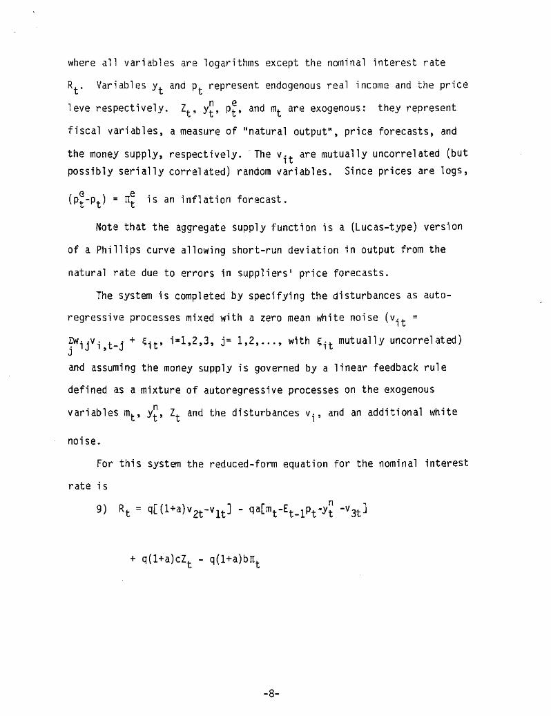
where all variables are logarithms except the nominal interest rate

Rt. Variables Yt and Pt represent endogenous real income and the price

leve respectively. Zt' y~, p~, and mt are exogenous: they represent

fiscal variables, a measure of "natural output", price forecasts, and

the money supply, respectively. The vi t are mutually uncorrelated (but

possibly serially correlated) random variables. Since prices are logs,

(p~-Pt) = II~ is an inflation forecast.

Note that the aggregate supply function is a (Lucas-type) version

of a Phillips curve allowing short-run deviation in output from the

natural rate due to errors in supp l i er s ' price forecasts.

The system is completed by specifying the disturbances as auto-

regressive processes mixed with a zero mean

the money supply is governed by a linear feedback rule

.EW··v· t'+jlJl,-J

and assuming

~it' i=1,2,3, j= 1,2, ... , with

white noise (vi t =

<it mutually uncorrel at ed )

defined as a mixture of autoregressive processes on the exogenous

variables mt, y~, Zt and the disturbances Vi' and an additional white

noise.

For this system the reduced-form equation for the nominal interest

rate is

+ q(l+a)cZt - q(l+albITt

-8-

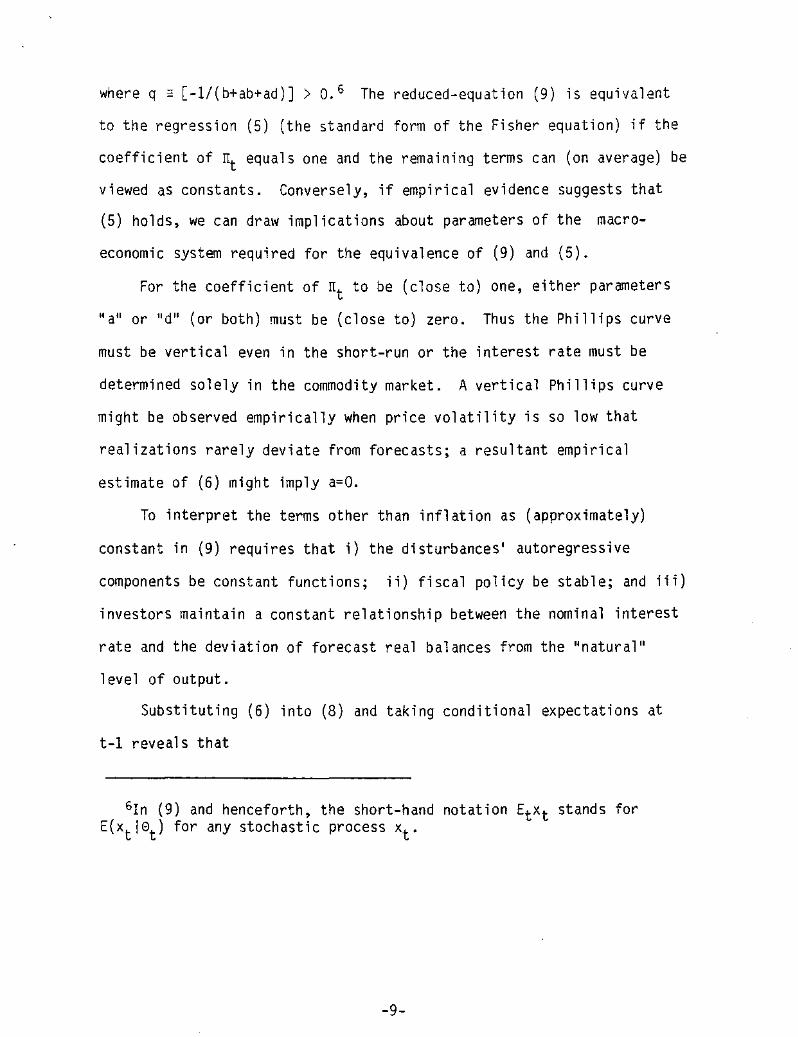
where q ~ [-lI(b+ab+ad)] > O.G The reduced-equation (9) is equivalent

to the regression (5) (the standard form of the Fisher equation) if the

coefficient of I\ equals one and the remaining terms can (on average) be

viewed as constants. Conversely, if empirical evidence suggests that

(5) holds, we can dr aw impl ications about parameters of the macro­

economic system required for the equivalence of (9) and (5).

For the coefficient of ITt to be (close to) one, either parameters

"a" or lid" (or both) must be (close to) zero. Thus the Phillips curve

must be vertical even in the short-run or the interest rate must be

determined solely ;n the commodity market. A vertical Phillips curve

might be observed empirically when price volatility is so low that

realizations rarely deviate from forecasts; a resultant empirical

estimate of (6) might imply a=O.

To interpret the terms other than inflation as (approximately)

constant in (9) requires that i) the disturbances· autoregressive

components be constant functions; ii) fiscal policy be stable; and iii)

investors maintain a constant relationship between the nominal interest

rate and the deviation of forecast real balances from the "natur al"

level of output.

SUbstituting (6) into (8) and taking conditional expectations at

t-l reveals that

6In (9) and henceforth, the short-hand notation EtXt stands forE(xt let) for any stochastic process xt•

-9-

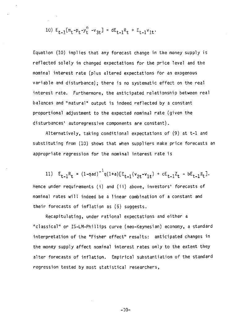
Equation (10) implies that any forecast change in the money supply is

reflected solely in changed expectations for the price level and the

nominal interest rate (plus altered expectations for an exogenous

variable and disturbance); there is no systematic effect on the real

interest rate. Furthermore, the anticipated relationship between real

balances and "natur-al" output is indeed reflected by a constant

proportional adjustment to the expected nominal rate (given the

disturbances' autoregressive components are constant).

Alternatively, taking conditional expectations of (g) at t-I and

subst i tut inq from (10) shows that when suppliers make price forecasts an

appropriate regression for the nominal interest rate ;s

Hence under requirements (i) and (ii) above, investors' forecasts of

nominal rates will indeed be a linear combination of a constant and

their forecasts of inflation as (5) suggests.

Recapitulating, under rational expectations and either a

"cl assic al" or IS-LM-Phillips curve (neo-Keynesian) economy, a standard

interpretation of the "Fisher eff'ec t" results: anticipated changes in

the money supply affect nominal interest rates only to the extent they

alter forecasts of inflation. Empirical substantiation of the standard

regression tested by most statistical researchers,

-10-

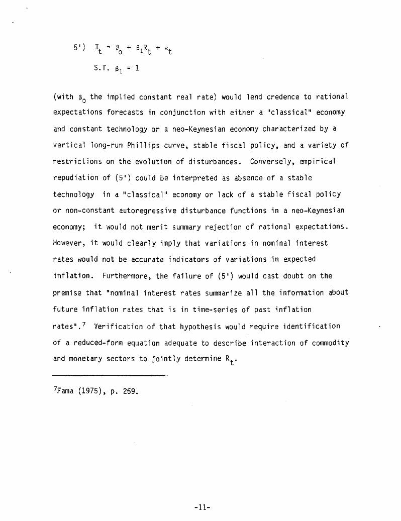
5') TIt = So + SjRt + et

S.T. Pj=1

(with 13 0 the implied constant real rate) would lend credence to rational

expectations forecasts in conjunction with either a "e1ass ic al " economy

and constant technology or a neD-Keynesian economy characterized by a

vertical long-run Phillips curve, stable fiscal policy, and a variety of

restrictions on the evolution of disturbances. Conversely, empirical

repudiation of (5') could be interpreted as absence of a stable

technology tn a "c l as s ical" economy or lack of a stable fiscal policy

or non-constant autoregressive disturbance functions in a neD-Keynesian

economy; it would not merit summary rejection of rational expectations.

However, it would clearly imply that variations in nominal interest

rates would not be accurate indicators of variations in expected

inflation. Furthermore, the failure of (51) would cast doubt on the

premise that "norni nal interest rates surrrrnarize all the information about

future inflation rates that is in time-series of past inflation

r atesv.? Verification of that hypothesis would require identification

of a reduced-form equation adequate to describe interaction of commodity

and monetary sectors to jointly determine Rt.

7Fama (1975), p. 269.

-11-

r

II. Conflicting empirical results: Fisher versus Fama

A. Fisher's empirical "cont.radiction" of the theory

Fisher (1930) was the first to subject (3a) and (5) to rigorous

statistical testing. Analyzing data on short-and long-term interest

rates in Britain and the United States, Fisher found no corroboration

for the hypothesis that expected inflation ;s immediately and perfectly

reflected in variations of nominal interest rates. Fisherls results may

be characterized as follows:

1) Over long periods, R and IT moved together; however short-term

contemporanou5 correlations between R and IT were not high (some were

even negative). For example, decennial averages of R and II were highly

correlated but quarterly or annual averages were not.

2) Variations in R tended to be less than those in IT. Quoting

Fi sher,

when prices are rising, the rate of interesttends to be high but not so high as it shouldbe to compensate for the rise; and when pricesare falling, the rate of interest tends to below but not so low as it should be to compen­sate for the fa'l.'

3) The influence of inflation seemed to be "dt str-tbut.ed over

time. Fisher found that correlations between R and distributed lags of

, Fisher (1930, p. 43).

-12-

past inflation rates rose consistently with the number of lags. He

interpreted the finding to indicate "that interest rates follow price

changes closely in degree, though rather distantly in time". 9

Subsequent researchers have hypothesized that investors forecast

inflation by "adaptive expect at tons", Then (3a) becomes

12)

Investigators like Sargent (1969), Yohe and Karnosky, and Gibson found

in tests of (12) that coefficients on past rates of inflation were

statistically significiant for very long lags; furthermore, the weights

summed to less than one. If prices are in logs (pt=log Pt) so

inflation can be defined as TIt=Pt+1- Pt' (12) can be rewritten as

(12' )

This is a statement of the Gibson paradox: the tendency of nominal

interest rates to be highly correlated with a time series of the price

level rather then the expected inflation rate. Sargent (1973) has

suggested how the Gibson paradox could arise in a stochastic macro-

economi c system even if expectat ions are "rat iona111• Can sequent' y,

empirical evidence supporting (12 1) is insufficient to disprove rational

expectations (efficient markets). Conversely, any reduced form equation

'Ibid .• p. 451.

-13-

for the nominal interest rate must be rich enough to explain the

empirical evidence for the Gibson paradox.

B. Fama and efficient markets

Using data from a different time period--January 1953 to July 1971­

-Fama (1975) claimed to find a very different set of facts. He

concluded that

... one •.• cannot reject the hypothesis that allvariation through time in one- to six-monthnominal rates of interest mirrors variation incorrectly assessed one- to six-month expectedrates of change in purchasing power ... Thenominal interest rate Rt ... is the best possiblepredictor of inflation from t-l to t.

Fama chose his sample period for the following reasons: (i) the Federal

Reserve's bond support program during and after World War II prevented

interest rates from reflecting expected inflation; (ii) the Consumer

-14-

Price Index (CPI) was "improved" in 1953;10 and (iii) price controls

from August 1971 to mid·1974 meant that "observed values of the CPI"

differed from the "true costs of goods to consumer s" (Fama, 1975, p.

275) .

Rather than inflation (ITt), Fama defined the variable "purchas inq

power change" (lit) such that_1

13) (l+ITt ) = (1+,\) .

Then appropriate restatements of (3a) and (5) are

10According to Fama, the "substantial upgrading of the CPI lIin 1953was because the "number of items in the Index increased substantially,and monthly sampling of major items become the general rule. For testsof market efficiency based on monthly data, monthly sampling of majoritems in the CPI is critical. Sampling items less frequently thanmonthly ... creates spurious autocorrelation in the Index ," making testsof "market efficiency on pre-1953 data difficult to f nter-pr-et ;" (Fama,1975, p. 274).

While it is true that the numbers of items and sources sampled wereincreased in 1953 (See BLS Bulletins 1948, p. 69, and 1711, p. 75), wehave been able to find no reference to an increase in the frequency ofsampling at that time. In fact, the frequency of sampling since 1953,and indeed since 1948, has probably been considerably less than between1940 and 1948. IIA reduction of one-third in appropriations for fiscalyear 1948 necessitated changes in the frequency of pricing for nonfooditems and in the number of items currently pr iced" (BLS, Bulletin 1517,p. 4; also see Bulletin 965, pp. 35-36). Since that time, most nonfooditems have been sampled every month only in the five largest urban areasand once every three months in other areas. Several items are sampledonly semiannually or annually.

This does not mean that Fama was wrong to begin with 1953, for theFederal Reserve1s bond support program during and after World War !Iprevented interest rates from reflecting expected inflation. But ltdoes suggest that he may have exaggerated the superiority of the post­1952 years as the appropriate sample for tests of market efficiency.And his emphasis on the importance of sampling frequency lends supportto use of the WPI, where most items really are sampled monthly.

-15-

14)

15) '.=~-R+E" 0 t t

where £t is orthogonal to the constant real rate Bo and nominal rate Rt ,

Equation (15) may be tested by the OLS regression

16)

where we expect al = -1. From the properties of the forecast error for

*the projection developed earlier, £t (and hence €t) should contain no

serial correlation. Furthermore, combining (14) and (15) shows

17) r t - ~o = Etso autocorrelations of the time series of realized real rates have the

properties of the forecast error; hence autocorrelations of rt

should be

zero for all lags. Finally, if Etllt = ~o - EtRt is the projection of lit

onto 0t, then the addition of II t_ 1 E 0t to the right hand side of (15)

should result in a2 = 0 when testing the OLS regression

Using price data from Salomon Brothers' daily release for one- to

six-month Treasury bills, selecting bills maturing closest to monthls

end, and employing the revised CPI, Fama calculated time series for

-16-

't' Rt, and r t to test the OLS regressions (16) and (18) and autocor­

relations of the time series (toll When maturity exceeded one month.

non-overlapping data were selected to avoid introducing spurious auto­

correlation.

For his sample period, Fama discovered that dutocorrelations of the

the real rate were indeed zero for all lags, al was close to -1 as

predicted by theory, and u2 (the coefficient of purchasing power change

lagged one period) was insignificantly different from zero. 12 He

concluded that variations in nominal interest rates were the best

available predictors of inflation: current market values appeared to

incorporate all information available in time series of lagged

purchasing power change (inflation).

Fama explained the contrast of his results with his predecessors'

findings by noting that ' 3

.•. earlier studies ... are based primarily on pre­1953 data. and the negative results on marketefficiency may to a large extent just reflect poorcommodity price data. By the same token. theSuccess of the tests reported here is probably to anon-negligible extent a consequence of theavailability of good data beginning in 1953.

llAlthough theory has been developed in terms of linearapproximations like (3a), the time series rt was calculated from theprecise relationship rt = (l+Rt)(l+'t) - 1.

12Numerical highlights of Fama's findings appear in the next section forcontrast.

13Shiller obtained results similar to Fama's on postwar data.

-17-

He further hypothesized that the Gibson paradox prevalent in data prior

to 1953 resulted from poor price data (a "noisy" price index) obscuring

the Fisher effect by spurious autocorrelation while picking up long­

run price movements. 14

III. A return to Fishter's world: evidence conflicting with theory

Sufficient time has elapsed since the end of the price controls in

April 1974 to test Fama's hypotheses outside his sample per-tod.Jf

Unfortunately~ it appears that postwar years (particulary 1953-71) were

not earmarked by improved data collection or a public more highly

attuned to the costs of inflation. Rather~ Fama's results stem from

the selection of a sample period of price placidity unparalleled during

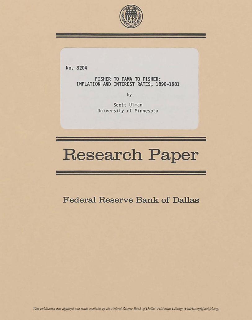
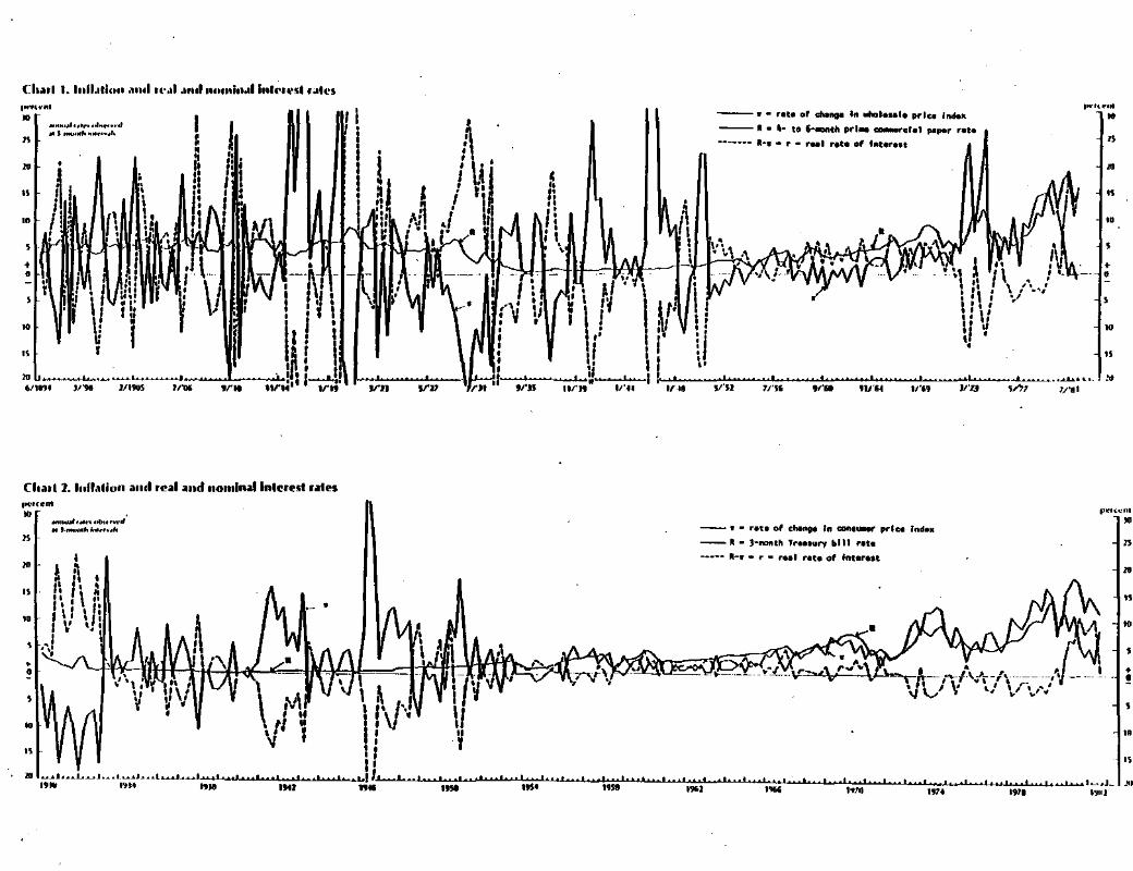
the twentieth century. Perusal of Charts 1 and 2 indicates that

1953-71 was a period of such price tranquility that even the most ardent

foes of rational expectations should not react incredulously to

assertions that agents acted as though they knew the underlying

14sargent (1976) agreed with Fama that a break in data behaviorapparently occurred near World War II: postwar tests seemed to supporta rational expectations hypothesis. However, Sargent suggested that anyconclusions would be speculative in the absence of a verifiable theoryfor the Gibson paradox in prewar data.

15Sector-by-sector decontrol began October 25, 1973, so when theEconomic Stabilization Act expired in April 1974 less than one-fourth ofthe economy was subject to controls. Thus we would not expect anysudden rise in prices in May 1974 due to a "bui l d-up" effect. Forfurther details, see Department of the Treasury~ Historical Working Paperon the Economic Stabilization Program: 8/15/71-4/30/74~ Officeof Economic Stabi1ization. In any case, what matters to the theory isprediction of price movements~ whatever the cause~ whether due to theending of controls or not.

-18-

ch.ul t. hlll.lllu" ami n'.lld,ul II0ndl1olll"l('u'slfolit's

--- nt. or .... I" ..... ' ...1. ,..Ie. , ..--- It- to ""-do ",1__cr.1 "".,. .

------- It- , nt. or I" u.

I....·~.. '• .."""' ",, ...... J HhH ~

"

"..,••

.."

or.

, i

i 'I I• I• 01

'II

"~

or" or..

c"",I, 'Ii, '1\

I :fV V,IIo

rn" trn........ ...

V'JI 71'H" , ....... ,....".fl. IIJ'5-I

I "! \. 1\1 '\ \ ,., I"I' ,-',I ,.,,', • I ,

i/: VI ••

.,........I •1/'69 JI'1J

I"''' ~,"•

.."

,••

n

Chil.1 1. luflallol1 illUl reill ilnd nomllUllnlerest ..tes

•!

,

n

..

"

..

"

,

I'H"~'"

•

.• ' .......... JL•.•J.__~I

''I'')'W.'..,.... "" .......... ,•• 1, .. '."',,,-,..,' ... '.,,' ,,'

-~--

-- 0'. e...... In _._ ,..1 ... Ind8•

-- It .. )- th Tnllury bill ..It.

----- 11- , ..It. of Int......

..

I , "" .ItSlI 1')(;2

•

NI• U'0/1 I

-, , , "... ,- ~ ""

s

•"

IrJ\!01I'

III i9':,I •••L~J'~·'i'I~J.·.l~~~.'O~;'~'~~'"'.''''I"'"'.''L."."~\~"~;~'.'.""'.'.''''I''._. ~~•...1...'...11M'" ·1···..··~'" ,..,,.....,

n

••

,""U,"•"

..

probability distribution of the price level during the era. Chart 1

shows 5-month observations on the 4-6 month prime commercial paper rate

(R, the fairly steady solid line), the rate of change in the Wholesale

Price Index (n, the volatile solid line), and R-n (the dashed line)

between 1894 and 1981. Chart 2 displays 3-month observations on the 3­

month Treasury bill rate and the CPI from 1929 to 1982.1 6

During the 1953-71 period of low price volatility, the rational

expectations "Ft sher eff ect" model is easily corroborable. The result

is hi9hly robust and apparently independent of i) the source of yield

data; ii) the price index used (CPI or WPI); and iii) the type of

short-term instrument (Treasury bill or commercial paper) generating the

nominal rate series~ However, in periods characterized by higher price

volatility (viz. prior to 1953 or subsequent to the recent removal of

price controls, i.e., 4/74-present), regression tests

of (16) and (18) and autocorrelation tests on the real ized real rate

series soundly reject rational expectations in conjunction with the

maintained hypotheses described earlier.

Table 1 presents a comparison of sample autocorrelations for three­

month real rates during Fama1s sample period. The time-series for rtgenerating the autocorrelations were calculated using the CPI and three

data sources: i) Fama's data supplied from Salomon Brothers' daily

quote sheets for the bill maturing closest to month's end; ii) data

160ata for the 4-6 month prime commercial paper rate and the 3-monthTreasury bill rate first became available in 1894 and 1929,respectively.

-19-

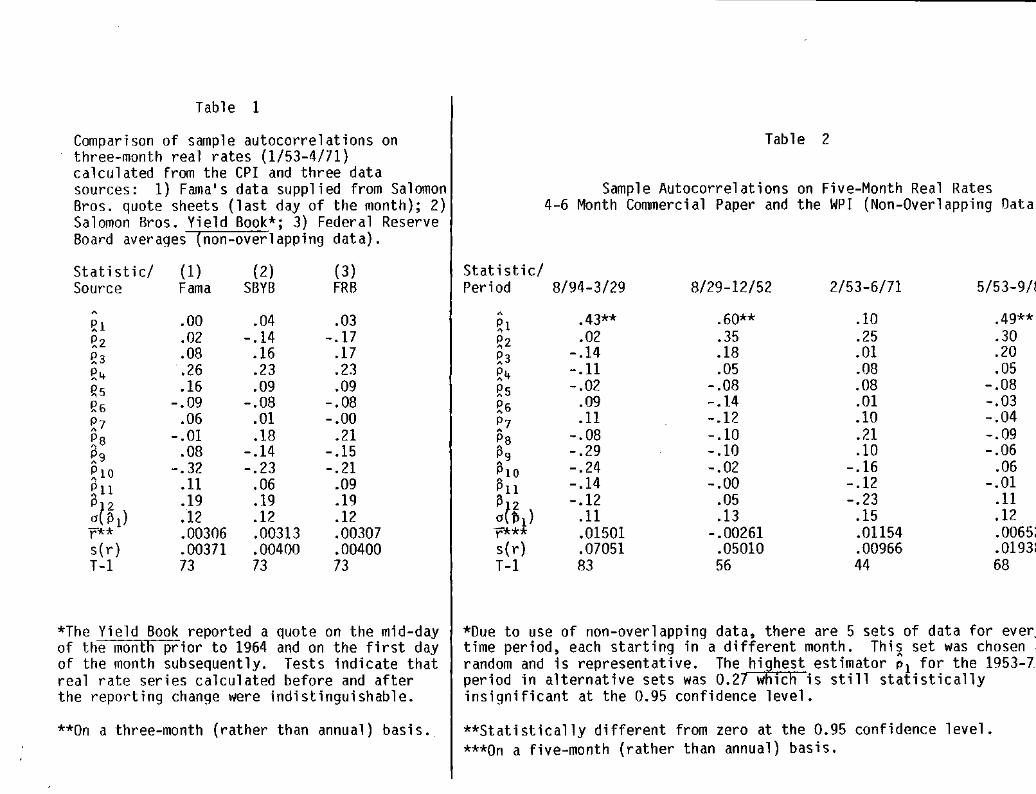
Table 1

Comparison of sample autocorrelations onthree-month real rates (1/53-4/71)calculated from the cpr and three datasources: 1) Fama's data supplied from SalomonBros. quote sheets (last day of the month); 2)Salomon Bros. Yield Book*; 3) Federal ReserveBoard averages (non-overlapping data).

Table 2

Sample Autocorrelations on Five-Month Real Rates4-6 Month Commercial Paper and the WPI (Non-Overlappin9 Data

Statistic/ (1) (2) (3) Statistic/Source Fama SBYB FRB Per;ad 8/94-3/29 8/29-12/52 2/53-6/71 5/53-9/1

.00 .04 .03 • .43** .60** .10 .49**~l ~,

~2 .02 -.14 -.17 ~2 .02 .35 .25 .30£3 .08 .16 .17 ~3 -.14 .18 .01 .20£. .26 .23 .23 ~4 -.11 .05 .08 .05~s .16 .09 .09 ~s - .02 -.08 .08 -.08~6 -.09 -.08 -. 08 ~6 .09 -.14 .01 -.03~7 .06 .01 -.00 P7 .11 -.12 .10 -.04

-.01 •18 .21 • -.08 -.10 .21 -.09£8 P8£9 .08 -.14 -.15 ~9 - .29 -.10 .10 -.06P,o -.32 -.23 -.21 ~10 -.24 -.02 -.16 .06all .11 .06 .09 ~ll -.14 -.00 -.12 -.01• .19 .19 .19 ~12 -.12 .05 -.23 .11PI 2a ~ ,) .12 .12 .12 o ~l) .11 .13 .15 .12r H .00306 .00313 .00307 r'*"** .01501 -.00261 .01154 .0065:s(r) .00371 .00400 .00400 s(r) .07051 .05010 .00966 .0193:T-1 73 73 73 T-1 83 56 44 68

*The Yield Book reported a quote on the mid-dayof the month prior to 1964 and on the first dayof the month subsequently. Tests indicate thatreal rate series calculated before and afterthe reporting change were indistinguishable.

**On a three-month (rather than annual) basis.

*Due to use of non-overl apping data, there are 5 sets of data for ever.time period, each starting in a different month. Thi~ set was chosenrandom and is representative. The hi~hest estimator Pl for the 1953-7period in alternative sets was 0.27 w ich is still statisticallyinsignificant at the 0.95 confidence level.

**Statistically different from zero at the 0.95 confidence level.***On a five-month (rather than annual) basis.

from Salomon Brothers· Yield Book which reported a quote on the mid-day

of the month prior to 1964 and the first day of the month subsequently;

and iii) Federal Reserve Board data, reported as monthly averages of

daily quotes. Non-overlapping data were utilized throughout the study

to avoid introducing spurious autocorrelations. Note that the sample

autocorrelation series for twelve lags are nearly indistinguishable in

magnitude and sign pattern regardless of data source.

Table 2 displays sample autocorrelations on five-month real rates

generated from 4-6 month prime commercial paper and the WPI. Hence the

instrument used is not totally riskless (in the sense of default risk)

and the price index is more volatile than the CPl. Note that in each

historical period except Fama·s 1953-71 subperiod, first-order

autocorrelation coefficients are significantly different from zero,

violating the theory.

Table 3 extends the evidence that Fama·s conclusions result from

the sample period selected rather than removal of noise from the price

index. It depicts sample autocorrelations on three-month real rates

generated from Federal Reserve Board average yields and, alternatively,

the CPI or WPI, over three sample periods: pre-Fama, Fama, and post­

Fama. As anticipated, autocorrelations are close to zero for all lags

during the Fama period regardless of the price index used to generate

the real rate time series. In both pre- and post-Fama periods, first­

order autocorrelation estimates are significantly different from zero at

the 0.95 confidence level.

-20-

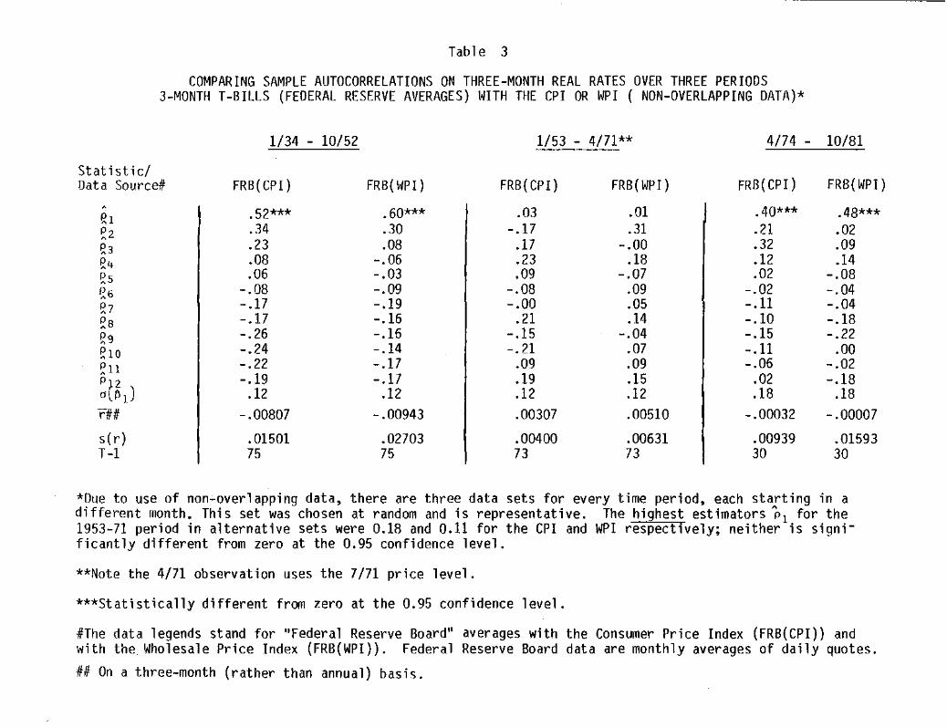
Table 3

COMPARING SAMPLE AUTOCORRELATIONS ON THREE-MONTH REAL RATES OVER THREE PERIOOS3-MONTH T-BILLS (FEOERAL RESERVE AVERAGES) WITH THE CPI OR WPI ( NON-OVERLAPPING OATA)*

1/34 - 10/52 1/53 - 4/71** 4/74 - 10/81

Statistic/Data Source# FRB(CPI) FRB( WPI) FRB(CPI) FRB(WPI) FRB(CPI) FRB( WPI)

,.52*** .60*** .03 .01 .40*** .48***gl

~2 .34 .30 -.17 .31 .21 .02g3 .23 .08 .17 -.00 .32 .09~4 .08 -.06 .23 .IB .12 .14~s .06 - .03 .09 -.07 .02 -.08~6 -.08 -.09 -.08 .09 -.02 -.04g, -.17 -.19 -.00 .05 -. II -.04~B -.17 -.16 .21 .14 - .10 -.IB~9 -.26 -.16 -.15 -.04 -.15 -.22~lO -.24 -.14 -.21 .07 -. II .00~ll -.22 -.17 .09 .09 -.06 -.02

P1 2 -.19 -.17 .19 .15 .02 -.18a ~l) .12 .12 .12 .12 .18 .18rUi -.00807 -.00943 .00307 .00510 -.00032 -.00007

s(r) .01501 .02703 .00400 .00631 .00939 .01593T-I 75 75 73 73 30 30

*Due to use of non-overlapping data, there are three data sets for every time period, each starting in adifferent month. This set was chosen at random and is representative. The highest estimators PI for the1953-71 period in alternative sets were 0.18 and 0.11 for the CPI and WPI respectively; neither is signi­ficantly different from zero at the 0.95 confidence level.

**Note the 4/71 observation uses the 7/71 price level.

***Statistically different from zero at the 0.95 confidence level.

·ffThe data legends stand for "Federal Reserve Board" averages with the Consumer Price Index (FRB(CPI)) andwith the Wholesale Price Index (FRB(WPI)). Federal Reserve Board data are monthly averages of daily quotes.

## On a three-month (rather than annual) basis.

These results are duplicated in Table 4 for one-month real rates

generated from Salomon Brothers ' Yield Book quotes and either the CPI or

WPI in Fama and post-Fama settings. Fama1s sample autocorrelations are

included for comparison. Once again, the data source or price index

used is immaterial between 1953-71; the "ef'f i cient markets" hypothesis

is upheld even if the price index is the WPI. However, in the 4/74-9/81

period, the same hypothesis is rejected. Combining the results of

Tables 1-4 supports our previous conclusions about the robustness of the

"efficient markets" hypothesis during the 1953-71 sample period and its

complete failure elsewhere.

For those unconvinced by autocorrelation tests, the results of

regressions (16) and (18) are reported in Table 5 for one-month Treasury

bills (quotes from Salomon Brothers' Yield Book) and the CPI during

Fama1s period, the period subsequent to removal of price controls, and

the two periods jointly. Table 6 displays corresponding outcomes for

the WPI. Fama's regression results are reproduced for contrast since

his data source for bond yields is slightly different from ours.

Once again, our results duplicate Fama's during the 1953-71 sample

period. However, for the period 4/74-9/81, corroboration of the

"effic i ent markets" hypothesis fails: the coefficient on the nominal

interest rate is not close to -1.0 and the first three sample

autocorrelation coefficients for the residuals are significantly

different from zero at the 0.95 confidence level. Seriously

autocorrelated residuals appear in the combined sample period 1/53-9/81

(excluding price contrOls), although the coefficient of Rt is again

close to -1.0.

-21-

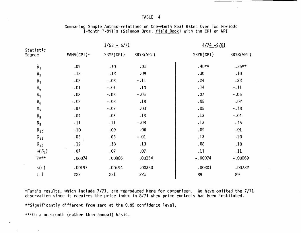
TABLE 4

Comparing Sample Autocorrelations on One-Month Real Rates Over Two PeriodsI-Month T-Bi11 s (Salomon Bros. Yield Book) with the CPI or WPI

1/53 - 6/71 4/74 -9/81StatisticSource FAMA(CPI)* SBYB( CPI) SBYB(WPI) SBYB(CPI) S8YB( WPI)

· .09 .10 .01 .40** .35**PI· .13 .13 .09 .30 .10P2· -.02 -.03 -.n .24 .23P3· -.01 -.01 .10 .14 -.np.· -.02 -.03 -.05 .07 -.05Ps• -.02 -.03 .18 .05 .02P6• -.07 -.07 .03 .05 -.18P7• .04 .03 .13 .13 -.04P8· .n .n -.08 .13 .15P9

PIa .10 .09 .06 .09 .01· .03 .03 -.01 .13 .10Pn· .19 .18 .13 .08 .18P12o( "1) .07 .07 .07 .n .nr*** .00074 .00086 .00154 -.00074 -.00069

s(r) .00197 .00194 .00353 .00301 .00732T-1 222 221 221 89 89

*Fa~a's results, which include 7/71, are reproduced here for comparison. We have omitted the 7/71observation since it requires the price index in 8/71 when price controls had been instituted.

**Significantly different from zero at the 0.95 confidence level.

***On a one-month (rather than annual) basis.

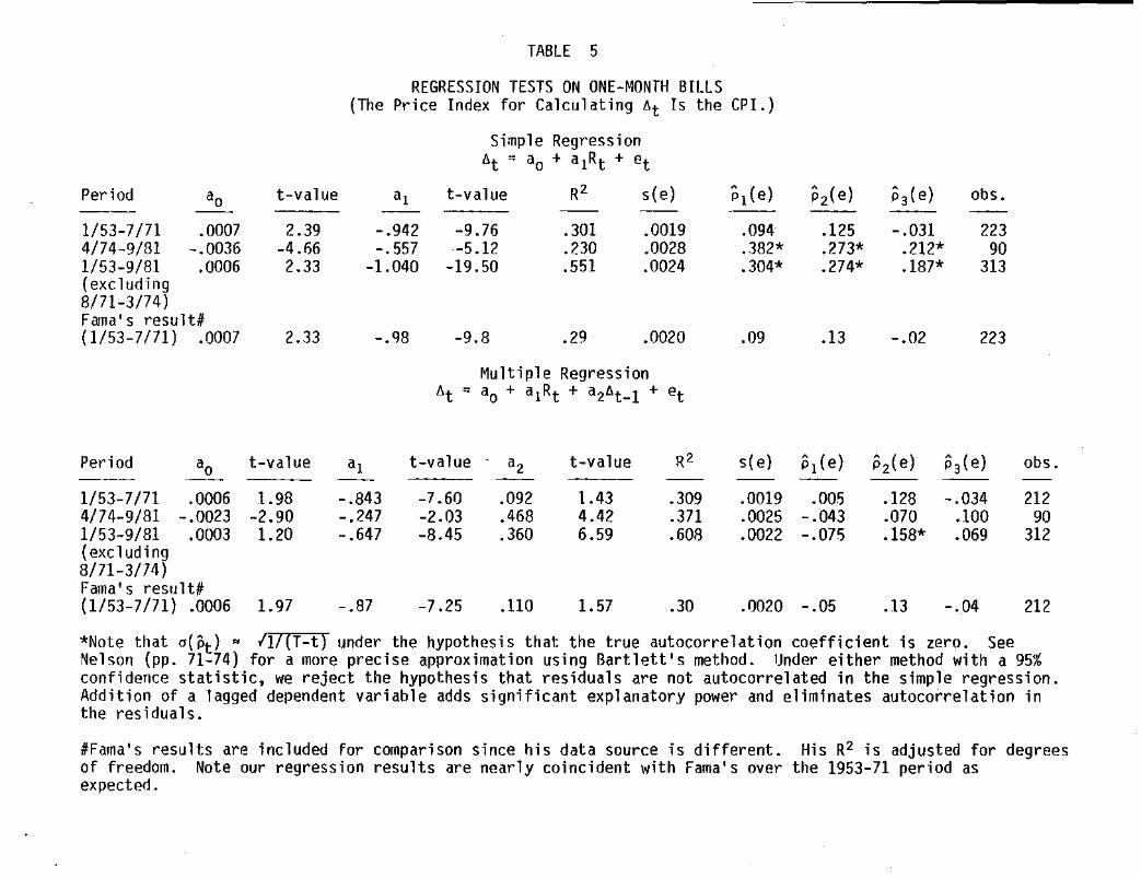
TABLE 5

.0007-.0036.0006

REGRESSION TESTS ON ONE-MONTH BILLS(The Price Index for Calculating at Is the CPl.)

Simple Regression6t =' ao + a1Rt + et

t-value aj t-value R2 s(e) "j (e) "2(e) P3(e) obs.._-2.39 - .942 -9.76 .301 .0019 .094 .125 -.031 223

-4.66 -.557 -5.12 .230 .0028 .382* .273* .212* 902.33 -1.040 -19.50 .551 .0024 .304* .274* .187* 313

Period ao

1/53-7/714/74-9/811/53-9/81(excluding8/71-3/74)Fama IS resu ltU(1/53-7/71) .0007 2.33 -.98 -9.8 .29 .0020 .09 .13 -.02 223

Multiple RegressionAt :: ao + aiRt + a2l1 t_ 1 + et

Period

.0006-.0023

.0003

t-value aj t-value . a2 t-value

1.98 -.843 -7.60 .092 1.43-2.90 -.247 -2.03 .468 4.421.20 -.647 -8.45 .360 6.59

s(e) Pj(e) P2(e) P3(e) obs.

212

21290

312

-.034.100.069

-.04.13

.128

.070

.158*

.0020 -.05

.0019 .005

.0025 -.043

.0022 -.075

.30

.309

.371

.608

1.57.110-7.25-.871.97

1/53-7/714/74-9/811/53-9/81(excluding8/71-3/74 )Fama's result#(1/53-7/71) .0006

*Note that o(Pt) • 117(T-t) under the hypothesis that the true autocorrelation coefficient is zero. SeeNe 1son (pp. 71-74) for a more preci se approx imati on us; nq Bart1ett I s method. Under either method with a 95%confidence statistic, we reject the hypothesis that residuals are not autocorrelated in the simple regression.Addition of a lagged dependent variable adds significant explanatory power and eliminates autocorrelation inthe residuals.

#Fama's results are included for comparison since his data source is different.of freedom. Note our regression results are nearly coincident with Fama1s overexpected.

His R2 is adjusted forthe 1953-71 period as

degrees

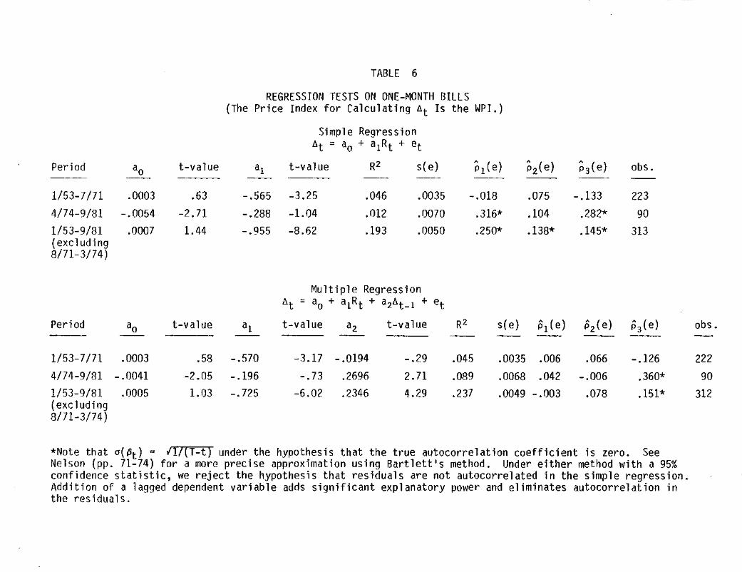
TABLE 6

REGRESSION TESTS ON ONE-MONTH BILLS(The Price Index for Calculating 't Is the WPI.)

Simple Regressionl!.t = ao + a1Rt + et

Period ao t-value a, t-value R2 s(e) p, (e) ;'2(e) ;'3(e) obs.

1/53-7/71 .0003 .63 - .565 -3.25 .046 .0035 -.018 .075 - .133 223

4/74-9/81 -.0054 -2.71 -.288 -1.04 .012 .0070 .316* .104 .282* 901/53-9/81 .0007 1.44 -.955 -8.62 .193 .0050 .250* .138* .145* 313(excluding8/71-3/74)

MUltiple Regression't = ao + alRt + a2l!.t_l + et

Period ao t-value a1 t-value a2 t.-value R2 s(e) "1(e) "2(e) "3(e) obs.

1/53-7/71 .0003 .58 -.570 -3.17 -.0194 -.29 .045 .0035 .006 .066 -.126 2224/74-9/81 -.0041 -2.05 -.196 -.73 .2696 2.71 .089 .0068 .042 -.006 .360* 901/53-9/81 .0005 1.03 -.725 -6.02 .2346 4.29 .237 .0049 -.003 .078 .151* 312(excluding8/71-3/74)

*Note that a(~t} ~ II!(T-t) under the hypothesis that the true autocorrelation coefficient is zero. SeeNelson (pp. 71-74) for a more precise approximation using Bartlett's method. Under either method with a 95%confidence statistic, we reject the hypothesis that residuals are not autocorrelated in the simple regression.Addition of a lagged dependent variable adds significant explanatory power and eliminates autocorrelation inthe residuals.

The addition of a single lagged purchasing-power explanatory

variable, 6t_ 1, transforms the simple regression (16) to the multiple

regression (18). During Fama's period, the coefficient of 6t_1 is not

significantly different from zero, further corroborating the "effic i ent

markets" hypothes t s i l? However, during the post-Fama period and the

joint period 1/53-9/81 (excludin9 price controls), the coefficient of

6t_1 is relatively large, significantly different from zero, and adds a

large amount of explanatory power to the regressions. Furthermore, the

residual sample autocorrelations are close to zero. i S Consequently,

variations in nominal interest rates are clearly acceptable as "best"

predictors of forecast inflation durin9 the period 1/1953-7/1971 but

fail from 4/1974-9/1981 (and from 1/53-9/81 with the price control

subset excluded).19 Table 6 shows analogous results when the price

17However , Nelson and Schwert found that a Box-Jenkins distributedla9 on inflation (in place of Fama's '\-1) improved the R2 s l i qht ly(from .29 to .31) and was statistically si9nificant.

i8This should not be surprising since the residuals in the sampleregression (16) are autocorrelated during post-Fama and joint periods.Assuming an AR(l) process for the errors, multiple regression (18) ishi9hly anal090us to a generalized (first) difference re9ression of (16).The lack of autocorrelation is important in the presence of a laggeddependent variable because we can then claim our parameter estimates areunbiased and consistent.

19For statistical purists, an F-test can be constructed to test whetherparameters in the multiple regression (18) come from the same populationdurin9 the 1/53-7/71 and 4/74-9/81 periods. The null hypothesis is

Ho : ~ = apFwhere ~ and BP.F are the parameter vectors in the Fama and post­Fama period regressions respectively. It is rejected if the F-statisticfrom the regression (F*) exceeds the critical value F(l-a; R, N-K) where(I-a) is the confidence level, R the number of restrictions, and N-K thedegrees of freedom. For the multiple regression reported in Table 5, F*= 14.86 ~ Fcv(.99, 3, 306) ~ 3.8 so we can safely reject the hypothesisthat the two are similar.

-22-

index is the WPI. The major difference between the WPI and CPI

regressions is the lower explanatory power of the WPI.

IV. Conclusions

It is evident that in general, variations in nominal interest rates

are not appropriate measures of variations in expected inflatiJn. The

classical "Fisher effect" equation is inadequate to describe the

intricate interactions between financial and commodity sectors in

determining the interest rate. The Gibson paradox observed in pre-World

War II data does not stem from "no i sy" commodity price data; it

reappears with the resurgence of sustained higher levels of price

volatility as suggested by Charts 1 and 2. Inflation forecasts can

evidently only be inferred from a non-classical reduced-form equation.

It is relatively easy to argue that (g) or an equation implied by

the linear least-squares projection (11) might fit the data for both

periods 1/53-7/71 and 4/74-9/81. During the earlier period, fiscal

policy was relatively stable; furthermore, price volatility was

sufficiently low that one might argue price forecasts differed from

realizations too little to generate even short-run systematic deviations

from "natural" output. With the resurrection of greater price

volatility and more erratic fiscal policy in the 4/74-9/81 period,

several maintained hypotheses could be violated, resulting in the

failure of (9) (or its analogue implied by (11)) to collapse to the

classical Fisher equation; nevertheless, expectations could still be

-23-

formed rationally. Thus a system with a non-constant real rate (where

we interpret the ureal r ate" as the sum of all terms in a reduced form

equation like (9) other than the inflation term) is broadly consistent

with rational expectations (efficient markets).

Much recent empirical work on the relationship between interest

rates and inflation has focused on this implied non-constancy of the

real rate. For example, Tanzi, Cargill and Meyer, Fama and Gibbons,

Mishkin, and Startz have estimated equations of the Fisher-Fama type

using a variety of distributed lag schemes (intended to capture

inflationary expectations) and real variables (presumed to influence the

real rate of interest) and most have concluded that the real rate is not

constant. Essentially the same result has been obtained within multi­

equation, macroeconomic frameworks by Elliott and Shiller and Siegel.

All of these studies except the last assume, with Fisher and Fama, that

money is both exogenous and the primary source of the inflationary

process, i.e., that inflations are precipitated by exogenous monetary

disturbances. Thus, these studies are consistent with the assumed

exogeneity of money in the macroeconomic system (6)-(8) which led to the

reduced form (9).

Clearly, however, other macro systems, price forecasting

mechanisms, and monetary endogeneity, would lead to alternative feasible

reduced-form equations. Another explanation of the data reported above

might emanate from a model completed by i) endogenizing the behavior of

the central bank and therefore of the money suppply and ii) making

explicit the causal connections between the real rate of interest and

other real variables. Such a model is best described as Wicksellian,

-24-

in which i) disturbances emanate from the real side of the economy

through forces affecting supplies and demands for goods, the most

important of which may be categorized under the headings "savings" and

U investment"; i i) these di sturbances affect the equil ibri urn real rate

of interest (Wicksell's natural rate); and iii) a monetary authority

fond of stable interest rates resists the adjustment of the market rate

to the natural rate, iv) thereby accentuating the price changes induced

by the initiating real disturbances. zu This approach, which must take

disequilibria into account, could explain the strong, long-term

tendencies of money, inflation, nominal interest rates, and real

investment and/or government expenditures (as the most volatile real

variables in the system) to vary together. However, since nominal

interest rates vary less than inflation, partly due to the central

bank's resistance, real interest rates move oppositely to these

variables. The high autocorrelations observed in expost real rates are

thus broadly consistent with Wicksell's analysis.

ZUShiller and Siegel rejected their version of Wicksell1s model buttheir tests treated high-powered money as exogenous. However, theyadmitted the possibility "that central bank behavior, in attempting toa~tenuate interest rate changes, will result in a correlation betweenhlgh-powered money and interest rates and hence give rise to the GibsonPar-adox" •

-25-

References

Cargill, 1. and R. Meyer, "The Term Structure of Inflationary Expecta­tions and Market Efficiency," Journal of Finance, 1980, 57-70.

Elliott, J.W., IIMeasuring the Expected Real Rate of Interest: anExploration of Macroeconomic Alternatives", American Economic Review,1977, 67, 429-43.

Fama, E., "Shor t-Term Interest Rates as Predictors of Infl at i on, II

American Economic Review, 65, June 1975, 269-82.

Fama, E.F. and M. R. Gibbons, "Infl at ion , Real Returns, and CapitalInvestment, Working Paper #41, Graduate School of Business, Universityof Chicago, 1980.

Fisher, I., The Rate of Interest, Macmillan, New York, 1907.

____________, The Theory of Interest, Macmillan, New York, 1930.

Gibson, W., "Pr i ce-Expectat tons Effects on Interest Rates," Journal ofFinance, 25, March 1970, 19-34.

Lucas, R.E., "An Equilibrium Model of the Business Cyc l e ," Journal ofPolitical Economy, 1975, 83, 1113-44.

Mishkin, F., "The Real Interest Rate: an Empirical Inves t iqat ion ,"Carnegie-Rochester Conference Series on Public Policy, 1981.

Nelson, C., Applied Time Series Analysis, Holden-Day, San Francisco,1973.

Nelson, C.Infl ation:Constant ,II

and G.W. Schwert, "Shor-t-term Interest Rates as Predi ctors ofon Testing the Hypothesis that the Real Rate of Interest IsAmerican Economic Review, 67, June 1977, 478-86.

Salomon Brothers Hutzler Yield Book, New York, 1981.

Sargent 1., "Commodity Price Expectations and the Interest Rate,"Quarterly Journal of Economics, 1969, 83, 127-40.

Sargent, T., "Rational Expectations, the Real Rate of Interest, andthe Natural Rate of Unemployment," Brookings Papers on EconomicActivity, 1973, 2, 429-80.

Sargent, T., II Interest Rates and Expected Infl at i on: a Select i ve SU1lTi1aryof Recent Research," Explorations in Economic Research, Summer 1976, 3,303-25.

Sargent, T., Macroeconomic Theory, Academic Press, New York, 1979.

Shiller, R., Rational Ex¥ectations and the Structure of Interest Rates,Ph.D. dissertation, M.I .. , 1972.

Shiller, R. and J. Siegel, "The Gibson Paradox and Historical Movementsin Real Interest Rates ," Journal of Political Economy, 1977, 5, 891-907.

Startz, R., "Unempl ojmentof Inflation NeutralitY,1l77.

and Real Interest Rates: Econometric TestingAmerican Economic Review, December 1981, 969-

ToW"'a"'sh"'1'"'n"g"'t"o"n:

Tanzi, V., "Infl at ion ary Expectations, Economic Activity, Taxes, andInterest Rates ll

, American Economic Review, 1980, 70, 12-21.

U.S. Bureau of Labor Statistics, Retail Prices of Food, 1948, Bulletin965, Washin9ton, D.C., 1949.

Handbook of Methods for Surveys and Studies, Bulletin 1458,D.C., 1966

1517,

T.r>OTC~~~' Handbook of Methods for Surveys and Studies, Bulletin 1711,wash,ngton, D.C., 1971.

U.S. Department of the Treasury, Historical Working Papers on theEconomic Stabilization Program: 8!15!11-4!3D!74, Dffice of EconomicStabilization.

Yohe, W., and D. Karnosky, "Interest Rates and Pr i ce Leve 1 Ch anges , II

Review, Federal Reserve Bank of St. Louis, December 1969, 19-36.