Feature Tracking Using Reeb Graphs

Gunther Weber1, Peer-Timo Bremer2, Marcus Day1, John Bell1, and Valerio Pascucci3

1 Lawrence Berkeley National Laboratory, {GHWeber|MSDay|JBBell}@lbl.gov2 Lawrence Livermore National Laboratory, ptbremer@llnl.gov

3 University of Utah, pascucci@sci.utah.edu

Abstract. Tracking features and exploring their temporal dynamics can aid sci-entists in identifying interesting time intervals in a simulation and serve as basisfor performing quantitative analyses of temporal phenomena. In this paper, wedevelop a novel approach for tracking subsets of isosurfaces, such as burning re-gions in simulated flames, which are defined as areas of high fuel consumptionon a temperature isosurface. Tracking such regions as they merge and split overtime can provide important insights into the impact of turbulence on the combus-tion process. However, the convoluted nature of the temperature isosurface andits rapid movement make this analysis particularly challenging.Our approach tracks burning regions by extracting a temperature isovolume fromthe four-dimensional space-time temperature field. It then obtains isosurfaces forthe original simulation time steps and labels individual connected “burning” re-gions based on the local fuel consumption value. Based on this information, aboundary surface between burning and non-burning regions is constructed. TheReeb graph of this boundary surface is the tracking graph for burning regions.

Key words: Topological data analysis, Feature tracking, Combustion simulation,Reeb graph, Tracking graph, Tracking accuracy

1 IntroductionUnderstanding combustion processes is a fundamental problem impacting areas suchas engine and stationary power plant design, both in terms of production efficiencyand pollutant emission. Fuel-lean flame configurations are of particular interest sincesuch flames generically produce far lower pollutants than comparable fuel-rich or sto-ichiometrically mixed flames. However, such flames are difficult to stabilize in thesort of quasi-steady robust configurations necessary for practical applications, partic-ularly when using advanced fuel mixtures, such as hydrogen-air and hydrogen-seededmethane-air. These advanced fuel mixtures, selected to reduce the use of carbon-basedfuels and subsequent emissions, often burn in cellular patterns of intense chemical re-action, separated by regions of local extinction. A broad range of classical flame propa-gation models used in analysis and engineering design of practical combustion systemsare based on the notion that a flame is a thin continuous interface separating cold reac-tants from hot products. Such models are not suitable for modelling cellular flames. Ittherefore is of great practical interest to understand this mode of combustion, with theultimate goal of incorporating the cellular burning behavior into revised engineeringdesign models.

In the present study, detailed numerical simulation is used to evolve a turbulent re-acting hydrogen-air mixture in an idealized configuration. Characteristics of the flow

2 Weber et al.

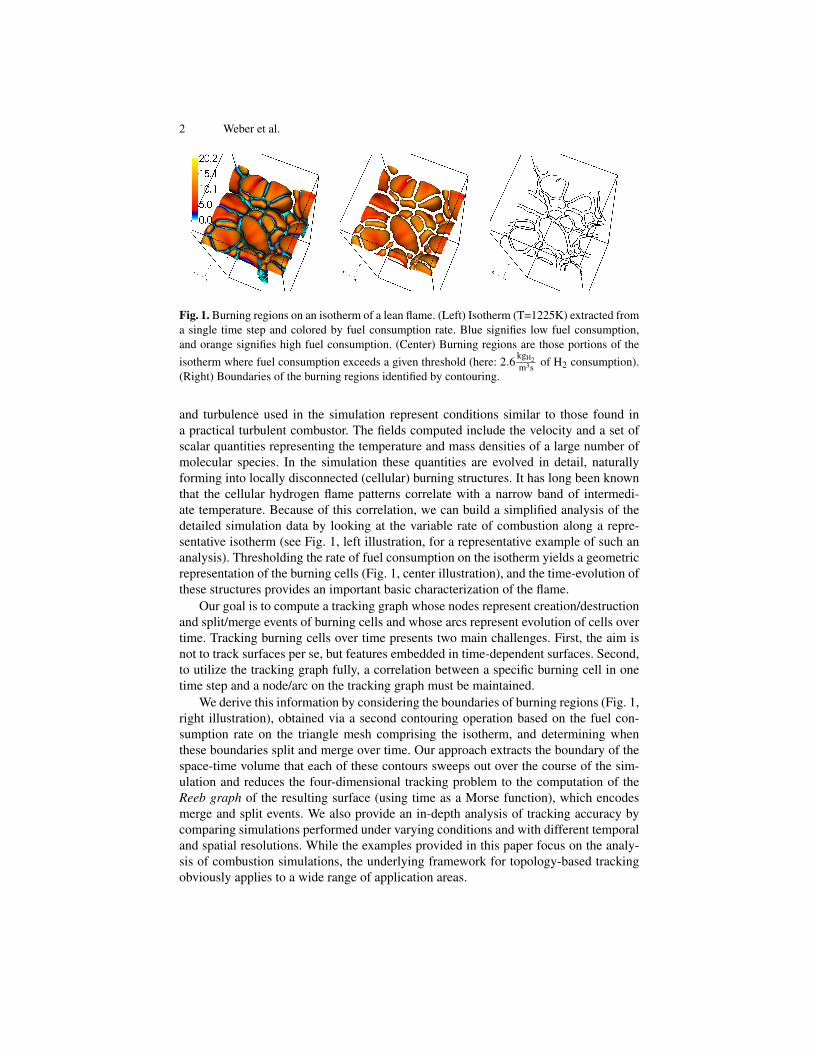
Fig. 1. Burning regions on an isotherm of a lean flame. (Left) Isotherm (T=1225K) extracted froma single time step and colored by fuel consumption rate. Blue signifies low fuel consumption,and orange signifies high fuel consumption. (Center) Burning regions are those portions of theisotherm where fuel consumption exceeds a given threshold (here: 2.6

kgH2m3s of H2 consumption).

(Right) Boundaries of the burning regions identified by contouring.

and turbulence used in the simulation represent conditions similar to those found ina practical turbulent combustor. The fields computed include the velocity and a set ofscalar quantities representing the temperature and mass densities of a large number ofmolecular species. In the simulation these quantities are evolved in detail, naturallyforming into locally disconnected (cellular) burning structures. It has long been knownthat the cellular hydrogen flame patterns correlate with a narrow band of intermedi-ate temperature. Because of this correlation, we can build a simplified analysis of thedetailed simulation data by looking at the variable rate of combustion along a repre-sentative isotherm (see Fig. 1, left illustration, for a representative example of such ananalysis). Thresholding the rate of fuel consumption on the isotherm yields a geometricrepresentation of the burning cells (Fig. 1, center illustration), and the time-evolution ofthese structures provides an important basic characterization of the flame.

Our goal is to compute a tracking graph whose nodes represent creation/destructionand split/merge events of burning cells and whose arcs represent evolution of cells overtime. Tracking burning cells over time presents two main challenges. First, the aim isnot to track surfaces per se, but features embedded in time-dependent surfaces. Second,to utilize the tracking graph fully, a correlation between a specific burning cell in onetime step and a node/arc on the tracking graph must be maintained.

We derive this information by considering the boundaries of burning regions (Fig. 1,right illustration), obtained via a second contouring operation based on the fuel con-sumption rate on the triangle mesh comprising the isotherm, and determining whenthese boundaries split and merge over time. Our approach extracts the boundary of thespace-time volume that each of these contours sweeps out over the course of the sim-ulation and reduces the four-dimensional tracking problem to the computation of theReeb graph of the resulting surface (using time as a Morse function), which encodesmerge and split events. We also provide an in-depth analysis of tracking accuracy bycomparing simulations performed under varying conditions and with different temporaland spatial resolutions. While the examples provided in this paper focus on the analy-sis of combustion simulations, the underlying framework for topology-based trackingobviously applies to a wide range of application areas.

Feature Tracking Using Reeb Graphs 3

2 Related WorkTime-dependent Isosurface Extraction. Given a manifold M and a scalar functionf : M → R, an isosurface or level set of f at isovalue s is defined as all points onM with function value s. If M is described by a three-dimensional rectilinear grid,isosurfaces can be efficiently constructed using the Marching Cubes algorithm [1, 2].More recent work [3] has extended this approach using convex hull computations todefine triangulations within a grid cell. This method eliminates the need for extensivecase tables, ensures consistency, and easily generalizes to higher dimensions.

One can exploit this generality to visualize time-varying isosurfaces by treatingtime as an additional dimension creating the space-time manifold M×R. Extractinga level set of M×R results in a three-dimensional hypersurface (embedded in four-dimensional space-time) comprised of tetrahedra. Intersecting this volumetric space-time mesh with planes of constant time values results in traditional two-dimensionalisosurfaces at a given time. Therefore, the hypersurface is a comprehensive descriptionof the temporal evolution of the corresponding two-dimensional isosurfaces.Topological Analysis and Reeb Graphs. By construction, a level set of f provides onlylimited information on f as a whole, but very detailed information about a specific func-tion value. To understand the global behavior of f , it is useful to analyze its contours,which are the connected components of all level sets of f . Contracting the contours ofa Morse function f into points creates the Reeb graph, which encodes the topology ofall level sets of f . Nodes of the Reeb graph are formed by the contours passing throughcritical points of f , i.e., points where contour topology changes. Its arcs are formed bythe remaining contours, i.e., by the family of contours that do not change topology. Formore details on Reeb graphs and algorithms to construct them efficiently, we refer thereader to the description by Pascucci et al. [4].

In our application, the boundaries of burning regions sweep out a two-dimensionalspace-time surface S (see Fig. 2). Using the time-coordinate of all vertices of S as thefunction f , the level set of f at value t describes the cell boundaries at time t. Thus, theReeb graph of f encodes the temporal evolution of the boundaries and can be used asthe tracking graph describing how cells merge and split over time.Feature Tracking. Defining and tracking features has long been of interest to the vi-sualization community. Most relevant to our work is feature tracking in the context ofscalar field visualization. Here, one usually is interested in tracking features defined bythresholding or isosurface extraction [5].

Tracking algorithms can roughly be divided into two categories: tracking by geom-etry and tracking by topology. Methods in the former category use various forms ofoverlap and/or distance between geometric attributes, e.g., the center of gravity [6] orvolume overlap [7, 8] for tracking. Laney et al. [9] use a similar approach to track bub-ble structures in turbulent mixing. Ji et al. [10, 11] track the evolution of isosurfaces ina time-dependent volume by extracting the 3D space-time isosurface in a 4D space.

Methods in the latter category [12, 13] compute tracking information topologicallyusing, for example, Jacobi sets [14], which describe the paths all critical points takeover time. Sohn and Bajaj [15] introduce a hybrid approach using volume matchingsimilar to Silver and Wang [7, 8] instead of topological information [13, 14] to definecorrespondences between contour trees.

4 Weber et al.

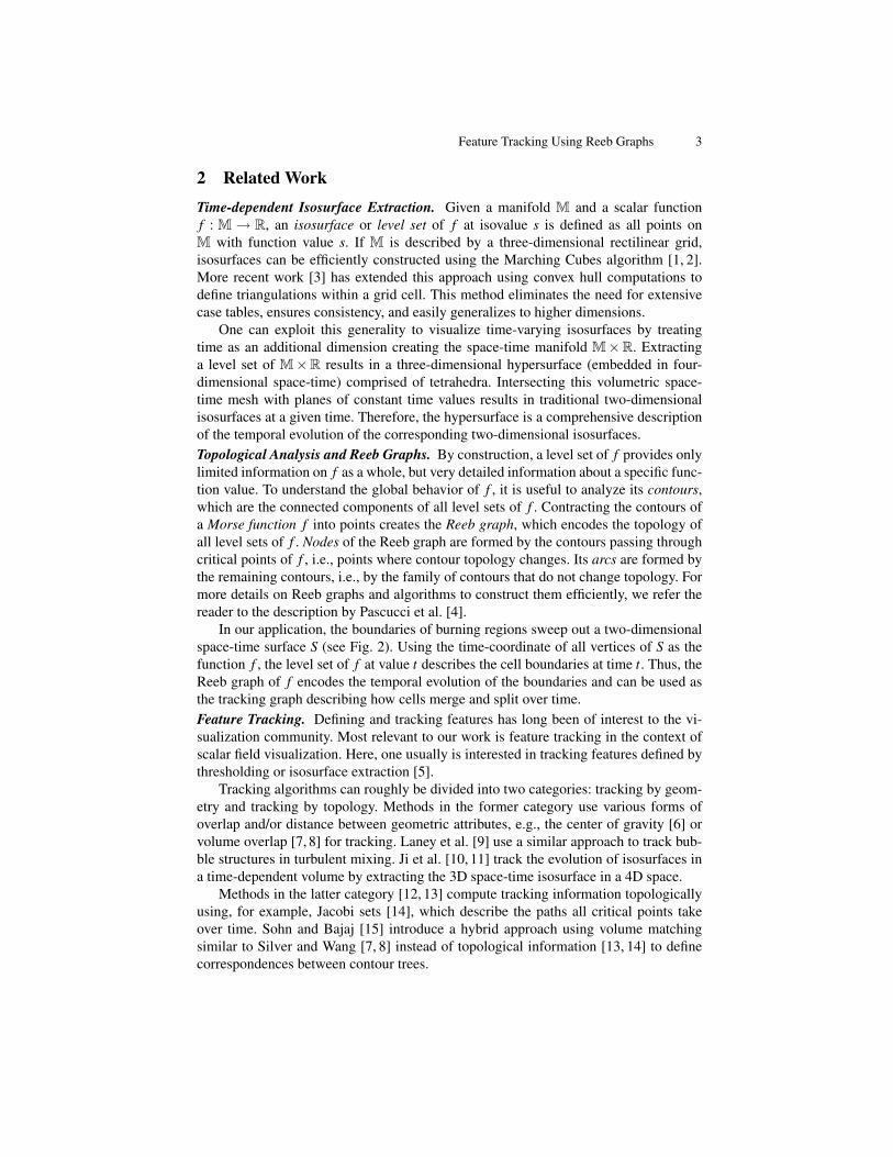
Fig. 2. Traced over time, the boundaries of the burning regions (Fig. 1, right illustration) sweepout surfaces. In this figure, the swept out surfaces are colored according to time (ranging fromblue for early time steps to red for later time steps), which we use as the Morse function in a Reebgraph construction step.

Geometric tracking, in general, is ill-suited for the flame surfaces of interest here.As illustrated by Fig. 1, flame surfaces may be convoluted and contain many denselypacked burning cells. As a result, geometric distance is not a good predictor for trackingburning cells, as flame sheets may fold on themselves, creating cells in close proximityyet far apart relative to the flame surface. Current algorithms for topological trackingusing Jacobi sets are not capable of dealing with large embedded surfaces.

3 Feature Tracking Algorithm

An important aspect of the combustion process is how burning cells evolve over time. Inparticular, scientists are interested in determining how and when cells are created/des-troyed and merge/split. To obtain this information, we track the boundaries of burningcells over time. For each time step, these boundaries are a set of curves, as shown inFig. 1, right illustration.

If we follow these boundary lines over time, they sweep out surfaces; see Fig. 2.Using a 3D time surface in four dimensions, it is possible to extract this swept surfacedirectly. In a first step, one views the data set as a 4D data set, with time as the fourthdimension, by concatenating all available time steps. The resulting data set serves asinput for Marching Cubes to extract a 3D time surface comprised of tetrahedra. Fur-thermore, one also calculates the fuel consumption rate at the vertex positions and as-sociates the rates with the individual vertices. A second step computes an isosurface offuel consumption rate on this tetrahedral mesh, resulting in the swept boundary surfaceas shown in Fig. 2.

Based on this swept surface, it then is possible to track how burning regions change.If we take this swept boundary surface as a manifold, then the elapsed simulation time isa Morse function on it, and level sets correspond to boundaries at a given time. Criticalpoints, where the number of contours of the level set changes, correspond to the changesof the number of burning cells. For example, in Fig. 2, in the area marked with the letter“A” a new burning region is created, and in the area around the letter “B,” a burningregion splits into two separate burning cells. Consequently, the Reeb graph of the sweptboundary surface with time as a Morse function also is a tracking graph for individualburning cells (after simplification).

Feature Tracking Using Reeb Graphs 5

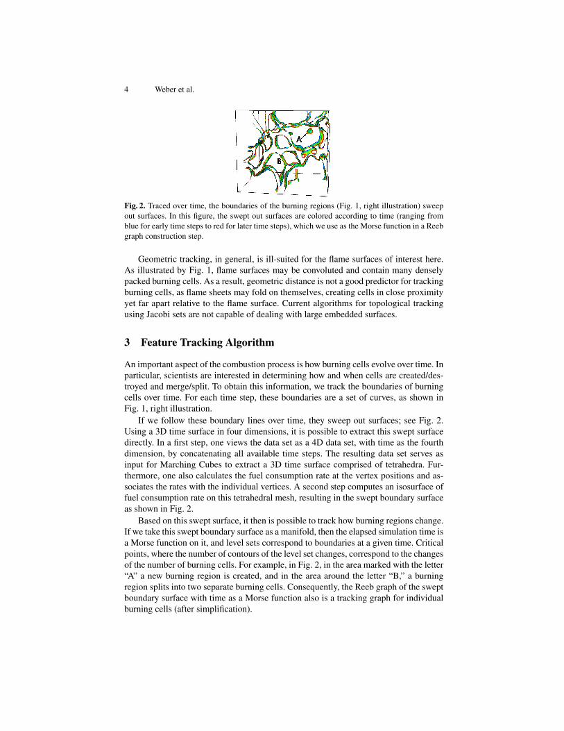
(a) (b) (c)

(d) (e) (f)Fig. 3. Our method traces the evolution of burning regions and extinction pockets by trackingtheir boundaries. This figure illustrates the underlying concepts for the 2D case; the 3D case isanalogous. (a) Input data comes as a set of discrete time slices. (b) We treat time as an additional,third dimension and extract an isosurface. The resulting time surface makes it possible to correlateisotherms from different time steps with each other. (c) We then extract isotherms (contour linesin 2D) for all original time steps by filtering all lines that have only vertices in the time step ofinterest (bold red lines in the figure). (d) We classify isotherm vertices at original time steps aseither burning (solid black discs in the figure) or non-burning (empty circles in the figure) basedon the local fuel consumption rates and simplify the segmentation using a Morse complex-basedmethod. We note that vertices between time steps (arrowed vertex in figure) are not classified,yet. (e) We classify vertices between time steps (arrowed vertex in figure) by thresholding, andextract boundaries separating burning regions and extinction pockets (bold orange lines). (f) Tosimplify this step, we snap intersection points on edges that connect burning and non-burningvertices to the burning vertex (bold orange lines). We do so because it simplifies data processingand does not change the topology of the boundary surface. The Reeb graph (not shown) of theresulting surface is the desired tracking graph.

Our actual implementation is based on this fundamental concept with some addi-tional refinements that we describe in the following. Due to data set size, we pipeline in-dividual processing steps and stream data sets through this pipeline. While our pipelineperforms all these steps on 3D data sets, we use the 2D case shown in Fig. 3 to illustratethe underlying concepts.

Extracting the Time Surface and Isosurfaces at the Original Time Steps. To extractthe boundary of burning cells over time, we need a means to correlate isosurfaces indifferent time steps to each other. For this purpose, we add time as an additional dimen-sion to the original 3D grid, resulting in a (virtual) 4D hyper-grid containing all timesteps of the simulation. We then extract a 3D isovolume that encodes the time evolutionof the flame surface, see Fig. 3(b). Intersecting this 3D (tetrahedral) isovolume with aplane of constant time produces the flame surface for that particular time step. We usethe algorithm of Bhaniramka et al. to compute the isovolume and refer the reader to [3]for a more detailed description.

Here we are interested only in isosurfaces at times that correspond to original timesteps in the simulation. In this special case, intersecting with a plane of constant time

6 Weber et al.

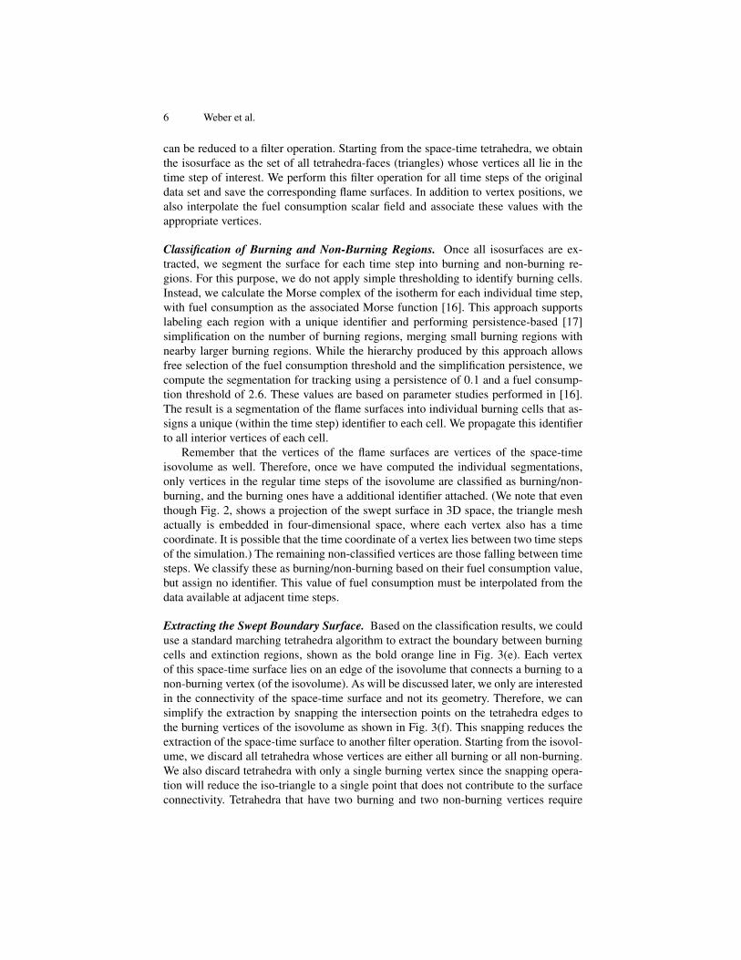
can be reduced to a filter operation. Starting from the space-time tetrahedra, we obtainthe isosurface as the set of all tetrahedra-faces (triangles) whose vertices all lie in thetime step of interest. We perform this filter operation for all time steps of the originaldata set and save the corresponding flame surfaces. In addition to vertex positions, wealso interpolate the fuel consumption scalar field and associate these values with theappropriate vertices.

Classification of Burning and Non-Burning Regions. Once all isosurfaces are ex-tracted, we segment the surface for each time step into burning and non-burning re-gions. For this purpose, we do not apply simple thresholding to identify burning cells.Instead, we calculate the Morse complex of the isotherm for each individual time step,with fuel consumption as the associated Morse function [16]. This approach supportslabeling each region with a unique identifier and performing persistence-based [17]simplification on the number of burning regions, merging small burning regions withnearby larger burning regions. While the hierarchy produced by this approach allowsfree selection of the fuel consumption threshold and the simplification persistence, wecompute the segmentation for tracking using a persistence of 0.1 and a fuel consump-tion threshold of 2.6. These values are based on parameter studies performed in [16].The result is a segmentation of the flame surfaces into individual burning cells that as-signs a unique (within the time step) identifier to each cell. We propagate this identifierto all interior vertices of each cell.

Remember that the vertices of the flame surfaces are vertices of the space-timeisovolume as well. Therefore, once we have computed the individual segmentations,only vertices in the regular time steps of the isovolume are classified as burning/non-burning, and the burning ones have a additional identifier attached. (We note that eventhough Fig. 2, shows a projection of the swept surface in 3D space, the triangle meshactually is embedded in four-dimensional space, where each vertex also has a timecoordinate. It is possible that the time coordinate of a vertex lies between two time stepsof the simulation.) The remaining non-classified vertices are those falling between timesteps. We classify these as burning/non-burning based on their fuel consumption value,but assign no identifier. This value of fuel consumption must be interpolated from thedata available at adjacent time steps.

Extracting the Swept Boundary Surface. Based on the classification results, we coulduse a standard marching tetrahedra algorithm to extract the boundary between burningcells and extinction regions, shown as the bold orange line in Fig. 3(e). Each vertexof this space-time surface lies on an edge of the isovolume that connects a burning to anon-burning vertex (of the isovolume). As will be discussed later, we only are interestedin the connectivity of the space-time surface and not its geometry. Therefore, we cansimplify the extraction by snapping the intersection points on the tetrahedra edges tothe burning vertices of the isovolume as shown in Fig. 3(f). This snapping reduces theextraction of the space-time surface to another filter operation. Starting from the isovol-ume, we discard all tetrahedra whose vertices are either all burning or all non-burning.We also discard tetrahedra with only a single burning vertex since the snapping opera-tion will reduce the iso-triangle to a single point that does not contribute to the surfaceconnectivity. Tetrahedra that have two burning and two non-burning vertices require

Feature Tracking Using Reeb Graphs 7

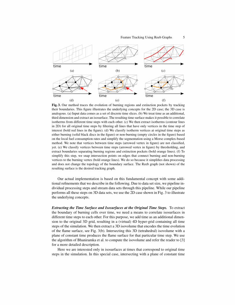
(a) (b) (c)

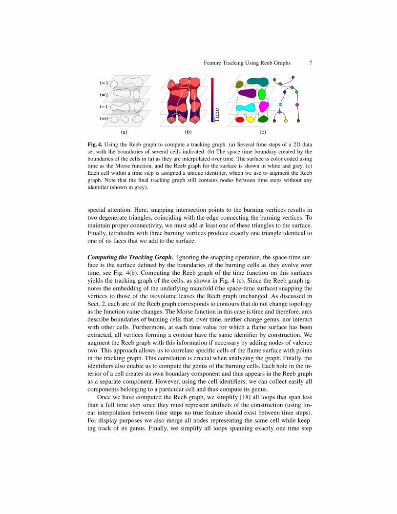
Fig. 4. Using the Reeb graph to compute a tracking graph. (a) Several time steps of a 2D dataset with the boundaries of several cells indicated. (b) The space-time boundary created by theboundaries of the cells in (a) as they are interpolated over time. The surface is color coded usingtime as the Morse function, and the Reeb graph for the surface is shown in white and grey. (c)Each cell within a time step is assigned a unique identifier, which we use to augment the Reebgraph. Note that the final tracking graph still contains nodes between time steps without anyidentifier (shown in grey).

special attention. Here, snapping intersection points to the burning vertices results intwo degenerate triangles, coinciding with the edge connecting the burning vertices. Tomaintain proper connectivity, we must add at least one of these triangles to the surface.Finally, tetrahedra with three burning vertices produce exactly one triangle identical toone of its faces that we add to the surface.

Computing the Tracking Graph. Ignoring the snapping operation, the space-time sur-face is the surface defined by the boundaries of the burning cells as they evolve overtime, see Fig. 4(b). Computing the Reeb graph of the time function on this surfacesyields the tracking graph of the cells, as shown in Fig. 4 (c). Since the Reeb graph ig-nores the embedding of the underlying manifold (the space-time surface) snapping thevertices to those of the isovolume leaves the Reeb graph unchanged. As discussed inSect. 2, each arc of the Reeb graph corresponds to contours that do not change topologyas the function value changes. The Morse function in this case is time and therefore, arcsdescribe boundaries of burning cells that, over time, neither change genus, nor interactwith other cells. Furthermore, at each time value for which a flame surface has beenextracted, all vertices forming a contour have the same identifier by construction. Weaugment the Reeb graph with this information if necessary by adding nodes of valencetwo. This approach allows us to correlate specific cells of the flame surface with pointsin the tracking graph. This correlation is crucial when analyzing the graph. Finally, theidentifiers also enable us to compute the genus of the burning cells. Each hole in the in-terior of a cell creates its own boundary component and thus appears in the Reeb graphas a separate component. However, using the cell identifiers, we can collect easily allcomponents belonging to a particular cell and thus compute its genus.

Once we have computed the Reeb graph, we simplify [18] all loops that span lessthan a full time step since they must represent artifacts of the construction (using lin-ear interpolation between time steps no true feature should exist between time steps).For display purposes we also merge all nodes representing the same cell while keep-ing track of its genus. Finally, we simplify all loops spanning exactly one time step

8 Weber et al.

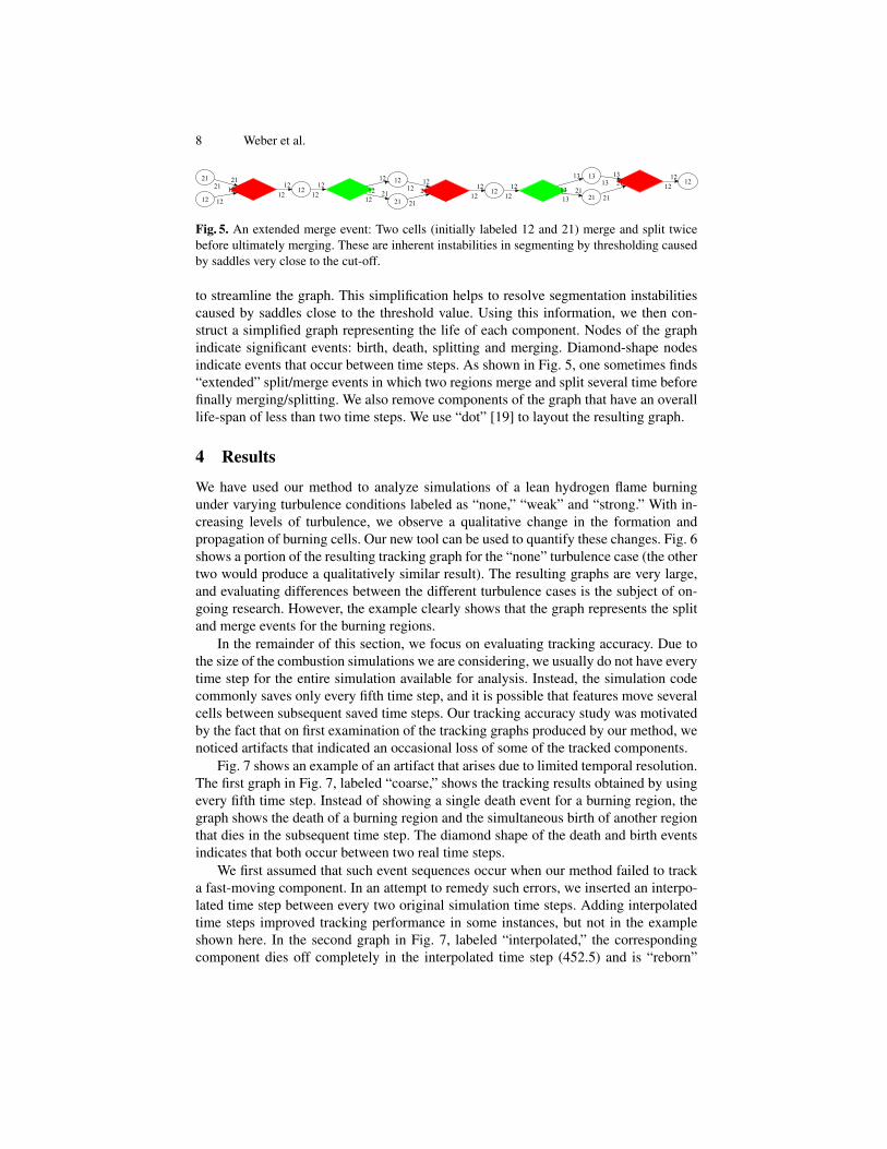
Fig. 5. An extended merge event: Two cells (initially labeled 12 and 21) merge and split twicebefore ultimately merging. These are inherent instabilities in segmenting by thresholding causedby saddles very close to the cut-off.

to streamline the graph. This simplification helps to resolve segmentation instabilitiescaused by saddles close to the threshold value. Using this information, we then con-struct a simplified graph representing the life of each component. Nodes of the graphindicate significant events: birth, death, splitting and merging. Diamond-shape nodesindicate events that occur between time steps. As shown in Fig. 5, one sometimes finds“extended” split/merge events in which two regions merge and split several time beforefinally merging/splitting. We also remove components of the graph that have an overalllife-span of less than two time steps. We use “dot” [19] to layout the resulting graph.

4 Results

We have used our method to analyze simulations of a lean hydrogen flame burningunder varying turbulence conditions labeled as “none,” “weak” and “strong.” With in-creasing levels of turbulence, we observe a qualitative change in the formation andpropagation of burning cells. Our new tool can be used to quantify these changes. Fig. 6shows a portion of the resulting tracking graph for the “none” turbulence case (the othertwo would produce a qualitatively similar result). The resulting graphs are very large,and evaluating differences between the different turbulence cases is the subject of on-going research. However, the example clearly shows that the graph represents the splitand merge events for the burning regions.

In the remainder of this section, we focus on evaluating tracking accuracy. Due tothe size of the combustion simulations we are considering, we usually do not have everytime step for the entire simulation available for analysis. Instead, the simulation codecommonly saves only every fifth time step, and it is possible that features move severalcells between subsequent saved time steps. Our tracking accuracy study was motivatedby the fact that on first examination of the tracking graphs produced by our method, wenoticed artifacts that indicated an occasional loss of some of the tracked components.

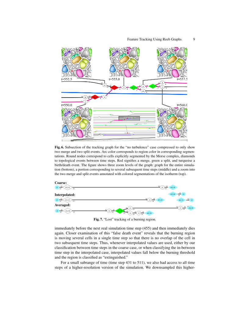
Fig. 7 shows an example of an artifact that arises due to limited temporal resolution.The first graph in Fig. 7, labeled “coarse,” shows the tracking results obtained by usingevery fifth time step. Instead of showing a single death event for a burning region, thegraph shows the death of a burning region and the simultaneous birth of another regionthat dies in the subsequent time step. The diamond shape of the death and birth eventsindicates that both occur between two real time steps.

We first assumed that such event sequences occur when our method failed to tracka fast-moving component. In an attempt to remedy such errors, we inserted an interpo-lated time step between every two original simulation time steps. Adding interpolatedtime steps improved tracking performance in some instances, but not in the exampleshown here. In the second graph in Fig. 7, labeled “interpolated,” the correspondingcomponent dies off completely in the interpolated time step (452.5) and is “reborn”

Feature Tracking Using Reeb Graphs 9

Fig. 6. Subsection of the tracking graph for the “no turbulence” case compressed to only showtwo merge and two split events. Arc color corresponds to region color in corresponding segmen-tations. Round nodes correspond to cells explicitly segmented by the Morse complex, diamondsto topological events between time steps. Red signifies a merge, green a split, and turquoise abirth/death event. The figure shows three zoom levels of the graph: graph for the entire simula-tion (bottom), a portion corresponding to several subsequent time steps (middle) and a zoom intothe two merge and split events annotated with colored segmentations of the isotherm (top).

Coarse:

Interpolated:

Averaged:

Fig. 7. “Lost” tracking of a burning region.

immediately before the next real simulation time step (455) and then immediately diesagain. Closer examination of this “false death event” reveals that the burning regionis moving several cells in a single time step so that there is no overlap of the cell intwo subsequent time steps. Thus, whenever interpolated values are used, either by ourclassification between time steps in the coarse case, or when classifying the in-betweentime step in the interpolated case, interpolated values fall below the burning thresholdand the region is classified as “extinguished.”

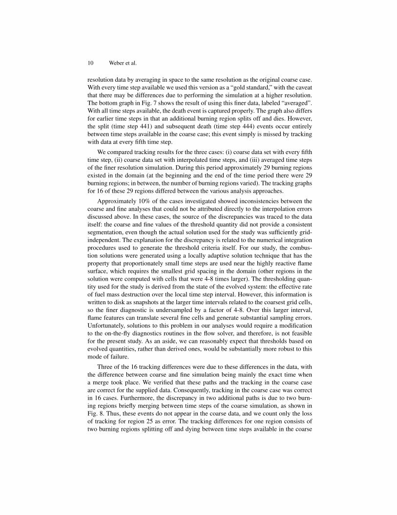
For a small subrange of time (time step 431 to 511), we also had access to all timesteps of a higher-resolution version of the simulation. We downsampled this higher-

10 Weber et al.

resolution data by averaging in space to the same resolution as the original coarse case.With every time step available we used this version as a “gold standard,” with the caveatthat there may be differences due to performing the simulation at a higher resolution.The bottom graph in Fig. 7 shows the result of using this finer data, labeled “averaged”.With all time steps available, the death event is captured properly. The graph also differsfor earlier time steps in that an additional burning region splits off and dies. However,the split (time step 441) and subsequent death (time step 444) events occur entirelybetween time steps available in the coarse case; this event simply is missed by trackingwith data at every fifth time step.

We compared tracking results for the three cases: (i) coarse data set with every fifthtime step, (ii) coarse data set with interpolated time steps, and (iii) averaged time stepsof the finer resolution simulation. During this period approximately 29 burning regionsexisted in the domain (at the beginning and the end of the time period there were 29burning regions; in between, the number of burning regions varied). The tracking graphsfor 16 of these 29 regions differed between the various analysis approaches.

Approximately 10% of the cases investigated showed inconsistencies between thecoarse and fine analyses that could not be attributed directly to the interpolation errorsdiscussed above. In these cases, the source of the discrepancies was traced to the dataitself: the coarse and fine values of the threshold quantity did not provide a consistentsegmentation, even though the actual solution used for the study was sufficiently grid-independent. The explanation for the discrepancy is related to the numerical integrationprocedures used to generate the threshold criteria itself. For our study, the combus-tion solutions were generated using a locally adaptive solution technique that has theproperty that proportionately small time steps are used near the highly reactive flamesurface, which requires the smallest grid spacing in the domain (other regions in thesolution were computed with cells that were 4-8 times larger). The thresholding quan-tity used for the study is derived from the state of the evolved system: the effective rateof fuel mass destruction over the local time step interval. However, this information iswritten to disk as snapshots at the larger time intervals related to the coarsest grid cells,so the finer diagnostic is undersampled by a factor of 4-8. Over this larger interval,flame features can translate several fine cells and generate substantial sampling errors.Unfortunately, solutions to this problem in our analyses would require a modificationto the on-the-fly diagnostics routines in the flow solver, and therefore, is not feasiblefor the present study. As an aside, we can reasonably expect that thresholds based onevolved quantities, rather than derived ones, would be substantially more robust to thismode of failure.

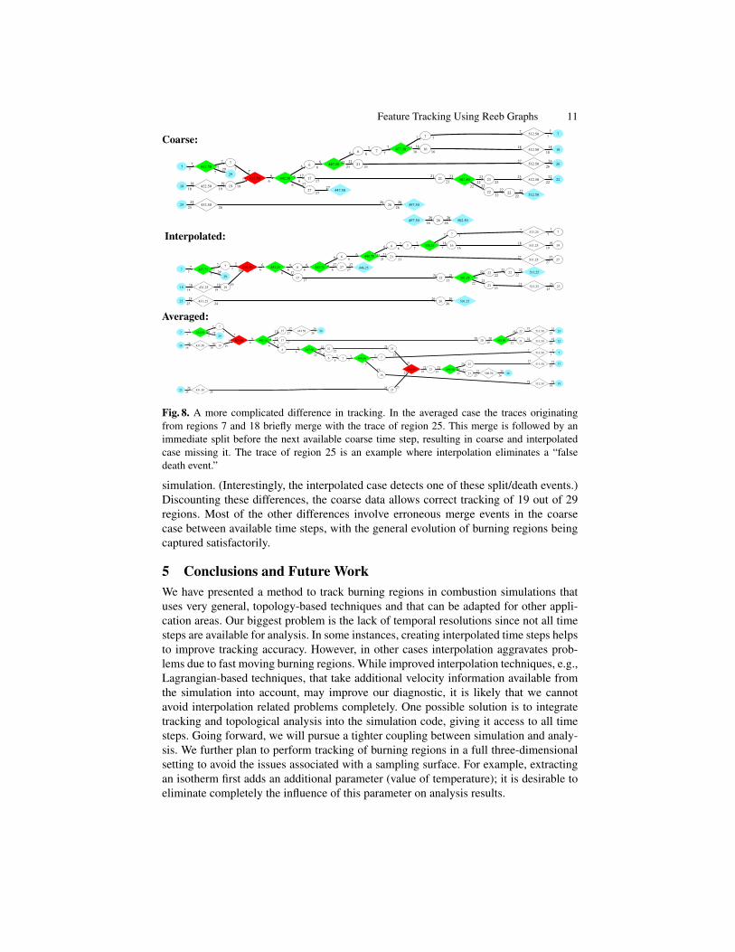
Three of the 16 tracking differences were due to these differences in the data, withthe difference between coarse and fine simulation being mainly the exact time whena merge took place. We verified that these paths and the tracking in the coarse caseare correct for the supplied data. Consequently, tracking in the coarse case was correctin 16 cases. Furthermore, the discrepancy in two additional paths is due to two burn-ing regions briefly merging between time steps of the coarse simulation, as shown inFig. 8. Thus, these events do not appear in the coarse data, and we count only the lossof tracking for region 25 as error. The tracking differences for one region consists oftwo burning regions splitting off and dying between time steps available in the coarse

Feature Tracking Using Reeb Graphs 11

Coarse:

Interpolated:

Averaged:

Fig. 8. A more complicated difference in tracking. In the averaged case the traces originatingfrom regions 7 and 18 briefly merge with the trace of region 25. This merge is followed by animmediate split before the next available coarse time step, resulting in coarse and interpolatedcase missing it. The trace of region 25 is an example where interpolation eliminates a “falsedeath event.”

simulation. (Interestingly, the interpolated case detects one of these split/death events.)Discounting these differences, the coarse data allows correct tracking of 19 out of 29regions. Most of the other differences involve erroneous merge events in the coarsecase between available time steps, with the general evolution of burning regions beingcaptured satisfactorily.

5 Conclusions and Future WorkWe have presented a method to track burning regions in combustion simulations thatuses very general, topology-based techniques and that can be adapted for other appli-cation areas. Our biggest problem is the lack of temporal resolutions since not all timesteps are available for analysis. In some instances, creating interpolated time steps helpsto improve tracking accuracy. However, in other cases interpolation aggravates prob-lems due to fast moving burning regions. While improved interpolation techniques, e.g.,Lagrangian-based techniques, that take additional velocity information available fromthe simulation into account, may improve our diagnostic, it is likely that we cannotavoid interpolation related problems completely. One possible solution is to integratetracking and topological analysis into the simulation code, giving it access to all timesteps. Going forward, we will pursue a tighter coupling between simulation and analy-sis. We further plan to perform tracking of burning regions in a full three-dimensionalsetting to avoid the issues associated with a sampling surface. For example, extractingan isotherm first adds an additional parameter (value of temperature); it is desirable toeliminate completely the influence of this parameter on analysis results.

12 Weber et al.

6 AcknowledgmentsThis work was supported by the Director, Office of Advanced Scientific Computing Re-search, Office of Science, of the U.S. Department of Energy under Contract Nos. DE-AC02-05CH11231 (Lawrence Berkeley National Laboratory), DE-AC52-07NA27344(Lawrence Livermore National Laboratory) and DE-FC02-06ER25781 (University ofUtah) through the Scientific Discovery through Advanced Computing (SciDAC) pro-gram’s Visualization and Analytics Center for Enabling Technologies (VACET) andthe use of resources of the National Energy Research Scientific Computing Center(NERSC).

References1. Lorensen, W., Cline, H.: Marching cubes: A high resolution 3d surface construction algo-

rithm. SIGGRAPH Comp. Graph. 21(4) (1987) 163–1692. Nielson, G.: On marching cubes. IEEE Trans. Vis. Comp. Graph. 9(3) (2003) 341–3513. Bhaniramka, P., Wenger, R., Crawfis, R.: Isosurface construction in any dimension using

convex hulls. IEEE Trans. Vis. Comp. Graph. 10(2) (2004) 130–1414. Pascucci, V., Scorzelli, G., Bremer, P.T., Mascarenhas, A.: Robust on-line computation of

Reeb graphs: Simplicity and speed. ACM Trans. Graph. 26(3) (2007) 58.1–58.95. Mascarenhas, A., Snoeyink, J. In: Isocontour based Visualization of Time-varying Scalar

Fields. Springer Verlag (2009) 41–68 ISBN 978-3-540-25076-0.6. Samtaney, R., Silver, D., Zabusky, N., Cao, J.: Visualizing features and tracking their evolu-

tion. IEEE Computer 27(7) (1994) 20–277. Silver, D., Wang, X.: Tracking and visualizing turbulent 3d features. IEEE Trans. Vis. Comp.

Graph. 3(2) (1997) 129–1418. Silver, D., Wang, X.: Tracking scalar features in unstructured datasets. In: Proc. IEEE

Visualization ’98. (1998) 79–869. Laney, D., Bremer, P.T., Mascarenhas, A., Miller, P., Pascucci, V.: Understanding the struc-

ture of the turbulent mixing layer in hydrodynamic instabilities. IEEE Trans. Vis. Comp.Graph. 12(5) (2006) 1052–1060

10. Ji, G., Shen, H.W., Wegner, R.: Volume tracking using higher dimensional isocontouring.In: Proc. IEEE Visualization ’03. (2003) 209–216

11. Ji, G., Shen, H.W.: Efficient isosurface tracking using precomputed correspondence table.In: Proc. IEEE/Eurographics Symposium Visualization ’04. (2004) 283–292

12. Edelsbrunner, H., Harer, J., Mascarenhas, A., Pascuccii, V., Snoeyink, J.: Time-varying Reebgraphs for continuous space-time data. Comp. Geom. 41(3) (2008) 149–166

13. Szymczak, A.: Subdomain-aware contour trees and contour tree evolution in time-dependentscalar fields. In: Proc. Shape Modeling International ’05. (2005) 136–144

14. Edelsbrunner, H., Harer, J.: Jacobi sets of multiple Morse functions. In: Found. of Comput.Math., Minneapolis 2002. Cambridge Univ. Press, England (2002) 37–57

15. Sohn, B.S., Bajaj, C.: Time-varying contour topology. IEEE Trans. Vis. Comp. Graph. 12(1)(2006) 14–25

16. Bremer, P.T., Weber, G., Pascucci, V., Day, M., Bell, J.: Analyzing and tracking burningstructures in lean premixed hydrogen flames. IEEE Trans. Vis. Comp. Graph. 16(2) (2010)

17. Edelsbrunner, H., Letscher, D., Zomorodian., A.: Topological persistence and simplification.Disc. Comput. Geom. 28(4) (2002) 511–533

18. Agarwal, P., Edelsbrunner, H., Harer, J., Wang, Y.: Extreme elevation on a 2-manifold. Disc.Comput. Geom. 36(4) (2006) 553–572

19. Koutsofios, E., North, S.: Drawing graphs with dot. Technical Report 910904-59113-08TM,AT&T Bell Laboratories, Murray Hill, NJ (1991)