Embed Size (px)
Citation preview

FEATURE SELECTION
VIA
JOINT LIKELIHOOD
A thesis submitted to the University of Manchester
for the degree of Doctor of Philosophy
in the Faculty of Engineering and Physical Sciences
2012
By
Adam C Pocock
School of Computer Science

Contents
Abstract 11
Declaration 13
Copyright 14
Acknowledgements 15
Notation 16
1 Introduction 17
1.1 Prediction and data collection . . . . . . . . . . . . . . . . . . . . 17
1.2 Research Questions . . . . . . . . . . . . . . . . . . . . . . . . . . 20
1.3 Contributions of this thesis . . . . . . . . . . . . . . . . . . . . . . 21
1.4 Structure of this thesis . . . . . . . . . . . . . . . . . . . . . . . . 22
1.5 Publications and Software . . . . . . . . . . . . . . . . . . . . . . 23
2 Background 26
2.1 Classification . . . . . . . . . . . . . . . . . . . . . . . . . . . . . 26
2.1.1 Probability, Likelihood and Bayes Theorem . . . . . . . . 31
2.1.2 Classification algorithms . . . . . . . . . . . . . . . . . . . 34
2.2 Cost-Sensitive Classification . . . . . . . . . . . . . . . . . . . . . 36
2.2.1 Bayesian Decision Theory . . . . . . . . . . . . . . . . . . 37
2.2.2 Constructing a cost-sensitive classifier . . . . . . . . . . . . 37
2.3 Information Theory . . . . . . . . . . . . . . . . . . . . . . . . . . 38
2.3.1 Shannon’s Information Theory . . . . . . . . . . . . . . . . 39
2.3.2 Bayes error and conditional entropy . . . . . . . . . . . . . 42
2.3.3 Estimating the mutual information . . . . . . . . . . . . . 44
2.4 Weighted Information Theory . . . . . . . . . . . . . . . . . . . . 45
2

2.5 Chapter Summary . . . . . . . . . . . . . . . . . . . . . . . . . . 47
3 What is feature selection? 49
3.1 Feature Selection . . . . . . . . . . . . . . . . . . . . . . . . . . . 49
3.1.1 Filters . . . . . . . . . . . . . . . . . . . . . . . . . . . . . 52
3.1.2 Wrappers . . . . . . . . . . . . . . . . . . . . . . . . . . . 54
3.1.3 Embedded methods . . . . . . . . . . . . . . . . . . . . . . 54
3.2 Information theoretic feature selection . . . . . . . . . . . . . . . 55
3.3 Feature selection with priors . . . . . . . . . . . . . . . . . . . . . 58
3.4 Multi-class and cost-sensitive feature selection . . . . . . . . . . . 60
3.5 Bayesian Networks . . . . . . . . . . . . . . . . . . . . . . . . . . 62
3.6 Structure Learning . . . . . . . . . . . . . . . . . . . . . . . . . . 64
3.6.1 Conditional independence testing . . . . . . . . . . . . . . 65
3.6.2 Score and search methods . . . . . . . . . . . . . . . . . . 68
3.7 Chapter Summary . . . . . . . . . . . . . . . . . . . . . . . . . . 72
4 Deriving a selection criterion 74
4.1 Minimising a Loss Function . . . . . . . . . . . . . . . . . . . . . 74
4.1.1 Defining the feature selection problem . . . . . . . . . . . 75
4.1.2 A discriminative model for feature selection . . . . . . . . 76
4.1.3 Optimizing the feature selection parameters . . . . . . . . 81
4.2 Chapter Summary . . . . . . . . . . . . . . . . . . . . . . . . . . 85
5 Unifying information theoretic filters 87
5.1 Retrofitting Successful Heuristics . . . . . . . . . . . . . . . . . . 87
5.1.1 Bounding the criteria . . . . . . . . . . . . . . . . . . . . . 96
5.1.2 Summary of theoretical findings . . . . . . . . . . . . . . . 97
5.2 Experimental Study . . . . . . . . . . . . . . . . . . . . . . . . . . 98
5.2.1 How stable are the criteria to small changes in the data? . 99
5.2.2 How similar are the criteria? . . . . . . . . . . . . . . . . . 102
5.2.3 How do criteria behave in small-sample situations? . . . . 104
5.2.4 What is the relationship between stability and accuracy? . 106
5.2.5 Summary of empirical findings . . . . . . . . . . . . . . . . 110
5.3 Performance on the NIPS Feature Selection Challenge . . . . . . . 110
5.3.1 GISETTE testing data results . . . . . . . . . . . . . . . . 114
5.3.2 MADELON testing data results . . . . . . . . . . . . . . . 114
3

5.4 An Information Theoretic View of Strong and Weak Relevance . . 115
5.5 Chapter Summary . . . . . . . . . . . . . . . . . . . . . . . . . . 119
6 Priors for filter feature selection 120
6.1 Maximising the Joint Likelihood . . . . . . . . . . . . . . . . . . . 120
6.2 Constructing a prior . . . . . . . . . . . . . . . . . . . . . . . . . 122
6.2.1 A factored prior . . . . . . . . . . . . . . . . . . . . . . . . 122
6.2.2 Update rules . . . . . . . . . . . . . . . . . . . . . . . . . 123
6.2.3 Encoding sparsity or domain knowledge . . . . . . . . . . 124
6.3 Incorporating a prior into IAMB . . . . . . . . . . . . . . . . . . . 125
6.4 Empirical Evaluation . . . . . . . . . . . . . . . . . . . . . . . . . 128
6.5 Chapter Summary . . . . . . . . . . . . . . . . . . . . . . . . . . 134
7 Cost-sensitive feature selection 135
7.1 Deriving a Cost Sensitive Filter Method . . . . . . . . . . . . . . 135
7.1.1 Notation . . . . . . . . . . . . . . . . . . . . . . . . . . . . 136
7.1.2 Deriving cost-sensitive criteria . . . . . . . . . . . . . . . . 137
7.1.3 Iterative minimisation . . . . . . . . . . . . . . . . . . . . 140
7.2 Weighted Information Theory . . . . . . . . . . . . . . . . . . . . 141
7.2.1 Non-negativity of the weighted mutual information . . . . 142
7.2.2 The chain rule of weighted mutual information . . . . . . . 143
7.3 Constructing filter criteria . . . . . . . . . . . . . . . . . . . . . . 145
7.4 Empirical study of Weighted Feature Selection . . . . . . . . . . . 146
7.4.1 Handwritten Digits . . . . . . . . . . . . . . . . . . . . . . 146
7.4.2 Document Classification . . . . . . . . . . . . . . . . . . . 152
7.5 Chapter Summary . . . . . . . . . . . . . . . . . . . . . . . . . . 153
8 Conclusions and future directions 155
8.1 What did we learn in this thesis? . . . . . . . . . . . . . . . . . . 155
8.1.1 Can we derive a feature selection criterion which minimises
the error rate? . . . . . . . . . . . . . . . . . . . . . . . . . 155
8.1.2 What implicit assumptions are made by the information
theoretic criteria in the literature? . . . . . . . . . . . . . . 157
8.1.3 Developing informative priors for feature selection . . . . . 159
8.1.4 How should we construct a cost-sensitive feature selection
algorithm? . . . . . . . . . . . . . . . . . . . . . . . . . . . 159
4

8.2 Future Work . . . . . . . . . . . . . . . . . . . . . . . . . . . . . . 160
Bibliography 163
Word Count: 42409
5

List of Tables
2.1 Summarising different kinds of misclassification. . . . . . . . . . . 29
3.1 Various information-based criteria from the literature. In Chapter
5 we investigate the links between these criteria and incorporate
them into a single theoretical framework. . . . . . . . . . . . . . . 58
5.1 Datasets used in experiments. The final column indicates the dif-
ficulty of the data in feature selection, a smaller value indicating a
more challenging problem. . . . . . . . . . . . . . . . . . . . . . . 100
5.2 Datasets from Peng et al. [86], used in small-sample experiments. 106
5.3 Column 1: Non-dominated Rank of different criteria for the
trade-off of accuracy/stability. Criteria with a higher rank (closer
to 1.0) provide a better trade-off than those with a lower rank.
Column 2: As column 1 but using Kuncheva’s Stability Index.
Column 3: Average ranks for accuracy alone. . . . . . . . . . . . 110
5.4 Datasets from the NIPS challenge, used in experiments. . . . . . . 112
5.5 NIPS FS Challenge Results: GISETTE. . . . . . . . . . . . . . . 114
5.6 NIPS FS Challenge Results: MADELON. . . . . . . . . . . . . . 115
6.1 Dataset properties. # |MB| ≥ 2 is the number of features (nodes)
in the network with an MB of at least size 2. Mean |MB| is the
mean size of these blankets. Median arity indicates the number
of possible values for a feature. A large MB and high feature
arity indicates a more challenging problem with limited data; i.e.
Alarm is (relatively) the simplest dataset, while Barley is the most
challenging with both a large mean MB size and the highest feature
arity. . . . . . . . . . . . . . . . . . . . . . . . . . . . . . . . . . . 128
6.2 Win/Draw/Loss results for ALARM network. . . . . . . . . . . . 132
6.3 Win/Draw/Loss results for Barley network. . . . . . . . . . . . . 133
6

6.4 Win/Draw/Loss results on Hailfinder . . . . . . . . . . . . . . . . 133
6.5 Win/Draw/Loss results for Insurance. . . . . . . . . . . . . . . . . 134
7.1 An example of a negative wI, wI(X;Y ) = −0.0214. . . . . . . . . 142
7.2 MNIST results, averaged across all digits. Each value is the differ-
ence (x 100) in Precision, Recall or F-Measure, against the cost-
insensitive baseline. . . . . . . . . . . . . . . . . . . . . . . . . . . 149
7.3 MNIST results, digit 4. Each value is the difference (x 100) in
Precision, Recall or F-Measure, against the cost-insensitive baseline.149
7.4 MNIST results, averaged across all digits. Each value is the differ-
ence (x 100) in Precision, Recall or F-Measure, against the cost-
insensitive baseline. . . . . . . . . . . . . . . . . . . . . . . . . . . 152
7.5 Summary of text classification datasets. . . . . . . . . . . . . . . . 153
7.6 Document classification results: F-Measure W/D/L across all la-
bels, with the costly label given w(y) = 10. . . . . . . . . . . . . . 153
7

List of Figures
2.1 Two example classification boundaries. The solid line is from a
linear classifier, and the dashed line is from a non-linear classifier. 28
3.1 A Bayesian network, with the target node shaded in red, and the
Markov Blanket of that node shaded in cyan. . . . . . . . . . . . . 63
4.1 The graphical model for the likelihood specified in Equation (4.1). 76
5.1 Figure 5.1a shows the scatter plot between X1 and X2. Figure 5.1b
shows the scatter plot between X1 and X2 when Y = 1. Figure
5.1c shows the scatter plot between X1 and X2 when Y = 2. . . . 90
5.2 The full space of linear filter criteria, describing several examples
from Table 3.1. Note that all criteria in this space adopt Assump-
tion 1. Additionally, the γ and β axes represent the criteria belief
in Assumptions 2 and 3, respectively. The left hand axis is where
the mRMR and MIFS algorithms sit. The bottom left corner,
MIM, is the assumption of completely independent features, us-
ing just marginal mutual information. Note that some criteria are
equivalent at particular sizes of the current feature set |S|. . . . . 95
5.3 Kuncheva’s Stability Index [67] across 15 datasets. The box in-
dicates the upper/lower quartiles, the horizontal line within each
shows the median value, while the dotted crossbars indicate the
maximum/minimum values. For convenience of interpretation, cri-
teria on the x-axis are ordered by their median value. . . . . . . 102
8

5.4 Yu et al.’s Information Stability Index [111] across 15 datasets. For
comparison, criteria on the x-axis are ordered identically to Figure
5.3. A similar general picture emerges to that using Kuncheva’s
measure, though the information stability index is able to take
feature redundancy into account, showing that some criteria are
slightly more stable than expected. . . . . . . . . . . . . . . . . . 103
5.5 Relations between feature sets generated by different criteria, on
average over 15 datasets. 2D visualisation generated by classical
multi-dimensional scaling. . . . . . . . . . . . . . . . . . . . . . . 104
5.6 Average ranks of criteria in terms of test error, selecting 10 fea-
tures, across 11 datasets. Note the clear dominance of criteria
which do not allow the redundancy term to overwhelm the rele-
vancy term (stars) over those that allow redundancy to grow with
the size of the feature set (circles). . . . . . . . . . . . . . . . . . 105
5.7 LOO results on Peng’s datasets: Colon, Lymphoma, Leukemia,
Lung, NCI9. . . . . . . . . . . . . . . . . . . . . . . . . . . . . . . 107
5.8 Stability (y-axes) versus Accuracy (x-axes) over 50 bootstraps for
the final quarter of the UCI datasets. The pareto-optimal rankings
are summarised in Table 5.3. . . . . . . . . . . . . . . . . . . . . . 109
5.9 Significant dominance partial-order diagram. Criteria are placed
top to bottom in the diagram by their rank taken from column
3 of Table 5.3. A link joining two criteria means a statistically
significant difference is observed with a Nemenyi post-hoc test at
the specified confidence level. For example JMI is significantly su-
perior to MIFS (β = 1) at the 99% confidence level. Note that the
absence of a link does not signify the lack of a statistically signifi-
cant difference, but that the Nemenyi test does not have sufficient
power (in terms of number of datasets) to determine the outcome
[29]. It is interesting to note that the four bottom ranked criteria
correspond to the corners of the unit square in Figure 5.2; while
the top three (JMI/mRMR/DISR) are all very similar, scaling the
redundancy terms by the size of the feature set. The middle ranks
belong to CMIM/ICAP, which are similar in that they use the
min/max strategy instead of a linear combination of terms. . . . 111
5.10 Validation Error curve using GISETTE. . . . . . . . . . . . . . . 113
9

5.11 Validation Error curve using MADELON. . . . . . . . . . . . . . 113
6.1 Toy problem, 5 feature nodes (X1 . . . X5) and their estimated mu-
tual information with the target node Y on a particular data sam-
ple. X1, X2, X5 form the Markov Blanket of Y . . . . . . . . . . . . 129
6.2 Average results: (a) Small sample, correct prior; (b) Large sam-
ple, correct prior; (c) Small sample, misspecified prior; (d) Large
sample, misspecified prior. . . . . . . . . . . . . . . . . . . . . . . 131
7.1 The average pixel values across all 4s in our sample of MNIST. . . 148
7.2 MNIST Results, with “4” as the costly digit. . . . . . . . . . . . . 148
7.3 MNIST Results, with “4” as the costly digit, using w(y = 4) =
1, 5, 10, 15, 20, 25, 50, 100 and (w)JMI. LEFT: Note that as costs
for mis-classifying “4” increase, the weighted FS method increases
F-measure, while the weighted SVM suffers a decrease. RIGHT:
The black dot is the cost-insensitive methodology. Note that the
weighted SVM can increase recall above the 90% mark, but it does
so by sacrificing precision. In contrast, the weighted FS method
pushes the cluster of points up and to the right, increasing both
recall and precision. . . . . . . . . . . . . . . . . . . . . . . . . . 149
7.4 MNIST Results, with both “4” and “9” as the costly digits, us-
ing w(y = (4 ∨ 9)) = 1, 5, 10, 15, 20, 25, 50, 100 and (w)JMI, F-
Measure. . . . . . . . . . . . . . . . . . . . . . . . . . . . . . . . 150
7.5 MNIST Results, with both “4” and “9” as the costly digits, using
w(y = (4 ∨ 9)) = 1, 5, 10, 15, 20, 25, 50, 100 and (w)JMI, Preci-
sion/Recall plot. . . . . . . . . . . . . . . . . . . . . . . . . . . . 151
7.6 MNIST Results, using wMIM comparing against SpreadFX, with
“4” as the costly digit. . . . . . . . . . . . . . . . . . . . . . . . . 152
7.7 Ohscal results. Cost of mis-predicting class 9 is set to ten times
more than other classes. The weighted SVM and oversampling
approaches clearly focus on producing high recall, far higher than
our method, however, this is only achievable by sacrificing preci-
sion. Our approach improves precision and recall, giving higher
F-measure overall. . . . . . . . . . . . . . . . . . . . . . . . . . . . 154
10

Abstract
Feature selection via Joint LikelihoodAdam C Pocock
A thesis submitted to the University of Manchesterfor the degree of Doctor of Philosophy, 2012
We study the nature of filter methods for feature selection. In particular, we ex-
amine information theoretic approaches to this problem, looking at the literature
over the past 20 years. We consider this literature from a different perspective, by
viewing feature selection as a process which minimises a loss function. We choose
to use the model likelihood as the loss function, and thus we seek to maximise
the likelihood. The first contribution of this thesis is to show that the problem of
information theoretic filter feature selection can be rephrased as maximising the
likelihood of a discriminative model.
From this novel result we can unify the literature revealing that many of
these selection criteria are approximate maximisers of the joint likelihood. Many
of these heuristic criteria were hand-designed to optimise various definitions of
feature “relevancy” and “redundancy”, but with our probabilistic interpretation
we naturally include these concepts, plus the “conditional redundancy”, which is
a measure of positive interactions between features. This perspective allows us
to derive the different criteria from the joint likelihood by making different inde-
pendence assumptions on the underlying probability distributions. We provide
an empirical study which reinforces our theoretical conclusions, whilst revealing
implementation considerations due to the varying magnitudes of the relevancy
and redundancy terms.
We then investigate the benefits our probabilistic perspective provides for the
application of these feature selection criteria in new areas. The joint likelihood
11

automatically includes a prior distribution over the selected feature sets and so
we investigate how including prior knowledge affects the feature selection process.
We can now incorporate domain knowledge into feature selection, allowing the
imposition of sparsity on the selected feature set without using heuristic stopping
criteria. We investigate the use of priors mainly in the context of Markov Blanket
discovery algorithms, in the process showing that a family of algorithms based
upon IAMB are iterative maximisers of our joint likelihood with respect to a
particular sparsity prior. We thus extend the IAMB family to include a prior for
domain knowledge in addition to the sparsity prior.
Next we investigate what the choice of likelihood function implies about the
resulting filter criterion. We do this by applying our derivation to a cost-weighted
likelihood, showing that this likelihood implies a particular cost-sensitive filter
criterion. This criterion is based on a weighted branch of information theory and
we prove several novel results justifying its use as a feature selection criterion,
namely the positivity of the measure, and the chain rule of mutual information.
We show that the feature set produced by this cost-sensitive filter criterion can be
used to convert a cost-insensitive classifier into a cost-sensitive one by adjusting
the features the classifier sees. This can be seen as an analogous process to
that of adjusting the data via over or undersampling to create a cost-sensitive
classifier, but with the crucial difference that it does not artificially alter the data
distribution.
Finally we conclude with a summary of the benefits this loss function view
of feature selection has provided. This perspective can be used to analyse other
feature selection techniques other than those based upon information theory, and
new groups of selection criteria can be derived by considering novel loss functions.
12

Declaration
No portion of the work referred to in this thesis has been
submitted in support of an application for another degree
or qualification of this or any other university or other
institute of learning.
13

Copyright
i. The author of this thesis (including any appendices and/or schedules to
this thesis) owns certain copyright or related rights in it (the “Copyright”)
and s/he has given The University of Manchester certain rights to use such
Copyright, including for administrative purposes.
ii. Copies of this thesis, either in full or in extracts and whether in hard or
electronic copy, may be made only in accordance with the Copyright, De-
signs and Patents Act 1988 (as amended) and regulations issued under it
or, where appropriate, in accordance with licensing agreements which the
University has from time to time. This page must form part of any such
copies made.
iii. The ownership of certain Copyright, patents, designs, trade marks and other
intellectual property (the “Intellectual Property”) and any reproductions of
copyright works in the thesis, for example graphs and tables (“Reproduc-
tions”), which may be described in this thesis, may not be owned by the
author and may be owned by third parties. Such Intellectual Property and
Reproductions cannot and must not be made available for use without the
prior written permission of the owner(s) of the relevant Intellectual Property
and/or Reproductions.
iv. Further information on the conditions under which disclosure, publication
and commercialisation of this thesis, the Copyright and any Intellectual
Property and/or Reproductions described in it may take place is available
in the University IP Policy (see http://documents.manchester.ac.uk/
DocuInfo.aspx?DocID=487), in any relevant Thesis restriction declarations
deposited in the University Library, The University Library’s regulations
(see http://www.manchester.ac.uk/library/aboutus/regulations) and
in The University’s policy on presentation of Theses
14

Acknowledgements
First I would like to thank my supervisors Gavin Brown and Mikel Lujan, for
their guidance and help throughout my PhD. Even when they both insist on
sneaking up on me.
Thanks to everyone in the MLO lab, though you will have to fix your own
computers when I am gone. Special thanks to Richard S, Richard A, Joe, Peter,
Freddie, Nicolo, Mauricio, and Kevin for ensuring I retained a small measure of
sanity. Thanks also to the iTLS team, even if I never got chance to play with all
that data.
Thanks are due to my flatmates Alex and Jon, even if none of us were partic-
ularly acquainted with the vacuum cleaner. Thanks to the rest of my friends in
Manchester for sticking around as my life was slowly sacrificed to the PhD gods,
being ready for some gaming or a trip to Sandbar as and when I escaped the lab.
And finally thanks to my parents, my brother Matt and Sarah, without whom
I would not be capable of anything.
15

Notation
d Dimension of the feature space (i.e. the number of features)
N Number of datapoints
Y Random variable denoting the output
Xi, X Random variable denoting the i’th input/feature, and the joint ran-
dom variable of all the features X1, . . . , Xd
|Y | The number of states in Y
y, yi, y A label y ∈ Y , the i’th datapoint’s label, and a predicted label
x, xi A feature vector x ∈ X, and the i’th datapoint’s feature vector
w, w(y) A |Y | − 1 dimensional non-negative weight vector, a weight function
based upon the label y
D A dataset of N x,y tuples
θ, θi A d-dimensional bit vector, and the i’th element of the vector, θi = 1
denotes the i’th feature is selected
¬θ The logical inverse of θ, i.e. the unselected features
Xθ, xθ The selected subset of features Xθ ⊆ X, and a feature vector xθ ∈ Xθ
λ, τ Generative parameters for creating x, discriminative parameters for
determining y from a particular x
p(y), p(y) A true probability distribution, and an estimated distribution
q(y|x, τ) The probability of label y conditioned on x from a predictive model
using parameters τ
L, −` The likelihood function, and the negative log-likelihood
S The selected feature set — equivalent to Xθ
J(Xj) Scoring criterion measuring the quality of the feature Xj
θt The selected feature vector at time t
16

Chapter 1
Introduction
If we wish to make a decision about an important subject, the first step is of-
ten to gather data about the problem. For example, if we need to decide which
University to study at for a degree, it would be sensible to gather relevant in-
formation like the courses offered by different Universities, what the surrounding
environment is like, and what the job prospects are for graduates of the insti-
tutions. If we instead chose to base our decision on irrelevant information like
the colour of the cars parked outside each University, then our choice would not
be well informed and the course might be entirely unsuitable. The problem of
choosing what information to base our decisions on must be solved before we can
even attempt the larger problem of making a decision. The task of automatically
making decisions falls under the remit of Artificial Intelligence, and specifically
the field of Machine Learning. Machine Learning is about constructing models
which make predictions based upon data, and in this thesis we focus on that first
step in producing a prediction, namely selecting the relevant data.
In this chapter we motivate the problem of feature selection, giving a brief
introduction to the relevant topics and explaining the importance of the problem.
We state the specific questions that this thesis answers, explaining the relevancy
of those questions to the field. We then provide a brief outline of the thesis
structure, and detail the publications which have resulted from this thesis.
1.1 Prediction and data collection
In this section we will look at the process of making a prediction at a high
level. We consider the problem of predicting what university undergraduate
17

18 CHAPTER 1. INTRODUCTION
course would best suit a particular student. As we outlined above, a crucial
first step is deciding what data we should base our predictions on. In this task
basing our predictions on the colour of houses in southern Peru is unlikely to
give much insight, but basing our predictions on that student’s strengths and the
qualities of the university would allow a much improved prediction. Therefore
choosing the inputs (also known as features) to a learning algorithm is as im-
portant as the choice of learning algorithm, as without good inputs nothing can
be learned. Once we have selected a set of appropriate inputs, it is possible to
analyse those choices and decipher how each input relates to the thing we wish
to predict. Feature selection is the process of finding those inputs and learning
how they relate to each other.
If we consider the task of feature selection, we can separate out features into
three different classes: relevant, redundant and irrelevant (we will give precise
definitions of each of these concepts in Chapter 3). Relevant features are those
which contain information which will help solve the prediction problem. Without
these features it is likely we will have incomplete information about the problem
we are trying to solve, therefore our predictions will be poor. As mentioned
previously, the proportion of graduates who have jobs or gone on to further study
would be a very relevant feature when choosing a degree course. Redundant
features are those which contain useful information that we already know from
another source. If we have two features, one which tells us a university has 256
Computer Science (CS) undergraduates, and the other tells us the same university
has more than 200 CS undergraduates, then the second is clearly redundant as the
first feature tells us exactly how many students there are (assuming both features
give true information). If we didn’t know the first feature, then the second would
give useful information about the popularity of the CS course, but it doesn’t add
any extra information to the first feature. Irrelevant features are those which
contain no useful information about the problem. It is easy to think of irrelevant
features for any given problem, for example the equatorial circumference of the
Moon is unlikely to be relevant to the problem of choosing a degree course. If
we could go through our data, and label each feature relevant, redundant or
irrelevant then the feature selection task would be easy. We would simply select
all the relevant features, and discard the rest. We could then move on to the
complex problem of learning how to predict based upon those features.
Unfortunately, as with many things in machine learning, the high level view

1.1. PREDICTION AND DATA COLLECTION 19
sounds simple but the details of implementing such a process can be very hard.
In the extreme examples described above it was simple to determine if a feature
was relevant, irrelevant, or redundant in the presence of other features. In real
problems it is usually much more difficult. For example, if one of our features
is the number of bricks in the Computer Science building at the university, will
that feature help us decide if the Computer Science undergraduate course will
be good? Intuitively we might expect this feature to be irrelevant, but this is
not necessarily the case. We might imagine that a large number means there
is a large CS building, (hopefully) full of fascinating lectures and the latest in
computer hardware. Equally the number could be very small, if the building is
modern and built from glass and steel, and yet still contain the truly relevant
(but hard to quantify) things which will make a good undergraduate course. The
number could also be somewhere in the middle, indicating a smaller building
with fewer students. This feature could interact with other features we have
collected, changing the meaning of that feature. Our prospective undergraduate
could prefer going to a large department with many students, where there is more
potential for socialising and working with different people. Or they could prefer
a small department which is less busy and where it is possible to know all the
students and staff. These two features (the number of bricks, and our prospective
student’s preference) interact, so a student who wants a large department might
prefer a course with a large number of bricks (or a very small number) denoting
a large CS building. The student who favours a small department might prefer a
course with a medium number of bricks, denoting a smaller CS building. However
without considering both of these features together our feature selection process
might believe the number of bricks to be irrelevant, as small, medium and large
values all lead to good and bad choices of undergraduate course, because the
choice also depends on the student’s preference.
Determining if a feature is redundant is an equally hard problem. In our
example if we knew both the number of bricks and the amount of floor space in
the CS building we might think the former is redundant in the presence of the
latter. In the previous example we simply used the number of bricks as a proxy
for the size of the building, so knowing the size of the building surely makes that
feature redundant? As always the answer is not quite so simple, as very small
numbers of bricks also told us that the building might be modern and made
from steel. Our new feature of the size of the building does not provide that

20 CHAPTER 1. INTRODUCTION
information, and so does not make the number of bricks completely redundant.
If analysing features to determine these properties is so difficult for humans,
how can we construct algorithms to perform the task automatically? The stan-
dard approach is to use supervised learning where we take a dataset of features,
label them with the appropriate class, and then try to learn the relationship be-
tween the features and the class. In our example we would measure all of the
features for each different university course, gather a sample of prospective under-
graduates, survey their preferences for courses and finally record their choice of
course and whether they were happy with that choice. For each student we would
have a list of features pertaining to their chosen university course, their individ-
ual preferences, and a label which stated if they were happy with the course. We
then test each feature to see how relevant it is to the happiness of the student.
The choice of the relevancy test (or selection criterion) is one of the principle
areas of research in feature selection, and forms the topic of this thesis.
One further question we might ask is why analyse the features at all. Surely
if we find a sufficiently sophisticated machine learning algorithm to make our
prediction about the choice of course then we do not need to separately anal-
yse the features. While many modern machine learning methods are capable of
learning in the presence of irrelevant features, this comes at the expense of extra
run time and requires additional computer power. In addition to these strictly
computational benefits, there are also reductions in cost by not collecting the
irrelevant features. If collecting each feature has a material or time cost (such as
interviewing lecturers at a university, or surveying the surrounding towns), then
if we do not need those features we can avoid that collection cost. We can see
that even if we assume our learning algorithm can cope with irrelevant features
there are benefits to removing them through feature selection.
1.2 Research Questions
The literature surrounding feature selection contains many different kinds of se-
lection criteria [50]. Most of these criteria have been constructed on an ad-hoc
basis, attempting to find a trade off between the relevancy and redundancy of
the selected feature set. The heuristic nature of selection criteria is particularly
apparent in the field of information theoretic feature selection, upon which this

1.3. CONTRIBUTIONS OF THIS THESIS 21
thesis focuses. There has been little work which aims to derive the optimal fea-
ture selection criterion based upon a particular evaluation measure that we wish
to minimise/maximise (e.g. we might wish to minimise the number of mistakes
our prediction algorithm makes when given a particular feature set). Therefore
the first question is “Can we derive a feature selection criteria which minimises
the error rate (or a suitable proxy for the error rate)?”. Having achieved this
we wish to understand the confusing literature of information theoretic feature
selection criteria, by relating them to our optimal criterion. The next question is
therefore “What implicit assumptions are made by the literature on information
theoretic criteria, and how do they relate to the optimal criterion?”. Once we
have understood the literature we should look at what other benefits a princi-
pled framework for feature selection might provide, and how we could extend the
framework to other interesting areas, such as cost-sensitivity. We therefore ask
one final question, “How should we construct a cost-sensitive feature selection
algorithm?”.
1.3 Contributions of this thesis
This thesis focuses on filter feature selection criteria, specifically those which use
information theoretic functions to score features. The main contribution is an
interpretation of this field as approximate iterative maximisers of a discriminative
model likelihood. We provide a summary of the contributions here, with a more
thorough description given in the Conclusions chapter (Chapter 8).
• A derivation of the optimal information theoretic feature selection criterion
which iteratively maximises a discriminative model likelihood (Chapter 4).
• Theoretical analysis of a selection of information theoretic criteria showing
how they are approximations to the optimal criterion derived in Chapter
4. This leads to an analysis of the assumptions inherent in these criteria
(Chapter 5).
• Empirical study of the same criteria, showing how they behave in terms of
stability and accuracy across a range of datasets (15 UCI, 5 gene expression,
and 2 from the NIPS-FS Challenge). This study shows how the different
criteria respond to differing amounts of data, and how the theoretical points
influence empirical performance (Chapter 5).

22 CHAPTER 1. INTRODUCTION
• An investigation into the use of priors with information theoretic criteria,
in particular showing a Markov Blanket discovery algorithm to be a special
case of the iterative maximisers from Chapter 4, using a specific sparsity
prior. We then extend this algorithm to include domain knowledge (Chapter
6).
• A derivation of cost-sensitive feature selection, from a weighted form of
the conditional likelihood which bounds the empirical risk. Development
of approximate criteria which maximise this likelihood, and produce cost-
sensitive feature sets (Chapter 7).
• Proofs for two important properties of the Weighted Mutual Information,
namely non-negativity and a version of the chain rule (Chapter 7).
• An empirical study of cost-sensitive feature selection, showing how it can
be combined with a cost-insensitive classification algorithm to produce an
overall cost-sensitive system (Chapter 7).
1.4 Structure of this thesis
In Chapter 2 we present the background material in Machine Learning, classifica-
tion and Information Theory which is necessary to understand the contributions
of the thesis. We cover the different evaluation metrics we use to measure the
performance of our feature selection algorithms, and the simple classifiers we use
to produce predictions based upon the feature sets. We look at the problem
of cost-sensitive classification, where some kinds of errors are more costly than
others, and review the common approaches used for solving those problems. Fi-
nally we review Information Theory as a way of measuring the links between two
random variables.
In Chapter 3 we present the literature surrounding feature selection itself,
which provides the landscape for the contributions of this thesis. We look at the
state-of-the-art in information theoretic feature selection, and how researchers
have attempted to link together the complex literature. We review feature selec-
tion algorithms which incorporate domain knowledge, and those which can cope
with cost-sensitive problems. Finally we look at the related area of Bayesian
Networks and specifically structure learning, which has many links to the topic
of feature selection particularly when using Information Theory.

1.5. PUBLICATIONS AND SOFTWARE 23
In Chapter 4 we present the central result of this thesis, namely a derivation
of information theoretic feature selection as the optimisation of a discriminative
model likelihood. We then derive the appropriate update rules which select fea-
tures to maximise this likelihood.
In Chapter 5 we use the derivation from the previous chapter to unify the
literature in information theoretic feature selection, showing that many of the
common criteria are in fact approximate maximisers of the discriminative model
likelihood. We state the implicit assumptions made by these criteria, and in-
vestigate the impact of these assumptions on the empirical performance of the
selection criteria across a wide range of problems.
In Chapter 6 we look at the benefits our probabilistic framework gives, focus-
ing on how to use it to incorporate domain knowledge into the feature selection
process. We find that a well-known structure learning algorithm can be inter-
preted as yet another maximiser of our discriminative model likelihood, under a
specific sparsity prior. We extend that algorithm to incorporate other kinds of
domain knowledge, showing how it improves the performance even when half the
“knowledge” is incorrect.
In Chapter 7 we look at what happens to the feature selection criteria if we
change the underlying likelihood. Specifically we investigate a cost-sensitive like-
lihood, and derive cost-sensitive feature selection criteria based upon a weighted
variant of information theory. We prove several results related to the weighted
information measure to ensure its suitability as a feature selection criteria, before
benchmarking the new cost-sensitive criteria on a variety of problems.
In Chapter 8 we conclude the thesis, reviewing the material presented and
looking at how this has contributed to the field of feature selection. We suggest
several interesting future directions for feature selection which have arisen during
the course of this research.
1.5 Publications and Software
The work presented in this thesis has resulted in several publications with one
further paper currently in preparation:
[14] — G. Brown, A. Pocock, M.-J. Zhao and M. Lujan. Conditional Likeli-
hood Maximisation: A Unifying Framework for Information Theoretic Feature
Selection. Journal of Machine Learning Research (JMLR), 2012.

24 CHAPTER 1. INTRODUCTION
[88] — A. Pocock, M. Lujan and G. Brown. Informative Priors for Markov
Blanket Discovery. 15th International Conference on AI and Statistics (AISTATS
2012).
[87] — A. Pocock, N. Edakunni, M.-J. Zhao, M. Lujan and G. Brown. Infor-
mation Theoretic Feature Selection for Cost-Sensitive Problems. In preparation,
2012.
Chapters 4 and 6 are expanded versions of the material presented in the
AISTATS paper [88]. Chapter 5 is an updated version of the material presented
in the JMLR paper [14]. The JMLR paper also presents an earlier version of the
derivation given in Chapter 4. Chapter 7 is an expanded version of the material
of the paper in preparation [87].
Other published work
In collaboration with other members of the iTLS project, several other papers
were published which contain work which is not relevant to this thesis.
[89] — A. Pocock, P. Yiapanis, J. Singer, M. Lujan and G. Brown. Online Non-
Stationary Boosting. In J. Kittler, N. El-Gayar, F. Roli, editors, 9th International
Workshop on Multiple Classifier Systems, (MCS 2010).
[57] — N. Ioannou, J. Singer, S. Khan, P. Xekalakis, P. Yiapanis, A. Pocock,
G. Brown, M. Lujan, I. Watson, and M. Cintra. Toward a more accurate under-
standing of the limits of the TLS execution paradigm. 2010 IEEE Symposium
on Workload Characterisation, (IISWC 2010).
[98] — J. Singer, P. Yiapanis, A. Pocock, M. Lujan, G. Brown, N. Ioannou,
and M. Cintra. Static Java program features for intelligent squash prediction.
Statistical and Machine learning approaches to ARchitecture and compilaTion
(SMART10).
Software
To support the experimental studies in this thesis several libraries were developed:
• MIToolbox: A mutual information library for C or MATLAB, provides
common information theoretic functions such as Entropy, Mutual Informa-
tion. Also includes an implementation of Renyi’s entropy and divergence.
Available at MLOSS (http://mloss.org/software/view/325/).

1.5. PUBLICATIONS AND SOFTWARE 25
• JavaMI: A reimplementation of MIToolbox in Java. Available here (http:
//www.cs.man.ac.uk/~pococka4/JavaMI.html).
• FEAST: A feature selection toolbox for C or MATLAB, provides imple-
mentations of all the algorithms considered in Chapter 5. Available at
MLOSS (http://mloss.org/software/view/386/).
• Weighted MIToolbox/Weighted FEAST: A weighted information the-
ory library for C or MATLAB. Available once the corresponding paper is
published or upon request (forms an update to MIToolbox).

Chapter 2
Background
In the previous chapter we briefly investigated the notions of feature selection and
prediction. We now provide a fuller treatment of those areas, and providing the
background material necessary to understand the ideas presented in this thesis.
We also introduce much of the common notation used throughout the thesis.
As this material is common to many branches of machine learning it forms the
basis of many textbooks, the particular references used for this chapter (unless
otherwise stated) are Bishop [10], Duda et al. [35] and over & Thomas [24].
We begin by revisiting the classification problem in Section 2.1, giving a for-
mal definition of the problem before detailing some of the common methods for
evaluating classification problems. We also explore the notions of likelihood and
probabilistic modelling, which are central to the results in the later chapters.
We review the literature around cost-sensitive classification algorithms in Section
2.2. Finally we introduce Information Theory in Section 2.3, and explore the
two variants we use in this thesis, Shannon’s original formulation of Entropy and
Information [97], and Guiasu’s formulation of the Weighted Entropy [46]. We
then review the links between information theory and the classification problem
in the current literature.
2.1 Classification
The most common task in machine learning is predicting an unknown property
of an object. We base the predictions on a set of inputs or features, and the
predictions themselves come in two main kinds. Classification is the process
of predicting an integer or categorical label from the features. Regression is
26

2.1. CLASSIFICATION 27
the process of predicting a real-numbered value from the features. Whilst these
processes are similar, as regression can be seen as classification in an ordered
space, the two processes are usually treated separately. For the remainder of this
thesis we will focus on classification problems.
We can formally express a classification problem as an unknown mapping
φ : X → Y from a d-dimensional vector of the real numbers, X ∈ Rd, to a member
of the set of class labels, Y ∈ y1, y2, · · · . The problem for any given classification
algorithm is to learn the general form of this mapping. In supervised learning
tasks we learn this mapping from a set of data examples which have been labelled
beforehand. This is a difficult task as labelled data is more expensive to acquire
than unlabelled data, as it requires more processing (and usually some human
oversight). Each data example forms a tuple x, y of a feature vector x and
the associated class label y. In general we will assume our data is independently
and identically distributed (i.i.d. ) which means that each training example tuple
is drawn independently from the same underlying distribution. We can think
of this mapping as producing a decision boundary which separates the feature
space into subspaces based upon what class label is mapped to a subspace. A
classification model is the estimated mapping function f , which takes in x and
some parameters τ and returns a predicted class label y,
y = f(x, τ). (2.1)
The task is then to find the model parameters τ which give the best predictions
y. We will look at how to measure the quality of the predictions in more detail
later.
In general we wish to minimise the number of parameters which are fitted by
the classification algorithm. This is an application of Occam’s Razor, we wish
to find the simplest rule which explains all the data, as we expect this will lead
to the best performance on unseen data. As the number of parameters increases
there are more different ways to fit the available training data, and any given
classification rule (which is a function of the parameters) becomes more complex.
In Figure 2.1 we can see two example classification boundaries which separate the
circles and stars. The solid line is a linear boundary, and thus has few parameters
(as any straight line in d dimensions has d + 1 parameters). This line does not
perfectly separate the two classes, it incorrectly classifies 6 training examples.
The dashed line is a non-linear boundary, and thus has comparatively many

28 CHAPTER 2. BACKGROUND
Figure 2.1: Two example classification boundaries. The solid line is from a linearclassifier, and the dashed line is from a non-linear classifier.
parameters to control the different line segments. This line perfectly separates
the two classes on the training data, but we would expect it to perform poorly
on testing data as it has overfit to the training data. Each class in the figure
is drawn from a 2-dimensional Gaussian distribution with unit variance, if we
drew some testing data from those Gaussians the non-linear boundary would
perform very poorly compared to the linear one. This phenomenon of overfitting
is something which feature selection can help reduce, as it reduces the dimension
of the problem which in turn reduces the potential for overfitting.
We can measure the performance of classification algorithms in multiple dif-
ferent ways, with the most common being the error rate, i.e. the number of mis-
classified examples divided by the total number of examples tested. Using yi to
denote the predicted label for the ith example and yi to denote the corresponding
true label we express the error rate for a dataset D and model f as,
err(D, f) =1
N
N∑i=1
1− δyi,yi (2.2)
where δyi,yi is the Kronecker delta function, which returns one if the arguments
are identical (i.e. if yi = yi), and zero otherwise (i.e. yi 6= yi). The Bayes Error
2.1. CLASSIFICATION 29
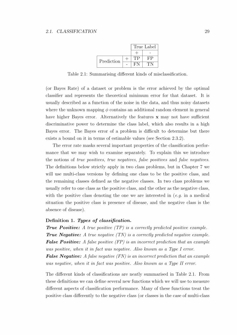
True Label+ -
Prediction+ TP FP- FN TN
Table 2.1: Summarising different kinds of misclassification.
(or Bayes Rate) of a dataset or problem is the error achieved by the optimal
classifier and represents the theoretical minimum error for that dataset. It is
usually described as a function of the noise in the data, and thus noisy datasets
where the unknown mapping φ contains an additional random element in general
have higher Bayes error. Alternatively the features x may not have sufficient
discriminative power to determine the class label, which also results in a high
Bayes error. The Bayes error of a problem is difficult to determine but there
exists a bound on it in terms of estimable values (see Section 2.3.2).
The error rate masks several important properties of the classification perfor-
mance that we may wish to examine separately. To explain this we introduce
the notions of true positives, true negatives, false positives and false negatives.
The definitions below strictly apply in two class problems, but in Chapter 7 we
will use multi-class versions by defining one class to be the positive class, and
the remaining classes defined as the negative classes. In two class problems we
usually refer to one class as the positive class, and the other as the negative class,
with the positive class denoting the one we are interested in (e.g. in a medical
situation the positive class is presence of disease, and the negative class is the
absence of disease).
Definition 1. Types of classification.
True Positive: A true positive (TP) is a correctly predicted positive example.
True Negative: A true negative (TN) is a correctly predicted negative example.
False Positive: A false positive (FP) is an incorrect prediction that an example
was positive, when it in fact was negative. Also known as a Type I error.
False Negative: A false negative (FN) is an incorrect prediction that an example
was negative, when it in fact was positive. Also known as a Type II error.
The different kinds of classifications are neatly summarised in Table 2.1. From
these definitions we can define several new functions which we will use to measure
different aspects of classification performance. Many of these functions treat the
positive class differently to the negative class (or classes in the case of multi-class

30 CHAPTER 2. BACKGROUND
problems), so throughout the thesis we will take care to define the positive class
when using these measures. These functions come in pairs, and we first detail
the precision and recall.
Definition 2. Precision and Recall.
Precision: the fraction of predicted positives which are actually positive.
Precision =TP
TP + FP(2.3)
Recall: the fraction of actual positives which are correctly predicted positive.
Recall =TP
TP + FN(2.4)
The precision and recall can be used in multi-class problems to measure the
predictive performance of the classifier for a particular class, as they do not require
the calculation of the number of true negatives, which is not well defined for multi-
class problems. Another common pair of error functions are the sensitivity and
specificity.
Definition 3. Sensitivity and Specificity.
Sensitivity: the fraction of actual positives which are correctly predicted positive.
Also known as the true positive rate.
Sensitivity =TP
TP + FN(2.5)
Specificity: the fraction of actual negatives which are correctly predicted nega-
tive. Also known as the true negative rate.
Specificity =TN
TN + FP(2.6)
We note that the sensitivity and recall are different names for the same func-
tion, but in this thesis we will use the appropriate name depending on the other
measure in use. There are two further functions that we will use to evaluate clas-
sification performance, the balanced error rate and the F-Measure (or F-score).
Definition 4. Balanced Error Rate and F-Measure.
Balanced Error Rate (BER): the mean of the sensitivity and specificity.
BER =Sensitivity + Specificity
2(2.7)

2.1. CLASSIFICATION 31
F-Measure: The F-Measure (technically the F1-Measure1) is the harmonic mean
of the precision and the recall. Written in terms of true positives, false positives
and false negatives it is,
F-Measure =2× TP
2× TP + FN + FP(2.8)
The balanced error rate is useful to determine the classification performance when
the data has a class-imbalance, e.g. there are many more negative examples than
positive examples. The F-Measure is useful to summarise the predictive perfor-
mance of a particular class, as it takes into account the true positives, the false
positives, and the false negatives.
2.1.1 Probability, Likelihood and Bayes Theorem
If we base our decisions on the output of a classifier we would like to know how
confident the classifier is that the prediction is correct. We denote the confidence
in the occurrence of an event x by its probability 0 ≤ p(x) ≤ 1, with 1 denoting we
are certain this event will occur and 0 denoting we are certain this event will not
occur. We can construct a distribution of probabilities for a variable X (denoted
p(X)) by incorporating all the possible states or events x ∈ X and normalising
them so the sum of the probabilities is 1. If we have a classifier which predicts
a particular y ∈ y1, y2 with p(y) = 0.51, then it has a low confidence in that
prediction, yet it is still the most likely prediction. If our classifier predicts y with
p(y) = 0.9 then it is more certain that y is the correct class label. Of course our
classifier makes predictions based upon the input we give it, so our probability
should be conditioned on the data, i.e. we should calculate p(y|x) where x is our
test datapoint. This denotes the conditional probability, the probability of the
outcome y when the value x is known. Again a distribution over the conditional
probabilities can be formed, p(Y |x), denoting the probabilities of each of the
class labels based upon our test datapoint. This can be normalised over all the
possible distributions for the different values of x, resulting in p(Y |X) which is
the conditional probability distribution over all the possible states of Y , for all
possible states of X. These distributions do not take into account the likelihood
of a particular value of X, which is important to the expected performance of
1The F-Measure is usually parameterised as the Fβ measure, where β controls the relativeweighting of the precision and recall.

32 CHAPTER 2. BACKGROUND
any given classifier. If our classifier performs well on the majority of data, but
poorly on rare examples (i.e. ones with a small p(x)) then it will perform well in
expectation. Similarly, good performance across most of the states of X does not
guarantee good performance in expectation if the classifier is poor at predicting
in the most common states. To incorporate this information we need a joint
probability p(y,x), which is the probability of both events y and x happening
together. The joint probability distribution over Y and X can be constructed
from p(Y |X) by multiplying by p(X), so
p(X, Y ) = p(Y |X)p(X). (2.9)
We can now construct one of the most important formulae in Machine Learn-
ing, Bayes’ Theorem (or Bayes’ Rule), which we can use to convert probabilities
we can estimate from the data into the probability of a particular class label given
that data. Bayes’ Theorem follows from the commutativity of probability (i.e.
p(x, y) = p(y, x)) and the definition of joint probability given in Equation (2.9),
resulting in,
p(Y |X) =p(X|Y )p(Y )
p(X). (2.10)
We can estimate the probability of the data, p(X), and the probability of the
class label, p(Y ), from our training dataset. We can also estimate p(X|Y ) by
partitioning the dataset by class label and separately estimating p(X|Y = y) for
each y. Then we can use Bayes’ Theorem to produce the probability of each of
the possible labels for a particular datapoint x. In the context of Bayes’ Theorem
we call p(Y ) the prior, which reflects our belief in the probability of Y a priori
(i.e. before seeing any data), and we call p(Y |X) the posterior, which reflects our
updated belief in the probability of Y once we have seen the data X. If we use
Bayes’ Theorem and return the most likely class label as our prediction, we have
chosen the mode of the distribution p(Y |X) which is the maximum a posteriori
(MAP) solution. This is an alternative to the Maximum Likelihood solution,
which is simply the largest p(X|Y ), otherwise known as the model likelihood.
We return to the concept of the MAP solution in Chapter 4 where we explore the
MAP solution to the feature selection problem.
In general we do not have access to the true probability distribution p, and
so this needs to be estimated from our training data. There are many different
approaches to this estimation process but in this thesis we will focus on discrete

2.1. CLASSIFICATION 33
probability distributions rather than probability densities, and thus we use sim-
ple histogram estimators. These count the number of occurrences of a state in a
dataset, and return the normalised count as a probability. This approach returns
the correct distribution in the limit of infinite data, and is a reasonable approxi-
mation with finite data. As the distribution becomes higher dimensional (e.g. as
we model more and more features) our estimate of the distribution takes longer to
converge to the true distribution. This problem is commonly known as the “curse
of dimensionality” [35], and is the reason many machine learning algorithms seek
low dimensional approximations to the true joint distribution p(x, y). Other ap-
proaches commonly used involve assuming each distribution follows a particular
functional form, such as a Gaussian, and then estimating the parameters which
control that distribution by fitting it to the data (e.g. the mean and the variance
for the Gaussian distribution). This approach is more popular when taking the
fully Bayesian approach to modelling a system [10], where everything is expressed
in terms of a probability distribution or density, and there are no hard values re-
turned. We will look at the Bayesian approach to modelling systems more in
Chapter 3 when we look at Bayesian Networks.
When dealing with classification algorithms we often have parameters we can
tune to alter the behaviour of the algorithm. These are referred to as “hyper-
parameters” of the model, in contrast to the model parameters which are fit
by the training process. We would like to express the probability of our model
parameters given the data, and to optimise those parameters to maximise the
probability, which in turn minimises our error rate. When used in this way we re-
fer to the likelihood, L, of the data given the parameters, where parameters with
higher likelihood fit the data better. We then construct our prior distribution
over the parameters and use Bayes’ Theorem to calculate the probability of our
parameters given the data.
The likelihood of a model is a central concept in this thesis, as it represents
how well a model fits a given dataset. The likelihood of a set of model parameters
is
L(τ) =N∏i=1
q(yi,xi|τ). (2.11)
Here q is our predictive model which returns a probability for a given yi,xi pair,
based upon the parameters τ . The likelihood takes the form of a product of these
probabilities over the datapoints due to the i.i.d. assumption made about the

34 CHAPTER 2. BACKGROUND
dataset. It is often useful to incorporate a measure of how likely the parameters
τ are a priori, to incorporate domain knowledge about the parameter settings, or
to explicitly include Occam’s razor by preferring smaller numbers of parameters.
We call a likelihood which includes this prior distribution over τ , p(τ), the joint
likelihood of a model,
L(y,x, τ) = p(τ)N∏i=1
q(yi,xi|τ). (2.12)
Maximising this value means we find the parameters τ that both model the data,
and are a priori most likely. We use a variant of this joint likelihood in Chapter
4 to investigate feature selection.
In classification problems we care about maximising the discriminative per-
formance, i.e. how well our model predicts yi from a given xi. This is represented
by the conditional likelihood of the labels with respect to the parameters,
L(τ |D) =N∏i=1
q(yi|xi, τ). (2.13)
We look at cost-weighted versions of this likelihood in Chapter 7.
2.1.2 Classification algorithms
In this thesis we focus on the selection of the inputs into a classification algorithm,
rather than the construction of new classification algorithms. We thus briefly
discuss the classifiers we use to benchmark our feature selection algorithms.
The k-Nearest Neighbour (k-NN) algorithm [23] is conceptually the simplest
of all classification algorithms. It searches for the k nearest neighbours of the
test datapoint in the training data, and then returns the most popular label
amongst those neighbours. If there is a tie for the most popular class then it
chooses between them at random. The notion of “nearest” is determined by
the choice of distance metric, though the most commonly used is the Euclidean
distance. Whilst it is a simple classifier to describe, it draws complex non-linear
decision boundaries, and requires the storage of all of the training data in the
classifier. In this sense it is a very complex classifier as each training datapoint
is an extra d parameters in the model (one for each dimension or feature). This
means it does not provide a compact representation of the training data, which

2.1. CLASSIFICATION 35
could be analysed to deduce properties of the problem space. However it makes
very few assumptions about the distribution of the data, beyond the presence of
“smoothness” in the label space (i.e. examples which are close together have the
same labels).
A common probabilistic technique is the Naıve Bayes classifier [35]. The
classifier is based on an approximation of Bayes Rule, given in Equation (2.10),
which makes it tractable with small amounts of data. Bayes Rule gives the
optimal classification boundary, but calculating the terms involved is intractable
due to the amount of data required to estimate each term. When generating
classifications (instead of finding the probability of each class) the denominator
is unnecessary, all that is required is to find the y s.t. p(X|Y = y)p(Y = y) is
maximal. Unfortunately even the p(X|Y = y) term is difficult to estimate when
there are tens of features, or each feature is multinomial/real valued. This is
where the naıve assumption is required, which states that p(X|Y = y) can be
approximated by assuming all the features Xj are jointly independent given the
label Y , i.e. all the features are class conditionally independent of each other.
The classification rule can then be rewritten as follows
arg maxy∈Y
p(Y = y)d∏i=1
p(Xi|Y = y). (2.14)
The conditional independence factorises the joint distribution into the product
of marginal distributions for each feature. As we shall see when we consider fea-
ture selection, the assumption of class-conditional independence is not generally
a valid one, and thus the Naıve Bayes classifier is suboptimal in many cases.
However it provides surprisingly good classification performance even when the
naıve assumption is provably untrue [33]. In addition, it is fast to train on a given
dataset, and is equally fast at classifying a test dataset. In the next chapter we
will look at Bayesian Networks, and see how the Naıve Bayes classifier can be
interpreted as a simple Bayesian Network.
Support Vector Machines (SVMs) [22] are an optimal way of drawing a linear
classification boundary which maximises the margin (the distance between the
classification boundary and the closest datapoints of each class). The problem
of finding the maximum margin boundary is solved by identifying the support
vectors which control the position of the boundary (usually the examples on the
convex hull of each class). SVMs have become ubiquitous in Machine Learning,

36 CHAPTER 2. BACKGROUND
as the problem formulation has a convex solution (so there is a unique minima)
which can be found using quadratic programming solvers so the optimal solution
is always returned. While the SVM only finds linear boundaries and thus has in-
sufficient complexity to model non-linear functions, it is possible to transform the
feature space into a higher dimension which might permit a linear solution. This
is called the kernel trick as the mapping is done through a kernel function, and
it is a powerful property of the SVM algorithm. When the (high-dimensional)
linear boundary is mapped back into the original (low-dimensional) space it pro-
duces a non-linear boundary, though one which is still optimal in terms of the
margin. The SVM is a two-class classifier, in contrast to the k-NN and Naive
Bayes methods described above which can deal with multi-class problems, though
there are extensions to the SVM which give multi-class classifiers.
These are the three classifiers we will use throughout the remainder of the
thesis, though of course there exist many other classifiers tailored to different
problems. One important class of algorithms are ensemble techniques which com-
bine multiple classification models into one classification system [66]. We refer
the reader to Kuncheva [66] for more detail on ensemble algorithms, but note
that these algorithms are popular when dealing with complex cost-sensitive clas-
sification problems and we now review the literature surrounding cost-sensitive
problems.
2.2 Cost-Sensitive Classification
In many classification problems one kind of error can be more costly than other
kinds, e.g. false negatives are usually much more costly than false positives in
medical situations, as the cost of not treating the disease is generally higher than
the cost of unnecessary treatment. If we have asymmetric costs (where one class
is more important than another) we would like to train a classifier which could
focus on correctly classifying examples of that class. A closely related problem is
classifying in unbalanced datasets, where there are vastly more examples of one
class than another. In these datasets it is simple to achieve a low error rate by
continually predicting the majority class, though the classifier has learned little
about the structure of the problem beyond the asymmetry in the class priors.

2.2. COST-SENSITIVE CLASSIFICATION 37
2.2.1 Bayesian Decision Theory
We can formalise the problem of cost-sensitive classification by constructing it as
a decision theory problem, using Bayesian Decision Theory [35]. This provides a
formal language for making optimal predictions given that some errors are more
costly than others. The standard approach for specifying these costs is through
a cost matrix. In decision theoretic terminology, the expected loss of a prediction
procedure p(y|x) is the conditional risk:
R(y|x) =∑y∈Y
c(y, y)p(y|x). (2.15)
Here c(y, y) is the entry in the cost matrix associated with predicting class y
given that the true class is y. The Bayes risk, is achieved by predicting the class
label which minimises the conditional risk R(y|x). This is the optimal prediction
in terms of reducing the misprediction costs. Elkan [38] shows that in two-class
problems the cost matrix is over-specified as there are only 2 degrees of freedom,
each of which controls the cost for mispredicting one label. While the cost matrix
approach is simple to understand it has some restrictions, as it does not allow
the costs to be example dependent. Elkan proposed a more general framework
[38, 114] which gives each example a weight based upon how important it is to
classify correctly. This allows the weight to be a function of both y and x, allowing
it to vary with the value of the features as well as the label. This approach can
be extended to the multi-class case by giving each example a vector of |Y | − 1
weights, where |Y | is the number of classes.
2.2.2 Constructing a cost-sensitive classifier
There are many examples of cost-sensitive classifiers, where the cost matrix or
some function thereof is incorporated into the final decision rule. A very simple
strategy to minimise risk is to tune a threshold on class probability predictions,
encouraging more predictions of a particular (costly) class, though this does tend
to introduce false positives. Dmochowski et al. [31] showed that adjusting the
threshold is an optimal solution to the problem if and only if the classification
model is sufficiently expressive to fit the true underlying process which generated
the data.
A more popular strategy is perturbing the data so that a cost-insensitive

38 CHAPTER 2. BACKGROUND
classifier trained on the new data behaves like a cost-sensitive classifier trained
on the original data. Examples of this are the widely used SMOTE technique
[19], and the Costing ensemble algorithm [114]. These approaches resample the
data according to the cost of each example, before training a standard (cost-
insensitive) classifier on the newly resampled data. However, this strategy has the
consequence of distorting the natural data distribution p(x, y), and so the supplied
training data will not be i.i.d. with respect to the testing data, potentially causing
problems with overfitting. The MetaCost algorithm [32] relabels the data based
upon an ensemble prediction and the risk, before training a standard classifier on
the relabelled data. We can view these approaches as distorting how the classifier
“sees” the world – encouraging it to focus on particular types of problems in the
data. The popular LibSVM [17] implementation of the SVM classifier uses an
analogous system where the internal cost function of the classifier is changed so
some examples are more costly to classify incorrectly.
Dmochowski et al. [31] investigate using a weighted likelihood function to
integrate misclassification costs into the (binary) classification process. Each
example is assigned a weight based upon the tuple x,y, and the likelihood of
that example is raised to the power of the assigned weight. They prove that
the negative weighted log likelihood forms a tight, convex upper bound on the
empirical loss, which is the expected conditional risk across a dataset. This
property is used to argue that maximising the weighted likelihood is the preferred
approach in the case where the classifier cannot perfectly fit the true model. We
will look at this weighted likelihood in more detail in Chapter 7.
2.3 Information Theory
If we wish to investigate the relationship between two variables, we first need to
decide upon an appropriate measure of similarity or correlation. We would like
this measure to be a function of the interaction between the variables, rather than
a function of their values, and we would also like it measure as many different
kinds of interaction as possible, rather than measuring a single kind of interaction,
such as the linear correlation measured by Pearson’s Product-Moment Correla-
tion Coefficient [85]. We could think of this measure as the amount of shared
information between two variables, as variables which are identical share exactly
the same information. However to develop this idea we first need to quantify

2.3. INFORMATION THEORY 39
information. The area of mathematics which deals with measuring information
is innovatively named Information Theory.
In Information Theory, the essential quantity of information is taken to be the
reduction in uncertainty in one variable when another is known. Thus before we
can define information we need to define the uncertainty in a random variable,
and the uncertainty in that variable when another is known. We can then define
the reduction in uncertainty and thus the information content.
2.3.1 Shannon’s Information Theory
Claude Shannon developed the first comprehensive set of answers to these ques-
tions in 1948, in his landmark paper “A Mathematical Theory of Communication”
[97]. He defines three crucial measures which form the basis of much of the rest
of the work we present in this thesis. They are the Entropy, H(X), for a ran-
dom variable X, the Conditional Entropy of X given another random variable
Y , H(X|Y ), and the Mutual Information between two variables, I(X;Y ). All
three are non-negative quantities. A detailed treatment of these three concepts
is given in Cover and Thomas [24]. In this thesis we will work with discrete ran-
dom variables, and so we give definitions for the discrete entropies and mutual
informations. When working with continuous random variables the summations
over possible states are replaced with integrations over the support of the random
variable.
The Entropy of a random variableX, measures the uncertainty about the state
of a sample x from X. The entropy of X is defined in terms of the probability
distribution p(x) over the states of X as follows,
H(X) = −∑x∈X
p(x) log p(x). (2.16)
The logarithm base defines the units of entropy, with log2 using bits, and loge
using nats. In general the choice of base does not matter provided it is consistent
throughout all calculations. In this thesis we will calculate entropy using log2
unless otherwise stated. High values of entropy mean the state of x is very uncer-
tain (and thus highly random), and low values mean the state of x is more certain
(and thus less random). Entropy also increases with the number of possible states
of X, as if X has 4 states there are more possibilities for the state of x than if
X had 2 states. Entropy is maximised when all states of X are equally likely,

40 CHAPTER 2. BACKGROUND
as then the state of x is most uncertain/hardest to predict, and H(X) = log |X|where |X| denotes the number of states of X.
The Conditional Entropy of X conditioned on Y measures the expected un-
certainty of the state of a sample of x when Y is known. It is averaged over
the possible states of Y so it gives a useful measure in the abstract when Y is
unknown. This has two equivalent definitions, in terms of the joint probability
distribution p(x, y),
H(X|Y ) =∑y∈Y
p(y)H(X|Y = y) (2.17)
= −∑x∈X
∑y∈Y
p(x, y) log p(x|y). (2.18)
The conditional entropy can also be defined as the entropy of the joint variable
XY minus the entropy of Y ,
H(X|Y ) = H(XY )−H(Y ). (2.19)
The conditional entropy is upper bounded by the marginal entropy, and lower
bounded by 0.
0 ≤ H(X|Y ) ≤ H(X) (2.20)
This lower bound is attained when knowledge of Y enables perfect prediction of
the state of X, and the upper bound is reached when X and Y are independent.
By itself the conditional entropy tells us little about the interaction between
two variables, we need to know the entropy of X before we can derive any useful
information. The difference between the entropy and the conditional entropy for
a pair of variables is called the Mutual Information, I(X;Y ). It measures the
average reduction in uncertainty in the state of X when the state of Y is known,
and thus the increase in information. The mutual information is a symmetric
measure, in that I(X;Y ) = I(Y ;X), i.e. the information gained about X when
Y is known is equal to the information gained about Y when X is known. This
leads to several equivalent definitions for the mutual information,
I(X;Y ) = H(X)−H(X|Y ) (2.21)
= H(Y )−H(Y |X) (2.22)
= H(X) +H(Y )−H(XY ) (2.23)

2.3. INFORMATION THEORY 41
The mutual information can also be expressed as the KL-Divergence2 between the
joint distribution p(x, y) and the product of both marginal distributions p(x)p(y),
defined as follows
I(X;Y ) =∑x∈X
∑y∈Y
p(x, y) logp(x, y)
p(x)p(y). (2.24)
With this formulation we can see how the mutual information reaches its max-
imal and minimal values more easily. The maximal value is the minimum of
the two entropies H(X) and H(Y ), and occurs when knowledge of one variable
allows perfect prediction of the state of the other. In the above equation this
is due to p(x, y) becoming equal to either p(x) or p(y) for all values, and then
the KL-Divergence cancels down to Equation (2.16), the standard entropy. The
minimal value is 0, which occurs when X and Y are independent. In the above
equation this causes p(x, y) to factorise into p(x)p(y), thus the fraction is unity,
and the logarithm becomes zero. In the field of feature selection it is common to
use a normalised function of the mutual information, termed the Symmetric Un-
certainty. This is the mutual information between the two variables normalised
by the sum of their marginal entropies, therefore
SU(X;Y ) =I(X;Y )
H(X) +H(Y )(2.25)
It is commonly advocated instead of the mutual information as unlike the mutual
information it is not biased towards high arity variables, and is thus useful when
comparing the scores for variables with differing numbers of states.
There is one final commonly used concept in Information Theory, the Con-
ditional Mutual Information between two variables, conditioned on a third. The
most common definition is in terms of the chain rule of mutual information, which
describes how the information content of a pair of variables can be broken down
in several equivalent ways,
I(XZ;Y ) = I(Z;Y ) + I(X;Y |Z) (2.26)
= I(X;Y ) + I(Z;Y |X) (2.27)
= I(X;Y ) + I(Z;Y )− I(X;Z) + I(X;Z|Y ). (2.28)
2The KL-Divergence is also referred to as the relative entropy.

42 CHAPTER 2. BACKGROUND
The conditional mutual information measures the dependency between two vari-
ables when the state of a third is known, and is defined in terms of an expected
KL-Divergence as follows,
I(X;Y |Z) =∑z∈Z
p(z)I(X;Y |Z = z) (2.29)
=∑z∈Z
p(z)∑x∈X
∑y∈Y
p(x, y|z) logp(x, y|z)
p(x|z)p(y|z). (2.30)
Unlike the conditional entropy, the conditional mutual information can be larger
than the unconditioned mutual information. This is due to a positive interaction
between the variables, where the dependency between two variables is increased
by the knowledge of the state of a third. Again like the mutual information, the
conditional mutual information is zero when the two variables are independent,
conditioned on the presence of the third variable. The maximal value of the
conditional mutual information is the minimum of the two conditional entropies
H(X|Z) and H(Y |Z), again achieved when knowledge of one variable (and the
conditioning variable) allows perfect prediction of the state of the other. We will
see an important use of the conditional mutual information when we investigate
structure learning in Bayesian Networks in the next chapter. In Chapters 4 and
5 we will see how the conditional mutual information is particularly important in
the context of filter feature selection.
2.3.2 Bayes error and conditional entropy
One of the reasons for the popularity of Information Theory in Machine Learning
is the existence of bounds on the Bayes Error of a classification problem, defined
in terms of the Conditional Entropy. There exists both an upper and lower
bound in terms of the conditional entropy and the range between these bounds
shrinks as the conditional entropy decreases. The lower bound was proved by
Fano in 1961 [39], and the upper bound was proved by Hellman and Raviv in
1970 [55]. They form the informal basis for the use of mutual informations as
feature selection criteria, which we explore in the next chapter. We will derive an
alternate justification for the use of mutual information based criteria in Chapter
4.
For a two class problem the Bayes error is bounded by the conditional entropy

2.3. INFORMATION THEORY 43
as follows:H(Y |X)− 1
log |Y |≤ ebayes ≤
1
2H(Y |X). (2.31)
With these bounds we can see that the conditional entropy represents the con-
straint placed upon the class label by the data. If the data does not constrain
the choice of class label then for any given feature vector, there may be multiple
different classes which could be assigned, so there is still a large amount of un-
certainty in the choice of class label, and thus the Bayes error will be high. If the
data tightly constrains the choice of class label then on average a given feature
vector will only have one possible class, and thus the Bayes error will be low.
Therefore a large value of H(Y |X) implies the features alone do not have enough
information to create a good classification boundary, whereas a small value of
H(Y |X) implies the features contain sufficient information to produce a good
boundary.
We can see the link between mutual information and feature selection by con-
sidering how the mutual information decomposes into sums of entropies, as in
Equation (2.21). As the entropy of the class label H(Y ) is constant, maximising
the mutual information I(X;Y ) between the features and the class label is equiv-
alent to minimising the conditional entropy H(Y |X), which in turn minimises the
Bayes Error. Therefore finding a feature set Xθ which maximises I(Xθ;Y ) will
minimise the bound on the Bayes rate, and thus provide an informative feature
set for any future classification process. We will look at the literature in informa-
tion theoretic feature selection more closely in the next chapter, before deriving a
more concrete link between the mutual information and the classification process
in Chapter 4.
One further important point about the conditional entropy is that it is the
limit of the scaled conditional log-likelihood of the labels given the data,
limN→∞
1
Nlog
N∏i=1
p(yi|xi) = H(Y |X). (2.32)
This assumes that the distribution p is perfectly estimated, which is in general
untrue. Estimating these information theoretic quantities is a topic we review in
the next section, whilst we return to the link between likelihood and information
theory in Chapter 4.

44 CHAPTER 2. BACKGROUND
2.3.3 Estimating the mutual information
The problem of calculating mutual informations reduces to that of entropy es-
timation, and in turn to the problem of estimating probability distributions. A
thorough review of this topic is available in Paninski [83], and we provide a brief
summary of the relevant issues in this section. We begin with some extra nota-
tion, introducing p to denote a probability distribution which has been estimated
from a dataset sampled from the true distribution p. We can write the mutual
information as the expected logarithm of a ratio of probabilities:
I(X;Y ) = Exy
log
p(x, y)
p(x)p(y)
. (2.33)
We can estimate this from data, as the Strong Law of Large Numbers assures us
that the sample estimate using p converges almost surely to the expected value
— for an i.i.d. dataset of N observations (xi, yi),
I(X;Y ) ≈ I(X;Y ) =1
N
N∑i=1
logp(xi, yi)
p(xi)p(yi). (2.34)
In order to calculate this we need the estimated distributions p(x, y), p(x), and
p(y). The computation of entropies for continuous or ordinal data is highly
non-trivial, and requires an assumed model of the underlying distributions —
to simplify experiments throughout this thesis, we use discrete data and estimate
distributions with histogram estimators using fixed-width bins. The maximum
likelihood estimate of the probability of an event p(X = x) is given by the fre-
quency of occurrence of the event X = x divided by the total number of events
(i.e. datapoints). There exist many other methods for estimating entropy, though
they fall into two main approaches: plug-in estimators which first estimate the
probability distributions p, and direct entropy estimators which calculate the en-
tropy from data without constructing probability distributions (e.g. Poczos and
Schneider [90]). For more information on alternative entropy estimation proce-
dures, we refer the reader to Paninski [83].
At this point we must note that the approximation above holds only if N is
large relative to the dimension of the distributions over x and y. For example
if x, y are binary, N ≈ 100 should be more than sufficient to get reliable esti-
mates; however if x, y are multinomial, this will likely be insufficient. If we wish

2.4. WEIGHTED INFORMATION THEORY 45
to measure the information between a set of variables Xθ and a particular target
variable then the quality of our estimate depends on the number of states in our
set Xθ. As the dimension of the variable Xθ grows then the necessary probabil-
ity distributions become more high-dimensional, and hence our estimate of the
mutual information becomes less reliable. This in turn causes increasingly poor
judgements in any process we might base upon the mutual information. For pre-
cisely this reason, the feature selection literature contains many low-dimensional
approximations to the complex high-dimensional mutual information. We review
a selection of these approximations in Section 3.2, and a unification of these var-
ious criteria (found in Chapter 5) forms a substantial part of the contributions of
this thesis.
For the remainder of this thesis, we use notation I(X;Y ) to denote the ideal
case of being able to compute the mutual information, though in practice on real
data we use the finite sample estimate I(X;Y ).
2.4 Weighted Information Theory
We now briefly explore Guiasu’s formulation of Information Theory as an alter-
native way of measuring the uncertainty in a random variable, incorporating a
measure of how important or costly each state is. This topic has received little
attention in the literature, and one of the contributions of Chapter 7 will be a
more thorough treatment of the weighted mutual information.
The weighted entropy was first defined as the “Quantitative-Qualitative mea-
sure of information” by Belis and Guiasu [8]. It was termed this as it incorporated
“qualitative” measures of the importance of a state into the “quantitative” mea-
sure of the entropy, using the probabilities of each state. An extensive theoretical
treatment of the subject was written by Guiasu [46] where the measure is re-
named the Weighted Entropy. It is defined for a variable X with respect to the
distribution p(x) and a set of weights w(x) ≥ 0 as follows,
Hw(X) = −∑x∈X
w(x)p(x) log p(x). (2.35)
Due to the presence of the weights, it is no longer bounded with respect to the
number of states in X, but by wmax log |X|, where wmax denotes the largest weight
in w. This measure is non-negative like the Shannon Entropy, and reduces to the

46 CHAPTER 2. BACKGROUND
Shannon Entropy when all the weights are equal to one. The weights w do not
have to be normalised into the range 0 ≤ w ≤ 1, though any such normalisa-
tion will not change the relative values of the entropy, due to the linearity of
expectation.
To ensure that Hw conforms to the axioms of an entropy measure (as listed in
Guiasu [46]) the weights for joint events must be constructed in a specific way. For
any joint event E∪F the weight w(E∪F ) is defined in terms of the probabilities
and the weights of the individual events E and F . In general w(E∪F ) is defined
as follows,
w(E ∪ F ) =p(E)w(E) + p(F )w(F )
p(E ∪ F ). (2.36)
We can express this definition in a more useful form, with respect to distributions
over the states x ∈ X and y ∈ Y as follows,
w(x)p(x) =∑y∈Y
p(x, y)w(x, y). (2.37)
It is this property of the weights which allows the definition of a conditional
entropy as the joint entropy minus a marginal entropy,
Hw(X, Y ) = Hw(Y |X) +Hw(X)
= Hw(X|Y ) +Hw(Y ). (2.38)
This is in contrast to other extensions to entropy such as Renyi’s [92] or Tsallis’
[105], which do not lead to natural definitions of the conditional entropy as a
function of the joint distribution. It is precisely this marginalisation property
of the conditional entropy which ensures the three definitions of the (Shannon)
mutual information given in Equations (2.21—2.24) are equivalent.
In the same book [46] Guiasu briefly defines a “weighted entropic measure
of cohesion”, which is the sum of two marginal weighted entropies, minus the
joint weighted entropy. Luan et al. [75] also defined a similar quantity as the
“Quantitative-Qualitative measure of mutual information”, and Schaffernicht and
Gross [96] define this quantity as the Weighted Mutual Information. This lat-
ter term is the one we will use throughout this thesis. The weighted mutual
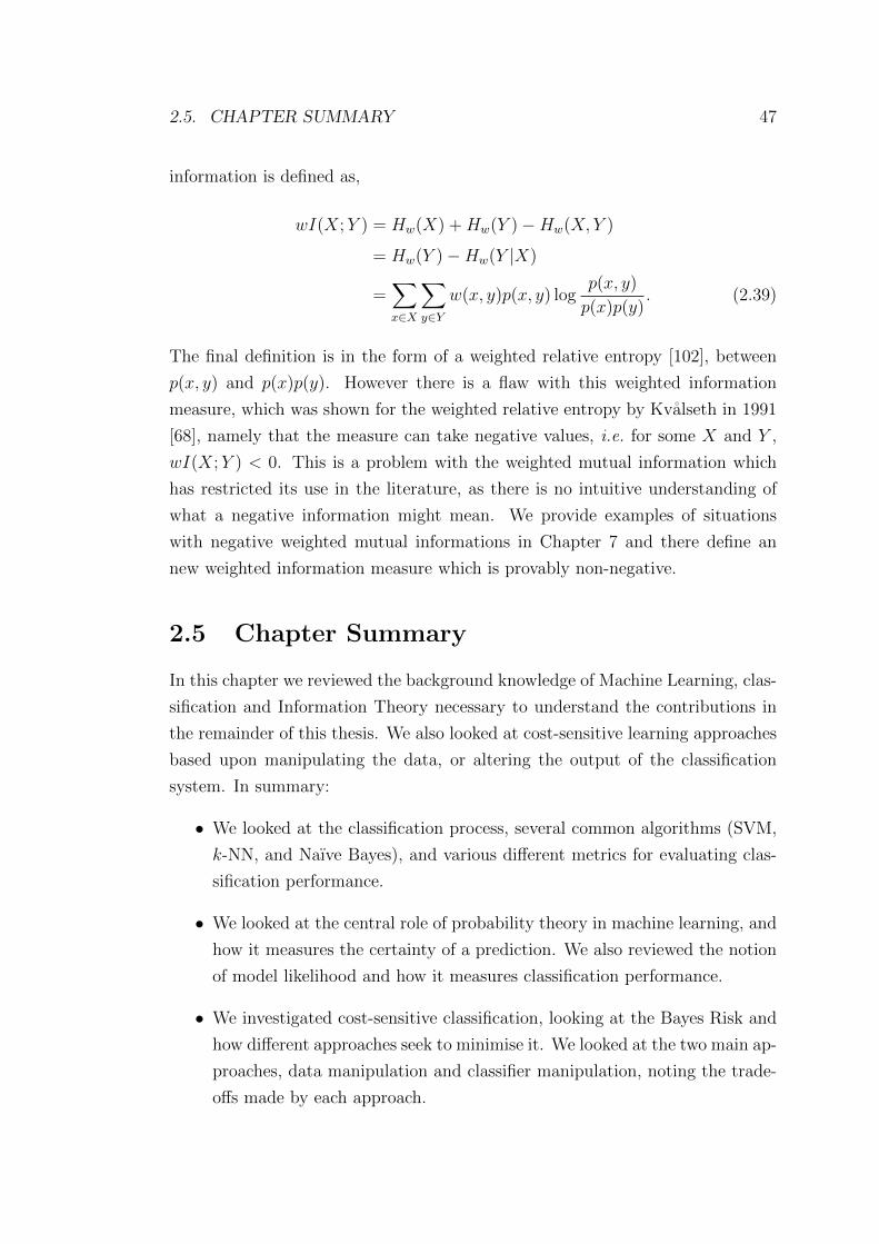
2.5. CHAPTER SUMMARY 47
information is defined as,
wI(X;Y ) = Hw(X) +Hw(Y )−Hw(X, Y )
= Hw(Y )−Hw(Y |X)
=∑x∈X
∑y∈Y
w(x, y)p(x, y) logp(x, y)
p(x)p(y). (2.39)
The final definition is in the form of a weighted relative entropy [102], between
p(x, y) and p(x)p(y). However there is a flaw with this weighted information
measure, which was shown for the weighted relative entropy by Kvalseth in 1991
[68], namely that the measure can take negative values, i.e. for some X and Y ,
wI(X;Y ) < 0. This is a problem with the weighted mutual information which
has restricted its use in the literature, as there is no intuitive understanding of
what a negative information might mean. We provide examples of situations
with negative weighted mutual informations in Chapter 7 and there define an
new weighted information measure which is provably non-negative.
2.5 Chapter Summary
In this chapter we reviewed the background knowledge of Machine Learning, clas-
sification and Information Theory necessary to understand the contributions in
the remainder of this thesis. We also looked at cost-sensitive learning approaches
based upon manipulating the data, or altering the output of the classification
system. In summary:
• We looked at the classification process, several common algorithms (SVM,
k-NN, and Naıve Bayes), and various different metrics for evaluating clas-
sification performance.
• We looked at the central role of probability theory in machine learning, and
how it measures the certainty of a prediction. We also reviewed the notion
of model likelihood and how it measures classification performance.
• We investigated cost-sensitive classification, looking at the Bayes Risk and
how different approaches seek to minimise it. We looked at the two main ap-
proaches, data manipulation and classifier manipulation, noting the trade-
offs made by each approach.

48 CHAPTER 2. BACKGROUND
• Finally we looked at Information Theory, examined the basic methods of
measuring information, and saw the strong links between information the-
oretic values and classification performance. We also looked briefly at an
extension of information theory which incorporates weights, leading to a
measure of how costly the uncertainty in a variable is.
In the next chapter we have a detailed review of the literature in feature selec-
tion and structure learning which gives the landscape in which the contributions
exist, detailing the state of the art in feature selection and pinpointing areas
where this thesis advances the state of the art.

Chapter 3
What is feature selection?
In this chapter we review the literature surrounding feature selection. We begin
by introducing the topic of feature selection, detailing the major concepts and
approaches. In Section 3.1 we explore the three main paradigms for feature selec-
tion: filters, wrappers and embedded methods. We present a detailed review of
the literature surrounding information theoretic filter feature selection in Section
3.2. We look at more general feature selection approaches which include prior
knowledge in Section 3.3, and feature selection in multi-class spaces in Section
3.4. In Section 3.5 we explore Bayesian Networks as a way of modelling systems,
and investigate how learning the structure of a Bayesian Network is a special
case of the feature selection problem. Finally we detail the main algorithms for
structure learning in Section 3.6, looking at the differences between global and
local algorithms, and those which use conditional independence tests versus those
which optimise a function of the network.
3.1 Feature Selection
Feature Selection is the process of determining what inputs should be presented to
a classification algorithm. Originally feature selection was performed by domain
experts as they chose what properties of an object should be measured to try
and determine the class label. Modern classification problems attempt to collect
all possible features, (e.g. in gene expression tasks, many thousands of genes are
tested) and then use a statistical feature selection process to determine which
features are relevant for the classification problem. In Chapter 6 we develop
a novel method for integrating domain experts back into the feature selection
49

50 CHAPTER 3. WHAT IS FEATURE SELECTION?
process.
Feature selection algorithms of all kinds rely upon a single assumption about
the data, that the feature set contains irrelevant and/or redundant features. Ir-
relevant features contain no useful information about the classification problem,
and redundant features contain information which is already present in more in-
formative features. If we can select a feature set which does not include these
irrelevant or redundant features then we can reduce the collection cost of the
feature set, and we can investigate the remaining relevant features to determine
how they relate to the class label. We may also improve classification perfor-
mance by reducing the potential for overfitting when shrinking the feature set.
These heuristic notions of relevancy and redundancy were formalised by Kohavi
& John [62] into three classes: strongly relevant, weakly relevant, and irrelevant.
In the definitions below, Xi indicates the ith feature in the overall set X, and X\i
indicates the set X\Xi, i.e. all features except the ith.
Definition 5. Strongly Relevant Feature [62]
Feature Xi is strongly relevant to Y iff there exists an assignment of values xi,
y, x\i for which p(Xi = xi, X\i = x\i) > 0 and p(Y = y|Xi = xi, X\i = x\i) 6=p(Y = y|X\i = x\i).
Definition 6. Weakly Relevant Feature [62]
Feature Xi is weakly relevant to Y iff it is not strongly relevant and there exists
a subset Z ⊂ X\i, and an assignment of values xi, y, z for which p(Xi = xi, Z =
z) > 0 such that p(Y = y|Xi = xi, Z = z) 6= p(Y = y|Z = z).
Definition 7. Irrelevant Feature [62]
Feature Xi is irrelevant to Y iff it is not strongly or weakly relevant.
The strongly relevant features are not redundant as each one contains use-
ful information that is not present in any other combination of features. The
weakly relevant features contain information which is either already present in
the strongly relevant features, or exists in other weakly relevant features. The
irrelevant features contain no useful information about the problem. We would
like a feature selection algorithm to return the set of strongly relevant features,
plus a (potentially empty) subset of the weakly relevant features, excluding the
irrelevant features. Unfortunately these definitions do not lend themselves to
the construction of a feature selection algorithm, as they require checking expo-
nentially many combinations of features to ascertain weak relevancy. They also

3.1. FEATURE SELECTION 51
are quite abstract quantities, and we will relate their notions of relevancy and
irrelevancy to concrete information theoretic quantities in Chapter 5.
We now introduce a small amount of notation and thus formally define the
feature selection problem. Throughout this thesis we will use θ as a binary vector
of length d where d is the number of features, θi = 1 means the i’th feature is
selected and θi = 0 means it is ignored. We shall define ¬θ as the negation of
the vector θ, thus denoting the unselected features. We formally define feature
selection by stating the mapping φ : X → Y uses a subset of the features θrel, with
the remaining features ¬θrel being redundant or irrelevant. Therefore φ : X → Y
is equivalent to φ′ : Xθrel → Y where Xθrel is the subset of X containing the
features selected by θrel. The concept of sparsity in the statistics literature [10]
is related to the process of feature selection. A sparse solution to a prediction
problem means that few of the features are involved in the prediction, hence we
can think of feature selection as enforcing sparsity on the solution. The term
arises from matrices where a sparse matrix is one with few non-zero elements. In
our case we say θ is sparse if it has few set bits, thus the feature set selected by
θ is also sparse. The choice of search function is important in feature selection
problems as the space of possible feature subsets is the powerset of the dimension,
thus the number of possible feature sets is 2d. Therefore examining all possible
feature sets is intractable for any reasonably sized problem.
Feature selection algorithms are a subset of the more general feature extraction
algorithms. Feature extraction techniques produce a new feature set by processing
the original set. This can be by combining multiple features, or projecting the
feature set into a higher or lower dimensional space. Such techniques are useful
when the classification algorithm cannot understand the current representation,
e.g. we can see the kernel trick in SVM classifiers as a form of feature extraction
(see Section 2.1.2). In feature selection we extract features by returning a relevant
subset of the input feature set. For the remainder of this thesis we will focus on
feature selection algorithms, of which there are three main kinds: filters, wrappers
and embedded methods. Filters and wrappers are defined by two things, the
evaluation function or criterion which scores the utility of a feature or a feature
set (which we term J), and the search algorithm which generates new candidate
features or feature sets for evaluation. We show the general form of a filter
or wrapper algorithm in Algorithm 1. Embedded methods are feature selection
techniques which are integrated into a particular classification algorithm therefore

52 CHAPTER 3. WHAT IS FEATURE SELECTION?
Algorithm 1 The general form of a filter/wrapper
Require: A dataset D, with features X and label YInitialise candidate feature subset Swhile Stopping criterion == False do
Propose new candidate subset S ′ based on SEvaluate J(S ′)if J(S ′) > J(S) thenS = S ′
end ifend while
separating out the evaluation function from the search procedure is more difficult.
We explore the main differences between the three approaches below.
3.1.1 Filters
Filter approaches use a measure of relevancy or separation between the candidate
feature or feature set and the class label as the scoring function for that feature
or feature set. These measures range from simple correlation measures such as
Pearson’s Correlation Coefficient [85], through complex correlation measures such
as the mutual information (discussed in Section 2.3), to complex measures of inter
and intra class distances, used in the Relief algorithm [60]. All these measures
return a number which represents the strength of the relationship between the
candidate feature set and the class label. This relationship might be a measure of
information, or a measure of the separability of the classes based on that feature
set. Other common measures, are based upon probabilistic independence, which
is a topic we discuss in more detail in Section 3.5. Much of the early work in filter
feature selection focused on different kinds of distance or divergence metrics, both
probabilistic and based directly upon the data [30]. We call the scoring function
a feature selection criterion, and the study of the criteria based on information
theoretic measures is the topic of this thesis.
Filter algorithms can be further divided into those which measure univariate
relationships or multivariate relationships. Univariate measures only consider the
relationship between the candidate feature and the class label, ignoring any inter-
actions with the previously selected features. In contrast, multivariate methods
measure the relationship in the context of previously selected features. This can
either increase or decrease the strength of the relationship between the candidate

3.1. FEATURE SELECTION 53
feature and the class label, but (in general) better represents how it would work
in a classifier. A more detailed review of scoring criteria is found in Duch [34]. In
this thesis we focus on a set of filter algorithms which use variations on informa-
tion theoretic measures (see Section 2.3 for a description of Information Theory)
to measure the interaction between features, and to measure the correlation with
the class label. We review the information theoretic filter literature in more detail
in Section 3.2.
The scoring criteria is coupled with a search method which describes how
the candidate feature sets are selected (see Reunanen [93] for a review of search
strategies for both filter and wrapper approaches). The complexity of the scoring
criteria usually dictates the complexity of the search method, as univariate criteria
will not benefit from complex search methods, due to their inability to consider
feature interactions. Many common filters (e.g. Relief [60] or mRMR [86]) use
greedy forward or backward searches, testing each feature in turn for inclusion
(exclusion) and adding (removing) the feature which scores the highest (lowest).
More complex searches include “floating” methods [91] which dynamically adjust
the size of the selected feature set, adding features when they improve the scoring
criteria and removing those features which do not decrease the criteria. There
exist optimal search strategies based upon Branch & Bound methods [99] which
can exclude groups of features from consideration if they can never improve in
performance. However such complex search algorithms are unnecessary in certain
situations, notably in the case of Bayesian Networks where the Markov Blanket
can be recovered using a greedy search (see Section 3.6). For the remainder of
this thesis we will use greedy searches to test our scoring criteria, and leave the
investigation of more complex search methods to future work.
The choice of stopping criterion is also an important question in filter methods,
as there is no error measure to monitor the performance. In general either a fixed
number of features is selected or the search continues until the score measure
for all remaining unselected features drops below a threshold. Again as we are
interested in the scoring criterion itself we will leave the investigation of stopping
criteria to future work, and simply select a fixed number of features.
One benefit of filter methods is due to the use of abstract measures of correla-
tion between variables, they return a feature set which should perform well across
a wide range of classification algorithms, assuming the filter does not have dras-
tically different assumptions to the classifier (a topic we investigate in Chapter

54 CHAPTER 3. WHAT IS FEATURE SELECTION?
5). Filter methods are usually the fastest of the three kinds of feature selection
technique mentioned here as they do not require the training of a classification
algorithm to score the features.
3.1.2 Wrappers
In contrast to filters, wrapper approaches (e.g. Kohavi & John [62]) use the
performance of a classification algorithm on a particular testing dataset as the
evaluation function. This means the feature set is closely tailored to the classifi-
cation algorithm used, and may not perform well if used with a different classifier.
The name comes from the feature selection process being “wrapped” around a
particular classification algorithm.
To evaluate the utility of a particular feature, it is included in the current
selected feature set and the performance of the feature set as a whole is tested
on the training data. This is a time intensive process as it involves training the
classifier, and then testing on all the datapoints. However it does fully capture
all the interactions between the features (that the classifier can use), and is thus
unlikely to select redundant features.
In general the classification algorithm used in the wrapper is the same as the
final classification algorithm which will form the final system, and so the main
issue with wrapper methods is the choice of search method and stopping criterion.
Much of what was mentioned in the previous section on filter methods is valid
for the choice of search method and stopping criterion with wrappers.
3.1.3 Embedded methods
Embedded methods are a disparate group of feature selection algorithms which
are similar to wrappers in that they use a classification algorithm in the feature
selection. The feature selection process is “embedded” into the construction of
the classifier, as the classifier learns the appropriate weights for a given feature,
and potentially removes it from consideration. The term embedded methods thus
covers a wide range of different feature selection techniques, making it difficult to
analyse them as a group beyond their dependency on a particular classification
algorithm. Common examples of this approach are the Recursive Feature Elim-
ination algorithm for SVMs (SVM-RFE) [51] which repeatedly trains an SVM,
at each stage removing features which are given a low weight by the SVM; and

3.2. INFORMATION THEORETIC FEATURE SELECTION 55
the LASSO regression algorithm [104] which drives the weights of irrelevant fea-
tures to zero in the process of constructing a linear model. We will look at Lasso
in more detail when we discuss feature selection algorithms which include prior
knowledge in Section 3.3. Like wrapper algorithms, embedded methods produce
feature sets which are closely tied to the classification algorithm used. Again this
may cause the feature sets to perform poorly when used with other classification
algorithms, or if the feature set is used for further analysis of the underlying
problem.
We have now reviewed the three main approaches to feature selection. Now
we will explore the literature surrounding information theoretic filter algorithms,
which are the topic of this thesis.
3.2 Information theoretic feature selection
An information theoretic filter algorithm is one that uses a measure drawn from
Information Theory (such as the mutual information we described in Chapter
2) as the evaluation criterion. Evaluation criteria are designed to measure how
useful a feature or feature subset is when used to construct a classifier. We will
use J to denote an evaluation criterion which measures the performance of a
particular feature or set of features in the context of the currently selected set.
The most common heuristic evaluation criteria in information theoretic feature
selection is simply selecting the feature with the highest mutual information to
the class label Y , resulting in
Jmim(Xk) = I(Xk;Y ). (3.1)
We refer to this feature scoring criterion as ‘MIM’, standing for Mutual Infor-
mation Maximisation. This heuristic, which considers a score for each feature
independently of others, has been used many times in the literature, the first
mention of such a scoring procedure is in Lewis (1962) [73] though it is not ex-
plicitly referred to as a mutual information. It reappears in more recent work
under different guises, e.g. Lewis (1992) [72]. This criterion is very simple, and
thus the choice of stopping condition in the search is more important than the
search algorithm itself. This is because it is a univariate measure, and so each
feature’s score is independent of the other selected features. If we wish to select

56 CHAPTER 3. WHAT IS FEATURE SELECTION?
k features using MIM we will pick the top k features, ranked according to their
mutual information with the class. We could also select features until we had
reached a predefined threshold of mutual information or another condition, but
the choice of search would make little difference. We saw in Chapter 2 how the
mutual information can be used to construct both an upper and lower bound on
the Bayes error rate [39, 55], and these bounds form the justification for the use
of this simple criterion. Unfortunately the independence assumed by measuring
each feature’s score without considering the currently selected features is a se-
rious limitation of this approach. If all the features are independent then the
assumption holds, and MIM will select a useful feature set. However the assump-
tion of independent features is untrue in the vast majority of cases, and thus this
approach is usually suboptimal.
We saw in the previous section that a useful and parsimonious set of features
should not only be individually relevant, but also should not be redundant with
respect to each other — selected features should not be highly correlated to other
selected features. We note that while this statement is appealingly intuitive, it
is not strictly correct, as we shall see in the next chapter. In spite of this, several
criteria have been proposed that attempt to pursue this ‘relevancy-redundancy’
goal. For example, Battiti [6] presents the Mutual Information Feature Selection
(MIFS) criterion:
Jmifs(Xk) = I(Xk;Y )− β∑Xj∈S
I(Xk;Xj), (3.2)
where S is the set of currently selected features. This includes the I(Xk;Y )
term to ensure feature relevance, but introduces a penalty to enforce low corre-
lations with features already selected in S. MIFS was constructed (like many of
the criteria in this chapter) to use a simple sequential forward search, greedily
selecting the best feature in each iteration. The β in the MIFS criterion is a
configurable parameter, which must be set experimentally. Using β = 0 is equiv-
alent to Jmim(Xk), selecting features independently, while a larger value will place
more emphasis on reducing inter-feature dependencies. In experiments, Battiti
found that β = 1 is often optimal, though with no strong theory to explain why.
The MIFS criterion focuses on reducing redundancy; an alternative approach was
proposed by Yang and Moody [110], and also later by Meyer et al. [80] using the
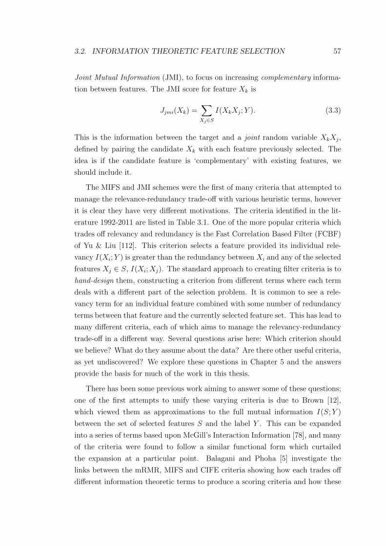
3.2. INFORMATION THEORETIC FEATURE SELECTION 57
Joint Mutual Information (JMI), to focus on increasing complementary informa-
tion between features. The JMI score for feature Xk is
Jjmi(Xk) =∑Xj∈S
I(XkXj;Y ). (3.3)
This is the information between the target and a joint random variable XkXj,
defined by pairing the candidate Xk with each feature previously selected. The
idea is if the candidate feature is ‘complementary’ with existing features, we
should include it.
The MIFS and JMI schemes were the first of many criteria that attempted to
manage the relevance-redundancy trade-off with various heuristic terms, however
it is clear they have very different motivations. The criteria identified in the lit-
erature 1992-2011 are listed in Table 3.1. One of the more popular criteria which
trades off relevancy and redundancy is the Fast Correlation Based Filter (FCBF)
of Yu & Liu [112]. This criterion selects a feature provided its individual rele-
vancy I(Xi;Y ) is greater than the redundancy between Xi and any of the selected
features Xj ∈ S, I(Xi;Xj). The standard approach to creating filter criteria is to
hand-design them, constructing a criterion from different terms where each term
deals with a different part of the selection problem. It is common to see a rele-
vancy term for an individual feature combined with some number of redundancy
terms between that feature and the currently selected feature set. This has lead to
many different criteria, each of which aims to manage the relevancy-redundancy
trade-off in a different way. Several questions arise here: Which criterion should
we believe? What do they assume about the data? Are there other useful criteria,
as yet undiscovered? We explore these questions in Chapter 5 and the answers
provide the basis for much of the work in this thesis.
There has been some previous work aiming to answer some of these questions;
one of the first attempts to unify these varying criteria is due to Brown [12],
which viewed them as approximations to the full mutual information I(S;Y )
between the set of selected features S and the label Y . This can be expanded
into a series of terms based upon McGill’s Interaction Information [78], and many
of the criteria were found to follow a similar functional form which curtailed
the expansion at a particular point. Balagani and Phoha [5] investigate the
links between the mRMR, MIFS and CIFE criteria showing how each trades off
different information theoretic terms to produce a scoring criteria and how these

58 CHAPTER 3. WHAT IS FEATURE SELECTION?
Criterion Full name RefMIM Mutual Information Maximisation [72]MIFS Mutual Information Feature Selection [6]KS Koller-Sahami metric [63]JMI Joint Mutual Information [110]MIFS-U MIFS-‘Uniform’ [69]IF Informative Fragments [109]FCBF Fast Correlation Based Filter [112]AMIFS Adaptive MIFS [103]CMIM Conditional Mutual Info Maximisation [40]mRMR Min-Redundancy Max-Relevance [86]ICAP Interaction Capping [58]CIFE Conditional Infomax Feature Extraction [74]DISR Double Input Symmetrical Relevance [79]MINRED Minimum Redundancy [34]IGFS Interaction Gain Feature Selection [36]SOA Second Order Approximation [48]mIMR Min-Interaction Max-Relevance [11]CMIFS Conditional MIFS [20]
Table 3.1: Various information-based criteria from the literature. In Chapter 5we investigate the links between these criteria and incorporate them into a singletheoretical framework.
terms affect the selected feature set. We present a different view of all these
criteria in Chapter 5 where we investigate the links between them at a deeper
level, namely what assumptions are they making about the underlying probability
distribution p.
We now investigate an area with little relation to the information theoretic
algorithms we have discussed, namely that of feature selection incorporating prior
(domain) knowledge. In Chapter 6 we will see how to construct information
theoretic algorithms which naturally incorporate such knowledge.
3.3 Feature selection with priors
We now turn to algorithms which allow the inclusion of prior knowledge into the
feature selection process. This knowledge can take many forms, from information
about the relevancy of specific features, or groups of features, to a preference for a
certain size of feature set (or sparseness of the solution). The canonical algorithm
which includes a sparsity prior is the LASSO [104] for regression using generalised

3.3. FEATURE SELECTION WITH PRIORS 59
linear models. The LASSO performs an L1 regularisation of the weight vector
of the linear model, necessarily driving many of the weights to zero, leaving only
the weights (and thus features) which are necessary for a good prediction. This
can be expressed as follows,
E(D,w) =N∑i=1
(yi −wTxi)2 + λ
d∑j=1
|wj|. (3.4)
This is the error for a given training dataset D and weight vector w, where λ
is a parameter which controls the strength of the regularisation, and thus the
amount of non-zero weights in w. There have been many extensions to the basic
framework, incorporating different kinds of knowledge in addition to a general
sparsity prior. Helleputte and Dupont [54] present a good example of this recent
work in informative priors for regularized linear models. They develop a prior
for an approximate zero-norm minimization, constraining some of the dimensions
according to knowledge gained from the biological literature.
Yu et al. [113] encode knowledge via constraints on a kernel canonical corre-
lation analysis (KCCA) used to estimate the mutual information between a pair
of features. They incorporated this modified mutual information estimate into
the FCBF [112] algorithm, and use it to select features as inputs to regression.
These constraints forced the KCCA to return a score above a certain value if their
knowledge indicated a link between the features. However they do not investigate
the effects of imposing incorrect constraints on their algorithm.
Krupka et al. [65] define meta-features, where each feature is qualified by addi-
tional information, and a mapping is learnt from meta-features to some measure
of feature ‘quality’. Knowledge can then be transferred between tasks by learning
the feature-quality mapping for similar problems; however the challenge remains
to define a good quality measure and reliably learn the mapping.
When we look at Bayesian Networks and structure learning in Section 3.6 we
will find other algorithms which can incorporate prior knowledge into the feature
selection process in terms of explicit prior structure, and more general network
features.

60 CHAPTER 3. WHAT IS FEATURE SELECTION?
3.4 Multi-class and cost-sensitive feature selec-
tion
Multi-class datasets pose a particular problem for feature selection algorithms,
as features predictive of one class may not help predict others. In the binary
case this is unlikely to lead to poor performance but in a multi-class problem
this can lead to a feature set which has poor predictive performance for entire
classes. This problem can be linked to the issue of cost-sensitive classification
which we reviewed in the previous chapter, as with more classes there is more
opportunity for them to have unbalanced misclassification costs. There may also
be an unbalanced class distribution where some classes have a very small number
of training examples, which can be interpreted as a cost-sensitive problem. In this
section we review the literature in multi-class and cost-sensitive feature selection
which will form the basis of the novel material in Chapter 7 where we derive
a cost-sensitive feature selection criteria. A more extensive survey of empirical
performance on multi-class datasets is found in Forman [42].
One work which highlights the main issue in multi-class feature selection is by
Forman [43], which explores the problem of classes which have different predictive
feature sets. The analysis shows that even when each class has the same number
of examples, common filter feature selection algorithms like MIM and χ2 ranking
fail to select features which are predictive of all the classes. This leads to poor
performance on certain classes with few predictive features and good performance
on other classes which have strongly predictive features. The proposed solution
to this problem is termed Spread-FX, which generates a feature ranking for each
class using an input algorithm such as MIM, before selecting features using a
scheduler from the different feature rankings. The per class feature ranking is
generated by converting the multi-class problem into a one-versus-all problem,
where the current class is the positive label, and all other classes are the negative
label. The scheduling algorithm is then either an explicit round robin scheduler,
where the top ranked feature is selected from each class label in turn, or a proba-
bilistic scheduler where the next class is chosen by sampling from the distribution
over classes. This technique is shown to improve performance against all the uni-
variate ranking techniques in a wide variety of text-classification problems. An
extension is proposed to cost-sensitive feature selection by altering the distribu-
tion sampled by the probabilistic scheduler to incorporate cost information. One

3.4. MULTI-CLASS AND COST-SENSITIVE FEATURE SELECTION 61
issue with this technique is that it is unclear how to adapt it to multivariate rank-
ing algorithms like MIFS or JMI, where the score given to a particular feature is
dependent upon the previously selected features.
The FCCF algorithm proposed by Chidlovskii and Lecerf [21] approaches the
multi-class problem from a different perspective. It is based upon the FCBF
algorithm discussed in Section 3.2, but modified so the exclusion heuristic takes
into account the presence of multiple classes. In addition to the standard FCBF
exclusion heuristic that the candidate feature Xi has shares more information
with a selected feature than the class label, it must also have less class specific
information than that selected feature. Therefore the feature Xi is excluded iff
∃ y ∈ Y,Xj ∈ S s.t. SU(Y = y;Xj) ≥ SU(Y = y;Xi) and SU(Xi;Xj) ≥SU(Y ;Xi), where SU(X;Y ) is the symmetric uncertainty between X and Y (see
Section 2.3).
Chapelle and Keerthi [18] present a modification of L1-SVM to extend it to
the multi-class case. L1-SVM is a regularised version of the standard binary
SVM algorithm which like LASSO mentioned in the previous section performs
an L1 regularisation of the feature weight vector driving most of those weights to
zero, resulting in a sparse selected feature set. As SVMs are binary classification
algorithms the standard RFE and L1 methods select independent feature subsets
for each possible class. The proposed method shares the regularisation penalty
across all the individual SVM optimisation functions, thus ensuring that each
binary problem is properly penalised by the number of features in use.
The final algorithm we review is an explicit cost-sensitive feature selection al-
gorithm, which aims to select features which minimise the misclassification cost.
This approach is due to Robnik-Sikonja [95], and works with many univariate fea-
ture ranking procedures used in decision trees as splitting criteria. The proposed
technique adjusts the probabilities of each split criteria, altering the probability
for each class based upon the expected risk of misclassification as follows,
εy =1
1− p(y)
|Y |∑y 6=y
p(y)C(y, y) (3.5)
p′(y) =p(y)εy∑|Y |y p(y)εy
. (3.6)
In the equation above C(y, y) is the cost of misclassifying class y as y, and p(y) is
the marginal probability of the label y. This approach can be seen as extending

62 CHAPTER 3. WHAT IS FEATURE SELECTION?
the work of Elkan [38] to feature selection, as it effectively resamples the data
according to its expected misclassification cost. The new probability values can
then be incorporated into a function such as the mutual information to score the
features.
We now move to a different but related section of the literature, that relating
to Bayesian Networks and specifically the learning of network structure.
3.5 Bayesian Networks
A Bayesian Network is a model of a probability distribution which shows how the
variables interact in a system. They are first defined by Pearl [84] as a method
for encoding the interactions between variables, showing the independences in the
system. The whole system is modelled as a directed acyclic graph (DAG), with
the variables being nodes in the graph, and the arrows denoting the direction
of influence. In classification problems we also include the class label as a node
in the graph, in addition to all the features. Each node takes a state which is
probabilistically dependent on its parent nodes, and only those nodes. The graph
is acyclic (i.e. has no directed path from one node back to itself) to ensure no node
ends up as its own ancestor, as this could cause nodes to oscillate between states.
If there is no path between any two variables then the probability distributions
of those variables are independent. Any node is made conditionally independent
from the rest of the graph by its Markov Blanket, the set of all parents, children
and spouses (other parents of the child nodes) of that particular node. Any
set of nodes which removes the dependence between two other nodes is said to
d-separate those two nodes. The Markov Blanket can be seen as d-separating
the target node from the rest of the network. This is useful as it means that
only the states of the nodes in the Markov Blanket are required to predict the
state of the target node. A Bayesian Network classifier can be constructed by
encoding a set of independence statements between the features and the class
label, and then learning the probability distributions over the states of each node
conditioned on its parents. The Naıve Bayes classifier is an example of a Bayesian
Network classifier, where all the features are child nodes of the class label, and
are thus class-conditionally independent of each other. Figure 3.1 shows a generic
Bayesian Network, highlighting the Markov Blanket for the central node.
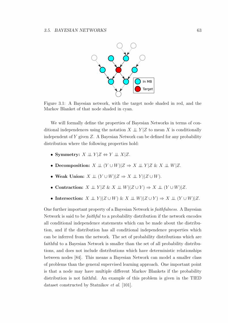
3.5. BAYESIAN NETWORKS 63
In MB
Target
Figure 3.1: A Bayesian network, with the target node shaded in red, and theMarkov Blanket of that node shaded in cyan.
We will formally define the properties of Bayesian Networks in terms of con-
ditional independences using the notation X ⊥⊥ Y |Z to mean X is conditionally
independent of Y given Z. A Bayesian Network can be defined for any probability
distribution where the following properties hold:
• Symmetry: X ⊥⊥ Y |Z ⇔ Y ⊥⊥ X|Z.
• Decomposition: X ⊥⊥ (Y ∪W )|Z ⇒ X ⊥⊥ Y |Z & X ⊥⊥ W |Z.
• Weak Union: X ⊥⊥ (Y ∪W )|Z ⇒ X ⊥⊥ Y |(Z ∪W ).
• Contraction: X ⊥⊥ Y |Z & X ⊥⊥ W |(Z ∪ Y ) ⇒ X ⊥⊥ (Y ∪W )|Z.
• Intersection: X ⊥⊥ Y |(Z ∪W ) & X ⊥⊥ W |(Z ∪ Y ) ⇒ X ⊥⊥ (Y ∪W )|Z.
One further important property of a Bayesian Network is faithfulness. A Bayesian
Network is said to be faithful to a probability distribution if the network encodes
all conditional independence statements which can be made about the distribu-
tion, and if the distribution has all conditional independence properties which
can be inferred from the network. The set of probability distributions which are
faithful to a Bayesian Network is smaller than the set of all probability distribu-
tions, and does not include distributions which have deterministic relationships
between nodes [84]. This means a Bayesian Network can model a smaller class
of problems than the general supervised learning approach. One important point
is that a node may have multiple different Markov Blankets if the probability
distribution is not faithful. An example of this problem is given in the TIED
dataset constructed by Statnikov et al. [101].

64 CHAPTER 3. WHAT IS FEATURE SELECTION?
3.6 Structure Learning
An important part of learning with Bayesian Networks is determining the graph
structure which relates the nodes. This can either be done by hand, where do-
main experts construct the relationships between the nodes, or through statistical
inference. The process is termed Structure Learning when the network is learned
algorithmically from a particular dataset. There are two different approaches to
structure learning, constraint-based or score and search. Constraint-based struc-
ture learning finds variables which are dependent upon each other and links the
two nodes. Once all links have been found, they are oriented using a variety
of different statistical tests, to produce the required DAG. Alternatively some
constraint-based algorithms start from a fully connected graph and use indepen-
dence tests to remove links between nodes which are conditionally independent.
Score and search methods use a scoring metric for how well the current network
structure fits the data, and then search in the space of possible structures for the
structure which maximises the score measure. The scoring metric is invariant to
certain valid permutations of the graph, therefore multiple graphs may have the
same score and so another method is required to differentiate between them.
There are strong links between structure learning algorithms and feature selec-
tion algorithms. This is due to the properties of Markov Blankets. As a Markov
Blanket is the set of nodes which make the target node independent from the rest
of the graph, it is also the set of features required for optimal prediction of that
target node [107]. Thus a structure learning algorithm can be thought of as a
global feature selection algorithm, which learns the features required to predict
each node in turn. In problems where the probability distribution p(x, y) is not
faithful to a Bayesian Network then there may be multiple possible structures,
all of which are in some sense a valid representation of that distribution. In this
case there are multiple Markov Blankets and thus many equally valid solutions
to the feature selection problem.
Conditional independence testing algorithms can be further divided into those
which do “local” learning, and those which do “global” learning [2]. Local learn-
ing algorithms are concerned with finding the Markov Blanket of a particular
node, and thus only give the local structure around that node. Global learning
algorithms aim to find the whole structure of the Bayesian Network, this struc-
ture can then be examined separately to find the Markov Blanket for any given
node.

3.6. STRUCTURE LEARNING 65
3.6.1 Conditional independence testing
As mentioned previously the Markov Blanket of a node is a solution to the feature
selection problem when working with Bayesian Networks. The Markov Blanket
discovery task is easier than the full structure learning task, as it does not re-
quire the orientation of the links between nodes, nor differentiating between the
indirectly connected spouse nodes and the directly connected parent and child
nodes. We first explore the local learning algorithms which use conditional inde-
pendence testing to find Markov Blankets. These algorithms are in practice very
similar to the filter feature selection algorithms we looked at in Section 3.2, and
we investigate these links in Chapter 6. They are also known as constraint-based
structure learning algorithms, and we will use the shorthand CB to refer to them
as a group. We then look at methods for combining local structure into global
structure, and other global structure learning methods.
Local structure learning
The first algorithm which attempted to learn the Markov Blanket of a node was
strictly a feature selection approach, presented in Koller & Sahami [63]. It pro-
ceeded via backwards elimination from the full feature set, removing the feature
which had the smallest interaction with the class label, given its (approximate)
Markov Blanket. This approximate algorithm is closest to the CMIM algorithm
we discuss as part of Chapter 5, in that each feature is scored by its minimal
interaction when conditioned on the selected feature set. This algorithm does
not return the Markov Blanket of the target node (usually the class label), but it
was used as a baseline in the development of other structure learning algorithms.
The first true structure learning algorithm is the Grow-Shrink (GS) algorithm
by Margaritis and Thrun [77]. This adopted the two stage algorithm which is
common to many local learning algorithms, first growing the candidate Markov
Blanket by adding new features until all remaining unselected features are condi-
tionally independent of the target, then shrinking the candidate Markov Blanket
to remove any false positives which may have been selected. This local algorithm
for constructing Markov Blankets is then ran over each node of the network, and
the resulting subgraphs are combined to construct a DAG for the entire network.
The choice of conditional independence test used in the algorithm is left unspec-
ified, as there are multiple ones which are suitable. The IAMB algorithm by
Tsamardinos and Aliferis [107] is a refinement of the GS algorithm. It uses a

66 CHAPTER 3. WHAT IS FEATURE SELECTION?
different ordering heuristic to choose in what order to select and remove features,
compared to the GS algorithm. This heuristic simply selects the feature which
has the largest conditional mutual information, and removes the feature which
has the smallest conditional mutual information. They state that this heuristic
improves the runtime of the algorithm by prioritising features which most improve
the quality of the returned Markov Blanket. The algorithm for IAMB is given in
Algorithm 2, though the general structure is true for most of the local structure
learning algorithms we explore in this section. The f(X;Y |CMB) in Algorithm
2 represents the conditional independence test used, and is a parameter of the
algorithm.
Algorithm 2 IAMB [107].
Phase 1 (forward)CMB = ∅while CMB has changed do
Find X ∈ Ω \ CMB to maximise f(X;Y |CMB)if f(X;Y |CMB) > ε then
Add X to CMBend if
end whilePhase 2 (backward)while CMB has changed do
Find X ∈ CMB to minimise f(X;Y |CMB \X)if f(X;Y |CMB \X) < ε then
Remove X from CMBend if
end while
The authors of IAMB proceeded to publish several more data efficient variants
of the IAMB algorithm, which require fewer samples to accurately estimate the
necessary tests. The most common variants are the MMMB [106] and HITON [4]
algorithms. MMMB first finds the set of parents and children of a target node, by
finding the minimal set of nodes which makes each node most independent of the
target. This is similar to the heuristic proposed by Koller & Sahami for Markov
Blanket recovery in classification problems. Once the set of parents and children
have been found these are added to the candidate Markov Blanket. Then the
parents and children are found for each node in the candidate Markov Blanket,
and these are tested to see if they are spouse nodes of the original target. This
approach reduces the computation by only conditioning on the minimal set of

3.6. STRUCTURE LEARNING 67
nodes (i.e. the set of parents and children of the target). The HITON algorithm is
essentially similar to the MMMB algorithm, but is tailored for prediction tasks. It
uses a final wrapper to prune the candidate Markov Blanket by removing features
which do not affect classification performance.
One further local structure learning algorithm is the new variant of GS devel-
oped by Margaritis [76]. This extends the GS framework beyond the learning of
Markov Blankets to the general case of learning Markov Boundaries. This is still
a set of variables which make a particular node probabilistically independent from
the rest, but it includes cases which cannot be expressed as Bayesian Networks,
such as in the TIED dataset [101], where there are multiple different Markov
Blankets (which is not possible in a true Bayesian Network). The algorithm is
extended to test sets of variables for dependence in the inclusion phase. This
makes the algorithm exponential rather than polynomial in the number of nodes,
which precludes its usage in practice. Margaritis thus proposes a randomised ver-
sion, which randomly samples sets of a fixed size, tests each set for dependence,
and adds the set with the largest measured dependence (similar to the heuristic
ordering added in the IAMB algorithm).
Global structure learning
One of the first global structure learning algorithms was based upon the condi-
tional independence testing methodology, namely the PC algorithm by Spirtes
et al. [100]. This first constructs an undirected graph where the absence of a
link between two nodes indicates they are conditionally independent. After this
construction process each link is oriented (if possible) by analysing the graph
structure, as a Bayesian Network is an acyclic graph, so there are no directed
paths starting at one node and returning to that node. The PC algorithm is not
usually able to orient all the edges, and thus returns a partially directed graph
where some edges are left undirected. These partially directed graphs are usually
called “patterns” or “essential graphs”.
The PC algorithm is unusually reliant upon the quality of the independence
test used, as it uses the current graph state to construct the set of independence
tests needed for the next node. This causes errors to cascade through the graph
structure as one mistake produces an incorrect structure to base the next test
on, which in turn causes more failures [27]. This problem is partially solved by
the LGL family of algorithms developed by Aliferis et al. [2, 3] which learn the

68 CHAPTER 3. WHAT IS FEATURE SELECTION?
local structure for each node independently before combining each local structure
to learn the full graph. A local learning algorithm such as an IAMB variant is
used to learn the set of parents and children for each node in turn. Those local
structures are then used to produce an undirected graph for the whole structure
(as it cannot differentiate between the parents and the children) before using
another algorithm to orient the edges. In the paper they explore the use of the
BDeu score to orient the edges, which is an example of the score and search
methods we review in the next section.
3.6.2 Score and search methods
Score and search (S&S) methods for structure learning aim to maximise a function
of the network structure with respect to a given dataset. This can be analysed
in a similar way to a filter feature selection algorithm, as indicated by the name
score and search. Each technique is made up of the scoring function (or criterion)
and the search method used to maximise that scoring function.
Many of the techniques use similar search techniques based upon the concept
of a neighbourhood in graph space. From a given graph structure G the neigh-
bourhood of G, η(G), is defined as all DAGs which can be constructed from G
via addition, deletion or reversal of a single edge [82]. Within this neighbourhood
view there are many different search strategies based upon hillclimbing [53], Sim-
ulated Annealing [61], and Markov-Chain Monte-Carlo (MCMC) [82] techniques.
We will briefly outline a few scoring functions along with their associated search
methods.
The most common approaches found in the S&S literature are based upon the
Bayesian Dirichlet (BD) score [53]. This family of scoring functions make several
assumptions about the underlying true network which they are trying to recover:
1. The data is drawn from a multinomial, with positive probability everywhere
(i.e. there are no logical relationships between variables).
2. That the data generating parameters are both globally independent across
the network, and locally independent with respect to the state of the parent
set of a node.
3. That each node’s parameters only depend upon the parent set of that node.
4. That each node’s parameters form a Dirichlet distribution.

3.6. STRUCTURE LEARNING 69
The most popular member of this family is the BDe (Bayesian Dirichlet equiva-
lence) metric [53], which imposes an additional assumption, that equivalent net-
work structures should have the same score. This effectively replaces the Dirichlet
assumption, as the assumption of equivalence implies that all node parameters
are Dirichlet distributed. The BDe score for any given graph G given a training
dataset D is
p(D, G) = p(G)d∏i
Πi∏j=1
Γ(N ′ij)
Γ(N ′ij +Nij)
ri∏k=1
Γ(N ′ijk +Nijk)
Γ(N ′ijk). (3.7)
In the equation above N is the number of datapoints, N ′ is the equivalent sample
size in the prior network (i.e. how strong the prior is), Nijk is the number of
examples where the ith node takes the kth state and the parent set of i takes the
jth state, and Γ is the gamma function. It is also possible to add more specific
domain knowledge about the possible structures by defining the prior p(G). This
measure is then paired with a neighbourhood search based upon hillclimbing or
simulated annealing. The hillclimbing approach simply moves to the graph in the
neighbourhood which most improves the BDe score, terminating when no graph
in the neighbourhood improves the score. This search method is very dependent
upon a good choice of the initial graph, which is usually constructed incorporating
all the available domain knowledge. Simulated annealing provides a more general
approach, where the next graph structure is allowed to have a lower BDe score
with a given probability based upon the current temperature. This temperature
is gradually lowered as the search progresses, allowing fewer and fewer moves
which decrease the score. The search terminates when a particular temperature
is reached and no more moves which increase the score are available. The BDeu
score mentioned previously is simply the BDe score with a uniform distribution
over possible structures [15].
Mukherjee and Speed [82] construct different kinds of structure priors for use
with the BDe score. This allows the prior knowledge to constrain abstract graph
features such as the number of parents of a node, or the connectivity between
two groups of nodes. They couple the BDe score and the structure priors with an
MCMC based search. The search aims to sample from the distribution p(G|D),
so the probability of various graph features can be calculated, along with the
most probable graph (i.e. the MAP solution). The proposal distribution for the
Metropolis-Hastings sampler used is based on the neighbourhood of the graph,

70 CHAPTER 3. WHAT IS FEATURE SELECTION?
only allowing proposals which are within the neighbourhood of the current graph.
This proposal distribution can optionally be modified to incorporate the prior
distributions over graph features. This in turn means graphs which are a priori
more likely to be proposed more often.
Grossman and Domingos [45] present a different take on the score and search
paradigm, as they wish to learn the structure of a Bayesian Network to construct a
classifier for a particular node. This can be seen as generalising the construction of
a Naıve Bayes classifier (see Chapter 2) to arbitrary network structures around the
class node Y . They do this by aiming to maximise the conditional log-likelihood
of the structure, inferring the individual node parameters from their maximum
likelihood estimates. This takes a discriminative approach to the learning of
structure which is a perspective we will examine more closely in the next chapter.
Each network structure is scored by the likelihood, L, of Y given the inputs X
as follows,
L(G|D) =N∑i=1
log p(yi|xi1, . . . , xid). (3.8)
This scoring function is coupled with the simple hillclimbing search used in BDe,
except it starts from the empty network which has no arcs. Unfortunately this
scoring function requires the estimation of the complex distribution p(y|x), which
requires a relatively large amount of data to calculate when there are many nodes
connected to Y . Carvalho et al. [16] present a new scoring function approximat-
ing the conditional log-likelihood which decomposes over the network structure,
allowing it to be calculated on a per node basis (thus reducing the complexity of
each estimated distribution). This function is an approximate factorised condi-
tional log-likelihood, and can be expressed as the sum of information theoretic
components plus a fixed constant which does not depend upon the network,
fL(G|D) =d∑i=1
(α+β)NI(Xi; Π(Xi)|Y ) +βλNI(Y ;Xi; Π(Xi)) + const. (3.9)
In the above notation I(. . . ) denotes the interaction information [78], α, β
and λ are constants which do not depend on the network structure, and Π(Xi)
denotes the parent set of Xi. This is a decomposable measure, which means
each node contributes independently to the overall score for a particular graph
G. This score in particular links the conditional likelihood, information theory
and structure learning in a way which parallels the results presented in Chapters
3.6. STRUCTURE LEARNING 71
4 & 6, though our results provide a more general framework, and are applicable
to the general feature selection problem.
One final relevant score and search approach is that of de Campos [28]. This
paper describes a scoring function which is based upon measures of conditional
independence as calculated by the mutual information. Each node is scored by
the mutual information with it’s current parent set, penalised by a function of
the χ value expected if the parents are independent of the node. This leads to
a scoring function which is not a probability or log-probability unlike the other
measures we have discussed and is expressed as,
f(G,D) =d∑i=1
(2NI(Xi; Π(Xi))−max
σi
|Π(Xi)|∑j=1
χα,li,σi
). (3.10)
In the above equation α is the confidence level of the χ2 test, |Π(Xi)| is the
number of parents of Xi, σi are the possible permutations of the parent set, and
li,σi is the degrees of freedom, based upon the number of possible states for each
permutation. Again this scoring function can be decomposed over the nodes, and
can be interpreted under the Minimum Description Length (MDL) framework
[94] as the decrease in description length between the candidate graph G and the
empty graph.
The twin approaches of conditional independence testing and score & search
initially appear to be very different, as the CB methods add links based upon
the value of an independence test, and S&S measures the change in global score
as the links are added, removed or inverted. In fact in the global case instances
of these two approaches are equivalent. Cowell [25] showed that for a given node
ordering with complete data, independence testing based upon the KL-Divergence
is identical to scoring networks by their log-likelihood. In Chapter 6 we present a
similar result for local structure learning with mutual information, showing that
this is exactly equivalent to hill-climbing the joint likelihood of the local structure
(which is a greedy search on the neighbourhood of the local structure graph).

72 CHAPTER 3. WHAT IS FEATURE SELECTION?
3.7 Chapter Summary
In this chapter we reviewed the literature surrounding feature selection and
Bayesian Networks which provide the landscape for the contributions of this the-
sis. In summary,
• We looked at feature selection, and the three main paradigms: filters, which
select features based upon a statistical measure of correlation; wrappers,
which select features based upon the performance of a classification algo-
rithm; and embedded methods, a wide group of algorithms which select
features as part of the classification process.
• We reviewed the literature on information theoretic filter algorithms, where
the relevancy and redundancy of a feature is scored using concepts such as
the mutual information.
• We looked at feature selection algorithms which can incorporate prior (do-
main) knowledge about the sparseness of the solution, or the relevancy of
particular features.
• We reviewed a selection of feature selection algorithms designed specifically
for multi-class environments, and looked at how they try to ensure they
have predictive features for all the classes.
• We looked at how Bayesian Network classifiers can be constructed to solve
classification problems, whilst giving more information about the structure
of the problem. We also saw how learning the structure of a Bayesian
Network is equivalent to the feature selection problem.
• Finally we reviewed literature on structure learning in Bayesian Networks,
investigating the two main paradigms: constraint based methods, and score
& search methods. We saw how several of the constraint based meth-
ods used mutual information measures to rank features and how these ap-
proaches are similar to the information theoretic filter literature.
In the next chapter we present the central result of this thesis, a deriva-
tion of mutual information based feature selection criteria from a clearly defined
loss function, namely the joint likelihood of a discriminative model. We derive
update rules for this loss function which allow us to iteratively maximise the

3.7. CHAPTER SUMMARY 73
joint likelihood by selecting the feature which maximises the conditional mutual
information. In Chapter 5 we use this probabilistic framework to understand
the different approximations and assumptions made by the information theoretic
heuristics we have reviewed in this chapter. In Chapter 6 we link our probabilistic
framework to the problem of Markov Blanket discovery, showing in the process
that some common local structure learning algorithms are actually maximising
the joint likelihood under a flat prior over network structure.

Chapter 4
Deriving a selection criterion
In Chapter 3 we briefly outlined the three main classes of feature selection algo-
rithms: filters, wrappers, and embedded methods. We saw how many of the filter
techniques are heuristic, combining different kinds of correlation terms without
any understanding of the objective function they were optimising. We now recast
the feature selection problem as a constrained optimisation problem in a high
dimensional space, so our task is to find a n-dimensional bit vector θ with at
most k bits set, representing our selected features. We should then choose θ to
optimise some evaluation criterion. There has been much attention given to this
problem of search in high dimensional spaces (see Reunanen [93] for a review of
search strategies in feature selection), and a good search technique is an integral
part of any feature selection algorithm. There has been a similarly large amount
of attention given to the construction of evaluation criteria, but many of these
criteria are based upon heuristics, with little investigation into the underlying
metrics which they are attempting to optimise. We will focus on the derivation
of these evaluation criteria, and leave the question of constructing a search al-
gorithm which best optimises our criteria for future work. In particular we will
derive the optimal evaluation criterion for a particular loss function which we
wish to optimise.
4.1 Minimising a Loss Function
We now formally develop feature selection as the optimisation of a discriminative
model likelihood, following Lasserre et al. [70], and Minka [81] in the construction
of such a model. This derivation of feature selection forms the basis of the rest of
74

4.1. MINIMISING A LOSS FUNCTION 75
this thesis. In Chapter 5 we will investigate the links between our formal frame-
work based upon the likelihood and the literature of feature selection heuristics
based upon mutual information. In Chapter 6 we will look at what benefits our
likelihood framework gives when we wish to extend these criteria to incorporate
prior information. In Chapter 7 we will use a similar derivation to construct
cost-sensitive feature selection criteria.
4.1.1 Defining the feature selection problem
We assume an underlying i.i.d. process p : X → Y , from which we have a sample
of N observations. Each observation is a pair (x, y), consisting of a d-dimensional
feature vector x = [x1, ..., xd]T , and a target class y, drawn from the underlying
random variables X = X1, ..., Xd and Y . We further assume that p(y|x) is
defined by a subset, X∗, of the features X, while the remaining features are re-
dundant or irrelevant. Our modeling task is therefore two-fold: firstly to identify
the features that play a functional role, and secondly to use these features to
perform predictions.
We adopt a d-dimensional binary vector θ, specifying the selected features: a
1 indicates the feature is selected, and a 0 indicates it is discarded. We use ¬θfor the negation of θ, i.e. the unselected features. We then define Xθ as the set
of selected features, and X¬θ as the set complement of Xθ, the set of unselected
features. Therefore X = Xθ ∪X¬θ, as Xθ and X¬θ form a partition. We use xθ
for an observation of the selected features Xθ, and similarly for x¬θ. We define
p(y|x,θ) as p(y|xθ), and use the latter when specifically talking about feature
selection. As mentioned, we assume the process p is defined by a subset of the
features, so for some unknown optimal vector θ∗, we have that p(y|x) = p(y|xθ∗).We then formally define X∗ as the minimal feature set s.t. ∀ x, y p(y|xθ∗) = p(y|x)
and use θ∗ as the vector indicating this feature set. The feature selection problem
is to identify this vector. We define τ as the other model parameters involved in
the generation of class labels, and λ as the generative parameters which create the
observations x. Each of these model parameters, λ, τ,θ, has an associated prior
probability distribution, p(λ), p(τ,θ), which represents our belief a priori in each
particular value of the parameters. Note that τ and θ are jointly distributed, as
the feature set influences the classification model parameters.

76 CHAPTER 4. DERIVING A SELECTION CRITERION
Figure 4.1: The graphical model for the likelihood specified in Equation (4.1).
4.1.2 A discriminative model for feature selection
We approximate the true distribution p with a hypothetical model q, with sep-
arate parameters for the feature selection, θ, and for classification, τ . Following
Minka [81] and Lasserre et al. [70], in the construction of a discriminative model,
our joint likelihood is
L(D,θ, τ, λ) = p(θ, τ)p(λ)N∏i=1
q(yi|xi,θ, τ)q(xi|λ). (4.1)
This is the joint likelihood for the graphical model specified in Figure 4.1. In dis-
criminative models we wish to maximise our classification performance, therefore
we maximize L with respect to θ (our feature selection parameters) and τ (our
model parameters). We therefore ignore the generative parameters λ as they do
not directly influence the classification performance. Excluding the generative
terms gives
L(D,θ, τ, λ) ∝ p(θ, τ)N∏i=1
q(yi|xi,θ, τ). (4.2)
We wish to find the Maximum a Posteriori (MAP) solution, the mode of the
distribution L, with respect to the parameters θ, τ. This means we will find
a single feature set which maximises our likelihood. We leave a fully Bayesian
treatment of the feature selection problem, where we calculate a probability dis-
tribution over possible feature sets, to future work.
We choose to work with the scaled negative log-likelihood, −`, converting
our maximization problem into a minimization problem, without changing the
position of the optima. This gives
−` = − 1
N
( N∑i=1
log q(yi|xi,θ, τ) + log p(θ, τ)
)(4.3)

4.1. MINIMISING A LOSS FUNCTION 77
which is the function we will minimize with respect to θ, τ; the scaling term is
to simplify exposition later.
We wish to decompose this log-likelihood to extract terms directly related to
feature selection and to classification performance. This will allow us to express
the feature selection problem directly and to find what functions maximise the
likelihood of our model. We first compare our predictive model against the true
distribution of p(yi|xi), and so we introduce the ratio p(yi|xi)p(yi|xi) into the logarithm.
This is the probability of the correct class given all the data, without any feature
selection. As this ratio is unity it does not change the value of the log-likelihood,
nor the positions of its optima. We can then expand the resulting logarithm to
give several terms,
−` = − 1
N
( N∑i=1
logq(yi|xi,θ, τ)
p(yi|xi)+
N∑i=1
log p(yi|xi) + log p(θ, τ)
). (4.4)
These terms are: the log-likelihood ratio between the true model and our predic-
tive model, the log-likelihood of the true model, and the prior term. The first
term is small when our predictive model is a good approximation to the true
distribution. We can see that the middle term is a finite sample approximation
to the conditional entropy H(Y |X) as follows,
H(Y |X) = −∑
x∈X,y∈Y
p(x, y) log p(y|x) ≈ − 1
N
N∑i=1
log p(yi|xi). (4.5)
This represents the total amount of uncertainty there is about the class label
given the data. The conditional entropy is large when the features we have do
not constrain the class label well, i.e. it is hard to accurately predict the label
from the features. The conditional entropy is the log-likelihood of the true model
when taking the limit of data points, and thus provides a lower bound on our
performance, as our model cannot perform better than the data allows.
We are concerned with separating out the influence of feature selection and
classification in our model, and thus introduce an extra ratio p(yi|xi,θ)p(yi|xi,θ)
into the
first term. This is the probability of the correct class given the features we have
selected with θ, and thus represents how useful a set of features we have selected.

78 CHAPTER 4. DERIVING A SELECTION CRITERION
We can then further expand the first logarithm as follows,
−` = − 1
N
( N∑i=1
logq(yi|xi,θ, τ)
p(yi|xi,θ)+
N∑i=1
logp(yi|xi,θ)
p(yi|xi)
+N∑i=1
log p(yi|xi) + log p(θ, τ)
). (4.6)
We then bring the minus sign inside the brackets, and flip the ratios inside the
logarithms, which gives
−` =1
N
( N∑i=1
logp(yi|xi,θ)
q(yi|xi,θ, τ)+
N∑i=1
logp(yi|xi)p(yi|xi,θ)
−N∑i=1
log p(yi|xi)− log p(θ, τ)
). (4.7)
As before the last two terms are the log likelihood of the true model and the
prior term. We have now separated out the first log likelihood ratio into two
terms. The first term is the log ratio between our predictive model and the true
distribution of the labels given our selected subset of features. This represents
how well our model fits the data given the current set of features. When the ratio
is 1, the log ratio is 0 and our model has the best possible fit given the features
selected. The second term is the log ratio between the true distribution given
the selected features, and the true distribution of the labels given all the data.
This measures the quality of the selected feature set θ, based on how close the
conditional distribution of y is to the one conditioned on all the data. We can see
that this term is a finite sample approximation to the expected KL-Divergence
between p(y|x) and p(y|x,θ) as follows
Ex,yp(y|x)||p(y|x,θ) =∑
x∈X,y∈Y
p(x, y) logp(y|x)
p(y|x,θ)≈ 1
N
N∑i=1
logp(yi|xi)p(yi|xi,θ)
.
(4.8)
This KL-Divergence has appeared before in the feature selection literature. Koller
and Sahami [63] introduce this divergence as a sensible objective for a feature se-
lection algorithm to minimise. With our expansion we show it to be a direct
consequence of optimising a discriminative model likelihood, though their ap-
proach ignores the prior over the features. As x = xθ,x¬θ, we can further

4.1. MINIMISING A LOSS FUNCTION 79
develop this term:
∆KS = Ex,yp(y|xθ,x¬θ)||p(y|xθ)
=∑x
p(x)∑y
p(y|x) logp(y|xθ,x¬θ)
p(y|xθ)
=∑x,y
p(x, y) logp(y|xθ,x¬θ)
p(y|xθ)
p(x¬θ|xθ)
p(x¬θ|xθ)
=∑x,y
p(x, y) logp(x¬θ, y|xθ)
p(x¬θ|xθ)p(y|xθ)
= I(X¬θ;Y |Xθ). (4.9)
This is the conditional mutual information between the class label and the re-
maining features, given the selected features. We can now write the negative
log-likelihood as the sum of information theoretic quantities plus the prior over
θ, τ,
−` ≈ Ex,y
log
p(yi|xi,θ)
q(yi|xi,θ, τ)
+I(X¬θ;Y |Xθ)+H(Y |X)− 1
Nlog p(θ, τ). (4.10)
Assuming for the moment that we have the optimal feature set or a superset
thereof (i.e. X∗ ⊆ Xθ) then p(y|x,θ) = p(y|x). Then as the expectation in the
first term is over p(y,x), the first term can be seen as a finite sample approxima-
tion to the expected KL-Divergence over p(x) representing how well the predictive
model fits the true distribution, given a superset of the optimal feature set.
The first term is a measure of the difference between the predictive model q,
and the true distribution p given the selected features. When a superset of the
optimal feature set has been found, it becomes the KL-Divergence between p and
q. The second term is I(X¬θ;Y |Xθ), the conditional mutual information between
the class label and the unselected features, given the selected features. The size of
this term depends solely on the choice of features, and will decrease as the selected
feature set Xθ explains more about Y , until eventually becoming zero when the
remaining features X¬θ contain no additional information about Y in the context
of Xθ. Note that due to the chain rule, I(AB;Y ) = I(A;Y ) + I(B;Y |A), and
X = Xθ ∪X¬θ,
I(X;Y ) = I(Xθ;Y ) + I(X¬θ;Y |Xθ). (4.11)
Since I(X;Y ) is constant, minimizing I(X¬θ;Y |Xθ) is equivalent to maximizing

80 CHAPTER 4. DERIVING A SELECTION CRITERION
I(Xθ;Y ), which is the goal of many mutual information based filter algorithms.
The third term in Eq (4.10) is H(Y |X), the conditional entropy of the labels
given all features ; this is an irreducible constant, dependent only on the dataset
D. As mentioned previously this term represents the quality of the data, and
how predictive X is of Y . When this value is small the data constrains the choice
of Y , and thus it has a low Bayes rate, whereas when this value is large the data
does not constrain the choice of Y , and the Bayes rate is higher.
This expansion makes explicit the effect of the feature selection parameters
θ, separating them from the effect of the parameters τ in the model that uses
those features. If we somehow had the optimal feature subset θ∗, which perfectly
captured the underlying process p, then I(X¬θ;Y |Xθ) would be zero. The re-
maining (reducible) error is then down to the KL divergence p||q, expressing how
well the predictive model q can make use of the provided features. Of course,
different models q will have different predictive ability: a good feature subset will
not necessarily be put to good use if the model is too simple to express the under-
lying function. This perspective was also considered by Tsamardinos and Aliferis
[107], and earlier by Kohavi and John [62] — the above results place these in
the context of a precise objective function, the joint likelihood of a discriminative
model.
We now make an assumption made implicitly by all filter methods, that model
fitting can be separated from the feature selection process. For completeness we
formalise this assumption as:
Definition 8. Filter assumption
Given an objective function for a classifier, we can address the problems of op-
timizing the feature set and optimizing the classifier in two stages: first picking
good features, then building the classifier to use them.
In our framework we make this assumption explicit by specifying that the
prior p(θ, τ) factorizes into p(θ)p(τ), thus decoupling the model fitting from the
feature selection. We note that τ is independent of the second term in our expan-
sion, and by factorising the prior we can select features before fitting the model.
This assumes that our model q will fit the distribution p(y|x,θ) and that it can
exploit all information given in the feature set. We therefore can optimise the
feature selection first, as with enough data our model will fit the true distribution
p(y|x,θ) optimally, and the first ratio in Equation (4.10) will become zero. This

4.1. MINIMISING A LOSS FUNCTION 81
is a valid assumption if our model q is a consistent estimator of p, as with in-
creasing N it will more closely approximate the true distribution. In essence this
assumption means the classification model is sufficiently complex to adapt to any
feature set, without making additional limiting assumptions about the distribu-
tion. Whereas the filter criteria literature makes the filter assumption implicitly,
the formalism we have presented has made it explicit. In filters, to maximize the
likelihood of the feature set we are only concerned with how p(y|x,θ) approx-
imates p(y|x,θ∗), so we can now specify the optimization problem that defines
the feature selection task for the model in Equation (4.1) as,
θ∗ = arg minθ
(I(X¬θ;Y |Xθ)− 1
Nlog p(θ)
). (4.12)
This optimisation problem relies upon the prior to ensure there is a unique global
optimum, as with a flat prior any superset of an optimal feature set is also optimal.
In the next section we will tighten our definition of the feature selection task to
remove this problem.
We note that in contrast to filter algorithms, wrapper and embedded ap-
proaches optimise jointly over the first two terms in Equation (4.10), by fitting
the classification model together with the feature selection.
We now turn to the problem of how to optimise the parameter θ, i.e. how do
we choose a feature. We show how the commonly used simple greedy searches are
iterative maximisers of the likelihood, and under what conditions such a search
returns the optimal solution.
4.1.3 Optimizing the feature selection parameters
Under the filter assumption in Definition 8, Equation (4.12) specifies the optimal
feature set, in the sense of maximising the joint likelihood. However there may of
course be multiple global optima giving multiple optimal feature sets, in addition
to the trivial optima of selecting all features. In fact, due to the nature of the
mutual information, any feature set which contains the optimal feature set will
be a global optima of the likelihood. As we wish to perform feature selection,
we express a preference for the smallest such feature set which maximises the
likelihood.
With this in mind, we can introduce a minimality constraint on the size of

82 CHAPTER 4. DERIVING A SELECTION CRITERION
the feature set, and define our problem:
θ∗ = arg minθ′
|θ′| : θ′ = arg min
θ
(I(X¬θ;Y |Xθ)− 1
Nlog p(θ)
). (4.13)
This is the smallest feature setXθ, such that the mutual information I(X¬θ;Y |Xθ)
plus the prior is minimal, and thus the joint likelihood is maximal. It should be
remembered that the likelihood is only our proxy for classification error, and the
minimal feature set in terms of classification could be smaller than that which
optimises likelihood.
A common heuristic approach is a sequential search considering features one-
by-one for addition/removal; this is used for example in Markov Blanket learning
algorithms such as IAMB [108] (we will return to the IAMB algorithm in Chap-
ter 6). We will now demonstrate that this sequential search heuristic is in fact
equivalent to a greedy iterative optimisation of Equation (4.13). First we derive
the appropriate update rules for a iterative optimisation of Equation (4.13) and
then in Section 5.1 we show how different assumptions coupled with these greedy
update rules generates many of the different criteria in the literature.
We first introduce extra notation, θt and θt+1, denoting the selected feature
set at timesteps t and t+1. We use J t to denote our objective function (Equation
4.12) at the timestep t. We define a simple greedy sequential search, so only one
feature is added/removed at each timestep, so there is exactly one bit different
between θt and θt+1. The flipped bit we denote as θk.
We define a greedy forward step as the selection of the feature, Xk, which
most improves our selected feature set θt. Therefore:
X∗k = arg maxXk∈X¬θt
(Jt − Jt+1
)Xθt+1 ← Xθt ∪X∗kX¬θt+1 ← X¬θt \X∗k
We now derive the update for a forward search which optimises the likelihood.
Theorem 1. The forward step that optimizes Eq (4.12) at timestep t+ 1 from
timestep t is to add the feature,
X∗k = arg maxXk∈X¬θt
(I(Xk;Y |Xθt) +
1
Nlog
p(θt+1)
p(θt)
). (4.14)

4.1. MINIMISING A LOSS FUNCTION 83
Proof. We wish to minimize Jt+1 from Jt. This is equivalent to maximizing the
difference (Jt − Jt+1) by selecting the feature Xk. The objective at an arbitrary
timestep t is:
Jt = I(X¬θt ;Y |Xθt)−1
Nlog p(θt). (4.15)
and at timestep t+ 1 is:
Jt+1 = I(X¬θt+1 ;Y |Xθt+1)− 1
Nlog p(θt+1) (4.16)
We wish to add the feature Xk that minimizes Jt+1, and thus maximizes the
difference Jt − Jt+1,
Jt − Jt+1 = I(X¬θt ;Y |Xθt)−1
Nlog p(θt)− I(X¬θt+1 ;Y |Xθt+1) +
1
Nlog p(θt+1).
(4.17)
After applying the chain rule of mutual information we arrive at:
X∗k = arg maxXk∈X¬θt
(Jt − Jt+1
)= arg max
Xk∈X¬θt
(I(Xk;Y |Xθt) +
1
Nlog
p(θt+1)
p(θt)
).
Thus the feature which minimises Jt+1 from Jt is the feature
X∗k = arg maxXk∈X¬θt
(I(Xk;Y |Xθt) +
1
Nlog
p(θt+1)
p(θt)
). (4.18)
A subtle (but important) implementation point for this selection heuristic is that
it should not add another feature if
∀Xk, I(Xk;Y |Xθ) +1
Nlog
p(θt+1)
p(θt)≤ 0. (4.19)
This ensures we will not unnecessarily increase the size of the feature set.
We define a greedy backwards step along similar lines. We remove the feature

84 CHAPTER 4. DERIVING A SELECTION CRITERION
Xk which minimises the difference between J t and J t+1. Therefore:
X∗k = arg minXk∈X¬θt
(Jt − Jt+1
)Xθt+1 ← Xθt \X∗kX¬θt+1 ← X¬θt ∪X∗k
We now derive the update for a backward search which optimises the likelihood.
Theorem 2. The backward step that optimizes (4.12) at timestep t+ 1 from
timestep t is to remove the feature,
X∗k = arg minXk∈Xθt
(I(Xk;Y |Xθt \Xk) +
1
Nlog
p(θt+1)
p(θt)
). (4.20)
Proof. We wish to keep Jt+1 ≈ Jt. This is equivalent to minimising the difference
(Jt − Jt+1, by removing the feature Xk. As before our objective at an arbitrary
timestep t is:
Jt = I(X¬θt ;Y |Xθt)−1
Nlog p(θt). (4.21)
and at timestep t+ 1 is:
Jt+1 = I(X¬θt+1 ;Y |Xθt+1)− 1
Nlog p(θt+1) (4.22)
We wish to remove the feature Xk that maximises Jt+1, and thus minimises the
difference Jt − Jt+1,
X∗k = arg minXk∈Xθt
(Jt − Jt+1
)= arg min
Xk∈Xθt
(I(Xk;Y |Xθt \Xk) +
1
Nlog
p(θt+1)
p(θt)
).
Thus the feature which minimises Jt+1 from Jt is the feature
X∗k = arg minXk∈Xθt
(I(Xk;Y |Xθt \Xk) +
1
Nlog
p(θt+1)
p(θt)
). (4.23)
To strictly achieve our optimization goal, a backward step should only remove a

4.2. CHAPTER SUMMARY 85
feature if
I(Xk;Y |Xθt\Xk) +1
Nlog
p(θt+1)
p(θt)≤ 0. (4.24)
With an uninformative prior p(θ) ∝ 1, the prior ratio in both of the updates
cancels, and we recover the maximum likelihood estimate of the optimal feature
set, with the forward iterative minimization update becoming
X∗k = arg maxXk∈X¬θt
I(Xk;Y |Xθt). (4.25)
The prior ratio similarly disappears from the backward iterative update, resulting
in
X∗k = arg minXk∈Xθt
I(Xk;Y |Xθt \Xk). (4.26)
These two updates look very familiar in the context of the different criteria we
reviewed in the previous chapter. The next chapter explores the links between
optimising the model likelihood and the information theoretic feature selection
literature, showing many common techniques to be approximate maximisers of
the model likelihood. We return to the full model including priors over the feature
selection parameters in Chapter 6.
4.2 Chapter Summary
In this chapter we approached the problem of feature selection from a theoretical
perspective. We asked two questions: what do we want from a feature selection
algorithm, and how do we measure the performance? We answered these ques-
tions by turning to the statistical concept of likelihood, deciding that maximising
the joint likelihood of a discriminative model would be the target of our system,
rather than trying to minimise the error rate, or maximise the information held
in our feature set.
We showed that choosing to maximise the likelihood implies a particular fea-
ture selection criterion, namely the conditional mutual information between the
unselected features and the class, conditioned on the selected features. Max-
imising this quantity maximises the joint likelihood of our model. This term is
penalised by a prior term which allows the incorporation of domain knowledge
into the feature selection process, a topic we return to in Chapter 6. We then con-
structed hillclimbers on the likelihood, which iteratively maximise it by adding

86 CHAPTER 4. DERIVING A SELECTION CRITERION
or removing features. We now take the insights from our probabilistic model
and apply them to the literature surrounding information theoretic feature selec-
tion, linking our iterative maximisers of the likelihood to feature selection criteria
found in the literature.

Chapter 5
Unifying information theoretic
filters
In the previous chapter we derived an information theoretic feature selection
criterion directly from our choice of loss function (the joint likelihood). In this
chapter we investigate how our derived criterion links to the existing literature on
information theoretic feature selection which we looked at in Chapter 3. These
algorithms, referred to collectively as information theoretic filters, have proven
popular over the past 20 years as the mutual information provides a strong link
to the Bayes error of a classification problem. A feature set which has high
mutual information with the class label, is a feature set with a low conditional
entropy H(Y |X), which forms an upper bound on the Bayes error. Therefore
maximising the mutual information, minimises the conditional entropy, which in
turn minimises an upper bound on the Bayes error (see Section 2.3.2). In light
of the derivation from the previous chapter we can now see that by using the
mutual information they are in fact optimising a discriminative model likelihood.
We use this viewpoint to unify these information theoretic criteria, and expose
the implicit assumptions they make about the underlying data. We show how
Equation (4.25) can be seen as a root criterion from which all others are derived
by making different assumptions about the underlying distribution p.
5.1 Retrofitting Successful Heuristics
In the previous chapter, starting from a clearly defined discriminative model, we
derived a greedy optimization process which maximises the joint likelihood of
87

88 CHAPTER 5. UNIFYING INFORMATION THEORETIC FILTERS
that model by assessing features based on a simple scoring criterion on the utility
of including a feature Xk ∈ X¬θ. We now consider how we can relate various
criteria which have appeared in the literature to our framework. None of these
criteria include the prior term, so we assume a flat prior with p(θ) ∝ 1, which
gives the maximum likelihood updates in Equations (4.25) and (4.26). We will
consider the use of priors with these criteria in next Chapter. From the previous
chapter we note that the ML scoring criterion for a feature Xk is,
Jcmi(Xk) = I(Xk;Y |S), (5.1)
where cmi stands for conditional mutual information, and for notational brevity
we now use S = Xθ for the currently selected set. We wish to investigate how
Equation (5.1) relates to existing heuristics in the literature, such as the MIFS cri-
terion we discussed in Chapter 3? Repeating the definition of the MIFS criterion
for clarity,
Jmifs(Xk) = I(Xk;Y )− β∑Xj∈S
I(Xk;Xj). (5.2)
We can see that we first need to rearrange Equation (5.1) into the form of a simple
relevancy term between Xk and Y , plus some additional terms, before we can
compare it to MIFS. Using the identity I(A;B|C)−I(A;B) = I(A;C|B)−I(A;C)
(a variant of the chain rule of mutual information), we can re-express Equation
(5.1) as,
Jcmi(Xk) = I(Xk;Y |S) = I(Xk;Y )− I(Xk;S) + I(Xk;S|Y ). (5.3)
It is interesting to see terms in this expression corresponding to the concepts
of “relevancy” and “redundancy”, i.e. I(Xk;Y ) and I(Xk;S). The score will be
increased if the relevancy of Xk is large and the redundancy with existing features
is small. This is in accordance with a common view in the feature selection
literature, observing that we wish to avoid redundant variables. However, we
can also see an important additional term I(Xk;S|Y ), which is not traditionally
accounted for in the feature selection literature — we call this the conditional
redundancy (this notion was first explored by Brown [12]). This term has the
opposite sign to the redundancy I(Xk;S), hence Jcmi will be increased when this
is large, i.e. a strong class-conditional dependence of Xk with the existing set
S. Thus, we come to the important conclusion that the inclusion of correlated

5.1. RETROFITTING SUCCESSFUL HEURISTICS 89
features can be useful, provided the correlation within classes is stronger than the
overall correlation. We note that this is a similar observation to that of Guyon
[50], that “correlation does not imply redundancy” — Equation (5.3) embodies
this statement in information theoretic terms.
We present a graphical demonstration of these properties in Figure 5.1 (based
upon an example from Guyon [50]). We plot the two features X1 and X2 against
each other, and denote the class by either a red circle or a blue star. Here we can
see how the class conditional information is useful, by rewriting I(X1;X2|Y ) as
follows:
I(X1;X2|Y ) =∑y∈Y
p(y)I(X1;X2|Y = y). (5.4)
Individually the features are irrelevant, as I(X1;Y ) ≈ I(X2;Y ) ≈ 0, as the
feature has equal numbers of positive and negative classes for each value. The
redundancy term, I(X1;X2) is similarly small as for each value of X1 there are
both large and small values of X2. However when we break down the class-
conditional term as in Equation (5.4), we can see that I(X1;X2|Y ) ≈ 1. These
values are approximate as this is calculated on a continuous random variable
rather than the discrete random variables considered throughout the rest of this
thesis. We would say that X1 and X2 are complementary variables, as they
combine to improve performance beyond the sum of their parts.
The sum of the last two terms in Equation (5.3) represents the three-way
interaction between the existing feature set S, the target Y , and the candidate
feature Xk being considered for inclusion in S. This is known as the Interac-
tion Information [78], I(X, Y, Z), which measures dependencies within a set of
variables. To further understand this, we can note the following property:
I(XkS;Y ) = I(S;Y ) + I(Xk;Y |S)
= I(S;Y ) + I(Xk;Y )− I(Xk;S) + I(Xk;S|Y ). (5.5)
We see that if I(Xk;S) > I(Xk;S|Y ), then the total utility when including Xk,
that is I(XkS;Y ), is less than the sum of the individual relevancies I(S;Y ) +
I(Xk;Y ). This can be interpreted as Xk having unnecessary duplicated informa-
tion, which means the total information is less than the sum of the parts, hence we
call this a negative interaction. In the opposite case, when I(Xk;S) < I(Xk;S|Y ),
then Xk and S combine well and provide more information together than by the
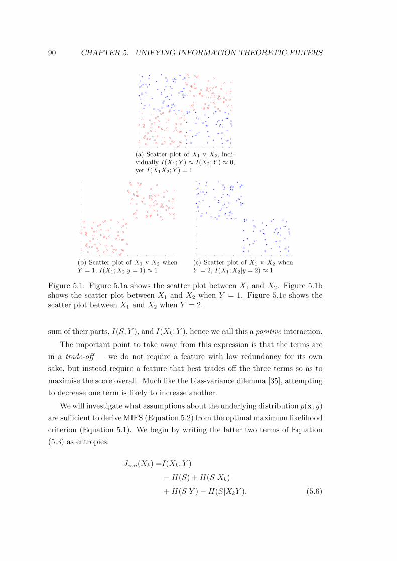
90 CHAPTER 5. UNIFYING INFORMATION THEORETIC FILTERS
(a) Scatter plot of X1 v X2, indi-vidually I(X1;Y ) ≈ I(X2;Y ) ≈ 0,yet I(X1X2;Y ) = 1
(b) Scatter plot of X1 v X2 whenY = 1, I(X1;X2|y = 1) ≈ 1
(c) Scatter plot of X1 v X2 whenY = 2, I(X1;X2|y = 2) ≈ 1
Figure 5.1: Figure 5.1a shows the scatter plot between X1 and X2. Figure 5.1bshows the scatter plot between X1 and X2 when Y = 1. Figure 5.1c shows thescatter plot between X1 and X2 when Y = 2.
sum of their parts, I(S;Y ), and I(Xk;Y ), hence we call this a positive interaction.
The important point to take away from this expression is that the terms are
in a trade-off — we do not require a feature with low redundancy for its own
sake, but instead require a feature that best trades off the three terms so as to
maximise the score overall. Much like the bias-variance dilemma [35], attempting
to decrease one term is likely to increase another.
We will investigate what assumptions about the underlying distribution p(x, y)
are sufficient to derive MIFS (Equation 5.2) from the optimal maximum likelihood
criterion (Equation 5.1). We begin by writing the latter two terms of Equation
(5.3) as entropies:
Jcmi(Xk) =I(Xk;Y )
−H(S) +H(S|Xk)
+H(S|Y )−H(S|XkY ). (5.6)
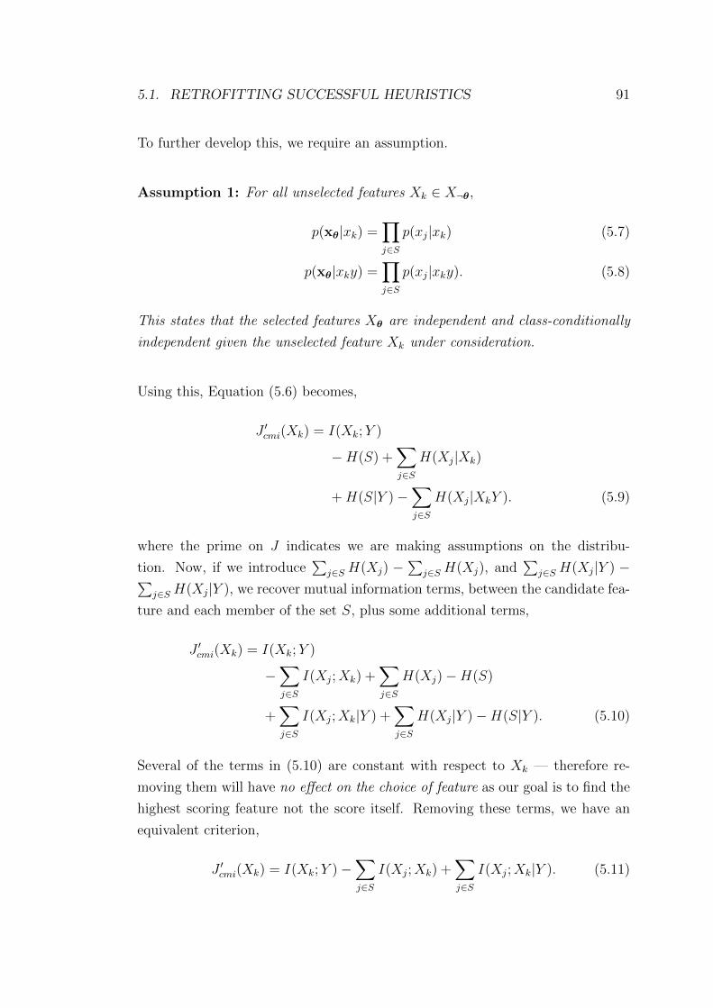
5.1. RETROFITTING SUCCESSFUL HEURISTICS 91
To further develop this, we require an assumption.
Assumption 1: For all unselected features Xk ∈ X¬θ,
p(xθ|xk) =∏j∈S
p(xj|xk) (5.7)
p(xθ|xky) =∏j∈S
p(xj|xky). (5.8)
This states that the selected features Xθ are independent and class-conditionally
independent given the unselected feature Xk under consideration.
Using this, Equation (5.6) becomes,
J ′cmi(Xk) = I(Xk;Y )
−H(S) +∑j∈S
H(Xj|Xk)
+H(S|Y )−∑j∈S
H(Xj|XkY ). (5.9)
where the prime on J indicates we are making assumptions on the distribu-
tion. Now, if we introduce∑
j∈S H(Xj) −∑
j∈S H(Xj), and∑
j∈S H(Xj|Y ) −∑j∈S H(Xj|Y ), we recover mutual information terms, between the candidate fea-
ture and each member of the set S, plus some additional terms,
J ′cmi(Xk) = I(Xk;Y )
−∑j∈S
I(Xj;Xk) +∑j∈S
H(Xj)−H(S)
+∑j∈S
I(Xj;Xk|Y ) +∑j∈S
H(Xj|Y )−H(S|Y ). (5.10)
Several of the terms in (5.10) are constant with respect to Xk — therefore re-
moving them will have no effect on the choice of feature as our goal is to find the
highest scoring feature not the score itself. Removing these terms, we have an
equivalent criterion,
J ′cmi(Xk) = I(Xk;Y )−∑j∈S
I(Xj;Xk) +∑j∈S
I(Xj;Xk|Y ). (5.11)

92 CHAPTER 5. UNIFYING INFORMATION THEORETIC FILTERS
This has in fact already appeared in the literature as a filter criterion, orig-
inally proposed by Lin et al. [74], as Conditional Infomax Feature Extraction
(CIFE), though it has been repeatedly rediscovered by other authors [36, 48]. It
is particularly interesting as it represents a sort of ‘root’ criterion, from which
several others can be derived. For example, the link to MIFS can be seen with
one further assumption, that the features are pairwise class-conditionally inde-
pendent.
Assumption 2: For all features i, j,
p(xixj|y) = p(xi|y)p(xj|y). (5.12)
This states that the features are pairwise class-conditionally independent.
With this assumption, the term∑I(Xj;Xk|Y ) will be zero, and Equation (5.11)
becomes Equation (5.2), the MIFS criterion, with β = 1. The β parameter in
MIFS can be interpreted as encoding a strength of belief in another assumption,
that of unconditional independence.
Assumption 3: For all features i, j,
p(xixj) = p(xi)p(xj). (5.13)
This states that the features are pairwise independent.
A β close to zero implies very strong belief in the independence statement, indi-
cating that any measured association I(Xj;Xk) is in fact spurious, possibly due
to noise in the data. A β value closer to 1 implies a lesser belief, that any mea-
sured dependency I(Xj;Xk) should be incorporated into the feature score exactly
as observed. Since the MIM criterion is produced by setting β = 0, we can see
that MIM also adopts Assumption 3. The same line of reasoning can be applied
to a very similar (and very popular) criterion proposed by Peng et al. [86], the
Minimum-Redundancy Maximum-Relevance criterion,
Jmrmr(Xk) = I(Xk;Y )− 1
|S|∑j∈S
I(Xk;Xj). (5.14)

5.1. RETROFITTING SUCCESSFUL HEURISTICS 93
Since mRMR omits the conditional redundancy term entirely, it is implicitly using
Assumption 2. The β coefficient has been set inversely proportional to the size of
the current feature set. If we have a large set S, then β will be extremely small.
The interpretation is then that as the set S grows, mRMR adopts a stronger
belief in Assumption 3. In the original paper, [86, section 2.3], it is claimed that
mRMR is a first order approximation to Equation (5.1). By making explicit the
intrinsic assumptions of the criterion we have clearly illustrated that this claim
is incorrect as it does not include a conditional redundancy term, and in fact the
mRMR criterion does not allow for any positive interactions between features.
The relation of the MIFS/mRMR to Equation (5.11) is relatively straight-
forward. It is more challenging to consider how closely other criteria might be
re-expressed in this form. Yang and Moody [110] propose using Joint Mutual
Information (JMI),
Jjmi(Xk) =∑j∈S
I(XkXj;Y ). (5.15)
Using some relatively simple manipulations (see Brown [12]) this can be re-written
as,
Jjmi(Xk) = I(Xk;Y )− 1
|S|∑j∈S
[I(Xk;Xj)− I(Xk;Xj|Y )
].
The criterion (5.16) returns exactly the same set of features as the JMI criterion
(5.15); however in this form, we can see the relation to our proposed framework.
The JMI criterion, like mRMR, has a stronger belief in the pairwise independence
assumptions as the feature set S grows. Similarities can of course be observed
between JMI, MIFS and mRMR — the differences being the scaling factor and
the conditional term — and their subsequent relation to Equation (5.11). It
is in fact possible to identify numerous criteria from the literature that can all
be re-written into a common form, corresponding to different assumptions made
upon Equation (5.11). A space of potential criteria can be imagined, where we
parametrise criterion (5.11) as:
J ′cmi = I(Xk;Y )− β∑j∈S
I(Xj;Xk) + γ∑j∈S
I(Xj;Xk|Y ). (5.16)
Figure 5.2 shows how the criteria we have discussed so far can all be fitted
inside this unit square corresponding to β/γ parameters. MIFS sits on the left

94 CHAPTER 5. UNIFYING INFORMATION THEORETIC FILTERS
hand axis of the square — with γ = 0 and β ∈ [0, 1]. The MIM criterion, Equa-
tion (3.1), which simply assesses each feature individually without any regard of
others, sits at the bottom left, with γ = 0, β = 0. The top right of the square
corresponds to γ = 1, β = 1, which is the CIFE criterion [74], also suggested by
El Akadi et al. [36] and Guo and Nixon [48]. A very similar criterion, using an
assumption to approximate the terms, was proposed by Cheng et al. [20].
The JMI and mRMR criteria are different from CIFE and MIFS in that they
move linearly within the space as the feature set S grows. As the size of the
set S increases they move closer towards the origin and the MIM criterion. The
particularly interesting point about this property is that the relative magnitude
of the relevancy term to the redundancy terms stays approximately constant as
S grows, whereas with MIFS, the redundancy term will in general be |S| times
bigger than the relevancy term. We explore the practical consequences of this in
Section 5.2 where we see it plays an important role in explaining the experimental
results. Any criterion expressible in the unit square has made independence
Assumption 1. In addition, any criteria that sit at points other than β = 1, γ = 1
have adopted varying degrees of belief in Assumptions 2 and 3.
A further interesting point about this square is simply that it is sparsely popu-
lated, an obvious unexplored region is the bottom right, the corner corresponding
to β = 0, γ = 1; though there is no clear intuitive justification for this point, for
completeness in the experimental section we will evaluate it, as the conditional
redundancy or ‘condred’ criterion.
A paper by Brown [12] explores this unit square, though from a different
perspective gained by expanding the multivariate mutual information. In fact
much of this thesis arises from extensive consideration of the results in that
paper, though the approach presented here is quite different. Our probabilistic
perspective, deriving our selection criteria from the joint likelihood of a specific
model allows the precise specification of the underlying assumptions required to
produce different criteria from Equation (5.16). Further (unpublished) work by
Brown [13] has shown that the space of criteria with fixed β and γ is not in general
competitive with the criteria which move through the space, such as mRMR or
JMI.
All the criteria in Figure 5.2 are linear, as they take linear combinations of
the relevance/redundancy terms. One interesting perspective is to look at the
criteria not as points but as paths through this space, mRMR is a line along the

5.1. RETROFITTING SUCCESSFUL HEURISTICS 95
0 0.2 0.4 0.6 0.8 10
0.2
0.4
0.6
0.8
1mifs / mrmr |S|=2 cife/jmi |S|=2
mrmr |S|=3 jmi |S|=3
mrmr |S|=4 jmi |S|=4
mim
γ
β
Figure 5.2: The full space of linear filter criteria, describing several examples fromTable 3.1. Note that all criteria in this space adopt Assumption 1. Additionally,the γ and β axes represent the criteria belief in Assumptions 2 and 3, respectively.The left hand axis is where the mRMR and MIFS algorithms sit. The bottom leftcorner, MIM, is the assumption of completely independent features, using justmarginal mutual information. Note that some criteria are equivalent at particularsizes of the current feature set |S|.
β axis, and JMI is a line along β = γ. Once we have understood this property
it is natural to ask can there be other paths through this space. Indeed there
exist other criteria which follow a similar form to these linear criteria, except
they include other operations like minimizations, making them take a non-linear
path.
Fleuret [40] proposed the Conditional Mutual Information Maximization cri-
terion,
Jcmim(Xk) = minXj∈S
[I(Xk;Y |Xj)
]. (5.17)
This can be re-written,
Jcmim(Xk) = I(Xk;Y )−maxXj∈S
[I(Xk;Xj)− I(Xk;Xj|Y )
]. (5.18)
Again these manipulations are found in Brown [12]. Due to the max operator, the
probabilistic interpretation is less straightforward. It is clear however that CMIM
adopts Assumption 1, since it evaluates only pairwise feature statistics. Vidal-
Naquet and Ullman [109] propose another criterion used in Computer Vision,

96 CHAPTER 5. UNIFYING INFORMATION THEORETIC FILTERS
which we refer to as Informative Fragments,
Jif (Xk) = minXj∈S
[I(XkXj;Y )− I(Xj;Y )
]. (5.19)
The authors motivate this criterion by noting that it measures the gain of com-
bining a new feature Xk with each existing feature Xj, over simply using Xj by
itself. The Xj with the least ‘gain’ from being paired with Xk is taken as the score
for Xk. Interestingly, using the chain rule I(XkXj;Y ) = I(Xj;Y ) + I(Xk;Y |Xj),
therefore IF is equivalent to CMIM, i.e. Jif (Xk) = Jcmim(Xk), making the same
assumptions. In a similar vein, Jakulin [58] proposed the ICAP criterion,
Jicap(Xk) = I(Xk;Y )−∑Xj∈S
max[0, I(Xk;Xj)− I(Xk;Xj|Y )
]. (5.20)
Again, this adopts Assumption 1, using the same redundancy and conditional
redundancy terms, yet the exact probabilistic interpretation is unclear. This
criteria is designed to penalise criteria which interact negatively, but does not
select those which interact positively. It is designed for use with classifiers which
make similar assumptions of class conditional independence, such as the Naıve
Bayes classifier.
An interesting class of criteria use a normalisation term on the mutual infor-
mation to offset the inherent bias toward high arity features [34]. An example
of this is Double Input Symmetrical Relevance [79], a modification of the JMI
criterion:
Jdisr(Xk) =∑Xj∈S
I(XkXj;Y )
H(XkXjY ). (5.21)
The inclusion of this normalisation term breaks the strong theoretical link to a
likelihood function, but again for completeness we will include this in our empiri-
cal investigations. While the criteria in the unit square can have their probabilis-
tic assumptions made explicit, the non-linearity in the CMIM, ICAP and DISR
criteria make such an interpretation far more difficult.
5.1.1 Bounding the criteria
There is one more important factor to note about many of these filter criteria,
and that is their relative size compared to the optimal criterion of Equation (5.1).
Using the properties of the mutual information we reviewed in Section 2.3 we can

5.1. RETROFITTING SUCCESSFUL HEURISTICS 97
upper bound each mutual information term by various different entropies (all
Shannon mutual information terms are lower bound by zero). In particular we
can bound J∗ as follows,
0 ≤ J∗(Xk) = I(Xk;Y |S) ≤ H(Xk|S) ≤ H(Xk). (5.22)
If we consider the CIFE criterion (repeated for clarity),
Jcife(Xk) = I(Xk;Y )−∑Xj∈S
I(Xk;Xj) +∑Xj∈S
I(Xk;Xj|Y ), (5.23)
we can bound the individual terms separately,
I(Xk;Y ) ≤ H(Xk)∑Xj∈S
I(Xk;Xj) ≤ |S| ·H(Xk)∑Xj∈S
I(Xk;Xj|Y ) ≤ |S| ·H(Xk|Y ) ≤ |S| ·H(Xk). (5.24)
However the entire CIFE criterion is not so well behaved, as it is neither bounded
above by H(Xk) nor bounded below by 0. This is because the redundancy and
conditional redundancy terms are bound by a function of |S|, and so grow in
size compared to the relevancy term. This issue is also apparent in the MIFS
and ICAP criteria, and we will see how it explains many of the differences in
experimental performance.
If we consider the JMI criterion, we can see that the averaging of the redun-
dancy and conditional redundancy terms removes this problem, stopping those
terms from growing as a function of |S|. However the JMI criterion poses another
problem, as it has multiple variants. We presented two versions of this criterion
in Equations (5.15) and (5.16) and stated that they rank features identically.
However we might expect that these different versions would interact in different
ways with the prior term which exists in the derivation. We will return to this
issue when we address informative priors in Chapter 6.
5.1.2 Summary of theoretical findings
In this section we have shown that numerous criteria published over the past two
decades of research can be “retro-fitted” into the framework we have proposed

98 CHAPTER 5. UNIFYING INFORMATION THEORETIC FILTERS
— the criteria are approximations to Equation (5.1), each making different as-
sumptions on the underlying distributions. Since in the previous section we saw
that accepting the top ranked feature according to Equation (5.1) provides the
maximum possible increase in the likelihood, we see now that the criteria are
approximate maximisers of the likelihood under an uninformative prior over the
choice of features. Whether or not they indeed provide the maximum increase
at each step will depend on how well the implicit assumptions on the data dis-
tribution match the true distribution. Also, it should be remembered that even
if we used the optimal stepwise criterion, it is not guaranteed to find the global
optimum of the likelihood, since (a) it is a greedy search, and (b) finite data will
mean distributions cannot be accurately modelled. There are a subset of prob-
lems where this greedy search is optimal, namely in Markov Blanket discovery
algorithms, which we return to in Chapter 6. In this case, we have reached the
limit of what a theoretical analysis can tell us about these criteria, and we must
close the remaining ‘gaps’ in our understanding with an experimental study.
5.2 Experimental Study
In this section we empirically evaluate a selection of the criteria in the literature
against one another. Note that we are not pursuing an exhaustive analysis,
attempting to identify the ‘winning’ criterion that provides best performance
overall1 — rather, we primarily observe how the theoretical properties of criteria
relate to the similarity of the returned feature sets. While these properties are
interesting, we of course must acknowledge that classification performance is the
ultimate evaluation of a criterion — hence we also include here classification
results on UCI datasets and in Section 5.3 on the well-known benchmark NIPS
Feature Selection Challenge.
In the following sections, we ask the questions: “how stable is a criterion to
small changes in the training data set?”, “how similar are the criteria to each
other?”, “how do the different criteria behave in small-sample situations?”, and
finally, “what is the relationship between stability and accuracy?”.
To address these questions, we use the 15 datasets detailed in Table 5.1. These
are chosen to have a wide variety of example-feature ratios, and a range of multi-
class problems. The features within each dataset have a variety of characteristics
1In any case, the No Free Lunch Theorem applies [107].

5.2. EXPERIMENTAL STUDY 99
— some binary/discrete, and some continuous. Continuous features were discre-
tised, using an equal-width strategy into 5 bins, while features already with a
categorical range were left untouched. The ‘ratio’ statistic quoted in the final
column is an indicator of the difficulty of the feature selection for each dataset.
This uses the number of datapoints (N), the median arity of the features (m), and
the number of classes (c) — the ratio quoted in the table for each dataset is Nmc
— hence a smaller value indicates a more challenging feature selection problem.
A key feature of this work is to understand the statistical assumptions on
the data imposed by the feature selection criteria — if our classification model
were to make even more assumptions, this is likely to obscure the experimental
observations relating performance to theoretical properties. For this reason, in the
experiments in this chapter we use a simple nearest neighbour classifier (k = 3),
this is chosen as it makes few (if any) assumptions about the data, and we avoid
the need for parameter tuning. We apply the filter criteria using a simple forward
selection to select a fixed number of features, before being used with the classifier.
The number of features selected varies between the experiments, but is detailed
for each experiment. We will consider the 9 criteria previously studied in our
theoretical analysis for all the experiments. One important criterion which we
cannot use in this study is a direct implementation of Equation (5.1), which we
showed to be the optimal criterion for iteratively maximising the likelihood. This
criterion requires the estimation of an |S| dimensional probability distribution,
which is in general intractable for small and medium sized datasets, and thus we
will not use it for this section of the empirical study. However in Section 5.3 we
will look at two larger datasets, and there we will benchmark the performance of
Equation (5.1), referring to it as the CMI criterion.
5.2.1 How stable are the criteria to small changes in the
data?
The set of features selected by any procedure will of course depend on the data
provided. It is a plausible complaint if the set of returned features varies wildly
with only slight variations in the supplied data. In general we do not wish the
feature set to have high variance, i.e. small changes in the data should have con-
sequently small changes in the selected feature set. This is an issue reminiscent
of the bias-variance dilemma, where the sensitivity of a classifier to its initial

100 CHAPTER 5. UNIFYING INFORMATION THEORETIC FILTERS
Data Features Examples Classes Ratiobreast 30 569 2 57congress 16 435 2 72heart 13 270 2 34ionosphere 34 351 2 35krvskp 36 3196 2 799landsat 36 6435 6 214lungcancer 56 32 3 4parkinsons 22 195 2 20semeion 256 1593 10 80sonar 60 208 2 21soybeansmall 35 47 4 6spect 22 267 2 67splice 60 3175 3 265waveform 40 5000 3 333wine 13 178 3 12
Table 5.1: Datasets used in experiments. The final column indicates the difficultyof the data in feature selection, a smaller value indicating a more challengingproblem.
conditions causes high variance responses. However, while the bias-variance de-
composition is well-defined and understood, the corresponding issue for feature
selection, the “stability”, has only recently been studied. The stability of a fea-
ture selection criterion requires a measure to quantify the similarity between two
selected feature sets. This was first discussed by Kalousis et al. [59], who in-
vestigated several measures, with the final recommendation being the Tanimoto
distance between sets. Such set-intersection measures seem appropriate, but have
limitations; for example, if two criteria selected identical feature sets of size 10,
we might be less surprised if we knew the overall pool of features was of size 12,
than if it was size 12,000. Kuncheva [67] presents a consistency index which takes
this into account, based on the hypergeometric distribution with a correction for
the probability of selecting the same feature set at random.
Definition 9. The consistency for two subsets A,B ⊂ X, such that |A| = |B| =k, and r = |A ∩B|, where 0 < k < |X| = d, is
C(A,B) =rd− k2
k(d− k). (5.25)

5.2. EXPERIMENTAL STUDY 101
The consistency takes values in the range [−1,+1], with a positive value in-
dicating similar sets, a zero value indicating a purely random relation, and a
negative value indicating a strong anti-correlation between the features sets.
One problem with the consistency index is that it does not take feature re-
dundancy into account. That is, two procedures could select features which have
different indices, so are identified as “different”, but in fact are so highly corre-
lated that they are effectively identical. A method to deal with this situation
was proposed by Yu et al. [111]. This method constructs a weighted complete
bipartite graph, where the two node sets correspond to two different feature sets,
and weights are assigned to the arcs are the normalized mutual information be-
tween the features at the nodes, also sometimes referred to as the symmetrical
uncertainty. The weight between node i in set A, and node j in set B, is
w(A(i), B(j)) =I(XA(i);XB(j))
H(XA(i)) +H(XB(j)). (5.26)
The Hungarian algorithm is then applied to identify the maximum weighted
matching between the two node sets, and the overall similarity between sets A
and B is the final matching cost. This is the information consistency of the two
sets. For more details, we refer the reader to Yu et al. [111].
An ideal consistency metric would include both of these properties, a correc-
tion for random selection and an ability to detect when similar features have been
selected. However we leave the construction of such a metric for future research.
We now compare these two measures on the criteria from the previous sections.
For each dataset, we take a bootstrap sample and select a set of features using
each feature selection criterion. The (information) stability of a single criterion is
quantified as the average pairwise (information) consistency across 50 bootstraps
from the training data.
Figure 5.3 shows Kuncheva’s stability measure on average over 15 datasets,
selecting feature sets of size 10; note that the criteria have been displayed ordered
left-to-right by their median value of stability over the 15 datasets. The marginal
mutual information, MIM, is as expected the most stable, given that it has the
lowest dimensional distribution to estimate. The next most stable is JMI which
includes the relevancy/redundancy terms, but averages over the current feature
set; this averaging process might therefore be interpreted empirically as a form
of ‘smoothing’, enabling the criteria overall to be resistant to poor estimation of

102 CHAPTER 5. UNIFYING INFORMATION THEORETIC FILTERS
0
0.2
0.4
0.6
0.8
1
mim jmi disr condred mrmr cmim mifs icap cife
Stability
Figure 5.3: Kuncheva’s Stability Index [67] across 15 datasets. The box indi-cates the upper/lower quartiles, the horizontal line within each shows the medianvalue, while the dotted crossbars indicate the maximum/minimum values. Forconvenience of interpretation, criteria on the x-axis are ordered by their medianvalue.
probability distributions. It can be noted that the far right of Figure 5.3 consists
of the MIFS, ICAP and CIFE criteria, all of which do not attempt to average the
redundancy terms.
Figure 5.4 shows the same datasets, but instead the information stability
is computed; as mentioned, this should take into account the fact that some
features are highly correlated. Interestingly, the two box-plots show broadly
similar results. MIM is the most stable, and CIFE is the least stable, though here
we see that JMI, DISR, and mRMR are actually more stable than Kuncheva’s
stability index can reflect.
5.2.2 How similar are the criteria?
Two criteria can be directly compared with the same methodology: by measuring
the consistency and information consistency between selected feature subsets on
a common set of data. We calculate the mean consistencies between two feature
sets of size 10, repeatedly selected over 50 bootstraps from the original data. This
is then arranged in a similarity matrix, and we use classical multi-dimensional
scaling [26] to visualise this as a 2D map, shown in Figures 5.5a and 5.5b. Note

5.2. EXPERIMENTAL STUDY 103
0.15
0.2
0.25
0.3
0.35
0.4
0.45
0.5
mim jmi disr condred mrmr cmim mifs icap cife
Info
rmat
ion
Stab
ility
Figure 5.4: Yu et al.’s Information Stability Index [111] across 15 datasets. Forcomparison, criteria on the x-axis are ordered identically to Figure 5.3. A similargeneral picture emerges to that using Kuncheva’s measure, though the informa-tion stability index is able to take feature redundancy into account, showing thatsome criteria are slightly more stable than expected.
again that while the indices may return different absolute values (one is a nor-
malized mean of a hypergeometric distribution and the other is a pairwise sum
of mutual information terms) they show very similar relative ‘distances’ between
criteria.
Both diagrams show a cluster of several criteria, and 4 clear outliers: MIFS,
CIFE, ICAP and CondRed. The 5 criteria clustering in the upper left of the
space appear to return relatively similar feature sets. The 4 outliers appear
to return quite significantly different feature sets, both from the clustered set,
and from each other. A common characteristic of these 4 outliers is that they
do not scale the redundancy or conditional redundancy information terms. In
these criteria, the upper bound on the redundancy term∑
j∈S I(Xk;Xj) grows
linearly with the number of selected features, whilst the upper bound on the
relevancy term I(Xk;Y ) remains constant. When this happens the relevancy term
is overwhelmed by the redundancy term and thus the criterion selects features
with minimal redundancy, rather than trading off between the two terms. This
leads to strongly divergent feature sets being selected, which is reflected in the
stability of the criteria. Each of the outliers are different from each other as they
have different combinations of redundancy and conditional redundancy. We will

104 CHAPTER 5. UNIFYING INFORMATION THEORETIC FILTERS
mim
disr
jmi
mrmr
cmim
icap
cife
condred
mifs
(a) Kuncheva’s Consistency Index.
mim jmi
disr
condred
mrmr
cmim
mifs
icap
cife
mim jmi
disr
condred
mrmr
cmim
mifs
icap
cife
mim jmi
disr
condred
mrmr
cmim
mifs
icap
cife
(b) Yu et al.’s Information Stability Index.
Figure 5.5: Relations between feature sets generated by different criteria, on av-erage over 15 datasets. 2D visualisation generated by classical multi-dimensionalscaling.
see this “balance” between relevancy and redundancy emerge as an important
property in the experiments over the next few sections.
5.2.3 How do criteria behave in small-sample situations?
To assess how criteria behave in data poor situations, we vary the number of
datapoints supplied to perform the feature selection. The procedure was to ran-
domly select 140 datapoints, then use the remaining data as a hold-out set. From
this 140, the number provided to each criterion was increased in steps of 10, from
a minimal set of size 20. To allow a reasonable testing set size, we limited this
assessment to only datasets with at least 200 datapoints total; this gives us 11
datasets from the 15, omitting lungcancer, parkinsons, soybeansmall, and wine.
For each dataset we select 10 features and apply the 3-NN classifier, recording
the rank-order of the criteria in terms of their generalisation error. This process
was repeated and averaged over 50 trials, giving the results in Figure 5.6.
To aid interpretation we label MIM with a simple point marker, MIFS, CIFE,
CondRed, and ICAP with a circle, and the remaining criteria (DISR, JMI, mRMR
and CMIM) with a star. The criteria labelled with a star balance the relative
magnitude of the relevancy and redundancy terms, those with a circle do not

5.2. EXPERIMENTAL STUDY 105
attempt to balance them, and MIM contains no redundancy term. There is a
clear separation between those criteria with a star outperforming those with a
circle, and MIM varying in performance between the two groups as we allow more
training datapoints.
Notice that the highest ranked criteria coincide with those in the cluster at
the top left of Figures 5.5a and 5.5b. We suggest that the relative difference in
performance is due to the same reason noted in Section 5.2.2, that the redundancy
term grows with the size of the selected feature set. In this case, the redundancy
term eventually grows to outweigh the relevancy by a large degree, and the new
features are selected solely on the basis of redundancy, ignoring the relevance,
thus leading to poor classification performance.
20 40 60 80 100 120 140
1
2
3
4
5
6
7
8
9
Training points
Ran
k
mimdisrjmimrmrmifscondredcifecmimicap
Figure 5.6: Average ranks of criteria in terms of test error, selecting 10 features,across 11 datasets. Note the clear dominance of criteria which do not allow theredundancy term to overwhelm the relevancy term (stars) over those that allowredundancy to grow with the size of the feature set (circles).
Extreme small-sample experiments
In the previous sections we discussed two theoretical properties of information-
based feature selection criteria: whether it balances the relative magnitude of
relevancy against redundancy, and whether it includes a class-conditional redun-
dancy term. Empirically on the UCI datasets, we see that the balancing is far
more important than the inclusion of the conditional redundancy term — for
example, mRMR succeeds in many cases, while MIFS performs poorly. Now, we

106 CHAPTER 5. UNIFYING INFORMATION THEORETIC FILTERS
Data Features Examples ClassesColon 2000 62 2Leukemia 7070 72 2Lung 325 73 7Lymph 4026 96 9NCI9 9712 60 9
Table 5.2: Datasets from Peng et al. [86], used in small-sample experiments.
consider whether the same property may hold in extreme small-sample situations,
when the number of examples is so low that reliable estimation of distributions
becomes extremely difficult. We use data sourced from Peng et al. [86], detailed
in Table 5.2.
Results are shown in Figure 5.7, selecting 50 features from each dataset and
plotting leave-one-out classification error. It should of course be remembered that
on such small datasets, making just one additional datapoint error can result in
seemingly large changes in accuracy. For example, the difference between the best
and worst criteria on Leukemia was just 3 datapoints. In contrast to the UCI
results, the picture is less clear. On Colon, the criteria all perform similarly; this
is the least complex of all the datasets, having the smallest number of classes with
a (relatively) small number of features. As we move through the datasets with
increasing numbers of features/classes, we see that MIFS, CondRed, CIFE and
ICAP start to break away, performing poorly compared to the others. Again, we
note that these do not attempt to balance relevancy/redundancy. This difference
is clearest on the NCI9 data, the most complex with 9 classes and 9712 features.
However, as we may expect with such high dimensional and challenging problems,
there are some exceptions — the Colon data as mentioned, and also the Lung
data where ICAP/MIFS perform well.
5.2.4 What is the relationship between stability and ac-
curacy?
An important question is whether we can find a good balance between the stability
of a criterion and the classification accuracy. This was considered by Gulgezen
et al. [47], who studied the stability/accuracy trade-off for the mRMR criterion.
In the following, we consider this trade-off in the context of Pareto-optimality,
across the 9 criteria, and the 15 datasets from Table 5.1. Experimental protocol

5.2. EXPERIMENTAL STUDY 107
0 10 20 30 40 500
5
10
15
20
25
30
35
40
45pengcolon
Number of features selected
LOO
num
ber o
f mis
take
s
mimjmidisrcondredmrmrcmimmifsicapcife
0 10 20 30 40 500
5
10
15pengleuk
Number of features selected
LOO
num
ber o
f mis
take
s
0 10 20 30 40 500
5
10
15
20
25
30
35
40
45
50penglung
Number of features selected
LOO
num
ber o
f mis
take
s
0 5 10 15 20 25 30 35 40 45 500
5
10
15
20
25
30
35
40
45
50penglymp
Number of features selected
LOO
num
ber o
f mis
take
s
0 10 20 30 40 5020
25
30
35
40
45
50
55pengnci9
Number of features selected
LOO
num
ber o
f mis
take
s
Figure 5.7: LOO results on Peng’s datasets: Colon, Lymphoma, Leukemia, Lung,NCI9.

108 CHAPTER 5. UNIFYING INFORMATION THEORETIC FILTERS
was to take 50 bootstraps from the dataset, each time calculating the out-of-
bag error using the 3-NN. The stability measure was Kuncheva’s stability index
calculated from the 50 feature sets, and the accuracy was the mean out-of-bag
accuracy across the 50 bootstraps. The experiments were also repeated using the
Information Stability measure, revealing almost identical results. Results using
Kuncheva’s stability index are shown in Figure 5.8.
The Pareto-optimal set is defined as the set of criteria for which no other
criterion has both a higher accuracy and a higher stability, hence the members
of the Pareto-optimal set are said to be non-dominated [41]. Thus in each of the
graphs in Figure 5.8, criteria that appear further to the top-right of the space
dominate those toward the bottom left — in such a situation there is no reason
to choose those at the bottom left, since they are dominated on both objectives
by other criteria.
A summary (for both stability and information stability) is provided in the
first two columns of Table 5.3, showing the non-dominated rank of the different
criteria. This is computed per dataset as the number of other criteria which
dominate a given criterion, in the Pareto-optimal sense, then averaged over the
15 datasets. We can see that these rankings are similar to the results earlier, with
MIFS, ICAP, CIFE and CondRed performing poorly. We note that JMI, (which
both balances the relevancy and redundancy terms and includes the conditional
redundancy) outperforms all other criteria.
We present the average accuracy ranks across the 50 bootstraps in the third
column of Table 5.3. These are similar to the results from Figure 5.6 but use
a bootstrap of the full dataset, rather than a small sample from it. Following
Demsar [29] we analysed these ranks using a Friedman test to determine which
criteria are statistically significantly different from each other. We then used
a Nemenyi post-hoc test to determine which criteria differed, with statistical
significances at 90%, 95%, and 99% confidences. These give a partial ordering
for the criteria which we present in Figure 5.9, showing a Significant Dominance
Partial Order diagram. Note that this style of diagram encapsulates the same
information as a Critical Difference diagram [29], but allows us to display multiple
levels of statistical significance. A bold line connecting two criteria signifies a
difference at the 99% confidence level, a dashed line at the 95% level, and a
dotted line at the 90% level. Absence of a link signifies that we do not have the
statistical power to determine the difference one way or another. Reading Figure

5.2. EXPERIMENTAL STUDY 109
0.88 0.9 0.92 0.940.5
0.6
0.7
0.8
0.9
1breast
Mean Accuracy
Kuncheva S
tabili
ty
mim
jmi
disrcondred
mrmrcmim
mifs
icapcife
0.8 0.85 0.9 0.95 10.4
0.5
0.6
0.7
0.8
0.9
1congress
mim
jmi
disr
condred
mrmr
cmim
mifsicapcife
0.76 0.77 0.78 0.79 0.80.4
0.5
0.6
0.7
0.8
0.9heart
mim
jmi
disr
condred
mrmr
cmim
mifs
icap
cife
0.84 0.85 0.86 0.87 0.88
0.4
0.5
0.6
0.7
0.8
0.9
1ionosphere
mimjmi
disr
condred
mrmr
cmimmifs
icap
cife
0.84 0.86 0.88 0.9 0.920.4
0.5
0.6
0.7
0.8
0.9
1krvskp
mimjmi
disr
condred
mrmr
cmimmifs
icapcife
0.68 0.7 0.72 0.74 0.760.4
0.5
0.6
0.7
0.8
0.9
1landsat
mim
jmidisr
condred
mrmr
cmim
mifsicapcife
0.4 0.45 0.5 0.55 0.60.2
0.25
0.3
0.35
0.4
0.45lungcancer
mim
jmi
disr
condred
mrmr
cmim
mifs
icap
cife
0.8 0.82 0.84 0.86 0.88
0.4
0.5
0.6
0.7
0.8
0.9
1parkinsons
mim
jmi
disr
condred
mrmr
cmim
mifs
icap
cife
0.2 0.4 0.6 0.8
0.4
0.5
0.6
0.7
0.8
0.9
1semeion
mim
jmidisr
condred
mrmr
cmimmifsicap
cife
0.65 0.7 0.75 0.80.2
0.3
0.4
0.5
0.6
0.7sonar
mim
jmi
disr
condred
mrmr
cmim
mifs
icapcife
0.8 0.85 0.9 0.95 10.5
0.6
0.7
0.8
0.9soybeansmall
mimjmidisrcondred
mrmr
cmimmifs
icap
cife
0.66 0.68 0.7 0.720.2
0.25
0.3
0.35
0.4spect
mimjmi
disr
condred
mrmrcmim
mifs
icap
cife
0.78 0.8 0.82 0.84 0.860.5
0.6
0.7
0.8
0.9
1splice
mimjmidisrcondredmrmrcmim
mifs
icap
cife
0.5 0.6 0.7 0.8 0.9
0.4
0.5
0.6
0.7
0.8
0.9
1waveform
mim
jmidisr
condred
mrmrcmim
mifs
icapcife
0.9 0.92 0.94 0.96
0.4
0.5
0.6
0.7
0.8
0.9
1wine
mimjmi
disr
condred
mrmr
cmim
mifs
icapcife
Figure 5.8: Stability (y-axes) versus Accuracy (x-axes) over 50 bootstraps for thefinal quarter of the UCI datasets. The pareto-optimal rankings are summarisedin Table 5.3.

110 CHAPTER 5. UNIFYING INFORMATION THEORETIC FILTERS
Accuracy/Stability(Yu) Accuracy/Stability(Kuncheva) AccuracyJMI (1.6) JMI (1.5) JMI (2.6)
DISR (2.3) DISR (2.2) mRMR (3.6)MIM (2.4) MIM (2.3) DISR (3.7)
mRMR (2.5) mRMR (2.5) CMIM (4.5)CMIM (3.3) CONDRED (3.2) ICAP (5.3)ICAP (3.6) CMIM (3.4) MIM (5.4)
CONDRED (3.7) ICAP (4.3) CIFE (5.9)CIFE (4.3) CIFE (4.8) MIFS (6.5)MIFS (4.5) MIFS (4.9) CONDRED (7.4)
Table 5.3: Column 1: Non-dominated Rank of different criteria for the trade-offof accuracy/stability. Criteria with a higher rank (closer to 1.0) provide a bettertrade-off than those with a lower rank. Column 2: As column 1 but usingKuncheva’s Stability Index. Column 3: Average ranks for accuracy alone.
5.9, we see that with 99% confidence JMI is significantly superior to CondRed,
and MIFS, but not statistically significantly different from the other criteria. As
we lower our confidence level, more differences appear, for example mRMR and
MIFS are only significantly different at the 90% confidence level.
5.2.5 Summary of empirical findings
From experiments in this section, we conclude that the balance of relevancy and
redundancy terms is extremely important, while the inclusion of a class condi-
tional term seems to matter less. We find that some criteria are inherently more
stable than others, and that the trade-off between accuracy (using a simple k-
NN classifier) and stability of the feature sets differs between criteria. The best
overall trade-off for accuracy/stability was found in the JMI and mRMR criteria.
In the following section we check these findings in the context of two problems
posed for the NIPS Feature Selection Challenge.
5.3 Performance on the NIPS Feature Selection
Challenge
In this section we investigate performance of the criteria on datasets taken from
the NIPS Feature Selection Challenge [49]. We present results using GISETTE (a
handwriting recognition task), and MADELON (an artificially generated dataset).
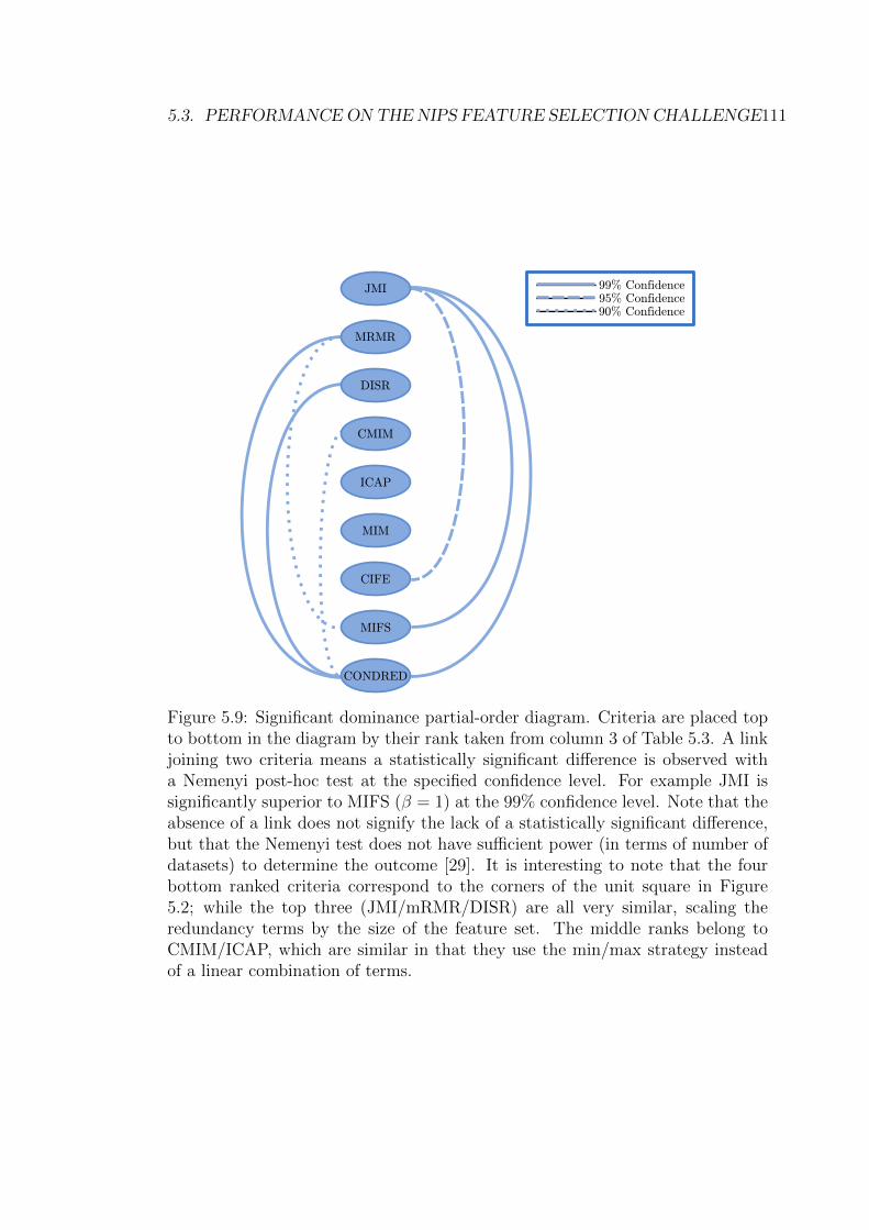
5.3. PERFORMANCEON THE NIPS FEATURE SELECTION CHALLENGE111
JMI
MRMR
ICAP
DISR
CMIM
CIFE
MIFS
CONDRED
MIM
99% Confidence
95% Confidence
90% Confidence
Figure 5.9: Significant dominance partial-order diagram. Criteria are placed topto bottom in the diagram by their rank taken from column 3 of Table 5.3. A linkjoining two criteria means a statistically significant difference is observed witha Nemenyi post-hoc test at the specified confidence level. For example JMI issignificantly superior to MIFS (β = 1) at the 99% confidence level. Note that theabsence of a link does not signify the lack of a statistically significant difference,but that the Nemenyi test does not have sufficient power (in terms of number ofdatasets) to determine the outcome [29]. It is interesting to note that the fourbottom ranked criteria correspond to the corners of the unit square in Figure5.2; while the top three (JMI/mRMR/DISR) are all very similar, scaling theredundancy terms by the size of the feature set. The middle ranks belong toCMIM/ICAP, which are similar in that they use the min/max strategy insteadof a linear combination of terms.

112 CHAPTER 5. UNIFYING INFORMATION THEORETIC FILTERS
Data Features Examples (Tr/Val) ClassesGISETTE 5000 6000/1000 2MADELON 500 2000/600 2
Table 5.4: Datasets from the NIPS challenge, used in experiments.
To apply the mutual information criteria, we estimate the necessary distri-
butions using histogram estimators: features were discretised independently into
10 equal width bins, with bin boundaries determined from training data. After
the feature selection process the original (undiscretised) datasets were used to
classify the validation data. Each criterion was used to generate a ranking for
the top 200 features in each dataset. We show results using the full top 200 for
GISETTE, but only the top 20 for MADELON as after this point all criteria
demonstrated severe overfitting. We use the Balanced Error Rate, for fair com-
parison with previously published work on the NIPS datasets. We accept that
this does not necessarily share the same optima as the classification error (nor
the same maxima of the joint likelihood). We investigate cost-sensitive versions
of the model likelihood in Chapter 7, where we derive criteria which could be
tailored to the Balanced Error Rate (on the training data).
Validation data results are presented in Figure 5.10 (GISETTE) and Figure
5.11 (MADELON). The minimum of the validation error was used to select the
best performing feature set size, the training data alone used to classify the testing
data, and finally test labels were submitted to the challenge website. Test results
are provided in Table 5.5 for GISETTE, and Table 5.6 for MADELON2.
Unlike in Section 5.2, the datasets we use from the NIPS Feature Selection
Challenge have many more datapoints (GISETTE has 6000 training examples,
MADELON has 2000) and thus we can present results using a direct implemen-
tation of Equation (5.1) as a criterion. We refer to this criterion as CMI, as it is
using the conditional mutual information to score features. Unfortunately there
are still estimation errors in this calculation when selecting a large number of
features, even given the large number of datapoints and so the criterion fails to
select features after a certain point, as each feature appears equally irrelevant. In
GISETTE, CMI selected 13 features, and so the top 10 features were used and
one result is shown. In MADELON, CMI selected 7 features and so 7 results are
shown.
2We do not provide classification confidences as we used a nearest neighbour classifier andthus the AUC is equal to 1− BER.

5.3. PERFORMANCEON THE NIPS FEATURE SELECTION CHALLENGE113
0 50 100 150 2000
0.05
0.1
0.15
0.2
0.25
0.3
0.35
0.4
0.45
0.5
Number of Features
Valid
atio
n Er
ror
mimmifscifeicapcmimcmimrmrjmidisr
Figure 5.10: Validation Error curve using GISETTE.
0 5 10 15 200
0.05
0.1
0.15
0.2
0.25
0.3
0.35
0.4
0.45
0.5
Number of Features
Valid
atio
n Er
ror
mimmifscifeicapcmimcmimrmrjmidisr
Figure 5.11: Validation Error curve using MADELON.

114 CHAPTER 5. UNIFYING INFORMATION THEORETIC FILTERS
5.3.1 GISETTE testing data results
In Table 5.5 there are several distinctions between the criteria, the most striking
of which is the failure of MIFS to select an informative feature set. The impor-
tance of balancing the magnitude of the relevancy and the redundancy can be
seen whilst looking at the other criteria in this test. Those criteria which bal-
ance the magnitudes, (CMIM, JMI, & mRMR) perform better than those which
do not (ICAP,CIFE). The DISR criterion forms an outlier here as it performs
poorly when compared to JMI. The only difference between these two criteria
is the normalization in DISR — as such, this is likely the cause of the observed
poor performance, due to the introduction of more variance by estimating the
normalization term H(Xk, Xj, Y ).
We can also see how important the low dimensional approximation is, as even
with 6000 training examples CMI cannot estimate the required joint distribution
to avoid selecting probes, despite being a direct iterative maximisation of the
joint likelihood, under a flat prior, in the limit of datapoints.
Criterion BER AUC Features (%) Probes (%)MIM 4.18 95.82 4.00 0.00MIFS 42.00 58.00 4.00 58.50CIFE 6.85 93.15 2.00 0.00ICAP 4.17 95.83 1.60 0.00CMIM 2.86 97.14 2.80 0.00CMI 8.06 91.94 0.20 20.00mRMR 2.94 97.06 3.20 0.00JMI 3.51 96.49 4.00 0.00DISR 8.03 91.97 4.00 0.00
Winning Challenge Entry 1.35 98.71 18.3 0.0
Table 5.5: NIPS FS Challenge Results: GISETTE.
5.3.2 MADELON testing data results
The MADELON results (Table 5.6) show a particularly interesting point — the
top performers (in terms of BER) are JMI and CIFE. Both these criteria include
the class-conditional redundancy term, but CIFE does not balance the influence
of relevancy against redundancy. In this case, it appears the ‘balancing’ issue,
so important in our previous experiments, appears unimportant — instead, the
presence of the conditional redundancy term is the differentiating factor between

5.4. AN INFORMATION THEORETIC VIEWOF STRONGANDWEAKRELEVANCE115
Criterion BER AUC Features (%) Probes (%)MIM 10.78 89.22 2.20 0.00MIFS 46.06 53.94 2.60 92.31CIFE 9.50 90.50 3.80 0.00ICAP 11.11 88.89 1.60 0.00CMIM 11.83 88.17 2.20 0.00CMI 21.39 78.61 0.80 0.00mRMR 35.83 64.17 3.40 82.35JMI 9.50 90.50 3.20 0.00DISR 9.56 90.44 3.40 0.00
Winning Challenge Entry 7.11 96.95 1.6 0.0
Table 5.6: NIPS FS Challenge Results: MADELON.
criteria (note the poor performance of MIFS/mRMR). This is perhaps not sur-
prising given the nature of the MADELON data, constructed precisely to require
features to be evaluated jointly.
It is interesting to note that the challenge organisers benchmarked a 3-NN
using the optimal feature set, achieving a 10% test error [49]. Many of the
criteria managed to select feature sets which achieved a similar error rate using
a 3-NN, and it is likely that a more sophisticated classifier is required to further
improve performance.
Our experimental results have shown another difference between the criteria,
which was less apparent from our theoretical study. The criteria which imple-
mented scaling, or some other method of balancing the size of the relevancy and
redundancy terms have outperformed all others. The criteria which do not, like
CIFE and MIFS, perform poorly across many datasets. We now integrate our
theoretical view of feature relevancy and redundancy into that of Kohavi and
John’s notions of Strong and Weak Relevance from their landmark 1997 paper
[62].
5.4 An Information Theoretic View of Strong
and Weak Relevance
We reviewed the definitions of relevance and irrelevance given by Kohavi and
John [62] in Section 3.1. These definitions are statements about the conditional
probability distributions of the variables involved. We can re-state the definitions

116 CHAPTER 5. UNIFYING INFORMATION THEORETIC FILTERS
of Kohavi and John (hereafter KJ) in terms of mutual information, and see how
they can fit into our likelihood maximisation framework. In the notation below,
notation Xi indicates the ith feature in the overall set X, and notation X\i
indicates the set X\Xi, all features except the ith. The definitions of strong
and weak relevance are taken from KJ’s paper, but the corollaries are novel
restatements in information theoretic terms. We also extend the notion of weak
relevance by separating it into two disjoint definitions.
Definition 10. Strongly Relevant Feature [62]
Feature Xi is strongly relevant to Y iff there exists an assignment of values xi,
y, x\i for which p(Xi = xi, X\i = x\i) > 0 and p(Y = y|Xi = xi, X\i = x\i) 6=p(Y = y|X\i = x\i).
Corollary 1. A feature Xi is strongly relevant iff I(Xi;Y |X\i) > 0.
Proof. The KL divergence DKL(p(y|x, z) || p(y|z)) > 0 iff p(y|x, z) 6= p(y|z)
for some assignment of values x, y, z. A simple re-application of the manipula-
tions leading to Equation (4.9) demonstrates that the expected KL-divergence
Exzp(y|x, z)||p(y|z) is equal to the mutual information I(X;Y |Z). In the def-
inition of strong relevance, if there exists a single assignment of values xi, y,
x\i that satisfies the inequality, then Exp(y|xix\i)||p(y|x\i) > 0 and therefore
I(Xi;Y |X\i) > 0.
Given the framework we have presented, we can note that this strong relevance
comes from a combination of three terms,
I(Xi;Y |X\i) = I(Xi;Y )− I(Xi;X\i) + I(Xi;X\i|Y ). (5.27)
This view of strong relevance demonstrates explicitly that a feature may be indi-
vidually irrelevant (i.e. p(y|xi) = p(y) and thus I(Xi;Y ) = 0), but still strongly
relevant if I(Xi;X\i|Y )− I(Xi;X\i) > 0.
Definition 11. Weakly Relevant Feature [62]
Feature Xi is weakly relevant to Y iff it is not strongly relevant and there exists
a subset Z ⊂ X\i, and an assignment of values xi, y, z for which p(Xi = xi, Z =
z) > 0 such that p(Y = y|Xi = xi, Z = z) 6= p(Y = y|Z = z).
Corollary 2. A feature Xi is weakly relevant to Y iff it is not strongly relevant
and I(Xi;Y |Z) > 0 for some Z ⊂ X\i.

5.4. AN INFORMATION THEORETIC VIEWOF STRONGANDWEAKRELEVANCE117
Proof. This follows immediately from the proof for the strong relevance above.
The notion of weak relevance can however be refined further, if we constrain
the subset Z such that it must contain all the strongly relevant features.
Definition 12. Weak Redundancy
Feature Xi is weakly redundant if it is weakly relevant and ∃Z ⊂ X\i such that
I(Xi;Y |Z, SR) > 0 where SR is the set of strongly relevant features.
Definition 13. Strong Redundancy
Feature Xi is strongly redundant if it is weakly relevant and ∀Z ⊂ X\i I(Xi;Y |Z, SR) =
0 where SR is the set of strongly relevant features.
The optimal subset (i.e. contains the necessary and sufficient features) is
therefore all the strongly relevant and some weakly redundant features. The
optimal subset does not contain any of the strongly redundant or irrelevant fea-
tures. From this perspective the weakly redundant features are those which share
the same data, some of them are necessary to capture all the available informa-
tion but to select all of them would include redundant features. Note that this
coincides with the definition of a Surely Sufficient Feature Subset [50, pg 19].
Another way of seeing this is, of the weakly relevant features, there are those
which duplicate information in SR (the strongly redundant set), and those which
complement information in SR (the weakly redundant set).
It is interesting, and somewhat non-intuitive, that there can be cases where
there are no strongly relevant features, but all are weakly relevant. This will
occur for example in a dataset where all features have exact duplicates: we have
2M features and ∀i, XM+i = Xi. In this case, for any Xk (such that k < M)
we will have I(Xk;Y |X\i) = 0 since its duplicate feature XM+k will carry the
same information. In this case, for any feature Xk (such that k < M) that is
strongly relevant in the dataset X1, ..., XM, it is weakly relevant in the dataset
X1, ..., X2M.This issue can be dealt with by refining our definition of relevance with respect
to a subset of the full feature space. A particular subset about which we have
some information is the currently selected set S. We can relate our framework to
KJ’s definitions in this context. Following KJ’s formulations,
Definition 14. Relevance with respect to the current set S.
Feature Xi is relevant to Y with respect to S iff there exists an assignment of

118 CHAPTER 5. UNIFYING INFORMATION THEORETIC FILTERS
values xi, y, s for which p(Xi = xi, S = s) > 0 and p(Y = y|Xi = xi, S = s) 6=p(Y = y|S = s).
Corollary 3. Feature Xi is relevant to Y with respect to S, iff I(Xi;Y |S) > 0.
A feature that is relevant with respect to S is either strongly or weakly relevant
(in the KJ sense) but it is not possible to determine in which class it lies, as we
have not conditioned on X\i. Notice that the definition coincides exactly with the
forward selection heuristic (Equation 4.14) when using an uninformative prior,
which we have shown is a hill-climber on the joint likelihood of our discriminative
model. As a result, we see that hill-climbing on the joint likelihood corresponds
to adding the most relevant feature with respect to the current set S. Again we
re-emphasize, that the resultant gain in the likelihood comes from a combination
of three sources:
I(Xi;Y |S) = I(Xi;Y )− I(Xi;S) + I(Xi;S|Y ). (5.28)
It could easily be the case that I(Xi;Y ) = 0, that is a feature is entirely irrel-
evant when considered on its own — but the sum of the two redundancy terms
results in a positive value for I(Xi;Y |S). We see that if a criterion does not at-
tempt to model both of the redundancy terms, even if only using low dimensional
approximations, it runs the risk of evaluating the relevance of Xi incorrectly.
Definition 15. Irrelevance with respect to the current set S.
Feature Xi is irrelevant to Y with respect to S iff ∀ xi, y, s for which p(Xi =
xi, S = s) > 0 and p(Y = y|Xi = xi, S = s) = p(Y = y|S = s).
Corollary 4. Feature Xi is irrelevant to Y with respect to S, iff I(Xi;Y |S) = 0.
In a forward step, if a feature Xi is irrelevant with respect to S, adding it alone
to S will not increase the joint likelihood. However, there may be further additions
to S in the future, giving us a selected set S ′; we may then find that Xi is then
relevant with respect to S ′. This is because the relevance measure is composed of
the three terms mentioned previously, and the conditional redundancy depends
upon the features which have already been selected. As we noted when talking
about strong relevancy even if I(Xi;Y ) = 0 the feature can still be strongly
relevant. In a backward step we check whether a feature is irrelevant with respect
to S\Xi, using the test I(Xi;Y |S\Xi) = 0. In this case, removing this feature
will not decrease the joint likelihood.

5.5. CHAPTER SUMMARY 119
5.5 Chapter Summary
In this chapter we have unified 20 years of literature on the construction of mutual
information based feature selection criteria. We took the view of feature selec-
tion as likelihood maximisation from the previous chapter and showed how the
various different mutual information criteria can be seen as approximate max-
imisers of this likelihood with an uninformative prior. Each of the criteria we
discussed makes an of approximation to the true update rule, by assuming the
underlying data distribution has various properties such as feature independence,
or pairwise independence. By using our probabilistic formulation we can make
these assumptions explicit. The most important theoretical difference between
the criteria was how many of the information theory terms they included. Many
criteria included both the relevancy and redundancy term, but fewer included the
conditional redundancy term which accounts for how two features can combine to
become more informative than their separate components. We then performed an
empirical investigation into nine of these criteria, comparing their performance
over a variety of metrics. We investigated their stability with respect to changes
in the datasets, how the criteria perform with small sample sizes, and what the
trade off is between accuracy and stability. We also benchmarked them on the
NIPS feature selection challenge datasets to provide comparable results with the
literature. In this comparison we saw how balancing the size of the relevancy and
redundancy terms is the most important factor in determining empirical perfor-
mance. Finally we related our likelihood based view of mutual information to
the commonly referenced work of Kohavi and John, in the process splitting their
notion of weak relevance into two categories.

Chapter 6
Priors for filter feature selection
In the previous chapter we showed how many common information theoretic
feature selection criteria are approximate optimisers of the joint likelihood of
a specific probabilistic model. We explored the theoretical implications of this
result, analysing how different criteria assumed different factorisations (or inde-
pendences) in the underlying probabilistic model. In this chapter we focus on
what additional benefits we can extract from this novel perspective on feature
selection. Specifically the joint likelihood of a model includes a prior distribution
over the features which encodes how likely any feature is to be selected a priori
(before we have examined any data). In the previous chapter we assumed this
prior was flat or uninformative, now we investigate different kinds of informa-
tive priors, and how they influence the feature selection process. We develop
greedy updates which maximise our joint likelihood under both sparsity and do-
main knowledge priors. We show that an algorithm for structure learning in
Bayesian Networks called IAMB is an exact maximiser of the joint likelihood,
under a specific sparsity prior. We then show how to include domain knowledge
into IAMB.We present experimental results investigating the influence of domain
knowledge on the performance of the modified criteria.
6.1 Maximising the Joint Likelihood
In Chapter 4 we specified our model as a function of θ, τ and λ,
L(D,θ, τ, λ) = p(θ, τ)p(λ)N∏i=1
q(yi|xi,θ, τ)q(xi|λ). (6.1)
120

6.1. MAXIMISING THE JOINT LIKELIHOOD 121
We saw how to expand this likelihood into the sum of several terms,
−` ≈ Ex,y
log
p(yi|xi,θ)
q(yi|xi,θ, τ)
+ I(X¬θ;Y |Xθ) +H(Y |X)− 1
Nlog p(θ, τ). (6.2)
Then we can maximise this model with respect to θ by finding θ∗,
θ∗ = arg minθ
(I(X¬θ;Y |Xθ)− 1
Nlog p(θ)
). (6.3)
Finally we saw that we can greedily maximise the likelihood by selecting features
one by one according to this optimal criterion,
X∗k = arg maxXk∈X¬θt
(I(Xk;Y |Xθt) +
1
Nlog
p(θt+1)
p(θt)
). (6.4)
In the previous chapter we took this framework and looked at how the process
of optimising Equation (6.4) under a flat prior relates to the literature. This
framework explains many common information theoretic feature selection criteria
by showing they derive from making different assumptions about the various
probability distributions involved.
We now investigate combining these information theoretic filters with domain
knowledge, in the form of informative prior distributions for θ as opposed to the
flat priors studied previously. We focus on fully factorised priors, where each
feature is considered independently of the others, though the general framework
presented in Chapter 4 can include more structured information.
In Section 3.6 we looked at structure learning algorithms for Bayesian Net-
works, focusing particularly on IAMB [107] and its derivatives. If we now look
at IAMB from the perspective of the previous chapter we can see how it appears
to directly optimise the joint likelihood. Features are selected greedily if they
have a positive conditional mutual information, given all other selected features.
Then IAMB has a backwards pruning step which removes features which have
been made redundant. These two stages appear to be direct implementations of
Equations (4.14) and (4.20), and the algorithm terminates when all remaining un-
selected features have zero information. In practice when working with real data
it is likely that the estimate of the mutual information will differ from the true
value, and it is rare that these calculated values will be exactly zero. Therefore
IAMB uses a threshold value above zero to decide if the true mutual information

122 CHAPTER 6. PRIORS FOR FILTER FEATURE SELECTION
is non-zero. We will see how this threshold value can be interpreted as a spar-
sity prior controlling the number of selected features. We begin by constructing
factorised priors to encode sparsity and domain knowledge.
6.2 Constructing a prior
We will construct priors assuming independence between all the features. As we
saw in the previous chapter this assumption corresponds to the MIM algorithm,
though we do not investigate the use of weaker assumptions in prior construc-
tion. We will use a Bernoulli distribution over the selection probability of each
feature, and then show how to use this prior to impose sparsity or include domain
knowledge.
6.2.1 A factored prior
As mentioned above we treat each feature independently, and assume each p(θi)
is a Bernoulli random variable. Therefore the prior over p(θ) is
p(θ) =d∏i
p(θi) =d∏i
βθii (1− βi)1−θi . (6.5)
We further define the success probability, βi, of the Bernoulli as a logistic function,
βi =eαwi
1 + eαwi=
1
1 + e−αwi. (6.6)
We define α > 0 as a scaling factor and wi as a per-feature weight with wi = 0
denoting no preference, wi < 0 indicating we believe Xi /∈ X∗, and wi > 0
indicating we believe Xi ∈ X∗. We then define w as the vector of wi elements.
Therefore the prior for p(θ) is,
p(θ) =d∏i
(eαwi
1 + eαwi
)θi(1− eαwi
1 + eαwi
)(1−θi)
. (6.7)
We can rewrite this prior into a more common form using the fact that θi is

6.2. CONSTRUCTING A PRIOR 123
binary, as follows,
p(θ) =d∏i
(eαwi
1 + eαwi)θi(1− eαwi
1 + eαwi)(1−θi)
=d∏i
(eαwi
1 + eαwi)θi(
1
1 + eαwi)(1−θi)
=d∏i
1
1 + eαwi(eαwi)θi1(1−θi)
=d∏i
eαwiθi
1 + eαwi
=
∏di e
αwiθi∏di (1 + eαwi)
=eα
∑di wiθi∏d
i (1 + eαwi)
=eαw
T θ∏di (1 + eαwi)
(6.8)
As∏d
i (1 + eαwi) is constant with respect to θ this is equivalent to specifying p(θ)
as
p(θ) ∝ eαwT θ. (6.9)
As the prior terms in our greedy maximisation of the likelihood are ratios, then
we do not need the normalisation constant or any other constant factors for this
prior. We note that this formulation is of a similar exponential form to the priors
specified by Mukherjee and Speed [82], and we could extend our framework to
incorporate many of their graph structure priors.
6.2.2 Update rules
When using this factored prior we can rewrite the update rules in Equations (4.14)
and (4.20). The ratio term simplifies as each update only includes or excludes
a single feature, and most of the terms in the prior are constant and cancel.
Therefore the prior ratio when selecting an additional feature is,
p(θt+1)
p(θt)= eαwk (6.10)

124 CHAPTER 6. PRIORS FOR FILTER FEATURE SELECTION
where wk denotes the weight of the candidate feature. The prior ratio when
removing a feature isp(θt+1)
p(θt)= e−αwk . (6.11)
The full update rule when selecting a new feature (i.e. a forward step) is:
X∗k = arg maxXk∈X¬θt
(I(Xk;Y |Xθt) +
αwkN
)(6.12)
with a similar update for the backward step. These updates form a greedy max-
imisation of the joint likelihood given in Equation (6.1), where the α and wk
control the strength and class of knowledge respectively.
6.2.3 Encoding sparsity or domain knowledge
We now turn to how exactly to encode knowledge into our prior. When using the
factorised prior described in Equation (6.9) we can specify priors for sparsity or
domain knowledge.
We encode sparsity by setting all wi = −1, and using the α parameter to
decide how much sparsity we wish to impose. Increasing α in this case lowers
the success probability of the Bernoulli distribution for each feature, and it is
this probability that encodes how sparse a solution we impose. A lower success
probability makes each feature less likely to be selected, and thus a smaller number
of features are selected overall. The sparsity term effectively forms a fixed penalty
on the usefulness of each feature. We will denote sparsity priors using the notation
ps(θ) and αs. We therefore define a sparsity prior as
ps(θ) ∝ e−αs|θ|. (6.13)
We use |θ| to represent the number of selected features in θ. This derives directly
from setting all the wi = −1 in Equation (6.9).
By allowing the wi values to range freely we can encode varying levels of
information into the prior, as these again change the success probability of the
Bernoulli, thus encoding how useful a priori we think a given feature is. A
positive wi denotes that the feature is useful and the domain knowledge suggests
it should be selected, and a negative wi denotes the feature has no value and
should not be selected. When wi = 0 we have no extra information to include

6.3. INCORPORATING A PRIOR INTO IAMB 125
about that particular feature and thus give it an equal probability of selection
and remaining unselected. We will denote such knowledge priors with pd(θ) and
αd leading to an knowledge prior where
pd(θ) ∝ eαdwT θ. (6.14)
We have now described two kinds of priors which we can integrate into any crite-
rion derived from our discriminative model assumption. To combine both spar-
sity and domain knowledge into the same prior we will define p(θ) ∝ ps(θ)pd(θ).
When using our greedy updates the normalisation constants again disappear as
the prior is only considered in a ratio. If we use this prior then the sparsity and
domain knowledge terms separate out in the forward update as follows
X∗k = arg maxXk∈X¬θt
(I(Xk;Y |Xθ) +
1
Nlog
ps(θt+1)
ps(θt)+
1
Nlog
pd(θt+1)
pd(θt)
). (6.15)
Which then further simplify to
X∗k = arg maxXk∈X¬θt
(I(Xk;Y |Xθ)− αs
N+αdwkN
). (6.16)
We now turn to the issue of integrating these priors into a feature selection
algorithm. We choose to look at the IAMB algorithm [107], and show how it
maximises the joint likelihood with a sparsity prior.
6.3 Incorporating a prior into IAMB
In Chapter 3 we looked at structure learning algorithms for Bayesian Networks.
We saw how algorithms which recover the Markov Blanket solve a special case
of the feature selection problem, and how the IAMB family of Markov Blanket
discovery algorithms use a conditional independence test based on the mutual
information. In this section we explore the links between IAMB and our dis-
criminative model framework, showing how IAMB optimises the joint likelihood
under a specific sparsity prior.
We repeat the IAMB algorithm [107] in Algorithm 3. The algorithm is param-
eterised by the choice of a conditional independence test, f(X;Y |CMB), which
measures the association of a candidate feature X to the target Y in the context

126 CHAPTER 6. PRIORS FOR FILTER FEATURE SELECTION
of the currently estimated Markov Blanket. Tsamardinos & Aliferis recommend
that instead of a test against zero, that a threshold value is used — when the
measured association is above this threshold, the variables are considered depen-
dent. IAMB has two phases, a greedy forward search of the feature space until
all remaining features are independent of the class given the currently selected
set, and a backward search to remove false positives. Equating the notation in
Algorithm 3 with our own, we have Ω = X, CMB = Xθ, and the independence
test f(X;Y |CMB) = I(Xk;Y |Xθ).
Algorithm 3 IAMB [107].
Phase 1 (forward)CMB = ∅while CMB has changed do
Find X ∈ Ω \ CMB to maximise f(X;Y |CMB)if f(X;Y |CMB) > ε then
Add X to CMBend if
end whilePhase 2 (backward)while CMB has changed do
Find X ∈ CMB to minimise f(X;Y |CMB \X)if f(X;Y |CMB \X) < ε then
Remove X from CMBend if
end while
Given our probabilistic perspective we can interpret the threshold ε in the
IAMB algorithm as a sparsity prior, ps, by rearranging the independence test in
Algorithm 3,
I(Xk;Y |Xθ) > ε
I(Xk;Y |Xθ)− ε > 0
I(Xk;Y |Xθ) +1
Nlog
ps(θt+1)
ps(θt)=⇒ −ε =
1
Nlog
ps(θt+1)
ps(θt).
−ε = −αsN
αs = εN (6.17)
We can then see that the threshold ε is a special case of the sparsity prior in Eq
(6.13) with αs = εN , where the strength of the prior is dependent on the number

6.3. INCORPORATING A PRIOR INTO IAMB 127
of samples N , and a parameter ε.
Theorem 3. Tsamardinos and Aliferis [107] proved that IAMB returns the true
Markov Blanket under the condition of a perfect independence test f(X;Y |CMB).
Given this condition is satisfied, then IAMB is an iterative maximization of the
discriminative model in Equation (6.1), under a specific sparsity prior.
Proof. A perfect independence test comes as a result of sufficient data to estimate
all necessary distributions. In this situation, the first KL term in Equation (6.2)
will be zero. In the previous chapter we derived iterative update steps for our
model, in Equations (4.14) and (4.20) — if we use a sparsity prior of the form
in Equation (6.13), these coincide exactly with the steps employed by IAMB,
therefore it is an iterative maximization of the discriminative model specified in
Equation (6.1).
We can now extend IAMB by introducing informative priors into the Markov
Blanket discovery process. First we define p(θ) ∝ ps(θ)pd(θ) where ps(θ) is
the sparsity prior (or threshold), and pd(θ) is our knowledge prior specified in
Equation (6.14). We can ignore the normalisation constant as we only consider
the ratio of the prior terms. We then use
I(Xk;Y |Xθ) +1
Nlog
ps(θt+1)
ps(θt)+
1
Nlog
pd(θt+1)
pd(θt)> 0 (6.18)
as the independence test having expanded out the prior p(θ). Incorporating
pd(θ) into IAMB lowers the “threshold” for features we believe are in the Markov
Blanket and increases it for those we believe are not. We call this modified version
IAMB-IP (IAMB-Informative Prior).
In some cases the knowledge prior, pd, may be larger than the sparsity prior,
ps, causing the algorithm to unconditionally include feature Xk without reference
to the data. We wish to blend the domain knowledge into the statistical evidence
from the data, and so a prior which is strong enough to include features without
reference to the data is undesirable. We therefore recommend a bound on the
strength of the domain knowledge prior, by fixing αd ≤ αs. This bounds the
domain knowledge prior from above and below to ensure it is not strong enough
to blindly include a feature without some evidence from the data.

128 CHAPTER 6. PRIORS FOR FILTER FEATURE SELECTION
Table 6.1: Dataset properties. # |MB| ≥ 2 is the number of features (nodes) inthe network with an MB of at least size 2. Mean |MB| is the mean size of theseblankets. Median arity indicates the number of possible values for a feature.A large MB and high feature arity indicates a more challenging problem withlimited data; i.e. Alarm is (relatively) the simplest dataset, while Barley is themost challenging with both a large mean MB size and the highest feature arity.
Name Features #|MB| ≥ 2 Mean |MB| Median ArityAlarm 37 31 4 2Barley 48 48 5.25 8Hailfinder 56 43 4.30 4Insurance 27 25 5.52 3
6.4 Empirical Evaluation
We compare our novel IAMB-IP against the original IAMB algorithm using a
selection of problems on MB discovery in artificial Bayesian Networks; these
provide a ground truth feature set to compare the selected feature sets against.
The networks used are standard benchmarks for MB discovery: Alarm [7], Barley
[64], Hailfinder [1] and Insurance [9], downloaded from the Bayesian Network
Repository [37]. We sample 20,000 data points from each network for use in all
the experiments. More details are given in Table 6.1.
As our datasets are Bayesian Networks from fields with which we have no
experience, we simulate the process of prior elicitation by selecting certain features
at random. Features can be either upweighted, i.e. we believe them to be in the
MB, or downweighted, i.e. we believe they are not in the MB. Upweighting feature
Xi corresponds to wi = 1, while downweighting sets wi = −1. With this process,
we emulate two types of correct prior knowledge: A true positive (TP) — a feature
Xj ∈ MB that we upweight. A true negative (TN) — a feature Xj /∈ MB that we
downweight. Real prior knowledge is unlikely to be completely correct, hence we
must also test the resilience of IAMB-IP when presented with false information.
A false positive (FP) — a feature Xj /∈ MB that we upweight. A false negative
(FN) — a feature Xj ∈ MB that we downweight. Note that these definitions are
slightly different to those given for TP etc in the general classification problem
in Chapter 2. We will use the term correct priors to denote priors which only
contain True Positives and True Negatives (e.g. 2 TP, TPTN). We will use the
term misspecified priors to denote priors which contain a mixture of true and
false information (e.g. TPFN, TPFP). We expect that these misspecified priors

6.4. EMPIRICAL EVALUATION 129
Figure 6.1: Toy problem, 5 feature nodes (X1 . . . X5) and their estimated mutualinformation with the target node Y on a particular data sample. X1, X2, X5 formthe Markov Blanket of Y .
more accurately reflect the state of domain knowledge. In all experiments we only
consider nodes with a Markov Blanket containing two or more features and we
assess performance using the F-Measure (harmonic mean of precision & recall),
comparing against the ground truth.
In Figure 6.1 we show a toy problem to illustrate the different effects prior
knowledge can have on the Markov Blanket discovery process. FeaturesX1, X2, X5
are in the Markov Blanket of Y and features X3 and X4 are not. IAMB (with the
default threshold) would select only X1 as the MB, based upon the estimated mu-
tual informations given. The performance of IAMB-IP will depend upon what
knowledge is put into the prior. If we upweight X1 it is a true positive, as it
actually lies in the MB, similarly if we downweight X3 it is a true negative. If
we upweight X4 it is a false positive, as it does not lie in the MB of Y , and
similarly downweighting X2 is a false negative as it does lie in the MB of Y . If
we upweighted only X1 IAMB-IP would perform similarly to IAMB, as X1 has a
strong measured association with Y , however upweighting X2 would include that
variable and then X5, as X2 only has a weak measured association with Y and so
the prior will increase it. If X4 is upweighted, (introducing a false positive into
the prior) then it is unlikely to be included, as it has no measured association
with Y , however X3 would be included if it was upweighted. If we downweight
X2, (introducing a false negative) we can see this would remove both X2 and X5,
as X5 only becomes relevant when X2 is included. We can see that false nega-
tives in the prior are more problematic for IAMB-IP, as they can cause multiple
variables to be incorrectly removed from the candidate MB.

130 CHAPTER 6. PRIORS FOR FILTER FEATURE SELECTION
Algorithm 4 Experimental Protocol
for each valid feature dofor dataRepeats times do
data ← selectFold()MB-I = IAMB(data,feature)Calculate MB-I F-measurefor 40 repeats do
Generate random priorMB-IP = IAMB-IP(data,feature,prior)Calculate MB-IP F-measure
end forCalculate mean and std. err. for IAMB-IPDetermine win/draw/loss
end forend forAverage wins/draws/losses over the features
We use the protocol in Algorithm 4 to test the relative performance for two
groups of sample sizes: 10 to 100 samples in steps of 10 (small sample), and 200 to
1000 samples in steps of 100 (large sample). For the large sample we perform 10
trials over independent data samples, and for the smaller sizes we expect a greater
variance and thus use 30 trials. The wins/draws/losses were assessed using a 95%
confidence interval over the IAMB-IP results, compared to the IAMB result. The
variance in IAMB-IP is due to the random selection of features which are included
in the prior, which was repeated 40 times. We set αd = log 99, except when this
was above the bound αd ≤ αs where we set αd = αs. This is equivalent to setting
individual priors p(θi = 1) = 0.99 for upweighted features and p(θi = 1) = 0.01
for downweighted features. We set αs so t = 0.02 for both IAMB and IAMB-IP.
We average these wins/draws/losses over all valid features in a dataset, where a
valid feature is one with a Markov Blanket containing two or more features.
We first investigate the performance of IAMB-IP when using a correct prior.
We tested priors that included 2 true positives, and 1 true positive and 1 true
negative. The average results over the 4 datasets are in the first two columns of
Figure 6.2. We can see that when incorporating correct priors IAMB-IP performs
better than IAMB or equivalently to it in the vast majority of cases. The draws
between IAMB and IAMB-IP are due to the overlap between the statistical infor-
mation in the data and the information in the prior. When the prior upweights a
feature with a strong signal from the data, then the behavior of IAMB-IP is the

6.4. EMPIRICAL EVALUATION 131
Small, Correct Large, Correct Small, Flawed Large, Flawed0
0.2
0.4
0.6
0.8
1
Experiment
Fra
ctio
n
LossesDrawsWins
Figure 6.2: Average results: (a) Small sample, correct prior; (b) Large sample,correct prior; (c) Small sample, misspecified prior; (d) Large sample, misspecifiedprior.
same as IAMB. It is when the prior upweights a feature with a weak signal that
the behavior of the two algorithms diverges, and similarly for features that are
downweighted.
We now investigate the more interesting case of misspecified priors, where the
prior contains some incorrect information. We tested priors using 1 true positive
& 1 false negative, and 1 true positive & 1 false positive. These are presented in
the last two columns of Figure 6.2. We can see that IAMB-IP performs equiva-
lently or better than IAMB in four-fifths of the repeats, on average. We present
results for Alarm in Table 6.2, for Barley in Table 6.3, for Hailfinder in Table 6.4
and for Insurance in Table 6.5. We can see that the algorithm is more sensitive
to false negatives than false positives especially when there are small amounts
of data, as the prior knowledge is more important in those situations, hence any
flaws impact performance more. This is because false negatives may remove chil-
dren from the MB, which in turn means no spouse nodes (the other parents of
the common child node) will be included, which magnifies the effect of the false
information.
In summary we can see that the addition of informative priors into IAMB
to give IAMB-IP improves performance in many cases, even when half the prior

132 CHAPTER 6. PRIORS FOR FILTER FEATURE SELECTION
Table 6.2: Win/Draw/Loss results for ALARM network.
Size 2 TP TPTN TPFN TPFP10 12/18/0 12/17/0 12/16/2 12/17/120 12/18/0 12/18/0 11/17/2 12/18/130 13/17/0 11/19/0 11/16/2 11/18/140 12/17/0 12/17/0 10/17/3 11/17/250 13/17/1 12/17/1 11/15/4 12/16/260 13/17/1 12/17/1 10/15/5 11/16/370 13/17/0 12/17/1 11/14/5 12/15/480 12/17/1 13/16/1 10/14/6 12/14/490 13/16/1 14/15/1 10/13/7 12/13/6100 16/13/1 16/13/1 13/12/6 14/11/4
Mean 13/17/1 13/17/1 11/15/4 12/15/3
200 5/4/0 5/4/0 4/4/2 4/3/3300 6/3/0 6/3/0 4/3/3 4/3/4400 6/4/0 6/4/0 4/4/3 4/3/4500 5/4/0 6/4/0 4/4/3 4/3/3600 4/6/0 4/5/0 3/5/2 3/4/3700 4/6/0 5/5/0 3/5/2 3/4/3800 4/6/0 4/6/0 3/5/2 3/4/3900 3/7/0 3/7/0 2/6/2 2/5/21000 3/7/0 3/6/0 2/6/2 3/6/2Mean 5/5/0 5/5/0 3/4/2 3/4/3
knowledge given is incorrect. This improvement can be seen in extremely small
sample environments with as few as 10 datapoints and 56 features, and still
provides a performance benefit with 1000 datapoints.
We have focused on adding true positives to the prior, and how they interact
with the false information. In our datasets true positives are rarer than true neg-
atives and thus more important, because the Markov Blankets are much smaller
than the number of features. Therefore when we construct the prior at random,
we are more likely to select true positives where the prior information is useful
(i.e. there is not enough statistical information in the data to include the true
positive) as there are fewer true positives to select from. When including true
negatives the prior only improves performance if the true negative appears to be
statistically dependent on the target (and then it is penalised by the prior and
not included), if it does not appear dependent, then the prior information has no
effect on its inclusion. Therefore when only including true negatives IAMB-IP
performs similarly to IAMB.

6.4. EMPIRICAL EVALUATION 133
Table 6.3: Win/Draw/Loss results for Barley network.
Size 2 TP TPTN TPFN TPFP10 10/20/0 10/20/0 11/19/1 10/19/120 21/9/0 21/9/0 21/8/0 21/7/230 20/10/0 20/10/0 20/8/2 20/8/340 15/15/0 14/16/0 15/14/2 14/15/150 10/20/0 9/21/0 9/19/2 9/20/160 12/18/0 12/18/0 11/17/2 11/18/170 17/13/0 16/14/0 16/13/1 16/13/180 20/10/0 20/10/0 20/9/1 20/8/290 21/9/0 21/8/0 21/8/1 21/7/2100 22/8/0 22/8/0 21/7/1 22/6/2
Mean 17/13/0 17/13/0 17/12/1 16/12/1
200 7/3/0 6/3/0 6/3/1 7/2/1300 9/1/0 8/2/0 8/1/0 8/2/1400 8/2/0 8/2/0 8/2/0 8/1/1500 8/2/0 7/3/0 7/2/1 7/2/1600 7/3/0 7/3/0 6/3/1 6/3/1700 6/4/0 5/5/0 5/4/1 5/4/1800 5/5/0 5/5/0 5/5/1 4/5/1900 5/5/0 4/6/0 4/5/1 4/5/11000 4/6/0 4/6/0 4/5/1 4/5/1Mean 7/3/0 6/4/0 6/3/1 6/3/1
Table 6.4: Win/Draw/Loss results on Hailfinder
Size 2 TP TPTN TPFN TPFP10 16/14/0 15/15/0 15/12/3 15/14/120 13/17/0 13/17/0 12/15/3 12/17/130 12/18/0 12/18/0 11/15/4 11/18/140 10/19/0 11/19/0 10/16/3 10/19/150 14/16/0 14/16/0 12/14/4 12/16/160 12/18/0 12/18/0 11/14/5 11/17/170 10/20/0 10/20/0 9/16/5 9/20/180 11/19/0 10/20/0 10/16/4 10/19/190 12/17/0 12/18/0 11/15/4 12/17/1100 15/15/0 15/14/1 13/12/5 14/14/1
Mean 12/17/0 12/18/0 11/14/4 12/17/1
200 6/4/0 6/4/0 5/4/2 5/4/1300 6/4/0 6/4/0 5/4/2 6/4/1400 6/4/0 6/4/0 5/4/2 5/4/1500 6/4/0 5/4/0 4/4/2 5/4/1600 6/4/0 5/5/0 4/4/2 4/4/1700 5/5/0 5/5/0 4/4/2 4/5/1800 4/6/0 4/6/0 4/4/2 4/5/1900 4/6/0 3/6/0 3/5/2 4/6/01000 4/6/0 3/6/0 3/6/2 3/6/0Mean 5/5/0 5/5/0 4/4/2 4/5/1
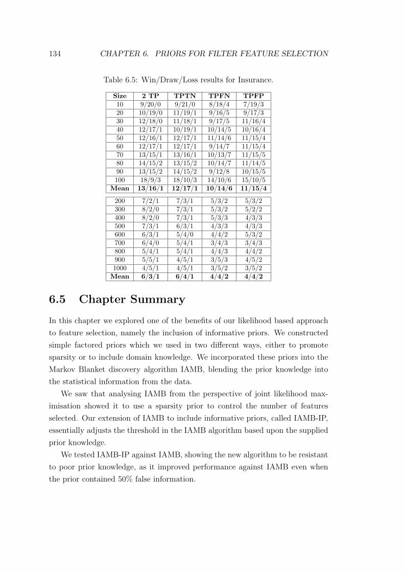
134 CHAPTER 6. PRIORS FOR FILTER FEATURE SELECTION
Table 6.5: Win/Draw/Loss results for Insurance.
Size 2 TP TPTN TPFN TPFP10 9/20/0 9/21/0 8/18/4 7/19/320 10/19/0 11/19/1 9/16/5 9/17/330 12/18/0 11/18/1 9/17/5 11/16/440 12/17/1 10/19/1 10/14/5 10/16/450 12/16/1 12/17/1 11/14/6 11/15/460 12/17/1 12/17/1 9/14/7 11/15/470 13/15/1 13/16/1 10/13/7 11/15/580 14/15/2 13/15/2 10/14/7 11/14/590 13/15/2 14/15/2 9/12/8 10/15/5100 18/9/3 18/10/3 14/10/6 15/10/5
Mean 13/16/1 12/17/1 10/14/6 11/15/4
200 7/2/1 7/3/1 5/3/2 5/3/2300 8/2/0 7/3/1 5/3/2 5/2/2400 8/2/0 7/3/1 5/3/3 4/3/3500 7/3/1 6/3/1 4/3/3 4/3/3600 6/3/1 5/4/0 4/4/2 5/3/2700 6/4/0 5/4/1 3/4/3 3/4/3800 5/4/1 5/4/1 4/4/3 4/4/2900 5/5/1 4/5/1 3/5/3 4/5/21000 4/5/1 4/5/1 3/5/2 3/5/2Mean 6/3/1 6/4/1 4/4/2 4/4/2
6.5 Chapter Summary
In this chapter we explored one of the benefits of our likelihood based approach
to feature selection, namely the inclusion of informative priors. We constructed
simple factored priors which we used in two different ways, either to promote
sparsity or to include domain knowledge. We incorporated these priors into the
Markov Blanket discovery algorithm IAMB, blending the prior knowledge into
the statistical information from the data.
We saw that analysing IAMB from the perspective of joint likelihood max-
imisation showed it to use a sparsity prior to control the number of features
selected. Our extension of IAMB to include informative priors, called IAMB-IP,
essentially adjusts the threshold in the IAMB algorithm based upon the supplied
prior knowledge.
We tested IAMB-IP against IAMB, showing the new algorithm to be resistant
to poor prior knowledge, as it improved performance against IAMB even when
the prior contained 50% false information.

Chapter 7
Cost-sensitive feature selection
In the previous three chapters we looked at how feature selection using infor-
mation theory maximises the joint likelihood of a discriminative model. This
allows us to combine information theoretic measurements from the data, with
prior knowledge from domain experts and therefore select features which best
combines these two sources of information. In this chapter we apply the machin-
ery from Chapter 4 to a different loss function, namely the weighted conditional
likelihood [31]. In the binary classification problem this loss function is a bound
on the empirical risk of the dataset, which measures how costly misclassification
is for each example. We thus derive a cost-sensitive filter feature selection cri-
teria, which coincides with Guiasu’s definition of weighted information theory
[46]. We prove several novel results with respect to this variant of information
theory, to allow its use as a feature selection criteria. We present experimental
results showing that the cost-sensitive selection criteria can be combined with a
cost-insensitive classifier to create an overall cost-sensitive system.
7.1 Deriving a Cost Sensitive Filter Method
In Chapter 2 we briefly looked at the weighted likelihood from Dmochowski et
al. [31], detailing its properties. We now briefly revise those properties before
moving on to novel material.
Dmochowski et al. [31] investigate using a weighted likelihood function to
integrate misclassification costs into the (binary) classification process. Each
example is assigned a weight based upon the tuple x, y, and the likelihood of
that example is raised to the power of the assigned weight. They prove that
135

136 CHAPTER 7. COST-SENSITIVE FEATURE SELECTION
the negative weighted log likelihood forms a tight, convex upper bound on the
empirical loss, which is the expected conditional risk across a dataset. This
property is used to argue that maximising the weighted likelihood is the preferred
approach in the case where the classifier cannot perfectly fit the true model.
Unfortunately the weighted likelihood has only been shown to bound the
risk in binary cost-sensitive problems. In multi-class cost-sensitive problems the
likelihood does not accurately represent the misclassification probabilities of the
other classes, as the sum of these values is equal to 1 − p(yi|xi) and they may
be unevenly weighted by the per example weight vector. Any weighted feature
selection process is likely to work best in the multi-class case as then it is more
probable that each label will have a different set of predictive features. Therefore
we avoid this problem by adjusting the weight of each datapoint in the likelihood.
We propose that if we use the sum of the per example weight vector,
ws(yi,xi) =
∑y∈Y,y 6=yi
w(yi,xi, y) (7.1)
we will ensure the weighted likelihood still forms an upper bound on the em-
pirical risk. This takes a pessimistic view of the classification problem, as a
mis-prediction which has a high weight may have a very low probability, but the
weighted likelihood will still be small. We note that this forms a looser upper
bound on the empirical risk than in the binary case, but reduces to the same
likelihood in binary problems. Cost-sensitive feature selection is an interesting
case of the general cost-sensitive problem as when using a filter technique it is
difficult to generate predicted labels with which to calculate the misclassifica-
tion error. This generalisation of the weighted likelihood provides an objective
function which allows the construction of cost-sensitive feature selection.
7.1.1 Notation
We use similar notation to Chapter 4 summarised here for clarity, with exten-
sions to include misclassification costs. We assume an underlying i.i.d. process
p : X → Y , from which we have a sample of N observations. Each observation is
a tuple (x, y,w), consisting of a d-dimensional feature vector x = [x1, ..., xd]T , a
target class y, and an associated non-negative |Y | − 1 dimensional weight vector,
w, for that observation, with x and y drawn from the underlying random vari-
ables X = X1, ..., Xd and Y . Furthermore, we assume that p(y|x) is defined

7.1. DERIVING A COST SENSITIVE FILTER METHOD 137
by a subset of the d features in x, while the remaining features are irrelevant or
redundant. We consider the weight for a particular example to be a function
only of the label y. This important restriction is necessary (see Section 7.2) to
ensure the weighted mutual information has a unique non-negative value. This
is a slightly less general formulation for the weights than the standard definition
given by Elkan [38], but is still flexible enough to include cost-matrices which do
not depend upon x.
We adopt a d-dimensional binary vector θ: a 1 indicating the feature is se-
lected, a 0 indicating it is discarded. Notation xθ indicates the vector of selected
features, i.e. the full vector x projected onto the dimensions specified by θ. No-
tation x¬θ is the complement, i.e. the unselected features. The full feature vector
can therefore be expressed as x = xθ,x¬θ. As mentioned, we assume the pro-
cess p is defined by a subset of the features, so for some unknown optimal vector
θ∗, we have that p(y|x) = p(y|xθ∗). In this chapter we consider the conditional
likelihood of the labels given the data, rather than the full joint likelihood anal-
ysed in Chapter 4. This is due to the bound in Dmochowski et al. only being
proved for the weighted conditional likelihood. The construction of a weighted
discriminative model likelihood is left to future work. Therefore our model does
not consider the generation of the datapoints, thus we only have two layers of
parameters in our hypothetical model q, namely: θ representing which features
are selected, and τ representing parameters used to predict y.
7.1.2 Deriving cost-sensitive criteria
In this section we take the weighted likelihood from Dmochowski et al. [31] and
decompose it into a sum of terms, where each term relates to a different part
of the classification process. This follows a similar process to the derivation in
Chapter 4. If we further make the filter assumption (Definition 8) we derive a
weighted feature selection criterion, which uses the weighted mutual information
(see Section 7.2) to score features. As mentioned previously when working in
the multi-class case, we use the sum of the per-example weight vector, wi as the
weight w(yi) in the likelihood.
We approximate the true distribution p with our model q, with separate pa-
rameters for the feature selection, θ, and for classification, τ . We define the

138 CHAPTER 7. COST-SENSITIVE FEATURE SELECTION
conditional likelihood as follows,
Lw(D,θ, τ) =N∏i=1
q(yi|xi,θ, τ)w(yi). (7.2)
We choose to work with the scaled negative log-likelihood, −`w, converting our
maximisation problem into a minimisation problem. This gives
−`w = − 1
N
N∑i=1
w(yi) log q(yi|xi,θ, τ) (7.3)
which is the function we will minimise with respect to θ, τ (this is the initial
position of Dmochowski et al. as they only consider the log-likelihood). We first
introduce the ratio p(y|x)p(y|x)
into the logarithm, this is the probability of the correct
class given all the features. We can then expand the logarithm into two terms,
−` = − 1
N
( N∑i=1
w(yi) logq(yi|xi,θ, τ)
p(yi|xi)+
N∑i=1
w(yi) log p(yi|xi)). (7.4)
The first term is the weighted log-likelihood ratio between the true model and our
predictive model, and the second term is the weighted log-likelihood of the true
model. This latter term is a finite sample approximation to the weighted condi-
tional entropy [46]. This represents both the amount of uncertainty in the data,
and how costly that uncertainty is. It forms a bound on the maximum amount
of performance we can extract from our dataset, in terms of the conditional risk.
We now wish to separate out feature selection from the classification process.
We do this by introducing another ratio into the first logarithm, namely p(y|x,θ)p(y|x,θ)
.
This is the probability of the correct class given the features selected by θ. We
can then further expand the first logarithm as follows,
−`w = − 1
N
( N∑i=1
w(yi) logq(yi|xi,θ, τ)
p(yi|xi,θ)+
N∑i=1
w(yi) logp(yi|xi,θ)
p(yi|xi)
+N∑i=1
w(yi) log p(yi|xi)). (7.5)
Similarly to the previous expansion from Chapter 4, we have expanded the
weighted conditional likelihood into a sum of three terms. In this case each term is

7.1. DERIVING A COST SENSITIVE FILTER METHOD 139
weighted by a per example cost. As our weights are functions of the class label y,
the per-example weight w(yi) and the per-state weight w(y) are identical. We can
then treat each of the summations above as approximations to the expectation
over each term, replacing the per-example weights with per-state weights. It is
this step which removes some of the power of our weighted likelihood as compared
to the weighted likelihood used in Dmochowski et al. , though we shall see it is
necessary to ensure the information theoretic values remain non-negative.
Again by similar logic to Chapter 4, we can interpret the second term in
Equation (7.5) as a finite sample approximation to the weighted conditional mu-
tual information Iw(X¬θ;Y |Xθ),
Iw(X¬θ;Y |Xθ) =∑
x,y∈X,Y
w(y)p(x, y) logp(x¬θ, y|xθ)
p(x¬θ|xθ)p(y|xθ)
≈ − 1
N
N∑i=1
w(yi) logp(yi|xi,θ)
p(yi|xi). (7.6)
and the third term as a finite sample approximation to the weighted conditional
entropy Hw(Y |X),
Hw(Y |X) = −∑
x,y∈X,Y
w(y)p(x, y) log p(y|x) ≈ − 1
N
N∑i=1
w(yi) log p(yi|xi).
We can now write −`w as the sum of weighted information theoretic quantities,
−`w ≈ Ex,y
w(y) log
p(yi|xi,θ)
q(yi|xi,θ, τ)
+ Iw(X¬θ;Y |Xθ) +Hw(Y |X). (7.7)
We note that the optimal feature set θ∗ is the set which makes Iw(X¬θ;Y |Xθ) =
0. This can only occur when p(x¬θ, y|xθ) = p(x¬θ|xθ)p(y|xθ), as the addition of
weights does not change position of the minima of the mutual information.
If we have discovered the optimal feature set or a superset thereof (i.e. X∗ ⊆Xθ) then p(y|x,θ) = p(y|x). The expectation in the first term can also then be
seen as a finite sample approximation to a weighted KL-Divergence (also known
as the weighted relative entropy [102]). This divergence represents how well the
predictive model fits the true distribution, given a superset of the optimal feature
set and how important each prediction is.
We have now decomposed the weighted conditional likelihood `w into three

140 CHAPTER 7. COST-SENSITIVE FEATURE SELECTION
terms, which relate to the cost-weighted classification performance of an arbitrary
probabilistic predictor, the quality of the chosen feature set, and the quality of the
data respectively. An important point to note about this formulation of weighted
feature selection is that the addition of weights does not change the optimal
feature set, in the sense that the feature set θ∗ which makes p(y|x,θ∗) = p(y|x)
is identical for all possible weightings. This is because the Markov Blanket for
the class label does not change when using a different evaluation metric. Thus
the use of the weighted mutual information as a selection criteria gives the same
optimal set as the standard mutual information. However, in the case where we
iteratively construct a feature set, the relative selection order can be different
between the weighted and unweighted information. Also if we select features
using an approximate criterion like those examined in Chapter 5 which cannot
recover the Markov Blanket, we can expect that the weighted variant will return
a different feature set. This is because while the minima of Iw(X¬θ;Y |Xθ) are
identical to the minima of I(X¬θ;Y |Xθ), the same is not necessarily true for (for
example) the JMI criterion. We will explore this effect in the experiments, and
show how different the top 50 features are when chosen using a weighted mutual
information versus the standard mutual information.
In the following section, we derive iterative update rules for the feature set,
that guarantee an increase in weighted mutual information.
7.1.3 Iterative minimisation
We now derive iterative update rules which greedily maximise our formulation of
the weighted likelihood. These derivations are similar to the derivations given in
Chapter 4 but use the weighted mutual information. The literature surrounding
the weighted mutual information has no proof for non-negativity or an equivalent
definition for the chain rule of mutual information, which are necessary for the
derivation of iterative update rules. We provide such proofs in the next section,
and in this section assume the existence of such proofs.
By using the chain rule, we can separate out the most informative feature
from X¬θ and add it to Xθ. We add a superscript t to θ to denote which time
step the feature sets are from, and proceed to derive the forward update that
maximises the weighted likelihood. The proof takes a similar form to the proof
of Theorem 1 from Chapter 4.

7.2. WEIGHTED INFORMATION THEORY 141
Theorem 4. The forward update which maximises the weighted likelihood is to
select the feature Xj ∈ X¬θ,
Xj = arg maxXj∈X¬θ
Iw(Xj;Y |Xθ). (7.8)
Proof. The feature which maximises the weighted likelihood is the feature which
minimises Iw(X¬θt+1 ;Y |Xθt+1) from Iw(X¬θt ;Y |Xθt), where Xθt+1 = Xθt ∪ Xj
and X¬θt+1 = X¬θt \Xj for some Xj ∈ X¬θt . We can express this as,
Iw(X¬θt+1 ;Y |Xθt+1) = Iw(X¬θt ;Y |Xθt)− Iw(Xj;Y |Xθt). (7.9)
Then we see that the feature Xj which minimises Iw(X¬θt+1 ;Y |Xθt+1) is,
Xj = arg maxXj∈X¬θt
Iw(Xj;Y |Xθt). (7.10)
A similar update can be found for the backwards step, analogous to Theorem 2
from Chapter 4. Both these updates are similar to the updates derived in Chapter
4 (which might be expected due to the machinery involved in generating them)
though they use the weighted mutual information developed by Guiasu, rather
than Shannon’s formulation. In Section 7.3 we proceed to create a weighted
variant of the JMI filter criterion [110], by substituting the weighted mutual
information for the Shannon mutual information, and supplying appropriate cost
vectors. First we must prove the non-negativity property and the chain rule used
in the above theorem.
7.2 Weighted Information Theory
The weighted mutual information has appeared several times in the literature
[46, 75, 96] but there has been little investigation of the theoretical properties
of such a measure. As mentioned previously this literature lacks two important
properties necessary for feature selection using the kind of iterative updates used
throughout this thesis. We now review those important properties of the weighted
mutual information, namely, non-negativity and the chain rule.

142 CHAPTER 7. COST-SENSITIVE FEATURE SELECTION
Table 7.1: An example of a negative wI, wI(X;Y ) = −0.0214.
w y = 1 y = 2x = 1 1 1x = 2 1 2
p(x, y) y = 1 y = 2x = 1 0.3 0.3x = 2 0.3 0.1
Value p(x) p(y)1 0.6 0.62 0.4 0.4
7.2.1 Non-negativity of the weighted mutual information
Non-negativity is an important property to ensure that adding a feature does
not reduce our measure of the information held in Xθ. The non-negativity of
Shannon’s mutual information is a well-known axiom of information theory, as
it is based upon the KL-Divergence, which can be proved to be non-negative
via Jensen’s inequality [24]. Unfortunately the weighted mutual information is a
form of weighted relative entropy [102], which was shown by Kvalseth [68] to take
negative values in certain situations. We first present a concrete example with a
negative weighted mutual information before providing a variant of the measure
which is proved to be non-negative for all valid inputs.
The definition of the weighted mutual information given by Guiasu [46] (de-
fined as the Q-MI by Luan et al. [75] and wI by Schaffernicht and Gross [96]) is
as follows,
wI(X;Y ) =∑x∈X
∑y∈Y
w(x, y)p(x, y) logp(x, y)
p(x)p(y). (7.11)
Note that this weight depends on the value of both x and y; in this case, the
information can be negative. Table 7.1 presents an example distribution for X and
Y which gives a negative weighted mutual information; in this case wI(X;Y ) =
−0.0214.
Therefore, knowledge of the variable X reduces what we know about Y 1. We
can avoid this problem with our measure if we define the weights so that they
are dependent upon a single variable i.e. ∀x, y w(x, y) = w(y). This still gives
valid weights under the conditions of weighted information theory, i.e. p(y)w(y) =∑x∈X w(x, y)p(x, y), which is the necessary condition for the definition of a unique
mutual information [46]. We restricted the weights in our weighted likelihood such
that they only depend upon y, therefore this limitation does not affect our earlier
derivation. We therefore define our weighted mutual information as a function
1An alternative explanation is that knowledge of X may cause us to make more costlypredictions for Y .

7.2. WEIGHTED INFORMATION THEORY 143
only of the class labels, as follows,
Iw(X;Y ) =∑x∈X
∑y∈Y
w(y)p(x, y) logp(x, y)
p(x)p(y). (7.12)
Theorem 5. The weighted mutual information, Iw, is non-negative if the weights
are a function of a single random variable. Therefore ∀X, Y,w Iw(X;Y ) ≥ 0.
Proof. We begin by relating the weighted mutual information to the (unweighted)
KL-Divergence.
Iw(X;Y ) =∑x∈X
∑y∈Y
w(y)p(x, y) logp(x, y)
p(x)p(y)
=∑y∈Y
w(y)∑x∈X
p(x, y) logp(x, y)
p(x)p(y)
=∑y∈Y
w(y)p(y)∑x∈X
p(x|y) logp(x|y)p(y)
p(x)p(y)
=∑y∈Y
w(y)p(y)∑x∈X
p(x|y) logp(x|y)
p(x)
=∑y∈Y
w(y)p(y)DKLp(x|y)||p(x). (7.13)
As all the weights w(y) are non-negative, p(y) is non-negative, and the KL-
Divergence is non-negative, then our new weighted mutual information, Iw, is
non-negative.
7.2.2 The chain rule of weighted mutual information
One further essential property of an information measure defines how variables
interact. In the standard formulation of Shannon’s Information Theory this is
the chain rule of mutual information, I(AB;Y ) = I(A;Y ) + I(B;Y |A), and
separates out the information shared between a joint random variable and a target
random variable into two components, the individual mutual information of the
first variable and the target, plus the second variable and the target conditioned
upon the first. We provide an equivalent rule for the weighted mutual information.

144 CHAPTER 7. COST-SENSITIVE FEATURE SELECTION
Theorem 6. The weighted mutual information, Iw, between a joint random vari-
able and a single random variable can be decomposed as follows,
Iw(AB;Y ) = Iw(A;Y ) + Iw(B;Y |A). (7.14)
Proof. Due to Theorem 5 we only define the chain rule such that Y is never
conditioned upon, and we define ∀x, z, y w(x, z, y) = w(y). We thus define the
chain rule as follows,
Iw(XZ;Y ) =∑x∈X
∑y∈Y
∑z∈Z
w(y)p(x, y, z) logp(x, y, z)
p(x, z)p(y)
=∑x∈X
∑y∈Y
∑z∈Z
w(y)p(x, y, z) logp(x, y)p(z|y, x)
p(z|x)p(x)p(y)
=∑x∈X
∑y∈Y
w(y)p(x, y) logp(x, y)
p(x)p(y)
+∑x∈X
∑y∈Y
∑z∈Z
w(y)p(x, y, z) logp(z|y, x)
p(z|x)
= Iw(X;Y )
+∑x∈X
∑y∈Y
∑z∈Z
w(y)p(x, y, z) logp(z, y|x)
p(z|x)p(y|x)
= Iw(X;Y ) + Iw(Z;Y |X).
This property is independent of the restriction on the weights defined in Theorem
5, though the non-negativity property is crucial to ensure the iterative updates
maximise the weighted likelihood. We can now see due to the chain rule and the
definition of X = Xθ, X¬θ that,
Iw(X;Y ) = Iw(Xθ;Y ) + Iw(X¬θ;Y |Xθ). (7.15)
Therefore, since Iw(X;Y ) is a constant with respect to θ, minimizing Iw(X¬θ;Y |Xθ)
is equivalent to maximising Iw(Xθ;Y ).
We now turn to the task of constructing filter criteria which approximate the
difficult to estimate update rules given in Section 7.1.3.

7.3. CONSTRUCTING FILTER CRITERIA 145
7.3 Constructing filter criteria
We note from our work in the previous section that we can only construct weighted
mutual informations which include the variable Y which our weights are defined
over. This limits the possible feature selection criteria, but fortunately many of
the common ones can be re-expressed in the right form. We focus on adapting
the JMI criterion [110], as this is the best performing criterion from our earlier
empirical study (see Chapter 5). We also use a weighted variant of MIM, which
ranks features according to their univariate weighted mutual information. We
expect that the other criteria we investigated in that chapter could be adapted to
work in this weighted likelihood framework, and the weighted mutual information,
provided they can be expressed using mutual informations between Y and X.
Unfortunately this restriction excludes popular criteria such as mRMR, as they
cannot be written in the necessary form.
We define the weighted variant of the MIM criterion (referred to as wMIM)
as follows:
Jwmim(Xk, w) = Iw(Xk;Y ). (7.16)
Similarly, we define the weighted variant of the JMI criterion (referred to as
wJMI) as follows:
Jwjmi(Xk, S, w) =∑Xj∈S
Iw(XkXj;Y ). (7.17)
We then combine these criteria with a greedy forward search, to produce a fea-
ture selection algorithm. As mentioned previously the use of weights does not
change the minima of the likelihood with respect to θ, however when using an
approximate optimiser such as wJMI the feature sets returned are different. This
is due to the pairwise independence assumption made in the JMI criterion [14],
which stops the criterion from determining when it has reached the optima. We
shall see this effect in the empirical study, as the feature sets selected by JMI and
wJMI (and by MIM and wMIM) diverge.
One important point to note is that as we only consider the rankings of indi-
vidual features the magnitude of the weight vector is irrelevant. If we normalise
the weight vector w so it sums to 1, this will return exactly the same feature set
(using wJMI or wMIM) as if we multiplied each weight by a positive value.

146 CHAPTER 7. COST-SENSITIVE FEATURE SELECTION
7.4 Empirical study of Weighted Feature Selec-
tion
We compare our cost-sensitive feature selection algorithm against three different
competitors. The first is simply using a normal cost-insensitive feature selection
algorithm (in our case JMI), combined with a standard classifier (a linear SVM).
The second is the ‘standard’ cost-sensitive methodology, where a normal feature
selection algorithm is used with a cost-sensitive classifier, in our case a weighted
SVM [17], which aims to minimise the mis-classification cost of the training data.
The third approach is a form of oversampling of the costly class. As our likelihood
takes the form of examples raised to the power of a weight, it can be see as
replicating an example w(y) times. We mirror this process to produce a new
dataset using a deterministic oversampling process which repeats an example w(y)
times, where w(y) is the (integer) cost for that example’s label. We also present
results comparing against the multi-class feature selection algorithm (Spread-
FX) from Forman [43], using the random scheduler, modified to sample from the
weight distribution rather than the uniform distribution.
We use a selection of multi-class datasets to evaluate our new approach: the
well-known MNIST digit classification dataset, and 5 text-mining datasets taken
from Han and Karypis [52]. These datasets provide a large number of both
features and samples, and the features from the MNIST dataset [71] can be
easily visualised to show the differences between our technique and the cost-
insensitive baseline. As before we calculate all mutual informations on discretised
versions of the datasets, with 10 bins, using a histogram estimator of the necessary
probabilities. Our scoring metrics are the precision, recall and F-measure of the
costly class, along with the accuracy across all classes.
Our aim is to test the ability of cost-sensitive feature selection to produce a
cost-sensitive system when combined with a standard (cost-insensitive) classifier,
analogously to how resampling the training data produces a cost-sensitive system
when combined with a standard (cost-insensitive) classifier.
7.4.1 Handwritten Digits
We selected 500 instances at random from each class label in the MNIST data,
to give a 5000 example dataset, to reduce the training times of our classification
models. All results reported are 10-fold cross validation runs, selecting the top 50

7.4. EMPIRICAL STUDY OF WEIGHTED FEATURE SELECTION 147
features according to the various feature selection algorithms. We used a linear
Support Vector Machine (SVM) as the classification model, using the LibSVM
[17] implementation with default parameter settings.
In Figures 7.2 and 7.3 we present results from this dataset where the costly
class is the digit “4”. The average 4 in our dataset is presented in Figure 7.1.
Figure 7.2a shows the different algorithms tested with w(y =“4”) = 5, so the
digit “4” is five times more important than the other labels, which were given a
weight of one. Each group of bars represents a different approach to the cost-
sensitive problem: the first group is the standard cost-insensitive approach, where
the JMI algorithm is used to select 50 features, and then an SVM is trained on
those features. The second group is our approach, where we include the weight
in the feature selection process with wJMI and use a standard SVM to fit the
data. The third group uses JMI with a weighted SVM, and finally the fourth
group oversample the costly class according to the weight. We can see that the
introduction of weights does not alter the overall classification performance (the
leftmost bar in each group is approximately the same), but the precision, recall
and F-measure change when the weighted approaches are used. Our method
improves both precision and recall over the baseline, whereas using a weighted
classifier trades off precision for recall (i.e. it predicts many more false positives).
Figure 7.3a shows how the F-Measure on class 4 changes for the three weighted
methods using weights w(y = 4) = 1, 5, 10, 15, 20, 25, 50, 100. In contrast to
wJMI the weighted classifier degrades performance as it predicts many false pos-
itives. Figure 7.3b shows a precision/recall plot of the various approaches, with
the cost-insensitive approach appearing as a filled black circle. The size of the
marker represents the weight, from the range given above. We can see how the
weighted feature selection improves both precision and recall for all settings of
the weights whereas oversampling only improves recall, and the weighted classifier
improves recall at the cost of precision.
Finally in Figure 7.2b we show the different features selected by the standard
JMI algorithm, and the wJMI algorithm with w(y = 4) = 100. The light gray
features are those which were selected by JMI and not by wJMI, the dark gray
features are those selected by both algorithms, and the black features are those
selected by wJMI alone. This shows how the wJMI algorithm selects features
which are predictive of the presence or absence of a 4. The large black block
at the top of the image represents the area which differentiates a 4 from a 9 in

148 CHAPTER 7. COST-SENSITIVE FEATURE SELECTION
Figure 7.1: The average pixel values across all 4s in our sample of MNIST.
(a) Accuracy is across the whole dataset,with 95% Confidence across 10-fold CV, us-ing (w)JMI.
(b) Difference in selected features be-tween JMI and wJMI, w(y = 4) = 100
Figure 7.2: MNIST Results, with “4” as the costly digit.
the dataset, and the dark area in the bottom left differentiates a 4 from a 2, 5,
6, or 8 as those digits require pixels in that area. The other black features are
to positively detect a 4. We can see that this weighted approach selects features
which are predictive of the presence of a 4 and discriminate against false positives.
We present the average improvement in precision and recall across all digits
in our MNIST dataset in Table 7.2, where each digit in turn was given a weight
w(y) = 10. We can see that the weighted feature selection improves both precision
and recall, resulting in an improved F-measure, whereas the other approaches
have high recall, but low precision (i.e. predict many false positives), resulting
in little improvement in the F-measure. We also present the improvement in
precision and recall for the digit 4 in Table 7.3.

7.4. EMPIRICAL STUDY OF WEIGHTED FEATURE SELECTION 149
(a) F-Measure with 95% Confidence, across10-fold CV.
(b) Precision/Recall plot, where themarker size indicates the weight w.
Figure 7.3: MNIST Results, with “4” as the costly digit, using w(y = 4) =1, 5, 10, 15, 20, 25, 50, 100 and (w)JMI. LEFT: Note that as costs for mis-classifying “4” increase, the weighted FS method increases F-measure, while theweighted SVM suffers a decrease. RIGHT: The black dot is the cost-insensitivemethodology. Note that the weighted SVM can increase recall above the 90%mark, but it does so by sacrificing precision. In contrast, the weighted FS methodpushes the cluster of points up and to the right, increasing both recall and pre-cision.
Table 7.2: MNIST results, averaged across all digits. Each value is the difference(x 100) in Precision, Recall or F-Measure, against the cost-insensitive baseline.
Algorithm ∆ Pre ∆ Rec ∆ F-MeasurewJMI 6.3 5.1 5.7
weighted SVM -17.0 10.4 -7.0Oversampling -8.9 11.5 -0.6
Table 7.3: MNIST results, digit 4. Each value is the difference (x 100) in Preci-sion, Recall or F-Measure, against the cost-insensitive baseline.
Algorithm ∆ Pre ∆ Rec ∆ F-MeasurewJMI 18.5 18.5 18.5
weighted SVM -22.6 26.7 -6.7Oversampling 0.1 24.3 10.5

150 CHAPTER 7. COST-SENSITIVE FEATURE SELECTION
(a) F-Measure on the digit “4” with 95%Confidence, across 10-fold CV.
(b) F-Measure on the digit “9” with 95%Confidence, across 10-fold CV.
Figure 7.4: MNIST Results, with both “4” and “9” as the costly digits, usingw(y = (4 ∨ 9)) = 1, 5, 10, 15, 20, 25, 50, 100 and (w)JMI, F-Measure.
We might also wish to understand the performance of our weighted measure
when we upweight two classes simultaneously. We investigated this by upweight-
ing both “4” and “9” in the same run, as these digits are often confused by
pattern recognition systems. In Figure 7.4 we present the results as we increase
the weights on both 4s and 9s, in terms of the F-Measure. In Figure 7.5 we
present the same experiments as a scatter plot of precision and recall. We can see
that in this case the weighted SVM fails to differentiate between 4s and 9s, and is
dominated by both the oversampling and our weighted feature selection. Again
the oversampling improves the recall of the upweighted classes, and the weighted
feature selection improves both precision and recall, though the improvement in
recall is less than the oversampling approach. We note that our technique is suc-
cessful in improving both precision and recall in both of the upweighted classes,
showing it has selected features which can differentiate between 4s and 9s.
Finally we compare our weighted method against the SpreadFX algorithm
by Forman [43]. In Forman’s paper he suggests the extension of the SpreadFX
algorithm to use a random sampler on a non-uniform distribution. We create such
a distribution by normalising our weight vector so that it sums to one, and then
use it in the Rand-Robin scheduler. This leads to a cost-sensitive feature selection
algorithm, though it is quite different from our approach. SpreadFX converts any
given multi-class problem into a series of |Y | one-versus-all binary problems, then
performs feature selection on each sub-problem. The scheduler is then used to
select features from each of the rankings constructed on the sub-problem. This
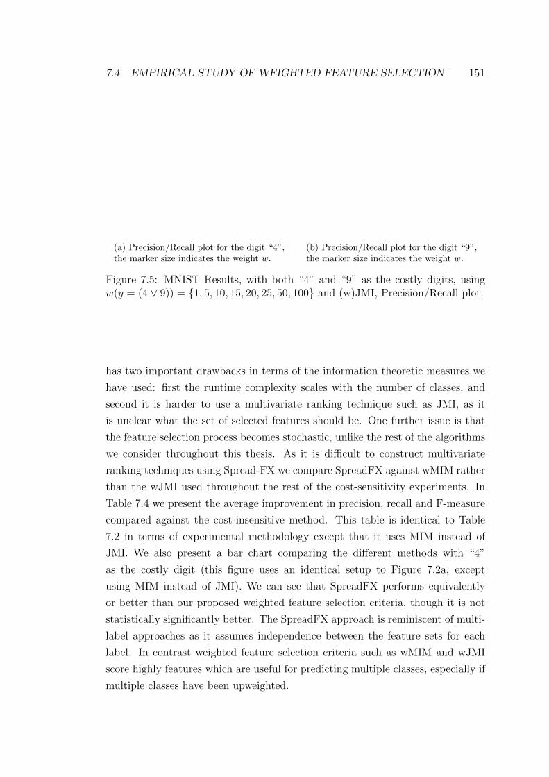
7.4. EMPIRICAL STUDY OF WEIGHTED FEATURE SELECTION 151
(a) Precision/Recall plot for the digit “4”,the marker size indicates the weight w.
(b) Precision/Recall plot for the digit “9”,the marker size indicates the weight w.
Figure 7.5: MNIST Results, with both “4” and “9” as the costly digits, usingw(y = (4 ∨ 9)) = 1, 5, 10, 15, 20, 25, 50, 100 and (w)JMI, Precision/Recall plot.
has two important drawbacks in terms of the information theoretic measures we
have used: first the runtime complexity scales with the number of classes, and
second it is harder to use a multivariate ranking technique such as JMI, as it
is unclear what the set of selected features should be. One further issue is that
the feature selection process becomes stochastic, unlike the rest of the algorithms
we consider throughout this thesis. As it is difficult to construct multivariate
ranking techniques using Spread-FX we compare SpreadFX against wMIM rather
than the wJMI used throughout the rest of the cost-sensitivity experiments. In
Table 7.4 we present the average improvement in precision, recall and F-measure
compared against the cost-insensitive method. This table is identical to Table
7.2 in terms of experimental methodology except that it uses MIM instead of
JMI. We also present a bar chart comparing the different methods with “4”
as the costly digit (this figure uses an identical setup to Figure 7.2a, except
using MIM instead of JMI). We can see that SpreadFX performs equivalently
or better than our proposed weighted feature selection criteria, though it is not
statistically significantly better. The SpreadFX approach is reminiscent of multi-
label approaches as it assumes independence between the feature sets for each
label. In contrast weighted feature selection criteria such as wMIM and wJMI
score highly features which are useful for predicting multiple classes, especially if
multiple classes have been upweighted.
152 CHAPTER 7. COST-SENSITIVE FEATURE SELECTION
Figure 7.6: MNIST Results, using wMIM comparing against SpreadFX, with “4”as the costly digit.
Table 7.4: MNIST results, averaged across all digits. Each value is the difference(x 100) in Precision, Recall or F-Measure, against the cost-insensitive baseline.
Algorithm δ Precision (%) δ Recall (%) δ F-Measure (%)wMIM 3.9 4.4 4.2
Weighted Classifier -13.5 10.3 -4.1SpreadFX 6.0 6.6 6.4
Oversampling -6.7 11.3 1.0
7.4.2 Document Classification
We chose 5 document classification datasets from Han and Karypis [52] (the
datasets are listed in Table 7.5). We tested these datasets using the same proce-
dure as the MNIST datasets, selecting 50 features with either our wJMI criterion,
or the standard JMI criterion and classifying using either a normal or weighted
SVM. We ran each experiment using 10-fold cross validation where each class
was upweighted in turn with w(y) = 10, and present the Wins/Draws/Losses
at the 95% confidence interval in Table 7.6. The first three columns are com-
paring against the cost-insensitive method, and we see that the weighted feature
selection improves the F-measure in some cases, but the weighted SVM and over-
sampling approaches degrade performance in many cases. When comparing the
weighted feature selection against the weighted classifier or oversampling (the last
two columns) we see that the weighted feature selection improves upon weighted
classification in many cases, particularly with the ohscal dataset, which was the
largest dataset we tested, with 11162 examples and 11465 features.

7.5. CHAPTER SUMMARY 153
Table 7.5: Summary of text classification datasets.
Dataset Features Examples Classesfbis 2000 2463 17la12 31472 6279 6
ohscal 11465 11162 10re0 2886 1504 13re1 3758 1657 25
Table 7.6: Document classification results: F-Measure W/D/L across all labels,with the costly label given w(y) = 10.
Data wJMI wSVM Oversample wJMI v wSVM wJMI v Oversamplefbis 4/13/0 1/13/3 5/11/1 7/10/0 2/15/0la12 1/5/0 0/3/3 0/5/1 4/2/0 2/4/0
ohscal 2/8/0 0/0/10 0/1/9 10/0/0 10/0/0re0 0/13/0 0/13/0 0/13/0 0/13/0 0/13/0re1 1/24/0 0/25/0 0/25/0 2/23/0 0/25/0
7.5 Chapter Summary
In this chapter we looked at the effects of choosing a different loss function than
the joint likelihood we considered in the previous three chapters. We saw that
choosing a cost-sensitive conditional likelihood allowed the derivation of cost-
sensitive feature selection criteria, based upon Guiasu’s weighted information
theory. We proved several essential properties of the weighted mutual information
measure to ensure it’s suitability as a selection criterion.
As with the criterion derived in Chapter 4, some assumptions are necessary
to produce a feature selection criterion which is estimable across many datasets.
We thus investigate a weighted variant of JMI as it was found to perform the
best in our empirical study from Chapter 5, and a weighted variant of MIM as a
baseline.
We show how the cost-sensitive nature of our new criteria allows the con-
struction of a cost-sensitive system from a cost-insensitive classifier coupled with
the cost-sensitive feature selection. This compares favourably with other cost-
sensitive techniques based around altering either the classifier or the training
data.

154 CHAPTER 7. COST-SENSITIVE FEATURE SELECTION
Figure 7.7: Ohscal results. Cost of mis-predicting class 9 is set to ten timesmore than other classes. The weighted SVM and oversampling approaches clearlyfocus on producing high recall, far higher than our method, however, this is onlyachievable by sacrificing precision. Our approach improves precision and recall,giving higher F-measure overall.

Chapter 8
Conclusions and future directions
We began this thesis by reviewing the literature on information theoretic feature
selection. This literature contained a forest of different selection criteria based
upon different permutations of information theoretic functions, with little under-
standing of the objective functions such criteria optimise. Our first result showed
that using an information theoretic criterion implies the objective function is the
log-likelihood of a particular model. We then proceeded to explore the literature
relating the different criteria to the one derived from the likelihood. Once we had
explained the literature we investigated the specific benefits of our framework,
looking at extensions which incorporate prior knowledge or cost-sensitivity. We
now provide a detailed summary of the contributions of this thesis, providing
answers to the questions posed in the first chapter.
8.1 What did we learn in this thesis?
The contributions of this thesis arose by considering the questions stated in Chap-
ter 1. We now review those questions, summarising the answers provided by this
thesis.
8.1.1 Can we derive a feature selection criterion which
minimises the error rate?
We answered this question in Chapter 4 by considering the joint likelihood of a
discriminative model as our objective function. This likelihood is maximised by
having a high predictive probability for all the true labels of a training dataset,
155
156 CHAPTER 8. CONCLUSIONS AND FUTURE DIRECTIONS
when using parameters which have a high probability a priori. It is a proxy
for the error rate as high likelihood is a sufficient condition for a low error rate,
though it is not a necessary one. We saw that this likelihood could be expanded
into a series of terms with each term relevant for a particular component of the
error. We repeat Equation 4.10 for clarity below,
−` ≈ Ex,y
log
p(yi|xi,θ)
q(yi|xi,θ, τ)
+ I(X¬θ;Y |Xθ) +H(Y |X)− 1
Nlog p(θ, τ).
The first term denotes the quality of our predictor compared to the optimal
predictions for the selected feature set, this takes the form of a KL-Divergence,
and is zero when our predictor makes the optimal predictions. The second term
denotes the quality of our selected feature set compared to the full feature set,
this takes the form of a conditional mutual information and is zero when our
selected feature set contains all the relevant information. The third term denotes
the quality of the data itself, and the final term is the prior probability of the
model parameters. We can therefore think of Equation 4.10 as expanding the
likelihood thus,
−` ≈ predictor + feature set + data + prior, (8.1)
where we wish to minimise the first three terms, and maximise the fourth. In
general we can do little to adjust the quality of our training data, and we should
not adjust our priors based upon the data, therefore the first two terms are the
quantities we can minimise. Making the filter assumption from Definition 8 allows
us to first select a feature set which maximises the likelihood, and then to build
a classifier which maximises the likelihood based on that feature set.
One further insight based upon this expansion is that filter methods which
choose to maximise this likelihood are in effect wrapper methods using a perfect
classification model. Even the filters themselves appear to be simple classifiers, as
they construct a probability distribution and measure its predictive performance
with a KL-Divergence. This perspective shows that when choosing to maximise
the joint likelihood filters and wrappers differ only in the method by which they
search the feature space, and the assumptions made by the classification model.
Using a classification model with few assumptions and maximising the model
likelihood can be seen as a filter maximising the mutual information of the feature
set.

8.1. WHAT DID WE LEARN IN THIS THESIS? 157
Returning to the specific problem of filter feature selection we can derive the
optimal selection criterion. If we choose to iteratively maximise the likelihood by
selecting (or removing) features greedily then we should select the feature which
maximises (minimises) the conditional mutual information between that feature
and the class label, conditioned upon the selected feature set plus the prior term
for the current feature set. We note that in the iterative updates the prior term
is a ratio therefore if we use a flat uninformative prior, the prior term cancels.
This leads to a maximum likelihood update rule based solely upon the conditional
mutual information. With this derivation and the iterative update rules we are
ready to answer the next question, by linking our derived updates to the selection
criteria from the literature.
8.1.2 What implicit assumptions are made by the infor-
mation theoretic criteria in the literature?
We looked at this question in Chapter 5, considering the criteria from the lit-
erature as approximations to our optimal criterion derived in Chapter 4. We
considered the link to our optimal criterion assuming there was a flat prior over
the possible feature sets, as the criteria we investigated did not include prior
knowledge. This link makes explicit the objective function underlying each of the
published criteria, namely the joint likelihood of a discriminative model.
As the optimal criterion is intractable to estimate, each of the published cri-
teria make implicit assumptions which reduce the complexity of the estimation
problem. These assumptions make the criteria approximate iterative maximisers
of the joint likelihood. The main theoretical difference between the criteria is
whether they assume the features are class-conditionally independent. Without
this assumption there is an additional class-conditional term in the criteria. One
other important theoretical point is whether they provide a mechanism to bal-
ance the relative magnitude of the redundancy terms against the relevancy term.
To ascertain how these differences impact the criteria in practice, we conducted
an empirical study of 9 different heuristic mutual information criteria across 22
datasets. We analysed how the criteria behave in large/small sample situations,
how the stability of returned feature sets varies between criteria, and how sim-
ilar criteria are in the feature sets they return. In particular, we looked at the
following empirical questions:

158 CHAPTER 8. CONCLUSIONS AND FUTURE DIRECTIONS
How do the theoretical properties translate to classifier accuracy?
Summarising the performance of the criteria under the above conditions, includ-
ing the class-conditional term is not always necessary. Various criteria, for exam-
ple mRMR, are successful without this term. However, without this term criteria
are blind to certain classes of problems, e.g. the MADELON dataset (see Section
5.3), and will perform poorly in these cases. Balancing the relevancy and redun-
dancy terms is however extremely important — criteria like MIFS, or CIFE, that
allow redundancy to swamp relevancy, are ranked lowest for accuracy in almost
all experiments. In addition, this imbalance makes the criteria unstable, causing
them to become sensitive to small changes in the supplied data.
How stable are the criteria to small changes in the data?
Several criteria return wildly different feature sets with just small changes in the
data, while others return similar sets each time, hence are ‘stable’ procedures. As
we might expect the most stable was the univariate mutual information as it has
the simplest distributions to estimate, followed closely by JMI [110, 80]; while
among the least stable are MIFS [6] and ICAP [58].
How do criteria behave in limited and extreme small-sample situations?
In extreme small-sample situations, it appears the above rules (regarding the
conditional term and the balancing of relevancy-redundancy) can be broken — the
poor estimation of distributions means the theoretical properties do not translate
immediately to performance.
Do the different criteria return different feature sets?
We might ask how the theoretical differences between the criteria impact the se-
lected feature sets, and so using the stability measures we compared the feature
sets returned by each of the criteria with each other criterion. If we visualise the
differences using multi-dimensional scaling (see Figure 5.5) we can see a cluster
of criteria which “balance” the relevancy and redundancy terms (or ignore redun-
dancy completely in the case of MIM), and each criterion which does not balance
the terms is very different from all other criteria. This explains why the empirical
performance of many of the criteria is so similar.

8.1. WHAT DID WE LEARN IN THIS THESIS? 159
Having explained the behaviour and performance of the criteria in the litera-
ture we looked at the other benefits provided by our probabilistic framework for
feature selection.
8.1.3 Developing informative priors for feature selection
One major benefit of our joint likelihood approach to feature selection is the nat-
ural incorporation of domain knowledge in the form of priors over the selected
feature set θ. In Chapter 6 we looked at simple forms for these priors, and
showed how to combine them with selection criteria from the literature. During
this process we saw how the IAMB algorithm for Markov Blanket discovery can
be seen as another special case of our joint likelihood framework, operating under
a specific sparsity prior. We used this insight to extend IAMB to include other
information in the prior, specifically to include domain knowledge over the pres-
ence or absence of nodes in the Markov Blanket. This result shows local structure
learning algorithms using conditional independence testing as instantiations of a
likelihood-based score and search technique, similar to the result by Cowell [25]
for global structure learning algorithms. As we might expect the inclusion of cor-
rect knowledge improved the recovery of the Markov Blanket in several artificial
datasets. However the performance still improved even when half the supplied
“knowledge” was incorrect. This improvement was greatest when using complex
datasets and small amounts of data.
8.1.4 How should we construct a cost-sensitive feature se-
lection algorithm?
In Chapter 7 we answer this question by deriving a cost-sensitive feature selection
criterion directly from a cost-weighted likelihood. This weighted likelihood min-
imises an upper bound on the empirical risk. The derived criterion is based upon
a weighted mutual information, which generalises Shannon’s mutual information
to incorporate the importance (or cost) of certain states. To allow the use of such
a function we proved two novel properties of this weighted measure, namely the
chain rule, and the non-negativity of information. Our derived criterion works
with costs which depend solely upon the label, as otherwise the non-negativity
property will not necessarily hold.
We then empirically tested this cost-sensitive criterion against several other

160 CHAPTER 8. CONCLUSIONS AND FUTURE DIRECTIONS
methods for creating cost-sensitive classification systems. We showed that us-
ing cost-sensitive information theoretic feature selection effectively converts a
cost-insensitive classifier into a cost-sensitive one, by adjusting the features the
classifier sees. We see this as an analogous process to that of adjusting the data
via over or undersampling to create a cost-sensitive classifier, but with the crit-
ical difference that we do not artificially alter the data distribution. We found
that while classical cost-sensitive classifiers traded off precision to improve recall,
our new cost-sensitive feature selection methodology improved both precision and
recall in the upweighted class(es).
As this thesis is of finite size there are obviously many interesting areas which
remain for future study in the field of information theoretic feature selection, and
we review some of them in the next section.
8.2 Future Work
While this thesis has consolidated much work in information theoretic feature se-
lection, allowing many techniques to be described as instantiations of a likelihood-
based framework, it has also revealed several interesting areas for future work.
The first area arises from the derivation in Chapter 4. In that chapter we
constructed a probabilistic framework to find the Maximum a Posteriori solution
to the feature selection problem. A natural extension of this work would be to
investigate a fully Bayesian solution to the feature selection problem. Our work
finds the modal value of the posterior distribution over θ, but it is well known that
the MAP solution may not be close to the center of mass of the full posterior [10],
and thus it may not accurately represent the posterior distribution. A Bayesian
solution to the feature selection problem would allow detailed investigations of the
posterior for θ, possibly highlighting feature sets which more accurately represent
the posterior distribution. We expect that such a solution would take the form of
a Dirichlet process across the space of possible θ values, though we have invested
little time in deriving such a solution.
The second area is based upon the insights gained into filter feature selec-
tion from Chapters 4 & 7. In those chapters we began by choosing a particular
objective function to maximise, respectively the joint likelihood and weighted
conditional likelihood. In each case we derived different selection criteria, though
both were based upon information theory. There exist many other filter criteria,
8.2. FUTURE WORK 161
many of which do not have links to precise objective functions. It may be in-
teresting to investigate the links between a criterion such as the Gini Index [34],
and derive the objective function implied by the choice of such a criterion. It is
interesting to note that the log-likelihood is an instance of a proper scoring func-
tion [44], and other such scoring functions may also have links to feature selection
criteria. One obvious extension would be to develop feature selection from a like-
lihood which combines both priors over θ, and differing misclassification costs,
to unify the methods proposed in Chapters 6 and 7.
The third area is based upon the literature in information theoretic feature
selection which we examined in Chapter 5. There we saw how the majority of
published criteria make specific assumptions about the underlying distributions,
and how all the criteria made the assumption that there are only pairwise in-
teractions between features. Relaxing this assumption leads to more complex
information theoretic terms, which consequently have higher data requirements
to ensure they accurately estimate the mutual information. An interesting topic
of study would be to combine this insight with work on entropy estimation [83] or
analysis of the variance of the mutual information [56], to determine for any given
dataset how many of these complex terms it is possible to estimate accurately,
then adjusting the feature selection criterion accordingly. This would allow an
adaptive feature selection criterion which adjusts to the amount of available data,
behaving like Jcmi when there are many thousands or millions of datapoints, and
scaling back through JMI towards MIM as the number of datapoints shrinks.
The fourth area is more theoretical in nature, and relates to the weighted
mutual information used in Chapter 7. In that chapter we defined the weighted
mutual information so that the weights are a function of a single variable, rather
than both variables in the mutual information. We proved how this ensures the
non-negativity of the measure, which is important for feature selection to ensure
we are maximising the likelihood. However the original weighted conditional
likelihood of Dmochowski et al. [31] does not include this constraint, and the
weights are allowed to depend upon both x and y. In this case it is possible for
the weighted mutual information to take negative values, and a very interesting
subject is the nature of such negative values. This gives rise to some interesting
questions: “What does a negative Iw imply about the nature of the relationship
between X and Y ?”, and “What does it imply about the cost-sensitive problem
that we wish to optimise?”.

162 CHAPTER 8. CONCLUSIONS AND FUTURE DIRECTIONS
The final area involves extending the techniques presented in this thesis to new
problems. The material on priors in Chapter 6 considered very simple priors, and
more performance may be available by utilising more complex and informative
priors. The material on cost-sensitivity is framed in the context of multi-class
problems as those are more likely to exhibit the property where each label has a
different group of predictive features. Exploring two class problems where this is
the case, and extending the framework to cope with multi-label datasets would
provide interesting applications of the weighted feature selection approach.
One topic which we chose not to consider in this thesis is the interaction
between the search method and the feature selection criterion. Preliminary work
suggests that for some of the criteria examined in Chapter 5 the choice of search
method is irrelevant to the feature set returned. Forward searches, backwards
searches and floating searches all returned the same (or very similar) feature sets,
across a number of datasets. Also using the sum of J(Xj) over the whole selected
feature set as the objective function returned the same feature sets as the more
greedy search methods mentioned earlier. It would be interesting to do a more
extensive empirical study to see if this strange effect is borne out across many
datasets as it implies the choice of search method has little relevance compared
to the choice of selection criterion. This is a rather counter-intuitive result given
the performance gains made with other feature selection criteria when changing
the search method (e.g. Pudil et al. [91]), and suggests there may be a deeper
insight into why information theory does not need complex search techniques.

Bibliography
[1] B. Abramson, J. Brown, W. Edwards, A. Murphy, and R. Winkler. Hail-
finder: A Bayesian system for forecasting severe weather. Int. Journal of
Forecasting, 12(1):57–71, 1996.
[2] C. Aliferis, A. Statnikov, I. Tsamardinos, S. Mani, and X. Koutsoukos.
Local causal and markov blanket induction for causal discovery and feature
selection for classification part i: Algorithms and empirical evaluation. The
Journal of Machine Learning Research (JMLR), 11:171–234, 2010.
[3] C. Aliferis, A. Statnikov, I. Tsamardinos, S. Mani, and X. Koutsoukos.
Local causal and markov blanket induction for causal discovery and feature
selection for classification part ii: Analysis and extensions. The Journal of
Machine Learning Research (JMLR), 11:235–284, 2010.
[4] C. Aliferis, I. Tsamardinos, and A. Statnikov. Hiton: a novel markov blan-
ket algorithm for optimal variable selection. In AMIA Annual Symposium
Proceedings, volume 2003, page 21. American Medical Informatics Associ-
ation, 2003.
[5] K. S. Balagani and V. V. Phoha. On the Feature Selection Criterion Based
on an Approximation of Multidimensional Mutual Information. IEEE
Transactions on Pattern Analysis and Machine Intelligence, 32(7):1342–
1343, 2010.
[6] R. Battiti. Using Mutual Information for Selecting Features in Supervised
Neural Net Learning. IEEE Transactions on Neural Networks, 5(4):537–
550, 1994.
[7] I. Beinlich, M. Suermondt, R. Chavez, and G. Cooper. A Case Study with
two Probabilistic Inference Techniques for Belief Networks. In 2nd European
Conference on Artificial Intelligence in Medicine, page 247, 1989.
163

164 BIBLIOGRAPHY
[8] M. Belis and S. Guiasu. A quantitative-qualitative measure of informa-
tion in cybernetic systems. IEEE Transactions on Information Theory,
14(4):593–594, 1968.
[9] J. Binder, D. Koller, S. Russell, and K. Kanazawa. Adaptive probabilistic
networks with hidden variables. Machine Learning, 29, 1997.
[10] C. Bishop. Machine Learning and Pattern Recognition. Springer, 2006.
[11] G. Bontempi and P. Meyer. Causal filter selection in microarray data. In
27th International Conference on Machine Learning, 2010.
[12] G. Brown. A New Perspective for Information Theoretic Feature Selection.
In 12th International Conference on Artificial Intelligence and Statistics,
volume 5, pages 49–56, 2009.
[13] G. Brown. Some thoughts at the interface of ensemble methods and fea-
ture selection (invited talk). In 9th International Workshop on Multiple
Classifier Systems (MCS 2010), volume 5997, page 314. Springer, 2010.
[14] G. Brown, A. Pocock, M.-J. Zhao, and M. Lujan. Conditional likelihood
maximisation: A unifying framework for information theoretic feature se-
lection. The Journal of Machine Learning Research (JMLR), 13:27–66,
2012.
[15] W. Buntine. Theory refinement on bayesian networks. In Proceedings of the
Seventh Conference on Uncertainty in Artificial Intelligence, pages 52–60.
Morgan Kaufmann Publishers Inc., 1991.
[16] A. Carvalho, T. Roos, A. Oliveira, and P. Myllymaki. Discriminative learn-
ing of bayesian networks via factorized conditional log-likelihood. The Jour-
nal of Machine Learning Research (JMLR), 12:2181–2210, 2011.
[17] C.-C. Chang and C.-J. Lin. LIBSVM: A library for support vector machines.
ACM Transactions on Intelligent Systems and Technology, 2:27:1–27:27,
2011.
[18] O. Chapelle and S. Keerthi. Multi-class feature selection with support
vector machines. In Proceedings of the American statistical association,
2008.

BIBLIOGRAPHY 165
[19] N. Chawla, K. Bowyer, L. Hall, and W. Kegelmeyer. SMOTE: Synthetic
Minority Over-sampling Technique. Journal of Artificial Intelligence Re-
search, 16:321–357, 2002.
[20] H. Cheng, Z. Qin, C. Feng, Y. Wang, and F. Li. Conditional mutual
information-based feature selection analyzing for synergy and redundancy.
Electronics and Telecommunications Research Institute (ETRI) Journal,
33(2), 2011.
[21] B. Chidlovskii and L. Lecerf. Scalable feature selection for multi-class prob-
lems. In European Conference on Machine Learning and Knowledge Dis-
covery in Databases (ECML 2008), pages 227–240. Springer, 2008.
[22] C. Cortes and V. Vapnik. Support-vector networks. Machine Learning,
20(3):273–297, 1995.
[23] T. Cover and P. Hart. Nearest neighbor pattern classification. IEEE Trans-
actions on Information Theory, 13(1):21–27, 1967.
[24] T. Cover and J. Thomas. Elements of information theory (2nd Edition).
Wiley, 2006.
[25] R. Cowell. Conditions under which conditional independence and scoring
methods lead to identical selection of bayesian network models. In Proceed-
ings of the Seventeenth conference on Uncertainty in Artificial Intelligence,
pages 91–97. Morgan Kaufmann Publishers Inc., 2001.
[26] T. Cox and M. Cox. Multidimensional Scaling (2nd Edition), volume 1.
Chapman and Hall, 2001.
[27] D. Dash and M. Druzdzel. Robust independence testing for constraint-based
learning of causal structure. In Proceedings of the Nineteenth conference on
Uncertainty in Artificial Intelligence, pages 167–174. Morgan Kaufmann
Publishers Inc., 2002.
[28] L. de Campos. A scoring function for learning bayesian networks based
on mutual information and conditional independence tests. The Journal of
Machine Learning Research (JMLR), 7:2149–2187, 2006.
166 BIBLIOGRAPHY
[29] J. Demsar. Statistical comparisons of Classifiers over Multiple data sets.
The Journal of Machine Learning Research (JMLR), 7:1–30, 2006.
[30] P. Devijver and J. Kittler. Pattern recognition: A statistical approach.
Prentice/Hall International, 1982.
[31] J. P. Dmochowski, P. Sajda, and L. C. Parra. Maximum likelihood in cost-
sensitive learning: Model specification, approximations, and upper bounds.
The Journal of Machine Learning Research (JMLR), 11:3313–3332, 2010.
[32] P. Domingos. Metacost: A general method for making classifiers cost-
sensitive. In International Conference on Knowledge Discovery and Data
Mining, pages 155–164. ACM, 1999.
[33] P. Domingos and M. Pazzani. On the optimality of the simple bayesian
classifier under zero-one loss. Machine Learning, 29(2):103–130, 1997.
[34] W. Duch. Filter methods. In I. Guyon, S. Gunn, M. Nikravesh, and
L. Zadeh, editors, Feature Extraction: Foundations and Applications, Stud-
ies in Fuzziness & Soft Computing, chapter 3, pages 89–117. Springer, 2006.
[35] R. Duda, P. Hart, and D. Stork. Pattern Classification. John Wiley & Sons,
2001.
[36] A. El Akadi, A. El Ouardighi, and D. Aboutajdine. A Powerful Feature
Selection approach based on Mutual Information. International Journal of
Computer Science and Network Security, 8(4):116, 2008.
[37] G. Elidan. Bayesian network repository. www.cs.huji.ac.il/~galel/
Repository/, 1998.
[38] C. Elkan. The foundations of cost-sensitive learning. In International Joint
Conference on Artificial Intelligence, volume 17, pages 973–978, 2001.
[39] R. Fano. Transmission of information. The MIT Press, 1961.
[40] F. Fleuret. Fast Binary Feature Selection with Conditional Mutual Infor-
mation. The Journal of Machine Learning Research (JMLR), 5:1531–1555,
2004.

BIBLIOGRAPHY 167
[41] C. Fonseca and P. Fleming. On the Performance Assessment and Compari-
son of Stochastic Multiobjective Optimizers. Parallel Problem Solving from
Nature, pages 584–593, 1996.
[42] G. Forman. An extensive empirical study of feature selection metrics for
text classification. The Journal of Machine Learning Research (JMLR),
3:1289–1305, 2003.
[43] G. Forman. A pitfall and solution in multi-class feature selection for text
classification. In Proceedings of the 21st International Conference on Ma-
chine Learning (ICML 2004). ACM, 2004.
[44] T. Gneiting and A. Raftery. Strictly proper scoring rules, prediction, and
estimation. Journal of the American Statistical Association, 102(477):359–
378, 2007.
[45] D. Grossman and P. Domingos. Learning bayesian network classifiers by
maximizing conditional likelihood. In Proceedings of the 21st International
Conference on Machine Learning (ICML 2004). ACM, 2004.
[46] S. Guiasu. Information theory with applications. McGraw-Hill, 1977.
[47] G. Gulgezen, Z. Cataltepe, and L. Yu. Stable and accurate feature selection.
Machine Learning and Knowledge Discovery in Databases, pages 455–468,
2009.
[48] B. Guo and M. S. Nixon. Gait Feature Subset Selection by Mutual Informa-
tion. IEEE Transactions on Systems, Man and Cybernetics, 39(1):36–46,
2009.
[49] I. Guyon. Design of experiments for the NIPS 2003 variable selection bench-
mark. http://www.nipsfsc.ecs.soton.ac.uk/papers/NIPS2003-Datasets.pdf,
2003.
[50] I. Guyon, S. Gunn, M. Nikravesh, and L. Zadeh, editors. Feature Extraction:
Foundations and Applications. Springer, 2006.
[51] I. Guyon, J. Weston, S. Barnhill, and V. Vapnik. Gene selection for cancer
classification using support vector machines. Machine learning, 46(1):389–
422, 2002.

168 BIBLIOGRAPHY
[52] E. Han and G. Karypis. Centroid-based document classification: Analysis
and experimental results. Principles of Data Mining & Knowledge Discov-
ery, page 116, 2000.
[53] D. Heckerman, D. Geiger, and D. Chickering. Learning bayesian networks:
The combination of knowledge and statistical data. Machine Learning,
20(3):197–243, 1995.
[54] T. Helleputte and P. Dupont. Partially supervised feature selection with
regularized linear models. In International Conference on Machine Learn-
ing, pages 409–416, 2009.
[55] M. Hellman and J. Raviv. Probability of error, equivocation, and the Cher-
noff bound. IEEE Transactions on Information Theory, 16(4):368–372,
1970.
[56] M. Hutter and M. Zaffalon. Distribution of mutual information from com-
plete and incomplete data. Computational Statistics & Data Analysis,
48(3):633–657, 2005.
[57] N. Ioannou, J. Singer, S. Khan, P. Xekalakis, P. Yiapanis, A. Pocock,
G. Brown, M. Lujan, I. Watson, and M. Cintra. Toward a more accu-
rate understanding of the limits of the tls execution paradigm. In 2010
IEEE International Symposium on Workload Characterization (IISWC),
pages 1–12. IEEE, 2010.
[58] A. Jakulin. Machine Learning Based on Attribute Interactions. PhD thesis,
University of Ljubljana, Slovenia, 2005.
[59] A. Kalousis, J. Prados, and M. Hilario. Stability of feature selection algo-
rithms: a study on high-dimensional spaces. Knowledge and information
systems, 12(1):95–116, 2007.
[60] K. Kira and L. Rendell. The feature selection problem: Traditional methods
and a new algorithm. In Proceedings of the National Conference on Artificial
Intelligence, pages 129–129. John Wiley & Sons Ltd, 1992.
[61] S. Kirkpatrick, C. Gelatt Jr, and M. Vecchi. Optimization by simulated
annealing. Science, 220(4598):671–680, 1983.

BIBLIOGRAPHY 169
[62] R. Kohavi and G. H. John. Wrappers for feature subset selection. Artificial
intelligence, 97(1-2):273–324, 1997.
[63] D. Koller and M. Sahami. Toward optimal feature selection. In International
Conference on Machine Learning, 1996.
[64] K. Kristensen and I. Rasmussen. The use of a Bayesian network in the
design of a decision support system for growing malting barley without
use of pesticides. Computers and Electronics in Agriculture, 33(3):197–217,
2002.
[65] E. Krupka, A. Navot, and N. Tishby. Learning to select features using their
properties. The Journal of Machine Learning Research (JMLR), 9:2349–
2376, 2008.
[66] L. Kuncheva. Combining Pattern Classifiers: Methods and Algorithms.
Wiley-Interscience, 2004.
[67] L. I. Kuncheva. A Stability index for Feature Selection. Proceedings of the
25th IASTED International Multi-Conference, pages 390–395, 2007.
[68] T. Kvalseth. The relative useful information measure: some comments.
Information sciences, 56(1-3):35–38, 1991.
[69] N. Kwak and C. H. Choi. Input Feature Selection for Classification Prob-
lems. IEEE Transactions on Neural Networks, 13(1):143–159, 2002.
[70] J. Lasserre, C. Bishop, and T. Minka. Principled hybrids of generative and
discriminative models. In Computer Vision and Pattern Recognition, pages
87–94, 2006.
[71] Y. LeCun and C. Cortes. The mnist database of handwritten digits, 1998.
[72] D. D. Lewis. Feature selection and feature extraction for text categorization.
In Proceedings of the workshop on Speech and Natural Language, pages 212–
217. Association for Computational Linguistics Morristown, NJ, USA, 1992.
[73] P. Lewis. The characteristic selection problem in recognition systems. IRE
Transactions on Information Theory, 8(2):171–178, 1962.

170 BIBLIOGRAPHY
[74] D. Lin and X. Tang. Conditional Infomax Learning: An Integrated Frame-
work for Feature Extraction and Fusion. In European Conference on Com-
puter Vision, 2006.
[75] H. Luan, F. Qi, Z. Xue, L. Chen, and D. Shen. Multimodality image
registration by maximization of quantitative-qualitative measure of mutual
information. Pattern Recognition, 41(1):285–298, 2008.
[76] D. Margaritis. Toward provably correct feature selection in arbitrary do-
mains. In Neural Information Processing Systems, volume 22, pages 1240–
1248, 2009.
[77] D. Margaritis and S. Thrun. Bayesian network induction via local neighbor-
hoods. In Advances in Neural Information Processing Systems, volume 12,
pages 505–511, 2000.
[78] W. McGill. Multivariate information transmission. Psychometrika,
19(2):97–116, June 1954.
[79] P. Meyer and G. Bontempi. On the Use of Variable Complementarity for
Feature Selection in Cancer Classification. In Evolutionary Computation
and Machine Learning in Bioinformatics, pages 91–102, 2006.
[80] P. E. Meyer, C. Schretter, and G. Bontempi. Information-theoretic feature
selection in microarray data using variable complementarity. IEEE Journal
of Selected Topics in Signal Processing, 2(3):261–274, 2008.
[81] T. Minka. Discriminative models, not discriminative training. Microsoft
Research Cambridge, Tech. Rep. TR-2005-144, 2005.
[82] S. Mukherjee and T. Speed. Network inference using informative priors.
Proc. of the National Academy of Sciences, 105(38):14313–14318, 2008.
[83] L. Paninski. Estimation of Entropy and Mutual Information. Neural Com-
putation, 15(6):1191–1253, 2003.
[84] J. Pearl. Probabilistic reasoning in intelligent systems: networks of plausible
inference. Morgan Kaufmann, 1988.

BIBLIOGRAPHY 171
[85] K. Pearson. On lines and planes of closest fit to systems of points in space.
The London, Edinburgh, and Dublin Philosophical Magazine and Journal
of Science, 2(11):559–572, 1901.
[86] H. Peng, F. Long, and C. Ding. Feature Selection Based on Mu-
tual Information: Criteria of Max-Dependency, Max-Relevance, and Min-
Redundancy. IEEE Transactions on Pattern Analysis and Machine Intel-
ligence, 27(8):1226–1238, 2005.
[87] A. Pocock, N. Edakunni, M.-J. Zhao, M. Lujan, and G. Brown. Information
theoretic feature selection for cost-sensitive problems. In preparation, 2012.
[88] A. Pocock, M. Lujan, and G. Brown. Informative priors for markov blanket
discovery. In 15th International Conference on Artificial Intelligence and
Statistics, volume 22, pages 905–913, 2012.
[89] A. Pocock, P. Yiapanis, J. Singer, M. Lujan, and G. Brown. Online non-
stationary boosting. In J. Kittler, N. El-Gayar, and F. Roli, editors, 9th
International Workshop on Multiple Classifier Systems (MCS 2010), pages
205–214. Springer, 2010.
[90] B. Poczos and J. Schneider. Nonparametric estimation of conditional in-
formation and divergences. In 15th International Conference on Artificial
Intelligence and Statistics, volume 22, pages 914–923, 2012.
[91] P. Pudil, J. Novovicova, and J. Kittler. Floating search methods in feature
selection. Pattern recognition letters, 15(11):1119–1125, 1994.
[92] A. Renyi. On Measures of Information and Entropy. Proceedings of the
4th Berkeley Symposium on Mathematics, Statistics and Probability, pages
547–561, 1960.
[93] J. Reunanen. Search strategies. In I. Guyon, S. Gunn, M. Nikravesh,
and L. Zadeh, editors, Feature Extraction: Foundations and Applications,
Studies in Fuzziness & Soft Computing, chapter 4, pages 119–136. Springer,
2006.
[94] J. Rissanen. Stochastic complexity and modeling. The Annals of Statistics,
pages 1080–1100, 1986.

172 BIBLIOGRAPHY
[95] M. Robnik-Sikonja. Experiments with cost-sensitive feature evaluation.
European Conference on Machine Learning (ECML 2003), pages 325–336,
2003.
[96] E. Schaffernicht and H. Gross. Weighted mutual information for feature
selection. Artificial Neural Networks and Machine Learning–ICANN 2011,
pages 181–188, 2011.
[97] C. Shannon. A mathematical theory of communication. The Bell System
Technical Journal, 27(7):379–423, 1948.
[98] J. Singer, P. Yiapanis, A. Pocock, M. Lujan, G. Brown, N. Ioannou, and
M. Cintra. Static java program features for intelligent squash prediction.
Workshop on Statistical and Machine learning approaches to ARchitecture
and compilaTion (SMART10), pages 48–59, 2010.
[99] P. Somol, P. Pudil, and J. Kittler. Fast branch & bound algorithms for opti-
mal feature selection. IEEE Transactions on Pattern Analysis and Machine
Intelligence, 26(7):900–912, 2004.
[100] P. Spirtes, C. Glymour, and R. Scheines. Causation, prediction, and search,
volume 81. The MIT Press, 2000.
[101] A. Statnikov and C. Aliferis. Tied: An artificially simulated dataset with
multiple markov boundaries. In NIPS 2009 Workshop on Causality, JMLR
WC & P, volume 3, pages 249—256, 2009.
[102] H. Taneja and R. Tuteja. Characterization of a quantitative-qualitative
measure of relative information. Information sciences, 33(3):217–222, 1984.
[103] M. Tesmer and P. A. Estevez. AMIFS: Adaptive Feature Selection by using
Mutual Information. In IEEE International Joint Conference on Neural
Networks, volume 1, 2004.
[104] R. Tibshirani. Regression shrinkage and selection via the lasso. Journal
of the Royal Statistical Society. Series B (Methodological), pages 267–288,
1996.
[105] C. Tsallis. Possible Generalization of Boltzmann-Gibbs Statistics. Journal
of statistical physics, 52(1):479–487, 1988.

BIBLIOGRAPHY 173
[106] I. Tsamardinos, C. Aliferis, and A. Statnikov. Time and sample efficient
discovery of markov blankets and direct causal relations. In Proceedings of
the ninth ACM SIGKDD international conference on Knowledge discovery
and data mining, pages 673–678. ACM, 2003.
[107] I. Tsamardinos and C. F. Aliferis. Towards principled feature selection:
Relevancy, filters and wrappers. In Proceedings of the Ninth International
Workshop on Artificial Intelligence and Statistics (AISTATS), 2003.
[108] I. Tsamardinos, C. F. Aliferis, and A. Statnikov. Algorithms for Large Scale
Markov Blanket Discovery. In 16th International FLAIRS Conference, vol-
ume 103, 2003.
[109] M. Vidal-Naquet and S. Ullman. Object recognition with informative fea-
tures and linear classification. In IEEE Conference on Computer Vision
and Pattern Recognition, 2003.
[110] H. Yang and J. Moody. Data Visualization and Feature Selection: New
Algorithms for Non-Gaussian Data. Advances in Neural Information Pro-
cessing Systems, 12, 1999.
[111] L. Yu, C. Ding, and S. Loscalzo. Stable feature selection via dense feature
groups. In Proceedings of the 14th ACM SIGKDD international conference
on Knowledge discovery and data mining, pages 803–811, 2008.
[112] L. Yu and H. Liu. Efficient Feature Selection via Analysis of Relevance
and Redundancy. The Journal of Machine Learning Research (JMLR),
5:1205–1224, 2004.
[113] T. Yu, S. Simoff, and D. Stokes. Incorporating prior domain knowledge
into a kernel based feature selection algorithm. Advances in Knowledge
Discovery and Data Mining, 4426:1064–1071, 2007.
[114] B. Zadrozny, J. Langford, and N. Abe. Cost-sensitive learning by cost-
proportionate example weighting. In International Conference on Data
Mining, pages 435–442, 2003.