CS540 Machine learningLecture 12

Feature selection

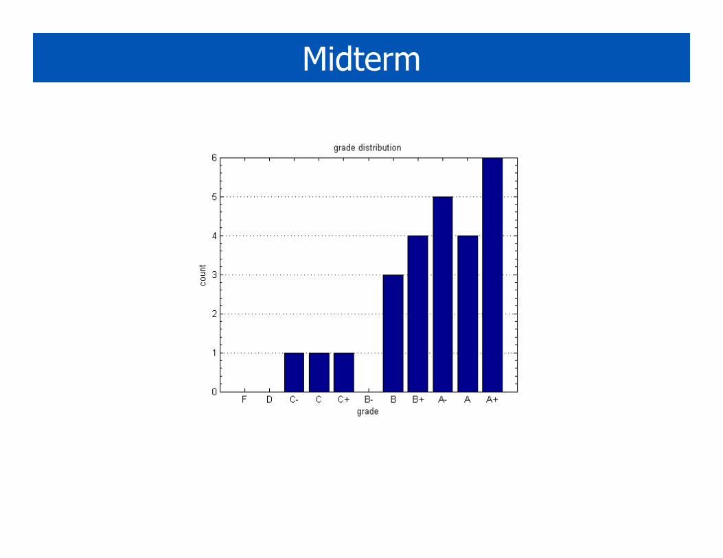
Midterm

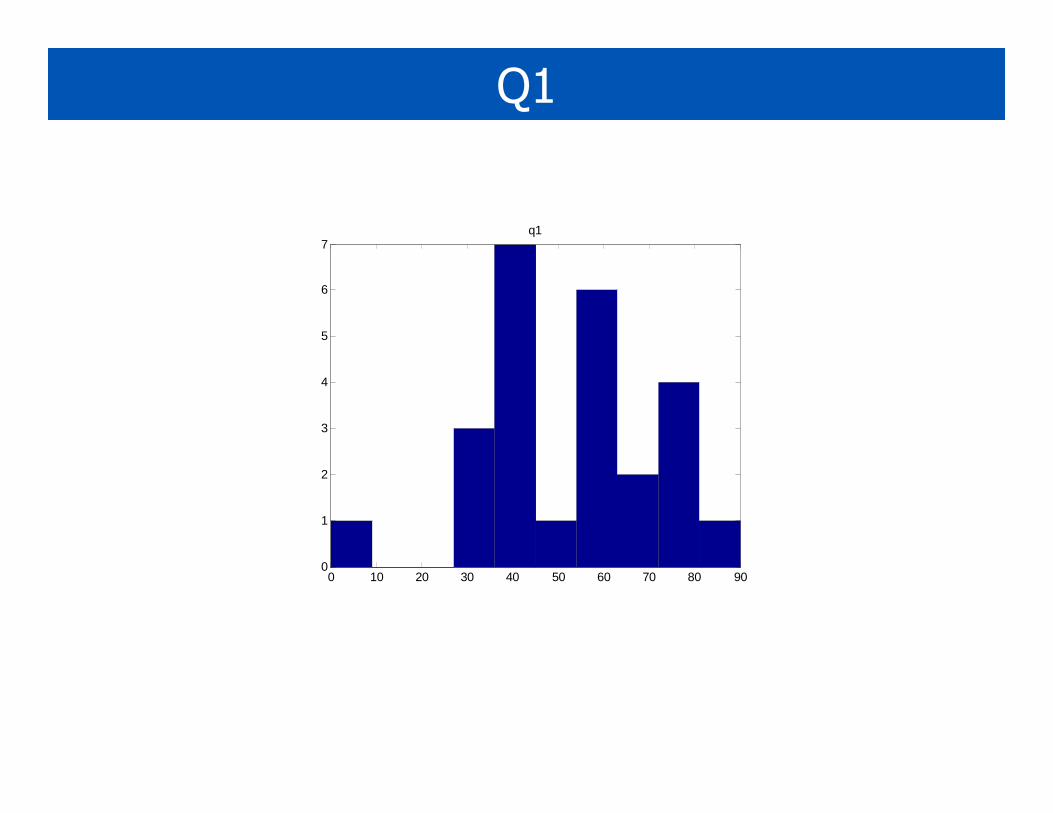
Q1

0 10 20 30 40 50 60 70 80 900

1

2

3

4

5

6

7q1

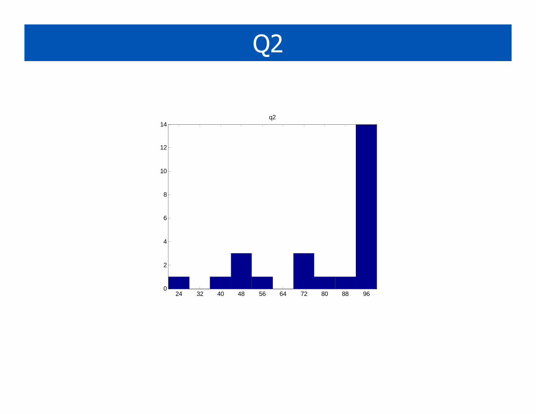
Q2

24 32 40 48 56 64 72 80 88 960

2

4

6

8

10

12

14q2

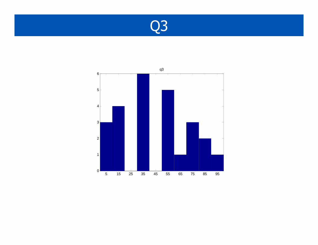
Q3

5 15 25 35 45 55 65 75 85 950

1

2

3

4

5

6q3

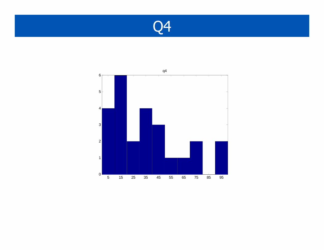
Q4

5 15 25 35 45 55 65 75 85 950

1

2

3

4

5

6q4

Outline

• Problem formulation

• Filter methods• Wrapper methods

• L1 methods

Feature selection

• If predictive accuracy is the goal, often best to keep all predictors and use L2 regularization

• We often want to select a subset of the inputs that are “most relevant” for predicting the output, to get sparse models – interpretability, speed, possibly better predictive accuracy

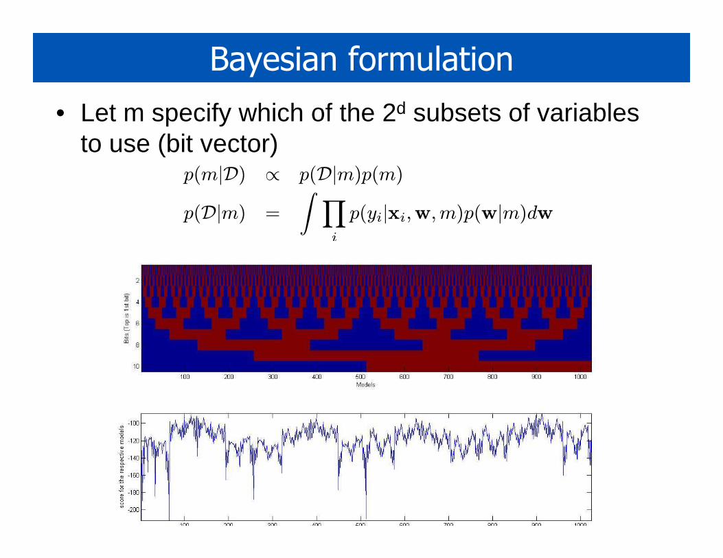
Bayesian formulation

• Let m specify which of the 2d subsets of variables to use (bit vector)

p(m|D) ∝ p(D|m)p(m)

p(D|m) =

∫ ∏

i

p(yi|xi,w,m)p(w|m)dw

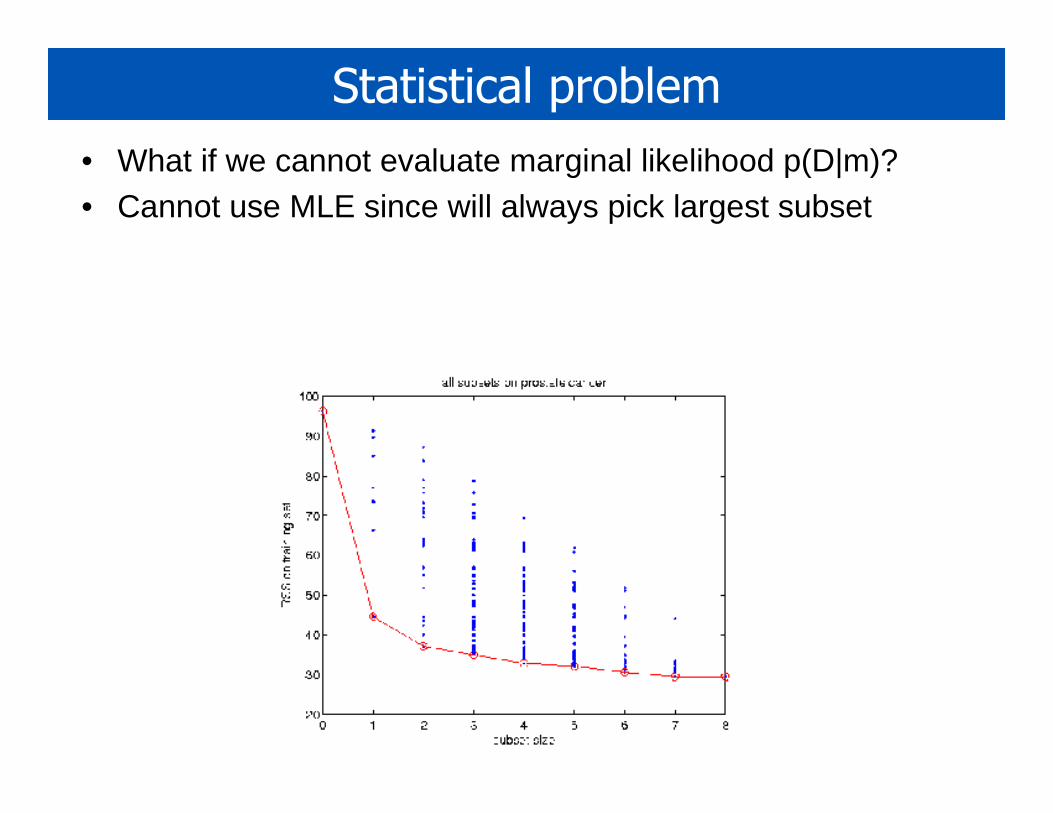
Statistical problem

• What if we cannot evaluate marginal likelihood p(D|m)?• Cannot use MLE since will always pick largest subset

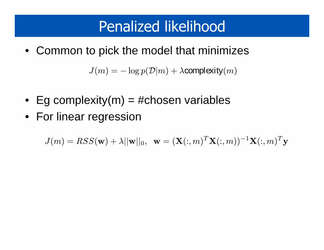
Penalized likelihood

• Common to pick the model that minimizes

• Eg complexity(m) = #chosen variables• For linear regression

J(m) = − log p(D|m) + λcomplexity(m)

J(m) = RSS(w) + λ||w||0, w = (X(:,m)TX(:,m))−1X(:,m)Ty

Computational problem

• 2^d subsets to evaluate

Filter methods

• Compute “relevance” of Xj to Y marginally

• Computationally efficient

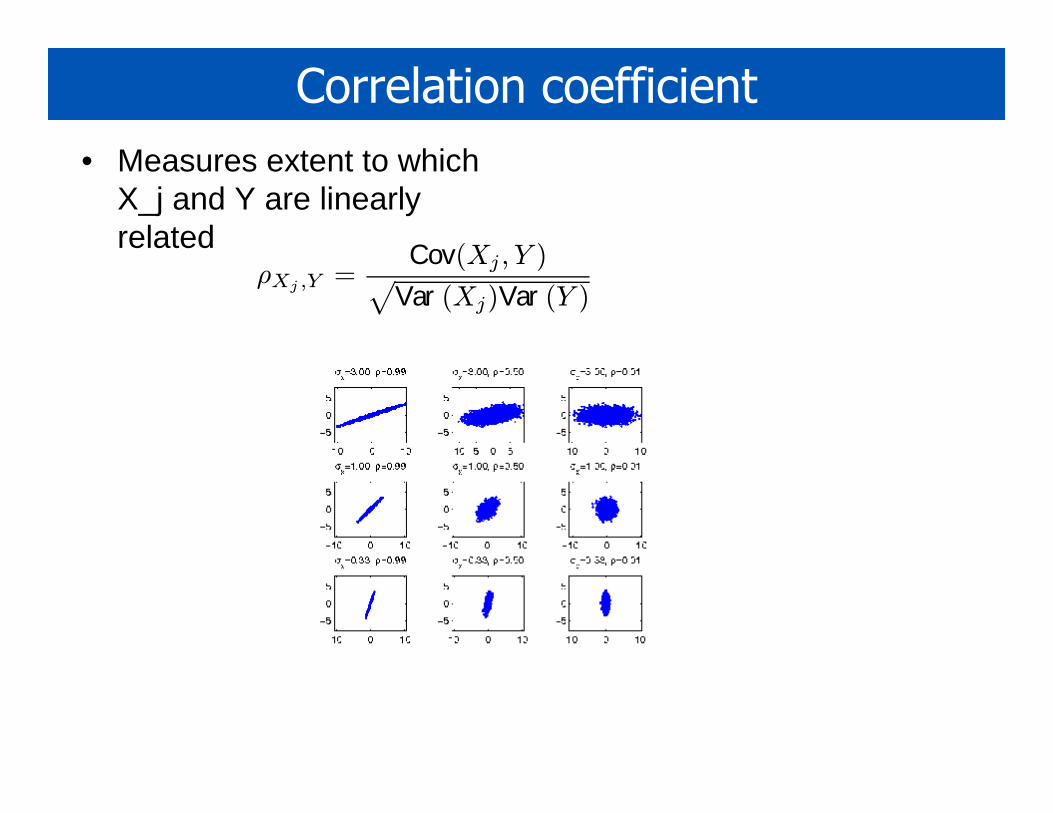
Correlation coefficient

• Measures extent to which X_j and Y are linearly related

ρXj ,Y =Cov(Xj , Y )√

Var (Xj)Var (Y )

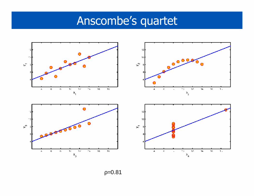
Anscombe’s quartet

ρ=0.81

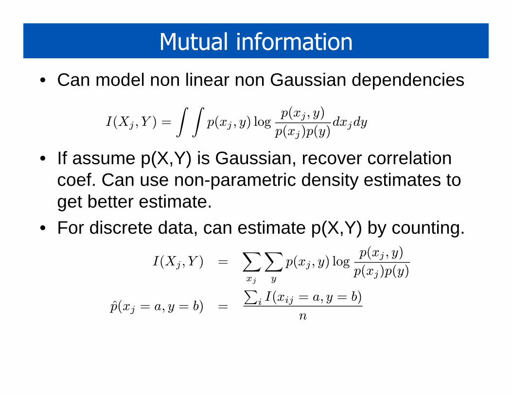
Mutual information

• Can model non linear non Gaussian dependencies

• If assume p(X,Y) is Gaussian, recover correlation coef. Can use non-parametric density estimates to get better estimate.

• For discrete data, can estimate p(X,Y) by counting.

I(Xj , Y ) =

∫ ∫p(xj , y) log

p(xj, y)

p(xj)p(y)dxjdy

I(Xj , Y ) =∑

xj

∑

y

p(xj, y) logp(xj , y)

p(xj)p(y)

p(xj = a, y = b) =

∑i I(xij = a, y = b)

n

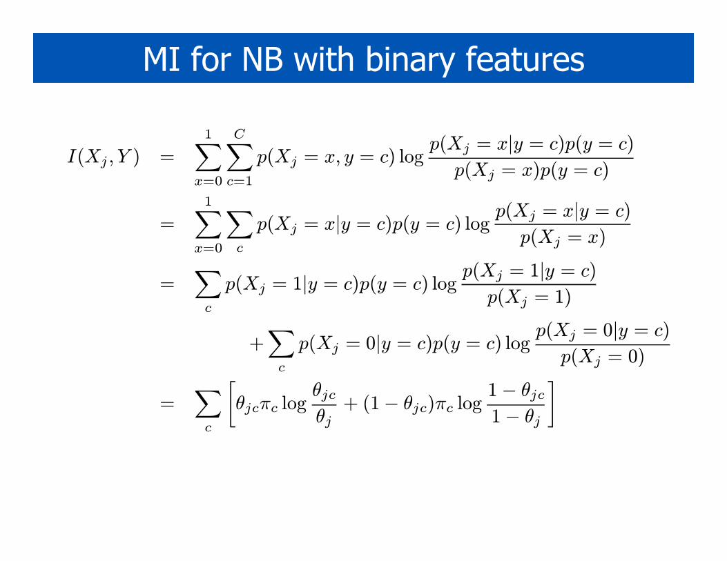
MI for NB with binary features

I(Xj , Y ) =1∑

x=0

C∑

c=1

p(Xj = x, y = c) logp(Xj = x|y = c)p(y = c)

p(Xj = x)p(y = c)

=1∑

x=0

∑

c

p(Xj = x|y = c)p(y = c) logp(Xj = x|y = c)

p(Xj = x)

=∑

c

p(Xj = 1|y = c)p(y = c) logp(Xj = 1|y = c)

p(Xj = 1)

+∑

c

p(Xj = 0|y = c)p(y = c) logp(Xj = 0|y = c)

p(Xj = 0)

=∑

c

[θjcπc log

θjcθj+ (1− θjc)πc log

1− θjc1− θj

]

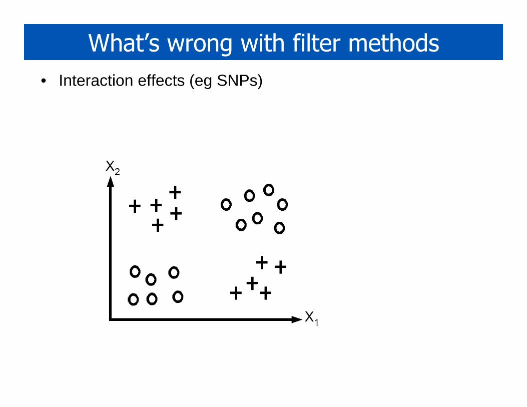
What’s wrong with filter methods

• Interaction effects (eg SNPs)

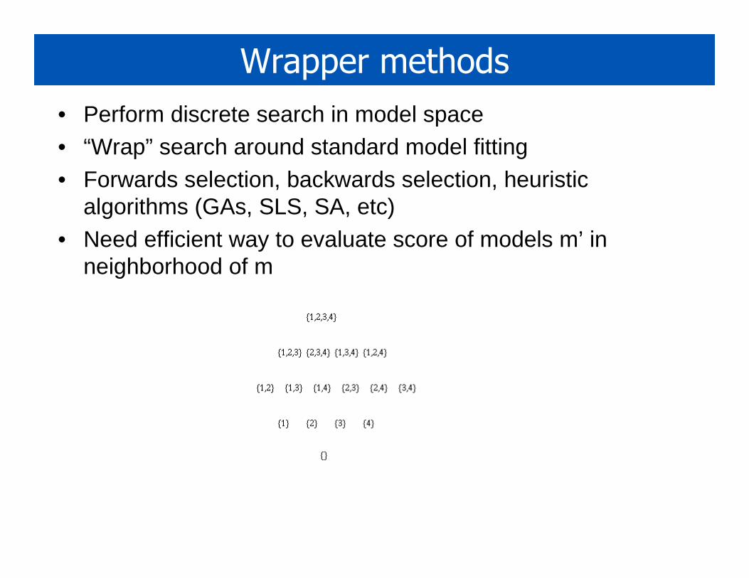
Wrapper methods

• Perform discrete search in model space• “Wrap” search around standard model fitting• Forwards selection, backwards selection, heuristic

algorithms (GAs, SLS, SA, etc)• Need efficient way to evaluate score of models m’ in

neighborhood of m

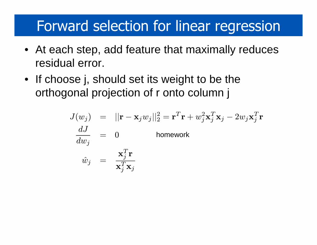
Forward selection for linear regression

• At each step, add feature that maximally reduces residual error.

• If choose j, should set its weight to be the orthogonal projection of r onto column j

J(wj) = ||r− xjwj ||22 = rT r+ w2jxTj xj − 2wjxTj r

dJ

dwj= 0

wj =xTj r

xTj xj

homework

Choosing the best feature

• Inserting formula for optimal w_j

•If features are unit norm, we pick j with largest inner product (smallest angle) to r

J(wj) = rT r+(xTj r)

2

xTj xj− 2

(xTj r)2

xTj xj= rT r−

(xTj r)2

xTj xj

k = argminj

J(wj) = argmaxj

(xTj r)2

xTj xj

k = argminj

J(wj) = argmaxj(xTj r)

2

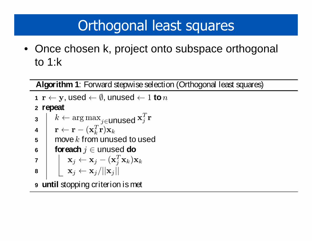
Orthogonal least squares

• Once chosen k, project onto subspace orthogonal to 1:k

Algorithm 1: Forward stepwiseselection (Orthogonal least squares)

r← y, used ← ∅, unused ← 1 ton1

repeat2

k ← argmaxj∈unused x

Tj r3

r← r− (xTk r)xk4

movek from unused to used5

foreach j ∈ unused do6

xj ← xj − (xTj xk)xk7

xj ← xj/||xj ||8

until stopping criterion is met9

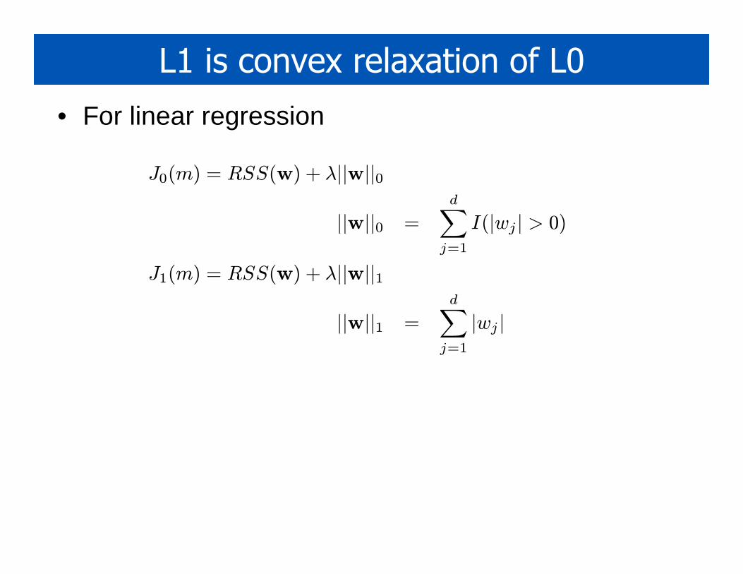
L1 is convex relaxation of L0

• For linear regression

J0(m) = RSS(w) + λ||w||0

||w||0 =d∑

j=1

I(|wj | > 0)

J1(m) = RSS(w) + λ||w||1

||w||1 =

d∑

j=1

|wj |

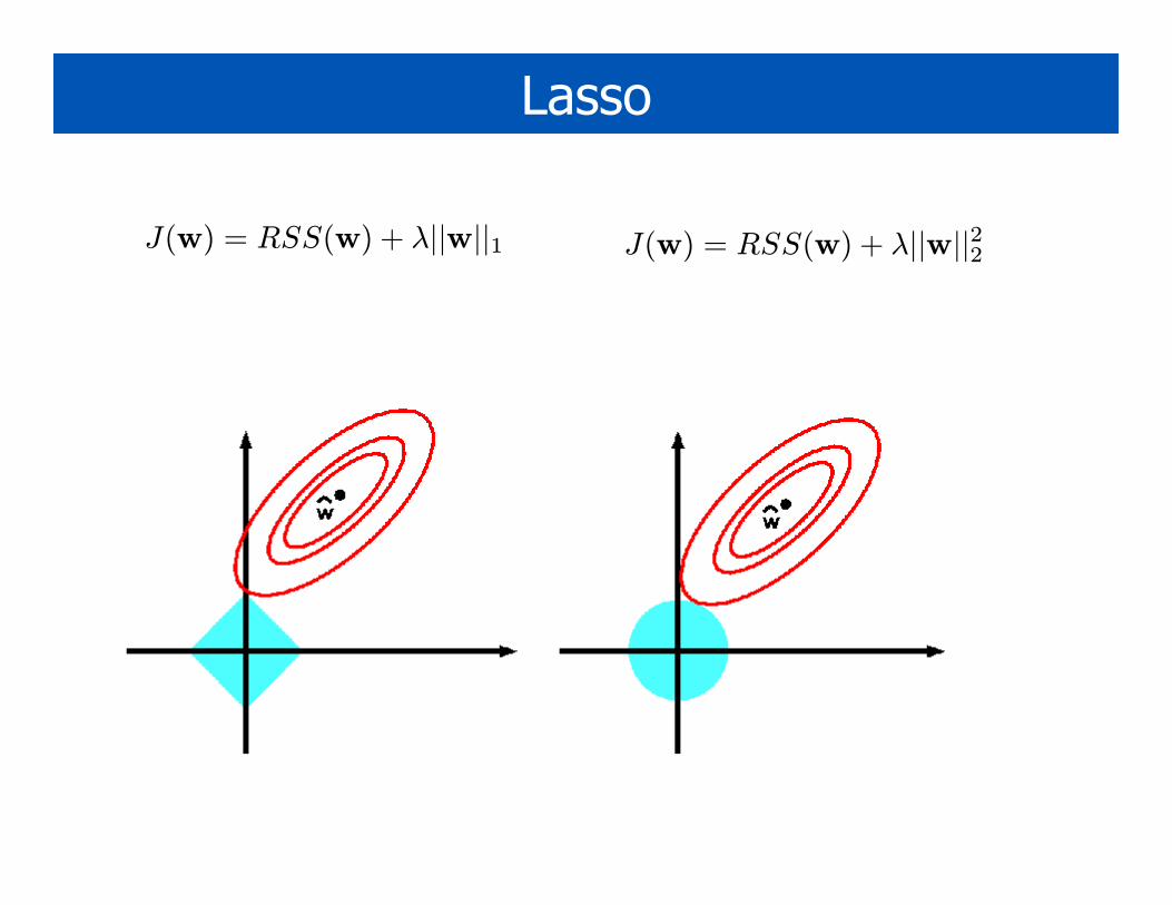
Lasso

J(w) = RSS(w) + λ||w||1 J(w) = RSS(w) + λ||w||22

Whence sparsity?

• Ridge prior: all points on unit circle equal under the prior

• Lasso prior: points on corner of simples more probable a priori

||(1, 0)||2 = ||(1/√2, 1/

√2||2 = 1

||(1, 0)||1 = 1 < ||(1/√2, 1/

√2||1 =

√2

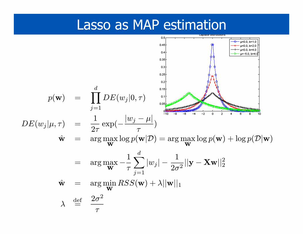
Lasso as MAP estimation

p(w) =

d∏

j=1

DE(wj|0, τ)

DE(wj|µ, τ) =1

2τexp(−|wj − µ|

τ)

w = argmaxw

log p(w|D) = argmaxw

log p(w) + log p(D|w)

= argmaxw

−1τ

d∑

j=1

|wj | −1

2σ2||y −Xw||22

w = argminw

RSS(w) + λ||w||1

λdef=

2σ2

τ

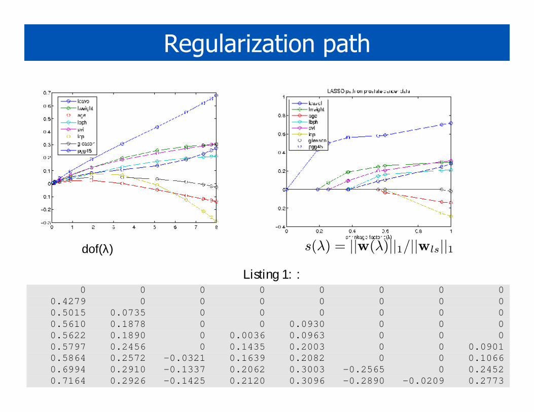
Regularization path

dof(λ) s(λ) = ||w(λ)||1/||wls||1Listing 1: :

0 0 0 0 0 0 0 00.4279 0 0 0 0 0 0 00.5015 0.0735 0 0 0 0 0 00.5610 0.1878 0 0 0.0930 0 0 00.5622 0.1890 0 0.0036 0.0963 0 0 00.5797 0.2456 0 0.1435 0.2003 0 0 0.09010.5864 0.2572 -0.0321 0.1639 0.2082 0 0 0.10660.6994 0.2910 -0.1337 0.2062 0.3003 -0.2565 0 0.24520.7164 0.2926 -0.1425 0.2120 0.3096 -0.2890 -0.0209 0.2773

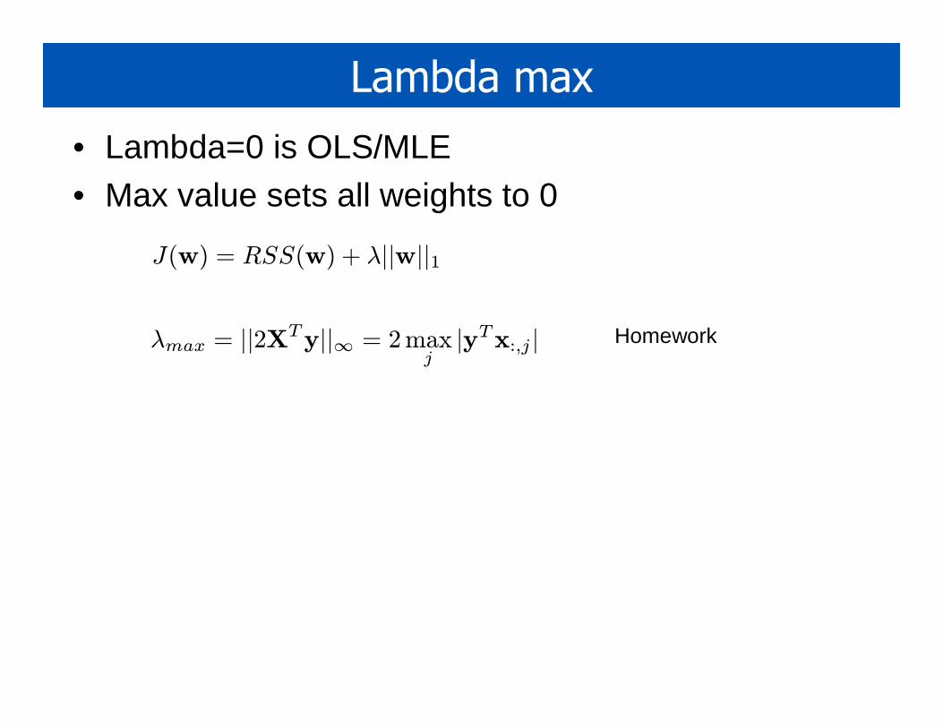
Lambda max

• Lambda=0 is OLS/MLE

• Max value sets all weights to 0

J(w) = RSS(w) + λ||w||1

λmax = ||2XTy||∞ = 2maxj|yTx:,j | Homework