Feature Mapping Techniques for Improving the · PDF fileFeature Mapping Techniques for Improving the Performance of Fault Diagnosis of Synchronous Generator ... mization is used when

Feature Mapping Techniques for Improving the Performance ofFault Diagnosis of Synchronous Generator

R. Gopinath1, C. Santhosh Kumar2, K. Vishnuprasad3, and K. I. Ramachandran4

1,2,3,4 Machine Intelligence Research Laboratory,Department of Electronics and Communication Engineering,

Amrita School of Engineering, Amrita Vishwa Vidyapeetham Coimbatore, Tamil Nadu, Indiar [email protected] [email protected]

[email protected] [email protected]

ABSTRACT

Support vector machine (SVM) is a popular machine learningalgorithm used extensively in machine fault diagnosis. In thispaper, linear, radial basis function (RBF), polynomial, andsigmoid kernels are experimented to diagnose inter-turn faultsin a 3kVA synchronous generator. From the preliminary re-sults, it is observed that the performance of the baseline sys-tem is not satisfactory since the statistical features are non-linear and does not match to the kernels used. In this work,the features are linearized to a higher dimensional space toimprove the performance of fault diagnosis system for a syn-chronous generator using feature mapping techniques, sparsecoding and locality constrained linear coding (LLC). Experi-ments and results show that LLC is superior to sparse codingfor improving the performance of fault diagnosis of a syn-chronous generator. For the balanced data set, LLC improvesthe overall fault identification accuracy of the baseline RBFsystem by 22.56%, 18.43% and 17.05% for the R, Y and B-phase faults respectively.

1. INTRODUCTION

Condition based maintenance (CBM) is the most preferredtechnique in many industrial applications for its reduced main-tenance costs and improved safety operations. CBM reducesthe downtime and increases the productivity (Jardine, Lin, &Banjevic, 2006). Data acquisition is the primary step in CBMwherein mechanical and electrical signals are collected fromthe machines to monitor its health. Feature extraction is animportant process in CBM which maps the measured signalinto the feature space. The performance of the fault diagnosisalgorithm is also dependent on the features (Saxena, Wu, &

Gopinath R., et al. This is an open-access article distributed under the termsof the Creative Commons Attribution 3.0 United States License, which per-mits unrestricted use, distribution, and reproduction in any medium, providedthe original author and source are credited.

Vachtsevanos, 2005; Wu et al., 2004; Wu, Saxena, Patrick, &Vachtsevanos, 2005). Signal processing based feature extrac-tion methods such as time-domain (Samanta & Al-Balushi,2003), frequency-domain (Chen, Du, & Qu, 1995), wavelet(Peter, Peng, & Yam, 2001; Lin & Zuo, 2004; Yan, Gao,& Wang, 2009), and empirical mode decomposition (Yan &Gao, 2008; He, Liu, & Kong, 2011) have been widely used inmachine condition monitoring applications. Many feature se-lection algorithms have been developed for effective fault di-agnosis (Chiang, Kotanchek, & Kordon, 2004; Casimir, Bout-leux, Clerc, & Yahoui, 2006; Verron, Tiplica, & Kobi, 2008;Y. Yang, Liao, Meng, & Lee, 2011; K. Zhang, Li, Scarf,& Ball, 2011) which are used to select the fault discrimina-tive features from the feature space for better classification.Feature transformation approaches are also used to improvethe fault identification performance (Widodo, Yang, & Han,2007; Widodo & Yang, 2007; Y. Zhang, 2009).

Choosing an appropriate classification algorithm for a partic-ular application is a difficult task. It also depends on the char-acteristics of extracted features from the raw data. SVM isan important supervised machine learning algorithm widelyused in various applications including machine fault diag-nosis (Nayak, Naik, & Behera, 2015). The performance ofthe SVM classifier could be affected by the kernel functions,training sample size, and kernel parameters. Zhou et al. in-vestigated the effects of the training sample size, SVM order,and kernel parameters using least squares SVM for the linear,polynomial and Gaussian kernels (J. Zhou, Shi, & Li, 2011).Wang et al. reviewed SVM for uncertain data. Robust opti-mization is used when the direct model could not guarantee agood performance on uncertainty data set (X. Wang & Parda-los, 2015). Khang et al. proposed genetic algorithm basedkernel discriminative features to improve the performance ofmulti-class SVM for low speed bearing fault diagnosis (Kanget al., 2015). Fu et al. made a comparative study on grid

International Journal of Prognostics and Health Management, ISSN2153-2648, 2015 025 1

INTERNATIONAL JOURNAL OF PROGNOSTICS AND HEALTH MANAGEMENT

search (GS), genetic algorithm (GA), and particle swarm op-timization (PSO) to optimize the penalty factor λ and γ in akernel function in a training process (Fu, Tian, & Wu, 2015).

In this work, first the baseline system is developed using SVMkernels (linear, radial basis function (RBF), polynomial, andsigmoid) to identify inter-turn faults in a 3kVA synchronousgenerator. It is observed that the performance of the classifieris not satisfactory as the statistical features are non-linear anddoes not match with the kernels used. Performance of theSVM classifier can be improved by the following approaches:a) Select the features matching a particular kernel. b) Choosean appropriate kernel that fits the features. c) Linearize thefeatures to a higher dimensional space and match with linearkernel. In this paper, the third approach is experimented toimprove the performance of fault diagnosis of a synchronousgenerator using feature mapping techniques.

Sparse coding is an unsupervised machine learning algorithmused to represent feature vectors as a linear combination ofbasis vectors. Liu et al. used adaptive sparse features andclassified the faults using multi-class linear discriminant anal-ysis for machine fault diagnosis (Liu, Liu, & Huang, 2011).Liu et al. also pointed out that sparse coding requires highcomputational cost for dictionary learning for which fasteralgorithms are to be developed (Liu et al., 2011). Zhu et al.proposed an automatic and adaptive feature extraction tech-nique via K-SVD. Faults are diagnosed using the reconstruc-tion error of the sparse representation (Zhu et al., 2014). Fur-ther, fusion sparse coding technique was proposed to extractimpulse components from the vibration signals effectively(Deng, Jing, & Zhou, 2014). For a good classification per-formance, coding algorithm should generate similar codes forsimilar feature vectors. However, sparse coding might selectdifferent bases for similar feature vectors to support sparsity,thus fails to capture the correlations between codes (J. Wanget al., 2010).

Local coordinate coding (LCC) overcomes the drawbacks ofsparse coding by explicitly encouraging the bases to be localand consequently requires the codes to be sparse (Yu, Zhang,& Gong, 2009). However, sparse coding and LCC algorithmshave the computational complexity ofO(M2), whereM rep-resents the total number of vectors in the basis set. Wang etal. proposed locality constrained linear coding (LLC) methodfor the image classification applications (J. Wang et al., 2010)to represent the non-linear features that improve the perfor-mance using linear classifiers (J. Yang, Yu, Gong, & Huang,2009; X. Zhou, Cui, Li, Liang, & Huang, 2009). LLC is afast implementation of LCC which uses locality constraint toselect k nearest bases for each feature vector, therefore it re-duces the computational complexity from O(M2) to O(M +k2). Recent studies show that LLC have been applied to manyimage processing applications such as video summarization(Lu et al., 2014), human action recognition (B. Wang et al.,

2014; Rahmani, Mahmood, Huynh, & Mian, 2014), magneticresonance (MR) imaging (P. Zhang et al., 2013), and coloriza-tion for gray scale facial images for improved performance(Liang et al., 2014). In this paper, the performance of thesparse coding and locality constrained linear coding (LLC)are compared for improving the performance of fault diagno-sis of a synchronous generator. The details of the experimen-tal setup, data collection, feature extraction, sparse coding,locality constrained linear coding (LLC) and support vectormachine (SVM) are discussed in section 2. Experiments andresults are discussed in section 3 and finally, section 4 con-cludes this paper.

2. SYSTEM DESCRIPTION

2.1. Experimental Setup and Data Collection

In synchronous generators, short circuit faults may happen instator winding and field winding coils. Generally, stator andfield winding terminal of synchronous generator has taps at0% and 100% of the coil windings. The three phase 3kVAsynchronous generator is customized to inject faults in differ-ent magnitude. For example, 30%, 60%, and 82 % of the totalnumber of turns in the stator winding leads are made availableto the front panel for injecting short circuit faults between anyof these points.

Figure 1. Block diagram of the experimental setup

Each phase has 18 taps, making the total number of tapsacross three phases to 54, to inject different short circuit faultsin the generator. All terminal leads from the stator windingare taken to the front panel board. Block diagram of the ex-perimental setup is shown in Fig. 1. Photograph of the cus-tomized synchronous generator and experimental facility isshown in Figs. 2 and 3. Design details of the customized syn-chronous generator can be found in (Gopinath et al., 2013).

In this work, inter turn short circuit faults are injected in acontrolled manner. Generator is connected to the three phaseresistive load. Data acquisition system NI-PXI 62211 is usedto interface the current sensors. Each experiment is con-ducted for 10 seconds and current signals are sampled at 1kHz. This makes the number of samples available for eachtrial to be 10,000. The process is then repeated for different

1http://sine.ni.com/ds/app/doc/p/id/ds-15/lang/en

2


Figure 2. Customized 3 kVA Synchronous Generator

Figure 3. Experimental Facility

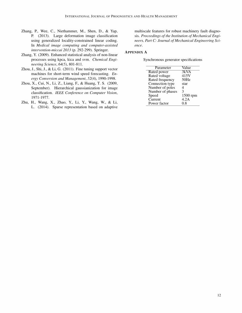
fault conditions to make the data collection process complete.Fig. 4, illustrates the current signatures acquired from the3kVA generator. Specifications of the synchronous genera-tor is listed in Appendix A. Short circuit faults are injected at30% (8 turns), 60% (16 turns), and 82% (22 turns) of the totalnumber of turns (27 turns). The data from each trial is dividedinto multiple frames with a window size of 512 samples. Thetime domain signal is converted into frequency domain usingFast Fourier Transform (FFT). Statistical frequency domainfeatures are used to extract the fault information from the rawdata. The details of the frequency domain features (Lei, He,& Zi, 2008) are listed in Table 1.

2.2. Sparse Coding

Sparse coding is an unsupervised learning method, learns theset of over-complete bases to represent the data efficiently(Olshausen & Field, 1997). Sparse coding finds the basis vec-tors such that, the input vectors X = [x1, x2, ......, xN ]T ∈RD×N , with D dimension can be expressed as a linear com-bination of these bases. The input vector can be expressed as(Olshausen & Field, 1997):

xi =

N∑i=1

bici (1)

where B = [b1, b2, ......, bM ] ∈ RD×M is basis vectors orcodebooks. Over-complete basis identifies the patterns in the

input data. However, coefficients or codes ci are not uniquelydetermined by the input vectors, with an over-complete basis.This necessitates to add the sparsity criterion for better repre-sentation (J. Yang et al., 2009), i.e., most of the coefficientsci are zero or nearly zero and only a few coefficients are non-zero to represent the input data efficiently. Sparse coding canbe expressed as (J. Yang et al., 2009):

minc

N∑i=1

‖xi −Bci‖2 + λ ‖ci‖l1 (2)

where λ ‖ci‖l1 is the sparse regularization term and it is deter-mined as l1 norm of ci. Sparse regularization ensures that thecodebook is over-complete and unique solution for the under-determined system, hence it captures the patterns in the inputdata.

2.3. Locality Constrained Linear Coding (LLC)

Locality constrained linear coding (LLC) is a feature map-ping technique used to represent non-linear features as linearfeatures (J. Wang et al., 2010). LLC codes are sparse andhigh dimensional. In LLC, each input vector is representedas a linear combination of k-nearest basis vectors. The basisvectors are computed from the data set using k-means clus-tering algorithm. Basis vectors are called as codebooks in thecontext of coding schemes algorithm (J. Wang et al., 2010).The LLC coding process is described in Fig. 5. LetX be a setof D- dimensional input database X = [x1, x2, ......, xN ] ∈RD×N . Given a codebook, B = [b1, b2, ......, bM ] ∈ RD×M ,coding algorithm converts each input data into a M - dimen-sional code, where [b1, b2, ......, bM ] are basis vectors and thesebasis vectors captures the patterns in the input data. Criteriafor the LLC code is expressed as (J. Wang et al., 2010):

minC

N∑i=1

‖xi −Bci‖2 + λ ‖di � ci‖2 (3)

s.t 1T ci = 1, ∀i

where � represents element-wise multiplication. Localityadaptor di ∈ RM provides freedom for each basis vector pro-portional to its similarity to the input feature xi. Localityadaptor can be expressed as (J. Wang et al., 2010):

di = exp

(dist(xi, B)

σ

)(4)

where dist(xi, B) is the Euclidean distance between xi andbj and it can be written as (J. Wang et al., 2010):

3


Table 1. Frequency Domain Features

Description Feature Description Feature

Mean Feat1 =∑K

k=1 s(k)

K Root Mean Square (RMS) Feat7 =

√∑Kk=1 f

2ks(k)∑K

k=1 s(k)

frequency

Variance Feat2 =∑K

k=1(s(k)−Feat1)2

K−1 Spectrum power convergence Feat8 =

√∑Kk=1 f

4ks(k)∑K

k=1 f2ks(k)

Skewness Feat3 =∑K

k=1(s(k)−Feat1)3

K(√Feat2)3

Stability factor Feat9 =∑K

k=1 f2ks(k)√∑K

k=1 s(k)∑K

k=1 f4ks(k)

Kurtosis Feat4 =∑K

k=1(s(k)−Feat1)4

K(Feat2)2Coefficient variability Feat10 = Feat6

Feat5

Frequency centre Feat5 =∑K

k=1 fks(k)∑Kk=1 s(k)

Skewness frequency Feat11 =∑K

k=1(fk−Feat5)3s(k)

K(Feat6)3

Standard deviation Feat6 =

√∑Kk=1(fk−Feat5)2s(k)

K Kurtosis frequency Feat12 =∑K

k=1(fk−Feat5)4s(k)

K(Feat6)4

frequency

Spectrum power Feat13 =∑K

k=1(fk−Feat5)12 s(k)

K√Feat6

positional factorwhere s(k) is the spectrum for k = 1, 2..K,K is the number of spectrum lines fk is the frequency value of the kth spectrum.

Figure 4. Current signature captured during no fault and inter turn fault conditions for the 3 kVA generator

dist(xi, B) = [dist(xi, b1), ...dist(xi, bM )]T

di is normalized to (0,1] by subtracting max(dist(xi, B))from dist(xi, B). σ adjusts the weight decay speed for thelocality adaptor. The constraints 1T ci = 1 indicates the shiftinvariant requirements of the LLC code. LLC selects the lo-cal bases from the basis set for each feature vector to form alocal coordinate system using Eq. (3). LLC encoding processcan be speeded up by using the k- nearest neighbors of xi asthe local basesBi instead of using all the bases in the Eq. (3).This approach is called as fast approximation LLC methodand it uses the following criteria (J. Wang et al., 2010):

minC̃

N∑i=1

‖Xi − c̃iBi‖2 (5)

s.t 1T c̃i = 1, ∀iFast approximation LLC method reduces the computation com-plexity fromO(M2) toO(M+k2). In this paper, fast approx-imation LLC is used for its reduced computational complex-ity and fast encoding process (J. Wang et al., 2010).

2.4. Support Vector Machine (SVM)

SVM (Vapnik & Vapnik, 1998) is a supervised learning algo-rithm which is widely used for classification problems. SVM

4


Figure 5. LLC coding process

constructs a hyperplane that separates two classes, and it canbe extended to multi-class classification problems. Fig. 6,pictorially explains how an SVM classifier finds the sepa-rating hyper-plane. The planes parallel to the hyperplaneare called bounding planes. The data points that lie on thebounding planes are called support vectors. The distance be-tween the two bounding planes is the margin. The centralhyperplane or classifier maximizes the margin and it can beobtained by finding the distance (d1 and d2) between eachbounding plane to the origin respectively, and subtracting be-tween the distances (d = d2−d1). Margin of the classifier canbe expressed as (Vapnik & Vapnik, 1998):

2

‖w‖2(6)

In order to maximize the margin, SVM learning is formulatedby rewriting the Eq. (6) as a minimization problem, and it canbe expressed as (Vapnik & Vapnik, 1998):

minw,b

‖w‖2

2(7)

Subject to the constraint:

yi[(wTxi)] + b ≥ 1

where xi = [x1, x2, ....xn] is the data set and yi ∈ {1,−1}be the class label of xi. b is the bias. Using the Lagrangemultipliers, the optimal solution can be computed by usingthe following equation:

minw,b

maxα≥0

{1

2‖w‖2 −

n∑i=1

αi[yi(wTxi − b

)− 1]

}(8)

Figure 6. Linear separating hyperplanes for a separable case

whereαi is a Lagrange multiplier. Using Karush Kuhn Tucker(KKT) conditions (Kuhn & Tucker, 1951), solution can beexpressed as the following:

w =

n∑i=1

αiyixi (9)

b =1

NSV

N∑i=1

wTxi − yi (10)

Using the definition for w as defined in Eq. (9), the problemcan be written in the dual form as:

maxαi

n∑i=1

αi −1

2

∑i,j

αiαjyiyjk(xi, xj)

(11)

subject to αi ≥ 0 and

n∑i=1

αiyi = 0.

where k(xi, xj) is a kernel function. αi can be obtained bysolving the Eq. (11), and the decision function can be ex-pressed as (Vapnik & Vapnik, 1998):

f(x) = sign(wTx+ b) = sign(

n∑i=1

αiyixiTx− b) (12)

5


When the data is not linearly separable, the non-linear kernelis applied for the classification, which transforms the featuresinto a higher dimensional space, where it is linearly separable.In this paper, linear and non-linear SVM are experimentedfor the fault diagnosis. The complete process of the proposedapproach is shown in the Fig. 7.

3. EXPERIMENTS AND RESULTS

In this work, the following experiments have been carried outfor diagnosing the inter-turn faults in the 3 kVA synchronousgenerator.

1. Develop baseline system using linear, polynomial, radialbasis function (RBF), and sigmoid SVM kernels for thefault classification

2. Improve the performance of the baseline system usingfeature mapping techniques, sparse coding and LLC.

3. Performance comparison of the feature mapping tech-niques using overall classification accuracy and receiveroperating characteristic (ROC) curve.

Inter-turn faults are injected in the R, Y, and B phases of a 3kVA generator stator winding. For every trial, current signalsare acquired from all the three phases. Frequency domainstatistical features are extracted from the raw data. Then, theexperiments with the R, Y, and B phase inter-turn faults aretreated as independent two class classification problems, i.e.,no-fault or fault in R phase, no-fault or fault in Y phase andno-fault or fault in B phase, of a 3 kVA generator. It may benoted that anN class problem may be realized asN two classproblems.

Experiments are conducted at different load conditions suchas 0.5 A, 1 A, 1.5 A, 2 A, 2.5 A, 3 A, and 3.5 A loads. Datafrom these loads are combined together for fault classifica-tion. However, training and test data are collected separately,and no data is shared between the training and test sets. Inthis work, the experiments have been performed using bal-anced and unbalanced data sets to check the effectiveness ofthe proposed approach. Further, k-fold cross validation tech-nique is also experimented using balanced data set separately.In addition, experiments using unseen load condition is per-formed to check the effectiveness of the proposed approach inremoving load dependencies of the features. Experiments arecarried out on a IBM X3100 M42 (Intel Xeon E3-1220v2 se-ries) server, with 8 GB memory and 3.1 GHz Quad-core pro-cessor. MATLAB3 toolboxes are used for computing sparse4

and LLC5 codes.

2http://www-03.ibm.com/systems/x/hardware/tower/x3100m4/3http://in.mathworks.com/products/matlab/4http://stanford.edu/˜boyd/l1 ls/5http://www.ifp.illinois.edu/˜jyang29/LLC.htm

3.1. Experiments using balanced data set

In this experiment, the data set used for training and test arenearly balanced (no-fault data: 55% and fault data: 45%).Details of the data sets used in our experiments are presentedin Table 2.

Table 2. Total data collected for no fault and fault conditions(No-fault data:55%; Fault-data:45%)

Machine conditionNo fault Inter-turn fault Total

Train data 13300 10640 23940Test data 5852 4683 10535Total 19152 15323 34475

Baseline system: The baseline system is developed usingSVM kernels such as linear, polynomial, RBF, and sigmoid.Table 3 lists the baseline system performance of the SVM ker-nels for the R, Y, and B phase faults. From the experiments,it is noted that RBF kernel performs better when compared toother kernels for the baseline system. It is observed that theperformance of the classifier is not encouraging since the fea-tures does not match with the kernels and exhibit non-linearcharacteristics. The classification accuracies are generallylow in the baseline system because the fault characteristicsvary largely across the load conditions. The classification ac-curacy can be improved by removing this load dependenciesof the features. In this paper, the objective is to improve theperformance of fault diagnosis of generator by linearizing thefeatures in a higher dimensional space using feature mappingtechniques.

Table 3. Baseline system classification performance (accu-racy in %) of SVM for the balanced data set

Kernel/Inter-turn fault R phase Y Phase B PhaseLinear 67.45 61.46 66.68c = 10, γ = 0.0256

RBF 76.66 81.35 82.31c = 10, γ = 0.0256

Polynomial 65.33 67.94 72.86c = 1, γ = 0.0256

Sigmoid 55.54 55.54 55.54c = 1, γ = 0.0256

where c is the cost and γ is the kernel parameter.

Sparse coding: First, codebook (basis set or dictionary) iscomputed from the training data set. Subsequently, the fea-ture vectors from the training and test data set are representedas a linear combination of the basis vectors from the code-book. In this process, codebook is common for the trainingand test data sets. Then the feature dimension is expandedfrom 39 (13 features per phase) to 256, 512, and 1024 fea-ture vectors. Linear SVM is then used to classify the sparserepresented features. Table 4 lists the classification perfor-

6


mance of the sparse coding for the inter-turn fault diagno-sis of the generator. Experiments are performed for the dif-ferent codebook sizes of 256, 512, and 1024, and obtainedthe improved performance for 256 codebooks. Sparse codingimproves the performance of the baseline RBF kernel, from76.66% to 87.35%, 81.35% to 87.37% and 82.31% to 91.14%for the R, Y and B phase faults respectively. Table 5 lists theimproved classification performance and its computation timefor sparse coding. Since the computation time is very large,it is not suitable for practical applications.

Table 4. Classification performance of sparse coding usinglinear SVM for the balanced data set

Inter-turn fault Classification accuracy (%)256 512 1024codebooks codebooks codebooks

R Phase 87.35 87.40 87.23Y Phase 87.37 86.91 86.82B Phase 91.14 90.85 91.44

Figure 7. Machine fault diagnosis using locality constrainedlinear coding (LLC)

LLC: In LLC, finding basis vectors is similar to sparse cod-ing, but the input data is represented as a linear combinationof k nearest basis vectors. Experiments are performed withdifferent codebook sizes and k-nearest neighbors (k-NN) toachieve a good classification performance for the fault iden-

Table 5. Improved classification performance and its compu-tation time for sparse coding (256 codebooks)

Inter-turn fault Accuracy (%) CPU time (Mins)R Phase 87.35 36.87Y Phase 87.37 35.43B Phase 91.14 39.93

tification system. Table 6 lists the performance of the LLCbased linear SVM for the different codebook size and k-NNrespectively. Codebook sizes 256, 512, and 1024 are used,and each codebook is experimented with 10, 20, 30, and 40nearest neighbors for the R, Y, and B phase inter-turn faultsrespectively. Though codebook sizes 256 and 512 improvesthe performance, 1024 codebooks achieve the best classifica-tion performance. For 1024 codebooks with a selection of 40nearest neighbors, LLC improves the baseline system (RBFkernel) by 22.56%, 18.43% and 17.05% absolute for the R, Yand B phase faults respectively.

Table 6. Classification performance of LLC using linearSVM for the balanced data set

Inter-turn k-NN Codebooks & accuracy (%)fault

256 512 1024R Phase 10 98.33 98.19 98.50

20 97.88 99.07 99.1430 96.43 99.12 99.1540 92.74 98.31 99.22

Y Phase 10 98.07 98.88 98.4820 98.01 99.34 99.1730 97.16 99.17 99.5840 95.95 97.96 99.78

B Phase 10 99.41 99.37 98.5620 99.20 99.64 99.3130 99.17 99.50 99.3440 99.01 99.23 99.36

Table 7. Improved classification performance and its compu-tation time for LLC (1024 codebooks)

Inter-turn fault kNN Accuracy (%) CPU time (Sec)R Phase 40 99.22 70.45Y Phase 40 99.78 63.90B Phase 40 99.36 50.13

Table 7 lists the improved classification performance and itscomputation time for LLC. From our experiments, it is notedthat LLC takes less computation time compared to sparsecoding, therefore LLC reduces computational complexity andachieves improved performance for the classifier.

3.2. Experiments using unbalanced data set

In practical applications, injecting faults and collecting largenumber of fault data is not possible, to capture the intelli-gence about the system. This necessitates to analyze the faultidentification system using smaller proportion of fault data, tocheck the effectiveness of the feature mapping techniques. Inthis work, the experiments were carried out using unbalanceddata (No-fault data:80%; Fault-data:20%) by taking smallerproportion of fault data for the training. However, equal pro-

7


portion of fault and no-fault data is taken for the testing for afair comparison of the results with the balanced data set ex-periments. Details of the data set used in our experiments islisted in Table 8. The performances of the baseline, sparsecoding and LLC for the unbalanced data set are listed in theTables 9 -11. From the results it is observed that, the perfor-mance of the baseline system, sparse coding and LLC havereduced for R, Y and B phases with the use of unbalanceddata set. For the sparse coding, 256 codebooks performs bet-ter than other codebook sizes. However, when compared tothe performance of the sparse coding for the balanced andunbalanced data set for 256 codebooks, the performance forthe unbalanced data set got decreased by 4.27%, 2.10%, and2.25% absolute for the R, Y, and B phases respectively. Simi-larly, the performance of the LLC with 1024 codebooks usingbalanced and unbalanced data set, the performance for the un-balanced data set got reduced by 3.84%, 1.77%, and 0.76%absolute for the R, Y, and B phases respectively. Thoughthe unbalanced data set affect the performance of the clas-sifier, the overall classification accuracy does not reduce sig-nificantly for the sparse coding and LLC, emphasizing thesealgorithms are suitable when data under fault conditions isscarce.

Table 8. Experiments using unbalanced data set (Trainingdata: No-fault data:80%; Fault-data:20%, Test data: No-faultdata:55%; Fault-data:45%)

Machine conditionNo-fault Inter-turn fault Total

Train data 13300 3346 16646Test data 5852 4683 10535Total 19152 8029 27181

Table 9. Baseline system classification performance (accu-racy in %) of the SVM for the unbalanced data set


RBF 59.54 59.92 59.49c = 10, γ = 0.0256

Polynomial 59.28 63.78 72.67c = 20, γ = 0.0256

Sigmoid 55.54 55.54 55.54c = 1, γ = 0.0256


3.3. ROC curve analysis

Receiver operating characteristic (ROC) curve is used to vi-sualize and evaluate the classifier performance (Japkowicz &Shah, 2011). It shows the trade-off between the probabilityof detection or true positives rate (TPR), and the probabil-ity of false alarm or false positives rate (FPR). In this work,the performance of the baseline RBF system, sparse coding

Table 10. Classification performance of sparse coding usinglinear SVM for the unbalanced data set



Table 11. Classification performance of LLC using linearSVM for the unbalanced data set


256 512 1024R Phase 10 95.67 94.60 93.76

20 95.48 94.65 94.7130 93.29 94.86 94.9340 90.56 96.44 95.38

Y Phase 10 95.87 96.25 96.0120 94.69 97.69 97.2730 93.59 97.09 98.0140 94.30 94.40 97.82

B Phase 10 97.05 97.19 96.7720 98.32 97.84 97.8630 97.03 98.69 98.1540 97.31 98.25 98.60

and LLC are compared using ROC curve for the balancedand unbalanced data set (smaller proportion of fault data isconsidered for the training). Figure 8 -10 shows the perfor-mance comparison of the feature mapping techniques for theR, Y, and B phase faults. It is observed that area under curve(AUC) value becomes closer to 1 for the LLC compared tobaseline RBF and sparse coding techniques. However, forthe experiments using unbalanced AUC value got reduced forthe baseline RBF, sparse coding and LLC.

3.4. k-fold cross validation using balanced data set

The experiments discussed in the subsections 3.1 and 3.2 wereperformed using one partition of data only. However, the useof fixed data set may over-fit the model. To overcome thisproblem, k-fold cross validation technique is used to assessthe performance of the classifier. The balanced data set isused for evaluating the performance of the classifier. In thisexperiment, 19152 samples of no-fault and 15323 of faultsamples are used for 10-fold cross validation. The perfor-mance of the baseline system, sparse coding and LLC for the10-fold cross validation technique is listed in Table 12-14.

From the experiments it is noted that RBF kernel performsbetter than other kernels. Sparse coding improves the perfor-mance by 7.61%, 1.07% and 5.37% for the R, Y, and B phasesrespectively for 256 codebooks. Similarly, LLC improves the

8


0 0.1 0.2 0.3 0.4 0.5 0.6 0.7 0.8 0.9 10

0.1

0.2

0.3

0.4

0.5

0.6

0.7

0.8

0.9

1

False Positive Rate

Tru

e P

osi

tive

Ra

tePerformance comparison of feature mapping techniques for R phase fault

Balanced data set − Baseline RBF; AUC=0.9788Balanced data set − Sparse coding (256 codebooks); AUC=0.9191Balanced data set − LLC (1024 codebooks, 40 knn); AUC=0.9996Unbalanced data set − Baseline RBF; AUC=0.955Unbalanced data set − Sparse coding (256 codebooks); AUC=0.9105Unbalanced data set − LLC (1024 codebooks, 40knn); AUC=0.9935

Figure 8. ROC plot for the performance comparison of fea-ture mapping technniques for the R phase fault

0 0.1 0.2 0.3 0.4 0.5 0.6 0.7 0.8 0.9 10

0.1

0.2

0.3

0.4

0.5

0.6

0.7

0.8

0.9

1

False Positive Rate

Tru

e P

osi

tive

Ra

te

Performance comparison of feature mapping techniques for Y phase fault

Balanced data set − Baseline system RBF; AUC=0.9853 Balanced data set − Sparse coding (256 codebooks); AUC=0.9391Balanced data set − LLC (1024 codebooks, 40 knn); AUC=0.9997Unbalanced data set − Baseline system RBF; AUC=0.9593Unbalanced data set − Sparse coding (256 codebooks); AUC=0.9116Unbalanced data set − LLC (1024 codebooks, 30 knn); AUC=0.9940

Figure 9. ROC plot for the performance comparison of fea-ture mapping techniques for the Y phase fault

Table 12. Baseline system classification performance (accu-racy in %) of the SVM using 10-fold cross validation


RBF 80.01 85.77 86.02c = 10, γ = 0.0256

Polynomial 63.05 67.16 65.43c = 30, γ = 0.0256

Sigmoid 55.55 55.55 55.55c = 10, γ = 0.0256


performance by 18.97%, 13.83%, and 13.76% for the R, Y,and B phases respectively for 1024 codebooks. It is observedthat, the experiments using 10-fold cross validation technique

0 0.1 0.2 0.3 0.4 0.5 0.6 0.7 0.8 0.9 10

0.1

0.2

0.3

0.4

0.5

0.6

0.7

0.8

0.9

1

False Positive Rate

Tru

e P

osi

tive

Ra

te

Performance comparison of feature mapping techniques for B phase fault

Balanced data set − Baseline system RBF; AUC=0.9805Balanced data set − Sparse coding (256 codebooks); AUC=0.9735Balanced data set − LLC (1024 codebooks, 40 knn); AUC=0.9994Unbalanced data set − Baseline system RBF; AUC=0.9559Unbalanced data set − Sparse coding (256 codebooks); AUC=0.9669Unbalanced data set − LLC (1024 codebooks, 40 knn); AUC=0.9981

Figure 10. ROC plot for the performance comparison of fea-ture mapping techniques for the B phase fault

Table 13. Classification performance of sparse coding usinglinear SVM for the 10-fold cross validation



Table 14. Classification performance of LLC using linearSVM for the 10-fold cross validation


256 512 1024R Phase 10 98.47 98.86 98.98

20 98.10 99.08 98.3230 96.31 99.04 98.3140 93.47 98.03 98.42

Y Phase 10 98.00 98.61 98.6720 98.36 99.32 99.4630 98.04 99.29 99.6040 99.01 99.23 99.60

B Phase 10 99.41 99.37 99.4220 99.20 99.64 99.7330 99.17 99.50 99.7540 99.01 99.23 99.78

for the balanced data set does not affect the performance ofthe feature mapping techniques significantly compared to ex-periments using single partition of data.

9


3.5. Experiments on unseen load condition

Experiments are also carried out for unseen load condition of3 kVA synchronous generator to check the effectiveness ofLLC in removing the load dependencies of the features. Themodel is trained using 0.5A, 1A, 2A, 2.5A, 3A, and 3.5A loadconditions and tested on 1.5A load. Total samples of 18240and 1338 are used for training and testing, respectively, withan equal proportion of no-fault and fault data. From the ex-periments, it is observed that the best performance for thebaseline system is obtained using linear kernel with an over-all classification accuracy of 59.04%, 72.79% and 80.94%for the R, Y, and B phases respectively. The improved per-formance is obtained using LLC with an overall accuracy of73.46%, 78.70%, and 87.66% by selecting 8, 23, and 36 near-est neighbors for the R, Y, and B phases respectively, with thecodebook size of 64. Experimental results show that LLCcould perform better even if unseen load condition is used forfault diagnosis.

4. CONCLUSIONS

In this paper, feature mapping algorithms, sparse coding andLLC are used to improve the performance of SVM for theinter-turn fault identification of 3kVA synchronous genera-tor. As the features are non-linear, feature mapping tech-niques are used to linearize the features in a higher dimen-sional space to improve performance of the fault diagnosissystem. Experiments are performed for the balanced and un-balanced data using single partition of data. Sparse codingimproves the performance significantly with a high compu-tational cost. Therefore, LLC is used to reduce the com-putational complexity and enhance the performance of thesystem. By using the balanced data set, 1024 codebookswith 40 nearest neighbors are selected empirically for its bestperformance. LLC improves the overall fault identificationaccuracy of the baseline RBF system by 22.56%, 18.43%and 17.05% absolute for the R, Y and B-phase faults respec-tively. The performance of the feature mapping techniquesare also illustrated through ROC curves. The AUC value be-comes closer to one for LLC compared to the sparse codingand baseline RBF system. The performance of the classi-fier is also assessed using 10-fold cross validation technique.From the experiments, it is observed that LLC outperformssparse coding in terms of classification performance and com-putational cost for the inter-turn fault diagnosis of the syn-chronous generator. Though LLC has been used widely inimage classification problems, the reported experimental re-sults show that, LLC could be used for other applications alsoif the features used in the system does not match with SVMkernels and exhibits non-linear characteristics.

ACKNOWLEDGEMENT

Authors would like to acknowledge the financial support pro-vided by Aeronautical Development Agency (ADA) -NationalProgramme on Micro and Smart Systems (NPMASS), India.Authors thank Dr. Vanam Upendranath and Mr. P. V. R.Sai kiran, Structural Technologies Division, CSIR- NationalAerospace Laboratories, Bangalore, India for their help dur-ing the course of this work. Authors also thank Mr. Pushpara-jan, M., Mr. Kuruvachan K. George., and Mr. Sreekumar, K.T., for their support through out this work.

REFERENCES

Casimir, R., Boutleux, E., Clerc, G., & Yahoui, A. (2006).The use of features selection and nearest neighbors rulefor faults diagnostic in induction motors. EngineeringApplications of Artificial Intelligence, 19(2), 169-177.

Chen, Y. D., Du, R., & Qu, L. S. (1995). Fault featuresof large rotating machinery and diagnosis using sensorfusion. Journal of Sound and Vibration, 188(2), 227-242.

Chiang, L. H., Kotanchek, M. E., & Kordon, A. K. (2004).Fault diagnosis based on fisher discriminant analysisand support vector machines. Computers & chemicalengineering, 28(8), 1389-1401.

Deng, S., Jing, B., & Zhou, H. (2014). Fusion sparse codingalgorithm for impulse feature extraction in machineryweak fault detection. In Prognostics and system healthmanagement conference (phm-2014 hunan) (p. 251-256).

Fu, M., Tian, Y., & Wu, F. (2015). Step-wise support vec-tor machines for classification of overlapping samples.Neurocomputing, 155, 159-166.

Gopinath, R., Nambiar, T. N. P., Abhishek, S., Pramodh,S. M., Pushparajan, M., Ramachandran, K. I., . . .Thirugnanam, R. (2013). Fault injection capable syn-chronous generator for condition based maintenance.In Intelligent systems and control (isco), 2013 7th in-ternational conference on ieee (p. 60-64).

He, Q., Liu, Y., & Kong, F. (2011). Machine fault signatureanalysis by midpoint-based empirical mode decompo-sition. Measurement Science and Technology, 22(1),015702.

Japkowicz, N., & Shah, M. (2011). Evaluating learning al-gorithms: a classification perspective. Cambridge Uni-versity Press.

Jardine, A. K., Lin, D., & Banjevic, D. (2006). A review onmachinery diagnostics and prognostics implementingcondition based maintenance. Mechanical systems andsignal processing, 1483-1510.

Kang, M., Kim, J., Kim, J., Tan, A., Kim, E. Y., & Choi,B. (2015). Reliable fault diagnosis for low-speed bear-ings using individually trained support vector machines

10


with kernel discriminative feature analysis. PowerElectronics, IEEE Transactions on, 30(5), 2786-2797.

Kuhn, H. W., & Tucker, A. W. (1951). Nonlinear pro-gramming. In Proceedings of the second berkeleysymposium on mathematical statistics and probability(p. 481-492). University of California Press.

Lei, Y., He, Z., & Zi, Y. (2008). A new approach to intelligentfault diagnosis of rotating machinery. expert systemswith applications. Expert Systems with Applications,1593-1600.

Liang, Y., Song, M., Bu, J., & Chen, C. (2014). Coloriza-tion for gray scale facial image by locality-constrainedlinear coding. Journal of Signal Processing Systems,74(1), 59-67.

Lin, J., & Zuo, M. J. (2004). Extraction of periodic compo-nents for gearbox diagnosis combining wavelet filter-ing and cyclostationary analysis. Journal of vibrationand acoustics, 126(3), 449-451.

Liu, H., Liu, C., & Huang, Y. (2011). Adaptive feature extrac-tion using sparse coding for machinery fault diagno-sis. Mechanical Systems and Signal Processing, 25(2),558-574.

Lu, S., Wang, Z., Mei, T., Guan, G., & Feng, D. D. (2014).A bag-of-importance model with locality-constrainedcoding based feature learning for video summarization.Multimedia, IEEE Transactions on IEEE, 16(6), 1497-1509.

Nayak, J., Naik, B., & Behera, H. S. (2015). A comprehen-sive survey on support vector machine in data miningtasks: Applications and challenges. International Jour-nal of Database Theory and Application, 8(1), 169-186.

Olshausen, B. A., & Field, D. J. (1997). Sparse coding withan overcomplete basis set: A strategy employed by v1?Vision research, 37(23), 3311-3325.

Peter, W. T., Peng, Y. H., & Yam, R. (2001). Wavelet analysisand envelope detection for rolling element bearing faultdiagnosis their effectiveness and flexibilities. Journalof Vibration and Acoustics, 123(3), 303-310.

Rahmani, H., Mahmood, A., Huynh, D., & Mian, A. (2014).Action classification with locality-constrained linearcoding. In Pattern recognition (icpr), 2014 22nd in-ternational conference on ieee (p. 3511-3516).

Samanta, B., & Al-Balushi, K. R. (2003). Artificial neu-ral network based fault diagnostics of rolling elementbearings using time-domain features. Mechanical sys-tems and signal processing, 17(2), 317-328.

Saxena, A., Wu, B., & Vachtsevanos, G. (2005, June). Amethodology for analyzing vibration data from plane-tary gear systems using complex morlet wavelets. Pro-ceedings of IEEE American Control Conference, 4730-4735.

Vapnik, V. N., & Vapnik, V. (1998). Statistical learningtheory (Vol. 2). New York: Wiley.

Verron, S., Tiplica, T., & Kobi, A. (2008). Fault detectionand identification with a new feature selection based onmutual information. Journal of Process Control, 18(5),479-490.

Wang, B., Gai, W., Guo, S., Liu, Y., Wang, W., & Zhang, M.(2014). Spatially regularized and locality-constrainedlinear coding for human action recognition. OpticalReview, 21(3), 226-236.

Wang, J., Yang, J., Yu, K., Lv, F., Huang, T., & Gong,Y. (2010). Locality-constrained linear coding for im-age classification. IEEE Computer Vision and PatternRecognition (CVPR) conference, 3360-3367.

Wang, X., & Pardalos, P. M. (2015). A survey of supportvector machines with uncertainties. Annals of Data Sci-ence, 1(3-4), 293-309.

Widodo, A., & Yang, B. S. (2007). Application of non-linearfeature extraction and support vector machines for faultdiagnosis of induction motors. Expert Systems with Ap-plications, 33(1), 241-250.

Widodo, A., Yang, B. S., & Han, T. (2007). Combinationof independent component analysis and support vectormachines for intelligent faults diagnosis of inductionmotors. Expert Systems with Applications, 32(2), 299-312.

Wu, B., Saxena, A., Khawaja, T. S., Patrick, R., Vachtse-vanos, G., & Sparis, P. (2004, September). An ap-proach to fault diagnosis of helicopter planetary gears.Proceedings of IEEE AUTOTESTCON, 475-481.

Wu, B., Saxena, A., Patrick, R., & Vachtsevanos, G. (2005,July). Vibration monitoring for fault diagnosis of he-licopter planetary gears. In Proceedings of 16th IFACWorld Congress.

Yan, R., & Gao, R. X. (2008). Rotary machine health diag-nosis based on empirical mode decomposition. Journalof Vibration and Acoustics, 130(2), 21007.

Yan, R., Gao, R. X., & Wang, C. (2009). Experimental eval-uation of a unified time-scale-frequency technique forbearing defect feature extraction. Journal of Vibrationand Acoustics, 131(4), 041012.

Yang, J., Yu, K., Gong, Y., & Huang, T. (2009). Linearspatial pyramid matching using sparse coding for im-age classification. IEEE Computer Vision and PatternRecognition conference, 1794-1801.

Yang, Y., Liao, Y., Meng, G., & Lee, J. (2011). A hybrid fea-ture selection scheme for unsupervised learning and itsapplication in bearing fault diagnosis. Expert Systemswith Applications, 38(9), 11311-11320.

Yu, K., Zhang, T., & Gong, Y. (2009). Nonlinear learningusing local coordinate coding. Advances in neural in-formation processing systems, 2223-2231.

Zhang, K., Li, Y., Scarf, P., & Ball, A. (2011). Feature se-lection for high-dimensional machinery fault diagnosisdata using multiple models and radial basis functionnetworks. Neurocomputing, 74(17), 2941-2952.

11


Zhang, P., Wee, C., Niethammer, M., Shen, D., & Yap,P. (2013). Large deformation image classificationusing generalized locality-constrained linear coding.In Medical image computing and computer-assistedintervention-miccai 2013 (p. 292-299). Springer.

Zhang, Y. (2009). Enhanced statistical analysis of non-linearprocesses using kpca, kica and svm. Chemical Engi-neering Science, 64(5), 801-811.

Zhou, J., Shi, J., & Li, G. (2011). Fine tuning support vectormachines for short-term wind speed forecasting. En-ergy Conversion and Management, 52(4), 1990-1998.

Zhou, X., Cui, N., Li, Z., Liang, F., & Huang, T. S. (2009,September). Hierarchical gaussianization for imageclassification. IEEE Conference on Computer Vision,1971-1977.

Zhu, H., Wang, X., Zhao, Y., Li, Y., Wang, W., & Li,L. (2014). Sparse representation based on adaptive

multiscale features for robust machinery fault diagno-sis. Proceedings of the Institution of Mechanical Engi-neers, Part C: Journal of Mechanical Engineering Sci-ence.

APPENDIX A

Synchronous generator specifications

Parameter ValueRated power 3kVARated voltage 415VRated frequency 50HzConnection type starNumber of poles 4Number of phases 3Speed 1500 rpmCurrent 4.2APower factor 0.8

12

Documents

Feature Mapping Techniques for Improving the · PDF fileFeature Mapping Techniques for Improving the Performance of Fault Diagnosis of Synchronous Generator ... mization is used when