Feature learning for multi-label land cover classification

Konstantinos Karalasa,b, Grigorios Tsagkatakisb, Michalis Zervakisa, andPanagiotis Tsakalidesa,c

aSchool of Electronic & Computer Engineering, Technical University of Crete, Chania, Greece;bInstitute of Computer Science, Foundation for Research and Technology, Heraklion, Greece;

cDepartment of Computer Science, University of Crete, Heraklion, Greece

ABSTRACT

While single-class classification has been a highly active topic in optical remote sensing, much less effort hasbeen given to the multi-label classification framework, where pixels are associated with more than one labels, anapproach closer to the reality than single-label classification. Given the complexity of this problem, identifyingrepresentative features extracted from raw images is of paramount importance. In this work, we investigatefeature learning as a feature extraction process in order to identify the underlying explanatory patterns hiddenin low-level satellite data for the purpose of multi-label classification. Sparse autoencoders composed of a singlehidden layer, as well as stacked in a greedy layer-wise fashion formulate the core concept of our approach. Theresults suggest that learning such sparse and abstract representations of the features can aid in both remotesensing and multi-label problems. The results presented in the paper correspond to a novel real dataset ofannotated spectral imagery naturally leading to the multi-label formulation.

Keywords: Remote sensing, feature learning, representation learning, autoencoders, sparse autoencoders, deeplearning, multi-label classification, modis, corine.

1. INTRODUCTION

The performance of machine learning algorithms is heavily dependent on the choice of data representation(features) on which they are applied1 , an observation that is particularly evident in computer vision tasks,where carefully designed hand-crafted features, such as Scale Invariant Feature Transform (SIFT) or Histogramof Oriented Gradients (HOG), have shown great effectiveness in a variety of tasks. The main drawback ofthese descriptors is that significant human intervention is required during their design. Furthermore, suchfeatures are highly domain-specific and have limited generalization ability. This motivates the need for efficientfeature representations extracted automatically from data through representation learning1 , a set of techniqueswhich aim to learn useful (i.e., discriminative, robust, smooth) representations of the raw data for the purposeof higher level tasks (e.g., classification, recognition) and minimize the dependency of learning algorithms onfeature engineering.

Learning such features is especially difficult in problems where the underlying data are subject to many factorsof variation.2 For example, in a speech recognition task, the factors might be the gender of the speaker andthe background noise. In remote sensing, there are also analogous factors including the ground environmentalconditions as well as cloud contamination. In this work, we aim to find “good representations” for satellite dataunder a real-world scenario. More specifically, we are interested in land cover classification, a highly significanttopic for the understanding of climate and biodiversity dynamics, through a multi-label learning approach.While land cover classification is typically treated as a single-label problem, where a remote sensing pixel isassociated with a particular label or class, pixels of the acquired images usually encode a mix of materials, dueboth to instrumentation and physical interactions of light. The situation where a specific example is associatedwith multiple labels is a well-known machine learning paradigm, the multi-label classification problem3,4 , withnumerous applications in text, image, audio and bioinformatics classification.

Further author information: (Send correspondence to K.K.)E-mails: K.K.: kkaralas@isc.tuc.gr, G.T.: greg@ics.forth.gr, M.Z.: michalis@display.tuc.gr, P.T.: tsakalid@ics.forth.gr

The key novelty of this work is that we combine the real-life problem of multispectral image annotationthrough multi-label learning with innovated ideas from the representation learning theory. More specifically, inthis work we focus on a particularly successful unsupervised representation learning approach by consideringthe framework of sparse autoencoders5,6 , a type of artificial neural network which employs nonlinear codes andimposes sparsity constraints for representing the original data. The proposed scheme utilizes a series of stackedsparse autoencoders in order to train a deep model, using different types of inputs, in the context of multi-labelclassification. In this context image annotation is associated with land cover, obtained through real ground-truthdata collected by the European Environment Agency. The end-to-end design of the proposed scheme is composedof a three-stage pipeline consisting of:

• preprocessing and normalization of the features.

• feature-mapping using sparse autoencoders.

• multi-label classification through the learned feature-mapping.

For each module, we have experimented with several options. Through our analysis we try to evaluate the impactof several options to the final performance estimation.

The rest of the paper is organized as follows. Section 2 gives a brief review of related approaches fromthe literature. In Section 3 we present the basic theory of autoencoders followed by the sparse variant used insingle- and multi-layer stacked way. In Section 4 we describe the multi-label classification algorithms that areincorporated at the top layer of our system. Section 5 provides an overview of the dataset used, the performanceevaluation measures and the experimental setup of our system. Section 6 demonstrates the experimental results,while in Section 7 we conclude the paper.

2. RELATED WORK

In general, representation learning encompasses a variety methods, most of them based on neural networks thatcombine linear and nonlinear transformations of the data. This way, autoencoders (or autoassociators) wereadopted with impressive success as feature learning architectures, although they were initially studied in the late80’s as a technique for dimensionality reduction by considering a limited hidden layer (forming a bottleneck)with fewer units compared to the input. More recently, extending their initial use, overcomplete basis vectorshave been employed to obtain more expressive representations, where the number of features exceeds the numberof raw inputs. In this setting, a form of regularization during autoencoder learning is needed in order to avoidtrivial solutions where the autoencoder could reconstruct the input perfectly, without needing to extract anymeaningful features. Recently, several autoencoder variants have been developed that introduce regularizationin the latent space, including the denoising7 , the contractive8 , the saturating9 , and the sparse5,6 autoencoder.

Apart from modifying the regularization term, effort has also being given on the investigation of the impactof other choices on system performance, especially in terms of the network architecture. For instance, recursivenetworks10 which apply the same set of weights recursively over a structure (directed acyclic graphs), recur-rent networks11 where connections between units form a directed cycle, convolutional networks with whiteningtransformation and pooling operations for visual tasks12 , and neural networks with rectified hidden units13 .

While it has been shown that one hidden layer can approximate a function to a very high level of precision,this approach becomes impractical due to the increase in the number of the required computational units14 .Inspired by the human cognitive system, researchers have tried to incorporate depth into learning algorithms,which would allow to achieve function representation more compactly15 , and obtain increasingly more abstractrepresentations. Although theoretical results have been encouraging, in practice, it has been impossible to trainsufficiently deep architectures, since gradient-based optimization methods starting from random initial weightstended to get fixated near poor local optima16 .

Deep learning was revolutionized in the past decade, when the strategy of greedy layer-wise unsupervised“pretraining” followed by supervised fine-tuning was introduced5,17 . This technique was first applied usingRestricted Boltzmann Machines (RBMs) for a digit recognition task, but has proved to be an efficient approach by

incorporating autoencoders in various contexts too. Nevertheless, one should keep in mind that deep architecturesdo not guarantee a superiority over shallow architectures for every type of problem18 , although the behavior inspecific settings is under extensive investigation.

We should note that the ideas underlying deep learning has been motivated by the way the human brainseems not only to be organized in a deep architecture, but also to process received stimuli through a chain ofmultiple transformation stages14 . For example, it has been experimentally shown that for the object recognitiontasks, representations produced by deep architectures can resemble those features observed in the first two stagesof the visual system, i.e. edges and shapes detected by the V1 and V2 areas of visual cortex.

3. FEATURE LEARNING FRAMEWORK

In this section, we present the formulation of the autoencoders scheme, one of the fundamental paradigms forunsupervised feature learning. More specifically, we investigate sparse autoencoders and how they can be appliedin the concept of deep learning.

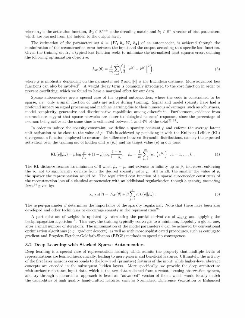
(a) Architecture of an autoencoder with an overcompletehidden layer. The encoder takes the input X and computesa prediction of the best value of the latent code h. Thedecoder is symmetric to the encoder and computes a recon-struction of X from h.

(b) A 5 layer autoencoder network [3-4-4-4-2], where thecircles denote the feature units. The black color is used todenote the hidden, whereas the white the visible layers. Thethree middle layers constitute an encoder.

Figure 1: The autoencoder concept. The bias units are not considered for simplicity.

3.1 Single-Layer Sparse Autoencoders

A classical autoencoder is a deterministic feed-forward artificial neural network comprised of an input and anoutput layer of the same size with a hidden layer in between, as illustrated in Figure 1a . Typically, the modelis trained with backpropagation19 in a fully unsupervised manner, aiming to learn an approximation x of theinput which would be ideally more useful compared to the raw input.

The feature mapping that transforms an input pattern x ∈ Rn into a hidden representation h (called code)of k neurons (units), is defined by the encoder function:

f(x) = h = αf (W1x + b1), (1)

where αf : R 7→ R is the activation function applied component-wise to the input vector. The activationfunction is usually chosen to be nonlinear; examples include the logistic sigmoid and the hyperbolic tangent.Recently, there is a growing interest in Rectified Linear Units (ReLU), which seem to work better in supervisedrecognition tasks. The activation function is parametrized by a weight matrix W1 ∈ Rk×n with weights learnedon the connections from the input to the hidden layer and a bias vector b1 ∈ Rk×1. The network output is thencomputed by mapping the resulting hidden representation h back into a reconstructed vector x ∈ Rn×1 using aseparate decoder function of the form:

g(f(x)) = x = αg(W2h + b2), (2)

where αg is the activation function, W2 ∈ Rn×k is the decoding matrix and b2 ∈ Rn a vector of bias parameterswhich are learned from the hidden to the output layer.

The estimation of the parameters set θ = {W1, b1,W2, b2} of an autoencoder, is achieved through theminimization of the reconstruction error between the input and the output according to a specific loss function.Given the training set X, a typical loss function seeks to minimize the normalized least squares error, definingthe following optimization objective:

JAE(θ) =1

m

m∑i=1

(1

2

∥∥∥x(i) − x(i)∥∥∥2), (3)

where x is implicitly dependent on the parameter set θ and ‖·‖ is the Euclidean distance. More advanced lossfunctions can also be involved7 . A weight decay term is commonly introduced to the cost function in order toprevent overfitting, which we found to have a marginal effort for our data.

Sparse autoencoders are a special case of the typical autoencoders, where the code is constrained to besparse, i.e. only a small fraction of units are active during training. Signal and model sparsity have had aprofound impact on signal processing and machine learning due to their numerous advantages, such as robustness,model complexity, generative and discriminative capabilities among others20,21 . Furthermore, evidence fromneuroscience suggest that sparse networks are closer to biological neurons’ responses, since the percentage ofneurons being active at the same time is estimated between 1 and 4% of the total22,23 .

In order to induce the sparsity constraint, we define a sparsity constant ρ and enforce the average latentunit activation to be close to the value of ρ. This is achieved by penalizing it with the Kullback-Leibler (KL)divergence, a function employed to measure the difference between Bernoulli distributions, namely the expectedactivation over the training set of hidden unit u (ρu) and its target value (ρ) in our case:

KL(ρ||ρu) = ρ logρ

ρu+ (1− ρ) log

1− ρ1− ρu

, ρu =1

m

m∑i=1

[αu

(x(i))], u = 1, . . . , k . (4)

The KL distance reaches its minimum of 0 when ρu = ρ, and extends to infinity up as ρu increases, enforcingthe ρu not to significantly deviate from the desired sparsity value ρ. All in all, the smaller the value of ρ,the sparser the representation would be. The regularized cost function of a sparse autoencoder constitutes ofthe reconstruction loss of a classical autoencoder with an additional regularization though a sparsity promotingterm24 given by:

JspAE(θ) = JAE(θ) + β

k∑j=1

KL(ρ||ρu) . (5)

The hyper-parameter β determines the importance of the sparsity regularizer. Note that there have been alsodeveloped and other techniques to encourage sparsity in the representation25 .

A particular set of weights is updated by calculating the partial derivatives of JspAE and applying thebackpropagation algorithm19 . This way, the training typically converges to a minimum, hopefully a global one,after a small number of iterations. The minimization of the model parameters θ can be achieved by conventionaloptimization algorithms (e.g., gradient descent), as well as with more sophisticated procedures, such as conjugategradient and Broyden-Fletcher-Goldfarb-Shanno (BFGS) methods to speed up convergence.

3.2 Deep Learning with Stacked Sparse Autoencoders

Deep learning is a special case of representation learning which admits the property that multiple levels ofrepresentations are learned hierarchically, leading to more generic and beneficial features. Ultimately, the activityof the first layer neurons corresponds to the low-level (primitive) features of the input, while higher-level abstractconcepts are encoded in the subsequent hidden layers. More specifically, we provide the deep architecturewith surface reflectance input data, which is the raw data collected from a remote sensing observation system,and try through a hierarchical approach to learn an “advanced” version of them, which would ideally matchthe capabilities of high quality hand-crafted features, such as Normalized Difference Vegetation or Enhanced

Vegetation Indices (NDVI/EVI). In this way, we aim at bypassing the requirements of manual design of thesefeatures and automatically learn representations which can substitute and enhance them. In parallel, due to theunsupervised nature of the processing, the proposed approach is more universal and could also work with othertypes of targets which are not chlorophyll sensitive, such as structures in urban areas, where analogous ratioshave not been defined.

Architectures with two or more hidden layers can be created by stacking single layer autoencoders on topof each other as depicted in Figure 1b. Formally, one starts by training a sparse autoencoder with the rawdata as input. Then the decoder layer is discarded so that the activations of the hidden units (layer-1 features)become the visible input for training the second autoencoder layer (feed-forward), which in turn produces anotherrepresentation (layer-2 features). This greedy layer-by-layer process keeps the previous layers fixed and ignoresinteractions with subsequent layers, thus dramatically reducing the search over the parameter space. While thisprocess can be repeated multiple times, rarely more than three hidden layers are involved. We can formalize astacked autoencoder according to:

h(L) = f (L)(· · · f (2)

(f (1) (x)

)), (6)

where h(L) denotes the representation learned by the top layer L. The output of the entire architecture can beused to fed a stand-alone classifier, offering a “better” representation of the data compared to the raw input.

The challenge in deep learning is that the gradient information is difficult to pass efficiently through a seriesof randomly initialized layers, since a good starting point is hard to identify. Unsupervised pretraining17 is arecently developed yet very influential protocol that helps to alleviate this optimization problem by introducingprior knowledge for initializing the weights of each layer, allowing gradients to “flow well”. Autoencoders, beinga fundamental example of unsupervised learning, have attracted a lot of attention as a method for pretrainingdeep neural networks. Formally, we use the sparse autoencoder as the building block to train one layer at a time,in a bottom up fashion, for a fixed number of updates (epochs). Up until this point, the procedure is completelyunsupervised. Supervised refinements are subsequently introduced in the top layer of the deep architecture inorder to fine-tune the gradient-based optimization algorithm with respect to a supervised criterion, a processtermed fine-tuning phase15 . As a last optional training stage, it is possible to further optimize the parameterswith a global fine-tuning, which uses backpropagation through the whole network architecture at once, howeverstarting from a very good initial model.

3.3 Data Preprocessing

A critical aspect of sparse autoencoder models is the need for data normalization. To that end, several normal-ization steps are usually performed in order to adapt the raw data into appropriate inputs for neural networks.Experimental results have shown that when the input variables are close to zero, neural network training isusually typically more efficient since convergence is faster and the likelihood of getting stuck in local optima isreduced. Formally, let the training set of instance-label pairs X = {

(x(i), t(i)

)|i = 1, . . . ,m} be the set of m

training examples where the j-th feature of x(i) is x(i)j , j = 1, . . . , n. We consider normalization of each feature

vector j to [0, 1] by subtracting the minimum value of each element and dividing it by its range (the differencebetween the maximum and the minimum value):

x(i)j =

x(i)j −minj

maxj −minj, (7)

where the minimum values and ranges are stored for later use.

4. MULTI-LABEL CLASSIFICATION

The purpose of the representation learning system is to by incorporated into a data classification framework.Typical classification approaches are focused on the single class classification problem where each training andtesting example is associated with a single label or belongs to a single class. In many real-life scenarios however,this is not the case. The illustrative example we consider in this case, is labeling multispectral satellite datawith ground-gathered measurements in an effort to provide up-to-date land cover usage. Due to the difference in

scale, each multispectral pixel may be associated with multiple labels, naturally leading to the case of multi-labelannotation. In this work, we consider state-of-the-art multi-label classifiers that operate not on the originalraw data, but in features extracted though the stacked autoencoder network hoping to reach and overcome theclassification performance achieved by hand-crafted features.

A typical strategy to deal with a multi-label classification problem, is to decompose the original multi-label problem into a set of binary classification problems and acquire predictions through conventional single-label classification algorithms, a method known as problem transformation3 . The most representative examplesof problem transformation methods is the Binary Relevance (BR) and the Label Powerset (LP) techniques.According to the former method, a single-label classifier is trained independently for each label leading to a setof n classifiers, whose union forms the final prediction, whereas with the latter, each distinct subset of labelsthat exists in the training set, is regarded as a different class of a new single class problem.

Recently, problem transformation techniques have involved in ensemble methods, such as RAndom k-labELsets(RAkEL)26 and Ensemble of Classifier Chains (ECC),27 in order to achieve even higher classification performance.RAkEL randomly breaks the initial set of labels into a number of small subsets and then for each labelset trainsa multi-label classifier using the LP technique. From the other side, ECC extends the Classifier Chains (CC)model27 that transforms a multi-label learning problem into a chain of n BR classifiers. Although CC schemamanages take into account label dependencies, it runs the risk of low classification accuracy, since it is stronglydependent on the label order. ECC reduces this risk and achieves predictive completeness by building an ensembleof chains, each with a random label order.

Both of these techniques can be used with any off-the-shelf binary classifier. In this work, we incorporateSupport Vector Machines (SVM)28 as the base classifier, which is considered as one of the most efficient classifiersfor remote sensing data. Given the training set X with binary labels t(i) ∈ {0, 1}, the SVM classifier tries to finda linear separating hyperplane with the maximal margin in this higher dimensional space. Formally, when thekernel function is linear, the SVM seeks a solution to the following constraint optimization problem:

minimizew,ξ(i)

1

2wᵀw + C

m∑i=1

ξ(i)

subject to wᵀ x(i) t(i) ≥ 1− ξ(i), ξ(i) ≥ 0, i = 1, . . . ,m,

(8)

where the parameter C > 0 controls the trade-off between the slack variable penalty and the margin.

5. EXPERIMENTAL SETUP

5.1 Dataset and Motivation

In this work, we consider the introduction of a multi-label learning scheme, adapted to a remote sensing ap-plication with real complex data. Formally, we combine real satellite data from Moderate Resolution ImagingSpectroradiometer (MODIS) instrument and high spatial resolution ground data from the CORINE Land Cover(CLC) project developed by the European Environment Agency (EEA). More specifically, the features are ob-tained from the MODIS sensor aboard Terra satellite∗, where we consider the 7 surface reflectance bands fromthe MOD09A1 product, acquired at 500m2 spatial resolution and having an 8-day revisit frequency. We seek forland cover classification, thus we collect all available data from the growing season (May to October) leading in161 spectral bands in total. We underline that we are particularly interested in this feature set, since these arethe data which are provided directly from a satellite imaging system and thus can be obtained and be accessiblein short time, without the need of extra processing. Moreover, in this paper we focus in deep learning, thuswe have to provide our system with primitive data in order to be able to discover the more explanatory factorshidden in that data, since by incorporating hand-crafted features the hierarchical structure of the data needed fordeep learning is lost due to their inherent complex makeup, and no extra valuable information can be revealed.

Regarding the associated ground-truth map for these inputs, we take advantage of the CORINE map† by theEEA, where we select data from the year 2000 annotated with 20 labels, whereas the region of interest corresponds

∗https://lpdaac.usgs.gov/data access/data pool†http://www.eea.europa.eu/data-and-maps/data/corine-land-cover-2000-raster-3

to the h19v04 tile of MODIS. Note that CORINE has a higher resolution of 100m2 than MOD09A1 product,which naturally leads to the multi-label case since each spectral pixel is associated with multiple CLC codes. Inaccordance with multispectral and hyperspectral image single-label classification, we aim in classification withlimited training examples.

5.2 Performance Evaluation

The performance evaluation of multi-label classifiers is more complicated than conventional single-label learning,since an example may be partially correct. As a consequence, several metrics have been proposed for classificationand ranking4 . In this work, we quantify the performance in terms of the following six state-of-the-art metrics.

Let K be the number of testing examples in the multi-label dataset with L labels and Yi/Zi is the actual andthe predicted set of labels. Then the example-based hamming loss are calculated by:

Hamming Loss =1

K

K∑i=1

|Yi∆Zi|L

, (9)

where ∆ stands for the symmetric difference (corresponds to the XOR operator in Boolean logic) between thetwo sets. Conceptually speaking, hamming loss measures how many times a relevant label to an example is notpredicted or an irrelevant is incorrectly predicted, reaching its best performance at score 0 and worst score at 1.

Average precision is an example-based ranking metric, which evaluates the average fraction of relevant labelsranked higher than a particular label. It is thus given by:

Average Precision =1

K

K∑i=1

1

|Yi|∑λ∈Yi

|{λ′ ∈ Yi : ri(λ) ≤ ri(λ′)}|ri(λ)

, (10)

where r(λ) is the ordered list of labels for label λ. This score corresponds to the area under precision-recallcurve.

In extending a binary metric to multi-label problems, there exist a number of ways to average binary metriccalculations across the set of labels. Given the True Positives (TP), True Negatives (TN), False Positives (FP),and False Negatives (FN) test samples, we calculate metrics by assuming macro- and micro-averaging across allclass labels, which give equal weight for labels and instances respectively, defined as follows:

Bmicro = B

m∑j=1

TPλj,

m∑j=1

TNλj,

m∑j=1

FPλj,

m∑j=1

FPλj

, Bmacro =1

m

m∑j=1

B(TPλj,TNλj

,FPλj,FNλj

). (11)

B could be any of the binary classification metrics, here the F1 score or the Area Under the ROC Curve (AUC).In a nutshell, F-Measure conveys the balance between the precision and the recall, whereas AUC considers TPand FP rates. The bigger value obtained, the better the performance of the classifier for these metrics.

5.3 Network Architecture

In order to train a deep neural network there are several hyper-parameters which need to be set, including thosewhich specify the structure of the network itself and those which determine how the network is trained. Thetype of the nonlinearity in the activation function is one of the first such hyper-parameters that needs to beconsidered. We adopt the logistic sigmoid activation αf (φ) = αg(φ) = σ(φ) = 1/(1 + e−φ) in the hidden layerswhich has an output range in the interval [0,1] (and is in accordance to the the initial scaling from Eq. 7). Thebias units are initialized to zero, whereas the initial weights are randomly drawn from a uniform distributionU(-r,r) with r = 4

√6/(fan-in + fan-out), where fan-in is the size of the previous layer and fan-out the number

of hidden units in current layer29 . Tied weights (W2 = W ᵀ1 ) are commonly used to reduce the complexity, yet

untied (W2 6= W ᵀ1 ) weights seem to generalize better in our case. Therefore, in the following results untied

weights are employed in all layers.

Neural network models demand significant effort and time during training, making an exhaustive grid searchin the space of hyper-parameters intractable. In addition, since the particular dataset we consider has not beenexplored before, not prior information on where these hyperparameters approximately lie is available. As such,for the specification of the hyper-parameters ρ and β which control the sparseness of the autoencoder, we firstperformed a coarse grid search in reasonable values and in all cases, model selection was performed accordingthe lowest mean square error of the validation set, which is composed of 20% of the training data (randomlysampled). More specifically, the grid is constructed by considering the set produced by the Cartesian productof ρ ∈ {0.001, 0.01, 0.1, 0.3, 0.5, 0.7, 0.9} and β ∈ {1, 5, 10, 15, 20} values. The models were trained for 5000unsupervised learning epochs, while at the supervised learning stage, we use 3000 epochs with early stopping29 ,a typical approach to prevent overfitting, where we monitor the validation error every 100 iterations and if it hasnot decreased for 500 consecutive epochs, early stopping is enabled. Reported results are averaged over 10 Monte-Carlo trials, in order to minimize the effects of the initial random seed. For the implementation of the sparseautoencoder we considered the framework described in24 . The optimization algorithm used for minimizing thecost function of the sparse autoencoder was the BFGS gradient descent method with limited-memory variation(L-BFGS)‡ and a stopping criterion of 10−8, a quasi-Newton method for unconstrained optimization that hasproved to work well for the particular type of optimization.

For the implementation of RAkEL and ECC we consider the open-source MULAN§ Java library for multi-label learning that works on the top of WEKA¶ data mining software. As suggested by the authors, we set thesize of each labelset in RAkEL to 3 and the number of models to 2n = 40, while for ECC we use 10 models. SVMproblem is solved with linear kernel by the Sequential minimal optimization (SMO) algorithm that is availablewithin WEKA.

6. EXPERIMENTAL RESULTS

In this section, we initially investigate typically used features and their effect on the particular multi-labelclassification problem, serving as baseline. Subsequently, we provide a detailed performance analysis of theproposed feature learning and classification scheme by considering three key system parameters, namely theimpact of the number of neurons for a single layer, as well as additional normalization tasks, the sensitivity ofthe feature learning models and the impact of depth on the performance of multi-label classification algorithms,on real data. We notice that there are also a number of other critical hyperparameters of the neural networkwhich one can experiment on, such as the regularization parameter, the type of the nonlinearity, or even thenumber of units of the second hidden layer; careful selection of such parameters can potentially further improvesystem’s performance.

6.1 Performance of Raw and Hand-crafted Features

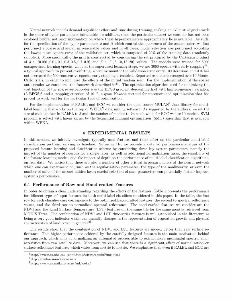
In order to obtain a clear understanding regarding the effects of the features, Table 1 presents the performancefor different types of input features for both multi-label classifiers considered in this paper. In the table, the firstrow for each classifier case corresponds to the optimized hand-crafted features, the second to spectral reflectancevalues, and the third row to normalized spectral reflectance. The hand-crafted features we consider are theNDVI and the Land Surface Temperature (LST) features on the same tile for the same months retrieved fromMODIS Terra. The combination of NDVI and LST time-series features is well established in the literature asbeing a very good indicator which can quantify changes in the representation of vegetation growth and physicalcharacteristics of land cover in general30 .

The results show that the combination of NDVI and LST features are indeed better than raw surface re-flectance. This higher performance achieved by the carefully designed features is the main motivation behindour approach, which aims at formalizing an automated process able to extract more meaningful spectral char-acteristics from raw satellite data. Moreover, we can see that there is a significant effect of normalization onsurface reflectance features, which varies from metric to metric. We emphasize than even if RAkEL and ECC are

‡http://www.cs.ubc.ca/ schmidtm/Software/minFunc.html§http://mulan.sourceforge.net/¶http://www.cs.waikato.ac.nz/ml/weka/

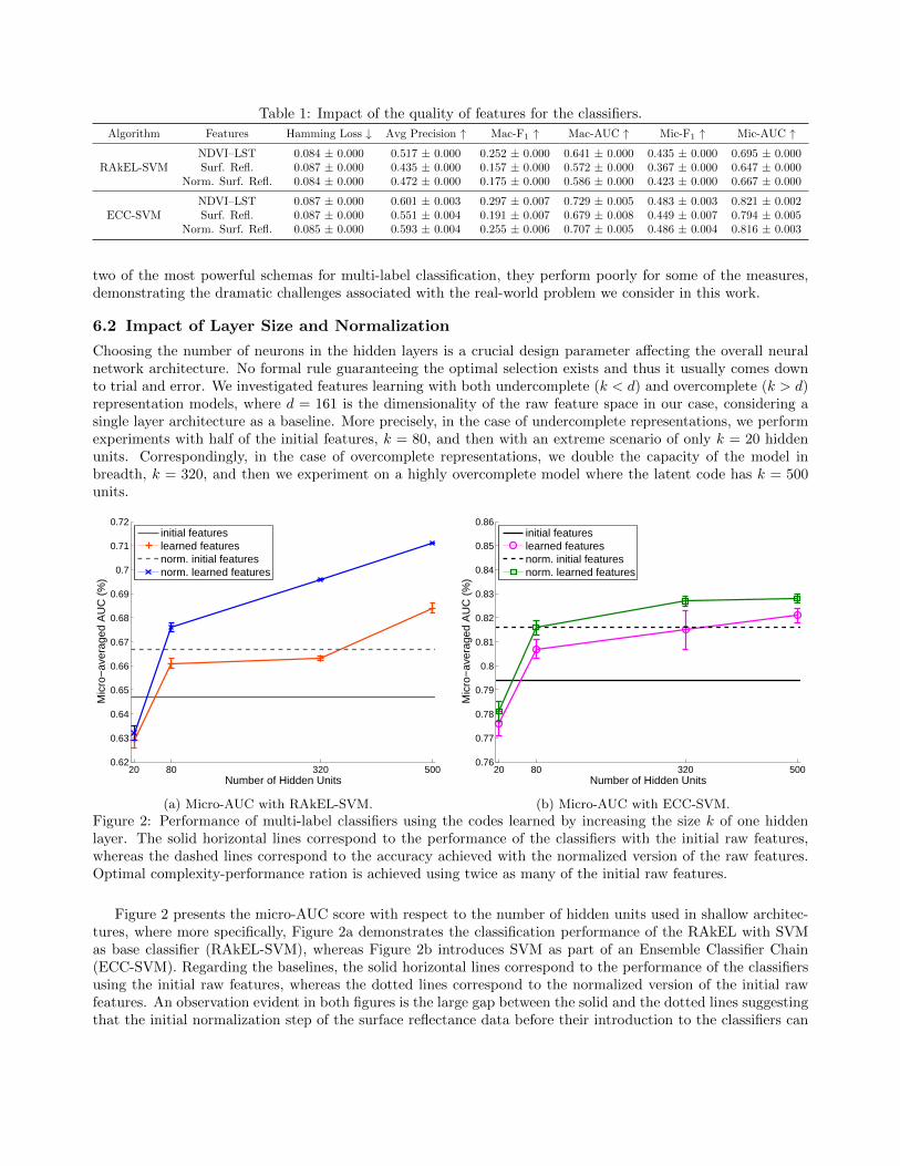
Table 1: Impact of the quality of features for the classifiers.

Algorithm Features Hamming Loss ↓ Avg Precision ↑ Mac-F1 ↑ Mac-AUC ↑ Mic-F1 ↑ Mic-AUC ↑

RAkEL-SVMNDVI–LST 0.084 ± 0.000 0.517 ± 0.000 0.252 ± 0.000 0.641 ± 0.000 0.435 ± 0.000 0.695 ± 0.000Surf. Refl. 0.087 ± 0.000 0.435 ± 0.000 0.157 ± 0.000 0.572 ± 0.000 0.367 ± 0.000 0.647 ± 0.000

Norm. Surf. Refl. 0.084 ± 0.000 0.472 ± 0.000 0.175 ± 0.000 0.586 ± 0.000 0.423 ± 0.000 0.667 ± 0.000

ECC-SVMNDVI–LST 0.087 ± 0.000 0.601 ± 0.003 0.297 ± 0.007 0.729 ± 0.005 0.483 ± 0.003 0.821 ± 0.002Surf. Refl. 0.087 ± 0.000 0.551 ± 0.004 0.191 ± 0.007 0.679 ± 0.008 0.449 ± 0.007 0.794 ± 0.005

Norm. Surf. Refl. 0.085 ± 0.000 0.593 ± 0.004 0.255 ± 0.006 0.707 ± 0.005 0.486 ± 0.004 0.816 ± 0.003

two of the most powerful schemas for multi-label classification, they perform poorly for some of the measures,demonstrating the dramatic challenges associated with the real-world problem we consider in this work.

6.2 Impact of Layer Size and Normalization

Choosing the number of neurons in the hidden layers is a crucial design parameter affecting the overall neuralnetwork architecture. No formal rule guaranteeing the optimal selection exists and thus it usually comes downto trial and error. We investigated features learning with both undercomplete (k < d) and overcomplete (k > d)representation models, where d = 161 is the dimensionality of the raw feature space in our case, considering asingle layer architecture as a baseline. More precisely, in the case of undercomplete representations, we performexperiments with half of the initial features, k = 80, and then with an extreme scenario of only k = 20 hiddenunits. Correspondingly, in the case of overcomplete representations, we double the capacity of the model inbreadth, k = 320, and then we experiment on a highly overcomplete model where the latent code has k = 500units.

20 80 320 5000.62

0.63

0.64

0.65

0.66

0.67

0.68

0.69

0.7

0.71

0.72

Number of Hidden Units

Mic

ro−

aver

aged

AU

C (

%)

initial featureslearned featuresnorm. initial featuresnorm. learned features

(a) Micro-AUC with RAkEL-SVM.

20 80 320 5000.76

0.77

0.78

0.79

0.8

0.81

0.82

0.83

0.84

0.85

0.86

Number of Hidden Units

Mic

ro−

aver

aged

AU

C (

%)

initial featureslearned featuresnorm. initial featuresnorm. learned features

(b) Micro-AUC with ECC-SVM.

Figure 2: Performance of multi-label classifiers using the codes learned by increasing the size k of one hiddenlayer. The solid horizontal lines correspond to the performance of the classifiers with the initial raw features,whereas the dashed lines correspond to the accuracy achieved with the normalized version of the raw features.Optimal complexity-performance ration is achieved using twice as many of the initial raw features.

Figure 2 presents the micro-AUC score with respect to the number of hidden units used in shallow architec-tures, where more specifically, Figure 2a demonstrates the classification performance of the RAkEL with SVMas base classifier (RAkEL-SVM), whereas Figure 2b introduces SVM as part of an Ensemble Classifier Chain(ECC-SVM). Regarding the baselines, the solid horizontal lines correspond to the performance of the classifiersusing the initial raw features, whereas the dotted lines correspond to the normalized version of the initial rawfeatures. An observation evident in both figures is the large gap between the solid and the dotted lines suggestingthat the initial normalization step of the surface reflectance data before their introduction to the classifiers can

have a dramatic impact on the performance. This is in line with the observation that algorithms that workwith distances and make parametric assumptions regarding the distribution of the data, such as SVM or logisticregression, are usually affected positively by normalization. We should notice also that the computational timeis much smaller with the use of normalization.

Overall, for both classifiers 20 units are too few to adequately encode the signals in the hidden layer resultingin significant degradation performance. By increasing the number of hidden units to 80, the performance inboth schemes surpasses the score achieved using raw un-normalized features as inputs. However, the gain offeredby the feature learning, is outweighed to some extent by the effort of normalization of the raw input data, asindicated by the dotted line. Furthermore, by considering 320 units, the performance of the feature learningscheme is almost the same by utilizing 80 hidden units, whereas there is an improvement for the 500 units butat a higher computational cost. A key observation point is that the normalization after the feature-mappingcan also play a significant role and boost the performance of classifiers. In detail, we observe that in the caseof the undercomplete feature learning architectures, the accuracy does not significantly change with or withoutthis normalization step. Nonetheless, it is evident that in the case of overcomplete systems, the performance ishigher and can clearly surpass the enhanced baseline versions with the normalized feature vectors.

With respect to the different classifiers, one can easily notice the dominance of the ECC scheme comparedto the RAkEL approach. Moreover, ECC is less affected by the normalization steps, but has a greater varianceon the results. Last, we have to mention that we need the contribution of such powerful ensemble multi-labellearning schemes in order to achieve reasonable performance, due to both the limited training examples and themany factors of variation that inhere in our real dataset, allowing us to test the limits of current state-of-the-artclassifiers.

6.3 Model Sensitivity

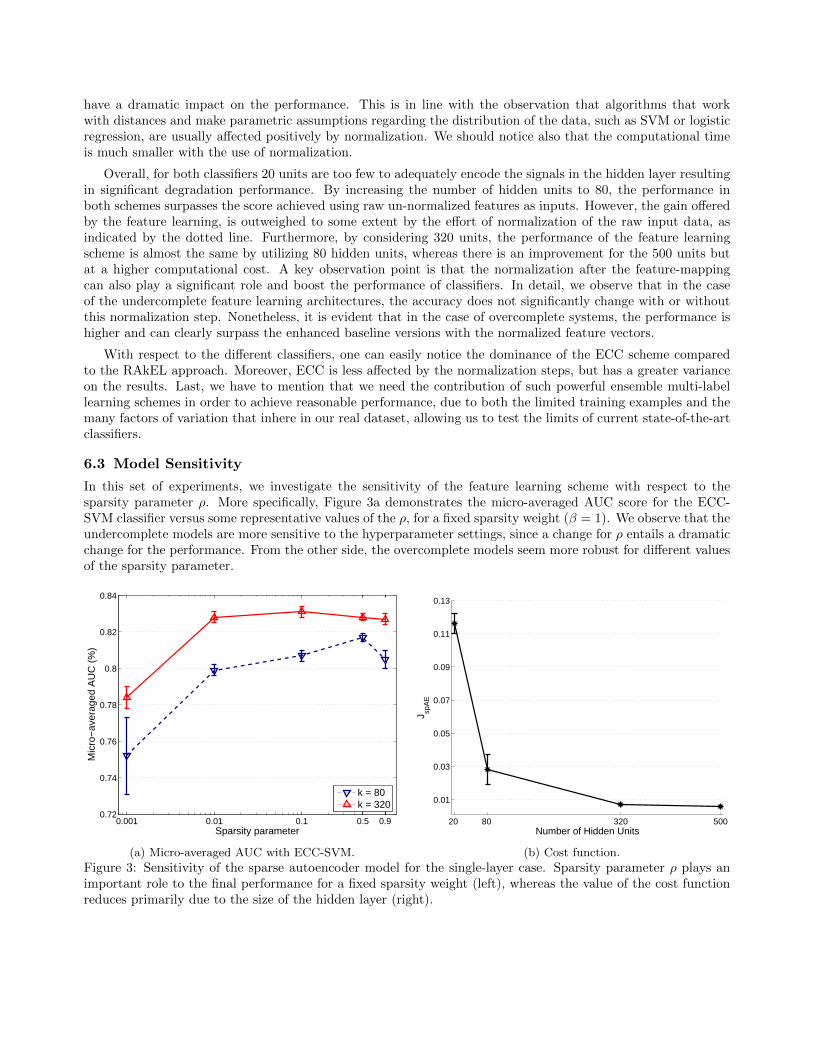
In this set of experiments, we investigate the sensitivity of the feature learning scheme with respect to thesparsity parameter ρ. More specifically, Figure 3a demonstrates the micro-averaged AUC score for the ECC-SVM classifier versus some representative values of the ρ, for a fixed sparsity weight (β = 1). We observe that theundercomplete models are more sensitive to the hyperparameter settings, since a change for ρ entails a dramaticchange for the performance. From the other side, the overcomplete models seem more robust for different valuesof the sparsity parameter.

0.001 0.01 0.1 0.5 0.90.72

0.74

0.76

0.78

0.8

0.82

0.84

Sparsity parameter

Mic

ro−

aver

aged

AU

C (

%)

k = 80k = 320

(a) Micro-averaged AUC with ECC-SVM.

20 80 320 500

0.01

0.03

0.05

0.07

0.09

0.11

0.13

Number of Hidden Units

J spA

E

(b) Cost function.

Figure 3: Sensitivity of the sparse autoencoder model for the single-layer case. Sparsity parameter ρ plays animportant role to the final performance for a fixed sparsity weight (left), whereas the value of the cost functionreduces primarily due to the size of the hidden layer (right).

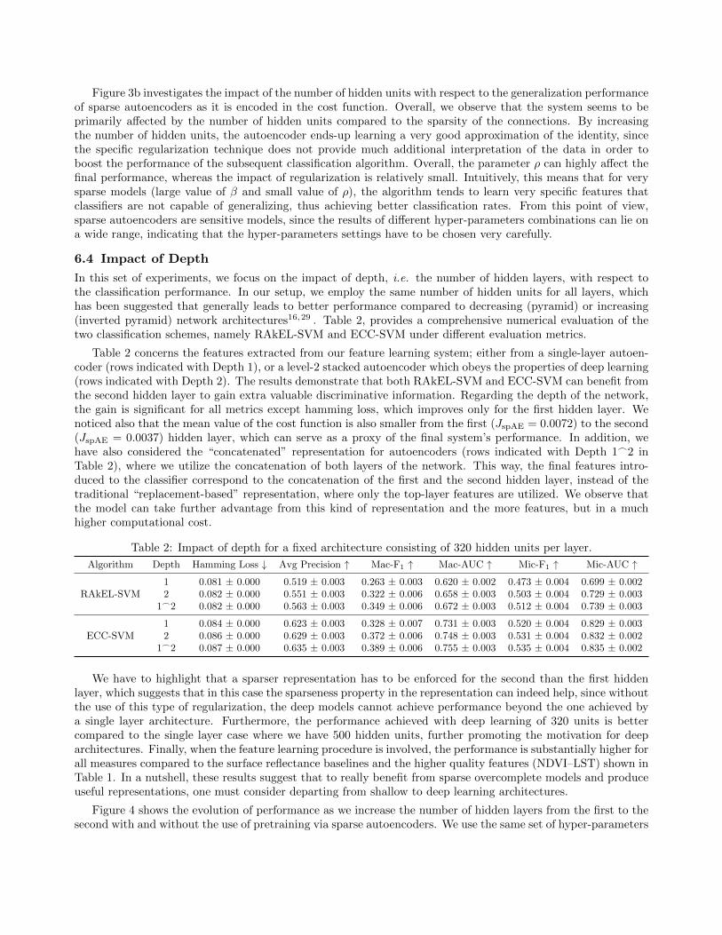
Figure 3b investigates the impact of the number of hidden units with respect to the generalization performanceof sparse autoencoders as it is encoded in the cost function. Overall, we observe that the system seems to beprimarily affected by the number of hidden units compared to the sparsity of the connections. By increasingthe number of hidden units, the autoencoder ends-up learning a very good approximation of the identity, sincethe specific regularization technique does not provide much additional interpretation of the data in order toboost the performance of the subsequent classification algorithm. Overall, the parameter ρ can highly affect thefinal performance, whereas the impact of regularization is relatively small. Intuitively, this means that for verysparse models (large value of β and small value of ρ), the algorithm tends to learn very specific features thatclassifiers are not capable of generalizing, thus achieving better classification rates. From this point of view,sparse autoencoders are sensitive models, since the results of different hyper-parameters combinations can lie ona wide range, indicating that the hyper-parameters settings have to be chosen very carefully.

6.4 Impact of Depth

In this set of experiments, we focus on the impact of depth, i.e. the number of hidden layers, with respect tothe classification performance. In our setup, we employ the same number of hidden units for all layers, whichhas been suggested that generally leads to better performance compared to decreasing (pyramid) or increasing(inverted pyramid) network architectures16,29 . Table 2, provides a comprehensive numerical evaluation of thetwo classification schemes, namely RAkEL-SVM and ECC-SVM under different evaluation metrics.

Table 2 concerns the features extracted from our feature learning system; either from a single-layer autoen-coder (rows indicated with Depth 1), or a level-2 stacked autoencoder which obeys the properties of deep learning(rows indicated with Depth 2). The results demonstrate that both RAkEL-SVM and ECC-SVM can benefit fromthe second hidden layer to gain extra valuable discriminative information. Regarding the depth of the network,the gain is significant for all metrics except hamming loss, which improves only for the first hidden layer. Wenoticed also that the mean value of the cost function is also smaller from the first (JspAE = 0.0072) to the second(JspAE = 0.0037) hidden layer, which can serve as a proxy of the final system’s performance. In addition, wehave also considered the “concatenated” representation for autoencoders (rows indicated with Depth 1_2 inTable 2), where we utilize the concatenation of both layers of the network. This way, the final features intro-duced to the classifier correspond to the concatenation of the first and the second hidden layer, instead of thetraditional “replacement-based” representation, where only the top-layer features are utilized. We observe thatthe model can take further advantage from this kind of representation and the more features, but in a muchhigher computational cost.

Table 2: Impact of depth for a fixed architecture consisting of 320 hidden units per layer.

Algorithm Depth Hamming Loss ↓ Avg Precision ↑ Mac-F1 ↑ Mac-AUC ↑ Mic-F1 ↑ Mic-AUC ↑

RAkEL-SVM1 0.081 ± 0.000 0.519 ± 0.003 0.263 ± 0.003 0.620 ± 0.002 0.473 ± 0.004 0.699 ± 0.0022 0.082 ± 0.000 0.551 ± 0.003 0.322 ± 0.006 0.658 ± 0.003 0.503 ± 0.004 0.729 ± 0.003

1_2 0.082 ± 0.000 0.563 ± 0.003 0.349 ± 0.006 0.672 ± 0.003 0.512 ± 0.004 0.739 ± 0.003

ECC-SVM1 0.084 ± 0.000 0.623 ± 0.003 0.328 ± 0.007 0.731 ± 0.003 0.520 ± 0.004 0.829 ± 0.0032 0.086 ± 0.000 0.629 ± 0.003 0.372 ± 0.006 0.748 ± 0.003 0.531 ± 0.004 0.832 ± 0.002

1_2 0.087 ± 0.000 0.635 ± 0.003 0.389 ± 0.006 0.755 ± 0.003 0.535 ± 0.004 0.835 ± 0.002

We have to highlight that a sparser representation has to be enforced for the second than the first hiddenlayer, which suggests that in this case the sparseness property in the representation can indeed help, since withoutthe use of this type of regularization, the deep models cannot achieve performance beyond the one achieved bya single layer architecture. Furthermore, the performance achieved with deep learning of 320 units is bettercompared to the single layer case where we have 500 hidden units, further promoting the motivation for deeparchitectures. Finally, when the feature learning procedure is involved, the performance is substantially higher forall measures compared to the surface reflectance baselines and the higher quality features (NDVI–LST) shown inTable 1. In a nutshell, these results suggest that to really benefit from sparse overcomplete models and produceuseful representations, one must consider departing from shallow to deep learning architectures.

Figure 4 shows the evolution of performance as we increase the number of hidden layers from the first to thesecond with and without the use of pretraining via sparse autoencoders. We use the same set of hyper-parameters

L = 1 L = 2

0.59

0.6

0.61

0.62

0.63

0.64

0.65

0.66

0.67

Number of Hidden Layers

Mac

ro−

aver

aged

AU

C (

%)

With pretrainingWithout pretraining

(a) RAkEL-SVM.

L = 1 L = 2

0.69

0.7

0.71

0.72

0.73

0.74

0.75

0.76

0.77

Number of Hidden Layers

Mac

ro−

aver

aged

AU

C (

%)

With pretrainingWithout pretraining

(b) ECC-SVM.

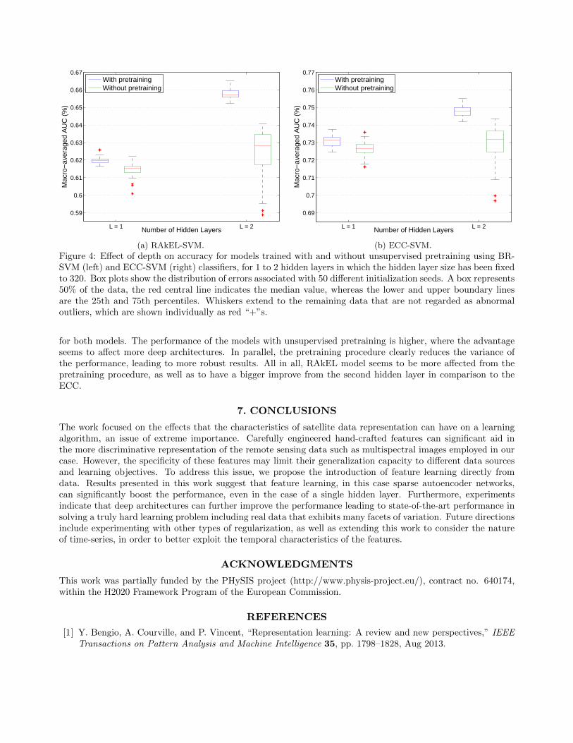
Figure 4: Effect of depth on accuracy for models trained with and without unsupervised pretraining using BR-SVM (left) and ECC-SVM (right) classifiers, for 1 to 2 hidden layers in which the hidden layer size has been fixedto 320. Box plots show the distribution of errors associated with 50 different initialization seeds. A box represents50% of the data, the red central line indicates the median value, whereas the lower and upper boundary linesare the 25th and 75th percentiles. Whiskers extend to the remaining data that are not regarded as abnormaloutliers, which are shown individually as red “+”s.

for both models. The performance of the models with unsupervised pretraining is higher, where the advantageseems to affect more deep architectures. In parallel, the pretraining procedure clearly reduces the variance ofthe performance, leading to more robust results. All in all, RAkEL model seems to be more affected from thepretraining procedure, as well as to have a bigger improve from the second hidden layer in comparison to theECC.

7. CONCLUSIONS

The work focused on the effects that the characteristics of satellite data representation can have on a learningalgorithm, an issue of extreme importance. Carefully engineered hand-crafted features can significant aid inthe more discriminative representation of the remote sensing data such as multispectral images employed in ourcase. However, the specificity of these features may limit their generalization capacity to different data sourcesand learning objectives. To address this issue, we propose the introduction of feature learning directly fromdata. Results presented in this work suggest that feature learning, in this case sparse autoencoder networks,can significantly boost the performance, even in the case of a single hidden layer. Furthermore, experimentsindicate that deep architectures can further improve the performance leading to state-of-the-art performance insolving a truly hard learning problem including real data that exhibits many facets of variation. Future directionsinclude experimenting with other types of regularization, as well as extending this work to consider the natureof time-series, in order to better exploit the temporal characteristics of the features.

ACKNOWLEDGMENTS

This work was partially funded by the PHySIS project (http://www.physis-project.eu/), contract no. 640174,within the H2020 Framework Program of the European Commission.

REFERENCES

[1] Y. Bengio, A. Courville, and P. Vincent, “Representation learning: A review and new perspectives,” IEEETransactions on Pattern Analysis and Machine Intelligence 35, pp. 1798–1828, Aug 2013.

[2] H. Larochelle, D. Erhan, A. Courville, J. Bergstra, and Y. Bengio, “An empirical evaluation of deep ar-chitectures on problems with many factors of variation,” in Int. Conf. on Machine Learning, ICML ’07,pp. 473–480, ACM, (New York, NY, USA), 2007.

[3] G. Tsoumakas and I. Katakis, “Multi-label classification: An overview,” International Journal of DataWarehousing and Mining 3(3), pp. 1–13, 2007.

[4] M.-L. Zhang and Z.-H. Zhou, “A review on multi-label learning algorithms,” IEEE Transactions on Knowl-edge and Data Engineering 26, pp. 1819–1837, Aug 2014.

[5] C. Poultney, S. Chopra, and Y. Lecun, “Efficient learning of sparse representations with an energy-basedmodel,” in Advances in Neural Information Processing Systems (NIPS), MIT Press, 2006.

[6] I. Goodfellow, H. Lee, Q. V. Le, A. Saxe, and A. Y. Ng, “Measuring invariances in deep networks,” inAdvances in Neural Information Processing Systems, Y. Bengio, D. Schuurmans, J. Lafferty, C. Williams,and A. Culotta, eds., pp. 646–654, Curran Associates, Inc., 2009.

[7] P. Vincent, H. Larochelle, I. Lajoie, Y. Bengio, and P.-A. Manzagol, “Stacked denoising autoencoders:Learning useful representations in a deep network with a local denoising criterion,” J. Mach. Learn. Res. 11,pp. 3371–3408, Dec. 2010.

[8] S. Rifai, P. Vincent, X. Muller, X. Glorot, and Y. Bengio, “Contracting auto-encoders: Explicit invarianceduring feature extraction,” in Int. Conf. on Machine Learning, 2011.

[9] R. Goroshin and Y. LeCun, “Saturating auto-encoder,” CoRR abs/1301.3577, 2013.

[10] R. Socher, J. Pennington, E. H. Huang, A. Y. Ng, and C. D. Manning, “Semi-supervised recursive au-toencoders for predicting sentiment distributions,” in Conf. on Empirical Methods in Natural LanguageProcessing, EMNLP ’11, pp. 151–161, Association for Computational Linguistics, (Stroudsburg, PA, USA),2011.

[11] A. Graves, A.-R. Mohamed, and G. Hinton, “Speech recognition with deep recurrent neural networks,” inInt. Conf. on Acoustics, Speech and Signal Processing (ICASSP), pp. 6645–6649, May 2013.

[12] K. Jarrett, K. Kavukcuoglu, M. Ranzato, and Y. LeCun, “What is the best multi-stage architecture forobject recognition?,” in Int. Conf. on Computer Vision, pp. 2146–2153, Sept 2009.

[13] X. Glorot, A. Bordes, and Y. Bengio, “Deep sparse rectifier neural networks,” in Int. Conf. on ArtificialIntelligence and Statistics (AISTATS-11), G. J. Gordon and D. B. Dunson, eds., 15, pp. 315–323, Journalof Machine Learning Research - Workshop and Conference Proceedings, 2011.

[14] Y. Bengio, “Learning deep architectures for ai,” Found. Trends Mach. Learn. 2, pp. 1–127, Jan. 2009.

[15] Y. Bengio, P. Lamblin, D. Popovici, H. Larochelle, U. D. Montral, and M. Qubec, “Greedy layer-wisetraining of deep networks,” in Advances in Neural Information Processing Systems (NIPS), MIT Press,2007.

[16] H. Larochelle, Y. Bengio, J. Louradour, and P. Lamblin, “Exploring strategies for training deep neuralnetworks,” J. Mach. Learn. Res. 10, pp. 1–40, June 2009.

[17] G. E. Hinton and R. R. Salakhutdinov, “Reducing the dimensionality of data with neural networks,” Sci-ence 313(5786), pp. 504–507, 2006.

[18] R. Salakhutdinov and I. Murray, “On the quantitative analysis of deep belief networks,” in Int. Conf. onMachine Learning, ICML ’08, pp. 872–879, ACM, (New York, NY, USA), 2008.

[19] Y. A. LeCun, L. Bottou, G. B. Orr, and K.-R. Muller, “Efficient backprop,” in Neural Networks: Tricks ofthe Trade, G. Montavon, G. Orr, and K.-R. Muller, eds., Lecture Notes in Computer Science 7700, pp. 9–48,Springer Berlin Heidelberg, 2012.

[20] K. Fotiadou, G. Tsagkatakis, and P. Tsakalides, “Low light image enhancement via sparse representations,”in Image Analysis and Recognition, pp. 84–93, Springer International Publishing, 2014.

[21] G. Tsagkatakis and A. Savakis, “Sparse representations and distance learning for attribute based categoryrecognition,” in Trends and Topics in Computer Vision, pp. 29–42, Springer Berlin Heidelberg, 2012.

[22] P. Lennie, “The cost of cortical computation,” Current Biology 13(6), pp. 493 – 497, 2003.

[23] P. Petrantonakis and P. Poirazi, “A compressed sensing perspective of hippocampal function,” Frontiers insystems neuroscience 8, 2014.

[24] A. Ng, “Sparse autoencoder,” CS294A Lecture notes 72, 2011.

[25] K. Kavukcuoglu, M. Ranzato, R. Fergus, and Y. LeCun, “Learning invariant features through topographicfilter maps,” in IEEE Conf. on Computer Vision and Pattern Recognition, pp. 1605–1612, June 2009.

[26] G. Tsoumakas, I. Katakis, and L. Vlahavas, “Random k-labelsets for multilabel classification,” IEEE Trans-actions on Knowledge and Data Engineering 23, pp. 1079–1089, July 2011.

[27] J. Read, B. Pfahringer, G. Holmes, and E. Frank, “Classifier chains for multi-label classification,” MachineLearning 85(3), pp. 333–359, 2011.

[28] C. Cortes and V. Vapnik, “Support-vector networks,” Machine Learning 20(3), pp. 273–297, 1995.

[29] Y. Bengio, “Practical recommendations for gradient-based training of deep architectures,” in Neural Net-works: Tricks of the Trade, G. Montavon, G. Orr, and K.-R. Mller, eds., Lecture Notes in Computer Science7700, pp. 437–478, Springer Berlin Heidelberg, 2012.

[30] Z. W. C. author, P. Wang, and X. Li, “Using modis land surface temperature and normalized differencevegetation index products for monitoring drought in the southern great plains, usa,” International Journalof Remote Sensing 25(1), pp. 61–72, 2004.