Feature Curves and Surfaces of 3D Asymmetric Tensor Fields

Shih-Hsuan Hung, Yue Zhang, Member, IEEE, Harry Yeh, Eugene Zhang, Senior Member, IEEE

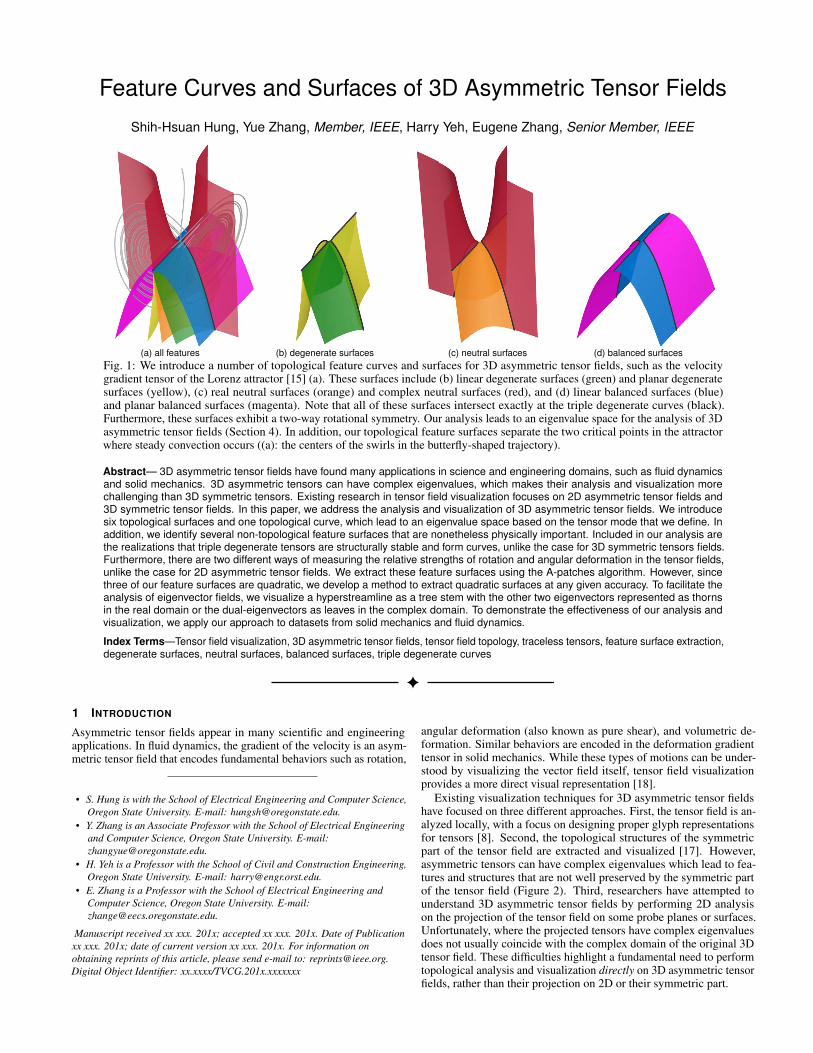
(a) all features (b) degenerate surfaces (c) neutral surfaces (d) balanced surfacesFig. 1: We introduce a number of topological feature curves and surfaces for 3D asymmetric tensor fields, such as the velocitygradient tensor of the Lorenz attractor [15] (a). These surfaces include (b) linear degenerate surfaces (green) and planar degeneratesurfaces (yellow), (c) real neutral surfaces (orange) and complex neutral surfaces (red), and (d) linear balanced surfaces (blue)and planar balanced surfaces (magenta). Note that all of these surfaces intersect exactly at the triple degenerate curves (black).Furthermore, these surfaces exhibit a two-way rotational symmetry. Our analysis leads to an eigenvalue space for the analysis of 3Dasymmetric tensor fields (Section 4). In addition, our topological feature surfaces separate the two critical points in the attractorwhere steady convection occurs ((a): the centers of the swirls in the butterfly-shaped trajectory).

Abstract— 3D asymmetric tensor fields have found many applications in science and engineering domains, such as fluid dynamicsand solid mechanics. 3D asymmetric tensors can have complex eigenvalues, which makes their analysis and visualization morechallenging than 3D symmetric tensors. Existing research in tensor field visualization focuses on 2D asymmetric tensor fields and3D symmetric tensor fields. In this paper, we address the analysis and visualization of 3D asymmetric tensor fields. We introducesix topological surfaces and one topological curve, which lead to an eigenvalue space based on the tensor mode that we define. Inaddition, we identify several non-topological feature surfaces that are nonetheless physically important. Included in our analysis arethe realizations that triple degenerate tensors are structurally stable and form curves, unlike the case for 3D symmetric tensors fields.Furthermore, there are two different ways of measuring the relative strengths of rotation and angular deformation in the tensor fields,unlike the case for 2D asymmetric tensor fields. We extract these feature surfaces using the A-patches algorithm. However, sincethree of our feature surfaces are quadratic, we develop a method to extract quadratic surfaces at any given accuracy. To facilitate theanalysis of eigenvector fields, we visualize a hyperstreamline as a tree stem with the other two eigenvectors represented as thornsin the real domain or the dual-eigenvectors as leaves in the complex domain. To demonstrate the effectiveness of our analysis andvisualization, we apply our approach to datasets from solid mechanics and fluid dynamics.

Index Terms—Tensor field visualization, 3D asymmetric tensor fields, tensor field topology, traceless tensors, feature surface extraction,degenerate surfaces, neutral surfaces, balanced surfaces, triple degenerate curves

1 INTRODUCTION

Asymmetric tensor fields appear in many scientific and engineeringapplications. In fluid dynamics, the gradient of the velocity is an asym-metric tensor field that encodes fundamental behaviors such as rotation,

• S. Hung is with the School of Electrical Engineering and Computer Science,Oregon State University. E-mail: hungsh@oregonstate.edu.

• Y. Zhang is an Associate Professor with the School of Electrical Engineeringand Computer Science, Oregon State University. E-mail:zhangyue@oregonstate.edu.

• H. Yeh is a Professor with the School of Civil and Construction Engineering,Oregon State University. E-mail: harry@engr.orst.edu.

• E. Zhang is a Professor with the School of Electrical Engineering andComputer Science, Oregon State University. E-mail:zhange@eecs.oregonstate.edu.

Manuscript received xx xxx. 201x; accepted xx xxx. 201x. Date of Publicationxx xxx. 201x; date of current version xx xxx. 201x. For information onobtaining reprints of this article, please send e-mail to: reprints@ieee.org.Digital Object Identifier: xx.xxxx/TVCG.201x.xxxxxxx

angular deformation (also known as pure shear), and volumetric de-formation. Similar behaviors are encoded in the deformation gradienttensor in solid mechanics. While these types of motions can be under-stood by visualizing the vector field itself, tensor field visualizationprovides a more direct visual representation [18].

Existing visualization techniques for 3D asymmetric tensor fieldshave focused on three different approaches. First, the tensor field is an-alyzed locally, with a focus on designing proper glyph representationsfor tensors [8]. Second, the topological structures of the symmetricpart of the tensor field are extracted and visualized [17]. However,asymmetric tensors can have complex eigenvalues which lead to fea-tures and structures that are not well preserved by the symmetric partof the tensor field (Figure 2). Third, researchers have attempted tounderstand 3D asymmetric tensor fields by performing 2D analysison the projection of the tensor field on some probe planes or surfaces.Unfortunately, where the projected tensors have complex eigenvaluesdoes not usually coincide with the complex domain of the original 3Dtensor field. These difficulties highlight a fundamental need to performtopological analysis and visualization directly on 3D asymmetric tensorfields, rather than their projection on 2D or their symmetric part.

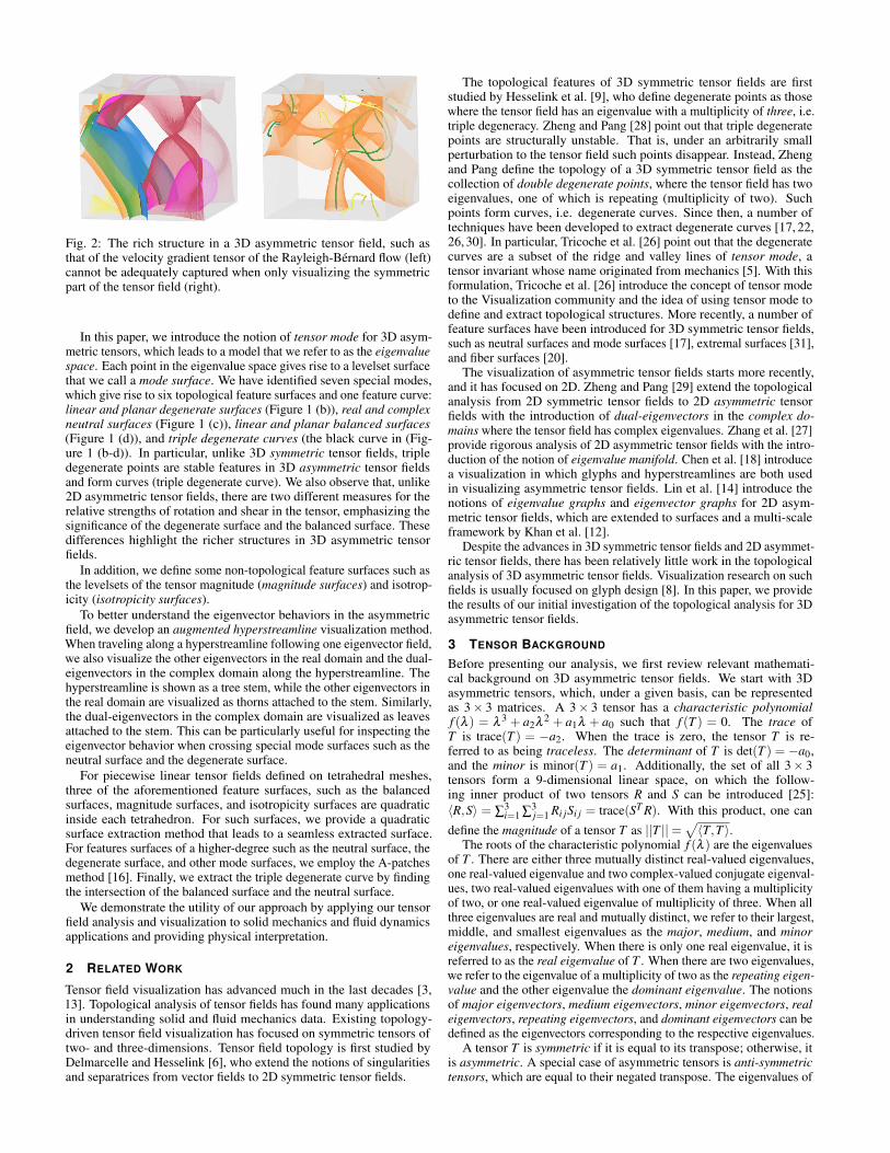
Fig. 2: The rich structure in a 3D asymmetric tensor field, such asthat of the velocity gradient tensor of the Rayleigh-Bernard flow (left)cannot be adequately captured when only visualizing the symmetricpart of the tensor field (right).

In this paper, we introduce the notion of tensor mode for 3D asym-metric tensors, which leads to a model that we refer to as the eigenvaluespace. Each point in the eigenvalue space gives rise to a levelset surfacethat we call a mode surface. We have identified seven special modes,which give rise to six topological feature surfaces and one feature curve:linear and planar degenerate surfaces (Figure 1 (b)), real and complexneutral surfaces (Figure 1 (c)), linear and planar balanced surfaces(Figure 1 (d)), and triple degenerate curves (the black curve in (Fig-ure 1 (b-d)). In particular, unlike 3D symmetric tensor fields, tripledegenerate points are stable features in 3D asymmetric tensor fieldsand form curves (triple degenerate curve). We also observe that, unlike2D asymmetric tensor fields, there are two different measures for therelative strengths of rotation and shear in the tensor, emphasizing thesignificance of the degenerate surface and the balanced surface. Thesedifferences highlight the richer structures in 3D asymmetric tensorfields.

In addition, we define some non-topological feature surfaces such asthe levelsets of the tensor magnitude (magnitude surfaces) and isotrop-icity (isotropicity surfaces).

To better understand the eigenvector behaviors in the asymmetricfield, we develop an augmented hyperstreamline visualization method.When traveling along a hyperstreamline following one eigenvector field,we also visualize the other eigenvectors in the real domain and the dual-eigenvectors in the complex domain along the hyperstreamline. Thehyperstreamline is shown as a tree stem, while the other eigenvectors inthe real domain are visualized as thorns attached to the stem. Similarly,the dual-eigenvectors in the complex domain are visualized as leavesattached to the stem. This can be particularly useful for inspecting theeigenvector behavior when crossing special mode surfaces such as theneutral surface and the degenerate surface.

For piecewise linear tensor fields defined on tetrahedral meshes,three of the aforementioned feature surfaces, such as the balancedsurfaces, magnitude surfaces, and isotropicity surfaces are quadraticinside each tetrahedron. For such surfaces, we provide a quadraticsurface extraction method that leads to a seamless extracted surface.For features surfaces of a higher-degree such as the neutral surface, thedegenerate surface, and other mode surfaces, we employ the A-patchesmethod [16]. Finally, we extract the triple degenerate curve by findingthe intersection of the balanced surface and the neutral surface.

We demonstrate the utility of our approach by applying our tensorfield analysis and visualization to solid mechanics and fluid dynamicsapplications and providing physical interpretation.

2 RELATED WORK

Tensor field visualization has advanced much in the last decades [3,13]. Topological analysis of tensor fields has found many applicationsin understanding solid and fluid mechanics data. Existing topology-driven tensor field visualization has focused on symmetric tensors oftwo- and three-dimensions. Tensor field topology is first studied byDelmarcelle and Hesselink [6], who extend the notions of singularitiesand separatrices from vector fields to 2D symmetric tensor fields.

The topological features of 3D symmetric tensor fields are firststudied by Hesselink et al. [9], who define degenerate points as thosewhere the tensor field has an eigenvalue with a multiplicity of three, i.e.triple degeneracy. Zheng and Pang [28] point out that triple degeneratepoints are structurally unstable. That is, under an arbitrarily smallperturbation to the tensor field such points disappear. Instead, Zhengand Pang define the topology of a 3D symmetric tensor field as thecollection of double degenerate points, where the tensor field has twoeigenvalues, one of which is repeating (multiplicity of two). Suchpoints form curves, i.e. degenerate curves. Since then, a number oftechniques have been developed to extract degenerate curves [17, 22,26, 30]. In particular, Tricoche et al. [26] point out that the degeneratecurves are a subset of the ridge and valley lines of tensor mode, atensor invariant whose name originated from mechanics [5]. With thisformulation, Tricoche et al. [26] introduce the concept of tensor modeto the Visualization community and the idea of using tensor mode todefine and extract topological structures. More recently, a number offeature surfaces have been introduced for 3D symmetric tensor fields,such as neutral surfaces and mode surfaces [17], extremal surfaces [31],and fiber surfaces [20].

The visualization of asymmetric tensor fields starts more recently,and it has focused on 2D. Zheng and Pang [29] extend the topologicalanalysis from 2D symmetric tensor fields to 2D asymmetric tensorfields with the introduction of dual-eigenvectors in the complex do-mains where the tensor field has complex eigenvalues. Zhang et al. [27]provide rigorous analysis of 2D asymmetric tensor fields with the intro-duction of the notion of eigenvalue manifold. Chen et al. [18] introducea visualization in which glyphs and hyperstreamlines are both usedin visualizing asymmetric tensor fields. Lin et al. [14] introduce thenotions of eigenvalue graphs and eigenvector graphs for 2D asym-metric tensor fields, which are extended to surfaces and a multi-scaleframework by Khan et al. [12].

Despite the advances in 3D symmetric tensor fields and 2D asymmet-ric tensor fields, there has been relatively little work in the topologicalanalysis of 3D asymmetric tensor fields. Visualization research on suchfields is usually focused on glyph design [8]. In this paper, we providethe results of our initial investigation of the topological analysis for 3Dasymmetric tensor fields.

3 TENSOR BACKGROUND

Before presenting our analysis, we first review relevant mathemati-cal background on 3D asymmetric tensor fields. We start with 3Dasymmetric tensors, which, under a given basis, can be representedas 3× 3 matrices. A 3× 3 tensor has a characteristic polynomialf (λ ) = λ 3 + a2λ 2 + a1λ + a0 such that f (T ) = 0. The trace ofT is trace(T ) = −a2. When the trace is zero, the tensor T is re-ferred to as being traceless. The determinant of T is det(T ) = −a0,and the minor is minor(T ) = a1. Additionally, the set of all 3× 3tensors form a 9-dimensional linear space, on which the follow-ing inner product of two tensors R and S can be introduced [25]:

〈R,S〉 = ∑3i=1 ∑3

j=1 Ri jSi j = trace(ST R). With this product, one can

define the magnitude of a tensor T as ||T ||=√〈T,T 〉.The roots of the characteristic polynomial f (λ ) are the eigenvalues

of T . There are either three mutually distinct real-valued eigenvalues,one real-valued eigenvalue and two complex-valued conjugate eigenval-ues, two real-valued eigenvalues with one of them having a multiplicityof two, or one real-valued eigenvalue of multiplicity of three. When allthree eigenvalues are real and mutually distinct, we refer to their largest,middle, and smallest eigenvalues as the major, medium, and minoreigenvalues, respectively. When there is only one real eigenvalue, it isreferred to as the real eigenvalue of T . When there are two eigenvalues,we refer to the eigenvalue of a multiplicity of two as the repeating eigen-value and the other eigenvalue the dominant eigenvalue. The notionsof major eigenvectors, medium eigenvectors, minor eigenvectors, realeigenvectors, repeating eigenvectors, and dominant eigenvectors can bedefined as the eigenvectors corresponding to the respective eigenvalues.

A tensor T is symmetric if it is equal to its transpose; otherwise, itis asymmetric. A special case of asymmetric tensors is anti-symmetrictensors, which are equal to their negated transpose. The eigenvalues of

(a)

realdomain

outercomplexdomain

innercomplexdomain

w1

w2

(b) (c) (d)Fig. 3: We visualize a hyperstreamline following an eigenvector field as a tree stem, with the other eigenvectors in the real domain as thorns, andthe dual-eigenvectors in the complex domain as leaves (a). A segment of the hyperstreamline is textured with a wood texture inside the realdomain and given a smooth appearance in the inner complex domain. The segment inside the outer complex domain is a composition of the twoappearances. When crossing the degenerate surface (b), the dominant eigenvector field (tree stem in this case) in the real domain changes into thereal eigenvector field in the complex domain. Notice that the repeating eigenvector at the crossing point is the limit of the other two eigenvectors(thorns) from the real domain and the major dual-eigenvector (long axes of the leaves) from the complex domain. When crossing the tripledegenerate curve (c), all three eigenvectors from the real domain converge to the only eigenvector at the triple degenerate point. Additionally, thedominant eigenvector field is discontinuous at the real neutral surface (d).

a symmetric tensor are guaranteed to be real-valued, while the eigen-values of an asymmetric tensor can be either real-valued or complex-valued. Furthermore, eigenvectors belonging to different eigenvaluesform an orthonormal basis for symmetric tensors. For asymmetrictensors, even when the eigenvalues are real-valued, their respectiveeigenvectors are not mutually perpendicular.

A tensor field is a continuous tensor-valued function defined in thedomain. A hyperstreamline is a curve that is tangent to an eigenvectorfield everywhere along its path. For example, a dominant hyperstream-line follows the dominant eigenvector field, while a real hyperstream-line follows the real eigenvector field.

4 ANALYSIS OF 3D ASYMMETRIC TENSOR FIELDS

In this section, we describe our analysis of 3D asymmetric tensor fields.An 3×3 asymmetric tensor T can be uniquely decomposed as

T = D+A, (1)

where D =trace(T )

3 I is a multiple of the identity matrix I and A = T −Dis a traceless tensor that is referred to the deviator of T . Note that Tand A have the same set of eigenvectors, i.e. anisotropy. Therefore,we begin with the analysis of 3D traceless asymmetric tensors in thefollowing subsections.

4.1 Dual-EigenvectorsA traceless asymmetric tensor with complex eigenvalues has a real

Schur form [1] of

⎛⎝a −c d

c b e0 0 −a−b

⎞⎠ where (a− b)2 < 4c2 under

some orthonormal basis 〈v1,v2,v3〉. T has one real eigenvalue λ3 =

−a−b and two complex eigenvalues λ1,2 =(a+b)±

√4c2−(a−b)2i2 . Note

that the eigenvectors corresponding to the complex eigenvalues are alsocomplex-valued. We extend the notion of dual-eigenvectors from 2Dasymmetric tensor fields [29] to 3D. In the plane spanned by 〈v1,v2〉,the projection of T has the form

(a −cc b

), whose major and minor

dual-eigenvectors are well-defined. We refer to the dual eigenvectorsof the projection tensor as the dual-eigenvectors of T .

4.2 Degenerate SurfaceGiven a 3D asymmetric tensor field, the set of points in the tensor fieldwith three mutually distinct real eigenvalues is referred to as the realdomain of the field, while the set of points with one real eigenvalueand two complex conjugate eigenvalues is referred to as the complexdomain of the field. The boundary between the real domain and thecomplex domain consists of points with one real-valued eigenvalue

with a multiplicity of at least two. We refer to such a boundary pointas a degenerate point. The real Schur form for degenerate traceless

tensors is expressed as

⎛⎝a c d

0 a e0 0 −2a

⎞⎠ . When a = 0, T has one real

eigenvalue 0 with a multiplicity of three. It is therefore referred to as atriple degenerate tensor. Otherwise, T has one real eigenvalue a witha multiplicity of two and another real eigenvalue −2a. In this case, Tis a double degenerate tensor. Furthermore, for a double degeneratetensor, the 2×2 sub-block corresponds to a plane, and the projectionof the tensor onto the plane is a 2D degenerate tensor.

In general, a traceless tensor is degenerate if and only if its discrim-inant Δ(T ) = 0 where Δ(T ) =−27det(T )2−4minor(T )3. Note thatthe discriminant Δ can be negative for asymmetric tensors. Conse-quently, the set of degenerate points is co-dimension one and forms asurface which we refer to as the degenerate surface. Additionally, theset of triple degenerate tensors has one additional constraint which isa = 0. Therefore, this set of tensors forms curves, i.e. triple degeneratecurve. Notice that in 3D symmetric tensor fields, the complex domainis empty, triple degenerate tensors are structurally unstable, and doubledegenerate tensors form curves. Contrasting these properties with theproperties of 3D asymmetric tensor fields suggests that features in a 3Dasymmetric tensor field cannot be properly represented by the featuresin its symmetric part [17].

We wish to understand the eigenvector behavior at the degeneratesurface. For this, we travel along a dominant hyperstreamline towardsthe degenerate surface as shown in Figure 3. Since there are twomore eigenvectors in the real domain and two dual-eigenvectors in thecomplex domain, we develop a visualization metaphor in which thehyperstreamline is the stem of a plant to which thorns and leaves canbe attached. Along the stem, the other eigenvectors are represented asthorns and the dual-eigenvectors as leaves (Figure 3 (a)). We refer to ahyperstreamline with thorns and leaves as an augmented hyperstream-line. Notice that when traveling along the dominant hyperstreamlinetowards the degenerate surface from the real domain (Figure 3 (b)), theother two eigenvectors converge and become the same at the degeneratesurface, which is the repeating eigenvector. On the other hand, whentraveling from the complex domain towards the degenerate surface, theeccentricities of the leaves increase towards one (the ellipse becomesa thin line). The major dual-eigenvectors converge to the repeatingeigenvector at the degenerate surface. It is also possible to cross thetriple degenerate curve. In this case (Figure 3 (c)), all three eigenvec-tors in the real domain converge to the only eigenvector at the tripledegenerate curve (the three stems become tangent at their commonintersection point). On the other side, the real eigenvector from thecomplex domain also converges to the same eigenvector at the tripledegenerate curve. These behaviors at the degenerate surface and triple

degenerate curve signify their topological importance.

4.3 Neutral SurfaceIn the real domain, a 3D asymmetric traceless tensor T has threemutually distinct real eigenvalues (i.e. λ1 > λ2 > λ3) which sumto zero. There are three cases: i) linear: λ2 < 0 where the majoreigenvalue λ1 is the dominant eigenvalue, ii) planar: λ2 > 0 wherethe minor eigenvalue λ3 is the dominant eigenvalue, and iii) neutral:λ2 = 0 where the dominant eigenvalue is not well-defined, since themajor eigenvalue and minor eigenvalue have an equal absolute valuebut opposite signs.

Similarly, we can classify degenerate traceless tensors as beinglinear, planar, or neutral if the repeating eigenvalue (correspondingto λ2 in the real domain) is negative, positive, or zero, respectively.Note that the set of neutral degenerate tensors is exactly the set oftriple degenerate tensors. Furthermore, the dominant eigenvalue of adegenerate tensor is positive (linear), negative (planar), and not well-defined (neutral).

In the complex domain, we also classify tensors in a similar fashion.Such tensors have only one real eigenvalue, which is the dominanteigenvalue. We refer to such a tensor as linear, planar, or neutral if thereal eigenvalue is positive, negative, or zero, respectively. Note thatthis classification of linearity/planarity/neutrality is consistent with thatfor the real domain and degenerate surface. That is, when travellingalong a path from the real domain to the complex domain without everreaching any neutral tensor, the linearity/planarity does not change.

The real Schur form of real neutral tensors is

⎛⎝a c d

0 −a e0 0 0

⎞⎠ .

The projection of the tensor onto the plane spanned by the majorand minor eigenvectors is traceless and has two real eigenvalues ±a.On the other hand, the real Schur form of complex neutral tensors

is

⎛⎝a −c d

c −a e0 0 0

⎞⎠ . The projection of such a tensor onto the plane

spanned by the dual-eigenvectors is also traceless and has a pair ofconjugate complex eigenvalues.

The collection of real neutral tensors, triple degenerate tensors, andcomplex neutral tensors form a surface which we refer to as the neu-tral surface. It separates the domain of the tensor field into the lineardomain and the planar domain. Furthermore, the neutral surface ischaracterized by det(T ) = 0. When one travels from the linear domaininto the planar domain through the real neutral surface, the dominanteigenvalue (and eigenvector) switches from the major eigenvalue (andeigenvector) to the minor eigenvalue (and eigenvector). Notice thesudden change in the hyperstreamline direction in Figure 3 (d). Further-more, the degenerate surface intersects the neutral surface at exactlythe triple degenerate curve.

4.4 Balanced SurfaceA traceless asymmetric tensor T can be uniquely decomposed as thesum of a symmetric tensor S and an anti-symmetric tensor R. WhenT is the velocity gradient of an incompressible flow, S represents therate of angular deformation and R the rate of rotation in the fluids. We

define the strength of rotation as τR =√〈R,R〉 and the strength of the

angular deformation (shear) as τS =√〈S,S〉, respectively. A tensor T

is shear-dominant if τS > τR. On the other hand, T is rotation-dominantif τS < τR. When τS = τR, we refer to T as a balanced tensor.

In the 2D case, a 2× 2 tensor T has complex eigenvalues if andonly if τR > τS. Otherwise, it has only real eigenvalues. That is, thecomplex domain is identical to the rotation-dominant domain, and thereal domain is identical to the shear-dominant domain.

However, the situation is different in 3D. It can be verified that atensor T is balanced, i.e. τR = τS, if and only if minor(T ) = 0. The

real Schur form for a balanced tensor T is

⎛⎝a −c d

c b e0 0 −a−b

⎞⎠ where

c2 = a2 +ab+b2. In this case, |a|, |b|, and |c| form the side lengths

of a triangle with the angle between sides of |a| and |b| being 120◦ ifab > 0 and 60◦ if ab < 0. Furthermore, T is linear if a+ b < 0 andplanar if a+b > 0. Note that a balanced tensor T must have complexeigevalues except when a = b = 0, i.e. the tensor is triple degenerate.Consequently, the set of balanced tensors is not the same as the set ofdegenerate tensors. That is, the complex domain is not the same as therotation-dominant domain for 3D asymmetric tensor fields.

The balanced surface divides the complex domain into i) inner com-plex domain (dominated by rotation), and ii) outer complex domain(dominated by shear). This signifies the importance of the balanced sur-face as a feature in the tensor field. Moreover, the difference betweenthe balanced surface and the degenerate surface shows the richer struc-ture in 3D asymmetric tensor fields when it comes to understanding theinteraction between rotation and shearing. Another important observa-tion is that the neutral surface, the degenerate surface, and the balancedsurface intersect exactly at the triple degenerate curve, signifying thelatter’s topological importance.

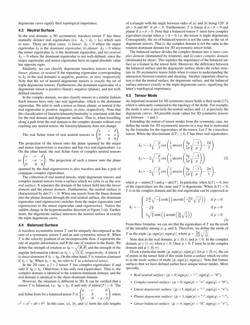
4.5 Tensor ModeAn important invariant for 3D symmetric tensor fields is their mode [17],which is intricately connected to the topology of the fields. For example,the mode is zero at precisely the neutral surface and ±1 at precisely thedegenerate curves. All possible mode values for 3D symmetric tensorsare between −1 and 1.

Extending the notion of tensor modes from the symmetric case, wedefine the mode for 3D asymmetric tensors in a way that is motivatedby the formulas for the eigenvalues of the tensor. Let T be a tracelesstensor. When the discriminant Δ(T )≥ 0, T has three real eigenvalues:

λ1 =−2

√− p

3cos

(1

3arccos

(3q2p

√−3

p

)+

2π3

)

λ2 =−2

√− p

3cos

(1

3arccos

(3q2p

√−3

p

))

λ3 =−2

√− p

3cos

(1

3arccos

(3q2p

√−3

p

)− 2π

3

),

(2)

where p=minor(T ) and q= det(T ). In particular, when Δ(T ) = 0, twoof the eigenvalues are the same and T is degenerate. When Δ(T )< 0,T is in the complex domain and the real eigenvalue can be expressed as

λ1 =−

⎧⎪⎪⎪⎪⎨⎪⎪⎪⎪⎩

2|q|q

√− p

3 cosh(

13 arcosh

(−3|q|2p

√−3p

))if p < 0

− 3√

q if p = 0

2√

p3 sinh

(13 arsinh

(3q2p

√3p

))if p > 0

(3)From these formulas, we can see that the eigenvalues of T are the resultof the interplay among p, q, and Δ. Therefore, we define the mode of

T as the triple (μ,sign(p),sign(q)) where μ =3|q|2|p|√

3|p| .

Note that in the real domain, μ ∈ [0,1] and p < 0. In the complexdomain, μ ∈ (1,∞) when p < 0. Once p > 0, T must be in the complexdomain and μ ∈ [0,∞).

Given a particular mode (μ,sign(p),sign(q)) for μ ∈ [0,∞], the setof points in the tensor field of this mode forms a surface which we referto as the mode surface of mode (μ,sign(p),sign(q)). Note that featuresurfaces that we have defined earlier have unique tensor modes. Morespecially,

• Real neutral surface: (μ = 0,sign(p) = “-”,sign(q) = “0”),

• Complex neutral surface: (μ = 0,sign(p) = “+”,sign(q) = “0”),

• Linear degenerate surface: (μ = 1,sign(p) = “-”,sign(q) = “+”),

• Planar degenerate surface: (μ = 1,sign(p) = “-”,sign(q) = “-”),

• Linear balanced surface: (μ = ∞,sign(p) = “0”,sign(q) = “+”),

• Planar balanced surface: (μ = ∞,sign(p) = “0”,sign(q) = “-”).

Another special mode is when sign(p) = “0” and sign(q) = “0”; in thiscase, μ is undefined. The set of points with this mode is precisely thetriple degenerate curve.

4.6 Eigenvalue Space

The definition of tensor mode allows us to construct a model for all 3Dasymmetric tensors, which we refer to as the eigenvalue space for 3Dasymmetric tensors. We first consider the set of all traceless tensors,which we map to the border of a hexagon and its center as shown inFigure 4. Each point on the border of the hexagon represents a uniquetensor mode. Starting from the top and continuing counterclockwise,we encounter special modes in the order of real neutral tensors, lineardegenerate tensors, linear balanced tensors, complex neutral tensors,planar balanced tensors, and planar degenerate tensors, as shown inFigure 4. In addition, the center of the hexagon corresponds to the tripledegenerate tensors. On the other hand, points inside the hexagon otherthan the center do not correspond to any valid tensor mode. Note thatthe real domain consists of two edges in the hexagon (upper-left andupper-right), while the complex domain consists of the other four edges.The left and right edges correspond to the outer complex domain, whilethe lower-left and lower-right edges correspond to the inner complexdomain. Furthermore, the left half and the right half of the hexagonsignify the symmetry between linear and planar tensors.

Note that the triple degenerate curve is adjacent to every modesurface. The domain of the tensor field is the disjoint union of all themode surfaces. We can consider the volume being a book with eachmode surface as a page and the triple degenerate curve as the bookspine. Figure 1 (a) illustrates this idea with a tensor field.

For a tensor T that may have a non-zero trace, we define the notion

Fig. 4: The eigenvalue space contains seven special tensors basedon the tensor mode: real neutral tensors, complex neutral tensors,linear degenerate tensors, planar degenerate tensors, linear balancedtensors, planar balanced tensors, and triple degenerate tensors. Whenthe tensor represents the velocity gradient of some incompressible flow,the corresponding flow patterns are illustrated next to the tensor. Noticethat the flow pattern inside the 2D plane is simple shear when thetensor is degenerate (linear, planar, and triple). For neutral tensors,the projection is either a saddle (real neutral) or an elliptical pattern(complex neutral). For linear tensors, the flow leaves the plane in thethird dimension, while for planar tensors, the flow enters the plane inthe third dimension.

-1

0

1

Isotropicity

Fig. 5: We add to our eigenvalue space two additional special tensorswith isotropicity of ±1 at the top (brown dot) and the bottom (pink dot)and model the eigenvalue space as a hexagonal double cone with oneadditional line segment.

of isotropicity as

η(T ) =trace(T )√

3||T || (4)

Note that the isotropicity of a tensor must be between −1 and 1, wherethe isotropicity of ±1 corresponds to a positive and negative multipleof the identity matrix, respectively.

Given a 3D asymmetric tensor of unit magnitude, its mode andisotropocity uniquely determine its eigenvalues. In addition, when atensor has an isotropicity of ±1, its deviator is zero, making its modenot well-defined. Consequently, we add to our eigenvalue space twoadditional special tensors: isotropicity of 1 and isotropicity of −1. Thisleads to a double hexagonal cone and line segment in the middle asshown in Figure 5. The base of the double cone corresponds to trace-less tensors, which are modeled by the hexagon in Figure 4. The topand bottom tip points in the double cone correspond to the 1 and −1isotropocities, respectively. Each point on the surface of this doublecone as well as the line between the top and bottom tips correspondsto a unique combination of eigenvalues in a tensor up to a positivemultiple. We refer to the double cone and the center line segment as theeigenvalue space for 3D asymmetric tensors. Note that pure isotropoc-ity tensors (i.e. η(T ) =±1) are co-dimension eight in the space of 3Dasymmetric tensors. Thus, they are structurally unstable. However, weinclude them in our eigenvalue space for their theoretical values. Theset of points in the field with a given isotropicity η �=±1 is a surface,which we refer to as an isotropicity surface. A special isotropicitysurface is the traceless surface, whose corresponding isotropicity valueis zero. Note that for incompressible fluid data, its gradient tensor isalways traceless; thus, the traceless surface becomes the whole domain.Another feature surface that we visualize is the magnitude surface,which consists of the points in the field with the same tensor magni-tude that is not zero. Note that the set of zero magnitude tensors isco-dimension nine in the tensor field and thus structurally unstable.

5 EXTRACTION OF FEATURE CURVES AND SURFACES

The input data to our visualization is a piecewise linear tensor fielddefined on a tetrahedral mesh. To extract the aforementioned featurecurves and surfaces, we consider their complexity. Inside a tetrahedron,the tensor field is linear and can be locally expressed as T (x,y,z) =T0+xTx+yTy+zTz where T0, Tx, Ty, and Tz are 3D asymmetric tensors.

5.1 Magnitude SurfaceThe magnitude surface of a given magnitude s > 0 is thus character-ized by ||T ||2 = s2. Note that when T (x,y,z) is linear, f (x,y,z) =||T (x,y,z)||2− s2 is a quadratic polynomial of x, y, and z. Under struc-turally stable conditions, a quadratic surface is part of either an ellip-soid, a single-sheet hyperboloid, or a double-sheet hyperboloid. Note

(a)

f (x,y,z)

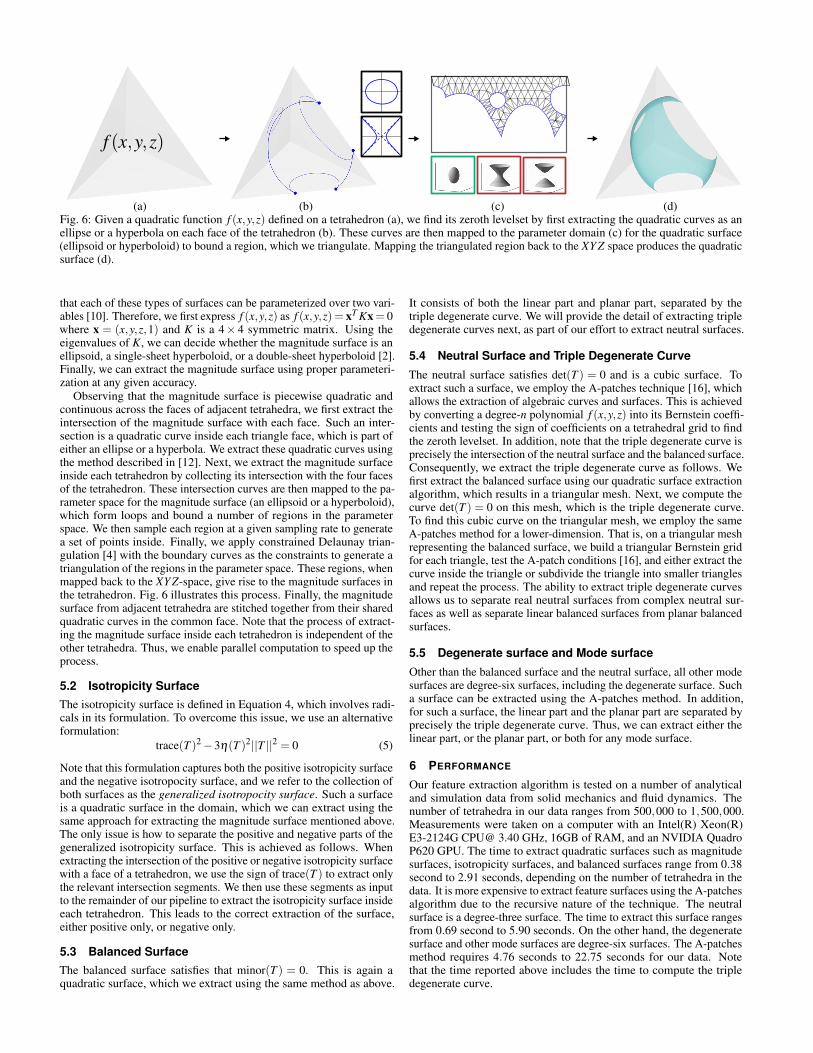
(b) (c) (d)Fig. 6: Given a quadratic function f (x,y,z) defined on a tetrahedron (a), we find its zeroth levelset by first extracting the quadratic curves as anellipse or a hyperbola on each face of the tetrahedron (b). These curves are then mapped to the parameter domain (c) for the quadratic surface(ellipsoid or hyperboloid) to bound a region, which we triangulate. Mapping the triangulated region back to the XY Z space produces the quadraticsurface (d).

that each of these types of surfaces can be parameterized over two vari-ables [10]. Therefore, we first express f (x,y,z) as f (x,y,z) = xT Kx= 0where x = (x,y,z,1) and K is a 4× 4 symmetric matrix. Using theeigenvalues of K, we can decide whether the magnitude surface is anellipsoid, a single-sheet hyperboloid, or a double-sheet hyperboloid [2].Finally, we can extract the magnitude surface using proper parameteri-zation at any given accuracy.

Observing that the magnitude surface is piecewise quadratic andcontinuous across the faces of adjacent tetrahedra, we first extract theintersection of the magnitude surface with each face. Such an inter-section is a quadratic curve inside each triangle face, which is part ofeither an ellipse or a hyperbola. We extract these quadratic curves usingthe method described in [12]. Next, we extract the magnitude surfaceinside each tetrahedron by collecting its intersection with the four facesof the tetrahedron. These intersection curves are then mapped to the pa-rameter space for the magnitude surface (an ellipsoid or a hyperboloid),which form loops and bound a number of regions in the parameterspace. We then sample each region at a given sampling rate to generatea set of points inside. Finally, we apply constrained Delaunay trian-gulation [4] with the boundary curves as the constraints to generate atriangulation of the regions in the parameter space. These regions, whenmapped back to the XY Z-space, give rise to the magnitude surfaces inthe tetrahedron. Fig. 6 illustrates this process. Finally, the magnitudesurface from adjacent tetrahedra are stitched together from their sharedquadratic curves in the common face. Note that the process of extract-ing the magnitude surface inside each tetrahedron is independent of theother tetrahedra. Thus, we enable parallel computation to speed up theprocess.

5.2 Isotropicity SurfaceThe isotropicity surface is defined in Equation 4, which involves radi-cals in its formulation. To overcome this issue, we use an alternativeformulation:

trace(T )2−3η(T )2||T ||2 = 0 (5)

Note that this formulation captures both the positive isotropicity surfaceand the negative isotropocity surface, and we refer to the collection ofboth surfaces as the generalized isotropocity surface. Such a surfaceis a quadratic surface in the domain, which we can extract using thesame approach for extracting the magnitude surface mentioned above.The only issue is how to separate the positive and negative parts of thegeneralized isotropicity surface. This is achieved as follows. Whenextracting the intersection of the positive or negative isotropicity surfacewith a face of a tetrahedron, we use the sign of trace(T ) to extract onlythe relevant intersection segments. We then use these segments as inputto the remainder of our pipeline to extract the isotropicity surface insideeach tetrahedron. This leads to the correct extraction of the surface,either positive only, or negative only.

5.3 Balanced SurfaceThe balanced surface satisfies that minor(T ) = 0. This is again aquadratic surface, which we extract using the same method as above.

It consists of both the linear part and planar part, separated by thetriple degenerate curve. We will provide the detail of extracting tripledegenerate curves next, as part of our effort to extract neutral surfaces.

5.4 Neutral Surface and Triple Degenerate Curve

The neutral surface satisfies det(T ) = 0 and is a cubic surface. Toextract such a surface, we employ the A-patches technique [16], whichallows the extraction of algebraic curves and surfaces. This is achievedby converting a degree-n polynomial f (x,y,z) into its Bernstein coeffi-cients and testing the sign of coefficients on a tetrahedral grid to findthe zeroth levelset. In addition, note that the triple degenerate curve isprecisely the intersection of the neutral surface and the balanced surface.Consequently, we extract the triple degenerate curve as follows. Wefirst extract the balanced surface using our quadratic surface extractionalgorithm, which results in a triangular mesh. Next, we compute thecurve det(T ) = 0 on this mesh, which is the triple degenerate curve.To find this cubic curve on the triangular mesh, we employ the sameA-patches method for a lower-dimension. That is, on a triangular meshrepresenting the balanced surface, we build a triangular Bernstein gridfor each triangle, test the A-patch conditions [16], and either extract thecurve inside the triangle or subdivide the triangle into smaller trianglesand repeat the process. The ability to extract triple degenerate curvesallows us to separate real neutral surfaces from complex neutral sur-faces as well as separate linear balanced surfaces from planar balancedsurfaces.

5.5 Degenerate surface and Mode surface

Other than the balanced surface and the neutral surface, all other modesurfaces are degree-six surfaces, including the degenerate surface. Sucha surface can be extracted using the A-patches method. In addition,for such a surface, the linear part and the planar part are separated byprecisely the triple degenerate curve. Thus, we can extract either thelinear part, or the planar part, or both for any mode surface.

6 PERFORMANCE

Our feature extraction algorithm is tested on a number of analyticaland simulation data from solid mechanics and fluid dynamics. Thenumber of tetrahedra in our data ranges from 500,000 to 1,500,000.Measurements were taken on a computer with an Intel(R) Xeon(R)E3-2124G CPU@ 3.40 GHz, 16GB of RAM, and an NVIDIA QuadroP620 GPU. The time to extract quadratic surfaces such as magnitudesurfaces, isotropicity surfaces, and balanced surfaces range from 0.38second to 2.91 seconds, depending on the number of tetrahedra in thedata. It is more expensive to extract feature surfaces using the A-patchesalgorithm due to the recursive nature of the technique. The neutralsurface is a degree-three surface. The time to extract this surface rangesfrom 0.69 second to 5.90 seconds. On the other hand, the degeneratesurface and other mode surfaces are degree-six surfaces. The A-patchesmethod requires 4.76 seconds to 22.75 seconds for our data. Notethat the time reported above includes the time to compute the tripledegenerate curve.

7 APPLICATIONS

In this section, we apply our novel analysis to a number of analytical andsimulation datasets in solid mechanics and fluid dynamics. Additionally,we provide some physical interpretation of our visualization based onour tensor field analysis.

7.1 Solid Mechanics

Twisted bundles of steel cables can be found in many places in reallife, from those embedded in truck tires to bring additional support, tothose used for suspension structures such as cable cars, elevators, andcranes (machines). The cables can fail due to the wear and tear fromthe cables untwisting under stress (heavy weight lifting). Such failurescan in turn lead to property damages and loss of lives. To understandthe potential weakness in the steel cables under stress due to twisting,we consider the first Piola-Kirchhoff (PK1) stress tensor [11] used tostudy metal plasticity. Unlike the perhaps better-known Cauchy stresswhich is symmetric, the PK1 stress tensor is asymmetric as it is the

30%

100%

(a) deformation (b) Cauchy stress (c) PK1 stress

Fig. 7: We visualize the features at 30% and 100% of the loading of thetwisting scenario. The images from the left to the right column are (a)the deformation, (b) the degenerate curves of the Cauchy stress tensorfields, and (c) the degenerate surfaces of the PK1 stress tensor fields.

(a) η(T ) =±0.7 (b) η(T ) =±0.5 (c) η(T ) = 0

(d) ‖T‖= 50 (e) ‖T‖= 100 (f) ‖T‖= 150

Fig. 8: We visualize three isotropicity surfaces (a-c) and three magni-tude surfaces (d-f). The magnitude surfaces are colored in navy blue,while the positive and negative isotropicity surfaces are colored inbrown and pink, respectively. The traceless surface (zero isotropicity)is colored in teal.

product of the Cauchy stress and the deformation gradient tensor.The twisting scenario is simulated with SIMULIA [24]. Figure 7

shows two twisting stages of a block whose front face is fixed and theback face is twisted: (top) 30% of the full twist, and (bottom) fullytwisted (18◦). We observe that the degenerate curves in the Cauchystress tensor fields (Figure 7 (b): colored curves) and the degeneratesurfaces in the PK1 stress tensor fields (Figure 7 (c): colored surfaces)both have a twisting structure. However, the Cauchy stress tensor fields(Figure 7 (b)) do not have a complex domain and the set of degeneratetensors in the field form curves. This is visible from the visualizationshown in the middle column, where linear degenerate curves are coloredin green and planar degenerate curves are colored in yellow. Note thatdespite the significantly different twists at different stages, the Cauchystress leads to the nearly identical set of degenerate curves (Figure 7 (b):top and bottom). In contrast, the visualization of the PK1 tensor fields(Figure 7 (c)) shows a clear difference in the degenerate surfaces for thetwo stages. While at 30% (Figure 7 (c): top), the degenerate surface inthe PK1 tensor is similar to the degenerate curves in the Cauchy stress(Figure 7 (b): top), at 100%, a pronounced difference is shown (Figure 7(b-c): bottom). This highlights the potential benefits of visualizing theasymmetric PK1 stress over the symmetric Cauchy stress for twistingmotions. Moreover, in the PK1 stress tensor fields, the linear and planardegenerate surfaces point out the boundary conditions of the fixedside and the twisting side of the block. Since the fixed side has lessdeformation, the region of the complex domain is smaller. Furthermore,while the loading is increasing, the complex region is growing, whichindicates that the rotation-dominant domain is getting larger.

Figure 8 visualizes the isotropicity surfaces and the magnitude sur-faces which have a skew-symmetric structure as well. In addition, theisotropicity surfaces illustrate the material is compressed at the centerand isotropically stretched on the boundary. Insights such as these aredependent on the ability to perform tensor field analysis.

Note that both the PK1 stress and the Cauchy stress can provideimportant insights into the underlying mechanics as such insights arecomplementary. As tensor fields, certain tools are available for bothsymmetric and asymmetric tensor fields, such as eigenvalue analysis.On the other hand, the interpretation of such analysis depends on manyfactors such as the type of the tensors and the physical quantities thatthey represent. Consequently, visualizing both types of tensor fieldsand understanding the connection between their structures, i.e. multi-field visualization, can provide a more holistic view of the underlyingphysics than using only one of them.

7.2 Fluid DynamicsThe velocity gradient tensor field of a flow plays an important role inunderstanding fluid dynamics, and asymmetric tensor field analysisof such a field can lead to complementary insight to existing vectorfield visualization methods [27]. In this paper, we perform analysisand visualization of 3D velocity gradient tensor fields directly insteadof their 2D projections onto some lower-dimensional surface or probeplane. We will discuss our data sets: (1) the Lorenz attractor, (2) theRayleigh-Bernard flow, (3) the Arnold–Beltrami–Childress flow, and(4) an open-channel flow (Appendix).

Lorenz attractor is a set of chaotic solutions to the Lorenz sys-tem [15] with system parameters σ , ρ , and β . Figure 1 (a) shows thebutterfly-shaped attractor (the grey winding curve) in the system whenσ = 10, ρ = 28, and β = 8/3 [15]. We extract and visualize the featurecurve and surfaces in the gradient tensor, such as (b) linear degeneratesurfaces (green) and planar degenerate surfaces (yellow), (c) real neu-tral surfaces (orange) and complex neutral surfaces (red), and (d) linearbalanced surfaces (blue) and planar balanced surfaces (magenta). Notethat all of these surfaces intersect exactly at the triple degenerate curves(black). Moreover, topological feature surfaces separate the two criticalpoints in the attractor, and these surfaces exhibit a two-way rotationalsymmetry.

The Rayleigh-Bernard flow is thermal convection in a thin hori-zontal layer of fluid heated from below by maintaining the constanttemperature difference between the upper and lower boundaries. Theflow is characterized by the formation of two convection cells as shown

0 01

1

(a) vector field (b) degenerate surfaces (c) balanced surfaces (d) neutral surfacesFig. 9: This figure visualizes the Rayleigh-Bernard flow with (a) the vector field, (b) the linear and planar degenerate surfaces (green and yellow),(c) the real and complex neutral surfaces (orange and red) neutral surfaces, and (d) linear and planar balanced surfaces (blue and magenta). Noticethat the triple degenerate curve (black curves) can be considered as the spine to which the feature surfaces are attached.

(a) vector field (b) mode surfaces (c) triple degenerate curvesFig. 10: We magnify the center portion of the Bernard cell and show(a) the streamlines of the vector field, (b) the mode surfaces and (c) thetriple degenerate curves.

in Figure 9 (a). Identifying regions of stretching and compression aswell as the rotation-dominant region is useful yet challenging. With ourfeature surfaces, such spaces can be better perceived. Notice that thetriple degenerate curve (black) can be considered as a spine to whichother feature surfaces are attached.

In Figure 10 (a), we zoom in on the center portion of the Bernardcell (x ∈ [0.5,0.8]; y ∈ [0.35,0.65]; z ∈ [0.35,0.65]) and visualize theneutral surfaces, the degenerate surfaces, the balanced surfaces, and thetriple degenerate curves (Figure 10 (b)). Note that the left face of thecube corresponds to the center face that separates the pair of convectioncells and the lower-left corner contains the converging upwelling flow.There, we observe a quick transition of the relatively flat and parallelmode surfaces: the planar degenerate surface (leftmost, yellow), thereal neutral surface (orange), the linear degenerate surface (green),and the linear balanced surface (rightmost, blue). Near the bottom,underneath the real neutral surface, the converging flow is dominatedby shearing with compression (planar), and then becomes stretching-dominant (linear) by crossing the real neutral surface. Next, the strengthof the rotation gradually increases until the shear balances the rotationat the linear balanced surface (blue). Finally, we enter the rotation-dominant convection cell domain on the right-hand side of the linearbalanced surface (blue).

Furthermore, in the upper part of upwelling convection, the flowcharacteristic transitions exhibit more volumetric appearance: fromthe linear degenerate surface (leftmost, green), real neutral surface(orange), planar degenerate surface (yellow), planar balanced surface(magenta), to the complex neutral surface (rightmost, red) in the rota-tion cell. Lastly, we notice both the triple degenerate curves have an“M” shape, with the triple degenerate curve near the bottom of the cubebeing narrower (Figure 10 (c)). We conjecture that the converging flowpattern pushes the triple degenerate curves towards the center of thedomain, thus the “M” shapes. The above observations of the flow char-acteristics and behaviors can be difficult to detect and interpret correctlywith the 2D flow and tensor field visualization in probe planes. Suchcomprehensive analysis is attainable with the use of 3D visualizationof the velocity gradient tensors.

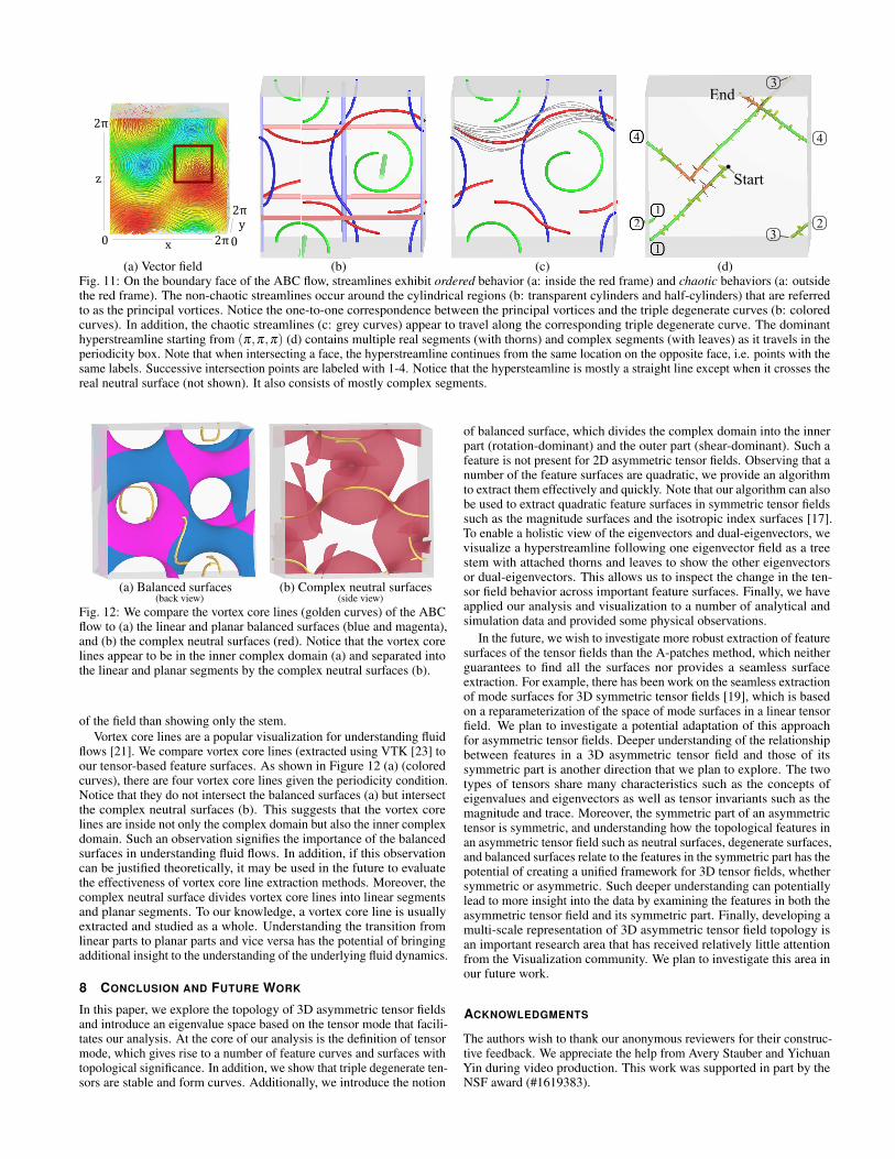
Arnold–Beltrami–Childress flow (ABC flow) is a 3D incompress-ible vector field that is a steady-state solution to Euler’s equations [7].The ABC flow is periodic in each of the X , Y , and Z directionswith a period of 2π and is usually studied in its periodicity box:[0,2π)× [0,2π)× [0,2π) (Figure 11 (a): the cube). One of the maincharacteristics of the ABC flow is the existence of chaotic streamlines,which, due to the periodicity in the flow, can intersect a face of theperiodicity box infinitely many times so that the set of the intersec-

tion points fills a region in the face [7]. When A = 1, B =√

2/3,

and C =√

1/3, chaotic streamlines occur outside the so-called prin-cipal vortices, each of which is a tubular region along one of the X ,Y , and Z axes (Figure 11 (b): colored cylinders and half-cylinders dueto periodicity). There are a total of six principal vortices, two alongeach axis. Inside a principal vortex, the streamlines’ orientations arepredominantly along the direction of the tube. Each such streamlineintersects a face of the cube at a set of points that are on a curve (in-stead of a region). Such streamlines are not chaotic. On the faces ofthe periodicity box, the intersection points with chaotic streamlines areoutside the principal vortices. While Dombre and Frisch [7] illustratethe principal vortices as cylinders, they point out that these regions arehelical, which, when traveling from one face to the opposite face ofthe cube, finish a turn of 2π . We observe that there is a one-to-onecorrespondence between the set of triple degenerate curves (Figure 11(b): colored curves) and the set of principal vortices. Note that someof the triple degenerate curves are divided into three segments by thefaces of the periodicity box. We notice that each triple degenerate curvealso has a helical shape and finishes a turn of 2π after traveling fromone face to the opposite face. Moreover, each triple degenerate curve isa loop under the periodic condition. In addition, the streamlines in aprincipal vortex (Figure 11 (c): grey curves) appear to be around thetriple degenerate curves. The correlation between the triple degeneratecurves and the principal vortices in terms of their numbers, locations,and shapes suggests that additional insights may be gained on the ABCflow by inspecting the topological structures in its gradient tensor field.

Besides the periodicity in the flow, there is an additional eight-foldsymmetry within the periodicity box [7] that leads to the fundamen-tal box: [0,π)× [0,π)× [0,π) which is one-eighth of the periodic-ity box. Given this, we compute the dominant hyperstreamline fromp = (π,π,π) in one direction. Figure 11 (d) shows the augmentedhyperstreamline through p, which, when intersecting a face of the pe-riodicity box, continues from the same location on the opposite face.Successive intersection points are labeled with 1-4. Notice that thehyperstreamline is mostly straight, except where the dominant eigen-vectors are discontinuous (crossing the real neutral surfaces). Thevariety of tensor field behavior along the hyperstreamline reflects therich structure in the ABC flow. This highlights the benefit of our tree-based augmented hyperstreamline visualization, which can be usedas a probing tool for the field with only one user-specified seed point.The eigenvector information in the field along the hyperstreamline iscaptured by the thorns and leaves, giving the user a more holistic view

00 22

2z

x y1

12 2

3

3

4 4

End

Start

1

12

4

E

(a) Vector field (b) (c) (d)Fig. 11: On the boundary face of the ABC flow, streamlines exhibit ordered behavior (a: inside the red frame) and chaotic behaviors (a: outsidethe red frame). The non-chaotic streamlines occur around the cylindrical regions (b: transparent cylinders and half-cylinders) that are referredto as the principal vortices. Notice the one-to-one correspondence between the principal vortices and the triple degenerate curves (b: coloredcurves). In addition, the chaotic streamlines (c: grey curves) appear to travel along the corresponding triple degenerate curve. The dominanthyperstreamline starting from (π,π,π) (d) contains multiple real segments (with thorns) and complex segments (with leaves) as it travels in theperiodicity box. Note that when intersecting a face, the hyperstreamline continues from the same location on the opposite face, i.e. points with thesame labels. Successive intersection points are labeled with 1-4. Notice that the hypersteamline is mostly a straight line except when it crosses thereal neutral surface (not shown). It also consists of mostly complex segments.

(a) Balanced surfaces(back view)

(b) Complex neutral surfaces(side view)

Fig. 12: We compare the vortex core lines (golden curves) of the ABCflow to (a) the linear and planar balanced surfaces (blue and magenta),and (b) the complex neutral surfaces (red). Notice that the vortex corelines appear to be in the inner complex domain (a) and separated intothe linear and planar segments by the complex neutral surfaces (b).

of the field than showing only the stem.

Vortex core lines are a popular visualization for understanding fluidflows [21]. We compare vortex core lines (extracted using VTK [23] toour tensor-based feature surfaces. As shown in Figure 12 (a) (coloredcurves), there are four vortex core lines given the periodicity condition.Notice that they do not intersect the balanced surfaces (a) but intersectthe complex neutral surfaces (b). This suggests that the vortex corelines are inside not only the complex domain but also the inner complexdomain. Such an observation signifies the importance of the balancedsurfaces in understanding fluid flows. In addition, if this observationcan be justified theoretically, it may be used in the future to evaluatethe effectiveness of vortex core line extraction methods. Moreover, thecomplex neutral surface divides vortex core lines into linear segmentsand planar segments. To our knowledge, a vortex core line is usuallyextracted and studied as a whole. Understanding the transition fromlinear parts to planar parts and vice versa has the potential of bringingadditional insight to the understanding of the underlying fluid dynamics.

8 CONCLUSION AND FUTURE WORK

In this paper, we explore the topology of 3D asymmetric tensor fieldsand introduce an eigenvalue space based on the tensor mode that facili-tates our analysis. At the core of our analysis is the definition of tensormode, which gives rise to a number of feature curves and surfaces withtopological significance. In addition, we show that triple degenerate ten-sors are stable and form curves. Additionally, we introduce the notion

of balanced surface, which divides the complex domain into the innerpart (rotation-dominant) and the outer part (shear-dominant). Such afeature is not present for 2D asymmetric tensor fields. Observing that anumber of the feature surfaces are quadratic, we provide an algorithmto extract them effectively and quickly. Note that our algorithm can alsobe used to extract quadratic feature surfaces in symmetric tensor fieldssuch as the magnitude surfaces and the isotropic index surfaces [17].To enable a holistic view of the eigenvectors and dual-eigenvectors, wevisualize a hyperstreamline following one eigenvector field as a treestem with attached thorns and leaves to show the other eigenvectorsor dual-eigenvectors. This allows us to inspect the change in the ten-sor field behavior across important feature surfaces. Finally, we haveapplied our analysis and visualization to a number of analytical andsimulation data and provided some physical observations.

In the future, we wish to investigate more robust extraction of featuresurfaces of the tensor fields than the A-patches method, which neitherguarantees to find all the surfaces nor provides a seamless surfaceextraction. For example, there has been work on the seamless extractionof mode surfaces for 3D symmetric tensor fields [19], which is basedon a reparameterization of the space of mode surfaces in a linear tensorfield. We plan to investigate a potential adaptation of this approachfor asymmetric tensor fields. Deeper understanding of the relationshipbetween features in a 3D asymmetric tensor field and those of itssymmetric part is another direction that we plan to explore. The twotypes of tensors share many characteristics such as the concepts ofeigenvalues and eigenvectors as well as tensor invariants such as themagnitude and trace. Moreover, the symmetric part of an asymmetrictensor is symmetric, and understanding how the topological features inan asymmetric tensor field such as neutral surfaces, degenerate surfaces,and balanced surfaces relate to the features in the symmetric part has thepotential of creating a unified framework for 3D tensor fields, whethersymmetric or asymmetric. Such deeper understanding can potentiallylead to more insight into the data by examining the features in both theasymmetric tensor field and its symmetric part. Finally, developing amulti-scale representation of 3D asymmetric tensor field topology isan important research area that has received relatively little attentionfrom the Visualization community. We plan to investigate this area inour future work.

ACKNOWLEDGMENTS

The authors wish to thank our anonymous reviewers for their construc-tive feedback. We appreciate the help from Avery Stauber and YichuanYin during video production. This work was supported in part by theNSF award (#1619383).

REFERENCES

[1] R. W. Aldhaheri and H. K. Khalil. A real schur form method for modeling

singularly perturbed systems. IEEE Transactions on Automatic Control,34(8):856–861, 1989. doi: 10.1109/9.29427

[2] W. H. Beyer. Crc standard mathematical tables and formulae. Boca Raton,

1991.

[3] L. Cammoun, C. A. Castano-Moraga, E. Munoz-Moreno, D. Sosa-Cabrera,

B. Acar, M. Rodriguez-Florido, A. Brun, H. Knutsson, J. Thiran, S. Aja-

Fernandez, R. de Luis Garcia, D. Tao, and X. Li. Tensors in Image Pro-cessing and Computer Vision. Advances in Pattern Recognition. Springer

London, London, 2009.

[4] L. P. Chew. Constrained delaunay triangulations. Algorithmica, 4(1):97–

108, 1989.

[5] J. C. Criscione, J. D. Humphrey, A. S. Douglas, and W. C. Hunter. An

invariant basis for natural strain which yields orthogonal stress response

terms in isotropic hyperelasticity. Journal of the Mechanics and Physics ofSolids, 48(12):2445 – 2465, 2000. doi: 10.1016/S0022-5096(00)00023-5

[6] T. Delmarcelle and L. Hesselink. Visualizing second-order tensor fields

with hyperstream lines. IEEE Computer Graphics and Applications,

13(4):25–33, July 1993.

[7] T. Dombre, U. Frisch, J. M. Greene, M. Henon, A. Mehr, and A. M.

Soward. Chaotic streamlines in the abc flows. Journal of Fluid Mechanics,

167:353–391, 1986.

[8] T. Gerrits, C. Rossl, and H. Theisel. Glyphs for general second-order

2d and 3d tensors. IEEE Transactions on Visualization and ComputerGraphics, 23(1):980–989, 2016.

[9] L. Hesselink, Y. Levy, and Y. Lavin. The topology of symmetric, second-

order 3D tensor fields. IEEE Transactions on Visualization and ComputerGraphics, 3(1):1–11, Mar. 1997.

[10] D. Hilbert and S. Cohn-Vossen. Geometry and the Imagination. Num-

ber 87. American Mathematical Soc., 1999.

[11] P. Kelly. Mechanics Lecture Notes Part III. University of Auckland, 2020.

[12] F. Khan, L. Roy, E. Zhang, B. Qu, S. H. Hung, H. Yeh, R. S. Laramee,

and Y. Zhang. Multi-scale topological analysis of asymmetric tensor fields

on surfaces. IEEE Transactions on Visualization and Computer Graphics,

26(1):270–279, 2020. doi: 10.1109/TVCG.2019.2934314

[13] A. Kratz, C. Auer, M. Stommel, and I. Hotz. Visualization and analysis of

second-order tensors: Moving beyond the symmetric positive-definite case.

Computer Graphics Forum, 32(1):49–74, 2013. doi: 10.1111/j.1467-8659.

2012.03231.x

[14] Z. Lin, H. Yeh, R. S. Laramee, and E. Zhang. 2D Asymmetric Tensor FieldTopology, pp. 191–204. Springer Berlin Heidelberg, Berlin, Heidelberg,

2012. doi: 10.1007/978-3-642-23175-9 13

[15] E. N. Lorenz. Deterministic nonperiodic flow. Journal of the AtmosphericSciences, 20(2):130–141, 1963.

[16] C. Luk and S. Mann. Tessellating algebraic curves and surfaces using

a-patches. In GRAPP, pp. 82–89, 2009.

[17] J. Palacios, H. Yeh, W. Wang, Y. Zhang, R. S. Laramee, R. Sharma,

T. Schultz, and E. Zhang. Feature surfaces in symmetric tensor fields

based on eigenvalue manifold. IEEE Transactions on Visualization andComputer Graphics, 22(3):1248–1260, Mar. 2016. doi: 10.1109/TVCG.

2015.2484343

[18] D. Palke, Z. Lin, G. Chen, H. Yeh, P. Vincent, R. Laramee, and E. Zhang.

Asymmetric tensor field visualization for surfaces. IEEE Transactions onVisualization and Computer Graphics, 17(12):1979–1988, Dec. 2011. doi:

10.1109/TVCG.2011.170

[19] B. Qu, L. Roy, Y. Zhang, and E. Zhang. Mode surfaces of symmetric tensor

fields: Topological analysis and seamless extraction. IEEE Transactionson Visualization and Computer Graphics, 27(2):583–592, 2021. doi: 10.

1109/TVCG.2020.3030431

[20] F. Raith, C. Blecha, T. Nagel, F. Parisio, O. Kolditz, F. Gunther, M. Stom-

mel, and G. Scheuermann. Tensor field visualization using fiber surfaces

of invariant space. IEEE Transactions on Visualization and ComputerGraphics, 25(1):1122–1131, 2019.

[21] M. Roth and R. Peikert. A higher-order method for finding vortex core

lines. In Proceedings Visualization’98 (Cat. No. 98CB36276), pp. 143–

150. IEEE, 1998.

[22] L. Roy, P. Kumar, Y. Zhang, and E. Zhang. Robust and fast extraction of

3d symmetric tensor field topology. IEEE Transactions on Visualizationand Computer Graphics, 25(1):1102–1111, 2019. doi: 10.1109/TVCG.

2018.2864768

[23] W. Schroeder, K. Martin, and B. Lorensen. The Visualization Toolkit.

Kitware, 2006.

[24] M. Smith. ABAQUS/Standard User’s Manual, Version 6.14. Dassault

Systemes Simulia Corp, United States, 2015.

[25] L. E. Spence, A. J. Insel, and S. H. Friedberg. Elementary Linear Algebra.

Prentice Hall, 2000.

[26] X. Tricoche, G. Kindlmann, and C.-F. Westin. Invariant crease lines for

topological and structural analysis of tensor fields. IEEE Transactions onVisualization and Computer Graphics, 14(6):1627–1634, 2008. doi: 10.

1109/TVCG.2008.148

[27] E. Zhang, H. Yeh, Z. Lin, and R. S. Laramee. Asymmetric tensor analysis

for flow visualization. IEEE Transactions on Visualization and ComputerGraphics, 15(1):106–122, 2009.

[28] X. Zheng and A. Pang. Topological lines in 3d tensor fields. In ProceedingsIEEE Visualization 2004, VIS ’04, pp. 313–320. IEEE Computer Society,

Washington, DC, USA, 2004. doi: 10.1109/VISUAL.2004.105

[29] X. Zheng and A. Pang. 2D asymmetric tensor analysis. IEEE Proceedingson Visualization, pp. 3–10, Oct 2005.

[30] X. Zheng, B. N. Parlett, and A. Pang. Topological lines in 3d tensor fields

and discriminant hessian factorization. IEEE Transactions on Visualizationand Computer Graphics, 11(4):395–407, July 2005.

[31] V. Zobel and G. Scheuermann. Extremal curves and surfaces in symmetric

tensor fields. The Visual Computer, Oct 2017. doi: 10.1007/s00371-017

-1450-1