Embed Size (px)
Citation preview

Clemson UniversityTigerPrints
All Theses Theses
12-2015
Feasibility Study of Porous Media Compressed AirEnergy Storage In South Carolina, United States ofAmericaAlexandra-Selene JarvisClemson University, [email protected]
Follow this and additional works at: https://tigerprints.clemson.edu/all_theses
Part of the Environmental Sciences Commons, and the Geology Commons
This Thesis is brought to you for free and open access by the Theses at TigerPrints. It has been accepted for inclusion in All Theses by an authorizedadministrator of TigerPrints. For more information, please contact [email protected].
Recommended CitationJarvis, Alexandra-Selene, "Feasibility Study of Porous Media Compressed Air Energy Storage In South Carolina, United States ofAmerica" (2015). All Theses. 2256.https://tigerprints.clemson.edu/all_theses/2256
i
FEASIBILITY STUDY OF POROUS MEDIA COMPRESSED AIR ENERGY
STORAGE IN SOUTH CAROLINA, UNITED STATES OF AMERICA
________________________________________________________________________
A Thesis
Presented to
the Graduate School of
Clemson University
________________________________________________________________________
In Partial Fulfillment
of the Requirements for the Degree
Master of Science
Hydrogeology
________________________________________________________________________
by
Alexandra-Selene Jarvis
December 2015
________________________________________________________________________
Accepted by:
Dr. Ronald Falta, Committee Chair
Dr. Lawrence Murdoch
Dr. James Castle

ii
ABSTRACT
Renewable Energy Systems (RES) such as solar and wind, are expected to play a
progressively significant role in electricity production as the world begins to move away
from an almost total reliance on nonrenewable sources of power. In the US there is
increasing investment in RES as the Department of Energy (DOE) expands its wind
power network to encompass the use of offshore wind resources in places such as the
South Carolina (SC) Atlantic Coastal Plain.
Because of their unstable nature, RES cannot be used as reliable grid-scale power
sources unless power is somehow stored during excess production and recovered at times
of insufficiency. Only two technologies have been cited as capable of storing renewable
energy at this scale: Pumped Hydro Storage and Compressed Air Energy Storage
(CAES). Both CAES power plants in existence today use solution-mined caverns as their
storage spaces. This project focuses on exploring the feasibility of employing the CAES
method to store excess wind energy in sand aquifers. The numerical multiphase flow
code, TOUGH2, was used to build models that approximate subsurface sand formations
similar to those found in SC. Although the aquifers of SC have very low dips, less than
10, the aquifers in this study were modeled as flat, or having dips of 00.
Cycle efficiency is defined here as the amount of energy recovered compared to
the amount of energy injected. Both 2D and 3D simulations have shown that the greatest
control on cycle efficiency is the volume of air that can be recovered from the aquifer
after injection. Results from 2D simulations showed that using a dual daily peak load

iii
schedule instead of a single daily peak load schedule increased cycle efficiency as do the
following parameters: increased anisotropy, screening the well in the upper portions of
the aquifer, reduced aquifer thickness, and an initial water displacement by the
continuous injection of air for at least 60 days.
Aquifer permeability of 1x10-12 m2 produced a cycle efficiency of 80%. A
decrease of permeability to 1x10-13 m2 reduced efficiency to 70%, while an increase to
1x10-11 m2 seemed to enhance efficiency, but significantly reduced the volume of air that
could be injected and recovered. The highest cycle efficiency that could be achieved
using the 3D simulation, without depleting aquifer pressure to preset limits, was 80%.
Attempts to improve cycle efficiency compromised air recovery. Further work is
necessary to determine the effects of low aquifer dips on air recovery and cycle
efficiency.

iv
AKNOWLEDGMENTS
I take this opportunity to thank The Environmental Engineering and Earth Science
Department of Clemson University for affording me an Assistantship without which I
would not have had the chance to pursue my MS degree.
I thank my committee chair, Dr. Ronald Falta and committee members Dr. James
Castle and Dr. Lawrence Murdoch for their knowledge, guidance and support throughout
this arduous graduate experience. I also thank Professor Alan Coulson, supervisor of the
Teaching Assistants.
I thank my parents, Leitha and Stephen Jarvis, whose sacrifices made it possible
for me to obtain my primary and secondary school educations. I thank my brother
Christian Giles for all the support he has given me through all of my tertiary level
education programs. Lastly I thank my best friend, Noor, for being there whenever I
needed laughter even as late or as early as 3 am.
v
TABLE OF CONTENTS
Page
TITLE PAGE……………………………………………………………………….……....i
ABSTRACT……….……………………………………………………………………....ii
ACKNOWLEDGMENTS………………………………………………………………...iv
TABLE OF CONTENTS…………………………………………………………….........v
LIST OF TABLES…………………………………………………………..……….….viii
LIST OF FIGURES…………………………………………………………….…...….....ix
1 INTRODUCTION…………………………………………………………..….….1
2 WIND ENERGY RESOURCES IN THE USA AND SOUTH CAROLINA……..5
2.1 Introduction………………………………………………………………...5
2.2 Future of wind energy in the USA……………………………………..…..5
2.3 Current Energy Sources, Generation and Use in South Carolina………….8
2.4 Wind Resource Potential and Development in South Carolina…………...11
2.5 Offshore Wind Potential Exploration in South Carolina.…….…………..16
3 THE TECHNOLOGY OF COMPRESSED AIR ENERGY STORAGE…....…..18
3.1 Introduction to Compressed Air Energy Storage (CAES)………………..18
3.2 The Traditional Gas Turbine……………………………………………...20
3.3 The Joule or Brayton Constant Pressure Cycle…………………………...22
3.4 Compressed Air Power Plant Turbines…………………………………...24
3.5 Existing CAES Power Plants………………………………………...…...26
3.6 Porous Media CAES……………………………………………………...31
4 CAES AS A BULK ENERGY STORAGE OPTION……………………...…….34
4.1 Motivations for Bulk Energy Storage…………………………………….34
4.2 The Evolving Interest in CAES as a Bulk Energy Storage Option………36
4.3 Addressing the Variability of Wind Energy………………………..…….38
vi
5 GEOLOGY OF SOUTH CAROLINA AND THE PMCAES SYSTEM………..40
5.1 The Proposed PMCAES System...……………………………………….40
5.2 General Geology of South Carolina……………………………………...40
5.3 The Atlantic Coastal Plain of South Carolina……………………………41
6 BASE CASE MODEL…………………………………………………………...50
6.1 Introduction……………………...……………………………………….50
6.2 Base Case Conceptual Model……………………………………………50
6.3 Numerical Model and Methodology……………………………………..55
6.4 Simulation of the PM-CAES Air Cycling……………………………….59
6.4.1 Overall Operating Procedures……………………………………59
6.4.2 Injection Procedures……………………………………………...60
6.4.3 Well Production and Productivity………………………………..62
6.5 Simulation Results and Analysis………………………………………...67
6.5.1 Initial Bubble Formation…………………………………………67
6.5.2 Air Cycling Results………………………………………………73
6.5.3 Quantitative Analysis…………………………………………….80
6.6 Wellbore Heat Loss………………………………………………………81
7 SENSITIVITY ANALYSIS TO PARAMETER CHANGES………………...…76
7.1 Introduction………………………………………………………………83
7.2 System Performance under Variable Cycle Length, Injection and
Production Rates………………………………………………….……...85
7.3 Effects of Aquifer Depth…………………………………………………91
7.4 Effects of Permeability………………………………………………..…95
7.5 Effects of Screen Length and Position………………………………...…98
7.6 Effects of Bubble Size…………………………………..…………..….100
7.7 Effects of Anisotropy…………………………………...………………103
7.8 Effects of Aquifer Thickness……………………..……….…………....106
Table of Contents (Continued) Page

vii
8 3D SIMULATION OF PMCAES........................................................................110
8.1 3D Model Parameters and Settings..........................................................110
8.2 Results and Analysis................................................................................114
8.3 An attempt to recover 100% of the Injected Energy................................123
9 PROJECT SUMMARY.......................................................................................127
10 CLOSING REMARKS........................................................................................129
REFERENCES.................................................................................................................131
Table of Contents (Continued) Page

viii
LIST OF TABLES
Page
Table 3.1: Characteristics of CAES plants currently in existence......................................31
Table 5.1 Transmissivity and Hydraulic Conductivity data for the SCCP aquifers...........44
Table 5.2. Range of permeability values for SC aquifers...................................................45
Table 5.3. General descriptions of hydrogeological units of SC........................................46
Table 5.4. Salinity zones in southeast USA........................................................................48
Table 6.1: PM-CAES base case model dimensions, initial conditions and comments.......53
Table 6.2: Material properties used in the numerical base case model...............................57
Table 6.3: Discretization attributes of layers and comments on the numerical model
of the base case.........................................................................................................58
Table 7.1: Model settings for all 14 scenarios presented in this chapter.............................84
Table 7.2 Injection and Production mass rates and cycle efficiencies for Scenarios
0, 1and 2....................................................................................................................87
Table 8.1: PM-CAES 3D model dimensions, initial conditions and comments................111
Table 8.2: Material properties used in the 3D model.........................................................112
ix
LIST OF FIGURES
Page
Figure 2.1: Installed wind capacity at the end of 2013 by state……………..…………....8
Figure 2.2: Electricity generation in South Carolina by type…………..............................9
Figure 2.3. Energy consumption of SC…………………………………………………..10
Figure 2.4: South Carolina offshore 90 m height map and wind resources potential……14
Figure 3.1: Schematic of a simple gas turbine for electric power generation……............21
Figure 3.2: P-V and T-s diagrams for the constant pressure Brayton/Joule cycle……….23
Figure 3.3: Schematic of the Huntorf Power Plant............................................................28
Figure 3.4: Schematic of the McIntosh Power Plant………………………………….…30
Figure 4.1: a Typical weekly electricity load/demand curve……………………...……..35
Figure 4.1: b Price of electricity in US dollars per MWh………..……………………....35
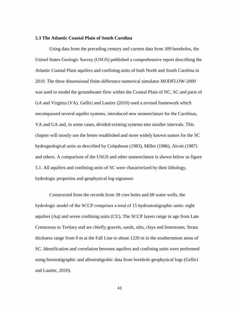
Figure 5.1: Comparison of hydrostratigraphic nomenclature of the SCCP…………...…42
Figure 5.2: Generalized geological cross section of South Carolina and locations of
sections……………………………………………………………………...49
Figure 6.1: Schematic of the conceptual model………………………………………….52
Figure 6.2: Radial cross section of the numerical model of the base case………….........56
Figure 6.3: Illustration of the air cycling procedure……………………………………..60
Figure 6.4: Plot of pressure distribution in the caprock 1 m away from the wellbore at
various injection pressures……………………...…………………………....61
Figure 6.5: Variation of air density with temperature and depth………………………...62
Figure 6.6: Plots of air production rates for 8 hours after the initial injection using various
PI values…………………………………………..………………………….65
Figure 6.7: Mass flow of air for 12 successive production cycles……………………….66
Figure 6.8: The average production rate from the 12 production cycles shown in figure
6.7…………………………………………………………………………...67
Figure 6.9: Temperature variation at the wellhead and aquifer top during bubble
development……………………………………………………………...…..69
x
Figure 6.10: Truncated radial cross sectional contour plots of the gas saturation
distribution in the aquifer around the vicinity of the wellbore during initial
bubble creation……………………………………………………………..70
Figure 6.11: Truncated radial cross sectional contour plots of the pressure distribution
in the aquifer around the vicinity of the wellbore during initial bubble
creation……………………………………………………………………71
Figure 6.12: Truncated radial cross sectional contour plots of the temperature distribution
in the aquifer around the vicinity of the wellbore during initial bubble
creation…………………………………………...………………...………72
Figure 6.13: Temperature variation along the wellbore at the well top and aquifer top
during first week of cycling………………………………...……………...74
Figure 6.14: Temperature variation along the wellbore at the well top and aquifer top
during three months of cycling………………………………..…………...74
Figure 6.15: Pressure distribution measured at the wellbore at the aquifer top during air
cycling………………...…………………………….………...……………75
Figure 6.16: Truncated radial cross sectional contour plots of the gas saturation
distribution in the aquifer around the vicinity of the wellbore at different
times during continuous cycling……………...………………...…………76
Figure 6.17: Truncated radial cross sectional contour plots of the temperature distribution
in the aquifer around the vicinity of the wellbore at different times during
continuous cycling…………………………………………………….…...77
Figure 6.18: Gas volume fraction during production section of cycles for 3 months of air
cycling………………………….…………….…………………….....……79
Figure 6.19: Energy efficiency for three months………………………………...………81
Figure 6.20: Comparison between energy storage efficiencies with or without considering
wellbore losses………………………………………….……………..…...82
Figure 7.1: Illustration of dual load scheme air cycling procedure………………...……85
Figure 7.2. Pressure measured at the wellbore at the top of the aquifer during cycling for
scenarios 0, 1 and 2……………………………….…………………….……88
Figure 7.3: Pressure measured within the wellbore at the top of the aquifer during cycling
using various production rates for the Huntorf schedule…………......….…..89
Figure 7.4: Cycle efficiencies calculated using different load schemes as designated
by S0, S1 and S2…………………………..……………………………..…..90
Figure 7.5. Air volume fraction produced during cycling using single, dual and the
Huntorf load schedules………………………………………………………90
List of Figures (Continued) Page
xi
Figure 7.6: Pressure measured within the wellbore at the aquifer top at different
depths during air cycling………………….…………………..………….…..92
Figure 7.7: Air fraction volume during production at different depths and different
injection and production rates………………....…………………….....….....93
Figure 7.8: Wellbore temperature at different depths ……………………………...……94
Figure 7.9: Cycle efficiency at various depths …………………………………..............94
Figure 7.10: Cycling pressure at different permeabilities. ……...……………….………96
Figure 7.11: Cycle efficiency using various permeabilities ……………………..............97
Figure 7.12: Air mass fraction at various permeabilities ……………………………......97
Figure 7.13: Air volume fraction at various permeabilities……………………………...98
Figure 7.14: Cycling pressure at different screen lengths and positions………………...99
Figure 7.15: Volume fraction of air produced with fully screened and half screened
wellbores…………………………………………………………….....…100
Figure 7.16: Cycle efficiencies with fully screened and partially screened
wellbores……………………………………………………………….....100
Figure 7.17: Cycling pressure for different bubble sizes……………………………….101
Figure 7.18: Air mass flow rates during production for S0, S9 and S10…….…...…….102
Figure 7.19: Cycle efficiency by bubble size………………………………………...…103
Figure 7.20: Cycling pressure measured in the wellbore at the top of the aquifer with
different degrees of anisotropy…………………………………………...104
Figure 7.21: Volume fraction of water produced using various degrees of anisotropy...105
Figure 7.22: Cycle efficiency using different values of anisotropy……………...……..106
Figure 7.23: Pressure measured at the wellbore at the top of the aquifer during cycling for
scenarios 0, 13 and 14……………………….……………...……..……...107
Figure 7.24: Air volume fraction during S0, S13 and S14……………………………..108
Figure 7.25: Cycle efficiency by aquifer thickness…………………………..….……..109
Figure 8.1: Map views of the polygonal mesh used for the 3D model and detailed view
around the wells to show mesh refinement………………………………..110
Figure 8.2: Plot of aquifer pressure within wellbore 1 at a well spacing of 5 m…….....113
Figure 8.3. Sg cross sectional and contour plots during first 90 days of the bubble
formation........................................................................................................115
List of Figures (Continued) Page

xii
Figure 8.4: Sg cross sectional and contour plots during the 2nd stage of bubble
formation…………………..……………......................................................116
Figure 8.5: Sg cross sectional and contour plots during cycling.………………...……..118
Figure 8.6: Sg cross sectional and contour plots at the end of 1 year of cycling.…...….119
Figure 8.7: Excerpts of the pressure measured during cycling at the center well during
one year of cycling for a production rate of 8 k g/s.……………..…………121
Figure 8.8: Average volume fraction of air produced from all 9 wells………………...122
Figure 8.9: Average cycle efficiency calculated from all 9 wells………………………122
Figure 8.10: Sg cross sectional and contour plots at the end of 1 year of cycling…..….124
Figure 8.11: Excerpts of the pressure measured during cycling at the center well during
the one year of cycling for a production rate of 10 kg/s.………………...125
Figure 8.12: Average volume fraction of air produced from all 9 wells……………….126
Figure 8.13. Average cycle efficiency calculated from all 9 wells…………………….126
List of Figures (Continued) Page

1
CHAPTER 1
INTRODUCTION
Efforts to reduce greenhouse gas emissions are leading to a reduced reliance on
conventional energy resources and an increased interest in renewable energy systems
(RES) such as wind and solar power (Lund and Salgi, 2009). Although RES are
becoming increasingly evident in energy markets, large scale use creates a challenge
because of their intermittent availability or their unstable nature because they do not
produce a steady energy output throughout the entire day. Energy storage is one of the
available technologies that can overcome the fluctuations associated with RES (Salgi and
Lund, 2008) so that when there is surplus production, the excess can be stored and
recovered when supply is insufficient. Although various storage technologies have been
explored, only pumped hydro storage and Compressed Air Energy Storage (CAES)
systems have the capability for large scaled energy integration (Baeaudin and
Schellenberglabe, 2010).
As the United States seeks to diversify its energy portfolio, increase the security
of domestic sources of energy, and decrease fossil fuel derived pollutants, investment in
renewable energy, particularly solar and wind, continues to grow. It has been estimated
that the demand for electricity in the USA will increase by 39% from 2005 to 2030 to 5.8
billion megawatt-hours (MWh) (DOE, 2014). To meet just 20% of this potential demand,
the wind power capacity in the USA would have to exceed 300 gigawatts (GW), which
represents an increase of more than 290 GW by 2030. In fact, the Department of Energy

2
(DOE) aims to use wind energy to supply 35 % of the nation’s end-use electricity
demand by 2050. The report concluded that the east and west coasts of the U.S. have the
fastest growing populations and offshore wind energy will assist in meeting the inherent
increasing energy demand (DOE, 2014).
CAES requires the use of a gas turbine and an underground storage reservoir such
as an aquifer, a salt cavern or a mined hard rock cavern (Doherty, 1982). The compressor
and turbine sections of the gas turbine are alternately coupled to a motor or generator for
operation during different electricity demand times (Allen et al., 1983). During off- peak
periods or when intermittent energy sources are producing an excess of power, low-cost
power is utilized to compress the air which will then be stored in the subsurface reservoir.
During times of low electricity production or peak demand, the compressed air is
recovered from storage and electricity is regenerated by combusting a small amount of
fuel and expanding the combustion products through a turbine (Allen et al., 1983,
Kushnir et al., 2010).
CAES has been proven to be an effective storage option for decades (Raju and
Khaitan, 2012). There are two CAES plants currently producing electricity on a
commercial scale: the E.N. Kraftwerke 290 MW plant in Huntorf, Germany and the 110
MW plant owned by the Alabama Electric Cooperative in McIntosh, Alabama, USA
(Raju and Khaitan, 2012). Both plants use caverns as their storage space. To date, there is
no commercial CAES plant that uses the subsurface porous media storage option for the
compressed air (Kushnir et al, 2010).

3
Previous publications (McGrail et al., 2013; Allen et al., 1983; Black and Veatch;
Rogers, 1982 and others) have examined using anticlinal reservoirs for PM-CAES
because of their trapping ability, but this limits the potential of siting locations for CAES
plants. This project’s principal objective is to quantify the amount of energy that can be
stored and effectively recovered from flat subsurface reservoirs by using a conceptual
model with attributes of a typical sand reservoir. This aquifer type was chosen because a
literature search completed by this author resulted in finding that no anticlinal reservoirs
have been mapped in the South Carolina Coastal Plain (SCCP) as yet, and because sand
aquifers are among the most common in that state. Consequently, another aim of this
project is to explore an air injection and recovery schedule which could be applied to
areas where anticlinal structures are unavailable, thereby increasing the number of
potential sites at which PMCAES could be performed. Lastly, this study investigates
which aquifer parameters exercise the greatest control on energy recovery to provide
some guidance on the ranges of parameter values which may be considered viable for
PMCAES applications.
SC already meets the important criteria for developing offshore wind farms:
strong winds in shallow waters, access to commercial port facilities and large coastal
demand for energy. Through a DOE grant, SC now hosts the world’s most advanced
wind turbine drivetrain testing facility. These factors make SC a suitable study area for
the possible implementation of PMCAES technology. Developing PMCAES in SC and
other coastal regions will make substantial contributions towards reducing pollution

4
while simultaneously satisfying increases in demand for electricity by overcoming the
problem of fluctuations in wind energy production.
This study uses a multiphase flow code to create numerous 2D models in which
aquifer parameters were varied to gain insight in the processes which occur in the
subsurface during air storage and recovery. The parameters explored include
permeability, anisotropy, depth and thickness. The results from the 2D simulations were
used to guide the construction of a 3D model to determine if PMCAES could be
accomplished in flat reservoirs.

5
CHAPTER 2
WIND ENERGY RESOURCES IN THE USA AND SOUTH CAROLINA
2.1 Introduction
As the United States seeks to diversify its energy portfolio, increase the security
of domestic sources of energy, and reduce fossil fuel derived pollution, South Carolina is
well positioned to benefit from the expansion of electricity generation from wind
resources. The intermittent nature of wind, however, creates a need for energy storage in
times of excess production, and energy recovery in times of insufficient supply.
Compressed Air Energy Storage is one technique that can achieve this.
2.2 Future of wind energy in the USA
In the United States interest and investment in renewable energy, particularly solar
and wind continues to grow. In 2008, the DOE, in collaboration with industry,
environmental organizations, academic institutions, and national laboratories, released the
“20% Wind Energy by 2030 Report” which states that the US government seeks to
diversify its energy portfolio by including additional sources of clean, renewable energy
while economically increasing the nation’s domestic energy generation. This approach
greatly reduces the impact of fluctuations in energy prices and supply uncertainties without
contributing to global climate change or causing adverse environmental problems. Later, in
2014, the DOE published the “Wind Vision Report”, in which the DOE modified their
objectives. Now they aim to use wind energy to supply 10% of national end-use electricity
demand by 2020, 20% by 2030, and 35% by 2050. The report concluded that wind

6
generation can be deployed in both a viable and economic way for domestic, low carbon,
low pollutant power generation.
As of 2013 the cost of wind generated power is higher than the national average
for natural gas and coal. However, the DOE expects that with added government
incentives and continued cost reductions, the cost of wind power will approach and
eventually be lower than that of fossil fuels. They estimate that while there will be about
a 1% increase in electricity cost until 2030, there will be a long term savings of 2% by
2050 (DOE, 2014).
The overall positive benefits of wind generated power to the USA include avoiding
global damage from Green House Gases (GHGs) by reducing emissions by 12.3
gigatonnes (GT) through 2050. The main form of GHGs is carbon dioxide but also
includes fine particulate matter, nitrogen oxides and sulphur dioxides. Consumer savings
are expected to reach as much as $280 billion from reduced demand for natural gas.
Water consumed by the electricity sector is estimated to decrease by 23%, which will be
particularly beneficial to locations were water availability is constrained. Transmission
capacity expansions will be similar to present-day annual national level of 1400 km (870
miles) assuming single-circuit 345-kilovolt lines with 900 MW carrying capacity and
land use for turbines. Additional roads and other necessary wind farm and plant
infrastructure is expected to be as little as 0.04% of the US land area (DOE, 2014).
Wind power is a quickly expanding source of electricity supply and since 2000 it
has become the largest source of renewable power generation in the USA, tripling from

7
1.5% of annual electricity end-use demand in 2008, to 4.5% in 2013 (DOE, 2014) with
cumulative utility-scale wind deployment reaching 61 GW across 39 states. Figure 2.1
shows wind capacity by state at the end of 2014 when the total capacity reached
approximately 66000 MW. At the end of 2013, all wind generated power in the US had
been land based but offshore projects have been proposed and are now being developed
as the US government is taking a strong interest in offshore wind deployment.
By examining offshore wind generation around the world, the DOE has concluded
that offshore turbines should be located near load centers with some of the highest
electricity rates in the US. This will provide an alternative to long distance transmission
of land-based wind power from the interior. The North and South Atlantic, Great Lakes,
Gulf of Mexico, and West Coast states all contain significant offshore wind resources,
and projects have been proposed in each of these regions. A few full-scale projects are
under development within the domestic offshore market. It has been reported that a total
of 14 offshore wind projects, with a combined generation of 4,900 MW, has reached an
“advanced stage of development” by the close of 2014 and the first of these projects is
expected to come online by the end of 2015 (DOE, 2014).
Within the US, new investments in wind energy averaged 13 billion USD/year
between 2008 and 2013. Interest and investment in wind power generation is expected to
maintain its growth particularly because of its abundant resource potential, estimated to
be more than 10 times higher than the current electricity demand. Other incentives for
investors include wind energy’s expected long-term pricing stability particularly because
the cost of wind turbine hardware has been decreasing in recent years. The DOE (2014)

8
reported that the combined import share of wind equipment as a fraction of total
equipment-related turbine costs declined from about 80% from 2006 to 2007 to 30% in
2012-2013.
Figure 2.1: Installed wind capacity at the end of 2013 by state from the National Renewable Energy
Laboratory (NREL) and the American Wind Energy Association 2014 Market Report. Total capacity is
65879 MW. Used with permission.
2.3 Current Energy Sources, Generation and Use in South Carolina
The United States Energy Information Administration (USEIA) reports that SC
has no fossil fuel reserves or production but uses substantial amounts of natural gas, as
much as 232.3 billion ft3 in 2013. Since 2008 natural gas consumption has increased
9
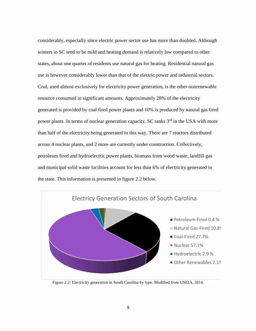
considerably, especially since electric power sector use has more than doubled. Although
winters in SC tend to be mild and heating demand is relatively low compared to other
states, about one quarter of residents use natural gas for heating. Residential natural gas
use is however considerably lower than that of the electric power and industrial sectors.
Coal, used almost exclusively for electricity power generation, is the other nonrenewable
resource consumed in significant amounts. Approximately 28% of the electricity
generated is provided by coal fired power plants and 10% is produced by natural gas fired
power plants. In terms of nuclear generation capacity, SC ranks 3rd in the USA with more
than half of the electricity being generated in this way. There are 7 reactors distributed
across 4 nuclear plants, and 2 more are currently under construction. Collectively,
petroleum fired and hydroelectric power plants, biomass from wood waste, landfill gas
and municipal solid waste facilities account for less than 6% of electricity generated in
the state. This information is presented in figure 2.2 below.
Figure 2.2: Electricity generation in South Carolina by type. Modified from USEIA, 2014.
Electricy Generation Sectors of South Carolina
Petroleum-Fired 0.4 %
Natural Gas-Fired 10.8%
Coal-Fired 27.7%
Nuclear 57.1%
Hydroelectric 2.9 %
Other Renewables 2.1%
10
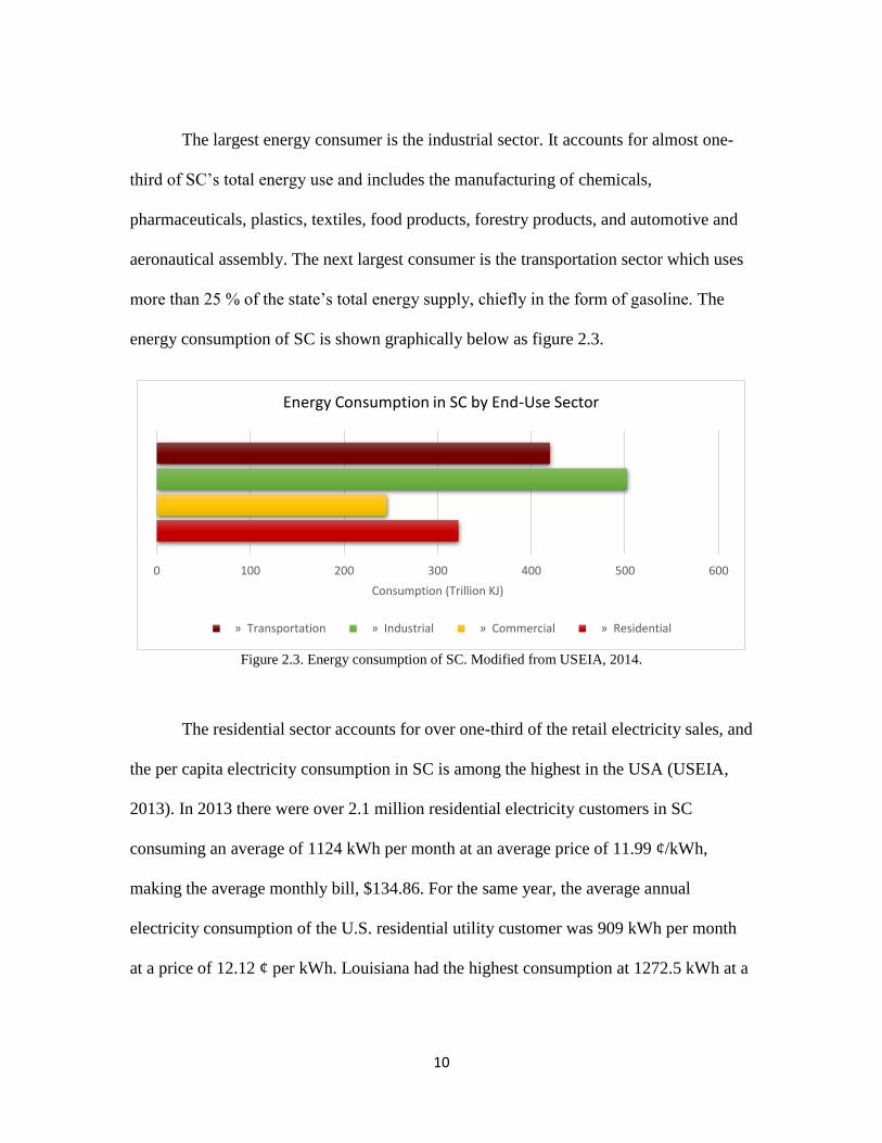
The largest energy consumer is the industrial sector. It accounts for almost one-
third of SC’s total energy use and includes the manufacturing of chemicals,
pharmaceuticals, plastics, textiles, food products, forestry products, and automotive and
aeronautical assembly. The next largest consumer is the transportation sector which uses
more than 25 % of the state’s total energy supply, chiefly in the form of gasoline. The
energy consumption of SC is shown graphically below as figure 2.3.
Figure 2.3. Energy consumption of SC. Modified from USEIA, 2014.
The residential sector accounts for over one-third of the retail electricity sales, and
the per capita electricity consumption in SC is among the highest in the USA (USEIA,
2013). In 2013 there were over 2.1 million residential electricity customers in SC
consuming an average of 1124 kWh per month at an average price of 11.99 ¢/kWh,
making the average monthly bill, $134.86. For the same year, the average annual
electricity consumption of the U.S. residential utility customer was 909 kWh per month
at a price of 12.12 ¢ per kWh. Louisiana had the highest consumption at 1272.5 kWh at a
0 100 200 300 400 500 600
Consumption (Trillion KJ)
Energy Consumption in SC by End-Use Sector
» Transportation » Industrial » Commercial » Residential
11
lower price of 9.43 ¢ per kWh resulting in a monthly bill of $119.98, while Hawaii had
the lowest consumption at 514.7 kWh but at a higher average price of 36.98¢ and a
monthly bill of $190.36 (USEIA, 2013).
In SC, high summer temperatures and air-conditioning use are responsible for
extended peak energy durations of up to 8 hours (Duke Power, 2014). High electricity
demands are also incurred because SC has the second lowest median household income
in the USA. Typically, low-income households are unable to invest in high-efficiency
heating and air-conditioning systems and appliances which would greatly reduce
electricity consumption. More than 60% of SC homes use electricity as the primary
energy source for home heating (USEIA, 2013).
2.4 Wind Resource Potential and Development in South Carolina
South Carolina has recently become an industrial hub of wind energy interest and
investment. In 2005, The South Carolina Energy Office (SCEO) and the DOE partnered
with the electrical utility company, Santee Cooper, and produced a series of wind maps
which presented the mean annual wind speeds across SC at heights of 30, 50, 70 and 100 m
above ground (SCEO, 2009). These maps were constructed to ascertain the wind speed
“hub” height because the power of a wind turbine is related to the cube of the wind speed.
Hub height is the distance from the turbine platform to the rotor of an installed wind
turbine, not including the length of the turbine blades. Wind turbines are sized according
to the required energy load needed based on the specific application. This study concluded
then that while offshore wind in SC is as viable as other wind farms installed in other
12
locations in the USA, onshore locations are not desirable for commercial scale
development.
In 2009, another important study was performed in SC in response to the South
Carolina Act 318 of 2008. This Act amended Section 48-52-620, the Code of Laws of SC,
1976, which relates to energy conservation plans for the state (South Carolina General
Assembly, 2008). As required by the Act, The Wind Energy Production Farms Feasibility
Study Committee was formed and tasked with reviewing, studying and making
recommendations regarding the feasibility of wind farms in South Carolina to assess if the
state was suitable for wind power generation both onshore and offshore. The committee
also investigated the economic and environmental impact to SC and the cost of wind farm
installation and operation (SCEO, 2009). The Committee formulated 18 recommendations
to support, promote and prepare the state for wind power generation.
These recommendations included establishing policies for strong support for
renewable energy development and establishing a clean energy portfolio for the state of
SC, with a target of 1000 MW offshore power generation by 2018. It was stipulated that a
leasing and permit framework for offshore coastal ocean activities in state waters should be
developed. A marine spatial plan for offshore coastal water activities, coordinated with
neighbouring states of Georgia (GA) and North Carolina (NC), which would protect and
preserve existing ocean uses and natural habitats, should be established. Existing tax credits
for renewable energy, which already cover solar and small hydropower project equipment,
are to be amended and expanded to include wind and revenue provided to ensure the
certainty of offshore projects for a fixed number of years in order to balance utility rates

13
and profitability. Another important recommendation took the form of increasing education
and public awareness of wind energy through the USDOE’s Wind Powering America
(WPA) program. These outreach programs would make use of the outstanding marine
research programs like the Ft. Johnson Marine Resources Center Complex, the Coastal
Carolina University Center for Marine and Wetland Studies and the University of SC
Environmental Institute. The Committee also suggested that wind energy manufacturing
incentives should be provided and that wind research activities and the refurbishment of the
Ports of Charleston and Georgetown be funded (SCEO, 2009).
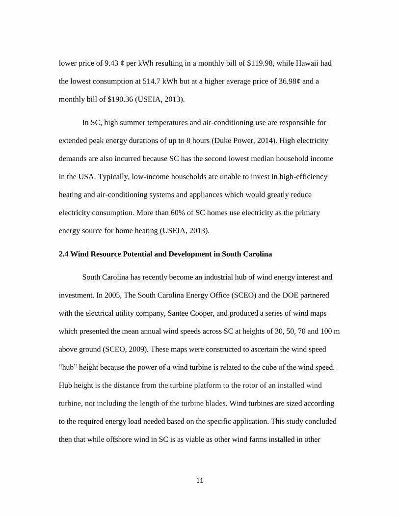
The National Renewable Energy Laboratory (NREL) produced a series of maps
which explored the wind generation potential of SC. One such map, the offshore 90 m
height wind map, is shown below as figure 2.4. According to Wiser and Bolinger (2014)
areas with annual average wind speeds of at least 7 m/s at this height are considered
suitable for offshore development and the DOE (2008) reports that areas with an annual
average wind speed of 6.5 m/s or more at a height of 80 m is considered suitable for wind
energy development.
In 2009 the DOE’s Office of Energy Efficiency & Renewable Energy awarded a
$45 million grant to Clemson University to design, build and operate a facility capable of
full-scaled, highly accelerated testing of the next-generation wind turbine drive train
technology for both land-based and offshore application. In 2013, the Wind Turbine
Drivetrain Testing Facility opened in Northern Charleston at the Clemson University
Restoration Institute. Here, multi-megawatt (up to 15 MW generation capacity) wind
14
turbine systems, from US and international manufactures, are being tested and verified
for performance before being commercially deployed.
Figure 2.4: South Carolina offshore 90 m height map and wind resources potential estimates produced
by NREL. Used with permission.
The population in the USA is growing most rapidly on the eastern and western
coasts and so too will these regions’ energy demands. Today, SC is considered by the DOE
as one of the eastern states with ideal conditions for offshore wind energy development
because of its strong wind speeds in shallow areas extending to as much as 50 km off the

15
coastline; large commercial port facilities, particularly Charleston and Georgetown; and its
established large-scale ship building facilities and manufacturing activities which includes
the building of turbines. These attributes were particularly important when the decision was
made to make South Carolina the home of one of the two most advanced wind turbine
testing facilities in the world.
Job creation is another significant advantage of developing wind technology in SC.
Particularly so since SC currently ranks 7th in the US for highest unemployment rates (US
Department of Labor, 2015). A study completed by Colbert-Busch et al., (2012) concluded
that the development of a 1000 MW windfarm off the coast of SC will provide an average
of about 3300 additional jobs per year.
The DOE (2012) has stated that because of technological advances in land-based
wind generation technology, hub height and rotor diameter have been steadily increasing
for the previous few years and so areas like the Southeast region of the USA, with wind
speeds which were previously considered too low, will become more viable in the near
future. South Carolina’s wind generation potential is therefore expected to expand beyond
what was concluded by the SCEO 2009 report because onshore wind development on a
commercial scale is expected to become a reality. Land-based, utility scaled wind turbines
are usually installed between 80 and 100 m and with continued technological advances,
heights of turbine installations are increasing to up to 140 m (Wiser and Bolinger, 2014).

16
2.5 Offshore Wind Potential Exploration in South Carolina
As of 2014, there are a number of studies being performed to better assess the
suitability of wind power potential in SC. These include the Palmetto Wind Project which
is pioneering the offshore wind farm initiative located off the coast of Georgetown. It is a
collaborative work of Clemson University’s Restoration Institute, Santee Cooper, Coastal
Carolina University and the SCEO, studying the possibilities of generating wind energy
off the coast. This project is currently performing a series of studies to gather and analyze
wind speed, direction and frequency using buoys, carrying out wind assessments using
LIDAR and sonic detection ranging (SODAR). The SC Wind for Schools project is
investigating the feasibility of using wind power to generate electricity on a commercial
level along Waties Island, an underdeveloped area in Horry County. The installed
anemometers are being monitored by students from Clemson University and Coastal
Carolina University. The SC Wind Powering America Grant is a joint project between SC
and GA which focuses on public outreach and state information sharing and best practice
development in the hope of acquiring strong market acceptance for wind energy in SC
and GA.
SC is currently developing its wind resources and CAES has been cited numerous
times as one of only two technologies currently available to store grid scale electrical
power (Barnhart and Benson, 2013; Beaudin et al., 2010; Salgi and Lund, 2009; and
others), and hence energy storage should be explored. Currently CAES is done in
solution mined caverns. Studies examining PMCAES have focused on storing air in
anticlinal traps (McGrail et al., 2013; Allen et al., 1983; Black and Veatch, Rogers, 1982

17
and others). The lack of large enough salt deposits and anticlines limits the number of
potential sites where CAES can be done. In SC these types of structures have not been
mapped yet and so this project will focus on the processes of PMCAES in flat subsurface
structures. These concepts are explored in subsequent chapters of this document and a
brief review of the geology of SC is given in chapter 5.

18
CHAPTER 3
THE TECHNOLOGY OF COMPRESSED AIR ENERGY STORAGE
3.1 Introduction to Compressed Air Energy Storage (CAES)
CAES is a technique in which compressed air is captured and stored underground
when power is in excess and available during low load periods. The compressed air is
then recovered during peak demand times when loads have increased and there is need
for grid balancing. (Doherty, 1981; Hoffeins, 1994; Pollack, 1994). Today there are only
two operating CAES plants in the world: the Huntorf Plant located in Germany and the
McIntosh plant in McIntosh, Alabama, USA.
The turbines utilized in CAES plants work similarly to the traditional gas turbine
but with one key difference: the compressor and the turbines are on separate shafts and
therefore can work independently of each other. This means that that all of the useful
power the turbine produces will be available for power generation and sale during high
peak times. Consequently, the Huntorf and McIntosh plants produces three times the
power that a gas plant of similar size does (Hoffeins, 1994; Pollack, 1994). During low
load periods inexpensive electricity from the grid is used to power the compressors alone.
The compressed air is then stored underground and recovered later in the day and fed
directly to the turbine when electricity is priced higher. This cycle is repeated daily.
To date no CAES power plant uses the aquifer reservoir storage option (Kushnir
et al, 2010). Although both existing plants use salt caverns, excavated by solution mining

19
as their storage space, there are two major disadvantages with this storage option. Firstly,
there are very high costs associated with the cavern creation since this is directly related
to the quantity of air that must be stored (Katz and Lady, 1976) and secondly, the
occurrence of salt deposits of sufficient size is limited. Consequently, many studies have
been carried out to explore and test the suitability of other storage options. The two other
subsurface options considered viable today, given that certain criteria are met, are hard
rock caverns (Kim et al., 2012; Succar and Williams, 2008; and others) and porous media
such as aquifers (McGrail et al., 2013; Allen et al., 1983; and others). Aquifers are of
special interest because of their ubiquitous availability, large storage capability and lower
construction cost (Allen et al., 1983) where water displacement during injection can
provide a nearly constant hydrostatic backpressure during withdrawal (Schulte et al.,
2012). Porous media CAES (PMCAES), however, is not without its inherent
disadvantages.
Salt caverns have determinable volumes and as long as cavern integrity is
maintained by injecting and storing air below cavern fracturing pressures, air loss will not
be a problem. This is the main advantage over PMCAES; because of the inherent
complexity and inhomogeneity of porous media, there is no way to completely prevent
air loss (Katz and Lady, 1976). Nevertheless, porous rock structures may enable a CAES
plant to provide energy storage capacity on the grid scale.
Most studies have named anticlinal structures as the most suitable PMCAES
subsurface formation because of their trapping ability (McGrail et al., 2013; Allen et al.,
1983; Black and Veatch, Rogers, 1982 and others). However, like the occurrence of salt

20
deposits, this again limits the potential of siting locations for CAES plants. Since the
migration of air away from the injection and production well is a problem, it seems
apparent that PMCAES in flat formations should be performed on daily cycles and
therefore considered less suitable for grid energy balancing on a seasonal scale. Instead,
PMCAES in flat formations would be best utilized to provide electricity on shorter, quick
cycles such as the diurnal peak-to-off-peak load shifting scheme. To better understand
how CAES works a brief introduction to gas turbine technology will be covered and
comparisons made between the traditional gas turbines and the turbines used in CAES.
3.2 The Traditional Gas Turbine
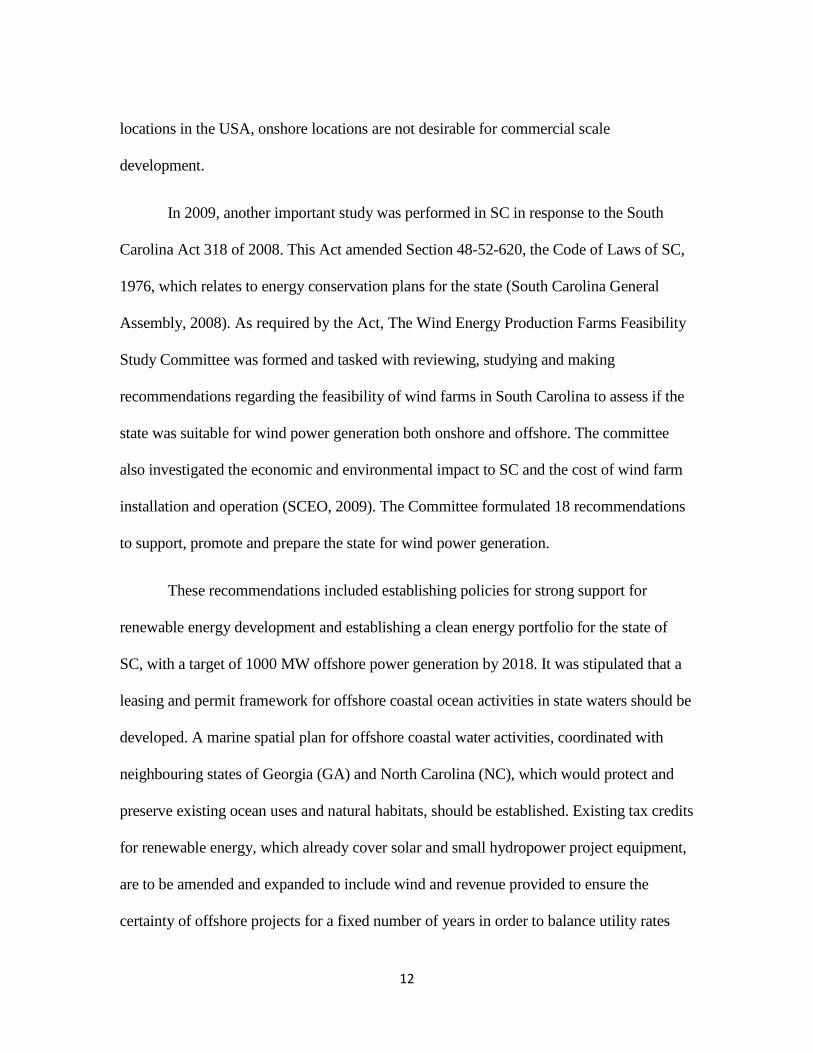
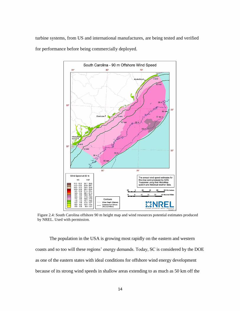
Figure 3.1 presents a schematic of a simple-cycle single-shaft gas turbine. Air is
drawn through the intake by a compressor which is attached to the main shaft unto which
the turbine is also connected. At start up the compressor will be powered by an external
source of electricity derived from the grid since the turbine will not be working at this
time. During the compressor stage the air experiences a decrease in volume and an
increase in temperature and pressure without any addition of heat. The air leaving the
compressor then makes its way to combustion chambers but only about 20 % of the total
air mass, called primary air, enters the flame tubes and is used in the combustion process
while the remaining 80%, the secondary air, is used for cooling (Brooks, 2000).
Fuel, for example natural gas, is injected under pressure into the combustion
chamber and mixed in with the incoming primary air. This combustible mixture is ignited
21
and combustion becomes continuous and the pressure within the combustion chamber for
a given fuel flow is constant. The secondary air is mixed in with the burning gases and
Figure 3.1: Schematic of a simple gas turbine for electric power generation. Arrows show air
direction and flow.
cools it sufficiently to allow the gases to flow through the turbine at a temperature which
is safe for the turbine material. In the turbine section of the system, the energy of the hot
combustion gases is converted into work. The thermal energy is converted to kinetic
energy which causes the turbine disks to rotate to drive a synchronous generator,
producing the electrical power output.
Since turbines normally operate at very high rotational speeds of 12000
revolutions per minute (rpm) or more, they have to be connected to the generator via a
reduction gear box since the rpm must be reduced depending on the AC frequency of the
electricity grid. Once the generator comes online the external source of electricity is no
longer needed to power the compressor and approximately 60% of the power produced

22
by the turbine is used to run the compressor so that only the remainder is available to
produce useful electricity for sale.
This system only works if it produces a net work output such that the turbine must
produce enough work required to simultaneously power the compressor and overcome
mechanical losses in the system. Both the compression and the expansion processes are
irreversible and adiabatic and therefore the work required in the compression process for
a given pressure ratio is higher than the work developed in the expansion process. This
means that the energy losses due to irreversibilities must be reduced as much as possible
for the system to be viable (Eastop and McConkey, 2011).
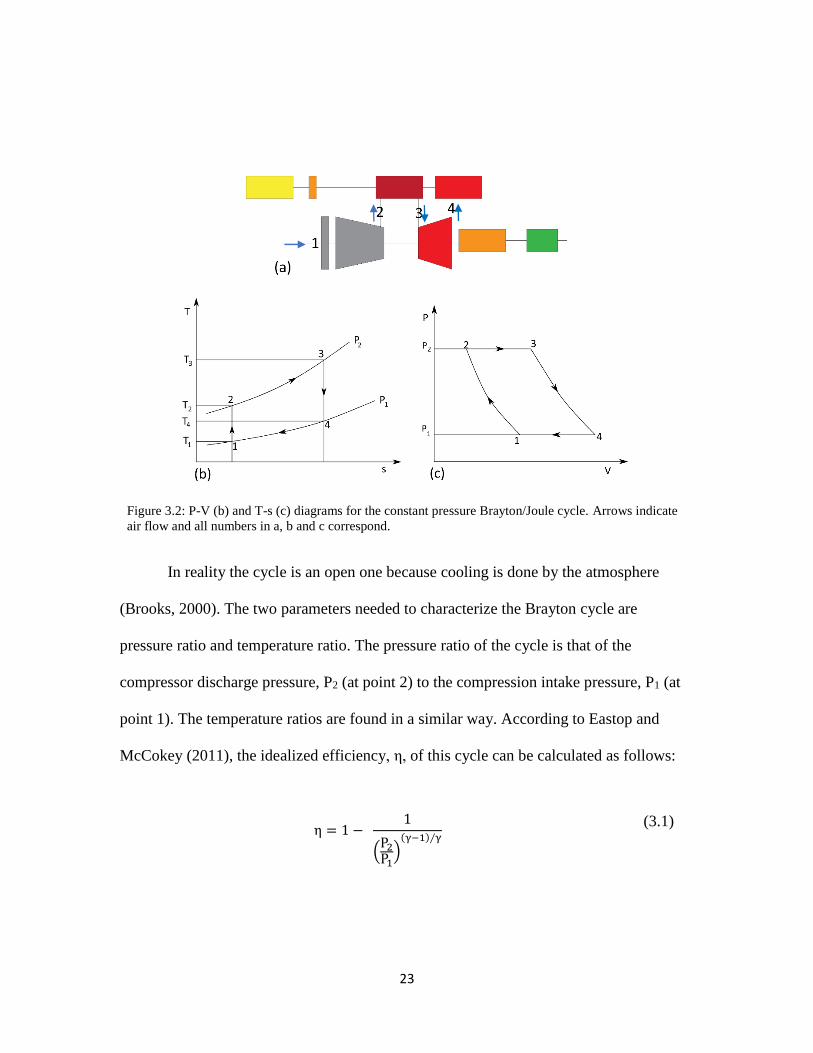
3.3 The Joule or Brayton Constant Pressure Cycle
The idealized thermodynamic cycle upon which all gas turbines are based is
called the Joule or Brayton cycle. Figure 3.2 shows the classic pressure-volume (P-V)
and temperature-entropy (T-s) diagrams for this cycle. All path numbers in diagrams (a),
(b) and (c), correspond to each other. Path 1-2 represents the compression step, path 2-3
represents the addition of heat under constant pressure in the combustion chamber and
path 3-4 is the expansion that occurs in the turbine. The entire cycle, pathway 1-4 is
called the Joule or Brayton cycle. In this idealized, close cycle the heat supplied and
rejected occur reversibly and both the compression and expansion processes are
isentropic where entropy remains constant and so the working fluid (air) flows steadily
around the cycle assuming that velocity changes cancel each other out and therefore can
be ignored. (Eastop and McConkey, 2011).
23
Figure 3.2: P-V (b) and T-s (c) diagrams for the constant pressure Brayton/Joule cycle. Arrows indicate
air flow and all numbers in a, b and c correspond.
In reality the cycle is an open one because cooling is done by the atmosphere
(Brooks, 2000). The two parameters needed to characterize the Brayton cycle are
pressure ratio and temperature ratio. The pressure ratio of the cycle is that of the
compressor discharge pressure, P2 (at point 2) to the compression intake pressure, P1 (at
point 1). The temperature ratios are found in a similar way. According to Eastop and
McCokey (2011), the idealized efficiency, η, of this cycle can be calculated as follows:
η = 1 − 1
(P2P1
)(γ−1)∕γ
(3.1)
24
Where γ is the ratio of the specific heat at constant pressure, cp to the specific heat
capacity at constant volume, cv. That is
γ = cp
cv
(3.2)
Full derivations of equation 3.1 and 3.2 can be found in Eastop and McConkey (2011).
Equation 3.2 shows that for this constant pressure cycle, the cycle efficiency
depends only on the pressure ratio. The ideal value of γ is constant and equal to 1.4
(Eastop and McConkey, 2011). However because of eddying of air as it flows through the
compressor and the turbine which are both rotary machines, the actual cycle efficiency is
reduced.
3.4 Compressed Air Power Plant Turbines
The processes which are performed in a CAES power plant are very similar to
traditional gas turbines but with two fundamental differences. The first difference is the
result of the compressor and turbine being coupled at different times, achieved by placing
each on separate shafts. The compressor and turbine sections of the gas turbine are
alternately coupled to a motor/generator for operation during different electricity demand
times (Allen et al., 1983) through the use of clutches. Schematics of the CAES plants can
be found in figures 3.3 and 3.4. This separation means that all of the useful power of the
turbine is available during power generation, creating a marked advantage over
conventional gas plants (Hoffeins, 1994). In typical power plants the gas turbines require
approximately two thirds of the mechanical energy that is generated to power the plants’
compressors, making only one third of the energy available for electrical generation
25
(Meyer, 2007). The Huntorf and McIntosh plants consequently produce three times the
power that a gas plant of similar size does (Hoffeins, 1994; Pollack, 1994).
During off-peak periods or, in this case, when intermittent energy sources are
producing an excess of power, low-cost or excess power will be utilized to compress the
air which will then be stored in the subsurface reservoir. During this time, the power
plant is said to be in compressor mode (CM). The expansion-turbine clutch is disengaged
and the compressor clutch is engaged so that the motor/generator acts as a motor and air
can be compressed and stored in the underground reservoir. During times of peak demand
or when there is insufficient wind to produce enough electricity, the compressed air will
be recovered from storage and the power plant will then operate in generation mode
(GM) where the compressor clutch is disengaged and the turbine clutch is engaged so that
the motor/generator now performs as a generator. Electricity can now be produced by
combusting natural gas and expanding the combustion products through a turbine without
the use of the compressors (Allen et al., 1983, Kushnir et al., 2010).
The second important difference between air storage gas turbines and the
conventional gas turbines exist in how they are controlled. Load control in traditional
turbines is achieved by adjusting the fuel quantity since the air flow remains constant
resulting in a relatively high heat consumption at partial loads. In air-storage gas turbines
the air flow is adjusted according to the power required, by controlling the inlet and
exhaust temperatures across the turbine. This means that heat consumption is lower
resulting in these gas turbines being more economical for load control applications
(Hoffeins, 1994).

26
3.5 Existing CAES Power Plants
The two existing CAES power plants are both peaking plants. According to
Hoffeins (1994), for a power plant to be considered a peaking plant, the plant must have a
simple method of control and maintenance and be readily available for operation while
exhibiting a high reliability. Peak times typically occur early in the morning when people
are getting ready for the day and in the afternoon, especially during the summer when air
conditioning units are in high demand, and in the evening and night when dinner is being
prepared. The variability of load demand is explored further in chapter 4. A summary of
the main attributes of these power plants can be found in Table 3.1 below.
The Huntorf CAES Plant
Prior to the construction of the Huntorf CAES Plant utilities used gas turbines
coupled with hydraulic pumped storage for peak time production. Hydraulic pumped
storage not only provided high power output but provided the added advantage of
displacing peak electricity generation periods, during times of low demand, by storing
excess power which would be later recovered and returned to the system during peak
demand periods (Hoffeins, 1994). The capital cost of pumped hydraulic storage is not
only higher than that of a conventional gas turbine unit, but also requires a difference in
geodetic height and easy access to large volumes of water. These three requirements
create severe restrictions on energy storage options in areas with flat or gently sloping
topography. The Huntorf CAES plant was constructed to overcome these restrictions
(Hoffeins, 1994).
27
Commissioned in 1978 as a 290 MW plant, the Huntorf plant is the first and
larger utility scale CAES facility (Meyers, 2007). It was designed to be a peaking plant,
generating power for 3 hours daily, working at full turbine load (Hoffeins, 1994). It takes
12 hours to recharge the storage caverns and hence the compressions were designed for
only one quarter of the air consumption of the turbine making the charging to recovery
ratio 1:4 (Hoffeins, 1994). As expected, the mass flow rates of air during injection and
recovery also follow this 1:4 ratio with air being injected at about 108 kg/s and recovered
at 417 kg/s equally distributed over the plant’s two storage caverns.
When in compressor mode during low load periods, usually at night, Huntorf’s
motor/generator is used as a motor and takes low-cost power from the grid to compress
atmospheric air for storage in its underground caverns. Carved out by leaching salt
deposits, these two caverns have the total approximate volume of 3 x 10⁶ m3 and are
located at a depth between 650 and 800 m below ground surface. Charging takes about 12
hours to complete, raising the cavern pressure to a maximum of 72 bars. A schematic of
the plant can be seen in figure 3.3 below (Hoffeins, 1994). For a PMCAES application
the cavern depth used at Huntorf would have a corresponding hydrostatic pressure of
about 64 to 79 bars.
Later, in generator mode, the energy stored in the compressed air is recovered
during peak load demand times to supply the gas turbine. Air is allowed to flow into the
high pressure combustion chamber of the two stage gas turbine at a constant pressure of
42 bars where it is combusted in the presence of natural gas. This pressure is considerably
28
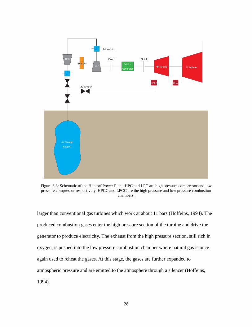
Figure 3.3: Schematic of the Huntorf Power Plant. HPC and LPC are high pressure compressor and low
pressure compressor respectively. HPCC and LPCC are the high pressure and low pressure combustion
chambers.
larger than conventional gas turbines which work at about 11 bars (Hoffeins, 1994). The
produced combustion gases enter the high pressure section of the turbine and drive the
generator to produce electricity. The exhaust from the high pressure section, still rich in
oxygen, is pushed into the low pressure combustion chamber where natural gas is once
again used to reheat the gases. At this stage, the gases are further expanded to
atmospheric pressure and are emitted to the atmosphere through a silencer (Hoffeins,
1994).

29
Optimization tests done at Huntorf showed that the plant has the best economic
performance when storage pressures are kept between 46 and 66 bars since the
relationship between useful work and pumping work is the most economical. At
pressures higher than this range, while the fuel consumption is decreased, the size and the
cost of equipment is substantially higher. At lower pressures, the storage volume or the
cavern size must be increased, also making the manufacturing cost higher. (Hoffeins,
1994). It will be assumed in this project that pressures within the aquifer should therefore
be kept between the 44 to 66 bar range when air cycling is simulated.
In 2006 Huntorf’s original design was improved upon by incorporating a heat
recuperator, a form of heat exchanger system which employs the hot gases produced by
the plant’s turbines to impart heat to the compressed air recovered from the cavern
storage. It was upgraded to a 321 MW unit and functions at around a 95% reliability.
The pressure range of 46 to 66 bars however did not change.
The McIntosh CAES Power Plant
The McIntosh CAES facility owned and operated by Power South Energy
Cooperative, located in McIntosh, Alabama was commissioned in 1991 and uses a single
cavern of almost 5.4 x 10⁵ m3 capacity. The maximum output is 350 MW produced by
two conventional turbine units and a 110 MW CAES unit. During the night when
demands are off peak and utility demand and cost is at its lowest, the CAES unit operates
in Compression Mode and uses the power produced from the base load gas turbine power
plants to compress and force air into the underground cavern up to a pressure of about
30
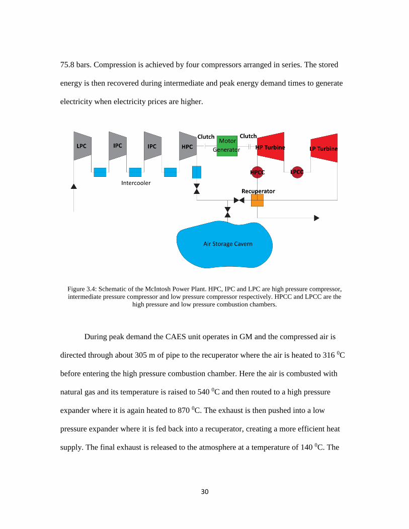
75.8 bars. Compression is achieved by four compressors arranged in series. The stored
energy is then recovered during intermediate and peak energy demand times to generate
electricity when electricity prices are higher.
Figure 3.4: Schematic of the McIntosh Power Plant. HPC, IPC and LPC are high pressure compressor,
intermediate pressure compressor and low pressure compressor respectively. HPCC and LPCC are the
high pressure and low pressure combustion chambers.
During peak demand the CAES unit operates in GM and the compressed air is
directed through about 305 m of pipe to the recuperator where the air is heated to 316 0C
before entering the high pressure combustion chamber. Here the air is combusted with
natural gas and its temperature is raised to 540 0C and then routed to a high pressure
expander where it is again heated to 870 0C. The exhaust is then pushed into a low
pressure expander where it is fed back into a recuperator, creating a more efficient heat
supply. The final exhaust is released to the atmosphere at a temperature of 140 0C. The
31
combined work done by the high and low pressure expanders rotates the generator and
produces electricity. A schematic of the power plant is shown above as figure 3.4. The
CAES generator is capable of producing electricity within 14 minutes of startup. At full
capacity, the CAES facility produces enough electricity to power approximately 11000
homes for 26 hours.
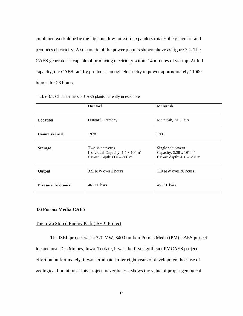
Table 3.1: Characteristics of CAES plants currently in existence
Huntorf McIntosh
Location Huntorf, Germany McIntosh, AL, USA
Commissioned 1978 1991
Storage Two salt caverns
Individual Capacity: 1.5 x 10⁵ m3
Cavern Depth: 600 – 800 m
Single salt cavern
Capacity: 5.38 x 10⁵ m3
Cavern depth: 450 – 750 m
Output 321 MW over 2 hours 110 MW over 26 hours
Pressure Tolerance 46 - 66 bars 45 - 76 bars
3.6 Porous Media CAES
The Iowa Stored Energy Park (ISEP) Project
The ISEP project was a 270 MW, $400 million Porous Media (PM) CAES project
located near Des Moines, Iowa. To date, it was the first significant PMCAES project
effort but unfortunately, it was terminated after eight years of development because of
geological limitations. This project, nevertheless, shows the value of proper geological

32
assessment to the success of any PMCAES project. A brief history of the geological
assessment of the site, as given by Schulte et al., (2012) is presented below.
In 2002, the Iowa Association of Municipal Utilities (IAMU) study indicated the
need to secure intermediate electricity supply resources. Intermediate energy refers to
energy resources that are neither baseload (operating continuously) nor peaking
(operating only at peak load times). Instead, they operate on a daily basis (typically
during daylight hours on weekdays) to meet the rise and fall of utility customers’ typical
electricity usage. Having a wind power capacity of almost 5700 MW (refer to figure 2.1),
makes Iowa the state with the second highest wind power capacity; where capacity is
defined as the maximum electricity output under specified conditions. It was determined
then that CAES technology could meet this need and so in 2006, after a state wide
selection process, the Mt. Simon Formation near Des Moines was chosen primarily
because of its perceived favorable geology and its proximity to the edge of one of the best
places for wind energy in Iowa. For the next four years the chosen site was studied in
more detail.
In 2010 the first test well, called Keith #1 (K1), was drilled to help define the top
of the Mt. Simon anticline and it was found that the structure’s thickness of 15 m, rather
than that of 46 m, as originally thought, represented a 50% reduction in air capacity than
originally estimated in 2007. Pump tests indicated a lower permeability of 3 md but that
was then attributed to caprock materials. Additional exploratory wells were then deemed
necessary to better access the subsurface geologic structure. Core sampling performed on
K1 and pump tests on the second well, Mortimer #1 (M1), confirmed that the reservoir

33
had low permeability which would prove problematic. M1 did provide enough data to
revise the structural map which then showed that the anticline had approximately a 21 m
closure of an area of about 2.4 km2. In early 2011, because of the significance of geology
to the overall success of the project, the board of directors approved the drilling of a third
test well, Mortimer #2 (M2), and an objective, third-party peer review to gain a second
opinion on the geology of the area was sought.
It was finally concluded that the area’s capacity was 75% of what it was originally
estimated to be in 2007 and although the structure’s porosity which was estimated to be
16 to 17 % was consistent with original estimates, the low permeability of the Mt. Simon
sandstone presented a serious problem. A revised and more robust reservoir model was
completed and in July 2011, it was concluded that the geology was “dramatically
different” from the original model and that the porosity and permeability of the multiple
lenses of Mt. Simon “are not conducive to air development in the vertical direction and
represent the lower limit of reservoir permeability values for the economic air production
from vertical and/or horizontal wells”. Numerical simulation studies showed that
although horizontal wells would be unable to support a 135 MW power plant because
there would be a pressure drop below the minimum required operating pressure, a 65
MW plant may be possible. A 65 MW plant was not economically feasible for the
investment and, furthermore, air injection tests would be necessary to test the overall
feasibility of this project. To proceed, however, would have required a further investment
of $12 to $ 20 million or more and so on July 28th, 2011, the board of directors
unanimously decided to terminate the project.

34
CHAPTER 4
CAES AS A BULK ENERGY STORAGE OPTION
4.1 Motivations for Bulk Energy Storage
There is a need for energy storage, particularly for the electricity generation
sector. The principal arguments supporting this include: for energy conservation; for
levelling out electricity demand (Glendenning, 1981); to increase energy security
(Barnhart and Benson, 2013); to overcoming the intermittent and the unstable nature of
renewable energy resources; and for the reduction of fossil fuel produced pollutants
(Salgi and Lund, 2008).
All electricity providers share the common problem of satisfying a fluctuating
load of energy demand while simultaneously maintaining the lowest possible steady
supply of energy. Grid scale operations are also required to instantaneously match
consumer power demand. (Barnhart and Benson, 2013). To economically solve this
problem, various modes of storing reserve supplies to meet the peak load must be
employed. Electricity demand is cyclic in nature and is characterized by daytime peaks
and night-time troughs or off-peak times during the weekday and a lower average
demand on weekends (Katz and Lady, 1976; Glendenning, 1981; and others). A typical
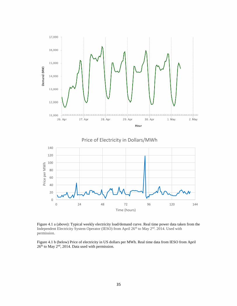
weekly electricity load curve is shown in figure 4.1a. Electricity is sold at a higher price
during peak times (figure 4.1b) to maximize profits.
In the temperate regions of the world, this is superimposed on an annual seasonal
cycle which usually involves winter and summer peaks (Glendenning, 1981) and, based
35
Figure 4.1 a (above): Typical weekly electricity load/demand curve. Real time power data taken from the
Independent Electricity System Operator (IESO) from April 26th to May 2nd. 2014. Used with
permission.
Figure 4.1 b (below) Price of electricity in US dollars per MWh. Real time data from IESO from April
26th to May 2nd, 2014. Data used with permission.
0
20
40
60
80
100
120
140
0 24 48 72 96 120 144
Pri
ce p
er M
Wh
Time (hours)
Price of Electricity in Dollars/MWh

36
on the latitude of locations, one usually out-demands the other. These demand patterns
are usually successfully met by appropriate scheduling of available power whereby ‘base
load’ power needs are supplied by power stations with the lowest operation costs, such as
nuclear stations which operate continuously. When the load exceeds the capacities of the
base load power plants, electricity generation is supplemented by ‘peaking power’ plants
which command higher prices per KWh for electricity (Glendenning, 1981).
4.2 The Evolving Interest in CAES as a Bulk Energy Storage Option
Interest in CAES can be traced back to the late 1960s when it emerged primarily
as a peaking plant alternative to pumped hydraulic storage. In 1975 the first CAES plant
was constructed in Huntorf, Germany and would become fully operational 3 years later.
For the first time a power plant had the advantages associated with peak load gas turbine
power plants and that of a of pumped storage plant simultaneously (Hoffeins, 1994).
Excessive oil prices following the 1973-1974 oil embargo and nationwide
conservation attempts made energy storage more attractive in the USA than in previous
years because it presented a way to reduce oil consumption and fuel costs (Katz and
Lady, 1976). The then expanding nuclear energy power industry in the USA resulted in a
perceived potential for maximizing profit because of the price differential which exists
between the comparatively inexpensive base load power generated by nuclear plants to
that generated during peak times (Succar and Williams, 2008). This created a strong
interest in bulk energy storage options like CAES in the USA because it meant that

37
cheaper off-peak energy could be stored and then recovered during peak times, creating
an appealing profit.
Numerous studies were carried out during the 1970s and 1980s. In 1976, Katz and
Lady published “Compressed Air for Energy Storage for Electrical Power Generation” in
which they used the technology already developed for the underground storage of natural
gas to propose how porous media (PM) such as aquifers could be used as the storage
space for compressed air. By that time natural gas had been successfully stored
underground for about 35 years. This publication presented a brief but overall
introduction to air flow, the potential for aquifers for storage, how power could be
generated and even a sample design of a power plant.
The DOE, the Electric Power Research Institute (EPRI) and various electricity
utility industries also carried out considerable work in evaluating CAES technologies. For
example, in 1978 EPRI funded a project which performed an assessment of the state of
Kansas for suitability for PMCAES. The Pittsfield Aquifer test was carried out in Illinois
in 1981 by the DOE in which air was injected into the St. Peter’s Sandstone and
successfully recovered. Allen et al., (1983) produced a document which explored the
factors affecting PMCAES. Studies like these eventually culminated in the
commissioning of the 110 MW CAES plant located in Alabama. (Succar and Williams,
2008).
By the end of the 1980s when oil prices decreased again and the nuclear
industry’s growth slowed and the gas turbine with combined cycle generation emerged as

38
a lower cost option when constructing peaking plants, the perception of abundant
domestic natural gas resources and supplies caused an eroding interest in bulk energy
storage and CAES (Succar and Williams, 2008). However, recent efforts to move
towards a more diversified energy industry, less reliance on fossil fuels and the expansion
of renewable resources to decrease pollution have reestablished interest in CAES.
4.3 Addressing the Variability of Wind Energy
Efforts to reduce greenhouse gas emissions have led to an increased interest in
renewable energy sources (RES) such as wind, solar, waves and hydroelectric power
(Lund and Salgi, 2009). Although RES are becoming increasingly evident in energy
markets, their wide variability and unpredictability in energy output means that there is
often a mismatch between the peak electricity demand and the peak power generation
(Glendenning, 1981). Any power system in which RES presents a significant portion of
the power generation must therefore operate differently from a power system operated by
conventional based resources (Milligan et al., 2011). Energy storage will allow for an
improved and more efficient harnessing and availability to the utility system. Energy
storage would also be very important to isolated communities with no grid scale sources
of power (Glendenning, 1981).
Global wind power capacity has grown rapidly in recent years from 4.8 GW in
1995 to almost 370 GW by the end of 2014, as reported by the Global Wind Energy
Council (GWEC). Wind energy must be stored during times of surplus production.
Various storage systems have been proposed including pumped hydroelectric storage

39
(Pickard et al., 2009, Brown et al., 2008), batteries (Chang et al., 2009), hydrogen storage
(Agaudo et al., 2009), capacitors and super capacitors and flywheel (Beaudin et al.,
2010), super conducting magnetic storage (Buckles, 2000), and compressed air energy
storage (CAES) (Cavallo, 2007). Among these, only pumped hydro storage and CAES
systems have the capability for large scaled energy integration (Beaudin et al., 2010).

40
CHAPTER 5
GEOLOGY OF SOUTH CAROLINA AND THE PMCAES SYSTEM
5.1 The Proposed PMCAES System
The proposed PMCAES system comprises three core components: powerlines or
access to an existing electricity grid, the CAES power generation facility, and the
subsurface porous media reservoir complete with the injection and production wells. This
PMCAES project is proposed to examine and possibly utilize the SC geology to take
advantage of the state’s future wind generation potential. As wind energy applications
expand across the USA, this project makes the assumption that eventually the necessary
grid electricity would be derived from wind farms.
5.2 General Geology of South Carolina
A transverse from the southeast to the northwest, across SC, exhibits a general
rise in elevation of land crossed by numerous rivers. The Low Coastal Plain, rises slowly
from the coast until the Fall Line which is marked by an area of rapids and waterfalls.
From this line lies the Up Country which consists mainly of forested hills of the
Piedmont and the SC Blue Ridge. A cross section of the SC Coastal Plain (SCCP) offered
as figure 5.2 below, from which it can be seen that sand aquifers are the most common
and widespread in the state.
41
5.3 The Atlantic Coastal Plain of South Carolina
Using data from the preceding century and current data from 309 boreholes, the
United States Geologic Survey (USGS) published a comprehensive report describing the
Atlantic Coastal Plain aquifers and confining units of both North and South Carolina in
2010. The three dimensional finite-difference numerical simulator MODFLOW-2000
was used to model the groundwater flow within the Coastal Plain of NC, SC and parts of
GA and Virginia (VA). Gellici and Lautier (2010) used a revised framework which
encompassed several aquifer systems, introduced new nomenclature for the Carolinas,
VA and GA and, in some cases, divided existing systems into smaller intervals. This
chapter will mostly use the better established and more widely known names for the SC
hydrogeological units as described by Colquhoun (1983), Miller (1986), Alcott (1987)
and others. A comparison of the USGS and other nomenclature is shown below as figure
5.1. All aquifers and confining units of SC were characterized by their lithology,
hydrologic properties and geophysical log-signature.
Constructed from the records from 38 core holes and 68 water wells, the
hydrologic model of the SCCP comprises a total of 15 hydrostratigraphic units: eight
aquifers (Aq) and seven confining units (CU). The SCCP layers range in age from Late
Cretaceous to Tertiary and are chiefly gravels, sands, silts, clays and limestones. Strata
thickness range from 0 m at the Fall Line to about 1220 m in the southernmost areas of
SC. Identification and correlation between aquifers and confining units were performed
using biostratigraphic and allostratigrahic data from borehole geophysical logs (Gellici
and Lautier, 2010).
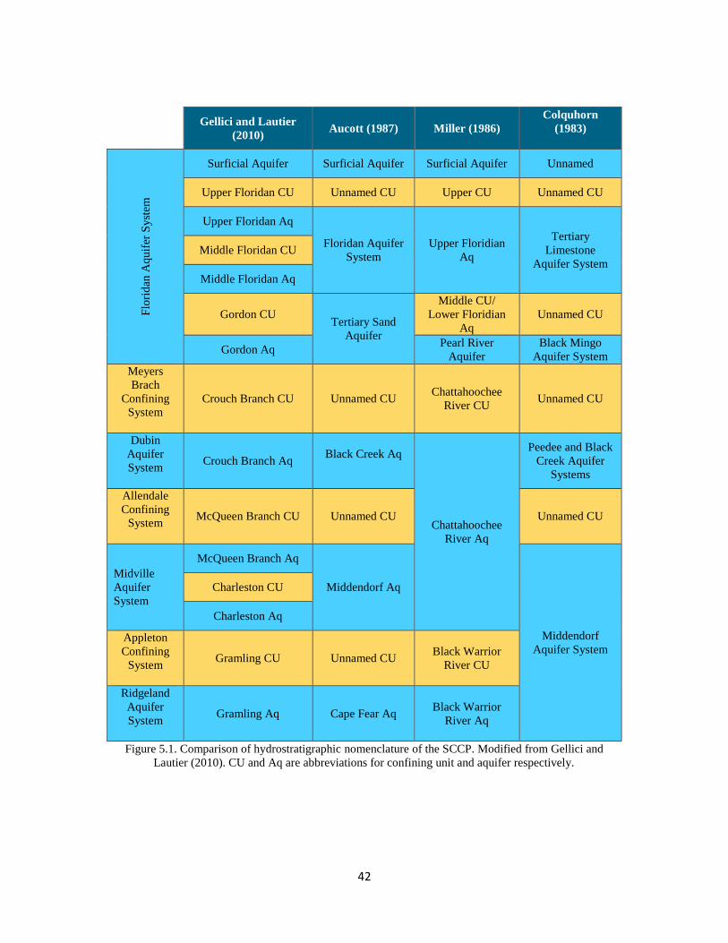
42
Gellici and Lautier
(2010) Aucott (1987) Miller (1986)
Colquhorn
(1983)
Flo
rid
an A
qu
ifer
Sy
stem
Surficial Aquifer Surficial Aquifer Surficial Aquifer Unnamed
Upper Floridan CU Unnamed CU Upper CU Unnamed CU
Upper Floridan Aq
Floridan Aquifer
System
Upper Floridian
Aq
Tertiary
Limestone
Aquifer System
Middle Floridan CU
Middle Floridan Aq
Gordon CU Tertiary Sand
Aquifer
Middle CU/
Lower Floridian
Aq
Unnamed CU
Gordon Aq Pearl River
Aquifer
Black Mingo
Aquifer System
Meyers
Brach
Confining
System
Crouch Branch CU Unnamed CU Chattahoochee
River CU Unnamed CU
Dubin
Aquifer
System Crouch Branch Aq
Black Creek Aq
Chattahoochee
River Aq
Peedee and Black
Creek Aquifer
Systems
Allendale
Confining
System McQueen Branch CU Unnamed CU Unnamed CU
Midville
Aquifer
System
McQueen Branch Aq
Middendorf Aq
Middendorf
Aquifer System
Charleston CU
Charleston Aq
Appleton
Confining
System Gramling CU Unnamed CU
Black Warrior
River CU
Ridgeland
Aquifer
System Gramling Aq Cape Fear Aq
Black Warrior
River Aq
Figure 5.1. Comparison of hydrostratigraphic nomenclature of the SCCP. Modified from Gellici and
Lautier (2010). CU and Aq are abbreviations for confining unit and aquifer respectively.

43
The aquifers are, in descending order, the Surficial aquifer, the Floridan Aquifer
System (divided into the Upper Floridan, Middle Floridan and Black Mingo (Gordon)
aquifers, the Peedee and Black Creek Aquifer Systems (also called the Crouch Brach
Aquifer) and the Middendorf Aquifer system (consisting of the McQueen Branch,
Charleston and Cape Fear aquifers). Each aquifer, except for the unconfined Surficial
aquifer, has an associated confining unit of the same name located stratigraphically above
the aquifer.
Information such as porosity and permeability of individual units is limited. SC is
not a hydrocarbon bearing state, and therefore, all subsurface information comes from
hydrological data. The PMCAES models presented in chapters 6 and 7 will therefore
explore a range of parameters typical for SC type sediments. The aquifers of the
Middendorf Formation are the most productive aquifers in the Coastal Plain of SC and
are the most tested (Gellici and Lautier, 2010). Hydraulic conductivity data were derived
chiefly from multiday regional aquifer pumping tests as those performed in Dillon,
Florence, Marion, and Marlboro Counties (Rodriguez, 1994 and others). Transmissivity
(T) data were collected from various reports in which different methods were used.
Winner and Coble (1996) used geophysical and lithological data from wells to estimate
average horizontal conductivities while Dale and Park (1999) calculated T from aquifers
at Hilton Head Island, and horizontal hydraulic conductivities were measured from core
samples by Temples and Englehardt (1997). Vertical hydraulic conductivity tests are
sparse. Permeameter tests were done on 3 clay samples of the Gordon confining unit, and
18 clay samples of the Crouch Branch CU were tested (Aadland et al., 1995). Nine clay
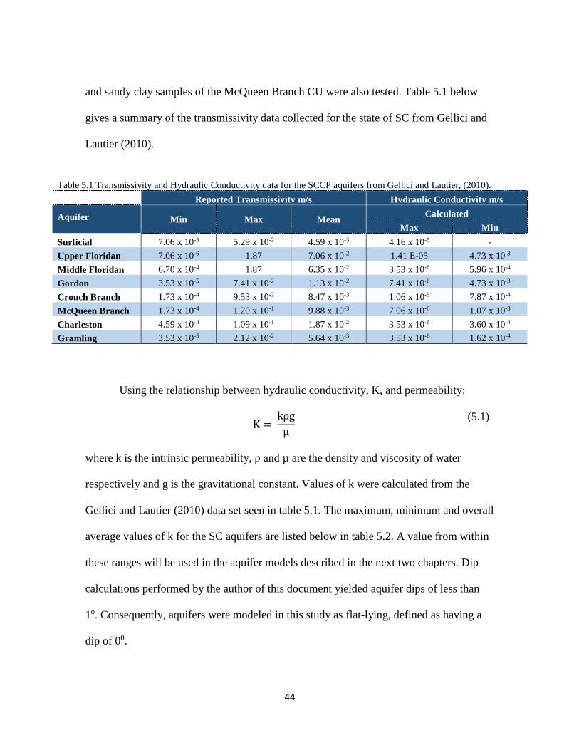
44
and sandy clay samples of the McQueen Branch CU were also tested. Table 5.1 below
gives a summary of the transmissivity data collected for the state of SC from Gellici and
Lautier (2010).
Table 5.1 Transmissivity and Hydraulic Conductivity data for the SCCP aquifers from Gellici and Lautier, (2010).
Reported Transmissivity m/s Hydraulic Conductivity m/s
Aquifer
Min Max Mean
Calculated
Max Min
Surficial 7.06 x 10⁻⁵ 5.29 x 10⁻² 4.59 x 10⁻³ 4.16 x 10⁻⁵ -
Upper Floridan 7.06 x 10⁻⁶ 1.87 7.06 x 10⁻² 1.41 E-05 4.73 x 10⁻³
Middle Floridan 6.70 x 10⁻⁴ 1.87 6.35 x 10⁻² 3.53 x 10⁻⁶ 5.96 x 10⁻⁴
Gordon 3.53 x 10⁻⁵ 7.41 x 10⁻² 1.13 x 10⁻² 7.41 x 10⁻⁶ 4.73 x 10⁻³
Crouch Branch 1.73 x 10⁻⁴ 9.53 x 10⁻² 8.47 x 10⁻³ 1.06 x 10⁻⁵ 7.87 x 10⁻⁴
McQueen Branch 1.73 x 10⁻⁴ 1.20 x 10⁻¹ 9.88 x 10⁻³ 7.06 x 10⁻⁶ 1.07 x 10⁻³
Charleston 4.59 x 10⁻⁴ 1.09 x 10⁻¹ 1.87 x 10⁻² 3.53 x 10⁻⁶ 3.60 x 10⁻⁴
Gramling 3.53 x 10⁻⁵ 2.12 x 10⁻² 5.64 x 10⁻³ 3.53 x 10⁻⁶ 1.62 x 10⁻⁴
Using the relationship between hydraulic conductivity, K, and permeability:
K = kρg
µ
(5.1)
where k is the intrinsic permeability, ρ and µ are the density and viscosity of water
respectively and g is the gravitational constant. Values of k were calculated from the
Gellici and Lautier (2010) data set seen in table 5.1. The maximum, minimum and overall
average values of k for the SC aquifers are listed below in table 5.2. A value from within
these ranges will be used in the aquifer models described in the next two chapters. Dip
calculations performed by the author of this document yielded aquifer dips of less than
1o. Consequently, aquifers were modeled in this study as flat-lying, defined as having a
dip of 00.
45
Table 5.2. Range of permeability values for SC aquifers
Aquifer k min (m2) k max (m2)
Surficial 6.9 x 10⁻¹¹ 6.9 x 10⁻¹¹
Upper Floridan 6.4 x 10⁻¹³ 3.7 x 10⁻¹⁰
Middle Floridan 6.4 x 10⁻¹³ 8.3 x 10⁻¹¹
Gordon 2.6 x 10⁻¹³ 5.4 x 10⁻¹¹
Crouch Branch 2.6 x 10⁻¹³ 5.7 x 10⁻¹¹
McQueen Branch 2.6 x 10⁻¹³ 5.6 x 10⁻¹¹
Charleston 1.6 x 10⁻¹³ 4.1 x 10⁻¹¹
Gramling 4.5 x 10⁻¹³ 2.1 x 10⁻¹¹
k average (m2) 9.0 x 10⁻¹² 9.4 x 10⁻¹¹
Table 5.3 presents brief geological descriptions of the SCCP layers and it can be
seen that generally speaking the SCCP comprises unconsolidated sand aquifers and
impermeable clay and clay-rich confining units. Consequently, the simplest approach to
this project would be considering aquifers as unconsolidated sands sandwiched between
clay layers. A range of parameter values typical for these types of aquifers were therefore
used for the base case model and the sensitivity analyses performed in chapters 6 and 7.
In the absence of anticlinal structures, air’s smaller density, when compared to
that of water, would result in injected air rising towards the upper confining layer and
travelling laterally until no pressure differential between fluids exist. Air could travel
some distance and could therefore pose a hazard to water pumping equipment, should
water wells be installed into air bearing zones. It should therefore be noted that if
PMCAES is to be done in flat formations that it should be at depths below which water
would be extracted. Since this project looks at potential wind farms in SC which are

46
Table 5.3. General descriptions of hydrogeological units of SC. Descriptions taken from Gellici and Lautier, (2010).
Layer General Geology
Median b
(m)
Max b
(m)
Flo
ridan
Aq
uifer S
ystem
Superficial Aq Quartz, gravel, sand, silt, clay, shelly sand 10.7 64.9
Cooper Marl
(Upper Floridan CU)
Clayey sand, sandy clay, sandy dolomitic limestone, clayey
limestone 2.7 77.7
Santee Limestone
(Upper Floridan Aq) White to light grey fossiliferous limestone 3 94.7
Middle Floridan CU
Fine calcarenites and calcilutites containing minor amounts of
quartz sand and clay. Poorly consolidated and interbedded with
thin layers of limestone
4.3 221.3
Middle Floridan Aq Hard moldic limestone interbedded with poorly consolidated
shelly limestone in a lime mud matrix. 5.5 78.3
Gordon CU
Fine-grained glauconitic clayey sand and clay. Laminated
clayey calcilutite, calcarenite, and calcareous silt and clay with
indurated limestone nodules and lenses. Glauconite content can
be as great as 30 %.
4.6 35.4
Tertiary Sand/Black
Mingo Aq
(Gordon Aq)
Unconsolidated, poorly to moderately sorted fine- to coarse-
grained sand and clayey sand with local gravel. 10.7 107.6
Chattahoochee River
CU
(Crouch Branch CU)
Carbonaceous silty-clay that is thinly laminated with well-
sorted very fine to fine quartz sand and silt. 13.1 110.9
Peedee and Black
Creek Aq System
(Crouch Branch Aq)
Unconsolidated, poorly sorted, fine- to coarse-grained sand and
clayey sand in a kaolinite matrix and by interbedded fine sand
and carbonaceous clay.
94.2 210.3

47
Layer General Geology Median b
(m)
Max b
(m)
Mid
den
do
rf Aq
uifer S
ystem
McQueen Branch CU
Laminated sand and silty clay in a carbonaceous clay matrix
(Coachman Formation). Shelly calcareous clay (Bladen
Formation); sandy marl, calcareous clay, and carbonaceous
clay (lower and middle Donoho Creek units) and silty clay
with fine-grained sand
14.9 75.9
McQueen Branch Aq
Characterized by unconsolidated, poorly sorted, fine- to
coarse-grained sand and clayey sand with local gravel. The
sand fraction consists of quartz
39.6 131.7
Charleston CU
Noncalcareous to slightly calcareous clay, silty clay, clayey
silt, and clayey fine sand. The formation typically is laminated
with very fine to fine-grained quartz sand.
26.8 141.1
Charleston Aq
Unconsolidated sand, clayey sand, and clay. The sand fraction
consists of poorly sorted, fine- to very coarse-grained quartz
with up to 10 percent mica.
43.3 190.2
Cape Fear CU
(Grambling CU)
Unconsolidated to semiconsolidated beds of clay, clayey sand,
sand, and gravel. The sand fraction consists of poorly sorted,
fine- to very coarse-grained quartz with minor feldspar and
sparse mica, lignite, and monazite. Interstitial clay can be high
due to weathering of feldspar to kaolinite.
39.6 248.4
Cape Fear Aq
(Grambling Aq)
Unconsolidated to semiconsolidated interbedded and laminated
sand, clayey sand, silt, and clay. The sand fraction consists
mainly of quartz but can contain moderate amounts of feldspar
85.6 322.5
Lower Creataceous CU Unmapped in SC. Bedrock
expected to be installed along the coastline, then it is possible that PMCAES would take
place closer to the shoreline where there is salt water intrusion and where water would
not be used for drinking.

48
The USGS conducted three pilot saline studies from 2010 to 2012 on regional
scales and the one which covered the Southeastern US was performed to determine the
potential of brackish or saline waters to supplement existing freshwater supplies in the
southeast. Williams (2012), the principal investigator, examined two aquifer systems and
mapped them based on their concentrations of dissolved solids. These concentrations
were estimated from borehole geophysical logs and water-quality data from various
wells, and four zones, as described in table 5.4 below, were delineated.
Table 5.4. Salinity zones in southeast USA. Data taken from Williams, 2012.
Zone Dissolved solid concentration (mg/L)
Freshwater Less than 103
Brackish-water Between 103 and 104
Salinity Transition Between 104 and 3.5 x 10⁴
Saline Water and/or Brine Greater than 105
Brackish zones were mapped in the Chattahoochee River, the Middendorf aquifer
systems and in the Upper and Lower Floridan aquifers at depths of a few hundred meters.
Differences in permeability, the proximity to recharge areas and the presence of relic
brine or seawater means that the vertical and lateral variations in salinity is complicated.
In SC the shallowest brackish groundwater can be found in the Upper Floridan aquifer at
depths as low as 520 m and mostly along the coastal areas. Deeper and less accessible
aquifers with brackish groundwater are present throughout much of southeast SC
(Williams, 2012). This suggests that PMCAES could possibly take place within coastline
aquifers.
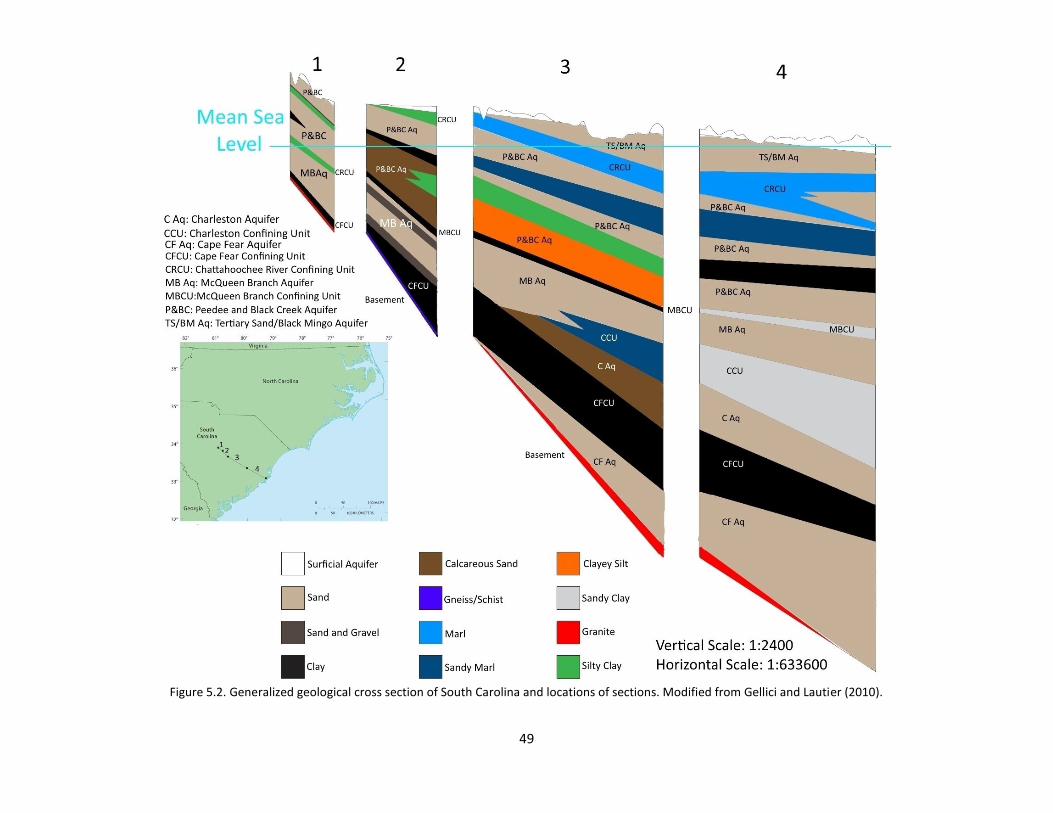
49
Figure 5.2. Generalized geological cross section of South Carolina and locations of sections. Modified from Gellici and Lautier (2010).

50
CHAPTER 6
BASE CASE MODEL
6.1 Introduction
The first step in assessing the technical feasibility of PMCAES in flat lying
formations is constructing a conceptual model to evaluate system performance. The
complexity modelling multiphase flow in porous media necessitates the use of numerical
modeling to simulate the behavior of the PMCAES system. TOUGH2, a numerical
modeling program useful for multi-dimensional and multiphase fluid and heat flow in
porous and fractured media (Pruess et al., 1999) was utilized to construct the aquifer
model and the results were used to assess the following:
The amount of energy that can be stored in a subsurface sand formation.
The amount of energy that can be recovered
The energy efficiency of this storage system
The wellbore energy loss
6.2 Base Case Conceptual Model
The model comprises a flat-lying, fully confined 12.5-m-thick sand storage
aquifer sandwiched between a 50-m-thick caprock and an 87.5-m lower confining layer.
There is a 450-m layer of overburden above the caprock. In the first few attempts to
model an aquifer, a thickness of 50 m was used. This was deemed inappropriate since this
thickness yielded low energy recovery efficiencies. When the aquifer thickness was

51
reduced by a factor of 2, to 25 m, energy recovery was also inefficient and so it was
decided to reduce the thickness once again by another factor of 2 so that a 12.5 m aquifer
was used as this base case model. The effects of aquifer thickness were further explored
in chapter 7.
Although the aquifers of the SCCP have very low dips, less than 1o, for simplicity
aquifers will be modeled as being perfectly flat-lying, or having dips of 0o. All four layers
are assumed to be homogeneous and anisotropic. The aquifer has a horizontal
permeability (kh) of 1x 10-11 m2 and a vertical permeability (kz) of 1.0 x 10⁻¹² m2. The
chosen vertical permeability falls within the range of values (4.5 x 10⁻¹³ to 2.1 x 10⁻¹¹ m2)
calculated for the deepest aquifer tested in SC and presented in chapter 5 of this study. A
porosity (φ) of 0.2 and a residual water saturation (Srw) of 0.27 is also assumed. These
two parameters are of typical values for sand aquifers at this depth (Miller, 1999; Bear,
1979 and others). A sand aquifer was chosen since it is one of the most common aquifer
formations in the USA (Miller, 1999) and are widespread in SC (Gellici and Lautier,
2010).
The porosity, bulk density, and thermal conductivities of sedimentary rocks are
sensitive to burial depth and therefore parameters were chosen by taking this into
consideration. The confining layers located above and below the aquifer are modeled as
clay and are assumed to have a porosity of 0.35, and very low kh and kz permeabilities of
1.0 x 10⁻¹⁷ m2 and 1.0 x 10⁻¹⁸ m2 respectively. Clay confining layers are common in the
SCCP. These porosities and permeabilities are within the range quoted by Fetter (2001),
Bear (1979) and others. Bloomer (1981) investigated 115 samples from 12 clays and
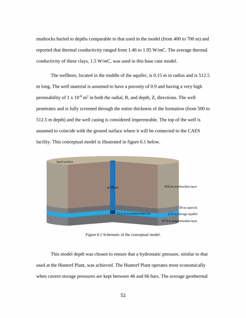
52
mudrocks buried to depths comparable to that used in the model (from 400 to 700 m) and
reported that thermal conductivity ranged from 1.46 to 1.95 W/mC. The average thermal
conductivity of these clays, 1.5 W/mC, was used in this base case model.
The wellbore, located in the middle of the aquifer, is 0.15 m in radius and is 512.5
m long. The well material is assumed to have a porosity of 0.9 and having a very high
permeability of 1 x 10⁻⁸ m2 in both the radial, R, and depth, Z, directions. The well
penetrates and is fully screened through the entire thickness of the formation (from 500 to
512.5 m depth) and the well casing is considered impermeable. The top of the well is
assumed to coincide with the ground surface where it will be connected to the CAES
facility. This conceptual model is illustrated in figure 6.1 below.
Figure 6.1 Schematic of the conceptual model.
This model depth was chosen to ensure that a hydrostatic pressure, similar to that
used at the Huntorf Plant, was achieved. The Huntorf Plant operates most economically
when cavern storage pressures are kept between 46 and 66 bars. The average geothermal
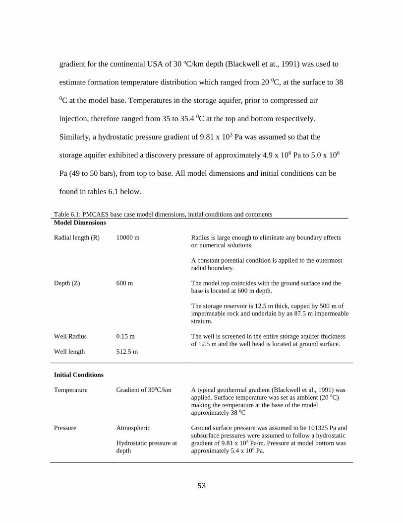
53
gradient for the continental USA of 30 oC/km depth (Blackwell et at., 1991) was used to
estimate formation temperature distribution which ranged from 20 0C, at the surface to 38
0C at the model base. Temperatures in the storage aquifer, prior to compressed air
injection, therefore ranged from 35 to 35.4 0C at the top and bottom respectively.
Similarly, a hydrostatic pressure gradient of 9.81 x 10³ Pa was assumed so that the
storage aquifer exhibited a discovery pressure of approximately 4.9 x 10⁶ Pa to 5.0 x 10⁶
Pa (49 to 50 bars), from top to base. All model dimensions and initial conditions can be
found in tables 6.1 below.
Table 6.1: PMCAES base case model dimensions, initial conditions and comments
Model Dimensions
Radial length (R) 10000 m Radius is large enough to eliminate any boundary effects
on numerical solutions
A constant potential condition is applied to the outermost
radial boundary.
Depth (Z) 600 m The model top coincides with the ground surface and the
base is located at 600 m depth.
The storage reservoir is 12.5 m thick, capped by 500 m of
impermeable rock and underlain by an 87.5 m impermeable
stratum.
Well Radius 0.15 m The well is screened in the entire storage aquifer thickness
of 12.5 m and the well head is located at ground surface.
Well length 512.5 m
Initial Conditions
Temperature Gradient of 300C/km A typical geothermal gradient (Blackwell et al., 1991) was
applied. Surface temperature was set as ambient (20 0C)
making the temperature at the base of the model
approximately 38 0C
Pressure Atmospheric
Hydrostatic pressure at
depth
Ground surface pressure was assumed to be 101325 Pa and
subsurface pressures were assumed to follow a hydrostatic
gradient of 9.81 x 10³ Pa/m. Pressure at model bottom was
approximately 5.4 x 10⁶ Pa.

54
The introduction of air into a fully saturated aquifer changes a single phase
system into a multiphase system in which there will be the simultaneous movement of
two fluids, air and water. According to Bear (1972), when two immiscible fluids are in
contact in the interstices of a porous medium, there will be a discontinuity in pressure
across their interface. This pressure difference is called the capillary pressure and given
the symbol, Pc such that:
Pc = Pnw – Pw (6.1)
Pnw and Pw refer to the pressure of the nonwetting fluid and wetting fluid respectively.
When two fluids are present in the pore space of porous media, one will be preferentially
attracted to the solid matrix. The concept of wettability is a measurement of this
preferential attraction. In this case, the aquifer is assumed to be, like most others,
hydrophilic in nature and therefore water wet. Consequently, air is considered the
nonwetting fluid. (Symkiewicz, 2013).
Bear (1972) states that as the air and water flow simultaneously through the
aquifer each fluid will establish its own tortuous paths eventually forming stable channels
where each fluid adopts a unique set of pathways corresponding to their respective degree
of saturation. As the wetting fluid is displaced by the injected air and its saturation, Sw,
decreases, the channels of the wetting fluid tend to break down and become
discontinuous until the irreducible wetting fluid saturation, Sir is reached. Similarly, as
Snw is reduced, the channels of the nonwetting fluid will break down until only isolated
regions of it remain at residual nonwetting fluid saturation. When any of these fluids
becomes discontinuous throughout the flow domain, no flow of that fluid can take place.

55
When flow is multiphase in nature, permeability of the solid matrix must be modified
because of the presence of the second phase. When steady flow of both phases has been
established, Darcy’s Law, which originally described flow of the single fluid, can be
assumed and extended to describe the flow of each of the two immiscible fluids. The flux
of each phase are therefore given by the multiphase version of Darcy's law:
Vβ = − k krβ ρβ
µβ (∇Pβ - ρβ g) (6.2)
Where Vβ is the Darcy velocity of phase β, k is absolute permeability, krβ is relative
permeability to phase β and µβ is the viscosity of phase β.
6.3 Numerical Model and Methodology
A numerical model of the base case described above was created using the
TOUGH2 simulator (Pruess et al., 1999). TOUGH2 employs an integral finite difference
method (IFDM) where spatial discretization is applied directly from the integral form of
the mass and energy conservation equations without converting them into partial
differential equations (Pruess et al., 1999). Time is discretized implicitly as a first-order
backward finite difference and employs a 100 % upstream weighting of flux terms at
interfaces. The discretization results in a set of strongly coupled nonlinear algebraic
equations. Fluid advection is described with a multiphase extension of Darcy’s law,
diffusive mass transport occurs in all phases and heat flow is achieved by convection, via
sensible and latent heat effects, and conduction (Preuss, et al., 1999).

56
TOUGH2 is written to handle a wide variety of multicomponent, multiphase flow
systems and the governing equations for a specific problem are selected through the
implementation of the appropriate Equation of State (EOS) module. The EOS 3 module
was built to simulate the two component system of water and air present in both the
liquid and gas phases. The liquid phase consists of liquid water and dissolved air and the
gaseous phase comprises gaseous air and water vapor. Air is approximated as an ideal gas
and the total gas pressure is assumed to be the sum of the air and vapor partial pressures
(Preuss et al., 1999). TOUGH2 also offers some of the most widely used analytical
models to simulate relative permeability and capillary pressure. The Brooks and Corey
method was chosen to model the former and another well-known model, introduced by
van Genuchten, was chosen to model the latter.
Figure 6.2: Radial cross section of the numerical model of the base case.
A radial mesh is used to model the storage aquifer, the two overlying layers and
the lower bounding layer. Figure 6.2 above shows a radial cross section of the model
which is 10 km and 600 m in length and height respectively. This large radial length is
used to eliminate any errors incurred on the numerical solutions by boundary effects. The

57
numerical model consists of horizontal layers which mimic the conceptual base case
model. Material properties of each layer are presented in table 6.2.
Table 6.2: Material properties used in the numerical base case model
Impermeable Layers
Porosity 0.35
Permeability kx 1x 10-17 m2
kz 1 x 10-18 m2
Grain density 2600 kg/m3
Saturated Thermal conductivity 1.5 W/mC *
Grain Heat capacity (Cp) 1000J/kgC §
Capillary Pressure Parameters
(van Genuchten, 1980)
van Genuchten m 0.09 +
Aqueous phase residual saturation, Sar 0.25
Characteristic Capillary Pressure, Pcap0 1.0 x 10⁶ Pa
Maximum possible value for Capillary Pressure, Cpmax 1.0 x 10⁷
Aqueous saturation, Sws 1.0
Relative Permeability Parameters
(Corey,1954)
Aqueous residual saturation, Srw 0.27
Gas phase residual saturation, Srg 0.01
Wellbore
Porosity 0.9
Permeability kx 1x 10⁻⁸ m2
kz 1 x 10⁻⁸ m2
Storage Aquifer
Porosity (ϕ) 0.2
Permeability (k) kx 1x 10-12 m2
kz 1 x 10-13 m2
Grain density 2600 kg/m3
Saturated Thermal conductivity 2.51 W/mC
Grain Heat capacity (Cp) 920J/kgC
Capillary Pressure Parameters
(van Genuchten, 1980)
Van Genucten m 0.2
Aqueous phase residual saturation, Sar 0.25
Characteristic Capillary Pressure, Pcap0 1189 Pa
Maximum possible value for Capillary Pressure, Cpmax 1.0 x 10⁵
Aqueous saturation, Sws 1.0
Relative Permeability Parameters
(Corey,1954)
Aqueous residual saturation, Srw 0.27
Gas phase residual saturation, Srg 0.01
* Average clay value from Bloomer (1981) § Eppelbaum, et al.(2014) + Oldenburg and Pan (2012)

58
Table 6.3: Discretization attributes of layers and comments on the numerical model of the base case.
Layer Z Discretization Attributes
Overburden 5 Impermeable surface layers with the least grid refinement
Caprock 10 Grid block refinement closer to the storage formation
Storage
Aquifer
20 Greatest mesh refinement
Basement 10 Impermeable layer 87.5 m thick with grid refinement
Horizontal discretization uses 100 radial cells which increase outwardly at a factor of 1.076
The mesh size is refined within the storage aquifer and in the surrounding upper
and lower layers to increase solution accuracy. Although a coarser mesh was used in the
overburden layer to reduce CPU usage and simulation run time, realistic pressure and
temperature gradients were imposed on the entire model. A comparable process was used
with the radial mesh discretization. The innermost column of grid blocks comprised the
wellbore and was assigned a radius of 0.15 m and grid block size increased outwardly by
a factor of about 1.08. Specifics of the layer discretization can be found in table 6.3.
When compressed air cycling commenced, a constant potential boundary
condition (BC) was imposed on the outermost ring of grid blocks. This outermost
boundary is considered distant because in this transient simulation the stresses imposed
by the air injection and production will not reach the outermost boundary of the
simulation. It is therefore assumed that heads in the vicinity of the boundary will not
change during the simulation (Anderson and Woessner, 2002).
59
6.4 Simulation of the PMCAES Air Cycling
6.4.1 Overall Operating Procedures
The PMCAES process consists of three primary processes: injection (Inj), storage
(Stor) and production (Pro). Since air migration within flat lying formations is of concern
to compressed air recovery, Stor processes were minimized as much as possible. Since
the principal aim in PMCAES is to store energy during low load periods and recover that
energy during peak times, in this base case model, a simple scenario of injection and
production is used.
In South Carolina during the summer months from June 1st to September 30th,
peak residential customer electricity demand occurs for 8 hours daily between the hours
of 1:00 and 9:00 pm on weekdays. All other times including weekends are considered off
peak. During the winter season, from October 1st to May 31st, peak time occurs for 7
hours from 6:00 am to 1:00 pm on weekdays. Throughout the year, all other weekday
hours and all day on Saturdays and Sundays are considered off peak (Duke Energy
Schedule, 2014). The daily cycling schedule was thus chosen to be as follows: 16 hours
continuous injection during off peak times followed by 8 hours of production during peak
times. A month is simulated to be 28 days and although there are no peak times on
weekends, in order to not introduce more complexity into the model, the injection and
production schedule remained unchanged on the 6th and 7th days of the week. The
operating procedure is illustrated in figure 6.3. An injection rate of 5 kg/s and a
production rate of 8 kg/s were used. How these rates were determined are discussed
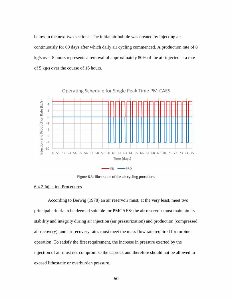
60
below in the next two sections. The initial air bubble was created by injecting air
continuously for 60 days after which daily air cycling commenced. A production rate of 8
kg/s over 8 hours represents a removal of approximately 80% of the air injected at a rate
of 5 kg/s over the course of 16 hours.
Figure 6.3: Illustration of the air cycling procedure.
6.4.2 Injection Procedures
According to Berwig (1978) an air reservoir must, at the very least, meet two
principal criteria to be deemed suitable for PMCAES: the air reservoir must maintain its
stability and integrity during air injection (air pressurization) and production (compressed
air recovery), and air recovery rates must meet the mass flow rate required for turbine
operation. To satisfy the first requirement, the increase in pressure exerted by the
injection of air must not compromise the caprock and therefore should not be allowed to
exceed lithostatic or overburden pressure.
-10
-8
-6
-4
-2
0
2
4
6
50 51 52 53 54 55 56 57 58 59 60 61 62 63 64 65 66 67 68 69 70 71 72 73 74 75Inje
ctio
n a
nd
Pro
du
ctio
n R
ate
(kg/
s)
Time (days)
Operating Schedule for Single Peak Time PM-CAES
INJ PRO
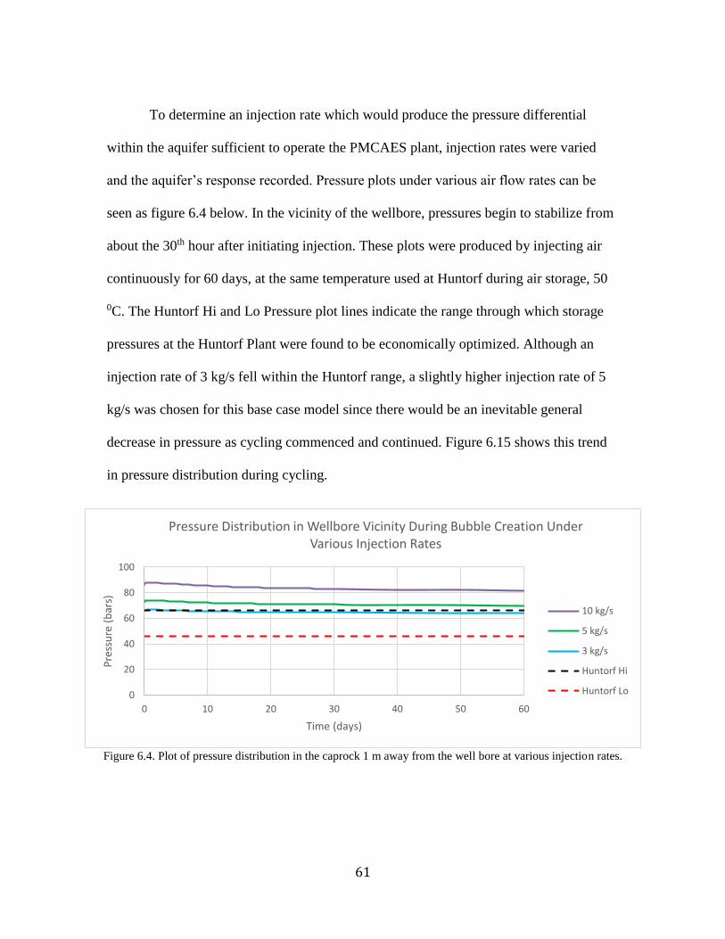
61
To determine an injection rate which would produce the pressure differential
within the aquifer sufficient to operate the PMCAES plant, injection rates were varied
and the aquifer’s response recorded. Pressure plots under various air flow rates can be
seen as figure 6.4 below. In the vicinity of the wellbore, pressures begin to stabilize from
about the 30th hour after initiating injection. These plots were produced by injecting air
continuously for 60 days, at the same temperature used at Huntorf during air storage, 50
0C. The Huntorf Hi and Lo Pressure plot lines indicate the range through which storage
pressures at the Huntorf Plant were found to be economically optimized. Although an
injection rate of 3 kg/s fell within the Huntorf range, a slightly higher injection rate of 5
kg/s was chosen for this base case model since there would be an inevitable general
decrease in pressure as cycling commenced and continued. Figure 6.15 shows this trend
in pressure distribution during cycling.
Figure 6.4. Plot of pressure distribution in the caprock 1 m away from the well bore at various injection rates.
0
20
40
60
80
100
0 10 20 30 40 50 60
Pre
ssu
re (
bar
s)
Time (days)
Pressure Distribution in Wellbore Vicinity During Bubble Creation Under Various Injection Rates
10 kg/s
5 kg/s
3 kg/s
Huntorf Hi
Huntorf Lo
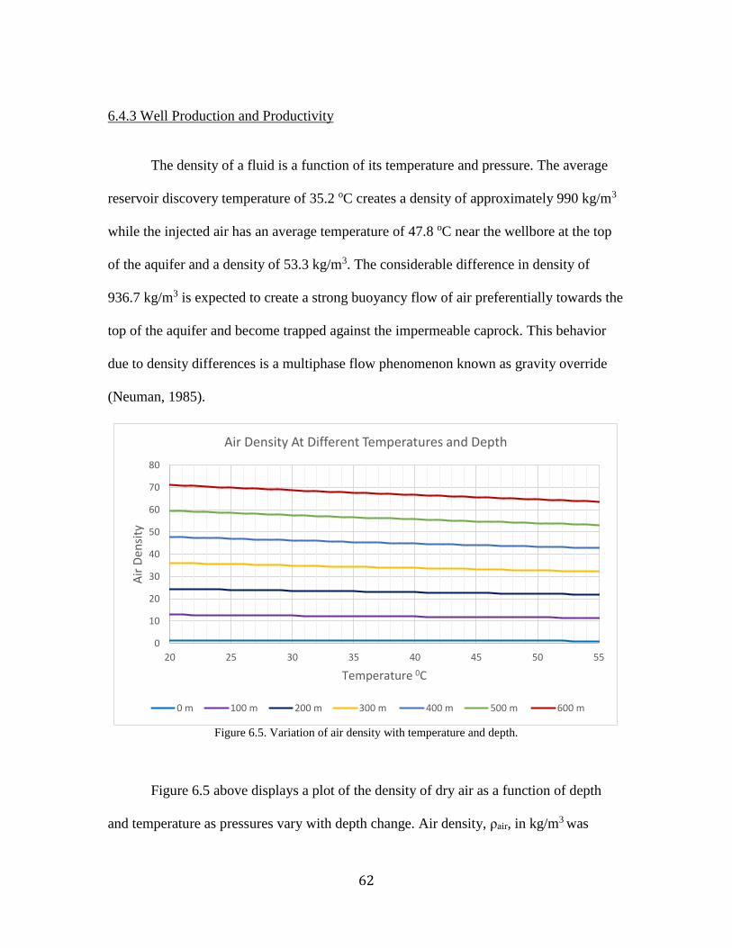
62
6.4.3 Well Production and Productivity
The density of a fluid is a function of its temperature and pressure. The average
reservoir discovery temperature of 35.2 oC creates a density of approximately 990 kg/m3
while the injected air has an average temperature of 47.8 oC near the wellbore at the top
of the aquifer and a density of 53.3 kg/m3. The considerable difference in density of
936.7 kg/m3 is expected to create a strong buoyancy flow of air preferentially towards the
top of the aquifer and become trapped against the impermeable caprock. This behavior
due to density differences is a multiphase flow phenomenon known as gravity override
(Neuman, 1985).
Figure 6.5 above displays a plot of the density of dry air as a function of depth
and temperature as pressures vary with depth change. Air density, ρair, in kg/m3 was
Figure 6.5. Variation of air density with temperature and depth.
0
10
20
30
40
50
60
70
80
20 25 30 35 40 45 50 55
Air
Den
sity
Temperature 0C
Air Density At Different Temperatures and Depth
0 m 100 m 200 m 300 m 400 m 500 m 600 m
63
calculated as the ratio of the air’s pressure in Pa, to the product of the gas constant for dry
air, R, assumed to be 287.1 J/kgK, and the absolute temperature of the air, T.
ρair =P
R T
(6.3)
The introduction of air into a saturated aquifer creates a pressure difference
between the fluids. This means that at the end of the injection period, when the air
compressors in the surface facility are switched off, air flow should spontaneously
reverse into the wellbore and up towards the surface under its own pressure gradient
without the assistance of above-ground pumps because of buoyancy effects.
To investigate this expected behavior, the concept of Productivity Index (PI) is
used. PI was originally used in the oil industry to measure the ability of a vertical well to
produce, and relates the total fluid flow rate to the pressure drawdown for water-free oil
production (Ahmed, 2010). The PI can be calculated by the deliverability option available
in TOUGH2. Here wells produce against a prescribed flowing bottom pressure, Pwb with
a chosen PI value. When using this option the mass production of phase β from a grid
block with phase pressure Pβ such that:
qβ =krβ
μβρβPI(Pβ − Pwb )
(6.4)
The Well on Deliverability (DELV) option in TOUGH2 defines a boundary condition at
which the designated cell produces to a fixed pressure. The user defines both the PI and
the outlet pressure existing at the top of the wellbore. In this base case model the outlet
pressure was chosen to be 42 bars, the same outlet pressure used at the Huntorf Plant.
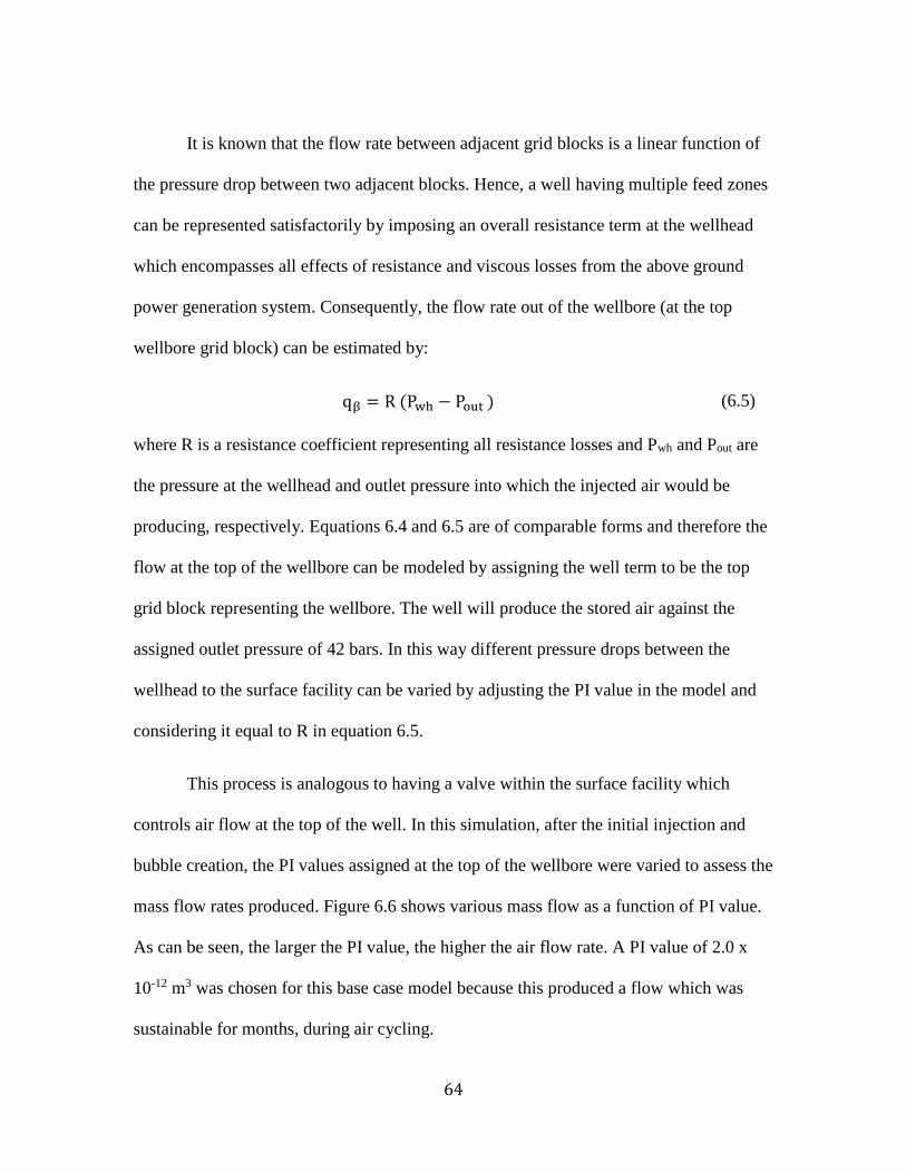
64
It is known that the flow rate between adjacent grid blocks is a linear function of
the pressure drop between two adjacent blocks. Hence, a well having multiple feed zones
can be represented satisfactorily by imposing an overall resistance term at the wellhead
which encompasses all effects of resistance and viscous losses from the above ground
power generation system. Consequently, the flow rate out of the wellbore (at the top
wellbore grid block) can be estimated by:
qβ = R (Pwh − Pout ) (6.5)
where R is a resistance coefficient representing all resistance losses and Pwh and Pout are
the pressure at the wellhead and outlet pressure into which the injected air would be
producing, respectively. Equations 6.4 and 6.5 are of comparable forms and therefore the
flow at the top of the wellbore can be modeled by assigning the well term to be the top
grid block representing the wellbore. The well will produce the stored air against the
assigned outlet pressure of 42 bars. In this way different pressure drops between the
wellhead to the surface facility can be varied by adjusting the PI value in the model and
considering it equal to R in equation 6.5.
This process is analogous to having a valve within the surface facility which
controls air flow at the top of the well. In this simulation, after the initial injection and
bubble creation, the PI values assigned at the top of the wellbore were varied to assess the
mass flow rates produced. Figure 6.6 shows various mass flow as a function of PI value.
As can be seen, the larger the PI value, the higher the air flow rate. A PI value of 2.0 x
10-12 m3 was chosen for this base case model because this produced a flow which was
sustainable for months, during air cycling.
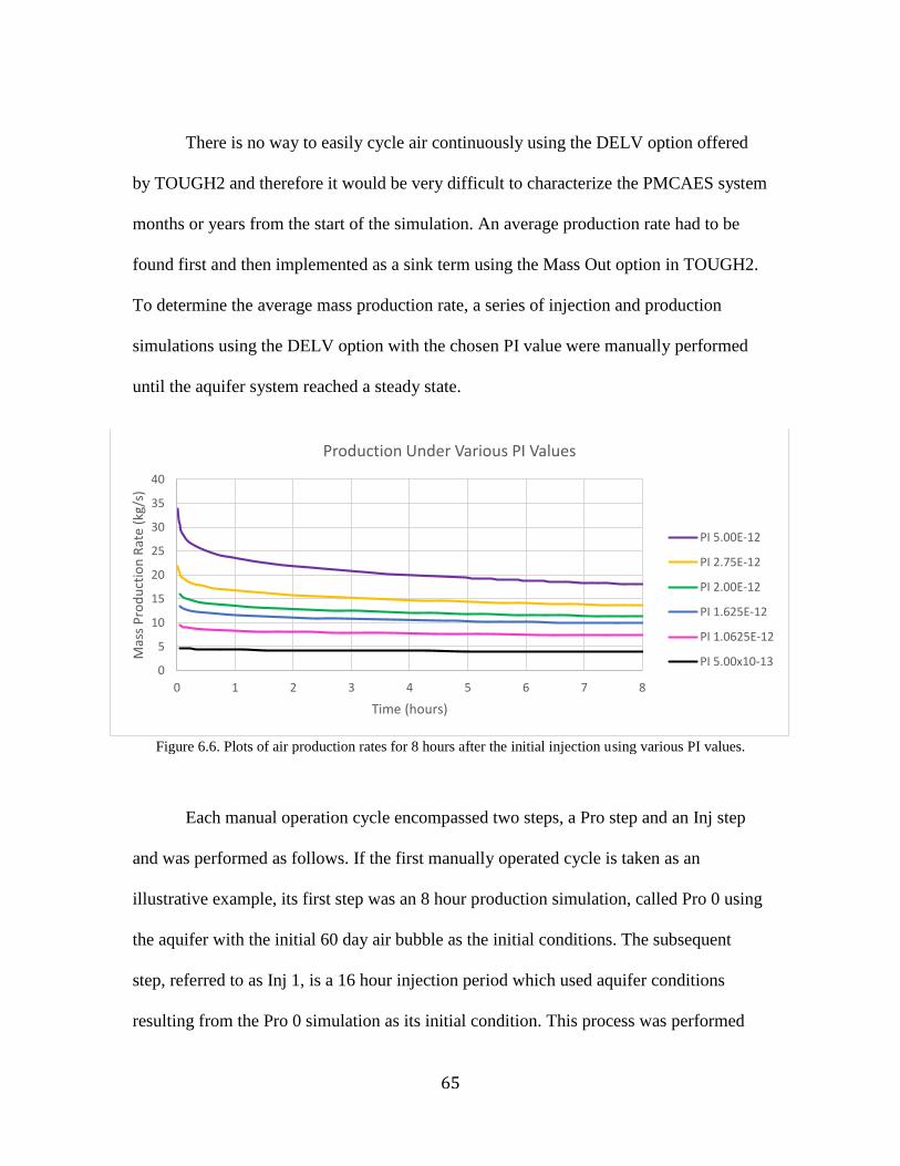
65
There is no way to easily cycle air continuously using the DELV option offered
by TOUGH2 and therefore it would be very difficult to characterize the PMCAES system
months or years from the start of the simulation. An average production rate had to be
found first and then implemented as a sink term using the Mass Out option in TOUGH2.
To determine the average mass production rate, a series of injection and production
simulations using the DELV option with the chosen PI value were manually performed
until the aquifer system reached a steady state.
Figure 6.6. Plots of air production rates for 8 hours after the initial injection using various PI values.
Each manual operation cycle encompassed two steps, a Pro step and an Inj step
and was performed as follows. If the first manually operated cycle is taken as an
illustrative example, its first step was an 8 hour production simulation, called Pro 0 using
the aquifer with the initial 60 day air bubble as the initial conditions. The subsequent
step, referred to as Inj 1, is a 16 hour injection period which used aquifer conditions
resulting from the Pro 0 simulation as its initial condition. This process was performed
0
5
10
15
20
25
30
35
40
0 1 2 3 4 5 6 7 8
Mas
s P
rod
uct
ion
Rat
e (k
g/s)
Time (hours)
Production Under Various PI Values
PI 5.00E-12
PI 2.75E-12
PI 2.00E-12
PI 1.625E-12
PI 1.0625E-12
PI 5.00x10⁻¹³
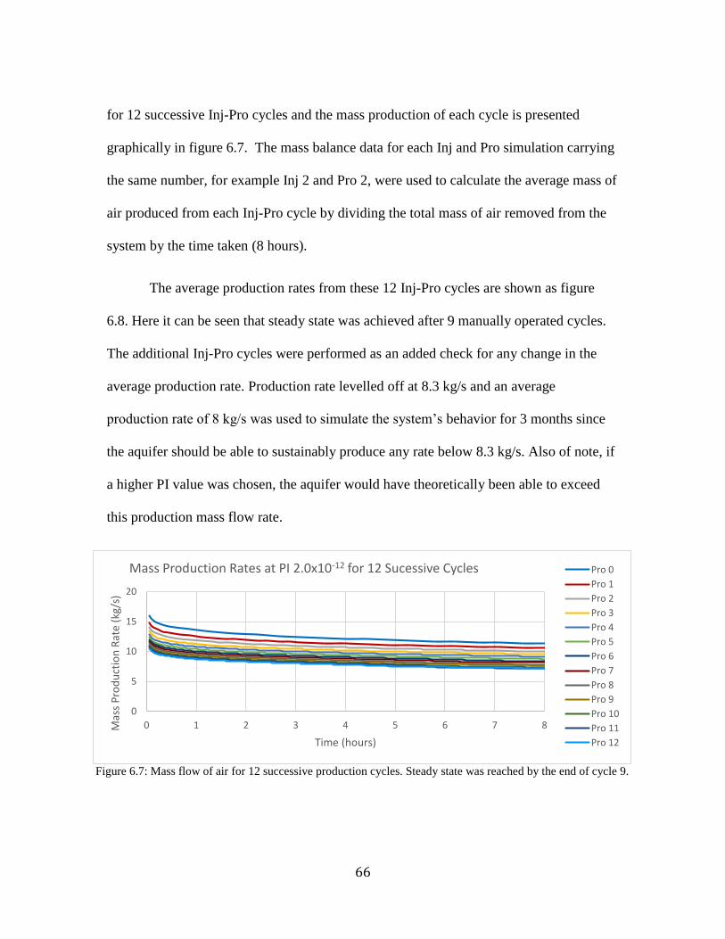
66
for 12 successive Inj-Pro cycles and the mass production of each cycle is presented
graphically in figure 6.7. The mass balance data for each Inj and Pro simulation carrying
the same number, for example Inj 2 and Pro 2, were used to calculate the average mass of
air produced from each Inj-Pro cycle by dividing the total mass of air removed from the
system by the time taken (8 hours).
The average production rates from these 12 Inj-Pro cycles are shown as figure
6.8. Here it can be seen that steady state was achieved after 9 manually operated cycles.
The additional Inj-Pro cycles were performed as an added check for any change in the
average production rate. Production rate levelled off at 8.3 kg/s and an average
production rate of 8 kg/s was used to simulate the system’s behavior for 3 months since
the aquifer should be able to sustainably produce any rate below 8.3 kg/s. Also of note, if
a higher PI value was chosen, the aquifer would have theoretically been able to exceed
this production mass flow rate.
Figure 6.7: Mass flow of air for 12 successive production cycles. Steady state was reached by the end of cycle 9.
0
5
10
15
20
0 1 2 3 4 5 6 7 8Mas
s P
rod
uct
ion
Rat
e (k
g/s)
Time (hours)
Mass Production Rates at PI 2.0x10⁻¹² for 12 Sucessive Cycles Pro 0
Pro 1
Pro 2
Pro 3
Pro 4
Pro 5
Pro 6
Pro 7
Pro 8
Pro 9
Pro 10
Pro 11
Pro 12
67
Figure 6.8: The average production rate from the 12 production cycles shown in figure 6.7.
6.5 Simulation Results and Analysis
6.5.1 Initial Bubble Formation
A single working Inj-Stor-Pro cycle for this base case model comprises the
injection of air at a rate of 5 kg/s at a temperature of 50 0C over 16 hours and production
at 8 kg/s over 8 hours with no Stor time. In flat formations, there is no trapping structure
for the air and so to maximize recovery, the extraction rate should be kept greater than
the injection rate, especially since, in this case, the injection time is twice as long as the
production time. Storage time and the ratio of injection rate to production rate are
coupled and because their effects on this system are quite significant, these variables will
be explored in the next chapter. Increasing production rates is expected to increase the
fraction of water produced. Recovering water in excess not only creates a serious hazard
0
2
4
6
8
10
12
14
0 1 2 3 4 5 6 7 8 9 10 11 12
Ave
rage
Pro
du
ctio
n F
low
Rat
e
Cycle Number
Change in Mass Flow Rate of Air with Cycle Number
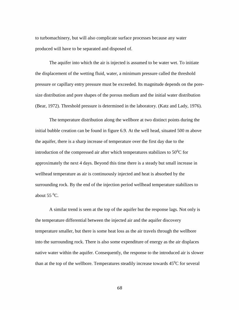
68
to turbomachinery, but will also complicate surface processes because any water
produced will have to be separated and disposed of.
The aquifer into which the air is injected is assumed to be water wet. To initiate
the displacement of the wetting fluid, water, a minimum pressure called the threshold
pressure or capillary entry pressure must be exceeded. Its magnitude depends on the pore-
size distribution and pore shapes of the porous medium and the initial water distribution
(Bear, 1972). Threshold pressure is determined in the laboratory. (Katz and Lady, 1976).
The temperature distribution along the wellbore at two distinct points during the
initial bubble creation can be found in figure 6.9. At the well head, situated 500 m above
the aquifer, there is a sharp increase of temperature over the first day due to the
introduction of the compressed air after which temperatures stabilizes to 500C for
approximately the next 4 days. Beyond this time there is a steady but small increase in
wellhead temperature as air is continuously injected and heat is absorbed by the
surrounding rock. By the end of the injection period wellhead temperature stabilizes to
about 55 0C.
A similar trend is seen at the top of the aquifer but the response lags. Not only is
the temperature differential between the injected air and the aquifer discovery
temperature smaller, but there is some heat loss as the air travels through the wellbore
into the surrounding rock. There is also some expenditure of energy as the air displaces
native water within the aquifer. Consequently, the response to the introduced air is slower
than at the top of the wellbore. Temperatures steadily increase towards 450C for several
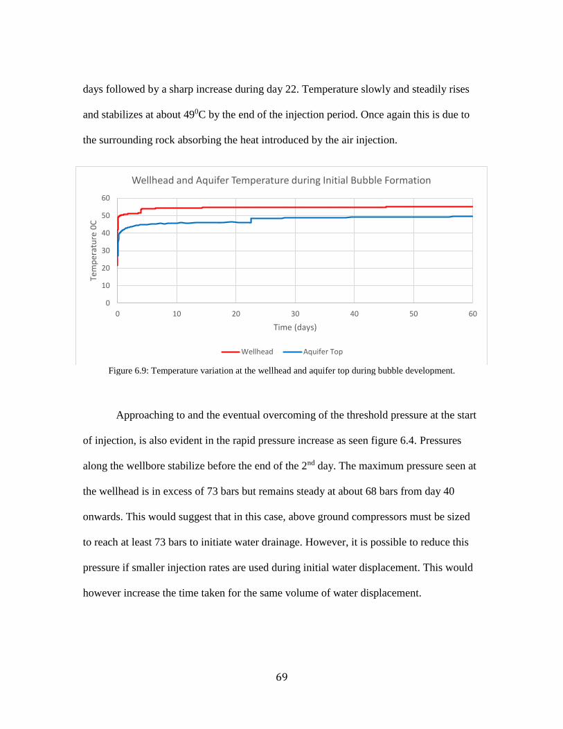
69
days followed by a sharp increase during day 22. Temperature slowly and steadily rises
and stabilizes at about 490C by the end of the injection period. Once again this is due to
the surrounding rock absorbing the heat introduced by the air injection.
Figure 6.9: Temperature variation at the wellhead and aquifer top during bubble development.
Approaching to and the eventual overcoming of the threshold pressure at the start
of injection, is also evident in the rapid pressure increase as seen figure 6.4. Pressures
along the wellbore stabilize before the end of the 2nd day. The maximum pressure seen at
the wellhead is in excess of 73 bars but remains steady at about 68 bars from day 40
onwards. This would suggest that in this case, above ground compressors must be sized
to reach at least 73 bars to initiate water drainage. However, it is possible to reduce this
pressure if smaller injection rates are used during initial water displacement. This would
however increase the time taken for the same volume of water displacement.
0
10
20
30
40
50
60
0 10 20 30 40 50 60
Tem
per
atu
re 0
C
Time (days)
Wellhead and Aquifer Temperature during Initial Bubble Formation
Wellhead Aquifer Top
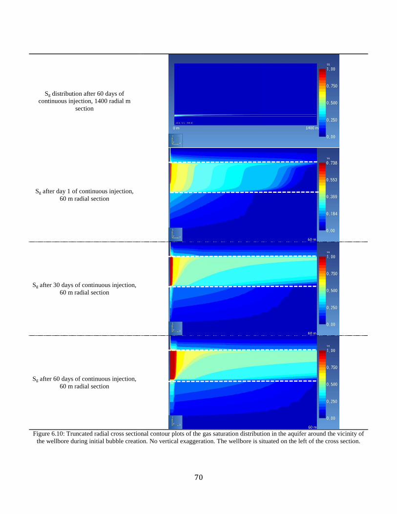
70
Sg distribution after 60 days of
continuous injection, 1400 radial m
section
Sg after day 1 of continuous injection,
60 m radial section
Sg after 30 days of continuous injection,
60 m radial section
Sg after 60 days of continuous injection,
60 m radial section
Figure 6.10: Truncated radial cross sectional contour plots of the gas saturation distribution in the aquifer around the vicinity of
the wellbore during initial bubble creation. No vertical exaggeration. The wellbore is situated on the left of the cross section.
71
Pressure distribution after 60 days of
continuous injection, 1400 m radial
section
Pressure after day 1 of continuous
injection, 60 m radial section
Pressure after 30 days of continuous
injection, 60 m section
Pressure after 60 days of continuous
injection, 60 m radial section
Figure 6.11: Truncated radial cross sectional contour plots of the pressure distribution in the aquifer around the vicinity of the
wellbore during initial bubble creation. No vertical exaggeration. The wellbore is situated on the left of the cross section.
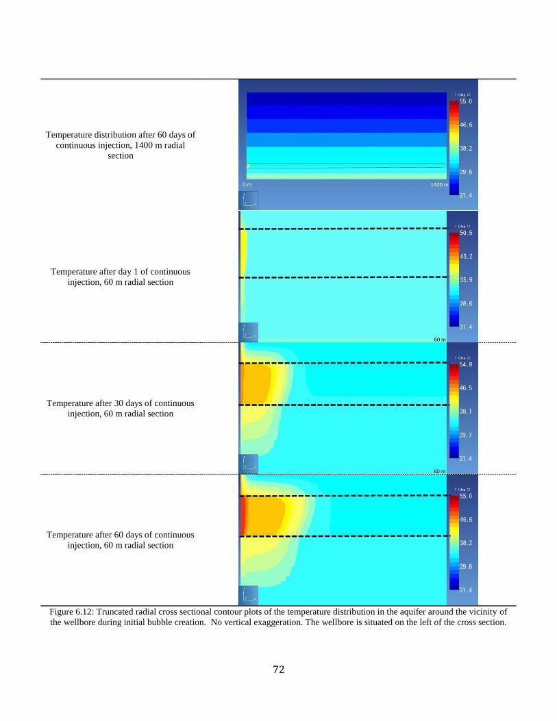
72
Temperature distribution after 60 days of
continuous injection, 1400 m radial
section
Temperature after day 1 of continuous
injection, 60 m radial section
Temperature after 30 days of continuous
injection, 60 m radial section
Temperature after 60 days of continuous
injection, 60 m radial section
Figure 6.12: Truncated radial cross sectional contour plots of the temperature distribution in the aquifer around the vicinity of
the wellbore during initial bubble creation. No vertical exaggeration. The wellbore is situated on the left of the cross section.
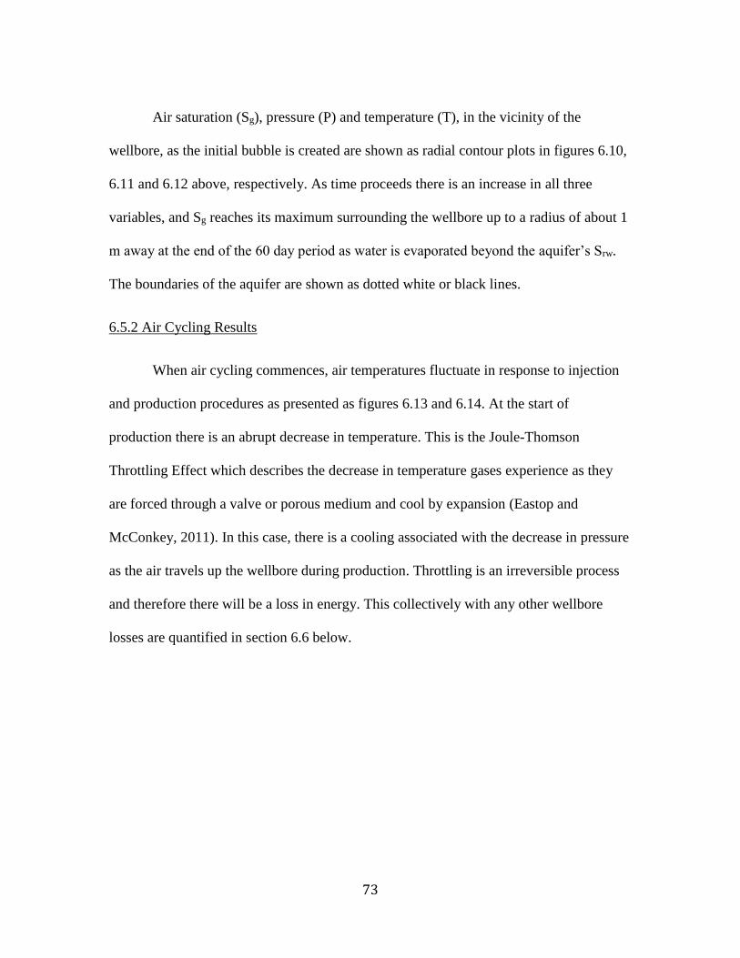
73
Air saturation (Sg), pressure (P) and temperature (T), in the vicinity of the
wellbore, as the initial bubble is created are shown as radial contour plots in figures 6.10,
6.11 and 6.12 above, respectively. As time proceeds there is an increase in all three
variables, and Sg reaches its maximum surrounding the wellbore up to a radius of about 1
m away at the end of the 60 day period as water is evaporated beyond the aquifer’s Srw.
The boundaries of the aquifer are shown as dotted white or black lines.
6.5.2 Air Cycling Results
When air cycling commences, air temperatures fluctuate in response to injection
and production procedures as presented as figures 6.13 and 6.14. At the start of
production there is an abrupt decrease in temperature. This is the Joule-Thomson
Throttling Effect which describes the decrease in temperature gases experience as they
are forced through a valve or porous medium and cool by expansion (Eastop and
McConkey, 2011). In this case, there is a cooling associated with the decrease in pressure
as the air travels up the wellbore during production. Throttling is an irreversible process
and therefore there will be a loss in energy. This collectively with any other wellbore
losses are quantified in section 6.6 below.
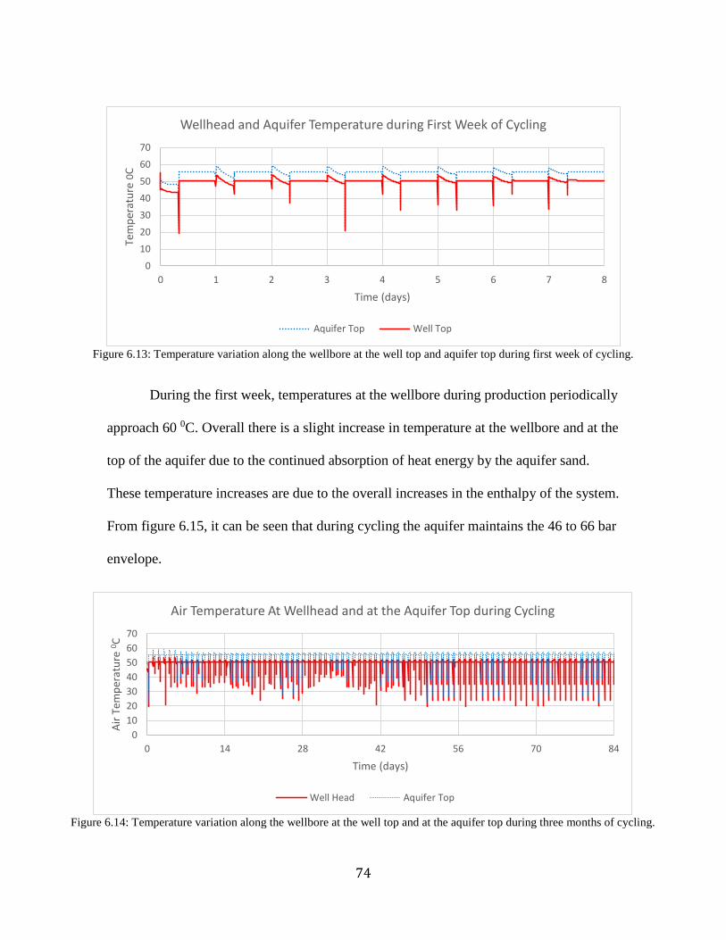
74
Figure 6.13: Temperature variation along the wellbore at the well top and aquifer top during first week of cycling.
During the first week, temperatures at the wellbore during production periodically
approach 60 0C. Overall there is a slight increase in temperature at the wellbore and at the
top of the aquifer due to the continued absorption of heat energy by the aquifer sand.
These temperature increases are due to the overall increases in the enthalpy of the system.
From figure 6.15, it can be seen that during cycling the aquifer maintains the 46 to 66 bar
envelope.
Figure 6.14: Temperature variation along the wellbore at the well top and at the aquifer top during three months of cycling.
0
10
20
30
40
50
60
70
0 1 2 3 4 5 6 7 8
Tem
per
atu
re 0
C
Time (days)
Wellhead and Aquifer Temperature during First Week of Cycling
Aquifer Top Well Top
0
10
20
30
40
50
60
70
0 14 28 42 56 70 84
Air
Tem
per
atu
re 0 C
Time (days)
Air Temperature At Wellhead and at the Aquifer Top during Cycling
Well Head Aquifer Top
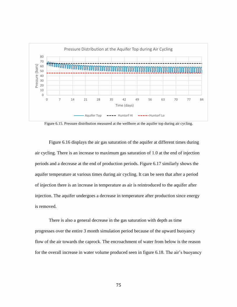
75
Figure 6.15. Pressure distribution measured at the wellbore at the aquifer top during air cycling.
Figure 6.16 displays the air gas saturation of the aquifer at different times during
air cycling. There is an increase to maximum gas saturation of 1.0 at the end of injection
periods and a decrease at the end of production periods. Figure 6.17 similarly shows the
aquifer temperature at various times during air cycling. It can be seen that after a period
of injection there is an increase in temperature as air is reintroduced to the aquifer after
injection. The aquifer undergoes a decrease in temperature after production since energy
is removed.
There is also a general decrease in the gas saturation with depth as time
progresses over the entire 3 month simulation period because of the upward buoyancy
flow of the air towards the caprock. The encroachment of water from below is the reason
for the overall increase in water volume produced seen in figure 6.18. The air’s buoyancy
0
10
20
30
40
50
60
70
80
0 7 14 21 28 35 42 49 56 63 70 77 84
Pre
ssu
re(b
ars)
Time (days)
Pressure Distribution at the Aquifer Top during Air Cycling
Aquifer Top Huntorf Hi Huntorf Lo
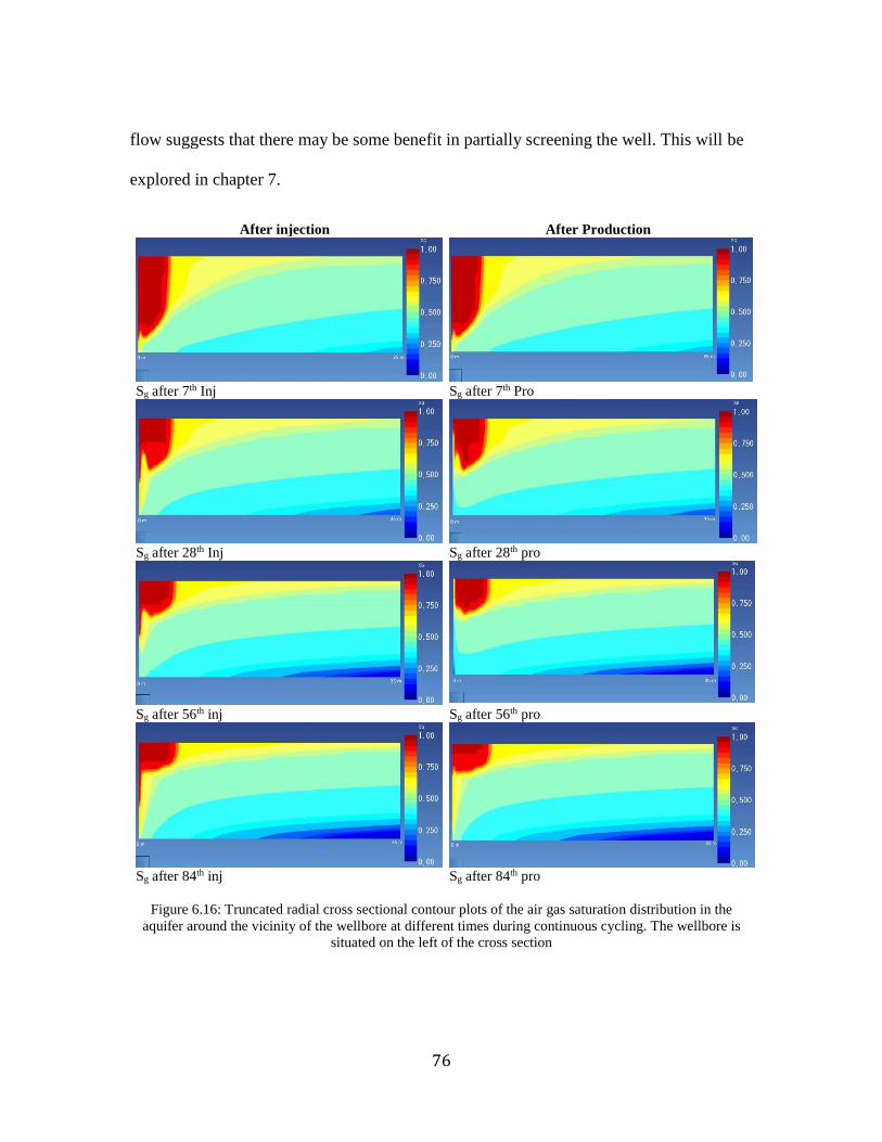
76
flow suggests that there may be some benefit in partially screening the well. This will be
explored in chapter 7.
After injection After Production
Sg after 7th Inj Sg after 7th Pro
Sg after 28th Inj Sg after 28th pro
Sg after 56th inj Sg after 56th pro
Sg after 84th inj Sg after 84th pro
Figure 6.16: Truncated radial cross sectional contour plots of the air gas saturation distribution in the
aquifer around the vicinity of the wellbore at different times during continuous cycling. The wellbore is
situated on the left of the cross section
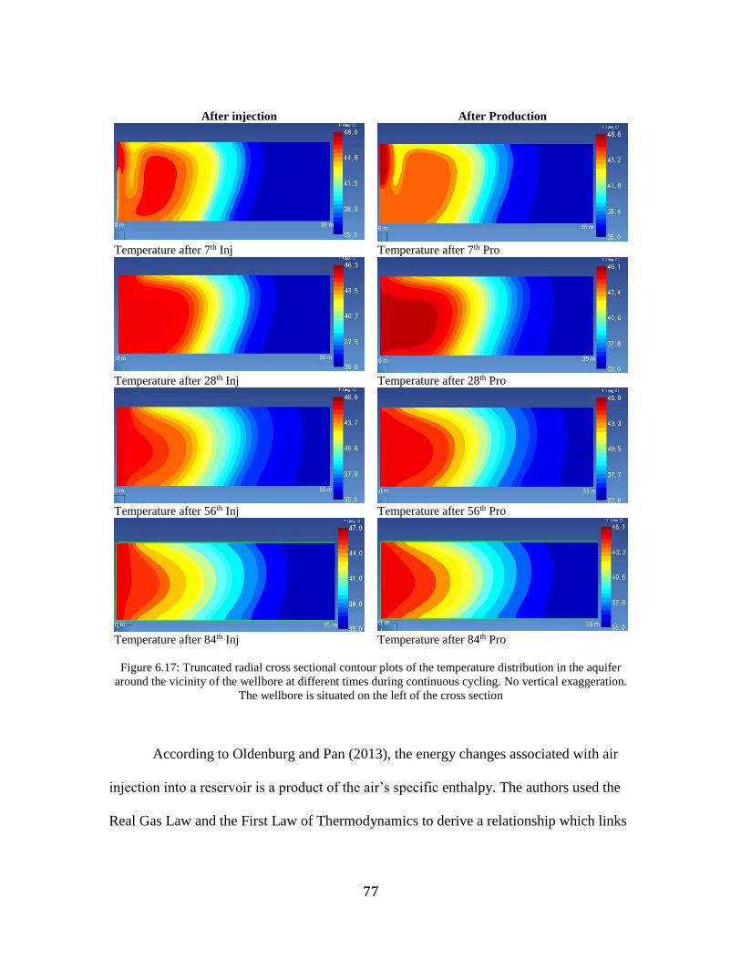
77
After injection After Production
Temperature after 7th Inj Temperature after 7th Pro
Temperature after 28th Inj Temperature after 28th Pro
Temperature after 56th Inj Temperature after 56th Pro
Temperature after 84th Inj Temperature after 84th Pro
Figure 6.17: Truncated radial cross sectional contour plots of the temperature distribution in the aquifer
around the vicinity of the wellbore at different times during continuous cycling. No vertical exaggeration.
The wellbore is situated on the left of the cross section
According to Oldenburg and Pan (2013), the energy changes associated with air
injection into a reservoir is a product of the air’s specific enthalpy. The authors used the
Real Gas Law and the First Law of Thermodynamics to derive a relationship which links
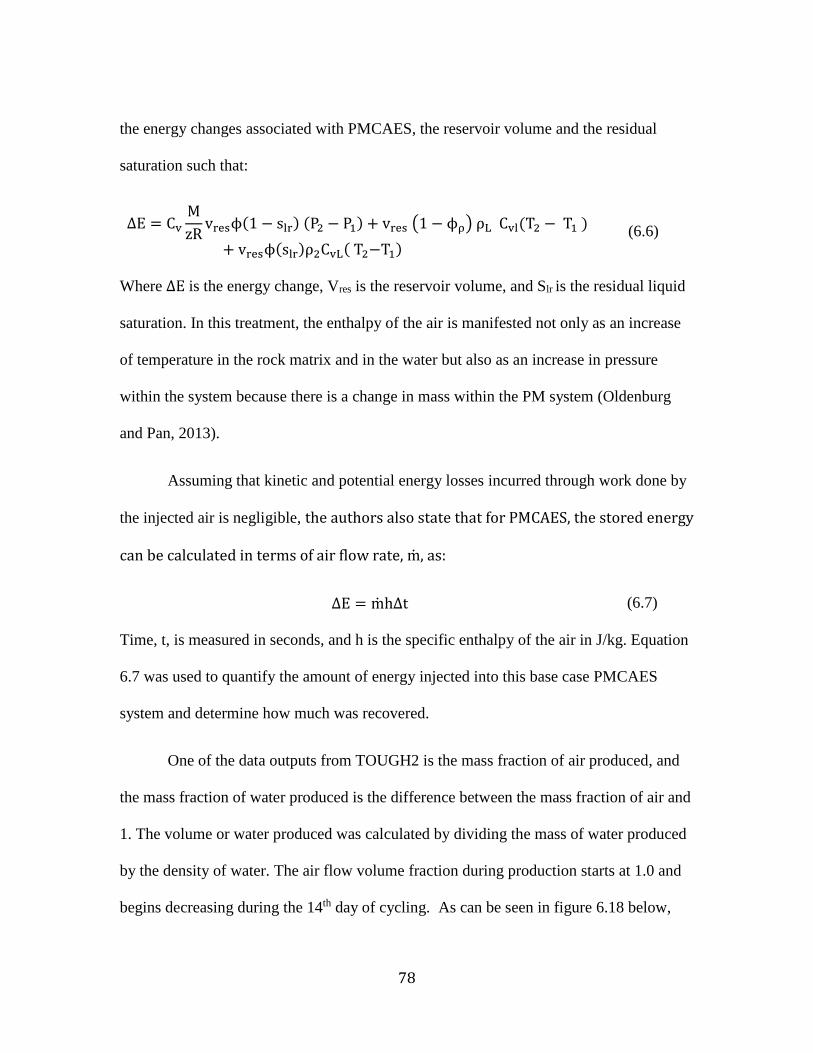
78
the energy changes associated with PMCAES, the reservoir volume and the residual
saturation such that:
ΔE = Cv
M
zRvresϕ(1 − slr) (P2 − P1) + vres (1 − ϕρ) ρL Cvl(T2 − T1 )
+ vresϕ(slr)ρ2CvL( T2−T1)(6.6)
Where ΔE is the energy change, Vres is the reservoir volume, and Slr is the residual liquid
saturation. In this treatment, the enthalpy of the air is manifested not only as an increase
of temperature in the rock matrix and in the water but also as an increase in pressure
within the system because there is a change in mass within the PM system (Oldenburg
and Pan, 2013).
Assuming that kinetic and potential energy losses incurred through work done by
the injected air is negligible, the authors also state that for PMCAES, the stored energy
can be calculated in terms of air flow rate, m, as:
ΔE = mhΔt (6.7)
Time, t, is measured in seconds, and h is the specific enthalpy of the air in J/kg. Equation
6.7 was used to quantify the amount of energy injected into this base case PMCAES
system and determine how much was recovered.
One of the data outputs from TOUGH2 is the mass fraction of air produced, and
the mass fraction of water produced is the difference between the mass fraction of air and
1. The volume or water produced was calculated by dividing the mass of water produced
by the density of water. The air flow volume fraction during production starts at 1.0 and
begins decreasing during the 14th day of cycling. As can be seen in figure 6.18 below,
79
the decrease is very small and over the entire 3 month period it does not exceed 0.002 %.
As stated before, any water poses a threat to turbomachinery and therefore has to be kept
at a minimum or ideally be completely eliminated. Reducing the extraction rate could
reduce the volume of water produced but since the amount of energy recovered is directly
linked to the mass rate of air produced (see section 6.5.2), the cost to cycle efficiency is
too great to justify the use of lower production rates when removing water from the
incoming air stream can be easily solved by engineering design. On the outlet of
production wells, a piece of equipment called a knock-out drum will have to be installed.
Figure 6.18: Gas Volume Fraction during production section of cycles for 3 months of air cycling
According to Walas (1990), a knock-out drum is a standard piece of equipment
capable of separating liquid from a gas stream. It utilizes a mesh, the thickness of which
is determined by the gas flow velocity and the difference in density between the gas and
the liquid entrained within. High efficiency meshes will reduce liquid content by up to
99.9%. As air flows through the mesh and its velocity decreases across the mesh, so too
does its momentum whereby reducing its ability to carry the water and so any water
0.9998
0.99985
0.9999
0.99995
1
0 7 14 21 28 35 42 49 56 63 70 77 84
Air
Vo
lum
e Fr
acti
on
Time (days)
Volume Fraction of Air Produced
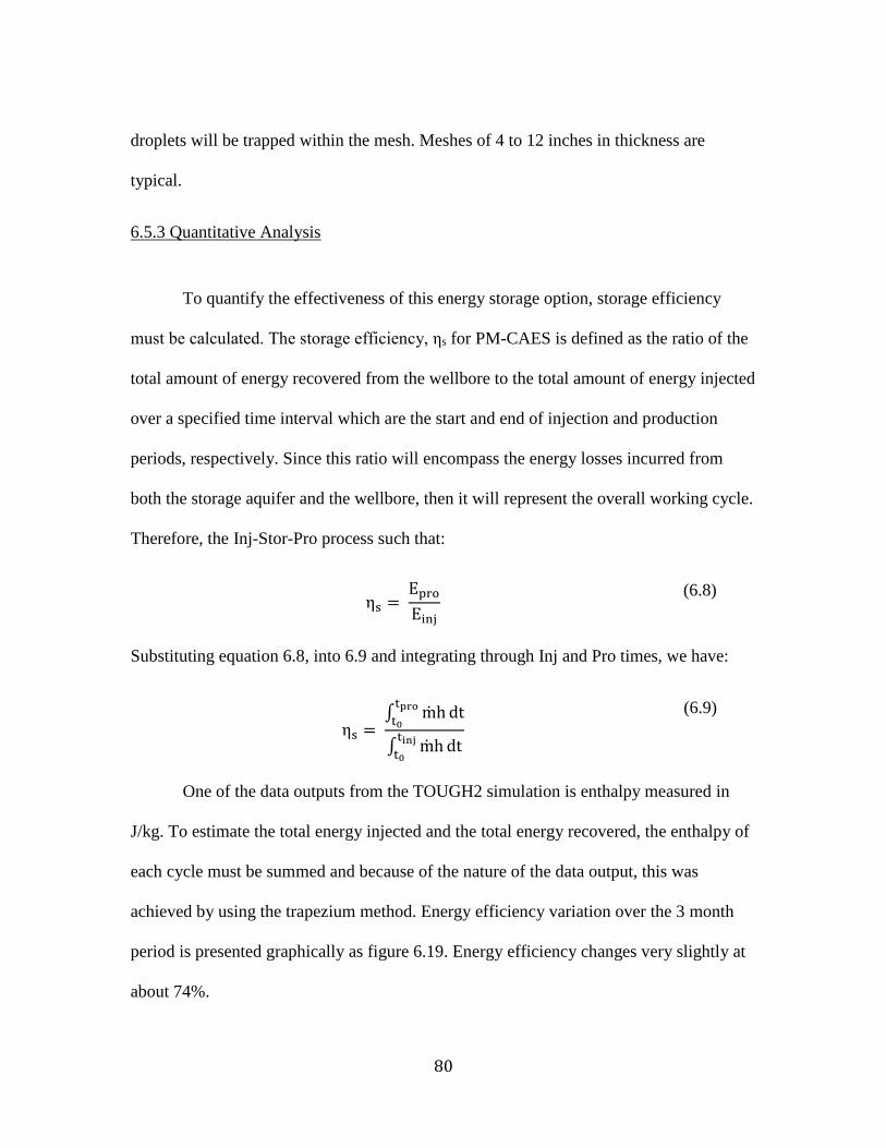
80
droplets will be trapped within the mesh. Meshes of 4 to 12 inches in thickness are
typical.
6.5.3 Quantitative Analysis
To quantify the effectiveness of this energy storage option, storage efficiency
must be calculated. The storage efficiency, ηs for PM-CAES is defined as the ratio of the
total amount of energy recovered from the wellbore to the total amount of energy injected
over a specified time interval which are the start and end of injection and production
periods, respectively. Since this ratio will encompass the energy losses incurred from
both the storage aquifer and the wellbore, then it will represent the overall working cycle.
Therefore, the Inj-Stor-Pro process such that:
ηs = Epro
Einj
(6.8)
Substituting equation 6.8, into 6.9 and integrating through Inj and Pro times, we have:
ηs = ∫ mh
tpro
t0dt
∫ mhtinj
t0dt
(6.9)
One of the data outputs from the TOUGH2 simulation is enthalpy measured in
J/kg. To estimate the total energy injected and the total energy recovered, the enthalpy of
each cycle must be summed and because of the nature of the data output, this was
achieved by using the trapezium method. Energy efficiency variation over the 3 month
period is presented graphically as figure 6.19. Energy efficiency changes very slightly at
about 74%.
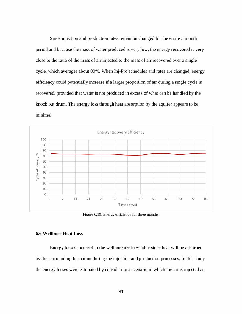
81
Since injection and production rates remain unchanged for the entire 3 month
period and because the mass of water produced is very low, the energy recovered is very
close to the ratio of the mass of air injected to the mass of air recovered over a single
cycle, which averages about 80%. When Inj-Pro schedules and rates are changed, energy
efficiency could potentially increase if a larger proportion of air during a single cycle is
recovered, provided that water is not produced in excess of what can be handled by the
knock out drum. The energy loss through heat absorption by the aquifer appears to be
minimal.
Figure 6.19. Energy efficiency for three months.
6.6 Wellbore Heat Loss
Energy losses incurred in the wellbore are inevitable since heat will be adsorbed
by the surrounding formation during the injection and production processes. In this study
the energy losses were estimated by considering a scenario in which the air is injected at
0
10
20
30
40
50
60
70
80
90
100
0 7 14 21 28 35 42 49 56 63 70 77 84
Cyc
le e
ffic
ien
cy %
Time (days)
Energy Recovery Efficiency
82
the top of the formation rather than at the top of the wellbore situated 500 m above the
aquifer surface. Apart from the location of the source, the entire model remains the same.
Line plots of efficiencies calculated using equation 6.9 are shown as figure 6.20. Energy
recovery is higher, with an average efficiency increase of approximately 5.4% but no
higher than 6.5% when the wellbore is neglected.
Figure 6.20: Comparison between energy storage efficiencies with or without considering wellbore losses.
0
10
20
30
40
50
60
70
80
90
100
0 7 14 21 28 35 42 49 56 63 70 77 84
Energy Recovery Efficiency With and Without Wellbore
Without Wellbore With Wellbore
83
CHAPTER 7
SENSITIVITY ANALYSIS TO PARAMETER CHANGES
7.1 Introduction
This chapter examines the effects of aquifer parameters, initial bubble size, and
injection and production cycles coupled with load schedules on cycle efficiency. The
aquifer parameters explored are aquifer depth, aquifer thickness, permeability and
isotropy. Since wellbore loss was quantified in the previous chapter, the simulations
performed for this chapter used the aquifer-only-set-up where the caprock and the
underlying layers were included but the overburden layers were ignored. This was done
because simulation time was reduced considerably.
It should be noted that during every simulation, the pressure within the aquifer
was kept between the 46 and 66 bar pressure envelope during cycling since it was
assumed that the above ground PMCAES plant would utilize the same turbomachinery
used at the Huntorf Plant. It is important to note that this pressure range constrained the
injection and production mass flow rates which could be used in the 14 simulations
described in this chapter. Table 7.1 presents a summary of the main parameters used for
all simulations.
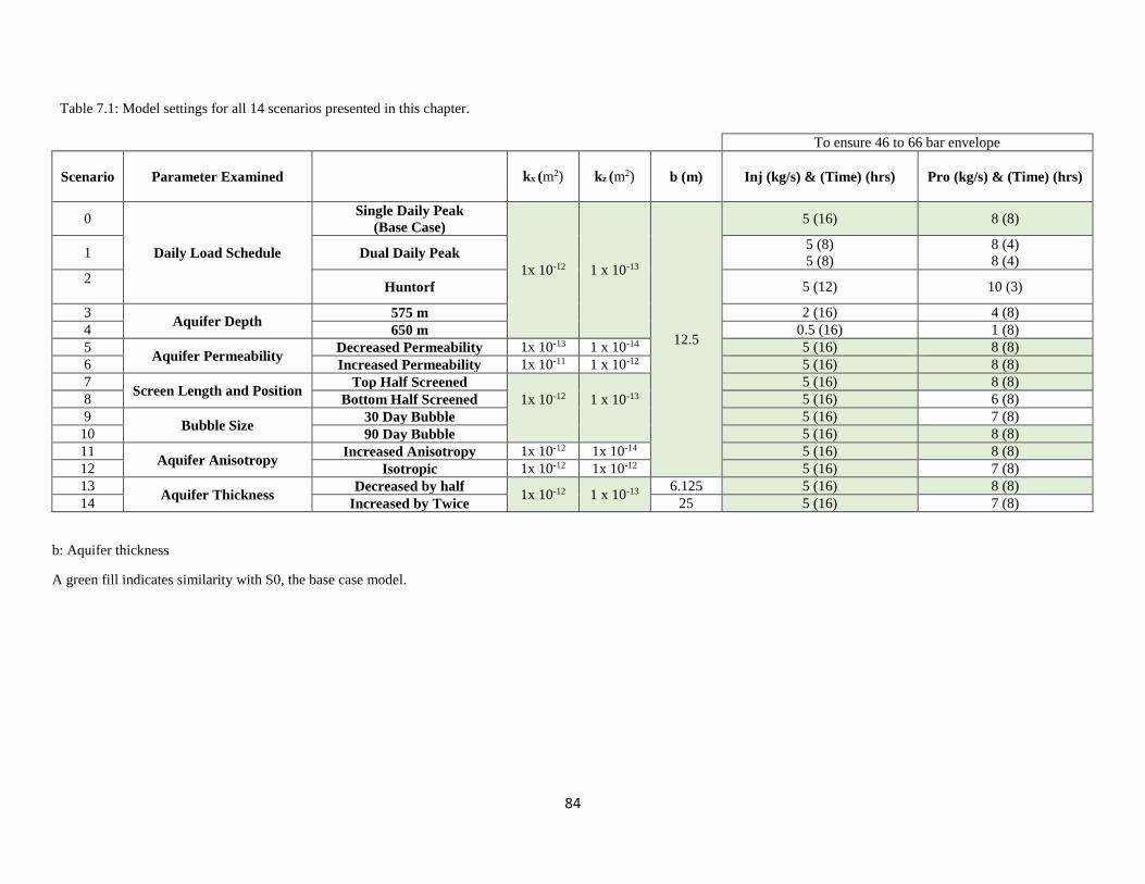
84
Table 7.1: Model settings for all 14 scenarios presented in this chapter.
To ensure 46 to 66 bar envelope
Scenario Parameter Examined kx (m2) kz (m2) b (m) Inj (kg/s) & (Time) (hrs) Pro (kg/s) & (Time) (hrs)
0
Daily Load Schedule
Single Daily Peak
(Base Case)
1x 10-12 1 x 10-13
12.5
5 (16) 8 (8)
1 Dual Daily Peak 5 (8)
5 (8)
8 (4)
8 (4)
2 Huntorf 5 (12) 10 (3)
3 Aquifer Depth
575 m 2 (16) 4 (8)
4 650 m 0.5 (16) 1 (8)
5 Aquifer Permeability
Decreased Permeability 1x 10-13 1 x 10-14 5 (16) 8 (8)
6 Increased Permeability 1x 10-11 1 x 10-12 5 (16) 8 (8)
7 Screen Length and Position
Top Half Screened
1x 10-12 1 x 10-13
5 (16) 8 (8)
8 Bottom Half Screened 5 (16) 6 (8)
9 Bubble Size
30 Day Bubble 5 (16) 7 (8)
10 90 Day Bubble 5 (16) 8 (8)
11 Aquifer Anisotropy
Increased Anisotropy 1x 10-12 1x 10-14 5 (16) 8 (8)
12 Isotropic 1x 10-12 1x 10-12 5 (16) 7 (8)
13 Aquifer Thickness
Decreased by half 1x 10-12 1 x 10-13
6.125 5 (16) 8 (8)
14 Increased by Twice 25 5 (16) 7 (8)
b: Aquifer thickness
A green fill indicates similarity with S0, the base case model.
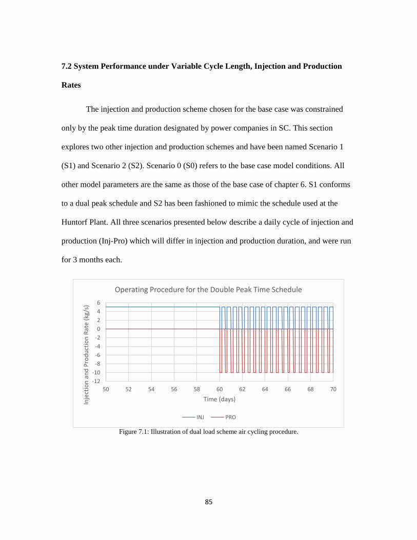
85
7.2 System Performance under Variable Cycle Length, Injection and Production
Rates
The injection and production scheme chosen for the base case was constrained
only by the peak time duration designated by power companies in SC. This section
explores two other injection and production schemes and have been named Scenario 1
(S1) and Scenario 2 (S2). Scenario 0 (S0) refers to the base case model conditions. All
other model parameters are the same as those of the base case of chapter 6. S1 conforms
to a dual peak schedule and S2 has been fashioned to mimic the schedule used at the
Huntorf Plant. All three scenarios presented below describe a daily cycle of injection and
production (Inj-Pro) which will differ in injection and production duration, and were run
for 3 months each.
Figure 7.1: Illustration of dual load scheme air cycling procedure.
-12
-10
-8
-6
-4
-2
0
2
4
6
50 52 54 56 58 60 62 64 66 68 70
Inje
ctio
n a
nd
Pro
du
ctio
n R
ate
(kg/
s)
Time (days)
Operating Procedure for the Double Peak Time Schedule
INJ PRO
86
The dual operation peak schedule is shown in figure 7.1 above. The dual peak
time schedule is similar to that used by the Pacific Power Company of California during
winter. In both cases injection was performed during low load periods and production
during peak times. In a single day there are two low load periods lasting 8 hours each,
during which injection was simulated, punctuated by two high load periods of 4 hours
each, during which air was recovered. The Huntorf schedule repeats daily as follows. A
12 hour recharge period followed by a 4.5 hour shut in period where there is no injection
or recovery. Air is recovered over a 3 hour production period and finally there is another
4.5 hour shut in period.
The aquifer is able to maintain a higher pressure during cycling in S1 since
pressure has less time to dissipate away from the wellbore before air is reintroduced to
the aquifer. At the end of an injection period there will be a natural decrease in pressure
in the vicinity of the wellbore as the buoyancy of air causes it to travel toward the
caprock. This decrease is heavily compounded by the recovery of air during the
production period. The daily dual injection and production scheme means that air is
reintroduced into the aquifer twice in a single day. Pressures during cycling for all 3
scenarios measured at the top of the aquifer within the wellbore can be found in figure
7.2.
To maintain the 46 to 66 bar envelope of pressure, injection and extraction rates
were varied. Higher rates were not used since the pressure dropped below 46 bars. The
mass flow rates and comments on each scenario are recorded below as table 7.2. Two
other production rates of 20, 15 kg/s were considered using the Huntorf cycling schedule.
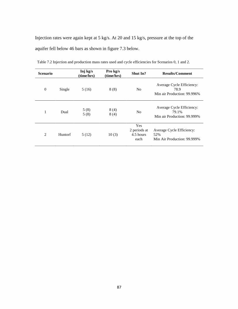
87
Injection rates were again kept at 5 kg/s. At 20 and 15 kg/s, pressure at the top of the
aquifer fell below 46 bars as shown in figure 7.3 below.
Table 7.2 Injection and production mass rates used and cycle efficiencies for Scenarios 0, 1 and 2.
Scenario Inj kg/s
(time/hrs)
Pro kg/s
(time/hrs) Shut In? Results/Comment
0 Single 5 (16) 8 (8) No
Average Cycle Efficiency:
78.9
Min air Production: 99.996%
1 Dual 5 (8)
5 (8)
8 (4)
8 (4) No
Average Cycle Efficiency:
79.1%
Min air Production: 99.999%
2 Huntorf 5 (12) 10 (3)
Yes
2 periods at
4.5 hours
each
Average Cycle Efficiency:
52%
Min Air Production: 99.999%
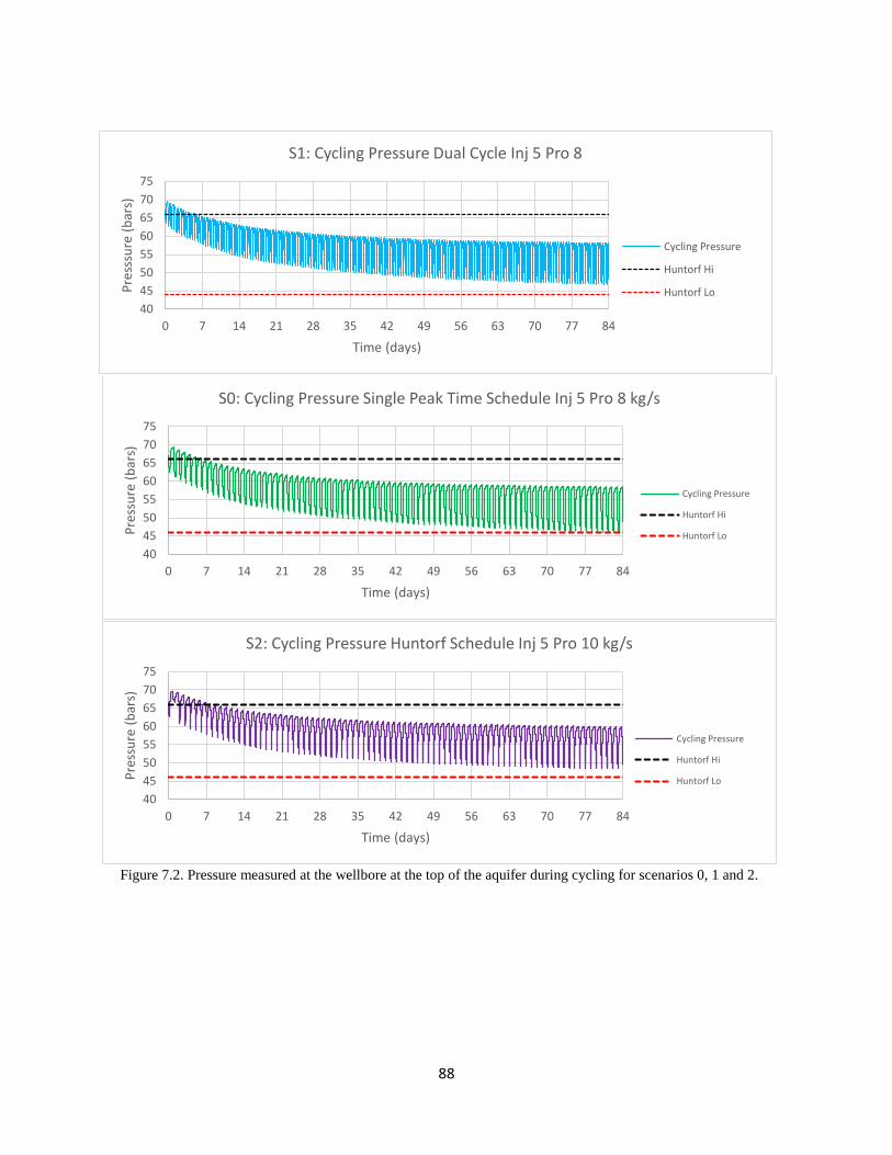
88
Figure 7.2. Pressure measured at the wellbore at the top of the aquifer during cycling for scenarios 0, 1 and 2.
40
45
50
55
60
65
70
75
0 7 14 21 28 35 42 49 56 63 70 77 84
Pre
sssu
re (
bar
s)
Time (days)
S1: Cycling Pressure Dual Cycle Inj 5 Pro 8
Cycling Pressure
Huntorf Hi
Huntorf Lo
40
45
50
55
60
65
70
75
0 7 14 21 28 35 42 49 56 63 70 77 84
Pre
ssu
re (
bar
s)
Time (days)
S0: Cycling Pressure Single Peak Time Schedule Inj 5 Pro 8 kg/s
Cycling Pressure
Huntorf Hi
Huntorf Lo
40
45
50
55
60
65
70
75
0 7 14 21 28 35 42 49 56 63 70 77 84
Pre
ssu
re (
bar
s)
Time (days)
S2: Cycling Pressure Huntorf Schedule Inj 5 Pro 10 kg/s
Cycling Pressure
Huntorf Hi
Huntorf Lo
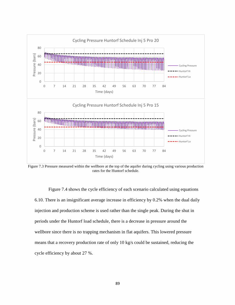
89
Figure 7.3 Pressure measured within the wellbore at the top of the aquifer during cycling using various production
rates for the Huntorf schedule.
Figure 7.4 shows the cycle efficiency of each scenario calculated using equations
6.10. There is an insignificant average increase in efficiency by 0.2% when the dual daily
injection and production scheme is used rather than the single peak. During the shut in
periods under the Huntorf load schedule, there is a decrease in pressure around the
wellbore since there is no trapping mechanism in flat aquifers. This lowered pressure
means that a recovery production rate of only 10 kg/s could be sustained, reducing the
cycle efficiency by about 27 %.
0
20
40
60
80
0 7 14 21 28 35 42 49 56 63 70 77 84
Pre
ssu
re (
bar
s)
Time (days)
Cycling Pressure Huntorf Schedule Inj 5 Pro 20
Cycling Pressure
Huntorf Hi
Huntorf Lo
0
20
40
60
80
0 7 14 21 28 35 42 49 56 63 70 77 84
Pre
ssu
re (
bar
s)
Time (days)
Cycling Pressure Huntorf Schedule Inj 5 Pro 15
Cycling Pressure
Huntorf Hi
Huntorf Lo
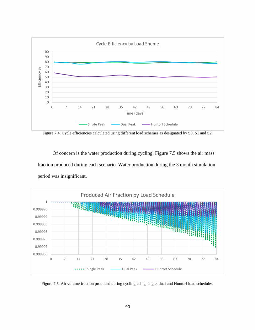
90
Figure 7.4. Cycle efficiencies calculated using different load schemes as designated by S0, S1 and S2.
Of concern is the water production during cycling. Figure 7.5 shows the air mass
fraction produced during each scenario. Water production during the 3 month simulation
period was insignificant.
Figure 7.5. Air volume fraction produced during cycling using single, dual and Huntorf load schedules.
0
10
20
30
40
50
60
70
80
90
100
0 7 14 21 28 35 42 49 56 63 70 77 84
Effi
cien
cy %
Time (days)
Cycle Efficiency by Load Sheme
Single Peak Dual Peak Huntorf Schedule
0.999965
0.99997
0.999975
0.99998
0.999985
0.99999
0.999995
1
0 7 14 21 28 35 42 49 56 63 70 77 84
Produced Air Fraction by Load Schedule
Single Peak Dual Peak Huntorf Schedule

91
7.3 Effects of Aquifer Depth
Aquifer depth was changed while maintaining all other aquifer parameters. The
top of the aquifer was varied to be 575 m (Scenario 3, S3) and then to 650 m (Scenario 4,
S4). A greater depth was not used since the background hydrostatic pressure would be in
excess of the highest pressure stipulated by the Huntorf optimization analysis (66 bars). A
single peak daily schedule was used where air was injected over 16 hours and recovered
for 8 hours.
Figure 7.6 below shows the cycling pressure for S3, S0 and S4. Note that the
injection rates had to also be changed since, with an increase in depth, there is a
corresponding increase in native hydrostatic pressure which should be able to
accommodate higher flow rates. At a depth of 650 m, even a small injection rate of 0.5
kg/s produced pressures in excess of the 66 bar maximum. A 35 day shut in period was
simulated to allow pressures within the aquifer to decrease close to 66 bars before air
cycling was initiated and its effect was examined.
From figure 7.7, which displays the volume fraction of water produced, it can be
noted that with the injection and production rates used, water production is insignificant.
Using lower injection and extraction rates increases the water fraction slightly because of
the smaller volume of air being injected which correspondingly displaced a smaller
volume of water within the vicinity of the wellbore.
In the early stages of energy recovery, cycle efficiency is in excess of the
maximum theoretical efficiency of 100%. This is due to heat energy being harvested from
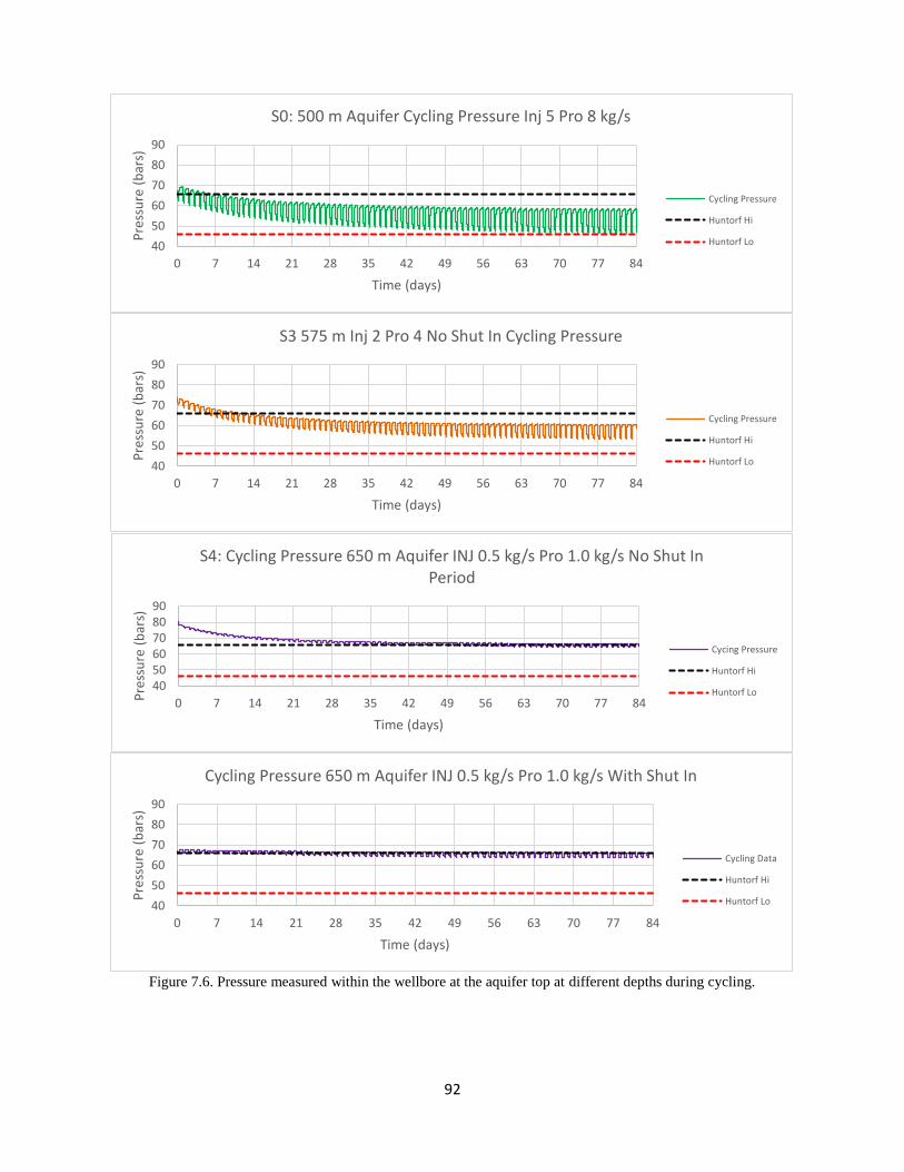
92
Figure 7.6. Pressure measured within the wellbore at the aquifer top at different depths during cycling.
40
50
60
70
80
90
0 7 14 21 28 35 42 49 56 63 70 77 84
Pre
ssu
re (
bar
s)
Time (days)
S0: 500 m Aquifer Cycling Pressure Inj 5 Pro 8 kg/s
Cycling Pressure
Huntorf Hi
Huntorf Lo
40
50
60
70
80
90
0 7 14 21 28 35 42 49 56 63 70 77 84
Pre
ssu
re (
bar
s)
Time (days)
S3 575 m Inj 2 Pro 4 No Shut In Cycling Pressure
Cycling Pressure
Huntorf Hi
Huntorf Lo
405060708090
0 7 14 21 28 35 42 49 56 63 70 77 84Pre
ssu
re (
bar
s)
Time (days)
S4: Cycling Pressure 650 m Aquifer INJ 0.5 kg/s Pro 1.0 kg/s No Shut In Period
Cycing Pressure
Huntorf Hi
Huntorf Lo
40
50
60
70
80
90
0 7 14 21 28 35 42 49 56 63 70 77 84
Pre
ssu
re (
bar
s)
Time (days)
Cycling Pressure 650 m Aquifer INJ 0.5 kg/s Pro 1.0 kg/s With Shut In
Cycling Data
Huntorf Hi
Huntorf Lo
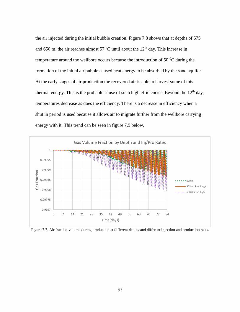
93
the air injected during the initial bubble creation. Figure 7.8 shows that at depths of 575
and 650 m, the air reaches almost 57 oC until about the 12th day. This increase in
temperature around the wellbore occurs because the introduction of 50 0C during the
formation of the initial air bubble caused heat energy to be absorbed by the sand aquifer.
At the early stages of air production the recovered air is able to harvest some of this
thermal energy. This is the probable cause of such high efficiencies. Beyond the 12th day,
temperatures decrease as does the efficiency. There is a decrease in efficiency when a
shut in period is used because it allows air to migrate further from the wellbore carrying
energy with it. This trend can be seen in figure 7.9 below.
Figure 7.7. Air fraction volume during production at different depths and different injection and production rates.
0.9997
0.99975
0.9998
0.99985
0.9999
0.99995
1
0 7 14 21 28 35 42 49 56 63 70 77 84
Gas
Fra
ctio
n
Time(days)
Gas Volume Fraction by Depth and Inj/Pro Rates
500 m
575 m 2 vs 4 kg/s
650 0.5 vs 1 kg/s
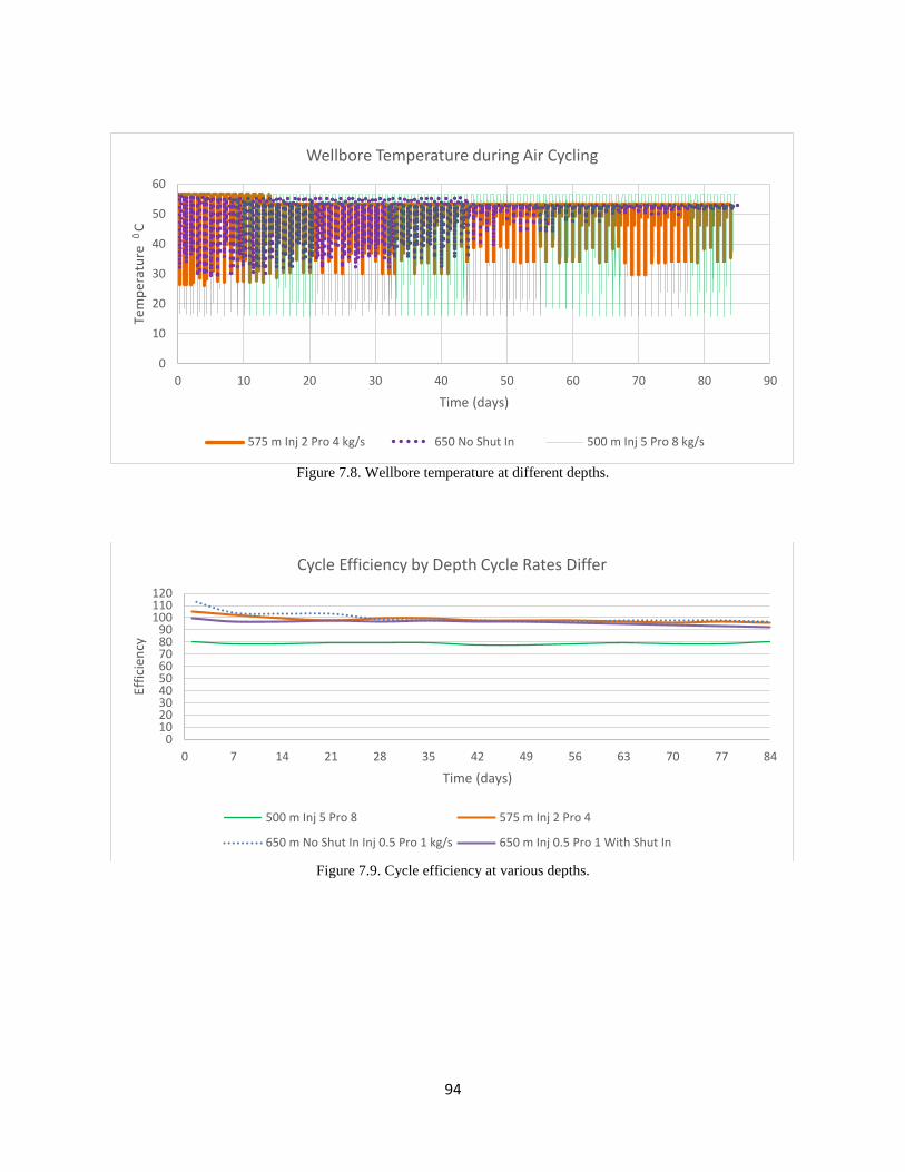
94
Figure 7.8. Wellbore temperature at different depths.
Figure 7.9. Cycle efficiency at various depths.
0
10
20
30
40
50
60
0 10 20 30 40 50 60 70 80 90
Tem
per
atu
re 0
C
Time (days)
Wellbore Temperature during Air Cycling
575 m Inj 2 Pro 4 kg/s 650 No Shut In 500 m Inj 5 Pro 8 kg/s
0102030405060708090
100110120
0 7 14 21 28 35 42 49 56 63 70 77 84
Effi
cien
cy
Time (days)
Cycle Efficiency by Depth Cycle Rates Differ
500 m Inj 5 Pro 8 575 m Inj 2 Pro 4
650 m No Shut In Inj 0.5 Pro 1 kg/s 650 m Inj 0.5 Pro 1 With Shut In
95
7.4 Effects of Permeability
In this section permeability was varied. In Scenario 5 (S5) the permeability was
reduced by a factor of 10 and in Scenario 6, (S6), it was increased by 10, as compared to
the base case. A single peak schedule was used where air was injected for 16 hours and
produced for 8 hours on a daily basis. Injection and production rates however were
changed to maintain the necessary pressure range of 46 to 66 bars in the aquifer at the top
of the wellbore. Cycling pressures for S5 and S6 are shown in figure 7.10.
For the lower permeability aquifer, injection and production rates used were 0.5
and 1 kg/s respectively. The higher permeability aquifer could sustain an air flow of 10
kg/s during production with injection rates of 5 kg/s. Although a lower permeability gives
an increase in cycle efficiency, the injection and extraction rates of 0.5 and 1.0 kg/s
respectively are too small to effectively store and recovery energy. The number of wells
needed would create forbidding costs. A higher permeability allowed for an increase in
recovery rates to 10 kg/s, while the aquifer maintained the necessary pressure, but there
was a decrease in cycle efficiency, as seen in figure 7.11. This decrease in efficiency was
a result of the increase in the mass of water produced during cycling. As presented in
figure 7.12, the mass fraction of air recovered with a permeability of 1x10-11 m2 reached
as low as 50%. Since the energy recovered is based on the mass of air produced, the
decrease in air mass directly impacts the efficiency of the cycle. Figure 7.13 shows the
volume fraction of air produced from which it can be seen that the water production by
volume is minor in each case.
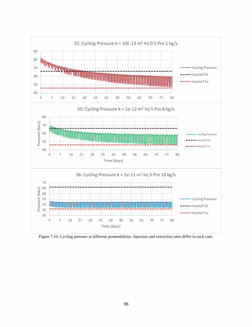
96
Figure 7.10. Cycling pressure at different permeabilities. Injection and extraction rates differ in each case.
40
50
60
70
80
90
0 7 14 21 28 35 42 49 56 63 70 77 84
S5: Cycling Pressure k = 10E-13 m2 Inj 0.5 Pro 1 kg/s
Cycling Pressure
Huntorf Hi
Huntorf Lo
40
50
60
70
80
0 7 14 21 28 35 42 49 56 63 70 77 84
Pre
ssu
re (
bar
s)
Time (days)
S0: Cycling Pressure k = 1e-12 m2 Inj 5 Pro 8 kg/s
Cycling Pressure
Huntorf Hi
Huntorf Lo
40
45
50
55
60
65
70
0 7 14 21 28 35 42 49 56 63 70 77 84
Pre
ssu
re (
bar
s)
Time (days)
S6: Cycling Pressure k = 1e-11 m2 Inj 5 Pro 10 kg/s
Cycling Pressure
Huntorf Hi
Huntorf Lo
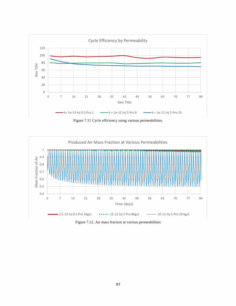
97
Figure 7.11 Cycle efficiency using various permeabilities.
Figure 7.12. Air mass fraction at various permeabilities
0
20
40
60
80
100
120
0 7 14 21 28 35 42 49 56 63 70 77 84
Axi
s Ti
tle
Axis Title
Cycle Efficiency by Permeability
k= 1e-13 Inj 0.5 Pro 1 k = 1e-12 Inj 5 Pro 8 k = 1e-11 Inj 5 Pro 10
0.4
0.5
0.6
0.7
0.8
0.9
1
0 7 14 21 28 35 42 49 56 63 70 77 84
Mas
s Fr
acti
on
of
Air
Time (days)
Produced Air Mass Fraction at Various Permeabilities
1.E-13 Inj 0.5 Pro 1kg/s 1E-12 Inj 5 Pro 8kg/s 1E-11 Inj 5 Pro 10 kg/s
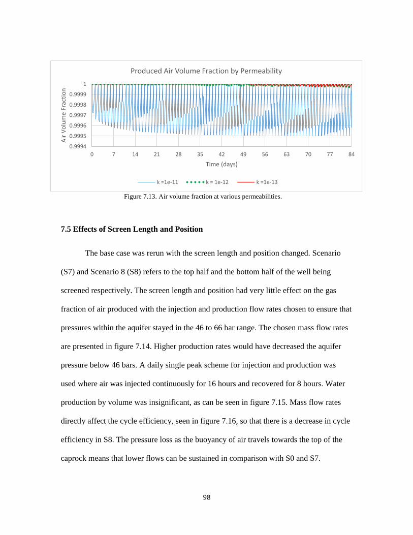
98
Figure 7.13. Air volume fraction at various permeabilities.
7.5 Effects of Screen Length and Position
The base case was rerun with the screen length and position changed. Scenario
(S7) and Scenario 8 (S8) refers to the top half and the bottom half of the well being
screened respectively. The screen length and position had very little effect on the gas
fraction of air produced with the injection and production flow rates chosen to ensure that
pressures within the aquifer stayed in the 46 to 66 bar range. The chosen mass flow rates
are presented in figure 7.14. Higher production rates would have decreased the aquifer
pressure below 46 bars. A daily single peak scheme for injection and production was
used where air was injected continuously for 16 hours and recovered for 8 hours. Water
production by volume was insignificant, as can be seen in figure 7.15. Mass flow rates
directly affect the cycle efficiency, seen in figure 7.16, so that there is a decrease in cycle
efficiency in S8. The pressure loss as the buoyancy of air travels towards the top of the
caprock means that lower flows can be sustained in comparison with S0 and S7.
0.9994
0.9995
0.9996
0.9997
0.9998
0.9999
1
0 7 14 21 28 35 42 49 56 63 70 77 84
Air
Vo
lum
e Fr
acti
on
Time (days)
Produced Air Volume Fraction by Permeability
k =1e-11 k = 1e-12 k =1e-13
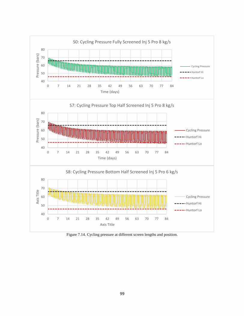
99
Figure 7.14. Cycling pressure at different screen lengths and position.
40
50
60
70
80
0 7 14 21 28 35 42 49 56 63 70 77 84
Pre
ssu
re (
bar
s)
Time (days)
S0: Cycling Pressure Fully Screened Inj 5 Pro 8 kg/s
Cycling Pressure
Huntorf Hi
Huntorf Lo
40
50
60
70
80
0 7 14 21 28 35 42 49 56 63 70 77 84
Pre
ssu
re (
bar
s)
Time (days)
S7: Cycling Pressure Top Half Screened Inj 5 Pro 8 kg/s
Cycling Pressure
Huntorf Hi
Huntorf Lo
40
50
60
70
80
0 7 14 21 28 35 42 49 56 63 70 77 84
Axi
s Ti
tle
Axis Title
S8: Cycling Pressure Bottom Half Screened Inj 5 Pro 6 kg/s
Cycling Pressure
Huntorf Hi
Huntorf Lo
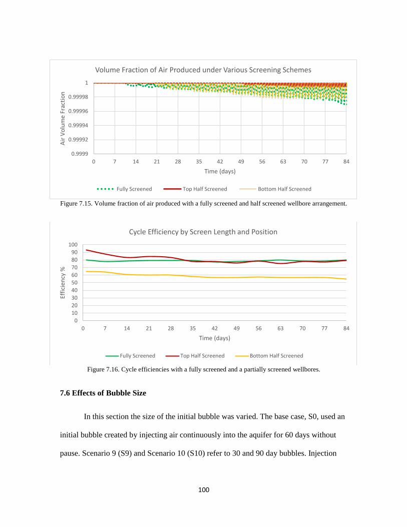
100
Figure 7.15. Volume fraction of air produced with a fully screened and half screened wellbore arrangement.
Figure 7.16. Cycle efficiencies with a fully screened and a partially screened wellbores.
7.6 Effects of Bubble Size
In this section the size of the initial bubble was varied. The base case, S0, used an
initial bubble created by injecting air continuously into the aquifer for 60 days without
pause. Scenario 9 (S9) and Scenario 10 (S10) refer to 30 and 90 day bubbles. Injection
0.9999
0.99992
0.99994
0.99996
0.99998
1
0 7 14 21 28 35 42 49 56 63 70 77 84
Air
Vo
lum
e Fr
acti
on
Time (days)
Volume Fraction of Air Produced under Various Screening Schemes
Fully Screened Top Half Screened Bottom Half Screened
0
10
20
30
40
50
60
70
80
90
100
0 7 14 21 28 35 42 49 56 63 70 77 84
Effi
cien
cy %
Time (days)
Cycle Efficiency by Screen Length and Position
Fully Screened Top Half Screened Bottom Half Screened
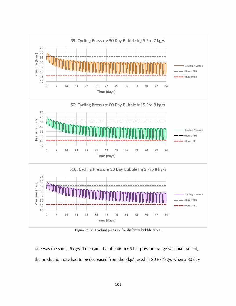
101
Figure 7.17. Cycling pressure for different bubble sizes.
rate was the same, 5kg/s. To ensure that the 46 to 66 bar pressure range was maintained,
the production rate had to be decreased from the 8kg/s used in S0 to 7kg/s when a 30 day
40
45
50
55
60
65
70
75
0 7 14 21 28 35 42 49 56 63 70 77 84
Pre
ssu
re (
bar
s)
Time (days)
S9: Cycling Pressure 30 Day Bubble Inj 5 Pro 7 kg/s
Cycling Pressure
Huntorf Hi
Huntorf Lo
40
45
50
55
60
65
70
75
0 7 14 21 28 35 42 49 56 63 70 77 84
Pre
ssu
re (
bar
s)
Time (days)
S0: Cycling Pressure 60 Day Bubble Inj 5 Pro 8 kg/s
Cycling Pressure
Huntorf Hi
Huntorf Lo
40
45
50
55
60
65
70
75
0 7 14 21 28 35 42 49 56 63 70 77 84
Pre
ssu
re (
bar
s)
Time (days)
S10: Cycling Pressure 90 Day Bubble Inj 5 Pro 8 kg/s
Cycling Pressure
Huntorf Hi
Huntorf Lo
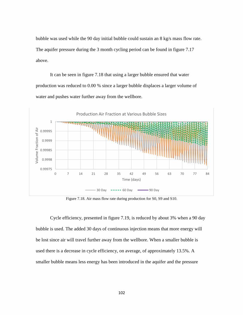
102
bubble was used while the 90 day initial bubble could sustain an 8 kg/s mass flow rate.
The aquifer pressure during the 3 month cycling period can be found in figure 7.17
above.
It can be seen in figure 7.18 that using a larger bubble ensured that water
production was reduced to 0.00 % since a larger bubble displaces a larger volume of
water and pushes water further away from the wellbore.
Figure 7.18. Air mass flow rate during production for S0, S9 and S10.
Cycle efficiency, presented in figure 7.19, is reduced by about 3% when a 90 day
bubble is used. The added 30 days of continuous injection means that more energy will
be lost since air will travel further away from the wellbore. When a smaller bubble is
used there is a decrease in cycle efficiency, on average, of approximately 13.5%. A
smaller bubble means less energy has been introduced in the aquifer and the pressure
0.99975
0.9998
0.99985
0.9999
0.99995
1
0 7 14 21 28 35 42 49 56 63 70 77 84
Vo
lum
e Fr
acti
on
of
Air
Time (days)
Production Air Fraction at Various Bubble Sizes
30 Day 60 Day 90 Day
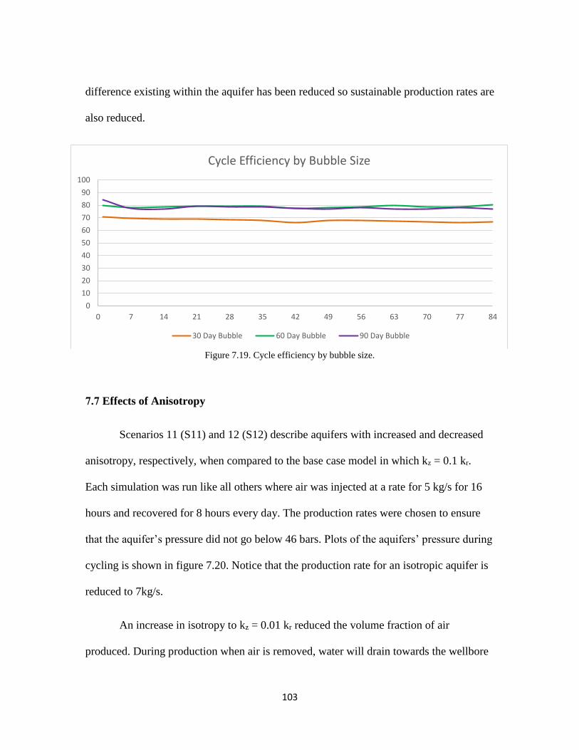
103
difference existing within the aquifer has been reduced so sustainable production rates are
also reduced.
Figure 7.19. Cycle efficiency by bubble size.
7.7 Effects of Anisotropy
Scenarios 11 (S11) and 12 (S12) describe aquifers with increased and decreased
anisotropy, respectively, when compared to the base case model in which kz = 0.1 kr.
Each simulation was run like all others where air was injected at a rate for 5 kg/s for 16
hours and recovered for 8 hours every day. The production rates were chosen to ensure
that the aquifer’s pressure did not go below 46 bars. Plots of the aquifers’ pressure during
cycling is shown in figure 7.20. Notice that the production rate for an isotropic aquifer is
reduced to 7kg/s.
An increase in isotropy to kz = 0.01 kr reduced the volume fraction of air
produced. During production when air is removed, water will drain towards the wellbore
0
10
20
30
40
50
60
70
80
90
100
0 7 14 21 28 35 42 49 56 63 70 77 84
Cycle Efficiency by Bubble Size
30 Day Bubble 60 Day Bubble 90 Day Bubble
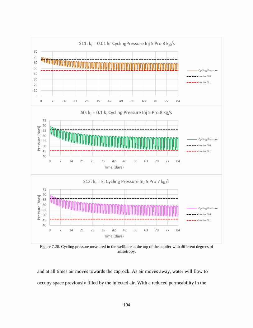
104
Figure 7.20. Cycling pressure measured in the wellbore at the top of the aquifer with different degrees of
anisotropy.
and at all times air moves towards the caprock. As air moves away, water will flow to
occupy space previously filled by the injected air. With a reduced permeability in the
0
10
20
30
40
50
60
70
80
0 7 14 21 28 35 42 49 56 63 70 77 84
S11: kz = 0.01 kr CyclingPressure Inj 5 Pro 8 kg/s
Cycling Pressure
Huntorf Hi
Huntorf Lo
40
45
50
55
60
65
70
75
0 7 14 21 28 35 42 49 56 63 70 77 84
Pre
ssu
re (
bar
s)
Time (days)
S0: kz = 0.1 kr Cycling Pressure Inj 5 Pro 8 kg/s
Cycling Pressure
Huntorf Hi
Huntorf Lo
40
45
50
55
60
65
70
75
0 7 14 21 28 35 42 49 56 63 70 77 84
Pre
ssu
re (
bar
s)
Time (days)
S12: kz = kr Cycling Pressure Inj 5 Pro 7 kg/s
Cycling Pressure
Huntorf Hi
Huntorf Lo
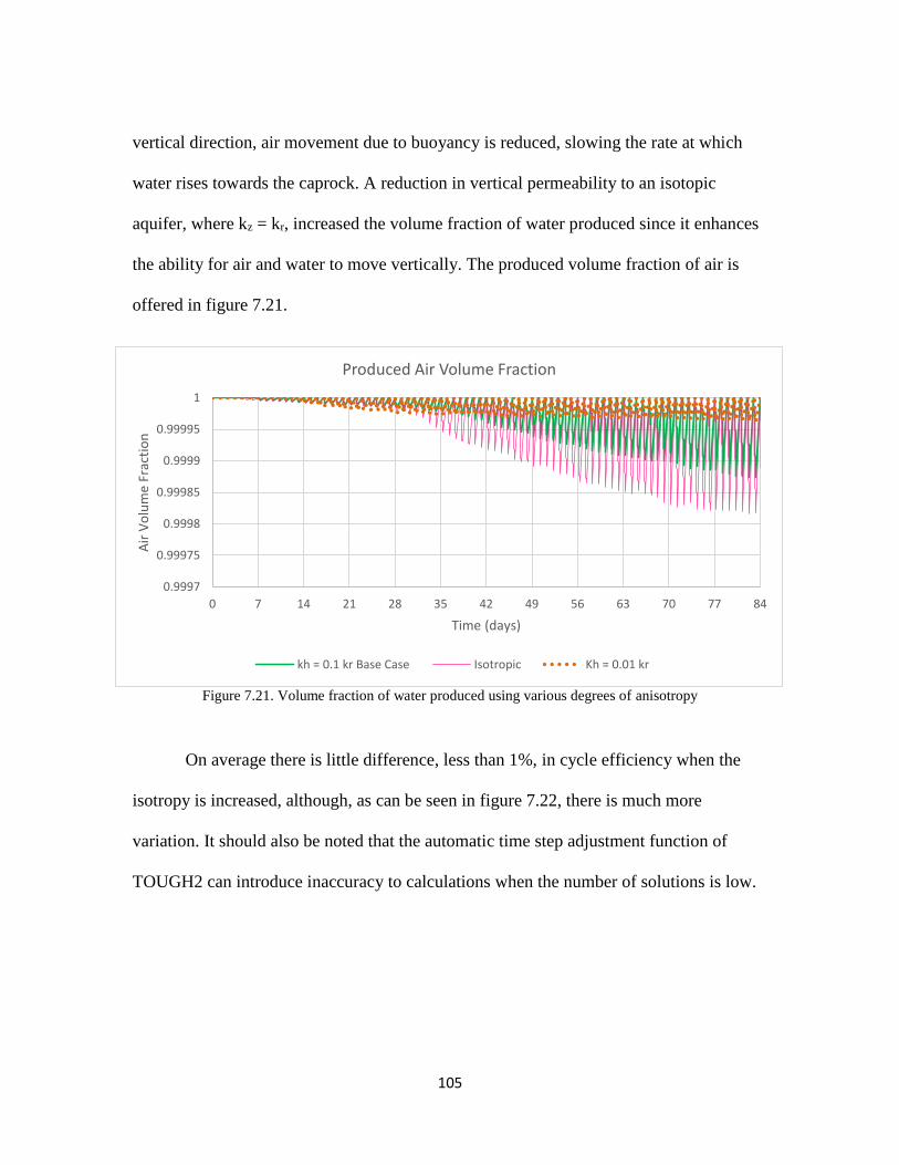
105
vertical direction, air movement due to buoyancy is reduced, slowing the rate at which
water rises towards the caprock. A reduction in vertical permeability to an isotopic
aquifer, where kz = kr, increased the volume fraction of water produced since it enhances
the ability for air and water to move vertically. The produced volume fraction of air is
offered in figure 7.21.
Figure 7.21. Volume fraction of water produced using various degrees of anisotropy
On average there is little difference, less than 1%, in cycle efficiency when the
isotropy is increased, although, as can be seen in figure 7.22, there is much more
variation. It should also be noted that the automatic time step adjustment function of
TOUGH2 can introduce inaccuracy to calculations when the number of solutions is low.
0.9997
0.99975
0.9998
0.99985
0.9999
0.99995
1
0 7 14 21 28 35 42 49 56 63 70 77 84
Air
Vo
lum
e Fr
acti
on
Time (days)
Produced Air Volume Fraction
kh = 0.1 kr Base Case Isotropic Kh = 0.01 kr
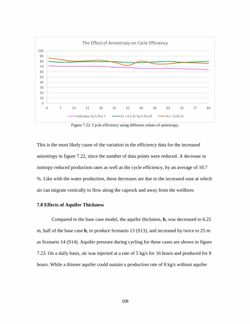
106
Figure 7.22. Cycle efficiency using different values of anisotropy.
This is the most likely cause of the variation in the efficiency data for the increased
anisotropy in figure 7.22, since the number of data points were reduced. A decrease in
isotropy reduced production rates as well as the cycle efficiency, by an average of 10.7
%. Like with the water production, these decreases are due to the increased ease at which
air can migrate vertically to flow along the caprock and away from the wellbore.
7.8 Effects of Aquifer Thickness
Compared to the base case model, the aquifer thickness, b, was decreased to 6.25
m, half of the base case b, to produce Scenario 13 (S13), and increased by twice to 25 m
as Scenario 14 (S14). Aquifer pressure during cycling for these cases are shown in figure
7.23. On a daily basis, air was injected at a rate of 5 kg/s for 16 hours and produced for 8
hours. While a thinner aquifer could sustain a production rate of 8 kg/s without aquifer
0
10
20
30
40
50
60
70
80
90
100
0 7 14 21 28 35 42 49 56 63 70 77 84
The Effect of Anisotropy on Cycle Efficiency
Isotropic Inj 5 Pro 7 kz = 0.1 kr Inj 5 Pro 8 kz = 0.01 kr
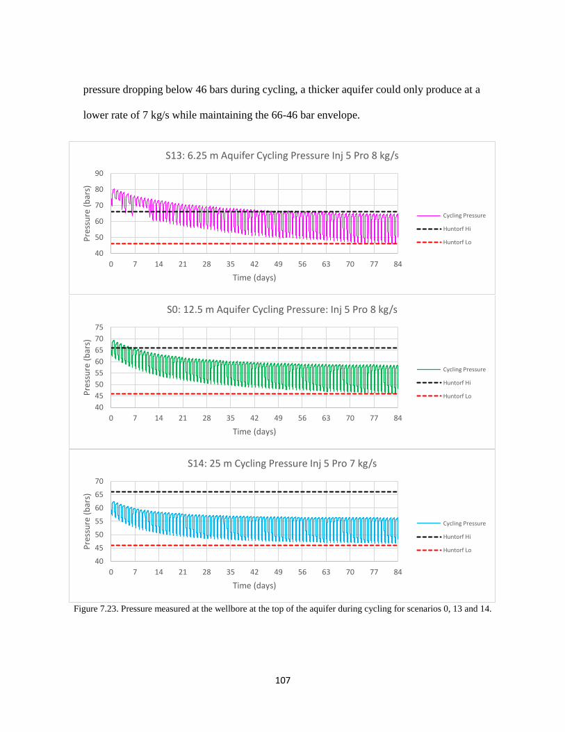
107
pressure dropping below 46 bars during cycling, a thicker aquifer could only produce at a
lower rate of 7 kg/s while maintaining the 66-46 bar envelope.
Figure 7.23. Pressure measured at the wellbore at the top of the aquifer during cycling for scenarios 0, 13 and 14.
40
50
60
70
80
90
0 7 14 21 28 35 42 49 56 63 70 77 84
Pre
ssu
re (
bar
s)
Time (days)
S13: 6.25 m Aquifer Cycling Pressure Inj 5 Pro 8 kg/s
Cycling Pressure
Huntorf Hi
Huntorf Lo
40
45
50
55
60
65
70
75
0 7 14 21 28 35 42 49 56 63 70 77 84
Pre
ssu
re (
bar
s)
Time (days)
S0: 12.5 m Aquifer Cycling Pressure: Inj 5 Pro 8 kg/s
Cycling Pressure
Huntorf Hi
Huntorf Lo
40
45
50
55
60
65
70
0 7 14 21 28 35 42 49 56 63 70 77 84
Pre
ssu
re (
bar
s)
Time (days)
S14: 25 m Cycling Pressure Inj 5 Pro 7 kg/s
Cycling Pressure
Huntorf Hi
Huntorf Lo
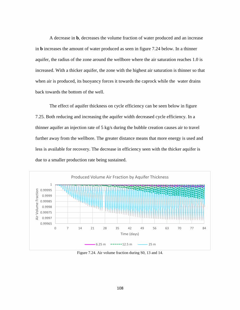
108
A decrease in b, decreases the volume fraction of water produced and an increase
in b increases the amount of water produced as seen in figure 7.24 below. In a thinner
aquifer, the radius of the zone around the wellbore where the air saturation reaches 1.0 is
increased. With a thicker aquifer, the zone with the highest air saturation is thinner so that
when air is produced, its buoyancy forces it towards the caprock while the water drains
back towards the bottom of the well.
The effect of aquifer thickness on cycle efficiency can be seen below in figure
7.25. Both reducing and increasing the aquifer width decreased cycle efficiency. In a
thinner aquifer an injection rate of 5 kg/s during the bubble creation causes air to travel
further away from the wellbore. The greater distance means that more energy is used and
less is available for recovery. The decrease in efficiency seen with the thicker aquifer is
due to a smaller production rate being sustained.
Figure 7.24. Air volume fraction during S0, 13 and 14.
0.99965
0.9997
0.99975
0.9998
0.99985
0.9999
0.99995
1
0 7 14 21 28 35 42 49 56 63 70 77 84
Air
Vo
lum
e Fr
acti
on
Time (days)
Produced Volume Air Fraction by Aquifer Thickness
6.25 m 12.5 m 25 m
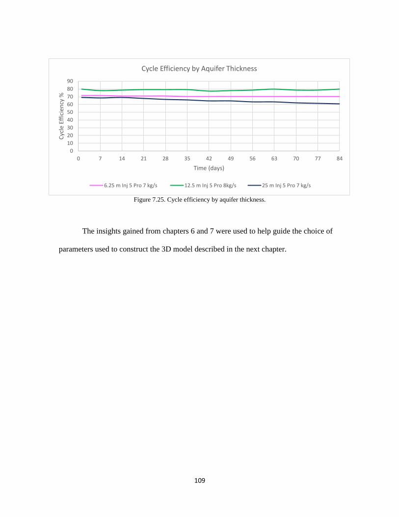
109
Figure 7.25. Cycle efficiency by aquifer thickness.
The insights gained from chapters 6 and 7 were used to help guide the choice of
parameters used to construct the 3D model described in the next chapter.
0
10
20
30
40
50
60
70
80
90
0 7 14 21 28 35 42 49 56 63 70 77 84
Cyc
le E
ffic
ien
cy %
Time (days)
Cycle Efficiency by Aquifer Thickness
6.25 m Inj 5 Pro 7 kg/s 12.5 m Inj 5 Pro 8kg/s 25 m Inj 5 Pro 7 kg/s
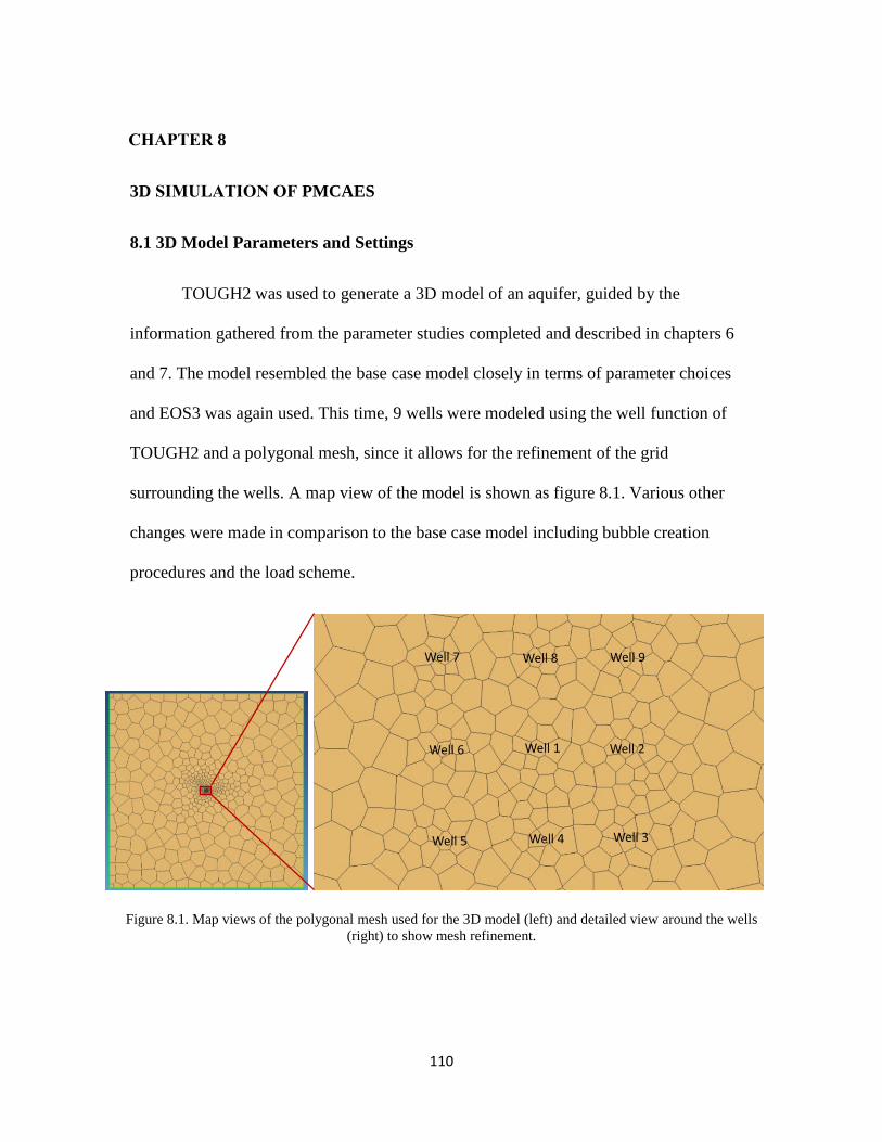
110
CHAPTER 8
3D SIMULATION OF PMCAES
8.1 3D Model Parameters and Settings
TOUGH2 was used to generate a 3D model of an aquifer, guided by the
information gathered from the parameter studies completed and described in chapters 6
and 7. The model resembled the base case model closely in terms of parameter choices
and EOS3 was again used. This time, 9 wells were modeled using the well function of
TOUGH2 and a polygonal mesh, since it allows for the refinement of the grid
surrounding the wells. A map view of the model is shown as figure 8.1. Various other
changes were made in comparison to the base case model including bubble creation
procedures and the load scheme.
Figure 8.1. Map views of the polygonal mesh used for the 3D model (left) and detailed view around the wells
(right) to show mesh refinement.

111
The model is 3000 m in length, 3000 m in width, 550-m-thick and comprises a
flat-lying, fully confined 12.5 m thick sand storage aquifer set between a 50 m thick
caprock and a 37.5 m lower confining layer. Both the caprock and the underlying layers
are made of clay as is the 450 m overburden layer. A large size is used to minimize or
eliminate errors incurred on the numerical solutions by boundary effects. Model
dimensions and initial conditions are listed in table 8.1 below.
Table 8.1: PM-CAES 3D model dimensions, initial conditions and comments
Model Dimensions
Length (y)
Width (x)
3000 m
3000 m
Large enough to eliminate any boundary effects on numerical
solutions
A constant potential condition is applied to the outermost
boundaries.
Depth (Z) 550 m The model top coincides with the ground surface and the
base is located at 550 m depth.
The storage reservoir is 12.5 m thick and capped by 500 m of
impermeable rock and underlain by a 37.5 m impermeable
stratum.
Length of Wells 512.5 m The well is screened in the entire12.5 m thickness of the
storage reservoir and the well head is located at ground
surface.
Initial Conditions
Temperature Gradient of 300C/km A typical geothermal gradient (Blackwell et al., 1991) was
applied. Surface temperature was set as ambient (20 0C)
making the temperature at the base of the model
approximately 36.5 0C
Pressure Atmospheric
Hydrostatic pressure at
depth
Ground surface pressure was assumed to be 101325 Pa and
subsurface pressures were assumed to follow a hydrostatic
gradient of 9.81 x 10³ Pa/m. Pressure at model bottom was
approximately 5.4 x 10⁶ Pa.
The aquifer has a kxy permeability of 1 x 10-12 m2 and a vertical permeability (kz)
of 1.0 x 10 -13 m2, a porosity (φ) of 0.2 and a residual water saturation (Srw) of 0.27. The
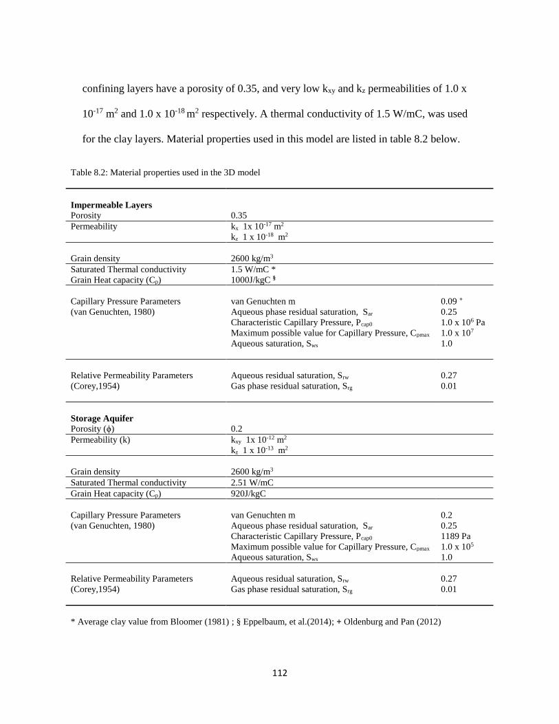
112
confining layers have a porosity of 0.35, and very low kxy and kz permeabilities of 1.0 x
10-17 m2 and 1.0 x 10⁻¹⁸ m2 respectively. A thermal conductivity of 1.5 W/mC, was used
for the clay layers. Material properties used in this model are listed in table 8.2 below.
Table 8.2: Material properties used in the 3D model
Impermeable Layers
Porosity 0.35
Permeability kx 1x 10-17 m2
kz 1 x 10-18 m2
Grain density 2600 kg/m3
Saturated Thermal conductivity 1.5 W/mC *
Grain Heat capacity (Cp) 1000J/kgC §
Capillary Pressure Parameters
(van Genuchten, 1980)
van Genuchten m 0.09 +
Aqueous phase residual saturation, Sar 0.25
Characteristic Capillary Pressure, Pcap0 1.0 x 10⁶ Pa
Maximum possible value for Capillary Pressure, Cpmax 1.0 x 10⁷
Aqueous saturation, Sws 1.0
Relative Permeability Parameters
(Corey,1954)
Aqueous residual saturation, Srw 0.27
Gas phase residual saturation, Srg 0.01
Storage Aquifer
Porosity (ϕ) 0.2
Permeability (k) kxy 1x 10-12 m2
kz 1 x 10-13 m2
Grain density 2600 kg/m3
Saturated Thermal conductivity 2.51 W/mC
Grain Heat capacity (Cp) 920J/kgC
Capillary Pressure Parameters
(van Genuchten, 1980)
van Genuchten m 0.2
Aqueous phase residual saturation, Sar 0.25
Characteristic Capillary Pressure, Pcap0 1189 Pa
Maximum possible value for Capillary Pressure, Cpmax 1.0 x 10⁵
Aqueous saturation, Sws 1.0
Relative Permeability Parameters
(Corey,1954)
Aqueous residual saturation, Srw 0.27
Gas phase residual saturation, Srg 0.01
* Average clay value from Bloomer (1981) ; § Eppelbaum, et al.(2014); + Oldenburg and Pan (2012)
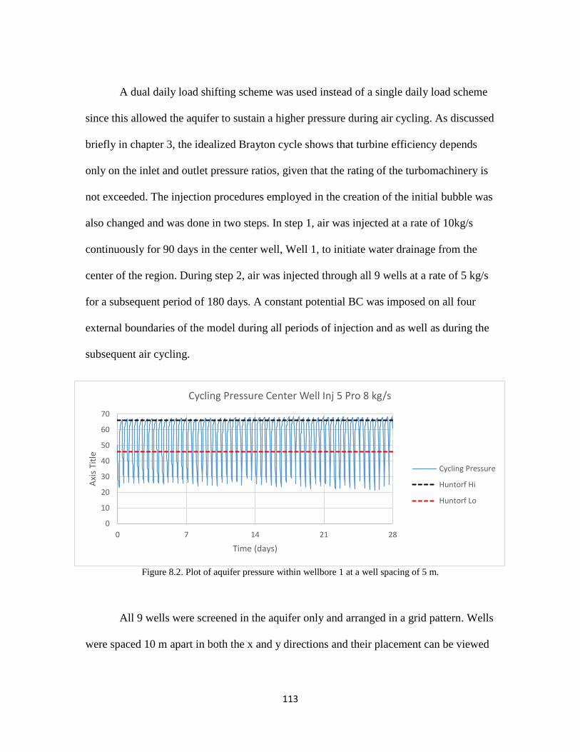
113
A dual daily load shifting scheme was used instead of a single daily load scheme
since this allowed the aquifer to sustain a higher pressure during air cycling. As discussed
briefly in chapter 3, the idealized Brayton cycle shows that turbine efficiency depends
only on the inlet and outlet pressure ratios, given that the rating of the turbomachinery is
not exceeded. The injection procedures employed in the creation of the initial bubble was
also changed and was done in two steps. In step 1, air was injected at a rate of 10kg/s
continuously for 90 days in the center well, Well 1, to initiate water drainage from the
center of the region. During step 2, air was injected through all 9 wells at a rate of 5 kg/s
for a subsequent period of 180 days. A constant potential BC was imposed on all four
external boundaries of the model during all periods of injection and as well as during the
subsequent air cycling.
Figure 8.2. Plot of aquifer pressure within wellbore 1 at a well spacing of 5 m.
All 9 wells were screened in the aquifer only and arranged in a grid pattern. Wells
were spaced 10 m apart in both the x and y directions and their placement can be viewed
0
10
20
30
40
50
60
70
0 7 14 21 28
Axi
s Ti
tle
Time (days)
Cycling Pressure Center Well Inj 5 Pro 8 kg/s
Cycling Pressure
Huntorf Hi
Huntorf Lo
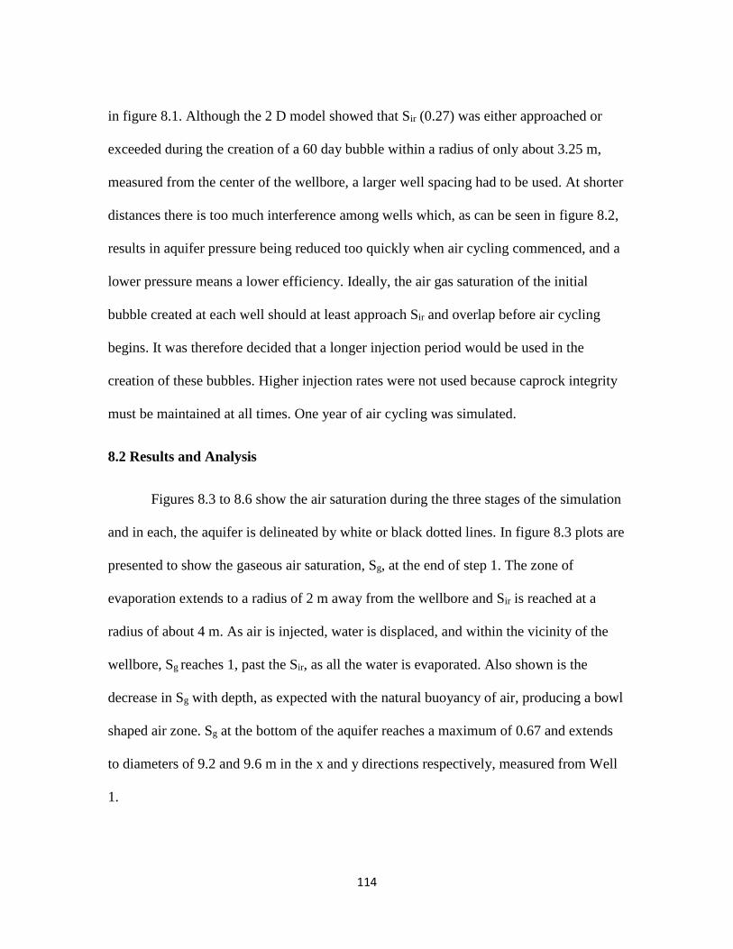
114
in figure 8.1. Although the 2 D model showed that Sir (0.27) was either approached or
exceeded during the creation of a 60 day bubble within a radius of only about 3.25 m,
measured from the center of the wellbore, a larger well spacing had to be used. At shorter
distances there is too much interference among wells which, as can be seen in figure 8.2,
results in aquifer pressure being reduced too quickly when air cycling commenced, and a
lower pressure means a lower efficiency. Ideally, the air gas saturation of the initial
bubble created at each well should at least approach Sir and overlap before air cycling
begins. It was therefore decided that a longer injection period would be used in the
creation of these bubbles. Higher injection rates were not used because caprock integrity
must be maintained at all times. One year of air cycling was simulated.
8.2 Results and Analysis
Figures 8.3 to 8.6 show the air saturation during the three stages of the simulation
and in each, the aquifer is delineated by white or black dotted lines. In figure 8.3 plots are
presented to show the gaseous air saturation, Sg, at the end of step 1. The zone of
evaporation extends to a radius of 2 m away from the wellbore and Sir is reached at a
radius of about 4 m. As air is injected, water is displaced, and within the vicinity of the
wellbore, Sg reaches 1, past the Sir, as all the water is evaporated. Also shown is the
decrease in Sg with depth, as expected with the natural buoyancy of air, producing a bowl
shaped air zone. Sg at the bottom of the aquifer reaches a maximum of 0.67 and extends
to diameters of 9.2 and 9.6 m in the x and y directions respectively, measured from Well
1.
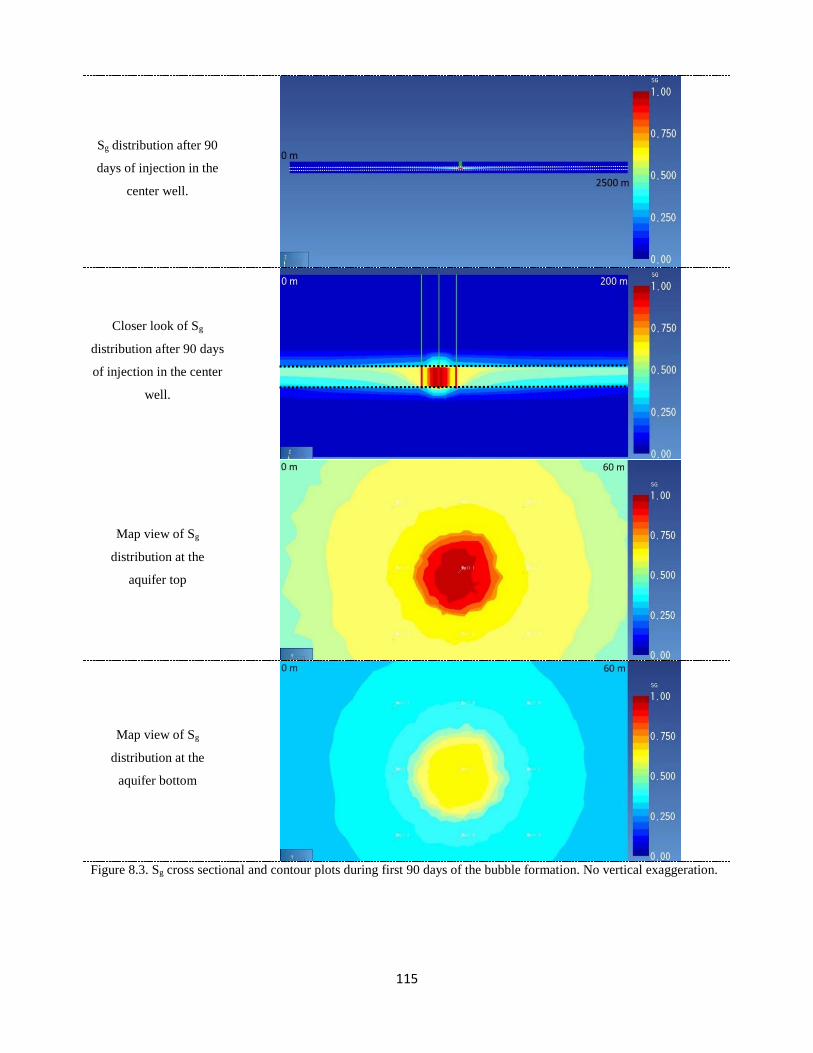
115
Sg distribution after 90
days of injection in the
center well.
Closer look of Sg
distribution after 90 days
of injection in the center
well.
Map view of Sg
distribution at the
aquifer top
Map view of Sg
distribution at the
aquifer bottom
Figure 8.3. Sg cross sectional and contour plots during first 90 days of the bubble formation. No vertical exaggeration.
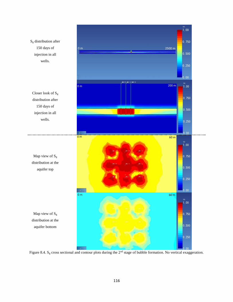
116
Sg distribution after
150 days of
injection in all
wells.
Closer look of Sg
distribution after
150 days of
injection in all
wells.
Map view of Sg
distribution at the
aquifer top
Map view of Sg
distribution at the
aquifer bottom
Figure 8.4. Sg cross sectional and contour plots during the 2nd stage of bubble formation. No vertical exaggeration.
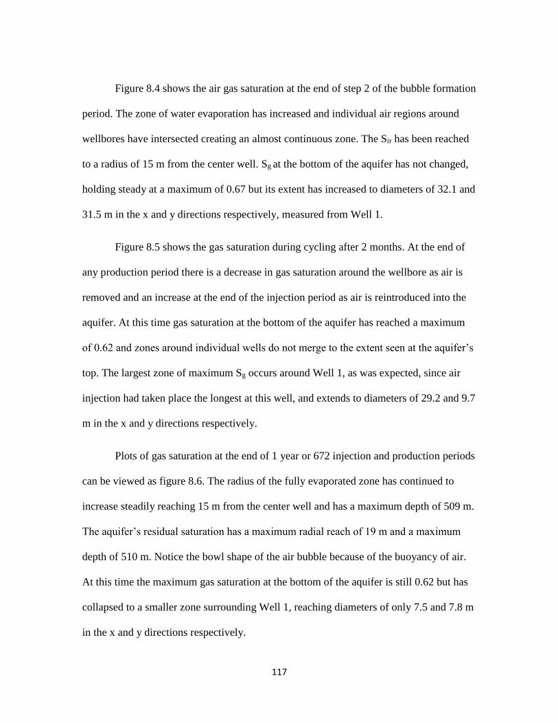
117
Figure 8.4 shows the air gas saturation at the end of step 2 of the bubble formation
period. The zone of water evaporation has increased and individual air regions around
wellbores have intersected creating an almost continuous zone. The Sir has been reached
to a radius of 15 m from the center well. Sg at the bottom of the aquifer has not changed,
holding steady at a maximum of 0.67 but its extent has increased to diameters of 32.1 and
31.5 m in the x and y directions respectively, measured from Well 1.
Figure 8.5 shows the gas saturation during cycling after 2 months. At the end of
any production period there is a decrease in gas saturation around the wellbore as air is
removed and an increase at the end of the injection period as air is reintroduced into the
aquifer. At this time gas saturation at the bottom of the aquifer has reached a maximum
of 0.62 and zones around individual wells do not merge to the extent seen at the aquifer’s
top. The largest zone of maximum Sg occurs around Well 1, as was expected, since air
injection had taken place the longest at this well, and extends to diameters of 29.2 and 9.7
m in the x and y directions respectively.
Plots of gas saturation at the end of 1 year or 672 injection and production periods
can be viewed as figure 8.6. The radius of the fully evaporated zone has continued to
increase steadily reaching 15 m from the center well and has a maximum depth of 509 m.
The aquifer’s residual saturation has a maximum radial reach of 19 m and a maximum
depth of 510 m. Notice the bowl shape of the air bubble because of the buoyancy of air.
At this time the maximum gas saturation at the bottom of the aquifer is still 0.62 but has
collapsed to a smaller zone surrounding Well 1, reaching diameters of only 7.5 and 7.8 m
in the x and y directions respectively.
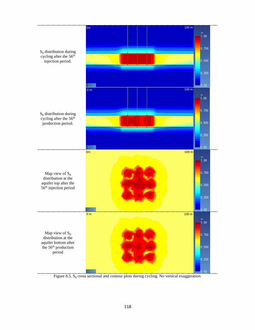
118
Sg distribution during
cycling after the 56th
injection period.
Sg distribution during
cycling after the 56th
production period.
Map view of Sg
distribution at the
aquifer top after the
56th injection period
Map view of Sg
distribution at the
aquifer bottom after
the 56th production
period
Figure 8.5. Sg cross sectional and contour plots during cycling. No vertical exaggeration.
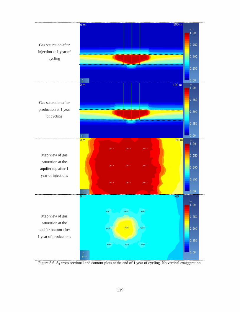
119
Gas saturation after
injection at 1 year of
cycling
Gas saturation after
production at 1 year
of cycling
Map view of gas
saturation at the
aquifer top after 1
year of injections
Map view of gas
saturation at the
aquifer bottom after
1 year of productions
Figure 8.6. Sg cross sectional and contour plots at the end of 1 year of cycling. No vertical exaggeration.
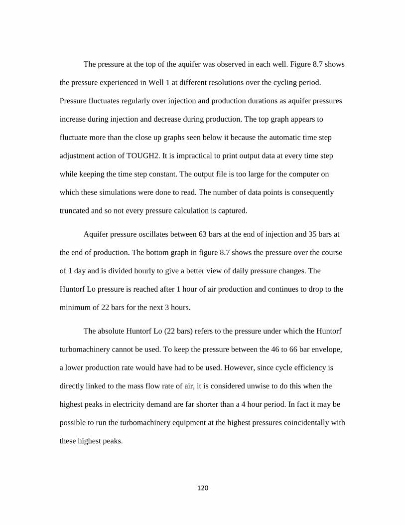
120
The pressure at the top of the aquifer was observed in each well. Figure 8.7 shows
the pressure experienced in Well 1 at different resolutions over the cycling period.
Pressure fluctuates regularly over injection and production durations as aquifer pressures
increase during injection and decrease during production. The top graph appears to
fluctuate more than the close up graphs seen below it because the automatic time step
adjustment action of TOUGH2. It is impractical to print output data at every time step
while keeping the time step constant. The output file is too large for the computer on
which these simulations were done to read. The number of data points is consequently
truncated and so not every pressure calculation is captured.
Aquifer pressure oscillates between 63 bars at the end of injection and 35 bars at
the end of production. The bottom graph in figure 8.7 shows the pressure over the course
of 1 day and is divided hourly to give a better view of daily pressure changes. The
Huntorf Lo pressure is reached after 1 hour of air production and continues to drop to the
minimum of 22 bars for the next 3 hours.
The absolute Huntorf Lo (22 bars) refers to the pressure under which the Huntorf
turbomachinery cannot be used. To keep the pressure between the 46 to 66 bar envelope,
a lower production rate would have had to be used. However, since cycle efficiency is
directly linked to the mass flow rate of air, it is considered unwise to do this when the
highest peaks in electricity demand are far shorter than a 4 hour period. In fact it may be
possible to run the turbomachinery equipment at the highest pressures coincidentally with
these highest peaks.
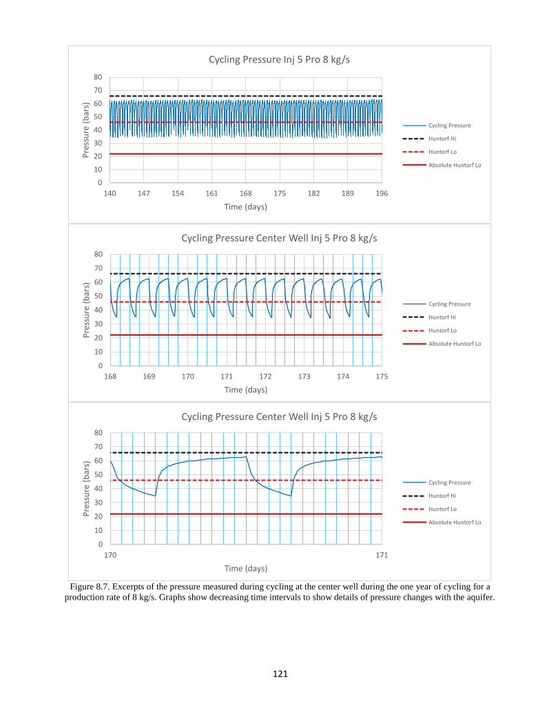
121
Figure 8.7. Excerpts of the pressure measured during cycling at the center well during the one year of cycling for a
production rate of 8 kg/s. Graphs show decreasing time intervals to show details of pressure changes with the aquifer.
0
10
20
30
40
50
60
70
80
140 147 154 161 168 175 182 189 196
Pre
ssu
re (
bar
s)
Time (days)
Cycling Pressure Inj 5 Pro 8 kg/s
Cycling Pressure
Huntorf Hi
Huntorf Lo
Absolute Huntorf Lo
0
10
20
30
40
50
60
70
80
168 169 170 171 172 173 174 175
Pre
ssu
re (
bar
s)
Time (days)
Cycling Pressure Center Well Inj 5 Pro 8 kg/s
Cycling Pressure
Huntorf Hi
Huntorf Lo
Absolute Huntorf Lo
0
10
20
30
40
50
60
70
80
170 171
Pre
ssu
re (
bar
s)
Time (days)
Cycling Pressure Center Well Inj 5 Pro 8 kg/s
Cycling Pressure
Huntorf Hi
Huntorf Lo
Absolute Huntorf Lo
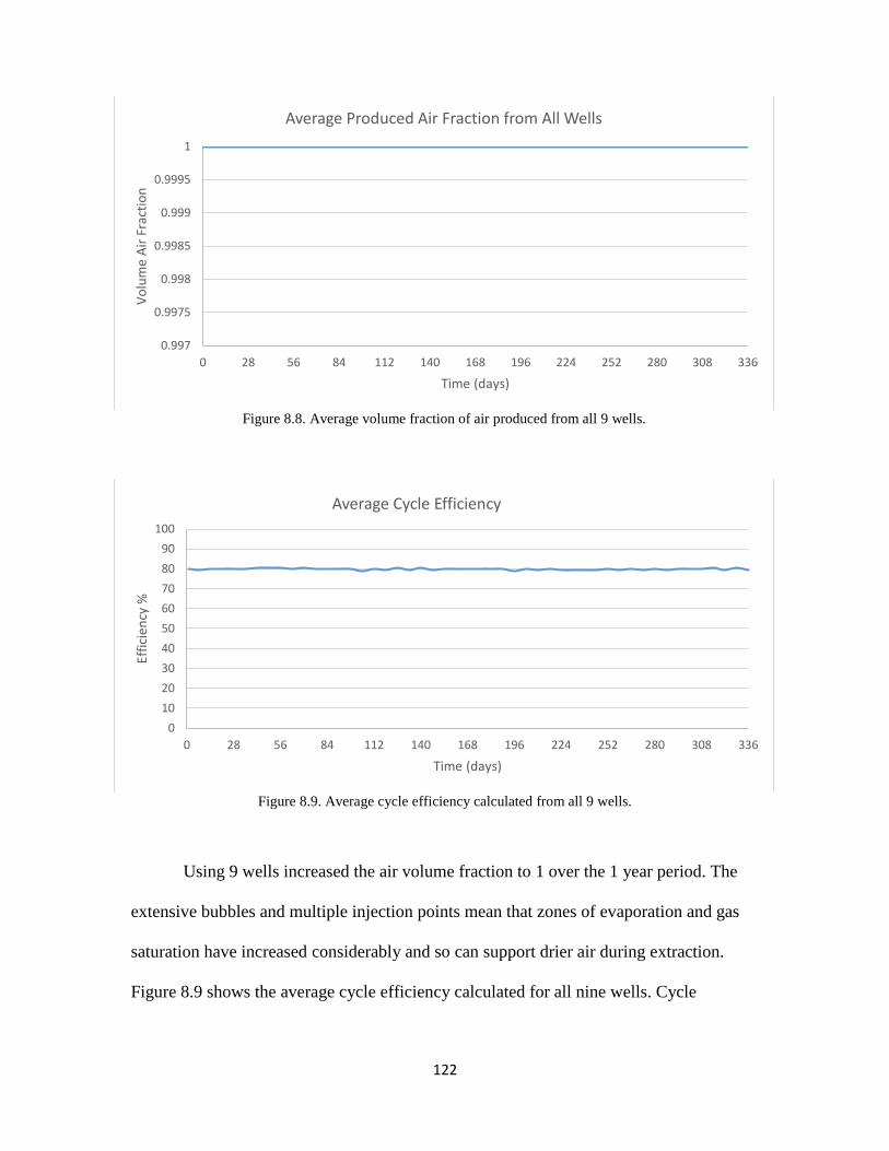
122
Figure 8.9. Average cycle efficiency calculated from all 9 wells.
Using 9 wells increased the air volume fraction to 1 over the 1 year period. The
extensive bubbles and multiple injection points mean that zones of evaporation and gas
saturation have increased considerably and so can support drier air during extraction.
Figure 8.9 shows the average cycle efficiency calculated for all nine wells. Cycle
0
10
20
30
40
50
60
70
80
90
100
0 28 56 84 112 140 168 196 224 252 280 308 336
Effi
cien
cy %
Time (days)
Average Cycle Efficiency
Figure 8.8. Average volume fraction of air produced from all 9 wells.
0.997
0.9975
0.998
0.9985
0.999
0.9995
1
0 28 56 84 112 140 168 196 224 252 280 308 336
Vo
lum
e A
ir F
ract
ion
Time (days)
Average Produced Air Fraction from All Wells
123
efficiency is at an average of 79.8%. This is slightly higher than the average efficiency
calculated by the Scenario 1 (2 D dual cycle, no shut in period), average efficiency of
79.1 %.
8.3 An Attempt to Recover 100% of the Injected Energy
Another 3D simulation using the same aquifer and aquifer parameters was run in
the attempt to maximize the amount of energy recovered. All settings described above
were kept the same, but the production rate was increased to 10 kg/s in each well instead
of using 8 kg/s. The 2 step bubble formation procedure was also maintained and during
cycling for 1 year, air was injected into all 9 wells at a rate of 5 kg/s on a daily schedule
of 16 hours and recovered for 8 hours.
Figure 8.10 shows cross sectional and contour plots of the aquifer after 1 year of
air cycling. At the end of 1 year, the maximum gas saturation of 1.00 at the top of the
aquifer extended to a diameter of 23.8 and 21.8 m in the x and y directions respectively
and the Sir covered a diameter of 38.3 and 38.7 m in the x and y directions respectively.
The maximum saturation at the bottom of the aquifer is the same as when a production
rate of 8 kg/s was used, 0.62, but it has a much smaller diameter of 0.15 and 0.27 m in the
x and y directions. A higher extraction rate removes a larger volume of air per daily cycle
and decreased the size of the air zone considerably.
A higher production rate reduces the aquifer pressure during cycling below the 22
bars needed to ensure that the turbomachinery patterned after that of Huntorf is able to
work. Although the recovery efficiency is increased to almost 100 %, as can be seen in
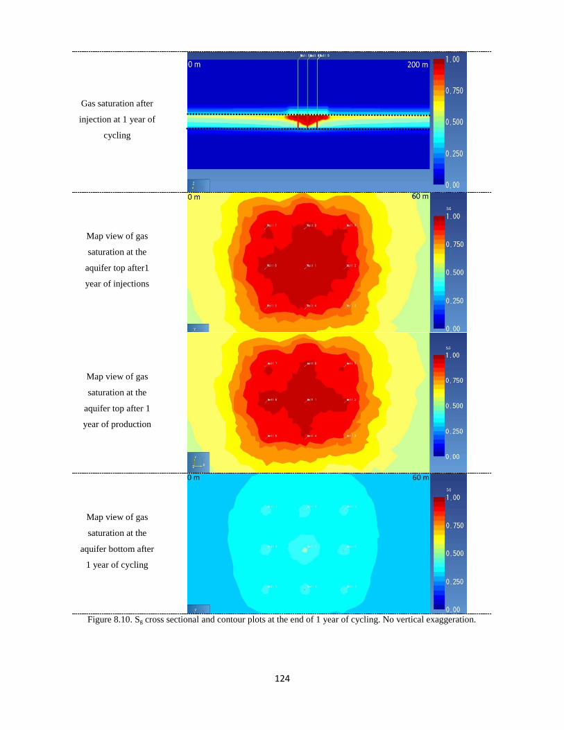
124
Gas saturation after
injection at 1 year of
cycling
Map view of gas
saturation at the
aquifer top after1
year of injections
Map view of gas
saturation at the
aquifer top after 1
year of production
Map view of gas
saturation at the
aquifer bottom after
1 year of cycling
Figure 8.10. Sg cross sectional and contour plots at the end of 1 year of cycling. No vertical exaggeration.
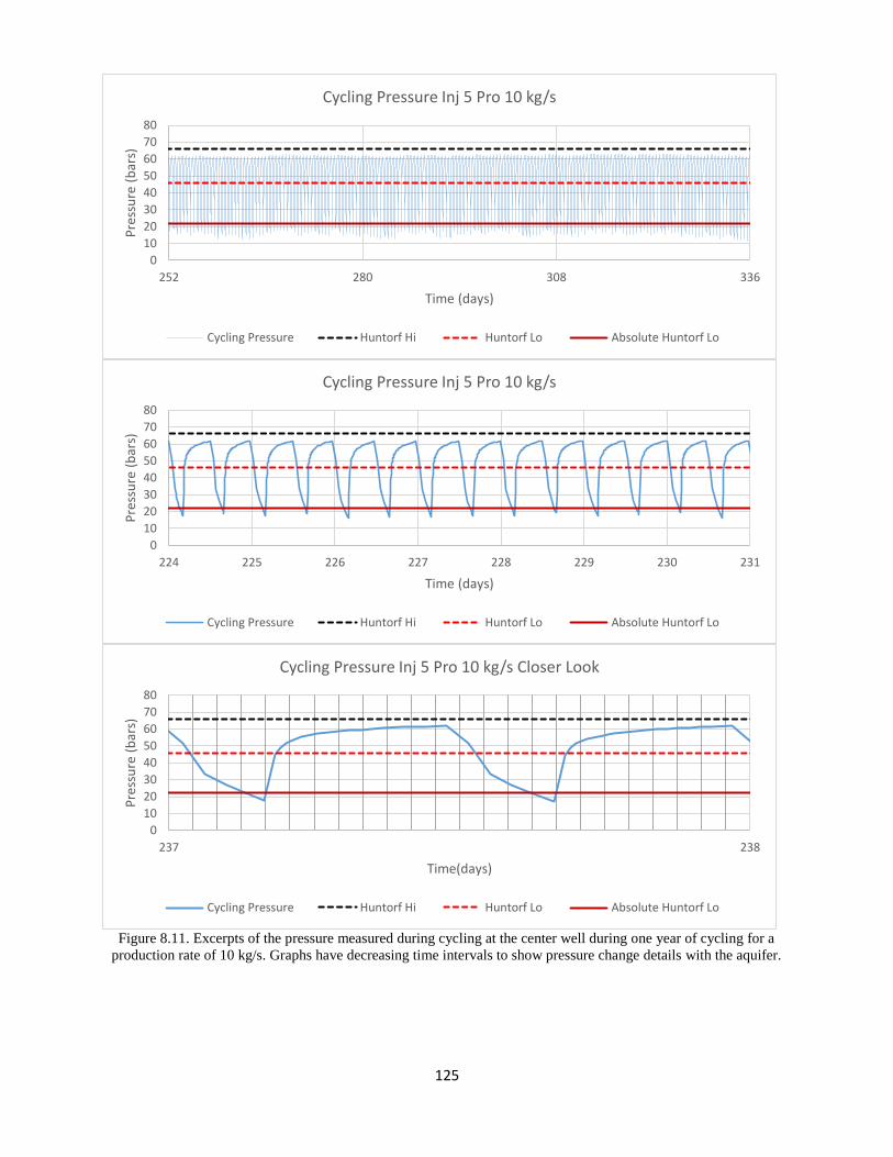
125
Figure 8.11. Excerpts of the pressure measured during cycling at the center well during one year of cycling for a
production rate of 10 kg/s. Graphs have decreasing time intervals to show pressure change details with the aquifer.
0
10
20
30
40
50
60
70
80
252 280 308 336
Pre
ssu
re (
bar
s)
Time (days)
Cycling Pressure Inj 5 Pro 10 kg/s
Cycling Pressure Huntorf Hi Huntorf Lo Absolute Huntorf Lo
0
10
20
30
40
50
60
70
80
224 225 226 227 228 229 230 231
Pre
ssu
re (
bar
s)
Time (days)
Cycling Pressure Inj 5 Pro 10 kg/s
Cycling Pressure Huntorf Hi Huntorf Lo Absolute Huntorf Lo
0
10
20
30
40
50
60
70
80
237 238
Pre
ssu
re (
bar
s)
Time(days)
Cycling Pressure Inj 5 Pro 10 kg/s Closer Look
Cycling Pressure Huntorf Hi Huntorf Lo Absolute Huntorf Lo
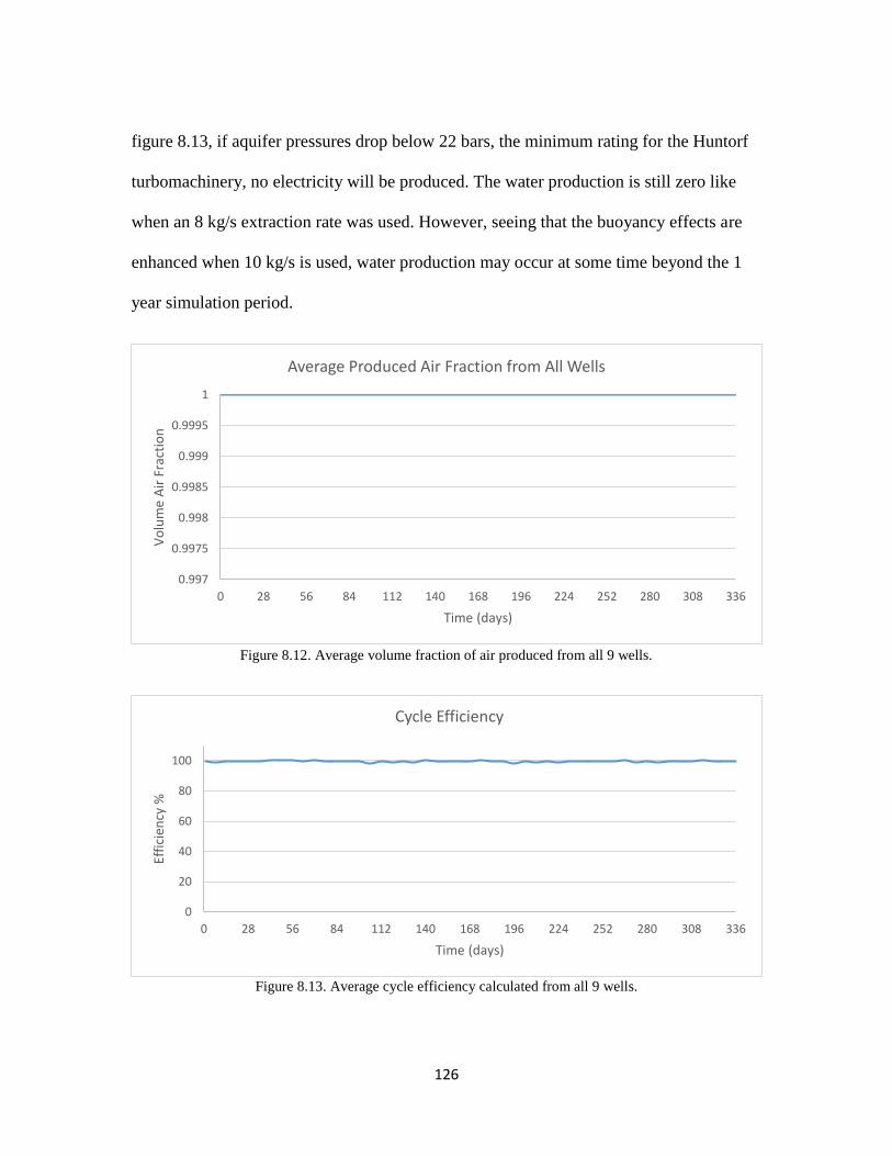
126
figure 8.13, if aquifer pressures drop below 22 bars, the minimum rating for the Huntorf
turbomachinery, no electricity will be produced. The water production is still zero like
when an 8 kg/s extraction rate was used. However, seeing that the buoyancy effects are
enhanced when 10 kg/s is used, water production may occur at some time beyond the 1
year simulation period.
Figure 8.12. Average volume fraction of air produced from all 9 wells.
Figure 8.13. Average cycle efficiency calculated from all 9 wells.
0.997
0.9975
0.998
0.9985
0.999
0.9995
1
0 28 56 84 112 140 168 196 224 252 280 308 336
Vo
lum
e A
ir F
ract
ion
Time (days)
Average Produced Air Fraction from All Wells
0
20
40
60
80
100
0 28 56 84 112 140 168 196 224 252 280 308 336
Effi
cien
cy %
Time (days)
Cycle Efficiency

127
CHAPTER 9
PROJECT SUMMARY
This project evaluated the feasibility for the storage of compressed air in flat-lying
porous reservoirs as an alternative to storing compressed air in caverns.
The major findings and conclusions from the 2D numerical models are summarized as
follows:
1. The greatest control on cycle efficiency is the volume of air that can be recovered
from the aquifer. This volume of air is directly linked to the pressure that can be
maintained by the aquifer to ensure air flow. Cycle efficiency is defined as the
amount of energy contained within the recovered air compared to the amount of
energy in the injected air.
2. 2D models show that a dual daily peak schedule sustains aquifer pressures better
and therefore will increase cycle efficiency on a longer time scale.
3. Using shut in periods decrease aquifer pressures so that lower mass flow rates are
sustained thereby lowering cycle efficiency.
4. Higher hydrostatic pressures at greater depths enhance the percentage of air that
can be produced. The increased background pressure, however, will increase
pressure requirements on turbomachinery.
5. While a higher permeability allowed for increased air production rates, it also
improves the ease with which water can drain back towards the wellbore,
compromising cycle efficiency.

128
6. Screening the top half of the well enhances cycle efficiency because it takes
advantage of the buoyancy flow of air introduced into an aquifer.
7. Using a larger initial bubble meant that a higher flow rate could be sustained for a
longer period after air cycling begins. It also decreased the mass of water
produced since a larger bubble displaces more water and increases the zone
surrounding the wellbore in which air is contained.
8. Aquifers with increased anisotropy delay the buoyancy flow of air, allowing for
greater production rates to be sustained which in turn improves cycle efficiency. It
also decreased the volume of water produced.
The 3D simulation model’s findings and conclusions are summarized as follows:
1. The 3D model shows that cycling for 1 year produces 0.00% water and can give a
cycle efficiency of about 80 % without reducing aquifer pressures below that
which is considered useful. This assumes that the turbomachinery similar to that
used in the Huntorf Power Plant would have been implemented in the PMCAES
facility.
2. Attempts to increase cycle efficiency proved ineffective since a higher extraction
rate reduced aquifer pressures to levels below 22 bars, the lowest possible
pressure for the assumed above-ground turbomachinery. Therefore, despite
calculations suggesting that the cycle efficiency improved, actually, the
production rate of 10 kg/s would have produced zero electricity generation.

129
CHAPTER 10
CLOSING REMARKS
In closing, this project’s feasibility analysis for PMCAES in flat-lying formations has
shown the following:
1. PMCAES can be done in flat-lying sand formations. Although dip angles in SC
are less than 10, since the effect of dip was not explored, its effect needs to be
examined and quantified.
2. Energy recovery efficiency of 80% can be achieved.
3. Using turbomachinery similar to that used at the Huntorf Power Plant, limited the
operating pressures which the aquifer had to maintain during cycling. The
turbomachinery available today covers a large range of pressure ratings and the
possible combinations of such equipment is outside the scope of this study.
Therefore, it may be possible to increase energy recovery efficiency through the
choice of alternative equipment.
4. As long as PMCAES is not done in aquifers where wells are installed for
acquiring groundwater, the injected air would pose no danger to water pumping
equipment.
5. In SC, potential windfarms, as of now, are being considered to be constructed
along the SC coastal areas where salinity levels do not allow for the recovery of
groundwater for drinking and therefore PMCAES should be done in coastal areas.

130
This seems suitable since the PMCAES areas would ideally be located near to the
windfarms.
6. Turbomachinery should be chosen based on the mass flow rates which the aquifer
in question can sustainably produce. However, setting the pressure envelope of 46
to 66 bars was realistic since turbomachinery is always rated. Rating refers to the
pressure (and temperature) ranges through which the machinery can perform.

131
REFERENCES
Aadland, R.K., Gellici, J.A., and Thayer, P.A., 1995, Hydrogeologic framework of west-
central South Carolina: South Carolina Department of Natural Resources Water
Resources Division Report 5, 200 p.
Aguado M, Ayerbe E, Azcarate C, Blanco R, Garde R, Mallor F, 2009 . Economical
assessment of a wind-hydrogen energy system using windhygen ® software.
International Journal of Hydrogen Energy v. 34 no. 7 p. 2845- 2854.
Ahmed, T, 2000, Reservoir Engineering Handbook: Gulf Professional Publishing, 484 p.
Allen, R.D., Doherty, T.J., Erikson, R. L., Wiles, L. E., 1983, Factors Affecting Storage
of Compressed Air in Porous Rock Reservoirs, Pacific Northwest Laboratory
Operated for the U.S. Department of Energy.
Anderson, M. P., Woessner, W.W., 2002, Applied groundwater modeling simulation of
flow and advective transport: San Diego, Academic Press, 102 p.
Aucott, W.R., Davis, M.E., and Speiran, G.K., 1987, Geohydrologic framework of the
coastal plain aquifers of South Carolina: U.S. Geological Survey Water-
Resources Investigations Report 85–4271.
Barnhart, J and Benson, S. M., 2013, On the importance of reducing the energetic and
material demands of electrical energy storage, Energy & Environmental Science,
v 6. p. 1083-1092.
Beaudin M, Zareipour H, Schellenberglabe A, Rosehart W., 2010, Energy storage for
mitigating the variability of renewable electricity sources: an updated review,
Energy for Sustainable Development v. 14 no. 4 p. 302- 314.
Bear, J, 1972, Dynamics of fluid flow in porous media: New York, Dover Publications
Inc.
Bear, J., 1979, Hydraulics of groundwater: New York, Dover Publications Inc.

132
Berwig, D, 1978, Geological Assessment of Compressed Air Energy Storage Sites in
Kansas Final Report Electrical Power Research Institute Research Project K102-
1.
Black and Veatch, 1978, Geological assessment of compressed air storage sites in
Kansas, EPRI EM-877 Research Project k102-1.
Blackwell, D.D., Steele, J.L. and Carter, L., 1991. Heat flow patterns of the North
American continent: A discussion of the DNAG geothermal map of North
America. Neotectonics of North America: Geological Society of America DNAG,
Decade Map, 1: 423-437.
Bloomer, J.R., 1981, Thermal conductivities of mudrocks in the United Kingdom,
Quarterly Journal of Engineering Geology and Hydrogeology, v 14, p. 357-362.
Brooks, F. J., 2000, GE gas turbine performance characteristics, General Electric Energy,
GER-3567H: http://site.ge-
energy.com/prod_serv/products/tech_docs/en/downloads/ger3567h.pdf (accessed
November, 2014).
Brown P, Lopes J, Matos M., 2009, Optimization of pumped storage capacity in an
isolated power system with large renewable penetration, IEEE Transactions on
Power Systems, v. 23 no. 2 p. 523- 531.
Buckles W., Hassenzahl, W., 2000, Superconducting magnetic energy storage. IEEE
Power Engineering Review, v. 20 no. 5 p. 16- 20.
Cavallo A., 2007, Controllable and affordable utility-scale electricity from intermittent
wind resources and compressed air energy storage (CAES). IEEE Transactions on
Power Systems v. 32 no. 2 p. 120- 127.
Chang Y, Mao X, Zhao Y, Feng S, Chen H, Finlow D., 2009, Lead-acid battery use in the
development of renewable energy systems in China, Journal of Power Sources v
191 p. 176- 183.
Campbell, B.G., and Coes, A.L., eds., 2010, Groundwater availability in the Atlantic
Coastal Plain of North and South Carolina: U.S. Geological Survey Professional
Paper 1773, 241 p., 7 pls.

133
Colbert-Busch, E, Carey, R. T., and Saltzman, E. W., 2012, South Carolina wind energy
supply chain survey and offshore wind economic impact study, South Carolina
Energy Office.
Colquhoun, D.J., Woollen, I.D., Van Nieuwenhuise, D.S., Padgett, G.G., Oldham, R.W.,
Boylan, D.C., Bishop, J.W., and Howell, P.D., 1983, Surface and subsurface
stratigraphy, structure and aquifers of the South Carolina Coastal Plain:
University of South Carolina, Department of Geology, 78 p.
Corey, A.T., 1954, The interrelation between gas and oil relative permeabilities:
Producers Mon. v. 19, p. 38–41.
Dale, M. W. and Park, A. D., 1999. Irrigation supply potential of the shallow aquifer,
Hilton Head Island, South Carolina SCDNR Water Resources Report 20.
DOE, 2008, 20% Wind energy by 2030 Increasing Wind Energy’s Contribution to US.
Electricity Supply, DOE/GO-102008-2567.
DOE, 2014, Wind vision: a new era of wind power in the United States,
http://energy.gov/sites/prod/files/2015/03/f20/wv_full_report.pdf (accessed
February, 2015).
Doherty, T. J., 1981, Air storage systems in Proceedings of the International Conference
on Seasonal Thermal Energy Storage and Compressed air energy storage, v. 2, pp.
455-468, National Technical Information Service Conference 811066,
Springfield, Virginia.
Duke Energy Schedule, 2014, Schedule opt (SC) optional power service, time-of-use
http://www.considerthecarolinas.com/pdfs/scscheduleopt.pdf (accessed February,
2015).
EIA, Annual Energy Outlook, 2007.
Eastop, T. D., and McConkey, A., 2011, Applied thermodynamics for engineering
technologists 5th e.: Essex, Pearson Education Limited.
Eppelbaum, L. Kutasov, I, Pilchin, A., 2014, Thermal properties of rocks and fluid
density, Applied Geothermics.
Fetter, C.W., 2001, Applied Hydrogeology: New Jersey, Prentice-Hall, Inc, 85 p.
134
Gellici, J.A. and Lautier, J. C., 2010, Hydrogeologic framework of the Atlantic Coastal
Plain, North and South Carolina, in Campbell, B.G., and Coes, A.L., eds., 2010,
Groundwater availability in the Atlantic Coastal Plain of North and South
Carolina: U.S. Geological Survey Professional Paper 1773.
Glendenning, I, 1981, Compressed air storage, Physics in Technology Vol. 12, p. 103-
110.
GWEC, 2014, Global Wind Report 2014 - Annual market update
http://www.gwec.net/publications/global-wind-report-2/global-wind-report-2014-
annual-market-update/ (accessed January, 2015)
Hoffeins, H., 1994, Huntorf Air Storage Gas Turbine Power Plant, Energy Supply,
Brown Boveri Publications DGK 90 202 E
https://www.eon.com/content/dam/eon-content-pool/eon/company-asset-
finder/asset-profiles/shared-ekk/BBC_Huntorf_engl.pdf (accessed November,
2014).
Katz, D.L. and Lady, E.R., 1976, Compressed air energy storage for electric power
generation, Ulrich Books.
Kim, H, Rutqvist, J and Choi, B, 2012, Feasibility analysis of underground compressed
air energy storage in lined rock caverns using the TOUGH-FLAC simulator in
Proceedings, TOUGH Symposium, Lawrence Berkeley National Laboratory,
Berkeley, California.
Kushnir, R., Ullman, A. Dayan, A., 2010, Compressed air flow within aquifer reservoirs
of CAES plants, Transport in Porous Media, v. 81 p. 219- 240.
Laney, R.L., and Davidson, C.B., 1986, Aquifer-nomenclature guidelines: U.S.
Geological Survey Open-File Report 86–534, 46 p.
Manger, G. E., 1963, Porosity and bulk density of sedimentary rocks: Geological Survey
Bulletin 1144-E, p. E1-E55.
McGrail, B.P, Cabe, J.E., Davidson, C.L., Knudsen, F.S., Bacon, D.H., Bearden, M.D.,
Chamness, M.A., Horner, J.A., Reidel, S.P., Schaef, H.T., Spane, S.A., Thorne,
P.D., 2013, Techno-economic performance evaluation of compressed air energy
storage in the Pacific Northwest, DOE PNNL-22235.

135
Meyer, F., 2007, Compressed air energy storage power plants, Bine Informationnsdienst,
FIZ KarlsruheD-76344 Eggenstein-Leopoldshfen.
Miller, J.A., 1986, Hydrogeologic framework of the Floridan aquifer system in Florida
and in parts of Georgia and South Carolina: U.S. Geological Survey Professional
Paper 1403–B, 91 p.
Milligan, M, Ela, E., Hodge, B., Kirby, B., Lew, B., Clark, C., Decsario, J., Lynn, K.,
2011, Cost-Causation and Integration Cost Analysis for Variable Generation,
NREL Technical Report TP-5500-51860.
Neuman, C. H., 1985, A gravity override model, Journal of Petroleum Technology, v. 37,
p. 163-169.
Oldenburg, C. M and Pan, L., 2013, Porous media compressed-air energy storage (PM-
CAES): theory and simulation of the coupled wellbore–reservoir system,
Transport in Porous Media, v 97 (2), p. 201-221.
Pickard W, Shen AQ, Hansing N., 2009, Parking the power: strategies and physical
limitations for bulk energy storage in supply-demand matching on a grid whose
input power is provided by intermittent sources. Renewable and Sustainable
Energy Reviews v. 13 no. 8 p. 1934- 1945.
Pollack, R., 1994, History of first US compressed-air energy storage (CAES) plant (110
MW 26h) volume 2: Construction, EPRI TR-101751-V2.
Pruess, K., Oldenburg, C. and Moridis, G., 1999, Tough user’s guide, version 2.0,
Lawrence Berkley National Laboratory, LBNL-43134.
Rodriquez, J. A., Newcome, R., Wachob, A., 1994, Ground-Water Resources of
Darlington, Dillon, Florence, Marion, and Marlboro Counties, South Carolina
with an analysis of management alternatives for the city of Florence, SCDNR
Water Resources Report 1.
Rogers, L.J., 1982, Compressed air energy preliminary storage design and site
development in an aquifer, DOE ET-78-C-01-2159.
SACE, 2013, Sea Power South Carolina’s offshore and nearshore wing resources
coincidence with electrical demand.
136
Salgi, G and Lund, H., 2009, The role of compressed air energy storage (CAES) in future
sustainability energy systems, Energy Conservation and Management v. 50 p.
1172-1179.
SCEO, 2009, South Carolina’s role in offshore wind energy development,
http://www.energy.sc.gov/files/view/WindEnProdFarmsFeasStudyComFinalRepo
rt12-09.pdf (accessed November, 2014).
South Carolina State Profile and Energy Estimates,
http://www.eia.gov/state/analysis.cfm?sid=SC (accessed November, 2014).
Schulte, R, Holst, K., Critelli, N., Huff, G., 2012, Lessons learned from Iowa:
development of a 270 megawatt compressed air energy storage project in
Midwest independent system operator, Sandia Laboratories.
South Carolina General Assembly 117th Session, 2007-2008,
http://www.scstatehouse.gov/sess117_2007-2008/bills/4766.htm (accessed online,
Jan 2015)
Succar, S. and Williams, R. H., 2008, Compressed air energy storage: theory, resources,
and applications for wind energy,
http://www.princeton.edu/pei/energy/publications/texts/SuccarWilliams_PEI_CA
ES_2008April8.pdf (accessed on November, 2013).
Szymkiewicz, A., 2013, Modelling water flow in unsaturated porous media accounting
for nonlinear permeability and material heterogeneity: Berlin, Springe-Verlag, 10
p.
Temples, T.J., and Englehardt, D., 1997, Stratigraphy, depositional environments and
sequence stratigraphy of the Upper Cretaceous in the Hilton Head Island Test
Well #1, Beaufort County South Carolina, Southeastern Geology, v. 36, no. 4, p.
177–186.
US Department of Labor, Bureau of Labor Statistics, Unemployment Rates for States
http://www.bls.gov/web/laus/laumstrk.htm (accessed July, 2015).
US DOE, 2002, Wind climate analyses for national weather service stations in the
southeast, WSRC-TR-2002-00515,
http://sti.srs.gov/fulltext/tr2002515/tr2002515.pdf (accessed Jan, 2015).

137
US DOE, 2008, 20% Wind energy by 2030 increasing wind energy’s contribution to U.S.
electricity supply, DOE/GO-102008-2567.
US DOE 2012, 2012 wind technologies market report,
https://www1.eere.energy.gov/wind/pdfs/2012_wind_technologies_market_report
.pdf (accessed January, 2015).
US DOE, 2014, Wind vision: a new era for wind power in the United States,
http://www.energy.gov/eere/wind/maps/wind-vision (accessed January, 2015).
USDOE, 2014, What is wind power, wind and water power program - WINDExchange,
http://apps2.eere.energy.gov/wind/windexchange/what_is_wind.asp?&print
(accessed November, 2014).
USEIA, 2013, State electricity profiles:
http://www.eia.gov/electricity/state/southcarolina/ (accessed January, 2015).
van Genuchten, M.T, 1980, A closed-form equation for predicting the hydraulic
conductivity of unsaturated soils: Soil Sci. Soc. Am. J. v 44(5) p. 892–898.
Walas, S. M., 1990, Chemical process equipment selection and design: Boston,
Butterworth-Heinemann.
Winner, M.D., Cobel, R.W., 1996, Hydrogeologic framework of the North Carolina
Coastal Plain by regional aquifer system analysis of the Northern Atlantic Coastal
Plain, USGS Professional Paper 1404-1.
Williams, L., http://water.usgs.gov/ogw/gwrp/brackishgw/pilot.html (accessed August,
2015).
Wiser, R. and Bolinger, M., 2014, Wind technologies market report, DOE,
http://eetd.lbl.gov/sites/all/files/lbnl-6809e.pdf accessed January, 2015.