Embed Size (px)
Citation preview

1. Report No. 2. Government Accession No.
FHW A/TX-95/1408-lF
4. Title and Subtitle
FEASIBILITY STUDY FOR HYDRAULIC MODELING FACILITY FOR SCOUR PROBLEMS
7. Author(s)
Francis C.K. Ting, Jean-Louis Briaud, Subba Rao Gudavalli, and Suresh Babu Perugu
9. Performing Organization Name and Address
Texas Transportation Institute The Texas A&M University System College Station, Texas 77843-3135
12. Sponsoring Agency Name and Address
Texas Department of Transportation Research and Technology Transfer Office P. 0. Box 5080 Austin, Texas 78763-5080
15. Supplementary Notes
Technical Report Documentation Page
3. Recipient's Catalog No.
5. Report Date
November 1994
6. Performing Organization Code
8. Performing Organization Report No.
Research Report 1408-lF
10. Work Unit No. (TRAIS)
11. Contract or Grant No.
Study No. 0-1408
13. Type of Report and Period Covered
Final: September 1993 -August 1994
14. Sponsoring Agency Code
Research performed in cooperation with the Texas Department of Transportation and the U.S. Department of Transportation, Federal Highway Administration Research Study Title: Feasibility Study for Hydraulic Modeling Facility for Scour Problems
16. Abstract
The feasibility of building a large scale scour modeling facility to help evaluate the 26,018 bridges over water which exist in Texas is studied. First, the scour problem in Texas is reviewed and tends to indicate that many bridges are built on clay. Second, the fundamental laws of hydraulic and soil modeling are detailed. These laws show that it is not possible to scale all the components of the problem properly. It is also shown that when the model soil has particles smaller than 0.1 mm, additional difficulties occur. This makes the physical modeling of clays nearly impossible. Third, five bridge case histories are used to calculate the necessary size of scaled models. Scales of 1/15 to 1/100 would be used in the proposed facility. Fourth, the results of a paper survey and visits of prominent scour modeling laboratories in the USA are presented. They show that these laboratories are relatively well equipped. Fifth, the new facility is designed and the cost is estimated at $6.7 M. Finally, the advantages and disadvantages of building a new facility versus using existing facilities are outlined.
17. Key Words 18. Distribution Statement
Scour, Physical Modeling, Soil Modeling, Hydraulic Facilities, Cost, Rivers, Case Histories
No restrictions. This document is available to the public through NTIS:
19. Security Classif. (of this report)
Unclassified Form DOT F 17uu.7 (8-72)
National Technical Information Service 5285 Port Royal Road Springfield, Virginia 22161
20. Security Classif.(of this page)
Unclassified Reproduction of completed page authorized
21. No. of Pages
138 22. Price


FEASIBILITY STUDY FOR HYDRAULIC MODELING FACILITY FOR SCOUR PROBLEMS
by
Francis C.K. Ting
Assistant Research Scientist
Texas Transportation Institute
Jean-Louis Briaud
Research Engineer
Texas Transportation Institute
Subba Rao Gudavalli
Graduate Research Assistant
Department of Civil Engineering
and
Suresh Babu Perugu
Graduate Research Assistant
Department of Civil Engineering
Research Study Number:0-1408
Research Study Title: Feasibility Study for Hydraulic Modeling Facility for Scour Problems
Sponsored by the
Texas Department of Transportation
In cooperation with
U.S. Department of Transportation and
Federal Highway Adminstration
November 1994
TEXAS TRANSPORTATION INSTITUTE
The Texas A&M University System
College Station, Texas-77843-3135


IMPLEMENTATION STATEMENT
The implementation of this project is in the hands of the Texas Department of
Transportation (TxDOT). TxDOT needs to decide if it wants to build a scour facility or
not. The estimated cost of such a facility as well as its advantages and disadvantages are
included in the Conclusions of this report. These conclusions are reached on the basis of
literature search, data collection, numerical, similitude and dimensional analysis, laboratory
visits and expert interviews and cost estimating. It is the opinion of the researchers that
the facility should be built if TxDOT needs to simulate 2 bridges or more per year. It is
also felt that research needs to be conducted to develop alternatives to the physical
modeling approach. In particular, a site specific technique for the prediction of scour in
clay is necessary since many Texas bridges are in clay and since no physical modeling
approach is likely to give a reliable prediction in this case.
v


DISCLAIMER
The contents of this report reflect the views of the authors who are responsible for
the facts and the accuracy of the data presented herein. The contents do not necessarily
reflect the official view or policies of the Texas Department of Transportation. This
report does not constitute a standard, specification, or regulation, nor is it intended for
construction, bidding, or permit purposes. The engineer in charge of the project was Jean
Louis Briaud, Texas P.E. # 48690.
There was no invention or discovery conceived or first actually reduced to practice
in the course of or under this contract, including any art, method, process, machine,
manufacture, design or composition of matter, or any new useful improvement thereof, or
any variety of plant, which is or may be patentable under the patent laws of the United
States of America or any foreign country.
vii


ACKNOWLEDGMENTS
The sponsor of this project is the Texas Department of Transportation. The
Project Director at TxDOT was Mr. Jay Vose; his help, constructive criticisms, and very
positive attitude created an excellent atmosphere during the course of this research and
Ms. Melinda Luna for her help and information. We also wish to thank Mr. Antony
Schneider and Mr. George Odom of TxDOT, Mr. Peter Smith, formerly with TxDOT, and
Mr. David Dunn of the United States Geological Survey (USGS), Texas district.
At the Texas A&M University System, we wish to thank Dr. Billy Edge and Dr.
Richard Seymour for their support. We also would like to thank Mr. Ken Krejci of the
Physical Plant at Texas A&M University for assistance with the cost estimate. The
managers of the four facilities visited by the research team: Dr. Bobby Brown, Mr. Randy
Oswalt and Mr. Tom Pokrefke of the Hydraulic Laboratory at U.S.A.E. Waterways
Experiment Station; Mr. Sterling Jones of the Federal Highway Administration (FHW A)
Turner Fairbank Highway Research Center; Dr. Gary Parker and Mr. Richard Voigt of the
St. Anthony Falls Hydraulic Laboratory, University of Minnesota; and Dr. Steven Abt of
Colorado State University are thanked for sharing their experience. Dr. E.V. Richardson
was the general consultant of this project and shared valuable comments.
At the FHW A, Mr. Sterling Jones and Dr. Roy Trent provided help at various
occasions. Their contributions are appreciated. We would also like to express our thanks
to Mr. John Hobbs at the Texas Transportation Institute.
viii


TABLE OF CONTENTS Page No
1. IN"TRODUCTION .. . . . . . . . .. . . . . . ... . .. . . . . . . . . .......... .... .. .. . . . . .. . . . . . . . . ... . . . . . . . . . . . . . 1
2. TEXAS SCOUR PROBLEM
2.1. Hydraulic Conditions of Rivers and Flood Plains in Texas . . . ... . . ... .... ... 3
2.1.1. Canadian River................................................................. . . . 3
2.1.2. Red River......................................................................... . . . 7
2.1.3. Trinity River........................................................................ 7
2.1.4. Brazos River........................................................................ 8
2.1. 5. Colorado River................................................................. . . . 8
2.1.6. Gudalupe River.................................................................... 8
2.1.7. Flood Plains in Texas........................................................... 9
2.2 Geology and Soil Conditions in Texas................................................. 9
2.2.1. Background on Soil Shear Strength ..................................... 17
2.3. Different Types of Scour .................................................................... 18
2.3.1. General Scour ...................................................................... 18
2.3.2. Constriction Scour. .............................................................. 18
2.3.3. Local Scour ......................................................................... 18
2.3.4. Clear Water Scour ............................................................... 18
2.3. 5. Live Bed Scour................................................................. . . . 19
2.4. The Texas Scour Approach ................................................................ 19
2. 5. The Project Objectives ....................................................................... 24
3. HYDRAULIC MODELIN"G
3 .1. Basic Open Channel Hydraulics .......................................................... 25
3 .1.1. Bed Shear Stress .................................................................. 25
3.1.2. Froude Number ................................................................... 28
3 .1.3. Reynolds Number ................................................................ 28
3.2. Similitude .......................................................................................... 29
3.2.1. Similarity Laws .................................................................... 30
3.2.2. Other Model Laws ............................................................... 32
3 .2.3. Empirical Approach ............................................................. 34
3.2.4. Types ofModels .................................................................. 35
ix

Page No
3.2.4.1. Fixed Bed Model.. ................................................. 35
3.2.4.2. Movable Bed Models ............................................ 35
3.2.4.3. Undistorted Models ............................................... 36
3.2.4.4. Distorted Models .................................................. 36
3.2.4.5. Advantages and Limitations ................................... 37
3.3. Existing Software and its Applications ................................................ 38
3 .3 .1. WSPRO (Model for Water Surface Profile Computations) ... 38
3 .3 .1.1. Surface Profile Calculations ................................... 3 8
3.3.1.2. Model Capabilities ................................................. 39
3.3.1.3. Limitations ............................................................ 39
3.3.2. FESWMS-2DH(Finite Element Surface-Water Modeling System:
Two Dimensional Flow in a Horizontal Plane) .................... 39
3.3.2.1. Assumptions ......................................................... 40
3.3.2.2. Applications .......................................................... 40
3.3.2.3. Methodology ......................................................... 40
4. SOIL MODELING
4.1 Background ........................................................................................ 43
4.2 Bed Load Criterion ............................................................................. 43
4.3. Suspended Load Criterion .................................................................. 47
4.4. Soil Simulants .................................................................................... 48
4.4.1. Sand .................................................................................... 48
4.4.2. Coal .................................................................................... 48
4.4.3. Plastics ................................................................................ 49
4.4.4. Pumice ................................................................................ 49
4.4.5. Walnut Shells ....................................................................... 49
4.4.6. Bakelite ............................................................................... 49
4.5. Current Practice for Soil Modeling ..................................................... 50
4.6. Preparation of Clay Beds .................................................................... 51
5. CASE STUDIES
5 .1. Introduction ....................................................................................... 53
5.2. Case Study 1 -Guadalupe River ......................................................... 54
5 .2.1. Objective ............................................................................. 54
5.2.2. Analysis ............................................................................... 57
x

Page No
5.2.3. Conclusions ......................................................................... 58
5.3. Case Study 2 -Colorado River. ........................................................... 58
5.3.1. Objective ............................................................................. 61
5.3.2. Analysis ............................................................................... 61
5.3.3. Conclusions ......................................................................... 62
5 .4. Case Study 3 -Trinity River ................................................................ 62
5.4.1. Objective ............................................................................. 65
5.4.2. Analysis ............................................................................... 65
5.4.3. Conclusions ......................................................................... 67
5.5. Case Study 4 -Guadalupe River ......................................................... 67
5.5.1. Objective ............................................................................. 67
5.5.2. Analysis ............................................................................... 70
5.5.3. Conclusions ......................................................................... 72
5.6. Case Study 5 -Navasota River ............................................................ 72
5.6.1. Objective ............................................................................. 72
5.6.2. Analysis ............................................................................... 72
5.6.3. Conclusions ......................................................................... 73
6. SURVEY OF EXISTING HYDRAULIC LABORATORIES
6 .1. Objective of the Survey ...................................................................... 79
6.2. The Questionnaire .............................................................................. 79
6.2.1. Personnel and Experience .................................................... 79
6.2.2. Physical Dimensions and Instrumentation ............................. 80
6.2.3. Physical Modeling ................................................................ 80
6.2.4. Cost of the Facility .............................................................. 81
6.3. The Visits .......................................................................................... 81
6.3.1. Personnel and Experience .................................................... 82
6.3.2. Physical Dimensions and Instrumentation ............................. 84
6.3.3. Physical Modeling ................................................................ 88
6.3.4. Cost of the Facility .............................................................. 91
6.4. Impressions from the Visits ................................................................ 93
6.4.1. USAE Waterways Experiment Station ................................. 93
6.4.2. FHW A Hydraulic Laboratory ............................................... 93
xi

Page No
6.4.3. University of Minnesota Hydraulic Laboratory ..................... 93
6.4.4. Colorado State University Hydraulic Laboratory .................. 94
6.4.5. Advantages and Disadvantages of the Existing Facilities ...... 94
7. NEW SCOUR FACILITY CHARACTERISTICS
7 .1. Introduction ....................................................................................... 95
7.2. Design of2-Dimensional Facility ........................................................ 95
7.2.1. Selection ofModel Parameters ........................................... 96
7.2.2. Preliminary Design of the Flume .......................................... 97
7.2.3. Sump Design (2-D) .............................................................. 97
7.2.4. Pump Capacity .................................................................... 101
7.3. Design of the 3-Dimensional Facility .................................................. 102
7. 3 .1. Selection of Model Parameters ........................................... 102
7.3.2. Sump Design (3-D) .............................................................. 104
7.3.3. Pump Capacity (3-D) ........................................................... 106
7.4. Flow Control Devices ........................................................................ 107
7. 5. Flow Distribution ............................................................................... 107
7.6. Surface Elevations .............................................................................. 108
7. 7. Flow Measuring Devices .................................................................... 108
7.8. Live Bed Scour .................................................................................. 111
7.9. River Banks ....................................................................................... 111
7 .10. Soils .......................................................................................... 111
7 .11. Cost Estimate for Proposed Modeling Facility .................................. 112
8. CONCLUSIONS ................................................................................. 115
References .......................................................................................... 117
xii

LIST OF FIGURES Page No
2.1. Average Annual Precipitation in Texas ........................................................ 4
2.2. Average Annual Runoff in Texas ................................................................ 5
2.3. River and Coastal Basins in Texas ............................................................... 6
2.4. Diagram Illustrating the Formation ofModem Soils ................................... 10
2.5. Surface Geology ofTexas .......................................................................... 13
2.6. Physiography ofTexas ............................................................................... 14
2.7. (a) Generalized Soils of Texas ................................................................... 15
(b) Legends for the Soils in Texas .............................................................. 16
2.8. Shear Strength for Cohesionless Soils ........................................................ 17
2.9. Scour Depth for a Given Pier and Sediment as
(a) Function of Time and (b) Function of Approach Velocity ..................... 20
2.10. Schematic Adopted by TxDOT for Scour Evaluation ................................ 23
3 .1. Shield's Diagram ....................................................................................... 27
4.1 Definitions of 'r and <J' .• ••.••••••••••••••....••••••••••.••.•.•••••••••••••••...........•.••••••••...•. 44
4.2. Bed Load Shear Stress ............................................................................... 45
4. 3. Sheild's Representation .............................................................................. 46
5.1. Topographic Map of Bridge Site Where State Highway 80 Crosses
the Guadalupe River Near Belmont, Texas ................................................ 55
5.2. Scour Envelope (500-year Discharge) for Bridge Section Where
State Highway 80 Crosses the Guadalupe River Near Belmont, Texas ....... 56
5.3. Topographic Map of Bridge Site Where FM 973 is Crossing the
Colorado River Near Austin, Texas ............................................................ 59
5.4. Scour Envelope (500-year Discharge) for Bridge Section Where
FM 973 is Crossing the Colorado River Near Austin, Texas ...................... 60
5.5. Topographic Map of Bridge Site Where State Highway 7
Crosses the Trinity River Near Crockett, Texas .......................................... 63
5.6. Scour Envelope (500-year Discharge) for Bridge Section Where
State Highway 7 Crosses the Trinity River Near Crockett, Texas ............... 64
5.7. Topographic Map ofBridge Site Where US Highway 183 is Crossing
the Guadalupe River Near Hochhiem, Texas .............................................. 68
5.8. Scour Envelope (500-year Discharge) for Bridge Section Where
US Highway 183 Crossing the Guadalupe River Near Hochhiem, Texas ..... 69
xiii

LIST OF FIGURES (Continued) 5.9. Topomap of a Section of Navasota River and its Flood Plain ...................... 74
5.10. Network of Elements on the Flood Plain ofNavasota River ....................... 75
5 .11. Ground Contours and Network of Elements on the Flood
Plain of Navasota River .............................................................................. 76
5 .12. Water Surface Contours and Velocity Vectors on the Flood Plain .............. 77
7 .1. Plan of Open Channel Flume and Sump ...................................................... 98
7.2. 2-D Open Channel Flume and Sump .......................................................... 100
7.3. 3-D River Hydraulics Sediment Transport Basin ........................................ 103
7.4. 3-D River Hydraulics Sediment Transport Basin with
Sump Below the Ground ........................................................................... 105
7.5. Plan of Hydraulic Modeling Facility ........................................................... 113
xiv

LIST OF TABLES
2.1 Geologic Time ....................................................................................... 11
2.2 Cenozoic Time ....................................................................................... 12
xv


LIST OF SYMBOLS AND ABBREVIATIONS
s = Shear strength
a = Normal stress of the soil grains
u = Pore water pressure
t/J = Angle of internal friction between the soil grains
Su = Undrained shear strength
c = Cohesion
To = Unit tractive force
r = Specific weight of water
R = Hydraulic mean radius
s = Slope of the channel bottom
u. = Shear velocity
Pw = Density of water
Ps Density of soil
(Tot = Critical shear stress for initiation of motion
rs Specific weight of sediment particles
d = Grain size diameter
v = Kinematic viscosity
R,, = Boundary Reynolds number
fj/ = Shields parameter
Fr = Froude number
g = Acceleration due to gravity
D = Depth of water
v = Velocity of water
Re = Reynolds number
µ = Dynamic viscosity
F = Force on the fluid flow
M = Mass of the fluid
a = Acceleration of the fluid
Fv = Viscous force
Fg = Gravity force
n = Mannings roughness coefficient
L = Length
LH = Horizontal scale length
Ly = Vertical scale length
xvi

d = Particle size
w = Weight of water element
b = Width of the water element
h = Height of water element
a = Angle of the bed
x = Ratio of u*to Vs
As = Cross sectional area of sump
Q = Discharge
H = Total head
17 = Efficiency of the pump
Cd = Coefficient of discharge
ai = Cross sectional area of the pipe
a1 = Cross sectional area of the throat of the venture meter
A suffix 'r' indicates scale ratio; a suffix of 'm' indicates the parameter related to
model; a suffix of 'p' indicates the parameter related to prototype; a subscript of H
indicates the parameter is related to horizontal scale; and a subscript of V indicates a
parameter related to vertical scale.
xvii

SUMMARY
This project entitled "Feasibility Study for Hydraulic Modeling Facility for Scour
Problems" was undertaken to determine if the development of a scour facility in Texas
would be a sound idea. The perceived need was based on the following reasons and the
questions:
1. The TxDOT has a need to evaluate bridges for scour problems.
2. There are no adequate facilities for modeling scour problems in Texas.
3. Are the hydraulic modeling facilities available elsewhere appropriate for Texas
problems?
4. What are the required dimensions for a facility dedicated to the Texas scour problem?
5. What would be the approximate cost of such a facility?
The work consisted of a study of the Texas scour problem including the hydraulic
and soil characteristics of the rivers in Texas, a study of fundamental principles of
hydraulic and soil modeling, model analysis by similitude theory of five bridge case studies
in Texas, discussions with recognized scour experts, and a survey and visit to four leading
scour facilities in the country.
The following conclusions were reached :
1. The facility should have two basins: a 2-D flume for local scour studies and a
3-D basin for global scour studies.
2. The 2-D flume should be above ground, 36.6 m long (120 ft), 6.1 m wide (20ft),
and 3.6 m deep (12 ft). The sump should be below ground; it should surround
the flume and be 3 m (10 ft) wide and 3 m (10 ft) deep. A 240 HP pump
delivering 2.8 m3/sec (100 cfs) is necessary to feed this flume.
3. The 3-D basin should be above ground, 45 m (150 ft) long, 30 m (100 ft) wide
and 1 m (3 ft) deep. The sump should be below ground under the center of the
basin, parallel to the 50 m side of the basin; it should be 3 m wide ( 10 ft) and
1.8m (6 ft) deep. A 24 HP pump delivering 0.4 m3/sec (12 cfs) is necessary to
feed this basin.
4. The 2-D flume would allow local scour models with undistorted scales in the
range of 1/15 to 1/25.
5. The 3-D basin would allow general scour models with undistorted scales in the
range of 1/50 to 1/100.
xix

6. The cost of the facility and its major components is estimated to be as follows:
The overall facility = $6. 70 M
The building = $4.25 M
The 3-D basin with sump and pump = $0.19 M
The 2-D basin with sump and pump = $0.35 M
Measuring instruments = $0.61 M
7. The advantages and disadvantages ofthis facility are:
Advantages Disadvantages
1. Availability 1. Initial cost
2. Develop local expertise 2. Delay until built
3. Latest technology 3. Inexperienced personnel at first
4. Very large scale
5. Low overhead
6. Easy contracts
7. Short travel time
8. Existing facilities do not compare favorably with the facility described above.
However, a few of them can provide very valuable data on scour modeling at a
reasonably large scale.
9. The advantages and the disadvantages of the existing facilities are :
Advantages Disadvantages
1. No delay for use 1. Higher overhead
2. No initial cost 2. No local expertise developed
3. Exoerienced personnel 3. Older equipment
4. Longer travel time
5. First come first serve availability
10. The decision should be based on the estimated need in the next IO to 20 years
for such a facility by TxDOT and neighboring states. Decreasing the cost by
using an existing building would make a big difference. It should also be kept
in mind that Texas rivers have a mixture of sand and clay beds, and the
usefulness of modeling facilities for scour in clay is limited.
xx

1. INTRODUCTION
Scour in rivers is a major problem to be addressed by the Departments of
Transportation across the country. The Federal Highway Adminstration requires that all
bridges over waterways be evaluated for scour by January 1997. Texas has close to
40,000 such bridges; the task is obviously enormous, yet crucial. TxDOT has decided to
take advantage of this effort on scour to also evaluate the research on this topic.
The overwhelming majority of research projects on this topic have concentrated on
the experimental approach. This is due to the complexity of the problem in terms of
hydraulics and sediment transport. Physical models with a scale varying from 1/10 to
1/200 are tested in large basins.
This project entitled "Feasibility Study for Hydraulic Modeling Facility for Scour
Problems" was undertaken to determine if the development of a scour facility in Texas
would be a sound idea. The perceived need was based on the following reasons and the
questions:
I. The TxDOT has a need to evaluate bridges for scour problems.
2. There are no adequate facilities for modeling scour problems in Texas.
3. Are the hydraulic modeling facilities available elsewhere appropriate for the Texas
problems?
4. What are the required dimensions for a facility dedicated to the Texas scour problem?
5. What would be the approximate cost of such a facility?
The following chapters present the results of the study. First, the Texas scour
problem is described. Second, a background is given on hydraulic modeling. Third, a
similar background is given on soil modeling. Fourth, five case studies are analyzed to
determine an appropriate model size in each case. Fifth, the results of a survey of existing
facilities for scour modeling in the USA are presented. Sixth, the characteristics of a new
TXDOT Scour Facility including dimensions and costs are determined and presented.
Finally conclusions are presented on the advantages and disadvantages of such a facility
1


2. TEXAS SCOUR PROBLEM
2.1. HYDRAULIC CONDITIONS OF RIVERS AND FLOOD PLAINS IN TEXAS
The State of Texas has 15 river basins and 8 coastal basins. The 23 river and
coastal basins have approximately 3700 streams and tributaries and 128,800 km (80,000
miles) of stream bed (Moody et al. 1985). Geological and climatological features may
vary dramatically from the head water to outlets into other rivers or at the Gulf of
Mexico. For instance, long term average annual precipitation contributing to runoff and
surface water supplies varies dramatically across the state, ranging from 1.4 m (56
inches) near Beaumont in East Texas to 0.2 m (8 inches) in far West Texas near El Paso
(USGS, 1988-89). Average annual runoff is about 6.04x10¹⁰ m3 (49 million ac-ft).
The average annual precipitation and annual stream flow are shown in the Figures 2.1.
and 2.2. Between 1940 and 1970, state wide runoff varied from an average 7.027x10¹⁰
m3/year (57 million ac-ft/year) during the wettest period (1940-50) to as little as
2.835x10¹⁰ m3/year (23 million ac-ft/year) during the most severe recorded state wide
drought of the early 1950s (Moody et al. 1985). There are currently 188 major
reservoirs and 6.16 x 10⁶ m3 (5000 ac-ft) or greater storage capacity in Texas. Figure
2.3 illustrates the 23 major river and coastal basins and zones. Some of the major
features of rivers and their basins are discussed briefly in the following sections ..
2.1.1. CANADIAN RIVER
The Canadian River heads in northeastern New Mexico, flows across the Texas
Panhandle, and merges with the Arkansas River in eastern Oklahoma. The total length
of the river is 1459 km (906 miles). The Texas part of the basin comprises a total area of
about 32,920 km2 (12,700 mi2) out of the total drainage area of 123,656 km2 (47,705
mi2). The average discharge (arithmetic average of annual average discharges during the
period of analysis) during the period (1939-83) of analysis is 9.3 m3/sec (331 ft3/sec)
near Amarillo where the drainage area is 39,856 km2 (15,376 mi2). The 100-yr. flood at
that location is 3780 m3/sec (135,000 ft3/sec). Average annual runoff to the Canadian
River during the 26-year period (1939-1964) ranged from 11,890 m3fkm2 (25 ac-ft!mi2)
in the western part of the basin to 21,401 m3fkm2 (45 ac-ft!mi2) in the eastern part of
the basin (Moody et al. 1985). Large floods occur infrequently in the basin, and these
floods are characterized by rapid rise and fall and high stream velocities.
3

Average annual discharge In mllllons of acre-feet
SCALE 1:7,500,000
O 50 100 MILES
50 100 KILOMETERS
EXPLANATION
-24-
• Line of equal average annual precipitation
Interval 4 inches
National Weather Service precip.itation gage-Monthly data shown . in be.graphs
Figure 2.1. Average Annual Precipitation in Texas (Moody et al. ·1985)
4

EXPLANATION
- 9 - Line of equal average annual runoff Interval. in inches. is variable
100
• USGS stream-gaging station-Monthly data shown in bar graphs
RUNOFF
Figure 2.2. Average Annual Runoff in Texas (Moody et al. 1985)
5

'-<- ~...... --
NEW MEXICO
EXPLANATION
..,,..-- Basin BaundonH .., Existl1t9 Reservoirs
Eslsiino Major Conveyonc~ Focllittes
~ Reservoirs Uncter Canslruc1ion
-,....___
.._, Prcpm:ed Reservoirs for Woter Requirements 10 2020
-- Prooosed M"ajor Conveyance Facilitiot
~ Addillonol Reservoirs for PolantioJ Devdoam1n1
~·-'"~'h Addlllonal Major Conveyance Focilify for Potential Devefoomenl
~ Ge:ntratiud Baundnry af 00011010 Fcrmotion
OKL,AHOL\A
Figure 2.3. River and Coastal Basins in Texas (TWDB, l/968)
6
STATE OF TEXAS lixas water Oavelopment Board
A11s1in, l~
~ .. : ... :...:
2.1.2. RED RIVER
The total length of the Red River is 2,190 km (1,360 miles). The Red River is
bounded on the north by the Canadian River basin and on the south, from west to east by
the Brazos, Trinity, and Sulfur River basins (TWDB, 1968). Beginning in the High
Plains of eastern New Mexico at an elevation of about 1,454 m (4,800 feet), the Red
River flows east, forming the northern boundary of Texas east of the Panhandle. The
average discharge is 60 m3/sec (2117 ft3/sec) near Terral, Oklahoma where the drainage
area is 59,066 km2 (22,787 mi2). The total drainage area of the Red River upstream
from the northeast corner of Texas is 124,499 km2 (48,030 mi2). The total drainage
area of the basin in Texas is 63,411 km2 (24,463 mi2). Average annual runoff within the
basin in Texas ranges from more than 380,463 m3/km2 (800 acre-ft/mi2) at the northeast
corner of the state to less than 23,779 m3/km2 (50 acre-ft/mi2) in contributing areas of
the basin west of the 1 OOth meridian. Large floods occur infrequently in the upper part
of the Red River.
2.1.3. TRINITY RIVER
The Trinity River basin is bounded on the north by the Red River basin, on the
east by the Sabine and Neches River basins and the Neches-Trinity Coastal basin, and on
the west by the Brazos and San Jacinto River basins and Trinity San Jacinto Coastal
basins (TWDB 1968). West Fort Trinity River rises in southeastern Archer County at an
elevation of about 364 m (1,200 ft) and flows southeasterly to be joined successively by
Clear Fork at Fort Worth and Elm Fork at Dallas. The total drainage area of the basin at
the mouth of the river is 46,578 km2(17,969 mi2). Average annual runoff ranges from
the maximum of about 309,126 m3/km2 (650 ac-ft/mi2) near the mouth of the river to a
minimum of about 47,558 m3/km2 (100 ac-ft/mi2) near the head waters. The Trinity
River basin has widely varying flood characteristics. In the upper basin, floods rise and
fall rapidly and with higher velocities than floods in the lower basin. However, large
floods have occurred throughout the basin causing extensive and costly damage. Major
flooding has occurred on the average of once every four years in the upper basin, and
about every five years in the lower basin. The average discharge at Romayor (near its
mouth) is 210 m3/sec (7,417 ft3/sec) and the drainage area is 44,548 km2(17,186 mi2)
(Moody et al. 1985).
7

2.1.4. BRAZOS RIVER :
The Brazos River originates in the high plains of New Mexico and discharge to
the Gulf of Mexico. The total length of the river is 1353 km (840 miles). The Brazos
River is bounded on the north by the Red River basin on the east by the Trinity and San
Jacinto River basins and the San Jacinto-Brazos Coastal basin, and on the south and west
by the Colorado River basin and the Brazos Colorado coastal basin. The basin has a
total drainage area of 118,130 km2 (45,573 mi2) of which 42,840 km2 (42840 mi2) is in
Texas. The Brazos River basin varies in width from about 113 km (70 miles) in the
High Plains to 177 km (110 miles) in the vicinity of Waco (Moody et al. 1985). Average
discharge at the mouth of the Brazos River is 207 m3/sec (7,320 ft3/sec). Runoff
decreases east to west.
2.1.5. COLORADO RIVER
The length of the Colorado River is 1,393 km (865 mi). The Colorado River
basin is bounded on the north and the east by the Brazos River basin and Brazos
Colorado Coastal basin, and on the west and south by the Rio Grande, Nueces,
Guadalupe, and Lavaca River basins {TWDB, 1968). The river flows southeasterly
along its entire length. The basin has a total drainage area of 109,692 km2 (42,318 mi2)
at the mouth, of which 103,407 km2 (39,893 mi2) is in Texas. Average annual runoff in
the basin ranges from a maximum of about 166,452 m3fkm2 (350 ac-ft!mi2) near the
mouth of the Colorado River to less than 23,779 m3fkm2 (50 ac-ft/mi2) in the
contributing area of the basin west of Coke County. There have been many large floods
throughout the Colorado basin. Extensive overflows are restricted mostly to the coastal
plains downstream from Austin. Average discharge at the mouth of the Colorado River
is 68 m3/sec (2,395 ft3/sec) (Moody et al. 1985).
2.1.6. GUADALUPE RIVER
The Guadalupe River basin is bounded on the north by the Colorado
River basin, on the east by the Lavaca River basin and Lavaca-Guadalupe Coastal basin,
and on the west and south by the Nueces and San Antonio River basins. The total
drainage area of the River basin is 15,734 km2 {6,070 mi2). Average annual runoff in
the Guadalupe River basin ranges from a maximum of about 95,116 m3Jkm2 (200 ac
ft/mi2) in the eastern part of the basin to a minimum of about 47,558 m3Jkm2 (100 ac-
8
ft/mi2) in the western part of the basin (National Water Summary, 1985). The average
discharge at the Spring branch is 8.80 m3/sec (311 ft3/sec).
2.1.7. FLOOD PLAINS IN TEXAS
Most of the State of Texas is made of plains with cohesive soils. TxDOT
provided a typical range of values of geometric parameters for rivers in the State of
Texas which are given below.
Average channel velocity
Channel discharge
Flood plains width
Maximum water depth
=
=
=
=
0.30 to 3.03 m/sec (1 to 10 ft/sec)
85 to 5,097 m3/sec
(3000 to 180,000 ft3/sec)
0.91to6.44 km (300 ft to 4 miles)
1.53 to 15.3 m (5 to 50 ft)
(not including scour depth)
Damaging floods have occurred frequently throughout Texas resulting in serious
economic losses. In the eastern part of Texas where rainfall is abundant, streams are
commonly characterized by broad, flat valleys. Runoff is comparatively slow and stream
velocities are generally low. These conditions generally produce broad, flat-crested
floods which move slowly in the lower regions of the basins. Runoff is more rapid in the
central and western parts of Texas due to steep to moderately steep slopes; high peak
flows with higher stream velocities occur there.
2.2. GEOLOGY AND SOIL CONDITIONS IN TEXAS
The earth cooled down sufficiently to form the first hard rock crust 4.6 billion
years ago. Since that time, weathering has transformed some of the rocks into soils.
Those soils either stayed in place (sedentary or residual soils) or were transported
(transported soils) (Figure 2.4). The transport mechanisms are erosion due to water, wind,
or ice. Alluvium soils are transported by water; dunes and loess are transported by wind;
till or glacial drift are transported by glaciers; and colluvium soils are moved downhill by
gravity. Soils have widely varying grain sizes. Clays have many particles smaller than
0.002 mm (0.000078 in), silts have many particles in the range 0.002 mm (0.000078 in) to
0.075 mm (0.0029 in), sands have many particles in the 0.075 mm (0.0029 in) to 4.75 mm
(0.187 in) range, and gravels have many particles larger than 4.75 mm (0.187 in).
9

Geologic history goes back to the first hardening of the molten rock and is shown
m Tables 2.1 and 2.2, as well as in Figure 2.5 for the soils of Texas. Also, the
physiography of Texas is shown in Figure 2.6.
Sedentary
t Igneous Solidified from a melt
Modem soils
Surface deposits
Weathers and erodes to
Bedrock
Metamorphic Altered from other rocks by temperature and pressure
Transported
t Sedimentary Consolidated from surface deposits
Figure 2.4. Diagram Illustrating the Formation of Modem Soils
(Hunt, 1972)
10

Table 2.1. Geologic Time (Hunt, 1972)
Millions of years ago Eras Periods
f---- Today Quatenary
Cenozoic (Recent Life)
f---- 50 Tertiary
f---- 100 Cretaceous
Mesozoic f---- 150 (Middle Life) Jurassic
f---- 200 Triassic
f----250 Permian
f----300 Pennsylvanian
f----350 Mississippian
f----400 Devonian
Paleozoic
f----450 (Ancient Life) Silurian
f----500 Odrovician
- 550 Cambrian
, lJ\IV
~ Precambrian
4,700
11

Table 2.2. Cenozoic Time (Hunt, 1972)
Period Epoch Glaciation futerglaciation Years ago (Estimated)
Holocene Today
Wisconsinan 11,000
Sangamon 70,000
Quaternary Illinoian
Pleistocene Y armouthian
Kansan
Aftonian 750,000
Nebraskan
1,000,000?
Blancan?
3,000,000 Pliocene
10,000,000
Miocene
Tertiary Oligocene
30,000,000
Eocene
Paleocene 60,000,000
The soils of Texas formed by repeated marine regressions and transgressions finally ending
with a major regression. This type of low energy geologic environment favors the
deposition of very fine particles. As a result, many clay deposits are found in Texas. This
is exemplified by Figures 2.7.a and 2.7.b.
Hallmark et al. (1986) gathered data on Texas soils between the ground surface
and a depth of 2 to 3 m (6.6 ft to 10 ft). They indicate the soil type as well as many other
index properties. The data shows that approximately 80% of the 0.2 m (0.66 ft) deep
zone is made of clay. This and the geology of Texas tends to show that scour in clay for
Texas rivers is likely to be an important problem.
12

GEOLOGIC AGES •
CT) . .
Qu<:1ternory
~ ~ Pliocene, Miocene,
& Oligocene •
~~ Cretciceous . . (Gulf Series)
b~t\~~~(] Cn~toceous (Comanche Series]
~ Jurassic & Triossic
-Permian
~ Pennsylvanian & Miuiuippion
~ Devonian, Silurian, Ordovician,
Cambrian, & Paleozoic
~ ~ Pre-Cambrian (schist & gneiss!
- Igneous (undifferentiated)
8ufeou of E<onomi< Geofogy. The UniYC!uity of T~ui.os.
·Geologic Mop of Te1tos, · 1933 _
Figure 2.5. Surface Geology of Texas
(Arbingast et al. 1976)
13
N
1 0 10 2tl
Miles

Figure 2.6. Physiography of Texas
( Arbingast et al. 197 6)
14
0 50 100
- ""!" W I Mi!ea

N
I
Figure 2.7. (a) Generalized Soils of Texas
(Source : Texas Agricultural Experiment Station, Types of Fanning in Texas, Bulletin 964, 1960)
15

B=~3:-~ EAST TEXAS TIMBERLANDS Uplands--Light-colored, acid, sandy loams and sands, some red soils. Bottomlands--Light-brown to dark-gray, acid, sandy loams, clay loams, and some clays.
I COAST MARSH Light- and dark-coloi:ed, acid sands, sandy. loams, and clays.
~COAST PRAIRIE Uplands--Dark-colored, neutral to slightly acid clay loams and clays, with some lighter colored sandy loams; acid soils mostly east of Trinity River. Bottomlands--Reddish-brown to dark-gray, calcareous clay loams and clays.
- BLACKLAND PRAIRIE Uplands--Dark-colored calcareous clays. Some grayish-brown, acid sandy loams and clay loams along eastern edge of the major prairie and interspersed in the minor prairies. Bottomlands--Dark-gray to reddish-brown calcareous clay loams and clays.
EAST CROSS TIMBERS Light-colored, acid loamy sands and sandy
loams.
~ GRAND PRAIRIE Uplands--Dark-colored, deep-to-shallow and stony calcareous clays over limestone. Bottomlands--Reddish-brown to dark-gray
clay loams and clays.
r:::::::t WEST CROSS TIMBERS Light-colored, slightly acid sandy loams, loamy sands, and sands.
NORTH CENTRAL PRAIRIES Reddish-brown to grayish-brown, neut::-ai slightly acid sandy loams and clay loams,~. some areas of stony _soi~s. . '
CENTRAL BASIN Reddish-brown to brown, neutral to slig~ acid gravelly and stony sandy loams. ·
f~:::::.(~:~~~ RIO GRANDE PLAIN Uplands--Dark calcareous to neutral cla'· and clay loams. Reddish-brown, neutral'. slightly acid sandy loams. Grayish-brow\. neutral sandy loams and clay loams; so; saline s~ils near coast. Bottomlands --Brown to dark-gray, calcan' ous clay loams and clays; some saline s.oi:
I:: : ::::I EDWARDS PLATEAU Dark, calcareous stony clays and some cla{ loams.
lf~iffi'] ROLLING PLAINS Dark-brown to reddish-brown, neutral t:
slightly calcareous sandy loams, clay loamC and clays.
ltlttll HIGH PLAINS Dark-brown to reddish-brown neutral sand•• sandy loams, and clay loams; some very shal' low calcareous clay loams.
It?\\\] TRANS-PECOS Uplands--Light reddish-brown to brown sandH clay loams, and clays, mostly calcareous. some saline; and rough stony lands. . Bottomlands--Dark grayish-brown to reddiSl!J brown calcareous clay loams, and clays, sornl\ saline.
Figure 2.7. (b) Legends for the Soils in Texas
(Arbingast et al. 1976)
16

2.2.1. BACKGROUND ON SOIL SHEAR STRENGTH
Soils are usually dealt with by distinguishing between cohesionless soils and
cohesive soils. Cohesionless soils are frictional materials; their resistance to shear is linked
directly to the normal stress on the failure plane (contact between grains). The shear
strength law is (see Figure 2.8):
s = ( o--u)tan¢ Eq .. 2.1
where s = the shear strength ( o-- u) = the normal stress due to the buoyant weight of the soil grains
tan¢ = the coefficient of friction between soil grains
(cr - u)
Soil Grain
--------Soil Grain
Figure 2.8. Shear Strength for Cohesionless Soils
If one considers only one particle on top of another (ground surface), the larger the particles are, the larger ( o-- u) is and the larger "s" is. Therefore, the larger the particles,
the higher the resistance to scour. This is part of the reason why gravel resists scour
better than sand.
Cohesive soils are fine grained soils. Since the grains are small (< 0.075 mm or
0.0029 in), water does not flow easily through the voids. As a result, two extreme types
of behavior are considered: the undrained behavior and the drained behavior. The
undrained behavior refers to the case where the soil is loaded fast enough not to allow any
drainage. The undrained shear strength is:
17

Eq .. 2.2
The value of Su varies from a few kPa for very soft clay to over 200 kPa for hard clays.
The drained behavior refers to the case where the soil is loaded slowly enough to allow
complete drainage. The drained shear strength s is:
s = c + (CJ- u) tan¢ Eq .. 2.3
where c is the cohesion. The cohesion can be significant in over-consolidated clays. By
comparing the shear stress imposed by the flowing water on the soil surface to the shear
strength available, one can predict whether scour will occur or not.
2.3. DIFFERENT TYPES OF SCOUR
Scour is the erosive action of water which excavates and transports material from
the stream beds and banks. The erosive action may start when the boundary shear stress
exceeds a certain threshold value called the critical tractive force. Note that the shear
stress is proportional to the square of the velocity. High velocities frequently occur at
bridge piers and abutments.
From the point of view of bridge engineering, three types of scour can be
recognized:
2.3.1. General Scour: Scour of the stream bed that occurs as a result of natural processes
whether there is a structure or not.
2.3.2. Constriction Scour: Scour caused by the constriction of the waterway by
placement of a structure.
2.3.3. Local Scour: Scour resulting directly from the interference of the structure with the
natural flow. Local scour can occur concurrently with general and constriction scour.
Two scouring regimes may be identified according to the condition of sediment
transport in the river:
2.3.4. Clear Water Scour: The bed material upstream of the scour area is at rest. The
velocity and bed shear stresses away from the scour area are less than the threshold values
18

for initiation of particle movement. In clear-water scour, the material is removed from the
scour hole, but not replenished by the approach flow. As the scour depth increases, the
strength of the flow decreases near the bottom of the scour hole until finally it can no
longer dislodge particles. This condition represents the maximum scour to be attained by
the prevailing flow conditions.
2.3.5. Live Bed Scour: There is sediment transport in the stream. The velocity and bed
shear stresses upstream of the scour area are greater than the threshold values for the
initiation of particle movement. In the scour hole, the strength of flow near the bottom
decreases with increasing scour depth, but maximum scour is attained when the rate of
sediment removal is equal to the rate of sediment transport into the scour hole by the
stream. For a given pier and sediment, this depth is less than the maximum scour depth
achieved in clear water conditions.
It is important to differentiate between clear-water scour and live-bed scour
because both the development of the scour hole with time and the relationship between
scour depth and approach flow velocity depend upon which type of scour is occurring.
Figure 2.9 (a) shows variations of the scour depth with time in clear-water scour and live
bed scour. Clear-water scour approaches equilibrium asymptotically over a short period.
This is because clear water scour occurs mainly in coarse bed material streams. Live-bed
scour approaches equilibrium rapidly, and its depth fluctuates in response to the passage
of bed features. Figure 2.9.(b) shows the scour depth as a function of shear velocity.
Note that the maximum scour depth occurs at the transition between clear-water and live
bed scour. For live-bed scour, a hydraulic facility must have the capability to recirculate
the soil-water mixture in order to simulate live-bed scour.
2.4. THE TEXAS SCOUR APPROACH
The State of Texas has 26,018 bridges over waterways (on system), one of the
largest inventories in the nation in this category. The Federal Highway Administration
(FHW A) has mandated that all state highway agencies evaluate existing and proposed
bridges for susceptibility to scour related failure. This requirement must be completed
before January 1997. Through an initial screening process (known as "Level l" analysis),
the Texas Department of Transportation (TxDOT) has identified 7,803 bridges as being
possibly scour susceptible and in need of further evaluation.
19

..c +-' Q. Q)
0 L-
::J 0 0 (j)
..c +-' Q. Q)
0 L-
:J 0 0 (j)
dmax
---
Clear Water
' Live Bed
Time
(a)
l-o.1dm: - - -
Live Bed
Velocity
( b)
Figure 2.9. Scour Depth for a Given Pier and Sediment as a (a) Function of Time,
(b) Function of Approach Velocity (Raudkivi et al. 1993)
20

The detailed evaluation involves hydraulic and scour analysis, often known as
"Level 2" analysis. The important constraint for the Level 2 analysis is its cost. At an
estimated cost of$ 10,000 or more per bridge the cost to TxDOT would be$ 20,000,000
per year over the next four years to complete the on-system bridges only. A state wide
training program for scour evaluation for TxDOT engineers has increased the department's
ability to perform evaluations.
To assess the preliminary stability of the Texas bridges, a plan is established which
is known as the Texas Bridge Scour Evaluation And Mitigation Plan (TBSEAMP). This
plan is carried out in two phases. The first phase takes place in the office. Necessary
bridge plans, topographic maps of the site, and a questionnaire regarding hydraulic
information of the bridge are prepared. The next phase is a field investigation. It includes
channel bed measurements in the vicinity of the bridge, recording the measurements on the
existing bridge plan set, and a geomorphic survey. In order to categorize the bridges, data
obtained in the above two phases is used to complete a questionnaire titled "Scour
Vulnerability Examination and Ranking Format" (SVEAR). This process (Level 1
analysis) provides an indication of the wlnerability of a bridge to scour and of the overall
stability of the channel.
As a result ofthis process, TxDOT has found that :
Total bridges susceptible to scour = 7,018
Bridges with known scour problem = 621
Bridges with high susceptibility to scour = 4,153
Bridges with medium susceptibility to scour = 2,244
Bridges with low risk = 3,186
Bridges over waterways and Average Daily Traffic (ADT) of over 150 vehicles per
day (vpd) have been subjected to the SVEAR process. Each bridge inspected using
SVEAR received a coding indicating its scour wlnerability. This coding was entered in the
Bridge Inventory, Inspection, and Appraisal Program (BRINSAP) database. The
prioritization procedure was based on elements of risk that pertain to scour wlnerability,
foundation type, span type, and safety of traveling public. For example, a bridge receiving
top "priority" for scour evaluation would have a known scour problem, high ADT, spread
footings, and single spans.
21

HEC-18 (Richardson, et al. 1993) and HEC-20 (Lagasse, et al. 1991) are design
manuals related to scour susceptibility. A bridge scour evaluation modeled with HEC-18
and HEC-20 consists of three stages:
1. A quantitative assessment largely based on stream geomorphology.
2. An interdisciplinary engineering analysis.
3. A hydraulic model considering sediment transport.
This evaluation is called a comprehensive Level 2 analysis.
To perform a comprehensive Level 2 analysis on all the bridges would require
considerable engineering cost and effort, as pointed out earlier. Hence, a simplified Level
2 analysis called the Texas Secondary Evaluation and Analysis for Scour (TSEAS) was
developed by TxDOT, proposed to FHWA (Federal Highway Administration), and
accepted by FHW A. The United States Geological Survey (USGS), Texas district,
assisted TxDOT to perform the TSEAS on a number of bridges. The format for a TSEAS
analysis report is as follows:
1). Introduction
2). Procedure
A). Field survey and site data
B). Topography map showing locations
3). Hydrology
4). Bed samples, if necessary
5). Hydraulic modeling
6). Results and discussions
A). Summary of findings
B). Waterway adequacy
C). Substructure
D). Channel and channel protection
7). Computations - Scour equation forms or HY-9
8). Plot of original ground surface under bridge vs the present ground surface
9). Plot of ultimate scour envelope
10). Recommendation
The completed scour evaluation for a bridge over a waterway with scourable bed
is then forwarded to the Division of Bridges and Structures, Hydraulics Section, TxDOT.
There, an Interdisciplinary Scour Evaluation Team (ISET) determines whether or not a
bridge is vulnerable to scour. ISET proposes an action plan for each bridge and provisions
22

for bridge closure, if necessary. This plan also includes the timely inspection of scour
counter measures to mitigate the scour potential of the bridge.
~ HEC-18 and HEC-20 Comprehensive Level 2 Analysis
i
TBSEAMP (Texas Bridge Scour Evaluation And Mitigation Plan)
l SVEAR
(Scour Vulnerability Examination Ranking Format)
Phase - l in Office Phase - 2 in Field Level -1 Analysis
~r
Coding for Scour Vulnerability into BRINSAP ( Bridge Inventory, Inspection and Appraisal Program)
+
,, Decision on Mitigation Measures
~ TSE AS
(Texas Secondary Evaluation and Analysis for Scour)
Simplified Level 2 Analysis
i
Figure 2.10. Schematic Adopted by TXDOT for Scour Evaluation
The Texas Bridge Scour Evaluation and Mitigation Plan (TBSEAMP) presented
above (Figure 2.10) has made substantial progress in the assessment of scour vulnerability
of Texas bridges. However, research is needed for better scour prediction procedures as
well as cost-effective scour mitigation and design.
23
L---------------------------------------------------- -

2.5. THE PROJECT OBJECTIVES
Many transportation structures are built over streams where the stream bed is
susceptible to scour. Scour can lead to structural failures which can both endanger human
welfare and be extremely expensive to repair. There are relatively few experts with
experience in these types of hydraulic problems. Even if such experts. were available for
all problems which arise, the unique characteristics of different structures mean that it
frequently would be much more desirable and reliable to conduct hydraulic model studies
of particular structures than to rely on experience which was gained from other situations
and which, therefore, may not be applicable to the problem being considered. However,
the required cost and time may prohibit building individual models for each structure
which needs detailed study. It would be much more feasible to conduct problem-specific
hydraulic model studies for structures if a general modeling facility were available,
designed specifically for riverine sediment movement.
A feasibility study was performed for developing a general-purpose hydraulic
modeling facility for studying scour problems. This study included the development of a
preliminary design and an evaluation of the cost. Factors to be considered in evaluating
the feasibility are the size and length of the facility, whether an adjustable slope is needed,
the required water flow rates and flow control devices, types and sizes of bed materials to
be used for different types of problems, and instrumentation and testing procedures. The
objective is to consider a facility large enough and functionally flexible enough to allow
the placement of a scale model of an entire structure or to study single structural
components such as piers and embankments as is presently possible.
24

3. HYDRAULIC MODELING
3.1. BASIC OPEN CHANNEL HYDRAULICS
A physical model is a useful tool for predicting the behavior of some physical
phenomena. Physical models are usually more accurate than mathematical models and
usually more reliable when they are designed properly. The reproduction of a physical
phenomenon at a small scale can be a valid model if its pertinent quantitative
characteristics are related to their counterparts in the prototype by the appropriate laws of
similitude. To construct a physical model, one needs to understand the concepts of bed
shear stress, bottom roughness, Reynolds number, Froude number, similarity laws, and
types of models. Some of the basic concepts in open channel hydraulics are explained
briefly in the following sections.
3.1.1. Bed Shear Stress
Bed shear stress 1s an important parameter in bed-load dominated sediment
transport and movable bed models. To get proper scaling of hydrodynamic forces,
similarity in shear stress must be attempted. When water flows in a channel, a force will
be developed on the channel bed which will act in the direction of flow. This force is
developed as a pull of water on the wetted area, and it is known as the tractive force. This
tractive force is equal to the effective component of the gravity force acting on the body of
water and parallel to the channel bottom. For a very wide open channel in which the hydraulic radius is equal to the depth of flow 'y', the unit tractive force, T
0, is
T0
= yRS Eq. 3.1
where y = specific weight of water
R = hydraulic mean radius
S = slope of the channel bottom.
The above tractive force is also known as shear force or drag force. The unit
tractive force or shear force is not uniformly distributed along the wetted perimeter due to
the difference in the roughness along the wetted perimeter of the channel. Turbulent
conditions in the channel are generally expressed with a quantity 'u.' called shear velocity,
which is a measure of the intensity of turbulent fluctuations. The friction velocity is
defined as:
25

u.~fi Eq.3.2
Sediment in the bed will start to move when the lift and drag exerted on individual
grains by the water flow exceeds the stabilizing force due to the immersed weight of the
grains. Shields (1936) proposed a criterion which is obtained by expressing the mobility,
i.e., the ratio of the fluid shear stress to immersed weight of the surface layer of particles
as a function of the Reynolds number of the grains. For the initiation of motion, Shields
proposed the dimensionless relationship which is shown in the following equation.
where
( 'tJcr = t( u.d) (rs -y )d v
rs = specific weight of sediment particles
r = specific weight of water (-z-
0 ) = critical shear stress for initiation of sediment motion
er
d = grain size diameter
v =kinematic viscosity.
Eq.3.3
By substituting equation (3.1) into equation (3.3), the above relationship can also be
expressed as
f//= /(R.) Eq.3.4
where R. =( u~) is the shear Reynolds number, and the left hand side of the equation is
the critical non-dimensional boundary shear stress (Shields parameter) which is defined as
where
SR f//= [(Gs - l)d]
f// = Shields parameter
R = hydraulic mean radius
S = slope of the channel
d = grain size diameter (Gs - 1) = submerged specific gravity of the sediment particles.
Eq.3.5
The above functional relationship between f// and R. was established by Shields
from experimental data. The result is plotted in Figure 3.1.(Vanoni, 1964) and is known
as the Shields diagram with dimensionless critical shear stress vs. shear Reynolds number.
26

N ~ <• 1--o
Q)
t)
§ a
p.. Cl)
"'O Q) :.E CZ)
"'
1.0
0.8
0.6 0.
0.4
5
0. :;
0. 2
- 0.10 0 )o..
.. ~...,0.08
0.06 0.0 0.04
;.loo
5
0.0 :;
0.02
0.0 1 0.1
'\.
I"\. ~ :i
0.2 0.3 04
I 1-I
"-, 1'. '
'\. ' Motion ·-I\ r\
"'" . Sonds in turbulent boundory loyer
~ I\ ' t: _ 1_ 0 1'. .... ____
- - .... --- --- --- --- 0 = ,_ ~
"' '"" ""'( t;:.
~ ID -19 'I"'-" ·' • ., 'I'-....+ ' ~ '-- '-""~
IT"' N ~c ~ .. -- (, I 11'1'1___:.....Ctl- r\ ~ ,. ..,-Shields curve
No motion
I· i I I I 0.6 0.8 1.0 2 :; 4 5 6 7 8 10 2 I 5 6 8 100 2 :; 4 5 6 8 1000 2 3
Boundary Reynolds Number
Figure 3.1 Shields Diagram (Vanoni, 1964)

From the diagram it can be observed that for any given shear Reynolds number, if the
value of the critical shear stress is above the Shields curve, the sediments will be in
motion. The condition of similarity may be simply derived from equating the value of
' ( SR ) ' in the model and prototype. d Gs-I
3.1.2. Froude Number
Froude number 'Fr' is defined as the ratio of inertial forces to gravity
forces and can be written as
where
F = {V2 r vgij
V = velocity of water
D = depth of water
g = acceleration due to gravity
Eq.3.6
Keeping the Froude number the same is the basic similitude criterion in
river models because gravity is the predominant force. In free surface flows, the inertia
forces are balanced primarily by gravity forces which can be expressed with the Froude
number. The flow is said to be critical if the Froude number is equal to one. Velocity in
this state of flow (critical state) is called critical velocity. If the velocity is less than the
critical velocity and the depth is more than the critical depth, the Froude number is less
than one and the flow is sub critical. If the Froude number is greater than one, the flow is
super critical. Super critical flows normally occur in channels with steep slopes. In the
models constructed with steep slopes, controlling super critical flows by tailgates at the
downstream side is difficult. In this case, gates may need to be provided at the upstream
side to control the flow. In case of sub critical flow, gates can be provided at the
downstream side. So, the type of flow must be known to determine the location of flow
controlling structures in the model.
3.1.3. Reynolds Number
Reynolds number is defined as the ratio of inertial forces to viscous forces and can
be written as
R =pVD e µ
28
Eq.3.7

where V =velocity
D =depth
µ = dynamic viscosity
p = density of water.
Reynolds number is a non-dimensional ratio and quantifies the relative importance
of the inertia to the viscous forces occurring in the flow system. Flow becomes turbulent
ifthe Reynolds number is greater than 2000. In physical modeling, the importance of the
Reynolds number progressively decreases when its numerical value increases. In physical
modeling, if viscosity is the predominant force the Reynolds number similarity must be
satisfied. However, it was found from many model calculations that it is very difficult to
satisfy the Reynolds number completely at a reduced scale. In the prototype the viscous
forces usually are not dominant. Therefore, it is advisable to have the model as large as
possible to ensure that the viscous forces are not dominating.
3.2. SIMILITUDE
There are, in general, three types of similarities to be established for complete
similarity to exist between the model and its prototype. These are:
1) Geometric Similarity
2) Kinematic Similarity
3) Dynamic Similarity.
1 ). Geometric Similarity: Geometric Similarity exists between the model and the
prototype if the ratios of corresponding length dimensions in the model and the prototype
are equal.
2). Kinematic Similarity: Kinematic similarity can be achieved between the model and
the prototype if (a) the paths of the homologous moving particles are geometrically
similar, and (b) if the ratios of the velocities, as well as accelerations of the homologous
particles, are equal. Kinematic similarity can be attained if flownets for the model and the
prototype are geometrically similar, which in tum means that by mere change in scale the
two flownets- one for the model and the other for the prototype can be superimposed.
29

3). Dynamic Similarity: Dynamic similarity exists between the model and the prototype
which are geometrically and kinematically similar if the ratio of all the forces acting at the
homologous points are equal. In problems concerning fluid flow, the forces acting may be
any one, or a combination of the several of the many forces in existence such as inertia
forces, friction or viscous forces, gravity forces, pressure forces, elastic forces, and surface
tension forces. For complete dynamic similarity, the ratio of inertia forces of the two
systems must be equal to the ratio of the resultant forces as shown in the following
equation.
where
(:2:F) (Ma) --~m- m
(:2:F) - (Ma) p p
F = force on the fluid flow
M = mass of the fluid
a= acceleration of the fluid flow.
Eq.3.8
In addition to the above condition, the ratio of the inertia forces of the two systems must
also be equal to the ratio of individual component forces as shown in the following
relationship.
where
(Fv )m (Fg )m (Ma)m (Fv) =u
9 =(Ma)
p p p
Fv =viscous force Fg = gravity force
M = mass of the fluid
a = acceleration of the fluid flow.
Eq.3.9
Thus, when the two systems are geometrically, kinematically, and
dynamically similar, then they are said to be completely similar.
3.2.1. Similarity Laws
The results obtained from the model tests may be transferred to the prototype by
the use of model laws which may be developed from the principles of dynamic similarity.
Various model laws such as Reynolds Model Law, Froude Model Law, Mach Model Law,
and Euler Model Law have been developed depending upon the significant influence of
each of the forces on the different phenomena.
30

1). Reynolds Model Law
For the flows where in addition to inertia, viscous force is the only other
predominant force, the similarity of flow in the model and its prototype can be established
if the Reynolds number is same for both the systems. This is known as Reynolds Model
Law, according to which
or PrV,.Lr = 1 µr
Eq.3.10
where Pr= Pm i.e., density of the fluid in the model I density of the fluid in prototype Pp
~ = Vm i.e., velocity in the model I velocity in the prototype VP
Lr= Lm i.e., length dimension in the model I length dimension in the prototype LP
µr = µm i.e., dynamic viscosity in the model/dynamic viscosity in the prototype µp
Some of the phenomena for which the Reynolds Model Law can be a sufficient criterion
for similarity of flow in the model and the prototype are: flow of incompressible fluid in
closed pipes, motion of airplanes and flow around structures without a free surface.
2). Froude Model Law
When the force of gravity can be considered to be the only predominant force
which controls the motion in addition to the force of inertia, the similarity of the flow in
any two such systems can be established if the Froude number for both systems is the
same. This is the Froude Model Law according to which
or
where
(~)m = (~)p.
vr = 1 ~grDr V r = velocity scale ratio
gr = gravitational force ratio
Dr = depth scale ratio
Eq.3.11
31

Some of the phenomena for which the Froude model law can be a sufficient criterion for
dynamic similarity to be established in the model and the prototype are: free surface flows
such as flows over spillways, and through sluices in which gravity is the driving force.
3.2.2. Other Model Laws
Model laws are very important in establishing the relationships between various
parameters of the prototype and the model. The following scale ratios are derived based
on the Froude law of similarity. Froude law is the basic similitude criteria in the river
models. In addition to this, surface roughness must also be given careful consideration
(Modi and Seth, 1984). For a given discharge, there will be significant change in the
velocity due to the change in the roughness parameter, as shown in the Manning's
equation. It is obvious that the change in velocity will affect the water surface elevation.
When all the dimensions of the prototype are scaled down, depth and velocities will be
reduced depending on the scale. To maintain these reduced values, it is required to scale
down the roughness in order to simulate the resistance to flow in the model, which can be
done based on the Manning's relation. Therefore, it is required to determine the roughness
in the model for a given roughness in the prototype. The scale relationships for river
models are usually based on Manning's formula given in the following equation.
where
R 213 S 112
V=---n
V=velocity
R = hydraulic mean radius
S =slope
n = Manning's roughness
Eq.3.12
It is a relationship between various parameters, including roughness, from which
the following ratios can easily be derived. Most of the river models are distorted with
either vertical exaggeration or slope exaggeration. Based on Froude scaling, the following
relationship can be found using Equation 3.12.
32

L 2138 i12
V = r r r Eq.3.13
nr where vr = the ratio between the velocity in the model and the velocity in the prototype
Lr = the ratio between the length dimensions in the model and the prototype
Sr = the slope scale ratio in the model and the prototype
nr =the ratio of Manning's roughness in the model and in the prototype
If the velocities, slopes, and depths are known in the model and prototype, then the
roughness scale ratio can be found from the above equation. The hydraulic radius 'R' is
dependent upon both horizontal and vertical dimensions. As an approximation for wide rivers, Rr =Dr. Also, the slope scale ratio 'Sr', is:
Sr =fr Eq.3.14 r
where Rr = hydraulic radius scale ratio
Dr = depth scale ratio
Lr =length scale ratio.
Thus, the velocity scale ratio 'Vr' may be expressed as:
D 716
Vr= ~ 112 nr r
Eq.3.15
The value of 'nr' can thus be controlled by suitably fixing the scale ratios. If we assume
the Froude number similarity for an undistorted model, V,. = Dr 112 = Lr 112, then the above
equation reduces to:
n _ L 116 r - r Eq.3.16
From the above equation, the ratio of the Manning's roughness in the model and
that in the prototype can be found for a given scale and, therefore, the roughness in the model. The value of the scale ratio for Manning's coefficient 'nr'can also be controlled by
tilting the model which is otherwise geometrically similar. Such models are called tilted
models or models with slope distortion. For such models, according to Froude Law and
Manning's formula:
2/3
V =~S 112 r n r
r Eq.3.17
33

The Manning's roughness ratio will become:
where Dr= depth scale ratio
Lr= length scale ratio
Eq.3.18
Because the model is distorted, the above scale ratios Equations 3. 16 and 3. 18 are
different from each other. In this case, the roughness in the model can be determined for
given horizontal and vertical scale ratios.
3.2.3. Empirical Approach
With movable bed models, it is the type of bed roughness, the bed configuration,
and the bed-material motion which determine the roughness. When a model is distorted,
the longitudinal slope is increased (Graf, 1971). This has a direct influence on the velocity
profile which, in turn, has a direct bearing on the sediment movement. Since it is difficult
to control the roughness, it is equally difficult to control the velocity profile; thus, dynamic
similarity may be destroyed. At the same time, distortion will allow for an easier bed
material movement since the shear stress is proportional to the slope. The essentials of the
empirical approach are summarized as: if a model can be adjusted to reproduce events that
have occurred in the prototype, it should indicate events that will occur in the prototype.
In such a model with its low velocities and shallow depths, a very light sediment
material must be used. Light weight particles may be either small particles or particles
with low specific gravity. Generally, it is unreasonable to apply the scale ratio to the
prototype sand grains since the resulting model grains would be much too small.
However, it is customary to alter the specific gravity. It is also recommended that the
distortion ratio of movable-bed models never be greater than about 6, i.e.,:
(LP) :(LP) ~1: 6 Lm V Lm H
Eq.3.19
where Lm = length scale in model
Lp = length scale in prototype
Subscripts V, H represent vertical and horizontal or a compromise between the sediment-
motion and water-motion similarity.
34

3.2.4. Types of Models
The river flow in the prototype is normally unsteady in nature. A river model can
be constructed with a fixed or movable bed. Concrete, gravel, and some other material
which cannot be moved is normally used in the construction of fixed bed models.
Movable bed models normally have fixed banks, and overbanks are constructed with a
movable bed by using crushed coal, sand, and some other material that can be moved by
the fluid. The above models are explained in detail in the following sections.
3.2.4. l. Fixed Bed Model
Use of the frictional force criterion instead of the Reynolds number
criterion is common practice in fixed bed models. The usual practice is to build the model
as large as possible to make the viscosity effect negligible. It is customary to conduct
river models with water and, thus, with the same kinematic viscosity as the prototype.
The model roughness can be obtained through a trial-and-error procedure by adjusting
until the calculated model flow rate and surface elevations are obtained. In general, it is
difficult to satisfy the conditions of both the Reynolds number ratio and the Froude
number ratio in the model (Tebbutt, 1985). So the model scale must be large enough that
viscous effects do not dominate the flow in the model. An important consideration in
producing similarity between model and prototype is the simulation of resistance to flow.
Surface roughness, abrupt changes in flow direction, and sudden change in the size of the
channel are the causes of the resistance to flow. A fixed model must be adjusted to
reproduce the stage-discharge relationship of the prototype~ this can be accomplished by
adjusting the roughness elements until the model reproduces the prototype stages and
discharges.
3.2.4.2. Movable Bed Models
The design and understanding of movable-bed models remain intricate. In addition
to friction and gravity criterion, other criteria involving the mechanics of sediment
transport have to be introduced. With movable-bed models, it is the type of bed
roughness, the bed configuration, and bed-material motion which determine the roughness
of the sediment transport in open channel flow. Some commonly used materials are sand,
crushed coal, burnt shale, sawdust, and various plastics. The quantity of bed material
introduced in the model must vary with the discharge, similar to the bed movement in the
35

prototype. A movable-bed model is almost always distorted to make it function properly
(Petersen, 1986). To induce movement of the bed material, larger velocities are required
for large sizes of particles.
3.2.4.3. Undistorted Models
An undistorted model is one which is geometrically similar to its prototype; that is,
the scale ratios for corresponding linear dimensions of the model and its prototype are the
same. The model is perfectly defined by the only choice of the geometric scale number.
However, the question is now to verify that frictional forces are scaled in the same manner
as the inertial reactions. Since the basic condition of perfect similitude is satisfied,
prediction in the case of such models is relatively easy, and many of the results obtained
from the model tests can be readily transferred to the prototype. For undistorted models,
three conditions have to be fulfilled which are given in the following:
1) the Froude number must be the same in the model and the prototype,
2) the roughness of the model must be correct, and
3) the flow in the model must be turbulent.
3.2.4.4. Distorted Models
A distorted model is one in which one or more terms of the model are not identical
with their counterparts in the prototype. Since the basic condition of perfect similitude is
not satisfied, the results obtained with the help of a distorted model are liable to distortion.
A distorted model may have either geometrical distortion, material distortion, distortion of
hydraulic quantities, or a combination of these. In geometrical distortion, the distortion
can be either of dimension or configuration. When different scale ratios are adopted for
the longitudinal, transverse, and vertical dimensions, it is said to be a distortion of
dimensions. Distortion of dimensions is frequently adopted in river models. Models with
vertical scales greater than horizontal scales are called 'vertically exaggerated' models.
Often, the view is taken that in case of distortion of depth, an equal distortion of slope is
needed. The horizontal scale ratio for model rivers and harbors should be:
(LH) 100 < ( LH) p < 2000
m
Eq.3.20
36

where ( LH ) is the horizontal scale length in the prototype, and p
( L H ) is the horizontal scale length in the model. m
The vertical scale ratio is given as:
(Lv\ 50 < (Lv )m <150
where ( 4 ) is the vertical scale length in the prototype, and p
( 4 ) is the vertical scale length in the model. m
Eq.3.21
In the physical modeling, the greater the model is distorted, the greater the
exaggeration of roughness. There are reasons for adopting distorted models:
1. To maintain accuracy in vertical measurements.
2. To maintain turbulent flow.
3. To obtain suitable bed material and its adequate movement.
3.2.4.5. Advantages and Limitations
The merits of distorted models may be summed up as follows:
1. Measurement of water surface elevation will become easy due to its vertical
exaggeration.
2. Reynolds number will be increased considerably.
3. Sufficient tractive force can be developed to produce adequate bed movement
with a reasonably small model.
Besides the above merits, there are certain limitations, as follows:
1. The magnitude and distribution of velocities are incorrectly reproduced.
2. Slopes of river bends, earth cuts, and dikes are often so steep that they can't be
molded satisfactorily.
3. Some of the flow details may not be correctly reproduced because distortion
increases longitudinal slopes.
37

3.3. EXISTING SOFTWARE AND ITS APPLICATIONS
Some software that is useful to compute the water surface elevations, velocity
distribution in the channel and also on the flood plain are explained in detail in the
following section. The computed model results are often used to calibrate physical
models.
3.3.1. WSPRO (Model for Water-Surface Profile Computations)
WSPRO was developed by the USGS under a contract with the FHW A. WSPRO
was developed for computations of flow through bridge openings, combination of road
overflow and bridge-opening flow, and multiple waterway openings. This model is a
comprehensive, design oriented model, and it is very well suited for analyzing alternative
designs of bridge openings and their associated approach embankments. Water-surface
profile computational procedures unaffected by bridges are completely compatible with
those of existing models. But computations through bridges are based upon more recent
developments. This model has the capability to analyze cases where flow through the
bridge occurs in combination with the flow over the approach embankments.
3. 3 .1.1. Surface Profile Calculations
The model uses the standard step method similar to that described by Chow
(1959). The standard step method is based upon the principle of conservation of energy,
i.e., the total energy head at the upstream section must be equal to the total energy at the
downstream section plus any energy losses that occur between the sections. In this
method, the total length of the reach will be subdivided into relatively short subreaches.
The model requires definition of the geometry and roughness of each cross section.
A series of coordinates are used to describe the cross sectional geometry. These
coordinates define the horizontal station and ground elevation of each ground point across
the section. The roughness of the section is defined by Manning's 'n' values. Convention
for computational direction in this model are 1) upstream for subcritical flow and 2)
downstream for supercritical flow.
38

3.3.1.2. Model Capabilities
The following are some of the capabilities related to input and output.
1. Missing data in the present cross-section will be propagated from the previous section.
2. It is possible to fabricate valley cross-sections from a template cross section when two
or more cross sections are very similar.
3. Bridge openings may be defined either by a series of coordinates or in terms of
geometric parameters of bridge components which are combined with a valley
cross section.
4. The combination of subcritical, critical, and supercritical flow profiles may be analyzed
for one dimensional, gradually varied, and steady flow.
5. Up to 20 profiles for different discharges may be computed at the same time.
6. Variable Manning's roughness coefficients may be specified for any cross-section.
7. Backwater for both free-surface and pressure flow situations at a bridge can be
computed.
8. The model can compute water surface profiles when road overflow occurs
in conjunction with flow through the bridge opening.
9. The model is capable of computing water surface profiles through multiple waterway
operungs.
10. Culverts can be included in multiple opening analysis.
3.3.1.3. Limitations
1. Within each subreach, flow should be gradually varied and steady.
2. Flow should be one-dimensional.
3.3.2. FESWMS-2DH (Finite Element Surface-Water Modeling System: Two
Dimensional Flow In a Horizontal Plane)
FESWMS-2DH (Froehlich, 1989) is a modular set of computer programs
developed to simulate two dimensional water surface flow. This modeling system has
been designed specifically to analyze flow at bridge crossings. The programs that follow
the core of the modeling system are :
1. The data input module (DINMOD),
2. The depth of flow module (FLOMOD), and
3. The analysis of output module (ANOMOD).
39

DINMOD is used to generate two dimensional finite element networks (grid): FLOMOD
simulates both steady and unsteady two dimensional surface water flow. The program is
based on the finite element method of analysis to solve the unsteady integrated equations
of motion and continuity to obtain velocities and flow depth. ANOMOD is used to
present the results in the form of hard copies and also graphically. It acts as a post
processor in the modeling system.
3.3.2.1. Assumptions
The assumptions made in developing this software are:
1. The flow is assumed to be two dimensional, and
2. The velocity in the vertical direction is assumed to be negligible.
3.3.2.2. Applications
Flow in water bodies that have irregular topography and geometrical features, such
as islands and highway embankments, can be simulated using this modeling system. This
modeling system can also be used to model flow over dams, weirs, highway embankments,
through bridges, culverts, and grid openings.
3.3.2.3. Methodology
The Galerkin finite element method is used to solve the governing equations of
motion and continuity. Application of this method causes the water body to be divided in
smaller regions called elements. The shape of the element can be either triangular or
quadrangular. The elements are defined by a series of nodal points. The Galerkin finite
element method requires the governing equations to be weighted. Gaussian quadrative is
used to perform numerical integration.
The steps generally followed to operate FESWMS-2DH are:
3.3.2.3.1. Data Collection: The data required are classified as either topographic or
hydraulic data. Topographic data include geometry of the physical system and also
evaluation of surface roughness, velocity measurements, high water marks, rating curves,
and limit of flooding.
40

3.3.2.3.2. Network Design: Constructing the finite element network is the next step in
operating the system. In the network design process, the surface water body is subdivided
into an assemblage of finite elements. The basic objective of the design is to create a
representation of the water body. The size and shape of the elements depends on the
desired level of detail in that particular area. Any combination of 6-node triangular, 8-
node quadrangular, or 9-node quadrangular elements that have straight or curved sides
can be used for complex geometries.
3.3.2.3.3. Calibration: The model dimensions have to be adjusted so that values computed
by a model reproduce as closely as possible values measured on site. Measured values of
water surface elevation, total flow rates, and velocities can be used for calibration of this
modeling system.
3.3.2.3.4. Validation: The testing of a calibrated model, to see if computed values
compare reasonably to measured values, is called validation of the results. If the model is
able to reproduce the additional measured values without any further adjustment of model
parameters, then the model can be used to simulate conditions outside the range of
calibration. Often, it is impossible to validate a model because of insufficient data.
3.3.2.3.5. Application: After the completion of the above steps, a model can be used to
simulate a variety of flow conditions. After a model has been calibrated and validated, it
can be used to gain valuable insights to the response of a surface water flow system.
41


4. SOIL MODELING
4.1. BACKGROUND
The model in the laboratory is significantly smaller than the prototype because of
scaling limitations. As a result, the water depth in the model is smaller. In order to
maintain the same hydraulic condition in the model and in the prototype, the Froude
number (Fr), which is a ratio of viscous force to gravitational force, must be the same in
the model and the prototype (Section 3.1.2).
where,
Also
where,
Fr
Vmand VP
g
hm and hp
Lr
Therefore,
Eq.4.1
= Froude Number,
= velocities in the model and prototype, respectively,
= acceleration due to gravity, and
= water depths in model and prototype, respectively.
h h =_!_
m L r
= scale ratio. vm 1
VP= JL:
Eq.4.2
Eq.4.3
This shows that in order to keep the same hydraulic condition in the model and
prototype, V m must be smaller than V p· The smaller water depth and the smaller velocity
lead to a smaller erosion potential of the soil in the model. As a result, if the soil from the
prototype is placed in the model, this soil which would be eroded in the prototype may not
be eroded in the model. It is, therefore, necessary to reduce the size or the weight of the
soil grains in the model in order to maintain the same erosion potential.
The selection of a model soil is based on one of two sediment transoort criteria:
the bed load criterion and the suspended load criterion.
4.2. BED LOAD CRITERION
The bed load criterion refers to the transport condition where the soil grains are
barely dislodged from their position; they roll slightly on the river bottom and then stop.
43

This transport phenomenon occurs when the shear stress, r, imposed by the water flowing
over the particle becomes equal to the shear resistance between particles. For cohesionless
soils, the shear resistance, S, is proportional to the normal stress, o-, on the plane of failure (Figure 4.1). The Shields parameter 'ff essentially represents the ratio between r and o-.
It is defined as:
Where Ps = soil density,
Pw = water density,
g = acceleration due to gravity, and
d = particle size.
Water
't
!W/l~,;;w~!:,!£~~,@;} ~ t Soil
(J
Figure 4.1. Definitions of r and o-
Eq.4.4
The denominator represents the buoyant weight of a cubic soil particle divided by
the contact base : a= (ps - pJgd3
d2
The shear stress r can be calculated as shown in Figure 4.2.
44
Eq.4.5

where
Where
a
b
I\~ ~-f k-
h
Water
Soil
Figure 4.2. Bed Load Shear Stress
The weight of the water element W is W=ybh
r = unit weight of water,
b = width of the water element, and
h = height of the water element.
The component of the weight parallel to the river bottom is T: T= ybh Sina
The shear stress T is, therefore,
r= T = ybh Sin a 1
A b Cos a
=pi SinaCosa
For small angle of a, Equation 4.8 can be written as: -r=yhs
't = shear strength along the soil-water interface, and
s = slope of the river bed. Now, If/ can be expressed as
'l' = yhs (ps - Pw)gd
Eq.4.6
Eq.4.7
Eq.4.8
Eq.4.9
Eq.4.10
If the value of If/ becomes large, sediment transport is likely to occur. If If/ is small
enough, no transport occurs. There is a boundary value for If/~ Vanoni (1964) established
what that boundary was for a number of cohesionless soils (Figure 4.3). For a given case,
45

the value of f// is calculated together with the boundary Reynolds number ( R.. ); the f// and
R.. point is plotted on Figure 4.3, and a conclusion is reached on the scour potential. Note
that R.. is the ratio of the inertia force to viscous force and is defined as :
Where
R. = u,, d v
u. = shear velocity
~ (:.r v = dynamic viscosity of the fluid
1.00
\If 0.10
hields aramete
Sheilds Curve
Motion
No motion
R Reynolds Number
0.056
Figure 4.3. Shield's Representation (Vanoni, 1964)
Eq.4.11
Eq.4.12
In the modeling process it is essential to maintain the same value of f// for the
model and for the prototype. Since his smaller in the model, then (ps -pJgd must also
be reduced by the same ratio. This can be achieved by reducing (ps -pJ (lighter soil
particles) or by reducing d (smaller soil particles).
46

4.3. SUSPENDED LOAD CRITERION
The suspended load criterion refers to the transport condition where the soil grains
are not only dislodged from their position but also stirred up into the water flow and
transported in suspension downstream. This is a higher energy environment which creates
a higher scour potential. It occurs when the flow is turbulent and the boundary Reynolds
number is very high. In steady uniform flow carrying sediment in suspension, under
equilibrium conditions, the change in concentration at any level will be minimum. The
settling of the suspended particles will be balanced by the net upward flux of particles due
to turbulent flow near the river bottom.
The ratio of the river bed water velocity u. over the velocity with which a soil
grain will settle in water Vs is useful in characterizing suspended load transport. This ratio
z can be expressed as:
u. x=-~
Eq.4.13
The velocity vb is given by Equations 4.9 and 4.12. The velocity V8 is given by Stokes
law (for very fine particles under steady state):
V = (ps - pJ gd2 s 18 µ
Eq.4.14
Therefore, z becomes:
Eq.4.15
Where µ = absolute viscosity of the fluid
For proper modeling, it is necessary to maintain the same value of z for the model
and the prototype. Since h is smaller in the model, then either (ps - pJ (lighter soil grain)
or d (size of soil grains) must be reduced by the same ratio. Note that this leads to a
different requirement compared to the bed load criterion. In both criteria, however, the
choice is between soil with lighter grains or with smaller grains.
47
4.4. SOIL SIMULANTS
A number of studies have been carried out to determine a suitable bed material for
use in movable bed models. Different materials have been tested by different researchers
(Section 6.3.3.) including sand, crushed coal, plastics, and crushed walnut shells. They are
all made of either smaller grains or lighter grains.
4.4.1. Sand
Sand is one of the most commonly used bed materials. It has a specific gravity of
2.65 like all other mineral soils. Therefore, it can only be used to model scour problems
for soils having larger grains in the prototype. For example, if a uniform fine sand with a 1
mm grain size is used in a 1/10 scale model, the bed load criterion (Equation 4.10.) the soil
in the prototype has a grain size of 10 mm, which is gravel.
The sand used at USAE Waterways Experiment Station (WES) has a mean
diameter of 0 .20 mm. Sands must be washed free of clay and silt. Sloping the model river
bed can move the sand particles. When using sand in outdoor bed models, erosion is
possible due to rain or other weather conditions. Otherwise, sand is not appreciably
affected by weather. Any damages done to sand beds can also be easily rectified. The
disadvantages of using sand in movable beds are the formation of the ripples and the larger
forces required to move the sand particles. Ripples change the bed shape and alter the
roughness of the channel bed.
4.4.2. Coal
Coal used in bed modeling is a special coal without any impurities. Generally, the
specific gravity of the coal used is 1.3. Therefore, if the coal has a grain size equal to the
grain size of the prototype soil, this lower specific gravity allows us to simulate the
'l' al al (Ps1 -PwJ (2.65-1.0) , d prototype s01 ma model at a sc e equ to: (Ps
2
-pwJ = (1. 30-1.0) = 5.5. Unlike san ,
coal, if properly reduced in size, will not form ripples. Coal has to be crushed, screened,
and washed thoroughly to remove dust. It is not suggested to use coal in outdoor
facilities as it can be affected by weather.
48

4.4.3. Plastics
One advantage of using plastics in bed models is their shape, size, color, and
specific gravity; but it is expensive to obtain plastics in small quantities with specific
requirements. If plastics used in bed models have a specific gravity substantially less than
coal, they may float in water. Therefore, there is a limit to decreasing Ps· Getting too
close to Pw will create many problems.
4.4.4. Pumice
Pumice is a sedimentary formation with air trapped in the material. Hence, the
submerged weight varies with the air trapped inside. "Pumice, which is used in some
European laboratories, usually mixed with coal to provide material moving in suspension
does not contribute to the model channel development but is included to indicate the
movement of material that goes into suspension and areas where such material might be
deposited" (Franco, 1989). The material is good in reproducing bank caving or dredged
clay.
4.4.5. Walnut Shells
Ground walnut shell has a specific gravity of 1.3. Therefore, it allows the same
reduction in scale as coal. Walnut shells are used for bed material at WES and University
of Minnesota. Ground walnut shells have a tendency to decompose to form cakes and
produce gas with an objectionable odor. This material also becomes fluffy in water and
forms ripples.
4.4.6. Bakelite
"Ground bakelite has been used in outdoor movable bed river models. The particle
sizes observed appeared to be rather large (about 0.63 mm) and cubical in shape. The
model using this material appeared to be highly distorted, indicating the specific gravity of
the bed material to be higher than that of coal but probably less than that of sand. Because
of the large grain size, models observed using bakelite did not ripple but moved in rather
large waves or dunes"(Franco, 1989).
49

4.5. CURRENT PRACTICE FOR SOIL MODELING
The current approach in soil modeling is to reduce the size of the particles or to
use a soil simulant with lighter particles. Most of the laboratories visited by the principal
investigators of the project scale the soil in some fashion to use the results quantitatively.
One laboratory was making efforts to obtain a properly scaled soil simulant according to
the principles described in Sections 4.2 and 4.3 to determine the scour depth. Another
laboratory was not making such an effort and was only interested in qualitative results.
Most other laboratories ensured as a minimum that the soil simulant used could be eroded
at a velocity equal to or less than the model velocity.
Some researchers are of the opinion that all soils erode and the final scour depth is
independent of grain size. Others disagree with this idea. Those who agree feel that by
modeling the soil and measuring the final scour depth in a physical modeling facility, it can
be scaled up directly to predict the final scour depth for the prototype independently of the
soil type. Even if this idea is correct, it is clear that the rate of erosion will depend on the
soil type and grain size.
For cohesionless soils, scaling down the soil particles presents a problem beyond
0 .1 mm. When the grain size of the soil is reduced, the surface area of the particles
increases. Therefore, cohesion in the model is likely to be more pronounced than in the
prototype due to electromagnetic forces. This causes less erosion. The electromagnetic
forces around the clay particles increase when the soil is scaled down. The soil structure
is also disturbed. Thus, as the model particle size gets smaller and smaller, the changes in
the behavior of the soil mass becomes more drastic. Hence, it is always better to reduce
the weight of the soil particles than reduce the size of the particles, provided the soil mass
behavior can be maintained. At this time, no one knows how to properly model clay beds,
and the approach seems to be to simply ignore the scaling problem for clays. This is not
correct and, therefore, modeling facilities are of limited use at this time to study scour in
clay beds.
Most of the soil simulants discussed are used to reconstruct the bed.
Reconstructing a sand bed is easier than reconstructing a clay bed. In clays, the
interaction between the soil water and the clay particles plays an important role, especially
from the chemistry point of view. Hence, it might be better to prepare a localized clay bed
50

than to scale a cohesive soil and prepare a large scale model bed. Parametric studies on
clay soils by preparing these localized beds around obstacles may lead to some useful
results.
4.6. PREPARATION OF CLAY BEDS
Preparing a uniform bed of clay is a difficult and time consuming task. The clay
may be obtained in blocks approximately 0.15 m x 0.15 m x 0.30 min dimension. The
undrained shear strength of the clay can be approximately in the range of 10 to 100 kPa.
Each layer consists of placing the blocks of medium soft clay side by side. In order to
properly mold that layer in place, a heavy plunger having the same area as the container
can be placed on the clay, loaded with a surcharge and left for several hours. When the
container is ready, it can be placed in the flume for testing.
As the depth of clay increases, it becomes more difficult to drain the soil and
consolidate it. The time taken for drainage of a clay bed increases as the square of the
depth of the clay bed. Most clay beds are prepared in the unsaturated state because of
time limitation. For example, the time required to reach 90% consolidation of a 0.3m
thick clay layer with top and bottom drainage and with an average coefficient of
consolidation of 1 Q-4 cm2/s is 3 months.
51


5. CASE STUDIES
5.1. INTRODUCTION
The case studies are used to determine the size of the basins needed, to evaluate
scaling of flow, and to determine the storage and flow capacity of the facility. Five
reports were obtained from TxDOT; the potential problems for those rivers and bridges
were examined and taken as the case studies. All the reports describe Level II Bridge
Scour Analysis prepared by the USGS, Water Resources Division in cooperation with
TxDOT. For each bridge site, cross sections were surveyed and given in the reports.
The bed-material data, mean particle size distribution, annual peak flows, roughness in
the channel, and energy grade line slope were also obtained for the major rivers from the
above reports. Ultimate contraction, pier, and abutment scour depths were computed by
using the bridge-scour analysis procedure as documented in HEC-18 (Richardson et al.
1993). In the case studies, potential problems that might be encountered at the individual
sites were considered for physical modeling in the facility. Each case study entails the
computation of the hydraulic conditions using WSPRO resulting from the 500-yr peak
discharge. The starting downstream water surface elevations for the water surface
profiles were computed using the slope-conveyance option within WSPRO. The 100-yr
and 500-yr peak discharges were obtained from a USGS gauging station for each case
study. The starting Energy Grade Line (EGL) slope at the down stream section was
estimated from USGS topo map and was given in the reports. Bed samples were analyzed, and the D50 sizes in each case study were determined from the mean particle
size distribution curve. All the elevations are referenced to a benchmark near the USGS
gage house located at the sites. Later, all these prototype values are scaled down by
suitable scale to compute model parameters. Some of the rivers used in the case studies
are Guadaloupe River, Trinity River, and Colorado River.
Consideration of engineering and economics render it desirable to construct two
modeling facilities: a 3-dimensional river basin and a 2-dimensional open channel flume.
The initial size of the 3-D facility is taken as 45.75 m (150 ft) long, 30.0 m (100 ft) wide,
and 1.0 m (3.3 ft) deep; size of the 2-D facility is taken as 36.6 m (120 ft) long, 6.1 m (20
ft) wide, and 3.66 m (12 ft) deep. While designing the modeling facility, 500-yr
recurrence interval peak flow is used. This discharge and other parameters are scaled
down based on the Froude model law. The scale chosen is very much dependent on the
size of the modeling facility and the nature of the problem that needs study. Some of the
53

model to prototype ratios (based on the Froude model law) which are used in the case
studies are given below.
Length ratio
Depth ratio
C. S. area ratio Ar
Time ratio
Velocity ratio
Discharge ratio
=L r =d r
= Lrdr I
t =Ld-2 r r r
I
u =d2 r r
Difficulties are explained in each case study and alternatives examined by adopting
different methods like scale distortion, slope distortion, and selection of light weight
material; thus, compromises may be required. Some of the case studies are explained in
detail in the following sections.
5.2. CASE STUDY I-GUADALUPE RIVER
This case study involves State Highway 80 crossing the Guadalupe River near
Belmont. The Guadalupe River is a perennial stream with a sand and clay bed in the
vicinity of this highway crossing. There are significant meanders upstream and
downstream of the crossing. The bridge crossing is located immediately downstream of a
large meander. Erosion and deposition pattern can change the course of the river from
time to time. This would change the scour depth at the bridge section to a large extent.
At this location, the 100-yr and 500-yr peak discharges are 1792 m3/sec (63,300 cfs) and
2587 m3/sec (91,400 cfs), respectively. The site selected to model in the facility is shown
in Figure 5 .1, and the cross section of the river with the predicted scour envelope at the
bridge location is shown in Figure 5.2.
5.2.1. Objective
The erosion and deposition pattern in the meanders on the upstream side of
the crossing can change the scour depth around the bridge piers. The main objective of
this case study is to determine the erosion and deposition pattern in the meanders and to
suggest the appropriate location for rip-rap placement to prevent further erosion.
54

.. --· ...... -...... ·, ..._ : ··, .....__. ', __
' J . I
.... ~·· ·--... ~: ~-'
~r•~· . :~·- ··~ ~;~:.· • .., • (~"T' .,; I
.J
·_: ( ,,--
L : D-::._-C
: --3~2: .. -.~
\
- ~~--·~. :_ -~·~; ~.-- ~:::_,._if.:-·
.-····
Figure 5 .1. Topographic Map of Bridge Site Where State Highway 80 Crosses the
Guadalupe River Near Belmont, Texas
(Source: Level II Bridge Scour Analysis, January, 1993 by USGS, Water Resources Division, Texas)
55

115
112
~ ............. 109
I\ -~
I ~
I\ - ---106
103 --- - --.__- -- ----!- - - -- - - - - - - - --- -- - - -- - - - - ----
IJ _.._
- ----100
- ,_ - - - I-97 - - _ k::Contraction - - - -- -
9 4
---f:, Total
9 1 Bridge.Cross Section, Au9usi 1992
~~~~~!ajo_p~-----------8 8 2636
. 2666
' 2696 2726 2756 2786 I
2816 2846 2 87 6 2906 2936
Station (m) Oriented Downstream
Figure 5.2. Scour Envelope (500-year Discharge) for Bridge Section Where State
Highway Crosses the Guadalupe River Near Belmont, Texas
(Source: Level II Bridge Scour Analysis, January, 1993 by USGS, Water Resources Division, Texas)
56
/ iJ --_,_
.._ - --
2966

5.2.2. Analysis
To study this problem, a rectangular area comprising the crossing and the large
meander located upstream of the crossing was selected as shown in Figure 5 .1. The size
of the area selected is 918 x 918 m2 (3010 x 3010 ft2). To study this area in the facility,
the optimum scale selected was 1 :36 with which the entire area would be fit into the
facility. With this scale, the model parameters were calculated as shown in the table
below. This kind of meandering problem can be studied only in the 3-D facility. For the
above scale, the Reynolds numbers are calculated as 90,392 and 35,275 for maximum and
minimum depths, respectively, using a mean velocity of 0.24 m/sec (0.79 ft/sec) in the
model. The flow in the model is turbulent for both maximum and minimum depths
because the Reynolds numbers are greater than 2000, as discussed in Section 3 .1.3.
In this case study, Froude modeling was employed to scale the flow; that is, Froude numbers for both model and prototype were made to match for each flow. D50
in the model is a median bed material size which is about 0.0061 mm and is a cohesive
material. Cohesive material would not move at all in the model. To overcome this problem, light weight material with a submerged specific gravity of 0.35 and D50 of 0.2
mm was used. This will assure a mobile bed and also some suspension. The prototype
and model parameters were computed using a scale of 1:36 and given below.
Condition for initiation of motion: At a higher Reynolds number, any particle will be
dislodged for a 'fl/' value larger than 0.056. For the above prototype conditions, fl/ =
2.87. This value is about 51 times the value required for the initiation of motion. For the model conditions, if the real material from the prototype is used, fl/= 0.08. This value is
about 1.43 times the value required for the initiation of the motion. If the light weight material with a submerged specific gravity of 0.35 and D50 of 0.2 mm is used, fl/ takes a
value of0.42 which is about 7 times the value required for the initiation of motion.
Prototype Model
Mean velocity, m/sec (ft/sec) 1.45 (4.74) 0.24 (0.79)
500-yr discharge, m3/sec (ft3/sec) 2587 (91,400) 0.33 (11. 75)
Width of the area selected, m (ft) 918 (3010) 25.5 (83.60)
Length of the area, m (ft) 918 (3010) 25.5 (83.60)
Max. flow depth, m (ft) 13.46 (44.12) 0.375 (1.23)
Mean depth, m (ft) 5.22 (17.12) 0.146 (0.48)
57

C.S. area of the flow, m2 (ft2)
Hydraulic gradient
Fr. number
Dso· mm
Flow volume, m3 (ft3)
5.2.3. Conclusions
1794 (19,289)
0.0002
0.28 0.22
1.64x10⁶ (5.8x10⁷)
1.39 (14.88)
0.0002
0.28 0.0061
35.21 (1244)
For the above scale, the Reynolds number in the prototype is calculated as 90,392,
and it is 35,275 in the model which indicates the flow is turbulent in both cases. The flow
volume in the model is computed as 35.21 m3 (1244 ft3) which can be used in the design
of the sump. Meandering on the upstream side of the crossing may change the velocity
distribution, location of the banks, and sediment load in the water at the bridge crossing,
which would eventually effect the scour at the bridge piers. This kind of problem can be
studied in a 3-D modeling facility.
5.3. CASE STUDY 2 - COLORADO RIVER
In this case study, prototype and model parameters are estimated for the site near
Austin where State Highway 973 is crossing the Colorado River. The Colorado River in
the vicinity of FM 973 is a perennial stream with a sand and clay bed. The crossing is
located on a large bend with a radius of 2440 m (8000 ft). Some reservoirs are located
upstream which will deplete the sediment flow through the bridge. The banks are lined heavily with vegetation cover. A D50 of 0.52 mm was estimated from the particle size
distribution curve. The 100-yr and 500-yr peak discharges are 2103 m3 (74,300 ft3) and
2708 m3 (95, 700 ft3), respectively. The site selected to model in the facility is shown in
Figure 5.3, and the cross section with the predicted scour envelope at the bridge location
is shown in Figure 5 .4.
58

~ 0 ~ a 8.
~i .' Q'
1· 3:: "' 8. '.\} ~
5· (TO
.. ..... , I /
't........ ---· __ , ...... --
Figure 5.3. Topographic Map of Bridge Site Where FM 973 is Crossing the Colorado
River Near Austin, Texas
(Source : Level II Bridge Scour Analysis, January, 1993 by USGS, Water Resources Division, Texas)
59
I

5.3.1. Objective
The Colorado River at the present site has a large bend with a radius of 2440 m
(8000 ft). Due to this bend, there may be considerable change in velocity distribution
across the river at the bridge location. The objective here is to study the change in the
velocity distribution
5.3.2. Analysis
The width of the channel at this crossing is 136.34 m (447 ft) which is taken from
the report. Using WSPRO, the total width of the flood plain for the 500-yr recurrence
interval peak flow is estimated as 228.14 m (748 ft). The bridge is located on a large
bend with a radius of 2440 m (8000 ft). In this case study, the effect of the bend on the
velocity distribution in one-dimension, can be found by using WSPRO. However, it is
important to study this problem in the modeling facility to determine the change in
velocity distribution in three-dimension. The site selected is 1449.36 m (4752 ft) in
length and 483.4 m (1585 ft) in width, which is selected arbitrarily. However, the logical
approach would be to model as large an area as possible while maintaining turbulent flow
in the model. Most of this length is assumed to be on the upstream side of the bridge
location because the pattern of the river on the upstream of the crossing will affect the
velocity distribution at the crossing. From the survey of the bridge cross-section (Figure
5. 4 ), it was found that the predicted scour depth is significant around all the piers across
the section. Because the width of the channel is comparatively less, some part of the
flood plain can also be modeled in the facility. The model and prototype parameters are
given below. The scale used in this case study is 1 :40.
Condition for initiation of motion: The Reynolds number corresponding to maximum
flow depth is calculated as 84,820, and it is 31,582 for mean flow depth which indicates
the flow is turbulent in both cases. At a higher Reynolds number, any particle will be
dislodged for a 'If/' value larger than 0.056. For the above prototype conditions, If/ =
2.47. This value is about 44 times the value required for the initiation of motion. For the
Model conditions, if the real material from the prototype is used, If/= 0.062. This value
is about 1.1 times the value required for the initiation of motion. If the light weight material with a submerged specific gravity of 0.35 and D50 of0.2 mm is used, If/ takes a
value of 0. 7 6 which is about 14 times the value required for the initiation of motion.
61
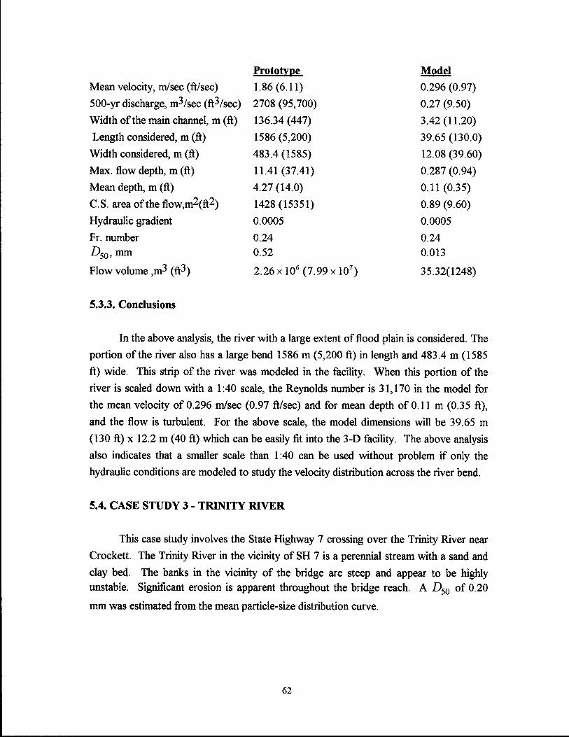
Prototype Model
Mean velocity, m/sec (ft/sec) 1.86 (6.11) 0.296 (0.97)
500-yr discharge, m3 /sec (ft3 /sec) 2708 (95, 700) 0.27 (9.50)
Width of the main channel, m (ft) 136.34 (447) 3.42 (11.20)
Length considered, m (ft) 1586 (5,200) 39.65 (130.0)
Width considered, m (ft) 483.4 (1585) 12.08 (39.60)
Max. flow depth, m (ft) 11.41 (37.41) 0.287 (0.94)
Mean depth, m (ft) 4.27 (14.0) 0.11 (0.35)
C.S. area of the flow,m2(ft2) 1428 (15351) 0.89 (9.60)
Hydraulic gradient 0.0005 0.0005
Fr. number 0.24 0.24
Dso• mm 0.52 0.013
Flow volume ,m3 (ft3) 2.26 x 10⁶ (7.99x10⁷) 35.32(1248)
5.3.3. Conclusions
In the above analysis, the river with a large extent of flood plain is considered. The
portion of the river also has a large bend 1586 m (5,200 ft) in length and 483.4 m (1585
ft) wide. This strip of the river was modeled in the facility. When this portion of the
river is scaled down with a 1:40 scale, the Reynolds number is 31, 170 in the model for
the mean velocity of 0.296 m/sec (0.97 ft/sec) and for mean depth of 0.11 m (0.35 ft),
and the flow is turbulent. For the above scale, the model dimensions will be 39.65 m
(130 ft) x 12.2 m (40 ft) which can be easily fit into the 3-D facility. The above analysis
also indicates that a smaller scale than 1:40 can be used without problem if only the
hydraulic conditions are modeled to study the velocity distribution across the river bend.
5.4. CASE STUDY 3 - TRINITY RIVER
This case study involves the State Highway 7 crossing over the Trinity River near
Crockett. The Trinity River in the vicinity of SH 7 is a perennial stream with a sand and
clay bed. The banks in the vicinity of the bridge are steep and appear to be highly unstable. Significant erosion is apparent throughout the bridge reach. A D50 of 0.20
mm was estimated from the mean particle-size distribution curve.
62

. ' ·• •. .r ~~-~.
~ i £ . . ' - '
·~.... . . . ..
Site selected for J :25 scale Modeling
. -~ - - --=::--:--:----=--=--~~+~~~ {} ... ' • • . r • • • ..
; I
.. CJ
..
. . . .. ~ • : I
: : ·' . . _,.
.t • . , ·1
., ..
..
-1
I ""
. ..... '·
Figure 5.5. Topographic Map of Bridge Site Where State Highway 7 Crosses the
Trinity River Near Crockett, Texas /
(Source: Level II Bridge Scour Analysis, January, 1993 by USGS, Water Resources Division, Texas)
63
·~··
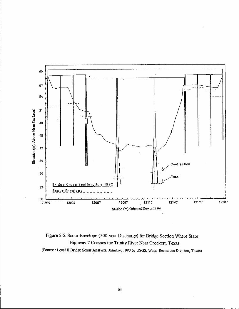
60
57
54
] 51
gj tll 48
j ~ 45
~
~ 42 c: 0
·~ ill 39
36
33·
30 11997
Bridge Cross Section, July 1992
~~~~~~ajo_p~---------
12027 12057 12087 12117
Station (m) Oriented Downstream
~Contraction
12147 12177
Figure 5.6. Scour Envelope (500-year Discharge) for Bridge Section Where State
Highway 7 Crosses the Trinity River Near Crockett, Texas
(Source: Level II Bridge Scour Analysis, January, 1993 byUSGS, Water Resources Division, Texas) /
64
12207

The 100-yr and 500-yr peak discharges were determined to be 3297 m3 (116,500 ft3)
and 4322 m3 (152,700 ft3), respectively. The site selected to model in the facility is
shown in Figure 5.5, and the cross section with the predicted scour envelope at the bridge
location is shown in Figure 5.6.
5.4.1. Objective
The predicted scour depth is significant in the main channel as shown in Figure 5.6,
and the foundation would be undermined if it is not protected. Because the scour depth
is not significant in the overbank areas, only the main channel needs to be considered for
physical modeling. The main objective here is to model the main channel for detailed
analysis of scour depth and placement of scour counter measures.
5.4.2. Analysis
According to the hydraulic calculations and the scour equations, significant scour
occurs only at the two central piers of the bridge as can be seen in the scour envelope
(Figure 5.6). Because scour around the piers in the left and right overbank areas is not
significant, only a part of the channel is taken for modeling in the facility. To model this
part of the channel, discharge in this part of the channel, width, depth, area of cross
section, and water surface elevation are computed using WSPRO. The flood plain is not
modeled in this example because the scour depth is not significant in the flood plain.
Some of the model and prototype parameters are given below. The total width of the
channel considered is 103 m (3 3 8 ft). Scales of 1: 17 and 1 :25 are used in this case study.
The length of the prototype that can be modeled in the facility is 622.2 m (2040 ft) if a
1: 17 scale is used, and 851 m (2790 ft) if a 1 :25 scale is used.
Condition for initiation of motion: At a higher Reynolds number, any particle will be
dislodged for a' If/' value of 0.056. For the above prototype conditions, If/= 4.53. This
value is about 80 times the value required for the initiation of motion. For the model
conditions, ifthe real material from the prototype is used, If/= 0.226. This value is about
4 times the value required for the initiation of motion. If a light weight material with a submerged specific gravity of 0.35 and D50 of 0.2 mm is used, If/ takes a value of 1.056
which is about 19 times the value required for the initiation of motion.
65

Prototype Model
Scale 1:17
Mean velocity, m/sec (ft/sec) 1.49 (4.89) 1.15 (0.35)
500-yr discharge, m3/sec (ft3/sec) 1885(66,600) 1.58 (55.89)
Width of the main channel, m (ft) 209.5 (687) 12.33 (40.41)
Left edge of the channel, m (ft) 159.2 (522)
Right edge of the channel, m (ft) 262.3 (860)
Width of the channel considered, m (ft) 103 (338) 6.1 (19.88)
Max. flow depth, m (ft) 17.6 (57.71) 1.03 (3.39)
Mean depth, m (ft) 12.66 (41.51) 0.74 (2.44)
C.S. area of the flow, m2 (ft2) 1304 (14,021 ft2) 4.51 (48.52)
Hydraulic gradient 0.0001 0.0001
Fr. number 0.21 0.21
Dso 0.20 0.012
Flow volume, m3 (ft3) 1.11x10⁶( 3.91x10⁷
) 165 (5822)
Prototype Model
Scale 1:25
Mean velocity, m/sec (ft/sec) 1.45 (4.75) 0.29 (0.95)
500-yr discharge, m3/sec (ft3/sec) 1885(66,600) 0.60 (21.31)
Width of the main channel, m (ft) 209.5 (687) 8.38 (27.48)
Left edge of the channel, m (ft) 159.2 (522)
Right edge of the channel, m (ft) 262.3 (860)
Width of the channel considered, m (ft) 103 (338) 4.12 (13.52)
Max. flow depth, m (ft) 17.6 (57.71) 0.7 (2.31)
Mean depth, m (ft) 12.66 (41.51) 0.51 (1.66)
C.S. area of the flow, m2 (ft2) 1304 (14,021) 2.09 (22.43)
Hydraulic gradient 0.0001 0.0001
Fr. number 0.21 0.21
Dso 0.20 0.012
Flow volume, m3 (ft3) 1.11 x 10⁶ ( 3. 91 x 10 7 ) 71.0 (2503)
66
5.4.3 Conclusions
In this case study, the scour is not significant around the piers in the left and right
overbanks. The scour is significant only in the main channel around the piers located in
the central part of the river. Therefore, it is concluded that it is necessary to test only
that part of the channel in the modeling facility. So, some part of the channel, whose
width is 103.1 m (338 ft), was considered where the scour is significant. With 1:17 scale
the model flow volume was computed as 165 m3 (5822 ft3). Since this model flow
volume is relatively large, a scale of 1 :25 was selected, and the model parameters were
computed as shown in the above table. Because the modeling of the flood plain is not
necessary, and also the depth is relatively large, the two-dimensional facility should be
used for this study.
5.5. CASE STUDY 4 - GUADALUPE RIVER
This case study involves the US Highway 183 crossing over the Guadalupe
River near Hochheim, Texas. The Guadalupe River in the vicinity of this crossing is a
perennial stream with a sand and clay bed. Significant meanders are present upstream of
the crossing. The channel is located near the left boundary of the flood plain where the terrain rises sharply up a steep hill. A D50of 0.60 mm was estimated from the mean
particle size distribution curve. The 100-yr and 500-yr peak discharges were found to be
4302 m3 (152,000 ft3) and 7839 m3 (277,000 ft3), respectively. The site selected to
model in the facility is shown in Figure 5. 7, and the cross section with the predicted scour
envelope at the bridge location is shown in Figure 5.8.
5.5.1. Objective
In this case study, the width of the flood plain is 1322.18 m (4335 ft) which is
considered to be very large compared to the other flood plains. The main objective of
this case study is to study the scour around the piers located across the entire channel
cross-section due to pressure flow which will occur if the discharge exceeds 4613 m3
(163,00 ft3).
67
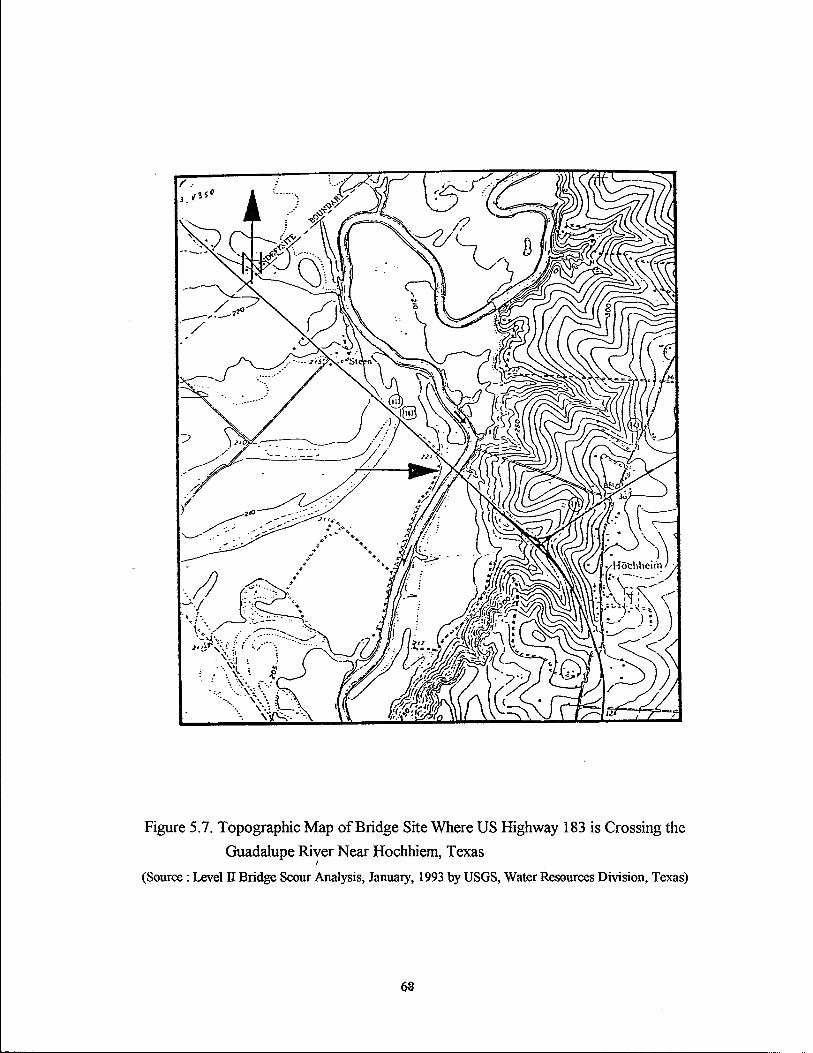
-~~ .~./
---PJ'
Figure 5.7. Topographic Map of Bridge Site Where US Highway 183 is Crossing the
Guadalupe River Near Hochhiem, Texas ..
(Source : Level II Bridge Scour Analysis, January, 1993 by USGS, Water Resources Division, Texas)

] ...:I
"' G) Cl)
l G)
> 0
~ g c:
.9
~ m
66
63
60
57 -
54
S1
48
Contraction
~
~ Tot at
-1-
-------~-- ------ --
Bridge Cross Section, August 1992
~~~~~~~~~-----------45..._....~~~~~~~~~~~~~~~~~~~ .......... ~~~~~~ .......... ~~ ........... ~ .......... ~ .......... ..._._ ......
1822 1852 1882 1912 1972 2002 2032
Station (m) Oriented Downstream
Figure 5.8. Scour Envelope (500-year Discharge) for Bridge Section where US Highway
183 Crossing the <:Juadalupe River Near Hochheim, Texas
(Source: Level II Bridge Scour Analysis, January, 1993 by USGS, Water Resources Division, Texas)
69
2055

5.5.2. Analysis
The Guadalupe River in the vicinity of US 183 is a perennial stream with
significant meanders present upstream of the crossing. The overtopping discharge that
would reach the low steel elevation of the main bridge was estimated as 4613 m3
(163,000 ft3). This discharge will be the largest discharge in all of the case studies, and
the facility designed for this discharge will probably have the largest sump and highest
pump capacity if we use a large scale model in the 2-D flume. So, this case study is more
useful for the design of the above components of the facility.
Because the width of the flood plain is 1322 m (4,335 ft) compared to the main
channel width of232 m (760 ft), it may also be required to model the flood plain. But it
may not be necessary to model the entire flood plain. Some part of it can be truncated by
analyzing velocity distribution on the flood plain using FESWMS.
Some of the prototype and model parameters computed with a scale of 1 : 50 are
given below. For the above scale, the mean depth in the channel is very small. This very
small depth might not provide reliable information on scour depth. Therefore, these
values of the 3-D model may be good for studying the flow distribution. If the scour
depth is to be studied only in the main channel, a scale of 1: 15 is selected and the model
parameters are computed as shown in the following table. In the model (1 :50), the
Reynolds number is calculated as 9,502 using a mean velocity of 0.21 m/sec (0.69 ft/sec)
and a mean flow depth of0.05 m (0.15 ft). The above Reynolds number indicates that the
flow is turbulent in the model, since it is greater than 2,000.
Condition for initiation of motion: At a higher Reynolds number, any particle will be
dislodged for a' f//' value of 0.056. For the above prototype conditions, f// = 1.18. This
value is about 21 times the value required for the initiation of motion. For the model
conditions, if the real material from the prototype is used, f// = 0.02. This value is about
0. 41 times the value required for the initiation of motion. Therefore, the material may not move. If the light weight material with a submerged specific gravity of0.35 and D50
of 0.2 mm is used, f// takes a value of 0.32 which is about 6 times the value required for
the initiation of motion.
70

Prototype Model
Scale 1: 50
Mean velocity, m/sec (ft/sec) 1.49 (4.89) 0.21 (0.69)
500-yr discharge,m3/sec (ft3/sec) 4613 (163,000) 0.261 (9.22)
Width of the main channel, m (ft) 232 (760) 4.64 (15.2)
Width of the flood plain, m (ft) 1322.18 (4,335) 26.44 (86.7)
Length, m (ft) 2135 (7000) 42.7 (140)
Max. flow depth, m (ft) 15.39 (50.46) 0.31 (1.01)
Mean depth~ m (ft) 2.35 (7.70) 0.05 (0.15)
C.S. area of the flow, m2 (ft2) 3103 (33,360) 1.24 (13.34)
Hydraulic gradient 0.0005 0.0005
Froude number 0.39 0.39
Dso, mm 0.6 0.012
Flow volume, m3 (ft3) 6.61x10⁶ (2.34x10⁸) 52.86 (1868)
To model this as a 2-D model, a part of the main channel is selected from the left
edge of the channel at 1824 m (5980 ft) to the right edge of the channel at 1908 m (6257
ft), i.e., a total width of 84.5 m (277 ft). The model parameters for 1:15 scale are shown
in the following table.
Prototype Model
Scale 1:15
Mean velocity, m/sec (ft/sec) 1.49 (4.89) 0.38 (1.26)
500-yr discharge, m3/sec (ft3/sec) 1072 (37873) 1.23 (43.5)
Width of the channel, m (ft) 84.49 (277) 5.64 (18.5)
Width of the flood plain, m (ft) 1322.18 (4,335) 26.44 (86. 7)
Length, m (ft) 549 (1800) 36.6 (120)
Max. flow depth, m (ft) 15.39 (50.46) 1.03 (3.36)
Mean depth, m (ft) 8.53 (27.96) 0.57 (1.86)
C.S. area of the flow, m2 (ft2) 720.5 (7745) 3.2 (34.4)
Hydraulic gradient 0.0005 0.0005
Fr. number 0.39 0.39
Dso, mm 0.6 0.04
Flow volume, m3 (ft3) 3.94x10⁵ (1.39x10⁷) 117 (4128)
71

5.5.3 Conclusions
The width of the flood plain in this case study is extremely large and can be
modeled only in the three-dimensional facility. Scour is also significant in the entire
cross-section. The overtopping discharge is very large in the river, which, when modeled
in the facility, can be used for sizing the pump capacity and sump size. These sizes are
determined later in the design of the facility. To avoid laminar flow for low discharges,
some kind of artificial roughness may be required in the model. A scale of 1: 50 was
chosen to model the river in the 3-D model. The total length of the prototype that can be
modeled in the facility is 1982.5 m (6,500 ft) with a model dimension of39.65 m (130 ft).
If this is considered in the 2-D model, the flow capacity is calculated as 1.23 m3/sec (43.5
ft3/sec).
5.6. CASE STUDY 5 - NAVASOTA RIVER:
In this case study, a section of the Navasota River which is shown in Figure 5.9 is
taken, and velocity distribution across the flood plain is found using FESWMS. Figure 5.9
shows contours for a section of the Navasota River. The upstream open boundary is at
the top of the map, while the downstream open boundary is the solid line near the bottom
of the map. The flow rate is taken as 849 m3/sec (30,000 ft3/sec), and the corresponding
downstream water surface elevation is 65.58 m (215 ft). The map scale is 1 in= 1500 ft.
The roughness coeffient of the shaded area is 0.15, and the open area roughness
coefficient is 0. 08.
5.6.1. Objective
Modeling the entire flood plain in the physical modeling facility is difficult because
of scale selection. The flood plain can be truncated knowing the velocity distribution on
the flood plain. The objective here is to demonstrate how the flood plain can be truncated
before modeling in the facility.
5.6.2. Analysis:
The total flood plain is divided into number of elements as shown in Figure 5.10.
Initially, a network of elements is designed and plotted using DINMOD. Ground contours
are also plotted using DINMOD and shown in Figure 5.11 in combination with the
72

network of elements. A discharge of 849 m3/sec (30,000 ft:3/sec) and a corresponding
downstream water surface elevation of 65.58 m (215 ft) are used as the input data for
FLOMOD and water surface elevations at regular intervals, velocity vectors, and velocity
distribution are found across the flood plain. The velocity vectors and water surface
contours are plotted using ANOMOD and shown in Figure 5.12. Let 'A' be a point in the
flood plain which is on the left side of the river and 'B' be a point in the flood plain which
is on the right side of the river as shown in Figure 5.12. Because it is difficult to model
the entire width of the flood plain, it is truncated and the portion which is between A and
B can be considered for modeling. The discharge passing across AB can be calculated
since the depth and velocity at any given point in this portion of the flood plain is known.
This discharge will be used in the model while maintaining the velocity distribution and
water surface elevation across AB in the model. The width of the flood nlain can be
truncated along the entire length of the flood plain, i.e., from the upstream boundary to the
downstream boundary so the central portion including the river can be modeled for any
discharge after finding the velocity distribution and water surface elevations by using
FESWMS.
5.6.3. Conclusions
The width of the flood plain in this case study needs to be truncated in order to fit
into the facility using the reasonable scale. The left side of point A and right side of point
B is truncated, and the portion across AB is to be modeled after knowing the velocity
distribution, water surface elevation, and discharge which are computed by FESWMS.
This description is for the section across the flood plain and along AB. Similarly, the width
of the flood plain can be truncated along the length on both sides of the river. As shown
in Figure 5.12, the portion between the lines PAQ and RBS can be modeled in the facility
when the velocity distribution, water surface elevation, and discharge obtained from
FESWMS is reduced to scale and by maintaining them in the model.
73

J
Figure 5.9. Topomap of a Section of Navasota River and its Flood Plain
(Source: Finite Element Surface Water Modeling System (FESWMS-2DH)-Users Manual)
74

,,_-,----.----,.---"il'----iUpstream boundary
Elements
Figure 5.10. Network of Elements on the Flood Plain of Navasota River
75

Figure 5.12. Water Surface Contours and Velocity Vectors on the Flood Plain
77

6. SURVEY OF EXISTING HYDRAULIC LABORATORIES
6.1. OBJECTIVE OF THE SURVEY
At the meeting held in College Station with TxDOT officials and others in
November 1993, it was decided to visit some major hydraulic laboratories in the country
to evaluate the type of models and scales used at existing large facilities. It was also
decided at the same meeting to prepare a questionnaire to be sent to all the labs that were
to be visited by the principal investigators of the project. The facilities visited were the
USAE Waterways Experiment Station (WES), Vicksburg, Mississippi; the Federal
Highway Administration (FHW A) Hydraulic Laboratory, McLean, Virginia; the University
of Minnesota (St Antony Falls) Minneapolis, Minnesota; and Colorado State University
(CSU) Fort Collins, Colorado.
6.2. THE QUESTIONNAIRE
A questionnaire was prepared to circulate to the persons-in-charge of the four
above mentioned hydraulic facilities. The prepared questionnaire was circulated to all the
persons present at the meeting to obtain their opinions. The questionnaire was organized
into four sections as listed below:
1. Personnel and their experience
2. Physical dimensions and instrumentation
3. Physical modeling
4. Cost analysis
The questions in each section are presented here. All the questions were answered
when the principal investigators visited these facilities.
6.2.1. Personnel and Experience
1. Please check one. You are a (a) Technician (2) Graduate Student (3) Professor
2. How long have you been involved with hydraulic facilities?
3. How long have you been involved with this facility?
4. Is this facility indoor or outdoor?
5. What is your opinion of an outdoor facility?
79

6. How many people are employed in your facility, and what is their expertise?
7. What type of problems do you model in your facility?
6.2.2. Physical Dimensions and Instrumentation
1. What kind of facility do you have to study river hydraulics and bridge scour problems?
2. What are the physical dimensions of the facility?
3. How do you arrive at these dimensions?
4. What was the criterion used to decide on the maximum flow rate that needed to be
handled by the facility?
5. What flow control devices do you have to control
(A) The discharge into the flume?
(B) The water surface profile?
6. How do you recirculate the flow?
7. Where is the location of the pumps in your facility?
What type of pumps do you use?
8. What is the instrumentation used in your facility to measure flow velocity and bed
profile?
9. What additional instrumentation would you like to have in your facility?
10. What improvement would you like to make to your facility?
6.2.3. Physical Modeling
1. What problems associated with river modeling and scour modeling have you studied in
your facility?
2. What kind of prototype to model scale ratios do you typically use?
Do you use distorted models or undistorted models?
3. How do you model and scale cohesive soil in the facility?
4. How do you model and scale cohesionless soil in the facility?
5. Have you ever modeled rate of scour in your facility? If yes, how do you relate the
rate of scour in the model to the rate of scour in the field?
6. How do you convert the scour depth in the model to the scour depth in the field?
7. Have you ever conducted testing for stream stability problem? If yes, what kind of
problem did you study?
8. How do you model a river bend?
9. How do you model non-uniform flow in similar situations?
80

10. How do you approach the problem of modeling the extent of a flood plain?
11. If you were asked to develop a new and large facility to simulate scour problem, what
would you pay particular attention to?
6.2.4. Cost of the Facility
1. What is the cost of the major installations in your facility?
(a) Pumps
(b) Flumes
2. How much would the facility cost, if it were built today?
3. What is the current operation and maintenance cost?
4. How do you meet this expenditure?
5. What is the availability of the facility ? Is there any waiting time?
6. What are the charges normally collected for usage of the facility?
6.3. THE VISITS
The visits to the above mentioned facilities took place between January 3-
6, 1994 and on January 21st, 1994 (CSU). The main objective of these visits was to
evaluate the existing facilities for their use by the TXDOT and also examine whether these
facilities can be effectively utilized to study the scour problem in bridges. The summary of
results is presented in tabular form as follows:
81
6.3.1. Personnel and Experience
Q.No WES FHWA U Of Minnesota CSU
1 Person Interviewed Facility Manager Facility Manger Facility Manager Facility Manager
and Faculty Member
2 Experience with 12 Yrs
Hydraulic Facilities 32 Yrs 30 Yrs & 25 Yrs
21 Yrs
3 Experience with 12 Yrs
Present Facility 32 Yrs 10 Yrs & 5 Yrs
16 Yrs
4 Indoor or Outdoor Mainly Indoor Indoor Indoor Both
Facility
5 Is Outdoor facility Limitation is Wind Limitation is Climate Climatic Limitation Necessary but
Necessary? and Weather limited by Weather

00 w
Q.No
6
7
No. of Persons
Employed
Type of Problems
Modeled
WES FHWA
140 in Hyd. Lab 2 Full-time
REs, Scientists, 2 Part-time
Technicians
* Any Hydraulic *Highway drainage
Structure *Culvert
* Movable and *Scour
Fixed Bed Models *Abutments
U of Minnesota CSU
12 Faculty 12 Faculty
7 Staff IRA
36 Graduate 25 Graduate and
Students Undergraduate
Students
7 in Work Shop
*General Hydraulics *Erosion &
*Wind Engineering Sedimentation
*Intake Structures *Stream Stability
*Spillways *Hydraulic
*Movable Bed Structures
Models *Hydromechanics
*Flow
Measurements

6.3.2. Physical Dimensions and Instrumentation
Q.No WES FHWA U of Minnesota CSU
1 Type ofFacility And Study of Various One Dimensional 3-D Flumes and Four Flumes
Description Hydraulic Problems Flume Channel Flumes Two 3-D Flumes
2 Physical Dimensions 67 x30 51 x9.1 x0.6 60.1 x 2.4 x 1.2
Length(m) x 237 x 6.7 x 3.6 13.7 x 7.6 x 1.52 54 x 6.1x2.4
Width(m) x Rip rap facility 21x1.82 x 0.6 12.2 x 7.6 x 0.91 30 x 6.1x1.2
depth(m) 76.2 x 2.7 x 1.82 30 x 6.1x2.4
Channel 36 x 12 x 1.2
* Tilting type also
but not necessary
for Scour.
3 How Physical * Money Available *Experience *Available Space *Project Specific
Dimensions are *Space available
arrived at?

Q.No WES FHWA U of Minnesota CSU
4 Max. Flow Rate *Produce the Design *Velocities to be "' Design Flood *Project Specific
Criterion Stage Flood Created (for Mississippi
*Max. Sub-Critical 0.42 m3/sec(15 cfs) 8.5 m3/sec or 300 Up to 6 m/sec (20
Flow cfs) ft/s) flume
*Most Flood Upto 2.8 m3/sec
Channel ( 100 cfs) Indoor
5.6 m3/sec (200 cfs) >4.2 m3/sec (150
for rip rap cfs) Outdoor
facility
5 Control Devices
(A) For Flow "' Venturi Meter "' Bypass Valves, "'Orifices "' Orifice plate on
"' Valves, Weirs *Pumps with "' Venturi Meters pipe line with
Variable Frequency "'Valves manometer or
Drive pressure transducer
(B) Water Surface "' Point Gauges to *Point gauges "' Point gauges
Profiles Measure "' Tail gate on Flume *Tail gates "'Tail gate
"' Tail Gates to
Control

00 .--.!
Q.No
9
10
WES
Additional "' Automation
Instrumentation
Required
Improvements like to Temperature Control
have for the present
Facility
FHWA U of Minnesota CSU
"' Direct Measure of * Automation "' Laser Doppler
Shear Stress
(Velocity Profile)
Laser- Expensive
Recirculate Sediment "' Better Flow "' Automation
Control Devices "'Great
"' Maintenance variability
"'440 Motors
instead of 110 or
220

6.3.3. Physical Modeling
Q.No WES FHWA U of Minnesota CSU
1 Problems Studied Bridge scour Protection around Stream stability Pier and abutment
Development of piers of different Flow changes scour,
navigation channel shapes created by new Particle size,
Rip rap protection structures Physical scour
against erosion model,
Rip rap and tetrapod
for erosion control,
Pressure scour
2 Scale Ratios In River Engineering 1:20 to 1:50 1:10 to 1:500 1:3 to 1 :40
1 : 100 Vertical Undistorted models Based on Reynolds Undistorted models
1 :250 Horizontal and Froude numbers
Distorted Models
For Hyd. Structures
1:24 to 1:36
l:lOto 1:120
Undistorted models

Q.No WES FHWA U of Minnesota CSU
3 Model Cohesive Clay Electrochemical
soils Properties,
Stratigraphy,
Do not model ......... Bentonite, ... ......
Fly ash.
4 Modeling Criteria Crushed Coal, Do not Scale Soil, • u: Natural Soil, 't
= (PX, -1)gD Sand, Gravel, and Match Incipient Scale by Length
Crushed stone Velocity ratio, forBed load
Scale by Specific LI· - for suspended Gravity Vs
load
5 Rate of Scour ............... ... ............ For Bridge Piers Not Important for
Constriction Scour cohesionless soils
6 Converting Scour Qualitative rather Dmodel X Scale Dmodel X Scale By Scaling in
Depth To Prototype than quantitative for Vertical Direction
hydraulic structures
Believe deeper in the
model than in field

Q.No WES FHWA U. of Minneosta CSU
7 Stream Stability Limited as difficult
to model ***"'"' Some Experience Some Experience
8 Model River Bend Right shape and go Field radius of Curve In large flume
to next bend way = Scale X Radius of
*"'*** Curve in laboratorv
9 Nonuniform Flow Let the river shape By using manifolds
the flow, Tail water control,
Use the model for "'"'*** **"'** Modify the model.
inflow pattern
surface pattern
10 Flood Plain Model to the levee HEC2Runs. Scale the whole plain
and adjust horizontal Truncate the model. and distort the
scale, ***** 1/4 to 1/3 of flood model,
If needed, give up on plain at least. Cut off based on
the flood plain expenence.
11 Attention to be paid Big Scale like 1: 10 Nature of Problems, Smaller scale for Velocity > 10 ft/sec,
to 1: 1. Reach Length, global feature, Depth
Large flow capacity Channel Migration, Local scale large,
Type of Materials

6.3.4. Cost of the Facility
Q.No WES FHWA U of Minnesota CSU
1 Cost of Major
Installations 1.46 m3/sec (50 cfs)
(A) Pumps - $ 40,000 0.28 m3/sec (10 cfs) 600 hp pump 1.46 small $30,000
0.28 m3/sec (10 cfs) - $ 30,000 m3/sec (50 cfs) cost For whole facility
- $ 15,000 $ 0.25 million $ 20 millions
(B) Flumes 30 m x 60 m with Big Indoor tilting
sump - $ 2 million $ 450,000 includes :l'c:l'c:l'c:,.,l(:l'c type $ 1.2 million.
(Sump, Flume, 0.14 m3/sec (5 cfs) Outdoor $ 0 .4
Water supply and pump, million
Building) Building - $0.5
Rip rap Facility million
$ 1.2 Million
2 Cost today Mississippi river 10 yrs of inflation $ 10 million.
model - $ 0.25
million ******** Bridge scour facility
- $ 5-10 millions

Q.No WES FHWA U. of Minnesota CSU
3 O&MCost Rip rap and river $ 150,000 per year Electricity, utilities $ 40,000 per year
model operation cost includes two people and 3-4 people for plus backlog $ 1. 0
- $ 25,000 per the whole facility - Million
month. $150,000 per year.
Maintenance - $1000
per month
4 How to meet the R&D budget Budget + Support Soft money over ...............
expenditure services Contract head
5 Availability of the Rip rap through Sets own priority - Responsive Depends
facility 1996 5 year plan cooperative Immediate to 4
67 m x 30 m (220 ft Plan for DOTs months to 2 years
x 100 ft) available Flexible work force.
now with 0.56
m3/sec (20 cfs)
6 Charges for testing Approx $25, 000 No charge for DOTs No separate charge, Model-$ 65,000
per month for Testing+ Total - $ 150,000
engineering and construction for
technical + model 9.1 m x 30 m (30 ft x
building 100 ft) is
$ 150,000.
Construction - $ 80-
100 k.

6.4. IMPRESSIONS FROM THE VISITS
Following the visits to the facilities, a summary of the impressions of the principal
investigators is presented below.
6.4.1. USAE Waterways Experiment Station
1. Very extensive and large scale facility.
2. The facility can be easily modified for scour studies.
3. The personnel is most experienced with river qualitative hydraulics studies in movable
beds.
4. They have experience with movable beds in cohesionless soils only.
5. The soil simulant used is crushed coal, mostly loosely placed and drained.
6. They do not believe that scour in model can represent scour in the prototype
quantitatively.
7. Cost appears to be high.
8. Availability could be a problem. The priority in this facility is to WES business.
9. They have no experience in cohesive soils and rate of scour.
10. Stream stability problems are not modeled in this facility because cohesiveness of the
banks can not be modeled.
11. Most models used are 0.3 m of soil and 0.2 m of water or less.
12. They proposed a full scale scour experiment behind a Corps of Engineers dam.
6.4.2. FHW A Hydraulic Laboratory
1. A small laboratory when compared to other laboratories visited.
2. Small scale scour tests are conducted on specific requests from states.
3. Not big enough to develop as a facility that could be used by TxDOT in the future.
4. The facility works very well for what it was intended to be.
6.4.3. University of Minnesota Hydraulic Laboratory
1. The personnel is very knowledgeable and has sound fundamental principals.
2. They have experience in fundamental research using a combination of numerical
simulation and physical modeling.
3. This is a very busy facility.
93

4. They conduct 75% of basic research and 25% of problem oriented research.
5. Testing area is smaller than the one in WES.
6. Water capacity is very large as the facility takes water directly from river.
7. They have a sound understanding for cohesionless soils scaling.
8. They have experience in stream stability problems and, to some extent, with the rate of
scour also.
6.4.4. Colorado State University Hydraulic Laboratory
1. The personnel is knowledgeable in scour problems.
2. The research conducted in this facility is applied research.
3. This is a busy facility.
4. Water capacity is large.
5. The size of the facility is very large and can handle large 3-D and 2-D models.
6.4.5. Advantages and Disadvantages of Existing Facilities
The advantages and disadvantages of the existing facilities and of the new facility
are:
For an existing facility, there is no initial investment, and experienced personnel are
readily available. Overhead rates are many times higher (approximately 45%) than what
can be offered under the SP&R program (7%). The availability of an existing facility is
not very sure. Travel expenditure will be very high for TxDOT personnel when traveling
to an existing facility compared to a Texas facility.
If a new facility is developed, the TxDOT will have low overheads (7% ), and low
travel expenditure. It will also develop local expertise. It will be easy to draw contracts,
and availability will be a enhanced. The drawbacks will be a sizable initial investment and
personnel with limited experience to start with.
94
7.0. NEW SCOUR FACILITY CHARACTERISTICS
7.1. INTRODUCTION
A physical modeling facility is a useful tool for studying problems associated with
river hydraulics, pier scour, gradation, scour at site specific-locationi sizing of rip-rap,
pressure scour, constriction scour, and bank erosion. The design of a physical modeling
facility requires hydraulic particulars at the bridge site and also the data regarding the soil.
These data were obtained from TxDOT which included field measurements conducted at
various locations on five major rivers in Texas. The following range of hydraulic
conditions were provided by TxDOT.
Channel velocity
Channel discharge
Flood plain width
Depth of river
= 0.3048 mis to 3.048 mis (1 to IO ft/s)
= 85 m3/sec to 5097 m3/sec (3000 to 180,000 cfs)
= 91 m to 6.4 km (300 ft to 4 miles)
= 1.524 m to 15.24 m (5 to 50 ft)
Hydraulic conditions may vary significantly from one river to another. Detailed
information at five sites were obtained from reports on Level II bridge-scour analysis done
by the United States Geological Survey (USGS) Texas District for TxDOT.
7.2. DESIGN OF THE 2-DIMENSIONAL FACILITY
A preliminary design is done for the hydraulic testing facility based on the data
available from the reports by USGS. It is not feasible or economical to study all the
features of scour problems in one modeling facility due to the wide range of prototype
conditions that may be encountered. Considerable advantage and economy can be gained
by constructing two modeling facilities:
a) a 2-D flume for studying bridge-scour at fairly large scale, and
b) a 3-D river basin for studying problems related to flood plain, for example, at a
smaller scale than the 2-D models.
Some values from the case studies are used to design the components of the
modeling facility. The Trinity River case study is used to design a 2-D modeling facility.
This case study is selected because a large volume of flow is required to model this site.
Similarly, data were taken from other case studies to design a 3-D river basin. For
95

example, the flow volume from case study-4 with a I : 50 scale is used to design the sump,
and the model discharge is taken from case study-I to design the pump capacity for the 3-
D modeling facility. In the design, the following components are discussed.
1. Dimensions of the 2-D flume and the 3-D river basin
2. Sump to store the water
3. Pump capacity
4. Flow control devices
5. Flow distribution
6. Surface Elevations
7. Flow Measuring Devices
8. Operation and maintenance
9. River banks
10. Soil used for sediments
7 .2.1. Selection of Model Parameters
To design a 2-D modeling facility, case study-3 or case study-4 with I: 15 scale can
be used. Out of these two case studies, case study-3 has the largest discharge and flow
volume that can be used in the design of the pump capacity and sump capacity in the
facility. The sump designed in this case study is useful for the 2-D facility because the
model parameters are pertaining to a 2-D model in which the flood plain did not need to
be modeled. So, in the design of 2-D facility, the parameters from case study-3, i.e., the
hydraulic data near the bridge site at the State Highway 7 crossing over the Trinity River
near Crockett, is used. The parameters are given below:
Width of the River Wp = 208.2 m (687 ft)
Width of the channel considered = 102.4 m (338 ft)
Depth of the River Dp = 12.58 m (41.51 ft)
Area of Cross Section Ap = 1288 m2 (14,021 ft2)
500 year discharge Qp = 1885 m3/sec (66,600 ft3/sec)
Width of the facility = 6.06 m (20 ft)
Length of the facility = 30.3 m (120 ft)
Mean velocity in the river Vp = 1.45 m/sec (4.75 ft/sec)
96

Assume a scale of 1 : 17 and an undistorted model.
Model width = 6.024 m (19.88 ft)
Model Depth Dm = 0.74 m (2.44 ft)
Velocity in the model Vm = 0.35 m/sec (1.15 ft/sec)
Discharge in the model for 500 year flood, Qm = 1.58 m3/sec (55.89 ft3/sec)
Cross section of the model at the bridge location, Am= 4.51 m2 (48.52 ft2).
7 .2.2. Preliminary Design of the Flume
As mentioned in chapter 5 the dimensions of the 2-D flume are taken as 36.6 m
(120 ft) length, 6. lm (20 ft) wide, and 3.66 m (12 ft) deep which is shown in Figure 7.1.
Considering a scale of 1 :20, the parameters of the prototype that can be modeled in the
basin are estimated as:
Width= 121 m (400 ft)
Length= 727 m (2400 ft)
In case studies 3 and 4, the widths and lengths of the prototypes are less than the above
values which indicates that the basin dimensions are sufficient to model major rivers in
Texas at a large scale.
7.2.3. Sump design (2-D)
The size of the sump is based on the maximum storage volume that should be
handled in the model study. The storage volume of the flume must be stored in the sump
when the model is not working. As mentioned in the previous section, the size of the
flume is taken as 36.6 m (120 ft) length, 6.1 m (20 ft) wide, and 3.66 m (12 ft) deep.
Assume the depth of water in the flume is 1.8 m (6 ft). Storage volume in the flume is
equal to 36.6 x 6.1 x 1.83 = 408.57 m3 (14,400 ft3). The sump must be able to handle the
storage volume of 408.57 m3. Since the flow volumes in case studies 3 and 4 are smaller
than the above storage volume, the sump can easily handle the flow volumes in the case
studies.
97

Cylindrical pier
Sediment recess
Sump (3.03 m wide) Tail gate
6.1 m
1-- 36.6 01
Figure 7.1. Plan of Open Channel Flume and Sump
Assuming the sump is constructed all around the facility, the cross section area of the
sump 1s: - 408.57 - 2 ( 43 ft2) A5 - 2(36.6 +6.1) -4. 78 m 51.
Assume a width of3.03 m (10.0 ft).
Depth of the sump, D 8 = 1.57 m (5.14 ft)
In order to store excess water in the sump when the model is running for a 500-yr flood,
there must be some excess depth which can be taken as 0.61 m (2.0 ft). With a free board
of 0.61 m (2.0 ft), the total depth of the sump becomes 2.79 m (9.14 ft). Therefore, the
sump will run around the facility with a width of 3.03 m (10.0 ft) and a depth of 2.79 m
(9.14 ft).
In the 2-D facility, the total cross-section of the river does not need to be modeled.
If the scour around the pier is to be studied, then some portion around the pier can be
taken and modeled. Similarly if the scour at the left abutment is to be studied, then the
cross-section of the left overbank will be taken and modeled. This is possible if the
velocity distribution is known. Let the pier be located at the center of the river. The
cross-sectional area of the flow around the pier is taken as 4.51 m2 (48.52 ft2) (Ref: case
study-3). Storage in the model for the 500 year flood simulation is calculated by
multiplying the total length of the model that can be built with the cross-sectional area of
the model river.
Storage of water in the model = 165 m3 (5822 ft3)
The sump size can be determined based on the above storage volume. Assuming
that the sump is constructed all around the facility, the cross section area of the sump is:
A = 165
= 1.93 m2 (20.74 ft2) s 2(36.6+6.1)
Assume a width of3.03 m (10 ft)
Depth of the sump, D 8 = 0.63 m (2.08 ft)
In order to store excess water in the sump when the model is running for the 500-
yr flood, there must be some excess depth which can be taken as 0.61 m (2.0 ft). With a
free board of 0.61 m (2.0 ft) the total depth of the sump becomes 1.85 m (6.08 ft). The
sump will run around the facility with a width of 3.03 m (10.0 ft) and a depth of 1.85 m
(6.08 ft). The sump designed for this case study is smaller than the previous one. So, the
sump which is designed by taking the flume storage will be sufficient for all the 2-D case
studies. The drawing of the sump is shown in Figure 7 .2.
99

...... 0 0
Cylindrical pier
/ (0.3mdia)
.------~~----__, 36.6m
Sediment recess(l m dia)
Sump
F igure 7.2. 2-D Open channel Flume and Sump
False bottom (Plywood)

The sump could also be placed at one location, or more than one can be
constructed based on the requirements at various locations; all these sumps may be
interconnected. When the pumps are running with maximum flow capacity, the flow can
be directed from other sumps, and when the pumps are running slow, water can be
redirected back into the other sumps. The other alternative is to build a large sump and
have it compartmented when its full capacity is not required.
7.2.4. Pump Capacity (2-D)
The design of the pump capacity is done in two steps. First, preliminary design is
done by taking the maximum discharge from the range of hydraulic particulars in Texas
which are given in the introduction of this chapter. QP = 5094 m3/sec (180,000 ft3/sec)
Assuming a scale of 1:20 for an undistorted model, Q 5094
Qm = -f = - 5-= 2.85 m3/sec (100.62 ft3/sec). /r2 202
The above value will be the maximum discharge that must be handled by any pump
when it is required to model the largest 500-yr flood in Texas. If this value is used to
design the pump capacity, the pump can handle any discharge in the case studies which are
smaller. The capacity of the pump is designed as follows:
Assume a soil thickness of 1.0 m (3.03 ft)above the floor.
Suction head = 2.79 m (9.0 ft)(taken from sump design)
Delivery head 2.00 m (6.0 ft)
Total head H = 4.79 m (15 ft)
Discharge Q = 2.85 m3/sec (100.62 ft3/sec)
Since future expansion of the facility may require higher flow rate, the discharge is taken
as 3.00 m3/sec.
Assume the efficiency, 11 = 80 %
WQH = 1000x3.0x4.79 Capacity of the pump = 75q 75x0.8
= 239.5 H.P
Threfore, the maximum capacity of the pump that would be needed for a general purpose
modeling facility is 239.5 H.P.
101

In the second step, the capacity of the pump is determined by taking the maximum flow
discharge from the case studies.
Assume a soil thickness of 1.0 m above the floor.
Suction head = 2.79 m (9.0 ft)
Delivery head = 2.00 m (6.6 ft)
Total head H = 4.79 m (15.0 ft)
Discharge Q = 1.95 m3 /sec (68.84 ft3/sec)
While designing, the discharge is taken as 2.5 m3/sec (88.26 ft3/sec) for future expansion
of modeling capability.
Assume the efficiency, 11 = 80 %
Capacity of the pump = WQH 75ri
1000 x 2.5 x 4. 79
75 x 0.8 = 199.58 HP
A pump of 199.58 HP may be provided or, depending on the availability of the
pumps in the commercial market a suitable number of pumps may be chosen. The capacity
of this pump is smaller when compared to the previous pump capacity. One pump with a
large capacity may be more suitable for future expansion of the modeling facility. Pumps
are kept at higher elevations and dry and can be installed at the end of the sump.
7.3. DESIGN OF THE 3-DIMENSIONAL FACILITY
In the 3-D facility, the total cross-section including the flood plain will be
considered. The 3-D facility is preferable if the scour is significant in the entire cross
section of the river as well as in the flood plain. In order to model the flood plain it is
necessary to know the velocity distribution in the prototype. The flow distribution across
the river and the flood plain can be found using FESWMS. The dimensions of the 3-D
basin are shown in Figure 7.3.
7.3.1. Selection of Model Parameters
Flow volume and flow discharge are some of the important parameters required in
the design of the sump and pump capacities of the facility.
102
1~ 30m
Figure 7.3. 3-D River Hydraulics Sediment Transport Basin
103

Out of all the case studies, case study-4 with 1 : 50 scale has the largest volume, and
case study-I has the largest flow discharge. These values should be used in the design of
sump and pump capacity. The values are given in the following:
Flow volume at any instant of time for 500-year discharge= 52.86 m3 (1868 ft3)
Discharge= 0.33 m3/sec (11.75 ft3/sec ).
7.3.2. Sump Design (3-D)
The size of the sump depends on the flow volume in the model corresponding to a
500-yr flood in the prototype, which should be modeled. Storage in the model (Case
study-4) for a 500-year flood simulation is calculated by multiplying the total length of the
model that can be built with the cross-sectional area of the model.
Storage of water in the model = 52.86 m3 (1868 ft3)
Assuming that the sump is constructed all along the facility, the cross section area
of the sump, A 8 will be obtained by dividing the flow volume by the length of the model.
A = 52
·86
= 1.16 m2 (12.45 ft2) s 45.75
Assume a width of3.03 m (10 ft)
Depth of the sump, D 8 = 0.379 m (1.25 ft)
In order to store excess water in the sump when the model is running for a 500-yr
flood, there must be some excess depth which can be taken as 0.61 m (2.0 ft). With a free
board of0.61 m (2.0 ft), the total depth of the sump becomes 1.59 m (5.25 ft).
The sump will be constructed at the center and parallel to the length of the facility
with a width of3.03 m (10.0 ft) and a depth of 1.59 m (5.25 ft). The drawing of the sump
is shown in Figure 7.4. The sump could be placed at one location as a large one, or more
than one can be constructed based on the requirements at various locations; all these may
be interconnected. When the pumps are running fast, flow can be directed from other
sumps, and when the pumps are running slow, water can be redirected back into the other
sumps.
104

-0 u.
Flood Plain delineation
River Banks
1.59m / Note: ,...,_ Flood Plain delineation line ......,,.._ ...
/
!::::: - - ~ Main River Banks
1 ..... 3.03m
Figure 7.4. 3-D River Hydraulics Sediment Transport Basin with sump below the ground

7.3.3. Pump Capacity(3-D)
The design of the pump capacity is done in two steps. First, preliminary design is
done by taking the maximum discharge from the range of hydraulic particulars in Texas
which are given in the introduction of this chapter and by using the 1 : 50 scale. QP = 5094 m3/sec (180,000 ft3/sec)
Assuming a scale of 1 : 50 for an undistorted model,
- Qp 5094 - 3 . 3 Qm--5 =-5--0.29m /sec(10.18ft /sec). l/i 152
The above value will be the maximum discharge that must be handled by any pump
when it is required to model the largest 500-yr flood in Texas. If this value is taken to
design the pump capacity, the pump can handle any discharge in the case studies which are
relatively smaller. The capacity of the pump is designed as follows:
Assume a soil thickness of 1.0 m above the floor.
Suction head = 1.59 m (5.2 ft)(taken from the sump design)
Delivery head = 2.00 m (6.6 ft)
Total head H = 3.59 m (12.0 ft)
Discharge Q = 0.29 m3/sec (10.18 ft3/sec)
Since future expansion of the facility may require higher flow rate, the discharge is taken
as 0.35 m3/sec (12.35 ft3/sec).
Assume the efficiency, fl = 80 %
Capacityofthepump = WQH = IOOOx0. 35 x 3.59 = 20.95H.P 75ri 75x 0.8
Therefore, the capacity of the pump that would be useful in all cases for this 3-D modeling
capability is 20.95 H.P.
In the second step, the capacity of the pump is determined by taking the maximum flow
discharge from the case study-1.
Assume a soil thickness of 1.0 m above the floor.
Suction head = 1.59 m (5.2 ft)
Delivery head = 2.00 m (6.6 ft)
Total head H = 3.59 m (12.0 ft)
Discharge Q = 0.33 m3/sec (11.65 ft3/sec)
While designing, the discharge is taken as 0.39 m3/sec (13.75 ft3/sec) for future
expansion of modeling capability.
Assume the efficiency, fl = 80 %
106

Capacity of the pump = WQH 75'11
lOOOx 0.39 x 3.59 _ 23
_34
H.P 75 x 0.8
One pump of 23.34 HP may be provided or depending on the availability of the
pumps in the commercial market, a suitable number of pumps may be chosen. The
capacity of this pump is larger when compared to the previous pump capacity. One pump
with a large capacity may be more suitable for future expansion of the modeling facility.
Pumps are kept at higher elevations and dry and can be installed at the end of the sump.
7.4. FLOW CONTROL DEVICES
The control of flow in the model should be given proper attention. To maintain
the required water-surface elevations, model discharge, and model flow velocity, it may be
necessary to have different flow control devices. For example, a tail gate is required to
maintain the water surface elevations; a venture meter or an orifice meter is required to
measure the flow rate. Variable speed pumps are desirable to provide a required rate of
flow in the model close to the design flow rate, while a bypass valve can be used to divert
excess flow back to the sump. Knowing the surface elevations at different cross sections
along the length of the river, it is possible to maintain the water surface profile in the
model. Prototype water surface elevations can be obtained by running WSPRO or HEC-
2. In all the case studies, it was found that the Froude number is less than unity, which
indicates that the flow is subcritical. Because the flow is subcritical, a tilting flume is not
essential for the model study.
7.5. FLOW DISTRIBUTION
Knowing the velocity distribution at any cross-section on the upstream side of the
bridge location is very important. After the velocity distribution is predicted at a particular
section by using WSPRO or FESWMS, manifolds can be used to reproduce the predicted
velocity distribution in the model at that particular section. The reproduction of velocity
distribution at the upstream section will be useful in reproducing the velocity distribution
at the bridge location where the scour takes place. WSPRO or HEC-2 can be used to
determine the distribution of the flow in the river and also on the flood plain. WSPRO will
divide the entire cross-section into twenty small cross-sections parallel to the flow
direction. Each of these twenty channels will carry 5% of the total discharge. Velocity in
all these channels parallel to the flow is obtained using WSPRO. Mannings equation is
107

used to compute the velocity. This leads to the assumption that the flow is uniform in the
river. Sometimes it is difficult to measure the velocities and the depth because they are
very low in the scaled model. The most common measuring device is the miniature
current meter with a plastic rotor. The hot film anemometer has been discarded because
of the fragility of the film and errors due to temperature fluctuations. A laser doppler
anemometer can be used, but is more expensive.
FESWMS (Finite Element Surface Water Modeling System) can also be used to
determine the two dimensional flow distribution on a horizontal plane in the river cross
section, as well as in the flood plain. The velocity distribution at the bridge section can
also be modeled using FESWMS. The model will give the water surface elevation
contours across the flood plain. After knowing the water surface elevation at any cross
section across the flood plain, the flood plain can be truncated to some limited extent.
7.6. SURFACE ELEVATIONS
Surface elevation along the river can be obtained by running WSPRO. The
elevations that can be obtained are bed elevation, bank elevation, maximum water surface
elevation, bridge low chord elevation, and road elevation. These surface elevations can be
determined at required sections along the length of the river.
Hook or point gauges can be used in case of steady state studies to measure the
water elevations. In case of unsteady state flows, it is advisable to equip the model with
water elevation recorders connected to a computer. These are moving probes which
follow the water for slow water movements or capacitance gauges for rapid water
phenomena like flood waves. For measuring bed surface elevations, a surveying staff and
bed profiler can be used.
7.7. FLOW MEASURING DEVICES
To determine the rate of flow, velocity of flow, and bed profile in the model, some
of the measuring devices listed below can be used.
(a) Venture Meter: A venture meter is a device which is used for measuring the rate of
fluid flow through a pipe. The basic principle on which a venture meter works is that by
reducing the cross-sectional area of the flow passage, a pressure difference is created and
108
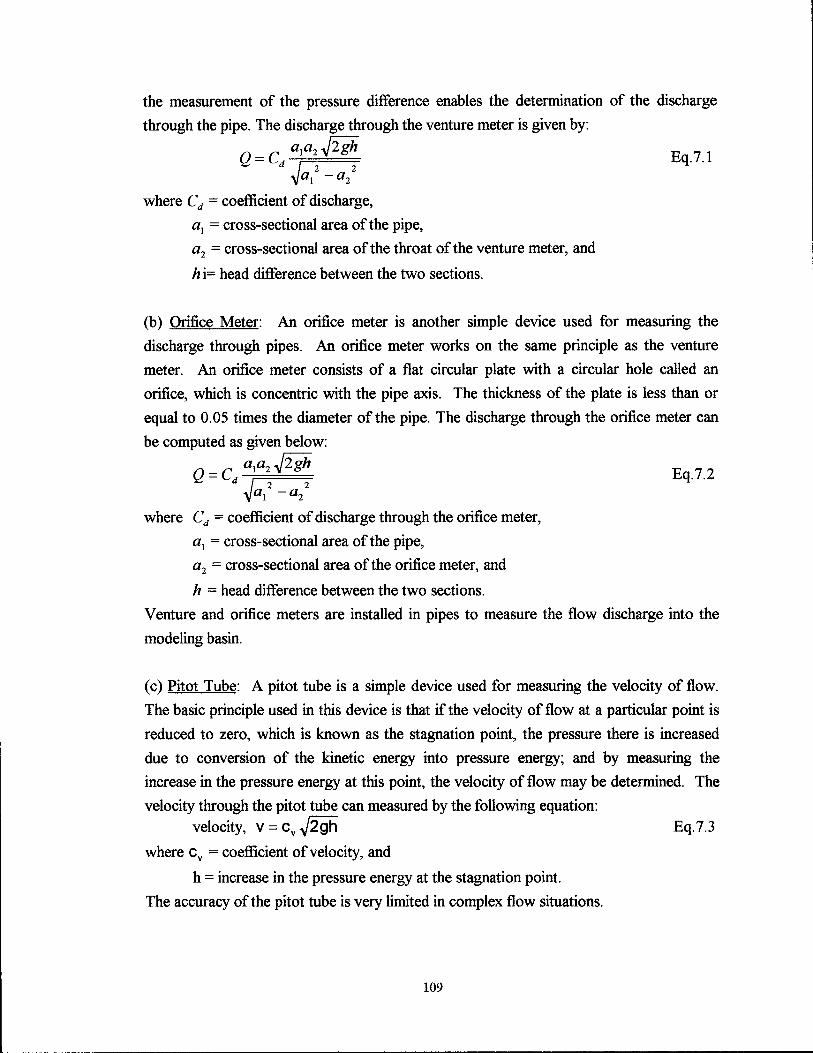
the measurement of the pressure difference enables the determination of the discharge
through the pipe. The discharge through the venture meter is given by:
Q = C a1a2 .J2iii d ~ 2 2 a1 -a2
where Cd = coefficient of discharge,
a1 = cross-sectional area of the pipe,
a2 =cross-sectional area of the throat of the venture meter, and
hi= head difference between the two sections.
Eq.7.1
(b) Orifice Meter: An orifice meter is another simple device used for measuring the
discharge through pipes. An orifice meter works on the same principle as the venture
meter. An orifice meter consists of a flat circular plate with a circular hole called an
orifice, which is concentric with the pipe axis. The thickness of the plate is less than or
equal to 0.05 times the diameter of the pipe. The discharge through the orifice meter can
be computed as given below:
Q - C a1a2 .J2iii - d I 2 2
val -a2
where Cd = coefficient of discharge through the orifice meter,
a1 = cross-sectional area of the pipe,
a2 = cross-sectional area of the orifice meter, and
h = head difference between the two sections.
Eq.7.2
Venture and orifice meters are installed in pipes to measure the flow discharge into the
modeling basin.
( c) Pitot Tube: A pitot tube is a simple device used for measuring the velocity of flow.
The basic principle used in this device is that if the velocity of flow at a particular point is
reduced to zero, which is known as the stagnation point, the pressure there is increased
due to conversion of the kinetic energy into pressure energy; and by measuring the
increase in the pressure energy at this point, the velocity of flow may be determined. The
velocity through the pitot tube can measured by the following equation: velocity, v = cv ..j2gh Eq.7.3
where cv = coefficient of velocity, and
h = increase in the pressure energy at the stagnation point.
The accuracy of the pitot tube is very limited in complex flow situations.
109

(d) Laser-Doppler Anemometer (LDA): This instrument measures the Doppler shift in
light scattered off tracer particles in moving fluids. The measured frequency shift is then
used to compute the fluid velocity. Laser-Doppler anemometer is expensive, but it has
numerous advantages over other less expensive velocity measuring devices such as the
electro-magnetic current meter and acoustic Doppler anemometer. All three components
of the velocity can be measured at the same point. The measuring volume is well below 1
mm3, and a fiber-optic immersible probe can be used to bring the light beams close to the
measuring point. The LDA has a frequency response typically above 1000 Hz so it is
capable of measuring turbulent velocity fluctuations.
(e) Acoustic Doppler Velocimeter (ADV): This instrument uses Doppler shift of sound
waves in water to measure the single point three-dimensional water velocity. The Doppler
shift is derived from signals scattered from small particles in the flow. The occurrence of
the suspended sediments in the water column may act as natural tracer particles, or
seeding particles can be introduced. The ADV is rather insensitive to water quality and
works well in turbid water. It is relatively expensive compared to the LDA and is
generally adequate if the turbulent velocity fluctuations need not be measured.
(f) Electro-Magnetic Current Meter: This instrument senses changes in magnetic flux in
the water created by flows around the sensor. The resulting voltage change in the electric
circuit is proportional to the speed of the flowing water. This instrument can measure two
velocity components simultaneously. Its measuring volume is much larger than the LDA
and the ADV. In addition, the response time is of the order of 10 Hz thus, it cannot
detect the turbulent velocity.
(g) Electronic Bed Profiler: This instrument consists of a probe placed vertically in the
water. A servo-mechanism maintains the tip of the probe at a constant distance above the
bed. When the instrument is being displaced in a horizontal direction, the probe will
follow the configuration of the bed continuously. The principle of operation is the
appreciable difference between the electronic conductivities of water and the bed material.
The probe outputs an analog voltage whose magnitude is directly proportional to the
vertical movement of the probe. The probe can be used without stopping the flow.
Therefore, time development of the bed configuration can be obtained.
110

7.8. LIVE-BED SCOUR
To study live-bed scour, sediments can be introduced at the upstream end and
collected at the downstream end. At the upstream end, specially designed feeders may be
used to ensure a controlled sediment rate of inflow. At the downstream end, sediment can
be collected in a sediment trap which can be reused. The recording of bed evolution can
be made at the end of each run by draining the model carefully in depth increments equal
to the required contour intervals. At each step, a thin, clearly visible cord is laid along the
water edge. This represents a contour line and its position may be recorded by overhead
photography. Bed elevation can also be measured continuously by a bed profiler that is
moved across a beam spanning the model and basin. There are two types of bed profilers.
One operates by measuring the conductance between two electrodes, and the other is an
ultrasonic device.
7.9. RIVERBANKS
River banks should be non-erodable and stable. They should not contribute to the
sediment in the model. The most common method for accurately reproducing the river
cross sections is the use of the templates with cement mortar. Fine sheets of metal
following the contour lines are more suitable to model flood plain or hilly sections of the
river. For qualitative study of river migration and river bends, cohesionless soils could be
used. Radius of curvature in the field is the product of radius of curvature in the model
and the scale.
7.10. SOILS
The soil grains need to be scaled down to ensure that they will be subjected to the
same erosion potential after the velocity of the water has been scaled down. The laws
governing the reduction factor for the soil grains are described in Sections 4.2 and 4.3.
There are two ways to scale the soil grains appropriately. The first one consists of
decreasing the size of the grains. The limit for this process is 0.1 mm. Once the soil
grains in the model become smaller than 0 .1 mm, the soil in the model ceases to be
cohesionless like the one in the prototype because the electromagnetic forces between
grains start to become sizable compared to the gravity forces. If the required size of the
grains for proper modeling are smaller than that, it is possible to use a different and lighter
material for the grains in the model. Coal, crushed shells, and plastics are all used and
111

provide an additional reduction factor approximately equal to 5 .5. Such light particles
with sizes in the 0 .1 mm range are, therefore, equivalent to 0. 02 mm. If this is still not
small enough, the soil cannot be properly scaled. Then, the practice is simply to use such
small and light particles to ensure that the soil in the model can be eroded at the model
velocity. Generally, fine sands, silts, and clays cannot be properly modeled, and much
work remains to be done for these soils.
7.11. COST ESTIMATE FOR PROPOSED MODELING FACILITY
The modeling facility is proposed to have both a 3-D basin and a 2-D open channel
flume in the same building as shown in Figure 7.5. It will also have an overhead crane and
pumps for both the 3-D basin and 2-D flume. Some space in the building is provided for
different purposes such as office, loading zone, storage area, and workshop. The cost of
the overall facility, including the components, is given below.
ITEM DESCRIPTION
Building
1. Building 51.85x76.25 m (170 ft x 250 ft)
@ $1075/m2($100/ft2 ) (Figure 7.5)
Office & Workshop
2. Office 4.58 x30.5 m (15 ft x 100 ft)
@ $376/m2($35/tt2 )
3. Workshop 9.15 x 22.88 m (30 ft x 75 ft)
@ $806/m2 ($75/ft2 )
Subtotal
Fixed Equipment
4. River Basin
Underground Sump (3-D)
Pump (12 cfs, 25 H.P)
5. Open Channel Flume (2-D)
Underground Sump
Pumps 3 No.s (Each of 35 cfs, 100 H.P)
6. Overhead Crane
Subtotal
112
ESTIMATED COST
$ 4,250,000
$ 52,500
$ 168,750
221,250
$ 125,000
$ 50,000
$ 15,000
$ 85,000
$ 160,000
$ 100,000
$ 100,000
$ 635,000

....------------------------- - -
Columns ,/ ,/
::c ~ ::c ::c I
C'<l r----------------1 ~ I I d) I I 0.0 C'<l 36.6 x 6.1 x 3.66 m Concrete Flume ~ I I B (100 cfs, 240 H.P. Pump) ti) I I
I 3 .03 wide Sump I L ________________ J Workshop
& Soil Lab 45.75 x 30 x 1 m River Basin
(12 cfs, 24 H.P Pump) --VJ Overhead Crane ~-------------------s
I 45.75 x 3.03 x 1.59 m Sump below the ground ......_
I(")
OC! -I(") ,,.... i---------------------
(!) u
Loading C'<l 0.
Zone IZl (!) u ~ 0
::c m· .. ::c :r: :r: :r:
\< 76.25 m >I Figure 7.5. Plan of Hydraulic Modeling Facility

Various Equipment & Instrumentation
7. Data acquisition (4 PC/486, acquisition board and
accessories, 2 Laser jet printers) $ 20,000
8. One three-component, fiber optic Laser-Doppler
anemometer $ 200,000
9. Four two-component, electro-magnetic current meters $ 50,000
10. One bed profiler $ 25,000
11. Flowmeters $ 15,000
12. Suspended sediment concentration measuring device $ 200,000
13. Water surface elevation measuring devices
(resistance/capacitance gages) $ 50,000
14. Instrument carriages $ 20,000
15. Video camera and recorder $ 10,000
16. Computer software $ 20,000
Subtotal $ 610,000
Miscellaneous
17. A&E Fee (10% of building cost) $ 425,000
18. Utilities (Water, electricity, gas) $ 25,000
19. Contingency $ 500,000
Subtotal $ 950,000
Total Project Cost $ 626662250
114

8. CONCLUSIONS
These conclusions are based on a study of the Texas scour problem, including the
hydraulic and soil characteristics of the rivers in Texas; on the study of the known
fundamental principles of hydraulic and soil modeling; on the model analysis by similitude
theory of five bridge case studies in Texas; on the discussions with recognized scour
experts; and on a survey and visit of four leading scour facilities in the country.
The following conclusions are reached :
1. The facility should have two basins: a 2-D flume for local scour studies and a
3-D basin for global scour studies.
2. The 2-D flume should be above ground, 36 m long (120 ft), 6 m wide (20 ft),
and 3 m deep (10 ft). The sump should be below ground; it should surround
the flume and be 3 m (10 ft) wide, and 3 m (10 ft) deep. A 240 HP pump
delivering 28 m3/sec (100 cfs) is necessary to feed this flume.
3. The 3-D basin should be above ground, 45 m ( 150 ft) long, 30 m ( 100 ft) wide
and 1 m (3 ft) deep. The sump should be below ground under the center of the
basin, parallel to the 50 m side of the basin; it should be 3 m wide ( 10 ft) and
I.Sm (6 ft) deep. A 25 HP pump delivering 0.4 m3/sec (12 cfs) is necessary to
feed this basin.
4. The 2-D flume would allow local scour models with undistorted scales in the
range of 1115 to 1/25.
5. The 3-D basin would allow general scour models with undistorted scales in the
range of 1/50 to 1/100.
6. The cost of the facility and its major components is estimated to be a follows:
The overall facility = $6.70 M
The building = $4.25 M
The 3-D basin with sump and pump = $0.19 M
The 2-D basin with sump and pump = $0.35 M
Measuring instruments = $0.61 M
115

7. The advantages and disadvantages of this facility are:
Advantages Disadvantages
1. Availability 1. Initial cost
2. Develop local expertise 2. Delay until built
3. Latest technology 3. Inexperience personnel at first
4. Very large scale
5. Low overhead
6. Easy contracts
7. Short travel time
8. Existing facilities do not compare favorably with the facility described above.
However, a few of them can provide very valuable data on scour modeling at
reasonably large scale.
9. The advantages and the disadvantages of the existing facilities are:
Advantages Disadvantages
1. No delay for use 1. Higher overhead
2. No initial cost 2. No local expertise developed
3. Experienced personnel 3. Older equipment
4. Longer travel time
5. First come first serve availability
10. The decision should be based on the estimated need in the next 10 to 20 years
for such a facility by TxDOT and neighboring states. Using an existing building
is a way to decrease the cost that would make a big difference. It should also be
kept in mind that Texas rivers have a mixture of sand and clay beds, and that the
usefulness of modeling facilities for scour in clay is limited.
116

REFERENCES
1. Arbingast, S.A., Kennamer, L.G, Ryan, R.H., Buchanan, J.R., Hezlep W.L., Ellis, L.T.,
Jordan, T.G., Granger, C.T., and Zlatkovich, C.P. (1976) "Atlas of Texas," Bereau of
Business Research, The University of Texas at Austin, Austin, 78712.
2. Chow, V. T. (1959) "Open Channel Hydraulics," McGraw-Hill Inc., New York.
3. Graf, W. H. (1971) "Hydraulics of Sediment Transport," McGraw-Hill Inc., NewYork.
4. Franco, J.J. (1989) "Guidelines for the Design, Adjustment and Generation of Models
for the Study ofRiver Sedimentation Problems," Instruction Report No: H-8-1,
Hydraulic Laboratories, USAE Waterways Experiment Station, 3909,
Vicksburg, Mississippi, 3918-6199, October 1989.
5. Froehlich, D.C. (1989) "Finite Element Surface-Water Modeling System: Two
Dimensional Flow in a Horizontal Plane (FESWMS-2DH) Users Manual," Publication
NumberFHWA-RD-88-177, April 1989.
6. Hallmark, C.T., West, L.T., Wilding, L.P., and Dress, L.R. (1986)
"Characterization Data for Selected Texas Soils," Report No: MP-1583, Texas
Agricultural Experiment Station, Department of Soil and Crop Sciences, Texas A&M
University, College Station, Texas.
7. Lagasse, P.F., Schall, J.D., Johnson, F., Richardson, E.V., Richardson, J.R., and
Chang, F. (1991) "Stream Stability at Highway Structures," Hydraulic Engineering
Circular-20 (HEC-20), 2nd Edition, National Technical Information Services,
Springfield, Virginia.
8. Modi, P. N. and Seth, S. M. (1984) "Hydraulics and Fluid Mechanics," Standard
Book House, New Delhi.
9. Petersen, M. S.(1986) "River Engineering," Prentice-Hall, Englewood Cliffs, N.J.
10. Richardson, E.V., Harrison, L., Richardson, J.R., and Davis, S.R. (1993)
"Evaluating Scour at Bridges," Hydraulic Engineering Circular - 18 (HEC-18), 2nd
Edition, National Technical Information Services, Springfield, Virginia.
11. Raudkivi, A.J. (1990)" Loose Boundary Hydraulics," 3rd Ed., Pergamon Press,
New York.
12. Raudkivi, A.J. and Ettema, R.(1983) "Clear-Water Scour at Cylindrical Piers,"
Journal of Hydraulic Engineering, ASCE, Vol. 101, No. 3, March 1983.
117

13. Shields (1936) "An wer dung der Achnlichkeirt-muhanik and der Turbulenz
forschung anf dil Geschil be Wegung," Presessische Veruchsan Staet tur Wasseoban
and Schiflban, Berlin, Heft 26.
14. Tebbutt, T. H. Y. (1985) "Advances in Water Engineering," Elsevier Applied Science
Publishers.
15. TWDB (Texas Water Development Board) (1968) "The Texas Water Plan,"
November 1968.
16. TSEAS (1993) "Texas Secondary Evaluation and Analysis for Scour," Bridges and
Structures Division, Hydraulics Section, TxDOT.
17. TxDOT (1993) Five case study reports sent by TxDOT officials:
1. State Highway 71 Crossing the Colorado River Near Columbus, Texas.
2. State Highway 80 Crossing the Guadaloupe River Near Belmont, Texas.
3. FM 973 Crossing the Colorado River Near Austin, Texas.
4. State Highway 7 Crossing the Trinity River Near Crockett, Texas.
5. US Highway 183 Crossing the Colorado River Near Hochheim, Texas.
18. Moody, D.W., Chase, E.B., and Aronson, D.A. (1985) "National Water Summary
1985 - Hydrologic Events and Surface Water Resources," (USGS Water Supply Paper
2300), US Government Printing Office, Washington, D.C.
19. USGS (1988-89) "Floods and Droughts: Texas," (Water Supply Paper 2375) US
Government Printing Office, Washington, D.C.
20. Vanoni, (1964) "Measurements of Critical Shear Stress for Entraining Five
Sediments in a Boundary Layer," Report No: KH-R-7, W.M. Keck Laboratory,
California Institute of Technology, Pasadena, California, May 1964.
118