Feasibility of various condition assessment techniques for ... · Feasibility of various condition assessment techniques for residual strength and life prediction T TG 5 A G Dutton

`

Feasibility of various condition assessment techniques for residual strength and life

prediction

TG 5

A G Dutton

(CCLRC-RAL)

OB_TG5_R015 rev. 000

Version 1 Confidential

OPTIMAT BLADES

OB_TG5_R015_000 OPTIMAT BLADES Page 2 of 32

Last saved: 5/3/2006 4:26:00 PM

Change record

Issue/revision date pages Summary of changes Version 1 03/05/2006 32


Last saved: 5/3/2006 4:26:00 PM

1. INTRODUCTION....................................................................................................................................4

2. TEST SPECIMENS .................................................................................................................................5

3. TEST SETUP............................................................................................................................................6 3.1. EQUIPMENT.........................................................................................................................................6 3.2. TEST PROCEDURE ...............................................................................................................................6 3.3. CONDITION MONITORING METHODS...................................................................................................6

4. RESULTS..................................................................................................................................................8 4.1. ACOUSTIC EMISSION MONITORING .....................................................................................................8 4.2. THERMOELASTIC STRESS TEMPERATURE CORRECTION....................................................................11

5. REFERENCES .......................................................................................................................................17

6. APPENDIX: SPECIFIC TEST RESULTS..........................................................................................18 6.1. THERMOELASTIC AREA ANALYSIS IN MATLAB: ...............................................................................32


Last saved: 5/3/2006 4:26:00 PM

1. Introduction

This document has been prepared within the scope of Task Group 5 of the OPTIMAT Blades project to report on the feasibility of using either acoustic emission monitoring or thermoelastic stress analysis (TSA) in the characterisation of residual strength of test specimens during the various load phases of the TG5 residual strength test [1-3]. Acoustic emission (AE) measurements were carried out by UP and CCLRC-RAL and thermoelastic stress measurements by CCLRC-RAL on the standard OPTIMAT UD and MD materials. The use of acoustic emission monitoring by UP has been reported elsewhere [4] so this report will concentrate on the results from the CCLRC-RAL tests. The acoustic emission test programme followed the proof-loading test specification in [2], although this was amended following early results from [4] to include more detailed analysis of the RST part of the test. Acoustic emission monitoring added considerably to the overall RST test complexity and could not be used on all test specimens to avoid undue delay with the experimental timetable. Unfortunately, a substantial fraction of the acoustic emission data that was collected was inadvertently deleted from the hard disk drive before being transferred to the archiving network. These two facts have limited the usefulness of the AE data, although some indicative trends have been identified. Considerable internal heating effects were observed, which rendered interpretation of the TSA data extremely difficult. Results are presented of the high temperatures reached by Optimat specimens under the nominal fatigue loading conditions. While these were supposed to have been intended to keep specimen temperature below 35 oC, surface temperatures in excess of 50 oC were commonly encountered, particularly for the MD specimens. It is understood that in other laboratories these high temperatures were alleviated by the use of fan-cooling; at RAL this was not considered as an option due to the desire to use thermal monitoring of the techniques. In tests without thermal monitoring, high temperature effects were alleviated by reducing test frequency. It is possible that (unknown) high internal temperatures and temperature gradients may have had an influence on Optimat fatigue failures.


Last saved: 5/3/2006 4:26:00 PM

2. Test Specimens

Standard OB multi-directional (MD) coupons were manufactured to geometry GEV207-R0400 by LM Glasfiber with nominal dimensions shown in Figure 2-1. The nominal gauge length was 35 mm and the nominal coupon thickness 6.6 mm. The detailed dimensions are given alongside the residual strength data in the main test reports [5, 6]. Greater than expected variation was noted with the parallelism and thickness of tabs on the MD specimens.

Figure 2-1 : Basic specimen design for GEV207-R0400 (hnominal ~ 6.6 mm)


Last saved: 5/3/2006 4:26:00 PM

3. Test Setup

3.1. Equipment Tests were carried out an ESH 100 kN machine with manual jaws and with the 4 screws on each jaw set torqued to 150Nm. Strain was measured using a pair of in-house developed extensometers with a gauge length of 10 mm and mounted centrally on the two faces of the specimen (E1 & E2). The extensometers were connected to an RDP electronics model 628 strain gauge amplifier and logged using a PC with a UEI A to D board and Aligent VEE software. Air temperature was measured using a thermocouple place in the rig at the same height as the specimen. Specimen temperature was measured using a thermocouple in contact with the specimen edge1 just below the top tab. 3.2. Test Procedure The test procedure is proscribed in [2, 3]. This was followed (with minor changes) for all tests. The basic steps were: (i) The strain gauges on the extensometers were zeroed prior to the specimen being

mounted in the jaws. Considerable care was then taken to ensure the best alignment of the specimen in the test machine (note that tightening of both the top and bottom jaws was observed to cause some acoustic emission activity).

(ii) Tensile tests were preformed at a rate of 0.25 mm/min and compression at 1 mm/min.

(iii) An initial stiffness test or Acoustic Emission Load (AEL) test was performed at 1 mm/min incorporating 2500 ue and –2500 ue to enable stiffness calculation.

(iv) A cyclic constant amplitude load test to a pre-determined fraction of the expected fatigue life was applied.

(v) If the specimen survived, the stiffness and/or AEL test was repeated, and (vi) The specimen was then tested to destruction in a final residual strength test. 3.3. Condition monitoring methods A principal aim of the Task Group was to assess the viability of using condition monitoring techniques to predict the ultimate residual strength. RAL and UPAT both applied variations of acoustic emission monitoring techniques to try to assess damage from the fatigue cycling phase during the final stiffness evaluation and/or the residual strength test.

1 Note that the specimen edge was used for consistency of method with other test laboratories. RAL argued in favour of measurement preferable on the specimen face at the centreline, but, since that was generally inaccessible due to positioning of strain measurement transducers, in the middle of the face just beneath the tab. Infra red thermography measurements consistently showed peak temperatures on the specimen face centre-line for most of the duration of a cyclic load test.


Last saved: 5/3/2006 4:26:00 PM

A procedure for evaluating acoustic emission during the initial and final stiffness tests was included in the Task Group 5 test procedure [2] (see Figure 3-1). Specimens tested in this manner are marked (AE) in the main data tables in [5, 6]. Although the load level selected for the evaluation was regarded as safe from the point of view of not damaging the specimen, it was not sufficiently high to give rise to any significant AE activity even after fatigue. Attempts to extract meaningful data from the acoustic emission during the fatigue cycle and residual strength parts of the test were therefore also made during the latter part of the test programme. In these phases, AE activity was monitored throughout the test. Unfortunately the AE data from 6 MD tests was lost when the directory containing the files was inadvertently erased. Acousto-ultrasonics was also considered as a possible way to determine residual strength, based on the hypothesis that micro-structural damage might alter the speed of wave transmission in the test specimens [7].

-3000

-2000

-1000

0

1000

2000

3000

Time on test

Load

(mic

rost

rain

) Stiffness Test

Initial AEL (at start

of test only)

Diagnostic AEL

Start new AE logging file

Figure 3-1 : Acoustic Emission Evaluation Load (AEL) and stiffness measurement

Thermoelastic stress analysis methods were also applied during the fatigue cycling phase of certain tests. The system used (Deltatherm) was upgraded during the course of the test programme enabling field temperature as well as full field thermoelastic stress measurement. Thermo-viscoelastic (self-)heating effects were found to significantly affect the thermoelastic signal, making the interpretation of damage progression impossible to assess. A short parametric study load magnitude and frequency effects was carried out on a single MD test specimen to try to quantify these effects.


Last saved: 5/3/2006 4:26:00 PM

4. Results

4.1. Acoustic emission monitoring Figure 4-1 shows the acoustic emission activity in terms of the Amplitude parameter during the initial AE evaluation load cycle, final AE evaluation load cycle, and the residual strength test for two UD test specimens fatigued to 80% of nominal fatigue lifetime. The use of the stiffness proof cycle as an AE evaluation load cycle to characterise strength is clearly untenable from the evidence provided in these two tests. Although a scattering of high amplitude events is recorded in each case during the initial load cycle of virgin material (i1), these are not repeated during the repeated initial cycle (i2) and there is no activity at all during the final AE evaluation.

(a) (b)

Figure 4-1 : Acoustic emission during static load phases for two 80% fatigue lifetime specimens exhibiting high residual strength (a) and intermediate residual strength (b)

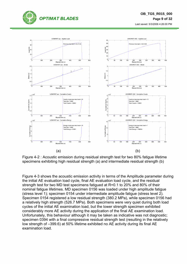
Examining the AE behaviour during the final residual strength test in more detail (Figure 4-2) reveals only large bursts of Counts and Energy at loads substantially higher than the preceding maximum fatigue load. Again this is not a useful discriminator, since loads higher than the maximum fatigue load will not be allowed during a certification type of test. In any case, in contrast with MD coupons for this test, there is no clear difference between the high and medium strength cases. The type of fatigue loading is also shown to have little effect on the AE activity since one test (0395) contained fatigue loading conducted at R=0.1 and the other (0400) at R=-1. Additional AE results for UD specimens can be found in [5].


Last saved: 5/3/2006 4:26:00 PM

(a) (b)

Figure 4-2 : Acoustic emission during residual strength test for two 80% fatigue lifetime specimens exhibiting high residual strength (a) and intermediate residual strength (b) Figure 4-3 shows the acoustic emission activity in terms of the Amplitude parameter during the initial AE evaluation load cycle, final AE evaluation load cycle, and the residual strength test for two MD test specimens fatigued at R=0.1 to 20% and 80% of their nominal fatigue lifetimes. MD specimen 0156 was loaded under high amplitude fatigue (stress level 1); specimen 0154 under intermediate amplitude fatigue (stress level 2). Specimen 0154 registered a low residual strength (380.2 MPa), while specimen 0156 had a relatively high strength (526.7 MPa). Both specimens were very quiet during both load cycles of the initial AE examination load, but the lower strength specimen exhibited considerably more AE activity during the application of the final AE examination load. Unfortunately, this behaviour although it may be taken as indicative was not diagnostic; specimen 0394 with a final compressive residual strength test (resulting in the relatively low strength of –399.6) at 50% lifetime exhibited no AE activity during its final AE examination load.


Last saved: 5/3/2006 4:26:00 PM

(a) (b)

Figure 4-3 : Acoustic emission during static load phases for two MD specimens exhibiting high residual strength (a) and low residual strength (b)

Figure 4-4 : Acoustic emission during residual strength test for two MD specimens exhibiting high residual strength (a) and intermediate residual strength (b)


Last saved: 5/3/2006 4:26:00 PM

Figure 4-4 shows acoustic emission activity during the final residual strength test for the same two MD specimens with differing final residual strength. The high strength specimen (156) has generally lower Counts and Energy than the intermediate strength specimen (154). In addition, the intermediate strength specimen starts to give significant acoustic emission at a smaller fraction of its nominal strength (though unfortunately the correlated applied load curve was not available in this case), but still above the previous load level. AE data from several other high strength specimens shows similar characteristics, but there is insufficient data from low strength specimens to draw firm conclusions. 4.2. Thermoelastic stress temperature correction From Planck’s law, the spectral energy density at a given wavelength is given by:

⎟⎟⎟

⎠

⎞

⎜⎜⎜

⎝

⎛

−

=⎟⎠⎞

⎜⎝⎛

1

18)( 5kTch

e

hcTEλ

λ λπ (1)

or in terms of the specific intensity or brightness as:

⎟⎟⎟

⎠

⎞

⎜⎜⎜

⎝

⎛

−

==⎟⎠⎞

⎜⎝⎛

1

12)(4

)( 5

2

kTch

e

hcTEcTQλ

λλ λπ (2)

and the photon radiance at the sensor is determined by the integral:

∫=2

1

det

λ

λλ λdQAQ ector (3)

where A is a constant accounting for the transmittance, the optics of the system, and the geometry of the detector and λ1 and λ2 represent the cut-off frequencies of the detector. Plotting the photon energy at the sensor in the wavebands of the two most widely used sensors gives the temperature sensitivity shown in Figure 4-5 and Figure 4-6. The InSb sensor (operating in the 3-5 um waveband) used in the Deltatherm system has a lower response for room temperature objects and, critically, the relative increase with temperature is more severe than the MgCdTe sensor used in the former SPATE system. This implies that if the object temperature changes due to thermo-viscoelasticity or damage processes then a correction will need to be applied to the thermoelastic data.


Last saved: 5/3/2006 4:26:00 PM

Photon energy as f(T) for sensor waveband

0.000000E+00

5.000000E+00

1.000000E+01

1.500000E+01

2.000000E+01

2.500000E+01

270 280 290 300 310 320 330

Temperature (K)

Phot

on e

nerg

y E(

Wav

elen

gth

rang

e)

3-5 um

8-12 um

Figure 4-5 : Photon energy as a function of Temperature for commonly used infra red sensor wavebands

Photon energy relative to 273 K as f(T) for sensor waveband

0.000000E+00

1.000000E+00

2.000000E+00

3.000000E+00

4.000000E+00

5.000000E+00

6.000000E+00

7.000000E+00

270 280 290 300 310 320 330

Temperature (K)

Phot

on E

nerg

y re

lativ

e to

val

ue a

t 273

K

3-5 um

8-12 um

Figure 4-6 : Photon energy relative to 273K for commonly used infra red sensor wavebands


Last saved: 5/3/2006 4:26:00 PM

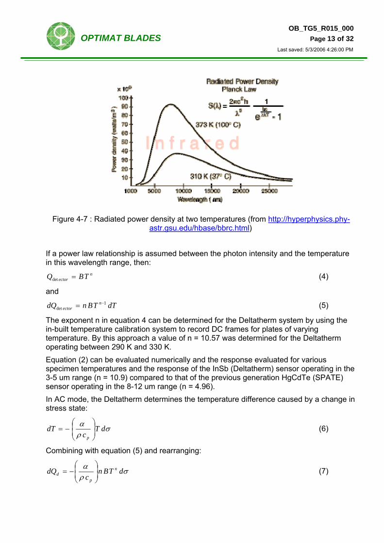
Figure 4-7 : Radiated power density at two temperatures (from http://hyperphysics.phy-astr.gsu.edu/hbase/bbrc.html)

If a power law relationship is assumed between the photon intensity and the temperature in this wavelength range, then:

nector TBQ =det (4)

and

dTTBndQ nector

1det

−= (5)

The exponent n in equation 4 can be determined for the Deltatherm system by using the in-built temperature calibration system to record DC frames for plates of varying temperature. By this approach a value of n = 10.57 was determined for the Deltatherm operating between 290 K and 330 K. Equation (2) can be evaluated numerically and the response evaluated for various specimen temperatures and the response of the InSb (Deltatherm) sensor operating in the 3-5 um range (n = 10.9) compared to that of the previous generation HgCdTe (SPATE) sensor operating in the 8-12 um range (n = 4.96). In AC mode, the Deltatherm determines the temperature difference caused by a change in stress state:

σρα dTc

dTp⎟⎟⎠

⎞⎜⎜⎝

⎛−= (6)

Combining with equation (5) and rearranging:

σρα dTBnc

dQ n

pd ⎟

⎟⎠

⎞⎜⎜⎝

⎛−= (7)


Last saved: 5/3/2006 4:26:00 PM

Therefore, for a given stress condition measured at two different temperatures, the signal response will vary according to the ratio:

1

2

1

2

1

2

d

dn

QQ

TT

SS

=⎟⎟⎠

⎞⎜⎜⎝

⎛= (8)

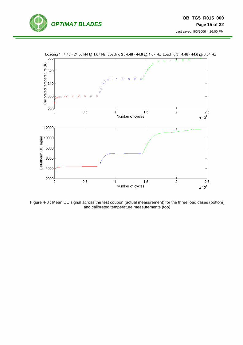
A series step tests were carried out on OPTIMAT MD coupon GE207-R0400-0407. The specific load regimes were:

Load case Load (kN) Frequency (Hz) Cycles

1 4.46 – 24.53 1.67 0 – 7000

2 4.46 – 44.6 1.67 7000 – 14400

3 4.46 – 44.6 3.34 14,400 – 22,500 (failure) Initial loading and adjustments between load regimes were made gradually over the course of approximately 300 cycles. Figure 4-8 shows that the specimen temperature increased from an initial value of 295K to 330K at failure. For load case 1 and load case 2, the temperature stabilises at a new equilibrium value with 1000-1500 cycles. Inspection of the individual temperature fields shows that the peak temperature developed in the centre of the specimen. During load case 3, the temperature continues to rise throughout the loading; inspection of the individual temperature fields shows that this was due to a new peak temperature area developing somewhere in the upper tab region. Figure 4-9 shows both raw and temperature-corrected (by equation (8)) thermoelastic stress measurements. The size of the temperature correction appears to over-compensate for the effect (e.g. for load case 2, a stress doubling is expected, whereas the corrected stress values are only 1.5 times the original stress level).


Last saved: 5/3/2006 4:26:00 PM

Figure 4-8 : Mean DC signal across the test coupon (actual measurement) for the three load cases (bottom) and calibrated temperature measurements (top)


Last saved: 5/3/2006 4:26:00 PM

Figure 4-9 : Mean AC signal across the test coupon (actual measurement) for the three load cases compared with the mean AC signal referred back to the initial temperature


Last saved: 5/3/2006 4:26:00 PM

5. References

[1] Dutton, A.G., Detailed Plan of Action WP13 and WP14 (TG5), OB_TG5_R001, 2003

[2] Blanch, M.J., Dutton, A.G., Philippidis, T.P., Nijssen, R., Recommended procedure for conducting OPTIMAT Blades residual strength test, OB_TG5_R002, November 2003

[3] Krause, O., Philippidis, T.P.,General test specification, OB_TC_R014, March 2004 (and revision July 2004)

[4] Philippidis, T.P., Validated engineering model for residual life evaluation and strategy for condition assessment, OB_TG5_R014, May 2006

[5] Dutton, A.G., Robertson, S.J., Canfer, S.J., Blanch, M.J., Residual strength testing of OPTIMAT UD specimens – tests by CCLRC-RAL, OB_TG5_R011, May 2006

[6] Dutton, A.G., Robertson, S.J., Canfer, S.J., Blanch, M.J., Residual strength testing of OPTIMAT MD specimens – tests by CCLRC-RAL, OB_TG5_R012, May 2006

[7] Ruddell, A., Dutton, A.G., The use of acousto-ultrasonic techniques to measure propagation time through glass-fibre reinforced coupons, OB_TG5_R010, February 2006.


Last saved: 5/3/2006 4:26:00 PM

6. Appendix: Specific test results

(a) (b)

(c) (d)

Figure 6-1 : MD specimen GE207-R0400-0407 temperature distribution (autoscaled): (a) before loading; (b)

after 7000 cycles (end of loading 1); (c) after 14,200 cycles (end of loading 2); (d) after 22,000 cycles (immediately before failure)


Last saved: 5/3/2006 4:26:00 PM

(a) (b)

(c)

Figure 6-2 : MD specimen GE207-R0400-0407 thermoelastic stress (X-value) distribution: (a) after 7000 cycles (end of loading 1); (b) after 14,200 cycles (end of loading 2); (c) after 16,200 cycles (after 2000

cycles of loading 3)


Last saved: 5/3/2006 4:26:00 PM

(a) (b)

(c) (d)

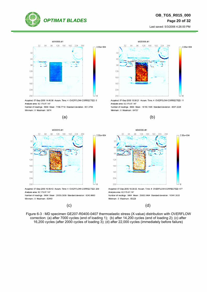
Figure 6-3 : MD specimen GE207-R0400-0407 thermoelastic stress (X-value) distribution with OVERFLOW correction: (a) after 7000 cycles (end of loading 1); (b) after 14,200 cycles (end of loading 2); (c) after

16,200 cycles (after 2000 cycles of loading 3); (d) after 22,000 cycles (immediately before failure)


Last saved: 5/3/2006 4:26:00 PM

(a) (b)

(c) (d)

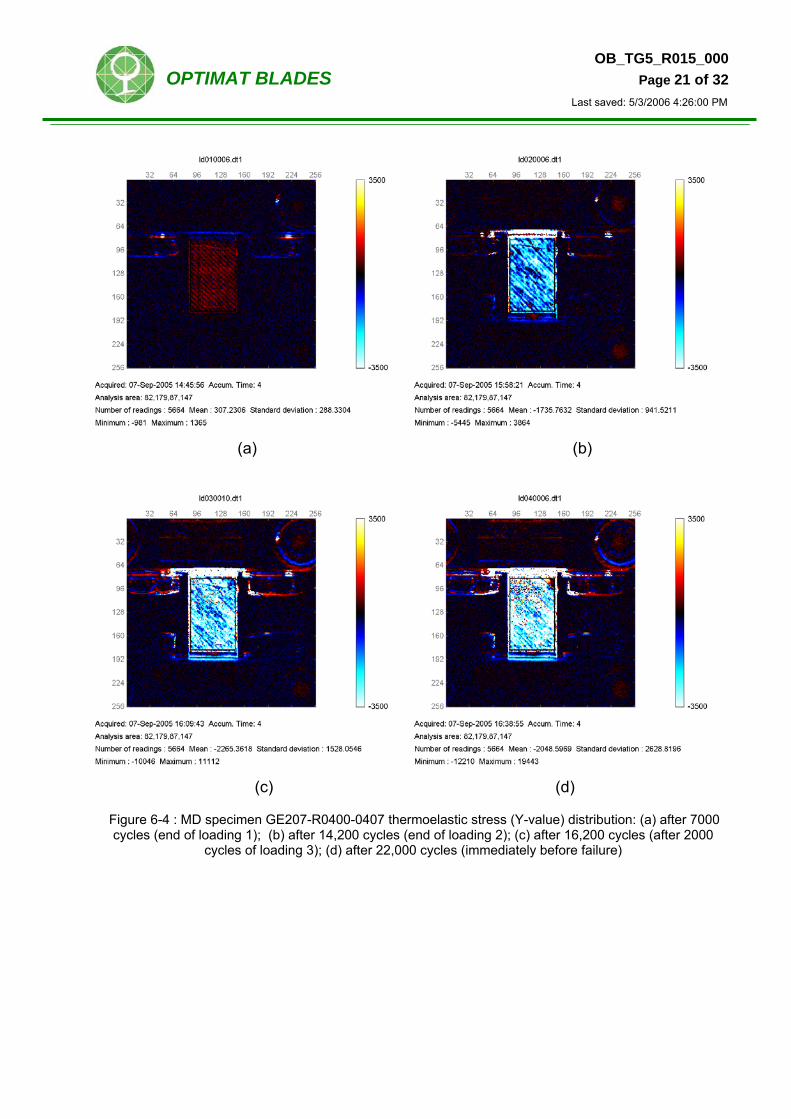
Figure 6-4 : MD specimen GE207-R0400-0407 thermoelastic stress (Y-value) distribution: (a) after 7000 cycles (end of loading 1); (b) after 14,200 cycles (end of loading 2); (c) after 16,200 cycles (after 2000

cycles of loading 3); (d) after 22,000 cycles (immediately before failure)


Last saved: 5/3/2006 4:26:00 PM

(a) (b)

(c) (d)

Figure 6-5 : MD specimen GE207-R0400-0407 temperature distribution (constant scale): (a) after 7000 cycles (end of loading 1); (b) after 14,200 cycles (end of loading 2); (c) after 16,200 cycles (after 2000

cycles of loading 3); (d) after 22,000 cycles (immediately before failure)


Last saved: 5/3/2006 4:26:00 PM

(a) (b)

(c) (d)

Figure 6-6 : UD specimen GE206-R0300-0411 temperature distribution (auto-scaled): (a) immediately after fatigue load established; (b) after 700 cycles; (c) after 1000 cycles; (d)

immediately before failure at bottom grip Note hot spots at top and bottom of specimen from the start of the test (compare with central hot spot in MD specimens). Initial hottest part (top) does not indicate location of failure (bottom).


Last saved: 5/3/2006 4:26:00 PM

(a) (b)

(c) (d)

Figure 6-7 : UD specimen GE206-R0300-0411 thermoelastic stress (X-value) distribution: (a) immediately after fatigue load established; (b) after 700 cycles; (c) after 1000 cycles;

(d) immediately before failure at bottom grip Note how fibre orientation clearest in first images after loading: (a) and (b). Note signal overflow at bottom right hand corner in (d).


Last saved: 5/3/2006 4:26:00 PM

(a) (b)

(c) (d)

Figure 6-8 : UD specimen GE206-R0300-0411 thermoelastic stress (Y-value) distribution: (a) immediately after fatigue load established; (b) after 700 cycles; (c) after 1000 cycles;

(d) immediately before failure at bottom grip


Last saved: 5/3/2006 4:26:00 PM

(a) (b)

(c) (d)

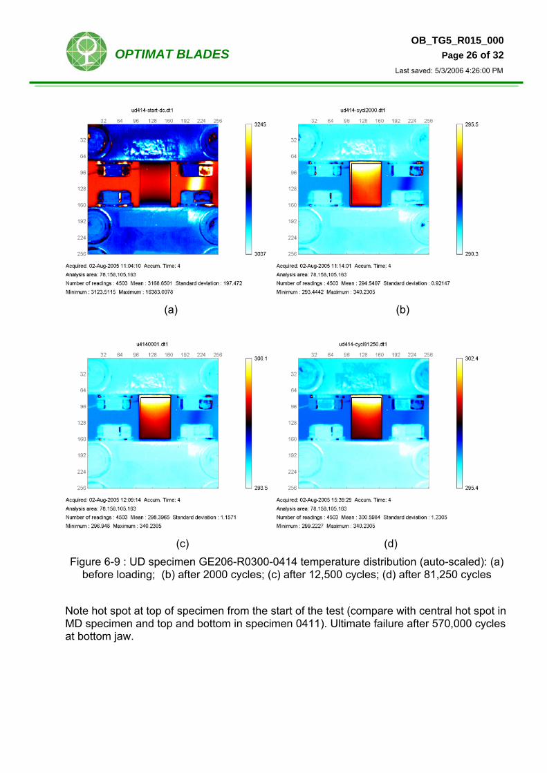
Figure 6-9 : UD specimen GE206-R0300-0414 temperature distribution (auto-scaled): (a) before loading; (b) after 2000 cycles; (c) after 12,500 cycles; (d) after 81,250 cycles

Note hot spot at top of specimen from the start of the test (compare with central hot spot in MD specimen and top and bottom in specimen 0411). Ultimate failure after 570,000 cycles at bottom jaw.


Last saved: 5/3/2006 4:26:00 PM

(a) (b)

(c) (d)

Figure 6-10 : UD specimen GE206-R0300-0414 thermoelastic stress (X-value) distribution: (a) after 4100 cycles; (b) after 12,500 cycles; (c) after 81,250 cycles; (d) after 93,000

cycles


Last saved: 5/3/2006 4:26:00 PM

(a) (b)

(c)

Figure 6-11 : UD specimen GE206-R0300-0414 thermoelastic stress (Y-value) distribution: (a) after 4100 cycles; (b) after 12,500 cycles; (c) after 93,000 cycles


Last saved: 5/3/2006 4:26:00 PM

(a) (b)

(c) (d)

Figure 6-12 : MD specimen GE207-R0400-0418 temperature distribution (auto-scaled): (a) after 2430 cycles; (b) after 8060 cycles; (c) after 14,830 cycles; (d) immediately before

40,000 cycles Note hottest spot in centre of specimen gauge length.


Last saved: 5/3/2006 4:26:00 PM

(a) (b)

(c) (d)

Figure 6-13 : MD specimen GE207-R0400-0418 thermoelastic stress (X-value) distribution: (a) after 2430 cycles; (b) after 8060 cycles; (c) after 14,830 cycles; (d) immediately before 40,000 cycles Note significant thermoelastic signal overflows (stippled pattern) from very early in the test.


Last saved: 5/3/2006 4:26:00 PM

(a) (b)

(c) (d)

Figure 6-14 : MD specimen GE207-R0400-0418 thermoelastic stress (Y-value) distribution: (a) after 2430 cycles; (b) after 8060 cycles; (c) after 14,830 cycles; (d)

immediately before 40,000 cycles


Last saved: 5/3/2006 4:26:00 PM

6.1. Thermoelastic area analysis in Matlab: 1. Run gd_ob001_upgrade and select .DT1 file 2. Set Area = [Row1 Row2 Col1 Col2] (initial guess) 3. Set ScaleXYZ = []; 4. Set inc_exclude_frame = 0 5. Execute

[Out]=gd_interactive_area_01(DataZ,Header01,PlotOpt,ScaleXYZ,Area,PlotTitle1,PlotTitle2,PlotTitle3,datafile,inc_exclude_frame)

6. Iterate Area 7. When Area is satisfactory execute gd_ob001_fileseq_dt or

gd_ob002_fileseq_dt (if overflow correction required)

Documents

Feasibility of various condition assessment techniques for ... · Feasibility of various condition assessment techniques for residual strength and life prediction T TG 5 A G Dutton