Agricultural Economics Report No. 208 June 1986

Feasibility of EstablishingSmall Livestock Slaughter Plants

in North DakotaBy

Scott M. Wulff, Timothy A. Petry,Delmer L. Helgeson and Randal C. Coon

Department of Agricultural EconomicsNORTH DAKOTA STATE UNIVERSITY

of Agriculture and Applied ScienceFARGO, NORTH DAKOTA 58105

In Cooperation withN.D. AGRICULTURAL PRODUCTS UTILIZATION COMMISSION

4023 N. State StreetBISMARCK, NORTH DAKOTA 58501

Preface

The authors are indebted to numerous private businesses andgovernmental agencies who provided information and data for this study.Special appreciation is given to Mr. Alvin Whitmer, Vice-President, FacilitiesDivision of Koch Supplies, Inc., Kansas City, Missouri, for assistance indeveloping specific investment cost data. North Dakota meat plant owners arealso acknowledged for helpful assistance in supplying and verifying certainoperational data.

Special recognition for financial support is given to the North DakotaAgricultural Products Utilization Commission and the North Dakota AgriculturalExperiment Station.

Gratefully acknowledged are the manuscript reviewers, Drs. GordonErlandson and Donald Scott, Department of Agricultural Economics; Dr. DeanMcllroy, Director, North.Dakota Products Utilization Commission; Dr. MartinMarchello, Department of Animal Science; and Dr. Harlan Hughes, ExtensionLivestock Economist. Also acknowledged with special thanks are DarlaChristensen who typed preliminary and final drafts, Jackie Grossman for finalediting, and Carol VavRosky for preparing the figures. The authors acceptsole responsibility for any omissions or errors in the text.

Table of Contents

Page

List of Tables . . .. ................

List of Figures . . . . . . . . . . . . . . . . . . . .

Highlights ......... .

Regulation of the Meat Industry .. . . ........Federal Inspection Regulations . ...Custom Exempt Regulations .. . . . .........Retail Exempt Regulations .. . . . .........

North Dakota Slaughter and Processing Plants ..

North Dakota Livestock Supply and Commercial Slaughter

Economic Analysis .. . .......Plant Characteristics and UtilizationCost and Revenue Analysis .. ....

Investment Costs .......Building Requirements and CostsLand Requirements and Costs . . .Equipment Requirements and Costs

Operating Capital Requirements .Labor Requirements and Costs . . .Utilities . . . . . . . . . . . . .

Electrical Requirements and CostsWater Requirements and CostsNatural Gas Requirements and Costs

Levels. . . .

. . . .

. . . .

. . . .

* .

. . . .

. . . .

* . . .. . * .

. . . .. . .*

. . . .

. . . .

. . . *

Other Costs .. . ....Revenue Analysis . .Cost and Revenue Summary

Economic Profitability . .

Economic Impact .. . ....Input-Output Model . . .Local Expenditures . . .Total Business ActivityTax Collections .. . . .

Summary and Conclusions . . .....

Appendix A . . . . . . . . . . . . . .

Appendix B .. .. . . . . .

Appendix C .. . . . ....

References .. . . . .....

iii

V

. . . . . . . vii

. . . . . . ix

1223

4

7

1111141415151516161818192123252729

3535383940

40

43

49

53

57

.*

.*

.*

.*

.*

.*

.*

.*

· · · · · · · ·

· · · · II··

· ·

I,

O

or.*

.*

.*

.*

.*

.*

.*

.*

.*

. . . . .

.*

.*

.*

.*

.*

.*

.*

.*

.*

.*

.*

.*

.*

.*

.*

.*

· · 0·················~

· · · · · · · · · · · · · · · · · · · ·

List of Tables

Table Page

1 NUMBER OF NORTH DAKOTA FEDERALLY INSPECTED AND CUSTOM EXEMPTSLAUGHTER AND PROCESSING MEAT PLANTS BY COUNTY IN 1985 ANDCHANGES FROM 1977. . . . . . . . . . . . ............ 6

2 LIVESTOCK MARKETINGS IN NORTH DAKOTA, 1978 AND 1982 . .. . ..... 73 LIVESTOCK MARKETED BY COUNTY, NORTH DAKOTA, 1982 . ...... .. 84 ANNUAL NORTH DAKOTA COMMERCIAL SLAUGHTER, 1975-1985 .... . . . . . 115 CHARACTERISTICS OF MODEL SLAUGHTER AND PROCESSING PLANTS, NORTH

DAKOTA, 1985 .. .. .... ................. 136 ANNUAL SLAUGHTER AND PROCESSING VOLUME FOR MODEL PLANTS, NORTH

DAKOTA, 1985 . . ... ........ . .. . .. . . . .... .. . 147 INVESTMENT COSTS FOR MODEL PLANTS, NORTH DAKOTA, 1985 .. . ... . 148 AVERAGE INVESTMENT PER HEAD OF DESIGNED CAPACITY FOR MODEL

PLANTS, NORTH DAKOTA, 1985 ............. . . . . . . 159 OPERATING CAPITAL REQUIREMENTS, MODEL PLANTS, NORTH DAKOTA,

1985 . . . ..... .. . ....... .. ... . .... .. 1610 PERSONNEL REQUIREMENTS FOR MODEL PLANTS AT 100 PERCENT

UTILIZATION LEVEL BY DEPARTMENT, NORTH DAKOTA, 1985 . . . . . . . 1711 WAGE RATES FOR MODEL PLANTS, NORTH DAKOTA, 1985 .. ...... . . 1712 ANNUAL LABOR AND FRINGE BENEFIT COSTS FOR MODEL PLANTS, NORTH

DAKOTA, 1985 . . . . . . . . ... . . ...... . ..... .. . 1813 ANNUAL ELECTRICAL REQUIREMENTS IN KILOWATT-HOURS FOR MODEL

PLANTS, NORTH DAKOTA, 1985 . ... . .. .. . ... ... .. . .. . 1814 ANNUAL ELECTRICAL COSTS FOR MODEL PLANTS, NORTH DAKOTA, 1985 . . . 1915 ESTIMATED WATER USAGE FOR MODEL PLANTS FOR SELECTED FUNCTIONS,

NORTH DAKOTA, 1985 .. ..... . .. . . ... . .. . . 2016 ANNUAL WATER USAGE FOR MODEL PLANTS, NORTH DAKOTA, 1985 .. .. . 2017 ANNUAL WATER COSTS FOR MODEL PLANTS, NORTH DAKOTA, 1985 . ..... . 2118 ANNUAL NATURAL GAS USAGE IN CCF FOR HOT WATER HEATING AND

OPERATION OF SMOKEHOUSE FOR MODEL PLANTS, NORTH DAKOTA, 1985 . . 2119 ANNUAL NATURAL GAS COSTS FOR HOT WATER HEATING AND OPERATION OF

SMOKEHOUSE FOR MODEL PLANTS, NORTH DAKOTA, 1985 ... . ...... . 2220 ANNUAL HEATING COST FOR MODEL PLANTS, NORTH DAKOTA, 1985 . . . . . 2221 OTHER NONVARIABLE ANNUAL COSTS FOR MODEL PLANTS, NORTH DAKOTA,

1985 . . . ... . . . . . ... . .. . ... .. . . . . . ... . 2322 ANNUAL COMMISSION AND TRUCKING FEES FOR MODEL PLANTS, NORTH

DAKOTA, 1985 . . . . . . . . . . . . . . . . . .. . . . . . . . . 2423 ANNUAL PRODUCT LIABILITY INSURANCE COSTS FOR MODEL PLANTS, NORTH

DAKOTA, 1985 ..... . . . . . . . . . ...... .... . . 2424 ANNUAL VARIABLE DELIVERY EXPENSE FOR MODEL PLANTS, NORTH DAKOTA,

1985 . . . . . . . . . . . . . . . . . . . . . . . . . . . . . . . 2425 ANNUAL COSTS OF SUPPLIES AND OTHER COSTS FOR MODEL PLANTS, NORTH

DAKOTA, 1985. . . . . . . . . . . . . . . . . . . 2526 GROSS MARGINS PER HEAD BY TYPE OF SALE FOR MODEL PLANTS, NORTH

DAKOTA, 1985. . . . . . . . . ..... . ........ . . 2627 TOTAL ANNUAL REVENUE ABOVE LIVESTOCK PURCHASES FOR MODEL PLANTS,

NORTH DAKOTA, 1985 . . . . . . . . .. . . . . . . . . . . . . . 2728 SUMMARY OF INVESTMENT OUTLAYS, ANNUAL REVENUES, AND ANNUAL COSTS

FOR MODEL PLANTS, NORTH DAKOTA, 1985 . ............ . . . 28

v

List of Tables (Continued)

Table Pag<

29 HYPOTHETICAL CASH FLOW EXAMPLE FOR A MODEL B SIZE SLAUGHTERINGPLANT . .. . . . . . . . . . . . . . . . . . . . . . . . . . . . .. 30

30 INTERNAL RATE OF RETURN FOR MODEL PLANT A, NORTH DAKOTA, 1985 . . . 3331 INTERNAL RATE OF RETURN FOR MODEL PLANT B, NORTH DAKOTA, 1985 . . . 3332 INTERNAL RATE OF RETURN FOR MODEL PLANT C, NORTH DAKOTA, 1985 . . . 3433 INPUT-OUTPUT INTERDEPENDENCE COEFFICIENTS, BASED ON TECHNICAL

COEFFICIENTS FOR 17-SECTOR MODEL FOR NORTH DAKOTA . . . . . . 3634 ESTIMATED LOCAL CONSTRUCTION AND OPERATIONAL PHASE EXPENDITURES

ASSOCIATED WITH THREE SIZES OF LIVESTOCK SLAUGHTER PLANTS,NORTH DAKOTA, 1986 .. . . . . . . . . . ..... ... . .. . . 38

35 ESTIMATED PERSONAL INCOME, RETAIL SALES, BUSINESS ACTIVITY OFALL BUSINESS (NONAGRICULTURAL) SECTORS, AND TOTAL BUSINESSACTIVITY RESULTING FROM CONSTRUCTION AND OPERATION OF THREESIZES OF LIVESTOCK SLAUGHTER PLANTS, NORTH DAKOTA, 1986 . ..... . 39

36 ESTIMATED TAX REVENUES RESULTING FROM CONSTRUCTION AND OPERATIONOF THREE SIZES OF LIVESTOCK SLAUGHTER PLANTS, NORTH DAKOTA,1986 .. . . . . . . . .. . . ... ... ....... ... . . . 40

vi

List of Figures

Figure Page

1 Distribution of Federally Inspected and Custom Exempt Slaughterand Meat Processing Plants, North Dakota, 1985 . ......... 5

2 Distribution of All Cattle by Counties, North Dakota, January 1,1985 .. . .. . ..... . ... . . ........ ..... . 9

3 Distribution of All Hogs by Counties, North Dakota, December 1,1984 . . ...... . . . . . . . . . . . . . . . . . ... . 10

4 North Dakota's 1985 Monthly Commercial Cattle Slaughter as aPercentage of the 1985 Average . ................ . .12

5 North Dakota's 1985 Monthly Commercial Hog Slaughter as aPercentage of the 1985 Average .................. 12

6 Short-run Average Total Cost, Model Plants Operating at VaryingUtilization Levels, North Dakota, 1985 ... ......... .. . 31

vii

Highlights

An economic feasibility analysis of small multi-species slaughterplants was conducted to determine the costs and returns associated withconstruction and operations. Three model plants were developed ranging insize from an annual slaughter capacity of 1,200 head of cattle and 743 hogs to3,750 head of cattle and 2,321 hogs. Detailed plant investment costs andoperating budgets were developed. Different plant utilization levels wereconsidered as well as plant size to evaluate how each influenced the finaloperating results. The smallest plant (using an opportunity cost of 12.55percent) was marginally profitable when operating at 85 percent of capacity,the middle sized plant at 70 percent of capacity, and the largest plant at 55percent of capacity. A high level of plant utilization must be achievedthroughout the year if the smallest plants are to be profitable. The largerplant can be operated profitably at slightly lower levels of plant utilizationbecause of the ability to capture certain economies of size that serve tolower per unit costs.

Small meat plants were found to be economically feasible based onresearch assumptions. However, a high degree of management expertise would berequired to operate plants profitably given the seasonality in livestockproduction and demand for meat products and services that exist in theindustry.

The direct economic impact of these plants was not large, but would besubstantial for smaller cities within the state. Total business activityresulting from annual slaughter plant expenditures would amount to anestimated $498,000 for the smallest plant, $892,000 for the middle sizedplant, and $1,354,000 for the largest plant. Direct slaughter plantemployment was estimated at 7, 12, and 18 employees for each of three sizes ofplants. These employment levels would be a significant economic developmentforce for the rural areas of the state.

ix

Feasibility of Establishing Small Livestock SlaughterPlants in North Dakota

by

Scott M. Wulff, Timothy A. Petry, Delmer L. Helgeson, and Randal C. Coon*

Many rural communities in North Dakota attempt to solve problems ofunemployment and population decline by increasing economic development. Onepotential economic development project considered by North Dakota communitiesis the establishment of new small slaughter and meat processing plants.

This study's primary objective was to determine the costs and returnsassociated with the construction and operation of small multi-speciesslaughter and meat processing plants in North Dakota. These estimated costsand returns can be used by state developers, city planners, financial institu-tions, and potential investors in their respective decision-making processes.

Specific objectives of this study include (1) review of legislationregarding meat inspection, (2) identification of present slaughter and meatprocessing plants in North Dakota, (3) overview of the current livestocksupply in North Dakota,. (4) identification of the capital investment andoperating costs for a North Dakota based plant, (5) analysis of the economicprofitability of a North Dakota plant, and (6) projection of the economicbenefits of a new livestock slaughter and meat processing plant on local andstate economies.

SRegulation of the Meat Industry

Legislation regarding meat inspection has existed for over 85 years.The first comprehensive Federal Meat Inspection Act was passed in 1891(Williams 1969). This act became necessary due to the increasing animaldisease problems in the United States. It provided for inspection of theanimal and meat prior to and after slaughter.

The Meat Inspection Act of 1906 extended the provisions of the 1891 Actto include sanitation standards for slaughter and processing plants trading ininterstate commerce. It became the basis for all federal meat inspectionuntil December 15, 1967, when the Wholesome Meat Act of 1967 became law. TheWholesome Meat Act of 1967 amended the Meat Inspection Act of 1906 to includethe inspection of meat plants that formerly sold meat only within the state(USDA 1969).

The 1967 law gave state legislatures until December 15, 1969, toinitiate state inspection of livestock slaughter and meat processing plantsthat were not previously federally inspected (Dunn 1970). Federal inspectionwas to become mandatory in those states not having an acceptable stateinspection program prior to December 15, 1969. Individual states were allowedan additional year beyond the December 15 deadline, if the state could

*Wulff is Research Assistant, Petry is Associate Professor, Helgeson isProfessor, and Coon is Research Specialist, Department of AgriculturalEconomics, North Dakota State University.

-2-

demonstrate satisfactory progress in establishing a meat inspection programwhich met federal standards.

The North Dakota Legislature passed a state inspection bill. However,because of insufficient funds allocated by the state legislature to implementthe inspection program, federal inspection was initiated in North Dakota onApril 16, 1970.

The Curtis Amendment, passed on July 16, 1970, amended the WholesomeMeat Law of 1967 to allow retail firms which sold federally inspected meat andcustom firms involved in slaughter and processing of meat for the customers'own consumption to be exempt from federal inspection status.

Federal Inspection Regulations

According to present meat acts and regulations (Wholesome Meat Act,Sections 1-10; Poultry Products Inspection Act, Sections 1-9; and MeatInspection Regulations, Part 301.2) the term "federally inspected" refers to:

Any meat product or poultry product that is identified byan official mark or official inspection legend, as prescribed byregulation of the Secretary of Agriculture, has been inspected andpassed by inspectors appointed for that purpose in establish-ments at which inspection is maintained. At the time the productis prepared it is inspected, passed and identified, and found tobe wholesome, not adulterated, and not mislabeled.

To assure that the meat and poultry products are distri-buted into commerce as wholesome, not adulterated or misbranded,these products are subjected to examination and inspection duringantemortem, postmortem, upon entry into any department wherein theproducts shall be treated or prepared for meat food and poultryproducts (processing).

The establishment at which inspection is maintained shallmaintain sanitation according to the prescribed rules and regula-tions of sanitation, and permit access by inspectors at all timesto every part of said establishment for the purposes of anyexamination and inspection.

Custom Exempt Regulations

The Wholesome Meat Act (Section 23) and Federal Meat InspectionRegulations (Part 303.1) define provisions for plants operating under customexempt status in the following terms:

The provisions for "federally inspected" requiring theinspection of the slaughter of animals and the preparation of thecarcasses, parts thereof, meat and meat food products atestablishments conducting such operations for commerce shall notapply to the slaughtering by any person of animals of his ownraising, and the preparation by him and transportation in commercein the carcasses, parts thereof, meat and meat food products of

- 3-

such animals exclusively for use by him and members of hishousehold and his nonpaying guests and employees; not to thecustom slaughter by any person, firm or corporation of cattle,sheep, swine or goats delivered by the owner thereof for suchslaughter, and the preparation by such slaughter and transporta-tion in commerce of the carcasses, parts thereof, meat and meatfood products of such animals, exclusively for use, in thehousehold of such owner by him, and members of his household andhis nonpaying guests and employees.

The adulteration and misbranding provisions, other than therequirement of the inspection legend, shall apply to the articleswhich are exempted from inspection.

The custom prepared products are plainly marked "NOT FORSALE" immediately after being prepared by the custom operator andare kept so identified until delivered to the owner.

Retail Exempt Regulations

Meat plants subject to retail exempt status are to follow theprescribed guidelines and definitions as set forth by the Wholesome Meat Act(Section 301c) and the Meat Inspection Regulations (Part 303.1d):

The provisions of this act requiring inspection of theslaughter of animals and the preparation of carcasses, partsthereof, meat and meat food products shall not apply to operationsof types traditionally and usually conducted at retail stores andrestaurants, when conducted at any retail store or restaurant orsimilar retail-type establishment for sale in normal retailquantities or service of such articles to consumers at suchestablishments.

Operations of types traditionally and usually conductedat retail stores and restaurants are the following:

(a) cutting up, slicing, and trimming carcasses, halves,quarters, or wholesale cuts into retail cuts such assteaks, chops, and roasts, and freezing such cuts;

(b) grinding and freezing products, made from meat;

(c) curing, cooking, smoking, rendering or refining oflivestock fat, or other preparation of products, exceptslaughtering or the retort processing of canned products;

(d) breaking bulk shipments of products;

(e) wrapping or rewrapping products.

Any quantity or product purchased by the consumer from aparticular retail supplier shall be deemed to be a normal retailquantity if the quantity so purchased does not in the aggregateexceed one-half carcass.

-4-

A retail store is any place of business where the sales ofproduct are made to consumers only; at least 75 percent, in termsof dollar value, of total dollar value of sales of product tohousehold consumers and the total dollar value of sales of productto consumers other than household consumers does not exceed$28,0001 per calendar year (January 1 through December 31); onlyfederally or state inspected and passed product is handled or usedin the preparation of any retail product.

A restaurant is an establishment where product is preparedonly for sale or service, in meals, or in entrees, directly toindividual consumers or such product prepared at a retail exemptstore is handled or used in the preparation of any product.

North Dakota Slaughter and Processing Plants

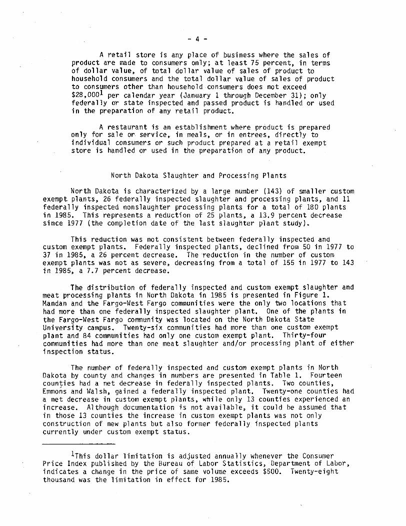
North Dakota is characterized by a large number (143) of smaller customexempt plants, 26 federally inspected slaughter and processing plants, and 11federally inspected nonslaughter processing plants for a total of 180 plantsin 1985. This represents a reduction of 25 plants, a 13.9 percent decreasesince 1977 (the completion date of the last slaughter plant study).

This reduction was not consistent between federally inspected andcustom exempt plants. Federally inspected plants, declined from 50 in 1977 to37 in 1985, a 26 percent decrease. The reduction in the number of customexempt plants was not as severe, decreasing from a total of 155 in 1977 to 143in 1985, a 7.7 percent decrease.

The distribution of federally inspected and custom exempt slaughter andmeat processing plants in North Dakota in 1985 is presented in Figure 1.Mandan and the Fargo-West Fargo communities were the only two locations thathad more than one federally inspected slaughter plant. One of the plants inthe Fargo-West Fargo community was located on the North Dakota StateUniversity campus. Twenty-six communities had more than one custom exemptplant and 84 communities had only one custom exempt plant. Thirty-fourcommunities had more than one meat slaughter and/or processing plant of eitherinspection status.

The number of federally inspected and custom exempt plants in NorthDakota by county and changes in numbers are presented in Table 1. Fourteencounties had a net decrease in federally inspected plants. Two counties,Emmons and Walsh, gained a federally inspected plant. Twenty-one counties hada net decrease in custom exempt plants, while only 13 counties experienced anincrease. Although documentation is not available, it could be assumed thatin those 13 counties the increase in custom exempt plants was not onlyconstruction of new plants but also former federally inspected plantscurrently under custom exempt status.

1 This dollar limitation is adjusted annually whenever the ConsumerPrice Index published by the Bureau of Labor Statistics, Department of Labor,indicates a change in the price of same volume exceeds $500. Twenty-eightthousand was the limitation in effect for 1985.

A Federally inspected slaughter plant

D Federally inspected non-slaughter plant

. 0 Custom exempt plant

Figure 1. Distribution of Federally Inspected and Custom Exempt Slaughter and Meat Processing Plants,North Dakota, 1985

0 00

cn

-6-

TABLE 1. NUMBER OF NORTH DAKOTA FEDERALLY INSPECTED ANDMEAT PLANTS BY COUNTY IN 1985 AND CHANGES FROM 1977

CUSTOM EXEMPT SLAUGHTER AND PROCESSING

Federally Inspected Custom ExemptCounty Number Change from 1977 Number Change from 1977

AdamsBarnesBensonBillingsBottineau

BowmanBurkeBurleighCassCavalier

DickeyDivideDunnEddyEmmons

FosterGolden ValleyGrand ForksGrantGriggs

HettingerKidderLaMoureLoganMcHenry

McIntoshMcKenzieMcLeanMercer,Morton

MountrailNelsonOliverPembinaPierce

RamseyRansomRenvilleRichlandRolette

SargentSheridanSiouxSlopeStark

SteeleStutsmanTownerTraillWalsh

WardWellsWilliams

N.D. Total

12001

00072

0000

0&200.

00000

0000

1001

20020

0

2

000

1

11202

112

(1)a

(1)

(1)(1)

(1)

1

(1)

(1)

(1)-

(1)

(1)

(1)

- |I-

1

(2)

(1)

(13)37

12203

32410

40334

34531

30444

45647

33030

(1)(1)

(1)

(1)(1)

(1)

(1)

12(1)

113(1)

1

(2)

1

(2)2(2)1

1

(1)(3)

1(1)

1

(2)

1

(1)(2)

(1)

(1)

(12)

22151

12005

04113

844

143

parentheses ( ) signify a decrease.

-aNumbers enclosed in

- 7-

The distribution of federally inspected slaughter plants in NorthDakota reflects the competitiveness of the industry. Results from a 1985survey of federally inspected slaughter plant managers reported an averageutilization of 54.75 percent of plant capacity. This demonstrates the problemof insufficient demand that many small slaughter plants face. Such a lowlevel of utilization for small slaughter plants is also national in scope.Baker (1976) reported that United States federally inspected plants,slaughtering cattle with a design capacity of up to 9,562 head annually, wereutilizing only 38.8 percent of their engineered capacity in 1973.

North Dakota Livestock Supply and Commercial Slaughter

North Dakota meat processors have been generally facing a decline inlivestock marketings. Data taken from the 1982 Census of Agriculture forNorth Dakota indicate a reduction in cattle and calf marketings of 7.4percent, an increase in fed cattle of 9.2 percent, a reduction of 16.9 percentin the number of hogs and pigs marketed, and a 16.4 percent reduction inmarketings of hogs and pigs other than feeder pigs, for the period from 1978to 1982 (Table 2). The categories cattle fattened on grain; and hogs and pigssold, other than feeder pigs; were included to more fully reflect thelivestock supply a slaughter or processing plant would encounter.

TABLE 2. LIVESTOCK MARKETINGS IN NORTH DAKOTA, 1978 AND 1982

Marketings % .ChangeClassification 1978 1982 From 1978

Cattle and calves sold 1,099,421 1,018,516 (7.4)

Cattle fattened on grain 99,669 108,854 9.2

Hogs and pigs sold 538,492 447,738 (16.9)

Hogs and pigs sold, otherthan feeder pigs 371,477 310,501 (16.4)

SOURCE: 1982 Census of Agriculture.

County marketing data are presented in Table 3. The relative increaseand decrease in state marketings were not consistent across all counties.Only 15, 32, 13, and 9 out of a total of 53 counties reported increases inmarketings, respectively, for all cattle, fed cattle, all hogs, and hogs andpigs other than feeder pigs. The number of counties reporting a decrease inmarketings were 38, 20, 38, and 35, respectively.

North Dakota's January 1, 1985, inventory of all cattle was 2,050,000head and the December 1, 1984, inventory of all hogs was 255,000 head (NorthDakota Agricultural Statistics 1985). County concentrations of cattle andhogs are presented in Figures 2 and 3, respectively. Cattle production wasconcentrated in the south central areas of the state and hog production in thesoutheastern areas of the state.

-8-

TABLE 3. LIVESTOCK MARKETED BY COUNTY, NORTH DAKOTA, 1982

Cattle & Calves Cattle Fattened Hogs and Hogs & Pigs Sold OtherCounty Sold on Grain Pigs Sold Than Feeder Pigs

---- --- ----------- numbers-----------------

AdamsBarnesBensonBillingsBottineau

BowmanBurkeBurleighCassCavalier

DickeyDivideDunnEddyEmmons

FosterGolden ValleyGrand ForksGrantGriggs

HettingerKidderLaMoureLoganMcHenry

McIntoshMcKenzieMcLeanMercerMorton

MountrailNelsonOltverPembinaPierce

RamseyRansomRenvilleRichlandRolette

SargentSheridanSiouxSlopeStark

SteeleStutsmanTownerTraillWalsh

WardWellsWilliams

N.D. Total

16,38617,77118,067*13,3429,755

16,0298,20334,745*20,3914,133

29,3268,21042,29710,56536,956*

9,10719,681*10,30132,84212,274*

14,38732,84420,01932,040*35,330

28,188*37,44627,223*26,717*50,408

20,2108,779*14,6055,36815,425*

3,94916,4944,752

22,393*11,098

18,58813,86321,578*14,00130,503

3,17838,3654,198*2,7878,442

21,38025,419*17,160

1,018,516

1,060*2,796*1,010*

597*558

804323

2,123*11,555*

440

7,935*536

2,965*703*

1,854*

1,4401,597*4,277*1,737*1,209

1,6666*1,667*2,887*

792*1,859*

1,5811,829*1,9971,0744,078*

1,644*840*547

1,251455

7282,324*

2506,043*866

4,062869*NA762*

1,972*

5563,911*

323892

2,080

1,281*NA591

108,854*

4,87717,1623,853

653*2,693

2,6921,348

13,01838,144*8,095

25,481*2,4484,8771,7309,130

5,422*4,810

10,753*20,142

3,137

14,237*5,026

20,462*4,1403,655

5,0344,8904,1242,779

10,829

1,1604,321

11,173*15,2891,224

4,67912,3381,800*

41,9151,929

25,468*1,924

NA9,499*8,261

1,368*9,9553,267*

10,05614,270*

5,8202,2911,834

447,738

2,88011,820

NA599*

2,290

1,926*900*

10,93528,670*7,203*

19,9202,2863,2931,6157,221

3,312*NA

7,750*11,570

1,094

8,137884

9,933788

2,794

3,0344,295

NANA

6,714

5642,2803,274

11,463NA

3,2739,727

NA28,494

NA

19,7881,4261,4468,792*5,045

NA6,5673,096

NA9,403*

4,7022,1481,183

310,501

*Indicates an increase from 1978.Note: NA indicates data not available.SOURCE: 1982 Census of Agriculture.

SLess than 20,000 head 30,000 - 49,999 head

W 20,000 - 29,999 head 50,000 head and over

SOURCE: North Dakota Agricultural Statistics.

Figure 2. Distribution of All Cattle by Counties, North Dakota, January 1, 1985

7L

Sioux

i Less than 2,500 head El 5,000 - 7,499 head

2,500 - 4,999 head 7,500 head and over

SOURCE: North Dakota Agricultural Statistics..

Figure 3. Distribution of All Hogs by Counties, North Dakota, December 1, 1984

V//C)

- 11 -

Contrary to marketing data, actual commercialhas been increasing since the late 1970s (Table 4).

slaughter in North DakotaCommercial cattle

TABLE 4. ANNUAL NORTH DAKOTA COMMERCIAL SLAUGHTER, 1975-1985

Year Cattle Calves Sheep Hogs- ------------------------ thousand head --------------

1975 283.2 .4 1.3 21.91976 273.6 .4 1.2 22.41977 276.0 1.5 .8 20.11978 116.9a .4 .6 20.31979 57.3a .3 .7 27.41980 134.5 .4 .9 50.71981 165.7 .4 1.0 57.61982 170.0 .3 1.0 49.31983 159.0 .4 1.0 70.21984 182.3 .4 1.0 78.41985 161.4 .3 .9 84.8

aA major slaughter plant was not operating during part of 1979.

SOURCE: Crop Reporting Board, Statistical Reporting Service, USDA.

slaughter in North Dakota fell from 283,200 head in 1975 to 116,900 in 1978 buthas since recovered to 182,300 in 1984 and 161,400 in 1985. Calf and sheepslaughter have remained relatively constant. Hog slaughter has been steadilyincreasing from the 20,000 level for most of the 1970s to 84,800 in 1985.

North Dakota slaughter plants also encounter a very volatile monthlylivestock slaughter volume. Monthly commercial cattle slaughter, as apercentage of the 1985 average, ranged from 64.7 percent to 137.6 percent in1985 (Figure 4). Monthly commercial hog slaughter, as a percentage of the 1985average, ranged from a low of 73.5 percent to a high of 119 percent in 1985(Figure 5).

Economic Analysis

Economic feasibility analysis of new small slaughter and processingplants in North Dakota will be presented in three sections: (1) model plantcharacteristics and utilization levels, (2) cost and revenue analysis, and(3) economic profitability. The analysis will be based on operational levelsutilizing 55, 70, 85, and 100 percent of model plant capacity.

Plant Characteristics and Utilization Levels

Model plants were designed for annual volumes of 1,600, 3,000, and5,000 head of cattle. These plants will be referred to as Plants A, B, or C,hereafter; Plant A being the smallest, B the medium-sized plant, and C the

- 12 -

Percent

of

Monthly

Average

SOURCE: USDA Annual Livestock Summry

Figure 4. North Dakota's 1985 Monthly Commercial Cattle Slaughtas a Percentage of the 1985 Average

140

130

120Percent

of 110

Monthly

Average100

90

80

70

60J F M A J J A JS 0 N D

SOURCE: USDA Annual Livestock Su=aary

Figure 5. North Dakota's 1985 Monthly Commercial Hog Slaughteras a Percentage of the 1985 Average

1

er

- 13 -

largest. A factor of 1.857 hogs per head of cattle is used when convertingkill and processing capacity from number of cattle to number of hogs (Stinsonet al. 1978).

Annual capacity is based on the daily kill floor capacity, 250 workdaysper year, and an institutional constraint factor of .8. The institutionalconstraint was used. to adjust annual capacity due to seasonality of animalsupplies and consumer demand, and daily procurement problems. A slaughter andprocessing plant manager, unlike some other processing industries, does nothave the alternative (option) to inventory a supply of raw materials tomaintain a constant production process. The factor of .8 was estimated basedon the seasonality of the livestock marketings (as discussed earlier) andindustry estimates. This factor for annual capacity is considerably higherthan the current industry average, but was considered achievable with aboveaverage management.

All plants were designed for custom kill, wholesale, and retailoperations under federal inspection status. It was assumed one-third ofproduction was devoted to each of the following: (1) custom slaughter andprocessing, (2) wholesale, and (3) retail markets. Twenty-five percent of theoperational time of each model plant was allocated to hog slaughter andprocessing. Koch Supply, Inc. 2 provided the plant designs with each modeldesign representing actual plant designs of proposed or previously builtplants. Model plants were designed to meet all USDA federal inspectionstandards.

All model plants were equipped with a kill floor, chill cooler, holdingcooler, blast freezer, and smokehouse (Table 5). Plants B and C incorporatean additional holding freezer.

TABLE 5. CHARACTERISTICS OF MODEL SLAUGHTER AND PROCESSING PLANTS, NORTHDAKOTA, 1985

.. .Plant SizeItem A B C

Annual capacity - animal unitsa 1,600 3,000 5,000Kill floor capacity - number of cattle per day 8 15 25Chill cooler capacity - head of cattle 8 15 25Holding cooler capacity - head of cattle 16 20 35Blast freezer - 24 hour capacity in Ibs. 4,000 4,000 6,000Holding freezer - Ibs. of meat -- 7,500 15,000Smokehouse - holding capacity in Ibs. 500 500 500Total square footage of building 2,250 2,800 3,475

aOne animal unit equivalent to one head of cattle or 1.857 hogs.

2Koch Supplies, Inc., Kansas City, Missouri, 1985.

- 14 -

Annual slaughter and processing volumes were 1,200 head of cattle and743 head of hogs for Plant A; 2,250 head of cattle and 1,393 head of hogs forPlant B; and 3,750 head of cattle and 2,321 head of hogs for Plant C. Annualvolumes at plant utilization levels of 55, 70, 85, and 100 percent arepresented in Table 6.

TABLE 6.DAKOTA,

ANNUAL1985

SLAUGHTER AND PROCESSING VOLUME FOR MODEL PLANTS, NORTH

Plant Plant SizeUtilization A B C

Level Cattle Hogs Cattle Hogs Cattle Hogs

(percent) --------------------- number of head --------------------

55 660 409 1,238 766 2,063 1,27770 840 520 1,575 975 2,625 1,62585 1,020 631 1,913 1,184 3,188 1,973

100 1,200 743 2,250 1,393 3,750 2,321

Cost and Revenue Analysis

Investment Costs

Total investment costs for Model Plants A, B, and C were $235,841;$349,590; and $471,941, respectively (Table 7). Average investment per head

TABLE 7. INVESTMENT COSTS FOR MODEL PLANTS, NORTH DAKOTA, 1985

Plant SizeItem A B C

----------- dollars --------------

Land 5,165 6,428 7,978Building and excavation 110,496 146,303 201,883Drainlines and plumbing 9,000 17,500 38,920Electric lines and wiring 10,000 19,600 32,900Kill floor and processing equipment 53,339 78,879 103,663Refrigeration equipment 43,377 53,391 54,328Furnace 2,900 3,000 3,100Office equipment 1,564 1,989 2,469Delivery: truck -- 16,000 16,000

refrigeration unit -- 4,000 6,000insulated van - 2,500 4,700

Total investment costs 235,841 349,590 471,941

- 15 -

of designed daily capacity was $29,480 for Plant A, $23,306 for Plant B, and$18,878 for Plant C (Table 8). Significant economies of size existed for thelarger plant. Plant C's average investment per head was 36 percent less thanthat of Plant A.

TABLE 8. AVERAGE INVESTMENT PER HEAD OF DESIGNED CAPACITY FOR MODEL PLANTS,NORTH DAKOTA, 1985

SPlant SizeItem A B C

Total plant investment, dollars 235,841 349,590 471,941

Daily designed capacity,animal unitsa 8 15 25

Average investment per animal unitof designed daily capacity, dollars 29,480 23,306 18,878

a0ne animal unit equivalent to one head of cattle or 1.857 head of hogs.

Building Requirements and Costs. All building costs were based onconstruction estimates of actual plant designs. Specific designs wereslightly modified to maintain comparability between the three plants (Table7). All buildings have an expected life of 20 years with a salvage value of10 percent.

Land Requirements and Costs. Land requirements were computed at fivetimes the plant's square footage which would provide ample room for plantexpansion, employee and customer parking, truck access, and landscaping.Specific locational requirements include availability of city sewer and water.Land value was based on recent sales of industrial park real estate tracts.Values ranged from $16,000 to $25,000 per acre for various North Dakotacities. A value of $20,000 was assumed as reasonable for a North Dakota site.

Equipment Requirements and Costs. Equipment requirements wereestimated for slaughter and processing operations, office areas,refrigeration, and heating systems. Interviews and actual price quotes fromindustrial sources were used to determine equipment requirements and costs.

A refrigerated delivery truck was included to deliver 50 percent of allretail and wholesale meats for Model Plants B and C. Expected life ofslaughter and processing equipment, refrigeration equipment, delivery truck,and other equipment was estimated at 10, 15, 5, and 10 years, respectively.All equipment had an expected salvage value of 10 percent except the deliverytruck which was set at 40 percent.

- 16 -

Operating Capital Requirements

Operating capital requirements were estimated at $52,157; $97,794; and$162,990 for Plants A, B, and C at full capacity (Table 9). Operating capital

TABLE 9. OPERATING CAPITAL REQUIREMENTS, MODEL PLANTS, NORTH DAKOTA, 1985

PlantUtilization Plant Size

Level A B C

(percent) --------------------- dollars-------------------

55 28,686 53,787 89,64570 36,510 68,456 114,09385 44,333 83,125 138,542

100 52,157 97,794 162,990

requirements were estimated on the basis of a 25-day turnover between purchaseof live animals for wholesale and retail sales and the receipt of receivables.The 25-day turnover was estimated as a 5-day slaughter and processing timeplus a 20-day turnover in receivables for meat wholesalers as reported byRobert Morris Associates 3 (1985).

Labor Requirements and Costs

Labor requirements were synthesized for each plant size and utilizationlevel. These requirements were based on a USDA publication, Layout Guide forSmall Meat Plants (Brasington and Hammons 1976), and interviews with NorthDakta plant managers.

Personnel were divided into six departments; slaughter, processing,office and retail, sanitation and maintenance, delivery, and management (Table10). Labor productivity of slaughter and processing personnel was estimatedat 1-1/4 carcasses per man-hour for slaughter and 1,000 Ibs. of hangingcarcass weight per employee per eight-hour day for processing (Brasington andHammons 1976). Slaughter and processing labor requirements were consideredvariable.

Wage rates were estimated from three sources: American Meat Institute(1985); North Dakota Job Service Wage and Benefit Survey for Fargo, GrandForks, and Bismarck (1985); and interviews of North Dakota slaughter plant

3 Robert Morris Associates (RMA) is an organization whose members areprimarily officers of commercial banks who are concerned with business loansand credit information.

- 17 -

TABLE 10. PERSONNEL REQUIREMENTS FOR MODEL PLANTS AT 100 PERCENT UTILIZATIONLEVEL BY DEPARTMENT, NORTH DAKOTA, 1985

Plant SizeDepartment A B C

Slaughtera .78 1.46 2.43Processinga 3.63 6.86 11.35Office personnel and retail 1.00 1.50 2.00Delivery -- .50 .50Sanitation .50 .75 1.00Management 1.00 1.00 1.00

Total number of employeesb 6.91 12.07 18.28

aSlaughter and processing personnel requirements are variable with plantutilization levels and calculated as 1-1/4 carcasses per man-hour forslaughter and 125 Ibs. of hanging carcass weight per man-hour for processing.

bFractional employees can be accounted for by part-time and seasonalemployees.

managers (Table 11). Wage rates for Plant A, the smallest plant, aregenerally lower than for Plants B and C. This reflects the probable location

TABLE 11. WAGE RATES FOR MODEL PLANTS, NORTH DAKOTA, 1985

Plant SizeDepartment A B C

------------- dollars/hour--------------

Slaughter 6.00a 7 . 20 b 7.20bProcessing 5.50a 6 .10c 6.10cOffice personnel and retail 5.50a 6 . 00d 6.00dDelivery - 7 . 20 d 7.20dSanitation 5.50ae 4 . 95d 4.95d

-------------- annual salary --------------

Management $2 5 , 9 00 d $28, 1 8 0 d $31,040d

aSurvey of North Dakota Plant Managers, 1985.bNonunion labor rates for Midwest meat packers as reported by the American

Meat Institute (1985).cNonunion labor rates for Midwest meat processors as reported by the AmericanMeat Institute (1985).

dWage rates for similar occupations as reported by the North Dakota JobService (1985).

eDue to size of plant, sanitation in Plant A was assumed to be done by other.personnel, therefore, the same wage rate for processing personnel was used.

- 18 -

of Plant A in a smaller community relative to Plants B and C which,result, faces a less competitive labor market. Management salariesplants were based on wages reported by the North Dakota Job Servicemanagers of wholesale businesses.

as afor all(1985) for

Fringe benefits were estimated at 24.3 percent of total wages andsalaries. This was the cost of fringe benefits as reported by local packersby the American Meat Institute (1985). Total annual labor costs, includingfringe benefits, are summarized in Table 12. Annual labor cost at a 100percent utilization level for Plant A was $116,603, Plant B was $212,045, andPlant C was $312,608.

TABLE 12. ANNUAL LABOR AND FRINGE BENEFIT COSTS FOR MODEL PLANTS, NORTHDAKOTA, 1985

PlantUtilization Plant Size

Level A B C

(percent) --------------------- dollars ----------------------

55 81,650 136,537 194,83470 93,301 161,706 234,09285 104,952 186,875 273,350

100 116,603 212,045 312,608

Utilities

Electrical Requirements and Costs. Electricity was used in each modelplant for three purposes: lighting, operation of electric motors, andoperation of refrigeration units. Annual electrical consumption at the 100percent utilization level ranged from 131,343 kwh for Plant A to 187,674 kwhfor Plant B and 263,146 kwh for Plant C (Table 13). Energy calculations were

TABLE 13. ANNUAL ELECTRICAL REQUIREMENTS IN KILOWATT-HOURS FOR MODEL PLANTS,NORTH DAKOTA, 1985

PlantUtilization Plant Size

Level A B C

(percent) ------------------- kilowatt-hours ------------------

55 84,538 121,183 166,54670 101,829 143,346 198,74685 116,586 165,510 230,946

100 131,343 187,674 263,146

- 19 -

based on procedures outlined in the American Society of Heating, Refrigeration,and Air Conditioning Engineer's Handbook of FundamentaTs(1982). (See AppendixA for detailed electrical usage computational formulas.) Electrical rates werebased on the General Service Rate Schedule from the Northern States PowerCompany, Fargo, North Dakota. The energy charge was $.027 per kilowatt-hourand a demand charge of $5.59 per kilowatt (the weighted average of winter andsummer demand charges). Annual electrical costs when operating at a 100percent utilization level were $6,663, $9,444, and $13,169 for Plants A, B, andC, respectively (Table 14).

TABLE 14. ANNUAL ELECTRICAL COSTS FOR MODEL PLANTS, NORTH DAKOTA, 1985

Plant SizePlant A B C

Utilization Energy Demand Energy Demand Energy DemandLevel Chargea Chargeb Chargea Chargeb Chargea Chargeb

(percent) --------------------- dollars ------------------------

55 2,351 2,127 3,272 2,890 4,497 3,90470 2,749 2,457 3,870 3,385 5,366 4,62485 3,148 2,787 4,469 3,881 6,236 5,344

100 3,546 3,117 5,067 4,376 7,105 6,064

a$. 0 2 7 per kilowatt-hour.b$ 5 . 5 9 per kilowatt plus a monthly service charge of $15. Monthly demand inkilowatts estimated at 4 kilowatts per 1,000 kilowatt-hours of monthly use(Logan 1962).

Water Requirements and Costs. Water is used primarily for threepurposes in a slaughter plant: "TT washing of carcasses, (2) plant cleanup,and (3) employee needs. The schedule in Table 15 was used for determiningwater usage. Estimated water requirements were based on actual water usage bysmall slaughter plants as reported in Utility Usage in Small Slaughter Plants(Brasington 1977). Water usage is presented in Table 16. At a 100 percentutilization level water usage was estimated at 377,154 gallons for Plant A,582,294 gallons for Plant B, and 928,046 gallons for Plant C.

- 20 -

TABLE 15. ESTIMATED WATER USAGE FORNORTH DAKOTA, 1985

MODEL PLANTS FOR SELECTED FUNCTIONS,

Item Unit Calculated Usage

Slaughter room:Cattle dressing:

Head washing gal/head 2.44Offal-truck washing gal/head 3.23Carcass washing gal/lb 0.03Total per carcass gal/lb 0.09

Hog dressing:Carcass washing (skin off)a gal/lb 0.07Carcass washing (skin on)a gal/lb 0.02Total per carcass (skin off)a gaT/1b 0.14Total per carcass (skin on)a gal/lb 0.35

Plant cleanup:Cleanup during slaughter:

Between species gal/ft 2 0.07During work break gal/ft 2 0.05At end of day gal/ft 2 0.27

Holding pens gal/ft 2 0.19Inedible-offal room gal/ft 2 0.21Chill cooler gal/ft2 0.07Holding cooler gal/ft2 0.13Fabrication room gal/ft2 0.27

Employee needs: gal/day/employee 25

Unaccounted water usage % of total water usage 25%

aAll estimators calculated on a live weight basis.

SOURCE: Utility Usage in Small Slaughter Plants (Brasington 1977).

TABLE 16. ANNUAL WATER USAGE FOR MODEL PLANTS, NORTH DAKOTA, 1985

PlantUtilization Plant Size

Level A B C

(percent) ---------------------- gallons--- ---------------

55 300,484 438,537 688,45170 326,041 486,456 768,31685 351,598 534,375 848,181

100 377,154 582,294 928,046

- 21 -

Two charges for water usage are involved in cost calculations. Theseare a basic water charge and a sewage charge. The average commercial chargefor all North Dakota cities larger than 5,000 was used (North Dakota League ofCities 1982). The averages were $1.35 per 1,000 gallons for the basic watercharge and $.24 per 1,000 gallons for the sewage charge. Total annual watercharges at a 100 percent utilization level were $574 for Plant A, $887 forPlant B, and $1,413 for Plant C (see Table 17 for costs at differentutilization levels).

TABLE 17. ANNUAL WATER COSTS FOR MODEL PLANTS, NORTH DAKOTA, 1985

PlantUtilization Plant Size

Level A B C(percent) ---------------------- dollars ----------------------

55 458 668 104870 497 741 117085 535 814 1292

100 574 887 1413

Natural Gas Requirement and Costs. Natural gas was used for threepurposes: (1) heating of water, (2) operation of the smokehouse, and (3)heating of the building. In determining gas usage for heating of water it wasassumed that all water used for plant cleanup was heated to 180*F and allother water was tempered to 75"F. A water heater efficiency factor of 75percent was used. The smokehouse operated at 50,000 BTU per hour, 75 percentefficiency, 500 pound load, and a 12-hour smoking period. It was assumed that18 percent of the pork carcass, representing hams, was smoked. Natural gasusage for heating of water and operation of the smokehouse was 3,597 ccf (100cubic feet) for Plant A; 5,030 ccf for Plant B; and 7,787 ccf for Plant C whenoperating at a 100 percent utilization level (Table 18). Gas costs were based

TABLE 18. ANNUAL NATURAL GAS USAGE IN CCF FOR HOT WATER HEATING AND OPERATIONOF SMOKEHOUSE FOR MODEL PLANTS, NORTH DAKOTA, 1985

PlantUtilization Plant Size

Level A B C

(percent) ---------------- 100 cubic feet (ccf) ---------------

55 3,042 3,990 6,05370 3,227 4,337 6,63185 3,412 4,684 7,209

100 3,597 5,030 7,787

- 22 -

on the General Service Schedule from Northern States Power Company, Fargo,North Dakota. Natural gas costs were $1,906; $2,610; and $3,965 for Plants A,B, and C, respectively, operating at a utilization level of 100 percent(Table 19).

TABLE 19. ANNUAL NATURAL GAS COSTS FOR HOT WATER HEATING AND OPERATION OFSMOKEHOUSE FOR MODEL PLANTS, NORTH DAKOTA, 1985a

PlantUtilization Plant Size

Level A B C

(percent) ---------------- - dollars ------------------

55 1,633 2,099 3,11370 1,724 2,269 3,39785 1,815 2,440 3,681

100 1,906 2,610 3,965

aCalculated as: $.54144/ccf up to 30 ccf/month,$.49144/ccf for usage beyond 30 ccf/month, anda monthly service charge of $10.

Building heating costs were estimated at $2,050; $2,526; and $3,372 forPlants A, B, and C, respectively, when operating at full capacity (Table 20).

TABLE 20. ANNUAL HEATING COST FOR MODEL PLANTS, NORTH DAKOTA, 1985

PlantUtilization Plant Size

Level A B C

(percent) --------------- - dollars ---------------------

55 1,643 1,991 2,67870 1,779 2,169 2,91085 1,914 2,348 3,141

100 2,050 2,526 3,372

The heating requirements were estimated using the computerized North DakotaState University Cooperative Extension Service's AGNET Heating Cost Program(1985). Basic heating costs were assumed to not vary with plant utilizationlevels but were adjusted for heat loss due to infiltration from meat coolersand freezers which did vary with respect to utilization levels.

- 23 -

Other Costs

Other costs include those that are annual and do not vary with outputand those that are variable with the output level. Those that do not varywith output are repairs and maintenance, premise liability, fire insurance,truck insurance, and property tax (see Table 21 for a listing of other costson an annual basis).

TABLE 21. OTHER NONVARIABLE ANNUAL COSTS FOR MODEL PLANTS, NORTH DAKOTA,1985

Plant SizeCost Item A B C

S-_------ -_-l-_ --„ dollars----------------

Repairs and maintenance 6,920 9,620 13,118Premise liability 450 560 695Fire insurance 3,460 4,810 6,559Property tax 4,808 6,672 9,087Truck insurance -- 1,010a 1,310

alncludes a state license fee of $110.

Repairs and maintenance were estimated at 3 percent of initial plantinvestment (Schupp and Roy 1973). This figure overestimates repairs andmaintenance costs during the first few years of plant operation butunderestimates cost in later years. A constant rate of 3 percent was used forbudgetary reasons. Premise liability insurance was budgeted at $.20 persquare foot of building area. Fire insurance was estimated at $1.50 per $100value of buildings and equipment. Truck insurance was budgeted at $900 and$1,200 for Model Plants B and C. All insurance estimates were based oninterviews with major insurance companies. Property tax was estimated at$410.45 per $1,000 of taxable valuation. Taxable value is 10 percent ofassessed value and assessed value is calculated at 50 percent of full and fairmarket value (North Dakota Tax Department 1984). Full and fair market valueis estimated at the total initial investment in buildings and plant equipment.The tax rate of $410.45 was calculated as the state average of county millrates, $58.64, plus a city mill rate of $351.81. The city mill rate wasestimated from the average of Fargo, Jamestown, and Grand Forks rates. Othervariable operating costs include commission and trucking fees, deliveryexpense, product liability, and supplies and other costs.

Commission fees were estimated at $.50 per cwt for the purchase oflivestock for noncustom sales and trucking fees were estimated at $.80 per cwt(Table 22). These rates were obtained from interviews of local order buyersand truckers. It was assumed that all livestock processed for retail andwholesale trade are purchased through an order buyer and trucked a distanceof 25 to 100 miles.

- 24 -

TABLE 22. ANNUAL COMMISSION AND TRUCKING FEES FOR MODEL PLANTS, NORTH DAKOTA,1985a

PlantUtilization Plant Size

Level A B C

(percent) -------------------- dollars ----------------------

55 6,820 12,787 21,31270 8,680 16,274 27,12485 10,540 19,762 32,936

100 12,399 23,249 38,748

aEstimated at $.50 per cwt for commission buying and $.80 per cwt for truckingof animals purchased for retail and wholesale sales.

Product liability insurance was calculated at $.51 per $1,000 ofwholesale and retail sales (Table 23). The product liability insurance ratewas obtained from major insurance companies. Delivery expenses were estimatedat 21.45 cents per mile. This estimate was based on a gas cost of $1.25 per

TABLE 23. ANNUAL PRODUCT LIABILITY INSURANCE COSTS FOR MODEL PLANTS, NORTHDAKOTA, 1985

PlantUtilization Plant Size

Level A B C

(percent) ---------------------- dollars---------------------

55 215 402 67170 273 512 85385 332 622 1,036

100 390 731 1,219

gallon, average fuel economy of seven miles per gallon, a tire expense of $.01per mile, and repairs and maintenance at $.026 per mile. These estimates werebased on interviews with local trucking firms. It was assumed Plant B'sdelivery truck would travel 18,000 miles annually and Plant C's truck 24,000miles annually when operating at a 100 percent utilization level (Table 24).

- 25 -

TABLE 24. ANNUAL VARIABLE DELIVERY EXPENSE FOR MODEL PLANTS, NORTH DAKOTA,1985

PlantUtilization Plant Size

Level A B C

(percent) ------------------- dollars -----------------

55 -- 2,132 2,84370 - 2,714 3,61885 -- 3,295 4,394

100 -- 3,877 5,169

The category "supplies and other costs" include slaughter andprocessing supplies, office supplies, condemnations by USDA meat inspector,laundry, telephone, professional dues, and advertising. This variablecomponent was estimated at $.034 per pound of dressed carcass weight (Table25). The figure of $.034 per pound was the average reported by several North

TABLE 25. ANNUAL COSTS OF SUPPLIES AND OTHER COSTS FOR MODEL PLANTS, NORTHDAKOTA, 1985

PlantUtilization Plant Size

Level A B C

(percent) ---------------------- dollars --------------------

55 16,833 31,562 52,60470 21,424 40,170 66,95185 26,015 48,778 81,297

100 30,606 57,386 95,644

Dakota firms in 1985 and is consistent with the figure of 3.26 percent ofgross sales as reported by the American Meat Institute (1985) for supplies andcontainers.

Revenue Analysis

Revenue was calculated on the basis of gross margin per animalslaughtered and processed. Gross margin was defined as the total revenuereceived per animal slaughtered and processed minus the cost of the liveanimal purchased. The gross margin is the amount of revenue available to thefirm to cover all operating and investment costs for each animal slaughtered.This approach allows use of the USDA's reported farm-retail price spread forcattle and pork in calculating revenues from retail sales. Use of the pricespreads eliminates the need to estimate retail prices and livestock prices.These prices tend to be volatile over time. Farm-retail price spreads havebeen more constant over time than either retail or livestock prices.

- 26 -

The gross margins assumed for custom slaughter and processing were$42.65 per hog and $134.34 per head of cattle. These gross margins were basedon a 1985 mail survey of federally inspected North Dakota slaughter plants.Custom charges for hogs were estimated at $8.25 per head for slaughter, $.17per pound of hanging weight for cutting, wrapping, and freezing, and $.25 perpound charge for smoking hams. Custom charges for cattle were estimated at$11.00 a head for slaughter, $.17 per pound of hanging carcass weight forcutting, wrapping, and freezing, and a by-product value of $12.50 per head forhides. Wholesale gross margins were estimated at $42.65 per hog and $134.34per head of cattle (Table 26). The wholesale gross margins were estimated at

TABLE 26. GROSS MARGINS PER HEAD BY TYPE OF SALE FOR MODEL SLAUGHTER PLANTS,NORTH DAKOTA, 1985

Type of Sale Hogsa Cattleb------ -------- dollars --------------

Custom 42.65 134.34Wholesale 42.65 134.34Retail 69.42 252.66

aBased on 220 pound live weight, a carcass weight of 160 pounds yielding 129pounds of retail cuts and 28.8 pounds of smoked hams.

bBased on 1,050 pounds live weight, a carcass weight of 651 pounds yielding437.5 pounds of retail cuts and a by-product value of $12.50 per head.

the same gross margin as for custom sales. This was a necessary proceduregiven an inadequate wholesale pricing mechanism for deriving revenuecalculations. It was assumed that the firm would expect to receive the samegross margin for wholesale sales as for their custom sales.

Gross margins for retail sales were estimated at $69.42 per hog and$252.66 per head of cattle (Table 26). Gross margins for retail sales werecalculated at 66 percent of the average 1981 to 1985 farm-retail spread net ofby-product value as reported by the USDA (Livestock and Poultry Outlook andSituation 1985). The 1981 to 1985 average USDA farm-retail spread net ofby-product value was $81.28 per cwt of retail pork cuts and $82.35 per cwt ofretail cattle cuts. A by-product value of $12.50 per head of cattle wasincluded for the hide.

The net result of the gross margins for wholesale and retail salesmethods, assuming an average hog price of $48.09 per cwt and a cattle price of$63.84 per cwt (these were the 1984 USDA monthly average prices for 200-230pound US Number 1-2 hogs and USDA Choice 2-4, 900-1,100 pound steers at WestFargo, North Dakota),. was an overall markup of 29.3 percent for combinedwholesale and retail sales. This compares favorably with the range of the 23to 35 percent markup reported by several North Dakota slaughter and processingplant operators in 1985.

- 27 -

No allowance was made for by-products other than cattle hides, namelyoffal, blood, inedible fats, and bone. The market value of these by-productswas considered minimal for a small slaughter and processing plant.

Total annual revenue above livestock purchases ranged from $246,883 forPlant A to $771,511 for Plant C when operating at full capacity (Table 27).Values in Table 27 represent total revenues above livestock purchasesavailable to pay for all operating and investment costs incurred by the modelplants at various levels of utilization.

TABLE 27. TOTAL ANNUAL REVENUE ABOVE LIVESTOCK PURCHASES FOR MODEL PLANTS,NORTH DAKOTA, 1985

PlantUtilization Plant Size

Level A B C

(percent) --------------------- dollars -----------------

55 135,786 254,599 424,33170 172,818 324,035 540,05885 209,851 393,471 655,784

100 246,883 462,906 771,511

Cost and Revenue Summary

Total investment, operating capital requirements, annual revenues netof livestock purchases, and annual expenses are summarized in Table 28. Totalannual costs when operating at full capacity were $223,579; $394,004; and$588,153 for Plants A, B, and C, respectively. Annual net funds generatedbefore state and federal income taxes ranged from $27,386 for Plant Aoperating at a 55 percent utilization level to $183,358 for Plant C operatingat full capacity. These annual revenues and expenses could be used as a basisfor estimating a cash flow projection.

Information required to convert the estimated cost and revenue figurespresented in Table 28 to a cash flow projection are (1) the amount and termsof debt used to finance the project, (2) the tax status of the investor, and(3) estimates of plant utilization levels during each year. The requiredadjustments include interest expense, income taxes, principal payment on loan,and changes in working capital requirements (working capital requirementsincrease when utilization levels increase).

Due to the infinite number of financing options and the tax status ofthe investment, it is impossible to construct a representative cash flowprojection for the model plants. However, a hypothetical cash flow projectionfor an investment in a size B plant is presented. The cash flow projectionillustrates how the estimated cost and revenue figures summarized in Table 28can be used to evaluate a potential livestock slaughtering and processinginvestment.

TABLE 28. SUMMARY OF INVESTMENT OUTLAYS, ANNUAL REVENUES. AND ANNUAL COSTS FOR MODEL PLANTS, NORTH DAKOTA, 1985.

Plant Utilization Level

Plant Size A Plant Size B Plant Size CItem 55 70 85 100" 55 70 85 100 55 7'0 85 100

Total Investment 235,851 235,851 235,851 235,851 349,590 349,590 349,590 349,590 471,961 471,961 471,961 471,961Net working capital 28,686 36,510 44,333 52,157 53,787 68,456 83,125 97,794 89,645 114,093 138,542 162,990

Total capital requirements 264.537 272,361 280.184 288,008 403.277 418,046 432.715 .447.384 561,606 586054 610503 634.95

Revenue (net of livestock purchases) 135,786 172,818 209,851 246,883 254,599 324,035 393,471 462,906 424,331 540,058 655,784 771,511

Annual depreciationa 13,632 13,632 13,632 13,632 21,510 21,510 21,510 21,510 28,292 28,292 28,292 28,292Interest on average plant investmentb 16,571 16,571 16,571 16,571 24 795 24,795 24,795 24,795 33,329 33,329 33,329 33,329Interest on net working capitalc 3,600 4,582 5,564 6,546 6,750 8,591 10,432 12,273 11,250 14,319 17,387 20,455Property tax 4,808 4,808 4,808 4,808 6,672 6,672 6,672 6,672 9,087 9,087 9,087 9,087Fire insurance 3,460 3,460 3,460 3,460 4,810 4,810 4,810 4,810 6,559 6,559 6,559 6,559Premise liability 450 450 450 450 560 560 560 560 695 695 695 695

Total fixed expenses 42.522 43.504 44.486 45.467 65.09 66.937 68.778 70.619 89 212 92.280 95.349 9.117

Repairs and maintenance 6,920 6,292 0,920 6,920 9,620 9,620 9,620 9,620 13,118 13,118 13,118 13,118Labor 65,688 75,061 84,434 93,807 109,845 130,094 150,342 170,591 156,745 188,329 219,912 251,495Fringe benefits 15,962 18,240 20,518 22,795 26,692 31,613 36,533 41,454 38,089 45,764 53,439 61,113Electricity 4,478 5,206 5,935 6,663 6,162 7,256 8,350 9,444 8,401 9,990 11,579 13,169Fuel 3,276 3,503 3,729 3,956 4,090 4,439 4,788 5,136 5,791 6,306 6,822 7,337Water 458 497 535 574 668 741 814 887 1,048 1,170 1,292 1,413Supplies and other expenses 16,833 21,424 26,015 30,606 31,562 40,170 48,778 57,386 52,604 66,951 81,297 95,644Truck insurance and fees 0 0 0 0 1,010 1,010 1,010 1,010 1,310 1,310 1,310 1,310Delivery expenses 0 0 0 0 2,132 2,714 3,295 3,877 2,843 3,618 4,394 5,169Buyer commission and trucking fees 6,820 8,680 10,540 12,399 12,787 16,274 19,762 23,249 21,312 27,124 32,936 38,748Product liability insurance 215 273 332 390 402 512 622 731 670 853 1,036 1,219

Total operational expenses 120.650 139.804 158957 178.111 204.971 244.442 283.913 323.385 301,932 364.533 427.135 489.7

Total annual cost 163,172 183,307 203,443 223,579 270,067 311,379 352,692 394,004 391,144 456,813 522,483 588,153

Annual funds available for principalpayments, income taxes, and dividendson equity (27,386) (10,489) 6,408 23,304 (15,468) 12,655 40,779 68,903 33,187 83,244 133,301 183,358

aAnnual depreciation estimated on the straight line depreciation method where depreciable life is equal to useful economic life.bAn opportunity cost of 12.55 percent (the 1976-1985 average interest rate for U.S. domestic corporate Baa bonds) was charged against average plant

investment. Average plant investment was $132,037; $197,567, and $265,557 for Plant size A, B, and C. (See Appendix B for calculations.)CCalculated at 12.55 percent times net working capital.

I

ro00

I

- 29 -

The cash flow projections for years one through five for an investmentin Model Plant B are presented in Table 29. The following assumptions weremade:

1) Fifty percent of the initial plant investment was financed byborrowed capital. Initial loan balance was $174,795. Annual loanpayment was $31,636. Loan was amortized over 10 years at 12.55percent, the 1976-1985 average of United States domestic corporateBaa bonds.

2) Working capital requirements were financed exclusively by borrowedcapital. Working capital requirements increased as plantutilization levels increased. Due to yearly changes in workingcapital requirements the loan was not amortized, but an annualinterest charge for borrowed working capital was included in fixedexpenses.

3) Plant utilization levels of 55 percent the first year, 70 percentthe second, 85 percent the third, and 100 percent the fourth andfifth, were assumed.

4) The investment project was treated as a separate corporate entityfor tax purposes.

The project incurs a projected cash flow deficit, before a payment onequity, of $22,309 in year one and $9,613 in year two. Cash flow projectionis positive in years three through five. Consequently, in year one and twosufficient equity or borrowed capital must be available to carry the plantforward to year three when a positive return is generated. An incomesufficient to cover all costs is not generated from plant operations untilyear four.

Economies of size are readily apparent when plant size increases.Short-run average production cost curves for the model plants are presented inFigure 6. Average cost of processing decreased dramatically for all plantswhen utilization levels increased. The inefficiency incurred when plants areincorrectly sized for a given market area is illustrated in Figure 6. Forexample, Plant B at a 55 percent utilization has significantly higher averagecost than Plant A at 100 percent of capacity, even though total output is thesame. The costliness of oversizing a plant decreases as plant size increases.The cost difference between Plant B at 100 percent and Plant C at the samevolume of output is smaller than the difference between Plant A at 100 percentof capacity and Plant B at the same volume level of output.

Economic Profitability

The goal of economic profitability analysis is to determine if aninvestment project will contribute to the overall profits of the investor(Boehlje and Eidman 1984). The investor may be an existing firm, that is acorporation, partnership or single proprietorship, or a newly formedorganization entering the business. Consequently, determination of economicprofitability is dependent upon the characteristics of the individualinvestor. The major characteristics that are different among investors are

- 30 -

TABLE 29. HYPOTHETICAL CASH FLOW EXAMPLE FOR A MODEL B SIZE SLAUGHTERING PLANT

Year1 2 3 4 5

Revenue (net of livestockpurchases)

Equipment replacementaInterest on plant investment loanInterest expense on working capitalbProperty taxFire insurancePremise liabilityRepairs and maintenanceLaborFringe benefitsElectricityFuelWaterSupplies and other expensesTruck insurance and feesDelivery expensesBuyer commission and trucking feesProduct liability insurance

254,599 324,035 393,471 462,906 462,906

21,51021,9376,7506,6724,810

5609,620

109,84526,6926,1624,090

66831,5621,0102,132

12,787402

21,51020,7208,491.6,6724,810

5609,620

130,09431,6137,2564,439

74140,1701,0102,714

16,274512

21,51019,35010,4326,6724,810

5609,620

150,34236,5338,3504,788

81448,778

1,0103,295

19,762622

21,51017,80812,2736,6724,810

5609,620

170,59141,454

9,4445,136

88757,3861,0103,877

23,249731

21,51016.07212,2736,6724,810

5609,620

170,59141,4549,4445,136

88757,386

1,0103,877

23,249731

Total expenses 267.209 302J•04 47246 387.017 385.282

Taxable incomeTaxable income plus carryover

loss from previous year

Income taxesc

Additional net working capitald

Principal paymente

Surplus (deficit)f

Opportunity cost of equityg

Surplus (deficit) aboveopportunity cost of equityh

(12,610) 16,730 46,224 75,890

0 4,120 46,224 75,890

0

77,625

77,625

758 10,815 22,409 23,286

0 14,669 14,669 14,669 0

9,699 10,916 12,286 13,828 15,563

(22.309) (9.613) 8.453 24 983 38 776

21,937 21,937 21,937 21,937 21,937

(44.246) (31.550) (13.484) 3.046 16.839

aThe budgeted figure for equipment replacement may overstate actual equipment replacementin the early years of the plant's life.

bCalculated at an interest rate of 12.55 percent.cFederal and State corporate income taxes.dAdditional working capital is required when increasing plant utilization levels.ePrincipal payment is the balance of the annual loan payment of $31,636 less annualinterest expense.

fSurplus (deficit) is the funds available for a payment to equity when a surplus occursor the additional funds required from equity or debt to maintain current loan payments.O9pportunity cost of equity calculated at 12.55 percent (the 1976-1985 average of UnitedStates domestic corporate Baa bonds) on an initial investment of $174,795.

hSurplus (deficit) is the annual funds generated by the project above all expensesincluding an opportunity cost charge on equity.

.35

.325

.3

Cost/lb..275

in

$/lb.

.25

.225

.2

n I I I I

Utilization Level

0 -55Srl - 70n

I,

500,000 1,000000 100000 500000 2000000 2,000,000 2,500,000 3,000,000

Annual Plant Volume in lbs.a

aPlant volume in lbs. calculated on a hanging carcass weight of 6511/beef and160f/hog.

Figure 6. Short-run Average Total Cost, Model Plants Operating at Varying Utilization Levels,North Dakota, 1985

_ · ___

'CA)

- 32 -

marginal tax rates 4 , (which have an impact on tax benefits from depreciationand interest expense) returns from alternative investments, and cost ofborrowed funds.

An analysis of the different sized slaughter and processing plants willbe illustrated under marginal tax rates of 0, 20, 35, and 50 percent. Theinternal rate of return (IRR) 5 is the method chosen to calculate the expectedreturns from the plants under various operational levels and marginal taxrates.

The IRR is superior to other analytical methods because it takes thetime value of money into consideration and it allows incorporation of timelags between initial investment and operation of the plant at designedcapacity levels.

The criterion for deciding if the IRR is an acceptable return is theinvestor's after-tax weighted average cost of capital (WACOC). WACOC isdefined as:

WACOC = KeWe + Kd(1-t)Wd

where

We = proportion of equityWd = proportion of debtKe = the required after tax return on equityKd = cost of debt (borrowed funds)t = marginal tax rate

The project (investment) is economically profitable if the IRR for theproposed investment equals or exceeds the investor's cost of capital. If thepreceeding criterion is met the project will generate a return to the investorabove the cost of capital.

The IRR for the model plants are presented in Tables 30 through 32.The internal rates of return ranged from 13 percent for Plant A to 25.8percent for Plant C when operation was at 100 percent of capacity with amarginal tax rate of 35 percent. Impacts of reduced operational levels aresignificant in all plant sizes. Plant A's pretax IRR fell from 18.5 percentwhen operating at 100 percent of capacity to only 5.5 percent when operatingat 70 percent of capacity. When a new project (business) does not replace anexisting business it is rare that the plant is able to start operation at fullcapacity. This can have a significant impact on the IRR for that investment.The assumption that a plant would not start at full capacity, but beginoperation at 55 percent and reach full capacity during the fourth year, woulddecrease the pretax IRR from 18.5 percent to 14.2 percent for Plant A, 25.3percent to 20 percent for Plant B, and from 36.2 percent to 28.9 percent forPlant C (Tables 30, 31, and 32).

4Marginal tax rate is the rate additional income is taxed at.5 The internal rate of return (IRR) is usually thought of as the rate of

return the project (investment) earns during the investment's planninghorizon.

- 33 -

TABLE 30. INTERNAL RATE OF RETURN FOR MODEL PLANT A, NORTH DAKOTA, 1985

PlantUtilization Marginal Tax Rate (Percent)

Levela 0 20 35 50----- ------------ - ---- percent ------------------------------

557085

10055-70b55-85c55-100d

(4.8)5.5

12.618.54.9

10.514.2

(3.8)4.5

10.515.4

4.08.9

12.1

(3.0)3.78.7

13.03.37.5

10.4

(2.3)2.96.9

10.42.66.18.6

aA twenty-year planning horizon (the expected life of the building) and asix-month time lag from initial construction and investment outlays to startof operation is assumed.

bUtilization level is 55 percent for year one and 70 percent for years 2through 20.

CUtilization level is 55 percent for year one, 70 percent for year two, and85 percent for years 3 through 20.

dUtilization level is 55 percent for year one, 70 percent for year two, 85percent for year three, and 100 percent for years 4 through 20.

TABLE 31. INTERNAL RATE OF RETURN FOR MODEL PLANT B, NORTH DAKOTA, 1985

PlantUtilization Marginal Tax Rate (Percent)

Levela 0 20 35 50-- ---------------- percent ---- - - --

557085100

55-70b55-85C55-100d

5.613.419.925.312.617.120.0

4.611.216.621.210.514.517.2

3.89.4

14.017.98.8

12.414.8

2.97.4

11.214.47.1

10.112.2

aA twenty-year planning horizon (the expected life of the building) and asix-month time lag from initial construction and investment outlays tostart of operation is assumed.

bUtilization level is 55 percent for year one and 70 percent for years 2through 20.

CUtilization level is 55 percent for year one, 70 percent for year two, and85 percent for years 3 through 20.

dUtilization level is 55 percent for year one, 70 percent for year two, 85percent for year three, and 100 percent for years 4 through 20.

- 34 -

TABLE 32. INTERNAL RATE OF RETURN FOR MODEL PLANT C, NORTH DAKOTA, 1985

PlantUtilization Marginal Tax Rate (Percent)

Levela 0 20 35 50„-------------------------------- percent------------------------------

55 16.2 13.6 11.4 9.170 24.0 20.0 16.9 13.685 30.5 25.5 21.6 17.5100 36.2 30.4 25.8 20.9

55-70b 22.5 19.0 16.2 13.155-85c 26.4 22.5 19.4 15.955-100d 28.9 24.8 21.5 17.8

aA twenty-year planning horizon (the expected life of the building) and asix-month time lag from initial construction and investment outlays tostart of operation is assumed.

bUtilization level is 55 percent for year one and 70 percent for years 2through 20.

cUtilization level is 55 percent for year one, 70 percent for year two, and85 percent for years 3 through 20.

dUtilization level is 55 percent for year one, 70 percent for year two, 85percent for year three, and 100 percent for years 4 through 20.

An example of a specific investor's decision-making process regardingthe economic profitability of an investment in a meat slaughter and processingplant is included in Appendix C.

In summary, assuming a pretax opportunity cost of equity capital andcost of debt rate of 12.55 percent (the 10-year, 1976-1985 average ofcorporate Baa bonds reported by Moody's Investors Service, United StatesDepartment of Commerce) 6 , Plant A becomes marginally profitable when operatingat 85 percent of capacity, Plant B at 70 percent, and Plant C at 55 percent.Taking into consideration lower levels of utilization during the early years,Plant A was not economically profitable until operating at full capacity, andPlant B was only marginally profitable at the 70 percent utilization level.Plant C remained economically profitable at all utilization levels analyzed.Larger plants reached profitability at lower levels of utilization dueprimarily to lower investment costs per unit of output (Tables 30, 31, and32).

6United States Department of Commerce, Bureau of Economic Analysis.Survey of Current Business. Selected monthly issues. Washington, DC: UnitedStates Government Printing Office.

- 35 -

Economic Impacts

The economic impacts resulting from the construction and operation of alivestock slaughter plant in North Dakota can be measured in terms of severalkey economic variables. Numerous direct, indirect, and induced impacts wouldoccur within the state. These include increased levels of business activity,retail sales, and personal income. Also, additional tax revenue would begenerated.

All three sizes of livestock slaughter plants were considered for thisanalysis; with each assumed to be operating at full capacity (for adescription of the capacities associated with each plant size, see theeconomic analysis section earlier in this report). Because a specificlocation was not determined for the plant, the impacts will be reported onlyas occurring in North Dakota. Impacts resulting from the slaughter plant wereanalyzed in two phases, construction and operational. The construction impactrefers to the "one time" business activity generated as a result of theconstruction of the facility. These impacts would be distributed throughoutthe duration of the construction, which was assumed to be less than one yearfor all three sizes of plants. Economic impacts resulting from the operationof a slaughter plant would result each year the plant is in operation. Theseimpacts are annually recurring, but were determined for one year based on theexpected expenditures that would result from the operation of the plant. Theimpact analysis was computed in terms of 1986 dollar values.

Input-Output Model

The impacts resulting from construction and operation of a livestockslaughter plant were analyzed using the North Dakota Input-Output Model.Input-output analysis is a technique for tabulating the linkages orinterdependencies between various industrial groups within an economy. For acomplete discussion of input-output theory and methodology, as well as areview of the North Dakota Input-Output Model, see Coon et al. (1985).

Economic impacts were calculated by applying the local expenditures forconstruction and operation to the North Dakota input-output interdependencecoefficients. These input-output interdependence coefficients are commonlycalled multipliers because they measure the number of times a dollar of income"turns over" in the state. The multiplier effect results when each producingsector buys some fraction of its inputs from other sectors of the state'seconomy and these sectors, in turn, use some fraction of that income to buysome of their inputs from still other sectors, and so on. The multipliereffect is due to the spending and respending within the state's economy ofpart of each dollar that enters the state. North Dakota's input-outputinterdependence coefficients are presented in Table 33.

Several tax revenues can also be estimated using the input-outputmodel. These include state personal income tax, corporate income tax, andsales and use tax collections. Tax revenues are based on historicrelationships between tax collections and input-output model estimates ofgross business volume for selected sectors. Estimating equations were used tocalculate North Dakota personal income tax (2.1 percent times the input-outputmodel's personal income estimate), corporate income tax (.31 percent times the

model's estimate of total business activity of all business sectors), and

TABLE 33. INPUT-OUTPUT INTERDEPENDENCE COEFFICIENTS, BASEDDAKOTA

ON TECHNICAL COEFFICIENTS FOR 17-SECTOR MODEL FOR NORTH

(1) (2) (3) (4) (5) (6) (7) (8) (9)Ag, Ag. Nonmetallic Corn & Ag Proc £ Retail

Sector Lvstk Crops Mining Const Trans Pub Util Misc Mfg Trade FIRE

Ag. LivestockAg, CropsNonmetallic MiningConstructionTransportationConm & Public UtilAg Proc & Misc MfgRetail TradeFin, Ins. Real EstateBus i Pers ServicesProf & Soc ServicesHouseholdsGovernmentCoal MiningThermal-Elec GenerationPet Exp/ExtPet Refining

1.20720.39380.00830.07220.01510.09210.57300.70710.15260.05620.07101.04580.09870.00000.00000.00000.0000

0.07741.09210.00680.07940.01130.08360.16120.81300.16770.06840.06430.96420.09570.00000.00000.00000.00000

0.04450.01741.03950.05210.02840.15560.02720.52320.11390.04300.05590.84240.08530.00000.00000.00000.0000

0.03430.01340.03021.05010.01050.06040.02070.41000.08370.02870.0402.0.60890.05190. 00000.00000.00000.0000

0.04550.01780.00920.04961.00790.08390.02770.54750. 12040.04610.05190.78760.25830.00000.00000.00000.0000

0.03790.01510.00430.06530.01351.10060.02390.43170.11280.03740.05260.79510.09990.0000

0.000000.00000.0000

0.19110.64880.00630.06180.01280.07661.74010.61130.13220.05140.05300.78590.07960.00000.000000.00000.00000

0.08890.03170.00240.03470.01040.05290.04521.27340.05770.01940.02760.40340.03940.00000.00000.00000.0000

0.06170.03680.00490.07400.01200.13210.07040.67641.14240.07660.08161.20180.10710.00000.00000.00000.0000

Gross Receipts Multiplier 4.4931 3.6851 3.0284 2.4430 3.0534 2.7901 4.4509 2.0871 3.6778

- continued -

( 1)( 2)( 3)( 4)( 5)( 6)( 7)( 8)( 9)(10)(11)(12)(13)(14)(15)(16)(17)

O,onI

- -- --

TABLE 33. INPUT-OUTPUT INTERDEPENDENCEDAKOTA (CONTINUED)

COEFFICIENTS, BASED ON TECHNICAL COEFFICIENTS FOR 17-SECTOR MODEL FOR NORTH

(10) (11) (12) (13) (14) (15) (16) (17)Bus & Pers Prof & Soc Coal Thermal-Elec Pet Pet

Sector Service Service Households Govt Mining Generation Exp/Ext Refining

Ag, LivestockAg, CropsNonmetallic MiningConstructionTransportationCorm & Public UtilAg Proc & Misc MfgRetail TradeFin, Ins, Real EstateBus & Pers ServicesProf & Soc ServicesHouseholdsGovernmentCoal MiningThermal-Elec GenerationPet Exp/ExtPet Refining

0.03840.01520.00430.05460.01180.11040.02370.45250.10841.05090.04970.71600.07740.00000.00000.00000.0000

0.05710.02290.00500.07870.01000.11920.03620.66680.14010.04551.10261.04370.08810.00000.00000.00000.0000

0.06740.02660.00570.09020.00930.10550.04170.74470.16810.06050.09821.55240.10800.00000.00000.00000.0000

0.00000.00000.00000.00000.00000.00000.00000.00000.00000.00000,00000.00001.00000.00000.00000.000000.0000

0.03760.02850.00320.05260.00840.07120.06180.39950.07710.02890.04930.66660.05111.00000.00000.01380.0168

0.02510.03210.00190.03280.00480.03780.07820.22660.09770.02010.03010.39730.04440.15821.00000.00840.0102

0.01590.00620.00450.11480.01800.05100.00970.18380.03880.01390.02100.32050.02800.00030.00001.09810.0000

0.01450.00570.00370.09290.01720.04440.00890.16750.03580.01270.01950.29510.02850.00020.00000.82271.0000

Gros Reeit Mutpir 133419 308 1.0000- 2.66 201 1925 259

( 1)( 2)( 3)( 4)( 5)( 6)( 7)( 8)( 9)(10)(11)(12)(13)(14)(15)(16)(17)Gross Receipts Multiplier 2.71333.4159 3.0783 1*0000 2,56642o2O57 1.9245 2,5693

- 38 -

sales and use tax (4.06 percent times the model's retail trade activity)collections attributable to the livestock slaughter plant (Coon et al. 1984).Tax revenues were estimated separately for the construction and operationalphases.

Local Expenditures

Local expenditures during the construction phase totaled $129,000,$183,000, and $274,000 for plant sizes A, B, and C, respectively (Table 34).

TABLE 34. ESTIMATED LOCAL CONSTRUCTION AND OPERATIONALa PHASE EXPENDITURESASSOCIATED WITH THREE SIZES OF LIVESTOCK SLAUGHTER PLANTS, NORTH DAKOTA,1986

SectorComm & House-

Item Const Trans Pub Util Retail FIRE holds Total

------------------- thousand dollars------------------

Construction Phase:Size A 129 - - - -- -- 129Size B 183 - - - -- - 183Size C 274 - -- -- -- -- 274

Operational Phase:Size A -- 12 11 38 4 109 174Size B -- 23 15 71 7 197 313Size C - 39 22 114 10 292 477

aExcludes livestock purchases.

These outlays were for building and site preparation; all machinery andequipment required to outfit the plant was assumed to be purchased outside ofNorth Dakota. Operational phase expenditures (i.e., annual expenditures tostaff and operate the plant) did not include payments for livestock to beslaughtered in the plant. Purchases of livestock do not have an economicimpact. The animals would be sold regardless of whether the slaughter plantpurchased them or not, because they could be sold to an alternative market.Total annual operational expenditures, excluding out-of-state and taxexpenses, for plant size A was $174,000, for plant size B was $313,000, andfor plant size C was $477,000 (Table 34). Expenditures during the operationalphase were distributed through five sectors of the economy with the householdsector receiving the greatest amount. This means that the wages and salarieswill be the largest nonlivestock expenditure for the slaughter plant on anannual basis.

- 39 -

Total Business Activity

Applying construction and operational phase expenditures to themultipliers provided estimates of personal income, retail trade, totalbusiness activity for all business sectors, and total business activityattributable to the livestock slaughter plant. The construction phase (aone-time injection into the local economy) generated $79,000, $111,000, and$167,000 of personal income for plant sizes A, B, and C, respectively(Table 35). Retail trade activity associated with the construction of Plant Awas $53,000, Plant B was $75,000, and Plant C totaled $112,000. Totalbusiness activity generated as a result of the construction of plant sizes A,B, and C were $315,000, $447,000, and $669,000, respectively.

TABLE 35. ESTIMATED PERSONAL INCOME, RETAIL SALES, BUSINESS ACTIVITY OF ALLBUSINESS (NONAGRICULTURAL) SECTORS, AND TOTAL BUSINESS ACTIVITY RESULTINGFROM CONSTRUCTION AND OPERATIONa OF THREE SIZES OF LIVESTOCK SLAUGHTERPLANTS, NORTH DAKOTA, 1986

Personal Retail Business Activity of Total BusinessItem Income Sales All Business Sectors Activity

------------------- thousand dollars-----------------

Construction Phase:Size A 79 53 223 315Size B 111 75 319 447Size C 167 112 475 669

Operational Phase:Size A 207 144 259 498Size B 373 261 459 892Size C 559 399 699 1,354

aExcludes meat sales.

Total business activity resulting from annual local expenditures tooperate the livestock slaughter plant was $498,000 for plant size A, $892,000for plant size B, and $1,354,000 for plant size C (Table 35). Personal incomeattributable to operation was $207,000, $373,000, and $559,000, respectively,for Plants A, B, and C. Retail trade activity occurring as a result of theplant operations amounted to $144,000 for size A, $261,000 for size B, and$399,000 for size C.

For plant size B, total local construction expenditures of $183,000generate a total level of business activity of $447,000; this means that everydollar spent by the slaughter plant will generate another $1.44 of businessactivity, giving a total of $2.44. Every dollar spent by the slaughter plantduring the operational phase will create another $1.85 in the local economybased on plant size B's annual expenditure patterns. Operational expenditureswould generate a total of $2.85 in business activity, a level slightly higherthan that of the construction phase.

- 40 -

Tax Collections

Data in Table 35 provided the necessary measures of business activityto estimate tax revenues generated by the livestock slaughter plant. Taxrevenues calculated included North Dakota personal income, corporate income,and sales and use. Total tax revenues associated with the construction phasewere $5,000, $6,000, and $11,000, respectively, for Plants A, B, and C (Table36). These revenues were rather small due to the lack of local purchases of

TABLE 36. ESTIMATED TAX REVENUES RESULTING FROM CONSTRUCTION AND OPERATION OFTHREE SIZES OF LIVESTOCK SLAUGHTER PLANTS, NORTH DAKOTA, 1986

Sales and Personal CorporateItem Use Tax Income Tax Income Tax Total

------------------ thousand dollars ---------------

Construction Phase:Size A 2 2 1 5Size B 3 2 1 6Size C 5 4 2 11

Operational Phase:Size A 6 4 1 11Size B 11 8 1 20Size C 16 12 2 30

machinery and equipment to outfit the plant. However, tax revenues wereconsiderably larger during the operational phase with total annual collectionsbeing $11,000 for plant size A, $20,000 for size B, and $30,000 for size C.Over half of the tax revenues was from sales and use tax for each plant size.Sales and use tax collections amounted to $6,000, $11,000, and $16,000 forPlants A, B, and C, respectively.

Summary and Conclusions

The primary objective of this study was to determine the costs andreturns associated with the construction and operation of small multi-speciesslaughter and meat processing plants in North Dakota. Additionalinformation was provided regarding (1) legislation of the meat industry,(2) present slaughter and meat processing plants in North Dakota, (3) currentlivestock supply in North Dakota, (4) capital investment requirements,(5) operating cost and revenue information, and (6) the economic impacts of anew plant. Results were intended to apply across the state as opposed tobeing site specific. Potential investors should use the analysis as a guidefor initial assessment of feasibility, and then substitute site specificinformation to determine the ultimate feasibility for establishing a plant ata specific location.

- 41 -

Three sizes of plants were modeled. They ranged from a small plantslaughtering 1,200 head of cattle and 743 hogs annually to 3,750 head ofcattle and 2,321 hogs for the largest plant at full capacity. Employmentranged from seven for the smallest plant to 18 for the largest plant.

Pretax internal rate of returns for the three plant sizes were 18.5percent, 25.3 percent, and 36.2 percent, respectively, for the small, medium,and large size plants when operating at full capacity. The profitability ofall plants was quite dependent on plant utilization levels. If plantutilization fell to 55 percent, the pretax IRR would be -4.8 percent, 5.6percent, and 16.2 percent for Plants A, B, and C, respectively. A plantutilization level of 55 percent is not uncommon in North Dakota slaughter andmeat processing plants.

Small multi-species slaughter and processing plants are economicallyfeasible based on research assumptions. However, a high degree of managementexpertise would be necessary to successfully operate a small meat processingplant. Of particular concern to potential managers should be the seasonalityin livestock production and seasonality in demand for meat plant products andservices, especially custom services which may include wild game processing.Although economically feasible, depending on financing arrangements, aninvestment in a slaughter and meat processing plant may not generatesufficient funds for debt repayment and a cash return to equity during theinitial years of operation.

Contractual arrangements with livestock producers to guarantee a sourceof slaughter livestock could aid managers in dealing with the supply problem.Developing reliable markets for products such as contractual arrangements inthe hotel, restaurant, and institutional (HRI) trade (including militaryinstallations and USDA bulk purchases) should be considered. Productdevelopment such as specialty sausages and unique services and products thatpromote customer loyalty should be an organizational strategy.

It was assumed that the value of by-products other than cattle hideswas minimal. However, meat plant managers may find unique ways to merchandiseby-products to increase the competitiveness of the firm.

One of the first steps in identifying the potential for establishing ameat plant in a local community should be an assessment of resources andlegal, environmental, and economic factors by community leaders and potentialinvestors. Important factors include the availability of livestock, potentialdemand for products and services, and the availability of capital, labor, andland including water and sewage disposal facilities.

Identifying methods of financing the initial investment, such ascommunity financial institution cooperation with Small Business Administrationor Bank of North Dakota guaranteed loans may be necessary. Issuing MunicipalIndustrial Development Act (MIDA) bonds, property tax relief, and other areasof community support may be considered. However, caution must be taken sothat existing businesses are not treated unfairly.

.The economic impact of the model plants was not large when compared toseveral other economic development projects in the state. However, a smallmeat plant could have a significant impact on a small community. Annualbusiness activity generated was $450,000; $794,000, and $1,200,000 for thethree plants. Direct employment was estimated at 7, 12, and 18 employees.

APPENDIX A

- 45 -

Electrical Computational Formulas

The computational formulas used for determining electrical consumptionfor lighting and refrigeration are as follows:

Lighting: Determining electrical consumption for lighting incorporatesthree formulas.

1) Lighting requirements = number of lumens =

footcandles of illumination x floor area in sq. ft.coefficient of utilization x maintenance factor

2) Number of lamps = number of lumensnumber of lumens/lamp

3) Annual kilowatt-hours = number of lamps x bulb wattagel x hours used1,000 watts per kwh

Refrigeration: Electrical consumption is determined by estimating theheat gain in British thermal units (BTUs) and dividing the heat gain by theefficiency of the refrigeration units in BTUs per kilowatt-hour.

Heat gain for refrigeration purposes is comprised of three majorcomponents: 1) product load, 2) transmission load, and 3) infiltration airload.

Product load is the heat removal requirement to reduce producttemperature from initial temperature to final storage temperature. Theformulas for calculating the heat gain in BTUs are:

1) Heat removal in cooling from the initial temperature to some lowertemperature above freezing:

q1 = Mc1 (tl-t 2 )

2) Heat removal in cooling from the initial temperature to thefreezing point of the product:

q2 = Mcl(tl-tf)

3) Heat removal to freeze the product:

q3 = Mhif

4) Heat removal in cooling from the freezing point to the finaltemperature below the freezing point:

q4 = Mc2 (tf-t 3 )

lIf flourescent lighting is used the wattage of ballist unit must alsobe included.

- 46 -

where

q1, 92 , q3 , q4 = heat removal, BTUM = mass of the product, lb.cl = specific heat of the product above freezing, BTU/lb. per

deg. F.tl = initial temperature of the product above freezing, deg. F.t2 = lower temperature of the product above freezing, deg. F.tf = freezing temperature of the product, deg. F.hif = latent heat of fusion of the product, BTU/lb.C2 = specific heat of the product below freezing, BTU/lb. per

deg. F.t3 = final temperature of the product below freezing, F.

Transmission load is the heat gain through walls, floor, and ceiling.It depends on the following factors: type of insulation, thickness ofinsulation, outside wall areas, and the temperature difference between therefrigerated space and ambient air.

The overall coefficient of heat transfer, U, of a wall, floor, orceiling can be derived by the following equation:

U = 1x7k

where

U = overall heat transfer coefficient, BTU/h. x ft. 2 per deg. F.x = wall thickness, in.k = thermal conductivity of wall material, BTU x in/h x ft. 2 per

deg. F.

After establishing the coefficient of heat transfer, U, the heat gainin B.T.U./h is given by the equation:

Q = UAAt

where

Q = heat leakage, BTU/h.A = outside area of section, ft. 2.At = difference between outside air temperature and air temperature of

the refrigerated space, deg F.

Infiltration air load is the heat gain due to infiltration of heatedair through doors and other openings into the refrigerated space. It isestimated using the following equation:

Qt = VA(hi-hr)er

- 47 -

where

Qt = average hourly refrigerated load, BTU/lb.V = volume of refrigerated space, ft.3

A = number of air changes per hourhi = enthalpy of infiltration air, BTU/lb.hr = enthalpy of refrigerated air, BTU/lb.er = density of refrigerated air, lb./ft. 3

APPENDIX B

- 51 -

Average Plant Investment

Average plant investment equals the sum of the average investment ofindividual assets. Average investment of an asset is estimated using thefollowing formula:

Average Investment = (Initial + Ending Investment)/2

APPENDIX TABLE 1. AVERAGE PLANT INVESTMENT FOR MODEL PLANTS, NORTH DAKOTA1985

Initial Ending AverageItem Investment Investmenta Investment

Model Plant A

Buildings & equipment (excluding 230,676 23,068 126,872land and delivery trucks)

Land 5,165 5,165 5,165Delivery trucks -

Total average plant investment 132,037

Model Plant B

Buildings & equipment (excluding 327,162 32,716 179,939land and delivery trucks)

Land 6,428 6,428 6,428Delivery trucks 16,000 6,400 11,200

Total average plant investment 197,567

Model Plant C

Buildings & equipment (excluding 447,963 44,796 246,380land and delivery trucks)

Land 7,978 7,978 7,978Delivery trucks 16,000 6,400 11,200

Total average plant investment 265,558

aEnding investment was estimated as the salvage value of the assets. Salvagevalue was 10 percent of the initial investment for all assets excluding landand delivery trucks. Land is not a depreciable asset therefore endinginvestment equals initial investment. Salvage value of delivery trucks isestimated at 40 percent of initial investment.

APPENDIX C

- 55 -

Internal Rate of Return and Weighted AverageCost of Capital Example

This is an example of the procedure an investor would use indetermining if a slaughter plant would be profitable based on his source offunds. Essentially the investor will compare his weighted average cost ofcapital (WACOC) to the estimated internal rate of return (IRR) as presentedearlier. If the IRR for the proposed plant equals or exceeds the investor'sWACOC, the plant or investment is profitable and will contribute to theinvestor's overall profit. The example will be based on the followingassumptions:

1) The proposed location has sufficient demand to support a plant ofsize B at a 70 percent utilization level or greater.

2) The project will be financed over the long run equally by debt andequity.

3) Cost of borrowed funds is 12 percent.

4) Required after-tax rate of return on equity is 9 percent.

5) The investor has a marginal tax rate of 35 percent.

Substituting in the following equation:

WACOC = KeWe + Kd(l-t)Wd = 9%(.50) + 12%(1-.35).50 = 8.35%

where

WE = proportion of equityWd = proportion of debtKe = the required after tax return on equityKd = cost of debt (borrowed funds)t = marginal tax rate

WACOC is equal to 8.35 percent. A project with an IRR greater than 8.35percent will be profitable. The proposed plant's IRR is 9.4 percent (Table31, utilization level of 70 percent and a marginal tax rate of 35 percent) andis consequently determined to be profitable. Taking lower levels ofutilization into consideration during the first year, utilization level of 55percent, the IRR falls from 9.4 percent to 8.8 percent (Table 31).Consequently, the plant is only marginally profitable, an IRR of 8.8 percentversus a WACOC of 8.35 percent.

- 57 -

References

American Meat Institute. 1985. Financial Review of the Meat PackingIndustry, 1984. P 0. Box 3556, Washington, DC.

ASHRAE. 1985. Handbook of Fundamentals. American Society of Heating,Refrigerating, and-Tir-Conditioning Engineers, Inc. Atlanta, GA.

Baker, Allen J. 1976. Federally Inspected Livestock Slaughter by Size andType of Plant. Statistical Bulletin No. 549, Economic ResearchService, USDA, Washington, DC.

Boehlje, Michael D. and Vernon R. Eidman. 1984. Farm Management.NY: John Wiley & Sons.

New York,

Brasington, Clayton F. 1978. Utility Usage in Small Slaughter Plants.Agriculural Research Service, USDA, Washington, DC.

Brasington, Clayton F. and Donald R. Rammons. 1976. Layout Guide for SmallMeat Plants. Marketing Research Rept. No. 1057, AgriculturaTResearchService, USDA, Washington, DC.

Bureau of the Census. 1984.Commerce.

1982 Census of Agriculture. US Dept. of

Bureau of Economic Analysis. Survey of Current Business.summaries, US Dept. of Commerce.

Selected annual

Coon, Randal C., F. Larry Leistritz, Thor Hertzgaard, and Arlen G. Leholm.1985. The North Dakota Input-Output Model: A Tool for AnalyzingEconomic Linkages. Agr. Econ. Rept. No. 187, Dept. of Agr. Econ.,NDSU, Fargo, ND.

Coon, Randal C., Carlena F. Vocke, William Ransom-Nelson, and F. LarryLeistritz. 1984. North Dakota Economic-Demographic Assessment Model(NEDAM): Technical Description of Update and Enhancement. Agr. Econ.Misc. Rept. No. 75, Dept. of Agr. Econ., NDSU, Fargo, ND.

Job Service North Dakota. 1985.1985. Bismarck, ND.

Job Service North Dakota. 1985.Bismarck, ND.

Job Service North Dakota. 1985.Bismarck, ND.

Bismarck-Mandan Wage and Benefit Survey

Fargo Wage and Benefit Survey 1985.

Grand Forks Wage and Benefit Survey 1985.

Logan, Samuel H. and Gordon A. King. 1962. Economies of Scale in BeefSlaughter Plants. Giannini Foundation Research Rept. No.76T.California Agr. Exp. Sta., University of California, Davis, CA.

North Dakota Crop & Livestock Reporting Service. 1985. North DakotaAgricultural Statistics. Fargo, ND.

- 58 -

North Dakota League of Cities. 1982. Water and Sewer Rate Survey.Development Commission, Bismarck, ND.

North Dakota Tax Department. 1985 Property Tax Statistical Report.ND.

Economic

Bismarck,

Robert Morris Associates. 1985. Robert Morris Annual Statement Studies.Philadelphia, PA: Robert Morris Asociates.

Schupp, Alvin R. and Ewell P. Roy. 1973. Economic Feasibility of HogSlaughtering and Processing Facilities in Central Louisiana. Dept. ofAgr. Econ., Research Rept. No. 455, Louisiana State University, BatonRouge, LA.

Staroba, Arlyn, G.M. Bedker, and E.V. Dunn. 1977. Costs and Returns forSmall Livestock Slaughter Plants in North Dakota. Agr. Econ. Rept. No.119, Dept. of Agr. Econ., NDSU, Fargo.

Stinson, Robert L., P. Geoffrey Allen, Robert L. Christensen. 1978. TheEconomic Feasibility of Constructing Additional Livestock SlaughterFacilities in Massachusetts. Research Bulletin No. 660, Dept. of Foodand Resource Econ., University of Massachusetts, Amherst, MA.

USDA Economic Research Service. 1985. Livestock and Poultry Outlook andSituation Report. Washington, DC.

USDA Food Safety andRegulations.

Inspection Service. Meat and Poultry InspectionWashington, DC.

USDA Food Safety and Inspection Service. 1985.Directory. Washington, DC.

USDA StatisticalSummary.

Reporting Service. 1976-1985.Washington, DC.

Meat and Poultry Inspection

Livestock Slaughter Annual