Feasibility of Addressing Steelhead Management

Objectives in Lakes Michigan and Huron through a Mass

Marking Study

Report #2014-01

Green Bay Fish and Wildlife Conservation Office

2661 Scott Tower Drive

New Franken, Wisconsin 54229

Phone: 920-866-1717; FAX 920-866-1761

2

Citation: Kornis, M. S, J. L. Webster, A. A. Lane, K. W. Pankow, and C.R. Bronte. 2014. Feasibility of addressing steelhead management objectives in lakes Michigan and Huron through a mass marking study. Report #2014-01, USFWS-Green Bay Fish and Wildlife Conservation Office, New Franken, WI.

July 2014

3

Lakes Michigan/Huron Steelhead Mass Marking Study Feasibility

Matthew S. Kornis, J. L. Webster, A. A. Lane, K. W. Pankow, and Charles R. Bronte

Executive Summary Background and Goal Statement

Illinois, Indiana, Michigan and Wisconsin DNRs wish to study the efficacy and impact of their introductions of

steelhead (O. mykiss) by coded-wire tagging all fish stocked into Lakes Michigan and Huron. This study would

address three previously identified core objectives of interest to all four agencies, and four additional objectives

of interest to a subset of agencies. Our ability to address these objectives depends on recovering enough tagged

fish to provide a high degree of confidence in estimates of population characteristics, and to detect significant

differences among groups of interest. The aim of this exercise is to determine the feasibility of manageably

addressing each of these objectives. We accomplish this by estimating annual steelhead harvest rates of each

potential stocking lot (definition depends on the objective) and determining the likelihood of suitably addressing

each objective given various scenarios of wild recruitment and fish encounters by the recovery effort.

Limitations of this exercise

Our ability to address each objective will also depend on the number of tag lots each hatchery can hold, and on

whether or not data collection beyond the open water fishery is required. These issues will be incorporated into

study design at a later stage. In addition, estimates of recaptures in this exercise reflect sampling during the

final year(s) of the study, when all hatchery cohorts have been tagged, because data from these years are best

suited for addressing the study objectives. Steelhead are mostly recaptured in the fishery at ages 3, 4, and 5,

and thus we don’t expect to encounter many tagged fish until they reach age 3.

Abbreviated Statistical Methods

We use two methods of statistical analysis to determine our ability to address the seven potential study

objectives. First, we determined 95% confidence intervals around estimates of population characteristics (such

as % wild recruitment) by drawing 1,000 unique random samples from a simulated population with a known

population characteristic value. Each random sample contained X recovered fish, with X determined by

estimates of steelhead harvest and the 2013 tag recovery data. Second, we used power analyses to determine

the probability of detecting small, medium, or large effects (following published standard effect size values) at α

= 0.05 under specific sample size constraints. See the full report attached for details.

Abbreviated Methods of Estimating Harvest and Tag Recovery Rates of Stocked Steelhead

Each jurisdiction knows the number of steelhead stocked in a given year, and estimates annual harvest from

creel surveys. In addition, earlier studies estimated that 30-50% of the population is comprised of wild

individuals. Given this information, we can provide a first estimate of the number of stocked fish that will be

harvested from each strain, jurisdiction, and hatchery, under different wild recruitment scenarios. Harvest

estimates were based on the number of steelhead currently held by the hatcheries. We assumed:

1. That each stocked fish has an equal chance of being harvested (separate treatment of Mich. and Huron).

2. That the ratio of harvested fish to stocked fish will be the same as in prior years.

3. That steelhead stocked as yearlings are 2.4 times as likely as fall fingerlings to be harvested (Seelbach

1987)

4. That the ratio of yearlings vs. fingerlings stocked by INDNR will be the same as in prior years.

4

5. That MIDNR hatchery fish will be split 50/50 between Lakes Michigan and Huron, as in prior years.

Next, we assumed that each harvested fish has an equal probability of being encountered by a tag recovery

team. Based on this assumption, we estimated the number of stocked fish from each strain/hatchery that will

be recovered by the study during its final year(s), when all cohorts have been tagged. We evaluated two

recovery levels: 2013 levels (2,531 steelhead from Lake Michigan and 152 from Lake Huron; recoveries would

likely be higher if steelhead were targets of the recovery effort), and a total of 6,000 steelhead recoveries with

same percentage breakdown between the lakes (5,660 fish in Lake Michigan, 340 fish in Lake Huron). Both

recovery level estimates include stocked and wild fish. We use 6,000 steelhead recoveries here and throughout

the analysis because this is our estimate of the number of steelhead we would recover from the open-water

fishery if it was prioritized as a target species. Often we highlight performance under the scenario of 6,000

steelhead recoveries and 50% wild recruitment because it combines the most likely number of recaptures with

the most conservative estimate of the percent of the fishery comprised of stocked fish.

CORE OBJECTIVES

Objective 1 – Estimate wild recruitment of steelhead

Objective 1 is easily attainable for Lake Michigan, and possibly attainable for Lake Huron. We should be able

to estimate the proportion of wild fish to within ± 1 to 2% in Lake Michigan and within ± 3.1% to ±4.7% in Lake

Huron (ranges reflect a total of four scenarios, including two levels of wild recruitment (33.3 and 50.0%) and two

levels of fish recoveries (2013 levels and 6,000 recovered fish in total).

Objective 2 – What is the relative contribution of stocked fish to each jurisdictional fishery?

Objective 2 is attainable, and includes several sub-questions. We should be able to address this objective by

mapping returns of stocked fish, estimating the overall contribution of fish from each jurisdiction to the lake-

wide fishery, and by analyzing return data through a series of Comparison of Proportions tests.

Question 1 – Is the relative contribution of stocked fish (from anywhere) to each jurisdictional fishery the

same? Here:

H0 = the proportion of stocked vs. wild fish in the fishery harvest is the same in all jurisdictions

could be addressed by a comparison of proportions test. Even under 2013 recovery levels, power analysis

suggests there is a high probability of detecting small (at least 68.7%), medium (100%) and large (100%) effects if

they exist among all jurisdictions of Lake Michigan. If 6,000 fish are encountered (as expected if steelhead are

targeted), the probability of detecting a small difference among jurisdictions increases to 95.6%. These values

assume much higher returns of steelhead from Illinois than in 2013, which is likely because Illinois largely did not

report catches of species other than lake trout and Chinook salmon.

Questions 2 and 3 – Are return rates from fishes stocked by each jurisdiction/hatchery the same? What is the

overall contribution of fish from each jurisdiction/hatchery to the lake-wide fishery? Both of these questions

are similar, and can be tested by evaluating:

H0 = the relative return rate of fish from each jurisdiction (controlling for numbers stocked) will be equal on a

lake-wide scale.

5

As with Objective 1, confidence intervals derived from simulated data suggest that this question should be easily

addressable: we should be able to estimate the percent contribution of fishes stocked by each jurisdiction to

the lake-wide fishery to ± 1 or 2% depending on the total recoveries (ranging from 2500 to 6000). Ideally, we

would also be able to test for a strain effect by comparing each strain separately (see Objective 4). Some strains

(especially MI and Skamina) will be better represented than others due to differences in stocking numbers.

However, we would expect to recover a minimum of 177 individuals from each strain given the most likely

recovery scenario (6,000 recaptures total) and the highest wild recruitment scenario (50% wild recruitment).

Thus, there may be enough recaptures to detect differences in strain-specific return rates among jurisdictions

for some strains assuming there are no hatchery effects. Strain and hatchery effects are mixed together and

may mask one another because strains are reared in different numbers at each hatchery, and two strains

(Chambers Creek and Ganaraska) are only reared at a single hatchery.

Question 4 - Are the proportions of fish recaptured from each jurisdiction that were stocked from a specific

jurisdiction the same across jurisdictions? For example, do fish stocked in Wisconsin contribute equally to all

jurisdictions, or are they disproportionately recovered from Wisconsin? Here:

H0 = The proportion of fish stocked by a particular jurisdiction will be recovered at equal rates from all

jurisdictions.

This question can also be addressed with a comparison of proportions test. If 6,000 total fish are encountered

(most likely scenario if steelhead are targeted) and there is 50% wild recruitment (highest estimate of wild

recruitment from current studies), power analysis suggests that there is a 73.6 to 95.0% chance of detecting

small differences in proportions if they exist among Wisconsin, Michigan, and Indiana, and a 100% chance of

detecting medium and large differences if they exist among jurisdictions. Similar probabilities likely exist for

comparisons with Illinois, but we don’t have a solid estimate of Illinois steelhead return rates because the 2012

and 2013 recover efforts only targeted lake trout and Chinook salmon.

Objective 3 – Compare the relative survival/return rates across stocking sites to determine whether some

sites are superior to others in terms of contribution to the fishery

Objective 3 is probably attainable in Lake Michigan, and possibly attainable in Lake Huron, if stocking sites are

lumped together into larger stocking regions. A stocking-site specific design would require 102 unique tag lots,

with many of those lots containing small (< 20,000) numbers of fish (based on 2013 stocking practices, in which

there were 83 stocking sites in Lake Michigan, 19 sites in Lake Huron, and <20,000 fish stocked at 81% of these

sites; Great Lakes Fish Stocking Database, FWS/GLFC). Therefore, it is not feasible to compare return rates

across individual stocking sites because of logistical concerns (e.g., time, money, manpower, and number of

hatchery raceways).

Following MIDNR’s suggestion for Lake Huron, I propose dividing Lake Michigan into specific stocking regions,

rather than stocking sites. Although this would not determine the recovery rates of particular sites, it would

provide estimates for groups of sites located within the same geographical area. I propose dividing Lake

Michigan into 11 regions based on the existing 16 statistical districts, with some districts lumped together due to

low stocking numbers. In this scenario, a different CWT code would be needed for each stocking region (11 for

Lake Michigan and 5 for Lake Huron, see maps in full report). Each scenario would hopefully produce a

manageable number of CWT lots, which could be analyzed for differences in return rate. Here:

6

H0 = the proportion of recovered stocked fish is equal among stocking regions of origin

We determined the number of steelhead stocked into each region in 2013, and estimated the number of

recovered fish using the same methods described above. Based on simulated data, we should be able to

estimate the proportion of recovered stocked fish from each stocking region to within ± 1.5 to 2.7% in Lake

Michigan and within ± 6.4% to ±11.4% in Lake Huron, with accuracies of 1.6% and 7.7% in Lakes Michigan and

Huron respectively given 6,000 total encounters and 50% wild recruitment. The simulated dataset approach is

the same as Objective 1, except with lower sample sizes because only stocked fish are considered (hence,

different estimates of confidence). However, this assumes suitable recovery from each stocking district, which

would depend on the number of fish stocked in each district. We would anticipate recovering 54 to 251 fish

from each stocking district in Lake Michigan and 20 to 46 fish from each stocking district in Lake Huron given

6,000 total encounters and 50% wild recruitment. Power analysis suggests that comparison of proportions tests

would have a good chance of detecting medium and large differences that exist among stocking regions, but a

poor chance of detecting small differences.

ADDITIONAL OBJECTIVES

Objective 4 – Compare the relative survival among strains (of interest to all but MIDNR) for Lake Michigan

Objective 4 is attainable, assuming that hatchery effects are negligible. We will use ‘return rate’ as a surrogate

for survival, which assumes that each strain is equally susceptible to capture. As in Objective 3, we are

determining the confidence in estimating the proportion of recovered stocked fish belonging to a particular

group.

H0 = the proportion of recovered stocked fish is equal among strains.

The lake-wide proportion of recovered stocked fish belonging to each strain, with respect to numbers stocked,

should be estimated to within ± 1.5 to 2.7% (depending on number of total stocked fish recovered [ranging from

1250 to 4000, based on the percentage of wild recruits ranging from 33.3 to 50%]).

Objective 5* – Compare the relative survival of fall fingerlings (FF) vs. yearling (Y) releases (Indiana only)

Objective 5 is attainable if the a priori expectation is that relative recovery rates would deviate by >5 %;

however, this objective should be a low priority because it has been addressed by earlier studies in other

jurisdictions. Yearlings consistently have superior survival and greater cost efficiency (Seelbach 1987; Seelbach

1994; others). For example, in the Little Manistee River (MI) 7.1% of fall yearlings (mean length 190 mm) and

48.2% of large spring yearlings (mean length 200 mm) survived to the smolt stage post-stocking, compared to

only 2.9% of fall fingerlings (mean length of about 50 mm)(Seelbach 1987). Why would results differ in Indiana?

Although we would expect a large difference in survival, power analysis suggests there is only a 20.1% chance of

detecting a large difference in sample groups, assuming each year is treated as an independent sample. Here

H0 = recovered stocked fish from Indiana, corrected for numbers stocked, would be equal between FF and Y.

We could also address this question by describing the confidence intervals around the proportions of recovered

fish stocked by Indiana that were fingerlings and yearlings. If 6,000 fish are recovered in total and there is 50%

wild recruitment, we estimate recovery of 588 fish from Indiana. Under this scenario, simulated data suggest

7

that we could estimate the proportion of those 588 fish that were yearlings and fingerlings to ± 4.1% with 95%

confidence. This should be adequate to detect differences of those reported by Seelbach 1987, which were

several times greater than the difference needed for detection.

Objective 6* – Compare the relative survival of fish from the two Indiana hatcheries

Objective 6 is probably attainable if the a priori expectation is that relative recovery rates would deviate by >

5% from those expected by random chance. Here:

H0 = recovered stocked fish from Indiana, corrected for numbers stocked, would be equal between hatcheries

Power analysis suggests a t-test would probably be insufficient for detecting even large differences among

hatcheries. A distribution of random samples from a simulated dataset suggests that the % of recovered fish

stocked by Indiana belonging to each hatchery could be estimated to ± 4.1% under a scenario of 6,000 total fish

encountered and 50% wild recruitment. As in Objective 5, we use the estimated recovery rate of Indiana-

stocked fishes to determine sample size (estimates from different scenarios varied from 263 to 785 fish

recovered). This is because the best question for addressing this objective is “of the fish stocked by Indiana that

were recovered, what proportion was from Mixsawbah, and what proportion was from Bodine?” We would

control for the number of stocked individuals in our test by comparing sample proportions to proportions

expected with all else being equal. We anticipate being able to estimate the proportion of fish from each

hatchery at 95% confidence to ± 3.5 to 6.3%, and at ±4.1% under the 6,000 fish/50% wild recruitment scenario.

*Note: Objectives 5 and 6 are evaluated independently of one another and of possible strain effects.

Confidence intervals would become larger if hatchery, stage (fingerling vs. yearling), and strain were considered

simultaneously, which may be necessary if initial tests reveal a significant strain, hatchery, or stage effect.

Objective 7 – Compare returns of net pen growout fish with hatchery fish (Michigan-Huron only)

Objective 7 is probably not attainable if GLFSD records of stocked net-pen fish are accurate, because not many

net-pen fish (3 to 11) would be expected to be recovered. Here:

H0 = the proportion of recovered stocked fish, corrected for numbers stocked, is equal among rearing methods

If growout and conventional fish were stocked at a 50:50 ratio, we should be able to estimate the proportion of

recovered stocked fish from each rearing method to within ± 6.4% to ±11.4% in Lake Huron, and to ± 7.7% given

6,000 total encounters and 50% wild recruitment. However, if very few net pen fish are stocked, recovery rates

of net-pen fish may be so low as to preclude analysis. The Great Lakes Fish Stocking Database (GLFSD) indicates

that in 2013, net pen fish were stocked at two sites: Van Etten River (19,894 fish stocked over 2 occasions) and

Lake Huron at Harbor Beach (15,017 fish stocked over 2 occasions). In total, this represents 4.9% of all fish

stocked in Lake Huron in 2013. Given our all-else-being-equal estimates of recovery, we would expect to

recover between 3 and 11 net-pen fish (8 fish under 6,000 recoveries and 50% wild recruitment). This is

problematic for two reasons. First, our recovery estimates are based on several assumptions, and actual

recovery may deviate from predicted values; expectations of 3 to 11 recaptures leave very little wiggle room.

Second, all else being equal, at 95% confidence we would anticipate a range of values that includes negative

percentages (e.g., we’d expect that 4.9 ± 7.7 % of recovered fish to be from net pens), which is not possible.

8

Full Report OBJECTIVES OF THE PROPOSED STUDY

Illinois, Indiana, Michigan and Wisconsin DNRs wish to study the efficacy and impact of their introductions of

steelhead (O. mykiss) by coded-wire tagging all fish stocked into Lakes Michigan and Huron. This study would

address several previously identified core objectives of interest to all four agencies, including:

1. Estimates of wild recruitment

2. Estimates of the relative contribution of stocked fish to each jurisdictional fishery (mixing and

movement)

3. Compare the relative survival/return rates across stocking sites to determine whether some sites are

superior to others in terms of contribution to the fishery.

There are also additional objectives of interest to a subset of agencies, including:

4. Compare the relative survival of Skamina, Arlee, MI, Chambers Creek, and Ganaraska strains of

steelhead (of interest to all but MIDNR).

5. Compare the relative survival of fall fingerling vs. yearling releases (Indiana only)

6. Compare the relative survival of fish between two hatcheries (Indiana only)

7. Compare returns of net pen growout fish with truck-released hatchery fish (Michigan-Huron only)

The aim of this exercise: Our ability to address these 7 objectives depends largely on recovering a sample size of

tagged fish large enough to provide a high degree of confidence in estimates of population characteristics, or to

detect significant differences among groups of interest. Recoveries will be limited by annual steelhead harvest

rates and will largely depend on the offshore sport fishery, because stream angling during spawning runs is

primarily catch-and-release. The aim of this exercise is to estimate annual steelhead harvest rates of each

potential stocking lot (definition depends on the objective) and determine the likelihood of suitably addressing

each objective given various scenarios of wild recruitment and fish encounters by the recovery effort. This will

reveal those objectives that could be manageably addressed, and those that would require an unreasonably

high amount of recovery effort.

Limitations of this exercise: Our ability to address each objective will also depend on the number of tag lots

each hatchery can hold, and on whether or not data collection beyond the open water fishery is required.

Electrofishing during spawning runs, when steelhead are primarily a catch-and-release fishery, would increase

the number of recovered fish and therefore improve our ability to address the above objectives. These issues

will be incorporated into study design at a later stage. In addition, estimates of recaptures in this exercise

reflect sampling during the final year(s) of the study, when all hatchery cohorts have been tagged, because data

from these years are best suited for addressing the study objectives. Steelhead are mostly recaptured in the

fishery at ages 3, 4, and 5, and thus we don’t expect to encounter many tagged fish until they reach age 3.

Recapture rates will be lower during the initial years, when fewer tagged fish are available in the population.

METHODS BRIEF

We evaluate our ability to address the 7 objectives above using two methods of statistical analysis: using

simulated data to determine confidence intervals around estimates of population characteristics, and using

power analysis to determine the probability of detecting existing differences between two or more groups.

9

Confidence Intervals on Estimates Derived from Simulated Data: For several objectives, we aim to estimate

populations-level characteristics such as wild recruitment and relative return rates. In such cases, we are most

interested in our ability to accurately estimate these parameters, particularly on a lake-wide scale (or a

jurisdiction-wide scale, such as evaluating return rates from Indiana hatcheries). In these cases, we can estimate

our confidence at a given recovery rate from simulated populations where the value of the characteristic of

interest is known. For example, in objective 1 we create a population of 30,000 fish with a known wild

recruitment rate of 50% (i.e., the simulated population is comprised of 15,000 wild and 15,000 stocked fish). We

can then create a distribution of wild recruitment rate estimates from random samples containing a specific

number of recovered fish. In this exercise, we typically create 1,000 unique estimates of the population

characteristic by collecting 1,000 random samples of fish from the population of 30,000. Each random sample

contains a set number of fish informed by our estimates of harvest and of recovery returns, and the population

characteristic is estimated separately from each of the 1,000 random samples. We then evaluate the

distribution of the 1,000 population characteristic estimates to create a 95% confidence interval. Since we are

usually estimating a population characteristic on a lake-wide or jurisdiction-wide scale, sample size = 1 (one

population), and the 95% confidence interval equation reduces to:

µ ± 1.96𝜎

where µ and σ are the mean and standard deviation (respectively) of the 1,000 estimated values for the

characteristic of interest. The value of σ gets smaller as the number of recovered fish increases, and thus our

ability to accurately estimate lake-wide population characteristics depends on the number of fish encountered

by the recovery effort.

Power Analysis: Power analysis takes advantage of four quantities that have a known relationship:

1. Sample size

2. Effect size (e.g., magnitude of differences among strains, stocking sites, etc.)

3. Significance level (α = 0.05 in this study, defined as the probability of rejecting the null hypothesis when

it is true – in other words, the probability of detecting an effect where no effect actually exists)

4. Power (the probability of correctly rejecting the null hypothesis when it is false – in other words, the

probability of detecting effect that actually exists)

Given any three, we can determine the fourth. In this exercise, we use power analysis to determine the

probability of detecting an effect of a given size at α = 0.05 under specific sample size constraints. Power

analysis can also be used to determine the sample size needed to detect an effect of a given size. Several of our

objectives entail estimating population-level characteristics (e.g., wild recruitment, survival) on a lake-wide

scale. For these objectives, we typically employ power analysis for a comparison of proportions test to

complement confidence interval estimates from simulated data. In other cases, we present power analysis

considering each sample year, sample day, or statistical district as an independent sampling unit.

We follow Cohen (1992) for guidelines of small, medium, and large effect sizes. For t-tests, effect size, d, is

calculated by:

𝑑 =µ1 − µ2

𝜎𝑝𝑜𝑜𝑙𝑒𝑑

10

Where µ1 and µ2 are the means of groups 1 and 2 and σpooled is the common standard deviation. d Values of 0.2,

0.5, and 0.8 approximate small, medium, and large effect sizes, respectively.

For ANOVAs, effect size f is calculated by:

𝑓 = √∑ 𝑝𝑖

𝑘𝑖=1 (µ𝑖 − µ)2

𝜎2

Where µi is the mean of group i, and µ is the grand mean, pi is ni/N (where ni is the number of observations in

group i and N is the total number of observations), and σ2 is the error variance within groups.

Cohen suggests that f values of 0.1, 0.25, and 0.4 represent small, medium, and large effect sizes respectively.

For Tests of Proportions, effect size h is calculated by:

ℎ = 2 arcsin √𝑝1 − 2 arcsin √𝑝2

Where p1 and p2 are the proportion of a given characteristic in groups 1 and 2. In this test, the number of

individuals captured is important, because power is dependent on the standard error associated with each

proportion, which is based on the number of individuals recovered. Cohen suggests that h values of 0.2, 0.5, and

0.8 approximate small, medium, and large effect sizes, respectively.

Sample Sizes: In this analysis, we often consider each Great Lake, each jurisdiction, or each year as the unit of

replication because we plan to estimate survival, recruitment, and recovery at lake-wide and jurisdiction-wide

scales. Statistical power would be improved and confidence intervals would shrink if we considered each

sample day to be an independent sample, or each total-whole-haul or partial-whole-haul sample as an

independent sample (e.g., calculate % recruitment and recovery rate on a day-by-day or cooler-by-cooler basis).

In some cases, we explore a scenario in which each sample day is considered independent, and the number of

sample days from 2013 in which at least one steelhead was recovered (114) is used as the number of

observations. Further discussion about the independence of days/coolers would be needed before deciding to

move forward with either day or cooler as the unit of replication (we have data at that scale).

STEP 1 – ESTIMATING HARVEST RATES AND ENCOUNTER RATES OF STOCKED STEELHEAD

Each jurisdiction knows the number of steelhead stocked in a given year, and estimates annual harvest from

creel surveys. In addition, earlier studies estimated that 30-50% of the population is comprised of wild

individuals. Given this information, we can provide a first estimate of the number of stocked fish that are

harvested from each strain, jurisdiction, and hatchery under the following assumptions:

1. Within each great lake (e.g., treating Lakes Michigan and Huron separately), we assume that every

stocked fish has an equal chance of being harvested. Although the amount of harvest that occurs from

each strain, stocking jurisdiction, and hatchery may differ, these figures are not known, and so this is the

most reasonable assumption for this exercise

2. We estimate the number of harvested fish by assuming that the ratio of harvested to stocked fish will

be the same as in prior years (i.e., that more stocked fish will produce more harvested fish). This

assumption is likely far from reality, as it assumes that angling effort will remain constant, that harvest

11

per unit effort is not near saturation, and that increasing the number of stocked fish will not affect per

capita survival rates. However, we justify this assumption for the current analysis because it’s the best

we can do with the information currently available.

3. We assume that steelhead stocked as yearlings are 2.4 times as likely as fall fingerlings to be harvested.

This is based on the findings of Seelbach et al. (1987), which found that 7.1% of steelhead stocked as fall

yearlings produce smolts vs. 2.9% of fall fingerlings in the Little Manistee River, Michigan. We used the

Seelbach 1987 value for fall yearlings instead of large spring yearlings (48.2% smolt production) because

the size of yearlings stocked in 2013 (average of 183mm, GLFSD) were more comparable to the size of

Seelbach’s fall yearlings (190 mm) than large yearlings (200 mm). If season of stocking is more

important the size at stocking, harvest may be even more dramatically tilted towards fish stocked as

yearlings.

4. We assume that the ratio of yearlings vs. fingerlings stocked by INDNR will be the same as in prior years.

5. We assume that MIDNR hatchery fish will be split 50/50 between Lakes Michigan and Huron, as

yearlings have been in prior years.

Given these assumptions, and given steelhead numbers currently in hatcheries (compiled by Jim Webster,

USFWS), we estimated the number of stocked steelheads annually harvested in Lake Michigan (black letters) and

Lake Huron (red letters) (Table 1).

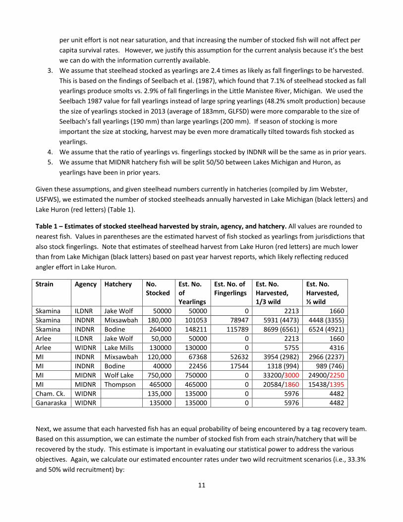
Table 1 – Estimates of stocked steelhead harvested by strain, agency, and hatchery. All values are rounded to

nearest fish. Values in parentheses are the estimated harvest of fish stocked as yearlings from jurisdictions that

also stock fingerlings. Note that estimates of steelhead harvest from Lake Huron (red letters) are much lower

than from Lake Michigan (black latters) based on past year harvest reports, which likely reflecting reduced

angler effort in Lake Huron.

Strain Agency Hatchery No. Stocked

Est. No. of Yearlings

Est. No. of Fingerlings

Est. No. Harvested, 1/3 wild

Est. No. Harvested, ½ wild

Skamina ILDNR Jake Wolf 50000 50000 0 2213 1660

Skamina INDNR Mixsawbah 180,000 101053 78947 5931 (4473) 4448 (3355)

Skamina INDNR Bodine 264000 148211 115789 8699 (6561) 6524 (4921)

Arlee ILDNR Jake Wolf 50,000 50000 0 2213 1660

Arlee WIDNR Lake Mills 130000 130000 0 5755 4316

MI INDNR Mixsawbah 120,000 67368 52632 3954 (2982) 2966 (2237)

MI INDNR Bodine 40000 22456 17544 1318 (994) 989 (746)

MI MIDNR Wolf Lake 750,000 750000 0 33200/3000 24900/2250

MI MIDNR Thompson 465000 465000 0 20584/1860 15438/1395

Cham. Ck. WIDNR 135,000 135000 0 5976 4482

Ganaraska WIDNR 135000 135000 0 5976 4482

Next, we assume that each harvested fish has an equal probability of being encountered by a tag recovery team.

Based on this assumption, we can estimate the number of stocked fish from each strain/hatchery that will be

recovered by the study. This estimate is important in evaluating our statistical power to address the various

objectives. Again, we calculate our estimated encounter rates under two wild recruitment scenarios (i.e., 33.3%

and 50% wild recruitment) by:

12

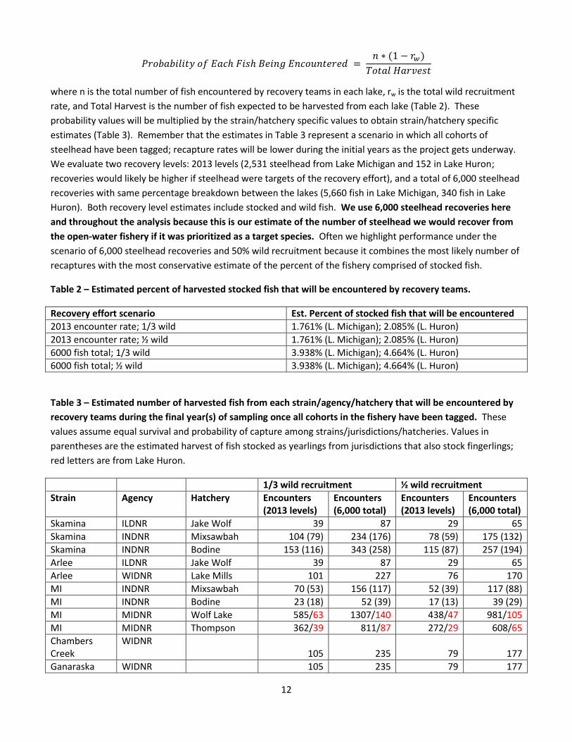
𝑃𝑟𝑜𝑏𝑎𝑏𝑖𝑙𝑖𝑡𝑦 𝑜𝑓 𝐸𝑎𝑐ℎ 𝐹𝑖𝑠ℎ 𝐵𝑒𝑖𝑛𝑔 𝐸𝑛𝑐𝑜𝑢𝑛𝑡𝑒𝑟𝑒𝑑 = 𝑛 ∗ (1 − 𝑟𝑤)

𝑇𝑜𝑡𝑎𝑙 𝐻𝑎𝑟𝑣𝑒𝑠𝑡

where n is the total number of fish encountered by recovery teams in each lake, rw is the total wild recruitment

rate, and Total Harvest is the number of fish expected to be harvested from each lake (Table 2). These

probability values will be multiplied by the strain/hatchery specific values to obtain strain/hatchery specific

estimates (Table 3). Remember that the estimates in Table 3 represent a scenario in which all cohorts of

steelhead have been tagged; recapture rates will be lower during the initial years as the project gets underway.

We evaluate two recovery levels: 2013 levels (2,531 steelhead from Lake Michigan and 152 in Lake Huron;

recoveries would likely be higher if steelhead were targets of the recovery effort), and a total of 6,000 steelhead

recoveries with same percentage breakdown between the lakes (5,660 fish in Lake Michigan, 340 fish in Lake

Huron). Both recovery level estimates include stocked and wild fish. We use 6,000 steelhead recoveries here

and throughout the analysis because this is our estimate of the number of steelhead we would recover from

the open-water fishery if it was prioritized as a target species. Often we highlight performance under the

scenario of 6,000 steelhead recoveries and 50% wild recruitment because it combines the most likely number of

recaptures with the most conservative estimate of the percent of the fishery comprised of stocked fish.

Table 2 – Estimated percent of harvested stocked fish that will be encountered by recovery teams.

Recovery effort scenario Est. Percent of stocked fish that will be encountered

2013 encounter rate; 1/3 wild 1.761% (L. Michigan); 2.085% (L. Huron)

2013 encounter rate; ½ wild 1.761% (L. Michigan); 2.085% (L. Huron)

6000 fish total; 1/3 wild 3.938% (L. Michigan); 4.664% (L. Huron)

6000 fish total; ½ wild 3.938% (L. Michigan); 4.664% (L. Huron)

Table 3 – Estimated number of harvested fish from each strain/agency/hatchery that will be encountered by

recovery teams during the final year(s) of sampling once all cohorts in the fishery have been tagged. These

values assume equal survival and probability of capture among strains/jurisdictions/hatcheries. Values in

parentheses are the estimated harvest of fish stocked as yearlings from jurisdictions that also stock fingerlings;

red letters are from Lake Huron.

1/3 wild recruitment ½ wild recruitment

Strain Agency Hatchery Encounters (2013 levels)

Encounters (6,000 total)

Encounters (2013 levels)

Encounters (6,000 total)

Skamina ILDNR Jake Wolf 39 87 29 65

Skamina INDNR Mixsawbah 104 (79) 234 (176) 78 (59) 175 (132)

Skamina INDNR Bodine 153 (116) 343 (258) 115 (87) 257 (194)

Arlee ILDNR Jake Wolf 39 87 29 65

Arlee WIDNR Lake Mills 101 227 76 170

MI INDNR Mixsawbah 70 (53) 156 (117) 52 (39) 117 (88)

MI INDNR Bodine 23 (18) 52 (39) 17 (13) 39 (29)

MI MIDNR Wolf Lake 585/63 1307/140 438/47 981/105

MI MIDNR Thompson 362/39 811/87 272/29 608/65

Chambers Creek

WIDNR 105 235 79 177

Ganaraska WIDNR 105 235 79 177

13

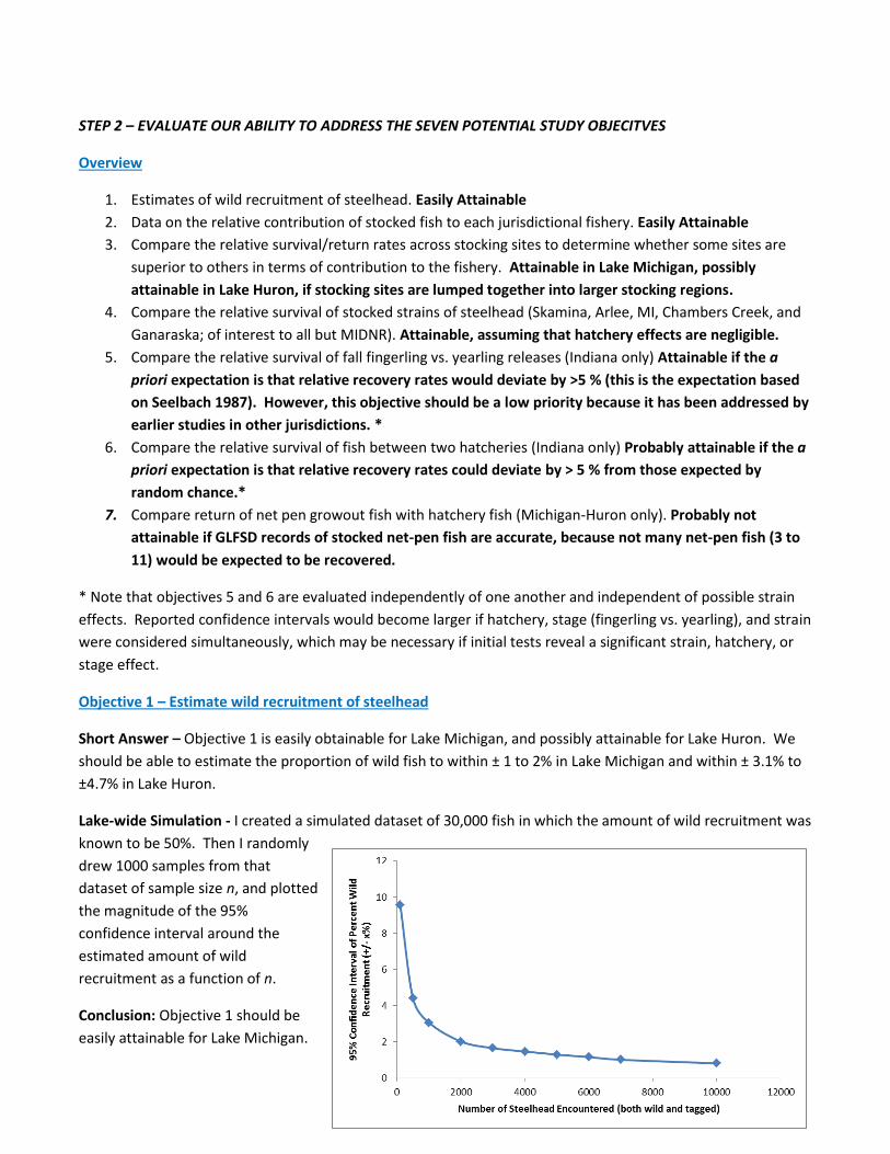
STEP 2 – EVALUATE OUR ABILITY TO ADDRESS THE SEVEN POTENTIAL STUDY OBJECITVES

Overview

1. Estimates of wild recruitment of steelhead. Easily Attainable

2. Data on the relative contribution of stocked fish to each jurisdictional fishery. Easily Attainable

3. Compare the relative survival/return rates across stocking sites to determine whether some sites are

superior to others in terms of contribution to the fishery. Attainable in Lake Michigan, possibly

attainable in Lake Huron, if stocking sites are lumped together into larger stocking regions.

4. Compare the relative survival of stocked strains of steelhead (Skamina, Arlee, MI, Chambers Creek, and

Ganaraska; of interest to all but MIDNR). Attainable, assuming that hatchery effects are negligible.

5. Compare the relative survival of fall fingerling vs. yearling releases (Indiana only) Attainable if the a

priori expectation is that relative recovery rates would deviate by >5 % (this is the expectation based

on Seelbach 1987). However, this objective should be a low priority because it has been addressed by

earlier studies in other jurisdictions. *

6. Compare the relative survival of fish between two hatcheries (Indiana only) Probably attainable if the a

priori expectation is that relative recovery rates could deviate by > 5 % from those expected by

random chance.*

7. Compare return of net pen growout fish with hatchery fish (Michigan-Huron only). Probably not

attainable if GLFSD records of stocked net-pen fish are accurate, because not many net-pen fish (3 to

11) would be expected to be recovered.

* Note that objectives 5 and 6 are evaluated independently of one another and independent of possible strain

effects. Reported confidence intervals would become larger if hatchery, stage (fingerling vs. yearling), and strain

were considered simultaneously, which may be necessary if initial tests reveal a significant strain, hatchery, or

stage effect.

Objective 1 – Estimate wild recruitment of steelhead

Short Answer – Objective 1 is easily obtainable for Lake Michigan, and possibly attainable for Lake Huron. We

should be able to estimate the proportion of wild fish to within ± 1 to 2% in Lake Michigan and within ± 3.1% to

±4.7% in Lake Huron.

Lake-wide Simulation - I created a simulated dataset of 30,000 fish in which the amount of wild recruitment was

known to be 50%. Then I randomly

drew 1000 samples from that

dataset of sample size n, and plotted

the magnitude of the 95%

confidence interval around the

estimated amount of wild

recruitment as a function of n.

Conclusion: Objective 1 should be

easily attainable for Lake Michigan.

14

During 2013, fish recovery teams encountered about 2500 steelhead even though steelhead were not targeted.

At 2500 encounters, percent wild recruits would be estimated within ± 1.8% (at 95% confidence) in Lake

Michigan. Wild recruitment could be estimated at ± 1.2% and at ± 1% with 6,000 and 7,000 steelhead

encounters respectively, either of which may be achievable if the fish recovery effort targets steelhead. Lower

recoveries in Lake Huron (152 in 2013; 340 estimated encounters if steelhead are a targeted species) would

reduce confidence in estimates of wild recruitment to ± 3.1 to 4.7%.

Objective 2 – What is the relative contribution of stocked fish to each jurisdictional fishery?

Short Answer – This is a multifaceted objective with many potential sub-questions. We should be able to

address this objective by mapping returns of stocked fish, and by analyzing return data through either ANOVA

(using sample day as unit of replication) or through a series of Comparison of Proportions tests.

Question 1 – Is the relative contribution of stocked fish (from anywhere) to each jurisdictional fishery the

same? Here:

H0 = the proportion of stocked vs. wild fish in the fishery harvest is the same in all jurisdictions

could be addressed by a comparison of proportions test. We use the jurisdictional recovery values for steelhead

in 2013 to estimate sample size, and assume that ratios among jurisdictions would remain constant if recovery

rate increased to 6,000 fish total (see Table 5 under Objective 2). We also assume that steelhead recoveries

would have been higher in Illinois in 2013 if that jurisdiction hadn’t focused almost solely on recovering lake

trout and Chinook salmon.

Even under 2013 recovery levels, power analysis suggests there is a high probability of detecting small (at least

68.7%), medium (100%) and large (100%) effects if they exist among all jurisdictions of Lake Michigan. If 6,000

fish are encountered (as expected if steelhead are targeted), the probability of detecting a small difference

among jurisdictions increases to 95.6%. These values assume much higher returns of steelhead from Illinois

than in 2013, which is likely because Illinois largely did not report catches of species other than lake trout and

Chinook salmon.

Questions 2 and 3 – Are return rates from fishes stocked by each jurisdiction the same? What is the overall

contribution of fish from each jurisdiction to the lake-wide fishery? Both of these questions are similar, and

can be tested by evaluating:

H0 = the relative return rate of fish from each jurisdiction (controlling for numbers stocked) will be equal on a

lake-wide scale.

As with Objective 1, this question should be easily addressable. The simulation in Objective 1 also holds true for

evaluating the proportion of recovered fish from a given jurisdiction because we are determining the confidence

in estimating the proportion of a known sample. Confidence intervals for our estimated sample sizes suggest we

could estimate the percent contribution of fishes stocked by each jurisdiction to the lake-wide fishery to ± 1 or

2% depending on the total recoveries (ranging from 2500 to 6000).

A complimentary approach would be to compare the estimated recaptures for each stocking jurisdiction (Table

4; assumes equal movement and survival among all stocked fish) with the actual number of stocked steelhead

recovered from each jurisdiction (Table 5). Comparing Tables 4 (expected recovery based on number stocked)

15

and 5 (actual recovery) could provide insight into differences in the relative contribution of each stocked fish to

each jurisdictional fishery. For this comparison to be meaningful, recovery data (Table 5) will need to be

corrected to account for disproportional sampling effort by recovery teams in certain jurisdictions.

Ideally, we would also be able to test for a strain effect by comparing each strain separately (see Objective 4).

Some strains (especially MI and Skamina) will be better represented than others due to differences in stocking

numbers. However, we would expect to recover a minimum of 177 individuals from each strain given the most

likely recovery scenario (6,000 recaptures total) and the highest wild recruitment scenario (50% wild

recruitment). Thus, there may be enough recaptures to detect differences in strain-specific return rates among

jurisdictions for some strains assuming there are no hatchery effects. Strain and hatchery effects are mixed

together and may mask one another because strains are reared in different numbers at each hatchery, and two

strains (Chambers Creek and Ganaraska) are only reared at a single hatchery.

Table 4 – Estimated number of stocked fish recovered from each jurisdiction, assuming equal movement and

survival among stocked strains. Parenthetical values in the Indiana row are the estimated recoveries if only

yearlings receive a CWT. Red values in the Michigan row are estimated recoveries from Lake Huron.

Number of Estimated Recoveries

Jurisdiction Where Fish Were Stocked

1/3 wild recruitment, recovery at 2013 levels

1/3 wild recruitment, 6,000 fish recovered

½ wild recruitment, recovery at 2013 levels

½ wild recruitment, 6,000 fish recovered

Illinois 78 174 58 130

Indiana 350 (266) 785 (590) 263 (195) 588 (443)

Michigan 947/102 2,118/227 710/76 1,589/170

Wisconsin 311 697 234 524

Table 5 – Number of steelhead recovered from each jurisdiction in 2013 (stocked and wild combined), and

estimated number of steelhead recovered from each jurisdiction if 6,000 fish were recaptured in total,

assuming 2013-level ratios among jurisdictions.

No. steelhead encountered in 2013 No. steelhead if 6,000 fish are encountered

Jurisdiction Total recovered

Stocked fish recovered, 33.3% wild

Stocked fish recovered, 50% wild

Total recovered

Stocked fish recovered, 33.3% wild

Stocked fish recovered, 50% wild

Illinois* 8 5 4 18 12 9

Indiana 343 229 172 767 511 384

Michigan 266 (L. Mich.) and 152 (L. Huron)

177 (LM) and 133 (LH)

133 (LM) and 76 (LH)

595 (LM) and 340 (LH)

397 (LM) and 227 (LH)

298 (LM) and 170 (LH)

Wisconsin 1914 1276 957 4280 2853 2140

*Note: Illinois almost exclusively focused on collecting data from lake trout and Chinook salmon only and usually

did not report catches of other species. Thus, Illinois recoveries of steelhead would likely be much larger than

suggested by 2013 numbers if recovery of steelhead was made a priority.

16

Question 4 - Are the proportions of fish recaptured from each jurisdiction that were stocked from a specific

jurisdiction the same across jurisdictions? For example, do fish stocked in Wisconsin contribute equally to all

jurisdictions, or are they disproportionately recovered from Wisconsin? Here:

H0 = The proportion of fish stocked by a particular jurisdiction will be recovered at equal rates from all

jurisdictions.

This question can also be addressed with a comparison of proportions test. If 6,000 total fish are encountered

(most likely scenario if steelhead are targeted) and there is 50% wild recruitment (highest estimate of wild

recruitment from current studies), power analysis suggests that there is a 73.6 to 95.0% chance of detecting

small differences in proportions if they exist among Wisconsin, Michigan, and Indiana, and a 100% chance of

detecting medium and large differences if they exist among jurisdictions. Similar probabilities likely exist for

comparisons with Illinois, but we don’t have a solid estimate of Illinois steelhead return rates because the 2012

and 2013 recover efforts targeting only lake trout and Chinook salmon.

Details on power analysis for comparison of proportions test – There are four proportions, one for each

jurisdiction, that will be compared to one another in pairwise fashion (Lake Michigan only). The specific

proportions being evaluated here are the proportion of fish recaptured from each jurisdiction that were stocked

from a specific jurisdiction. This will help identify the composition of each jurisdictional fishery in terms of

jurisdiction of stocking. In this case, the values in Table 5 are most appropriate to use because they are based

on real recovery data (rather than Table 4, which is based on the number of fish stocked). Multiple scenarios

exist – below I present the scenario for the most likely number of recaptures (6,000 fish in total) and the most

conservative estimate of wild recruitment (50%)

a. Illinois vs. Michigan: 9.1, 31.5, and 65.7% chance of detecting small, medium and large effects

b. Illinois vs. Indiana: 9.1, 31.7, and 66.0% chance of detecting small, medium and large effects

c. Illinois vs. Wisconsin: 9.2, 32.2, and 66.8% chance of detecting small, medium, and large effects

d. Mich. vs. Ind.: 73.6, 100.0, and 100.0 % chance of detecting small, medium, and large effects

e. Mich. vs. Wisc.: 89.9, 100.0, and 100.0 % chance of detecting small, medium, and large effects

f. Ind. vs. Wisc.: 95.0, 100.0, and 100.0 % chance of detecting small, medium, and large effects

Objective 3 – Compare the relative survival/return rates across stocking sites to determine whether some

sites are superior to others in terms of contribution to the fishery

Short Answer – A stocking-site specific design would require 102 unique tag lots, with many of those lots

containing small (< 20,000) numbers of fish (based on 2013 stocking practices, in which there were 83 stocking

sites in Lake Michigan, 19 sites in Lake Huron, and <20,000 fish stocked at 81% of these sites; Great Lakes Fish

Stocking Database, FWS/GLFC). Therefore, it is not feasible to compare return rates across individual stocking

sites because of logistical concerns (e.g., time, money, manpower, and number of hatchery raceways). I propose

dividing fish stocked in Lake Michigan into regions (as suggested by MIDNR for Lake Huron). Although this

would not determine the recovery rates of particular sites, it would provide estimates for groups of sites located

within the same geographical area. Here:

H0 = the proportion of recovered stocked fish is equal among stocking regions of origin

17

Simulated data suggests we could estimate the proportion of recovered stocked fish belonging to each stocking

region within ± 1.6% for Lake Michigan and 7.7% for Lake Huron (assuming 6,000 total recoveries and 50% wild

recruitment). Power analysis suggests that comparison of proportions tests would have a good chance of

detecting medium and large differences that exist among stocking regions, but a poor chance of detecting small

differences.

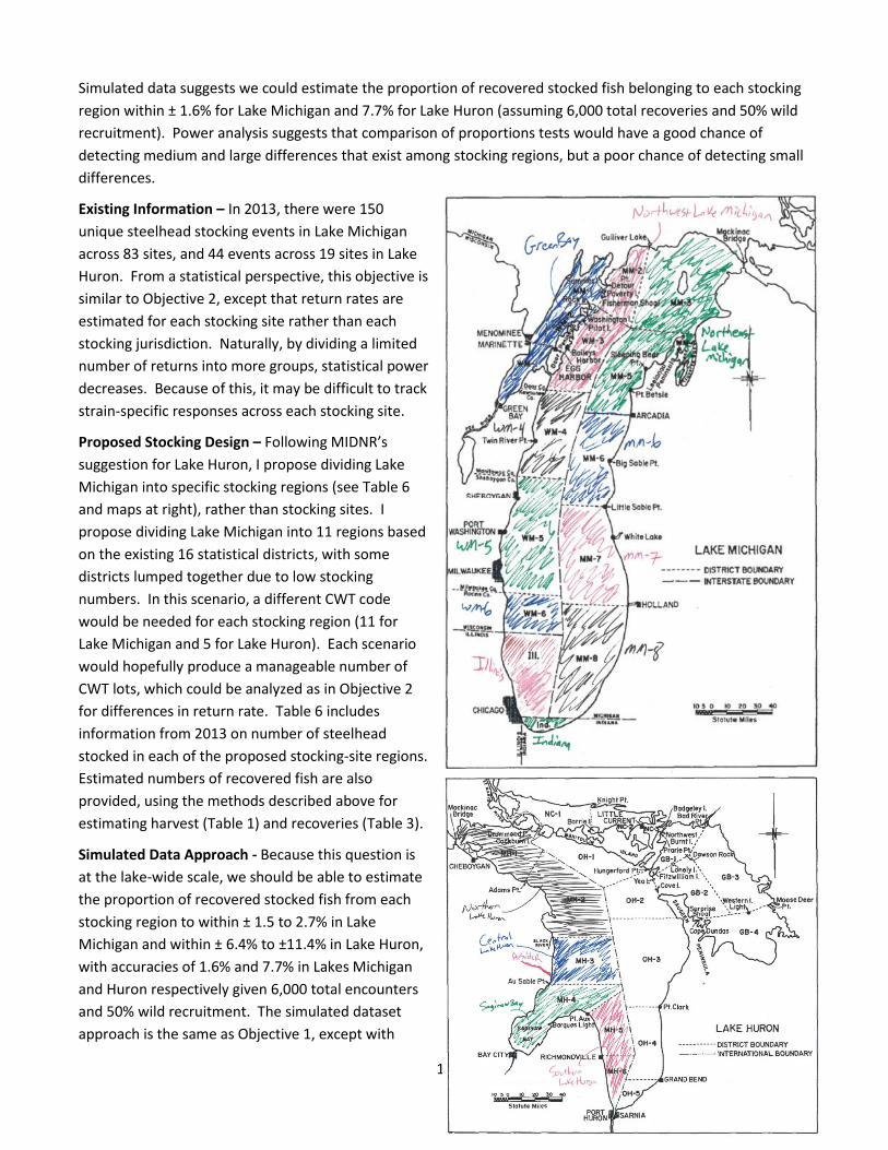
Existing Information – In 2013, there were 150

unique steelhead stocking events in Lake Michigan

across 83 sites, and 44 events across 19 sites in Lake

Huron. From a statistical perspective, this objective is

similar to Objective 2, except that return rates are

estimated for each stocking site rather than each

stocking jurisdiction. Naturally, by dividing a limited

number of returns into more groups, statistical power

decreases. Because of this, it may be difficult to track

strain-specific responses across each stocking site.

Proposed Stocking Design – Following MIDNR’s

suggestion for Lake Huron, I propose dividing Lake

Michigan into specific stocking regions (see Table 6

and maps at right), rather than stocking sites. I

propose dividing Lake Michigan into 11 regions based

on the existing 16 statistical districts, with some

districts lumped together due to low stocking

numbers. In this scenario, a different CWT code

would be needed for each stocking region (11 for

Lake Michigan and 5 for Lake Huron). Each scenario

would hopefully produce a manageable number of

CWT lots, which could be analyzed as in Objective 2

for differences in return rate. Table 6 includes

information from 2013 on number of steelhead

stocked in each of the proposed stocking-site regions.

Estimated numbers of recovered fish are also

provided, using the methods described above for

estimating harvest (Table 1) and recoveries (Table 3).

Simulated Data Approach - Because this question is

at the lake-wide scale, we should be able to estimate

the proportion of recovered stocked fish from each

stocking region to within ± 1.5 to 2.7% in Lake

Michigan and within ± 6.4% to ±11.4% in Lake Huron,

with accuracies of 1.6% and 7.7% in Lakes Michigan

and Huron respectively given 6,000 total encounters

and 50% wild recruitment. The simulated dataset

approach is the same as Objective 1, except with

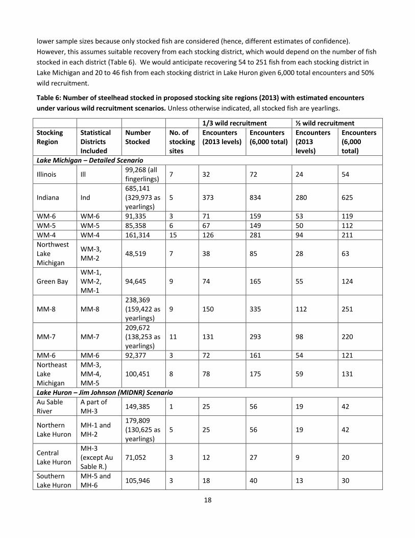
18

lower sample sizes because only stocked fish are considered (hence, different estimates of confidence).

However, this assumes suitable recovery from each stocking district, which would depend on the number of fish

stocked in each district (Table 6). We would anticipate recovering 54 to 251 fish from each stocking district in

Lake Michigan and 20 to 46 fish from each stocking district in Lake Huron given 6,000 total encounters and 50%

wild recruitment.

Table 6: Number of steelhead stocked in proposed stocking site regions (2013) with estimated encounters

under various wild recruitment scenarios. Unless otherwise indicated, all stocked fish are yearlings.

1/3 wild recruitment ½ wild recruitment

Stocking Region

Statistical Districts Included

Number Stocked

No. of stocking sites

Encounters (2013 levels)

Encounters (6,000 total)

Encounters (2013 levels)

Encounters (6,000 total)

Lake Michigan – Detailed Scenario

Illinois Ill 99,268 (all fingerlings)

7 32 72 24 54

Indiana Ind 685,141 (329,973 as yearlings)

5 373 834 280 625

WM-6 WM-6 91,335 3 71 159 53 119

WM-5 WM-5 85,358 6 67 149 50 112

WM-4 WM-4 161,314 15 126 281 94 211

Northwest Lake Michigan

WM-3, MM-2

48,519 7 38 85 28 63

Green Bay WM-1, WM-2, MM-1

94,645 9 74 165 55 124

MM-8 MM-8 238,369 (159,422 as yearlings)

9 150 335 112 251

MM-7 MM-7 209,672 (138,253 as yearlings)

11 131 293 98 220

MM-6 MM-6 92,377 3 72 161 54 121

Northeast Lake Michigan

MM-3, MM-4, MM-5

100,451 8 78 175 59 131

Lake Huron – Jim Johnson (MIDNR) Scenario

Au Sable River

A part of MH-3

149,385 1 25 56 19 42

Northern Lake Huron

MH-1 and MH-2

179,809 (130,625 as yearlings)

5 25 56 19 42

Central Lake Huron

MH-3 (except Au Sable R.)

71,052 3 12 27 9 20

Southern Lake Huron

MH-5 and MH-6

105,946 3 18 40 13 30

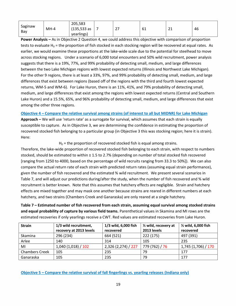
19

Saginaw Bay

MH-4 205,583 (135,533 as yearlings)

7 27 61 21 46

Power Analysis – As in Objective 2 Question 4, we could address this objective with comparison of proportion

tests to evaluate H0 = the proportion of fish stocked in each stocking region will be recovered at equal rates. As

earlier, we would examine these proportions at the lake-wide scale due to the potential for steelhead to move

across stocking regions. Under a scenario of 6,000 total encounters and 50% wild recruitment, power analysis

suggests that there is a 19%, 77%, and 99% probability of detecting small, medium, and large differences

between the two Lake Michigan regions with lowest expected returns (Illinois and Northwest Lake Michigan).

For the other 9 regions, there is at least a 33%, 97%, and 99% probability of detecting small, medium, and large

differences that exist between regions (based off of the regions with the third and fourth lowest expected

returns, WM-5 and WM-6). For Lake Huron, there is an 11%, 41%, and 79% probability of detecting small,

medium, and large differences that exist among the regions with lowest expected returns (Central and Southern

Lake Huron) and a 15.5%, 65%, and 96% probability of detecting small, medium, and large differences that exist

among the other three regions.

Objective 4 – Compare the relative survival among strains (of interest to all but MIDNR) for Lake Michigan

Approach – We will use ‘return rate’ as a surrogate for survival, which assumes that each strain is equally

susceptible to capture. As in Objective 3, we are determining the confidence in estimating the proportion of

recovered stocked fish belonging to a particular group (in Objective 3 this was stocking region; here it is strain).

Here:

H0 = the proportion of recovered stocked fish is equal among strains.

Therefore, the lake-wide proportion of recovered stocked fish belonging to each strain, with respect to numbers

stocked, should be estimated to within ± 1.5 to 2.7% (depending on number of total stocked fish recovered

[ranging from 1250 to 4000, based on the percentage of wild recruits ranging from 33.3 to 50%]). We can also

compare the actual return rate of each strain with predicted return rates (assuming equal strain performance),

given the number of fish recovered and the estimated % wild recruitment. We present several scenarios in

Table 7, and will adjust our predictions during/after the study, when the number of fish recovered and % wild

recruitment is better known. Note that this assumes that hatchery effects are negligible. Strain and hatchery

effects are mixed together and may mask one another because strains are reared in different numbers at each

hatchery, and two strains (Chambers Creek and Ganaraska) are only reared at a single hatchery.

Table 7 – Estimated number of fish recovered from each strain, assuming equal survival among stocked strains

and equal probability of capture by various field teams. Parenthetical values in Skamina and MI rows are the

estimated recoveries if only yearlings receive a CWT. Red values are estimated recoveries from Lake Huron.

Strain 1/3 wild recruitment, recovery at 2013 levels

1/3 wild, 6,000 fish recovered

½ wild, recovery at 2013 levels

½ wild, 6,000 fish recovered

Skamina 296 (234) 664 (521) 222 (175) 497 (391)

Arlee 140 314 105 235

MI 1,040 (1,018) / 102 2,326 (2,274) / 227 779 (762) / 76 1,745 (1,706) / 170

Chambers Creek 105 235 79 177

Ganaraska 105 235 79 177

Objective 5 – Compare the relative survival of fall fingerlings vs. yearling releases (Indiana only)

20

Short Answer – This question has been addressed by earlier studies in other jurisdictions, and yearlings have

consistently been found to have superior survival and be of greater cost efficiency (Seelbach 1987; Seelbach

1994; others). For example, in the Little Manistee River (MI) 7.1% of fall yearlings (mean length 190 mm) and

48.2% of large spring yearlings (mean length 200 mm) survived to the smolt stage post-stocking, compared to

only 2.9% of fall fingerlings (mean length of about 50 mm)(Seelbach 1987). Why would results differ in Indiana?

Although we would expect a large difference in survival, power analysis suggests there is only a 20.1% chance of

detecting a large difference in sample groups, assuming each year is treated as an independent sample (H0 =

recovery rates with respect to numbers stocked would be equal between groups). We could also address this

question by describing the confidence intervals around the proportions of recovered fish stocked by Indiana that

were fingerlings and yearlings. If 6,000 fish are recovered in total and there is 50% wild recruitment, we

estimate recovery of 588 fish from Indiana (Table 4). Under this scenario, simulated data suggest that we could

estimate the proportion of those 588 fish that were yearlings and fingerlings to ± 4.1% with 95% confidence.

This should be adequate to detect differences of those reported by Seelbach 1987. Based on projected

numbers, we would anticipate that 60.1 % of recovered fish would be yearlings and 39.9% of recovered fish

would be fingerlings if survival was equal. This means that we could detect differences in survivorship if actual

percentages were > ±4.1% of these values. If survivorship differs as in Seelbach 1987 for fall fingerlings vs. fall

yearlings, we would expect 75.3 % yearlings and 24.7% fingerlings, which is about 3.7 times greater than the

difference needed for detection. Differences would be even greater if survivorship of yearlings is more similar

to the Seelbach 1987 values for large spring yearlings.

Power Analysis – This analysis would be a simple t-test comparing mean return rates of yearlings vs. fall

fingerlings, conducted separately for each strain. If we considered each year of the study an independent

sample, we would have a power analysis of n=5 (5 sample years/year classes), resulting in:

a. The probability of detecting a large effect (d=0.8) is 20.1%

b. The probability of detecting a medium effect (d=0.5) is 10.8%

c. The probability of detecting a small effect (d=0.2) is 5.9%

Objective 6 – Compare the relative survival of fish from the two Indiana hatcheries

H0 = recovered stocked fish from Indiana, corrected for numbers stocked, would be equal between hatcheries

Short Answer – Power analysis suggests a t-test would be insufficient for detecting even large differences

among hatcheries. A distribution of random samples from a simulated dataset suggests that the % of recovered

fish stocked by Indiana belonging to each hatchery could be estimated to ± 4.1% under a scenario of 6,000 total

fish encountered and 50% wild recruitment. Therefore, it seems likely that we could detect hatchery-specific

differences if the a priori expectation is that relative recovery rates will deviate by about > 5 % from those

expected by random chance.

Power Analysis - This analysis would be a simple t-test comparing mean return rates from Mixsawbah vs. Bodine

hatcheries. If we considered each year of the study an independent sample, we would have a power analysis of

n=5 (5 sample years/year classes). This power analysis indicates that the probability of detecting small (d=0.2),

medium (d=0.5), and large (d=0.8) effects is 5.9%, 10.8%, and 20.1% respectively.

Simulated Data – Given the bleak outlook for the t-test, we also estimated the confidence intervals of the

proportion Indiana fish recovered from each hatchery. In this case, we use the estimated recovery rate of

Indiana-stocked fishes to determine sample size (estimates varied from 263 to 785 fish recovered, Table 4). This

21

is because the best question for addressing this objective is “of the fish stocked by Indiana that were recovered,

what proportion was from Mixsawbah, and what proportion was from Bodine?” We would control for the

number of stocked individuals in our test by comparing sample proportions to proportions expected with all else

being equal (as in Objective 5). We tested a simulated dataset of 30,000 fish where the proportion of fish from

each hatchery was 50%, and then determined the 95% confidence interval for each estimate given estimated

return rates. We anticipate being able to estimate the proportion of fish from each hatchery at 95% confidence

to ± 3.5 to 6.3%, and at ±4.1% under the 6,000 fish/50% wild recruitment scenario.

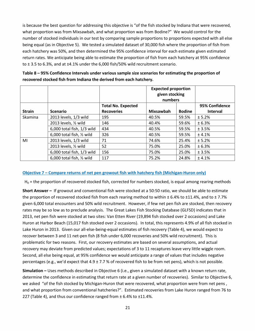
Table 8 – 95% Confidence Intervals under various sample size scenarios for estimating the proportion of

recovered stocked fish from Indiana the derived from each hatchery.

Expected proportion given stocking

numbers

Strain Scenario Total No. Expected Recoveries Mixsawbah Bodine

95% Confidence Interval

Skamina 2013 levels, 1/3 wild 195 40.5% 59.5% ± 5.2%

2013 levels, ½ wild 146 40.4% 59.6% ± 6.3%

6,000 total fish, 1/3 wild 434 40.5% 59.5% ± 3.5%

6,000 total fish, ½ wild 326 40.5% 59.5% ± 4.1%

MI 2013 levels, 1/3 wild 71 74.6% 25.4% ± 5.2%

2013 levels, ½ wild 52 75.0% 25.0% ± 6.3%

6,000 total fish, 1/3 wild 156 75.0% 25.0% ± 3.5%

6,000 total fish, ½ wild 117 75.2% 24.8% ± 4.1%

Objective 7 – Compare returns of net pen growout fish with hatchery fish (Michigan-Huron only)

H0 = the proportion of recovered stocked fish, corrected for numbers stocked, is equal among rearing methods

Short Answer – If growout and conventional fish were stocked at a 50:50 ratio, we should be able to estimate

the proportion of recovered stocked fish from each rearing method to within ± 6.4% to ±11.4%, and to ± 7.7%

given 6,000 total encounters and 50% wild recruitment. However, if few net pen fish are stocked, then recovery

rates may be so low as to preclude analysis. The Great Lakes Fish Stocking Database (GLFSD) indicates that in

2013, net pen fish were stocked at two sites: Van Etten River (19,894 fish stocked over 2 occasions) and Lake

Huron at Harbor Beach (15,017 fish stocked over 2 occasions). In total, this represents 4.9% of all fish stocked in

Lake Huron in 2013. Given our all-else-being-equal estimates of fish recovery (Table 4), we would expect to

recover between 3 and 11 net-pen fish (8 fish under 6,000 recoveries and 50% wild recruitment). This is

problematic for two reasons. First, our recovery estimates are based on several assumptions, and actual

recovery may deviate from predicted values; expectations of 3 to 11 recaptures leave very little wiggle room.

Second, all else being equal, at 95% confidence we would anticipate a range of values that includes negative

percentages (e.g., we’d expect that 4.9 ± 7.7 % of recovered fish to be from net pens), which is not possible.

Simulation – Uses methods described in Objective 6 (i.e., given a simulated dataset with a known return rate,

determine the confidence in estimating that return rate at a given number of recoveries). Similar to Objective 6,

we asked “of the fish stocked by Michigan-Huron that were recovered, what proportion were from net pens ,

and what proportion from conventional hatcheries?”. Estimated recoveries from Lake Huron ranged from 76 to

227 (Table 4), and thus our confidence ranged from ± 6.4% to ±11.4%.

22

Power Analysis – If each statistical district of Lake Huron is considered an independent sampling unit (fish

recovery teams sample a total of 6 districts, MH-1 through MH-6), there is a 24.1% probability of detecting a

large difference in net pen vs. conventional hatchery fish; a 12.3% probability of detecting a medium effect; and

a 6.1% probability of detecting a small effect.

23

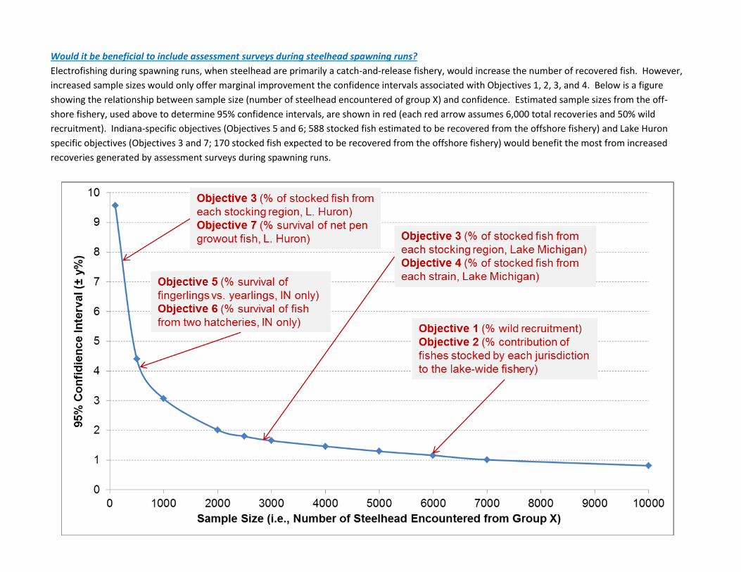
Would it be beneficial to include assessment surveys during steelhead spawning runs?

Electrofishing during spawning runs, when steelhead are primarily a catch-and-release fishery, would increase the number of recovered fish. However,

increased sample sizes would only offer marginal improvement the confidence intervals associated with Objectives 1, 2, 3, and 4. Below is a figure

showing the relationship between sample size (number of steelhead encountered of group X) and confidence. Estimated sample sizes from the off-

shore fishery, used above to determine 95% confidence intervals, are shown in red (each red arrow assumes 6,000 total recoveries and 50% wild

recruitment). Indiana-specific objectives (Objectives 5 and 6; 588 stocked fish estimated to be recovered from the offshore fishery) and Lake Huron

specific objectives (Objectives 3 and 7; 170 stocked fish expected to be recovered from the offshore fishery) would benefit the most from increased

recoveries generated by assessment surveys during spawning runs.