Embed Size (px)
Citation preview

8/3/2019 Fear of Appreciation
http://slidepdf.com/reader/full/fear-of-appreciation 1/39
Policy R eseaRch W oRking P aPeR 4387
Fear o Appreciation
Eduardo Levy-Yeyati
Federico Sturzenegger
The World Bank Latin America and the Caribbean RegionOfce o the Chie EconomistNovember 2007
WPS4387

8/3/2019 Fear of Appreciation
http://slidepdf.com/reader/full/fear-of-appreciation 2/39
Produced by the Research Support Team
Abstract
The Policy Research Working Paper Series disseminates the fndings o work in progress to encourage the exchange o ideas about development
issues. An objective o the series is to get the fndings out quickly, even i the presentations are less than ully polished. The papers carry the
names o the authors and should be cited accordingly. The fndings, interpretations, and conclusions expressed in this paper are entirely those
o the authors. They do not necessarily represent the views o the International Bank or Reconstruction and Development/World Bank and
its afliated organizations, or those o the Executive Directors o the World Bank or the governments they represent.
Policy R eseaRch W oRking P aPeR 4387
In recent years the term "ear o foating" has been usedto describe exchange rate regimes that, while ocially fexible, in practice intervene heavily to avoid sudden
or large depreciations. However, the data reveals that inmost cases (and increasingly so in the 2000s) interventionhas been aimed at limiting appreciations rather thandepreciations, oten motivated by the neo-mercantilistview o a depreciated real exchange rate as protection ordomestic industries. As a rst step to address the broader
This paper is a product o the Oce o the Chie Economist o Latin America and the Caribbean Region Policy Research Working Papers are also posted on the Web at http://econ.worldbank.org. The author may be contacted at [email protected].
question o whether this view delivers on its promise, theauthors examine whether this “ear o appreciation” hasa positive impact on growth perormance in developing
economies. The authors show that depreciated exchangerates appear to induce higher growth, but that the eect,rather than through import substitution or exportbooms as argued by the mercantilist view, works largely through the deepening o domestic savings and capitalaccumulation.

8/3/2019 Fear of Appreciation
http://slidepdf.com/reader/full/fear-of-appreciation 3/39
Fear of Appreciation 1
Eduardo Levy-Yeyati
The World Bank and Universidad Torcuato Di Tella
Federico Sturzenegger
Kennedy School of Government, Harvard University and Universidad Torcuato Di Tella
1 We thank César Calderón, Luis Cubeddu, Javier Finkman, Jeff Frankel, Ricardo Hausmann, Robert Lawrence, RicardoLopez Murphy, Guillermo Perry, Dani Rodrik, Luis Servén, and seminar participants at the Harvard Kennedy School, theIDB, the IMF, the Central Bank of Turkey and the Central Bank of Argentina for helpful comments. We thank LuisCasanova, Pablo Gluzmann, Victoria Coccoz and Ramiro Blázquez for excellent research assistance. The usual disclaimersapply.

8/3/2019 Fear of Appreciation
http://slidepdf.com/reader/full/fear-of-appreciation 4/39

8/3/2019 Fear of Appreciation
http://slidepdf.com/reader/full/fear-of-appreciation 5/39
globalization led to a growing ineffectiveness of monetary policy. More precisely, capital controls were
found to be decreasingly effective as economies became more sophisticated, thus strengthening the
restrictions imposed by the impossible trinity –previously circumvented due to the absence of de facto
financial integration (Rose, 2006)– all of which made floating regimes more attractive. Second, the role
of (domestic and external) financial dollarization, namely, the foreign currency denomination of
residents’ assets and liabilities that, to the extent that it introduced currency exposures that raised the
risk associated with exchange rate jumps, made pegged regimes look more attractive. 3 Indeed, it was
the risk of balance sheet losses to financially dollarized governments and firms in the event of a
devaluation –stressed in the third generation models of currency crises popularized in the context of
the Asian crisis– that led to the definition of fear of floating (Calvo and Reinhart, 2002), namely,
recurrent de facto exchange rate intervention in officially floating regimes.
The first aspect of the debate led naturally to the bipolar view (the inherent ineffectiveness and
instability of conventional exchange rate bands and pegs in the presence of de facto capital mobility)
that argued that financially integrated economies could either float or hard peg. 4 Combined with the
fear of floating view, this approach derived naturally into a “unipolar view” according to which hard
pegs were the only sensible option for financially dollarized economies: if devaluations were
contractionary due to balance sheet effects, exchange rate flexibility would only amplify the cycle,
rather than smooth it out as predicated by the standard theory.5
However, while theory was going one way, policy seemed to head in the opposite direction. By the
end of the decade, the success in building central bank autonomy and monetary credibility, together
with the resulting decline in inflation and exchange rate pass-through, led to the growing popularity of
the flexible pole of the bipolar view as the background for different varieties of inflation targeting
arrangements that prioritized the inflation rate, rather than the exchange rate, as the key nominal
anchor. Not surprisingly, among emerging countries, this trend started in economies with relatively
low levels of financial dollarization (Chile, New Zealand, South Africa, Brazil), gradually extending toother countries pari passu with a reduction in their degree of dollarization. In addition, the
disappointing Argentine experience with a currency board cast doubt on the premises (monetary and
3 See Levy Yeyati (2006).4 See Eichengreen (1994) and Fischer (2002).5 See Frankel (2005) on balance sheet effects and contractionary devaluations, and Calvo (2000) on the unipolar view.

8/3/2019 Fear of Appreciation
http://slidepdf.com/reader/full/fear-of-appreciation 6/39
fiscal discipline) on which the case for hard pegs had been predicated. 6 Ultimately, the debate in the
new millennium appears to have converged to an inverted unipolar view, whereby flexible regimes are
seen as the only sensible (and durable) choice as economies grow financially integrated and
sophisticated.7
To evaluate whether this shift towards the flexible pole is actually taking place, in this paper we update
and extend Levy Yeyati and Sturzenegger’s (2005) dataset (LYS) on de facto exchange rate regimes.
Based on this evidence, we find that the convergence to the FIT paradigm is not taking place across
the board: the share of non-floats (intermediates, conventional and hard pegs) represents 75% of the
sample, exactly the same share as in 2000.
Does that mean that fear of floating has continued to be prevalent despite the favorable context andthe reduced currency exposure? To get a full answer to that question, it is crucial to note a semantic
nuance that has been surprisingly understated in the recent exchange rate regime literature: fear of
floating, as originally defined by Calvo and Reinhart (2002), entails a clearly asymmetric exchange rate
policy. Since only depreciations trigger fears of financial distress or inflation pass-through, under fear
of floating the intervention response should be stronger for (if not limited to) upward exchange rate
movements. More generally, the incentives and implications to intervene in order to avoid an
appreciation are radically different from those related to avoiding a depreciation: where the latter focus
on short-run financial crises, the former is usually predicated on long-term economic growth.
Similarly, the context conducive to one or the other differs: whereas fear of floating would tend to
arise in times of financial turmoil, fear of appreciation will likely be triggered by economic bonanzas.
At any rate, treating interventions in a symmetric way –in particular, attributing any intervention to
fear of floating as has been previously the case in the literature– may lead to overstate the incidence of
financial factors –more so in recent years when fear of appreciation appears to have prevailed.
The mercantilist view that exchange rate policy –more precisely, a temporarily undervalued currency– could be used to protect infant industries as a development strategy has a long tradition in economic
theory and have recently enjoyed a minor revival. The issue of undervalued exchange rates has
received considerable attention as a result of China’s reluctance to float its exchange rate, a strategy
6 See De la Torre et al. (2002) for a discussion of the Argentine debacle and its implications for the exchange rate debate.7 See Levy Yeyati (2005) and references therein. Rose (2006) makes an eloquent case for the new FIT paradigm.

8/3/2019 Fear of Appreciation
http://slidepdf.com/reader/full/fear-of-appreciation 7/39
presumed to be aimed at preserving the competitiveness of China’s exports. 8 In academic circles, the
role of depreciated real exchange rates for stimulating growth has been discussed in Rodrik (2007), it
has also been found important in growth accelerations (Hausmann et al., 2005 and Johnson, Ostry and
Subramanian, 2006), and has been regarded as an efficient development tool (Rodrik, 2006). More
recently, the effects of overvaluation have been invoked to explain the “dutch desease” effect of
foreign aid (Rajan and Subramanian, 2006) or the disappointing growth dividends of financial
integration (see Prassad, Rajan and Subramanian, 2006). Despite this indicative evidence, neo-
mercantilist views have been saluted, at best, with skepticism.
To assess the economic impact of fear of appreciation, we proceed in two steps. First, we refine the de
facto regime classification to identify two types of foreign exchange interventions: one aimed at
defending the domestic currency (as in the traditional fear of floating), and one aimed at depressing it(as in fear of appreciation). In turn, with this finer classification at hand, we assess the economic
implications of fear of appreciation. Specifically, we evaluate whether foreign exchange interventions
geared towards containing a process of appreciation actually help sustain a depreciated real exchange
rate and, once this fact is established, we study the effect of interventions on growth. We find that fear
of appreciation lead to faster output and productivity growth, which is not restricted to short-term
cyclical output changes: we report a significant positive effect on the long-run component of GDP
growth. However, as opposed to what it is usually argued, we find that the effect seems to come not
from export-led expansions or import substitution, but rather from increased domestic savings and
investment rates.
The paper is organized as follows. Section II introduces our extended exchange rate regime
classification and reports some stylized facts on exchange rate policy in recent years. Section III
characterizes fear of appreciation and documents its relative importance over time. Section IV
explores the economic implications of fear of appreciation, identifying links with the real exchange
rate and economic growth, and examining alternatives channels that could account for the growtheffect. Section V reviews alternative theoretical explanations for our findings, and concludes.
8 See Aizenmann and Lee (2007).

8/3/2019 Fear of Appreciation
http://slidepdf.com/reader/full/fear-of-appreciation 8/39
II. De facto regime classification: Updating
In Levy-Yeyati and Sturzenegger (2001) we introduced a de facto classification of exchange rates that
relied on clustering country-year observations on the basis of three classifying variables: the
movements of the nominal exchange rate within each year, the movements in central bank reserves
(intended to capture interventions in exchange rate markets) and changes in the rate of change of the
exchange rate (to capture crawling-peg regimes).9 The use of reserves changes distinguished our
classification from later attempts at classifying exchange rate regimes that relied solely on exchange
rate volatility,10 and was critical to characterize exchange rate policy –as opposed to exchange rate
volatility. It was this measure of foreign exchange intervention that allowed us to tell whether a stable
exchange rate was the result of an active policy aimed at limiting exchange rate volatility (as is often
assumed), or just the reflection of a stable environment in the context of a flexible exchange rate thatdoes not impose any constraint on macroeconomic policy. In turn, the direction of the intervention
will be the key variable to identify fear of floating from fear of appreciation in the finer regime
classification that we propose here.
Central Bank interventions are notoriously difficult to measure and they usually differ from a simple
measure of reserve variation. To approximate as closely as possible the intervention impact of changes
in reserves, we subtract government deposits at the central bank from the Central Bank’s net foreign
assets.11 More specifically, we define net reserves in dollars as:
(1)t
t t t t
e
DepositsGov s Liabilitie Foreign Assets Foreign R
.−−=
9 The methodology classifies the country year data by the k-means algorithm, through a two step procedure with five
groupings. See Levy Yeyati and Sturzenegger (2004a, 2004b, 2005) for further reference.10 See, among others, Reinhart and Rogoff (2003) and Shambaugh (2004).11 Oil producing countries and countries with important privatization programs are examples of cases where the lattercorrection matters. Calvo and Reinhart (2000) indicate other reasons (hidden foreign exchange transactions, use of creditlines, derivative transactions, or issuance of debt in foreign currency) that make it difficult to compute the real movementin reserves. To these one could add coordinated intervention by other central banks (though this should be limited to G-3economies) and the measurement error introduced by the fact that all accounts are transformed to dollar units. If theCentral Bank holds a portfolio of assets with several currencies, changes in the parities between the reserve currencies canbe mistaken for foreign exchange interventions. We believe this measurement error problem should not be significant asmost of the reserves are held in dollar-denominated assets.
8/3/2019 Fear of Appreciation
http://slidepdf.com/reader/full/fear-of-appreciation 9/39
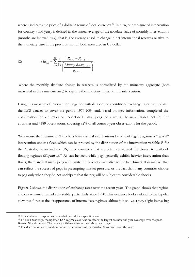
where e indicates the price of a dollar in terms of local currency. 12 In turn, our measure of intervention
for country s and year j is defined as the annual average of the absolute value of monthly interventions
(months are indexed by t ), that is, the average absolute change in net international reserves relative to
the monetary base in the previous month, both measured in US dollar:
(2) ∑=
−
−
−
⎟⎟ ⎠
⎞⎜⎜⎝
⎛
−=
12
1
1,,
1,,
1,,,,
,12
1
t
t j s
t j s
t j st j s
j s
e
BaseMoney
R RMR ,
where the monthly absolute change in reserves is normalized by the monetary aggregate (both
measured in the same currency) to capture the monetary impact of the intervention.
Using this measure of intervention, together with data on the volatility of exchange rates, we updated
the LYS dataset to cover the period 1974-2004 and, based on new information, completed the
classification for a number of undisclosed basket pegs. As a result, the new dataset includes 179
countries and 4189 observations, covering 82% of all country-year observations for the period.13
We can use the measure in (1) to benchmark actual interventions by type of regime against a “typical”
intervention under a float, which can be proxied by the distribution of the intervention variable R for
the Australia, Japan and the US, three countries that are often considered the closest to textbook
floating regimes ( Figure 1 ).14 As can be seen, while pegs generally exhibit heavier intervention than
floats, there are still many pegs with limited intervention –relative to the benchmark floats–a fact that
can reflect the success of pegs in preempting market pressure, or the fact that many countries choose
to peg only when they do not anticipate that the peg will be subject to considerable shocks.
Figure 2 shows the distribution of exchange rates over the recent years. The graph shows that regime
choices remained remarkably stable, particularly since 1990. This evidence looks unkind to the bipolar
view that forecast the disappearance of intermediate regimes, although it shows a very slight increasing
12 All variables correspond to the end of period for a specific month.13 To our knowledge, the updated LYS regime classification offers the largest country and year coverage over the post-Bretton Woods period. The data is available online at the authors’ web pages.14 The distributions are based on pooled observations of the variable R averaged over the year.

8/3/2019 Fear of Appreciation
http://slidepdf.com/reader/full/fear-of-appreciation 10/39
trend in floating regimes. Furthermore, as noted in the introduction, de facto floats continue to
represent less than one fourth of the total sample.15
III. Fear of appreciation
As noted in the introduction, the nature of de facto intermediate and pegged regimes involves a clear
asymmetry. While the prototypic fear of floater would exhibit a low tolerance to exchange rate
depreciations, there is little in the story to motivate the defense of a depreciated real exchange rate
through (often unsterilized) reserve accumulation. Grouping both types of interventions together
when studying the implications of the regime choice is likely to misrepresent either of them.
Because the LYS classification is already built on actual interventions, we can identify these two types
of intervention with only minor additional work. The simplest way to do so is to sort out countries
according to whether they intervene to depress or to defend the exchange rate, i.e. whether the
intervention in (2) is positive or negative. We capture this dichotomy in a new measure of intervention
Int 1 defined as the annual average of the monthly interventions:
(3) ∑=−
−
−
⎟⎟ ⎠
⎞⎜⎜⎝
⎛
−
=
12
1
1,,
1,,
1,,,,
, ,12
1
1 t
t j s
t j s
t j st j s
j s
e
MBase
R R
Int
which now will be negative or positive according to whether the central bank is selling or purchasing
the foreign currency.
Figure 3 distinguishes among intermediate regimes by indicating the percentage of cases where
intervention is positive. As the figure shows, the direction of intervention has changed dramatically (and predictably) over time. The debt crises years found most developing countries selling foreign
15 This broad distribution masks important differences across groups of countries. For example, Latin American countriesseem to have embraced floating arrangements full-heartedly (mostly in combination with inflation targeting regimes), withthe amount of floats doubling between 2000 and 2004 at the expense of both intermediate and pegged regimes. On theother hand, emerging Asia has preserved its bias toward more rigid arrangements. Interestingly, this evidence is a priori atodds with the bipolar view, since currency mismatches in Latin America are large, and certainly larger than in Asia.

8/3/2019 Fear of Appreciation
http://slidepdf.com/reader/full/fear-of-appreciation 11/39

8/3/2019 Fear of Appreciation
http://slidepdf.com/reader/full/fear-of-appreciation 12/39
To address this potential concern, we adopt a conservative strategy: we modify our intervention
measure to filter out the effect of changes in money demand. Specifically, we define first the ratio of
reserves to broad money ( M2 ):18
(4)t j s
t j sM
t j s Assets Foreign R
,,
,,
,,2 = ,
and then we compute a new intervention measure, Int 2, as the annual average change of this ratio:
(5) ( )∑=
−−=12
1
1,,,,, .2212
12
t
t j st j s j s R R Int
Notice that a positive Int 2 implies a strong degree of intervention, because for intervention to be
positive reserve accumulation must exceed the increase in monetary aggregates. Thus, positive values
of this “strong intervention” measure cannot be interpreted as a response to an increase in money
demand. For robustness, in the empirical tests that follow we use both intervention measures.
a. The real exchange rate
The first critical link to be explored empirically is the one between intervention and real appreciations,
that is, whether interventions indeed manage to preserve a depreciated real exchange rate. We do this
in Table 1, where we run a panel regression of the log changes of the real exchange rate on key
determinants of the exchange rate: terms of trade, the output of trading partners, and capital inflows. 19
All regressions include year dummies to control for global factors such as international liquidity or risk
appetite, as well as country fixed effects. Finally, we include estimates for 2- and 3-year non-
overlapping intervals to test for cumulative effects. Our sample, here as well as in the following tests,
comprises all developing economies.
Our benchmark specification is given by:
18 Alternative estimations using the ratio to base money provide the same results and are available upon request.19 We choose the bilateral over the multilateral exchange rate for these tests because it is the one typically targeted by intervention. However, comparable results are obtained using the IMF’s real effective exchange rates are comparable.

8/3/2019 Fear of Appreciation
http://slidepdf.com/reader/full/fear-of-appreciation 13/39
(6) yi,t+s – yi,t = β (1/ s) Σ j=t,t+s Int i,j + γ’ X i,t…t+s + μt+s + θi + εi,t+s ,
where y is the log of the real exchange rate, X is a vector of controls including the log difference of the
terms of trade, the log difference of the trade-weighted average of the GDP of the country’s trading
partners, and the ratio of the financial account over GDP (to measure capital inflows), and , ,
are, respectively, the year and country dummies and the error term.
Exchange rates and reserves tend to change dramatically and endogenously over periods of financial
distress that may lead to strong positive correlations (for example, a reserve drain followed by a
currency collapse) that could be misleadingly construed as a policy choice. To make sure that these
extreme events do not contaminate our results, in all regressions we exclude extreme values of the
intervention measure and the dependent variable. 20
Table 1 shows our results. We find the expected positive effect of intervention on the real exchange
rate: the contemporaneous effect is positive and significant. The results indicate that a 10% increase in
the reserves-to-broad money ratio leads to a contemporaneous 1.69% increase in the real exchange
rate and that the effect almost doubles if intervention is sustained over two years. The estimated effect
is smaller (but still significant) for Int 1. The effect appears to decline (and ceases to be significant)
beyond the second year.
It is important to note at this point that reverse causality should not be a concern here: since positive
interventions are likely to be triggered by real appreciations, endogeneity, if anything, would offset the
positive correlation found in the table. Similarly, to the extent that mercantilist interventions occur
when potentially unobservable “good things happen”, it is unlikely that omitted variables can account
for the observed positive coefficient: on the contrary, uncontrolled favorable external factors would
tend to weaken the positive association between intervention and the real exchange rate.
To complete the characterization of fear of appreciation, standard economic theory provides another
natural testable implication: intervention to prevent a downward exchange rate adjustment should
20Specifically, we include values of Int1 between -150% and 150%, and values of Int2 between -100% and 100%. Similarly,
we restrict our sample to values of the dependent variable within 2 standard deviations from the mean.

8/3/2019 Fear of Appreciation
http://slidepdf.com/reader/full/fear-of-appreciation 14/39
derive, in the absence of price controls, in inflationary pressures, as the system countervails the effects
of intervention to move the exchange rate gradually towards its equilibrium level. Table 2 shows this
by estimating a standard log differenced money demand equation (including the lagged dependent
variable to control for inertial inflation), where intervention variables are added as additional controls.
The data shows that, while intervention is not significantly correlated with inflation, it is associated
with price increases when the latter is measured on the change in the implicit GDP deflator, which is
fully in line with the expected increase in the price of tradables relative to non-tradables due to foreign
exchange intervention. This is confirmed in columns 5 and 6, and again –for tree-years averages– in
columns 7 and 8, where we find that the ratio of the GDP deflator over the CPI is positively related to
foreign exchange intervention.21
In sum, we can preliminary conclude that both measures of intervention (particularly the second oneinvolving an increase in the international reserves backing of monetary aggregates) are associated with
a contemporaneous increase in the real exchange rate, which results in an increase in domestic prices
due to the higher price of tradables, rather than in higher consumer prices driven by expansionary
monetary policies –which, in turn, may reflect the fact that, at least in recent years, these interventions
have been largely sterilized. In what follows, we explore the consequences of this association for
economic performance, and the channels through which they materialize.
b. Output and productivity growth
Does fear of appreciation have any influence on economic activity? If so, is it related with short-lived
and quickly reverted cyclical fluctuations, or does it contribute to long-lasting output expansions? To
explore this issues empirically, we face two methodological problems. On the one hand, there is the
already noted positive link between the growth of output and monetary aggregates, which we address
here introducing a second intervention variable ( Int 2) that traces reserve accumulation in excess of
monetary expansions.
22
On the other hand, there is the possibility that interventions and growth
21 The tradable component of the GDP is typically larger than that of the consumption basket. Note that, if real wages arekept constant, this difference should translate into an increase in the retribution to capital relative to labor, a point to which we come back in the next section.22 While in principle there seems to be no reason why the ratio or reserves over broad money ( Int 2) should increase during economic booms, an argument can be made that in the presence of mean reversing real exchange rate swings, a currency mismatched country should prevent appreciation for fear of an ulterior depreciation (Levy Yeyati, 2005). See Caballero andLorenzoni (2006) for an analytical model along these lines.

8/3/2019 Fear of Appreciation
http://slidepdf.com/reader/full/fear-of-appreciation 15/39
respond to common factors. Favorable conditions (both domestic and external) are expected to lead
both to faster growth and stronger demand for domestic assets, creating appreciation pressures.
Moreover, growth itself can stimulate capital inflows that add to the appreciation bias. In both cases,
fear of appreciation may lead the monetary authorities to intervene, inducing a positive association
between intervention and economic performance that may be incorrectly interpreted as the result of a
positive growth effect of intervention.
Our additional controls (terms of trade, external demand shocks, and capital inflows) should help
alleviate this potential problem. We also control for initial wealth (proxied by the initial per capital
GDP) and population growth. As before, we include country dummies, and year dummies to capture
the effect of global factors such as international liquidity or risk appetite. We also control for initial
wealth (proxied by the initial per capital GDP) and population growth.
One potential caveat of the present analysis is the possibility that an association between intervention
(that is, growing reserves) and growth captures the recovery that typically follows a financial crisis or,
conversely, a protracted output contraction after a boom. While extreme events are already excluded
from the regression, the results may nonetheless capture the aftermath of the crisis. To make sure that
this is not the case, we add the initial output gap (computed as the HP-cyclical component of output)
as an additional control.23
Table 3 reports the results. The intervention effect appears to be consistently significant and
economically important. Column (1)-(4) tells us that a 10% intervention is associated with roughly a
0.14% increase in the growth rate in the following year. As expected, for the stronger Int2 , the
associated increase ranges from 0.18% to .29%. The results are remarkably consistent when estimated
over three-year averages. Are these results the reflection of a crisis, that is, an economic downturn at a
time when reserves are falling? Columns (2) and (4) dispel this concern: it is not negative intervention
(a defensive sale of reserves by central banks under attack) that is driving the results. On the contrary,negative interventions have no additional impact on output growth; if anything, they exert (as in the
specification of column 4) no significant impact on economic activity.
23 We also tested an alternative measure of past output drops, namely, the current depth of the recession that measures the vertical distance to the previous local GDP maximum. Results were virtually unchanged and are omitted for brevity.

8/3/2019 Fear of Appreciation
http://slidepdf.com/reader/full/fear-of-appreciation 16/39
Similar results are obtained when we substitute labor productivity (measured as real GDP per worker)
for real growth in the previous specification. Table 4 reproduces the specification of Table 3 with the
new dependent variable. The findings are more mixed. This is not unexpected: while it is not unlikely
that a one year intervention may in itself trigger a growth process, interventions may have a higher
chance to elicit productivity gains only over time.
The previous results are subject to (at least) two potential criticisms. The first one is related to the fact
that, by working with short one- and three-year windows, our findings may be the reflection of short-
lived cyclical effects on GDP. Moreover, if intervention is induced by economic expansions driven by
domestic real shocks not captured by the additional controls, the positive intervention-growth link
may be in part reflecting a reverse causality not fully eliminated by the lagging of the independent variables. On a more conceptual ground, the mercantilist view is based on the infant-industry premise
that temporary protection leads to permanent effects in terms of competitiveness. More generally, the
case for active exchange rate policy is certainly stronger if the effects of temporary intervention prove
to be persistent.
A straightforward way of testing for this is to examine the effect of intervention on the trend and cycle
components of GDP separately. We do that in Table 5, where we re-run the baseline specification of
Table 3 for output cycle and trend, respectively, where the latter are constructed, alternatively, using
the Hodrick-Prescott (HP) filter and the Baxter-King’s (BK) band-pass procedure, and add the first
three lags if the intervention variable. The main result, which do not diverge qualitatively across
methodologies, show a positive and significant effect on the long-run component (the effect on the
cyclical component is significant only for the first intervention variable). The number, again, indicates
sizeable economic effects: based on the BK decomposition, a 10% increase in Int1 and Int2 leads,
respectively, to cumulative 0.15% and 0.6% increases in long-run growth over four years. All things
considered, the evidence suggests a robust, persistent and economically important effect of intervention on economic growth.
The previous statement, however, should be taken with a grain of salt. While growth regressions have
been standard in the macroeconomic literature due to their ability to exploit large cross-country
datasets amenable to statistical testing, they often raise concerns regarding the robustness of the

8/3/2019 Fear of Appreciation
http://slidepdf.com/reader/full/fear-of-appreciation 17/39
results, among other reasons because of the combination of potential simultaneity and endogeneity
problems and the fact that it is virtually impossible to find credibly exogenous variables to instrument
the relevant controls –almost any time-varying macroeconomic variables have been found to be
correlated with growth in the prolific growth literature. 24
The fact that the link between intervention and growth identified here still holds over three-year
periods and for long-run output trends should help dispel part of the natural skepticism associated
with growth regressions. This notwithstanding, in order for the argument to be convincing, it needs to
provide a clear empirical characterization of the channel through which this link materializes. Hence,
the second criticism mentioned above, to which we turn next.
IV. Intervention and growth: The channel
If we accept for a moment the implication of the previous findings, namely, that there is indeed an
effect of exchange rate intervention on growth, where does this effect come from? Is it by promoting
import substitution and stimulating the production and export of more sophisticated manufactures
previously overpriced relative to international competitors, as the mercantilist view predicates? Does it
induce a shift in the production structure that moves the economy to high productivity growth
tradable sectors? This is certainly the prime suspect in this case, and the one we examine first in this
section.
To do so, we start by looking at the export-import effects, both as a share of GDP, and in terms of
their real growth rates. Export and import shares are often used in the literature to measure the impact
of the exchange rates on trade. However, they suffer from an important drawback in this context
because they are bound to reflect changes in the relative price of tradables. In particular, the shares
should increase with a real devaluation, thus delivering almost by definition a positive relation between
depreciation and their participation in output even if the former has no effect on traded volumes. It ismore accurate to look at the growth volume of exports and imports.
We present the two sets of regressions in Table 6. The specifications are similar to those in Table 3.
In addition, the growth of trade volumes is conditioned on GDP growth to filter the influence of
24 See Rodrik (2005).
8/3/2019 Fear of Appreciation
http://slidepdf.com/reader/full/fear-of-appreciation 18/39
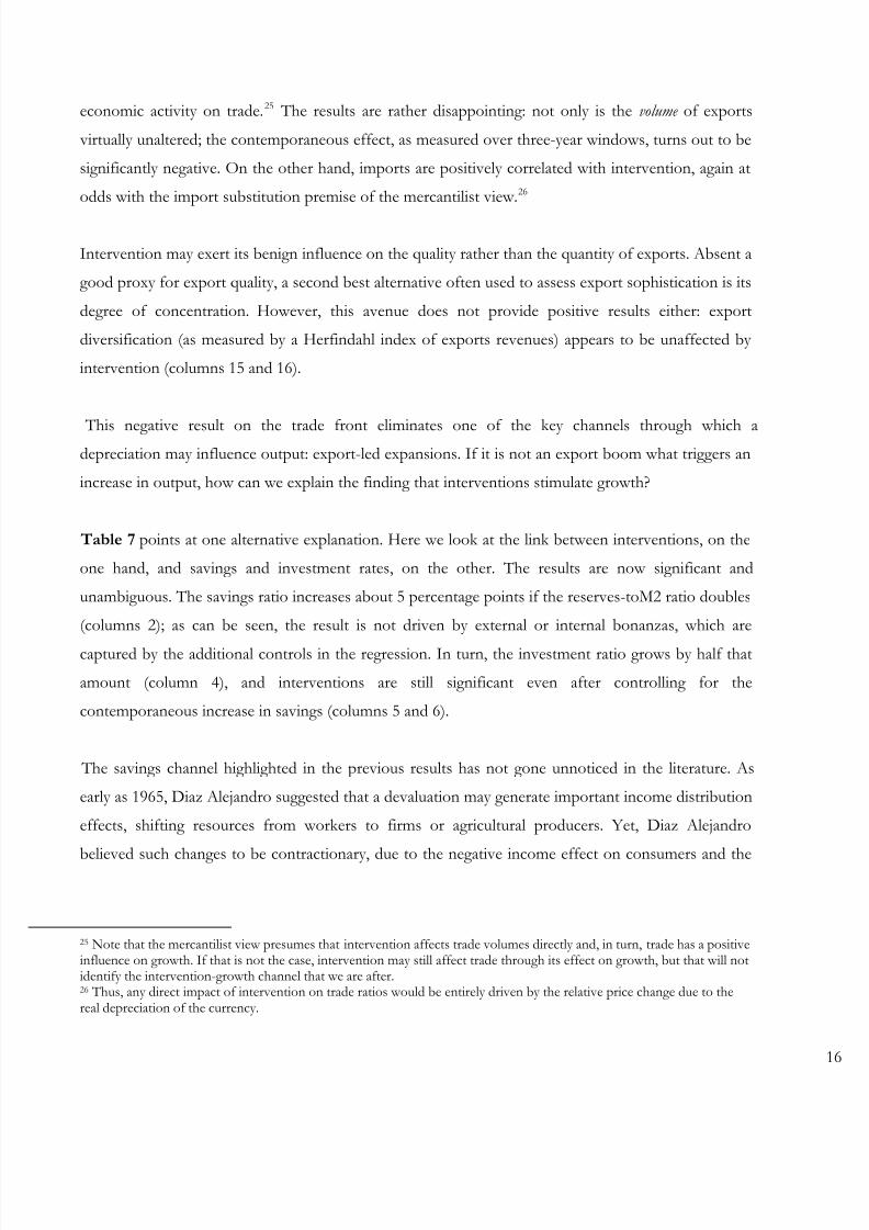
economic activity on trade.25 The results are rather disappointing: not only is the volume of exports
virtually unaltered; the contemporaneous effect, as measured over three-year windows, turns out to be
significantly negative. On the other hand, imports are positively correlated with intervention, again at
odds with the import substitution premise of the mercantilist view.26
Intervention may exert its benign influence on the quality rather than the quantity of exports. Absent a
good proxy for export quality, a second best alternative often used to assess export sophistication is its
degree of concentration. However, this avenue does not provide positive results either: export
diversification (as measured by a Herfindahl index of exports revenues) appears to be unaffected by
intervention (columns 15 and 16).
This negative result on the trade front eliminates one of the key channels through which adepreciation may influence output: export-led expansions. If it is not an export boom what triggers an
increase in output, how can we explain the finding that interventions stimulate growth?
Table 7 points at one alternative explanation. Here we look at the link between interventions, on the
one hand, and savings and investment rates, on the other. The results are now significant and
unambiguous. The savings ratio increases about 5 percentage points if the reserves-toM2 ratio doubles
(columns 2); as can be seen, the result is not driven by external or internal bonanzas, which are
captured by the additional controls in the regression. In turn, the investment ratio grows by half that
amount (column 4), and interventions are still significant even after controlling for the
contemporaneous increase in savings (columns 5 and 6).
The savings channel highlighted in the previous results has not gone unnoticed in the literature. As
early as 1965, Diaz Alejandro suggested that a devaluation may generate important income distribution
effects, shifting resources from workers to firms or agricultural producers. Yet, Diaz Alejandro
believed such changes to be contractionary, due to the negative income effect on consumers and the
25 Note that the mercantilist view presumes that intervention affects trade volumes directly and, in turn, trade has a positiveinfluence on growth. If that is not the case, intervention may still affect trade through its effect on growth, but that will notidentify the intervention-growth channel that we are after.26 Thus, any direct impact of intervention on trade ratios would be entirely driven by the relative price change due to thereal depreciation of the currency.

8/3/2019 Fear of Appreciation
http://slidepdf.com/reader/full/fear-of-appreciation 19/39
associated slump in domestic absorption.27 A “modern” view, in turn, would stress the contractionary
effect of balance sheet effects in the presence of financial dollarization. Firms with foreign currency
denominated liabilities will find themselves increasingly cash-constrained following a sharp
devaluation, triggering a potentially large fall in investment. 28
A consistent story for our findings could be built, however, by combining Díaz Alejandro’s story with
the presence of financial constraints. To the extent that a real devaluation reduces labor costs, it
contributes internal funds to financially constrained firms, thereby fostering savings and investment.
Alternatively, in a financially constrained economy, the implicit transfer from low-income, low-saving
propensity workers to high income capitalists should boost overall savings, lowering the cost of capital
to the same effect.29 Unlike in the original story, in this version the real devaluation should be
expansionary because it relaxes the borrowing constraints that bind the firms (in the first case) of theeconomy (in the second).
Why isn’t this benign effect on financial constraints outweighed by the adverse balance sheet effect?
Presumably, the policy decision to keep the currency undervalued is not independent of the financial
dollarization: fear of appreciation is likely to arise in countries where balance sheet effects are small or
inexistent. At any rate, the hypothesis that fear of appreciation induces a redistribution towards
financially constrained firms relies on the premise that interventions –and, in turn, devaluations– entail
a transfer of income from labor to capital (or, more precisely, an increase in the profitability of capital
at the expense of labor income). We should examine, then, whether this intervention-induced
redistributions actually materialize in practice.
We do this in two ways. First, we look directly at the effects of intervention on the ratio of labor over
capital income ( Table 8 ) –an exercise that, to our knowledge, was last done in this context by
Edwards (1989). We first run the specification in Table 3, which controls for population growth, and
external factors (terms of trade shocks, external demand shocks and capital inflows). Since a lowerlabor income ratio may signal a higher productivity of capital, we add lagged productivity growth as an
27 In fact, his work led to a long debate on whether devaluations were contractionary of expansionary, long before financialdollarization introduced an additional –and often dominating– ingredient in the equation.28 This is the channel popularized by the sudden stop literature (Krugman, 1999; Chang and Velasco, 2001) that led to theunipolar view of exchange rate policy.29 The first channel is more likely to apply to small and medium enterprises with limited access to finance; the second, tolarge companies that fund their investments in capital markets.

8/3/2019 Fear of Appreciation
http://slidepdf.com/reader/full/fear-of-appreciation 20/39
additional control (which comes up with the expected negative sign). The results are encouraging. We
find that a 10% intervention leads to a 0.9% cumulative decline in the labor share over two years when
intervention is measured by Int1, and to a 5% decline when it is measured by Int2 .
A second way to test the premise of the redistribution story is through the effect of interventions on
the labor market, more specifically, its incidence on unemployment ( Table 9 ). Either when we include
our set of external indicators in columns 1 and 3, or when we control for the effect of current output
growth (which has the expected negative coefficient) in columns 2 and 4, interventions exhibit a
significantly negative effect on unemployment. The fact that the redistribution from labor to capital
indeed happens at a time of declining unemployment further supports the view that the effect of fear
appreciation on real variables, at least in the medium run captured by the previous tests, is mainly
driven by a decline in real wages.
Note that these results are in line with our findings in Table 2. To the extent that intervention induces
inflationary pressures, less than perfect wage indexation should results in lower real wages. However,
this is not necessary to explain the redistribution effect reported in Table 8: inasmuch as the higher
relative price of tradables is not fully passed through to the CPI (as our results in Table 2 indicate),
capital income should increase relative to labor income even if wages are kept constant in terms of the
local CPI. Indeed, the higher return from exports due to the undervalued currency may boost
employment and real wages at the same time – particularly in the case of commodity producers with a
low component of imported capital where the countervailing effect of a high exchange rate on the
cost of imports is only minor.30
V. Discussion: Evidence in search of a theory
Our findings provide an interesting vantage point from which we can revisit the link between nominal
and real variables and, in particular, the several hypotheses that have been suggested by the literatureregarding the role of exchange rates as a development strategy. While our results support the claim
that undervalued exchange rates foster growth, they cast doubts on the channel of import substitution
cum export stimulus often highlighted by its advocates. Instead, our tests suggest that the mechanism
30 Note that the same applies to countries where capital and infrastructure investment has been made at the previous lowerexchange rate, or is curently subsidized (or regulated) by the government.

8/3/2019 Fear of Appreciation
http://slidepdf.com/reader/full/fear-of-appreciation 21/39
is associated with an increase in aggregate savings and investment, and a decline in labor income
relative to capital compensation.
This preliminary evidence seems to assign a more limited role for the more recent incarnations of
export-led strategies such as self discovery (Hausmann and Rodrik, 2005). The presumed benign
influence of mercantilist interventions on export growth and diversification appears not to be there,
although the consequences in terms of their potential to foster growth by improving the quality of the
export mix (Hausmann, Hwang and Rodrik, 2005) remain to be tested. Moreover, our results seem at
odds with previous findings on the effects of overvaluation on the tradable sector by Rajan and
Subramanian (2006). However, it is conceivable that those results simply reflect the effect of the
relative price change on the output of sectors with varying degrees of exportability. 31 By contrast, the
findings, reported in the same paper, that an undervalued currency fosters growth in labor intensivesectors is fully in line with the negative correlations between fear of appreciation and labor
compensation documented here.
Our empirical results point at two alternative channels through which devaluations may contribute to
growth. The first one is a labor market enhancing effect reminiscent of the channels identified in
classical models of economies with unlimited supply of labor (Lewis, 1958, Fei and Ranis, 1961). In
those models, the development challenge was to move workers from unproductive subsistence
agricultural jobs into high productivity industrial jobs. While a depreciated exchange rate may be a
plausible vehicle to entice firms to hire this surplus labor, the quantitative effects that we find are
relatively minor (a 10% increase in the reserve-to-M2 ratio leading to a 0.4% change in the
unemployment rate).
A second, alternative channel relates to the benign effect of lower labor costs on access to internal
funds by financially constrained enterprises, an aspect that has been highlighted as a source of the
rapid recovery in the aftermath of recent emerging market crises (Calvo and Talvi, 2006) and, moregenerally, as a source of growth in developing economies (Aghion et al. 2006). 32 This channel should
31 The paper looks at the nominal value added by sector, deflated by a GDP implicit price level. As a result, a realdevaluation should reflect positively in the valued added of exportable industries that benefit from higher prices, even if produced quantities remain constant or even decline.32 In Aghion et al (2006), rather than a source of finance, internal funds are a vehicle that domestic financial markets use tocollateralize a joint projects with foreign direct investors carrying state-of-the-art technology.

8/3/2019 Fear of Appreciation
http://slidepdf.com/reader/full/fear-of-appreciation 22/39
be particularly relevant for low and middle income economies where financial constraints are more
prevalent. Interestingly, the same authors have also flagged, elsewhere, the deleterious effects of a
devaluation on firms with foreign-currency liabilities (Calvo et al., 2005; Aghion et al., 2002). Two
factors help reconcile these two seemingly contradictory claims. The first one has already been noted:
the degree of financial dollarization or, more precisely, its gradual decline in the developing world. 33
The second factor relates to the fact that fear of appreciation, as measured here, captures voluntary
interventions to bring down the exchange rate, rather than the involuntary depreciations that occur in
period of financial stress despite defensive exchange rate intervention, which underlie the predictions of
the traditional fear of floating literature.
A final aspect that divides the earlier and modern version of the redistribution argument deserves to
be noted: How does the income transfer from labor to capital that was contractionary in the earlier version (Díaz Alejandro, 1965) becomes expansionary here? The previous discussion offers a possible
explanation. Diaz Alejandro’s view, embedded in a Keynesian framework, revolved around the
question of how the income that was transferred from workers to capitalists was ultimately spent.
Because Diaz Alejandro was thinking on an agricultural society (his 1965 piece was inspired by the
Argentine economy), he did not see these increased savings translating into sources of domestic
finance but rather going abroad in the form of foreign assets; hence, the depressed aggregate demand
that explained the drop in output. Our findings suggest that the funds that in the earlier version were
spent abroad, may in fact be allocated domestically to productive investment previously postponed
due to insufficient financing.
Given the currently benign international context, and the recent changes in debt composition and
policy in developing countries, we anticipate that the fear of appreciation analyzed here will be the
main contender to the current FIT paradigm among developing economies. In this paper, we
contributed to the ongoing debate on exchange rate policy by characterizing this policy and
documenting its implications for the real economy. The promising results reported here only confirmthat the exchange rate debate is still alive and in need of a reappraisal.
33 Financial dollarization is possibly the sole aspect that may turn the exchange rate from a countercyclical shock absorberinto a procyclical source of economic contractions (see Frankel, 2005; and Levy Yeyati, 2006). Given that the pro-growthconsequences of fear of appreciation are more likely to materialize in the absence of the severe currency mismatchesusually found in financially dollarized economies, it is not surprising that its popularity has grown in recent years pari passu with a gradual dedollarization of financial markets in developing countries in the 2000s.

8/3/2019 Fear of Appreciation
http://slidepdf.com/reader/full/fear-of-appreciation 23/39
Figure 1
United States, Japan and Australia
0
10
20
30
40
50
60
- 0 . 1 5
- 0 . 1 3
- 0 . 1 1
- 0 . 0 9
- 0 . 0 7
- 0 . 0 5
- 0 . 0 3
- 0 . 0 1
0 . 0 1
0 . 0 3
0 . 0 5
0 . 0 7
0 . 0 9
0 . 1 1
0 . 1 3
0 . 1 5
Annual average intervention index
The facto floats
0
5
10
15
20
25
30
Annual average intervention index
Intermediate and Pegs
0
2
4
6
8
10
12
14
16
18
- 0 . 1 5
- 0 . 1 3
- 0 . 1 1
- 0 . 0 9
- 0 . 0 7
- 0 . 0 5
- 0 . 0 3
- 0 . 0 1
0 . 0 1
0 . 0 3
0 . 0 5
0 . 0 7
0 . 0 9
0 . 1 1
0 . 1 3
0 . 1 5
Annual average intervention index

8/3/2019 Fear of Appreciation
http://slidepdf.com/reader/full/fear-of-appreciation 24/39
Figure 2
Distribution of regimes over the years LYS classification (1974-2004) – All countries
% Fix
% Float
% Interm
0%
10%
20%
30%
40%
50%
60%
70%
80%
90%
100%
1974 1980 1990 2000 2004

8/3/2019 Fear of Appreciation
http://slidepdf.com/reader/full/fear-of-appreciation 25/39
Percentage of countries with a positive annual average of intervention indexIntermediate and Pegs
(variable int.1)
0.00
0.10
0.20
0.30
0.40
0.50
0.60
0.70
0.80
0.90
1974 1980 1986 1992 1998 2004
%
Percentage of countries with a positive annual average of intervention indexOnly intermediate Regimes
(variable Int.1)
0.40
0.50
0.60
0.70
0.80
0.90
%
0.00
0.10
0.20
0.30
1974 1980 1986 1992 1998 2004
Figure 3
% of positives (excluding obs. inside of non-direction band)
% of positives
% of positives (demeaned data)
% of positives
% of positives (excluding obs. inside of non-direction band)
% of positives (demeaned data)

8/3/2019 Fear of Appreciation
http://slidepdf.com/reader/full/fear-of-appreciation 26/39
T a b l e 1
S a m p
l e o
f 1
9 7 4 - 2
0 0 4
D e p e n
d e n t
V a r i a
b l e :
L o g a r i t h m
o f R e a
l E x c
h a n g e
R a
t e
V a r i a b l e s
[ 1 ]
[ 2 ]
[ 3 ]
[ 4 ]
[ 5 ]
[ 6 ]
i n t 1 . I n d e x ( t )
0 . 0 3 6 *
0 . 1 0 9 * *
0 . 0 4 8
( 0 . 0 2 2 )
( 0 . 0 5 5 )
( 0 . 0 7 2 )
i n t 2 . I n d e x ( t )
0 . 1 6 9 * *
0 . 2 6 2 * *
0 . 2 0 8
( 0 . 0 7 5 )
( 0 . 1 2 0 )
( 0 . 1 6 9
)
C o n
t r o l V a r i a
b l e s
∆ L o g ( T o T )
0 . 0 0 0
0 . 0 0 0
0 . 0 0 0
- 0
. 0 0 1
- 0 . 0 0 2
- 0 . 0 0 2
( 0 . 0 0 1 )
0 . 0 0 0
( 0 . 0 0 1 )
( 0 . 0 0 1 )
( 0 . 0 0 2 )
( 0 . 0 0 1
)
T r a d i n g p a r
t n e r s g r o w t h
- 0 . 0 0 8
- 0 . 0 0 7
- 0 . 0 1 1
- 0
. 0 0 7
- 0 . 0 1 3
- 0 . 0 1 1
( 0 . 0 0 5 )
( 0 . 0 0 5 )
( 0 . 0 0 8 )
( 0 . 0 0 8 )
( 0 . 0 1 4 )
( 0 . 0 1 2
)
F i n a n c i a l a c
c o u n t t o G D P
- 0 . 0 1 2 * * *
- 0 . 0 1 0 * * *
- 0 . 0 1 3 * * *
- 0 . 0
1 3 * * *
- 0 . 0 1 7 * * *
- 0 . 0 1 4 * * *
( 0 . 0 0 2 )
( 0 . 0 0 2 )
( 0 . 0 0 3 )
( 0 . 0 0 2 )
( 0 . 0 0 4 )
( 0 . 0 0 3
)
O b s e r v a t i o n s
/ C o u n t r i e s
1 3 5 0 / 7 6
1 4 3 3 / 8 0
6 7 5 / 7 6
7 7 8 / 8 0
4 8 5 / 7 6
5 4 9 / 8
0
R - s q u a r e d
0 . 9 8 9
0 . 9 9
0 . 9 9
0 . 9 9 1
0 . 9 9
0 . 9 9 1
M e a n
D e p . v a r .
3 . 7 1 8
3 . 7 3 3
3 . 7 3 3
3 . 7 3 3
3 . 7 3 3
3 . 7 3 3
S t D e v
D e p .
v a r .
2 . 4 1 4
2 . 4 7 5
2 . 4 8 9
2 . 4 8 9
2 . 4 7 5
2 . 4 7 5
N o t e : y ( t , t + s )
c o r r e s p o n d s t o t h e a v e r a g e o v e r t h e p e r i o d t t o t + s o f t h e v a r i a b l e y .
E x c e p t o t h e r w i s e i n d i c a t e d , a l l c o n t r o l s a r e a v e r a g e s f o r t h e p e r i o d o v e r w h i c h t h e d e p e n d e n t v a r i a b l e i s m e a s u r e d .
A l l r e g r e s s i o n s
i n c l u d e d c o u n t r y f i x e d e f f e c t s a n d T i m e d u m
m i e s
R o b u s t s t a n d a r d e r r o r s i n p a r e n t h e s e s / * s i g n i f i c a n t a t 1 0 %
; * * s i g n i f i c a n t a t 5 % ; * * * s i g n i f i c a n t a t 1 %
T C R
( t )
( t )
( 2 - y e a r a v e r a g e )
( t )
( 3 - y e a r a v e r a g e )
2 4

8/3/2019 Fear of Appreciation
http://slidepdf.com/reader/full/fear-of-appreciation 27/39
T a b l e 2
S a m p l e o f 1 9 7 4 - 2 0 0 4
D e p e n d e n t V a r i a b l e : P e r c e n t a g e o f
C h a n g e o f C o n s u m e r P r i c e I n d e x a n d G
D P D e f l a t o r
V a r i a b l e s
[ 1 ]
[ 2 ]
[ 3 ]
[ 4 ]
[ 5 ]
[ 6 ]
[ 7 ]
[ 8 ]
i n t 1 . I n d e x ( t )
0 . 3 2 5
1 . 4 0 8
1 .
0 8 5 * *
2 . 2 4 8
* *
( 0 . 7 5 3 )
( 0 . 8 9 1 )
( 0
. 4 2 5 )
( 1 . 0 3
2 )
i n t 2 . I n d e x ( t )
1 . 9 7 2
1 4 . 2 6 7 * * *
3 . 1 0 9 * *
1 1 . 0 7 1 * * *
( 2 . 9 7 8 )
( 3 . 5 9 9 )
( 1 . 5 2 0 )
( 2 . 6 4 7 )
C o n t r o l V a r i a b l e s
L a g g e d d e p . v a r .
0 . 1 5 4 * * *
0 . 1 3 8 * * *
0 . 1 6 7 * * *
0 . 1 6 8 * * *
0
. 0 2 4
0 . 0 3 1
- 0 . 0 3
1
- 0 . 0 1 4
( 0 . 0 3 2 )
( 0 . 0 2 8 )
( 0 . 0 3 2 )
( 0 . 0 2 4 )
( 0
. 0 3 5 )
( 0 . 0 3 4 )
( 0 . 0 5
2 )
( 0 . 0 5 2 )
∆ % G D P
- 0 . 1 2 2 * *
- 0 . 1 2 9 * *
- 0 . 1 2 9 * *
- 0 . 1 7 4 * * *
-
0 . 0 1
- 0 . 0 1 3
0 . 1 1 0 *
0 . 0 8 6
( 0 . 0 5 8 )
( 0 . 0 5 8 )
( 0 . 0 6 4 )
( 0 . 0 6 4 )
( 0
. 0 3 5 )
( 0 . 0 3 5 )
( 0 . 0 6
5 )
( 0 . 0 6 3 )
∆ % M 2
0 . 1 0 1 * * *
0 . 1 2 4 * * *
0 . 1 8 3 * * *
0 . 2 2 9 * * *
- 0
. 0 1 5
- 0 . 0 0 6
0 . 0 1 8 *
0 . 0 1 7
( 0 . 0 3 9 )
( 0 . 0 3 8 )
( 0 . 0 5 6 )
( 0 . 0 5 2 )
( 0
. 0 1 0 )
( 0 . 0 1 1 )
( 0 . 0 1
0 )
( 0 . 0 1 1 )
I n t e r e s t R a t e
3 . 9 0 2 4 * * *
3 . 9 9 4 7 * * *
4 . 6 8 5 5 * * *
4 . 2 3 8 5 * * *
- 0
. 6 8 3
- 2 . 0 5 1
0 . 7 4 7
0 . 4 4 2
( 4 . 9 9 )
( 4 . 8 2 )
( 4 . 9 8 )
( 4 . 9 5 )
( 2 . 1 2 )
( 2 . 0 8 )
( 2 . 6 8 )
( 2 . 7 2 )
O b s e r v a t i o n s / C o u n t r i e s
1 2 5 5 / 8 3
1 2 8 2 / 8 5
1 3 6 2 / 8 6
1 4 2 9 / 9 0
1 2 0 0 / 8 2
1 2 3 2 / 8 4
4 0 9 /
8 2
4 5 4 / 8 3
R - s q u a r e d
0 . 7 2 2
0 . 7 2 2
0 . 7 0 9
0 . 7 1 4
0
. 1 6 2
0 . 1 5 9
0 . 3 0
5
0 . 2 9
M e a n
D e p . v a r .
9 . 5 9 2
9 . 7 3 8
1 0 . 6 3 8
1 0 . 7 8
- 0 . 0 2 8
- 0 . 0 3 3
- 0 . 0 6
5
- 0 . 0 1 6
S t D e v
D e p . v a r .
1 1 . 1 7
1 1 . 3 2 7
1 3 . 6 1
1 3 . 8 5 1
4
. 1 1 8
4 . 1 6 3
2 . 7 7
5
3 . 0 5 7
N o t e : y ( t , t + s ) c o r r e s p o n d s t o t h e a v e r a g e o v e r t h e p e r i o d t t o t + s o f t h e v a r i a b l e y .
E x c e p t o t h e r w i s e i n d i c a t e d , a l l c o n t r o l s a r e a v e r a g e s f o r t h e p e r i o d o v e r w h i c h t h e d e p e n d e n t v a r i a b l e i s m e a s u r e d .
A l l r e g r e s s i o n s i n c l u d e d c o u n t r y f i x e d e f f e
c t s a n d T i m e d u m m i e s
R o b u s t s t a n d a r d e r r o r s i n p a r e n t h e s e s / *
s i g n i f i c a n t a t 1 0 % ; * * s i g n i f i c a n t a t 5 % ; * * * s i g n i f i c a n t a t 1 %
∆ % D
e f l a t o r - ∆ % C P I
( 3 - y e a r a v e r a g e )
( t )
∆ % D e f l a t o r - ∆ % C P I
∆ % C P I
∆ % D e f l a t o r
2 5

8/3/2019 Fear of Appreciation
http://slidepdf.com/reader/full/fear-of-appreciation 28/39
2 6
T a b l e 3
S a m p l e o f 1 9 7 4 - 2 0 0 4
D e p e n d e n t V a r i a b l e : P e r c e n t a g e o f C h a n g e o f t h e R
e a l G r o s s D o m e s t i c P r o d u c t
V a r i a b l e s
[ 1 ]
[ 2 ]
[ 3 ]
[ 4 ]
[ 5 ]
[ 6 ]
i n t 1 . I n d e x ( t )
1 . 2 6 9
* * *
1 . 4 3 6 * * *
1 . 3 5 2 * *
( 0 . 2 7
0 )
( 0 . 4 2 8 )
( 0 . 6 6 1 )
i n t 1 . I n d e x_ n e
g ( t )
- 0 . 3 7
( 0 . 7 4 3 )
i n t 2 . I n d e x ( t )
1 . 7 9 0 * *
2 . 8 6 2 * *
3 . 2
9 2 * *
( 0 . 8 1 0 )
( 1 . 4 4 7 )
( 1 .
6 2 8 )
i n t 2 . I n d e x_ n e
g ( t )
- 2 . 3 5 3
( 2 . 3 1 2 )
C o n t r o l V a r i a b
l e s
L a g g e d d e p . v a r .
0 . 2 9 2
* * *
0 . 2 9 2 * * *
0 . 3 0 7 * * *
0 . 3 0 7 * * *
- 0 . 0 3 5
- 0 . 0 4 8
( 0 . 0 3
2 )
( 0 . 0 3 2 )
( 0 . 0 3 1 )
( 0 . 0 3 1 )
( 0 . 0 4 2 )
( 0 .
0 3 3 )
L G D P_
H P_ c y
c l e ( t )
- 3 8 . 1 2
4 * * *
- 3 8 . 0 9 1 * * *
- 4 0 . 0 1 6 * * *
- 3 9 . 9 6 6 * * *
( 3 . 0 4
6 )
( 3 . 0 5 3 )
( 3 . 0 3 8 )
( 3 . 0 5 1 )
∆ L o g ( T o T )
0 . 0 3 8
* * *
0 . 0 3 8 * * *
0 . 0 3 8 * * *
0 . 0 3 8 * * *
0 . 0 7 1 * * *
0 . 0
7 0 * * *
( 0 . 0 0
6 )
( 0 . 0 0 6 )
( 0 . 0 0 6 )
( 0 . 0 0 6 )
( 0 . 0 1 7 )
( 0 .
0 1 3 )
P o p u l a t i o n g r o w t h
0 . 2 2
0 . 2 3
0 . 2 1 5
0 . 2 2 0
0 . 5 5 9 * * *
0 . 5
7 3 * * *
( 0 . 1 4
7 )
( 0 . 1 4 7 )
( 0 . 1 5 2 )
( 0 . 1 5 2 )
( 0 . 1 7 0 )
( 0 .
1 9 6 )
F i n a n c i a l a c c o u n t t o G D P
0 . 0 3 9 *
0 . 0 4 0 *
0 . 0 6 2 * * *
0 . 0 6 2 * * *
0 . 0 5 9 * *
0 . 0
8 7 * * *
( 0 . 0 2
0 )
( 0 . 0 2 0 )
( 0 . 0 2 1 )
( 0 . 0 2 1 )
( 0 . 0 2 8 )
( 0 .
0 2 5 )
T r a d i n g p a r t n e r s g r o w t h
0 . 2 0 6
* *
0 . 2 0 6 * *
0 . 2 1 5 * * *
0 . 2 1 4 * * *
0 . 3 0 9 *
0 . 3
4 7 * *
( 0 . 0 8
3 )
( 0 . 0 8 3 )
( 0 . 0 8 3 )
( 0 . 0 8 3 )
( 0 . 1 7 5 )
( 0 .
1 4 7 )
G D P ( t )
- 0 . 1
7
- 0 . 1 9
0 . 1 0 3
0 . 0 7 6
- 5 . 4 7 9 * * *
- 5 . 4
7 1 * * *
( 0 . 6 7
4 )
( 0 . 6 7 6 )
( 0 . 7 0 0 )
( 0 . 7 0 1 )
( 0 . 9 3 3 )
( 0 .
8 0 2 )
O b s e r v a t i o n s
/ C o u n t r i e s
1 4 9 6 / 8 4
1 4 9 6 / 8 4
1 5 7 7 / 8 8
1 5 7 7 / 8 8
5 1 0 / 8 4
5 7 7
/ 8 8
R - s q u a r e d
0 . 4 4
2
0 . 4 4 2
0 . 4 3 6
0 . 4 3 6
0 . 4 6 4
0 .
4 5 1
M e a n
D e p . v a r .
3 . 5 9
3 . 5 9
3 . 5 1 9
3 . 5 1 9
3 . 5 2 1
3
. 3 8
S t D e v
D e p . v a r .
4 . 0 9
9
4 . 0 9 9
4 . 1 6 5
4 . 1 6 5
3 . 0 9 4
3 .
1 3 5
N o t e : y ( t , t + s ) c o r r e s p o n d s t o t h e a v e r a g e o v e r t h e p e r i o d t t o t + s o f t h e v a r i a b l e y .
E x c e p t o t h e r w i s e
i n d i c a t e d , a l l c o n t r o l s a r e a v e r a g e s f o r t h e p e r i o d
o v e r w h i c h t h e d e p e n d e n t v a r i a b l e i s m e a s u r e d .
( t + 1 )
( t + 1 )
( 3 - y e a r a v e r a g e )
∆ % G
D P
A l l r e g r e s s i o n s i n c l u d e d c o u n t r y f i x e d e f f e c t s a n d T i m e d u m m i e s / R o b u s t s t a n d a r d e r r o r s i n p a r e n t h e s e s / * s i g n i f i c a n t a t 1 0 % ; * * s i g n i f i c a n t a t 5 % ; * * * s i g n i f i c a n t a t 1 %

8/3/2019 Fear of Appreciation
http://slidepdf.com/reader/full/fear-of-appreciation 29/39
2 7
T a b l e 4
S a m p l e o f 1 9 7 4 - 2
0 0 4
D e p e n d e n t V a r i a b l e : P e r c e n t a g e o f C h a n g e o f t h e G r
o s s D o m e s t i c P r o d u c t P e r W o r k e r
V a r i a b l e s
[ 1 ]
[ 2 ]
[ 3 ]
[ 4 ]
[ 5 ]
[ 6 ]
i n t 1 . I n d e x ( t )
0 . 6 8 3 * *
1 . 2 0 7 * *
0 . 8 5 2
( 0 . 3 2 5 )
( 0 . 5 1 4 )
( 0 . 8 0 3 )
i n t 1 . I n d e x_ n e g ( t )
- 1 . 1 5 2 0
( 0 . 8 9 7 )
i n t 2 . I n d e x ( t )
0 . 5 8 2
2 . 5 8 4
6 . 6 3
1 * * *
( 1 . 1 4 1 )
(
1 . 6 9 6 )
( 2 . 3
3 4 )
i n t 2 . I n d e x_ n e g ( t )
- 4 . 4 5 2
(
3 . 2 7 1 )
C o n t r o l V a r i a b l e s
L a g g e d D e p . v a r .
0 . 1 5 6 * * *
0 . 1 5 7 * * *
0 . 1 5 9 * * *
0
. 1 6 0 * * *
0 . 0 1 6
- 0 . 0
0 7
( 0 . 0 2 8 )
( 0 . 0 2 7 )
( 0 . 0 2 7 )
(
0 . 0 2 7 )
( 0 . 0 5 8 )
( 0 . 0
5 1 )
L G D P_
H P_ c y c l e ( t )
- 2 2 . 2 7 6 * * *
- 2 2 . 2 6 0 * * *
- 2 4 . 1 0 2 * * *
- 2 4 . 1 4 3 * * *
( 3 . 3 0 4 )
( 3 . 3 0 6 )
( 3 . 2 2 0 )
(
3 . 2 3 2 )
∆ L o g ( T o T )
0 . 0 3 8 * * *
0 . 0 3 8 * * *
0 . 0 3 4 * * *
0
. 0 3 3 * * *
0 . 0 6 3 * * *
0 . 0 5
9 * * *
( 0 . 0 0 8 )
( 0 . 0 0 8 )
( 0 . 0 0 8 )
(
0 . 0 0 8 )
( 0 . 0 1 8 )
( 0 . 0
1 6 )
P o p u l a t i o n g r o w t h
0 . 0 2
0 . 0 2
- 0 . 0 0 3
0 . 0 1 0
0 . 2 7 3
0 . 2
9 0
( 0 . 1 7 7 )
( 0 . 1 7 8 )
( 0 . 1 8 0 )
(
0 . 1 7 9 )
( 0 . 2 7 9 )
( 0 . 2
7 2 )
F i n a n c i a l a c c o u n t t o G D P
0 . 0 4 2 *
0 . 0 4 3 *
0 . 0 6 3 * * *
0
. 0 6 4 * * *
0 . 0 7 7 *
0 . 0 8 6 * *
( 0 . 0 2 4 )
( 0 . 0 2 4 )
( 0 . 0 2 4 )
(
0 . 0 2 4 )
( 0 . 0 4 1 )
( 0 . 0
3 6 )
T r a d i n g p a r t n e r s g r o w t h
0 . 1 4
0 . 1 4
0 . 1 5 7
0 . 1 5 7
0 . 1 8 9
0 . 3
( 0 . 1 0 3 )
( 0 . 1 0 3 )
( 0 . 1 0 2 )
(
0 . 1 0 2 )
( 0 . 2 0 5 )
( 0 . 2
0 1 )
G D P p w ( t )
- 2 . 1 5 5 * * *
- 2 . 1 8 2 * * *
- 1 . 8 4 7 * *
- 1 . 8 6 3 * *
- 6 . 7 5 4 * * *
- 6 . 6 1
8 * * *
( 0 . 8 2 3 )
( 0 . 8 2 4 )
( 0 . 8 1 8 )
(
0 . 8 1 4 )
( 1 . 0 4 9 )
( 0 . 9
8 0 )
O b s e r v a t i o n s / C o u
n t r i e s
1 4 3 1 / 8 1
1 4 3 1 / 8 1
1 5 0 9 / 8 7
1 5
0 9 / 8 7
5 1 3 / 8 3
5 7 8
/ 8 7
R - s q u a r e d
0 . 3 0 8
0 . 3 0 9
0 . 3 1 1
0 . 3 1 3
0 . 3 8 2
0 . 4
0 5
M e a n
D e p . v a r .
1 . 0 2 5
1 . 0 2 5
0 . 9 6 2
0 . 9 6 2
1 . 0 6 4
0 . 9
5 4
S t D e v
D e p . v a r .
4 . 4 9 8
4 . 4 9 8
4 . 5 4 2
4 . 5 4 2
3 . 4 5 5
3 . 4
9 4
N o t e : y ( t , t + s ) c o r r e s p
o n d s t o t h e a v e r a g e o v e r t h e p e r i o d t t o t + s o f
t h e v a r i a b l e y .
E x c e p t o t h e r w i s e i n d i c
a t e d , a l l c o n t r o l s a r e a v e r a g e s f o r t h e p e r i o d o
v e r w h i c h t h e d e p e n d e n t v a r i a b l e i s m e a s u r e d
.
( t + 1 )
( t + 1 ) ( 3 - y e a r a v e r a g
e )
∆ % G D P
p w
A l l r e g r e s s i o n s i n c l u d e
d c o u n t r y f i x e d e f f e c t s a n d T i m e d u m m i e s / R o b u s t s t a n d a r d e r r o r s i n p a r e n t h e s e s / * s i g n i f i c a n t a t 1 0 % ; * * s i g n i f i c a n t a t 5 % ; * * * s i g n i f i c a n
t a t 1 %

8/3/2019 Fear of Appreciation
http://slidepdf.com/reader/full/fear-of-appreciation 30/39
2 8
T a b l e 5
S a m p l e o f 1 9 7 4 - 2 0 0 4
D e p e n d e n t V a r i a b l e : P e r c e n t a g e o f C h a n g e o f t h e R e a l G r o s s D o m e s t i c P
r o d u c t
V a r i a b l e s
[ 1 ]
[ 2 ]
[ 3 ]
[ 4 ]
[ 5 ]
[ 6 ]
[ 7 ]
[ 8 ]
i n t 1 . I n d e x ( t )
0 . 5 6 2 * * *
0 . 2 7 0 * * *
0 . 5 9 9 * * *
1 . 0 7 8 * * *
( 0 . 1 6 4 )
( 0 . 1 0 4 )
( 0 . 2 2 2 )
( 0 . 2 6 9 )
i n t 1 . I n d e x ( t - 1 )
0 . 5 9 8 * * *
0 . 3 4 5 * * *
( 0 . 1 6 5 )
( 0 . 1 0 6 )
i n t 1 . I n d e x ( t - 2 )
0 . 3 5 4 * *
0 . 2 3 8 * *
( 0 . 1 6 9 )
( 0 . 1 0 4 )
i n t 1 . I n d e x ( t - 3 )
0 . 1 1 7
0 . 1 9 6 *
( 0 . 1 6 8 )
( 0 . 1 0 5 )
i n t 2 . I n d e x ( t )
1 . 5 5 5 * * *
0 . 9 6 9 * * *
- 0 . 4 5 1
0 . 8 1 4
( 0 . 5 4 )
( 0 . 3 3 )
( 0 . 7 1 2 )
( 0 . 8 0 3 )
i n t 2 . I n d e x ( t - 1 )
1 . 8 1 0 * * *
0 . 8 1 8 * * *
( 0 . 5 2 )
( 0 . 3 1 )
i n t 2 . I n d e x ( t - 2 )
1 . 8 9 2 * * *
0 . 8 6 1 * * *
( 0 . 5 0 4 )
( 0 . 3 0 3 )
i n t 2 . I n d e x ( t - 3 )
1 . 1 7 7 *
0 . 7 8 8 * *
( 0 . 6 5 9 )
( 0 . 3 4 4 )
C o n t r o l V a r i a b l e s
L G D P_
B K_
t r e n d ( t )
- 3 . 1 5 7 * * *
- 2 . 8 9 4 * * *
( 0 . 4 7 8 )
( 0 . 4 9 2 )
L G D P_
H P_
t r e n d ( t )
- 2 . 1 6 3 * * *
- 1 . 9 4 6 * * *
( 0 . 3 1 3 )
( 0 . 3 1 4 )
L G D P_
B K_ c y c l e ( t )
- 6 4 . 4 5 0 * * *
- 6 4 . 6 5 4 * * *
( 3 . 5 5 5 )
( 3 . 4 5 5 )
L G D P_
H P_ c y c l e ( t )
- 3 0 . 0 1 6 * * *
- 3 0 . 5 4 3 * * *
( 2 . 4 4 4 )
( 2 . 4 1 9 )
∆ L o g ( T o T )
0 . 0 2 4 * * *
0 . 0 2 4 * * *
0 . 0 1 1 * * *
0 . 0 1 1 * * *
0 . 0 1 7 * * *
0 . 0 1 6 * * *
0 . 0 3 3 * * *
0 . 0 3 1 * * *
( 0 . 0 0 4 )
( 0 . 0 0 4 )
( 0 . 0 0 3 )
( 0 . 0 0 3 )
( 0 . 0 0 5 )
( 0 . 0 0 5 )
( 0 . 0 0 6 )
( 0 . 0 0 6 )
P o p u l a t i o n g r o w t h
0 . 3 6 1 * * *
0 . 3 6 8 * * *
0 . 2 4 9 * * *
0 . 2 6 2 * * *
- 0 . 1 2 4
- 0 . 1 3 9
0 . 0 3 0
0 . 0 3 0
( 0 . 1 2 8 )
( 0 . 1 3 0 )
( 0 . 0 8 2 )
( 0 . 0 8 3 )
( 0 . 1 4 8 )
( 0 . 1 4 4 )
( 0 . 1 3 2 )
( 0 . 1 3 5 )
F i n a n c i a l a c c o u n t t o G D P
0 . 0 3 8 * * *
0 . 0 4 8 * * *
0 . 0 3 4 * * *
0 . 0 3 9 * * *
0
. 0 3 2 * *
0 . 0 3 8 * *
0 . 0 4 3 * *
0 . 0 6 3 * * *
( 0 . 0 1 3 )
( 0 . 0 1 3 )
( 0 . 0 0 9 )
( 0 . 0 0 8 )
( 0 . 0 1 5 )
( 0 . 0 1 5 )
( 0 . 0 1 9 )
( 0 . 0 2 0 )
T r a d i n g p a r t n e r s g r o w t h
0 . 1 2 1 * *
0 . 1 2 9 * *
0 . 0 5
0 . 0 6
0 . 0 0 8
- 0 . 0 1 5
0 . 1 5 0 * *
0 . 1 4 1 *
( 0 . 0 5 2 )
( 0 . 0 5 4 )
( 0 . 0 3 2 )
( 0 . 0 3 4 )
( 0 . 0 5 9 )
( 0 . 0 5 9 )
( 0 . 0 7 4 )
( 0 . 0 7 4 )
O b s e r v a t i o n s / C o u n t r i e s
1 2 9 8 / 8 2
1 3 5 2 / 8 1
1 4 7 7 / 8 2
1 5 4 8 / 8 2
1 3
2 7 / 8 2
1 3 9 0 / 8 2
1 4 9 8 / 8 2
1 5 7 7 / 8 2
R - s q u a r e d
0 . 4 7 4
0 . 4 8 1
0 . 6 0 2
0 . 6 0 7
0 . 4 1 5
0 . 4 0 1
0 . 3 0 1
0 . 2 8 6
M e a n
D e p . v a r .
3 . 3 2 9
3 . 2 8
3 . 2 9 8
3 . 2 4 6
0 . 1 4 9
0 . 1 7 5
0 . 3 2 3
0 . 3 1 6
S t D e v D e p . v a r .
2 . 5 9 1
2 . 6 0 8
2 . 0 0 1
1 . 9 9 4
3 . 1 0 8
3 . 1 1 4
3 . 5 1 6
3 . 5 4 7
N o t e : y ( t , t + s ) c o r r e s p o n d s t o t h e a v e
r a g e o v e r t h e p e r i o d t t o t + s o f t h e v a r i a b l e y .
E x c e p t o t h e r w i s e i n d i c a t e d , a l l c o n t r o
l s a r e a v e r a g e s f o r t h e p e r i o d o v e r w h i c h t h e d e p e n d e n t v a r i a b l e i s m e a s u r e d .
A l l r e g r e s s i o n s i n c l u d e d c o u n t r y f i x e d
e f f e c t s a n d T i m e d u m m i e s / R o b u s t s t a n d a r d e r r o r s i n p a r e n t h e s e s / * s i g n i f i c a n t a t 1 0 % ; * * s i g n i f i c a n t a t 5 % ; * * *
s i g n i f i c a n t a t 1 %
t r e n d ( % c
h a n g e )
c y c l e ( % c
h a n g e )
( t + 1 )
( t + 1 )
B K
H P
B K
H P

8/3/2019 Fear of Appreciation
http://slidepdf.com/reader/full/fear-of-appreciation 31/39

8/3/2019 Fear of Appreciation
http://slidepdf.com/reader/full/fear-of-appreciation 32/39
T a b l e 7
S a m p l e o f 1 9
7 4 - 2 0 0 4
V a r i a b l e s
[ 1 ]
[ 2 ]
[ 3 ]
[ 4 ]
[ 5 ]
[ 6 ]
i n t 1 . I n d e x ( t )
1 . 0 5 8 * *
1 . 9 6 8 * * *
1 . 7 2 9 * * *
( 0 . 4 7 7 )
( 0 . 2 6 4 )
( 0 . 2 5 8 )
i n t 2 . I n d e x ( t )
5 . 0 2 7 * * *
2 . 5 7 6 * * *
1 . 5 6 6 *
( 1 . 3 4 0 )
( 0 . 9 3 9 )
( 0 . 8 7 0 )
C o n t r o l V a r i a
b l e s
L a g g e d d e p .
v a r .
0 . 6 4 1 * * *
0 . 6 4 1 * * *
0 . 6 0 0 * * *
0 . 5 9 7 * * *
( 0 . 0 2 9 )
( 0 . 0 2 9 )
( 0 . 0 3 0 )
( 0 . 0 3 0 )
∆ % G D P ( t )
0 . 1 5 8 * * *
0 . 1 6 2 * * *
( 0 . 0 3 9 )
( 0 . 0 3 8 )
S a v i n g s / G D P
0 . 1 6 2 * * *
0 . 1 6 8 * * *
- 0 . 0 2 1
- 0 . 0 2 1
∆ L o g ( T o T )
0 . 0 5 9 * * *
0 . 0 6 2 * * *
0 . 0 0
0 . 0 0
- 0 . 0 1
- 0
. 0 1
( 0 . 0 1 1 )
( 0 . 0 1 0 )
( 0 . 0 0 7 )
( 0 . 0 0 7 )
( 0 . 0 0 7 )
( 0 . 0 0 7 )
P o p u l a t i o n g r o w t h
- 0 . 0 2
0 . 0 3
0 . 0 1
0 . 0 5
0 . 0 1
0 . 0 4
( 0 . 1 8 7 )
( 0 . 1 8 3 )
( 0 . 1 3 4 )
( 0 . 1 4 2 )
( 0 . 1 5 0 )
( 0 . 1 5 7 )
F i n a n c i a l a c c
o u n t t o G D P
- 0 . 1 7 1 * * *
- 0 . 1 4 2 * * *
0 . 1 0 8 * * *
0 . 1 3 8 * * *
0 . 1 5 6 * * *
0 . 1 8 1 * * *
( 0 . 0 3 6 )
( 0 . 0 3 3 )
( 0 . 0 2 5 )
( 0 . 0 2 5 )
( 0 . 0 2 8 )
( 0 . 0 2 8 )
T r a d i n g p a r t n e r s g r o w t h
- 0 . 1 0
- 0 . 0 8
0 . 2 1 0 * *
0 . 2 3 1 * * *
0 . 2 4 6 * * *
0 . 2 6 4 * * *
( 0 . 1 3 7 )
( 0 . 1 3 2 )
( 0 . 0 8 5 )
( 0 . 0 8 7 )
( 0 . 0 8 4 )
( 0 . 0 8 6 )
O b s e r v a t i o n s / C o u n t r i e s
1 4 6 7 / 8 4
1 5 4 4 / 8 8
1 4 4 6 / 8 1
1 5 2 5 / 8 5
1 4 4 5 / 8 1
1 5 2 4 / 8 5
R - s q u a r e d
0 . 8 0 5
0 . 8 1
0 . 8 2 8
0 . 8 2
0 . 8 4
0 . 8 3 3
M e a n
1 6 . 0 6 4
1 6 . 3 6 9
2 0 . 9 5
2 0 . 9 3 3
2 0 . 9 5
2 0 . 9 3 3
S t D e v
1 0 . 8 0 5
1 0 . 8 7 7
5 . 9 8 8
6 . 1 5 6
5 . 9 8 8
6 . 1 5 6
N o t e : y ( t , t + s ) c o r r e s p o n d s t o t h e a v e r a g e o v e r t h e p e r i o d t t o
t + s o f t h e v a r i a b l e y .
E x c e p t o t h e r w i s e i n d i c a t e d , a l l c o n t r o l s a r e a v e r a g e s f o r t h e p e r i o d o v e r w h i c h t h e d e p e n d e n t v a r i a b l e i s m e
a s u r e d .
A l l r e g r e s s i o n s i n c l u d e d c o u n t r y f i x e d e f f e c t s a n d T i m e d u m m i e s
R o b u s t s t a n d a r d
e r r o r s i n p a r e n t h e s e s
* s i g n i f i c a n t a t 1 0 % ; * * s i g n i f i c a n t a t 5 % ; * * * s i g n i f i c a n t a t 1 %
D e p e n d e n t V
a r i a b l e : N o m i n a l G r o s s d o m e s t i c s a
v i n g s , R e a l G r o s s c a p i t a l f o r m a t i o n
a s a s h a r e o f G D P
R e a l
G r o s s c a p i t a l f o r m a t i o n a s %
G D
P
( t + 1 )
N o m i n a l G r o s s d o m e s t i c s a v i n g s a s
%
G D P
( t + 1 )
3 0

8/3/2019 Fear of Appreciation
http://slidepdf.com/reader/full/fear-of-appreciation 33/39
T a b
l e 8
S a m
p l e o
f 1 9 7 4 - 2
0 0 4
D e p e n
d e n
t V a r i a
b l e :
R a
t i o o
f R e
t r i b u
t i o n
t o L a
b o r
t o C a p
i t a l C o m p e n s a
t i o n ,
( w L / r K )
V a r i a b l e s
[ 1 ]
[ 2 ]
i n t 1 .
I n d e x ( t )
- 3 . 0 4 1 *
( 1 . 7 8 7 )
i n t 1 .
I n d e x ( t - 1 , t - 3 )
- 5 . 8 7 2 * *
( 2 . 8 8 5 )
i n t 2 .
I n d e x ( t )
- 1 8 . 9 4 3 * * *
( 6 . 7 9 4 )
i n t 2 .
I n d e x ( t - 1 , t - 3 )
- 3 4 . 8 4 2 * *
( 1 4 . 0 1 1 )
C o n
t r o l V a r i a
b l e s
∆ L o g ( T o T )
- 0 . 2 0 9 * * *
- 0 . 2 2 6 * * *
( 0 . 0 6 0 )
( 0 . 0 5 9 )
P o p u l a t i o n g r o w t h
2 . 4 3 4
2 . 9 5 2 *
( 1 . 7 4 9 )
( 1 . 6 8 5 )
F i n a
n c i a l a c c o u n t t o G D P
- 0 . 5 1 9 * *
- 0 . 8 0 7 * * *
( 0 . 2 5 1 )
( 0 . 2 3 4 )
T r a d
i n g p a r t n e r s g r o w t h
- 0 . 5 0 9
- 0 . 1 8 1
( 0 . 7 1 9 )
( 0 . 6 7 3 )
∆ % G
D P p w ( t - 1 )
- 0 . 4 6 7 * *
- 0 . 3 1 9 *
( 0 . 2 0 4 )
( 0 . 1 7 7 )
O b s e r v a t i o n s / C o u n t r i e s
5 9 5 / 5 1
6 3 5 / 5 3
R - s q
u a r e d
0 . 7 8 7
0 . 7 8 3
M e a
n
D e p . v a r .
7 6 . 7 0 8
7 6 . 9 1 1
S t D
e v
D e p . v a r .
3 5 . 8 2 5
3 5 . 2 7 3
N o t e :
y ( t , t + s ) c o r r e s p o n d s t o t h e a v e r a g e o v e r t h e
p e r i o d t t o t + s o f t h e v a r i a b l e y .
E x c e p t o t h e r w i s e i n d i c a t e d , a l l c o n t r o l s a r e a v e r a g e
s f o r t h e p e r i o d o v e r w h i c h t h e d e p e n d e n t v a r i a b l e i s m e a s u r e d .
A l l r e g r e s s i o n s i n c l u d e d c o u n t r y f i x e d e f f e c t s a n d T i m e d u m m i e s
R o b u s t s t a n d a r d e r r o r s i n p a r e n t h e s e s
* s i g n
i f i c a n t a t 1 0 % ; * * s i g n i f i c a n t a t 5 % ; * * * s i g n i f i c a n t a t 1 %
( t )
R e t r i b u t i o n t o L a b o r a
s %
C a p i t a l C o m p e n s a t i o n
3 1

8/3/2019 Fear of Appreciation
http://slidepdf.com/reader/full/fear-of-appreciation 34/39
3 2
T a b l e 9
S a m p
l e o
f 1 9 7 4 - 2
0 0 4
D e p e n
d e n
t V a r i a
b l e :
U n e m p
l o y m e n t
R a
t e
V a r i a b l e s
[ 1 ]
[ 2 ]
[ 3 ]
[ 4 ]
i n t 1 . I n d e x ( t )
i n t 1 . I n d e x ( t - 1 )
i n t 2 . I n d e x ( t )
i n t 2 . I n d e x ( t - 1 )
C o n
t r o l V a r i a
b l e
- 0 . 4 1 4 *
- 0 . 4 3 9 * *
( 0 . 2 2 1 )
( 0 . 2 0 3 )
0 . 0 6 7
0 . 2 4 4
( 0 . 2 1 1 )
( 0 . 1 9 1 )
- 2 . 9 1 2 * * *
- 1 . 8 3 0 * *
( 0 . 7 7 1 )
( 0 . 7 4 1 )
- 1 . 9 4 6 * * *
- 0 . 9 3 5
( 0 . 7 4 9 )
( 0 . 6 6 1 )
s
L a g g e d d e p . v a
∆ L o g ( T o T )
P o p u l a t i o n g r o w
F i n a n c i a l a c c o u
T r a d i n g p a r t n e r s
∆ % G D P ( t )
O b s e r v a t i o n s / C
R - s q u a r e d
M e a n
D e p . v a r .
S t D e v
D e p . v a
N o t e : y ( t , t + s ) c o r r e s
E x c e p t o t h e r w i s e i n d
A l l r e g r e s s i o n s i n c l u d
R o b u s t s t a n d a r d e r r o
* s i g n i f i c a n t a t 1 0 % ;
( t +
1 )
U n e m p l o y m e n t R a t e ( i n % )
r .
0 . 7 6 0 * * *
0 . 7 4 5 * * *
0 . 7 3 8 * * *
0 . 7 2 2 * * *
( 0 . 0 3 7 )
( 0 . 0 3 4 )
( 0 . 0 3 5 )
( 0 . 0 3 1 )
- 0 . 0 0 9
- 0 . 0 1 3
( 0 . 0 0 8 )
( 0 . 0 0 8 )
t h
0 . 0 0 9
- 0 . 1
( 0 . 1 9 4 )
( 0 . 1 9 4 )
n t t o G D P
0 . 0 0 9
- 0 . 0 2 1
( 0 . 0 2 2 )
( 0 . 0 2 1 )
g r o w t h
- 0 . 1 1 2
- 0 . 0 7 9
( 0 . 0 7 0 )
( 0 . 0 6 4 )
- 0 . 0 3 6 *
- 0 . 0 5 0 * * *
( 0 . 0 1 9 )
( 0 . 0 1 7 )
o u n t r i e s
4 9 1 / 4 4
5 9 1 / 5 6
5 2 3 / 4 6
6 3 2 / 5 8
0 . 9 1 5
0 . 9 2 5
0 . 9 2 2
0 . 9 2 7
7 . 7 3 4
8 . 3 9 8
8 . 2 8 4
8 . 8 5 2
r .
3 . 9 8 5
4 . 3 1 2
4 . 1 2 9
4 . 3 4 5
p o n d s t o t h e a v e r a g e o v e r t h e p e r i o d t t o t + s o f t h e v a r i a b l e y .
i c a t e d , a l l c o n t r o l s a r e a v e
r a g e s f o r t h e p e r i o d o v e r w h i c h t h e d e p e n d e n t
v a r i a b l e i s m e a s u r e d .
e d c o u n t r y f i x e d e f f e c t s a n d T i m e d u m m i e s
r s i n p a r e n t h e s e s
* * s i g n i f i c a n t a t 5 % ; * * * s i g
n i f i c a n t a t 1 %
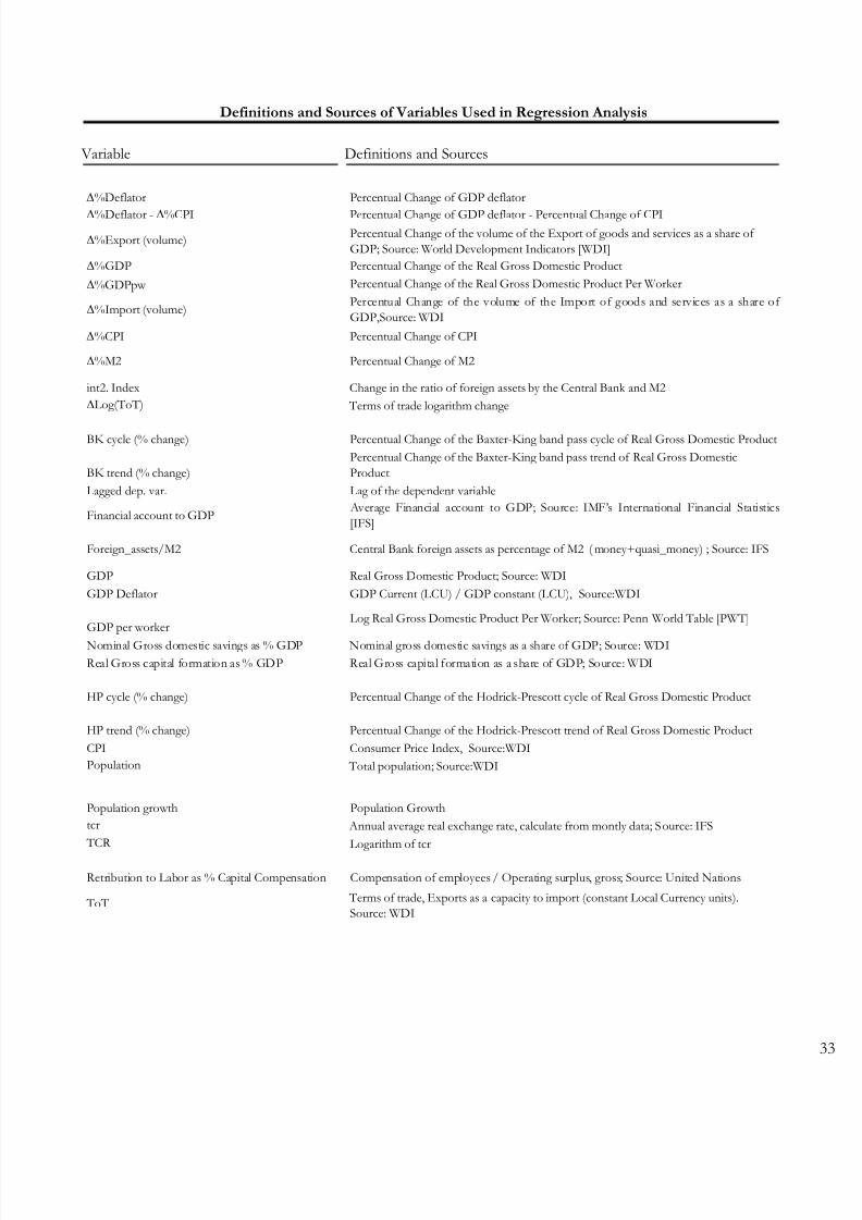
8/3/2019 Fear of Appreciation
http://slidepdf.com/reader/full/fear-of-appreciation 35/39
Variable Definitions and Sources
∆%Deflator Percentual Change of GDP deflator
∆%Deflator - ∆%CPI Percentual Change of GDP deflator - Percentual Change of CPI
∆%Export (volume)Percentual Change of the volume of the Export of goods and services as a share of
GDP; Source: World Development Indicators [WDI]
∆%GDP Percentual Change of the Real Gross Domestic Product
∆%GDPpw Percentual Change of the Real Gross Domestic Product Per Worker
∆%Import (volume)Percentual Change of the volume of the Import of goods and services as a share of
GDP,Source: WDI
∆%CPI Percentual Change of CPI
∆%M2 Percentual Change of M2
int2. Index Change in the ratio of foreign assets by the Central Bank and M2
∆Log(ToT) Terms of trade logarithm change
BK cycle (% change) Percentual Change of the Baxter-King band pass cycle of Real Gross Domestic Product
BK trend (% change)
Percentual Change of the Baxter-King band pass trend of Real Gross Domestic
Product
Lagged dep. var. Lag of the dependent variable
Financial account to GDP Average Financial account to GDP; Source: IMF’s International Financial Statistics
[IFS]
Foreign_assets/M2 Central Bank foreign assets as percentage of M2 ( money+quasi_money) ; Source: IFS
GDP Real Gross Domestic Product; Source: WDI
GDP Deflator GDP Current (LCU) / GDP constant (LCU), Source:WDI
GDP per workerLog Real Gross Domestic Product Per Worker; Source: Penn World Table [PWT]
Nominal Gross domestic savings as % GDP Nominal gross domestic savings as a share of GDP; Source: WDI
Real Gross capital formation as % GDP Real Gross capital formation as a share of GDP; Source: WDI
HP cycle (% change) Percentual Change of the Hodrick-Prescott cycle of Real Gross Domestic Product
HP trend (% change) Percentual Change of the Hodrick-Prescott trend of Real Gross Domestic Product
CPI Consumer Price Index, Source:WDI
Population Total population; Source:WDI
Population growth Population Growth
tcr Annual average real exchange rate, calculate from montly data; Source: IFS
TCR Logarithm of tcr
Retribution to Labor as % Capital Compensation Compensation of employees / Operating surplus, gross; Source: United Nations
ToT Terms of trade, Exports as a capacity to import (constant Local Currency units).
Source: WDI
Definitions and Sources of Variables Used in Regression Analysis

8/3/2019 Fear of Appreciation
http://slidepdf.com/reader/full/fear-of-appreciation 36/39
Variable Definitions and Sources
Trading Partners GrowthExternal Demand Growth ; Source: IFS & Balance of Payments Statistics, IMF
Unemployment Rate (in %) Share of labor force including people available for and seeking employment.Source:
International Labour Organization [ILO]int1. Index Index int1
∆%M2 Percentual Change of M2
M2 Money + quasi_money; Source: IFS
LGDP_HP_cycle Hodrick Prescott cycle of natural logarithm of GDP
LGDP_BK_trend Baxter-King trend of natural logarithm of GDP
LGDP_HP_trend Hodrick Prescott trend of natural logarithm of GDP
LGDP_BK_cycle Baxter-King cycle of natural logarithm of GDP
int1. Index negative Index of negative int1 values
int2. Index negative Negative change in the ratio of foreign assets by the Central Bank and M2
∆%ExportHerfin
Percentual Change of the Herfindal index of export value; Source: Lederman &
Maloney (200X)Saving nominal/GDP Nominal gross domestic savings as a share of GDP; Source: WDI
Interest Rate Nominal interest rate; Source: IFS

8/3/2019 Fear of Appreciation
http://slidepdf.com/reader/full/fear-of-appreciation 37/39
Eference
Aghion, P., Comin D. and Howitt, P. (2006), “When Does Domestic Saving Matter for EconomicGrowth?”, NBER Working Paper No. 1227, June.
Aizenman, J. and Lee, J. (2007), “International Reserves: Precautionary Versus Mercantilist Views, Theory and Evidence”, Open Economies Review, Vol. 18, issue 2, pp. 191-214.
Caballero, R.J. and Lorenzoni,G. (2006), “Persistent Appreciations, Overshooting and OptimalExchange Rate Intervention,” MIT, Mimeo
Calvo, G. and Reinhart, C. (2002), “Fear Of Floating”, The Quarterly Journal of Economics , MIT Press , Vol. 117, Vol. 2 (May), pp. 379-408.
Calvo, G. A . (2000), “The Case for Hard Pegs in the Brave New World of Global Finance”, Mimeo,University of Maryland.
Calvo G., A. Izquierdo and R. Loo-Kung (2005), “Relative Price Volatility under Sudden Stops: The Relevance of Balance-Sheet Effects”, Journal of international Economics , June 2006, also NBER Working Paper No.11492
Calvo G. and E. Talvi, (2006) “Phoenix Recoveries” Mimeo IADB.
Chang, R. and Velasco, A . (2001), “A Model of Financial Crises in Emerging Markets”, Quarterly Journal of Economics , Vol.116, pp. 489-517.
De la Torre, A., Levy Yeyati, E. and Schmukler, S. (2003), “Living and Dying with Hard Pegs: The
Rise and Fall of Argentina’s Currency Board”, Economía, Vol. 5 (2), pp. 43-99.
Diaz Alejandro, C. (1965), “Exchange Rate Devaluation in a Semi-Industrialized Country”,Cambridge, United States: MIT Press.
Dooley, M., Folkerts-Landau, D. and Garber P. (2004), “The Revised Bretton Woods System”,International Journal of Finance and Economics , No. 9(October), pp. 307-313.
Edwards, S. (1989), “Real Exchange Rates, Devaluation, and Adjustment”, Cambridge, MA: TheMIT Press.
Eichengreen, B. (1994), “International Monetary Arrangements for the 21st Century” Washington,DC. The Brookings Institution .
Fisher, S. (2001), "Exchange Rate Regimes: Is The Bipolar View Correct?", Journal of Economic Perspective s, Vol. 15(2)(Spring), pp. 3-24.
Frankel J. (2005),“Contractionary Currency Crises in Developing Countries”, IMF Staff Papers , Vol.52, No.2.

8/3/2019 Fear of Appreciation
http://slidepdf.com/reader/full/fear-of-appreciation 38/39
Hausman, R., L. Pritchett, and D. Rodrik (2005), “Growth Accelerations,” Kennedy School of Government , Mimeo.
Hausmann, R. and Rodrik, D. (2005), “It is not how much you export but what you export”. John
F. Kennedy School of Government, Universidad de Harvard, august, Cambridge, MA
Hausmann, R., Hwang, J. and Rodrik, D. (2006). "What You Export Matters," CEPR Discussion Papers No.5444
Johnson, Simon, Jonathan Ostry and Arvind Subramanian (2006), “Leves for Growth, Financeand Development”, March Vol. 43, No. 1.
Krugman, P.R ., (1987), “The Narrow Moving Band, the Dutch Disease, and the EconomicConsequences of Mrs. Thatcher,” The Journal of Development Economics , Vol. 27, pp. 41-55.
Krugman, P. (1999), “Balance Sheets, the Transfer Problem, and Financial Crises.” International Tax
and Public Finance, Vol.6(4)(November), pp. 459-72.
Levy-Yeyati, E. and Sturzenegger, F. (2005), “Classifying Exchange Rate Regimes: Deeds vs. Words.”, European Economic Review , Vol. 49 (August), pp. 1603-1635.
Levy Yeyati, E. and F. Sturzenegger (2001), “Exchange Rate Regimes and EconomicPerformance”, IMF Staff Papers , Vol. 47, pp. 62-98.
Levy Yeyati, E. and F. Sturzenegger (2003a), “ To Float or to Trail: Evidence on the Impact of Exchange Rate Regimes”, American Economic Review ,Vol. 93, No. 4, September 2003.
Levy Yeyati, E. and F. Sturzenegger (2003b), “ A de facto Classification of Exchange Rate Regimes: A Methodological Note”, posted at http://www.aeaweb.org/aer/contents/ of American Economic Review , Vol. 93, No. 4, September.
Levy-Yeyati, E. (2005), “Exchange Rate Regimes in the 2000s: A Latin American Perspective”,prepared for the Conference on A New Economic Development Agenda for Latin America, Salamanca , October8-9.
Levy-Yeyati, E. (2006), “Financial Dollarization: Evaluating its Consequences”, Economic Policy, Vol.21, No. 45, pp. 61-118, January.
Lewis, WA (1958) “Unlimited Supplies of Labour: Further Notes”, The Manchester School , Vol. 26, 1:1-32.
Prasad, Eswar, Raghuram Rajan, and Arvind Subramanian (2006) Foreign Capital and EconomicGrowth, Research Department IMF, August 30.
Rajan, Raghuram and Arvind Subramanian (2005) What Undermines Aid’s Impact on Growth?,IMF Working Paper, June.
8/3/2019 Fear of Appreciation
http://slidepdf.com/reader/full/fear-of-appreciation 39/39
Rajan, Raghuram and Arvind Subramanian (2006) Aid, Dutch Disease, and Manufacturing Growth, June 2006
Reinhart, C. and Rogoff, K. (2003), "The Modern History of Exchange Rate Arrangements: A
Reinterpretation" (May 2002). NBER Working Paper
No. W8963. Revised version March 2003, Quarterly Journal of Economics , Vol. CXIX No. 1, February 2004, 1-48.
Rodrik, Dani (2006) Industrial Development: Stylized Facts and Policies, Mimeo Kennedy School of Government.
Rodrik, Dani (2005), “Why we learn nothing from regressing economic growth on policies,”Manuscript, Harvard
Rodrik, Dani (2007) “The Real Exchange Rae and Economic Growth: Theory and Evidence”, MimeoKennedy School of Government, Harvard University.
Rose, Andrew K. (2006), “ A Stable International Monetary System Emerges: Inflation Targeting IsBretton Woods, Reversed”, NBER Working Paper No. 12711
Shambaugh J. (2004), “The Effect of Fixed Exchange Rates on Monetary Policy”, The Quarterly Journal of Economics , Vol. 119, pp. 300-351.


![Welcome! [militaryfamilieslearningnetwork.org]...Share Feelings; Respect Differences • Suffering, Struggle, Fear, Regrets • Pride, Appreciation, Joy, Humor, Fun • Refuel Energies](https://img.pdfslide.us/doc/110x75/5ecaaf9047af58370650f38e/welcome-militaryfam-share-feelings-respect-differences-a-suffering-struggle.jpg)