FE661 - Statistical Methods for Financial Engineering Jitkomut Songsiri …jitkomut.eng.chula.ac.th/fe661/prob.pdf · 2017-08-19 · FE661 - Statistical Methods for Financial Engineering

FE661 - Statistical Methods for Financial Engineering Jitkomut Songsiri

3. Probability and Statistics

• definitions, probability measures

• conditional expectations

• correlation and covariance

• some important random variables

• multivariate random variables

3-1

Definition

a random variable X is a function mapping an outcome to a real number

• the sample space, S, is the domain of the random variable

• SX is the range of the random variable

example: toss a coin three times and note the sequence of heads and tails

S = {HHH,HHT,HTH,THH,HTT,THT,TTH,TTT}

Let X be the number of heads in the three tosses

SX = {0, 1, 2, 3}

Probability and Statistics 3-2

Probability measures

Cumulative distribution function (CDF)

F (a) = P (X ≤ a)

Probability mass function (PMF) for discrete RVs

p(k) = P (X = k)

Probability density function (PDF) for continuous RVs

f(x) =dF (x)

dx


Probability Density Function

Probability Density Function (PDF)

• f(x) ≥ 0

• P (a ≤ X ≤ b) =∫ b

af(x)dx

• F (x) =x∫

−∞f(u)du

Probability Mass Function (PMF)

• p(k) ≥ 0 for all k

•∑k∈S

p(k) = 1


Expected values

let g(X) be a function of random variable X

E[g(X)] =

∑x∈S

g(x)p(x) X is discrete

∞∫−∞

g(x)f(x)dx X is continuous

Mean

µ = E[X] =

∑x∈S

xp(x) X is discrete

∞∫−∞

xf(x)dx X is continuous

Varianceσ2 = var[X] = E[(X − µ)2]

nth MomentE[Xn]


Facts

Let Y = g(X) = aX + b, a, b are constants

• E[Y ] = aE[X] + b

• var[Y ] = a2 var[X]

• var[X] = E[X2]− (E[X])2


Example of Random Variables

Discrete RVs

• Bernoulli

• Binomial

• Geometric

• Negative binomial

• Poisson

• Uniform

Continuous RVs

• Uniform

• Exponential

• Gaussian (Normal)

• Gamma, Chi-squared, Student’s t,F

• Logistics


Joint cumulative distribution function

FXY (a, b) = P (X ≤ a, Y ≤ b)

• a joint CDF is a nondecreasing function of x and y:

FXY (x1, y1) ≤ FXY (x2, y2), if x1 ≤ x2 and y1 ≤ y2

• FXY (x1,−∞) = 0, FXY (−∞, y1) = 0, FXY (∞,∞) = 1

• P (x1 < X ≤ x2, y1 < Y ≤ y2)

= FXY (x2, y2)− FXY (x2, y1)− FXY (x1, y2) + FXY (x1, y1)


Joint PMF for discrete RVs

pXY (x, y) = P (X = x, Y = y), (x, y) ∈ S

Joint PDF for continuous RVs

fXY (x, y) =∂2FXY (x, y)

∂x∂y

Marginal PMF

pX(x) =∑y∈S

pXY (x, y), pY (y) =∑x∈S

pXY (x, y)

Marginal PDF

fX(x) =

∫ ∞

−∞fXY (x, z)dz, fY (y) =

∫ ∞

−∞fXY (z, y)dz


Conditional Probability

Discrete RVs

the conditional PMF of Y given X = x is defined by

pY |X(y|x) = P (Y = y|X = x) =P (X = x, Y = y)

P (X = x)

=pXY (x, y)

pX(x)

Continuous RVs

the conditional PDF of Y given X = x is defined by

fY |X(y|x) =fXY (x, y)

fX(x)


Conditional Expectation

the conditional expectation of Y given X = x is defined by

Continuous RVs

E[Y |X] =

∫ ∞

−∞y fY |X(y|x)dy

Discrete RVsE[Y |X] =

∑y

y pY |X(y|x)

• E[Y |X] is the center of mass associated with the conditional pdf or pmf

• E[Y |X] can be viewed as a function of random variable X

• E[E[Y |X]] = E[Y ]


in fact, we can show that

E[h(Y )] = E[E[h(Y )|X]]

for any function h(·) that E[|h(Y )|] < ∞

proof.

E[E[h(Y )|X]] =

∫ ∞

−∞E[h(Y )|x]fX(x)dx

=

∫ ∞

−∞

∫ ∞

−∞h(y)fY |X(y|x)dy fX(x)dx

=

∫ ∞

−∞h(y)

∫ ∞

−∞fXY (x, y) dxdy

=

∫ ∞

−∞h(y)fY (y) dy

= E[h(Y )]


Independence of two random variables

X and Y are independent if and only if

FXY (x, y) = FX(x)FY (y), ∀x, y

this is equivalent to

Discrete Random Variables

pXY (x, y) = pX(x)pY (y)

pY |X(y|x) = pY (y)

Continuous Random Variables

fXY (x, y) = fX(x)fY (y)

fY |X(y|x) = fY |X(y)

If X and Y are independent, so are any pair of functions g(X) and h(Y )


Expected Values and Covariance

the expected value of Z = g(X,Y ) is defined as

E[Z] =

∫ ∞

−∞

∫ ∞

−∞g(x, y) fXY (x, y) dx dy X, Y continuous

E[Z] =∑x

∑y

g(x, y) pXY (x, y) X,Y discrete

• E[X + Y ] = E[X] +E[Y ]

• E[XY ] = E[X]E[Y ] if X and Y are independent

Covariance of X and Y

cov(X,Y ) = E[(X −E[X])(Y −E[Y ])] = E[XY ]−E[X]E[Y ]

• cov(X,Y ) = 0 if X and Y are independent (the converse is NOT true)


Correlation Coefficient

denoteσX =

√var(X), σY =

√var(Y )

the standard deviations of X and Y

the correlation coefficient of X and Y is defined by

ρXY =cov(X,Y )

σXσY

• −1 ≤ ρXY ≤ 1

• ρXY gives the linear dependence between X and Y : for Y = aX + b,

ρXY = 1 if a > 0 and ρXY = −1 if a < 0

• X and Y are said to be uncorrelated if ρXY = 0


if X and Y are independent then X and Y are uncorrelated

but the converse is NOT true


Law of Total Variance

suppose that X and Y are random variables

var(Y ) = E[var(Y |X)] + var(E[Y |X])

aka Eve’s Law; we say the unconditional variance equals EV plus VE

Proof. using E[E[Y |X]] = E[Y ]

var(Y ) = E[Y 2]− (E[Y ])2

= E[E[Y 2|X]]− (E[E[Y |X]])2

= E[var(Y |X)] +E[(E[Y |X])2]− (E[E[Y |X]])2

= E[var(Y |X)] + var[E[Y |X]]


Moment Generating Functions

the moment generating function (MGF) Φ(t) is defined for all t by

Φ(t) = E[etX] =

{∫∞−∞ etxf(x)dx, X is continuous∑x e

txp(x), X is discrete

• except for a sign change, Φ(t) is the 2-sided Laplace transform of pdf

• knowing Φ(t) is equivalent to knowing f(x)

• E[Xn] = dnΦ(t)dtn

∣∣∣t=0

• MGF of the sum of independent RVs is the product of the individual MGF

ΦX+Y (t) = E[et(X+Y )] = ΦX(t)ΦY (t)


Gaussian (Normal) random variables

• arise as the outcome of the central limit theorem

• the sum of a large number of RVs is distributed approximately normally

• many results involving Gaussian RVs can be derived in analytical form

• let X be a Gaussian RV with parameters mean µ and variance σ2

Notation X ∼ N (µ, σ2)

PDF

f(x) =1√2πσ2

exp− (x− µ)2

2σ2, −∞ < x < ∞

Mean E[X] = µ Variance var[X] = σ2

MGF Φ(t) = eµt+σ2t2/2


let Z ∼ N (0, 1) be the normalized Gaussian variable

CDF of Z is

FZ(z) =1√2π

∫ z

−∞e−t2/2dt ≜ Φ(z)

then CDF of X ∼ N (µ, σ2) can be obtained by

FX(x) = Φ

(x− µ

σ

)in MATLAB, the error function is defined as

erf(x) =2√π

∫ x

0

e−t2dt

hence, Φ(z) can be computed via the erf command as

Φ(z) =1

2

[1 + erf

(z√2

)]


Gamma random variables

PDF

f(x) =λ(λx)α−1e−λx

Γ(α), x ≥ 0; α, λ > 0

where Γ(z) is the gamma function, defined by

Γ(z) =

∫ ∞

0

xz−1e−xdx, z > 0

Mean E[X] = αλ Variance var[X] = α

λ2

MGF Φ(t) =(

λλ−t

)α−1

• if X1 and X2 are independent gamma RVs with parameters (α1, λ) and(α2, λ) then X1 +X2 is a gamma RV with parameters (α1 + α2, λ)


Properties of the gamma function

Γ(1/2) =√π

Γ(z + 1) = zΓ(z) for z > 0

Γ(m+ 1) = m!, for m a nonnegative integer

Special cases

a Gamma RV becomes

• exponential RV when α = 1

• m-Erlang RV when α = m, a positive integer

• chi-square RV with n DF when α = n/2, λ = 1/2


Chi-square random variables

if Z1, Z2, . . . , Zn are independent normal RVs, then X defined by

X = Z21 + Z2

2 + · · ·+ Z2n ∼ χ2

n

is said to have a chi-square distribution with n degrees of freedom

• Φ(t) = E[∏n

i=1 etZ2

i ] =∏n

i=1E[etZ2i ] = (1− 2t)−n/2

• we recognize that X is a gamma RV with parameters (n/2, 1/2)

• sum of independent chi-square RVs with n1 and n2 DF is the chi-square withn1 + n2 DF

PDF

f(x) =(1/2)e−x/2(x/2)n/2−1

Γ(n/2), x > 0

Mean E[X] = n Variance var(X) = 2n


t random variables

if Z ∼ N (0, 1) and χ2n are independent then

Tn =Z√χ2n/n

is said to have a t-distribution with n degree of freedom

• t density is symmetric about zero

• t has greater variability than the normal

• Tn → Z for n large

• for 0 < α < 1 such that P (Tn ≥ tα,n) = α),

P (Tn ≥ −tα,n) = 1− α ⇒ −tα,n = t1−α,n


F random variables

if χ2n and χ2

m are independent chi-square RVs then the RV Fn,m defined by

Fn,m =χ2n/n

χ2m/m

is said to have an F -distribution with n and m degree of freedoms

• for any α ∈ (0, 1), let Fα,n,m be such that P (Fn,m > Fα,n,m) = α then

P

(χ2m/m

χ2n/n

≥ 1

Fα,n,m

)= 1− α

• sinceχ2m/m

χ2n/n

is another Fm,n RV, it follows that

1− α = P

(χ2m/m

χ2n/n

≥ F1−α,n,m

)⇒ 1

Fα,n,m= F1−α,m,n


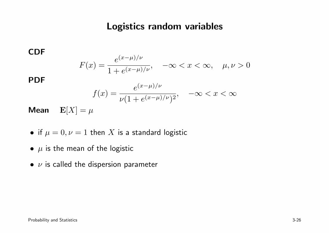
Logistics random variables

CDF

F (x) =e(x−µ)/ν

1 + e(x−µ)/ν, −∞ < x < ∞, µ, ν > 0

PDF

f(x) =e(x−µ)/ν

ν(1 + e(x−µ)/ν)2, −∞ < x < ∞

Mean E[X] = µ

• if µ = 0, ν = 1 then X is a standard logistic

• µ is the mean of the logistic

• ν is called the dispersion parameter


Multivariate Random Variables

• probabilities

• cross correlation, cross covariance

• Gaussian random vectors


Random vectors

we denote X a random vector

X is a function that maps each outcome ζ to a vector of real numbers

an n-dimensional random variable has n components:

X =

X1

X2...

Xn

also called a multivariate or multiple random variable


Probabilities

Joint CDF

F (X) ≜ FX(x1, x2, . . . , xn) = P (X1 ≤ x1, X2 ≤ x2, . . . , Xn ≤ xn)

Joint PMF

p(X) ≜ pX(x1, x2, . . . , xn) = P (X1 = x1, X2 = x2, . . . , Xn = xn)

Joint PDF

f(X) ≜ fX(x1, x2, . . . , xn) =∂n

∂x1 . . . ∂xnF (X)


Marginal PMF

pXj(xj) = P (Xj = xj) =

∑x1

. . .∑xj−1

∑xj+1

. . .∑xn

pX(x1, x2, . . . , xn)

Marginal PDF

fXj(xj) =

∫ ∞

−∞. . .

∫ ∞

−∞fX(x1, x2, . . . , xn) dx1 . . . dxj−1dxj+1 . . . dxn

Conditional PDF: the PDF of Xn given X1, . . . , Xn−1 is

f(xn|x1, . . . , xn−1) =fX(x1, . . . , xn)

fX1,...,Xn−1(x1, . . . , xn−1)


Characteristic Function

the characteristic function of an n-dimensional RV is defined by

Φ(ω) = Φ(ω1, . . . , ωn) = E[ei(ω1X1+···+ωnXn)]

=

∫X

eiωTXf(X)dX

where

ω =

ω1

ω2...ωn

, X =

x1

x2...xn

Φ(ω) is the n-dimensional Fourier transform of f(X)


Independence

the random variables X1, . . . , Xn are independent if

the joint pdf (or pmf) is equal to the product of their marginal’s

DiscretepX(x1, . . . , xn) = pX1(x1) · · · pXn(xn)

ContinuousfX(x1, . . . , xn) = fX1(x1) · · · fXn(xn)

we can specify an RV by the characteristic function in place of the pdf,

X1, . . . , Xn are independent if

Φ(ω) = Φ1(ω1) · · ·Φn(ωn)


Expected Values

the expected value of a function

g(X) = g(X1, . . . , Xn)

of a vector random variable X is defined by

E[g(X)] =

∫x

g(x)f(x)dx Continuous

E[g(X)] =∑x

g(x)p(x) Discrete

Mean vector

µ = E[X] = E

X1

X2...

Xn

≜

E[X1]E[X2]

...E[Xn]


Correlation and Covariance matrices

Correlation matrix has the second moments of X as its entries:

R ≜ E[XXT ] =

E[X1X1] E[X1X2] · · · E[X1Xn]E[X2X1] E[X2X2] · · · E[X2Xn]

... ... . . . ...E[XnX1] E[XnX2] · · · E[XnXn]

with

Rij = E[XiXj]

Covariance matrix has the second-order central moments as its entries:

C ≜ E[(X − µ)(X − µ)T ]

withCij = cov(Xi, Xj) = E[(Xi − µi)(Xj − µj)]


Properties of correlation and covariance matrices

let X be a (real) n-dimensional random vector with mean µ

Facts:

• R and C are n× n symmetric matrices

• R and C are positive semidefinite

• If X1, . . . , Xn are independent, then C is diagonal

• the diagonals of C are given by the variances of Xk

• if X has zero mean, then R = C

• C = R− µµT


Cross Correlation and Cross Covariance

let X,Y be vector random variables with means µX, µY respectively

Cross Correlation

cor(X,Y ) = E[XY T ]

if cor(X,Y ) = 0 then X and Y are said to be orthogonal

Cross Covariance

cov(X,Y ) = E[(X − µX)(Y − µY )T ]

= cor(X,Y )− µXµTY

if cov(X,Y ) = 0 then X and Y are said to be uncorrelated


Affine transformation

let Y be an affine transformation of X:

Y = AX + b

where A and b are deterministic matrices

• µY = AµX + b

µY = E[AX + b] = AE[X] +E[b] = AµX + b

• CY = ACXAT

CY = E[(Y − µY )(Y − µY )T ] = E[(A(X − µX))(A(X − µX))T ]

= AE[(X − µX)(X − µX)T ]AT = ACXAT


Gaussian random vector

X1, . . . , Xn are said to be jointly Gaussian if their joint pdf is given by

f(X) ≜ fX(x1, x2, . . . , xn) =1

(2π)n/2 det(Σ)1/2exp − 1

2(X − µ)TΣ−1(X − µ)

µ is the mean (n× 1) and Σ ≻ 0 is the covariance matrix (n× n):

µ =

µ1

µ2...µn

, Σ =

Σ11 Σ12 · · · Σ1n

Σ21 Σ22 · · · Σ2n... ... . . . ...

Σn1 Σn2 · · · Σnn

and

µk = E[Xk], Σij = E[(Xi − µi)(Xj − µj)]


example: the joint density function of X (not normalized) is given by

f(x1, x2, x3) = exp − x21 + 3x2

2 + 2(x3 − 1)2 + 2x1(x3 − 1)

2

• f is an exponential of negative quadratic in x so X must be a Gaussian

f(x1, x2, x3) = exp − 1

2

x1

x2

x3 − 1

T 1 0 10 3 01 0 2

x1

x2

x3 − 1

• the mean vector is (0, 0, 1)

• the covariance matrix is

C =

1 0 10 3 01 0 2

−1

=

2 0 −10 1/3 0−1 0 1


• the variance of x1 is highest while x2 is smallest

• x1 and x2 are uncorrelated, so are x2 and x3


examples of Gaussian density contour (the exponent of exponential)

[x1

x2

]T [Σ11 Σ12

Σ12 Σ22

]−1 [x1

x2

]= 1

uncorrelated different variances correlated

Σ =

[1 00 1

]Σ =

[1/2 00 1

]Σ =

[1 −1−1 2

]


Properties of Gaussian variables

many results on Gaussian RVs can be obtained analytically:

• marginal’s of X is also Gaussian

• conditional pdf of Xk given the other variables is a Gaussian distribution

• uncorrelated Gaussian random variables are independent

• any affine transformation of a Gaussian is also a Gaussian

these are well-known facts

and more can be found in the areas of estimation, statistical learning, etc.


Characteristic function of Gaussian

Φ(ω) = Φ(ω1, ω2, . . . , ωn) = eiµTω e−

ωTΣω2

Proof. By definition and arranging the quadratic term in the power of exp

Φ(ω) =1

(2π)n/2|Σ|1/2

∫X

eiXTω e−

(X−µ)TΣ−1(X−µ)2 dx

=eiµ

Tω e−ωTΣω

2

(2π)n/2|Σ|1/2

∫X

e−(X−µ−iΣω)TΣ−1(X−µ−iΣω)

2 dx

= exp (iµTω) exp (−1

2ωTΣω)

(the integral equals 1 since it is a form of Gaussian distribution)

for one-dimensional Gaussian with zero mean and variance Σ = σ2,

Φ(ω) = e−σ2ω2

2


Affine Transformation of a Gaussian is Gaussian

let X be an n-dimensional Gaussian, X ∼ N (µ,Σ) and define

Y = AX + b

where A is m× n and b is m× 1 (so Y is m× 1)

ΦY (ω) = E[eiωTY ] = E[eiω

T (AX+b)]

= E[eiωTAX · eiω

T b] = eiωT bΦX(ATω)

= eiωT b · eiµ

TATω · e−ωTAΣATω/2

= eiωT (Aµ+b) · e−ωTAΣATω/2

we read off that Y is Gaussian with mean Aµ+ b and covariance AΣAT


Marginal of Gaussian is Gaussian

the kth component of X is obtained by

Xk =[0 · · · 1 0

]X ≜ eTkX

(ek is a standard unit column vector; all entries are zero except the kth position)

hence, Xk is simply a linear transformation (in fact, a projection) of X

Xk is then a Gaussian with mean

eTkµ = µk

and covarianceeTk Σ ek = Σkk


Uncorrelated Gaussians are independent

suppose (X,Y ) is a jointly Gaussian vector with

mean µ =

[µx

µy

]and covariance

[CX 00 CY

]in otherwords, X and Y are uncorrelated Gaussians:

cov(X,Y ) = E[XY T ]−E[X]E[Y ]T = 0

the joint density can be written as

fXY (x, y) =1

(2π)n|CX|1/2|CY |1/2exp − 1

2

[x− µx

y − µy

]T [C−1

X 00 C−1

Y

] [x− µx

y − µy

]=

1

(2π)n/2|CX|1/2e−

12(x−µx)

TC−1X

(x−µx) · 1

(2π)n/2|CY |1/2e−

12(y−µy)

TC−1Y

(y−µy)

proving the independence


Conditional of Gaussian is Gaussian

let Z be an n-dimensional Gaussian which can be decomposed as

Z =

[XY

]∼ N

([µx

µy

],

[Σxx Σxy

ΣTxy Σyy

])

the conditional pdf of X given Y is also Gaussian with conditional mean

µX|Y = µx +ΣxyΣ−1yy (Y − µy)

and conditional covariance

ΣX|Y = Σx − ΣxyΣ−1yyΣ

Txy


Proof:

from the matrix inversion lemma, Σ−1 can be written as

Σ−1 =

S−1 −S−1ΣxyΣ−1yy

−Σ−1yyΣ

TxyS

−1 Σ−1yy +Σ−1

yyΣTxyS

−1ΣxyΣ−1yy

where S is called the Schur complement of Σxx in Σ and

S = Σxx − ΣxyΣ−1yyΣ

Txy

detΣ = detS · detΣyy

we can show that Σ ≻ 0 if any only if S ≻ 0 and Σyy ≻ 0


from fX|Y (x|y) = fX(x, y)/fY (y), we calculate the exponent terms

[x− µx

y − µy

]TΣ−1

[x− µx

y − µy

]− (y − µy)

TΣ−1yy (y − µy)

= (x− µx)TS−1(x− µx)− (x− µx)

TS−1ΣxyΣ−1yy (y − µy)

−(y − µy)TΣ−1

yyΣTxyS

−1(x− µx)

+(y − µy)T (Σ−1

yyΣTxyS

−1ΣxyΣ−1yy )(y − µy)

= [x− µx − ΣxyΣ−1yy (y − µy)]

TS−1[x− µx − ΣxyΣ−1yy (y − µy)]

≜ (x− µX|Y )TΣ−1

X|Y (x− µX|Y )

fX|Y (x|y) is an exponential of quadratic function in x

so it has a form of Gaussian


Standard Gaussian vectors

for an n-dimensional Gaussian vector X ∼ N (µ,C) with C ≻ 0

let A be an n× n invertible matrix such that

AAT = C

(A is called a factor of C)

then the random vectorZ = A−1(X − µ)

is a standard Gaussian vector, i.e.,

Z ∼ N (0, I)

(obtain A via eigenvalue decomposition or Cholesky factorization)


Quadratic Form Theorems

let X = (X1, . . . , Xn) be a standard n-dimensional Gaussian vector:

X ∼ N (0, I)

then the following results hold

• XTX ∼ χ2(n)

• let A be a symmetric and idempotent matrix and m = tr(A) then

XTAX ∼ χ2(m)


Proof: the eigenvalue decomposition of A: A = UDUT where

λ(A) = 0, 1 UTU = UUT = I

it follows that

XTAX = XTUDUTX = Y TDY =

n∑i=1

diiY2i

• since U is orthogonal, Y is also a standard Gaussian vector

• since A is idempotent, dii is either 0 or 1 and tr(D) = m

therefore XTAX is the m-sum of standard normal RVs


References

Chapter 1-3 in

J.M. Wooldridge, Econometric Analysis of Cross Section and Panel Data, 2ndedition, the MIT press, 2010

Chapter 1-5 in

S.M. Ross, Introduction to Probability and Statistics for Engineers andScientists, 4th edition, Academic press, 2009

Appendix A in

A.C. Cameron and P.K. Trevedi, Microeconometrics: Method and Applications,Cambridge University Press, 2005


Documents

FE661 - Statistical Methods for Financial Engineering Jitkomut Songsiri …jitkomut.eng.chula.ac.th/fe661/prob.pdf · 2017-08-19 · FE661 - Statistical Methods for Financial Engineering