FDTD Method - Allgemeine und theoretische Elektrotechnik ... · PDF fileMaxwell‘s Equations Electric Field Magnetic Field Excitation Parameters ¾Hyperbolic partial differential

FDTD Method

Basics

• Maxwell‘s Equations

• Spatial discretisation/Time discretisation

• Equivalent Circuit for FDTD

• Stability

• Ports

Simple Examples

Accuracy and Losses

Speedups on modern Computers

Conclusions

Outline

Nov-07 © IMST GmbH - All rights reserved

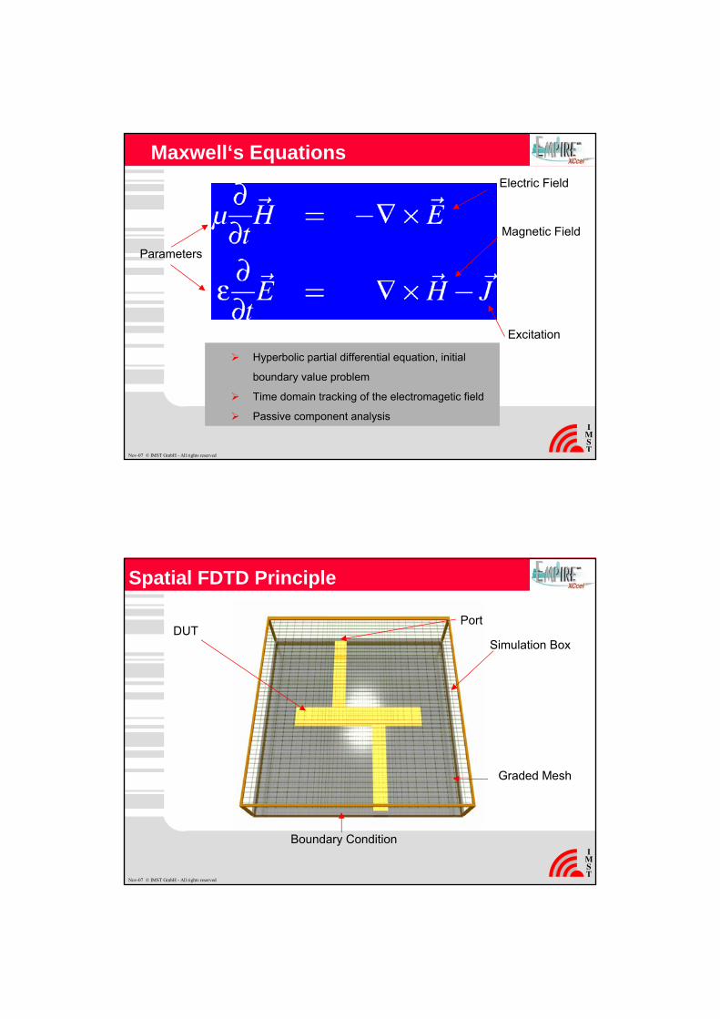
Maxwell‘s EquationsElectric Field

Magnetic Field

Excitation

Parameters

Hyperbolic partial differential equation, initial

boundary value problem

Time domain tracking of the electromagetic field

Passive component analysis


Simulation Box

Boundary Condition

Graded Mesh

DUTPort

Spatial FDTD Principle


Ez

Ex

Ey

Hx

Hz

Hy

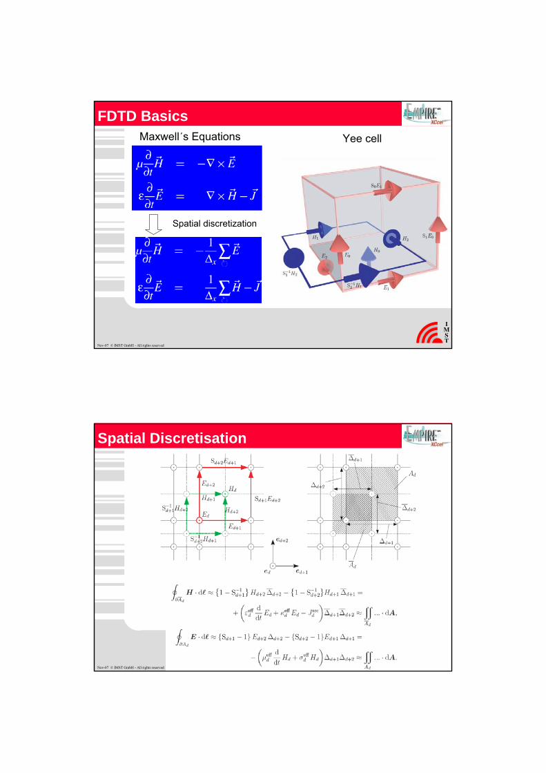
FDTD BasicsYee cellMaxwell´s Equations

Spatial discretizationEz

Ex

Ey

Hx

Hz

Hy


Hz

Spatial Discretisation


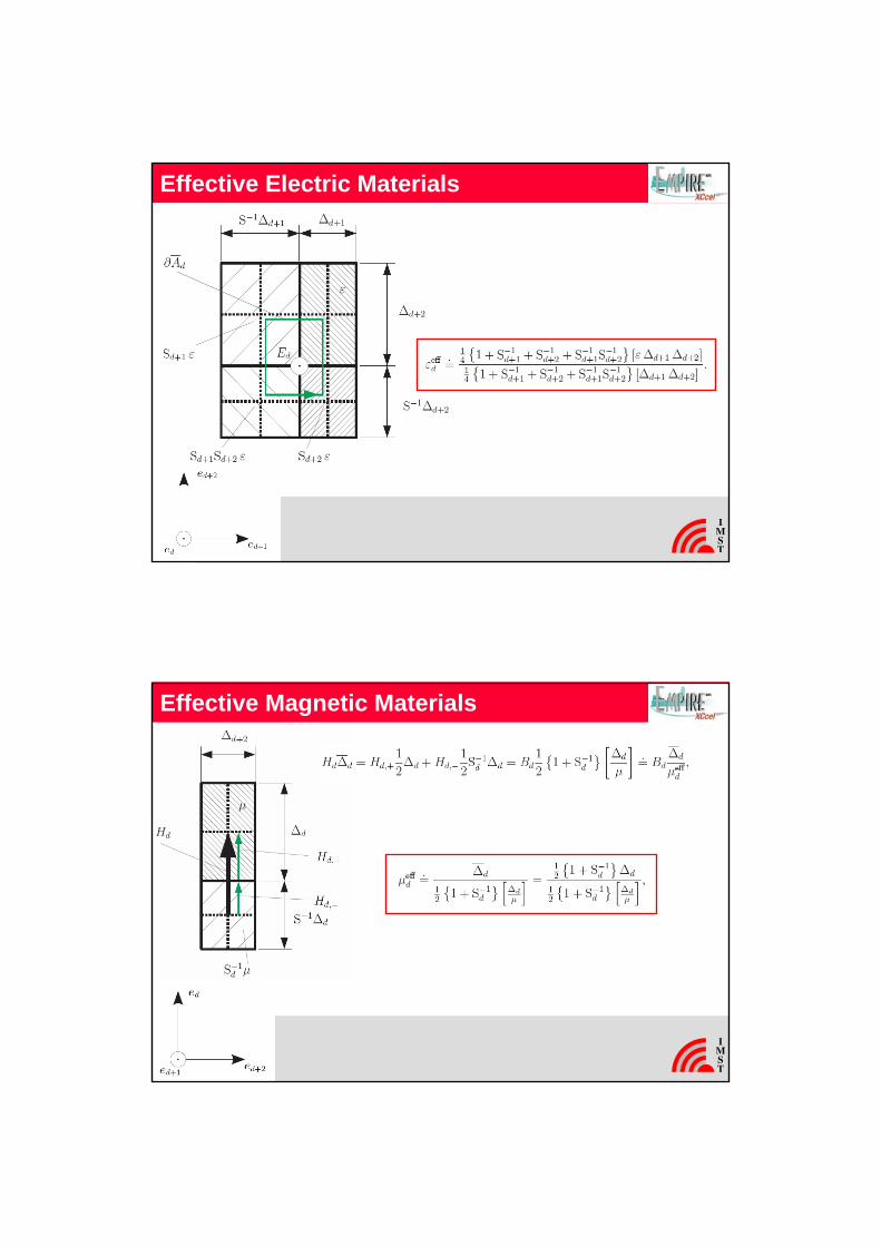
Effective Electric Materials


Effective Magnetic Materials


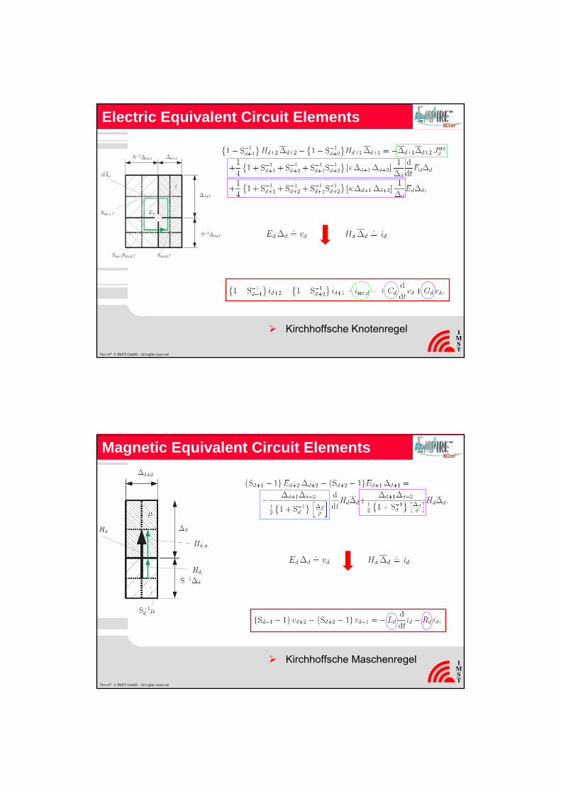
Electric Equivalent Circuit Elements


Kirchhoffsche Knotenregel

Magnetic Equivalent Circuit Elements


Kirchhoffsche Maschenregel

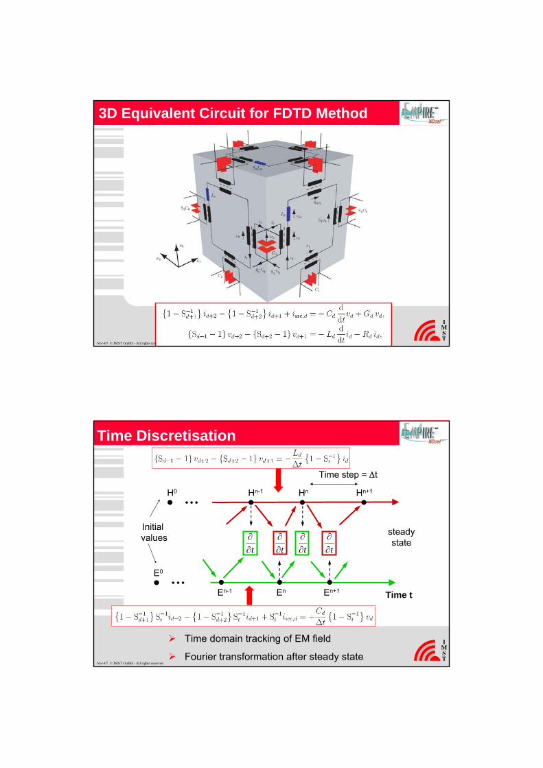
Hz

3D Equivalent Circuit for FDTD Method


Time t

H0 Hn-1 Hn Hn+1

En-1 En En+1

E0

t∂∂

t∂∂

t∂∂

t∂∂

Time step = Δt

Initial values steady

state

Time domain tracking of EM field

Fourier transformation after steady state

Time Discretisation


Hz

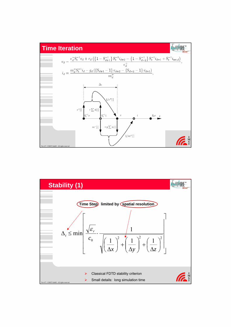
Time Iteration


Stability (1)

Classical FDTD stability criterion

Small details: long simulation time

Time Step limited by spatial resolution

⎥⎥⎥⎥⎥

⎦

⎤

⎢⎢⎢⎢⎢

⎣

⎡

⎟⎠⎞

⎜⎝⎛Δ

+⎟⎟⎠

⎞⎜⎜⎝

⎛Δ

+⎟⎠⎞

⎜⎝⎛Δ

⋅≤Δ222

0 111

1min

zyx

cr

t

ε


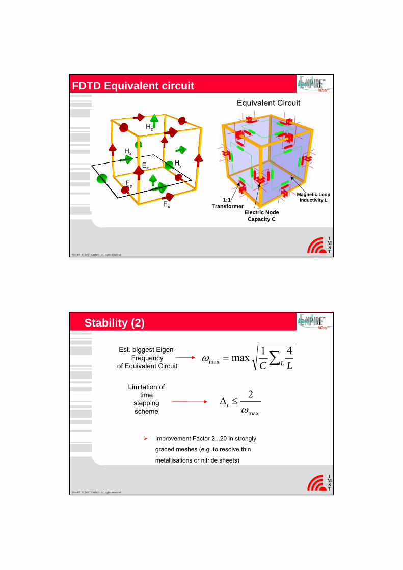
FDTD Equivalent circuitEquivalent Circuit

Electric NodeCapacity C

Magnetic LoopInductivity L1:1

Transformer

Ez

Ex

Ey

Hx

Hz

Hy


Stability (2)

Est. biggest Eigen-Frequency

of Equivalent Circuit

Limitation of time

steppingscheme

Improvement Factor 2...20 in strongly

graded meshes (e.g. to resolve thin

metallisations or nitride sheets)

max

2ω

≤Δt

∑=L LC

41maxmaxω


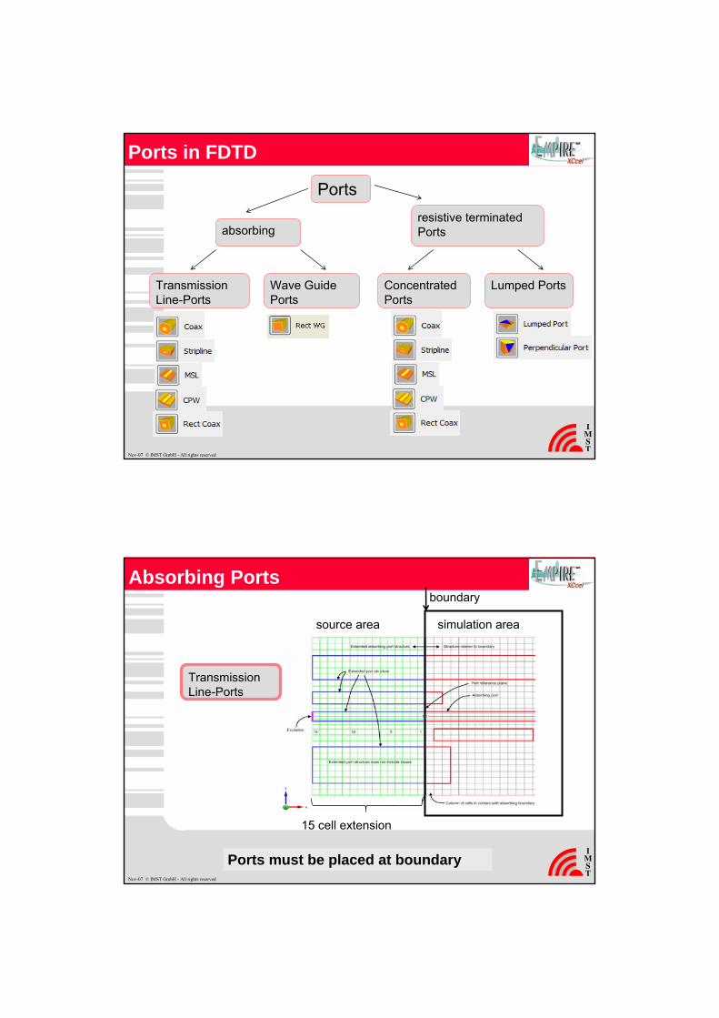
Ports in FDTD

Ports

absorbingresistive terminated Ports

Transmission Line-Ports

Wave GuidePorts

Concentrated Ports

Lumped Ports


Absorbing Ports

Transmission Line-Ports

source area simulation area

15 cell extension

boundary

Ports must be placed at boundaryNov-07 © IMST GmbH - All rights reserved

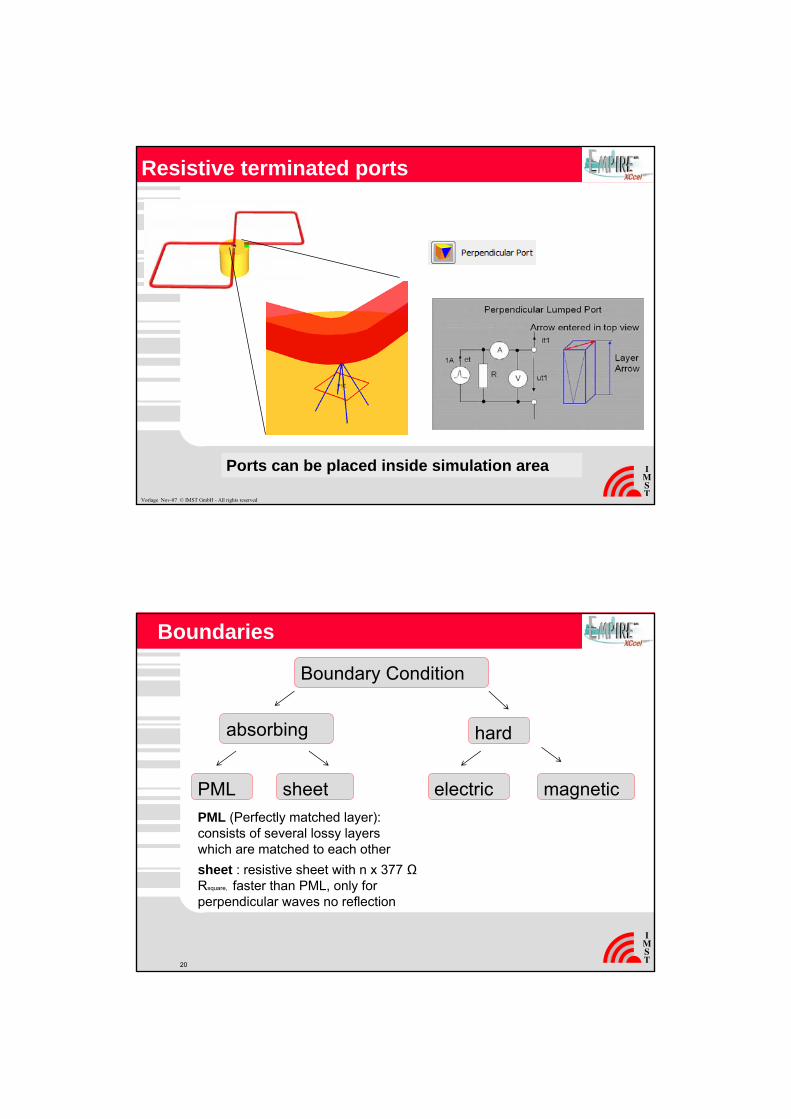
Resistive terminated ports

Vorlage Nov-07 © IMST GmbH - All rights reserved

Ports can be placed inside simulation area

20

Boundaries

Boundary Condition

absorbing hard

PML sheet electric magneticPML (Perfectly matched layer):consists of several lossy layerswhich are matched to each other sheet : resistive sheet with n x 377 ΩRsquare, faster than PML, only for perpendicular waves no reflection

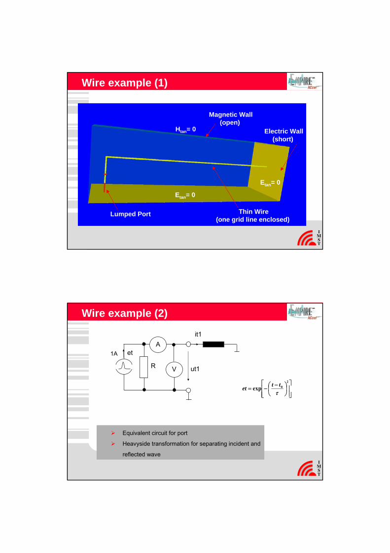
Wire example (1)

Etan= 0

Etan= 0

Electric Wall(short)

Magnetic Wall(open)

Lumped Port Thin Wire(one grid line enclosed)

Htan= 0

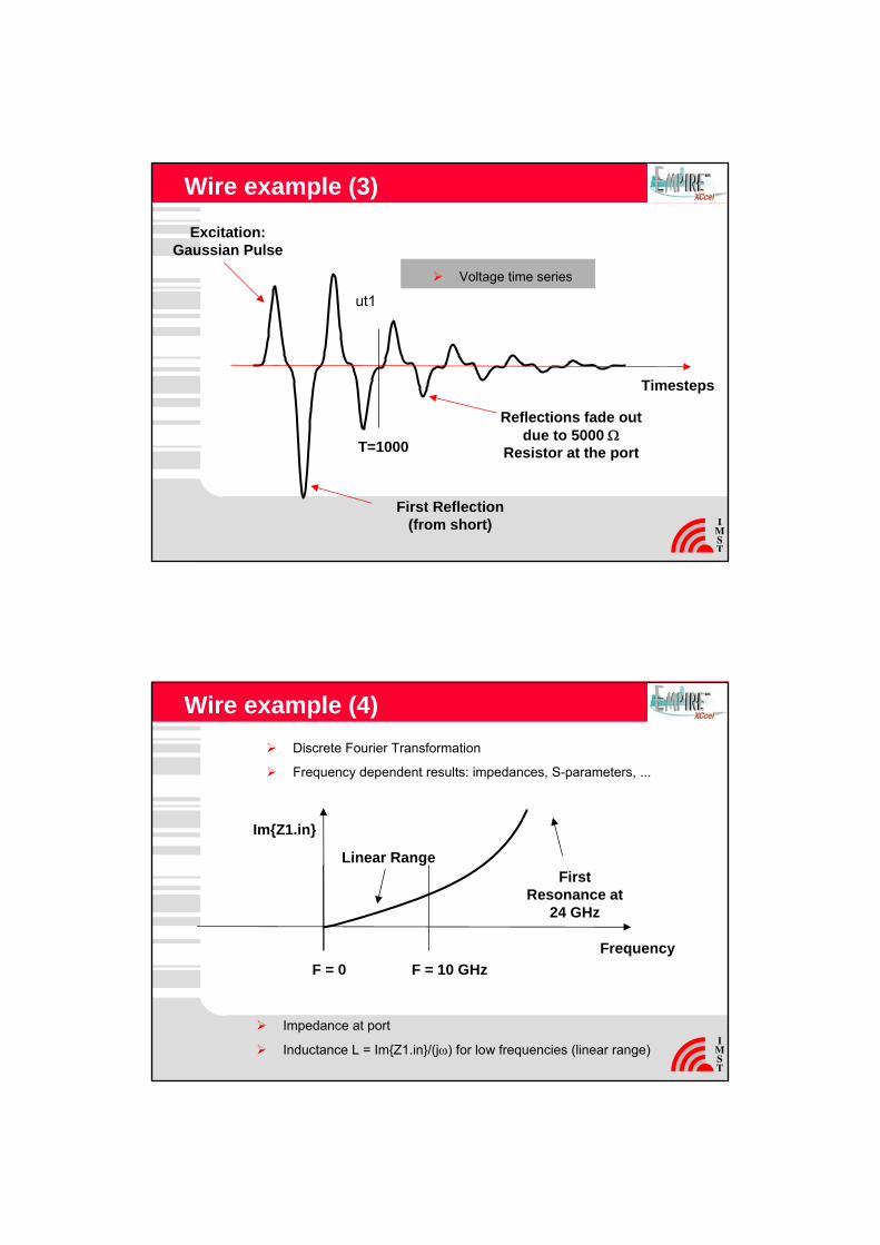
Equivalent circuit for port

Heavyside transformation for separating incident and

reflected wave

Wire example (2)

1AA

VR ut1

it1

et

⎥⎥⎦

⎤

⎢⎢⎣

⎡⎟⎠⎞

⎜⎝⎛ −

−=2

0expτ

ttet

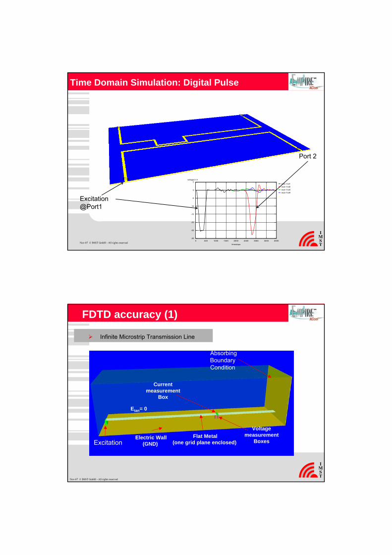
Wire example (3)

Excitation:Gaussian Pulse

Timesteps

T=1000

First Reflection(from short)

Voltage time series

Reflections fade out due to 5000 Ω

Resistor at the port

ut1

Impedance at port

Inductance L = ImZ1.in/(jω) for low frequencies (linear range)

Wire example (4)

FrequencyF = 0

Linear Range

F = 10 GHz

ImZ1.in

First Resonance at

24 GHz

Discrete Fourier Transformation

Frequency dependent results: impedances, S-parameters, ...


Excitation@Port1

-30

-25

-20

-15

-10

-5

0

5

0 500 1000 1500 2000 2500 3000 3500 4000

voltage in V

timesteps

./sub-1/ut1

./sub-1/ut2

./sub-1/ut3

./sub-1/ut4

Port 2

Time Domain Simulation: Digital Pulse

Etan= 0

Electric Wall(GND)

Currentmeasurement

Box

ExcitationFlat Metal

(one grid plane enclosed)

Voltagemeasurement

Boxes

AbsorbingBoundaryCondition

FDTD accuracy (1)

Infinite Microstrip Transmission Line


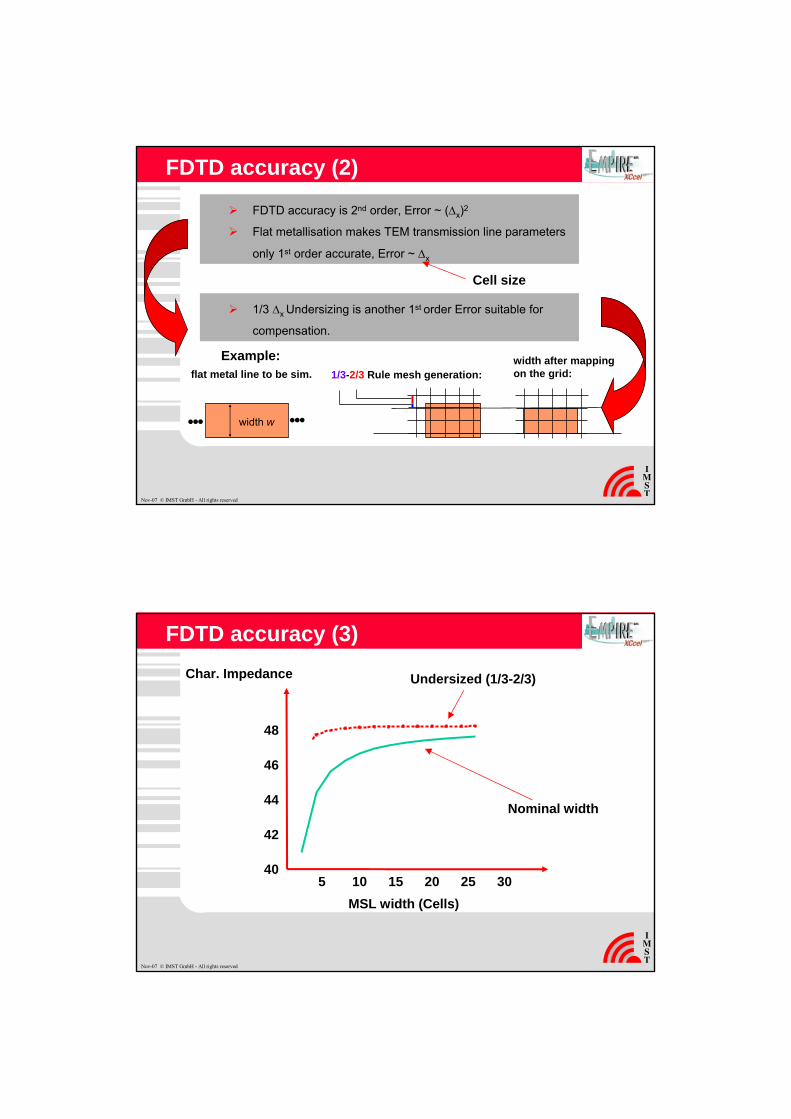
FDTD accuracy (2)

FDTD accuracy is 2nd order, Error ~ (Δx)2

Flat metallisation makes TEM transmission line parameters

only 1st order accurate, Error ~ Δx

1/3 Δx Undersizing is another 1st order Error suitable for

compensation.

Cell size

flat metal line to be sim. 1/3-2/3 Rule mesh generation:width after mappingon the grid:

Example:

width w


FDTD accuracy (3)

40

42

44

46

48

5 10 15 20 25 30

Char. Impedance

MSL width (Cells)

Nominal width

Undersized (1/3-2/3)


Excitation

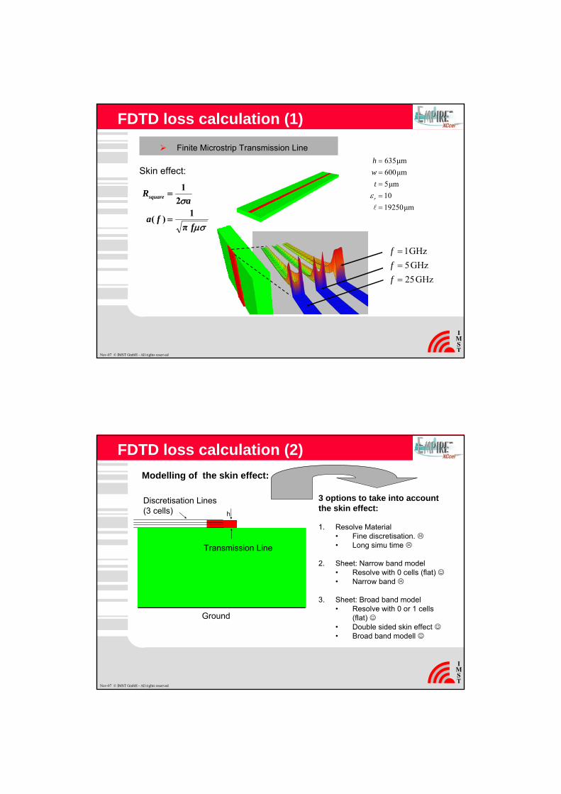
FDTD loss calculation (1)Finite Microstrip Transmission Line

μm1925010μm5μm600μm635

=====

lr

twh

ε

Skin effect:

μσ

σ

ffa

aRsquare

π1)(

21

=

=

GHz25GHz5GHz1

===

fff


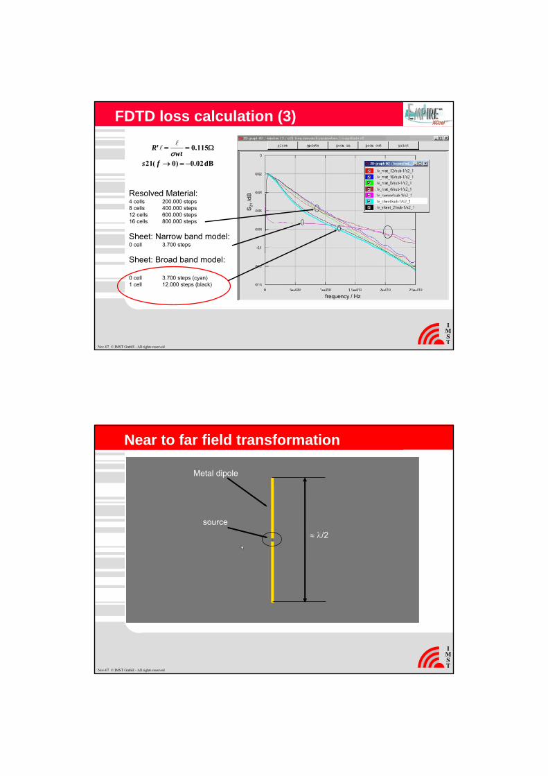
FDTD loss calculation (2)

h

Modelling of the skin effect:

Transmission Line

Discretisation Lines (3 cells)

3 options to take into accountthe skin effect:

1. Resolve Material• Fine discretisation. • Long simu time

2. Sheet: Narrow band model• Resolve with 0 cells (flat) • Narrow band

3. Sheet: Broad band model• Resolve with 0 or 1 cells

(flat) • Double sided skin effect • Broad band modell

Ground


Excitation

FDTD loss calculation (3)

Resolved Material:4 cells 200.000 steps8 cells 400.000 steps12 cells 600.000 steps16 cells 800.000 steps

Sheet: Narrow band model:0 cell 3.700 steps

Sheet: Broad band model:

0 cell 3.700 steps (cyan)1 cell 12.000 steps (black)

dB02.0)0(21

115.0'

−=→

Ω==

fswt

Rσl

l

frequency / Hz

S21

/dB


Metal dipole

source≈ λ/2

Near to far field transformation


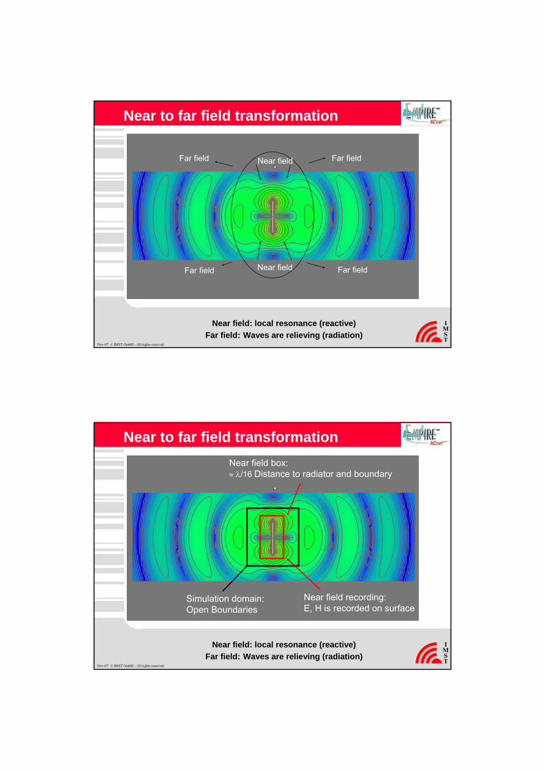
Near field: local resonance (reactive)Far field: Waves are relieving (radiation)

Near field

Far field Far field

Far field Far field

Near field



Near field: local resonance (reactive)Far field: Waves are relieving (radiation)


Simulation domain:Open Boundaries

Near field recording:E, H is recorded on surface

Near field box:≈ λ/16 Distance to radiator and boundary


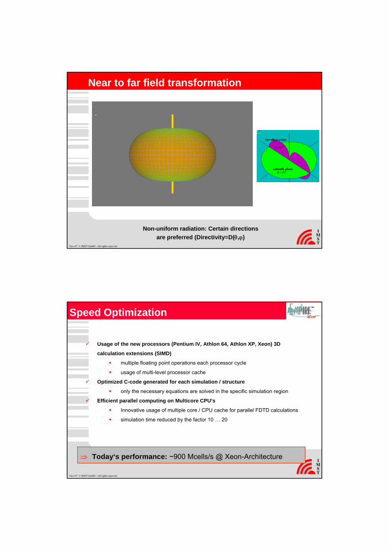
Non-uniform radiation: Certain directionsare preferred (Directivity=D(θ,ϕ)



Usage of the new processors (Pentium IV, Athlon 64, Athlon XP, Xeon) 3D

calculation extensions (SIMD)

multiple floating point operations each processor cycle

usage of multi-level processor cache

Optimized C-code generated for each simulation / structure

only the necessary equations are solved in the specific simulation region

Efficient parallel computing on Multicore CPU’s

Innovative usage of multiple core / CPU cache for parallel FDTD calculations

simulation time reduced by the factor 10 … 20

Speed Optimization

⇒ Today‘s performance: ~900 Mcells/s @ Xeon-Architecture



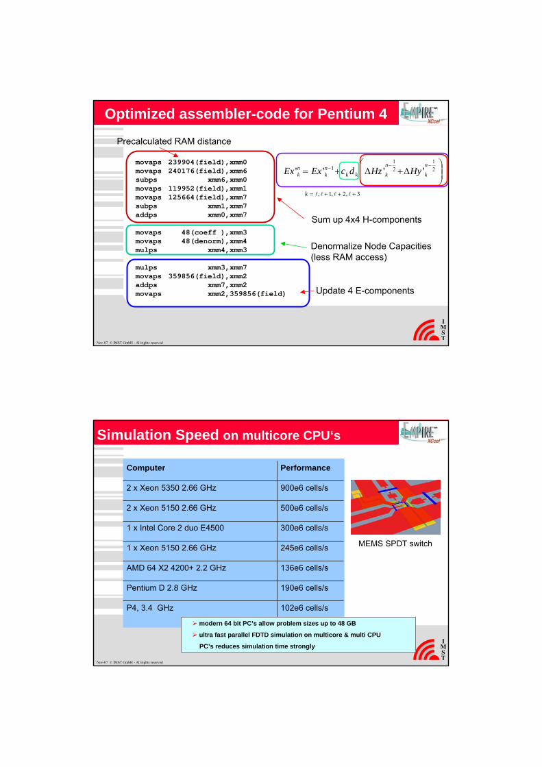
Optimized assembler-code for Pentium 4

movaps 239904(field),xmm0movaps 240176(field),xmm6subps xmm6,xmm0movaps 119952(field),xmm1movaps 125664(field),xmm7subps xmm1,xmm7addps xmm0,xmm7

movaps 48(coeff ),xmm3movaps 48(denorm),xmm4mulps xmm4,xmm3

mulps xmm3,xmm7movaps 359856(field),xmm2addps xmm7,xmm2movaps xmm2,359856(field)

Sum up 4x4 H-components

Denormalize Node Capacities(less RAM access)

Update 4 E-components

Precalculated RAM distance

⎟⎟⎠

⎞⎜⎜⎝

⎛Δ+Δ+=

−−− 21

21

1 ''''n

k

n

kkknk

nk HyHzdcExEx

3,2,1, +++= llllk


Simulation Speed on multicore CPU‘s

Computer Performance

2 x Xeon 5350 2.66 GHz 900e6 cells/s


1 x Intel Core 2 duo E4500 300e6 cells/s


AMD 64 X2 4200+ 2.2 GHz 136e6 cells/s

Pentium D 2.8 GHz 190e6 cells/s

P4, 3.4 GHz 102e6 cells/s

MEMS SPDT switch

modern 64 bit PC’s allow problem sizes up to 48 GB

ultra fast parallel FDTD simulation on multicore & multi CPU

PC’s reduces simulation time strongly


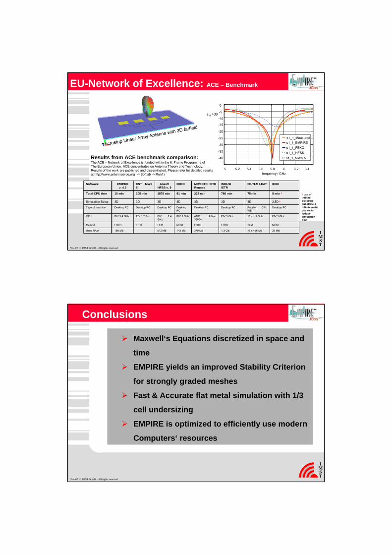
Microstrip Linear Array Antenna with 3D farfield

EU-Network of Excellence: ACE – Benchmark

Software EMIPRE v. 4.2

CST MWS 5

AnsoftHFSS v. 9

FEKO MR/FDTD IETR Rennes

IMELSIIETR

FP-TLM LEAT IE3D

Total CPU time 10 min 105 min 1879 min 91 min 222 min 780 min 75min 8 min *

Simulation Setup 3D 3D 3D 3D 3D 3D 3D 2.5D *

Type of machine Desktop PC Desktop PC Desktop PC Desktop PC

Desktop PC Desktop PC Parallel CPU WS

Desktop PC

CPU PIV 3.4 GHz PIV 1.7 GHz PIV 2.4 GHz

PIV 3 GHz AMD Athlon3500+

PIV 3 GHz 16 x 1.3 GHz PIV 3 GHz

Method FDTD FITD FEM MOM FDTD FDTD TLM MOM

Used RAM 180 MB 512 MB 143 MB 370 MB 1.3 GB 16 x 466 MB 29 MB

* use of infinite dielectric substrate & infinite metal planes to reduce simulation time

-40

-35

-30

-25

-20

-15

-10

-5

0

5 5.2 5.4 5.6 5.8 6 6.2 6.4

s11 / dB

frequency / GHz

s1_1_MWS 5

s1_1_EMPIREs1_1_FEKOs1_1_HFSS

s1_1_Measured

Results from ACE benchmark comparison:The ACE – Network of Excellence is funded within the 6. Frame Programme ofThe European Union. ACE concentrates on Antenna Theory and Technology. Results of the work are published and disseminated. Please refer for detailed results at http://www.antennasvce.org -> Softlab -> Run1)

Maxwell‘s Equations discretized in space and

time

EMPIRE yields an improved Stability Criterion

for strongly graded meshes

Fast & Accurate flat metal simulation with 1/3

cell undersizing

EMPIRE is optimized to efficiently use modern

Computers‘ resources

Conclusions


Documents

FDTD Method - Allgemeine und theoretische Elektrotechnik ... · PDF fileMaxwell‘s Equations Electric Field Magnetic Field Excitation Parameters ¾Hyperbolic partial differential