Fault Intelligence: Distribution Grid Fault Detection and … · 2018-06-11 · PNNL -27602 . Prepared for the U.S. Department of Energy under Contract DE-AC05-76RL01830 . Fault Intelligence:

PNNL-27602

Prepared for the U.S. Department of Energy under Contract DE-AC05-76RL01830

Fault Intelligence: Distribution Grid Fault Detection and Classification September 2017

JD Taft

Fault Intelligence: Distribution Grid Fault Detection and Classification JD Taft, PhD September 2017 Prepared for the U.S. Department of Energy under Contract DE-AC05-76RL01830 Pacific Northwest National Laboratory Richland, Washington 99352

iii

Abstract

As grid observability increases, we have the opportunity to implement increasingly powerful methods for detecting, locating, and characterizing all types of grid faults, including bolted faults, open phase faults, and high impedance faults. The key to efficient implementation is to recognize the common elements of the fault analysis tasks, and then make best use of the available sensing elements and data produced by them in a comprehensive approach to fault intelligence. In this way, we can max best use of the infrastructure investment by sharing the same sensors, processors, and even much of the same software over numerous applications.

This document describes and classifies common (and some not so common) fault types, along with characteristics, and analytics data requirements, so that we can identify opportunities for synergy among what would ordinarily be a siloed set of fault analytics applications. In this document, we define ten bolted fault classes, seven open phase fault classes, and seven high impedance fault classes, as well as defining two meta-classes: static faults and evolving faults. We also define nine categories of phasor-based fault analytics (seven for sags and two for open phase faults). In addition, we examine fault direction and distance computation techniques. From this basis, we can develop a comprehensive approach to the design of fault analytics software for smart sensors, substation analytics, and control center analytics.

v

Contents

Abstract ........................................................................................................................................................ iii 1.0 Fault Definitions and Taxonomy ....................................................................................................... 1.1 2.0 Fault Types and Grid State Behavior ................................................................................................. 2.1 3.0 Fault Characterization Data Requirements ........................................................................................ 3.1 4.0 Voltage Phasor Behavior and Relation to Faults: Sags and Open Phases ......................................... 4.1 5.0 Arc Characteristics ............................................................................................................................ 5.1 6.0 Fault Localization .............................................................................................................................. 6.1 7.0 Fault Response Times ........................................................................................................................ 7.1 8.0 Distributed Generation (DG) ............................................................................................................. 8.1 9.0 Conclusions ....................................................................................................................................... 9.1 10.0 References ....................................................................................................................................... 10.2

vi

Figures

1.1 Grid Fault Taxonomy ......................................................................................................................... 1.2 4.1 Inter-phasor Angles ............................................................................................................................ 4.2 4.2 Three Phase, P-P, and SLG Fault -Induced Voltage Sag Phasor Shift Diagrams .............................. 4.3 4.3 DLG and 2P-P Fault-Induced Voltage Sag Phasor Shift Diagrams ................................................... 4.3 5.1 Arc Waveforms .................................................................................................................................. 5.1

vii

Tables

2.1 Fault Types and Grid State Indicators ............................................................................................... 2.1 3.1 Grid Fault Analytics Data Items and Sources .................................................................................... 3.1 4.1 Phasor Discriminators ........................................................................................................................ 4.1 4.2 Partial Fault Classification Groups .................................................................................................... 4.4 4.3 Sag Duration Classifications .............................................................................................................. 4.4 6.1 Fault Location Methods ..................................................................................................................... 6.1 6.2 Fault Direction Determination Methods ............................................................................................ 6.3 7.1 Delay Times for Relay and Recloser Fault Responses ...................................................................... 7.1 8.1 Distributed Generation Grid Issues .................................................................................................... 8.1

1.1

1.0 Fault Definitions and Taxonomy

Power grid faults are defined as physical conditions that cause a circuit element to fail to perform in the required manner. This includes physical short circuits, open circuits, failed devices and overloads. Practically speaking, most faults involve some type of short circuit and the term fault is often synonymous with short circuit. A short circuit is some form of abnormal connection that causes current to flow in some path other that the one intended for proper circuit operation. Short circuit faults may have very low impedance (also known as “bolted faults”) or may have some significant amount of fault impedance. In most cases, bolted faults will result in the operation of a protective device, yielding an outage to some utility customers. Faults that have enough impedance to prevent a protective device from operating are known as high impedance (high Z) faults. Such high impedance faults may not result in outages, but can cause significant power quality issues, and can result in serious utility equipment damage. In the case of downed but still energized lines, high impedance faults also pose a safety hazard.

The IEEE also recognizes so-called open phase faults, where a conductor has become disconnected, but does not create a short circuit. Open phase faults can be the result of a conductor failure resulting in disconnection, or can be the side effect of a bolted phase fault, wherein a lateral phase fuse has blown, leaving that phase effectively disconnected. Such open phase faults can result in loss of service to customers, but can also result in safety hazards because a seemingly disconnected phase line may still be energized through a process called backfeed. Open phase faults are often the result of a wire connection failure at a pole-top switch.

Any fault may change into another fault type through physical instability or through the effects of arcing, wire burndown, electromagnetic forces, etc. Such faults are called evolving faults and the detection of evolution processes and fault type stages are of interest to utility engineers.

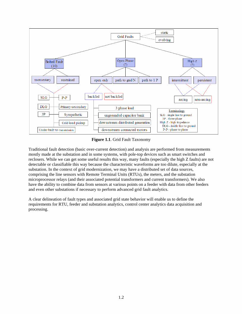
We wish to detect faults, to classify them, and to locate them as precisely as the instrumentation will permit. These steps involve various parameter measurements and event correlation logic to be described later in this document. Figure 1.1 below shows a taxonomy of grid faults.

We classify bolted faults as either momentary (basically self-clearing) or sustained (requiring a protective device to interrupt power until the fault is cleared by field crews). For high impedance faults, we distinguish between intermittent (happening on a recurring basis but not frequently) and persistent (happening at random but more or less constantly). We also recognize that faults may be static or evolving (also known as multi-stage faults, see e.g., Bollen, Styvaktakis, and Gu [1]). Evolving faults start out as one type, or involving one phase or pair of phases, then over time change to another type or to involve more phases. An example of an evolving fault is a Single Line to Ground (SLG) fault that causes a line fuse to blow. If the plasma drifts upward into overbuilt lines, a phase-to-phase fault may then evolve from the initial SLG fault.

1.2

Figure 1.1. Grid Fault Taxonomy

Traditional fault detection (basic over-current detection) and analysis are performed from measurements mostly made at the substation and in some systems, with pole-top devices such as smart switches and reclosers. While we can get some useful results this way, many faults (especially the high Z faults) are not detectable or classifiable this way because the characteristic waveforms are too dilute, especially at the substation. In the context of grid modernization, we may have a distributed set of data sources, comprising the line sensors with Remote Terminal Units (RTUs), the meters, and the substation microprocessor relays (and their associated potential transformers and current transformers). We also have the ability to combine data from sensors at various points on a feeder with data from other feeders and even other substations if necessary to perform advanced grid fault analytics.

A clear delineation of fault types and associated grid state behavior will enable us to define the requirements for RTU, feeder and substation analytics, control center analytics data acquisition and processing.

2.1

2.0 Fault Types and Grid State Behavior

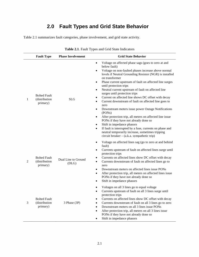
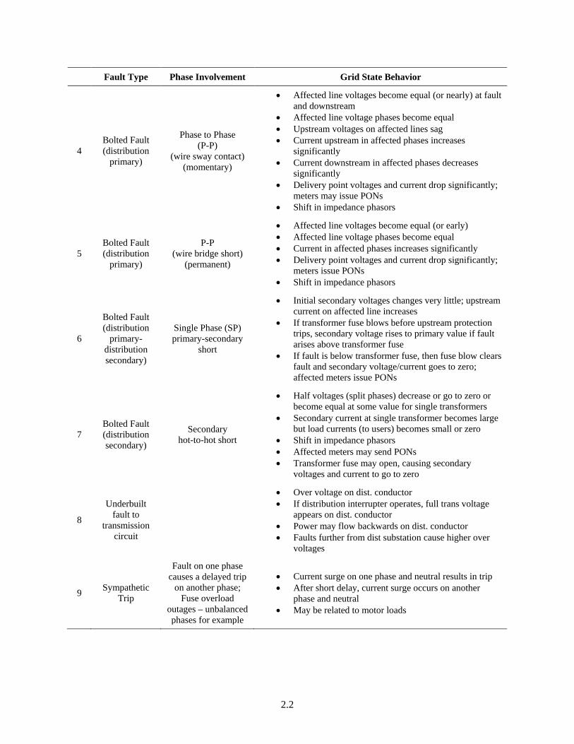
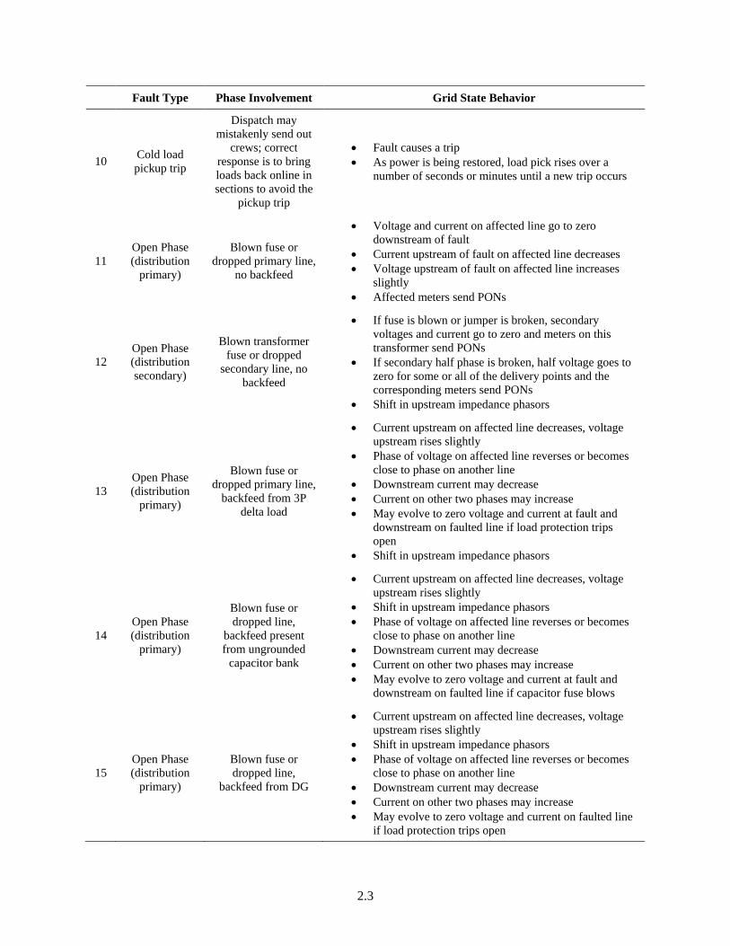
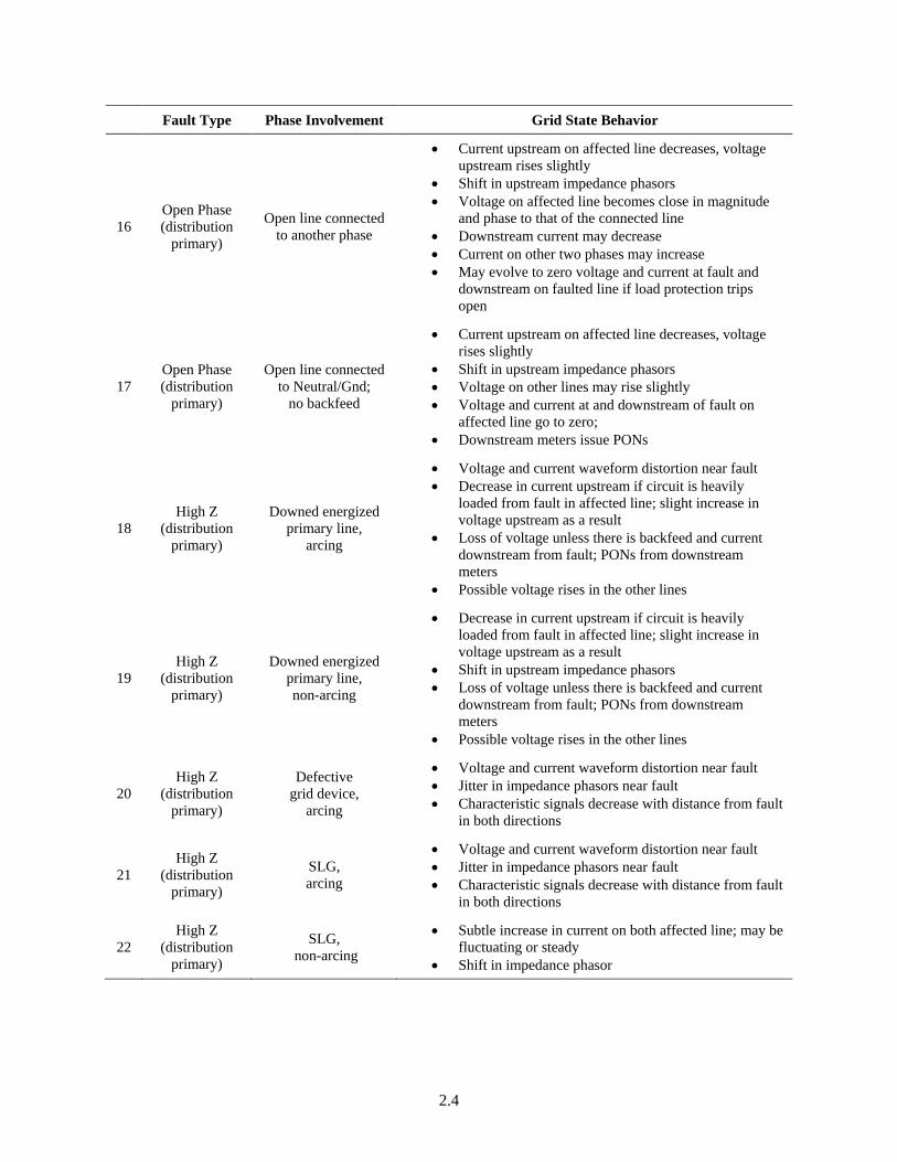
Table 2.1 summarizes fault categories, phase involvement, and grid state activity.

Table 2.1. Fault Types and Grid State Indicators

Fault Type Phase Involvement Grid State Behavior

1 Bolted Fault (distribution

primary) SLG

• Voltage on affected phase sags (goes to zero at and below fault)

• Voltage on non-faulted phases increase above normal levels if Neutral Grounding Resistor (NGR) is installed on transformer

• Phase current upstream of fault on affected line surges until protection trips

• Neutral current upstream of fault on affected line surges until protection trips

• Current on affected line shows DC offset with decay • Current downstream of fault on affected line goes to

zero • Downstream meters issue power Outage Notifications

(PONs) • After protection trip, all meters on affected line issue

PONs if they have not already done so • Shift in impedance phasors • If fault is interrupted by a fuse, currents on phase and

neutral temporarily increase, sometimes tripping circuit breaker – (a.k.a. sympathetic trip)


primary)

Dual Line to Ground (DLG)

• Voltage on affected lines sag (go to zero at and behind fault)

• Currents upstream of fault on affected lines surge until protection trips

• Currents on affected lines show DC offset with decay • Currents downstream of fault on affected lines go to

zero • Downstream meters on affected lines issue PONs • After protection trip, all meters on affected lines issue

PONs if they have not already done so • Shift in impedance phasors


primary) 3 Phase (3P)

• Voltages on all 3 lines go to equal voltage • Currents upstream of fault on all 3 lines surge until

protection trips • Currents on affected lines show DC offset with decay • Currents downstream of fault on all 3 lines go to zero • Downstream meters on all 3 lines issue PONs • After protection trip, all meters on all 3 lines issue

PONs if they have not already done so • Shift in impedance phasors

2.2



primary)

Phase to Phase (P-P)

(wire sway contact) (momentary)

• Affected line voltages become equal (or nearly) at fault and downstream

• Affected line voltage phases become equal • Upstream voltages on affected lines sag • Current upstream in affected phases increases

significantly • Current downstream in affected phases decreases

significantly • Delivery point voltages and current drop significantly;

meters may issue PONs • Shift in impedance phasors


primary)

P-P (wire bridge short)

(permanent)

• Affected line voltages become equal (or early) • Affected line voltage phases become equal • Current in affected phases increases significantly • Delivery point voltages and current drop significantly;

meters issue PONs • Shift in impedance phasors

6

Bolted Fault (distribution

primary-distribution secondary)

Single Phase (SP) primary-secondary

short

• Initial secondary voltages changes very little; upstream current on affected line increases

• If transformer fuse blows before upstream protection trips, secondary voltage rises to primary value if fault arises above transformer fuse

• If fault is below transformer fuse, then fuse blow clears fault and secondary voltage/current goes to zero; affected meters issue PONs

7 Bolted Fault (distribution secondary)

Secondary hot-to-hot short

• Half voltages (split phases) decrease or go to zero or become equal at some value for single transformers

• Secondary current at single transformer becomes large but load currents (to users) becomes small or zero

• Shift in impedance phasors • Affected meters may send PONs • Transformer fuse may open, causing secondary

voltages and current to go to zero

8

Underbuilt fault to

transmission circuit

• Over voltage on dist. conductor • If distribution interrupter operates, full trans voltage

appears on dist. conductor • Power may flow backwards on dist. conductor • Faults further from dist substation cause higher over

voltages

9 Sympathetic Trip

Fault on one phase causes a delayed trip

on another phase; Fuse overload

outages – unbalanced phases for example

• Current surge on one phase and neutral results in trip • After short delay, current surge occurs on another

phase and neutral • May be related to motor loads

2.3


10 Cold load pickup trip

Dispatch may mistakenly send out

crews; correct response is to bring loads back online in sections to avoid the

pickup trip

• Fault causes a trip • As power is being restored, load pick rises over a

number of seconds or minutes until a new trip occurs

11 Open Phase (distribution

primary)

Blown fuse or dropped primary line,

no backfeed

• Voltage and current on affected line go to zero downstream of fault

• Current upstream of fault on affected line decreases • Voltage upstream of fault on affected line increases

slightly • Affected meters send PONs

12 Open Phase (distribution secondary)

Blown transformer fuse or dropped

secondary line, no backfeed

• If fuse is blown or jumper is broken, secondary voltages and current go to zero and meters on this transformer send PONs

• If secondary half phase is broken, half voltage goes to zero for some or all of the delivery points and the corresponding meters send PONs

• Shift in upstream impedance phasors


primary)

Blown fuse or dropped primary line,

backfeed from 3P delta load

• Current upstream on affected line decreases, voltage upstream rises slightly

• Phase of voltage on affected line reverses or becomes close to phase on another line

• Downstream current may decrease • Current on other two phases may increase • May evolve to zero voltage and current at fault and

downstream on faulted line if load protection trips open

• Shift in upstream impedance phasors


primary)

Blown fuse or dropped line,

backfeed present from ungrounded

capacitor bank


• Shift in upstream impedance phasors • Phase of voltage on affected line reverses or becomes

close to phase on another line • Downstream current may decrease • Current on other two phases may increase • May evolve to zero voltage and current at fault and

downstream on faulted line if capacitor fuse blows


primary)

Blown fuse or dropped line,

backfeed from DG


• Shift in upstream impedance phasors • Phase of voltage on affected line reverses or becomes

close to phase on another line • Downstream current may decrease • Current on other two phases may increase • May evolve to zero voltage and current on faulted line

if load protection trips open

2.4



primary)

Open line connected to another phase


• Shift in upstream impedance phasors • Voltage on affected line becomes close in magnitude

and phase to that of the connected line • Downstream current may decrease • Current on other two phases may increase • May evolve to zero voltage and current at fault and

downstream on faulted line if load protection trips open


primary)

Open line connected to Neutral/Gnd;

no backfeed

• Current upstream on affected line decreases, voltage rises slightly

• Shift in upstream impedance phasors • Voltage on other lines may rise slightly • Voltage and current at and downstream of fault on

affected line go to zero; • Downstream meters issue PONs

18 High Z

(distribution primary)

Downed energized primary line,

arcing

• Voltage and current waveform distortion near fault • Decrease in current upstream if circuit is heavily

loaded from fault in affected line; slight increase in voltage upstream as a result

• Loss of voltage unless there is backfeed and current downstream from fault; PONs from downstream meters

• Possible voltage rises in the other lines

19 High Z


Downed energized primary line, non-arcing

• Decrease in current upstream if circuit is heavily loaded from fault in affected line; slight increase in voltage upstream as a result

• Shift in upstream impedance phasors • Loss of voltage unless there is backfeed and current

downstream from fault; PONs from downstream meters

• Possible voltage rises in the other lines

20 High Z


Defective grid device,

arcing

• Voltage and current waveform distortion near fault • Jitter in impedance phasors near fault • Characteristic signals decrease with distance from fault

in both directions

21 High Z


SLG, arcing

• Voltage and current waveform distortion near fault • Jitter in impedance phasors near fault • Characteristic signals decrease with distance from fault

in both directions

22 High Z


SLG, non-arcing

• Subtle increase in current on both affected line; may be fluctuating or steady

• Shift in impedance phasor

2.5


23 High Z


Phase to phase, arcing

• Voltage and current waveform distortion near fault on both affected lines

• Jitter in impedance phasors near fault • Subtle increase in current on both affected lines; will

fluctuate randomly

24 High Z


Phase to phase, non-arcing

• Subtle increase in current on both affected lines; may be fluctuating or steady

• Shift in impedance phasor

The purposes of automated grid fault analytics are many:

• Enabling advanced control functions

• Enabling advanced switching strategies for fault isolation

• Supporting efficient crew dispatch for power restoration

• Providing data for asset management

• Providing data for fault mitigation programs

• Providing data for mitigating outages

• Providing data for system planning

• Providing data for system performance evaluation

• Providing the basis for automatic grid event correlation

All of these functions are carried out in electric utilities in one fashion or another today and various systems and products exist to address individual elements, but there are no fully integrated end-to-end solutions for grid fault analytics.

3.1

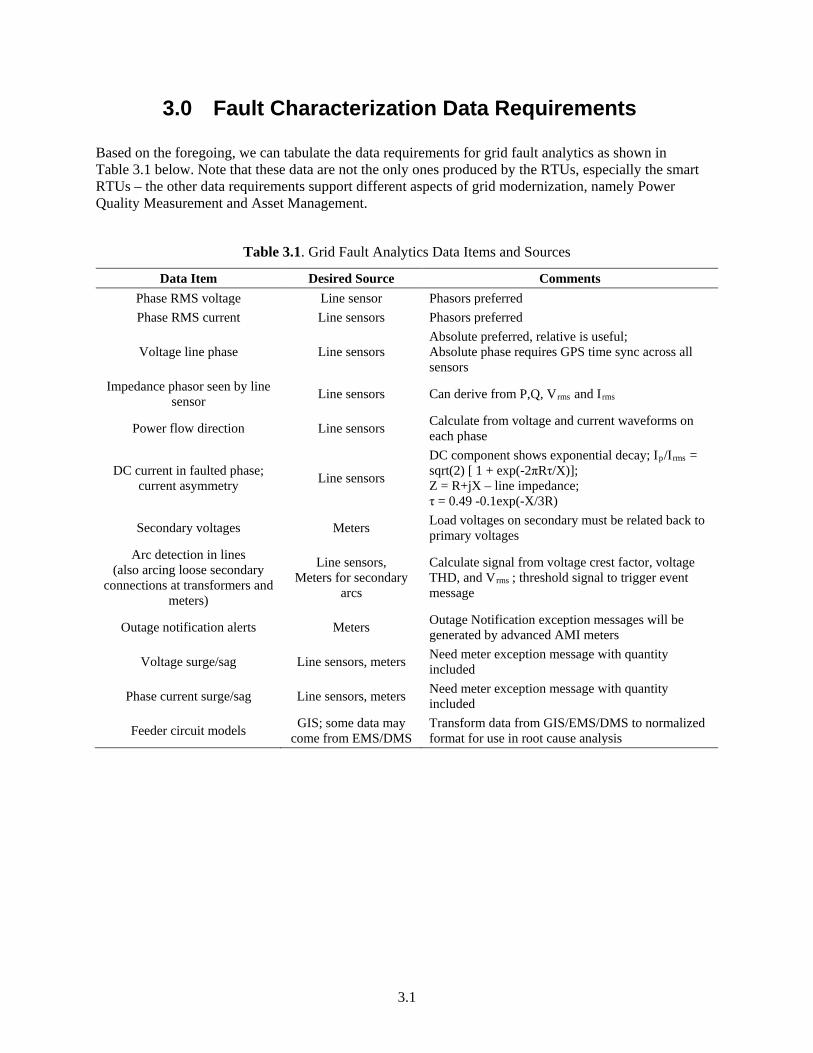
3.0 Fault Characterization Data Requirements

Based on the foregoing, we can tabulate the data requirements for grid fault analytics as shown in Table 3.1 below. Note that these data are not the only ones produced by the RTUs, especially the smart RTUs – the other data requirements support different aspects of grid modernization, namely Power Quality Measurement and Asset Management.

Table 3.1. Grid Fault Analytics Data Items and Sources

Data Item Desired Source Comments Phase RMS voltage Line sensor Phasors preferred Phase RMS current Line sensors Phasors preferred

Voltage line phase Line sensors Absolute preferred, relative is useful; Absolute phase requires GPS time sync across all sensors

Impedance phasor seen by line sensor Line sensors Can derive from P,Q, Vrms and Irms

Power flow direction Line sensors Calculate from voltage and current waveforms on each phase

DC current in faulted phase; current asymmetry Line sensors

DC component shows exponential decay; Ip/Irms = sqrt(2) [ 1 + exp(-2πRτ/X)]; Z = R+jX – line impedance; τ = 0.49 -0.1exp(-X/3R)

Secondary voltages Meters Load voltages on secondary must be related back to primary voltages

Arc detection in lines (also arcing loose secondary

connections at transformers and meters)

Line sensors, Meters for secondary

arcs

Calculate signal from voltage crest factor, voltage THD, and Vrms ; threshold signal to trigger event message

Outage notification alerts Meters Outage Notification exception messages will be generated by advanced AMI meters

Voltage surge/sag Line sensors, meters Need meter exception message with quantity included

Phase current surge/sag Line sensors, meters Need meter exception message with quantity included

Feeder circuit models GIS; some data may come from EMS/DMS

Transform data from GIS/EMS/DMS to normalized format for use in root cause analysis

4.1

4.0 Voltage Phasor Behavior and Relation to Faults: Sags and Open Phases

Voltage sags (dips, in IEC terminology) are closely related to faults; therefore detection and classification of voltage sags are crucial to fault analytics. The actual definition of voltage sag varies somewhat in the literature. Here we define voltage sag as any reduction in RMS voltage that takes the voltage magnitude down inside the range of 0.9 to 0.1 p. u, as per IEEE Std 1159 [2]. In some cases, the utility may choose to define sag as when voltage descends below 0.95 p. u., to be consistent with voltage regulation specifications.

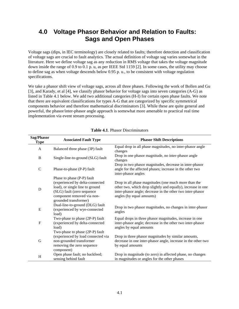
We take a phasor shift view of voltage sags, across all three phases. Following the work of Bollen and Gu [3], and Karady, et al [4], we classify phasor behavior for voltage sags into seven categories (A-G) as listed in Table 4.1 below. We add two additional categories (H-I) for certain open phase faults. We note that there are equivalent classifications for types A-G that are categorized by specific symmetrical components behavior and therefore mathematical discriminators [3]. While these are quite general and powerful, the phasor/inter-phasor angle approach is somewhat more amenable to practical real time implementation via event stream processing.

Table 4.1. Phasor Discriminators

Sag/Phasor Type Associated Fault Type Phasor Shift Descriptions

A Balanced three phase (3P) fault Equal drop in all phase magnitudes, no inter-phasor angle changes

B Single-line-to-ground (SLG) fault Drop in one phasor magnitude, no inter-phasor angle changes

C Phase-to-phase (P-P) fault Drop in two phasor magnitudes, decrease in inter-phasor angle for the affected phases; increase in the other two inter-phasor angles

D

Phase to phase (P-P) fault (experienced by delta-connected load), or single line to ground (SLG) fault (zero sequence component removed via non-grounded transformer)

Drop in all phase magnitudes (one much more than the other two, which drop slightly and equally), increase in one inter-phasor angle; decrease in the other two inter-phasor angles (by equal amounts)

E Dual-line-to-ground (DLG) fault (experienced by wye-connected load)

Drop in two phasor magnitudes, no changes in inter-phasor angles

F Two-phase to phase (2P-P) fault (experienced by delta-connected load)

Equal drops in three phasor magnitudes, increase in one inter-phasor angle; decrease in the other two inter-phasor angles by equal amounts

G

Two-phase to phase (2P-P) fault (experienced by load connected via non-grounded transformer removing the zero sequence component)

Drop in three phasor magnitudes by similar amounts, decrease in one inter-phasor angle, increase in the other two by equal amounts

H Open phase fault; no backfeed; sensing behind fault

Drop in magnitude (to zero) in affected phase, no changes in magnitudes or angles for the other phases

4.2

Sag/Phasor Type Associated Fault Type Phasor Shift Descriptions

I Open phase fault; backfeed; sensing behind fault location

Affected phasor rotates by approximately π radians, one inter-phasor angle is unaffected, the other two inter-phasor interior angles become small and the three add to less than 2π; in some cases this fault may be detected via an alternate technique: negative sequence over current, however this is not a voltage phasor method and can fail for fault far from the substation where currents are small

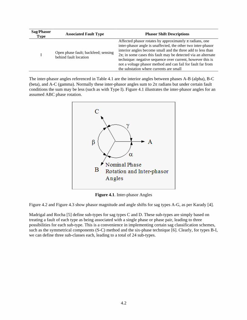
The inter-phasor angles referenced in Table 4.1 are the interior angles between phases A-B (alpha), B-C (beta), and A-C (gamma). Normally these inter-phasor angles sum to 2π radians but under certain fault conditions the sum may be less (such as with Type I). Figure 4.1 illustrates the inter-phasor angles for an assumed ABC phase rotation.

Figure 4.1. Inter-phasor Angles

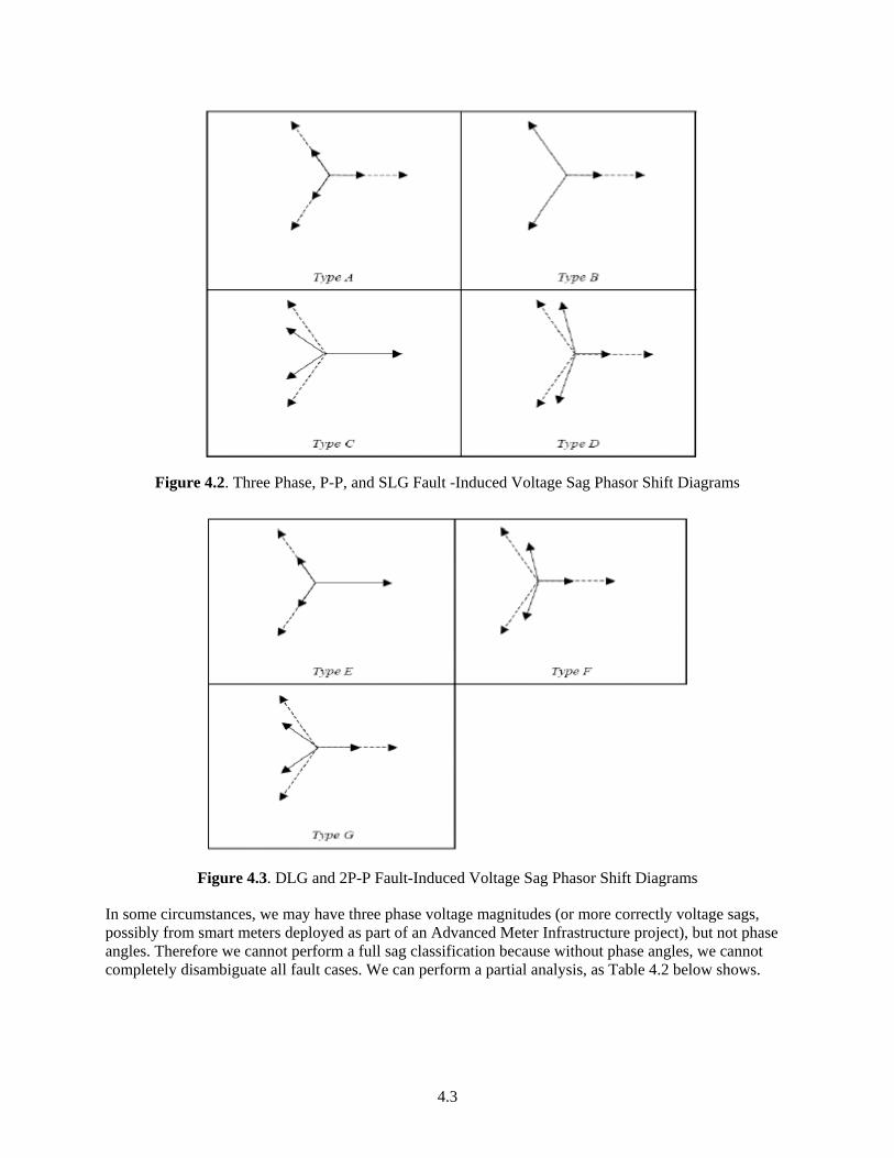
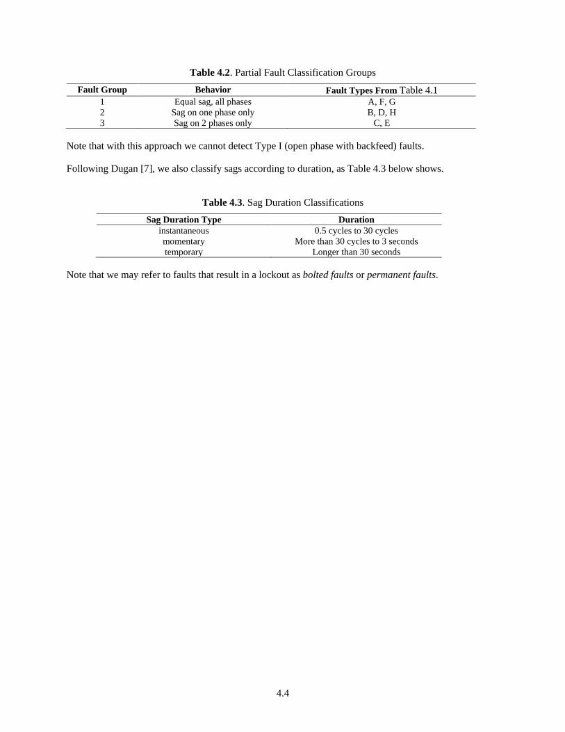
Figure 4.2 and Figure 4.3 show phasor magnitude and angle shifts for sag types A-G, as per Karady [4].

Madrigal and Rocha [5] define sub-types for sag types C and D. These sub-types are simply based on treating a fault of each type as being associated with a single phase or phase pair, leading to three possibilities for each sub-type. This is a convenience in implementing certain sag classification schemes, such as the symmetrical components (S-C) method and the six-phase technique [6]. Clearly, for types B-I, we can define three sub-classes each, leading to a total of 24 sub-types.

4.3

Figure 4.2. Three Phase, P-P, and SLG Fault -Induced Voltage Sag Phasor Shift Diagrams

Figure 4.3. DLG and 2P-P Fault-Induced Voltage Sag Phasor Shift Diagrams

In some circumstances, we may have three phase voltage magnitudes (or more correctly voltage sags, possibly from smart meters deployed as part of an Advanced Meter Infrastructure project), but not phase angles. Therefore we cannot perform a full sag classification because without phase angles, we cannot completely disambiguate all fault cases. We can perform a partial analysis, as Table 4.2 below shows.

4.4

Table 4.2. Partial Fault Classification Groups

Fault Group Behavior Fault Types From Table 4.1 1 Equal sag, all phases A, F, G 2 Sag on one phase only B, D, H 3 Sag on 2 phases only C, E

Note that with this approach we cannot detect Type I (open phase with backfeed) faults.

Following Dugan [7], we also classify sags according to duration, as Table 4.3 below shows.

Table 4.3. Sag Duration Classifications

Sag Duration Type Duration instantaneous 0.5 cycles to 30 cycles momentary More than 30 cycles to 3 seconds temporary Longer than 30 seconds

Note that we may refer to faults that result in a lockout as bolted faults or permanent faults.

5.1

5.0 Arc Characteristics

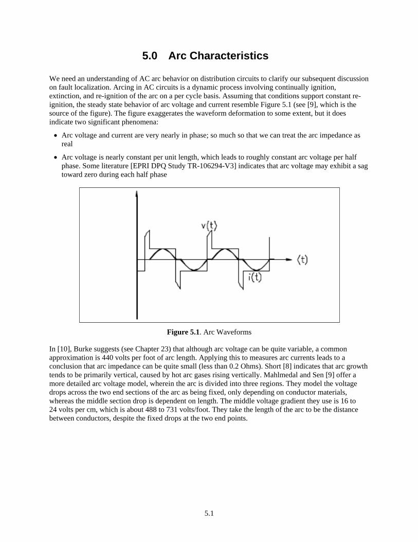
We need an understanding of AC arc behavior on distribution circuits to clarify our subsequent discussion on fault localization. Arcing in AC circuits is a dynamic process involving continually ignition, extinction, and re-ignition of the arc on a per cycle basis. Assuming that conditions support constant re-ignition, the steady state behavior of arc voltage and current resemble Figure 5.1 (see [9], which is the source of the figure). The figure exaggerates the waveform deformation to some extent, but it does indicate two significant phenomena:

• Arc voltage and current are very nearly in phase; so much so that we can treat the arc impedance as real

• Arc voltage is nearly constant per unit length, which leads to roughly constant arc voltage per half phase. Some literature [EPRI DPQ Study TR-106294-V3] indicates that arc voltage may exhibit a sag toward zero during each half phase

Figure 5.1. Arc Waveforms

In [10], Burke suggests (see Chapter 23) that although arc voltage can be quite variable, a common approximation is 440 volts per foot of arc length. Applying this to measures arc currents leads to a conclusion that arc impedance can be quite small (less than 0.2 Ohms). Short [8] indicates that arc growth tends to be primarily vertical, caused by hot arc gases rising vertically. Mahlmedal and Sen [9] offer a more detailed arc voltage model, wherein the arc is divided into three regions. They model the voltage drops across the two end sections of the arc as being fixed, only depending on conductor materials, whereas the middle section drop is dependent on length. The middle voltage gradient they use is 16 to 24 volts per cm, which is about 488 to 731 volts/foot. They take the length of the arc to be the distance between conductors, despite the fixed drops at the two end points.

6.1

6.0 Fault Localization

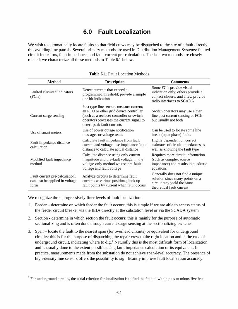
We wish to automatically locate faults so that field crews may be dispatched to the site of a fault directly, this avoiding line patrols. Several primary methods are used in Distribution Management Systems: faulted circuit indicators, fault impedance, and fault current pre-calculation. The last two methods are closely related; we characterize all these methods in Table 6.1 below.

Table 6.1. Fault Location Methods

Method Description Comments

Faulted circuited indicators (FCIs)

Detect currents that exceed a programmed threshold; provide a simple one bit indication

Some FCIs provide visual indication only; others provide a contact closure, and a few provide radio interfaces to SCADA

Current surge sensing

Post type line sensors measure current; an RTU or other grid device controller (such as a recloser controller or switch operator) processes the current signal to detect peak fault currents

Switch operators may use either line post current sensing or FCIs, but usually not both

Use of smart meters Use of power outage notification messages or voltage reads

Can be used to locate some line break (open phase) faults

Fault impedance distance calculation

Calculate fault impedance from fault current and voltage; use impedance /unit distance to calculate actual distance

Highly dependent on correct estimates of circuit impedances as well as knowing the fault type

Modified fault impedance method

Calculate distance using only current magnitude and pre-fault voltage; in the voltage-only method we use pre-fault voltage and fault voltage

Requires more circuit information (such as complex source impedance) and results in quadratic equations

Fault current pre-calculation; can also be applied in voltage form

Analyze circuits to determine fault currents at various positions; look up fault points by current when fault occurs

Generally does not find a unique solution since many points on a circuit may yield the same theoretical fault current

We recognize three progressively finer levels of fault localization:

1. Feeder – determine on which feeder the fault occurs; this is simple if we are able to access status of the feeder circuit breaker via the IEDs directly at the substation level or via the SCADA system

2. Section - determine in which section the fault occurs; this is mainly for the purpose of automatic sectionalizing and is often done through current surge sensing at the sectionalizing switches

3. Span – locate the fault to the nearest span (for overhead circuits) or equivalent for underground circuits; this is for the purpose of dispatching the repair crew to the right location and in the case of underground circuit, indicating where to dig.1 Naturally this is the most difficult form of localization and is usually done to the extent possible using fault impedance calculation or its equivalent. In practice, measurements made from the substation do not achieve span-level accuracy. The presence of high-density line sensors offers the possibility to significantly improve fault localization accuracy.

1 For underground circuits, the usual criterion for localization is to find the fault to within plus or minus five feet.

6.2

Faulted circuit indicators (FCIs) have been available for a number of years. They operate by detecting fault surge currents and trip when the line currents that monitor exceed a set threshold. Most devices have a number of automatic and manual reset modes. FCI networks can be used to perform fault detection and, to some extent, localization. The degree of granularity of the localization depends on the number of FCIs, since the devices only detect surge current, and provide no means to locate the actual distance to the point where the actual fault is located. A few utilities have used large numbers of FCIs on feeder circuits to provide finely granular fault localization.

A related technique is the use of line post sensors to measure current. The normal application calls for the line post current sensors to be co-located with sectionalizing switches, with the switch operator accepting the line post signals. This approach matches fault location capability exactly with sectionalizing capability, so that faulted sections can be isolated immediately and automatically. The location of the fault within the faulted section is not determined unless the line post sensors also measure voltage, in which case it may be possible to apply fault direction and distance computations as described below.

When voltage and current waveforms or RMS values are monitored on a high speed basis (say anywhere from once per several cycles up to once per cycle), then we may calculate distance from the sensing point to the fault, provided we have a model for the impedance of the circuit section involved. The basic idea is to measure the peak fault current and the line voltage, and use these to calculate impedance seen at that point. With the assumption that the fault current is large with respect to load currents and that the actual fault impedance is real and small enough to be negligible, we may then apply the impedance per unit distance to obtain a distance to the fault. In practice, this becomes a bit complicated, since we must know the type of fault in order to select the correct impedance (line to ground vs. line to line) and the ground return impedance estimate may introduce errors. We must also use the appropriate voltages and in cases where we need line to ground voltages and we only have line to line voltage, we must have the zero sequence source impedance so that we can convert line to line voltages to line to ground voltages. Under some circumstances we may employ only currents or only voltages; these formulations result in quadratic equations [10]. For these approaches, we must have knowledge of the impedance between the source (substation transformer) and the sensing point. Normally this would be the source impedance at the bus (if we were measuring at the substation), but since the sensors may be located anywhere along the feeder, we must account for impedance in the upstream portion of the feeder.

Since arc impedance is approximately real, we may use this fact to iterate the fault distance solution by changing ground impedance until the imaginary part of the solution becomes very small. As an alternative (and because we may not have full phasor measurements but just magnitudes of relevant quantities) we can formulate the fault distance calculation entirely in terms of magnitude, with no complex arithmetic involved. We can expect to sacrifice some accuracy with this approach, in exchange for the ability to use less costly instrumentation. We may be able to obtain the necessary data from feeder meters instead of using V-I waveform sensors and smart RTU computations, using this approach.

The fault current pre-calculation method is clearly the same as the fault impedance method, except that it is implemented as a two stage process where we first calculate all possible peak fault currents based on circuit impedance models before we begin operations, and then at fault time we perform what amounts to a table lookup for all the points on the circuit that are a reasonable match to the actual fault current. Both of these methods suffer from three types of inexactitude:

• Accuracy of the method inherently varies inversely as the electrical distance of the fault from the sensing point (usually the substation) because fault current profiles do; therefore ∂I/∂R approaches zero as distance R increases and sensitivity is lost

• The method requires accurate knowledge of circuit impedance at all points along the path from the sensing point to the fault; even if this is known at some time, the values change over time.

6.3

Furthermore, the impedance to be used depends on the type of fault, so that fault classification is required; also, conductors of various sizes may be used to construct a single circuit, causing impedance to be non-uniform; finally, ground return impedance vary in unpredictable ways, affecting the calculations for single line and dual line to ground faults

• The method may find equivalent electrical distances on many branches of the same feeder, yielding ambiguity in fault location.

When Advanced Meter Infrastructure (AMI) exists, it may be possible to use the meters as sensors to locate certain faults. This is based on the ability of such meters to sense secondary voltage, and therefore is limited to location of open phase faults with no backfeed. We may use the asynchronous power outage notification exception messages in the context of feeder and lateral topology. We may also use specific meter voltage readings, if the AMI system supports on-demand voltage reads. Through the use of circuit topology context, we can use the meter data to distinguish between open phase feeder faults and open secondary or downed service drop faults. If we use advanced meters such as the A3 Alpha on the feeders as line sensors, then we can expand our capability to classify faults, even without line sensors. With voltage sag magnitude records from the meters’ sag logs, we can perform the partial classifications shown in Table 4.2. If we are able to construct phasors from the combination of phase angle data and sag log records (problematic for very deep sags, as phase angles tend to become very noisy at low voltage magnitudes), then we may be able to implement the full classification of Table 4.1. With this same data, we may able be able to implement fault distance localization via impedance methods. These analytics could not be implemented in a form sufficiently fast for use in automated control modification or automated fault isolation, but could be implemented well enough to be used for field force dispatch purposes.

Fault direction determination is crucial to fault location when we are using distributed sensor networks on the feeders, as opposed to sensing at the substation only. In the substation-only case, there is only one direction to the fault (downstream) so that fault distance is the only necessary parameter (until we must contend with feeder branching and the resultant ambiguity of fault location – several branch points may have the same electrical distance from the substation, or equivalently, several branch locations may have nearly equal peak fault current limit values). In the distributed sensor case, two directions to the fault are possible in general: upstream or downstream. This is further complicated in the case of feeders with branches. There are three primary approaches to determining the direction to a fault from a sensing point. These methods are exemplified by the entries in Table 6.2.

Table 6.2. Fault Direction Determination Methods

Method Description Comments Phase change method of Pradhan, Routray, and Madhan [11]

Uses positive sequence fault current phase angle with respect to voltage on the faulted phase

Requires phasor measurements at the sensing points

Traveling wave method Compare polarities of superimposed quantities (ΔV and ΔI)

Fails if fault initiates near a voltage zero crossing

Transient energy method

Three phase power is calculated on a per sample basis and then integrated for several consecutive samples to determine the transient energy and its sign,

Considered to be fast and very sensitive; used primarily on transmission lines

7.1

7.0 Fault Response Times

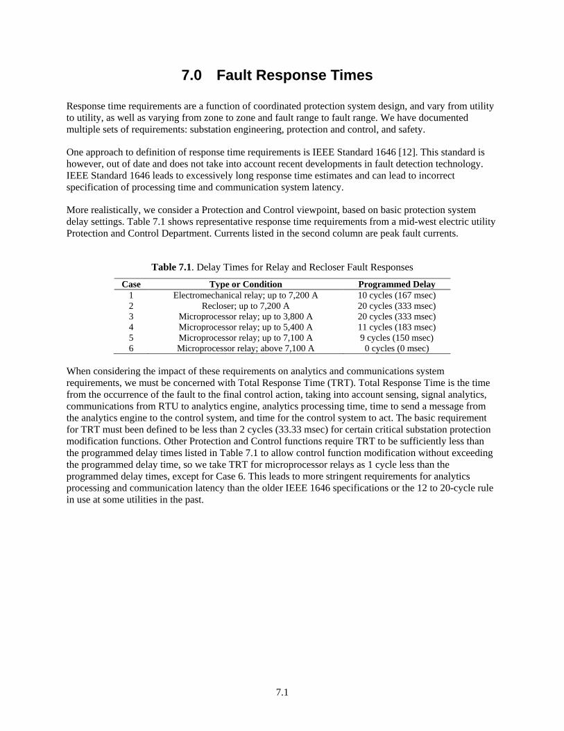
Response time requirements are a function of coordinated protection system design, and vary from utility to utility, as well as varying from zone to zone and fault range to fault range. We have documented multiple sets of requirements: substation engineering, protection and control, and safety.

One approach to definition of response time requirements is IEEE Standard 1646 [12]. This standard is however, out of date and does not take into account recent developments in fault detection technology. IEEE Standard 1646 leads to excessively long response time estimates and can lead to incorrect specification of processing time and communication system latency.

More realistically, we consider a Protection and Control viewpoint, based on basic protection system delay settings. Table 7.1 shows representative response time requirements from a mid-west electric utility Protection and Control Department. Currents listed in the second column are peak fault currents.

Table 7.1. Delay Times for Relay and Recloser Fault Responses

Case Type or Condition Programmed Delay 1 Electromechanical relay; up to 7,200 A 10 cycles (167 msec) 2 Recloser; up to 7,200 A 20 cycles (333 msec) 3 Microprocessor relay; up to 3,800 A 20 cycles (333 msec) 4 Microprocessor relay; up to 5,400 A 11 cycles (183 msec) 5 Microprocessor relay; up to 7,100 A 9 cycles (150 msec) 6 Microprocessor relay; above 7,100 A 0 cycles (0 msec)

When considering the impact of these requirements on analytics and communications system requirements, we must be concerned with Total Response Time (TRT). Total Response Time is the time from the occurrence of the fault to the final control action, taking into account sensing, signal analytics, communications from RTU to analytics engine, analytics processing time, time to send a message from the analytics engine to the control system, and time for the control system to act. The basic requirement for TRT must been defined to be less than 2 cycles (33.33 msec) for certain critical substation protection modification functions. Other Protection and Control functions require TRT to be sufficiently less than the programmed delay times listed in Table 7.1 to allow control function modification without exceeding the programmed delay time, so we take TRT for microprocessor relays as 1 cycle less than the programmed delay times, except for Case 6. This leads to more stringent requirements for analytics processing and communication latency than the older IEEE 1646 specifications or the 12 to 20-cycle rule in use at some utilities in the past.

8.1

8.0 Distributed Generation (DG)

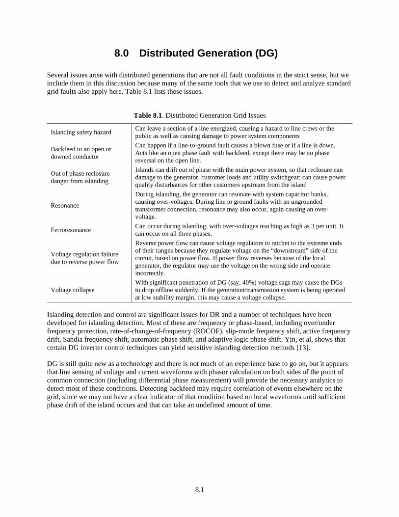
Several issues arise with distributed generations that are not all fault conditions in the strict sense, but we include them in this discussion because many of the same tools that we use to detect and analyze standard grid faults also apply here. Table 8.1 lists these issues.

Table 8.1. Distributed Generation Grid Issues

Islanding safety hazard Can leave a section of a line energized, causing a hazard to line crews or the public as well as causing damage to power system components

Backfeed to an open or downed conductor

Can happen if a line-to-ground fault causes a blown fuse or if a line is down. Acts like an open phase fault with backfeed, except there may be no phase reversal on the open line.

Out of phase reclosure danger from islanding

Islands can drift out of phase with the main power system, so that reclosure can damage to the generator, customer loads and utility switchgear; can cause power quality disturbances for other customers upstream from the island

Resonance

During islanding, the generator can resonate with system capacitor banks, causing over-voltages. During line to ground faults with an ungrounded transformer connection, resonance may also occur, again causing an over-voltage.

Ferroresonance Can occur during islanding, with over-voltages reaching as high as 3 per unit. It can occur on all three phases.

Voltage regulation failure due to reverse power flow

Reverse power flow can cause voltage regulators to ratchet to the extreme ends of their ranges because they regulate voltage on the “downstream” side of the circuit, based on power flow. If power flow reverses because of the local generator, the regulator may use the voltage on the wrong side and operate incorrectly.

Voltage collapse With significant penetration of DG (say, 40%) voltage sags may cause the DGs to drop offline suddenly. If the generation/transmission system is being operated at low stability margin, this may cause a voltage collapse.

Islanding detection and control are significant issues for DR and a number of techniques have been developed for islanding detection. Most of these are frequency or phase-based, including over/under frequency protection, rate-of-change-of-frequency (ROCOF), slip-mode frequency shift, active frequency drift, Sandia frequency shift, automatic phase shift, and adaptive logic phase shift. Yin, et al, shows that certain DG inverter control techniques can yield sensitive islanding detection methods [13].

DG is still quite new as a technology and there is not much of an experience base to go on, but it appears that line sensing of voltage and current waveforms with phasor calculation on both sides of the point of common connection (including differential phase measurement) will provide the necessary analytics to detect most of these conditions. Detecting backfeed may require correlation of events elsewhere on the grid, since we may not have a clear indicator of that condition based on local waveforms until sufficient phase drift of the island occurs and that can take an undefined amount of time.

9.1

9.0 Conclusions

Faults are a serious and continuous concern for any electric utility. Despite the media attention given to transmission-level outages, it is crucial that we be capable of dealing with distribution level faults since about 78-88% of outages arise on distribution grids, where fault effects are quite complex [14]. A great deal of effort goes into the design of protective systems intended to prevent or limit system damage when faults occur, as they inevitably do. Traditional utility methods of detecting, characterizing, and locating faults have severe limitations directly traceable to lack of grid observability. Increased observability of the distribution grid results in massive amounts of raw data that can be used to assist the fault management process, but automated analytics are required to handle this new data. With a proper view of fault behavior, we can design distributed systems that partition analytics processing over smart sensors, substations, and control center systems to provide advanced fault analytics and therefore superior fault management processes.

10.2

10.0 References

[1] Bollen, M. H. J., E. Styvaktakis, and I. Y. H. Gu, ”Analysis of Voltage Sags for Event Identification”, Power Quality: Monitoring and Solutions, (Ref No. 2000/136), Power Systems Research Center.

[2] “Recommended Practice for Monitoring Electric Power Quality”, IEEE Standard 1159, 1995.

[3] Bollen, Math H. J., and Irene Y. H. Gu, Signal Processing of Power Quality Disturbances, John Wiley and Sons, Inc IEEE Press, 2006, pp. 452-486.

[4] Karady, George C., S. Saksena, B. Shi, and N. Senroy, “Effect of Voltage Sags on Loads in a Distribution System”, PSERC Publication 05-63, October 2005, Power Systems Engineering Research Center.

[5] Madrigal, M., and B.H. Rocha, “A Contribution for Characterizing Measured Three-Phase Unbalanced Voltage Sags Algorithm”, IEEE Transactions on Power Delivery, Vol. 22, No. 3, pp. 1885-1890, July 2007.

[6] Bollen, M. H., “Algorithms for Characterizing Measured Three-Phase Unbalanced Voltage Dips”, IEEE Transactions on Power Delivery, Vol. 18, No. 3, pp. 937-994, July 2003.

[7] R. C. Dugan et al., Electrical Power Systems Quality, 2nd Ed. New, York: McGraw-Hill, 2002.

[8] Short, T. S., Electric Power Distribution Handbook, CRC Press, New York, 2004, pp 338-342.

[9] Mahlmedal, Keith, and P. K. Sen, Arcing faults and Their Effect on the Settings of Ground Fault Relays in Solidly Grounded Low Voltage Systems

[10] Grigsby, Leonard L., et al, Electric Power Generation, Transmission, and Distribution, CRC Press, New York, 2007, Chap 23, p15.

[11] Pradhan, A. K., A. Routray and S. Madhan Gudipalli, “Fault Direction Estimation in Radial Distribution System Using Phase Change in Sequence Current”, IEEE Transactions on Power Delivery, Vol. 22, No. 4, pp 2065-2071, October 2007.

[12] “Standard Communication Delivery Time Performance Requirements for Electric Power Substation Automation”, IEEE Standard 1646-2004, Feb 25, 2005.

[13] Yin, Jun, Chris Peter Diduch, and Liucheng Chang, “Islanding Detection Using Proportional Power Spectral Density”, IEEE Transactions on Power Delivery, Vol. 23, No. 2, pp. 776-784, April 2008.

[14] Brown, Richard E., Electric Power Distribution Reliability, Marcel Dekker, Inc., New York, 2002, Chap 1, p 7.

Documents

Fault Intelligence: Distribution Grid Fault Detection and … · 2018-06-11 · PNNL -27602 . Prepared for the U.S. Department of Energy under Contract DE-AC05-76RL01830 . Fault Intelligence: