Fault Hamiltonicity and Fault Hamiltonian Connectivity of the Arrangement Graphs

7/31/2019 Fault Hamiltonicity and Fault Hamiltonian Connectivity of the Arrangement Graphs

http://slidepdf.com/reader/full/fault-hamiltonicity-and-fault-hamiltonian-connectivity-of-the-arrangement-graphs 1/15

Fault Hamiltonicity and Fault HamiltonianConnectivity of the Arrangement GraphsHong-Chun Hsu, Tseng-Kuei Li, Member , IEEE , Jimmy J.M. Tan, and Lih-Hsing Hsu

Abstract —The arrangement graph An;k is a generalization of the star graph. There are some results concerning fault Hamiltonicity andfault Hamiltonian connectivity of the arrangement graph. However, these results are restricted in some particular cases and, thus, areless completed. In this paper, we improve these results and obtain a stronger and simpler statement. Let n À k ! 2 andF V ðAn;kÞ [ E ðAn;k Þ. We prove that An;k À F is Hamiltonian if jF j kðn À kÞ À2 and An;k À F is Hamiltonian connected ifjF j kðn À kÞ À3. These results are optimal.

Index Terms —Hamiltonian cycle, Hamiltonian connected, fault tolerance, arrangement graph.

æ

1 INTRODUCTION

THE interconnection network has been an importantresearch area for parallel and distributed computer

systems. Designing an interconnection network is multi-objected and complicated. For simplifying this task, weusually use a graph to represent the network’s topology,where vertices represent processors and edges representlinks between processors. The hypercube [15] and the stargraph [1], [2] are two examples. The hypercube possessesmany good properties and is implemented as manymultiprocessor systems. Akers et. al. [1] proposed the stargraph, which has smaller degree, diameter, and averagedistance than the hypercube while reserving symmetryproperties and desirable fault-tolerant characteristics. As aresult, the star graph has been recognized as an alternativeto the hypercube. However, the hypercube and the star are

less flexible in adjusting their sizes.The arrangement graph [6] was proposed by Day andTripathi as a generalization of the star graph. It is moreflexible in its size than the star graph. Given two positiveintegers n and k with n > k , the ðn; kÞ-arrangement graphAn;k is the graph ðV ; E Þ, where V ¼ f p j p is an arrangementof k elements out of the n symbols: 1; 2 Á Á Á; ng and E ¼fð p; q Þ jp; q 2 V and p; q differ in exactly one position g. Amore precise definition and an example will be given in thenext section. An;k is a regular graph of degree kðn À kÞwith

n!ðnÀkÞ! vertices. An;1 is isomorphic to the complete graph K nand An;n À1 is isomorphic to the n-dimensional star graph.Moreover, An;k is vertex symmetric and edge symmetric [6].

Hamiltonicity is an important property for networktopologies. Thus, the existence of a Hamiltonian cycle is adesired property for a new proposed topology. Hamiltonianconnectivity is a related property of Hamiltonicity, namely,there is a Hamiltonian path between any two vertices of a

graph. Since processors or links may fail sometimes, faultHamiltonicity and fault Hamiltonian connectivity areconcerned in many studies on network topologies, such ashypercubes [4], [11], twisted cubes [10], deBruijn networks[14], and star graphs [16], [9]. We say that a graph G cantolerate f faults when embedding a Hamiltonian cycle if there is a Hamiltonian cycle in G À F for any F V ðGÞ [ E ðGÞ with jF j f . We use f-Hamiltonian to denotethis property of G. Similarly, we use f-Hamiltonian connectedto denote the property that there is a Hamiltonian path between any two vertices in G À F for any F V ðGÞ [E ðGÞ with jF j f .

There are also some studies concerning fault Hamiltoni-city and fault Hamiltonian connectivity of the arrangementgraph. Hsieh et al. [8] studied the existence of Hamiltoniancycles in faulty arrangement graphs. It is proven that An;k ÀF is Hamiltonian if it satisfies one of the followingconditions:

1. (k ¼ 2 and n À k ! 3, or k ! 3, n À k ! 4 þ d k2eÞ, and

F E ðAn;kÞ with jF j kðn À kÞ À2,2. k ! 2, n À k ! 2 þ d k

2e, a nd F E ðAn;kÞ w i t hjF j kðn À k À 3Þ À1,

3. k ! 2, n À k ! 3, and F E ðAn;kÞ with jF j k,4. n À k ! 3, and F V ðAn;kÞ with jF j k À 3, or5. n À k ! 3, and F E ðAn;kÞ [ V ðAn;kÞ with jF j k.

Lo and Chen [12] studied the edge fault Hamiltonianconnectivity of the arrangement graph. They restricted the

fault distribution and then showed that An;k is kðn À kÞ À2edge fault Hamiltonian connected. However, these resultsare more restricted and less complete.

In this paper, we improve these results to get a muchstronger and simpler statement. We prove that An;k is ðkðn ÀkÞ À2Þ-Hamiltonian an d ðkðn À kÞ À3Þ-Hamiltonian con-nected if n À k ! 2, where the faults can be vertices andedges . Fo r n À k ¼ 1, An;n À1 i s i s omo rp h ic t o t h en-dimensional star graph, which is bipartite and thus cannottolerate any vertex fault when embedding Hamiltoniancycles and paths. Observing that a regular graph of degree d i s a t most ðd À 2Þ-Hamiltonian and ðd À 3Þ-Hamiltonianconnected, our results are optimal. In the following section,

we discuss some basic properties of the arrangement

IEEE TRANSACTIONS ON COMPUTERS, VOL. 53, NO. 1, JANUARY 2004 39

. H.-C. Hsu, J.J.M. Tan, and L.-H. Hsu are with the Department of Computer and Information Science, National Chiao Tung University, Hsinchu, Taiwan 300, ROC.

. T.-K. Li is with the Department of Computer Science and InformationEngineering, Ching Yun Institute of Technology, JungLi, Taiwan 320,ROC. E-mail: [email protected].

Manuscript received 5 Dec. 2002; revised 10 Jan. 2003; accepted 8 May 2003.For information on obtaining reprints of this article, please send e-mail to:

[email protected], and reference IEEECS Log Number 117883.0018-9340/04/$17.00 ß 2004 IEEE Published by the IEEE Computer Society



graphs. In Section 3, we prove our main theorem. Sincethe proof of the main theorem is rather long, several stepsare broken into lemmas. We prove these lemmas inSections 4, 5, and in the Appendix.

2 S OME P ROPERTIES OF THE ARRANGEMENTGRAPHS

In this paper, we concentrate on loopless undirected graphs.For the graph definition and notation, we follow [3]. G ¼ðV ; E Þ is a graph if V is a finite set and E is a subset of fða; bÞ j ða; bÞis an unordered pair of V }. We say that V is the

vertex set and E is the edge set. Two vertices, a and b, areadjacent i f ða; bÞ 2 E . A path i s r e pr e se n te d b yhv0; v1; v2 Á Á Á; vki . We also write the path hv0; v1; v2 Á Á Á; vkias hv0; P 1; vi ; viþ 1 Á Á Á; v j ; P 2 ; vt ; Á Á Á; vki , where P 1 is the pathhv0; v1; Á Á Á; vi i and P 2 is the path hv j ; v jþ 1; Á Á Á; vt i . A path is a Hamiltonian path if its vertices are distinct and span V . Acycle is a path with at least three vertices such that the firstvertex is the same as the last vertex. A cycle is a Hamiltoniancycleif it traverses every vertex of G exactly once. A graph is Hamiltonian if it has a Hamiltonian cycle.

Let n and k be two positive integers with n > k . And, lethni and hki denote the sets f 1; 2; Á Á Á; ng and f 1; 2; Á Á Á; kg,respectively. Then, the vertex set of An;k , V ðAn;kÞ is f p j p ¼

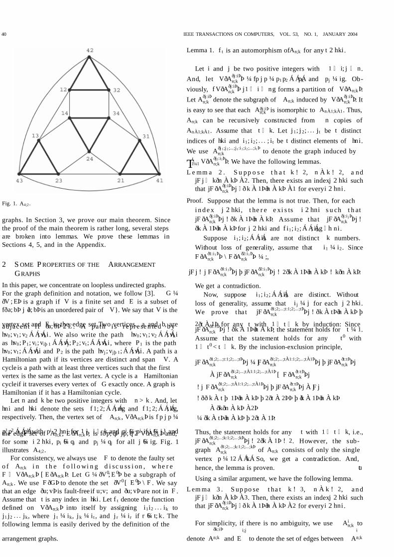
p1 p2 Á Á Á pk with pi 2 hni for 1 i k and pi 6¼ p j if i 6¼ j } andthe edge set of An;k , E ðAn;kÞ, is fð p; q Þ jp; q 2 V ðAn;kÞ and,for some i 2 hki , pi 6¼ q i and p j ¼ q j for all j 6¼ ig. Fig. 1illustrates A4;2.

For consistency, we always use F to denote the faulty seto f An;k i n t h e f o l l o wi n g d i sc u ss i on , w he r eF V ðAn;kÞ [ E ðAn;kÞ. Let G ¼ ðV 0; E 0Þ be a subgraph of An;k . We use F ðGÞ to denote the set ðV 0[ E 0Þ \ F . We saythat an edge ðu; vÞ is fault-free if u;v; and ðu; vÞare not in F .Assume that t is any index in hki . Let f t denote the functiondefined on V ðAn;kÞ into itself by assigning i1i2 . . . ik to j1 j2 . . . jk, where j t ¼ ik, j k ¼ i t , and j r ¼ ir if r 6¼ t; k . Thefollowing lemma is easily derived by the definition of the

arrangement graphs.

Lemma 1. f t is an automorphism of An;k for any t 2 hki .

Let i and j be two positive integers with 1 i; j n .And, let V ðAð j :iÞ

n;k Þ ¼ f p j p ¼ p1 p2 Á Á Á pk and p j ¼ ig. Ob-viously, f V ðAð j:iÞ

n;k Þ j1 i ng forms a partition of V ðAn;kÞ.Let Að j:iÞ

n;k denote the subgraph of An;k induced by V ðAð j :iÞn;k Þ. It

is easy to see that each Að j :iÞn;k is isomorphic to AnÀ1;kÀ1. Thus,

An;k can be recursively constructed from n copies of AnÀ1;kÀ1. Assume that t k. Let j 1; j 2; . . . j t be t distinctindices of hki and i1; i2; . . . ; i t be t distinct elements of hn i .We use Að j1 ;j 2 ;...;j t :i1 ;i2 ;... ;it Þ

n;k to denote the graph induced by

Ttl¼1 V ðAð j l :i lÞ

n;k Þ. We have the following lemmas.L e mm a 2 . S u pp o s e t h a t k ! 2, n À k ! 2, a nd

jF j kðn À kÞ À2. Then, there exists an indexj 2 hki suchthat jF ðAð j:iÞ

n;k Þj ðk À 1Þðn À kÞ À1 for everyi 2 hni .

Proof. Suppose that the lemma is not true. Then, for eachi n d e x j 2 hki , t he r e e xi s ts i 2 hni s u ch t h atjF ðAð j:iÞ

n;k Þj ! ðk À 1Þðn À kÞ. Assume that jF ðAð j :i j Þn;k Þj !

ðk À 1Þðn À kÞ for j 2 hki and f i1; i2; Á Á Á; ikg h ni .Suppose i1; i2; Á Á Á; ik are not distinct k numbers.

Without loss of generality, assume that i1 ¼ i2. SinceF ðAð1:i1Þ

n;k Þ \ F ðAð2:i1Þn;k Þ ¼ ;,

jF j ! j F ðAð1:i1Þn;k Þj þ jF ðAð2:i1Þ

n;k Þj ! 2ðk À 1Þðn À kÞ ! kðn À kÞ:

We get a contradiction.Now, suppose i1; i2; Á Á Á; ik are distinct. Without

loss of generality, assume that i j ¼ j for each j 2 hki .We p rove tha t jF ðAð1;2;... ;t:1;2;...;tÞ

n;k Þj ! ðk À tÞðn À kÞ þ

2ðt À 1Þ for any t with 1 t k by induction: SincejF ðAð1:1Þ

n;k Þj ! ðk À 1Þðn À kÞ, the statement holds for t ¼ 1.Assume that the statement holds for any t0 with1 t0 < t k. By the inclusion-exclusion principle,

jF ðAð1;2;...;t:1;2;... ;tÞn;k Þj ¼ jF ðAð1;2;... ;tÀ1:1;2;... ;tÀ1Þ

n;k Þj þ jF ðAðt :tÞn;k Þj

À jF ðAð1;2;...;tÀ1:1;2;... ;tÀ1Þn;k [ F ðAðt :tÞ

n;k Þj

! j F ðAð1;2;... ;tÀ1:1;2;...;tÀ1Þn;k Þj þ jF ðAðt:tÞ

n;k Þj À jF j

! ðð k À t þ 1Þðn À kÞ þ 2ðt À 2ÞÞ þ ðk À 1Þðn À kÞÀ ðkðn À kÞ À2Þ

¼ ðk À tÞðn À kÞ þ 2ðt À 1Þ:

Thus, the statement holds for any t with 1 t k, i.e.,jF ðAð1;2;... ;k:1;2;... ;kÞ

n;k Þj ! 2ðk À 1Þ ! 2. However, the sub-graph Að1;2;... ;k:1;2;... ;kÞ

n;k of An;k consists of only the singlevertex p ¼ 12 Á Á Ák. So, we get a contradiction. And,hence, the lemma is proven. tuUsing a similar argument, we have the following lemma.

L em ma 3 . S up po se t ha t k ! 3, n À k ! 2, a n djF j kðn À kÞ À3. Then, there exists an indexj 2 hki suchthat jF ðAð j:iÞ

n;k Þj ðk À 1Þðn À kÞ À2 for everyi 2 hni .

For simplicity, if there is no ambiguity, we use Ain;k to

denote Aðk:iÞ

n;k and E i;j

to denote the set of edges between Ain;k

40 IEEE TRANSACTIONS ON COMPUTERS, VOL. 53, NO. 1, JANUARY 2004

Fig. 1. A4;2 .



and A jn;k . Assume that I is any subset of f 1; 2; . . . ; ng. We

use AI n;k to denote the subgraph of An;k induced by

Si2 I V ðAin;kÞ. The following proposition follows directly

from the definition of the arrangement graphs.Proposition 1. Let i and j be two distinct elements of hn i .

1. jE i;j

j ¼ðnÀ2Þ!

ðnÀkÀ1Þ! .2. If ðu; vÞ and ðu0; v0Þ are distinct edges inE i;j , then

a. f u; vg \ f u0; v0g ¼ ; andb. ðu; u 0Þ 2 E ðAi

n;kÞ if and only if ðv; v0Þ 2 E ðA jn;kÞ.

Let u 2 V ðAin;kÞfor some i 2 hni . We use N I ðuÞ to denote

the set of all neighbors of u which are in AI n;k . Particularly,

we use N ÃðuÞ as an abbreviation of N hniÀf igðuÞ. We callvertices in N ÃðuÞ the outer neighbors of u. Obviously,jN f igðuÞj ¼ ðk À 1Þðn À kÞ and jN ÃðuÞj ¼ ðn À kÞ. We saythat u is adjacent to A j

n;k if u has an outer neighbor inA j

n;k . Then, we define the adjacent set AS ðuÞ of u as

f j j u is adjacent to A jn;kg. And, we have the followingproposition:Proposition 2. For n > k > 1, if u and v are two distinct vertices

in Ain;k with d ðu; vÞ 2, then AS ðuÞ 6¼ AS ðvÞ.

Proof. Let u ¼ u1u2 Á Á Áuk and v ¼ v1v2 Á Á Ávk. If d ðu; vÞ ¼1,there is an index j 2 hk À 1i such that u j 6¼ v j . Then,v j 2 AS ðuÞ, but v j 62 AS ðvÞ. The statement follows.

If d ðu; vÞ ¼2, there is a vertex w 2 V ðAin;kÞ such that

d ðu; wÞ ¼d ðv; wÞ ¼1. Let w ¼ w1w2 Á Á Áwk. And, let j 1 and j2 be two indices such that w j1 6¼ u j1 and v j2 6¼ w j2 .Obviously, j 1 6¼ j 2. Otherwise, d ðu; vÞ ¼1. So, w j1 is notin f u1; u2; Á Á Á; ukg but in f v1; v2; Á Á Á; vkg. By definition, w j1

is in AS ðuÞ but not in AS ðvÞ. Thus, the result alsofollows. tu

Let F be a faulty set. The good edge setGE i;j ðF Þ is the setof edges ðu; vÞ 2 E i;j such that f u;v; ðu; vÞg \ F ¼ ; . Then,we have following statement.Proposition 3. Let n > k > 3, n À k ! 2, I h n i , a nd

F V ðAn;kÞ [ E ðAn;kÞ. Then,

1. If jF ðAI n;kÞj kðn À kÞ À3, then jGE i;j ðF Þj ! 3 for

every i 6¼ j 2 I , and2. If jF ðAI

n;kÞj ¼kðn À kÞ À2, then there exists only oneði; j Þwith jGE i;j ðF Þj ¼2 if ði; j Þ is the only pair suchthat jGE i;j ðF Þj< 3.

Proof. First, consider that jF ðAI n;kÞj kðn À kÞ À3. Sup-

pose that jGE i;j ðF Þj< 3 for some i; j 2 hn i . SincejE i;j j ¼ ðn À 2Þ!=ðn À k À 1Þ! ! ð n À 2Þðn À kÞ ! kðn À kÞ,jF ðAf i;j g

n;k Þj> k ðn À kÞ À3. We get a contradiction.Now, consider that jF ðAI

n;kÞj ¼kðn À kÞ À2. If jI j 2,the statement follows. Assume that jI j 3. Suppose thatthere are two pairs f i; j g 6¼ f i0; j 0g such that jGE i;j ðF Þj< 3and jGE i

0;j 0ðF Þj< 3. If f i; j g \ f i0; j 0g ¼ ; , F ðAf i;j gn;k Þ \

F ðAf i0;j 0gn;k Þ ¼ ; and

jF ðAI n;kÞj ! ðjE i;j j À 2Þ þ ðjE i

0;j 0j À 2Þ> k ðn À kÞ À2:

So, f i; j g \ f i0; j 0g 6¼ ; . Assume that i ¼ i0 and j 6¼ j 0. LetV j ¼ f v 2 V ðAi

n;kÞ jv be adjacent to A jn;kg, V j0 ¼ f v 2

V ðAin;kÞ jv be adjacent to A j0

n;kg, and V V ¼ V j \ V j0. Then,

jF ðAI n;kÞj ! ðjE i;j j À 2Þ þ ðjE i;j

0j À 2Þ À jV V \ F j

! 2ðkðn À kÞ À2Þ À jV V \ F j:

So, jV V \ F j ¼ kðn À kÞ À2, i.e., F V V . Note that thenumber of faulty edges inside subgraphs do not affectthe number of fault-free edges between subgraphs.

However,

jV j À V V j ¼ jfv ¼ v1 Á Á Ávk j vk ¼ i; j 62 f v1; Á Á Á; vkÀ1g; j0 2 f v1; Á Á Á; vkÀ1ggj ¼ ðk À 1Þðn À 3Þ Á Á Á ðn À kÞ! ð k À 1Þðn À kÞ ! 4:

So, jGE i;j ðF Þj ! 4. We get a contradiction. Thus, there isonly one pair f i; j g such that jGE i;j ðF Þj< 3. Then,suppose that jGE i;j ðF Þj 1.

jF ðAI n;kÞj ! jE

i;jj À 1 ! kðn À kÞ À1:

So, jGE i;j ðF Þj ¼2. Hence, the statement follows. tu

Lemma 4. Suppose that

1. k ! 3 and n À k ! 2,2. I h ni with jI j ! 2,3. F V ðAn;kÞ [ E ðAn;kÞ, and4. Al

n;k À F is Hamiltonian connected for eachl 2 I andjF ðAI

n;kÞj kðn À kÞ À3.Then, for any x 2 V ðAi

n;kÞ and y 2 V ðA jn;kÞ with i 6¼ j 2 I ,

there is a Hamiltonian path of AI n;k À F joining x and y.

Proof. Since jF ðAI n;kÞj kðn À kÞ À3, by Proposition 3,jGE i1 ;i2 ðF Þj ! 3 for every i1 6¼ i2 2 I . We prove thislemma by induction on jI j. Suppose that jI j ¼ 2. Then,I ¼ f i; j g for some i; j . Since jGE i;j ðF Þj ! 3, there existsan edge ðu; vÞ 2 GE i;j ðF Þ such that u 6¼ x 2 V ðAi

n;kÞ andv 6¼ y 2 V ðA j

n;kÞ. Then, by assumption that each Aln;k À F

is Hamiltonian connected, there is a Hamiltonian path P 1of Ai

n;k À F from x to u and a Hamiltonian path P 2 of A j

n;k À F from v to y. Thus, hx; P 1;u;v;P 2; yi forms aHamiltonian path of AI

n;k À F from x to y.Now, assume that the lemma is true for all I 0 with

2 j I 0j < I . Thus, there is an i0 2 I with i0 6¼ i; j . Since

jGE i0;j ðF Þj ! 3, we can find an edge ðu; vÞ 2 GE i

0;j ðF Þ

with u 2 V ðAi0

n;kÞ and v 6¼ y 2 V ðA jn;kÞ. Then, there is a

Hamiltonian path P 1 of AI Àf jgn;k À F from x to u and a

Hamiltonian path P 2 of A jn;k À F from v to y. Thus,

hx; P 1;u;v;P 2; yi forms a Hamiltonian path of AI n;k À F

from x to y. tuThe following lemma is proven by Ore [13].

Lemma 5. A graph G is Hamiltonian if G has at least C nÀ12 þ 2

edges and Hamiltonian connected if G has at least C nÀ12 þ 3

edges.Lemma 6. Assume that n ! 3. Then, K n is ðn À 3Þ-fault

Hamiltonian and ðn À 4Þ-fault Hamiltonian connected.

HSU ET AL.: FAULT HAMILTONICITY AND FAULT HAMILTONIAN CONNECTIVITY OF THE ARRANGEMENT GRAPHS 41



Proof. Let F ¼ F v [ F e for F v V ðK nÞand F e E ðK n Þsuchthat jF j n À i for i ¼ 2 or 3. Then, K n À F is isomorphicto K nÀjF vj À F 0 for some F 0 E ðK nÀjF vjÞ with jF 0j j F ej.So, the number of edges in K nÀjF vj À F 0 is at leastC nÀjF vjÀ1

2 þ i. Hence, the proof of this lemma followsfrom Lemma 5. tu

3 MAIN THEOREM

Lemma 7. Let G ¼ ðV ; E Þ be a loopless undirected graph and be the minimum degree of G. Then, G is at most À 2 Hamiltonian if ! 2 and À 3 Hamiltonian connected if ! 3.

Proof. Let u 2 V ðGÞ be a vertex of degree . Removingð À 1Þedges connecting to u results in the isolation of u.Clearly, the remaining graph is not Hamiltonian. Then,consider removing ð À 2Þedges which connect to u. Letv1 and v2 be the remaining vertices connecting to u. Since ! 3, jV ðGÞj ! 4. Thus, it is impossible that there is aHamiltonian path in the remaining graph between v1 and

v2 since u connects to only v1 and v2. Hence, the lemmafollows. tuTheorem 1. Let n and k be two positive integers withn À k ! 2.

Then, An;k is kðn À kÞ À2 Hamiltonian and kðn À kÞ À3 Hamiltonian connected.

Proof. Our proof is by induction on k. However, the proof of the induction is rather long. We break the whole proof into lemmas and prove them in the following sections.

The induction bases are An;1 and An;2. Since An;1 is K n , by Lemma 6, the theorem is true for An;1. The case of An;2

is stated in the following lemma and its proof is in theAppendix.

Lemma 8. An;2 is 2ðn À 2Þ À2 Hamiltonian and 2ðn À 2Þ À3 Hamiltonian connected if n ! 4.

We use the following two lemmas in the inductionsteps for the cases k ! 3:

Lemma 9. Suppose that,for somek ! 3 and n À k ! 2, AnÀ1;kÀ1 isðk À 1Þðn À kÞ À2 Hamiltonian and ðk À 1Þðn À kÞ À3 Ha-miltonian connected. Then,An;k is kðn À kÞ À2 Hamiltonian.

Lemma 10. Suppose that, for some k ! 3 and n À k ! 2,AnÀ1;kÀ1 is ðk À 1Þðn À kÞ À2 Hamiltonian and ðk À 1Þðn ÀkÞ À3 Hamiltonian connected. Then, An;k is kðn À kÞ À3 Hamiltonian connected.

The proofs of the two lemmas are in Sections 4 and 5,respectively. With these lemmas, the theorem isproven. tu

Hence, our results are optimal.

4 P ROOF OF LEMMA 9Assume that F is any faulty set of An;k withjF j kðn À kÞ À2. By Lemma 2, there exists an index j 2hki such that jF ðAð j :iÞ

n;k Þj ðk À 1Þðn À kÞ À1 for everyi 2 hni . By Lemma 1, we may assume that j ¼ k. So,jF ðAi

n;kÞj ðk À 1Þðn À kÞ À1 for every i 2 hn i . Without loss

of generality, we further assume that

jF ðA1n;kÞj ! jF ðA2

n;k Þj ! ÁÁ Á ! jF ðAnn;kÞj:

For convenience, we use N ÃF ðuÞ to denote the set of outerneighbors of u in An;k À F , i .e. , N ÃF ðuÞ ¼ fv j ðu; vÞ 2E ðAn;k Þ ÀF and v 2 N ÃðuÞ ÀF g.

Case 1: jF ðA1n;kÞj ðk À 1Þðn À kÞ À3. Then, by induction

hypothesis, Ain;k À F is still Hamiltonian connected for

every i 2 hni . Consider two subcases:Subcase 1.1: jGE i;j ðF Þj ! 3 for every i 6¼ j 2 hni . If F ¼ ; ,

the lemma follows. If F 6¼ ; , there is an index i such thatjF ðA1

n;kÞj þ Pl6¼i jE i;l \ F j ! 1. Obviously, there are twodistinct indices, j and l, for j; l 6¼ i such that jGE i;j ðF Þj ! 3and jGE i;lðF Þj ! 3. Thus, we can find two edges ðu; xÞ 2GE i;j ðF Þ and ðv; yÞ 2 GE i;lðF Þ such that u 6¼ v 2 V ðAi

n;kÞ,x 2 V ðA j

n;kÞ, and y 2 V ðAln;kÞ. Then, there is a Hamiltonian

path P 1 of Ain;k À F from u to v and, by Lemma 4, there is a

Hamiltonian path P 2 of Ahn iÀf ign;k À F from y to x. Therefore,

hu; P 1;v;y;P 2;x ;u i is a Hamiltonian cycle of An;k À F .Subcase 1.2: jGE i;j ðF Þj< 3 for some i 6¼ j 2 hn i . By

Proposition 3, there is only one pair i; j with jGE i;j ðF Þj ¼

2 and jGE i0;j 0

ðF Þj ! 3 for any f i0

; j0

g 6¼ f i; j g. So, we can findtwo edges, ðu; xÞ 2 GE i;j ðF Þand ðv; yÞ 2 GE i;lðF Þ, such thatu 6¼ v 2 V ðAi

n;kÞ, x 2 V ðA jn;kÞ, and y 2 V ðAl

n;kÞ for l 6¼ i; j .Then, there is a Hamiltonian path P 1 of Ai

n;k À F from u to vand, by Lemma 4, there is a Hamiltonian path P 2 of Ahn iÀf ig

n;k À F from y to x. Therefore, hu; P 1;v;y;P 2;x ;u i is aHamiltonian cycle of An;k À F . See Fig. 2 for an illustration.

Case 2: jF ðA1n;kÞj ¼ ðk À 1Þðn À kÞ À2. So, A1

n;k À F is stillHamiltonian. Let C be a Hamiltonian cycle of A1

n;k À F .Consider two cases:

Subcase 2.1: jF ðA2n;kÞj< ðk À 1Þðn À kÞ À2. Then, Ai

n;k ÀF is still Hamiltonian connected for every i 2 hni À f 1g.Since there are at most ðn À kÞ faults outside A1

n;k and

jV ðA1n;kÞ ÀF j ! ð n À 1Þðn À 2Þ À ðk À 1Þðn À kÞ þ 2

! ð n À 1 À k þ 1Þðn À 2Þ ! 3ðn À kÞ;

there exists a vertex u on C such that N ÃF ðuÞ ¼N ÃðuÞ.Consider the two neighbors of u on C , say v and v0.Clearly, jN ÃF ðvÞ [ N ÃF ðv0Þj ! 1. Thus, we may assume thatthere is an edge ðv; yÞ 2 GE 1;iðF Þ for some i 2 hni À f 1g.(If N ÃF ðvÞ ¼ ;, we use v0 in place of v.) Then, there is anedge ðu; xÞ 2 GE 1;j ðF Þ with j 6¼ i since N ÃF ðuÞ ! 2. SincejF ðAhniÀf 1g

n;k Þj< k ðn À kÞ À2, by Lemma 4, there is a Hamil-tonian path hx; P 1; yi of Ahn iÀf 1g

n;k À F between x and y. LetC ¼ hu;v;P 2; v0; ui . Then, hu;x;P 1;y;v;P 2; v0; ui forms aHamiltonian cycle of An;k À F . See Fig. 3a for an illustration.

Subcase 2 .2 : jF ðA2n;kÞj ¼ ðk À 1Þðn À kÞ À2. T hen ,

n ¼ 5, k ¼ 3, and no fault is outside A15;3 and A2

5;3.So, A2

5;3 À F is still Hamiltonian and A35;3 À F , A4

5;3 À F ,and A5

5;3 À F are Hamiltonian connected. Let C 2 be aHamiltonian cycle of A2

5;3 À F . Since jGE 1;2ðF Þj ! 2, letðu; vÞ 2 GE 1;2ðF Þ for some u 2 V ðA1

5;3Þ and v 2 V ðA25;3Þ.

And, let C ¼ hu; u 0; P 1; u00; ui and C 2 ¼ hv; P 2; v0; vi . SinceN Ãðv0Þ ¼2, there exists ðv0; yÞ 2 GE 2;iðF Þ for some y 2V ðAi

5;3Þ with i 6¼ 1. By Proposition 2, AS ðu0Þ 6¼ AS ðu00Þand then jAS ðu0Þ [ AS ðu00Þj ! 3. So, we can assumethat there exists ðu0Þ 2 GE 1;j ðF Þ for some x 2 V ðA j

5;3Þ

with j 6¼ 2; i . By Lemma 4, there is a Hamiltonian




path hy; P 3; xi of Af 3;4;5g5;3 between x and y. So,

hu;v;P 2 ; v0;y ;P 3;x ;u0; P 1; u00; ui forms a Hamiltonian cycleof A5;3 À F . See Fig. 3b for an illustration.

Case 3: jF ðA1n;kÞj ¼ ðk À 1Þðn À kÞ À1. Then, there are at

most ðn À kÞ À1 faults outside A1n;k . So, jF ðA

in;kÞj ðn ÀkÞ À1 2ðn À kÞ À3 ð k À 1Þðn À kÞ À3 f o r e v er y i 2

hni À f 1g and, by induction hypothesis, Ain;k À F is still

Hamiltonian connected. Let f 2 F ðA1n;kÞ. f is either a vertex

or an edge. Since jF ðA1n;kÞ Àf j ¼ ðk À 1Þðn À kÞ À2, there is

a Hamiltonian cycle C of A1n;k À ðF À f Þ. Then, we consider

the following three cases:

1. f isnoton C .Let u; v be any two adjacent vertices on C .2. f is an edge on C . Let u; v be the two vertices linked

by f .3. f is a vertex on C . Let u; v be the two vertices which

are adjacent to f on C .

Thus, we have a Hamiltonian path hu; P 1; vi of A1n;k À F .Since jN ÃðuÞj ¼ jN ÃðvÞj ¼ ðn À kÞ and

jAS ðuÞ [ AS ðvÞj ¼n À k þ 1;

there must exist two edges ðu; xÞ 2 GE 1;iðF Þ and ðv; yÞ 2GE 1;j ðF Þ with i 6¼ j 2 hni À f 1g. By Lemma 4, there is aHamiltonian path hy; P 2; xi of Ahn iÀf 1g

n;k between x and y. So,hu; P 1;v;y;P 2;x ;u i is a Hamiltonian cycle of An;k À F . SeeFig. 4 for an illustration

This completes the induction proof. And, hence, thelemma follows. tu

5 P ROOF OF LEMMA 10Assume that F is any faulty set of An;k withjF j kðn À kÞ À3. By Lemma 3, there exists an index j 2 hki such that jF ðAð j :iÞ

n;k Þj ðk À 1Þðn À kÞ À2 for everyi 2 hn i . By Lemma 1, we may assume that j ¼ k. So,jF ðAi

n;kÞj ðk À 1Þðn À kÞ À2 for every i 2 hn i . Without

l os s o f g en er al it y, w e f ur th er a ss um e t ha tjF ðA1n;kÞj ! jF ðA2

n;kÞj ! ÁÁ Á ! jF ðAnn;kÞj. Let x 2 Ai

n;k and y 2A j

n;k with i; j 2 hni be two arbitrary vertices. We shallconstruct a Hamiltonian path of An;k À F between x and y.For convenience, again we use N ÃF ðuÞ to denote the set of outer neighbors of u in An;k À F , i.e., N ÃF ðuÞ ¼ fv j ðu; vÞ 2E ðAn;k Þ ÀF and v 2 N ÃðuÞ ÀF g.

Case 1: jF ðA1n;kÞj ðk À 1Þðn À kÞ À3. Then, by induction

hypothesis, Ain;k À F is still Hamiltonian connected for

every i 2 hni . Consider two subcases:Subcase 1.1: i 6¼ j . Since jF j kðn À kÞ À3, by Lemma 4,

there is a Hamiltonian path of An;k À F joining x to y.Subcase 1.2: i ¼ j . By induction hypothesis, there is a

Hamiltonian path P of Ain;k À F from x to y. Let l be thenumber of vertices on P . Then,

l ¼ðn À 1Þ!ðn À kÞ!

À jF \ V ðAin;kÞj ! ðn À 1Þðn À 2Þ À jF ðA1

n;kÞj

! ð n À 1Þk À ðk À 1Þðn À kÞ þ 3

! kðn À 1Þ Àkðn À kÞ ¼kðk À 1Þ ! 2k:

We claim that there exist two adjacent vertices u and v on P such that jN ÃF ðuÞj ! 1 and jN ÃF ðvÞj ! 2. Suppose that thestatement is false. Then, for every two adjacent vertices u0

and v0 on P , jN ÃF ðu0Þj þ jN ÃF ðv0Þj max f 2; n À kg ¼ n À k.Thus, jF j ! b l=2cðn À kÞ ! kðn À kÞ. We get a contradiction.Therefore, there exist two neighbors a and b of u and v,respectively, such that ðu; a Þ 2 GE i;i0ðF Þ and ðv; bÞ 2GE i;j

0ðF Þ with i0 6¼ j 0 2 hni À f ig. Since jF j kðn À kÞ À3,

by Lemma 4, there is a Hamiltonian path ha; P 1; bi of Ahn iÀf ig

n;k À F . The Hamiltonian path P of Ain;k À F can be

written as hx; P 2;u;v;P 3; yi for some subpaths P 1 and P 2.Then, hx; P 2;u;a;P 1;b;v;P 3; yi is a Hamiltonian path of An;k À F from x to y. See Fig. 5 for an illustration.

Case 2: jF ðA1n;kÞj ¼ ðk À 1Þðn À kÞ À2. So, A1

n;k À F is stillHamiltonian and there are at most ðn À kÞ À1 faults outsideA1

n;k . Let C be a Hamiltonian cycle of A1n;k À F . Now,

consider the following four subcases:


Fig. 2. Lemma 9, case 1.

Fig. 3. Lemma 9, subcase 2.1 and subcase 2.2.





2. None of N ÃðuÞ and N ÃðvÞ is f x; yg. Then, there is anindex i0 2 AS ðuÞ [ AS ðvÞ such that i0 62 f 1; i ; j g. As-sume that there is an edge ðu; a Þ 2 GE 1;i0ðF Þfor somea 2 V ðAi0

n;kÞ. Consider N ÃF ðvÞ. Suppose that there is anouter neighbor b of v in Ai

n;k or A jn;k . We may assume

that b 2 V ðAin;kÞ. Then, there is a Hamiltonian path

hx; P 2; bi of Ain;k À F and a Hamiltonian path ha; P 3; yiof Ahn iÀf 1;ig

n;k À F . And, we have a Hamiltonian pathhx; P 2;b;v;P 1;u;a;P 3; yi of An;k À F . Suppose thatthere is no outer neighbor of v in Ai

n;k or A jn;k . Since

jAS ðvÞj ! 2 and i; j 62 AS ðvÞ, there is an edge ðv; bÞ 2GE 1;j 0ðF Þ for some b 2 V ðA j0

n;kÞ with j 0 62 f 1; i ; j ; i 0g.Then, there is a Hamiltonian path hx; P 2; bi of Af i;j 0g

n;k ÀF and a Hamiltonian path ha; P 3 ; yi of Ahn iÀf 1;i;j 0g

n;k À F .So, hx; P 2;b;v;P 1 ;u;a;P 3; yi is a Hamiltonian path of An;k À F . See Fig. 8b for an illustration.

Hence, the lemma follows. tu

6 CONCLUSION AND DISCUSSION

There are many studies concerning fault-tolerant Hamilto-nicity and fault-tolerant Hamiltonian connectivity. We findthat the current results on the arrangement graphs [8], [9]are not optimal. In this paper, we obtain an optimal resultthat the arrangement graph An;k for n À k ! 2 is ðkðn À kÞ À2Þ-Hamiltonian and ðkðn À kÞ À3Þ-Hamiltonian connected.For the case n À k ¼ 1, since An;n À1 is isomorphic to ann-dimensional star graph which is bipartite, it cannottolerate any vertex fault as far as fault Hamiltonicity andfault Hamiltonian connectivity are concerned.

In order to establish the fault-tolerant Hamiltonianproperty, we find that it is difficult to construct a fault-free Hamiltonian cycle directly. Therefore, we propose anew idea for proving this result. We propose to use faultHamiltonian connectivity as a tool to attack the faultHamiltonicity of the arrangement graph. We prove that itis f fault-tolerant Hamiltonian by simultaneously proving itis f À 1 fault-tolerant Hamiltonian connected. This strategymakes the proof tractable and systematic. It would be usefulto apply this strategy to other interconnection networks forthe same type of problems.

APPENDIX

P ROOF OF LEMMA 8In this section, we concentrate our discussion on An;2. Asthe degree of An;2 is relatively larger than that of An;k fork ! 3, it can tolerate more faults. This makes the proof complex and we must use some special properties of An;2.In fact, when n is small, such as 4; 5; 6, the resource (vertices

or edges) which we can use is few. To prove these cases isvery tedious. With a long and detailed discussion, we havecompleted the theoretical proof for a small value of n(n ¼ 4; 5; 6). Nevertheless, we do not present them in thispaper for reducing complexity. However, we can also verifythese small cases directly using the computer by translatingthe original proof into a program.

Now, we give a quick view of An;2 and then present someof its special properties. An;2 consists of nðn À 1Þ verticesand nðn À 1Þðn À 2Þ edges. Indeed, it admits a vertexdecomposition into n subgraphs, each isomorphic to K nÀ1.Each vertex is labeled by a 2-digit string and, clearly,connects to 2ðn À 2Þneighbors, where half of them are outer

neighbors. So, AS ðuÞ ¼n À 2 and there is only one sub-graph not adjacent to u for any vertex u 2 V ðAn;2Þ. (Recallthat AS ðuÞ is the adjacent set of u.) On the other hand,jE i;j j ¼ n À 2 for any i; j 2 hn i , so there is only one vertex inAi

n;2 not adjacent to A jn;2. These two properties are important

for our proof. In the following, we first show two usefulpropositions. Then, we divide the proof of Lemma 8 intotwo parts: first for Hamiltonicity and second for Hamilto-nian connectivity.

Given any F V ðAn;2Þ [ E ðAn;2Þ, by Lemma 1, we mayassume that

maxi2hn i

fj F ðA1:in;2Þg ! jF ðA1

n;2Þj ! j F ðA2n;2j ! Á Á Á ! jF ðAn

n;2Þj:


Fig. 6. Lemma 10, subcase 2.1 and subcase 2.2.

Fig. 7. Lemma 10, subcase 2.3.



Recall that Ain;2 is the abbreviation of A2:i

n;2. So, we have thefollowing proposition:Proposition 4 (Fault distribution in An;2). Let F

V ðAn;2Þ [ E ðAn;2Þ with jF j 2n À 6 and

maxi2hn i

fj F ðA1:in;2Þjg ! jF ðA1

n;2Þj ! jF ðA2n;2j ! Á ÁÁ ! jF ðAn

n;2Þj:

Then, jF ðA1n;2Þj n À 3. In other words,

jF ðA2n;2Þj j F j À 2jF ðA1

n;2Þj þ 2:

Proof. Let j be the index such that

jF ðA1: jn;2Þj ¼max

i2hnifj F ðA1:i

n;2Þjg:

Suppose that jF ðA1n;2Þj ! n À 2. The intersection of

A1: jn;2 and A1

n;2 contains only the vertex j 1 for j 6¼ 1 or

is empty for j ¼ 1, so jF ðA1: jn;2Þ \ F ðA1n;2Þj 1. Thus,jF j ! j F ðA1: j

n;2Þj þ jF ðA1n;2Þj À1 ! 2n À 5, which contra-

dicts the given condition. So, jF ðA1n;2Þj n À 3.

Then, consider jF ðA2n;2Þj. Let l ¼ jF ðA1

n;2Þj. SincejF ðA1: j

n;2Þ \ F ðA2n;2Þj 1,

F ðA2n;2Þ j F j À jF ðA1: j

n;2Þ [ F ðA1n;2Þ ÀF ðA2

n;2Þj

j F j À ð2l À 1Þ þ jF ðA1: jn;2Þ \ F ðA2

n;2Þj

þ j F ðA1n;2Þ \ F ðA2

n;2Þj

j F j À ð2l À 1Þ þ 1 þ 0 ¼ jF j À 2l þ 2:

Hence, the statement follows. tu

The following proposition uses a method similar to thatused in Lemma 4 which helps us to construct a Hamiltonianpath between any two given vertices in a given index set I of subgraphs of An;2. Notice that all subgraphs of An;2 areisomorphic to K nÀ1, which is ðn À 3ÞHamiltonian and ðn À4ÞHamiltonian connected. For convenience, we introduce anew notation, EF ðAi

n;2Þ, called extended faulty set of Ain;2.

EF ðAin;2Þ is defined to be the set F ðAi

n;2Þ þ Pl6¼iðE i;l \ F Þ.

Lemma 11. Let F V ðAn;2Þ [ E ðAn;2Þand I h ni with n ! 7

and jI j ! 2. Let x 2 V ðAin;2Þand y 2 V ðA j

n;2Þwith i 6¼ j 2 I .Then, there is a Hamiltonian pathof AI

n;2 À F betweenx and y if

jF ðAI n;2Þj n À 7 þ j I j and jF ðA

ln;2Þj n À 5 for eachl 2 I .

Proof. Since each subgraph of An;2 is isomorphic to K nÀ1, bythe givencondition, Al

n;2 À F contains at least four verticesand, by Lemma 6, is still Hamiltonian connected for eachl 2 I . We prove this proposition by induction on jI j:

Case 1: jI j ¼ 2. Then, I ¼ f i; j g and jF j n À 5. SincejE i;j j ¼ n À 2, jGE i;j ðF Þj ! 3. There is an edge ðu; vÞ 2GE i;j ðF Þ for u 6¼ x 2 V ðAi

n;2Þ and v 6¼ y 2 V ðA jn;2Þ. Since

Ain;2 À F and A j

n;2 À F are still Hamiltonian connected,there are a Hamiltonian path hx; P 1; ui of Ai

n;2 À F and aH a mi l t o ni a n p a t h hv; P 2; yi of A j

n;2 À F . T hu s ,hx; P 1;u;v;P 2; yi forms a Hamiltonian path of AI

n;2 À F between x and y.

Case 2: jI j ¼ d ! 3. Assume that, for any I 0 h ni with2 j I 0j < d , the statement is true. Consider the followingtwo cases:

Subcase 2.1: jF ðAI Àf i;j gn;2 Þj n þ d À 8. Without loss

of generality, assume that jEF ðAin;2Þj ! jEF ðA j

n;2Þj.Thus , jF ðAI Àf ig

n;2 Þj ¼ jF ðAI n;2Þj À jEF ðAi

n;2Þj n þ d À 8.(Remember that jF ðAI

n;2Þj n þ d À 7.) Since jF ðAin;2Þj

n À 5 and jE i;l j ¼ n À 2 for l 6¼ i, there is an index i0 6¼ jsuch that jGE i;i

0ðF Þj ! 2. Otherwise, jGE i;i

0ðF Þj 1 for

all i0 6¼ i; j and

jEF ðAin;2Þj ¼ jF ðAi

n;2Þj þ Xl6¼i

ðE i;l \ F Þ

! n À 5 þ ðn À 3 À ðn À 5ÞÞ Ã ðd À 2Þ> n þ d À 7

for d ! 3 which gives a contradiction. Thus, there isan edge ðu; vÞ 2 GE i;i

0ðF Þ for u 6¼ x 2 V ðAin;2Þ and

v 2 V ðAi0n;2Þ. Since Ain;2 À F is Hamiltonian connected,

there are a Hamiltonian path hx; P 1; ui of it and, byinduction hypothesis, a Hamiltonian path hv; P 2; yi of AI Àf ig

n;2 À F . So, the path hx; P 1;u;v;P 2; yi forms a Hamil-tonian path of AI

n;2 between x and y.S ub ca s e 2 .2 : jF ðAI Àf i;j g

n;2 Þj ¼n þ d À 7. Th en ,jEF ðAi

n;2Þj ¼ jEF ðA jn;2Þj ¼0. If I ¼ f i;j;i 0g, i.e., d ¼ 3,

then jF ðAi0

n;2Þj ¼n À 4, which contradicts the givencondition. So, jI j ¼ d ! 4. Since n ! 7, there is an indexi0 2 I À f i; j g such that jEF ðAi0

n;2Þj ! 2. So,

F AI Àf i;i 0gn;2 n þ d À 9:





However, jF ðAf i;i 0gn;2 Þj n À 5. So, jGE i;i

0ðF Þj ! 3 and thenthere are two edges, ðu; u 0Þ; ðv; v0Þ 2 GE i;i

0ðF Þ, where

u; v 2 V ðAin;2Þ and u0; v0 2 V ðAi0

n;2Þ such that u; v 6¼ x. Let j0 62 f i; i 0; jg. Since jGE i;j

0ðF Þj ! 3, there is an edgeða; bÞ 2 GE i;j

0ðF Þ, where a 2 V ðAi

n;2Þ and b 2 V ðA j0

n;2Þ À

F such that a 6¼ x; u . Note that v and a can be the samevertex. Since Ai

n;2 À f v; ag is still Hamiltonian connected,there is a Hamiltonian path hx; P 1; ui of Ai

n;2 À f v; ag.Since Ai0

n;2 À F is Hamiltonian connected, there is aHamiltonian path hu0; P 2; v0i of it. By induction hypoth-esis, there is a Hamiltonian path hb; P 3; yi of AI Àf i;i 0g

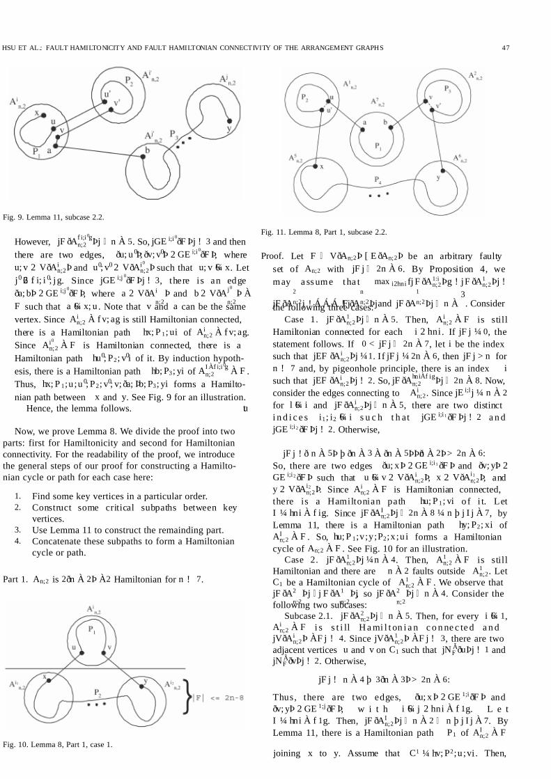
n;2 À F .Thus, hx; P 1;u ;u 0; P 2; v0; v; ða; Þb; P 3; yi forms a Hamilto-nian path between x and y. See Fig. 9 for an illustration.


Now, we prove Lemma 8. We divide the proof into twoparts: first for Hamiltonicity and second for Hamiltonianconnectivity. For the readability of the proof, we introducethe general steps of our proof for constructing a Hamilto-nian cycle or path for each case here:

1. Find some key vertices in a particular order.2. Construct some critical subpaths between key

vertices.3. Use Lemma 11 to construct the remainding part.4. Concatenate these subpaths to form a Hamiltonian

cycle or path.

Part 1. An;2 is 2ðn À 2Þ À2 Hamiltonian for n ! 7.

Proof. Let F V ðAn;2Þ [ E ðAn;2Þ be an arbitrary faultyset of An;2 with jF j 2n À 6. By Proposition 4, wemay a ss ume t ha t max i2hn i fj F ðA1:i

n;2Þg ! jF ðA1n;2Þj !

jF ðA2

n;2j ! Á Á Á ! jF ðAnn;2Þjand jF ðA

1

n;2Þj n À3. Considerthe following three cases:

Case 1. jF ðA1n;2Þj n À 5. Then, Ai

n;2 À F is stillHamiltonian connected for each i 2 hni . If jF j ¼ 0, thestatement follows. If 0 < jF j 2n À 7, let i be the indexsuch that jEF ðAi

n;2Þj ¼1. If jF j ¼ 2n À 6, then jF j > n forn ! 7 and, by pigeonhole principle, there is an index isuch that jEF ðAi

n;2Þj ! 2. So, jF ðAhn iÀf ign;2 Þj 2n À 8. Now,

consider the edges connecting to Ain;2. Since jE i;l j ¼ n À 2

for l 6¼ i and jF ðAin;2Þj n À 5, there are two distinct

i n d i c e s i1; i2 6¼ i s u c h t h at jGE i;i 1 ðF Þj ! 2 a n djGE i;i 2 ðF Þj ! 2. Otherwise,

jF j ! ð n À 5Þ þ ðn À 3 À ðn À 5ÞÞðn À 2Þ> 2n À 6:So, there are two edges ðu; xÞ 2 GE i;i1 ðF Þ and ðv; yÞ 2GE i;i 2 ðF Þ such that u 6¼ v 2 V ðAi

n;2Þ, x 2 V ðAi1n;2Þ, and

y 2 V ðAi2n;2Þ. Since Ai

n;2 À F is Hamiltonian connected,there is a Hamiltonian path hu; P 1; vi of i t. LetI ¼ hni À f ig. Since jF ðAI

n;2Þj 2n À 8 ¼ n þ j I j À 7, byLemma 11, there is a Hamiltonian path hy; P 2; xi of AI

n;2 À F . So, hu; P 1;v;y;P 2;x ;u i forms a Hamiltoniancycle of An;2 À F . See Fig. 10 for an illustration.

Case 2. jF ðA1n;2Þj ¼n À 4. Then, A1

n;2 À F is stillHamiltonian and there are n À 2 faults outside A1

n;2. LetC 1 be a Hamiltonian cycle of A1

n;2 À F . We observe thatjF ðA2

n;2Þj j F ðA1

n;2Þj, so jF ðA2

n;2Þj n À 4. Consider the

following two subcases:Subcase 2.1. jF ðA2

n;2Þj n À 5. Then, for every i 6¼ 1,Ai

n;2 À F i s s t i ll H a mi l t on i a n c o n ne c te d a n djV ðAi

n;2Þ ÀF j ! 4. Since jV ðA1n;2Þ ÀF j ! 3, there are two

adjacent vertices u and v on C 1 such that jN ÃF ðuÞj ! 1 andjN ÃF ðvÞj ! 2. Otherwise,

jF j ! n À 4 þ 3ðn À 3Þ> 2n À 6:

Thus, there are two edges, ðu; x Þ 2 GE 1;iðF Þ andðv; yÞ 2 GE 1;j ðF Þ, w i t h i 6¼ j 2 hni À f 1g. L e tI ¼ hni À f 1g. Then, jF ðAI

n;2Þj n À 2 n þ j I j À 7. ByLemma 11, there is a Hamiltonian path P 1 of AI

n;2 À F

joining x to y. Assume that C 1 ¼ hv; P 2;u ;vi . Then,



Fig. 10. Lemma 8, Part 1, case 1.

Fig. 11. Lemma 8, Part 1, subcase 2.2.



hu;x;P 1;y;v;P 2; ui forms a Hamil tonian cyc le o f An;2 À F .

Subcase 2.2. jF ðA2n;2Þj ¼n À 4. So, A2

n;2 À F is still

Hamiltonian andAi

n;2 is Hamiltonian connected forevery i 2 hn i À f 1; 2g. Let C 2 be a Hamiltonian cycle of A2

n;2 À F . Clearly, there are at most two faults outsideAf 1;2g

n;2 and, so, there are at least three indices is suchthat jF ðAi

n;2Þj þ jE 1;i \ F j þ j E 2;i \ F j ¼ 0. Assume that4; 5; 7 are such indices. Since jV ðA1

n;2 À F Þj ! 3 andjV ðA2

n;2 À F Þj ! 3, jGE 1;7ðF Þj ! 2 and jGE 2;7ðF Þj ! 2.There are two vertices a 6¼ b in A7

n;2 such that ðu; a Þ 2GE 1;7ðF Þ and ðv; bÞ 2 GE 2;7ðF Þ for some u 2 V ðA1

n;2Þand v 2 V ðA2

n;2Þ. Clearly, there is a Hamiltonian pathP 1 of A7

n;2 joining b to a. Consider the two neighbors of

u on C 1. There must be one of them adjacent to A5n;2.Let u0 be such a vertex and ðu0; xÞ 2 E 1;5 for somex 2 V ðA5

n;2Þ. Obviously, ðu1; xÞ 2 GE 1;5ðF Þ. Similarly,there is a vertex v0 adjacent to v on C 2 and an edgeðv0; yÞ 2 GE 2;6ðF Þ f or s ome y 2 V ðA6

n;2Þ. Let C 1 ¼hu; P 2 ; u0; ui and C 2 ¼ hv; v0; P 3; vi , respectively. LetI ¼ hni À f 1; 2; 7g. Then jF ðAI

n;2Þj 2 n þ j I j À 7. ByLemma 11, there is a Hamiltonian path P 4 of AI

n;2 À F joining x to y. Thus, hu; P 2; u0;x ;P 4;y ;v0; P 3;v;b;P 1 ;a ;u iforms a Hamiltonian cycle of An;2 À F . See Fig. 11 foran illustration.

Case 3. jF ðA1n;2Þj ¼n À 3. Then, A1

n;2 À F may not beHamiltonian. However, similar to Case 3 of Lemma 9,there is a Hamiltonian path hu; P 1; vi of A1

n;2 À F for somevertices u; v 2 V ðA1

n;2Þ ÀF . By Proposition 4, jF ðA2n;2Þj

2n À 6 À 2ðn À 3Þ þ 2 ¼ 2 n À 5 for n ! 7 and, then,Ai

n;2 À F are Hamiltonian connected for each i 6¼ 1. SincejN ÃðuÞj ¼ jN ÃðvÞj ¼n À 2, jN ÃF ðuÞj ! 1 and jN ÃF ðvÞj ! 2.Otherwise,

jF j ! n À 3 þ max f n À 2; 2ðn À 3Þg> 2n À 6:

So, there exist two edges ðu; xÞ 2 GE 1;iðF Þ andðv; yÞ 2 GE 1;j ðF Þ w i t h i 6¼ j 2 hni À f 1g. S i n c e

jF ðAhn iÀf 1g

n;2 Þj n À 3, byLemma 11,thereis a Hamiltonian

path hy; P 2; xi of Ahn iÀf 1gn;2 À F . So , hu; P 1;v;y;P 2;x ;u i

forms a Hamiltonian path of An;2 À F .This completes the proof of Part 1. tu

Part 2. An;2 is 2ðn À 2Þ À3 Hamiltonian connected forn ! 7.Proof. Let F V ðAn;2Þ [ E ðAn;2Þbe an arbitrary faulty set of

An;2 with jF j 2n À 7. By Proposition 4, we may assumethat

maxi2hn i

fj F ðA1:in;2Þg ! jF ðA1

n;2Þj ! jF ðA2n;2j ! ÁÁ Á ! jF ðAn

n;2Þj

and jF ðA1n;2Þj n À 3. Let x 2 V ðAi

n;2Þand y 2 V ðA jn;2Þfor

some i; j 2 hni . We claim that there is a Hamiltonian pathof An;2 À F from x to y. Consider the following cases:

Case 1. jF ðA1n;2Þj n À 5. Then, for every i 2 hn i ,

Ain;2 À F i s H a m i l t o n i a n c o n n e c t e d a n d

jV ðAin;2Þ ÀF j ! 4. Consider the following two subcases:

Subcase 1.1. i 6¼ j . By Lemma 11, there is a Hamilto-nian path of An;2 À F from x to y.

Subcase 1.2. i ¼ j . Let P be a Hamiltonian path of Ai

n;2 À F f r o m x t o y. F i rs t , c o ns i de r t h atjF ðAhn iÀf ig

n;2 Þj 2n À 8. Since jV ðAin;2Þ ÀF j ! 4, there are

two vertices u and v adjacent on P such that jN ÃF ðuÞj ! 1and jN ÃF ðvÞj ! 2. Otherwise,

jF j ! max f 2ðn À 2Þ; 4ðn À 3Þg> 2n À 7:

Thus, there are two edges, ðu; a Þ 2 GE i;i0ðF Þ and

ðv; bÞ 2 GE i;j0ðF Þ, for some a 2 V ðAi0

n;2Þ and b 2 V ðA j0

n;2Þwith i0 6¼ j 0. Notice that u, v, x, and y are not necessarilydistinct. Then, let P ¼ hx; P 1;u;v;P 2; yi , where P 1 or P 2






m ay b e o f l en gt h 0. L et I ¼ hni À f ig. T he n,

jF ðAI n;2Þj 2n À 8 ¼ n þ j I j À 7. By Lemma 11, there is

a Hamiltonian path P 3 of AI n;2 À F from a to b. So,

hx; P 1 ;u;a;P 3;b;v;P 2; yi forms a Hamiltonian path of

An;2 À F from x to y. See Fig. 12a for an illustration.Next, consider that jF ðAhn iÀf ig

n;2 Þj ¼2n À 7. Then,jEF ðAi

n;2Þj ¼0. By pigeonhole principle, there is anindex i1 such that jEF ðAi1

n;2Þj ! 2. Since jF ðAi1n;2Þj

n À 5 and jEF ðAin;2Þj ¼0, jGE i;i1 ðF Þj ! 3 and then there

is an edge ðu; u 0Þ 2 GE i;i 1 ðF Þfor u 2 V ðAin;2 À f x; ygÞand

u0 2 V ðAi1n;2Þ. Consider the two neighbors of u on P .

There must be one of them, say v, such that N ÃF ðvÞ ! 2.(Otherwise, jF j ! 2ðn À 3Þ> 2n À 7.) Then, there is anedge ðv; bÞ 2 GE i;i2 ðF Þ for b 2 V ðAi2

n;2Þ with i2 6¼ i1. InAi1

n;2, since jV ðAi1n;2 À F Þj ! 4, there is a vertex v0 6¼ u0 2

V ðAi1n;2 À F Þ s u ch t ha t jN ÃF ðv0Þj ! 3. ( O t he r w is e ,

jF j ! 3ðn À 4Þ> 2n À 7.) So, there is an edge ðv0; aÞ 2GE i1 ;i3 ðF Þ for a 2 V ðAi3

n;2Þ with i3 6¼ i; i 2 . Le t P ¼hx; P 1 ;u;v;P 2; yi and let P 3 be a Hamiltonian path of Ai1

n;2 À F between u0 and v0. Let I ¼ hn i À f i; i 1g. SincejF ðAI

n;2Þj 2n À 9 ¼ n À 7 þ j I j, by Lemma 11, there is aHamiltonian path P 4 of AI

n;2 À F between a and b. Thus,hx; P 1 ;u ;u0P 3; v0;a ;P 4;b;v;P 2; yi forms a Hamiltonianpath of An;2 À F . See Fig. 12b for an illustration.

Case 2: jF ðA1n;2Þj ¼n À 4 and jF ðA2

n;2Þj n À 5. Then,A1

n;2 À F is still Hamiltonian and all the other subgraphsare still Hamiltonian connected. Let C 1 be a Hamiltoniancycle of A1

n;2 À F . Consider the following four subcases:

Subcase 2.1: i ¼ j ¼ 1. If x and y are adjacent on C 1,the proof is similar to the first situation of subcase 1.2. So,consider that x and y are not adjacent on C 1. Then,jV ðA1

n;2Þ ÀF j ! 4. (Otherwise, x and y must be adjacent.)Let C 1 ¼ hx; P 1;u;y;P 2;v;xi , where x;u;y;v are distinct.Since there are at most ðn À 3Þfaults outside A1

n;2, we canassume that jN ÃF ðuÞj ! 1 and jN ÃF ðvÞj ! 2. (Otherwise,jF j ! n À 4 þ 2ðn À 3Þ> 2n À 7.) So, there are two edgesðu; a Þ 2 GE 1;i0ðF Þ and ðv; bÞ 2 GE 1;j 0ðF Þ for a 2 V ðAi0

n;2Þand b 2 V ðA j0

n;2Þ with i0 6¼ j 0. Let I ¼ hn i À f 1g. Then,jF ðAI

n;2Þj n À 3 n þ j I j À 7. By Lemma 11, there is aHamiltonian path P 3 of AI

n;2 À F from a to b. So,hx; P 1 ;u;a;P 3;b;v;P 2; yi forms a Hamiltonian path of

An;2 À F from x to y. See Fig. 13 for an illustration.

Subcase 2.2: i ¼ j 6¼ 1. Let P be a Hamiltonian path of Ai

n;2 À F from x to y. First, consider that there is an edgeðu0; uÞ 2 GE 1;iðF Þfor u 2 V ðAi

n;2Þand u0 2 V ðA1n;2Þ. With-

out loss of generality, assume that u 6¼ y. (u may be x.)Let P ¼ hx; P 1 ;u;v;P 2; yi , where P 1 or P 2 may be of length 0. Suppose that there is an edge ðv; bÞ 2 GE i;i

0for

b 2 V ðAi0

n;2Þwith i0 6¼ 1. Then, consider the two neighborsof u0 on C 1, where C 1 is a fault-free Hamiltonian cycle of A1

n;2 À F . There must be one of them, say v0, such thatN ÃF ðv0Þ ! 3. (Otherwise, jF j ! n À 4 þ 2ðn À 4Þ> 2n À 7.)Let C 1 ¼ hu0; P 3; v0; u0i . Then, there is an edge ðv0; aÞ 2GE 1;j 0

ðF Þ f o r a 2 V ðA j0

n;2Þ w i t h j 0 6¼ i; i 0. L e tI ¼ hni À f 1; ig. Since jF ðAI

n;2Þj n À 3 n þ j I j À 7, byLemma 11, there is a Hamiltonian path ha; P 4; bi of

AI n;2 À F . Then, hx; P 1;u ;u0; P 3; v0;a ;P 4;b;v;P 2; yi forms aHamiltonian path of An;2 À F from x to y. See Fig. 14a foran illustration.

Now, consider the case that there is no such vertex b asabove. Then, there are ðn À 3Þ edge (or vertex) faultsconnecting to v such that these faults are not in A1

n;2 nor inAi

n;2. Thus, besides these faults, all faults are in A1n;2.

F ðAin;2Þ ¼ ;.Let w 6¼ x;u;y;v. Then, there is a Hamiltonian

path P 1 of Ain;2 À f x; ug between w and y since Ai

n;2 is ðn À5Þ-Hamiltonian connected. Clearly, jN ÃF ðwÞj> 1. There is


Fig. 14. Lemma 8, Part 2, situations 1 and 2 of subcase 2.2.

Fig. 15. Lemma 8, Part 2, situation 3 of subcase 2.2.



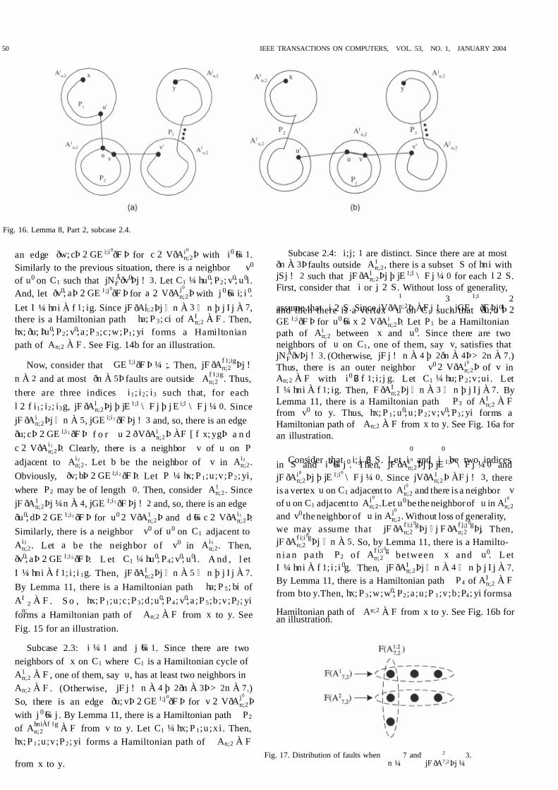
an edge ðw; cÞ 2 GE i;i0ðF Þ for c 2 V ðAi0

n;2Þ with i0 6¼ 1.Similarly to the previous situation, there is a neighbor v0

of u0 on C 1 such that jN ÃF ðv0Þj ! 3. Let C 1 ¼ hu0; P 2; v0; u0i .And, let ðv0; aÞ 2 GE 1;j 0ðF Þ for a 2 V ðA j0

n;2Þ with j 0 6¼ i; i 0.Let I ¼ hni À f 1; ig. Since jF ðAI n;2Þj n À 3 n þ j I j À 7,there is a Hamiltonian path ha; P 3; ci of AI

n;2 À F . Then,hx; ðu; Þu0; P 2; v0;a ;P 3;c ;w;P 1; yi forms a Hamiltonianpath of An;2 À F . See Fig. 14b for an illustration.

Now, consider that GE 1;iðF Þ ¼ ;. Then, jF ðAf 1;ign;2 Þj !

n À 2 and at most ðn À 5Þ faults are outside Af 1;ign;2 . Thus,

there are three indices i1; i2; i3 such that, for eachl 2 f i1; i2; i3g, jF ðAl

n;2Þj þ jE 1;l \ F j þ j E i;l \ F j ¼ 0. SincejF ðAi

n;2Þj n À 5, jGE i;i 1 ðF Þj ! 3 and, so, there is an edgeðu; cÞ 2 GE i;i1 ðF Þ f o r u 2 ðV ðAi

n;2Þ ÀF [ f x; ygÞ a n dc 2 V ðAi1

n;2Þ. Clearly, there is a neighbor v of u on P adjacent to Ai2

n;2. Let b be the neighbor of v in Ai2n;2.

Obviously, ðv; bÞ 2 GE i;i 2 ðF Þ. Let P ¼ hx; P 1;u;v;P 2; yi ,where P 2 may be of length 0. Then, consider A1

n;2. SincejF ðA1

n;2Þj ¼n À 4, jGE 1;i1 ðF Þj ! 2 and, so, there is an edgeðu0; d Þ 2 GE 1;i1 ðF Þ for u0 2 V ðA1

n;2Þ and d 6¼ c 2 V ðAi1n;2Þ.

Similarly, there is a neighbor v0 of u0 on C 1 adjacent toAi3

n;2. Let a be the neighbor of v0 in Ai3n;2. Then,

ðv0; aÞ 2 GE 1;i3 ðF Þ. L et C 1 ¼ hu0; P 4; v0; u0i . A nd , l etI ¼ hni À f 1; i ; i 1g. Then, jF ðAI

n;2Þj n À 5 n þ j I j À 7.By Lemma 11, there is a Hamiltonian path ha; P 5; bi of AI

n;2 À F . S o , hx; P 1;u;c;P 3;d ;u0; P 4; v0;a ;P 5;b;v;P 2; yi

forms a Hamiltonian path of An;2 À F from x to y. SeeFig. 15 for an illustration.

Subcase 2.3: i ¼ 1 and j 6¼ 1. Since there are twoneighbors of x on C 1 where C 1 is a Hamiltonian cycle of A1

n;2 À F , one of them, say u, has at least two neighbors inAn;2 À F . (Otherwise, jF j ! n À 4 þ 2ðn À 3Þ> 2n À 7.)So, there is an edge ðu; vÞ 2 GE 1;j 0ðF Þ for v 2 V ðA j0

n;2Þwith j 0 6¼ j . By Lemma 11, there is a Hamiltonian path P 2of Ahn iÀf 1g

n;2 À F from v to y. Let C 1 ¼ hx; P 1;u ;x i . Then,hx; P 1 ;u;v;P 2; yi forms a Hamiltonian path of An;2 À F

from x to y.

Subcase 2.4: i;j; 1 are distinct. Since there are at mostðn À 3Þfaults outside A1

n;2, there is a subset S of hni withjS j ! 2 such that jF ðAl

n;2Þj þ jE 1;l \ F j ¼ 0 for each l 2 S .First, consider that i or j 2 S . Without loss of generality,

assume that i 2 S . Since jV ðA1

n;2Þ ÀF j !3, jGE

1;i

ðF Þj !2

and then there is a vertex u on C 1 such that ðu; u 0Þ 2GE 1;iðF Þ for u0 6¼ x 2 V ðAi

n;2Þ. Let P 1 be a Hamiltonianpath of Ai

n;2 between x and u0. Since there are twoneighbors of u on C 1, one of them, say v, satisfies thatjN ÃF ðvÞj ! 3. (Otherwise, jF j ! n À 4 þ 2ðn À 4Þ> 2n À 7.)Thus, there is an outer neighbor v0 2 V ðAi0

n;2Þ of v inAn;2 À F with i0 62 f 1; i ; j g. Let C 1 ¼ hu; P 2;v;ui . LetI ¼ hni À f 1; ig. Then, F ðAI

n;2Þj n À 3 n þ j I j À 7. ByLemma 11, there is a Hamiltonian path P 3 of AI

n;2 À F from v0 to y. Thus, hx; P 1; u0;u ;P 2;v;v0; P 3; yi forms aHamiltonian path of An;2 À F from x to y. See Fig. 16a foran illustration.

Consider that i; j 62 S . Let i0

and j0

be two indicesin S and i0 6¼ j 0. Then, jF ðAi0

n;2Þj þ jE 1;i0 \ F j ¼ 0 andjF ðAi0

n;2Þj þ jE 1;i0\ F j ¼ 0. Since jV ðA1

n;2Þ ÀF j ! 3, thereis a vertex u on C 1 adjacent to Ai0

n;2 and there is a neighbor vof u on C 1 adjacent to A j0

n;2.Let u0 be the neighborof u in Ai0

n;2

and v0the neighbor of u in A j0

n;2. Without loss of generality,we may assume that jF ðAf i;i 0g

n;2 Þj j F ðAf j;j 0gn;2 Þj. Then,

jF ðAf i;i 0gn;2 Þj n À 5. So, by Lemma 11, there is a Hamilto-

n i a n p a th P 2 of Af i;i0gn;2 between x and u0. L et

I ¼ hni À f 1; i ; i 0g. Then, jF ðAI n;2Þj n À 4 n þ j I j À 7.

By Lemma 11, there is a Hamiltonian path P 4 of AI n;2 À F

from bto y.Then, hx; P 3 ;w;w0; P 2;a ;u;P 1 ;v;b;P 4; yi formsa

Hamiltonian path of An;2 À F from x to y. See Fig. 16b foran illustration.



Fig. 17. Distribution of faults whenn ¼

7 andjF ðA

2

7;2Þj ¼3.



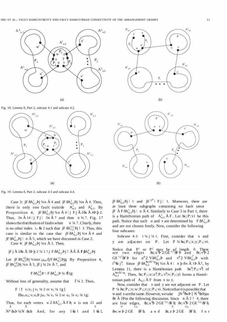
Case 3: jF ðA1n;2Þj ¼n À 4 and jF ðA2

n;2Þj ¼n À 4. Then,there is only one fault outside A1

n;2 and A2n;2. By

Proposi tion 4 , jF ðA2n;2Þj ¼n À 4 j F j À 2ðn À 4Þ þ 2.

Thus, 3n À 14 j F j 2n À 7 and then n ¼ 7. Fig. 17shows the distribution of faults when n ¼ 7. Clearly, thereis no other index i1 6¼ 2 such that jF ðA1:i1

7;2 Þj ! 3. Thus, thiscase is similar to the case that jF ðA1

n;2Þj ¼n À 4 andjF ðA2

n;2Þj n À 5, which we have discussed in Case 2.Case 4: jF ðA1

n;2Þj ¼n À 3. Then,

jF j À 2ðn À 3Þ þ 2 ¼ 1 ! j F ðA2n;2Þj ! ÁÁ Á ! jF ðAn

n;2Þj:

Let jF ðA1:iin;2Þj ¼max l2hn i fj F ðA1:l

n;2Þjg. By Proposition 4,jF ðA1: ii

n;2Þj ¼n À 3, jF j ¼ 2n À 7, and

F ðA1: iin;2Þ \ F ðA1

n;2Þ ¼ fii1g:

Without loss of generality, assume that ii ¼ 2. Then,

F f v1v2 j v1 ¼ 2 or v2 ¼ 1g [fðu1u2; v1v2Þ ju1 ¼ v1 ¼ 2 or u2 ¼ v2 ¼ 1g:

Thus, for each vertex u 2 ðA1n;2 À F Þ, u is not 21 and

N ÃF ðuÞ ¼N

Ã

ðuÞ. And, for any l 6¼ 1 and l0

6¼ l,

jF ðAln;2Þj 1 and jE l;l

0 \ F j 1. Moreover, there areat least three subgraphs containing no fault sincejF À F ðA1

n;2Þj n À 4. Similarly to Case 3 in Part 1, thereis a Hamiltonian path of A1

n;2 À F . Let hu;P ;v i be thispath. Notice that such u and v are determined by F ðA1

n;2Þand are not chosen freely. Now, consider the followingfour subcases:

Subcase 4.1: i ¼ j ¼ 1. First, consider that x andy are adjacent on P . Let P ¼ hu; P 1;x;y;P 2; vi .

Notice that P 1 or P 2 may be of length 0. Thereare two edges ðu; u 0Þ 2 GE 1;i0ðF Þ and ðv; v0Þ 2GE 1;j 0

ðF Þ for u0 2 V ðAi0

n;2Þ and v0 2 V ðA j0

n;2Þ withi0 6¼ j 0. Since jF ðAhn iÀf 1g

n;2 Þj ¼n À 4 n þ ðn À 1Þ À7, byLemma 11, there is a Hamiltonian path hu0; P 3; v0i of Ahn iÀf 1g

n;2 . Then, hx; P 1;u ;u0; P 3; v0;v;P 2 ; yi forms a Hamil-tonian path of An;2 À F from x to y.

Now, consider that x and y are not adjacent on P . LetP ¼ hu; P 1;x;w;P 2;z ;y;P 3; vi . Noticethat it is possible thatw and z arethe same. However, we take jN ÃðwÞ [ N Ãðz Þjasðn À 2Þin the following discussion. Since n À 2 ! 4, thereare four edges, ðu; u 0Þ 2 GE 1;i1 ðF Þ, ðv; v0Þ 2 GE 1;i2 ðF Þ,

ðw; w0

Þ 2 GE 1;i3

ðF Þ, a n d ðz; z 0

Þ 2 GE 1;i4

ðF Þ, f o r


Fig. 18. Lemma 8, Part 2, subcase 4.1 and subcase 4.2.

Fig. 19. Lemma 8, Part 2, subcase 4.3 and subcase 4.4.



u0 2 V ðAi1n;2Þ, v0 2 V ðAi2

n;2Þ, w0 2 V ðAi3n;2Þ, and z 0 2 V ðAi4

n;2Þsuch that i1; i2 ; i3; and i4 are four distinct indices. Sinced ðu; wÞ ¼1 in A1

n;2, by Lemma 2,

AS ðuÞ [ AS ðvÞ ¼ hni À f 1g:

So, we may assume that Ai1n;2 and Ai3

n;2 contain no fault. LetI ¼ f i1; i3g and I 0 ¼ hni À f 1; i1; i3g. Then, jF ðAI

n;2Þj 1and jF ðAI 0n;2Þj n À 4 n þ j I 0j À 7. By Lemma 11, thereare a Hamiltonian path hu0; P 4; w0i of AI

n;2 À F and aHa mi l t o n ia n p a t h hz 0; P 5; v0i of AI 0

n;2 À F . T hu s ,hx; P 1 ;u ;u0; P 4; w0;w;P 2;z ;z 0; P 5; v0;v;P 3; yi forms a Hamil-tonian path of An;2 À F . See Fig. 18a for an illustration.

Subcase 4.2: i ¼ j 6¼ 1. Since d ðu; vÞ ¼1 in A1n;2,

i 2 AS ðuÞ [ AS ðvÞ. We may assume that u is adjacent toAi

n;2 and the neighbor of u in Ain;2 is u0. Without loss of

generality, we may assume that u0 6¼ y. Since jF ðAin;2j 1,

t he r e i s a H am i lt o ni a n p a th o f Ain;2 À F . L e t

hx; P 1 ; u0;w ;P 2; yi be the path, where w 6¼ u0. Since thereareatmost ðn À 4Þfaultsoutside A1

n;2, jN ÃF ðwÞj ! 2.Thereisan edge ðw; z Þ 2 GE i;i

0ðF Þfor z 2 V ðAi0

n;2Þwith i 6¼ 1. Since

jN ÃF ðvÞj ¼n À 2 ! 4, there is anedge ðv; v

0Þ 2 GE

1;j 0

ðF Þforv0 2 V ðA j0

n;2Þ with j 0 62 f i; i 0g. Let I ¼ hni À f 1; ig. Then,jF ðAI

n;2Þj n À 4 n þ j I j À 7. By Lemma 11, there is aH a m i l to n i a n p a t h hv0; P 3; z i o f AI

n;2 À F . S o ,hx; P 1 ; u0;u ;P ;v ;v0; P 3;z ;w;P 2; yi forms a Hamiltonianpath of An;2 À F . See Fig. 18b for an illustration.

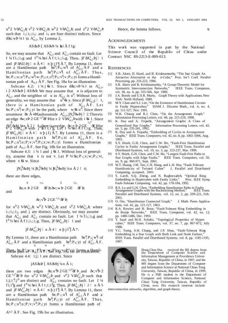
Subcase 4.3: i ¼ 1 and j 6¼ 1. Without loss of general-ity, assume that x is not v. Let P ¼ hu; P 1;x;w;P 2; vi ,where x 6¼ w. Since

jN ÃF ðuÞj ¼ jN ÃF ðvÞj ¼ jN ÃF ðwÞj ¼n À 2 ! 4;

there are three edges,

ðu; u0

Þ 2 GE 1;i1

ðF Þ; ðw; w0

Þ 2 GE 1;i2

ðF Þ;and

ðv; v0Þ 2 GE 1;i3 ðF Þ;

for u0 2 V ðAi1n;2Þ, w0 2 V ðAi2

n;2Þ, and v0 2 V ðAi3n;2Þ, where

i1; i2; i3, and j are distinct. Obviously, we may assumethat Ai1

n;2 and Ai2n;2 contain no fault. Let I ¼ f i1; i2g and

I 0 ¼ hni À f 1; i1; i2g. Then, jF ðAI n;2Þj 1 and

jF ðAI 0n;2Þj n À 4 n þ j I 0j À 7:

By Lemma 11, there are a Hamiltonian path hu0; P 3; w0i of AI

n;2 À F and a Hamiltonian path hv0; P 4; yi of AI 0n;2 À F .

Then, hx; P 1;u ;u0

; P 3; w0

;w ;P 2;v ;v0

; P 4; yi forms a Hamil-tonian path of An;2 À F . See Fig. 19a for an illustration.Subcase 4.4: i;j; 1 are distinct. Since

jAS ðuÞ [ AS ðvÞj ¼n À 1;

there are two edges ðu; u 0Þ 2 GE 1;i0ðF Þ and ðv; v0Þ 2GE 1;j 0ðF Þ for u0 2 V ðAi0

n;2Þ and v0 2 V ðA j0

n;2Þ such thati;j;i 0; j 0 are distinct and Ai0

n;2 contains no fault. Let I ¼f i; i 0g and I 0 ¼ hn i À f 1; i ; i 0g. Then, jF ðAI

n;2Þj 2 n À 5and jF ðAI 0

n;2Þj n À 4 n þ j I 0j À 7. By Lemma 11, thereare a Hamiltonian path hx; P 1; u0i of AI

n;2 À F and aHa mil t o n i an p a t h hv0; P 2; yi of AI 0

n;2 À F . T hu s,hx; P 1 ; u0;u ;P ;v ;v0; P 2; yi forms a Hamiltonian path of

An;2 À F . See Fig. 19b for an illustration.


ACKNOWLEDGMENTS

This work was supported in part by the NationalScience Council of the Republic of China underContract NSC 89-2213-E-009-013.

REFERENCES[1] S.B. Akers, D. Harel, and B. Krishnamurthy, “The Star Graph: An

Attractive Alternative to the n-Cube,” Proc. Int’l Conf. ParallelProcessing, pp. 216-223, 1986.

[2] S.B. Akers and B. Krishnamurthy, “A Group-Theoretic Model forSymmetric Interconnection Networks,” IEEE Trans. Computers,vol. 38, no. 4, pp. 555-566, Apr. 1989.

[3] J.A. Bondy and U.S.R. Murty, Graph Theory with Applications.NewYork: North Holland, 1980.

[4] M.Y. Chan and S.J. Lee, “On the Existence of Hamiltonian Circuitsin Faulty Hypercubes,” SIAM J. Discrete Math., vol. 4, no. 4,pp. 511-527, Nov. 1991.

[5] W.K. Chiang and R.J. Chen, “On the Arrangement Graph,”Information Processing Letters, vol. 66, pp. 215-219, 1998.

[6] K. Day and A. Tripathi, “Arrangement Graphs: A Class of Generalized Star Graphs,” Information Processing Letters, vol. 42,no. 5, pp. 235-241, 1992.

[7] K. Day and A. Tripathi, “Embedding of Cycles in ArrangementGraphs,” IEEE Trans. Computers, vol. 42, no. 8, pp. 1002-1006, Aug.1993.

[8] S.Y. Hsieh, G.H. Chen, and C.W. Ho, “Fault-Free HamiltonianCycles in Faulty Arrangement Graphs,” IEEE Trans. Parallel andDistributed Systems, vol. 10, no. 3, pp. 223-237, Mar. 1999.

[9] S.Y. Hsieh, G.H. Chen, and C.W. Ho, “Longest Fault-Free Paths inStar Graphs with Edge Faults,” IEEE Trans. Computers, vol. 50,no. 9, pp. 960-971, Sept. 2001.

[10] W.T. Huang, J.M. Tan, C.N. Hung, and L.H. Hsu, “Fault-TolerantHamiltonicity of Twisted Cubes” J. Parallel and DistributedComputing, accepted, 2001.

[11] S. Latifi, S.Q. Zheng, and N. Bagherzadeh, “Optimal RingEmbedding in Hypercubes with Faulty Links,” Proc. IEEE Symp.Fault-Tolerant Computing, vol. 42, pp. 178-184, 1992.

[12] R.S. Lo and G.H. Chen, “Embedding Hamiltonian Paths in FaultyArrangement Graphs with the Backtracking Method,” IEEE Trans.Parrallel and Distributed Systems, vol. 12, no. 2, pp. 209-221, Feb.2001.

[13] O. Ore, “Hamiltonian Connected Graph,” J. Math. Pures Applica-tions, vol. 42, pp. 121-127, 1963.

[14] R.A. Rowley and B. Bose, “Fault-Tolerant Ring Embedding inde Bruijn Networks,” IEEE Trans. Computers, vol. 42, no. 12,pp. 1480-1486, Dec. 1993.

[15] Y. Saad and M.H. Schultz, “Topological Properties of Hyper-cubes,” IEEE Trans. Computers, vol. 37, no. 7, pp. 867-872, July1988.

[16] Y.C. Tseng, S.H. Chang, and J.P. Sheu, “Fault-Tolerant RingEmbedding in a Star Graph with Both Link and Node Failure,”IEEE Trans. Parallel and Distributed Systems, vol. 8, pp. 1185-1195,1997.

Hong-Chun Hsu received the BS degree fromthe Department of Computer Science andInformation Management at Providence Univer-sity, Taiwan, Republic of China, in 1997, and theMS degree from the Department of Computerand Information Science at National Chiao TungUniversity, Taiwan, Republic of China, in 1999.He is a PhD student in the Department ofComputer and Information Science, NationalChiao Tung University, Taiwan, Republic ofChina, now. His research interests include

interconnection networks, algorithm, and graph theory.




Tseng-Kuei Li received the BS degree ineducation from National Taiwan Normal Uni-versity in 1994 and the PhD degree incomputer and information science from Na-tional Chiao Tung University, Taiwan, in2002. He is currently an assistant professorin the Department of Computer Science andInformation Engineering, Ching Yun Instituteof Technology, Taiwan. His research inter-

ests include interconnection networks, algo-rithms, and graph theory. He is a member of the IEEE.

Jimmy J.M. Tan received the BS and MSdegrees in mathematics from National TaiwanUniversity in 1970 and 1973, respectively, andthe PhD degree from Carleton University,Ottawa, Canada, in 1981. He has been on thefaculty of the Department of Computer andInformation Science, National Chiao Tung Uni-versity, since 1983. His research interestsinclude design and analysis of algorithms,combinatorial optimization, interconnection net-

works, and graph theory.

Lih-Hsing Hsu received the BS degree inmathematics from Chung Yuan Christian Uni-versity, Taiwan, Republic of China, in 1975, andthe PhD degree in mathematics from the StateUniversity of New York at Stony Brook in 1981.He is currently a professor in the Department ofComputer and Information Science, NationalChiao Tung University, Taiwan, Republic ofChina. His research Interests include intercon-

nection networks, algorithm, graph theory, andVLSI layout.

. For more information on this or any computing topic, please visitour Digital Library at http://computer.org/publications/dlib.


Documents

Fault Hamiltonicity and Fault Hamiltonian Connectivity of the Arrangement Graphs