Fault Diagnosis of Interconnected Cyber-Physical Systems

Fault Diagnosis of Interconnected Cyber-Physical Systems

Marios M. Polycarpou

Professor, IEEE Fellow, IFAC FellowDirector, KIOS Research and Innovation Center of Excellence

Dept. Electrical and Computer EngineeringUniversity of Cyprus

7th oCPS PhD School on Cyber-Physical SystemsLucca, Italy, 14th June 2017

Motivation for fault diagnosis

Interconnected cyber-physical systems

Foundations of fault diagnosis

Sensor fault diagnosis

Application example: Smart Buildings

Concluding Remarks

Presentation Outline

Smart Phones

Smart Cars

Smart Grids

Smart Buildings

Smart Cities

Smart Camera Networks

Smart Water Networks

The Smart Revolution

Smart Phones

Smart Cars

Smart Grids

Smart Buildings

Smart Cities

Smart Camera Networks

Smart Water Networks

Smart-X

The Smart Revolution

HARDWARE

Sensing & actuation devices

Embedded computing

Wide area connectivity

Characteristics of Smart-X

SOFTWARE

Data management

Decision making algorithms

Learning algorithms

Optimization and control

Digital advances provide the ICT infrastructure not the INTELLIGENCE (so far)

Infrastructure will be further enhanced via the IoT

Smart-X vs. Smart-ready-X

Smart-X vs Smart-ready-X

Digital advances provide the ICT infrastructure not the INTELLIGENCE (so far)

Infrastructure will be further enhanced via the IoT

Smart-X vs. Smart-ready-X

Control systems and machine learning are at the heart of transforming Smart-ready-X to Smart-X

Smart-X vs Smart-ready-X

More proactive, more planning ahead

More discrete-event, more event-triggered

More machine learning, handling of larger volume of data, more heterogeneous data

Handling of more uncertainty, fault tolerance

Handling of human-machine interaction

Control Systems in the Smart-X Era

Fragility

The technological trend is towards: more complex and large-scale systems

more interconnected systems

more automation and autonomy

However if the data is faulty/inconsistent/missing, this may lead to: wrong decisions or escalation to a catastrophic failure

fault propagation from one subsystem to another

Unreliable and untrustworthy automation procedures

Fragility

The technological trend is towards: more complex and large-scale systems

more interconnected systems

more automation and autonomy

However if the data is faulty/inconsistent/missing, this may lead to: wrong decisions or escalation to a catastrophic failure

fault propagation from one subsystem to another

Unreliable and untrustworthy automation procedures

moreFRAGILE

Fragility of Interconnected Systems

Fragility is a crucial issue in an interconnected cyber-physical-social world

Fault Monitoring and Fault Tolerance are necessary components of Smart-X architectures

Black Swan Theory – Nassim Nicholas Talebmetaphor that describes an event that comes as a surprise, has a major effect, and is often inappropriately rationalized after the fact with the benefit of hindsight (extreme outliers)

Monitoring and Control

System

FaultMonitoring

and Diagnosis

u y

d f


SystemController u yr

d f


System

FaultAccommodation

Controller

FaultMonitoring

and Diagnosis

u yrd f

SupervisoryAlgorithm

Control Algorithm

Fault Scenarios

System/Process Faults

Actuator Faults

Sensor Faults

Communication Faults

Controller Faults

Environment Faults

Malicious Attacks (cyber-security)

P

FA

C

FD

Fault Diagnosis Steps

fault detection

fault isolation

fault identification and risk assessment

fault accommodation

Key Challenges for Fault Diagnosis

distinguish between faults and modeling uncertainty or measurement noise

exploit spatial and temporal correlations between variables

handle multiple faults

isolate faults in a large-scale system (needle in a haystack)

prevent “small” faults from escalating into a major failure

accommodate the fault – what to do in the presence of information about a fault?

Design smart SOFTWARE to handle faulty HARDWARE

Key Books on Fault Diagnosis

J. Gertler. Fault Detection and Diagnosis in Engineering Systems. CRC Press, 1998.

J. Chen and R. J. Patton. Robust Model-based Fault Diagnosis for Dynamic Systems. Kluwer Academic Publishers, 1999.

R. Isermann. Fault-Diagnosis Systems: An Introduction from Fault Detection to Fault Tolerance. Springer Verlag, 2006.

S. X. Ding. Model-based Fault Diagnosis Techniques: Design Schemes, Algorithms, and Tools. Springer-Verlag London, 2008.

M. Blanke, M. Kinnaert, J. Lunze, and M. Staroswiecki. Diagnosis and Fault-Tolerant Control. Springer-Verlag Berlin Heidelberg, 2016.

N interconnected CPS. I‐th CPS: described by the pair

: physical part of the I‐th CPS, : cyber part of the I‐th CPS.

Interconnected CPS

( ) ( ),I I ( )I

( )I

Interconnected CPS – Single Agent

Interconnected CPS

Objective: Detect and isolate multiple faults that may occur in one or more CPS

Problem Formulation

where:

state vectorinput vector

Nominal state dynamics

Modeling uncertainty

Change in the system due to fault

Time profile of the fault

Interconnection dynamics

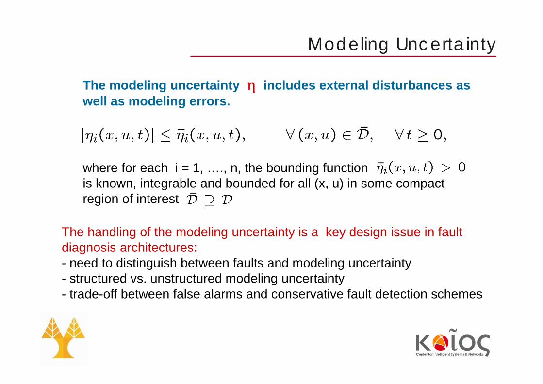
Modeling Uncertainty

The modeling uncertainty includes external disturbances as well as modeling errors.

where for each i = 1, …., n, the bounding function is known, integrable and bounded for all (x, u) in some compact region of interest

The handling of the modeling uncertainty is a key design issue in fault diagnosis architectures:- need to distinguish between faults and modeling uncertainty- structured vs. unstructured modeling uncertainty- trade-off between false alarms and conservative fault detection schemes

Fault Modeling

The term represents the deviations in the dynamics of the system due to a fault.

• is the fault function• The matrix characterizes the time profile of a fault which occurs at some unknown time

where denotes the unknown fault evolution rate.

Fault Influence for Distributed Systems

• Local Faults

• Distributed Faults

• Distributed Faults with Overlapping Signature

• Propagating Faults

Fault Isolation

Types of FAULT ISOLATION:• identify the type of fault that has occurred• identify the physical location of the fault

Class of fault functions :

where:• is an unknown parameter vector, which is assumed to belong to a known compact set

• is a known smooth vector field

Fault Diagnosis Architecture

There are N+1 Nonlinear Adaptive Estimators (NAEs) One of the NAEs is used for detecting and approximating faults The remaining N NAEs are isolation estimators used only after a fault has been detected for the purpose of fault isolation.

Decision Scheme

inputreference

FeedbackController

Estimatorand Approximation

Bank of Fault

Decision Scheme

Activation

Fault Detection and Isolation Architecture

Fault Detection

Fault Isolation

Fault Detection

Isolation Estimators

u Nonlinear Plant x

Alarm

Identification of thefault that has occurred

Fault Handling

T0

Tisol

x (t)

x (t)d

detectedfault

isolatedfault

Monitoring

Module

Td

t

occurredfault

0 < t < T0 : system is operating in a healthy condition. T0 < t < Td : period in which there is a fault, which however has

not yet been detected. Td < t < Tisol : period during which the fault has been detected,

but it is not yet known which particular fault has occurred. t > Tisol : the fault has been isolated.

Fault Detection and Approximation Estimator

where:

Adaptive approximation model

estimation poles

The initial weight vector is chosen such that

(healthy situation)

adjustable weights of the on-line neural approximator

estimated state vector

Adaptive Approximation Model

Nonlinear approximation model with adjustable parameters (e.g., neural networks) Linearly parameterized vs. nonlinearly parameterized It provides the adaptive structure for approximating on-line: Local modeling errors interconnection dynamics unknown fault functions

Learning Algorithm

where:

regressor matrix

The projection operator restricts the parameter estimation vector to a predefined compact and convex region.

state estimation error

Positive definite learning rate matrix

Dead-zone operator

Detection Threshold

where:

In the special case of a uniform bound on the modeling uncertainty the detection threshold becomes:

Robustness of the fault detection scheme is the ability to avoid false alarms. The above threshold make the FD scheme robust.

Detectability Conditions

Result holds for the special case of constant bound on the modeling uncertainty.

We are also able to obtain more simplified detectability conditions, but they are more conservative.

In general there is an inherent trade-off between robustness and fault detectability.

],[ 21 ttIf there exists an interval of time such that at least one component of the fault vector satisfies the condition

then a fault will be detected.

),( uxfi

Fault Isolation Estimators

N NAEs are activated for isolation (isolation estimators) after thedetection of a fault

Learning Algorithm

• Each isolation estimator corresponds to one of the possible types of parametric faults

• Adaptive threshold are designed based on the available information, similar to the concept of a matching filter

• isolation is achieved if every threshold is exceeded, except one (the one corresponding to the fault)

Incipient Fault Isolability

Intuitively, fault are easier to isolate if they are sufficiently “mutually different” in terms of a suitable measure

Fault isolability condition

Fault Mismatch FunctionThe difference between the actual fault function and the estimated fault function associated with any isolation estimator

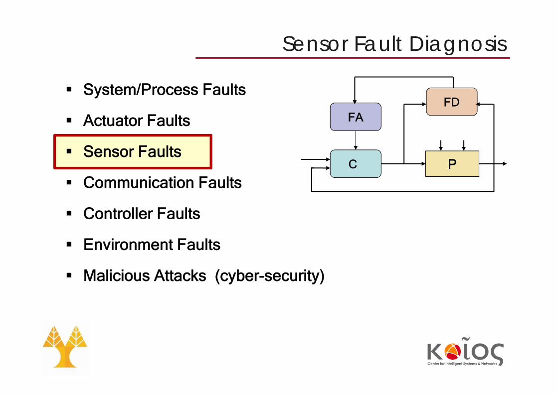
Sensor Fault Diagnosis

System/Process Faults

Actuator Faults

Sensor Faults

Communication Faults

Controller Faults

Environment Faults

Malicious Attacks (cyber-security)

P

FA

C

FD

N interconnected CPS. I‐th CPS: described by the pair

: physical part of the I‐th CPS, : cyber part of the I‐th CPS.

Interconnected CPS

( ) ( ),I I ( )I

( )I

Interconnected CPS

(physical part) a nonlinear system ( )I

( )I

( ) ( ) ( ) ( ) ( ) ( )

( ) ( ) ( ) ( ) ( )

( ) ( ) ( )

known local dynamics

known interconnection dynamics

modeling uncertainty

( , )

( , , )

( , , )

I I I I I I

I I I I Iz

I I I

x A x x u

h x u C z

x u t

( )

( )

)

( )

( ) (

: local state vector: local input vector generated by a

feedback control agent using : interc

onnection vector

I

I

I

I

Ir

xu

z

Interconnected CPS

(physical part) Sensor set used for measuring the linear combination of states

( )I

( )I

( ) ( ) ( ) ( ) ( )( ) ( ) ( ) ( )I I I I Iy t C x t d t f t

( )

( )

( )

: local output vector : measurement noise : fault vector

I

I

I

ydf

( ) ( ) I IC x

Interconnected CPS

( ) ( ) ( ) ( ) ( )( ) ( ) ( ) ( )I I I I Iz z z zy t C z t d t f t

(cyber part) control agent that generates the input based on some reference signal , the measured output and the transmitted sensor information

( )Iu

( )Ir

( )I

( )I

( )Iz

Interconnected CPS

Objective: Detect and isolate multiple sensor faults that may occur in one or more CPS

Distributed Sensor Fault Diagnosis Architecture

(cyber part)monitoring agent allowed to exchange information with the neighboring agents

( )I( )I

Task:Detection & isolation of multiple sensor faults in

Detection of propagated sensor faults in

( )I

( )Iz

( )Iz

G : global decision logic collects and processes combinatorially the decisions of the monitoring agents

Task: Isolation of sensor faults propagated in the cyber layer due to the information exchange between monitoring agents

Distributed Sensor Fault Diagnosis Architecture

Monitoring Agent

monitoring agent ( )I

Monitoring Agent

The monitoring of the local sensor set is decomposed into NI modules The module monitors the group of sensors

( )I

( , )I q ( , )I q( , ) ( , ) ( , ) ( ) ( , ) ( , ): yI q I q I q I I q I qC x d f

Monitoring Agent

Task: Detection of sensor faults in and/or ( , )I q

: q‐th module of the I‐th monitoring agent( , )I q

( )Iz

Monitoring Agent

The decisions of the NI modules are aggregated and processed combinatorially for isolating the combination of multiple sensor faults that have occurred and inferring the presence of propagated sensor faults

j‐th residual,

• : estimation model based on thenonlinear observer

( , ) ( , )( ( ,) ( ) )ˆ ,j j

I II q I q qj

Iy y C x j

( , )ˆ I qx

( , ) ( ) ( , ) ( ) ( , ) ( )

( ) ( , ) ( )

(

( )

( , ), ) ( , ) ( , )

ˆ ˆ ˆ( , )ˆ ( , , )

ˆ

I q I I q I I q I

I I q I

I q I q I q

Iz

I q

x A x x uh x u

L C

y

y x

( , )j

I qy

(1)

(2)

Monitoring Module

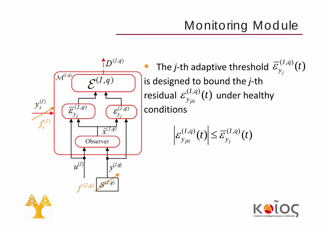
The j‐th adaptive threshold is designed to bound the j‐th residual under healthy conditions

( , ) ( )j

I qy t

( , ) ( )jH

I qy t

Monitoring Module

( , ) ( , )( ) ( )jH j

I q I qy yt t

The j‐th adaptive threshold can be implemented using linear filters

( , ) ( , ) ( ) ( , ) ( , )ˆ( ) ( ( ), ( ), ) (( ) ) ( )j

I q I q I I q I qy I jt x t u t t Z t YH s t

Adaptive Threshold Computation

1

2

( , ) ( , ) ( , )

1 2( , ) ( , )(

( , ) (

, ) (

, ) ( , )

( , ) ( , ) ( )

, )

( , )

( ) ( ) ( )

ˆ( ) ( ( ), ( ), ) ( )

( )

( )

( ) , ( ) , ( )

,

I I I

I q I

I q I q I q

I q I q I

q I qj I

I q I qI q I qj I

I qB

I h

H s

H s

H s H s H s

Z t E t E t

E t x t u t

s s

t E t

s

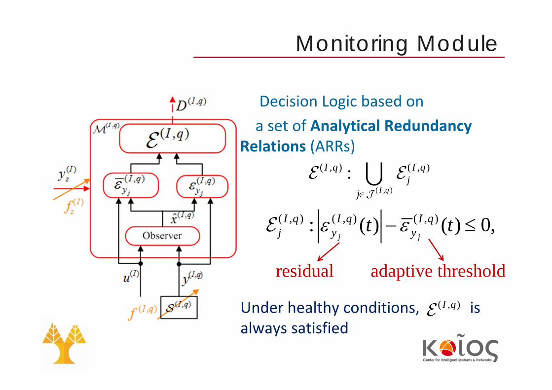
Decision Logic based on a set of Analytical Redundancy

Relations (ARRs)

( , ) ( , ) ( , ): ( ) ( ) 0,j j

I q I q I qj y yt t

( , )

( , ) ( , ):I q

I q I qj

j

residual adaptive threshold

Monitoring Module

Under healthy conditions, is always satisfied

( , )I q

Robustness and Structured Fault SensitivityTheorem: The distributed sensor fault diagnosis design guarantees that:

(a) Robustness: If neither the local sensor set nor the transmitted sensor information are affected by sensor faults, then the set of ARRs is always satisfied.

(b) Structured fault sensitivity: If there is a time instant at which is not satisfied, then the occurrence of at least one sensor fault in is guaranteed.

( , )I q

( )Izy

( , )I q

( , )I q

( , ) ( )I q Iz

V. Reppa, M. Polycarpou and C. Panayiotou, “Distributed Sensor Fault Diagnosis for a Network of Interconnected Cyber-Physical Systems,” IEEE Transactions on Control of Network Systems, vol 2, no. 1, pp. 11-23, March 2015.

Monitoring Agent

Local Multiple Sensor Fault Isolation

Example:

( ,1) ( )

( ,2) ( ) ( )

( ,3) ( )

{1} ,

{2}, {3}

{3}

I I

I I I

I I

( ) ( ) ( ) ( ) ( ) ( ) ( ) ( ) ( ) ( ) ( ) ( ) ( ) ( )1 2 3 1 2 1 3 2

( )

( ,1)

( ,2)

( ,3

2

)

3 1 3, , , , , ,

1 0 0 1 1 0 1 1 10 1 1 1 1 1 1 1 10 0 1 0 1 1 1 1 1

I I I I I I I I I I I I I I Ic

I

z

I

I

zf f f f f f f f f f f f f f

( )Izy

( )

1( ) 1

0

ID t

( ) ( ) ( )1 2( ) , I I I

s t f f

( ) ( ) ( ) ( ) ( ) ( ) ( ) ( ) ( ) ( ) ( ) ( ) ( ) ( )1 2 3 1 2 1 3 2

( )

( ,1)

( ,2)

( ,3

2

)

3 1 3, , , , , ,

1 0 0 1 1 0 1 1 10 1 1 1 1 1 1 1 10 0 1 0 1 1 1 1 1


I

z

I

I


Diagnosis Set:

Decision on the presence of sensor faults in ( ) ( )

( )( ) ( )

0, ( ) ( )

1, ( )

I II z s

z I Iz s

f tD t

f t


( )zIy

( ) ( )( )

( ) ( )

0, ( ) ( )

1, ( )

I II z s

z I Iz s

f tD t

f t

( ) ( ) ( ) ( ) ( ) ( ) ( ) ( ) ( ) ( ) ( ) ( ) ( ) ( )1 2 3 1 2 1 3 2

( )

( ,1)

( ,2)

( ,3

2

)

3 1 3, , , , , ,

1 0 0 1 1 0 1 1 10 1 1 1 1 1 1 1 10 0 1 0 1 1 1 1 1


I

z

I

I


( )

1( ) 1

1

ID t

( ) ( ) ( ) ( ) ( ) ( ) ( ) ( ) ( )1 3 1 2 3( ) , , , , , , ,I I I I I I I I I

s z z ct f f f f f f f

Diagnosis Set:

Decision on the presence of sensor faults in


( )zIy

Global Multiple Sensor Fault Isolation

Observed pattern of sensor faults in transmitted sensor information: (1) (2) ( )( ) ( ) ( ) ( )N

z z z zD t D t D t D t

(1) (2) (3) (1) (2) (1) (3) (2) (3) (1) (2) (3)5 1 4 5 1 5 4 1 4 5 1

(1)

(2)

(3)

4, , , , ,

1 0 * 1 1 * 10 1 * 1 * 1 1* * 1 * 1 1 1

f f f f f f f f f f f f

Semantics of ‘*’: the sensor fault involved in the ARR can explain why the ARR is violated, while the ARR may be satisfied although the corresponding fault has occurred

Global Multiple Sensor Fault Isolation

Learning Approaches for Fault Diagnosis

Reduce adaptive thresholds by reducing the bound of the modeling uncertainty using learning techniques.

Design and analysis of an adaptive approximation methodology to learn the modeling uncertainty

V. Reppa, M. Polycarpou and C. Panayiotou, “Adaptive approximation for multiple sensor fault detection and isolation of nonlinear uncertain,” IEEE Transactions on Neural Networks and Learning Systems, vol 25, no. 1, pp. 137-153, January 2014.

Fault Diagnosis and Cybersecurity

Targeted faults

Early detection is crucial

Sensor placement is a key issue

Need to consider the impact dynamics

Application Example: Smart Buildings

48% of energy consumption is for buildings (27% for transportation; 25% for factories)

76% of electricity consumption is for buildings (23% for factories; 1% for transportation)

87% of our time is spent indoors

How critical are buildings?

48% of energy consumption is for buildings (27% for transportation; 25% for factories)

76% of electricity consumption is for buildings (23% for factories; 1% for transportation)

87% of our time is spent indoors

6% in automobiles and public transportation

7% outdoors

How critical are buildings?

The Transformation of Buildings

The Transformation of Buildings

Sensors (more self-aware)

Actuators (more automation)

Intelligent decision making (energy efficiency, safety and security, fault diagnosis, etc.)

Communication devices (building to user; user to building; building to building; etc.)

The Electronic Transformation Inside

Sensors (more self-aware)

Actuators (more automation)

Intelligent decision making (energy efficiency, safety and security, fault diagnosis, etc.)

Communication devices (building to user; user to building; building to building; etc.)

Internet of Things (IoT)

The Electronic Transformation Inside

Need to monitor and control: indoor living conditions and safety of the occupants energy consumption of large-scale buildings

The technology is available (smart-ready): building automation is well established Cyber-physical systems for smart buildings sensing and actuation devices are widely available

Need to develop smart software to enable the coordination and scheduling of actions for handling dynamic and uncertain environments

Motivation for Smart Buildings

Topics pursued at KIOS Research Center

• KIOS Research Center for Intelligent Systems and Networks was founded in 2008

• Currently about 50 researchers working on Monitoring, Control and Security of Critical Infrastructure Systems

• Awarded a TEAMING project from H2020 to upgrade to a Center of Excellence for Research and Innovation (more than €40M)

Smart Buildings Topics pursued at KIOS

• Distributed fault diagnosis and control of HVAC systems

• Contamination event detection and isolation in large-scale buildings

• Security surveillance using smart camera networks

• Cognitive agents for on-line reconfiguration of in smart buildings


• Distributed control and fault diagnosis of large-scale HVAC systems

• V. Reppa, P. Papadopoulos, M. Polycarpou and C. Panayiotou, “A Distributed Architecture for HVAC Sensor Fault Detection and Isolation,” IEEE Transactions on Control Systems Technology, vol. 23, pp. 1323‐1337, July 2015.

• V. Reppa, P. Papadopoulos, M. Polycarpou, and C. Panayiotou, “A Distributed Virtual Sensor Scheme for Smart Buildings based on Adaptive Aproximation,” Proceedings of the International Joint Conference on Neural Networks, World Congress on Computational Intelligence (IJCNN 2014), pp. 99‐106, July 2014.

Zone 1 Zone 2

Zone 3 Zon

e 4

Zone 5

Zone 6

Zone 7

,12dA

,13dA ,23dA

,24dA ,45dA

,34dA,56dA

,46dA

,67dA

,47dA

Zone N Zone N-1

Zone N-2

1u

Storage Tank

Condenser

Heat Pump

stu

2u 5u

4u

3u6u

7u

2Nu

Nu 1Nu



• M. Michaelides, V. Reppa, M. Christodoulou, C. Panayiotou and M. Polycarpou, “Contaminant Event Monitoring in Multi‐zone Buildings Using the State‐Space Method,” Building and Environment, vol. 71, pp. 140‐152, January 2014. (2014 Best Paper Award).

• D. Eliades, M. P. Michaelides, C. Panayiotou and M. Polycarpou, “Security‐Oriented Sensor Placement in Intelligent Buildings”, Building and Environment, vol. 63, pp. 114‐121, March 2013.



• C. Laoudias, P. Tsangaridis, M. Polycarpou, C. Panayiotou, C. Kyrkou and T. Theocharides, “'Cooperative Fault‐Tolerant Target Tracking in Camera Sensor Networks," Proceedings of the IEEE International Conference on Communications (ICC’2015), June 2015.

• C. Kyrkou, C. Laoudias, T. Theocharides, C. Panayiotou and M. Polycarpou, "Adaptive Energy‐Oriented Multi‐Task Allocation in Smart Camera Networks", IEEE Embedded Systems Letters, vol. 8, no. 2, pp. 37‐40, June 2016.


• Cognitive agent for on-line reconfiguration in smart buildings

• G. Milis, D. Eliades, C.G. Panayiotou and M. Polycarpou, “A Cognitive Fault‐Detection Design Architecture,” in Proceedings of IEEE World Congress on Computational Intelligence (WCCI’2016), July 2016.

• G. Milis, C.G. Panayiotou and M. Polycarpou, “Semantically‐Enhanced Online Configuration of Feedback Control Schemes,” IEEE Transactions on Cybernetics, 2017 (to appear).


• Distributed fault diagnosis and control of HVAC systems



• Cognitive agent for on-line reconfiguration of in smart buildings

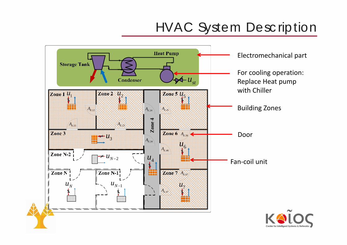
HVAC Description

HVAC systems consist of: A number of electrical and mechanical components for

Heating (i.e., boilers, heating coils, heat pump) Cooling (i.e., cooling towers, chillers, cooling coils) Ventilating (i.e., fans, supply/return ducts, mixing boxes)

A number of building zones (i.e., interconnected or not) the dynamics of a zone in the building are affected by the dynamics of their neighbouring zones

Types of faults in HVAC systems: actuator/process faults (i.e., fouled heat exchangers, stuck dampers, leaking

valves, broken fans) sensor faults (i.e., drifting, stuck‐at‐zero), communication faults (i.e., wire break).

Faulty Situations in HVAC Systems

The recovery of faulty situations in HVAC systems: shutting down the operation of the system (inconvenient and possibly

ineffective from the viewpoint of energy) reconfiguring the controller(s) via a fault tolerant control scheme, using the

outcome of a fault detection and isolation mechanism

Early diagnosis and accommodation of faults is critical since local faults effects may propagate from a local subsystem to neighbouring subsystems the physical interconnections the distributed control scheme (local controllers may use information

transmitted from neighbouring controllers to achieve the best possible tracking performance)

Zon

e 4

,12dA

,13dA ,23dA

,24dA ,45dA

,34dA,56dA

,46dA

,67dA

,47dA

1ustu

2u 5u

4u

3u6u

7u

2Nu

Nu 1Nu

Fan‐coil unit

For cooling operation: Replace Heat pump with Chiller

Electromechanical part

Building Zones

Door

HVAC System Description

HVAC System Description

Storage Tank

Condenser

Heat Pump

stu

,, ( )( ) ( ) ( ) ( )

( ( )) ( ),

( )1 1 , ( ) ( )( )

1, ( ) (

( ) ( ) ( )

(

)

)

( )( )

i

stst st

st

st max szs st i i max

ist st

st stpl st

st st

ost o max

s ma

st

x

st o m

z

s

x

t

a

Ud aP u t u t Udt C C

a a

T t T t T t

T T t T tC C

T tp T t T t

t

T tT t

TP T

T t T t T

T t

Zone 1 Zone 2

Zone 3 Zon

e 4

Zone 5

Zone 6

Zone 7

,12dA

,13dA ,23dA

,24dA ,45dA

,34dA,56dA

,46dA

,67dA

,47dA

Zone N Zone N-1

Zone N-2

1u 2u 5u

4u

3u6u

7u

2Nu

Nu 1Nu

Storage Tank

Condenser

Heat Pump

stu

Zone 1

,12dA

,13dA

1u

,

1

( ) ( ) ( (

( )

( )( )

( )

(

( )

( ) ( )

))

1( ( ) ) ( ) ( )

( )

, ) 2(max( )

(

)

)

(

( )

( )

i

i i

i i

ij i

i

i

i i

i i i

ii

i

j

j

j

i

i jj

i i

zi max szi amb

z z

w zi z zz

z

z z

jz z

z

z

a

z z

z z

s

ir p

jz

d p v

z

z

t

T t

T t

T t T

T tT t T t

T t T t

T t

d aU au t T t

dt C C

hA aT t a T t

C C C

T t

C

T t

sgnC

C tA C

) ,( )iz

T t

( ) ( )1 1 , ( ) ( )( ( ))

1, ( ) ( )

st ost o max

s st max

st o max

T t T tp T t T t TP T t T

T t T t T

Temperature nonlinear dynamics for water in the storage tank:

Performance coefficient of the heat pump

HVAC System Modelling

M. Zaheer‐Uddin and R. Patel, “Optimal tracking control of multizone indoor environmental spaces,” Journal of Dynamic Systems, Measurement and Control, vol. 117, no. 3, pp. 292–303, 1995.

,,

( ) ( ( )) ( ) ( ) ( ( ) ( ))

( ( ) ( )) ( ),

i

st maxst szs st st i i max z st

ist st

st stst pl st

st st

UdT t aP T t u t u t U T t T tdt C C

a aT t T t T tC C

1,..., N

Temperature nonlinear dynamics of air in the i‐th zone


i iz air p zC C V

air heat capacity

,

1

( )( ( ) ( )) ( ) ( ( ) ( ))

1( ( ) ( )) ( ( ) ( )) ( )

( ( ) ( )) ( ) 2( ) ( ) ( ) ,

i i

i i

i i

i i

i ij i j i

ii i i

j i ij i j i

ii

z zi max szst z i z amb

z z

w zi z z z z z

jz z z

air pz z d z p v z z

jz

dT t aU aT t T t u t T t T t

dt C C

hA aT t T t a T t T t T t

C C C

Csgn T t T t A T t C C T t T t

C

HVAC System with Feedback Control

(1) (1)

(2)

( )Ncu

(2)y

(1)cu (1)y

( ) N ( ) N

(2)cu

( )Ny

(2)

(1)

(2)

( ) N( )Nrefy

(1)refy

(2)refy

local linear and nonlinear dynamics

( ) ( ) ( ) ( ) ( ) ( )

interconnection dynamics

( ) ( ) ( )

modknown disturbances

( ) ( ) ( )

( ) ( ) ( ( ), ( )) ( )

( ( ), ( ))

( ( )) ( )

i i i i s i i

i i j

i i i

x t A x t g x t x t u t

h x t x t

d t r t

eling uncertainty

( ) ( )

permanent actuator f

( )

ault

(,

( ) ( ) ,)ai

cii fu t u t t

(1)

( )Ncu

(1)cu

( ) N

(2)cu (2)

(1)

( )Ncu

(1)cu

(1)y

( ) N

(2)cu

( )Ny

(2)

(1)

(2)

( ) N( )Nrefy

(1)refy

(2)refy

(2)y

( ) ( ) ( )( ) ( )

( ) ( ) ( )

( ) ( ) ( )

( ) ( ) ( )

reference signal

( ) ( )

permanent actuator fa

(

lt

)

u

1( ) ( )( ( ), ( ))( ( ), ( ))

( )

( ( )) ( )

( ) ( )

( ) ( ) ,

i i ic i s i

i i j

i i iref

i i ir

ia

ef

i ic

u t A x tg x t x th x t x t

d t y t

k y t x t

u t u t f t

( ) ( ) ( ) ( )

permanentsensor fau

(

l

)

t

: ( ) ( ) ( ) ( ),: ( ) ( ) ( ) ,( )

s s s s ss

si ii i i

y t x t n t f ty t x t n f tt

(1) (1)

( )Ncu

(2)y

(1)cu (1)y

( ) N ( ) N

(2)cu

( )Ny

(2)

(1)

(2)

( ) N( )Nrefy

(1)refy

(2)refy (2)


HVAC temperature dynamics represented in nonlinear state space form


interconnection dynamics known disturbances modeling uncertainty

: ( ) ( ) ( ( ), ( )) ( )

( ( ), ( ), ( )) ( ) ( ) ,

s s s s s s s s

s s s s s

x t A x t g x t d t u t

h x t x t u t d t r t


( ) ( ) ( ) ( ) ( ) ( ) ( )

interconnection dynamics known disturbances

( ) ( ) ( ) ( ) ( ) ( )

: ( ) ( ) ( ( ), ( )) ( )

( ( ), ( )) ( ( ))

i i i i i s i i

i i j i i i

x t A x t g x t x t u t

h x t x t d t r

modeling uncertainty

( ) ,t

Nominal Distributed Control

Distributed control laws: Control law for :

Control law for :

Sensor’s Structure:

reference signal

1( ) ( ) ( ( ), ( ), ( ))( ( ), ( ))

( ( )) ( ) ( ) ( )

s s s s sc s s s

s s s s s sref ref

u t A x t h x t x t u tg x t d t

d t k y t x t y t

( ) ( ) ( ) ( ) ( ) ( )( ) ( )

( ) ( ) ( ) ( ) ( ) ( )

reference signal

1( ) ( ) ( ( ), ( ))( ( ), ( ))

( ( )) ( ) ( ) ( )

i i i i i jc i s i

i i i i i iref ref

u t A x t h x t x tg x t x t

d t k y t x t y t

( ) ( ) ( ) ( )

permanentsensor fau

(

l

)

t

: ( ) ( ) ( ) ( ),

: ( ) ( ) ( ) ,( )

s s s s ss

si ii i i

y t x t n t f t

y t x t n f tt

( ) ( )

permanent actuator fau t

(

l

)

( ) ( ) ( ),

( ) ( ) ,( )

s s sc a

i i iac

u t u t f t

u t u t f t

Faults in Actuators:

Distributed Sensor Fault Diagnosis Scheme

(1) (1) (1) (1) (1) (1) (1

(

)

(1) (1) (1) (2 1 ( )) ) 1

: ( ) ( ) ( ( ), ( )) ( )( ( ), ) (( ) ( )) ( )

sx t A x t g x t x t u th x t d t rx t t

(2) (2) (2) (2) (2) (2) (2

(

)

(2) (2) (2) (1 2 ( )) ) 2

: ( ) ( ) ( ( ), ( )) ( )( ( ), ) (( ) ( )) ( )

sx t A x t g x t x t u th x t d t rx t t

ARR: Boolean decision signal:

Residual generation:

Distributed nonlinear estimator:

( )( )

( )

0, ( ) ,

1,

ii D

iD

t tD t

t t

( ) ( ) ( ):| ( ) | ( ),i i iy yt t

( ) ( ) ( ){ 0 :| ( ) | ( )}i i iD y yt inf t t t

( ) ( ) ( )ˆ( ) ( ) ( )i i iy t y t x t

( ) ( ) ( ) ( ) ( ) ( )

( ) ( ) ( ) ( )

( ) ( ) ( )

( )

ˆ ˆ( ) ( ) ( ( ), ( )) ( )

( ( ), ( )) ( ( ))

ˆ( ) ( ) ,

( ) ( ) : ,[ ]

i

i

i i i i s i ic

i i i i

i i i

ji

x t A x t g y t y t u t

h y t y t d t

L y t x t

y t y t j


Distributed Fault Detection: Analytical redundancy relation (ARR): Boolean decision signal:


Distributed nonlinear estimator:


( )( )

( )

0, ( ) ,

1,

ii D

iD

t tD t

t t

( ) ( ) ( ):| ( ) | ( ),i i iy yt t

( ) ( ) ( ){ 0 :| ( ) | ( )}i i iD y yt inf t t t

( ) ( ) ( )ˆ( ) ( ) ( )i i iy t y t x t

( ) ( ) ( ) ( ) ( ) ( ) ( ) ( )

( ) ( ) ( ) ( ) ( )

( )

ˆ ˆ( ) ( ) ( ( ), ( )) ( ) ( ( ), ( ))

ˆ( ( )) ( ) ( ) ,

( ) ( ) : ,[ ]

i

i

i i i i s i i i ic

i i i i i

ji

x t A x t g y t y t u t h y t y t

d t L y t x t

y t y t j

Adaptive threshold:


( ) ( ) ( ) ( ) ( )| | ( , ),i i i s i i sg n n g n n

( ) ( ) ( ) ( ) ( ) ( ) ( ) ( ) ( )1| | ( , ) ( , , , )ij ij i i

i iij

i i i i j j i i id z

jz

h p A y y a n h n n y yC

( ) ( ) ( )( ) ( ) ( ) ( ) ( ) ( )

( ) ( ) ( ) ( )

2 3( , ) ,

2 2

j i ii i j i j i

ej i j i

y y yy y n n

y y y y

( ) ( )( ) ( ) ( ) ( ) ( ) ( ) ( ) ( ) ( )

0

( ) ( ) ( ) ( ) ( ) ( )( , , ) ( , , , ) ,

()

i i

i i

ti i t i i i t i i iy

i i s i i i ic

e x n e L n r

g n n u h n n y y d

( ) ( )| ( ) |i ix t x( ) ( )( )| |i i

LA t i te e

ARR’s:

Boolean decisions functions:


( ) ( ) ( )

( ) ( ) ( )

:| ( ) | ( ),

:| ( ) | ( ),a a

s s

i i ia y y

i i is y y

E t t

E t t

( ) ( )( ) ( )

( ) ( )

0, 0, ( ) , ( ) ,

1, 1, a s

a s

i iI Ii i

a si iI I

t t t tI t I t

t t t t

( ) ( ) ( ) ( )

( ) ( ) ( ) ( )

{ :| ( ) | ( )}

{ :| ( ) | ( )}a a a

s s s

i i i iI D y y

i i i iI D y y

t inf t t t t

t inf t t t t

( ) ( ) ( )

( ) ( ) ( ) ( )

ˆ( ) ( ) ( ),ˆˆ( ) ( ) ( ) ,

a

s

i i iy a

i i i iy s s

t y t x t

t y t x t f

( ) ( ) ( ) ( ) ( ) ( )

( ) ( ) ( ) ( )

( ) ( ) ( ) ( )

adaptive filter

( ) ( ) ( ) ( ) ( )

( )ˆ ˆ( ) ( ) ( ( ), ( ))( ( ) )( ( ), ( )) ( ( ))

ˆ( ) (

ˆ ( )

) ( ),

( ) ( ) ( ( ), ( ))

i

a

i i i i i isa a c

i i i i

i i i ia y a a

i i i i isa aL

iax t A x t g y t y t u t

h y t y t d t

L t t f t

t A t g y t y

f t

t

adaptive law

( ) ( ) ( ) ( ) ( )

,

ˆ ( ) ( ) ( ) ,ai i i i i

a a a yf t t D t

nonlinear estimator

( ) ( ) ( ) ( ) ( ) ( )

( ) ( )

( ) ( ) ( ) ( ) ( ) ( )

( ) ( )

( )

(

(

)

ˆ ˆ( ) ( ) ( ( ), ( ) ) ( )

( ( ) , ( ))

ˆ( ( )) ( ) ( ) ( )

ˆ ( )ˆ

,

( )

( )i

s

i i i i s i is s c

i i

i i i i i is y s

i

i i is L

s

is

s

x t A x t g y t y t u t

h y t y t

d t L t t f t

t

f t

A

f t

adaptive filter

) ( ) ( ) ( )

( )( ) ( ) ( )

( )

adaptive law

( ) ( ) ( ) ( ) ( )

( )

( ) ( )

, ,

ˆ ( ) ( ( ) 1) ( )

ˆ

,

ij

i

s

i i is c

ii i j

d ij K

i i i i is

s

s s y

i

t L u t

p A y yfx

f t t D t


Local Fault Identification: ARR’s:

Boolean decisions functions:



( ) ( ) ( )

( ) ( ) ( )

:| ( ) | ( ),

:| ( ) | ( ),a a

s s

i i ia y y

i i is y y

E t t

E t t

( ) ( )( ) ( )

( ) ( )

0, 0, ( ) , ( ) ,

1, 1, a s

a s

i iI Ii i

a si iI I

t t t tI t I t

t t t t

( ) ( ) ( ) ( )

( ) ( ) ( ) ( )

{ :| ( ) | ( )}

{ :| ( ) | ( )}a a a

s s s

i i i iI D y y

i i i iI D y y

t inf t t t t

t inf t t t t

( ) ( ) ( )

( ) ( ) ( ) ( )

ˆ( ) ( ) ( ),ˆˆ( ) ( ) ( ) ,

a

s

i i iy a

i i i iy s s

t y t x t

t y t x t f

Local Fault Identification: Distributed adaptive nonlinear estimation scheme:


nonlinear estimator

( ) ( ) ( ) ( ) ( ) ( ) ( ) ( ) ( ) ( )

( ) ( ) ( ) ( )

( )

( )ˆ ˆ( ) ( ) ( ( ), ( ))( ( ) ) ( ( ), ( )) ( ( ))

ˆ( ) ( ) ( ),

(

( )

ˆ )i

a

i i i i s i i i i i ia a c

i i i ia y

i

a

a

a

a

iL

x t A x t g y t y t u t h y t y t d t

L t t f t

f t

t A

adaptive lawadaptive filter

( ) ( ) ( ) ( ) ( ) ( ) ( ) ( ) ( )ˆ( ) ( ( ), ( )), ( ) ( ) ( ) ,a

i i i s i i i i i ia a a a yt g y t y t f t t D t

nonlinear estimator

( ) ( ) ( ) ( ) ( ) ( ) ( ) ( ) ( ) ( )

( ) ( ) ( ) ( )

( ) ( )ˆ ˆ( ) ( ) ( ( ), ( ) ) ( ) ( ( ) , ( )) ( ( ))

ˆ( ) ( ) ( ),

ˆ ˆ( ) ( )i

s

i i i i s i i i i i is s c

i i i is y

i is s

s

x t A x t g y t y t u t h y t y t d t

L t t f

f t f t

t

adaptive filter adaptive law

( )( ) ( ) ( ) ( ) ( ) ( ) ( ) ( ) (( ) ) ( ) ( ) ( ) ( ) ( )

( )ˆ( ) ( ) ( ) , , ( ) ( ( ) 1) ( ) ,ˆ

ij s

i

ii i i i i i i i j i i i i i

s L s s c d s s s yii

j Kst A t L u t p A y yf f t t D t

x

Fault Isolation Observed fault pattern: Fault isolation signature matrix

( ) ( ) ( )( ) [ ( ), ( )]i i ia sI t I t I t

( )iF

i

i

( ) ( ) (i) (i)K I( )

(i) (i) (i)s I K I

0, if ( ) f (t) or D (t)=0( )

1, if f (t) or f (t)i

i is Ii

K

f tI t


Distributed Fault Isolation: Observed fault pattern of propagated sensor faults: Fault isolation signature matrix


( )i

iF

( )( ) ( ) : { }i j

jK K iI t I t j K i

(1,2) (1) (2),s ssf f f (1,3) (1) (3),s ssf f f (2,3) (2) (3),s ssf f f (1,2,3) (1) (2) (3), ,ss s sf f f f

Simulation Results

Consider a seven‐zone HVAC system where the architectural arrangement of the seven zones is presented by the diagram

PARA METERS OF THE SEVEN-ZONE HVAC SYSTEM

Symbol Value Unitsazi , i ∈{ 1,2,3,4,5,6,7} 740 kJ/hoCaz12, az13, az24 , az34, az45 , az46, az47 , az56 , az67 50 kJ/hoCast 12 kJ/kgoCasz 0.6 kJ/kgoCCst 837 kJ/oCCp 1.004 kJ/kgoCCv 0.717 kJ/kgoCr air 1.225 kg/m3

Czi , i ∈{ 1,2,3,4,5,6,7} 370 kJ/oCUi,max, i ∈{ 1,2,3,4,5,6,7} 3700 kg/hUst,max 27.36 ×104 kJ/hPmax 3.5DTmax 45 oCAw,i , i ∈{ 1,2,3,4,5,6,7} 120 m2

h 8.29 W/moCAd,12, Ad,13, Ad,24, Ad,34 2.60 m2

Ad,45, Ad,46, Ad,47, Ad,56, Ad,67 2.60 m2

Zon

e 4

,12dA

,13dA ,23dA

,24dA ,45dA

,34dA,56dA

,46dA

,67dA

,47dA

1ustu

2u 5u

4u

3u6u

7u

2Nu

Nu 1Nu

Simulation Results

Consider a seven‐zone HVAC system where the architectural arrangement of the seven zones is presented by the diagram

Zon

e 4

,12dA

,13dA ,23dA

,24dA ,45dA

,34dA,56dA

,46dA

,67dA

,47dA

1ustu

2u 5u

4u

3u6u

7u

2Nu

Nu 1Nu

Sensor fault

Sensor fault

Simulation Results

(1)s

(7)

(2) (3)

(4) (5) (6)

Simulation Results

s (1)

(2) (3)

(4)

(5)

(6)

(7)

Simulation Results

Consider a 83‐zone HVAC system where the architectural arrangement of the 83 zones is presented by the diagram

Papadopoulos M. P., Reppa V., Polycarpou M. M., Panayiotou C., “Distributed Diagnosis of Actuator and Sensor Faults in HVAC systems,” IFAC World Congress 2017.

Simulation Results

Multiple Faults occurring consecutively

Actuator fault

Sensor fault

(1) (1) (1)( 2 30%)a f nuf t

(3) (3) (3)( 2. 20%5) ref fs t yf

Simulation Results

Multiple Fault Scenario

Actuator fault in : Sensor fault in :

The parameters of each subsystem are:

It is assumed that the exogenous uncontrollable signals are constant

The modeling uncertainty in each subsystem

(1)(3)

(1) (1) (1)( 2 30%)a f nuf t (3) (3) (3)( 2. 20%5) ref fs t yf

5, ,

740, {1, , }, 50, 12, 0.6, 83700, 1.004,

0.717, 1.22, 370, 3700, {1, , }, 27.36 10 , 2.5,

45, 120, {1, , }, 8.29, 1.95, {1, , },

i ij

i

i ij

z z st sz st p

v air z i max st max

max w d i

a i N a a a C C

C C U i N U p

T A i N h A i N j

( ) ( )1 2 1 210 , 5 , 5 , 10 , {1, , }s o s o i o i od C d C d C d C i N

1( ) ( )

1

10% sin(0.1 ),

10% sin(0.1 )

s s

i i

r d t

r d t

Simulation Results

Have a look at the distributed monitoring agents located at:Zones { 1‐10, 81, 82, 83}

1‐10

83

81 82

Simulation Results

Simulation Results

Simulation Results

Local Fault Identification in Zone 1:

Simulation Results

Local Fault Identification in Zone 3:

Remarks on Fault Diagnosis for HVAC Systems

A distributed fault diagnosis (FD)methodology for isolating actuator and sensor faults in a multi‐zone HVAC system is presented.

The proposed architecture relies on the deployment of several distributed monitoring agents, which are allowed to exchange information.

Every agent is designed to detect the presence of faults, identify the type and infer the number and location (local or propagated faults).

Concluding Remarks

Monitoring and security of interconnected cyber-physical systems is a key area of growth

Fault diagnosis will play a key role in big data computing and Internet of Things (IoT)

Trend towards more sensors but cheaper sensors more susceptible to faults

Need for smart software to address faulty behavior of hardware

Acknowledgements

Colleagues and Graduate Students: Vasso Reppa, Christos Panayiotou, Thomas Parisini, Xiaodong Zhang, Panayiotis Papadopoulos, Demetris Eliades, Michalis Michaelides, Chris Keliris, Stelios Timotheou, Riccardo Ferrari.

This work is funded by the European Research Council Advanced Grant FAULT-ADAPTIVE (ERC-AdG-291508)

Documents

Fault Diagnosis of Interconnected Cyber-Physical Systems