Fault Detection in High Speed Helical Gears Considering ... · developed in MATLAB software. Then, in order to detect the presence of the fault the frequency spectrum of IMF’s are

2113

Abstract In the present study, in order to detect the fault of the gearmeshs, two engaged gears based on research department of a major auto-motive company have been modeled. First off, by using the CAT-IA software the fault was induced to the output gear. Then, the faulty gearmesh and non-faulty gearmesh is modeled to find the fault pattern to predict and estimate the failure of the gearmesh. The induced defect is according to the frequently practical fault that takes place to the teeth of gears. In order to record the accel-eration signals to calculate the decomposition algorithm, mount the accelerometer on accessible place of the output shaft to recog-nize the pattern. Then, for more realistic simulation, noise is add-ed to the output signal. At the first step by means of Butterworth low pass digital, the noise has to be removed from signals after that by using the Empirical Mode Decomposition (EMD), signals have decomposed into the Instinct Mode Function (IMF) and every IMF were tested by using the Instantaneous Frequency (IF) in way of Hillbert Transform (HT). For this purpose a code was developed in MATLAB software. Then, in order to detect the presence of the fault the frequency spectrum of IMF’s are created and defect is detected in gearmesh frequency of the spectrum. Keywords Signal Processing, Condition monitoring, Fault detection and EMD, Hillbert Transform (HT), Helical Gears.

Fault Detection in High Speed Helical Gears Considering Signal Processing Method in Real Simulation

1 INTRODUCTION

In industrial sites and instruments there are always unavoidably faults in machinery. Therefore, because of fault existence in equipment, they do not work properly. In the other words, faults do not allow any part of the system work efficiently and will cause the irreparable damages to machin-eries. For this reason the condition monitoring process had invented to pave the way of maintaining industrial instruments at the healthy condition and keep them work properly. In maintenance part

Amir Ali Tabatabai Adnani a

Arash Dokami b

Mehdi Morovati c,*

a Mathematics Department, Islamic Azad university, Central Tehran Branch, Teh-ran, Iran. Email: [email protected] b School of Automotive Engineering, Iran University of Science and Technology, Tehran, Iran. Email: [email protected] c Young Researches and Elite Club, Central Tehran Branch, Islamic Azad University, Tehran, Iran. Email: [email protected] *Corresponding Author http://dx.doi.org/10.1590/1679-78252290 Received 13.07.2015 In revised form 08.05.2016 Accepted 31.05.2016 Available online 07.06.2016

2114 A.A.T. Adnani et al. / Fault Detection in High Speed Helical Gears Considering Signal Processing Method in Real Simulation

Latin American Journal of Solids and Structures 13 (2016) 2113-2140

there are always three strategic and particular ways to keep instruments work properly with high efficiency. These strategic and particular ways include run to break, time-based maintenance and the more complex way condition-based maintenance. First off, the simplest way is run to break which has nothing to discuss. In the second way, i.e., time-based maintenance, a company may ap-point inspector to set the interval to check up the tools and may be failure occurred at the middle of interval time and sometimes it is crucial to stop the operation to run checkup. The third way is the real time update and complex way to run maintenance which checks the machinery every sec-ond without abruptly disruption in operating system. Condition-based maintenance frequently has four basic ways which are consist of vibration analysis, lubricant analysis, performance analysis and thermography. In vibrational analysis condition-based monitoring, every machinery or industrial tools have same pattern of vibration. These kinds of prevalent vibrations which are like mechanical signature make inspector capable to specifically recognize the health condition. For a century re-searchers make their researches in order to damp these types of vibrations and still they are trying to damp it, because this kind of vibrations may leave unwanted effect on parts, but nowadays be-cause of information that these types of vibrations carry with themselves, they become more im-portant and reliable in comparison to the past and also some researchers try to use it as a means for fault detection. So, they can be so useful in a way they have healthy information of the system. It should be noted that these vibrations are still unwanted and in some case dangerous to some sys-tems.

In the signal processing method, a wavelet transform is able to decompose all kind of signals with respect to the mother function but because of the shape of the mother function only some sort of the signals could be decomposed Li Li et al (2007). Some researchers make their effort to detect the faults by means of combined time-frequency entropy base on the Hilbert-transform Dejie et al (2007). Cheng et al (2008) used Empirical Mode Decomposition (EMD) and local Hilbert energy to detect the faults. Some authors like Chuan and Liang (2012), Junsheng Cheng et al. (2010) tried to detect the defects by using the time-frequency analysis. Chuan and Ming (2012) introduced and used Generalized Synchrosqueezing Transform (GST) transform to detect the gearbox fault. That method of analyzing works properly at variable rotating speed of run up and down conditions, so it is suitable for amplitude and frequency modulated (AM-FM) signals. Cheng et al (2010) used both generalized demodulation time-frequency analysis and order spectrum to detect the fault in the gear matting systems. After decomposition process was done and then each envelope was re-sampled in an angle domain and finally the spectrum analysis applied to each re-sampled signal to make fault become detected. Cheng et al (2012) investigated envelope order spectrum based on Generalized Demodulation Method (GDM) to trace of faults in operating systems. They first decompose multi-component signal in mono-component signal and then they reveal fault with the aid of envelope spectrum time-frequency analysis. Cheng et al (2012) introduced the Local Mean Decomposition (LMD) to detect the faults. The LMD algorithm is a self-adaptive algorithm which is suitable for decompose multi-component AM-FM signal in mono-component signal which is introduced as Pro-ductive Function (PF). Each PF’s includes the meaningful frequency information of signal. Wang and Heyns (2011) studied re-sampling method of an Intrinsic Mode Function (IMF). They showed that re-sampling process had an advantage to reconstruct zero mean oscillating and symmetric sig-nals for frequency analysis of non-stationary signals. Li et al (2011) developed wavelet as a tool to

A.A.T. Adnani et al. / Fault Detection in High Speed Helical Gears Considering Signal Processing Method in Real Simulation 2115


decompose signals in different scales. They used Hermitian wavelet mother function which was de-rived from Gaussian function. In this article the wavelet tool applied to extract the intrinsic mode to detect the crack in variable speed. Ricci and Pennacchi (2011) indicated the Hilbert Huang transform to diagnosis process. They defined the merit index to show which IMF contains fault information and by means of merit index they could choose which IMF was suitable, for frequency spectrum analysis to reveal faults. Yu et al (2007) defined the mathematical expression as time-frequency entropy. In order to gear fault diagnosis, they used time-frequency entropy based on Hil-bert Huang transform. Loutridis (2006) introduced the energy density to detect the faults. In his work the feature of highly value of energy of fault signal was concerned and with aid of wavelet the fault was diagnosed. Zheng et al. (2002) could found a new approach with aim of wavelet transform. In their work the useful concept of Time Average Wavelet Spectrum (TAWS) based on Morlet family of wavelet was used. Finally, in order to fault detection two ways which were Spectrum Comparison Method (SCM) and Feature Energy Method (FEM) were used. Chen et al. (2002) by means of wavelet tool, decomposed the signal into the patterns and then by using the multilayer neural network pattern recognition instead of human directly control, the fault was recognized. Samanata (2004) used Artificial Neural Network (ANN), Genetic Algorithm (GA) and feature of pattern recognition of artificial process to recognize the fault. Wang and Mcfadden (1996) were able to detect the fault of helicopter gearbox by using the wavelet method. Litak (2013) tried to study the response of milling process with variable depth. They used the continue wavelet map, which was composed of convolution mean force response with modulated Morelet wavelet with Gaussian function and Hilbert Haung transform. They made their calculation with aim of MATLAB soft-ware. Rubio (2014) in order to keep a shaft safe from abruptly crack failure, they studied the effect of the crack breathing with existence of eccentric mass in different position. They used their result at the trend of crack propagation and evaluation of Stress Intensity Factor (SIF).

In some experimental, analytical and simulating works which reviewed above, the experimental specifications which were not really practical, was imposed theoretically ideal condition on experi-ment. Prior noted point left inaccuracy effect on whole result and conclusion in which no gear-mating transmitting load, truly positioning sensor and practical rotation speed over really commer-cially non-standard gearmesh were used. In other words, the aim of gear-mating process is transmit-ting torque and rotation speed and all the industrial gears are not based on standard regulation and are based on the R&D section of its company. In order to reduce vibration and avoidance of fault occur in each gear which works at specific speed under specific load, they have specific tip relief and specific tooth profile. Each geometrical situation of practical gearbox may allow attaching sensor on specific bearing at specific location which may cause the modulation on vibrating signal and make it harder to decompose.

In this research the study was done in semi-practical situation, because of the nature of some practical factors which are not the kind of simulation factor by the software. The selected gear was based on conventional gear in automobile industrial and also rotation speed was based on real epi-demic linear vehicle speed with real torque transmitting based on engine generated torque. In order to have more practical work, the location of sensor was chosen based on accessibility in gear box.



2 EMPIRICAL MODE DECOMPOSITION ALGORITHM

In the past, every customary vibration signals which were acquired for fault detection by every tools were analyzed by means of Fourier analysis, wavelet transformation, etc. In all these types of pro-cesses it was assumed that signals are based on linear stationary signal. However, against all as-sumptions in real world, the generated vibrational signals are non-stationary and have transient nature in time frame Loutridis (2006).

In the presented method, it assumed to all signals were generated by number of IMFs which is oscillated in time platform. Each generated IMF has number of extremums which allow linearly and non-linearly to vibrate. Every point of oscillated signal represents simple vibration with same num-ber of extremum and zero crossing for every IMF. In addition, each oscillated IMF is symmetric with respect to local average which makes symmetric signals with regard to horizontal local average axis and it is possible for each point of signal to be member of another IMF. For original signal being composed of some IMF will results in time superposition which makes a complicated signal decomposed in more physical frequency meaning Huang and Shen, (2005).

Each signal has its own local scale which defines the inherent physical meaning of what was done during data acquisition. Considering to oscillation in local scale is one of the advantages of the EMD algorithm, which allow decomposing the signal with respect to the frequency and rather than basic signal frequency, higher magnificent frequency result can be concluded. In this algorithm each IMF represent the oscillating mode and constructed by means of following instruction:

In all data the number of extermums and zero crossing must be equal or difference in one ex-termum or one zero crossing.

In each point mean value of defined data with respect to the envelope of local maximum and envelope of the local minimum must be zero.

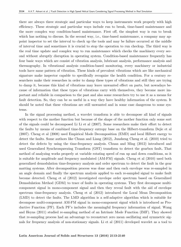
The simple harmonic functions of former decomposition method represent the constant ampli-tude and constant frequency modes. On the contrary, IMFs include variable amplitude and variable frequency. As it seems in Figure 1, all local extermums make envelope by green color and set of local maximums form one cluster which connected to each other by means of third orders spline. Then, by using this procedure again, set of local minimum connected to each other in another same independent cluster by aim of third orders spline. Now both of upper and lower sides of data enve-lope were built as illustrated in Figure 1 and by calculating the difference between upper and lower envelope first and higher frequency IMF can be extracted.

Let 1m be the difference between two envelopes so 1h can be produced by using the simple sub-

traction which is shown in Equation 1.

1 1h x t m (1)

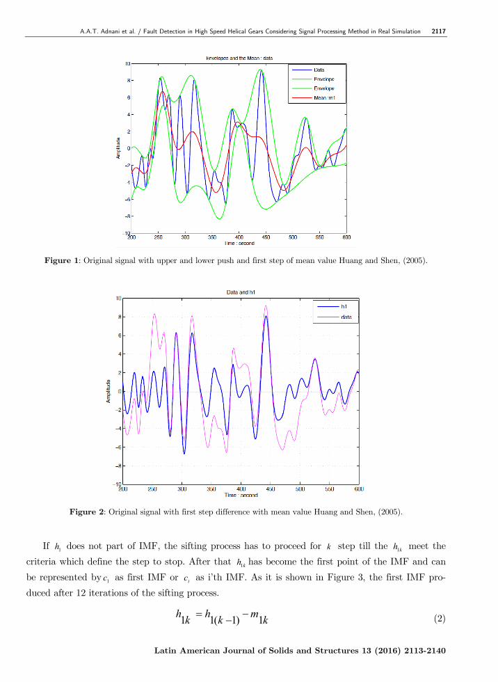
The produced 1h and initial signal is shown in Figure 2. Practically the generated extermums

which obtained after running one step of this procedure make reveal appropriate mode extermums which initially were lost into the original signals. In the other words, repeating the sifting process make more improvement with low amplitude signals and it makes signal more symmetric and elim-inates the dominant low frequency mode.



Figure 1: Original signal with upper and lower push and first step of mean value Huang and Shen, (2005).

Figure 2: Original signal with first step difference with mean value Huang and Shen, (2005).

If 1h does not part of IMF, the sifting process has to proceed for k step till the 1kh meet the

criteria which define the step to stop. After that 1kh has become the first point of the IMF and can

be represented by 1c as first IMF or ic as i’th IMF. As it is shown in Figure 3, the first IMF pro-

duced after 12 iterations of the sifting process.

1 1( 1) 1h h mk k k (2)



1 1c hk

(3)

Figure 3: The result of first step sifting process Huang and Shen, (2005).

In 1998 the first stopping criteria was proposed by Haung, Huang and Shen, (2005). They were

proposed to use normalized square difference for two sequential steps to stop the sifting process. This criteria as it is shown in Equation 4, was based on convergence Cauchy test. In the year of 2003, according to the Haung researches the value of kSD was proposed to be 0.0002. If the calcu-

lated value of kSD was greater than 0.0002, the sifting process went to the next level. Otherwise, it

stopped and original signal had to subtract by created IMF in order to generate the residual signal for other IMF. As it was shown in Equation 3, the residual signal created with respect to the ex-tracted IMF. For more illustration, original signals and residual signal after extraction of the first IMF is shown in Figure 4. Finally, Equation 6 is applied to take summation of all IMF’s and final residual signal to reconstruct the original signal.

2( ) ( )10

21

0

Th t h tk k

tSDk T

hkt

(4)

( )1 1r x t c (5)

( )1

nx t c rj n

j

(6)



Figure 4: Original signal with first step residual Huang and Shen, (2005).

2.1 Numerical Test

In order to demonstrate the power of the EMD algorithm by means of MATLAB software, Set of artificial sinusoidal combined signal is created which is based on Equation 7. This set of data is included different frequency sine wave which is varied from 20 Hz to 400 Hz and also has different amplitudes to examine the EMD algorithm. The artificial signal is shown in Figure 5 which can be interpreted in terms of time in second.

s(t)=sin(40. .t)+1.5sin(200. .t)+2sin(400. .t) (7)

Figure 5: Numerical test signal generated in MATLAB software.

0 0.1 0.2 0.3 0.4 0.5 0.6 0.7 0.8 0.9 1-4

-3

-2

-1

0

1

2

3

4

Time (s)

Am

plitu

de s(

t)



After decomposition process which is taken a few times, the artificial signal is decomposed into six IMF which are in descending order of frequency variable. In Table 1, the number of iteration for each IMF is shown. Table 1 shows that after how many times iterations the signals were decom-posed into six IMF’s. It is important because it shows how fast and simple EMD can decompose the signals. Besides, it shows that how fast basic IMFs are decomposed (first, second and third IMF’s) they take respectively 4, 1 and 4 iterations to be decomposed in comparison to other IMF’s which are shown the interaction of basic IMF’s.

The first triplex cluster decomposed waves include three basic frequency spectrum. The first cluster is shown in Figure 6. In this figure, frequency from upper graph to lower graph varies from 400, 200 and 40 Hz, respectively. It is clear that EMD algorithm can decompose the original signal into the basic elements of itself properly. However, these elements have some interaction with each other which are decomposed in another triplex cluster of IMFs and one residual signal. The second cluster and residual signal are shown in Figure 7. In fact, second cluster IMFs are the excess de-composition of EMD algorithm and technically these are not the basic components of original sig-nal. It should be noted that second cluster and residual signal have meaningless frequency. They are just the result of basic element interaction. It should be mentioned that the residual signal shows the general attitude of signal which is more related to the strongest frequency component of signal. For instance, the sine wave at frequency of 400 Hz and amplitude of 2 is dominant component which defines general trend of the signal.

IMF 1th IMF

2th IMF

3th IMF

4th IMF

5th IMF

6th IMF

Number of iteration

4 1 4 77 28 7

Table 1: Number of iteration of each IMF.

Figure 6: First cluster decomposed IMF’s of numerical test in different frequencies a: 400Hz, b: 200Hz and c: 40Hz.

0 0.1 0.2 0.3 0.4 0.5 0.6 0.7 0.8 0.9 1

-2

0

2

a. Time (s)

Am

plitu

de c1

0 0.1 0.2 0.3 0.4 0.5 0.6 0.7 0.8 0.9 1-2

0

2

b. Time (s)

Am

plitu

de c2

0 0.1 0.2 0.3 0.4 0.5 0.6 0.7 0.8 0.9 1

-1

0

1

c. Time (s)

Am

plitu

de c3



Figure 7: the second cluster of IMFs (a, b and c) and general trend (d).

2.2 Noise Effects on Signal Decomposition

In real application of decomposition method, noise and its effect should be taken into account as epidemic existing factor in signal processing which may cause different kinds of problem. Equation 8 determines that the ratio of standard deviation of noise and signals is 0.1 in the same words it’s actually define the power or frequency content of the noise. So, By using the equation 8, the added noise is defined as a high frequency component of signals that was generated while it was measur-ing. In the other words, data acquisition tool induce the high frequency component into the signal. It happens because measuring tools are the main cause of noise generation. In order to examine the power of EMD algorithm, first of all, a randomly definite noise based on Equation 8 is added to original signal. In order to have more realistic simulation the value of added noise is based on measuring data apparatus. The conventional data acquisition tools gather data with same amount of adding noise. The usual and industrial data acquisition tools corporations claim that the ratio of standard deviation of pure signal over noise is equal to 0.1. Then, noise is added to signal which is showed in Figure 8 and is going to separate by EMD algorithm. Therefore, the behavior of EMD algorithm in the presence of noise is determined. The noise which is added to the signal is generated by using Rand function in MATLAB software.

( ) 0.1( )

STD NoiseSTD Signal

(8)

In the first graph (part a) of Figure 8, the generated signal is shown. Besides, in part b, c and d of Figure 8, added noise, noisy signal or impure signal and zoomed pure signal versus noisy signal are shown respectively. The added noise has to be a zero mean graph which makes the noise sym-metric with respect to pure signal. Finally, in the lower graph the original pure signal in the pres-

0 0.1 0.2 0.3 0.4 0.5 0.6 0.7 0.8 0.9 1

-0.2

-0.1

0

0.1

0.2

0.3

a. Time (s)

Am

plitu

de c4

0 0.1 0.2 0.3 0.4 0.5 0.6 0.7 0.8 0.9 1

-0.2

-0.1

0

0.1

0.2

0.3

b. Time (s)

Am

plitu

de c5

0 0.1 0.2 0.3 0.4 0.5 0.6 0.7 0.8 0.9 1-0.1

-0.05

0

0.05

0.1

c. Time (s)

Am

plitu

de c6

0 0.1 0.2 0.3 0.4 0.5 0.6 0.7 0.8 0.9 1

-0.2

-0.1

0

0.1

0.2

d. time (s)

Am

plitu

de o

f re

sidua

l sig

nal



ence of the noisy signal is shown in order to the effect of noise in miniature scale become more de-termined.

Figure 8: a: numerical test signal, b: noise, c: noisy numerical test signal and

d: magnified comparison of noisy and pure numerical test signal.

In Figure 9, the first six IMF is shown. As it is shown, every six IMF is useless noise. They oc-

cur because of frequency order of EMD algorithm which is decomposing signal from higher frequen-cy to lower. Added noise becomes one of the signal components and it has to be decomposed like the basic frequency part of signal. Noise always has higher frequency rather than basic frequency of signal. It also indicates that EMD algorithm treat signal as a de-noising low pass filter like Butter-worth low pass filters with different cut off frequency per each IMF.

Figure 9: Noise effect on EMD, all first IMF to sixth IMF’s are noise in a, b, c, d, e and f, respectively.

0 0.1 0.2 0.3 0.4 0.5 0.6 0.7 0.8 0.9 1-5

0

5

a. Time (s)

Am

plitu

des(

t)

0 0.001 0.002 0.003 0.004 0.005 0.006 0.007 0.008 0.009 0.01-0.5

0

0.5

b. Time (s)

Am

plitu

deN

oise

0 0.1 0.2 0.3 0.4 0.5 0.6 0.7 0.8 0.9 1-5

0

5

c. Time (s)

Am

plitu

deN

oisy

sign

al

0.2054 0.2056 0.2058 0.206 0.2062 0.2064 0.2066 0.2068 0.207 0.2072

0123

d. Time(s)

Am

plitu

deN

oisy

sign

al&

Pur

e sig

nal

Original signalNoisy signal

0 0.1 0.2 0.3 0.4 0.5 0.6 0.7 0.8 0.9 1-0.5

0

0.5

a. Time (s)

Am

plitu

de

c1

0 0.1 0.2 0.3 0.4 0.5 0.6 0.7 0.8 0.9 1-0.5

0

0.5

b. Time (s)

Am

plitu

de

c2

0 0.1 0.2 0.3 0.4 0.5 0.6 0.7 0.8 0.9 1-0.5

0

0.5

c. Time (s)

Am

plitu

de

c3

0 0.1 0.2 0.3 0.4 0.5 0.6 0.7 0.8 0.9 1-0.5

0

0.5

d. Time (s)

Am

plitu

de

c4

0 0.1 0.2 0.3 0.4 0.5 0.6 0.7 0.8 0.9 1-0.2

0

0.2

e. Time (s)

Am

plitu

de

c5

0 0.1 0.2 0.3 0.4 0.5 0.6 0.7 0.8 0.9 1-0.2

0

0.2

f. Time (s)

Am

plitu

de

c6



Figure 10 demonstrates important component of signal which is consisting of four graphs. The graph a from Figure 10 shows incomplete part of higher component frequency of signal. This imper-fection is done because of interaction with induced noise. In graph (a) of Figure 11 by means of FFT algorithm, the frequency spectrum of 7C IMF is shown. In this spectrum, the presence of

higher component of original signal is illustrated and noise effect of signal is detected by some other peak frequency in the vicinity of 200Hz. In graph b from Figure 11, there are some evidence which indicate the presence of 200Hz frequency component and a little of 100Hz frequency component which are formed IMF 8C in graph b of Figure 10. In the other words, the higher frequency portion

of signal is composed of incomplete IMF 7C and incomplete IMF 8C . However, some missed part of

IMF 8C can be completed by IMF 7C . By looking at graph c from Figure 11, it is obvious that IMF

9C in Figure 10 is the second higher frequency part of original signal which is consists of only 100Hz

frequency part. However, some part of this component is missed and by reconsidering graph b from Figure 11, cause of missing some part of IMF 9C becomes clear. Also, in graph b from Figure 11

there are two frequency peaks which are 200Hz and 100Hz and little missing part of IMF 9C is in the

context of IMF 8C . At last the third part of frequency component is properly decomposed in IMF

10C which is shown in graph d from Figure 10 and its frequency spectrum is also shown in Figure

11.

Figure 10: Decomposition of a: first IMF, b: second IMF, c: third IMF and d: fourth IMF.

3 BASIC CHARACTERIZATION OF SIMULATION

0 0.1 0.2 0.3 0.4 0.5 0.6 0.7 0.8 0.9 1-3

-2

-1

0

1

2

3

a. Time (s)

Am

plitu

dec7

0 0.1 0.2 0.3 0.4 0.5 0.6 0.7 0.8 0.9 1-3

-2

-1

0

1

2

3

b. Time (s)

Am

plitu

dec8

0 0.1 0.2 0.3 0.4 0.5 0.6 0.7 0.8 0.9 1-2

-1

0

1

2

c. Time (s)

Am

plitu

dec9

0 0.1 0.2 0.3 0.4 0.5 0.6 0.7 0.8 0.9 1-1.5

-1

-0.5

0

0.5

1

1.5

d. Time (s)

Am

plitu

dec1

0



In order to run more reliable simulation which is more adapted to actual world, the used gear mesh is according to real productive automobile corporation standard which is now available in the mar-ket. In order to simulate the gear mesh in high velocity with respect to what research have done till now, the fourth gear engaged is chosen. In Figure 12 (Upper side), the input shaft and its installed gear is shown. In this figure, the input shaft which is the initial receiver of engine torque and angu-lar velocity is shown. In Figure 12 (Upper side), first, second, rear and fourth gears from left to right also are shown, respectively.

Figure 12 (lower side) depicts the output shaft. In this figure, the third and fourth gear from left to right is shown, respectively. There are two places for bearing to locate. One of them is hard access and another one is easy access. In order to have a better simulation the acceleration sensor in MSC Visual Nastran software is attached with respect to the accessibility of bearing and also, for output shaft the data acquisition is attached on accessible bearing.

The position of gears over the input and output shaft and the position of accessible and inac-cessible bearings are shown Figure 12. Accessible bearing on input shaft and accessible bearing on output shaft are at the distance of 110.725 mm and 112.486 mm, respectively from fourth gears. In order to constraint the two shafts; four bearings are applied in the geometrical models which are placed at the real position of the bearings with the equal length to real bearings. Each shaft has two ball bearings which are placed at the end and beginning of the shaft to make the shaft under constraint and all of the ball bearings have low friction coefficient. The friction of the bear-ings is calculated by means of wet friction factor which is according to the SKF catalog. The fric-tion coefficient is set to 0.002 and the clearance is set to 0.05 mm between ball bearings and out-side of the shaft.

Figure 11: FFT spectrum of a: first IMF, b: second IMF, c: third IMF and d: fourth IMF.

0 50 100 150 200 250 300 350 4000

0.1

0.2

0.3

0.4

a. Frequency (Hz)

Abs

olut

e val

ueof

FFT

c7

0 50 100 150 200 250 3000

0.5

1

1.5

2

b. Frequency (Hz)

Abs

olut

e val

ueof

FFT

c8

0 20 40 60 80 100 120 140 160 180 2000

0.2

0.4

0.6

0.8

1

1.2

1.4

c. Frequency (Hz)

Abs

olut

e val

ueof

FFT

c9

0 5 10 15 20 25 30 35 40 45 500

0.2

0.4

0.6

0.8

1

d. Frequency (Hz)

Abs

olut

e val

ueof

FFT

c10



Figure 12: Locations of gears and bearings on input shaft (upper side) and output shaft (lower side).

The technical properties’ of couple gears are shown in table 2. According to this table, the fac-

tor of this engagement with considers the number of tooth of input and output fourth gears, is 1.05.

Properties Input gear Output gear Units

Number of teeth 41 39 --------

Distance between shaft 70 70 mm

Helical angle 27.10 27.10 deg

Tip circle diameter 76.05 72.75 mm

Base circle diameter 65.90 62.45 mm

Pitch circle diameter 74.14 65.87 mm

Pressure angle 15 15 deg

Table 2: Input and output gear characteristics.

In order to have correct RPM and correct input and output torque values which had to be ex-erted on input and output shaft respectively, the practical engine map is useful tool. Engine map includes the generated engine output torque versus revolutionary rate of engine; the fourth gear conventional velocity lay between 60Kmph to 80Kmph. So, first of all the rotating velocity of input gear has to be determined. For this purpose the CARSIM software is chosen to simulate the really feature of practical vehicle to calculate the engine RPM at 80Kmph and 60Kmph velocity of the vehicle and the result of this simulation is shown in table 3. The chosen RPM is 2674 rpm which is equal to 44.57 Hz.



RPM (Hz) RPM (Rpm) Linear velocity of vehicle (Kmph)

44.57 2674 60

59.43 3566 80

Table 3: Rotating and linear velocity of output engine and vehicle, respectively.

In order to determine the input and output exerted torque by using the engine map, the output torque of engine which is exerted on input shaft is read as 144 N.m. The engine map which is used for this simulation is also shown in Figure 13. For determination of output torque on output shaft with respect to the first assumption that is constant linear velocity, the force equilibrium condition is considered and output torque by using the gearbox ratio at fourth gear and input torque is calcu-lated 136.98 N.m.

Figure 13: Applied engine map for simulation.

In Figure 14, the position of sensor, the length of bearings, the point where the torque exerted

(input and output torque respectively on input and output gearbox) and also the scheme of assem-bly are shown. In practical mechanism, all ball bearings have to hold moving components at their places and allow them to rotate freely without friction forces or torques. Therefore, in the procedure of simulation the fixed constraint put on the bearings which is prevented the bearing from vary and also it should be noted that, between all six components there are impenetrate constraint which force whole six geometrical model not to penetrate each other. In order to have more effective con-trol over impulse between all models, restitution coefficient is set to 0.8. All four ball bearings were fixed at each place and into the CARSIM software each shaft and its bearings were defined to be impenetrable to each other. This being impenetrable defined a rule which allows software to make the collision between each shaft and specific bearings with define restitution and friction factor.

1500 2000 2500 3000 3500 4000 4500 5000 5500 6000 650090

100

110

120

130

140

150

RPM (Rev/min)

Engi

ne o

utpu

t tpr

que (

N.m

)



Figure 14: Locations of accessible bearing for data acquisition on simple model.

3.1 Mesh Independency Analysis

In order to have best feasible size of mesh and to reach the minimum possible element size, at the first step above of all, simple static structure model with 100 N.m and different element size is run. As it is shown in Figure 15, the place where the engine exerts, 100 N.m torque is located. The only axial rotations of six degree of freedom are opened to the model and the output place of output shaft is fixed. Finally, for the boundary conditions at right hand bearings, the axial rotation of shaft is the only freedom degree of the model.

Figure 15: Boundary condition for static simulation for choosing mesh length.

For the first step of mesh independency, the geometrical model is meshed at 10 mm lengths el-

ement which is generated 4954 and 18540 for number of nodes and number of elements of output shaft, respectively. Because it is supposed that fault is occurred in input shaft, the only input shaft is meshed in order to reduce the time and calculation source. The amount of torque which is exert-ed to the mesh model is 100 N.m. In Figure 16, the maximum principle stress of input shaft is shown at 0.25 mm mesh length. In the graph of Figure 17, the maximum principle stress versus the element length is plotted and the length which maximum stress is converged is chosen to re-mesh the output and input shaft again and make both of them ready to dynamic simulation. The chosen length for element length is 0.5 mm which is created the 559534 and 2726092 number of nodes and elements, respectively. The meshed geometrical model is also shown in Figure 18.



Figure 16: Static simulation result of input gear for mesh independency.

Figure 17: Convergence of mesh length of mesh independency.

Figure 18: Meshed model of input gear with length of 0.5 mm.

0 1 2 3 4 5 6 7 8 9 105

5.5

6

6.5

7

7.5

8x 107

Mesh length (mm)

Max

imum

prin

cipl

e str

ess (

Pa)



4 DYNAMIC SIMULATION OF ENGAGED GEARS

In this step the geometrical model is imported to the MSC Visual Nastran software and the con-straint is added to the model to complete the simulation process. At the first step, the gear without fault is imported to reach the conventional no fault vibration as reference pattern. As it mentioned, the input gear is meshed with 49424 elements and 8290 nodes of tetrahedral geometrical shape. Then, the output gear is imported and meshed with 43846 elements and 74048 nodes. Then, for two gears in order to having no penetration in each other, the collision between them is defined. The next step is the import of four bearings. The four bearings are imported and in order to make sure of being bearings immobilized the fix constrain make them freeze. Fix constraints do not mean that the rotations of two shafts are ignored, but it means the all bearing in their position are fixed and they do not have any motion. The collisions between each bearings and relevant shaft are defined by means of constitution factor and friction factor of bearings which are 0.8 and 0.02, respectively. Then, 144 and 136.98 N.m torques are added to input and output shaft, respectively. In order to make the system rotation the motor on input shaft is used to create the angular velocity of 16045.2 Deg/s which is equal to 44.57 Hz. By using the meter tools in MSC Nastran software angular posi-tion, linear translation and linear acceleration of output shaft are recorded by data acquisition fre-quency of 524288 Hz. The pure signal of angular position, lateral position of axis and linear acceler-ation of output shaft is shown in Figure 19.

Figure 19: a: angular position, b: position and c: acceleration of input shaft.

In order to have more real signals, the noise should be added to the signal. Therefore, based on

Equation 8, based on the sensor production company catalogue, the noise is added to the pure sig-nal. According to the sensor production company catalogue, the ratio of standard deviation of rec-orded noise per standard deviation of pure signals is less than 0.1. So, by using Equation 8, the noise is added to the pure signal and make it impure and ready to analyze. For more illustration, the impure signal is shown in Figure 20 at two graphs. The first upper graph is impure signal and

0 0.01 0.02 0.03 0.04 0.05 0.06 0.07 0.08 0.09-200

-100

0

100

200

a. Time (s)

Ang

ular

pos

ition

of

inpu

t sha

ft (d

eg)

0 0.01 0.02 0.03 0.04 0.05 0.06 0.07 0.08 0.09-2

-1

0

1

2x 10-4

b. Time (s)

Posit

ion

ofou

tput

shaf

t (m

)

0 0.01 0.02 0.03 0.04 0.05 0.06 0.07 0.08 0.09-50

0

50

c. Time (s)

Acc

eler

atio

n of

outp

ut sh

aft (

m/s2 )



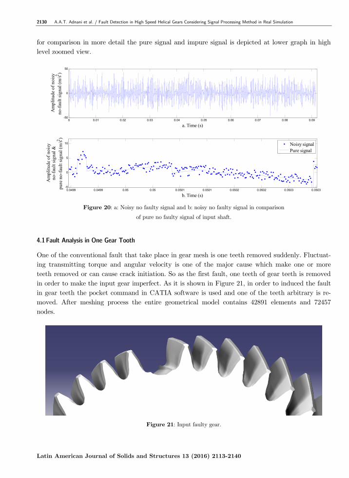
for comparison in more detail the pure signal and impure signal is depicted at lower graph in high level zoomed view.

Figure 20: a: Noisy no faulty signal and b: noisy no faulty signal in comparison

of pure no faulty signal of input shaft.

4.1 Fault Analysis in One Gear Tooth

One of the conventional fault that take place in gear mesh is one teeth removed suddenly. Fluctuat-ing transmitting torque and angular velocity is one of the major cause which make one or more teeth removed or can cause crack initiation. So as the first fault, one teeth of gear teeth is removed in order to make the input gear imperfect. As it is shown in Figure 21, in order to induced the fault in gear teeth the pocket command in CATIA software is used and one of the teeth arbitrary is re-moved. After meshing process the entire geometrical model contains 42891 elements and 72457 nodes.

Figure 21: Input faulty gear.

0 0.01 0.02 0.03 0.04 0.05 0.06 0.07 0.08 0.09-50

0

50

a. Time (s)

Am

plitu

de o

f noi

syno

-faul

t sig

nal (

m/s2 )

0.0499 0.0499 0.05 0.05 0.0501 0.0501 0.0502 0.0502 0.0503 0.0503-5

0

5

10

b. Time (s)

Am

plitu

de o

f noi

syno

-faul

t sig

nal &

pure

no-

faul

t sig

nal (

m/s2 )

Noisy signalPure signal



The entire simulation steps for this kind of fault are the same as no fault simulation. In Figure 22, pure signal of angular position, lateral position of axis and linear acceleration of input shaft of one teeth fault are shown.

Figure 22: a: angular position, b: Position and c: acceleration of faulty input shaft.

In Figure 23, the impure faulty signal is shown at upper section and for more comparison im-

pure and pure fault signal is also shown in lower section.

Figure 23: a: Noisy faulty signal and b: noisy faulty signal in comparison of pure faulty signal of faulty input shaft.

0 0.01 0.02 0.03 0.04 0.05 0.06 0.07 0.08 0.09-200

-100

0

100

200

a. Time (s)Ang

ular

pos

irion

of

inpu

t sha

ft (d

eg)

0 0.01 0.02 0.03 0.04 0.05 0.06 0.07 0.08 0.09-2

-1

0

1

2x 10-4

b. Time (s)

Posit

ion

of

outp

ut sh

aft (

m)

0 0.01 0.02 0.03 0.04 0.05 0.06 0.07 0.08 0.09-50

0

50

c. Time (s)

Acc

eler

atio

n of

outp

ut sh

aft (

m/s2 )

0 0.01 0.02 0.03 0.04 0.05 0.06 0.07 0.08 0.09-50

0

50

a. time (s)

Am

plitu

de o

f noi

syfa

ult s

igna

l (m

/s2 )

0.062 0.0622 0.0624 0.0626 0.0628 0.063

-4

-3

-2

-1

0

1

2

b. time (s)

Am

plitu

de o

f noi

syfa

ult s

igna

l &pu

re fa

ult s

igna

l (m

/s2 )

Noisy signalPure signal



4.2 Fault Analysis of Partially One Gear Tooth

Like previous section, the other possibility of fault occurrence is partially tooth removed on effect of abruptly change in transmitting torque and angular velocity in which particular conditions always leads to have critical condition. In order to make fault on gear, a-fourth of one teeth helical length is removed as it mentioned by using the pocket command in CATIA software. The length of remov-ing teeth is 3.9 mm which is a-fourth length of whole helix length in no-fault gear. In Figure 24, the partially removed teeth is shown.

Figure 24: Input partial faulty gear.

Just like pervious section, the entire simulation steps are done with this kind of fault and in

Figure 25, pure signal of angular position, lateral position of axis and linear acceleration of input shaft of a fourth one teeth fault is shown, respectively. In Figure 26, the impure signal of a fourth teeth removed is shown at upper section and for more comparison impure and pure faulty signal is shown in lower section.

Figure 25: a: angular position, b: Position and c: acceleration of partial faulty input shaft.

0 0.01 0.02 0.03 0.04 0.05 0.06 0.07 0.08 0.09-200

0

200

a. Time (s)Ang

ular

pos

ition

of

outp

ut sh

aft (

deg)

0 0.01 0.02 0.03 0.04 0.05 0.06 0.07 0.08 0.09-2

0

2x 10-4

b. Time (s)

Posit

ion

ofou

tput

shaf

t (m

)

0 0.01 0.02 0.03 0.04 0.05 0.06 0.07 0.08 0.09-50

0

50

c. Time (s)

Acc

eler

atio

n of

outp

ut sh

aft (

m/s2 )



Figure 26: a: Noisy partial faulty signal and b: noisy partial faulty signal in comparison

of pure partial faulty signal of faulty input shaft.

5 SIMULATION RESULTS

In the previous section, the three sets of pair gears were simulated and the noise was added to all data with respect to the Equation 8. In this section, at the first step the added noise should be re-moved. For this purpose, the 5th kind of Butterworth low pass filter is used with cut off frequency of 5 KHz and sampling frequency of 524288 Hz is applied. The low pass filter parameter is calculat-ed by try and error process. In order to avoid frequency damage to data, the cut off frequency value is chosen in a way which is far away from frequency information. For more illustration, linear fre-quency response in decibel unit and linear phase response in radian unit is depicted in Figure 27. In the gear fault detection the important and usable frequency data is formed at the gearmesh fre-quency of defected gear, which is production of teeth number with rotation frequency. The gearmesh frequency is about 1800 Hz. So, in order to avoid missing important information the cut off frequency of low pass filter is selected as 5 KHz.

Figure 27: Butterworth low pass filter phase and magnitude in linear system.

0 0.01 0.02 0.03 0.04 0.05 0.06 0.07 0.08 0.09-50

0

50

a. Time (s)

Am

plitu

de o

f noi

syfa

ult s

igna

l (m

/s2 )

0.045 0.0455 0.046 0.0465 0.047 0.0475 0.048

0.5

1

1.5

2

2.5

3

b. Time (s)

Am

plitu

de o

f noi

syfa

ult s

igna

l &pu

re fa

ult s

igna

l (m

/s2 )

Pure signalNoisy signal

0 5 10 15 20 25 30-80

-70

-60

-50

-40

-30

-20

-10

0

10

Frequency (kHz)

Mag

nitu

de (d

B)

Magnitude (dB) and Phase Responses

-8.2467

-7.3441

-6.4416

-5.539

-4.6365

-3.7339

-2.8314

-1.9288

-1.0263

-0.1237

Phas

e (ra

dian

s)

Butterworth: MagnitudeButterworth: Phase



5.1 Analysis of No Fault Gear Engaged Simulation

For no faulty gear analysis, the first step should be de-noising generated data. So, as it was men-tioned in order to de-noise the data the low pass 5th Butterworth filter with 5 KHz cut off frequen-cy was applied to data and this result is shown in Figure 28 and for more illustration the figure have two segments include the un-zoomed and zoomed view.

Figure 28: a: zoomed and b: un-zoomed filtered no faulty signal.

In order to reveal the fault at the second step, by using the FFT algorithm the frequency spec-

trum of undecomposed no faulty gearmesh data is obtained. The frequency spectrum of no faulty gearmesh is shown in Figure 29. It is obvious that there is no sign of peak frequency at 1738.23 Hz. So, in order to dig deeper and get more details from de-noised data, the decomposition process should be run.

Figure 29: FFT spectrum of no faulty filtered signal.

0 0.01 0.02 0.03 0.04 0.05 0.06 0.07 0.08 0.09-20

-10

0

10

20

a. Time (s)

Filte

red

no-fa

ult

signa

l (m

/s2 )

0.06 0.0605 0.061 0.0615 0.062 0.0625 0.063 0.0635

-10

-5

0

5

10

15

b. time (s)

Zoom

ed fi

ltere

d no

-faul

t sig

nal (

m/s2 )

0 0.5 1 1.5 2 2.5 30

0.1

0.2

0.3

0.4

0.5

0.6

0.7

0.8

0.9

1

Frequency (kHz)

Abs

olut

e val

ue o

f FFT



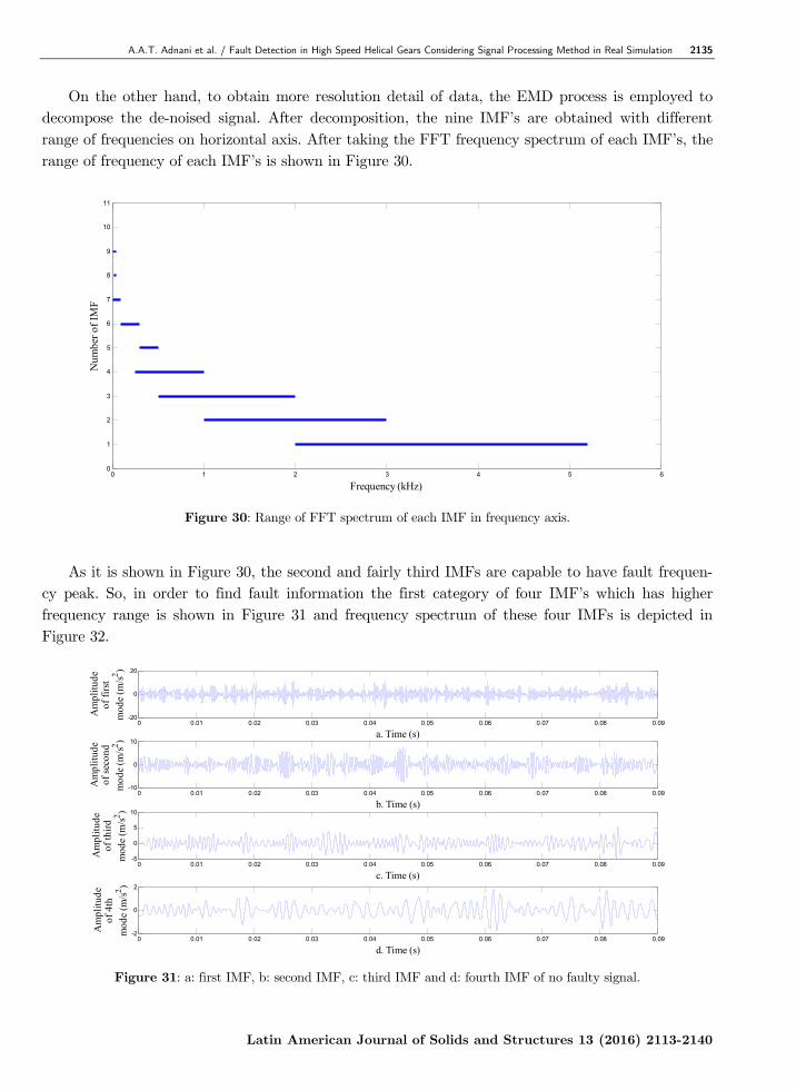
On the other hand, to obtain more resolution detail of data, the EMD process is employed to decompose the de-noised signal. After decomposition, the nine IMF’s are obtained with different range of frequencies on horizontal axis. After taking the FFT frequency spectrum of each IMF’s, the range of frequency of each IMF’s is shown in Figure 30.

Figure 30: Range of FFT spectrum of each IMF in frequency axis.

As it is shown in Figure 30, the second and fairly third IMFs are capable to have fault frequen-

cy peak. So, in order to find fault information the first category of four IMF’s which has higher frequency range is shown in Figure 31 and frequency spectrum of these four IMFs is depicted in Figure 32.

Figure 31: a: first IMF, b: second IMF, c: third IMF and d: fourth IMF of no faulty signal.

0 1 2 3 4 5 60

1

2

3

4

5

6

7

8

9

10

11

Frequency (kHz)

Num

ber o

f IM

F

0 0.01 0.02 0.03 0.04 0.05 0.06 0.07 0.08 0.09-20

0

20

a. Time (s)

Am

plitu

deof

firs

tm

ode (

m/s2 )

0 0.01 0.02 0.03 0.04 0.05 0.06 0.07 0.08 0.09-10

0

10

b. Time (s)

Am

plitu

deof

seco

ndm

ode (

m/s2 )

0 0.01 0.02 0.03 0.04 0.05 0.06 0.07 0.08 0.09-5

0

5

10

c. Time (s)

Am

plitu

deof

third

mod

e (m

/s2 )

0 0.01 0.02 0.03 0.04 0.05 0.06 0.07 0.08 0.09-2

0

2

d. Time (s)

Am

plitu

deof

4th

mod

e (m

/s2 )



Figure 32: FFT spectrum of a: first IMF, b: second IMF, c: third IMF and d: fourth IMF of no faulty signal.

As it seems neither in frequency spectrum of IMF’s of first category of four IMF’s, nor in the

other IMF’s and residual signal, there is no sign of frequency peak at 1738.23Hz and it means there is no fault in gear mating. 5.2 Fault Analysis of One Tooth from One Gear

In this section like the previous one, analysis of one gear tooth faulty signal is discussed to find the trace of fault in frequency information. At the first step, using butter worth low pass filter the de-noising process is done with 5 KHz cut off frequency and its result is also shown in Figure 33 in two moods from top to bottom, i.e., the zoomed and un-zoomed view, respectively.

Figure 33: a: zoomed and b: un-zoomed filtered one teeth faulty signal.

0 0.5 1 1.5 2 2.5 3 3.5 4 4.5 50

0.5

1

a. Frequency (KHz)

Abs

olut

eva

lue o

f FFT

of fi

rst I

MF

0 0.5 1 1.5 2 2.5 3 3.5 4 4.5 50

0.5

1

b. Frequency (KHz)

Abs

olut

eva

lue o

f FFT

of 2

th IM

F

0 0.5 1 1.5 2 2.5 3 3.5 4 4.5 50

0.2

0.4

c. Frequency (KHz)

Abs

olut

eva

lue o

f FFT

of 3

th IM

F

0 0.5 1 1.5 2 2.5 3 3.5 4 4.5 50

0.2

0.4

d. Frequency (KHz)

Abs

olut

eva

lue o

f FFT

of 4

th IM

F

0 0.01 0.02 0.03 0.04 0.05 0.06 0.07 0.08 0.09-20

-10

0

10

20

a. Time (s)

Filte

red

faul

tsig

nal (

m/s2 )

0.047 0.0475 0.048 0.0485 0.049 0.0495 0.05 0.0505-20

-10

0

10

20

b. Time (s)

Zoom

ed fi

ltere

d fa

ult

signa

l (m

/s2 )



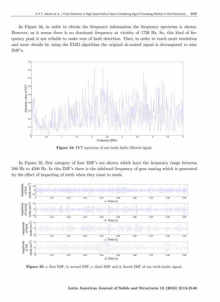
In Figure 34, in order to obtain the frequency information the frequency spectrum is shown. However, as it seems there is no dominant frequency at vicinity of 1738 Hz. So, this kind of fre-quency peak is not reliable to make sure of fault detection. Then, in order to reach more resolution and more details by using the EMD algorithm the original de-noised signal is decomposed to nine IMF’s.

Figure 34: FFT spectrum of one teeth faulty filtered signal.

In Figure 35, first category of four IMF’s are shown which have the frequency range between

500 Hz to 4500 Hz. In this IMF’s there is the sideband frequency of gear mating which is generated by the effect of impacting of teeth when they come to mesh.

Figure 35: a: first IMF, b: second IMF, c: third IMF and d: fourth IMF of one teeth faulty signal.

0 0.5 1 1.5 2 2.5 3 3.5 4 4.5 50

0.1

0.2

0.3

0.4

0.5

0.6

0.7

0.8

0.9

Frequency (kHz)

Abs

olut

e val

ue o

f FFT

0 0.01 0.02 0.03 0.04 0.05 0.06 0.07 0.08 0.09

-10

0

10

a. Time (s)

Am

plitu

deof

firs

tm

ode (

m/s2 )

0 0.01 0.02 0.03 0.04 0.05 0.06 0.07 0.08 0.09-10

0

10

b. Time (s)

Am

plitu

deof

seco

ndm

ode (

m/s2 )

0 0.01 0.02 0.03 0.04 0.05 0.06 0.07 0.08 0.09-5

0

5

c. Time (s)

Am

plitu

deof

third

mod

e (m

/s2 )

0 0.01 0.02 0.03 0.04 0.05 0.06 0.07 0.08 0.09-2

0

2

d. Time (s)

Am

plitu

deof

4th

mod

e (m

/s2 )



As it is shown in Figure 36, the frequency spectrum of second IMF, there is peak frequency with magnitude of 1738 Hz which is the gearmesh frequency of output gear. This peak of frequency is the indication of fault existing in gear meshing. This peak is indicated at output gearmesh frequency. So, this fault is belonging to the output gear. The input gear has 41 teeth and the output gearmesh frequency is 1827.37 Hz and at 1837.37 Hz there is no reliable peak frequency.

Figure 36: FFT spectrum of a: first IMF, b: second IMF, c: third IMF and d: fourth IMF of one teeth faulty signal.

5.3 Fault Analysis of Partially One Teeth of Gear

In Figure 37, the de-noised signal is shown at first upper segment of figure and the second IMF which is more important from others is depicted at middle segment of Figure 37 and at last there is frequency spectrum of second IMF at bottom segment of Figure 37.

Figure 37: a: filtered signal, b: second IMF and c: FFT spectrum of second IMF of partial faulty signal.

0 500 1000 1500 2000 2500 3000 3500 4000 4500 50000

0.5

1

a, Frequency (Hz)

Abs

olut

eva

lue o

f FFT

of fi

rst I

MF

0 500 1000 1500 2000 2500 3000 3500 4000 4500 50000

0.5

1

b, Frequency (Hz)

Abs

olut

eva

lue o

f FFT

of se

cond

IMF

0 500 1000 1500 2000 2500 3000 3500 4000 4500 50000

0.5

c, Frequency (Hz)

Abs

olut

eva

lue o

f FFT

of 3

th IM

F

0 500 1000 1500 2000 2500 3000 3500 4000 4500 50000

0.2

0.4

d, Frequency (Hz)

Abs

olut

eva

lue o

f FFT

of 4

th IM

F

0 0.01 0.02 0.03 0.04 0.05 0.06 0.07 0.08 0.09

-10

0

10

a. Time (s)

Parti

ally

toot

hfa

ult (

m/s2 )

0 0.01 0.02 0.03 0.04 0.05 0.06 0.07 0.08 0.09-10

-5

0

5

10

b. Time (s)

Am

plitu

deof

seco

ndm

ode (

m/s2 )

0 500 1000 1500 2000 2500 3000 3500 4000 4500 50000

0.2

0.4

0.6

0.8

c. Frequency (Hz)

Abs

olut

eva

lue s

econ

dIM

F of

FFT



Just like whole tooth fault, at partially teeth fault there is frequency peak at output gearmesh frequency which indicates the present fault in the output and because of this frequency peak is the dominant peak like the other peak, it is reliable sign of fault. It should be noted that the dominancy of whole teeth fault is more recognizable. So, with respect to the partially teeth fault the whole teeth fault is the prominent fault in frequency spectrum. 6 CONCLUSION

In the present work, the fault detection of two mating gears was discussed and the fault was detect-ed by means of signal processing method. First of all, the real and practical gear which is used in the industry was provided using CATIA software and then, by means of MSC Nastran software the no faulty gearmeshing simulation in practical speed of gear working and practical gear torque transmission was done and for more realization the noise was added to all generated signals. Then, the generated signal was processed using MATLAB software to reach the pattern of FFT spectrum. In the processing stage, the Butterworth low pass filter with cut off frequency of 5 KHz was applied to signal to de-noise the entire nuisance signal and it was completed the signals purification process. Then, the EMD algorithm was decomposed the signal into the IMF’s and each frequency IMF spec-trum were shown the pattern of no faulty gearmeshing process and these results were saved as healthy pattern reference. In next stage of this research, in order to reach the faults pattern refer-ences, the entire previous stage was implemented in the presence of fault which is consist of two faults. First, the whole tooth broken and then, the partial tooth broken and these kinds of faults could be revealed by using EMD algorithm and FFT spectrum. After the simulation and signal processing were done, the following results are reported as follows:

The location of sensor was chosen at distance of 112 mm from input gear which may cause the more complicated signal with regard to shaft properties. This altercation in the location affect the signal and make it AM-FM signal and reduced the strength or power of signals be-cause of long distance to the acquisition location and it also may leave resonance effect on signals and randomly changes the frequency spectrum.

If it is just necessary to the de-noise signal without decomposition, the EMD algorithm can de-noise signal, but if it is necessary to de-noise and then decompose the signals, the EMD algorithm could not be a useful tool.

In non-stationary signals EMD algorithm in comparison with wavelet which is based on con-stant sifting function, has an advantage to decompose the signal into basic intrinsic functions which are lay into the signal.

In the existence of noise, the EMD algorithm has bad behaviour in a way that the noise are decomposed into initials IMF’s and absolutely the noise should be removed before decomposi-tion process. The noise could leave a bad effect in decomposition process.

Detection of one tooth broken fault has high resolution with respect to the partial tooth bro-ken.

Reference

B. Samanata, (2004) Gear Fault Detection Using Artificial Neural Networks And Support Vector Machines With Genetic Algorithms, Mechanical Systems and Signal Processing 18: 625–644



Chuan Li, Ming Liang, (2012) Time–Frequency Signal Analysis for Gearbox Fault Diagnosis Using a Generalized Synchrosqueezing Transform, Mechanical Systems and Signal Processing 26: 205–217.

D. Chen, W. J. Wang, (2002) Classification of wavelet map Patterns using Multi-Layer neural networks For gear Fault Detection, Mechanical Systems and Signal Processing 16(4): 695–704.

Dejie Yu, Yu Yang, Junsheng Cheng, (2007) Application of Time–Frequency Entropy Method Based on Hilbert–Huang Transform to Gear Fault Diagnosis, Measurement 40: 823–830.

Grzegorz Litak, Krzysztof Kecik, Rafal Rusinek, (2013) Cutting force response in milling of Inconel Analysis by wavelet and Hilbert-Huang Transforms, Latin American Journal of Solids and Structures 10: 133–140.

H. Zheng, Z. Li, X. Chen, (2002) Gear Fault Diagnosis Based on continuous Wavelet Transform, Mechanical Sys-tems and Signal Processing 16(2–3): 447–457

Hui Li, Yuping Zhang, Haiqi Zheng, (2011) Application of Hermitian Wavelet to Crack Fault Detection in Gearbox, Mechanical Systems and Signal Processing 25: 1353–1363.

Junsheng Cheng, Kang Zhang, Yu Yang, (2012) An Order Tracking Technique for the Gear Fault Diagnosis Using Local Mean Decomposition Method, Mechanism and Machine Theory 55: 67–76.

Junsheng Cheng, Yi Yang, Yu Yang, (2012) A Rotating Machinery Fault Diagnosis Method Based on Local Mean Decomposition, Digital Signal Processing 22: 356–366.

Junsheng Cheng, YuYang, DejieYu, (2008) Application of frequency family separation method based upon EMD and local Hilbert energy spectrum method to gear fault diagnosis, Mechanical Systems and Signal Processing 43: 712–723.

Junsheng Cheng, YuYang, DejieYu, (2010) The Envelope Order Spectrum Based on Generalized Demodulation Time–Frequency Analysis and Its Application to Gear Fault Diagnosis, Mechanical Systems and Signal Processing 24: 508–521.

K.S. Wang, P.S. Heyns, (2011) An Empirical Re-Sampling Method on Intrinsic Mode Function to Deal with Speed Variation in Machine Fault Diagnostics, Applied Soft Computing 11: 5015–5027.

Li Li, Liangsheng Qu, Xianghui Liao, (2007) Haar wavelet for machine fault diagnosis, Mechanical Systems and Signal Processing 21: 1773–1786.

Lourdes Rubio, Belen Munoz-Abella, Patricia Rubio, Laura Montero, (2014) Quasi-static numerical study of the breathing mechanism of an elliptical crack in an unbalanced rotating shaft, Latin American Journal of Solids and Structures 11: 2333–2350.

Norden E Huang, Samuel S P Shen, (2005) Hilbert-Huang Transform and Its Applications, World Scientific Publish-ing Co. Pte. Ltd Volume 5

Roberto Ricci, Paolo Pennacchi, (2011) Diagnostics of Gear Faults Based on EMD and Automatic Selection of In-trinsic Mode Functions, Mechanical Systems and Signal Processing 25: 821–838.

S.J. Loutridis, (2006) Instantaneous energy density as a feature for gear fault detection, Mechanical Systems and Signal Processing 20: 1239–1253

W. J. WANG, P. D. Mcfadden, (1996) Application Of Wavelets To Gearbox Vibration Signals For Fault Detection, Journal of Sound and Vibration 192(5): 816_828

Documents

Fault Detection in High Speed Helical Gears Considering ... · developed in MATLAB software. Then, in order to detect the presence of the fault the frequency spectrum of IMF’s are