Embed Size (px)
Citation preview

I
Fault Detection for Gas Turbine Engine
Fuel Valves with Kalman Filter
Weiwei Chen
August 2010
Supervisor : Dr R F Harrison
A dissertation submitted in partial fulfilment of the requirements
for the degree of Master of Science in Control System

I
Author Weiwei Chen
MSc in Control System in August 2010
Abstract
Fault detection has been introduced into the most of fields, such as medical, industry,
and manufactory for their process control system for the requirement of safety and
reliability
In the past few years, the sensors were used for fault detection, however, they are
been sifted out, due to their high price which will increase the costs of the industry.
In this project, kalman filter been introduced for fault detection. Standard kalman
filter is used for the linear system, while extended kalman filter to be applied for
nonlinear system. The aim of this project is to generate the standard kalman and
extended kalman filter code to estimate the linear DC motor system with additive
fault influence and residual of stepper motor in nonlinear system.
II
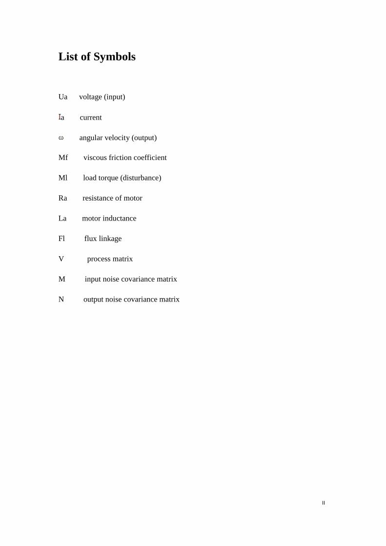
List of Symbols
Ua voltage (input)
a current
angular velocity (output)
Mf viscous friction coefficient
Ml load torque (disturbance)
Ra resistance of motor
La motor inductance
Fl flux linkage
V process matrix
M input noise covariance matrix
N output noise covariance matrix

III
List of Figures
Fig 1.1 General structure of fault detection and diagnosis……………………….…3
Fig 1.2 Structure of fault detection method…………………………………………5
Fig 2.1 Signal models for fault detection………………………………………..…12
Fig 2.2 Structure of signal model-based analysis…...……………………………...13
Fig 3.1 Cycle of kalman filter………………………………………………...……16
Fig3.2 A complete diagram of kalman filter implementation……………………...18
Fig4.1 A complete diagram of extended kalman filter implementation……………23
Fig 5.1 Excited DC motor in permanently…………………………………………24
Fig.5.2 DC motor states estimation with kalman filter…………………………….25
Fig 5.3 DC motor with input fault additive………………………………………...26
Fig 5.4 DC motor with current fault additive………………………………………27
Fig 5.5 DC motor with load torque additive……………………………………….27
Fig 5.6 DC motor with speed fault additive………………………………………..27
Fig 6.1 Full structure model of stepper motor with driver and clock input………..34
Fig 6.2 Model of stepper motor state estimation with EKF………………………..36

IV
Table of Contents
1. Introducton ............................................................................................................ 1
1.1 Definition and Categories, Causes of Fault .................................................. 1
1.1.1 Definition of Fault.............................................................................. 1
1.1.2 Classification of Fault ........................................................................ 2
1.1.3 Causes of Fault ................................................................................... 2
1.2 Fault Detection ............................................................................................. 3
1.3 Project Aim ................................................................................................... 6
1.4 Report Structure............................................................................................ 7
2 Literature Review ............................................................................... 8
2.1 Fault Detection with Model Analysis Method ............................................. 8
2.1.1 Model Free-Method ........................................................................... 8
2.1.2 Model-Based Method in Mathematic ................................................ 9
2.2 Fault Detection with Signal Analysis Method ............................................ 12
3 Kalman Filter .................................................................................... 14
3.1 Standard Kalman Filter............................................................................... 14
3.2 Algorithm of Kalman Filter ........................................................................ 16
4. Extended Kalman Filter ................................................................... 19
4.1. Extended Kalman Filter Procedure ............................................................ 19
4.2. Algorithm of Extended Kalman Filter ........................................................ 21
5. Model Constructions and Result Analysis ...................................... 24
5.1. Linear DC Motor States Estimation with Kalman Filter ............................ 24
5.2. DC Motor Residual Reduction ................................................................... 29
5.2.1. Sample Time Alteration ................................................................... 29
5.2.2. Viscous Friction Coefficient Mf ...................................................... 30
6. Stepper Motor in Nonlinear Signals Estimated by Extended
Kalman Filter ........................................................................................ 34
6.1. Stepper Motor Model ................................................................................. 34
6.2. Stepper Motor States Linearization and Original Setting ........................... 37
7. Goal achieved .................................................................................... 40
8. Conclusion ......................................................................................... 42
9. Reference ........................................................................................... 44

V
Acknowledgement
First of all I would appreciate my project supervisor, Dr. R.F. Harrison for his
precious guidance and kind attention to my MSc project in last four month. His
support and help are essential for me to complete this project in time. He always there
to listen and give me valuable advices, as well as helpful comments on my job, and
his kindness made my study more enjoyable.
I wish to thank Rolls-Royce University Technology Centre in Control System
Engineering at the University of Sheffield. And the special thanks go to Andy Mills,
who is responsible for helping me for worthy discussion and support.
I am deeply appreciate to my parents for their love, support encourage and
understanding in the past year. They are not in the UK; however, I got the confidence
from them via phone, which will guide me in the future as well.

1
1. Introduction
For recent few decades, the highest quality of products and their efficiency have been
played more concentration, they are inevitable that the benefits and reputation are
achieving for industries. Despite their significant benefits, the shortcoming of them is
that adjusting and improving the system of products is difficult to operation with
increasing industries‟ costs. System of products failure occurs when the system does
not match its requirement or out of reliable fault range. For the aerospace field, the
system failure means not only the cost lost for the airplane company, but also the key
issue is it takes numbers of live away easily. Fault detection method is an advanced
detection for system supervision, which based on heuristic knowledge in process
analyzing and variables observing (Isermann, 2006). Fault detection being used as
early as possible would ensure the aircrafts more reliability, availability and safety.
1.1 Definition and Categories, Causes of Fault
1.1.1 Definition of Fault
In the past year, the failure was usually used to identify the system bad performance.
Conversely, it is not fair to indicate poor performance system lead to failure. Hence in
Isermann (2006), the fault is defined that “a fault is unpermitted deviation of at least
one characteristic (property)of the system form the acceptable, usual, standard
condition.” For the fault, it approves a state in the abnormal values which cause a

2
system performance decrease or lose of, deviating the usual value of tolerant.
1.1.2 Classification of Fault
Fault are divided into intermittent fault and permanent fault based on it duration
(Zhou, 1998), the former one could be recover on the short time, while latter one
should hold on the system until the components changed.
Meanwhile, with respect to system model, the faults are distinguished into two
categories (Li, 2002):
The measurement influenced by the additive faults by its means changing.
The spectral characteristic of observation changing with impact on the
non-additive faults.
1.1.3 Causes of Fault
Characteristic estimates on operational process
Incorrect technical description
Alterability of component and equipment
Design error
Assemble, testing, or installation error
Maintenance error
(Li, 2002)

3
1.2 Fault Detection
Fault detection method concern the design of system and monitor the performance of
it, identifying the fault location and time when it occurs, illustrate in Fig 1.1
Fault
System input System output
Fault location fault time
Actual System
Model of
observed system
Model of nominal
system Model of faulty
system
parity observer detection
space scheme filter
parameter
estimation
Generation of
Residuals
Parity function
Parameter estimates
Decision function
generation
Fault detection
logic
Fault interpretation

4
Fig 1.1 General structure of fault detection and diagnosis
The fault detection instrument detects the input and output signal which goes through
the observer and comparing the estimating parameter to generates the residual. After
that, the residuals are checked whether it is in the tolerance area by fault function
generation. If not, system would alarm and specify the fault location and time.
The fault detection method identified by Isermann (2006) as Fig 1.2, where method is
separated into two portions that detection with single signals and detection with
multiple signals and models. Both of them are classify averagely, each of them has six
methods, e.g. fixed threshold, adaptive thresholds and change detection methods is
associated to limit checking and trend checking. While, signal models separated into
correlation, spectrum analysis and wavelet analysis.
Multi-variant data analysis would be based on principal component analysis.
Parameter estimation, neural networks, state observers, state estimates, and parity
equation are be used in process models analysis.

5

6
Fault detection are monitoring and protecting the system automatically, which could
stop the system and alarm the emergency when residuals over tolerance threshold by
comparing the states of actual parameters and design model measurements
1.3 Project Aim
The aim of this project is to apply kalman filter for system fault detection in DC
motor and extended Kalman filter for the stepper motor
Object 1
Generate code for generate kalman filter.
Object 2
Estimate states by the kalman filter in DC motor
Object 3
Build stepper motor model with the extended kalman filter.
Object 4
Matlab code generation for stepper motor states estimation by extended kalman filter.

7
1.4 Report Structure
In chapter two, fault detection method in model analysis method and signal analysis
method are reviewed.
DC motor states estimated by the kalman filter for fault detection to reduce the
residual, as well as changing parameters of model to eliminate mismatch, which
introduced on chapter three
In the chapter 4, it introduces the extended kalman filter applies on the stepper motor,
where will implement nonlinear signal linearization and transfer continuous signature
to discrete one at the first stage, then generate the extended kalman filter code for
stepper motor posterior states estimation.

8
2 Literature Review
Detection of fault has tended to be a significant task on computer/operator or both to
monitor the system on-line performance, which widely used in the products
manufactory and industry such as space vehicles and nuclear reactor (Boucherma,
1994).
The fault detection techniques classified into two types
Fault detection in model analysis method
Fault detection in signal analysis method
2.1 Fault Detection with Model Analysis Method
2.1.1 Model Free-Method
In this method, system process is supervised by the measureable inputs and outputs
variables.
(1) Limit checking in absolute value and trend
Limit checking is simple method used for fault detection, which measures the outputs
signal Y(t) to identify whether it locates on the acceptable threshold.
Ymin<Y(t)<Ymax (2.1)
This method is applied in the most automation system, for instance, oil pressure or

9
coolant of combustion engines (Isermann, 2006). The tolerance zone is selected based
on the operator experience.
The limited checking is applied not only on the absolute value, but also on the trend
(2.2)
The advantage for trend checking is it alarm early when the tolerance zone is not lager
enough, because the signal proceeding prediction (Isermann, 1981).
2.1.2 Model-Based Method in Mathematic
Model-based analysis method in mathematic using in the fault detection on the system
performance, which mainly rely on comparing the differences between actual values
which expected and estimate values obtained from the model. These differences
named residual (Boucherma, 1994. Schwarte, 2003).
Residual generated in the diverse ways, such as input/output equation (Gertler and
Singer, 1985), states attempted in observers (Patton and Willcox, 1985), kalman
filtering (Tylee, 1983), and identification concept (Isermann, 1985).
Residual generation (Zhou, 1998) formula becomes
r(s)= Gu(s)u(s)+Gy(s)y(s) (2.3)
where u(s), y(s) and r(s) are represent system input, output and residual, respectively,
Gu and Gy are transfer matrices
and define r(t)=0, no fault

10
r(t) 0, fault
From equation (2.3) and its restriction, it is obviously that residual is expected tend to
be zero by the model design, but it deviate from zero lead to fault occurs (Zhou,
1998).
The model-based fault detection consists of three portions: parity space approach,
state observers approach, as well as parameter estimate approach (Boucherma, 1994,
Zhou, 1998)
Parity Space Approach
Parity space approach mainly to check consistency of actual measurements and model
measurements, which been approved by Chow & Willsky (1984) and Luo et al. (1986)
that results can be achieved by combining present and past values of inputs and
outputs in the aero of systematic procedure (Zhou, 1998).
Isermann (2006) promoted output error and polynomial error to checking the
consistency of the actual system and model signals. This method describe the residual
can be made with transfer functions or in state space for state-space models.
States Observers Approach
In the approach which is comparing the actual outputs with estimate outputs by using
observer and generate residual (Zhou, 1998)

11
For instance, the observer-based model as
(t)=Ax(t)+Bu(t) (2.4)
y(t)=Cx(t) (2.5)
(Boucherma, 1994, Isermann, 2006)
For state-observer the formula construct based on measured inputs and outputs
illustrate (Isermann, 2006)
(t)=A (2.6)
e(t)=y(t)-C (2.7)
Isermann (2006) combines 2.6 and 2.7 to obtain the state-observer
(t)=[A-HC] +Bu(t)+Hy(t) (2.8)
where H is observer matrix.
(2.4) subtract to (2.8) yields the implementation form of state error
= (t)- (t)=[A-HC] (Isermann,2006)
[A-HC] named measurement residual. A residual equal to zero means that the actual
system and the model signal are complete agreement (Welch and Bishop, 2006).
Parameter Estimate Approach
The parameter estimate approach is relates to physical parameter altering in the model
which been detected (Chinag, Russell, Braatz, 2001).
The polynomial equation for the parametric model generated by Boucherma (1994)
y(u)= o+ 1u+ 2u2+…
(2.9)

12
model parameters can be estimated by the recursive least square (RLS) method, which
generate dynamic parameters for the system in order to determine whether the model
parameters deviated the actual values (Zhou, 1998).
2.2 Fault Detection with Signal Analysis Method
The fault detection used to measure the harmonic or stochastic noise, or both, which
respect to the actuator, process and sensor shown in the Fig 2.2 The detected signal
through the signal model-based fault detection for generating feature which been
compared with the feature comes from the actual system in each states of component.
If the residuals locate on the tolerance threshold, the detection would keep working,
or stop the system and alarm, simultaneity.
13
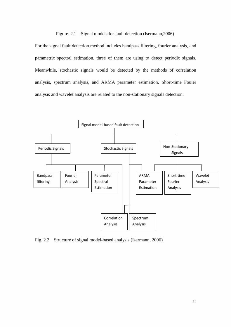
Figure. 2.1 Signal models for fault detection (Isermann,2006)
For the signal fault detection method includes bandpass filtering, fourier analysis, and
parametric spectral estimation, three of them are using to detect periodic signals.
Meanwhile, stochastic signals would be detected by the methods of correlation
analysis, spectrum analysis, and ARMA parameter estimation. Short-time Fouier
analysis and wavelet analysis are related to the non-stationary signals detection.
Fig. 2.2 Structure of signal model-based analysis (Isermann, 2006)
Signal model-based fault detection
Periodic Signals Non-Stationary
Signals Stochastic Signals
Bandpass
filtering
Fourier
Analysis
Parameter
Spectral
Estimation
Correlation
Analysis
Spectrum
Analysis
ARMA
Parameter
Estimation
Short-time
Fourier
Analysis
Wavelet
Analysis

14
3 Kalman Filter
Kalman filter is introduced by R. Kalman in 1960, which is applying to solve dynamic
system in recursive procedure which does not need the store past measurements for
the current states estimation (The Analytic Sciences Corporation, 1974, Welch and
Bishop, 2006). It estimates posteriori states vector at the k+1 step based on the priori
states vector at the k step, in order to minimize the estimation residuals. It applies for
the prediction and smoothing (Harvey, 1989). The covariance of the states will be
estimated by it as well, at each time step the new measurement achieved, which was
applied for updating the mean and covariance of the states (Simon, 2006).
3.1 Standard Kalman Filter
For linear system with discrete time signals with stochastic disturbance, the states
estimates equation
x(k+1)=Ax(k)+Bu(k)+w(k) (3.1)
with measurement y that is
z(k+1)=Cx(k)+v(k) (3.2)
(Welch and Bishop, 2006, Harvey and Proietti, 2005)
A in the equation 3.1 is a n n matrix which relates to the former states at step k to the
latter states at step k+1. For B, it is a n l dynamic matrix, which relates to control
input signal to the state, meanwhile C (m m matrix) is regard to output measurement

15
states (Harvey, 1989. Shah, 2004, Welch and Bishop, 2006).
The stochastic variables of w(k) and v(k) represent process and measurement
disturbance, respectively, to be assumed independent, white, and normal probability
distributions
p(w)~N(0,Q) (3.3)
p(v)~N(0,R) (3.4)
(Welch and Bishop, 2006).
Q and R represent process noise covariance and measurement noise covariance,
respectively, which are assumed to be a constant, though they are altering each time
step and measurement, in the real world (Welch and Bishop, 2006).
At step k, (k) is state shows the priori states which would be used to estimates
(k+1) for calculating measurement z(k+1). Hence the error of priori and posteriori
states estimates as
(k+1|k) (k+1) - (k+1|k)
(3.5)
e(k+1|k+1) x(k+1) - (k+1|k+1) (3.6)
(Isermann, 2006, Welch and Bishop, 2006).
with the error covariance matrices of priori and posteriori represent
(k+1|k)=E[e(k+1|k)eT(k+1|k)] (3.7)
P(k+1|k+1)=E[e(k+1|k+1)eT(k+1|k+1)] (3.8)
respectively (Isermann, 2006).
The posteriori states estimate x(k+1|k+1) represented by priori states estimate x(k+1|k)

16
as
x(k+1|k+1)=x(k+1|k)+K(z(k+1)-Hx(k+1|k)) (3.9)
(Welch and Bishop, 2006)
where K is n matrix kalman filter gain
Hx(k+1|k) is prediction measurement
Kalman filter gain K selected in order to minimize covariance error of posteriori,
which formula as
K=P(k+1|k)HT(HP(k+1|k)H
T+N)
-1 (3.10)
(Welch and Bishop, 2006).
where N is output noise covariance.
z(k+1)-Hx(k+1|k) represents the different on the actual measurement and prediction
measurement, which named residual. A residual equal to zero, it means the results of
the dynamic system are match completely (Welch and Bishop, 2006).
3.2 Algorithm of Kalman Filter
Welch and Bishop (2006) recommended that Kalman filter states estimate by
following recursive method with close loop feedback
Time Update(Prediction) Measurement Update(Correction)
17
Fig 3.1 Cycle of kalman filter
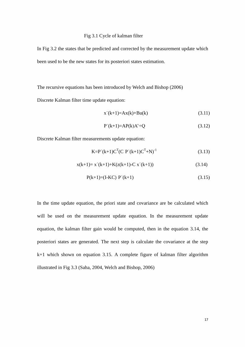
In Fig 3.2 the states that be predicted and corrected by the measurement update which
been used to be the new states for its posteriori states estimation.
The recursive equations has been introduced by Welch and Bishop (2006)
Discrete Kalman filter time update equation:
xֿ(k+1)=Ax(k)+Bu(k) (3.11)
Pֿ(k+1)=AP(k)A‟+Q (3.12)
Discrete Kalman filter measurements update equation:
K=Pֿ(k+1)CT(C Pֿ(k+1)C
T+N)
-1 (3.13)
x(k+1)= xֿ(k+1)+K(z(k+1)-C xֿ(k+1)) (3.14)
P(k+1)=(I-KC) Pֿ(k+1) (3.15)
In the time update equation, the priori state and covariance are be calculated which
will be used on the measurement update equation. In the measurement update
equation, the kalman filter gain would be computed, then in the equation 3.14, the
posteriori states are generated. The next step is calculate the covariance at the step
k+1 which shown on equation 3.15. A complete figure of kalman filter algorithm
illustrated in Fig 3.3 (Saha, 2004, Welch and Bishop, 2006)

18
(1) Project the state ahead (1) Compute Kalman gain
xֿ(k+1)=Ax(k)+Bu(k) K=Pֿ(k+1)CT(C Pֿ(k+1)C
T+N)
-1
(2) Project the error covariance ahead (2) Update estimate with measurement z(k)
Pֿ(k+1)=AP(k)A‟+Q x(k+1)= xֿ(k+1)+K(z(k+1)-C xֿ(k+1))
(3) Update error covariance
P(k+1)=(I-KC) Pֿ(k+1)
Initial estimates for xֿ(k+1)
and Pֿ(k+1)
Fig3.2 A complete diagram of kalman filter implementation
Time Update (“Prediction”) Measurement Update(“Correction”)

19
4. Extended Kalman Filter
Standard kalman filter is used to estimate states on the linear system by a linear
difference equation (Saha, 2004), however, in the real world, the system would be
nonlinear stochastic system, whose states cannot be estimated by the Standard kalman
filter so far. Therefore, extended kalman filter (EKF) is a recursive state estimator
which used for the nonlinear system states and measurement estimation (Saha, 2004).
The estimation stage of extended kalman filter will be introduced in the chapter.
4.1. Extended Kalman Filter Procedure
In the extended kalman filter, it has some difference to the standard kalman filter, due
to the dynamic states controlled by the nonlinear differential equations or nonlinear
states transformation (Grewal, S and Anderws, A, 2008). Hence, its first stage is
predicting the states using mathematic method (Saha, 2004). This process is to
segment the nonlinear signal into several section and hypothesis it as the linear
signature. The second and third stage as the standard kalman filter does, to estimate
the posteriori states based on the priori ones, and then achieve the new measurement
for the next states estimation.
The nonlinear system difference equation is given by Shalom and Fortmann 1988 as
x(k+1)=f[x(k), u(k), v(k)] (4.1)

20
where x is state, u is input, and v is input noise
measurement output as
z(k)=h[x(k), w(k)] (4.2)
where w represent measurement noise
For nonlinear stochastic system, Jacobian matrix is introduced for linearize the model
signal. In practice, the noise of inputs and outputs cannot be measured and assure to
be white and independent with zero means (Saha, 2004, Welch and Bishop, 2006).
In order to estimate the relationship between non-linear difference and measurement,
the states linearization equation are illustrated in equation 4.3 and 4.4
x(k+1) (k+1)+A(x(k)- (k))+Ww(k) (4.3)
z(k) (k)+H(x(k)- (k))+Vv(k) (4.4)
where
x(k+1) and z(k) are the actual state and measurement
(k+1) and (k) are the approximate state and measurement
(k) is a posteriori estimate states based on states at step k
w(k) and v(k) is process and measurement noise
(Saha, 2004, Welch and Bishop, 2006)
The states and measurement equation are approximated without noise effect
where states equation as
(k+1)=f[x(k), u(k), 0] (4.5)
measurements equation becomes

21
(k+1)=h[x(k),0] (4.6)
(Welch and Bishop, 2006)
Following to equation 4.3 and 4.4, nonlinear system linearize in Jacobian matrix as
A is the Jacobian matrix of partial derivatives of f in relates to x,
A[i j] = =[ (k-1), u(k-1), 0] (4.7)
B is the Jacobian matrix of partial derivatives of f in relates to w,
W[i j]= =[ (k-1), u(k-1), 0] (4.8)
H is the Jacobian matrix of partial derivative of h in relates to x,
H[i j]= =[ (k),0] (4.9)
V is the Jacobian matrix of partial derivative of h in relates to v,
V[i j]= =[ (k),0] (4.10)
(Saha, 2004 .Welch and Bishop, 2006)
Equation 4.7 to 4.10 segment the nonlinear system, and ensure signal which been
estimated to be linear at each step.
4.2. Algorithm of Extended Kalman Filter
The extended kalman filter lies on standard kalman filter, hence its algorithm is
similar to kalman filter, and its equations are shown below:
Time update equations of extended kalman filter

22
-(k+1)=f[ (k), u(k), 0] (4.10)
Pֿ(k+1)=A(k)P(k)A(k)‟+W(k)Q(k)WT(k) (4.11)
Measurements update equation of extended kalman filter
K=Pֿ(k)H(k)T(H(k) P(k)ֿH(k)
T+V(k)R(k)V
T(k))
-1 (4.12)
x(k)= xֿ(k)+K(z(k)-h(-(k), 0)) (4.13)
P(k+1)=(I-K(k)H(k))P(k+1|k) (4.14)
where A is priori states Jacobian matrix at step k following 4.11
W and V is input and output noise Jacobian matrix at step k according to 4.11 and 4.12
H is measurement Jacobian matrix at step k which been generated in 4.14
(Welch and Bishop, 2006. Ristic.B, 2004)
In the extended kalman filter, the posteriori states are generated in time update
equations, and the measurement update equation apply to correct the state and
covariance.
In the Fig 4.1, it illustrates the whole picture of extended kalman filter algorithm
(Saha, 2004. Welch and Bishop, 2006)

23
Initial estimate for x xֿ(k) and Pֿ(k)
(1) Project the state ahead (1) Compute Kalman gain
xֿ(k+1)=f( (k), u(k),0) K=Pֿ(k)H(k)T(H(k) P(k)ֿH(k)T+V(k)R(k)VT(k))-1
(2) Project the error covariance ahead (2) Update estimate with measurement z(k)
Pֿ(k+1)=A(k)P(k)A(k)‟+W(k)Q(k)WT(k) x(k)= xֿ(k)+K(z(k)-h(-(k), 0))
(3) Update error covariance
P(k)=(I-K(k)H(k)) Pֿ(k)
Fig4.1 A complete diagram of extended kalman filter implementation
Extended kalman filter apply to nonlinear system process state and measurement state
estimation. The mathematic method are introduced into EKF to linearize the Jacobian
matrices of plant A(k), measurement H(k), which are relates to the on line state
estimates. For the error covariance P(k) and Kalman gain K(k) are calculated based
upon the current states with time altering as well. Extended kalman filter
implementation is a complex process computation (Saha, 2004).
Time Update (“Predict”) Measurement Update (“Correct”)

24
5. Model Constructions and Result Analysis
5.1. Linear DC Motor States Estimation with Kalman Filter
In order to understand standard kalman filter procedure and implementation, in the
chapter, it present the kalman filter executing based on exciting DC motor with linear
signal.
Fig 5.1 Excited DC motor in permanently (Isermann, 2006)
For the circuit equation of DC motor
La a(t)+RaIa(t)+ (5.1)
with mechanical equation as
J (t)= Ia(t)-Mf (t)-Ml(t) (5.2)
Combine 5.1and 5.2 , the steady-state formula as
= + (5.3)

25
Measurement equation becomes
y(t)= (5.4)
(Isermann, 2006)
According to 5.3, DC motor has two states been estimated, and following 5.4 it has
two measurement outputs. Therefore, constructing the kalman filter for DC motor
states estimation, model becomes
Fig.5.2 DC motor states estimation with kalman filter
In the input of kalman filter which separate into two portion, system input Ua and
load torque Ml represent control input for kalman filter, meanwhile, the current Ia and
speed as the measurement inputs connect to the kalman filter. New states of
current Ia and speed the kalman filter output, respectively. The kalman filter
code shown on the Appendix A.
The new states of system which estimated by the kalman filter are compared with the

26
states which generated by the actual system to get the residual, the equations
generated by Isermann (2006) as
r1(k)=Iameas(k)-Iaest(k) (5.5)
r2(k)= ameas(k)- aest(k) (5.6)
The next stages shown performance of DC motor in kalman filter estimation with
additive fault, without input excitation, which proved from voltage Ua fault additive
current Ia fault additive, load torque Ml fault additive, and speed
Setting
Ra=1.52 La=0.00682Ωs Fl=0.33 Vs J=0.00192kg m2 Mf=0.0036 N m s
N=1.2e-3*eye(2) M=1.2e-3*eye(2) V=
and the fault additive value equal to 1 with the sample time at 0.01
Fig 5.3 DC motor with input fault additive

27
Fig 5.4 DC motor with current fault additive
Fig 5.5 DC motor with load torque additive
Fig 5.6 DC motor with speed fault additive

28
From Fig 5.3 to Fig 5.6 represent the residual of current Ia and speed , which
generated by the diverse additive faults active on the DC motor. For the input additive
fault, the residual of Ia=0.00267 and = 0.015. The residual approximate to -0.992 on
Ia and 0.0096 on on current active by fault. Meanwhile, when load torque Ml
acted by the fault the residual as -0.014 to the current, however it is interest that the
residual of speed equal to 0.09 during this fault additive. The speed fault add to the
model Ia= 0.00166 and =-0.998. The oscillations occurs at the stating time
because of the disturbance influence.
Residuals performances can be summarized as Table 5.1
Table 5.1 Additive fault performance in diverse section of DC motor
Additive Faults
Ua Ia
r1 + - - +
r2 + + + -
In the Table 5.1, the symbol „+‟ and „-„ means the residuals locates on the positive or
negative away from the actual system performance. Hence , following Table 5.1, it is
clear that if the residual of current locates the above the actual system ideal value, it
means the inputs or outputs, or both effect on the model performance. Meanwhile,
speed would be influenced on by outputs fault additive on the model if its residuals in
the negative part actual system. Kalman filter using, the key point is to minimise the
29
residuals occur and eliminate mismatch between model and system in on-line
detection. However, in order to build better models and ensure them comparability,
the parameter of system will be changed.
5.2. DC Motor Residual Reduction
The input and output noise cannot be measured. Hence, in this section, the first
portion is change sample time of kalman filter to determine the alteration of residual.
On the other hand, the parameter of model on viscous friction coefficient Mf,
resistance of motor Ra, motor inductance La and flux linkage Fl would be changed to
illustrate their influences on the model residual
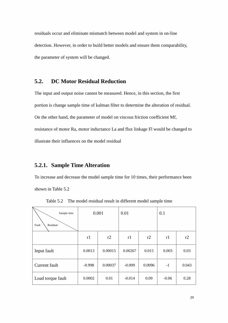
5.2.1. Sample Time Alteration
To increase and decrease the model sample time for 10 times, their performance been
shown in Table 5.2
Table 5.2 The model residual result in different model sample time
Sample time
Fault Residual
0.001 0.01 0.1
r1 r2 r1 r2 r1 r2
Input fault 0.0013
0.00015
0.00267
0.015
0.003
0.03
Current fault -0.998 0.00037 -0.009 0.0096 -1 0.043
Load torque fault 0.0002 0.01 -0.014 0.09 -0.06 0.28

30
Speed fault 0.00042 -0.997 0.00166 -0.998 0.0025 -0.991
From the Table 4.2 shown above, it is clear that, when sample time select to be 0.001,
r1 reduce from 0.00267 to 0.0013 when the input fault act on the model which sample
time equal to 0.01, the similar trend occurs the current fault, load torque fault and
speed fault add to the model. Meanwhile, it is interest to see that residual increase to
-1 when sample time at 0.1 by compare the result of sample time at 0.01. Hence,
increase the sample time would reduce the precise of the residual, by comparatively
that the value of residual would reduce when the sample time goes up.
5.2.2. Viscous Friction Coefficient Mf
Table 5.2 Viscous friction coefficient at 0.01N m s and 0.001N m s
Parameter
Fault Residual
0.01 0.001
Ia Ia
Input fault 0.005 0.0075 0.0049 0.0087
Current fault -0.992 0.01 -0.092 0.01
Load torque fault -0.014 0.11 -0.017 0.11
Speed fault 0.00162 -0.997 0.00167 -0.998

31
Table 5.3 Resistance of motor at 5.52 and 0.152
Parameter
Fault Residual
5.52 0.152
Ia Ia
Input fault 0 0.0038 0.007 0.021
Current fault -1 0.006 -0.98 0.02
Load torque fault -0.025 0.07 0.02 0.13
Speed fault 0.00054 -1 0.00365 -0.996
Table 5.4 Motor inductance at 0.0682 s and 0.00182 s
Parameter
Fault Residual
0.0682 0.00182
Ia Ia
Input fault 0.001 0 0.0045 0.01
Current fault -1 0 -1 0.015
Load torque fault 0 0.1 -0.02 0.09
Speed fault 0.00042 -1 0.00158 -1

32
Table 5.5 Flux linkage at 0.73 s and 0.08 s
Parameter
Fault Residual
0.73 0.08
Ia Ia
Input fault 0.001 0 0 0.09
Current fault -1 0.02 -1 0.006
Load torque fault -0.025 0.065 -0.0005 0.11
Speed fault 0.002 -1 0.0045 -1
Table 5.2 to 5.5 represent the diverse residual performance of model with different
parameters influenced by fault additive. When parameter altering, the residuals
increase or decrease. System disturbance and noise cannot be measured; hence,
changing the parameters would ensure residual locates on the tolerance threshold. A
model been detected effected by input fault, current residual can be reduced by
decreasing flux linkage, for example in the Table 5.5 that when flux linkage reduce to
0.08 V s, residual of current equal to zero. The other example that motor inductance
can be increase when the load torque fault affecting on the model if current residual
expect decrease.
Kalman filter used for the linear system states estimation by predicting the posteriori
states based on the priori ones, and to minimize the covariance of states. For

33
Non-linear system, it states been predicted by the similar algorithm as kalman filter
does. It use to extended kalman filter for states estimation, which been introduced in
next chapter.

34
6. Stepper Motor in Nonlinear Signals Estimated by
Extended Kalman Filter
Stepper motor is simulated for the aircraft engine of gas turbine fuel valves system.
In this chapter, the extended kalman filter would be applied to the nonlinear stepper
motor system for its state estimation.
6.1. Stepper Motor Model
The stepper motor is droved by the driver board with input clock signal where
generates 4-phase voltage with 90 degree phase different them where named Va, Vb,
Vc and Vd. Following fig6.1, the output of the stepper motor, there are 12 output
which include 4 output signals for voltage and current, and the other 4 output signals
represent for electromagnetic torque, angular velocity, angular displacement and
linear displacement.
Fig 6.1 Full structure model of stepper motor with driver and clock input
(Cheng, 2010)

35
Stepper motor model states illustrated
(6.1)
= (6.2)
= (6.3)
(6.4)
= (6.5)
= (6.6)
According to 6.1 to 6.6, the stepper motor has 6 states to be estimated, hence the
stepper motor states estimation with EKF modelling shown in Fig 6.2, where include
12 inputs for model measurement and 4 inputs for control inputs. 6 outputs been set in
EKF outputs, where in relates to the model states which been measured

36
Fig 6.2 Model of stepper motor state estimation with EKF
The initial condition of the model as
Table 6.1 Parameters of Stepper Motor
Motor Parameter Symbol Value Units
Viscous Friction B 7.76606*10-4
N m s
Rotor Load Inertia J 8.057*10-6
kg m2
Self Inductance of Winding L 0.10854 H
Resistance in Phase Winding R 28.925
Motor Torque Constant Km 0.19038 V s/rad
(Cheng, 2010)
with control noise (CN)=0.0001, acceleration noise (AN)=0.05, measurement
noise(MN)=0.1

37
6.2. Stepper Motor States Linearization and Original Setting
As mentioned in the chapter 4, the EKF estimate the discrete time model, hence for
nonlinear system states estimation, the linearization method is introduced to linearize
the model.
In the Appendix 2, setting the differential time dt=0.0001, then the next interval time
states equation becomes
dxh=dxh+dxh*dt
and it equalize to the priori states of model (xhm). By comparison the model with
dt=0.0001, taking long the differential time of model which be more smooth than the
former model, because of the in the small interval time that would make model more
linearization, and similar to the nonlinear model closely.
To complete the EKF, the matrix of A, W, H and V are different at each time step,
therefore the Jacobian method been used for them computation based on the states
equation of model from equation 6.1 to 6.6, and matrix F(6 ) are shown below
F=[0 1 0 0 0 0;
km*N/J*(-x3)*cos(N*x1)+x4*sin(N*x1)+x5*cos(N*x1)-x6*sin(N*x1) -B/J
-km/J*sin(N*x1) -km/J*cos(N*x1) km/J*sin(N*x1) km/J*cos(N*x1);
km*N/L*x2*cos(N*x1) km/L*sin(N*x1) -R/L 0 0 0;
-km*N/L*x2*sin(N*x1) km/L*cos(N*x1) 0 -R/L 0 0;
-km*N/L*x2*cos(N*x1) -km/L*sin(N*x1) 0 0 -R/L 0;
km*N/L*x2*sin(N*x1) -km/L*cos(N*x1) 0 0 0 -R/L;] (6.7)

38
The matrix F is used for calculating the coefficient of prediction parameter where
updates the prediction matrix in the time update equation.
The time update equation
dxh1=x2;
dxh2=(-km*x3*sin(N*x1)-km*x4*cos(N*x1)+km*x5*sin(N*x1)+km*x6*cos(N*x1)
-B*x2-T1)/J;
dxh3=(Va-R*x3+km*x2*sin(N*x1))/L;
dxh4=(Vb-R*x4+km*x2*cos(N*x1))/L;
dxh5=(Vc-R*x5-km*x2*sin(N*x1))/L;
dxh6=(Vd-R*x6-km*x2*cos(N*x1))/L;
dxh=dxh+dxh*dt
xhm=dxh;
Pm=phi*P*phi'+delta*Qk*delta';
P=P+Pm*dt;
Pkm=P;
Measurement update equation
K=Pkm*H'*(inv(H*Pkm*H'+Rn));
xhp=xhm+K*(um-H*xhm);
Pkp=(eye(6)-K*H)*Pkm*(eye(6)-K*H')+K*Rn*K';
xh=xhp;
P=Pkp;

39
Based on the algorithm in this chapter, the stepper motor states estimation in
nonlinear system been generated shown above. Due to the time constraint, it does not
attempt. Another main issue is the measurements output is 12 1 matrix which consist
of 4 voltage and current, as well as one signal for electromagnetic torque, angular
velocity, angular displacement and linear displacement, respectively. However the
number of states which been estimated based on the equation 6.1 to 6.6 is 6. Hence
when to estimate posteriori states, the measurement dimension does not match to the
priori states dimension.

40
7. Goal Achievement
Object 1
Write code to generate kalman filter.
Achievement: based on kalman filter principle and algorithm generates kalman filter
on time update equation and measurement update equation.
Object 2
Estimate states by the kalman filter in DC motor.
Achievement: the residuals achieved where model influenced by input/output, current
and speed additive fault. To change sample time of kalman filer will alter the residual
of the model. Residual result guaranteed on the tolerant threshold by changing the
model parameter value.
Object 3
Build stepper motor model in extended kalman filter.
Achievement: the stepper motor model built for simulating aircraft gas turbine engine
of fuel valves system
Object 4
Matlab code generation for stepper motor states estimation by extended kalman filter.
Achievement: to linearze the nonlinear signals by setting sample time and translate

41
continuous signals to discrete form. And according to the principle and algorithm of
extended kalman filter generate the time update equation and measurement update
equation.

42
8. Conclusion
Kalman filter to be used for the online states estimation which has been approved in
the chapter 5. The posteriori states estimated based on the priori states, which
different to the observer states estimation that it is without the posteriori states
prediction procedure , which would generates high level of residual between actual
system and model . And for the kalman filter, the posteriori states been predicted
before it estimated would eliminate above situation occurs. Meanwhile, kalman filter
does not need to all old states for the current states estimation, which would save time
and easier for designer to identify where and when do the faults occur.
For linear system, standard kalman filter been applied that the DC motor model
shown different residual performance when the additive fault inject from input/ output,
current and load torque. In the chapter 4.2 illustrates that altering sample time of
kalman filter would reduce the residuals, however, the parameters changed would
make sure residual locate out of the tolerance threshold where model is failure or
malfunction.
A stepper motor is used to simulate the aircraft gas turbine engine of fuel valves
system, where it is relates to non-linear system. Hence the Extended kalman filter
been introduced. The main idea in extended kalman filter code is to linearize the
nonlinear signals to the linear ones for the states estimation. The implementation of
EKF on the stepper motor did not finished due to the limit knowledge of stepper

43
motor in electronic performance and project time constraint.
8.1. Future Research
The stepper motor states estimation has been attempted in the project, hence for the
future
Improve the knowledge of stepper motor before the it applied
Stepper model output should be checked, due to for this model, it has 6 states
would be estimated, however, in the measurement input (um) does include 12
signals which occurs the matrix unmatchable
The unscented kalman filter used for the nonlinear system

44
9. Reference
1. Boucherma, M. (1994) Turbo-Generator Fault-Detection and Diagnosis
Based on Artificial Neural Networks. Ph.D Thesis. University of Sheffield
2. Cheng, W.Y. (2010). Fault Detection and Monitoring in Gas Turbine Engine
Fuel Valves. MSc Thesis. University of Sheffield in Industrial Systems. Great
Britain: Springer.
3. The Analytic Sciences Corporation. (1974). Applied Optimal Estimation.
United States of America: The Analytic Sciences Corporation.
4. Grewal, M and Andrews. A. (2008). Kalman Filtering Theory and Practice
Using Matlab. United States of America: John Wiley & Sons, Inc.
5. Harvey, A. (1989). Forecasting Structural Time Series Models and the K
6. Chiang, L.H et al. (2001). Fault Detection and Diagnosis alman Filter. UK:
Cambridge University Press
7. Harvey, A and Proietti. T (2005). Readings in Unobserved Components
Models. Great Brain: Newgen Imaging Systems (P) Ltd.
8. Isermann, R. (1981). Fault Detection methods for supervision of technical
processes. Process Automation.
9. Isermann, R. (1984). Process Fault Detection Based on Modeling and
Estimation Method a Survey. Auotmatica, vol. 20, 387-404.
10. Isermann, R. (2006). Fault-Diagnosis Systems. Germany: Springer.
11. Li, P. (2002). Fault Detection and Isolation in Nonlinear Stochastic Systems-
45
Monte Carlo Filtering Based Approaches. Ph.D Thesis. University of
Sheffield.
12. Ristic, B et al. (2004).Beyond the Kalman Filter. Defence Science and
Technology Organisation.
13. Saedtler, E. (1979) Hypothesis testing and system identification methods for
on-line vibration monitoring of nuclear power reactors, 5th
IFAC Symposium
on Identification and System Parameter Estimation. Darmstadt.
14. Shah, C. (2004) Sensorless Control of Stepper Motor. MSc Thesis, Department
of Electrical and Computing Engineering. Cleveland State University
15. Schwart, A. et al (2003). Model-Based Fault Detection of A Diesel Enginewith
Turbo Charger- A Case Study. University of Technology, Darmstadt Institute
of Automatic Control.
16. Simon, D. Optimal State Estimation. Cleveland States University. New Jersey:
John Wiley & Sons,Inc.
17. Welch, G and Bishop, G. (2006). An Introduction to Kalman Filter.
University of North Carnolia.
18. Williams, M.M.R, and Sher, R. (1979) Progress in Nuclear Energy. vol.I
Pergamon Press, Oxford.
19. Zhou, J. (1998). Intelligent Fault Diagnosis with Applications to Gas Turbine
Engines. Ph.D Thesis. University of Sheffield.