Embed Size (px)
Citation preview
CALIFORNIA PATH PROGRAMINSTITUTE OF TRANSPORTATION STUDIESUNIVERSITY OF CALIFORNIA, BERKELEY
Fault Detection and Identification withApplication to Advanced Vehicle C:ontrolSystems: Final ReportRandal K. Douglas, Jason L. Speyer,D. Lewis Mingori, Robert H. Chen,Durga P. Malladi, Walter H. Chung
California PATH Research Report
UCB-ITS-PRR-96-25
This work was performed as part of the California PATH Program of theUniversity of California, in cooperation with the State of California Business,Transportation, and Housing Agency, Department of Transportation; and theUnited States Department of Transportation, Federal Highway Administration.
The contents of this report reflect the views of the authors who are responsiblefor the facts and the accuracy of the data presented herein. The contents do notnecessarily reflect the official views or policies of the State of California. Thisreport does not constitute a standard, specification, or regulation.
September 1996
ISSN 1055-1425


Fault Detection and IdentificationWith Application to
Advanced Vehicle Control Systems
Award No. 65H998, M.O.V. 126
Randal K. Douglas, Durga P. Malladi, Robert H. Chen,
Walter H. Chung, Thanh M. Nguyen, Jason L. Speyer and
D. Lewis Mingori
Mechanical and Aerospace Engineering DepartmentUniversity of California, Los Angeles
Los Angeles, California 90095
June 20, 1996


Fault Detection and Identification With Application toAdvanced Vehicle Control Systems
Award No. 65H998, M.O.V. 126
Randal K. Douglas, Durga P. Malladi, Robert H. Chen, Walter H. Chung,Thanh M. Nguyen, Jason L. Speyer and D. Lewis Mingori
Mechanical and Aerospace Engineering DepartmentUniversity of California, Los Angeles
Los Angeles, California 90095
June 20, 1996
Abstract
A preliminary design of a health monitoring system for automated vehicles is developed
and tests in a high-fidelity nonlinear simulation are very encouraging. A new detailed
nonlinear vehicle simulation which extends the current simulation is documented and will
be used as a future testbed for evaluating the performance of the health monitoring system.
A health monitoring system has been constructed for the lateral and longitudinal modes that
monitors twelve sensors and three actuators. The approach is to fuse data from dissimilar
instruments using modeled dynamic relationships and fault detection and identification
filters. The filters are constructed so that the residual process has directional characteristics
associated with the presence of a fault, that is, static patterns. Sensor noise, process
disturbances, system parameter variations, unmodeled dynamics and nonlinearities can
distort these static patterns. Two candidate residual processing schemes are developed
and tested. A Bayesian neural network is trained to announce a fault and the probability
of fault occurrence by recognizing fault patterns embedded in the residual. A new multiple
hypothesis Shiryayev probability ratio test is also developed. Finally, development of a
v
time-varying fault detection filter, applicable to maneuvering vehicles with time-varying
dynamics, is described.
Keywords. Automated Highway Systems, Automatic Vehicle Monitoring, Fault Detection
and Fault Tolerant Control, Neural Networks, Reliability, Sensors, Vehicle Monitoring.
vi

Fault Detection and Identification With Application toAdvanced Vehicle Control Systems
Award No. 65H998, M.O.V. 126
Executive Summary
A preliminary design of a health monitoring system for automated vehicles is developed
and tests in a high-fidelity nonlinear simulation are very encouraging. A new detailed
nonlinear vehicle simulation which extends the current simulation is documented and will
be used as a future testbed for evaluating the performance of the health monitoring system.
A health monitoring system has been constructed for the lateral and longitudinal modes that
monitors twelve sensors and three actuators. The approach is to fuse data from dissimilar
instruments using modeled dynamic relationships and fault detection and identification
filters. The filters are constructed so that the residual process has directional characteristics
associated with the presence of a fault, that is, static patterns. Sensor noise, process
disturbances, system parameter variations, unmodeled dynamics and nonlinearities can
distort these static patterns. Two candidate residual processing schemes are developed
and tested. A Bayesian neural network is trained to announce a fault and the probability
of fault occurrence by recognizing fault patterns embedded in the residual. A new multiple
hypothesis Shiryayev probability ratio test is also developed. Finally, development of a
time-varying fault detection filter, applicable to maneuvering vehicles with time-varying
dynamics, is described.
vii

Abstract .
Executive Summary.
List of Figures
List of Tables .
Chapter 1 Introduction.
Chapter 2 Vehicle Model and Simulation Development .
2.1 Modification of Berkeley's Model
2.1.1 Suspension System
2.1.2 Road Roughness
2.1.3 Slope ...
2.1.4 Evaluation ..
2.2 Linear Model .....
2.3 Reduced-Order Model
ix
Contents
v
vii
xv
xix
1
7
8
8
10
10
11
1216
x
Chapter 3 Fault Selection .
3.1 Sensor Fault Models ..
3.2 Actuator Fault Models .
Chapter 4 Fault Detection Filter Design
4.1 Fault Detection Filter Configuration
4.2 Eigenstructure Placement . .
4.2.1 Sensor Fault Design .
4.2.2 Actuator Fault Design
Chapter 5 Fault Detection Filter Evaluation
5.1 Fault Detection Filter Evaluation On A Curved Road .
5.1.1 Evaluation On Smooth Road .
5.1.2 Evaluation On Rough Road .
5.2 Fault Detection Filter Evaluation On A Straight Rough Road
Chapter 6 Bayesian Neural Networks .
6.1 Notation .
6.2 Bayesian Feature Classification and Neural Networks
6.2.1 A Maximum Likelihood Gaussian Classifier as a Multilayer
Perceptron .
6.2.2 A Bayesian Neural Network Provides Feature Classification
Probabilities .
6.3 Learning Algorithms for Neural Networks
6.3.1 Deterministic Learning Algorithms
6.3.2 Stochastic Learning Algorithms . .
6.4 Bayesian Neural Networks as Residual Processors
6.5 Simulation Results .
6.5.1 Step Faults .
6.5.2 Ramp Faults
6.6 Discussion......
Chapter 7 Sequential Probability Ratio Tests .7.1 Preliminaries and Notation .
7.2 Development of a Multiple Hypothesis Shiryayev SPRT
7.2.1 Recursive Relation for the Posteriori Probability
7.2.2 Dynamic Programming Formulation
7.2.3 Thresholds for the Optimal policy .
Contents
23
25
27
29
30
34
3539
45
45
46
48
52
61
63
63
..... 65
66
68
68
69
70
71
72
73
74
8183
84
85
87
92
Contents
7.2.4 Detection of Unknown Changes
7.3 Examples .
7.3.1 Example 1 .
7.3.2 Example 2 .
7.4 Application to Advanced Vehicle Control Systems.7.5 Summary of SPRT Development and Application
Chapter 8 Vehicle Nonlinear Equations of Motion8.1 NonLinear Longitudinal Vehicle Model
8.1.1 Reference Frames .
8.1.2 Vehicle Dynamics .
Rotational Equations of Motion .Translational Equations of Motion
8.1.3 Suspension Model .8.1.4 Forces .8.1.5 Moments About the Vehicle Center of Mass8.1.6 Brake Dynamics ..
8.1.7 Wheel Dynamics ..
8.1.8 Tire Traction Model
8.1.9 Engine Model ....8.2 Nonlinear Lateral and Longitudinal Model .
8.2.1 Reference Frames .8.2.2 Vehicle Dynamics. . . . . . . . . .
Rotational Equations of Motion . .Translational Equations of Motion
8.2.3 Suspension Model .
8.2.4 Forces .
8.2.5 Moments About the Vehicle Center of Mass8.2.6 Brake Dynamics .8.2.7 Wheel Dynamics and Tire Traction Model .8.2.8 Engine Model . . . . . . . . . . .8.2.9 Steering Model . . . . . . . . . .8.2.10 Random Road Excitation Model
8.3 Simulation Results . . . . . . . . . . . .8.3.1 Longitudinal Model .
Response of Vehicle to Various InputsSmall Angle Approximation . . . . . .Linearization at a Nominal Operating Point
xi
94
94
94
95101
105
107109
109110
110111112116118119120
121
123124
124129129130
131
133134135135138139140141141141144147
xii
8.3.2 Lateral and Longitudinal Model ....
Response of Vehicle to Various InputsSmall Angle Approximation . . . . . .Linearization Around a Constant Steering Angle
804 Summary of Model Development and Suggestions for Future Work
Contents
152
152155157159
Chapter 9 A Game Theoretic Fault Detection Filter 1679.1 A Disturbance Attenuation Approach to Fault Detection. . . . . . 169
9.2 A Game Theoretic Filter for Fault Detection in a General Class of Systems 171
9.2.1 Maximization with Respect to x(to) and jJ, 2 .•.••.••.... " 1739.2.2 Minimization with Respect to x and Maximization with Respect to y 175
9.2.3 Steady-State Results . . . . . . . . . . . . . . . . . . . . . . . . 1779.2.4 Finding the Limiting Solution. . . . . . . . . . . . . . . . . . . 178
9.3 The Limiting Case Solution via Singular Optimal Control Techniques. 1789.3.1 Conditions for Game Cost Non-Positivity: A Game LMI . . . . 1789.3.2 A Riccati Equation for the Limiting Form of the Game Theoretic
Filter 181
9.4 An Unobservability Subspace Structure in the Limit . . . . . . . . . . . 1859.5 Fault Detection with the Limiting Form of the Game Theoretic Filter. 1929.6 Application to AVCS: An Engine Air Mass Sensor Fault Detection Filter. 200
9.6.1 Full-Order Filter Design . . . . . . . . . . . . . . . . . . . . . 2049.6.2 Reduced-Order Filter Design via the Goh Riccati Equations. 207
9.7 Discussion..... 211
Chapter 10 Conclusions 213
Appendix A Fault Detection Filter Background . 217A.1 The Detection Filter Problem . . . . . 218A.2 Sensor Fault Models . . . . . . . . . . . . . . . 219A.3 Solving The Detection Filter Problem ..... 221AA The Restricted Diagonal Detection Filter Problem 223
Appendix B Parameter Robustness By Left Eigenvector Assignment 227
Appendix C An Boo Bounded Fault Detection Filter 235C.1 Detection Filter Gain Parameterization. . . . . . 237C.2 A Disturbance Robust Detection Filter Problem. 242C.3 An Hoc Bounded Detection Filter 245C.4 Fault Enhancement . . . . . . . . . . . . . . . . . 249

Contents
C.5 Application to an Aircraft Fault Detection SystemCo6 Conclusions 0 • • 0 0 • • • • • • • • • •
Appendix D Vehicle Linear Model Data 0
Appendix E Fault Detection Filter Design DataEo! Design Data for Fault Group Three 0
E.2 Design Data for Fault Group Four
References. 0 0 • • • • • • 0 • • 0 • • 0 • •
xiii
253
257
261
267267273
281

List of Figures
Figure 2.1
Figure 2.2
Figure 2.3
Figure 2.4
Figure 2.5
Figure 2.6
Figure 2.7
Figure 4.1
Figure 4.2
Figure 4.3
Figure 4.4
Simplified suspension and tire model . . . . . . . . . . . . . . . . . . . .
Constant non-zero road slope is simulated by rotating the gravity vector
Rough road simulation .
Rough road simulation . . . . . . . . . . . . . . . . . . . . . . . .
Rough road simulation . . . . . . . . . . . . . . . . . . . . . . . .
Singular value frequency response of full-order and fourteen state
reduced-order models .
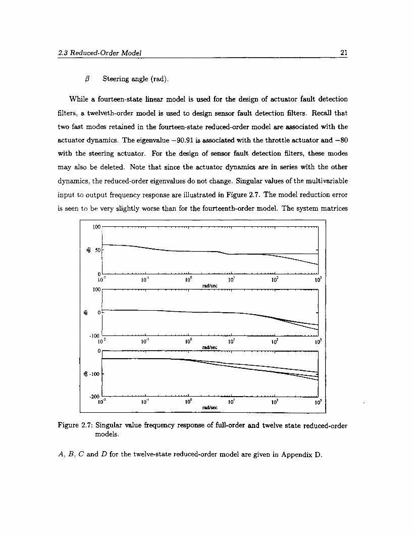
Singular value frequency response of full-order and twelve state
reduced-order models .
Singular value frequency response from all faults to residuals of faultdetection filter one . . . . . . . . . . . . . . . . . . . . . . . . . . . .
Singular value frequency response from all faults to residuals of fault
detection filter two . . . . . . . . . . . . . . . . . . . . . . . . . . . .
Singular value frequency response from all faults to residuals of fault
detection filter three . . . . . . . . . . . . . . . . . . . . . . . . . . .
Singular value frequency response from all faults to residuals of faultdetection filter four . . . . . . . . . . . . . . . . . . . . . . . . .
xv
9
11
12
13
14
20
21
39
40
41
43
xvi List of Figures
Figure 5.1 Residuals for fault detection filter one . 49
Figure 5.2 Residuals for fault detection filter two . 49
Figure 5.3 Residuals for fault detection filter three 50
Figure 5.4 Residuals for fault detection filter four 50Figure 5.5 Residuals for fault detection filter four 51Figure 5.6 Residuals for fault detection filter one 52Figure 5.7 Residuals for fault detection filter one 53Figure 5.8 Residuals for fault detection filter two 53Figure 5.9 Residuals for fault detection filter two 54
Figure 5.10 Residuals for fault detection filter three 54
Figure 5.11 Residuals for fault detection filter three 55
Figure 5.12 Residuals for fault detection filter four, no fault 55
Figure 5.13 Residuals for fault detection filter four, throttle actuator fault +2 deg 56Figure 5.14 Residuals for fault detection filter four, throttle actuator fault -2 deg . 56Figure 5.15 Residuals for fault detection filter four, brake actuator fault +100 Nm 57Figure 5.16 Residuals for fault detection filter four, steering actuator fault +0.001 rad 57Figure 5.17 Residuals for fault detection filter four, steering actuator fault -0.001 rad 58
Figure 5.18 Residuals for fault detection filter four, air mass sensor fault 0.07 kg .. 58
Figure 5.19 Residuals for fault detection filter one: air mass sensor, engine speed sensor
and forward accelerometer . . . . . . . . . . . . . . . . . . . . . . . . .. 59
Figure 5.20 Residuals for fault detection filter two: pitch rate sensor, forward wheelspeed sensor and rear wheel speed sensor 59
Figure 5.21 Residuals for fault detection filter three: vertical accelerometer, pitch ratesensor and rear wheel speed sensor . . . . . . . . . . . . . . . . . . . .. 60
Figure 5.22 Residuals for fault detection filter four: throttle actuator and brake actuator 60
Figure 6.1
Figure 6.2
Figure 6.3Figure 6.4Figure 6.5Figure 6.6Figure 6.7Figure 6.8Figure 6.9
Figure 7.1Figure 7.2
Bayesian neural network with feedback .
Residual processing scheme for the longitudinal simulation .
Posterior probability of a fault in the pitch rate sensor . . .Posterior probability of a fault in the front wheel speed sensor.Posterior probability of a fault in the rear wheel speed sensorRamp fault in pitch rate sensor . . . . . .Ramp fault in vertical accelerometer ...Ramp fault in longitudinal accelerometerRamp fault in air mass sensor . . . . . . .
Change from Ho to H2 at time t = 1 sec.
Change from Ho to H2 at time t = 1 sec.
64
75
76767777787879
95
98
List of Figures
Figure 7.3 Fault detection scheme for Aves .
Figure 7.4 Pitch rate sensor fault occurs at 8 sec .
Figure 7.5 Vertical accelerometer fault occurs at 8 sec
Figure 7.6 Longitudinal accelerometer fault occurs at 8 sec .
xvii
102104104
105
Figure 8.1 Vehicle configuration for the nonlinear longitudinal model 110Figure 8.2 Schematic view of suspension and tire models showing the front half of
the vehicle. . . . . . . . . . . . . . . . . . . . . . . . . . . . . . . . . .. 113Figure 8.3 Geometric constraints involving the suspension height showing the front
half of the vehicle for planar and arbitrary road surfaces 114
Figure 8.4 Damper characteristic . . . . . . . . . . . . . . . . . . . . . . . . . .. 118
Figure 8.5 Wheel rotation . . . . . . . . . . . . . . . . . . . . . . . . . . . . . .. 120
Figure 8.6 Exaggerated plot of the Magic Formula, showing the influence of thecoefficients 122
Figure 8.7 Representation of nonlinear vehicle model 125
Figure 8.8 Relationship between reference frames . . 126Figure 8.9 Definition of road frame . . . . . . . . . . 127
Figure 8.10 Aerodynamic forces acting on the vehicle have three components 134
Figure 8.11 Top view of a tire under steering maneuver . . . . . 137
Figure 8.12 Lumped-mass representation of the steering system. . . . . . . . 139
Figure 8.13 Vehicle response due to a step throttle input 143
Figure 8.14 Vehicle response due to a step brake input subsequent to a step throttleinput. . . . . . . . . . . . . . . . . . . . . . . . . . . . . 144
Figure 8.15 Vehicle response when decending down a 5% grade road 145Figure 8.16 Vehicle response when passing over a sinusoidal bump . 146Figure 8.17 Vehicle response due to random road excitation . . . . . 147
Figure 8.18 Power spectral densities of simulated and theoretical random noise processes148
Figure 8.19 Effect of making a small angle approximation of the relative pitch angle 149
Figure 8.20 Effect of making a small angle approximation of the absolute pitch angle 150Figure 8.21 Effect of perturbation size on numerical derivative computation . . 151Figure 8.22 Transient response of the linearized and nonlinear systems with a
perturbed throttle input (+15%) . . . . . . . . . . . . . . . . . . . 152Figure 8.23 Effect of perturbation size on numerical derivative computation . . 153Figure 8.24 Steady-state response of the linearized and nonlinear systems with a
perturbed brake input (+34 N) . . . . . . . . . . . . . . . 154
Figure 8.25 Vehicle response due to step steering input of 0.01 radian 155
Figure 8.26 Vehicle response due to a crosswind pulse of 15 s~c 156Figure 8.27 Vehicle response due to road noise . . . . . . . . . . . . . 161
xviii List of Figures
Figure 8.28 Spectral densities and coherency functions of left and right tracks .. " 162
Figure 8.29 Effect of making a small angle approximation of the roll angle .... " 163
Figure 8.30 Comparison of vehicle linearized and nonlinear system responses wheresteering angle is perturbed by 0.01 radian . . . . . . . . . . . . . . . " 163
Figure 8.31 Comparison of vehicle linearized and nonlinear system responses wherethrottle position is perturbed by 15% " 164
Figure 8.32 Comparison of vehicle linearized and nonlinear system responses where
brake torque is perturbed by 27 N . . . . . . . . . . . . . . . . . . . .. 164
Figure 8.33 Comparison of vehicle linearized and nonlinear system responses where
steering angle is perturbed by 25% . . . . . . . . . . . . 165
Figure 9.1Figure 9.2
Figure 9.3
Figure 9.4
Figure 9.5
Figure 9.6
Figure 9.7
Figure c.l
Figure c.2Figure c.3
Figure c.4
Commutative diagram for fault detection filter structure 189Game Theoretic Filter Singular Value Plot of Air Mass Fault Signal versusSingular Values of Engine Speed and Accelerometer Faults " 206Beard-Jones Filter Singular Value Plot of Air Mass Fault Signal versus
Singular Values of Engine Speed and Accelerometer Faults. . . . . . " 207
Beard-Jones Filter Singular Value Plot of Air Mass Fault Signal versus
Singular Values of Engine Speed and Accelerometer Faults " 208Game Theoretic Filter Singular Value Plot of Air Mass Fault Signal versusNuisance Faults and Noise. . . . . . . . . . . . . . . . . . . . . . . . 209Reduced-Order Goh Filter Residual due to step in J.LA z (fault to bedetected) 210
Reduced-Order Goh Filter Residual due to step in J.Lwg (nuisance fault) 211
Magnitude of transfer functions to the normal accelerometer fault isolation
residual . . . . . . . . . . . . . . . . . . . . . . . . . . . . . . . . . . .. 257
Magnitude of transfer functions to the elevon fault isolation residual .. 258Normal accelerometer fault isolation residual. 2 s!~ accelerometer faultoccurs at t=1 sec . . . . . . . . . . . . . . . . . . . . . . . . . . . . .. 258Elevon fault isolation residual. 2 degree elevon fault occurs at t=l sec . 259

List of Tables
Table 2.1 Eigenvalues for the vehicle dynamics using two model reduction methods 19
Table 8.1 Tire model coefficients .
Table 8.2 Effective range of the linearized system
xix
137159

CHAPTER 1
Introduction
A PROPOSED TRANSPORTATION SYSTEM with vehicles traveling at high speed, in close
formation and under automatic control demands a high degree of system reliability. This
requires a health monitoring and maintenance system capable of detecting a fault as it
occurs, identifying the faulty component and determining a course of action that restores
safe operation of the system. This report is concerned with vehicle fault detection and
identification and describes a vehicle health monitoring system approach based on analytic
redundancy.
Analytic redundancy methods for fault detection and isolation use a modeled dynamic
relationship between system inputs and measured system outputs to form a residual process.
Nominally, the residual process is nonzero only when a fault has occurred and is zero at other
times. For an observable system, this simple definition is met by the innovations process of
any stable linear observer. A detection filter is a linear observer with the gain constructed
so that when a fault occurs, the residual responds in a known and fixed direction. Thus,
when a nonzero residual is detected, a fault can be announced and identified.
1
2 Chapter 1: Introduction
A complication arises when there are many possible faults because a fault detection filter
can only be designed to detect a limited number of faults. This is related to the order of
the vehicle dynamics. When more faults need to be identified, several fault detection filters
have to be used with each filter designed to detect and identify some but not all possible
faults. The vehicle fault detection system described in this report has four fault detection
filters. This raises two difficult design issues. First, some and probably all faults will not
be included in the design of one or more fault detection filters. When such a fault occurs,
the residual of all filters will respond, even the residuals of the filters that do not have the
fault included in their design. If a fault is not included in a fault detection filter design, the
directional characteristics of the residual will be undefined and the fault cannot be properly
identified. The challenge is to build a mechanism that recognizes when a fault detection
filter is responding to a fault for which it has not been designed and then to exclude the
residual of all such filters from the fault identification process. If it can be assumed that
only one fault occurs at a time, then the residual processor can exclude the residual of any
fault detection filters that point to two or more faults.
A second design issue is how the faults should be grouped and identification delegated
among the fault detection filters. Several approaches are taken in the design described in
this report. In one, the functional form of a given sensor is restricted. In particular, it is
assumed that the sensor fault is a bias of unknown magnitude. The assumption allows this
sensor and a certain actuator to be isolated by a single fault detection filter. This point
is significant because the conventional approach to fault detection filter design would not
allow a single filter to isolate these two faults and would require this task to be passed on
to the residual processing module.
A second fault grouping design consideration is a newly apparent tradeoff between
filter parameter robustness, as determined by the eigenvector conditioning, and fault input
observability. Using an eigenstructure assignment algorithm, a design objective is to place
well-conditioned eigenvectors. However, it has been found recently that for some fault
groups, a fault might have only one highly observable direction. This means that while a

Chapter 1: Introduction 3
fault might be large and dynamically active, the residual is small most of the time. The
residual would always be large if all associated eigenvectors were placed close to being
collinear with the most observable direction. Hence a tradeoff exists. An objective in
assigning faults to fault groups is to minimize the impact of this tradeoff.
A third fault grouping design consideration is discussed in (Douglas et al. 1995). In
a fault detection system that consists of a bank of fault detection filters and a residual
processor such as a neural network, fault isolation is done through the combined effort of
both system elements. The fault detection filter is a carefully tuned device that uses known
dynamic relationships to isolate a fault. The neural network residual processor combines
the residuals from several filters and resolves any ambiguity. It is suggested that identifying
a fault among a group of dynamically similar faults requires the precision of and is best
delegated to the fault detection filters. Furthermore, it is suggested that the reliability of
the neural network training would be improved if the fault groups associated with each of
the fault detection filters are dynamically dissimilar.
In applications it is unrealistic to expect that a residual process would be nonzero only
when a fault has occurred. Sensor noise, process disturbances, system parameter variations,
unmodeled dynamics and nonlinearities all contribute to the magnitude of a residual. There
are many methods to reduce the impact of these effects on the residual but none reduce
their effect to zero. This means that some threshold detection mechanism must be built.
A simple threshold detection mechanism announces a fault when the size of a residual
exceeds some prescribed value. This prescribed value could be determined from empirical
studies which balance a rate of false alarm against a rate of miss alarm. A more complicated
residual processor might take into account the thresholds of all other residuals as well.
Reasoning that if the probability of simultaneous failures is very small, no fault is announced
when more than one residual exceeds a threshold. It is more likely that the nonzero residuals
are caused by noise or nonlinearities or some cause other than multiple faults.
Two residual processing systems are described in this report. In the first, a Bayesian
neural network considers the residuals from all fault detection filters as constituting a
4 Chapter 1: Introduction
pattern, a pattern which contains information about the presence or absence of a fault.
Hence, residual processing is treated as a pattern recognition problem.
The objective of a neural network as a feature classifier is to associate a given feature
vector with a pattern class taken from a set of pattern classes defined apriori. In an
application to residual processing, the feature vector is a fault detection filter residual and
the pattern classes are a partitioning of the residual space into fault directions which include
the null fault. A Bayesian neural network also provides probabilities of feature classification
conditioned on an observation history. A stochastic training algorithm enhances robustness
by treating training sets as as sample sets providing information about the entire population.
A second approach to residual processing described in this report is a modified Shiryayev
sequential probability ratio test extended to include multiple hypotheses. The algorithm,
which is derived as a dynamic programming problem, detects and isolates the occurrence
of a failure in a conditionally independent measurement sequence in minimum time. The
test has been further extended to the detection and identification of changes with unknown
parameters.
This report is organized as follows. Section 2 describes the car models used for fault
detection filter design and evaluation. A nonlinear model is derived directly from one
provided by the Berkeley PATH research team (Peng 1992). Low-dimensional linear models
that include coupled longitudinal and lateral vehicle dynamics are used for fault detection
filter design. The high fidelity nonlinear model is used for evaluation and to obtain the
linear models used for design. Section 3 describes the faults to be identified by the fault
detection system. Section 4 describes the design of the fault detection filters. This includes
how the faults are grouped for each fault detection filter design and how the fault detection
filter eigenstructure placement is done. Section 5 presents an evaluation of the performance
of the fault detection filters in a nonlinear simulation.
Sections 6 and 7 describe two candidate fault detection filter residual processing systems.
In Section 6 a Bayesian neural network is developed and in Section 7 a multiple hypothesis
Shiryayev sequential probability ratio test is described. Both are used to process residuals
Cbapter 1: Introduction 5
from all fault detection filters to detect and identify which if any fault has occurred.
In section 8 a six degree of freedom nonlinear vehicle model is developed independently
of the model used for the Berkeley simulation of Section 2. This work is done to provide
a model that better accommodates a nonplanar, rough road surface, one where the road
gradient is different for all four wheels. The model will be used to evaluate the robustness
of the health monitoring system to road excitation. This effort is a continuation of the work
reported in (Douglas et al. 1995).
In section 9 describes a new, disturbance attenuation approach to fault detection filter
design. Here, a differential game is defined where one player is the state estimate and the
adversaries are all the exogenous signals except for the fault to be detected. By treating
faults as disturbances to be attenuated, the usual invariant subspace structure associated
with fault detection filters is not present except in the limit. By treating model uncertainty
as another element in the differential game, sensitivity to parameter variations can be
reduced.
Section 9 also introduces the notion of a fault detection filter for time-varying systems.
This is especially important in applications where a vehicle follows a maneuver such as a
merge or a split. While first considered in the game theoretic filter derivation, it is expected
that the Beard-Jones fault detection filter definition will be extended to time-varying
systems in the same way.
Appendix A provides a theoretical review of the Beard-Jones detection filter problem.
This appendix also includes some early work in extending the Beard-Jones fault detection
filter definition to time-varying systems.
Appendix B provides a review of a fault detection filter left eigenvector assignment
design algorithm (Douglas and Speyer 1996). The algorithm gives the user eigenvector
conditioning information and provides a direct method for achieving maximally achievable
eigenvector conditioning. This algorithm is used for the designs in this report.
Appendix C describes a stabilizing fault detection filter gain that bounds the 'Hoo norm
of the transfer matrix from system disturbances and sensor noise to the residual. For

6 Chapter 1: Introduction
multi-dimensional faults, a residual direction is identified that enhances the fault signal to
noise ratio while maintaining the 'Hoo norm bound.
CHAPTER 2
Vehicle Model and Simulation Development
IN THIS SECTION, vehicle models are developed for the design and evaluation of fault
detection filters. The starting point is a model obtained from the Berkeley PATH research
team and derived in (Peng 1992). A version of this model coded in C also is available from
Berkeley.
Two variations of the Berkeley model are considered in this section. First, modifications
are made to allow for variations in road slope and road noise. The slope is restricted to a
constant because of assumptions made in the original derivation of the equations of motion.
After modifications, the nonlinear model has 32 states, 3 control inputs and 3 noise inputs.
Second, reduced-order linearized models used for detection filter design are developed for a
vehicle in a constant radius turn. Linearized models developed for a vehicle operating with
zero steering angle are described in (Douglas et al. 1995).
An independent derivation of a six degree of freedom nonlinear vehicle model is also
developed to be sure that we understand all the assumptions, definitions and issues which
7
8 Chapter 2: Vehicle Model and Simulation Development
underlie the Berkeley model. This model allows for arbitrary variations in road slope and
road noise. Since this model represents a significant effort that was not completed in time
to be used in the fault detection filter development, it is described later in Section 8.
2.1 Modification of Berkeley's Model
Primary sources of vehicle dynamic disturbances are road roughness and variations in the
road slope. First, allowing for a road roughness disturbance requires a modification to the
suspension system of the Berkeley nonlinear model. A simple tire model is introduced so
that high bandwidth road noise generates physically realistic suspension damping forces.
Next a road noise model is desribed. Finally, the nonlinear model is modified to allow
for nonzero road slope. It is important to note that because of assumptions made in the
original derivation of the equations of motion, the slope is still a constant although now not
necessarily zero.
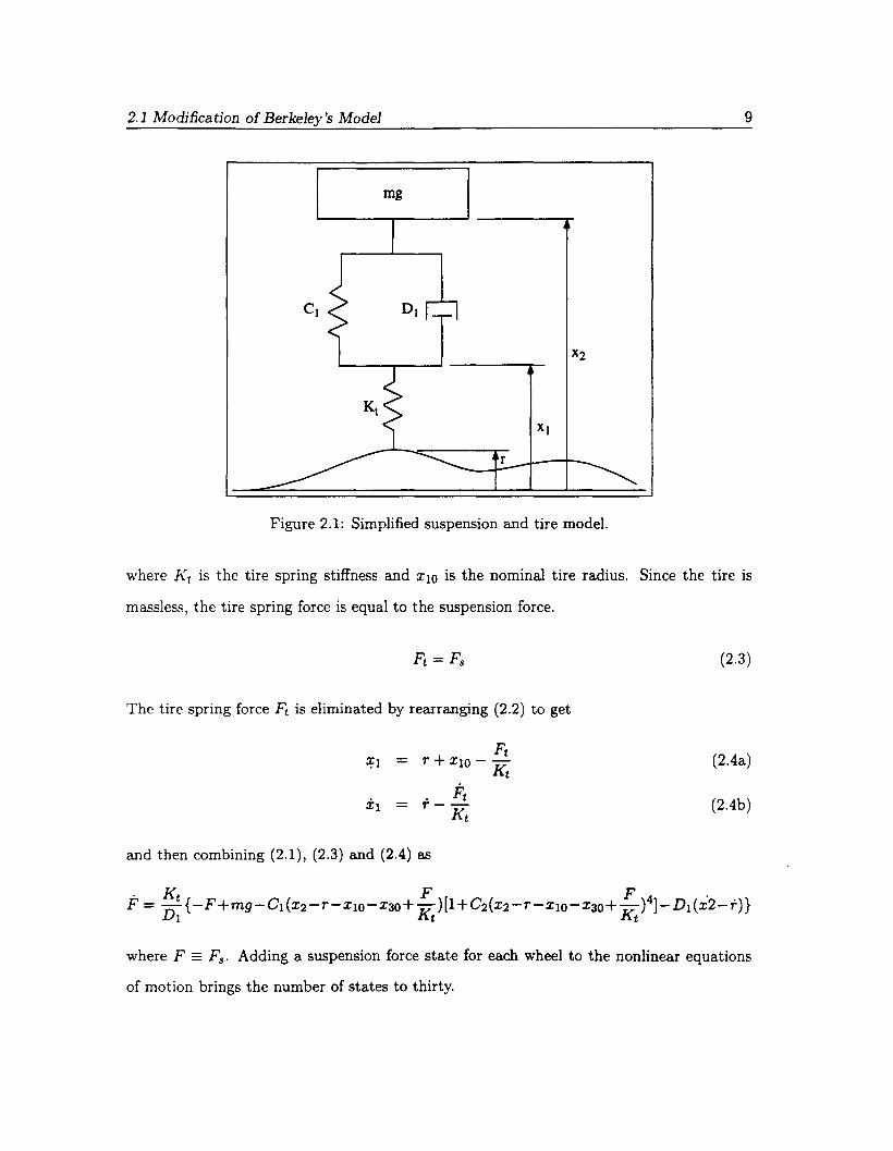
2.1.1 Suspension System
In the Berkeley nonlinear model, the suspension system is modeled as a spring and damper
and the tire is stiff. The stiff tire causes road displacements to pass directly to the suspension
system resulting in unreasonably large damping forces. Modeling the tire as a mass and
linear spring allows the tire to act as a low pass filter with respect to road displacements
and eliminates the unrealistic suspension damping forces. Since the mass of the tire is
very small relative to the car, the tire model is simplified to a linear spring as shown in
Figure 2.1. The vehicle equations are modified by adding four states, the suspension force
of each wheel, which are derived as follows. The suspension force Fa acting on each wheel
is given by
where X30 is the length of the suspension system when a nominal load mg is applied. The
force Ft transmitted to the suspension by the tire spring is given by
(2.2)
2.1 Modification of Berkeley's Model
mg
9
r
Figure 2.1: Simplified suspension and tire model.
where K t is the tire spring stiffness and XlO is the nominal tire radius. Since the tire is
massless, the tire spring force is equal to the suspension force.
The tire spring force Ft is eliminated by rearranging (2.2) to get
Ft~l = r+ XlO -
Kt
. . FtXl = r-
Kt
and then combining (2.1), (2.3) and (2.4) as
(2.3)
(2.4a)
(2.4b)
where F == Fs . Adding a suspension force state for each wheel to the nonlinear equations
of motion brings the number of states to thirty.
10
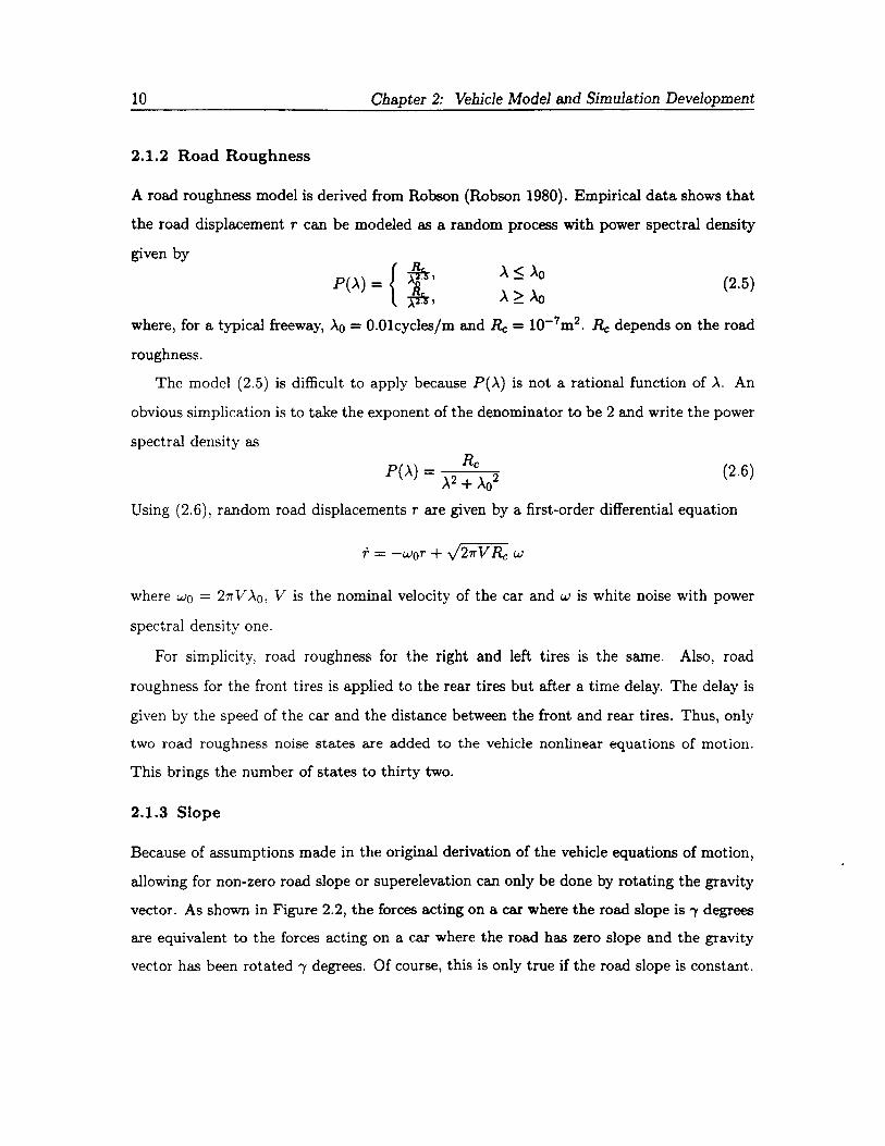
2.1.2 Road Roughness
Cbapter 2: Vebicle Model and Simulation Development
A road roughness model is derived from Robson (Robson 1980). Empirical data shows that
the road displacement r can be modeled as a random process with power spectral density
given by
{.& ,X<,X
P(,X) = Afl' - 0 (2.5)X¥.t, ,X ~ Ao
where, for a typical freeway, 'xo = O.Olcyc1es/m and Rc = 10-7m2. Rc depends on the road
roughness.
The model (2.5) is difficult to apply because P('x) is not a rational function of ..\. An
obvious simplication is to take the exponent of the denominator to be 2 and write the power
spectral density as
P(..\) _ Rc (2.6)- ..\2 + 'x02
Using (2.6), random road displacements r are given by a first-order differential equation
r = -wor + J27rV Rc w
where Wo = 27rV"\o, V is the nominal velocity of the car and w is white noise with power
spectral density one.
For simplicity, road roughness for the right and left tires is the same. Also, road
roughness for the front tires is applied to the rear tires but after a time delay. The delay is
given by the speed of the car and the distance between the front and rear tires. Thus, only
two road roughness noise states are added to the vehicle nonlinear equations of motion.
This brings the number of states to thirty two.
2.1.3 Slope
Because of assumptions made in the original derivation of the vehicle equations of motion,
allowing for non-zero road slope or superelevation can only be done by rotating the gravity
vector. As shown in Figure 2.2, the forces acting on a car where the road slope is ; degrees
are equivalent to the forces acting on a car where the road has zero slope and the gravity
vector has been rotated; degrees. Of course, this is only true if the road slope is constant.
2.1 Modification of Berkeley's Model 11
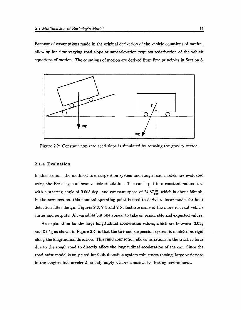
Because of assumptions made in the original derivation of the vehicle equations of motion,
allowing for time varying road slope or superelevation requires rederivation of the vehicle
equations of motion. The equations of motion are derived from first principles in Section 8.
mg
Figure 2.2: Constant non-zero road slope is simulated by rotating the gravity vector.
2.1.4 Evaluation
In this section, the modified tire, suspension system and rough road models are evaluated
using the Berkeley nonlinear vehicle simulation. The car is put in a constant radius turn
with a steering angle of 0.005 deg. and constant speed of 24.87 s~c which is about 56mph.
In the next section, this nominal operating point is used to derive a linear model for fault
detection filter design. Figures 2.3, 2.4 and 2.5 illustrate some of the more relevant vehicle
states and outputs. All variables but one appear to take on reasonable and expected values.
An explanation for the large longitudinal acceleration values, which are between -0.05g
and 0.05g as shown in Figure 2.4, is that the tire and suspension system is modeled as rigid
along the longitudinal direction. This rigid connection allows variations in the tractive force
due to the rough road to directly affect the longitudinal acceleration of the car. Since the
road noise model is only used for fault detection system robustness testing, large variations
in the longitudinal acceleration only imply a more conservative testing environment.

12 Chapter 2: Vehicle Model and Simulation Development
Road Displacement0.01,....------..;....-------,
E
-0.01 0~--~2---4~--~6-----'8
Time (sec)
Vertical Velocity
0.01
~-0.01
-0.02
-0.03 '-----------------'02468
Time (sec)
Vertical Position0.49S,....------~-----~
E
0.48S
0.480L---~2---4~---,---...J8
Time (sec)
Vertical Acceleration0.4,....--------------,
-0.4 L- ___'
02468Time (sec)
Figure 2.3: Rough road simulation.
2.2 Linear Model
In this section, a linearized model for a car making a constant radius turn is developed using
the modified Berkeley nonlinear model. Linearized models developed for a vehicle operating
with zero steering angle are described in (Douglas et al. 1995). Linearized models are found
numerically rather than analytically. An analytical approach taking partial derivatives is
impractical because the nonlinear model is too complicated. The procedure is as follows.
First, a computer run is made in which the car makes a turn at a constant speed of
24.87:::C :::= 56mph to obtain steady state values for each state. The tire steering angle is
0.005 rad which produces about 0.1g lateral acceleration and a 638.73 meter radius turn.
The nonlinear model is then linearized about this nominal operating point using the central
difference method.
The nonlinear model has the form:
x = f(x,u)
y = Cx+Dx
(2.7a)
(2.7b)

2.2 Linear Model 13
8246Time (sec)
Lateral Acceleration
Loneitudinal AccelerationO.S ,....-------------...,
0.04,....-------------...,
-O.S 0
Lonptudinal Velocity
26.9820.l:----::2:----~4---6~-~8
Time (sec)
Lateral Velocity-0.1 ISS ,....--------------:--1
-0.116
Ii! -0.1 16S P-\-+-4,.n.+.-H,......,"P-r..-+-IH'-+++l
~ -0.117
-0.117S
-0.118 0'----2----4---6~----'8
Time (sec)
-0.04 0~---::2----4---6----'8
Time (sec)
Figure 2.4: Rough road simulation.
Suppose the nominal operating point is (xo, uo) where f(xo, uo) = O. Take perturbations
X, u about the nominal point, that is, let
x = Xo + X
u = uo+u
Also approximate ~ and ~ as
!:::afAx =
ofaxofou
f(x + x,u) - f(x - x,u) I2x x=xo,u=uo
!:::af = f(x, u + u) - f(x, u - u) I!:::au 2u x=xo,u=uo
Equation (2.7a) may now be approximated as
. .:. f( ) of I - of I -Xo + x = xo, tLQ + £1 x + !L U+ ...vX x=xo,u=uo uu x=xo,u=uo
Truncating the higher order terms and using the approximations given above for the partial
derivatives, produces the following linear equations in the perturbed state X, input u and
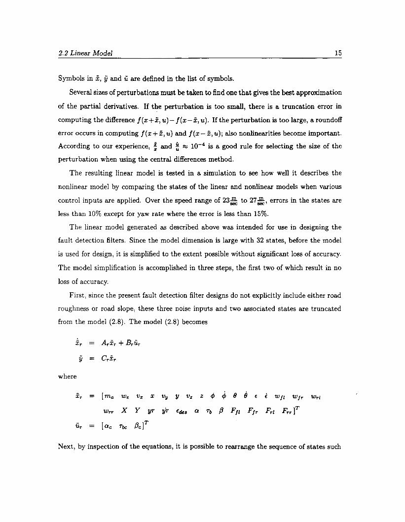
14 . Cbapter 2: Vebicle Model and Simulation Development
468Time (sec)
Roll Rate
Pitch Rate
i 0
-I
-28 0 2 4 6 8
Time (sec)
0.0292~--~------'!'-----'024
Time (sec)
0.0294
X 10') Pitch An.le 10')-2 6
X
4-2.S
2
"! -3 40
-2-3.S
-4
2 4 6 8-6
0 2Time (sec)
Roll An.le 2 x 10')0.03
0.0298
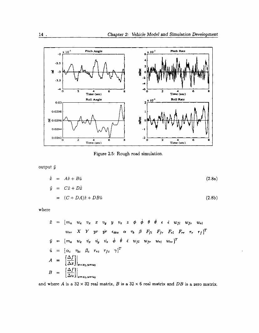
Figure 2.5: Rough road simulation.
output ii
x = Ax+Bu
y ex + D£
= (C + DA)x + DBu
where
x = [rna We Vx X VII Y Vz z cP cP 9 iJ E
Wrr X y yT y'T Edes a 7"b /3 Ffl Ffr
y = [rna We V% VII Vz ;p iJ i. Wfl wfr Wrl
U = lac rbc /3c Trc Tfc "'tfA = [~;] 1%=%0,u=uo
B = [~~] Ix=xo,u=uo
(2.8a)
(2.8b)
E Wfl wfr Wrl
l:" l:" T Tf]Trrl rrr r
wrrf
and where A is a 32 x 32 real matrix, B is a 32 x 6 real matrix and DB is a zero matrix.
2.2 Linear Model 15
Symbols in X, y and U are defined in the list of symbols.
Several sizes of perturbations must be taken to find one that gives the best approximation
of the partial derivatives. If the perturbation is too small, there is a truncation error in
computing the difference f(x+x, u)- f(x-x, u). If the perturbation is too large, a roundoff
error occurs in computing f(x +x, u) and f(x - x, u); also nonlinearities become important.
According to our experience, ~ and ~ ~ 10-4 is a good rule for selecting the size of the
perturbation when using the central differences method.
The resulting linear model is tested in a simulation to see how well it describes the
nonlinear model by comparing the states of the linear and nonlinear models when various
control inputs are applied. Over the speed range of 23S: to 27S:' errors in the states are
less than 10% except for yaw rate where the error is less than 15%.
The linear model generated as described above was intended for use in designing the
fault detection filters. Since the model dimension is large with 32 states, before the model
is used for design, it is simplified to the extent possible without significant loss of accuracy.
The model simplification is accomplished in three steps, the first two of which result in no
loss of accuracy.
First, since the present fault detection filter designs do not explicitly include either road
roughness or road slope, these three noise inputs and two associated states are truncated
from the model (2.8). The model (2.8) becomes
x r = Arxr + Brur
y = Grxr
where
I r = [rna We V x X V y Y V z z ¢ ¢ () iJ E i WII Wlr Wrl
W rr X y yr 'liT Edes Q Tb {3 Ffl Ffr Frl Frrf
Ur = [ Q e Tbc {3e]T
Next, by inspection of the equations, it is possible to rearrange the sequence of states such

16 Cbapter 2: Vehicle Model and Simulation Development
that the linearized equations assume the following partitioned form:
xr = [:~ ]= [ Al o ] [ ~l ] + [ Bl ] UrA 2l A2 X2 B2
Y = [ Cl o ] [ :~ ]where
Xl = [rna We Vx Vy Vz z tP tP () e i Wfl Wfr Wrl Wrr
Q Tb {3 Ffl F fr Frl Frrf
X2 = [x y € X Y yr '!ir €des ]T
In this form, both Xl and ii are independent of X2. Thus X2 can be deleted from the model
without affecting the transfer function from uto ii. Based on this observation, X2 is removed
from the model, which then becomes
where Al is an 22 x 22 matrix, Bl is an 22 x 3 matrix and Cl is a 12 x 22 matrix.
As shown in (Douglas et al. 1995), when the nominal operating point associated with
the linearized system is one where the car is not making a turn, the longitudinal and
lateral dynamics decouple exactly. However, the case considered here has a nonzero nominal
steering angle so the longitudinal and lateral dynamics do not decouple. All 22 states are
included in the linear model order reduction process explained in the next section.
2.3 Reduced-Order Model
Previous manipulation involved no approximation. For further model simplification, some
approximation must occur. After the linear model is derived, the first thing one should
do is check the eigenvalues. Then, two approaches are presented to get reduced-order
models. The first approach is to set the derivatives of certain fast states to zero. Using this
philosophy, states with large negative eigenvalues can be dropped. However, a correction
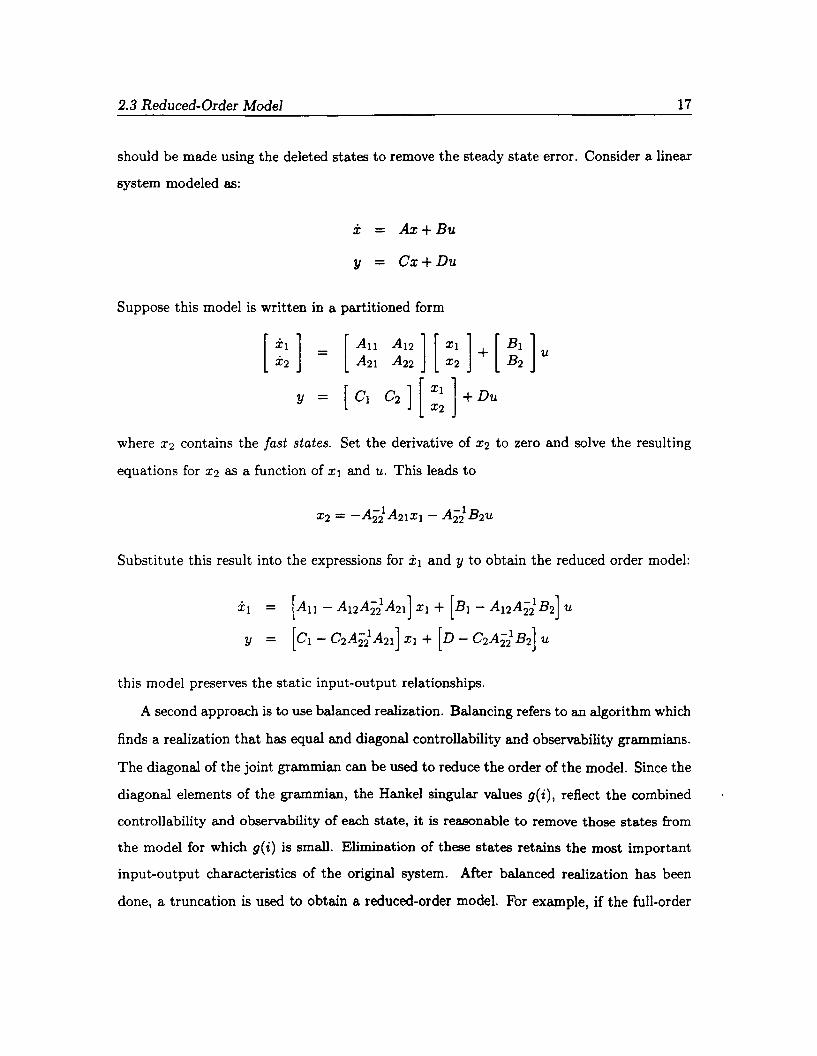
2.3 Reduced-Order Model 17
should be made using the deleted states to remove the steady state error. Consider a linear
system modeled as:
x = Ax+Bu
y = Cx+Du
Suppose this model is written in a partitioned form
y =
where X2 contains the fast states. Set the derivative of X2 to zero and solve the resulting
equations for X2 as a function of Xl and u. This leads to
Substitute this result into the expressions for Xl and y to obtain the reduced order model:
Xl = [Au - A12 A2":l A2l ] Xl + [Bl - A12A2":l B2] u
Y = [Cl -C2A2":lA21 ]Xl+ [D-C2A2":lB2]U
this model preserves the static input-output relationships.
A second approach is to use balanced realization. Balancing refers to an algorithm which
finds a realization that has equal and diagonal controllability and observability grammians.
The diagonal of the joint grammian can be used to reduce the order of the model. Since the
diagonal elements of the grammian, the Hankel singular values g(i), reflect the combined
controllability and observability of each state, it is reasonable to remove those states from
the model for which g(i) is small. Elimination of these states retains the most important
input-output characteristics of the original system. After balanced realization has been
done, a truncation is used to obtain a reduced-order model. For example, if the full-order
18
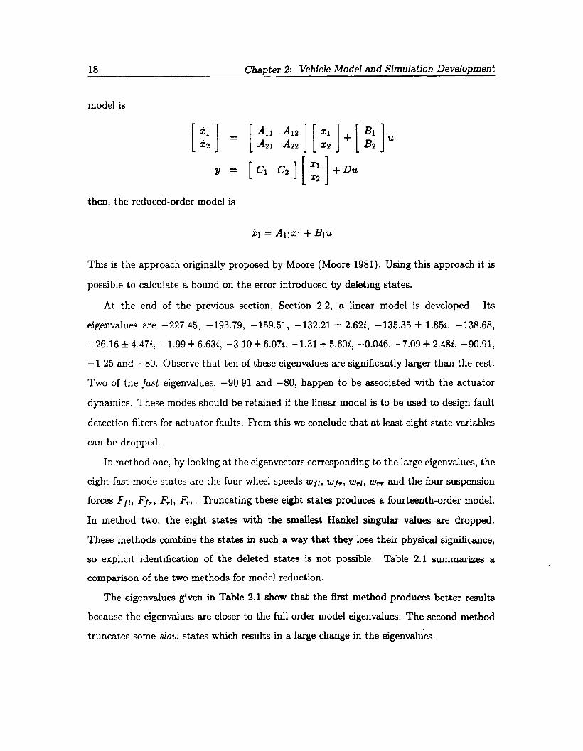
model is
y =
then, the reduced-order model is
Chapter 2: Vehicle Model and Simulation Development
This is the approach originally proposed by Moore (Moore 1981). Using this approach it is
possible to calculate a bound on the error introduced by deleting states.
At the end of the previous section, Section 2.2, a linear model is developed. Its
eigenvalues are -227.45, -193.79, -159.51, -132.21 ± 2.62i, -135.35 ± 1.85i, -138.68,
-26.16 ± 4.47i, -1.99 ± 6.63i, -3.10 ± 6.07i, -1.31 ± 5.60i, -0.046, -7.09 ± 2.48i, -90.91,
-1.25 and -80. Observe that ten of these eigenvalues are significantly larger than the rest.
Two of the fast eigenvalues, -90.91 and -80, happen to be associated with the actuator
dynamics. These modes should be retained if the linear model is to be used to design fault
detection filters for actuator faults. From this we conclude that at least eight state variables
can be dropped.
In method one, by looking at the eigenvectors corresponding to the large eigenvalues, the
eight fast mode states are the four wheel speeds Wfll Wfr, Wrl, Wrr and the four suspension
forces Fjl, Fjr, Frl, F rr . Truncating these eight states produces a fourteenth-order model.
In method two, the eight states with the smallest Hankel singular values are dropped.
These methods combine the states in such a way that they lose their physical significance,
so explicit identification of the deleted states is not possible. Table 2.1 summarizes a
comparison of the two methods for model reduction.
The eigenvalues given in Table 2.1 show that the first method produces better results
because the eigenvalues are closer to the full-order model eigenvalues. The second method
truncates some slow states which results in a large change in the eigenvalues.
2.3 Reduced-Order Model 19
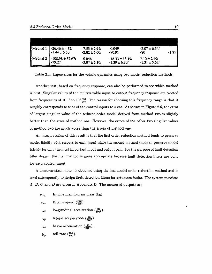
- -
----------------------------------Method 1 -26.46 ±4.32i -7.53±2.94i -0.049 -2.07 ±6.54i
-1.44 ±5.50i -2.82 ±5.6Oi -90.91 -80 -1.25
Method 2 -108.98 ± 37.67i -0.046 -18.33 ± 13.19i 7.10 ±2.49i-79.27 -3.07 ±6.1 Oi -2.39 ±6.30i -1.31 ±5.62i
Table 2.1: Eigenvalues for the vehicle dynamics using two model reduction methods.
Another test, based on frequency response, can also be performed to see which method
is best. Singular values of the multivariable input to output frequency response are plotted
from frequencies of 10-1 to 102~. The reason for choosing this frequency range is that it
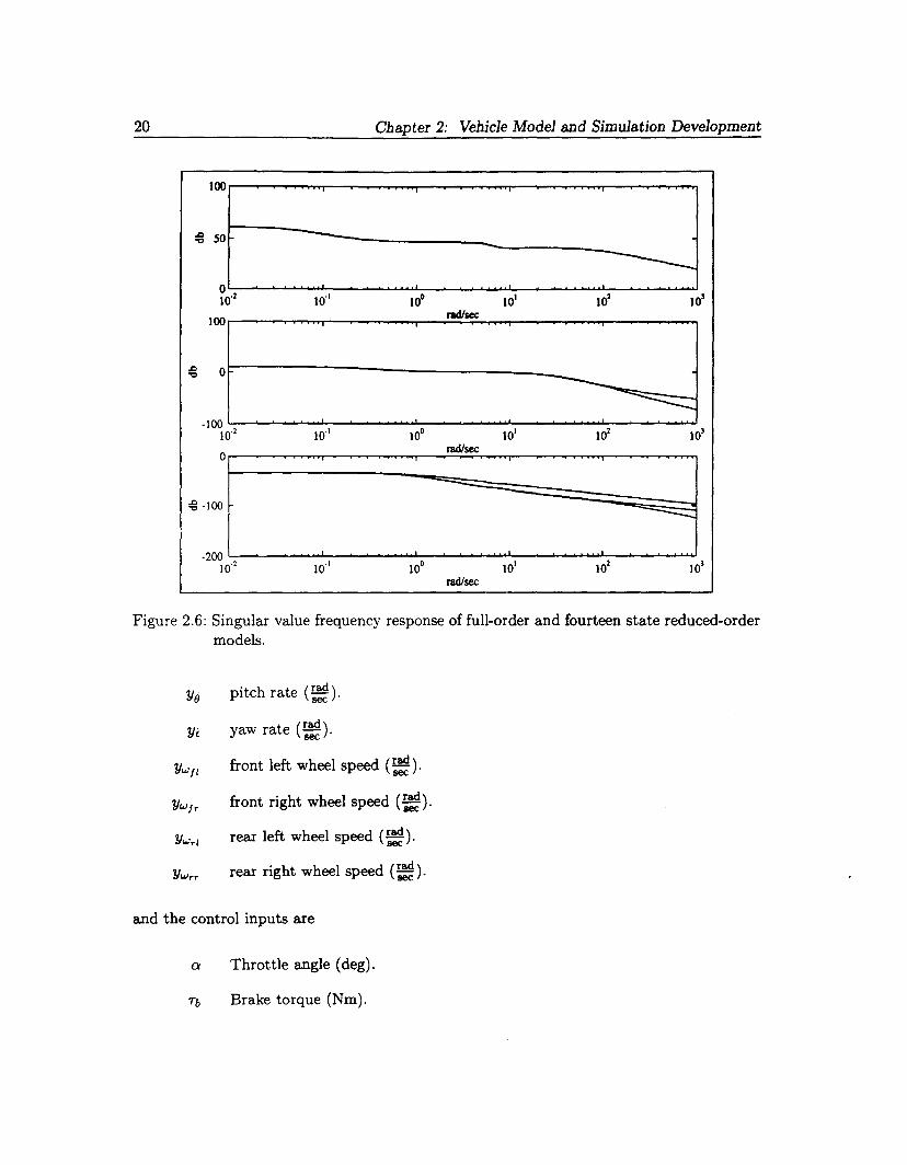
roughly corresponds to that of the control inputs to a car. As shown in Figure 2.6, the error
of largest singular value of the reduced-order model derived from method two is slightly
better than the error of method one. However, the errors of the other two singular values
of method two are much worse than the errors of method one.
An interpretation of this result is that the first order reduction method tends to preserve
model fidelity with respect to each input while the second method tends to preserve model
fidelity for only the most important input and output pair. For the purpose offault detection
filter design, the first method is more appropriate because fault detection filters are built
for each control input.
A fourteen-state model is obtained using the first model order reduction method and is
used subsequently to design fault detection filters for actuators faults. The system matrices
A, B, C and D are given in Appendix D. The measured outputs are
Yma Engine manifold air mass (kg).
YWe Engine speed (=).
Yx longitudinal acceleration (~).
Yji lateral acceleration (~).
Yz heave acceleration (~).
Yti> roll rate (~).
20 Chapter 2: Vehicle Model and Simulation Development
100
:@ so - ------010.2 10·· 10° 10
1 102
103
100radlsec:
~ 0'l:l
--.:.:::::::-100
10-2 10"1 10° 10· 102
103
0radlsec
-:@ -100 ---200
10"2 10"' 10° 101
102 103
radlsec
Figure 2.6: Singular value frequency response of full-order and fourteen state reduced-ordermodels.
YiJ pitch rate (~).
Yi yaw rate (::).
YWjl front left wheel speed (:;).
YWjr front right wheel speed (~).
YWrl rear left wheel speed (~).
YWrr rear right wheel speed (~).
and the control inputs are
Q Throttle angle (deg).
Tb Brake torque (Nm).
2.3 Reduced-Order Model
f3 Steering angle (rad).
21
While a fourteen-state linear model is used for the design of actuator fault detection
filters, a twelveth-order model is used to design sensor fault detection filters. Recall that
two fast modes retained in the fourteen-state reduced-order model are associated with the
actuator dynamics. The eigenvalue -90.91 is associated with the throttle actuator and -80
with the steering actuator. For the design of sensor fault detection filters, these modes
may also be deleted. Note that since the actuator dynamics are in series with the other
dynamics, the reduced-order eigenvalues do not change. Singular values of the multivariable
input to output frequency response are illustrated in Figure 2.7. The model reduction error
is seen to be very slightly worse than for the fourteenth-order model. The system matrices
:§ 50r----------.__---==-__~-----:§ o~----------------_~
--..:.:::::::10,1 10° 10' 102
103
radlsec
---..:: ---10" 10° 10' 102
103
radlsec
Figure 2.7: Singular value frequency response of full-order and twelve state reduced-ordermodels.
A, B, C and D for the twelve-state reduced-order model are given in Appendix D.