Embed Size (px)
Citation preview

CE 6504 HIGHWAY ENGINEERING
FATIMA MICHAEL COLLEGE OF ENGINEERING
Prepared by
MrsCArthi Jenifer ME
Assistant ProfessorCivil
FMCETMadurai 1
FATIMA MICHAEL ENGINEERING
COLLEGE AND
TECHNOLOGY
Department of Civil Engineering
CE 6504 HIGHWAY ENGINEERING
Lecture notes
Prepared by
C A R T H I J E N I F E R
CE 6504 HIGHWAY ENGINEERING
FATIMA MICHAEL COLLEGE OF ENGINEERING
Prepared by
MrsCArthi Jenifer ME
Assistant ProfessorCivil
FMCETMadurai 2
CE 6504 HIGHWAY ENGINEERING 3 0 0 3
OBJECTIVE
The objective of the course is to educate the students on the various components of Highway
Engineering It exposes the students to highway planning engineering surveys for highway
alignment Design of Geometric Elements of Highways and Urban roads and Rigid and Flexible
pavements design The students further learn the desirable properties of highway materials and
various practices adopted for construction This course enables the students to develop skill on
evaluation of the pavements and to decide appropriate types of maintenance
HIGHWAY PLANNING AND ALIGNMENT 9
History of Road Construction Highway Development in India - Jayakar Committee
Recommendations and Realizations Twenty-year Road Development Plans Concepts of Ongoing
Highway Development Programme at National Level Institutions for Highway Development at
National level - Indian Roads Congress Highway Research Board National Highway Authority of
India Ministry of Road Transport and Highways (MORTH) and Central Road Research Institute
Requirements of Ideal Alignment Factors Controlling Highway Alignment Engineering Surveys for
Alignment - Conventional Methods and Modern Methods (Remote Sensing GIS and GPS
techniques) Classification and Cross Section of Urban and Rural Roads (IRC) Highway Cross
Sectional Elements ndash Right of Way Carriage Way Camber Krebs Shoulders and Footpaths [IRC
Standards] Cross sections of different Class of Roads ndash Principles of Highway Financing
GEOMETRIC DESIGN OF HIGHWAYS 9
Design of Horizontal Alignment ndash Horizontal Curves Super elevation Widening of Pavements on
Horizontal Curves and Transition Curves Design of Vertical Alignments ndash Rolling Limiting
Exceptional and Minimum Gradients Summit and Valley Curves-Sight Distances ndash Factors
affecting Sight Distances PIEV theory Stopping Sight Distance (SSD) Overtaking Sight Distance
(OSD) Sight Distance at Intersections Intermediate Sight Distance and Illumination Sight Distance
[Derivations and Problems in SSD and OSD] -Geometric Design of Hill Roads [IRC Standards
Only]
FLEXIBLE AND RIGID PAVEMENTS 9
Rigid and Flexible Pavements- Components and their Functions -Design Principles of Flexible and
Rigid Pavements Factors affecting the Design of Pavements - ESWL Climate Sub-grade Soil and
Traffic - Design Practice for Flexible Pavements [IRC Method and Recommendations- Problems] -
Design Practice for Rigid Pavements ndash IRC Recommendations - concepts only
HIGHWAY MATERIALS AND CONSTRUCTION PRACTICE 9
Desirable Properties and Testing of Highway Materials Soil ndash California Bearing Ratio Test Field
Density Test - Aggregate - Crushing Abrasion Impact Tests Water absorption Flakiness and
Elongation indices and Stone polishing value test - Bitumen - Penetration Ductility
CE 6504 HIGHWAY ENGINEERING
FATIMA MICHAEL COLLEGE OF ENGINEERING
Prepared by
MrsCArthi Jenifer ME
Assistant ProfessorCivil
FMCETMadurai 3
Viscosity Binder content and Softening point Tests - Construction Practice - Water Bound
Macadam Road Bituminous Road and Cement Concrete Road [as per IRC and MORTH
specifications] ndash Highway Drainage [IRC Recommendations]
EVALUATION HIGHWAY MAINTENANCE 9
Types of defects in Flexible pavements ndash Surface defects Cracks Deformation Disintegration ndash
Symptoms Causes and Treatments - Types of Pavement Failures in Rigid Pavements ndash Scaling
Shrinkage Warping Structural Cracks Spalling of Joints and Mud Pumping ndash and Special Repairs -
Pavement Evaluation ndash Pavement Surface Conditions and Structural Evaluation Evaluation of
pavement Failure and strengthening - Overlay design by Benkelman Beam Method [Procedure
only]
TOTAL 45 PERIODS
TEXT BOOKS
1 Khanna K and Justo C E G Highway Engineering Khanna Publishers Roorkee 2001
2 KadiyaliLR L R Principles and Practice of Highway Engineering Khanna Technical
Publications Delhi 2000
REFERENCES
1 Transportation Engineering amp Planning CS Papa Costas PD Prevedouros Prentice Hall
of India Pvt ltd 2006
2 IRC Standards (IRC 37 - 2001 amp IRC 58 -1998)
3 Bureau of Indian Standards (BIS) Publications on Highway Materials
4 Specifications for Road and Bridges MORTH (India)
CE 6504 HIGHWAY ENGINEERING
FATIMA MICHAEL COLLEGE OF ENGINEERING
Prepared by
MrsCArthi Jenifer ME
Assistant ProfessorCivil
FMCETMadurai 4
UNIT 1 HIGHWAY PLANNNING AND ALIGNMENT
Significance of highway planning
Wide Geographical Coverage provided by roads
Roads can be constructed to penetrate the interior of any region and to connect remote villages The
advantage becomes particularly evident when planning the communication system in hilly regions
and sparsely populated areas
Low Capital investment
Roads can be constructed at comparatively lower initial cost than railways The cost of roads varies
with specifications but even the best road is cheaper than a railway line
Quick and assured deliveries
Time is great value for a wide range of articles including both perishables and high value is
manufactured products Road transport by its quick deliveries reduces the need for larger inventories
and locking up of working capital a great cost
Flexibility
Road transport offers a flexible service free from fixed schedules Any number of trucks or buses
can be pressed into service quickly to meet sudden demand or withdrawn Such a flexibility is
absent in railways which operate generally according to fixed schedules
Door-to-door services
Road transport offers door-to-door service free from transshipments from origin to destination
Railways on the other hand have to depend upon road transport for picking up loads and making
deliveries
Simpler packaging
Road transport permits simpler packaging and crating for the protection of goods against breakage
Personalized service
A personal touch is generally present in road transport The customer is given in individualized
attention in various matters
Employment potential
Road transport has a high employment potential This is an important factor in a country with a large
and employment problem
Personalized travel
Travel by private car or motorized two wheeler or even a cycle satisfies personal pleasuresThis is
one of the main reasons for the popularity of personalized travel mode in the developed countries
Short hauls
For short hauls transport is there only economical means if a major project is to be constructed and
is the construction materials have to be transported through short distances one turns only to road
transport
Safety
One of the serious advantages of road transport is its poor record of safety Road accidents have
become a serious menace claiming enormous economic loss to the nation
Environmental pollution
Road transport has been one of the major causes for environmental pollution noise fumes vibration
loss of aesthetics ribbon development these are the some ill effects
CE 6504 HIGHWAY ENGINEERING
FATIMA MICHAEL COLLEGE OF ENGINEERING
Prepared by
MrsCArthi Jenifer ME
Assistant ProfessorCivil
FMCETMadurai 5
Parking problem
Road transport has caused parking problem of serious proportions in city streets
Long hauls
It has been found that most commodity movements are cheaper by road for short hauls up to 300-
350 kms but beyond this range the cost advantage lies with the railways
Energy
Road transport consumes greater energy per passenger km and tone km than railways
History of road development in India
Roads in India perform a variety of roles in achieving speedy economic development Some of the
important aspects are discussed below
Connection to villages
India is a country having 590000 villages scattered into small habitations and often located in the
extreme interior Thus social uplift health and education of the village population is aided by roads
Communications in hilly terrain
For the hill states located along the Himalayan range communication facility is possible only by
roads because of the steep terrain involved
Strategic importance
The defense of the northern north-eastern and western borders of the country is dependent to a large
extent on the road system
Helps agricultural development
Roads have fostered quicker agricultural development facilitating movement of modern inputs such
as fertilizers and high yielding seeds
Helps dairy development
Since the cattle wealth of the nation is concentrated in innumerable villages and small habitations
the collection and processing of surplus milk only because of roads
Forestry development
The forest wealth of the country is being exploited mainly because of the roads which penetrate in to
the thick jungles
Fisheries Development The Development of the fisheries along the coast line has been rendered possible because of the
construction of link roads leading to the coast
Tourism Development
Some of the ancient monuments religious places natural parks and sanctuaries are accessible only
roads Tourism both domestic and international has been greatly aided by roads serving such as
places of interest
Employment
As already stated roads and road transport provide employment to a large number of people in the
country Since road construction involves labour intensive techniques in India the large unemployed
labor force gets gainful employment
Famine and flood relief
Roads have helped operations pertaining to flood and famine relief The affected people are
frequently employed on road construction to build durable assets
Administrative convenience
CE 6504 HIGHWAY ENGINEERING
FATIMA MICHAEL COLLEGE OF ENGINEERING
Prepared by
MrsCArthi Jenifer ME
Assistant ProfessorCivil
FMCETMadurai 6
Roads have helped the effective administration of this large country Maintenance of law and order
and dispensation of justice have been aided by roads National integration and cohesion have been
brought about by roads which traverse the length and breath of the country and which link people
from different parts together
Tresaguet construction
Pierre Tresaguet (1716-1796) developed an improved method of construction in France by
the year 1964The main feature of his proposal was that the thickness of construction need be
only in the order of 30 cm
Tresaguet was the inspector General of roads in France from 1775 to 1785So his method of
construction was implemented in that country in 1775
The typical cross section of tresaguets road construction is given in fig and the construction
steps may be enumerated as below
i) The sub grade was prepared and layers of large foundation stones were laid on edge by
hand At the two edges of the pavement large stones were embedded edge wise to serve
as submerged Krebs stones
ii) The corners of the heavy foundation stones were hammered and then the interstices filled
with smaller stones
iii) The top-wearing course was made of smaller stones and compacted to a thickness of
about 5 cm at the edges and gradually increased towards the center
iv) The shoulders were also provides cross slope to drain the surface water to the side drain
Macadam Construction
John Macadam put forward an entirely new method of road construction as compared to all the
previous methods A typical cross section of Macadam construction
CE 6504 HIGHWAY ENGINEERING
FATIMA MICHAEL COLLEGE OF ENGINEERING
Prepared by
MrsCArthi Jenifer ME
Assistant ProfessorCivil
FMCETMadurai 7
i) The importance of sub grade drainage and compaction were recognized and the sub
grade was compacted and was prepared with a cross slope of 1 in 36
ii) Macadam was the first person to suggest the heavy foundation stones are not at all
necessary to be placed at the bottom layer of construction
iii) Though the total thickness of construction was less than previous methods This
technique could serve the purpose in a better way
iv) The size of broken stones for the top layer was decided based on the stability under
animal drawn vehicles
Macadamrsquos method is the first method based on scientific thinking
The construction steps are
i) Sub grade is compacted and prepared with a cross slope of 1 in 36 up to a desired width
ii) Broken stones of a strong variety all passing through 5 cm size sieve were compacted to
a uniform thickness of 10cm
iii) The second layer of strong broken stones of size 375 cm was compacted to thickness of
10 cm
iv) The top layer consisted of stones of size less than 2 cm compacted to a thickness of about
5 cm The cross slope of pavement surface was also 1 in 36
Classification of roads
Road classification
The roads can be classified in many ways The classification based on speed and
accessibility is the most generic one Note that as the accessibility of road increases the
speed reducesAccordingly the roads can be classified as follows in the order of
increased accessibility and reduced speeds
Freeways Freeways are access-controlled divided highways Most freeways are
four lanes two lanes each direction but many freeways widen to incorporate
more lanes as they enter urban areas Access is controlled through the use of
interchanges and the type of interchange depends upon the kind of intersecting
road way (rural roads another freeway etc)
Expressways They are superior type of highways and are designed for high
CE 6504 HIGHWAY ENGINEERING
FATIMA MICHAEL COLLEGE OF ENGINEERING
Prepared by
MrsCArthi Jenifer ME
Assistant ProfessorCivil
FMCETMadurai 8
speeds (120 kmhr is common) high traffic volume and safety They are
generally provided with grade separations at intersections Parking loading and
unloading of goods and pedestrian traffic is not allowed on expressways
Highways They represent the superior type of roads in the country Highways are
of two types - rural highways and urban highways Rural highways are those
passing through rural areas (villages) and urban highways are those passing
through large cities and towns ie urban areas
Arterials It is a general term denoting a street primarily meant for through traffic
usually on a continuous route They are generally divided highways with fully or
partially controlled access Parking loading and unloading activities are usually
restricted and regulated Pedestrians are allowed to cross only at
intersectionsdesignated pedestrian crossings
Local streets A local street is the one which is primarily intended for access to
residence business or abutting property It does not normally carry large volume
of traffic and also it allows unrestricted parking and pedestrian movements
Collector streets These are streets intended for collecting and distributing traffic
to and from local streets and also for providing access to arterial streets Normally
full access is provided on these streets There are few parking restrictions except
during peak hours
Figure 1 Speed vs accessibility
CE 6504 HIGHWAY ENGINEERING
FATIMA MICHAEL COLLEGE OF ENGINEERING
Prepared by
MrsCArthi Jenifer ME
Assistant ProfessorCivil
FMCETMadurai 9
FACTORS AFFECTING HIGHWAY ALIGHNMENT
Design speed
Design speed is the single most important factor that affects the geometric design It
directly affects the sight distance horizontal curve and the length of vertical curves
Since the speed of vehicles vary with driver terrain etc a design speed is adopted for all
the geometric design
Design speed is defined as the highest continuous speed at which individual vehicles can
travel with safety on the highway when weather conditions are conducive Design speed
is different from the legal speed limit which is the speed limit imposed to curb a common
tendency of drivers to travel beyond an accepted safe speed Design speed is also
different from the desired speed which is the maximum speed at which a driver would
travel when unconstrained by either traffic or local geometry
Since there are wide variations in the speed adopted by different drivers and by different
types of vehicles design speed should be selected such that it satisfy nearly all drivers At
the same time a higher design speed has cascading effect in other geometric designs and
thereby cost escalation Therefore an 85th percentile design speed is normally adopted
This speed is defined as that speed which is greater than the speed of 85 of drivers In
some countries this is as high as 95 to 98 percentile speed
Topography
The next important factor that affects the geometric design is the topography It is easier to
construct roads with required standards for a plain terrain However for a given design speed the
construction cost increases multiform with the gradient and the terrain Therefore geometric design
standards are different for different terrain to keep the cost of construction and time of construction
under control This is characterized by sharper curves and steeper gradients
Other factors
CE 6504 HIGHWAY ENGINEERING
FATIMA MICHAEL COLLEGE OF ENGINEERING
Prepared by
MrsCArthi Jenifer ME
Assistant ProfessorCivil
FMCETMadurai 10
In addition to design speed and topography there are various other factors that affect the geometric
design and they are briefly discussed below
Vehicle The dimensions weight of the axle and operating characteristics of a vehicle
influence the design aspects such as width of the pavement radii of the curve clearances
parking geometrics etc A design vehicle which has standard weight dimensions and
operating characteristics are used to establish highway design controls to accommodate
vehicles of a designated type
Human The important human factors that influence geometric design are the mental and
psychological characteristics of the driver and pedestrians like the reaction time
Traffic It will be uneconomical to design the road for peak traffic flow Therefore a
reasonable value of traffic volume is selected as the design hourly volume which is
determined from the various traffic data collected The geometric design is thus based on
this design volume capacity etc
Environmental Factors like air pollution noise pollution etc should be given due
consideration in the geometric design of roads
Economy The design adopted should be economical as far as possible It should match
with the funds allotted for capital cost and maintenance cost
Others Geometric design should be such that the aesthetics of the region is not affected
Nagpur classification
In Nagpur road classification all roads were classified into five categories as National highways
State highways Major district roads Other district roads and village roads
National highways
They are main highways running through the length and breadth of India connecting major
ports foreign highways capitals of large states and large industrial and tourist centers
including roads required for strategic movements
It was recommended by Jayakar committee that the National highways should be the frame
on which the entire road communication should be based
All the national highways are assigned the respective numbers
For eg the highway connecting Delhi-Ambala-Amritsar is denoted as NH-1 (Delhi-
Amritsar) where as a bifurcation of this highway beyond Full under to Srinagar and Uri is
denoted as NH-1_A
They are constructed and maintained by CPWD
The total lengths of National highway in the country is 58112 Kms and constitute about 2
of total road networks of India and carry 40 of total traffic
State highways
They are the arterial roads of a state connecting up with the national highways of adjacent
states district headquarters and important cities within the state
They also serve as main arteries to and from district roads
Total length of all SH in the country is 1 37119 Kms
Major district roads
Important roads with in a district serving areas of production and markets connecting those
with each other or with the major highways
India has a total of 4 70000 Kms of MDR
CE 6504 HIGHWAY ENGINEERING
FATIMA MICHAEL COLLEGE OF ENGINEERING
Prepared by
MrsCArthi Jenifer ME
Assistant ProfessorCivil
FMCETMadurai 11
Other district roads
Roads serving rural areas of production and providing them with outlet to market centers or
other important roads like MDR or SH
Village roads
They are roads connecting villages or group of villages with each other or to the nearest
road of a higher category like ODR or MDR
India has 2650000 kms of ODR+VR out of the total 3315231 kms of all type of roads
Roads classification criteria
Apart from the classification given by the different plans roads were also classified based on some
other criteria They are given in detail below
Based on usage
This classification is based on whether the roads can be used during different seasons of the year
All-weather roads Those roads which are negotiable during all weathers except at major
river crossings where interruption of traffic is permissible up to a certain extent are called all
weather roads
Fair-weather roads Roads which are negotiable only during fair weather are called fair
weather roads
Based on carriage way
This classification is based on the type of the carriage way or the road pavement
Paved roads with hards surface If they are provided with a hard pavement course such
roads are called paved roads(eg stones Water bound macadam (WBM) Bituminous
macadam (BM) concrete roads)
Unpaved roads Roads which are not provided with a hard course of atleast a WBM layer
they is called unpaved roads Thus earth and gravel roads come under this category
Alignment The position or the layout of the central line of the highway on the ground is called the
alignment Horizontal alignment includes straight and curved paths Vertical alignment
includes level and gradients Alignment decision is important because a bad alignment
will enhance the construction maintenance and vehicle operating costs Once an
alignment is fixed and constructed it is not easy to change it due to increase in cost of
adjoining land and construction of costly structures by the roadside
Requirements The requirements of an ideal alignment are
The alignment between two terminal stations should be short and as far as
possible be straight but due to some practical considerations deviations may be
needed
The alignment should be easy to construct and maintain It should be easy for the
operation of vehicles So to the maximum extend easy gradients and curves
should be provided
It should be safe both from the construction and operating point of view
especially at slopes embankments and cutting It should have safe geometric
features
The alignment should be economical and it can be considered so only when the
initial cost maintenance cost and operating cost are minimum
CE 6504 HIGHWAY ENGINEERING
FATIMA MICHAEL COLLEGE OF ENGINEERING
Prepared by
MrsCArthi Jenifer ME
Assistant ProfessorCivil
FMCETMadurai 12
Factors controlling alignment
We have seen the requirements of an alignment But it is not always possible to satisfy all
these requirements Hence we have to make a judicial choice considering all the factors
The various factors that control the alignment are as follows
Obligatory points These are the control points governing the highway alignment
These points are classified into two categories Points through which it should
pass and points through which it should not pass Some of the examples are
o Bridge site The bridge can be located only where the river has straight
and permanent path and also where the abutment and pier can be strongly
founded The road approach to the bridge should not be curved and skew
crossing should be avoided as possible Thus to locate a bridge the
highway alignment may be changed
o Mountain While the alignment passes through a mountain the various alternatives are to either construct a tunnel or to go round the hills The suitability of the alternative depends on factors like topography site
conditions and construction and operation cost
o Intermediate town The alignment may be slightly deviated to connect an intermediate town or village nearby
These were some of the obligatory points through which the alignment should pass
Coming to the second category that is the points through which the alignment should not
pass are
Religious places These have been protected by the law from being acquired for
any purpose Therefore these points should be avoided while aligning
Very costly structures Acquiring such structures means heavy compensation
which would result in an increase in initial cost So the alignment may be deviated
not to pass through that point
Lakesponds etc The presence of a lake or pond on the alignment path would also
necessitate deviation of the alignment
Traffic The alignment should suit the traffic requirements Based on the origin-
destination data of the area the desire lines should be drawn The new alignment should
be drawn keeping in view the desire lines traffic flow pattern etc Geometric design
Geometric design factors such as gradient radius of curve sight distance etc also govern
the alignment of the highway To keep the radius of curve minimum it may be required
to change the alignment The alignments should be finalized such that the obstructions to
visibility do not restrict the minimum requirements of sight distance The design
standards vary with the class of road and the terrain and accordingly the highway should
be aligned Economy The alignment finalized should be economical All the three costs
ie construction maintenance and operating cost should be minimum The construction
cost can be decreased much if it is possible to maintain a balance between cutting and
filling Also try to avoid very high embankments and very deep cuttings as the
construction cost will be very higher in these cases
Road ecology
The features of the cross-section of the pavement influences the life of the pavement as
CE 6504 HIGHWAY ENGINEERING
FATIMA MICHAEL COLLEGE OF ENGINEERING
Prepared by
MrsCArthi Jenifer ME
Assistant ProfessorCivil
FMCETMadurai 13
well as the riding comfort and safety Of these pavement surface characteristics affect
both of these Camber kerbs and geometry of various cross-sectional elements are
important aspects to be considered in this regard They are explained briefly in this
chapter
Camber
Camber or cant is the cross slope provided to raise middle of the road surface in the
transverse direction to drain off rain water from road surface The objectives of providing
camber are
Surface protection especially for gravel and bituminous roads
Sub-grade protection by proper drainage
Quick drying of pavement which in turn increases safety
Too steep slope is undesirable for it will erode the surface Camber is measured in 1 in n
or n (Eg 1 in 50 or 2) and the value depends on the type of pavement surface The
value suggested by IRC for various categories of pavement is given in Table 1 The
common types of camber are parabolic straight or combination of them (Figure 1)
Figure 1 Different types of camber
Table 1 IRC Value
s for ca
mber
Heavy
Light
Surface
rain
type
rain
17
ConcreteBituminous
2
25
GravelWBM
3
30
Earthen
4
CE 6504 HIGHWAY ENGINEERING
FATIMA MICHAEL COLLEGE OF ENGINEERING
Prepared by
MrsCArthi Jenifer ME
Assistant ProfessorCivil
FMCETMadurai 14
Engineering surveys for alignment
The stages of the engineering surveys are a) Map study
b) Reconnaissance
c) Preliminary surveys
d) Final location and detailed surveys
Map study -
) In the topographic map to suggest the likely routes of roads In India topographic
maps are available from the survey of India with 15 or 30-meter contour intervals
) The main feature like rivers hills and valleys etc The probable alignment can be
located on the map from the following details available on the map
Alignment avoiding valleys ponds or lakes
When the road has to cross a row of hills possibility crossing through a mountain pass
Approximate location of bridge site for crossing rivers avoiding bend of the river
When a road is to be connected between two stations one of the top and the other on the foot
of the hill then alternate routes can be suggested keeping in view the permissible alignment
Suppose the scale of the contour map is known and then the contour intervals it is possible
to decide the length of road required between two consecutive contours keeping the gradient
within allowable limits
In the fig Let A and B be two stations to be connected by road AB is the shortest route
(Straight line) APQB is a steep route in which the gradient positively exceeds 1 in 20 as the
distance between the contour intervals is only about 200 meter
APLMNB is a route with an approximate slope of 1 in 20 whereas APEFGB is an alternate
alignment with the same gradient
Thus the map study also is possible to drop a certain route in view of any unavoidable
obstructions (or) undesirable ground enroute
Reconnaissance-
The second stage of surveys for highway location is the reconnaissance to examine the general
character of the area for deciding the most feasible routes for detailed studies
Some of the details to be collected during reconnaissance are given below
Valleys ponds lakes marshy land ridge hills permanent structures and other obstructions
along the route which are not available in the map
Approximate values of gradient length of gradients and radius of curves of alternate
alignments
Number and types of cross drainage structures maximum flood level and natural
groundwater level along the probable routes
Soil type along the routes from field identification tests and observation of geological
features
Sources of construction materials water and location of stone quarries
When the road passes through hilly or mountainous terrain additional data regarding the
geological formation types of rocks dip of strata seepage flow etc
Preliminary survey -
CE 6504 HIGHWAY ENGINEERING
FATIMA MICHAEL COLLEGE OF ENGINEERING
Prepared by
MrsCArthi Jenifer ME
Assistant ProfessorCivil
FMCETMadurai 15
The main objectives of the preliminary surveys are
To survey the various alternate alignments proposed after the reconnaissance and to collect
all the necessary physical information and details of topography drainage and soil
To compare the different proposals in view of the requirements of a good alignment
To estimate quantity of earthwork materials and other construction aspects and to work out
the cost of alternate proposals
To finalize the best alignment from all considerations
The procedure of the conventional methods of preliminary surveys the given steps
Primary survey -
For alternate alignments either secondary traverses (or) independent primary traverses may be
necessary
Topographical features -
All geographical and other man made features along the traverse and for a certain width on either
side surveyed and plotted
Leveling work -
Levelling work is also carried out side by side to give the centerline profiles and typical cross
sections The leveling work in the preliminary survey is kept to a minimum just sufficient to obtain
the approximate earthwork in the alternate alignments
Drainage studies -
Drainage investigations and hydrological data are collected so as to estimate the type number and
approximate size of cross and drainage structures
Soil survey -
The soil survey conducted at this stage helps to working out details of earthwork slopes suitability
of materials subsoil and surface drainage requirements and pavement type and the approximate
thickness requirements
Material survey -
The survey for naturally occurring materials like stone aggregates soft aggregates etc and
identification of suitable quarries should be made
Traffic survey -
Traffic surveys conducted in the region from basis for deciding the number of traffic lanes and
roadway width pavement design and economic analysis of highway project
Locations and functions
Final location and detailed survey - The alignment finalized at the design office after the preliminary survey is to be first located on the
field by establishing the centerline The detailed survey should be carried out for collecting the
information technology for the preparation of plans and construction details
Location -
The centerline of the road finalized in the drawings to be translated on the ground
during the location survey
Major and minor control points are established on the ground and center pegs are
driven checking the geometric design requirements
Detailed survey -
CE 6504 HIGHWAY ENGINEERING
FATIMA MICHAEL COLLEGE OF ENGINEERING
Prepared by
MrsCArthi Jenifer ME
Assistant ProfessorCivil
FMCETMadurai 16
Levels along his final centerline should be taken at all staked points Levelling work is to
great importance as the vertical alignment
A detailed soil survey is carried out to enable drawing of the soil profile
The data during the detailed survey should be elaborate and complete for preparing detailed
plans design and estimates of the project
Soil suitability analysis
The methodology for locating appropriate sites for each land use activity is guided by the intent to
minimize the possible adverse effects of development on the environment and on existing
communities and to emphasize the positive impacts of such development by locating them in a
most suitable location
This is achieved by examining a number of individual criteria assigning them relative levels of
importance as a whole and using a mathematical resultant model to identify the most suitable
location
By adopting this site suitability method it is possible to systematically identify the criteria
considered clearly document the relative importance of one criterion over another analyze the net
outcome using a Geographic Information System and then possibly revisit the mathematical
relationships in this ldquodecision modelrdquo
By revising the relative importance to identified criteria based upon the particular land use under
consideration it is possible to generate ldquosuitability mapsrdquo for each individual land use and then
generate a final composite land use that is based on a best possible collective suitability of multiple
land uses
To achieve this all the criteria are assigned a ldquorankrdquo denoting their relative levels of importance
within the suitability study These ranks are assigned as numeric values ranging from 1 to 10 with 1
reflecting a low level of importance and 10 reflecting a high level of importance For example
within the criteria of road networks national highways would have a different level of influence on
the suitability for a particular land use as compared with local roads Further the distance from each
of these features would further modify the relative suitability of a land use based on the proximity to
a particular type of road
Criteria for Site Suitability Analysis
The decision criteria for site selection are examined for assigning relative ranks and individual
feature weights based on the land use type for which suitability is being examined For benefit of
analysis the criteria under consideration in this paper activity are organized as
Critical Criteria Criteria that will be very significant in the site selection of the identified land use
and will act as key drivers in the selection of the geographic location These criteria can be clustered
into a single decision model and the outcome collectively reviewed These criteria have a strong
influence in the final suitability
Additional Criteria Criteria that will have to be examined one at a time to carefully assess its
relationship with the proposed land use activity These criteria have a positive influence in the final
suitability
CE 6504 HIGHWAY ENGINEERING
FATIMA MICHAEL COLLEGE OF ENGINEERING
Prepared by
MrsCArthi Jenifer ME
Assistant ProfessorCivil
FMCETMadurai 17
Constrained Criteria These criteria impose strong negative opportunities in the selection of areas
for the identified land use Consequently they inform of us of where the particular land use under
consideration should not be located These criteria serve to limit or exclude areas from the final
suitability
GIS Site Suitability Analysis Model We were developed a tourism site suitability analysis model
in ArcGIS - 931 which is shown in Figure -
CE 6504 HIGHWAY ENGINEERING
FATIMA MICHAEL COLLEGE OF ENGINEERING
Prepared by
MrsCArthi Jenifer ME
Assistant ProfessorCivil
FMCETMadurai 18
UNIT 2 GEOMETRIC DESIGN OF HIGHWAYS
Typical cross section of urban and rural roads
A cross section is a vertical plane (slice) taken at right angles to the road control line showing the
various elements that make up the roads structure It is normally viewed in the direction of
increasing chainage
The width of a roadway is an important design consideration to ensure that it is appropriately sized
to serve its function Because of the diversity within the County two major roadway categories have
been established 1 Rural Road Standards 2 Urban Road Standards Urban Road Standards will
serve those areas which tend to be more developed and need to provide for multiple users
(bicyclists pedestrians parallel parking etc) whereas many rural roads will primarily serve only
vehicular traffic
Cross sections are created to provide a visual guide depicting the initial interim and ultimate phase
cross sections for these road classifications The typical sections illustrated in the following pages
are recommendations tied to transportation planning aspects such as right‐of‐way lineage sidewalk
width etc Threshold daily traffic can be used as a guide for a starting point when determining
which cross section is most applicable
1 Rural Road Standards
The rural roadways will not typically require curb and gutter or sidewalk although the County may
require either or both in unique circumstances Widths of lanes and shoulders will vary depending
upon the specific classification and the potential traffic volume which the roadway may carry Roads
carrying fewer than 200 vehicles per day need not be paved or treated for dust control The need for
paved shoulders is also dependent upon the level of traffic and safety
Final design and construction details will be determined by the Public Works Department Final
Design and construction criteria taken into consideration may include but are not limited to use of
the roadway density of development topographical characteristics and nearby development For
construction in which only a portion of the ultimate cross‐section is intended to be completed the
partial design will need to allow for the eventual widening to the ultimate cross‐section The design
for the partial or interim cross‐section roadway will need to incorporate ultimate design information
to ensure that the first phase of roadway construction is appropriate and would not need to be
removed at a future date when the full width cross‐section is completed
2 Urban Road Standards
Three roadway classifications are identified for those areas that are associated with the communityrsquos
urban growth areas They include arterial collector and local street classifications Transportation
Plan shows the key elements of the urban road standards Urban road standards will include 12‐foot
lanes sidewalk and curb amp gutter arterials and collectors will also include a striped bike lane Turn
lanes may be necessary as determined by the County Since almost all of the municipalities have
different right‐of‐way cross sections adopted for their community it makes it very difficult for the
County to match them all Therefore the philosophy was to encourage a baseline amount of
right‐of‐way reservation that could ensure the adjacent community enough area for coordination of
future roadway improvements until such time the road
CE 6504 HIGHWAY ENGINEERING
FATIMA MICHAEL COLLEGE OF ENGINEERING
Prepared by
MrsCArthi Jenifer ME
Assistant ProfessorCivil
FMCETMadurai 19
CE 6504 HIGHWAY ENGINEERING
FATIMA MICHAEL COLLEGE OF ENGINEERING
Prepared by
MrsCArthi Jenifer ME
Assistant ProfessorCivil
FMCETMadurai 20
Cross sectional elements
Kerbs
Kerbs indicate the boundary between the carriage way and the shoulder or islands or footpaths Different types of kerbs are
CE 6504 HIGHWAY ENGINEERING
FATIMA MICHAEL COLLEGE OF ENGINEERING
Prepared by
MrsCArthi Jenifer ME
Assistant ProfessorCivil
FMCETMadurai 21
Low or mountable kerbs This type of kerbs is provided such that they
encourage the traffic to remain in the through traffic lanes and also allow the
driver to enter the shoulder area with little difficulty The height of this kerb is
about 10 cm above the pavement edge with a slope which allows the vehicle to
climb easily This is usually provided at medians and channelization schemes and
also helps in longitudinal drainage
Semi-barrier type kerbs When the pedestrian traffic is high these kerbs are
provided Their height is 15 cm above the pavement edge This type of kerb
prevents encroachment of parking vehicles but at acute emergency it is possible
to drive over this kerb with some difficulty
Barrier type kerbs They are designed to discourage vehicles from leaving the
pavement They are provided when there is considerable amount of pedestrian
traffic They are placed at a height of 20 cm above the pavement edge with a steep
batter
Submerged kerbs They are used in rural roads The kerbs are provided at
pavement edges between the pavement edge and shoulders They provide lateral
confinement and stability to the pavement
Figure 1 Different types of kerbs
Shoulders Shoulders are provided along the road edge and are intended for accommodation of
stopped vehicles serve as an emergency lane for vehicles and provide lateral support
for base and surface courses The shoulder should be strong enough to bear the weight
of a fully loaded truck even in wet conditions The shoulder width should be adequate
for giving working space around a stopped vehicle It is desirable to have a width of
46 m for the shoulders A minimum width of 25 m is recommended for 2-lane rural
highways in India Parking lanes
Parking lanes are provided in urban lanes for side parking Parallel parking is preferred
because it is safe for the vehicles moving on the road The parking lane should have a
minimum of 30 m width in the case of parallel parking
CE 6504 HIGHWAY ENGINEERING
FATIMA MICHAEL COLLEGE OF ENGINEERING
Prepared by
MrsCArthi Jenifer ME
Assistant ProfessorCivil
FMCETMadurai 22
Bus-bays
Bus bays are provided by recessing the kerbs for bus stops They are provided so that
they do not obstruct the movement of vehicles in the carriage way They should be at
least 75 meters away from the intersection so that the traffic near the intersections is not
affected by the bus-bay
Service roads Service roads or frontage roads give access to access controlled highways like freeways
and expressways They run parallel to the highway and will be usually isolated by a
separator and access to the highway will be provided only at selected points These roads
are provided to avoid congestion in the expressways and also the speed of the traffic in
those lanes is not reduced
Drainage
The pavement surface should be absolutely impermeable to prevent seepage of water into
the pavement layers Further both the geometry and texture of pavement surface should
help in draining out the water from the surface in less time
Footpath
Footpaths are exclusive right of way to pedestrians especially in urban areas They are
provided for the safety of the pedestrians when both the pedestrian traffic and vehicular
traffic is high Minimum width is 15 meter and may be increased based on the traffic
The footpath should be either as smooth as the pavement or more smoother than that to
induce the pedestrian to use the footpath
Right of way
Right of way (ROW) or land width is the width of land acquired for the road along its
alignment It should be adequate to accommodate all the cross-sectional elements of the
highway and may reasonably provide for future development To prevent ribbon
development along highways control lines and building lines may be provided Control
line is a line which represents the nearest limits of future uncontrolled building activity
in relation to a road Building line represents a line on either side of the road between
which and the road no building activity is permitted at all The right of way width is
governed by
Width of formation It depends on the category of the highway and width of
roadway and road margins
Height of embankment or depth of cutting It is governed by the topography and
the vertical alignment
Side slopes of embankment or cutting It depends on the height of the slope soil
type etc
Drainage system and their size which depends on rainfall topography etc
Sight distance considerations On curves etc there is restriction to the visibility
on the inner side of the curve due to the presence of some obstructions like
building structures etc
Reserve land for future widening Some land has to be acquired in advance
CE 6504 HIGHWAY ENGINEERING
FATIMA MICHAEL COLLEGE OF ENGINEERING
Prepared by
MrsCArthi Jenifer ME
Assistant ProfessorCivil
FMCETMadurai 23
Table 2 Desig
n speed in as per IRC (ruling and minimum)
Steep
Type
Plain
Rolling
Hilly
40-30
NSampSH
100-80
80-65
50-40
MDR
80-65
65-50
40-30
30-20
25-20
ODR
65-50
50-40
30-25
25-20
VR
50-40
40-35
25-20
anticipating future developments like widening of the road
Table 1 No
right of way for open areas
Roadway width in m
Road
Plain and
Mountainous and
classification
steep terrain
rolling terrain
Open areas
45
24
NHSH
18
MDR
25
15
15
ODR
12
9
VR
Built-up areas
20
NHSH
30
MDR
20
15
ODR
15
12
9
VR
10
CE 6504 HIGHWAY ENGINEERING
FATIMA MICHAEL COLLEGE OF ENGINEERING
Prepared by
MrsCArthi Jenifer ME
Assistant ProfessorCivil
FMCETMadurai 24
Horizontal curve
The presence of horizontal curve imparts centrifugal force which is a reactive force
acting outward on a vehicle negotiating it Centrifugal force depends on speed and radius
of the horizontal curve and is counteracted to a certain extent by transverse friction
between the tyre and pavement surface On a curved road this force tends to cause the
vehicle to overrun or to slide outward from the centre of road curvature For proper
design of the curve an understanding of the forces acting on a vehicle taking a horizontal
curve is necessary Various forces acting on the vehicle are illustrated in the figure 1
Figure 1 Effect of horizontal curve They are the centrifugal force (P) acting outward weight of the vehicle (W) acting
downward and the reaction of the ground on the wheels ( and ) The centrifugal
force and the weight is assumed to be from the centre of gravity which is at h units above
the ground Let the wheel base be assumed as b units The centrifugal force in
is given by
(1)
where is the weight of the vehicle in is the speed of the vehicle in is
the acceleration due to gravity in and is the radius of the curve in
The centrifugal ratio or the impact factor is given by
CE 6504 HIGHWAY ENGINEERING
FATIMA MICHAEL COLLEGE OF ENGINEERING
Prepared by
MrsCArthi Jenifer ME
Assistant ProfessorCivil
FMCETMadurai 25
(1)
The centrifugal force has two effects A tendency to overturn the vehicle about the outer
wheels and a tendency for transverse skidding Taking moments of the forces with
respect to the outer wheel when the vehicle is just about to override
At the equilibrium over turning is possible when
and for safety the following condition must satisfy
(2)
The second tendency of the vehicle is for transverse skidding ie When the the
centrifugal force is greater than the maximum possible transverse skid resistance due to
friction between the pavement surface and tyre The transverse skid resistance (F) is
given by
where and is the fractional force at tyre and and is the reaction at
tyre and is the lateral coefficient of friction and is the weight of the vehicle
This is counteracted by the centrifugal force (P) and equating
At equilibrium when skidding takes place (from equation1)
and for safety the following condition must satisfy
CE 6504 HIGHWAY ENGINEERING
FATIMA MICHAEL COLLEGE OF ENGINEERING
Prepared by
MrsCArthi Jenifer ME
Assistant ProfessorCivil
FMCETMadurai 26
(3)
Equation 2 and 3 give the stable condition for design If equation 2 is violated the vehicle
will overturn at the horizontal curve and if equation 3 is violated the vehicle will skid at
the horizontal
Curve Analysis of super-elevation
Super-elevation or cant or banking is the transverse slope provided at horizontal curve to
counteract the centrifugal force by raising the outer edge of the pavement with respect to
the inner edge throughout the length of the horizontal curve When the outer edge is
raised a component of the curve weight will be complimented in counteracting the effect
of centrifugal force In order to find out how much this raising should be the following
analysis may be done The forces acting on a vehicle while taking a horizontal curve with
super elevation is shown in figure 1
Figure 1 Analysis of super-elevation
Forces acting on a vehicle on horizontal curve of radius at a speed of are
the centrifugal force acting horizontally out-wards through the center of
gravity
the weight of the vehicle acting down-wards through the center of gravity and
the friction force between the wheels and the pavement along the surface
inward
CE 6504 HIGHWAY ENGINEERING
FATIMA MICHAEL COLLEGE OF ENGINEERING
Prepared by
MrsCArthi Jenifer ME
Assistant ProfessorCivil
FMCETMadurai 27
At equilibrium by resolving the forces parallel to the surface of the pavement we get where
friction
is the weight of the vehicle is the centrifugal force is the coefficient of
is the transverse slope due to superelevation Dividing by we get
CE 6504 HIGHWAY ENGINEERING
FATIMA MICHAEL COLLEGE OF ENGINEERING
Prepared by
MrsCArthi Jenifer ME
Assistant ProfessorCivil
FMCETMadurai 28
Step 1
Find for 75 percent of design speed neglecting ie
Step 2
If then else if go to step 3
Step 3
Find for the design speed and max ie If
then the maximum is safe for the design speed else go to
step 4
Step 4
Find the allowable speed for the maximum and
If then the design is adequate otherwise use speed adopt
control measures or look for speed control measures
Maximum and minimum super-elevation
Depends on (a) slow moving vehicle and (b) heavy loaded trucks with high CG IRC
specifies a maximum super-elevation of 7 percent for plain and rolling terrain while that
of hilly terrain is 10 percent and urban road is 4 percent The minimum super elevation is
2-4 percent for drainage purpose especially for large radius of the horizontal curve
Attainment of super-elevation
1 Elimination of the crown of the cambered section by
1 Rotating the outer edge about the crown The outer half of the cross slope
is rotated about the crown at a desired rate such that this surface falls on
the same plane as the inner half
2 Shifting the position of the crown This method is also known as diagonal
crown method Here the position of the crown is progressively
shifted outwards thus increasing the width of the inner half of cross section
progressively
2 Rotation of the pavement cross section to attain full super elevation byThere are
two methods of attaining super elevation by rotating the pavement
1 Rotation about the center line The pavement is rotated such that the inner
edge is depressed and the outer edge is raised both by half the total amount
of super elevation ie by with respect to the centre
2 Rotation about the inner edge Here the pavement is rotated raising the
outer edge as well as the centre such that the outer edge is raised by the
full amount of super elevation with respect to the inner edge
Horizontal Transition Curves
CE 6504 HIGHWAY ENGINEERING
FATIMA MICHAEL COLLEGE OF ENGINEERING
Prepared by
MrsCArthi Jenifer ME
Assistant ProfessorCivil
FMCETMadurai 29
Transition curve is provided to change the horizontal alignment from straight to circular
curve gradually and has a radius which decreases from infinity at the straight end
(tangent point) to the desired radius of the circular curve at the other end (curve point)
There are five objectives for providing transition curve and are given below
1 to introduce gradually the centrifugal force between the tangent point and the
beginning of the circular curve avoiding sudden jerk on the vehicle This
increases the comfort of passengers
2 to enable the driver turn the steering gradually for his own comfort and security
3 to provide gradual introduction of super elevation and
4 to provide gradual introduction of extra widening
5 to enhance the aesthetic appearance of the road
Type of transition curve
Different types of transition curves are spiral or clothoid cubic parabola and Lemniscate
IRC recommends spiral as the transition curve because
1 it fulfills the requirement of an ideal transition curve that is
1 rate of change or centrifugal acceleration is consistent (smooth) and
2 radius of the transition curve is at the straight edge and changes to at
the curve point ( ) and calculation and field implementation is
very easy
Length of transition curve The length of the transition curve should be determined as the maximum of the following
three criteria rate of change of centrifugal acceleration rate of change of super elevation
and an empirical formula given by IRC Rate of change of centrifugal acceleration
At the tangent point radius is infinity and hence centrifugal acceleration is zero At the
end of the transition the radius R has minimum value R The rate of change of
centrifugal acceleration should be adopted such that the design should not cause
discomfort to the drivers If is the rate of change of centrifugal acceleration it can be
written as
Therefore the length of the transition curve in is
CE 6504 HIGHWAY ENGINEERING
FATIMA MICHAEL COLLEGE OF ENGINEERING
Prepared by
MrsCArthi Jenifer ME
Assistant ProfessorCivil
FMCETMadurai 30
(1)
where is the rate of change of centrifugal acceleration given by an empirical formula
suggested by by IRC as below
(2) 2 Rate of introduction of super-elevation
Raise ( ) of the outer edge with respect to inner edge is given by
The rate of change of this raise from to is achieved
gradually with a gradient of in over the length of the transition curve (typical range
of is 60-150) Therefore the length of the transition curve is
(3)
3 By empirical formula
IRC suggest the length of the transition curve is minimum for a plain and rolling terrain
(4)
and for steep and hilly terrain is
(5)
CE 6504 HIGHWAY ENGINEERING
FATIMA MICHAEL COLLEGE OF ENGINEERING
Prepared by
MrsCArthi Jenifer ME
Assistant ProfessorCivil
FMCETMadurai 31
and the shift as
(
6
) The length of the transition curve is the maximum of
equations 1 3 and 4or5 ie
(
7
Case (a)
For single lane roads
(
1
)
Therefore
(
2
)
Figure 1 Set-back for single lane roads (
CE 6504 HIGHWAY ENGINEERING
FATIMA MICHAEL COLLEGE OF ENGINEERING
Prepared by
MrsCArthi Jenifer ME
Assistant ProfessorCivil
FMCETMadurai 32
For multi lane roads if is the distance between centerline of the road and the centerline
of the inner lane then
(3)
(4)
Figure 2 Set-back for multi-lane roads ( )
Case (a)
For single lane roads
(1)
Therefore
(2)
Gradient
Gradient is the rate of rise or fall along the length of the road with respect to the
horizontal While aligning a highway the gradient is decided for designing the vertical
curve Before finalizing the gradients the construction cost vehicular operation cost and
the practical problems in the site also has to be considered Usually steep gradients are
avoided as far as possible because of the difficulty to climb and increase in the
CE 6504 HIGHWAY ENGINEERING
FATIMA MICHAEL COLLEGE OF ENGINEERING
Prepared by
MrsCArthi Jenifer ME
Assistant ProfessorCivil
FMCETMadurai 33
construction cost More about gradients are discussed below
Effect of gradient
The effect of long steep gradient on the vehicular speed is considerable This is
particularly important in roads where the proportion of heavy vehicles is significant Due
to restrictive sight distance at uphill gradients the speed of traffic is often controlled by
these heavy vehicles As a result not only the operating costs of the vehicles are
increased but also capacity of the roads will have to be reduced Further due to high
differential speed between heavy and light vehicles and between uphill and downhill
gradients accidents abound in gradients
Representation of gradient
The positive gradient or the ascending gradient is denoted as and the negative gradient as The deviation angle is when two grades meet the angle which
measures the change of direction and is given by the algebraic difference between the two
grades
steep gradient while 1 in 50 = 2 representation is illustrated in the figure 1
Example 1 in 30 = 333 is a
is a flatter gradient The gradient
CE 6504 HIGHWAY ENGINEERING
FATIMA MICHAEL COLLEGE OF ENGINEERING
Prepared by
MrsCArthi Jenifer ME
Assistant ProfessorCivil
FMCETMadurai 34
Figure 1 Representation of gradient
Types of gradient
Many studies have shown that gradient upto seven percent can have considerable effect
on the speeds of the passenger cars On the contrary the speeds of the heavy vehicles are
considerably reduced when long gradients as flat as two percent is adopted Although
flatter gradients are desirable it is evident that the cost of construction will also be very
high Therefore IRC has specified the desirable gradients for each terrain However it
may not be economically viable to adopt such gradients in certain locations steeper
gradients are permitted for short duration Different types of grades are discussed below
Ruling gradient
The ruling gradient or the design gradient is the maximum gradient with which the
designer attempts to design the vertical profile of the road This depends on the terrain
length of the grade speed pulling power of the vehicle and the presence of the horizontal
curve In flatter terrain it may be possible to provide flat gradients but in hilly terrain it
is not economical and sometimes not possible also The ruling gradient is adopted by the
designer by considering a particular speed as the design speed and for a design vehicle
with standard dimensions But our country has a heterogeneous traffic and hence it is not
possible to lay down precise standards for the country as a whole Hence IRC has
recommended some values for ruling gradient for different types of terrain
Limiting gradient
This gradient is adopted when the ruling gradient results in enormous increase in cost of
construction On rolling terrain and hilly terrain it may be frequently necessary to adopt
limiting gradient But the length of the limiting gradient stretches should be limited and
must be sandwiched by either straight roads or easier grades
Exceptional gradient
Exceptional gradient are very steeper gradients given at unavoidable situations They
should be limited for short stretches not exceeding about 100 metres at a stretch In
mountainous and steep terrain successive exceptional gradients must be separated by a
minimum 100 metre length gentler gradient At hairpin bends the gradient is restricted to
25
Critical length of the grade
The maximum length of the ascending gradient which a loaded truck can operate without
undue reduction in speed is called critical length of the grade A speed of 25 kmph is a
CE 6504 HIGHWAY ENGINEERING
FATIMA MICHAEL COLLEGE OF ENGINEERING
Prepared by
MrsCArthi Jenifer ME
Assistant ProfessorCivil
FMCETMadurai 35
reasonable value This value depends on the size power load grad-ability of the truck
initial speed final desirable minimum speed
Minimum gradient
This is important only at locations where surface drainage is important Camber will take
care of the lateral drainage But the longitudinal drainage along the side drains require
some slope for smooth flow of water Therefore minimum gradient is provided for
drainage purpose and it depends on the rain fall type of soil and other site conditions A
minimum of 1 in 500 may be sufficient for concrete drain and 1 in 200 for open soil
drains are found to give satisfactory performance Sight distance available from a point is the actual distance along the road surface which a driver
from a specified height above the carriage way has visibility of stationary or moving objects
Sight distance required by drivers applies to both geometric design of highways and for
traffic control The sight distance situations are considered in the design
i) Stopping or absolute minimum sight distance
ii) Safe overtaking or passing sight distance
iii) Safe sight distance for entering into uncontrolled intersections
Apart from the three situations mentioned above the following sight distance are considered by the
IRC in highway design
Intermediate sight distance
This is defined as twice the stopping sight distance when overtaking sight distance
cannot be provided intermediate sight distance is provided to give limited overtaking opportunities
to fast vehicles
Head light sight distance
This is the distance visible to a driver during night driving under the illumination of the
vehicle head lights
Stopping sight distance
The minimum sight distance available on a highway at any spot should be of sufficient
length to stop a vehicle traveling at design speed safely without collision with any other obstruction
The absolute minimum sight distance is therefore equal to the stopping sight distance
which is also sometimes called nonpassing sight distance The sight distance available on a road to a
driver at any instance depends on
i) Features of the road
ii) Height of the drivers eye above the road surface
iii) Height of the object above the road surface
The distance within which a motor vehicle can be stopped depends upon the factors listed below
a) Total reactions time of the driver
b) Speed of vehicle
c) Efficiency of breaks
d) Frictional resistance between the road and tyres
e) Gradient of the road
Total reaction time
) Reaction time of the driver is the time taken from the instant the object is visible to the
driver to the instant the brakes are effectively applied
) The total reaction time may be split up into two parts
CE 6504 HIGHWAY ENGINEERING
FATIMA MICHAEL COLLEGE OF ENGINEERING
Prepared by
MrsCArthi Jenifer ME
Assistant ProfessorCivil
FMCETMadurai 36
i) Perception time
ii) Brake reaction time
PIEV theory
According to this theory the total reaction time of the driver is split into four parts
i) Perception
ii) Intellection
iii) Emotion
iv) Volition
Speed of Vehicle
The stopping distance depends very much on the speed of the vehicle first during the
total reaction time of the driver the distance moved by the vehicle will depend on the speed
Efficiency of brakes
The braking efficiency is said to be 100 percent if the wheels are fully licked preventing
them from rotating on application of the brakes This will result in 100 percent skidding which is
normally undesirable except in utmost emergency
Frictional resistance between road and tyres
The frictional resistance developed between road and tyres or the skid resistance depends
on the type and condition of the road surface and the tyres IRC has specified a design friction
coefficient of 035 to 04 depending upon the speed to be used for finding the braking distance in the
calculation of stopping sight distance
Analysis of stopping distance
i) The distance traveled by the vehicle during the total reaction time known as lag
distance
ii) The distance traveled by the vehicle after the application of the brakes is known as
braking distance
Overtaking sight distance
The minimum distance open to the vision of the driver of a vehicle intending to overtake
slow vehicle ahead with safety against the traffic of opposite direction is known as the minimum
overtaking sight distance(OSD) or Safe passing sight distance available
The overtaking sight distance is the distance measured along the center of the road which
a driver with his eye level 12m above the road surface can see the top of an object 12m above the
road surface
Some of the important factors on which the minimum overtaking sight distance required
a) Speed of
i) overtaking vehicle
ii) overtaken vehicle
iii) The vehicle coming from opposite direction
b) Distance between the overtaking and overtaken vehicles the minimum spacing
depends on the steeds
a) Skill and reaction time of the driver
b) Rate of acceleration of overtaking vehicle
c) Gradient of the road
Criteria for sight distance requirements on highway
) The absolute minimum sight distance required throughout the length of the road is the
SSD which should invariably be provided at all places
CE 6504 HIGHWAY ENGINEERING
FATIMA MICHAEL COLLEGE OF ENGINEERING
Prepared by
MrsCArthi Jenifer ME
Assistant ProfessorCivil
FMCETMadurai 37
) On horizontal curves the obstruction on the inner side of the curves should be cleared
to provide the required set back distance and absolute minimum sight distance
) On vertical summit curves the sight distance requirement may be fulfilled by proper
design of the vertical alignment
Hairpin bent
TYPES OF CURVES ON HILL ROADS
The following are the important types of curves provided on hill Roads-
1 Hair-Pin Curves
2 Salient Curves
3 Re-entrant Curves 1 Hair-pin curves - The curve in a hill road which changes its direction through an angle of 180
degree or so down the hill on the same side is known as hair-pin curve
A Hair-Pin Bend
This curve is so called because it conforms to the shape of a hair-pin The bend so formed at the
hair-pin curve in a hill road is known as hair-pin bend This type of curve should be located on a
hill side having the minimum slope and maximum stability It must also be safe from view point of
landslides and ground water Hair-pin bends with long arms and farther spacing are always
preferred They reduce construction problems and expensive protective works Hair-pin curves or
bends of serpentine nature are difficult to negotiate and should therefore be avoided as far as
possible
Salient curves - The curves having their convexity on the outer edges of a hill road are called
salient curves The centre of curvature of a salient curve lies towards the hill side This type of curve
occurs in the road length constructed on the ridge of a hill the bend so formed at the salient curve in
a hill road known as corner bend
Salient curves are very dangerous for fast moving traffic At such a curve or at corner bend the
portion of projecting hill side is usually cut down to improve the visibility as shown in fig (Re-
entrant curve) The outer edge of the road at such a curve is essentially provided with a parapet wall
for protection of the vehicles from falling down the hill slope
CE 6504 HIGHWAY ENGINEERING
FATIMA MICHAEL COLLEGE OF ENGINEERING
Prepared by
MrsCArthi Jenifer ME
Assistant ProfessorCivil
FMCETMadurai 38
3 Re-entrant curves - The curves having their convexity on the inner edge of a hill road are called
re-entrant curves
Re-entrant curves
The centre of curvature of a re-entrant curves lies away from the hill side This type of curve occurs
in the road length constructed in the calley of a hill
These curves are less dangereous as they provide adequate visibility to the fast moving traffic At
such curves the parapet wall is provided only for safety of fast moving traffic
CE 6504 HIGHWAY ENGINEERING
FATIMA MICHAEL COLLEGE OF ENGINEERING
Prepared by
MrsCArthi Jenifer ME
Assistant ProfessorCivil
FMCETMadurai 39
UNIT ndash III DESIGN OF RIGID AND FLEXIBLE PAVEMENTS
COMPARISON OF RIGID AND FLEXIBLE PAVEMENTS
The comparisons are
i) Design precision
A cement concrete pavement is amerable to a much more precise structural analysis
than a flexible pavement Flexible pavements designs are mainly empirical Computer aided analysis
of layered system is making the flexible pavement design more exact than hitherto
ii) Life
) Cement concrete slabs of a thin section constructed in the early 1940rsquos are still in
existence in India though many of them have cracked badly and a few of them have been ripped
open and rebuilt in recent ties
) A major project in cement concrete road construction between Agra and Mathura It can
safely be said that a well-designed concrete slab has a life of about 40 years
) Compared to this the life of a flexible pavement generally varies from 10 to 20 years
iii) Maintenance
) A well-designed cement concrete pavement needs very little maintenance The only
maintenance needed is I respect of joints
) The surface is unaffected by spillage of oil and lubricants bituminous surfaces on the
other hand need great inputs in maintenance
) The surface is affected by spillage of oil and lubricants The surface is also affected by
natural weathering agents like air water ad temperature changes
) A cement concrete pavement on the other hand needs a small amount for maintaining
joints
iv) Initial cost
) The argument so far used against a cement concrete slab is that it is much more costly
than a flexible pavement
) The latter specifications no doubt represent the rock-bottom needs of a road in India but
these specifications can hardly provide a smooth and durable surface
v) Stage construction ) Road construction is generally done adopting a policy of stage construction especially for
low volume roads As traffic grows additional layers in the form of water bound macadam and
superior surfacing are added on
) Initial outlay is minimum and additional outlays are in keeping with traffic growth This is
a great advantage when dealing with new roads in an atmosphere of austerity
vi) Availability of materials
) Cement bitumen stone aggregates and gravelsand are the major materials involved in
pavement Construction Cement has been in serious short supply in the country for the past many
decades
) Bitumen is also not available plentifully in India There is also the danger of the entire oil
reserves in the world shrinking during the next two or three decades
) In locations where stone aggregates are scarce cement concrete may have an advantage
for flexible pavements
vii) Surface characterstics
CE 6504 HIGHWAY ENGINEERING
FATIMA MICHAEL COLLEGE OF ENGINEERING
Prepared by
MrsCArthi Jenifer ME
Assistant ProfessorCivil
FMCETMadurai 40
) A good cement concrete surface is smooth and free from rutting potholes and
corrugations In a bituminous surface it is only the asphaltic concrete surface that can give
comparable rideablity
) A well-constructed cement concrete pavement surface can have a permanent nonskid
surface A bituminous surface can also be designed to have a good skid resistant surface
viii) Utility location
) In cement concrete slabs proper thought has to be given to locate utilities such as water
pipes telephone lines and electric cables
) It is difficult to rip open the slab and restore it to be the original condition if any changes
in the utilities lines are to be made
ix) Glame and night visibility
) Concrete pavements have a gray color which can cause glam under sunlight Colored
cement can reduce the grave
) On the other hand bituminous roads need more street lighting
x) Traffic dislocation during construction
) A cement concrete pavement requires 28 days before it can be thrown open to traffic On
the other hand a bituminous surface can be thrown open to traffic shortly after it is rolled
xi) Environmental considerations during construction
) The process of heating of bitumen and aggregates and mixing them together on hot mix
plants can prove to be much more hazardous to the environment than cement concrete construction
where no heating of any material is involved
xii) Overall economy on a life cycle basis
) A good road is costly to construct but once constructed such a road requires little
maintenance and results in savings in vehicle operating costs
) The comparative economy of a flexible pavement and a rigid pavement has proved that on
overall economic considerations
Types of pavement structure
Based on the structural behavior pavements are generally classified into three
categories
i) Flexible pavements
ii) Rigid pavements
iii) Semi rigid pavements
Flexible pavements
) Flexible pavements are those which on the whole have low or negligible flexural
strength and are rather flexible in their structural action under the loadsThe flexible pavement
layers reflect the deformation of the lower layers on to the surface of the layer
) A flexible pavement consists of four components(i) Soil subgrade (ii) sub base
course (iii) base course (iv) Surface course
CE 6504 HIGHWAY ENGINEERING
FATIMA MICHAEL COLLEGE OF ENGINEERING
Prepared by
MrsCArthi Jenifer ME
Assistant ProfessorCivil
FMCETMadurai 41
) The flexible pavement layers transmit the vertical or compressive stresses to the lower layers
by grain to grain transfer through the points of contact in the granular structure A well
compacted granular structure consisting of strong added aggregate can transfer the compressive
stresses
) The load spreading ability of this layer therefore depends on the type of the materials and mix
design factors Bituminous concrete is one of the best flexible pavements layer materials Other
materials which fall under the group are all granular materials with or without bituminous
binder granular base and sub base course materials
) The vertical compressive stress is maximum on the pavement surface directly under the wheel
and is equal to the contact pressure under the wheel The flexible pavement may be constructed
in a number of layers and the top layer has to be strongest as the highest compressive stresses
) Flexible pavements are commonly designed using empirical design charts or equations taking
into account some of the design factors there are also semi empirical and theoretical design
methods
Rigid pavements
) Rigid pavements are those which possess note flexural strength or flexural rigidity
The stresses are not transferred from grain to grain to the lower layers as in the ease of flexible
pavements layers
) The rigid pavements are made of Portland cement concrete plain reinforced or
prestressed concrete The plain cement concrete slabs are expected to take up about 40 kgcm2
flexural stress
) The rigid pavement has the slab action and is capable of transmitting the wheel
load stresses through a wider area below The main point of difference in the structural behavior
of rigid pavement as compared to the flexible pavement is that the critical condition of stress in
the rigid pavement is the maximum flexural stress occurring in the slab due to wheel load and
the temperature changes whereas in the flexible pavement
) As the rigid pavement slab has tensile strength tensile stresses are developed due
to the bending of the slab under wheel load and temperature variations Thus the types of
stresses developed and their distribution within the cement concrete slab are quirt different
) The cement concrete pavement slab can very well serve as a wearing surface as
well an effective base course The rigid pavement structure consists of a cement concrete slab
below which a granular base or sub base course may be provided
) Though the cement concrete slab can also be laid directly over the soil subgrade
consists of fine grained soil
) the rigid pavements are usually designed and the stresses are analyzed using the
elastic theory assuming the pavements as a n elastic plate resting over an elastic or a viscous
foundation
Semi rigid pavements
) when bonded materials like the pozzolanic concrete lean cement concrete or soil
cement are used in the base course or sub base course layer the pavement layer has considerably
higher flexural strength than the common flexible pavement layers
) when this intermediate class of materials are used in the base or sub base course
layer of the pavements they are called semi rigid pavements
CE 6504 HIGHWAY ENGINEERING
FATIMA MICHAEL COLLEGE OF ENGINEERING
Prepared by
MrsCArthi Jenifer ME
Assistant ProfessorCivil
FMCETMadurai 42
) This third category of semi rigid pavement are either designed as flexible
pavements with some correction factors to find the thickness requirements based on experience
or by using a new design approach
) The semi rigid pavement materials have low resistance to impact and abrasion and
therefore are usually provided with flexible pavement surface course
Various functions of pavement components
The functions are
Soil sub grade and its evaluation
) The soil sub grade is a layer of natural soil prepared to receive the layers of pavement
materials placed over it It is essential that at no time the soil sub grade is overstressed it means that
the pressure transmitted on the top of the sub grade is within the allowable limit
) Many tests are known for measuring the strength properties of the sub grades Some of the
tests have been standardized for the use The common strength test for the evaluation of soil
subgrade is
i) California bearing ratio test
ii) California resistance value test
iii) Triaxial compression test
iv) Plate bearing test
CALIFORNIA BEARING RATIO (CBR) TEST
It is evolved for the empirical method of flexible pavement design The CBR test is carried
out either in the laboratory on prepared specimens or in the field by taking in situ measurements
California resistance value
It is found by using have been stabliometerThis test is used in an empirical method of
flexible pavement design based on soil strength
Triaxial test
It is the most important soil strength but still the test is not very commonly used in structural
design of pavements
Plate bearing test
It is carried out using a relatively large diameter plate to evaluate the load supporting
capacity of supporting power of the pavement layers The results are plate bearing tests are used in
flexible pavement design method like McLeod method on based on layer system analysis by
brumister
Sub base and base courses and their evaluation
) There layers are made of broken stones bound or unbound aggreagatesome times in sub
base course a layer of stabilized soil(or) Selected granular soil is also used
) however at the sub base course it is desirable to use smaller size graded aggregates When
the sub grade consists of fine grained soil and when the pavement carries heavy wheel loads
CE 6504 HIGHWAY ENGINEERING
FATIMA MICHAEL COLLEGE OF ENGINEERING
Prepared by
MrsCArthi Jenifer ME
Assistant ProfessorCivil
FMCETMadurai 43
) Sub base course primarily has the similar function as of the base course and is provided
with inferior materials than of base course Base courses are used under rigid pavement for
i) Preventing pumping
ii) Protecting the sub grade against frost action
) Thus the fundamental purpose of abase course and sub base course is to provide a stress
transmitting medium to spread the surface wheel loads in such manner
) The sub base and base course layers may be evaluated by suitable strength or stability test
like plate bearing CBR test
WEARING COURSE AND ITS EVALUATION
) The purpose of the wearing course is to give a smooth riding surface that is dense It
resists pressure exerted by tyres and takes up wear and tear due to the traffic
) Wearing course also offers a water tight layer against the surface water infiltration The
flexible pavement normally a bituminous surfacing is used as a wearing course
) In rigid pavements the cement concrete acts like a base course as well as wearing course
Most popular test in use is marshal stability test where in the optimum content of bitumen binder is
worked out based on the stability density
) Plate bearing test and Bankelman beam test are also sometimes made use of for evaluating
the wearing course and the pavement as a whole
Various factors to be considered in pavement design and the significance
Pavement design consists of two parts
i) Mix design of materials to be used in each pavement component layer Thickness design of the
pavement and the component layers
The various factors to be considered for the design of pavements are given below
i) Design wheel load
ii) Sub grade soil
iii) Climatic factors
iv) Pavement component layers
v) Environmental factors
vi) Special factors in the design of different types of pavements
Design wheel load
The various wheel load factors to be considered in pavement design are
i) Maximum wheel load
ii) Contact pressure
iii) Dual or multiple wheel loads
iv) Repetition of loads
Maximum wheel load
The wheel load configurations are important to know the way in which the loads of a given
vehicle are applied on the pavement surface
) For highways the maximum legal axle load as specified by Indian road congress is 8170
kg with a maximum equivalent single wheel load of 4085 kg
) The evaluation for vertical stress computations under a uniformly distribute of circular
load based on Boussineqrsquos theory is given by
CE 6504 HIGHWAY ENGINEERING
FATIMA MICHAEL COLLEGE OF ENGINEERING
Prepared by
MrsCArthi Jenifer ME
Assistant ProfessorCivil
FMCETMadurai 44
2
322
3
1
za
zpz
σz = vertical stress at depth z
P= surface pressure
Z=depth at which σz computed
A=radius of loaded area
Contact pressure
Generally the wheel load is assumed to be distributed over a circular area But by
measurement of the imprints of tyers with different load and inflation pressures Three terms in use
with reference to tyre pressure are
Tyre pressure
Inflation pressure
Contact pressure
Tyre pressure and inflation pressure mean exactly the same the contact pressure is found to be more
than tyre pressure when the tyre pressure is less than 7 kgm2 and it is vice versa when the tyre
pressure exceeds this value
Contact pressure can be measured by the relationship
Load on wheel
Contact pressure = ----------------------------------------
Contact area or area of imprint
The general variation between the tyre pressure and measured contact pressure is shown in this fig
The ratio of contact pressure to type pressure is defined as rigidity factor Thus value of rigidity
factor is 10 for an average tyre pressure of 7 Kgcm2This value is higher than unity for lower type
pressures and less than unity for tyre pressures higher than 7 kgcm2
Equivalent single wheel load (ESWL)
) The maximum wheel load within the specified limit and to carry greater load it is
necessary to provide dual wheel assembly to the rear axles of the roads vehicles
) In other words the pressure at a certain depth below the pavement surface cannot be
obtained by numerically adding the pressure caused by any one wheel
) The effect is in between the single load and two times load carried by one wheel The load
dispersion is assumed to be at an angle of 450In the dual wheel load assembly let d be the clear gap
between the two wheels S be the spacing between the centers of the wheels and a be the radius of
the circular contact area of each wheel Then S = (d + 2a)
) ESWL may be determined based on either equivalent deflection or equivalent stress
criterianMultiple wheel loads are convert to ESWL and this value is used in pavement design The
ESWL is usually determined by the equivalent stress criterion using a simple graphical method
CE 6504 HIGHWAY ENGINEERING
FATIMA MICHAEL COLLEGE OF ENGINEERING
Prepared by
MrsCArthi Jenifer ME
Assistant ProfessorCivil
FMCETMadurai 45
) A straight line relationship is assumed between ESWL and depth on log scales For
determining ESWL the plot is made as shown in fig
) Two points A and B are plotted on the log-log graph with coordinates of A (Pd2) and
B(2p2s)line AB is a plot which is the focus of points where any single wheel load is equivalent to a
certain set of dual wheels
) To Calculate the ESWL for a dual assembly it is essential to estimate a design thickness of
the pavement If the design thickness so obtained is equal to the estimated thickness then the ESWL
calculations could be considered as correct Otherwise trials are made
) In heavy trucks and trailers the load on each wheel may be further reduced by multiple
wheels and tandem axles
Repetition of loads
) The deformation of load pavement (or) sub grade due to a single application of wheel load
may be small It required carrying out traffic surveys for accounting the factor of repetitions for
wheel loads in the design of pavement
) Data collected are converted to some constant equivalent wheel loads Equivalent wheel
load is a single load equivalent to the repeated applications of any particular wheel load on a
pavement which requires the same thickness and strength of pavements
) McLeod has given a procedure for evolving equivalent load factors for designing flexible
pavements
Various methods of flexible pavement design
) The flexible pavement is built with number of layers In the design process it is to be
ensured that under the application of load none of the layers is overstressed
) The maximum intensity of stresses occurs in the top layer of the pavement The
magnitude of load stresses reduces at lower layers
) In the design of flexible pavements it has yet not been possible to have a rational design
method wherein design process and service behavior of the pavement can be expressed by
mathematical laws
) Flexible pavement design methods are accordingly either empirical or semi empirical In
these methods the knowledge and experience gained on the behavior of the pavements in the past
are usefully utilized
Various approaches of flexible pavement design may be thus classified into three groups
i) Empirical method
ii) Semi-empirical or Semi theoretical method
iii) Theoretical method
) Empirical methods are either based on physical properties or strength parameters of soil
sub grade When the design is based on stress strain function and modified base on experience it
may be called semi-empirical or semi-theoretical There are design methods based on theoretical
analysis and mathematical computations
Out of the flexible pavement design method available is
i) Group index method
ii) California bearing ratio method
iii) California R value (or) Stabiliometer method
iv) Triaxial test method
CE 6504 HIGHWAY ENGINEERING
FATIMA MICHAEL COLLEGE OF ENGINEERING
Prepared by
MrsCArthi Jenifer ME
Assistant ProfessorCivil
FMCETMadurai 46
v) McLeod method
vi) Burmister method
Group index method
) Group index value is an arbitrary index assigned to the soil type in numerical equations
base on the percent fines liquid limit and plasticity index
) The design chart for group index method for determining the pavement thickness is given
in fig
The traffic volume in this method is divided in three groups
Traffic volume No of vehicles per day
Light Less than 50
Medium 50 to 300
Heavy Over 300
The design of the pavement thickness by this method first the G1 value of the soil is found the
anticipated traffic is estimated and is designated as light medium or heavy as indicated
The G1 method of pavement design is essentially an empirical method based on physical properties
of the subgrade soil This method does not consider the strength characteristics of the subgrade soil
and therefore is open to question regarding the reliability of the design based on the index properties
of the soil only
California bearing ratio method
) California division of highways in the USA developed CBR method for
pavement design The majority of design curves developed later are base on the original curves
proposed by OJporter
) One of the chief advantages of CBR method is the simplicity of the test procedure
The CBR tests were carried out by the California state highway department on existing pavement
layers including subgrade sub base and base course
) Based on the extensive CBR test data collected on pavement which behaved
satisfactory and those which failed an empirical design chart was developed correlating the CBR
value and the pavement thickness The basis of the design chart is that a material with a given CBR
required a certain thickness of pavement layer as a cover
) A higher load needs a thicker pavement layer to protect the sub grade Design
curves correlating the CBR value with total pavement thickness cover were developed by the
California state highway department for wheel loads of 3175kg and 5443 kg representing light and
heavy traffic The design curves are shown in this fig
It is possible to extend the CBR design curves for various loading conditions nusing the expression
t= 2
1
1751
pCBRp
t=2
1
751
A
CBR
p
Hence
CE 6504 HIGHWAY ENGINEERING
FATIMA MICHAEL COLLEGE OF ENGINEERING
Prepared by
MrsCArthi Jenifer ME
Assistant ProfessorCivil
FMCETMadurai 47
t= pavement thickness cm
p=Wheel load kg
CBR= California bearing ratio percent
P=tyre pressure kgcm2
A= area of contactcm2
IRC Recommendations
a) The CBR tests should be performed on remoulded soils in the laboratory The specimens should
be prepared by static compaction wherever possible and otherwise by dynamic compaction
b) For the design of new roads the sub grade soil sample should be compacted at OMC to proctor
density whenever suitable compaction equipment
c) The CBR test samples may be soaked in water for four days period before testing the annual
rainfall is less than 50 cm and the water table is too deep to affect the sub grade and imperable
surfacing is provided to carrying out CBR test
d) If the maximum variations in CBR value of the three specimens exceed the specified limits the
design CBR should be average of at least six samples
e) The top 50 cm of sub grade should be compacted at least up to 95 to 100 percent of proctor
density
f) An estimate of the traffic should be carried by the road pavements at the end of expected in view
the existing traffic and probable growth rate of traffic
g) The traffic for the design is considered in units of heavy vehicles per day in both directions and is
divided into seven categories A to G The design thickness is considered applicable for single axle
loads up to 8200 kg and tandom axle loads up to 14500 kg
h) When sub base course materials contain substantial proportion of aggregates of size above 20mm
the CBR value of these materials would not be valid for the design of subsequent layers above them
The CBR method of pavement design gives the total thickness requirement of the pavement above a
sub grade and thickness value would remain the same quality of materials used in component layers
California resistance value method
) In this design method based on stabliometer R-value and cohesiometer C-value
Based on performance data it was established by pavement thickness varies directly with R value
and algorithm of load repetitions It varies inversely with fifth root of c valueThe expression for
pavement thickness is given by the empirical equation
T=
5
1
1 90
C
RTK
Hence
T=total thickness of pavement cm
K=Numerical constant 0166
T1=traffic index
R= stabiliometer resistance value
C=Cohesiometer value
CE 6504 HIGHWAY ENGINEERING
FATIMA MICHAEL COLLEGE OF ENGINEERING
Prepared by
MrsCArthi Jenifer ME
Assistant ProfessorCivil
FMCETMadurai 48
In the design of flexible pavements based on California resistance value method for the following
data are needed
) R-value of soil subgrade
) T1 value
) Equivalent C-value
) R value of soil subgrade is obtained from the test using stablio meterThe
computation of T1 value has been explained
Equivalent C-value
) The cohesion meter value c is obtained for each layer of pavement material
separately from tests However the composite or equivalent C-value of the pavement may be
estimated if the thickness of each component layer and the c-value of the material of the layer are
known
) while designing a pavement as the thickness of the pavement is not known it is
easier if the pavement is first assumed to consist of any one material like gravel base course with
known C-value
) Subsequently the individual thickness of each layer is converted in terms of gravel
equivalent by using relationship
5
1
1
2
2
1
C
C
t
t
) t1 and t2 are the thickness values of any two pavement layersc1 and c2 are their
corresponding cohesiometer values
CE 6504 HIGHWAY ENGINEERING
FATIMA MICHAEL COLLEGE OF ENGINEERING
Prepared by
MrsCArthi Jenifer ME
Assistant ProfessorCivil
FMCETMadurai 49
UNIT 4 MATERIAL AND MAINTENANCE
SUMMIT CURVE
Summit curves are vertical curves with gradient upwards They are formed when two
gradients meet as illustrated in figure 1 in any of the following four ways
1 When a positive gradient meets another positive gradient [figure 1a]
2 When positive gradient meets a flat gradient [figure 1b]
3 When an ascending gradient meets a descending gradient [figure 1c]
4 When a descending gradient meets another descending gradient [figure 1d]
Type of Summit Curve
Many curve forms can be used with satisfactory results the common practice has been to
use parabolic curves in summit curves This is primarily because of the ease with it can
be laid out as well as allowing a comfortable transition from one gradient to another
Although a circular curve offers equal sight distance at every point on the curve for very
small deviation angles a circular curve and parabolic curves are almost congruent
Furthermore the use of parabolic curves were found to give excellent riding comfort
Figure 1 Types of summit curves
Design Consideration
In determining the type and length of the vertical curve the design considerations are
comfort and security of the driver and the appearance of the profile alignment Among
these sight distance requirements for the safety are most important on summit curves
The stopping sight distance or absolute minimum sight distance should be provided on
these curves and where overtaking is not prohibited overtaking sight distance or
intermediate sight distance should be provided as far as possible When a fast moving
vehicle travels along a summit curve there is less discomfort to the passengers This is
because the centrifugal force will be acting upwards while the vehicle negotiates a
summit curve which is against the gravity and hence a part of the tyre pressure is
relieved Also if the curve is provided with adequate sight distance the length would be
sufficient to ease the shock due to change in gradient Circular summit curves are
identical since the radius remains same throughout and hence the sight distance From
CE 6504 HIGHWAY ENGINEERING
FATIMA MICHAEL COLLEGE OF ENGINEERING
Prepared by
MrsCArthi Jenifer ME
Assistant ProfessorCivil
FMCETMadurai 50
this point of view transition curves are not desirable since it has varying radius and so the
sight distance will also vary The deviation angles provided on summit curves for
highways are very large and so the simple parabola is almost congruent to a circular arc
between the same tangent points Parabolic curves are easy for computation and also it
had been found out that it provides good riding comfort to the drivers It is also easy for
field implementation Due to all these reasons a simple parabolic curve is preferred as
summit curve Length of the summit curve
The important design aspect of the summit curve is the determination of the length of the
curve which is parabolic As noted earlier the length of the curve is guided by the sight
distance consideration That is a driver should be able to stop his vehicle safely if there is
an obstruction on the other side of the road Equation of the parabola is given by
where where N is the deviation angle and is the length of the In
deriving the length of the curve two situations can arise depending on the uphill and
downhill gradients when the length of the curve is greater than the sight distance and the
length of the curve is greater than the sight distance
Let is the length of the summit curve is the SSDISDOSD is the deviation angle
drivers eye height (12 m) and the height of the obstruction then the length of the
summit curve can be derived for the following two cases The length of the summit curve
can be derived from the simple geometry as shown below
Case a Length of summit curve greater than sight distance( )
Figure 1 Length of summit curve ( )
The situation when the sight distance is less than the length of the curve is shown in
figure 1
CE 6504 HIGHWAY ENGINEERING
FATIMA MICHAEL COLLEGE OF ENGINEERING
Prepared by
MrsCArthi Jenifer ME
Assistant ProfessorCivil
FMCETMadurai 51
(1)
Case b Length of summit curve less than sight distance
The second case is illustrated in figure 1
Figure 1 Length of summit curve
CE 6504 HIGHWAY ENGINEERING
FATIMA MICHAEL COLLEGE OF ENGINEERING
Prepared by
MrsCArthi Jenifer ME
Assistant ProfessorCivil
FMCETMadurai 52
From the basic geometry one can write
(1)
Therefore for a given and to get minimum differentiate the above equation
with respect to and equate it to zero Therefore
Solving the quadratic equation for
(2)
Now we can substitute back to get the value of minimum value of for a given
and Therefore
Solving for
CE 6504 HIGHWAY ENGINEERING
FATIMA MICHAEL COLLEGE OF ENGINEERING
Prepared by
MrsCArthi Jenifer ME
Assistant ProfessorCivil
FMCETMadurai 53
(3) (4
CE 6504 HIGHWAY ENGINEERING
FATIMA MICHAEL COLLEGE OF ENGINEERING
Prepared by
MrsCArthi Jenifer ME
Assistant ProfessorCivil
FMCETMadurai 54
When stopping sight distance is considered the height of drivers eye above the road
surface ( ) is taken as 12 metres and height of object above the pavement surface ( )
is taken as 015 metres If overtaking sight distance is considered then the value of
drivers eye height ( ) and the height of the obstruction ( ) are taken equal as 12
metres
Valley curve
Valley curve or sag curves are vertical curves with convexity downwards They are
formed when two gradients meet as illustrated in figure 1 in any of the following four
ways
Figure 1 Types of valley curve
1 When a descending gradient meets another descending gradient [figure 1a]
2 When a descending gradient meets a flat gradient [figure 1b]
3 When a descending gradient meets an ascending gradient [figure 1c]
4 When an ascending gradient meets another ascending gradient [figure
Design considerations
There is no restriction to sight distance at valley curves during day time But visibility is
reduced during night In the absence or inadequacy of street light the only source for
visibility is with the help of headlights Hence valley curves are designed taking into
account of headlight distance In valley curves the centrifugal force will be acting
downwards along with the weight of the vehicle and hence impact to the vehicle will be
more This will result in jerking of the vehicle and cause discomfort to the passengers
Thus the most important design factors considered in valley curves are (1) impact-free
movement of vehicles at design speed and (2) availability of stopping sight distance
under headlight of vehicles for night driving
For gradually introducing and increasing the centrifugal force acting downwards the best
shape that could be given for a valley curve is a transition curve Cubic parabola is
generally preferred in vertical valley curves See figure 1
CE 6504 HIGHWAY ENGINEERING
FATIMA MICHAEL COLLEGE OF ENGINEERING
Prepared by
MrsCArthi Jenifer ME
Assistant ProfessorCivil
FMCETMadurai 55
Figure 1 Valley curve details
During night under headlight driving condition sight distance reduces and availability of
stopping sight distance under head light is very important The head light sight distance
should be at least equal to the stopping sight distance There is no problem of overtaking
sight distance at night since the other vehicles with headlights could be seen from a
considerable distance
Length of the valley curve
The valley curve is made fully transitional by providing two similar transition curves of
equal length The transitional curve is set out by a cubic parabola where
The length of the valley transition curve is designed based on two criteria
1 comfort criteria that is allowable rate of change of centrifugal acceleration is
limited to a comfortable level of about
2 safety criteria that is the driver should have adequate headlight sight distance at
any part of the country
Comfort criteria
The length of the valley curve based on the rate of change of centrifugal acceleration that
will ensure comfort Let is the rate of change of acceleration the minimum radius of
the curve is the design speed and is the time then is give
CE 6504 HIGHWAY ENGINEERING
FATIMA MICHAEL COLLEGE OF ENGINEERING
Prepared by
MrsCArthi Jenifer ME
Assistant ProfessorCivil
FMCETMadurai 56
For a cubic parabola the Value Safety criter Length of the valley curve for headlight distance may be determined for two conditions
(1) length of the valley curve greater than stopping sight distance and (2) length of the
valley curve less than the stopping sight distance of for length is given by
Case 1 Length of valley curve greater than stopping sight distance ( )
The total length of valley curve is greater than the stopping sight distance SSD The
sight distance available will be minimum when the vehicle is in the lowest point in the
valley This is because the beginning of the curve will have infinite radius and the bottom
of the curve will have minimum radius which is a property of the transition curve The
case is shown in figure 1
Figure 1 Valley curve case 1
From the geometry of the figure we have
CE 6504 HIGHWAY ENGINEERING
FATIMA MICHAEL COLLEGE OF ENGINEERING
Prepared by
MrsCArthi Jenifer ME
Assistant ProfessorCivil
FMCETMadurai 57
(1)
where is the deviation angle in radians is the height of headlight beam is the
head beam inclination in degrees and is the sight distance The inclination is 1
degree
Case 2 Length of valley curve less than stopping sight distance ( )
The length of the curve is less than SSD In this case the minimum sight distance is
from the beginning of the curve The important points are the beginning of the curve and
the bottom most part of the curve If the vehicle is at the bottom of the curve then its
headlight beam will reach far beyond the endpoint of the curve whereas if the vehicle is
at the beginning of the curve then the headlight beam will hit just outside the curve
Therefore the length of the curve is derived by assuming the vehicle at the beginning of
the curve The case is shown in figure 1
From the figure
(1) Note that the above expression is approximate and is satisfactory because in practice the gradients
are very small and is acceptable for all practical purposes We will not be able to know prior to
which case to be adopted Therefore both has to be calculated and the one which satisfies the
condition is adopted
1 Flexible pavement
2 Rigid pavement
Flexible pavement
These pavements reflect the deformation of sub grade and the subsequent layers to the
surface
Rigid pavement
The rigid characteristic of the pavement are associated with rigidity or flexural strength
CE 6504 HIGHWAY ENGINEERING
FATIMA MICHAEL COLLEGE OF ENGINEERING
Prepared by
MrsCArthi Jenifer ME
Assistant ProfessorCivil
FMCETMadurai 58
or slab action so the load is distributed over a wide area of sub grade soil
Flexible pavement Definition
These pavements reflect the deformation of sub grade and the subsequent layers to the
surface Flexible usually asphalt is laid with no reinforcement or with a specialized
fabric reinforcement that permits limited flow or repositioning of the roadbed under
ground changes
The design of flexible pavement is based on load distributing characteristic of the
component layers The black top pavement including water amp gravel bound macadam fall
in this category
Flexible pavement on the whole has low or negligible flexible strength flexible in their
structural action) The flexible pavement layers transmit the vertical or compressive
stresses to the lower layers by grain transfer through contact points of granular structure
The vertical compressive stress is maximum on the pavement surface directly under the
wheel load and is equal to contact pressure under the wheels Due to the ability to
distribute the stress to large area in the shape of truncated cone the stresses get decreased
in the lower layer
As such the flexible pavement may be constructed in a number of layers and the top
layer has to be strongest as the highest compressive stresses
To be sustained by this layer in addition to wear and tear the lower layer have to take
up only lesser magnitude of stress as there is no direct wearing action die to traffic loads
therefore inferior material with lower cast can be used in the lower layers
Rigid pavement Definition
The rigid characteristic of the pavement are associated with rigidity or flexural strength
or slab action so the load is distributed over a wide area of sub grade soil Rigid pavement
is laid in slabs with steel reinforcement
The rigid pavements are made of cement concrete either plan reinforced or prestressed
concrete
Critical condition of stress in the rigid pavement is the maximum flexural stress occurring in the slab due to wheel load and the temperature changes
Rigid pavement is designed and analyzed by using the elastic theory
CE 6504 HIGHWAY ENGINEERING
FATIMA MICHAEL COLLEGE OF ENGINEERING
Prepared by
MrsCArthi Jenifer ME
Assistant ProfessorCivil
FMCETMadurai 59
UNIT-5 EVALUATION AND MAINTENANCE OF PAVEMENTS
TRAFFIC PARAMETERS
Design life
Design life is the number of years (or number of standard axle repetitions) for which the
pavement is being designed A pavement is expected to serve satisfactorily within the
design life For concrete pavements 20 to 40 years may be assumed as the design life
(PCA 1984 IRC58 2002)
Basic design principle
Though different approaches for concrete pavement design are suggested in various
guidelines the design principles tend to remain similar across different guidelines for
example PCA (1994) Austroads (2004) NCHRP (2004) IRC58 (2002) etc except the
AASHTO (1993) provisions which is based on empirical approach The basic steps
involved in the design of concrete pavement method can be summarized as follows
The developed stresses due to load for a trial thickness of the concrete slab are
calculated for various loading configuration and the critical one is chosen The
axle loads are generally divided into different axle load groups and the load
stresses are calculated individually
The ratio between the load stress and Modulus of Rupture (MOR) is known as
stress ratio The stress ratio determines how many repetitions the pavement can
sustain (ie allowable traffic repetitions) for the individual axle load group If the
stress ratio is 055 or lower it can withstand virtually infinite number of traffic
repetitions (PCA 1984)
The ratio between the allowable repetitions to the expected traffic repetitions is
the damage fraction The calculation process is repeated for various axle loads
(sometimes for various seasons or various timings of the day) and the sum of
individual damage fractions (c u m u l a t i v e fatigue damage) should be less
than equal to one for pavement design being safe If found unsafe the trial
thickness is changed and the design process is repeated
The design process may also include considerations for temperature stress
moisture stresses and erosion distress
A brief discussion on concrete pavement design approaches suggested by various design
practices viz PCA method (1984) Austroads method (2004) AASHTO method (1993)
NCHRP mechanistic-empirical method (2004) and the Indian Roads Congress (IRC)
method (2002) are placed in the following
Portland cement Association (PCA) Method
The PCA method is based on Westergaard Picket and Rays work and further theoretical
analysis by Finite Element Method (Huang 1993) The data used to develop the PCA
method is generated from various road tests like ASSHO road test Arlington test
(conducted by PCA) Bates test road and Maryland road test (PCA 1984) The PCA
design method is based on the following two considerations (PCA 1984)
The fatigue damage on the concrete slab due to repetitive application of traffic
load is estimated The cumulative fatigue damage principle is used to estimate the
design thickness of the slab Edge stress between the mid-ways of the
CE 6504 HIGHWAY ENGINEERING
FATIMA MICHAEL COLLEGE OF ENGINEERING
Prepared by
MrsCArthi Jenifer ME
Assistant ProfessorCivil
FMCETMadurai 60
transverse joint is taken as critical configuration
The stresses due to warping and curling (due to temperature and moisture
gradient) are not considered in the fatigue analysis as per PCA recommendation
because most of the time the stresses generated are subtractive to the load stress
The possibility of erosion of pavement materials placed below the concrete slab is
evaluated The rate at which the slab is deflected due to axle load is used as a
criterion for erosion Theoretically it can be shown that a thin pavement with
smaller deflection basin is subjected to faster rate of deflection compared to
thicker slab Hence thin slab is more susceptible to erosion In a similar way the
cumulative erosion damage is calculated for individual axle load groups If this
value is greater than one then the design needs to be revised
Austroads method
Austroads method has been adopted from PCA (1984) approach with modifications
suited to Australian conditions (Austroads 2004) A bound mix or lean cement concrete is
used as sub-base material For a given CBR value of the subgrade and given thickness of
cemented sub-base the effective subgrade strength can be obtained from the chart
provided Figure-19 schematically shows such a chart For different levels of traffic
Austroads (2004) suggests minimum values of the base thicknesses to be provided
CE 6504 HIGHWAY ENGINEERING
FATIMA MICHAEL COLLEGE OF ENGINEERING
Prepared by
MrsCArthi Jenifer ME
Assistant ProfessorCivil
FMCETMadurai 61
figure-19 Schematic diagram of Austroads (2004) chart for estimation of effective
subgrade strength
As per Astroads (2004) the concrete pavement slab thickness for a given expected
traffic repetitions is designed considering the (i) flexural fatigue of the concrete slab and
the (ii) subgrade erosion arising out of repeated deflections For both the considerations
equations are suggested to calculate the allowable traffic repetitions If the allowable
traffic is less than the expected traffic the design is revised by increasing the slab
thickness The concrete shoulders adopted are of integral type or structural type
AASHTO method
The AASHTO method (1993) for design of concrete pavement has evolved from the
AASHO road test (AASHO 1962) The AASHTO pavement design follows an empirical
approach Pavement performance in terms of present serviceability index ( PSI ) loss of
serviceability sub-grade and sub-base strength cumulative traffic properties of concrete
joint load transfer efficiency drainage condition overall standard deviation and
reliability are the input parameters considered in the pavement design
The PSI value of the fresh pavement is assumed as 45 and the pavement is deemed to
have failed when the PSI value reaches 25 The resilient moduli of the subgrade and sub-
base materials are determined in the laboratory simulating the seasonal moisture content
and stress situation Suggested values are also available for given moisture content
plasticity index etc The composite modulus of sub-grade reaction (k) is estimated from
modulus of sub-grade reaction and elastic modulus of sub-base for various seasons and
the depth of rigid foundation and the thickness of the sub-base
Design equation as well nomographs are available to estimate the slab thickness (D) from
these input parameters
NCHRP mechanistic-empirical (M-E) metho
The NCHRP (2004) has recently developed concrete pavement design procedure based
on mechanistic-empirical (M-E) approach This approach attempts to reduce the extent of
empiricism prevalent in the existing AASHTO (1993) guidelines This proposed NCHRP
pavement design system is modular in nature that is the design approach can be
modified by parts (as and when new knowledge is available) without disrupting the
overall design procedure This approach also can take care of various wheel-axle loa
configuration
As per this approach trial thickness of the slab is first assumed and the stress strain and
displacement values are obtained From these values the performance of the pavement in
terms of distresses (such as faulting cracking) and smoothness and predicted If these
predicted performance parameters does not satisfy the required performance for a given
reliability
The design approach includes a large data-base as input parameters for example average
daily traffic traffic growth rate traffic composition hourly weather data on air
temperature precipitation wind speed percentage sunshine relative humidity pavement
material engineering parameters ground water depth infiltration drainage hydraulic
conductivity thermal conductivity heat capacity etc The temperature stress is
considered in this method but the temperature profile is linearized to enhance
computational efficiency (NCHRP 2004)
CE 6504 HIGHWAY ENGINEERING
FATIMA MICHAEL COLLEGE OF ENGINEERING
Prepared by
MrsCArthi Jenifer ME
Assistant ProfessorCivil
FMCETMadurai 62
INDIAN ROADS CONGRESS (IRC) METHOD
The Indian Roads Congress (IRC) guidelines IRC58 (2002) has adopted the
Westergaards equation to estimate load stress and Brdaburys equation to estimate
temperature stress The load stress is highest at the corner of the slab lesser in edge and
least in the interior The order of variation of temperature stress is just the reverse of this
As per IRC58 (2002) it is recommended that the design needs to be done for edge stress
condition and subsequently check needs to be performed for corner stress condition so as
to finalize the design The following are the steps followed as per IRC58 (2002)
guideline for the design of concrete pavement
The input parameters are obtained to formulate the design problem The joint
spacing and the slab dimensions are decided If there is a bound sub-base layer
over the subgrade a suitable value of effective k is to be adopted
A trial thickness of the concrete slab is assumed
The edge stress is estimated for various axle loads from the given charts Figure-
20 schematically shows such a chart The cumulative fatigue damage principle for
fatigue is applied to check the adequacy of the slab thickness
The sum of edge stress due to load for the highest axle load group and the
temperature stress should be less than the MOR of concrete otherwise the design
is revised
The adequacy of corner stress is checked with respect to MOR value and
accordingly the design is finalized Westergaards corner stress formula
Figure-20 Schematic diagram of IRC58 chart for estimation of load stress at the edge
(IRC58 2002)
CE 6504 HIGHWAY ENGINEERING
FATIMA MICHAEL COLLEGE OF ENGINEERING
Prepared by
MrsCArthi Jenifer ME
Assistant ProfessorCivil
FMCETMadurai 63
estimation of corner stress due to load and the corner stress due to temperature is
assumed to be zero
Estimation of layer thicknesses
The thickness of the pavement is adjusted in such a way that the stress strain
developed is less than the allowable values obtained from past performance
information
The two major modes of structural failure of pavement are fatigue and rutting
o Fatigue Traffic applies repetitive load to the pavement surface and the
cracks start from bottom the bound layer slab and propagate upwards
When the extent of surface cracks reaches a predefined level the
pavement is said to have failed due to flexural fatigue
FUNCTIONAL DESIGN
The functional pavement design involves considerations of skid resistance roughness
surface distresses reflectivity of pavement surface etc The functional pavement design
considers mainly the surface features of a pavement
Drainage design
A road needs to be designed in such a way that the rain snow precipitation is drained off
the pavement and its surroundings A suitable surface drainage system for the pavement
is designed for this purpose Some water however will percolate into the pavement from
its top surface and needs to be taken out of the pavement - this is done by providing an
internal drainage system to the pavement Water will also try to enter into the pavement
from bottom due to capillary rise or due to rise in water table A suitably designed sub-
surface drainage system tries to avoid such a problem
PAVEMENT THICKNESS DESIGN CHARTS
For the design of pavements to carry traffic in the range of 1 to 10 msa use chart 1 and for
traffic in the range 10 to 150 msa use chart 2 of IRC37 2001 The design curves relate
pavement thickness to the cumulative number of standard axles to be carried over the
design life for different sub-grade CBR values ranging from 2 to 10 The design
charts will give the total thickness of the pavement for the above inputs The total
thickness consists of granular sub-base granular base and bituminous surfacing The
individual layers are designed based on the the recommendations given below and the
subsequent tables
Pavement composition
Sub-base
Sub-base materials comprise natural sand gravel laterite brick metal crushed
stone or combinations thereof meeting the prescribed grading and physical
requirements The sub-base material should have a minimum CBR of 20 and
30 for traffic upto 2 msa and traffic exceeding 2 msa respectively Sub-base
usually consist of granular or WBM and the thickness should not be less than 150
mm for design traffic less than 10 msa and 200 mm for design traffic
Base
The recommended designs are for unbounded granular bases which comprise
CE 6504 HIGHWAY ENGINEERING
FATIMA MICHAEL COLLEGE OF ENGINEERING
Prepared by
MrsCArthi Jenifer ME
Assistant ProfessorCivil
FMCETMadurai 64
conventional water bound macadam (WBM) or wet mix macadam (WMM) or
equivalent confirming to MOST specifications The materials should be of good
quality with minimum thickness of 225 mm for traffic up to 2 msa an 150 mm for
traffic
Bituminoussurfacing The surfacing consists of a wearing course or a binder
course plus wearing course The most commonly used wearing courses are
surface dressing open graded premix carpet mix seal surfacing semi-
dense bituminous concrete and bituminous concrete For binder course
MOST specifies it is desirable to use bituminous macadam (BM) for traffic
upto o 5 msa and dense bituminous macadam (DBM) for traffic more than 5
msa
Numerical example
Design the pavement for construction of a new bypass with the following data
1 Two lane carriage way
2 Initial traffic in the year of completion of construction = 400 CVPD (sum of both
directions)
3 Traffic growth rate = 75
4 Design life = 15 years
5 Vehicle damage factor based on axle load survey = 25 standard axle per
commercial vehicle
6 Design CBR of subgrade soil = 4
Solution
1 Distribution factor = 075
2
3 Total pavement thickness for CBR 4 and traffic 72 msa from IRC37 2001
chart1 = 660 mm
4 Pavement composition can be obtained by interpolation from Pavement Design
Catalogue (IRC37 2001)
1 Bituminous surfacing = 25 mm SDBC + 70 mm DBM
2 Road-base = 250 mm WBM
3 sub-base = 315 mm granular material of CBR not less than 30
CE 6504 HIGHWAY ENGINEERING
FATIMA MICHAEL COLLEGE OF ENGINEERING
Prepared by
MrsCArthi Jenifer ME
Assistant ProfessorCivil
FMCETMadurai 65
Generally bound base layers are used for concrete pavement construction As per Indian
specification some example of such base layers are Dry Lean Concrete (DLC) Roller
Compacted Concrete (RCC) (IRC15-2002)
The concrete slab is generally of M40 to M50 grade of concrete as
per Indian specifications and is called as paving quality concrete (PQC)
(IRC15-2002)
BITUMINOUS PAVEMENT
The subgrade is a compacted soil layer
The base and sub-base course could be made up of bound or unbound granular layer As
per Indian specifications (MORTampH 2001) some examples of base or sub-base layers
are Granular sub-base(GSB) Water Bound Macadam (WBM) Wet Mix Macadam
(WMM) etc
The binder course is made up bituminous material As per Indian specifications
(MORTampH 2001) some examples of binder course are Bituminous Macadam (BM)
Dense Bituminous Macadam (DBM) etc
The wearing course is the top bituminous layer which is comes in contact to the
vehicle tyre Wearing course provides impermeability to the pavement surface
against water percolation (Chakroborty and Das 2003) The binder course and wearing
course together are called bituminous surfacing
IRC METHOD OF FLEXIBLE PAVEMENT MIX DESIGN
These guidelines will apply to design of flexible pavements for Expressway National Highways
State Highways Major District Roads and other categories of roads Flexible pavements are
considered to include the pavements which have bituminous surfacing and granular base and sub-
base courses conforming to IRC MOST standards These guidelines apply to new pavements
Design criteria
The flexible pavements has been modeled as a three layer structure and stresses and strains at
critical locations have been computed using the linear elastic model To give proper consideration
to the aspects of performance the following three types of pavement distress resulting from
repeated (cyclic) application of traffic loads are considered
1 Vertical compressive strain at the top of the sub-grade which can cause sub-grade
deformation resulting in permanent deformation at the pavement surface
2 Horizontal tensile strain or stress at the bottom of the bituminous layer which can cause
fracture of the bituminous layer
3 Pavement deformation within the bituminous layer
CE 6504 HIGHWAY ENGINEERING
FATIMA MICHAEL COLLEGE OF ENGINEERING
Prepared by
MrsCArthi Jenifer ME
Assistant ProfessorCivil
FMCETMadurai 66
While the permanent deformation within the bituminous layer can be controlled by meeting the
mix design requirements thickness of granular and bituminous layers are selected using the
analytical design approach so that strains at the critical points are within the allowable limits For
calculating tensile strains at the bottom of the bituminous layer the stiffness of dense bituminous
macadam (DBM) layer with 6070 bitumen has been used in the analysis
FAILURE CRITERIA
Critical locations in pavement
A and B are the critical locations for tensile strains Maximum value of the strain is
adopted for design C is the critical location for the vertical subgrade strain since the
maximum value of the occurs mostly at C
CE 6504 HIGHWAY ENGINEERING
FATIMA MICHAEL COLLEGE OF ENGINEERING
Prepared by
MrsCArthi Jenifer ME
Assistant ProfessorCivil
FMCETMadurai 67
Fatigue Criteria
Bituminous surfacings of pavements display flexural fatigue cracking if the tensile strain
at the bottom of the bituminous layer is beyond certain limit The relation between the
fatigue life of the pavement and the tensile strain in the bottom of the bituminous layer
was obtained as
(1)
in which is the allowable number of load repetitions to control fatigue cracking and
is the Elastic modulus of bituminous layer The use of equation 1 would result in
fatigue cracking of 20 of the total area
Rutting Criteria
The allowable number of load repetitions to control permanent deformation can be
expressed as
(2)
is the number of cumulative standard axles to produce rutting of 20 mm
CE 6504 HIGHWAY ENGINEERING
FATIMA MICHAEL COLLEGE OF ENGINEERING
Prepared by
MrsCArthi Jenifer ME
Assistant ProfessorCivil
FMCETMadurai 68
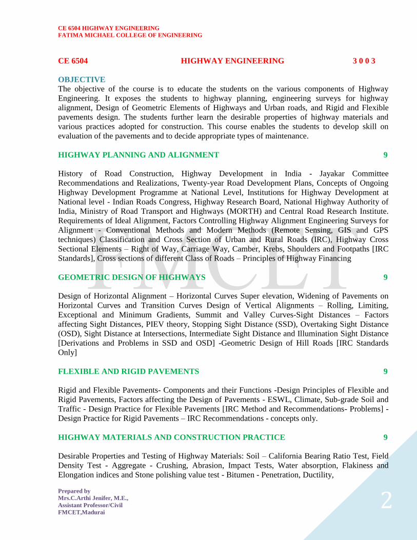
CE 6504 HIGHWAY ENGINEERING
FATIMA MICHAEL COLLEGE OF ENGINEERING
Prepared by
MrsCArthi Jenifer ME
Assistant ProfessorCivil
FMCETMadurai 2
CE 6504 HIGHWAY ENGINEERING 3 0 0 3
OBJECTIVE
The objective of the course is to educate the students on the various components of Highway
Engineering It exposes the students to highway planning engineering surveys for highway
alignment Design of Geometric Elements of Highways and Urban roads and Rigid and Flexible
pavements design The students further learn the desirable properties of highway materials and
various practices adopted for construction This course enables the students to develop skill on
evaluation of the pavements and to decide appropriate types of maintenance
HIGHWAY PLANNING AND ALIGNMENT 9
History of Road Construction Highway Development in India - Jayakar Committee
Recommendations and Realizations Twenty-year Road Development Plans Concepts of Ongoing
Highway Development Programme at National Level Institutions for Highway Development at
National level - Indian Roads Congress Highway Research Board National Highway Authority of
India Ministry of Road Transport and Highways (MORTH) and Central Road Research Institute
Requirements of Ideal Alignment Factors Controlling Highway Alignment Engineering Surveys for
Alignment - Conventional Methods and Modern Methods (Remote Sensing GIS and GPS
techniques) Classification and Cross Section of Urban and Rural Roads (IRC) Highway Cross
Sectional Elements ndash Right of Way Carriage Way Camber Krebs Shoulders and Footpaths [IRC
Standards] Cross sections of different Class of Roads ndash Principles of Highway Financing
GEOMETRIC DESIGN OF HIGHWAYS 9
Design of Horizontal Alignment ndash Horizontal Curves Super elevation Widening of Pavements on
Horizontal Curves and Transition Curves Design of Vertical Alignments ndash Rolling Limiting
Exceptional and Minimum Gradients Summit and Valley Curves-Sight Distances ndash Factors
affecting Sight Distances PIEV theory Stopping Sight Distance (SSD) Overtaking Sight Distance
(OSD) Sight Distance at Intersections Intermediate Sight Distance and Illumination Sight Distance
[Derivations and Problems in SSD and OSD] -Geometric Design of Hill Roads [IRC Standards
Only]
FLEXIBLE AND RIGID PAVEMENTS 9
Rigid and Flexible Pavements- Components and their Functions -Design Principles of Flexible and
Rigid Pavements Factors affecting the Design of Pavements - ESWL Climate Sub-grade Soil and
Traffic - Design Practice for Flexible Pavements [IRC Method and Recommendations- Problems] -
Design Practice for Rigid Pavements ndash IRC Recommendations - concepts only
HIGHWAY MATERIALS AND CONSTRUCTION PRACTICE 9
Desirable Properties and Testing of Highway Materials Soil ndash California Bearing Ratio Test Field
Density Test - Aggregate - Crushing Abrasion Impact Tests Water absorption Flakiness and
Elongation indices and Stone polishing value test - Bitumen - Penetration Ductility
CE 6504 HIGHWAY ENGINEERING
FATIMA MICHAEL COLLEGE OF ENGINEERING
Prepared by
MrsCArthi Jenifer ME
Assistant ProfessorCivil
FMCETMadurai 3
Viscosity Binder content and Softening point Tests - Construction Practice - Water Bound
Macadam Road Bituminous Road and Cement Concrete Road [as per IRC and MORTH
specifications] ndash Highway Drainage [IRC Recommendations]
EVALUATION HIGHWAY MAINTENANCE 9
Types of defects in Flexible pavements ndash Surface defects Cracks Deformation Disintegration ndash
Symptoms Causes and Treatments - Types of Pavement Failures in Rigid Pavements ndash Scaling
Shrinkage Warping Structural Cracks Spalling of Joints and Mud Pumping ndash and Special Repairs -
Pavement Evaluation ndash Pavement Surface Conditions and Structural Evaluation Evaluation of
pavement Failure and strengthening - Overlay design by Benkelman Beam Method [Procedure
only]
TOTAL 45 PERIODS
TEXT BOOKS
1 Khanna K and Justo C E G Highway Engineering Khanna Publishers Roorkee 2001
2 KadiyaliLR L R Principles and Practice of Highway Engineering Khanna Technical
Publications Delhi 2000
REFERENCES
1 Transportation Engineering amp Planning CS Papa Costas PD Prevedouros Prentice Hall
of India Pvt ltd 2006
2 IRC Standards (IRC 37 - 2001 amp IRC 58 -1998)
3 Bureau of Indian Standards (BIS) Publications on Highway Materials
4 Specifications for Road and Bridges MORTH (India)
CE 6504 HIGHWAY ENGINEERING
FATIMA MICHAEL COLLEGE OF ENGINEERING
Prepared by
MrsCArthi Jenifer ME
Assistant ProfessorCivil
FMCETMadurai 4
UNIT 1 HIGHWAY PLANNNING AND ALIGNMENT
Significance of highway planning
Wide Geographical Coverage provided by roads
Roads can be constructed to penetrate the interior of any region and to connect remote villages The
advantage becomes particularly evident when planning the communication system in hilly regions
and sparsely populated areas
Low Capital investment
Roads can be constructed at comparatively lower initial cost than railways The cost of roads varies
with specifications but even the best road is cheaper than a railway line
Quick and assured deliveries
Time is great value for a wide range of articles including both perishables and high value is
manufactured products Road transport by its quick deliveries reduces the need for larger inventories
and locking up of working capital a great cost
Flexibility
Road transport offers a flexible service free from fixed schedules Any number of trucks or buses
can be pressed into service quickly to meet sudden demand or withdrawn Such a flexibility is
absent in railways which operate generally according to fixed schedules
Door-to-door services
Road transport offers door-to-door service free from transshipments from origin to destination
Railways on the other hand have to depend upon road transport for picking up loads and making
deliveries
Simpler packaging
Road transport permits simpler packaging and crating for the protection of goods against breakage
Personalized service
A personal touch is generally present in road transport The customer is given in individualized
attention in various matters
Employment potential
Road transport has a high employment potential This is an important factor in a country with a large
and employment problem
Personalized travel
Travel by private car or motorized two wheeler or even a cycle satisfies personal pleasuresThis is
one of the main reasons for the popularity of personalized travel mode in the developed countries
Short hauls
For short hauls transport is there only economical means if a major project is to be constructed and
is the construction materials have to be transported through short distances one turns only to road
transport
Safety
One of the serious advantages of road transport is its poor record of safety Road accidents have
become a serious menace claiming enormous economic loss to the nation
Environmental pollution
Road transport has been one of the major causes for environmental pollution noise fumes vibration
loss of aesthetics ribbon development these are the some ill effects
CE 6504 HIGHWAY ENGINEERING
FATIMA MICHAEL COLLEGE OF ENGINEERING
Prepared by
MrsCArthi Jenifer ME
Assistant ProfessorCivil
FMCETMadurai 5
Parking problem
Road transport has caused parking problem of serious proportions in city streets
Long hauls
It has been found that most commodity movements are cheaper by road for short hauls up to 300-
350 kms but beyond this range the cost advantage lies with the railways
Energy
Road transport consumes greater energy per passenger km and tone km than railways
History of road development in India
Roads in India perform a variety of roles in achieving speedy economic development Some of the
important aspects are discussed below
Connection to villages
India is a country having 590000 villages scattered into small habitations and often located in the
extreme interior Thus social uplift health and education of the village population is aided by roads
Communications in hilly terrain
For the hill states located along the Himalayan range communication facility is possible only by
roads because of the steep terrain involved
Strategic importance
The defense of the northern north-eastern and western borders of the country is dependent to a large
extent on the road system
Helps agricultural development
Roads have fostered quicker agricultural development facilitating movement of modern inputs such
as fertilizers and high yielding seeds
Helps dairy development
Since the cattle wealth of the nation is concentrated in innumerable villages and small habitations
the collection and processing of surplus milk only because of roads
Forestry development
The forest wealth of the country is being exploited mainly because of the roads which penetrate in to
the thick jungles
Fisheries Development The Development of the fisheries along the coast line has been rendered possible because of the
construction of link roads leading to the coast
Tourism Development
Some of the ancient monuments religious places natural parks and sanctuaries are accessible only
roads Tourism both domestic and international has been greatly aided by roads serving such as
places of interest
Employment
As already stated roads and road transport provide employment to a large number of people in the
country Since road construction involves labour intensive techniques in India the large unemployed
labor force gets gainful employment
Famine and flood relief
Roads have helped operations pertaining to flood and famine relief The affected people are
frequently employed on road construction to build durable assets
Administrative convenience
CE 6504 HIGHWAY ENGINEERING
FATIMA MICHAEL COLLEGE OF ENGINEERING
Prepared by
MrsCArthi Jenifer ME
Assistant ProfessorCivil
FMCETMadurai 6
Roads have helped the effective administration of this large country Maintenance of law and order
and dispensation of justice have been aided by roads National integration and cohesion have been
brought about by roads which traverse the length and breath of the country and which link people
from different parts together
Tresaguet construction
Pierre Tresaguet (1716-1796) developed an improved method of construction in France by
the year 1964The main feature of his proposal was that the thickness of construction need be
only in the order of 30 cm
Tresaguet was the inspector General of roads in France from 1775 to 1785So his method of
construction was implemented in that country in 1775
The typical cross section of tresaguets road construction is given in fig and the construction
steps may be enumerated as below
i) The sub grade was prepared and layers of large foundation stones were laid on edge by
hand At the two edges of the pavement large stones were embedded edge wise to serve
as submerged Krebs stones
ii) The corners of the heavy foundation stones were hammered and then the interstices filled
with smaller stones
iii) The top-wearing course was made of smaller stones and compacted to a thickness of
about 5 cm at the edges and gradually increased towards the center
iv) The shoulders were also provides cross slope to drain the surface water to the side drain
Macadam Construction
John Macadam put forward an entirely new method of road construction as compared to all the
previous methods A typical cross section of Macadam construction
CE 6504 HIGHWAY ENGINEERING
FATIMA MICHAEL COLLEGE OF ENGINEERING
Prepared by
MrsCArthi Jenifer ME
Assistant ProfessorCivil
FMCETMadurai 7
i) The importance of sub grade drainage and compaction were recognized and the sub
grade was compacted and was prepared with a cross slope of 1 in 36
ii) Macadam was the first person to suggest the heavy foundation stones are not at all
necessary to be placed at the bottom layer of construction
iii) Though the total thickness of construction was less than previous methods This
technique could serve the purpose in a better way
iv) The size of broken stones for the top layer was decided based on the stability under
animal drawn vehicles
Macadamrsquos method is the first method based on scientific thinking
The construction steps are
i) Sub grade is compacted and prepared with a cross slope of 1 in 36 up to a desired width
ii) Broken stones of a strong variety all passing through 5 cm size sieve were compacted to
a uniform thickness of 10cm
iii) The second layer of strong broken stones of size 375 cm was compacted to thickness of
10 cm
iv) The top layer consisted of stones of size less than 2 cm compacted to a thickness of about
5 cm The cross slope of pavement surface was also 1 in 36
Classification of roads
Road classification
The roads can be classified in many ways The classification based on speed and
accessibility is the most generic one Note that as the accessibility of road increases the
speed reducesAccordingly the roads can be classified as follows in the order of
increased accessibility and reduced speeds
Freeways Freeways are access-controlled divided highways Most freeways are
four lanes two lanes each direction but many freeways widen to incorporate
more lanes as they enter urban areas Access is controlled through the use of
interchanges and the type of interchange depends upon the kind of intersecting
road way (rural roads another freeway etc)
Expressways They are superior type of highways and are designed for high
CE 6504 HIGHWAY ENGINEERING
FATIMA MICHAEL COLLEGE OF ENGINEERING
Prepared by
MrsCArthi Jenifer ME
Assistant ProfessorCivil
FMCETMadurai 8
speeds (120 kmhr is common) high traffic volume and safety They are
generally provided with grade separations at intersections Parking loading and
unloading of goods and pedestrian traffic is not allowed on expressways
Highways They represent the superior type of roads in the country Highways are
of two types - rural highways and urban highways Rural highways are those
passing through rural areas (villages) and urban highways are those passing
through large cities and towns ie urban areas
Arterials It is a general term denoting a street primarily meant for through traffic
usually on a continuous route They are generally divided highways with fully or
partially controlled access Parking loading and unloading activities are usually
restricted and regulated Pedestrians are allowed to cross only at
intersectionsdesignated pedestrian crossings
Local streets A local street is the one which is primarily intended for access to
residence business or abutting property It does not normally carry large volume
of traffic and also it allows unrestricted parking and pedestrian movements
Collector streets These are streets intended for collecting and distributing traffic
to and from local streets and also for providing access to arterial streets Normally
full access is provided on these streets There are few parking restrictions except
during peak hours
Figure 1 Speed vs accessibility
CE 6504 HIGHWAY ENGINEERING
FATIMA MICHAEL COLLEGE OF ENGINEERING
Prepared by
MrsCArthi Jenifer ME
Assistant ProfessorCivil
FMCETMadurai 9
FACTORS AFFECTING HIGHWAY ALIGHNMENT
Design speed
Design speed is the single most important factor that affects the geometric design It
directly affects the sight distance horizontal curve and the length of vertical curves
Since the speed of vehicles vary with driver terrain etc a design speed is adopted for all
the geometric design
Design speed is defined as the highest continuous speed at which individual vehicles can
travel with safety on the highway when weather conditions are conducive Design speed
is different from the legal speed limit which is the speed limit imposed to curb a common
tendency of drivers to travel beyond an accepted safe speed Design speed is also
different from the desired speed which is the maximum speed at which a driver would
travel when unconstrained by either traffic or local geometry
Since there are wide variations in the speed adopted by different drivers and by different
types of vehicles design speed should be selected such that it satisfy nearly all drivers At
the same time a higher design speed has cascading effect in other geometric designs and
thereby cost escalation Therefore an 85th percentile design speed is normally adopted
This speed is defined as that speed which is greater than the speed of 85 of drivers In
some countries this is as high as 95 to 98 percentile speed
Topography
The next important factor that affects the geometric design is the topography It is easier to
construct roads with required standards for a plain terrain However for a given design speed the
construction cost increases multiform with the gradient and the terrain Therefore geometric design
standards are different for different terrain to keep the cost of construction and time of construction
under control This is characterized by sharper curves and steeper gradients
Other factors
CE 6504 HIGHWAY ENGINEERING
FATIMA MICHAEL COLLEGE OF ENGINEERING
Prepared by
MrsCArthi Jenifer ME
Assistant ProfessorCivil
FMCETMadurai 10
In addition to design speed and topography there are various other factors that affect the geometric
design and they are briefly discussed below
Vehicle The dimensions weight of the axle and operating characteristics of a vehicle
influence the design aspects such as width of the pavement radii of the curve clearances
parking geometrics etc A design vehicle which has standard weight dimensions and
operating characteristics are used to establish highway design controls to accommodate
vehicles of a designated type
Human The important human factors that influence geometric design are the mental and
psychological characteristics of the driver and pedestrians like the reaction time
Traffic It will be uneconomical to design the road for peak traffic flow Therefore a
reasonable value of traffic volume is selected as the design hourly volume which is
determined from the various traffic data collected The geometric design is thus based on
this design volume capacity etc
Environmental Factors like air pollution noise pollution etc should be given due
consideration in the geometric design of roads
Economy The design adopted should be economical as far as possible It should match
with the funds allotted for capital cost and maintenance cost
Others Geometric design should be such that the aesthetics of the region is not affected
Nagpur classification
In Nagpur road classification all roads were classified into five categories as National highways
State highways Major district roads Other district roads and village roads
National highways
They are main highways running through the length and breadth of India connecting major
ports foreign highways capitals of large states and large industrial and tourist centers
including roads required for strategic movements
It was recommended by Jayakar committee that the National highways should be the frame
on which the entire road communication should be based
All the national highways are assigned the respective numbers
For eg the highway connecting Delhi-Ambala-Amritsar is denoted as NH-1 (Delhi-
Amritsar) where as a bifurcation of this highway beyond Full under to Srinagar and Uri is
denoted as NH-1_A
They are constructed and maintained by CPWD
The total lengths of National highway in the country is 58112 Kms and constitute about 2
of total road networks of India and carry 40 of total traffic
State highways
They are the arterial roads of a state connecting up with the national highways of adjacent
states district headquarters and important cities within the state
They also serve as main arteries to and from district roads
Total length of all SH in the country is 1 37119 Kms
Major district roads
Important roads with in a district serving areas of production and markets connecting those
with each other or with the major highways
India has a total of 4 70000 Kms of MDR
CE 6504 HIGHWAY ENGINEERING
FATIMA MICHAEL COLLEGE OF ENGINEERING
Prepared by
MrsCArthi Jenifer ME
Assistant ProfessorCivil
FMCETMadurai 11
Other district roads
Roads serving rural areas of production and providing them with outlet to market centers or
other important roads like MDR or SH
Village roads
They are roads connecting villages or group of villages with each other or to the nearest
road of a higher category like ODR or MDR
India has 2650000 kms of ODR+VR out of the total 3315231 kms of all type of roads
Roads classification criteria
Apart from the classification given by the different plans roads were also classified based on some
other criteria They are given in detail below
Based on usage
This classification is based on whether the roads can be used during different seasons of the year
All-weather roads Those roads which are negotiable during all weathers except at major
river crossings where interruption of traffic is permissible up to a certain extent are called all
weather roads
Fair-weather roads Roads which are negotiable only during fair weather are called fair
weather roads
Based on carriage way
This classification is based on the type of the carriage way or the road pavement
Paved roads with hards surface If they are provided with a hard pavement course such
roads are called paved roads(eg stones Water bound macadam (WBM) Bituminous
macadam (BM) concrete roads)
Unpaved roads Roads which are not provided with a hard course of atleast a WBM layer
they is called unpaved roads Thus earth and gravel roads come under this category
Alignment The position or the layout of the central line of the highway on the ground is called the
alignment Horizontal alignment includes straight and curved paths Vertical alignment
includes level and gradients Alignment decision is important because a bad alignment
will enhance the construction maintenance and vehicle operating costs Once an
alignment is fixed and constructed it is not easy to change it due to increase in cost of
adjoining land and construction of costly structures by the roadside
Requirements The requirements of an ideal alignment are
The alignment between two terminal stations should be short and as far as
possible be straight but due to some practical considerations deviations may be
needed
The alignment should be easy to construct and maintain It should be easy for the
operation of vehicles So to the maximum extend easy gradients and curves
should be provided
It should be safe both from the construction and operating point of view
especially at slopes embankments and cutting It should have safe geometric
features
The alignment should be economical and it can be considered so only when the
initial cost maintenance cost and operating cost are minimum
CE 6504 HIGHWAY ENGINEERING
FATIMA MICHAEL COLLEGE OF ENGINEERING
Prepared by
MrsCArthi Jenifer ME
Assistant ProfessorCivil
FMCETMadurai 12
Factors controlling alignment
We have seen the requirements of an alignment But it is not always possible to satisfy all
these requirements Hence we have to make a judicial choice considering all the factors
The various factors that control the alignment are as follows
Obligatory points These are the control points governing the highway alignment
These points are classified into two categories Points through which it should
pass and points through which it should not pass Some of the examples are
o Bridge site The bridge can be located only where the river has straight
and permanent path and also where the abutment and pier can be strongly
founded The road approach to the bridge should not be curved and skew
crossing should be avoided as possible Thus to locate a bridge the
highway alignment may be changed
o Mountain While the alignment passes through a mountain the various alternatives are to either construct a tunnel or to go round the hills The suitability of the alternative depends on factors like topography site
conditions and construction and operation cost
o Intermediate town The alignment may be slightly deviated to connect an intermediate town or village nearby
These were some of the obligatory points through which the alignment should pass
Coming to the second category that is the points through which the alignment should not
pass are
Religious places These have been protected by the law from being acquired for
any purpose Therefore these points should be avoided while aligning
Very costly structures Acquiring such structures means heavy compensation
which would result in an increase in initial cost So the alignment may be deviated
not to pass through that point
Lakesponds etc The presence of a lake or pond on the alignment path would also
necessitate deviation of the alignment
Traffic The alignment should suit the traffic requirements Based on the origin-
destination data of the area the desire lines should be drawn The new alignment should
be drawn keeping in view the desire lines traffic flow pattern etc Geometric design
Geometric design factors such as gradient radius of curve sight distance etc also govern
the alignment of the highway To keep the radius of curve minimum it may be required
to change the alignment The alignments should be finalized such that the obstructions to
visibility do not restrict the minimum requirements of sight distance The design
standards vary with the class of road and the terrain and accordingly the highway should
be aligned Economy The alignment finalized should be economical All the three costs
ie construction maintenance and operating cost should be minimum The construction
cost can be decreased much if it is possible to maintain a balance between cutting and
filling Also try to avoid very high embankments and very deep cuttings as the
construction cost will be very higher in these cases
Road ecology
The features of the cross-section of the pavement influences the life of the pavement as
CE 6504 HIGHWAY ENGINEERING
FATIMA MICHAEL COLLEGE OF ENGINEERING
Prepared by
MrsCArthi Jenifer ME
Assistant ProfessorCivil
FMCETMadurai 13
well as the riding comfort and safety Of these pavement surface characteristics affect
both of these Camber kerbs and geometry of various cross-sectional elements are
important aspects to be considered in this regard They are explained briefly in this
chapter
Camber
Camber or cant is the cross slope provided to raise middle of the road surface in the
transverse direction to drain off rain water from road surface The objectives of providing
camber are
Surface protection especially for gravel and bituminous roads
Sub-grade protection by proper drainage
Quick drying of pavement which in turn increases safety
Too steep slope is undesirable for it will erode the surface Camber is measured in 1 in n
or n (Eg 1 in 50 or 2) and the value depends on the type of pavement surface The
value suggested by IRC for various categories of pavement is given in Table 1 The
common types of camber are parabolic straight or combination of them (Figure 1)
Figure 1 Different types of camber
Table 1 IRC Value
s for ca
mber
Heavy
Light
Surface
rain
type
rain
17
ConcreteBituminous
2
25
GravelWBM
3
30
Earthen
4
CE 6504 HIGHWAY ENGINEERING
FATIMA MICHAEL COLLEGE OF ENGINEERING
Prepared by
MrsCArthi Jenifer ME
Assistant ProfessorCivil
FMCETMadurai 14
Engineering surveys for alignment
The stages of the engineering surveys are a) Map study
b) Reconnaissance
c) Preliminary surveys
d) Final location and detailed surveys
Map study -
) In the topographic map to suggest the likely routes of roads In India topographic
maps are available from the survey of India with 15 or 30-meter contour intervals
) The main feature like rivers hills and valleys etc The probable alignment can be
located on the map from the following details available on the map
Alignment avoiding valleys ponds or lakes
When the road has to cross a row of hills possibility crossing through a mountain pass
Approximate location of bridge site for crossing rivers avoiding bend of the river
When a road is to be connected between two stations one of the top and the other on the foot
of the hill then alternate routes can be suggested keeping in view the permissible alignment
Suppose the scale of the contour map is known and then the contour intervals it is possible
to decide the length of road required between two consecutive contours keeping the gradient
within allowable limits
In the fig Let A and B be two stations to be connected by road AB is the shortest route
(Straight line) APQB is a steep route in which the gradient positively exceeds 1 in 20 as the
distance between the contour intervals is only about 200 meter
APLMNB is a route with an approximate slope of 1 in 20 whereas APEFGB is an alternate
alignment with the same gradient
Thus the map study also is possible to drop a certain route in view of any unavoidable
obstructions (or) undesirable ground enroute
Reconnaissance-
The second stage of surveys for highway location is the reconnaissance to examine the general
character of the area for deciding the most feasible routes for detailed studies
Some of the details to be collected during reconnaissance are given below
Valleys ponds lakes marshy land ridge hills permanent structures and other obstructions
along the route which are not available in the map
Approximate values of gradient length of gradients and radius of curves of alternate
alignments
Number and types of cross drainage structures maximum flood level and natural
groundwater level along the probable routes
Soil type along the routes from field identification tests and observation of geological
features
Sources of construction materials water and location of stone quarries
When the road passes through hilly or mountainous terrain additional data regarding the
geological formation types of rocks dip of strata seepage flow etc
Preliminary survey -
CE 6504 HIGHWAY ENGINEERING
FATIMA MICHAEL COLLEGE OF ENGINEERING
Prepared by
MrsCArthi Jenifer ME
Assistant ProfessorCivil
FMCETMadurai 15
The main objectives of the preliminary surveys are
To survey the various alternate alignments proposed after the reconnaissance and to collect
all the necessary physical information and details of topography drainage and soil
To compare the different proposals in view of the requirements of a good alignment
To estimate quantity of earthwork materials and other construction aspects and to work out
the cost of alternate proposals
To finalize the best alignment from all considerations
The procedure of the conventional methods of preliminary surveys the given steps
Primary survey -
For alternate alignments either secondary traverses (or) independent primary traverses may be
necessary
Topographical features -
All geographical and other man made features along the traverse and for a certain width on either
side surveyed and plotted
Leveling work -
Levelling work is also carried out side by side to give the centerline profiles and typical cross
sections The leveling work in the preliminary survey is kept to a minimum just sufficient to obtain
the approximate earthwork in the alternate alignments
Drainage studies -
Drainage investigations and hydrological data are collected so as to estimate the type number and
approximate size of cross and drainage structures
Soil survey -
The soil survey conducted at this stage helps to working out details of earthwork slopes suitability
of materials subsoil and surface drainage requirements and pavement type and the approximate
thickness requirements
Material survey -
The survey for naturally occurring materials like stone aggregates soft aggregates etc and
identification of suitable quarries should be made
Traffic survey -
Traffic surveys conducted in the region from basis for deciding the number of traffic lanes and
roadway width pavement design and economic analysis of highway project
Locations and functions
Final location and detailed survey - The alignment finalized at the design office after the preliminary survey is to be first located on the
field by establishing the centerline The detailed survey should be carried out for collecting the
information technology for the preparation of plans and construction details
Location -
The centerline of the road finalized in the drawings to be translated on the ground
during the location survey
Major and minor control points are established on the ground and center pegs are
driven checking the geometric design requirements
Detailed survey -
CE 6504 HIGHWAY ENGINEERING
FATIMA MICHAEL COLLEGE OF ENGINEERING
Prepared by
MrsCArthi Jenifer ME
Assistant ProfessorCivil
FMCETMadurai 16
Levels along his final centerline should be taken at all staked points Levelling work is to
great importance as the vertical alignment
A detailed soil survey is carried out to enable drawing of the soil profile
The data during the detailed survey should be elaborate and complete for preparing detailed
plans design and estimates of the project
Soil suitability analysis
The methodology for locating appropriate sites for each land use activity is guided by the intent to
minimize the possible adverse effects of development on the environment and on existing
communities and to emphasize the positive impacts of such development by locating them in a
most suitable location
This is achieved by examining a number of individual criteria assigning them relative levels of
importance as a whole and using a mathematical resultant model to identify the most suitable
location
By adopting this site suitability method it is possible to systematically identify the criteria
considered clearly document the relative importance of one criterion over another analyze the net
outcome using a Geographic Information System and then possibly revisit the mathematical
relationships in this ldquodecision modelrdquo
By revising the relative importance to identified criteria based upon the particular land use under
consideration it is possible to generate ldquosuitability mapsrdquo for each individual land use and then
generate a final composite land use that is based on a best possible collective suitability of multiple
land uses
To achieve this all the criteria are assigned a ldquorankrdquo denoting their relative levels of importance
within the suitability study These ranks are assigned as numeric values ranging from 1 to 10 with 1
reflecting a low level of importance and 10 reflecting a high level of importance For example
within the criteria of road networks national highways would have a different level of influence on
the suitability for a particular land use as compared with local roads Further the distance from each
of these features would further modify the relative suitability of a land use based on the proximity to
a particular type of road
Criteria for Site Suitability Analysis
The decision criteria for site selection are examined for assigning relative ranks and individual
feature weights based on the land use type for which suitability is being examined For benefit of
analysis the criteria under consideration in this paper activity are organized as
Critical Criteria Criteria that will be very significant in the site selection of the identified land use
and will act as key drivers in the selection of the geographic location These criteria can be clustered
into a single decision model and the outcome collectively reviewed These criteria have a strong
influence in the final suitability
Additional Criteria Criteria that will have to be examined one at a time to carefully assess its
relationship with the proposed land use activity These criteria have a positive influence in the final
suitability
CE 6504 HIGHWAY ENGINEERING
FATIMA MICHAEL COLLEGE OF ENGINEERING
Prepared by
MrsCArthi Jenifer ME
Assistant ProfessorCivil
FMCETMadurai 17
Constrained Criteria These criteria impose strong negative opportunities in the selection of areas
for the identified land use Consequently they inform of us of where the particular land use under
consideration should not be located These criteria serve to limit or exclude areas from the final
suitability
GIS Site Suitability Analysis Model We were developed a tourism site suitability analysis model
in ArcGIS - 931 which is shown in Figure -
CE 6504 HIGHWAY ENGINEERING
FATIMA MICHAEL COLLEGE OF ENGINEERING
Prepared by
MrsCArthi Jenifer ME
Assistant ProfessorCivil
FMCETMadurai 18
UNIT 2 GEOMETRIC DESIGN OF HIGHWAYS
Typical cross section of urban and rural roads
A cross section is a vertical plane (slice) taken at right angles to the road control line showing the
various elements that make up the roads structure It is normally viewed in the direction of
increasing chainage
The width of a roadway is an important design consideration to ensure that it is appropriately sized
to serve its function Because of the diversity within the County two major roadway categories have
been established 1 Rural Road Standards 2 Urban Road Standards Urban Road Standards will
serve those areas which tend to be more developed and need to provide for multiple users
(bicyclists pedestrians parallel parking etc) whereas many rural roads will primarily serve only
vehicular traffic
Cross sections are created to provide a visual guide depicting the initial interim and ultimate phase
cross sections for these road classifications The typical sections illustrated in the following pages
are recommendations tied to transportation planning aspects such as right‐of‐way lineage sidewalk
width etc Threshold daily traffic can be used as a guide for a starting point when determining
which cross section is most applicable
1 Rural Road Standards
The rural roadways will not typically require curb and gutter or sidewalk although the County may
require either or both in unique circumstances Widths of lanes and shoulders will vary depending
upon the specific classification and the potential traffic volume which the roadway may carry Roads
carrying fewer than 200 vehicles per day need not be paved or treated for dust control The need for
paved shoulders is also dependent upon the level of traffic and safety
Final design and construction details will be determined by the Public Works Department Final
Design and construction criteria taken into consideration may include but are not limited to use of
the roadway density of development topographical characteristics and nearby development For
construction in which only a portion of the ultimate cross‐section is intended to be completed the
partial design will need to allow for the eventual widening to the ultimate cross‐section The design
for the partial or interim cross‐section roadway will need to incorporate ultimate design information
to ensure that the first phase of roadway construction is appropriate and would not need to be
removed at a future date when the full width cross‐section is completed
2 Urban Road Standards
Three roadway classifications are identified for those areas that are associated with the communityrsquos
urban growth areas They include arterial collector and local street classifications Transportation
Plan shows the key elements of the urban road standards Urban road standards will include 12‐foot
lanes sidewalk and curb amp gutter arterials and collectors will also include a striped bike lane Turn
lanes may be necessary as determined by the County Since almost all of the municipalities have
different right‐of‐way cross sections adopted for their community it makes it very difficult for the
County to match them all Therefore the philosophy was to encourage a baseline amount of
right‐of‐way reservation that could ensure the adjacent community enough area for coordination of
future roadway improvements until such time the road
CE 6504 HIGHWAY ENGINEERING
FATIMA MICHAEL COLLEGE OF ENGINEERING
Prepared by
MrsCArthi Jenifer ME
Assistant ProfessorCivil
FMCETMadurai 19
CE 6504 HIGHWAY ENGINEERING
FATIMA MICHAEL COLLEGE OF ENGINEERING
Prepared by
MrsCArthi Jenifer ME
Assistant ProfessorCivil
FMCETMadurai 20
Cross sectional elements
Kerbs
Kerbs indicate the boundary between the carriage way and the shoulder or islands or footpaths Different types of kerbs are
CE 6504 HIGHWAY ENGINEERING
FATIMA MICHAEL COLLEGE OF ENGINEERING
Prepared by
MrsCArthi Jenifer ME
Assistant ProfessorCivil
FMCETMadurai 21
Low or mountable kerbs This type of kerbs is provided such that they
encourage the traffic to remain in the through traffic lanes and also allow the
driver to enter the shoulder area with little difficulty The height of this kerb is
about 10 cm above the pavement edge with a slope which allows the vehicle to
climb easily This is usually provided at medians and channelization schemes and
also helps in longitudinal drainage
Semi-barrier type kerbs When the pedestrian traffic is high these kerbs are
provided Their height is 15 cm above the pavement edge This type of kerb
prevents encroachment of parking vehicles but at acute emergency it is possible
to drive over this kerb with some difficulty
Barrier type kerbs They are designed to discourage vehicles from leaving the
pavement They are provided when there is considerable amount of pedestrian
traffic They are placed at a height of 20 cm above the pavement edge with a steep
batter
Submerged kerbs They are used in rural roads The kerbs are provided at
pavement edges between the pavement edge and shoulders They provide lateral
confinement and stability to the pavement
Figure 1 Different types of kerbs
Shoulders Shoulders are provided along the road edge and are intended for accommodation of
stopped vehicles serve as an emergency lane for vehicles and provide lateral support
for base and surface courses The shoulder should be strong enough to bear the weight
of a fully loaded truck even in wet conditions The shoulder width should be adequate
for giving working space around a stopped vehicle It is desirable to have a width of
46 m for the shoulders A minimum width of 25 m is recommended for 2-lane rural
highways in India Parking lanes
Parking lanes are provided in urban lanes for side parking Parallel parking is preferred
because it is safe for the vehicles moving on the road The parking lane should have a
minimum of 30 m width in the case of parallel parking
CE 6504 HIGHWAY ENGINEERING
FATIMA MICHAEL COLLEGE OF ENGINEERING
Prepared by
MrsCArthi Jenifer ME
Assistant ProfessorCivil
FMCETMadurai 22
Bus-bays
Bus bays are provided by recessing the kerbs for bus stops They are provided so that
they do not obstruct the movement of vehicles in the carriage way They should be at
least 75 meters away from the intersection so that the traffic near the intersections is not
affected by the bus-bay
Service roads Service roads or frontage roads give access to access controlled highways like freeways
and expressways They run parallel to the highway and will be usually isolated by a
separator and access to the highway will be provided only at selected points These roads
are provided to avoid congestion in the expressways and also the speed of the traffic in
those lanes is not reduced
Drainage
The pavement surface should be absolutely impermeable to prevent seepage of water into
the pavement layers Further both the geometry and texture of pavement surface should
help in draining out the water from the surface in less time
Footpath
Footpaths are exclusive right of way to pedestrians especially in urban areas They are
provided for the safety of the pedestrians when both the pedestrian traffic and vehicular
traffic is high Minimum width is 15 meter and may be increased based on the traffic
The footpath should be either as smooth as the pavement or more smoother than that to
induce the pedestrian to use the footpath
Right of way
Right of way (ROW) or land width is the width of land acquired for the road along its
alignment It should be adequate to accommodate all the cross-sectional elements of the
highway and may reasonably provide for future development To prevent ribbon
development along highways control lines and building lines may be provided Control
line is a line which represents the nearest limits of future uncontrolled building activity
in relation to a road Building line represents a line on either side of the road between
which and the road no building activity is permitted at all The right of way width is
governed by
Width of formation It depends on the category of the highway and width of
roadway and road margins
Height of embankment or depth of cutting It is governed by the topography and
the vertical alignment
Side slopes of embankment or cutting It depends on the height of the slope soil
type etc
Drainage system and their size which depends on rainfall topography etc
Sight distance considerations On curves etc there is restriction to the visibility
on the inner side of the curve due to the presence of some obstructions like
building structures etc
Reserve land for future widening Some land has to be acquired in advance
CE 6504 HIGHWAY ENGINEERING
FATIMA MICHAEL COLLEGE OF ENGINEERING
Prepared by
MrsCArthi Jenifer ME
Assistant ProfessorCivil
FMCETMadurai 23
Table 2 Desig
n speed in as per IRC (ruling and minimum)
Steep
Type
Plain
Rolling
Hilly
40-30
NSampSH
100-80
80-65
50-40
MDR
80-65
65-50
40-30
30-20
25-20
ODR
65-50
50-40
30-25
25-20
VR
50-40
40-35
25-20
anticipating future developments like widening of the road
Table 1 No
right of way for open areas
Roadway width in m
Road
Plain and
Mountainous and
classification
steep terrain
rolling terrain
Open areas
45
24
NHSH
18
MDR
25
15
15
ODR
12
9
VR
Built-up areas
20
NHSH
30
MDR
20
15
ODR
15
12
9
VR
10
CE 6504 HIGHWAY ENGINEERING
FATIMA MICHAEL COLLEGE OF ENGINEERING
Prepared by
MrsCArthi Jenifer ME
Assistant ProfessorCivil
FMCETMadurai 24
Horizontal curve
The presence of horizontal curve imparts centrifugal force which is a reactive force
acting outward on a vehicle negotiating it Centrifugal force depends on speed and radius
of the horizontal curve and is counteracted to a certain extent by transverse friction
between the tyre and pavement surface On a curved road this force tends to cause the
vehicle to overrun or to slide outward from the centre of road curvature For proper
design of the curve an understanding of the forces acting on a vehicle taking a horizontal
curve is necessary Various forces acting on the vehicle are illustrated in the figure 1
Figure 1 Effect of horizontal curve They are the centrifugal force (P) acting outward weight of the vehicle (W) acting
downward and the reaction of the ground on the wheels ( and ) The centrifugal
force and the weight is assumed to be from the centre of gravity which is at h units above
the ground Let the wheel base be assumed as b units The centrifugal force in
is given by
(1)
where is the weight of the vehicle in is the speed of the vehicle in is
the acceleration due to gravity in and is the radius of the curve in
The centrifugal ratio or the impact factor is given by
CE 6504 HIGHWAY ENGINEERING
FATIMA MICHAEL COLLEGE OF ENGINEERING
Prepared by
MrsCArthi Jenifer ME
Assistant ProfessorCivil
FMCETMadurai 25
(1)
The centrifugal force has two effects A tendency to overturn the vehicle about the outer
wheels and a tendency for transverse skidding Taking moments of the forces with
respect to the outer wheel when the vehicle is just about to override
At the equilibrium over turning is possible when
and for safety the following condition must satisfy
(2)
The second tendency of the vehicle is for transverse skidding ie When the the
centrifugal force is greater than the maximum possible transverse skid resistance due to
friction between the pavement surface and tyre The transverse skid resistance (F) is
given by
where and is the fractional force at tyre and and is the reaction at
tyre and is the lateral coefficient of friction and is the weight of the vehicle
This is counteracted by the centrifugal force (P) and equating
At equilibrium when skidding takes place (from equation1)
and for safety the following condition must satisfy
CE 6504 HIGHWAY ENGINEERING
FATIMA MICHAEL COLLEGE OF ENGINEERING
Prepared by
MrsCArthi Jenifer ME
Assistant ProfessorCivil
FMCETMadurai 26
(3)
Equation 2 and 3 give the stable condition for design If equation 2 is violated the vehicle
will overturn at the horizontal curve and if equation 3 is violated the vehicle will skid at
the horizontal
Curve Analysis of super-elevation
Super-elevation or cant or banking is the transverse slope provided at horizontal curve to
counteract the centrifugal force by raising the outer edge of the pavement with respect to
the inner edge throughout the length of the horizontal curve When the outer edge is
raised a component of the curve weight will be complimented in counteracting the effect
of centrifugal force In order to find out how much this raising should be the following
analysis may be done The forces acting on a vehicle while taking a horizontal curve with
super elevation is shown in figure 1
Figure 1 Analysis of super-elevation
Forces acting on a vehicle on horizontal curve of radius at a speed of are
the centrifugal force acting horizontally out-wards through the center of
gravity
the weight of the vehicle acting down-wards through the center of gravity and
the friction force between the wheels and the pavement along the surface
inward
CE 6504 HIGHWAY ENGINEERING
FATIMA MICHAEL COLLEGE OF ENGINEERING
Prepared by
MrsCArthi Jenifer ME
Assistant ProfessorCivil
FMCETMadurai 27
At equilibrium by resolving the forces parallel to the surface of the pavement we get where
friction
is the weight of the vehicle is the centrifugal force is the coefficient of
is the transverse slope due to superelevation Dividing by we get
CE 6504 HIGHWAY ENGINEERING
FATIMA MICHAEL COLLEGE OF ENGINEERING
Prepared by
MrsCArthi Jenifer ME
Assistant ProfessorCivil
FMCETMadurai 28
Step 1
Find for 75 percent of design speed neglecting ie
Step 2
If then else if go to step 3
Step 3
Find for the design speed and max ie If
then the maximum is safe for the design speed else go to
step 4
Step 4
Find the allowable speed for the maximum and
If then the design is adequate otherwise use speed adopt
control measures or look for speed control measures
Maximum and minimum super-elevation
Depends on (a) slow moving vehicle and (b) heavy loaded trucks with high CG IRC
specifies a maximum super-elevation of 7 percent for plain and rolling terrain while that
of hilly terrain is 10 percent and urban road is 4 percent The minimum super elevation is
2-4 percent for drainage purpose especially for large radius of the horizontal curve
Attainment of super-elevation
1 Elimination of the crown of the cambered section by
1 Rotating the outer edge about the crown The outer half of the cross slope
is rotated about the crown at a desired rate such that this surface falls on
the same plane as the inner half
2 Shifting the position of the crown This method is also known as diagonal
crown method Here the position of the crown is progressively
shifted outwards thus increasing the width of the inner half of cross section
progressively
2 Rotation of the pavement cross section to attain full super elevation byThere are
two methods of attaining super elevation by rotating the pavement
1 Rotation about the center line The pavement is rotated such that the inner
edge is depressed and the outer edge is raised both by half the total amount
of super elevation ie by with respect to the centre
2 Rotation about the inner edge Here the pavement is rotated raising the
outer edge as well as the centre such that the outer edge is raised by the
full amount of super elevation with respect to the inner edge
Horizontal Transition Curves
CE 6504 HIGHWAY ENGINEERING
FATIMA MICHAEL COLLEGE OF ENGINEERING
Prepared by
MrsCArthi Jenifer ME
Assistant ProfessorCivil
FMCETMadurai 29
Transition curve is provided to change the horizontal alignment from straight to circular
curve gradually and has a radius which decreases from infinity at the straight end
(tangent point) to the desired radius of the circular curve at the other end (curve point)
There are five objectives for providing transition curve and are given below
1 to introduce gradually the centrifugal force between the tangent point and the
beginning of the circular curve avoiding sudden jerk on the vehicle This
increases the comfort of passengers
2 to enable the driver turn the steering gradually for his own comfort and security
3 to provide gradual introduction of super elevation and
4 to provide gradual introduction of extra widening
5 to enhance the aesthetic appearance of the road
Type of transition curve
Different types of transition curves are spiral or clothoid cubic parabola and Lemniscate
IRC recommends spiral as the transition curve because
1 it fulfills the requirement of an ideal transition curve that is
1 rate of change or centrifugal acceleration is consistent (smooth) and
2 radius of the transition curve is at the straight edge and changes to at
the curve point ( ) and calculation and field implementation is
very easy
Length of transition curve The length of the transition curve should be determined as the maximum of the following
three criteria rate of change of centrifugal acceleration rate of change of super elevation
and an empirical formula given by IRC Rate of change of centrifugal acceleration
At the tangent point radius is infinity and hence centrifugal acceleration is zero At the
end of the transition the radius R has minimum value R The rate of change of
centrifugal acceleration should be adopted such that the design should not cause
discomfort to the drivers If is the rate of change of centrifugal acceleration it can be
written as
Therefore the length of the transition curve in is
CE 6504 HIGHWAY ENGINEERING
FATIMA MICHAEL COLLEGE OF ENGINEERING
Prepared by
MrsCArthi Jenifer ME
Assistant ProfessorCivil
FMCETMadurai 30
(1)
where is the rate of change of centrifugal acceleration given by an empirical formula
suggested by by IRC as below
(2) 2 Rate of introduction of super-elevation
Raise ( ) of the outer edge with respect to inner edge is given by
The rate of change of this raise from to is achieved
gradually with a gradient of in over the length of the transition curve (typical range
of is 60-150) Therefore the length of the transition curve is
(3)
3 By empirical formula
IRC suggest the length of the transition curve is minimum for a plain and rolling terrain
(4)
and for steep and hilly terrain is
(5)
CE 6504 HIGHWAY ENGINEERING
FATIMA MICHAEL COLLEGE OF ENGINEERING
Prepared by
MrsCArthi Jenifer ME
Assistant ProfessorCivil
FMCETMadurai 31
and the shift as
(
6
) The length of the transition curve is the maximum of
equations 1 3 and 4or5 ie
(
7
Case (a)
For single lane roads
(
1
)
Therefore
(
2
)
Figure 1 Set-back for single lane roads (
CE 6504 HIGHWAY ENGINEERING
FATIMA MICHAEL COLLEGE OF ENGINEERING
Prepared by
MrsCArthi Jenifer ME
Assistant ProfessorCivil
FMCETMadurai 32
For multi lane roads if is the distance between centerline of the road and the centerline
of the inner lane then
(3)
(4)
Figure 2 Set-back for multi-lane roads ( )
Case (a)
For single lane roads
(1)
Therefore
(2)
Gradient
Gradient is the rate of rise or fall along the length of the road with respect to the
horizontal While aligning a highway the gradient is decided for designing the vertical
curve Before finalizing the gradients the construction cost vehicular operation cost and
the practical problems in the site also has to be considered Usually steep gradients are
avoided as far as possible because of the difficulty to climb and increase in the
CE 6504 HIGHWAY ENGINEERING
FATIMA MICHAEL COLLEGE OF ENGINEERING
Prepared by
MrsCArthi Jenifer ME
Assistant ProfessorCivil
FMCETMadurai 33
construction cost More about gradients are discussed below
Effect of gradient
The effect of long steep gradient on the vehicular speed is considerable This is
particularly important in roads where the proportion of heavy vehicles is significant Due
to restrictive sight distance at uphill gradients the speed of traffic is often controlled by
these heavy vehicles As a result not only the operating costs of the vehicles are
increased but also capacity of the roads will have to be reduced Further due to high
differential speed between heavy and light vehicles and between uphill and downhill
gradients accidents abound in gradients
Representation of gradient
The positive gradient or the ascending gradient is denoted as and the negative gradient as The deviation angle is when two grades meet the angle which
measures the change of direction and is given by the algebraic difference between the two
grades
steep gradient while 1 in 50 = 2 representation is illustrated in the figure 1
Example 1 in 30 = 333 is a
is a flatter gradient The gradient
CE 6504 HIGHWAY ENGINEERING
FATIMA MICHAEL COLLEGE OF ENGINEERING
Prepared by
MrsCArthi Jenifer ME
Assistant ProfessorCivil
FMCETMadurai 34
Figure 1 Representation of gradient
Types of gradient
Many studies have shown that gradient upto seven percent can have considerable effect
on the speeds of the passenger cars On the contrary the speeds of the heavy vehicles are
considerably reduced when long gradients as flat as two percent is adopted Although
flatter gradients are desirable it is evident that the cost of construction will also be very
high Therefore IRC has specified the desirable gradients for each terrain However it
may not be economically viable to adopt such gradients in certain locations steeper
gradients are permitted for short duration Different types of grades are discussed below
Ruling gradient
The ruling gradient or the design gradient is the maximum gradient with which the
designer attempts to design the vertical profile of the road This depends on the terrain
length of the grade speed pulling power of the vehicle and the presence of the horizontal
curve In flatter terrain it may be possible to provide flat gradients but in hilly terrain it
is not economical and sometimes not possible also The ruling gradient is adopted by the
designer by considering a particular speed as the design speed and for a design vehicle
with standard dimensions But our country has a heterogeneous traffic and hence it is not
possible to lay down precise standards for the country as a whole Hence IRC has
recommended some values for ruling gradient for different types of terrain
Limiting gradient
This gradient is adopted when the ruling gradient results in enormous increase in cost of
construction On rolling terrain and hilly terrain it may be frequently necessary to adopt
limiting gradient But the length of the limiting gradient stretches should be limited and
must be sandwiched by either straight roads or easier grades
Exceptional gradient
Exceptional gradient are very steeper gradients given at unavoidable situations They
should be limited for short stretches not exceeding about 100 metres at a stretch In
mountainous and steep terrain successive exceptional gradients must be separated by a
minimum 100 metre length gentler gradient At hairpin bends the gradient is restricted to
25
Critical length of the grade
The maximum length of the ascending gradient which a loaded truck can operate without
undue reduction in speed is called critical length of the grade A speed of 25 kmph is a
CE 6504 HIGHWAY ENGINEERING
FATIMA MICHAEL COLLEGE OF ENGINEERING
Prepared by
MrsCArthi Jenifer ME
Assistant ProfessorCivil
FMCETMadurai 35
reasonable value This value depends on the size power load grad-ability of the truck
initial speed final desirable minimum speed
Minimum gradient
This is important only at locations where surface drainage is important Camber will take
care of the lateral drainage But the longitudinal drainage along the side drains require
some slope for smooth flow of water Therefore minimum gradient is provided for
drainage purpose and it depends on the rain fall type of soil and other site conditions A
minimum of 1 in 500 may be sufficient for concrete drain and 1 in 200 for open soil
drains are found to give satisfactory performance Sight distance available from a point is the actual distance along the road surface which a driver
from a specified height above the carriage way has visibility of stationary or moving objects
Sight distance required by drivers applies to both geometric design of highways and for
traffic control The sight distance situations are considered in the design
i) Stopping or absolute minimum sight distance
ii) Safe overtaking or passing sight distance
iii) Safe sight distance for entering into uncontrolled intersections
Apart from the three situations mentioned above the following sight distance are considered by the
IRC in highway design
Intermediate sight distance
This is defined as twice the stopping sight distance when overtaking sight distance
cannot be provided intermediate sight distance is provided to give limited overtaking opportunities
to fast vehicles
Head light sight distance
This is the distance visible to a driver during night driving under the illumination of the
vehicle head lights
Stopping sight distance
The minimum sight distance available on a highway at any spot should be of sufficient
length to stop a vehicle traveling at design speed safely without collision with any other obstruction
The absolute minimum sight distance is therefore equal to the stopping sight distance
which is also sometimes called nonpassing sight distance The sight distance available on a road to a
driver at any instance depends on
i) Features of the road
ii) Height of the drivers eye above the road surface
iii) Height of the object above the road surface
The distance within which a motor vehicle can be stopped depends upon the factors listed below
a) Total reactions time of the driver
b) Speed of vehicle
c) Efficiency of breaks
d) Frictional resistance between the road and tyres
e) Gradient of the road
Total reaction time
) Reaction time of the driver is the time taken from the instant the object is visible to the
driver to the instant the brakes are effectively applied
) The total reaction time may be split up into two parts
CE 6504 HIGHWAY ENGINEERING
FATIMA MICHAEL COLLEGE OF ENGINEERING
Prepared by
MrsCArthi Jenifer ME
Assistant ProfessorCivil
FMCETMadurai 36
i) Perception time
ii) Brake reaction time
PIEV theory
According to this theory the total reaction time of the driver is split into four parts
i) Perception
ii) Intellection
iii) Emotion
iv) Volition
Speed of Vehicle
The stopping distance depends very much on the speed of the vehicle first during the
total reaction time of the driver the distance moved by the vehicle will depend on the speed
Efficiency of brakes
The braking efficiency is said to be 100 percent if the wheels are fully licked preventing
them from rotating on application of the brakes This will result in 100 percent skidding which is
normally undesirable except in utmost emergency
Frictional resistance between road and tyres
The frictional resistance developed between road and tyres or the skid resistance depends
on the type and condition of the road surface and the tyres IRC has specified a design friction
coefficient of 035 to 04 depending upon the speed to be used for finding the braking distance in the
calculation of stopping sight distance
Analysis of stopping distance
i) The distance traveled by the vehicle during the total reaction time known as lag
distance
ii) The distance traveled by the vehicle after the application of the brakes is known as
braking distance
Overtaking sight distance
The minimum distance open to the vision of the driver of a vehicle intending to overtake
slow vehicle ahead with safety against the traffic of opposite direction is known as the minimum
overtaking sight distance(OSD) or Safe passing sight distance available
The overtaking sight distance is the distance measured along the center of the road which
a driver with his eye level 12m above the road surface can see the top of an object 12m above the
road surface
Some of the important factors on which the minimum overtaking sight distance required
a) Speed of
i) overtaking vehicle
ii) overtaken vehicle
iii) The vehicle coming from opposite direction
b) Distance between the overtaking and overtaken vehicles the minimum spacing
depends on the steeds
a) Skill and reaction time of the driver
b) Rate of acceleration of overtaking vehicle
c) Gradient of the road
Criteria for sight distance requirements on highway
) The absolute minimum sight distance required throughout the length of the road is the
SSD which should invariably be provided at all places
CE 6504 HIGHWAY ENGINEERING
FATIMA MICHAEL COLLEGE OF ENGINEERING
Prepared by
MrsCArthi Jenifer ME
Assistant ProfessorCivil
FMCETMadurai 37
) On horizontal curves the obstruction on the inner side of the curves should be cleared
to provide the required set back distance and absolute minimum sight distance
) On vertical summit curves the sight distance requirement may be fulfilled by proper
design of the vertical alignment
Hairpin bent
TYPES OF CURVES ON HILL ROADS
The following are the important types of curves provided on hill Roads-
1 Hair-Pin Curves
2 Salient Curves
3 Re-entrant Curves 1 Hair-pin curves - The curve in a hill road which changes its direction through an angle of 180
degree or so down the hill on the same side is known as hair-pin curve
A Hair-Pin Bend
This curve is so called because it conforms to the shape of a hair-pin The bend so formed at the
hair-pin curve in a hill road is known as hair-pin bend This type of curve should be located on a
hill side having the minimum slope and maximum stability It must also be safe from view point of
landslides and ground water Hair-pin bends with long arms and farther spacing are always
preferred They reduce construction problems and expensive protective works Hair-pin curves or
bends of serpentine nature are difficult to negotiate and should therefore be avoided as far as
possible
Salient curves - The curves having their convexity on the outer edges of a hill road are called
salient curves The centre of curvature of a salient curve lies towards the hill side This type of curve
occurs in the road length constructed on the ridge of a hill the bend so formed at the salient curve in
a hill road known as corner bend
Salient curves are very dangerous for fast moving traffic At such a curve or at corner bend the
portion of projecting hill side is usually cut down to improve the visibility as shown in fig (Re-
entrant curve) The outer edge of the road at such a curve is essentially provided with a parapet wall
for protection of the vehicles from falling down the hill slope
CE 6504 HIGHWAY ENGINEERING
FATIMA MICHAEL COLLEGE OF ENGINEERING
Prepared by
MrsCArthi Jenifer ME
Assistant ProfessorCivil
FMCETMadurai 38
3 Re-entrant curves - The curves having their convexity on the inner edge of a hill road are called
re-entrant curves
Re-entrant curves
The centre of curvature of a re-entrant curves lies away from the hill side This type of curve occurs
in the road length constructed in the calley of a hill
These curves are less dangereous as they provide adequate visibility to the fast moving traffic At
such curves the parapet wall is provided only for safety of fast moving traffic
CE 6504 HIGHWAY ENGINEERING
FATIMA MICHAEL COLLEGE OF ENGINEERING
Prepared by
MrsCArthi Jenifer ME
Assistant ProfessorCivil
FMCETMadurai 39
UNIT ndash III DESIGN OF RIGID AND FLEXIBLE PAVEMENTS
COMPARISON OF RIGID AND FLEXIBLE PAVEMENTS
The comparisons are
i) Design precision
A cement concrete pavement is amerable to a much more precise structural analysis
than a flexible pavement Flexible pavements designs are mainly empirical Computer aided analysis
of layered system is making the flexible pavement design more exact than hitherto
ii) Life
) Cement concrete slabs of a thin section constructed in the early 1940rsquos are still in
existence in India though many of them have cracked badly and a few of them have been ripped
open and rebuilt in recent ties
) A major project in cement concrete road construction between Agra and Mathura It can
safely be said that a well-designed concrete slab has a life of about 40 years
) Compared to this the life of a flexible pavement generally varies from 10 to 20 years
iii) Maintenance
) A well-designed cement concrete pavement needs very little maintenance The only
maintenance needed is I respect of joints
) The surface is unaffected by spillage of oil and lubricants bituminous surfaces on the
other hand need great inputs in maintenance
) The surface is affected by spillage of oil and lubricants The surface is also affected by
natural weathering agents like air water ad temperature changes
) A cement concrete pavement on the other hand needs a small amount for maintaining
joints
iv) Initial cost
) The argument so far used against a cement concrete slab is that it is much more costly
than a flexible pavement
) The latter specifications no doubt represent the rock-bottom needs of a road in India but
these specifications can hardly provide a smooth and durable surface
v) Stage construction ) Road construction is generally done adopting a policy of stage construction especially for
low volume roads As traffic grows additional layers in the form of water bound macadam and
superior surfacing are added on
) Initial outlay is minimum and additional outlays are in keeping with traffic growth This is
a great advantage when dealing with new roads in an atmosphere of austerity
vi) Availability of materials
) Cement bitumen stone aggregates and gravelsand are the major materials involved in
pavement Construction Cement has been in serious short supply in the country for the past many
decades
) Bitumen is also not available plentifully in India There is also the danger of the entire oil
reserves in the world shrinking during the next two or three decades
) In locations where stone aggregates are scarce cement concrete may have an advantage
for flexible pavements
vii) Surface characterstics
CE 6504 HIGHWAY ENGINEERING
FATIMA MICHAEL COLLEGE OF ENGINEERING
Prepared by
MrsCArthi Jenifer ME
Assistant ProfessorCivil
FMCETMadurai 40
) A good cement concrete surface is smooth and free from rutting potholes and
corrugations In a bituminous surface it is only the asphaltic concrete surface that can give
comparable rideablity
) A well-constructed cement concrete pavement surface can have a permanent nonskid
surface A bituminous surface can also be designed to have a good skid resistant surface
viii) Utility location
) In cement concrete slabs proper thought has to be given to locate utilities such as water
pipes telephone lines and electric cables
) It is difficult to rip open the slab and restore it to be the original condition if any changes
in the utilities lines are to be made
ix) Glame and night visibility
) Concrete pavements have a gray color which can cause glam under sunlight Colored
cement can reduce the grave
) On the other hand bituminous roads need more street lighting
x) Traffic dislocation during construction
) A cement concrete pavement requires 28 days before it can be thrown open to traffic On
the other hand a bituminous surface can be thrown open to traffic shortly after it is rolled
xi) Environmental considerations during construction
) The process of heating of bitumen and aggregates and mixing them together on hot mix
plants can prove to be much more hazardous to the environment than cement concrete construction
where no heating of any material is involved
xii) Overall economy on a life cycle basis
) A good road is costly to construct but once constructed such a road requires little
maintenance and results in savings in vehicle operating costs
) The comparative economy of a flexible pavement and a rigid pavement has proved that on
overall economic considerations
Types of pavement structure
Based on the structural behavior pavements are generally classified into three
categories
i) Flexible pavements
ii) Rigid pavements
iii) Semi rigid pavements
Flexible pavements
) Flexible pavements are those which on the whole have low or negligible flexural
strength and are rather flexible in their structural action under the loadsThe flexible pavement
layers reflect the deformation of the lower layers on to the surface of the layer
) A flexible pavement consists of four components(i) Soil subgrade (ii) sub base
course (iii) base course (iv) Surface course
CE 6504 HIGHWAY ENGINEERING
FATIMA MICHAEL COLLEGE OF ENGINEERING
Prepared by
MrsCArthi Jenifer ME
Assistant ProfessorCivil
FMCETMadurai 41
) The flexible pavement layers transmit the vertical or compressive stresses to the lower layers
by grain to grain transfer through the points of contact in the granular structure A well
compacted granular structure consisting of strong added aggregate can transfer the compressive
stresses
) The load spreading ability of this layer therefore depends on the type of the materials and mix
design factors Bituminous concrete is one of the best flexible pavements layer materials Other
materials which fall under the group are all granular materials with or without bituminous
binder granular base and sub base course materials
) The vertical compressive stress is maximum on the pavement surface directly under the wheel
and is equal to the contact pressure under the wheel The flexible pavement may be constructed
in a number of layers and the top layer has to be strongest as the highest compressive stresses
) Flexible pavements are commonly designed using empirical design charts or equations taking
into account some of the design factors there are also semi empirical and theoretical design
methods
Rigid pavements
) Rigid pavements are those which possess note flexural strength or flexural rigidity
The stresses are not transferred from grain to grain to the lower layers as in the ease of flexible
pavements layers
) The rigid pavements are made of Portland cement concrete plain reinforced or
prestressed concrete The plain cement concrete slabs are expected to take up about 40 kgcm2
flexural stress
) The rigid pavement has the slab action and is capable of transmitting the wheel
load stresses through a wider area below The main point of difference in the structural behavior
of rigid pavement as compared to the flexible pavement is that the critical condition of stress in
the rigid pavement is the maximum flexural stress occurring in the slab due to wheel load and
the temperature changes whereas in the flexible pavement
) As the rigid pavement slab has tensile strength tensile stresses are developed due
to the bending of the slab under wheel load and temperature variations Thus the types of
stresses developed and their distribution within the cement concrete slab are quirt different
) The cement concrete pavement slab can very well serve as a wearing surface as
well an effective base course The rigid pavement structure consists of a cement concrete slab
below which a granular base or sub base course may be provided
) Though the cement concrete slab can also be laid directly over the soil subgrade
consists of fine grained soil
) the rigid pavements are usually designed and the stresses are analyzed using the
elastic theory assuming the pavements as a n elastic plate resting over an elastic or a viscous
foundation
Semi rigid pavements
) when bonded materials like the pozzolanic concrete lean cement concrete or soil
cement are used in the base course or sub base course layer the pavement layer has considerably
higher flexural strength than the common flexible pavement layers
) when this intermediate class of materials are used in the base or sub base course
layer of the pavements they are called semi rigid pavements
CE 6504 HIGHWAY ENGINEERING
FATIMA MICHAEL COLLEGE OF ENGINEERING
Prepared by
MrsCArthi Jenifer ME
Assistant ProfessorCivil
FMCETMadurai 42
) This third category of semi rigid pavement are either designed as flexible
pavements with some correction factors to find the thickness requirements based on experience
or by using a new design approach
) The semi rigid pavement materials have low resistance to impact and abrasion and
therefore are usually provided with flexible pavement surface course
Various functions of pavement components
The functions are
Soil sub grade and its evaluation
) The soil sub grade is a layer of natural soil prepared to receive the layers of pavement
materials placed over it It is essential that at no time the soil sub grade is overstressed it means that
the pressure transmitted on the top of the sub grade is within the allowable limit
) Many tests are known for measuring the strength properties of the sub grades Some of the
tests have been standardized for the use The common strength test for the evaluation of soil
subgrade is
i) California bearing ratio test
ii) California resistance value test
iii) Triaxial compression test
iv) Plate bearing test
CALIFORNIA BEARING RATIO (CBR) TEST
It is evolved for the empirical method of flexible pavement design The CBR test is carried
out either in the laboratory on prepared specimens or in the field by taking in situ measurements
California resistance value
It is found by using have been stabliometerThis test is used in an empirical method of
flexible pavement design based on soil strength
Triaxial test
It is the most important soil strength but still the test is not very commonly used in structural
design of pavements
Plate bearing test
It is carried out using a relatively large diameter plate to evaluate the load supporting
capacity of supporting power of the pavement layers The results are plate bearing tests are used in
flexible pavement design method like McLeod method on based on layer system analysis by
brumister
Sub base and base courses and their evaluation
) There layers are made of broken stones bound or unbound aggreagatesome times in sub
base course a layer of stabilized soil(or) Selected granular soil is also used
) however at the sub base course it is desirable to use smaller size graded aggregates When
the sub grade consists of fine grained soil and when the pavement carries heavy wheel loads
CE 6504 HIGHWAY ENGINEERING
FATIMA MICHAEL COLLEGE OF ENGINEERING
Prepared by
MrsCArthi Jenifer ME
Assistant ProfessorCivil
FMCETMadurai 43
) Sub base course primarily has the similar function as of the base course and is provided
with inferior materials than of base course Base courses are used under rigid pavement for
i) Preventing pumping
ii) Protecting the sub grade against frost action
) Thus the fundamental purpose of abase course and sub base course is to provide a stress
transmitting medium to spread the surface wheel loads in such manner
) The sub base and base course layers may be evaluated by suitable strength or stability test
like plate bearing CBR test
WEARING COURSE AND ITS EVALUATION
) The purpose of the wearing course is to give a smooth riding surface that is dense It
resists pressure exerted by tyres and takes up wear and tear due to the traffic
) Wearing course also offers a water tight layer against the surface water infiltration The
flexible pavement normally a bituminous surfacing is used as a wearing course
) In rigid pavements the cement concrete acts like a base course as well as wearing course
Most popular test in use is marshal stability test where in the optimum content of bitumen binder is
worked out based on the stability density
) Plate bearing test and Bankelman beam test are also sometimes made use of for evaluating
the wearing course and the pavement as a whole
Various factors to be considered in pavement design and the significance
Pavement design consists of two parts
i) Mix design of materials to be used in each pavement component layer Thickness design of the
pavement and the component layers
The various factors to be considered for the design of pavements are given below
i) Design wheel load
ii) Sub grade soil
iii) Climatic factors
iv) Pavement component layers
v) Environmental factors
vi) Special factors in the design of different types of pavements
Design wheel load
The various wheel load factors to be considered in pavement design are
i) Maximum wheel load
ii) Contact pressure
iii) Dual or multiple wheel loads
iv) Repetition of loads
Maximum wheel load
The wheel load configurations are important to know the way in which the loads of a given
vehicle are applied on the pavement surface
) For highways the maximum legal axle load as specified by Indian road congress is 8170
kg with a maximum equivalent single wheel load of 4085 kg
) The evaluation for vertical stress computations under a uniformly distribute of circular
load based on Boussineqrsquos theory is given by
CE 6504 HIGHWAY ENGINEERING
FATIMA MICHAEL COLLEGE OF ENGINEERING
Prepared by
MrsCArthi Jenifer ME
Assistant ProfessorCivil
FMCETMadurai 44
2
322
3
1
za
zpz
σz = vertical stress at depth z
P= surface pressure
Z=depth at which σz computed
A=radius of loaded area
Contact pressure
Generally the wheel load is assumed to be distributed over a circular area But by
measurement of the imprints of tyers with different load and inflation pressures Three terms in use
with reference to tyre pressure are
Tyre pressure
Inflation pressure
Contact pressure
Tyre pressure and inflation pressure mean exactly the same the contact pressure is found to be more
than tyre pressure when the tyre pressure is less than 7 kgm2 and it is vice versa when the tyre
pressure exceeds this value
Contact pressure can be measured by the relationship
Load on wheel
Contact pressure = ----------------------------------------
Contact area or area of imprint
The general variation between the tyre pressure and measured contact pressure is shown in this fig
The ratio of contact pressure to type pressure is defined as rigidity factor Thus value of rigidity
factor is 10 for an average tyre pressure of 7 Kgcm2This value is higher than unity for lower type
pressures and less than unity for tyre pressures higher than 7 kgcm2
Equivalent single wheel load (ESWL)
) The maximum wheel load within the specified limit and to carry greater load it is
necessary to provide dual wheel assembly to the rear axles of the roads vehicles
) In other words the pressure at a certain depth below the pavement surface cannot be
obtained by numerically adding the pressure caused by any one wheel
) The effect is in between the single load and two times load carried by one wheel The load
dispersion is assumed to be at an angle of 450In the dual wheel load assembly let d be the clear gap
between the two wheels S be the spacing between the centers of the wheels and a be the radius of
the circular contact area of each wheel Then S = (d + 2a)
) ESWL may be determined based on either equivalent deflection or equivalent stress
criterianMultiple wheel loads are convert to ESWL and this value is used in pavement design The
ESWL is usually determined by the equivalent stress criterion using a simple graphical method
CE 6504 HIGHWAY ENGINEERING
FATIMA MICHAEL COLLEGE OF ENGINEERING
Prepared by
MrsCArthi Jenifer ME
Assistant ProfessorCivil
FMCETMadurai 45
) A straight line relationship is assumed between ESWL and depth on log scales For
determining ESWL the plot is made as shown in fig
) Two points A and B are plotted on the log-log graph with coordinates of A (Pd2) and
B(2p2s)line AB is a plot which is the focus of points where any single wheel load is equivalent to a
certain set of dual wheels
) To Calculate the ESWL for a dual assembly it is essential to estimate a design thickness of
the pavement If the design thickness so obtained is equal to the estimated thickness then the ESWL
calculations could be considered as correct Otherwise trials are made
) In heavy trucks and trailers the load on each wheel may be further reduced by multiple
wheels and tandem axles
Repetition of loads
) The deformation of load pavement (or) sub grade due to a single application of wheel load
may be small It required carrying out traffic surveys for accounting the factor of repetitions for
wheel loads in the design of pavement
) Data collected are converted to some constant equivalent wheel loads Equivalent wheel
load is a single load equivalent to the repeated applications of any particular wheel load on a
pavement which requires the same thickness and strength of pavements
) McLeod has given a procedure for evolving equivalent load factors for designing flexible
pavements
Various methods of flexible pavement design
) The flexible pavement is built with number of layers In the design process it is to be
ensured that under the application of load none of the layers is overstressed
) The maximum intensity of stresses occurs in the top layer of the pavement The
magnitude of load stresses reduces at lower layers
) In the design of flexible pavements it has yet not been possible to have a rational design
method wherein design process and service behavior of the pavement can be expressed by
mathematical laws
) Flexible pavement design methods are accordingly either empirical or semi empirical In
these methods the knowledge and experience gained on the behavior of the pavements in the past
are usefully utilized
Various approaches of flexible pavement design may be thus classified into three groups
i) Empirical method
ii) Semi-empirical or Semi theoretical method
iii) Theoretical method
) Empirical methods are either based on physical properties or strength parameters of soil
sub grade When the design is based on stress strain function and modified base on experience it
may be called semi-empirical or semi-theoretical There are design methods based on theoretical
analysis and mathematical computations
Out of the flexible pavement design method available is
i) Group index method
ii) California bearing ratio method
iii) California R value (or) Stabiliometer method
iv) Triaxial test method
CE 6504 HIGHWAY ENGINEERING
FATIMA MICHAEL COLLEGE OF ENGINEERING
Prepared by
MrsCArthi Jenifer ME
Assistant ProfessorCivil
FMCETMadurai 46
v) McLeod method
vi) Burmister method
Group index method
) Group index value is an arbitrary index assigned to the soil type in numerical equations
base on the percent fines liquid limit and plasticity index
) The design chart for group index method for determining the pavement thickness is given
in fig
The traffic volume in this method is divided in three groups
Traffic volume No of vehicles per day
Light Less than 50
Medium 50 to 300
Heavy Over 300
The design of the pavement thickness by this method first the G1 value of the soil is found the
anticipated traffic is estimated and is designated as light medium or heavy as indicated
The G1 method of pavement design is essentially an empirical method based on physical properties
of the subgrade soil This method does not consider the strength characteristics of the subgrade soil
and therefore is open to question regarding the reliability of the design based on the index properties
of the soil only
California bearing ratio method
) California division of highways in the USA developed CBR method for
pavement design The majority of design curves developed later are base on the original curves
proposed by OJporter
) One of the chief advantages of CBR method is the simplicity of the test procedure
The CBR tests were carried out by the California state highway department on existing pavement
layers including subgrade sub base and base course
) Based on the extensive CBR test data collected on pavement which behaved
satisfactory and those which failed an empirical design chart was developed correlating the CBR
value and the pavement thickness The basis of the design chart is that a material with a given CBR
required a certain thickness of pavement layer as a cover
) A higher load needs a thicker pavement layer to protect the sub grade Design
curves correlating the CBR value with total pavement thickness cover were developed by the
California state highway department for wheel loads of 3175kg and 5443 kg representing light and
heavy traffic The design curves are shown in this fig
It is possible to extend the CBR design curves for various loading conditions nusing the expression
t= 2
1
1751
pCBRp
t=2
1
751
A
CBR
p
Hence
CE 6504 HIGHWAY ENGINEERING
FATIMA MICHAEL COLLEGE OF ENGINEERING
Prepared by
MrsCArthi Jenifer ME
Assistant ProfessorCivil
FMCETMadurai 47
t= pavement thickness cm
p=Wheel load kg
CBR= California bearing ratio percent
P=tyre pressure kgcm2
A= area of contactcm2
IRC Recommendations
a) The CBR tests should be performed on remoulded soils in the laboratory The specimens should
be prepared by static compaction wherever possible and otherwise by dynamic compaction
b) For the design of new roads the sub grade soil sample should be compacted at OMC to proctor
density whenever suitable compaction equipment
c) The CBR test samples may be soaked in water for four days period before testing the annual
rainfall is less than 50 cm and the water table is too deep to affect the sub grade and imperable
surfacing is provided to carrying out CBR test
d) If the maximum variations in CBR value of the three specimens exceed the specified limits the
design CBR should be average of at least six samples
e) The top 50 cm of sub grade should be compacted at least up to 95 to 100 percent of proctor
density
f) An estimate of the traffic should be carried by the road pavements at the end of expected in view
the existing traffic and probable growth rate of traffic
g) The traffic for the design is considered in units of heavy vehicles per day in both directions and is
divided into seven categories A to G The design thickness is considered applicable for single axle
loads up to 8200 kg and tandom axle loads up to 14500 kg
h) When sub base course materials contain substantial proportion of aggregates of size above 20mm
the CBR value of these materials would not be valid for the design of subsequent layers above them
The CBR method of pavement design gives the total thickness requirement of the pavement above a
sub grade and thickness value would remain the same quality of materials used in component layers
California resistance value method
) In this design method based on stabliometer R-value and cohesiometer C-value
Based on performance data it was established by pavement thickness varies directly with R value
and algorithm of load repetitions It varies inversely with fifth root of c valueThe expression for
pavement thickness is given by the empirical equation
T=
5
1
1 90
C
RTK
Hence
T=total thickness of pavement cm
K=Numerical constant 0166
T1=traffic index
R= stabiliometer resistance value
C=Cohesiometer value
CE 6504 HIGHWAY ENGINEERING
FATIMA MICHAEL COLLEGE OF ENGINEERING
Prepared by
MrsCArthi Jenifer ME
Assistant ProfessorCivil
FMCETMadurai 48
In the design of flexible pavements based on California resistance value method for the following
data are needed
) R-value of soil subgrade
) T1 value
) Equivalent C-value
) R value of soil subgrade is obtained from the test using stablio meterThe
computation of T1 value has been explained
Equivalent C-value
) The cohesion meter value c is obtained for each layer of pavement material
separately from tests However the composite or equivalent C-value of the pavement may be
estimated if the thickness of each component layer and the c-value of the material of the layer are
known
) while designing a pavement as the thickness of the pavement is not known it is
easier if the pavement is first assumed to consist of any one material like gravel base course with
known C-value
) Subsequently the individual thickness of each layer is converted in terms of gravel
equivalent by using relationship
5
1
1
2
2
1
C
C
t
t
) t1 and t2 are the thickness values of any two pavement layersc1 and c2 are their
corresponding cohesiometer values
CE 6504 HIGHWAY ENGINEERING
FATIMA MICHAEL COLLEGE OF ENGINEERING
Prepared by
MrsCArthi Jenifer ME
Assistant ProfessorCivil
FMCETMadurai 49
UNIT 4 MATERIAL AND MAINTENANCE
SUMMIT CURVE
Summit curves are vertical curves with gradient upwards They are formed when two
gradients meet as illustrated in figure 1 in any of the following four ways
1 When a positive gradient meets another positive gradient [figure 1a]
2 When positive gradient meets a flat gradient [figure 1b]
3 When an ascending gradient meets a descending gradient [figure 1c]
4 When a descending gradient meets another descending gradient [figure 1d]
Type of Summit Curve
Many curve forms can be used with satisfactory results the common practice has been to
use parabolic curves in summit curves This is primarily because of the ease with it can
be laid out as well as allowing a comfortable transition from one gradient to another
Although a circular curve offers equal sight distance at every point on the curve for very
small deviation angles a circular curve and parabolic curves are almost congruent
Furthermore the use of parabolic curves were found to give excellent riding comfort
Figure 1 Types of summit curves
Design Consideration
In determining the type and length of the vertical curve the design considerations are
comfort and security of the driver and the appearance of the profile alignment Among
these sight distance requirements for the safety are most important on summit curves
The stopping sight distance or absolute minimum sight distance should be provided on
these curves and where overtaking is not prohibited overtaking sight distance or
intermediate sight distance should be provided as far as possible When a fast moving
vehicle travels along a summit curve there is less discomfort to the passengers This is
because the centrifugal force will be acting upwards while the vehicle negotiates a
summit curve which is against the gravity and hence a part of the tyre pressure is
relieved Also if the curve is provided with adequate sight distance the length would be
sufficient to ease the shock due to change in gradient Circular summit curves are
identical since the radius remains same throughout and hence the sight distance From
CE 6504 HIGHWAY ENGINEERING
FATIMA MICHAEL COLLEGE OF ENGINEERING
Prepared by
MrsCArthi Jenifer ME
Assistant ProfessorCivil
FMCETMadurai 50
this point of view transition curves are not desirable since it has varying radius and so the
sight distance will also vary The deviation angles provided on summit curves for
highways are very large and so the simple parabola is almost congruent to a circular arc
between the same tangent points Parabolic curves are easy for computation and also it
had been found out that it provides good riding comfort to the drivers It is also easy for
field implementation Due to all these reasons a simple parabolic curve is preferred as
summit curve Length of the summit curve
The important design aspect of the summit curve is the determination of the length of the
curve which is parabolic As noted earlier the length of the curve is guided by the sight
distance consideration That is a driver should be able to stop his vehicle safely if there is
an obstruction on the other side of the road Equation of the parabola is given by
where where N is the deviation angle and is the length of the In
deriving the length of the curve two situations can arise depending on the uphill and
downhill gradients when the length of the curve is greater than the sight distance and the
length of the curve is greater than the sight distance
Let is the length of the summit curve is the SSDISDOSD is the deviation angle
drivers eye height (12 m) and the height of the obstruction then the length of the
summit curve can be derived for the following two cases The length of the summit curve
can be derived from the simple geometry as shown below
Case a Length of summit curve greater than sight distance( )
Figure 1 Length of summit curve ( )
The situation when the sight distance is less than the length of the curve is shown in
figure 1
CE 6504 HIGHWAY ENGINEERING
FATIMA MICHAEL COLLEGE OF ENGINEERING
Prepared by
MrsCArthi Jenifer ME
Assistant ProfessorCivil
FMCETMadurai 51
(1)
Case b Length of summit curve less than sight distance
The second case is illustrated in figure 1
Figure 1 Length of summit curve
CE 6504 HIGHWAY ENGINEERING
FATIMA MICHAEL COLLEGE OF ENGINEERING
Prepared by
MrsCArthi Jenifer ME
Assistant ProfessorCivil
FMCETMadurai 52
From the basic geometry one can write
(1)
Therefore for a given and to get minimum differentiate the above equation
with respect to and equate it to zero Therefore
Solving the quadratic equation for
(2)
Now we can substitute back to get the value of minimum value of for a given
and Therefore
Solving for
CE 6504 HIGHWAY ENGINEERING
FATIMA MICHAEL COLLEGE OF ENGINEERING
Prepared by
MrsCArthi Jenifer ME
Assistant ProfessorCivil
FMCETMadurai 53
(3) (4
CE 6504 HIGHWAY ENGINEERING
FATIMA MICHAEL COLLEGE OF ENGINEERING
Prepared by
MrsCArthi Jenifer ME
Assistant ProfessorCivil
FMCETMadurai 54
When stopping sight distance is considered the height of drivers eye above the road
surface ( ) is taken as 12 metres and height of object above the pavement surface ( )
is taken as 015 metres If overtaking sight distance is considered then the value of
drivers eye height ( ) and the height of the obstruction ( ) are taken equal as 12
metres
Valley curve
Valley curve or sag curves are vertical curves with convexity downwards They are
formed when two gradients meet as illustrated in figure 1 in any of the following four
ways
Figure 1 Types of valley curve
1 When a descending gradient meets another descending gradient [figure 1a]
2 When a descending gradient meets a flat gradient [figure 1b]
3 When a descending gradient meets an ascending gradient [figure 1c]
4 When an ascending gradient meets another ascending gradient [figure
Design considerations
There is no restriction to sight distance at valley curves during day time But visibility is
reduced during night In the absence or inadequacy of street light the only source for
visibility is with the help of headlights Hence valley curves are designed taking into
account of headlight distance In valley curves the centrifugal force will be acting
downwards along with the weight of the vehicle and hence impact to the vehicle will be
more This will result in jerking of the vehicle and cause discomfort to the passengers
Thus the most important design factors considered in valley curves are (1) impact-free
movement of vehicles at design speed and (2) availability of stopping sight distance
under headlight of vehicles for night driving
For gradually introducing and increasing the centrifugal force acting downwards the best
shape that could be given for a valley curve is a transition curve Cubic parabola is
generally preferred in vertical valley curves See figure 1
CE 6504 HIGHWAY ENGINEERING
FATIMA MICHAEL COLLEGE OF ENGINEERING
Prepared by
MrsCArthi Jenifer ME
Assistant ProfessorCivil
FMCETMadurai 55
Figure 1 Valley curve details
During night under headlight driving condition sight distance reduces and availability of
stopping sight distance under head light is very important The head light sight distance
should be at least equal to the stopping sight distance There is no problem of overtaking
sight distance at night since the other vehicles with headlights could be seen from a
considerable distance
Length of the valley curve
The valley curve is made fully transitional by providing two similar transition curves of
equal length The transitional curve is set out by a cubic parabola where
The length of the valley transition curve is designed based on two criteria
1 comfort criteria that is allowable rate of change of centrifugal acceleration is
limited to a comfortable level of about
2 safety criteria that is the driver should have adequate headlight sight distance at
any part of the country
Comfort criteria
The length of the valley curve based on the rate of change of centrifugal acceleration that
will ensure comfort Let is the rate of change of acceleration the minimum radius of
the curve is the design speed and is the time then is give
CE 6504 HIGHWAY ENGINEERING
FATIMA MICHAEL COLLEGE OF ENGINEERING
Prepared by
MrsCArthi Jenifer ME
Assistant ProfessorCivil
FMCETMadurai 56
For a cubic parabola the Value Safety criter Length of the valley curve for headlight distance may be determined for two conditions
(1) length of the valley curve greater than stopping sight distance and (2) length of the
valley curve less than the stopping sight distance of for length is given by
Case 1 Length of valley curve greater than stopping sight distance ( )
The total length of valley curve is greater than the stopping sight distance SSD The
sight distance available will be minimum when the vehicle is in the lowest point in the
valley This is because the beginning of the curve will have infinite radius and the bottom
of the curve will have minimum radius which is a property of the transition curve The
case is shown in figure 1
Figure 1 Valley curve case 1
From the geometry of the figure we have
CE 6504 HIGHWAY ENGINEERING
FATIMA MICHAEL COLLEGE OF ENGINEERING
Prepared by
MrsCArthi Jenifer ME
Assistant ProfessorCivil
FMCETMadurai 57
(1)
where is the deviation angle in radians is the height of headlight beam is the
head beam inclination in degrees and is the sight distance The inclination is 1
degree
Case 2 Length of valley curve less than stopping sight distance ( )
The length of the curve is less than SSD In this case the minimum sight distance is
from the beginning of the curve The important points are the beginning of the curve and
the bottom most part of the curve If the vehicle is at the bottom of the curve then its
headlight beam will reach far beyond the endpoint of the curve whereas if the vehicle is
at the beginning of the curve then the headlight beam will hit just outside the curve
Therefore the length of the curve is derived by assuming the vehicle at the beginning of
the curve The case is shown in figure 1
From the figure
(1) Note that the above expression is approximate and is satisfactory because in practice the gradients
are very small and is acceptable for all practical purposes We will not be able to know prior to
which case to be adopted Therefore both has to be calculated and the one which satisfies the
condition is adopted
1 Flexible pavement
2 Rigid pavement
Flexible pavement
These pavements reflect the deformation of sub grade and the subsequent layers to the
surface
Rigid pavement
The rigid characteristic of the pavement are associated with rigidity or flexural strength
CE 6504 HIGHWAY ENGINEERING
FATIMA MICHAEL COLLEGE OF ENGINEERING
Prepared by
MrsCArthi Jenifer ME
Assistant ProfessorCivil
FMCETMadurai 58
or slab action so the load is distributed over a wide area of sub grade soil
Flexible pavement Definition
These pavements reflect the deformation of sub grade and the subsequent layers to the
surface Flexible usually asphalt is laid with no reinforcement or with a specialized
fabric reinforcement that permits limited flow or repositioning of the roadbed under
ground changes
The design of flexible pavement is based on load distributing characteristic of the
component layers The black top pavement including water amp gravel bound macadam fall
in this category
Flexible pavement on the whole has low or negligible flexible strength flexible in their
structural action) The flexible pavement layers transmit the vertical or compressive
stresses to the lower layers by grain transfer through contact points of granular structure
The vertical compressive stress is maximum on the pavement surface directly under the
wheel load and is equal to contact pressure under the wheels Due to the ability to
distribute the stress to large area in the shape of truncated cone the stresses get decreased
in the lower layer
As such the flexible pavement may be constructed in a number of layers and the top
layer has to be strongest as the highest compressive stresses
To be sustained by this layer in addition to wear and tear the lower layer have to take
up only lesser magnitude of stress as there is no direct wearing action die to traffic loads
therefore inferior material with lower cast can be used in the lower layers
Rigid pavement Definition
The rigid characteristic of the pavement are associated with rigidity or flexural strength
or slab action so the load is distributed over a wide area of sub grade soil Rigid pavement
is laid in slabs with steel reinforcement
The rigid pavements are made of cement concrete either plan reinforced or prestressed
concrete
Critical condition of stress in the rigid pavement is the maximum flexural stress occurring in the slab due to wheel load and the temperature changes
Rigid pavement is designed and analyzed by using the elastic theory
CE 6504 HIGHWAY ENGINEERING
FATIMA MICHAEL COLLEGE OF ENGINEERING
Prepared by
MrsCArthi Jenifer ME
Assistant ProfessorCivil
FMCETMadurai 59
UNIT-5 EVALUATION AND MAINTENANCE OF PAVEMENTS
TRAFFIC PARAMETERS
Design life
Design life is the number of years (or number of standard axle repetitions) for which the
pavement is being designed A pavement is expected to serve satisfactorily within the
design life For concrete pavements 20 to 40 years may be assumed as the design life
(PCA 1984 IRC58 2002)
Basic design principle
Though different approaches for concrete pavement design are suggested in various
guidelines the design principles tend to remain similar across different guidelines for
example PCA (1994) Austroads (2004) NCHRP (2004) IRC58 (2002) etc except the
AASHTO (1993) provisions which is based on empirical approach The basic steps
involved in the design of concrete pavement method can be summarized as follows
The developed stresses due to load for a trial thickness of the concrete slab are
calculated for various loading configuration and the critical one is chosen The
axle loads are generally divided into different axle load groups and the load
stresses are calculated individually
The ratio between the load stress and Modulus of Rupture (MOR) is known as
stress ratio The stress ratio determines how many repetitions the pavement can
sustain (ie allowable traffic repetitions) for the individual axle load group If the
stress ratio is 055 or lower it can withstand virtually infinite number of traffic
repetitions (PCA 1984)
The ratio between the allowable repetitions to the expected traffic repetitions is
the damage fraction The calculation process is repeated for various axle loads
(sometimes for various seasons or various timings of the day) and the sum of
individual damage fractions (c u m u l a t i v e fatigue damage) should be less
than equal to one for pavement design being safe If found unsafe the trial
thickness is changed and the design process is repeated
The design process may also include considerations for temperature stress
moisture stresses and erosion distress
A brief discussion on concrete pavement design approaches suggested by various design
practices viz PCA method (1984) Austroads method (2004) AASHTO method (1993)
NCHRP mechanistic-empirical method (2004) and the Indian Roads Congress (IRC)
method (2002) are placed in the following
Portland cement Association (PCA) Method
The PCA method is based on Westergaard Picket and Rays work and further theoretical
analysis by Finite Element Method (Huang 1993) The data used to develop the PCA
method is generated from various road tests like ASSHO road test Arlington test
(conducted by PCA) Bates test road and Maryland road test (PCA 1984) The PCA
design method is based on the following two considerations (PCA 1984)
The fatigue damage on the concrete slab due to repetitive application of traffic
load is estimated The cumulative fatigue damage principle is used to estimate the
design thickness of the slab Edge stress between the mid-ways of the
CE 6504 HIGHWAY ENGINEERING
FATIMA MICHAEL COLLEGE OF ENGINEERING
Prepared by
MrsCArthi Jenifer ME
Assistant ProfessorCivil
FMCETMadurai 60
transverse joint is taken as critical configuration
The stresses due to warping and curling (due to temperature and moisture
gradient) are not considered in the fatigue analysis as per PCA recommendation
because most of the time the stresses generated are subtractive to the load stress
The possibility of erosion of pavement materials placed below the concrete slab is
evaluated The rate at which the slab is deflected due to axle load is used as a
criterion for erosion Theoretically it can be shown that a thin pavement with
smaller deflection basin is subjected to faster rate of deflection compared to
thicker slab Hence thin slab is more susceptible to erosion In a similar way the
cumulative erosion damage is calculated for individual axle load groups If this
value is greater than one then the design needs to be revised
Austroads method
Austroads method has been adopted from PCA (1984) approach with modifications
suited to Australian conditions (Austroads 2004) A bound mix or lean cement concrete is
used as sub-base material For a given CBR value of the subgrade and given thickness of
cemented sub-base the effective subgrade strength can be obtained from the chart
provided Figure-19 schematically shows such a chart For different levels of traffic
Austroads (2004) suggests minimum values of the base thicknesses to be provided
CE 6504 HIGHWAY ENGINEERING
FATIMA MICHAEL COLLEGE OF ENGINEERING
Prepared by
MrsCArthi Jenifer ME
Assistant ProfessorCivil
FMCETMadurai 61
figure-19 Schematic diagram of Austroads (2004) chart for estimation of effective
subgrade strength
As per Astroads (2004) the concrete pavement slab thickness for a given expected
traffic repetitions is designed considering the (i) flexural fatigue of the concrete slab and
the (ii) subgrade erosion arising out of repeated deflections For both the considerations
equations are suggested to calculate the allowable traffic repetitions If the allowable
traffic is less than the expected traffic the design is revised by increasing the slab
thickness The concrete shoulders adopted are of integral type or structural type
AASHTO method
The AASHTO method (1993) for design of concrete pavement has evolved from the
AASHO road test (AASHO 1962) The AASHTO pavement design follows an empirical
approach Pavement performance in terms of present serviceability index ( PSI ) loss of
serviceability sub-grade and sub-base strength cumulative traffic properties of concrete
joint load transfer efficiency drainage condition overall standard deviation and
reliability are the input parameters considered in the pavement design
The PSI value of the fresh pavement is assumed as 45 and the pavement is deemed to
have failed when the PSI value reaches 25 The resilient moduli of the subgrade and sub-
base materials are determined in the laboratory simulating the seasonal moisture content
and stress situation Suggested values are also available for given moisture content
plasticity index etc The composite modulus of sub-grade reaction (k) is estimated from
modulus of sub-grade reaction and elastic modulus of sub-base for various seasons and
the depth of rigid foundation and the thickness of the sub-base
Design equation as well nomographs are available to estimate the slab thickness (D) from
these input parameters
NCHRP mechanistic-empirical (M-E) metho
The NCHRP (2004) has recently developed concrete pavement design procedure based
on mechanistic-empirical (M-E) approach This approach attempts to reduce the extent of
empiricism prevalent in the existing AASHTO (1993) guidelines This proposed NCHRP
pavement design system is modular in nature that is the design approach can be
modified by parts (as and when new knowledge is available) without disrupting the
overall design procedure This approach also can take care of various wheel-axle loa
configuration
As per this approach trial thickness of the slab is first assumed and the stress strain and
displacement values are obtained From these values the performance of the pavement in
terms of distresses (such as faulting cracking) and smoothness and predicted If these
predicted performance parameters does not satisfy the required performance for a given
reliability
The design approach includes a large data-base as input parameters for example average
daily traffic traffic growth rate traffic composition hourly weather data on air
temperature precipitation wind speed percentage sunshine relative humidity pavement
material engineering parameters ground water depth infiltration drainage hydraulic
conductivity thermal conductivity heat capacity etc The temperature stress is
considered in this method but the temperature profile is linearized to enhance
computational efficiency (NCHRP 2004)
CE 6504 HIGHWAY ENGINEERING
FATIMA MICHAEL COLLEGE OF ENGINEERING
Prepared by
MrsCArthi Jenifer ME
Assistant ProfessorCivil
FMCETMadurai 62
INDIAN ROADS CONGRESS (IRC) METHOD
The Indian Roads Congress (IRC) guidelines IRC58 (2002) has adopted the
Westergaards equation to estimate load stress and Brdaburys equation to estimate
temperature stress The load stress is highest at the corner of the slab lesser in edge and
least in the interior The order of variation of temperature stress is just the reverse of this
As per IRC58 (2002) it is recommended that the design needs to be done for edge stress
condition and subsequently check needs to be performed for corner stress condition so as
to finalize the design The following are the steps followed as per IRC58 (2002)
guideline for the design of concrete pavement
The input parameters are obtained to formulate the design problem The joint
spacing and the slab dimensions are decided If there is a bound sub-base layer
over the subgrade a suitable value of effective k is to be adopted
A trial thickness of the concrete slab is assumed
The edge stress is estimated for various axle loads from the given charts Figure-
20 schematically shows such a chart The cumulative fatigue damage principle for
fatigue is applied to check the adequacy of the slab thickness
The sum of edge stress due to load for the highest axle load group and the
temperature stress should be less than the MOR of concrete otherwise the design
is revised
The adequacy of corner stress is checked with respect to MOR value and
accordingly the design is finalized Westergaards corner stress formula
Figure-20 Schematic diagram of IRC58 chart for estimation of load stress at the edge
(IRC58 2002)
CE 6504 HIGHWAY ENGINEERING
FATIMA MICHAEL COLLEGE OF ENGINEERING
Prepared by
MrsCArthi Jenifer ME
Assistant ProfessorCivil
FMCETMadurai 63
estimation of corner stress due to load and the corner stress due to temperature is
assumed to be zero
Estimation of layer thicknesses
The thickness of the pavement is adjusted in such a way that the stress strain
developed is less than the allowable values obtained from past performance
information
The two major modes of structural failure of pavement are fatigue and rutting
o Fatigue Traffic applies repetitive load to the pavement surface and the
cracks start from bottom the bound layer slab and propagate upwards
When the extent of surface cracks reaches a predefined level the
pavement is said to have failed due to flexural fatigue
FUNCTIONAL DESIGN
The functional pavement design involves considerations of skid resistance roughness
surface distresses reflectivity of pavement surface etc The functional pavement design
considers mainly the surface features of a pavement
Drainage design
A road needs to be designed in such a way that the rain snow precipitation is drained off
the pavement and its surroundings A suitable surface drainage system for the pavement
is designed for this purpose Some water however will percolate into the pavement from
its top surface and needs to be taken out of the pavement - this is done by providing an
internal drainage system to the pavement Water will also try to enter into the pavement
from bottom due to capillary rise or due to rise in water table A suitably designed sub-
surface drainage system tries to avoid such a problem
PAVEMENT THICKNESS DESIGN CHARTS
For the design of pavements to carry traffic in the range of 1 to 10 msa use chart 1 and for
traffic in the range 10 to 150 msa use chart 2 of IRC37 2001 The design curves relate
pavement thickness to the cumulative number of standard axles to be carried over the
design life for different sub-grade CBR values ranging from 2 to 10 The design
charts will give the total thickness of the pavement for the above inputs The total
thickness consists of granular sub-base granular base and bituminous surfacing The
individual layers are designed based on the the recommendations given below and the
subsequent tables
Pavement composition
Sub-base
Sub-base materials comprise natural sand gravel laterite brick metal crushed
stone or combinations thereof meeting the prescribed grading and physical
requirements The sub-base material should have a minimum CBR of 20 and
30 for traffic upto 2 msa and traffic exceeding 2 msa respectively Sub-base
usually consist of granular or WBM and the thickness should not be less than 150
mm for design traffic less than 10 msa and 200 mm for design traffic
Base
The recommended designs are for unbounded granular bases which comprise
CE 6504 HIGHWAY ENGINEERING
FATIMA MICHAEL COLLEGE OF ENGINEERING
Prepared by
MrsCArthi Jenifer ME
Assistant ProfessorCivil
FMCETMadurai 64
conventional water bound macadam (WBM) or wet mix macadam (WMM) or
equivalent confirming to MOST specifications The materials should be of good
quality with minimum thickness of 225 mm for traffic up to 2 msa an 150 mm for
traffic
Bituminoussurfacing The surfacing consists of a wearing course or a binder
course plus wearing course The most commonly used wearing courses are
surface dressing open graded premix carpet mix seal surfacing semi-
dense bituminous concrete and bituminous concrete For binder course
MOST specifies it is desirable to use bituminous macadam (BM) for traffic
upto o 5 msa and dense bituminous macadam (DBM) for traffic more than 5
msa
Numerical example
Design the pavement for construction of a new bypass with the following data
1 Two lane carriage way
2 Initial traffic in the year of completion of construction = 400 CVPD (sum of both
directions)
3 Traffic growth rate = 75
4 Design life = 15 years
5 Vehicle damage factor based on axle load survey = 25 standard axle per
commercial vehicle
6 Design CBR of subgrade soil = 4
Solution
1 Distribution factor = 075
2
3 Total pavement thickness for CBR 4 and traffic 72 msa from IRC37 2001
chart1 = 660 mm
4 Pavement composition can be obtained by interpolation from Pavement Design
Catalogue (IRC37 2001)
1 Bituminous surfacing = 25 mm SDBC + 70 mm DBM
2 Road-base = 250 mm WBM
3 sub-base = 315 mm granular material of CBR not less than 30
CE 6504 HIGHWAY ENGINEERING
FATIMA MICHAEL COLLEGE OF ENGINEERING
Prepared by
MrsCArthi Jenifer ME
Assistant ProfessorCivil
FMCETMadurai 65
Generally bound base layers are used for concrete pavement construction As per Indian
specification some example of such base layers are Dry Lean Concrete (DLC) Roller
Compacted Concrete (RCC) (IRC15-2002)
The concrete slab is generally of M40 to M50 grade of concrete as
per Indian specifications and is called as paving quality concrete (PQC)
(IRC15-2002)
BITUMINOUS PAVEMENT
The subgrade is a compacted soil layer
The base and sub-base course could be made up of bound or unbound granular layer As
per Indian specifications (MORTampH 2001) some examples of base or sub-base layers
are Granular sub-base(GSB) Water Bound Macadam (WBM) Wet Mix Macadam
(WMM) etc
The binder course is made up bituminous material As per Indian specifications
(MORTampH 2001) some examples of binder course are Bituminous Macadam (BM)
Dense Bituminous Macadam (DBM) etc
The wearing course is the top bituminous layer which is comes in contact to the
vehicle tyre Wearing course provides impermeability to the pavement surface
against water percolation (Chakroborty and Das 2003) The binder course and wearing
course together are called bituminous surfacing
IRC METHOD OF FLEXIBLE PAVEMENT MIX DESIGN
These guidelines will apply to design of flexible pavements for Expressway National Highways
State Highways Major District Roads and other categories of roads Flexible pavements are
considered to include the pavements which have bituminous surfacing and granular base and sub-
base courses conforming to IRC MOST standards These guidelines apply to new pavements
Design criteria
The flexible pavements has been modeled as a three layer structure and stresses and strains at
critical locations have been computed using the linear elastic model To give proper consideration
to the aspects of performance the following three types of pavement distress resulting from
repeated (cyclic) application of traffic loads are considered
1 Vertical compressive strain at the top of the sub-grade which can cause sub-grade
deformation resulting in permanent deformation at the pavement surface
2 Horizontal tensile strain or stress at the bottom of the bituminous layer which can cause
fracture of the bituminous layer
3 Pavement deformation within the bituminous layer
CE 6504 HIGHWAY ENGINEERING
FATIMA MICHAEL COLLEGE OF ENGINEERING
Prepared by
MrsCArthi Jenifer ME
Assistant ProfessorCivil
FMCETMadurai 66
While the permanent deformation within the bituminous layer can be controlled by meeting the
mix design requirements thickness of granular and bituminous layers are selected using the
analytical design approach so that strains at the critical points are within the allowable limits For
calculating tensile strains at the bottom of the bituminous layer the stiffness of dense bituminous
macadam (DBM) layer with 6070 bitumen has been used in the analysis
FAILURE CRITERIA
Critical locations in pavement
A and B are the critical locations for tensile strains Maximum value of the strain is
adopted for design C is the critical location for the vertical subgrade strain since the
maximum value of the occurs mostly at C
CE 6504 HIGHWAY ENGINEERING
FATIMA MICHAEL COLLEGE OF ENGINEERING
Prepared by
MrsCArthi Jenifer ME
Assistant ProfessorCivil
FMCETMadurai 67
Fatigue Criteria
Bituminous surfacings of pavements display flexural fatigue cracking if the tensile strain
at the bottom of the bituminous layer is beyond certain limit The relation between the
fatigue life of the pavement and the tensile strain in the bottom of the bituminous layer
was obtained as
(1)
in which is the allowable number of load repetitions to control fatigue cracking and
is the Elastic modulus of bituminous layer The use of equation 1 would result in
fatigue cracking of 20 of the total area
Rutting Criteria
The allowable number of load repetitions to control permanent deformation can be
expressed as
(2)
is the number of cumulative standard axles to produce rutting of 20 mm
CE 6504 HIGHWAY ENGINEERING
FATIMA MICHAEL COLLEGE OF ENGINEERING
Prepared by
MrsCArthi Jenifer ME
Assistant ProfessorCivil
FMCETMadurai 68
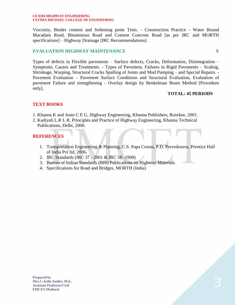
CE 6504 HIGHWAY ENGINEERING
FATIMA MICHAEL COLLEGE OF ENGINEERING
Prepared by
MrsCArthi Jenifer ME
Assistant ProfessorCivil
FMCETMadurai 3
Viscosity Binder content and Softening point Tests - Construction Practice - Water Bound
Macadam Road Bituminous Road and Cement Concrete Road [as per IRC and MORTH
specifications] ndash Highway Drainage [IRC Recommendations]
EVALUATION HIGHWAY MAINTENANCE 9
Types of defects in Flexible pavements ndash Surface defects Cracks Deformation Disintegration ndash
Symptoms Causes and Treatments - Types of Pavement Failures in Rigid Pavements ndash Scaling
Shrinkage Warping Structural Cracks Spalling of Joints and Mud Pumping ndash and Special Repairs -
Pavement Evaluation ndash Pavement Surface Conditions and Structural Evaluation Evaluation of
pavement Failure and strengthening - Overlay design by Benkelman Beam Method [Procedure
only]
TOTAL 45 PERIODS
TEXT BOOKS
1 Khanna K and Justo C E G Highway Engineering Khanna Publishers Roorkee 2001
2 KadiyaliLR L R Principles and Practice of Highway Engineering Khanna Technical
Publications Delhi 2000
REFERENCES
1 Transportation Engineering amp Planning CS Papa Costas PD Prevedouros Prentice Hall
of India Pvt ltd 2006
2 IRC Standards (IRC 37 - 2001 amp IRC 58 -1998)
3 Bureau of Indian Standards (BIS) Publications on Highway Materials
4 Specifications for Road and Bridges MORTH (India)
CE 6504 HIGHWAY ENGINEERING
FATIMA MICHAEL COLLEGE OF ENGINEERING
Prepared by
MrsCArthi Jenifer ME
Assistant ProfessorCivil
FMCETMadurai 4
UNIT 1 HIGHWAY PLANNNING AND ALIGNMENT
Significance of highway planning
Wide Geographical Coverage provided by roads
Roads can be constructed to penetrate the interior of any region and to connect remote villages The
advantage becomes particularly evident when planning the communication system in hilly regions
and sparsely populated areas
Low Capital investment
Roads can be constructed at comparatively lower initial cost than railways The cost of roads varies
with specifications but even the best road is cheaper than a railway line
Quick and assured deliveries
Time is great value for a wide range of articles including both perishables and high value is
manufactured products Road transport by its quick deliveries reduces the need for larger inventories
and locking up of working capital a great cost
Flexibility
Road transport offers a flexible service free from fixed schedules Any number of trucks or buses
can be pressed into service quickly to meet sudden demand or withdrawn Such a flexibility is
absent in railways which operate generally according to fixed schedules
Door-to-door services
Road transport offers door-to-door service free from transshipments from origin to destination
Railways on the other hand have to depend upon road transport for picking up loads and making
deliveries
Simpler packaging
Road transport permits simpler packaging and crating for the protection of goods against breakage
Personalized service
A personal touch is generally present in road transport The customer is given in individualized
attention in various matters
Employment potential
Road transport has a high employment potential This is an important factor in a country with a large
and employment problem
Personalized travel
Travel by private car or motorized two wheeler or even a cycle satisfies personal pleasuresThis is
one of the main reasons for the popularity of personalized travel mode in the developed countries
Short hauls
For short hauls transport is there only economical means if a major project is to be constructed and
is the construction materials have to be transported through short distances one turns only to road
transport
Safety
One of the serious advantages of road transport is its poor record of safety Road accidents have
become a serious menace claiming enormous economic loss to the nation
Environmental pollution
Road transport has been one of the major causes for environmental pollution noise fumes vibration
loss of aesthetics ribbon development these are the some ill effects
CE 6504 HIGHWAY ENGINEERING
FATIMA MICHAEL COLLEGE OF ENGINEERING
Prepared by
MrsCArthi Jenifer ME
Assistant ProfessorCivil
FMCETMadurai 5
Parking problem
Road transport has caused parking problem of serious proportions in city streets
Long hauls
It has been found that most commodity movements are cheaper by road for short hauls up to 300-
350 kms but beyond this range the cost advantage lies with the railways
Energy
Road transport consumes greater energy per passenger km and tone km than railways
History of road development in India
Roads in India perform a variety of roles in achieving speedy economic development Some of the
important aspects are discussed below
Connection to villages
India is a country having 590000 villages scattered into small habitations and often located in the
extreme interior Thus social uplift health and education of the village population is aided by roads
Communications in hilly terrain
For the hill states located along the Himalayan range communication facility is possible only by
roads because of the steep terrain involved
Strategic importance
The defense of the northern north-eastern and western borders of the country is dependent to a large
extent on the road system
Helps agricultural development
Roads have fostered quicker agricultural development facilitating movement of modern inputs such
as fertilizers and high yielding seeds
Helps dairy development
Since the cattle wealth of the nation is concentrated in innumerable villages and small habitations
the collection and processing of surplus milk only because of roads
Forestry development
The forest wealth of the country is being exploited mainly because of the roads which penetrate in to
the thick jungles
Fisheries Development The Development of the fisheries along the coast line has been rendered possible because of the
construction of link roads leading to the coast
Tourism Development
Some of the ancient monuments religious places natural parks and sanctuaries are accessible only
roads Tourism both domestic and international has been greatly aided by roads serving such as
places of interest
Employment
As already stated roads and road transport provide employment to a large number of people in the
country Since road construction involves labour intensive techniques in India the large unemployed
labor force gets gainful employment
Famine and flood relief
Roads have helped operations pertaining to flood and famine relief The affected people are
frequently employed on road construction to build durable assets
Administrative convenience
CE 6504 HIGHWAY ENGINEERING
FATIMA MICHAEL COLLEGE OF ENGINEERING
Prepared by
MrsCArthi Jenifer ME
Assistant ProfessorCivil
FMCETMadurai 6
Roads have helped the effective administration of this large country Maintenance of law and order
and dispensation of justice have been aided by roads National integration and cohesion have been
brought about by roads which traverse the length and breath of the country and which link people
from different parts together
Tresaguet construction
Pierre Tresaguet (1716-1796) developed an improved method of construction in France by
the year 1964The main feature of his proposal was that the thickness of construction need be
only in the order of 30 cm
Tresaguet was the inspector General of roads in France from 1775 to 1785So his method of
construction was implemented in that country in 1775
The typical cross section of tresaguets road construction is given in fig and the construction
steps may be enumerated as below
i) The sub grade was prepared and layers of large foundation stones were laid on edge by
hand At the two edges of the pavement large stones were embedded edge wise to serve
as submerged Krebs stones
ii) The corners of the heavy foundation stones were hammered and then the interstices filled
with smaller stones
iii) The top-wearing course was made of smaller stones and compacted to a thickness of
about 5 cm at the edges and gradually increased towards the center
iv) The shoulders were also provides cross slope to drain the surface water to the side drain
Macadam Construction
John Macadam put forward an entirely new method of road construction as compared to all the
previous methods A typical cross section of Macadam construction
CE 6504 HIGHWAY ENGINEERING
FATIMA MICHAEL COLLEGE OF ENGINEERING
Prepared by
MrsCArthi Jenifer ME
Assistant ProfessorCivil
FMCETMadurai 7
i) The importance of sub grade drainage and compaction were recognized and the sub
grade was compacted and was prepared with a cross slope of 1 in 36
ii) Macadam was the first person to suggest the heavy foundation stones are not at all
necessary to be placed at the bottom layer of construction
iii) Though the total thickness of construction was less than previous methods This
technique could serve the purpose in a better way
iv) The size of broken stones for the top layer was decided based on the stability under
animal drawn vehicles
Macadamrsquos method is the first method based on scientific thinking
The construction steps are
i) Sub grade is compacted and prepared with a cross slope of 1 in 36 up to a desired width
ii) Broken stones of a strong variety all passing through 5 cm size sieve were compacted to
a uniform thickness of 10cm
iii) The second layer of strong broken stones of size 375 cm was compacted to thickness of
10 cm
iv) The top layer consisted of stones of size less than 2 cm compacted to a thickness of about
5 cm The cross slope of pavement surface was also 1 in 36
Classification of roads
Road classification
The roads can be classified in many ways The classification based on speed and
accessibility is the most generic one Note that as the accessibility of road increases the
speed reducesAccordingly the roads can be classified as follows in the order of
increased accessibility and reduced speeds
Freeways Freeways are access-controlled divided highways Most freeways are
four lanes two lanes each direction but many freeways widen to incorporate
more lanes as they enter urban areas Access is controlled through the use of
interchanges and the type of interchange depends upon the kind of intersecting
road way (rural roads another freeway etc)
Expressways They are superior type of highways and are designed for high
CE 6504 HIGHWAY ENGINEERING
FATIMA MICHAEL COLLEGE OF ENGINEERING
Prepared by
MrsCArthi Jenifer ME
Assistant ProfessorCivil
FMCETMadurai 8
speeds (120 kmhr is common) high traffic volume and safety They are
generally provided with grade separations at intersections Parking loading and
unloading of goods and pedestrian traffic is not allowed on expressways
Highways They represent the superior type of roads in the country Highways are
of two types - rural highways and urban highways Rural highways are those
passing through rural areas (villages) and urban highways are those passing
through large cities and towns ie urban areas
Arterials It is a general term denoting a street primarily meant for through traffic
usually on a continuous route They are generally divided highways with fully or
partially controlled access Parking loading and unloading activities are usually
restricted and regulated Pedestrians are allowed to cross only at
intersectionsdesignated pedestrian crossings
Local streets A local street is the one which is primarily intended for access to
residence business or abutting property It does not normally carry large volume
of traffic and also it allows unrestricted parking and pedestrian movements
Collector streets These are streets intended for collecting and distributing traffic
to and from local streets and also for providing access to arterial streets Normally
full access is provided on these streets There are few parking restrictions except
during peak hours
Figure 1 Speed vs accessibility
CE 6504 HIGHWAY ENGINEERING
FATIMA MICHAEL COLLEGE OF ENGINEERING
Prepared by
MrsCArthi Jenifer ME
Assistant ProfessorCivil
FMCETMadurai 9
FACTORS AFFECTING HIGHWAY ALIGHNMENT
Design speed
Design speed is the single most important factor that affects the geometric design It
directly affects the sight distance horizontal curve and the length of vertical curves
Since the speed of vehicles vary with driver terrain etc a design speed is adopted for all
the geometric design
Design speed is defined as the highest continuous speed at which individual vehicles can
travel with safety on the highway when weather conditions are conducive Design speed
is different from the legal speed limit which is the speed limit imposed to curb a common
tendency of drivers to travel beyond an accepted safe speed Design speed is also
different from the desired speed which is the maximum speed at which a driver would
travel when unconstrained by either traffic or local geometry
Since there are wide variations in the speed adopted by different drivers and by different
types of vehicles design speed should be selected such that it satisfy nearly all drivers At
the same time a higher design speed has cascading effect in other geometric designs and
thereby cost escalation Therefore an 85th percentile design speed is normally adopted
This speed is defined as that speed which is greater than the speed of 85 of drivers In
some countries this is as high as 95 to 98 percentile speed
Topography
The next important factor that affects the geometric design is the topography It is easier to
construct roads with required standards for a plain terrain However for a given design speed the
construction cost increases multiform with the gradient and the terrain Therefore geometric design
standards are different for different terrain to keep the cost of construction and time of construction
under control This is characterized by sharper curves and steeper gradients
Other factors
CE 6504 HIGHWAY ENGINEERING
FATIMA MICHAEL COLLEGE OF ENGINEERING
Prepared by
MrsCArthi Jenifer ME
Assistant ProfessorCivil
FMCETMadurai 10
In addition to design speed and topography there are various other factors that affect the geometric
design and they are briefly discussed below
Vehicle The dimensions weight of the axle and operating characteristics of a vehicle
influence the design aspects such as width of the pavement radii of the curve clearances
parking geometrics etc A design vehicle which has standard weight dimensions and
operating characteristics are used to establish highway design controls to accommodate
vehicles of a designated type
Human The important human factors that influence geometric design are the mental and
psychological characteristics of the driver and pedestrians like the reaction time
Traffic It will be uneconomical to design the road for peak traffic flow Therefore a
reasonable value of traffic volume is selected as the design hourly volume which is
determined from the various traffic data collected The geometric design is thus based on
this design volume capacity etc
Environmental Factors like air pollution noise pollution etc should be given due
consideration in the geometric design of roads
Economy The design adopted should be economical as far as possible It should match
with the funds allotted for capital cost and maintenance cost
Others Geometric design should be such that the aesthetics of the region is not affected
Nagpur classification
In Nagpur road classification all roads were classified into five categories as National highways
State highways Major district roads Other district roads and village roads
National highways
They are main highways running through the length and breadth of India connecting major
ports foreign highways capitals of large states and large industrial and tourist centers
including roads required for strategic movements
It was recommended by Jayakar committee that the National highways should be the frame
on which the entire road communication should be based
All the national highways are assigned the respective numbers
For eg the highway connecting Delhi-Ambala-Amritsar is denoted as NH-1 (Delhi-
Amritsar) where as a bifurcation of this highway beyond Full under to Srinagar and Uri is
denoted as NH-1_A
They are constructed and maintained by CPWD
The total lengths of National highway in the country is 58112 Kms and constitute about 2
of total road networks of India and carry 40 of total traffic
State highways
They are the arterial roads of a state connecting up with the national highways of adjacent
states district headquarters and important cities within the state
They also serve as main arteries to and from district roads
Total length of all SH in the country is 1 37119 Kms
Major district roads
Important roads with in a district serving areas of production and markets connecting those
with each other or with the major highways
India has a total of 4 70000 Kms of MDR
CE 6504 HIGHWAY ENGINEERING
FATIMA MICHAEL COLLEGE OF ENGINEERING
Prepared by
MrsCArthi Jenifer ME
Assistant ProfessorCivil
FMCETMadurai 11
Other district roads
Roads serving rural areas of production and providing them with outlet to market centers or
other important roads like MDR or SH
Village roads
They are roads connecting villages or group of villages with each other or to the nearest
road of a higher category like ODR or MDR
India has 2650000 kms of ODR+VR out of the total 3315231 kms of all type of roads
Roads classification criteria
Apart from the classification given by the different plans roads were also classified based on some
other criteria They are given in detail below
Based on usage
This classification is based on whether the roads can be used during different seasons of the year
All-weather roads Those roads which are negotiable during all weathers except at major
river crossings where interruption of traffic is permissible up to a certain extent are called all
weather roads
Fair-weather roads Roads which are negotiable only during fair weather are called fair
weather roads
Based on carriage way
This classification is based on the type of the carriage way or the road pavement
Paved roads with hards surface If they are provided with a hard pavement course such
roads are called paved roads(eg stones Water bound macadam (WBM) Bituminous
macadam (BM) concrete roads)
Unpaved roads Roads which are not provided with a hard course of atleast a WBM layer
they is called unpaved roads Thus earth and gravel roads come under this category
Alignment The position or the layout of the central line of the highway on the ground is called the
alignment Horizontal alignment includes straight and curved paths Vertical alignment
includes level and gradients Alignment decision is important because a bad alignment
will enhance the construction maintenance and vehicle operating costs Once an
alignment is fixed and constructed it is not easy to change it due to increase in cost of
adjoining land and construction of costly structures by the roadside
Requirements The requirements of an ideal alignment are
The alignment between two terminal stations should be short and as far as
possible be straight but due to some practical considerations deviations may be
needed
The alignment should be easy to construct and maintain It should be easy for the
operation of vehicles So to the maximum extend easy gradients and curves
should be provided
It should be safe both from the construction and operating point of view
especially at slopes embankments and cutting It should have safe geometric
features
The alignment should be economical and it can be considered so only when the
initial cost maintenance cost and operating cost are minimum
CE 6504 HIGHWAY ENGINEERING
FATIMA MICHAEL COLLEGE OF ENGINEERING
Prepared by
MrsCArthi Jenifer ME
Assistant ProfessorCivil
FMCETMadurai 12
Factors controlling alignment
We have seen the requirements of an alignment But it is not always possible to satisfy all
these requirements Hence we have to make a judicial choice considering all the factors
The various factors that control the alignment are as follows
Obligatory points These are the control points governing the highway alignment
These points are classified into two categories Points through which it should
pass and points through which it should not pass Some of the examples are
o Bridge site The bridge can be located only where the river has straight
and permanent path and also where the abutment and pier can be strongly
founded The road approach to the bridge should not be curved and skew
crossing should be avoided as possible Thus to locate a bridge the
highway alignment may be changed
o Mountain While the alignment passes through a mountain the various alternatives are to either construct a tunnel or to go round the hills The suitability of the alternative depends on factors like topography site
conditions and construction and operation cost
o Intermediate town The alignment may be slightly deviated to connect an intermediate town or village nearby
These were some of the obligatory points through which the alignment should pass
Coming to the second category that is the points through which the alignment should not
pass are
Religious places These have been protected by the law from being acquired for
any purpose Therefore these points should be avoided while aligning
Very costly structures Acquiring such structures means heavy compensation
which would result in an increase in initial cost So the alignment may be deviated
not to pass through that point
Lakesponds etc The presence of a lake or pond on the alignment path would also
necessitate deviation of the alignment
Traffic The alignment should suit the traffic requirements Based on the origin-
destination data of the area the desire lines should be drawn The new alignment should
be drawn keeping in view the desire lines traffic flow pattern etc Geometric design
Geometric design factors such as gradient radius of curve sight distance etc also govern
the alignment of the highway To keep the radius of curve minimum it may be required
to change the alignment The alignments should be finalized such that the obstructions to
visibility do not restrict the minimum requirements of sight distance The design
standards vary with the class of road and the terrain and accordingly the highway should
be aligned Economy The alignment finalized should be economical All the three costs
ie construction maintenance and operating cost should be minimum The construction
cost can be decreased much if it is possible to maintain a balance between cutting and
filling Also try to avoid very high embankments and very deep cuttings as the
construction cost will be very higher in these cases
Road ecology
The features of the cross-section of the pavement influences the life of the pavement as
CE 6504 HIGHWAY ENGINEERING
FATIMA MICHAEL COLLEGE OF ENGINEERING
Prepared by
MrsCArthi Jenifer ME
Assistant ProfessorCivil
FMCETMadurai 13
well as the riding comfort and safety Of these pavement surface characteristics affect
both of these Camber kerbs and geometry of various cross-sectional elements are
important aspects to be considered in this regard They are explained briefly in this
chapter
Camber
Camber or cant is the cross slope provided to raise middle of the road surface in the
transverse direction to drain off rain water from road surface The objectives of providing
camber are
Surface protection especially for gravel and bituminous roads
Sub-grade protection by proper drainage
Quick drying of pavement which in turn increases safety
Too steep slope is undesirable for it will erode the surface Camber is measured in 1 in n
or n (Eg 1 in 50 or 2) and the value depends on the type of pavement surface The
value suggested by IRC for various categories of pavement is given in Table 1 The
common types of camber are parabolic straight or combination of them (Figure 1)
Figure 1 Different types of camber
Table 1 IRC Value
s for ca
mber
Heavy
Light
Surface
rain
type
rain
17
ConcreteBituminous
2
25
GravelWBM
3
30
Earthen
4
CE 6504 HIGHWAY ENGINEERING
FATIMA MICHAEL COLLEGE OF ENGINEERING
Prepared by
MrsCArthi Jenifer ME
Assistant ProfessorCivil
FMCETMadurai 14
Engineering surveys for alignment
The stages of the engineering surveys are a) Map study
b) Reconnaissance
c) Preliminary surveys
d) Final location and detailed surveys
Map study -
) In the topographic map to suggest the likely routes of roads In India topographic
maps are available from the survey of India with 15 or 30-meter contour intervals
) The main feature like rivers hills and valleys etc The probable alignment can be
located on the map from the following details available on the map
Alignment avoiding valleys ponds or lakes
When the road has to cross a row of hills possibility crossing through a mountain pass
Approximate location of bridge site for crossing rivers avoiding bend of the river
When a road is to be connected between two stations one of the top and the other on the foot
of the hill then alternate routes can be suggested keeping in view the permissible alignment
Suppose the scale of the contour map is known and then the contour intervals it is possible
to decide the length of road required between two consecutive contours keeping the gradient
within allowable limits
In the fig Let A and B be two stations to be connected by road AB is the shortest route
(Straight line) APQB is a steep route in which the gradient positively exceeds 1 in 20 as the
distance between the contour intervals is only about 200 meter
APLMNB is a route with an approximate slope of 1 in 20 whereas APEFGB is an alternate
alignment with the same gradient
Thus the map study also is possible to drop a certain route in view of any unavoidable
obstructions (or) undesirable ground enroute
Reconnaissance-
The second stage of surveys for highway location is the reconnaissance to examine the general
character of the area for deciding the most feasible routes for detailed studies
Some of the details to be collected during reconnaissance are given below
Valleys ponds lakes marshy land ridge hills permanent structures and other obstructions
along the route which are not available in the map
Approximate values of gradient length of gradients and radius of curves of alternate
alignments
Number and types of cross drainage structures maximum flood level and natural
groundwater level along the probable routes
Soil type along the routes from field identification tests and observation of geological
features
Sources of construction materials water and location of stone quarries
When the road passes through hilly or mountainous terrain additional data regarding the
geological formation types of rocks dip of strata seepage flow etc
Preliminary survey -
CE 6504 HIGHWAY ENGINEERING
FATIMA MICHAEL COLLEGE OF ENGINEERING
Prepared by
MrsCArthi Jenifer ME
Assistant ProfessorCivil
FMCETMadurai 15
The main objectives of the preliminary surveys are
To survey the various alternate alignments proposed after the reconnaissance and to collect
all the necessary physical information and details of topography drainage and soil
To compare the different proposals in view of the requirements of a good alignment
To estimate quantity of earthwork materials and other construction aspects and to work out
the cost of alternate proposals
To finalize the best alignment from all considerations
The procedure of the conventional methods of preliminary surveys the given steps
Primary survey -
For alternate alignments either secondary traverses (or) independent primary traverses may be
necessary
Topographical features -
All geographical and other man made features along the traverse and for a certain width on either
side surveyed and plotted
Leveling work -
Levelling work is also carried out side by side to give the centerline profiles and typical cross
sections The leveling work in the preliminary survey is kept to a minimum just sufficient to obtain
the approximate earthwork in the alternate alignments
Drainage studies -
Drainage investigations and hydrological data are collected so as to estimate the type number and
approximate size of cross and drainage structures
Soil survey -
The soil survey conducted at this stage helps to working out details of earthwork slopes suitability
of materials subsoil and surface drainage requirements and pavement type and the approximate
thickness requirements
Material survey -
The survey for naturally occurring materials like stone aggregates soft aggregates etc and
identification of suitable quarries should be made
Traffic survey -
Traffic surveys conducted in the region from basis for deciding the number of traffic lanes and
roadway width pavement design and economic analysis of highway project
Locations and functions
Final location and detailed survey - The alignment finalized at the design office after the preliminary survey is to be first located on the
field by establishing the centerline The detailed survey should be carried out for collecting the
information technology for the preparation of plans and construction details
Location -
The centerline of the road finalized in the drawings to be translated on the ground
during the location survey
Major and minor control points are established on the ground and center pegs are
driven checking the geometric design requirements
Detailed survey -
CE 6504 HIGHWAY ENGINEERING
FATIMA MICHAEL COLLEGE OF ENGINEERING
Prepared by
MrsCArthi Jenifer ME
Assistant ProfessorCivil
FMCETMadurai 16
Levels along his final centerline should be taken at all staked points Levelling work is to
great importance as the vertical alignment
A detailed soil survey is carried out to enable drawing of the soil profile
The data during the detailed survey should be elaborate and complete for preparing detailed
plans design and estimates of the project
Soil suitability analysis
The methodology for locating appropriate sites for each land use activity is guided by the intent to
minimize the possible adverse effects of development on the environment and on existing
communities and to emphasize the positive impacts of such development by locating them in a
most suitable location
This is achieved by examining a number of individual criteria assigning them relative levels of
importance as a whole and using a mathematical resultant model to identify the most suitable
location
By adopting this site suitability method it is possible to systematically identify the criteria
considered clearly document the relative importance of one criterion over another analyze the net
outcome using a Geographic Information System and then possibly revisit the mathematical
relationships in this ldquodecision modelrdquo
By revising the relative importance to identified criteria based upon the particular land use under
consideration it is possible to generate ldquosuitability mapsrdquo for each individual land use and then
generate a final composite land use that is based on a best possible collective suitability of multiple
land uses
To achieve this all the criteria are assigned a ldquorankrdquo denoting their relative levels of importance
within the suitability study These ranks are assigned as numeric values ranging from 1 to 10 with 1
reflecting a low level of importance and 10 reflecting a high level of importance For example
within the criteria of road networks national highways would have a different level of influence on
the suitability for a particular land use as compared with local roads Further the distance from each
of these features would further modify the relative suitability of a land use based on the proximity to
a particular type of road
Criteria for Site Suitability Analysis
The decision criteria for site selection are examined for assigning relative ranks and individual
feature weights based on the land use type for which suitability is being examined For benefit of
analysis the criteria under consideration in this paper activity are organized as
Critical Criteria Criteria that will be very significant in the site selection of the identified land use
and will act as key drivers in the selection of the geographic location These criteria can be clustered
into a single decision model and the outcome collectively reviewed These criteria have a strong
influence in the final suitability
Additional Criteria Criteria that will have to be examined one at a time to carefully assess its
relationship with the proposed land use activity These criteria have a positive influence in the final
suitability
CE 6504 HIGHWAY ENGINEERING
FATIMA MICHAEL COLLEGE OF ENGINEERING
Prepared by
MrsCArthi Jenifer ME
Assistant ProfessorCivil
FMCETMadurai 17
Constrained Criteria These criteria impose strong negative opportunities in the selection of areas
for the identified land use Consequently they inform of us of where the particular land use under
consideration should not be located These criteria serve to limit or exclude areas from the final
suitability
GIS Site Suitability Analysis Model We were developed a tourism site suitability analysis model
in ArcGIS - 931 which is shown in Figure -
CE 6504 HIGHWAY ENGINEERING
FATIMA MICHAEL COLLEGE OF ENGINEERING
Prepared by
MrsCArthi Jenifer ME
Assistant ProfessorCivil
FMCETMadurai 18
UNIT 2 GEOMETRIC DESIGN OF HIGHWAYS
Typical cross section of urban and rural roads
A cross section is a vertical plane (slice) taken at right angles to the road control line showing the
various elements that make up the roads structure It is normally viewed in the direction of
increasing chainage
The width of a roadway is an important design consideration to ensure that it is appropriately sized
to serve its function Because of the diversity within the County two major roadway categories have
been established 1 Rural Road Standards 2 Urban Road Standards Urban Road Standards will
serve those areas which tend to be more developed and need to provide for multiple users
(bicyclists pedestrians parallel parking etc) whereas many rural roads will primarily serve only
vehicular traffic
Cross sections are created to provide a visual guide depicting the initial interim and ultimate phase
cross sections for these road classifications The typical sections illustrated in the following pages
are recommendations tied to transportation planning aspects such as right‐of‐way lineage sidewalk
width etc Threshold daily traffic can be used as a guide for a starting point when determining
which cross section is most applicable
1 Rural Road Standards
The rural roadways will not typically require curb and gutter or sidewalk although the County may
require either or both in unique circumstances Widths of lanes and shoulders will vary depending
upon the specific classification and the potential traffic volume which the roadway may carry Roads
carrying fewer than 200 vehicles per day need not be paved or treated for dust control The need for
paved shoulders is also dependent upon the level of traffic and safety
Final design and construction details will be determined by the Public Works Department Final
Design and construction criteria taken into consideration may include but are not limited to use of
the roadway density of development topographical characteristics and nearby development For
construction in which only a portion of the ultimate cross‐section is intended to be completed the
partial design will need to allow for the eventual widening to the ultimate cross‐section The design
for the partial or interim cross‐section roadway will need to incorporate ultimate design information
to ensure that the first phase of roadway construction is appropriate and would not need to be
removed at a future date when the full width cross‐section is completed
2 Urban Road Standards
Three roadway classifications are identified for those areas that are associated with the communityrsquos
urban growth areas They include arterial collector and local street classifications Transportation
Plan shows the key elements of the urban road standards Urban road standards will include 12‐foot
lanes sidewalk and curb amp gutter arterials and collectors will also include a striped bike lane Turn
lanes may be necessary as determined by the County Since almost all of the municipalities have
different right‐of‐way cross sections adopted for their community it makes it very difficult for the
County to match them all Therefore the philosophy was to encourage a baseline amount of
right‐of‐way reservation that could ensure the adjacent community enough area for coordination of
future roadway improvements until such time the road
CE 6504 HIGHWAY ENGINEERING
FATIMA MICHAEL COLLEGE OF ENGINEERING
Prepared by
MrsCArthi Jenifer ME
Assistant ProfessorCivil
FMCETMadurai 19
CE 6504 HIGHWAY ENGINEERING
FATIMA MICHAEL COLLEGE OF ENGINEERING
Prepared by
MrsCArthi Jenifer ME
Assistant ProfessorCivil
FMCETMadurai 20
Cross sectional elements
Kerbs
Kerbs indicate the boundary between the carriage way and the shoulder or islands or footpaths Different types of kerbs are
CE 6504 HIGHWAY ENGINEERING
FATIMA MICHAEL COLLEGE OF ENGINEERING
Prepared by
MrsCArthi Jenifer ME
Assistant ProfessorCivil
FMCETMadurai 21
Low or mountable kerbs This type of kerbs is provided such that they
encourage the traffic to remain in the through traffic lanes and also allow the
driver to enter the shoulder area with little difficulty The height of this kerb is
about 10 cm above the pavement edge with a slope which allows the vehicle to
climb easily This is usually provided at medians and channelization schemes and
also helps in longitudinal drainage
Semi-barrier type kerbs When the pedestrian traffic is high these kerbs are
provided Their height is 15 cm above the pavement edge This type of kerb
prevents encroachment of parking vehicles but at acute emergency it is possible
to drive over this kerb with some difficulty
Barrier type kerbs They are designed to discourage vehicles from leaving the
pavement They are provided when there is considerable amount of pedestrian
traffic They are placed at a height of 20 cm above the pavement edge with a steep
batter
Submerged kerbs They are used in rural roads The kerbs are provided at
pavement edges between the pavement edge and shoulders They provide lateral
confinement and stability to the pavement
Figure 1 Different types of kerbs
Shoulders Shoulders are provided along the road edge and are intended for accommodation of
stopped vehicles serve as an emergency lane for vehicles and provide lateral support
for base and surface courses The shoulder should be strong enough to bear the weight
of a fully loaded truck even in wet conditions The shoulder width should be adequate
for giving working space around a stopped vehicle It is desirable to have a width of
46 m for the shoulders A minimum width of 25 m is recommended for 2-lane rural
highways in India Parking lanes
Parking lanes are provided in urban lanes for side parking Parallel parking is preferred
because it is safe for the vehicles moving on the road The parking lane should have a
minimum of 30 m width in the case of parallel parking
CE 6504 HIGHWAY ENGINEERING
FATIMA MICHAEL COLLEGE OF ENGINEERING
Prepared by
MrsCArthi Jenifer ME
Assistant ProfessorCivil
FMCETMadurai 22
Bus-bays
Bus bays are provided by recessing the kerbs for bus stops They are provided so that
they do not obstruct the movement of vehicles in the carriage way They should be at
least 75 meters away from the intersection so that the traffic near the intersections is not
affected by the bus-bay
Service roads Service roads or frontage roads give access to access controlled highways like freeways
and expressways They run parallel to the highway and will be usually isolated by a
separator and access to the highway will be provided only at selected points These roads
are provided to avoid congestion in the expressways and also the speed of the traffic in
those lanes is not reduced
Drainage
The pavement surface should be absolutely impermeable to prevent seepage of water into
the pavement layers Further both the geometry and texture of pavement surface should
help in draining out the water from the surface in less time
Footpath
Footpaths are exclusive right of way to pedestrians especially in urban areas They are
provided for the safety of the pedestrians when both the pedestrian traffic and vehicular
traffic is high Minimum width is 15 meter and may be increased based on the traffic
The footpath should be either as smooth as the pavement or more smoother than that to
induce the pedestrian to use the footpath
Right of way
Right of way (ROW) or land width is the width of land acquired for the road along its
alignment It should be adequate to accommodate all the cross-sectional elements of the
highway and may reasonably provide for future development To prevent ribbon
development along highways control lines and building lines may be provided Control
line is a line which represents the nearest limits of future uncontrolled building activity
in relation to a road Building line represents a line on either side of the road between
which and the road no building activity is permitted at all The right of way width is
governed by
Width of formation It depends on the category of the highway and width of
roadway and road margins
Height of embankment or depth of cutting It is governed by the topography and
the vertical alignment
Side slopes of embankment or cutting It depends on the height of the slope soil
type etc
Drainage system and their size which depends on rainfall topography etc
Sight distance considerations On curves etc there is restriction to the visibility
on the inner side of the curve due to the presence of some obstructions like
building structures etc
Reserve land for future widening Some land has to be acquired in advance
CE 6504 HIGHWAY ENGINEERING
FATIMA MICHAEL COLLEGE OF ENGINEERING
Prepared by
MrsCArthi Jenifer ME
Assistant ProfessorCivil
FMCETMadurai 23
Table 2 Desig
n speed in as per IRC (ruling and minimum)
Steep
Type
Plain
Rolling
Hilly
40-30
NSampSH
100-80
80-65
50-40
MDR
80-65
65-50
40-30
30-20
25-20
ODR
65-50
50-40
30-25
25-20
VR
50-40
40-35
25-20
anticipating future developments like widening of the road
Table 1 No
right of way for open areas
Roadway width in m
Road
Plain and
Mountainous and
classification
steep terrain
rolling terrain
Open areas
45
24
NHSH
18
MDR
25
15
15
ODR
12
9
VR
Built-up areas
20
NHSH
30
MDR
20
15
ODR
15
12
9
VR
10
CE 6504 HIGHWAY ENGINEERING
FATIMA MICHAEL COLLEGE OF ENGINEERING
Prepared by
MrsCArthi Jenifer ME
Assistant ProfessorCivil
FMCETMadurai 24
Horizontal curve
The presence of horizontal curve imparts centrifugal force which is a reactive force
acting outward on a vehicle negotiating it Centrifugal force depends on speed and radius
of the horizontal curve and is counteracted to a certain extent by transverse friction
between the tyre and pavement surface On a curved road this force tends to cause the
vehicle to overrun or to slide outward from the centre of road curvature For proper
design of the curve an understanding of the forces acting on a vehicle taking a horizontal
curve is necessary Various forces acting on the vehicle are illustrated in the figure 1
Figure 1 Effect of horizontal curve They are the centrifugal force (P) acting outward weight of the vehicle (W) acting
downward and the reaction of the ground on the wheels ( and ) The centrifugal
force and the weight is assumed to be from the centre of gravity which is at h units above
the ground Let the wheel base be assumed as b units The centrifugal force in
is given by
(1)
where is the weight of the vehicle in is the speed of the vehicle in is
the acceleration due to gravity in and is the radius of the curve in
The centrifugal ratio or the impact factor is given by
CE 6504 HIGHWAY ENGINEERING
FATIMA MICHAEL COLLEGE OF ENGINEERING
Prepared by
MrsCArthi Jenifer ME
Assistant ProfessorCivil
FMCETMadurai 25
(1)
The centrifugal force has two effects A tendency to overturn the vehicle about the outer
wheels and a tendency for transverse skidding Taking moments of the forces with
respect to the outer wheel when the vehicle is just about to override
At the equilibrium over turning is possible when
and for safety the following condition must satisfy
(2)
The second tendency of the vehicle is for transverse skidding ie When the the
centrifugal force is greater than the maximum possible transverse skid resistance due to
friction between the pavement surface and tyre The transverse skid resistance (F) is
given by
where and is the fractional force at tyre and and is the reaction at
tyre and is the lateral coefficient of friction and is the weight of the vehicle
This is counteracted by the centrifugal force (P) and equating
At equilibrium when skidding takes place (from equation1)
and for safety the following condition must satisfy
CE 6504 HIGHWAY ENGINEERING
FATIMA MICHAEL COLLEGE OF ENGINEERING
Prepared by
MrsCArthi Jenifer ME
Assistant ProfessorCivil
FMCETMadurai 26
(3)
Equation 2 and 3 give the stable condition for design If equation 2 is violated the vehicle
will overturn at the horizontal curve and if equation 3 is violated the vehicle will skid at
the horizontal
Curve Analysis of super-elevation
Super-elevation or cant or banking is the transverse slope provided at horizontal curve to
counteract the centrifugal force by raising the outer edge of the pavement with respect to
the inner edge throughout the length of the horizontal curve When the outer edge is
raised a component of the curve weight will be complimented in counteracting the effect
of centrifugal force In order to find out how much this raising should be the following
analysis may be done The forces acting on a vehicle while taking a horizontal curve with
super elevation is shown in figure 1
Figure 1 Analysis of super-elevation
Forces acting on a vehicle on horizontal curve of radius at a speed of are
the centrifugal force acting horizontally out-wards through the center of
gravity
the weight of the vehicle acting down-wards through the center of gravity and
the friction force between the wheels and the pavement along the surface
inward
CE 6504 HIGHWAY ENGINEERING
FATIMA MICHAEL COLLEGE OF ENGINEERING
Prepared by
MrsCArthi Jenifer ME
Assistant ProfessorCivil
FMCETMadurai 27
At equilibrium by resolving the forces parallel to the surface of the pavement we get where
friction
is the weight of the vehicle is the centrifugal force is the coefficient of
is the transverse slope due to superelevation Dividing by we get
CE 6504 HIGHWAY ENGINEERING
FATIMA MICHAEL COLLEGE OF ENGINEERING
Prepared by
MrsCArthi Jenifer ME
Assistant ProfessorCivil
FMCETMadurai 28
Step 1
Find for 75 percent of design speed neglecting ie
Step 2
If then else if go to step 3
Step 3
Find for the design speed and max ie If
then the maximum is safe for the design speed else go to
step 4
Step 4
Find the allowable speed for the maximum and
If then the design is adequate otherwise use speed adopt
control measures or look for speed control measures
Maximum and minimum super-elevation
Depends on (a) slow moving vehicle and (b) heavy loaded trucks with high CG IRC
specifies a maximum super-elevation of 7 percent for plain and rolling terrain while that
of hilly terrain is 10 percent and urban road is 4 percent The minimum super elevation is
2-4 percent for drainage purpose especially for large radius of the horizontal curve
Attainment of super-elevation
1 Elimination of the crown of the cambered section by
1 Rotating the outer edge about the crown The outer half of the cross slope
is rotated about the crown at a desired rate such that this surface falls on
the same plane as the inner half
2 Shifting the position of the crown This method is also known as diagonal
crown method Here the position of the crown is progressively
shifted outwards thus increasing the width of the inner half of cross section
progressively
2 Rotation of the pavement cross section to attain full super elevation byThere are
two methods of attaining super elevation by rotating the pavement
1 Rotation about the center line The pavement is rotated such that the inner
edge is depressed and the outer edge is raised both by half the total amount
of super elevation ie by with respect to the centre
2 Rotation about the inner edge Here the pavement is rotated raising the
outer edge as well as the centre such that the outer edge is raised by the
full amount of super elevation with respect to the inner edge
Horizontal Transition Curves
CE 6504 HIGHWAY ENGINEERING
FATIMA MICHAEL COLLEGE OF ENGINEERING
Prepared by
MrsCArthi Jenifer ME
Assistant ProfessorCivil
FMCETMadurai 29
Transition curve is provided to change the horizontal alignment from straight to circular
curve gradually and has a radius which decreases from infinity at the straight end
(tangent point) to the desired radius of the circular curve at the other end (curve point)
There are five objectives for providing transition curve and are given below
1 to introduce gradually the centrifugal force between the tangent point and the
beginning of the circular curve avoiding sudden jerk on the vehicle This
increases the comfort of passengers
2 to enable the driver turn the steering gradually for his own comfort and security
3 to provide gradual introduction of super elevation and
4 to provide gradual introduction of extra widening
5 to enhance the aesthetic appearance of the road
Type of transition curve
Different types of transition curves are spiral or clothoid cubic parabola and Lemniscate
IRC recommends spiral as the transition curve because
1 it fulfills the requirement of an ideal transition curve that is
1 rate of change or centrifugal acceleration is consistent (smooth) and
2 radius of the transition curve is at the straight edge and changes to at
the curve point ( ) and calculation and field implementation is
very easy
Length of transition curve The length of the transition curve should be determined as the maximum of the following
three criteria rate of change of centrifugal acceleration rate of change of super elevation
and an empirical formula given by IRC Rate of change of centrifugal acceleration
At the tangent point radius is infinity and hence centrifugal acceleration is zero At the
end of the transition the radius R has minimum value R The rate of change of
centrifugal acceleration should be adopted such that the design should not cause
discomfort to the drivers If is the rate of change of centrifugal acceleration it can be
written as
Therefore the length of the transition curve in is
CE 6504 HIGHWAY ENGINEERING
FATIMA MICHAEL COLLEGE OF ENGINEERING
Prepared by
MrsCArthi Jenifer ME
Assistant ProfessorCivil
FMCETMadurai 30
(1)
where is the rate of change of centrifugal acceleration given by an empirical formula
suggested by by IRC as below
(2) 2 Rate of introduction of super-elevation
Raise ( ) of the outer edge with respect to inner edge is given by
The rate of change of this raise from to is achieved
gradually with a gradient of in over the length of the transition curve (typical range
of is 60-150) Therefore the length of the transition curve is
(3)
3 By empirical formula
IRC suggest the length of the transition curve is minimum for a plain and rolling terrain
(4)
and for steep and hilly terrain is
(5)
CE 6504 HIGHWAY ENGINEERING
FATIMA MICHAEL COLLEGE OF ENGINEERING
Prepared by
MrsCArthi Jenifer ME
Assistant ProfessorCivil
FMCETMadurai 31
and the shift as
(
6
) The length of the transition curve is the maximum of
equations 1 3 and 4or5 ie
(
7
Case (a)
For single lane roads
(
1
)
Therefore
(
2
)
Figure 1 Set-back for single lane roads (
CE 6504 HIGHWAY ENGINEERING
FATIMA MICHAEL COLLEGE OF ENGINEERING
Prepared by
MrsCArthi Jenifer ME
Assistant ProfessorCivil
FMCETMadurai 32
For multi lane roads if is the distance between centerline of the road and the centerline
of the inner lane then
(3)
(4)
Figure 2 Set-back for multi-lane roads ( )
Case (a)
For single lane roads
(1)
Therefore
(2)
Gradient
Gradient is the rate of rise or fall along the length of the road with respect to the
horizontal While aligning a highway the gradient is decided for designing the vertical
curve Before finalizing the gradients the construction cost vehicular operation cost and
the practical problems in the site also has to be considered Usually steep gradients are
avoided as far as possible because of the difficulty to climb and increase in the
CE 6504 HIGHWAY ENGINEERING
FATIMA MICHAEL COLLEGE OF ENGINEERING
Prepared by
MrsCArthi Jenifer ME
Assistant ProfessorCivil
FMCETMadurai 33
construction cost More about gradients are discussed below
Effect of gradient
The effect of long steep gradient on the vehicular speed is considerable This is
particularly important in roads where the proportion of heavy vehicles is significant Due
to restrictive sight distance at uphill gradients the speed of traffic is often controlled by
these heavy vehicles As a result not only the operating costs of the vehicles are
increased but also capacity of the roads will have to be reduced Further due to high
differential speed between heavy and light vehicles and between uphill and downhill
gradients accidents abound in gradients
Representation of gradient
The positive gradient or the ascending gradient is denoted as and the negative gradient as The deviation angle is when two grades meet the angle which
measures the change of direction and is given by the algebraic difference between the two
grades
steep gradient while 1 in 50 = 2 representation is illustrated in the figure 1
Example 1 in 30 = 333 is a
is a flatter gradient The gradient
CE 6504 HIGHWAY ENGINEERING
FATIMA MICHAEL COLLEGE OF ENGINEERING
Prepared by
MrsCArthi Jenifer ME
Assistant ProfessorCivil
FMCETMadurai 34
Figure 1 Representation of gradient
Types of gradient
Many studies have shown that gradient upto seven percent can have considerable effect
on the speeds of the passenger cars On the contrary the speeds of the heavy vehicles are
considerably reduced when long gradients as flat as two percent is adopted Although
flatter gradients are desirable it is evident that the cost of construction will also be very
high Therefore IRC has specified the desirable gradients for each terrain However it
may not be economically viable to adopt such gradients in certain locations steeper
gradients are permitted for short duration Different types of grades are discussed below
Ruling gradient
The ruling gradient or the design gradient is the maximum gradient with which the
designer attempts to design the vertical profile of the road This depends on the terrain
length of the grade speed pulling power of the vehicle and the presence of the horizontal
curve In flatter terrain it may be possible to provide flat gradients but in hilly terrain it
is not economical and sometimes not possible also The ruling gradient is adopted by the
designer by considering a particular speed as the design speed and for a design vehicle
with standard dimensions But our country has a heterogeneous traffic and hence it is not
possible to lay down precise standards for the country as a whole Hence IRC has
recommended some values for ruling gradient for different types of terrain
Limiting gradient
This gradient is adopted when the ruling gradient results in enormous increase in cost of
construction On rolling terrain and hilly terrain it may be frequently necessary to adopt
limiting gradient But the length of the limiting gradient stretches should be limited and
must be sandwiched by either straight roads or easier grades
Exceptional gradient
Exceptional gradient are very steeper gradients given at unavoidable situations They
should be limited for short stretches not exceeding about 100 metres at a stretch In
mountainous and steep terrain successive exceptional gradients must be separated by a
minimum 100 metre length gentler gradient At hairpin bends the gradient is restricted to
25
Critical length of the grade
The maximum length of the ascending gradient which a loaded truck can operate without
undue reduction in speed is called critical length of the grade A speed of 25 kmph is a
CE 6504 HIGHWAY ENGINEERING
FATIMA MICHAEL COLLEGE OF ENGINEERING
Prepared by
MrsCArthi Jenifer ME
Assistant ProfessorCivil
FMCETMadurai 35
reasonable value This value depends on the size power load grad-ability of the truck
initial speed final desirable minimum speed
Minimum gradient
This is important only at locations where surface drainage is important Camber will take
care of the lateral drainage But the longitudinal drainage along the side drains require
some slope for smooth flow of water Therefore minimum gradient is provided for
drainage purpose and it depends on the rain fall type of soil and other site conditions A
minimum of 1 in 500 may be sufficient for concrete drain and 1 in 200 for open soil
drains are found to give satisfactory performance Sight distance available from a point is the actual distance along the road surface which a driver
from a specified height above the carriage way has visibility of stationary or moving objects
Sight distance required by drivers applies to both geometric design of highways and for
traffic control The sight distance situations are considered in the design
i) Stopping or absolute minimum sight distance
ii) Safe overtaking or passing sight distance
iii) Safe sight distance for entering into uncontrolled intersections
Apart from the three situations mentioned above the following sight distance are considered by the
IRC in highway design
Intermediate sight distance
This is defined as twice the stopping sight distance when overtaking sight distance
cannot be provided intermediate sight distance is provided to give limited overtaking opportunities
to fast vehicles
Head light sight distance
This is the distance visible to a driver during night driving under the illumination of the
vehicle head lights
Stopping sight distance
The minimum sight distance available on a highway at any spot should be of sufficient
length to stop a vehicle traveling at design speed safely without collision with any other obstruction
The absolute minimum sight distance is therefore equal to the stopping sight distance
which is also sometimes called nonpassing sight distance The sight distance available on a road to a
driver at any instance depends on
i) Features of the road
ii) Height of the drivers eye above the road surface
iii) Height of the object above the road surface
The distance within which a motor vehicle can be stopped depends upon the factors listed below
a) Total reactions time of the driver
b) Speed of vehicle
c) Efficiency of breaks
d) Frictional resistance between the road and tyres
e) Gradient of the road
Total reaction time
) Reaction time of the driver is the time taken from the instant the object is visible to the
driver to the instant the brakes are effectively applied
) The total reaction time may be split up into two parts
CE 6504 HIGHWAY ENGINEERING
FATIMA MICHAEL COLLEGE OF ENGINEERING
Prepared by
MrsCArthi Jenifer ME
Assistant ProfessorCivil
FMCETMadurai 36
i) Perception time
ii) Brake reaction time
PIEV theory
According to this theory the total reaction time of the driver is split into four parts
i) Perception
ii) Intellection
iii) Emotion
iv) Volition
Speed of Vehicle
The stopping distance depends very much on the speed of the vehicle first during the
total reaction time of the driver the distance moved by the vehicle will depend on the speed
Efficiency of brakes
The braking efficiency is said to be 100 percent if the wheels are fully licked preventing
them from rotating on application of the brakes This will result in 100 percent skidding which is
normally undesirable except in utmost emergency
Frictional resistance between road and tyres
The frictional resistance developed between road and tyres or the skid resistance depends
on the type and condition of the road surface and the tyres IRC has specified a design friction
coefficient of 035 to 04 depending upon the speed to be used for finding the braking distance in the
calculation of stopping sight distance
Analysis of stopping distance
i) The distance traveled by the vehicle during the total reaction time known as lag
distance
ii) The distance traveled by the vehicle after the application of the brakes is known as
braking distance
Overtaking sight distance
The minimum distance open to the vision of the driver of a vehicle intending to overtake
slow vehicle ahead with safety against the traffic of opposite direction is known as the minimum
overtaking sight distance(OSD) or Safe passing sight distance available
The overtaking sight distance is the distance measured along the center of the road which
a driver with his eye level 12m above the road surface can see the top of an object 12m above the
road surface
Some of the important factors on which the minimum overtaking sight distance required
a) Speed of
i) overtaking vehicle
ii) overtaken vehicle
iii) The vehicle coming from opposite direction
b) Distance between the overtaking and overtaken vehicles the minimum spacing
depends on the steeds
a) Skill and reaction time of the driver
b) Rate of acceleration of overtaking vehicle
c) Gradient of the road
Criteria for sight distance requirements on highway
) The absolute minimum sight distance required throughout the length of the road is the
SSD which should invariably be provided at all places
CE 6504 HIGHWAY ENGINEERING
FATIMA MICHAEL COLLEGE OF ENGINEERING
Prepared by
MrsCArthi Jenifer ME
Assistant ProfessorCivil
FMCETMadurai 37
) On horizontal curves the obstruction on the inner side of the curves should be cleared
to provide the required set back distance and absolute minimum sight distance
) On vertical summit curves the sight distance requirement may be fulfilled by proper
design of the vertical alignment
Hairpin bent
TYPES OF CURVES ON HILL ROADS
The following are the important types of curves provided on hill Roads-
1 Hair-Pin Curves
2 Salient Curves
3 Re-entrant Curves 1 Hair-pin curves - The curve in a hill road which changes its direction through an angle of 180
degree or so down the hill on the same side is known as hair-pin curve
A Hair-Pin Bend
This curve is so called because it conforms to the shape of a hair-pin The bend so formed at the
hair-pin curve in a hill road is known as hair-pin bend This type of curve should be located on a
hill side having the minimum slope and maximum stability It must also be safe from view point of
landslides and ground water Hair-pin bends with long arms and farther spacing are always
preferred They reduce construction problems and expensive protective works Hair-pin curves or
bends of serpentine nature are difficult to negotiate and should therefore be avoided as far as
possible
Salient curves - The curves having their convexity on the outer edges of a hill road are called
salient curves The centre of curvature of a salient curve lies towards the hill side This type of curve
occurs in the road length constructed on the ridge of a hill the bend so formed at the salient curve in
a hill road known as corner bend
Salient curves are very dangerous for fast moving traffic At such a curve or at corner bend the
portion of projecting hill side is usually cut down to improve the visibility as shown in fig (Re-
entrant curve) The outer edge of the road at such a curve is essentially provided with a parapet wall
for protection of the vehicles from falling down the hill slope
CE 6504 HIGHWAY ENGINEERING
FATIMA MICHAEL COLLEGE OF ENGINEERING
Prepared by
MrsCArthi Jenifer ME
Assistant ProfessorCivil
FMCETMadurai 38
3 Re-entrant curves - The curves having their convexity on the inner edge of a hill road are called
re-entrant curves
Re-entrant curves
The centre of curvature of a re-entrant curves lies away from the hill side This type of curve occurs
in the road length constructed in the calley of a hill
These curves are less dangereous as they provide adequate visibility to the fast moving traffic At
such curves the parapet wall is provided only for safety of fast moving traffic
CE 6504 HIGHWAY ENGINEERING
FATIMA MICHAEL COLLEGE OF ENGINEERING
Prepared by
MrsCArthi Jenifer ME
Assistant ProfessorCivil
FMCETMadurai 39
UNIT ndash III DESIGN OF RIGID AND FLEXIBLE PAVEMENTS
COMPARISON OF RIGID AND FLEXIBLE PAVEMENTS
The comparisons are
i) Design precision
A cement concrete pavement is amerable to a much more precise structural analysis
than a flexible pavement Flexible pavements designs are mainly empirical Computer aided analysis
of layered system is making the flexible pavement design more exact than hitherto
ii) Life
) Cement concrete slabs of a thin section constructed in the early 1940rsquos are still in
existence in India though many of them have cracked badly and a few of them have been ripped
open and rebuilt in recent ties
) A major project in cement concrete road construction between Agra and Mathura It can
safely be said that a well-designed concrete slab has a life of about 40 years
) Compared to this the life of a flexible pavement generally varies from 10 to 20 years
iii) Maintenance
) A well-designed cement concrete pavement needs very little maintenance The only
maintenance needed is I respect of joints
) The surface is unaffected by spillage of oil and lubricants bituminous surfaces on the
other hand need great inputs in maintenance
) The surface is affected by spillage of oil and lubricants The surface is also affected by
natural weathering agents like air water ad temperature changes
) A cement concrete pavement on the other hand needs a small amount for maintaining
joints
iv) Initial cost
) The argument so far used against a cement concrete slab is that it is much more costly
than a flexible pavement
) The latter specifications no doubt represent the rock-bottom needs of a road in India but
these specifications can hardly provide a smooth and durable surface
v) Stage construction ) Road construction is generally done adopting a policy of stage construction especially for
low volume roads As traffic grows additional layers in the form of water bound macadam and
superior surfacing are added on
) Initial outlay is minimum and additional outlays are in keeping with traffic growth This is
a great advantage when dealing with new roads in an atmosphere of austerity
vi) Availability of materials
) Cement bitumen stone aggregates and gravelsand are the major materials involved in
pavement Construction Cement has been in serious short supply in the country for the past many
decades
) Bitumen is also not available plentifully in India There is also the danger of the entire oil
reserves in the world shrinking during the next two or three decades
) In locations where stone aggregates are scarce cement concrete may have an advantage
for flexible pavements
vii) Surface characterstics
CE 6504 HIGHWAY ENGINEERING
FATIMA MICHAEL COLLEGE OF ENGINEERING
Prepared by
MrsCArthi Jenifer ME
Assistant ProfessorCivil
FMCETMadurai 40
) A good cement concrete surface is smooth and free from rutting potholes and
corrugations In a bituminous surface it is only the asphaltic concrete surface that can give
comparable rideablity
) A well-constructed cement concrete pavement surface can have a permanent nonskid
surface A bituminous surface can also be designed to have a good skid resistant surface
viii) Utility location
) In cement concrete slabs proper thought has to be given to locate utilities such as water
pipes telephone lines and electric cables
) It is difficult to rip open the slab and restore it to be the original condition if any changes
in the utilities lines are to be made
ix) Glame and night visibility
) Concrete pavements have a gray color which can cause glam under sunlight Colored
cement can reduce the grave
) On the other hand bituminous roads need more street lighting
x) Traffic dislocation during construction
) A cement concrete pavement requires 28 days before it can be thrown open to traffic On
the other hand a bituminous surface can be thrown open to traffic shortly after it is rolled
xi) Environmental considerations during construction
) The process of heating of bitumen and aggregates and mixing them together on hot mix
plants can prove to be much more hazardous to the environment than cement concrete construction
where no heating of any material is involved
xii) Overall economy on a life cycle basis
) A good road is costly to construct but once constructed such a road requires little
maintenance and results in savings in vehicle operating costs
) The comparative economy of a flexible pavement and a rigid pavement has proved that on
overall economic considerations
Types of pavement structure
Based on the structural behavior pavements are generally classified into three
categories
i) Flexible pavements
ii) Rigid pavements
iii) Semi rigid pavements
Flexible pavements
) Flexible pavements are those which on the whole have low or negligible flexural
strength and are rather flexible in their structural action under the loadsThe flexible pavement
layers reflect the deformation of the lower layers on to the surface of the layer
) A flexible pavement consists of four components(i) Soil subgrade (ii) sub base
course (iii) base course (iv) Surface course
CE 6504 HIGHWAY ENGINEERING
FATIMA MICHAEL COLLEGE OF ENGINEERING
Prepared by
MrsCArthi Jenifer ME
Assistant ProfessorCivil
FMCETMadurai 41
) The flexible pavement layers transmit the vertical or compressive stresses to the lower layers
by grain to grain transfer through the points of contact in the granular structure A well
compacted granular structure consisting of strong added aggregate can transfer the compressive
stresses
) The load spreading ability of this layer therefore depends on the type of the materials and mix
design factors Bituminous concrete is one of the best flexible pavements layer materials Other
materials which fall under the group are all granular materials with or without bituminous
binder granular base and sub base course materials
) The vertical compressive stress is maximum on the pavement surface directly under the wheel
and is equal to the contact pressure under the wheel The flexible pavement may be constructed
in a number of layers and the top layer has to be strongest as the highest compressive stresses
) Flexible pavements are commonly designed using empirical design charts or equations taking
into account some of the design factors there are also semi empirical and theoretical design
methods
Rigid pavements
) Rigid pavements are those which possess note flexural strength or flexural rigidity
The stresses are not transferred from grain to grain to the lower layers as in the ease of flexible
pavements layers
) The rigid pavements are made of Portland cement concrete plain reinforced or
prestressed concrete The plain cement concrete slabs are expected to take up about 40 kgcm2
flexural stress
) The rigid pavement has the slab action and is capable of transmitting the wheel
load stresses through a wider area below The main point of difference in the structural behavior
of rigid pavement as compared to the flexible pavement is that the critical condition of stress in
the rigid pavement is the maximum flexural stress occurring in the slab due to wheel load and
the temperature changes whereas in the flexible pavement
) As the rigid pavement slab has tensile strength tensile stresses are developed due
to the bending of the slab under wheel load and temperature variations Thus the types of
stresses developed and their distribution within the cement concrete slab are quirt different
) The cement concrete pavement slab can very well serve as a wearing surface as
well an effective base course The rigid pavement structure consists of a cement concrete slab
below which a granular base or sub base course may be provided
) Though the cement concrete slab can also be laid directly over the soil subgrade
consists of fine grained soil
) the rigid pavements are usually designed and the stresses are analyzed using the
elastic theory assuming the pavements as a n elastic plate resting over an elastic or a viscous
foundation
Semi rigid pavements
) when bonded materials like the pozzolanic concrete lean cement concrete or soil
cement are used in the base course or sub base course layer the pavement layer has considerably
higher flexural strength than the common flexible pavement layers
) when this intermediate class of materials are used in the base or sub base course
layer of the pavements they are called semi rigid pavements
CE 6504 HIGHWAY ENGINEERING
FATIMA MICHAEL COLLEGE OF ENGINEERING
Prepared by
MrsCArthi Jenifer ME
Assistant ProfessorCivil
FMCETMadurai 42
) This third category of semi rigid pavement are either designed as flexible
pavements with some correction factors to find the thickness requirements based on experience
or by using a new design approach
) The semi rigid pavement materials have low resistance to impact and abrasion and
therefore are usually provided with flexible pavement surface course
Various functions of pavement components
The functions are
Soil sub grade and its evaluation
) The soil sub grade is a layer of natural soil prepared to receive the layers of pavement
materials placed over it It is essential that at no time the soil sub grade is overstressed it means that
the pressure transmitted on the top of the sub grade is within the allowable limit
) Many tests are known for measuring the strength properties of the sub grades Some of the
tests have been standardized for the use The common strength test for the evaluation of soil
subgrade is
i) California bearing ratio test
ii) California resistance value test
iii) Triaxial compression test
iv) Plate bearing test
CALIFORNIA BEARING RATIO (CBR) TEST
It is evolved for the empirical method of flexible pavement design The CBR test is carried
out either in the laboratory on prepared specimens or in the field by taking in situ measurements
California resistance value
It is found by using have been stabliometerThis test is used in an empirical method of
flexible pavement design based on soil strength
Triaxial test
It is the most important soil strength but still the test is not very commonly used in structural
design of pavements
Plate bearing test
It is carried out using a relatively large diameter plate to evaluate the load supporting
capacity of supporting power of the pavement layers The results are plate bearing tests are used in
flexible pavement design method like McLeod method on based on layer system analysis by
brumister
Sub base and base courses and their evaluation
) There layers are made of broken stones bound or unbound aggreagatesome times in sub
base course a layer of stabilized soil(or) Selected granular soil is also used
) however at the sub base course it is desirable to use smaller size graded aggregates When
the sub grade consists of fine grained soil and when the pavement carries heavy wheel loads
CE 6504 HIGHWAY ENGINEERING
FATIMA MICHAEL COLLEGE OF ENGINEERING
Prepared by
MrsCArthi Jenifer ME
Assistant ProfessorCivil
FMCETMadurai 43
) Sub base course primarily has the similar function as of the base course and is provided
with inferior materials than of base course Base courses are used under rigid pavement for
i) Preventing pumping
ii) Protecting the sub grade against frost action
) Thus the fundamental purpose of abase course and sub base course is to provide a stress
transmitting medium to spread the surface wheel loads in such manner
) The sub base and base course layers may be evaluated by suitable strength or stability test
like plate bearing CBR test
WEARING COURSE AND ITS EVALUATION
) The purpose of the wearing course is to give a smooth riding surface that is dense It
resists pressure exerted by tyres and takes up wear and tear due to the traffic
) Wearing course also offers a water tight layer against the surface water infiltration The
flexible pavement normally a bituminous surfacing is used as a wearing course
) In rigid pavements the cement concrete acts like a base course as well as wearing course
Most popular test in use is marshal stability test where in the optimum content of bitumen binder is
worked out based on the stability density
) Plate bearing test and Bankelman beam test are also sometimes made use of for evaluating
the wearing course and the pavement as a whole
Various factors to be considered in pavement design and the significance
Pavement design consists of two parts
i) Mix design of materials to be used in each pavement component layer Thickness design of the
pavement and the component layers
The various factors to be considered for the design of pavements are given below
i) Design wheel load
ii) Sub grade soil
iii) Climatic factors
iv) Pavement component layers
v) Environmental factors
vi) Special factors in the design of different types of pavements
Design wheel load
The various wheel load factors to be considered in pavement design are
i) Maximum wheel load
ii) Contact pressure
iii) Dual or multiple wheel loads
iv) Repetition of loads
Maximum wheel load
The wheel load configurations are important to know the way in which the loads of a given
vehicle are applied on the pavement surface
) For highways the maximum legal axle load as specified by Indian road congress is 8170
kg with a maximum equivalent single wheel load of 4085 kg
) The evaluation for vertical stress computations under a uniformly distribute of circular
load based on Boussineqrsquos theory is given by
CE 6504 HIGHWAY ENGINEERING
FATIMA MICHAEL COLLEGE OF ENGINEERING
Prepared by
MrsCArthi Jenifer ME
Assistant ProfessorCivil
FMCETMadurai 44
2
322
3
1
za
zpz
σz = vertical stress at depth z
P= surface pressure
Z=depth at which σz computed
A=radius of loaded area
Contact pressure
Generally the wheel load is assumed to be distributed over a circular area But by
measurement of the imprints of tyers with different load and inflation pressures Three terms in use
with reference to tyre pressure are
Tyre pressure
Inflation pressure
Contact pressure
Tyre pressure and inflation pressure mean exactly the same the contact pressure is found to be more
than tyre pressure when the tyre pressure is less than 7 kgm2 and it is vice versa when the tyre
pressure exceeds this value
Contact pressure can be measured by the relationship
Load on wheel
Contact pressure = ----------------------------------------
Contact area or area of imprint
The general variation between the tyre pressure and measured contact pressure is shown in this fig
The ratio of contact pressure to type pressure is defined as rigidity factor Thus value of rigidity
factor is 10 for an average tyre pressure of 7 Kgcm2This value is higher than unity for lower type
pressures and less than unity for tyre pressures higher than 7 kgcm2
Equivalent single wheel load (ESWL)
) The maximum wheel load within the specified limit and to carry greater load it is
necessary to provide dual wheel assembly to the rear axles of the roads vehicles
) In other words the pressure at a certain depth below the pavement surface cannot be
obtained by numerically adding the pressure caused by any one wheel
) The effect is in between the single load and two times load carried by one wheel The load
dispersion is assumed to be at an angle of 450In the dual wheel load assembly let d be the clear gap
between the two wheels S be the spacing between the centers of the wheels and a be the radius of
the circular contact area of each wheel Then S = (d + 2a)
) ESWL may be determined based on either equivalent deflection or equivalent stress
criterianMultiple wheel loads are convert to ESWL and this value is used in pavement design The
ESWL is usually determined by the equivalent stress criterion using a simple graphical method
CE 6504 HIGHWAY ENGINEERING
FATIMA MICHAEL COLLEGE OF ENGINEERING
Prepared by
MrsCArthi Jenifer ME
Assistant ProfessorCivil
FMCETMadurai 45
) A straight line relationship is assumed between ESWL and depth on log scales For
determining ESWL the plot is made as shown in fig
) Two points A and B are plotted on the log-log graph with coordinates of A (Pd2) and
B(2p2s)line AB is a plot which is the focus of points where any single wheel load is equivalent to a
certain set of dual wheels
) To Calculate the ESWL for a dual assembly it is essential to estimate a design thickness of
the pavement If the design thickness so obtained is equal to the estimated thickness then the ESWL
calculations could be considered as correct Otherwise trials are made
) In heavy trucks and trailers the load on each wheel may be further reduced by multiple
wheels and tandem axles
Repetition of loads
) The deformation of load pavement (or) sub grade due to a single application of wheel load
may be small It required carrying out traffic surveys for accounting the factor of repetitions for
wheel loads in the design of pavement
) Data collected are converted to some constant equivalent wheel loads Equivalent wheel
load is a single load equivalent to the repeated applications of any particular wheel load on a
pavement which requires the same thickness and strength of pavements
) McLeod has given a procedure for evolving equivalent load factors for designing flexible
pavements
Various methods of flexible pavement design
) The flexible pavement is built with number of layers In the design process it is to be
ensured that under the application of load none of the layers is overstressed
) The maximum intensity of stresses occurs in the top layer of the pavement The
magnitude of load stresses reduces at lower layers
) In the design of flexible pavements it has yet not been possible to have a rational design
method wherein design process and service behavior of the pavement can be expressed by
mathematical laws
) Flexible pavement design methods are accordingly either empirical or semi empirical In
these methods the knowledge and experience gained on the behavior of the pavements in the past
are usefully utilized
Various approaches of flexible pavement design may be thus classified into three groups
i) Empirical method
ii) Semi-empirical or Semi theoretical method
iii) Theoretical method
) Empirical methods are either based on physical properties or strength parameters of soil
sub grade When the design is based on stress strain function and modified base on experience it
may be called semi-empirical or semi-theoretical There are design methods based on theoretical
analysis and mathematical computations
Out of the flexible pavement design method available is
i) Group index method
ii) California bearing ratio method
iii) California R value (or) Stabiliometer method
iv) Triaxial test method
CE 6504 HIGHWAY ENGINEERING
FATIMA MICHAEL COLLEGE OF ENGINEERING
Prepared by
MrsCArthi Jenifer ME
Assistant ProfessorCivil
FMCETMadurai 46
v) McLeod method
vi) Burmister method
Group index method
) Group index value is an arbitrary index assigned to the soil type in numerical equations
base on the percent fines liquid limit and plasticity index
) The design chart for group index method for determining the pavement thickness is given
in fig
The traffic volume in this method is divided in three groups
Traffic volume No of vehicles per day
Light Less than 50
Medium 50 to 300
Heavy Over 300
The design of the pavement thickness by this method first the G1 value of the soil is found the
anticipated traffic is estimated and is designated as light medium or heavy as indicated
The G1 method of pavement design is essentially an empirical method based on physical properties
of the subgrade soil This method does not consider the strength characteristics of the subgrade soil
and therefore is open to question regarding the reliability of the design based on the index properties
of the soil only
California bearing ratio method
) California division of highways in the USA developed CBR method for
pavement design The majority of design curves developed later are base on the original curves
proposed by OJporter
) One of the chief advantages of CBR method is the simplicity of the test procedure
The CBR tests were carried out by the California state highway department on existing pavement
layers including subgrade sub base and base course
) Based on the extensive CBR test data collected on pavement which behaved
satisfactory and those which failed an empirical design chart was developed correlating the CBR
value and the pavement thickness The basis of the design chart is that a material with a given CBR
required a certain thickness of pavement layer as a cover
) A higher load needs a thicker pavement layer to protect the sub grade Design
curves correlating the CBR value with total pavement thickness cover were developed by the
California state highway department for wheel loads of 3175kg and 5443 kg representing light and
heavy traffic The design curves are shown in this fig
It is possible to extend the CBR design curves for various loading conditions nusing the expression
t= 2
1
1751
pCBRp
t=2
1
751
A
CBR
p
Hence
CE 6504 HIGHWAY ENGINEERING
FATIMA MICHAEL COLLEGE OF ENGINEERING
Prepared by
MrsCArthi Jenifer ME
Assistant ProfessorCivil
FMCETMadurai 47
t= pavement thickness cm
p=Wheel load kg
CBR= California bearing ratio percent
P=tyre pressure kgcm2
A= area of contactcm2
IRC Recommendations
a) The CBR tests should be performed on remoulded soils in the laboratory The specimens should
be prepared by static compaction wherever possible and otherwise by dynamic compaction
b) For the design of new roads the sub grade soil sample should be compacted at OMC to proctor
density whenever suitable compaction equipment
c) The CBR test samples may be soaked in water for four days period before testing the annual
rainfall is less than 50 cm and the water table is too deep to affect the sub grade and imperable
surfacing is provided to carrying out CBR test
d) If the maximum variations in CBR value of the three specimens exceed the specified limits the
design CBR should be average of at least six samples
e) The top 50 cm of sub grade should be compacted at least up to 95 to 100 percent of proctor
density
f) An estimate of the traffic should be carried by the road pavements at the end of expected in view
the existing traffic and probable growth rate of traffic
g) The traffic for the design is considered in units of heavy vehicles per day in both directions and is
divided into seven categories A to G The design thickness is considered applicable for single axle
loads up to 8200 kg and tandom axle loads up to 14500 kg
h) When sub base course materials contain substantial proportion of aggregates of size above 20mm
the CBR value of these materials would not be valid for the design of subsequent layers above them
The CBR method of pavement design gives the total thickness requirement of the pavement above a
sub grade and thickness value would remain the same quality of materials used in component layers
California resistance value method
) In this design method based on stabliometer R-value and cohesiometer C-value
Based on performance data it was established by pavement thickness varies directly with R value
and algorithm of load repetitions It varies inversely with fifth root of c valueThe expression for
pavement thickness is given by the empirical equation
T=
5
1
1 90
C
RTK
Hence
T=total thickness of pavement cm
K=Numerical constant 0166
T1=traffic index
R= stabiliometer resistance value
C=Cohesiometer value
CE 6504 HIGHWAY ENGINEERING
FATIMA MICHAEL COLLEGE OF ENGINEERING
Prepared by
MrsCArthi Jenifer ME
Assistant ProfessorCivil
FMCETMadurai 48
In the design of flexible pavements based on California resistance value method for the following
data are needed
) R-value of soil subgrade
) T1 value
) Equivalent C-value
) R value of soil subgrade is obtained from the test using stablio meterThe
computation of T1 value has been explained
Equivalent C-value
) The cohesion meter value c is obtained for each layer of pavement material
separately from tests However the composite or equivalent C-value of the pavement may be
estimated if the thickness of each component layer and the c-value of the material of the layer are
known
) while designing a pavement as the thickness of the pavement is not known it is
easier if the pavement is first assumed to consist of any one material like gravel base course with
known C-value
) Subsequently the individual thickness of each layer is converted in terms of gravel
equivalent by using relationship
5
1
1
2
2
1
C
C
t
t
) t1 and t2 are the thickness values of any two pavement layersc1 and c2 are their
corresponding cohesiometer values
CE 6504 HIGHWAY ENGINEERING
FATIMA MICHAEL COLLEGE OF ENGINEERING
Prepared by
MrsCArthi Jenifer ME
Assistant ProfessorCivil
FMCETMadurai 49
UNIT 4 MATERIAL AND MAINTENANCE
SUMMIT CURVE
Summit curves are vertical curves with gradient upwards They are formed when two
gradients meet as illustrated in figure 1 in any of the following four ways
1 When a positive gradient meets another positive gradient [figure 1a]
2 When positive gradient meets a flat gradient [figure 1b]
3 When an ascending gradient meets a descending gradient [figure 1c]
4 When a descending gradient meets another descending gradient [figure 1d]
Type of Summit Curve
Many curve forms can be used with satisfactory results the common practice has been to
use parabolic curves in summit curves This is primarily because of the ease with it can
be laid out as well as allowing a comfortable transition from one gradient to another
Although a circular curve offers equal sight distance at every point on the curve for very
small deviation angles a circular curve and parabolic curves are almost congruent
Furthermore the use of parabolic curves were found to give excellent riding comfort
Figure 1 Types of summit curves
Design Consideration
In determining the type and length of the vertical curve the design considerations are
comfort and security of the driver and the appearance of the profile alignment Among
these sight distance requirements for the safety are most important on summit curves
The stopping sight distance or absolute minimum sight distance should be provided on
these curves and where overtaking is not prohibited overtaking sight distance or
intermediate sight distance should be provided as far as possible When a fast moving
vehicle travels along a summit curve there is less discomfort to the passengers This is
because the centrifugal force will be acting upwards while the vehicle negotiates a
summit curve which is against the gravity and hence a part of the tyre pressure is
relieved Also if the curve is provided with adequate sight distance the length would be
sufficient to ease the shock due to change in gradient Circular summit curves are
identical since the radius remains same throughout and hence the sight distance From
CE 6504 HIGHWAY ENGINEERING
FATIMA MICHAEL COLLEGE OF ENGINEERING
Prepared by
MrsCArthi Jenifer ME
Assistant ProfessorCivil
FMCETMadurai 50
this point of view transition curves are not desirable since it has varying radius and so the
sight distance will also vary The deviation angles provided on summit curves for
highways are very large and so the simple parabola is almost congruent to a circular arc
between the same tangent points Parabolic curves are easy for computation and also it
had been found out that it provides good riding comfort to the drivers It is also easy for
field implementation Due to all these reasons a simple parabolic curve is preferred as
summit curve Length of the summit curve
The important design aspect of the summit curve is the determination of the length of the
curve which is parabolic As noted earlier the length of the curve is guided by the sight
distance consideration That is a driver should be able to stop his vehicle safely if there is
an obstruction on the other side of the road Equation of the parabola is given by
where where N is the deviation angle and is the length of the In
deriving the length of the curve two situations can arise depending on the uphill and
downhill gradients when the length of the curve is greater than the sight distance and the
length of the curve is greater than the sight distance
Let is the length of the summit curve is the SSDISDOSD is the deviation angle
drivers eye height (12 m) and the height of the obstruction then the length of the
summit curve can be derived for the following two cases The length of the summit curve
can be derived from the simple geometry as shown below
Case a Length of summit curve greater than sight distance( )
Figure 1 Length of summit curve ( )
The situation when the sight distance is less than the length of the curve is shown in
figure 1
CE 6504 HIGHWAY ENGINEERING
FATIMA MICHAEL COLLEGE OF ENGINEERING
Prepared by
MrsCArthi Jenifer ME
Assistant ProfessorCivil
FMCETMadurai 51
(1)
Case b Length of summit curve less than sight distance
The second case is illustrated in figure 1
Figure 1 Length of summit curve
CE 6504 HIGHWAY ENGINEERING
FATIMA MICHAEL COLLEGE OF ENGINEERING
Prepared by
MrsCArthi Jenifer ME
Assistant ProfessorCivil
FMCETMadurai 52
From the basic geometry one can write
(1)
Therefore for a given and to get minimum differentiate the above equation
with respect to and equate it to zero Therefore
Solving the quadratic equation for
(2)
Now we can substitute back to get the value of minimum value of for a given
and Therefore
Solving for
CE 6504 HIGHWAY ENGINEERING
FATIMA MICHAEL COLLEGE OF ENGINEERING
Prepared by
MrsCArthi Jenifer ME
Assistant ProfessorCivil
FMCETMadurai 53
(3) (4
CE 6504 HIGHWAY ENGINEERING
FATIMA MICHAEL COLLEGE OF ENGINEERING
Prepared by
MrsCArthi Jenifer ME
Assistant ProfessorCivil
FMCETMadurai 54
When stopping sight distance is considered the height of drivers eye above the road
surface ( ) is taken as 12 metres and height of object above the pavement surface ( )
is taken as 015 metres If overtaking sight distance is considered then the value of
drivers eye height ( ) and the height of the obstruction ( ) are taken equal as 12
metres
Valley curve
Valley curve or sag curves are vertical curves with convexity downwards They are
formed when two gradients meet as illustrated in figure 1 in any of the following four
ways
Figure 1 Types of valley curve
1 When a descending gradient meets another descending gradient [figure 1a]
2 When a descending gradient meets a flat gradient [figure 1b]
3 When a descending gradient meets an ascending gradient [figure 1c]
4 When an ascending gradient meets another ascending gradient [figure
Design considerations
There is no restriction to sight distance at valley curves during day time But visibility is
reduced during night In the absence or inadequacy of street light the only source for
visibility is with the help of headlights Hence valley curves are designed taking into
account of headlight distance In valley curves the centrifugal force will be acting
downwards along with the weight of the vehicle and hence impact to the vehicle will be
more This will result in jerking of the vehicle and cause discomfort to the passengers
Thus the most important design factors considered in valley curves are (1) impact-free
movement of vehicles at design speed and (2) availability of stopping sight distance
under headlight of vehicles for night driving
For gradually introducing and increasing the centrifugal force acting downwards the best
shape that could be given for a valley curve is a transition curve Cubic parabola is
generally preferred in vertical valley curves See figure 1
CE 6504 HIGHWAY ENGINEERING
FATIMA MICHAEL COLLEGE OF ENGINEERING
Prepared by
MrsCArthi Jenifer ME
Assistant ProfessorCivil
FMCETMadurai 55
Figure 1 Valley curve details
During night under headlight driving condition sight distance reduces and availability of
stopping sight distance under head light is very important The head light sight distance
should be at least equal to the stopping sight distance There is no problem of overtaking
sight distance at night since the other vehicles with headlights could be seen from a
considerable distance
Length of the valley curve
The valley curve is made fully transitional by providing two similar transition curves of
equal length The transitional curve is set out by a cubic parabola where
The length of the valley transition curve is designed based on two criteria
1 comfort criteria that is allowable rate of change of centrifugal acceleration is
limited to a comfortable level of about
2 safety criteria that is the driver should have adequate headlight sight distance at
any part of the country
Comfort criteria
The length of the valley curve based on the rate of change of centrifugal acceleration that
will ensure comfort Let is the rate of change of acceleration the minimum radius of
the curve is the design speed and is the time then is give
CE 6504 HIGHWAY ENGINEERING
FATIMA MICHAEL COLLEGE OF ENGINEERING
Prepared by
MrsCArthi Jenifer ME
Assistant ProfessorCivil
FMCETMadurai 56
For a cubic parabola the Value Safety criter Length of the valley curve for headlight distance may be determined for two conditions
(1) length of the valley curve greater than stopping sight distance and (2) length of the
valley curve less than the stopping sight distance of for length is given by
Case 1 Length of valley curve greater than stopping sight distance ( )
The total length of valley curve is greater than the stopping sight distance SSD The
sight distance available will be minimum when the vehicle is in the lowest point in the
valley This is because the beginning of the curve will have infinite radius and the bottom
of the curve will have minimum radius which is a property of the transition curve The
case is shown in figure 1
Figure 1 Valley curve case 1
From the geometry of the figure we have
CE 6504 HIGHWAY ENGINEERING
FATIMA MICHAEL COLLEGE OF ENGINEERING
Prepared by
MrsCArthi Jenifer ME
Assistant ProfessorCivil
FMCETMadurai 57
(1)
where is the deviation angle in radians is the height of headlight beam is the
head beam inclination in degrees and is the sight distance The inclination is 1
degree
Case 2 Length of valley curve less than stopping sight distance ( )
The length of the curve is less than SSD In this case the minimum sight distance is
from the beginning of the curve The important points are the beginning of the curve and
the bottom most part of the curve If the vehicle is at the bottom of the curve then its
headlight beam will reach far beyond the endpoint of the curve whereas if the vehicle is
at the beginning of the curve then the headlight beam will hit just outside the curve
Therefore the length of the curve is derived by assuming the vehicle at the beginning of
the curve The case is shown in figure 1
From the figure
(1) Note that the above expression is approximate and is satisfactory because in practice the gradients
are very small and is acceptable for all practical purposes We will not be able to know prior to
which case to be adopted Therefore both has to be calculated and the one which satisfies the
condition is adopted
1 Flexible pavement
2 Rigid pavement
Flexible pavement
These pavements reflect the deformation of sub grade and the subsequent layers to the
surface
Rigid pavement
The rigid characteristic of the pavement are associated with rigidity or flexural strength
CE 6504 HIGHWAY ENGINEERING
FATIMA MICHAEL COLLEGE OF ENGINEERING
Prepared by
MrsCArthi Jenifer ME
Assistant ProfessorCivil
FMCETMadurai 58
or slab action so the load is distributed over a wide area of sub grade soil
Flexible pavement Definition
These pavements reflect the deformation of sub grade and the subsequent layers to the
surface Flexible usually asphalt is laid with no reinforcement or with a specialized
fabric reinforcement that permits limited flow or repositioning of the roadbed under
ground changes
The design of flexible pavement is based on load distributing characteristic of the
component layers The black top pavement including water amp gravel bound macadam fall
in this category
Flexible pavement on the whole has low or negligible flexible strength flexible in their
structural action) The flexible pavement layers transmit the vertical or compressive
stresses to the lower layers by grain transfer through contact points of granular structure
The vertical compressive stress is maximum on the pavement surface directly under the
wheel load and is equal to contact pressure under the wheels Due to the ability to
distribute the stress to large area in the shape of truncated cone the stresses get decreased
in the lower layer
As such the flexible pavement may be constructed in a number of layers and the top
layer has to be strongest as the highest compressive stresses
To be sustained by this layer in addition to wear and tear the lower layer have to take
up only lesser magnitude of stress as there is no direct wearing action die to traffic loads
therefore inferior material with lower cast can be used in the lower layers
Rigid pavement Definition
The rigid characteristic of the pavement are associated with rigidity or flexural strength
or slab action so the load is distributed over a wide area of sub grade soil Rigid pavement
is laid in slabs with steel reinforcement
The rigid pavements are made of cement concrete either plan reinforced or prestressed
concrete
Critical condition of stress in the rigid pavement is the maximum flexural stress occurring in the slab due to wheel load and the temperature changes
Rigid pavement is designed and analyzed by using the elastic theory
CE 6504 HIGHWAY ENGINEERING
FATIMA MICHAEL COLLEGE OF ENGINEERING
Prepared by
MrsCArthi Jenifer ME
Assistant ProfessorCivil
FMCETMadurai 59
UNIT-5 EVALUATION AND MAINTENANCE OF PAVEMENTS
TRAFFIC PARAMETERS
Design life
Design life is the number of years (or number of standard axle repetitions) for which the
pavement is being designed A pavement is expected to serve satisfactorily within the
design life For concrete pavements 20 to 40 years may be assumed as the design life
(PCA 1984 IRC58 2002)
Basic design principle
Though different approaches for concrete pavement design are suggested in various
guidelines the design principles tend to remain similar across different guidelines for
example PCA (1994) Austroads (2004) NCHRP (2004) IRC58 (2002) etc except the
AASHTO (1993) provisions which is based on empirical approach The basic steps
involved in the design of concrete pavement method can be summarized as follows
The developed stresses due to load for a trial thickness of the concrete slab are
calculated for various loading configuration and the critical one is chosen The
axle loads are generally divided into different axle load groups and the load
stresses are calculated individually
The ratio between the load stress and Modulus of Rupture (MOR) is known as
stress ratio The stress ratio determines how many repetitions the pavement can
sustain (ie allowable traffic repetitions) for the individual axle load group If the
stress ratio is 055 or lower it can withstand virtually infinite number of traffic
repetitions (PCA 1984)
The ratio between the allowable repetitions to the expected traffic repetitions is
the damage fraction The calculation process is repeated for various axle loads
(sometimes for various seasons or various timings of the day) and the sum of
individual damage fractions (c u m u l a t i v e fatigue damage) should be less
than equal to one for pavement design being safe If found unsafe the trial
thickness is changed and the design process is repeated
The design process may also include considerations for temperature stress
moisture stresses and erosion distress
A brief discussion on concrete pavement design approaches suggested by various design
practices viz PCA method (1984) Austroads method (2004) AASHTO method (1993)
NCHRP mechanistic-empirical method (2004) and the Indian Roads Congress (IRC)
method (2002) are placed in the following
Portland cement Association (PCA) Method
The PCA method is based on Westergaard Picket and Rays work and further theoretical
analysis by Finite Element Method (Huang 1993) The data used to develop the PCA
method is generated from various road tests like ASSHO road test Arlington test
(conducted by PCA) Bates test road and Maryland road test (PCA 1984) The PCA
design method is based on the following two considerations (PCA 1984)
The fatigue damage on the concrete slab due to repetitive application of traffic
load is estimated The cumulative fatigue damage principle is used to estimate the
design thickness of the slab Edge stress between the mid-ways of the
CE 6504 HIGHWAY ENGINEERING
FATIMA MICHAEL COLLEGE OF ENGINEERING
Prepared by
MrsCArthi Jenifer ME
Assistant ProfessorCivil
FMCETMadurai 60
transverse joint is taken as critical configuration
The stresses due to warping and curling (due to temperature and moisture
gradient) are not considered in the fatigue analysis as per PCA recommendation
because most of the time the stresses generated are subtractive to the load stress
The possibility of erosion of pavement materials placed below the concrete slab is
evaluated The rate at which the slab is deflected due to axle load is used as a
criterion for erosion Theoretically it can be shown that a thin pavement with
smaller deflection basin is subjected to faster rate of deflection compared to
thicker slab Hence thin slab is more susceptible to erosion In a similar way the
cumulative erosion damage is calculated for individual axle load groups If this
value is greater than one then the design needs to be revised
Austroads method
Austroads method has been adopted from PCA (1984) approach with modifications
suited to Australian conditions (Austroads 2004) A bound mix or lean cement concrete is
used as sub-base material For a given CBR value of the subgrade and given thickness of
cemented sub-base the effective subgrade strength can be obtained from the chart
provided Figure-19 schematically shows such a chart For different levels of traffic
Austroads (2004) suggests minimum values of the base thicknesses to be provided
CE 6504 HIGHWAY ENGINEERING
FATIMA MICHAEL COLLEGE OF ENGINEERING
Prepared by
MrsCArthi Jenifer ME
Assistant ProfessorCivil
FMCETMadurai 61
figure-19 Schematic diagram of Austroads (2004) chart for estimation of effective
subgrade strength
As per Astroads (2004) the concrete pavement slab thickness for a given expected
traffic repetitions is designed considering the (i) flexural fatigue of the concrete slab and
the (ii) subgrade erosion arising out of repeated deflections For both the considerations
equations are suggested to calculate the allowable traffic repetitions If the allowable
traffic is less than the expected traffic the design is revised by increasing the slab
thickness The concrete shoulders adopted are of integral type or structural type
AASHTO method
The AASHTO method (1993) for design of concrete pavement has evolved from the
AASHO road test (AASHO 1962) The AASHTO pavement design follows an empirical
approach Pavement performance in terms of present serviceability index ( PSI ) loss of
serviceability sub-grade and sub-base strength cumulative traffic properties of concrete
joint load transfer efficiency drainage condition overall standard deviation and
reliability are the input parameters considered in the pavement design
The PSI value of the fresh pavement is assumed as 45 and the pavement is deemed to
have failed when the PSI value reaches 25 The resilient moduli of the subgrade and sub-
base materials are determined in the laboratory simulating the seasonal moisture content
and stress situation Suggested values are also available for given moisture content
plasticity index etc The composite modulus of sub-grade reaction (k) is estimated from
modulus of sub-grade reaction and elastic modulus of sub-base for various seasons and
the depth of rigid foundation and the thickness of the sub-base
Design equation as well nomographs are available to estimate the slab thickness (D) from
these input parameters
NCHRP mechanistic-empirical (M-E) metho
The NCHRP (2004) has recently developed concrete pavement design procedure based
on mechanistic-empirical (M-E) approach This approach attempts to reduce the extent of
empiricism prevalent in the existing AASHTO (1993) guidelines This proposed NCHRP
pavement design system is modular in nature that is the design approach can be
modified by parts (as and when new knowledge is available) without disrupting the
overall design procedure This approach also can take care of various wheel-axle loa
configuration
As per this approach trial thickness of the slab is first assumed and the stress strain and
displacement values are obtained From these values the performance of the pavement in
terms of distresses (such as faulting cracking) and smoothness and predicted If these
predicted performance parameters does not satisfy the required performance for a given
reliability
The design approach includes a large data-base as input parameters for example average
daily traffic traffic growth rate traffic composition hourly weather data on air
temperature precipitation wind speed percentage sunshine relative humidity pavement
material engineering parameters ground water depth infiltration drainage hydraulic
conductivity thermal conductivity heat capacity etc The temperature stress is
considered in this method but the temperature profile is linearized to enhance
computational efficiency (NCHRP 2004)
CE 6504 HIGHWAY ENGINEERING
FATIMA MICHAEL COLLEGE OF ENGINEERING
Prepared by
MrsCArthi Jenifer ME
Assistant ProfessorCivil
FMCETMadurai 62
INDIAN ROADS CONGRESS (IRC) METHOD
The Indian Roads Congress (IRC) guidelines IRC58 (2002) has adopted the
Westergaards equation to estimate load stress and Brdaburys equation to estimate
temperature stress The load stress is highest at the corner of the slab lesser in edge and
least in the interior The order of variation of temperature stress is just the reverse of this
As per IRC58 (2002) it is recommended that the design needs to be done for edge stress
condition and subsequently check needs to be performed for corner stress condition so as
to finalize the design The following are the steps followed as per IRC58 (2002)
guideline for the design of concrete pavement
The input parameters are obtained to formulate the design problem The joint
spacing and the slab dimensions are decided If there is a bound sub-base layer
over the subgrade a suitable value of effective k is to be adopted
A trial thickness of the concrete slab is assumed
The edge stress is estimated for various axle loads from the given charts Figure-
20 schematically shows such a chart The cumulative fatigue damage principle for
fatigue is applied to check the adequacy of the slab thickness
The sum of edge stress due to load for the highest axle load group and the
temperature stress should be less than the MOR of concrete otherwise the design
is revised
The adequacy of corner stress is checked with respect to MOR value and
accordingly the design is finalized Westergaards corner stress formula
Figure-20 Schematic diagram of IRC58 chart for estimation of load stress at the edge
(IRC58 2002)
CE 6504 HIGHWAY ENGINEERING
FATIMA MICHAEL COLLEGE OF ENGINEERING
Prepared by
MrsCArthi Jenifer ME
Assistant ProfessorCivil
FMCETMadurai 63
estimation of corner stress due to load and the corner stress due to temperature is
assumed to be zero
Estimation of layer thicknesses
The thickness of the pavement is adjusted in such a way that the stress strain
developed is less than the allowable values obtained from past performance
information
The two major modes of structural failure of pavement are fatigue and rutting
o Fatigue Traffic applies repetitive load to the pavement surface and the
cracks start from bottom the bound layer slab and propagate upwards
When the extent of surface cracks reaches a predefined level the
pavement is said to have failed due to flexural fatigue
FUNCTIONAL DESIGN
The functional pavement design involves considerations of skid resistance roughness
surface distresses reflectivity of pavement surface etc The functional pavement design
considers mainly the surface features of a pavement
Drainage design
A road needs to be designed in such a way that the rain snow precipitation is drained off
the pavement and its surroundings A suitable surface drainage system for the pavement
is designed for this purpose Some water however will percolate into the pavement from
its top surface and needs to be taken out of the pavement - this is done by providing an
internal drainage system to the pavement Water will also try to enter into the pavement
from bottom due to capillary rise or due to rise in water table A suitably designed sub-
surface drainage system tries to avoid such a problem
PAVEMENT THICKNESS DESIGN CHARTS
For the design of pavements to carry traffic in the range of 1 to 10 msa use chart 1 and for
traffic in the range 10 to 150 msa use chart 2 of IRC37 2001 The design curves relate
pavement thickness to the cumulative number of standard axles to be carried over the
design life for different sub-grade CBR values ranging from 2 to 10 The design
charts will give the total thickness of the pavement for the above inputs The total
thickness consists of granular sub-base granular base and bituminous surfacing The
individual layers are designed based on the the recommendations given below and the
subsequent tables
Pavement composition
Sub-base
Sub-base materials comprise natural sand gravel laterite brick metal crushed
stone or combinations thereof meeting the prescribed grading and physical
requirements The sub-base material should have a minimum CBR of 20 and
30 for traffic upto 2 msa and traffic exceeding 2 msa respectively Sub-base
usually consist of granular or WBM and the thickness should not be less than 150
mm for design traffic less than 10 msa and 200 mm for design traffic
Base
The recommended designs are for unbounded granular bases which comprise
CE 6504 HIGHWAY ENGINEERING
FATIMA MICHAEL COLLEGE OF ENGINEERING
Prepared by
MrsCArthi Jenifer ME
Assistant ProfessorCivil
FMCETMadurai 64
conventional water bound macadam (WBM) or wet mix macadam (WMM) or
equivalent confirming to MOST specifications The materials should be of good
quality with minimum thickness of 225 mm for traffic up to 2 msa an 150 mm for
traffic
Bituminoussurfacing The surfacing consists of a wearing course or a binder
course plus wearing course The most commonly used wearing courses are
surface dressing open graded premix carpet mix seal surfacing semi-
dense bituminous concrete and bituminous concrete For binder course
MOST specifies it is desirable to use bituminous macadam (BM) for traffic
upto o 5 msa and dense bituminous macadam (DBM) for traffic more than 5
msa
Numerical example
Design the pavement for construction of a new bypass with the following data
1 Two lane carriage way
2 Initial traffic in the year of completion of construction = 400 CVPD (sum of both
directions)
3 Traffic growth rate = 75
4 Design life = 15 years
5 Vehicle damage factor based on axle load survey = 25 standard axle per
commercial vehicle
6 Design CBR of subgrade soil = 4
Solution
1 Distribution factor = 075
2
3 Total pavement thickness for CBR 4 and traffic 72 msa from IRC37 2001
chart1 = 660 mm
4 Pavement composition can be obtained by interpolation from Pavement Design
Catalogue (IRC37 2001)
1 Bituminous surfacing = 25 mm SDBC + 70 mm DBM
2 Road-base = 250 mm WBM
3 sub-base = 315 mm granular material of CBR not less than 30
CE 6504 HIGHWAY ENGINEERING
FATIMA MICHAEL COLLEGE OF ENGINEERING
Prepared by
MrsCArthi Jenifer ME
Assistant ProfessorCivil
FMCETMadurai 65
Generally bound base layers are used for concrete pavement construction As per Indian
specification some example of such base layers are Dry Lean Concrete (DLC) Roller
Compacted Concrete (RCC) (IRC15-2002)
The concrete slab is generally of M40 to M50 grade of concrete as
per Indian specifications and is called as paving quality concrete (PQC)
(IRC15-2002)
BITUMINOUS PAVEMENT
The subgrade is a compacted soil layer
The base and sub-base course could be made up of bound or unbound granular layer As
per Indian specifications (MORTampH 2001) some examples of base or sub-base layers
are Granular sub-base(GSB) Water Bound Macadam (WBM) Wet Mix Macadam
(WMM) etc
The binder course is made up bituminous material As per Indian specifications
(MORTampH 2001) some examples of binder course are Bituminous Macadam (BM)
Dense Bituminous Macadam (DBM) etc
The wearing course is the top bituminous layer which is comes in contact to the
vehicle tyre Wearing course provides impermeability to the pavement surface
against water percolation (Chakroborty and Das 2003) The binder course and wearing
course together are called bituminous surfacing
IRC METHOD OF FLEXIBLE PAVEMENT MIX DESIGN
These guidelines will apply to design of flexible pavements for Expressway National Highways
State Highways Major District Roads and other categories of roads Flexible pavements are
considered to include the pavements which have bituminous surfacing and granular base and sub-
base courses conforming to IRC MOST standards These guidelines apply to new pavements
Design criteria
The flexible pavements has been modeled as a three layer structure and stresses and strains at
critical locations have been computed using the linear elastic model To give proper consideration
to the aspects of performance the following three types of pavement distress resulting from
repeated (cyclic) application of traffic loads are considered
1 Vertical compressive strain at the top of the sub-grade which can cause sub-grade
deformation resulting in permanent deformation at the pavement surface
2 Horizontal tensile strain or stress at the bottom of the bituminous layer which can cause
fracture of the bituminous layer
3 Pavement deformation within the bituminous layer
CE 6504 HIGHWAY ENGINEERING
FATIMA MICHAEL COLLEGE OF ENGINEERING
Prepared by
MrsCArthi Jenifer ME
Assistant ProfessorCivil
FMCETMadurai 66
While the permanent deformation within the bituminous layer can be controlled by meeting the
mix design requirements thickness of granular and bituminous layers are selected using the
analytical design approach so that strains at the critical points are within the allowable limits For
calculating tensile strains at the bottom of the bituminous layer the stiffness of dense bituminous
macadam (DBM) layer with 6070 bitumen has been used in the analysis
FAILURE CRITERIA
Critical locations in pavement
A and B are the critical locations for tensile strains Maximum value of the strain is
adopted for design C is the critical location for the vertical subgrade strain since the
maximum value of the occurs mostly at C
CE 6504 HIGHWAY ENGINEERING
FATIMA MICHAEL COLLEGE OF ENGINEERING
Prepared by
MrsCArthi Jenifer ME
Assistant ProfessorCivil
FMCETMadurai 67
Fatigue Criteria
Bituminous surfacings of pavements display flexural fatigue cracking if the tensile strain
at the bottom of the bituminous layer is beyond certain limit The relation between the
fatigue life of the pavement and the tensile strain in the bottom of the bituminous layer
was obtained as
(1)
in which is the allowable number of load repetitions to control fatigue cracking and
is the Elastic modulus of bituminous layer The use of equation 1 would result in
fatigue cracking of 20 of the total area
Rutting Criteria
The allowable number of load repetitions to control permanent deformation can be
expressed as
(2)
is the number of cumulative standard axles to produce rutting of 20 mm
CE 6504 HIGHWAY ENGINEERING
FATIMA MICHAEL COLLEGE OF ENGINEERING
Prepared by
MrsCArthi Jenifer ME
Assistant ProfessorCivil
FMCETMadurai 68
CE 6504 HIGHWAY ENGINEERING
FATIMA MICHAEL COLLEGE OF ENGINEERING
Prepared by
MrsCArthi Jenifer ME
Assistant ProfessorCivil
FMCETMadurai 4
UNIT 1 HIGHWAY PLANNNING AND ALIGNMENT
Significance of highway planning
Wide Geographical Coverage provided by roads
Roads can be constructed to penetrate the interior of any region and to connect remote villages The
advantage becomes particularly evident when planning the communication system in hilly regions
and sparsely populated areas
Low Capital investment
Roads can be constructed at comparatively lower initial cost than railways The cost of roads varies
with specifications but even the best road is cheaper than a railway line
Quick and assured deliveries
Time is great value for a wide range of articles including both perishables and high value is
manufactured products Road transport by its quick deliveries reduces the need for larger inventories
and locking up of working capital a great cost
Flexibility
Road transport offers a flexible service free from fixed schedules Any number of trucks or buses
can be pressed into service quickly to meet sudden demand or withdrawn Such a flexibility is
absent in railways which operate generally according to fixed schedules
Door-to-door services
Road transport offers door-to-door service free from transshipments from origin to destination
Railways on the other hand have to depend upon road transport for picking up loads and making
deliveries
Simpler packaging
Road transport permits simpler packaging and crating for the protection of goods against breakage
Personalized service
A personal touch is generally present in road transport The customer is given in individualized
attention in various matters
Employment potential
Road transport has a high employment potential This is an important factor in a country with a large
and employment problem
Personalized travel
Travel by private car or motorized two wheeler or even a cycle satisfies personal pleasuresThis is
one of the main reasons for the popularity of personalized travel mode in the developed countries
Short hauls
For short hauls transport is there only economical means if a major project is to be constructed and
is the construction materials have to be transported through short distances one turns only to road
transport
Safety
One of the serious advantages of road transport is its poor record of safety Road accidents have
become a serious menace claiming enormous economic loss to the nation
Environmental pollution
Road transport has been one of the major causes for environmental pollution noise fumes vibration
loss of aesthetics ribbon development these are the some ill effects
CE 6504 HIGHWAY ENGINEERING
FATIMA MICHAEL COLLEGE OF ENGINEERING
Prepared by
MrsCArthi Jenifer ME
Assistant ProfessorCivil
FMCETMadurai 5
Parking problem
Road transport has caused parking problem of serious proportions in city streets
Long hauls
It has been found that most commodity movements are cheaper by road for short hauls up to 300-
350 kms but beyond this range the cost advantage lies with the railways
Energy
Road transport consumes greater energy per passenger km and tone km than railways
History of road development in India
Roads in India perform a variety of roles in achieving speedy economic development Some of the
important aspects are discussed below
Connection to villages
India is a country having 590000 villages scattered into small habitations and often located in the
extreme interior Thus social uplift health and education of the village population is aided by roads
Communications in hilly terrain
For the hill states located along the Himalayan range communication facility is possible only by
roads because of the steep terrain involved
Strategic importance
The defense of the northern north-eastern and western borders of the country is dependent to a large
extent on the road system
Helps agricultural development
Roads have fostered quicker agricultural development facilitating movement of modern inputs such
as fertilizers and high yielding seeds
Helps dairy development
Since the cattle wealth of the nation is concentrated in innumerable villages and small habitations
the collection and processing of surplus milk only because of roads
Forestry development
The forest wealth of the country is being exploited mainly because of the roads which penetrate in to
the thick jungles
Fisheries Development The Development of the fisheries along the coast line has been rendered possible because of the
construction of link roads leading to the coast
Tourism Development
Some of the ancient monuments religious places natural parks and sanctuaries are accessible only
roads Tourism both domestic and international has been greatly aided by roads serving such as
places of interest
Employment
As already stated roads and road transport provide employment to a large number of people in the
country Since road construction involves labour intensive techniques in India the large unemployed
labor force gets gainful employment
Famine and flood relief
Roads have helped operations pertaining to flood and famine relief The affected people are
frequently employed on road construction to build durable assets
Administrative convenience
CE 6504 HIGHWAY ENGINEERING
FATIMA MICHAEL COLLEGE OF ENGINEERING
Prepared by
MrsCArthi Jenifer ME
Assistant ProfessorCivil
FMCETMadurai 6
Roads have helped the effective administration of this large country Maintenance of law and order
and dispensation of justice have been aided by roads National integration and cohesion have been
brought about by roads which traverse the length and breath of the country and which link people
from different parts together
Tresaguet construction
Pierre Tresaguet (1716-1796) developed an improved method of construction in France by
the year 1964The main feature of his proposal was that the thickness of construction need be
only in the order of 30 cm
Tresaguet was the inspector General of roads in France from 1775 to 1785So his method of
construction was implemented in that country in 1775
The typical cross section of tresaguets road construction is given in fig and the construction
steps may be enumerated as below
i) The sub grade was prepared and layers of large foundation stones were laid on edge by
hand At the two edges of the pavement large stones were embedded edge wise to serve
as submerged Krebs stones
ii) The corners of the heavy foundation stones were hammered and then the interstices filled
with smaller stones
iii) The top-wearing course was made of smaller stones and compacted to a thickness of
about 5 cm at the edges and gradually increased towards the center
iv) The shoulders were also provides cross slope to drain the surface water to the side drain
Macadam Construction
John Macadam put forward an entirely new method of road construction as compared to all the
previous methods A typical cross section of Macadam construction
CE 6504 HIGHWAY ENGINEERING
FATIMA MICHAEL COLLEGE OF ENGINEERING
Prepared by
MrsCArthi Jenifer ME
Assistant ProfessorCivil
FMCETMadurai 7
i) The importance of sub grade drainage and compaction were recognized and the sub
grade was compacted and was prepared with a cross slope of 1 in 36
ii) Macadam was the first person to suggest the heavy foundation stones are not at all
necessary to be placed at the bottom layer of construction
iii) Though the total thickness of construction was less than previous methods This
technique could serve the purpose in a better way
iv) The size of broken stones for the top layer was decided based on the stability under
animal drawn vehicles
Macadamrsquos method is the first method based on scientific thinking
The construction steps are
i) Sub grade is compacted and prepared with a cross slope of 1 in 36 up to a desired width
ii) Broken stones of a strong variety all passing through 5 cm size sieve were compacted to
a uniform thickness of 10cm
iii) The second layer of strong broken stones of size 375 cm was compacted to thickness of
10 cm
iv) The top layer consisted of stones of size less than 2 cm compacted to a thickness of about
5 cm The cross slope of pavement surface was also 1 in 36
Classification of roads
Road classification
The roads can be classified in many ways The classification based on speed and
accessibility is the most generic one Note that as the accessibility of road increases the
speed reducesAccordingly the roads can be classified as follows in the order of
increased accessibility and reduced speeds
Freeways Freeways are access-controlled divided highways Most freeways are
four lanes two lanes each direction but many freeways widen to incorporate
more lanes as they enter urban areas Access is controlled through the use of
interchanges and the type of interchange depends upon the kind of intersecting
road way (rural roads another freeway etc)
Expressways They are superior type of highways and are designed for high
CE 6504 HIGHWAY ENGINEERING
FATIMA MICHAEL COLLEGE OF ENGINEERING
Prepared by
MrsCArthi Jenifer ME
Assistant ProfessorCivil
FMCETMadurai 8
speeds (120 kmhr is common) high traffic volume and safety They are
generally provided with grade separations at intersections Parking loading and
unloading of goods and pedestrian traffic is not allowed on expressways
Highways They represent the superior type of roads in the country Highways are
of two types - rural highways and urban highways Rural highways are those
passing through rural areas (villages) and urban highways are those passing
through large cities and towns ie urban areas
Arterials It is a general term denoting a street primarily meant for through traffic
usually on a continuous route They are generally divided highways with fully or
partially controlled access Parking loading and unloading activities are usually
restricted and regulated Pedestrians are allowed to cross only at
intersectionsdesignated pedestrian crossings
Local streets A local street is the one which is primarily intended for access to
residence business or abutting property It does not normally carry large volume
of traffic and also it allows unrestricted parking and pedestrian movements
Collector streets These are streets intended for collecting and distributing traffic
to and from local streets and also for providing access to arterial streets Normally
full access is provided on these streets There are few parking restrictions except
during peak hours
Figure 1 Speed vs accessibility
CE 6504 HIGHWAY ENGINEERING
FATIMA MICHAEL COLLEGE OF ENGINEERING
Prepared by
MrsCArthi Jenifer ME
Assistant ProfessorCivil
FMCETMadurai 9
FACTORS AFFECTING HIGHWAY ALIGHNMENT
Design speed
Design speed is the single most important factor that affects the geometric design It
directly affects the sight distance horizontal curve and the length of vertical curves
Since the speed of vehicles vary with driver terrain etc a design speed is adopted for all
the geometric design
Design speed is defined as the highest continuous speed at which individual vehicles can
travel with safety on the highway when weather conditions are conducive Design speed
is different from the legal speed limit which is the speed limit imposed to curb a common
tendency of drivers to travel beyond an accepted safe speed Design speed is also
different from the desired speed which is the maximum speed at which a driver would
travel when unconstrained by either traffic or local geometry
Since there are wide variations in the speed adopted by different drivers and by different
types of vehicles design speed should be selected such that it satisfy nearly all drivers At
the same time a higher design speed has cascading effect in other geometric designs and
thereby cost escalation Therefore an 85th percentile design speed is normally adopted
This speed is defined as that speed which is greater than the speed of 85 of drivers In
some countries this is as high as 95 to 98 percentile speed
Topography
The next important factor that affects the geometric design is the topography It is easier to
construct roads with required standards for a plain terrain However for a given design speed the
construction cost increases multiform with the gradient and the terrain Therefore geometric design
standards are different for different terrain to keep the cost of construction and time of construction
under control This is characterized by sharper curves and steeper gradients
Other factors
CE 6504 HIGHWAY ENGINEERING
FATIMA MICHAEL COLLEGE OF ENGINEERING
Prepared by
MrsCArthi Jenifer ME
Assistant ProfessorCivil
FMCETMadurai 10
In addition to design speed and topography there are various other factors that affect the geometric
design and they are briefly discussed below
Vehicle The dimensions weight of the axle and operating characteristics of a vehicle
influence the design aspects such as width of the pavement radii of the curve clearances
parking geometrics etc A design vehicle which has standard weight dimensions and
operating characteristics are used to establish highway design controls to accommodate
vehicles of a designated type
Human The important human factors that influence geometric design are the mental and
psychological characteristics of the driver and pedestrians like the reaction time
Traffic It will be uneconomical to design the road for peak traffic flow Therefore a
reasonable value of traffic volume is selected as the design hourly volume which is
determined from the various traffic data collected The geometric design is thus based on
this design volume capacity etc
Environmental Factors like air pollution noise pollution etc should be given due
consideration in the geometric design of roads
Economy The design adopted should be economical as far as possible It should match
with the funds allotted for capital cost and maintenance cost
Others Geometric design should be such that the aesthetics of the region is not affected
Nagpur classification
In Nagpur road classification all roads were classified into five categories as National highways
State highways Major district roads Other district roads and village roads
National highways
They are main highways running through the length and breadth of India connecting major
ports foreign highways capitals of large states and large industrial and tourist centers
including roads required for strategic movements
It was recommended by Jayakar committee that the National highways should be the frame
on which the entire road communication should be based
All the national highways are assigned the respective numbers
For eg the highway connecting Delhi-Ambala-Amritsar is denoted as NH-1 (Delhi-
Amritsar) where as a bifurcation of this highway beyond Full under to Srinagar and Uri is
denoted as NH-1_A
They are constructed and maintained by CPWD
The total lengths of National highway in the country is 58112 Kms and constitute about 2
of total road networks of India and carry 40 of total traffic
State highways
They are the arterial roads of a state connecting up with the national highways of adjacent
states district headquarters and important cities within the state
They also serve as main arteries to and from district roads
Total length of all SH in the country is 1 37119 Kms
Major district roads
Important roads with in a district serving areas of production and markets connecting those
with each other or with the major highways
India has a total of 4 70000 Kms of MDR
CE 6504 HIGHWAY ENGINEERING
FATIMA MICHAEL COLLEGE OF ENGINEERING
Prepared by
MrsCArthi Jenifer ME
Assistant ProfessorCivil
FMCETMadurai 11
Other district roads
Roads serving rural areas of production and providing them with outlet to market centers or
other important roads like MDR or SH
Village roads
They are roads connecting villages or group of villages with each other or to the nearest
road of a higher category like ODR or MDR
India has 2650000 kms of ODR+VR out of the total 3315231 kms of all type of roads
Roads classification criteria
Apart from the classification given by the different plans roads were also classified based on some
other criteria They are given in detail below
Based on usage
This classification is based on whether the roads can be used during different seasons of the year
All-weather roads Those roads which are negotiable during all weathers except at major
river crossings where interruption of traffic is permissible up to a certain extent are called all
weather roads
Fair-weather roads Roads which are negotiable only during fair weather are called fair
weather roads
Based on carriage way
This classification is based on the type of the carriage way or the road pavement
Paved roads with hards surface If they are provided with a hard pavement course such
roads are called paved roads(eg stones Water bound macadam (WBM) Bituminous
macadam (BM) concrete roads)
Unpaved roads Roads which are not provided with a hard course of atleast a WBM layer
they is called unpaved roads Thus earth and gravel roads come under this category
Alignment The position or the layout of the central line of the highway on the ground is called the
alignment Horizontal alignment includes straight and curved paths Vertical alignment
includes level and gradients Alignment decision is important because a bad alignment
will enhance the construction maintenance and vehicle operating costs Once an
alignment is fixed and constructed it is not easy to change it due to increase in cost of
adjoining land and construction of costly structures by the roadside
Requirements The requirements of an ideal alignment are
The alignment between two terminal stations should be short and as far as
possible be straight but due to some practical considerations deviations may be
needed
The alignment should be easy to construct and maintain It should be easy for the
operation of vehicles So to the maximum extend easy gradients and curves
should be provided
It should be safe both from the construction and operating point of view
especially at slopes embankments and cutting It should have safe geometric
features
The alignment should be economical and it can be considered so only when the
initial cost maintenance cost and operating cost are minimum
CE 6504 HIGHWAY ENGINEERING
FATIMA MICHAEL COLLEGE OF ENGINEERING
Prepared by
MrsCArthi Jenifer ME
Assistant ProfessorCivil
FMCETMadurai 12
Factors controlling alignment
We have seen the requirements of an alignment But it is not always possible to satisfy all
these requirements Hence we have to make a judicial choice considering all the factors
The various factors that control the alignment are as follows
Obligatory points These are the control points governing the highway alignment
These points are classified into two categories Points through which it should
pass and points through which it should not pass Some of the examples are
o Bridge site The bridge can be located only where the river has straight
and permanent path and also where the abutment and pier can be strongly
founded The road approach to the bridge should not be curved and skew
crossing should be avoided as possible Thus to locate a bridge the
highway alignment may be changed
o Mountain While the alignment passes through a mountain the various alternatives are to either construct a tunnel or to go round the hills The suitability of the alternative depends on factors like topography site
conditions and construction and operation cost
o Intermediate town The alignment may be slightly deviated to connect an intermediate town or village nearby
These were some of the obligatory points through which the alignment should pass
Coming to the second category that is the points through which the alignment should not
pass are
Religious places These have been protected by the law from being acquired for
any purpose Therefore these points should be avoided while aligning
Very costly structures Acquiring such structures means heavy compensation
which would result in an increase in initial cost So the alignment may be deviated
not to pass through that point
Lakesponds etc The presence of a lake or pond on the alignment path would also
necessitate deviation of the alignment
Traffic The alignment should suit the traffic requirements Based on the origin-
destination data of the area the desire lines should be drawn The new alignment should
be drawn keeping in view the desire lines traffic flow pattern etc Geometric design
Geometric design factors such as gradient radius of curve sight distance etc also govern
the alignment of the highway To keep the radius of curve minimum it may be required
to change the alignment The alignments should be finalized such that the obstructions to
visibility do not restrict the minimum requirements of sight distance The design
standards vary with the class of road and the terrain and accordingly the highway should
be aligned Economy The alignment finalized should be economical All the three costs
ie construction maintenance and operating cost should be minimum The construction
cost can be decreased much if it is possible to maintain a balance between cutting and
filling Also try to avoid very high embankments and very deep cuttings as the
construction cost will be very higher in these cases
Road ecology
The features of the cross-section of the pavement influences the life of the pavement as
CE 6504 HIGHWAY ENGINEERING
FATIMA MICHAEL COLLEGE OF ENGINEERING
Prepared by
MrsCArthi Jenifer ME
Assistant ProfessorCivil
FMCETMadurai 13
well as the riding comfort and safety Of these pavement surface characteristics affect
both of these Camber kerbs and geometry of various cross-sectional elements are
important aspects to be considered in this regard They are explained briefly in this
chapter
Camber
Camber or cant is the cross slope provided to raise middle of the road surface in the
transverse direction to drain off rain water from road surface The objectives of providing
camber are
Surface protection especially for gravel and bituminous roads
Sub-grade protection by proper drainage
Quick drying of pavement which in turn increases safety
Too steep slope is undesirable for it will erode the surface Camber is measured in 1 in n
or n (Eg 1 in 50 or 2) and the value depends on the type of pavement surface The
value suggested by IRC for various categories of pavement is given in Table 1 The
common types of camber are parabolic straight or combination of them (Figure 1)
Figure 1 Different types of camber
Table 1 IRC Value
s for ca
mber
Heavy
Light
Surface
rain
type
rain
17
ConcreteBituminous
2
25
GravelWBM
3
30
Earthen
4
CE 6504 HIGHWAY ENGINEERING
FATIMA MICHAEL COLLEGE OF ENGINEERING
Prepared by
MrsCArthi Jenifer ME
Assistant ProfessorCivil
FMCETMadurai 14
Engineering surveys for alignment
The stages of the engineering surveys are a) Map study
b) Reconnaissance
c) Preliminary surveys
d) Final location and detailed surveys
Map study -
) In the topographic map to suggest the likely routes of roads In India topographic
maps are available from the survey of India with 15 or 30-meter contour intervals
) The main feature like rivers hills and valleys etc The probable alignment can be
located on the map from the following details available on the map
Alignment avoiding valleys ponds or lakes
When the road has to cross a row of hills possibility crossing through a mountain pass
Approximate location of bridge site for crossing rivers avoiding bend of the river
When a road is to be connected between two stations one of the top and the other on the foot
of the hill then alternate routes can be suggested keeping in view the permissible alignment
Suppose the scale of the contour map is known and then the contour intervals it is possible
to decide the length of road required between two consecutive contours keeping the gradient
within allowable limits
In the fig Let A and B be two stations to be connected by road AB is the shortest route
(Straight line) APQB is a steep route in which the gradient positively exceeds 1 in 20 as the
distance between the contour intervals is only about 200 meter
APLMNB is a route with an approximate slope of 1 in 20 whereas APEFGB is an alternate
alignment with the same gradient
Thus the map study also is possible to drop a certain route in view of any unavoidable
obstructions (or) undesirable ground enroute
Reconnaissance-
The second stage of surveys for highway location is the reconnaissance to examine the general
character of the area for deciding the most feasible routes for detailed studies
Some of the details to be collected during reconnaissance are given below
Valleys ponds lakes marshy land ridge hills permanent structures and other obstructions
along the route which are not available in the map
Approximate values of gradient length of gradients and radius of curves of alternate
alignments
Number and types of cross drainage structures maximum flood level and natural
groundwater level along the probable routes
Soil type along the routes from field identification tests and observation of geological
features
Sources of construction materials water and location of stone quarries
When the road passes through hilly or mountainous terrain additional data regarding the
geological formation types of rocks dip of strata seepage flow etc
Preliminary survey -
CE 6504 HIGHWAY ENGINEERING
FATIMA MICHAEL COLLEGE OF ENGINEERING
Prepared by
MrsCArthi Jenifer ME
Assistant ProfessorCivil
FMCETMadurai 15
The main objectives of the preliminary surveys are
To survey the various alternate alignments proposed after the reconnaissance and to collect
all the necessary physical information and details of topography drainage and soil
To compare the different proposals in view of the requirements of a good alignment
To estimate quantity of earthwork materials and other construction aspects and to work out
the cost of alternate proposals
To finalize the best alignment from all considerations
The procedure of the conventional methods of preliminary surveys the given steps
Primary survey -
For alternate alignments either secondary traverses (or) independent primary traverses may be
necessary
Topographical features -
All geographical and other man made features along the traverse and for a certain width on either
side surveyed and plotted
Leveling work -
Levelling work is also carried out side by side to give the centerline profiles and typical cross
sections The leveling work in the preliminary survey is kept to a minimum just sufficient to obtain
the approximate earthwork in the alternate alignments
Drainage studies -
Drainage investigations and hydrological data are collected so as to estimate the type number and
approximate size of cross and drainage structures
Soil survey -
The soil survey conducted at this stage helps to working out details of earthwork slopes suitability
of materials subsoil and surface drainage requirements and pavement type and the approximate
thickness requirements
Material survey -
The survey for naturally occurring materials like stone aggregates soft aggregates etc and
identification of suitable quarries should be made
Traffic survey -
Traffic surveys conducted in the region from basis for deciding the number of traffic lanes and
roadway width pavement design and economic analysis of highway project
Locations and functions
Final location and detailed survey - The alignment finalized at the design office after the preliminary survey is to be first located on the
field by establishing the centerline The detailed survey should be carried out for collecting the
information technology for the preparation of plans and construction details
Location -
The centerline of the road finalized in the drawings to be translated on the ground
during the location survey
Major and minor control points are established on the ground and center pegs are
driven checking the geometric design requirements
Detailed survey -
CE 6504 HIGHWAY ENGINEERING
FATIMA MICHAEL COLLEGE OF ENGINEERING
Prepared by
MrsCArthi Jenifer ME
Assistant ProfessorCivil
FMCETMadurai 16
Levels along his final centerline should be taken at all staked points Levelling work is to
great importance as the vertical alignment
A detailed soil survey is carried out to enable drawing of the soil profile
The data during the detailed survey should be elaborate and complete for preparing detailed
plans design and estimates of the project
Soil suitability analysis
The methodology for locating appropriate sites for each land use activity is guided by the intent to
minimize the possible adverse effects of development on the environment and on existing
communities and to emphasize the positive impacts of such development by locating them in a
most suitable location
This is achieved by examining a number of individual criteria assigning them relative levels of
importance as a whole and using a mathematical resultant model to identify the most suitable
location
By adopting this site suitability method it is possible to systematically identify the criteria
considered clearly document the relative importance of one criterion over another analyze the net
outcome using a Geographic Information System and then possibly revisit the mathematical
relationships in this ldquodecision modelrdquo
By revising the relative importance to identified criteria based upon the particular land use under
consideration it is possible to generate ldquosuitability mapsrdquo for each individual land use and then
generate a final composite land use that is based on a best possible collective suitability of multiple
land uses
To achieve this all the criteria are assigned a ldquorankrdquo denoting their relative levels of importance
within the suitability study These ranks are assigned as numeric values ranging from 1 to 10 with 1
reflecting a low level of importance and 10 reflecting a high level of importance For example
within the criteria of road networks national highways would have a different level of influence on
the suitability for a particular land use as compared with local roads Further the distance from each
of these features would further modify the relative suitability of a land use based on the proximity to
a particular type of road
Criteria for Site Suitability Analysis
The decision criteria for site selection are examined for assigning relative ranks and individual
feature weights based on the land use type for which suitability is being examined For benefit of
analysis the criteria under consideration in this paper activity are organized as
Critical Criteria Criteria that will be very significant in the site selection of the identified land use
and will act as key drivers in the selection of the geographic location These criteria can be clustered
into a single decision model and the outcome collectively reviewed These criteria have a strong
influence in the final suitability
Additional Criteria Criteria that will have to be examined one at a time to carefully assess its
relationship with the proposed land use activity These criteria have a positive influence in the final
suitability
CE 6504 HIGHWAY ENGINEERING
FATIMA MICHAEL COLLEGE OF ENGINEERING
Prepared by
MrsCArthi Jenifer ME
Assistant ProfessorCivil
FMCETMadurai 17
Constrained Criteria These criteria impose strong negative opportunities in the selection of areas
for the identified land use Consequently they inform of us of where the particular land use under
consideration should not be located These criteria serve to limit or exclude areas from the final
suitability
GIS Site Suitability Analysis Model We were developed a tourism site suitability analysis model
in ArcGIS - 931 which is shown in Figure -
CE 6504 HIGHWAY ENGINEERING
FATIMA MICHAEL COLLEGE OF ENGINEERING
Prepared by
MrsCArthi Jenifer ME
Assistant ProfessorCivil
FMCETMadurai 18
UNIT 2 GEOMETRIC DESIGN OF HIGHWAYS
Typical cross section of urban and rural roads
A cross section is a vertical plane (slice) taken at right angles to the road control line showing the
various elements that make up the roads structure It is normally viewed in the direction of
increasing chainage
The width of a roadway is an important design consideration to ensure that it is appropriately sized
to serve its function Because of the diversity within the County two major roadway categories have
been established 1 Rural Road Standards 2 Urban Road Standards Urban Road Standards will
serve those areas which tend to be more developed and need to provide for multiple users
(bicyclists pedestrians parallel parking etc) whereas many rural roads will primarily serve only
vehicular traffic
Cross sections are created to provide a visual guide depicting the initial interim and ultimate phase
cross sections for these road classifications The typical sections illustrated in the following pages
are recommendations tied to transportation planning aspects such as right‐of‐way lineage sidewalk
width etc Threshold daily traffic can be used as a guide for a starting point when determining
which cross section is most applicable
1 Rural Road Standards
The rural roadways will not typically require curb and gutter or sidewalk although the County may
require either or both in unique circumstances Widths of lanes and shoulders will vary depending
upon the specific classification and the potential traffic volume which the roadway may carry Roads
carrying fewer than 200 vehicles per day need not be paved or treated for dust control The need for
paved shoulders is also dependent upon the level of traffic and safety
Final design and construction details will be determined by the Public Works Department Final
Design and construction criteria taken into consideration may include but are not limited to use of
the roadway density of development topographical characteristics and nearby development For
construction in which only a portion of the ultimate cross‐section is intended to be completed the
partial design will need to allow for the eventual widening to the ultimate cross‐section The design
for the partial or interim cross‐section roadway will need to incorporate ultimate design information
to ensure that the first phase of roadway construction is appropriate and would not need to be
removed at a future date when the full width cross‐section is completed
2 Urban Road Standards
Three roadway classifications are identified for those areas that are associated with the communityrsquos
urban growth areas They include arterial collector and local street classifications Transportation
Plan shows the key elements of the urban road standards Urban road standards will include 12‐foot
lanes sidewalk and curb amp gutter arterials and collectors will also include a striped bike lane Turn
lanes may be necessary as determined by the County Since almost all of the municipalities have
different right‐of‐way cross sections adopted for their community it makes it very difficult for the
County to match them all Therefore the philosophy was to encourage a baseline amount of
right‐of‐way reservation that could ensure the adjacent community enough area for coordination of
future roadway improvements until such time the road
CE 6504 HIGHWAY ENGINEERING
FATIMA MICHAEL COLLEGE OF ENGINEERING
Prepared by
MrsCArthi Jenifer ME
Assistant ProfessorCivil
FMCETMadurai 19
CE 6504 HIGHWAY ENGINEERING
FATIMA MICHAEL COLLEGE OF ENGINEERING
Prepared by
MrsCArthi Jenifer ME
Assistant ProfessorCivil
FMCETMadurai 20
Cross sectional elements
Kerbs
Kerbs indicate the boundary between the carriage way and the shoulder or islands or footpaths Different types of kerbs are
CE 6504 HIGHWAY ENGINEERING
FATIMA MICHAEL COLLEGE OF ENGINEERING
Prepared by
MrsCArthi Jenifer ME
Assistant ProfessorCivil
FMCETMadurai 21
Low or mountable kerbs This type of kerbs is provided such that they
encourage the traffic to remain in the through traffic lanes and also allow the
driver to enter the shoulder area with little difficulty The height of this kerb is
about 10 cm above the pavement edge with a slope which allows the vehicle to
climb easily This is usually provided at medians and channelization schemes and
also helps in longitudinal drainage
Semi-barrier type kerbs When the pedestrian traffic is high these kerbs are
provided Their height is 15 cm above the pavement edge This type of kerb
prevents encroachment of parking vehicles but at acute emergency it is possible
to drive over this kerb with some difficulty
Barrier type kerbs They are designed to discourage vehicles from leaving the
pavement They are provided when there is considerable amount of pedestrian
traffic They are placed at a height of 20 cm above the pavement edge with a steep
batter
Submerged kerbs They are used in rural roads The kerbs are provided at
pavement edges between the pavement edge and shoulders They provide lateral
confinement and stability to the pavement
Figure 1 Different types of kerbs
Shoulders Shoulders are provided along the road edge and are intended for accommodation of
stopped vehicles serve as an emergency lane for vehicles and provide lateral support
for base and surface courses The shoulder should be strong enough to bear the weight
of a fully loaded truck even in wet conditions The shoulder width should be adequate
for giving working space around a stopped vehicle It is desirable to have a width of
46 m for the shoulders A minimum width of 25 m is recommended for 2-lane rural
highways in India Parking lanes
Parking lanes are provided in urban lanes for side parking Parallel parking is preferred
because it is safe for the vehicles moving on the road The parking lane should have a
minimum of 30 m width in the case of parallel parking
CE 6504 HIGHWAY ENGINEERING
FATIMA MICHAEL COLLEGE OF ENGINEERING
Prepared by
MrsCArthi Jenifer ME
Assistant ProfessorCivil
FMCETMadurai 22
Bus-bays
Bus bays are provided by recessing the kerbs for bus stops They are provided so that
they do not obstruct the movement of vehicles in the carriage way They should be at
least 75 meters away from the intersection so that the traffic near the intersections is not
affected by the bus-bay
Service roads Service roads or frontage roads give access to access controlled highways like freeways
and expressways They run parallel to the highway and will be usually isolated by a
separator and access to the highway will be provided only at selected points These roads
are provided to avoid congestion in the expressways and also the speed of the traffic in
those lanes is not reduced
Drainage
The pavement surface should be absolutely impermeable to prevent seepage of water into
the pavement layers Further both the geometry and texture of pavement surface should
help in draining out the water from the surface in less time
Footpath
Footpaths are exclusive right of way to pedestrians especially in urban areas They are
provided for the safety of the pedestrians when both the pedestrian traffic and vehicular
traffic is high Minimum width is 15 meter and may be increased based on the traffic
The footpath should be either as smooth as the pavement or more smoother than that to
induce the pedestrian to use the footpath
Right of way
Right of way (ROW) or land width is the width of land acquired for the road along its
alignment It should be adequate to accommodate all the cross-sectional elements of the
highway and may reasonably provide for future development To prevent ribbon
development along highways control lines and building lines may be provided Control
line is a line which represents the nearest limits of future uncontrolled building activity
in relation to a road Building line represents a line on either side of the road between
which and the road no building activity is permitted at all The right of way width is
governed by
Width of formation It depends on the category of the highway and width of
roadway and road margins
Height of embankment or depth of cutting It is governed by the topography and
the vertical alignment
Side slopes of embankment or cutting It depends on the height of the slope soil
type etc
Drainage system and their size which depends on rainfall topography etc
Sight distance considerations On curves etc there is restriction to the visibility
on the inner side of the curve due to the presence of some obstructions like
building structures etc
Reserve land for future widening Some land has to be acquired in advance
CE 6504 HIGHWAY ENGINEERING
FATIMA MICHAEL COLLEGE OF ENGINEERING
Prepared by
MrsCArthi Jenifer ME
Assistant ProfessorCivil
FMCETMadurai 23
Table 2 Desig
n speed in as per IRC (ruling and minimum)
Steep
Type
Plain
Rolling
Hilly
40-30
NSampSH
100-80
80-65
50-40
MDR
80-65
65-50
40-30
30-20
25-20
ODR
65-50
50-40
30-25
25-20
VR
50-40
40-35
25-20
anticipating future developments like widening of the road
Table 1 No
right of way for open areas
Roadway width in m
Road
Plain and
Mountainous and
classification
steep terrain
rolling terrain
Open areas
45
24
NHSH
18
MDR
25
15
15
ODR
12
9
VR
Built-up areas
20
NHSH
30
MDR
20
15
ODR
15
12
9
VR
10
CE 6504 HIGHWAY ENGINEERING
FATIMA MICHAEL COLLEGE OF ENGINEERING
Prepared by
MrsCArthi Jenifer ME
Assistant ProfessorCivil
FMCETMadurai 24
Horizontal curve
The presence of horizontal curve imparts centrifugal force which is a reactive force
acting outward on a vehicle negotiating it Centrifugal force depends on speed and radius
of the horizontal curve and is counteracted to a certain extent by transverse friction
between the tyre and pavement surface On a curved road this force tends to cause the
vehicle to overrun or to slide outward from the centre of road curvature For proper
design of the curve an understanding of the forces acting on a vehicle taking a horizontal
curve is necessary Various forces acting on the vehicle are illustrated in the figure 1
Figure 1 Effect of horizontal curve They are the centrifugal force (P) acting outward weight of the vehicle (W) acting
downward and the reaction of the ground on the wheels ( and ) The centrifugal
force and the weight is assumed to be from the centre of gravity which is at h units above
the ground Let the wheel base be assumed as b units The centrifugal force in
is given by
(1)
where is the weight of the vehicle in is the speed of the vehicle in is
the acceleration due to gravity in and is the radius of the curve in
The centrifugal ratio or the impact factor is given by
CE 6504 HIGHWAY ENGINEERING
FATIMA MICHAEL COLLEGE OF ENGINEERING
Prepared by
MrsCArthi Jenifer ME
Assistant ProfessorCivil
FMCETMadurai 25
(1)
The centrifugal force has two effects A tendency to overturn the vehicle about the outer
wheels and a tendency for transverse skidding Taking moments of the forces with
respect to the outer wheel when the vehicle is just about to override
At the equilibrium over turning is possible when
and for safety the following condition must satisfy
(2)
The second tendency of the vehicle is for transverse skidding ie When the the
centrifugal force is greater than the maximum possible transverse skid resistance due to
friction between the pavement surface and tyre The transverse skid resistance (F) is
given by
where and is the fractional force at tyre and and is the reaction at
tyre and is the lateral coefficient of friction and is the weight of the vehicle
This is counteracted by the centrifugal force (P) and equating
At equilibrium when skidding takes place (from equation1)
and for safety the following condition must satisfy
CE 6504 HIGHWAY ENGINEERING
FATIMA MICHAEL COLLEGE OF ENGINEERING
Prepared by
MrsCArthi Jenifer ME
Assistant ProfessorCivil
FMCETMadurai 26
(3)
Equation 2 and 3 give the stable condition for design If equation 2 is violated the vehicle
will overturn at the horizontal curve and if equation 3 is violated the vehicle will skid at
the horizontal
Curve Analysis of super-elevation
Super-elevation or cant or banking is the transverse slope provided at horizontal curve to
counteract the centrifugal force by raising the outer edge of the pavement with respect to
the inner edge throughout the length of the horizontal curve When the outer edge is
raised a component of the curve weight will be complimented in counteracting the effect
of centrifugal force In order to find out how much this raising should be the following
analysis may be done The forces acting on a vehicle while taking a horizontal curve with
super elevation is shown in figure 1
Figure 1 Analysis of super-elevation
Forces acting on a vehicle on horizontal curve of radius at a speed of are
the centrifugal force acting horizontally out-wards through the center of
gravity
the weight of the vehicle acting down-wards through the center of gravity and
the friction force between the wheels and the pavement along the surface
inward
CE 6504 HIGHWAY ENGINEERING
FATIMA MICHAEL COLLEGE OF ENGINEERING
Prepared by
MrsCArthi Jenifer ME
Assistant ProfessorCivil
FMCETMadurai 27
At equilibrium by resolving the forces parallel to the surface of the pavement we get where
friction
is the weight of the vehicle is the centrifugal force is the coefficient of
is the transverse slope due to superelevation Dividing by we get
CE 6504 HIGHWAY ENGINEERING
FATIMA MICHAEL COLLEGE OF ENGINEERING
Prepared by
MrsCArthi Jenifer ME
Assistant ProfessorCivil
FMCETMadurai 28
Step 1
Find for 75 percent of design speed neglecting ie
Step 2
If then else if go to step 3
Step 3
Find for the design speed and max ie If
then the maximum is safe for the design speed else go to
step 4
Step 4
Find the allowable speed for the maximum and
If then the design is adequate otherwise use speed adopt
control measures or look for speed control measures
Maximum and minimum super-elevation
Depends on (a) slow moving vehicle and (b) heavy loaded trucks with high CG IRC
specifies a maximum super-elevation of 7 percent for plain and rolling terrain while that
of hilly terrain is 10 percent and urban road is 4 percent The minimum super elevation is
2-4 percent for drainage purpose especially for large radius of the horizontal curve
Attainment of super-elevation
1 Elimination of the crown of the cambered section by
1 Rotating the outer edge about the crown The outer half of the cross slope
is rotated about the crown at a desired rate such that this surface falls on
the same plane as the inner half
2 Shifting the position of the crown This method is also known as diagonal
crown method Here the position of the crown is progressively
shifted outwards thus increasing the width of the inner half of cross section
progressively
2 Rotation of the pavement cross section to attain full super elevation byThere are
two methods of attaining super elevation by rotating the pavement
1 Rotation about the center line The pavement is rotated such that the inner
edge is depressed and the outer edge is raised both by half the total amount
of super elevation ie by with respect to the centre
2 Rotation about the inner edge Here the pavement is rotated raising the
outer edge as well as the centre such that the outer edge is raised by the
full amount of super elevation with respect to the inner edge
Horizontal Transition Curves
CE 6504 HIGHWAY ENGINEERING
FATIMA MICHAEL COLLEGE OF ENGINEERING
Prepared by
MrsCArthi Jenifer ME
Assistant ProfessorCivil
FMCETMadurai 29
Transition curve is provided to change the horizontal alignment from straight to circular
curve gradually and has a radius which decreases from infinity at the straight end
(tangent point) to the desired radius of the circular curve at the other end (curve point)
There are five objectives for providing transition curve and are given below
1 to introduce gradually the centrifugal force between the tangent point and the
beginning of the circular curve avoiding sudden jerk on the vehicle This
increases the comfort of passengers
2 to enable the driver turn the steering gradually for his own comfort and security
3 to provide gradual introduction of super elevation and
4 to provide gradual introduction of extra widening
5 to enhance the aesthetic appearance of the road
Type of transition curve
Different types of transition curves are spiral or clothoid cubic parabola and Lemniscate
IRC recommends spiral as the transition curve because
1 it fulfills the requirement of an ideal transition curve that is
1 rate of change or centrifugal acceleration is consistent (smooth) and
2 radius of the transition curve is at the straight edge and changes to at
the curve point ( ) and calculation and field implementation is
very easy
Length of transition curve The length of the transition curve should be determined as the maximum of the following
three criteria rate of change of centrifugal acceleration rate of change of super elevation
and an empirical formula given by IRC Rate of change of centrifugal acceleration
At the tangent point radius is infinity and hence centrifugal acceleration is zero At the
end of the transition the radius R has minimum value R The rate of change of
centrifugal acceleration should be adopted such that the design should not cause
discomfort to the drivers If is the rate of change of centrifugal acceleration it can be
written as
Therefore the length of the transition curve in is
CE 6504 HIGHWAY ENGINEERING
FATIMA MICHAEL COLLEGE OF ENGINEERING
Prepared by
MrsCArthi Jenifer ME
Assistant ProfessorCivil
FMCETMadurai 30
(1)
where is the rate of change of centrifugal acceleration given by an empirical formula
suggested by by IRC as below
(2) 2 Rate of introduction of super-elevation
Raise ( ) of the outer edge with respect to inner edge is given by
The rate of change of this raise from to is achieved
gradually with a gradient of in over the length of the transition curve (typical range
of is 60-150) Therefore the length of the transition curve is
(3)
3 By empirical formula
IRC suggest the length of the transition curve is minimum for a plain and rolling terrain
(4)
and for steep and hilly terrain is
(5)
CE 6504 HIGHWAY ENGINEERING
FATIMA MICHAEL COLLEGE OF ENGINEERING
Prepared by
MrsCArthi Jenifer ME
Assistant ProfessorCivil
FMCETMadurai 31
and the shift as
(
6
) The length of the transition curve is the maximum of
equations 1 3 and 4or5 ie
(
7
Case (a)
For single lane roads
(
1
)
Therefore
(
2
)
Figure 1 Set-back for single lane roads (
CE 6504 HIGHWAY ENGINEERING
FATIMA MICHAEL COLLEGE OF ENGINEERING
Prepared by
MrsCArthi Jenifer ME
Assistant ProfessorCivil
FMCETMadurai 32
For multi lane roads if is the distance between centerline of the road and the centerline
of the inner lane then
(3)
(4)
Figure 2 Set-back for multi-lane roads ( )
Case (a)
For single lane roads
(1)
Therefore
(2)
Gradient
Gradient is the rate of rise or fall along the length of the road with respect to the
horizontal While aligning a highway the gradient is decided for designing the vertical
curve Before finalizing the gradients the construction cost vehicular operation cost and
the practical problems in the site also has to be considered Usually steep gradients are
avoided as far as possible because of the difficulty to climb and increase in the
CE 6504 HIGHWAY ENGINEERING
FATIMA MICHAEL COLLEGE OF ENGINEERING
Prepared by
MrsCArthi Jenifer ME
Assistant ProfessorCivil
FMCETMadurai 33
construction cost More about gradients are discussed below
Effect of gradient
The effect of long steep gradient on the vehicular speed is considerable This is
particularly important in roads where the proportion of heavy vehicles is significant Due
to restrictive sight distance at uphill gradients the speed of traffic is often controlled by
these heavy vehicles As a result not only the operating costs of the vehicles are
increased but also capacity of the roads will have to be reduced Further due to high
differential speed between heavy and light vehicles and between uphill and downhill
gradients accidents abound in gradients
Representation of gradient
The positive gradient or the ascending gradient is denoted as and the negative gradient as The deviation angle is when two grades meet the angle which
measures the change of direction and is given by the algebraic difference between the two
grades
steep gradient while 1 in 50 = 2 representation is illustrated in the figure 1
Example 1 in 30 = 333 is a
is a flatter gradient The gradient
CE 6504 HIGHWAY ENGINEERING
FATIMA MICHAEL COLLEGE OF ENGINEERING
Prepared by
MrsCArthi Jenifer ME
Assistant ProfessorCivil
FMCETMadurai 34
Figure 1 Representation of gradient
Types of gradient
Many studies have shown that gradient upto seven percent can have considerable effect
on the speeds of the passenger cars On the contrary the speeds of the heavy vehicles are
considerably reduced when long gradients as flat as two percent is adopted Although
flatter gradients are desirable it is evident that the cost of construction will also be very
high Therefore IRC has specified the desirable gradients for each terrain However it
may not be economically viable to adopt such gradients in certain locations steeper
gradients are permitted for short duration Different types of grades are discussed below
Ruling gradient
The ruling gradient or the design gradient is the maximum gradient with which the
designer attempts to design the vertical profile of the road This depends on the terrain
length of the grade speed pulling power of the vehicle and the presence of the horizontal
curve In flatter terrain it may be possible to provide flat gradients but in hilly terrain it
is not economical and sometimes not possible also The ruling gradient is adopted by the
designer by considering a particular speed as the design speed and for a design vehicle
with standard dimensions But our country has a heterogeneous traffic and hence it is not
possible to lay down precise standards for the country as a whole Hence IRC has
recommended some values for ruling gradient for different types of terrain
Limiting gradient
This gradient is adopted when the ruling gradient results in enormous increase in cost of
construction On rolling terrain and hilly terrain it may be frequently necessary to adopt
limiting gradient But the length of the limiting gradient stretches should be limited and
must be sandwiched by either straight roads or easier grades
Exceptional gradient
Exceptional gradient are very steeper gradients given at unavoidable situations They
should be limited for short stretches not exceeding about 100 metres at a stretch In
mountainous and steep terrain successive exceptional gradients must be separated by a
minimum 100 metre length gentler gradient At hairpin bends the gradient is restricted to
25
Critical length of the grade
The maximum length of the ascending gradient which a loaded truck can operate without
undue reduction in speed is called critical length of the grade A speed of 25 kmph is a
CE 6504 HIGHWAY ENGINEERING
FATIMA MICHAEL COLLEGE OF ENGINEERING
Prepared by
MrsCArthi Jenifer ME
Assistant ProfessorCivil
FMCETMadurai 35
reasonable value This value depends on the size power load grad-ability of the truck
initial speed final desirable minimum speed
Minimum gradient
This is important only at locations where surface drainage is important Camber will take
care of the lateral drainage But the longitudinal drainage along the side drains require
some slope for smooth flow of water Therefore minimum gradient is provided for
drainage purpose and it depends on the rain fall type of soil and other site conditions A
minimum of 1 in 500 may be sufficient for concrete drain and 1 in 200 for open soil
drains are found to give satisfactory performance Sight distance available from a point is the actual distance along the road surface which a driver
from a specified height above the carriage way has visibility of stationary or moving objects
Sight distance required by drivers applies to both geometric design of highways and for
traffic control The sight distance situations are considered in the design
i) Stopping or absolute minimum sight distance
ii) Safe overtaking or passing sight distance
iii) Safe sight distance for entering into uncontrolled intersections
Apart from the three situations mentioned above the following sight distance are considered by the
IRC in highway design
Intermediate sight distance
This is defined as twice the stopping sight distance when overtaking sight distance
cannot be provided intermediate sight distance is provided to give limited overtaking opportunities
to fast vehicles
Head light sight distance
This is the distance visible to a driver during night driving under the illumination of the
vehicle head lights
Stopping sight distance
The minimum sight distance available on a highway at any spot should be of sufficient
length to stop a vehicle traveling at design speed safely without collision with any other obstruction
The absolute minimum sight distance is therefore equal to the stopping sight distance
which is also sometimes called nonpassing sight distance The sight distance available on a road to a
driver at any instance depends on
i) Features of the road
ii) Height of the drivers eye above the road surface
iii) Height of the object above the road surface
The distance within which a motor vehicle can be stopped depends upon the factors listed below
a) Total reactions time of the driver
b) Speed of vehicle
c) Efficiency of breaks
d) Frictional resistance between the road and tyres
e) Gradient of the road
Total reaction time
) Reaction time of the driver is the time taken from the instant the object is visible to the
driver to the instant the brakes are effectively applied
) The total reaction time may be split up into two parts
CE 6504 HIGHWAY ENGINEERING
FATIMA MICHAEL COLLEGE OF ENGINEERING
Prepared by
MrsCArthi Jenifer ME
Assistant ProfessorCivil
FMCETMadurai 36
i) Perception time
ii) Brake reaction time
PIEV theory
According to this theory the total reaction time of the driver is split into four parts
i) Perception
ii) Intellection
iii) Emotion
iv) Volition
Speed of Vehicle
The stopping distance depends very much on the speed of the vehicle first during the
total reaction time of the driver the distance moved by the vehicle will depend on the speed
Efficiency of brakes
The braking efficiency is said to be 100 percent if the wheels are fully licked preventing
them from rotating on application of the brakes This will result in 100 percent skidding which is
normally undesirable except in utmost emergency
Frictional resistance between road and tyres
The frictional resistance developed between road and tyres or the skid resistance depends
on the type and condition of the road surface and the tyres IRC has specified a design friction
coefficient of 035 to 04 depending upon the speed to be used for finding the braking distance in the
calculation of stopping sight distance
Analysis of stopping distance
i) The distance traveled by the vehicle during the total reaction time known as lag
distance
ii) The distance traveled by the vehicle after the application of the brakes is known as
braking distance
Overtaking sight distance
The minimum distance open to the vision of the driver of a vehicle intending to overtake
slow vehicle ahead with safety against the traffic of opposite direction is known as the minimum
overtaking sight distance(OSD) or Safe passing sight distance available
The overtaking sight distance is the distance measured along the center of the road which
a driver with his eye level 12m above the road surface can see the top of an object 12m above the
road surface
Some of the important factors on which the minimum overtaking sight distance required
a) Speed of
i) overtaking vehicle
ii) overtaken vehicle
iii) The vehicle coming from opposite direction
b) Distance between the overtaking and overtaken vehicles the minimum spacing
depends on the steeds
a) Skill and reaction time of the driver
b) Rate of acceleration of overtaking vehicle
c) Gradient of the road
Criteria for sight distance requirements on highway
) The absolute minimum sight distance required throughout the length of the road is the
SSD which should invariably be provided at all places
CE 6504 HIGHWAY ENGINEERING
FATIMA MICHAEL COLLEGE OF ENGINEERING
Prepared by
MrsCArthi Jenifer ME
Assistant ProfessorCivil
FMCETMadurai 37
) On horizontal curves the obstruction on the inner side of the curves should be cleared
to provide the required set back distance and absolute minimum sight distance
) On vertical summit curves the sight distance requirement may be fulfilled by proper
design of the vertical alignment
Hairpin bent
TYPES OF CURVES ON HILL ROADS
The following are the important types of curves provided on hill Roads-
1 Hair-Pin Curves
2 Salient Curves
3 Re-entrant Curves 1 Hair-pin curves - The curve in a hill road which changes its direction through an angle of 180
degree or so down the hill on the same side is known as hair-pin curve
A Hair-Pin Bend
This curve is so called because it conforms to the shape of a hair-pin The bend so formed at the
hair-pin curve in a hill road is known as hair-pin bend This type of curve should be located on a
hill side having the minimum slope and maximum stability It must also be safe from view point of
landslides and ground water Hair-pin bends with long arms and farther spacing are always
preferred They reduce construction problems and expensive protective works Hair-pin curves or
bends of serpentine nature are difficult to negotiate and should therefore be avoided as far as
possible
Salient curves - The curves having their convexity on the outer edges of a hill road are called
salient curves The centre of curvature of a salient curve lies towards the hill side This type of curve
occurs in the road length constructed on the ridge of a hill the bend so formed at the salient curve in
a hill road known as corner bend
Salient curves are very dangerous for fast moving traffic At such a curve or at corner bend the
portion of projecting hill side is usually cut down to improve the visibility as shown in fig (Re-
entrant curve) The outer edge of the road at such a curve is essentially provided with a parapet wall
for protection of the vehicles from falling down the hill slope
CE 6504 HIGHWAY ENGINEERING
FATIMA MICHAEL COLLEGE OF ENGINEERING
Prepared by
MrsCArthi Jenifer ME
Assistant ProfessorCivil
FMCETMadurai 38
3 Re-entrant curves - The curves having their convexity on the inner edge of a hill road are called
re-entrant curves
Re-entrant curves
The centre of curvature of a re-entrant curves lies away from the hill side This type of curve occurs
in the road length constructed in the calley of a hill
These curves are less dangereous as they provide adequate visibility to the fast moving traffic At
such curves the parapet wall is provided only for safety of fast moving traffic
CE 6504 HIGHWAY ENGINEERING
FATIMA MICHAEL COLLEGE OF ENGINEERING
Prepared by
MrsCArthi Jenifer ME
Assistant ProfessorCivil
FMCETMadurai 39
UNIT ndash III DESIGN OF RIGID AND FLEXIBLE PAVEMENTS
COMPARISON OF RIGID AND FLEXIBLE PAVEMENTS
The comparisons are
i) Design precision
A cement concrete pavement is amerable to a much more precise structural analysis
than a flexible pavement Flexible pavements designs are mainly empirical Computer aided analysis
of layered system is making the flexible pavement design more exact than hitherto
ii) Life
) Cement concrete slabs of a thin section constructed in the early 1940rsquos are still in
existence in India though many of them have cracked badly and a few of them have been ripped
open and rebuilt in recent ties
) A major project in cement concrete road construction between Agra and Mathura It can
safely be said that a well-designed concrete slab has a life of about 40 years
) Compared to this the life of a flexible pavement generally varies from 10 to 20 years
iii) Maintenance
) A well-designed cement concrete pavement needs very little maintenance The only
maintenance needed is I respect of joints
) The surface is unaffected by spillage of oil and lubricants bituminous surfaces on the
other hand need great inputs in maintenance
) The surface is affected by spillage of oil and lubricants The surface is also affected by
natural weathering agents like air water ad temperature changes
) A cement concrete pavement on the other hand needs a small amount for maintaining
joints
iv) Initial cost
) The argument so far used against a cement concrete slab is that it is much more costly
than a flexible pavement
) The latter specifications no doubt represent the rock-bottom needs of a road in India but
these specifications can hardly provide a smooth and durable surface
v) Stage construction ) Road construction is generally done adopting a policy of stage construction especially for
low volume roads As traffic grows additional layers in the form of water bound macadam and
superior surfacing are added on
) Initial outlay is minimum and additional outlays are in keeping with traffic growth This is
a great advantage when dealing with new roads in an atmosphere of austerity
vi) Availability of materials
) Cement bitumen stone aggregates and gravelsand are the major materials involved in
pavement Construction Cement has been in serious short supply in the country for the past many
decades
) Bitumen is also not available plentifully in India There is also the danger of the entire oil
reserves in the world shrinking during the next two or three decades
) In locations where stone aggregates are scarce cement concrete may have an advantage
for flexible pavements
vii) Surface characterstics
CE 6504 HIGHWAY ENGINEERING
FATIMA MICHAEL COLLEGE OF ENGINEERING
Prepared by
MrsCArthi Jenifer ME
Assistant ProfessorCivil
FMCETMadurai 40
) A good cement concrete surface is smooth and free from rutting potholes and
corrugations In a bituminous surface it is only the asphaltic concrete surface that can give
comparable rideablity
) A well-constructed cement concrete pavement surface can have a permanent nonskid
surface A bituminous surface can also be designed to have a good skid resistant surface
viii) Utility location
) In cement concrete slabs proper thought has to be given to locate utilities such as water
pipes telephone lines and electric cables
) It is difficult to rip open the slab and restore it to be the original condition if any changes
in the utilities lines are to be made
ix) Glame and night visibility
) Concrete pavements have a gray color which can cause glam under sunlight Colored
cement can reduce the grave
) On the other hand bituminous roads need more street lighting
x) Traffic dislocation during construction
) A cement concrete pavement requires 28 days before it can be thrown open to traffic On
the other hand a bituminous surface can be thrown open to traffic shortly after it is rolled
xi) Environmental considerations during construction
) The process of heating of bitumen and aggregates and mixing them together on hot mix
plants can prove to be much more hazardous to the environment than cement concrete construction
where no heating of any material is involved
xii) Overall economy on a life cycle basis
) A good road is costly to construct but once constructed such a road requires little
maintenance and results in savings in vehicle operating costs
) The comparative economy of a flexible pavement and a rigid pavement has proved that on
overall economic considerations
Types of pavement structure
Based on the structural behavior pavements are generally classified into three
categories
i) Flexible pavements
ii) Rigid pavements
iii) Semi rigid pavements
Flexible pavements
) Flexible pavements are those which on the whole have low or negligible flexural
strength and are rather flexible in their structural action under the loadsThe flexible pavement
layers reflect the deformation of the lower layers on to the surface of the layer
) A flexible pavement consists of four components(i) Soil subgrade (ii) sub base
course (iii) base course (iv) Surface course
CE 6504 HIGHWAY ENGINEERING
FATIMA MICHAEL COLLEGE OF ENGINEERING
Prepared by
MrsCArthi Jenifer ME
Assistant ProfessorCivil
FMCETMadurai 41
) The flexible pavement layers transmit the vertical or compressive stresses to the lower layers
by grain to grain transfer through the points of contact in the granular structure A well
compacted granular structure consisting of strong added aggregate can transfer the compressive
stresses
) The load spreading ability of this layer therefore depends on the type of the materials and mix
design factors Bituminous concrete is one of the best flexible pavements layer materials Other
materials which fall under the group are all granular materials with or without bituminous
binder granular base and sub base course materials
) The vertical compressive stress is maximum on the pavement surface directly under the wheel
and is equal to the contact pressure under the wheel The flexible pavement may be constructed
in a number of layers and the top layer has to be strongest as the highest compressive stresses
) Flexible pavements are commonly designed using empirical design charts or equations taking
into account some of the design factors there are also semi empirical and theoretical design
methods
Rigid pavements
) Rigid pavements are those which possess note flexural strength or flexural rigidity
The stresses are not transferred from grain to grain to the lower layers as in the ease of flexible
pavements layers
) The rigid pavements are made of Portland cement concrete plain reinforced or
prestressed concrete The plain cement concrete slabs are expected to take up about 40 kgcm2
flexural stress
) The rigid pavement has the slab action and is capable of transmitting the wheel
load stresses through a wider area below The main point of difference in the structural behavior
of rigid pavement as compared to the flexible pavement is that the critical condition of stress in
the rigid pavement is the maximum flexural stress occurring in the slab due to wheel load and
the temperature changes whereas in the flexible pavement
) As the rigid pavement slab has tensile strength tensile stresses are developed due
to the bending of the slab under wheel load and temperature variations Thus the types of
stresses developed and their distribution within the cement concrete slab are quirt different
) The cement concrete pavement slab can very well serve as a wearing surface as
well an effective base course The rigid pavement structure consists of a cement concrete slab
below which a granular base or sub base course may be provided
) Though the cement concrete slab can also be laid directly over the soil subgrade
consists of fine grained soil
) the rigid pavements are usually designed and the stresses are analyzed using the
elastic theory assuming the pavements as a n elastic plate resting over an elastic or a viscous
foundation
Semi rigid pavements
) when bonded materials like the pozzolanic concrete lean cement concrete or soil
cement are used in the base course or sub base course layer the pavement layer has considerably
higher flexural strength than the common flexible pavement layers
) when this intermediate class of materials are used in the base or sub base course
layer of the pavements they are called semi rigid pavements
CE 6504 HIGHWAY ENGINEERING
FATIMA MICHAEL COLLEGE OF ENGINEERING
Prepared by
MrsCArthi Jenifer ME
Assistant ProfessorCivil
FMCETMadurai 42
) This third category of semi rigid pavement are either designed as flexible
pavements with some correction factors to find the thickness requirements based on experience
or by using a new design approach
) The semi rigid pavement materials have low resistance to impact and abrasion and
therefore are usually provided with flexible pavement surface course
Various functions of pavement components
The functions are
Soil sub grade and its evaluation
) The soil sub grade is a layer of natural soil prepared to receive the layers of pavement
materials placed over it It is essential that at no time the soil sub grade is overstressed it means that
the pressure transmitted on the top of the sub grade is within the allowable limit
) Many tests are known for measuring the strength properties of the sub grades Some of the
tests have been standardized for the use The common strength test for the evaluation of soil
subgrade is
i) California bearing ratio test
ii) California resistance value test
iii) Triaxial compression test
iv) Plate bearing test
CALIFORNIA BEARING RATIO (CBR) TEST
It is evolved for the empirical method of flexible pavement design The CBR test is carried
out either in the laboratory on prepared specimens or in the field by taking in situ measurements
California resistance value
It is found by using have been stabliometerThis test is used in an empirical method of
flexible pavement design based on soil strength
Triaxial test
It is the most important soil strength but still the test is not very commonly used in structural
design of pavements
Plate bearing test
It is carried out using a relatively large diameter plate to evaluate the load supporting
capacity of supporting power of the pavement layers The results are plate bearing tests are used in
flexible pavement design method like McLeod method on based on layer system analysis by
brumister
Sub base and base courses and their evaluation
) There layers are made of broken stones bound or unbound aggreagatesome times in sub
base course a layer of stabilized soil(or) Selected granular soil is also used
) however at the sub base course it is desirable to use smaller size graded aggregates When
the sub grade consists of fine grained soil and when the pavement carries heavy wheel loads
CE 6504 HIGHWAY ENGINEERING
FATIMA MICHAEL COLLEGE OF ENGINEERING
Prepared by
MrsCArthi Jenifer ME
Assistant ProfessorCivil
FMCETMadurai 43
) Sub base course primarily has the similar function as of the base course and is provided
with inferior materials than of base course Base courses are used under rigid pavement for
i) Preventing pumping
ii) Protecting the sub grade against frost action
) Thus the fundamental purpose of abase course and sub base course is to provide a stress
transmitting medium to spread the surface wheel loads in such manner
) The sub base and base course layers may be evaluated by suitable strength or stability test
like plate bearing CBR test
WEARING COURSE AND ITS EVALUATION
) The purpose of the wearing course is to give a smooth riding surface that is dense It
resists pressure exerted by tyres and takes up wear and tear due to the traffic
) Wearing course also offers a water tight layer against the surface water infiltration The
flexible pavement normally a bituminous surfacing is used as a wearing course
) In rigid pavements the cement concrete acts like a base course as well as wearing course
Most popular test in use is marshal stability test where in the optimum content of bitumen binder is
worked out based on the stability density
) Plate bearing test and Bankelman beam test are also sometimes made use of for evaluating
the wearing course and the pavement as a whole
Various factors to be considered in pavement design and the significance
Pavement design consists of two parts
i) Mix design of materials to be used in each pavement component layer Thickness design of the
pavement and the component layers
The various factors to be considered for the design of pavements are given below
i) Design wheel load
ii) Sub grade soil
iii) Climatic factors
iv) Pavement component layers
v) Environmental factors
vi) Special factors in the design of different types of pavements
Design wheel load
The various wheel load factors to be considered in pavement design are
i) Maximum wheel load
ii) Contact pressure
iii) Dual or multiple wheel loads
iv) Repetition of loads
Maximum wheel load
The wheel load configurations are important to know the way in which the loads of a given
vehicle are applied on the pavement surface
) For highways the maximum legal axle load as specified by Indian road congress is 8170
kg with a maximum equivalent single wheel load of 4085 kg
) The evaluation for vertical stress computations under a uniformly distribute of circular
load based on Boussineqrsquos theory is given by
CE 6504 HIGHWAY ENGINEERING
FATIMA MICHAEL COLLEGE OF ENGINEERING
Prepared by
MrsCArthi Jenifer ME
Assistant ProfessorCivil
FMCETMadurai 44
2
322
3
1
za
zpz
σz = vertical stress at depth z
P= surface pressure
Z=depth at which σz computed
A=radius of loaded area
Contact pressure
Generally the wheel load is assumed to be distributed over a circular area But by
measurement of the imprints of tyers with different load and inflation pressures Three terms in use
with reference to tyre pressure are
Tyre pressure
Inflation pressure
Contact pressure
Tyre pressure and inflation pressure mean exactly the same the contact pressure is found to be more
than tyre pressure when the tyre pressure is less than 7 kgm2 and it is vice versa when the tyre
pressure exceeds this value
Contact pressure can be measured by the relationship
Load on wheel
Contact pressure = ----------------------------------------
Contact area or area of imprint
The general variation between the tyre pressure and measured contact pressure is shown in this fig
The ratio of contact pressure to type pressure is defined as rigidity factor Thus value of rigidity
factor is 10 for an average tyre pressure of 7 Kgcm2This value is higher than unity for lower type
pressures and less than unity for tyre pressures higher than 7 kgcm2
Equivalent single wheel load (ESWL)
) The maximum wheel load within the specified limit and to carry greater load it is
necessary to provide dual wheel assembly to the rear axles of the roads vehicles
) In other words the pressure at a certain depth below the pavement surface cannot be
obtained by numerically adding the pressure caused by any one wheel
) The effect is in between the single load and two times load carried by one wheel The load
dispersion is assumed to be at an angle of 450In the dual wheel load assembly let d be the clear gap
between the two wheels S be the spacing between the centers of the wheels and a be the radius of
the circular contact area of each wheel Then S = (d + 2a)
) ESWL may be determined based on either equivalent deflection or equivalent stress
criterianMultiple wheel loads are convert to ESWL and this value is used in pavement design The
ESWL is usually determined by the equivalent stress criterion using a simple graphical method
CE 6504 HIGHWAY ENGINEERING
FATIMA MICHAEL COLLEGE OF ENGINEERING
Prepared by
MrsCArthi Jenifer ME
Assistant ProfessorCivil
FMCETMadurai 45
) A straight line relationship is assumed between ESWL and depth on log scales For
determining ESWL the plot is made as shown in fig
) Two points A and B are plotted on the log-log graph with coordinates of A (Pd2) and
B(2p2s)line AB is a plot which is the focus of points where any single wheel load is equivalent to a
certain set of dual wheels
) To Calculate the ESWL for a dual assembly it is essential to estimate a design thickness of
the pavement If the design thickness so obtained is equal to the estimated thickness then the ESWL
calculations could be considered as correct Otherwise trials are made
) In heavy trucks and trailers the load on each wheel may be further reduced by multiple
wheels and tandem axles
Repetition of loads
) The deformation of load pavement (or) sub grade due to a single application of wheel load
may be small It required carrying out traffic surveys for accounting the factor of repetitions for
wheel loads in the design of pavement
) Data collected are converted to some constant equivalent wheel loads Equivalent wheel
load is a single load equivalent to the repeated applications of any particular wheel load on a
pavement which requires the same thickness and strength of pavements
) McLeod has given a procedure for evolving equivalent load factors for designing flexible
pavements
Various methods of flexible pavement design
) The flexible pavement is built with number of layers In the design process it is to be
ensured that under the application of load none of the layers is overstressed
) The maximum intensity of stresses occurs in the top layer of the pavement The
magnitude of load stresses reduces at lower layers
) In the design of flexible pavements it has yet not been possible to have a rational design
method wherein design process and service behavior of the pavement can be expressed by
mathematical laws
) Flexible pavement design methods are accordingly either empirical or semi empirical In
these methods the knowledge and experience gained on the behavior of the pavements in the past
are usefully utilized
Various approaches of flexible pavement design may be thus classified into three groups
i) Empirical method
ii) Semi-empirical or Semi theoretical method
iii) Theoretical method
) Empirical methods are either based on physical properties or strength parameters of soil
sub grade When the design is based on stress strain function and modified base on experience it
may be called semi-empirical or semi-theoretical There are design methods based on theoretical
analysis and mathematical computations
Out of the flexible pavement design method available is
i) Group index method
ii) California bearing ratio method
iii) California R value (or) Stabiliometer method
iv) Triaxial test method
CE 6504 HIGHWAY ENGINEERING
FATIMA MICHAEL COLLEGE OF ENGINEERING
Prepared by
MrsCArthi Jenifer ME
Assistant ProfessorCivil
FMCETMadurai 46
v) McLeod method
vi) Burmister method
Group index method
) Group index value is an arbitrary index assigned to the soil type in numerical equations
base on the percent fines liquid limit and plasticity index
) The design chart for group index method for determining the pavement thickness is given
in fig
The traffic volume in this method is divided in three groups
Traffic volume No of vehicles per day
Light Less than 50
Medium 50 to 300
Heavy Over 300
The design of the pavement thickness by this method first the G1 value of the soil is found the
anticipated traffic is estimated and is designated as light medium or heavy as indicated
The G1 method of pavement design is essentially an empirical method based on physical properties
of the subgrade soil This method does not consider the strength characteristics of the subgrade soil
and therefore is open to question regarding the reliability of the design based on the index properties
of the soil only
California bearing ratio method
) California division of highways in the USA developed CBR method for
pavement design The majority of design curves developed later are base on the original curves
proposed by OJporter
) One of the chief advantages of CBR method is the simplicity of the test procedure
The CBR tests were carried out by the California state highway department on existing pavement
layers including subgrade sub base and base course
) Based on the extensive CBR test data collected on pavement which behaved
satisfactory and those which failed an empirical design chart was developed correlating the CBR
value and the pavement thickness The basis of the design chart is that a material with a given CBR
required a certain thickness of pavement layer as a cover
) A higher load needs a thicker pavement layer to protect the sub grade Design
curves correlating the CBR value with total pavement thickness cover were developed by the
California state highway department for wheel loads of 3175kg and 5443 kg representing light and
heavy traffic The design curves are shown in this fig
It is possible to extend the CBR design curves for various loading conditions nusing the expression
t= 2
1
1751
pCBRp
t=2
1
751
A
CBR
p
Hence
CE 6504 HIGHWAY ENGINEERING
FATIMA MICHAEL COLLEGE OF ENGINEERING
Prepared by
MrsCArthi Jenifer ME
Assistant ProfessorCivil
FMCETMadurai 47
t= pavement thickness cm
p=Wheel load kg
CBR= California bearing ratio percent
P=tyre pressure kgcm2
A= area of contactcm2
IRC Recommendations
a) The CBR tests should be performed on remoulded soils in the laboratory The specimens should
be prepared by static compaction wherever possible and otherwise by dynamic compaction
b) For the design of new roads the sub grade soil sample should be compacted at OMC to proctor
density whenever suitable compaction equipment
c) The CBR test samples may be soaked in water for four days period before testing the annual
rainfall is less than 50 cm and the water table is too deep to affect the sub grade and imperable
surfacing is provided to carrying out CBR test
d) If the maximum variations in CBR value of the three specimens exceed the specified limits the
design CBR should be average of at least six samples
e) The top 50 cm of sub grade should be compacted at least up to 95 to 100 percent of proctor
density
f) An estimate of the traffic should be carried by the road pavements at the end of expected in view
the existing traffic and probable growth rate of traffic
g) The traffic for the design is considered in units of heavy vehicles per day in both directions and is
divided into seven categories A to G The design thickness is considered applicable for single axle
loads up to 8200 kg and tandom axle loads up to 14500 kg
h) When sub base course materials contain substantial proportion of aggregates of size above 20mm
the CBR value of these materials would not be valid for the design of subsequent layers above them
The CBR method of pavement design gives the total thickness requirement of the pavement above a
sub grade and thickness value would remain the same quality of materials used in component layers
California resistance value method
) In this design method based on stabliometer R-value and cohesiometer C-value
Based on performance data it was established by pavement thickness varies directly with R value
and algorithm of load repetitions It varies inversely with fifth root of c valueThe expression for
pavement thickness is given by the empirical equation
T=
5
1
1 90
C
RTK
Hence
T=total thickness of pavement cm
K=Numerical constant 0166
T1=traffic index
R= stabiliometer resistance value
C=Cohesiometer value
CE 6504 HIGHWAY ENGINEERING
FATIMA MICHAEL COLLEGE OF ENGINEERING
Prepared by
MrsCArthi Jenifer ME
Assistant ProfessorCivil
FMCETMadurai 48
In the design of flexible pavements based on California resistance value method for the following
data are needed
) R-value of soil subgrade
) T1 value
) Equivalent C-value
) R value of soil subgrade is obtained from the test using stablio meterThe
computation of T1 value has been explained
Equivalent C-value
) The cohesion meter value c is obtained for each layer of pavement material
separately from tests However the composite or equivalent C-value of the pavement may be
estimated if the thickness of each component layer and the c-value of the material of the layer are
known
) while designing a pavement as the thickness of the pavement is not known it is
easier if the pavement is first assumed to consist of any one material like gravel base course with
known C-value
) Subsequently the individual thickness of each layer is converted in terms of gravel
equivalent by using relationship
5
1
1
2
2
1
C
C
t
t
) t1 and t2 are the thickness values of any two pavement layersc1 and c2 are their
corresponding cohesiometer values
CE 6504 HIGHWAY ENGINEERING
FATIMA MICHAEL COLLEGE OF ENGINEERING
Prepared by
MrsCArthi Jenifer ME
Assistant ProfessorCivil
FMCETMadurai 49
UNIT 4 MATERIAL AND MAINTENANCE
SUMMIT CURVE
Summit curves are vertical curves with gradient upwards They are formed when two
gradients meet as illustrated in figure 1 in any of the following four ways
1 When a positive gradient meets another positive gradient [figure 1a]
2 When positive gradient meets a flat gradient [figure 1b]
3 When an ascending gradient meets a descending gradient [figure 1c]
4 When a descending gradient meets another descending gradient [figure 1d]
Type of Summit Curve
Many curve forms can be used with satisfactory results the common practice has been to
use parabolic curves in summit curves This is primarily because of the ease with it can
be laid out as well as allowing a comfortable transition from one gradient to another
Although a circular curve offers equal sight distance at every point on the curve for very
small deviation angles a circular curve and parabolic curves are almost congruent
Furthermore the use of parabolic curves were found to give excellent riding comfort
Figure 1 Types of summit curves
Design Consideration
In determining the type and length of the vertical curve the design considerations are
comfort and security of the driver and the appearance of the profile alignment Among
these sight distance requirements for the safety are most important on summit curves
The stopping sight distance or absolute minimum sight distance should be provided on
these curves and where overtaking is not prohibited overtaking sight distance or
intermediate sight distance should be provided as far as possible When a fast moving
vehicle travels along a summit curve there is less discomfort to the passengers This is
because the centrifugal force will be acting upwards while the vehicle negotiates a
summit curve which is against the gravity and hence a part of the tyre pressure is
relieved Also if the curve is provided with adequate sight distance the length would be
sufficient to ease the shock due to change in gradient Circular summit curves are
identical since the radius remains same throughout and hence the sight distance From
CE 6504 HIGHWAY ENGINEERING
FATIMA MICHAEL COLLEGE OF ENGINEERING
Prepared by
MrsCArthi Jenifer ME
Assistant ProfessorCivil
FMCETMadurai 50
this point of view transition curves are not desirable since it has varying radius and so the
sight distance will also vary The deviation angles provided on summit curves for
highways are very large and so the simple parabola is almost congruent to a circular arc
between the same tangent points Parabolic curves are easy for computation and also it
had been found out that it provides good riding comfort to the drivers It is also easy for
field implementation Due to all these reasons a simple parabolic curve is preferred as
summit curve Length of the summit curve
The important design aspect of the summit curve is the determination of the length of the
curve which is parabolic As noted earlier the length of the curve is guided by the sight
distance consideration That is a driver should be able to stop his vehicle safely if there is
an obstruction on the other side of the road Equation of the parabola is given by
where where N is the deviation angle and is the length of the In
deriving the length of the curve two situations can arise depending on the uphill and
downhill gradients when the length of the curve is greater than the sight distance and the
length of the curve is greater than the sight distance
Let is the length of the summit curve is the SSDISDOSD is the deviation angle
drivers eye height (12 m) and the height of the obstruction then the length of the
summit curve can be derived for the following two cases The length of the summit curve
can be derived from the simple geometry as shown below
Case a Length of summit curve greater than sight distance( )
Figure 1 Length of summit curve ( )
The situation when the sight distance is less than the length of the curve is shown in
figure 1
CE 6504 HIGHWAY ENGINEERING
FATIMA MICHAEL COLLEGE OF ENGINEERING
Prepared by
MrsCArthi Jenifer ME
Assistant ProfessorCivil
FMCETMadurai 51
(1)
Case b Length of summit curve less than sight distance
The second case is illustrated in figure 1
Figure 1 Length of summit curve
CE 6504 HIGHWAY ENGINEERING
FATIMA MICHAEL COLLEGE OF ENGINEERING
Prepared by
MrsCArthi Jenifer ME
Assistant ProfessorCivil
FMCETMadurai 52
From the basic geometry one can write
(1)
Therefore for a given and to get minimum differentiate the above equation
with respect to and equate it to zero Therefore
Solving the quadratic equation for
(2)
Now we can substitute back to get the value of minimum value of for a given
and Therefore
Solving for
CE 6504 HIGHWAY ENGINEERING
FATIMA MICHAEL COLLEGE OF ENGINEERING
Prepared by
MrsCArthi Jenifer ME
Assistant ProfessorCivil
FMCETMadurai 53
(3) (4
CE 6504 HIGHWAY ENGINEERING
FATIMA MICHAEL COLLEGE OF ENGINEERING
Prepared by
MrsCArthi Jenifer ME
Assistant ProfessorCivil
FMCETMadurai 54
When stopping sight distance is considered the height of drivers eye above the road
surface ( ) is taken as 12 metres and height of object above the pavement surface ( )
is taken as 015 metres If overtaking sight distance is considered then the value of
drivers eye height ( ) and the height of the obstruction ( ) are taken equal as 12
metres
Valley curve
Valley curve or sag curves are vertical curves with convexity downwards They are
formed when two gradients meet as illustrated in figure 1 in any of the following four
ways
Figure 1 Types of valley curve
1 When a descending gradient meets another descending gradient [figure 1a]
2 When a descending gradient meets a flat gradient [figure 1b]
3 When a descending gradient meets an ascending gradient [figure 1c]
4 When an ascending gradient meets another ascending gradient [figure
Design considerations
There is no restriction to sight distance at valley curves during day time But visibility is
reduced during night In the absence or inadequacy of street light the only source for
visibility is with the help of headlights Hence valley curves are designed taking into
account of headlight distance In valley curves the centrifugal force will be acting
downwards along with the weight of the vehicle and hence impact to the vehicle will be
more This will result in jerking of the vehicle and cause discomfort to the passengers
Thus the most important design factors considered in valley curves are (1) impact-free
movement of vehicles at design speed and (2) availability of stopping sight distance
under headlight of vehicles for night driving
For gradually introducing and increasing the centrifugal force acting downwards the best
shape that could be given for a valley curve is a transition curve Cubic parabola is
generally preferred in vertical valley curves See figure 1
CE 6504 HIGHWAY ENGINEERING
FATIMA MICHAEL COLLEGE OF ENGINEERING
Prepared by
MrsCArthi Jenifer ME
Assistant ProfessorCivil
FMCETMadurai 55
Figure 1 Valley curve details
During night under headlight driving condition sight distance reduces and availability of
stopping sight distance under head light is very important The head light sight distance
should be at least equal to the stopping sight distance There is no problem of overtaking
sight distance at night since the other vehicles with headlights could be seen from a
considerable distance
Length of the valley curve
The valley curve is made fully transitional by providing two similar transition curves of
equal length The transitional curve is set out by a cubic parabola where
The length of the valley transition curve is designed based on two criteria
1 comfort criteria that is allowable rate of change of centrifugal acceleration is
limited to a comfortable level of about
2 safety criteria that is the driver should have adequate headlight sight distance at
any part of the country
Comfort criteria
The length of the valley curve based on the rate of change of centrifugal acceleration that
will ensure comfort Let is the rate of change of acceleration the minimum radius of
the curve is the design speed and is the time then is give
CE 6504 HIGHWAY ENGINEERING
FATIMA MICHAEL COLLEGE OF ENGINEERING
Prepared by
MrsCArthi Jenifer ME
Assistant ProfessorCivil
FMCETMadurai 56
For a cubic parabola the Value Safety criter Length of the valley curve for headlight distance may be determined for two conditions
(1) length of the valley curve greater than stopping sight distance and (2) length of the
valley curve less than the stopping sight distance of for length is given by
Case 1 Length of valley curve greater than stopping sight distance ( )
The total length of valley curve is greater than the stopping sight distance SSD The
sight distance available will be minimum when the vehicle is in the lowest point in the
valley This is because the beginning of the curve will have infinite radius and the bottom
of the curve will have minimum radius which is a property of the transition curve The
case is shown in figure 1
Figure 1 Valley curve case 1
From the geometry of the figure we have
CE 6504 HIGHWAY ENGINEERING
FATIMA MICHAEL COLLEGE OF ENGINEERING
Prepared by
MrsCArthi Jenifer ME
Assistant ProfessorCivil
FMCETMadurai 57
(1)
where is the deviation angle in radians is the height of headlight beam is the
head beam inclination in degrees and is the sight distance The inclination is 1
degree
Case 2 Length of valley curve less than stopping sight distance ( )
The length of the curve is less than SSD In this case the minimum sight distance is
from the beginning of the curve The important points are the beginning of the curve and
the bottom most part of the curve If the vehicle is at the bottom of the curve then its
headlight beam will reach far beyond the endpoint of the curve whereas if the vehicle is
at the beginning of the curve then the headlight beam will hit just outside the curve
Therefore the length of the curve is derived by assuming the vehicle at the beginning of
the curve The case is shown in figure 1
From the figure
(1) Note that the above expression is approximate and is satisfactory because in practice the gradients
are very small and is acceptable for all practical purposes We will not be able to know prior to
which case to be adopted Therefore both has to be calculated and the one which satisfies the
condition is adopted
1 Flexible pavement
2 Rigid pavement
Flexible pavement
These pavements reflect the deformation of sub grade and the subsequent layers to the
surface
Rigid pavement
The rigid characteristic of the pavement are associated with rigidity or flexural strength
CE 6504 HIGHWAY ENGINEERING
FATIMA MICHAEL COLLEGE OF ENGINEERING
Prepared by
MrsCArthi Jenifer ME
Assistant ProfessorCivil
FMCETMadurai 58
or slab action so the load is distributed over a wide area of sub grade soil
Flexible pavement Definition
These pavements reflect the deformation of sub grade and the subsequent layers to the
surface Flexible usually asphalt is laid with no reinforcement or with a specialized
fabric reinforcement that permits limited flow or repositioning of the roadbed under
ground changes
The design of flexible pavement is based on load distributing characteristic of the
component layers The black top pavement including water amp gravel bound macadam fall
in this category
Flexible pavement on the whole has low or negligible flexible strength flexible in their
structural action) The flexible pavement layers transmit the vertical or compressive
stresses to the lower layers by grain transfer through contact points of granular structure
The vertical compressive stress is maximum on the pavement surface directly under the
wheel load and is equal to contact pressure under the wheels Due to the ability to
distribute the stress to large area in the shape of truncated cone the stresses get decreased
in the lower layer
As such the flexible pavement may be constructed in a number of layers and the top
layer has to be strongest as the highest compressive stresses
To be sustained by this layer in addition to wear and tear the lower layer have to take
up only lesser magnitude of stress as there is no direct wearing action die to traffic loads
therefore inferior material with lower cast can be used in the lower layers
Rigid pavement Definition
The rigid characteristic of the pavement are associated with rigidity or flexural strength
or slab action so the load is distributed over a wide area of sub grade soil Rigid pavement
is laid in slabs with steel reinforcement
The rigid pavements are made of cement concrete either plan reinforced or prestressed
concrete
Critical condition of stress in the rigid pavement is the maximum flexural stress occurring in the slab due to wheel load and the temperature changes
Rigid pavement is designed and analyzed by using the elastic theory
CE 6504 HIGHWAY ENGINEERING
FATIMA MICHAEL COLLEGE OF ENGINEERING
Prepared by
MrsCArthi Jenifer ME
Assistant ProfessorCivil
FMCETMadurai 59
UNIT-5 EVALUATION AND MAINTENANCE OF PAVEMENTS
TRAFFIC PARAMETERS
Design life
Design life is the number of years (or number of standard axle repetitions) for which the
pavement is being designed A pavement is expected to serve satisfactorily within the
design life For concrete pavements 20 to 40 years may be assumed as the design life
(PCA 1984 IRC58 2002)
Basic design principle
Though different approaches for concrete pavement design are suggested in various
guidelines the design principles tend to remain similar across different guidelines for
example PCA (1994) Austroads (2004) NCHRP (2004) IRC58 (2002) etc except the
AASHTO (1993) provisions which is based on empirical approach The basic steps
involved in the design of concrete pavement method can be summarized as follows
The developed stresses due to load for a trial thickness of the concrete slab are
calculated for various loading configuration and the critical one is chosen The
axle loads are generally divided into different axle load groups and the load
stresses are calculated individually
The ratio between the load stress and Modulus of Rupture (MOR) is known as
stress ratio The stress ratio determines how many repetitions the pavement can
sustain (ie allowable traffic repetitions) for the individual axle load group If the
stress ratio is 055 or lower it can withstand virtually infinite number of traffic
repetitions (PCA 1984)
The ratio between the allowable repetitions to the expected traffic repetitions is
the damage fraction The calculation process is repeated for various axle loads
(sometimes for various seasons or various timings of the day) and the sum of
individual damage fractions (c u m u l a t i v e fatigue damage) should be less
than equal to one for pavement design being safe If found unsafe the trial
thickness is changed and the design process is repeated
The design process may also include considerations for temperature stress
moisture stresses and erosion distress
A brief discussion on concrete pavement design approaches suggested by various design
practices viz PCA method (1984) Austroads method (2004) AASHTO method (1993)
NCHRP mechanistic-empirical method (2004) and the Indian Roads Congress (IRC)
method (2002) are placed in the following
Portland cement Association (PCA) Method
The PCA method is based on Westergaard Picket and Rays work and further theoretical
analysis by Finite Element Method (Huang 1993) The data used to develop the PCA
method is generated from various road tests like ASSHO road test Arlington test
(conducted by PCA) Bates test road and Maryland road test (PCA 1984) The PCA
design method is based on the following two considerations (PCA 1984)
The fatigue damage on the concrete slab due to repetitive application of traffic
load is estimated The cumulative fatigue damage principle is used to estimate the
design thickness of the slab Edge stress between the mid-ways of the
CE 6504 HIGHWAY ENGINEERING
FATIMA MICHAEL COLLEGE OF ENGINEERING
Prepared by
MrsCArthi Jenifer ME
Assistant ProfessorCivil
FMCETMadurai 60
transverse joint is taken as critical configuration
The stresses due to warping and curling (due to temperature and moisture
gradient) are not considered in the fatigue analysis as per PCA recommendation
because most of the time the stresses generated are subtractive to the load stress
The possibility of erosion of pavement materials placed below the concrete slab is
evaluated The rate at which the slab is deflected due to axle load is used as a
criterion for erosion Theoretically it can be shown that a thin pavement with
smaller deflection basin is subjected to faster rate of deflection compared to
thicker slab Hence thin slab is more susceptible to erosion In a similar way the
cumulative erosion damage is calculated for individual axle load groups If this
value is greater than one then the design needs to be revised
Austroads method
Austroads method has been adopted from PCA (1984) approach with modifications
suited to Australian conditions (Austroads 2004) A bound mix or lean cement concrete is
used as sub-base material For a given CBR value of the subgrade and given thickness of
cemented sub-base the effective subgrade strength can be obtained from the chart
provided Figure-19 schematically shows such a chart For different levels of traffic
Austroads (2004) suggests minimum values of the base thicknesses to be provided
CE 6504 HIGHWAY ENGINEERING
FATIMA MICHAEL COLLEGE OF ENGINEERING
Prepared by
MrsCArthi Jenifer ME
Assistant ProfessorCivil
FMCETMadurai 61
figure-19 Schematic diagram of Austroads (2004) chart for estimation of effective
subgrade strength
As per Astroads (2004) the concrete pavement slab thickness for a given expected
traffic repetitions is designed considering the (i) flexural fatigue of the concrete slab and
the (ii) subgrade erosion arising out of repeated deflections For both the considerations
equations are suggested to calculate the allowable traffic repetitions If the allowable
traffic is less than the expected traffic the design is revised by increasing the slab
thickness The concrete shoulders adopted are of integral type or structural type
AASHTO method
The AASHTO method (1993) for design of concrete pavement has evolved from the
AASHO road test (AASHO 1962) The AASHTO pavement design follows an empirical
approach Pavement performance in terms of present serviceability index ( PSI ) loss of
serviceability sub-grade and sub-base strength cumulative traffic properties of concrete
joint load transfer efficiency drainage condition overall standard deviation and
reliability are the input parameters considered in the pavement design
The PSI value of the fresh pavement is assumed as 45 and the pavement is deemed to
have failed when the PSI value reaches 25 The resilient moduli of the subgrade and sub-
base materials are determined in the laboratory simulating the seasonal moisture content
and stress situation Suggested values are also available for given moisture content
plasticity index etc The composite modulus of sub-grade reaction (k) is estimated from
modulus of sub-grade reaction and elastic modulus of sub-base for various seasons and
the depth of rigid foundation and the thickness of the sub-base
Design equation as well nomographs are available to estimate the slab thickness (D) from
these input parameters
NCHRP mechanistic-empirical (M-E) metho
The NCHRP (2004) has recently developed concrete pavement design procedure based
on mechanistic-empirical (M-E) approach This approach attempts to reduce the extent of
empiricism prevalent in the existing AASHTO (1993) guidelines This proposed NCHRP
pavement design system is modular in nature that is the design approach can be
modified by parts (as and when new knowledge is available) without disrupting the
overall design procedure This approach also can take care of various wheel-axle loa
configuration
As per this approach trial thickness of the slab is first assumed and the stress strain and
displacement values are obtained From these values the performance of the pavement in
terms of distresses (such as faulting cracking) and smoothness and predicted If these
predicted performance parameters does not satisfy the required performance for a given
reliability
The design approach includes a large data-base as input parameters for example average
daily traffic traffic growth rate traffic composition hourly weather data on air
temperature precipitation wind speed percentage sunshine relative humidity pavement
material engineering parameters ground water depth infiltration drainage hydraulic
conductivity thermal conductivity heat capacity etc The temperature stress is
considered in this method but the temperature profile is linearized to enhance
computational efficiency (NCHRP 2004)
CE 6504 HIGHWAY ENGINEERING
FATIMA MICHAEL COLLEGE OF ENGINEERING
Prepared by
MrsCArthi Jenifer ME
Assistant ProfessorCivil
FMCETMadurai 62
INDIAN ROADS CONGRESS (IRC) METHOD
The Indian Roads Congress (IRC) guidelines IRC58 (2002) has adopted the
Westergaards equation to estimate load stress and Brdaburys equation to estimate
temperature stress The load stress is highest at the corner of the slab lesser in edge and
least in the interior The order of variation of temperature stress is just the reverse of this
As per IRC58 (2002) it is recommended that the design needs to be done for edge stress
condition and subsequently check needs to be performed for corner stress condition so as
to finalize the design The following are the steps followed as per IRC58 (2002)
guideline for the design of concrete pavement
The input parameters are obtained to formulate the design problem The joint
spacing and the slab dimensions are decided If there is a bound sub-base layer
over the subgrade a suitable value of effective k is to be adopted
A trial thickness of the concrete slab is assumed
The edge stress is estimated for various axle loads from the given charts Figure-
20 schematically shows such a chart The cumulative fatigue damage principle for
fatigue is applied to check the adequacy of the slab thickness
The sum of edge stress due to load for the highest axle load group and the
temperature stress should be less than the MOR of concrete otherwise the design
is revised
The adequacy of corner stress is checked with respect to MOR value and
accordingly the design is finalized Westergaards corner stress formula
Figure-20 Schematic diagram of IRC58 chart for estimation of load stress at the edge
(IRC58 2002)
CE 6504 HIGHWAY ENGINEERING
FATIMA MICHAEL COLLEGE OF ENGINEERING
Prepared by
MrsCArthi Jenifer ME
Assistant ProfessorCivil
FMCETMadurai 63
estimation of corner stress due to load and the corner stress due to temperature is
assumed to be zero
Estimation of layer thicknesses
The thickness of the pavement is adjusted in such a way that the stress strain
developed is less than the allowable values obtained from past performance
information
The two major modes of structural failure of pavement are fatigue and rutting
o Fatigue Traffic applies repetitive load to the pavement surface and the
cracks start from bottom the bound layer slab and propagate upwards
When the extent of surface cracks reaches a predefined level the
pavement is said to have failed due to flexural fatigue
FUNCTIONAL DESIGN
The functional pavement design involves considerations of skid resistance roughness
surface distresses reflectivity of pavement surface etc The functional pavement design
considers mainly the surface features of a pavement
Drainage design
A road needs to be designed in such a way that the rain snow precipitation is drained off
the pavement and its surroundings A suitable surface drainage system for the pavement
is designed for this purpose Some water however will percolate into the pavement from
its top surface and needs to be taken out of the pavement - this is done by providing an
internal drainage system to the pavement Water will also try to enter into the pavement
from bottom due to capillary rise or due to rise in water table A suitably designed sub-
surface drainage system tries to avoid such a problem
PAVEMENT THICKNESS DESIGN CHARTS
For the design of pavements to carry traffic in the range of 1 to 10 msa use chart 1 and for
traffic in the range 10 to 150 msa use chart 2 of IRC37 2001 The design curves relate
pavement thickness to the cumulative number of standard axles to be carried over the
design life for different sub-grade CBR values ranging from 2 to 10 The design
charts will give the total thickness of the pavement for the above inputs The total
thickness consists of granular sub-base granular base and bituminous surfacing The
individual layers are designed based on the the recommendations given below and the
subsequent tables
Pavement composition
Sub-base
Sub-base materials comprise natural sand gravel laterite brick metal crushed
stone or combinations thereof meeting the prescribed grading and physical
requirements The sub-base material should have a minimum CBR of 20 and
30 for traffic upto 2 msa and traffic exceeding 2 msa respectively Sub-base
usually consist of granular or WBM and the thickness should not be less than 150
mm for design traffic less than 10 msa and 200 mm for design traffic
Base
The recommended designs are for unbounded granular bases which comprise
CE 6504 HIGHWAY ENGINEERING
FATIMA MICHAEL COLLEGE OF ENGINEERING
Prepared by
MrsCArthi Jenifer ME
Assistant ProfessorCivil
FMCETMadurai 64
conventional water bound macadam (WBM) or wet mix macadam (WMM) or
equivalent confirming to MOST specifications The materials should be of good
quality with minimum thickness of 225 mm for traffic up to 2 msa an 150 mm for
traffic
Bituminoussurfacing The surfacing consists of a wearing course or a binder
course plus wearing course The most commonly used wearing courses are
surface dressing open graded premix carpet mix seal surfacing semi-
dense bituminous concrete and bituminous concrete For binder course
MOST specifies it is desirable to use bituminous macadam (BM) for traffic
upto o 5 msa and dense bituminous macadam (DBM) for traffic more than 5
msa
Numerical example
Design the pavement for construction of a new bypass with the following data
1 Two lane carriage way
2 Initial traffic in the year of completion of construction = 400 CVPD (sum of both
directions)
3 Traffic growth rate = 75
4 Design life = 15 years
5 Vehicle damage factor based on axle load survey = 25 standard axle per
commercial vehicle
6 Design CBR of subgrade soil = 4
Solution
1 Distribution factor = 075
2
3 Total pavement thickness for CBR 4 and traffic 72 msa from IRC37 2001
chart1 = 660 mm
4 Pavement composition can be obtained by interpolation from Pavement Design
Catalogue (IRC37 2001)
1 Bituminous surfacing = 25 mm SDBC + 70 mm DBM
2 Road-base = 250 mm WBM
3 sub-base = 315 mm granular material of CBR not less than 30
CE 6504 HIGHWAY ENGINEERING
FATIMA MICHAEL COLLEGE OF ENGINEERING
Prepared by
MrsCArthi Jenifer ME
Assistant ProfessorCivil
FMCETMadurai 65
Generally bound base layers are used for concrete pavement construction As per Indian
specification some example of such base layers are Dry Lean Concrete (DLC) Roller
Compacted Concrete (RCC) (IRC15-2002)
The concrete slab is generally of M40 to M50 grade of concrete as
per Indian specifications and is called as paving quality concrete (PQC)
(IRC15-2002)
BITUMINOUS PAVEMENT
The subgrade is a compacted soil layer
The base and sub-base course could be made up of bound or unbound granular layer As
per Indian specifications (MORTampH 2001) some examples of base or sub-base layers
are Granular sub-base(GSB) Water Bound Macadam (WBM) Wet Mix Macadam
(WMM) etc
The binder course is made up bituminous material As per Indian specifications
(MORTampH 2001) some examples of binder course are Bituminous Macadam (BM)
Dense Bituminous Macadam (DBM) etc
The wearing course is the top bituminous layer which is comes in contact to the
vehicle tyre Wearing course provides impermeability to the pavement surface
against water percolation (Chakroborty and Das 2003) The binder course and wearing
course together are called bituminous surfacing
IRC METHOD OF FLEXIBLE PAVEMENT MIX DESIGN
These guidelines will apply to design of flexible pavements for Expressway National Highways
State Highways Major District Roads and other categories of roads Flexible pavements are
considered to include the pavements which have bituminous surfacing and granular base and sub-
base courses conforming to IRC MOST standards These guidelines apply to new pavements
Design criteria
The flexible pavements has been modeled as a three layer structure and stresses and strains at
critical locations have been computed using the linear elastic model To give proper consideration
to the aspects of performance the following three types of pavement distress resulting from
repeated (cyclic) application of traffic loads are considered
1 Vertical compressive strain at the top of the sub-grade which can cause sub-grade
deformation resulting in permanent deformation at the pavement surface
2 Horizontal tensile strain or stress at the bottom of the bituminous layer which can cause
fracture of the bituminous layer
3 Pavement deformation within the bituminous layer
CE 6504 HIGHWAY ENGINEERING
FATIMA MICHAEL COLLEGE OF ENGINEERING
Prepared by
MrsCArthi Jenifer ME
Assistant ProfessorCivil
FMCETMadurai 66
While the permanent deformation within the bituminous layer can be controlled by meeting the
mix design requirements thickness of granular and bituminous layers are selected using the
analytical design approach so that strains at the critical points are within the allowable limits For
calculating tensile strains at the bottom of the bituminous layer the stiffness of dense bituminous
macadam (DBM) layer with 6070 bitumen has been used in the analysis
FAILURE CRITERIA
Critical locations in pavement
A and B are the critical locations for tensile strains Maximum value of the strain is
adopted for design C is the critical location for the vertical subgrade strain since the
maximum value of the occurs mostly at C
CE 6504 HIGHWAY ENGINEERING
FATIMA MICHAEL COLLEGE OF ENGINEERING
Prepared by
MrsCArthi Jenifer ME
Assistant ProfessorCivil
FMCETMadurai 67
Fatigue Criteria
Bituminous surfacings of pavements display flexural fatigue cracking if the tensile strain
at the bottom of the bituminous layer is beyond certain limit The relation between the
fatigue life of the pavement and the tensile strain in the bottom of the bituminous layer
was obtained as
(1)
in which is the allowable number of load repetitions to control fatigue cracking and
is the Elastic modulus of bituminous layer The use of equation 1 would result in
fatigue cracking of 20 of the total area
Rutting Criteria
The allowable number of load repetitions to control permanent deformation can be
expressed as
(2)
is the number of cumulative standard axles to produce rutting of 20 mm
CE 6504 HIGHWAY ENGINEERING
FATIMA MICHAEL COLLEGE OF ENGINEERING
Prepared by
MrsCArthi Jenifer ME
Assistant ProfessorCivil
FMCETMadurai 68

CE 6504 HIGHWAY ENGINEERING
FATIMA MICHAEL COLLEGE OF ENGINEERING
Prepared by
MrsCArthi Jenifer ME
Assistant ProfessorCivil
FMCETMadurai 5
Parking problem
Road transport has caused parking problem of serious proportions in city streets
Long hauls
It has been found that most commodity movements are cheaper by road for short hauls up to 300-
350 kms but beyond this range the cost advantage lies with the railways
Energy
Road transport consumes greater energy per passenger km and tone km than railways
History of road development in India
Roads in India perform a variety of roles in achieving speedy economic development Some of the
important aspects are discussed below
Connection to villages
India is a country having 590000 villages scattered into small habitations and often located in the
extreme interior Thus social uplift health and education of the village population is aided by roads
Communications in hilly terrain
For the hill states located along the Himalayan range communication facility is possible only by
roads because of the steep terrain involved
Strategic importance
The defense of the northern north-eastern and western borders of the country is dependent to a large
extent on the road system
Helps agricultural development
Roads have fostered quicker agricultural development facilitating movement of modern inputs such
as fertilizers and high yielding seeds
Helps dairy development
Since the cattle wealth of the nation is concentrated in innumerable villages and small habitations
the collection and processing of surplus milk only because of roads
Forestry development
The forest wealth of the country is being exploited mainly because of the roads which penetrate in to
the thick jungles
Fisheries Development The Development of the fisheries along the coast line has been rendered possible because of the
construction of link roads leading to the coast
Tourism Development
Some of the ancient monuments religious places natural parks and sanctuaries are accessible only
roads Tourism both domestic and international has been greatly aided by roads serving such as
places of interest
Employment
As already stated roads and road transport provide employment to a large number of people in the
country Since road construction involves labour intensive techniques in India the large unemployed
labor force gets gainful employment
Famine and flood relief
Roads have helped operations pertaining to flood and famine relief The affected people are
frequently employed on road construction to build durable assets
Administrative convenience
CE 6504 HIGHWAY ENGINEERING
FATIMA MICHAEL COLLEGE OF ENGINEERING
Prepared by
MrsCArthi Jenifer ME
Assistant ProfessorCivil
FMCETMadurai 6
Roads have helped the effective administration of this large country Maintenance of law and order
and dispensation of justice have been aided by roads National integration and cohesion have been
brought about by roads which traverse the length and breath of the country and which link people
from different parts together
Tresaguet construction
Pierre Tresaguet (1716-1796) developed an improved method of construction in France by
the year 1964The main feature of his proposal was that the thickness of construction need be
only in the order of 30 cm
Tresaguet was the inspector General of roads in France from 1775 to 1785So his method of
construction was implemented in that country in 1775
The typical cross section of tresaguets road construction is given in fig and the construction
steps may be enumerated as below
i) The sub grade was prepared and layers of large foundation stones were laid on edge by
hand At the two edges of the pavement large stones were embedded edge wise to serve
as submerged Krebs stones
ii) The corners of the heavy foundation stones were hammered and then the interstices filled
with smaller stones
iii) The top-wearing course was made of smaller stones and compacted to a thickness of
about 5 cm at the edges and gradually increased towards the center
iv) The shoulders were also provides cross slope to drain the surface water to the side drain
Macadam Construction
John Macadam put forward an entirely new method of road construction as compared to all the
previous methods A typical cross section of Macadam construction
CE 6504 HIGHWAY ENGINEERING
FATIMA MICHAEL COLLEGE OF ENGINEERING
Prepared by
MrsCArthi Jenifer ME
Assistant ProfessorCivil
FMCETMadurai 7
i) The importance of sub grade drainage and compaction were recognized and the sub
grade was compacted and was prepared with a cross slope of 1 in 36
ii) Macadam was the first person to suggest the heavy foundation stones are not at all
necessary to be placed at the bottom layer of construction
iii) Though the total thickness of construction was less than previous methods This
technique could serve the purpose in a better way
iv) The size of broken stones for the top layer was decided based on the stability under
animal drawn vehicles
Macadamrsquos method is the first method based on scientific thinking
The construction steps are
i) Sub grade is compacted and prepared with a cross slope of 1 in 36 up to a desired width
ii) Broken stones of a strong variety all passing through 5 cm size sieve were compacted to
a uniform thickness of 10cm
iii) The second layer of strong broken stones of size 375 cm was compacted to thickness of
10 cm
iv) The top layer consisted of stones of size less than 2 cm compacted to a thickness of about
5 cm The cross slope of pavement surface was also 1 in 36
Classification of roads
Road classification
The roads can be classified in many ways The classification based on speed and
accessibility is the most generic one Note that as the accessibility of road increases the
speed reducesAccordingly the roads can be classified as follows in the order of
increased accessibility and reduced speeds
Freeways Freeways are access-controlled divided highways Most freeways are
four lanes two lanes each direction but many freeways widen to incorporate
more lanes as they enter urban areas Access is controlled through the use of
interchanges and the type of interchange depends upon the kind of intersecting
road way (rural roads another freeway etc)
Expressways They are superior type of highways and are designed for high
CE 6504 HIGHWAY ENGINEERING
FATIMA MICHAEL COLLEGE OF ENGINEERING
Prepared by
MrsCArthi Jenifer ME
Assistant ProfessorCivil
FMCETMadurai 8
speeds (120 kmhr is common) high traffic volume and safety They are
generally provided with grade separations at intersections Parking loading and
unloading of goods and pedestrian traffic is not allowed on expressways
Highways They represent the superior type of roads in the country Highways are
of two types - rural highways and urban highways Rural highways are those
passing through rural areas (villages) and urban highways are those passing
through large cities and towns ie urban areas
Arterials It is a general term denoting a street primarily meant for through traffic
usually on a continuous route They are generally divided highways with fully or
partially controlled access Parking loading and unloading activities are usually
restricted and regulated Pedestrians are allowed to cross only at
intersectionsdesignated pedestrian crossings
Local streets A local street is the one which is primarily intended for access to
residence business or abutting property It does not normally carry large volume
of traffic and also it allows unrestricted parking and pedestrian movements
Collector streets These are streets intended for collecting and distributing traffic
to and from local streets and also for providing access to arterial streets Normally
full access is provided on these streets There are few parking restrictions except
during peak hours
Figure 1 Speed vs accessibility
CE 6504 HIGHWAY ENGINEERING
FATIMA MICHAEL COLLEGE OF ENGINEERING
Prepared by
MrsCArthi Jenifer ME
Assistant ProfessorCivil
FMCETMadurai 9
FACTORS AFFECTING HIGHWAY ALIGHNMENT
Design speed
Design speed is the single most important factor that affects the geometric design It
directly affects the sight distance horizontal curve and the length of vertical curves
Since the speed of vehicles vary with driver terrain etc a design speed is adopted for all
the geometric design
Design speed is defined as the highest continuous speed at which individual vehicles can
travel with safety on the highway when weather conditions are conducive Design speed
is different from the legal speed limit which is the speed limit imposed to curb a common
tendency of drivers to travel beyond an accepted safe speed Design speed is also
different from the desired speed which is the maximum speed at which a driver would
travel when unconstrained by either traffic or local geometry
Since there are wide variations in the speed adopted by different drivers and by different
types of vehicles design speed should be selected such that it satisfy nearly all drivers At
the same time a higher design speed has cascading effect in other geometric designs and
thereby cost escalation Therefore an 85th percentile design speed is normally adopted
This speed is defined as that speed which is greater than the speed of 85 of drivers In
some countries this is as high as 95 to 98 percentile speed
Topography
The next important factor that affects the geometric design is the topography It is easier to
construct roads with required standards for a plain terrain However for a given design speed the
construction cost increases multiform with the gradient and the terrain Therefore geometric design
standards are different for different terrain to keep the cost of construction and time of construction
under control This is characterized by sharper curves and steeper gradients
Other factors
CE 6504 HIGHWAY ENGINEERING
FATIMA MICHAEL COLLEGE OF ENGINEERING
Prepared by
MrsCArthi Jenifer ME
Assistant ProfessorCivil
FMCETMadurai 10
In addition to design speed and topography there are various other factors that affect the geometric
design and they are briefly discussed below
Vehicle The dimensions weight of the axle and operating characteristics of a vehicle
influence the design aspects such as width of the pavement radii of the curve clearances
parking geometrics etc A design vehicle which has standard weight dimensions and
operating characteristics are used to establish highway design controls to accommodate
vehicles of a designated type
Human The important human factors that influence geometric design are the mental and
psychological characteristics of the driver and pedestrians like the reaction time
Traffic It will be uneconomical to design the road for peak traffic flow Therefore a
reasonable value of traffic volume is selected as the design hourly volume which is
determined from the various traffic data collected The geometric design is thus based on
this design volume capacity etc
Environmental Factors like air pollution noise pollution etc should be given due
consideration in the geometric design of roads
Economy The design adopted should be economical as far as possible It should match
with the funds allotted for capital cost and maintenance cost
Others Geometric design should be such that the aesthetics of the region is not affected
Nagpur classification
In Nagpur road classification all roads were classified into five categories as National highways
State highways Major district roads Other district roads and village roads
National highways
They are main highways running through the length and breadth of India connecting major
ports foreign highways capitals of large states and large industrial and tourist centers
including roads required for strategic movements
It was recommended by Jayakar committee that the National highways should be the frame
on which the entire road communication should be based
All the national highways are assigned the respective numbers
For eg the highway connecting Delhi-Ambala-Amritsar is denoted as NH-1 (Delhi-
Amritsar) where as a bifurcation of this highway beyond Full under to Srinagar and Uri is
denoted as NH-1_A
They are constructed and maintained by CPWD
The total lengths of National highway in the country is 58112 Kms and constitute about 2
of total road networks of India and carry 40 of total traffic
State highways
They are the arterial roads of a state connecting up with the national highways of adjacent
states district headquarters and important cities within the state
They also serve as main arteries to and from district roads
Total length of all SH in the country is 1 37119 Kms
Major district roads
Important roads with in a district serving areas of production and markets connecting those
with each other or with the major highways
India has a total of 4 70000 Kms of MDR
CE 6504 HIGHWAY ENGINEERING
FATIMA MICHAEL COLLEGE OF ENGINEERING
Prepared by
MrsCArthi Jenifer ME
Assistant ProfessorCivil
FMCETMadurai 11
Other district roads
Roads serving rural areas of production and providing them with outlet to market centers or
other important roads like MDR or SH
Village roads
They are roads connecting villages or group of villages with each other or to the nearest
road of a higher category like ODR or MDR
India has 2650000 kms of ODR+VR out of the total 3315231 kms of all type of roads
Roads classification criteria
Apart from the classification given by the different plans roads were also classified based on some
other criteria They are given in detail below
Based on usage
This classification is based on whether the roads can be used during different seasons of the year
All-weather roads Those roads which are negotiable during all weathers except at major
river crossings where interruption of traffic is permissible up to a certain extent are called all
weather roads
Fair-weather roads Roads which are negotiable only during fair weather are called fair
weather roads
Based on carriage way
This classification is based on the type of the carriage way or the road pavement
Paved roads with hards surface If they are provided with a hard pavement course such
roads are called paved roads(eg stones Water bound macadam (WBM) Bituminous
macadam (BM) concrete roads)
Unpaved roads Roads which are not provided with a hard course of atleast a WBM layer
they is called unpaved roads Thus earth and gravel roads come under this category
Alignment The position or the layout of the central line of the highway on the ground is called the
alignment Horizontal alignment includes straight and curved paths Vertical alignment
includes level and gradients Alignment decision is important because a bad alignment
will enhance the construction maintenance and vehicle operating costs Once an
alignment is fixed and constructed it is not easy to change it due to increase in cost of
adjoining land and construction of costly structures by the roadside
Requirements The requirements of an ideal alignment are
The alignment between two terminal stations should be short and as far as
possible be straight but due to some practical considerations deviations may be
needed
The alignment should be easy to construct and maintain It should be easy for the
operation of vehicles So to the maximum extend easy gradients and curves
should be provided
It should be safe both from the construction and operating point of view
especially at slopes embankments and cutting It should have safe geometric
features
The alignment should be economical and it can be considered so only when the
initial cost maintenance cost and operating cost are minimum
CE 6504 HIGHWAY ENGINEERING
FATIMA MICHAEL COLLEGE OF ENGINEERING
Prepared by
MrsCArthi Jenifer ME
Assistant ProfessorCivil
FMCETMadurai 12
Factors controlling alignment
We have seen the requirements of an alignment But it is not always possible to satisfy all
these requirements Hence we have to make a judicial choice considering all the factors
The various factors that control the alignment are as follows
Obligatory points These are the control points governing the highway alignment
These points are classified into two categories Points through which it should
pass and points through which it should not pass Some of the examples are
o Bridge site The bridge can be located only where the river has straight
and permanent path and also where the abutment and pier can be strongly
founded The road approach to the bridge should not be curved and skew
crossing should be avoided as possible Thus to locate a bridge the
highway alignment may be changed
o Mountain While the alignment passes through a mountain the various alternatives are to either construct a tunnel or to go round the hills The suitability of the alternative depends on factors like topography site
conditions and construction and operation cost
o Intermediate town The alignment may be slightly deviated to connect an intermediate town or village nearby
These were some of the obligatory points through which the alignment should pass
Coming to the second category that is the points through which the alignment should not
pass are
Religious places These have been protected by the law from being acquired for
any purpose Therefore these points should be avoided while aligning
Very costly structures Acquiring such structures means heavy compensation
which would result in an increase in initial cost So the alignment may be deviated
not to pass through that point
Lakesponds etc The presence of a lake or pond on the alignment path would also
necessitate deviation of the alignment
Traffic The alignment should suit the traffic requirements Based on the origin-
destination data of the area the desire lines should be drawn The new alignment should
be drawn keeping in view the desire lines traffic flow pattern etc Geometric design
Geometric design factors such as gradient radius of curve sight distance etc also govern
the alignment of the highway To keep the radius of curve minimum it may be required
to change the alignment The alignments should be finalized such that the obstructions to
visibility do not restrict the minimum requirements of sight distance The design
standards vary with the class of road and the terrain and accordingly the highway should
be aligned Economy The alignment finalized should be economical All the three costs
ie construction maintenance and operating cost should be minimum The construction
cost can be decreased much if it is possible to maintain a balance between cutting and
filling Also try to avoid very high embankments and very deep cuttings as the
construction cost will be very higher in these cases
Road ecology
The features of the cross-section of the pavement influences the life of the pavement as
CE 6504 HIGHWAY ENGINEERING
FATIMA MICHAEL COLLEGE OF ENGINEERING
Prepared by
MrsCArthi Jenifer ME
Assistant ProfessorCivil
FMCETMadurai 13
well as the riding comfort and safety Of these pavement surface characteristics affect
both of these Camber kerbs and geometry of various cross-sectional elements are
important aspects to be considered in this regard They are explained briefly in this
chapter
Camber
Camber or cant is the cross slope provided to raise middle of the road surface in the
transverse direction to drain off rain water from road surface The objectives of providing
camber are
Surface protection especially for gravel and bituminous roads
Sub-grade protection by proper drainage
Quick drying of pavement which in turn increases safety
Too steep slope is undesirable for it will erode the surface Camber is measured in 1 in n
or n (Eg 1 in 50 or 2) and the value depends on the type of pavement surface The
value suggested by IRC for various categories of pavement is given in Table 1 The
common types of camber are parabolic straight or combination of them (Figure 1)
Figure 1 Different types of camber
Table 1 IRC Value
s for ca
mber
Heavy
Light
Surface
rain
type
rain
17
ConcreteBituminous
2
25
GravelWBM
3
30
Earthen
4
CE 6504 HIGHWAY ENGINEERING
FATIMA MICHAEL COLLEGE OF ENGINEERING
Prepared by
MrsCArthi Jenifer ME
Assistant ProfessorCivil
FMCETMadurai 14
Engineering surveys for alignment
The stages of the engineering surveys are a) Map study
b) Reconnaissance
c) Preliminary surveys
d) Final location and detailed surveys
Map study -
) In the topographic map to suggest the likely routes of roads In India topographic
maps are available from the survey of India with 15 or 30-meter contour intervals
) The main feature like rivers hills and valleys etc The probable alignment can be
located on the map from the following details available on the map
Alignment avoiding valleys ponds or lakes
When the road has to cross a row of hills possibility crossing through a mountain pass
Approximate location of bridge site for crossing rivers avoiding bend of the river
When a road is to be connected between two stations one of the top and the other on the foot
of the hill then alternate routes can be suggested keeping in view the permissible alignment
Suppose the scale of the contour map is known and then the contour intervals it is possible
to decide the length of road required between two consecutive contours keeping the gradient
within allowable limits
In the fig Let A and B be two stations to be connected by road AB is the shortest route
(Straight line) APQB is a steep route in which the gradient positively exceeds 1 in 20 as the
distance between the contour intervals is only about 200 meter
APLMNB is a route with an approximate slope of 1 in 20 whereas APEFGB is an alternate
alignment with the same gradient
Thus the map study also is possible to drop a certain route in view of any unavoidable
obstructions (or) undesirable ground enroute
Reconnaissance-
The second stage of surveys for highway location is the reconnaissance to examine the general
character of the area for deciding the most feasible routes for detailed studies
Some of the details to be collected during reconnaissance are given below
Valleys ponds lakes marshy land ridge hills permanent structures and other obstructions
along the route which are not available in the map
Approximate values of gradient length of gradients and radius of curves of alternate
alignments
Number and types of cross drainage structures maximum flood level and natural
groundwater level along the probable routes
Soil type along the routes from field identification tests and observation of geological
features
Sources of construction materials water and location of stone quarries
When the road passes through hilly or mountainous terrain additional data regarding the
geological formation types of rocks dip of strata seepage flow etc
Preliminary survey -
CE 6504 HIGHWAY ENGINEERING
FATIMA MICHAEL COLLEGE OF ENGINEERING
Prepared by
MrsCArthi Jenifer ME
Assistant ProfessorCivil
FMCETMadurai 15
The main objectives of the preliminary surveys are
To survey the various alternate alignments proposed after the reconnaissance and to collect
all the necessary physical information and details of topography drainage and soil
To compare the different proposals in view of the requirements of a good alignment
To estimate quantity of earthwork materials and other construction aspects and to work out
the cost of alternate proposals
To finalize the best alignment from all considerations
The procedure of the conventional methods of preliminary surveys the given steps
Primary survey -
For alternate alignments either secondary traverses (or) independent primary traverses may be
necessary
Topographical features -
All geographical and other man made features along the traverse and for a certain width on either
side surveyed and plotted
Leveling work -
Levelling work is also carried out side by side to give the centerline profiles and typical cross
sections The leveling work in the preliminary survey is kept to a minimum just sufficient to obtain
the approximate earthwork in the alternate alignments
Drainage studies -
Drainage investigations and hydrological data are collected so as to estimate the type number and
approximate size of cross and drainage structures
Soil survey -
The soil survey conducted at this stage helps to working out details of earthwork slopes suitability
of materials subsoil and surface drainage requirements and pavement type and the approximate
thickness requirements
Material survey -
The survey for naturally occurring materials like stone aggregates soft aggregates etc and
identification of suitable quarries should be made
Traffic survey -
Traffic surveys conducted in the region from basis for deciding the number of traffic lanes and
roadway width pavement design and economic analysis of highway project
Locations and functions
Final location and detailed survey - The alignment finalized at the design office after the preliminary survey is to be first located on the
field by establishing the centerline The detailed survey should be carried out for collecting the
information technology for the preparation of plans and construction details
Location -
The centerline of the road finalized in the drawings to be translated on the ground
during the location survey
Major and minor control points are established on the ground and center pegs are
driven checking the geometric design requirements
Detailed survey -
CE 6504 HIGHWAY ENGINEERING
FATIMA MICHAEL COLLEGE OF ENGINEERING
Prepared by
MrsCArthi Jenifer ME
Assistant ProfessorCivil
FMCETMadurai 16
Levels along his final centerline should be taken at all staked points Levelling work is to
great importance as the vertical alignment
A detailed soil survey is carried out to enable drawing of the soil profile
The data during the detailed survey should be elaborate and complete for preparing detailed
plans design and estimates of the project
Soil suitability analysis
The methodology for locating appropriate sites for each land use activity is guided by the intent to
minimize the possible adverse effects of development on the environment and on existing
communities and to emphasize the positive impacts of such development by locating them in a
most suitable location
This is achieved by examining a number of individual criteria assigning them relative levels of
importance as a whole and using a mathematical resultant model to identify the most suitable
location
By adopting this site suitability method it is possible to systematically identify the criteria
considered clearly document the relative importance of one criterion over another analyze the net
outcome using a Geographic Information System and then possibly revisit the mathematical
relationships in this ldquodecision modelrdquo
By revising the relative importance to identified criteria based upon the particular land use under
consideration it is possible to generate ldquosuitability mapsrdquo for each individual land use and then
generate a final composite land use that is based on a best possible collective suitability of multiple
land uses
To achieve this all the criteria are assigned a ldquorankrdquo denoting their relative levels of importance
within the suitability study These ranks are assigned as numeric values ranging from 1 to 10 with 1
reflecting a low level of importance and 10 reflecting a high level of importance For example
within the criteria of road networks national highways would have a different level of influence on
the suitability for a particular land use as compared with local roads Further the distance from each
of these features would further modify the relative suitability of a land use based on the proximity to
a particular type of road
Criteria for Site Suitability Analysis
The decision criteria for site selection are examined for assigning relative ranks and individual
feature weights based on the land use type for which suitability is being examined For benefit of
analysis the criteria under consideration in this paper activity are organized as
Critical Criteria Criteria that will be very significant in the site selection of the identified land use
and will act as key drivers in the selection of the geographic location These criteria can be clustered
into a single decision model and the outcome collectively reviewed These criteria have a strong
influence in the final suitability
Additional Criteria Criteria that will have to be examined one at a time to carefully assess its
relationship with the proposed land use activity These criteria have a positive influence in the final
suitability
CE 6504 HIGHWAY ENGINEERING
FATIMA MICHAEL COLLEGE OF ENGINEERING
Prepared by
MrsCArthi Jenifer ME
Assistant ProfessorCivil
FMCETMadurai 17
Constrained Criteria These criteria impose strong negative opportunities in the selection of areas
for the identified land use Consequently they inform of us of where the particular land use under
consideration should not be located These criteria serve to limit or exclude areas from the final
suitability
GIS Site Suitability Analysis Model We were developed a tourism site suitability analysis model
in ArcGIS - 931 which is shown in Figure -
CE 6504 HIGHWAY ENGINEERING
FATIMA MICHAEL COLLEGE OF ENGINEERING
Prepared by
MrsCArthi Jenifer ME
Assistant ProfessorCivil
FMCETMadurai 18
UNIT 2 GEOMETRIC DESIGN OF HIGHWAYS
Typical cross section of urban and rural roads
A cross section is a vertical plane (slice) taken at right angles to the road control line showing the
various elements that make up the roads structure It is normally viewed in the direction of
increasing chainage
The width of a roadway is an important design consideration to ensure that it is appropriately sized
to serve its function Because of the diversity within the County two major roadway categories have
been established 1 Rural Road Standards 2 Urban Road Standards Urban Road Standards will
serve those areas which tend to be more developed and need to provide for multiple users
(bicyclists pedestrians parallel parking etc) whereas many rural roads will primarily serve only
vehicular traffic
Cross sections are created to provide a visual guide depicting the initial interim and ultimate phase
cross sections for these road classifications The typical sections illustrated in the following pages
are recommendations tied to transportation planning aspects such as right‐of‐way lineage sidewalk
width etc Threshold daily traffic can be used as a guide for a starting point when determining
which cross section is most applicable
1 Rural Road Standards
The rural roadways will not typically require curb and gutter or sidewalk although the County may
require either or both in unique circumstances Widths of lanes and shoulders will vary depending
upon the specific classification and the potential traffic volume which the roadway may carry Roads
carrying fewer than 200 vehicles per day need not be paved or treated for dust control The need for
paved shoulders is also dependent upon the level of traffic and safety
Final design and construction details will be determined by the Public Works Department Final
Design and construction criteria taken into consideration may include but are not limited to use of
the roadway density of development topographical characteristics and nearby development For
construction in which only a portion of the ultimate cross‐section is intended to be completed the
partial design will need to allow for the eventual widening to the ultimate cross‐section The design
for the partial or interim cross‐section roadway will need to incorporate ultimate design information
to ensure that the first phase of roadway construction is appropriate and would not need to be
removed at a future date when the full width cross‐section is completed
2 Urban Road Standards
Three roadway classifications are identified for those areas that are associated with the communityrsquos
urban growth areas They include arterial collector and local street classifications Transportation
Plan shows the key elements of the urban road standards Urban road standards will include 12‐foot
lanes sidewalk and curb amp gutter arterials and collectors will also include a striped bike lane Turn
lanes may be necessary as determined by the County Since almost all of the municipalities have
different right‐of‐way cross sections adopted for their community it makes it very difficult for the
County to match them all Therefore the philosophy was to encourage a baseline amount of
right‐of‐way reservation that could ensure the adjacent community enough area for coordination of
future roadway improvements until such time the road
CE 6504 HIGHWAY ENGINEERING
FATIMA MICHAEL COLLEGE OF ENGINEERING
Prepared by
MrsCArthi Jenifer ME
Assistant ProfessorCivil
FMCETMadurai 19
CE 6504 HIGHWAY ENGINEERING
FATIMA MICHAEL COLLEGE OF ENGINEERING
Prepared by
MrsCArthi Jenifer ME
Assistant ProfessorCivil
FMCETMadurai 20
Cross sectional elements
Kerbs
Kerbs indicate the boundary between the carriage way and the shoulder or islands or footpaths Different types of kerbs are
CE 6504 HIGHWAY ENGINEERING
FATIMA MICHAEL COLLEGE OF ENGINEERING
Prepared by
MrsCArthi Jenifer ME
Assistant ProfessorCivil
FMCETMadurai 21
Low or mountable kerbs This type of kerbs is provided such that they
encourage the traffic to remain in the through traffic lanes and also allow the
driver to enter the shoulder area with little difficulty The height of this kerb is
about 10 cm above the pavement edge with a slope which allows the vehicle to
climb easily This is usually provided at medians and channelization schemes and
also helps in longitudinal drainage
Semi-barrier type kerbs When the pedestrian traffic is high these kerbs are
provided Their height is 15 cm above the pavement edge This type of kerb
prevents encroachment of parking vehicles but at acute emergency it is possible
to drive over this kerb with some difficulty
Barrier type kerbs They are designed to discourage vehicles from leaving the
pavement They are provided when there is considerable amount of pedestrian
traffic They are placed at a height of 20 cm above the pavement edge with a steep
batter
Submerged kerbs They are used in rural roads The kerbs are provided at
pavement edges between the pavement edge and shoulders They provide lateral
confinement and stability to the pavement
Figure 1 Different types of kerbs
Shoulders Shoulders are provided along the road edge and are intended for accommodation of
stopped vehicles serve as an emergency lane for vehicles and provide lateral support
for base and surface courses The shoulder should be strong enough to bear the weight
of a fully loaded truck even in wet conditions The shoulder width should be adequate
for giving working space around a stopped vehicle It is desirable to have a width of
46 m for the shoulders A minimum width of 25 m is recommended for 2-lane rural
highways in India Parking lanes
Parking lanes are provided in urban lanes for side parking Parallel parking is preferred
because it is safe for the vehicles moving on the road The parking lane should have a
minimum of 30 m width in the case of parallel parking
CE 6504 HIGHWAY ENGINEERING
FATIMA MICHAEL COLLEGE OF ENGINEERING
Prepared by
MrsCArthi Jenifer ME
Assistant ProfessorCivil
FMCETMadurai 22
Bus-bays
Bus bays are provided by recessing the kerbs for bus stops They are provided so that
they do not obstruct the movement of vehicles in the carriage way They should be at
least 75 meters away from the intersection so that the traffic near the intersections is not
affected by the bus-bay
Service roads Service roads or frontage roads give access to access controlled highways like freeways
and expressways They run parallel to the highway and will be usually isolated by a
separator and access to the highway will be provided only at selected points These roads
are provided to avoid congestion in the expressways and also the speed of the traffic in
those lanes is not reduced
Drainage
The pavement surface should be absolutely impermeable to prevent seepage of water into
the pavement layers Further both the geometry and texture of pavement surface should
help in draining out the water from the surface in less time
Footpath
Footpaths are exclusive right of way to pedestrians especially in urban areas They are
provided for the safety of the pedestrians when both the pedestrian traffic and vehicular
traffic is high Minimum width is 15 meter and may be increased based on the traffic
The footpath should be either as smooth as the pavement or more smoother than that to
induce the pedestrian to use the footpath
Right of way
Right of way (ROW) or land width is the width of land acquired for the road along its
alignment It should be adequate to accommodate all the cross-sectional elements of the
highway and may reasonably provide for future development To prevent ribbon
development along highways control lines and building lines may be provided Control
line is a line which represents the nearest limits of future uncontrolled building activity
in relation to a road Building line represents a line on either side of the road between
which and the road no building activity is permitted at all The right of way width is
governed by
Width of formation It depends on the category of the highway and width of
roadway and road margins
Height of embankment or depth of cutting It is governed by the topography and
the vertical alignment
Side slopes of embankment or cutting It depends on the height of the slope soil
type etc
Drainage system and their size which depends on rainfall topography etc
Sight distance considerations On curves etc there is restriction to the visibility
on the inner side of the curve due to the presence of some obstructions like
building structures etc
Reserve land for future widening Some land has to be acquired in advance
CE 6504 HIGHWAY ENGINEERING
FATIMA MICHAEL COLLEGE OF ENGINEERING
Prepared by
MrsCArthi Jenifer ME
Assistant ProfessorCivil
FMCETMadurai 23
Table 2 Desig
n speed in as per IRC (ruling and minimum)
Steep
Type
Plain
Rolling
Hilly
40-30
NSampSH
100-80
80-65
50-40
MDR
80-65
65-50
40-30
30-20
25-20
ODR
65-50
50-40
30-25
25-20
VR
50-40
40-35
25-20
anticipating future developments like widening of the road
Table 1 No
right of way for open areas
Roadway width in m
Road
Plain and
Mountainous and
classification
steep terrain
rolling terrain
Open areas
45
24
NHSH
18
MDR
25
15
15
ODR
12
9
VR
Built-up areas
20
NHSH
30
MDR
20
15
ODR
15
12
9
VR
10
CE 6504 HIGHWAY ENGINEERING
FATIMA MICHAEL COLLEGE OF ENGINEERING
Prepared by
MrsCArthi Jenifer ME
Assistant ProfessorCivil
FMCETMadurai 24
Horizontal curve
The presence of horizontal curve imparts centrifugal force which is a reactive force
acting outward on a vehicle negotiating it Centrifugal force depends on speed and radius
of the horizontal curve and is counteracted to a certain extent by transverse friction
between the tyre and pavement surface On a curved road this force tends to cause the
vehicle to overrun or to slide outward from the centre of road curvature For proper
design of the curve an understanding of the forces acting on a vehicle taking a horizontal
curve is necessary Various forces acting on the vehicle are illustrated in the figure 1
Figure 1 Effect of horizontal curve They are the centrifugal force (P) acting outward weight of the vehicle (W) acting
downward and the reaction of the ground on the wheels ( and ) The centrifugal
force and the weight is assumed to be from the centre of gravity which is at h units above
the ground Let the wheel base be assumed as b units The centrifugal force in
is given by
(1)
where is the weight of the vehicle in is the speed of the vehicle in is
the acceleration due to gravity in and is the radius of the curve in
The centrifugal ratio or the impact factor is given by
CE 6504 HIGHWAY ENGINEERING
FATIMA MICHAEL COLLEGE OF ENGINEERING
Prepared by
MrsCArthi Jenifer ME
Assistant ProfessorCivil
FMCETMadurai 25
(1)
The centrifugal force has two effects A tendency to overturn the vehicle about the outer
wheels and a tendency for transverse skidding Taking moments of the forces with
respect to the outer wheel when the vehicle is just about to override
At the equilibrium over turning is possible when
and for safety the following condition must satisfy
(2)
The second tendency of the vehicle is for transverse skidding ie When the the
centrifugal force is greater than the maximum possible transverse skid resistance due to
friction between the pavement surface and tyre The transverse skid resistance (F) is
given by
where and is the fractional force at tyre and and is the reaction at
tyre and is the lateral coefficient of friction and is the weight of the vehicle
This is counteracted by the centrifugal force (P) and equating
At equilibrium when skidding takes place (from equation1)
and for safety the following condition must satisfy
CE 6504 HIGHWAY ENGINEERING
FATIMA MICHAEL COLLEGE OF ENGINEERING
Prepared by
MrsCArthi Jenifer ME
Assistant ProfessorCivil
FMCETMadurai 26
(3)
Equation 2 and 3 give the stable condition for design If equation 2 is violated the vehicle
will overturn at the horizontal curve and if equation 3 is violated the vehicle will skid at
the horizontal
Curve Analysis of super-elevation
Super-elevation or cant or banking is the transverse slope provided at horizontal curve to
counteract the centrifugal force by raising the outer edge of the pavement with respect to
the inner edge throughout the length of the horizontal curve When the outer edge is
raised a component of the curve weight will be complimented in counteracting the effect
of centrifugal force In order to find out how much this raising should be the following
analysis may be done The forces acting on a vehicle while taking a horizontal curve with
super elevation is shown in figure 1
Figure 1 Analysis of super-elevation
Forces acting on a vehicle on horizontal curve of radius at a speed of are
the centrifugal force acting horizontally out-wards through the center of
gravity
the weight of the vehicle acting down-wards through the center of gravity and
the friction force between the wheels and the pavement along the surface
inward
CE 6504 HIGHWAY ENGINEERING
FATIMA MICHAEL COLLEGE OF ENGINEERING
Prepared by
MrsCArthi Jenifer ME
Assistant ProfessorCivil
FMCETMadurai 27
At equilibrium by resolving the forces parallel to the surface of the pavement we get where
friction
is the weight of the vehicle is the centrifugal force is the coefficient of
is the transverse slope due to superelevation Dividing by we get
CE 6504 HIGHWAY ENGINEERING
FATIMA MICHAEL COLLEGE OF ENGINEERING
Prepared by
MrsCArthi Jenifer ME
Assistant ProfessorCivil
FMCETMadurai 28
Step 1
Find for 75 percent of design speed neglecting ie
Step 2
If then else if go to step 3
Step 3
Find for the design speed and max ie If
then the maximum is safe for the design speed else go to
step 4
Step 4
Find the allowable speed for the maximum and
If then the design is adequate otherwise use speed adopt
control measures or look for speed control measures
Maximum and minimum super-elevation
Depends on (a) slow moving vehicle and (b) heavy loaded trucks with high CG IRC
specifies a maximum super-elevation of 7 percent for plain and rolling terrain while that
of hilly terrain is 10 percent and urban road is 4 percent The minimum super elevation is
2-4 percent for drainage purpose especially for large radius of the horizontal curve
Attainment of super-elevation
1 Elimination of the crown of the cambered section by
1 Rotating the outer edge about the crown The outer half of the cross slope
is rotated about the crown at a desired rate such that this surface falls on
the same plane as the inner half
2 Shifting the position of the crown This method is also known as diagonal
crown method Here the position of the crown is progressively
shifted outwards thus increasing the width of the inner half of cross section
progressively
2 Rotation of the pavement cross section to attain full super elevation byThere are
two methods of attaining super elevation by rotating the pavement
1 Rotation about the center line The pavement is rotated such that the inner
edge is depressed and the outer edge is raised both by half the total amount
of super elevation ie by with respect to the centre
2 Rotation about the inner edge Here the pavement is rotated raising the
outer edge as well as the centre such that the outer edge is raised by the
full amount of super elevation with respect to the inner edge
Horizontal Transition Curves
CE 6504 HIGHWAY ENGINEERING
FATIMA MICHAEL COLLEGE OF ENGINEERING
Prepared by
MrsCArthi Jenifer ME
Assistant ProfessorCivil
FMCETMadurai 29
Transition curve is provided to change the horizontal alignment from straight to circular
curve gradually and has a radius which decreases from infinity at the straight end
(tangent point) to the desired radius of the circular curve at the other end (curve point)
There are five objectives for providing transition curve and are given below
1 to introduce gradually the centrifugal force between the tangent point and the
beginning of the circular curve avoiding sudden jerk on the vehicle This
increases the comfort of passengers
2 to enable the driver turn the steering gradually for his own comfort and security
3 to provide gradual introduction of super elevation and
4 to provide gradual introduction of extra widening
5 to enhance the aesthetic appearance of the road
Type of transition curve
Different types of transition curves are spiral or clothoid cubic parabola and Lemniscate
IRC recommends spiral as the transition curve because
1 it fulfills the requirement of an ideal transition curve that is
1 rate of change or centrifugal acceleration is consistent (smooth) and
2 radius of the transition curve is at the straight edge and changes to at
the curve point ( ) and calculation and field implementation is
very easy
Length of transition curve The length of the transition curve should be determined as the maximum of the following
three criteria rate of change of centrifugal acceleration rate of change of super elevation
and an empirical formula given by IRC Rate of change of centrifugal acceleration
At the tangent point radius is infinity and hence centrifugal acceleration is zero At the
end of the transition the radius R has minimum value R The rate of change of
centrifugal acceleration should be adopted such that the design should not cause
discomfort to the drivers If is the rate of change of centrifugal acceleration it can be
written as
Therefore the length of the transition curve in is
CE 6504 HIGHWAY ENGINEERING
FATIMA MICHAEL COLLEGE OF ENGINEERING
Prepared by
MrsCArthi Jenifer ME
Assistant ProfessorCivil
FMCETMadurai 30
(1)
where is the rate of change of centrifugal acceleration given by an empirical formula
suggested by by IRC as below
(2) 2 Rate of introduction of super-elevation
Raise ( ) of the outer edge with respect to inner edge is given by
The rate of change of this raise from to is achieved
gradually with a gradient of in over the length of the transition curve (typical range
of is 60-150) Therefore the length of the transition curve is
(3)
3 By empirical formula
IRC suggest the length of the transition curve is minimum for a plain and rolling terrain
(4)
and for steep and hilly terrain is
(5)
CE 6504 HIGHWAY ENGINEERING
FATIMA MICHAEL COLLEGE OF ENGINEERING
Prepared by
MrsCArthi Jenifer ME
Assistant ProfessorCivil
FMCETMadurai 31
and the shift as
(
6
) The length of the transition curve is the maximum of
equations 1 3 and 4or5 ie
(
7
Case (a)
For single lane roads
(
1
)
Therefore
(
2
)
Figure 1 Set-back for single lane roads (
CE 6504 HIGHWAY ENGINEERING
FATIMA MICHAEL COLLEGE OF ENGINEERING
Prepared by
MrsCArthi Jenifer ME
Assistant ProfessorCivil
FMCETMadurai 32
For multi lane roads if is the distance between centerline of the road and the centerline
of the inner lane then
(3)
(4)
Figure 2 Set-back for multi-lane roads ( )
Case (a)
For single lane roads
(1)
Therefore
(2)
Gradient
Gradient is the rate of rise or fall along the length of the road with respect to the
horizontal While aligning a highway the gradient is decided for designing the vertical
curve Before finalizing the gradients the construction cost vehicular operation cost and
the practical problems in the site also has to be considered Usually steep gradients are
avoided as far as possible because of the difficulty to climb and increase in the
CE 6504 HIGHWAY ENGINEERING
FATIMA MICHAEL COLLEGE OF ENGINEERING
Prepared by
MrsCArthi Jenifer ME
Assistant ProfessorCivil
FMCETMadurai 33
construction cost More about gradients are discussed below
Effect of gradient
The effect of long steep gradient on the vehicular speed is considerable This is
particularly important in roads where the proportion of heavy vehicles is significant Due
to restrictive sight distance at uphill gradients the speed of traffic is often controlled by
these heavy vehicles As a result not only the operating costs of the vehicles are
increased but also capacity of the roads will have to be reduced Further due to high
differential speed between heavy and light vehicles and between uphill and downhill
gradients accidents abound in gradients
Representation of gradient
The positive gradient or the ascending gradient is denoted as and the negative gradient as The deviation angle is when two grades meet the angle which
measures the change of direction and is given by the algebraic difference between the two
grades
steep gradient while 1 in 50 = 2 representation is illustrated in the figure 1
Example 1 in 30 = 333 is a
is a flatter gradient The gradient
CE 6504 HIGHWAY ENGINEERING
FATIMA MICHAEL COLLEGE OF ENGINEERING
Prepared by
MrsCArthi Jenifer ME
Assistant ProfessorCivil
FMCETMadurai 34
Figure 1 Representation of gradient
Types of gradient
Many studies have shown that gradient upto seven percent can have considerable effect
on the speeds of the passenger cars On the contrary the speeds of the heavy vehicles are
considerably reduced when long gradients as flat as two percent is adopted Although
flatter gradients are desirable it is evident that the cost of construction will also be very
high Therefore IRC has specified the desirable gradients for each terrain However it
may not be economically viable to adopt such gradients in certain locations steeper
gradients are permitted for short duration Different types of grades are discussed below
Ruling gradient
The ruling gradient or the design gradient is the maximum gradient with which the
designer attempts to design the vertical profile of the road This depends on the terrain
length of the grade speed pulling power of the vehicle and the presence of the horizontal
curve In flatter terrain it may be possible to provide flat gradients but in hilly terrain it
is not economical and sometimes not possible also The ruling gradient is adopted by the
designer by considering a particular speed as the design speed and for a design vehicle
with standard dimensions But our country has a heterogeneous traffic and hence it is not
possible to lay down precise standards for the country as a whole Hence IRC has
recommended some values for ruling gradient for different types of terrain
Limiting gradient
This gradient is adopted when the ruling gradient results in enormous increase in cost of
construction On rolling terrain and hilly terrain it may be frequently necessary to adopt
limiting gradient But the length of the limiting gradient stretches should be limited and
must be sandwiched by either straight roads or easier grades
Exceptional gradient
Exceptional gradient are very steeper gradients given at unavoidable situations They
should be limited for short stretches not exceeding about 100 metres at a stretch In
mountainous and steep terrain successive exceptional gradients must be separated by a
minimum 100 metre length gentler gradient At hairpin bends the gradient is restricted to
25
Critical length of the grade
The maximum length of the ascending gradient which a loaded truck can operate without
undue reduction in speed is called critical length of the grade A speed of 25 kmph is a
CE 6504 HIGHWAY ENGINEERING
FATIMA MICHAEL COLLEGE OF ENGINEERING
Prepared by
MrsCArthi Jenifer ME
Assistant ProfessorCivil
FMCETMadurai 35
reasonable value This value depends on the size power load grad-ability of the truck
initial speed final desirable minimum speed
Minimum gradient
This is important only at locations where surface drainage is important Camber will take
care of the lateral drainage But the longitudinal drainage along the side drains require
some slope for smooth flow of water Therefore minimum gradient is provided for
drainage purpose and it depends on the rain fall type of soil and other site conditions A
minimum of 1 in 500 may be sufficient for concrete drain and 1 in 200 for open soil
drains are found to give satisfactory performance Sight distance available from a point is the actual distance along the road surface which a driver
from a specified height above the carriage way has visibility of stationary or moving objects
Sight distance required by drivers applies to both geometric design of highways and for
traffic control The sight distance situations are considered in the design
i) Stopping or absolute minimum sight distance
ii) Safe overtaking or passing sight distance
iii) Safe sight distance for entering into uncontrolled intersections
Apart from the three situations mentioned above the following sight distance are considered by the
IRC in highway design
Intermediate sight distance
This is defined as twice the stopping sight distance when overtaking sight distance
cannot be provided intermediate sight distance is provided to give limited overtaking opportunities
to fast vehicles
Head light sight distance
This is the distance visible to a driver during night driving under the illumination of the
vehicle head lights
Stopping sight distance
The minimum sight distance available on a highway at any spot should be of sufficient
length to stop a vehicle traveling at design speed safely without collision with any other obstruction
The absolute minimum sight distance is therefore equal to the stopping sight distance
which is also sometimes called nonpassing sight distance The sight distance available on a road to a
driver at any instance depends on
i) Features of the road
ii) Height of the drivers eye above the road surface
iii) Height of the object above the road surface
The distance within which a motor vehicle can be stopped depends upon the factors listed below
a) Total reactions time of the driver
b) Speed of vehicle
c) Efficiency of breaks
d) Frictional resistance between the road and tyres
e) Gradient of the road
Total reaction time
) Reaction time of the driver is the time taken from the instant the object is visible to the
driver to the instant the brakes are effectively applied
) The total reaction time may be split up into two parts
CE 6504 HIGHWAY ENGINEERING
FATIMA MICHAEL COLLEGE OF ENGINEERING
Prepared by
MrsCArthi Jenifer ME
Assistant ProfessorCivil
FMCETMadurai 36
i) Perception time
ii) Brake reaction time
PIEV theory
According to this theory the total reaction time of the driver is split into four parts
i) Perception
ii) Intellection
iii) Emotion
iv) Volition
Speed of Vehicle
The stopping distance depends very much on the speed of the vehicle first during the
total reaction time of the driver the distance moved by the vehicle will depend on the speed
Efficiency of brakes
The braking efficiency is said to be 100 percent if the wheels are fully licked preventing
them from rotating on application of the brakes This will result in 100 percent skidding which is
normally undesirable except in utmost emergency
Frictional resistance between road and tyres
The frictional resistance developed between road and tyres or the skid resistance depends
on the type and condition of the road surface and the tyres IRC has specified a design friction
coefficient of 035 to 04 depending upon the speed to be used for finding the braking distance in the
calculation of stopping sight distance
Analysis of stopping distance
i) The distance traveled by the vehicle during the total reaction time known as lag
distance
ii) The distance traveled by the vehicle after the application of the brakes is known as
braking distance
Overtaking sight distance
The minimum distance open to the vision of the driver of a vehicle intending to overtake
slow vehicle ahead with safety against the traffic of opposite direction is known as the minimum
overtaking sight distance(OSD) or Safe passing sight distance available
The overtaking sight distance is the distance measured along the center of the road which
a driver with his eye level 12m above the road surface can see the top of an object 12m above the
road surface
Some of the important factors on which the minimum overtaking sight distance required
a) Speed of
i) overtaking vehicle
ii) overtaken vehicle
iii) The vehicle coming from opposite direction
b) Distance between the overtaking and overtaken vehicles the minimum spacing
depends on the steeds
a) Skill and reaction time of the driver
b) Rate of acceleration of overtaking vehicle
c) Gradient of the road
Criteria for sight distance requirements on highway
) The absolute minimum sight distance required throughout the length of the road is the
SSD which should invariably be provided at all places
CE 6504 HIGHWAY ENGINEERING
FATIMA MICHAEL COLLEGE OF ENGINEERING
Prepared by
MrsCArthi Jenifer ME
Assistant ProfessorCivil
FMCETMadurai 37
) On horizontal curves the obstruction on the inner side of the curves should be cleared
to provide the required set back distance and absolute minimum sight distance
) On vertical summit curves the sight distance requirement may be fulfilled by proper
design of the vertical alignment
Hairpin bent
TYPES OF CURVES ON HILL ROADS
The following are the important types of curves provided on hill Roads-
1 Hair-Pin Curves
2 Salient Curves
3 Re-entrant Curves 1 Hair-pin curves - The curve in a hill road which changes its direction through an angle of 180
degree or so down the hill on the same side is known as hair-pin curve
A Hair-Pin Bend
This curve is so called because it conforms to the shape of a hair-pin The bend so formed at the
hair-pin curve in a hill road is known as hair-pin bend This type of curve should be located on a
hill side having the minimum slope and maximum stability It must also be safe from view point of
landslides and ground water Hair-pin bends with long arms and farther spacing are always
preferred They reduce construction problems and expensive protective works Hair-pin curves or
bends of serpentine nature are difficult to negotiate and should therefore be avoided as far as
possible
Salient curves - The curves having their convexity on the outer edges of a hill road are called
salient curves The centre of curvature of a salient curve lies towards the hill side This type of curve
occurs in the road length constructed on the ridge of a hill the bend so formed at the salient curve in
a hill road known as corner bend
Salient curves are very dangerous for fast moving traffic At such a curve or at corner bend the
portion of projecting hill side is usually cut down to improve the visibility as shown in fig (Re-
entrant curve) The outer edge of the road at such a curve is essentially provided with a parapet wall
for protection of the vehicles from falling down the hill slope
CE 6504 HIGHWAY ENGINEERING
FATIMA MICHAEL COLLEGE OF ENGINEERING
Prepared by
MrsCArthi Jenifer ME
Assistant ProfessorCivil
FMCETMadurai 38
3 Re-entrant curves - The curves having their convexity on the inner edge of a hill road are called
re-entrant curves
Re-entrant curves
The centre of curvature of a re-entrant curves lies away from the hill side This type of curve occurs
in the road length constructed in the calley of a hill
These curves are less dangereous as they provide adequate visibility to the fast moving traffic At
such curves the parapet wall is provided only for safety of fast moving traffic
CE 6504 HIGHWAY ENGINEERING
FATIMA MICHAEL COLLEGE OF ENGINEERING
Prepared by
MrsCArthi Jenifer ME
Assistant ProfessorCivil
FMCETMadurai 39
UNIT ndash III DESIGN OF RIGID AND FLEXIBLE PAVEMENTS
COMPARISON OF RIGID AND FLEXIBLE PAVEMENTS
The comparisons are
i) Design precision
A cement concrete pavement is amerable to a much more precise structural analysis
than a flexible pavement Flexible pavements designs are mainly empirical Computer aided analysis
of layered system is making the flexible pavement design more exact than hitherto
ii) Life
) Cement concrete slabs of a thin section constructed in the early 1940rsquos are still in
existence in India though many of them have cracked badly and a few of them have been ripped
open and rebuilt in recent ties
) A major project in cement concrete road construction between Agra and Mathura It can
safely be said that a well-designed concrete slab has a life of about 40 years
) Compared to this the life of a flexible pavement generally varies from 10 to 20 years
iii) Maintenance
) A well-designed cement concrete pavement needs very little maintenance The only
maintenance needed is I respect of joints
) The surface is unaffected by spillage of oil and lubricants bituminous surfaces on the
other hand need great inputs in maintenance
) The surface is affected by spillage of oil and lubricants The surface is also affected by
natural weathering agents like air water ad temperature changes
) A cement concrete pavement on the other hand needs a small amount for maintaining
joints
iv) Initial cost
) The argument so far used against a cement concrete slab is that it is much more costly
than a flexible pavement
) The latter specifications no doubt represent the rock-bottom needs of a road in India but
these specifications can hardly provide a smooth and durable surface
v) Stage construction ) Road construction is generally done adopting a policy of stage construction especially for
low volume roads As traffic grows additional layers in the form of water bound macadam and
superior surfacing are added on
) Initial outlay is minimum and additional outlays are in keeping with traffic growth This is
a great advantage when dealing with new roads in an atmosphere of austerity
vi) Availability of materials
) Cement bitumen stone aggregates and gravelsand are the major materials involved in
pavement Construction Cement has been in serious short supply in the country for the past many
decades
) Bitumen is also not available plentifully in India There is also the danger of the entire oil
reserves in the world shrinking during the next two or three decades
) In locations where stone aggregates are scarce cement concrete may have an advantage
for flexible pavements
vii) Surface characterstics
CE 6504 HIGHWAY ENGINEERING
FATIMA MICHAEL COLLEGE OF ENGINEERING
Prepared by
MrsCArthi Jenifer ME
Assistant ProfessorCivil
FMCETMadurai 40
) A good cement concrete surface is smooth and free from rutting potholes and
corrugations In a bituminous surface it is only the asphaltic concrete surface that can give
comparable rideablity
) A well-constructed cement concrete pavement surface can have a permanent nonskid
surface A bituminous surface can also be designed to have a good skid resistant surface
viii) Utility location
) In cement concrete slabs proper thought has to be given to locate utilities such as water
pipes telephone lines and electric cables
) It is difficult to rip open the slab and restore it to be the original condition if any changes
in the utilities lines are to be made
ix) Glame and night visibility
) Concrete pavements have a gray color which can cause glam under sunlight Colored
cement can reduce the grave
) On the other hand bituminous roads need more street lighting
x) Traffic dislocation during construction
) A cement concrete pavement requires 28 days before it can be thrown open to traffic On
the other hand a bituminous surface can be thrown open to traffic shortly after it is rolled
xi) Environmental considerations during construction
) The process of heating of bitumen and aggregates and mixing them together on hot mix
plants can prove to be much more hazardous to the environment than cement concrete construction
where no heating of any material is involved
xii) Overall economy on a life cycle basis
) A good road is costly to construct but once constructed such a road requires little
maintenance and results in savings in vehicle operating costs
) The comparative economy of a flexible pavement and a rigid pavement has proved that on
overall economic considerations
Types of pavement structure
Based on the structural behavior pavements are generally classified into three
categories
i) Flexible pavements
ii) Rigid pavements
iii) Semi rigid pavements
Flexible pavements
) Flexible pavements are those which on the whole have low or negligible flexural
strength and are rather flexible in their structural action under the loadsThe flexible pavement
layers reflect the deformation of the lower layers on to the surface of the layer
) A flexible pavement consists of four components(i) Soil subgrade (ii) sub base
course (iii) base course (iv) Surface course
CE 6504 HIGHWAY ENGINEERING
FATIMA MICHAEL COLLEGE OF ENGINEERING
Prepared by
MrsCArthi Jenifer ME
Assistant ProfessorCivil
FMCETMadurai 41
) The flexible pavement layers transmit the vertical or compressive stresses to the lower layers
by grain to grain transfer through the points of contact in the granular structure A well
compacted granular structure consisting of strong added aggregate can transfer the compressive
stresses
) The load spreading ability of this layer therefore depends on the type of the materials and mix
design factors Bituminous concrete is one of the best flexible pavements layer materials Other
materials which fall under the group are all granular materials with or without bituminous
binder granular base and sub base course materials
) The vertical compressive stress is maximum on the pavement surface directly under the wheel
and is equal to the contact pressure under the wheel The flexible pavement may be constructed
in a number of layers and the top layer has to be strongest as the highest compressive stresses
) Flexible pavements are commonly designed using empirical design charts or equations taking
into account some of the design factors there are also semi empirical and theoretical design
methods
Rigid pavements
) Rigid pavements are those which possess note flexural strength or flexural rigidity
The stresses are not transferred from grain to grain to the lower layers as in the ease of flexible
pavements layers
) The rigid pavements are made of Portland cement concrete plain reinforced or
prestressed concrete The plain cement concrete slabs are expected to take up about 40 kgcm2
flexural stress
) The rigid pavement has the slab action and is capable of transmitting the wheel
load stresses through a wider area below The main point of difference in the structural behavior
of rigid pavement as compared to the flexible pavement is that the critical condition of stress in
the rigid pavement is the maximum flexural stress occurring in the slab due to wheel load and
the temperature changes whereas in the flexible pavement
) As the rigid pavement slab has tensile strength tensile stresses are developed due
to the bending of the slab under wheel load and temperature variations Thus the types of
stresses developed and their distribution within the cement concrete slab are quirt different
) The cement concrete pavement slab can very well serve as a wearing surface as
well an effective base course The rigid pavement structure consists of a cement concrete slab
below which a granular base or sub base course may be provided
) Though the cement concrete slab can also be laid directly over the soil subgrade
consists of fine grained soil
) the rigid pavements are usually designed and the stresses are analyzed using the
elastic theory assuming the pavements as a n elastic plate resting over an elastic or a viscous
foundation
Semi rigid pavements
) when bonded materials like the pozzolanic concrete lean cement concrete or soil
cement are used in the base course or sub base course layer the pavement layer has considerably
higher flexural strength than the common flexible pavement layers
) when this intermediate class of materials are used in the base or sub base course
layer of the pavements they are called semi rigid pavements
CE 6504 HIGHWAY ENGINEERING
FATIMA MICHAEL COLLEGE OF ENGINEERING
Prepared by
MrsCArthi Jenifer ME
Assistant ProfessorCivil
FMCETMadurai 42
) This third category of semi rigid pavement are either designed as flexible
pavements with some correction factors to find the thickness requirements based on experience
or by using a new design approach
) The semi rigid pavement materials have low resistance to impact and abrasion and
therefore are usually provided with flexible pavement surface course
Various functions of pavement components
The functions are
Soil sub grade and its evaluation
) The soil sub grade is a layer of natural soil prepared to receive the layers of pavement
materials placed over it It is essential that at no time the soil sub grade is overstressed it means that
the pressure transmitted on the top of the sub grade is within the allowable limit
) Many tests are known for measuring the strength properties of the sub grades Some of the
tests have been standardized for the use The common strength test for the evaluation of soil
subgrade is
i) California bearing ratio test
ii) California resistance value test
iii) Triaxial compression test
iv) Plate bearing test
CALIFORNIA BEARING RATIO (CBR) TEST
It is evolved for the empirical method of flexible pavement design The CBR test is carried
out either in the laboratory on prepared specimens or in the field by taking in situ measurements
California resistance value
It is found by using have been stabliometerThis test is used in an empirical method of
flexible pavement design based on soil strength
Triaxial test
It is the most important soil strength but still the test is not very commonly used in structural
design of pavements
Plate bearing test
It is carried out using a relatively large diameter plate to evaluate the load supporting
capacity of supporting power of the pavement layers The results are plate bearing tests are used in
flexible pavement design method like McLeod method on based on layer system analysis by
brumister
Sub base and base courses and their evaluation
) There layers are made of broken stones bound or unbound aggreagatesome times in sub
base course a layer of stabilized soil(or) Selected granular soil is also used
) however at the sub base course it is desirable to use smaller size graded aggregates When
the sub grade consists of fine grained soil and when the pavement carries heavy wheel loads
CE 6504 HIGHWAY ENGINEERING
FATIMA MICHAEL COLLEGE OF ENGINEERING
Prepared by
MrsCArthi Jenifer ME
Assistant ProfessorCivil
FMCETMadurai 43
) Sub base course primarily has the similar function as of the base course and is provided
with inferior materials than of base course Base courses are used under rigid pavement for
i) Preventing pumping
ii) Protecting the sub grade against frost action
) Thus the fundamental purpose of abase course and sub base course is to provide a stress
transmitting medium to spread the surface wheel loads in such manner
) The sub base and base course layers may be evaluated by suitable strength or stability test
like plate bearing CBR test
WEARING COURSE AND ITS EVALUATION
) The purpose of the wearing course is to give a smooth riding surface that is dense It
resists pressure exerted by tyres and takes up wear and tear due to the traffic
) Wearing course also offers a water tight layer against the surface water infiltration The
flexible pavement normally a bituminous surfacing is used as a wearing course
) In rigid pavements the cement concrete acts like a base course as well as wearing course
Most popular test in use is marshal stability test where in the optimum content of bitumen binder is
worked out based on the stability density
) Plate bearing test and Bankelman beam test are also sometimes made use of for evaluating
the wearing course and the pavement as a whole
Various factors to be considered in pavement design and the significance
Pavement design consists of two parts
i) Mix design of materials to be used in each pavement component layer Thickness design of the
pavement and the component layers
The various factors to be considered for the design of pavements are given below
i) Design wheel load
ii) Sub grade soil
iii) Climatic factors
iv) Pavement component layers
v) Environmental factors
vi) Special factors in the design of different types of pavements
Design wheel load
The various wheel load factors to be considered in pavement design are
i) Maximum wheel load
ii) Contact pressure
iii) Dual or multiple wheel loads
iv) Repetition of loads
Maximum wheel load
The wheel load configurations are important to know the way in which the loads of a given
vehicle are applied on the pavement surface
) For highways the maximum legal axle load as specified by Indian road congress is 8170
kg with a maximum equivalent single wheel load of 4085 kg
) The evaluation for vertical stress computations under a uniformly distribute of circular
load based on Boussineqrsquos theory is given by
CE 6504 HIGHWAY ENGINEERING
FATIMA MICHAEL COLLEGE OF ENGINEERING
Prepared by
MrsCArthi Jenifer ME
Assistant ProfessorCivil
FMCETMadurai 44
2
322
3
1
za
zpz
σz = vertical stress at depth z
P= surface pressure
Z=depth at which σz computed
A=radius of loaded area
Contact pressure
Generally the wheel load is assumed to be distributed over a circular area But by
measurement of the imprints of tyers with different load and inflation pressures Three terms in use
with reference to tyre pressure are
Tyre pressure
Inflation pressure
Contact pressure
Tyre pressure and inflation pressure mean exactly the same the contact pressure is found to be more
than tyre pressure when the tyre pressure is less than 7 kgm2 and it is vice versa when the tyre
pressure exceeds this value
Contact pressure can be measured by the relationship
Load on wheel
Contact pressure = ----------------------------------------
Contact area or area of imprint
The general variation between the tyre pressure and measured contact pressure is shown in this fig
The ratio of contact pressure to type pressure is defined as rigidity factor Thus value of rigidity
factor is 10 for an average tyre pressure of 7 Kgcm2This value is higher than unity for lower type
pressures and less than unity for tyre pressures higher than 7 kgcm2
Equivalent single wheel load (ESWL)
) The maximum wheel load within the specified limit and to carry greater load it is
necessary to provide dual wheel assembly to the rear axles of the roads vehicles
) In other words the pressure at a certain depth below the pavement surface cannot be
obtained by numerically adding the pressure caused by any one wheel
) The effect is in between the single load and two times load carried by one wheel The load
dispersion is assumed to be at an angle of 450In the dual wheel load assembly let d be the clear gap
between the two wheels S be the spacing between the centers of the wheels and a be the radius of
the circular contact area of each wheel Then S = (d + 2a)
) ESWL may be determined based on either equivalent deflection or equivalent stress
criterianMultiple wheel loads are convert to ESWL and this value is used in pavement design The
ESWL is usually determined by the equivalent stress criterion using a simple graphical method
CE 6504 HIGHWAY ENGINEERING
FATIMA MICHAEL COLLEGE OF ENGINEERING
Prepared by
MrsCArthi Jenifer ME
Assistant ProfessorCivil
FMCETMadurai 45
) A straight line relationship is assumed between ESWL and depth on log scales For
determining ESWL the plot is made as shown in fig
) Two points A and B are plotted on the log-log graph with coordinates of A (Pd2) and
B(2p2s)line AB is a plot which is the focus of points where any single wheel load is equivalent to a
certain set of dual wheels
) To Calculate the ESWL for a dual assembly it is essential to estimate a design thickness of
the pavement If the design thickness so obtained is equal to the estimated thickness then the ESWL
calculations could be considered as correct Otherwise trials are made
) In heavy trucks and trailers the load on each wheel may be further reduced by multiple
wheels and tandem axles
Repetition of loads
) The deformation of load pavement (or) sub grade due to a single application of wheel load
may be small It required carrying out traffic surveys for accounting the factor of repetitions for
wheel loads in the design of pavement
) Data collected are converted to some constant equivalent wheel loads Equivalent wheel
load is a single load equivalent to the repeated applications of any particular wheel load on a
pavement which requires the same thickness and strength of pavements
) McLeod has given a procedure for evolving equivalent load factors for designing flexible
pavements
Various methods of flexible pavement design
) The flexible pavement is built with number of layers In the design process it is to be
ensured that under the application of load none of the layers is overstressed
) The maximum intensity of stresses occurs in the top layer of the pavement The
magnitude of load stresses reduces at lower layers
) In the design of flexible pavements it has yet not been possible to have a rational design
method wherein design process and service behavior of the pavement can be expressed by
mathematical laws
) Flexible pavement design methods are accordingly either empirical or semi empirical In
these methods the knowledge and experience gained on the behavior of the pavements in the past
are usefully utilized
Various approaches of flexible pavement design may be thus classified into three groups
i) Empirical method
ii) Semi-empirical or Semi theoretical method
iii) Theoretical method
) Empirical methods are either based on physical properties or strength parameters of soil
sub grade When the design is based on stress strain function and modified base on experience it
may be called semi-empirical or semi-theoretical There are design methods based on theoretical
analysis and mathematical computations
Out of the flexible pavement design method available is
i) Group index method
ii) California bearing ratio method
iii) California R value (or) Stabiliometer method
iv) Triaxial test method
CE 6504 HIGHWAY ENGINEERING
FATIMA MICHAEL COLLEGE OF ENGINEERING
Prepared by
MrsCArthi Jenifer ME
Assistant ProfessorCivil
FMCETMadurai 46
v) McLeod method
vi) Burmister method
Group index method
) Group index value is an arbitrary index assigned to the soil type in numerical equations
base on the percent fines liquid limit and plasticity index
) The design chart for group index method for determining the pavement thickness is given
in fig
The traffic volume in this method is divided in three groups
Traffic volume No of vehicles per day
Light Less than 50
Medium 50 to 300
Heavy Over 300
The design of the pavement thickness by this method first the G1 value of the soil is found the
anticipated traffic is estimated and is designated as light medium or heavy as indicated
The G1 method of pavement design is essentially an empirical method based on physical properties
of the subgrade soil This method does not consider the strength characteristics of the subgrade soil
and therefore is open to question regarding the reliability of the design based on the index properties
of the soil only
California bearing ratio method
) California division of highways in the USA developed CBR method for
pavement design The majority of design curves developed later are base on the original curves
proposed by OJporter
) One of the chief advantages of CBR method is the simplicity of the test procedure
The CBR tests were carried out by the California state highway department on existing pavement
layers including subgrade sub base and base course
) Based on the extensive CBR test data collected on pavement which behaved
satisfactory and those which failed an empirical design chart was developed correlating the CBR
value and the pavement thickness The basis of the design chart is that a material with a given CBR
required a certain thickness of pavement layer as a cover
) A higher load needs a thicker pavement layer to protect the sub grade Design
curves correlating the CBR value with total pavement thickness cover were developed by the
California state highway department for wheel loads of 3175kg and 5443 kg representing light and
heavy traffic The design curves are shown in this fig
It is possible to extend the CBR design curves for various loading conditions nusing the expression
t= 2
1
1751
pCBRp
t=2
1
751
A
CBR
p
Hence
CE 6504 HIGHWAY ENGINEERING
FATIMA MICHAEL COLLEGE OF ENGINEERING
Prepared by
MrsCArthi Jenifer ME
Assistant ProfessorCivil
FMCETMadurai 47
t= pavement thickness cm
p=Wheel load kg
CBR= California bearing ratio percent
P=tyre pressure kgcm2
A= area of contactcm2
IRC Recommendations
a) The CBR tests should be performed on remoulded soils in the laboratory The specimens should
be prepared by static compaction wherever possible and otherwise by dynamic compaction
b) For the design of new roads the sub grade soil sample should be compacted at OMC to proctor
density whenever suitable compaction equipment
c) The CBR test samples may be soaked in water for four days period before testing the annual
rainfall is less than 50 cm and the water table is too deep to affect the sub grade and imperable
surfacing is provided to carrying out CBR test
d) If the maximum variations in CBR value of the three specimens exceed the specified limits the
design CBR should be average of at least six samples
e) The top 50 cm of sub grade should be compacted at least up to 95 to 100 percent of proctor
density
f) An estimate of the traffic should be carried by the road pavements at the end of expected in view
the existing traffic and probable growth rate of traffic
g) The traffic for the design is considered in units of heavy vehicles per day in both directions and is
divided into seven categories A to G The design thickness is considered applicable for single axle
loads up to 8200 kg and tandom axle loads up to 14500 kg
h) When sub base course materials contain substantial proportion of aggregates of size above 20mm
the CBR value of these materials would not be valid for the design of subsequent layers above them
The CBR method of pavement design gives the total thickness requirement of the pavement above a
sub grade and thickness value would remain the same quality of materials used in component layers
California resistance value method
) In this design method based on stabliometer R-value and cohesiometer C-value
Based on performance data it was established by pavement thickness varies directly with R value
and algorithm of load repetitions It varies inversely with fifth root of c valueThe expression for
pavement thickness is given by the empirical equation
T=
5
1
1 90
C
RTK
Hence
T=total thickness of pavement cm
K=Numerical constant 0166
T1=traffic index
R= stabiliometer resistance value
C=Cohesiometer value
CE 6504 HIGHWAY ENGINEERING
FATIMA MICHAEL COLLEGE OF ENGINEERING
Prepared by
MrsCArthi Jenifer ME
Assistant ProfessorCivil
FMCETMadurai 48
In the design of flexible pavements based on California resistance value method for the following
data are needed
) R-value of soil subgrade
) T1 value
) Equivalent C-value
) R value of soil subgrade is obtained from the test using stablio meterThe
computation of T1 value has been explained
Equivalent C-value
) The cohesion meter value c is obtained for each layer of pavement material
separately from tests However the composite or equivalent C-value of the pavement may be
estimated if the thickness of each component layer and the c-value of the material of the layer are
known
) while designing a pavement as the thickness of the pavement is not known it is
easier if the pavement is first assumed to consist of any one material like gravel base course with
known C-value
) Subsequently the individual thickness of each layer is converted in terms of gravel
equivalent by using relationship
5
1
1
2
2
1
C
C
t
t
) t1 and t2 are the thickness values of any two pavement layersc1 and c2 are their
corresponding cohesiometer values
CE 6504 HIGHWAY ENGINEERING
FATIMA MICHAEL COLLEGE OF ENGINEERING
Prepared by
MrsCArthi Jenifer ME
Assistant ProfessorCivil
FMCETMadurai 49
UNIT 4 MATERIAL AND MAINTENANCE
SUMMIT CURVE
Summit curves are vertical curves with gradient upwards They are formed when two
gradients meet as illustrated in figure 1 in any of the following four ways
1 When a positive gradient meets another positive gradient [figure 1a]
2 When positive gradient meets a flat gradient [figure 1b]
3 When an ascending gradient meets a descending gradient [figure 1c]
4 When a descending gradient meets another descending gradient [figure 1d]
Type of Summit Curve
Many curve forms can be used with satisfactory results the common practice has been to
use parabolic curves in summit curves This is primarily because of the ease with it can
be laid out as well as allowing a comfortable transition from one gradient to another
Although a circular curve offers equal sight distance at every point on the curve for very
small deviation angles a circular curve and parabolic curves are almost congruent
Furthermore the use of parabolic curves were found to give excellent riding comfort
Figure 1 Types of summit curves
Design Consideration
In determining the type and length of the vertical curve the design considerations are
comfort and security of the driver and the appearance of the profile alignment Among
these sight distance requirements for the safety are most important on summit curves
The stopping sight distance or absolute minimum sight distance should be provided on
these curves and where overtaking is not prohibited overtaking sight distance or
intermediate sight distance should be provided as far as possible When a fast moving
vehicle travels along a summit curve there is less discomfort to the passengers This is
because the centrifugal force will be acting upwards while the vehicle negotiates a
summit curve which is against the gravity and hence a part of the tyre pressure is
relieved Also if the curve is provided with adequate sight distance the length would be
sufficient to ease the shock due to change in gradient Circular summit curves are
identical since the radius remains same throughout and hence the sight distance From
CE 6504 HIGHWAY ENGINEERING
FATIMA MICHAEL COLLEGE OF ENGINEERING
Prepared by
MrsCArthi Jenifer ME
Assistant ProfessorCivil
FMCETMadurai 50
this point of view transition curves are not desirable since it has varying radius and so the
sight distance will also vary The deviation angles provided on summit curves for
highways are very large and so the simple parabola is almost congruent to a circular arc
between the same tangent points Parabolic curves are easy for computation and also it
had been found out that it provides good riding comfort to the drivers It is also easy for
field implementation Due to all these reasons a simple parabolic curve is preferred as
summit curve Length of the summit curve
The important design aspect of the summit curve is the determination of the length of the
curve which is parabolic As noted earlier the length of the curve is guided by the sight
distance consideration That is a driver should be able to stop his vehicle safely if there is
an obstruction on the other side of the road Equation of the parabola is given by
where where N is the deviation angle and is the length of the In
deriving the length of the curve two situations can arise depending on the uphill and
downhill gradients when the length of the curve is greater than the sight distance and the
length of the curve is greater than the sight distance
Let is the length of the summit curve is the SSDISDOSD is the deviation angle
drivers eye height (12 m) and the height of the obstruction then the length of the
summit curve can be derived for the following two cases The length of the summit curve
can be derived from the simple geometry as shown below
Case a Length of summit curve greater than sight distance( )
Figure 1 Length of summit curve ( )
The situation when the sight distance is less than the length of the curve is shown in
figure 1
CE 6504 HIGHWAY ENGINEERING
FATIMA MICHAEL COLLEGE OF ENGINEERING
Prepared by
MrsCArthi Jenifer ME
Assistant ProfessorCivil
FMCETMadurai 51
(1)
Case b Length of summit curve less than sight distance
The second case is illustrated in figure 1
Figure 1 Length of summit curve
CE 6504 HIGHWAY ENGINEERING
FATIMA MICHAEL COLLEGE OF ENGINEERING
Prepared by
MrsCArthi Jenifer ME
Assistant ProfessorCivil
FMCETMadurai 52
From the basic geometry one can write
(1)
Therefore for a given and to get minimum differentiate the above equation
with respect to and equate it to zero Therefore
Solving the quadratic equation for
(2)
Now we can substitute back to get the value of minimum value of for a given
and Therefore
Solving for
CE 6504 HIGHWAY ENGINEERING
FATIMA MICHAEL COLLEGE OF ENGINEERING
Prepared by
MrsCArthi Jenifer ME
Assistant ProfessorCivil
FMCETMadurai 53
(3) (4
CE 6504 HIGHWAY ENGINEERING
FATIMA MICHAEL COLLEGE OF ENGINEERING
Prepared by
MrsCArthi Jenifer ME
Assistant ProfessorCivil
FMCETMadurai 54
When stopping sight distance is considered the height of drivers eye above the road
surface ( ) is taken as 12 metres and height of object above the pavement surface ( )
is taken as 015 metres If overtaking sight distance is considered then the value of
drivers eye height ( ) and the height of the obstruction ( ) are taken equal as 12
metres
Valley curve
Valley curve or sag curves are vertical curves with convexity downwards They are
formed when two gradients meet as illustrated in figure 1 in any of the following four
ways
Figure 1 Types of valley curve
1 When a descending gradient meets another descending gradient [figure 1a]
2 When a descending gradient meets a flat gradient [figure 1b]
3 When a descending gradient meets an ascending gradient [figure 1c]
4 When an ascending gradient meets another ascending gradient [figure
Design considerations
There is no restriction to sight distance at valley curves during day time But visibility is
reduced during night In the absence or inadequacy of street light the only source for
visibility is with the help of headlights Hence valley curves are designed taking into
account of headlight distance In valley curves the centrifugal force will be acting
downwards along with the weight of the vehicle and hence impact to the vehicle will be
more This will result in jerking of the vehicle and cause discomfort to the passengers
Thus the most important design factors considered in valley curves are (1) impact-free
movement of vehicles at design speed and (2) availability of stopping sight distance
under headlight of vehicles for night driving
For gradually introducing and increasing the centrifugal force acting downwards the best
shape that could be given for a valley curve is a transition curve Cubic parabola is
generally preferred in vertical valley curves See figure 1
CE 6504 HIGHWAY ENGINEERING
FATIMA MICHAEL COLLEGE OF ENGINEERING
Prepared by
MrsCArthi Jenifer ME
Assistant ProfessorCivil
FMCETMadurai 55
Figure 1 Valley curve details
During night under headlight driving condition sight distance reduces and availability of
stopping sight distance under head light is very important The head light sight distance
should be at least equal to the stopping sight distance There is no problem of overtaking
sight distance at night since the other vehicles with headlights could be seen from a
considerable distance
Length of the valley curve
The valley curve is made fully transitional by providing two similar transition curves of
equal length The transitional curve is set out by a cubic parabola where
The length of the valley transition curve is designed based on two criteria
1 comfort criteria that is allowable rate of change of centrifugal acceleration is
limited to a comfortable level of about
2 safety criteria that is the driver should have adequate headlight sight distance at
any part of the country
Comfort criteria
The length of the valley curve based on the rate of change of centrifugal acceleration that
will ensure comfort Let is the rate of change of acceleration the minimum radius of
the curve is the design speed and is the time then is give
CE 6504 HIGHWAY ENGINEERING
FATIMA MICHAEL COLLEGE OF ENGINEERING
Prepared by
MrsCArthi Jenifer ME
Assistant ProfessorCivil
FMCETMadurai 56
For a cubic parabola the Value Safety criter Length of the valley curve for headlight distance may be determined for two conditions
(1) length of the valley curve greater than stopping sight distance and (2) length of the
valley curve less than the stopping sight distance of for length is given by
Case 1 Length of valley curve greater than stopping sight distance ( )
The total length of valley curve is greater than the stopping sight distance SSD The
sight distance available will be minimum when the vehicle is in the lowest point in the
valley This is because the beginning of the curve will have infinite radius and the bottom
of the curve will have minimum radius which is a property of the transition curve The
case is shown in figure 1
Figure 1 Valley curve case 1
From the geometry of the figure we have
CE 6504 HIGHWAY ENGINEERING
FATIMA MICHAEL COLLEGE OF ENGINEERING
Prepared by
MrsCArthi Jenifer ME
Assistant ProfessorCivil
FMCETMadurai 57
(1)
where is the deviation angle in radians is the height of headlight beam is the
head beam inclination in degrees and is the sight distance The inclination is 1
degree
Case 2 Length of valley curve less than stopping sight distance ( )
The length of the curve is less than SSD In this case the minimum sight distance is
from the beginning of the curve The important points are the beginning of the curve and
the bottom most part of the curve If the vehicle is at the bottom of the curve then its
headlight beam will reach far beyond the endpoint of the curve whereas if the vehicle is
at the beginning of the curve then the headlight beam will hit just outside the curve
Therefore the length of the curve is derived by assuming the vehicle at the beginning of
the curve The case is shown in figure 1
From the figure
(1) Note that the above expression is approximate and is satisfactory because in practice the gradients
are very small and is acceptable for all practical purposes We will not be able to know prior to
which case to be adopted Therefore both has to be calculated and the one which satisfies the
condition is adopted
1 Flexible pavement
2 Rigid pavement
Flexible pavement
These pavements reflect the deformation of sub grade and the subsequent layers to the
surface
Rigid pavement
The rigid characteristic of the pavement are associated with rigidity or flexural strength
CE 6504 HIGHWAY ENGINEERING
FATIMA MICHAEL COLLEGE OF ENGINEERING
Prepared by
MrsCArthi Jenifer ME
Assistant ProfessorCivil
FMCETMadurai 58
or slab action so the load is distributed over a wide area of sub grade soil
Flexible pavement Definition
These pavements reflect the deformation of sub grade and the subsequent layers to the
surface Flexible usually asphalt is laid with no reinforcement or with a specialized
fabric reinforcement that permits limited flow or repositioning of the roadbed under
ground changes
The design of flexible pavement is based on load distributing characteristic of the
component layers The black top pavement including water amp gravel bound macadam fall
in this category
Flexible pavement on the whole has low or negligible flexible strength flexible in their
structural action) The flexible pavement layers transmit the vertical or compressive
stresses to the lower layers by grain transfer through contact points of granular structure
The vertical compressive stress is maximum on the pavement surface directly under the
wheel load and is equal to contact pressure under the wheels Due to the ability to
distribute the stress to large area in the shape of truncated cone the stresses get decreased
in the lower layer
As such the flexible pavement may be constructed in a number of layers and the top
layer has to be strongest as the highest compressive stresses
To be sustained by this layer in addition to wear and tear the lower layer have to take
up only lesser magnitude of stress as there is no direct wearing action die to traffic loads
therefore inferior material with lower cast can be used in the lower layers
Rigid pavement Definition
The rigid characteristic of the pavement are associated with rigidity or flexural strength
or slab action so the load is distributed over a wide area of sub grade soil Rigid pavement
is laid in slabs with steel reinforcement
The rigid pavements are made of cement concrete either plan reinforced or prestressed
concrete
Critical condition of stress in the rigid pavement is the maximum flexural stress occurring in the slab due to wheel load and the temperature changes
Rigid pavement is designed and analyzed by using the elastic theory
CE 6504 HIGHWAY ENGINEERING
FATIMA MICHAEL COLLEGE OF ENGINEERING
Prepared by
MrsCArthi Jenifer ME
Assistant ProfessorCivil
FMCETMadurai 59
UNIT-5 EVALUATION AND MAINTENANCE OF PAVEMENTS
TRAFFIC PARAMETERS
Design life
Design life is the number of years (or number of standard axle repetitions) for which the
pavement is being designed A pavement is expected to serve satisfactorily within the
design life For concrete pavements 20 to 40 years may be assumed as the design life
(PCA 1984 IRC58 2002)
Basic design principle
Though different approaches for concrete pavement design are suggested in various
guidelines the design principles tend to remain similar across different guidelines for
example PCA (1994) Austroads (2004) NCHRP (2004) IRC58 (2002) etc except the
AASHTO (1993) provisions which is based on empirical approach The basic steps
involved in the design of concrete pavement method can be summarized as follows
The developed stresses due to load for a trial thickness of the concrete slab are
calculated for various loading configuration and the critical one is chosen The
axle loads are generally divided into different axle load groups and the load
stresses are calculated individually
The ratio between the load stress and Modulus of Rupture (MOR) is known as
stress ratio The stress ratio determines how many repetitions the pavement can
sustain (ie allowable traffic repetitions) for the individual axle load group If the
stress ratio is 055 or lower it can withstand virtually infinite number of traffic
repetitions (PCA 1984)
The ratio between the allowable repetitions to the expected traffic repetitions is
the damage fraction The calculation process is repeated for various axle loads
(sometimes for various seasons or various timings of the day) and the sum of
individual damage fractions (c u m u l a t i v e fatigue damage) should be less
than equal to one for pavement design being safe If found unsafe the trial
thickness is changed and the design process is repeated
The design process may also include considerations for temperature stress
moisture stresses and erosion distress
A brief discussion on concrete pavement design approaches suggested by various design
practices viz PCA method (1984) Austroads method (2004) AASHTO method (1993)
NCHRP mechanistic-empirical method (2004) and the Indian Roads Congress (IRC)
method (2002) are placed in the following
Portland cement Association (PCA) Method
The PCA method is based on Westergaard Picket and Rays work and further theoretical
analysis by Finite Element Method (Huang 1993) The data used to develop the PCA
method is generated from various road tests like ASSHO road test Arlington test
(conducted by PCA) Bates test road and Maryland road test (PCA 1984) The PCA
design method is based on the following two considerations (PCA 1984)
The fatigue damage on the concrete slab due to repetitive application of traffic
load is estimated The cumulative fatigue damage principle is used to estimate the
design thickness of the slab Edge stress between the mid-ways of the
CE 6504 HIGHWAY ENGINEERING
FATIMA MICHAEL COLLEGE OF ENGINEERING
Prepared by
MrsCArthi Jenifer ME
Assistant ProfessorCivil
FMCETMadurai 60
transverse joint is taken as critical configuration
The stresses due to warping and curling (due to temperature and moisture
gradient) are not considered in the fatigue analysis as per PCA recommendation
because most of the time the stresses generated are subtractive to the load stress
The possibility of erosion of pavement materials placed below the concrete slab is
evaluated The rate at which the slab is deflected due to axle load is used as a
criterion for erosion Theoretically it can be shown that a thin pavement with
smaller deflection basin is subjected to faster rate of deflection compared to
thicker slab Hence thin slab is more susceptible to erosion In a similar way the
cumulative erosion damage is calculated for individual axle load groups If this
value is greater than one then the design needs to be revised
Austroads method
Austroads method has been adopted from PCA (1984) approach with modifications
suited to Australian conditions (Austroads 2004) A bound mix or lean cement concrete is
used as sub-base material For a given CBR value of the subgrade and given thickness of
cemented sub-base the effective subgrade strength can be obtained from the chart
provided Figure-19 schematically shows such a chart For different levels of traffic
Austroads (2004) suggests minimum values of the base thicknesses to be provided
CE 6504 HIGHWAY ENGINEERING
FATIMA MICHAEL COLLEGE OF ENGINEERING
Prepared by
MrsCArthi Jenifer ME
Assistant ProfessorCivil
FMCETMadurai 61
figure-19 Schematic diagram of Austroads (2004) chart for estimation of effective
subgrade strength
As per Astroads (2004) the concrete pavement slab thickness for a given expected
traffic repetitions is designed considering the (i) flexural fatigue of the concrete slab and
the (ii) subgrade erosion arising out of repeated deflections For both the considerations
equations are suggested to calculate the allowable traffic repetitions If the allowable
traffic is less than the expected traffic the design is revised by increasing the slab
thickness The concrete shoulders adopted are of integral type or structural type
AASHTO method
The AASHTO method (1993) for design of concrete pavement has evolved from the
AASHO road test (AASHO 1962) The AASHTO pavement design follows an empirical
approach Pavement performance in terms of present serviceability index ( PSI ) loss of
serviceability sub-grade and sub-base strength cumulative traffic properties of concrete
joint load transfer efficiency drainage condition overall standard deviation and
reliability are the input parameters considered in the pavement design
The PSI value of the fresh pavement is assumed as 45 and the pavement is deemed to
have failed when the PSI value reaches 25 The resilient moduli of the subgrade and sub-
base materials are determined in the laboratory simulating the seasonal moisture content
and stress situation Suggested values are also available for given moisture content
plasticity index etc The composite modulus of sub-grade reaction (k) is estimated from
modulus of sub-grade reaction and elastic modulus of sub-base for various seasons and
the depth of rigid foundation and the thickness of the sub-base
Design equation as well nomographs are available to estimate the slab thickness (D) from
these input parameters
NCHRP mechanistic-empirical (M-E) metho
The NCHRP (2004) has recently developed concrete pavement design procedure based
on mechanistic-empirical (M-E) approach This approach attempts to reduce the extent of
empiricism prevalent in the existing AASHTO (1993) guidelines This proposed NCHRP
pavement design system is modular in nature that is the design approach can be
modified by parts (as and when new knowledge is available) without disrupting the
overall design procedure This approach also can take care of various wheel-axle loa
configuration
As per this approach trial thickness of the slab is first assumed and the stress strain and
displacement values are obtained From these values the performance of the pavement in
terms of distresses (such as faulting cracking) and smoothness and predicted If these
predicted performance parameters does not satisfy the required performance for a given
reliability
The design approach includes a large data-base as input parameters for example average
daily traffic traffic growth rate traffic composition hourly weather data on air
temperature precipitation wind speed percentage sunshine relative humidity pavement
material engineering parameters ground water depth infiltration drainage hydraulic
conductivity thermal conductivity heat capacity etc The temperature stress is
considered in this method but the temperature profile is linearized to enhance
computational efficiency (NCHRP 2004)
CE 6504 HIGHWAY ENGINEERING
FATIMA MICHAEL COLLEGE OF ENGINEERING
Prepared by
MrsCArthi Jenifer ME
Assistant ProfessorCivil
FMCETMadurai 62
INDIAN ROADS CONGRESS (IRC) METHOD
The Indian Roads Congress (IRC) guidelines IRC58 (2002) has adopted the
Westergaards equation to estimate load stress and Brdaburys equation to estimate
temperature stress The load stress is highest at the corner of the slab lesser in edge and
least in the interior The order of variation of temperature stress is just the reverse of this
As per IRC58 (2002) it is recommended that the design needs to be done for edge stress
condition and subsequently check needs to be performed for corner stress condition so as
to finalize the design The following are the steps followed as per IRC58 (2002)
guideline for the design of concrete pavement
The input parameters are obtained to formulate the design problem The joint
spacing and the slab dimensions are decided If there is a bound sub-base layer
over the subgrade a suitable value of effective k is to be adopted
A trial thickness of the concrete slab is assumed
The edge stress is estimated for various axle loads from the given charts Figure-
20 schematically shows such a chart The cumulative fatigue damage principle for
fatigue is applied to check the adequacy of the slab thickness
The sum of edge stress due to load for the highest axle load group and the
temperature stress should be less than the MOR of concrete otherwise the design
is revised
The adequacy of corner stress is checked with respect to MOR value and
accordingly the design is finalized Westergaards corner stress formula
Figure-20 Schematic diagram of IRC58 chart for estimation of load stress at the edge
(IRC58 2002)
CE 6504 HIGHWAY ENGINEERING
FATIMA MICHAEL COLLEGE OF ENGINEERING
Prepared by
MrsCArthi Jenifer ME
Assistant ProfessorCivil
FMCETMadurai 63
estimation of corner stress due to load and the corner stress due to temperature is
assumed to be zero
Estimation of layer thicknesses
The thickness of the pavement is adjusted in such a way that the stress strain
developed is less than the allowable values obtained from past performance
information
The two major modes of structural failure of pavement are fatigue and rutting
o Fatigue Traffic applies repetitive load to the pavement surface and the
cracks start from bottom the bound layer slab and propagate upwards
When the extent of surface cracks reaches a predefined level the
pavement is said to have failed due to flexural fatigue
FUNCTIONAL DESIGN
The functional pavement design involves considerations of skid resistance roughness
surface distresses reflectivity of pavement surface etc The functional pavement design
considers mainly the surface features of a pavement
Drainage design
A road needs to be designed in such a way that the rain snow precipitation is drained off
the pavement and its surroundings A suitable surface drainage system for the pavement
is designed for this purpose Some water however will percolate into the pavement from
its top surface and needs to be taken out of the pavement - this is done by providing an
internal drainage system to the pavement Water will also try to enter into the pavement
from bottom due to capillary rise or due to rise in water table A suitably designed sub-
surface drainage system tries to avoid such a problem
PAVEMENT THICKNESS DESIGN CHARTS
For the design of pavements to carry traffic in the range of 1 to 10 msa use chart 1 and for
traffic in the range 10 to 150 msa use chart 2 of IRC37 2001 The design curves relate
pavement thickness to the cumulative number of standard axles to be carried over the
design life for different sub-grade CBR values ranging from 2 to 10 The design
charts will give the total thickness of the pavement for the above inputs The total
thickness consists of granular sub-base granular base and bituminous surfacing The
individual layers are designed based on the the recommendations given below and the
subsequent tables
Pavement composition
Sub-base
Sub-base materials comprise natural sand gravel laterite brick metal crushed
stone or combinations thereof meeting the prescribed grading and physical
requirements The sub-base material should have a minimum CBR of 20 and
30 for traffic upto 2 msa and traffic exceeding 2 msa respectively Sub-base
usually consist of granular or WBM and the thickness should not be less than 150
mm for design traffic less than 10 msa and 200 mm for design traffic
Base
The recommended designs are for unbounded granular bases which comprise
CE 6504 HIGHWAY ENGINEERING
FATIMA MICHAEL COLLEGE OF ENGINEERING
Prepared by
MrsCArthi Jenifer ME
Assistant ProfessorCivil
FMCETMadurai 64
conventional water bound macadam (WBM) or wet mix macadam (WMM) or
equivalent confirming to MOST specifications The materials should be of good
quality with minimum thickness of 225 mm for traffic up to 2 msa an 150 mm for
traffic
Bituminoussurfacing The surfacing consists of a wearing course or a binder
course plus wearing course The most commonly used wearing courses are
surface dressing open graded premix carpet mix seal surfacing semi-
dense bituminous concrete and bituminous concrete For binder course
MOST specifies it is desirable to use bituminous macadam (BM) for traffic
upto o 5 msa and dense bituminous macadam (DBM) for traffic more than 5
msa
Numerical example
Design the pavement for construction of a new bypass with the following data
1 Two lane carriage way
2 Initial traffic in the year of completion of construction = 400 CVPD (sum of both
directions)
3 Traffic growth rate = 75
4 Design life = 15 years
5 Vehicle damage factor based on axle load survey = 25 standard axle per
commercial vehicle
6 Design CBR of subgrade soil = 4
Solution
1 Distribution factor = 075
2
3 Total pavement thickness for CBR 4 and traffic 72 msa from IRC37 2001
chart1 = 660 mm
4 Pavement composition can be obtained by interpolation from Pavement Design
Catalogue (IRC37 2001)
1 Bituminous surfacing = 25 mm SDBC + 70 mm DBM
2 Road-base = 250 mm WBM
3 sub-base = 315 mm granular material of CBR not less than 30
CE 6504 HIGHWAY ENGINEERING
FATIMA MICHAEL COLLEGE OF ENGINEERING
Prepared by
MrsCArthi Jenifer ME
Assistant ProfessorCivil
FMCETMadurai 65
Generally bound base layers are used for concrete pavement construction As per Indian
specification some example of such base layers are Dry Lean Concrete (DLC) Roller
Compacted Concrete (RCC) (IRC15-2002)
The concrete slab is generally of M40 to M50 grade of concrete as
per Indian specifications and is called as paving quality concrete (PQC)
(IRC15-2002)
BITUMINOUS PAVEMENT
The subgrade is a compacted soil layer
The base and sub-base course could be made up of bound or unbound granular layer As
per Indian specifications (MORTampH 2001) some examples of base or sub-base layers
are Granular sub-base(GSB) Water Bound Macadam (WBM) Wet Mix Macadam
(WMM) etc
The binder course is made up bituminous material As per Indian specifications
(MORTampH 2001) some examples of binder course are Bituminous Macadam (BM)
Dense Bituminous Macadam (DBM) etc
The wearing course is the top bituminous layer which is comes in contact to the
vehicle tyre Wearing course provides impermeability to the pavement surface
against water percolation (Chakroborty and Das 2003) The binder course and wearing
course together are called bituminous surfacing
IRC METHOD OF FLEXIBLE PAVEMENT MIX DESIGN
These guidelines will apply to design of flexible pavements for Expressway National Highways
State Highways Major District Roads and other categories of roads Flexible pavements are
considered to include the pavements which have bituminous surfacing and granular base and sub-
base courses conforming to IRC MOST standards These guidelines apply to new pavements
Design criteria
The flexible pavements has been modeled as a three layer structure and stresses and strains at
critical locations have been computed using the linear elastic model To give proper consideration
to the aspects of performance the following three types of pavement distress resulting from
repeated (cyclic) application of traffic loads are considered
1 Vertical compressive strain at the top of the sub-grade which can cause sub-grade
deformation resulting in permanent deformation at the pavement surface
2 Horizontal tensile strain or stress at the bottom of the bituminous layer which can cause
fracture of the bituminous layer
3 Pavement deformation within the bituminous layer
CE 6504 HIGHWAY ENGINEERING
FATIMA MICHAEL COLLEGE OF ENGINEERING
Prepared by
MrsCArthi Jenifer ME
Assistant ProfessorCivil
FMCETMadurai 66
While the permanent deformation within the bituminous layer can be controlled by meeting the
mix design requirements thickness of granular and bituminous layers are selected using the
analytical design approach so that strains at the critical points are within the allowable limits For
calculating tensile strains at the bottom of the bituminous layer the stiffness of dense bituminous
macadam (DBM) layer with 6070 bitumen has been used in the analysis
FAILURE CRITERIA
Critical locations in pavement
A and B are the critical locations for tensile strains Maximum value of the strain is
adopted for design C is the critical location for the vertical subgrade strain since the
maximum value of the occurs mostly at C
CE 6504 HIGHWAY ENGINEERING
FATIMA MICHAEL COLLEGE OF ENGINEERING
Prepared by
MrsCArthi Jenifer ME
Assistant ProfessorCivil
FMCETMadurai 67
Fatigue Criteria
Bituminous surfacings of pavements display flexural fatigue cracking if the tensile strain
at the bottom of the bituminous layer is beyond certain limit The relation between the
fatigue life of the pavement and the tensile strain in the bottom of the bituminous layer
was obtained as
(1)
in which is the allowable number of load repetitions to control fatigue cracking and
is the Elastic modulus of bituminous layer The use of equation 1 would result in
fatigue cracking of 20 of the total area
Rutting Criteria
The allowable number of load repetitions to control permanent deformation can be
expressed as
(2)
is the number of cumulative standard axles to produce rutting of 20 mm
CE 6504 HIGHWAY ENGINEERING
FATIMA MICHAEL COLLEGE OF ENGINEERING
Prepared by
MrsCArthi Jenifer ME
Assistant ProfessorCivil
FMCETMadurai 68
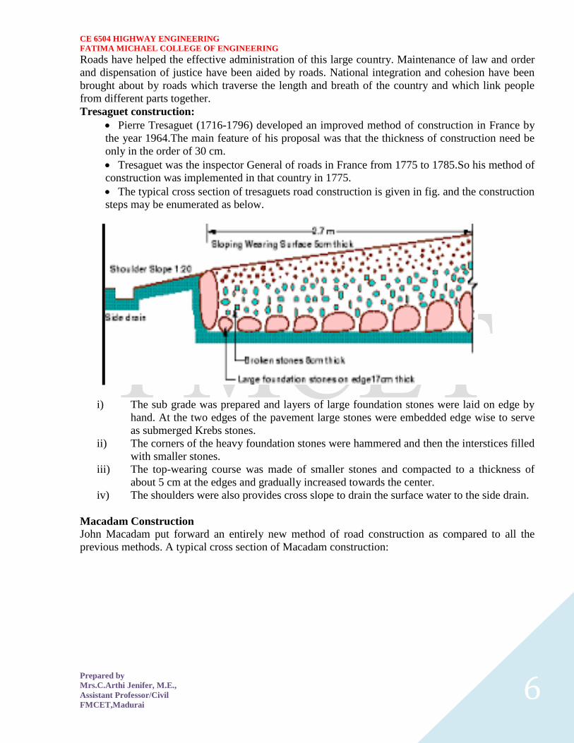
CE 6504 HIGHWAY ENGINEERING
FATIMA MICHAEL COLLEGE OF ENGINEERING
Prepared by
MrsCArthi Jenifer ME
Assistant ProfessorCivil
FMCETMadurai 6
Roads have helped the effective administration of this large country Maintenance of law and order
and dispensation of justice have been aided by roads National integration and cohesion have been
brought about by roads which traverse the length and breath of the country and which link people
from different parts together
Tresaguet construction
Pierre Tresaguet (1716-1796) developed an improved method of construction in France by
the year 1964The main feature of his proposal was that the thickness of construction need be
only in the order of 30 cm
Tresaguet was the inspector General of roads in France from 1775 to 1785So his method of
construction was implemented in that country in 1775
The typical cross section of tresaguets road construction is given in fig and the construction
steps may be enumerated as below
i) The sub grade was prepared and layers of large foundation stones were laid on edge by
hand At the two edges of the pavement large stones were embedded edge wise to serve
as submerged Krebs stones
ii) The corners of the heavy foundation stones were hammered and then the interstices filled
with smaller stones
iii) The top-wearing course was made of smaller stones and compacted to a thickness of
about 5 cm at the edges and gradually increased towards the center
iv) The shoulders were also provides cross slope to drain the surface water to the side drain
Macadam Construction
John Macadam put forward an entirely new method of road construction as compared to all the
previous methods A typical cross section of Macadam construction
CE 6504 HIGHWAY ENGINEERING
FATIMA MICHAEL COLLEGE OF ENGINEERING
Prepared by
MrsCArthi Jenifer ME
Assistant ProfessorCivil
FMCETMadurai 7
i) The importance of sub grade drainage and compaction were recognized and the sub
grade was compacted and was prepared with a cross slope of 1 in 36
ii) Macadam was the first person to suggest the heavy foundation stones are not at all
necessary to be placed at the bottom layer of construction
iii) Though the total thickness of construction was less than previous methods This
technique could serve the purpose in a better way
iv) The size of broken stones for the top layer was decided based on the stability under
animal drawn vehicles
Macadamrsquos method is the first method based on scientific thinking
The construction steps are
i) Sub grade is compacted and prepared with a cross slope of 1 in 36 up to a desired width
ii) Broken stones of a strong variety all passing through 5 cm size sieve were compacted to
a uniform thickness of 10cm
iii) The second layer of strong broken stones of size 375 cm was compacted to thickness of
10 cm
iv) The top layer consisted of stones of size less than 2 cm compacted to a thickness of about
5 cm The cross slope of pavement surface was also 1 in 36
Classification of roads
Road classification
The roads can be classified in many ways The classification based on speed and
accessibility is the most generic one Note that as the accessibility of road increases the
speed reducesAccordingly the roads can be classified as follows in the order of
increased accessibility and reduced speeds
Freeways Freeways are access-controlled divided highways Most freeways are
four lanes two lanes each direction but many freeways widen to incorporate
more lanes as they enter urban areas Access is controlled through the use of
interchanges and the type of interchange depends upon the kind of intersecting
road way (rural roads another freeway etc)
Expressways They are superior type of highways and are designed for high
CE 6504 HIGHWAY ENGINEERING
FATIMA MICHAEL COLLEGE OF ENGINEERING
Prepared by
MrsCArthi Jenifer ME
Assistant ProfessorCivil
FMCETMadurai 8
speeds (120 kmhr is common) high traffic volume and safety They are
generally provided with grade separations at intersections Parking loading and
unloading of goods and pedestrian traffic is not allowed on expressways
Highways They represent the superior type of roads in the country Highways are
of two types - rural highways and urban highways Rural highways are those
passing through rural areas (villages) and urban highways are those passing
through large cities and towns ie urban areas
Arterials It is a general term denoting a street primarily meant for through traffic
usually on a continuous route They are generally divided highways with fully or
partially controlled access Parking loading and unloading activities are usually
restricted and regulated Pedestrians are allowed to cross only at
intersectionsdesignated pedestrian crossings
Local streets A local street is the one which is primarily intended for access to
residence business or abutting property It does not normally carry large volume
of traffic and also it allows unrestricted parking and pedestrian movements
Collector streets These are streets intended for collecting and distributing traffic
to and from local streets and also for providing access to arterial streets Normally
full access is provided on these streets There are few parking restrictions except
during peak hours
Figure 1 Speed vs accessibility
CE 6504 HIGHWAY ENGINEERING
FATIMA MICHAEL COLLEGE OF ENGINEERING
Prepared by
MrsCArthi Jenifer ME
Assistant ProfessorCivil
FMCETMadurai 9
FACTORS AFFECTING HIGHWAY ALIGHNMENT
Design speed
Design speed is the single most important factor that affects the geometric design It
directly affects the sight distance horizontal curve and the length of vertical curves
Since the speed of vehicles vary with driver terrain etc a design speed is adopted for all
the geometric design
Design speed is defined as the highest continuous speed at which individual vehicles can
travel with safety on the highway when weather conditions are conducive Design speed
is different from the legal speed limit which is the speed limit imposed to curb a common
tendency of drivers to travel beyond an accepted safe speed Design speed is also
different from the desired speed which is the maximum speed at which a driver would
travel when unconstrained by either traffic or local geometry
Since there are wide variations in the speed adopted by different drivers and by different
types of vehicles design speed should be selected such that it satisfy nearly all drivers At
the same time a higher design speed has cascading effect in other geometric designs and
thereby cost escalation Therefore an 85th percentile design speed is normally adopted
This speed is defined as that speed which is greater than the speed of 85 of drivers In
some countries this is as high as 95 to 98 percentile speed
Topography
The next important factor that affects the geometric design is the topography It is easier to
construct roads with required standards for a plain terrain However for a given design speed the
construction cost increases multiform with the gradient and the terrain Therefore geometric design
standards are different for different terrain to keep the cost of construction and time of construction
under control This is characterized by sharper curves and steeper gradients
Other factors
CE 6504 HIGHWAY ENGINEERING
FATIMA MICHAEL COLLEGE OF ENGINEERING
Prepared by
MrsCArthi Jenifer ME
Assistant ProfessorCivil
FMCETMadurai 10
In addition to design speed and topography there are various other factors that affect the geometric
design and they are briefly discussed below
Vehicle The dimensions weight of the axle and operating characteristics of a vehicle
influence the design aspects such as width of the pavement radii of the curve clearances
parking geometrics etc A design vehicle which has standard weight dimensions and
operating characteristics are used to establish highway design controls to accommodate
vehicles of a designated type
Human The important human factors that influence geometric design are the mental and
psychological characteristics of the driver and pedestrians like the reaction time
Traffic It will be uneconomical to design the road for peak traffic flow Therefore a
reasonable value of traffic volume is selected as the design hourly volume which is
determined from the various traffic data collected The geometric design is thus based on
this design volume capacity etc
Environmental Factors like air pollution noise pollution etc should be given due
consideration in the geometric design of roads
Economy The design adopted should be economical as far as possible It should match
with the funds allotted for capital cost and maintenance cost
Others Geometric design should be such that the aesthetics of the region is not affected
Nagpur classification
In Nagpur road classification all roads were classified into five categories as National highways
State highways Major district roads Other district roads and village roads
National highways
They are main highways running through the length and breadth of India connecting major
ports foreign highways capitals of large states and large industrial and tourist centers
including roads required for strategic movements
It was recommended by Jayakar committee that the National highways should be the frame
on which the entire road communication should be based
All the national highways are assigned the respective numbers
For eg the highway connecting Delhi-Ambala-Amritsar is denoted as NH-1 (Delhi-
Amritsar) where as a bifurcation of this highway beyond Full under to Srinagar and Uri is
denoted as NH-1_A
They are constructed and maintained by CPWD
The total lengths of National highway in the country is 58112 Kms and constitute about 2
of total road networks of India and carry 40 of total traffic
State highways
They are the arterial roads of a state connecting up with the national highways of adjacent
states district headquarters and important cities within the state
They also serve as main arteries to and from district roads
Total length of all SH in the country is 1 37119 Kms
Major district roads
Important roads with in a district serving areas of production and markets connecting those
with each other or with the major highways
India has a total of 4 70000 Kms of MDR
CE 6504 HIGHWAY ENGINEERING
FATIMA MICHAEL COLLEGE OF ENGINEERING
Prepared by
MrsCArthi Jenifer ME
Assistant ProfessorCivil
FMCETMadurai 11
Other district roads
Roads serving rural areas of production and providing them with outlet to market centers or
other important roads like MDR or SH
Village roads
They are roads connecting villages or group of villages with each other or to the nearest
road of a higher category like ODR or MDR
India has 2650000 kms of ODR+VR out of the total 3315231 kms of all type of roads
Roads classification criteria
Apart from the classification given by the different plans roads were also classified based on some
other criteria They are given in detail below
Based on usage
This classification is based on whether the roads can be used during different seasons of the year
All-weather roads Those roads which are negotiable during all weathers except at major
river crossings where interruption of traffic is permissible up to a certain extent are called all
weather roads
Fair-weather roads Roads which are negotiable only during fair weather are called fair
weather roads
Based on carriage way
This classification is based on the type of the carriage way or the road pavement
Paved roads with hards surface If they are provided with a hard pavement course such
roads are called paved roads(eg stones Water bound macadam (WBM) Bituminous
macadam (BM) concrete roads)
Unpaved roads Roads which are not provided with a hard course of atleast a WBM layer
they is called unpaved roads Thus earth and gravel roads come under this category
Alignment The position or the layout of the central line of the highway on the ground is called the
alignment Horizontal alignment includes straight and curved paths Vertical alignment
includes level and gradients Alignment decision is important because a bad alignment
will enhance the construction maintenance and vehicle operating costs Once an
alignment is fixed and constructed it is not easy to change it due to increase in cost of
adjoining land and construction of costly structures by the roadside
Requirements The requirements of an ideal alignment are
The alignment between two terminal stations should be short and as far as
possible be straight but due to some practical considerations deviations may be
needed
The alignment should be easy to construct and maintain It should be easy for the
operation of vehicles So to the maximum extend easy gradients and curves
should be provided
It should be safe both from the construction and operating point of view
especially at slopes embankments and cutting It should have safe geometric
features
The alignment should be economical and it can be considered so only when the
initial cost maintenance cost and operating cost are minimum
CE 6504 HIGHWAY ENGINEERING
FATIMA MICHAEL COLLEGE OF ENGINEERING
Prepared by
MrsCArthi Jenifer ME
Assistant ProfessorCivil
FMCETMadurai 12
Factors controlling alignment
We have seen the requirements of an alignment But it is not always possible to satisfy all
these requirements Hence we have to make a judicial choice considering all the factors
The various factors that control the alignment are as follows
Obligatory points These are the control points governing the highway alignment
These points are classified into two categories Points through which it should
pass and points through which it should not pass Some of the examples are
o Bridge site The bridge can be located only where the river has straight
and permanent path and also where the abutment and pier can be strongly
founded The road approach to the bridge should not be curved and skew
crossing should be avoided as possible Thus to locate a bridge the
highway alignment may be changed
o Mountain While the alignment passes through a mountain the various alternatives are to either construct a tunnel or to go round the hills The suitability of the alternative depends on factors like topography site
conditions and construction and operation cost
o Intermediate town The alignment may be slightly deviated to connect an intermediate town or village nearby
These were some of the obligatory points through which the alignment should pass
Coming to the second category that is the points through which the alignment should not
pass are
Religious places These have been protected by the law from being acquired for
any purpose Therefore these points should be avoided while aligning
Very costly structures Acquiring such structures means heavy compensation
which would result in an increase in initial cost So the alignment may be deviated
not to pass through that point
Lakesponds etc The presence of a lake or pond on the alignment path would also
necessitate deviation of the alignment
Traffic The alignment should suit the traffic requirements Based on the origin-
destination data of the area the desire lines should be drawn The new alignment should
be drawn keeping in view the desire lines traffic flow pattern etc Geometric design
Geometric design factors such as gradient radius of curve sight distance etc also govern
the alignment of the highway To keep the radius of curve minimum it may be required
to change the alignment The alignments should be finalized such that the obstructions to
visibility do not restrict the minimum requirements of sight distance The design
standards vary with the class of road and the terrain and accordingly the highway should
be aligned Economy The alignment finalized should be economical All the three costs
ie construction maintenance and operating cost should be minimum The construction
cost can be decreased much if it is possible to maintain a balance between cutting and
filling Also try to avoid very high embankments and very deep cuttings as the
construction cost will be very higher in these cases
Road ecology
The features of the cross-section of the pavement influences the life of the pavement as
CE 6504 HIGHWAY ENGINEERING
FATIMA MICHAEL COLLEGE OF ENGINEERING
Prepared by
MrsCArthi Jenifer ME
Assistant ProfessorCivil
FMCETMadurai 13
well as the riding comfort and safety Of these pavement surface characteristics affect
both of these Camber kerbs and geometry of various cross-sectional elements are
important aspects to be considered in this regard They are explained briefly in this
chapter
Camber
Camber or cant is the cross slope provided to raise middle of the road surface in the
transverse direction to drain off rain water from road surface The objectives of providing
camber are
Surface protection especially for gravel and bituminous roads
Sub-grade protection by proper drainage
Quick drying of pavement which in turn increases safety
Too steep slope is undesirable for it will erode the surface Camber is measured in 1 in n
or n (Eg 1 in 50 or 2) and the value depends on the type of pavement surface The
value suggested by IRC for various categories of pavement is given in Table 1 The
common types of camber are parabolic straight or combination of them (Figure 1)
Figure 1 Different types of camber
Table 1 IRC Value
s for ca
mber
Heavy
Light
Surface
rain
type
rain
17
ConcreteBituminous
2
25
GravelWBM
3
30
Earthen
4
CE 6504 HIGHWAY ENGINEERING
FATIMA MICHAEL COLLEGE OF ENGINEERING
Prepared by
MrsCArthi Jenifer ME
Assistant ProfessorCivil
FMCETMadurai 14
Engineering surveys for alignment
The stages of the engineering surveys are a) Map study
b) Reconnaissance
c) Preliminary surveys
d) Final location and detailed surveys
Map study -
) In the topographic map to suggest the likely routes of roads In India topographic
maps are available from the survey of India with 15 or 30-meter contour intervals
) The main feature like rivers hills and valleys etc The probable alignment can be
located on the map from the following details available on the map
Alignment avoiding valleys ponds or lakes
When the road has to cross a row of hills possibility crossing through a mountain pass
Approximate location of bridge site for crossing rivers avoiding bend of the river
When a road is to be connected between two stations one of the top and the other on the foot
of the hill then alternate routes can be suggested keeping in view the permissible alignment
Suppose the scale of the contour map is known and then the contour intervals it is possible
to decide the length of road required between two consecutive contours keeping the gradient
within allowable limits
In the fig Let A and B be two stations to be connected by road AB is the shortest route
(Straight line) APQB is a steep route in which the gradient positively exceeds 1 in 20 as the
distance between the contour intervals is only about 200 meter
APLMNB is a route with an approximate slope of 1 in 20 whereas APEFGB is an alternate
alignment with the same gradient
Thus the map study also is possible to drop a certain route in view of any unavoidable
obstructions (or) undesirable ground enroute
Reconnaissance-
The second stage of surveys for highway location is the reconnaissance to examine the general
character of the area for deciding the most feasible routes for detailed studies
Some of the details to be collected during reconnaissance are given below
Valleys ponds lakes marshy land ridge hills permanent structures and other obstructions
along the route which are not available in the map
Approximate values of gradient length of gradients and radius of curves of alternate
alignments
Number and types of cross drainage structures maximum flood level and natural
groundwater level along the probable routes
Soil type along the routes from field identification tests and observation of geological
features
Sources of construction materials water and location of stone quarries
When the road passes through hilly or mountainous terrain additional data regarding the
geological formation types of rocks dip of strata seepage flow etc
Preliminary survey -
CE 6504 HIGHWAY ENGINEERING
FATIMA MICHAEL COLLEGE OF ENGINEERING
Prepared by
MrsCArthi Jenifer ME
Assistant ProfessorCivil
FMCETMadurai 15
The main objectives of the preliminary surveys are
To survey the various alternate alignments proposed after the reconnaissance and to collect
all the necessary physical information and details of topography drainage and soil
To compare the different proposals in view of the requirements of a good alignment
To estimate quantity of earthwork materials and other construction aspects and to work out
the cost of alternate proposals
To finalize the best alignment from all considerations
The procedure of the conventional methods of preliminary surveys the given steps
Primary survey -
For alternate alignments either secondary traverses (or) independent primary traverses may be
necessary
Topographical features -
All geographical and other man made features along the traverse and for a certain width on either
side surveyed and plotted
Leveling work -
Levelling work is also carried out side by side to give the centerline profiles and typical cross
sections The leveling work in the preliminary survey is kept to a minimum just sufficient to obtain
the approximate earthwork in the alternate alignments
Drainage studies -
Drainage investigations and hydrological data are collected so as to estimate the type number and
approximate size of cross and drainage structures
Soil survey -
The soil survey conducted at this stage helps to working out details of earthwork slopes suitability
of materials subsoil and surface drainage requirements and pavement type and the approximate
thickness requirements
Material survey -
The survey for naturally occurring materials like stone aggregates soft aggregates etc and
identification of suitable quarries should be made
Traffic survey -
Traffic surveys conducted in the region from basis for deciding the number of traffic lanes and
roadway width pavement design and economic analysis of highway project
Locations and functions
Final location and detailed survey - The alignment finalized at the design office after the preliminary survey is to be first located on the
field by establishing the centerline The detailed survey should be carried out for collecting the
information technology for the preparation of plans and construction details
Location -
The centerline of the road finalized in the drawings to be translated on the ground
during the location survey
Major and minor control points are established on the ground and center pegs are
driven checking the geometric design requirements
Detailed survey -
CE 6504 HIGHWAY ENGINEERING
FATIMA MICHAEL COLLEGE OF ENGINEERING
Prepared by
MrsCArthi Jenifer ME
Assistant ProfessorCivil
FMCETMadurai 16
Levels along his final centerline should be taken at all staked points Levelling work is to
great importance as the vertical alignment
A detailed soil survey is carried out to enable drawing of the soil profile
The data during the detailed survey should be elaborate and complete for preparing detailed
plans design and estimates of the project
Soil suitability analysis
The methodology for locating appropriate sites for each land use activity is guided by the intent to
minimize the possible adverse effects of development on the environment and on existing
communities and to emphasize the positive impacts of such development by locating them in a
most suitable location
This is achieved by examining a number of individual criteria assigning them relative levels of
importance as a whole and using a mathematical resultant model to identify the most suitable
location
By adopting this site suitability method it is possible to systematically identify the criteria
considered clearly document the relative importance of one criterion over another analyze the net
outcome using a Geographic Information System and then possibly revisit the mathematical
relationships in this ldquodecision modelrdquo
By revising the relative importance to identified criteria based upon the particular land use under
consideration it is possible to generate ldquosuitability mapsrdquo for each individual land use and then
generate a final composite land use that is based on a best possible collective suitability of multiple
land uses
To achieve this all the criteria are assigned a ldquorankrdquo denoting their relative levels of importance
within the suitability study These ranks are assigned as numeric values ranging from 1 to 10 with 1
reflecting a low level of importance and 10 reflecting a high level of importance For example
within the criteria of road networks national highways would have a different level of influence on
the suitability for a particular land use as compared with local roads Further the distance from each
of these features would further modify the relative suitability of a land use based on the proximity to
a particular type of road
Criteria for Site Suitability Analysis
The decision criteria for site selection are examined for assigning relative ranks and individual
feature weights based on the land use type for which suitability is being examined For benefit of
analysis the criteria under consideration in this paper activity are organized as
Critical Criteria Criteria that will be very significant in the site selection of the identified land use
and will act as key drivers in the selection of the geographic location These criteria can be clustered
into a single decision model and the outcome collectively reviewed These criteria have a strong
influence in the final suitability
Additional Criteria Criteria that will have to be examined one at a time to carefully assess its
relationship with the proposed land use activity These criteria have a positive influence in the final
suitability
CE 6504 HIGHWAY ENGINEERING
FATIMA MICHAEL COLLEGE OF ENGINEERING
Prepared by
MrsCArthi Jenifer ME
Assistant ProfessorCivil
FMCETMadurai 17
Constrained Criteria These criteria impose strong negative opportunities in the selection of areas
for the identified land use Consequently they inform of us of where the particular land use under
consideration should not be located These criteria serve to limit or exclude areas from the final
suitability
GIS Site Suitability Analysis Model We were developed a tourism site suitability analysis model
in ArcGIS - 931 which is shown in Figure -
CE 6504 HIGHWAY ENGINEERING
FATIMA MICHAEL COLLEGE OF ENGINEERING
Prepared by
MrsCArthi Jenifer ME
Assistant ProfessorCivil
FMCETMadurai 18
UNIT 2 GEOMETRIC DESIGN OF HIGHWAYS
Typical cross section of urban and rural roads
A cross section is a vertical plane (slice) taken at right angles to the road control line showing the
various elements that make up the roads structure It is normally viewed in the direction of
increasing chainage
The width of a roadway is an important design consideration to ensure that it is appropriately sized
to serve its function Because of the diversity within the County two major roadway categories have
been established 1 Rural Road Standards 2 Urban Road Standards Urban Road Standards will
serve those areas which tend to be more developed and need to provide for multiple users
(bicyclists pedestrians parallel parking etc) whereas many rural roads will primarily serve only
vehicular traffic
Cross sections are created to provide a visual guide depicting the initial interim and ultimate phase
cross sections for these road classifications The typical sections illustrated in the following pages
are recommendations tied to transportation planning aspects such as right‐of‐way lineage sidewalk
width etc Threshold daily traffic can be used as a guide for a starting point when determining
which cross section is most applicable
1 Rural Road Standards
The rural roadways will not typically require curb and gutter or sidewalk although the County may
require either or both in unique circumstances Widths of lanes and shoulders will vary depending
upon the specific classification and the potential traffic volume which the roadway may carry Roads
carrying fewer than 200 vehicles per day need not be paved or treated for dust control The need for
paved shoulders is also dependent upon the level of traffic and safety
Final design and construction details will be determined by the Public Works Department Final
Design and construction criteria taken into consideration may include but are not limited to use of
the roadway density of development topographical characteristics and nearby development For
construction in which only a portion of the ultimate cross‐section is intended to be completed the
partial design will need to allow for the eventual widening to the ultimate cross‐section The design
for the partial or interim cross‐section roadway will need to incorporate ultimate design information
to ensure that the first phase of roadway construction is appropriate and would not need to be
removed at a future date when the full width cross‐section is completed
2 Urban Road Standards
Three roadway classifications are identified for those areas that are associated with the communityrsquos
urban growth areas They include arterial collector and local street classifications Transportation
Plan shows the key elements of the urban road standards Urban road standards will include 12‐foot
lanes sidewalk and curb amp gutter arterials and collectors will also include a striped bike lane Turn
lanes may be necessary as determined by the County Since almost all of the municipalities have
different right‐of‐way cross sections adopted for their community it makes it very difficult for the
County to match them all Therefore the philosophy was to encourage a baseline amount of
right‐of‐way reservation that could ensure the adjacent community enough area for coordination of
future roadway improvements until such time the road
CE 6504 HIGHWAY ENGINEERING
FATIMA MICHAEL COLLEGE OF ENGINEERING
Prepared by
MrsCArthi Jenifer ME
Assistant ProfessorCivil
FMCETMadurai 19
CE 6504 HIGHWAY ENGINEERING
FATIMA MICHAEL COLLEGE OF ENGINEERING
Prepared by
MrsCArthi Jenifer ME
Assistant ProfessorCivil
FMCETMadurai 20
Cross sectional elements
Kerbs
Kerbs indicate the boundary between the carriage way and the shoulder or islands or footpaths Different types of kerbs are
CE 6504 HIGHWAY ENGINEERING
FATIMA MICHAEL COLLEGE OF ENGINEERING
Prepared by
MrsCArthi Jenifer ME
Assistant ProfessorCivil
FMCETMadurai 21
Low or mountable kerbs This type of kerbs is provided such that they
encourage the traffic to remain in the through traffic lanes and also allow the
driver to enter the shoulder area with little difficulty The height of this kerb is
about 10 cm above the pavement edge with a slope which allows the vehicle to
climb easily This is usually provided at medians and channelization schemes and
also helps in longitudinal drainage
Semi-barrier type kerbs When the pedestrian traffic is high these kerbs are
provided Their height is 15 cm above the pavement edge This type of kerb
prevents encroachment of parking vehicles but at acute emergency it is possible
to drive over this kerb with some difficulty
Barrier type kerbs They are designed to discourage vehicles from leaving the
pavement They are provided when there is considerable amount of pedestrian
traffic They are placed at a height of 20 cm above the pavement edge with a steep
batter
Submerged kerbs They are used in rural roads The kerbs are provided at
pavement edges between the pavement edge and shoulders They provide lateral
confinement and stability to the pavement
Figure 1 Different types of kerbs
Shoulders Shoulders are provided along the road edge and are intended for accommodation of
stopped vehicles serve as an emergency lane for vehicles and provide lateral support
for base and surface courses The shoulder should be strong enough to bear the weight
of a fully loaded truck even in wet conditions The shoulder width should be adequate
for giving working space around a stopped vehicle It is desirable to have a width of
46 m for the shoulders A minimum width of 25 m is recommended for 2-lane rural
highways in India Parking lanes
Parking lanes are provided in urban lanes for side parking Parallel parking is preferred
because it is safe for the vehicles moving on the road The parking lane should have a
minimum of 30 m width in the case of parallel parking
CE 6504 HIGHWAY ENGINEERING
FATIMA MICHAEL COLLEGE OF ENGINEERING
Prepared by
MrsCArthi Jenifer ME
Assistant ProfessorCivil
FMCETMadurai 22
Bus-bays
Bus bays are provided by recessing the kerbs for bus stops They are provided so that
they do not obstruct the movement of vehicles in the carriage way They should be at
least 75 meters away from the intersection so that the traffic near the intersections is not
affected by the bus-bay
Service roads Service roads or frontage roads give access to access controlled highways like freeways
and expressways They run parallel to the highway and will be usually isolated by a
separator and access to the highway will be provided only at selected points These roads
are provided to avoid congestion in the expressways and also the speed of the traffic in
those lanes is not reduced
Drainage
The pavement surface should be absolutely impermeable to prevent seepage of water into
the pavement layers Further both the geometry and texture of pavement surface should
help in draining out the water from the surface in less time
Footpath
Footpaths are exclusive right of way to pedestrians especially in urban areas They are
provided for the safety of the pedestrians when both the pedestrian traffic and vehicular
traffic is high Minimum width is 15 meter and may be increased based on the traffic
The footpath should be either as smooth as the pavement or more smoother than that to
induce the pedestrian to use the footpath
Right of way
Right of way (ROW) or land width is the width of land acquired for the road along its
alignment It should be adequate to accommodate all the cross-sectional elements of the
highway and may reasonably provide for future development To prevent ribbon
development along highways control lines and building lines may be provided Control
line is a line which represents the nearest limits of future uncontrolled building activity
in relation to a road Building line represents a line on either side of the road between
which and the road no building activity is permitted at all The right of way width is
governed by
Width of formation It depends on the category of the highway and width of
roadway and road margins
Height of embankment or depth of cutting It is governed by the topography and
the vertical alignment
Side slopes of embankment or cutting It depends on the height of the slope soil
type etc
Drainage system and their size which depends on rainfall topography etc
Sight distance considerations On curves etc there is restriction to the visibility
on the inner side of the curve due to the presence of some obstructions like
building structures etc
Reserve land for future widening Some land has to be acquired in advance
CE 6504 HIGHWAY ENGINEERING
FATIMA MICHAEL COLLEGE OF ENGINEERING
Prepared by
MrsCArthi Jenifer ME
Assistant ProfessorCivil
FMCETMadurai 23
Table 2 Desig
n speed in as per IRC (ruling and minimum)
Steep
Type
Plain
Rolling
Hilly
40-30
NSampSH
100-80
80-65
50-40
MDR
80-65
65-50
40-30
30-20
25-20
ODR
65-50
50-40
30-25
25-20
VR
50-40
40-35
25-20
anticipating future developments like widening of the road
Table 1 No
right of way for open areas
Roadway width in m
Road
Plain and
Mountainous and
classification
steep terrain
rolling terrain
Open areas
45
24
NHSH
18
MDR
25
15
15
ODR
12
9
VR
Built-up areas
20
NHSH
30
MDR
20
15
ODR
15
12
9
VR
10
CE 6504 HIGHWAY ENGINEERING
FATIMA MICHAEL COLLEGE OF ENGINEERING
Prepared by
MrsCArthi Jenifer ME
Assistant ProfessorCivil
FMCETMadurai 24
Horizontal curve
The presence of horizontal curve imparts centrifugal force which is a reactive force
acting outward on a vehicle negotiating it Centrifugal force depends on speed and radius
of the horizontal curve and is counteracted to a certain extent by transverse friction
between the tyre and pavement surface On a curved road this force tends to cause the
vehicle to overrun or to slide outward from the centre of road curvature For proper
design of the curve an understanding of the forces acting on a vehicle taking a horizontal
curve is necessary Various forces acting on the vehicle are illustrated in the figure 1
Figure 1 Effect of horizontal curve They are the centrifugal force (P) acting outward weight of the vehicle (W) acting
downward and the reaction of the ground on the wheels ( and ) The centrifugal
force and the weight is assumed to be from the centre of gravity which is at h units above
the ground Let the wheel base be assumed as b units The centrifugal force in
is given by
(1)
where is the weight of the vehicle in is the speed of the vehicle in is
the acceleration due to gravity in and is the radius of the curve in
The centrifugal ratio or the impact factor is given by
CE 6504 HIGHWAY ENGINEERING
FATIMA MICHAEL COLLEGE OF ENGINEERING
Prepared by
MrsCArthi Jenifer ME
Assistant ProfessorCivil
FMCETMadurai 25
(1)
The centrifugal force has two effects A tendency to overturn the vehicle about the outer
wheels and a tendency for transverse skidding Taking moments of the forces with
respect to the outer wheel when the vehicle is just about to override
At the equilibrium over turning is possible when
and for safety the following condition must satisfy
(2)
The second tendency of the vehicle is for transverse skidding ie When the the
centrifugal force is greater than the maximum possible transverse skid resistance due to
friction between the pavement surface and tyre The transverse skid resistance (F) is
given by
where and is the fractional force at tyre and and is the reaction at
tyre and is the lateral coefficient of friction and is the weight of the vehicle
This is counteracted by the centrifugal force (P) and equating
At equilibrium when skidding takes place (from equation1)
and for safety the following condition must satisfy
CE 6504 HIGHWAY ENGINEERING
FATIMA MICHAEL COLLEGE OF ENGINEERING
Prepared by
MrsCArthi Jenifer ME
Assistant ProfessorCivil
FMCETMadurai 26
(3)
Equation 2 and 3 give the stable condition for design If equation 2 is violated the vehicle
will overturn at the horizontal curve and if equation 3 is violated the vehicle will skid at
the horizontal
Curve Analysis of super-elevation
Super-elevation or cant or banking is the transverse slope provided at horizontal curve to
counteract the centrifugal force by raising the outer edge of the pavement with respect to
the inner edge throughout the length of the horizontal curve When the outer edge is
raised a component of the curve weight will be complimented in counteracting the effect
of centrifugal force In order to find out how much this raising should be the following
analysis may be done The forces acting on a vehicle while taking a horizontal curve with
super elevation is shown in figure 1
Figure 1 Analysis of super-elevation
Forces acting on a vehicle on horizontal curve of radius at a speed of are
the centrifugal force acting horizontally out-wards through the center of
gravity
the weight of the vehicle acting down-wards through the center of gravity and
the friction force between the wheels and the pavement along the surface
inward
CE 6504 HIGHWAY ENGINEERING
FATIMA MICHAEL COLLEGE OF ENGINEERING
Prepared by
MrsCArthi Jenifer ME
Assistant ProfessorCivil
FMCETMadurai 27
At equilibrium by resolving the forces parallel to the surface of the pavement we get where
friction
is the weight of the vehicle is the centrifugal force is the coefficient of
is the transverse slope due to superelevation Dividing by we get
CE 6504 HIGHWAY ENGINEERING
FATIMA MICHAEL COLLEGE OF ENGINEERING
Prepared by
MrsCArthi Jenifer ME
Assistant ProfessorCivil
FMCETMadurai 28
Step 1
Find for 75 percent of design speed neglecting ie
Step 2
If then else if go to step 3
Step 3
Find for the design speed and max ie If
then the maximum is safe for the design speed else go to
step 4
Step 4
Find the allowable speed for the maximum and
If then the design is adequate otherwise use speed adopt
control measures or look for speed control measures
Maximum and minimum super-elevation
Depends on (a) slow moving vehicle and (b) heavy loaded trucks with high CG IRC
specifies a maximum super-elevation of 7 percent for plain and rolling terrain while that
of hilly terrain is 10 percent and urban road is 4 percent The minimum super elevation is
2-4 percent for drainage purpose especially for large radius of the horizontal curve
Attainment of super-elevation
1 Elimination of the crown of the cambered section by
1 Rotating the outer edge about the crown The outer half of the cross slope
is rotated about the crown at a desired rate such that this surface falls on
the same plane as the inner half
2 Shifting the position of the crown This method is also known as diagonal
crown method Here the position of the crown is progressively
shifted outwards thus increasing the width of the inner half of cross section
progressively
2 Rotation of the pavement cross section to attain full super elevation byThere are
two methods of attaining super elevation by rotating the pavement
1 Rotation about the center line The pavement is rotated such that the inner
edge is depressed and the outer edge is raised both by half the total amount
of super elevation ie by with respect to the centre
2 Rotation about the inner edge Here the pavement is rotated raising the
outer edge as well as the centre such that the outer edge is raised by the
full amount of super elevation with respect to the inner edge
Horizontal Transition Curves
CE 6504 HIGHWAY ENGINEERING
FATIMA MICHAEL COLLEGE OF ENGINEERING
Prepared by
MrsCArthi Jenifer ME
Assistant ProfessorCivil
FMCETMadurai 29
Transition curve is provided to change the horizontal alignment from straight to circular
curve gradually and has a radius which decreases from infinity at the straight end
(tangent point) to the desired radius of the circular curve at the other end (curve point)
There are five objectives for providing transition curve and are given below
1 to introduce gradually the centrifugal force between the tangent point and the
beginning of the circular curve avoiding sudden jerk on the vehicle This
increases the comfort of passengers
2 to enable the driver turn the steering gradually for his own comfort and security
3 to provide gradual introduction of super elevation and
4 to provide gradual introduction of extra widening
5 to enhance the aesthetic appearance of the road
Type of transition curve
Different types of transition curves are spiral or clothoid cubic parabola and Lemniscate
IRC recommends spiral as the transition curve because
1 it fulfills the requirement of an ideal transition curve that is
1 rate of change or centrifugal acceleration is consistent (smooth) and
2 radius of the transition curve is at the straight edge and changes to at
the curve point ( ) and calculation and field implementation is
very easy
Length of transition curve The length of the transition curve should be determined as the maximum of the following
three criteria rate of change of centrifugal acceleration rate of change of super elevation
and an empirical formula given by IRC Rate of change of centrifugal acceleration
At the tangent point radius is infinity and hence centrifugal acceleration is zero At the
end of the transition the radius R has minimum value R The rate of change of
centrifugal acceleration should be adopted such that the design should not cause
discomfort to the drivers If is the rate of change of centrifugal acceleration it can be
written as
Therefore the length of the transition curve in is
CE 6504 HIGHWAY ENGINEERING
FATIMA MICHAEL COLLEGE OF ENGINEERING
Prepared by
MrsCArthi Jenifer ME
Assistant ProfessorCivil
FMCETMadurai 30
(1)
where is the rate of change of centrifugal acceleration given by an empirical formula
suggested by by IRC as below
(2) 2 Rate of introduction of super-elevation
Raise ( ) of the outer edge with respect to inner edge is given by
The rate of change of this raise from to is achieved
gradually with a gradient of in over the length of the transition curve (typical range
of is 60-150) Therefore the length of the transition curve is
(3)
3 By empirical formula
IRC suggest the length of the transition curve is minimum for a plain and rolling terrain
(4)
and for steep and hilly terrain is
(5)
CE 6504 HIGHWAY ENGINEERING
FATIMA MICHAEL COLLEGE OF ENGINEERING
Prepared by
MrsCArthi Jenifer ME
Assistant ProfessorCivil
FMCETMadurai 31
and the shift as
(
6
) The length of the transition curve is the maximum of
equations 1 3 and 4or5 ie
(
7
Case (a)
For single lane roads
(
1
)
Therefore
(
2
)
Figure 1 Set-back for single lane roads (
CE 6504 HIGHWAY ENGINEERING
FATIMA MICHAEL COLLEGE OF ENGINEERING
Prepared by
MrsCArthi Jenifer ME
Assistant ProfessorCivil
FMCETMadurai 32
For multi lane roads if is the distance between centerline of the road and the centerline
of the inner lane then
(3)
(4)
Figure 2 Set-back for multi-lane roads ( )
Case (a)
For single lane roads
(1)
Therefore
(2)
Gradient
Gradient is the rate of rise or fall along the length of the road with respect to the
horizontal While aligning a highway the gradient is decided for designing the vertical
curve Before finalizing the gradients the construction cost vehicular operation cost and
the practical problems in the site also has to be considered Usually steep gradients are
avoided as far as possible because of the difficulty to climb and increase in the
CE 6504 HIGHWAY ENGINEERING
FATIMA MICHAEL COLLEGE OF ENGINEERING
Prepared by
MrsCArthi Jenifer ME
Assistant ProfessorCivil
FMCETMadurai 33
construction cost More about gradients are discussed below
Effect of gradient
The effect of long steep gradient on the vehicular speed is considerable This is
particularly important in roads where the proportion of heavy vehicles is significant Due
to restrictive sight distance at uphill gradients the speed of traffic is often controlled by
these heavy vehicles As a result not only the operating costs of the vehicles are
increased but also capacity of the roads will have to be reduced Further due to high
differential speed between heavy and light vehicles and between uphill and downhill
gradients accidents abound in gradients
Representation of gradient
The positive gradient or the ascending gradient is denoted as and the negative gradient as The deviation angle is when two grades meet the angle which
measures the change of direction and is given by the algebraic difference between the two
grades
steep gradient while 1 in 50 = 2 representation is illustrated in the figure 1
Example 1 in 30 = 333 is a
is a flatter gradient The gradient
CE 6504 HIGHWAY ENGINEERING
FATIMA MICHAEL COLLEGE OF ENGINEERING
Prepared by
MrsCArthi Jenifer ME
Assistant ProfessorCivil
FMCETMadurai 34
Figure 1 Representation of gradient
Types of gradient
Many studies have shown that gradient upto seven percent can have considerable effect
on the speeds of the passenger cars On the contrary the speeds of the heavy vehicles are
considerably reduced when long gradients as flat as two percent is adopted Although
flatter gradients are desirable it is evident that the cost of construction will also be very
high Therefore IRC has specified the desirable gradients for each terrain However it
may not be economically viable to adopt such gradients in certain locations steeper
gradients are permitted for short duration Different types of grades are discussed below
Ruling gradient
The ruling gradient or the design gradient is the maximum gradient with which the
designer attempts to design the vertical profile of the road This depends on the terrain
length of the grade speed pulling power of the vehicle and the presence of the horizontal
curve In flatter terrain it may be possible to provide flat gradients but in hilly terrain it
is not economical and sometimes not possible also The ruling gradient is adopted by the
designer by considering a particular speed as the design speed and for a design vehicle
with standard dimensions But our country has a heterogeneous traffic and hence it is not
possible to lay down precise standards for the country as a whole Hence IRC has
recommended some values for ruling gradient for different types of terrain
Limiting gradient
This gradient is adopted when the ruling gradient results in enormous increase in cost of
construction On rolling terrain and hilly terrain it may be frequently necessary to adopt
limiting gradient But the length of the limiting gradient stretches should be limited and
must be sandwiched by either straight roads or easier grades
Exceptional gradient
Exceptional gradient are very steeper gradients given at unavoidable situations They
should be limited for short stretches not exceeding about 100 metres at a stretch In
mountainous and steep terrain successive exceptional gradients must be separated by a
minimum 100 metre length gentler gradient At hairpin bends the gradient is restricted to
25
Critical length of the grade
The maximum length of the ascending gradient which a loaded truck can operate without
undue reduction in speed is called critical length of the grade A speed of 25 kmph is a
CE 6504 HIGHWAY ENGINEERING
FATIMA MICHAEL COLLEGE OF ENGINEERING
Prepared by
MrsCArthi Jenifer ME
Assistant ProfessorCivil
FMCETMadurai 35
reasonable value This value depends on the size power load grad-ability of the truck
initial speed final desirable minimum speed
Minimum gradient
This is important only at locations where surface drainage is important Camber will take
care of the lateral drainage But the longitudinal drainage along the side drains require
some slope for smooth flow of water Therefore minimum gradient is provided for
drainage purpose and it depends on the rain fall type of soil and other site conditions A
minimum of 1 in 500 may be sufficient for concrete drain and 1 in 200 for open soil
drains are found to give satisfactory performance Sight distance available from a point is the actual distance along the road surface which a driver
from a specified height above the carriage way has visibility of stationary or moving objects
Sight distance required by drivers applies to both geometric design of highways and for
traffic control The sight distance situations are considered in the design
i) Stopping or absolute minimum sight distance
ii) Safe overtaking or passing sight distance
iii) Safe sight distance for entering into uncontrolled intersections
Apart from the three situations mentioned above the following sight distance are considered by the
IRC in highway design
Intermediate sight distance
This is defined as twice the stopping sight distance when overtaking sight distance
cannot be provided intermediate sight distance is provided to give limited overtaking opportunities
to fast vehicles
Head light sight distance
This is the distance visible to a driver during night driving under the illumination of the
vehicle head lights
Stopping sight distance
The minimum sight distance available on a highway at any spot should be of sufficient
length to stop a vehicle traveling at design speed safely without collision with any other obstruction
The absolute minimum sight distance is therefore equal to the stopping sight distance
which is also sometimes called nonpassing sight distance The sight distance available on a road to a
driver at any instance depends on
i) Features of the road
ii) Height of the drivers eye above the road surface
iii) Height of the object above the road surface
The distance within which a motor vehicle can be stopped depends upon the factors listed below
a) Total reactions time of the driver
b) Speed of vehicle
c) Efficiency of breaks
d) Frictional resistance between the road and tyres
e) Gradient of the road
Total reaction time
) Reaction time of the driver is the time taken from the instant the object is visible to the
driver to the instant the brakes are effectively applied
) The total reaction time may be split up into two parts
CE 6504 HIGHWAY ENGINEERING
FATIMA MICHAEL COLLEGE OF ENGINEERING
Prepared by
MrsCArthi Jenifer ME
Assistant ProfessorCivil
FMCETMadurai 36
i) Perception time
ii) Brake reaction time
PIEV theory
According to this theory the total reaction time of the driver is split into four parts
i) Perception
ii) Intellection
iii) Emotion
iv) Volition
Speed of Vehicle
The stopping distance depends very much on the speed of the vehicle first during the
total reaction time of the driver the distance moved by the vehicle will depend on the speed
Efficiency of brakes
The braking efficiency is said to be 100 percent if the wheels are fully licked preventing
them from rotating on application of the brakes This will result in 100 percent skidding which is
normally undesirable except in utmost emergency
Frictional resistance between road and tyres
The frictional resistance developed between road and tyres or the skid resistance depends
on the type and condition of the road surface and the tyres IRC has specified a design friction
coefficient of 035 to 04 depending upon the speed to be used for finding the braking distance in the
calculation of stopping sight distance
Analysis of stopping distance
i) The distance traveled by the vehicle during the total reaction time known as lag
distance
ii) The distance traveled by the vehicle after the application of the brakes is known as
braking distance
Overtaking sight distance
The minimum distance open to the vision of the driver of a vehicle intending to overtake
slow vehicle ahead with safety against the traffic of opposite direction is known as the minimum
overtaking sight distance(OSD) or Safe passing sight distance available
The overtaking sight distance is the distance measured along the center of the road which
a driver with his eye level 12m above the road surface can see the top of an object 12m above the
road surface
Some of the important factors on which the minimum overtaking sight distance required
a) Speed of
i) overtaking vehicle
ii) overtaken vehicle
iii) The vehicle coming from opposite direction
b) Distance between the overtaking and overtaken vehicles the minimum spacing
depends on the steeds
a) Skill and reaction time of the driver
b) Rate of acceleration of overtaking vehicle
c) Gradient of the road
Criteria for sight distance requirements on highway
) The absolute minimum sight distance required throughout the length of the road is the
SSD which should invariably be provided at all places
CE 6504 HIGHWAY ENGINEERING
FATIMA MICHAEL COLLEGE OF ENGINEERING
Prepared by
MrsCArthi Jenifer ME
Assistant ProfessorCivil
FMCETMadurai 37
) On horizontal curves the obstruction on the inner side of the curves should be cleared
to provide the required set back distance and absolute minimum sight distance
) On vertical summit curves the sight distance requirement may be fulfilled by proper
design of the vertical alignment
Hairpin bent
TYPES OF CURVES ON HILL ROADS
The following are the important types of curves provided on hill Roads-
1 Hair-Pin Curves
2 Salient Curves
3 Re-entrant Curves 1 Hair-pin curves - The curve in a hill road which changes its direction through an angle of 180
degree or so down the hill on the same side is known as hair-pin curve
A Hair-Pin Bend
This curve is so called because it conforms to the shape of a hair-pin The bend so formed at the
hair-pin curve in a hill road is known as hair-pin bend This type of curve should be located on a
hill side having the minimum slope and maximum stability It must also be safe from view point of
landslides and ground water Hair-pin bends with long arms and farther spacing are always
preferred They reduce construction problems and expensive protective works Hair-pin curves or
bends of serpentine nature are difficult to negotiate and should therefore be avoided as far as
possible
Salient curves - The curves having their convexity on the outer edges of a hill road are called
salient curves The centre of curvature of a salient curve lies towards the hill side This type of curve
occurs in the road length constructed on the ridge of a hill the bend so formed at the salient curve in
a hill road known as corner bend
Salient curves are very dangerous for fast moving traffic At such a curve or at corner bend the
portion of projecting hill side is usually cut down to improve the visibility as shown in fig (Re-
entrant curve) The outer edge of the road at such a curve is essentially provided with a parapet wall
for protection of the vehicles from falling down the hill slope
CE 6504 HIGHWAY ENGINEERING
FATIMA MICHAEL COLLEGE OF ENGINEERING
Prepared by
MrsCArthi Jenifer ME
Assistant ProfessorCivil
FMCETMadurai 38
3 Re-entrant curves - The curves having their convexity on the inner edge of a hill road are called
re-entrant curves
Re-entrant curves
The centre of curvature of a re-entrant curves lies away from the hill side This type of curve occurs
in the road length constructed in the calley of a hill
These curves are less dangereous as they provide adequate visibility to the fast moving traffic At
such curves the parapet wall is provided only for safety of fast moving traffic
CE 6504 HIGHWAY ENGINEERING
FATIMA MICHAEL COLLEGE OF ENGINEERING
Prepared by
MrsCArthi Jenifer ME
Assistant ProfessorCivil
FMCETMadurai 39
UNIT ndash III DESIGN OF RIGID AND FLEXIBLE PAVEMENTS
COMPARISON OF RIGID AND FLEXIBLE PAVEMENTS
The comparisons are
i) Design precision
A cement concrete pavement is amerable to a much more precise structural analysis
than a flexible pavement Flexible pavements designs are mainly empirical Computer aided analysis
of layered system is making the flexible pavement design more exact than hitherto
ii) Life
) Cement concrete slabs of a thin section constructed in the early 1940rsquos are still in
existence in India though many of them have cracked badly and a few of them have been ripped
open and rebuilt in recent ties
) A major project in cement concrete road construction between Agra and Mathura It can
safely be said that a well-designed concrete slab has a life of about 40 years
) Compared to this the life of a flexible pavement generally varies from 10 to 20 years
iii) Maintenance
) A well-designed cement concrete pavement needs very little maintenance The only
maintenance needed is I respect of joints
) The surface is unaffected by spillage of oil and lubricants bituminous surfaces on the
other hand need great inputs in maintenance
) The surface is affected by spillage of oil and lubricants The surface is also affected by
natural weathering agents like air water ad temperature changes
) A cement concrete pavement on the other hand needs a small amount for maintaining
joints
iv) Initial cost
) The argument so far used against a cement concrete slab is that it is much more costly
than a flexible pavement
) The latter specifications no doubt represent the rock-bottom needs of a road in India but
these specifications can hardly provide a smooth and durable surface
v) Stage construction ) Road construction is generally done adopting a policy of stage construction especially for
low volume roads As traffic grows additional layers in the form of water bound macadam and
superior surfacing are added on
) Initial outlay is minimum and additional outlays are in keeping with traffic growth This is
a great advantage when dealing with new roads in an atmosphere of austerity
vi) Availability of materials
) Cement bitumen stone aggregates and gravelsand are the major materials involved in
pavement Construction Cement has been in serious short supply in the country for the past many
decades
) Bitumen is also not available plentifully in India There is also the danger of the entire oil
reserves in the world shrinking during the next two or three decades
) In locations where stone aggregates are scarce cement concrete may have an advantage
for flexible pavements
vii) Surface characterstics
CE 6504 HIGHWAY ENGINEERING
FATIMA MICHAEL COLLEGE OF ENGINEERING
Prepared by
MrsCArthi Jenifer ME
Assistant ProfessorCivil
FMCETMadurai 40
) A good cement concrete surface is smooth and free from rutting potholes and
corrugations In a bituminous surface it is only the asphaltic concrete surface that can give
comparable rideablity
) A well-constructed cement concrete pavement surface can have a permanent nonskid
surface A bituminous surface can also be designed to have a good skid resistant surface
viii) Utility location
) In cement concrete slabs proper thought has to be given to locate utilities such as water
pipes telephone lines and electric cables
) It is difficult to rip open the slab and restore it to be the original condition if any changes
in the utilities lines are to be made
ix) Glame and night visibility
) Concrete pavements have a gray color which can cause glam under sunlight Colored
cement can reduce the grave
) On the other hand bituminous roads need more street lighting
x) Traffic dislocation during construction
) A cement concrete pavement requires 28 days before it can be thrown open to traffic On
the other hand a bituminous surface can be thrown open to traffic shortly after it is rolled
xi) Environmental considerations during construction
) The process of heating of bitumen and aggregates and mixing them together on hot mix
plants can prove to be much more hazardous to the environment than cement concrete construction
where no heating of any material is involved
xii) Overall economy on a life cycle basis
) A good road is costly to construct but once constructed such a road requires little
maintenance and results in savings in vehicle operating costs
) The comparative economy of a flexible pavement and a rigid pavement has proved that on
overall economic considerations
Types of pavement structure
Based on the structural behavior pavements are generally classified into three
categories
i) Flexible pavements
ii) Rigid pavements
iii) Semi rigid pavements
Flexible pavements
) Flexible pavements are those which on the whole have low or negligible flexural
strength and are rather flexible in their structural action under the loadsThe flexible pavement
layers reflect the deformation of the lower layers on to the surface of the layer
) A flexible pavement consists of four components(i) Soil subgrade (ii) sub base
course (iii) base course (iv) Surface course
CE 6504 HIGHWAY ENGINEERING
FATIMA MICHAEL COLLEGE OF ENGINEERING
Prepared by
MrsCArthi Jenifer ME
Assistant ProfessorCivil
FMCETMadurai 41
) The flexible pavement layers transmit the vertical or compressive stresses to the lower layers
by grain to grain transfer through the points of contact in the granular structure A well
compacted granular structure consisting of strong added aggregate can transfer the compressive
stresses
) The load spreading ability of this layer therefore depends on the type of the materials and mix
design factors Bituminous concrete is one of the best flexible pavements layer materials Other
materials which fall under the group are all granular materials with or without bituminous
binder granular base and sub base course materials
) The vertical compressive stress is maximum on the pavement surface directly under the wheel
and is equal to the contact pressure under the wheel The flexible pavement may be constructed
in a number of layers and the top layer has to be strongest as the highest compressive stresses
) Flexible pavements are commonly designed using empirical design charts or equations taking
into account some of the design factors there are also semi empirical and theoretical design
methods
Rigid pavements
) Rigid pavements are those which possess note flexural strength or flexural rigidity
The stresses are not transferred from grain to grain to the lower layers as in the ease of flexible
pavements layers
) The rigid pavements are made of Portland cement concrete plain reinforced or
prestressed concrete The plain cement concrete slabs are expected to take up about 40 kgcm2
flexural stress
) The rigid pavement has the slab action and is capable of transmitting the wheel
load stresses through a wider area below The main point of difference in the structural behavior
of rigid pavement as compared to the flexible pavement is that the critical condition of stress in
the rigid pavement is the maximum flexural stress occurring in the slab due to wheel load and
the temperature changes whereas in the flexible pavement
) As the rigid pavement slab has tensile strength tensile stresses are developed due
to the bending of the slab under wheel load and temperature variations Thus the types of
stresses developed and their distribution within the cement concrete slab are quirt different
) The cement concrete pavement slab can very well serve as a wearing surface as
well an effective base course The rigid pavement structure consists of a cement concrete slab
below which a granular base or sub base course may be provided
) Though the cement concrete slab can also be laid directly over the soil subgrade
consists of fine grained soil
) the rigid pavements are usually designed and the stresses are analyzed using the
elastic theory assuming the pavements as a n elastic plate resting over an elastic or a viscous
foundation
Semi rigid pavements
) when bonded materials like the pozzolanic concrete lean cement concrete or soil
cement are used in the base course or sub base course layer the pavement layer has considerably
higher flexural strength than the common flexible pavement layers
) when this intermediate class of materials are used in the base or sub base course
layer of the pavements they are called semi rigid pavements
CE 6504 HIGHWAY ENGINEERING
FATIMA MICHAEL COLLEGE OF ENGINEERING
Prepared by
MrsCArthi Jenifer ME
Assistant ProfessorCivil
FMCETMadurai 42
) This third category of semi rigid pavement are either designed as flexible
pavements with some correction factors to find the thickness requirements based on experience
or by using a new design approach
) The semi rigid pavement materials have low resistance to impact and abrasion and
therefore are usually provided with flexible pavement surface course
Various functions of pavement components
The functions are
Soil sub grade and its evaluation
) The soil sub grade is a layer of natural soil prepared to receive the layers of pavement
materials placed over it It is essential that at no time the soil sub grade is overstressed it means that
the pressure transmitted on the top of the sub grade is within the allowable limit
) Many tests are known for measuring the strength properties of the sub grades Some of the
tests have been standardized for the use The common strength test for the evaluation of soil
subgrade is
i) California bearing ratio test
ii) California resistance value test
iii) Triaxial compression test
iv) Plate bearing test
CALIFORNIA BEARING RATIO (CBR) TEST
It is evolved for the empirical method of flexible pavement design The CBR test is carried
out either in the laboratory on prepared specimens or in the field by taking in situ measurements
California resistance value
It is found by using have been stabliometerThis test is used in an empirical method of
flexible pavement design based on soil strength
Triaxial test
It is the most important soil strength but still the test is not very commonly used in structural
design of pavements
Plate bearing test
It is carried out using a relatively large diameter plate to evaluate the load supporting
capacity of supporting power of the pavement layers The results are plate bearing tests are used in
flexible pavement design method like McLeod method on based on layer system analysis by
brumister
Sub base and base courses and their evaluation
) There layers are made of broken stones bound or unbound aggreagatesome times in sub
base course a layer of stabilized soil(or) Selected granular soil is also used
) however at the sub base course it is desirable to use smaller size graded aggregates When
the sub grade consists of fine grained soil and when the pavement carries heavy wheel loads
CE 6504 HIGHWAY ENGINEERING
FATIMA MICHAEL COLLEGE OF ENGINEERING
Prepared by
MrsCArthi Jenifer ME
Assistant ProfessorCivil
FMCETMadurai 43
) Sub base course primarily has the similar function as of the base course and is provided
with inferior materials than of base course Base courses are used under rigid pavement for
i) Preventing pumping
ii) Protecting the sub grade against frost action
) Thus the fundamental purpose of abase course and sub base course is to provide a stress
transmitting medium to spread the surface wheel loads in such manner
) The sub base and base course layers may be evaluated by suitable strength or stability test
like plate bearing CBR test
WEARING COURSE AND ITS EVALUATION
) The purpose of the wearing course is to give a smooth riding surface that is dense It
resists pressure exerted by tyres and takes up wear and tear due to the traffic
) Wearing course also offers a water tight layer against the surface water infiltration The
flexible pavement normally a bituminous surfacing is used as a wearing course
) In rigid pavements the cement concrete acts like a base course as well as wearing course
Most popular test in use is marshal stability test where in the optimum content of bitumen binder is
worked out based on the stability density
) Plate bearing test and Bankelman beam test are also sometimes made use of for evaluating
the wearing course and the pavement as a whole
Various factors to be considered in pavement design and the significance
Pavement design consists of two parts
i) Mix design of materials to be used in each pavement component layer Thickness design of the
pavement and the component layers
The various factors to be considered for the design of pavements are given below
i) Design wheel load
ii) Sub grade soil
iii) Climatic factors
iv) Pavement component layers
v) Environmental factors
vi) Special factors in the design of different types of pavements
Design wheel load
The various wheel load factors to be considered in pavement design are
i) Maximum wheel load
ii) Contact pressure
iii) Dual or multiple wheel loads
iv) Repetition of loads
Maximum wheel load
The wheel load configurations are important to know the way in which the loads of a given
vehicle are applied on the pavement surface
) For highways the maximum legal axle load as specified by Indian road congress is 8170
kg with a maximum equivalent single wheel load of 4085 kg
) The evaluation for vertical stress computations under a uniformly distribute of circular
load based on Boussineqrsquos theory is given by
CE 6504 HIGHWAY ENGINEERING
FATIMA MICHAEL COLLEGE OF ENGINEERING
Prepared by
MrsCArthi Jenifer ME
Assistant ProfessorCivil
FMCETMadurai 44
2
322
3
1
za
zpz
σz = vertical stress at depth z
P= surface pressure
Z=depth at which σz computed
A=radius of loaded area
Contact pressure
Generally the wheel load is assumed to be distributed over a circular area But by
measurement of the imprints of tyers with different load and inflation pressures Three terms in use
with reference to tyre pressure are
Tyre pressure
Inflation pressure
Contact pressure
Tyre pressure and inflation pressure mean exactly the same the contact pressure is found to be more
than tyre pressure when the tyre pressure is less than 7 kgm2 and it is vice versa when the tyre
pressure exceeds this value
Contact pressure can be measured by the relationship
Load on wheel
Contact pressure = ----------------------------------------
Contact area or area of imprint
The general variation between the tyre pressure and measured contact pressure is shown in this fig
The ratio of contact pressure to type pressure is defined as rigidity factor Thus value of rigidity
factor is 10 for an average tyre pressure of 7 Kgcm2This value is higher than unity for lower type
pressures and less than unity for tyre pressures higher than 7 kgcm2
Equivalent single wheel load (ESWL)
) The maximum wheel load within the specified limit and to carry greater load it is
necessary to provide dual wheel assembly to the rear axles of the roads vehicles
) In other words the pressure at a certain depth below the pavement surface cannot be
obtained by numerically adding the pressure caused by any one wheel
) The effect is in between the single load and two times load carried by one wheel The load
dispersion is assumed to be at an angle of 450In the dual wheel load assembly let d be the clear gap
between the two wheels S be the spacing between the centers of the wheels and a be the radius of
the circular contact area of each wheel Then S = (d + 2a)
) ESWL may be determined based on either equivalent deflection or equivalent stress
criterianMultiple wheel loads are convert to ESWL and this value is used in pavement design The
ESWL is usually determined by the equivalent stress criterion using a simple graphical method
CE 6504 HIGHWAY ENGINEERING
FATIMA MICHAEL COLLEGE OF ENGINEERING
Prepared by
MrsCArthi Jenifer ME
Assistant ProfessorCivil
FMCETMadurai 45
) A straight line relationship is assumed between ESWL and depth on log scales For
determining ESWL the plot is made as shown in fig
) Two points A and B are plotted on the log-log graph with coordinates of A (Pd2) and
B(2p2s)line AB is a plot which is the focus of points where any single wheel load is equivalent to a
certain set of dual wheels
) To Calculate the ESWL for a dual assembly it is essential to estimate a design thickness of
the pavement If the design thickness so obtained is equal to the estimated thickness then the ESWL
calculations could be considered as correct Otherwise trials are made
) In heavy trucks and trailers the load on each wheel may be further reduced by multiple
wheels and tandem axles
Repetition of loads
) The deformation of load pavement (or) sub grade due to a single application of wheel load
may be small It required carrying out traffic surveys for accounting the factor of repetitions for
wheel loads in the design of pavement
) Data collected are converted to some constant equivalent wheel loads Equivalent wheel
load is a single load equivalent to the repeated applications of any particular wheel load on a
pavement which requires the same thickness and strength of pavements
) McLeod has given a procedure for evolving equivalent load factors for designing flexible
pavements
Various methods of flexible pavement design
) The flexible pavement is built with number of layers In the design process it is to be
ensured that under the application of load none of the layers is overstressed
) The maximum intensity of stresses occurs in the top layer of the pavement The
magnitude of load stresses reduces at lower layers
) In the design of flexible pavements it has yet not been possible to have a rational design
method wherein design process and service behavior of the pavement can be expressed by
mathematical laws
) Flexible pavement design methods are accordingly either empirical or semi empirical In
these methods the knowledge and experience gained on the behavior of the pavements in the past
are usefully utilized
Various approaches of flexible pavement design may be thus classified into three groups
i) Empirical method
ii) Semi-empirical or Semi theoretical method
iii) Theoretical method
) Empirical methods are either based on physical properties or strength parameters of soil
sub grade When the design is based on stress strain function and modified base on experience it
may be called semi-empirical or semi-theoretical There are design methods based on theoretical
analysis and mathematical computations
Out of the flexible pavement design method available is
i) Group index method
ii) California bearing ratio method
iii) California R value (or) Stabiliometer method
iv) Triaxial test method
CE 6504 HIGHWAY ENGINEERING
FATIMA MICHAEL COLLEGE OF ENGINEERING
Prepared by
MrsCArthi Jenifer ME
Assistant ProfessorCivil
FMCETMadurai 46
v) McLeod method
vi) Burmister method
Group index method
) Group index value is an arbitrary index assigned to the soil type in numerical equations
base on the percent fines liquid limit and plasticity index
) The design chart for group index method for determining the pavement thickness is given
in fig
The traffic volume in this method is divided in three groups
Traffic volume No of vehicles per day
Light Less than 50
Medium 50 to 300
Heavy Over 300
The design of the pavement thickness by this method first the G1 value of the soil is found the
anticipated traffic is estimated and is designated as light medium or heavy as indicated
The G1 method of pavement design is essentially an empirical method based on physical properties
of the subgrade soil This method does not consider the strength characteristics of the subgrade soil
and therefore is open to question regarding the reliability of the design based on the index properties
of the soil only
California bearing ratio method
) California division of highways in the USA developed CBR method for
pavement design The majority of design curves developed later are base on the original curves
proposed by OJporter
) One of the chief advantages of CBR method is the simplicity of the test procedure
The CBR tests were carried out by the California state highway department on existing pavement
layers including subgrade sub base and base course
) Based on the extensive CBR test data collected on pavement which behaved
satisfactory and those which failed an empirical design chart was developed correlating the CBR
value and the pavement thickness The basis of the design chart is that a material with a given CBR
required a certain thickness of pavement layer as a cover
) A higher load needs a thicker pavement layer to protect the sub grade Design
curves correlating the CBR value with total pavement thickness cover were developed by the
California state highway department for wheel loads of 3175kg and 5443 kg representing light and
heavy traffic The design curves are shown in this fig
It is possible to extend the CBR design curves for various loading conditions nusing the expression
t= 2
1
1751
pCBRp
t=2
1
751
A
CBR
p
Hence
CE 6504 HIGHWAY ENGINEERING
FATIMA MICHAEL COLLEGE OF ENGINEERING
Prepared by
MrsCArthi Jenifer ME
Assistant ProfessorCivil
FMCETMadurai 47
t= pavement thickness cm
p=Wheel load kg
CBR= California bearing ratio percent
P=tyre pressure kgcm2
A= area of contactcm2
IRC Recommendations
a) The CBR tests should be performed on remoulded soils in the laboratory The specimens should
be prepared by static compaction wherever possible and otherwise by dynamic compaction
b) For the design of new roads the sub grade soil sample should be compacted at OMC to proctor
density whenever suitable compaction equipment
c) The CBR test samples may be soaked in water for four days period before testing the annual
rainfall is less than 50 cm and the water table is too deep to affect the sub grade and imperable
surfacing is provided to carrying out CBR test
d) If the maximum variations in CBR value of the three specimens exceed the specified limits the
design CBR should be average of at least six samples
e) The top 50 cm of sub grade should be compacted at least up to 95 to 100 percent of proctor
density
f) An estimate of the traffic should be carried by the road pavements at the end of expected in view
the existing traffic and probable growth rate of traffic
g) The traffic for the design is considered in units of heavy vehicles per day in both directions and is
divided into seven categories A to G The design thickness is considered applicable for single axle
loads up to 8200 kg and tandom axle loads up to 14500 kg
h) When sub base course materials contain substantial proportion of aggregates of size above 20mm
the CBR value of these materials would not be valid for the design of subsequent layers above them
The CBR method of pavement design gives the total thickness requirement of the pavement above a
sub grade and thickness value would remain the same quality of materials used in component layers
California resistance value method
) In this design method based on stabliometer R-value and cohesiometer C-value
Based on performance data it was established by pavement thickness varies directly with R value
and algorithm of load repetitions It varies inversely with fifth root of c valueThe expression for
pavement thickness is given by the empirical equation
T=
5
1
1 90
C
RTK
Hence
T=total thickness of pavement cm
K=Numerical constant 0166
T1=traffic index
R= stabiliometer resistance value
C=Cohesiometer value
CE 6504 HIGHWAY ENGINEERING
FATIMA MICHAEL COLLEGE OF ENGINEERING
Prepared by
MrsCArthi Jenifer ME
Assistant ProfessorCivil
FMCETMadurai 48
In the design of flexible pavements based on California resistance value method for the following
data are needed
) R-value of soil subgrade
) T1 value
) Equivalent C-value
) R value of soil subgrade is obtained from the test using stablio meterThe
computation of T1 value has been explained
Equivalent C-value
) The cohesion meter value c is obtained for each layer of pavement material
separately from tests However the composite or equivalent C-value of the pavement may be
estimated if the thickness of each component layer and the c-value of the material of the layer are
known
) while designing a pavement as the thickness of the pavement is not known it is
easier if the pavement is first assumed to consist of any one material like gravel base course with
known C-value
) Subsequently the individual thickness of each layer is converted in terms of gravel
equivalent by using relationship
5
1
1
2
2
1
C
C
t
t
) t1 and t2 are the thickness values of any two pavement layersc1 and c2 are their
corresponding cohesiometer values
CE 6504 HIGHWAY ENGINEERING
FATIMA MICHAEL COLLEGE OF ENGINEERING
Prepared by
MrsCArthi Jenifer ME
Assistant ProfessorCivil
FMCETMadurai 49
UNIT 4 MATERIAL AND MAINTENANCE
SUMMIT CURVE
Summit curves are vertical curves with gradient upwards They are formed when two
gradients meet as illustrated in figure 1 in any of the following four ways
1 When a positive gradient meets another positive gradient [figure 1a]
2 When positive gradient meets a flat gradient [figure 1b]
3 When an ascending gradient meets a descending gradient [figure 1c]
4 When a descending gradient meets another descending gradient [figure 1d]
Type of Summit Curve
Many curve forms can be used with satisfactory results the common practice has been to
use parabolic curves in summit curves This is primarily because of the ease with it can
be laid out as well as allowing a comfortable transition from one gradient to another
Although a circular curve offers equal sight distance at every point on the curve for very
small deviation angles a circular curve and parabolic curves are almost congruent
Furthermore the use of parabolic curves were found to give excellent riding comfort
Figure 1 Types of summit curves
Design Consideration
In determining the type and length of the vertical curve the design considerations are
comfort and security of the driver and the appearance of the profile alignment Among
these sight distance requirements for the safety are most important on summit curves
The stopping sight distance or absolute minimum sight distance should be provided on
these curves and where overtaking is not prohibited overtaking sight distance or
intermediate sight distance should be provided as far as possible When a fast moving
vehicle travels along a summit curve there is less discomfort to the passengers This is
because the centrifugal force will be acting upwards while the vehicle negotiates a
summit curve which is against the gravity and hence a part of the tyre pressure is
relieved Also if the curve is provided with adequate sight distance the length would be
sufficient to ease the shock due to change in gradient Circular summit curves are
identical since the radius remains same throughout and hence the sight distance From
CE 6504 HIGHWAY ENGINEERING
FATIMA MICHAEL COLLEGE OF ENGINEERING
Prepared by
MrsCArthi Jenifer ME
Assistant ProfessorCivil
FMCETMadurai 50
this point of view transition curves are not desirable since it has varying radius and so the
sight distance will also vary The deviation angles provided on summit curves for
highways are very large and so the simple parabola is almost congruent to a circular arc
between the same tangent points Parabolic curves are easy for computation and also it
had been found out that it provides good riding comfort to the drivers It is also easy for
field implementation Due to all these reasons a simple parabolic curve is preferred as
summit curve Length of the summit curve
The important design aspect of the summit curve is the determination of the length of the
curve which is parabolic As noted earlier the length of the curve is guided by the sight
distance consideration That is a driver should be able to stop his vehicle safely if there is
an obstruction on the other side of the road Equation of the parabola is given by
where where N is the deviation angle and is the length of the In
deriving the length of the curve two situations can arise depending on the uphill and
downhill gradients when the length of the curve is greater than the sight distance and the
length of the curve is greater than the sight distance
Let is the length of the summit curve is the SSDISDOSD is the deviation angle
drivers eye height (12 m) and the height of the obstruction then the length of the
summit curve can be derived for the following two cases The length of the summit curve
can be derived from the simple geometry as shown below
Case a Length of summit curve greater than sight distance( )
Figure 1 Length of summit curve ( )
The situation when the sight distance is less than the length of the curve is shown in
figure 1
CE 6504 HIGHWAY ENGINEERING
FATIMA MICHAEL COLLEGE OF ENGINEERING
Prepared by
MrsCArthi Jenifer ME
Assistant ProfessorCivil
FMCETMadurai 51
(1)
Case b Length of summit curve less than sight distance
The second case is illustrated in figure 1
Figure 1 Length of summit curve
CE 6504 HIGHWAY ENGINEERING
FATIMA MICHAEL COLLEGE OF ENGINEERING
Prepared by
MrsCArthi Jenifer ME
Assistant ProfessorCivil
FMCETMadurai 52
From the basic geometry one can write
(1)
Therefore for a given and to get minimum differentiate the above equation
with respect to and equate it to zero Therefore
Solving the quadratic equation for
(2)
Now we can substitute back to get the value of minimum value of for a given
and Therefore
Solving for
CE 6504 HIGHWAY ENGINEERING
FATIMA MICHAEL COLLEGE OF ENGINEERING
Prepared by
MrsCArthi Jenifer ME
Assistant ProfessorCivil
FMCETMadurai 53
(3) (4
CE 6504 HIGHWAY ENGINEERING
FATIMA MICHAEL COLLEGE OF ENGINEERING
Prepared by
MrsCArthi Jenifer ME
Assistant ProfessorCivil
FMCETMadurai 54
When stopping sight distance is considered the height of drivers eye above the road
surface ( ) is taken as 12 metres and height of object above the pavement surface ( )
is taken as 015 metres If overtaking sight distance is considered then the value of
drivers eye height ( ) and the height of the obstruction ( ) are taken equal as 12
metres
Valley curve
Valley curve or sag curves are vertical curves with convexity downwards They are
formed when two gradients meet as illustrated in figure 1 in any of the following four
ways
Figure 1 Types of valley curve
1 When a descending gradient meets another descending gradient [figure 1a]
2 When a descending gradient meets a flat gradient [figure 1b]
3 When a descending gradient meets an ascending gradient [figure 1c]
4 When an ascending gradient meets another ascending gradient [figure
Design considerations
There is no restriction to sight distance at valley curves during day time But visibility is
reduced during night In the absence or inadequacy of street light the only source for
visibility is with the help of headlights Hence valley curves are designed taking into
account of headlight distance In valley curves the centrifugal force will be acting
downwards along with the weight of the vehicle and hence impact to the vehicle will be
more This will result in jerking of the vehicle and cause discomfort to the passengers
Thus the most important design factors considered in valley curves are (1) impact-free
movement of vehicles at design speed and (2) availability of stopping sight distance
under headlight of vehicles for night driving
For gradually introducing and increasing the centrifugal force acting downwards the best
shape that could be given for a valley curve is a transition curve Cubic parabola is
generally preferred in vertical valley curves See figure 1
CE 6504 HIGHWAY ENGINEERING
FATIMA MICHAEL COLLEGE OF ENGINEERING
Prepared by
MrsCArthi Jenifer ME
Assistant ProfessorCivil
FMCETMadurai 55
Figure 1 Valley curve details
During night under headlight driving condition sight distance reduces and availability of
stopping sight distance under head light is very important The head light sight distance
should be at least equal to the stopping sight distance There is no problem of overtaking
sight distance at night since the other vehicles with headlights could be seen from a
considerable distance
Length of the valley curve
The valley curve is made fully transitional by providing two similar transition curves of
equal length The transitional curve is set out by a cubic parabola where
The length of the valley transition curve is designed based on two criteria
1 comfort criteria that is allowable rate of change of centrifugal acceleration is
limited to a comfortable level of about
2 safety criteria that is the driver should have adequate headlight sight distance at
any part of the country
Comfort criteria
The length of the valley curve based on the rate of change of centrifugal acceleration that
will ensure comfort Let is the rate of change of acceleration the minimum radius of
the curve is the design speed and is the time then is give
CE 6504 HIGHWAY ENGINEERING
FATIMA MICHAEL COLLEGE OF ENGINEERING
Prepared by
MrsCArthi Jenifer ME
Assistant ProfessorCivil
FMCETMadurai 56
For a cubic parabola the Value Safety criter Length of the valley curve for headlight distance may be determined for two conditions
(1) length of the valley curve greater than stopping sight distance and (2) length of the
valley curve less than the stopping sight distance of for length is given by
Case 1 Length of valley curve greater than stopping sight distance ( )
The total length of valley curve is greater than the stopping sight distance SSD The
sight distance available will be minimum when the vehicle is in the lowest point in the
valley This is because the beginning of the curve will have infinite radius and the bottom
of the curve will have minimum radius which is a property of the transition curve The
case is shown in figure 1
Figure 1 Valley curve case 1
From the geometry of the figure we have
CE 6504 HIGHWAY ENGINEERING
FATIMA MICHAEL COLLEGE OF ENGINEERING
Prepared by
MrsCArthi Jenifer ME
Assistant ProfessorCivil
FMCETMadurai 57
(1)
where is the deviation angle in radians is the height of headlight beam is the
head beam inclination in degrees and is the sight distance The inclination is 1
degree
Case 2 Length of valley curve less than stopping sight distance ( )
The length of the curve is less than SSD In this case the minimum sight distance is
from the beginning of the curve The important points are the beginning of the curve and
the bottom most part of the curve If the vehicle is at the bottom of the curve then its
headlight beam will reach far beyond the endpoint of the curve whereas if the vehicle is
at the beginning of the curve then the headlight beam will hit just outside the curve
Therefore the length of the curve is derived by assuming the vehicle at the beginning of
the curve The case is shown in figure 1
From the figure
(1) Note that the above expression is approximate and is satisfactory because in practice the gradients
are very small and is acceptable for all practical purposes We will not be able to know prior to
which case to be adopted Therefore both has to be calculated and the one which satisfies the
condition is adopted
1 Flexible pavement
2 Rigid pavement
Flexible pavement
These pavements reflect the deformation of sub grade and the subsequent layers to the
surface
Rigid pavement
The rigid characteristic of the pavement are associated with rigidity or flexural strength
CE 6504 HIGHWAY ENGINEERING
FATIMA MICHAEL COLLEGE OF ENGINEERING
Prepared by
MrsCArthi Jenifer ME
Assistant ProfessorCivil
FMCETMadurai 58
or slab action so the load is distributed over a wide area of sub grade soil
Flexible pavement Definition
These pavements reflect the deformation of sub grade and the subsequent layers to the
surface Flexible usually asphalt is laid with no reinforcement or with a specialized
fabric reinforcement that permits limited flow or repositioning of the roadbed under
ground changes
The design of flexible pavement is based on load distributing characteristic of the
component layers The black top pavement including water amp gravel bound macadam fall
in this category
Flexible pavement on the whole has low or negligible flexible strength flexible in their
structural action) The flexible pavement layers transmit the vertical or compressive
stresses to the lower layers by grain transfer through contact points of granular structure
The vertical compressive stress is maximum on the pavement surface directly under the
wheel load and is equal to contact pressure under the wheels Due to the ability to
distribute the stress to large area in the shape of truncated cone the stresses get decreased
in the lower layer
As such the flexible pavement may be constructed in a number of layers and the top
layer has to be strongest as the highest compressive stresses
To be sustained by this layer in addition to wear and tear the lower layer have to take
up only lesser magnitude of stress as there is no direct wearing action die to traffic loads
therefore inferior material with lower cast can be used in the lower layers
Rigid pavement Definition
The rigid characteristic of the pavement are associated with rigidity or flexural strength
or slab action so the load is distributed over a wide area of sub grade soil Rigid pavement
is laid in slabs with steel reinforcement
The rigid pavements are made of cement concrete either plan reinforced or prestressed
concrete
Critical condition of stress in the rigid pavement is the maximum flexural stress occurring in the slab due to wheel load and the temperature changes
Rigid pavement is designed and analyzed by using the elastic theory
CE 6504 HIGHWAY ENGINEERING
FATIMA MICHAEL COLLEGE OF ENGINEERING
Prepared by
MrsCArthi Jenifer ME
Assistant ProfessorCivil
FMCETMadurai 59
UNIT-5 EVALUATION AND MAINTENANCE OF PAVEMENTS
TRAFFIC PARAMETERS
Design life
Design life is the number of years (or number of standard axle repetitions) for which the
pavement is being designed A pavement is expected to serve satisfactorily within the
design life For concrete pavements 20 to 40 years may be assumed as the design life
(PCA 1984 IRC58 2002)
Basic design principle
Though different approaches for concrete pavement design are suggested in various
guidelines the design principles tend to remain similar across different guidelines for
example PCA (1994) Austroads (2004) NCHRP (2004) IRC58 (2002) etc except the
AASHTO (1993) provisions which is based on empirical approach The basic steps
involved in the design of concrete pavement method can be summarized as follows
The developed stresses due to load for a trial thickness of the concrete slab are
calculated for various loading configuration and the critical one is chosen The
axle loads are generally divided into different axle load groups and the load
stresses are calculated individually
The ratio between the load stress and Modulus of Rupture (MOR) is known as
stress ratio The stress ratio determines how many repetitions the pavement can
sustain (ie allowable traffic repetitions) for the individual axle load group If the
stress ratio is 055 or lower it can withstand virtually infinite number of traffic
repetitions (PCA 1984)
The ratio between the allowable repetitions to the expected traffic repetitions is
the damage fraction The calculation process is repeated for various axle loads
(sometimes for various seasons or various timings of the day) and the sum of
individual damage fractions (c u m u l a t i v e fatigue damage) should be less
than equal to one for pavement design being safe If found unsafe the trial
thickness is changed and the design process is repeated
The design process may also include considerations for temperature stress
moisture stresses and erosion distress
A brief discussion on concrete pavement design approaches suggested by various design
practices viz PCA method (1984) Austroads method (2004) AASHTO method (1993)
NCHRP mechanistic-empirical method (2004) and the Indian Roads Congress (IRC)
method (2002) are placed in the following
Portland cement Association (PCA) Method
The PCA method is based on Westergaard Picket and Rays work and further theoretical
analysis by Finite Element Method (Huang 1993) The data used to develop the PCA
method is generated from various road tests like ASSHO road test Arlington test
(conducted by PCA) Bates test road and Maryland road test (PCA 1984) The PCA
design method is based on the following two considerations (PCA 1984)
The fatigue damage on the concrete slab due to repetitive application of traffic
load is estimated The cumulative fatigue damage principle is used to estimate the
design thickness of the slab Edge stress between the mid-ways of the
CE 6504 HIGHWAY ENGINEERING
FATIMA MICHAEL COLLEGE OF ENGINEERING
Prepared by
MrsCArthi Jenifer ME
Assistant ProfessorCivil
FMCETMadurai 60
transverse joint is taken as critical configuration
The stresses due to warping and curling (due to temperature and moisture
gradient) are not considered in the fatigue analysis as per PCA recommendation
because most of the time the stresses generated are subtractive to the load stress
The possibility of erosion of pavement materials placed below the concrete slab is
evaluated The rate at which the slab is deflected due to axle load is used as a
criterion for erosion Theoretically it can be shown that a thin pavement with
smaller deflection basin is subjected to faster rate of deflection compared to
thicker slab Hence thin slab is more susceptible to erosion In a similar way the
cumulative erosion damage is calculated for individual axle load groups If this
value is greater than one then the design needs to be revised
Austroads method
Austroads method has been adopted from PCA (1984) approach with modifications
suited to Australian conditions (Austroads 2004) A bound mix or lean cement concrete is
used as sub-base material For a given CBR value of the subgrade and given thickness of
cemented sub-base the effective subgrade strength can be obtained from the chart
provided Figure-19 schematically shows such a chart For different levels of traffic
Austroads (2004) suggests minimum values of the base thicknesses to be provided
CE 6504 HIGHWAY ENGINEERING
FATIMA MICHAEL COLLEGE OF ENGINEERING
Prepared by
MrsCArthi Jenifer ME
Assistant ProfessorCivil
FMCETMadurai 61
figure-19 Schematic diagram of Austroads (2004) chart for estimation of effective
subgrade strength
As per Astroads (2004) the concrete pavement slab thickness for a given expected
traffic repetitions is designed considering the (i) flexural fatigue of the concrete slab and
the (ii) subgrade erosion arising out of repeated deflections For both the considerations
equations are suggested to calculate the allowable traffic repetitions If the allowable
traffic is less than the expected traffic the design is revised by increasing the slab
thickness The concrete shoulders adopted are of integral type or structural type
AASHTO method
The AASHTO method (1993) for design of concrete pavement has evolved from the
AASHO road test (AASHO 1962) The AASHTO pavement design follows an empirical
approach Pavement performance in terms of present serviceability index ( PSI ) loss of
serviceability sub-grade and sub-base strength cumulative traffic properties of concrete
joint load transfer efficiency drainage condition overall standard deviation and
reliability are the input parameters considered in the pavement design
The PSI value of the fresh pavement is assumed as 45 and the pavement is deemed to
have failed when the PSI value reaches 25 The resilient moduli of the subgrade and sub-
base materials are determined in the laboratory simulating the seasonal moisture content
and stress situation Suggested values are also available for given moisture content
plasticity index etc The composite modulus of sub-grade reaction (k) is estimated from
modulus of sub-grade reaction and elastic modulus of sub-base for various seasons and
the depth of rigid foundation and the thickness of the sub-base
Design equation as well nomographs are available to estimate the slab thickness (D) from
these input parameters
NCHRP mechanistic-empirical (M-E) metho
The NCHRP (2004) has recently developed concrete pavement design procedure based
on mechanistic-empirical (M-E) approach This approach attempts to reduce the extent of
empiricism prevalent in the existing AASHTO (1993) guidelines This proposed NCHRP
pavement design system is modular in nature that is the design approach can be
modified by parts (as and when new knowledge is available) without disrupting the
overall design procedure This approach also can take care of various wheel-axle loa
configuration
As per this approach trial thickness of the slab is first assumed and the stress strain and
displacement values are obtained From these values the performance of the pavement in
terms of distresses (such as faulting cracking) and smoothness and predicted If these
predicted performance parameters does not satisfy the required performance for a given
reliability
The design approach includes a large data-base as input parameters for example average
daily traffic traffic growth rate traffic composition hourly weather data on air
temperature precipitation wind speed percentage sunshine relative humidity pavement
material engineering parameters ground water depth infiltration drainage hydraulic
conductivity thermal conductivity heat capacity etc The temperature stress is
considered in this method but the temperature profile is linearized to enhance
computational efficiency (NCHRP 2004)
CE 6504 HIGHWAY ENGINEERING
FATIMA MICHAEL COLLEGE OF ENGINEERING
Prepared by
MrsCArthi Jenifer ME
Assistant ProfessorCivil
FMCETMadurai 62
INDIAN ROADS CONGRESS (IRC) METHOD
The Indian Roads Congress (IRC) guidelines IRC58 (2002) has adopted the
Westergaards equation to estimate load stress and Brdaburys equation to estimate
temperature stress The load stress is highest at the corner of the slab lesser in edge and
least in the interior The order of variation of temperature stress is just the reverse of this
As per IRC58 (2002) it is recommended that the design needs to be done for edge stress
condition and subsequently check needs to be performed for corner stress condition so as
to finalize the design The following are the steps followed as per IRC58 (2002)
guideline for the design of concrete pavement
The input parameters are obtained to formulate the design problem The joint
spacing and the slab dimensions are decided If there is a bound sub-base layer
over the subgrade a suitable value of effective k is to be adopted
A trial thickness of the concrete slab is assumed
The edge stress is estimated for various axle loads from the given charts Figure-
20 schematically shows such a chart The cumulative fatigue damage principle for
fatigue is applied to check the adequacy of the slab thickness
The sum of edge stress due to load for the highest axle load group and the
temperature stress should be less than the MOR of concrete otherwise the design
is revised
The adequacy of corner stress is checked with respect to MOR value and
accordingly the design is finalized Westergaards corner stress formula
Figure-20 Schematic diagram of IRC58 chart for estimation of load stress at the edge
(IRC58 2002)
CE 6504 HIGHWAY ENGINEERING
FATIMA MICHAEL COLLEGE OF ENGINEERING
Prepared by
MrsCArthi Jenifer ME
Assistant ProfessorCivil
FMCETMadurai 63
estimation of corner stress due to load and the corner stress due to temperature is
assumed to be zero
Estimation of layer thicknesses
The thickness of the pavement is adjusted in such a way that the stress strain
developed is less than the allowable values obtained from past performance
information
The two major modes of structural failure of pavement are fatigue and rutting
o Fatigue Traffic applies repetitive load to the pavement surface and the
cracks start from bottom the bound layer slab and propagate upwards
When the extent of surface cracks reaches a predefined level the
pavement is said to have failed due to flexural fatigue
FUNCTIONAL DESIGN
The functional pavement design involves considerations of skid resistance roughness
surface distresses reflectivity of pavement surface etc The functional pavement design
considers mainly the surface features of a pavement
Drainage design
A road needs to be designed in such a way that the rain snow precipitation is drained off
the pavement and its surroundings A suitable surface drainage system for the pavement
is designed for this purpose Some water however will percolate into the pavement from
its top surface and needs to be taken out of the pavement - this is done by providing an
internal drainage system to the pavement Water will also try to enter into the pavement
from bottom due to capillary rise or due to rise in water table A suitably designed sub-
surface drainage system tries to avoid such a problem
PAVEMENT THICKNESS DESIGN CHARTS
For the design of pavements to carry traffic in the range of 1 to 10 msa use chart 1 and for
traffic in the range 10 to 150 msa use chart 2 of IRC37 2001 The design curves relate
pavement thickness to the cumulative number of standard axles to be carried over the
design life for different sub-grade CBR values ranging from 2 to 10 The design
charts will give the total thickness of the pavement for the above inputs The total
thickness consists of granular sub-base granular base and bituminous surfacing The
individual layers are designed based on the the recommendations given below and the
subsequent tables
Pavement composition
Sub-base
Sub-base materials comprise natural sand gravel laterite brick metal crushed
stone or combinations thereof meeting the prescribed grading and physical
requirements The sub-base material should have a minimum CBR of 20 and
30 for traffic upto 2 msa and traffic exceeding 2 msa respectively Sub-base
usually consist of granular or WBM and the thickness should not be less than 150
mm for design traffic less than 10 msa and 200 mm for design traffic
Base
The recommended designs are for unbounded granular bases which comprise
CE 6504 HIGHWAY ENGINEERING
FATIMA MICHAEL COLLEGE OF ENGINEERING
Prepared by
MrsCArthi Jenifer ME
Assistant ProfessorCivil
FMCETMadurai 64
conventional water bound macadam (WBM) or wet mix macadam (WMM) or
equivalent confirming to MOST specifications The materials should be of good
quality with minimum thickness of 225 mm for traffic up to 2 msa an 150 mm for
traffic
Bituminoussurfacing The surfacing consists of a wearing course or a binder
course plus wearing course The most commonly used wearing courses are
surface dressing open graded premix carpet mix seal surfacing semi-
dense bituminous concrete and bituminous concrete For binder course
MOST specifies it is desirable to use bituminous macadam (BM) for traffic
upto o 5 msa and dense bituminous macadam (DBM) for traffic more than 5
msa
Numerical example
Design the pavement for construction of a new bypass with the following data
1 Two lane carriage way
2 Initial traffic in the year of completion of construction = 400 CVPD (sum of both
directions)
3 Traffic growth rate = 75
4 Design life = 15 years
5 Vehicle damage factor based on axle load survey = 25 standard axle per
commercial vehicle
6 Design CBR of subgrade soil = 4
Solution
1 Distribution factor = 075
2
3 Total pavement thickness for CBR 4 and traffic 72 msa from IRC37 2001
chart1 = 660 mm
4 Pavement composition can be obtained by interpolation from Pavement Design
Catalogue (IRC37 2001)
1 Bituminous surfacing = 25 mm SDBC + 70 mm DBM
2 Road-base = 250 mm WBM
3 sub-base = 315 mm granular material of CBR not less than 30
CE 6504 HIGHWAY ENGINEERING
FATIMA MICHAEL COLLEGE OF ENGINEERING
Prepared by
MrsCArthi Jenifer ME
Assistant ProfessorCivil
FMCETMadurai 65
Generally bound base layers are used for concrete pavement construction As per Indian
specification some example of such base layers are Dry Lean Concrete (DLC) Roller
Compacted Concrete (RCC) (IRC15-2002)
The concrete slab is generally of M40 to M50 grade of concrete as
per Indian specifications and is called as paving quality concrete (PQC)
(IRC15-2002)
BITUMINOUS PAVEMENT
The subgrade is a compacted soil layer
The base and sub-base course could be made up of bound or unbound granular layer As
per Indian specifications (MORTampH 2001) some examples of base or sub-base layers
are Granular sub-base(GSB) Water Bound Macadam (WBM) Wet Mix Macadam
(WMM) etc
The binder course is made up bituminous material As per Indian specifications
(MORTampH 2001) some examples of binder course are Bituminous Macadam (BM)
Dense Bituminous Macadam (DBM) etc
The wearing course is the top bituminous layer which is comes in contact to the
vehicle tyre Wearing course provides impermeability to the pavement surface
against water percolation (Chakroborty and Das 2003) The binder course and wearing
course together are called bituminous surfacing
IRC METHOD OF FLEXIBLE PAVEMENT MIX DESIGN
These guidelines will apply to design of flexible pavements for Expressway National Highways
State Highways Major District Roads and other categories of roads Flexible pavements are
considered to include the pavements which have bituminous surfacing and granular base and sub-
base courses conforming to IRC MOST standards These guidelines apply to new pavements
Design criteria
The flexible pavements has been modeled as a three layer structure and stresses and strains at
critical locations have been computed using the linear elastic model To give proper consideration
to the aspects of performance the following three types of pavement distress resulting from
repeated (cyclic) application of traffic loads are considered
1 Vertical compressive strain at the top of the sub-grade which can cause sub-grade
deformation resulting in permanent deformation at the pavement surface
2 Horizontal tensile strain or stress at the bottom of the bituminous layer which can cause
fracture of the bituminous layer
3 Pavement deformation within the bituminous layer
CE 6504 HIGHWAY ENGINEERING
FATIMA MICHAEL COLLEGE OF ENGINEERING
Prepared by
MrsCArthi Jenifer ME
Assistant ProfessorCivil
FMCETMadurai 66
While the permanent deformation within the bituminous layer can be controlled by meeting the
mix design requirements thickness of granular and bituminous layers are selected using the
analytical design approach so that strains at the critical points are within the allowable limits For
calculating tensile strains at the bottom of the bituminous layer the stiffness of dense bituminous
macadam (DBM) layer with 6070 bitumen has been used in the analysis
FAILURE CRITERIA
Critical locations in pavement
A and B are the critical locations for tensile strains Maximum value of the strain is
adopted for design C is the critical location for the vertical subgrade strain since the
maximum value of the occurs mostly at C
CE 6504 HIGHWAY ENGINEERING
FATIMA MICHAEL COLLEGE OF ENGINEERING
Prepared by
MrsCArthi Jenifer ME
Assistant ProfessorCivil
FMCETMadurai 67
Fatigue Criteria
Bituminous surfacings of pavements display flexural fatigue cracking if the tensile strain
at the bottom of the bituminous layer is beyond certain limit The relation between the
fatigue life of the pavement and the tensile strain in the bottom of the bituminous layer
was obtained as
(1)
in which is the allowable number of load repetitions to control fatigue cracking and
is the Elastic modulus of bituminous layer The use of equation 1 would result in
fatigue cracking of 20 of the total area
Rutting Criteria
The allowable number of load repetitions to control permanent deformation can be
expressed as
(2)
is the number of cumulative standard axles to produce rutting of 20 mm
CE 6504 HIGHWAY ENGINEERING
FATIMA MICHAEL COLLEGE OF ENGINEERING
Prepared by
MrsCArthi Jenifer ME
Assistant ProfessorCivil
FMCETMadurai 68
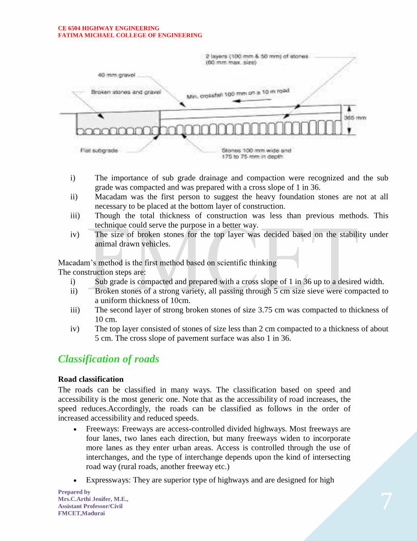
CE 6504 HIGHWAY ENGINEERING
FATIMA MICHAEL COLLEGE OF ENGINEERING
Prepared by
MrsCArthi Jenifer ME
Assistant ProfessorCivil
FMCETMadurai 7
i) The importance of sub grade drainage and compaction were recognized and the sub
grade was compacted and was prepared with a cross slope of 1 in 36
ii) Macadam was the first person to suggest the heavy foundation stones are not at all
necessary to be placed at the bottom layer of construction
iii) Though the total thickness of construction was less than previous methods This
technique could serve the purpose in a better way
iv) The size of broken stones for the top layer was decided based on the stability under
animal drawn vehicles
Macadamrsquos method is the first method based on scientific thinking
The construction steps are
i) Sub grade is compacted and prepared with a cross slope of 1 in 36 up to a desired width
ii) Broken stones of a strong variety all passing through 5 cm size sieve were compacted to
a uniform thickness of 10cm
iii) The second layer of strong broken stones of size 375 cm was compacted to thickness of
10 cm
iv) The top layer consisted of stones of size less than 2 cm compacted to a thickness of about
5 cm The cross slope of pavement surface was also 1 in 36
Classification of roads
Road classification
The roads can be classified in many ways The classification based on speed and
accessibility is the most generic one Note that as the accessibility of road increases the
speed reducesAccordingly the roads can be classified as follows in the order of
increased accessibility and reduced speeds
Freeways Freeways are access-controlled divided highways Most freeways are
four lanes two lanes each direction but many freeways widen to incorporate
more lanes as they enter urban areas Access is controlled through the use of
interchanges and the type of interchange depends upon the kind of intersecting
road way (rural roads another freeway etc)
Expressways They are superior type of highways and are designed for high
CE 6504 HIGHWAY ENGINEERING
FATIMA MICHAEL COLLEGE OF ENGINEERING
Prepared by
MrsCArthi Jenifer ME
Assistant ProfessorCivil
FMCETMadurai 8
speeds (120 kmhr is common) high traffic volume and safety They are
generally provided with grade separations at intersections Parking loading and
unloading of goods and pedestrian traffic is not allowed on expressways
Highways They represent the superior type of roads in the country Highways are
of two types - rural highways and urban highways Rural highways are those
passing through rural areas (villages) and urban highways are those passing
through large cities and towns ie urban areas
Arterials It is a general term denoting a street primarily meant for through traffic
usually on a continuous route They are generally divided highways with fully or
partially controlled access Parking loading and unloading activities are usually
restricted and regulated Pedestrians are allowed to cross only at
intersectionsdesignated pedestrian crossings
Local streets A local street is the one which is primarily intended for access to
residence business or abutting property It does not normally carry large volume
of traffic and also it allows unrestricted parking and pedestrian movements
Collector streets These are streets intended for collecting and distributing traffic
to and from local streets and also for providing access to arterial streets Normally
full access is provided on these streets There are few parking restrictions except
during peak hours
Figure 1 Speed vs accessibility
CE 6504 HIGHWAY ENGINEERING
FATIMA MICHAEL COLLEGE OF ENGINEERING
Prepared by
MrsCArthi Jenifer ME
Assistant ProfessorCivil
FMCETMadurai 9
FACTORS AFFECTING HIGHWAY ALIGHNMENT
Design speed
Design speed is the single most important factor that affects the geometric design It
directly affects the sight distance horizontal curve and the length of vertical curves
Since the speed of vehicles vary with driver terrain etc a design speed is adopted for all
the geometric design
Design speed is defined as the highest continuous speed at which individual vehicles can
travel with safety on the highway when weather conditions are conducive Design speed
is different from the legal speed limit which is the speed limit imposed to curb a common
tendency of drivers to travel beyond an accepted safe speed Design speed is also
different from the desired speed which is the maximum speed at which a driver would
travel when unconstrained by either traffic or local geometry
Since there are wide variations in the speed adopted by different drivers and by different
types of vehicles design speed should be selected such that it satisfy nearly all drivers At
the same time a higher design speed has cascading effect in other geometric designs and
thereby cost escalation Therefore an 85th percentile design speed is normally adopted
This speed is defined as that speed which is greater than the speed of 85 of drivers In
some countries this is as high as 95 to 98 percentile speed
Topography
The next important factor that affects the geometric design is the topography It is easier to
construct roads with required standards for a plain terrain However for a given design speed the
construction cost increases multiform with the gradient and the terrain Therefore geometric design
standards are different for different terrain to keep the cost of construction and time of construction
under control This is characterized by sharper curves and steeper gradients
Other factors
CE 6504 HIGHWAY ENGINEERING
FATIMA MICHAEL COLLEGE OF ENGINEERING
Prepared by
MrsCArthi Jenifer ME
Assistant ProfessorCivil
FMCETMadurai 10
In addition to design speed and topography there are various other factors that affect the geometric
design and they are briefly discussed below
Vehicle The dimensions weight of the axle and operating characteristics of a vehicle
influence the design aspects such as width of the pavement radii of the curve clearances
parking geometrics etc A design vehicle which has standard weight dimensions and
operating characteristics are used to establish highway design controls to accommodate
vehicles of a designated type
Human The important human factors that influence geometric design are the mental and
psychological characteristics of the driver and pedestrians like the reaction time
Traffic It will be uneconomical to design the road for peak traffic flow Therefore a
reasonable value of traffic volume is selected as the design hourly volume which is
determined from the various traffic data collected The geometric design is thus based on
this design volume capacity etc
Environmental Factors like air pollution noise pollution etc should be given due
consideration in the geometric design of roads
Economy The design adopted should be economical as far as possible It should match
with the funds allotted for capital cost and maintenance cost
Others Geometric design should be such that the aesthetics of the region is not affected
Nagpur classification
In Nagpur road classification all roads were classified into five categories as National highways
State highways Major district roads Other district roads and village roads
National highways
They are main highways running through the length and breadth of India connecting major
ports foreign highways capitals of large states and large industrial and tourist centers
including roads required for strategic movements
It was recommended by Jayakar committee that the National highways should be the frame
on which the entire road communication should be based
All the national highways are assigned the respective numbers
For eg the highway connecting Delhi-Ambala-Amritsar is denoted as NH-1 (Delhi-
Amritsar) where as a bifurcation of this highway beyond Full under to Srinagar and Uri is
denoted as NH-1_A
They are constructed and maintained by CPWD
The total lengths of National highway in the country is 58112 Kms and constitute about 2
of total road networks of India and carry 40 of total traffic
State highways
They are the arterial roads of a state connecting up with the national highways of adjacent
states district headquarters and important cities within the state
They also serve as main arteries to and from district roads
Total length of all SH in the country is 1 37119 Kms
Major district roads
Important roads with in a district serving areas of production and markets connecting those
with each other or with the major highways
India has a total of 4 70000 Kms of MDR
CE 6504 HIGHWAY ENGINEERING
FATIMA MICHAEL COLLEGE OF ENGINEERING
Prepared by
MrsCArthi Jenifer ME
Assistant ProfessorCivil
FMCETMadurai 11
Other district roads
Roads serving rural areas of production and providing them with outlet to market centers or
other important roads like MDR or SH
Village roads
They are roads connecting villages or group of villages with each other or to the nearest
road of a higher category like ODR or MDR
India has 2650000 kms of ODR+VR out of the total 3315231 kms of all type of roads
Roads classification criteria
Apart from the classification given by the different plans roads were also classified based on some
other criteria They are given in detail below
Based on usage
This classification is based on whether the roads can be used during different seasons of the year
All-weather roads Those roads which are negotiable during all weathers except at major
river crossings where interruption of traffic is permissible up to a certain extent are called all
weather roads
Fair-weather roads Roads which are negotiable only during fair weather are called fair
weather roads
Based on carriage way
This classification is based on the type of the carriage way or the road pavement
Paved roads with hards surface If they are provided with a hard pavement course such
roads are called paved roads(eg stones Water bound macadam (WBM) Bituminous
macadam (BM) concrete roads)
Unpaved roads Roads which are not provided with a hard course of atleast a WBM layer
they is called unpaved roads Thus earth and gravel roads come under this category
Alignment The position or the layout of the central line of the highway on the ground is called the
alignment Horizontal alignment includes straight and curved paths Vertical alignment
includes level and gradients Alignment decision is important because a bad alignment
will enhance the construction maintenance and vehicle operating costs Once an
alignment is fixed and constructed it is not easy to change it due to increase in cost of
adjoining land and construction of costly structures by the roadside
Requirements The requirements of an ideal alignment are
The alignment between two terminal stations should be short and as far as
possible be straight but due to some practical considerations deviations may be
needed
The alignment should be easy to construct and maintain It should be easy for the
operation of vehicles So to the maximum extend easy gradients and curves
should be provided
It should be safe both from the construction and operating point of view
especially at slopes embankments and cutting It should have safe geometric
features
The alignment should be economical and it can be considered so only when the
initial cost maintenance cost and operating cost are minimum
CE 6504 HIGHWAY ENGINEERING
FATIMA MICHAEL COLLEGE OF ENGINEERING
Prepared by
MrsCArthi Jenifer ME
Assistant ProfessorCivil
FMCETMadurai 12
Factors controlling alignment
We have seen the requirements of an alignment But it is not always possible to satisfy all
these requirements Hence we have to make a judicial choice considering all the factors
The various factors that control the alignment are as follows
Obligatory points These are the control points governing the highway alignment
These points are classified into two categories Points through which it should
pass and points through which it should not pass Some of the examples are
o Bridge site The bridge can be located only where the river has straight
and permanent path and also where the abutment and pier can be strongly
founded The road approach to the bridge should not be curved and skew
crossing should be avoided as possible Thus to locate a bridge the
highway alignment may be changed
o Mountain While the alignment passes through a mountain the various alternatives are to either construct a tunnel or to go round the hills The suitability of the alternative depends on factors like topography site
conditions and construction and operation cost
o Intermediate town The alignment may be slightly deviated to connect an intermediate town or village nearby
These were some of the obligatory points through which the alignment should pass
Coming to the second category that is the points through which the alignment should not
pass are
Religious places These have been protected by the law from being acquired for
any purpose Therefore these points should be avoided while aligning
Very costly structures Acquiring such structures means heavy compensation
which would result in an increase in initial cost So the alignment may be deviated
not to pass through that point
Lakesponds etc The presence of a lake or pond on the alignment path would also
necessitate deviation of the alignment
Traffic The alignment should suit the traffic requirements Based on the origin-
destination data of the area the desire lines should be drawn The new alignment should
be drawn keeping in view the desire lines traffic flow pattern etc Geometric design
Geometric design factors such as gradient radius of curve sight distance etc also govern
the alignment of the highway To keep the radius of curve minimum it may be required
to change the alignment The alignments should be finalized such that the obstructions to
visibility do not restrict the minimum requirements of sight distance The design
standards vary with the class of road and the terrain and accordingly the highway should
be aligned Economy The alignment finalized should be economical All the three costs
ie construction maintenance and operating cost should be minimum The construction
cost can be decreased much if it is possible to maintain a balance between cutting and
filling Also try to avoid very high embankments and very deep cuttings as the
construction cost will be very higher in these cases
Road ecology
The features of the cross-section of the pavement influences the life of the pavement as
CE 6504 HIGHWAY ENGINEERING
FATIMA MICHAEL COLLEGE OF ENGINEERING
Prepared by
MrsCArthi Jenifer ME
Assistant ProfessorCivil
FMCETMadurai 13
well as the riding comfort and safety Of these pavement surface characteristics affect
both of these Camber kerbs and geometry of various cross-sectional elements are
important aspects to be considered in this regard They are explained briefly in this
chapter
Camber
Camber or cant is the cross slope provided to raise middle of the road surface in the
transverse direction to drain off rain water from road surface The objectives of providing
camber are
Surface protection especially for gravel and bituminous roads
Sub-grade protection by proper drainage
Quick drying of pavement which in turn increases safety
Too steep slope is undesirable for it will erode the surface Camber is measured in 1 in n
or n (Eg 1 in 50 or 2) and the value depends on the type of pavement surface The
value suggested by IRC for various categories of pavement is given in Table 1 The
common types of camber are parabolic straight or combination of them (Figure 1)
Figure 1 Different types of camber
Table 1 IRC Value
s for ca
mber
Heavy
Light
Surface
rain
type
rain
17
ConcreteBituminous
2
25
GravelWBM
3
30
Earthen
4
CE 6504 HIGHWAY ENGINEERING
FATIMA MICHAEL COLLEGE OF ENGINEERING
Prepared by
MrsCArthi Jenifer ME
Assistant ProfessorCivil
FMCETMadurai 14
Engineering surveys for alignment
The stages of the engineering surveys are a) Map study
b) Reconnaissance
c) Preliminary surveys
d) Final location and detailed surveys
Map study -
) In the topographic map to suggest the likely routes of roads In India topographic
maps are available from the survey of India with 15 or 30-meter contour intervals
) The main feature like rivers hills and valleys etc The probable alignment can be
located on the map from the following details available on the map
Alignment avoiding valleys ponds or lakes
When the road has to cross a row of hills possibility crossing through a mountain pass
Approximate location of bridge site for crossing rivers avoiding bend of the river
When a road is to be connected between two stations one of the top and the other on the foot
of the hill then alternate routes can be suggested keeping in view the permissible alignment
Suppose the scale of the contour map is known and then the contour intervals it is possible
to decide the length of road required between two consecutive contours keeping the gradient
within allowable limits
In the fig Let A and B be two stations to be connected by road AB is the shortest route
(Straight line) APQB is a steep route in which the gradient positively exceeds 1 in 20 as the
distance between the contour intervals is only about 200 meter
APLMNB is a route with an approximate slope of 1 in 20 whereas APEFGB is an alternate
alignment with the same gradient
Thus the map study also is possible to drop a certain route in view of any unavoidable
obstructions (or) undesirable ground enroute
Reconnaissance-
The second stage of surveys for highway location is the reconnaissance to examine the general
character of the area for deciding the most feasible routes for detailed studies
Some of the details to be collected during reconnaissance are given below
Valleys ponds lakes marshy land ridge hills permanent structures and other obstructions
along the route which are not available in the map
Approximate values of gradient length of gradients and radius of curves of alternate
alignments
Number and types of cross drainage structures maximum flood level and natural
groundwater level along the probable routes
Soil type along the routes from field identification tests and observation of geological
features
Sources of construction materials water and location of stone quarries
When the road passes through hilly or mountainous terrain additional data regarding the
geological formation types of rocks dip of strata seepage flow etc
Preliminary survey -
CE 6504 HIGHWAY ENGINEERING
FATIMA MICHAEL COLLEGE OF ENGINEERING
Prepared by
MrsCArthi Jenifer ME
Assistant ProfessorCivil
FMCETMadurai 15
The main objectives of the preliminary surveys are
To survey the various alternate alignments proposed after the reconnaissance and to collect
all the necessary physical information and details of topography drainage and soil
To compare the different proposals in view of the requirements of a good alignment
To estimate quantity of earthwork materials and other construction aspects and to work out
the cost of alternate proposals
To finalize the best alignment from all considerations
The procedure of the conventional methods of preliminary surveys the given steps
Primary survey -
For alternate alignments either secondary traverses (or) independent primary traverses may be
necessary
Topographical features -
All geographical and other man made features along the traverse and for a certain width on either
side surveyed and plotted
Leveling work -
Levelling work is also carried out side by side to give the centerline profiles and typical cross
sections The leveling work in the preliminary survey is kept to a minimum just sufficient to obtain
the approximate earthwork in the alternate alignments
Drainage studies -
Drainage investigations and hydrological data are collected so as to estimate the type number and
approximate size of cross and drainage structures
Soil survey -
The soil survey conducted at this stage helps to working out details of earthwork slopes suitability
of materials subsoil and surface drainage requirements and pavement type and the approximate
thickness requirements
Material survey -
The survey for naturally occurring materials like stone aggregates soft aggregates etc and
identification of suitable quarries should be made
Traffic survey -
Traffic surveys conducted in the region from basis for deciding the number of traffic lanes and
roadway width pavement design and economic analysis of highway project
Locations and functions
Final location and detailed survey - The alignment finalized at the design office after the preliminary survey is to be first located on the
field by establishing the centerline The detailed survey should be carried out for collecting the
information technology for the preparation of plans and construction details
Location -
The centerline of the road finalized in the drawings to be translated on the ground
during the location survey
Major and minor control points are established on the ground and center pegs are
driven checking the geometric design requirements
Detailed survey -
CE 6504 HIGHWAY ENGINEERING
FATIMA MICHAEL COLLEGE OF ENGINEERING
Prepared by
MrsCArthi Jenifer ME
Assistant ProfessorCivil
FMCETMadurai 16
Levels along his final centerline should be taken at all staked points Levelling work is to
great importance as the vertical alignment
A detailed soil survey is carried out to enable drawing of the soil profile
The data during the detailed survey should be elaborate and complete for preparing detailed
plans design and estimates of the project
Soil suitability analysis
The methodology for locating appropriate sites for each land use activity is guided by the intent to
minimize the possible adverse effects of development on the environment and on existing
communities and to emphasize the positive impacts of such development by locating them in a
most suitable location
This is achieved by examining a number of individual criteria assigning them relative levels of
importance as a whole and using a mathematical resultant model to identify the most suitable
location
By adopting this site suitability method it is possible to systematically identify the criteria
considered clearly document the relative importance of one criterion over another analyze the net
outcome using a Geographic Information System and then possibly revisit the mathematical
relationships in this ldquodecision modelrdquo
By revising the relative importance to identified criteria based upon the particular land use under
consideration it is possible to generate ldquosuitability mapsrdquo for each individual land use and then
generate a final composite land use that is based on a best possible collective suitability of multiple
land uses
To achieve this all the criteria are assigned a ldquorankrdquo denoting their relative levels of importance
within the suitability study These ranks are assigned as numeric values ranging from 1 to 10 with 1
reflecting a low level of importance and 10 reflecting a high level of importance For example
within the criteria of road networks national highways would have a different level of influence on
the suitability for a particular land use as compared with local roads Further the distance from each
of these features would further modify the relative suitability of a land use based on the proximity to
a particular type of road
Criteria for Site Suitability Analysis
The decision criteria for site selection are examined for assigning relative ranks and individual
feature weights based on the land use type for which suitability is being examined For benefit of
analysis the criteria under consideration in this paper activity are organized as
Critical Criteria Criteria that will be very significant in the site selection of the identified land use
and will act as key drivers in the selection of the geographic location These criteria can be clustered
into a single decision model and the outcome collectively reviewed These criteria have a strong
influence in the final suitability
Additional Criteria Criteria that will have to be examined one at a time to carefully assess its
relationship with the proposed land use activity These criteria have a positive influence in the final
suitability
CE 6504 HIGHWAY ENGINEERING
FATIMA MICHAEL COLLEGE OF ENGINEERING
Prepared by
MrsCArthi Jenifer ME
Assistant ProfessorCivil
FMCETMadurai 17
Constrained Criteria These criteria impose strong negative opportunities in the selection of areas
for the identified land use Consequently they inform of us of where the particular land use under
consideration should not be located These criteria serve to limit or exclude areas from the final
suitability
GIS Site Suitability Analysis Model We were developed a tourism site suitability analysis model
in ArcGIS - 931 which is shown in Figure -
CE 6504 HIGHWAY ENGINEERING
FATIMA MICHAEL COLLEGE OF ENGINEERING
Prepared by
MrsCArthi Jenifer ME
Assistant ProfessorCivil
FMCETMadurai 18
UNIT 2 GEOMETRIC DESIGN OF HIGHWAYS
Typical cross section of urban and rural roads
A cross section is a vertical plane (slice) taken at right angles to the road control line showing the
various elements that make up the roads structure It is normally viewed in the direction of
increasing chainage
The width of a roadway is an important design consideration to ensure that it is appropriately sized
to serve its function Because of the diversity within the County two major roadway categories have
been established 1 Rural Road Standards 2 Urban Road Standards Urban Road Standards will
serve those areas which tend to be more developed and need to provide for multiple users
(bicyclists pedestrians parallel parking etc) whereas many rural roads will primarily serve only
vehicular traffic
Cross sections are created to provide a visual guide depicting the initial interim and ultimate phase
cross sections for these road classifications The typical sections illustrated in the following pages
are recommendations tied to transportation planning aspects such as right‐of‐way lineage sidewalk
width etc Threshold daily traffic can be used as a guide for a starting point when determining
which cross section is most applicable
1 Rural Road Standards
The rural roadways will not typically require curb and gutter or sidewalk although the County may
require either or both in unique circumstances Widths of lanes and shoulders will vary depending
upon the specific classification and the potential traffic volume which the roadway may carry Roads
carrying fewer than 200 vehicles per day need not be paved or treated for dust control The need for
paved shoulders is also dependent upon the level of traffic and safety
Final design and construction details will be determined by the Public Works Department Final
Design and construction criteria taken into consideration may include but are not limited to use of
the roadway density of development topographical characteristics and nearby development For
construction in which only a portion of the ultimate cross‐section is intended to be completed the
partial design will need to allow for the eventual widening to the ultimate cross‐section The design
for the partial or interim cross‐section roadway will need to incorporate ultimate design information
to ensure that the first phase of roadway construction is appropriate and would not need to be
removed at a future date when the full width cross‐section is completed
2 Urban Road Standards
Three roadway classifications are identified for those areas that are associated with the communityrsquos
urban growth areas They include arterial collector and local street classifications Transportation
Plan shows the key elements of the urban road standards Urban road standards will include 12‐foot
lanes sidewalk and curb amp gutter arterials and collectors will also include a striped bike lane Turn
lanes may be necessary as determined by the County Since almost all of the municipalities have
different right‐of‐way cross sections adopted for their community it makes it very difficult for the
County to match them all Therefore the philosophy was to encourage a baseline amount of
right‐of‐way reservation that could ensure the adjacent community enough area for coordination of
future roadway improvements until such time the road
CE 6504 HIGHWAY ENGINEERING
FATIMA MICHAEL COLLEGE OF ENGINEERING
Prepared by
MrsCArthi Jenifer ME
Assistant ProfessorCivil
FMCETMadurai 19
CE 6504 HIGHWAY ENGINEERING
FATIMA MICHAEL COLLEGE OF ENGINEERING
Prepared by
MrsCArthi Jenifer ME
Assistant ProfessorCivil
FMCETMadurai 20
Cross sectional elements
Kerbs
Kerbs indicate the boundary between the carriage way and the shoulder or islands or footpaths Different types of kerbs are
CE 6504 HIGHWAY ENGINEERING
FATIMA MICHAEL COLLEGE OF ENGINEERING
Prepared by
MrsCArthi Jenifer ME
Assistant ProfessorCivil
FMCETMadurai 21
Low or mountable kerbs This type of kerbs is provided such that they
encourage the traffic to remain in the through traffic lanes and also allow the
driver to enter the shoulder area with little difficulty The height of this kerb is
about 10 cm above the pavement edge with a slope which allows the vehicle to
climb easily This is usually provided at medians and channelization schemes and
also helps in longitudinal drainage
Semi-barrier type kerbs When the pedestrian traffic is high these kerbs are
provided Their height is 15 cm above the pavement edge This type of kerb
prevents encroachment of parking vehicles but at acute emergency it is possible
to drive over this kerb with some difficulty
Barrier type kerbs They are designed to discourage vehicles from leaving the
pavement They are provided when there is considerable amount of pedestrian
traffic They are placed at a height of 20 cm above the pavement edge with a steep
batter
Submerged kerbs They are used in rural roads The kerbs are provided at
pavement edges between the pavement edge and shoulders They provide lateral
confinement and stability to the pavement
Figure 1 Different types of kerbs
Shoulders Shoulders are provided along the road edge and are intended for accommodation of
stopped vehicles serve as an emergency lane for vehicles and provide lateral support
for base and surface courses The shoulder should be strong enough to bear the weight
of a fully loaded truck even in wet conditions The shoulder width should be adequate
for giving working space around a stopped vehicle It is desirable to have a width of
46 m for the shoulders A minimum width of 25 m is recommended for 2-lane rural
highways in India Parking lanes
Parking lanes are provided in urban lanes for side parking Parallel parking is preferred
because it is safe for the vehicles moving on the road The parking lane should have a
minimum of 30 m width in the case of parallel parking
CE 6504 HIGHWAY ENGINEERING
FATIMA MICHAEL COLLEGE OF ENGINEERING
Prepared by
MrsCArthi Jenifer ME
Assistant ProfessorCivil
FMCETMadurai 22
Bus-bays
Bus bays are provided by recessing the kerbs for bus stops They are provided so that
they do not obstruct the movement of vehicles in the carriage way They should be at
least 75 meters away from the intersection so that the traffic near the intersections is not
affected by the bus-bay
Service roads Service roads or frontage roads give access to access controlled highways like freeways
and expressways They run parallel to the highway and will be usually isolated by a
separator and access to the highway will be provided only at selected points These roads
are provided to avoid congestion in the expressways and also the speed of the traffic in
those lanes is not reduced
Drainage
The pavement surface should be absolutely impermeable to prevent seepage of water into
the pavement layers Further both the geometry and texture of pavement surface should
help in draining out the water from the surface in less time
Footpath
Footpaths are exclusive right of way to pedestrians especially in urban areas They are
provided for the safety of the pedestrians when both the pedestrian traffic and vehicular
traffic is high Minimum width is 15 meter and may be increased based on the traffic
The footpath should be either as smooth as the pavement or more smoother than that to
induce the pedestrian to use the footpath
Right of way
Right of way (ROW) or land width is the width of land acquired for the road along its
alignment It should be adequate to accommodate all the cross-sectional elements of the
highway and may reasonably provide for future development To prevent ribbon
development along highways control lines and building lines may be provided Control
line is a line which represents the nearest limits of future uncontrolled building activity
in relation to a road Building line represents a line on either side of the road between
which and the road no building activity is permitted at all The right of way width is
governed by
Width of formation It depends on the category of the highway and width of
roadway and road margins
Height of embankment or depth of cutting It is governed by the topography and
the vertical alignment
Side slopes of embankment or cutting It depends on the height of the slope soil
type etc
Drainage system and their size which depends on rainfall topography etc
Sight distance considerations On curves etc there is restriction to the visibility
on the inner side of the curve due to the presence of some obstructions like
building structures etc
Reserve land for future widening Some land has to be acquired in advance
CE 6504 HIGHWAY ENGINEERING
FATIMA MICHAEL COLLEGE OF ENGINEERING
Prepared by
MrsCArthi Jenifer ME
Assistant ProfessorCivil
FMCETMadurai 23
Table 2 Desig
n speed in as per IRC (ruling and minimum)
Steep
Type
Plain
Rolling
Hilly
40-30
NSampSH
100-80
80-65
50-40
MDR
80-65
65-50
40-30
30-20
25-20
ODR
65-50
50-40
30-25
25-20
VR
50-40
40-35
25-20
anticipating future developments like widening of the road
Table 1 No
right of way for open areas
Roadway width in m
Road
Plain and
Mountainous and
classification
steep terrain
rolling terrain
Open areas
45
24
NHSH
18
MDR
25
15
15
ODR
12
9
VR
Built-up areas
20
NHSH
30
MDR
20
15
ODR
15
12
9
VR
10
CE 6504 HIGHWAY ENGINEERING
FATIMA MICHAEL COLLEGE OF ENGINEERING
Prepared by
MrsCArthi Jenifer ME
Assistant ProfessorCivil
FMCETMadurai 24
Horizontal curve
The presence of horizontal curve imparts centrifugal force which is a reactive force
acting outward on a vehicle negotiating it Centrifugal force depends on speed and radius
of the horizontal curve and is counteracted to a certain extent by transverse friction
between the tyre and pavement surface On a curved road this force tends to cause the
vehicle to overrun or to slide outward from the centre of road curvature For proper
design of the curve an understanding of the forces acting on a vehicle taking a horizontal
curve is necessary Various forces acting on the vehicle are illustrated in the figure 1
Figure 1 Effect of horizontal curve They are the centrifugal force (P) acting outward weight of the vehicle (W) acting
downward and the reaction of the ground on the wheels ( and ) The centrifugal
force and the weight is assumed to be from the centre of gravity which is at h units above
the ground Let the wheel base be assumed as b units The centrifugal force in
is given by
(1)
where is the weight of the vehicle in is the speed of the vehicle in is
the acceleration due to gravity in and is the radius of the curve in
The centrifugal ratio or the impact factor is given by
CE 6504 HIGHWAY ENGINEERING
FATIMA MICHAEL COLLEGE OF ENGINEERING
Prepared by
MrsCArthi Jenifer ME
Assistant ProfessorCivil
FMCETMadurai 25
(1)
The centrifugal force has two effects A tendency to overturn the vehicle about the outer
wheels and a tendency for transverse skidding Taking moments of the forces with
respect to the outer wheel when the vehicle is just about to override
At the equilibrium over turning is possible when
and for safety the following condition must satisfy
(2)
The second tendency of the vehicle is for transverse skidding ie When the the
centrifugal force is greater than the maximum possible transverse skid resistance due to
friction between the pavement surface and tyre The transverse skid resistance (F) is
given by
where and is the fractional force at tyre and and is the reaction at
tyre and is the lateral coefficient of friction and is the weight of the vehicle
This is counteracted by the centrifugal force (P) and equating
At equilibrium when skidding takes place (from equation1)
and for safety the following condition must satisfy
CE 6504 HIGHWAY ENGINEERING
FATIMA MICHAEL COLLEGE OF ENGINEERING
Prepared by
MrsCArthi Jenifer ME
Assistant ProfessorCivil
FMCETMadurai 26
(3)
Equation 2 and 3 give the stable condition for design If equation 2 is violated the vehicle
will overturn at the horizontal curve and if equation 3 is violated the vehicle will skid at
the horizontal
Curve Analysis of super-elevation
Super-elevation or cant or banking is the transverse slope provided at horizontal curve to
counteract the centrifugal force by raising the outer edge of the pavement with respect to
the inner edge throughout the length of the horizontal curve When the outer edge is
raised a component of the curve weight will be complimented in counteracting the effect
of centrifugal force In order to find out how much this raising should be the following
analysis may be done The forces acting on a vehicle while taking a horizontal curve with
super elevation is shown in figure 1
Figure 1 Analysis of super-elevation
Forces acting on a vehicle on horizontal curve of radius at a speed of are
the centrifugal force acting horizontally out-wards through the center of
gravity
the weight of the vehicle acting down-wards through the center of gravity and
the friction force between the wheels and the pavement along the surface
inward
CE 6504 HIGHWAY ENGINEERING
FATIMA MICHAEL COLLEGE OF ENGINEERING
Prepared by
MrsCArthi Jenifer ME
Assistant ProfessorCivil
FMCETMadurai 27
At equilibrium by resolving the forces parallel to the surface of the pavement we get where
friction
is the weight of the vehicle is the centrifugal force is the coefficient of
is the transverse slope due to superelevation Dividing by we get
CE 6504 HIGHWAY ENGINEERING
FATIMA MICHAEL COLLEGE OF ENGINEERING
Prepared by
MrsCArthi Jenifer ME
Assistant ProfessorCivil
FMCETMadurai 28
Step 1
Find for 75 percent of design speed neglecting ie
Step 2
If then else if go to step 3
Step 3
Find for the design speed and max ie If
then the maximum is safe for the design speed else go to
step 4
Step 4
Find the allowable speed for the maximum and
If then the design is adequate otherwise use speed adopt
control measures or look for speed control measures
Maximum and minimum super-elevation
Depends on (a) slow moving vehicle and (b) heavy loaded trucks with high CG IRC
specifies a maximum super-elevation of 7 percent for plain and rolling terrain while that
of hilly terrain is 10 percent and urban road is 4 percent The minimum super elevation is
2-4 percent for drainage purpose especially for large radius of the horizontal curve
Attainment of super-elevation
1 Elimination of the crown of the cambered section by
1 Rotating the outer edge about the crown The outer half of the cross slope
is rotated about the crown at a desired rate such that this surface falls on
the same plane as the inner half
2 Shifting the position of the crown This method is also known as diagonal
crown method Here the position of the crown is progressively
shifted outwards thus increasing the width of the inner half of cross section
progressively
2 Rotation of the pavement cross section to attain full super elevation byThere are
two methods of attaining super elevation by rotating the pavement
1 Rotation about the center line The pavement is rotated such that the inner
edge is depressed and the outer edge is raised both by half the total amount
of super elevation ie by with respect to the centre
2 Rotation about the inner edge Here the pavement is rotated raising the
outer edge as well as the centre such that the outer edge is raised by the
full amount of super elevation with respect to the inner edge
Horizontal Transition Curves
CE 6504 HIGHWAY ENGINEERING
FATIMA MICHAEL COLLEGE OF ENGINEERING
Prepared by
MrsCArthi Jenifer ME
Assistant ProfessorCivil
FMCETMadurai 29
Transition curve is provided to change the horizontal alignment from straight to circular
curve gradually and has a radius which decreases from infinity at the straight end
(tangent point) to the desired radius of the circular curve at the other end (curve point)
There are five objectives for providing transition curve and are given below
1 to introduce gradually the centrifugal force between the tangent point and the
beginning of the circular curve avoiding sudden jerk on the vehicle This
increases the comfort of passengers
2 to enable the driver turn the steering gradually for his own comfort and security
3 to provide gradual introduction of super elevation and
4 to provide gradual introduction of extra widening
5 to enhance the aesthetic appearance of the road
Type of transition curve
Different types of transition curves are spiral or clothoid cubic parabola and Lemniscate
IRC recommends spiral as the transition curve because
1 it fulfills the requirement of an ideal transition curve that is
1 rate of change or centrifugal acceleration is consistent (smooth) and
2 radius of the transition curve is at the straight edge and changes to at
the curve point ( ) and calculation and field implementation is
very easy
Length of transition curve The length of the transition curve should be determined as the maximum of the following
three criteria rate of change of centrifugal acceleration rate of change of super elevation
and an empirical formula given by IRC Rate of change of centrifugal acceleration
At the tangent point radius is infinity and hence centrifugal acceleration is zero At the
end of the transition the radius R has minimum value R The rate of change of
centrifugal acceleration should be adopted such that the design should not cause
discomfort to the drivers If is the rate of change of centrifugal acceleration it can be
written as
Therefore the length of the transition curve in is
CE 6504 HIGHWAY ENGINEERING
FATIMA MICHAEL COLLEGE OF ENGINEERING
Prepared by
MrsCArthi Jenifer ME
Assistant ProfessorCivil
FMCETMadurai 30
(1)
where is the rate of change of centrifugal acceleration given by an empirical formula
suggested by by IRC as below
(2) 2 Rate of introduction of super-elevation
Raise ( ) of the outer edge with respect to inner edge is given by
The rate of change of this raise from to is achieved
gradually with a gradient of in over the length of the transition curve (typical range
of is 60-150) Therefore the length of the transition curve is
(3)
3 By empirical formula
IRC suggest the length of the transition curve is minimum for a plain and rolling terrain
(4)
and for steep and hilly terrain is
(5)
CE 6504 HIGHWAY ENGINEERING
FATIMA MICHAEL COLLEGE OF ENGINEERING
Prepared by
MrsCArthi Jenifer ME
Assistant ProfessorCivil
FMCETMadurai 31
and the shift as
(
6
) The length of the transition curve is the maximum of
equations 1 3 and 4or5 ie
(
7
Case (a)
For single lane roads
(
1
)
Therefore
(
2
)
Figure 1 Set-back for single lane roads (
CE 6504 HIGHWAY ENGINEERING
FATIMA MICHAEL COLLEGE OF ENGINEERING
Prepared by
MrsCArthi Jenifer ME
Assistant ProfessorCivil
FMCETMadurai 32
For multi lane roads if is the distance between centerline of the road and the centerline
of the inner lane then
(3)
(4)
Figure 2 Set-back for multi-lane roads ( )
Case (a)
For single lane roads
(1)
Therefore
(2)
Gradient
Gradient is the rate of rise or fall along the length of the road with respect to the
horizontal While aligning a highway the gradient is decided for designing the vertical
curve Before finalizing the gradients the construction cost vehicular operation cost and
the practical problems in the site also has to be considered Usually steep gradients are
avoided as far as possible because of the difficulty to climb and increase in the
CE 6504 HIGHWAY ENGINEERING
FATIMA MICHAEL COLLEGE OF ENGINEERING
Prepared by
MrsCArthi Jenifer ME
Assistant ProfessorCivil
FMCETMadurai 33
construction cost More about gradients are discussed below
Effect of gradient
The effect of long steep gradient on the vehicular speed is considerable This is
particularly important in roads where the proportion of heavy vehicles is significant Due
to restrictive sight distance at uphill gradients the speed of traffic is often controlled by
these heavy vehicles As a result not only the operating costs of the vehicles are
increased but also capacity of the roads will have to be reduced Further due to high
differential speed between heavy and light vehicles and between uphill and downhill
gradients accidents abound in gradients
Representation of gradient
The positive gradient or the ascending gradient is denoted as and the negative gradient as The deviation angle is when two grades meet the angle which
measures the change of direction and is given by the algebraic difference between the two
grades
steep gradient while 1 in 50 = 2 representation is illustrated in the figure 1
Example 1 in 30 = 333 is a
is a flatter gradient The gradient
CE 6504 HIGHWAY ENGINEERING
FATIMA MICHAEL COLLEGE OF ENGINEERING
Prepared by
MrsCArthi Jenifer ME
Assistant ProfessorCivil
FMCETMadurai 34
Figure 1 Representation of gradient
Types of gradient
Many studies have shown that gradient upto seven percent can have considerable effect
on the speeds of the passenger cars On the contrary the speeds of the heavy vehicles are
considerably reduced when long gradients as flat as two percent is adopted Although
flatter gradients are desirable it is evident that the cost of construction will also be very
high Therefore IRC has specified the desirable gradients for each terrain However it
may not be economically viable to adopt such gradients in certain locations steeper
gradients are permitted for short duration Different types of grades are discussed below
Ruling gradient
The ruling gradient or the design gradient is the maximum gradient with which the
designer attempts to design the vertical profile of the road This depends on the terrain
length of the grade speed pulling power of the vehicle and the presence of the horizontal
curve In flatter terrain it may be possible to provide flat gradients but in hilly terrain it
is not economical and sometimes not possible also The ruling gradient is adopted by the
designer by considering a particular speed as the design speed and for a design vehicle
with standard dimensions But our country has a heterogeneous traffic and hence it is not
possible to lay down precise standards for the country as a whole Hence IRC has
recommended some values for ruling gradient for different types of terrain
Limiting gradient
This gradient is adopted when the ruling gradient results in enormous increase in cost of
construction On rolling terrain and hilly terrain it may be frequently necessary to adopt
limiting gradient But the length of the limiting gradient stretches should be limited and
must be sandwiched by either straight roads or easier grades
Exceptional gradient
Exceptional gradient are very steeper gradients given at unavoidable situations They
should be limited for short stretches not exceeding about 100 metres at a stretch In
mountainous and steep terrain successive exceptional gradients must be separated by a
minimum 100 metre length gentler gradient At hairpin bends the gradient is restricted to
25
Critical length of the grade
The maximum length of the ascending gradient which a loaded truck can operate without
undue reduction in speed is called critical length of the grade A speed of 25 kmph is a
CE 6504 HIGHWAY ENGINEERING
FATIMA MICHAEL COLLEGE OF ENGINEERING
Prepared by
MrsCArthi Jenifer ME
Assistant ProfessorCivil
FMCETMadurai 35
reasonable value This value depends on the size power load grad-ability of the truck
initial speed final desirable minimum speed
Minimum gradient
This is important only at locations where surface drainage is important Camber will take
care of the lateral drainage But the longitudinal drainage along the side drains require
some slope for smooth flow of water Therefore minimum gradient is provided for
drainage purpose and it depends on the rain fall type of soil and other site conditions A
minimum of 1 in 500 may be sufficient for concrete drain and 1 in 200 for open soil
drains are found to give satisfactory performance Sight distance available from a point is the actual distance along the road surface which a driver
from a specified height above the carriage way has visibility of stationary or moving objects
Sight distance required by drivers applies to both geometric design of highways and for
traffic control The sight distance situations are considered in the design
i) Stopping or absolute minimum sight distance
ii) Safe overtaking or passing sight distance
iii) Safe sight distance for entering into uncontrolled intersections
Apart from the three situations mentioned above the following sight distance are considered by the
IRC in highway design
Intermediate sight distance
This is defined as twice the stopping sight distance when overtaking sight distance
cannot be provided intermediate sight distance is provided to give limited overtaking opportunities
to fast vehicles
Head light sight distance
This is the distance visible to a driver during night driving under the illumination of the
vehicle head lights
Stopping sight distance
The minimum sight distance available on a highway at any spot should be of sufficient
length to stop a vehicle traveling at design speed safely without collision with any other obstruction
The absolute minimum sight distance is therefore equal to the stopping sight distance
which is also sometimes called nonpassing sight distance The sight distance available on a road to a
driver at any instance depends on
i) Features of the road
ii) Height of the drivers eye above the road surface
iii) Height of the object above the road surface
The distance within which a motor vehicle can be stopped depends upon the factors listed below
a) Total reactions time of the driver
b) Speed of vehicle
c) Efficiency of breaks
d) Frictional resistance between the road and tyres
e) Gradient of the road
Total reaction time
) Reaction time of the driver is the time taken from the instant the object is visible to the
driver to the instant the brakes are effectively applied
) The total reaction time may be split up into two parts
CE 6504 HIGHWAY ENGINEERING
FATIMA MICHAEL COLLEGE OF ENGINEERING
Prepared by
MrsCArthi Jenifer ME
Assistant ProfessorCivil
FMCETMadurai 36
i) Perception time
ii) Brake reaction time
PIEV theory
According to this theory the total reaction time of the driver is split into four parts
i) Perception
ii) Intellection
iii) Emotion
iv) Volition
Speed of Vehicle
The stopping distance depends very much on the speed of the vehicle first during the
total reaction time of the driver the distance moved by the vehicle will depend on the speed
Efficiency of brakes
The braking efficiency is said to be 100 percent if the wheels are fully licked preventing
them from rotating on application of the brakes This will result in 100 percent skidding which is
normally undesirable except in utmost emergency
Frictional resistance between road and tyres
The frictional resistance developed between road and tyres or the skid resistance depends
on the type and condition of the road surface and the tyres IRC has specified a design friction
coefficient of 035 to 04 depending upon the speed to be used for finding the braking distance in the
calculation of stopping sight distance
Analysis of stopping distance
i) The distance traveled by the vehicle during the total reaction time known as lag
distance
ii) The distance traveled by the vehicle after the application of the brakes is known as
braking distance
Overtaking sight distance
The minimum distance open to the vision of the driver of a vehicle intending to overtake
slow vehicle ahead with safety against the traffic of opposite direction is known as the minimum
overtaking sight distance(OSD) or Safe passing sight distance available
The overtaking sight distance is the distance measured along the center of the road which
a driver with his eye level 12m above the road surface can see the top of an object 12m above the
road surface
Some of the important factors on which the minimum overtaking sight distance required
a) Speed of
i) overtaking vehicle
ii) overtaken vehicle
iii) The vehicle coming from opposite direction
b) Distance between the overtaking and overtaken vehicles the minimum spacing
depends on the steeds
a) Skill and reaction time of the driver
b) Rate of acceleration of overtaking vehicle
c) Gradient of the road
Criteria for sight distance requirements on highway
) The absolute minimum sight distance required throughout the length of the road is the
SSD which should invariably be provided at all places
CE 6504 HIGHWAY ENGINEERING
FATIMA MICHAEL COLLEGE OF ENGINEERING
Prepared by
MrsCArthi Jenifer ME
Assistant ProfessorCivil
FMCETMadurai 37
) On horizontal curves the obstruction on the inner side of the curves should be cleared
to provide the required set back distance and absolute minimum sight distance
) On vertical summit curves the sight distance requirement may be fulfilled by proper
design of the vertical alignment
Hairpin bent
TYPES OF CURVES ON HILL ROADS
The following are the important types of curves provided on hill Roads-
1 Hair-Pin Curves
2 Salient Curves
3 Re-entrant Curves 1 Hair-pin curves - The curve in a hill road which changes its direction through an angle of 180
degree or so down the hill on the same side is known as hair-pin curve
A Hair-Pin Bend
This curve is so called because it conforms to the shape of a hair-pin The bend so formed at the
hair-pin curve in a hill road is known as hair-pin bend This type of curve should be located on a
hill side having the minimum slope and maximum stability It must also be safe from view point of
landslides and ground water Hair-pin bends with long arms and farther spacing are always
preferred They reduce construction problems and expensive protective works Hair-pin curves or
bends of serpentine nature are difficult to negotiate and should therefore be avoided as far as
possible
Salient curves - The curves having their convexity on the outer edges of a hill road are called
salient curves The centre of curvature of a salient curve lies towards the hill side This type of curve
occurs in the road length constructed on the ridge of a hill the bend so formed at the salient curve in
a hill road known as corner bend
Salient curves are very dangerous for fast moving traffic At such a curve or at corner bend the
portion of projecting hill side is usually cut down to improve the visibility as shown in fig (Re-
entrant curve) The outer edge of the road at such a curve is essentially provided with a parapet wall
for protection of the vehicles from falling down the hill slope
CE 6504 HIGHWAY ENGINEERING
FATIMA MICHAEL COLLEGE OF ENGINEERING
Prepared by
MrsCArthi Jenifer ME
Assistant ProfessorCivil
FMCETMadurai 38
3 Re-entrant curves - The curves having their convexity on the inner edge of a hill road are called
re-entrant curves
Re-entrant curves
The centre of curvature of a re-entrant curves lies away from the hill side This type of curve occurs
in the road length constructed in the calley of a hill
These curves are less dangereous as they provide adequate visibility to the fast moving traffic At
such curves the parapet wall is provided only for safety of fast moving traffic
CE 6504 HIGHWAY ENGINEERING
FATIMA MICHAEL COLLEGE OF ENGINEERING
Prepared by
MrsCArthi Jenifer ME
Assistant ProfessorCivil
FMCETMadurai 39
UNIT ndash III DESIGN OF RIGID AND FLEXIBLE PAVEMENTS
COMPARISON OF RIGID AND FLEXIBLE PAVEMENTS
The comparisons are
i) Design precision
A cement concrete pavement is amerable to a much more precise structural analysis
than a flexible pavement Flexible pavements designs are mainly empirical Computer aided analysis
of layered system is making the flexible pavement design more exact than hitherto
ii) Life
) Cement concrete slabs of a thin section constructed in the early 1940rsquos are still in
existence in India though many of them have cracked badly and a few of them have been ripped
open and rebuilt in recent ties
) A major project in cement concrete road construction between Agra and Mathura It can
safely be said that a well-designed concrete slab has a life of about 40 years
) Compared to this the life of a flexible pavement generally varies from 10 to 20 years
iii) Maintenance
) A well-designed cement concrete pavement needs very little maintenance The only
maintenance needed is I respect of joints
) The surface is unaffected by spillage of oil and lubricants bituminous surfaces on the
other hand need great inputs in maintenance
) The surface is affected by spillage of oil and lubricants The surface is also affected by
natural weathering agents like air water ad temperature changes
) A cement concrete pavement on the other hand needs a small amount for maintaining
joints
iv) Initial cost
) The argument so far used against a cement concrete slab is that it is much more costly
than a flexible pavement
) The latter specifications no doubt represent the rock-bottom needs of a road in India but
these specifications can hardly provide a smooth and durable surface
v) Stage construction ) Road construction is generally done adopting a policy of stage construction especially for
low volume roads As traffic grows additional layers in the form of water bound macadam and
superior surfacing are added on
) Initial outlay is minimum and additional outlays are in keeping with traffic growth This is
a great advantage when dealing with new roads in an atmosphere of austerity
vi) Availability of materials
) Cement bitumen stone aggregates and gravelsand are the major materials involved in
pavement Construction Cement has been in serious short supply in the country for the past many
decades
) Bitumen is also not available plentifully in India There is also the danger of the entire oil
reserves in the world shrinking during the next two or three decades
) In locations where stone aggregates are scarce cement concrete may have an advantage
for flexible pavements
vii) Surface characterstics
CE 6504 HIGHWAY ENGINEERING
FATIMA MICHAEL COLLEGE OF ENGINEERING
Prepared by
MrsCArthi Jenifer ME
Assistant ProfessorCivil
FMCETMadurai 40
) A good cement concrete surface is smooth and free from rutting potholes and
corrugations In a bituminous surface it is only the asphaltic concrete surface that can give
comparable rideablity
) A well-constructed cement concrete pavement surface can have a permanent nonskid
surface A bituminous surface can also be designed to have a good skid resistant surface
viii) Utility location
) In cement concrete slabs proper thought has to be given to locate utilities such as water
pipes telephone lines and electric cables
) It is difficult to rip open the slab and restore it to be the original condition if any changes
in the utilities lines are to be made
ix) Glame and night visibility
) Concrete pavements have a gray color which can cause glam under sunlight Colored
cement can reduce the grave
) On the other hand bituminous roads need more street lighting
x) Traffic dislocation during construction
) A cement concrete pavement requires 28 days before it can be thrown open to traffic On
the other hand a bituminous surface can be thrown open to traffic shortly after it is rolled
xi) Environmental considerations during construction
) The process of heating of bitumen and aggregates and mixing them together on hot mix
plants can prove to be much more hazardous to the environment than cement concrete construction
where no heating of any material is involved
xii) Overall economy on a life cycle basis
) A good road is costly to construct but once constructed such a road requires little
maintenance and results in savings in vehicle operating costs
) The comparative economy of a flexible pavement and a rigid pavement has proved that on
overall economic considerations
Types of pavement structure
Based on the structural behavior pavements are generally classified into three
categories
i) Flexible pavements
ii) Rigid pavements
iii) Semi rigid pavements
Flexible pavements
) Flexible pavements are those which on the whole have low or negligible flexural
strength and are rather flexible in their structural action under the loadsThe flexible pavement
layers reflect the deformation of the lower layers on to the surface of the layer
) A flexible pavement consists of four components(i) Soil subgrade (ii) sub base
course (iii) base course (iv) Surface course
CE 6504 HIGHWAY ENGINEERING
FATIMA MICHAEL COLLEGE OF ENGINEERING
Prepared by
MrsCArthi Jenifer ME
Assistant ProfessorCivil
FMCETMadurai 41
) The flexible pavement layers transmit the vertical or compressive stresses to the lower layers
by grain to grain transfer through the points of contact in the granular structure A well
compacted granular structure consisting of strong added aggregate can transfer the compressive
stresses
) The load spreading ability of this layer therefore depends on the type of the materials and mix
design factors Bituminous concrete is one of the best flexible pavements layer materials Other
materials which fall under the group are all granular materials with or without bituminous
binder granular base and sub base course materials
) The vertical compressive stress is maximum on the pavement surface directly under the wheel
and is equal to the contact pressure under the wheel The flexible pavement may be constructed
in a number of layers and the top layer has to be strongest as the highest compressive stresses
) Flexible pavements are commonly designed using empirical design charts or equations taking
into account some of the design factors there are also semi empirical and theoretical design
methods
Rigid pavements
) Rigid pavements are those which possess note flexural strength or flexural rigidity
The stresses are not transferred from grain to grain to the lower layers as in the ease of flexible
pavements layers
) The rigid pavements are made of Portland cement concrete plain reinforced or
prestressed concrete The plain cement concrete slabs are expected to take up about 40 kgcm2
flexural stress
) The rigid pavement has the slab action and is capable of transmitting the wheel
load stresses through a wider area below The main point of difference in the structural behavior
of rigid pavement as compared to the flexible pavement is that the critical condition of stress in
the rigid pavement is the maximum flexural stress occurring in the slab due to wheel load and
the temperature changes whereas in the flexible pavement
) As the rigid pavement slab has tensile strength tensile stresses are developed due
to the bending of the slab under wheel load and temperature variations Thus the types of
stresses developed and their distribution within the cement concrete slab are quirt different
) The cement concrete pavement slab can very well serve as a wearing surface as
well an effective base course The rigid pavement structure consists of a cement concrete slab
below which a granular base or sub base course may be provided
) Though the cement concrete slab can also be laid directly over the soil subgrade
consists of fine grained soil
) the rigid pavements are usually designed and the stresses are analyzed using the
elastic theory assuming the pavements as a n elastic plate resting over an elastic or a viscous
foundation
Semi rigid pavements
) when bonded materials like the pozzolanic concrete lean cement concrete or soil
cement are used in the base course or sub base course layer the pavement layer has considerably
higher flexural strength than the common flexible pavement layers
) when this intermediate class of materials are used in the base or sub base course
layer of the pavements they are called semi rigid pavements
CE 6504 HIGHWAY ENGINEERING
FATIMA MICHAEL COLLEGE OF ENGINEERING
Prepared by
MrsCArthi Jenifer ME
Assistant ProfessorCivil
FMCETMadurai 42
) This third category of semi rigid pavement are either designed as flexible
pavements with some correction factors to find the thickness requirements based on experience
or by using a new design approach
) The semi rigid pavement materials have low resistance to impact and abrasion and
therefore are usually provided with flexible pavement surface course
Various functions of pavement components
The functions are
Soil sub grade and its evaluation
) The soil sub grade is a layer of natural soil prepared to receive the layers of pavement
materials placed over it It is essential that at no time the soil sub grade is overstressed it means that
the pressure transmitted on the top of the sub grade is within the allowable limit
) Many tests are known for measuring the strength properties of the sub grades Some of the
tests have been standardized for the use The common strength test for the evaluation of soil
subgrade is
i) California bearing ratio test
ii) California resistance value test
iii) Triaxial compression test
iv) Plate bearing test
CALIFORNIA BEARING RATIO (CBR) TEST
It is evolved for the empirical method of flexible pavement design The CBR test is carried
out either in the laboratory on prepared specimens or in the field by taking in situ measurements
California resistance value
It is found by using have been stabliometerThis test is used in an empirical method of
flexible pavement design based on soil strength
Triaxial test
It is the most important soil strength but still the test is not very commonly used in structural
design of pavements
Plate bearing test
It is carried out using a relatively large diameter plate to evaluate the load supporting
capacity of supporting power of the pavement layers The results are plate bearing tests are used in
flexible pavement design method like McLeod method on based on layer system analysis by
brumister
Sub base and base courses and their evaluation
) There layers are made of broken stones bound or unbound aggreagatesome times in sub
base course a layer of stabilized soil(or) Selected granular soil is also used
) however at the sub base course it is desirable to use smaller size graded aggregates When
the sub grade consists of fine grained soil and when the pavement carries heavy wheel loads
CE 6504 HIGHWAY ENGINEERING
FATIMA MICHAEL COLLEGE OF ENGINEERING
Prepared by
MrsCArthi Jenifer ME
Assistant ProfessorCivil
FMCETMadurai 43
) Sub base course primarily has the similar function as of the base course and is provided
with inferior materials than of base course Base courses are used under rigid pavement for
i) Preventing pumping
ii) Protecting the sub grade against frost action
) Thus the fundamental purpose of abase course and sub base course is to provide a stress
transmitting medium to spread the surface wheel loads in such manner
) The sub base and base course layers may be evaluated by suitable strength or stability test
like plate bearing CBR test
WEARING COURSE AND ITS EVALUATION
) The purpose of the wearing course is to give a smooth riding surface that is dense It
resists pressure exerted by tyres and takes up wear and tear due to the traffic
) Wearing course also offers a water tight layer against the surface water infiltration The
flexible pavement normally a bituminous surfacing is used as a wearing course
) In rigid pavements the cement concrete acts like a base course as well as wearing course
Most popular test in use is marshal stability test where in the optimum content of bitumen binder is
worked out based on the stability density
) Plate bearing test and Bankelman beam test are also sometimes made use of for evaluating
the wearing course and the pavement as a whole
Various factors to be considered in pavement design and the significance
Pavement design consists of two parts
i) Mix design of materials to be used in each pavement component layer Thickness design of the
pavement and the component layers
The various factors to be considered for the design of pavements are given below
i) Design wheel load
ii) Sub grade soil
iii) Climatic factors
iv) Pavement component layers
v) Environmental factors
vi) Special factors in the design of different types of pavements
Design wheel load
The various wheel load factors to be considered in pavement design are
i) Maximum wheel load
ii) Contact pressure
iii) Dual or multiple wheel loads
iv) Repetition of loads
Maximum wheel load
The wheel load configurations are important to know the way in which the loads of a given
vehicle are applied on the pavement surface
) For highways the maximum legal axle load as specified by Indian road congress is 8170
kg with a maximum equivalent single wheel load of 4085 kg
) The evaluation for vertical stress computations under a uniformly distribute of circular
load based on Boussineqrsquos theory is given by
CE 6504 HIGHWAY ENGINEERING
FATIMA MICHAEL COLLEGE OF ENGINEERING
Prepared by
MrsCArthi Jenifer ME
Assistant ProfessorCivil
FMCETMadurai 44
2
322
3
1
za
zpz
σz = vertical stress at depth z
P= surface pressure
Z=depth at which σz computed
A=radius of loaded area
Contact pressure
Generally the wheel load is assumed to be distributed over a circular area But by
measurement of the imprints of tyers with different load and inflation pressures Three terms in use
with reference to tyre pressure are
Tyre pressure
Inflation pressure
Contact pressure
Tyre pressure and inflation pressure mean exactly the same the contact pressure is found to be more
than tyre pressure when the tyre pressure is less than 7 kgm2 and it is vice versa when the tyre
pressure exceeds this value
Contact pressure can be measured by the relationship
Load on wheel
Contact pressure = ----------------------------------------
Contact area or area of imprint
The general variation between the tyre pressure and measured contact pressure is shown in this fig
The ratio of contact pressure to type pressure is defined as rigidity factor Thus value of rigidity
factor is 10 for an average tyre pressure of 7 Kgcm2This value is higher than unity for lower type
pressures and less than unity for tyre pressures higher than 7 kgcm2
Equivalent single wheel load (ESWL)
) The maximum wheel load within the specified limit and to carry greater load it is
necessary to provide dual wheel assembly to the rear axles of the roads vehicles
) In other words the pressure at a certain depth below the pavement surface cannot be
obtained by numerically adding the pressure caused by any one wheel
) The effect is in between the single load and two times load carried by one wheel The load
dispersion is assumed to be at an angle of 450In the dual wheel load assembly let d be the clear gap
between the two wheels S be the spacing between the centers of the wheels and a be the radius of
the circular contact area of each wheel Then S = (d + 2a)
) ESWL may be determined based on either equivalent deflection or equivalent stress
criterianMultiple wheel loads are convert to ESWL and this value is used in pavement design The
ESWL is usually determined by the equivalent stress criterion using a simple graphical method
CE 6504 HIGHWAY ENGINEERING
FATIMA MICHAEL COLLEGE OF ENGINEERING
Prepared by
MrsCArthi Jenifer ME
Assistant ProfessorCivil
FMCETMadurai 45
) A straight line relationship is assumed between ESWL and depth on log scales For
determining ESWL the plot is made as shown in fig
) Two points A and B are plotted on the log-log graph with coordinates of A (Pd2) and
B(2p2s)line AB is a plot which is the focus of points where any single wheel load is equivalent to a
certain set of dual wheels
) To Calculate the ESWL for a dual assembly it is essential to estimate a design thickness of
the pavement If the design thickness so obtained is equal to the estimated thickness then the ESWL
calculations could be considered as correct Otherwise trials are made
) In heavy trucks and trailers the load on each wheel may be further reduced by multiple
wheels and tandem axles
Repetition of loads
) The deformation of load pavement (or) sub grade due to a single application of wheel load
may be small It required carrying out traffic surveys for accounting the factor of repetitions for
wheel loads in the design of pavement
) Data collected are converted to some constant equivalent wheel loads Equivalent wheel
load is a single load equivalent to the repeated applications of any particular wheel load on a
pavement which requires the same thickness and strength of pavements
) McLeod has given a procedure for evolving equivalent load factors for designing flexible
pavements
Various methods of flexible pavement design
) The flexible pavement is built with number of layers In the design process it is to be
ensured that under the application of load none of the layers is overstressed
) The maximum intensity of stresses occurs in the top layer of the pavement The
magnitude of load stresses reduces at lower layers
) In the design of flexible pavements it has yet not been possible to have a rational design
method wherein design process and service behavior of the pavement can be expressed by
mathematical laws
) Flexible pavement design methods are accordingly either empirical or semi empirical In
these methods the knowledge and experience gained on the behavior of the pavements in the past
are usefully utilized
Various approaches of flexible pavement design may be thus classified into three groups
i) Empirical method
ii) Semi-empirical or Semi theoretical method
iii) Theoretical method
) Empirical methods are either based on physical properties or strength parameters of soil
sub grade When the design is based on stress strain function and modified base on experience it
may be called semi-empirical or semi-theoretical There are design methods based on theoretical
analysis and mathematical computations
Out of the flexible pavement design method available is
i) Group index method
ii) California bearing ratio method
iii) California R value (or) Stabiliometer method
iv) Triaxial test method
CE 6504 HIGHWAY ENGINEERING
FATIMA MICHAEL COLLEGE OF ENGINEERING
Prepared by
MrsCArthi Jenifer ME
Assistant ProfessorCivil
FMCETMadurai 46
v) McLeod method
vi) Burmister method
Group index method
) Group index value is an arbitrary index assigned to the soil type in numerical equations
base on the percent fines liquid limit and plasticity index
) The design chart for group index method for determining the pavement thickness is given
in fig
The traffic volume in this method is divided in three groups
Traffic volume No of vehicles per day
Light Less than 50
Medium 50 to 300
Heavy Over 300
The design of the pavement thickness by this method first the G1 value of the soil is found the
anticipated traffic is estimated and is designated as light medium or heavy as indicated
The G1 method of pavement design is essentially an empirical method based on physical properties
of the subgrade soil This method does not consider the strength characteristics of the subgrade soil
and therefore is open to question regarding the reliability of the design based on the index properties
of the soil only
California bearing ratio method
) California division of highways in the USA developed CBR method for
pavement design The majority of design curves developed later are base on the original curves
proposed by OJporter
) One of the chief advantages of CBR method is the simplicity of the test procedure
The CBR tests were carried out by the California state highway department on existing pavement
layers including subgrade sub base and base course
) Based on the extensive CBR test data collected on pavement which behaved
satisfactory and those which failed an empirical design chart was developed correlating the CBR
value and the pavement thickness The basis of the design chart is that a material with a given CBR
required a certain thickness of pavement layer as a cover
) A higher load needs a thicker pavement layer to protect the sub grade Design
curves correlating the CBR value with total pavement thickness cover were developed by the
California state highway department for wheel loads of 3175kg and 5443 kg representing light and
heavy traffic The design curves are shown in this fig
It is possible to extend the CBR design curves for various loading conditions nusing the expression
t= 2
1
1751
pCBRp
t=2
1
751
A
CBR
p
Hence
CE 6504 HIGHWAY ENGINEERING
FATIMA MICHAEL COLLEGE OF ENGINEERING
Prepared by
MrsCArthi Jenifer ME
Assistant ProfessorCivil
FMCETMadurai 47
t= pavement thickness cm
p=Wheel load kg
CBR= California bearing ratio percent
P=tyre pressure kgcm2
A= area of contactcm2
IRC Recommendations
a) The CBR tests should be performed on remoulded soils in the laboratory The specimens should
be prepared by static compaction wherever possible and otherwise by dynamic compaction
b) For the design of new roads the sub grade soil sample should be compacted at OMC to proctor
density whenever suitable compaction equipment
c) The CBR test samples may be soaked in water for four days period before testing the annual
rainfall is less than 50 cm and the water table is too deep to affect the sub grade and imperable
surfacing is provided to carrying out CBR test
d) If the maximum variations in CBR value of the three specimens exceed the specified limits the
design CBR should be average of at least six samples
e) The top 50 cm of sub grade should be compacted at least up to 95 to 100 percent of proctor
density
f) An estimate of the traffic should be carried by the road pavements at the end of expected in view
the existing traffic and probable growth rate of traffic
g) The traffic for the design is considered in units of heavy vehicles per day in both directions and is
divided into seven categories A to G The design thickness is considered applicable for single axle
loads up to 8200 kg and tandom axle loads up to 14500 kg
h) When sub base course materials contain substantial proportion of aggregates of size above 20mm
the CBR value of these materials would not be valid for the design of subsequent layers above them
The CBR method of pavement design gives the total thickness requirement of the pavement above a
sub grade and thickness value would remain the same quality of materials used in component layers
California resistance value method
) In this design method based on stabliometer R-value and cohesiometer C-value
Based on performance data it was established by pavement thickness varies directly with R value
and algorithm of load repetitions It varies inversely with fifth root of c valueThe expression for
pavement thickness is given by the empirical equation
T=
5
1
1 90
C
RTK
Hence
T=total thickness of pavement cm
K=Numerical constant 0166
T1=traffic index
R= stabiliometer resistance value
C=Cohesiometer value
CE 6504 HIGHWAY ENGINEERING
FATIMA MICHAEL COLLEGE OF ENGINEERING
Prepared by
MrsCArthi Jenifer ME
Assistant ProfessorCivil
FMCETMadurai 48
In the design of flexible pavements based on California resistance value method for the following
data are needed
) R-value of soil subgrade
) T1 value
) Equivalent C-value
) R value of soil subgrade is obtained from the test using stablio meterThe
computation of T1 value has been explained
Equivalent C-value
) The cohesion meter value c is obtained for each layer of pavement material
separately from tests However the composite or equivalent C-value of the pavement may be
estimated if the thickness of each component layer and the c-value of the material of the layer are
known
) while designing a pavement as the thickness of the pavement is not known it is
easier if the pavement is first assumed to consist of any one material like gravel base course with
known C-value
) Subsequently the individual thickness of each layer is converted in terms of gravel
equivalent by using relationship
5
1
1
2
2
1
C
C
t
t
) t1 and t2 are the thickness values of any two pavement layersc1 and c2 are their
corresponding cohesiometer values
CE 6504 HIGHWAY ENGINEERING
FATIMA MICHAEL COLLEGE OF ENGINEERING
Prepared by
MrsCArthi Jenifer ME
Assistant ProfessorCivil
FMCETMadurai 49
UNIT 4 MATERIAL AND MAINTENANCE
SUMMIT CURVE
Summit curves are vertical curves with gradient upwards They are formed when two
gradients meet as illustrated in figure 1 in any of the following four ways
1 When a positive gradient meets another positive gradient [figure 1a]
2 When positive gradient meets a flat gradient [figure 1b]
3 When an ascending gradient meets a descending gradient [figure 1c]
4 When a descending gradient meets another descending gradient [figure 1d]
Type of Summit Curve
Many curve forms can be used with satisfactory results the common practice has been to
use parabolic curves in summit curves This is primarily because of the ease with it can
be laid out as well as allowing a comfortable transition from one gradient to another
Although a circular curve offers equal sight distance at every point on the curve for very
small deviation angles a circular curve and parabolic curves are almost congruent
Furthermore the use of parabolic curves were found to give excellent riding comfort
Figure 1 Types of summit curves
Design Consideration
In determining the type and length of the vertical curve the design considerations are
comfort and security of the driver and the appearance of the profile alignment Among
these sight distance requirements for the safety are most important on summit curves
The stopping sight distance or absolute minimum sight distance should be provided on
these curves and where overtaking is not prohibited overtaking sight distance or
intermediate sight distance should be provided as far as possible When a fast moving
vehicle travels along a summit curve there is less discomfort to the passengers This is
because the centrifugal force will be acting upwards while the vehicle negotiates a
summit curve which is against the gravity and hence a part of the tyre pressure is
relieved Also if the curve is provided with adequate sight distance the length would be
sufficient to ease the shock due to change in gradient Circular summit curves are
identical since the radius remains same throughout and hence the sight distance From
CE 6504 HIGHWAY ENGINEERING
FATIMA MICHAEL COLLEGE OF ENGINEERING
Prepared by
MrsCArthi Jenifer ME
Assistant ProfessorCivil
FMCETMadurai 50
this point of view transition curves are not desirable since it has varying radius and so the
sight distance will also vary The deviation angles provided on summit curves for
highways are very large and so the simple parabola is almost congruent to a circular arc
between the same tangent points Parabolic curves are easy for computation and also it
had been found out that it provides good riding comfort to the drivers It is also easy for
field implementation Due to all these reasons a simple parabolic curve is preferred as
summit curve Length of the summit curve
The important design aspect of the summit curve is the determination of the length of the
curve which is parabolic As noted earlier the length of the curve is guided by the sight
distance consideration That is a driver should be able to stop his vehicle safely if there is
an obstruction on the other side of the road Equation of the parabola is given by
where where N is the deviation angle and is the length of the In
deriving the length of the curve two situations can arise depending on the uphill and
downhill gradients when the length of the curve is greater than the sight distance and the
length of the curve is greater than the sight distance
Let is the length of the summit curve is the SSDISDOSD is the deviation angle
drivers eye height (12 m) and the height of the obstruction then the length of the
summit curve can be derived for the following two cases The length of the summit curve
can be derived from the simple geometry as shown below
Case a Length of summit curve greater than sight distance( )
Figure 1 Length of summit curve ( )
The situation when the sight distance is less than the length of the curve is shown in
figure 1
CE 6504 HIGHWAY ENGINEERING
FATIMA MICHAEL COLLEGE OF ENGINEERING
Prepared by
MrsCArthi Jenifer ME
Assistant ProfessorCivil
FMCETMadurai 51
(1)
Case b Length of summit curve less than sight distance
The second case is illustrated in figure 1
Figure 1 Length of summit curve
CE 6504 HIGHWAY ENGINEERING
FATIMA MICHAEL COLLEGE OF ENGINEERING
Prepared by
MrsCArthi Jenifer ME
Assistant ProfessorCivil
FMCETMadurai 52
From the basic geometry one can write
(1)
Therefore for a given and to get minimum differentiate the above equation
with respect to and equate it to zero Therefore
Solving the quadratic equation for
(2)
Now we can substitute back to get the value of minimum value of for a given
and Therefore
Solving for
CE 6504 HIGHWAY ENGINEERING
FATIMA MICHAEL COLLEGE OF ENGINEERING
Prepared by
MrsCArthi Jenifer ME
Assistant ProfessorCivil
FMCETMadurai 53
(3) (4
CE 6504 HIGHWAY ENGINEERING
FATIMA MICHAEL COLLEGE OF ENGINEERING
Prepared by
MrsCArthi Jenifer ME
Assistant ProfessorCivil
FMCETMadurai 54
When stopping sight distance is considered the height of drivers eye above the road
surface ( ) is taken as 12 metres and height of object above the pavement surface ( )
is taken as 015 metres If overtaking sight distance is considered then the value of
drivers eye height ( ) and the height of the obstruction ( ) are taken equal as 12
metres
Valley curve
Valley curve or sag curves are vertical curves with convexity downwards They are
formed when two gradients meet as illustrated in figure 1 in any of the following four
ways
Figure 1 Types of valley curve
1 When a descending gradient meets another descending gradient [figure 1a]
2 When a descending gradient meets a flat gradient [figure 1b]
3 When a descending gradient meets an ascending gradient [figure 1c]
4 When an ascending gradient meets another ascending gradient [figure
Design considerations
There is no restriction to sight distance at valley curves during day time But visibility is
reduced during night In the absence or inadequacy of street light the only source for
visibility is with the help of headlights Hence valley curves are designed taking into
account of headlight distance In valley curves the centrifugal force will be acting
downwards along with the weight of the vehicle and hence impact to the vehicle will be
more This will result in jerking of the vehicle and cause discomfort to the passengers
Thus the most important design factors considered in valley curves are (1) impact-free
movement of vehicles at design speed and (2) availability of stopping sight distance
under headlight of vehicles for night driving
For gradually introducing and increasing the centrifugal force acting downwards the best
shape that could be given for a valley curve is a transition curve Cubic parabola is
generally preferred in vertical valley curves See figure 1
CE 6504 HIGHWAY ENGINEERING
FATIMA MICHAEL COLLEGE OF ENGINEERING
Prepared by
MrsCArthi Jenifer ME
Assistant ProfessorCivil
FMCETMadurai 55
Figure 1 Valley curve details
During night under headlight driving condition sight distance reduces and availability of
stopping sight distance under head light is very important The head light sight distance
should be at least equal to the stopping sight distance There is no problem of overtaking
sight distance at night since the other vehicles with headlights could be seen from a
considerable distance
Length of the valley curve
The valley curve is made fully transitional by providing two similar transition curves of
equal length The transitional curve is set out by a cubic parabola where
The length of the valley transition curve is designed based on two criteria
1 comfort criteria that is allowable rate of change of centrifugal acceleration is
limited to a comfortable level of about
2 safety criteria that is the driver should have adequate headlight sight distance at
any part of the country
Comfort criteria
The length of the valley curve based on the rate of change of centrifugal acceleration that
will ensure comfort Let is the rate of change of acceleration the minimum radius of
the curve is the design speed and is the time then is give
CE 6504 HIGHWAY ENGINEERING
FATIMA MICHAEL COLLEGE OF ENGINEERING
Prepared by
MrsCArthi Jenifer ME
Assistant ProfessorCivil
FMCETMadurai 56
For a cubic parabola the Value Safety criter Length of the valley curve for headlight distance may be determined for two conditions
(1) length of the valley curve greater than stopping sight distance and (2) length of the
valley curve less than the stopping sight distance of for length is given by
Case 1 Length of valley curve greater than stopping sight distance ( )
The total length of valley curve is greater than the stopping sight distance SSD The
sight distance available will be minimum when the vehicle is in the lowest point in the
valley This is because the beginning of the curve will have infinite radius and the bottom
of the curve will have minimum radius which is a property of the transition curve The
case is shown in figure 1
Figure 1 Valley curve case 1
From the geometry of the figure we have
CE 6504 HIGHWAY ENGINEERING
FATIMA MICHAEL COLLEGE OF ENGINEERING
Prepared by
MrsCArthi Jenifer ME
Assistant ProfessorCivil
FMCETMadurai 57
(1)
where is the deviation angle in radians is the height of headlight beam is the
head beam inclination in degrees and is the sight distance The inclination is 1
degree
Case 2 Length of valley curve less than stopping sight distance ( )
The length of the curve is less than SSD In this case the minimum sight distance is
from the beginning of the curve The important points are the beginning of the curve and
the bottom most part of the curve If the vehicle is at the bottom of the curve then its
headlight beam will reach far beyond the endpoint of the curve whereas if the vehicle is
at the beginning of the curve then the headlight beam will hit just outside the curve
Therefore the length of the curve is derived by assuming the vehicle at the beginning of
the curve The case is shown in figure 1
From the figure
(1) Note that the above expression is approximate and is satisfactory because in practice the gradients
are very small and is acceptable for all practical purposes We will not be able to know prior to
which case to be adopted Therefore both has to be calculated and the one which satisfies the
condition is adopted
1 Flexible pavement
2 Rigid pavement
Flexible pavement
These pavements reflect the deformation of sub grade and the subsequent layers to the
surface
Rigid pavement
The rigid characteristic of the pavement are associated with rigidity or flexural strength
CE 6504 HIGHWAY ENGINEERING
FATIMA MICHAEL COLLEGE OF ENGINEERING
Prepared by
MrsCArthi Jenifer ME
Assistant ProfessorCivil
FMCETMadurai 58
or slab action so the load is distributed over a wide area of sub grade soil
Flexible pavement Definition
These pavements reflect the deformation of sub grade and the subsequent layers to the
surface Flexible usually asphalt is laid with no reinforcement or with a specialized
fabric reinforcement that permits limited flow or repositioning of the roadbed under
ground changes
The design of flexible pavement is based on load distributing characteristic of the
component layers The black top pavement including water amp gravel bound macadam fall
in this category
Flexible pavement on the whole has low or negligible flexible strength flexible in their
structural action) The flexible pavement layers transmit the vertical or compressive
stresses to the lower layers by grain transfer through contact points of granular structure
The vertical compressive stress is maximum on the pavement surface directly under the
wheel load and is equal to contact pressure under the wheels Due to the ability to
distribute the stress to large area in the shape of truncated cone the stresses get decreased
in the lower layer
As such the flexible pavement may be constructed in a number of layers and the top
layer has to be strongest as the highest compressive stresses
To be sustained by this layer in addition to wear and tear the lower layer have to take
up only lesser magnitude of stress as there is no direct wearing action die to traffic loads
therefore inferior material with lower cast can be used in the lower layers
Rigid pavement Definition
The rigid characteristic of the pavement are associated with rigidity or flexural strength
or slab action so the load is distributed over a wide area of sub grade soil Rigid pavement
is laid in slabs with steel reinforcement
The rigid pavements are made of cement concrete either plan reinforced or prestressed
concrete
Critical condition of stress in the rigid pavement is the maximum flexural stress occurring in the slab due to wheel load and the temperature changes
Rigid pavement is designed and analyzed by using the elastic theory
CE 6504 HIGHWAY ENGINEERING
FATIMA MICHAEL COLLEGE OF ENGINEERING
Prepared by
MrsCArthi Jenifer ME
Assistant ProfessorCivil
FMCETMadurai 59
UNIT-5 EVALUATION AND MAINTENANCE OF PAVEMENTS
TRAFFIC PARAMETERS
Design life
Design life is the number of years (or number of standard axle repetitions) for which the
pavement is being designed A pavement is expected to serve satisfactorily within the
design life For concrete pavements 20 to 40 years may be assumed as the design life
(PCA 1984 IRC58 2002)
Basic design principle
Though different approaches for concrete pavement design are suggested in various
guidelines the design principles tend to remain similar across different guidelines for
example PCA (1994) Austroads (2004) NCHRP (2004) IRC58 (2002) etc except the
AASHTO (1993) provisions which is based on empirical approach The basic steps
involved in the design of concrete pavement method can be summarized as follows
The developed stresses due to load for a trial thickness of the concrete slab are
calculated for various loading configuration and the critical one is chosen The
axle loads are generally divided into different axle load groups and the load
stresses are calculated individually
The ratio between the load stress and Modulus of Rupture (MOR) is known as
stress ratio The stress ratio determines how many repetitions the pavement can
sustain (ie allowable traffic repetitions) for the individual axle load group If the
stress ratio is 055 or lower it can withstand virtually infinite number of traffic
repetitions (PCA 1984)
The ratio between the allowable repetitions to the expected traffic repetitions is
the damage fraction The calculation process is repeated for various axle loads
(sometimes for various seasons or various timings of the day) and the sum of
individual damage fractions (c u m u l a t i v e fatigue damage) should be less
than equal to one for pavement design being safe If found unsafe the trial
thickness is changed and the design process is repeated
The design process may also include considerations for temperature stress
moisture stresses and erosion distress
A brief discussion on concrete pavement design approaches suggested by various design
practices viz PCA method (1984) Austroads method (2004) AASHTO method (1993)
NCHRP mechanistic-empirical method (2004) and the Indian Roads Congress (IRC)
method (2002) are placed in the following
Portland cement Association (PCA) Method
The PCA method is based on Westergaard Picket and Rays work and further theoretical
analysis by Finite Element Method (Huang 1993) The data used to develop the PCA
method is generated from various road tests like ASSHO road test Arlington test
(conducted by PCA) Bates test road and Maryland road test (PCA 1984) The PCA
design method is based on the following two considerations (PCA 1984)
The fatigue damage on the concrete slab due to repetitive application of traffic
load is estimated The cumulative fatigue damage principle is used to estimate the
design thickness of the slab Edge stress between the mid-ways of the
CE 6504 HIGHWAY ENGINEERING
FATIMA MICHAEL COLLEGE OF ENGINEERING
Prepared by
MrsCArthi Jenifer ME
Assistant ProfessorCivil
FMCETMadurai 60
transverse joint is taken as critical configuration
The stresses due to warping and curling (due to temperature and moisture
gradient) are not considered in the fatigue analysis as per PCA recommendation
because most of the time the stresses generated are subtractive to the load stress
The possibility of erosion of pavement materials placed below the concrete slab is
evaluated The rate at which the slab is deflected due to axle load is used as a
criterion for erosion Theoretically it can be shown that a thin pavement with
smaller deflection basin is subjected to faster rate of deflection compared to
thicker slab Hence thin slab is more susceptible to erosion In a similar way the
cumulative erosion damage is calculated for individual axle load groups If this
value is greater than one then the design needs to be revised
Austroads method
Austroads method has been adopted from PCA (1984) approach with modifications
suited to Australian conditions (Austroads 2004) A bound mix or lean cement concrete is
used as sub-base material For a given CBR value of the subgrade and given thickness of
cemented sub-base the effective subgrade strength can be obtained from the chart
provided Figure-19 schematically shows such a chart For different levels of traffic
Austroads (2004) suggests minimum values of the base thicknesses to be provided
CE 6504 HIGHWAY ENGINEERING
FATIMA MICHAEL COLLEGE OF ENGINEERING
Prepared by
MrsCArthi Jenifer ME
Assistant ProfessorCivil
FMCETMadurai 61
figure-19 Schematic diagram of Austroads (2004) chart for estimation of effective
subgrade strength
As per Astroads (2004) the concrete pavement slab thickness for a given expected
traffic repetitions is designed considering the (i) flexural fatigue of the concrete slab and
the (ii) subgrade erosion arising out of repeated deflections For both the considerations
equations are suggested to calculate the allowable traffic repetitions If the allowable
traffic is less than the expected traffic the design is revised by increasing the slab
thickness The concrete shoulders adopted are of integral type or structural type
AASHTO method
The AASHTO method (1993) for design of concrete pavement has evolved from the
AASHO road test (AASHO 1962) The AASHTO pavement design follows an empirical
approach Pavement performance in terms of present serviceability index ( PSI ) loss of
serviceability sub-grade and sub-base strength cumulative traffic properties of concrete
joint load transfer efficiency drainage condition overall standard deviation and
reliability are the input parameters considered in the pavement design
The PSI value of the fresh pavement is assumed as 45 and the pavement is deemed to
have failed when the PSI value reaches 25 The resilient moduli of the subgrade and sub-
base materials are determined in the laboratory simulating the seasonal moisture content
and stress situation Suggested values are also available for given moisture content
plasticity index etc The composite modulus of sub-grade reaction (k) is estimated from
modulus of sub-grade reaction and elastic modulus of sub-base for various seasons and
the depth of rigid foundation and the thickness of the sub-base
Design equation as well nomographs are available to estimate the slab thickness (D) from
these input parameters
NCHRP mechanistic-empirical (M-E) metho
The NCHRP (2004) has recently developed concrete pavement design procedure based
on mechanistic-empirical (M-E) approach This approach attempts to reduce the extent of
empiricism prevalent in the existing AASHTO (1993) guidelines This proposed NCHRP
pavement design system is modular in nature that is the design approach can be
modified by parts (as and when new knowledge is available) without disrupting the
overall design procedure This approach also can take care of various wheel-axle loa
configuration
As per this approach trial thickness of the slab is first assumed and the stress strain and
displacement values are obtained From these values the performance of the pavement in
terms of distresses (such as faulting cracking) and smoothness and predicted If these
predicted performance parameters does not satisfy the required performance for a given
reliability
The design approach includes a large data-base as input parameters for example average
daily traffic traffic growth rate traffic composition hourly weather data on air
temperature precipitation wind speed percentage sunshine relative humidity pavement
material engineering parameters ground water depth infiltration drainage hydraulic
conductivity thermal conductivity heat capacity etc The temperature stress is
considered in this method but the temperature profile is linearized to enhance
computational efficiency (NCHRP 2004)
CE 6504 HIGHWAY ENGINEERING
FATIMA MICHAEL COLLEGE OF ENGINEERING
Prepared by
MrsCArthi Jenifer ME
Assistant ProfessorCivil
FMCETMadurai 62
INDIAN ROADS CONGRESS (IRC) METHOD
The Indian Roads Congress (IRC) guidelines IRC58 (2002) has adopted the
Westergaards equation to estimate load stress and Brdaburys equation to estimate
temperature stress The load stress is highest at the corner of the slab lesser in edge and
least in the interior The order of variation of temperature stress is just the reverse of this
As per IRC58 (2002) it is recommended that the design needs to be done for edge stress
condition and subsequently check needs to be performed for corner stress condition so as
to finalize the design The following are the steps followed as per IRC58 (2002)
guideline for the design of concrete pavement
The input parameters are obtained to formulate the design problem The joint
spacing and the slab dimensions are decided If there is a bound sub-base layer
over the subgrade a suitable value of effective k is to be adopted
A trial thickness of the concrete slab is assumed
The edge stress is estimated for various axle loads from the given charts Figure-
20 schematically shows such a chart The cumulative fatigue damage principle for
fatigue is applied to check the adequacy of the slab thickness
The sum of edge stress due to load for the highest axle load group and the
temperature stress should be less than the MOR of concrete otherwise the design
is revised
The adequacy of corner stress is checked with respect to MOR value and
accordingly the design is finalized Westergaards corner stress formula
Figure-20 Schematic diagram of IRC58 chart for estimation of load stress at the edge
(IRC58 2002)
CE 6504 HIGHWAY ENGINEERING
FATIMA MICHAEL COLLEGE OF ENGINEERING
Prepared by
MrsCArthi Jenifer ME
Assistant ProfessorCivil
FMCETMadurai 63
estimation of corner stress due to load and the corner stress due to temperature is
assumed to be zero
Estimation of layer thicknesses
The thickness of the pavement is adjusted in such a way that the stress strain
developed is less than the allowable values obtained from past performance
information
The two major modes of structural failure of pavement are fatigue and rutting
o Fatigue Traffic applies repetitive load to the pavement surface and the
cracks start from bottom the bound layer slab and propagate upwards
When the extent of surface cracks reaches a predefined level the
pavement is said to have failed due to flexural fatigue
FUNCTIONAL DESIGN
The functional pavement design involves considerations of skid resistance roughness
surface distresses reflectivity of pavement surface etc The functional pavement design
considers mainly the surface features of a pavement
Drainage design
A road needs to be designed in such a way that the rain snow precipitation is drained off
the pavement and its surroundings A suitable surface drainage system for the pavement
is designed for this purpose Some water however will percolate into the pavement from
its top surface and needs to be taken out of the pavement - this is done by providing an
internal drainage system to the pavement Water will also try to enter into the pavement
from bottom due to capillary rise or due to rise in water table A suitably designed sub-
surface drainage system tries to avoid such a problem
PAVEMENT THICKNESS DESIGN CHARTS
For the design of pavements to carry traffic in the range of 1 to 10 msa use chart 1 and for
traffic in the range 10 to 150 msa use chart 2 of IRC37 2001 The design curves relate
pavement thickness to the cumulative number of standard axles to be carried over the
design life for different sub-grade CBR values ranging from 2 to 10 The design
charts will give the total thickness of the pavement for the above inputs The total
thickness consists of granular sub-base granular base and bituminous surfacing The
individual layers are designed based on the the recommendations given below and the
subsequent tables
Pavement composition
Sub-base
Sub-base materials comprise natural sand gravel laterite brick metal crushed
stone or combinations thereof meeting the prescribed grading and physical
requirements The sub-base material should have a minimum CBR of 20 and
30 for traffic upto 2 msa and traffic exceeding 2 msa respectively Sub-base
usually consist of granular or WBM and the thickness should not be less than 150
mm for design traffic less than 10 msa and 200 mm for design traffic
Base
The recommended designs are for unbounded granular bases which comprise
CE 6504 HIGHWAY ENGINEERING
FATIMA MICHAEL COLLEGE OF ENGINEERING
Prepared by
MrsCArthi Jenifer ME
Assistant ProfessorCivil
FMCETMadurai 64
conventional water bound macadam (WBM) or wet mix macadam (WMM) or
equivalent confirming to MOST specifications The materials should be of good
quality with minimum thickness of 225 mm for traffic up to 2 msa an 150 mm for
traffic
Bituminoussurfacing The surfacing consists of a wearing course or a binder
course plus wearing course The most commonly used wearing courses are
surface dressing open graded premix carpet mix seal surfacing semi-
dense bituminous concrete and bituminous concrete For binder course
MOST specifies it is desirable to use bituminous macadam (BM) for traffic
upto o 5 msa and dense bituminous macadam (DBM) for traffic more than 5
msa
Numerical example
Design the pavement for construction of a new bypass with the following data
1 Two lane carriage way
2 Initial traffic in the year of completion of construction = 400 CVPD (sum of both
directions)
3 Traffic growth rate = 75
4 Design life = 15 years
5 Vehicle damage factor based on axle load survey = 25 standard axle per
commercial vehicle
6 Design CBR of subgrade soil = 4
Solution
1 Distribution factor = 075
2
3 Total pavement thickness for CBR 4 and traffic 72 msa from IRC37 2001
chart1 = 660 mm
4 Pavement composition can be obtained by interpolation from Pavement Design
Catalogue (IRC37 2001)
1 Bituminous surfacing = 25 mm SDBC + 70 mm DBM
2 Road-base = 250 mm WBM
3 sub-base = 315 mm granular material of CBR not less than 30
CE 6504 HIGHWAY ENGINEERING
FATIMA MICHAEL COLLEGE OF ENGINEERING
Prepared by
MrsCArthi Jenifer ME
Assistant ProfessorCivil
FMCETMadurai 65
Generally bound base layers are used for concrete pavement construction As per Indian
specification some example of such base layers are Dry Lean Concrete (DLC) Roller
Compacted Concrete (RCC) (IRC15-2002)
The concrete slab is generally of M40 to M50 grade of concrete as
per Indian specifications and is called as paving quality concrete (PQC)
(IRC15-2002)
BITUMINOUS PAVEMENT
The subgrade is a compacted soil layer
The base and sub-base course could be made up of bound or unbound granular layer As
per Indian specifications (MORTampH 2001) some examples of base or sub-base layers
are Granular sub-base(GSB) Water Bound Macadam (WBM) Wet Mix Macadam
(WMM) etc
The binder course is made up bituminous material As per Indian specifications
(MORTampH 2001) some examples of binder course are Bituminous Macadam (BM)
Dense Bituminous Macadam (DBM) etc
The wearing course is the top bituminous layer which is comes in contact to the
vehicle tyre Wearing course provides impermeability to the pavement surface
against water percolation (Chakroborty and Das 2003) The binder course and wearing
course together are called bituminous surfacing
IRC METHOD OF FLEXIBLE PAVEMENT MIX DESIGN
These guidelines will apply to design of flexible pavements for Expressway National Highways
State Highways Major District Roads and other categories of roads Flexible pavements are
considered to include the pavements which have bituminous surfacing and granular base and sub-
base courses conforming to IRC MOST standards These guidelines apply to new pavements
Design criteria
The flexible pavements has been modeled as a three layer structure and stresses and strains at
critical locations have been computed using the linear elastic model To give proper consideration
to the aspects of performance the following three types of pavement distress resulting from
repeated (cyclic) application of traffic loads are considered
1 Vertical compressive strain at the top of the sub-grade which can cause sub-grade
deformation resulting in permanent deformation at the pavement surface
2 Horizontal tensile strain or stress at the bottom of the bituminous layer which can cause
fracture of the bituminous layer
3 Pavement deformation within the bituminous layer
CE 6504 HIGHWAY ENGINEERING
FATIMA MICHAEL COLLEGE OF ENGINEERING
Prepared by
MrsCArthi Jenifer ME
Assistant ProfessorCivil
FMCETMadurai 66
While the permanent deformation within the bituminous layer can be controlled by meeting the
mix design requirements thickness of granular and bituminous layers are selected using the
analytical design approach so that strains at the critical points are within the allowable limits For
calculating tensile strains at the bottom of the bituminous layer the stiffness of dense bituminous
macadam (DBM) layer with 6070 bitumen has been used in the analysis
FAILURE CRITERIA
Critical locations in pavement
A and B are the critical locations for tensile strains Maximum value of the strain is
adopted for design C is the critical location for the vertical subgrade strain since the
maximum value of the occurs mostly at C
CE 6504 HIGHWAY ENGINEERING
FATIMA MICHAEL COLLEGE OF ENGINEERING
Prepared by
MrsCArthi Jenifer ME
Assistant ProfessorCivil
FMCETMadurai 67
Fatigue Criteria
Bituminous surfacings of pavements display flexural fatigue cracking if the tensile strain
at the bottom of the bituminous layer is beyond certain limit The relation between the
fatigue life of the pavement and the tensile strain in the bottom of the bituminous layer
was obtained as
(1)
in which is the allowable number of load repetitions to control fatigue cracking and
is the Elastic modulus of bituminous layer The use of equation 1 would result in
fatigue cracking of 20 of the total area
Rutting Criteria
The allowable number of load repetitions to control permanent deformation can be
expressed as
(2)
is the number of cumulative standard axles to produce rutting of 20 mm
CE 6504 HIGHWAY ENGINEERING
FATIMA MICHAEL COLLEGE OF ENGINEERING
Prepared by
MrsCArthi Jenifer ME
Assistant ProfessorCivil
FMCETMadurai 68
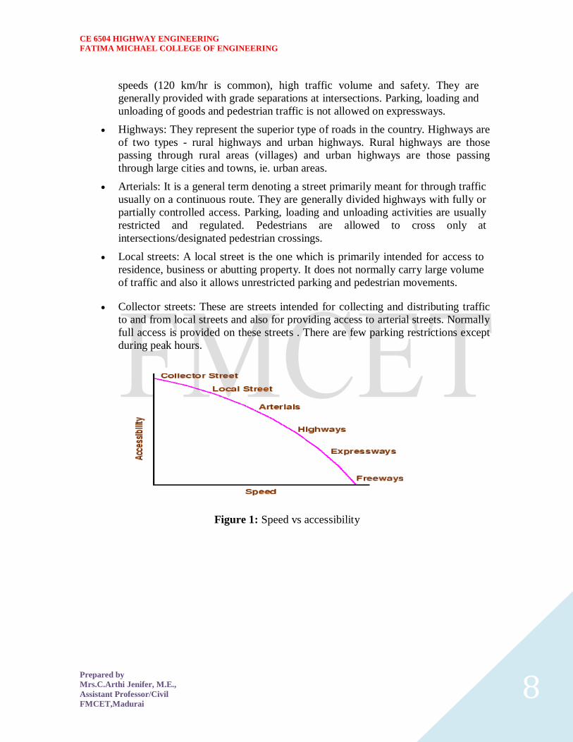
CE 6504 HIGHWAY ENGINEERING
FATIMA MICHAEL COLLEGE OF ENGINEERING
Prepared by
MrsCArthi Jenifer ME
Assistant ProfessorCivil
FMCETMadurai 8
speeds (120 kmhr is common) high traffic volume and safety They are
generally provided with grade separations at intersections Parking loading and
unloading of goods and pedestrian traffic is not allowed on expressways
Highways They represent the superior type of roads in the country Highways are
of two types - rural highways and urban highways Rural highways are those
passing through rural areas (villages) and urban highways are those passing
through large cities and towns ie urban areas
Arterials It is a general term denoting a street primarily meant for through traffic
usually on a continuous route They are generally divided highways with fully or
partially controlled access Parking loading and unloading activities are usually
restricted and regulated Pedestrians are allowed to cross only at
intersectionsdesignated pedestrian crossings
Local streets A local street is the one which is primarily intended for access to
residence business or abutting property It does not normally carry large volume
of traffic and also it allows unrestricted parking and pedestrian movements
Collector streets These are streets intended for collecting and distributing traffic
to and from local streets and also for providing access to arterial streets Normally
full access is provided on these streets There are few parking restrictions except
during peak hours
Figure 1 Speed vs accessibility
CE 6504 HIGHWAY ENGINEERING
FATIMA MICHAEL COLLEGE OF ENGINEERING
Prepared by
MrsCArthi Jenifer ME
Assistant ProfessorCivil
FMCETMadurai 9
FACTORS AFFECTING HIGHWAY ALIGHNMENT
Design speed
Design speed is the single most important factor that affects the geometric design It
directly affects the sight distance horizontal curve and the length of vertical curves
Since the speed of vehicles vary with driver terrain etc a design speed is adopted for all
the geometric design
Design speed is defined as the highest continuous speed at which individual vehicles can
travel with safety on the highway when weather conditions are conducive Design speed
is different from the legal speed limit which is the speed limit imposed to curb a common
tendency of drivers to travel beyond an accepted safe speed Design speed is also
different from the desired speed which is the maximum speed at which a driver would
travel when unconstrained by either traffic or local geometry
Since there are wide variations in the speed adopted by different drivers and by different
types of vehicles design speed should be selected such that it satisfy nearly all drivers At
the same time a higher design speed has cascading effect in other geometric designs and
thereby cost escalation Therefore an 85th percentile design speed is normally adopted
This speed is defined as that speed which is greater than the speed of 85 of drivers In
some countries this is as high as 95 to 98 percentile speed
Topography
The next important factor that affects the geometric design is the topography It is easier to
construct roads with required standards for a plain terrain However for a given design speed the
construction cost increases multiform with the gradient and the terrain Therefore geometric design
standards are different for different terrain to keep the cost of construction and time of construction
under control This is characterized by sharper curves and steeper gradients
Other factors
CE 6504 HIGHWAY ENGINEERING
FATIMA MICHAEL COLLEGE OF ENGINEERING
Prepared by
MrsCArthi Jenifer ME
Assistant ProfessorCivil
FMCETMadurai 10
In addition to design speed and topography there are various other factors that affect the geometric
design and they are briefly discussed below
Vehicle The dimensions weight of the axle and operating characteristics of a vehicle
influence the design aspects such as width of the pavement radii of the curve clearances
parking geometrics etc A design vehicle which has standard weight dimensions and
operating characteristics are used to establish highway design controls to accommodate
vehicles of a designated type
Human The important human factors that influence geometric design are the mental and
psychological characteristics of the driver and pedestrians like the reaction time
Traffic It will be uneconomical to design the road for peak traffic flow Therefore a
reasonable value of traffic volume is selected as the design hourly volume which is
determined from the various traffic data collected The geometric design is thus based on
this design volume capacity etc
Environmental Factors like air pollution noise pollution etc should be given due
consideration in the geometric design of roads
Economy The design adopted should be economical as far as possible It should match
with the funds allotted for capital cost and maintenance cost
Others Geometric design should be such that the aesthetics of the region is not affected
Nagpur classification
In Nagpur road classification all roads were classified into five categories as National highways
State highways Major district roads Other district roads and village roads
National highways
They are main highways running through the length and breadth of India connecting major
ports foreign highways capitals of large states and large industrial and tourist centers
including roads required for strategic movements
It was recommended by Jayakar committee that the National highways should be the frame
on which the entire road communication should be based
All the national highways are assigned the respective numbers
For eg the highway connecting Delhi-Ambala-Amritsar is denoted as NH-1 (Delhi-
Amritsar) where as a bifurcation of this highway beyond Full under to Srinagar and Uri is
denoted as NH-1_A
They are constructed and maintained by CPWD
The total lengths of National highway in the country is 58112 Kms and constitute about 2
of total road networks of India and carry 40 of total traffic
State highways
They are the arterial roads of a state connecting up with the national highways of adjacent
states district headquarters and important cities within the state
They also serve as main arteries to and from district roads
Total length of all SH in the country is 1 37119 Kms
Major district roads
Important roads with in a district serving areas of production and markets connecting those
with each other or with the major highways
India has a total of 4 70000 Kms of MDR
CE 6504 HIGHWAY ENGINEERING
FATIMA MICHAEL COLLEGE OF ENGINEERING
Prepared by
MrsCArthi Jenifer ME
Assistant ProfessorCivil
FMCETMadurai 11
Other district roads
Roads serving rural areas of production and providing them with outlet to market centers or
other important roads like MDR or SH
Village roads
They are roads connecting villages or group of villages with each other or to the nearest
road of a higher category like ODR or MDR
India has 2650000 kms of ODR+VR out of the total 3315231 kms of all type of roads
Roads classification criteria
Apart from the classification given by the different plans roads were also classified based on some
other criteria They are given in detail below
Based on usage
This classification is based on whether the roads can be used during different seasons of the year
All-weather roads Those roads which are negotiable during all weathers except at major
river crossings where interruption of traffic is permissible up to a certain extent are called all
weather roads
Fair-weather roads Roads which are negotiable only during fair weather are called fair
weather roads
Based on carriage way
This classification is based on the type of the carriage way or the road pavement
Paved roads with hards surface If they are provided with a hard pavement course such
roads are called paved roads(eg stones Water bound macadam (WBM) Bituminous
macadam (BM) concrete roads)
Unpaved roads Roads which are not provided with a hard course of atleast a WBM layer
they is called unpaved roads Thus earth and gravel roads come under this category
Alignment The position or the layout of the central line of the highway on the ground is called the
alignment Horizontal alignment includes straight and curved paths Vertical alignment
includes level and gradients Alignment decision is important because a bad alignment
will enhance the construction maintenance and vehicle operating costs Once an
alignment is fixed and constructed it is not easy to change it due to increase in cost of
adjoining land and construction of costly structures by the roadside
Requirements The requirements of an ideal alignment are
The alignment between two terminal stations should be short and as far as
possible be straight but due to some practical considerations deviations may be
needed
The alignment should be easy to construct and maintain It should be easy for the
operation of vehicles So to the maximum extend easy gradients and curves
should be provided
It should be safe both from the construction and operating point of view
especially at slopes embankments and cutting It should have safe geometric
features
The alignment should be economical and it can be considered so only when the
initial cost maintenance cost and operating cost are minimum
CE 6504 HIGHWAY ENGINEERING
FATIMA MICHAEL COLLEGE OF ENGINEERING
Prepared by
MrsCArthi Jenifer ME
Assistant ProfessorCivil
FMCETMadurai 12
Factors controlling alignment
We have seen the requirements of an alignment But it is not always possible to satisfy all
these requirements Hence we have to make a judicial choice considering all the factors
The various factors that control the alignment are as follows
Obligatory points These are the control points governing the highway alignment
These points are classified into two categories Points through which it should
pass and points through which it should not pass Some of the examples are
o Bridge site The bridge can be located only where the river has straight
and permanent path and also where the abutment and pier can be strongly
founded The road approach to the bridge should not be curved and skew
crossing should be avoided as possible Thus to locate a bridge the
highway alignment may be changed
o Mountain While the alignment passes through a mountain the various alternatives are to either construct a tunnel or to go round the hills The suitability of the alternative depends on factors like topography site
conditions and construction and operation cost
o Intermediate town The alignment may be slightly deviated to connect an intermediate town or village nearby
These were some of the obligatory points through which the alignment should pass
Coming to the second category that is the points through which the alignment should not
pass are
Religious places These have been protected by the law from being acquired for
any purpose Therefore these points should be avoided while aligning
Very costly structures Acquiring such structures means heavy compensation
which would result in an increase in initial cost So the alignment may be deviated
not to pass through that point
Lakesponds etc The presence of a lake or pond on the alignment path would also
necessitate deviation of the alignment
Traffic The alignment should suit the traffic requirements Based on the origin-
destination data of the area the desire lines should be drawn The new alignment should
be drawn keeping in view the desire lines traffic flow pattern etc Geometric design
Geometric design factors such as gradient radius of curve sight distance etc also govern
the alignment of the highway To keep the radius of curve minimum it may be required
to change the alignment The alignments should be finalized such that the obstructions to
visibility do not restrict the minimum requirements of sight distance The design
standards vary with the class of road and the terrain and accordingly the highway should
be aligned Economy The alignment finalized should be economical All the three costs
ie construction maintenance and operating cost should be minimum The construction
cost can be decreased much if it is possible to maintain a balance between cutting and
filling Also try to avoid very high embankments and very deep cuttings as the
construction cost will be very higher in these cases
Road ecology
The features of the cross-section of the pavement influences the life of the pavement as
CE 6504 HIGHWAY ENGINEERING
FATIMA MICHAEL COLLEGE OF ENGINEERING
Prepared by
MrsCArthi Jenifer ME
Assistant ProfessorCivil
FMCETMadurai 13
well as the riding comfort and safety Of these pavement surface characteristics affect
both of these Camber kerbs and geometry of various cross-sectional elements are
important aspects to be considered in this regard They are explained briefly in this
chapter
Camber
Camber or cant is the cross slope provided to raise middle of the road surface in the
transverse direction to drain off rain water from road surface The objectives of providing
camber are
Surface protection especially for gravel and bituminous roads
Sub-grade protection by proper drainage
Quick drying of pavement which in turn increases safety
Too steep slope is undesirable for it will erode the surface Camber is measured in 1 in n
or n (Eg 1 in 50 or 2) and the value depends on the type of pavement surface The
value suggested by IRC for various categories of pavement is given in Table 1 The
common types of camber are parabolic straight or combination of them (Figure 1)
Figure 1 Different types of camber
Table 1 IRC Value
s for ca
mber
Heavy
Light
Surface
rain
type
rain
17
ConcreteBituminous
2
25
GravelWBM
3
30
Earthen
4
CE 6504 HIGHWAY ENGINEERING
FATIMA MICHAEL COLLEGE OF ENGINEERING
Prepared by
MrsCArthi Jenifer ME
Assistant ProfessorCivil
FMCETMadurai 14
Engineering surveys for alignment
The stages of the engineering surveys are a) Map study
b) Reconnaissance
c) Preliminary surveys
d) Final location and detailed surveys
Map study -
) In the topographic map to suggest the likely routes of roads In India topographic
maps are available from the survey of India with 15 or 30-meter contour intervals
) The main feature like rivers hills and valleys etc The probable alignment can be
located on the map from the following details available on the map
Alignment avoiding valleys ponds or lakes
When the road has to cross a row of hills possibility crossing through a mountain pass
Approximate location of bridge site for crossing rivers avoiding bend of the river
When a road is to be connected between two stations one of the top and the other on the foot
of the hill then alternate routes can be suggested keeping in view the permissible alignment
Suppose the scale of the contour map is known and then the contour intervals it is possible
to decide the length of road required between two consecutive contours keeping the gradient
within allowable limits
In the fig Let A and B be two stations to be connected by road AB is the shortest route
(Straight line) APQB is a steep route in which the gradient positively exceeds 1 in 20 as the
distance between the contour intervals is only about 200 meter
APLMNB is a route with an approximate slope of 1 in 20 whereas APEFGB is an alternate
alignment with the same gradient
Thus the map study also is possible to drop a certain route in view of any unavoidable
obstructions (or) undesirable ground enroute
Reconnaissance-
The second stage of surveys for highway location is the reconnaissance to examine the general
character of the area for deciding the most feasible routes for detailed studies
Some of the details to be collected during reconnaissance are given below
Valleys ponds lakes marshy land ridge hills permanent structures and other obstructions
along the route which are not available in the map
Approximate values of gradient length of gradients and radius of curves of alternate
alignments
Number and types of cross drainage structures maximum flood level and natural
groundwater level along the probable routes
Soil type along the routes from field identification tests and observation of geological
features
Sources of construction materials water and location of stone quarries
When the road passes through hilly or mountainous terrain additional data regarding the
geological formation types of rocks dip of strata seepage flow etc
Preliminary survey -
CE 6504 HIGHWAY ENGINEERING
FATIMA MICHAEL COLLEGE OF ENGINEERING
Prepared by
MrsCArthi Jenifer ME
Assistant ProfessorCivil
FMCETMadurai 15
The main objectives of the preliminary surveys are
To survey the various alternate alignments proposed after the reconnaissance and to collect
all the necessary physical information and details of topography drainage and soil
To compare the different proposals in view of the requirements of a good alignment
To estimate quantity of earthwork materials and other construction aspects and to work out
the cost of alternate proposals
To finalize the best alignment from all considerations
The procedure of the conventional methods of preliminary surveys the given steps
Primary survey -
For alternate alignments either secondary traverses (or) independent primary traverses may be
necessary
Topographical features -
All geographical and other man made features along the traverse and for a certain width on either
side surveyed and plotted
Leveling work -
Levelling work is also carried out side by side to give the centerline profiles and typical cross
sections The leveling work in the preliminary survey is kept to a minimum just sufficient to obtain
the approximate earthwork in the alternate alignments
Drainage studies -
Drainage investigations and hydrological data are collected so as to estimate the type number and
approximate size of cross and drainage structures
Soil survey -
The soil survey conducted at this stage helps to working out details of earthwork slopes suitability
of materials subsoil and surface drainage requirements and pavement type and the approximate
thickness requirements
Material survey -
The survey for naturally occurring materials like stone aggregates soft aggregates etc and
identification of suitable quarries should be made
Traffic survey -
Traffic surveys conducted in the region from basis for deciding the number of traffic lanes and
roadway width pavement design and economic analysis of highway project
Locations and functions
Final location and detailed survey - The alignment finalized at the design office after the preliminary survey is to be first located on the
field by establishing the centerline The detailed survey should be carried out for collecting the
information technology for the preparation of plans and construction details
Location -
The centerline of the road finalized in the drawings to be translated on the ground
during the location survey
Major and minor control points are established on the ground and center pegs are
driven checking the geometric design requirements
Detailed survey -
CE 6504 HIGHWAY ENGINEERING
FATIMA MICHAEL COLLEGE OF ENGINEERING
Prepared by
MrsCArthi Jenifer ME
Assistant ProfessorCivil
FMCETMadurai 16
Levels along his final centerline should be taken at all staked points Levelling work is to
great importance as the vertical alignment
A detailed soil survey is carried out to enable drawing of the soil profile
The data during the detailed survey should be elaborate and complete for preparing detailed
plans design and estimates of the project
Soil suitability analysis
The methodology for locating appropriate sites for each land use activity is guided by the intent to
minimize the possible adverse effects of development on the environment and on existing
communities and to emphasize the positive impacts of such development by locating them in a
most suitable location
This is achieved by examining a number of individual criteria assigning them relative levels of
importance as a whole and using a mathematical resultant model to identify the most suitable
location
By adopting this site suitability method it is possible to systematically identify the criteria
considered clearly document the relative importance of one criterion over another analyze the net
outcome using a Geographic Information System and then possibly revisit the mathematical
relationships in this ldquodecision modelrdquo
By revising the relative importance to identified criteria based upon the particular land use under
consideration it is possible to generate ldquosuitability mapsrdquo for each individual land use and then
generate a final composite land use that is based on a best possible collective suitability of multiple
land uses
To achieve this all the criteria are assigned a ldquorankrdquo denoting their relative levels of importance
within the suitability study These ranks are assigned as numeric values ranging from 1 to 10 with 1
reflecting a low level of importance and 10 reflecting a high level of importance For example
within the criteria of road networks national highways would have a different level of influence on
the suitability for a particular land use as compared with local roads Further the distance from each
of these features would further modify the relative suitability of a land use based on the proximity to
a particular type of road
Criteria for Site Suitability Analysis
The decision criteria for site selection are examined for assigning relative ranks and individual
feature weights based on the land use type for which suitability is being examined For benefit of
analysis the criteria under consideration in this paper activity are organized as
Critical Criteria Criteria that will be very significant in the site selection of the identified land use
and will act as key drivers in the selection of the geographic location These criteria can be clustered
into a single decision model and the outcome collectively reviewed These criteria have a strong
influence in the final suitability
Additional Criteria Criteria that will have to be examined one at a time to carefully assess its
relationship with the proposed land use activity These criteria have a positive influence in the final
suitability
CE 6504 HIGHWAY ENGINEERING
FATIMA MICHAEL COLLEGE OF ENGINEERING
Prepared by
MrsCArthi Jenifer ME
Assistant ProfessorCivil
FMCETMadurai 17
Constrained Criteria These criteria impose strong negative opportunities in the selection of areas
for the identified land use Consequently they inform of us of where the particular land use under
consideration should not be located These criteria serve to limit or exclude areas from the final
suitability
GIS Site Suitability Analysis Model We were developed a tourism site suitability analysis model
in ArcGIS - 931 which is shown in Figure -
CE 6504 HIGHWAY ENGINEERING
FATIMA MICHAEL COLLEGE OF ENGINEERING
Prepared by
MrsCArthi Jenifer ME
Assistant ProfessorCivil
FMCETMadurai 18
UNIT 2 GEOMETRIC DESIGN OF HIGHWAYS
Typical cross section of urban and rural roads
A cross section is a vertical plane (slice) taken at right angles to the road control line showing the
various elements that make up the roads structure It is normally viewed in the direction of
increasing chainage
The width of a roadway is an important design consideration to ensure that it is appropriately sized
to serve its function Because of the diversity within the County two major roadway categories have
been established 1 Rural Road Standards 2 Urban Road Standards Urban Road Standards will
serve those areas which tend to be more developed and need to provide for multiple users
(bicyclists pedestrians parallel parking etc) whereas many rural roads will primarily serve only
vehicular traffic
Cross sections are created to provide a visual guide depicting the initial interim and ultimate phase
cross sections for these road classifications The typical sections illustrated in the following pages
are recommendations tied to transportation planning aspects such as right‐of‐way lineage sidewalk
width etc Threshold daily traffic can be used as a guide for a starting point when determining
which cross section is most applicable
1 Rural Road Standards
The rural roadways will not typically require curb and gutter or sidewalk although the County may
require either or both in unique circumstances Widths of lanes and shoulders will vary depending
upon the specific classification and the potential traffic volume which the roadway may carry Roads
carrying fewer than 200 vehicles per day need not be paved or treated for dust control The need for
paved shoulders is also dependent upon the level of traffic and safety
Final design and construction details will be determined by the Public Works Department Final
Design and construction criteria taken into consideration may include but are not limited to use of
the roadway density of development topographical characteristics and nearby development For
construction in which only a portion of the ultimate cross‐section is intended to be completed the
partial design will need to allow for the eventual widening to the ultimate cross‐section The design
for the partial or interim cross‐section roadway will need to incorporate ultimate design information
to ensure that the first phase of roadway construction is appropriate and would not need to be
removed at a future date when the full width cross‐section is completed
2 Urban Road Standards
Three roadway classifications are identified for those areas that are associated with the communityrsquos
urban growth areas They include arterial collector and local street classifications Transportation
Plan shows the key elements of the urban road standards Urban road standards will include 12‐foot
lanes sidewalk and curb amp gutter arterials and collectors will also include a striped bike lane Turn
lanes may be necessary as determined by the County Since almost all of the municipalities have
different right‐of‐way cross sections adopted for their community it makes it very difficult for the
County to match them all Therefore the philosophy was to encourage a baseline amount of
right‐of‐way reservation that could ensure the adjacent community enough area for coordination of
future roadway improvements until such time the road
CE 6504 HIGHWAY ENGINEERING
FATIMA MICHAEL COLLEGE OF ENGINEERING
Prepared by
MrsCArthi Jenifer ME
Assistant ProfessorCivil
FMCETMadurai 19
CE 6504 HIGHWAY ENGINEERING
FATIMA MICHAEL COLLEGE OF ENGINEERING
Prepared by
MrsCArthi Jenifer ME
Assistant ProfessorCivil
FMCETMadurai 20
Cross sectional elements
Kerbs
Kerbs indicate the boundary between the carriage way and the shoulder or islands or footpaths Different types of kerbs are
CE 6504 HIGHWAY ENGINEERING
FATIMA MICHAEL COLLEGE OF ENGINEERING
Prepared by
MrsCArthi Jenifer ME
Assistant ProfessorCivil
FMCETMadurai 21
Low or mountable kerbs This type of kerbs is provided such that they
encourage the traffic to remain in the through traffic lanes and also allow the
driver to enter the shoulder area with little difficulty The height of this kerb is
about 10 cm above the pavement edge with a slope which allows the vehicle to
climb easily This is usually provided at medians and channelization schemes and
also helps in longitudinal drainage
Semi-barrier type kerbs When the pedestrian traffic is high these kerbs are
provided Their height is 15 cm above the pavement edge This type of kerb
prevents encroachment of parking vehicles but at acute emergency it is possible
to drive over this kerb with some difficulty
Barrier type kerbs They are designed to discourage vehicles from leaving the
pavement They are provided when there is considerable amount of pedestrian
traffic They are placed at a height of 20 cm above the pavement edge with a steep
batter
Submerged kerbs They are used in rural roads The kerbs are provided at
pavement edges between the pavement edge and shoulders They provide lateral
confinement and stability to the pavement
Figure 1 Different types of kerbs
Shoulders Shoulders are provided along the road edge and are intended for accommodation of
stopped vehicles serve as an emergency lane for vehicles and provide lateral support
for base and surface courses The shoulder should be strong enough to bear the weight
of a fully loaded truck even in wet conditions The shoulder width should be adequate
for giving working space around a stopped vehicle It is desirable to have a width of
46 m for the shoulders A minimum width of 25 m is recommended for 2-lane rural
highways in India Parking lanes
Parking lanes are provided in urban lanes for side parking Parallel parking is preferred
because it is safe for the vehicles moving on the road The parking lane should have a
minimum of 30 m width in the case of parallel parking
CE 6504 HIGHWAY ENGINEERING
FATIMA MICHAEL COLLEGE OF ENGINEERING
Prepared by
MrsCArthi Jenifer ME
Assistant ProfessorCivil
FMCETMadurai 22
Bus-bays
Bus bays are provided by recessing the kerbs for bus stops They are provided so that
they do not obstruct the movement of vehicles in the carriage way They should be at
least 75 meters away from the intersection so that the traffic near the intersections is not
affected by the bus-bay
Service roads Service roads or frontage roads give access to access controlled highways like freeways
and expressways They run parallel to the highway and will be usually isolated by a
separator and access to the highway will be provided only at selected points These roads
are provided to avoid congestion in the expressways and also the speed of the traffic in
those lanes is not reduced
Drainage
The pavement surface should be absolutely impermeable to prevent seepage of water into
the pavement layers Further both the geometry and texture of pavement surface should
help in draining out the water from the surface in less time
Footpath
Footpaths are exclusive right of way to pedestrians especially in urban areas They are
provided for the safety of the pedestrians when both the pedestrian traffic and vehicular
traffic is high Minimum width is 15 meter and may be increased based on the traffic
The footpath should be either as smooth as the pavement or more smoother than that to
induce the pedestrian to use the footpath
Right of way
Right of way (ROW) or land width is the width of land acquired for the road along its
alignment It should be adequate to accommodate all the cross-sectional elements of the
highway and may reasonably provide for future development To prevent ribbon
development along highways control lines and building lines may be provided Control
line is a line which represents the nearest limits of future uncontrolled building activity
in relation to a road Building line represents a line on either side of the road between
which and the road no building activity is permitted at all The right of way width is
governed by
Width of formation It depends on the category of the highway and width of
roadway and road margins
Height of embankment or depth of cutting It is governed by the topography and
the vertical alignment
Side slopes of embankment or cutting It depends on the height of the slope soil
type etc
Drainage system and their size which depends on rainfall topography etc
Sight distance considerations On curves etc there is restriction to the visibility
on the inner side of the curve due to the presence of some obstructions like
building structures etc
Reserve land for future widening Some land has to be acquired in advance
CE 6504 HIGHWAY ENGINEERING
FATIMA MICHAEL COLLEGE OF ENGINEERING
Prepared by
MrsCArthi Jenifer ME
Assistant ProfessorCivil
FMCETMadurai 23
Table 2 Desig
n speed in as per IRC (ruling and minimum)
Steep
Type
Plain
Rolling
Hilly
40-30
NSampSH
100-80
80-65
50-40
MDR
80-65
65-50
40-30
30-20
25-20
ODR
65-50
50-40
30-25
25-20
VR
50-40
40-35
25-20
anticipating future developments like widening of the road
Table 1 No
right of way for open areas
Roadway width in m
Road
Plain and
Mountainous and
classification
steep terrain
rolling terrain
Open areas
45
24
NHSH
18
MDR
25
15
15
ODR
12
9
VR
Built-up areas
20
NHSH
30
MDR
20
15
ODR
15
12
9
VR
10
CE 6504 HIGHWAY ENGINEERING
FATIMA MICHAEL COLLEGE OF ENGINEERING
Prepared by
MrsCArthi Jenifer ME
Assistant ProfessorCivil
FMCETMadurai 24
Horizontal curve
The presence of horizontal curve imparts centrifugal force which is a reactive force
acting outward on a vehicle negotiating it Centrifugal force depends on speed and radius
of the horizontal curve and is counteracted to a certain extent by transverse friction
between the tyre and pavement surface On a curved road this force tends to cause the
vehicle to overrun or to slide outward from the centre of road curvature For proper
design of the curve an understanding of the forces acting on a vehicle taking a horizontal
curve is necessary Various forces acting on the vehicle are illustrated in the figure 1
Figure 1 Effect of horizontal curve They are the centrifugal force (P) acting outward weight of the vehicle (W) acting
downward and the reaction of the ground on the wheels ( and ) The centrifugal
force and the weight is assumed to be from the centre of gravity which is at h units above
the ground Let the wheel base be assumed as b units The centrifugal force in
is given by
(1)
where is the weight of the vehicle in is the speed of the vehicle in is
the acceleration due to gravity in and is the radius of the curve in
The centrifugal ratio or the impact factor is given by
CE 6504 HIGHWAY ENGINEERING
FATIMA MICHAEL COLLEGE OF ENGINEERING
Prepared by
MrsCArthi Jenifer ME
Assistant ProfessorCivil
FMCETMadurai 25
(1)
The centrifugal force has two effects A tendency to overturn the vehicle about the outer
wheels and a tendency for transverse skidding Taking moments of the forces with
respect to the outer wheel when the vehicle is just about to override
At the equilibrium over turning is possible when
and for safety the following condition must satisfy
(2)
The second tendency of the vehicle is for transverse skidding ie When the the
centrifugal force is greater than the maximum possible transverse skid resistance due to
friction between the pavement surface and tyre The transverse skid resistance (F) is
given by
where and is the fractional force at tyre and and is the reaction at
tyre and is the lateral coefficient of friction and is the weight of the vehicle
This is counteracted by the centrifugal force (P) and equating
At equilibrium when skidding takes place (from equation1)
and for safety the following condition must satisfy
CE 6504 HIGHWAY ENGINEERING
FATIMA MICHAEL COLLEGE OF ENGINEERING
Prepared by
MrsCArthi Jenifer ME
Assistant ProfessorCivil
FMCETMadurai 26
(3)
Equation 2 and 3 give the stable condition for design If equation 2 is violated the vehicle
will overturn at the horizontal curve and if equation 3 is violated the vehicle will skid at
the horizontal
Curve Analysis of super-elevation
Super-elevation or cant or banking is the transverse slope provided at horizontal curve to
counteract the centrifugal force by raising the outer edge of the pavement with respect to
the inner edge throughout the length of the horizontal curve When the outer edge is
raised a component of the curve weight will be complimented in counteracting the effect
of centrifugal force In order to find out how much this raising should be the following
analysis may be done The forces acting on a vehicle while taking a horizontal curve with
super elevation is shown in figure 1
Figure 1 Analysis of super-elevation
Forces acting on a vehicle on horizontal curve of radius at a speed of are
the centrifugal force acting horizontally out-wards through the center of
gravity
the weight of the vehicle acting down-wards through the center of gravity and
the friction force between the wheels and the pavement along the surface
inward
CE 6504 HIGHWAY ENGINEERING
FATIMA MICHAEL COLLEGE OF ENGINEERING
Prepared by
MrsCArthi Jenifer ME
Assistant ProfessorCivil
FMCETMadurai 27
At equilibrium by resolving the forces parallel to the surface of the pavement we get where
friction
is the weight of the vehicle is the centrifugal force is the coefficient of
is the transverse slope due to superelevation Dividing by we get
CE 6504 HIGHWAY ENGINEERING
FATIMA MICHAEL COLLEGE OF ENGINEERING
Prepared by
MrsCArthi Jenifer ME
Assistant ProfessorCivil
FMCETMadurai 28
Step 1
Find for 75 percent of design speed neglecting ie
Step 2
If then else if go to step 3
Step 3
Find for the design speed and max ie If
then the maximum is safe for the design speed else go to
step 4
Step 4
Find the allowable speed for the maximum and
If then the design is adequate otherwise use speed adopt
control measures or look for speed control measures
Maximum and minimum super-elevation
Depends on (a) slow moving vehicle and (b) heavy loaded trucks with high CG IRC
specifies a maximum super-elevation of 7 percent for plain and rolling terrain while that
of hilly terrain is 10 percent and urban road is 4 percent The minimum super elevation is
2-4 percent for drainage purpose especially for large radius of the horizontal curve
Attainment of super-elevation
1 Elimination of the crown of the cambered section by
1 Rotating the outer edge about the crown The outer half of the cross slope
is rotated about the crown at a desired rate such that this surface falls on
the same plane as the inner half
2 Shifting the position of the crown This method is also known as diagonal
crown method Here the position of the crown is progressively
shifted outwards thus increasing the width of the inner half of cross section
progressively
2 Rotation of the pavement cross section to attain full super elevation byThere are
two methods of attaining super elevation by rotating the pavement
1 Rotation about the center line The pavement is rotated such that the inner
edge is depressed and the outer edge is raised both by half the total amount
of super elevation ie by with respect to the centre
2 Rotation about the inner edge Here the pavement is rotated raising the
outer edge as well as the centre such that the outer edge is raised by the
full amount of super elevation with respect to the inner edge
Horizontal Transition Curves
CE 6504 HIGHWAY ENGINEERING
FATIMA MICHAEL COLLEGE OF ENGINEERING
Prepared by
MrsCArthi Jenifer ME
Assistant ProfessorCivil
FMCETMadurai 29
Transition curve is provided to change the horizontal alignment from straight to circular
curve gradually and has a radius which decreases from infinity at the straight end
(tangent point) to the desired radius of the circular curve at the other end (curve point)
There are five objectives for providing transition curve and are given below
1 to introduce gradually the centrifugal force between the tangent point and the
beginning of the circular curve avoiding sudden jerk on the vehicle This
increases the comfort of passengers
2 to enable the driver turn the steering gradually for his own comfort and security
3 to provide gradual introduction of super elevation and
4 to provide gradual introduction of extra widening
5 to enhance the aesthetic appearance of the road
Type of transition curve
Different types of transition curves are spiral or clothoid cubic parabola and Lemniscate
IRC recommends spiral as the transition curve because
1 it fulfills the requirement of an ideal transition curve that is
1 rate of change or centrifugal acceleration is consistent (smooth) and
2 radius of the transition curve is at the straight edge and changes to at
the curve point ( ) and calculation and field implementation is
very easy
Length of transition curve The length of the transition curve should be determined as the maximum of the following
three criteria rate of change of centrifugal acceleration rate of change of super elevation
and an empirical formula given by IRC Rate of change of centrifugal acceleration
At the tangent point radius is infinity and hence centrifugal acceleration is zero At the
end of the transition the radius R has minimum value R The rate of change of
centrifugal acceleration should be adopted such that the design should not cause
discomfort to the drivers If is the rate of change of centrifugal acceleration it can be
written as
Therefore the length of the transition curve in is
CE 6504 HIGHWAY ENGINEERING
FATIMA MICHAEL COLLEGE OF ENGINEERING
Prepared by
MrsCArthi Jenifer ME
Assistant ProfessorCivil
FMCETMadurai 30
(1)
where is the rate of change of centrifugal acceleration given by an empirical formula
suggested by by IRC as below
(2) 2 Rate of introduction of super-elevation
Raise ( ) of the outer edge with respect to inner edge is given by
The rate of change of this raise from to is achieved
gradually with a gradient of in over the length of the transition curve (typical range
of is 60-150) Therefore the length of the transition curve is
(3)
3 By empirical formula
IRC suggest the length of the transition curve is minimum for a plain and rolling terrain
(4)
and for steep and hilly terrain is
(5)
CE 6504 HIGHWAY ENGINEERING
FATIMA MICHAEL COLLEGE OF ENGINEERING
Prepared by
MrsCArthi Jenifer ME
Assistant ProfessorCivil
FMCETMadurai 31
and the shift as
(
6
) The length of the transition curve is the maximum of
equations 1 3 and 4or5 ie
(
7
Case (a)
For single lane roads
(
1
)
Therefore
(
2
)
Figure 1 Set-back for single lane roads (
CE 6504 HIGHWAY ENGINEERING
FATIMA MICHAEL COLLEGE OF ENGINEERING
Prepared by
MrsCArthi Jenifer ME
Assistant ProfessorCivil
FMCETMadurai 32
For multi lane roads if is the distance between centerline of the road and the centerline
of the inner lane then
(3)
(4)
Figure 2 Set-back for multi-lane roads ( )
Case (a)
For single lane roads
(1)
Therefore
(2)
Gradient
Gradient is the rate of rise or fall along the length of the road with respect to the
horizontal While aligning a highway the gradient is decided for designing the vertical
curve Before finalizing the gradients the construction cost vehicular operation cost and
the practical problems in the site also has to be considered Usually steep gradients are
avoided as far as possible because of the difficulty to climb and increase in the
CE 6504 HIGHWAY ENGINEERING
FATIMA MICHAEL COLLEGE OF ENGINEERING
Prepared by
MrsCArthi Jenifer ME
Assistant ProfessorCivil
FMCETMadurai 33
construction cost More about gradients are discussed below
Effect of gradient
The effect of long steep gradient on the vehicular speed is considerable This is
particularly important in roads where the proportion of heavy vehicles is significant Due
to restrictive sight distance at uphill gradients the speed of traffic is often controlled by
these heavy vehicles As a result not only the operating costs of the vehicles are
increased but also capacity of the roads will have to be reduced Further due to high
differential speed between heavy and light vehicles and between uphill and downhill
gradients accidents abound in gradients
Representation of gradient
The positive gradient or the ascending gradient is denoted as and the negative gradient as The deviation angle is when two grades meet the angle which
measures the change of direction and is given by the algebraic difference between the two
grades
steep gradient while 1 in 50 = 2 representation is illustrated in the figure 1
Example 1 in 30 = 333 is a
is a flatter gradient The gradient
CE 6504 HIGHWAY ENGINEERING
FATIMA MICHAEL COLLEGE OF ENGINEERING
Prepared by
MrsCArthi Jenifer ME
Assistant ProfessorCivil
FMCETMadurai 34
Figure 1 Representation of gradient
Types of gradient
Many studies have shown that gradient upto seven percent can have considerable effect
on the speeds of the passenger cars On the contrary the speeds of the heavy vehicles are
considerably reduced when long gradients as flat as two percent is adopted Although
flatter gradients are desirable it is evident that the cost of construction will also be very
high Therefore IRC has specified the desirable gradients for each terrain However it
may not be economically viable to adopt such gradients in certain locations steeper
gradients are permitted for short duration Different types of grades are discussed below
Ruling gradient
The ruling gradient or the design gradient is the maximum gradient with which the
designer attempts to design the vertical profile of the road This depends on the terrain
length of the grade speed pulling power of the vehicle and the presence of the horizontal
curve In flatter terrain it may be possible to provide flat gradients but in hilly terrain it
is not economical and sometimes not possible also The ruling gradient is adopted by the
designer by considering a particular speed as the design speed and for a design vehicle
with standard dimensions But our country has a heterogeneous traffic and hence it is not
possible to lay down precise standards for the country as a whole Hence IRC has
recommended some values for ruling gradient for different types of terrain
Limiting gradient
This gradient is adopted when the ruling gradient results in enormous increase in cost of
construction On rolling terrain and hilly terrain it may be frequently necessary to adopt
limiting gradient But the length of the limiting gradient stretches should be limited and
must be sandwiched by either straight roads or easier grades
Exceptional gradient
Exceptional gradient are very steeper gradients given at unavoidable situations They
should be limited for short stretches not exceeding about 100 metres at a stretch In
mountainous and steep terrain successive exceptional gradients must be separated by a
minimum 100 metre length gentler gradient At hairpin bends the gradient is restricted to
25
Critical length of the grade
The maximum length of the ascending gradient which a loaded truck can operate without
undue reduction in speed is called critical length of the grade A speed of 25 kmph is a
CE 6504 HIGHWAY ENGINEERING
FATIMA MICHAEL COLLEGE OF ENGINEERING
Prepared by
MrsCArthi Jenifer ME
Assistant ProfessorCivil
FMCETMadurai 35
reasonable value This value depends on the size power load grad-ability of the truck
initial speed final desirable minimum speed
Minimum gradient
This is important only at locations where surface drainage is important Camber will take
care of the lateral drainage But the longitudinal drainage along the side drains require
some slope for smooth flow of water Therefore minimum gradient is provided for
drainage purpose and it depends on the rain fall type of soil and other site conditions A
minimum of 1 in 500 may be sufficient for concrete drain and 1 in 200 for open soil
drains are found to give satisfactory performance Sight distance available from a point is the actual distance along the road surface which a driver
from a specified height above the carriage way has visibility of stationary or moving objects
Sight distance required by drivers applies to both geometric design of highways and for
traffic control The sight distance situations are considered in the design
i) Stopping or absolute minimum sight distance
ii) Safe overtaking or passing sight distance
iii) Safe sight distance for entering into uncontrolled intersections
Apart from the three situations mentioned above the following sight distance are considered by the
IRC in highway design
Intermediate sight distance
This is defined as twice the stopping sight distance when overtaking sight distance
cannot be provided intermediate sight distance is provided to give limited overtaking opportunities
to fast vehicles
Head light sight distance
This is the distance visible to a driver during night driving under the illumination of the
vehicle head lights
Stopping sight distance
The minimum sight distance available on a highway at any spot should be of sufficient
length to stop a vehicle traveling at design speed safely without collision with any other obstruction
The absolute minimum sight distance is therefore equal to the stopping sight distance
which is also sometimes called nonpassing sight distance The sight distance available on a road to a
driver at any instance depends on
i) Features of the road
ii) Height of the drivers eye above the road surface
iii) Height of the object above the road surface
The distance within which a motor vehicle can be stopped depends upon the factors listed below
a) Total reactions time of the driver
b) Speed of vehicle
c) Efficiency of breaks
d) Frictional resistance between the road and tyres
e) Gradient of the road
Total reaction time
) Reaction time of the driver is the time taken from the instant the object is visible to the
driver to the instant the brakes are effectively applied
) The total reaction time may be split up into two parts
CE 6504 HIGHWAY ENGINEERING
FATIMA MICHAEL COLLEGE OF ENGINEERING
Prepared by
MrsCArthi Jenifer ME
Assistant ProfessorCivil
FMCETMadurai 36
i) Perception time
ii) Brake reaction time
PIEV theory
According to this theory the total reaction time of the driver is split into four parts
i) Perception
ii) Intellection
iii) Emotion
iv) Volition
Speed of Vehicle
The stopping distance depends very much on the speed of the vehicle first during the
total reaction time of the driver the distance moved by the vehicle will depend on the speed
Efficiency of brakes
The braking efficiency is said to be 100 percent if the wheels are fully licked preventing
them from rotating on application of the brakes This will result in 100 percent skidding which is
normally undesirable except in utmost emergency
Frictional resistance between road and tyres
The frictional resistance developed between road and tyres or the skid resistance depends
on the type and condition of the road surface and the tyres IRC has specified a design friction
coefficient of 035 to 04 depending upon the speed to be used for finding the braking distance in the
calculation of stopping sight distance
Analysis of stopping distance
i) The distance traveled by the vehicle during the total reaction time known as lag
distance
ii) The distance traveled by the vehicle after the application of the brakes is known as
braking distance
Overtaking sight distance
The minimum distance open to the vision of the driver of a vehicle intending to overtake
slow vehicle ahead with safety against the traffic of opposite direction is known as the minimum
overtaking sight distance(OSD) or Safe passing sight distance available
The overtaking sight distance is the distance measured along the center of the road which
a driver with his eye level 12m above the road surface can see the top of an object 12m above the
road surface
Some of the important factors on which the minimum overtaking sight distance required
a) Speed of
i) overtaking vehicle
ii) overtaken vehicle
iii) The vehicle coming from opposite direction
b) Distance between the overtaking and overtaken vehicles the minimum spacing
depends on the steeds
a) Skill and reaction time of the driver
b) Rate of acceleration of overtaking vehicle
c) Gradient of the road
Criteria for sight distance requirements on highway
) The absolute minimum sight distance required throughout the length of the road is the
SSD which should invariably be provided at all places
CE 6504 HIGHWAY ENGINEERING
FATIMA MICHAEL COLLEGE OF ENGINEERING
Prepared by
MrsCArthi Jenifer ME
Assistant ProfessorCivil
FMCETMadurai 37
) On horizontal curves the obstruction on the inner side of the curves should be cleared
to provide the required set back distance and absolute minimum sight distance
) On vertical summit curves the sight distance requirement may be fulfilled by proper
design of the vertical alignment
Hairpin bent
TYPES OF CURVES ON HILL ROADS
The following are the important types of curves provided on hill Roads-
1 Hair-Pin Curves
2 Salient Curves
3 Re-entrant Curves 1 Hair-pin curves - The curve in a hill road which changes its direction through an angle of 180
degree or so down the hill on the same side is known as hair-pin curve
A Hair-Pin Bend
This curve is so called because it conforms to the shape of a hair-pin The bend so formed at the
hair-pin curve in a hill road is known as hair-pin bend This type of curve should be located on a
hill side having the minimum slope and maximum stability It must also be safe from view point of
landslides and ground water Hair-pin bends with long arms and farther spacing are always
preferred They reduce construction problems and expensive protective works Hair-pin curves or
bends of serpentine nature are difficult to negotiate and should therefore be avoided as far as
possible
Salient curves - The curves having their convexity on the outer edges of a hill road are called
salient curves The centre of curvature of a salient curve lies towards the hill side This type of curve
occurs in the road length constructed on the ridge of a hill the bend so formed at the salient curve in
a hill road known as corner bend
Salient curves are very dangerous for fast moving traffic At such a curve or at corner bend the
portion of projecting hill side is usually cut down to improve the visibility as shown in fig (Re-
entrant curve) The outer edge of the road at such a curve is essentially provided with a parapet wall
for protection of the vehicles from falling down the hill slope
CE 6504 HIGHWAY ENGINEERING
FATIMA MICHAEL COLLEGE OF ENGINEERING
Prepared by
MrsCArthi Jenifer ME
Assistant ProfessorCivil
FMCETMadurai 38
3 Re-entrant curves - The curves having their convexity on the inner edge of a hill road are called
re-entrant curves
Re-entrant curves
The centre of curvature of a re-entrant curves lies away from the hill side This type of curve occurs
in the road length constructed in the calley of a hill
These curves are less dangereous as they provide adequate visibility to the fast moving traffic At
such curves the parapet wall is provided only for safety of fast moving traffic
CE 6504 HIGHWAY ENGINEERING
FATIMA MICHAEL COLLEGE OF ENGINEERING
Prepared by
MrsCArthi Jenifer ME
Assistant ProfessorCivil
FMCETMadurai 39
UNIT ndash III DESIGN OF RIGID AND FLEXIBLE PAVEMENTS
COMPARISON OF RIGID AND FLEXIBLE PAVEMENTS
The comparisons are
i) Design precision
A cement concrete pavement is amerable to a much more precise structural analysis
than a flexible pavement Flexible pavements designs are mainly empirical Computer aided analysis
of layered system is making the flexible pavement design more exact than hitherto
ii) Life
) Cement concrete slabs of a thin section constructed in the early 1940rsquos are still in
existence in India though many of them have cracked badly and a few of them have been ripped
open and rebuilt in recent ties
) A major project in cement concrete road construction between Agra and Mathura It can
safely be said that a well-designed concrete slab has a life of about 40 years
) Compared to this the life of a flexible pavement generally varies from 10 to 20 years
iii) Maintenance
) A well-designed cement concrete pavement needs very little maintenance The only
maintenance needed is I respect of joints
) The surface is unaffected by spillage of oil and lubricants bituminous surfaces on the
other hand need great inputs in maintenance
) The surface is affected by spillage of oil and lubricants The surface is also affected by
natural weathering agents like air water ad temperature changes
) A cement concrete pavement on the other hand needs a small amount for maintaining
joints
iv) Initial cost
) The argument so far used against a cement concrete slab is that it is much more costly
than a flexible pavement
) The latter specifications no doubt represent the rock-bottom needs of a road in India but
these specifications can hardly provide a smooth and durable surface
v) Stage construction ) Road construction is generally done adopting a policy of stage construction especially for
low volume roads As traffic grows additional layers in the form of water bound macadam and
superior surfacing are added on
) Initial outlay is minimum and additional outlays are in keeping with traffic growth This is
a great advantage when dealing with new roads in an atmosphere of austerity
vi) Availability of materials
) Cement bitumen stone aggregates and gravelsand are the major materials involved in
pavement Construction Cement has been in serious short supply in the country for the past many
decades
) Bitumen is also not available plentifully in India There is also the danger of the entire oil
reserves in the world shrinking during the next two or three decades
) In locations where stone aggregates are scarce cement concrete may have an advantage
for flexible pavements
vii) Surface characterstics
CE 6504 HIGHWAY ENGINEERING
FATIMA MICHAEL COLLEGE OF ENGINEERING
Prepared by
MrsCArthi Jenifer ME
Assistant ProfessorCivil
FMCETMadurai 40
) A good cement concrete surface is smooth and free from rutting potholes and
corrugations In a bituminous surface it is only the asphaltic concrete surface that can give
comparable rideablity
) A well-constructed cement concrete pavement surface can have a permanent nonskid
surface A bituminous surface can also be designed to have a good skid resistant surface
viii) Utility location
) In cement concrete slabs proper thought has to be given to locate utilities such as water
pipes telephone lines and electric cables
) It is difficult to rip open the slab and restore it to be the original condition if any changes
in the utilities lines are to be made
ix) Glame and night visibility
) Concrete pavements have a gray color which can cause glam under sunlight Colored
cement can reduce the grave
) On the other hand bituminous roads need more street lighting
x) Traffic dislocation during construction
) A cement concrete pavement requires 28 days before it can be thrown open to traffic On
the other hand a bituminous surface can be thrown open to traffic shortly after it is rolled
xi) Environmental considerations during construction
) The process of heating of bitumen and aggregates and mixing them together on hot mix
plants can prove to be much more hazardous to the environment than cement concrete construction
where no heating of any material is involved
xii) Overall economy on a life cycle basis
) A good road is costly to construct but once constructed such a road requires little
maintenance and results in savings in vehicle operating costs
) The comparative economy of a flexible pavement and a rigid pavement has proved that on
overall economic considerations
Types of pavement structure
Based on the structural behavior pavements are generally classified into three
categories
i) Flexible pavements
ii) Rigid pavements
iii) Semi rigid pavements
Flexible pavements
) Flexible pavements are those which on the whole have low or negligible flexural
strength and are rather flexible in their structural action under the loadsThe flexible pavement
layers reflect the deformation of the lower layers on to the surface of the layer
) A flexible pavement consists of four components(i) Soil subgrade (ii) sub base
course (iii) base course (iv) Surface course
CE 6504 HIGHWAY ENGINEERING
FATIMA MICHAEL COLLEGE OF ENGINEERING
Prepared by
MrsCArthi Jenifer ME
Assistant ProfessorCivil
FMCETMadurai 41
) The flexible pavement layers transmit the vertical or compressive stresses to the lower layers
by grain to grain transfer through the points of contact in the granular structure A well
compacted granular structure consisting of strong added aggregate can transfer the compressive
stresses
) The load spreading ability of this layer therefore depends on the type of the materials and mix
design factors Bituminous concrete is one of the best flexible pavements layer materials Other
materials which fall under the group are all granular materials with or without bituminous
binder granular base and sub base course materials
) The vertical compressive stress is maximum on the pavement surface directly under the wheel
and is equal to the contact pressure under the wheel The flexible pavement may be constructed
in a number of layers and the top layer has to be strongest as the highest compressive stresses
) Flexible pavements are commonly designed using empirical design charts or equations taking
into account some of the design factors there are also semi empirical and theoretical design
methods
Rigid pavements
) Rigid pavements are those which possess note flexural strength or flexural rigidity
The stresses are not transferred from grain to grain to the lower layers as in the ease of flexible
pavements layers
) The rigid pavements are made of Portland cement concrete plain reinforced or
prestressed concrete The plain cement concrete slabs are expected to take up about 40 kgcm2
flexural stress
) The rigid pavement has the slab action and is capable of transmitting the wheel
load stresses through a wider area below The main point of difference in the structural behavior
of rigid pavement as compared to the flexible pavement is that the critical condition of stress in
the rigid pavement is the maximum flexural stress occurring in the slab due to wheel load and
the temperature changes whereas in the flexible pavement
) As the rigid pavement slab has tensile strength tensile stresses are developed due
to the bending of the slab under wheel load and temperature variations Thus the types of
stresses developed and their distribution within the cement concrete slab are quirt different
) The cement concrete pavement slab can very well serve as a wearing surface as
well an effective base course The rigid pavement structure consists of a cement concrete slab
below which a granular base or sub base course may be provided
) Though the cement concrete slab can also be laid directly over the soil subgrade
consists of fine grained soil
) the rigid pavements are usually designed and the stresses are analyzed using the
elastic theory assuming the pavements as a n elastic plate resting over an elastic or a viscous
foundation
Semi rigid pavements
) when bonded materials like the pozzolanic concrete lean cement concrete or soil
cement are used in the base course or sub base course layer the pavement layer has considerably
higher flexural strength than the common flexible pavement layers
) when this intermediate class of materials are used in the base or sub base course
layer of the pavements they are called semi rigid pavements
CE 6504 HIGHWAY ENGINEERING
FATIMA MICHAEL COLLEGE OF ENGINEERING
Prepared by
MrsCArthi Jenifer ME
Assistant ProfessorCivil
FMCETMadurai 42
) This third category of semi rigid pavement are either designed as flexible
pavements with some correction factors to find the thickness requirements based on experience
or by using a new design approach
) The semi rigid pavement materials have low resistance to impact and abrasion and
therefore are usually provided with flexible pavement surface course
Various functions of pavement components
The functions are
Soil sub grade and its evaluation
) The soil sub grade is a layer of natural soil prepared to receive the layers of pavement
materials placed over it It is essential that at no time the soil sub grade is overstressed it means that
the pressure transmitted on the top of the sub grade is within the allowable limit
) Many tests are known for measuring the strength properties of the sub grades Some of the
tests have been standardized for the use The common strength test for the evaluation of soil
subgrade is
i) California bearing ratio test
ii) California resistance value test
iii) Triaxial compression test
iv) Plate bearing test
CALIFORNIA BEARING RATIO (CBR) TEST
It is evolved for the empirical method of flexible pavement design The CBR test is carried
out either in the laboratory on prepared specimens or in the field by taking in situ measurements
California resistance value
It is found by using have been stabliometerThis test is used in an empirical method of
flexible pavement design based on soil strength
Triaxial test
It is the most important soil strength but still the test is not very commonly used in structural
design of pavements
Plate bearing test
It is carried out using a relatively large diameter plate to evaluate the load supporting
capacity of supporting power of the pavement layers The results are plate bearing tests are used in
flexible pavement design method like McLeod method on based on layer system analysis by
brumister
Sub base and base courses and their evaluation
) There layers are made of broken stones bound or unbound aggreagatesome times in sub
base course a layer of stabilized soil(or) Selected granular soil is also used
) however at the sub base course it is desirable to use smaller size graded aggregates When
the sub grade consists of fine grained soil and when the pavement carries heavy wheel loads
CE 6504 HIGHWAY ENGINEERING
FATIMA MICHAEL COLLEGE OF ENGINEERING
Prepared by
MrsCArthi Jenifer ME
Assistant ProfessorCivil
FMCETMadurai 43
) Sub base course primarily has the similar function as of the base course and is provided
with inferior materials than of base course Base courses are used under rigid pavement for
i) Preventing pumping
ii) Protecting the sub grade against frost action
) Thus the fundamental purpose of abase course and sub base course is to provide a stress
transmitting medium to spread the surface wheel loads in such manner
) The sub base and base course layers may be evaluated by suitable strength or stability test
like plate bearing CBR test
WEARING COURSE AND ITS EVALUATION
) The purpose of the wearing course is to give a smooth riding surface that is dense It
resists pressure exerted by tyres and takes up wear and tear due to the traffic
) Wearing course also offers a water tight layer against the surface water infiltration The
flexible pavement normally a bituminous surfacing is used as a wearing course
) In rigid pavements the cement concrete acts like a base course as well as wearing course
Most popular test in use is marshal stability test where in the optimum content of bitumen binder is
worked out based on the stability density
) Plate bearing test and Bankelman beam test are also sometimes made use of for evaluating
the wearing course and the pavement as a whole
Various factors to be considered in pavement design and the significance
Pavement design consists of two parts
i) Mix design of materials to be used in each pavement component layer Thickness design of the
pavement and the component layers
The various factors to be considered for the design of pavements are given below
i) Design wheel load
ii) Sub grade soil
iii) Climatic factors
iv) Pavement component layers
v) Environmental factors
vi) Special factors in the design of different types of pavements
Design wheel load
The various wheel load factors to be considered in pavement design are
i) Maximum wheel load
ii) Contact pressure
iii) Dual or multiple wheel loads
iv) Repetition of loads
Maximum wheel load
The wheel load configurations are important to know the way in which the loads of a given
vehicle are applied on the pavement surface
) For highways the maximum legal axle load as specified by Indian road congress is 8170
kg with a maximum equivalent single wheel load of 4085 kg
) The evaluation for vertical stress computations under a uniformly distribute of circular
load based on Boussineqrsquos theory is given by
CE 6504 HIGHWAY ENGINEERING
FATIMA MICHAEL COLLEGE OF ENGINEERING
Prepared by
MrsCArthi Jenifer ME
Assistant ProfessorCivil
FMCETMadurai 44
2
322
3
1
za
zpz
σz = vertical stress at depth z
P= surface pressure
Z=depth at which σz computed
A=radius of loaded area
Contact pressure
Generally the wheel load is assumed to be distributed over a circular area But by
measurement of the imprints of tyers with different load and inflation pressures Three terms in use
with reference to tyre pressure are
Tyre pressure
Inflation pressure
Contact pressure
Tyre pressure and inflation pressure mean exactly the same the contact pressure is found to be more
than tyre pressure when the tyre pressure is less than 7 kgm2 and it is vice versa when the tyre
pressure exceeds this value
Contact pressure can be measured by the relationship
Load on wheel
Contact pressure = ----------------------------------------
Contact area or area of imprint
The general variation between the tyre pressure and measured contact pressure is shown in this fig
The ratio of contact pressure to type pressure is defined as rigidity factor Thus value of rigidity
factor is 10 for an average tyre pressure of 7 Kgcm2This value is higher than unity for lower type
pressures and less than unity for tyre pressures higher than 7 kgcm2
Equivalent single wheel load (ESWL)
) The maximum wheel load within the specified limit and to carry greater load it is
necessary to provide dual wheel assembly to the rear axles of the roads vehicles
) In other words the pressure at a certain depth below the pavement surface cannot be
obtained by numerically adding the pressure caused by any one wheel
) The effect is in between the single load and two times load carried by one wheel The load
dispersion is assumed to be at an angle of 450In the dual wheel load assembly let d be the clear gap
between the two wheels S be the spacing between the centers of the wheels and a be the radius of
the circular contact area of each wheel Then S = (d + 2a)
) ESWL may be determined based on either equivalent deflection or equivalent stress
criterianMultiple wheel loads are convert to ESWL and this value is used in pavement design The
ESWL is usually determined by the equivalent stress criterion using a simple graphical method
CE 6504 HIGHWAY ENGINEERING
FATIMA MICHAEL COLLEGE OF ENGINEERING
Prepared by
MrsCArthi Jenifer ME
Assistant ProfessorCivil
FMCETMadurai 45
) A straight line relationship is assumed between ESWL and depth on log scales For
determining ESWL the plot is made as shown in fig
) Two points A and B are plotted on the log-log graph with coordinates of A (Pd2) and
B(2p2s)line AB is a plot which is the focus of points where any single wheel load is equivalent to a
certain set of dual wheels
) To Calculate the ESWL for a dual assembly it is essential to estimate a design thickness of
the pavement If the design thickness so obtained is equal to the estimated thickness then the ESWL
calculations could be considered as correct Otherwise trials are made
) In heavy trucks and trailers the load on each wheel may be further reduced by multiple
wheels and tandem axles
Repetition of loads
) The deformation of load pavement (or) sub grade due to a single application of wheel load
may be small It required carrying out traffic surveys for accounting the factor of repetitions for
wheel loads in the design of pavement
) Data collected are converted to some constant equivalent wheel loads Equivalent wheel
load is a single load equivalent to the repeated applications of any particular wheel load on a
pavement which requires the same thickness and strength of pavements
) McLeod has given a procedure for evolving equivalent load factors for designing flexible
pavements
Various methods of flexible pavement design
) The flexible pavement is built with number of layers In the design process it is to be
ensured that under the application of load none of the layers is overstressed
) The maximum intensity of stresses occurs in the top layer of the pavement The
magnitude of load stresses reduces at lower layers
) In the design of flexible pavements it has yet not been possible to have a rational design
method wherein design process and service behavior of the pavement can be expressed by
mathematical laws
) Flexible pavement design methods are accordingly either empirical or semi empirical In
these methods the knowledge and experience gained on the behavior of the pavements in the past
are usefully utilized
Various approaches of flexible pavement design may be thus classified into three groups
i) Empirical method
ii) Semi-empirical or Semi theoretical method
iii) Theoretical method
) Empirical methods are either based on physical properties or strength parameters of soil
sub grade When the design is based on stress strain function and modified base on experience it
may be called semi-empirical or semi-theoretical There are design methods based on theoretical
analysis and mathematical computations
Out of the flexible pavement design method available is
i) Group index method
ii) California bearing ratio method
iii) California R value (or) Stabiliometer method
iv) Triaxial test method
CE 6504 HIGHWAY ENGINEERING
FATIMA MICHAEL COLLEGE OF ENGINEERING
Prepared by
MrsCArthi Jenifer ME
Assistant ProfessorCivil
FMCETMadurai 46
v) McLeod method
vi) Burmister method
Group index method
) Group index value is an arbitrary index assigned to the soil type in numerical equations
base on the percent fines liquid limit and plasticity index
) The design chart for group index method for determining the pavement thickness is given
in fig
The traffic volume in this method is divided in three groups
Traffic volume No of vehicles per day
Light Less than 50
Medium 50 to 300
Heavy Over 300
The design of the pavement thickness by this method first the G1 value of the soil is found the
anticipated traffic is estimated and is designated as light medium or heavy as indicated
The G1 method of pavement design is essentially an empirical method based on physical properties
of the subgrade soil This method does not consider the strength characteristics of the subgrade soil
and therefore is open to question regarding the reliability of the design based on the index properties
of the soil only
California bearing ratio method
) California division of highways in the USA developed CBR method for
pavement design The majority of design curves developed later are base on the original curves
proposed by OJporter
) One of the chief advantages of CBR method is the simplicity of the test procedure
The CBR tests were carried out by the California state highway department on existing pavement
layers including subgrade sub base and base course
) Based on the extensive CBR test data collected on pavement which behaved
satisfactory and those which failed an empirical design chart was developed correlating the CBR
value and the pavement thickness The basis of the design chart is that a material with a given CBR
required a certain thickness of pavement layer as a cover
) A higher load needs a thicker pavement layer to protect the sub grade Design
curves correlating the CBR value with total pavement thickness cover were developed by the
California state highway department for wheel loads of 3175kg and 5443 kg representing light and
heavy traffic The design curves are shown in this fig
It is possible to extend the CBR design curves for various loading conditions nusing the expression
t= 2
1
1751
pCBRp
t=2
1
751
A
CBR
p
Hence
CE 6504 HIGHWAY ENGINEERING
FATIMA MICHAEL COLLEGE OF ENGINEERING
Prepared by
MrsCArthi Jenifer ME
Assistant ProfessorCivil
FMCETMadurai 47
t= pavement thickness cm
p=Wheel load kg
CBR= California bearing ratio percent
P=tyre pressure kgcm2
A= area of contactcm2
IRC Recommendations
a) The CBR tests should be performed on remoulded soils in the laboratory The specimens should
be prepared by static compaction wherever possible and otherwise by dynamic compaction
b) For the design of new roads the sub grade soil sample should be compacted at OMC to proctor
density whenever suitable compaction equipment
c) The CBR test samples may be soaked in water for four days period before testing the annual
rainfall is less than 50 cm and the water table is too deep to affect the sub grade and imperable
surfacing is provided to carrying out CBR test
d) If the maximum variations in CBR value of the three specimens exceed the specified limits the
design CBR should be average of at least six samples
e) The top 50 cm of sub grade should be compacted at least up to 95 to 100 percent of proctor
density
f) An estimate of the traffic should be carried by the road pavements at the end of expected in view
the existing traffic and probable growth rate of traffic
g) The traffic for the design is considered in units of heavy vehicles per day in both directions and is
divided into seven categories A to G The design thickness is considered applicable for single axle
loads up to 8200 kg and tandom axle loads up to 14500 kg
h) When sub base course materials contain substantial proportion of aggregates of size above 20mm
the CBR value of these materials would not be valid for the design of subsequent layers above them
The CBR method of pavement design gives the total thickness requirement of the pavement above a
sub grade and thickness value would remain the same quality of materials used in component layers
California resistance value method
) In this design method based on stabliometer R-value and cohesiometer C-value
Based on performance data it was established by pavement thickness varies directly with R value
and algorithm of load repetitions It varies inversely with fifth root of c valueThe expression for
pavement thickness is given by the empirical equation
T=
5
1
1 90
C
RTK
Hence
T=total thickness of pavement cm
K=Numerical constant 0166
T1=traffic index
R= stabiliometer resistance value
C=Cohesiometer value
CE 6504 HIGHWAY ENGINEERING
FATIMA MICHAEL COLLEGE OF ENGINEERING
Prepared by
MrsCArthi Jenifer ME
Assistant ProfessorCivil
FMCETMadurai 48
In the design of flexible pavements based on California resistance value method for the following
data are needed
) R-value of soil subgrade
) T1 value
) Equivalent C-value
) R value of soil subgrade is obtained from the test using stablio meterThe
computation of T1 value has been explained
Equivalent C-value
) The cohesion meter value c is obtained for each layer of pavement material
separately from tests However the composite or equivalent C-value of the pavement may be
estimated if the thickness of each component layer and the c-value of the material of the layer are
known
) while designing a pavement as the thickness of the pavement is not known it is
easier if the pavement is first assumed to consist of any one material like gravel base course with
known C-value
) Subsequently the individual thickness of each layer is converted in terms of gravel
equivalent by using relationship
5
1
1
2
2
1
C
C
t
t
) t1 and t2 are the thickness values of any two pavement layersc1 and c2 are their
corresponding cohesiometer values
CE 6504 HIGHWAY ENGINEERING
FATIMA MICHAEL COLLEGE OF ENGINEERING
Prepared by
MrsCArthi Jenifer ME
Assistant ProfessorCivil
FMCETMadurai 49
UNIT 4 MATERIAL AND MAINTENANCE
SUMMIT CURVE
Summit curves are vertical curves with gradient upwards They are formed when two
gradients meet as illustrated in figure 1 in any of the following four ways
1 When a positive gradient meets another positive gradient [figure 1a]
2 When positive gradient meets a flat gradient [figure 1b]
3 When an ascending gradient meets a descending gradient [figure 1c]
4 When a descending gradient meets another descending gradient [figure 1d]
Type of Summit Curve
Many curve forms can be used with satisfactory results the common practice has been to
use parabolic curves in summit curves This is primarily because of the ease with it can
be laid out as well as allowing a comfortable transition from one gradient to another
Although a circular curve offers equal sight distance at every point on the curve for very
small deviation angles a circular curve and parabolic curves are almost congruent
Furthermore the use of parabolic curves were found to give excellent riding comfort
Figure 1 Types of summit curves
Design Consideration
In determining the type and length of the vertical curve the design considerations are
comfort and security of the driver and the appearance of the profile alignment Among
these sight distance requirements for the safety are most important on summit curves
The stopping sight distance or absolute minimum sight distance should be provided on
these curves and where overtaking is not prohibited overtaking sight distance or
intermediate sight distance should be provided as far as possible When a fast moving
vehicle travels along a summit curve there is less discomfort to the passengers This is
because the centrifugal force will be acting upwards while the vehicle negotiates a
summit curve which is against the gravity and hence a part of the tyre pressure is
relieved Also if the curve is provided with adequate sight distance the length would be
sufficient to ease the shock due to change in gradient Circular summit curves are
identical since the radius remains same throughout and hence the sight distance From
CE 6504 HIGHWAY ENGINEERING
FATIMA MICHAEL COLLEGE OF ENGINEERING
Prepared by
MrsCArthi Jenifer ME
Assistant ProfessorCivil
FMCETMadurai 50
this point of view transition curves are not desirable since it has varying radius and so the
sight distance will also vary The deviation angles provided on summit curves for
highways are very large and so the simple parabola is almost congruent to a circular arc
between the same tangent points Parabolic curves are easy for computation and also it
had been found out that it provides good riding comfort to the drivers It is also easy for
field implementation Due to all these reasons a simple parabolic curve is preferred as
summit curve Length of the summit curve
The important design aspect of the summit curve is the determination of the length of the
curve which is parabolic As noted earlier the length of the curve is guided by the sight
distance consideration That is a driver should be able to stop his vehicle safely if there is
an obstruction on the other side of the road Equation of the parabola is given by
where where N is the deviation angle and is the length of the In
deriving the length of the curve two situations can arise depending on the uphill and
downhill gradients when the length of the curve is greater than the sight distance and the
length of the curve is greater than the sight distance
Let is the length of the summit curve is the SSDISDOSD is the deviation angle
drivers eye height (12 m) and the height of the obstruction then the length of the
summit curve can be derived for the following two cases The length of the summit curve
can be derived from the simple geometry as shown below
Case a Length of summit curve greater than sight distance( )
Figure 1 Length of summit curve ( )
The situation when the sight distance is less than the length of the curve is shown in
figure 1
CE 6504 HIGHWAY ENGINEERING
FATIMA MICHAEL COLLEGE OF ENGINEERING
Prepared by
MrsCArthi Jenifer ME
Assistant ProfessorCivil
FMCETMadurai 51
(1)
Case b Length of summit curve less than sight distance
The second case is illustrated in figure 1
Figure 1 Length of summit curve
CE 6504 HIGHWAY ENGINEERING
FATIMA MICHAEL COLLEGE OF ENGINEERING
Prepared by
MrsCArthi Jenifer ME
Assistant ProfessorCivil
FMCETMadurai 52
From the basic geometry one can write
(1)
Therefore for a given and to get minimum differentiate the above equation
with respect to and equate it to zero Therefore
Solving the quadratic equation for
(2)
Now we can substitute back to get the value of minimum value of for a given
and Therefore
Solving for
CE 6504 HIGHWAY ENGINEERING
FATIMA MICHAEL COLLEGE OF ENGINEERING
Prepared by
MrsCArthi Jenifer ME
Assistant ProfessorCivil
FMCETMadurai 53
(3) (4
CE 6504 HIGHWAY ENGINEERING
FATIMA MICHAEL COLLEGE OF ENGINEERING
Prepared by
MrsCArthi Jenifer ME
Assistant ProfessorCivil
FMCETMadurai 54
When stopping sight distance is considered the height of drivers eye above the road
surface ( ) is taken as 12 metres and height of object above the pavement surface ( )
is taken as 015 metres If overtaking sight distance is considered then the value of
drivers eye height ( ) and the height of the obstruction ( ) are taken equal as 12
metres
Valley curve
Valley curve or sag curves are vertical curves with convexity downwards They are
formed when two gradients meet as illustrated in figure 1 in any of the following four
ways
Figure 1 Types of valley curve
1 When a descending gradient meets another descending gradient [figure 1a]
2 When a descending gradient meets a flat gradient [figure 1b]
3 When a descending gradient meets an ascending gradient [figure 1c]
4 When an ascending gradient meets another ascending gradient [figure
Design considerations
There is no restriction to sight distance at valley curves during day time But visibility is
reduced during night In the absence or inadequacy of street light the only source for
visibility is with the help of headlights Hence valley curves are designed taking into
account of headlight distance In valley curves the centrifugal force will be acting
downwards along with the weight of the vehicle and hence impact to the vehicle will be
more This will result in jerking of the vehicle and cause discomfort to the passengers
Thus the most important design factors considered in valley curves are (1) impact-free
movement of vehicles at design speed and (2) availability of stopping sight distance
under headlight of vehicles for night driving
For gradually introducing and increasing the centrifugal force acting downwards the best
shape that could be given for a valley curve is a transition curve Cubic parabola is
generally preferred in vertical valley curves See figure 1
CE 6504 HIGHWAY ENGINEERING
FATIMA MICHAEL COLLEGE OF ENGINEERING
Prepared by
MrsCArthi Jenifer ME
Assistant ProfessorCivil
FMCETMadurai 55
Figure 1 Valley curve details
During night under headlight driving condition sight distance reduces and availability of
stopping sight distance under head light is very important The head light sight distance
should be at least equal to the stopping sight distance There is no problem of overtaking
sight distance at night since the other vehicles with headlights could be seen from a
considerable distance
Length of the valley curve
The valley curve is made fully transitional by providing two similar transition curves of
equal length The transitional curve is set out by a cubic parabola where
The length of the valley transition curve is designed based on two criteria
1 comfort criteria that is allowable rate of change of centrifugal acceleration is
limited to a comfortable level of about
2 safety criteria that is the driver should have adequate headlight sight distance at
any part of the country
Comfort criteria
The length of the valley curve based on the rate of change of centrifugal acceleration that
will ensure comfort Let is the rate of change of acceleration the minimum radius of
the curve is the design speed and is the time then is give
CE 6504 HIGHWAY ENGINEERING
FATIMA MICHAEL COLLEGE OF ENGINEERING
Prepared by
MrsCArthi Jenifer ME
Assistant ProfessorCivil
FMCETMadurai 56
For a cubic parabola the Value Safety criter Length of the valley curve for headlight distance may be determined for two conditions
(1) length of the valley curve greater than stopping sight distance and (2) length of the
valley curve less than the stopping sight distance of for length is given by
Case 1 Length of valley curve greater than stopping sight distance ( )
The total length of valley curve is greater than the stopping sight distance SSD The
sight distance available will be minimum when the vehicle is in the lowest point in the
valley This is because the beginning of the curve will have infinite radius and the bottom
of the curve will have minimum radius which is a property of the transition curve The
case is shown in figure 1
Figure 1 Valley curve case 1
From the geometry of the figure we have
CE 6504 HIGHWAY ENGINEERING
FATIMA MICHAEL COLLEGE OF ENGINEERING
Prepared by
MrsCArthi Jenifer ME
Assistant ProfessorCivil
FMCETMadurai 57
(1)
where is the deviation angle in radians is the height of headlight beam is the
head beam inclination in degrees and is the sight distance The inclination is 1
degree
Case 2 Length of valley curve less than stopping sight distance ( )
The length of the curve is less than SSD In this case the minimum sight distance is
from the beginning of the curve The important points are the beginning of the curve and
the bottom most part of the curve If the vehicle is at the bottom of the curve then its
headlight beam will reach far beyond the endpoint of the curve whereas if the vehicle is
at the beginning of the curve then the headlight beam will hit just outside the curve
Therefore the length of the curve is derived by assuming the vehicle at the beginning of
the curve The case is shown in figure 1
From the figure
(1) Note that the above expression is approximate and is satisfactory because in practice the gradients
are very small and is acceptable for all practical purposes We will not be able to know prior to
which case to be adopted Therefore both has to be calculated and the one which satisfies the
condition is adopted
1 Flexible pavement
2 Rigid pavement
Flexible pavement
These pavements reflect the deformation of sub grade and the subsequent layers to the
surface
Rigid pavement
The rigid characteristic of the pavement are associated with rigidity or flexural strength
CE 6504 HIGHWAY ENGINEERING
FATIMA MICHAEL COLLEGE OF ENGINEERING
Prepared by
MrsCArthi Jenifer ME
Assistant ProfessorCivil
FMCETMadurai 58
or slab action so the load is distributed over a wide area of sub grade soil
Flexible pavement Definition
These pavements reflect the deformation of sub grade and the subsequent layers to the
surface Flexible usually asphalt is laid with no reinforcement or with a specialized
fabric reinforcement that permits limited flow or repositioning of the roadbed under
ground changes
The design of flexible pavement is based on load distributing characteristic of the
component layers The black top pavement including water amp gravel bound macadam fall
in this category
Flexible pavement on the whole has low or negligible flexible strength flexible in their
structural action) The flexible pavement layers transmit the vertical or compressive
stresses to the lower layers by grain transfer through contact points of granular structure
The vertical compressive stress is maximum on the pavement surface directly under the
wheel load and is equal to contact pressure under the wheels Due to the ability to
distribute the stress to large area in the shape of truncated cone the stresses get decreased
in the lower layer
As such the flexible pavement may be constructed in a number of layers and the top
layer has to be strongest as the highest compressive stresses
To be sustained by this layer in addition to wear and tear the lower layer have to take
up only lesser magnitude of stress as there is no direct wearing action die to traffic loads
therefore inferior material with lower cast can be used in the lower layers
Rigid pavement Definition
The rigid characteristic of the pavement are associated with rigidity or flexural strength
or slab action so the load is distributed over a wide area of sub grade soil Rigid pavement
is laid in slabs with steel reinforcement
The rigid pavements are made of cement concrete either plan reinforced or prestressed
concrete
Critical condition of stress in the rigid pavement is the maximum flexural stress occurring in the slab due to wheel load and the temperature changes
Rigid pavement is designed and analyzed by using the elastic theory
CE 6504 HIGHWAY ENGINEERING
FATIMA MICHAEL COLLEGE OF ENGINEERING
Prepared by
MrsCArthi Jenifer ME
Assistant ProfessorCivil
FMCETMadurai 59
UNIT-5 EVALUATION AND MAINTENANCE OF PAVEMENTS
TRAFFIC PARAMETERS
Design life
Design life is the number of years (or number of standard axle repetitions) for which the
pavement is being designed A pavement is expected to serve satisfactorily within the
design life For concrete pavements 20 to 40 years may be assumed as the design life
(PCA 1984 IRC58 2002)
Basic design principle
Though different approaches for concrete pavement design are suggested in various
guidelines the design principles tend to remain similar across different guidelines for
example PCA (1994) Austroads (2004) NCHRP (2004) IRC58 (2002) etc except the
AASHTO (1993) provisions which is based on empirical approach The basic steps
involved in the design of concrete pavement method can be summarized as follows
The developed stresses due to load for a trial thickness of the concrete slab are
calculated for various loading configuration and the critical one is chosen The
axle loads are generally divided into different axle load groups and the load
stresses are calculated individually
The ratio between the load stress and Modulus of Rupture (MOR) is known as
stress ratio The stress ratio determines how many repetitions the pavement can
sustain (ie allowable traffic repetitions) for the individual axle load group If the
stress ratio is 055 or lower it can withstand virtually infinite number of traffic
repetitions (PCA 1984)
The ratio between the allowable repetitions to the expected traffic repetitions is
the damage fraction The calculation process is repeated for various axle loads
(sometimes for various seasons or various timings of the day) and the sum of
individual damage fractions (c u m u l a t i v e fatigue damage) should be less
than equal to one for pavement design being safe If found unsafe the trial
thickness is changed and the design process is repeated
The design process may also include considerations for temperature stress
moisture stresses and erosion distress
A brief discussion on concrete pavement design approaches suggested by various design
practices viz PCA method (1984) Austroads method (2004) AASHTO method (1993)
NCHRP mechanistic-empirical method (2004) and the Indian Roads Congress (IRC)
method (2002) are placed in the following
Portland cement Association (PCA) Method
The PCA method is based on Westergaard Picket and Rays work and further theoretical
analysis by Finite Element Method (Huang 1993) The data used to develop the PCA
method is generated from various road tests like ASSHO road test Arlington test
(conducted by PCA) Bates test road and Maryland road test (PCA 1984) The PCA
design method is based on the following two considerations (PCA 1984)
The fatigue damage on the concrete slab due to repetitive application of traffic
load is estimated The cumulative fatigue damage principle is used to estimate the
design thickness of the slab Edge stress between the mid-ways of the
CE 6504 HIGHWAY ENGINEERING
FATIMA MICHAEL COLLEGE OF ENGINEERING
Prepared by
MrsCArthi Jenifer ME
Assistant ProfessorCivil
FMCETMadurai 60
transverse joint is taken as critical configuration
The stresses due to warping and curling (due to temperature and moisture
gradient) are not considered in the fatigue analysis as per PCA recommendation
because most of the time the stresses generated are subtractive to the load stress
The possibility of erosion of pavement materials placed below the concrete slab is
evaluated The rate at which the slab is deflected due to axle load is used as a
criterion for erosion Theoretically it can be shown that a thin pavement with
smaller deflection basin is subjected to faster rate of deflection compared to
thicker slab Hence thin slab is more susceptible to erosion In a similar way the
cumulative erosion damage is calculated for individual axle load groups If this
value is greater than one then the design needs to be revised
Austroads method
Austroads method has been adopted from PCA (1984) approach with modifications
suited to Australian conditions (Austroads 2004) A bound mix or lean cement concrete is
used as sub-base material For a given CBR value of the subgrade and given thickness of
cemented sub-base the effective subgrade strength can be obtained from the chart
provided Figure-19 schematically shows such a chart For different levels of traffic
Austroads (2004) suggests minimum values of the base thicknesses to be provided
CE 6504 HIGHWAY ENGINEERING
FATIMA MICHAEL COLLEGE OF ENGINEERING
Prepared by
MrsCArthi Jenifer ME
Assistant ProfessorCivil
FMCETMadurai 61
figure-19 Schematic diagram of Austroads (2004) chart for estimation of effective
subgrade strength
As per Astroads (2004) the concrete pavement slab thickness for a given expected
traffic repetitions is designed considering the (i) flexural fatigue of the concrete slab and
the (ii) subgrade erosion arising out of repeated deflections For both the considerations
equations are suggested to calculate the allowable traffic repetitions If the allowable
traffic is less than the expected traffic the design is revised by increasing the slab
thickness The concrete shoulders adopted are of integral type or structural type
AASHTO method
The AASHTO method (1993) for design of concrete pavement has evolved from the
AASHO road test (AASHO 1962) The AASHTO pavement design follows an empirical
approach Pavement performance in terms of present serviceability index ( PSI ) loss of
serviceability sub-grade and sub-base strength cumulative traffic properties of concrete
joint load transfer efficiency drainage condition overall standard deviation and
reliability are the input parameters considered in the pavement design
The PSI value of the fresh pavement is assumed as 45 and the pavement is deemed to
have failed when the PSI value reaches 25 The resilient moduli of the subgrade and sub-
base materials are determined in the laboratory simulating the seasonal moisture content
and stress situation Suggested values are also available for given moisture content
plasticity index etc The composite modulus of sub-grade reaction (k) is estimated from
modulus of sub-grade reaction and elastic modulus of sub-base for various seasons and
the depth of rigid foundation and the thickness of the sub-base
Design equation as well nomographs are available to estimate the slab thickness (D) from
these input parameters
NCHRP mechanistic-empirical (M-E) metho
The NCHRP (2004) has recently developed concrete pavement design procedure based
on mechanistic-empirical (M-E) approach This approach attempts to reduce the extent of
empiricism prevalent in the existing AASHTO (1993) guidelines This proposed NCHRP
pavement design system is modular in nature that is the design approach can be
modified by parts (as and when new knowledge is available) without disrupting the
overall design procedure This approach also can take care of various wheel-axle loa
configuration
As per this approach trial thickness of the slab is first assumed and the stress strain and
displacement values are obtained From these values the performance of the pavement in
terms of distresses (such as faulting cracking) and smoothness and predicted If these
predicted performance parameters does not satisfy the required performance for a given
reliability
The design approach includes a large data-base as input parameters for example average
daily traffic traffic growth rate traffic composition hourly weather data on air
temperature precipitation wind speed percentage sunshine relative humidity pavement
material engineering parameters ground water depth infiltration drainage hydraulic
conductivity thermal conductivity heat capacity etc The temperature stress is
considered in this method but the temperature profile is linearized to enhance
computational efficiency (NCHRP 2004)
CE 6504 HIGHWAY ENGINEERING
FATIMA MICHAEL COLLEGE OF ENGINEERING
Prepared by
MrsCArthi Jenifer ME
Assistant ProfessorCivil
FMCETMadurai 62
INDIAN ROADS CONGRESS (IRC) METHOD
The Indian Roads Congress (IRC) guidelines IRC58 (2002) has adopted the
Westergaards equation to estimate load stress and Brdaburys equation to estimate
temperature stress The load stress is highest at the corner of the slab lesser in edge and
least in the interior The order of variation of temperature stress is just the reverse of this
As per IRC58 (2002) it is recommended that the design needs to be done for edge stress
condition and subsequently check needs to be performed for corner stress condition so as
to finalize the design The following are the steps followed as per IRC58 (2002)
guideline for the design of concrete pavement
The input parameters are obtained to formulate the design problem The joint
spacing and the slab dimensions are decided If there is a bound sub-base layer
over the subgrade a suitable value of effective k is to be adopted
A trial thickness of the concrete slab is assumed
The edge stress is estimated for various axle loads from the given charts Figure-
20 schematically shows such a chart The cumulative fatigue damage principle for
fatigue is applied to check the adequacy of the slab thickness
The sum of edge stress due to load for the highest axle load group and the
temperature stress should be less than the MOR of concrete otherwise the design
is revised
The adequacy of corner stress is checked with respect to MOR value and
accordingly the design is finalized Westergaards corner stress formula
Figure-20 Schematic diagram of IRC58 chart for estimation of load stress at the edge
(IRC58 2002)
CE 6504 HIGHWAY ENGINEERING
FATIMA MICHAEL COLLEGE OF ENGINEERING
Prepared by
MrsCArthi Jenifer ME
Assistant ProfessorCivil
FMCETMadurai 63
estimation of corner stress due to load and the corner stress due to temperature is
assumed to be zero
Estimation of layer thicknesses
The thickness of the pavement is adjusted in such a way that the stress strain
developed is less than the allowable values obtained from past performance
information
The two major modes of structural failure of pavement are fatigue and rutting
o Fatigue Traffic applies repetitive load to the pavement surface and the
cracks start from bottom the bound layer slab and propagate upwards
When the extent of surface cracks reaches a predefined level the
pavement is said to have failed due to flexural fatigue
FUNCTIONAL DESIGN
The functional pavement design involves considerations of skid resistance roughness
surface distresses reflectivity of pavement surface etc The functional pavement design
considers mainly the surface features of a pavement
Drainage design
A road needs to be designed in such a way that the rain snow precipitation is drained off
the pavement and its surroundings A suitable surface drainage system for the pavement
is designed for this purpose Some water however will percolate into the pavement from
its top surface and needs to be taken out of the pavement - this is done by providing an
internal drainage system to the pavement Water will also try to enter into the pavement
from bottom due to capillary rise or due to rise in water table A suitably designed sub-
surface drainage system tries to avoid such a problem
PAVEMENT THICKNESS DESIGN CHARTS
For the design of pavements to carry traffic in the range of 1 to 10 msa use chart 1 and for
traffic in the range 10 to 150 msa use chart 2 of IRC37 2001 The design curves relate
pavement thickness to the cumulative number of standard axles to be carried over the
design life for different sub-grade CBR values ranging from 2 to 10 The design
charts will give the total thickness of the pavement for the above inputs The total
thickness consists of granular sub-base granular base and bituminous surfacing The
individual layers are designed based on the the recommendations given below and the
subsequent tables
Pavement composition
Sub-base
Sub-base materials comprise natural sand gravel laterite brick metal crushed
stone or combinations thereof meeting the prescribed grading and physical
requirements The sub-base material should have a minimum CBR of 20 and
30 for traffic upto 2 msa and traffic exceeding 2 msa respectively Sub-base
usually consist of granular or WBM and the thickness should not be less than 150
mm for design traffic less than 10 msa and 200 mm for design traffic
Base
The recommended designs are for unbounded granular bases which comprise
CE 6504 HIGHWAY ENGINEERING
FATIMA MICHAEL COLLEGE OF ENGINEERING
Prepared by
MrsCArthi Jenifer ME
Assistant ProfessorCivil
FMCETMadurai 64
conventional water bound macadam (WBM) or wet mix macadam (WMM) or
equivalent confirming to MOST specifications The materials should be of good
quality with minimum thickness of 225 mm for traffic up to 2 msa an 150 mm for
traffic
Bituminoussurfacing The surfacing consists of a wearing course or a binder
course plus wearing course The most commonly used wearing courses are
surface dressing open graded premix carpet mix seal surfacing semi-
dense bituminous concrete and bituminous concrete For binder course
MOST specifies it is desirable to use bituminous macadam (BM) for traffic
upto o 5 msa and dense bituminous macadam (DBM) for traffic more than 5
msa
Numerical example
Design the pavement for construction of a new bypass with the following data
1 Two lane carriage way
2 Initial traffic in the year of completion of construction = 400 CVPD (sum of both
directions)
3 Traffic growth rate = 75
4 Design life = 15 years
5 Vehicle damage factor based on axle load survey = 25 standard axle per
commercial vehicle
6 Design CBR of subgrade soil = 4
Solution
1 Distribution factor = 075
2
3 Total pavement thickness for CBR 4 and traffic 72 msa from IRC37 2001
chart1 = 660 mm
4 Pavement composition can be obtained by interpolation from Pavement Design
Catalogue (IRC37 2001)
1 Bituminous surfacing = 25 mm SDBC + 70 mm DBM
2 Road-base = 250 mm WBM
3 sub-base = 315 mm granular material of CBR not less than 30
CE 6504 HIGHWAY ENGINEERING
FATIMA MICHAEL COLLEGE OF ENGINEERING
Prepared by
MrsCArthi Jenifer ME
Assistant ProfessorCivil
FMCETMadurai 65
Generally bound base layers are used for concrete pavement construction As per Indian
specification some example of such base layers are Dry Lean Concrete (DLC) Roller
Compacted Concrete (RCC) (IRC15-2002)
The concrete slab is generally of M40 to M50 grade of concrete as
per Indian specifications and is called as paving quality concrete (PQC)
(IRC15-2002)
BITUMINOUS PAVEMENT
The subgrade is a compacted soil layer
The base and sub-base course could be made up of bound or unbound granular layer As
per Indian specifications (MORTampH 2001) some examples of base or sub-base layers
are Granular sub-base(GSB) Water Bound Macadam (WBM) Wet Mix Macadam
(WMM) etc
The binder course is made up bituminous material As per Indian specifications
(MORTampH 2001) some examples of binder course are Bituminous Macadam (BM)
Dense Bituminous Macadam (DBM) etc
The wearing course is the top bituminous layer which is comes in contact to the
vehicle tyre Wearing course provides impermeability to the pavement surface
against water percolation (Chakroborty and Das 2003) The binder course and wearing
course together are called bituminous surfacing
IRC METHOD OF FLEXIBLE PAVEMENT MIX DESIGN
These guidelines will apply to design of flexible pavements for Expressway National Highways
State Highways Major District Roads and other categories of roads Flexible pavements are
considered to include the pavements which have bituminous surfacing and granular base and sub-
base courses conforming to IRC MOST standards These guidelines apply to new pavements
Design criteria
The flexible pavements has been modeled as a three layer structure and stresses and strains at
critical locations have been computed using the linear elastic model To give proper consideration
to the aspects of performance the following three types of pavement distress resulting from
repeated (cyclic) application of traffic loads are considered
1 Vertical compressive strain at the top of the sub-grade which can cause sub-grade
deformation resulting in permanent deformation at the pavement surface
2 Horizontal tensile strain or stress at the bottom of the bituminous layer which can cause
fracture of the bituminous layer
3 Pavement deformation within the bituminous layer
CE 6504 HIGHWAY ENGINEERING
FATIMA MICHAEL COLLEGE OF ENGINEERING
Prepared by
MrsCArthi Jenifer ME
Assistant ProfessorCivil
FMCETMadurai 66
While the permanent deformation within the bituminous layer can be controlled by meeting the
mix design requirements thickness of granular and bituminous layers are selected using the
analytical design approach so that strains at the critical points are within the allowable limits For
calculating tensile strains at the bottom of the bituminous layer the stiffness of dense bituminous
macadam (DBM) layer with 6070 bitumen has been used in the analysis
FAILURE CRITERIA
Critical locations in pavement
A and B are the critical locations for tensile strains Maximum value of the strain is
adopted for design C is the critical location for the vertical subgrade strain since the
maximum value of the occurs mostly at C
CE 6504 HIGHWAY ENGINEERING
FATIMA MICHAEL COLLEGE OF ENGINEERING
Prepared by
MrsCArthi Jenifer ME
Assistant ProfessorCivil
FMCETMadurai 67
Fatigue Criteria
Bituminous surfacings of pavements display flexural fatigue cracking if the tensile strain
at the bottom of the bituminous layer is beyond certain limit The relation between the
fatigue life of the pavement and the tensile strain in the bottom of the bituminous layer
was obtained as
(1)
in which is the allowable number of load repetitions to control fatigue cracking and
is the Elastic modulus of bituminous layer The use of equation 1 would result in
fatigue cracking of 20 of the total area
Rutting Criteria
The allowable number of load repetitions to control permanent deformation can be
expressed as
(2)
is the number of cumulative standard axles to produce rutting of 20 mm
CE 6504 HIGHWAY ENGINEERING
FATIMA MICHAEL COLLEGE OF ENGINEERING
Prepared by
MrsCArthi Jenifer ME
Assistant ProfessorCivil
FMCETMadurai 68
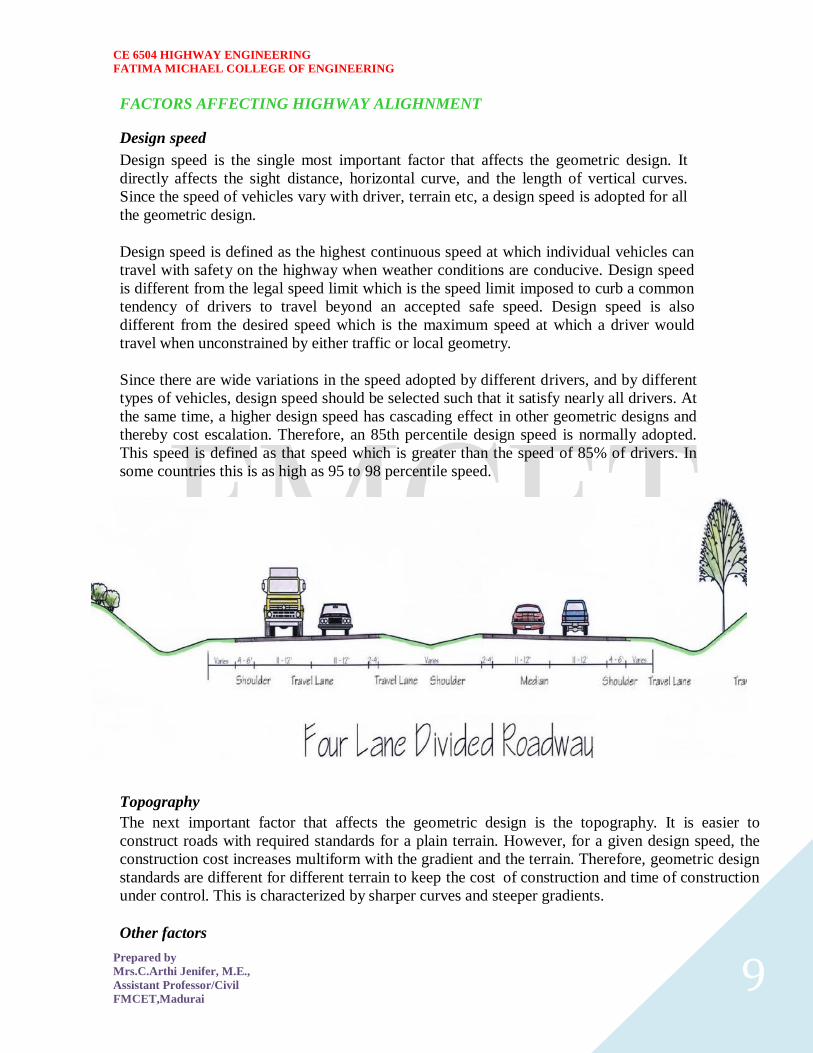
CE 6504 HIGHWAY ENGINEERING
FATIMA MICHAEL COLLEGE OF ENGINEERING
Prepared by
MrsCArthi Jenifer ME
Assistant ProfessorCivil
FMCETMadurai 9
FACTORS AFFECTING HIGHWAY ALIGHNMENT
Design speed
Design speed is the single most important factor that affects the geometric design It
directly affects the sight distance horizontal curve and the length of vertical curves
Since the speed of vehicles vary with driver terrain etc a design speed is adopted for all
the geometric design
Design speed is defined as the highest continuous speed at which individual vehicles can
travel with safety on the highway when weather conditions are conducive Design speed
is different from the legal speed limit which is the speed limit imposed to curb a common
tendency of drivers to travel beyond an accepted safe speed Design speed is also
different from the desired speed which is the maximum speed at which a driver would
travel when unconstrained by either traffic or local geometry
Since there are wide variations in the speed adopted by different drivers and by different
types of vehicles design speed should be selected such that it satisfy nearly all drivers At
the same time a higher design speed has cascading effect in other geometric designs and
thereby cost escalation Therefore an 85th percentile design speed is normally adopted
This speed is defined as that speed which is greater than the speed of 85 of drivers In
some countries this is as high as 95 to 98 percentile speed
Topography
The next important factor that affects the geometric design is the topography It is easier to
construct roads with required standards for a plain terrain However for a given design speed the
construction cost increases multiform with the gradient and the terrain Therefore geometric design
standards are different for different terrain to keep the cost of construction and time of construction
under control This is characterized by sharper curves and steeper gradients
Other factors
CE 6504 HIGHWAY ENGINEERING
FATIMA MICHAEL COLLEGE OF ENGINEERING
Prepared by
MrsCArthi Jenifer ME
Assistant ProfessorCivil
FMCETMadurai 10
In addition to design speed and topography there are various other factors that affect the geometric
design and they are briefly discussed below
Vehicle The dimensions weight of the axle and operating characteristics of a vehicle
influence the design aspects such as width of the pavement radii of the curve clearances
parking geometrics etc A design vehicle which has standard weight dimensions and
operating characteristics are used to establish highway design controls to accommodate
vehicles of a designated type
Human The important human factors that influence geometric design are the mental and
psychological characteristics of the driver and pedestrians like the reaction time
Traffic It will be uneconomical to design the road for peak traffic flow Therefore a
reasonable value of traffic volume is selected as the design hourly volume which is
determined from the various traffic data collected The geometric design is thus based on
this design volume capacity etc
Environmental Factors like air pollution noise pollution etc should be given due
consideration in the geometric design of roads
Economy The design adopted should be economical as far as possible It should match
with the funds allotted for capital cost and maintenance cost
Others Geometric design should be such that the aesthetics of the region is not affected
Nagpur classification
In Nagpur road classification all roads were classified into five categories as National highways
State highways Major district roads Other district roads and village roads
National highways
They are main highways running through the length and breadth of India connecting major
ports foreign highways capitals of large states and large industrial and tourist centers
including roads required for strategic movements
It was recommended by Jayakar committee that the National highways should be the frame
on which the entire road communication should be based
All the national highways are assigned the respective numbers
For eg the highway connecting Delhi-Ambala-Amritsar is denoted as NH-1 (Delhi-
Amritsar) where as a bifurcation of this highway beyond Full under to Srinagar and Uri is
denoted as NH-1_A
They are constructed and maintained by CPWD
The total lengths of National highway in the country is 58112 Kms and constitute about 2
of total road networks of India and carry 40 of total traffic
State highways
They are the arterial roads of a state connecting up with the national highways of adjacent
states district headquarters and important cities within the state
They also serve as main arteries to and from district roads
Total length of all SH in the country is 1 37119 Kms
Major district roads
Important roads with in a district serving areas of production and markets connecting those
with each other or with the major highways
India has a total of 4 70000 Kms of MDR
CE 6504 HIGHWAY ENGINEERING
FATIMA MICHAEL COLLEGE OF ENGINEERING
Prepared by
MrsCArthi Jenifer ME
Assistant ProfessorCivil
FMCETMadurai 11
Other district roads
Roads serving rural areas of production and providing them with outlet to market centers or
other important roads like MDR or SH
Village roads
They are roads connecting villages or group of villages with each other or to the nearest
road of a higher category like ODR or MDR
India has 2650000 kms of ODR+VR out of the total 3315231 kms of all type of roads
Roads classification criteria
Apart from the classification given by the different plans roads were also classified based on some
other criteria They are given in detail below
Based on usage
This classification is based on whether the roads can be used during different seasons of the year
All-weather roads Those roads which are negotiable during all weathers except at major
river crossings where interruption of traffic is permissible up to a certain extent are called all
weather roads
Fair-weather roads Roads which are negotiable only during fair weather are called fair
weather roads
Based on carriage way
This classification is based on the type of the carriage way or the road pavement
Paved roads with hards surface If they are provided with a hard pavement course such
roads are called paved roads(eg stones Water bound macadam (WBM) Bituminous
macadam (BM) concrete roads)
Unpaved roads Roads which are not provided with a hard course of atleast a WBM layer
they is called unpaved roads Thus earth and gravel roads come under this category
Alignment The position or the layout of the central line of the highway on the ground is called the
alignment Horizontal alignment includes straight and curved paths Vertical alignment
includes level and gradients Alignment decision is important because a bad alignment
will enhance the construction maintenance and vehicle operating costs Once an
alignment is fixed and constructed it is not easy to change it due to increase in cost of
adjoining land and construction of costly structures by the roadside
Requirements The requirements of an ideal alignment are
The alignment between two terminal stations should be short and as far as
possible be straight but due to some practical considerations deviations may be
needed
The alignment should be easy to construct and maintain It should be easy for the
operation of vehicles So to the maximum extend easy gradients and curves
should be provided
It should be safe both from the construction and operating point of view
especially at slopes embankments and cutting It should have safe geometric
features
The alignment should be economical and it can be considered so only when the
initial cost maintenance cost and operating cost are minimum
CE 6504 HIGHWAY ENGINEERING
FATIMA MICHAEL COLLEGE OF ENGINEERING
Prepared by
MrsCArthi Jenifer ME
Assistant ProfessorCivil
FMCETMadurai 12
Factors controlling alignment
We have seen the requirements of an alignment But it is not always possible to satisfy all
these requirements Hence we have to make a judicial choice considering all the factors
The various factors that control the alignment are as follows
Obligatory points These are the control points governing the highway alignment
These points are classified into two categories Points through which it should
pass and points through which it should not pass Some of the examples are
o Bridge site The bridge can be located only where the river has straight
and permanent path and also where the abutment and pier can be strongly
founded The road approach to the bridge should not be curved and skew
crossing should be avoided as possible Thus to locate a bridge the
highway alignment may be changed
o Mountain While the alignment passes through a mountain the various alternatives are to either construct a tunnel or to go round the hills The suitability of the alternative depends on factors like topography site
conditions and construction and operation cost
o Intermediate town The alignment may be slightly deviated to connect an intermediate town or village nearby
These were some of the obligatory points through which the alignment should pass
Coming to the second category that is the points through which the alignment should not
pass are
Religious places These have been protected by the law from being acquired for
any purpose Therefore these points should be avoided while aligning
Very costly structures Acquiring such structures means heavy compensation
which would result in an increase in initial cost So the alignment may be deviated
not to pass through that point
Lakesponds etc The presence of a lake or pond on the alignment path would also
necessitate deviation of the alignment
Traffic The alignment should suit the traffic requirements Based on the origin-
destination data of the area the desire lines should be drawn The new alignment should
be drawn keeping in view the desire lines traffic flow pattern etc Geometric design
Geometric design factors such as gradient radius of curve sight distance etc also govern
the alignment of the highway To keep the radius of curve minimum it may be required
to change the alignment The alignments should be finalized such that the obstructions to
visibility do not restrict the minimum requirements of sight distance The design
standards vary with the class of road and the terrain and accordingly the highway should
be aligned Economy The alignment finalized should be economical All the three costs
ie construction maintenance and operating cost should be minimum The construction
cost can be decreased much if it is possible to maintain a balance between cutting and
filling Also try to avoid very high embankments and very deep cuttings as the
construction cost will be very higher in these cases
Road ecology
The features of the cross-section of the pavement influences the life of the pavement as
CE 6504 HIGHWAY ENGINEERING
FATIMA MICHAEL COLLEGE OF ENGINEERING
Prepared by
MrsCArthi Jenifer ME
Assistant ProfessorCivil
FMCETMadurai 13
well as the riding comfort and safety Of these pavement surface characteristics affect
both of these Camber kerbs and geometry of various cross-sectional elements are
important aspects to be considered in this regard They are explained briefly in this
chapter
Camber
Camber or cant is the cross slope provided to raise middle of the road surface in the
transverse direction to drain off rain water from road surface The objectives of providing
camber are
Surface protection especially for gravel and bituminous roads
Sub-grade protection by proper drainage
Quick drying of pavement which in turn increases safety
Too steep slope is undesirable for it will erode the surface Camber is measured in 1 in n
or n (Eg 1 in 50 or 2) and the value depends on the type of pavement surface The
value suggested by IRC for various categories of pavement is given in Table 1 The
common types of camber are parabolic straight or combination of them (Figure 1)
Figure 1 Different types of camber
Table 1 IRC Value
s for ca
mber
Heavy
Light
Surface
rain
type
rain
17
ConcreteBituminous
2
25
GravelWBM
3
30
Earthen
4
CE 6504 HIGHWAY ENGINEERING
FATIMA MICHAEL COLLEGE OF ENGINEERING
Prepared by
MrsCArthi Jenifer ME
Assistant ProfessorCivil
FMCETMadurai 14
Engineering surveys for alignment
The stages of the engineering surveys are a) Map study
b) Reconnaissance
c) Preliminary surveys
d) Final location and detailed surveys
Map study -
) In the topographic map to suggest the likely routes of roads In India topographic
maps are available from the survey of India with 15 or 30-meter contour intervals
) The main feature like rivers hills and valleys etc The probable alignment can be
located on the map from the following details available on the map
Alignment avoiding valleys ponds or lakes
When the road has to cross a row of hills possibility crossing through a mountain pass
Approximate location of bridge site for crossing rivers avoiding bend of the river
When a road is to be connected between two stations one of the top and the other on the foot
of the hill then alternate routes can be suggested keeping in view the permissible alignment
Suppose the scale of the contour map is known and then the contour intervals it is possible
to decide the length of road required between two consecutive contours keeping the gradient
within allowable limits
In the fig Let A and B be two stations to be connected by road AB is the shortest route
(Straight line) APQB is a steep route in which the gradient positively exceeds 1 in 20 as the
distance between the contour intervals is only about 200 meter
APLMNB is a route with an approximate slope of 1 in 20 whereas APEFGB is an alternate
alignment with the same gradient
Thus the map study also is possible to drop a certain route in view of any unavoidable
obstructions (or) undesirable ground enroute
Reconnaissance-
The second stage of surveys for highway location is the reconnaissance to examine the general
character of the area for deciding the most feasible routes for detailed studies
Some of the details to be collected during reconnaissance are given below
Valleys ponds lakes marshy land ridge hills permanent structures and other obstructions
along the route which are not available in the map
Approximate values of gradient length of gradients and radius of curves of alternate
alignments
Number and types of cross drainage structures maximum flood level and natural
groundwater level along the probable routes
Soil type along the routes from field identification tests and observation of geological
features
Sources of construction materials water and location of stone quarries
When the road passes through hilly or mountainous terrain additional data regarding the
geological formation types of rocks dip of strata seepage flow etc
Preliminary survey -
CE 6504 HIGHWAY ENGINEERING
FATIMA MICHAEL COLLEGE OF ENGINEERING
Prepared by
MrsCArthi Jenifer ME
Assistant ProfessorCivil
FMCETMadurai 15
The main objectives of the preliminary surveys are
To survey the various alternate alignments proposed after the reconnaissance and to collect
all the necessary physical information and details of topography drainage and soil
To compare the different proposals in view of the requirements of a good alignment
To estimate quantity of earthwork materials and other construction aspects and to work out
the cost of alternate proposals
To finalize the best alignment from all considerations
The procedure of the conventional methods of preliminary surveys the given steps
Primary survey -
For alternate alignments either secondary traverses (or) independent primary traverses may be
necessary
Topographical features -
All geographical and other man made features along the traverse and for a certain width on either
side surveyed and plotted
Leveling work -
Levelling work is also carried out side by side to give the centerline profiles and typical cross
sections The leveling work in the preliminary survey is kept to a minimum just sufficient to obtain
the approximate earthwork in the alternate alignments
Drainage studies -
Drainage investigations and hydrological data are collected so as to estimate the type number and
approximate size of cross and drainage structures
Soil survey -
The soil survey conducted at this stage helps to working out details of earthwork slopes suitability
of materials subsoil and surface drainage requirements and pavement type and the approximate
thickness requirements
Material survey -
The survey for naturally occurring materials like stone aggregates soft aggregates etc and
identification of suitable quarries should be made
Traffic survey -
Traffic surveys conducted in the region from basis for deciding the number of traffic lanes and
roadway width pavement design and economic analysis of highway project
Locations and functions
Final location and detailed survey - The alignment finalized at the design office after the preliminary survey is to be first located on the
field by establishing the centerline The detailed survey should be carried out for collecting the
information technology for the preparation of plans and construction details
Location -
The centerline of the road finalized in the drawings to be translated on the ground
during the location survey
Major and minor control points are established on the ground and center pegs are
driven checking the geometric design requirements
Detailed survey -
CE 6504 HIGHWAY ENGINEERING
FATIMA MICHAEL COLLEGE OF ENGINEERING
Prepared by
MrsCArthi Jenifer ME
Assistant ProfessorCivil
FMCETMadurai 16
Levels along his final centerline should be taken at all staked points Levelling work is to
great importance as the vertical alignment
A detailed soil survey is carried out to enable drawing of the soil profile
The data during the detailed survey should be elaborate and complete for preparing detailed
plans design and estimates of the project
Soil suitability analysis
The methodology for locating appropriate sites for each land use activity is guided by the intent to
minimize the possible adverse effects of development on the environment and on existing
communities and to emphasize the positive impacts of such development by locating them in a
most suitable location
This is achieved by examining a number of individual criteria assigning them relative levels of
importance as a whole and using a mathematical resultant model to identify the most suitable
location
By adopting this site suitability method it is possible to systematically identify the criteria
considered clearly document the relative importance of one criterion over another analyze the net
outcome using a Geographic Information System and then possibly revisit the mathematical
relationships in this ldquodecision modelrdquo
By revising the relative importance to identified criteria based upon the particular land use under
consideration it is possible to generate ldquosuitability mapsrdquo for each individual land use and then
generate a final composite land use that is based on a best possible collective suitability of multiple
land uses
To achieve this all the criteria are assigned a ldquorankrdquo denoting their relative levels of importance
within the suitability study These ranks are assigned as numeric values ranging from 1 to 10 with 1
reflecting a low level of importance and 10 reflecting a high level of importance For example
within the criteria of road networks national highways would have a different level of influence on
the suitability for a particular land use as compared with local roads Further the distance from each
of these features would further modify the relative suitability of a land use based on the proximity to
a particular type of road
Criteria for Site Suitability Analysis
The decision criteria for site selection are examined for assigning relative ranks and individual
feature weights based on the land use type for which suitability is being examined For benefit of
analysis the criteria under consideration in this paper activity are organized as
Critical Criteria Criteria that will be very significant in the site selection of the identified land use
and will act as key drivers in the selection of the geographic location These criteria can be clustered
into a single decision model and the outcome collectively reviewed These criteria have a strong
influence in the final suitability
Additional Criteria Criteria that will have to be examined one at a time to carefully assess its
relationship with the proposed land use activity These criteria have a positive influence in the final
suitability
CE 6504 HIGHWAY ENGINEERING
FATIMA MICHAEL COLLEGE OF ENGINEERING
Prepared by
MrsCArthi Jenifer ME
Assistant ProfessorCivil
FMCETMadurai 17
Constrained Criteria These criteria impose strong negative opportunities in the selection of areas
for the identified land use Consequently they inform of us of where the particular land use under
consideration should not be located These criteria serve to limit or exclude areas from the final
suitability
GIS Site Suitability Analysis Model We were developed a tourism site suitability analysis model
in ArcGIS - 931 which is shown in Figure -
CE 6504 HIGHWAY ENGINEERING
FATIMA MICHAEL COLLEGE OF ENGINEERING
Prepared by
MrsCArthi Jenifer ME
Assistant ProfessorCivil
FMCETMadurai 18
UNIT 2 GEOMETRIC DESIGN OF HIGHWAYS
Typical cross section of urban and rural roads
A cross section is a vertical plane (slice) taken at right angles to the road control line showing the
various elements that make up the roads structure It is normally viewed in the direction of
increasing chainage
The width of a roadway is an important design consideration to ensure that it is appropriately sized
to serve its function Because of the diversity within the County two major roadway categories have
been established 1 Rural Road Standards 2 Urban Road Standards Urban Road Standards will
serve those areas which tend to be more developed and need to provide for multiple users
(bicyclists pedestrians parallel parking etc) whereas many rural roads will primarily serve only
vehicular traffic
Cross sections are created to provide a visual guide depicting the initial interim and ultimate phase
cross sections for these road classifications The typical sections illustrated in the following pages
are recommendations tied to transportation planning aspects such as right‐of‐way lineage sidewalk
width etc Threshold daily traffic can be used as a guide for a starting point when determining
which cross section is most applicable
1 Rural Road Standards
The rural roadways will not typically require curb and gutter or sidewalk although the County may
require either or both in unique circumstances Widths of lanes and shoulders will vary depending
upon the specific classification and the potential traffic volume which the roadway may carry Roads
carrying fewer than 200 vehicles per day need not be paved or treated for dust control The need for
paved shoulders is also dependent upon the level of traffic and safety
Final design and construction details will be determined by the Public Works Department Final
Design and construction criteria taken into consideration may include but are not limited to use of
the roadway density of development topographical characteristics and nearby development For
construction in which only a portion of the ultimate cross‐section is intended to be completed the
partial design will need to allow for the eventual widening to the ultimate cross‐section The design
for the partial or interim cross‐section roadway will need to incorporate ultimate design information
to ensure that the first phase of roadway construction is appropriate and would not need to be
removed at a future date when the full width cross‐section is completed
2 Urban Road Standards
Three roadway classifications are identified for those areas that are associated with the communityrsquos
urban growth areas They include arterial collector and local street classifications Transportation
Plan shows the key elements of the urban road standards Urban road standards will include 12‐foot
lanes sidewalk and curb amp gutter arterials and collectors will also include a striped bike lane Turn
lanes may be necessary as determined by the County Since almost all of the municipalities have
different right‐of‐way cross sections adopted for their community it makes it very difficult for the
County to match them all Therefore the philosophy was to encourage a baseline amount of
right‐of‐way reservation that could ensure the adjacent community enough area for coordination of
future roadway improvements until such time the road
CE 6504 HIGHWAY ENGINEERING
FATIMA MICHAEL COLLEGE OF ENGINEERING
Prepared by
MrsCArthi Jenifer ME
Assistant ProfessorCivil
FMCETMadurai 19
CE 6504 HIGHWAY ENGINEERING
FATIMA MICHAEL COLLEGE OF ENGINEERING
Prepared by
MrsCArthi Jenifer ME
Assistant ProfessorCivil
FMCETMadurai 20
Cross sectional elements
Kerbs
Kerbs indicate the boundary between the carriage way and the shoulder or islands or footpaths Different types of kerbs are
CE 6504 HIGHWAY ENGINEERING
FATIMA MICHAEL COLLEGE OF ENGINEERING
Prepared by
MrsCArthi Jenifer ME
Assistant ProfessorCivil
FMCETMadurai 21
Low or mountable kerbs This type of kerbs is provided such that they
encourage the traffic to remain in the through traffic lanes and also allow the
driver to enter the shoulder area with little difficulty The height of this kerb is
about 10 cm above the pavement edge with a slope which allows the vehicle to
climb easily This is usually provided at medians and channelization schemes and
also helps in longitudinal drainage
Semi-barrier type kerbs When the pedestrian traffic is high these kerbs are
provided Their height is 15 cm above the pavement edge This type of kerb
prevents encroachment of parking vehicles but at acute emergency it is possible
to drive over this kerb with some difficulty
Barrier type kerbs They are designed to discourage vehicles from leaving the
pavement They are provided when there is considerable amount of pedestrian
traffic They are placed at a height of 20 cm above the pavement edge with a steep
batter
Submerged kerbs They are used in rural roads The kerbs are provided at
pavement edges between the pavement edge and shoulders They provide lateral
confinement and stability to the pavement
Figure 1 Different types of kerbs
Shoulders Shoulders are provided along the road edge and are intended for accommodation of
stopped vehicles serve as an emergency lane for vehicles and provide lateral support
for base and surface courses The shoulder should be strong enough to bear the weight
of a fully loaded truck even in wet conditions The shoulder width should be adequate
for giving working space around a stopped vehicle It is desirable to have a width of
46 m for the shoulders A minimum width of 25 m is recommended for 2-lane rural
highways in India Parking lanes
Parking lanes are provided in urban lanes for side parking Parallel parking is preferred
because it is safe for the vehicles moving on the road The parking lane should have a
minimum of 30 m width in the case of parallel parking
CE 6504 HIGHWAY ENGINEERING
FATIMA MICHAEL COLLEGE OF ENGINEERING
Prepared by
MrsCArthi Jenifer ME
Assistant ProfessorCivil
FMCETMadurai 22
Bus-bays
Bus bays are provided by recessing the kerbs for bus stops They are provided so that
they do not obstruct the movement of vehicles in the carriage way They should be at
least 75 meters away from the intersection so that the traffic near the intersections is not
affected by the bus-bay
Service roads Service roads or frontage roads give access to access controlled highways like freeways
and expressways They run parallel to the highway and will be usually isolated by a
separator and access to the highway will be provided only at selected points These roads
are provided to avoid congestion in the expressways and also the speed of the traffic in
those lanes is not reduced
Drainage
The pavement surface should be absolutely impermeable to prevent seepage of water into
the pavement layers Further both the geometry and texture of pavement surface should
help in draining out the water from the surface in less time
Footpath
Footpaths are exclusive right of way to pedestrians especially in urban areas They are
provided for the safety of the pedestrians when both the pedestrian traffic and vehicular
traffic is high Minimum width is 15 meter and may be increased based on the traffic
The footpath should be either as smooth as the pavement or more smoother than that to
induce the pedestrian to use the footpath
Right of way
Right of way (ROW) or land width is the width of land acquired for the road along its
alignment It should be adequate to accommodate all the cross-sectional elements of the
highway and may reasonably provide for future development To prevent ribbon
development along highways control lines and building lines may be provided Control
line is a line which represents the nearest limits of future uncontrolled building activity
in relation to a road Building line represents a line on either side of the road between
which and the road no building activity is permitted at all The right of way width is
governed by
Width of formation It depends on the category of the highway and width of
roadway and road margins
Height of embankment or depth of cutting It is governed by the topography and
the vertical alignment
Side slopes of embankment or cutting It depends on the height of the slope soil
type etc
Drainage system and their size which depends on rainfall topography etc
Sight distance considerations On curves etc there is restriction to the visibility
on the inner side of the curve due to the presence of some obstructions like
building structures etc
Reserve land for future widening Some land has to be acquired in advance
CE 6504 HIGHWAY ENGINEERING
FATIMA MICHAEL COLLEGE OF ENGINEERING
Prepared by
MrsCArthi Jenifer ME
Assistant ProfessorCivil
FMCETMadurai 23
Table 2 Desig
n speed in as per IRC (ruling and minimum)
Steep
Type
Plain
Rolling
Hilly
40-30
NSampSH
100-80
80-65
50-40
MDR
80-65
65-50
40-30
30-20
25-20
ODR
65-50
50-40
30-25
25-20
VR
50-40
40-35
25-20
anticipating future developments like widening of the road
Table 1 No
right of way for open areas
Roadway width in m
Road
Plain and
Mountainous and
classification
steep terrain
rolling terrain
Open areas
45
24
NHSH
18
MDR
25
15
15
ODR
12
9
VR
Built-up areas
20
NHSH
30
MDR
20
15
ODR
15
12
9
VR
10
CE 6504 HIGHWAY ENGINEERING
FATIMA MICHAEL COLLEGE OF ENGINEERING
Prepared by
MrsCArthi Jenifer ME
Assistant ProfessorCivil
FMCETMadurai 24
Horizontal curve
The presence of horizontal curve imparts centrifugal force which is a reactive force
acting outward on a vehicle negotiating it Centrifugal force depends on speed and radius
of the horizontal curve and is counteracted to a certain extent by transverse friction
between the tyre and pavement surface On a curved road this force tends to cause the
vehicle to overrun or to slide outward from the centre of road curvature For proper
design of the curve an understanding of the forces acting on a vehicle taking a horizontal
curve is necessary Various forces acting on the vehicle are illustrated in the figure 1
Figure 1 Effect of horizontal curve They are the centrifugal force (P) acting outward weight of the vehicle (W) acting
downward and the reaction of the ground on the wheels ( and ) The centrifugal
force and the weight is assumed to be from the centre of gravity which is at h units above
the ground Let the wheel base be assumed as b units The centrifugal force in
is given by
(1)
where is the weight of the vehicle in is the speed of the vehicle in is
the acceleration due to gravity in and is the radius of the curve in
The centrifugal ratio or the impact factor is given by
CE 6504 HIGHWAY ENGINEERING
FATIMA MICHAEL COLLEGE OF ENGINEERING
Prepared by
MrsCArthi Jenifer ME
Assistant ProfessorCivil
FMCETMadurai 25
(1)
The centrifugal force has two effects A tendency to overturn the vehicle about the outer
wheels and a tendency for transverse skidding Taking moments of the forces with
respect to the outer wheel when the vehicle is just about to override
At the equilibrium over turning is possible when
and for safety the following condition must satisfy
(2)
The second tendency of the vehicle is for transverse skidding ie When the the
centrifugal force is greater than the maximum possible transverse skid resistance due to
friction between the pavement surface and tyre The transverse skid resistance (F) is
given by
where and is the fractional force at tyre and and is the reaction at
tyre and is the lateral coefficient of friction and is the weight of the vehicle
This is counteracted by the centrifugal force (P) and equating
At equilibrium when skidding takes place (from equation1)
and for safety the following condition must satisfy
CE 6504 HIGHWAY ENGINEERING
FATIMA MICHAEL COLLEGE OF ENGINEERING
Prepared by
MrsCArthi Jenifer ME
Assistant ProfessorCivil
FMCETMadurai 26
(3)
Equation 2 and 3 give the stable condition for design If equation 2 is violated the vehicle
will overturn at the horizontal curve and if equation 3 is violated the vehicle will skid at
the horizontal
Curve Analysis of super-elevation
Super-elevation or cant or banking is the transverse slope provided at horizontal curve to
counteract the centrifugal force by raising the outer edge of the pavement with respect to
the inner edge throughout the length of the horizontal curve When the outer edge is
raised a component of the curve weight will be complimented in counteracting the effect
of centrifugal force In order to find out how much this raising should be the following
analysis may be done The forces acting on a vehicle while taking a horizontal curve with
super elevation is shown in figure 1
Figure 1 Analysis of super-elevation
Forces acting on a vehicle on horizontal curve of radius at a speed of are
the centrifugal force acting horizontally out-wards through the center of
gravity
the weight of the vehicle acting down-wards through the center of gravity and
the friction force between the wheels and the pavement along the surface
inward
CE 6504 HIGHWAY ENGINEERING
FATIMA MICHAEL COLLEGE OF ENGINEERING
Prepared by
MrsCArthi Jenifer ME
Assistant ProfessorCivil
FMCETMadurai 27
At equilibrium by resolving the forces parallel to the surface of the pavement we get where
friction
is the weight of the vehicle is the centrifugal force is the coefficient of
is the transverse slope due to superelevation Dividing by we get
CE 6504 HIGHWAY ENGINEERING
FATIMA MICHAEL COLLEGE OF ENGINEERING
Prepared by
MrsCArthi Jenifer ME
Assistant ProfessorCivil
FMCETMadurai 28
Step 1
Find for 75 percent of design speed neglecting ie
Step 2
If then else if go to step 3
Step 3
Find for the design speed and max ie If
then the maximum is safe for the design speed else go to
step 4
Step 4
Find the allowable speed for the maximum and
If then the design is adequate otherwise use speed adopt
control measures or look for speed control measures
Maximum and minimum super-elevation
Depends on (a) slow moving vehicle and (b) heavy loaded trucks with high CG IRC
specifies a maximum super-elevation of 7 percent for plain and rolling terrain while that
of hilly terrain is 10 percent and urban road is 4 percent The minimum super elevation is
2-4 percent for drainage purpose especially for large radius of the horizontal curve
Attainment of super-elevation
1 Elimination of the crown of the cambered section by
1 Rotating the outer edge about the crown The outer half of the cross slope
is rotated about the crown at a desired rate such that this surface falls on
the same plane as the inner half
2 Shifting the position of the crown This method is also known as diagonal
crown method Here the position of the crown is progressively
shifted outwards thus increasing the width of the inner half of cross section
progressively
2 Rotation of the pavement cross section to attain full super elevation byThere are
two methods of attaining super elevation by rotating the pavement
1 Rotation about the center line The pavement is rotated such that the inner
edge is depressed and the outer edge is raised both by half the total amount
of super elevation ie by with respect to the centre
2 Rotation about the inner edge Here the pavement is rotated raising the
outer edge as well as the centre such that the outer edge is raised by the
full amount of super elevation with respect to the inner edge
Horizontal Transition Curves
CE 6504 HIGHWAY ENGINEERING
FATIMA MICHAEL COLLEGE OF ENGINEERING
Prepared by
MrsCArthi Jenifer ME
Assistant ProfessorCivil
FMCETMadurai 29
Transition curve is provided to change the horizontal alignment from straight to circular
curve gradually and has a radius which decreases from infinity at the straight end
(tangent point) to the desired radius of the circular curve at the other end (curve point)
There are five objectives for providing transition curve and are given below
1 to introduce gradually the centrifugal force between the tangent point and the
beginning of the circular curve avoiding sudden jerk on the vehicle This
increases the comfort of passengers
2 to enable the driver turn the steering gradually for his own comfort and security
3 to provide gradual introduction of super elevation and
4 to provide gradual introduction of extra widening
5 to enhance the aesthetic appearance of the road
Type of transition curve
Different types of transition curves are spiral or clothoid cubic parabola and Lemniscate
IRC recommends spiral as the transition curve because
1 it fulfills the requirement of an ideal transition curve that is
1 rate of change or centrifugal acceleration is consistent (smooth) and
2 radius of the transition curve is at the straight edge and changes to at
the curve point ( ) and calculation and field implementation is
very easy
Length of transition curve The length of the transition curve should be determined as the maximum of the following
three criteria rate of change of centrifugal acceleration rate of change of super elevation
and an empirical formula given by IRC Rate of change of centrifugal acceleration
At the tangent point radius is infinity and hence centrifugal acceleration is zero At the
end of the transition the radius R has minimum value R The rate of change of
centrifugal acceleration should be adopted such that the design should not cause
discomfort to the drivers If is the rate of change of centrifugal acceleration it can be
written as
Therefore the length of the transition curve in is
CE 6504 HIGHWAY ENGINEERING
FATIMA MICHAEL COLLEGE OF ENGINEERING
Prepared by
MrsCArthi Jenifer ME
Assistant ProfessorCivil
FMCETMadurai 30
(1)
where is the rate of change of centrifugal acceleration given by an empirical formula
suggested by by IRC as below
(2) 2 Rate of introduction of super-elevation
Raise ( ) of the outer edge with respect to inner edge is given by
The rate of change of this raise from to is achieved
gradually with a gradient of in over the length of the transition curve (typical range
of is 60-150) Therefore the length of the transition curve is
(3)
3 By empirical formula
IRC suggest the length of the transition curve is minimum for a plain and rolling terrain
(4)
and for steep and hilly terrain is
(5)
CE 6504 HIGHWAY ENGINEERING
FATIMA MICHAEL COLLEGE OF ENGINEERING
Prepared by
MrsCArthi Jenifer ME
Assistant ProfessorCivil
FMCETMadurai 31
and the shift as
(
6
) The length of the transition curve is the maximum of
equations 1 3 and 4or5 ie
(
7
Case (a)
For single lane roads
(
1
)
Therefore
(
2
)
Figure 1 Set-back for single lane roads (
CE 6504 HIGHWAY ENGINEERING
FATIMA MICHAEL COLLEGE OF ENGINEERING
Prepared by
MrsCArthi Jenifer ME
Assistant ProfessorCivil
FMCETMadurai 32
For multi lane roads if is the distance between centerline of the road and the centerline
of the inner lane then
(3)
(4)
Figure 2 Set-back for multi-lane roads ( )
Case (a)
For single lane roads
(1)
Therefore
(2)
Gradient
Gradient is the rate of rise or fall along the length of the road with respect to the
horizontal While aligning a highway the gradient is decided for designing the vertical
curve Before finalizing the gradients the construction cost vehicular operation cost and
the practical problems in the site also has to be considered Usually steep gradients are
avoided as far as possible because of the difficulty to climb and increase in the
CE 6504 HIGHWAY ENGINEERING
FATIMA MICHAEL COLLEGE OF ENGINEERING
Prepared by
MrsCArthi Jenifer ME
Assistant ProfessorCivil
FMCETMadurai 33
construction cost More about gradients are discussed below
Effect of gradient
The effect of long steep gradient on the vehicular speed is considerable This is
particularly important in roads where the proportion of heavy vehicles is significant Due
to restrictive sight distance at uphill gradients the speed of traffic is often controlled by
these heavy vehicles As a result not only the operating costs of the vehicles are
increased but also capacity of the roads will have to be reduced Further due to high
differential speed between heavy and light vehicles and between uphill and downhill
gradients accidents abound in gradients
Representation of gradient
The positive gradient or the ascending gradient is denoted as and the negative gradient as The deviation angle is when two grades meet the angle which
measures the change of direction and is given by the algebraic difference between the two
grades
steep gradient while 1 in 50 = 2 representation is illustrated in the figure 1
Example 1 in 30 = 333 is a
is a flatter gradient The gradient
CE 6504 HIGHWAY ENGINEERING
FATIMA MICHAEL COLLEGE OF ENGINEERING
Prepared by
MrsCArthi Jenifer ME
Assistant ProfessorCivil
FMCETMadurai 34
Figure 1 Representation of gradient
Types of gradient
Many studies have shown that gradient upto seven percent can have considerable effect
on the speeds of the passenger cars On the contrary the speeds of the heavy vehicles are
considerably reduced when long gradients as flat as two percent is adopted Although
flatter gradients are desirable it is evident that the cost of construction will also be very
high Therefore IRC has specified the desirable gradients for each terrain However it
may not be economically viable to adopt such gradients in certain locations steeper
gradients are permitted for short duration Different types of grades are discussed below
Ruling gradient
The ruling gradient or the design gradient is the maximum gradient with which the
designer attempts to design the vertical profile of the road This depends on the terrain
length of the grade speed pulling power of the vehicle and the presence of the horizontal
curve In flatter terrain it may be possible to provide flat gradients but in hilly terrain it
is not economical and sometimes not possible also The ruling gradient is adopted by the
designer by considering a particular speed as the design speed and for a design vehicle
with standard dimensions But our country has a heterogeneous traffic and hence it is not
possible to lay down precise standards for the country as a whole Hence IRC has
recommended some values for ruling gradient for different types of terrain
Limiting gradient
This gradient is adopted when the ruling gradient results in enormous increase in cost of
construction On rolling terrain and hilly terrain it may be frequently necessary to adopt
limiting gradient But the length of the limiting gradient stretches should be limited and
must be sandwiched by either straight roads or easier grades
Exceptional gradient
Exceptional gradient are very steeper gradients given at unavoidable situations They
should be limited for short stretches not exceeding about 100 metres at a stretch In
mountainous and steep terrain successive exceptional gradients must be separated by a
minimum 100 metre length gentler gradient At hairpin bends the gradient is restricted to
25
Critical length of the grade
The maximum length of the ascending gradient which a loaded truck can operate without
undue reduction in speed is called critical length of the grade A speed of 25 kmph is a
CE 6504 HIGHWAY ENGINEERING
FATIMA MICHAEL COLLEGE OF ENGINEERING
Prepared by
MrsCArthi Jenifer ME
Assistant ProfessorCivil
FMCETMadurai 35
reasonable value This value depends on the size power load grad-ability of the truck
initial speed final desirable minimum speed
Minimum gradient
This is important only at locations where surface drainage is important Camber will take
care of the lateral drainage But the longitudinal drainage along the side drains require
some slope for smooth flow of water Therefore minimum gradient is provided for
drainage purpose and it depends on the rain fall type of soil and other site conditions A
minimum of 1 in 500 may be sufficient for concrete drain and 1 in 200 for open soil
drains are found to give satisfactory performance Sight distance available from a point is the actual distance along the road surface which a driver
from a specified height above the carriage way has visibility of stationary or moving objects
Sight distance required by drivers applies to both geometric design of highways and for
traffic control The sight distance situations are considered in the design
i) Stopping or absolute minimum sight distance
ii) Safe overtaking or passing sight distance
iii) Safe sight distance for entering into uncontrolled intersections
Apart from the three situations mentioned above the following sight distance are considered by the
IRC in highway design
Intermediate sight distance
This is defined as twice the stopping sight distance when overtaking sight distance
cannot be provided intermediate sight distance is provided to give limited overtaking opportunities
to fast vehicles
Head light sight distance
This is the distance visible to a driver during night driving under the illumination of the
vehicle head lights
Stopping sight distance
The minimum sight distance available on a highway at any spot should be of sufficient
length to stop a vehicle traveling at design speed safely without collision with any other obstruction
The absolute minimum sight distance is therefore equal to the stopping sight distance
which is also sometimes called nonpassing sight distance The sight distance available on a road to a
driver at any instance depends on
i) Features of the road
ii) Height of the drivers eye above the road surface
iii) Height of the object above the road surface
The distance within which a motor vehicle can be stopped depends upon the factors listed below
a) Total reactions time of the driver
b) Speed of vehicle
c) Efficiency of breaks
d) Frictional resistance between the road and tyres
e) Gradient of the road
Total reaction time
) Reaction time of the driver is the time taken from the instant the object is visible to the
driver to the instant the brakes are effectively applied
) The total reaction time may be split up into two parts
CE 6504 HIGHWAY ENGINEERING
FATIMA MICHAEL COLLEGE OF ENGINEERING
Prepared by
MrsCArthi Jenifer ME
Assistant ProfessorCivil
FMCETMadurai 36
i) Perception time
ii) Brake reaction time
PIEV theory
According to this theory the total reaction time of the driver is split into four parts
i) Perception
ii) Intellection
iii) Emotion
iv) Volition
Speed of Vehicle
The stopping distance depends very much on the speed of the vehicle first during the
total reaction time of the driver the distance moved by the vehicle will depend on the speed
Efficiency of brakes
The braking efficiency is said to be 100 percent if the wheels are fully licked preventing
them from rotating on application of the brakes This will result in 100 percent skidding which is
normally undesirable except in utmost emergency
Frictional resistance between road and tyres
The frictional resistance developed between road and tyres or the skid resistance depends
on the type and condition of the road surface and the tyres IRC has specified a design friction
coefficient of 035 to 04 depending upon the speed to be used for finding the braking distance in the
calculation of stopping sight distance
Analysis of stopping distance
i) The distance traveled by the vehicle during the total reaction time known as lag
distance
ii) The distance traveled by the vehicle after the application of the brakes is known as
braking distance
Overtaking sight distance
The minimum distance open to the vision of the driver of a vehicle intending to overtake
slow vehicle ahead with safety against the traffic of opposite direction is known as the minimum
overtaking sight distance(OSD) or Safe passing sight distance available
The overtaking sight distance is the distance measured along the center of the road which
a driver with his eye level 12m above the road surface can see the top of an object 12m above the
road surface
Some of the important factors on which the minimum overtaking sight distance required
a) Speed of
i) overtaking vehicle
ii) overtaken vehicle
iii) The vehicle coming from opposite direction
b) Distance between the overtaking and overtaken vehicles the minimum spacing
depends on the steeds
a) Skill and reaction time of the driver
b) Rate of acceleration of overtaking vehicle
c) Gradient of the road
Criteria for sight distance requirements on highway
) The absolute minimum sight distance required throughout the length of the road is the
SSD which should invariably be provided at all places
CE 6504 HIGHWAY ENGINEERING
FATIMA MICHAEL COLLEGE OF ENGINEERING
Prepared by
MrsCArthi Jenifer ME
Assistant ProfessorCivil
FMCETMadurai 37
) On horizontal curves the obstruction on the inner side of the curves should be cleared
to provide the required set back distance and absolute minimum sight distance
) On vertical summit curves the sight distance requirement may be fulfilled by proper
design of the vertical alignment
Hairpin bent
TYPES OF CURVES ON HILL ROADS
The following are the important types of curves provided on hill Roads-
1 Hair-Pin Curves
2 Salient Curves
3 Re-entrant Curves 1 Hair-pin curves - The curve in a hill road which changes its direction through an angle of 180
degree or so down the hill on the same side is known as hair-pin curve
A Hair-Pin Bend
This curve is so called because it conforms to the shape of a hair-pin The bend so formed at the
hair-pin curve in a hill road is known as hair-pin bend This type of curve should be located on a
hill side having the minimum slope and maximum stability It must also be safe from view point of
landslides and ground water Hair-pin bends with long arms and farther spacing are always
preferred They reduce construction problems and expensive protective works Hair-pin curves or
bends of serpentine nature are difficult to negotiate and should therefore be avoided as far as
possible
Salient curves - The curves having their convexity on the outer edges of a hill road are called
salient curves The centre of curvature of a salient curve lies towards the hill side This type of curve
occurs in the road length constructed on the ridge of a hill the bend so formed at the salient curve in
a hill road known as corner bend
Salient curves are very dangerous for fast moving traffic At such a curve or at corner bend the
portion of projecting hill side is usually cut down to improve the visibility as shown in fig (Re-
entrant curve) The outer edge of the road at such a curve is essentially provided with a parapet wall
for protection of the vehicles from falling down the hill slope
CE 6504 HIGHWAY ENGINEERING
FATIMA MICHAEL COLLEGE OF ENGINEERING
Prepared by
MrsCArthi Jenifer ME
Assistant ProfessorCivil
FMCETMadurai 38
3 Re-entrant curves - The curves having their convexity on the inner edge of a hill road are called
re-entrant curves
Re-entrant curves
The centre of curvature of a re-entrant curves lies away from the hill side This type of curve occurs
in the road length constructed in the calley of a hill
These curves are less dangereous as they provide adequate visibility to the fast moving traffic At
such curves the parapet wall is provided only for safety of fast moving traffic
CE 6504 HIGHWAY ENGINEERING
FATIMA MICHAEL COLLEGE OF ENGINEERING
Prepared by
MrsCArthi Jenifer ME
Assistant ProfessorCivil
FMCETMadurai 39
UNIT ndash III DESIGN OF RIGID AND FLEXIBLE PAVEMENTS
COMPARISON OF RIGID AND FLEXIBLE PAVEMENTS
The comparisons are
i) Design precision
A cement concrete pavement is amerable to a much more precise structural analysis
than a flexible pavement Flexible pavements designs are mainly empirical Computer aided analysis
of layered system is making the flexible pavement design more exact than hitherto
ii) Life
) Cement concrete slabs of a thin section constructed in the early 1940rsquos are still in
existence in India though many of them have cracked badly and a few of them have been ripped
open and rebuilt in recent ties
) A major project in cement concrete road construction between Agra and Mathura It can
safely be said that a well-designed concrete slab has a life of about 40 years
) Compared to this the life of a flexible pavement generally varies from 10 to 20 years
iii) Maintenance
) A well-designed cement concrete pavement needs very little maintenance The only
maintenance needed is I respect of joints
) The surface is unaffected by spillage of oil and lubricants bituminous surfaces on the
other hand need great inputs in maintenance
) The surface is affected by spillage of oil and lubricants The surface is also affected by
natural weathering agents like air water ad temperature changes
) A cement concrete pavement on the other hand needs a small amount for maintaining
joints
iv) Initial cost
) The argument so far used against a cement concrete slab is that it is much more costly
than a flexible pavement
) The latter specifications no doubt represent the rock-bottom needs of a road in India but
these specifications can hardly provide a smooth and durable surface
v) Stage construction ) Road construction is generally done adopting a policy of stage construction especially for
low volume roads As traffic grows additional layers in the form of water bound macadam and
superior surfacing are added on
) Initial outlay is minimum and additional outlays are in keeping with traffic growth This is
a great advantage when dealing with new roads in an atmosphere of austerity
vi) Availability of materials
) Cement bitumen stone aggregates and gravelsand are the major materials involved in
pavement Construction Cement has been in serious short supply in the country for the past many
decades
) Bitumen is also not available plentifully in India There is also the danger of the entire oil
reserves in the world shrinking during the next two or three decades
) In locations where stone aggregates are scarce cement concrete may have an advantage
for flexible pavements
vii) Surface characterstics
CE 6504 HIGHWAY ENGINEERING
FATIMA MICHAEL COLLEGE OF ENGINEERING
Prepared by
MrsCArthi Jenifer ME
Assistant ProfessorCivil
FMCETMadurai 40
) A good cement concrete surface is smooth and free from rutting potholes and
corrugations In a bituminous surface it is only the asphaltic concrete surface that can give
comparable rideablity
) A well-constructed cement concrete pavement surface can have a permanent nonskid
surface A bituminous surface can also be designed to have a good skid resistant surface
viii) Utility location
) In cement concrete slabs proper thought has to be given to locate utilities such as water
pipes telephone lines and electric cables
) It is difficult to rip open the slab and restore it to be the original condition if any changes
in the utilities lines are to be made
ix) Glame and night visibility
) Concrete pavements have a gray color which can cause glam under sunlight Colored
cement can reduce the grave
) On the other hand bituminous roads need more street lighting
x) Traffic dislocation during construction
) A cement concrete pavement requires 28 days before it can be thrown open to traffic On
the other hand a bituminous surface can be thrown open to traffic shortly after it is rolled
xi) Environmental considerations during construction
) The process of heating of bitumen and aggregates and mixing them together on hot mix
plants can prove to be much more hazardous to the environment than cement concrete construction
where no heating of any material is involved
xii) Overall economy on a life cycle basis
) A good road is costly to construct but once constructed such a road requires little
maintenance and results in savings in vehicle operating costs
) The comparative economy of a flexible pavement and a rigid pavement has proved that on
overall economic considerations
Types of pavement structure
Based on the structural behavior pavements are generally classified into three
categories
i) Flexible pavements
ii) Rigid pavements
iii) Semi rigid pavements
Flexible pavements
) Flexible pavements are those which on the whole have low or negligible flexural
strength and are rather flexible in their structural action under the loadsThe flexible pavement
layers reflect the deformation of the lower layers on to the surface of the layer
) A flexible pavement consists of four components(i) Soil subgrade (ii) sub base
course (iii) base course (iv) Surface course
CE 6504 HIGHWAY ENGINEERING
FATIMA MICHAEL COLLEGE OF ENGINEERING
Prepared by
MrsCArthi Jenifer ME
Assistant ProfessorCivil
FMCETMadurai 41
) The flexible pavement layers transmit the vertical or compressive stresses to the lower layers
by grain to grain transfer through the points of contact in the granular structure A well
compacted granular structure consisting of strong added aggregate can transfer the compressive
stresses
) The load spreading ability of this layer therefore depends on the type of the materials and mix
design factors Bituminous concrete is one of the best flexible pavements layer materials Other
materials which fall under the group are all granular materials with or without bituminous
binder granular base and sub base course materials
) The vertical compressive stress is maximum on the pavement surface directly under the wheel
and is equal to the contact pressure under the wheel The flexible pavement may be constructed
in a number of layers and the top layer has to be strongest as the highest compressive stresses
) Flexible pavements are commonly designed using empirical design charts or equations taking
into account some of the design factors there are also semi empirical and theoretical design
methods
Rigid pavements
) Rigid pavements are those which possess note flexural strength or flexural rigidity
The stresses are not transferred from grain to grain to the lower layers as in the ease of flexible
pavements layers
) The rigid pavements are made of Portland cement concrete plain reinforced or
prestressed concrete The plain cement concrete slabs are expected to take up about 40 kgcm2
flexural stress
) The rigid pavement has the slab action and is capable of transmitting the wheel
load stresses through a wider area below The main point of difference in the structural behavior
of rigid pavement as compared to the flexible pavement is that the critical condition of stress in
the rigid pavement is the maximum flexural stress occurring in the slab due to wheel load and
the temperature changes whereas in the flexible pavement
) As the rigid pavement slab has tensile strength tensile stresses are developed due
to the bending of the slab under wheel load and temperature variations Thus the types of
stresses developed and their distribution within the cement concrete slab are quirt different
) The cement concrete pavement slab can very well serve as a wearing surface as
well an effective base course The rigid pavement structure consists of a cement concrete slab
below which a granular base or sub base course may be provided
) Though the cement concrete slab can also be laid directly over the soil subgrade
consists of fine grained soil
) the rigid pavements are usually designed and the stresses are analyzed using the
elastic theory assuming the pavements as a n elastic plate resting over an elastic or a viscous
foundation
Semi rigid pavements
) when bonded materials like the pozzolanic concrete lean cement concrete or soil
cement are used in the base course or sub base course layer the pavement layer has considerably
higher flexural strength than the common flexible pavement layers
) when this intermediate class of materials are used in the base or sub base course
layer of the pavements they are called semi rigid pavements
CE 6504 HIGHWAY ENGINEERING
FATIMA MICHAEL COLLEGE OF ENGINEERING
Prepared by
MrsCArthi Jenifer ME
Assistant ProfessorCivil
FMCETMadurai 42
) This third category of semi rigid pavement are either designed as flexible
pavements with some correction factors to find the thickness requirements based on experience
or by using a new design approach
) The semi rigid pavement materials have low resistance to impact and abrasion and
therefore are usually provided with flexible pavement surface course
Various functions of pavement components
The functions are
Soil sub grade and its evaluation
) The soil sub grade is a layer of natural soil prepared to receive the layers of pavement
materials placed over it It is essential that at no time the soil sub grade is overstressed it means that
the pressure transmitted on the top of the sub grade is within the allowable limit
) Many tests are known for measuring the strength properties of the sub grades Some of the
tests have been standardized for the use The common strength test for the evaluation of soil
subgrade is
i) California bearing ratio test
ii) California resistance value test
iii) Triaxial compression test
iv) Plate bearing test
CALIFORNIA BEARING RATIO (CBR) TEST
It is evolved for the empirical method of flexible pavement design The CBR test is carried
out either in the laboratory on prepared specimens or in the field by taking in situ measurements
California resistance value
It is found by using have been stabliometerThis test is used in an empirical method of
flexible pavement design based on soil strength
Triaxial test
It is the most important soil strength but still the test is not very commonly used in structural
design of pavements
Plate bearing test
It is carried out using a relatively large diameter plate to evaluate the load supporting
capacity of supporting power of the pavement layers The results are plate bearing tests are used in
flexible pavement design method like McLeod method on based on layer system analysis by
brumister
Sub base and base courses and their evaluation
) There layers are made of broken stones bound or unbound aggreagatesome times in sub
base course a layer of stabilized soil(or) Selected granular soil is also used
) however at the sub base course it is desirable to use smaller size graded aggregates When
the sub grade consists of fine grained soil and when the pavement carries heavy wheel loads
CE 6504 HIGHWAY ENGINEERING
FATIMA MICHAEL COLLEGE OF ENGINEERING
Prepared by
MrsCArthi Jenifer ME
Assistant ProfessorCivil
FMCETMadurai 43
) Sub base course primarily has the similar function as of the base course and is provided
with inferior materials than of base course Base courses are used under rigid pavement for
i) Preventing pumping
ii) Protecting the sub grade against frost action
) Thus the fundamental purpose of abase course and sub base course is to provide a stress
transmitting medium to spread the surface wheel loads in such manner
) The sub base and base course layers may be evaluated by suitable strength or stability test
like plate bearing CBR test
WEARING COURSE AND ITS EVALUATION
) The purpose of the wearing course is to give a smooth riding surface that is dense It
resists pressure exerted by tyres and takes up wear and tear due to the traffic
) Wearing course also offers a water tight layer against the surface water infiltration The
flexible pavement normally a bituminous surfacing is used as a wearing course
) In rigid pavements the cement concrete acts like a base course as well as wearing course
Most popular test in use is marshal stability test where in the optimum content of bitumen binder is
worked out based on the stability density
) Plate bearing test and Bankelman beam test are also sometimes made use of for evaluating
the wearing course and the pavement as a whole
Various factors to be considered in pavement design and the significance
Pavement design consists of two parts
i) Mix design of materials to be used in each pavement component layer Thickness design of the
pavement and the component layers
The various factors to be considered for the design of pavements are given below
i) Design wheel load
ii) Sub grade soil
iii) Climatic factors
iv) Pavement component layers
v) Environmental factors
vi) Special factors in the design of different types of pavements
Design wheel load
The various wheel load factors to be considered in pavement design are
i) Maximum wheel load
ii) Contact pressure
iii) Dual or multiple wheel loads
iv) Repetition of loads
Maximum wheel load
The wheel load configurations are important to know the way in which the loads of a given
vehicle are applied on the pavement surface
) For highways the maximum legal axle load as specified by Indian road congress is 8170
kg with a maximum equivalent single wheel load of 4085 kg
) The evaluation for vertical stress computations under a uniformly distribute of circular
load based on Boussineqrsquos theory is given by
CE 6504 HIGHWAY ENGINEERING
FATIMA MICHAEL COLLEGE OF ENGINEERING
Prepared by
MrsCArthi Jenifer ME
Assistant ProfessorCivil
FMCETMadurai 44
2
322
3
1
za
zpz
σz = vertical stress at depth z
P= surface pressure
Z=depth at which σz computed
A=radius of loaded area
Contact pressure
Generally the wheel load is assumed to be distributed over a circular area But by
measurement of the imprints of tyers with different load and inflation pressures Three terms in use
with reference to tyre pressure are
Tyre pressure
Inflation pressure
Contact pressure
Tyre pressure and inflation pressure mean exactly the same the contact pressure is found to be more
than tyre pressure when the tyre pressure is less than 7 kgm2 and it is vice versa when the tyre
pressure exceeds this value
Contact pressure can be measured by the relationship
Load on wheel
Contact pressure = ----------------------------------------
Contact area or area of imprint
The general variation between the tyre pressure and measured contact pressure is shown in this fig
The ratio of contact pressure to type pressure is defined as rigidity factor Thus value of rigidity
factor is 10 for an average tyre pressure of 7 Kgcm2This value is higher than unity for lower type
pressures and less than unity for tyre pressures higher than 7 kgcm2
Equivalent single wheel load (ESWL)
) The maximum wheel load within the specified limit and to carry greater load it is
necessary to provide dual wheel assembly to the rear axles of the roads vehicles
) In other words the pressure at a certain depth below the pavement surface cannot be
obtained by numerically adding the pressure caused by any one wheel
) The effect is in between the single load and two times load carried by one wheel The load
dispersion is assumed to be at an angle of 450In the dual wheel load assembly let d be the clear gap
between the two wheels S be the spacing between the centers of the wheels and a be the radius of
the circular contact area of each wheel Then S = (d + 2a)
) ESWL may be determined based on either equivalent deflection or equivalent stress
criterianMultiple wheel loads are convert to ESWL and this value is used in pavement design The
ESWL is usually determined by the equivalent stress criterion using a simple graphical method
CE 6504 HIGHWAY ENGINEERING
FATIMA MICHAEL COLLEGE OF ENGINEERING
Prepared by
MrsCArthi Jenifer ME
Assistant ProfessorCivil
FMCETMadurai 45
) A straight line relationship is assumed between ESWL and depth on log scales For
determining ESWL the plot is made as shown in fig
) Two points A and B are plotted on the log-log graph with coordinates of A (Pd2) and
B(2p2s)line AB is a plot which is the focus of points where any single wheel load is equivalent to a
certain set of dual wheels
) To Calculate the ESWL for a dual assembly it is essential to estimate a design thickness of
the pavement If the design thickness so obtained is equal to the estimated thickness then the ESWL
calculations could be considered as correct Otherwise trials are made
) In heavy trucks and trailers the load on each wheel may be further reduced by multiple
wheels and tandem axles
Repetition of loads
) The deformation of load pavement (or) sub grade due to a single application of wheel load
may be small It required carrying out traffic surveys for accounting the factor of repetitions for
wheel loads in the design of pavement
) Data collected are converted to some constant equivalent wheel loads Equivalent wheel
load is a single load equivalent to the repeated applications of any particular wheel load on a
pavement which requires the same thickness and strength of pavements
) McLeod has given a procedure for evolving equivalent load factors for designing flexible
pavements
Various methods of flexible pavement design
) The flexible pavement is built with number of layers In the design process it is to be
ensured that under the application of load none of the layers is overstressed
) The maximum intensity of stresses occurs in the top layer of the pavement The
magnitude of load stresses reduces at lower layers
) In the design of flexible pavements it has yet not been possible to have a rational design
method wherein design process and service behavior of the pavement can be expressed by
mathematical laws
) Flexible pavement design methods are accordingly either empirical or semi empirical In
these methods the knowledge and experience gained on the behavior of the pavements in the past
are usefully utilized
Various approaches of flexible pavement design may be thus classified into three groups
i) Empirical method
ii) Semi-empirical or Semi theoretical method
iii) Theoretical method
) Empirical methods are either based on physical properties or strength parameters of soil
sub grade When the design is based on stress strain function and modified base on experience it
may be called semi-empirical or semi-theoretical There are design methods based on theoretical
analysis and mathematical computations
Out of the flexible pavement design method available is
i) Group index method
ii) California bearing ratio method
iii) California R value (or) Stabiliometer method
iv) Triaxial test method
CE 6504 HIGHWAY ENGINEERING
FATIMA MICHAEL COLLEGE OF ENGINEERING
Prepared by
MrsCArthi Jenifer ME
Assistant ProfessorCivil
FMCETMadurai 46
v) McLeod method
vi) Burmister method
Group index method
) Group index value is an arbitrary index assigned to the soil type in numerical equations
base on the percent fines liquid limit and plasticity index
) The design chart for group index method for determining the pavement thickness is given
in fig
The traffic volume in this method is divided in three groups
Traffic volume No of vehicles per day
Light Less than 50
Medium 50 to 300
Heavy Over 300
The design of the pavement thickness by this method first the G1 value of the soil is found the
anticipated traffic is estimated and is designated as light medium or heavy as indicated
The G1 method of pavement design is essentially an empirical method based on physical properties
of the subgrade soil This method does not consider the strength characteristics of the subgrade soil
and therefore is open to question regarding the reliability of the design based on the index properties
of the soil only
California bearing ratio method
) California division of highways in the USA developed CBR method for
pavement design The majority of design curves developed later are base on the original curves
proposed by OJporter
) One of the chief advantages of CBR method is the simplicity of the test procedure
The CBR tests were carried out by the California state highway department on existing pavement
layers including subgrade sub base and base course
) Based on the extensive CBR test data collected on pavement which behaved
satisfactory and those which failed an empirical design chart was developed correlating the CBR
value and the pavement thickness The basis of the design chart is that a material with a given CBR
required a certain thickness of pavement layer as a cover
) A higher load needs a thicker pavement layer to protect the sub grade Design
curves correlating the CBR value with total pavement thickness cover were developed by the
California state highway department for wheel loads of 3175kg and 5443 kg representing light and
heavy traffic The design curves are shown in this fig
It is possible to extend the CBR design curves for various loading conditions nusing the expression
t= 2
1
1751
pCBRp
t=2
1
751
A
CBR
p
Hence
CE 6504 HIGHWAY ENGINEERING
FATIMA MICHAEL COLLEGE OF ENGINEERING
Prepared by
MrsCArthi Jenifer ME
Assistant ProfessorCivil
FMCETMadurai 47
t= pavement thickness cm
p=Wheel load kg
CBR= California bearing ratio percent
P=tyre pressure kgcm2
A= area of contactcm2
IRC Recommendations
a) The CBR tests should be performed on remoulded soils in the laboratory The specimens should
be prepared by static compaction wherever possible and otherwise by dynamic compaction
b) For the design of new roads the sub grade soil sample should be compacted at OMC to proctor
density whenever suitable compaction equipment
c) The CBR test samples may be soaked in water for four days period before testing the annual
rainfall is less than 50 cm and the water table is too deep to affect the sub grade and imperable
surfacing is provided to carrying out CBR test
d) If the maximum variations in CBR value of the three specimens exceed the specified limits the
design CBR should be average of at least six samples
e) The top 50 cm of sub grade should be compacted at least up to 95 to 100 percent of proctor
density
f) An estimate of the traffic should be carried by the road pavements at the end of expected in view
the existing traffic and probable growth rate of traffic
g) The traffic for the design is considered in units of heavy vehicles per day in both directions and is
divided into seven categories A to G The design thickness is considered applicable for single axle
loads up to 8200 kg and tandom axle loads up to 14500 kg
h) When sub base course materials contain substantial proportion of aggregates of size above 20mm
the CBR value of these materials would not be valid for the design of subsequent layers above them
The CBR method of pavement design gives the total thickness requirement of the pavement above a
sub grade and thickness value would remain the same quality of materials used in component layers
California resistance value method
) In this design method based on stabliometer R-value and cohesiometer C-value
Based on performance data it was established by pavement thickness varies directly with R value
and algorithm of load repetitions It varies inversely with fifth root of c valueThe expression for
pavement thickness is given by the empirical equation
T=
5
1
1 90
C
RTK
Hence
T=total thickness of pavement cm
K=Numerical constant 0166
T1=traffic index
R= stabiliometer resistance value
C=Cohesiometer value
CE 6504 HIGHWAY ENGINEERING
FATIMA MICHAEL COLLEGE OF ENGINEERING
Prepared by
MrsCArthi Jenifer ME
Assistant ProfessorCivil
FMCETMadurai 48
In the design of flexible pavements based on California resistance value method for the following
data are needed
) R-value of soil subgrade
) T1 value
) Equivalent C-value
) R value of soil subgrade is obtained from the test using stablio meterThe
computation of T1 value has been explained
Equivalent C-value
) The cohesion meter value c is obtained for each layer of pavement material
separately from tests However the composite or equivalent C-value of the pavement may be
estimated if the thickness of each component layer and the c-value of the material of the layer are
known
) while designing a pavement as the thickness of the pavement is not known it is
easier if the pavement is first assumed to consist of any one material like gravel base course with
known C-value
) Subsequently the individual thickness of each layer is converted in terms of gravel
equivalent by using relationship
5
1
1
2
2
1
C
C
t
t
) t1 and t2 are the thickness values of any two pavement layersc1 and c2 are their
corresponding cohesiometer values
CE 6504 HIGHWAY ENGINEERING
FATIMA MICHAEL COLLEGE OF ENGINEERING
Prepared by
MrsCArthi Jenifer ME
Assistant ProfessorCivil
FMCETMadurai 49
UNIT 4 MATERIAL AND MAINTENANCE
SUMMIT CURVE
Summit curves are vertical curves with gradient upwards They are formed when two
gradients meet as illustrated in figure 1 in any of the following four ways
1 When a positive gradient meets another positive gradient [figure 1a]
2 When positive gradient meets a flat gradient [figure 1b]
3 When an ascending gradient meets a descending gradient [figure 1c]
4 When a descending gradient meets another descending gradient [figure 1d]
Type of Summit Curve
Many curve forms can be used with satisfactory results the common practice has been to
use parabolic curves in summit curves This is primarily because of the ease with it can
be laid out as well as allowing a comfortable transition from one gradient to another
Although a circular curve offers equal sight distance at every point on the curve for very
small deviation angles a circular curve and parabolic curves are almost congruent
Furthermore the use of parabolic curves were found to give excellent riding comfort
Figure 1 Types of summit curves
Design Consideration
In determining the type and length of the vertical curve the design considerations are
comfort and security of the driver and the appearance of the profile alignment Among
these sight distance requirements for the safety are most important on summit curves
The stopping sight distance or absolute minimum sight distance should be provided on
these curves and where overtaking is not prohibited overtaking sight distance or
intermediate sight distance should be provided as far as possible When a fast moving
vehicle travels along a summit curve there is less discomfort to the passengers This is
because the centrifugal force will be acting upwards while the vehicle negotiates a
summit curve which is against the gravity and hence a part of the tyre pressure is
relieved Also if the curve is provided with adequate sight distance the length would be
sufficient to ease the shock due to change in gradient Circular summit curves are
identical since the radius remains same throughout and hence the sight distance From
CE 6504 HIGHWAY ENGINEERING
FATIMA MICHAEL COLLEGE OF ENGINEERING
Prepared by
MrsCArthi Jenifer ME
Assistant ProfessorCivil
FMCETMadurai 50
this point of view transition curves are not desirable since it has varying radius and so the
sight distance will also vary The deviation angles provided on summit curves for
highways are very large and so the simple parabola is almost congruent to a circular arc
between the same tangent points Parabolic curves are easy for computation and also it
had been found out that it provides good riding comfort to the drivers It is also easy for
field implementation Due to all these reasons a simple parabolic curve is preferred as
summit curve Length of the summit curve
The important design aspect of the summit curve is the determination of the length of the
curve which is parabolic As noted earlier the length of the curve is guided by the sight
distance consideration That is a driver should be able to stop his vehicle safely if there is
an obstruction on the other side of the road Equation of the parabola is given by
where where N is the deviation angle and is the length of the In
deriving the length of the curve two situations can arise depending on the uphill and
downhill gradients when the length of the curve is greater than the sight distance and the
length of the curve is greater than the sight distance
Let is the length of the summit curve is the SSDISDOSD is the deviation angle
drivers eye height (12 m) and the height of the obstruction then the length of the
summit curve can be derived for the following two cases The length of the summit curve
can be derived from the simple geometry as shown below
Case a Length of summit curve greater than sight distance( )
Figure 1 Length of summit curve ( )
The situation when the sight distance is less than the length of the curve is shown in
figure 1
CE 6504 HIGHWAY ENGINEERING
FATIMA MICHAEL COLLEGE OF ENGINEERING
Prepared by
MrsCArthi Jenifer ME
Assistant ProfessorCivil
FMCETMadurai 51
(1)
Case b Length of summit curve less than sight distance
The second case is illustrated in figure 1
Figure 1 Length of summit curve
CE 6504 HIGHWAY ENGINEERING
FATIMA MICHAEL COLLEGE OF ENGINEERING
Prepared by
MrsCArthi Jenifer ME
Assistant ProfessorCivil
FMCETMadurai 52
From the basic geometry one can write
(1)
Therefore for a given and to get minimum differentiate the above equation
with respect to and equate it to zero Therefore
Solving the quadratic equation for
(2)
Now we can substitute back to get the value of minimum value of for a given
and Therefore
Solving for
CE 6504 HIGHWAY ENGINEERING
FATIMA MICHAEL COLLEGE OF ENGINEERING
Prepared by
MrsCArthi Jenifer ME
Assistant ProfessorCivil
FMCETMadurai 53
(3) (4
CE 6504 HIGHWAY ENGINEERING
FATIMA MICHAEL COLLEGE OF ENGINEERING
Prepared by
MrsCArthi Jenifer ME
Assistant ProfessorCivil
FMCETMadurai 54
When stopping sight distance is considered the height of drivers eye above the road
surface ( ) is taken as 12 metres and height of object above the pavement surface ( )
is taken as 015 metres If overtaking sight distance is considered then the value of
drivers eye height ( ) and the height of the obstruction ( ) are taken equal as 12
metres
Valley curve
Valley curve or sag curves are vertical curves with convexity downwards They are
formed when two gradients meet as illustrated in figure 1 in any of the following four
ways
Figure 1 Types of valley curve
1 When a descending gradient meets another descending gradient [figure 1a]
2 When a descending gradient meets a flat gradient [figure 1b]
3 When a descending gradient meets an ascending gradient [figure 1c]
4 When an ascending gradient meets another ascending gradient [figure
Design considerations
There is no restriction to sight distance at valley curves during day time But visibility is
reduced during night In the absence or inadequacy of street light the only source for
visibility is with the help of headlights Hence valley curves are designed taking into
account of headlight distance In valley curves the centrifugal force will be acting
downwards along with the weight of the vehicle and hence impact to the vehicle will be
more This will result in jerking of the vehicle and cause discomfort to the passengers
Thus the most important design factors considered in valley curves are (1) impact-free
movement of vehicles at design speed and (2) availability of stopping sight distance
under headlight of vehicles for night driving
For gradually introducing and increasing the centrifugal force acting downwards the best
shape that could be given for a valley curve is a transition curve Cubic parabola is
generally preferred in vertical valley curves See figure 1
CE 6504 HIGHWAY ENGINEERING
FATIMA MICHAEL COLLEGE OF ENGINEERING
Prepared by
MrsCArthi Jenifer ME
Assistant ProfessorCivil
FMCETMadurai 55
Figure 1 Valley curve details
During night under headlight driving condition sight distance reduces and availability of
stopping sight distance under head light is very important The head light sight distance
should be at least equal to the stopping sight distance There is no problem of overtaking
sight distance at night since the other vehicles with headlights could be seen from a
considerable distance
Length of the valley curve
The valley curve is made fully transitional by providing two similar transition curves of
equal length The transitional curve is set out by a cubic parabola where
The length of the valley transition curve is designed based on two criteria
1 comfort criteria that is allowable rate of change of centrifugal acceleration is
limited to a comfortable level of about
2 safety criteria that is the driver should have adequate headlight sight distance at
any part of the country
Comfort criteria
The length of the valley curve based on the rate of change of centrifugal acceleration that
will ensure comfort Let is the rate of change of acceleration the minimum radius of
the curve is the design speed and is the time then is give
CE 6504 HIGHWAY ENGINEERING
FATIMA MICHAEL COLLEGE OF ENGINEERING
Prepared by
MrsCArthi Jenifer ME
Assistant ProfessorCivil
FMCETMadurai 56
For a cubic parabola the Value Safety criter Length of the valley curve for headlight distance may be determined for two conditions
(1) length of the valley curve greater than stopping sight distance and (2) length of the
valley curve less than the stopping sight distance of for length is given by
Case 1 Length of valley curve greater than stopping sight distance ( )
The total length of valley curve is greater than the stopping sight distance SSD The
sight distance available will be minimum when the vehicle is in the lowest point in the
valley This is because the beginning of the curve will have infinite radius and the bottom
of the curve will have minimum radius which is a property of the transition curve The
case is shown in figure 1
Figure 1 Valley curve case 1
From the geometry of the figure we have
CE 6504 HIGHWAY ENGINEERING
FATIMA MICHAEL COLLEGE OF ENGINEERING
Prepared by
MrsCArthi Jenifer ME
Assistant ProfessorCivil
FMCETMadurai 57
(1)
where is the deviation angle in radians is the height of headlight beam is the
head beam inclination in degrees and is the sight distance The inclination is 1
degree
Case 2 Length of valley curve less than stopping sight distance ( )
The length of the curve is less than SSD In this case the minimum sight distance is
from the beginning of the curve The important points are the beginning of the curve and
the bottom most part of the curve If the vehicle is at the bottom of the curve then its
headlight beam will reach far beyond the endpoint of the curve whereas if the vehicle is
at the beginning of the curve then the headlight beam will hit just outside the curve
Therefore the length of the curve is derived by assuming the vehicle at the beginning of
the curve The case is shown in figure 1
From the figure
(1) Note that the above expression is approximate and is satisfactory because in practice the gradients
are very small and is acceptable for all practical purposes We will not be able to know prior to
which case to be adopted Therefore both has to be calculated and the one which satisfies the
condition is adopted
1 Flexible pavement
2 Rigid pavement
Flexible pavement
These pavements reflect the deformation of sub grade and the subsequent layers to the
surface
Rigid pavement
The rigid characteristic of the pavement are associated with rigidity or flexural strength
CE 6504 HIGHWAY ENGINEERING
FATIMA MICHAEL COLLEGE OF ENGINEERING
Prepared by
MrsCArthi Jenifer ME
Assistant ProfessorCivil
FMCETMadurai 58
or slab action so the load is distributed over a wide area of sub grade soil
Flexible pavement Definition
These pavements reflect the deformation of sub grade and the subsequent layers to the
surface Flexible usually asphalt is laid with no reinforcement or with a specialized
fabric reinforcement that permits limited flow or repositioning of the roadbed under
ground changes
The design of flexible pavement is based on load distributing characteristic of the
component layers The black top pavement including water amp gravel bound macadam fall
in this category
Flexible pavement on the whole has low or negligible flexible strength flexible in their
structural action) The flexible pavement layers transmit the vertical or compressive
stresses to the lower layers by grain transfer through contact points of granular structure
The vertical compressive stress is maximum on the pavement surface directly under the
wheel load and is equal to contact pressure under the wheels Due to the ability to
distribute the stress to large area in the shape of truncated cone the stresses get decreased
in the lower layer
As such the flexible pavement may be constructed in a number of layers and the top
layer has to be strongest as the highest compressive stresses
To be sustained by this layer in addition to wear and tear the lower layer have to take
up only lesser magnitude of stress as there is no direct wearing action die to traffic loads
therefore inferior material with lower cast can be used in the lower layers
Rigid pavement Definition
The rigid characteristic of the pavement are associated with rigidity or flexural strength
or slab action so the load is distributed over a wide area of sub grade soil Rigid pavement
is laid in slabs with steel reinforcement
The rigid pavements are made of cement concrete either plan reinforced or prestressed
concrete
Critical condition of stress in the rigid pavement is the maximum flexural stress occurring in the slab due to wheel load and the temperature changes
Rigid pavement is designed and analyzed by using the elastic theory
CE 6504 HIGHWAY ENGINEERING
FATIMA MICHAEL COLLEGE OF ENGINEERING
Prepared by
MrsCArthi Jenifer ME
Assistant ProfessorCivil
FMCETMadurai 59
UNIT-5 EVALUATION AND MAINTENANCE OF PAVEMENTS
TRAFFIC PARAMETERS
Design life
Design life is the number of years (or number of standard axle repetitions) for which the
pavement is being designed A pavement is expected to serve satisfactorily within the
design life For concrete pavements 20 to 40 years may be assumed as the design life
(PCA 1984 IRC58 2002)
Basic design principle
Though different approaches for concrete pavement design are suggested in various
guidelines the design principles tend to remain similar across different guidelines for
example PCA (1994) Austroads (2004) NCHRP (2004) IRC58 (2002) etc except the
AASHTO (1993) provisions which is based on empirical approach The basic steps
involved in the design of concrete pavement method can be summarized as follows
The developed stresses due to load for a trial thickness of the concrete slab are
calculated for various loading configuration and the critical one is chosen The
axle loads are generally divided into different axle load groups and the load
stresses are calculated individually
The ratio between the load stress and Modulus of Rupture (MOR) is known as
stress ratio The stress ratio determines how many repetitions the pavement can
sustain (ie allowable traffic repetitions) for the individual axle load group If the
stress ratio is 055 or lower it can withstand virtually infinite number of traffic
repetitions (PCA 1984)
The ratio between the allowable repetitions to the expected traffic repetitions is
the damage fraction The calculation process is repeated for various axle loads
(sometimes for various seasons or various timings of the day) and the sum of
individual damage fractions (c u m u l a t i v e fatigue damage) should be less
than equal to one for pavement design being safe If found unsafe the trial
thickness is changed and the design process is repeated
The design process may also include considerations for temperature stress
moisture stresses and erosion distress
A brief discussion on concrete pavement design approaches suggested by various design
practices viz PCA method (1984) Austroads method (2004) AASHTO method (1993)
NCHRP mechanistic-empirical method (2004) and the Indian Roads Congress (IRC)
method (2002) are placed in the following
Portland cement Association (PCA) Method
The PCA method is based on Westergaard Picket and Rays work and further theoretical
analysis by Finite Element Method (Huang 1993) The data used to develop the PCA
method is generated from various road tests like ASSHO road test Arlington test
(conducted by PCA) Bates test road and Maryland road test (PCA 1984) The PCA
design method is based on the following two considerations (PCA 1984)
The fatigue damage on the concrete slab due to repetitive application of traffic
load is estimated The cumulative fatigue damage principle is used to estimate the
design thickness of the slab Edge stress between the mid-ways of the
CE 6504 HIGHWAY ENGINEERING
FATIMA MICHAEL COLLEGE OF ENGINEERING
Prepared by
MrsCArthi Jenifer ME
Assistant ProfessorCivil
FMCETMadurai 60
transverse joint is taken as critical configuration
The stresses due to warping and curling (due to temperature and moisture
gradient) are not considered in the fatigue analysis as per PCA recommendation
because most of the time the stresses generated are subtractive to the load stress
The possibility of erosion of pavement materials placed below the concrete slab is
evaluated The rate at which the slab is deflected due to axle load is used as a
criterion for erosion Theoretically it can be shown that a thin pavement with
smaller deflection basin is subjected to faster rate of deflection compared to
thicker slab Hence thin slab is more susceptible to erosion In a similar way the
cumulative erosion damage is calculated for individual axle load groups If this
value is greater than one then the design needs to be revised
Austroads method
Austroads method has been adopted from PCA (1984) approach with modifications
suited to Australian conditions (Austroads 2004) A bound mix or lean cement concrete is
used as sub-base material For a given CBR value of the subgrade and given thickness of
cemented sub-base the effective subgrade strength can be obtained from the chart
provided Figure-19 schematically shows such a chart For different levels of traffic
Austroads (2004) suggests minimum values of the base thicknesses to be provided
CE 6504 HIGHWAY ENGINEERING
FATIMA MICHAEL COLLEGE OF ENGINEERING
Prepared by
MrsCArthi Jenifer ME
Assistant ProfessorCivil
FMCETMadurai 61
figure-19 Schematic diagram of Austroads (2004) chart for estimation of effective
subgrade strength
As per Astroads (2004) the concrete pavement slab thickness for a given expected
traffic repetitions is designed considering the (i) flexural fatigue of the concrete slab and
the (ii) subgrade erosion arising out of repeated deflections For both the considerations
equations are suggested to calculate the allowable traffic repetitions If the allowable
traffic is less than the expected traffic the design is revised by increasing the slab
thickness The concrete shoulders adopted are of integral type or structural type
AASHTO method
The AASHTO method (1993) for design of concrete pavement has evolved from the
AASHO road test (AASHO 1962) The AASHTO pavement design follows an empirical
approach Pavement performance in terms of present serviceability index ( PSI ) loss of
serviceability sub-grade and sub-base strength cumulative traffic properties of concrete
joint load transfer efficiency drainage condition overall standard deviation and
reliability are the input parameters considered in the pavement design
The PSI value of the fresh pavement is assumed as 45 and the pavement is deemed to
have failed when the PSI value reaches 25 The resilient moduli of the subgrade and sub-
base materials are determined in the laboratory simulating the seasonal moisture content
and stress situation Suggested values are also available for given moisture content
plasticity index etc The composite modulus of sub-grade reaction (k) is estimated from
modulus of sub-grade reaction and elastic modulus of sub-base for various seasons and
the depth of rigid foundation and the thickness of the sub-base
Design equation as well nomographs are available to estimate the slab thickness (D) from
these input parameters
NCHRP mechanistic-empirical (M-E) metho
The NCHRP (2004) has recently developed concrete pavement design procedure based
on mechanistic-empirical (M-E) approach This approach attempts to reduce the extent of
empiricism prevalent in the existing AASHTO (1993) guidelines This proposed NCHRP
pavement design system is modular in nature that is the design approach can be
modified by parts (as and when new knowledge is available) without disrupting the
overall design procedure This approach also can take care of various wheel-axle loa
configuration
As per this approach trial thickness of the slab is first assumed and the stress strain and
displacement values are obtained From these values the performance of the pavement in
terms of distresses (such as faulting cracking) and smoothness and predicted If these
predicted performance parameters does not satisfy the required performance for a given
reliability
The design approach includes a large data-base as input parameters for example average
daily traffic traffic growth rate traffic composition hourly weather data on air
temperature precipitation wind speed percentage sunshine relative humidity pavement
material engineering parameters ground water depth infiltration drainage hydraulic
conductivity thermal conductivity heat capacity etc The temperature stress is
considered in this method but the temperature profile is linearized to enhance
computational efficiency (NCHRP 2004)
CE 6504 HIGHWAY ENGINEERING
FATIMA MICHAEL COLLEGE OF ENGINEERING
Prepared by
MrsCArthi Jenifer ME
Assistant ProfessorCivil
FMCETMadurai 62
INDIAN ROADS CONGRESS (IRC) METHOD
The Indian Roads Congress (IRC) guidelines IRC58 (2002) has adopted the
Westergaards equation to estimate load stress and Brdaburys equation to estimate
temperature stress The load stress is highest at the corner of the slab lesser in edge and
least in the interior The order of variation of temperature stress is just the reverse of this
As per IRC58 (2002) it is recommended that the design needs to be done for edge stress
condition and subsequently check needs to be performed for corner stress condition so as
to finalize the design The following are the steps followed as per IRC58 (2002)
guideline for the design of concrete pavement
The input parameters are obtained to formulate the design problem The joint
spacing and the slab dimensions are decided If there is a bound sub-base layer
over the subgrade a suitable value of effective k is to be adopted
A trial thickness of the concrete slab is assumed
The edge stress is estimated for various axle loads from the given charts Figure-
20 schematically shows such a chart The cumulative fatigue damage principle for
fatigue is applied to check the adequacy of the slab thickness
The sum of edge stress due to load for the highest axle load group and the
temperature stress should be less than the MOR of concrete otherwise the design
is revised
The adequacy of corner stress is checked with respect to MOR value and
accordingly the design is finalized Westergaards corner stress formula
Figure-20 Schematic diagram of IRC58 chart for estimation of load stress at the edge
(IRC58 2002)
CE 6504 HIGHWAY ENGINEERING
FATIMA MICHAEL COLLEGE OF ENGINEERING
Prepared by
MrsCArthi Jenifer ME
Assistant ProfessorCivil
FMCETMadurai 63
estimation of corner stress due to load and the corner stress due to temperature is
assumed to be zero
Estimation of layer thicknesses
The thickness of the pavement is adjusted in such a way that the stress strain
developed is less than the allowable values obtained from past performance
information
The two major modes of structural failure of pavement are fatigue and rutting
o Fatigue Traffic applies repetitive load to the pavement surface and the
cracks start from bottom the bound layer slab and propagate upwards
When the extent of surface cracks reaches a predefined level the
pavement is said to have failed due to flexural fatigue
FUNCTIONAL DESIGN
The functional pavement design involves considerations of skid resistance roughness
surface distresses reflectivity of pavement surface etc The functional pavement design
considers mainly the surface features of a pavement
Drainage design
A road needs to be designed in such a way that the rain snow precipitation is drained off
the pavement and its surroundings A suitable surface drainage system for the pavement
is designed for this purpose Some water however will percolate into the pavement from
its top surface and needs to be taken out of the pavement - this is done by providing an
internal drainage system to the pavement Water will also try to enter into the pavement
from bottom due to capillary rise or due to rise in water table A suitably designed sub-
surface drainage system tries to avoid such a problem
PAVEMENT THICKNESS DESIGN CHARTS
For the design of pavements to carry traffic in the range of 1 to 10 msa use chart 1 and for
traffic in the range 10 to 150 msa use chart 2 of IRC37 2001 The design curves relate
pavement thickness to the cumulative number of standard axles to be carried over the
design life for different sub-grade CBR values ranging from 2 to 10 The design
charts will give the total thickness of the pavement for the above inputs The total
thickness consists of granular sub-base granular base and bituminous surfacing The
individual layers are designed based on the the recommendations given below and the
subsequent tables
Pavement composition
Sub-base
Sub-base materials comprise natural sand gravel laterite brick metal crushed
stone or combinations thereof meeting the prescribed grading and physical
requirements The sub-base material should have a minimum CBR of 20 and
30 for traffic upto 2 msa and traffic exceeding 2 msa respectively Sub-base
usually consist of granular or WBM and the thickness should not be less than 150
mm for design traffic less than 10 msa and 200 mm for design traffic
Base
The recommended designs are for unbounded granular bases which comprise
CE 6504 HIGHWAY ENGINEERING
FATIMA MICHAEL COLLEGE OF ENGINEERING
Prepared by
MrsCArthi Jenifer ME
Assistant ProfessorCivil
FMCETMadurai 64
conventional water bound macadam (WBM) or wet mix macadam (WMM) or
equivalent confirming to MOST specifications The materials should be of good
quality with minimum thickness of 225 mm for traffic up to 2 msa an 150 mm for
traffic
Bituminoussurfacing The surfacing consists of a wearing course or a binder
course plus wearing course The most commonly used wearing courses are
surface dressing open graded premix carpet mix seal surfacing semi-
dense bituminous concrete and bituminous concrete For binder course
MOST specifies it is desirable to use bituminous macadam (BM) for traffic
upto o 5 msa and dense bituminous macadam (DBM) for traffic more than 5
msa
Numerical example
Design the pavement for construction of a new bypass with the following data
1 Two lane carriage way
2 Initial traffic in the year of completion of construction = 400 CVPD (sum of both
directions)
3 Traffic growth rate = 75
4 Design life = 15 years
5 Vehicle damage factor based on axle load survey = 25 standard axle per
commercial vehicle
6 Design CBR of subgrade soil = 4
Solution
1 Distribution factor = 075
2
3 Total pavement thickness for CBR 4 and traffic 72 msa from IRC37 2001
chart1 = 660 mm
4 Pavement composition can be obtained by interpolation from Pavement Design
Catalogue (IRC37 2001)
1 Bituminous surfacing = 25 mm SDBC + 70 mm DBM
2 Road-base = 250 mm WBM
3 sub-base = 315 mm granular material of CBR not less than 30
CE 6504 HIGHWAY ENGINEERING
FATIMA MICHAEL COLLEGE OF ENGINEERING
Prepared by
MrsCArthi Jenifer ME
Assistant ProfessorCivil
FMCETMadurai 65
Generally bound base layers are used for concrete pavement construction As per Indian
specification some example of such base layers are Dry Lean Concrete (DLC) Roller
Compacted Concrete (RCC) (IRC15-2002)
The concrete slab is generally of M40 to M50 grade of concrete as
per Indian specifications and is called as paving quality concrete (PQC)
(IRC15-2002)
BITUMINOUS PAVEMENT
The subgrade is a compacted soil layer
The base and sub-base course could be made up of bound or unbound granular layer As
per Indian specifications (MORTampH 2001) some examples of base or sub-base layers
are Granular sub-base(GSB) Water Bound Macadam (WBM) Wet Mix Macadam
(WMM) etc
The binder course is made up bituminous material As per Indian specifications
(MORTampH 2001) some examples of binder course are Bituminous Macadam (BM)
Dense Bituminous Macadam (DBM) etc
The wearing course is the top bituminous layer which is comes in contact to the
vehicle tyre Wearing course provides impermeability to the pavement surface
against water percolation (Chakroborty and Das 2003) The binder course and wearing
course together are called bituminous surfacing
IRC METHOD OF FLEXIBLE PAVEMENT MIX DESIGN
These guidelines will apply to design of flexible pavements for Expressway National Highways
State Highways Major District Roads and other categories of roads Flexible pavements are
considered to include the pavements which have bituminous surfacing and granular base and sub-
base courses conforming to IRC MOST standards These guidelines apply to new pavements
Design criteria
The flexible pavements has been modeled as a three layer structure and stresses and strains at
critical locations have been computed using the linear elastic model To give proper consideration
to the aspects of performance the following three types of pavement distress resulting from
repeated (cyclic) application of traffic loads are considered
1 Vertical compressive strain at the top of the sub-grade which can cause sub-grade
deformation resulting in permanent deformation at the pavement surface
2 Horizontal tensile strain or stress at the bottom of the bituminous layer which can cause
fracture of the bituminous layer
3 Pavement deformation within the bituminous layer
CE 6504 HIGHWAY ENGINEERING
FATIMA MICHAEL COLLEGE OF ENGINEERING
Prepared by
MrsCArthi Jenifer ME
Assistant ProfessorCivil
FMCETMadurai 66
While the permanent deformation within the bituminous layer can be controlled by meeting the
mix design requirements thickness of granular and bituminous layers are selected using the
analytical design approach so that strains at the critical points are within the allowable limits For
calculating tensile strains at the bottom of the bituminous layer the stiffness of dense bituminous
macadam (DBM) layer with 6070 bitumen has been used in the analysis
FAILURE CRITERIA
Critical locations in pavement
A and B are the critical locations for tensile strains Maximum value of the strain is
adopted for design C is the critical location for the vertical subgrade strain since the
maximum value of the occurs mostly at C
CE 6504 HIGHWAY ENGINEERING
FATIMA MICHAEL COLLEGE OF ENGINEERING
Prepared by
MrsCArthi Jenifer ME
Assistant ProfessorCivil
FMCETMadurai 67
Fatigue Criteria
Bituminous surfacings of pavements display flexural fatigue cracking if the tensile strain
at the bottom of the bituminous layer is beyond certain limit The relation between the
fatigue life of the pavement and the tensile strain in the bottom of the bituminous layer
was obtained as
(1)
in which is the allowable number of load repetitions to control fatigue cracking and
is the Elastic modulus of bituminous layer The use of equation 1 would result in
fatigue cracking of 20 of the total area
Rutting Criteria
The allowable number of load repetitions to control permanent deformation can be
expressed as
(2)
is the number of cumulative standard axles to produce rutting of 20 mm
CE 6504 HIGHWAY ENGINEERING
FATIMA MICHAEL COLLEGE OF ENGINEERING
Prepared by
MrsCArthi Jenifer ME
Assistant ProfessorCivil
FMCETMadurai 68
CE 6504 HIGHWAY ENGINEERING
FATIMA MICHAEL COLLEGE OF ENGINEERING
Prepared by
MrsCArthi Jenifer ME
Assistant ProfessorCivil
FMCETMadurai 12
Factors controlling alignment
We have seen the requirements of an alignment But it is not always possible to satisfy all
these requirements Hence we have to make a judicial choice considering all the factors
The various factors that control the alignment are as follows
Obligatory points These are the control points governing the highway alignment
These points are classified into two categories Points through which it should
pass and points through which it should not pass Some of the examples are
o Bridge site The bridge can be located only where the river has straight
and permanent path and also where the abutment and pier can be strongly
founded The road approach to the bridge should not be curved and skew
crossing should be avoided as possible Thus to locate a bridge the
highway alignment may be changed
o Mountain While the alignment passes through a mountain the various alternatives are to either construct a tunnel or to go round the hills The suitability of the alternative depends on factors like topography site
conditions and construction and operation cost
o Intermediate town The alignment may be slightly deviated to connect an intermediate town or village nearby
These were some of the obligatory points through which the alignment should pass
Coming to the second category that is the points through which the alignment should not
pass are
Religious places These have been protected by the law from being acquired for
any purpose Therefore these points should be avoided while aligning
Very costly structures Acquiring such structures means heavy compensation
which would result in an increase in initial cost So the alignment may be deviated
not to pass through that point
Lakesponds etc The presence of a lake or pond on the alignment path would also
necessitate deviation of the alignment
Traffic The alignment should suit the traffic requirements Based on the origin-
destination data of the area the desire lines should be drawn The new alignment should
be drawn keeping in view the desire lines traffic flow pattern etc Geometric design
Geometric design factors such as gradient radius of curve sight distance etc also govern
the alignment of the highway To keep the radius of curve minimum it may be required
to change the alignment The alignments should be finalized such that the obstructions to
visibility do not restrict the minimum requirements of sight distance The design
standards vary with the class of road and the terrain and accordingly the highway should
be aligned Economy The alignment finalized should be economical All the three costs
ie construction maintenance and operating cost should be minimum The construction
cost can be decreased much if it is possible to maintain a balance between cutting and
filling Also try to avoid very high embankments and very deep cuttings as the
construction cost will be very higher in these cases
Road ecology
The features of the cross-section of the pavement influences the life of the pavement as
CE 6504 HIGHWAY ENGINEERING
FATIMA MICHAEL COLLEGE OF ENGINEERING
Prepared by
MrsCArthi Jenifer ME
Assistant ProfessorCivil
FMCETMadurai 13
well as the riding comfort and safety Of these pavement surface characteristics affect
both of these Camber kerbs and geometry of various cross-sectional elements are
important aspects to be considered in this regard They are explained briefly in this
chapter
Camber
Camber or cant is the cross slope provided to raise middle of the road surface in the
transverse direction to drain off rain water from road surface The objectives of providing
camber are
Surface protection especially for gravel and bituminous roads
Sub-grade protection by proper drainage
Quick drying of pavement which in turn increases safety
Too steep slope is undesirable for it will erode the surface Camber is measured in 1 in n
or n (Eg 1 in 50 or 2) and the value depends on the type of pavement surface The
value suggested by IRC for various categories of pavement is given in Table 1 The
common types of camber are parabolic straight or combination of them (Figure 1)
Figure 1 Different types of camber
Table 1 IRC Value
s for ca
mber
Heavy
Light
Surface
rain
type
rain
17
ConcreteBituminous
2
25
GravelWBM
3
30
Earthen
4
CE 6504 HIGHWAY ENGINEERING
FATIMA MICHAEL COLLEGE OF ENGINEERING
Prepared by
MrsCArthi Jenifer ME
Assistant ProfessorCivil
FMCETMadurai 14
Engineering surveys for alignment
The stages of the engineering surveys are a) Map study
b) Reconnaissance
c) Preliminary surveys
d) Final location and detailed surveys
Map study -
) In the topographic map to suggest the likely routes of roads In India topographic
maps are available from the survey of India with 15 or 30-meter contour intervals
) The main feature like rivers hills and valleys etc The probable alignment can be
located on the map from the following details available on the map
Alignment avoiding valleys ponds or lakes
When the road has to cross a row of hills possibility crossing through a mountain pass
Approximate location of bridge site for crossing rivers avoiding bend of the river
When a road is to be connected between two stations one of the top and the other on the foot
of the hill then alternate routes can be suggested keeping in view the permissible alignment
Suppose the scale of the contour map is known and then the contour intervals it is possible
to decide the length of road required between two consecutive contours keeping the gradient
within allowable limits
In the fig Let A and B be two stations to be connected by road AB is the shortest route
(Straight line) APQB is a steep route in which the gradient positively exceeds 1 in 20 as the
distance between the contour intervals is only about 200 meter
APLMNB is a route with an approximate slope of 1 in 20 whereas APEFGB is an alternate
alignment with the same gradient
Thus the map study also is possible to drop a certain route in view of any unavoidable
obstructions (or) undesirable ground enroute
Reconnaissance-
The second stage of surveys for highway location is the reconnaissance to examine the general
character of the area for deciding the most feasible routes for detailed studies
Some of the details to be collected during reconnaissance are given below
Valleys ponds lakes marshy land ridge hills permanent structures and other obstructions
along the route which are not available in the map
Approximate values of gradient length of gradients and radius of curves of alternate
alignments
Number and types of cross drainage structures maximum flood level and natural
groundwater level along the probable routes
Soil type along the routes from field identification tests and observation of geological
features
Sources of construction materials water and location of stone quarries
When the road passes through hilly or mountainous terrain additional data regarding the
geological formation types of rocks dip of strata seepage flow etc
Preliminary survey -
CE 6504 HIGHWAY ENGINEERING
FATIMA MICHAEL COLLEGE OF ENGINEERING
Prepared by
MrsCArthi Jenifer ME
Assistant ProfessorCivil
FMCETMadurai 15
The main objectives of the preliminary surveys are
To survey the various alternate alignments proposed after the reconnaissance and to collect
all the necessary physical information and details of topography drainage and soil
To compare the different proposals in view of the requirements of a good alignment
To estimate quantity of earthwork materials and other construction aspects and to work out
the cost of alternate proposals
To finalize the best alignment from all considerations
The procedure of the conventional methods of preliminary surveys the given steps
Primary survey -
For alternate alignments either secondary traverses (or) independent primary traverses may be
necessary
Topographical features -
All geographical and other man made features along the traverse and for a certain width on either
side surveyed and plotted
Leveling work -
Levelling work is also carried out side by side to give the centerline profiles and typical cross
sections The leveling work in the preliminary survey is kept to a minimum just sufficient to obtain
the approximate earthwork in the alternate alignments
Drainage studies -
Drainage investigations and hydrological data are collected so as to estimate the type number and
approximate size of cross and drainage structures
Soil survey -
The soil survey conducted at this stage helps to working out details of earthwork slopes suitability
of materials subsoil and surface drainage requirements and pavement type and the approximate
thickness requirements
Material survey -
The survey for naturally occurring materials like stone aggregates soft aggregates etc and
identification of suitable quarries should be made
Traffic survey -
Traffic surveys conducted in the region from basis for deciding the number of traffic lanes and
roadway width pavement design and economic analysis of highway project
Locations and functions
Final location and detailed survey - The alignment finalized at the design office after the preliminary survey is to be first located on the
field by establishing the centerline The detailed survey should be carried out for collecting the
information technology for the preparation of plans and construction details
Location -
The centerline of the road finalized in the drawings to be translated on the ground
during the location survey
Major and minor control points are established on the ground and center pegs are
driven checking the geometric design requirements
Detailed survey -
CE 6504 HIGHWAY ENGINEERING
FATIMA MICHAEL COLLEGE OF ENGINEERING
Prepared by
MrsCArthi Jenifer ME
Assistant ProfessorCivil
FMCETMadurai 16
Levels along his final centerline should be taken at all staked points Levelling work is to
great importance as the vertical alignment
A detailed soil survey is carried out to enable drawing of the soil profile
The data during the detailed survey should be elaborate and complete for preparing detailed
plans design and estimates of the project
Soil suitability analysis
The methodology for locating appropriate sites for each land use activity is guided by the intent to
minimize the possible adverse effects of development on the environment and on existing
communities and to emphasize the positive impacts of such development by locating them in a
most suitable location
This is achieved by examining a number of individual criteria assigning them relative levels of
importance as a whole and using a mathematical resultant model to identify the most suitable
location
By adopting this site suitability method it is possible to systematically identify the criteria
considered clearly document the relative importance of one criterion over another analyze the net
outcome using a Geographic Information System and then possibly revisit the mathematical
relationships in this ldquodecision modelrdquo
By revising the relative importance to identified criteria based upon the particular land use under
consideration it is possible to generate ldquosuitability mapsrdquo for each individual land use and then
generate a final composite land use that is based on a best possible collective suitability of multiple
land uses
To achieve this all the criteria are assigned a ldquorankrdquo denoting their relative levels of importance
within the suitability study These ranks are assigned as numeric values ranging from 1 to 10 with 1
reflecting a low level of importance and 10 reflecting a high level of importance For example
within the criteria of road networks national highways would have a different level of influence on
the suitability for a particular land use as compared with local roads Further the distance from each
of these features would further modify the relative suitability of a land use based on the proximity to
a particular type of road
Criteria for Site Suitability Analysis
The decision criteria for site selection are examined for assigning relative ranks and individual
feature weights based on the land use type for which suitability is being examined For benefit of
analysis the criteria under consideration in this paper activity are organized as
Critical Criteria Criteria that will be very significant in the site selection of the identified land use
and will act as key drivers in the selection of the geographic location These criteria can be clustered
into a single decision model and the outcome collectively reviewed These criteria have a strong
influence in the final suitability
Additional Criteria Criteria that will have to be examined one at a time to carefully assess its
relationship with the proposed land use activity These criteria have a positive influence in the final
suitability
CE 6504 HIGHWAY ENGINEERING
FATIMA MICHAEL COLLEGE OF ENGINEERING
Prepared by
MrsCArthi Jenifer ME
Assistant ProfessorCivil
FMCETMadurai 17
Constrained Criteria These criteria impose strong negative opportunities in the selection of areas
for the identified land use Consequently they inform of us of where the particular land use under
consideration should not be located These criteria serve to limit or exclude areas from the final
suitability
GIS Site Suitability Analysis Model We were developed a tourism site suitability analysis model
in ArcGIS - 931 which is shown in Figure -
CE 6504 HIGHWAY ENGINEERING
FATIMA MICHAEL COLLEGE OF ENGINEERING
Prepared by
MrsCArthi Jenifer ME
Assistant ProfessorCivil
FMCETMadurai 18
UNIT 2 GEOMETRIC DESIGN OF HIGHWAYS
Typical cross section of urban and rural roads
A cross section is a vertical plane (slice) taken at right angles to the road control line showing the
various elements that make up the roads structure It is normally viewed in the direction of
increasing chainage
The width of a roadway is an important design consideration to ensure that it is appropriately sized
to serve its function Because of the diversity within the County two major roadway categories have
been established 1 Rural Road Standards 2 Urban Road Standards Urban Road Standards will
serve those areas which tend to be more developed and need to provide for multiple users
(bicyclists pedestrians parallel parking etc) whereas many rural roads will primarily serve only
vehicular traffic
Cross sections are created to provide a visual guide depicting the initial interim and ultimate phase
cross sections for these road classifications The typical sections illustrated in the following pages
are recommendations tied to transportation planning aspects such as right‐of‐way lineage sidewalk
width etc Threshold daily traffic can be used as a guide for a starting point when determining
which cross section is most applicable
1 Rural Road Standards
The rural roadways will not typically require curb and gutter or sidewalk although the County may
require either or both in unique circumstances Widths of lanes and shoulders will vary depending
upon the specific classification and the potential traffic volume which the roadway may carry Roads
carrying fewer than 200 vehicles per day need not be paved or treated for dust control The need for
paved shoulders is also dependent upon the level of traffic and safety
Final design and construction details will be determined by the Public Works Department Final
Design and construction criteria taken into consideration may include but are not limited to use of
the roadway density of development topographical characteristics and nearby development For
construction in which only a portion of the ultimate cross‐section is intended to be completed the
partial design will need to allow for the eventual widening to the ultimate cross‐section The design
for the partial or interim cross‐section roadway will need to incorporate ultimate design information
to ensure that the first phase of roadway construction is appropriate and would not need to be
removed at a future date when the full width cross‐section is completed
2 Urban Road Standards
Three roadway classifications are identified for those areas that are associated with the communityrsquos
urban growth areas They include arterial collector and local street classifications Transportation
Plan shows the key elements of the urban road standards Urban road standards will include 12‐foot
lanes sidewalk and curb amp gutter arterials and collectors will also include a striped bike lane Turn
lanes may be necessary as determined by the County Since almost all of the municipalities have
different right‐of‐way cross sections adopted for their community it makes it very difficult for the
County to match them all Therefore the philosophy was to encourage a baseline amount of
right‐of‐way reservation that could ensure the adjacent community enough area for coordination of
future roadway improvements until such time the road
CE 6504 HIGHWAY ENGINEERING
FATIMA MICHAEL COLLEGE OF ENGINEERING
Prepared by
MrsCArthi Jenifer ME
Assistant ProfessorCivil
FMCETMadurai 19
CE 6504 HIGHWAY ENGINEERING
FATIMA MICHAEL COLLEGE OF ENGINEERING
Prepared by
MrsCArthi Jenifer ME
Assistant ProfessorCivil
FMCETMadurai 20
Cross sectional elements
Kerbs
Kerbs indicate the boundary between the carriage way and the shoulder or islands or footpaths Different types of kerbs are
CE 6504 HIGHWAY ENGINEERING
FATIMA MICHAEL COLLEGE OF ENGINEERING
Prepared by
MrsCArthi Jenifer ME
Assistant ProfessorCivil
FMCETMadurai 21
Low or mountable kerbs This type of kerbs is provided such that they
encourage the traffic to remain in the through traffic lanes and also allow the
driver to enter the shoulder area with little difficulty The height of this kerb is
about 10 cm above the pavement edge with a slope which allows the vehicle to
climb easily This is usually provided at medians and channelization schemes and
also helps in longitudinal drainage
Semi-barrier type kerbs When the pedestrian traffic is high these kerbs are
provided Their height is 15 cm above the pavement edge This type of kerb
prevents encroachment of parking vehicles but at acute emergency it is possible
to drive over this kerb with some difficulty
Barrier type kerbs They are designed to discourage vehicles from leaving the
pavement They are provided when there is considerable amount of pedestrian
traffic They are placed at a height of 20 cm above the pavement edge with a steep
batter
Submerged kerbs They are used in rural roads The kerbs are provided at
pavement edges between the pavement edge and shoulders They provide lateral
confinement and stability to the pavement
Figure 1 Different types of kerbs
Shoulders Shoulders are provided along the road edge and are intended for accommodation of
stopped vehicles serve as an emergency lane for vehicles and provide lateral support
for base and surface courses The shoulder should be strong enough to bear the weight
of a fully loaded truck even in wet conditions The shoulder width should be adequate
for giving working space around a stopped vehicle It is desirable to have a width of
46 m for the shoulders A minimum width of 25 m is recommended for 2-lane rural
highways in India Parking lanes
Parking lanes are provided in urban lanes for side parking Parallel parking is preferred
because it is safe for the vehicles moving on the road The parking lane should have a
minimum of 30 m width in the case of parallel parking
CE 6504 HIGHWAY ENGINEERING
FATIMA MICHAEL COLLEGE OF ENGINEERING
Prepared by
MrsCArthi Jenifer ME
Assistant ProfessorCivil
FMCETMadurai 22
Bus-bays
Bus bays are provided by recessing the kerbs for bus stops They are provided so that
they do not obstruct the movement of vehicles in the carriage way They should be at
least 75 meters away from the intersection so that the traffic near the intersections is not
affected by the bus-bay
Service roads Service roads or frontage roads give access to access controlled highways like freeways
and expressways They run parallel to the highway and will be usually isolated by a
separator and access to the highway will be provided only at selected points These roads
are provided to avoid congestion in the expressways and also the speed of the traffic in
those lanes is not reduced
Drainage
The pavement surface should be absolutely impermeable to prevent seepage of water into
the pavement layers Further both the geometry and texture of pavement surface should
help in draining out the water from the surface in less time
Footpath
Footpaths are exclusive right of way to pedestrians especially in urban areas They are
provided for the safety of the pedestrians when both the pedestrian traffic and vehicular
traffic is high Minimum width is 15 meter and may be increased based on the traffic
The footpath should be either as smooth as the pavement or more smoother than that to
induce the pedestrian to use the footpath
Right of way
Right of way (ROW) or land width is the width of land acquired for the road along its
alignment It should be adequate to accommodate all the cross-sectional elements of the
highway and may reasonably provide for future development To prevent ribbon
development along highways control lines and building lines may be provided Control
line is a line which represents the nearest limits of future uncontrolled building activity
in relation to a road Building line represents a line on either side of the road between
which and the road no building activity is permitted at all The right of way width is
governed by
Width of formation It depends on the category of the highway and width of
roadway and road margins
Height of embankment or depth of cutting It is governed by the topography and
the vertical alignment
Side slopes of embankment or cutting It depends on the height of the slope soil
type etc
Drainage system and their size which depends on rainfall topography etc
Sight distance considerations On curves etc there is restriction to the visibility
on the inner side of the curve due to the presence of some obstructions like
building structures etc
Reserve land for future widening Some land has to be acquired in advance
CE 6504 HIGHWAY ENGINEERING
FATIMA MICHAEL COLLEGE OF ENGINEERING
Prepared by
MrsCArthi Jenifer ME
Assistant ProfessorCivil
FMCETMadurai 23
Table 2 Desig
n speed in as per IRC (ruling and minimum)
Steep
Type
Plain
Rolling
Hilly
40-30
NSampSH
100-80
80-65
50-40
MDR
80-65
65-50
40-30
30-20
25-20
ODR
65-50
50-40
30-25
25-20
VR
50-40
40-35
25-20
anticipating future developments like widening of the road
Table 1 No
right of way for open areas
Roadway width in m
Road
Plain and
Mountainous and
classification
steep terrain
rolling terrain
Open areas
45
24
NHSH
18
MDR
25
15
15
ODR
12
9
VR
Built-up areas
20
NHSH
30
MDR
20
15
ODR
15
12
9
VR
10
CE 6504 HIGHWAY ENGINEERING
FATIMA MICHAEL COLLEGE OF ENGINEERING
Prepared by
MrsCArthi Jenifer ME
Assistant ProfessorCivil
FMCETMadurai 24
Horizontal curve
The presence of horizontal curve imparts centrifugal force which is a reactive force
acting outward on a vehicle negotiating it Centrifugal force depends on speed and radius
of the horizontal curve and is counteracted to a certain extent by transverse friction
between the tyre and pavement surface On a curved road this force tends to cause the
vehicle to overrun or to slide outward from the centre of road curvature For proper
design of the curve an understanding of the forces acting on a vehicle taking a horizontal
curve is necessary Various forces acting on the vehicle are illustrated in the figure 1
Figure 1 Effect of horizontal curve They are the centrifugal force (P) acting outward weight of the vehicle (W) acting
downward and the reaction of the ground on the wheels ( and ) The centrifugal
force and the weight is assumed to be from the centre of gravity which is at h units above
the ground Let the wheel base be assumed as b units The centrifugal force in
is given by
(1)
where is the weight of the vehicle in is the speed of the vehicle in is
the acceleration due to gravity in and is the radius of the curve in
The centrifugal ratio or the impact factor is given by
CE 6504 HIGHWAY ENGINEERING
FATIMA MICHAEL COLLEGE OF ENGINEERING
Prepared by
MrsCArthi Jenifer ME
Assistant ProfessorCivil
FMCETMadurai 25
(1)
The centrifugal force has two effects A tendency to overturn the vehicle about the outer
wheels and a tendency for transverse skidding Taking moments of the forces with
respect to the outer wheel when the vehicle is just about to override
At the equilibrium over turning is possible when
and for safety the following condition must satisfy
(2)
The second tendency of the vehicle is for transverse skidding ie When the the
centrifugal force is greater than the maximum possible transverse skid resistance due to
friction between the pavement surface and tyre The transverse skid resistance (F) is
given by
where and is the fractional force at tyre and and is the reaction at
tyre and is the lateral coefficient of friction and is the weight of the vehicle
This is counteracted by the centrifugal force (P) and equating
At equilibrium when skidding takes place (from equation1)
and for safety the following condition must satisfy
CE 6504 HIGHWAY ENGINEERING
FATIMA MICHAEL COLLEGE OF ENGINEERING
Prepared by
MrsCArthi Jenifer ME
Assistant ProfessorCivil
FMCETMadurai 26
(3)
Equation 2 and 3 give the stable condition for design If equation 2 is violated the vehicle
will overturn at the horizontal curve and if equation 3 is violated the vehicle will skid at
the horizontal
Curve Analysis of super-elevation
Super-elevation or cant or banking is the transverse slope provided at horizontal curve to
counteract the centrifugal force by raising the outer edge of the pavement with respect to
the inner edge throughout the length of the horizontal curve When the outer edge is
raised a component of the curve weight will be complimented in counteracting the effect
of centrifugal force In order to find out how much this raising should be the following
analysis may be done The forces acting on a vehicle while taking a horizontal curve with
super elevation is shown in figure 1
Figure 1 Analysis of super-elevation
Forces acting on a vehicle on horizontal curve of radius at a speed of are
the centrifugal force acting horizontally out-wards through the center of
gravity
the weight of the vehicle acting down-wards through the center of gravity and
the friction force between the wheels and the pavement along the surface
inward
CE 6504 HIGHWAY ENGINEERING
FATIMA MICHAEL COLLEGE OF ENGINEERING
Prepared by
MrsCArthi Jenifer ME
Assistant ProfessorCivil
FMCETMadurai 27
At equilibrium by resolving the forces parallel to the surface of the pavement we get where
friction
is the weight of the vehicle is the centrifugal force is the coefficient of
is the transverse slope due to superelevation Dividing by we get
CE 6504 HIGHWAY ENGINEERING
FATIMA MICHAEL COLLEGE OF ENGINEERING
Prepared by
MrsCArthi Jenifer ME
Assistant ProfessorCivil
FMCETMadurai 28
Step 1
Find for 75 percent of design speed neglecting ie
Step 2
If then else if go to step 3
Step 3
Find for the design speed and max ie If
then the maximum is safe for the design speed else go to
step 4
Step 4
Find the allowable speed for the maximum and
If then the design is adequate otherwise use speed adopt
control measures or look for speed control measures
Maximum and minimum super-elevation
Depends on (a) slow moving vehicle and (b) heavy loaded trucks with high CG IRC
specifies a maximum super-elevation of 7 percent for plain and rolling terrain while that
of hilly terrain is 10 percent and urban road is 4 percent The minimum super elevation is
2-4 percent for drainage purpose especially for large radius of the horizontal curve
Attainment of super-elevation
1 Elimination of the crown of the cambered section by
1 Rotating the outer edge about the crown The outer half of the cross slope
is rotated about the crown at a desired rate such that this surface falls on
the same plane as the inner half
2 Shifting the position of the crown This method is also known as diagonal
crown method Here the position of the crown is progressively
shifted outwards thus increasing the width of the inner half of cross section
progressively
2 Rotation of the pavement cross section to attain full super elevation byThere are
two methods of attaining super elevation by rotating the pavement
1 Rotation about the center line The pavement is rotated such that the inner
edge is depressed and the outer edge is raised both by half the total amount
of super elevation ie by with respect to the centre
2 Rotation about the inner edge Here the pavement is rotated raising the
outer edge as well as the centre such that the outer edge is raised by the
full amount of super elevation with respect to the inner edge
Horizontal Transition Curves
CE 6504 HIGHWAY ENGINEERING
FATIMA MICHAEL COLLEGE OF ENGINEERING
Prepared by
MrsCArthi Jenifer ME
Assistant ProfessorCivil
FMCETMadurai 29
Transition curve is provided to change the horizontal alignment from straight to circular
curve gradually and has a radius which decreases from infinity at the straight end
(tangent point) to the desired radius of the circular curve at the other end (curve point)
There are five objectives for providing transition curve and are given below
1 to introduce gradually the centrifugal force between the tangent point and the
beginning of the circular curve avoiding sudden jerk on the vehicle This
increases the comfort of passengers
2 to enable the driver turn the steering gradually for his own comfort and security
3 to provide gradual introduction of super elevation and
4 to provide gradual introduction of extra widening
5 to enhance the aesthetic appearance of the road
Type of transition curve
Different types of transition curves are spiral or clothoid cubic parabola and Lemniscate
IRC recommends spiral as the transition curve because
1 it fulfills the requirement of an ideal transition curve that is
1 rate of change or centrifugal acceleration is consistent (smooth) and
2 radius of the transition curve is at the straight edge and changes to at
the curve point ( ) and calculation and field implementation is
very easy
Length of transition curve The length of the transition curve should be determined as the maximum of the following
three criteria rate of change of centrifugal acceleration rate of change of super elevation
and an empirical formula given by IRC Rate of change of centrifugal acceleration
At the tangent point radius is infinity and hence centrifugal acceleration is zero At the
end of the transition the radius R has minimum value R The rate of change of
centrifugal acceleration should be adopted such that the design should not cause
discomfort to the drivers If is the rate of change of centrifugal acceleration it can be
written as
Therefore the length of the transition curve in is
CE 6504 HIGHWAY ENGINEERING
FATIMA MICHAEL COLLEGE OF ENGINEERING
Prepared by
MrsCArthi Jenifer ME
Assistant ProfessorCivil
FMCETMadurai 30
(1)
where is the rate of change of centrifugal acceleration given by an empirical formula
suggested by by IRC as below
(2) 2 Rate of introduction of super-elevation
Raise ( ) of the outer edge with respect to inner edge is given by
The rate of change of this raise from to is achieved
gradually with a gradient of in over the length of the transition curve (typical range
of is 60-150) Therefore the length of the transition curve is
(3)
3 By empirical formula
IRC suggest the length of the transition curve is minimum for a plain and rolling terrain
(4)
and for steep and hilly terrain is
(5)
CE 6504 HIGHWAY ENGINEERING
FATIMA MICHAEL COLLEGE OF ENGINEERING
Prepared by
MrsCArthi Jenifer ME
Assistant ProfessorCivil
FMCETMadurai 31
and the shift as
(
6
) The length of the transition curve is the maximum of
equations 1 3 and 4or5 ie
(
7
Case (a)
For single lane roads
(
1
)
Therefore
(
2
)
Figure 1 Set-back for single lane roads (
CE 6504 HIGHWAY ENGINEERING
FATIMA MICHAEL COLLEGE OF ENGINEERING
Prepared by
MrsCArthi Jenifer ME
Assistant ProfessorCivil
FMCETMadurai 32
For multi lane roads if is the distance between centerline of the road and the centerline
of the inner lane then
(3)
(4)
Figure 2 Set-back for multi-lane roads ( )
Case (a)
For single lane roads
(1)
Therefore
(2)
Gradient
Gradient is the rate of rise or fall along the length of the road with respect to the
horizontal While aligning a highway the gradient is decided for designing the vertical
curve Before finalizing the gradients the construction cost vehicular operation cost and
the practical problems in the site also has to be considered Usually steep gradients are
avoided as far as possible because of the difficulty to climb and increase in the
CE 6504 HIGHWAY ENGINEERING
FATIMA MICHAEL COLLEGE OF ENGINEERING
Prepared by
MrsCArthi Jenifer ME
Assistant ProfessorCivil
FMCETMadurai 33
construction cost More about gradients are discussed below
Effect of gradient
The effect of long steep gradient on the vehicular speed is considerable This is
particularly important in roads where the proportion of heavy vehicles is significant Due
to restrictive sight distance at uphill gradients the speed of traffic is often controlled by
these heavy vehicles As a result not only the operating costs of the vehicles are
increased but also capacity of the roads will have to be reduced Further due to high
differential speed between heavy and light vehicles and between uphill and downhill
gradients accidents abound in gradients
Representation of gradient
The positive gradient or the ascending gradient is denoted as and the negative gradient as The deviation angle is when two grades meet the angle which
measures the change of direction and is given by the algebraic difference between the two
grades
steep gradient while 1 in 50 = 2 representation is illustrated in the figure 1
Example 1 in 30 = 333 is a
is a flatter gradient The gradient
CE 6504 HIGHWAY ENGINEERING
FATIMA MICHAEL COLLEGE OF ENGINEERING
Prepared by
MrsCArthi Jenifer ME
Assistant ProfessorCivil
FMCETMadurai 34
Figure 1 Representation of gradient
Types of gradient
Many studies have shown that gradient upto seven percent can have considerable effect
on the speeds of the passenger cars On the contrary the speeds of the heavy vehicles are
considerably reduced when long gradients as flat as two percent is adopted Although
flatter gradients are desirable it is evident that the cost of construction will also be very
high Therefore IRC has specified the desirable gradients for each terrain However it
may not be economically viable to adopt such gradients in certain locations steeper
gradients are permitted for short duration Different types of grades are discussed below
Ruling gradient
The ruling gradient or the design gradient is the maximum gradient with which the
designer attempts to design the vertical profile of the road This depends on the terrain
length of the grade speed pulling power of the vehicle and the presence of the horizontal
curve In flatter terrain it may be possible to provide flat gradients but in hilly terrain it
is not economical and sometimes not possible also The ruling gradient is adopted by the
designer by considering a particular speed as the design speed and for a design vehicle
with standard dimensions But our country has a heterogeneous traffic and hence it is not
possible to lay down precise standards for the country as a whole Hence IRC has
recommended some values for ruling gradient for different types of terrain
Limiting gradient
This gradient is adopted when the ruling gradient results in enormous increase in cost of
construction On rolling terrain and hilly terrain it may be frequently necessary to adopt
limiting gradient But the length of the limiting gradient stretches should be limited and
must be sandwiched by either straight roads or easier grades
Exceptional gradient
Exceptional gradient are very steeper gradients given at unavoidable situations They
should be limited for short stretches not exceeding about 100 metres at a stretch In
mountainous and steep terrain successive exceptional gradients must be separated by a
minimum 100 metre length gentler gradient At hairpin bends the gradient is restricted to
25
Critical length of the grade
The maximum length of the ascending gradient which a loaded truck can operate without
undue reduction in speed is called critical length of the grade A speed of 25 kmph is a
CE 6504 HIGHWAY ENGINEERING
FATIMA MICHAEL COLLEGE OF ENGINEERING
Prepared by
MrsCArthi Jenifer ME
Assistant ProfessorCivil
FMCETMadurai 35
reasonable value This value depends on the size power load grad-ability of the truck
initial speed final desirable minimum speed
Minimum gradient
This is important only at locations where surface drainage is important Camber will take
care of the lateral drainage But the longitudinal drainage along the side drains require
some slope for smooth flow of water Therefore minimum gradient is provided for
drainage purpose and it depends on the rain fall type of soil and other site conditions A
minimum of 1 in 500 may be sufficient for concrete drain and 1 in 200 for open soil
drains are found to give satisfactory performance Sight distance available from a point is the actual distance along the road surface which a driver
from a specified height above the carriage way has visibility of stationary or moving objects
Sight distance required by drivers applies to both geometric design of highways and for
traffic control The sight distance situations are considered in the design
i) Stopping or absolute minimum sight distance
ii) Safe overtaking or passing sight distance
iii) Safe sight distance for entering into uncontrolled intersections
Apart from the three situations mentioned above the following sight distance are considered by the
IRC in highway design
Intermediate sight distance
This is defined as twice the stopping sight distance when overtaking sight distance
cannot be provided intermediate sight distance is provided to give limited overtaking opportunities
to fast vehicles
Head light sight distance
This is the distance visible to a driver during night driving under the illumination of the
vehicle head lights
Stopping sight distance
The minimum sight distance available on a highway at any spot should be of sufficient
length to stop a vehicle traveling at design speed safely without collision with any other obstruction
The absolute minimum sight distance is therefore equal to the stopping sight distance
which is also sometimes called nonpassing sight distance The sight distance available on a road to a
driver at any instance depends on
i) Features of the road
ii) Height of the drivers eye above the road surface
iii) Height of the object above the road surface
The distance within which a motor vehicle can be stopped depends upon the factors listed below
a) Total reactions time of the driver
b) Speed of vehicle
c) Efficiency of breaks
d) Frictional resistance between the road and tyres
e) Gradient of the road
Total reaction time
) Reaction time of the driver is the time taken from the instant the object is visible to the
driver to the instant the brakes are effectively applied
) The total reaction time may be split up into two parts
CE 6504 HIGHWAY ENGINEERING
FATIMA MICHAEL COLLEGE OF ENGINEERING
Prepared by
MrsCArthi Jenifer ME
Assistant ProfessorCivil
FMCETMadurai 36
i) Perception time
ii) Brake reaction time
PIEV theory
According to this theory the total reaction time of the driver is split into four parts
i) Perception
ii) Intellection
iii) Emotion
iv) Volition
Speed of Vehicle
The stopping distance depends very much on the speed of the vehicle first during the
total reaction time of the driver the distance moved by the vehicle will depend on the speed
Efficiency of brakes
The braking efficiency is said to be 100 percent if the wheels are fully licked preventing
them from rotating on application of the brakes This will result in 100 percent skidding which is
normally undesirable except in utmost emergency
Frictional resistance between road and tyres
The frictional resistance developed between road and tyres or the skid resistance depends
on the type and condition of the road surface and the tyres IRC has specified a design friction
coefficient of 035 to 04 depending upon the speed to be used for finding the braking distance in the
calculation of stopping sight distance
Analysis of stopping distance
i) The distance traveled by the vehicle during the total reaction time known as lag
distance
ii) The distance traveled by the vehicle after the application of the brakes is known as
braking distance
Overtaking sight distance
The minimum distance open to the vision of the driver of a vehicle intending to overtake
slow vehicle ahead with safety against the traffic of opposite direction is known as the minimum
overtaking sight distance(OSD) or Safe passing sight distance available
The overtaking sight distance is the distance measured along the center of the road which
a driver with his eye level 12m above the road surface can see the top of an object 12m above the
road surface
Some of the important factors on which the minimum overtaking sight distance required
a) Speed of
i) overtaking vehicle
ii) overtaken vehicle
iii) The vehicle coming from opposite direction
b) Distance between the overtaking and overtaken vehicles the minimum spacing
depends on the steeds
a) Skill and reaction time of the driver
b) Rate of acceleration of overtaking vehicle
c) Gradient of the road
Criteria for sight distance requirements on highway
) The absolute minimum sight distance required throughout the length of the road is the
SSD which should invariably be provided at all places
CE 6504 HIGHWAY ENGINEERING
FATIMA MICHAEL COLLEGE OF ENGINEERING
Prepared by
MrsCArthi Jenifer ME
Assistant ProfessorCivil
FMCETMadurai 37
) On horizontal curves the obstruction on the inner side of the curves should be cleared
to provide the required set back distance and absolute minimum sight distance
) On vertical summit curves the sight distance requirement may be fulfilled by proper
design of the vertical alignment
Hairpin bent
TYPES OF CURVES ON HILL ROADS
The following are the important types of curves provided on hill Roads-
1 Hair-Pin Curves
2 Salient Curves
3 Re-entrant Curves 1 Hair-pin curves - The curve in a hill road which changes its direction through an angle of 180
degree or so down the hill on the same side is known as hair-pin curve
A Hair-Pin Bend
This curve is so called because it conforms to the shape of a hair-pin The bend so formed at the
hair-pin curve in a hill road is known as hair-pin bend This type of curve should be located on a
hill side having the minimum slope and maximum stability It must also be safe from view point of
landslides and ground water Hair-pin bends with long arms and farther spacing are always
preferred They reduce construction problems and expensive protective works Hair-pin curves or
bends of serpentine nature are difficult to negotiate and should therefore be avoided as far as
possible
Salient curves - The curves having their convexity on the outer edges of a hill road are called
salient curves The centre of curvature of a salient curve lies towards the hill side This type of curve
occurs in the road length constructed on the ridge of a hill the bend so formed at the salient curve in
a hill road known as corner bend
Salient curves are very dangerous for fast moving traffic At such a curve or at corner bend the
portion of projecting hill side is usually cut down to improve the visibility as shown in fig (Re-
entrant curve) The outer edge of the road at such a curve is essentially provided with a parapet wall
for protection of the vehicles from falling down the hill slope
CE 6504 HIGHWAY ENGINEERING
FATIMA MICHAEL COLLEGE OF ENGINEERING
Prepared by
MrsCArthi Jenifer ME
Assistant ProfessorCivil
FMCETMadurai 38
3 Re-entrant curves - The curves having their convexity on the inner edge of a hill road are called
re-entrant curves
Re-entrant curves
The centre of curvature of a re-entrant curves lies away from the hill side This type of curve occurs
in the road length constructed in the calley of a hill
These curves are less dangereous as they provide adequate visibility to the fast moving traffic At
such curves the parapet wall is provided only for safety of fast moving traffic
CE 6504 HIGHWAY ENGINEERING
FATIMA MICHAEL COLLEGE OF ENGINEERING
Prepared by
MrsCArthi Jenifer ME
Assistant ProfessorCivil
FMCETMadurai 39
UNIT ndash III DESIGN OF RIGID AND FLEXIBLE PAVEMENTS
COMPARISON OF RIGID AND FLEXIBLE PAVEMENTS
The comparisons are
i) Design precision
A cement concrete pavement is amerable to a much more precise structural analysis
than a flexible pavement Flexible pavements designs are mainly empirical Computer aided analysis
of layered system is making the flexible pavement design more exact than hitherto
ii) Life
) Cement concrete slabs of a thin section constructed in the early 1940rsquos are still in
existence in India though many of them have cracked badly and a few of them have been ripped
open and rebuilt in recent ties
) A major project in cement concrete road construction between Agra and Mathura It can
safely be said that a well-designed concrete slab has a life of about 40 years
) Compared to this the life of a flexible pavement generally varies from 10 to 20 years
iii) Maintenance
) A well-designed cement concrete pavement needs very little maintenance The only
maintenance needed is I respect of joints
) The surface is unaffected by spillage of oil and lubricants bituminous surfaces on the
other hand need great inputs in maintenance
) The surface is affected by spillage of oil and lubricants The surface is also affected by
natural weathering agents like air water ad temperature changes
) A cement concrete pavement on the other hand needs a small amount for maintaining
joints
iv) Initial cost
) The argument so far used against a cement concrete slab is that it is much more costly
than a flexible pavement
) The latter specifications no doubt represent the rock-bottom needs of a road in India but
these specifications can hardly provide a smooth and durable surface
v) Stage construction ) Road construction is generally done adopting a policy of stage construction especially for
low volume roads As traffic grows additional layers in the form of water bound macadam and
superior surfacing are added on
) Initial outlay is minimum and additional outlays are in keeping with traffic growth This is
a great advantage when dealing with new roads in an atmosphere of austerity
vi) Availability of materials
) Cement bitumen stone aggregates and gravelsand are the major materials involved in
pavement Construction Cement has been in serious short supply in the country for the past many
decades
) Bitumen is also not available plentifully in India There is also the danger of the entire oil
reserves in the world shrinking during the next two or three decades
) In locations where stone aggregates are scarce cement concrete may have an advantage
for flexible pavements
vii) Surface characterstics
CE 6504 HIGHWAY ENGINEERING
FATIMA MICHAEL COLLEGE OF ENGINEERING
Prepared by
MrsCArthi Jenifer ME
Assistant ProfessorCivil
FMCETMadurai 40
) A good cement concrete surface is smooth and free from rutting potholes and
corrugations In a bituminous surface it is only the asphaltic concrete surface that can give
comparable rideablity
) A well-constructed cement concrete pavement surface can have a permanent nonskid
surface A bituminous surface can also be designed to have a good skid resistant surface
viii) Utility location
) In cement concrete slabs proper thought has to be given to locate utilities such as water
pipes telephone lines and electric cables
) It is difficult to rip open the slab and restore it to be the original condition if any changes
in the utilities lines are to be made
ix) Glame and night visibility
) Concrete pavements have a gray color which can cause glam under sunlight Colored
cement can reduce the grave
) On the other hand bituminous roads need more street lighting
x) Traffic dislocation during construction
) A cement concrete pavement requires 28 days before it can be thrown open to traffic On
the other hand a bituminous surface can be thrown open to traffic shortly after it is rolled
xi) Environmental considerations during construction
) The process of heating of bitumen and aggregates and mixing them together on hot mix
plants can prove to be much more hazardous to the environment than cement concrete construction
where no heating of any material is involved
xii) Overall economy on a life cycle basis
) A good road is costly to construct but once constructed such a road requires little
maintenance and results in savings in vehicle operating costs
) The comparative economy of a flexible pavement and a rigid pavement has proved that on
overall economic considerations
Types of pavement structure
Based on the structural behavior pavements are generally classified into three
categories
i) Flexible pavements
ii) Rigid pavements
iii) Semi rigid pavements
Flexible pavements
) Flexible pavements are those which on the whole have low or negligible flexural
strength and are rather flexible in their structural action under the loadsThe flexible pavement
layers reflect the deformation of the lower layers on to the surface of the layer
) A flexible pavement consists of four components(i) Soil subgrade (ii) sub base
course (iii) base course (iv) Surface course
CE 6504 HIGHWAY ENGINEERING
FATIMA MICHAEL COLLEGE OF ENGINEERING
Prepared by
MrsCArthi Jenifer ME
Assistant ProfessorCivil
FMCETMadurai 41
) The flexible pavement layers transmit the vertical or compressive stresses to the lower layers
by grain to grain transfer through the points of contact in the granular structure A well
compacted granular structure consisting of strong added aggregate can transfer the compressive
stresses
) The load spreading ability of this layer therefore depends on the type of the materials and mix
design factors Bituminous concrete is one of the best flexible pavements layer materials Other
materials which fall under the group are all granular materials with or without bituminous
binder granular base and sub base course materials
) The vertical compressive stress is maximum on the pavement surface directly under the wheel
and is equal to the contact pressure under the wheel The flexible pavement may be constructed
in a number of layers and the top layer has to be strongest as the highest compressive stresses
) Flexible pavements are commonly designed using empirical design charts or equations taking
into account some of the design factors there are also semi empirical and theoretical design
methods
Rigid pavements
) Rigid pavements are those which possess note flexural strength or flexural rigidity
The stresses are not transferred from grain to grain to the lower layers as in the ease of flexible
pavements layers
) The rigid pavements are made of Portland cement concrete plain reinforced or
prestressed concrete The plain cement concrete slabs are expected to take up about 40 kgcm2
flexural stress
) The rigid pavement has the slab action and is capable of transmitting the wheel
load stresses through a wider area below The main point of difference in the structural behavior
of rigid pavement as compared to the flexible pavement is that the critical condition of stress in
the rigid pavement is the maximum flexural stress occurring in the slab due to wheel load and
the temperature changes whereas in the flexible pavement
) As the rigid pavement slab has tensile strength tensile stresses are developed due
to the bending of the slab under wheel load and temperature variations Thus the types of
stresses developed and their distribution within the cement concrete slab are quirt different
) The cement concrete pavement slab can very well serve as a wearing surface as
well an effective base course The rigid pavement structure consists of a cement concrete slab
below which a granular base or sub base course may be provided
) Though the cement concrete slab can also be laid directly over the soil subgrade
consists of fine grained soil
) the rigid pavements are usually designed and the stresses are analyzed using the
elastic theory assuming the pavements as a n elastic plate resting over an elastic or a viscous
foundation
Semi rigid pavements
) when bonded materials like the pozzolanic concrete lean cement concrete or soil
cement are used in the base course or sub base course layer the pavement layer has considerably
higher flexural strength than the common flexible pavement layers
) when this intermediate class of materials are used in the base or sub base course
layer of the pavements they are called semi rigid pavements
CE 6504 HIGHWAY ENGINEERING
FATIMA MICHAEL COLLEGE OF ENGINEERING
Prepared by
MrsCArthi Jenifer ME
Assistant ProfessorCivil
FMCETMadurai 42
) This third category of semi rigid pavement are either designed as flexible
pavements with some correction factors to find the thickness requirements based on experience
or by using a new design approach
) The semi rigid pavement materials have low resistance to impact and abrasion and
therefore are usually provided with flexible pavement surface course
Various functions of pavement components
The functions are
Soil sub grade and its evaluation
) The soil sub grade is a layer of natural soil prepared to receive the layers of pavement
materials placed over it It is essential that at no time the soil sub grade is overstressed it means that
the pressure transmitted on the top of the sub grade is within the allowable limit
) Many tests are known for measuring the strength properties of the sub grades Some of the
tests have been standardized for the use The common strength test for the evaluation of soil
subgrade is
i) California bearing ratio test
ii) California resistance value test
iii) Triaxial compression test
iv) Plate bearing test
CALIFORNIA BEARING RATIO (CBR) TEST
It is evolved for the empirical method of flexible pavement design The CBR test is carried
out either in the laboratory on prepared specimens or in the field by taking in situ measurements
California resistance value
It is found by using have been stabliometerThis test is used in an empirical method of
flexible pavement design based on soil strength
Triaxial test
It is the most important soil strength but still the test is not very commonly used in structural
design of pavements
Plate bearing test
It is carried out using a relatively large diameter plate to evaluate the load supporting
capacity of supporting power of the pavement layers The results are plate bearing tests are used in
flexible pavement design method like McLeod method on based on layer system analysis by
brumister
Sub base and base courses and their evaluation
) There layers are made of broken stones bound or unbound aggreagatesome times in sub
base course a layer of stabilized soil(or) Selected granular soil is also used
) however at the sub base course it is desirable to use smaller size graded aggregates When
the sub grade consists of fine grained soil and when the pavement carries heavy wheel loads
CE 6504 HIGHWAY ENGINEERING
FATIMA MICHAEL COLLEGE OF ENGINEERING
Prepared by
MrsCArthi Jenifer ME
Assistant ProfessorCivil
FMCETMadurai 43
) Sub base course primarily has the similar function as of the base course and is provided
with inferior materials than of base course Base courses are used under rigid pavement for
i) Preventing pumping
ii) Protecting the sub grade against frost action
) Thus the fundamental purpose of abase course and sub base course is to provide a stress
transmitting medium to spread the surface wheel loads in such manner
) The sub base and base course layers may be evaluated by suitable strength or stability test
like plate bearing CBR test
WEARING COURSE AND ITS EVALUATION
) The purpose of the wearing course is to give a smooth riding surface that is dense It
resists pressure exerted by tyres and takes up wear and tear due to the traffic
) Wearing course also offers a water tight layer against the surface water infiltration The
flexible pavement normally a bituminous surfacing is used as a wearing course
) In rigid pavements the cement concrete acts like a base course as well as wearing course
Most popular test in use is marshal stability test where in the optimum content of bitumen binder is
worked out based on the stability density
) Plate bearing test and Bankelman beam test are also sometimes made use of for evaluating
the wearing course and the pavement as a whole
Various factors to be considered in pavement design and the significance
Pavement design consists of two parts
i) Mix design of materials to be used in each pavement component layer Thickness design of the
pavement and the component layers
The various factors to be considered for the design of pavements are given below
i) Design wheel load
ii) Sub grade soil
iii) Climatic factors
iv) Pavement component layers
v) Environmental factors
vi) Special factors in the design of different types of pavements
Design wheel load
The various wheel load factors to be considered in pavement design are
i) Maximum wheel load
ii) Contact pressure
iii) Dual or multiple wheel loads
iv) Repetition of loads
Maximum wheel load
The wheel load configurations are important to know the way in which the loads of a given
vehicle are applied on the pavement surface
) For highways the maximum legal axle load as specified by Indian road congress is 8170
kg with a maximum equivalent single wheel load of 4085 kg
) The evaluation for vertical stress computations under a uniformly distribute of circular
load based on Boussineqrsquos theory is given by
CE 6504 HIGHWAY ENGINEERING
FATIMA MICHAEL COLLEGE OF ENGINEERING
Prepared by
MrsCArthi Jenifer ME
Assistant ProfessorCivil
FMCETMadurai 44
2
322
3
1
za
zpz
σz = vertical stress at depth z
P= surface pressure
Z=depth at which σz computed
A=radius of loaded area
Contact pressure
Generally the wheel load is assumed to be distributed over a circular area But by
measurement of the imprints of tyers with different load and inflation pressures Three terms in use
with reference to tyre pressure are
Tyre pressure
Inflation pressure
Contact pressure
Tyre pressure and inflation pressure mean exactly the same the contact pressure is found to be more
than tyre pressure when the tyre pressure is less than 7 kgm2 and it is vice versa when the tyre
pressure exceeds this value
Contact pressure can be measured by the relationship
Load on wheel
Contact pressure = ----------------------------------------
Contact area or area of imprint
The general variation between the tyre pressure and measured contact pressure is shown in this fig
The ratio of contact pressure to type pressure is defined as rigidity factor Thus value of rigidity
factor is 10 for an average tyre pressure of 7 Kgcm2This value is higher than unity for lower type
pressures and less than unity for tyre pressures higher than 7 kgcm2
Equivalent single wheel load (ESWL)
) The maximum wheel load within the specified limit and to carry greater load it is
necessary to provide dual wheel assembly to the rear axles of the roads vehicles
) In other words the pressure at a certain depth below the pavement surface cannot be
obtained by numerically adding the pressure caused by any one wheel
) The effect is in between the single load and two times load carried by one wheel The load
dispersion is assumed to be at an angle of 450In the dual wheel load assembly let d be the clear gap
between the two wheels S be the spacing between the centers of the wheels and a be the radius of
the circular contact area of each wheel Then S = (d + 2a)
) ESWL may be determined based on either equivalent deflection or equivalent stress
criterianMultiple wheel loads are convert to ESWL and this value is used in pavement design The
ESWL is usually determined by the equivalent stress criterion using a simple graphical method
CE 6504 HIGHWAY ENGINEERING
FATIMA MICHAEL COLLEGE OF ENGINEERING
Prepared by
MrsCArthi Jenifer ME
Assistant ProfessorCivil
FMCETMadurai 45
) A straight line relationship is assumed between ESWL and depth on log scales For
determining ESWL the plot is made as shown in fig
) Two points A and B are plotted on the log-log graph with coordinates of A (Pd2) and
B(2p2s)line AB is a plot which is the focus of points where any single wheel load is equivalent to a
certain set of dual wheels
) To Calculate the ESWL for a dual assembly it is essential to estimate a design thickness of
the pavement If the design thickness so obtained is equal to the estimated thickness then the ESWL
calculations could be considered as correct Otherwise trials are made
) In heavy trucks and trailers the load on each wheel may be further reduced by multiple
wheels and tandem axles
Repetition of loads
) The deformation of load pavement (or) sub grade due to a single application of wheel load
may be small It required carrying out traffic surveys for accounting the factor of repetitions for
wheel loads in the design of pavement
) Data collected are converted to some constant equivalent wheel loads Equivalent wheel
load is a single load equivalent to the repeated applications of any particular wheel load on a
pavement which requires the same thickness and strength of pavements
) McLeod has given a procedure for evolving equivalent load factors for designing flexible
pavements
Various methods of flexible pavement design
) The flexible pavement is built with number of layers In the design process it is to be
ensured that under the application of load none of the layers is overstressed
) The maximum intensity of stresses occurs in the top layer of the pavement The
magnitude of load stresses reduces at lower layers
) In the design of flexible pavements it has yet not been possible to have a rational design
method wherein design process and service behavior of the pavement can be expressed by
mathematical laws
) Flexible pavement design methods are accordingly either empirical or semi empirical In
these methods the knowledge and experience gained on the behavior of the pavements in the past
are usefully utilized
Various approaches of flexible pavement design may be thus classified into three groups
i) Empirical method
ii) Semi-empirical or Semi theoretical method
iii) Theoretical method
) Empirical methods are either based on physical properties or strength parameters of soil
sub grade When the design is based on stress strain function and modified base on experience it
may be called semi-empirical or semi-theoretical There are design methods based on theoretical
analysis and mathematical computations
Out of the flexible pavement design method available is
i) Group index method
ii) California bearing ratio method
iii) California R value (or) Stabiliometer method
iv) Triaxial test method
CE 6504 HIGHWAY ENGINEERING
FATIMA MICHAEL COLLEGE OF ENGINEERING
Prepared by
MrsCArthi Jenifer ME
Assistant ProfessorCivil
FMCETMadurai 46
v) McLeod method
vi) Burmister method
Group index method
) Group index value is an arbitrary index assigned to the soil type in numerical equations
base on the percent fines liquid limit and plasticity index
) The design chart for group index method for determining the pavement thickness is given
in fig
The traffic volume in this method is divided in three groups
Traffic volume No of vehicles per day
Light Less than 50
Medium 50 to 300
Heavy Over 300
The design of the pavement thickness by this method first the G1 value of the soil is found the
anticipated traffic is estimated and is designated as light medium or heavy as indicated
The G1 method of pavement design is essentially an empirical method based on physical properties
of the subgrade soil This method does not consider the strength characteristics of the subgrade soil
and therefore is open to question regarding the reliability of the design based on the index properties
of the soil only
California bearing ratio method
) California division of highways in the USA developed CBR method for
pavement design The majority of design curves developed later are base on the original curves
proposed by OJporter
) One of the chief advantages of CBR method is the simplicity of the test procedure
The CBR tests were carried out by the California state highway department on existing pavement
layers including subgrade sub base and base course
) Based on the extensive CBR test data collected on pavement which behaved
satisfactory and those which failed an empirical design chart was developed correlating the CBR
value and the pavement thickness The basis of the design chart is that a material with a given CBR
required a certain thickness of pavement layer as a cover
) A higher load needs a thicker pavement layer to protect the sub grade Design
curves correlating the CBR value with total pavement thickness cover were developed by the
California state highway department for wheel loads of 3175kg and 5443 kg representing light and
heavy traffic The design curves are shown in this fig
It is possible to extend the CBR design curves for various loading conditions nusing the expression
t= 2
1
1751
pCBRp
t=2
1
751
A
CBR
p
Hence
CE 6504 HIGHWAY ENGINEERING
FATIMA MICHAEL COLLEGE OF ENGINEERING
Prepared by
MrsCArthi Jenifer ME
Assistant ProfessorCivil
FMCETMadurai 47
t= pavement thickness cm
p=Wheel load kg
CBR= California bearing ratio percent
P=tyre pressure kgcm2
A= area of contactcm2
IRC Recommendations
a) The CBR tests should be performed on remoulded soils in the laboratory The specimens should
be prepared by static compaction wherever possible and otherwise by dynamic compaction
b) For the design of new roads the sub grade soil sample should be compacted at OMC to proctor
density whenever suitable compaction equipment
c) The CBR test samples may be soaked in water for four days period before testing the annual
rainfall is less than 50 cm and the water table is too deep to affect the sub grade and imperable
surfacing is provided to carrying out CBR test
d) If the maximum variations in CBR value of the three specimens exceed the specified limits the
design CBR should be average of at least six samples
e) The top 50 cm of sub grade should be compacted at least up to 95 to 100 percent of proctor
density
f) An estimate of the traffic should be carried by the road pavements at the end of expected in view
the existing traffic and probable growth rate of traffic
g) The traffic for the design is considered in units of heavy vehicles per day in both directions and is
divided into seven categories A to G The design thickness is considered applicable for single axle
loads up to 8200 kg and tandom axle loads up to 14500 kg
h) When sub base course materials contain substantial proportion of aggregates of size above 20mm
the CBR value of these materials would not be valid for the design of subsequent layers above them
The CBR method of pavement design gives the total thickness requirement of the pavement above a
sub grade and thickness value would remain the same quality of materials used in component layers
California resistance value method
) In this design method based on stabliometer R-value and cohesiometer C-value
Based on performance data it was established by pavement thickness varies directly with R value
and algorithm of load repetitions It varies inversely with fifth root of c valueThe expression for
pavement thickness is given by the empirical equation
T=
5
1
1 90
C
RTK
Hence
T=total thickness of pavement cm
K=Numerical constant 0166
T1=traffic index
R= stabiliometer resistance value
C=Cohesiometer value
CE 6504 HIGHWAY ENGINEERING
FATIMA MICHAEL COLLEGE OF ENGINEERING
Prepared by
MrsCArthi Jenifer ME
Assistant ProfessorCivil
FMCETMadurai 48
In the design of flexible pavements based on California resistance value method for the following
data are needed
) R-value of soil subgrade
) T1 value
) Equivalent C-value
) R value of soil subgrade is obtained from the test using stablio meterThe
computation of T1 value has been explained
Equivalent C-value
) The cohesion meter value c is obtained for each layer of pavement material
separately from tests However the composite or equivalent C-value of the pavement may be
estimated if the thickness of each component layer and the c-value of the material of the layer are
known
) while designing a pavement as the thickness of the pavement is not known it is
easier if the pavement is first assumed to consist of any one material like gravel base course with
known C-value
) Subsequently the individual thickness of each layer is converted in terms of gravel
equivalent by using relationship
5
1
1
2
2
1
C
C
t
t
) t1 and t2 are the thickness values of any two pavement layersc1 and c2 are their
corresponding cohesiometer values
CE 6504 HIGHWAY ENGINEERING
FATIMA MICHAEL COLLEGE OF ENGINEERING
Prepared by
MrsCArthi Jenifer ME
Assistant ProfessorCivil
FMCETMadurai 49
UNIT 4 MATERIAL AND MAINTENANCE
SUMMIT CURVE
Summit curves are vertical curves with gradient upwards They are formed when two
gradients meet as illustrated in figure 1 in any of the following four ways
1 When a positive gradient meets another positive gradient [figure 1a]
2 When positive gradient meets a flat gradient [figure 1b]
3 When an ascending gradient meets a descending gradient [figure 1c]
4 When a descending gradient meets another descending gradient [figure 1d]
Type of Summit Curve
Many curve forms can be used with satisfactory results the common practice has been to
use parabolic curves in summit curves This is primarily because of the ease with it can
be laid out as well as allowing a comfortable transition from one gradient to another
Although a circular curve offers equal sight distance at every point on the curve for very
small deviation angles a circular curve and parabolic curves are almost congruent
Furthermore the use of parabolic curves were found to give excellent riding comfort
Figure 1 Types of summit curves
Design Consideration
In determining the type and length of the vertical curve the design considerations are
comfort and security of the driver and the appearance of the profile alignment Among
these sight distance requirements for the safety are most important on summit curves
The stopping sight distance or absolute minimum sight distance should be provided on
these curves and where overtaking is not prohibited overtaking sight distance or
intermediate sight distance should be provided as far as possible When a fast moving
vehicle travels along a summit curve there is less discomfort to the passengers This is
because the centrifugal force will be acting upwards while the vehicle negotiates a
summit curve which is against the gravity and hence a part of the tyre pressure is
relieved Also if the curve is provided with adequate sight distance the length would be
sufficient to ease the shock due to change in gradient Circular summit curves are
identical since the radius remains same throughout and hence the sight distance From
CE 6504 HIGHWAY ENGINEERING
FATIMA MICHAEL COLLEGE OF ENGINEERING
Prepared by
MrsCArthi Jenifer ME
Assistant ProfessorCivil
FMCETMadurai 50
this point of view transition curves are not desirable since it has varying radius and so the
sight distance will also vary The deviation angles provided on summit curves for
highways are very large and so the simple parabola is almost congruent to a circular arc
between the same tangent points Parabolic curves are easy for computation and also it
had been found out that it provides good riding comfort to the drivers It is also easy for
field implementation Due to all these reasons a simple parabolic curve is preferred as
summit curve Length of the summit curve
The important design aspect of the summit curve is the determination of the length of the
curve which is parabolic As noted earlier the length of the curve is guided by the sight
distance consideration That is a driver should be able to stop his vehicle safely if there is
an obstruction on the other side of the road Equation of the parabola is given by
where where N is the deviation angle and is the length of the In
deriving the length of the curve two situations can arise depending on the uphill and
downhill gradients when the length of the curve is greater than the sight distance and the
length of the curve is greater than the sight distance
Let is the length of the summit curve is the SSDISDOSD is the deviation angle
drivers eye height (12 m) and the height of the obstruction then the length of the
summit curve can be derived for the following two cases The length of the summit curve
can be derived from the simple geometry as shown below
Case a Length of summit curve greater than sight distance( )
Figure 1 Length of summit curve ( )
The situation when the sight distance is less than the length of the curve is shown in
figure 1
CE 6504 HIGHWAY ENGINEERING
FATIMA MICHAEL COLLEGE OF ENGINEERING
Prepared by
MrsCArthi Jenifer ME
Assistant ProfessorCivil
FMCETMadurai 51
(1)
Case b Length of summit curve less than sight distance
The second case is illustrated in figure 1
Figure 1 Length of summit curve
CE 6504 HIGHWAY ENGINEERING
FATIMA MICHAEL COLLEGE OF ENGINEERING
Prepared by
MrsCArthi Jenifer ME
Assistant ProfessorCivil
FMCETMadurai 52
From the basic geometry one can write
(1)
Therefore for a given and to get minimum differentiate the above equation
with respect to and equate it to zero Therefore
Solving the quadratic equation for
(2)
Now we can substitute back to get the value of minimum value of for a given
and Therefore
Solving for
CE 6504 HIGHWAY ENGINEERING
FATIMA MICHAEL COLLEGE OF ENGINEERING
Prepared by
MrsCArthi Jenifer ME
Assistant ProfessorCivil
FMCETMadurai 53
(3) (4
CE 6504 HIGHWAY ENGINEERING
FATIMA MICHAEL COLLEGE OF ENGINEERING
Prepared by
MrsCArthi Jenifer ME
Assistant ProfessorCivil
FMCETMadurai 54
When stopping sight distance is considered the height of drivers eye above the road
surface ( ) is taken as 12 metres and height of object above the pavement surface ( )
is taken as 015 metres If overtaking sight distance is considered then the value of
drivers eye height ( ) and the height of the obstruction ( ) are taken equal as 12
metres
Valley curve
Valley curve or sag curves are vertical curves with convexity downwards They are
formed when two gradients meet as illustrated in figure 1 in any of the following four
ways
Figure 1 Types of valley curve
1 When a descending gradient meets another descending gradient [figure 1a]
2 When a descending gradient meets a flat gradient [figure 1b]
3 When a descending gradient meets an ascending gradient [figure 1c]
4 When an ascending gradient meets another ascending gradient [figure
Design considerations
There is no restriction to sight distance at valley curves during day time But visibility is
reduced during night In the absence or inadequacy of street light the only source for
visibility is with the help of headlights Hence valley curves are designed taking into
account of headlight distance In valley curves the centrifugal force will be acting
downwards along with the weight of the vehicle and hence impact to the vehicle will be
more This will result in jerking of the vehicle and cause discomfort to the passengers
Thus the most important design factors considered in valley curves are (1) impact-free
movement of vehicles at design speed and (2) availability of stopping sight distance
under headlight of vehicles for night driving
For gradually introducing and increasing the centrifugal force acting downwards the best
shape that could be given for a valley curve is a transition curve Cubic parabola is
generally preferred in vertical valley curves See figure 1
CE 6504 HIGHWAY ENGINEERING
FATIMA MICHAEL COLLEGE OF ENGINEERING
Prepared by
MrsCArthi Jenifer ME
Assistant ProfessorCivil
FMCETMadurai 55
Figure 1 Valley curve details
During night under headlight driving condition sight distance reduces and availability of
stopping sight distance under head light is very important The head light sight distance
should be at least equal to the stopping sight distance There is no problem of overtaking
sight distance at night since the other vehicles with headlights could be seen from a
considerable distance
Length of the valley curve
The valley curve is made fully transitional by providing two similar transition curves of
equal length The transitional curve is set out by a cubic parabola where
The length of the valley transition curve is designed based on two criteria
1 comfort criteria that is allowable rate of change of centrifugal acceleration is
limited to a comfortable level of about
2 safety criteria that is the driver should have adequate headlight sight distance at
any part of the country
Comfort criteria
The length of the valley curve based on the rate of change of centrifugal acceleration that
will ensure comfort Let is the rate of change of acceleration the minimum radius of
the curve is the design speed and is the time then is give
CE 6504 HIGHWAY ENGINEERING
FATIMA MICHAEL COLLEGE OF ENGINEERING
Prepared by
MrsCArthi Jenifer ME
Assistant ProfessorCivil
FMCETMadurai 56
For a cubic parabola the Value Safety criter Length of the valley curve for headlight distance may be determined for two conditions
(1) length of the valley curve greater than stopping sight distance and (2) length of the
valley curve less than the stopping sight distance of for length is given by
Case 1 Length of valley curve greater than stopping sight distance ( )
The total length of valley curve is greater than the stopping sight distance SSD The
sight distance available will be minimum when the vehicle is in the lowest point in the
valley This is because the beginning of the curve will have infinite radius and the bottom
of the curve will have minimum radius which is a property of the transition curve The
case is shown in figure 1
Figure 1 Valley curve case 1
From the geometry of the figure we have
CE 6504 HIGHWAY ENGINEERING
FATIMA MICHAEL COLLEGE OF ENGINEERING
Prepared by
MrsCArthi Jenifer ME
Assistant ProfessorCivil
FMCETMadurai 57
(1)
where is the deviation angle in radians is the height of headlight beam is the
head beam inclination in degrees and is the sight distance The inclination is 1
degree
Case 2 Length of valley curve less than stopping sight distance ( )
The length of the curve is less than SSD In this case the minimum sight distance is
from the beginning of the curve The important points are the beginning of the curve and
the bottom most part of the curve If the vehicle is at the bottom of the curve then its
headlight beam will reach far beyond the endpoint of the curve whereas if the vehicle is
at the beginning of the curve then the headlight beam will hit just outside the curve
Therefore the length of the curve is derived by assuming the vehicle at the beginning of
the curve The case is shown in figure 1
From the figure
(1) Note that the above expression is approximate and is satisfactory because in practice the gradients
are very small and is acceptable for all practical purposes We will not be able to know prior to
which case to be adopted Therefore both has to be calculated and the one which satisfies the
condition is adopted
1 Flexible pavement
2 Rigid pavement
Flexible pavement
These pavements reflect the deformation of sub grade and the subsequent layers to the
surface
Rigid pavement
The rigid characteristic of the pavement are associated with rigidity or flexural strength
CE 6504 HIGHWAY ENGINEERING
FATIMA MICHAEL COLLEGE OF ENGINEERING
Prepared by
MrsCArthi Jenifer ME
Assistant ProfessorCivil
FMCETMadurai 58
or slab action so the load is distributed over a wide area of sub grade soil
Flexible pavement Definition
These pavements reflect the deformation of sub grade and the subsequent layers to the
surface Flexible usually asphalt is laid with no reinforcement or with a specialized
fabric reinforcement that permits limited flow or repositioning of the roadbed under
ground changes
The design of flexible pavement is based on load distributing characteristic of the
component layers The black top pavement including water amp gravel bound macadam fall
in this category
Flexible pavement on the whole has low or negligible flexible strength flexible in their
structural action) The flexible pavement layers transmit the vertical or compressive
stresses to the lower layers by grain transfer through contact points of granular structure
The vertical compressive stress is maximum on the pavement surface directly under the
wheel load and is equal to contact pressure under the wheels Due to the ability to
distribute the stress to large area in the shape of truncated cone the stresses get decreased
in the lower layer
As such the flexible pavement may be constructed in a number of layers and the top
layer has to be strongest as the highest compressive stresses
To be sustained by this layer in addition to wear and tear the lower layer have to take
up only lesser magnitude of stress as there is no direct wearing action die to traffic loads
therefore inferior material with lower cast can be used in the lower layers
Rigid pavement Definition
The rigid characteristic of the pavement are associated with rigidity or flexural strength
or slab action so the load is distributed over a wide area of sub grade soil Rigid pavement
is laid in slabs with steel reinforcement
The rigid pavements are made of cement concrete either plan reinforced or prestressed
concrete
Critical condition of stress in the rigid pavement is the maximum flexural stress occurring in the slab due to wheel load and the temperature changes
Rigid pavement is designed and analyzed by using the elastic theory
CE 6504 HIGHWAY ENGINEERING
FATIMA MICHAEL COLLEGE OF ENGINEERING
Prepared by
MrsCArthi Jenifer ME
Assistant ProfessorCivil
FMCETMadurai 59
UNIT-5 EVALUATION AND MAINTENANCE OF PAVEMENTS
TRAFFIC PARAMETERS
Design life
Design life is the number of years (or number of standard axle repetitions) for which the
pavement is being designed A pavement is expected to serve satisfactorily within the
design life For concrete pavements 20 to 40 years may be assumed as the design life
(PCA 1984 IRC58 2002)
Basic design principle
Though different approaches for concrete pavement design are suggested in various
guidelines the design principles tend to remain similar across different guidelines for
example PCA (1994) Austroads (2004) NCHRP (2004) IRC58 (2002) etc except the
AASHTO (1993) provisions which is based on empirical approach The basic steps
involved in the design of concrete pavement method can be summarized as follows
The developed stresses due to load for a trial thickness of the concrete slab are
calculated for various loading configuration and the critical one is chosen The
axle loads are generally divided into different axle load groups and the load
stresses are calculated individually
The ratio between the load stress and Modulus of Rupture (MOR) is known as
stress ratio The stress ratio determines how many repetitions the pavement can
sustain (ie allowable traffic repetitions) for the individual axle load group If the
stress ratio is 055 or lower it can withstand virtually infinite number of traffic
repetitions (PCA 1984)
The ratio between the allowable repetitions to the expected traffic repetitions is
the damage fraction The calculation process is repeated for various axle loads
(sometimes for various seasons or various timings of the day) and the sum of
individual damage fractions (c u m u l a t i v e fatigue damage) should be less
than equal to one for pavement design being safe If found unsafe the trial
thickness is changed and the design process is repeated
The design process may also include considerations for temperature stress
moisture stresses and erosion distress
A brief discussion on concrete pavement design approaches suggested by various design
practices viz PCA method (1984) Austroads method (2004) AASHTO method (1993)
NCHRP mechanistic-empirical method (2004) and the Indian Roads Congress (IRC)
method (2002) are placed in the following
Portland cement Association (PCA) Method
The PCA method is based on Westergaard Picket and Rays work and further theoretical
analysis by Finite Element Method (Huang 1993) The data used to develop the PCA
method is generated from various road tests like ASSHO road test Arlington test
(conducted by PCA) Bates test road and Maryland road test (PCA 1984) The PCA
design method is based on the following two considerations (PCA 1984)
The fatigue damage on the concrete slab due to repetitive application of traffic
load is estimated The cumulative fatigue damage principle is used to estimate the
design thickness of the slab Edge stress between the mid-ways of the
CE 6504 HIGHWAY ENGINEERING
FATIMA MICHAEL COLLEGE OF ENGINEERING
Prepared by
MrsCArthi Jenifer ME
Assistant ProfessorCivil
FMCETMadurai 60
transverse joint is taken as critical configuration
The stresses due to warping and curling (due to temperature and moisture
gradient) are not considered in the fatigue analysis as per PCA recommendation
because most of the time the stresses generated are subtractive to the load stress
The possibility of erosion of pavement materials placed below the concrete slab is
evaluated The rate at which the slab is deflected due to axle load is used as a
criterion for erosion Theoretically it can be shown that a thin pavement with
smaller deflection basin is subjected to faster rate of deflection compared to
thicker slab Hence thin slab is more susceptible to erosion In a similar way the
cumulative erosion damage is calculated for individual axle load groups If this
value is greater than one then the design needs to be revised
Austroads method
Austroads method has been adopted from PCA (1984) approach with modifications
suited to Australian conditions (Austroads 2004) A bound mix or lean cement concrete is
used as sub-base material For a given CBR value of the subgrade and given thickness of
cemented sub-base the effective subgrade strength can be obtained from the chart
provided Figure-19 schematically shows such a chart For different levels of traffic
Austroads (2004) suggests minimum values of the base thicknesses to be provided
CE 6504 HIGHWAY ENGINEERING
FATIMA MICHAEL COLLEGE OF ENGINEERING
Prepared by
MrsCArthi Jenifer ME
Assistant ProfessorCivil
FMCETMadurai 61
figure-19 Schematic diagram of Austroads (2004) chart for estimation of effective
subgrade strength
As per Astroads (2004) the concrete pavement slab thickness for a given expected
traffic repetitions is designed considering the (i) flexural fatigue of the concrete slab and
the (ii) subgrade erosion arising out of repeated deflections For both the considerations
equations are suggested to calculate the allowable traffic repetitions If the allowable
traffic is less than the expected traffic the design is revised by increasing the slab
thickness The concrete shoulders adopted are of integral type or structural type
AASHTO method
The AASHTO method (1993) for design of concrete pavement has evolved from the
AASHO road test (AASHO 1962) The AASHTO pavement design follows an empirical
approach Pavement performance in terms of present serviceability index ( PSI ) loss of
serviceability sub-grade and sub-base strength cumulative traffic properties of concrete
joint load transfer efficiency drainage condition overall standard deviation and
reliability are the input parameters considered in the pavement design
The PSI value of the fresh pavement is assumed as 45 and the pavement is deemed to
have failed when the PSI value reaches 25 The resilient moduli of the subgrade and sub-
base materials are determined in the laboratory simulating the seasonal moisture content
and stress situation Suggested values are also available for given moisture content
plasticity index etc The composite modulus of sub-grade reaction (k) is estimated from
modulus of sub-grade reaction and elastic modulus of sub-base for various seasons and
the depth of rigid foundation and the thickness of the sub-base
Design equation as well nomographs are available to estimate the slab thickness (D) from
these input parameters
NCHRP mechanistic-empirical (M-E) metho
The NCHRP (2004) has recently developed concrete pavement design procedure based
on mechanistic-empirical (M-E) approach This approach attempts to reduce the extent of
empiricism prevalent in the existing AASHTO (1993) guidelines This proposed NCHRP
pavement design system is modular in nature that is the design approach can be
modified by parts (as and when new knowledge is available) without disrupting the
overall design procedure This approach also can take care of various wheel-axle loa
configuration
As per this approach trial thickness of the slab is first assumed and the stress strain and
displacement values are obtained From these values the performance of the pavement in
terms of distresses (such as faulting cracking) and smoothness and predicted If these
predicted performance parameters does not satisfy the required performance for a given
reliability
The design approach includes a large data-base as input parameters for example average
daily traffic traffic growth rate traffic composition hourly weather data on air
temperature precipitation wind speed percentage sunshine relative humidity pavement
material engineering parameters ground water depth infiltration drainage hydraulic
conductivity thermal conductivity heat capacity etc The temperature stress is
considered in this method but the temperature profile is linearized to enhance
computational efficiency (NCHRP 2004)
CE 6504 HIGHWAY ENGINEERING
FATIMA MICHAEL COLLEGE OF ENGINEERING
Prepared by
MrsCArthi Jenifer ME
Assistant ProfessorCivil
FMCETMadurai 62
INDIAN ROADS CONGRESS (IRC) METHOD
The Indian Roads Congress (IRC) guidelines IRC58 (2002) has adopted the
Westergaards equation to estimate load stress and Brdaburys equation to estimate
temperature stress The load stress is highest at the corner of the slab lesser in edge and
least in the interior The order of variation of temperature stress is just the reverse of this
As per IRC58 (2002) it is recommended that the design needs to be done for edge stress
condition and subsequently check needs to be performed for corner stress condition so as
to finalize the design The following are the steps followed as per IRC58 (2002)
guideline for the design of concrete pavement
The input parameters are obtained to formulate the design problem The joint
spacing and the slab dimensions are decided If there is a bound sub-base layer
over the subgrade a suitable value of effective k is to be adopted
A trial thickness of the concrete slab is assumed
The edge stress is estimated for various axle loads from the given charts Figure-
20 schematically shows such a chart The cumulative fatigue damage principle for
fatigue is applied to check the adequacy of the slab thickness
The sum of edge stress due to load for the highest axle load group and the
temperature stress should be less than the MOR of concrete otherwise the design
is revised
The adequacy of corner stress is checked with respect to MOR value and
accordingly the design is finalized Westergaards corner stress formula
Figure-20 Schematic diagram of IRC58 chart for estimation of load stress at the edge
(IRC58 2002)
CE 6504 HIGHWAY ENGINEERING
FATIMA MICHAEL COLLEGE OF ENGINEERING
Prepared by
MrsCArthi Jenifer ME
Assistant ProfessorCivil
FMCETMadurai 63
estimation of corner stress due to load and the corner stress due to temperature is
assumed to be zero
Estimation of layer thicknesses
The thickness of the pavement is adjusted in such a way that the stress strain
developed is less than the allowable values obtained from past performance
information
The two major modes of structural failure of pavement are fatigue and rutting
o Fatigue Traffic applies repetitive load to the pavement surface and the
cracks start from bottom the bound layer slab and propagate upwards
When the extent of surface cracks reaches a predefined level the
pavement is said to have failed due to flexural fatigue
FUNCTIONAL DESIGN
The functional pavement design involves considerations of skid resistance roughness
surface distresses reflectivity of pavement surface etc The functional pavement design
considers mainly the surface features of a pavement
Drainage design
A road needs to be designed in such a way that the rain snow precipitation is drained off
the pavement and its surroundings A suitable surface drainage system for the pavement
is designed for this purpose Some water however will percolate into the pavement from
its top surface and needs to be taken out of the pavement - this is done by providing an
internal drainage system to the pavement Water will also try to enter into the pavement
from bottom due to capillary rise or due to rise in water table A suitably designed sub-
surface drainage system tries to avoid such a problem
PAVEMENT THICKNESS DESIGN CHARTS
For the design of pavements to carry traffic in the range of 1 to 10 msa use chart 1 and for
traffic in the range 10 to 150 msa use chart 2 of IRC37 2001 The design curves relate
pavement thickness to the cumulative number of standard axles to be carried over the
design life for different sub-grade CBR values ranging from 2 to 10 The design
charts will give the total thickness of the pavement for the above inputs The total
thickness consists of granular sub-base granular base and bituminous surfacing The
individual layers are designed based on the the recommendations given below and the
subsequent tables
Pavement composition
Sub-base
Sub-base materials comprise natural sand gravel laterite brick metal crushed
stone or combinations thereof meeting the prescribed grading and physical
requirements The sub-base material should have a minimum CBR of 20 and
30 for traffic upto 2 msa and traffic exceeding 2 msa respectively Sub-base
usually consist of granular or WBM and the thickness should not be less than 150
mm for design traffic less than 10 msa and 200 mm for design traffic
Base
The recommended designs are for unbounded granular bases which comprise
CE 6504 HIGHWAY ENGINEERING
FATIMA MICHAEL COLLEGE OF ENGINEERING
Prepared by
MrsCArthi Jenifer ME
Assistant ProfessorCivil
FMCETMadurai 64
conventional water bound macadam (WBM) or wet mix macadam (WMM) or
equivalent confirming to MOST specifications The materials should be of good
quality with minimum thickness of 225 mm for traffic up to 2 msa an 150 mm for
traffic
Bituminoussurfacing The surfacing consists of a wearing course or a binder
course plus wearing course The most commonly used wearing courses are
surface dressing open graded premix carpet mix seal surfacing semi-
dense bituminous concrete and bituminous concrete For binder course
MOST specifies it is desirable to use bituminous macadam (BM) for traffic
upto o 5 msa and dense bituminous macadam (DBM) for traffic more than 5
msa
Numerical example
Design the pavement for construction of a new bypass with the following data
1 Two lane carriage way
2 Initial traffic in the year of completion of construction = 400 CVPD (sum of both
directions)
3 Traffic growth rate = 75
4 Design life = 15 years
5 Vehicle damage factor based on axle load survey = 25 standard axle per
commercial vehicle
6 Design CBR of subgrade soil = 4
Solution
1 Distribution factor = 075
2
3 Total pavement thickness for CBR 4 and traffic 72 msa from IRC37 2001
chart1 = 660 mm
4 Pavement composition can be obtained by interpolation from Pavement Design
Catalogue (IRC37 2001)
1 Bituminous surfacing = 25 mm SDBC + 70 mm DBM
2 Road-base = 250 mm WBM
3 sub-base = 315 mm granular material of CBR not less than 30
CE 6504 HIGHWAY ENGINEERING
FATIMA MICHAEL COLLEGE OF ENGINEERING
Prepared by
MrsCArthi Jenifer ME
Assistant ProfessorCivil
FMCETMadurai 65
Generally bound base layers are used for concrete pavement construction As per Indian
specification some example of such base layers are Dry Lean Concrete (DLC) Roller
Compacted Concrete (RCC) (IRC15-2002)
The concrete slab is generally of M40 to M50 grade of concrete as
per Indian specifications and is called as paving quality concrete (PQC)
(IRC15-2002)
BITUMINOUS PAVEMENT
The subgrade is a compacted soil layer
The base and sub-base course could be made up of bound or unbound granular layer As
per Indian specifications (MORTampH 2001) some examples of base or sub-base layers
are Granular sub-base(GSB) Water Bound Macadam (WBM) Wet Mix Macadam
(WMM) etc
The binder course is made up bituminous material As per Indian specifications
(MORTampH 2001) some examples of binder course are Bituminous Macadam (BM)
Dense Bituminous Macadam (DBM) etc
The wearing course is the top bituminous layer which is comes in contact to the
vehicle tyre Wearing course provides impermeability to the pavement surface
against water percolation (Chakroborty and Das 2003) The binder course and wearing
course together are called bituminous surfacing
IRC METHOD OF FLEXIBLE PAVEMENT MIX DESIGN
These guidelines will apply to design of flexible pavements for Expressway National Highways
State Highways Major District Roads and other categories of roads Flexible pavements are
considered to include the pavements which have bituminous surfacing and granular base and sub-
base courses conforming to IRC MOST standards These guidelines apply to new pavements
Design criteria
The flexible pavements has been modeled as a three layer structure and stresses and strains at
critical locations have been computed using the linear elastic model To give proper consideration
to the aspects of performance the following three types of pavement distress resulting from
repeated (cyclic) application of traffic loads are considered
1 Vertical compressive strain at the top of the sub-grade which can cause sub-grade
deformation resulting in permanent deformation at the pavement surface
2 Horizontal tensile strain or stress at the bottom of the bituminous layer which can cause
fracture of the bituminous layer
3 Pavement deformation within the bituminous layer
CE 6504 HIGHWAY ENGINEERING
FATIMA MICHAEL COLLEGE OF ENGINEERING
Prepared by
MrsCArthi Jenifer ME
Assistant ProfessorCivil
FMCETMadurai 66
While the permanent deformation within the bituminous layer can be controlled by meeting the
mix design requirements thickness of granular and bituminous layers are selected using the
analytical design approach so that strains at the critical points are within the allowable limits For
calculating tensile strains at the bottom of the bituminous layer the stiffness of dense bituminous
macadam (DBM) layer with 6070 bitumen has been used in the analysis
FAILURE CRITERIA
Critical locations in pavement
A and B are the critical locations for tensile strains Maximum value of the strain is
adopted for design C is the critical location for the vertical subgrade strain since the
maximum value of the occurs mostly at C
CE 6504 HIGHWAY ENGINEERING
FATIMA MICHAEL COLLEGE OF ENGINEERING
Prepared by
MrsCArthi Jenifer ME
Assistant ProfessorCivil
FMCETMadurai 67
Fatigue Criteria
Bituminous surfacings of pavements display flexural fatigue cracking if the tensile strain
at the bottom of the bituminous layer is beyond certain limit The relation between the
fatigue life of the pavement and the tensile strain in the bottom of the bituminous layer
was obtained as
(1)
in which is the allowable number of load repetitions to control fatigue cracking and
is the Elastic modulus of bituminous layer The use of equation 1 would result in
fatigue cracking of 20 of the total area
Rutting Criteria
The allowable number of load repetitions to control permanent deformation can be
expressed as
(2)
is the number of cumulative standard axles to produce rutting of 20 mm
CE 6504 HIGHWAY ENGINEERING
FATIMA MICHAEL COLLEGE OF ENGINEERING
Prepared by
MrsCArthi Jenifer ME
Assistant ProfessorCivil
FMCETMadurai 68
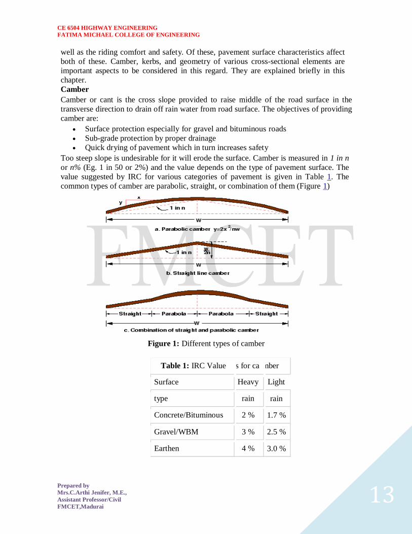
CE 6504 HIGHWAY ENGINEERING
FATIMA MICHAEL COLLEGE OF ENGINEERING
Prepared by
MrsCArthi Jenifer ME
Assistant ProfessorCivil
FMCETMadurai 13
well as the riding comfort and safety Of these pavement surface characteristics affect
both of these Camber kerbs and geometry of various cross-sectional elements are
important aspects to be considered in this regard They are explained briefly in this
chapter
Camber
Camber or cant is the cross slope provided to raise middle of the road surface in the
transverse direction to drain off rain water from road surface The objectives of providing
camber are
Surface protection especially for gravel and bituminous roads
Sub-grade protection by proper drainage
Quick drying of pavement which in turn increases safety
Too steep slope is undesirable for it will erode the surface Camber is measured in 1 in n
or n (Eg 1 in 50 or 2) and the value depends on the type of pavement surface The
value suggested by IRC for various categories of pavement is given in Table 1 The
common types of camber are parabolic straight or combination of them (Figure 1)
Figure 1 Different types of camber
Table 1 IRC Value
s for ca
mber
Heavy
Light
Surface
rain
type
rain
17
ConcreteBituminous
2
25
GravelWBM
3
30
Earthen
4
CE 6504 HIGHWAY ENGINEERING
FATIMA MICHAEL COLLEGE OF ENGINEERING
Prepared by
MrsCArthi Jenifer ME
Assistant ProfessorCivil
FMCETMadurai 14
Engineering surveys for alignment
The stages of the engineering surveys are a) Map study
b) Reconnaissance
c) Preliminary surveys
d) Final location and detailed surveys
Map study -
) In the topographic map to suggest the likely routes of roads In India topographic
maps are available from the survey of India with 15 or 30-meter contour intervals
) The main feature like rivers hills and valleys etc The probable alignment can be
located on the map from the following details available on the map
Alignment avoiding valleys ponds or lakes
When the road has to cross a row of hills possibility crossing through a mountain pass
Approximate location of bridge site for crossing rivers avoiding bend of the river
When a road is to be connected between two stations one of the top and the other on the foot
of the hill then alternate routes can be suggested keeping in view the permissible alignment
Suppose the scale of the contour map is known and then the contour intervals it is possible
to decide the length of road required between two consecutive contours keeping the gradient
within allowable limits
In the fig Let A and B be two stations to be connected by road AB is the shortest route
(Straight line) APQB is a steep route in which the gradient positively exceeds 1 in 20 as the
distance between the contour intervals is only about 200 meter
APLMNB is a route with an approximate slope of 1 in 20 whereas APEFGB is an alternate
alignment with the same gradient
Thus the map study also is possible to drop a certain route in view of any unavoidable
obstructions (or) undesirable ground enroute
Reconnaissance-
The second stage of surveys for highway location is the reconnaissance to examine the general
character of the area for deciding the most feasible routes for detailed studies
Some of the details to be collected during reconnaissance are given below
Valleys ponds lakes marshy land ridge hills permanent structures and other obstructions
along the route which are not available in the map
Approximate values of gradient length of gradients and radius of curves of alternate
alignments
Number and types of cross drainage structures maximum flood level and natural
groundwater level along the probable routes
Soil type along the routes from field identification tests and observation of geological
features
Sources of construction materials water and location of stone quarries
When the road passes through hilly or mountainous terrain additional data regarding the
geological formation types of rocks dip of strata seepage flow etc
Preliminary survey -
CE 6504 HIGHWAY ENGINEERING
FATIMA MICHAEL COLLEGE OF ENGINEERING
Prepared by
MrsCArthi Jenifer ME
Assistant ProfessorCivil
FMCETMadurai 15
The main objectives of the preliminary surveys are
To survey the various alternate alignments proposed after the reconnaissance and to collect
all the necessary physical information and details of topography drainage and soil
To compare the different proposals in view of the requirements of a good alignment
To estimate quantity of earthwork materials and other construction aspects and to work out
the cost of alternate proposals
To finalize the best alignment from all considerations
The procedure of the conventional methods of preliminary surveys the given steps
Primary survey -
For alternate alignments either secondary traverses (or) independent primary traverses may be
necessary
Topographical features -
All geographical and other man made features along the traverse and for a certain width on either
side surveyed and plotted
Leveling work -
Levelling work is also carried out side by side to give the centerline profiles and typical cross
sections The leveling work in the preliminary survey is kept to a minimum just sufficient to obtain
the approximate earthwork in the alternate alignments
Drainage studies -
Drainage investigations and hydrological data are collected so as to estimate the type number and
approximate size of cross and drainage structures
Soil survey -
The soil survey conducted at this stage helps to working out details of earthwork slopes suitability
of materials subsoil and surface drainage requirements and pavement type and the approximate
thickness requirements
Material survey -
The survey for naturally occurring materials like stone aggregates soft aggregates etc and
identification of suitable quarries should be made
Traffic survey -
Traffic surveys conducted in the region from basis for deciding the number of traffic lanes and
roadway width pavement design and economic analysis of highway project
Locations and functions
Final location and detailed survey - The alignment finalized at the design office after the preliminary survey is to be first located on the
field by establishing the centerline The detailed survey should be carried out for collecting the
information technology for the preparation of plans and construction details
Location -
The centerline of the road finalized in the drawings to be translated on the ground
during the location survey
Major and minor control points are established on the ground and center pegs are
driven checking the geometric design requirements
Detailed survey -
CE 6504 HIGHWAY ENGINEERING
FATIMA MICHAEL COLLEGE OF ENGINEERING
Prepared by
MrsCArthi Jenifer ME
Assistant ProfessorCivil
FMCETMadurai 16
Levels along his final centerline should be taken at all staked points Levelling work is to
great importance as the vertical alignment
A detailed soil survey is carried out to enable drawing of the soil profile
The data during the detailed survey should be elaborate and complete for preparing detailed
plans design and estimates of the project
Soil suitability analysis
The methodology for locating appropriate sites for each land use activity is guided by the intent to
minimize the possible adverse effects of development on the environment and on existing
communities and to emphasize the positive impacts of such development by locating them in a
most suitable location
This is achieved by examining a number of individual criteria assigning them relative levels of
importance as a whole and using a mathematical resultant model to identify the most suitable
location
By adopting this site suitability method it is possible to systematically identify the criteria
considered clearly document the relative importance of one criterion over another analyze the net
outcome using a Geographic Information System and then possibly revisit the mathematical
relationships in this ldquodecision modelrdquo
By revising the relative importance to identified criteria based upon the particular land use under
consideration it is possible to generate ldquosuitability mapsrdquo for each individual land use and then
generate a final composite land use that is based on a best possible collective suitability of multiple
land uses
To achieve this all the criteria are assigned a ldquorankrdquo denoting their relative levels of importance
within the suitability study These ranks are assigned as numeric values ranging from 1 to 10 with 1
reflecting a low level of importance and 10 reflecting a high level of importance For example
within the criteria of road networks national highways would have a different level of influence on
the suitability for a particular land use as compared with local roads Further the distance from each
of these features would further modify the relative suitability of a land use based on the proximity to
a particular type of road
Criteria for Site Suitability Analysis
The decision criteria for site selection are examined for assigning relative ranks and individual
feature weights based on the land use type for which suitability is being examined For benefit of
analysis the criteria under consideration in this paper activity are organized as
Critical Criteria Criteria that will be very significant in the site selection of the identified land use
and will act as key drivers in the selection of the geographic location These criteria can be clustered
into a single decision model and the outcome collectively reviewed These criteria have a strong
influence in the final suitability
Additional Criteria Criteria that will have to be examined one at a time to carefully assess its
relationship with the proposed land use activity These criteria have a positive influence in the final
suitability
CE 6504 HIGHWAY ENGINEERING
FATIMA MICHAEL COLLEGE OF ENGINEERING
Prepared by
MrsCArthi Jenifer ME
Assistant ProfessorCivil
FMCETMadurai 17
Constrained Criteria These criteria impose strong negative opportunities in the selection of areas
for the identified land use Consequently they inform of us of where the particular land use under
consideration should not be located These criteria serve to limit or exclude areas from the final
suitability
GIS Site Suitability Analysis Model We were developed a tourism site suitability analysis model
in ArcGIS - 931 which is shown in Figure -
CE 6504 HIGHWAY ENGINEERING
FATIMA MICHAEL COLLEGE OF ENGINEERING
Prepared by
MrsCArthi Jenifer ME
Assistant ProfessorCivil
FMCETMadurai 18
UNIT 2 GEOMETRIC DESIGN OF HIGHWAYS
Typical cross section of urban and rural roads
A cross section is a vertical plane (slice) taken at right angles to the road control line showing the
various elements that make up the roads structure It is normally viewed in the direction of
increasing chainage
The width of a roadway is an important design consideration to ensure that it is appropriately sized
to serve its function Because of the diversity within the County two major roadway categories have
been established 1 Rural Road Standards 2 Urban Road Standards Urban Road Standards will
serve those areas which tend to be more developed and need to provide for multiple users
(bicyclists pedestrians parallel parking etc) whereas many rural roads will primarily serve only
vehicular traffic
Cross sections are created to provide a visual guide depicting the initial interim and ultimate phase
cross sections for these road classifications The typical sections illustrated in the following pages
are recommendations tied to transportation planning aspects such as right‐of‐way lineage sidewalk
width etc Threshold daily traffic can be used as a guide for a starting point when determining
which cross section is most applicable
1 Rural Road Standards
The rural roadways will not typically require curb and gutter or sidewalk although the County may
require either or both in unique circumstances Widths of lanes and shoulders will vary depending
upon the specific classification and the potential traffic volume which the roadway may carry Roads
carrying fewer than 200 vehicles per day need not be paved or treated for dust control The need for
paved shoulders is also dependent upon the level of traffic and safety
Final design and construction details will be determined by the Public Works Department Final
Design and construction criteria taken into consideration may include but are not limited to use of
the roadway density of development topographical characteristics and nearby development For
construction in which only a portion of the ultimate cross‐section is intended to be completed the
partial design will need to allow for the eventual widening to the ultimate cross‐section The design
for the partial or interim cross‐section roadway will need to incorporate ultimate design information
to ensure that the first phase of roadway construction is appropriate and would not need to be
removed at a future date when the full width cross‐section is completed
2 Urban Road Standards
Three roadway classifications are identified for those areas that are associated with the communityrsquos
urban growth areas They include arterial collector and local street classifications Transportation
Plan shows the key elements of the urban road standards Urban road standards will include 12‐foot
lanes sidewalk and curb amp gutter arterials and collectors will also include a striped bike lane Turn
lanes may be necessary as determined by the County Since almost all of the municipalities have
different right‐of‐way cross sections adopted for their community it makes it very difficult for the
County to match them all Therefore the philosophy was to encourage a baseline amount of
right‐of‐way reservation that could ensure the adjacent community enough area for coordination of
future roadway improvements until such time the road
CE 6504 HIGHWAY ENGINEERING
FATIMA MICHAEL COLLEGE OF ENGINEERING
Prepared by
MrsCArthi Jenifer ME
Assistant ProfessorCivil
FMCETMadurai 19
CE 6504 HIGHWAY ENGINEERING
FATIMA MICHAEL COLLEGE OF ENGINEERING
Prepared by
MrsCArthi Jenifer ME
Assistant ProfessorCivil
FMCETMadurai 20
Cross sectional elements
Kerbs
Kerbs indicate the boundary between the carriage way and the shoulder or islands or footpaths Different types of kerbs are
CE 6504 HIGHWAY ENGINEERING
FATIMA MICHAEL COLLEGE OF ENGINEERING
Prepared by
MrsCArthi Jenifer ME
Assistant ProfessorCivil
FMCETMadurai 21
Low or mountable kerbs This type of kerbs is provided such that they
encourage the traffic to remain in the through traffic lanes and also allow the
driver to enter the shoulder area with little difficulty The height of this kerb is
about 10 cm above the pavement edge with a slope which allows the vehicle to
climb easily This is usually provided at medians and channelization schemes and
also helps in longitudinal drainage
Semi-barrier type kerbs When the pedestrian traffic is high these kerbs are
provided Their height is 15 cm above the pavement edge This type of kerb
prevents encroachment of parking vehicles but at acute emergency it is possible
to drive over this kerb with some difficulty
Barrier type kerbs They are designed to discourage vehicles from leaving the
pavement They are provided when there is considerable amount of pedestrian
traffic They are placed at a height of 20 cm above the pavement edge with a steep
batter
Submerged kerbs They are used in rural roads The kerbs are provided at
pavement edges between the pavement edge and shoulders They provide lateral
confinement and stability to the pavement
Figure 1 Different types of kerbs
Shoulders Shoulders are provided along the road edge and are intended for accommodation of
stopped vehicles serve as an emergency lane for vehicles and provide lateral support
for base and surface courses The shoulder should be strong enough to bear the weight
of a fully loaded truck even in wet conditions The shoulder width should be adequate
for giving working space around a stopped vehicle It is desirable to have a width of
46 m for the shoulders A minimum width of 25 m is recommended for 2-lane rural
highways in India Parking lanes
Parking lanes are provided in urban lanes for side parking Parallel parking is preferred
because it is safe for the vehicles moving on the road The parking lane should have a
minimum of 30 m width in the case of parallel parking
CE 6504 HIGHWAY ENGINEERING
FATIMA MICHAEL COLLEGE OF ENGINEERING
Prepared by
MrsCArthi Jenifer ME
Assistant ProfessorCivil
FMCETMadurai 22
Bus-bays
Bus bays are provided by recessing the kerbs for bus stops They are provided so that
they do not obstruct the movement of vehicles in the carriage way They should be at
least 75 meters away from the intersection so that the traffic near the intersections is not
affected by the bus-bay
Service roads Service roads or frontage roads give access to access controlled highways like freeways
and expressways They run parallel to the highway and will be usually isolated by a
separator and access to the highway will be provided only at selected points These roads
are provided to avoid congestion in the expressways and also the speed of the traffic in
those lanes is not reduced
Drainage
The pavement surface should be absolutely impermeable to prevent seepage of water into
the pavement layers Further both the geometry and texture of pavement surface should
help in draining out the water from the surface in less time
Footpath
Footpaths are exclusive right of way to pedestrians especially in urban areas They are
provided for the safety of the pedestrians when both the pedestrian traffic and vehicular
traffic is high Minimum width is 15 meter and may be increased based on the traffic
The footpath should be either as smooth as the pavement or more smoother than that to
induce the pedestrian to use the footpath
Right of way
Right of way (ROW) or land width is the width of land acquired for the road along its
alignment It should be adequate to accommodate all the cross-sectional elements of the
highway and may reasonably provide for future development To prevent ribbon
development along highways control lines and building lines may be provided Control
line is a line which represents the nearest limits of future uncontrolled building activity
in relation to a road Building line represents a line on either side of the road between
which and the road no building activity is permitted at all The right of way width is
governed by
Width of formation It depends on the category of the highway and width of
roadway and road margins
Height of embankment or depth of cutting It is governed by the topography and
the vertical alignment
Side slopes of embankment or cutting It depends on the height of the slope soil
type etc
Drainage system and their size which depends on rainfall topography etc
Sight distance considerations On curves etc there is restriction to the visibility
on the inner side of the curve due to the presence of some obstructions like
building structures etc
Reserve land for future widening Some land has to be acquired in advance
CE 6504 HIGHWAY ENGINEERING
FATIMA MICHAEL COLLEGE OF ENGINEERING
Prepared by
MrsCArthi Jenifer ME
Assistant ProfessorCivil
FMCETMadurai 23
Table 2 Desig
n speed in as per IRC (ruling and minimum)
Steep
Type
Plain
Rolling
Hilly
40-30
NSampSH
100-80
80-65
50-40
MDR
80-65
65-50
40-30
30-20
25-20
ODR
65-50
50-40
30-25
25-20
VR
50-40
40-35
25-20
anticipating future developments like widening of the road
Table 1 No
right of way for open areas
Roadway width in m
Road
Plain and
Mountainous and
classification
steep terrain
rolling terrain
Open areas
45
24
NHSH
18
MDR
25
15
15
ODR
12
9
VR
Built-up areas
20
NHSH
30
MDR
20
15
ODR
15
12
9
VR
10
CE 6504 HIGHWAY ENGINEERING
FATIMA MICHAEL COLLEGE OF ENGINEERING
Prepared by
MrsCArthi Jenifer ME
Assistant ProfessorCivil
FMCETMadurai 24
Horizontal curve
The presence of horizontal curve imparts centrifugal force which is a reactive force
acting outward on a vehicle negotiating it Centrifugal force depends on speed and radius
of the horizontal curve and is counteracted to a certain extent by transverse friction
between the tyre and pavement surface On a curved road this force tends to cause the
vehicle to overrun or to slide outward from the centre of road curvature For proper
design of the curve an understanding of the forces acting on a vehicle taking a horizontal
curve is necessary Various forces acting on the vehicle are illustrated in the figure 1
Figure 1 Effect of horizontal curve They are the centrifugal force (P) acting outward weight of the vehicle (W) acting
downward and the reaction of the ground on the wheels ( and ) The centrifugal
force and the weight is assumed to be from the centre of gravity which is at h units above
the ground Let the wheel base be assumed as b units The centrifugal force in
is given by
(1)
where is the weight of the vehicle in is the speed of the vehicle in is
the acceleration due to gravity in and is the radius of the curve in
The centrifugal ratio or the impact factor is given by
CE 6504 HIGHWAY ENGINEERING
FATIMA MICHAEL COLLEGE OF ENGINEERING
Prepared by
MrsCArthi Jenifer ME
Assistant ProfessorCivil
FMCETMadurai 25
(1)
The centrifugal force has two effects A tendency to overturn the vehicle about the outer
wheels and a tendency for transverse skidding Taking moments of the forces with
respect to the outer wheel when the vehicle is just about to override
At the equilibrium over turning is possible when
and for safety the following condition must satisfy
(2)
The second tendency of the vehicle is for transverse skidding ie When the the
centrifugal force is greater than the maximum possible transverse skid resistance due to
friction between the pavement surface and tyre The transverse skid resistance (F) is
given by
where and is the fractional force at tyre and and is the reaction at
tyre and is the lateral coefficient of friction and is the weight of the vehicle
This is counteracted by the centrifugal force (P) and equating
At equilibrium when skidding takes place (from equation1)
and for safety the following condition must satisfy
CE 6504 HIGHWAY ENGINEERING
FATIMA MICHAEL COLLEGE OF ENGINEERING
Prepared by
MrsCArthi Jenifer ME
Assistant ProfessorCivil
FMCETMadurai 26
(3)
Equation 2 and 3 give the stable condition for design If equation 2 is violated the vehicle
will overturn at the horizontal curve and if equation 3 is violated the vehicle will skid at
the horizontal
Curve Analysis of super-elevation
Super-elevation or cant or banking is the transverse slope provided at horizontal curve to
counteract the centrifugal force by raising the outer edge of the pavement with respect to
the inner edge throughout the length of the horizontal curve When the outer edge is
raised a component of the curve weight will be complimented in counteracting the effect
of centrifugal force In order to find out how much this raising should be the following
analysis may be done The forces acting on a vehicle while taking a horizontal curve with
super elevation is shown in figure 1
Figure 1 Analysis of super-elevation
Forces acting on a vehicle on horizontal curve of radius at a speed of are
the centrifugal force acting horizontally out-wards through the center of
gravity
the weight of the vehicle acting down-wards through the center of gravity and
the friction force between the wheels and the pavement along the surface
inward
CE 6504 HIGHWAY ENGINEERING
FATIMA MICHAEL COLLEGE OF ENGINEERING
Prepared by
MrsCArthi Jenifer ME
Assistant ProfessorCivil
FMCETMadurai 27
At equilibrium by resolving the forces parallel to the surface of the pavement we get where
friction
is the weight of the vehicle is the centrifugal force is the coefficient of
is the transverse slope due to superelevation Dividing by we get
CE 6504 HIGHWAY ENGINEERING
FATIMA MICHAEL COLLEGE OF ENGINEERING
Prepared by
MrsCArthi Jenifer ME
Assistant ProfessorCivil
FMCETMadurai 28
Step 1
Find for 75 percent of design speed neglecting ie
Step 2
If then else if go to step 3
Step 3
Find for the design speed and max ie If
then the maximum is safe for the design speed else go to
step 4
Step 4
Find the allowable speed for the maximum and
If then the design is adequate otherwise use speed adopt
control measures or look for speed control measures
Maximum and minimum super-elevation
Depends on (a) slow moving vehicle and (b) heavy loaded trucks with high CG IRC
specifies a maximum super-elevation of 7 percent for plain and rolling terrain while that
of hilly terrain is 10 percent and urban road is 4 percent The minimum super elevation is
2-4 percent for drainage purpose especially for large radius of the horizontal curve
Attainment of super-elevation
1 Elimination of the crown of the cambered section by
1 Rotating the outer edge about the crown The outer half of the cross slope
is rotated about the crown at a desired rate such that this surface falls on
the same plane as the inner half
2 Shifting the position of the crown This method is also known as diagonal
crown method Here the position of the crown is progressively
shifted outwards thus increasing the width of the inner half of cross section
progressively
2 Rotation of the pavement cross section to attain full super elevation byThere are
two methods of attaining super elevation by rotating the pavement
1 Rotation about the center line The pavement is rotated such that the inner
edge is depressed and the outer edge is raised both by half the total amount
of super elevation ie by with respect to the centre
2 Rotation about the inner edge Here the pavement is rotated raising the
outer edge as well as the centre such that the outer edge is raised by the
full amount of super elevation with respect to the inner edge
Horizontal Transition Curves
CE 6504 HIGHWAY ENGINEERING
FATIMA MICHAEL COLLEGE OF ENGINEERING
Prepared by
MrsCArthi Jenifer ME
Assistant ProfessorCivil
FMCETMadurai 29
Transition curve is provided to change the horizontal alignment from straight to circular
curve gradually and has a radius which decreases from infinity at the straight end
(tangent point) to the desired radius of the circular curve at the other end (curve point)
There are five objectives for providing transition curve and are given below
1 to introduce gradually the centrifugal force between the tangent point and the
beginning of the circular curve avoiding sudden jerk on the vehicle This
increases the comfort of passengers
2 to enable the driver turn the steering gradually for his own comfort and security
3 to provide gradual introduction of super elevation and
4 to provide gradual introduction of extra widening
5 to enhance the aesthetic appearance of the road
Type of transition curve
Different types of transition curves are spiral or clothoid cubic parabola and Lemniscate
IRC recommends spiral as the transition curve because
1 it fulfills the requirement of an ideal transition curve that is
1 rate of change or centrifugal acceleration is consistent (smooth) and
2 radius of the transition curve is at the straight edge and changes to at
the curve point ( ) and calculation and field implementation is
very easy
Length of transition curve The length of the transition curve should be determined as the maximum of the following
three criteria rate of change of centrifugal acceleration rate of change of super elevation
and an empirical formula given by IRC Rate of change of centrifugal acceleration
At the tangent point radius is infinity and hence centrifugal acceleration is zero At the
end of the transition the radius R has minimum value R The rate of change of
centrifugal acceleration should be adopted such that the design should not cause
discomfort to the drivers If is the rate of change of centrifugal acceleration it can be
written as
Therefore the length of the transition curve in is
CE 6504 HIGHWAY ENGINEERING
FATIMA MICHAEL COLLEGE OF ENGINEERING
Prepared by
MrsCArthi Jenifer ME
Assistant ProfessorCivil
FMCETMadurai 30
(1)
where is the rate of change of centrifugal acceleration given by an empirical formula
suggested by by IRC as below
(2) 2 Rate of introduction of super-elevation
Raise ( ) of the outer edge with respect to inner edge is given by
The rate of change of this raise from to is achieved
gradually with a gradient of in over the length of the transition curve (typical range
of is 60-150) Therefore the length of the transition curve is
(3)
3 By empirical formula
IRC suggest the length of the transition curve is minimum for a plain and rolling terrain
(4)
and for steep and hilly terrain is
(5)
CE 6504 HIGHWAY ENGINEERING
FATIMA MICHAEL COLLEGE OF ENGINEERING
Prepared by
MrsCArthi Jenifer ME
Assistant ProfessorCivil
FMCETMadurai 31
and the shift as
(
6
) The length of the transition curve is the maximum of
equations 1 3 and 4or5 ie
(
7
Case (a)
For single lane roads
(
1
)
Therefore
(
2
)
Figure 1 Set-back for single lane roads (
CE 6504 HIGHWAY ENGINEERING
FATIMA MICHAEL COLLEGE OF ENGINEERING
Prepared by
MrsCArthi Jenifer ME
Assistant ProfessorCivil
FMCETMadurai 32
For multi lane roads if is the distance between centerline of the road and the centerline
of the inner lane then
(3)
(4)
Figure 2 Set-back for multi-lane roads ( )
Case (a)
For single lane roads
(1)
Therefore
(2)
Gradient
Gradient is the rate of rise or fall along the length of the road with respect to the
horizontal While aligning a highway the gradient is decided for designing the vertical
curve Before finalizing the gradients the construction cost vehicular operation cost and
the practical problems in the site also has to be considered Usually steep gradients are
avoided as far as possible because of the difficulty to climb and increase in the
CE 6504 HIGHWAY ENGINEERING
FATIMA MICHAEL COLLEGE OF ENGINEERING
Prepared by
MrsCArthi Jenifer ME
Assistant ProfessorCivil
FMCETMadurai 33
construction cost More about gradients are discussed below
Effect of gradient
The effect of long steep gradient on the vehicular speed is considerable This is
particularly important in roads where the proportion of heavy vehicles is significant Due
to restrictive sight distance at uphill gradients the speed of traffic is often controlled by
these heavy vehicles As a result not only the operating costs of the vehicles are
increased but also capacity of the roads will have to be reduced Further due to high
differential speed between heavy and light vehicles and between uphill and downhill
gradients accidents abound in gradients
Representation of gradient
The positive gradient or the ascending gradient is denoted as and the negative gradient as The deviation angle is when two grades meet the angle which
measures the change of direction and is given by the algebraic difference between the two
grades
steep gradient while 1 in 50 = 2 representation is illustrated in the figure 1
Example 1 in 30 = 333 is a
is a flatter gradient The gradient
CE 6504 HIGHWAY ENGINEERING
FATIMA MICHAEL COLLEGE OF ENGINEERING
Prepared by
MrsCArthi Jenifer ME
Assistant ProfessorCivil
FMCETMadurai 34
Figure 1 Representation of gradient
Types of gradient
Many studies have shown that gradient upto seven percent can have considerable effect
on the speeds of the passenger cars On the contrary the speeds of the heavy vehicles are
considerably reduced when long gradients as flat as two percent is adopted Although
flatter gradients are desirable it is evident that the cost of construction will also be very
high Therefore IRC has specified the desirable gradients for each terrain However it
may not be economically viable to adopt such gradients in certain locations steeper
gradients are permitted for short duration Different types of grades are discussed below
Ruling gradient
The ruling gradient or the design gradient is the maximum gradient with which the
designer attempts to design the vertical profile of the road This depends on the terrain
length of the grade speed pulling power of the vehicle and the presence of the horizontal
curve In flatter terrain it may be possible to provide flat gradients but in hilly terrain it
is not economical and sometimes not possible also The ruling gradient is adopted by the
designer by considering a particular speed as the design speed and for a design vehicle
with standard dimensions But our country has a heterogeneous traffic and hence it is not
possible to lay down precise standards for the country as a whole Hence IRC has
recommended some values for ruling gradient for different types of terrain
Limiting gradient
This gradient is adopted when the ruling gradient results in enormous increase in cost of
construction On rolling terrain and hilly terrain it may be frequently necessary to adopt
limiting gradient But the length of the limiting gradient stretches should be limited and
must be sandwiched by either straight roads or easier grades
Exceptional gradient
Exceptional gradient are very steeper gradients given at unavoidable situations They
should be limited for short stretches not exceeding about 100 metres at a stretch In
mountainous and steep terrain successive exceptional gradients must be separated by a
minimum 100 metre length gentler gradient At hairpin bends the gradient is restricted to
25
Critical length of the grade
The maximum length of the ascending gradient which a loaded truck can operate without
undue reduction in speed is called critical length of the grade A speed of 25 kmph is a
CE 6504 HIGHWAY ENGINEERING
FATIMA MICHAEL COLLEGE OF ENGINEERING
Prepared by
MrsCArthi Jenifer ME
Assistant ProfessorCivil
FMCETMadurai 35
reasonable value This value depends on the size power load grad-ability of the truck
initial speed final desirable minimum speed
Minimum gradient
This is important only at locations where surface drainage is important Camber will take
care of the lateral drainage But the longitudinal drainage along the side drains require
some slope for smooth flow of water Therefore minimum gradient is provided for
drainage purpose and it depends on the rain fall type of soil and other site conditions A
minimum of 1 in 500 may be sufficient for concrete drain and 1 in 200 for open soil
drains are found to give satisfactory performance Sight distance available from a point is the actual distance along the road surface which a driver
from a specified height above the carriage way has visibility of stationary or moving objects
Sight distance required by drivers applies to both geometric design of highways and for
traffic control The sight distance situations are considered in the design
i) Stopping or absolute minimum sight distance
ii) Safe overtaking or passing sight distance
iii) Safe sight distance for entering into uncontrolled intersections
Apart from the three situations mentioned above the following sight distance are considered by the
IRC in highway design
Intermediate sight distance
This is defined as twice the stopping sight distance when overtaking sight distance
cannot be provided intermediate sight distance is provided to give limited overtaking opportunities
to fast vehicles
Head light sight distance
This is the distance visible to a driver during night driving under the illumination of the
vehicle head lights
Stopping sight distance
The minimum sight distance available on a highway at any spot should be of sufficient
length to stop a vehicle traveling at design speed safely without collision with any other obstruction
The absolute minimum sight distance is therefore equal to the stopping sight distance
which is also sometimes called nonpassing sight distance The sight distance available on a road to a
driver at any instance depends on
i) Features of the road
ii) Height of the drivers eye above the road surface
iii) Height of the object above the road surface
The distance within which a motor vehicle can be stopped depends upon the factors listed below
a) Total reactions time of the driver
b) Speed of vehicle
c) Efficiency of breaks
d) Frictional resistance between the road and tyres
e) Gradient of the road
Total reaction time
) Reaction time of the driver is the time taken from the instant the object is visible to the
driver to the instant the brakes are effectively applied
) The total reaction time may be split up into two parts
CE 6504 HIGHWAY ENGINEERING
FATIMA MICHAEL COLLEGE OF ENGINEERING
Prepared by
MrsCArthi Jenifer ME
Assistant ProfessorCivil
FMCETMadurai 36
i) Perception time
ii) Brake reaction time
PIEV theory
According to this theory the total reaction time of the driver is split into four parts
i) Perception
ii) Intellection
iii) Emotion
iv) Volition
Speed of Vehicle
The stopping distance depends very much on the speed of the vehicle first during the
total reaction time of the driver the distance moved by the vehicle will depend on the speed
Efficiency of brakes
The braking efficiency is said to be 100 percent if the wheels are fully licked preventing
them from rotating on application of the brakes This will result in 100 percent skidding which is
normally undesirable except in utmost emergency
Frictional resistance between road and tyres
The frictional resistance developed between road and tyres or the skid resistance depends
on the type and condition of the road surface and the tyres IRC has specified a design friction
coefficient of 035 to 04 depending upon the speed to be used for finding the braking distance in the
calculation of stopping sight distance
Analysis of stopping distance
i) The distance traveled by the vehicle during the total reaction time known as lag
distance
ii) The distance traveled by the vehicle after the application of the brakes is known as
braking distance
Overtaking sight distance
The minimum distance open to the vision of the driver of a vehicle intending to overtake
slow vehicle ahead with safety against the traffic of opposite direction is known as the minimum
overtaking sight distance(OSD) or Safe passing sight distance available
The overtaking sight distance is the distance measured along the center of the road which
a driver with his eye level 12m above the road surface can see the top of an object 12m above the
road surface
Some of the important factors on which the minimum overtaking sight distance required
a) Speed of
i) overtaking vehicle
ii) overtaken vehicle
iii) The vehicle coming from opposite direction
b) Distance between the overtaking and overtaken vehicles the minimum spacing
depends on the steeds
a) Skill and reaction time of the driver
b) Rate of acceleration of overtaking vehicle
c) Gradient of the road
Criteria for sight distance requirements on highway
) The absolute minimum sight distance required throughout the length of the road is the
SSD which should invariably be provided at all places
CE 6504 HIGHWAY ENGINEERING
FATIMA MICHAEL COLLEGE OF ENGINEERING
Prepared by
MrsCArthi Jenifer ME
Assistant ProfessorCivil
FMCETMadurai 37
) On horizontal curves the obstruction on the inner side of the curves should be cleared
to provide the required set back distance and absolute minimum sight distance
) On vertical summit curves the sight distance requirement may be fulfilled by proper
design of the vertical alignment
Hairpin bent
TYPES OF CURVES ON HILL ROADS
The following are the important types of curves provided on hill Roads-
1 Hair-Pin Curves
2 Salient Curves
3 Re-entrant Curves 1 Hair-pin curves - The curve in a hill road which changes its direction through an angle of 180
degree or so down the hill on the same side is known as hair-pin curve
A Hair-Pin Bend
This curve is so called because it conforms to the shape of a hair-pin The bend so formed at the
hair-pin curve in a hill road is known as hair-pin bend This type of curve should be located on a
hill side having the minimum slope and maximum stability It must also be safe from view point of
landslides and ground water Hair-pin bends with long arms and farther spacing are always
preferred They reduce construction problems and expensive protective works Hair-pin curves or
bends of serpentine nature are difficult to negotiate and should therefore be avoided as far as
possible
Salient curves - The curves having their convexity on the outer edges of a hill road are called
salient curves The centre of curvature of a salient curve lies towards the hill side This type of curve
occurs in the road length constructed on the ridge of a hill the bend so formed at the salient curve in
a hill road known as corner bend
Salient curves are very dangerous for fast moving traffic At such a curve or at corner bend the
portion of projecting hill side is usually cut down to improve the visibility as shown in fig (Re-
entrant curve) The outer edge of the road at such a curve is essentially provided with a parapet wall
for protection of the vehicles from falling down the hill slope
CE 6504 HIGHWAY ENGINEERING
FATIMA MICHAEL COLLEGE OF ENGINEERING
Prepared by
MrsCArthi Jenifer ME
Assistant ProfessorCivil
FMCETMadurai 38
3 Re-entrant curves - The curves having their convexity on the inner edge of a hill road are called
re-entrant curves
Re-entrant curves
The centre of curvature of a re-entrant curves lies away from the hill side This type of curve occurs
in the road length constructed in the calley of a hill
These curves are less dangereous as they provide adequate visibility to the fast moving traffic At
such curves the parapet wall is provided only for safety of fast moving traffic
CE 6504 HIGHWAY ENGINEERING
FATIMA MICHAEL COLLEGE OF ENGINEERING
Prepared by
MrsCArthi Jenifer ME
Assistant ProfessorCivil
FMCETMadurai 39
UNIT ndash III DESIGN OF RIGID AND FLEXIBLE PAVEMENTS
COMPARISON OF RIGID AND FLEXIBLE PAVEMENTS
The comparisons are
i) Design precision
A cement concrete pavement is amerable to a much more precise structural analysis
than a flexible pavement Flexible pavements designs are mainly empirical Computer aided analysis
of layered system is making the flexible pavement design more exact than hitherto
ii) Life
) Cement concrete slabs of a thin section constructed in the early 1940rsquos are still in
existence in India though many of them have cracked badly and a few of them have been ripped
open and rebuilt in recent ties
) A major project in cement concrete road construction between Agra and Mathura It can
safely be said that a well-designed concrete slab has a life of about 40 years
) Compared to this the life of a flexible pavement generally varies from 10 to 20 years
iii) Maintenance
) A well-designed cement concrete pavement needs very little maintenance The only
maintenance needed is I respect of joints
) The surface is unaffected by spillage of oil and lubricants bituminous surfaces on the
other hand need great inputs in maintenance
) The surface is affected by spillage of oil and lubricants The surface is also affected by
natural weathering agents like air water ad temperature changes
) A cement concrete pavement on the other hand needs a small amount for maintaining
joints
iv) Initial cost
) The argument so far used against a cement concrete slab is that it is much more costly
than a flexible pavement
) The latter specifications no doubt represent the rock-bottom needs of a road in India but
these specifications can hardly provide a smooth and durable surface
v) Stage construction ) Road construction is generally done adopting a policy of stage construction especially for
low volume roads As traffic grows additional layers in the form of water bound macadam and
superior surfacing are added on
) Initial outlay is minimum and additional outlays are in keeping with traffic growth This is
a great advantage when dealing with new roads in an atmosphere of austerity
vi) Availability of materials
) Cement bitumen stone aggregates and gravelsand are the major materials involved in
pavement Construction Cement has been in serious short supply in the country for the past many
decades
) Bitumen is also not available plentifully in India There is also the danger of the entire oil
reserves in the world shrinking during the next two or three decades
) In locations where stone aggregates are scarce cement concrete may have an advantage
for flexible pavements
vii) Surface characterstics
CE 6504 HIGHWAY ENGINEERING
FATIMA MICHAEL COLLEGE OF ENGINEERING
Prepared by
MrsCArthi Jenifer ME
Assistant ProfessorCivil
FMCETMadurai 40
) A good cement concrete surface is smooth and free from rutting potholes and
corrugations In a bituminous surface it is only the asphaltic concrete surface that can give
comparable rideablity
) A well-constructed cement concrete pavement surface can have a permanent nonskid
surface A bituminous surface can also be designed to have a good skid resistant surface
viii) Utility location
) In cement concrete slabs proper thought has to be given to locate utilities such as water
pipes telephone lines and electric cables
) It is difficult to rip open the slab and restore it to be the original condition if any changes
in the utilities lines are to be made
ix) Glame and night visibility
) Concrete pavements have a gray color which can cause glam under sunlight Colored
cement can reduce the grave
) On the other hand bituminous roads need more street lighting
x) Traffic dislocation during construction
) A cement concrete pavement requires 28 days before it can be thrown open to traffic On
the other hand a bituminous surface can be thrown open to traffic shortly after it is rolled
xi) Environmental considerations during construction
) The process of heating of bitumen and aggregates and mixing them together on hot mix
plants can prove to be much more hazardous to the environment than cement concrete construction
where no heating of any material is involved
xii) Overall economy on a life cycle basis
) A good road is costly to construct but once constructed such a road requires little
maintenance and results in savings in vehicle operating costs
) The comparative economy of a flexible pavement and a rigid pavement has proved that on
overall economic considerations
Types of pavement structure
Based on the structural behavior pavements are generally classified into three
categories
i) Flexible pavements
ii) Rigid pavements
iii) Semi rigid pavements
Flexible pavements
) Flexible pavements are those which on the whole have low or negligible flexural
strength and are rather flexible in their structural action under the loadsThe flexible pavement
layers reflect the deformation of the lower layers on to the surface of the layer
) A flexible pavement consists of four components(i) Soil subgrade (ii) sub base
course (iii) base course (iv) Surface course
CE 6504 HIGHWAY ENGINEERING
FATIMA MICHAEL COLLEGE OF ENGINEERING
Prepared by
MrsCArthi Jenifer ME
Assistant ProfessorCivil
FMCETMadurai 41
) The flexible pavement layers transmit the vertical or compressive stresses to the lower layers
by grain to grain transfer through the points of contact in the granular structure A well
compacted granular structure consisting of strong added aggregate can transfer the compressive
stresses
) The load spreading ability of this layer therefore depends on the type of the materials and mix
design factors Bituminous concrete is one of the best flexible pavements layer materials Other
materials which fall under the group are all granular materials with or without bituminous
binder granular base and sub base course materials
) The vertical compressive stress is maximum on the pavement surface directly under the wheel
and is equal to the contact pressure under the wheel The flexible pavement may be constructed
in a number of layers and the top layer has to be strongest as the highest compressive stresses
) Flexible pavements are commonly designed using empirical design charts or equations taking
into account some of the design factors there are also semi empirical and theoretical design
methods
Rigid pavements
) Rigid pavements are those which possess note flexural strength or flexural rigidity
The stresses are not transferred from grain to grain to the lower layers as in the ease of flexible
pavements layers
) The rigid pavements are made of Portland cement concrete plain reinforced or
prestressed concrete The plain cement concrete slabs are expected to take up about 40 kgcm2
flexural stress
) The rigid pavement has the slab action and is capable of transmitting the wheel
load stresses through a wider area below The main point of difference in the structural behavior
of rigid pavement as compared to the flexible pavement is that the critical condition of stress in
the rigid pavement is the maximum flexural stress occurring in the slab due to wheel load and
the temperature changes whereas in the flexible pavement
) As the rigid pavement slab has tensile strength tensile stresses are developed due
to the bending of the slab under wheel load and temperature variations Thus the types of
stresses developed and their distribution within the cement concrete slab are quirt different
) The cement concrete pavement slab can very well serve as a wearing surface as
well an effective base course The rigid pavement structure consists of a cement concrete slab
below which a granular base or sub base course may be provided
) Though the cement concrete slab can also be laid directly over the soil subgrade
consists of fine grained soil
) the rigid pavements are usually designed and the stresses are analyzed using the
elastic theory assuming the pavements as a n elastic plate resting over an elastic or a viscous
foundation
Semi rigid pavements
) when bonded materials like the pozzolanic concrete lean cement concrete or soil
cement are used in the base course or sub base course layer the pavement layer has considerably
higher flexural strength than the common flexible pavement layers
) when this intermediate class of materials are used in the base or sub base course
layer of the pavements they are called semi rigid pavements
CE 6504 HIGHWAY ENGINEERING
FATIMA MICHAEL COLLEGE OF ENGINEERING
Prepared by
MrsCArthi Jenifer ME
Assistant ProfessorCivil
FMCETMadurai 42
) This third category of semi rigid pavement are either designed as flexible
pavements with some correction factors to find the thickness requirements based on experience
or by using a new design approach
) The semi rigid pavement materials have low resistance to impact and abrasion and
therefore are usually provided with flexible pavement surface course
Various functions of pavement components
The functions are
Soil sub grade and its evaluation
) The soil sub grade is a layer of natural soil prepared to receive the layers of pavement
materials placed over it It is essential that at no time the soil sub grade is overstressed it means that
the pressure transmitted on the top of the sub grade is within the allowable limit
) Many tests are known for measuring the strength properties of the sub grades Some of the
tests have been standardized for the use The common strength test for the evaluation of soil
subgrade is
i) California bearing ratio test
ii) California resistance value test
iii) Triaxial compression test
iv) Plate bearing test
CALIFORNIA BEARING RATIO (CBR) TEST
It is evolved for the empirical method of flexible pavement design The CBR test is carried
out either in the laboratory on prepared specimens or in the field by taking in situ measurements
California resistance value
It is found by using have been stabliometerThis test is used in an empirical method of
flexible pavement design based on soil strength
Triaxial test
It is the most important soil strength but still the test is not very commonly used in structural
design of pavements
Plate bearing test
It is carried out using a relatively large diameter plate to evaluate the load supporting
capacity of supporting power of the pavement layers The results are plate bearing tests are used in
flexible pavement design method like McLeod method on based on layer system analysis by
brumister
Sub base and base courses and their evaluation
) There layers are made of broken stones bound or unbound aggreagatesome times in sub
base course a layer of stabilized soil(or) Selected granular soil is also used
) however at the sub base course it is desirable to use smaller size graded aggregates When
the sub grade consists of fine grained soil and when the pavement carries heavy wheel loads
CE 6504 HIGHWAY ENGINEERING
FATIMA MICHAEL COLLEGE OF ENGINEERING
Prepared by
MrsCArthi Jenifer ME
Assistant ProfessorCivil
FMCETMadurai 43
) Sub base course primarily has the similar function as of the base course and is provided
with inferior materials than of base course Base courses are used under rigid pavement for
i) Preventing pumping
ii) Protecting the sub grade against frost action
) Thus the fundamental purpose of abase course and sub base course is to provide a stress
transmitting medium to spread the surface wheel loads in such manner
) The sub base and base course layers may be evaluated by suitable strength or stability test
like plate bearing CBR test
WEARING COURSE AND ITS EVALUATION
) The purpose of the wearing course is to give a smooth riding surface that is dense It
resists pressure exerted by tyres and takes up wear and tear due to the traffic
) Wearing course also offers a water tight layer against the surface water infiltration The
flexible pavement normally a bituminous surfacing is used as a wearing course
) In rigid pavements the cement concrete acts like a base course as well as wearing course
Most popular test in use is marshal stability test where in the optimum content of bitumen binder is
worked out based on the stability density
) Plate bearing test and Bankelman beam test are also sometimes made use of for evaluating
the wearing course and the pavement as a whole
Various factors to be considered in pavement design and the significance
Pavement design consists of two parts
i) Mix design of materials to be used in each pavement component layer Thickness design of the
pavement and the component layers
The various factors to be considered for the design of pavements are given below
i) Design wheel load
ii) Sub grade soil
iii) Climatic factors
iv) Pavement component layers
v) Environmental factors
vi) Special factors in the design of different types of pavements
Design wheel load
The various wheel load factors to be considered in pavement design are
i) Maximum wheel load
ii) Contact pressure
iii) Dual or multiple wheel loads
iv) Repetition of loads
Maximum wheel load
The wheel load configurations are important to know the way in which the loads of a given
vehicle are applied on the pavement surface
) For highways the maximum legal axle load as specified by Indian road congress is 8170
kg with a maximum equivalent single wheel load of 4085 kg
) The evaluation for vertical stress computations under a uniformly distribute of circular
load based on Boussineqrsquos theory is given by
CE 6504 HIGHWAY ENGINEERING
FATIMA MICHAEL COLLEGE OF ENGINEERING
Prepared by
MrsCArthi Jenifer ME
Assistant ProfessorCivil
FMCETMadurai 44
2
322
3
1
za
zpz
σz = vertical stress at depth z
P= surface pressure
Z=depth at which σz computed
A=radius of loaded area
Contact pressure
Generally the wheel load is assumed to be distributed over a circular area But by
measurement of the imprints of tyers with different load and inflation pressures Three terms in use
with reference to tyre pressure are
Tyre pressure
Inflation pressure
Contact pressure
Tyre pressure and inflation pressure mean exactly the same the contact pressure is found to be more
than tyre pressure when the tyre pressure is less than 7 kgm2 and it is vice versa when the tyre
pressure exceeds this value
Contact pressure can be measured by the relationship
Load on wheel
Contact pressure = ----------------------------------------
Contact area or area of imprint
The general variation between the tyre pressure and measured contact pressure is shown in this fig
The ratio of contact pressure to type pressure is defined as rigidity factor Thus value of rigidity
factor is 10 for an average tyre pressure of 7 Kgcm2This value is higher than unity for lower type
pressures and less than unity for tyre pressures higher than 7 kgcm2
Equivalent single wheel load (ESWL)
) The maximum wheel load within the specified limit and to carry greater load it is
necessary to provide dual wheel assembly to the rear axles of the roads vehicles
) In other words the pressure at a certain depth below the pavement surface cannot be
obtained by numerically adding the pressure caused by any one wheel
) The effect is in between the single load and two times load carried by one wheel The load
dispersion is assumed to be at an angle of 450In the dual wheel load assembly let d be the clear gap
between the two wheels S be the spacing between the centers of the wheels and a be the radius of
the circular contact area of each wheel Then S = (d + 2a)
) ESWL may be determined based on either equivalent deflection or equivalent stress
criterianMultiple wheel loads are convert to ESWL and this value is used in pavement design The
ESWL is usually determined by the equivalent stress criterion using a simple graphical method
CE 6504 HIGHWAY ENGINEERING
FATIMA MICHAEL COLLEGE OF ENGINEERING
Prepared by
MrsCArthi Jenifer ME
Assistant ProfessorCivil
FMCETMadurai 45
) A straight line relationship is assumed between ESWL and depth on log scales For
determining ESWL the plot is made as shown in fig
) Two points A and B are plotted on the log-log graph with coordinates of A (Pd2) and
B(2p2s)line AB is a plot which is the focus of points where any single wheel load is equivalent to a
certain set of dual wheels
) To Calculate the ESWL for a dual assembly it is essential to estimate a design thickness of
the pavement If the design thickness so obtained is equal to the estimated thickness then the ESWL
calculations could be considered as correct Otherwise trials are made
) In heavy trucks and trailers the load on each wheel may be further reduced by multiple
wheels and tandem axles
Repetition of loads
) The deformation of load pavement (or) sub grade due to a single application of wheel load
may be small It required carrying out traffic surveys for accounting the factor of repetitions for
wheel loads in the design of pavement
) Data collected are converted to some constant equivalent wheel loads Equivalent wheel
load is a single load equivalent to the repeated applications of any particular wheel load on a
pavement which requires the same thickness and strength of pavements
) McLeod has given a procedure for evolving equivalent load factors for designing flexible
pavements
Various methods of flexible pavement design
) The flexible pavement is built with number of layers In the design process it is to be
ensured that under the application of load none of the layers is overstressed
) The maximum intensity of stresses occurs in the top layer of the pavement The
magnitude of load stresses reduces at lower layers
) In the design of flexible pavements it has yet not been possible to have a rational design
method wherein design process and service behavior of the pavement can be expressed by
mathematical laws
) Flexible pavement design methods are accordingly either empirical or semi empirical In
these methods the knowledge and experience gained on the behavior of the pavements in the past
are usefully utilized
Various approaches of flexible pavement design may be thus classified into three groups
i) Empirical method
ii) Semi-empirical or Semi theoretical method
iii) Theoretical method
) Empirical methods are either based on physical properties or strength parameters of soil
sub grade When the design is based on stress strain function and modified base on experience it
may be called semi-empirical or semi-theoretical There are design methods based on theoretical
analysis and mathematical computations
Out of the flexible pavement design method available is
i) Group index method
ii) California bearing ratio method
iii) California R value (or) Stabiliometer method
iv) Triaxial test method
CE 6504 HIGHWAY ENGINEERING
FATIMA MICHAEL COLLEGE OF ENGINEERING
Prepared by
MrsCArthi Jenifer ME
Assistant ProfessorCivil
FMCETMadurai 46
v) McLeod method
vi) Burmister method
Group index method
) Group index value is an arbitrary index assigned to the soil type in numerical equations
base on the percent fines liquid limit and plasticity index
) The design chart for group index method for determining the pavement thickness is given
in fig
The traffic volume in this method is divided in three groups
Traffic volume No of vehicles per day
Light Less than 50
Medium 50 to 300
Heavy Over 300
The design of the pavement thickness by this method first the G1 value of the soil is found the
anticipated traffic is estimated and is designated as light medium or heavy as indicated
The G1 method of pavement design is essentially an empirical method based on physical properties
of the subgrade soil This method does not consider the strength characteristics of the subgrade soil
and therefore is open to question regarding the reliability of the design based on the index properties
of the soil only
California bearing ratio method
) California division of highways in the USA developed CBR method for
pavement design The majority of design curves developed later are base on the original curves
proposed by OJporter
) One of the chief advantages of CBR method is the simplicity of the test procedure
The CBR tests were carried out by the California state highway department on existing pavement
layers including subgrade sub base and base course
) Based on the extensive CBR test data collected on pavement which behaved
satisfactory and those which failed an empirical design chart was developed correlating the CBR
value and the pavement thickness The basis of the design chart is that a material with a given CBR
required a certain thickness of pavement layer as a cover
) A higher load needs a thicker pavement layer to protect the sub grade Design
curves correlating the CBR value with total pavement thickness cover were developed by the
California state highway department for wheel loads of 3175kg and 5443 kg representing light and
heavy traffic The design curves are shown in this fig
It is possible to extend the CBR design curves for various loading conditions nusing the expression
t= 2
1
1751
pCBRp
t=2
1
751
A
CBR
p
Hence
CE 6504 HIGHWAY ENGINEERING
FATIMA MICHAEL COLLEGE OF ENGINEERING
Prepared by
MrsCArthi Jenifer ME
Assistant ProfessorCivil
FMCETMadurai 47
t= pavement thickness cm
p=Wheel load kg
CBR= California bearing ratio percent
P=tyre pressure kgcm2
A= area of contactcm2
IRC Recommendations
a) The CBR tests should be performed on remoulded soils in the laboratory The specimens should
be prepared by static compaction wherever possible and otherwise by dynamic compaction
b) For the design of new roads the sub grade soil sample should be compacted at OMC to proctor
density whenever suitable compaction equipment
c) The CBR test samples may be soaked in water for four days period before testing the annual
rainfall is less than 50 cm and the water table is too deep to affect the sub grade and imperable
surfacing is provided to carrying out CBR test
d) If the maximum variations in CBR value of the three specimens exceed the specified limits the
design CBR should be average of at least six samples
e) The top 50 cm of sub grade should be compacted at least up to 95 to 100 percent of proctor
density
f) An estimate of the traffic should be carried by the road pavements at the end of expected in view
the existing traffic and probable growth rate of traffic
g) The traffic for the design is considered in units of heavy vehicles per day in both directions and is
divided into seven categories A to G The design thickness is considered applicable for single axle
loads up to 8200 kg and tandom axle loads up to 14500 kg
h) When sub base course materials contain substantial proportion of aggregates of size above 20mm
the CBR value of these materials would not be valid for the design of subsequent layers above them
The CBR method of pavement design gives the total thickness requirement of the pavement above a
sub grade and thickness value would remain the same quality of materials used in component layers
California resistance value method
) In this design method based on stabliometer R-value and cohesiometer C-value
Based on performance data it was established by pavement thickness varies directly with R value
and algorithm of load repetitions It varies inversely with fifth root of c valueThe expression for
pavement thickness is given by the empirical equation
T=
5
1
1 90
C
RTK
Hence
T=total thickness of pavement cm
K=Numerical constant 0166
T1=traffic index
R= stabiliometer resistance value
C=Cohesiometer value
CE 6504 HIGHWAY ENGINEERING
FATIMA MICHAEL COLLEGE OF ENGINEERING
Prepared by
MrsCArthi Jenifer ME
Assistant ProfessorCivil
FMCETMadurai 48
In the design of flexible pavements based on California resistance value method for the following
data are needed
) R-value of soil subgrade
) T1 value
) Equivalent C-value
) R value of soil subgrade is obtained from the test using stablio meterThe
computation of T1 value has been explained
Equivalent C-value
) The cohesion meter value c is obtained for each layer of pavement material
separately from tests However the composite or equivalent C-value of the pavement may be
estimated if the thickness of each component layer and the c-value of the material of the layer are
known
) while designing a pavement as the thickness of the pavement is not known it is
easier if the pavement is first assumed to consist of any one material like gravel base course with
known C-value
) Subsequently the individual thickness of each layer is converted in terms of gravel
equivalent by using relationship
5
1
1
2
2
1
C
C
t
t
) t1 and t2 are the thickness values of any two pavement layersc1 and c2 are their
corresponding cohesiometer values
CE 6504 HIGHWAY ENGINEERING
FATIMA MICHAEL COLLEGE OF ENGINEERING
Prepared by
MrsCArthi Jenifer ME
Assistant ProfessorCivil
FMCETMadurai 49
UNIT 4 MATERIAL AND MAINTENANCE
SUMMIT CURVE
Summit curves are vertical curves with gradient upwards They are formed when two
gradients meet as illustrated in figure 1 in any of the following four ways
1 When a positive gradient meets another positive gradient [figure 1a]
2 When positive gradient meets a flat gradient [figure 1b]
3 When an ascending gradient meets a descending gradient [figure 1c]
4 When a descending gradient meets another descending gradient [figure 1d]
Type of Summit Curve
Many curve forms can be used with satisfactory results the common practice has been to
use parabolic curves in summit curves This is primarily because of the ease with it can
be laid out as well as allowing a comfortable transition from one gradient to another
Although a circular curve offers equal sight distance at every point on the curve for very
small deviation angles a circular curve and parabolic curves are almost congruent
Furthermore the use of parabolic curves were found to give excellent riding comfort
Figure 1 Types of summit curves
Design Consideration
In determining the type and length of the vertical curve the design considerations are
comfort and security of the driver and the appearance of the profile alignment Among
these sight distance requirements for the safety are most important on summit curves
The stopping sight distance or absolute minimum sight distance should be provided on
these curves and where overtaking is not prohibited overtaking sight distance or
intermediate sight distance should be provided as far as possible When a fast moving
vehicle travels along a summit curve there is less discomfort to the passengers This is
because the centrifugal force will be acting upwards while the vehicle negotiates a
summit curve which is against the gravity and hence a part of the tyre pressure is
relieved Also if the curve is provided with adequate sight distance the length would be
sufficient to ease the shock due to change in gradient Circular summit curves are
identical since the radius remains same throughout and hence the sight distance From
CE 6504 HIGHWAY ENGINEERING
FATIMA MICHAEL COLLEGE OF ENGINEERING
Prepared by
MrsCArthi Jenifer ME
Assistant ProfessorCivil
FMCETMadurai 50
this point of view transition curves are not desirable since it has varying radius and so the
sight distance will also vary The deviation angles provided on summit curves for
highways are very large and so the simple parabola is almost congruent to a circular arc
between the same tangent points Parabolic curves are easy for computation and also it
had been found out that it provides good riding comfort to the drivers It is also easy for
field implementation Due to all these reasons a simple parabolic curve is preferred as
summit curve Length of the summit curve
The important design aspect of the summit curve is the determination of the length of the
curve which is parabolic As noted earlier the length of the curve is guided by the sight
distance consideration That is a driver should be able to stop his vehicle safely if there is
an obstruction on the other side of the road Equation of the parabola is given by
where where N is the deviation angle and is the length of the In
deriving the length of the curve two situations can arise depending on the uphill and
downhill gradients when the length of the curve is greater than the sight distance and the
length of the curve is greater than the sight distance
Let is the length of the summit curve is the SSDISDOSD is the deviation angle
drivers eye height (12 m) and the height of the obstruction then the length of the
summit curve can be derived for the following two cases The length of the summit curve
can be derived from the simple geometry as shown below
Case a Length of summit curve greater than sight distance( )
Figure 1 Length of summit curve ( )
The situation when the sight distance is less than the length of the curve is shown in
figure 1
CE 6504 HIGHWAY ENGINEERING
FATIMA MICHAEL COLLEGE OF ENGINEERING
Prepared by
MrsCArthi Jenifer ME
Assistant ProfessorCivil
FMCETMadurai 51
(1)
Case b Length of summit curve less than sight distance
The second case is illustrated in figure 1
Figure 1 Length of summit curve
CE 6504 HIGHWAY ENGINEERING
FATIMA MICHAEL COLLEGE OF ENGINEERING
Prepared by
MrsCArthi Jenifer ME
Assistant ProfessorCivil
FMCETMadurai 52
From the basic geometry one can write
(1)
Therefore for a given and to get minimum differentiate the above equation
with respect to and equate it to zero Therefore
Solving the quadratic equation for
(2)
Now we can substitute back to get the value of minimum value of for a given
and Therefore
Solving for
CE 6504 HIGHWAY ENGINEERING
FATIMA MICHAEL COLLEGE OF ENGINEERING
Prepared by
MrsCArthi Jenifer ME
Assistant ProfessorCivil
FMCETMadurai 53
(3) (4
CE 6504 HIGHWAY ENGINEERING
FATIMA MICHAEL COLLEGE OF ENGINEERING
Prepared by
MrsCArthi Jenifer ME
Assistant ProfessorCivil
FMCETMadurai 54
When stopping sight distance is considered the height of drivers eye above the road
surface ( ) is taken as 12 metres and height of object above the pavement surface ( )
is taken as 015 metres If overtaking sight distance is considered then the value of
drivers eye height ( ) and the height of the obstruction ( ) are taken equal as 12
metres
Valley curve
Valley curve or sag curves are vertical curves with convexity downwards They are
formed when two gradients meet as illustrated in figure 1 in any of the following four
ways
Figure 1 Types of valley curve
1 When a descending gradient meets another descending gradient [figure 1a]
2 When a descending gradient meets a flat gradient [figure 1b]
3 When a descending gradient meets an ascending gradient [figure 1c]
4 When an ascending gradient meets another ascending gradient [figure
Design considerations
There is no restriction to sight distance at valley curves during day time But visibility is
reduced during night In the absence or inadequacy of street light the only source for
visibility is with the help of headlights Hence valley curves are designed taking into
account of headlight distance In valley curves the centrifugal force will be acting
downwards along with the weight of the vehicle and hence impact to the vehicle will be
more This will result in jerking of the vehicle and cause discomfort to the passengers
Thus the most important design factors considered in valley curves are (1) impact-free
movement of vehicles at design speed and (2) availability of stopping sight distance
under headlight of vehicles for night driving
For gradually introducing and increasing the centrifugal force acting downwards the best
shape that could be given for a valley curve is a transition curve Cubic parabola is
generally preferred in vertical valley curves See figure 1
CE 6504 HIGHWAY ENGINEERING
FATIMA MICHAEL COLLEGE OF ENGINEERING
Prepared by
MrsCArthi Jenifer ME
Assistant ProfessorCivil
FMCETMadurai 55
Figure 1 Valley curve details
During night under headlight driving condition sight distance reduces and availability of
stopping sight distance under head light is very important The head light sight distance
should be at least equal to the stopping sight distance There is no problem of overtaking
sight distance at night since the other vehicles with headlights could be seen from a
considerable distance
Length of the valley curve
The valley curve is made fully transitional by providing two similar transition curves of
equal length The transitional curve is set out by a cubic parabola where
The length of the valley transition curve is designed based on two criteria
1 comfort criteria that is allowable rate of change of centrifugal acceleration is
limited to a comfortable level of about
2 safety criteria that is the driver should have adequate headlight sight distance at
any part of the country
Comfort criteria
The length of the valley curve based on the rate of change of centrifugal acceleration that
will ensure comfort Let is the rate of change of acceleration the minimum radius of
the curve is the design speed and is the time then is give
CE 6504 HIGHWAY ENGINEERING
FATIMA MICHAEL COLLEGE OF ENGINEERING
Prepared by
MrsCArthi Jenifer ME
Assistant ProfessorCivil
FMCETMadurai 56
For a cubic parabola the Value Safety criter Length of the valley curve for headlight distance may be determined for two conditions
(1) length of the valley curve greater than stopping sight distance and (2) length of the
valley curve less than the stopping sight distance of for length is given by
Case 1 Length of valley curve greater than stopping sight distance ( )
The total length of valley curve is greater than the stopping sight distance SSD The
sight distance available will be minimum when the vehicle is in the lowest point in the
valley This is because the beginning of the curve will have infinite radius and the bottom
of the curve will have minimum radius which is a property of the transition curve The
case is shown in figure 1
Figure 1 Valley curve case 1
From the geometry of the figure we have
CE 6504 HIGHWAY ENGINEERING
FATIMA MICHAEL COLLEGE OF ENGINEERING
Prepared by
MrsCArthi Jenifer ME
Assistant ProfessorCivil
FMCETMadurai 57
(1)
where is the deviation angle in radians is the height of headlight beam is the
head beam inclination in degrees and is the sight distance The inclination is 1
degree
Case 2 Length of valley curve less than stopping sight distance ( )
The length of the curve is less than SSD In this case the minimum sight distance is
from the beginning of the curve The important points are the beginning of the curve and
the bottom most part of the curve If the vehicle is at the bottom of the curve then its
headlight beam will reach far beyond the endpoint of the curve whereas if the vehicle is
at the beginning of the curve then the headlight beam will hit just outside the curve
Therefore the length of the curve is derived by assuming the vehicle at the beginning of
the curve The case is shown in figure 1
From the figure
(1) Note that the above expression is approximate and is satisfactory because in practice the gradients
are very small and is acceptable for all practical purposes We will not be able to know prior to
which case to be adopted Therefore both has to be calculated and the one which satisfies the
condition is adopted
1 Flexible pavement
2 Rigid pavement
Flexible pavement
These pavements reflect the deformation of sub grade and the subsequent layers to the
surface
Rigid pavement
The rigid characteristic of the pavement are associated with rigidity or flexural strength
CE 6504 HIGHWAY ENGINEERING
FATIMA MICHAEL COLLEGE OF ENGINEERING
Prepared by
MrsCArthi Jenifer ME
Assistant ProfessorCivil
FMCETMadurai 58
or slab action so the load is distributed over a wide area of sub grade soil
Flexible pavement Definition
These pavements reflect the deformation of sub grade and the subsequent layers to the
surface Flexible usually asphalt is laid with no reinforcement or with a specialized
fabric reinforcement that permits limited flow or repositioning of the roadbed under
ground changes
The design of flexible pavement is based on load distributing characteristic of the
component layers The black top pavement including water amp gravel bound macadam fall
in this category
Flexible pavement on the whole has low or negligible flexible strength flexible in their
structural action) The flexible pavement layers transmit the vertical or compressive
stresses to the lower layers by grain transfer through contact points of granular structure
The vertical compressive stress is maximum on the pavement surface directly under the
wheel load and is equal to contact pressure under the wheels Due to the ability to
distribute the stress to large area in the shape of truncated cone the stresses get decreased
in the lower layer
As such the flexible pavement may be constructed in a number of layers and the top
layer has to be strongest as the highest compressive stresses
To be sustained by this layer in addition to wear and tear the lower layer have to take
up only lesser magnitude of stress as there is no direct wearing action die to traffic loads
therefore inferior material with lower cast can be used in the lower layers
Rigid pavement Definition
The rigid characteristic of the pavement are associated with rigidity or flexural strength
or slab action so the load is distributed over a wide area of sub grade soil Rigid pavement
is laid in slabs with steel reinforcement
The rigid pavements are made of cement concrete either plan reinforced or prestressed
concrete
Critical condition of stress in the rigid pavement is the maximum flexural stress occurring in the slab due to wheel load and the temperature changes
Rigid pavement is designed and analyzed by using the elastic theory
CE 6504 HIGHWAY ENGINEERING
FATIMA MICHAEL COLLEGE OF ENGINEERING
Prepared by
MrsCArthi Jenifer ME
Assistant ProfessorCivil
FMCETMadurai 59
UNIT-5 EVALUATION AND MAINTENANCE OF PAVEMENTS
TRAFFIC PARAMETERS
Design life
Design life is the number of years (or number of standard axle repetitions) for which the
pavement is being designed A pavement is expected to serve satisfactorily within the
design life For concrete pavements 20 to 40 years may be assumed as the design life
(PCA 1984 IRC58 2002)
Basic design principle
Though different approaches for concrete pavement design are suggested in various
guidelines the design principles tend to remain similar across different guidelines for
example PCA (1994) Austroads (2004) NCHRP (2004) IRC58 (2002) etc except the
AASHTO (1993) provisions which is based on empirical approach The basic steps
involved in the design of concrete pavement method can be summarized as follows
The developed stresses due to load for a trial thickness of the concrete slab are
calculated for various loading configuration and the critical one is chosen The
axle loads are generally divided into different axle load groups and the load
stresses are calculated individually
The ratio between the load stress and Modulus of Rupture (MOR) is known as
stress ratio The stress ratio determines how many repetitions the pavement can
sustain (ie allowable traffic repetitions) for the individual axle load group If the
stress ratio is 055 or lower it can withstand virtually infinite number of traffic
repetitions (PCA 1984)
The ratio between the allowable repetitions to the expected traffic repetitions is
the damage fraction The calculation process is repeated for various axle loads
(sometimes for various seasons or various timings of the day) and the sum of
individual damage fractions (c u m u l a t i v e fatigue damage) should be less
than equal to one for pavement design being safe If found unsafe the trial
thickness is changed and the design process is repeated
The design process may also include considerations for temperature stress
moisture stresses and erosion distress
A brief discussion on concrete pavement design approaches suggested by various design
practices viz PCA method (1984) Austroads method (2004) AASHTO method (1993)
NCHRP mechanistic-empirical method (2004) and the Indian Roads Congress (IRC)
method (2002) are placed in the following
Portland cement Association (PCA) Method
The PCA method is based on Westergaard Picket and Rays work and further theoretical
analysis by Finite Element Method (Huang 1993) The data used to develop the PCA
method is generated from various road tests like ASSHO road test Arlington test
(conducted by PCA) Bates test road and Maryland road test (PCA 1984) The PCA
design method is based on the following two considerations (PCA 1984)
The fatigue damage on the concrete slab due to repetitive application of traffic
load is estimated The cumulative fatigue damage principle is used to estimate the
design thickness of the slab Edge stress between the mid-ways of the
CE 6504 HIGHWAY ENGINEERING
FATIMA MICHAEL COLLEGE OF ENGINEERING
Prepared by
MrsCArthi Jenifer ME
Assistant ProfessorCivil
FMCETMadurai 60
transverse joint is taken as critical configuration
The stresses due to warping and curling (due to temperature and moisture
gradient) are not considered in the fatigue analysis as per PCA recommendation
because most of the time the stresses generated are subtractive to the load stress
The possibility of erosion of pavement materials placed below the concrete slab is
evaluated The rate at which the slab is deflected due to axle load is used as a
criterion for erosion Theoretically it can be shown that a thin pavement with
smaller deflection basin is subjected to faster rate of deflection compared to
thicker slab Hence thin slab is more susceptible to erosion In a similar way the
cumulative erosion damage is calculated for individual axle load groups If this
value is greater than one then the design needs to be revised
Austroads method
Austroads method has been adopted from PCA (1984) approach with modifications
suited to Australian conditions (Austroads 2004) A bound mix or lean cement concrete is
used as sub-base material For a given CBR value of the subgrade and given thickness of
cemented sub-base the effective subgrade strength can be obtained from the chart
provided Figure-19 schematically shows such a chart For different levels of traffic
Austroads (2004) suggests minimum values of the base thicknesses to be provided
CE 6504 HIGHWAY ENGINEERING
FATIMA MICHAEL COLLEGE OF ENGINEERING
Prepared by
MrsCArthi Jenifer ME
Assistant ProfessorCivil
FMCETMadurai 61
figure-19 Schematic diagram of Austroads (2004) chart for estimation of effective
subgrade strength
As per Astroads (2004) the concrete pavement slab thickness for a given expected
traffic repetitions is designed considering the (i) flexural fatigue of the concrete slab and
the (ii) subgrade erosion arising out of repeated deflections For both the considerations
equations are suggested to calculate the allowable traffic repetitions If the allowable
traffic is less than the expected traffic the design is revised by increasing the slab
thickness The concrete shoulders adopted are of integral type or structural type
AASHTO method
The AASHTO method (1993) for design of concrete pavement has evolved from the
AASHO road test (AASHO 1962) The AASHTO pavement design follows an empirical
approach Pavement performance in terms of present serviceability index ( PSI ) loss of
serviceability sub-grade and sub-base strength cumulative traffic properties of concrete
joint load transfer efficiency drainage condition overall standard deviation and
reliability are the input parameters considered in the pavement design
The PSI value of the fresh pavement is assumed as 45 and the pavement is deemed to
have failed when the PSI value reaches 25 The resilient moduli of the subgrade and sub-
base materials are determined in the laboratory simulating the seasonal moisture content
and stress situation Suggested values are also available for given moisture content
plasticity index etc The composite modulus of sub-grade reaction (k) is estimated from
modulus of sub-grade reaction and elastic modulus of sub-base for various seasons and
the depth of rigid foundation and the thickness of the sub-base
Design equation as well nomographs are available to estimate the slab thickness (D) from
these input parameters
NCHRP mechanistic-empirical (M-E) metho
The NCHRP (2004) has recently developed concrete pavement design procedure based
on mechanistic-empirical (M-E) approach This approach attempts to reduce the extent of
empiricism prevalent in the existing AASHTO (1993) guidelines This proposed NCHRP
pavement design system is modular in nature that is the design approach can be
modified by parts (as and when new knowledge is available) without disrupting the
overall design procedure This approach also can take care of various wheel-axle loa
configuration
As per this approach trial thickness of the slab is first assumed and the stress strain and
displacement values are obtained From these values the performance of the pavement in
terms of distresses (such as faulting cracking) and smoothness and predicted If these
predicted performance parameters does not satisfy the required performance for a given
reliability
The design approach includes a large data-base as input parameters for example average
daily traffic traffic growth rate traffic composition hourly weather data on air
temperature precipitation wind speed percentage sunshine relative humidity pavement
material engineering parameters ground water depth infiltration drainage hydraulic
conductivity thermal conductivity heat capacity etc The temperature stress is
considered in this method but the temperature profile is linearized to enhance
computational efficiency (NCHRP 2004)
CE 6504 HIGHWAY ENGINEERING
FATIMA MICHAEL COLLEGE OF ENGINEERING
Prepared by
MrsCArthi Jenifer ME
Assistant ProfessorCivil
FMCETMadurai 62
INDIAN ROADS CONGRESS (IRC) METHOD
The Indian Roads Congress (IRC) guidelines IRC58 (2002) has adopted the
Westergaards equation to estimate load stress and Brdaburys equation to estimate
temperature stress The load stress is highest at the corner of the slab lesser in edge and
least in the interior The order of variation of temperature stress is just the reverse of this
As per IRC58 (2002) it is recommended that the design needs to be done for edge stress
condition and subsequently check needs to be performed for corner stress condition so as
to finalize the design The following are the steps followed as per IRC58 (2002)
guideline for the design of concrete pavement
The input parameters are obtained to formulate the design problem The joint
spacing and the slab dimensions are decided If there is a bound sub-base layer
over the subgrade a suitable value of effective k is to be adopted
A trial thickness of the concrete slab is assumed
The edge stress is estimated for various axle loads from the given charts Figure-
20 schematically shows such a chart The cumulative fatigue damage principle for
fatigue is applied to check the adequacy of the slab thickness
The sum of edge stress due to load for the highest axle load group and the
temperature stress should be less than the MOR of concrete otherwise the design
is revised
The adequacy of corner stress is checked with respect to MOR value and
accordingly the design is finalized Westergaards corner stress formula
Figure-20 Schematic diagram of IRC58 chart for estimation of load stress at the edge
(IRC58 2002)
CE 6504 HIGHWAY ENGINEERING
FATIMA MICHAEL COLLEGE OF ENGINEERING
Prepared by
MrsCArthi Jenifer ME
Assistant ProfessorCivil
FMCETMadurai 63
estimation of corner stress due to load and the corner stress due to temperature is
assumed to be zero
Estimation of layer thicknesses
The thickness of the pavement is adjusted in such a way that the stress strain
developed is less than the allowable values obtained from past performance
information
The two major modes of structural failure of pavement are fatigue and rutting
o Fatigue Traffic applies repetitive load to the pavement surface and the
cracks start from bottom the bound layer slab and propagate upwards
When the extent of surface cracks reaches a predefined level the
pavement is said to have failed due to flexural fatigue
FUNCTIONAL DESIGN
The functional pavement design involves considerations of skid resistance roughness
surface distresses reflectivity of pavement surface etc The functional pavement design
considers mainly the surface features of a pavement
Drainage design
A road needs to be designed in such a way that the rain snow precipitation is drained off
the pavement and its surroundings A suitable surface drainage system for the pavement
is designed for this purpose Some water however will percolate into the pavement from
its top surface and needs to be taken out of the pavement - this is done by providing an
internal drainage system to the pavement Water will also try to enter into the pavement
from bottom due to capillary rise or due to rise in water table A suitably designed sub-
surface drainage system tries to avoid such a problem
PAVEMENT THICKNESS DESIGN CHARTS
For the design of pavements to carry traffic in the range of 1 to 10 msa use chart 1 and for
traffic in the range 10 to 150 msa use chart 2 of IRC37 2001 The design curves relate
pavement thickness to the cumulative number of standard axles to be carried over the
design life for different sub-grade CBR values ranging from 2 to 10 The design
charts will give the total thickness of the pavement for the above inputs The total
thickness consists of granular sub-base granular base and bituminous surfacing The
individual layers are designed based on the the recommendations given below and the
subsequent tables
Pavement composition
Sub-base
Sub-base materials comprise natural sand gravel laterite brick metal crushed
stone or combinations thereof meeting the prescribed grading and physical
requirements The sub-base material should have a minimum CBR of 20 and
30 for traffic upto 2 msa and traffic exceeding 2 msa respectively Sub-base
usually consist of granular or WBM and the thickness should not be less than 150
mm for design traffic less than 10 msa and 200 mm for design traffic
Base
The recommended designs are for unbounded granular bases which comprise
CE 6504 HIGHWAY ENGINEERING
FATIMA MICHAEL COLLEGE OF ENGINEERING
Prepared by
MrsCArthi Jenifer ME
Assistant ProfessorCivil
FMCETMadurai 64
conventional water bound macadam (WBM) or wet mix macadam (WMM) or
equivalent confirming to MOST specifications The materials should be of good
quality with minimum thickness of 225 mm for traffic up to 2 msa an 150 mm for
traffic
Bituminoussurfacing The surfacing consists of a wearing course or a binder
course plus wearing course The most commonly used wearing courses are
surface dressing open graded premix carpet mix seal surfacing semi-
dense bituminous concrete and bituminous concrete For binder course
MOST specifies it is desirable to use bituminous macadam (BM) for traffic
upto o 5 msa and dense bituminous macadam (DBM) for traffic more than 5
msa
Numerical example
Design the pavement for construction of a new bypass with the following data
1 Two lane carriage way
2 Initial traffic in the year of completion of construction = 400 CVPD (sum of both
directions)
3 Traffic growth rate = 75
4 Design life = 15 years
5 Vehicle damage factor based on axle load survey = 25 standard axle per
commercial vehicle
6 Design CBR of subgrade soil = 4
Solution
1 Distribution factor = 075
2
3 Total pavement thickness for CBR 4 and traffic 72 msa from IRC37 2001
chart1 = 660 mm
4 Pavement composition can be obtained by interpolation from Pavement Design
Catalogue (IRC37 2001)
1 Bituminous surfacing = 25 mm SDBC + 70 mm DBM
2 Road-base = 250 mm WBM
3 sub-base = 315 mm granular material of CBR not less than 30
CE 6504 HIGHWAY ENGINEERING
FATIMA MICHAEL COLLEGE OF ENGINEERING
Prepared by
MrsCArthi Jenifer ME
Assistant ProfessorCivil
FMCETMadurai 65
Generally bound base layers are used for concrete pavement construction As per Indian
specification some example of such base layers are Dry Lean Concrete (DLC) Roller
Compacted Concrete (RCC) (IRC15-2002)
The concrete slab is generally of M40 to M50 grade of concrete as
per Indian specifications and is called as paving quality concrete (PQC)
(IRC15-2002)
BITUMINOUS PAVEMENT
The subgrade is a compacted soil layer
The base and sub-base course could be made up of bound or unbound granular layer As
per Indian specifications (MORTampH 2001) some examples of base or sub-base layers
are Granular sub-base(GSB) Water Bound Macadam (WBM) Wet Mix Macadam
(WMM) etc
The binder course is made up bituminous material As per Indian specifications
(MORTampH 2001) some examples of binder course are Bituminous Macadam (BM)
Dense Bituminous Macadam (DBM) etc
The wearing course is the top bituminous layer which is comes in contact to the
vehicle tyre Wearing course provides impermeability to the pavement surface
against water percolation (Chakroborty and Das 2003) The binder course and wearing
course together are called bituminous surfacing
IRC METHOD OF FLEXIBLE PAVEMENT MIX DESIGN
These guidelines will apply to design of flexible pavements for Expressway National Highways
State Highways Major District Roads and other categories of roads Flexible pavements are
considered to include the pavements which have bituminous surfacing and granular base and sub-
base courses conforming to IRC MOST standards These guidelines apply to new pavements
Design criteria
The flexible pavements has been modeled as a three layer structure and stresses and strains at
critical locations have been computed using the linear elastic model To give proper consideration
to the aspects of performance the following three types of pavement distress resulting from
repeated (cyclic) application of traffic loads are considered
1 Vertical compressive strain at the top of the sub-grade which can cause sub-grade
deformation resulting in permanent deformation at the pavement surface
2 Horizontal tensile strain or stress at the bottom of the bituminous layer which can cause
fracture of the bituminous layer
3 Pavement deformation within the bituminous layer
CE 6504 HIGHWAY ENGINEERING
FATIMA MICHAEL COLLEGE OF ENGINEERING
Prepared by
MrsCArthi Jenifer ME
Assistant ProfessorCivil
FMCETMadurai 66
While the permanent deformation within the bituminous layer can be controlled by meeting the
mix design requirements thickness of granular and bituminous layers are selected using the
analytical design approach so that strains at the critical points are within the allowable limits For
calculating tensile strains at the bottom of the bituminous layer the stiffness of dense bituminous
macadam (DBM) layer with 6070 bitumen has been used in the analysis
FAILURE CRITERIA
Critical locations in pavement
A and B are the critical locations for tensile strains Maximum value of the strain is
adopted for design C is the critical location for the vertical subgrade strain since the
maximum value of the occurs mostly at C
CE 6504 HIGHWAY ENGINEERING
FATIMA MICHAEL COLLEGE OF ENGINEERING
Prepared by
MrsCArthi Jenifer ME
Assistant ProfessorCivil
FMCETMadurai 67
Fatigue Criteria
Bituminous surfacings of pavements display flexural fatigue cracking if the tensile strain
at the bottom of the bituminous layer is beyond certain limit The relation between the
fatigue life of the pavement and the tensile strain in the bottom of the bituminous layer
was obtained as
(1)
in which is the allowable number of load repetitions to control fatigue cracking and
is the Elastic modulus of bituminous layer The use of equation 1 would result in
fatigue cracking of 20 of the total area
Rutting Criteria
The allowable number of load repetitions to control permanent deformation can be
expressed as
(2)
is the number of cumulative standard axles to produce rutting of 20 mm
CE 6504 HIGHWAY ENGINEERING
FATIMA MICHAEL COLLEGE OF ENGINEERING
Prepared by
MrsCArthi Jenifer ME
Assistant ProfessorCivil
FMCETMadurai 68
CE 6504 HIGHWAY ENGINEERING
FATIMA MICHAEL COLLEGE OF ENGINEERING
Prepared by
MrsCArthi Jenifer ME
Assistant ProfessorCivil
FMCETMadurai 14
Engineering surveys for alignment
The stages of the engineering surveys are a) Map study
b) Reconnaissance
c) Preliminary surveys
d) Final location and detailed surveys
Map study -
) In the topographic map to suggest the likely routes of roads In India topographic
maps are available from the survey of India with 15 or 30-meter contour intervals
) The main feature like rivers hills and valleys etc The probable alignment can be
located on the map from the following details available on the map
Alignment avoiding valleys ponds or lakes
When the road has to cross a row of hills possibility crossing through a mountain pass
Approximate location of bridge site for crossing rivers avoiding bend of the river
When a road is to be connected between two stations one of the top and the other on the foot
of the hill then alternate routes can be suggested keeping in view the permissible alignment
Suppose the scale of the contour map is known and then the contour intervals it is possible
to decide the length of road required between two consecutive contours keeping the gradient
within allowable limits
In the fig Let A and B be two stations to be connected by road AB is the shortest route
(Straight line) APQB is a steep route in which the gradient positively exceeds 1 in 20 as the
distance between the contour intervals is only about 200 meter
APLMNB is a route with an approximate slope of 1 in 20 whereas APEFGB is an alternate
alignment with the same gradient
Thus the map study also is possible to drop a certain route in view of any unavoidable
obstructions (or) undesirable ground enroute
Reconnaissance-
The second stage of surveys for highway location is the reconnaissance to examine the general
character of the area for deciding the most feasible routes for detailed studies
Some of the details to be collected during reconnaissance are given below
Valleys ponds lakes marshy land ridge hills permanent structures and other obstructions
along the route which are not available in the map
Approximate values of gradient length of gradients and radius of curves of alternate
alignments
Number and types of cross drainage structures maximum flood level and natural
groundwater level along the probable routes
Soil type along the routes from field identification tests and observation of geological
features
Sources of construction materials water and location of stone quarries
When the road passes through hilly or mountainous terrain additional data regarding the
geological formation types of rocks dip of strata seepage flow etc
Preliminary survey -
CE 6504 HIGHWAY ENGINEERING
FATIMA MICHAEL COLLEGE OF ENGINEERING
Prepared by
MrsCArthi Jenifer ME
Assistant ProfessorCivil
FMCETMadurai 15
The main objectives of the preliminary surveys are
To survey the various alternate alignments proposed after the reconnaissance and to collect
all the necessary physical information and details of topography drainage and soil
To compare the different proposals in view of the requirements of a good alignment
To estimate quantity of earthwork materials and other construction aspects and to work out
the cost of alternate proposals
To finalize the best alignment from all considerations
The procedure of the conventional methods of preliminary surveys the given steps
Primary survey -
For alternate alignments either secondary traverses (or) independent primary traverses may be
necessary
Topographical features -
All geographical and other man made features along the traverse and for a certain width on either
side surveyed and plotted
Leveling work -
Levelling work is also carried out side by side to give the centerline profiles and typical cross
sections The leveling work in the preliminary survey is kept to a minimum just sufficient to obtain
the approximate earthwork in the alternate alignments
Drainage studies -
Drainage investigations and hydrological data are collected so as to estimate the type number and
approximate size of cross and drainage structures
Soil survey -
The soil survey conducted at this stage helps to working out details of earthwork slopes suitability
of materials subsoil and surface drainage requirements and pavement type and the approximate
thickness requirements
Material survey -
The survey for naturally occurring materials like stone aggregates soft aggregates etc and
identification of suitable quarries should be made
Traffic survey -
Traffic surveys conducted in the region from basis for deciding the number of traffic lanes and
roadway width pavement design and economic analysis of highway project
Locations and functions
Final location and detailed survey - The alignment finalized at the design office after the preliminary survey is to be first located on the
field by establishing the centerline The detailed survey should be carried out for collecting the
information technology for the preparation of plans and construction details
Location -
The centerline of the road finalized in the drawings to be translated on the ground
during the location survey
Major and minor control points are established on the ground and center pegs are
driven checking the geometric design requirements
Detailed survey -
CE 6504 HIGHWAY ENGINEERING
FATIMA MICHAEL COLLEGE OF ENGINEERING
Prepared by
MrsCArthi Jenifer ME
Assistant ProfessorCivil
FMCETMadurai 16
Levels along his final centerline should be taken at all staked points Levelling work is to
great importance as the vertical alignment
A detailed soil survey is carried out to enable drawing of the soil profile
The data during the detailed survey should be elaborate and complete for preparing detailed
plans design and estimates of the project
Soil suitability analysis
The methodology for locating appropriate sites for each land use activity is guided by the intent to
minimize the possible adverse effects of development on the environment and on existing
communities and to emphasize the positive impacts of such development by locating them in a
most suitable location
This is achieved by examining a number of individual criteria assigning them relative levels of
importance as a whole and using a mathematical resultant model to identify the most suitable
location
By adopting this site suitability method it is possible to systematically identify the criteria
considered clearly document the relative importance of one criterion over another analyze the net
outcome using a Geographic Information System and then possibly revisit the mathematical
relationships in this ldquodecision modelrdquo
By revising the relative importance to identified criteria based upon the particular land use under
consideration it is possible to generate ldquosuitability mapsrdquo for each individual land use and then
generate a final composite land use that is based on a best possible collective suitability of multiple
land uses
To achieve this all the criteria are assigned a ldquorankrdquo denoting their relative levels of importance
within the suitability study These ranks are assigned as numeric values ranging from 1 to 10 with 1
reflecting a low level of importance and 10 reflecting a high level of importance For example
within the criteria of road networks national highways would have a different level of influence on
the suitability for a particular land use as compared with local roads Further the distance from each
of these features would further modify the relative suitability of a land use based on the proximity to
a particular type of road
Criteria for Site Suitability Analysis
The decision criteria for site selection are examined for assigning relative ranks and individual
feature weights based on the land use type for which suitability is being examined For benefit of
analysis the criteria under consideration in this paper activity are organized as
Critical Criteria Criteria that will be very significant in the site selection of the identified land use
and will act as key drivers in the selection of the geographic location These criteria can be clustered
into a single decision model and the outcome collectively reviewed These criteria have a strong
influence in the final suitability
Additional Criteria Criteria that will have to be examined one at a time to carefully assess its
relationship with the proposed land use activity These criteria have a positive influence in the final
suitability
CE 6504 HIGHWAY ENGINEERING
FATIMA MICHAEL COLLEGE OF ENGINEERING
Prepared by
MrsCArthi Jenifer ME
Assistant ProfessorCivil
FMCETMadurai 17
Constrained Criteria These criteria impose strong negative opportunities in the selection of areas
for the identified land use Consequently they inform of us of where the particular land use under
consideration should not be located These criteria serve to limit or exclude areas from the final
suitability
GIS Site Suitability Analysis Model We were developed a tourism site suitability analysis model
in ArcGIS - 931 which is shown in Figure -
CE 6504 HIGHWAY ENGINEERING
FATIMA MICHAEL COLLEGE OF ENGINEERING
Prepared by
MrsCArthi Jenifer ME
Assistant ProfessorCivil
FMCETMadurai 18
UNIT 2 GEOMETRIC DESIGN OF HIGHWAYS
Typical cross section of urban and rural roads
A cross section is a vertical plane (slice) taken at right angles to the road control line showing the
various elements that make up the roads structure It is normally viewed in the direction of
increasing chainage
The width of a roadway is an important design consideration to ensure that it is appropriately sized
to serve its function Because of the diversity within the County two major roadway categories have
been established 1 Rural Road Standards 2 Urban Road Standards Urban Road Standards will
serve those areas which tend to be more developed and need to provide for multiple users
(bicyclists pedestrians parallel parking etc) whereas many rural roads will primarily serve only
vehicular traffic
Cross sections are created to provide a visual guide depicting the initial interim and ultimate phase
cross sections for these road classifications The typical sections illustrated in the following pages
are recommendations tied to transportation planning aspects such as right‐of‐way lineage sidewalk
width etc Threshold daily traffic can be used as a guide for a starting point when determining
which cross section is most applicable
1 Rural Road Standards
The rural roadways will not typically require curb and gutter or sidewalk although the County may
require either or both in unique circumstances Widths of lanes and shoulders will vary depending
upon the specific classification and the potential traffic volume which the roadway may carry Roads
carrying fewer than 200 vehicles per day need not be paved or treated for dust control The need for
paved shoulders is also dependent upon the level of traffic and safety
Final design and construction details will be determined by the Public Works Department Final
Design and construction criteria taken into consideration may include but are not limited to use of
the roadway density of development topographical characteristics and nearby development For
construction in which only a portion of the ultimate cross‐section is intended to be completed the
partial design will need to allow for the eventual widening to the ultimate cross‐section The design
for the partial or interim cross‐section roadway will need to incorporate ultimate design information
to ensure that the first phase of roadway construction is appropriate and would not need to be
removed at a future date when the full width cross‐section is completed
2 Urban Road Standards
Three roadway classifications are identified for those areas that are associated with the communityrsquos
urban growth areas They include arterial collector and local street classifications Transportation
Plan shows the key elements of the urban road standards Urban road standards will include 12‐foot
lanes sidewalk and curb amp gutter arterials and collectors will also include a striped bike lane Turn
lanes may be necessary as determined by the County Since almost all of the municipalities have
different right‐of‐way cross sections adopted for their community it makes it very difficult for the
County to match them all Therefore the philosophy was to encourage a baseline amount of
right‐of‐way reservation that could ensure the adjacent community enough area for coordination of
future roadway improvements until such time the road
CE 6504 HIGHWAY ENGINEERING
FATIMA MICHAEL COLLEGE OF ENGINEERING
Prepared by
MrsCArthi Jenifer ME
Assistant ProfessorCivil
FMCETMadurai 19
CE 6504 HIGHWAY ENGINEERING
FATIMA MICHAEL COLLEGE OF ENGINEERING
Prepared by
MrsCArthi Jenifer ME
Assistant ProfessorCivil
FMCETMadurai 20
Cross sectional elements
Kerbs
Kerbs indicate the boundary between the carriage way and the shoulder or islands or footpaths Different types of kerbs are
CE 6504 HIGHWAY ENGINEERING
FATIMA MICHAEL COLLEGE OF ENGINEERING
Prepared by
MrsCArthi Jenifer ME
Assistant ProfessorCivil
FMCETMadurai 21
Low or mountable kerbs This type of kerbs is provided such that they
encourage the traffic to remain in the through traffic lanes and also allow the
driver to enter the shoulder area with little difficulty The height of this kerb is
about 10 cm above the pavement edge with a slope which allows the vehicle to
climb easily This is usually provided at medians and channelization schemes and
also helps in longitudinal drainage
Semi-barrier type kerbs When the pedestrian traffic is high these kerbs are
provided Their height is 15 cm above the pavement edge This type of kerb
prevents encroachment of parking vehicles but at acute emergency it is possible
to drive over this kerb with some difficulty
Barrier type kerbs They are designed to discourage vehicles from leaving the
pavement They are provided when there is considerable amount of pedestrian
traffic They are placed at a height of 20 cm above the pavement edge with a steep
batter
Submerged kerbs They are used in rural roads The kerbs are provided at
pavement edges between the pavement edge and shoulders They provide lateral
confinement and stability to the pavement
Figure 1 Different types of kerbs
Shoulders Shoulders are provided along the road edge and are intended for accommodation of
stopped vehicles serve as an emergency lane for vehicles and provide lateral support
for base and surface courses The shoulder should be strong enough to bear the weight
of a fully loaded truck even in wet conditions The shoulder width should be adequate
for giving working space around a stopped vehicle It is desirable to have a width of
46 m for the shoulders A minimum width of 25 m is recommended for 2-lane rural
highways in India Parking lanes
Parking lanes are provided in urban lanes for side parking Parallel parking is preferred
because it is safe for the vehicles moving on the road The parking lane should have a
minimum of 30 m width in the case of parallel parking
CE 6504 HIGHWAY ENGINEERING
FATIMA MICHAEL COLLEGE OF ENGINEERING
Prepared by
MrsCArthi Jenifer ME
Assistant ProfessorCivil
FMCETMadurai 22
Bus-bays
Bus bays are provided by recessing the kerbs for bus stops They are provided so that
they do not obstruct the movement of vehicles in the carriage way They should be at
least 75 meters away from the intersection so that the traffic near the intersections is not
affected by the bus-bay
Service roads Service roads or frontage roads give access to access controlled highways like freeways
and expressways They run parallel to the highway and will be usually isolated by a
separator and access to the highway will be provided only at selected points These roads
are provided to avoid congestion in the expressways and also the speed of the traffic in
those lanes is not reduced
Drainage
The pavement surface should be absolutely impermeable to prevent seepage of water into
the pavement layers Further both the geometry and texture of pavement surface should
help in draining out the water from the surface in less time
Footpath
Footpaths are exclusive right of way to pedestrians especially in urban areas They are
provided for the safety of the pedestrians when both the pedestrian traffic and vehicular
traffic is high Minimum width is 15 meter and may be increased based on the traffic
The footpath should be either as smooth as the pavement or more smoother than that to
induce the pedestrian to use the footpath
Right of way
Right of way (ROW) or land width is the width of land acquired for the road along its
alignment It should be adequate to accommodate all the cross-sectional elements of the
highway and may reasonably provide for future development To prevent ribbon
development along highways control lines and building lines may be provided Control
line is a line which represents the nearest limits of future uncontrolled building activity
in relation to a road Building line represents a line on either side of the road between
which and the road no building activity is permitted at all The right of way width is
governed by
Width of formation It depends on the category of the highway and width of
roadway and road margins
Height of embankment or depth of cutting It is governed by the topography and
the vertical alignment
Side slopes of embankment or cutting It depends on the height of the slope soil
type etc
Drainage system and their size which depends on rainfall topography etc
Sight distance considerations On curves etc there is restriction to the visibility
on the inner side of the curve due to the presence of some obstructions like
building structures etc
Reserve land for future widening Some land has to be acquired in advance
CE 6504 HIGHWAY ENGINEERING
FATIMA MICHAEL COLLEGE OF ENGINEERING
Prepared by
MrsCArthi Jenifer ME
Assistant ProfessorCivil
FMCETMadurai 23
Table 2 Desig
n speed in as per IRC (ruling and minimum)
Steep
Type
Plain
Rolling
Hilly
40-30
NSampSH
100-80
80-65
50-40
MDR
80-65
65-50
40-30
30-20
25-20
ODR
65-50
50-40
30-25
25-20
VR
50-40
40-35
25-20
anticipating future developments like widening of the road
Table 1 No
right of way for open areas
Roadway width in m
Road
Plain and
Mountainous and
classification
steep terrain
rolling terrain
Open areas
45
24
NHSH
18
MDR
25
15
15
ODR
12
9
VR
Built-up areas
20
NHSH
30
MDR
20
15
ODR
15
12
9
VR
10
CE 6504 HIGHWAY ENGINEERING
FATIMA MICHAEL COLLEGE OF ENGINEERING
Prepared by
MrsCArthi Jenifer ME
Assistant ProfessorCivil
FMCETMadurai 24
Horizontal curve
The presence of horizontal curve imparts centrifugal force which is a reactive force
acting outward on a vehicle negotiating it Centrifugal force depends on speed and radius
of the horizontal curve and is counteracted to a certain extent by transverse friction
between the tyre and pavement surface On a curved road this force tends to cause the
vehicle to overrun or to slide outward from the centre of road curvature For proper
design of the curve an understanding of the forces acting on a vehicle taking a horizontal
curve is necessary Various forces acting on the vehicle are illustrated in the figure 1
Figure 1 Effect of horizontal curve They are the centrifugal force (P) acting outward weight of the vehicle (W) acting
downward and the reaction of the ground on the wheels ( and ) The centrifugal
force and the weight is assumed to be from the centre of gravity which is at h units above
the ground Let the wheel base be assumed as b units The centrifugal force in
is given by
(1)
where is the weight of the vehicle in is the speed of the vehicle in is
the acceleration due to gravity in and is the radius of the curve in
The centrifugal ratio or the impact factor is given by
CE 6504 HIGHWAY ENGINEERING
FATIMA MICHAEL COLLEGE OF ENGINEERING
Prepared by
MrsCArthi Jenifer ME
Assistant ProfessorCivil
FMCETMadurai 25
(1)
The centrifugal force has two effects A tendency to overturn the vehicle about the outer
wheels and a tendency for transverse skidding Taking moments of the forces with
respect to the outer wheel when the vehicle is just about to override
At the equilibrium over turning is possible when
and for safety the following condition must satisfy
(2)
The second tendency of the vehicle is for transverse skidding ie When the the
centrifugal force is greater than the maximum possible transverse skid resistance due to
friction between the pavement surface and tyre The transverse skid resistance (F) is
given by
where and is the fractional force at tyre and and is the reaction at
tyre and is the lateral coefficient of friction and is the weight of the vehicle
This is counteracted by the centrifugal force (P) and equating
At equilibrium when skidding takes place (from equation1)
and for safety the following condition must satisfy
CE 6504 HIGHWAY ENGINEERING
FATIMA MICHAEL COLLEGE OF ENGINEERING
Prepared by
MrsCArthi Jenifer ME
Assistant ProfessorCivil
FMCETMadurai 26
(3)
Equation 2 and 3 give the stable condition for design If equation 2 is violated the vehicle
will overturn at the horizontal curve and if equation 3 is violated the vehicle will skid at
the horizontal
Curve Analysis of super-elevation
Super-elevation or cant or banking is the transverse slope provided at horizontal curve to
counteract the centrifugal force by raising the outer edge of the pavement with respect to
the inner edge throughout the length of the horizontal curve When the outer edge is
raised a component of the curve weight will be complimented in counteracting the effect
of centrifugal force In order to find out how much this raising should be the following
analysis may be done The forces acting on a vehicle while taking a horizontal curve with
super elevation is shown in figure 1
Figure 1 Analysis of super-elevation
Forces acting on a vehicle on horizontal curve of radius at a speed of are
the centrifugal force acting horizontally out-wards through the center of
gravity
the weight of the vehicle acting down-wards through the center of gravity and
the friction force between the wheels and the pavement along the surface
inward
CE 6504 HIGHWAY ENGINEERING
FATIMA MICHAEL COLLEGE OF ENGINEERING
Prepared by
MrsCArthi Jenifer ME
Assistant ProfessorCivil
FMCETMadurai 27
At equilibrium by resolving the forces parallel to the surface of the pavement we get where
friction
is the weight of the vehicle is the centrifugal force is the coefficient of
is the transverse slope due to superelevation Dividing by we get
CE 6504 HIGHWAY ENGINEERING
FATIMA MICHAEL COLLEGE OF ENGINEERING
Prepared by
MrsCArthi Jenifer ME
Assistant ProfessorCivil
FMCETMadurai 28
Step 1
Find for 75 percent of design speed neglecting ie
Step 2
If then else if go to step 3
Step 3
Find for the design speed and max ie If
then the maximum is safe for the design speed else go to
step 4
Step 4
Find the allowable speed for the maximum and
If then the design is adequate otherwise use speed adopt
control measures or look for speed control measures
Maximum and minimum super-elevation
Depends on (a) slow moving vehicle and (b) heavy loaded trucks with high CG IRC
specifies a maximum super-elevation of 7 percent for plain and rolling terrain while that
of hilly terrain is 10 percent and urban road is 4 percent The minimum super elevation is
2-4 percent for drainage purpose especially for large radius of the horizontal curve
Attainment of super-elevation
1 Elimination of the crown of the cambered section by
1 Rotating the outer edge about the crown The outer half of the cross slope
is rotated about the crown at a desired rate such that this surface falls on
the same plane as the inner half
2 Shifting the position of the crown This method is also known as diagonal
crown method Here the position of the crown is progressively
shifted outwards thus increasing the width of the inner half of cross section
progressively
2 Rotation of the pavement cross section to attain full super elevation byThere are
two methods of attaining super elevation by rotating the pavement
1 Rotation about the center line The pavement is rotated such that the inner
edge is depressed and the outer edge is raised both by half the total amount
of super elevation ie by with respect to the centre
2 Rotation about the inner edge Here the pavement is rotated raising the
outer edge as well as the centre such that the outer edge is raised by the
full amount of super elevation with respect to the inner edge
Horizontal Transition Curves
CE 6504 HIGHWAY ENGINEERING
FATIMA MICHAEL COLLEGE OF ENGINEERING
Prepared by
MrsCArthi Jenifer ME
Assistant ProfessorCivil
FMCETMadurai 29
Transition curve is provided to change the horizontal alignment from straight to circular
curve gradually and has a radius which decreases from infinity at the straight end
(tangent point) to the desired radius of the circular curve at the other end (curve point)
There are five objectives for providing transition curve and are given below
1 to introduce gradually the centrifugal force between the tangent point and the
beginning of the circular curve avoiding sudden jerk on the vehicle This
increases the comfort of passengers
2 to enable the driver turn the steering gradually for his own comfort and security
3 to provide gradual introduction of super elevation and
4 to provide gradual introduction of extra widening
5 to enhance the aesthetic appearance of the road
Type of transition curve
Different types of transition curves are spiral or clothoid cubic parabola and Lemniscate
IRC recommends spiral as the transition curve because
1 it fulfills the requirement of an ideal transition curve that is
1 rate of change or centrifugal acceleration is consistent (smooth) and
2 radius of the transition curve is at the straight edge and changes to at
the curve point ( ) and calculation and field implementation is
very easy
Length of transition curve The length of the transition curve should be determined as the maximum of the following
three criteria rate of change of centrifugal acceleration rate of change of super elevation
and an empirical formula given by IRC Rate of change of centrifugal acceleration
At the tangent point radius is infinity and hence centrifugal acceleration is zero At the
end of the transition the radius R has minimum value R The rate of change of
centrifugal acceleration should be adopted such that the design should not cause
discomfort to the drivers If is the rate of change of centrifugal acceleration it can be
written as
Therefore the length of the transition curve in is
CE 6504 HIGHWAY ENGINEERING
FATIMA MICHAEL COLLEGE OF ENGINEERING
Prepared by
MrsCArthi Jenifer ME
Assistant ProfessorCivil
FMCETMadurai 30
(1)
where is the rate of change of centrifugal acceleration given by an empirical formula
suggested by by IRC as below
(2) 2 Rate of introduction of super-elevation
Raise ( ) of the outer edge with respect to inner edge is given by
The rate of change of this raise from to is achieved
gradually with a gradient of in over the length of the transition curve (typical range
of is 60-150) Therefore the length of the transition curve is
(3)
3 By empirical formula
IRC suggest the length of the transition curve is minimum for a plain and rolling terrain
(4)
and for steep and hilly terrain is
(5)
CE 6504 HIGHWAY ENGINEERING
FATIMA MICHAEL COLLEGE OF ENGINEERING
Prepared by
MrsCArthi Jenifer ME
Assistant ProfessorCivil
FMCETMadurai 31
and the shift as
(
6
) The length of the transition curve is the maximum of
equations 1 3 and 4or5 ie
(
7
Case (a)
For single lane roads
(
1
)
Therefore
(
2
)
Figure 1 Set-back for single lane roads (
CE 6504 HIGHWAY ENGINEERING
FATIMA MICHAEL COLLEGE OF ENGINEERING
Prepared by
MrsCArthi Jenifer ME
Assistant ProfessorCivil
FMCETMadurai 32
For multi lane roads if is the distance between centerline of the road and the centerline
of the inner lane then
(3)
(4)
Figure 2 Set-back for multi-lane roads ( )
Case (a)
For single lane roads
(1)
Therefore
(2)
Gradient
Gradient is the rate of rise or fall along the length of the road with respect to the
horizontal While aligning a highway the gradient is decided for designing the vertical
curve Before finalizing the gradients the construction cost vehicular operation cost and
the practical problems in the site also has to be considered Usually steep gradients are
avoided as far as possible because of the difficulty to climb and increase in the
CE 6504 HIGHWAY ENGINEERING
FATIMA MICHAEL COLLEGE OF ENGINEERING
Prepared by
MrsCArthi Jenifer ME
Assistant ProfessorCivil
FMCETMadurai 33
construction cost More about gradients are discussed below
Effect of gradient
The effect of long steep gradient on the vehicular speed is considerable This is
particularly important in roads where the proportion of heavy vehicles is significant Due
to restrictive sight distance at uphill gradients the speed of traffic is often controlled by
these heavy vehicles As a result not only the operating costs of the vehicles are
increased but also capacity of the roads will have to be reduced Further due to high
differential speed between heavy and light vehicles and between uphill and downhill
gradients accidents abound in gradients
Representation of gradient
The positive gradient or the ascending gradient is denoted as and the negative gradient as The deviation angle is when two grades meet the angle which
measures the change of direction and is given by the algebraic difference between the two
grades
steep gradient while 1 in 50 = 2 representation is illustrated in the figure 1
Example 1 in 30 = 333 is a
is a flatter gradient The gradient
CE 6504 HIGHWAY ENGINEERING
FATIMA MICHAEL COLLEGE OF ENGINEERING
Prepared by
MrsCArthi Jenifer ME
Assistant ProfessorCivil
FMCETMadurai 34
Figure 1 Representation of gradient
Types of gradient
Many studies have shown that gradient upto seven percent can have considerable effect
on the speeds of the passenger cars On the contrary the speeds of the heavy vehicles are
considerably reduced when long gradients as flat as two percent is adopted Although
flatter gradients are desirable it is evident that the cost of construction will also be very
high Therefore IRC has specified the desirable gradients for each terrain However it
may not be economically viable to adopt such gradients in certain locations steeper
gradients are permitted for short duration Different types of grades are discussed below
Ruling gradient
The ruling gradient or the design gradient is the maximum gradient with which the
designer attempts to design the vertical profile of the road This depends on the terrain
length of the grade speed pulling power of the vehicle and the presence of the horizontal
curve In flatter terrain it may be possible to provide flat gradients but in hilly terrain it
is not economical and sometimes not possible also The ruling gradient is adopted by the
designer by considering a particular speed as the design speed and for a design vehicle
with standard dimensions But our country has a heterogeneous traffic and hence it is not
possible to lay down precise standards for the country as a whole Hence IRC has
recommended some values for ruling gradient for different types of terrain
Limiting gradient
This gradient is adopted when the ruling gradient results in enormous increase in cost of
construction On rolling terrain and hilly terrain it may be frequently necessary to adopt
limiting gradient But the length of the limiting gradient stretches should be limited and
must be sandwiched by either straight roads or easier grades
Exceptional gradient
Exceptional gradient are very steeper gradients given at unavoidable situations They
should be limited for short stretches not exceeding about 100 metres at a stretch In
mountainous and steep terrain successive exceptional gradients must be separated by a
minimum 100 metre length gentler gradient At hairpin bends the gradient is restricted to
25
Critical length of the grade
The maximum length of the ascending gradient which a loaded truck can operate without
undue reduction in speed is called critical length of the grade A speed of 25 kmph is a
CE 6504 HIGHWAY ENGINEERING
FATIMA MICHAEL COLLEGE OF ENGINEERING
Prepared by
MrsCArthi Jenifer ME
Assistant ProfessorCivil
FMCETMadurai 35
reasonable value This value depends on the size power load grad-ability of the truck
initial speed final desirable minimum speed
Minimum gradient
This is important only at locations where surface drainage is important Camber will take
care of the lateral drainage But the longitudinal drainage along the side drains require
some slope for smooth flow of water Therefore minimum gradient is provided for
drainage purpose and it depends on the rain fall type of soil and other site conditions A
minimum of 1 in 500 may be sufficient for concrete drain and 1 in 200 for open soil
drains are found to give satisfactory performance Sight distance available from a point is the actual distance along the road surface which a driver
from a specified height above the carriage way has visibility of stationary or moving objects
Sight distance required by drivers applies to both geometric design of highways and for
traffic control The sight distance situations are considered in the design
i) Stopping or absolute minimum sight distance
ii) Safe overtaking or passing sight distance
iii) Safe sight distance for entering into uncontrolled intersections
Apart from the three situations mentioned above the following sight distance are considered by the
IRC in highway design
Intermediate sight distance
This is defined as twice the stopping sight distance when overtaking sight distance
cannot be provided intermediate sight distance is provided to give limited overtaking opportunities
to fast vehicles
Head light sight distance
This is the distance visible to a driver during night driving under the illumination of the
vehicle head lights
Stopping sight distance
The minimum sight distance available on a highway at any spot should be of sufficient
length to stop a vehicle traveling at design speed safely without collision with any other obstruction
The absolute minimum sight distance is therefore equal to the stopping sight distance
which is also sometimes called nonpassing sight distance The sight distance available on a road to a
driver at any instance depends on
i) Features of the road
ii) Height of the drivers eye above the road surface
iii) Height of the object above the road surface
The distance within which a motor vehicle can be stopped depends upon the factors listed below
a) Total reactions time of the driver
b) Speed of vehicle
c) Efficiency of breaks
d) Frictional resistance between the road and tyres
e) Gradient of the road
Total reaction time
) Reaction time of the driver is the time taken from the instant the object is visible to the
driver to the instant the brakes are effectively applied
) The total reaction time may be split up into two parts
CE 6504 HIGHWAY ENGINEERING
FATIMA MICHAEL COLLEGE OF ENGINEERING
Prepared by
MrsCArthi Jenifer ME
Assistant ProfessorCivil
FMCETMadurai 36
i) Perception time
ii) Brake reaction time
PIEV theory
According to this theory the total reaction time of the driver is split into four parts
i) Perception
ii) Intellection
iii) Emotion
iv) Volition
Speed of Vehicle
The stopping distance depends very much on the speed of the vehicle first during the
total reaction time of the driver the distance moved by the vehicle will depend on the speed
Efficiency of brakes
The braking efficiency is said to be 100 percent if the wheels are fully licked preventing
them from rotating on application of the brakes This will result in 100 percent skidding which is
normally undesirable except in utmost emergency
Frictional resistance between road and tyres
The frictional resistance developed between road and tyres or the skid resistance depends
on the type and condition of the road surface and the tyres IRC has specified a design friction
coefficient of 035 to 04 depending upon the speed to be used for finding the braking distance in the
calculation of stopping sight distance
Analysis of stopping distance
i) The distance traveled by the vehicle during the total reaction time known as lag
distance
ii) The distance traveled by the vehicle after the application of the brakes is known as
braking distance
Overtaking sight distance
The minimum distance open to the vision of the driver of a vehicle intending to overtake
slow vehicle ahead with safety against the traffic of opposite direction is known as the minimum
overtaking sight distance(OSD) or Safe passing sight distance available
The overtaking sight distance is the distance measured along the center of the road which
a driver with his eye level 12m above the road surface can see the top of an object 12m above the
road surface
Some of the important factors on which the minimum overtaking sight distance required
a) Speed of
i) overtaking vehicle
ii) overtaken vehicle
iii) The vehicle coming from opposite direction
b) Distance between the overtaking and overtaken vehicles the minimum spacing
depends on the steeds
a) Skill and reaction time of the driver
b) Rate of acceleration of overtaking vehicle
c) Gradient of the road
Criteria for sight distance requirements on highway
) The absolute minimum sight distance required throughout the length of the road is the
SSD which should invariably be provided at all places
CE 6504 HIGHWAY ENGINEERING
FATIMA MICHAEL COLLEGE OF ENGINEERING
Prepared by
MrsCArthi Jenifer ME
Assistant ProfessorCivil
FMCETMadurai 37
) On horizontal curves the obstruction on the inner side of the curves should be cleared
to provide the required set back distance and absolute minimum sight distance
) On vertical summit curves the sight distance requirement may be fulfilled by proper
design of the vertical alignment
Hairpin bent
TYPES OF CURVES ON HILL ROADS
The following are the important types of curves provided on hill Roads-
1 Hair-Pin Curves
2 Salient Curves
3 Re-entrant Curves 1 Hair-pin curves - The curve in a hill road which changes its direction through an angle of 180
degree or so down the hill on the same side is known as hair-pin curve
A Hair-Pin Bend
This curve is so called because it conforms to the shape of a hair-pin The bend so formed at the
hair-pin curve in a hill road is known as hair-pin bend This type of curve should be located on a
hill side having the minimum slope and maximum stability It must also be safe from view point of
landslides and ground water Hair-pin bends with long arms and farther spacing are always
preferred They reduce construction problems and expensive protective works Hair-pin curves or
bends of serpentine nature are difficult to negotiate and should therefore be avoided as far as
possible
Salient curves - The curves having their convexity on the outer edges of a hill road are called
salient curves The centre of curvature of a salient curve lies towards the hill side This type of curve
occurs in the road length constructed on the ridge of a hill the bend so formed at the salient curve in
a hill road known as corner bend
Salient curves are very dangerous for fast moving traffic At such a curve or at corner bend the
portion of projecting hill side is usually cut down to improve the visibility as shown in fig (Re-
entrant curve) The outer edge of the road at such a curve is essentially provided with a parapet wall
for protection of the vehicles from falling down the hill slope
CE 6504 HIGHWAY ENGINEERING
FATIMA MICHAEL COLLEGE OF ENGINEERING
Prepared by
MrsCArthi Jenifer ME
Assistant ProfessorCivil
FMCETMadurai 38
3 Re-entrant curves - The curves having their convexity on the inner edge of a hill road are called
re-entrant curves
Re-entrant curves
The centre of curvature of a re-entrant curves lies away from the hill side This type of curve occurs
in the road length constructed in the calley of a hill
These curves are less dangereous as they provide adequate visibility to the fast moving traffic At
such curves the parapet wall is provided only for safety of fast moving traffic
CE 6504 HIGHWAY ENGINEERING
FATIMA MICHAEL COLLEGE OF ENGINEERING
Prepared by
MrsCArthi Jenifer ME
Assistant ProfessorCivil
FMCETMadurai 39
UNIT ndash III DESIGN OF RIGID AND FLEXIBLE PAVEMENTS
COMPARISON OF RIGID AND FLEXIBLE PAVEMENTS
The comparisons are
i) Design precision
A cement concrete pavement is amerable to a much more precise structural analysis
than a flexible pavement Flexible pavements designs are mainly empirical Computer aided analysis
of layered system is making the flexible pavement design more exact than hitherto
ii) Life
) Cement concrete slabs of a thin section constructed in the early 1940rsquos are still in
existence in India though many of them have cracked badly and a few of them have been ripped
open and rebuilt in recent ties
) A major project in cement concrete road construction between Agra and Mathura It can
safely be said that a well-designed concrete slab has a life of about 40 years
) Compared to this the life of a flexible pavement generally varies from 10 to 20 years
iii) Maintenance
) A well-designed cement concrete pavement needs very little maintenance The only
maintenance needed is I respect of joints
) The surface is unaffected by spillage of oil and lubricants bituminous surfaces on the
other hand need great inputs in maintenance
) The surface is affected by spillage of oil and lubricants The surface is also affected by
natural weathering agents like air water ad temperature changes
) A cement concrete pavement on the other hand needs a small amount for maintaining
joints
iv) Initial cost
) The argument so far used against a cement concrete slab is that it is much more costly
than a flexible pavement
) The latter specifications no doubt represent the rock-bottom needs of a road in India but
these specifications can hardly provide a smooth and durable surface
v) Stage construction ) Road construction is generally done adopting a policy of stage construction especially for
low volume roads As traffic grows additional layers in the form of water bound macadam and
superior surfacing are added on
) Initial outlay is minimum and additional outlays are in keeping with traffic growth This is
a great advantage when dealing with new roads in an atmosphere of austerity
vi) Availability of materials
) Cement bitumen stone aggregates and gravelsand are the major materials involved in
pavement Construction Cement has been in serious short supply in the country for the past many
decades
) Bitumen is also not available plentifully in India There is also the danger of the entire oil
reserves in the world shrinking during the next two or three decades
) In locations where stone aggregates are scarce cement concrete may have an advantage
for flexible pavements
vii) Surface characterstics
CE 6504 HIGHWAY ENGINEERING
FATIMA MICHAEL COLLEGE OF ENGINEERING
Prepared by
MrsCArthi Jenifer ME
Assistant ProfessorCivil
FMCETMadurai 40
) A good cement concrete surface is smooth and free from rutting potholes and
corrugations In a bituminous surface it is only the asphaltic concrete surface that can give
comparable rideablity
) A well-constructed cement concrete pavement surface can have a permanent nonskid
surface A bituminous surface can also be designed to have a good skid resistant surface
viii) Utility location
) In cement concrete slabs proper thought has to be given to locate utilities such as water
pipes telephone lines and electric cables
) It is difficult to rip open the slab and restore it to be the original condition if any changes
in the utilities lines are to be made
ix) Glame and night visibility
) Concrete pavements have a gray color which can cause glam under sunlight Colored
cement can reduce the grave
) On the other hand bituminous roads need more street lighting
x) Traffic dislocation during construction
) A cement concrete pavement requires 28 days before it can be thrown open to traffic On
the other hand a bituminous surface can be thrown open to traffic shortly after it is rolled
xi) Environmental considerations during construction
) The process of heating of bitumen and aggregates and mixing them together on hot mix
plants can prove to be much more hazardous to the environment than cement concrete construction
where no heating of any material is involved
xii) Overall economy on a life cycle basis
) A good road is costly to construct but once constructed such a road requires little
maintenance and results in savings in vehicle operating costs
) The comparative economy of a flexible pavement and a rigid pavement has proved that on
overall economic considerations
Types of pavement structure
Based on the structural behavior pavements are generally classified into three
categories
i) Flexible pavements
ii) Rigid pavements
iii) Semi rigid pavements
Flexible pavements
) Flexible pavements are those which on the whole have low or negligible flexural
strength and are rather flexible in their structural action under the loadsThe flexible pavement
layers reflect the deformation of the lower layers on to the surface of the layer
) A flexible pavement consists of four components(i) Soil subgrade (ii) sub base
course (iii) base course (iv) Surface course
CE 6504 HIGHWAY ENGINEERING
FATIMA MICHAEL COLLEGE OF ENGINEERING
Prepared by
MrsCArthi Jenifer ME
Assistant ProfessorCivil
FMCETMadurai 41
) The flexible pavement layers transmit the vertical or compressive stresses to the lower layers
by grain to grain transfer through the points of contact in the granular structure A well
compacted granular structure consisting of strong added aggregate can transfer the compressive
stresses
) The load spreading ability of this layer therefore depends on the type of the materials and mix
design factors Bituminous concrete is one of the best flexible pavements layer materials Other
materials which fall under the group are all granular materials with or without bituminous
binder granular base and sub base course materials
) The vertical compressive stress is maximum on the pavement surface directly under the wheel
and is equal to the contact pressure under the wheel The flexible pavement may be constructed
in a number of layers and the top layer has to be strongest as the highest compressive stresses
) Flexible pavements are commonly designed using empirical design charts or equations taking
into account some of the design factors there are also semi empirical and theoretical design
methods
Rigid pavements
) Rigid pavements are those which possess note flexural strength or flexural rigidity
The stresses are not transferred from grain to grain to the lower layers as in the ease of flexible
pavements layers
) The rigid pavements are made of Portland cement concrete plain reinforced or
prestressed concrete The plain cement concrete slabs are expected to take up about 40 kgcm2
flexural stress
) The rigid pavement has the slab action and is capable of transmitting the wheel
load stresses through a wider area below The main point of difference in the structural behavior
of rigid pavement as compared to the flexible pavement is that the critical condition of stress in
the rigid pavement is the maximum flexural stress occurring in the slab due to wheel load and
the temperature changes whereas in the flexible pavement
) As the rigid pavement slab has tensile strength tensile stresses are developed due
to the bending of the slab under wheel load and temperature variations Thus the types of
stresses developed and their distribution within the cement concrete slab are quirt different
) The cement concrete pavement slab can very well serve as a wearing surface as
well an effective base course The rigid pavement structure consists of a cement concrete slab
below which a granular base or sub base course may be provided
) Though the cement concrete slab can also be laid directly over the soil subgrade
consists of fine grained soil
) the rigid pavements are usually designed and the stresses are analyzed using the
elastic theory assuming the pavements as a n elastic plate resting over an elastic or a viscous
foundation
Semi rigid pavements
) when bonded materials like the pozzolanic concrete lean cement concrete or soil
cement are used in the base course or sub base course layer the pavement layer has considerably
higher flexural strength than the common flexible pavement layers
) when this intermediate class of materials are used in the base or sub base course
layer of the pavements they are called semi rigid pavements
CE 6504 HIGHWAY ENGINEERING
FATIMA MICHAEL COLLEGE OF ENGINEERING
Prepared by
MrsCArthi Jenifer ME
Assistant ProfessorCivil
FMCETMadurai 42
) This third category of semi rigid pavement are either designed as flexible
pavements with some correction factors to find the thickness requirements based on experience
or by using a new design approach
) The semi rigid pavement materials have low resistance to impact and abrasion and
therefore are usually provided with flexible pavement surface course
Various functions of pavement components
The functions are
Soil sub grade and its evaluation
) The soil sub grade is a layer of natural soil prepared to receive the layers of pavement
materials placed over it It is essential that at no time the soil sub grade is overstressed it means that
the pressure transmitted on the top of the sub grade is within the allowable limit
) Many tests are known for measuring the strength properties of the sub grades Some of the
tests have been standardized for the use The common strength test for the evaluation of soil
subgrade is
i) California bearing ratio test
ii) California resistance value test
iii) Triaxial compression test
iv) Plate bearing test
CALIFORNIA BEARING RATIO (CBR) TEST
It is evolved for the empirical method of flexible pavement design The CBR test is carried
out either in the laboratory on prepared specimens or in the field by taking in situ measurements
California resistance value
It is found by using have been stabliometerThis test is used in an empirical method of
flexible pavement design based on soil strength
Triaxial test
It is the most important soil strength but still the test is not very commonly used in structural
design of pavements
Plate bearing test
It is carried out using a relatively large diameter plate to evaluate the load supporting
capacity of supporting power of the pavement layers The results are plate bearing tests are used in
flexible pavement design method like McLeod method on based on layer system analysis by
brumister
Sub base and base courses and their evaluation
) There layers are made of broken stones bound or unbound aggreagatesome times in sub
base course a layer of stabilized soil(or) Selected granular soil is also used
) however at the sub base course it is desirable to use smaller size graded aggregates When
the sub grade consists of fine grained soil and when the pavement carries heavy wheel loads
CE 6504 HIGHWAY ENGINEERING
FATIMA MICHAEL COLLEGE OF ENGINEERING
Prepared by
MrsCArthi Jenifer ME
Assistant ProfessorCivil
FMCETMadurai 43
) Sub base course primarily has the similar function as of the base course and is provided
with inferior materials than of base course Base courses are used under rigid pavement for
i) Preventing pumping
ii) Protecting the sub grade against frost action
) Thus the fundamental purpose of abase course and sub base course is to provide a stress
transmitting medium to spread the surface wheel loads in such manner
) The sub base and base course layers may be evaluated by suitable strength or stability test
like plate bearing CBR test
WEARING COURSE AND ITS EVALUATION
) The purpose of the wearing course is to give a smooth riding surface that is dense It
resists pressure exerted by tyres and takes up wear and tear due to the traffic
) Wearing course also offers a water tight layer against the surface water infiltration The
flexible pavement normally a bituminous surfacing is used as a wearing course
) In rigid pavements the cement concrete acts like a base course as well as wearing course
Most popular test in use is marshal stability test where in the optimum content of bitumen binder is
worked out based on the stability density
) Plate bearing test and Bankelman beam test are also sometimes made use of for evaluating
the wearing course and the pavement as a whole
Various factors to be considered in pavement design and the significance
Pavement design consists of two parts
i) Mix design of materials to be used in each pavement component layer Thickness design of the
pavement and the component layers
The various factors to be considered for the design of pavements are given below
i) Design wheel load
ii) Sub grade soil
iii) Climatic factors
iv) Pavement component layers
v) Environmental factors
vi) Special factors in the design of different types of pavements
Design wheel load
The various wheel load factors to be considered in pavement design are
i) Maximum wheel load
ii) Contact pressure
iii) Dual or multiple wheel loads
iv) Repetition of loads
Maximum wheel load
The wheel load configurations are important to know the way in which the loads of a given
vehicle are applied on the pavement surface
) For highways the maximum legal axle load as specified by Indian road congress is 8170
kg with a maximum equivalent single wheel load of 4085 kg
) The evaluation for vertical stress computations under a uniformly distribute of circular
load based on Boussineqrsquos theory is given by
CE 6504 HIGHWAY ENGINEERING
FATIMA MICHAEL COLLEGE OF ENGINEERING
Prepared by
MrsCArthi Jenifer ME
Assistant ProfessorCivil
FMCETMadurai 44
2
322
3
1
za
zpz
σz = vertical stress at depth z
P= surface pressure
Z=depth at which σz computed
A=radius of loaded area
Contact pressure
Generally the wheel load is assumed to be distributed over a circular area But by
measurement of the imprints of tyers with different load and inflation pressures Three terms in use
with reference to tyre pressure are
Tyre pressure
Inflation pressure
Contact pressure
Tyre pressure and inflation pressure mean exactly the same the contact pressure is found to be more
than tyre pressure when the tyre pressure is less than 7 kgm2 and it is vice versa when the tyre
pressure exceeds this value
Contact pressure can be measured by the relationship
Load on wheel
Contact pressure = ----------------------------------------
Contact area or area of imprint
The general variation between the tyre pressure and measured contact pressure is shown in this fig
The ratio of contact pressure to type pressure is defined as rigidity factor Thus value of rigidity
factor is 10 for an average tyre pressure of 7 Kgcm2This value is higher than unity for lower type
pressures and less than unity for tyre pressures higher than 7 kgcm2
Equivalent single wheel load (ESWL)
) The maximum wheel load within the specified limit and to carry greater load it is
necessary to provide dual wheel assembly to the rear axles of the roads vehicles
) In other words the pressure at a certain depth below the pavement surface cannot be
obtained by numerically adding the pressure caused by any one wheel
) The effect is in between the single load and two times load carried by one wheel The load
dispersion is assumed to be at an angle of 450In the dual wheel load assembly let d be the clear gap
between the two wheels S be the spacing between the centers of the wheels and a be the radius of
the circular contact area of each wheel Then S = (d + 2a)
) ESWL may be determined based on either equivalent deflection or equivalent stress
criterianMultiple wheel loads are convert to ESWL and this value is used in pavement design The
ESWL is usually determined by the equivalent stress criterion using a simple graphical method
CE 6504 HIGHWAY ENGINEERING
FATIMA MICHAEL COLLEGE OF ENGINEERING
Prepared by
MrsCArthi Jenifer ME
Assistant ProfessorCivil
FMCETMadurai 45
) A straight line relationship is assumed between ESWL and depth on log scales For
determining ESWL the plot is made as shown in fig
) Two points A and B are plotted on the log-log graph with coordinates of A (Pd2) and
B(2p2s)line AB is a plot which is the focus of points where any single wheel load is equivalent to a
certain set of dual wheels
) To Calculate the ESWL for a dual assembly it is essential to estimate a design thickness of
the pavement If the design thickness so obtained is equal to the estimated thickness then the ESWL
calculations could be considered as correct Otherwise trials are made
) In heavy trucks and trailers the load on each wheel may be further reduced by multiple
wheels and tandem axles
Repetition of loads
) The deformation of load pavement (or) sub grade due to a single application of wheel load
may be small It required carrying out traffic surveys for accounting the factor of repetitions for
wheel loads in the design of pavement
) Data collected are converted to some constant equivalent wheel loads Equivalent wheel
load is a single load equivalent to the repeated applications of any particular wheel load on a
pavement which requires the same thickness and strength of pavements
) McLeod has given a procedure for evolving equivalent load factors for designing flexible
pavements
Various methods of flexible pavement design
) The flexible pavement is built with number of layers In the design process it is to be
ensured that under the application of load none of the layers is overstressed
) The maximum intensity of stresses occurs in the top layer of the pavement The
magnitude of load stresses reduces at lower layers
) In the design of flexible pavements it has yet not been possible to have a rational design
method wherein design process and service behavior of the pavement can be expressed by
mathematical laws
) Flexible pavement design methods are accordingly either empirical or semi empirical In
these methods the knowledge and experience gained on the behavior of the pavements in the past
are usefully utilized
Various approaches of flexible pavement design may be thus classified into three groups
i) Empirical method
ii) Semi-empirical or Semi theoretical method
iii) Theoretical method
) Empirical methods are either based on physical properties or strength parameters of soil
sub grade When the design is based on stress strain function and modified base on experience it
may be called semi-empirical or semi-theoretical There are design methods based on theoretical
analysis and mathematical computations
Out of the flexible pavement design method available is
i) Group index method
ii) California bearing ratio method
iii) California R value (or) Stabiliometer method
iv) Triaxial test method
CE 6504 HIGHWAY ENGINEERING
FATIMA MICHAEL COLLEGE OF ENGINEERING
Prepared by
MrsCArthi Jenifer ME
Assistant ProfessorCivil
FMCETMadurai 46
v) McLeod method
vi) Burmister method
Group index method
) Group index value is an arbitrary index assigned to the soil type in numerical equations
base on the percent fines liquid limit and plasticity index
) The design chart for group index method for determining the pavement thickness is given
in fig
The traffic volume in this method is divided in three groups
Traffic volume No of vehicles per day
Light Less than 50
Medium 50 to 300
Heavy Over 300
The design of the pavement thickness by this method first the G1 value of the soil is found the
anticipated traffic is estimated and is designated as light medium or heavy as indicated
The G1 method of pavement design is essentially an empirical method based on physical properties
of the subgrade soil This method does not consider the strength characteristics of the subgrade soil
and therefore is open to question regarding the reliability of the design based on the index properties
of the soil only
California bearing ratio method
) California division of highways in the USA developed CBR method for
pavement design The majority of design curves developed later are base on the original curves
proposed by OJporter
) One of the chief advantages of CBR method is the simplicity of the test procedure
The CBR tests were carried out by the California state highway department on existing pavement
layers including subgrade sub base and base course
) Based on the extensive CBR test data collected on pavement which behaved
satisfactory and those which failed an empirical design chart was developed correlating the CBR
value and the pavement thickness The basis of the design chart is that a material with a given CBR
required a certain thickness of pavement layer as a cover
) A higher load needs a thicker pavement layer to protect the sub grade Design
curves correlating the CBR value with total pavement thickness cover were developed by the
California state highway department for wheel loads of 3175kg and 5443 kg representing light and
heavy traffic The design curves are shown in this fig
It is possible to extend the CBR design curves for various loading conditions nusing the expression
t= 2
1
1751
pCBRp
t=2
1
751
A
CBR
p
Hence
CE 6504 HIGHWAY ENGINEERING
FATIMA MICHAEL COLLEGE OF ENGINEERING
Prepared by
MrsCArthi Jenifer ME
Assistant ProfessorCivil
FMCETMadurai 47
t= pavement thickness cm
p=Wheel load kg
CBR= California bearing ratio percent
P=tyre pressure kgcm2
A= area of contactcm2
IRC Recommendations
a) The CBR tests should be performed on remoulded soils in the laboratory The specimens should
be prepared by static compaction wherever possible and otherwise by dynamic compaction
b) For the design of new roads the sub grade soil sample should be compacted at OMC to proctor
density whenever suitable compaction equipment
c) The CBR test samples may be soaked in water for four days period before testing the annual
rainfall is less than 50 cm and the water table is too deep to affect the sub grade and imperable
surfacing is provided to carrying out CBR test
d) If the maximum variations in CBR value of the three specimens exceed the specified limits the
design CBR should be average of at least six samples
e) The top 50 cm of sub grade should be compacted at least up to 95 to 100 percent of proctor
density
f) An estimate of the traffic should be carried by the road pavements at the end of expected in view
the existing traffic and probable growth rate of traffic
g) The traffic for the design is considered in units of heavy vehicles per day in both directions and is
divided into seven categories A to G The design thickness is considered applicable for single axle
loads up to 8200 kg and tandom axle loads up to 14500 kg
h) When sub base course materials contain substantial proportion of aggregates of size above 20mm
the CBR value of these materials would not be valid for the design of subsequent layers above them
The CBR method of pavement design gives the total thickness requirement of the pavement above a
sub grade and thickness value would remain the same quality of materials used in component layers
California resistance value method
) In this design method based on stabliometer R-value and cohesiometer C-value
Based on performance data it was established by pavement thickness varies directly with R value
and algorithm of load repetitions It varies inversely with fifth root of c valueThe expression for
pavement thickness is given by the empirical equation
T=
5
1
1 90
C
RTK
Hence
T=total thickness of pavement cm
K=Numerical constant 0166
T1=traffic index
R= stabiliometer resistance value
C=Cohesiometer value
CE 6504 HIGHWAY ENGINEERING
FATIMA MICHAEL COLLEGE OF ENGINEERING
Prepared by
MrsCArthi Jenifer ME
Assistant ProfessorCivil
FMCETMadurai 48
In the design of flexible pavements based on California resistance value method for the following
data are needed
) R-value of soil subgrade
) T1 value
) Equivalent C-value
) R value of soil subgrade is obtained from the test using stablio meterThe
computation of T1 value has been explained
Equivalent C-value
) The cohesion meter value c is obtained for each layer of pavement material
separately from tests However the composite or equivalent C-value of the pavement may be
estimated if the thickness of each component layer and the c-value of the material of the layer are
known
) while designing a pavement as the thickness of the pavement is not known it is
easier if the pavement is first assumed to consist of any one material like gravel base course with
known C-value
) Subsequently the individual thickness of each layer is converted in terms of gravel
equivalent by using relationship
5
1
1
2
2
1
C
C
t
t
) t1 and t2 are the thickness values of any two pavement layersc1 and c2 are their
corresponding cohesiometer values
CE 6504 HIGHWAY ENGINEERING
FATIMA MICHAEL COLLEGE OF ENGINEERING
Prepared by
MrsCArthi Jenifer ME
Assistant ProfessorCivil
FMCETMadurai 49
UNIT 4 MATERIAL AND MAINTENANCE
SUMMIT CURVE
Summit curves are vertical curves with gradient upwards They are formed when two
gradients meet as illustrated in figure 1 in any of the following four ways
1 When a positive gradient meets another positive gradient [figure 1a]
2 When positive gradient meets a flat gradient [figure 1b]
3 When an ascending gradient meets a descending gradient [figure 1c]
4 When a descending gradient meets another descending gradient [figure 1d]
Type of Summit Curve
Many curve forms can be used with satisfactory results the common practice has been to
use parabolic curves in summit curves This is primarily because of the ease with it can
be laid out as well as allowing a comfortable transition from one gradient to another
Although a circular curve offers equal sight distance at every point on the curve for very
small deviation angles a circular curve and parabolic curves are almost congruent
Furthermore the use of parabolic curves were found to give excellent riding comfort
Figure 1 Types of summit curves
Design Consideration
In determining the type and length of the vertical curve the design considerations are
comfort and security of the driver and the appearance of the profile alignment Among
these sight distance requirements for the safety are most important on summit curves
The stopping sight distance or absolute minimum sight distance should be provided on
these curves and where overtaking is not prohibited overtaking sight distance or
intermediate sight distance should be provided as far as possible When a fast moving
vehicle travels along a summit curve there is less discomfort to the passengers This is
because the centrifugal force will be acting upwards while the vehicle negotiates a
summit curve which is against the gravity and hence a part of the tyre pressure is
relieved Also if the curve is provided with adequate sight distance the length would be
sufficient to ease the shock due to change in gradient Circular summit curves are
identical since the radius remains same throughout and hence the sight distance From
CE 6504 HIGHWAY ENGINEERING
FATIMA MICHAEL COLLEGE OF ENGINEERING
Prepared by
MrsCArthi Jenifer ME
Assistant ProfessorCivil
FMCETMadurai 50
this point of view transition curves are not desirable since it has varying radius and so the
sight distance will also vary The deviation angles provided on summit curves for
highways are very large and so the simple parabola is almost congruent to a circular arc
between the same tangent points Parabolic curves are easy for computation and also it
had been found out that it provides good riding comfort to the drivers It is also easy for
field implementation Due to all these reasons a simple parabolic curve is preferred as
summit curve Length of the summit curve
The important design aspect of the summit curve is the determination of the length of the
curve which is parabolic As noted earlier the length of the curve is guided by the sight
distance consideration That is a driver should be able to stop his vehicle safely if there is
an obstruction on the other side of the road Equation of the parabola is given by
where where N is the deviation angle and is the length of the In
deriving the length of the curve two situations can arise depending on the uphill and
downhill gradients when the length of the curve is greater than the sight distance and the
length of the curve is greater than the sight distance
Let is the length of the summit curve is the SSDISDOSD is the deviation angle
drivers eye height (12 m) and the height of the obstruction then the length of the
summit curve can be derived for the following two cases The length of the summit curve
can be derived from the simple geometry as shown below
Case a Length of summit curve greater than sight distance( )
Figure 1 Length of summit curve ( )
The situation when the sight distance is less than the length of the curve is shown in
figure 1
CE 6504 HIGHWAY ENGINEERING
FATIMA MICHAEL COLLEGE OF ENGINEERING
Prepared by
MrsCArthi Jenifer ME
Assistant ProfessorCivil
FMCETMadurai 51
(1)
Case b Length of summit curve less than sight distance
The second case is illustrated in figure 1
Figure 1 Length of summit curve
CE 6504 HIGHWAY ENGINEERING
FATIMA MICHAEL COLLEGE OF ENGINEERING
Prepared by
MrsCArthi Jenifer ME
Assistant ProfessorCivil
FMCETMadurai 52
From the basic geometry one can write
(1)
Therefore for a given and to get minimum differentiate the above equation
with respect to and equate it to zero Therefore
Solving the quadratic equation for
(2)
Now we can substitute back to get the value of minimum value of for a given
and Therefore
Solving for
CE 6504 HIGHWAY ENGINEERING
FATIMA MICHAEL COLLEGE OF ENGINEERING
Prepared by
MrsCArthi Jenifer ME
Assistant ProfessorCivil
FMCETMadurai 53
(3) (4
CE 6504 HIGHWAY ENGINEERING
FATIMA MICHAEL COLLEGE OF ENGINEERING
Prepared by
MrsCArthi Jenifer ME
Assistant ProfessorCivil
FMCETMadurai 54
When stopping sight distance is considered the height of drivers eye above the road
surface ( ) is taken as 12 metres and height of object above the pavement surface ( )
is taken as 015 metres If overtaking sight distance is considered then the value of
drivers eye height ( ) and the height of the obstruction ( ) are taken equal as 12
metres
Valley curve
Valley curve or sag curves are vertical curves with convexity downwards They are
formed when two gradients meet as illustrated in figure 1 in any of the following four
ways
Figure 1 Types of valley curve
1 When a descending gradient meets another descending gradient [figure 1a]
2 When a descending gradient meets a flat gradient [figure 1b]
3 When a descending gradient meets an ascending gradient [figure 1c]
4 When an ascending gradient meets another ascending gradient [figure
Design considerations
There is no restriction to sight distance at valley curves during day time But visibility is
reduced during night In the absence or inadequacy of street light the only source for
visibility is with the help of headlights Hence valley curves are designed taking into
account of headlight distance In valley curves the centrifugal force will be acting
downwards along with the weight of the vehicle and hence impact to the vehicle will be
more This will result in jerking of the vehicle and cause discomfort to the passengers
Thus the most important design factors considered in valley curves are (1) impact-free
movement of vehicles at design speed and (2) availability of stopping sight distance
under headlight of vehicles for night driving
For gradually introducing and increasing the centrifugal force acting downwards the best
shape that could be given for a valley curve is a transition curve Cubic parabola is
generally preferred in vertical valley curves See figure 1
CE 6504 HIGHWAY ENGINEERING
FATIMA MICHAEL COLLEGE OF ENGINEERING
Prepared by
MrsCArthi Jenifer ME
Assistant ProfessorCivil
FMCETMadurai 55
Figure 1 Valley curve details
During night under headlight driving condition sight distance reduces and availability of
stopping sight distance under head light is very important The head light sight distance
should be at least equal to the stopping sight distance There is no problem of overtaking
sight distance at night since the other vehicles with headlights could be seen from a
considerable distance
Length of the valley curve
The valley curve is made fully transitional by providing two similar transition curves of
equal length The transitional curve is set out by a cubic parabola where
The length of the valley transition curve is designed based on two criteria
1 comfort criteria that is allowable rate of change of centrifugal acceleration is
limited to a comfortable level of about
2 safety criteria that is the driver should have adequate headlight sight distance at
any part of the country
Comfort criteria
The length of the valley curve based on the rate of change of centrifugal acceleration that
will ensure comfort Let is the rate of change of acceleration the minimum radius of
the curve is the design speed and is the time then is give
CE 6504 HIGHWAY ENGINEERING
FATIMA MICHAEL COLLEGE OF ENGINEERING
Prepared by
MrsCArthi Jenifer ME
Assistant ProfessorCivil
FMCETMadurai 56
For a cubic parabola the Value Safety criter Length of the valley curve for headlight distance may be determined for two conditions
(1) length of the valley curve greater than stopping sight distance and (2) length of the
valley curve less than the stopping sight distance of for length is given by
Case 1 Length of valley curve greater than stopping sight distance ( )
The total length of valley curve is greater than the stopping sight distance SSD The
sight distance available will be minimum when the vehicle is in the lowest point in the
valley This is because the beginning of the curve will have infinite radius and the bottom
of the curve will have minimum radius which is a property of the transition curve The
case is shown in figure 1
Figure 1 Valley curve case 1
From the geometry of the figure we have
CE 6504 HIGHWAY ENGINEERING
FATIMA MICHAEL COLLEGE OF ENGINEERING
Prepared by
MrsCArthi Jenifer ME
Assistant ProfessorCivil
FMCETMadurai 57
(1)
where is the deviation angle in radians is the height of headlight beam is the
head beam inclination in degrees and is the sight distance The inclination is 1
degree
Case 2 Length of valley curve less than stopping sight distance ( )
The length of the curve is less than SSD In this case the minimum sight distance is
from the beginning of the curve The important points are the beginning of the curve and
the bottom most part of the curve If the vehicle is at the bottom of the curve then its
headlight beam will reach far beyond the endpoint of the curve whereas if the vehicle is
at the beginning of the curve then the headlight beam will hit just outside the curve
Therefore the length of the curve is derived by assuming the vehicle at the beginning of
the curve The case is shown in figure 1
From the figure
(1) Note that the above expression is approximate and is satisfactory because in practice the gradients
are very small and is acceptable for all practical purposes We will not be able to know prior to
which case to be adopted Therefore both has to be calculated and the one which satisfies the
condition is adopted
1 Flexible pavement
2 Rigid pavement
Flexible pavement
These pavements reflect the deformation of sub grade and the subsequent layers to the
surface
Rigid pavement
The rigid characteristic of the pavement are associated with rigidity or flexural strength
CE 6504 HIGHWAY ENGINEERING
FATIMA MICHAEL COLLEGE OF ENGINEERING
Prepared by
MrsCArthi Jenifer ME
Assistant ProfessorCivil
FMCETMadurai 58
or slab action so the load is distributed over a wide area of sub grade soil
Flexible pavement Definition
These pavements reflect the deformation of sub grade and the subsequent layers to the
surface Flexible usually asphalt is laid with no reinforcement or with a specialized
fabric reinforcement that permits limited flow or repositioning of the roadbed under
ground changes
The design of flexible pavement is based on load distributing characteristic of the
component layers The black top pavement including water amp gravel bound macadam fall
in this category
Flexible pavement on the whole has low or negligible flexible strength flexible in their
structural action) The flexible pavement layers transmit the vertical or compressive
stresses to the lower layers by grain transfer through contact points of granular structure
The vertical compressive stress is maximum on the pavement surface directly under the
wheel load and is equal to contact pressure under the wheels Due to the ability to
distribute the stress to large area in the shape of truncated cone the stresses get decreased
in the lower layer
As such the flexible pavement may be constructed in a number of layers and the top
layer has to be strongest as the highest compressive stresses
To be sustained by this layer in addition to wear and tear the lower layer have to take
up only lesser magnitude of stress as there is no direct wearing action die to traffic loads
therefore inferior material with lower cast can be used in the lower layers
Rigid pavement Definition
The rigid characteristic of the pavement are associated with rigidity or flexural strength
or slab action so the load is distributed over a wide area of sub grade soil Rigid pavement
is laid in slabs with steel reinforcement
The rigid pavements are made of cement concrete either plan reinforced or prestressed
concrete
Critical condition of stress in the rigid pavement is the maximum flexural stress occurring in the slab due to wheel load and the temperature changes
Rigid pavement is designed and analyzed by using the elastic theory
CE 6504 HIGHWAY ENGINEERING
FATIMA MICHAEL COLLEGE OF ENGINEERING
Prepared by
MrsCArthi Jenifer ME
Assistant ProfessorCivil
FMCETMadurai 59
UNIT-5 EVALUATION AND MAINTENANCE OF PAVEMENTS
TRAFFIC PARAMETERS
Design life
Design life is the number of years (or number of standard axle repetitions) for which the
pavement is being designed A pavement is expected to serve satisfactorily within the
design life For concrete pavements 20 to 40 years may be assumed as the design life
(PCA 1984 IRC58 2002)
Basic design principle
Though different approaches for concrete pavement design are suggested in various
guidelines the design principles tend to remain similar across different guidelines for
example PCA (1994) Austroads (2004) NCHRP (2004) IRC58 (2002) etc except the
AASHTO (1993) provisions which is based on empirical approach The basic steps
involved in the design of concrete pavement method can be summarized as follows
The developed stresses due to load for a trial thickness of the concrete slab are
calculated for various loading configuration and the critical one is chosen The
axle loads are generally divided into different axle load groups and the load
stresses are calculated individually
The ratio between the load stress and Modulus of Rupture (MOR) is known as
stress ratio The stress ratio determines how many repetitions the pavement can
sustain (ie allowable traffic repetitions) for the individual axle load group If the
stress ratio is 055 or lower it can withstand virtually infinite number of traffic
repetitions (PCA 1984)
The ratio between the allowable repetitions to the expected traffic repetitions is
the damage fraction The calculation process is repeated for various axle loads
(sometimes for various seasons or various timings of the day) and the sum of
individual damage fractions (c u m u l a t i v e fatigue damage) should be less
than equal to one for pavement design being safe If found unsafe the trial
thickness is changed and the design process is repeated
The design process may also include considerations for temperature stress
moisture stresses and erosion distress
A brief discussion on concrete pavement design approaches suggested by various design
practices viz PCA method (1984) Austroads method (2004) AASHTO method (1993)
NCHRP mechanistic-empirical method (2004) and the Indian Roads Congress (IRC)
method (2002) are placed in the following
Portland cement Association (PCA) Method
The PCA method is based on Westergaard Picket and Rays work and further theoretical
analysis by Finite Element Method (Huang 1993) The data used to develop the PCA
method is generated from various road tests like ASSHO road test Arlington test
(conducted by PCA) Bates test road and Maryland road test (PCA 1984) The PCA
design method is based on the following two considerations (PCA 1984)
The fatigue damage on the concrete slab due to repetitive application of traffic
load is estimated The cumulative fatigue damage principle is used to estimate the
design thickness of the slab Edge stress between the mid-ways of the
CE 6504 HIGHWAY ENGINEERING
FATIMA MICHAEL COLLEGE OF ENGINEERING
Prepared by
MrsCArthi Jenifer ME
Assistant ProfessorCivil
FMCETMadurai 60
transverse joint is taken as critical configuration
The stresses due to warping and curling (due to temperature and moisture
gradient) are not considered in the fatigue analysis as per PCA recommendation
because most of the time the stresses generated are subtractive to the load stress
The possibility of erosion of pavement materials placed below the concrete slab is
evaluated The rate at which the slab is deflected due to axle load is used as a
criterion for erosion Theoretically it can be shown that a thin pavement with
smaller deflection basin is subjected to faster rate of deflection compared to
thicker slab Hence thin slab is more susceptible to erosion In a similar way the
cumulative erosion damage is calculated for individual axle load groups If this
value is greater than one then the design needs to be revised
Austroads method
Austroads method has been adopted from PCA (1984) approach with modifications
suited to Australian conditions (Austroads 2004) A bound mix or lean cement concrete is
used as sub-base material For a given CBR value of the subgrade and given thickness of
cemented sub-base the effective subgrade strength can be obtained from the chart
provided Figure-19 schematically shows such a chart For different levels of traffic
Austroads (2004) suggests minimum values of the base thicknesses to be provided
CE 6504 HIGHWAY ENGINEERING
FATIMA MICHAEL COLLEGE OF ENGINEERING
Prepared by
MrsCArthi Jenifer ME
Assistant ProfessorCivil
FMCETMadurai 61
figure-19 Schematic diagram of Austroads (2004) chart for estimation of effective
subgrade strength
As per Astroads (2004) the concrete pavement slab thickness for a given expected
traffic repetitions is designed considering the (i) flexural fatigue of the concrete slab and
the (ii) subgrade erosion arising out of repeated deflections For both the considerations
equations are suggested to calculate the allowable traffic repetitions If the allowable
traffic is less than the expected traffic the design is revised by increasing the slab
thickness The concrete shoulders adopted are of integral type or structural type
AASHTO method
The AASHTO method (1993) for design of concrete pavement has evolved from the
AASHO road test (AASHO 1962) The AASHTO pavement design follows an empirical
approach Pavement performance in terms of present serviceability index ( PSI ) loss of
serviceability sub-grade and sub-base strength cumulative traffic properties of concrete
joint load transfer efficiency drainage condition overall standard deviation and
reliability are the input parameters considered in the pavement design
The PSI value of the fresh pavement is assumed as 45 and the pavement is deemed to
have failed when the PSI value reaches 25 The resilient moduli of the subgrade and sub-
base materials are determined in the laboratory simulating the seasonal moisture content
and stress situation Suggested values are also available for given moisture content
plasticity index etc The composite modulus of sub-grade reaction (k) is estimated from
modulus of sub-grade reaction and elastic modulus of sub-base for various seasons and
the depth of rigid foundation and the thickness of the sub-base
Design equation as well nomographs are available to estimate the slab thickness (D) from
these input parameters
NCHRP mechanistic-empirical (M-E) metho
The NCHRP (2004) has recently developed concrete pavement design procedure based
on mechanistic-empirical (M-E) approach This approach attempts to reduce the extent of
empiricism prevalent in the existing AASHTO (1993) guidelines This proposed NCHRP
pavement design system is modular in nature that is the design approach can be
modified by parts (as and when new knowledge is available) without disrupting the
overall design procedure This approach also can take care of various wheel-axle loa
configuration
As per this approach trial thickness of the slab is first assumed and the stress strain and
displacement values are obtained From these values the performance of the pavement in
terms of distresses (such as faulting cracking) and smoothness and predicted If these
predicted performance parameters does not satisfy the required performance for a given
reliability
The design approach includes a large data-base as input parameters for example average
daily traffic traffic growth rate traffic composition hourly weather data on air
temperature precipitation wind speed percentage sunshine relative humidity pavement
material engineering parameters ground water depth infiltration drainage hydraulic
conductivity thermal conductivity heat capacity etc The temperature stress is
considered in this method but the temperature profile is linearized to enhance
computational efficiency (NCHRP 2004)
CE 6504 HIGHWAY ENGINEERING
FATIMA MICHAEL COLLEGE OF ENGINEERING
Prepared by
MrsCArthi Jenifer ME
Assistant ProfessorCivil
FMCETMadurai 62
INDIAN ROADS CONGRESS (IRC) METHOD
The Indian Roads Congress (IRC) guidelines IRC58 (2002) has adopted the
Westergaards equation to estimate load stress and Brdaburys equation to estimate
temperature stress The load stress is highest at the corner of the slab lesser in edge and
least in the interior The order of variation of temperature stress is just the reverse of this
As per IRC58 (2002) it is recommended that the design needs to be done for edge stress
condition and subsequently check needs to be performed for corner stress condition so as
to finalize the design The following are the steps followed as per IRC58 (2002)
guideline for the design of concrete pavement
The input parameters are obtained to formulate the design problem The joint
spacing and the slab dimensions are decided If there is a bound sub-base layer
over the subgrade a suitable value of effective k is to be adopted
A trial thickness of the concrete slab is assumed
The edge stress is estimated for various axle loads from the given charts Figure-
20 schematically shows such a chart The cumulative fatigue damage principle for
fatigue is applied to check the adequacy of the slab thickness
The sum of edge stress due to load for the highest axle load group and the
temperature stress should be less than the MOR of concrete otherwise the design
is revised
The adequacy of corner stress is checked with respect to MOR value and
accordingly the design is finalized Westergaards corner stress formula
Figure-20 Schematic diagram of IRC58 chart for estimation of load stress at the edge
(IRC58 2002)
CE 6504 HIGHWAY ENGINEERING
FATIMA MICHAEL COLLEGE OF ENGINEERING
Prepared by
MrsCArthi Jenifer ME
Assistant ProfessorCivil
FMCETMadurai 63
estimation of corner stress due to load and the corner stress due to temperature is
assumed to be zero
Estimation of layer thicknesses
The thickness of the pavement is adjusted in such a way that the stress strain
developed is less than the allowable values obtained from past performance
information
The two major modes of structural failure of pavement are fatigue and rutting
o Fatigue Traffic applies repetitive load to the pavement surface and the
cracks start from bottom the bound layer slab and propagate upwards
When the extent of surface cracks reaches a predefined level the
pavement is said to have failed due to flexural fatigue
FUNCTIONAL DESIGN
The functional pavement design involves considerations of skid resistance roughness
surface distresses reflectivity of pavement surface etc The functional pavement design
considers mainly the surface features of a pavement
Drainage design
A road needs to be designed in such a way that the rain snow precipitation is drained off
the pavement and its surroundings A suitable surface drainage system for the pavement
is designed for this purpose Some water however will percolate into the pavement from
its top surface and needs to be taken out of the pavement - this is done by providing an
internal drainage system to the pavement Water will also try to enter into the pavement
from bottom due to capillary rise or due to rise in water table A suitably designed sub-
surface drainage system tries to avoid such a problem
PAVEMENT THICKNESS DESIGN CHARTS
For the design of pavements to carry traffic in the range of 1 to 10 msa use chart 1 and for
traffic in the range 10 to 150 msa use chart 2 of IRC37 2001 The design curves relate
pavement thickness to the cumulative number of standard axles to be carried over the
design life for different sub-grade CBR values ranging from 2 to 10 The design
charts will give the total thickness of the pavement for the above inputs The total
thickness consists of granular sub-base granular base and bituminous surfacing The
individual layers are designed based on the the recommendations given below and the
subsequent tables
Pavement composition
Sub-base
Sub-base materials comprise natural sand gravel laterite brick metal crushed
stone or combinations thereof meeting the prescribed grading and physical
requirements The sub-base material should have a minimum CBR of 20 and
30 for traffic upto 2 msa and traffic exceeding 2 msa respectively Sub-base
usually consist of granular or WBM and the thickness should not be less than 150
mm for design traffic less than 10 msa and 200 mm for design traffic
Base
The recommended designs are for unbounded granular bases which comprise
CE 6504 HIGHWAY ENGINEERING
FATIMA MICHAEL COLLEGE OF ENGINEERING
Prepared by
MrsCArthi Jenifer ME
Assistant ProfessorCivil
FMCETMadurai 64
conventional water bound macadam (WBM) or wet mix macadam (WMM) or
equivalent confirming to MOST specifications The materials should be of good
quality with minimum thickness of 225 mm for traffic up to 2 msa an 150 mm for
traffic
Bituminoussurfacing The surfacing consists of a wearing course or a binder
course plus wearing course The most commonly used wearing courses are
surface dressing open graded premix carpet mix seal surfacing semi-
dense bituminous concrete and bituminous concrete For binder course
MOST specifies it is desirable to use bituminous macadam (BM) for traffic
upto o 5 msa and dense bituminous macadam (DBM) for traffic more than 5
msa
Numerical example
Design the pavement for construction of a new bypass with the following data
1 Two lane carriage way
2 Initial traffic in the year of completion of construction = 400 CVPD (sum of both
directions)
3 Traffic growth rate = 75
4 Design life = 15 years
5 Vehicle damage factor based on axle load survey = 25 standard axle per
commercial vehicle
6 Design CBR of subgrade soil = 4
Solution
1 Distribution factor = 075
2
3 Total pavement thickness for CBR 4 and traffic 72 msa from IRC37 2001
chart1 = 660 mm
4 Pavement composition can be obtained by interpolation from Pavement Design
Catalogue (IRC37 2001)
1 Bituminous surfacing = 25 mm SDBC + 70 mm DBM
2 Road-base = 250 mm WBM
3 sub-base = 315 mm granular material of CBR not less than 30
CE 6504 HIGHWAY ENGINEERING
FATIMA MICHAEL COLLEGE OF ENGINEERING
Prepared by
MrsCArthi Jenifer ME
Assistant ProfessorCivil
FMCETMadurai 65
Generally bound base layers are used for concrete pavement construction As per Indian
specification some example of such base layers are Dry Lean Concrete (DLC) Roller
Compacted Concrete (RCC) (IRC15-2002)
The concrete slab is generally of M40 to M50 grade of concrete as
per Indian specifications and is called as paving quality concrete (PQC)
(IRC15-2002)
BITUMINOUS PAVEMENT
The subgrade is a compacted soil layer
The base and sub-base course could be made up of bound or unbound granular layer As
per Indian specifications (MORTampH 2001) some examples of base or sub-base layers
are Granular sub-base(GSB) Water Bound Macadam (WBM) Wet Mix Macadam
(WMM) etc
The binder course is made up bituminous material As per Indian specifications
(MORTampH 2001) some examples of binder course are Bituminous Macadam (BM)
Dense Bituminous Macadam (DBM) etc
The wearing course is the top bituminous layer which is comes in contact to the
vehicle tyre Wearing course provides impermeability to the pavement surface
against water percolation (Chakroborty and Das 2003) The binder course and wearing
course together are called bituminous surfacing
IRC METHOD OF FLEXIBLE PAVEMENT MIX DESIGN
These guidelines will apply to design of flexible pavements for Expressway National Highways
State Highways Major District Roads and other categories of roads Flexible pavements are
considered to include the pavements which have bituminous surfacing and granular base and sub-
base courses conforming to IRC MOST standards These guidelines apply to new pavements
Design criteria
The flexible pavements has been modeled as a three layer structure and stresses and strains at
critical locations have been computed using the linear elastic model To give proper consideration
to the aspects of performance the following three types of pavement distress resulting from
repeated (cyclic) application of traffic loads are considered
1 Vertical compressive strain at the top of the sub-grade which can cause sub-grade
deformation resulting in permanent deformation at the pavement surface
2 Horizontal tensile strain or stress at the bottom of the bituminous layer which can cause
fracture of the bituminous layer
3 Pavement deformation within the bituminous layer
CE 6504 HIGHWAY ENGINEERING
FATIMA MICHAEL COLLEGE OF ENGINEERING
Prepared by
MrsCArthi Jenifer ME
Assistant ProfessorCivil
FMCETMadurai 66
While the permanent deformation within the bituminous layer can be controlled by meeting the
mix design requirements thickness of granular and bituminous layers are selected using the
analytical design approach so that strains at the critical points are within the allowable limits For
calculating tensile strains at the bottom of the bituminous layer the stiffness of dense bituminous
macadam (DBM) layer with 6070 bitumen has been used in the analysis
FAILURE CRITERIA
Critical locations in pavement
A and B are the critical locations for tensile strains Maximum value of the strain is
adopted for design C is the critical location for the vertical subgrade strain since the
maximum value of the occurs mostly at C
CE 6504 HIGHWAY ENGINEERING
FATIMA MICHAEL COLLEGE OF ENGINEERING
Prepared by
MrsCArthi Jenifer ME
Assistant ProfessorCivil
FMCETMadurai 67
Fatigue Criteria
Bituminous surfacings of pavements display flexural fatigue cracking if the tensile strain
at the bottom of the bituminous layer is beyond certain limit The relation between the
fatigue life of the pavement and the tensile strain in the bottom of the bituminous layer
was obtained as
(1)
in which is the allowable number of load repetitions to control fatigue cracking and
is the Elastic modulus of bituminous layer The use of equation 1 would result in
fatigue cracking of 20 of the total area
Rutting Criteria
The allowable number of load repetitions to control permanent deformation can be
expressed as
(2)
is the number of cumulative standard axles to produce rutting of 20 mm
CE 6504 HIGHWAY ENGINEERING
FATIMA MICHAEL COLLEGE OF ENGINEERING
Prepared by
MrsCArthi Jenifer ME
Assistant ProfessorCivil
FMCETMadurai 68

CE 6504 HIGHWAY ENGINEERING
FATIMA MICHAEL COLLEGE OF ENGINEERING
Prepared by
MrsCArthi Jenifer ME
Assistant ProfessorCivil
FMCETMadurai 15
The main objectives of the preliminary surveys are
To survey the various alternate alignments proposed after the reconnaissance and to collect
all the necessary physical information and details of topography drainage and soil
To compare the different proposals in view of the requirements of a good alignment
To estimate quantity of earthwork materials and other construction aspects and to work out
the cost of alternate proposals
To finalize the best alignment from all considerations
The procedure of the conventional methods of preliminary surveys the given steps
Primary survey -
For alternate alignments either secondary traverses (or) independent primary traverses may be
necessary
Topographical features -
All geographical and other man made features along the traverse and for a certain width on either
side surveyed and plotted
Leveling work -
Levelling work is also carried out side by side to give the centerline profiles and typical cross
sections The leveling work in the preliminary survey is kept to a minimum just sufficient to obtain
the approximate earthwork in the alternate alignments
Drainage studies -
Drainage investigations and hydrological data are collected so as to estimate the type number and
approximate size of cross and drainage structures
Soil survey -
The soil survey conducted at this stage helps to working out details of earthwork slopes suitability
of materials subsoil and surface drainage requirements and pavement type and the approximate
thickness requirements
Material survey -
The survey for naturally occurring materials like stone aggregates soft aggregates etc and
identification of suitable quarries should be made
Traffic survey -
Traffic surveys conducted in the region from basis for deciding the number of traffic lanes and
roadway width pavement design and economic analysis of highway project
Locations and functions
Final location and detailed survey - The alignment finalized at the design office after the preliminary survey is to be first located on the
field by establishing the centerline The detailed survey should be carried out for collecting the
information technology for the preparation of plans and construction details
Location -
The centerline of the road finalized in the drawings to be translated on the ground
during the location survey
Major and minor control points are established on the ground and center pegs are
driven checking the geometric design requirements
Detailed survey -
CE 6504 HIGHWAY ENGINEERING
FATIMA MICHAEL COLLEGE OF ENGINEERING
Prepared by
MrsCArthi Jenifer ME
Assistant ProfessorCivil
FMCETMadurai 16
Levels along his final centerline should be taken at all staked points Levelling work is to
great importance as the vertical alignment
A detailed soil survey is carried out to enable drawing of the soil profile
The data during the detailed survey should be elaborate and complete for preparing detailed
plans design and estimates of the project
Soil suitability analysis
The methodology for locating appropriate sites for each land use activity is guided by the intent to
minimize the possible adverse effects of development on the environment and on existing
communities and to emphasize the positive impacts of such development by locating them in a
most suitable location
This is achieved by examining a number of individual criteria assigning them relative levels of
importance as a whole and using a mathematical resultant model to identify the most suitable
location
By adopting this site suitability method it is possible to systematically identify the criteria
considered clearly document the relative importance of one criterion over another analyze the net
outcome using a Geographic Information System and then possibly revisit the mathematical
relationships in this ldquodecision modelrdquo
By revising the relative importance to identified criteria based upon the particular land use under
consideration it is possible to generate ldquosuitability mapsrdquo for each individual land use and then
generate a final composite land use that is based on a best possible collective suitability of multiple
land uses
To achieve this all the criteria are assigned a ldquorankrdquo denoting their relative levels of importance
within the suitability study These ranks are assigned as numeric values ranging from 1 to 10 with 1
reflecting a low level of importance and 10 reflecting a high level of importance For example
within the criteria of road networks national highways would have a different level of influence on
the suitability for a particular land use as compared with local roads Further the distance from each
of these features would further modify the relative suitability of a land use based on the proximity to
a particular type of road
Criteria for Site Suitability Analysis
The decision criteria for site selection are examined for assigning relative ranks and individual
feature weights based on the land use type for which suitability is being examined For benefit of
analysis the criteria under consideration in this paper activity are organized as
Critical Criteria Criteria that will be very significant in the site selection of the identified land use
and will act as key drivers in the selection of the geographic location These criteria can be clustered
into a single decision model and the outcome collectively reviewed These criteria have a strong
influence in the final suitability
Additional Criteria Criteria that will have to be examined one at a time to carefully assess its
relationship with the proposed land use activity These criteria have a positive influence in the final
suitability
CE 6504 HIGHWAY ENGINEERING
FATIMA MICHAEL COLLEGE OF ENGINEERING
Prepared by
MrsCArthi Jenifer ME
Assistant ProfessorCivil
FMCETMadurai 17
Constrained Criteria These criteria impose strong negative opportunities in the selection of areas
for the identified land use Consequently they inform of us of where the particular land use under
consideration should not be located These criteria serve to limit or exclude areas from the final
suitability
GIS Site Suitability Analysis Model We were developed a tourism site suitability analysis model
in ArcGIS - 931 which is shown in Figure -
CE 6504 HIGHWAY ENGINEERING
FATIMA MICHAEL COLLEGE OF ENGINEERING
Prepared by
MrsCArthi Jenifer ME
Assistant ProfessorCivil
FMCETMadurai 18
UNIT 2 GEOMETRIC DESIGN OF HIGHWAYS
Typical cross section of urban and rural roads
A cross section is a vertical plane (slice) taken at right angles to the road control line showing the
various elements that make up the roads structure It is normally viewed in the direction of
increasing chainage
The width of a roadway is an important design consideration to ensure that it is appropriately sized
to serve its function Because of the diversity within the County two major roadway categories have
been established 1 Rural Road Standards 2 Urban Road Standards Urban Road Standards will
serve those areas which tend to be more developed and need to provide for multiple users
(bicyclists pedestrians parallel parking etc) whereas many rural roads will primarily serve only
vehicular traffic
Cross sections are created to provide a visual guide depicting the initial interim and ultimate phase
cross sections for these road classifications The typical sections illustrated in the following pages
are recommendations tied to transportation planning aspects such as right‐of‐way lineage sidewalk
width etc Threshold daily traffic can be used as a guide for a starting point when determining
which cross section is most applicable
1 Rural Road Standards
The rural roadways will not typically require curb and gutter or sidewalk although the County may
require either or both in unique circumstances Widths of lanes and shoulders will vary depending
upon the specific classification and the potential traffic volume which the roadway may carry Roads
carrying fewer than 200 vehicles per day need not be paved or treated for dust control The need for
paved shoulders is also dependent upon the level of traffic and safety
Final design and construction details will be determined by the Public Works Department Final
Design and construction criteria taken into consideration may include but are not limited to use of
the roadway density of development topographical characteristics and nearby development For
construction in which only a portion of the ultimate cross‐section is intended to be completed the
partial design will need to allow for the eventual widening to the ultimate cross‐section The design
for the partial or interim cross‐section roadway will need to incorporate ultimate design information
to ensure that the first phase of roadway construction is appropriate and would not need to be
removed at a future date when the full width cross‐section is completed
2 Urban Road Standards
Three roadway classifications are identified for those areas that are associated with the communityrsquos
urban growth areas They include arterial collector and local street classifications Transportation
Plan shows the key elements of the urban road standards Urban road standards will include 12‐foot
lanes sidewalk and curb amp gutter arterials and collectors will also include a striped bike lane Turn
lanes may be necessary as determined by the County Since almost all of the municipalities have
different right‐of‐way cross sections adopted for their community it makes it very difficult for the
County to match them all Therefore the philosophy was to encourage a baseline amount of
right‐of‐way reservation that could ensure the adjacent community enough area for coordination of
future roadway improvements until such time the road
CE 6504 HIGHWAY ENGINEERING
FATIMA MICHAEL COLLEGE OF ENGINEERING
Prepared by
MrsCArthi Jenifer ME
Assistant ProfessorCivil
FMCETMadurai 19
CE 6504 HIGHWAY ENGINEERING
FATIMA MICHAEL COLLEGE OF ENGINEERING
Prepared by
MrsCArthi Jenifer ME
Assistant ProfessorCivil
FMCETMadurai 20
Cross sectional elements
Kerbs
Kerbs indicate the boundary between the carriage way and the shoulder or islands or footpaths Different types of kerbs are
CE 6504 HIGHWAY ENGINEERING
FATIMA MICHAEL COLLEGE OF ENGINEERING
Prepared by
MrsCArthi Jenifer ME
Assistant ProfessorCivil
FMCETMadurai 21
Low or mountable kerbs This type of kerbs is provided such that they
encourage the traffic to remain in the through traffic lanes and also allow the
driver to enter the shoulder area with little difficulty The height of this kerb is
about 10 cm above the pavement edge with a slope which allows the vehicle to
climb easily This is usually provided at medians and channelization schemes and
also helps in longitudinal drainage
Semi-barrier type kerbs When the pedestrian traffic is high these kerbs are
provided Their height is 15 cm above the pavement edge This type of kerb
prevents encroachment of parking vehicles but at acute emergency it is possible
to drive over this kerb with some difficulty
Barrier type kerbs They are designed to discourage vehicles from leaving the
pavement They are provided when there is considerable amount of pedestrian
traffic They are placed at a height of 20 cm above the pavement edge with a steep
batter
Submerged kerbs They are used in rural roads The kerbs are provided at
pavement edges between the pavement edge and shoulders They provide lateral
confinement and stability to the pavement
Figure 1 Different types of kerbs
Shoulders Shoulders are provided along the road edge and are intended for accommodation of
stopped vehicles serve as an emergency lane for vehicles and provide lateral support
for base and surface courses The shoulder should be strong enough to bear the weight
of a fully loaded truck even in wet conditions The shoulder width should be adequate
for giving working space around a stopped vehicle It is desirable to have a width of
46 m for the shoulders A minimum width of 25 m is recommended for 2-lane rural
highways in India Parking lanes
Parking lanes are provided in urban lanes for side parking Parallel parking is preferred
because it is safe for the vehicles moving on the road The parking lane should have a
minimum of 30 m width in the case of parallel parking
CE 6504 HIGHWAY ENGINEERING
FATIMA MICHAEL COLLEGE OF ENGINEERING
Prepared by
MrsCArthi Jenifer ME
Assistant ProfessorCivil
FMCETMadurai 22
Bus-bays
Bus bays are provided by recessing the kerbs for bus stops They are provided so that
they do not obstruct the movement of vehicles in the carriage way They should be at
least 75 meters away from the intersection so that the traffic near the intersections is not
affected by the bus-bay
Service roads Service roads or frontage roads give access to access controlled highways like freeways
and expressways They run parallel to the highway and will be usually isolated by a
separator and access to the highway will be provided only at selected points These roads
are provided to avoid congestion in the expressways and also the speed of the traffic in
those lanes is not reduced
Drainage
The pavement surface should be absolutely impermeable to prevent seepage of water into
the pavement layers Further both the geometry and texture of pavement surface should
help in draining out the water from the surface in less time
Footpath
Footpaths are exclusive right of way to pedestrians especially in urban areas They are
provided for the safety of the pedestrians when both the pedestrian traffic and vehicular
traffic is high Minimum width is 15 meter and may be increased based on the traffic
The footpath should be either as smooth as the pavement or more smoother than that to
induce the pedestrian to use the footpath
Right of way
Right of way (ROW) or land width is the width of land acquired for the road along its
alignment It should be adequate to accommodate all the cross-sectional elements of the
highway and may reasonably provide for future development To prevent ribbon
development along highways control lines and building lines may be provided Control
line is a line which represents the nearest limits of future uncontrolled building activity
in relation to a road Building line represents a line on either side of the road between
which and the road no building activity is permitted at all The right of way width is
governed by
Width of formation It depends on the category of the highway and width of
roadway and road margins
Height of embankment or depth of cutting It is governed by the topography and
the vertical alignment
Side slopes of embankment or cutting It depends on the height of the slope soil
type etc
Drainage system and their size which depends on rainfall topography etc
Sight distance considerations On curves etc there is restriction to the visibility
on the inner side of the curve due to the presence of some obstructions like
building structures etc
Reserve land for future widening Some land has to be acquired in advance
CE 6504 HIGHWAY ENGINEERING
FATIMA MICHAEL COLLEGE OF ENGINEERING
Prepared by
MrsCArthi Jenifer ME
Assistant ProfessorCivil
FMCETMadurai 23
Table 2 Desig
n speed in as per IRC (ruling and minimum)
Steep
Type
Plain
Rolling
Hilly
40-30
NSampSH
100-80
80-65
50-40
MDR
80-65
65-50
40-30
30-20
25-20
ODR
65-50
50-40
30-25
25-20
VR
50-40
40-35
25-20
anticipating future developments like widening of the road
Table 1 No
right of way for open areas
Roadway width in m
Road
Plain and
Mountainous and
classification
steep terrain
rolling terrain
Open areas
45
24
NHSH
18
MDR
25
15
15
ODR
12
9
VR
Built-up areas
20
NHSH
30
MDR
20
15
ODR
15
12
9
VR
10
CE 6504 HIGHWAY ENGINEERING
FATIMA MICHAEL COLLEGE OF ENGINEERING
Prepared by
MrsCArthi Jenifer ME
Assistant ProfessorCivil
FMCETMadurai 24
Horizontal curve
The presence of horizontal curve imparts centrifugal force which is a reactive force
acting outward on a vehicle negotiating it Centrifugal force depends on speed and radius
of the horizontal curve and is counteracted to a certain extent by transverse friction
between the tyre and pavement surface On a curved road this force tends to cause the
vehicle to overrun or to slide outward from the centre of road curvature For proper
design of the curve an understanding of the forces acting on a vehicle taking a horizontal
curve is necessary Various forces acting on the vehicle are illustrated in the figure 1
Figure 1 Effect of horizontal curve They are the centrifugal force (P) acting outward weight of the vehicle (W) acting
downward and the reaction of the ground on the wheels ( and ) The centrifugal
force and the weight is assumed to be from the centre of gravity which is at h units above
the ground Let the wheel base be assumed as b units The centrifugal force in
is given by
(1)
where is the weight of the vehicle in is the speed of the vehicle in is
the acceleration due to gravity in and is the radius of the curve in
The centrifugal ratio or the impact factor is given by
CE 6504 HIGHWAY ENGINEERING
FATIMA MICHAEL COLLEGE OF ENGINEERING
Prepared by
MrsCArthi Jenifer ME
Assistant ProfessorCivil
FMCETMadurai 25
(1)
The centrifugal force has two effects A tendency to overturn the vehicle about the outer
wheels and a tendency for transverse skidding Taking moments of the forces with
respect to the outer wheel when the vehicle is just about to override
At the equilibrium over turning is possible when
and for safety the following condition must satisfy
(2)
The second tendency of the vehicle is for transverse skidding ie When the the
centrifugal force is greater than the maximum possible transverse skid resistance due to
friction between the pavement surface and tyre The transverse skid resistance (F) is
given by
where and is the fractional force at tyre and and is the reaction at
tyre and is the lateral coefficient of friction and is the weight of the vehicle
This is counteracted by the centrifugal force (P) and equating
At equilibrium when skidding takes place (from equation1)
and for safety the following condition must satisfy
CE 6504 HIGHWAY ENGINEERING
FATIMA MICHAEL COLLEGE OF ENGINEERING
Prepared by
MrsCArthi Jenifer ME
Assistant ProfessorCivil
FMCETMadurai 26
(3)
Equation 2 and 3 give the stable condition for design If equation 2 is violated the vehicle
will overturn at the horizontal curve and if equation 3 is violated the vehicle will skid at
the horizontal
Curve Analysis of super-elevation
Super-elevation or cant or banking is the transverse slope provided at horizontal curve to
counteract the centrifugal force by raising the outer edge of the pavement with respect to
the inner edge throughout the length of the horizontal curve When the outer edge is
raised a component of the curve weight will be complimented in counteracting the effect
of centrifugal force In order to find out how much this raising should be the following
analysis may be done The forces acting on a vehicle while taking a horizontal curve with
super elevation is shown in figure 1
Figure 1 Analysis of super-elevation
Forces acting on a vehicle on horizontal curve of radius at a speed of are
the centrifugal force acting horizontally out-wards through the center of
gravity
the weight of the vehicle acting down-wards through the center of gravity and
the friction force between the wheels and the pavement along the surface
inward
CE 6504 HIGHWAY ENGINEERING
FATIMA MICHAEL COLLEGE OF ENGINEERING
Prepared by
MrsCArthi Jenifer ME
Assistant ProfessorCivil
FMCETMadurai 27
At equilibrium by resolving the forces parallel to the surface of the pavement we get where
friction
is the weight of the vehicle is the centrifugal force is the coefficient of
is the transverse slope due to superelevation Dividing by we get
CE 6504 HIGHWAY ENGINEERING
FATIMA MICHAEL COLLEGE OF ENGINEERING
Prepared by
MrsCArthi Jenifer ME
Assistant ProfessorCivil
FMCETMadurai 28
Step 1
Find for 75 percent of design speed neglecting ie
Step 2
If then else if go to step 3
Step 3
Find for the design speed and max ie If
then the maximum is safe for the design speed else go to
step 4
Step 4
Find the allowable speed for the maximum and
If then the design is adequate otherwise use speed adopt
control measures or look for speed control measures
Maximum and minimum super-elevation
Depends on (a) slow moving vehicle and (b) heavy loaded trucks with high CG IRC
specifies a maximum super-elevation of 7 percent for plain and rolling terrain while that
of hilly terrain is 10 percent and urban road is 4 percent The minimum super elevation is
2-4 percent for drainage purpose especially for large radius of the horizontal curve
Attainment of super-elevation
1 Elimination of the crown of the cambered section by
1 Rotating the outer edge about the crown The outer half of the cross slope
is rotated about the crown at a desired rate such that this surface falls on
the same plane as the inner half
2 Shifting the position of the crown This method is also known as diagonal
crown method Here the position of the crown is progressively
shifted outwards thus increasing the width of the inner half of cross section
progressively
2 Rotation of the pavement cross section to attain full super elevation byThere are
two methods of attaining super elevation by rotating the pavement
1 Rotation about the center line The pavement is rotated such that the inner
edge is depressed and the outer edge is raised both by half the total amount
of super elevation ie by with respect to the centre
2 Rotation about the inner edge Here the pavement is rotated raising the
outer edge as well as the centre such that the outer edge is raised by the
full amount of super elevation with respect to the inner edge
Horizontal Transition Curves
CE 6504 HIGHWAY ENGINEERING
FATIMA MICHAEL COLLEGE OF ENGINEERING
Prepared by
MrsCArthi Jenifer ME
Assistant ProfessorCivil
FMCETMadurai 29
Transition curve is provided to change the horizontal alignment from straight to circular
curve gradually and has a radius which decreases from infinity at the straight end
(tangent point) to the desired radius of the circular curve at the other end (curve point)
There are five objectives for providing transition curve and are given below
1 to introduce gradually the centrifugal force between the tangent point and the
beginning of the circular curve avoiding sudden jerk on the vehicle This
increases the comfort of passengers
2 to enable the driver turn the steering gradually for his own comfort and security
3 to provide gradual introduction of super elevation and
4 to provide gradual introduction of extra widening
5 to enhance the aesthetic appearance of the road
Type of transition curve
Different types of transition curves are spiral or clothoid cubic parabola and Lemniscate
IRC recommends spiral as the transition curve because
1 it fulfills the requirement of an ideal transition curve that is
1 rate of change or centrifugal acceleration is consistent (smooth) and
2 radius of the transition curve is at the straight edge and changes to at
the curve point ( ) and calculation and field implementation is
very easy
Length of transition curve The length of the transition curve should be determined as the maximum of the following
three criteria rate of change of centrifugal acceleration rate of change of super elevation
and an empirical formula given by IRC Rate of change of centrifugal acceleration
At the tangent point radius is infinity and hence centrifugal acceleration is zero At the
end of the transition the radius R has minimum value R The rate of change of
centrifugal acceleration should be adopted such that the design should not cause
discomfort to the drivers If is the rate of change of centrifugal acceleration it can be
written as
Therefore the length of the transition curve in is
CE 6504 HIGHWAY ENGINEERING
FATIMA MICHAEL COLLEGE OF ENGINEERING
Prepared by
MrsCArthi Jenifer ME
Assistant ProfessorCivil
FMCETMadurai 30
(1)
where is the rate of change of centrifugal acceleration given by an empirical formula
suggested by by IRC as below
(2) 2 Rate of introduction of super-elevation
Raise ( ) of the outer edge with respect to inner edge is given by
The rate of change of this raise from to is achieved
gradually with a gradient of in over the length of the transition curve (typical range
of is 60-150) Therefore the length of the transition curve is
(3)
3 By empirical formula
IRC suggest the length of the transition curve is minimum for a plain and rolling terrain
(4)
and for steep and hilly terrain is
(5)
CE 6504 HIGHWAY ENGINEERING
FATIMA MICHAEL COLLEGE OF ENGINEERING
Prepared by
MrsCArthi Jenifer ME
Assistant ProfessorCivil
FMCETMadurai 31
and the shift as
(
6
) The length of the transition curve is the maximum of
equations 1 3 and 4or5 ie
(
7
Case (a)
For single lane roads
(
1
)
Therefore
(
2
)
Figure 1 Set-back for single lane roads (
CE 6504 HIGHWAY ENGINEERING
FATIMA MICHAEL COLLEGE OF ENGINEERING
Prepared by
MrsCArthi Jenifer ME
Assistant ProfessorCivil
FMCETMadurai 32
For multi lane roads if is the distance between centerline of the road and the centerline
of the inner lane then
(3)
(4)
Figure 2 Set-back for multi-lane roads ( )
Case (a)
For single lane roads
(1)
Therefore
(2)
Gradient
Gradient is the rate of rise or fall along the length of the road with respect to the
horizontal While aligning a highway the gradient is decided for designing the vertical
curve Before finalizing the gradients the construction cost vehicular operation cost and
the practical problems in the site also has to be considered Usually steep gradients are
avoided as far as possible because of the difficulty to climb and increase in the
CE 6504 HIGHWAY ENGINEERING
FATIMA MICHAEL COLLEGE OF ENGINEERING
Prepared by
MrsCArthi Jenifer ME
Assistant ProfessorCivil
FMCETMadurai 33
construction cost More about gradients are discussed below
Effect of gradient
The effect of long steep gradient on the vehicular speed is considerable This is
particularly important in roads where the proportion of heavy vehicles is significant Due
to restrictive sight distance at uphill gradients the speed of traffic is often controlled by
these heavy vehicles As a result not only the operating costs of the vehicles are
increased but also capacity of the roads will have to be reduced Further due to high
differential speed between heavy and light vehicles and between uphill and downhill
gradients accidents abound in gradients
Representation of gradient
The positive gradient or the ascending gradient is denoted as and the negative gradient as The deviation angle is when two grades meet the angle which
measures the change of direction and is given by the algebraic difference between the two
grades
steep gradient while 1 in 50 = 2 representation is illustrated in the figure 1
Example 1 in 30 = 333 is a
is a flatter gradient The gradient
CE 6504 HIGHWAY ENGINEERING
FATIMA MICHAEL COLLEGE OF ENGINEERING
Prepared by
MrsCArthi Jenifer ME
Assistant ProfessorCivil
FMCETMadurai 34
Figure 1 Representation of gradient
Types of gradient
Many studies have shown that gradient upto seven percent can have considerable effect
on the speeds of the passenger cars On the contrary the speeds of the heavy vehicles are
considerably reduced when long gradients as flat as two percent is adopted Although
flatter gradients are desirable it is evident that the cost of construction will also be very
high Therefore IRC has specified the desirable gradients for each terrain However it
may not be economically viable to adopt such gradients in certain locations steeper
gradients are permitted for short duration Different types of grades are discussed below
Ruling gradient
The ruling gradient or the design gradient is the maximum gradient with which the
designer attempts to design the vertical profile of the road This depends on the terrain
length of the grade speed pulling power of the vehicle and the presence of the horizontal
curve In flatter terrain it may be possible to provide flat gradients but in hilly terrain it
is not economical and sometimes not possible also The ruling gradient is adopted by the
designer by considering a particular speed as the design speed and for a design vehicle
with standard dimensions But our country has a heterogeneous traffic and hence it is not
possible to lay down precise standards for the country as a whole Hence IRC has
recommended some values for ruling gradient for different types of terrain
Limiting gradient
This gradient is adopted when the ruling gradient results in enormous increase in cost of
construction On rolling terrain and hilly terrain it may be frequently necessary to adopt
limiting gradient But the length of the limiting gradient stretches should be limited and
must be sandwiched by either straight roads or easier grades
Exceptional gradient
Exceptional gradient are very steeper gradients given at unavoidable situations They
should be limited for short stretches not exceeding about 100 metres at a stretch In
mountainous and steep terrain successive exceptional gradients must be separated by a
minimum 100 metre length gentler gradient At hairpin bends the gradient is restricted to
25
Critical length of the grade
The maximum length of the ascending gradient which a loaded truck can operate without
undue reduction in speed is called critical length of the grade A speed of 25 kmph is a
CE 6504 HIGHWAY ENGINEERING
FATIMA MICHAEL COLLEGE OF ENGINEERING
Prepared by
MrsCArthi Jenifer ME
Assistant ProfessorCivil
FMCETMadurai 35
reasonable value This value depends on the size power load grad-ability of the truck
initial speed final desirable minimum speed
Minimum gradient
This is important only at locations where surface drainage is important Camber will take
care of the lateral drainage But the longitudinal drainage along the side drains require
some slope for smooth flow of water Therefore minimum gradient is provided for
drainage purpose and it depends on the rain fall type of soil and other site conditions A
minimum of 1 in 500 may be sufficient for concrete drain and 1 in 200 for open soil
drains are found to give satisfactory performance Sight distance available from a point is the actual distance along the road surface which a driver
from a specified height above the carriage way has visibility of stationary or moving objects
Sight distance required by drivers applies to both geometric design of highways and for
traffic control The sight distance situations are considered in the design
i) Stopping or absolute minimum sight distance
ii) Safe overtaking or passing sight distance
iii) Safe sight distance for entering into uncontrolled intersections
Apart from the three situations mentioned above the following sight distance are considered by the
IRC in highway design
Intermediate sight distance
This is defined as twice the stopping sight distance when overtaking sight distance
cannot be provided intermediate sight distance is provided to give limited overtaking opportunities
to fast vehicles
Head light sight distance
This is the distance visible to a driver during night driving under the illumination of the
vehicle head lights
Stopping sight distance
The minimum sight distance available on a highway at any spot should be of sufficient
length to stop a vehicle traveling at design speed safely without collision with any other obstruction
The absolute minimum sight distance is therefore equal to the stopping sight distance
which is also sometimes called nonpassing sight distance The sight distance available on a road to a
driver at any instance depends on
i) Features of the road
ii) Height of the drivers eye above the road surface
iii) Height of the object above the road surface
The distance within which a motor vehicle can be stopped depends upon the factors listed below
a) Total reactions time of the driver
b) Speed of vehicle
c) Efficiency of breaks
d) Frictional resistance between the road and tyres
e) Gradient of the road
Total reaction time
) Reaction time of the driver is the time taken from the instant the object is visible to the
driver to the instant the brakes are effectively applied
) The total reaction time may be split up into two parts
CE 6504 HIGHWAY ENGINEERING
FATIMA MICHAEL COLLEGE OF ENGINEERING
Prepared by
MrsCArthi Jenifer ME
Assistant ProfessorCivil
FMCETMadurai 36
i) Perception time
ii) Brake reaction time
PIEV theory
According to this theory the total reaction time of the driver is split into four parts
i) Perception
ii) Intellection
iii) Emotion
iv) Volition
Speed of Vehicle
The stopping distance depends very much on the speed of the vehicle first during the
total reaction time of the driver the distance moved by the vehicle will depend on the speed
Efficiency of brakes
The braking efficiency is said to be 100 percent if the wheels are fully licked preventing
them from rotating on application of the brakes This will result in 100 percent skidding which is
normally undesirable except in utmost emergency
Frictional resistance between road and tyres
The frictional resistance developed between road and tyres or the skid resistance depends
on the type and condition of the road surface and the tyres IRC has specified a design friction
coefficient of 035 to 04 depending upon the speed to be used for finding the braking distance in the
calculation of stopping sight distance
Analysis of stopping distance
i) The distance traveled by the vehicle during the total reaction time known as lag
distance
ii) The distance traveled by the vehicle after the application of the brakes is known as
braking distance
Overtaking sight distance
The minimum distance open to the vision of the driver of a vehicle intending to overtake
slow vehicle ahead with safety against the traffic of opposite direction is known as the minimum
overtaking sight distance(OSD) or Safe passing sight distance available
The overtaking sight distance is the distance measured along the center of the road which
a driver with his eye level 12m above the road surface can see the top of an object 12m above the
road surface
Some of the important factors on which the minimum overtaking sight distance required
a) Speed of
i) overtaking vehicle
ii) overtaken vehicle
iii) The vehicle coming from opposite direction
b) Distance between the overtaking and overtaken vehicles the minimum spacing
depends on the steeds
a) Skill and reaction time of the driver
b) Rate of acceleration of overtaking vehicle
c) Gradient of the road
Criteria for sight distance requirements on highway
) The absolute minimum sight distance required throughout the length of the road is the
SSD which should invariably be provided at all places
CE 6504 HIGHWAY ENGINEERING
FATIMA MICHAEL COLLEGE OF ENGINEERING
Prepared by
MrsCArthi Jenifer ME
Assistant ProfessorCivil
FMCETMadurai 37
) On horizontal curves the obstruction on the inner side of the curves should be cleared
to provide the required set back distance and absolute minimum sight distance
) On vertical summit curves the sight distance requirement may be fulfilled by proper
design of the vertical alignment
Hairpin bent
TYPES OF CURVES ON HILL ROADS
The following are the important types of curves provided on hill Roads-
1 Hair-Pin Curves
2 Salient Curves
3 Re-entrant Curves 1 Hair-pin curves - The curve in a hill road which changes its direction through an angle of 180
degree or so down the hill on the same side is known as hair-pin curve
A Hair-Pin Bend
This curve is so called because it conforms to the shape of a hair-pin The bend so formed at the
hair-pin curve in a hill road is known as hair-pin bend This type of curve should be located on a
hill side having the minimum slope and maximum stability It must also be safe from view point of
landslides and ground water Hair-pin bends with long arms and farther spacing are always
preferred They reduce construction problems and expensive protective works Hair-pin curves or
bends of serpentine nature are difficult to negotiate and should therefore be avoided as far as
possible
Salient curves - The curves having their convexity on the outer edges of a hill road are called
salient curves The centre of curvature of a salient curve lies towards the hill side This type of curve
occurs in the road length constructed on the ridge of a hill the bend so formed at the salient curve in
a hill road known as corner bend
Salient curves are very dangerous for fast moving traffic At such a curve or at corner bend the
portion of projecting hill side is usually cut down to improve the visibility as shown in fig (Re-
entrant curve) The outer edge of the road at such a curve is essentially provided with a parapet wall
for protection of the vehicles from falling down the hill slope
CE 6504 HIGHWAY ENGINEERING
FATIMA MICHAEL COLLEGE OF ENGINEERING
Prepared by
MrsCArthi Jenifer ME
Assistant ProfessorCivil
FMCETMadurai 38
3 Re-entrant curves - The curves having their convexity on the inner edge of a hill road are called
re-entrant curves
Re-entrant curves
The centre of curvature of a re-entrant curves lies away from the hill side This type of curve occurs
in the road length constructed in the calley of a hill
These curves are less dangereous as they provide adequate visibility to the fast moving traffic At
such curves the parapet wall is provided only for safety of fast moving traffic
CE 6504 HIGHWAY ENGINEERING
FATIMA MICHAEL COLLEGE OF ENGINEERING
Prepared by
MrsCArthi Jenifer ME
Assistant ProfessorCivil
FMCETMadurai 39
UNIT ndash III DESIGN OF RIGID AND FLEXIBLE PAVEMENTS
COMPARISON OF RIGID AND FLEXIBLE PAVEMENTS
The comparisons are
i) Design precision
A cement concrete pavement is amerable to a much more precise structural analysis
than a flexible pavement Flexible pavements designs are mainly empirical Computer aided analysis
of layered system is making the flexible pavement design more exact than hitherto
ii) Life
) Cement concrete slabs of a thin section constructed in the early 1940rsquos are still in
existence in India though many of them have cracked badly and a few of them have been ripped
open and rebuilt in recent ties
) A major project in cement concrete road construction between Agra and Mathura It can
safely be said that a well-designed concrete slab has a life of about 40 years
) Compared to this the life of a flexible pavement generally varies from 10 to 20 years
iii) Maintenance
) A well-designed cement concrete pavement needs very little maintenance The only
maintenance needed is I respect of joints
) The surface is unaffected by spillage of oil and lubricants bituminous surfaces on the
other hand need great inputs in maintenance
) The surface is affected by spillage of oil and lubricants The surface is also affected by
natural weathering agents like air water ad temperature changes
) A cement concrete pavement on the other hand needs a small amount for maintaining
joints
iv) Initial cost
) The argument so far used against a cement concrete slab is that it is much more costly
than a flexible pavement
) The latter specifications no doubt represent the rock-bottom needs of a road in India but
these specifications can hardly provide a smooth and durable surface
v) Stage construction ) Road construction is generally done adopting a policy of stage construction especially for
low volume roads As traffic grows additional layers in the form of water bound macadam and
superior surfacing are added on
) Initial outlay is minimum and additional outlays are in keeping with traffic growth This is
a great advantage when dealing with new roads in an atmosphere of austerity
vi) Availability of materials
) Cement bitumen stone aggregates and gravelsand are the major materials involved in
pavement Construction Cement has been in serious short supply in the country for the past many
decades
) Bitumen is also not available plentifully in India There is also the danger of the entire oil
reserves in the world shrinking during the next two or three decades
) In locations where stone aggregates are scarce cement concrete may have an advantage
for flexible pavements
vii) Surface characterstics
CE 6504 HIGHWAY ENGINEERING
FATIMA MICHAEL COLLEGE OF ENGINEERING
Prepared by
MrsCArthi Jenifer ME
Assistant ProfessorCivil
FMCETMadurai 40
) A good cement concrete surface is smooth and free from rutting potholes and
corrugations In a bituminous surface it is only the asphaltic concrete surface that can give
comparable rideablity
) A well-constructed cement concrete pavement surface can have a permanent nonskid
surface A bituminous surface can also be designed to have a good skid resistant surface
viii) Utility location
) In cement concrete slabs proper thought has to be given to locate utilities such as water
pipes telephone lines and electric cables
) It is difficult to rip open the slab and restore it to be the original condition if any changes
in the utilities lines are to be made
ix) Glame and night visibility
) Concrete pavements have a gray color which can cause glam under sunlight Colored
cement can reduce the grave
) On the other hand bituminous roads need more street lighting
x) Traffic dislocation during construction
) A cement concrete pavement requires 28 days before it can be thrown open to traffic On
the other hand a bituminous surface can be thrown open to traffic shortly after it is rolled
xi) Environmental considerations during construction
) The process of heating of bitumen and aggregates and mixing them together on hot mix
plants can prove to be much more hazardous to the environment than cement concrete construction
where no heating of any material is involved
xii) Overall economy on a life cycle basis
) A good road is costly to construct but once constructed such a road requires little
maintenance and results in savings in vehicle operating costs
) The comparative economy of a flexible pavement and a rigid pavement has proved that on
overall economic considerations
Types of pavement structure
Based on the structural behavior pavements are generally classified into three
categories
i) Flexible pavements
ii) Rigid pavements
iii) Semi rigid pavements
Flexible pavements
) Flexible pavements are those which on the whole have low or negligible flexural
strength and are rather flexible in their structural action under the loadsThe flexible pavement
layers reflect the deformation of the lower layers on to the surface of the layer
) A flexible pavement consists of four components(i) Soil subgrade (ii) sub base
course (iii) base course (iv) Surface course
CE 6504 HIGHWAY ENGINEERING
FATIMA MICHAEL COLLEGE OF ENGINEERING
Prepared by
MrsCArthi Jenifer ME
Assistant ProfessorCivil
FMCETMadurai 41
) The flexible pavement layers transmit the vertical or compressive stresses to the lower layers
by grain to grain transfer through the points of contact in the granular structure A well
compacted granular structure consisting of strong added aggregate can transfer the compressive
stresses
) The load spreading ability of this layer therefore depends on the type of the materials and mix
design factors Bituminous concrete is one of the best flexible pavements layer materials Other
materials which fall under the group are all granular materials with or without bituminous
binder granular base and sub base course materials
) The vertical compressive stress is maximum on the pavement surface directly under the wheel
and is equal to the contact pressure under the wheel The flexible pavement may be constructed
in a number of layers and the top layer has to be strongest as the highest compressive stresses
) Flexible pavements are commonly designed using empirical design charts or equations taking
into account some of the design factors there are also semi empirical and theoretical design
methods
Rigid pavements
) Rigid pavements are those which possess note flexural strength or flexural rigidity
The stresses are not transferred from grain to grain to the lower layers as in the ease of flexible
pavements layers
) The rigid pavements are made of Portland cement concrete plain reinforced or
prestressed concrete The plain cement concrete slabs are expected to take up about 40 kgcm2
flexural stress
) The rigid pavement has the slab action and is capable of transmitting the wheel
load stresses through a wider area below The main point of difference in the structural behavior
of rigid pavement as compared to the flexible pavement is that the critical condition of stress in
the rigid pavement is the maximum flexural stress occurring in the slab due to wheel load and
the temperature changes whereas in the flexible pavement
) As the rigid pavement slab has tensile strength tensile stresses are developed due
to the bending of the slab under wheel load and temperature variations Thus the types of
stresses developed and their distribution within the cement concrete slab are quirt different
) The cement concrete pavement slab can very well serve as a wearing surface as
well an effective base course The rigid pavement structure consists of a cement concrete slab
below which a granular base or sub base course may be provided
) Though the cement concrete slab can also be laid directly over the soil subgrade
consists of fine grained soil
) the rigid pavements are usually designed and the stresses are analyzed using the
elastic theory assuming the pavements as a n elastic plate resting over an elastic or a viscous
foundation
Semi rigid pavements
) when bonded materials like the pozzolanic concrete lean cement concrete or soil
cement are used in the base course or sub base course layer the pavement layer has considerably
higher flexural strength than the common flexible pavement layers
) when this intermediate class of materials are used in the base or sub base course
layer of the pavements they are called semi rigid pavements
CE 6504 HIGHWAY ENGINEERING
FATIMA MICHAEL COLLEGE OF ENGINEERING
Prepared by
MrsCArthi Jenifer ME
Assistant ProfessorCivil
FMCETMadurai 42
) This third category of semi rigid pavement are either designed as flexible
pavements with some correction factors to find the thickness requirements based on experience
or by using a new design approach
) The semi rigid pavement materials have low resistance to impact and abrasion and
therefore are usually provided with flexible pavement surface course
Various functions of pavement components
The functions are
Soil sub grade and its evaluation
) The soil sub grade is a layer of natural soil prepared to receive the layers of pavement
materials placed over it It is essential that at no time the soil sub grade is overstressed it means that
the pressure transmitted on the top of the sub grade is within the allowable limit
) Many tests are known for measuring the strength properties of the sub grades Some of the
tests have been standardized for the use The common strength test for the evaluation of soil
subgrade is
i) California bearing ratio test
ii) California resistance value test
iii) Triaxial compression test
iv) Plate bearing test
CALIFORNIA BEARING RATIO (CBR) TEST
It is evolved for the empirical method of flexible pavement design The CBR test is carried
out either in the laboratory on prepared specimens or in the field by taking in situ measurements
California resistance value
It is found by using have been stabliometerThis test is used in an empirical method of
flexible pavement design based on soil strength
Triaxial test
It is the most important soil strength but still the test is not very commonly used in structural
design of pavements
Plate bearing test
It is carried out using a relatively large diameter plate to evaluate the load supporting
capacity of supporting power of the pavement layers The results are plate bearing tests are used in
flexible pavement design method like McLeod method on based on layer system analysis by
brumister
Sub base and base courses and their evaluation
) There layers are made of broken stones bound or unbound aggreagatesome times in sub
base course a layer of stabilized soil(or) Selected granular soil is also used
) however at the sub base course it is desirable to use smaller size graded aggregates When
the sub grade consists of fine grained soil and when the pavement carries heavy wheel loads
CE 6504 HIGHWAY ENGINEERING
FATIMA MICHAEL COLLEGE OF ENGINEERING
Prepared by
MrsCArthi Jenifer ME
Assistant ProfessorCivil
FMCETMadurai 43
) Sub base course primarily has the similar function as of the base course and is provided
with inferior materials than of base course Base courses are used under rigid pavement for
i) Preventing pumping
ii) Protecting the sub grade against frost action
) Thus the fundamental purpose of abase course and sub base course is to provide a stress
transmitting medium to spread the surface wheel loads in such manner
) The sub base and base course layers may be evaluated by suitable strength or stability test
like plate bearing CBR test
WEARING COURSE AND ITS EVALUATION
) The purpose of the wearing course is to give a smooth riding surface that is dense It
resists pressure exerted by tyres and takes up wear and tear due to the traffic
) Wearing course also offers a water tight layer against the surface water infiltration The
flexible pavement normally a bituminous surfacing is used as a wearing course
) In rigid pavements the cement concrete acts like a base course as well as wearing course
Most popular test in use is marshal stability test where in the optimum content of bitumen binder is
worked out based on the stability density
) Plate bearing test and Bankelman beam test are also sometimes made use of for evaluating
the wearing course and the pavement as a whole
Various factors to be considered in pavement design and the significance
Pavement design consists of two parts
i) Mix design of materials to be used in each pavement component layer Thickness design of the
pavement and the component layers
The various factors to be considered for the design of pavements are given below
i) Design wheel load
ii) Sub grade soil
iii) Climatic factors
iv) Pavement component layers
v) Environmental factors
vi) Special factors in the design of different types of pavements
Design wheel load
The various wheel load factors to be considered in pavement design are
i) Maximum wheel load
ii) Contact pressure
iii) Dual or multiple wheel loads
iv) Repetition of loads
Maximum wheel load
The wheel load configurations are important to know the way in which the loads of a given
vehicle are applied on the pavement surface
) For highways the maximum legal axle load as specified by Indian road congress is 8170
kg with a maximum equivalent single wheel load of 4085 kg
) The evaluation for vertical stress computations under a uniformly distribute of circular
load based on Boussineqrsquos theory is given by
CE 6504 HIGHWAY ENGINEERING
FATIMA MICHAEL COLLEGE OF ENGINEERING
Prepared by
MrsCArthi Jenifer ME
Assistant ProfessorCivil
FMCETMadurai 44
2
322
3
1
za
zpz
σz = vertical stress at depth z
P= surface pressure
Z=depth at which σz computed
A=radius of loaded area
Contact pressure
Generally the wheel load is assumed to be distributed over a circular area But by
measurement of the imprints of tyers with different load and inflation pressures Three terms in use
with reference to tyre pressure are
Tyre pressure
Inflation pressure
Contact pressure
Tyre pressure and inflation pressure mean exactly the same the contact pressure is found to be more
than tyre pressure when the tyre pressure is less than 7 kgm2 and it is vice versa when the tyre
pressure exceeds this value
Contact pressure can be measured by the relationship
Load on wheel
Contact pressure = ----------------------------------------
Contact area or area of imprint
The general variation between the tyre pressure and measured contact pressure is shown in this fig
The ratio of contact pressure to type pressure is defined as rigidity factor Thus value of rigidity
factor is 10 for an average tyre pressure of 7 Kgcm2This value is higher than unity for lower type
pressures and less than unity for tyre pressures higher than 7 kgcm2
Equivalent single wheel load (ESWL)
) The maximum wheel load within the specified limit and to carry greater load it is
necessary to provide dual wheel assembly to the rear axles of the roads vehicles
) In other words the pressure at a certain depth below the pavement surface cannot be
obtained by numerically adding the pressure caused by any one wheel
) The effect is in between the single load and two times load carried by one wheel The load
dispersion is assumed to be at an angle of 450In the dual wheel load assembly let d be the clear gap
between the two wheels S be the spacing between the centers of the wheels and a be the radius of
the circular contact area of each wheel Then S = (d + 2a)
) ESWL may be determined based on either equivalent deflection or equivalent stress
criterianMultiple wheel loads are convert to ESWL and this value is used in pavement design The
ESWL is usually determined by the equivalent stress criterion using a simple graphical method
CE 6504 HIGHWAY ENGINEERING
FATIMA MICHAEL COLLEGE OF ENGINEERING
Prepared by
MrsCArthi Jenifer ME
Assistant ProfessorCivil
FMCETMadurai 45
) A straight line relationship is assumed between ESWL and depth on log scales For
determining ESWL the plot is made as shown in fig
) Two points A and B are plotted on the log-log graph with coordinates of A (Pd2) and
B(2p2s)line AB is a plot which is the focus of points where any single wheel load is equivalent to a
certain set of dual wheels
) To Calculate the ESWL for a dual assembly it is essential to estimate a design thickness of
the pavement If the design thickness so obtained is equal to the estimated thickness then the ESWL
calculations could be considered as correct Otherwise trials are made
) In heavy trucks and trailers the load on each wheel may be further reduced by multiple
wheels and tandem axles
Repetition of loads
) The deformation of load pavement (or) sub grade due to a single application of wheel load
may be small It required carrying out traffic surveys for accounting the factor of repetitions for
wheel loads in the design of pavement
) Data collected are converted to some constant equivalent wheel loads Equivalent wheel
load is a single load equivalent to the repeated applications of any particular wheel load on a
pavement which requires the same thickness and strength of pavements
) McLeod has given a procedure for evolving equivalent load factors for designing flexible
pavements
Various methods of flexible pavement design
) The flexible pavement is built with number of layers In the design process it is to be
ensured that under the application of load none of the layers is overstressed
) The maximum intensity of stresses occurs in the top layer of the pavement The
magnitude of load stresses reduces at lower layers
) In the design of flexible pavements it has yet not been possible to have a rational design
method wherein design process and service behavior of the pavement can be expressed by
mathematical laws
) Flexible pavement design methods are accordingly either empirical or semi empirical In
these methods the knowledge and experience gained on the behavior of the pavements in the past
are usefully utilized
Various approaches of flexible pavement design may be thus classified into three groups
i) Empirical method
ii) Semi-empirical or Semi theoretical method
iii) Theoretical method
) Empirical methods are either based on physical properties or strength parameters of soil
sub grade When the design is based on stress strain function and modified base on experience it
may be called semi-empirical or semi-theoretical There are design methods based on theoretical
analysis and mathematical computations
Out of the flexible pavement design method available is
i) Group index method
ii) California bearing ratio method
iii) California R value (or) Stabiliometer method
iv) Triaxial test method
CE 6504 HIGHWAY ENGINEERING
FATIMA MICHAEL COLLEGE OF ENGINEERING
Prepared by
MrsCArthi Jenifer ME
Assistant ProfessorCivil
FMCETMadurai 46
v) McLeod method
vi) Burmister method
Group index method
) Group index value is an arbitrary index assigned to the soil type in numerical equations
base on the percent fines liquid limit and plasticity index
) The design chart for group index method for determining the pavement thickness is given
in fig
The traffic volume in this method is divided in three groups
Traffic volume No of vehicles per day
Light Less than 50
Medium 50 to 300
Heavy Over 300
The design of the pavement thickness by this method first the G1 value of the soil is found the
anticipated traffic is estimated and is designated as light medium or heavy as indicated
The G1 method of pavement design is essentially an empirical method based on physical properties
of the subgrade soil This method does not consider the strength characteristics of the subgrade soil
and therefore is open to question regarding the reliability of the design based on the index properties
of the soil only
California bearing ratio method
) California division of highways in the USA developed CBR method for
pavement design The majority of design curves developed later are base on the original curves
proposed by OJporter
) One of the chief advantages of CBR method is the simplicity of the test procedure
The CBR tests were carried out by the California state highway department on existing pavement
layers including subgrade sub base and base course
) Based on the extensive CBR test data collected on pavement which behaved
satisfactory and those which failed an empirical design chart was developed correlating the CBR
value and the pavement thickness The basis of the design chart is that a material with a given CBR
required a certain thickness of pavement layer as a cover
) A higher load needs a thicker pavement layer to protect the sub grade Design
curves correlating the CBR value with total pavement thickness cover were developed by the
California state highway department for wheel loads of 3175kg and 5443 kg representing light and
heavy traffic The design curves are shown in this fig
It is possible to extend the CBR design curves for various loading conditions nusing the expression
t= 2
1
1751
pCBRp
t=2
1
751
A
CBR
p
Hence
CE 6504 HIGHWAY ENGINEERING
FATIMA MICHAEL COLLEGE OF ENGINEERING
Prepared by
MrsCArthi Jenifer ME
Assistant ProfessorCivil
FMCETMadurai 47
t= pavement thickness cm
p=Wheel load kg
CBR= California bearing ratio percent
P=tyre pressure kgcm2
A= area of contactcm2
IRC Recommendations
a) The CBR tests should be performed on remoulded soils in the laboratory The specimens should
be prepared by static compaction wherever possible and otherwise by dynamic compaction
b) For the design of new roads the sub grade soil sample should be compacted at OMC to proctor
density whenever suitable compaction equipment
c) The CBR test samples may be soaked in water for four days period before testing the annual
rainfall is less than 50 cm and the water table is too deep to affect the sub grade and imperable
surfacing is provided to carrying out CBR test
d) If the maximum variations in CBR value of the three specimens exceed the specified limits the
design CBR should be average of at least six samples
e) The top 50 cm of sub grade should be compacted at least up to 95 to 100 percent of proctor
density
f) An estimate of the traffic should be carried by the road pavements at the end of expected in view
the existing traffic and probable growth rate of traffic
g) The traffic for the design is considered in units of heavy vehicles per day in both directions and is
divided into seven categories A to G The design thickness is considered applicable for single axle
loads up to 8200 kg and tandom axle loads up to 14500 kg
h) When sub base course materials contain substantial proportion of aggregates of size above 20mm
the CBR value of these materials would not be valid for the design of subsequent layers above them
The CBR method of pavement design gives the total thickness requirement of the pavement above a
sub grade and thickness value would remain the same quality of materials used in component layers
California resistance value method
) In this design method based on stabliometer R-value and cohesiometer C-value
Based on performance data it was established by pavement thickness varies directly with R value
and algorithm of load repetitions It varies inversely with fifth root of c valueThe expression for
pavement thickness is given by the empirical equation
T=
5
1
1 90
C
RTK
Hence
T=total thickness of pavement cm
K=Numerical constant 0166
T1=traffic index
R= stabiliometer resistance value
C=Cohesiometer value
CE 6504 HIGHWAY ENGINEERING
FATIMA MICHAEL COLLEGE OF ENGINEERING
Prepared by
MrsCArthi Jenifer ME
Assistant ProfessorCivil
FMCETMadurai 48
In the design of flexible pavements based on California resistance value method for the following
data are needed
) R-value of soil subgrade
) T1 value
) Equivalent C-value
) R value of soil subgrade is obtained from the test using stablio meterThe
computation of T1 value has been explained
Equivalent C-value
) The cohesion meter value c is obtained for each layer of pavement material
separately from tests However the composite or equivalent C-value of the pavement may be
estimated if the thickness of each component layer and the c-value of the material of the layer are
known
) while designing a pavement as the thickness of the pavement is not known it is
easier if the pavement is first assumed to consist of any one material like gravel base course with
known C-value
) Subsequently the individual thickness of each layer is converted in terms of gravel
equivalent by using relationship
5
1
1
2
2
1
C
C
t
t
) t1 and t2 are the thickness values of any two pavement layersc1 and c2 are their
corresponding cohesiometer values
CE 6504 HIGHWAY ENGINEERING
FATIMA MICHAEL COLLEGE OF ENGINEERING
Prepared by
MrsCArthi Jenifer ME
Assistant ProfessorCivil
FMCETMadurai 49
UNIT 4 MATERIAL AND MAINTENANCE
SUMMIT CURVE
Summit curves are vertical curves with gradient upwards They are formed when two
gradients meet as illustrated in figure 1 in any of the following four ways
1 When a positive gradient meets another positive gradient [figure 1a]
2 When positive gradient meets a flat gradient [figure 1b]
3 When an ascending gradient meets a descending gradient [figure 1c]
4 When a descending gradient meets another descending gradient [figure 1d]
Type of Summit Curve
Many curve forms can be used with satisfactory results the common practice has been to
use parabolic curves in summit curves This is primarily because of the ease with it can
be laid out as well as allowing a comfortable transition from one gradient to another
Although a circular curve offers equal sight distance at every point on the curve for very
small deviation angles a circular curve and parabolic curves are almost congruent
Furthermore the use of parabolic curves were found to give excellent riding comfort
Figure 1 Types of summit curves
Design Consideration
In determining the type and length of the vertical curve the design considerations are
comfort and security of the driver and the appearance of the profile alignment Among
these sight distance requirements for the safety are most important on summit curves
The stopping sight distance or absolute minimum sight distance should be provided on
these curves and where overtaking is not prohibited overtaking sight distance or
intermediate sight distance should be provided as far as possible When a fast moving
vehicle travels along a summit curve there is less discomfort to the passengers This is
because the centrifugal force will be acting upwards while the vehicle negotiates a
summit curve which is against the gravity and hence a part of the tyre pressure is
relieved Also if the curve is provided with adequate sight distance the length would be
sufficient to ease the shock due to change in gradient Circular summit curves are
identical since the radius remains same throughout and hence the sight distance From
CE 6504 HIGHWAY ENGINEERING
FATIMA MICHAEL COLLEGE OF ENGINEERING
Prepared by
MrsCArthi Jenifer ME
Assistant ProfessorCivil
FMCETMadurai 50
this point of view transition curves are not desirable since it has varying radius and so the
sight distance will also vary The deviation angles provided on summit curves for
highways are very large and so the simple parabola is almost congruent to a circular arc
between the same tangent points Parabolic curves are easy for computation and also it
had been found out that it provides good riding comfort to the drivers It is also easy for
field implementation Due to all these reasons a simple parabolic curve is preferred as
summit curve Length of the summit curve
The important design aspect of the summit curve is the determination of the length of the
curve which is parabolic As noted earlier the length of the curve is guided by the sight
distance consideration That is a driver should be able to stop his vehicle safely if there is
an obstruction on the other side of the road Equation of the parabola is given by
where where N is the deviation angle and is the length of the In
deriving the length of the curve two situations can arise depending on the uphill and
downhill gradients when the length of the curve is greater than the sight distance and the
length of the curve is greater than the sight distance
Let is the length of the summit curve is the SSDISDOSD is the deviation angle
drivers eye height (12 m) and the height of the obstruction then the length of the
summit curve can be derived for the following two cases The length of the summit curve
can be derived from the simple geometry as shown below
Case a Length of summit curve greater than sight distance( )
Figure 1 Length of summit curve ( )
The situation when the sight distance is less than the length of the curve is shown in
figure 1
CE 6504 HIGHWAY ENGINEERING
FATIMA MICHAEL COLLEGE OF ENGINEERING
Prepared by
MrsCArthi Jenifer ME
Assistant ProfessorCivil
FMCETMadurai 51
(1)
Case b Length of summit curve less than sight distance
The second case is illustrated in figure 1
Figure 1 Length of summit curve
CE 6504 HIGHWAY ENGINEERING
FATIMA MICHAEL COLLEGE OF ENGINEERING
Prepared by
MrsCArthi Jenifer ME
Assistant ProfessorCivil
FMCETMadurai 52
From the basic geometry one can write
(1)
Therefore for a given and to get minimum differentiate the above equation
with respect to and equate it to zero Therefore
Solving the quadratic equation for
(2)
Now we can substitute back to get the value of minimum value of for a given
and Therefore
Solving for
CE 6504 HIGHWAY ENGINEERING
FATIMA MICHAEL COLLEGE OF ENGINEERING
Prepared by
MrsCArthi Jenifer ME
Assistant ProfessorCivil
FMCETMadurai 53
(3) (4
CE 6504 HIGHWAY ENGINEERING
FATIMA MICHAEL COLLEGE OF ENGINEERING
Prepared by
MrsCArthi Jenifer ME
Assistant ProfessorCivil
FMCETMadurai 54
When stopping sight distance is considered the height of drivers eye above the road
surface ( ) is taken as 12 metres and height of object above the pavement surface ( )
is taken as 015 metres If overtaking sight distance is considered then the value of
drivers eye height ( ) and the height of the obstruction ( ) are taken equal as 12
metres
Valley curve
Valley curve or sag curves are vertical curves with convexity downwards They are
formed when two gradients meet as illustrated in figure 1 in any of the following four
ways
Figure 1 Types of valley curve
1 When a descending gradient meets another descending gradient [figure 1a]
2 When a descending gradient meets a flat gradient [figure 1b]
3 When a descending gradient meets an ascending gradient [figure 1c]
4 When an ascending gradient meets another ascending gradient [figure
Design considerations
There is no restriction to sight distance at valley curves during day time But visibility is
reduced during night In the absence or inadequacy of street light the only source for
visibility is with the help of headlights Hence valley curves are designed taking into
account of headlight distance In valley curves the centrifugal force will be acting
downwards along with the weight of the vehicle and hence impact to the vehicle will be
more This will result in jerking of the vehicle and cause discomfort to the passengers
Thus the most important design factors considered in valley curves are (1) impact-free
movement of vehicles at design speed and (2) availability of stopping sight distance
under headlight of vehicles for night driving
For gradually introducing and increasing the centrifugal force acting downwards the best
shape that could be given for a valley curve is a transition curve Cubic parabola is
generally preferred in vertical valley curves See figure 1
CE 6504 HIGHWAY ENGINEERING
FATIMA MICHAEL COLLEGE OF ENGINEERING
Prepared by
MrsCArthi Jenifer ME
Assistant ProfessorCivil
FMCETMadurai 55
Figure 1 Valley curve details
During night under headlight driving condition sight distance reduces and availability of
stopping sight distance under head light is very important The head light sight distance
should be at least equal to the stopping sight distance There is no problem of overtaking
sight distance at night since the other vehicles with headlights could be seen from a
considerable distance
Length of the valley curve
The valley curve is made fully transitional by providing two similar transition curves of
equal length The transitional curve is set out by a cubic parabola where
The length of the valley transition curve is designed based on two criteria
1 comfort criteria that is allowable rate of change of centrifugal acceleration is
limited to a comfortable level of about
2 safety criteria that is the driver should have adequate headlight sight distance at
any part of the country
Comfort criteria
The length of the valley curve based on the rate of change of centrifugal acceleration that
will ensure comfort Let is the rate of change of acceleration the minimum radius of
the curve is the design speed and is the time then is give
CE 6504 HIGHWAY ENGINEERING
FATIMA MICHAEL COLLEGE OF ENGINEERING
Prepared by
MrsCArthi Jenifer ME
Assistant ProfessorCivil
FMCETMadurai 56
For a cubic parabola the Value Safety criter Length of the valley curve for headlight distance may be determined for two conditions
(1) length of the valley curve greater than stopping sight distance and (2) length of the
valley curve less than the stopping sight distance of for length is given by
Case 1 Length of valley curve greater than stopping sight distance ( )
The total length of valley curve is greater than the stopping sight distance SSD The
sight distance available will be minimum when the vehicle is in the lowest point in the
valley This is because the beginning of the curve will have infinite radius and the bottom
of the curve will have minimum radius which is a property of the transition curve The
case is shown in figure 1
Figure 1 Valley curve case 1
From the geometry of the figure we have
CE 6504 HIGHWAY ENGINEERING
FATIMA MICHAEL COLLEGE OF ENGINEERING
Prepared by
MrsCArthi Jenifer ME
Assistant ProfessorCivil
FMCETMadurai 57
(1)
where is the deviation angle in radians is the height of headlight beam is the
head beam inclination in degrees and is the sight distance The inclination is 1
degree
Case 2 Length of valley curve less than stopping sight distance ( )
The length of the curve is less than SSD In this case the minimum sight distance is
from the beginning of the curve The important points are the beginning of the curve and
the bottom most part of the curve If the vehicle is at the bottom of the curve then its
headlight beam will reach far beyond the endpoint of the curve whereas if the vehicle is
at the beginning of the curve then the headlight beam will hit just outside the curve
Therefore the length of the curve is derived by assuming the vehicle at the beginning of
the curve The case is shown in figure 1
From the figure
(1) Note that the above expression is approximate and is satisfactory because in practice the gradients
are very small and is acceptable for all practical purposes We will not be able to know prior to
which case to be adopted Therefore both has to be calculated and the one which satisfies the
condition is adopted
1 Flexible pavement
2 Rigid pavement
Flexible pavement
These pavements reflect the deformation of sub grade and the subsequent layers to the
surface
Rigid pavement
The rigid characteristic of the pavement are associated with rigidity or flexural strength
CE 6504 HIGHWAY ENGINEERING
FATIMA MICHAEL COLLEGE OF ENGINEERING
Prepared by
MrsCArthi Jenifer ME
Assistant ProfessorCivil
FMCETMadurai 58
or slab action so the load is distributed over a wide area of sub grade soil
Flexible pavement Definition
These pavements reflect the deformation of sub grade and the subsequent layers to the
surface Flexible usually asphalt is laid with no reinforcement or with a specialized
fabric reinforcement that permits limited flow or repositioning of the roadbed under
ground changes
The design of flexible pavement is based on load distributing characteristic of the
component layers The black top pavement including water amp gravel bound macadam fall
in this category
Flexible pavement on the whole has low or negligible flexible strength flexible in their
structural action) The flexible pavement layers transmit the vertical or compressive
stresses to the lower layers by grain transfer through contact points of granular structure
The vertical compressive stress is maximum on the pavement surface directly under the
wheel load and is equal to contact pressure under the wheels Due to the ability to
distribute the stress to large area in the shape of truncated cone the stresses get decreased
in the lower layer
As such the flexible pavement may be constructed in a number of layers and the top
layer has to be strongest as the highest compressive stresses
To be sustained by this layer in addition to wear and tear the lower layer have to take
up only lesser magnitude of stress as there is no direct wearing action die to traffic loads
therefore inferior material with lower cast can be used in the lower layers
Rigid pavement Definition
The rigid characteristic of the pavement are associated with rigidity or flexural strength
or slab action so the load is distributed over a wide area of sub grade soil Rigid pavement
is laid in slabs with steel reinforcement
The rigid pavements are made of cement concrete either plan reinforced or prestressed
concrete
Critical condition of stress in the rigid pavement is the maximum flexural stress occurring in the slab due to wheel load and the temperature changes
Rigid pavement is designed and analyzed by using the elastic theory
CE 6504 HIGHWAY ENGINEERING
FATIMA MICHAEL COLLEGE OF ENGINEERING
Prepared by
MrsCArthi Jenifer ME
Assistant ProfessorCivil
FMCETMadurai 59
UNIT-5 EVALUATION AND MAINTENANCE OF PAVEMENTS
TRAFFIC PARAMETERS
Design life
Design life is the number of years (or number of standard axle repetitions) for which the
pavement is being designed A pavement is expected to serve satisfactorily within the
design life For concrete pavements 20 to 40 years may be assumed as the design life
(PCA 1984 IRC58 2002)
Basic design principle
Though different approaches for concrete pavement design are suggested in various
guidelines the design principles tend to remain similar across different guidelines for
example PCA (1994) Austroads (2004) NCHRP (2004) IRC58 (2002) etc except the
AASHTO (1993) provisions which is based on empirical approach The basic steps
involved in the design of concrete pavement method can be summarized as follows
The developed stresses due to load for a trial thickness of the concrete slab are
calculated for various loading configuration and the critical one is chosen The
axle loads are generally divided into different axle load groups and the load
stresses are calculated individually
The ratio between the load stress and Modulus of Rupture (MOR) is known as
stress ratio The stress ratio determines how many repetitions the pavement can
sustain (ie allowable traffic repetitions) for the individual axle load group If the
stress ratio is 055 or lower it can withstand virtually infinite number of traffic
repetitions (PCA 1984)
The ratio between the allowable repetitions to the expected traffic repetitions is
the damage fraction The calculation process is repeated for various axle loads
(sometimes for various seasons or various timings of the day) and the sum of
individual damage fractions (c u m u l a t i v e fatigue damage) should be less
than equal to one for pavement design being safe If found unsafe the trial
thickness is changed and the design process is repeated
The design process may also include considerations for temperature stress
moisture stresses and erosion distress
A brief discussion on concrete pavement design approaches suggested by various design
practices viz PCA method (1984) Austroads method (2004) AASHTO method (1993)
NCHRP mechanistic-empirical method (2004) and the Indian Roads Congress (IRC)
method (2002) are placed in the following
Portland cement Association (PCA) Method
The PCA method is based on Westergaard Picket and Rays work and further theoretical
analysis by Finite Element Method (Huang 1993) The data used to develop the PCA
method is generated from various road tests like ASSHO road test Arlington test
(conducted by PCA) Bates test road and Maryland road test (PCA 1984) The PCA
design method is based on the following two considerations (PCA 1984)
The fatigue damage on the concrete slab due to repetitive application of traffic
load is estimated The cumulative fatigue damage principle is used to estimate the
design thickness of the slab Edge stress between the mid-ways of the
CE 6504 HIGHWAY ENGINEERING
FATIMA MICHAEL COLLEGE OF ENGINEERING
Prepared by
MrsCArthi Jenifer ME
Assistant ProfessorCivil
FMCETMadurai 60
transverse joint is taken as critical configuration
The stresses due to warping and curling (due to temperature and moisture
gradient) are not considered in the fatigue analysis as per PCA recommendation
because most of the time the stresses generated are subtractive to the load stress
The possibility of erosion of pavement materials placed below the concrete slab is
evaluated The rate at which the slab is deflected due to axle load is used as a
criterion for erosion Theoretically it can be shown that a thin pavement with
smaller deflection basin is subjected to faster rate of deflection compared to
thicker slab Hence thin slab is more susceptible to erosion In a similar way the
cumulative erosion damage is calculated for individual axle load groups If this
value is greater than one then the design needs to be revised
Austroads method
Austroads method has been adopted from PCA (1984) approach with modifications
suited to Australian conditions (Austroads 2004) A bound mix or lean cement concrete is
used as sub-base material For a given CBR value of the subgrade and given thickness of
cemented sub-base the effective subgrade strength can be obtained from the chart
provided Figure-19 schematically shows such a chart For different levels of traffic
Austroads (2004) suggests minimum values of the base thicknesses to be provided
CE 6504 HIGHWAY ENGINEERING
FATIMA MICHAEL COLLEGE OF ENGINEERING
Prepared by
MrsCArthi Jenifer ME
Assistant ProfessorCivil
FMCETMadurai 61
figure-19 Schematic diagram of Austroads (2004) chart for estimation of effective
subgrade strength
As per Astroads (2004) the concrete pavement slab thickness for a given expected
traffic repetitions is designed considering the (i) flexural fatigue of the concrete slab and
the (ii) subgrade erosion arising out of repeated deflections For both the considerations
equations are suggested to calculate the allowable traffic repetitions If the allowable
traffic is less than the expected traffic the design is revised by increasing the slab
thickness The concrete shoulders adopted are of integral type or structural type
AASHTO method
The AASHTO method (1993) for design of concrete pavement has evolved from the
AASHO road test (AASHO 1962) The AASHTO pavement design follows an empirical
approach Pavement performance in terms of present serviceability index ( PSI ) loss of
serviceability sub-grade and sub-base strength cumulative traffic properties of concrete
joint load transfer efficiency drainage condition overall standard deviation and
reliability are the input parameters considered in the pavement design
The PSI value of the fresh pavement is assumed as 45 and the pavement is deemed to
have failed when the PSI value reaches 25 The resilient moduli of the subgrade and sub-
base materials are determined in the laboratory simulating the seasonal moisture content
and stress situation Suggested values are also available for given moisture content
plasticity index etc The composite modulus of sub-grade reaction (k) is estimated from
modulus of sub-grade reaction and elastic modulus of sub-base for various seasons and
the depth of rigid foundation and the thickness of the sub-base
Design equation as well nomographs are available to estimate the slab thickness (D) from
these input parameters
NCHRP mechanistic-empirical (M-E) metho
The NCHRP (2004) has recently developed concrete pavement design procedure based
on mechanistic-empirical (M-E) approach This approach attempts to reduce the extent of
empiricism prevalent in the existing AASHTO (1993) guidelines This proposed NCHRP
pavement design system is modular in nature that is the design approach can be
modified by parts (as and when new knowledge is available) without disrupting the
overall design procedure This approach also can take care of various wheel-axle loa
configuration
As per this approach trial thickness of the slab is first assumed and the stress strain and
displacement values are obtained From these values the performance of the pavement in
terms of distresses (such as faulting cracking) and smoothness and predicted If these
predicted performance parameters does not satisfy the required performance for a given
reliability
The design approach includes a large data-base as input parameters for example average
daily traffic traffic growth rate traffic composition hourly weather data on air
temperature precipitation wind speed percentage sunshine relative humidity pavement
material engineering parameters ground water depth infiltration drainage hydraulic
conductivity thermal conductivity heat capacity etc The temperature stress is
considered in this method but the temperature profile is linearized to enhance
computational efficiency (NCHRP 2004)
CE 6504 HIGHWAY ENGINEERING
FATIMA MICHAEL COLLEGE OF ENGINEERING
Prepared by
MrsCArthi Jenifer ME
Assistant ProfessorCivil
FMCETMadurai 62
INDIAN ROADS CONGRESS (IRC) METHOD
The Indian Roads Congress (IRC) guidelines IRC58 (2002) has adopted the
Westergaards equation to estimate load stress and Brdaburys equation to estimate
temperature stress The load stress is highest at the corner of the slab lesser in edge and
least in the interior The order of variation of temperature stress is just the reverse of this
As per IRC58 (2002) it is recommended that the design needs to be done for edge stress
condition and subsequently check needs to be performed for corner stress condition so as
to finalize the design The following are the steps followed as per IRC58 (2002)
guideline for the design of concrete pavement
The input parameters are obtained to formulate the design problem The joint
spacing and the slab dimensions are decided If there is a bound sub-base layer
over the subgrade a suitable value of effective k is to be adopted
A trial thickness of the concrete slab is assumed
The edge stress is estimated for various axle loads from the given charts Figure-
20 schematically shows such a chart The cumulative fatigue damage principle for
fatigue is applied to check the adequacy of the slab thickness
The sum of edge stress due to load for the highest axle load group and the
temperature stress should be less than the MOR of concrete otherwise the design
is revised
The adequacy of corner stress is checked with respect to MOR value and
accordingly the design is finalized Westergaards corner stress formula
Figure-20 Schematic diagram of IRC58 chart for estimation of load stress at the edge
(IRC58 2002)
CE 6504 HIGHWAY ENGINEERING
FATIMA MICHAEL COLLEGE OF ENGINEERING
Prepared by
MrsCArthi Jenifer ME
Assistant ProfessorCivil
FMCETMadurai 63
estimation of corner stress due to load and the corner stress due to temperature is
assumed to be zero
Estimation of layer thicknesses
The thickness of the pavement is adjusted in such a way that the stress strain
developed is less than the allowable values obtained from past performance
information
The two major modes of structural failure of pavement are fatigue and rutting
o Fatigue Traffic applies repetitive load to the pavement surface and the
cracks start from bottom the bound layer slab and propagate upwards
When the extent of surface cracks reaches a predefined level the
pavement is said to have failed due to flexural fatigue
FUNCTIONAL DESIGN
The functional pavement design involves considerations of skid resistance roughness
surface distresses reflectivity of pavement surface etc The functional pavement design
considers mainly the surface features of a pavement
Drainage design
A road needs to be designed in such a way that the rain snow precipitation is drained off
the pavement and its surroundings A suitable surface drainage system for the pavement
is designed for this purpose Some water however will percolate into the pavement from
its top surface and needs to be taken out of the pavement - this is done by providing an
internal drainage system to the pavement Water will also try to enter into the pavement
from bottom due to capillary rise or due to rise in water table A suitably designed sub-
surface drainage system tries to avoid such a problem
PAVEMENT THICKNESS DESIGN CHARTS
For the design of pavements to carry traffic in the range of 1 to 10 msa use chart 1 and for
traffic in the range 10 to 150 msa use chart 2 of IRC37 2001 The design curves relate
pavement thickness to the cumulative number of standard axles to be carried over the
design life for different sub-grade CBR values ranging from 2 to 10 The design
charts will give the total thickness of the pavement for the above inputs The total
thickness consists of granular sub-base granular base and bituminous surfacing The
individual layers are designed based on the the recommendations given below and the
subsequent tables
Pavement composition
Sub-base
Sub-base materials comprise natural sand gravel laterite brick metal crushed
stone or combinations thereof meeting the prescribed grading and physical
requirements The sub-base material should have a minimum CBR of 20 and
30 for traffic upto 2 msa and traffic exceeding 2 msa respectively Sub-base
usually consist of granular or WBM and the thickness should not be less than 150
mm for design traffic less than 10 msa and 200 mm for design traffic
Base
The recommended designs are for unbounded granular bases which comprise
CE 6504 HIGHWAY ENGINEERING
FATIMA MICHAEL COLLEGE OF ENGINEERING
Prepared by
MrsCArthi Jenifer ME
Assistant ProfessorCivil
FMCETMadurai 64
conventional water bound macadam (WBM) or wet mix macadam (WMM) or
equivalent confirming to MOST specifications The materials should be of good
quality with minimum thickness of 225 mm for traffic up to 2 msa an 150 mm for
traffic
Bituminoussurfacing The surfacing consists of a wearing course or a binder
course plus wearing course The most commonly used wearing courses are
surface dressing open graded premix carpet mix seal surfacing semi-
dense bituminous concrete and bituminous concrete For binder course
MOST specifies it is desirable to use bituminous macadam (BM) for traffic
upto o 5 msa and dense bituminous macadam (DBM) for traffic more than 5
msa
Numerical example
Design the pavement for construction of a new bypass with the following data
1 Two lane carriage way
2 Initial traffic in the year of completion of construction = 400 CVPD (sum of both
directions)
3 Traffic growth rate = 75
4 Design life = 15 years
5 Vehicle damage factor based on axle load survey = 25 standard axle per
commercial vehicle
6 Design CBR of subgrade soil = 4
Solution
1 Distribution factor = 075
2
3 Total pavement thickness for CBR 4 and traffic 72 msa from IRC37 2001
chart1 = 660 mm
4 Pavement composition can be obtained by interpolation from Pavement Design
Catalogue (IRC37 2001)
1 Bituminous surfacing = 25 mm SDBC + 70 mm DBM
2 Road-base = 250 mm WBM
3 sub-base = 315 mm granular material of CBR not less than 30
CE 6504 HIGHWAY ENGINEERING
FATIMA MICHAEL COLLEGE OF ENGINEERING
Prepared by
MrsCArthi Jenifer ME
Assistant ProfessorCivil
FMCETMadurai 65
Generally bound base layers are used for concrete pavement construction As per Indian
specification some example of such base layers are Dry Lean Concrete (DLC) Roller
Compacted Concrete (RCC) (IRC15-2002)
The concrete slab is generally of M40 to M50 grade of concrete as
per Indian specifications and is called as paving quality concrete (PQC)
(IRC15-2002)
BITUMINOUS PAVEMENT
The subgrade is a compacted soil layer
The base and sub-base course could be made up of bound or unbound granular layer As
per Indian specifications (MORTampH 2001) some examples of base or sub-base layers
are Granular sub-base(GSB) Water Bound Macadam (WBM) Wet Mix Macadam
(WMM) etc
The binder course is made up bituminous material As per Indian specifications
(MORTampH 2001) some examples of binder course are Bituminous Macadam (BM)
Dense Bituminous Macadam (DBM) etc
The wearing course is the top bituminous layer which is comes in contact to the
vehicle tyre Wearing course provides impermeability to the pavement surface
against water percolation (Chakroborty and Das 2003) The binder course and wearing
course together are called bituminous surfacing
IRC METHOD OF FLEXIBLE PAVEMENT MIX DESIGN
These guidelines will apply to design of flexible pavements for Expressway National Highways
State Highways Major District Roads and other categories of roads Flexible pavements are
considered to include the pavements which have bituminous surfacing and granular base and sub-
base courses conforming to IRC MOST standards These guidelines apply to new pavements
Design criteria
The flexible pavements has been modeled as a three layer structure and stresses and strains at
critical locations have been computed using the linear elastic model To give proper consideration
to the aspects of performance the following three types of pavement distress resulting from
repeated (cyclic) application of traffic loads are considered
1 Vertical compressive strain at the top of the sub-grade which can cause sub-grade
deformation resulting in permanent deformation at the pavement surface
2 Horizontal tensile strain or stress at the bottom of the bituminous layer which can cause
fracture of the bituminous layer
3 Pavement deformation within the bituminous layer
CE 6504 HIGHWAY ENGINEERING
FATIMA MICHAEL COLLEGE OF ENGINEERING
Prepared by
MrsCArthi Jenifer ME
Assistant ProfessorCivil
FMCETMadurai 66
While the permanent deformation within the bituminous layer can be controlled by meeting the
mix design requirements thickness of granular and bituminous layers are selected using the
analytical design approach so that strains at the critical points are within the allowable limits For
calculating tensile strains at the bottom of the bituminous layer the stiffness of dense bituminous
macadam (DBM) layer with 6070 bitumen has been used in the analysis
FAILURE CRITERIA
Critical locations in pavement
A and B are the critical locations for tensile strains Maximum value of the strain is
adopted for design C is the critical location for the vertical subgrade strain since the
maximum value of the occurs mostly at C
CE 6504 HIGHWAY ENGINEERING
FATIMA MICHAEL COLLEGE OF ENGINEERING
Prepared by
MrsCArthi Jenifer ME
Assistant ProfessorCivil
FMCETMadurai 67
Fatigue Criteria
Bituminous surfacings of pavements display flexural fatigue cracking if the tensile strain
at the bottom of the bituminous layer is beyond certain limit The relation between the
fatigue life of the pavement and the tensile strain in the bottom of the bituminous layer
was obtained as
(1)
in which is the allowable number of load repetitions to control fatigue cracking and
is the Elastic modulus of bituminous layer The use of equation 1 would result in
fatigue cracking of 20 of the total area
Rutting Criteria
The allowable number of load repetitions to control permanent deformation can be
expressed as
(2)
is the number of cumulative standard axles to produce rutting of 20 mm
CE 6504 HIGHWAY ENGINEERING
FATIMA MICHAEL COLLEGE OF ENGINEERING
Prepared by
MrsCArthi Jenifer ME
Assistant ProfessorCivil
FMCETMadurai 68
CE 6504 HIGHWAY ENGINEERING
FATIMA MICHAEL COLLEGE OF ENGINEERING
Prepared by
MrsCArthi Jenifer ME
Assistant ProfessorCivil
FMCETMadurai 16
Levels along his final centerline should be taken at all staked points Levelling work is to
great importance as the vertical alignment
A detailed soil survey is carried out to enable drawing of the soil profile
The data during the detailed survey should be elaborate and complete for preparing detailed
plans design and estimates of the project
Soil suitability analysis
The methodology for locating appropriate sites for each land use activity is guided by the intent to
minimize the possible adverse effects of development on the environment and on existing
communities and to emphasize the positive impacts of such development by locating them in a
most suitable location
This is achieved by examining a number of individual criteria assigning them relative levels of
importance as a whole and using a mathematical resultant model to identify the most suitable
location
By adopting this site suitability method it is possible to systematically identify the criteria
considered clearly document the relative importance of one criterion over another analyze the net
outcome using a Geographic Information System and then possibly revisit the mathematical
relationships in this ldquodecision modelrdquo
By revising the relative importance to identified criteria based upon the particular land use under
consideration it is possible to generate ldquosuitability mapsrdquo for each individual land use and then
generate a final composite land use that is based on a best possible collective suitability of multiple
land uses
To achieve this all the criteria are assigned a ldquorankrdquo denoting their relative levels of importance
within the suitability study These ranks are assigned as numeric values ranging from 1 to 10 with 1
reflecting a low level of importance and 10 reflecting a high level of importance For example
within the criteria of road networks national highways would have a different level of influence on
the suitability for a particular land use as compared with local roads Further the distance from each
of these features would further modify the relative suitability of a land use based on the proximity to
a particular type of road
Criteria for Site Suitability Analysis
The decision criteria for site selection are examined for assigning relative ranks and individual
feature weights based on the land use type for which suitability is being examined For benefit of
analysis the criteria under consideration in this paper activity are organized as
Critical Criteria Criteria that will be very significant in the site selection of the identified land use
and will act as key drivers in the selection of the geographic location These criteria can be clustered
into a single decision model and the outcome collectively reviewed These criteria have a strong
influence in the final suitability
Additional Criteria Criteria that will have to be examined one at a time to carefully assess its
relationship with the proposed land use activity These criteria have a positive influence in the final
suitability
CE 6504 HIGHWAY ENGINEERING
FATIMA MICHAEL COLLEGE OF ENGINEERING
Prepared by
MrsCArthi Jenifer ME
Assistant ProfessorCivil
FMCETMadurai 17
Constrained Criteria These criteria impose strong negative opportunities in the selection of areas
for the identified land use Consequently they inform of us of where the particular land use under
consideration should not be located These criteria serve to limit or exclude areas from the final
suitability
GIS Site Suitability Analysis Model We were developed a tourism site suitability analysis model
in ArcGIS - 931 which is shown in Figure -
CE 6504 HIGHWAY ENGINEERING
FATIMA MICHAEL COLLEGE OF ENGINEERING
Prepared by
MrsCArthi Jenifer ME
Assistant ProfessorCivil
FMCETMadurai 18
UNIT 2 GEOMETRIC DESIGN OF HIGHWAYS
Typical cross section of urban and rural roads
A cross section is a vertical plane (slice) taken at right angles to the road control line showing the
various elements that make up the roads structure It is normally viewed in the direction of
increasing chainage
The width of a roadway is an important design consideration to ensure that it is appropriately sized
to serve its function Because of the diversity within the County two major roadway categories have
been established 1 Rural Road Standards 2 Urban Road Standards Urban Road Standards will
serve those areas which tend to be more developed and need to provide for multiple users
(bicyclists pedestrians parallel parking etc) whereas many rural roads will primarily serve only
vehicular traffic
Cross sections are created to provide a visual guide depicting the initial interim and ultimate phase
cross sections for these road classifications The typical sections illustrated in the following pages
are recommendations tied to transportation planning aspects such as right‐of‐way lineage sidewalk
width etc Threshold daily traffic can be used as a guide for a starting point when determining
which cross section is most applicable
1 Rural Road Standards
The rural roadways will not typically require curb and gutter or sidewalk although the County may
require either or both in unique circumstances Widths of lanes and shoulders will vary depending
upon the specific classification and the potential traffic volume which the roadway may carry Roads
carrying fewer than 200 vehicles per day need not be paved or treated for dust control The need for
paved shoulders is also dependent upon the level of traffic and safety
Final design and construction details will be determined by the Public Works Department Final
Design and construction criteria taken into consideration may include but are not limited to use of
the roadway density of development topographical characteristics and nearby development For
construction in which only a portion of the ultimate cross‐section is intended to be completed the
partial design will need to allow for the eventual widening to the ultimate cross‐section The design
for the partial or interim cross‐section roadway will need to incorporate ultimate design information
to ensure that the first phase of roadway construction is appropriate and would not need to be
removed at a future date when the full width cross‐section is completed
2 Urban Road Standards
Three roadway classifications are identified for those areas that are associated with the communityrsquos
urban growth areas They include arterial collector and local street classifications Transportation
Plan shows the key elements of the urban road standards Urban road standards will include 12‐foot
lanes sidewalk and curb amp gutter arterials and collectors will also include a striped bike lane Turn
lanes may be necessary as determined by the County Since almost all of the municipalities have
different right‐of‐way cross sections adopted for their community it makes it very difficult for the
County to match them all Therefore the philosophy was to encourage a baseline amount of
right‐of‐way reservation that could ensure the adjacent community enough area for coordination of
future roadway improvements until such time the road
CE 6504 HIGHWAY ENGINEERING
FATIMA MICHAEL COLLEGE OF ENGINEERING
Prepared by
MrsCArthi Jenifer ME
Assistant ProfessorCivil
FMCETMadurai 19
CE 6504 HIGHWAY ENGINEERING
FATIMA MICHAEL COLLEGE OF ENGINEERING
Prepared by
MrsCArthi Jenifer ME
Assistant ProfessorCivil
FMCETMadurai 20
Cross sectional elements
Kerbs
Kerbs indicate the boundary between the carriage way and the shoulder or islands or footpaths Different types of kerbs are
CE 6504 HIGHWAY ENGINEERING
FATIMA MICHAEL COLLEGE OF ENGINEERING
Prepared by
MrsCArthi Jenifer ME
Assistant ProfessorCivil
FMCETMadurai 21
Low or mountable kerbs This type of kerbs is provided such that they
encourage the traffic to remain in the through traffic lanes and also allow the
driver to enter the shoulder area with little difficulty The height of this kerb is
about 10 cm above the pavement edge with a slope which allows the vehicle to
climb easily This is usually provided at medians and channelization schemes and
also helps in longitudinal drainage
Semi-barrier type kerbs When the pedestrian traffic is high these kerbs are
provided Their height is 15 cm above the pavement edge This type of kerb
prevents encroachment of parking vehicles but at acute emergency it is possible
to drive over this kerb with some difficulty
Barrier type kerbs They are designed to discourage vehicles from leaving the
pavement They are provided when there is considerable amount of pedestrian
traffic They are placed at a height of 20 cm above the pavement edge with a steep
batter
Submerged kerbs They are used in rural roads The kerbs are provided at
pavement edges between the pavement edge and shoulders They provide lateral
confinement and stability to the pavement
Figure 1 Different types of kerbs
Shoulders Shoulders are provided along the road edge and are intended for accommodation of
stopped vehicles serve as an emergency lane for vehicles and provide lateral support
for base and surface courses The shoulder should be strong enough to bear the weight
of a fully loaded truck even in wet conditions The shoulder width should be adequate
for giving working space around a stopped vehicle It is desirable to have a width of
46 m for the shoulders A minimum width of 25 m is recommended for 2-lane rural
highways in India Parking lanes
Parking lanes are provided in urban lanes for side parking Parallel parking is preferred
because it is safe for the vehicles moving on the road The parking lane should have a
minimum of 30 m width in the case of parallel parking
CE 6504 HIGHWAY ENGINEERING
FATIMA MICHAEL COLLEGE OF ENGINEERING
Prepared by
MrsCArthi Jenifer ME
Assistant ProfessorCivil
FMCETMadurai 22
Bus-bays
Bus bays are provided by recessing the kerbs for bus stops They are provided so that
they do not obstruct the movement of vehicles in the carriage way They should be at
least 75 meters away from the intersection so that the traffic near the intersections is not
affected by the bus-bay
Service roads Service roads or frontage roads give access to access controlled highways like freeways
and expressways They run parallel to the highway and will be usually isolated by a
separator and access to the highway will be provided only at selected points These roads
are provided to avoid congestion in the expressways and also the speed of the traffic in
those lanes is not reduced
Drainage
The pavement surface should be absolutely impermeable to prevent seepage of water into
the pavement layers Further both the geometry and texture of pavement surface should
help in draining out the water from the surface in less time
Footpath
Footpaths are exclusive right of way to pedestrians especially in urban areas They are
provided for the safety of the pedestrians when both the pedestrian traffic and vehicular
traffic is high Minimum width is 15 meter and may be increased based on the traffic
The footpath should be either as smooth as the pavement or more smoother than that to
induce the pedestrian to use the footpath
Right of way
Right of way (ROW) or land width is the width of land acquired for the road along its
alignment It should be adequate to accommodate all the cross-sectional elements of the
highway and may reasonably provide for future development To prevent ribbon
development along highways control lines and building lines may be provided Control
line is a line which represents the nearest limits of future uncontrolled building activity
in relation to a road Building line represents a line on either side of the road between
which and the road no building activity is permitted at all The right of way width is
governed by
Width of formation It depends on the category of the highway and width of
roadway and road margins
Height of embankment or depth of cutting It is governed by the topography and
the vertical alignment
Side slopes of embankment or cutting It depends on the height of the slope soil
type etc
Drainage system and their size which depends on rainfall topography etc
Sight distance considerations On curves etc there is restriction to the visibility
on the inner side of the curve due to the presence of some obstructions like
building structures etc
Reserve land for future widening Some land has to be acquired in advance
CE 6504 HIGHWAY ENGINEERING
FATIMA MICHAEL COLLEGE OF ENGINEERING
Prepared by
MrsCArthi Jenifer ME
Assistant ProfessorCivil
FMCETMadurai 23
Table 2 Desig
n speed in as per IRC (ruling and minimum)
Steep
Type
Plain
Rolling
Hilly
40-30
NSampSH
100-80
80-65
50-40
MDR
80-65
65-50
40-30
30-20
25-20
ODR
65-50
50-40
30-25
25-20
VR
50-40
40-35
25-20
anticipating future developments like widening of the road
Table 1 No
right of way for open areas
Roadway width in m
Road
Plain and
Mountainous and
classification
steep terrain
rolling terrain
Open areas
45
24
NHSH
18
MDR
25
15
15
ODR
12
9
VR
Built-up areas
20
NHSH
30
MDR
20
15
ODR
15
12
9
VR
10
CE 6504 HIGHWAY ENGINEERING
FATIMA MICHAEL COLLEGE OF ENGINEERING
Prepared by
MrsCArthi Jenifer ME
Assistant ProfessorCivil
FMCETMadurai 24
Horizontal curve
The presence of horizontal curve imparts centrifugal force which is a reactive force
acting outward on a vehicle negotiating it Centrifugal force depends on speed and radius
of the horizontal curve and is counteracted to a certain extent by transverse friction
between the tyre and pavement surface On a curved road this force tends to cause the
vehicle to overrun or to slide outward from the centre of road curvature For proper
design of the curve an understanding of the forces acting on a vehicle taking a horizontal
curve is necessary Various forces acting on the vehicle are illustrated in the figure 1
Figure 1 Effect of horizontal curve They are the centrifugal force (P) acting outward weight of the vehicle (W) acting
downward and the reaction of the ground on the wheels ( and ) The centrifugal
force and the weight is assumed to be from the centre of gravity which is at h units above
the ground Let the wheel base be assumed as b units The centrifugal force in
is given by
(1)
where is the weight of the vehicle in is the speed of the vehicle in is
the acceleration due to gravity in and is the radius of the curve in
The centrifugal ratio or the impact factor is given by
CE 6504 HIGHWAY ENGINEERING
FATIMA MICHAEL COLLEGE OF ENGINEERING
Prepared by
MrsCArthi Jenifer ME
Assistant ProfessorCivil
FMCETMadurai 25
(1)
The centrifugal force has two effects A tendency to overturn the vehicle about the outer
wheels and a tendency for transverse skidding Taking moments of the forces with
respect to the outer wheel when the vehicle is just about to override
At the equilibrium over turning is possible when
and for safety the following condition must satisfy
(2)
The second tendency of the vehicle is for transverse skidding ie When the the
centrifugal force is greater than the maximum possible transverse skid resistance due to
friction between the pavement surface and tyre The transverse skid resistance (F) is
given by
where and is the fractional force at tyre and and is the reaction at
tyre and is the lateral coefficient of friction and is the weight of the vehicle
This is counteracted by the centrifugal force (P) and equating
At equilibrium when skidding takes place (from equation1)
and for safety the following condition must satisfy
CE 6504 HIGHWAY ENGINEERING
FATIMA MICHAEL COLLEGE OF ENGINEERING
Prepared by
MrsCArthi Jenifer ME
Assistant ProfessorCivil
FMCETMadurai 26
(3)
Equation 2 and 3 give the stable condition for design If equation 2 is violated the vehicle
will overturn at the horizontal curve and if equation 3 is violated the vehicle will skid at
the horizontal
Curve Analysis of super-elevation
Super-elevation or cant or banking is the transverse slope provided at horizontal curve to
counteract the centrifugal force by raising the outer edge of the pavement with respect to
the inner edge throughout the length of the horizontal curve When the outer edge is
raised a component of the curve weight will be complimented in counteracting the effect
of centrifugal force In order to find out how much this raising should be the following
analysis may be done The forces acting on a vehicle while taking a horizontal curve with
super elevation is shown in figure 1
Figure 1 Analysis of super-elevation
Forces acting on a vehicle on horizontal curve of radius at a speed of are
the centrifugal force acting horizontally out-wards through the center of
gravity
the weight of the vehicle acting down-wards through the center of gravity and
the friction force between the wheels and the pavement along the surface
inward
CE 6504 HIGHWAY ENGINEERING
FATIMA MICHAEL COLLEGE OF ENGINEERING
Prepared by
MrsCArthi Jenifer ME
Assistant ProfessorCivil
FMCETMadurai 27
At equilibrium by resolving the forces parallel to the surface of the pavement we get where
friction
is the weight of the vehicle is the centrifugal force is the coefficient of
is the transverse slope due to superelevation Dividing by we get
CE 6504 HIGHWAY ENGINEERING
FATIMA MICHAEL COLLEGE OF ENGINEERING
Prepared by
MrsCArthi Jenifer ME
Assistant ProfessorCivil
FMCETMadurai 28
Step 1
Find for 75 percent of design speed neglecting ie
Step 2
If then else if go to step 3
Step 3
Find for the design speed and max ie If
then the maximum is safe for the design speed else go to
step 4
Step 4
Find the allowable speed for the maximum and
If then the design is adequate otherwise use speed adopt
control measures or look for speed control measures
Maximum and minimum super-elevation
Depends on (a) slow moving vehicle and (b) heavy loaded trucks with high CG IRC
specifies a maximum super-elevation of 7 percent for plain and rolling terrain while that
of hilly terrain is 10 percent and urban road is 4 percent The minimum super elevation is
2-4 percent for drainage purpose especially for large radius of the horizontal curve
Attainment of super-elevation
1 Elimination of the crown of the cambered section by
1 Rotating the outer edge about the crown The outer half of the cross slope
is rotated about the crown at a desired rate such that this surface falls on
the same plane as the inner half
2 Shifting the position of the crown This method is also known as diagonal
crown method Here the position of the crown is progressively
shifted outwards thus increasing the width of the inner half of cross section
progressively
2 Rotation of the pavement cross section to attain full super elevation byThere are
two methods of attaining super elevation by rotating the pavement
1 Rotation about the center line The pavement is rotated such that the inner
edge is depressed and the outer edge is raised both by half the total amount
of super elevation ie by with respect to the centre
2 Rotation about the inner edge Here the pavement is rotated raising the
outer edge as well as the centre such that the outer edge is raised by the
full amount of super elevation with respect to the inner edge
Horizontal Transition Curves
CE 6504 HIGHWAY ENGINEERING
FATIMA MICHAEL COLLEGE OF ENGINEERING
Prepared by
MrsCArthi Jenifer ME
Assistant ProfessorCivil
FMCETMadurai 29
Transition curve is provided to change the horizontal alignment from straight to circular
curve gradually and has a radius which decreases from infinity at the straight end
(tangent point) to the desired radius of the circular curve at the other end (curve point)
There are five objectives for providing transition curve and are given below
1 to introduce gradually the centrifugal force between the tangent point and the
beginning of the circular curve avoiding sudden jerk on the vehicle This
increases the comfort of passengers
2 to enable the driver turn the steering gradually for his own comfort and security
3 to provide gradual introduction of super elevation and
4 to provide gradual introduction of extra widening
5 to enhance the aesthetic appearance of the road
Type of transition curve
Different types of transition curves are spiral or clothoid cubic parabola and Lemniscate
IRC recommends spiral as the transition curve because
1 it fulfills the requirement of an ideal transition curve that is
1 rate of change or centrifugal acceleration is consistent (smooth) and
2 radius of the transition curve is at the straight edge and changes to at
the curve point ( ) and calculation and field implementation is
very easy
Length of transition curve The length of the transition curve should be determined as the maximum of the following
three criteria rate of change of centrifugal acceleration rate of change of super elevation
and an empirical formula given by IRC Rate of change of centrifugal acceleration
At the tangent point radius is infinity and hence centrifugal acceleration is zero At the
end of the transition the radius R has minimum value R The rate of change of
centrifugal acceleration should be adopted such that the design should not cause
discomfort to the drivers If is the rate of change of centrifugal acceleration it can be
written as
Therefore the length of the transition curve in is
CE 6504 HIGHWAY ENGINEERING
FATIMA MICHAEL COLLEGE OF ENGINEERING
Prepared by
MrsCArthi Jenifer ME
Assistant ProfessorCivil
FMCETMadurai 30
(1)
where is the rate of change of centrifugal acceleration given by an empirical formula
suggested by by IRC as below
(2) 2 Rate of introduction of super-elevation
Raise ( ) of the outer edge with respect to inner edge is given by
The rate of change of this raise from to is achieved
gradually with a gradient of in over the length of the transition curve (typical range
of is 60-150) Therefore the length of the transition curve is
(3)
3 By empirical formula
IRC suggest the length of the transition curve is minimum for a plain and rolling terrain
(4)
and for steep and hilly terrain is
(5)
CE 6504 HIGHWAY ENGINEERING
FATIMA MICHAEL COLLEGE OF ENGINEERING
Prepared by
MrsCArthi Jenifer ME
Assistant ProfessorCivil
FMCETMadurai 31
and the shift as
(
6
) The length of the transition curve is the maximum of
equations 1 3 and 4or5 ie
(
7
Case (a)
For single lane roads
(
1
)
Therefore
(
2
)
Figure 1 Set-back for single lane roads (
CE 6504 HIGHWAY ENGINEERING
FATIMA MICHAEL COLLEGE OF ENGINEERING
Prepared by
MrsCArthi Jenifer ME
Assistant ProfessorCivil
FMCETMadurai 32
For multi lane roads if is the distance between centerline of the road and the centerline
of the inner lane then
(3)
(4)
Figure 2 Set-back for multi-lane roads ( )
Case (a)
For single lane roads
(1)
Therefore
(2)
Gradient
Gradient is the rate of rise or fall along the length of the road with respect to the
horizontal While aligning a highway the gradient is decided for designing the vertical
curve Before finalizing the gradients the construction cost vehicular operation cost and
the practical problems in the site also has to be considered Usually steep gradients are
avoided as far as possible because of the difficulty to climb and increase in the
CE 6504 HIGHWAY ENGINEERING
FATIMA MICHAEL COLLEGE OF ENGINEERING
Prepared by
MrsCArthi Jenifer ME
Assistant ProfessorCivil
FMCETMadurai 33
construction cost More about gradients are discussed below
Effect of gradient
The effect of long steep gradient on the vehicular speed is considerable This is
particularly important in roads where the proportion of heavy vehicles is significant Due
to restrictive sight distance at uphill gradients the speed of traffic is often controlled by
these heavy vehicles As a result not only the operating costs of the vehicles are
increased but also capacity of the roads will have to be reduced Further due to high
differential speed between heavy and light vehicles and between uphill and downhill
gradients accidents abound in gradients
Representation of gradient
The positive gradient or the ascending gradient is denoted as and the negative gradient as The deviation angle is when two grades meet the angle which
measures the change of direction and is given by the algebraic difference between the two
grades
steep gradient while 1 in 50 = 2 representation is illustrated in the figure 1
Example 1 in 30 = 333 is a
is a flatter gradient The gradient
CE 6504 HIGHWAY ENGINEERING
FATIMA MICHAEL COLLEGE OF ENGINEERING
Prepared by
MrsCArthi Jenifer ME
Assistant ProfessorCivil
FMCETMadurai 34
Figure 1 Representation of gradient
Types of gradient
Many studies have shown that gradient upto seven percent can have considerable effect
on the speeds of the passenger cars On the contrary the speeds of the heavy vehicles are
considerably reduced when long gradients as flat as two percent is adopted Although
flatter gradients are desirable it is evident that the cost of construction will also be very
high Therefore IRC has specified the desirable gradients for each terrain However it
may not be economically viable to adopt such gradients in certain locations steeper
gradients are permitted for short duration Different types of grades are discussed below
Ruling gradient
The ruling gradient or the design gradient is the maximum gradient with which the
designer attempts to design the vertical profile of the road This depends on the terrain
length of the grade speed pulling power of the vehicle and the presence of the horizontal
curve In flatter terrain it may be possible to provide flat gradients but in hilly terrain it
is not economical and sometimes not possible also The ruling gradient is adopted by the
designer by considering a particular speed as the design speed and for a design vehicle
with standard dimensions But our country has a heterogeneous traffic and hence it is not
possible to lay down precise standards for the country as a whole Hence IRC has
recommended some values for ruling gradient for different types of terrain
Limiting gradient
This gradient is adopted when the ruling gradient results in enormous increase in cost of
construction On rolling terrain and hilly terrain it may be frequently necessary to adopt
limiting gradient But the length of the limiting gradient stretches should be limited and
must be sandwiched by either straight roads or easier grades
Exceptional gradient
Exceptional gradient are very steeper gradients given at unavoidable situations They
should be limited for short stretches not exceeding about 100 metres at a stretch In
mountainous and steep terrain successive exceptional gradients must be separated by a
minimum 100 metre length gentler gradient At hairpin bends the gradient is restricted to
25
Critical length of the grade
The maximum length of the ascending gradient which a loaded truck can operate without
undue reduction in speed is called critical length of the grade A speed of 25 kmph is a
CE 6504 HIGHWAY ENGINEERING
FATIMA MICHAEL COLLEGE OF ENGINEERING
Prepared by
MrsCArthi Jenifer ME
Assistant ProfessorCivil
FMCETMadurai 35
reasonable value This value depends on the size power load grad-ability of the truck
initial speed final desirable minimum speed
Minimum gradient
This is important only at locations where surface drainage is important Camber will take
care of the lateral drainage But the longitudinal drainage along the side drains require
some slope for smooth flow of water Therefore minimum gradient is provided for
drainage purpose and it depends on the rain fall type of soil and other site conditions A
minimum of 1 in 500 may be sufficient for concrete drain and 1 in 200 for open soil
drains are found to give satisfactory performance Sight distance available from a point is the actual distance along the road surface which a driver
from a specified height above the carriage way has visibility of stationary or moving objects
Sight distance required by drivers applies to both geometric design of highways and for
traffic control The sight distance situations are considered in the design
i) Stopping or absolute minimum sight distance
ii) Safe overtaking or passing sight distance
iii) Safe sight distance for entering into uncontrolled intersections
Apart from the three situations mentioned above the following sight distance are considered by the
IRC in highway design
Intermediate sight distance
This is defined as twice the stopping sight distance when overtaking sight distance
cannot be provided intermediate sight distance is provided to give limited overtaking opportunities
to fast vehicles
Head light sight distance
This is the distance visible to a driver during night driving under the illumination of the
vehicle head lights
Stopping sight distance
The minimum sight distance available on a highway at any spot should be of sufficient
length to stop a vehicle traveling at design speed safely without collision with any other obstruction
The absolute minimum sight distance is therefore equal to the stopping sight distance
which is also sometimes called nonpassing sight distance The sight distance available on a road to a
driver at any instance depends on
i) Features of the road
ii) Height of the drivers eye above the road surface
iii) Height of the object above the road surface
The distance within which a motor vehicle can be stopped depends upon the factors listed below
a) Total reactions time of the driver
b) Speed of vehicle
c) Efficiency of breaks
d) Frictional resistance between the road and tyres
e) Gradient of the road
Total reaction time
) Reaction time of the driver is the time taken from the instant the object is visible to the
driver to the instant the brakes are effectively applied
) The total reaction time may be split up into two parts
CE 6504 HIGHWAY ENGINEERING
FATIMA MICHAEL COLLEGE OF ENGINEERING
Prepared by
MrsCArthi Jenifer ME
Assistant ProfessorCivil
FMCETMadurai 36
i) Perception time
ii) Brake reaction time
PIEV theory
According to this theory the total reaction time of the driver is split into four parts
i) Perception
ii) Intellection
iii) Emotion
iv) Volition
Speed of Vehicle
The stopping distance depends very much on the speed of the vehicle first during the
total reaction time of the driver the distance moved by the vehicle will depend on the speed
Efficiency of brakes
The braking efficiency is said to be 100 percent if the wheels are fully licked preventing
them from rotating on application of the brakes This will result in 100 percent skidding which is
normally undesirable except in utmost emergency
Frictional resistance between road and tyres
The frictional resistance developed between road and tyres or the skid resistance depends
on the type and condition of the road surface and the tyres IRC has specified a design friction
coefficient of 035 to 04 depending upon the speed to be used for finding the braking distance in the
calculation of stopping sight distance
Analysis of stopping distance
i) The distance traveled by the vehicle during the total reaction time known as lag
distance
ii) The distance traveled by the vehicle after the application of the brakes is known as
braking distance
Overtaking sight distance
The minimum distance open to the vision of the driver of a vehicle intending to overtake
slow vehicle ahead with safety against the traffic of opposite direction is known as the minimum
overtaking sight distance(OSD) or Safe passing sight distance available
The overtaking sight distance is the distance measured along the center of the road which
a driver with his eye level 12m above the road surface can see the top of an object 12m above the
road surface
Some of the important factors on which the minimum overtaking sight distance required
a) Speed of
i) overtaking vehicle
ii) overtaken vehicle
iii) The vehicle coming from opposite direction
b) Distance between the overtaking and overtaken vehicles the minimum spacing
depends on the steeds
a) Skill and reaction time of the driver
b) Rate of acceleration of overtaking vehicle
c) Gradient of the road
Criteria for sight distance requirements on highway
) The absolute minimum sight distance required throughout the length of the road is the
SSD which should invariably be provided at all places
CE 6504 HIGHWAY ENGINEERING
FATIMA MICHAEL COLLEGE OF ENGINEERING
Prepared by
MrsCArthi Jenifer ME
Assistant ProfessorCivil
FMCETMadurai 37
) On horizontal curves the obstruction on the inner side of the curves should be cleared
to provide the required set back distance and absolute minimum sight distance
) On vertical summit curves the sight distance requirement may be fulfilled by proper
design of the vertical alignment
Hairpin bent
TYPES OF CURVES ON HILL ROADS
The following are the important types of curves provided on hill Roads-
1 Hair-Pin Curves
2 Salient Curves
3 Re-entrant Curves 1 Hair-pin curves - The curve in a hill road which changes its direction through an angle of 180
degree or so down the hill on the same side is known as hair-pin curve
A Hair-Pin Bend
This curve is so called because it conforms to the shape of a hair-pin The bend so formed at the
hair-pin curve in a hill road is known as hair-pin bend This type of curve should be located on a
hill side having the minimum slope and maximum stability It must also be safe from view point of
landslides and ground water Hair-pin bends with long arms and farther spacing are always
preferred They reduce construction problems and expensive protective works Hair-pin curves or
bends of serpentine nature are difficult to negotiate and should therefore be avoided as far as
possible
Salient curves - The curves having their convexity on the outer edges of a hill road are called
salient curves The centre of curvature of a salient curve lies towards the hill side This type of curve
occurs in the road length constructed on the ridge of a hill the bend so formed at the salient curve in
a hill road known as corner bend
Salient curves are very dangerous for fast moving traffic At such a curve or at corner bend the
portion of projecting hill side is usually cut down to improve the visibility as shown in fig (Re-
entrant curve) The outer edge of the road at such a curve is essentially provided with a parapet wall
for protection of the vehicles from falling down the hill slope
CE 6504 HIGHWAY ENGINEERING
FATIMA MICHAEL COLLEGE OF ENGINEERING
Prepared by
MrsCArthi Jenifer ME
Assistant ProfessorCivil
FMCETMadurai 38
3 Re-entrant curves - The curves having their convexity on the inner edge of a hill road are called
re-entrant curves
Re-entrant curves
The centre of curvature of a re-entrant curves lies away from the hill side This type of curve occurs
in the road length constructed in the calley of a hill
These curves are less dangereous as they provide adequate visibility to the fast moving traffic At
such curves the parapet wall is provided only for safety of fast moving traffic
CE 6504 HIGHWAY ENGINEERING
FATIMA MICHAEL COLLEGE OF ENGINEERING
Prepared by
MrsCArthi Jenifer ME
Assistant ProfessorCivil
FMCETMadurai 39
UNIT ndash III DESIGN OF RIGID AND FLEXIBLE PAVEMENTS
COMPARISON OF RIGID AND FLEXIBLE PAVEMENTS
The comparisons are
i) Design precision
A cement concrete pavement is amerable to a much more precise structural analysis
than a flexible pavement Flexible pavements designs are mainly empirical Computer aided analysis
of layered system is making the flexible pavement design more exact than hitherto
ii) Life
) Cement concrete slabs of a thin section constructed in the early 1940rsquos are still in
existence in India though many of them have cracked badly and a few of them have been ripped
open and rebuilt in recent ties
) A major project in cement concrete road construction between Agra and Mathura It can
safely be said that a well-designed concrete slab has a life of about 40 years
) Compared to this the life of a flexible pavement generally varies from 10 to 20 years
iii) Maintenance
) A well-designed cement concrete pavement needs very little maintenance The only
maintenance needed is I respect of joints
) The surface is unaffected by spillage of oil and lubricants bituminous surfaces on the
other hand need great inputs in maintenance
) The surface is affected by spillage of oil and lubricants The surface is also affected by
natural weathering agents like air water ad temperature changes
) A cement concrete pavement on the other hand needs a small amount for maintaining
joints
iv) Initial cost
) The argument so far used against a cement concrete slab is that it is much more costly
than a flexible pavement
) The latter specifications no doubt represent the rock-bottom needs of a road in India but
these specifications can hardly provide a smooth and durable surface
v) Stage construction ) Road construction is generally done adopting a policy of stage construction especially for
low volume roads As traffic grows additional layers in the form of water bound macadam and
superior surfacing are added on
) Initial outlay is minimum and additional outlays are in keeping with traffic growth This is
a great advantage when dealing with new roads in an atmosphere of austerity
vi) Availability of materials
) Cement bitumen stone aggregates and gravelsand are the major materials involved in
pavement Construction Cement has been in serious short supply in the country for the past many
decades
) Bitumen is also not available plentifully in India There is also the danger of the entire oil
reserves in the world shrinking during the next two or three decades
) In locations where stone aggregates are scarce cement concrete may have an advantage
for flexible pavements
vii) Surface characterstics
CE 6504 HIGHWAY ENGINEERING
FATIMA MICHAEL COLLEGE OF ENGINEERING
Prepared by
MrsCArthi Jenifer ME
Assistant ProfessorCivil
FMCETMadurai 40
) A good cement concrete surface is smooth and free from rutting potholes and
corrugations In a bituminous surface it is only the asphaltic concrete surface that can give
comparable rideablity
) A well-constructed cement concrete pavement surface can have a permanent nonskid
surface A bituminous surface can also be designed to have a good skid resistant surface
viii) Utility location
) In cement concrete slabs proper thought has to be given to locate utilities such as water
pipes telephone lines and electric cables
) It is difficult to rip open the slab and restore it to be the original condition if any changes
in the utilities lines are to be made
ix) Glame and night visibility
) Concrete pavements have a gray color which can cause glam under sunlight Colored
cement can reduce the grave
) On the other hand bituminous roads need more street lighting
x) Traffic dislocation during construction
) A cement concrete pavement requires 28 days before it can be thrown open to traffic On
the other hand a bituminous surface can be thrown open to traffic shortly after it is rolled
xi) Environmental considerations during construction
) The process of heating of bitumen and aggregates and mixing them together on hot mix
plants can prove to be much more hazardous to the environment than cement concrete construction
where no heating of any material is involved
xii) Overall economy on a life cycle basis
) A good road is costly to construct but once constructed such a road requires little
maintenance and results in savings in vehicle operating costs
) The comparative economy of a flexible pavement and a rigid pavement has proved that on
overall economic considerations
Types of pavement structure
Based on the structural behavior pavements are generally classified into three
categories
i) Flexible pavements
ii) Rigid pavements
iii) Semi rigid pavements
Flexible pavements
) Flexible pavements are those which on the whole have low or negligible flexural
strength and are rather flexible in their structural action under the loadsThe flexible pavement
layers reflect the deformation of the lower layers on to the surface of the layer
) A flexible pavement consists of four components(i) Soil subgrade (ii) sub base
course (iii) base course (iv) Surface course
CE 6504 HIGHWAY ENGINEERING
FATIMA MICHAEL COLLEGE OF ENGINEERING
Prepared by
MrsCArthi Jenifer ME
Assistant ProfessorCivil
FMCETMadurai 41
) The flexible pavement layers transmit the vertical or compressive stresses to the lower layers
by grain to grain transfer through the points of contact in the granular structure A well
compacted granular structure consisting of strong added aggregate can transfer the compressive
stresses
) The load spreading ability of this layer therefore depends on the type of the materials and mix
design factors Bituminous concrete is one of the best flexible pavements layer materials Other
materials which fall under the group are all granular materials with or without bituminous
binder granular base and sub base course materials
) The vertical compressive stress is maximum on the pavement surface directly under the wheel
and is equal to the contact pressure under the wheel The flexible pavement may be constructed
in a number of layers and the top layer has to be strongest as the highest compressive stresses
) Flexible pavements are commonly designed using empirical design charts or equations taking
into account some of the design factors there are also semi empirical and theoretical design
methods
Rigid pavements
) Rigid pavements are those which possess note flexural strength or flexural rigidity
The stresses are not transferred from grain to grain to the lower layers as in the ease of flexible
pavements layers
) The rigid pavements are made of Portland cement concrete plain reinforced or
prestressed concrete The plain cement concrete slabs are expected to take up about 40 kgcm2
flexural stress
) The rigid pavement has the slab action and is capable of transmitting the wheel
load stresses through a wider area below The main point of difference in the structural behavior
of rigid pavement as compared to the flexible pavement is that the critical condition of stress in
the rigid pavement is the maximum flexural stress occurring in the slab due to wheel load and
the temperature changes whereas in the flexible pavement
) As the rigid pavement slab has tensile strength tensile stresses are developed due
to the bending of the slab under wheel load and temperature variations Thus the types of
stresses developed and their distribution within the cement concrete slab are quirt different
) The cement concrete pavement slab can very well serve as a wearing surface as
well an effective base course The rigid pavement structure consists of a cement concrete slab
below which a granular base or sub base course may be provided
) Though the cement concrete slab can also be laid directly over the soil subgrade
consists of fine grained soil
) the rigid pavements are usually designed and the stresses are analyzed using the
elastic theory assuming the pavements as a n elastic plate resting over an elastic or a viscous
foundation
Semi rigid pavements
) when bonded materials like the pozzolanic concrete lean cement concrete or soil
cement are used in the base course or sub base course layer the pavement layer has considerably
higher flexural strength than the common flexible pavement layers
) when this intermediate class of materials are used in the base or sub base course
layer of the pavements they are called semi rigid pavements
CE 6504 HIGHWAY ENGINEERING
FATIMA MICHAEL COLLEGE OF ENGINEERING
Prepared by
MrsCArthi Jenifer ME
Assistant ProfessorCivil
FMCETMadurai 42
) This third category of semi rigid pavement are either designed as flexible
pavements with some correction factors to find the thickness requirements based on experience
or by using a new design approach
) The semi rigid pavement materials have low resistance to impact and abrasion and
therefore are usually provided with flexible pavement surface course
Various functions of pavement components
The functions are
Soil sub grade and its evaluation
) The soil sub grade is a layer of natural soil prepared to receive the layers of pavement
materials placed over it It is essential that at no time the soil sub grade is overstressed it means that
the pressure transmitted on the top of the sub grade is within the allowable limit
) Many tests are known for measuring the strength properties of the sub grades Some of the
tests have been standardized for the use The common strength test for the evaluation of soil
subgrade is
i) California bearing ratio test
ii) California resistance value test
iii) Triaxial compression test
iv) Plate bearing test
CALIFORNIA BEARING RATIO (CBR) TEST
It is evolved for the empirical method of flexible pavement design The CBR test is carried
out either in the laboratory on prepared specimens or in the field by taking in situ measurements
California resistance value
It is found by using have been stabliometerThis test is used in an empirical method of
flexible pavement design based on soil strength
Triaxial test
It is the most important soil strength but still the test is not very commonly used in structural
design of pavements
Plate bearing test
It is carried out using a relatively large diameter plate to evaluate the load supporting
capacity of supporting power of the pavement layers The results are plate bearing tests are used in
flexible pavement design method like McLeod method on based on layer system analysis by
brumister
Sub base and base courses and their evaluation
) There layers are made of broken stones bound or unbound aggreagatesome times in sub
base course a layer of stabilized soil(or) Selected granular soil is also used
) however at the sub base course it is desirable to use smaller size graded aggregates When
the sub grade consists of fine grained soil and when the pavement carries heavy wheel loads
CE 6504 HIGHWAY ENGINEERING
FATIMA MICHAEL COLLEGE OF ENGINEERING
Prepared by
MrsCArthi Jenifer ME
Assistant ProfessorCivil
FMCETMadurai 43
) Sub base course primarily has the similar function as of the base course and is provided
with inferior materials than of base course Base courses are used under rigid pavement for
i) Preventing pumping
ii) Protecting the sub grade against frost action
) Thus the fundamental purpose of abase course and sub base course is to provide a stress
transmitting medium to spread the surface wheel loads in such manner
) The sub base and base course layers may be evaluated by suitable strength or stability test
like plate bearing CBR test
WEARING COURSE AND ITS EVALUATION
) The purpose of the wearing course is to give a smooth riding surface that is dense It
resists pressure exerted by tyres and takes up wear and tear due to the traffic
) Wearing course also offers a water tight layer against the surface water infiltration The
flexible pavement normally a bituminous surfacing is used as a wearing course
) In rigid pavements the cement concrete acts like a base course as well as wearing course
Most popular test in use is marshal stability test where in the optimum content of bitumen binder is
worked out based on the stability density
) Plate bearing test and Bankelman beam test are also sometimes made use of for evaluating
the wearing course and the pavement as a whole
Various factors to be considered in pavement design and the significance
Pavement design consists of two parts
i) Mix design of materials to be used in each pavement component layer Thickness design of the
pavement and the component layers
The various factors to be considered for the design of pavements are given below
i) Design wheel load
ii) Sub grade soil
iii) Climatic factors
iv) Pavement component layers
v) Environmental factors
vi) Special factors in the design of different types of pavements
Design wheel load
The various wheel load factors to be considered in pavement design are
i) Maximum wheel load
ii) Contact pressure
iii) Dual or multiple wheel loads
iv) Repetition of loads
Maximum wheel load
The wheel load configurations are important to know the way in which the loads of a given
vehicle are applied on the pavement surface
) For highways the maximum legal axle load as specified by Indian road congress is 8170
kg with a maximum equivalent single wheel load of 4085 kg
) The evaluation for vertical stress computations under a uniformly distribute of circular
load based on Boussineqrsquos theory is given by
CE 6504 HIGHWAY ENGINEERING
FATIMA MICHAEL COLLEGE OF ENGINEERING
Prepared by
MrsCArthi Jenifer ME
Assistant ProfessorCivil
FMCETMadurai 44
2
322
3
1
za
zpz
σz = vertical stress at depth z
P= surface pressure
Z=depth at which σz computed
A=radius of loaded area
Contact pressure
Generally the wheel load is assumed to be distributed over a circular area But by
measurement of the imprints of tyers with different load and inflation pressures Three terms in use
with reference to tyre pressure are
Tyre pressure
Inflation pressure
Contact pressure
Tyre pressure and inflation pressure mean exactly the same the contact pressure is found to be more
than tyre pressure when the tyre pressure is less than 7 kgm2 and it is vice versa when the tyre
pressure exceeds this value
Contact pressure can be measured by the relationship
Load on wheel
Contact pressure = ----------------------------------------
Contact area or area of imprint
The general variation between the tyre pressure and measured contact pressure is shown in this fig
The ratio of contact pressure to type pressure is defined as rigidity factor Thus value of rigidity
factor is 10 for an average tyre pressure of 7 Kgcm2This value is higher than unity for lower type
pressures and less than unity for tyre pressures higher than 7 kgcm2
Equivalent single wheel load (ESWL)
) The maximum wheel load within the specified limit and to carry greater load it is
necessary to provide dual wheel assembly to the rear axles of the roads vehicles
) In other words the pressure at a certain depth below the pavement surface cannot be
obtained by numerically adding the pressure caused by any one wheel
) The effect is in between the single load and two times load carried by one wheel The load
dispersion is assumed to be at an angle of 450In the dual wheel load assembly let d be the clear gap
between the two wheels S be the spacing between the centers of the wheels and a be the radius of
the circular contact area of each wheel Then S = (d + 2a)
) ESWL may be determined based on either equivalent deflection or equivalent stress
criterianMultiple wheel loads are convert to ESWL and this value is used in pavement design The
ESWL is usually determined by the equivalent stress criterion using a simple graphical method
CE 6504 HIGHWAY ENGINEERING
FATIMA MICHAEL COLLEGE OF ENGINEERING
Prepared by
MrsCArthi Jenifer ME
Assistant ProfessorCivil
FMCETMadurai 45
) A straight line relationship is assumed between ESWL and depth on log scales For
determining ESWL the plot is made as shown in fig
) Two points A and B are plotted on the log-log graph with coordinates of A (Pd2) and
B(2p2s)line AB is a plot which is the focus of points where any single wheel load is equivalent to a
certain set of dual wheels
) To Calculate the ESWL for a dual assembly it is essential to estimate a design thickness of
the pavement If the design thickness so obtained is equal to the estimated thickness then the ESWL
calculations could be considered as correct Otherwise trials are made
) In heavy trucks and trailers the load on each wheel may be further reduced by multiple
wheels and tandem axles
Repetition of loads
) The deformation of load pavement (or) sub grade due to a single application of wheel load
may be small It required carrying out traffic surveys for accounting the factor of repetitions for
wheel loads in the design of pavement
) Data collected are converted to some constant equivalent wheel loads Equivalent wheel
load is a single load equivalent to the repeated applications of any particular wheel load on a
pavement which requires the same thickness and strength of pavements
) McLeod has given a procedure for evolving equivalent load factors for designing flexible
pavements
Various methods of flexible pavement design
) The flexible pavement is built with number of layers In the design process it is to be
ensured that under the application of load none of the layers is overstressed
) The maximum intensity of stresses occurs in the top layer of the pavement The
magnitude of load stresses reduces at lower layers
) In the design of flexible pavements it has yet not been possible to have a rational design
method wherein design process and service behavior of the pavement can be expressed by
mathematical laws
) Flexible pavement design methods are accordingly either empirical or semi empirical In
these methods the knowledge and experience gained on the behavior of the pavements in the past
are usefully utilized
Various approaches of flexible pavement design may be thus classified into three groups
i) Empirical method
ii) Semi-empirical or Semi theoretical method
iii) Theoretical method
) Empirical methods are either based on physical properties or strength parameters of soil
sub grade When the design is based on stress strain function and modified base on experience it
may be called semi-empirical or semi-theoretical There are design methods based on theoretical
analysis and mathematical computations
Out of the flexible pavement design method available is
i) Group index method
ii) California bearing ratio method
iii) California R value (or) Stabiliometer method
iv) Triaxial test method
CE 6504 HIGHWAY ENGINEERING
FATIMA MICHAEL COLLEGE OF ENGINEERING
Prepared by
MrsCArthi Jenifer ME
Assistant ProfessorCivil
FMCETMadurai 46
v) McLeod method
vi) Burmister method
Group index method
) Group index value is an arbitrary index assigned to the soil type in numerical equations
base on the percent fines liquid limit and plasticity index
) The design chart for group index method for determining the pavement thickness is given
in fig
The traffic volume in this method is divided in three groups
Traffic volume No of vehicles per day
Light Less than 50
Medium 50 to 300
Heavy Over 300
The design of the pavement thickness by this method first the G1 value of the soil is found the
anticipated traffic is estimated and is designated as light medium or heavy as indicated
The G1 method of pavement design is essentially an empirical method based on physical properties
of the subgrade soil This method does not consider the strength characteristics of the subgrade soil
and therefore is open to question regarding the reliability of the design based on the index properties
of the soil only
California bearing ratio method
) California division of highways in the USA developed CBR method for
pavement design The majority of design curves developed later are base on the original curves
proposed by OJporter
) One of the chief advantages of CBR method is the simplicity of the test procedure
The CBR tests were carried out by the California state highway department on existing pavement
layers including subgrade sub base and base course
) Based on the extensive CBR test data collected on pavement which behaved
satisfactory and those which failed an empirical design chart was developed correlating the CBR
value and the pavement thickness The basis of the design chart is that a material with a given CBR
required a certain thickness of pavement layer as a cover
) A higher load needs a thicker pavement layer to protect the sub grade Design
curves correlating the CBR value with total pavement thickness cover were developed by the
California state highway department for wheel loads of 3175kg and 5443 kg representing light and
heavy traffic The design curves are shown in this fig
It is possible to extend the CBR design curves for various loading conditions nusing the expression
t= 2
1
1751
pCBRp
t=2
1
751
A
CBR
p
Hence
CE 6504 HIGHWAY ENGINEERING
FATIMA MICHAEL COLLEGE OF ENGINEERING
Prepared by
MrsCArthi Jenifer ME
Assistant ProfessorCivil
FMCETMadurai 47
t= pavement thickness cm
p=Wheel load kg
CBR= California bearing ratio percent
P=tyre pressure kgcm2
A= area of contactcm2
IRC Recommendations
a) The CBR tests should be performed on remoulded soils in the laboratory The specimens should
be prepared by static compaction wherever possible and otherwise by dynamic compaction
b) For the design of new roads the sub grade soil sample should be compacted at OMC to proctor
density whenever suitable compaction equipment
c) The CBR test samples may be soaked in water for four days period before testing the annual
rainfall is less than 50 cm and the water table is too deep to affect the sub grade and imperable
surfacing is provided to carrying out CBR test
d) If the maximum variations in CBR value of the three specimens exceed the specified limits the
design CBR should be average of at least six samples
e) The top 50 cm of sub grade should be compacted at least up to 95 to 100 percent of proctor
density
f) An estimate of the traffic should be carried by the road pavements at the end of expected in view
the existing traffic and probable growth rate of traffic
g) The traffic for the design is considered in units of heavy vehicles per day in both directions and is
divided into seven categories A to G The design thickness is considered applicable for single axle
loads up to 8200 kg and tandom axle loads up to 14500 kg
h) When sub base course materials contain substantial proportion of aggregates of size above 20mm
the CBR value of these materials would not be valid for the design of subsequent layers above them
The CBR method of pavement design gives the total thickness requirement of the pavement above a
sub grade and thickness value would remain the same quality of materials used in component layers
California resistance value method
) In this design method based on stabliometer R-value and cohesiometer C-value
Based on performance data it was established by pavement thickness varies directly with R value
and algorithm of load repetitions It varies inversely with fifth root of c valueThe expression for
pavement thickness is given by the empirical equation
T=
5
1
1 90
C
RTK
Hence
T=total thickness of pavement cm
K=Numerical constant 0166
T1=traffic index
R= stabiliometer resistance value
C=Cohesiometer value
CE 6504 HIGHWAY ENGINEERING
FATIMA MICHAEL COLLEGE OF ENGINEERING
Prepared by
MrsCArthi Jenifer ME
Assistant ProfessorCivil
FMCETMadurai 48
In the design of flexible pavements based on California resistance value method for the following
data are needed
) R-value of soil subgrade
) T1 value
) Equivalent C-value
) R value of soil subgrade is obtained from the test using stablio meterThe
computation of T1 value has been explained
Equivalent C-value
) The cohesion meter value c is obtained for each layer of pavement material
separately from tests However the composite or equivalent C-value of the pavement may be
estimated if the thickness of each component layer and the c-value of the material of the layer are
known
) while designing a pavement as the thickness of the pavement is not known it is
easier if the pavement is first assumed to consist of any one material like gravel base course with
known C-value
) Subsequently the individual thickness of each layer is converted in terms of gravel
equivalent by using relationship
5
1
1
2
2
1
C
C
t
t
) t1 and t2 are the thickness values of any two pavement layersc1 and c2 are their
corresponding cohesiometer values
CE 6504 HIGHWAY ENGINEERING
FATIMA MICHAEL COLLEGE OF ENGINEERING
Prepared by
MrsCArthi Jenifer ME
Assistant ProfessorCivil
FMCETMadurai 49
UNIT 4 MATERIAL AND MAINTENANCE
SUMMIT CURVE
Summit curves are vertical curves with gradient upwards They are formed when two
gradients meet as illustrated in figure 1 in any of the following four ways
1 When a positive gradient meets another positive gradient [figure 1a]
2 When positive gradient meets a flat gradient [figure 1b]
3 When an ascending gradient meets a descending gradient [figure 1c]
4 When a descending gradient meets another descending gradient [figure 1d]
Type of Summit Curve
Many curve forms can be used with satisfactory results the common practice has been to
use parabolic curves in summit curves This is primarily because of the ease with it can
be laid out as well as allowing a comfortable transition from one gradient to another
Although a circular curve offers equal sight distance at every point on the curve for very
small deviation angles a circular curve and parabolic curves are almost congruent
Furthermore the use of parabolic curves were found to give excellent riding comfort
Figure 1 Types of summit curves
Design Consideration
In determining the type and length of the vertical curve the design considerations are
comfort and security of the driver and the appearance of the profile alignment Among
these sight distance requirements for the safety are most important on summit curves
The stopping sight distance or absolute minimum sight distance should be provided on
these curves and where overtaking is not prohibited overtaking sight distance or
intermediate sight distance should be provided as far as possible When a fast moving
vehicle travels along a summit curve there is less discomfort to the passengers This is
because the centrifugal force will be acting upwards while the vehicle negotiates a
summit curve which is against the gravity and hence a part of the tyre pressure is
relieved Also if the curve is provided with adequate sight distance the length would be
sufficient to ease the shock due to change in gradient Circular summit curves are
identical since the radius remains same throughout and hence the sight distance From
CE 6504 HIGHWAY ENGINEERING
FATIMA MICHAEL COLLEGE OF ENGINEERING
Prepared by
MrsCArthi Jenifer ME
Assistant ProfessorCivil
FMCETMadurai 50
this point of view transition curves are not desirable since it has varying radius and so the
sight distance will also vary The deviation angles provided on summit curves for
highways are very large and so the simple parabola is almost congruent to a circular arc
between the same tangent points Parabolic curves are easy for computation and also it
had been found out that it provides good riding comfort to the drivers It is also easy for
field implementation Due to all these reasons a simple parabolic curve is preferred as
summit curve Length of the summit curve
The important design aspect of the summit curve is the determination of the length of the
curve which is parabolic As noted earlier the length of the curve is guided by the sight
distance consideration That is a driver should be able to stop his vehicle safely if there is
an obstruction on the other side of the road Equation of the parabola is given by
where where N is the deviation angle and is the length of the In
deriving the length of the curve two situations can arise depending on the uphill and
downhill gradients when the length of the curve is greater than the sight distance and the
length of the curve is greater than the sight distance
Let is the length of the summit curve is the SSDISDOSD is the deviation angle
drivers eye height (12 m) and the height of the obstruction then the length of the
summit curve can be derived for the following two cases The length of the summit curve
can be derived from the simple geometry as shown below
Case a Length of summit curve greater than sight distance( )
Figure 1 Length of summit curve ( )
The situation when the sight distance is less than the length of the curve is shown in
figure 1
CE 6504 HIGHWAY ENGINEERING
FATIMA MICHAEL COLLEGE OF ENGINEERING
Prepared by
MrsCArthi Jenifer ME
Assistant ProfessorCivil
FMCETMadurai 51
(1)
Case b Length of summit curve less than sight distance
The second case is illustrated in figure 1
Figure 1 Length of summit curve
CE 6504 HIGHWAY ENGINEERING
FATIMA MICHAEL COLLEGE OF ENGINEERING
Prepared by
MrsCArthi Jenifer ME
Assistant ProfessorCivil
FMCETMadurai 52
From the basic geometry one can write
(1)
Therefore for a given and to get minimum differentiate the above equation
with respect to and equate it to zero Therefore
Solving the quadratic equation for
(2)
Now we can substitute back to get the value of minimum value of for a given
and Therefore
Solving for
CE 6504 HIGHWAY ENGINEERING
FATIMA MICHAEL COLLEGE OF ENGINEERING
Prepared by
MrsCArthi Jenifer ME
Assistant ProfessorCivil
FMCETMadurai 53
(3) (4
CE 6504 HIGHWAY ENGINEERING
FATIMA MICHAEL COLLEGE OF ENGINEERING
Prepared by
MrsCArthi Jenifer ME
Assistant ProfessorCivil
FMCETMadurai 54
When stopping sight distance is considered the height of drivers eye above the road
surface ( ) is taken as 12 metres and height of object above the pavement surface ( )
is taken as 015 metres If overtaking sight distance is considered then the value of
drivers eye height ( ) and the height of the obstruction ( ) are taken equal as 12
metres
Valley curve
Valley curve or sag curves are vertical curves with convexity downwards They are
formed when two gradients meet as illustrated in figure 1 in any of the following four
ways
Figure 1 Types of valley curve
1 When a descending gradient meets another descending gradient [figure 1a]
2 When a descending gradient meets a flat gradient [figure 1b]
3 When a descending gradient meets an ascending gradient [figure 1c]
4 When an ascending gradient meets another ascending gradient [figure
Design considerations
There is no restriction to sight distance at valley curves during day time But visibility is
reduced during night In the absence or inadequacy of street light the only source for
visibility is with the help of headlights Hence valley curves are designed taking into
account of headlight distance In valley curves the centrifugal force will be acting
downwards along with the weight of the vehicle and hence impact to the vehicle will be
more This will result in jerking of the vehicle and cause discomfort to the passengers
Thus the most important design factors considered in valley curves are (1) impact-free
movement of vehicles at design speed and (2) availability of stopping sight distance
under headlight of vehicles for night driving
For gradually introducing and increasing the centrifugal force acting downwards the best
shape that could be given for a valley curve is a transition curve Cubic parabola is
generally preferred in vertical valley curves See figure 1
CE 6504 HIGHWAY ENGINEERING
FATIMA MICHAEL COLLEGE OF ENGINEERING
Prepared by
MrsCArthi Jenifer ME
Assistant ProfessorCivil
FMCETMadurai 55
Figure 1 Valley curve details
During night under headlight driving condition sight distance reduces and availability of
stopping sight distance under head light is very important The head light sight distance
should be at least equal to the stopping sight distance There is no problem of overtaking
sight distance at night since the other vehicles with headlights could be seen from a
considerable distance
Length of the valley curve
The valley curve is made fully transitional by providing two similar transition curves of
equal length The transitional curve is set out by a cubic parabola where
The length of the valley transition curve is designed based on two criteria
1 comfort criteria that is allowable rate of change of centrifugal acceleration is
limited to a comfortable level of about
2 safety criteria that is the driver should have adequate headlight sight distance at
any part of the country
Comfort criteria
The length of the valley curve based on the rate of change of centrifugal acceleration that
will ensure comfort Let is the rate of change of acceleration the minimum radius of
the curve is the design speed and is the time then is give
CE 6504 HIGHWAY ENGINEERING
FATIMA MICHAEL COLLEGE OF ENGINEERING
Prepared by
MrsCArthi Jenifer ME
Assistant ProfessorCivil
FMCETMadurai 56
For a cubic parabola the Value Safety criter Length of the valley curve for headlight distance may be determined for two conditions
(1) length of the valley curve greater than stopping sight distance and (2) length of the
valley curve less than the stopping sight distance of for length is given by
Case 1 Length of valley curve greater than stopping sight distance ( )
The total length of valley curve is greater than the stopping sight distance SSD The
sight distance available will be minimum when the vehicle is in the lowest point in the
valley This is because the beginning of the curve will have infinite radius and the bottom
of the curve will have minimum radius which is a property of the transition curve The
case is shown in figure 1
Figure 1 Valley curve case 1
From the geometry of the figure we have
CE 6504 HIGHWAY ENGINEERING
FATIMA MICHAEL COLLEGE OF ENGINEERING
Prepared by
MrsCArthi Jenifer ME
Assistant ProfessorCivil
FMCETMadurai 57
(1)
where is the deviation angle in radians is the height of headlight beam is the
head beam inclination in degrees and is the sight distance The inclination is 1
degree
Case 2 Length of valley curve less than stopping sight distance ( )
The length of the curve is less than SSD In this case the minimum sight distance is
from the beginning of the curve The important points are the beginning of the curve and
the bottom most part of the curve If the vehicle is at the bottom of the curve then its
headlight beam will reach far beyond the endpoint of the curve whereas if the vehicle is
at the beginning of the curve then the headlight beam will hit just outside the curve
Therefore the length of the curve is derived by assuming the vehicle at the beginning of
the curve The case is shown in figure 1
From the figure
(1) Note that the above expression is approximate and is satisfactory because in practice the gradients
are very small and is acceptable for all practical purposes We will not be able to know prior to
which case to be adopted Therefore both has to be calculated and the one which satisfies the
condition is adopted
1 Flexible pavement
2 Rigid pavement
Flexible pavement
These pavements reflect the deformation of sub grade and the subsequent layers to the
surface
Rigid pavement
The rigid characteristic of the pavement are associated with rigidity or flexural strength
CE 6504 HIGHWAY ENGINEERING
FATIMA MICHAEL COLLEGE OF ENGINEERING
Prepared by
MrsCArthi Jenifer ME
Assistant ProfessorCivil
FMCETMadurai 58
or slab action so the load is distributed over a wide area of sub grade soil
Flexible pavement Definition
These pavements reflect the deformation of sub grade and the subsequent layers to the
surface Flexible usually asphalt is laid with no reinforcement or with a specialized
fabric reinforcement that permits limited flow or repositioning of the roadbed under
ground changes
The design of flexible pavement is based on load distributing characteristic of the
component layers The black top pavement including water amp gravel bound macadam fall
in this category
Flexible pavement on the whole has low or negligible flexible strength flexible in their
structural action) The flexible pavement layers transmit the vertical or compressive
stresses to the lower layers by grain transfer through contact points of granular structure
The vertical compressive stress is maximum on the pavement surface directly under the
wheel load and is equal to contact pressure under the wheels Due to the ability to
distribute the stress to large area in the shape of truncated cone the stresses get decreased
in the lower layer
As such the flexible pavement may be constructed in a number of layers and the top
layer has to be strongest as the highest compressive stresses
To be sustained by this layer in addition to wear and tear the lower layer have to take
up only lesser magnitude of stress as there is no direct wearing action die to traffic loads
therefore inferior material with lower cast can be used in the lower layers
Rigid pavement Definition
The rigid characteristic of the pavement are associated with rigidity or flexural strength
or slab action so the load is distributed over a wide area of sub grade soil Rigid pavement
is laid in slabs with steel reinforcement
The rigid pavements are made of cement concrete either plan reinforced or prestressed
concrete
Critical condition of stress in the rigid pavement is the maximum flexural stress occurring in the slab due to wheel load and the temperature changes
Rigid pavement is designed and analyzed by using the elastic theory
CE 6504 HIGHWAY ENGINEERING
FATIMA MICHAEL COLLEGE OF ENGINEERING
Prepared by
MrsCArthi Jenifer ME
Assistant ProfessorCivil
FMCETMadurai 59
UNIT-5 EVALUATION AND MAINTENANCE OF PAVEMENTS
TRAFFIC PARAMETERS
Design life
Design life is the number of years (or number of standard axle repetitions) for which the
pavement is being designed A pavement is expected to serve satisfactorily within the
design life For concrete pavements 20 to 40 years may be assumed as the design life
(PCA 1984 IRC58 2002)
Basic design principle
Though different approaches for concrete pavement design are suggested in various
guidelines the design principles tend to remain similar across different guidelines for
example PCA (1994) Austroads (2004) NCHRP (2004) IRC58 (2002) etc except the
AASHTO (1993) provisions which is based on empirical approach The basic steps
involved in the design of concrete pavement method can be summarized as follows
The developed stresses due to load for a trial thickness of the concrete slab are
calculated for various loading configuration and the critical one is chosen The
axle loads are generally divided into different axle load groups and the load
stresses are calculated individually
The ratio between the load stress and Modulus of Rupture (MOR) is known as
stress ratio The stress ratio determines how many repetitions the pavement can
sustain (ie allowable traffic repetitions) for the individual axle load group If the
stress ratio is 055 or lower it can withstand virtually infinite number of traffic
repetitions (PCA 1984)
The ratio between the allowable repetitions to the expected traffic repetitions is
the damage fraction The calculation process is repeated for various axle loads
(sometimes for various seasons or various timings of the day) and the sum of
individual damage fractions (c u m u l a t i v e fatigue damage) should be less
than equal to one for pavement design being safe If found unsafe the trial
thickness is changed and the design process is repeated
The design process may also include considerations for temperature stress
moisture stresses and erosion distress
A brief discussion on concrete pavement design approaches suggested by various design
practices viz PCA method (1984) Austroads method (2004) AASHTO method (1993)
NCHRP mechanistic-empirical method (2004) and the Indian Roads Congress (IRC)
method (2002) are placed in the following
Portland cement Association (PCA) Method
The PCA method is based on Westergaard Picket and Rays work and further theoretical
analysis by Finite Element Method (Huang 1993) The data used to develop the PCA
method is generated from various road tests like ASSHO road test Arlington test
(conducted by PCA) Bates test road and Maryland road test (PCA 1984) The PCA
design method is based on the following two considerations (PCA 1984)
The fatigue damage on the concrete slab due to repetitive application of traffic
load is estimated The cumulative fatigue damage principle is used to estimate the
design thickness of the slab Edge stress between the mid-ways of the
CE 6504 HIGHWAY ENGINEERING
FATIMA MICHAEL COLLEGE OF ENGINEERING
Prepared by
MrsCArthi Jenifer ME
Assistant ProfessorCivil
FMCETMadurai 60
transverse joint is taken as critical configuration
The stresses due to warping and curling (due to temperature and moisture
gradient) are not considered in the fatigue analysis as per PCA recommendation
because most of the time the stresses generated are subtractive to the load stress
The possibility of erosion of pavement materials placed below the concrete slab is
evaluated The rate at which the slab is deflected due to axle load is used as a
criterion for erosion Theoretically it can be shown that a thin pavement with
smaller deflection basin is subjected to faster rate of deflection compared to
thicker slab Hence thin slab is more susceptible to erosion In a similar way the
cumulative erosion damage is calculated for individual axle load groups If this
value is greater than one then the design needs to be revised
Austroads method
Austroads method has been adopted from PCA (1984) approach with modifications
suited to Australian conditions (Austroads 2004) A bound mix or lean cement concrete is
used as sub-base material For a given CBR value of the subgrade and given thickness of
cemented sub-base the effective subgrade strength can be obtained from the chart
provided Figure-19 schematically shows such a chart For different levels of traffic
Austroads (2004) suggests minimum values of the base thicknesses to be provided
CE 6504 HIGHWAY ENGINEERING
FATIMA MICHAEL COLLEGE OF ENGINEERING
Prepared by
MrsCArthi Jenifer ME
Assistant ProfessorCivil
FMCETMadurai 61
figure-19 Schematic diagram of Austroads (2004) chart for estimation of effective
subgrade strength
As per Astroads (2004) the concrete pavement slab thickness for a given expected
traffic repetitions is designed considering the (i) flexural fatigue of the concrete slab and
the (ii) subgrade erosion arising out of repeated deflections For both the considerations
equations are suggested to calculate the allowable traffic repetitions If the allowable
traffic is less than the expected traffic the design is revised by increasing the slab
thickness The concrete shoulders adopted are of integral type or structural type
AASHTO method
The AASHTO method (1993) for design of concrete pavement has evolved from the
AASHO road test (AASHO 1962) The AASHTO pavement design follows an empirical
approach Pavement performance in terms of present serviceability index ( PSI ) loss of
serviceability sub-grade and sub-base strength cumulative traffic properties of concrete
joint load transfer efficiency drainage condition overall standard deviation and
reliability are the input parameters considered in the pavement design
The PSI value of the fresh pavement is assumed as 45 and the pavement is deemed to
have failed when the PSI value reaches 25 The resilient moduli of the subgrade and sub-
base materials are determined in the laboratory simulating the seasonal moisture content
and stress situation Suggested values are also available for given moisture content
plasticity index etc The composite modulus of sub-grade reaction (k) is estimated from
modulus of sub-grade reaction and elastic modulus of sub-base for various seasons and
the depth of rigid foundation and the thickness of the sub-base
Design equation as well nomographs are available to estimate the slab thickness (D) from
these input parameters
NCHRP mechanistic-empirical (M-E) metho
The NCHRP (2004) has recently developed concrete pavement design procedure based
on mechanistic-empirical (M-E) approach This approach attempts to reduce the extent of
empiricism prevalent in the existing AASHTO (1993) guidelines This proposed NCHRP
pavement design system is modular in nature that is the design approach can be
modified by parts (as and when new knowledge is available) without disrupting the
overall design procedure This approach also can take care of various wheel-axle loa
configuration
As per this approach trial thickness of the slab is first assumed and the stress strain and
displacement values are obtained From these values the performance of the pavement in
terms of distresses (such as faulting cracking) and smoothness and predicted If these
predicted performance parameters does not satisfy the required performance for a given
reliability
The design approach includes a large data-base as input parameters for example average
daily traffic traffic growth rate traffic composition hourly weather data on air
temperature precipitation wind speed percentage sunshine relative humidity pavement
material engineering parameters ground water depth infiltration drainage hydraulic
conductivity thermal conductivity heat capacity etc The temperature stress is
considered in this method but the temperature profile is linearized to enhance
computational efficiency (NCHRP 2004)
CE 6504 HIGHWAY ENGINEERING
FATIMA MICHAEL COLLEGE OF ENGINEERING
Prepared by
MrsCArthi Jenifer ME
Assistant ProfessorCivil
FMCETMadurai 62
INDIAN ROADS CONGRESS (IRC) METHOD
The Indian Roads Congress (IRC) guidelines IRC58 (2002) has adopted the
Westergaards equation to estimate load stress and Brdaburys equation to estimate
temperature stress The load stress is highest at the corner of the slab lesser in edge and
least in the interior The order of variation of temperature stress is just the reverse of this
As per IRC58 (2002) it is recommended that the design needs to be done for edge stress
condition and subsequently check needs to be performed for corner stress condition so as
to finalize the design The following are the steps followed as per IRC58 (2002)
guideline for the design of concrete pavement
The input parameters are obtained to formulate the design problem The joint
spacing and the slab dimensions are decided If there is a bound sub-base layer
over the subgrade a suitable value of effective k is to be adopted
A trial thickness of the concrete slab is assumed
The edge stress is estimated for various axle loads from the given charts Figure-
20 schematically shows such a chart The cumulative fatigue damage principle for
fatigue is applied to check the adequacy of the slab thickness
The sum of edge stress due to load for the highest axle load group and the
temperature stress should be less than the MOR of concrete otherwise the design
is revised
The adequacy of corner stress is checked with respect to MOR value and
accordingly the design is finalized Westergaards corner stress formula
Figure-20 Schematic diagram of IRC58 chart for estimation of load stress at the edge
(IRC58 2002)
CE 6504 HIGHWAY ENGINEERING
FATIMA MICHAEL COLLEGE OF ENGINEERING
Prepared by
MrsCArthi Jenifer ME
Assistant ProfessorCivil
FMCETMadurai 63
estimation of corner stress due to load and the corner stress due to temperature is
assumed to be zero
Estimation of layer thicknesses
The thickness of the pavement is adjusted in such a way that the stress strain
developed is less than the allowable values obtained from past performance
information
The two major modes of structural failure of pavement are fatigue and rutting
o Fatigue Traffic applies repetitive load to the pavement surface and the
cracks start from bottom the bound layer slab and propagate upwards
When the extent of surface cracks reaches a predefined level the
pavement is said to have failed due to flexural fatigue
FUNCTIONAL DESIGN
The functional pavement design involves considerations of skid resistance roughness
surface distresses reflectivity of pavement surface etc The functional pavement design
considers mainly the surface features of a pavement
Drainage design
A road needs to be designed in such a way that the rain snow precipitation is drained off
the pavement and its surroundings A suitable surface drainage system for the pavement
is designed for this purpose Some water however will percolate into the pavement from
its top surface and needs to be taken out of the pavement - this is done by providing an
internal drainage system to the pavement Water will also try to enter into the pavement
from bottom due to capillary rise or due to rise in water table A suitably designed sub-
surface drainage system tries to avoid such a problem
PAVEMENT THICKNESS DESIGN CHARTS
For the design of pavements to carry traffic in the range of 1 to 10 msa use chart 1 and for
traffic in the range 10 to 150 msa use chart 2 of IRC37 2001 The design curves relate
pavement thickness to the cumulative number of standard axles to be carried over the
design life for different sub-grade CBR values ranging from 2 to 10 The design
charts will give the total thickness of the pavement for the above inputs The total
thickness consists of granular sub-base granular base and bituminous surfacing The
individual layers are designed based on the the recommendations given below and the
subsequent tables
Pavement composition
Sub-base
Sub-base materials comprise natural sand gravel laterite brick metal crushed
stone or combinations thereof meeting the prescribed grading and physical
requirements The sub-base material should have a minimum CBR of 20 and
30 for traffic upto 2 msa and traffic exceeding 2 msa respectively Sub-base
usually consist of granular or WBM and the thickness should not be less than 150
mm for design traffic less than 10 msa and 200 mm for design traffic
Base
The recommended designs are for unbounded granular bases which comprise
CE 6504 HIGHWAY ENGINEERING
FATIMA MICHAEL COLLEGE OF ENGINEERING
Prepared by
MrsCArthi Jenifer ME
Assistant ProfessorCivil
FMCETMadurai 64
conventional water bound macadam (WBM) or wet mix macadam (WMM) or
equivalent confirming to MOST specifications The materials should be of good
quality with minimum thickness of 225 mm for traffic up to 2 msa an 150 mm for
traffic
Bituminoussurfacing The surfacing consists of a wearing course or a binder
course plus wearing course The most commonly used wearing courses are
surface dressing open graded premix carpet mix seal surfacing semi-
dense bituminous concrete and bituminous concrete For binder course
MOST specifies it is desirable to use bituminous macadam (BM) for traffic
upto o 5 msa and dense bituminous macadam (DBM) for traffic more than 5
msa
Numerical example
Design the pavement for construction of a new bypass with the following data
1 Two lane carriage way
2 Initial traffic in the year of completion of construction = 400 CVPD (sum of both
directions)
3 Traffic growth rate = 75
4 Design life = 15 years
5 Vehicle damage factor based on axle load survey = 25 standard axle per
commercial vehicle
6 Design CBR of subgrade soil = 4
Solution
1 Distribution factor = 075
2
3 Total pavement thickness for CBR 4 and traffic 72 msa from IRC37 2001
chart1 = 660 mm
4 Pavement composition can be obtained by interpolation from Pavement Design
Catalogue (IRC37 2001)
1 Bituminous surfacing = 25 mm SDBC + 70 mm DBM
2 Road-base = 250 mm WBM
3 sub-base = 315 mm granular material of CBR not less than 30
CE 6504 HIGHWAY ENGINEERING
FATIMA MICHAEL COLLEGE OF ENGINEERING
Prepared by
MrsCArthi Jenifer ME
Assistant ProfessorCivil
FMCETMadurai 65
Generally bound base layers are used for concrete pavement construction As per Indian
specification some example of such base layers are Dry Lean Concrete (DLC) Roller
Compacted Concrete (RCC) (IRC15-2002)
The concrete slab is generally of M40 to M50 grade of concrete as
per Indian specifications and is called as paving quality concrete (PQC)
(IRC15-2002)
BITUMINOUS PAVEMENT
The subgrade is a compacted soil layer
The base and sub-base course could be made up of bound or unbound granular layer As
per Indian specifications (MORTampH 2001) some examples of base or sub-base layers
are Granular sub-base(GSB) Water Bound Macadam (WBM) Wet Mix Macadam
(WMM) etc
The binder course is made up bituminous material As per Indian specifications
(MORTampH 2001) some examples of binder course are Bituminous Macadam (BM)
Dense Bituminous Macadam (DBM) etc
The wearing course is the top bituminous layer which is comes in contact to the
vehicle tyre Wearing course provides impermeability to the pavement surface
against water percolation (Chakroborty and Das 2003) The binder course and wearing
course together are called bituminous surfacing
IRC METHOD OF FLEXIBLE PAVEMENT MIX DESIGN
These guidelines will apply to design of flexible pavements for Expressway National Highways
State Highways Major District Roads and other categories of roads Flexible pavements are
considered to include the pavements which have bituminous surfacing and granular base and sub-
base courses conforming to IRC MOST standards These guidelines apply to new pavements
Design criteria
The flexible pavements has been modeled as a three layer structure and stresses and strains at
critical locations have been computed using the linear elastic model To give proper consideration
to the aspects of performance the following three types of pavement distress resulting from
repeated (cyclic) application of traffic loads are considered
1 Vertical compressive strain at the top of the sub-grade which can cause sub-grade
deformation resulting in permanent deformation at the pavement surface
2 Horizontal tensile strain or stress at the bottom of the bituminous layer which can cause
fracture of the bituminous layer
3 Pavement deformation within the bituminous layer
CE 6504 HIGHWAY ENGINEERING
FATIMA MICHAEL COLLEGE OF ENGINEERING
Prepared by
MrsCArthi Jenifer ME
Assistant ProfessorCivil
FMCETMadurai 66
While the permanent deformation within the bituminous layer can be controlled by meeting the
mix design requirements thickness of granular and bituminous layers are selected using the
analytical design approach so that strains at the critical points are within the allowable limits For
calculating tensile strains at the bottom of the bituminous layer the stiffness of dense bituminous
macadam (DBM) layer with 6070 bitumen has been used in the analysis
FAILURE CRITERIA
Critical locations in pavement
A and B are the critical locations for tensile strains Maximum value of the strain is
adopted for design C is the critical location for the vertical subgrade strain since the
maximum value of the occurs mostly at C
CE 6504 HIGHWAY ENGINEERING
FATIMA MICHAEL COLLEGE OF ENGINEERING
Prepared by
MrsCArthi Jenifer ME
Assistant ProfessorCivil
FMCETMadurai 67
Fatigue Criteria
Bituminous surfacings of pavements display flexural fatigue cracking if the tensile strain
at the bottom of the bituminous layer is beyond certain limit The relation between the
fatigue life of the pavement and the tensile strain in the bottom of the bituminous layer
was obtained as
(1)
in which is the allowable number of load repetitions to control fatigue cracking and
is the Elastic modulus of bituminous layer The use of equation 1 would result in
fatigue cracking of 20 of the total area
Rutting Criteria
The allowable number of load repetitions to control permanent deformation can be
expressed as
(2)
is the number of cumulative standard axles to produce rutting of 20 mm
CE 6504 HIGHWAY ENGINEERING
FATIMA MICHAEL COLLEGE OF ENGINEERING
Prepared by
MrsCArthi Jenifer ME
Assistant ProfessorCivil
FMCETMadurai 68
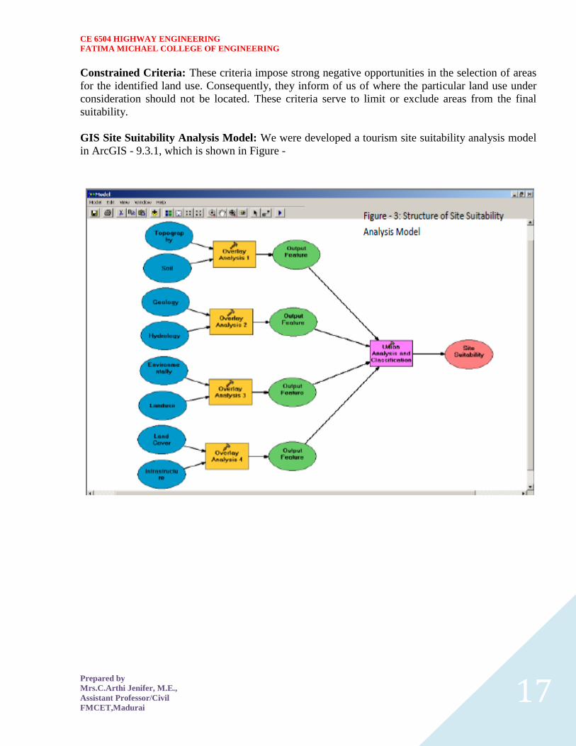
CE 6504 HIGHWAY ENGINEERING
FATIMA MICHAEL COLLEGE OF ENGINEERING
Prepared by
MrsCArthi Jenifer ME
Assistant ProfessorCivil
FMCETMadurai 17
Constrained Criteria These criteria impose strong negative opportunities in the selection of areas
for the identified land use Consequently they inform of us of where the particular land use under
consideration should not be located These criteria serve to limit or exclude areas from the final
suitability
GIS Site Suitability Analysis Model We were developed a tourism site suitability analysis model
in ArcGIS - 931 which is shown in Figure -
CE 6504 HIGHWAY ENGINEERING
FATIMA MICHAEL COLLEGE OF ENGINEERING
Prepared by
MrsCArthi Jenifer ME
Assistant ProfessorCivil
FMCETMadurai 18
UNIT 2 GEOMETRIC DESIGN OF HIGHWAYS
Typical cross section of urban and rural roads
A cross section is a vertical plane (slice) taken at right angles to the road control line showing the
various elements that make up the roads structure It is normally viewed in the direction of
increasing chainage
The width of a roadway is an important design consideration to ensure that it is appropriately sized
to serve its function Because of the diversity within the County two major roadway categories have
been established 1 Rural Road Standards 2 Urban Road Standards Urban Road Standards will
serve those areas which tend to be more developed and need to provide for multiple users
(bicyclists pedestrians parallel parking etc) whereas many rural roads will primarily serve only
vehicular traffic
Cross sections are created to provide a visual guide depicting the initial interim and ultimate phase
cross sections for these road classifications The typical sections illustrated in the following pages
are recommendations tied to transportation planning aspects such as right‐of‐way lineage sidewalk
width etc Threshold daily traffic can be used as a guide for a starting point when determining
which cross section is most applicable
1 Rural Road Standards
The rural roadways will not typically require curb and gutter or sidewalk although the County may
require either or both in unique circumstances Widths of lanes and shoulders will vary depending
upon the specific classification and the potential traffic volume which the roadway may carry Roads
carrying fewer than 200 vehicles per day need not be paved or treated for dust control The need for
paved shoulders is also dependent upon the level of traffic and safety
Final design and construction details will be determined by the Public Works Department Final
Design and construction criteria taken into consideration may include but are not limited to use of
the roadway density of development topographical characteristics and nearby development For
construction in which only a portion of the ultimate cross‐section is intended to be completed the
partial design will need to allow for the eventual widening to the ultimate cross‐section The design
for the partial or interim cross‐section roadway will need to incorporate ultimate design information
to ensure that the first phase of roadway construction is appropriate and would not need to be
removed at a future date when the full width cross‐section is completed
2 Urban Road Standards
Three roadway classifications are identified for those areas that are associated with the communityrsquos
urban growth areas They include arterial collector and local street classifications Transportation
Plan shows the key elements of the urban road standards Urban road standards will include 12‐foot
lanes sidewalk and curb amp gutter arterials and collectors will also include a striped bike lane Turn
lanes may be necessary as determined by the County Since almost all of the municipalities have
different right‐of‐way cross sections adopted for their community it makes it very difficult for the
County to match them all Therefore the philosophy was to encourage a baseline amount of
right‐of‐way reservation that could ensure the adjacent community enough area for coordination of
future roadway improvements until such time the road
CE 6504 HIGHWAY ENGINEERING
FATIMA MICHAEL COLLEGE OF ENGINEERING
Prepared by
MrsCArthi Jenifer ME
Assistant ProfessorCivil
FMCETMadurai 19
CE 6504 HIGHWAY ENGINEERING
FATIMA MICHAEL COLLEGE OF ENGINEERING
Prepared by
MrsCArthi Jenifer ME
Assistant ProfessorCivil
FMCETMadurai 20
Cross sectional elements
Kerbs
Kerbs indicate the boundary between the carriage way and the shoulder or islands or footpaths Different types of kerbs are
CE 6504 HIGHWAY ENGINEERING
FATIMA MICHAEL COLLEGE OF ENGINEERING
Prepared by
MrsCArthi Jenifer ME
Assistant ProfessorCivil
FMCETMadurai 21
Low or mountable kerbs This type of kerbs is provided such that they
encourage the traffic to remain in the through traffic lanes and also allow the
driver to enter the shoulder area with little difficulty The height of this kerb is
about 10 cm above the pavement edge with a slope which allows the vehicle to
climb easily This is usually provided at medians and channelization schemes and
also helps in longitudinal drainage
Semi-barrier type kerbs When the pedestrian traffic is high these kerbs are
provided Their height is 15 cm above the pavement edge This type of kerb
prevents encroachment of parking vehicles but at acute emergency it is possible
to drive over this kerb with some difficulty
Barrier type kerbs They are designed to discourage vehicles from leaving the
pavement They are provided when there is considerable amount of pedestrian
traffic They are placed at a height of 20 cm above the pavement edge with a steep
batter
Submerged kerbs They are used in rural roads The kerbs are provided at
pavement edges between the pavement edge and shoulders They provide lateral
confinement and stability to the pavement
Figure 1 Different types of kerbs
Shoulders Shoulders are provided along the road edge and are intended for accommodation of
stopped vehicles serve as an emergency lane for vehicles and provide lateral support
for base and surface courses The shoulder should be strong enough to bear the weight
of a fully loaded truck even in wet conditions The shoulder width should be adequate
for giving working space around a stopped vehicle It is desirable to have a width of
46 m for the shoulders A minimum width of 25 m is recommended for 2-lane rural
highways in India Parking lanes
Parking lanes are provided in urban lanes for side parking Parallel parking is preferred
because it is safe for the vehicles moving on the road The parking lane should have a
minimum of 30 m width in the case of parallel parking
CE 6504 HIGHWAY ENGINEERING
FATIMA MICHAEL COLLEGE OF ENGINEERING
Prepared by
MrsCArthi Jenifer ME
Assistant ProfessorCivil
FMCETMadurai 22
Bus-bays
Bus bays are provided by recessing the kerbs for bus stops They are provided so that
they do not obstruct the movement of vehicles in the carriage way They should be at
least 75 meters away from the intersection so that the traffic near the intersections is not
affected by the bus-bay
Service roads Service roads or frontage roads give access to access controlled highways like freeways
and expressways They run parallel to the highway and will be usually isolated by a
separator and access to the highway will be provided only at selected points These roads
are provided to avoid congestion in the expressways and also the speed of the traffic in
those lanes is not reduced
Drainage
The pavement surface should be absolutely impermeable to prevent seepage of water into
the pavement layers Further both the geometry and texture of pavement surface should
help in draining out the water from the surface in less time
Footpath
Footpaths are exclusive right of way to pedestrians especially in urban areas They are
provided for the safety of the pedestrians when both the pedestrian traffic and vehicular
traffic is high Minimum width is 15 meter and may be increased based on the traffic
The footpath should be either as smooth as the pavement or more smoother than that to
induce the pedestrian to use the footpath
Right of way
Right of way (ROW) or land width is the width of land acquired for the road along its
alignment It should be adequate to accommodate all the cross-sectional elements of the
highway and may reasonably provide for future development To prevent ribbon
development along highways control lines and building lines may be provided Control
line is a line which represents the nearest limits of future uncontrolled building activity
in relation to a road Building line represents a line on either side of the road between
which and the road no building activity is permitted at all The right of way width is
governed by
Width of formation It depends on the category of the highway and width of
roadway and road margins
Height of embankment or depth of cutting It is governed by the topography and
the vertical alignment
Side slopes of embankment or cutting It depends on the height of the slope soil
type etc
Drainage system and their size which depends on rainfall topography etc
Sight distance considerations On curves etc there is restriction to the visibility
on the inner side of the curve due to the presence of some obstructions like
building structures etc
Reserve land for future widening Some land has to be acquired in advance
CE 6504 HIGHWAY ENGINEERING
FATIMA MICHAEL COLLEGE OF ENGINEERING
Prepared by
MrsCArthi Jenifer ME
Assistant ProfessorCivil
FMCETMadurai 23
Table 2 Desig
n speed in as per IRC (ruling and minimum)
Steep
Type
Plain
Rolling
Hilly
40-30
NSampSH
100-80
80-65
50-40
MDR
80-65
65-50
40-30
30-20
25-20
ODR
65-50
50-40
30-25
25-20
VR
50-40
40-35
25-20
anticipating future developments like widening of the road
Table 1 No
right of way for open areas
Roadway width in m
Road
Plain and
Mountainous and
classification
steep terrain
rolling terrain
Open areas
45
24
NHSH
18
MDR
25
15
15
ODR
12
9
VR
Built-up areas
20
NHSH
30
MDR
20
15
ODR
15
12
9
VR
10
CE 6504 HIGHWAY ENGINEERING
FATIMA MICHAEL COLLEGE OF ENGINEERING
Prepared by
MrsCArthi Jenifer ME
Assistant ProfessorCivil
FMCETMadurai 24
Horizontal curve
The presence of horizontal curve imparts centrifugal force which is a reactive force
acting outward on a vehicle negotiating it Centrifugal force depends on speed and radius
of the horizontal curve and is counteracted to a certain extent by transverse friction
between the tyre and pavement surface On a curved road this force tends to cause the
vehicle to overrun or to slide outward from the centre of road curvature For proper
design of the curve an understanding of the forces acting on a vehicle taking a horizontal
curve is necessary Various forces acting on the vehicle are illustrated in the figure 1
Figure 1 Effect of horizontal curve They are the centrifugal force (P) acting outward weight of the vehicle (W) acting
downward and the reaction of the ground on the wheels ( and ) The centrifugal
force and the weight is assumed to be from the centre of gravity which is at h units above
the ground Let the wheel base be assumed as b units The centrifugal force in
is given by
(1)
where is the weight of the vehicle in is the speed of the vehicle in is
the acceleration due to gravity in and is the radius of the curve in
The centrifugal ratio or the impact factor is given by
CE 6504 HIGHWAY ENGINEERING
FATIMA MICHAEL COLLEGE OF ENGINEERING
Prepared by
MrsCArthi Jenifer ME
Assistant ProfessorCivil
FMCETMadurai 25
(1)
The centrifugal force has two effects A tendency to overturn the vehicle about the outer
wheels and a tendency for transverse skidding Taking moments of the forces with
respect to the outer wheel when the vehicle is just about to override
At the equilibrium over turning is possible when
and for safety the following condition must satisfy
(2)
The second tendency of the vehicle is for transverse skidding ie When the the
centrifugal force is greater than the maximum possible transverse skid resistance due to
friction between the pavement surface and tyre The transverse skid resistance (F) is
given by
where and is the fractional force at tyre and and is the reaction at
tyre and is the lateral coefficient of friction and is the weight of the vehicle
This is counteracted by the centrifugal force (P) and equating
At equilibrium when skidding takes place (from equation1)
and for safety the following condition must satisfy
CE 6504 HIGHWAY ENGINEERING
FATIMA MICHAEL COLLEGE OF ENGINEERING
Prepared by
MrsCArthi Jenifer ME
Assistant ProfessorCivil
FMCETMadurai 26
(3)
Equation 2 and 3 give the stable condition for design If equation 2 is violated the vehicle
will overturn at the horizontal curve and if equation 3 is violated the vehicle will skid at
the horizontal
Curve Analysis of super-elevation
Super-elevation or cant or banking is the transverse slope provided at horizontal curve to
counteract the centrifugal force by raising the outer edge of the pavement with respect to
the inner edge throughout the length of the horizontal curve When the outer edge is
raised a component of the curve weight will be complimented in counteracting the effect
of centrifugal force In order to find out how much this raising should be the following
analysis may be done The forces acting on a vehicle while taking a horizontal curve with
super elevation is shown in figure 1
Figure 1 Analysis of super-elevation
Forces acting on a vehicle on horizontal curve of radius at a speed of are
the centrifugal force acting horizontally out-wards through the center of
gravity
the weight of the vehicle acting down-wards through the center of gravity and
the friction force between the wheels and the pavement along the surface
inward
CE 6504 HIGHWAY ENGINEERING
FATIMA MICHAEL COLLEGE OF ENGINEERING
Prepared by
MrsCArthi Jenifer ME
Assistant ProfessorCivil
FMCETMadurai 27
At equilibrium by resolving the forces parallel to the surface of the pavement we get where
friction
is the weight of the vehicle is the centrifugal force is the coefficient of
is the transverse slope due to superelevation Dividing by we get
CE 6504 HIGHWAY ENGINEERING
FATIMA MICHAEL COLLEGE OF ENGINEERING
Prepared by
MrsCArthi Jenifer ME
Assistant ProfessorCivil
FMCETMadurai 28
Step 1
Find for 75 percent of design speed neglecting ie
Step 2
If then else if go to step 3
Step 3
Find for the design speed and max ie If
then the maximum is safe for the design speed else go to
step 4
Step 4
Find the allowable speed for the maximum and
If then the design is adequate otherwise use speed adopt
control measures or look for speed control measures
Maximum and minimum super-elevation
Depends on (a) slow moving vehicle and (b) heavy loaded trucks with high CG IRC
specifies a maximum super-elevation of 7 percent for plain and rolling terrain while that
of hilly terrain is 10 percent and urban road is 4 percent The minimum super elevation is
2-4 percent for drainage purpose especially for large radius of the horizontal curve
Attainment of super-elevation
1 Elimination of the crown of the cambered section by
1 Rotating the outer edge about the crown The outer half of the cross slope
is rotated about the crown at a desired rate such that this surface falls on
the same plane as the inner half
2 Shifting the position of the crown This method is also known as diagonal
crown method Here the position of the crown is progressively
shifted outwards thus increasing the width of the inner half of cross section
progressively
2 Rotation of the pavement cross section to attain full super elevation byThere are
two methods of attaining super elevation by rotating the pavement
1 Rotation about the center line The pavement is rotated such that the inner
edge is depressed and the outer edge is raised both by half the total amount
of super elevation ie by with respect to the centre
2 Rotation about the inner edge Here the pavement is rotated raising the
outer edge as well as the centre such that the outer edge is raised by the
full amount of super elevation with respect to the inner edge
Horizontal Transition Curves
CE 6504 HIGHWAY ENGINEERING
FATIMA MICHAEL COLLEGE OF ENGINEERING
Prepared by
MrsCArthi Jenifer ME
Assistant ProfessorCivil
FMCETMadurai 29
Transition curve is provided to change the horizontal alignment from straight to circular
curve gradually and has a radius which decreases from infinity at the straight end
(tangent point) to the desired radius of the circular curve at the other end (curve point)
There are five objectives for providing transition curve and are given below
1 to introduce gradually the centrifugal force between the tangent point and the
beginning of the circular curve avoiding sudden jerk on the vehicle This
increases the comfort of passengers
2 to enable the driver turn the steering gradually for his own comfort and security
3 to provide gradual introduction of super elevation and
4 to provide gradual introduction of extra widening
5 to enhance the aesthetic appearance of the road
Type of transition curve
Different types of transition curves are spiral or clothoid cubic parabola and Lemniscate
IRC recommends spiral as the transition curve because
1 it fulfills the requirement of an ideal transition curve that is
1 rate of change or centrifugal acceleration is consistent (smooth) and
2 radius of the transition curve is at the straight edge and changes to at
the curve point ( ) and calculation and field implementation is
very easy
Length of transition curve The length of the transition curve should be determined as the maximum of the following
three criteria rate of change of centrifugal acceleration rate of change of super elevation
and an empirical formula given by IRC Rate of change of centrifugal acceleration
At the tangent point radius is infinity and hence centrifugal acceleration is zero At the
end of the transition the radius R has minimum value R The rate of change of
centrifugal acceleration should be adopted such that the design should not cause
discomfort to the drivers If is the rate of change of centrifugal acceleration it can be
written as
Therefore the length of the transition curve in is
CE 6504 HIGHWAY ENGINEERING
FATIMA MICHAEL COLLEGE OF ENGINEERING
Prepared by
MrsCArthi Jenifer ME
Assistant ProfessorCivil
FMCETMadurai 30
(1)
where is the rate of change of centrifugal acceleration given by an empirical formula
suggested by by IRC as below
(2) 2 Rate of introduction of super-elevation
Raise ( ) of the outer edge with respect to inner edge is given by
The rate of change of this raise from to is achieved
gradually with a gradient of in over the length of the transition curve (typical range
of is 60-150) Therefore the length of the transition curve is
(3)
3 By empirical formula
IRC suggest the length of the transition curve is minimum for a plain and rolling terrain
(4)
and for steep and hilly terrain is
(5)
CE 6504 HIGHWAY ENGINEERING
FATIMA MICHAEL COLLEGE OF ENGINEERING
Prepared by
MrsCArthi Jenifer ME
Assistant ProfessorCivil
FMCETMadurai 31
and the shift as
(
6
) The length of the transition curve is the maximum of
equations 1 3 and 4or5 ie
(
7
Case (a)
For single lane roads
(
1
)
Therefore
(
2
)
Figure 1 Set-back for single lane roads (
CE 6504 HIGHWAY ENGINEERING
FATIMA MICHAEL COLLEGE OF ENGINEERING
Prepared by
MrsCArthi Jenifer ME
Assistant ProfessorCivil
FMCETMadurai 32
For multi lane roads if is the distance between centerline of the road and the centerline
of the inner lane then
(3)
(4)
Figure 2 Set-back for multi-lane roads ( )
Case (a)
For single lane roads
(1)
Therefore
(2)
Gradient
Gradient is the rate of rise or fall along the length of the road with respect to the
horizontal While aligning a highway the gradient is decided for designing the vertical
curve Before finalizing the gradients the construction cost vehicular operation cost and
the practical problems in the site also has to be considered Usually steep gradients are
avoided as far as possible because of the difficulty to climb and increase in the
CE 6504 HIGHWAY ENGINEERING
FATIMA MICHAEL COLLEGE OF ENGINEERING
Prepared by
MrsCArthi Jenifer ME
Assistant ProfessorCivil
FMCETMadurai 33
construction cost More about gradients are discussed below
Effect of gradient
The effect of long steep gradient on the vehicular speed is considerable This is
particularly important in roads where the proportion of heavy vehicles is significant Due
to restrictive sight distance at uphill gradients the speed of traffic is often controlled by
these heavy vehicles As a result not only the operating costs of the vehicles are
increased but also capacity of the roads will have to be reduced Further due to high
differential speed between heavy and light vehicles and between uphill and downhill
gradients accidents abound in gradients
Representation of gradient
The positive gradient or the ascending gradient is denoted as and the negative gradient as The deviation angle is when two grades meet the angle which
measures the change of direction and is given by the algebraic difference between the two
grades
steep gradient while 1 in 50 = 2 representation is illustrated in the figure 1
Example 1 in 30 = 333 is a
is a flatter gradient The gradient
CE 6504 HIGHWAY ENGINEERING
FATIMA MICHAEL COLLEGE OF ENGINEERING
Prepared by
MrsCArthi Jenifer ME
Assistant ProfessorCivil
FMCETMadurai 34
Figure 1 Representation of gradient
Types of gradient
Many studies have shown that gradient upto seven percent can have considerable effect
on the speeds of the passenger cars On the contrary the speeds of the heavy vehicles are
considerably reduced when long gradients as flat as two percent is adopted Although
flatter gradients are desirable it is evident that the cost of construction will also be very
high Therefore IRC has specified the desirable gradients for each terrain However it
may not be economically viable to adopt such gradients in certain locations steeper
gradients are permitted for short duration Different types of grades are discussed below
Ruling gradient
The ruling gradient or the design gradient is the maximum gradient with which the
designer attempts to design the vertical profile of the road This depends on the terrain
length of the grade speed pulling power of the vehicle and the presence of the horizontal
curve In flatter terrain it may be possible to provide flat gradients but in hilly terrain it
is not economical and sometimes not possible also The ruling gradient is adopted by the
designer by considering a particular speed as the design speed and for a design vehicle
with standard dimensions But our country has a heterogeneous traffic and hence it is not
possible to lay down precise standards for the country as a whole Hence IRC has
recommended some values for ruling gradient for different types of terrain
Limiting gradient
This gradient is adopted when the ruling gradient results in enormous increase in cost of
construction On rolling terrain and hilly terrain it may be frequently necessary to adopt
limiting gradient But the length of the limiting gradient stretches should be limited and
must be sandwiched by either straight roads or easier grades
Exceptional gradient
Exceptional gradient are very steeper gradients given at unavoidable situations They
should be limited for short stretches not exceeding about 100 metres at a stretch In
mountainous and steep terrain successive exceptional gradients must be separated by a
minimum 100 metre length gentler gradient At hairpin bends the gradient is restricted to
25
Critical length of the grade
The maximum length of the ascending gradient which a loaded truck can operate without
undue reduction in speed is called critical length of the grade A speed of 25 kmph is a
CE 6504 HIGHWAY ENGINEERING
FATIMA MICHAEL COLLEGE OF ENGINEERING
Prepared by
MrsCArthi Jenifer ME
Assistant ProfessorCivil
FMCETMadurai 35
reasonable value This value depends on the size power load grad-ability of the truck
initial speed final desirable minimum speed
Minimum gradient
This is important only at locations where surface drainage is important Camber will take
care of the lateral drainage But the longitudinal drainage along the side drains require
some slope for smooth flow of water Therefore minimum gradient is provided for
drainage purpose and it depends on the rain fall type of soil and other site conditions A
minimum of 1 in 500 may be sufficient for concrete drain and 1 in 200 for open soil
drains are found to give satisfactory performance Sight distance available from a point is the actual distance along the road surface which a driver
from a specified height above the carriage way has visibility of stationary or moving objects
Sight distance required by drivers applies to both geometric design of highways and for
traffic control The sight distance situations are considered in the design
i) Stopping or absolute minimum sight distance
ii) Safe overtaking or passing sight distance
iii) Safe sight distance for entering into uncontrolled intersections
Apart from the three situations mentioned above the following sight distance are considered by the
IRC in highway design
Intermediate sight distance
This is defined as twice the stopping sight distance when overtaking sight distance
cannot be provided intermediate sight distance is provided to give limited overtaking opportunities
to fast vehicles
Head light sight distance
This is the distance visible to a driver during night driving under the illumination of the
vehicle head lights
Stopping sight distance
The minimum sight distance available on a highway at any spot should be of sufficient
length to stop a vehicle traveling at design speed safely without collision with any other obstruction
The absolute minimum sight distance is therefore equal to the stopping sight distance
which is also sometimes called nonpassing sight distance The sight distance available on a road to a
driver at any instance depends on
i) Features of the road
ii) Height of the drivers eye above the road surface
iii) Height of the object above the road surface
The distance within which a motor vehicle can be stopped depends upon the factors listed below
a) Total reactions time of the driver
b) Speed of vehicle
c) Efficiency of breaks
d) Frictional resistance between the road and tyres
e) Gradient of the road
Total reaction time
) Reaction time of the driver is the time taken from the instant the object is visible to the
driver to the instant the brakes are effectively applied
) The total reaction time may be split up into two parts
CE 6504 HIGHWAY ENGINEERING
FATIMA MICHAEL COLLEGE OF ENGINEERING
Prepared by
MrsCArthi Jenifer ME
Assistant ProfessorCivil
FMCETMadurai 36
i) Perception time
ii) Brake reaction time
PIEV theory
According to this theory the total reaction time of the driver is split into four parts
i) Perception
ii) Intellection
iii) Emotion
iv) Volition
Speed of Vehicle
The stopping distance depends very much on the speed of the vehicle first during the
total reaction time of the driver the distance moved by the vehicle will depend on the speed
Efficiency of brakes
The braking efficiency is said to be 100 percent if the wheels are fully licked preventing
them from rotating on application of the brakes This will result in 100 percent skidding which is
normally undesirable except in utmost emergency
Frictional resistance between road and tyres
The frictional resistance developed between road and tyres or the skid resistance depends
on the type and condition of the road surface and the tyres IRC has specified a design friction
coefficient of 035 to 04 depending upon the speed to be used for finding the braking distance in the
calculation of stopping sight distance
Analysis of stopping distance
i) The distance traveled by the vehicle during the total reaction time known as lag
distance
ii) The distance traveled by the vehicle after the application of the brakes is known as
braking distance
Overtaking sight distance
The minimum distance open to the vision of the driver of a vehicle intending to overtake
slow vehicle ahead with safety against the traffic of opposite direction is known as the minimum
overtaking sight distance(OSD) or Safe passing sight distance available
The overtaking sight distance is the distance measured along the center of the road which
a driver with his eye level 12m above the road surface can see the top of an object 12m above the
road surface
Some of the important factors on which the minimum overtaking sight distance required
a) Speed of
i) overtaking vehicle
ii) overtaken vehicle
iii) The vehicle coming from opposite direction
b) Distance between the overtaking and overtaken vehicles the minimum spacing
depends on the steeds
a) Skill and reaction time of the driver
b) Rate of acceleration of overtaking vehicle
c) Gradient of the road
Criteria for sight distance requirements on highway
) The absolute minimum sight distance required throughout the length of the road is the
SSD which should invariably be provided at all places
CE 6504 HIGHWAY ENGINEERING
FATIMA MICHAEL COLLEGE OF ENGINEERING
Prepared by
MrsCArthi Jenifer ME
Assistant ProfessorCivil
FMCETMadurai 37
) On horizontal curves the obstruction on the inner side of the curves should be cleared
to provide the required set back distance and absolute minimum sight distance
) On vertical summit curves the sight distance requirement may be fulfilled by proper
design of the vertical alignment
Hairpin bent
TYPES OF CURVES ON HILL ROADS
The following are the important types of curves provided on hill Roads-
1 Hair-Pin Curves
2 Salient Curves
3 Re-entrant Curves 1 Hair-pin curves - The curve in a hill road which changes its direction through an angle of 180
degree or so down the hill on the same side is known as hair-pin curve
A Hair-Pin Bend
This curve is so called because it conforms to the shape of a hair-pin The bend so formed at the
hair-pin curve in a hill road is known as hair-pin bend This type of curve should be located on a
hill side having the minimum slope and maximum stability It must also be safe from view point of
landslides and ground water Hair-pin bends with long arms and farther spacing are always
preferred They reduce construction problems and expensive protective works Hair-pin curves or
bends of serpentine nature are difficult to negotiate and should therefore be avoided as far as
possible
Salient curves - The curves having their convexity on the outer edges of a hill road are called
salient curves The centre of curvature of a salient curve lies towards the hill side This type of curve
occurs in the road length constructed on the ridge of a hill the bend so formed at the salient curve in
a hill road known as corner bend
Salient curves are very dangerous for fast moving traffic At such a curve or at corner bend the
portion of projecting hill side is usually cut down to improve the visibility as shown in fig (Re-
entrant curve) The outer edge of the road at such a curve is essentially provided with a parapet wall
for protection of the vehicles from falling down the hill slope
CE 6504 HIGHWAY ENGINEERING
FATIMA MICHAEL COLLEGE OF ENGINEERING
Prepared by
MrsCArthi Jenifer ME
Assistant ProfessorCivil
FMCETMadurai 38
3 Re-entrant curves - The curves having their convexity on the inner edge of a hill road are called
re-entrant curves
Re-entrant curves
The centre of curvature of a re-entrant curves lies away from the hill side This type of curve occurs
in the road length constructed in the calley of a hill
These curves are less dangereous as they provide adequate visibility to the fast moving traffic At
such curves the parapet wall is provided only for safety of fast moving traffic
CE 6504 HIGHWAY ENGINEERING
FATIMA MICHAEL COLLEGE OF ENGINEERING
Prepared by
MrsCArthi Jenifer ME
Assistant ProfessorCivil
FMCETMadurai 39
UNIT ndash III DESIGN OF RIGID AND FLEXIBLE PAVEMENTS
COMPARISON OF RIGID AND FLEXIBLE PAVEMENTS
The comparisons are
i) Design precision
A cement concrete pavement is amerable to a much more precise structural analysis
than a flexible pavement Flexible pavements designs are mainly empirical Computer aided analysis
of layered system is making the flexible pavement design more exact than hitherto
ii) Life
) Cement concrete slabs of a thin section constructed in the early 1940rsquos are still in
existence in India though many of them have cracked badly and a few of them have been ripped
open and rebuilt in recent ties
) A major project in cement concrete road construction between Agra and Mathura It can
safely be said that a well-designed concrete slab has a life of about 40 years
) Compared to this the life of a flexible pavement generally varies from 10 to 20 years
iii) Maintenance
) A well-designed cement concrete pavement needs very little maintenance The only
maintenance needed is I respect of joints
) The surface is unaffected by spillage of oil and lubricants bituminous surfaces on the
other hand need great inputs in maintenance
) The surface is affected by spillage of oil and lubricants The surface is also affected by
natural weathering agents like air water ad temperature changes
) A cement concrete pavement on the other hand needs a small amount for maintaining
joints
iv) Initial cost
) The argument so far used against a cement concrete slab is that it is much more costly
than a flexible pavement
) The latter specifications no doubt represent the rock-bottom needs of a road in India but
these specifications can hardly provide a smooth and durable surface
v) Stage construction ) Road construction is generally done adopting a policy of stage construction especially for
low volume roads As traffic grows additional layers in the form of water bound macadam and
superior surfacing are added on
) Initial outlay is minimum and additional outlays are in keeping with traffic growth This is
a great advantage when dealing with new roads in an atmosphere of austerity
vi) Availability of materials
) Cement bitumen stone aggregates and gravelsand are the major materials involved in
pavement Construction Cement has been in serious short supply in the country for the past many
decades
) Bitumen is also not available plentifully in India There is also the danger of the entire oil
reserves in the world shrinking during the next two or three decades
) In locations where stone aggregates are scarce cement concrete may have an advantage
for flexible pavements
vii) Surface characterstics
CE 6504 HIGHWAY ENGINEERING
FATIMA MICHAEL COLLEGE OF ENGINEERING
Prepared by
MrsCArthi Jenifer ME
Assistant ProfessorCivil
FMCETMadurai 40
) A good cement concrete surface is smooth and free from rutting potholes and
corrugations In a bituminous surface it is only the asphaltic concrete surface that can give
comparable rideablity
) A well-constructed cement concrete pavement surface can have a permanent nonskid
surface A bituminous surface can also be designed to have a good skid resistant surface
viii) Utility location
) In cement concrete slabs proper thought has to be given to locate utilities such as water
pipes telephone lines and electric cables
) It is difficult to rip open the slab and restore it to be the original condition if any changes
in the utilities lines are to be made
ix) Glame and night visibility
) Concrete pavements have a gray color which can cause glam under sunlight Colored
cement can reduce the grave
) On the other hand bituminous roads need more street lighting
x) Traffic dislocation during construction
) A cement concrete pavement requires 28 days before it can be thrown open to traffic On
the other hand a bituminous surface can be thrown open to traffic shortly after it is rolled
xi) Environmental considerations during construction
) The process of heating of bitumen and aggregates and mixing them together on hot mix
plants can prove to be much more hazardous to the environment than cement concrete construction
where no heating of any material is involved
xii) Overall economy on a life cycle basis
) A good road is costly to construct but once constructed such a road requires little
maintenance and results in savings in vehicle operating costs
) The comparative economy of a flexible pavement and a rigid pavement has proved that on
overall economic considerations
Types of pavement structure
Based on the structural behavior pavements are generally classified into three
categories
i) Flexible pavements
ii) Rigid pavements
iii) Semi rigid pavements
Flexible pavements
) Flexible pavements are those which on the whole have low or negligible flexural
strength and are rather flexible in their structural action under the loadsThe flexible pavement
layers reflect the deformation of the lower layers on to the surface of the layer
) A flexible pavement consists of four components(i) Soil subgrade (ii) sub base
course (iii) base course (iv) Surface course
CE 6504 HIGHWAY ENGINEERING
FATIMA MICHAEL COLLEGE OF ENGINEERING
Prepared by
MrsCArthi Jenifer ME
Assistant ProfessorCivil
FMCETMadurai 41
) The flexible pavement layers transmit the vertical or compressive stresses to the lower layers
by grain to grain transfer through the points of contact in the granular structure A well
compacted granular structure consisting of strong added aggregate can transfer the compressive
stresses
) The load spreading ability of this layer therefore depends on the type of the materials and mix
design factors Bituminous concrete is one of the best flexible pavements layer materials Other
materials which fall under the group are all granular materials with or without bituminous
binder granular base and sub base course materials
) The vertical compressive stress is maximum on the pavement surface directly under the wheel
and is equal to the contact pressure under the wheel The flexible pavement may be constructed
in a number of layers and the top layer has to be strongest as the highest compressive stresses
) Flexible pavements are commonly designed using empirical design charts or equations taking
into account some of the design factors there are also semi empirical and theoretical design
methods
Rigid pavements
) Rigid pavements are those which possess note flexural strength or flexural rigidity
The stresses are not transferred from grain to grain to the lower layers as in the ease of flexible
pavements layers
) The rigid pavements are made of Portland cement concrete plain reinforced or
prestressed concrete The plain cement concrete slabs are expected to take up about 40 kgcm2
flexural stress
) The rigid pavement has the slab action and is capable of transmitting the wheel
load stresses through a wider area below The main point of difference in the structural behavior
of rigid pavement as compared to the flexible pavement is that the critical condition of stress in
the rigid pavement is the maximum flexural stress occurring in the slab due to wheel load and
the temperature changes whereas in the flexible pavement
) As the rigid pavement slab has tensile strength tensile stresses are developed due
to the bending of the slab under wheel load and temperature variations Thus the types of
stresses developed and their distribution within the cement concrete slab are quirt different
) The cement concrete pavement slab can very well serve as a wearing surface as
well an effective base course The rigid pavement structure consists of a cement concrete slab
below which a granular base or sub base course may be provided
) Though the cement concrete slab can also be laid directly over the soil subgrade
consists of fine grained soil
) the rigid pavements are usually designed and the stresses are analyzed using the
elastic theory assuming the pavements as a n elastic plate resting over an elastic or a viscous
foundation
Semi rigid pavements
) when bonded materials like the pozzolanic concrete lean cement concrete or soil
cement are used in the base course or sub base course layer the pavement layer has considerably
higher flexural strength than the common flexible pavement layers
) when this intermediate class of materials are used in the base or sub base course
layer of the pavements they are called semi rigid pavements
CE 6504 HIGHWAY ENGINEERING
FATIMA MICHAEL COLLEGE OF ENGINEERING
Prepared by
MrsCArthi Jenifer ME
Assistant ProfessorCivil
FMCETMadurai 42
) This third category of semi rigid pavement are either designed as flexible
pavements with some correction factors to find the thickness requirements based on experience
or by using a new design approach
) The semi rigid pavement materials have low resistance to impact and abrasion and
therefore are usually provided with flexible pavement surface course
Various functions of pavement components
The functions are
Soil sub grade and its evaluation
) The soil sub grade is a layer of natural soil prepared to receive the layers of pavement
materials placed over it It is essential that at no time the soil sub grade is overstressed it means that
the pressure transmitted on the top of the sub grade is within the allowable limit
) Many tests are known for measuring the strength properties of the sub grades Some of the
tests have been standardized for the use The common strength test for the evaluation of soil
subgrade is
i) California bearing ratio test
ii) California resistance value test
iii) Triaxial compression test
iv) Plate bearing test
CALIFORNIA BEARING RATIO (CBR) TEST
It is evolved for the empirical method of flexible pavement design The CBR test is carried
out either in the laboratory on prepared specimens or in the field by taking in situ measurements
California resistance value
It is found by using have been stabliometerThis test is used in an empirical method of
flexible pavement design based on soil strength
Triaxial test
It is the most important soil strength but still the test is not very commonly used in structural
design of pavements
Plate bearing test
It is carried out using a relatively large diameter plate to evaluate the load supporting
capacity of supporting power of the pavement layers The results are plate bearing tests are used in
flexible pavement design method like McLeod method on based on layer system analysis by
brumister
Sub base and base courses and their evaluation
) There layers are made of broken stones bound or unbound aggreagatesome times in sub
base course a layer of stabilized soil(or) Selected granular soil is also used
) however at the sub base course it is desirable to use smaller size graded aggregates When
the sub grade consists of fine grained soil and when the pavement carries heavy wheel loads
CE 6504 HIGHWAY ENGINEERING
FATIMA MICHAEL COLLEGE OF ENGINEERING
Prepared by
MrsCArthi Jenifer ME
Assistant ProfessorCivil
FMCETMadurai 43
) Sub base course primarily has the similar function as of the base course and is provided
with inferior materials than of base course Base courses are used under rigid pavement for
i) Preventing pumping
ii) Protecting the sub grade against frost action
) Thus the fundamental purpose of abase course and sub base course is to provide a stress
transmitting medium to spread the surface wheel loads in such manner
) The sub base and base course layers may be evaluated by suitable strength or stability test
like plate bearing CBR test
WEARING COURSE AND ITS EVALUATION
) The purpose of the wearing course is to give a smooth riding surface that is dense It
resists pressure exerted by tyres and takes up wear and tear due to the traffic
) Wearing course also offers a water tight layer against the surface water infiltration The
flexible pavement normally a bituminous surfacing is used as a wearing course
) In rigid pavements the cement concrete acts like a base course as well as wearing course
Most popular test in use is marshal stability test where in the optimum content of bitumen binder is
worked out based on the stability density
) Plate bearing test and Bankelman beam test are also sometimes made use of for evaluating
the wearing course and the pavement as a whole
Various factors to be considered in pavement design and the significance
Pavement design consists of two parts
i) Mix design of materials to be used in each pavement component layer Thickness design of the
pavement and the component layers
The various factors to be considered for the design of pavements are given below
i) Design wheel load
ii) Sub grade soil
iii) Climatic factors
iv) Pavement component layers
v) Environmental factors
vi) Special factors in the design of different types of pavements
Design wheel load
The various wheel load factors to be considered in pavement design are
i) Maximum wheel load
ii) Contact pressure
iii) Dual or multiple wheel loads
iv) Repetition of loads
Maximum wheel load
The wheel load configurations are important to know the way in which the loads of a given
vehicle are applied on the pavement surface
) For highways the maximum legal axle load as specified by Indian road congress is 8170
kg with a maximum equivalent single wheel load of 4085 kg
) The evaluation for vertical stress computations under a uniformly distribute of circular
load based on Boussineqrsquos theory is given by
CE 6504 HIGHWAY ENGINEERING
FATIMA MICHAEL COLLEGE OF ENGINEERING
Prepared by
MrsCArthi Jenifer ME
Assistant ProfessorCivil
FMCETMadurai 44
2
322
3
1
za
zpz
σz = vertical stress at depth z
P= surface pressure
Z=depth at which σz computed
A=radius of loaded area
Contact pressure
Generally the wheel load is assumed to be distributed over a circular area But by
measurement of the imprints of tyers with different load and inflation pressures Three terms in use
with reference to tyre pressure are
Tyre pressure
Inflation pressure
Contact pressure
Tyre pressure and inflation pressure mean exactly the same the contact pressure is found to be more
than tyre pressure when the tyre pressure is less than 7 kgm2 and it is vice versa when the tyre
pressure exceeds this value
Contact pressure can be measured by the relationship
Load on wheel
Contact pressure = ----------------------------------------
Contact area or area of imprint
The general variation between the tyre pressure and measured contact pressure is shown in this fig
The ratio of contact pressure to type pressure is defined as rigidity factor Thus value of rigidity
factor is 10 for an average tyre pressure of 7 Kgcm2This value is higher than unity for lower type
pressures and less than unity for tyre pressures higher than 7 kgcm2
Equivalent single wheel load (ESWL)
) The maximum wheel load within the specified limit and to carry greater load it is
necessary to provide dual wheel assembly to the rear axles of the roads vehicles
) In other words the pressure at a certain depth below the pavement surface cannot be
obtained by numerically adding the pressure caused by any one wheel
) The effect is in between the single load and two times load carried by one wheel The load
dispersion is assumed to be at an angle of 450In the dual wheel load assembly let d be the clear gap
between the two wheels S be the spacing between the centers of the wheels and a be the radius of
the circular contact area of each wheel Then S = (d + 2a)
) ESWL may be determined based on either equivalent deflection or equivalent stress
criterianMultiple wheel loads are convert to ESWL and this value is used in pavement design The
ESWL is usually determined by the equivalent stress criterion using a simple graphical method
CE 6504 HIGHWAY ENGINEERING
FATIMA MICHAEL COLLEGE OF ENGINEERING
Prepared by
MrsCArthi Jenifer ME
Assistant ProfessorCivil
FMCETMadurai 45
) A straight line relationship is assumed between ESWL and depth on log scales For
determining ESWL the plot is made as shown in fig
) Two points A and B are plotted on the log-log graph with coordinates of A (Pd2) and
B(2p2s)line AB is a plot which is the focus of points where any single wheel load is equivalent to a
certain set of dual wheels
) To Calculate the ESWL for a dual assembly it is essential to estimate a design thickness of
the pavement If the design thickness so obtained is equal to the estimated thickness then the ESWL
calculations could be considered as correct Otherwise trials are made
) In heavy trucks and trailers the load on each wheel may be further reduced by multiple
wheels and tandem axles
Repetition of loads
) The deformation of load pavement (or) sub grade due to a single application of wheel load
may be small It required carrying out traffic surveys for accounting the factor of repetitions for
wheel loads in the design of pavement
) Data collected are converted to some constant equivalent wheel loads Equivalent wheel
load is a single load equivalent to the repeated applications of any particular wheel load on a
pavement which requires the same thickness and strength of pavements
) McLeod has given a procedure for evolving equivalent load factors for designing flexible
pavements
Various methods of flexible pavement design
) The flexible pavement is built with number of layers In the design process it is to be
ensured that under the application of load none of the layers is overstressed
) The maximum intensity of stresses occurs in the top layer of the pavement The
magnitude of load stresses reduces at lower layers
) In the design of flexible pavements it has yet not been possible to have a rational design
method wherein design process and service behavior of the pavement can be expressed by
mathematical laws
) Flexible pavement design methods are accordingly either empirical or semi empirical In
these methods the knowledge and experience gained on the behavior of the pavements in the past
are usefully utilized
Various approaches of flexible pavement design may be thus classified into three groups
i) Empirical method
ii) Semi-empirical or Semi theoretical method
iii) Theoretical method
) Empirical methods are either based on physical properties or strength parameters of soil
sub grade When the design is based on stress strain function and modified base on experience it
may be called semi-empirical or semi-theoretical There are design methods based on theoretical
analysis and mathematical computations
Out of the flexible pavement design method available is
i) Group index method
ii) California bearing ratio method
iii) California R value (or) Stabiliometer method
iv) Triaxial test method
CE 6504 HIGHWAY ENGINEERING
FATIMA MICHAEL COLLEGE OF ENGINEERING
Prepared by
MrsCArthi Jenifer ME
Assistant ProfessorCivil
FMCETMadurai 46
v) McLeod method
vi) Burmister method
Group index method
) Group index value is an arbitrary index assigned to the soil type in numerical equations
base on the percent fines liquid limit and plasticity index
) The design chart for group index method for determining the pavement thickness is given
in fig
The traffic volume in this method is divided in three groups
Traffic volume No of vehicles per day
Light Less than 50
Medium 50 to 300
Heavy Over 300
The design of the pavement thickness by this method first the G1 value of the soil is found the
anticipated traffic is estimated and is designated as light medium or heavy as indicated
The G1 method of pavement design is essentially an empirical method based on physical properties
of the subgrade soil This method does not consider the strength characteristics of the subgrade soil
and therefore is open to question regarding the reliability of the design based on the index properties
of the soil only
California bearing ratio method
) California division of highways in the USA developed CBR method for
pavement design The majority of design curves developed later are base on the original curves
proposed by OJporter
) One of the chief advantages of CBR method is the simplicity of the test procedure
The CBR tests were carried out by the California state highway department on existing pavement
layers including subgrade sub base and base course
) Based on the extensive CBR test data collected on pavement which behaved
satisfactory and those which failed an empirical design chart was developed correlating the CBR
value and the pavement thickness The basis of the design chart is that a material with a given CBR
required a certain thickness of pavement layer as a cover
) A higher load needs a thicker pavement layer to protect the sub grade Design
curves correlating the CBR value with total pavement thickness cover were developed by the
California state highway department for wheel loads of 3175kg and 5443 kg representing light and
heavy traffic The design curves are shown in this fig
It is possible to extend the CBR design curves for various loading conditions nusing the expression
t= 2
1
1751
pCBRp
t=2
1
751
A
CBR
p
Hence
CE 6504 HIGHWAY ENGINEERING
FATIMA MICHAEL COLLEGE OF ENGINEERING
Prepared by
MrsCArthi Jenifer ME
Assistant ProfessorCivil
FMCETMadurai 47
t= pavement thickness cm
p=Wheel load kg
CBR= California bearing ratio percent
P=tyre pressure kgcm2
A= area of contactcm2
IRC Recommendations
a) The CBR tests should be performed on remoulded soils in the laboratory The specimens should
be prepared by static compaction wherever possible and otherwise by dynamic compaction
b) For the design of new roads the sub grade soil sample should be compacted at OMC to proctor
density whenever suitable compaction equipment
c) The CBR test samples may be soaked in water for four days period before testing the annual
rainfall is less than 50 cm and the water table is too deep to affect the sub grade and imperable
surfacing is provided to carrying out CBR test
d) If the maximum variations in CBR value of the three specimens exceed the specified limits the
design CBR should be average of at least six samples
e) The top 50 cm of sub grade should be compacted at least up to 95 to 100 percent of proctor
density
f) An estimate of the traffic should be carried by the road pavements at the end of expected in view
the existing traffic and probable growth rate of traffic
g) The traffic for the design is considered in units of heavy vehicles per day in both directions and is
divided into seven categories A to G The design thickness is considered applicable for single axle
loads up to 8200 kg and tandom axle loads up to 14500 kg
h) When sub base course materials contain substantial proportion of aggregates of size above 20mm
the CBR value of these materials would not be valid for the design of subsequent layers above them
The CBR method of pavement design gives the total thickness requirement of the pavement above a
sub grade and thickness value would remain the same quality of materials used in component layers
California resistance value method
) In this design method based on stabliometer R-value and cohesiometer C-value
Based on performance data it was established by pavement thickness varies directly with R value
and algorithm of load repetitions It varies inversely with fifth root of c valueThe expression for
pavement thickness is given by the empirical equation
T=
5
1
1 90
C
RTK
Hence
T=total thickness of pavement cm
K=Numerical constant 0166
T1=traffic index
R= stabiliometer resistance value
C=Cohesiometer value
CE 6504 HIGHWAY ENGINEERING
FATIMA MICHAEL COLLEGE OF ENGINEERING
Prepared by
MrsCArthi Jenifer ME
Assistant ProfessorCivil
FMCETMadurai 48
In the design of flexible pavements based on California resistance value method for the following
data are needed
) R-value of soil subgrade
) T1 value
) Equivalent C-value
) R value of soil subgrade is obtained from the test using stablio meterThe
computation of T1 value has been explained
Equivalent C-value
) The cohesion meter value c is obtained for each layer of pavement material
separately from tests However the composite or equivalent C-value of the pavement may be
estimated if the thickness of each component layer and the c-value of the material of the layer are
known
) while designing a pavement as the thickness of the pavement is not known it is
easier if the pavement is first assumed to consist of any one material like gravel base course with
known C-value
) Subsequently the individual thickness of each layer is converted in terms of gravel
equivalent by using relationship
5
1
1
2
2
1
C
C
t
t
) t1 and t2 are the thickness values of any two pavement layersc1 and c2 are their
corresponding cohesiometer values
CE 6504 HIGHWAY ENGINEERING
FATIMA MICHAEL COLLEGE OF ENGINEERING
Prepared by
MrsCArthi Jenifer ME
Assistant ProfessorCivil
FMCETMadurai 49
UNIT 4 MATERIAL AND MAINTENANCE
SUMMIT CURVE
Summit curves are vertical curves with gradient upwards They are formed when two
gradients meet as illustrated in figure 1 in any of the following four ways
1 When a positive gradient meets another positive gradient [figure 1a]
2 When positive gradient meets a flat gradient [figure 1b]
3 When an ascending gradient meets a descending gradient [figure 1c]
4 When a descending gradient meets another descending gradient [figure 1d]
Type of Summit Curve
Many curve forms can be used with satisfactory results the common practice has been to
use parabolic curves in summit curves This is primarily because of the ease with it can
be laid out as well as allowing a comfortable transition from one gradient to another
Although a circular curve offers equal sight distance at every point on the curve for very
small deviation angles a circular curve and parabolic curves are almost congruent
Furthermore the use of parabolic curves were found to give excellent riding comfort
Figure 1 Types of summit curves
Design Consideration
In determining the type and length of the vertical curve the design considerations are
comfort and security of the driver and the appearance of the profile alignment Among
these sight distance requirements for the safety are most important on summit curves
The stopping sight distance or absolute minimum sight distance should be provided on
these curves and where overtaking is not prohibited overtaking sight distance or
intermediate sight distance should be provided as far as possible When a fast moving
vehicle travels along a summit curve there is less discomfort to the passengers This is
because the centrifugal force will be acting upwards while the vehicle negotiates a
summit curve which is against the gravity and hence a part of the tyre pressure is
relieved Also if the curve is provided with adequate sight distance the length would be
sufficient to ease the shock due to change in gradient Circular summit curves are
identical since the radius remains same throughout and hence the sight distance From
CE 6504 HIGHWAY ENGINEERING
FATIMA MICHAEL COLLEGE OF ENGINEERING
Prepared by
MrsCArthi Jenifer ME
Assistant ProfessorCivil
FMCETMadurai 50
this point of view transition curves are not desirable since it has varying radius and so the
sight distance will also vary The deviation angles provided on summit curves for
highways are very large and so the simple parabola is almost congruent to a circular arc
between the same tangent points Parabolic curves are easy for computation and also it
had been found out that it provides good riding comfort to the drivers It is also easy for
field implementation Due to all these reasons a simple parabolic curve is preferred as
summit curve Length of the summit curve
The important design aspect of the summit curve is the determination of the length of the
curve which is parabolic As noted earlier the length of the curve is guided by the sight
distance consideration That is a driver should be able to stop his vehicle safely if there is
an obstruction on the other side of the road Equation of the parabola is given by
where where N is the deviation angle and is the length of the In
deriving the length of the curve two situations can arise depending on the uphill and
downhill gradients when the length of the curve is greater than the sight distance and the
length of the curve is greater than the sight distance
Let is the length of the summit curve is the SSDISDOSD is the deviation angle
drivers eye height (12 m) and the height of the obstruction then the length of the
summit curve can be derived for the following two cases The length of the summit curve
can be derived from the simple geometry as shown below
Case a Length of summit curve greater than sight distance( )
Figure 1 Length of summit curve ( )
The situation when the sight distance is less than the length of the curve is shown in
figure 1
CE 6504 HIGHWAY ENGINEERING
FATIMA MICHAEL COLLEGE OF ENGINEERING
Prepared by
MrsCArthi Jenifer ME
Assistant ProfessorCivil
FMCETMadurai 51
(1)
Case b Length of summit curve less than sight distance
The second case is illustrated in figure 1
Figure 1 Length of summit curve
CE 6504 HIGHWAY ENGINEERING
FATIMA MICHAEL COLLEGE OF ENGINEERING
Prepared by
MrsCArthi Jenifer ME
Assistant ProfessorCivil
FMCETMadurai 52
From the basic geometry one can write
(1)
Therefore for a given and to get minimum differentiate the above equation
with respect to and equate it to zero Therefore
Solving the quadratic equation for
(2)
Now we can substitute back to get the value of minimum value of for a given
and Therefore
Solving for
CE 6504 HIGHWAY ENGINEERING
FATIMA MICHAEL COLLEGE OF ENGINEERING
Prepared by
MrsCArthi Jenifer ME
Assistant ProfessorCivil
FMCETMadurai 53
(3) (4
CE 6504 HIGHWAY ENGINEERING
FATIMA MICHAEL COLLEGE OF ENGINEERING
Prepared by
MrsCArthi Jenifer ME
Assistant ProfessorCivil
FMCETMadurai 54
When stopping sight distance is considered the height of drivers eye above the road
surface ( ) is taken as 12 metres and height of object above the pavement surface ( )
is taken as 015 metres If overtaking sight distance is considered then the value of
drivers eye height ( ) and the height of the obstruction ( ) are taken equal as 12
metres
Valley curve
Valley curve or sag curves are vertical curves with convexity downwards They are
formed when two gradients meet as illustrated in figure 1 in any of the following four
ways
Figure 1 Types of valley curve
1 When a descending gradient meets another descending gradient [figure 1a]
2 When a descending gradient meets a flat gradient [figure 1b]
3 When a descending gradient meets an ascending gradient [figure 1c]
4 When an ascending gradient meets another ascending gradient [figure
Design considerations
There is no restriction to sight distance at valley curves during day time But visibility is
reduced during night In the absence or inadequacy of street light the only source for
visibility is with the help of headlights Hence valley curves are designed taking into
account of headlight distance In valley curves the centrifugal force will be acting
downwards along with the weight of the vehicle and hence impact to the vehicle will be
more This will result in jerking of the vehicle and cause discomfort to the passengers
Thus the most important design factors considered in valley curves are (1) impact-free
movement of vehicles at design speed and (2) availability of stopping sight distance
under headlight of vehicles for night driving
For gradually introducing and increasing the centrifugal force acting downwards the best
shape that could be given for a valley curve is a transition curve Cubic parabola is
generally preferred in vertical valley curves See figure 1
CE 6504 HIGHWAY ENGINEERING
FATIMA MICHAEL COLLEGE OF ENGINEERING
Prepared by
MrsCArthi Jenifer ME
Assistant ProfessorCivil
FMCETMadurai 55
Figure 1 Valley curve details
During night under headlight driving condition sight distance reduces and availability of
stopping sight distance under head light is very important The head light sight distance
should be at least equal to the stopping sight distance There is no problem of overtaking
sight distance at night since the other vehicles with headlights could be seen from a
considerable distance
Length of the valley curve
The valley curve is made fully transitional by providing two similar transition curves of
equal length The transitional curve is set out by a cubic parabola where
The length of the valley transition curve is designed based on two criteria
1 comfort criteria that is allowable rate of change of centrifugal acceleration is
limited to a comfortable level of about
2 safety criteria that is the driver should have adequate headlight sight distance at
any part of the country
Comfort criteria
The length of the valley curve based on the rate of change of centrifugal acceleration that
will ensure comfort Let is the rate of change of acceleration the minimum radius of
the curve is the design speed and is the time then is give
CE 6504 HIGHWAY ENGINEERING
FATIMA MICHAEL COLLEGE OF ENGINEERING
Prepared by
MrsCArthi Jenifer ME
Assistant ProfessorCivil
FMCETMadurai 56
For a cubic parabola the Value Safety criter Length of the valley curve for headlight distance may be determined for two conditions
(1) length of the valley curve greater than stopping sight distance and (2) length of the
valley curve less than the stopping sight distance of for length is given by
Case 1 Length of valley curve greater than stopping sight distance ( )
The total length of valley curve is greater than the stopping sight distance SSD The
sight distance available will be minimum when the vehicle is in the lowest point in the
valley This is because the beginning of the curve will have infinite radius and the bottom
of the curve will have minimum radius which is a property of the transition curve The
case is shown in figure 1
Figure 1 Valley curve case 1
From the geometry of the figure we have
CE 6504 HIGHWAY ENGINEERING
FATIMA MICHAEL COLLEGE OF ENGINEERING
Prepared by
MrsCArthi Jenifer ME
Assistant ProfessorCivil
FMCETMadurai 57
(1)
where is the deviation angle in radians is the height of headlight beam is the
head beam inclination in degrees and is the sight distance The inclination is 1
degree
Case 2 Length of valley curve less than stopping sight distance ( )
The length of the curve is less than SSD In this case the minimum sight distance is
from the beginning of the curve The important points are the beginning of the curve and
the bottom most part of the curve If the vehicle is at the bottom of the curve then its
headlight beam will reach far beyond the endpoint of the curve whereas if the vehicle is
at the beginning of the curve then the headlight beam will hit just outside the curve
Therefore the length of the curve is derived by assuming the vehicle at the beginning of
the curve The case is shown in figure 1
From the figure
(1) Note that the above expression is approximate and is satisfactory because in practice the gradients
are very small and is acceptable for all practical purposes We will not be able to know prior to
which case to be adopted Therefore both has to be calculated and the one which satisfies the
condition is adopted
1 Flexible pavement
2 Rigid pavement
Flexible pavement
These pavements reflect the deformation of sub grade and the subsequent layers to the
surface
Rigid pavement
The rigid characteristic of the pavement are associated with rigidity or flexural strength
CE 6504 HIGHWAY ENGINEERING
FATIMA MICHAEL COLLEGE OF ENGINEERING
Prepared by
MrsCArthi Jenifer ME
Assistant ProfessorCivil
FMCETMadurai 58
or slab action so the load is distributed over a wide area of sub grade soil
Flexible pavement Definition
These pavements reflect the deformation of sub grade and the subsequent layers to the
surface Flexible usually asphalt is laid with no reinforcement or with a specialized
fabric reinforcement that permits limited flow or repositioning of the roadbed under
ground changes
The design of flexible pavement is based on load distributing characteristic of the
component layers The black top pavement including water amp gravel bound macadam fall
in this category
Flexible pavement on the whole has low or negligible flexible strength flexible in their
structural action) The flexible pavement layers transmit the vertical or compressive
stresses to the lower layers by grain transfer through contact points of granular structure
The vertical compressive stress is maximum on the pavement surface directly under the
wheel load and is equal to contact pressure under the wheels Due to the ability to
distribute the stress to large area in the shape of truncated cone the stresses get decreased
in the lower layer
As such the flexible pavement may be constructed in a number of layers and the top
layer has to be strongest as the highest compressive stresses
To be sustained by this layer in addition to wear and tear the lower layer have to take
up only lesser magnitude of stress as there is no direct wearing action die to traffic loads
therefore inferior material with lower cast can be used in the lower layers
Rigid pavement Definition
The rigid characteristic of the pavement are associated with rigidity or flexural strength
or slab action so the load is distributed over a wide area of sub grade soil Rigid pavement
is laid in slabs with steel reinforcement
The rigid pavements are made of cement concrete either plan reinforced or prestressed
concrete
Critical condition of stress in the rigid pavement is the maximum flexural stress occurring in the slab due to wheel load and the temperature changes
Rigid pavement is designed and analyzed by using the elastic theory
CE 6504 HIGHWAY ENGINEERING
FATIMA MICHAEL COLLEGE OF ENGINEERING
Prepared by
MrsCArthi Jenifer ME
Assistant ProfessorCivil
FMCETMadurai 59
UNIT-5 EVALUATION AND MAINTENANCE OF PAVEMENTS
TRAFFIC PARAMETERS
Design life
Design life is the number of years (or number of standard axle repetitions) for which the
pavement is being designed A pavement is expected to serve satisfactorily within the
design life For concrete pavements 20 to 40 years may be assumed as the design life
(PCA 1984 IRC58 2002)
Basic design principle
Though different approaches for concrete pavement design are suggested in various
guidelines the design principles tend to remain similar across different guidelines for
example PCA (1994) Austroads (2004) NCHRP (2004) IRC58 (2002) etc except the
AASHTO (1993) provisions which is based on empirical approach The basic steps
involved in the design of concrete pavement method can be summarized as follows
The developed stresses due to load for a trial thickness of the concrete slab are
calculated for various loading configuration and the critical one is chosen The
axle loads are generally divided into different axle load groups and the load
stresses are calculated individually
The ratio between the load stress and Modulus of Rupture (MOR) is known as
stress ratio The stress ratio determines how many repetitions the pavement can
sustain (ie allowable traffic repetitions) for the individual axle load group If the
stress ratio is 055 or lower it can withstand virtually infinite number of traffic
repetitions (PCA 1984)
The ratio between the allowable repetitions to the expected traffic repetitions is
the damage fraction The calculation process is repeated for various axle loads
(sometimes for various seasons or various timings of the day) and the sum of
individual damage fractions (c u m u l a t i v e fatigue damage) should be less
than equal to one for pavement design being safe If found unsafe the trial
thickness is changed and the design process is repeated
The design process may also include considerations for temperature stress
moisture stresses and erosion distress
A brief discussion on concrete pavement design approaches suggested by various design
practices viz PCA method (1984) Austroads method (2004) AASHTO method (1993)
NCHRP mechanistic-empirical method (2004) and the Indian Roads Congress (IRC)
method (2002) are placed in the following
Portland cement Association (PCA) Method
The PCA method is based on Westergaard Picket and Rays work and further theoretical
analysis by Finite Element Method (Huang 1993) The data used to develop the PCA
method is generated from various road tests like ASSHO road test Arlington test
(conducted by PCA) Bates test road and Maryland road test (PCA 1984) The PCA
design method is based on the following two considerations (PCA 1984)
The fatigue damage on the concrete slab due to repetitive application of traffic
load is estimated The cumulative fatigue damage principle is used to estimate the
design thickness of the slab Edge stress between the mid-ways of the
CE 6504 HIGHWAY ENGINEERING
FATIMA MICHAEL COLLEGE OF ENGINEERING
Prepared by
MrsCArthi Jenifer ME
Assistant ProfessorCivil
FMCETMadurai 60
transverse joint is taken as critical configuration
The stresses due to warping and curling (due to temperature and moisture
gradient) are not considered in the fatigue analysis as per PCA recommendation
because most of the time the stresses generated are subtractive to the load stress
The possibility of erosion of pavement materials placed below the concrete slab is
evaluated The rate at which the slab is deflected due to axle load is used as a
criterion for erosion Theoretically it can be shown that a thin pavement with
smaller deflection basin is subjected to faster rate of deflection compared to
thicker slab Hence thin slab is more susceptible to erosion In a similar way the
cumulative erosion damage is calculated for individual axle load groups If this
value is greater than one then the design needs to be revised
Austroads method
Austroads method has been adopted from PCA (1984) approach with modifications
suited to Australian conditions (Austroads 2004) A bound mix or lean cement concrete is
used as sub-base material For a given CBR value of the subgrade and given thickness of
cemented sub-base the effective subgrade strength can be obtained from the chart
provided Figure-19 schematically shows such a chart For different levels of traffic
Austroads (2004) suggests minimum values of the base thicknesses to be provided
CE 6504 HIGHWAY ENGINEERING
FATIMA MICHAEL COLLEGE OF ENGINEERING
Prepared by
MrsCArthi Jenifer ME
Assistant ProfessorCivil
FMCETMadurai 61
figure-19 Schematic diagram of Austroads (2004) chart for estimation of effective
subgrade strength
As per Astroads (2004) the concrete pavement slab thickness for a given expected
traffic repetitions is designed considering the (i) flexural fatigue of the concrete slab and
the (ii) subgrade erosion arising out of repeated deflections For both the considerations
equations are suggested to calculate the allowable traffic repetitions If the allowable
traffic is less than the expected traffic the design is revised by increasing the slab
thickness The concrete shoulders adopted are of integral type or structural type
AASHTO method
The AASHTO method (1993) for design of concrete pavement has evolved from the
AASHO road test (AASHO 1962) The AASHTO pavement design follows an empirical
approach Pavement performance in terms of present serviceability index ( PSI ) loss of
serviceability sub-grade and sub-base strength cumulative traffic properties of concrete
joint load transfer efficiency drainage condition overall standard deviation and
reliability are the input parameters considered in the pavement design
The PSI value of the fresh pavement is assumed as 45 and the pavement is deemed to
have failed when the PSI value reaches 25 The resilient moduli of the subgrade and sub-
base materials are determined in the laboratory simulating the seasonal moisture content
and stress situation Suggested values are also available for given moisture content
plasticity index etc The composite modulus of sub-grade reaction (k) is estimated from
modulus of sub-grade reaction and elastic modulus of sub-base for various seasons and
the depth of rigid foundation and the thickness of the sub-base
Design equation as well nomographs are available to estimate the slab thickness (D) from
these input parameters
NCHRP mechanistic-empirical (M-E) metho
The NCHRP (2004) has recently developed concrete pavement design procedure based
on mechanistic-empirical (M-E) approach This approach attempts to reduce the extent of
empiricism prevalent in the existing AASHTO (1993) guidelines This proposed NCHRP
pavement design system is modular in nature that is the design approach can be
modified by parts (as and when new knowledge is available) without disrupting the
overall design procedure This approach also can take care of various wheel-axle loa
configuration
As per this approach trial thickness of the slab is first assumed and the stress strain and
displacement values are obtained From these values the performance of the pavement in
terms of distresses (such as faulting cracking) and smoothness and predicted If these
predicted performance parameters does not satisfy the required performance for a given
reliability
The design approach includes a large data-base as input parameters for example average
daily traffic traffic growth rate traffic composition hourly weather data on air
temperature precipitation wind speed percentage sunshine relative humidity pavement
material engineering parameters ground water depth infiltration drainage hydraulic
conductivity thermal conductivity heat capacity etc The temperature stress is
considered in this method but the temperature profile is linearized to enhance
computational efficiency (NCHRP 2004)
CE 6504 HIGHWAY ENGINEERING
FATIMA MICHAEL COLLEGE OF ENGINEERING
Prepared by
MrsCArthi Jenifer ME
Assistant ProfessorCivil
FMCETMadurai 62
INDIAN ROADS CONGRESS (IRC) METHOD
The Indian Roads Congress (IRC) guidelines IRC58 (2002) has adopted the
Westergaards equation to estimate load stress and Brdaburys equation to estimate
temperature stress The load stress is highest at the corner of the slab lesser in edge and
least in the interior The order of variation of temperature stress is just the reverse of this
As per IRC58 (2002) it is recommended that the design needs to be done for edge stress
condition and subsequently check needs to be performed for corner stress condition so as
to finalize the design The following are the steps followed as per IRC58 (2002)
guideline for the design of concrete pavement
The input parameters are obtained to formulate the design problem The joint
spacing and the slab dimensions are decided If there is a bound sub-base layer
over the subgrade a suitable value of effective k is to be adopted
A trial thickness of the concrete slab is assumed
The edge stress is estimated for various axle loads from the given charts Figure-
20 schematically shows such a chart The cumulative fatigue damage principle for
fatigue is applied to check the adequacy of the slab thickness
The sum of edge stress due to load for the highest axle load group and the
temperature stress should be less than the MOR of concrete otherwise the design
is revised
The adequacy of corner stress is checked with respect to MOR value and
accordingly the design is finalized Westergaards corner stress formula
Figure-20 Schematic diagram of IRC58 chart for estimation of load stress at the edge
(IRC58 2002)
CE 6504 HIGHWAY ENGINEERING
FATIMA MICHAEL COLLEGE OF ENGINEERING
Prepared by
MrsCArthi Jenifer ME
Assistant ProfessorCivil
FMCETMadurai 63
estimation of corner stress due to load and the corner stress due to temperature is
assumed to be zero
Estimation of layer thicknesses
The thickness of the pavement is adjusted in such a way that the stress strain
developed is less than the allowable values obtained from past performance
information
The two major modes of structural failure of pavement are fatigue and rutting
o Fatigue Traffic applies repetitive load to the pavement surface and the
cracks start from bottom the bound layer slab and propagate upwards
When the extent of surface cracks reaches a predefined level the
pavement is said to have failed due to flexural fatigue
FUNCTIONAL DESIGN
The functional pavement design involves considerations of skid resistance roughness
surface distresses reflectivity of pavement surface etc The functional pavement design
considers mainly the surface features of a pavement
Drainage design
A road needs to be designed in such a way that the rain snow precipitation is drained off
the pavement and its surroundings A suitable surface drainage system for the pavement
is designed for this purpose Some water however will percolate into the pavement from
its top surface and needs to be taken out of the pavement - this is done by providing an
internal drainage system to the pavement Water will also try to enter into the pavement
from bottom due to capillary rise or due to rise in water table A suitably designed sub-
surface drainage system tries to avoid such a problem
PAVEMENT THICKNESS DESIGN CHARTS
For the design of pavements to carry traffic in the range of 1 to 10 msa use chart 1 and for
traffic in the range 10 to 150 msa use chart 2 of IRC37 2001 The design curves relate
pavement thickness to the cumulative number of standard axles to be carried over the
design life for different sub-grade CBR values ranging from 2 to 10 The design
charts will give the total thickness of the pavement for the above inputs The total
thickness consists of granular sub-base granular base and bituminous surfacing The
individual layers are designed based on the the recommendations given below and the
subsequent tables
Pavement composition
Sub-base
Sub-base materials comprise natural sand gravel laterite brick metal crushed
stone or combinations thereof meeting the prescribed grading and physical
requirements The sub-base material should have a minimum CBR of 20 and
30 for traffic upto 2 msa and traffic exceeding 2 msa respectively Sub-base
usually consist of granular or WBM and the thickness should not be less than 150
mm for design traffic less than 10 msa and 200 mm for design traffic
Base
The recommended designs are for unbounded granular bases which comprise
CE 6504 HIGHWAY ENGINEERING
FATIMA MICHAEL COLLEGE OF ENGINEERING
Prepared by
MrsCArthi Jenifer ME
Assistant ProfessorCivil
FMCETMadurai 64
conventional water bound macadam (WBM) or wet mix macadam (WMM) or
equivalent confirming to MOST specifications The materials should be of good
quality with minimum thickness of 225 mm for traffic up to 2 msa an 150 mm for
traffic
Bituminoussurfacing The surfacing consists of a wearing course or a binder
course plus wearing course The most commonly used wearing courses are
surface dressing open graded premix carpet mix seal surfacing semi-
dense bituminous concrete and bituminous concrete For binder course
MOST specifies it is desirable to use bituminous macadam (BM) for traffic
upto o 5 msa and dense bituminous macadam (DBM) for traffic more than 5
msa
Numerical example
Design the pavement for construction of a new bypass with the following data
1 Two lane carriage way
2 Initial traffic in the year of completion of construction = 400 CVPD (sum of both
directions)
3 Traffic growth rate = 75
4 Design life = 15 years
5 Vehicle damage factor based on axle load survey = 25 standard axle per
commercial vehicle
6 Design CBR of subgrade soil = 4
Solution
1 Distribution factor = 075
2
3 Total pavement thickness for CBR 4 and traffic 72 msa from IRC37 2001
chart1 = 660 mm
4 Pavement composition can be obtained by interpolation from Pavement Design
Catalogue (IRC37 2001)
1 Bituminous surfacing = 25 mm SDBC + 70 mm DBM
2 Road-base = 250 mm WBM
3 sub-base = 315 mm granular material of CBR not less than 30
CE 6504 HIGHWAY ENGINEERING
FATIMA MICHAEL COLLEGE OF ENGINEERING
Prepared by
MrsCArthi Jenifer ME
Assistant ProfessorCivil
FMCETMadurai 65
Generally bound base layers are used for concrete pavement construction As per Indian
specification some example of such base layers are Dry Lean Concrete (DLC) Roller
Compacted Concrete (RCC) (IRC15-2002)
The concrete slab is generally of M40 to M50 grade of concrete as
per Indian specifications and is called as paving quality concrete (PQC)
(IRC15-2002)
BITUMINOUS PAVEMENT
The subgrade is a compacted soil layer
The base and sub-base course could be made up of bound or unbound granular layer As
per Indian specifications (MORTampH 2001) some examples of base or sub-base layers
are Granular sub-base(GSB) Water Bound Macadam (WBM) Wet Mix Macadam
(WMM) etc
The binder course is made up bituminous material As per Indian specifications
(MORTampH 2001) some examples of binder course are Bituminous Macadam (BM)
Dense Bituminous Macadam (DBM) etc
The wearing course is the top bituminous layer which is comes in contact to the
vehicle tyre Wearing course provides impermeability to the pavement surface
against water percolation (Chakroborty and Das 2003) The binder course and wearing
course together are called bituminous surfacing
IRC METHOD OF FLEXIBLE PAVEMENT MIX DESIGN
These guidelines will apply to design of flexible pavements for Expressway National Highways
State Highways Major District Roads and other categories of roads Flexible pavements are
considered to include the pavements which have bituminous surfacing and granular base and sub-
base courses conforming to IRC MOST standards These guidelines apply to new pavements
Design criteria
The flexible pavements has been modeled as a three layer structure and stresses and strains at
critical locations have been computed using the linear elastic model To give proper consideration
to the aspects of performance the following three types of pavement distress resulting from
repeated (cyclic) application of traffic loads are considered
1 Vertical compressive strain at the top of the sub-grade which can cause sub-grade
deformation resulting in permanent deformation at the pavement surface
2 Horizontal tensile strain or stress at the bottom of the bituminous layer which can cause
fracture of the bituminous layer
3 Pavement deformation within the bituminous layer
CE 6504 HIGHWAY ENGINEERING
FATIMA MICHAEL COLLEGE OF ENGINEERING
Prepared by
MrsCArthi Jenifer ME
Assistant ProfessorCivil
FMCETMadurai 66
While the permanent deformation within the bituminous layer can be controlled by meeting the
mix design requirements thickness of granular and bituminous layers are selected using the
analytical design approach so that strains at the critical points are within the allowable limits For
calculating tensile strains at the bottom of the bituminous layer the stiffness of dense bituminous
macadam (DBM) layer with 6070 bitumen has been used in the analysis
FAILURE CRITERIA
Critical locations in pavement
A and B are the critical locations for tensile strains Maximum value of the strain is
adopted for design C is the critical location for the vertical subgrade strain since the
maximum value of the occurs mostly at C
CE 6504 HIGHWAY ENGINEERING
FATIMA MICHAEL COLLEGE OF ENGINEERING
Prepared by
MrsCArthi Jenifer ME
Assistant ProfessorCivil
FMCETMadurai 67
Fatigue Criteria
Bituminous surfacings of pavements display flexural fatigue cracking if the tensile strain
at the bottom of the bituminous layer is beyond certain limit The relation between the
fatigue life of the pavement and the tensile strain in the bottom of the bituminous layer
was obtained as
(1)
in which is the allowable number of load repetitions to control fatigue cracking and
is the Elastic modulus of bituminous layer The use of equation 1 would result in
fatigue cracking of 20 of the total area
Rutting Criteria
The allowable number of load repetitions to control permanent deformation can be
expressed as
(2)
is the number of cumulative standard axles to produce rutting of 20 mm
CE 6504 HIGHWAY ENGINEERING
FATIMA MICHAEL COLLEGE OF ENGINEERING
Prepared by
MrsCArthi Jenifer ME
Assistant ProfessorCivil
FMCETMadurai 68
CE 6504 HIGHWAY ENGINEERING
FATIMA MICHAEL COLLEGE OF ENGINEERING
Prepared by
MrsCArthi Jenifer ME
Assistant ProfessorCivil
FMCETMadurai 18
UNIT 2 GEOMETRIC DESIGN OF HIGHWAYS
Typical cross section of urban and rural roads
A cross section is a vertical plane (slice) taken at right angles to the road control line showing the
various elements that make up the roads structure It is normally viewed in the direction of
increasing chainage
The width of a roadway is an important design consideration to ensure that it is appropriately sized
to serve its function Because of the diversity within the County two major roadway categories have
been established 1 Rural Road Standards 2 Urban Road Standards Urban Road Standards will
serve those areas which tend to be more developed and need to provide for multiple users
(bicyclists pedestrians parallel parking etc) whereas many rural roads will primarily serve only
vehicular traffic
Cross sections are created to provide a visual guide depicting the initial interim and ultimate phase
cross sections for these road classifications The typical sections illustrated in the following pages
are recommendations tied to transportation planning aspects such as right‐of‐way lineage sidewalk
width etc Threshold daily traffic can be used as a guide for a starting point when determining
which cross section is most applicable
1 Rural Road Standards
The rural roadways will not typically require curb and gutter or sidewalk although the County may
require either or both in unique circumstances Widths of lanes and shoulders will vary depending
upon the specific classification and the potential traffic volume which the roadway may carry Roads
carrying fewer than 200 vehicles per day need not be paved or treated for dust control The need for
paved shoulders is also dependent upon the level of traffic and safety
Final design and construction details will be determined by the Public Works Department Final
Design and construction criteria taken into consideration may include but are not limited to use of
the roadway density of development topographical characteristics and nearby development For
construction in which only a portion of the ultimate cross‐section is intended to be completed the
partial design will need to allow for the eventual widening to the ultimate cross‐section The design
for the partial or interim cross‐section roadway will need to incorporate ultimate design information
to ensure that the first phase of roadway construction is appropriate and would not need to be
removed at a future date when the full width cross‐section is completed
2 Urban Road Standards
Three roadway classifications are identified for those areas that are associated with the communityrsquos
urban growth areas They include arterial collector and local street classifications Transportation
Plan shows the key elements of the urban road standards Urban road standards will include 12‐foot
lanes sidewalk and curb amp gutter arterials and collectors will also include a striped bike lane Turn
lanes may be necessary as determined by the County Since almost all of the municipalities have
different right‐of‐way cross sections adopted for their community it makes it very difficult for the
County to match them all Therefore the philosophy was to encourage a baseline amount of
right‐of‐way reservation that could ensure the adjacent community enough area for coordination of
future roadway improvements until such time the road
CE 6504 HIGHWAY ENGINEERING
FATIMA MICHAEL COLLEGE OF ENGINEERING
Prepared by
MrsCArthi Jenifer ME
Assistant ProfessorCivil
FMCETMadurai 19
CE 6504 HIGHWAY ENGINEERING
FATIMA MICHAEL COLLEGE OF ENGINEERING
Prepared by
MrsCArthi Jenifer ME
Assistant ProfessorCivil
FMCETMadurai 20
Cross sectional elements
Kerbs
Kerbs indicate the boundary between the carriage way and the shoulder or islands or footpaths Different types of kerbs are
CE 6504 HIGHWAY ENGINEERING
FATIMA MICHAEL COLLEGE OF ENGINEERING
Prepared by
MrsCArthi Jenifer ME
Assistant ProfessorCivil
FMCETMadurai 21
Low or mountable kerbs This type of kerbs is provided such that they
encourage the traffic to remain in the through traffic lanes and also allow the
driver to enter the shoulder area with little difficulty The height of this kerb is
about 10 cm above the pavement edge with a slope which allows the vehicle to
climb easily This is usually provided at medians and channelization schemes and
also helps in longitudinal drainage
Semi-barrier type kerbs When the pedestrian traffic is high these kerbs are
provided Their height is 15 cm above the pavement edge This type of kerb
prevents encroachment of parking vehicles but at acute emergency it is possible
to drive over this kerb with some difficulty
Barrier type kerbs They are designed to discourage vehicles from leaving the
pavement They are provided when there is considerable amount of pedestrian
traffic They are placed at a height of 20 cm above the pavement edge with a steep
batter
Submerged kerbs They are used in rural roads The kerbs are provided at
pavement edges between the pavement edge and shoulders They provide lateral
confinement and stability to the pavement
Figure 1 Different types of kerbs
Shoulders Shoulders are provided along the road edge and are intended for accommodation of
stopped vehicles serve as an emergency lane for vehicles and provide lateral support
for base and surface courses The shoulder should be strong enough to bear the weight
of a fully loaded truck even in wet conditions The shoulder width should be adequate
for giving working space around a stopped vehicle It is desirable to have a width of
46 m for the shoulders A minimum width of 25 m is recommended for 2-lane rural
highways in India Parking lanes
Parking lanes are provided in urban lanes for side parking Parallel parking is preferred
because it is safe for the vehicles moving on the road The parking lane should have a
minimum of 30 m width in the case of parallel parking
CE 6504 HIGHWAY ENGINEERING
FATIMA MICHAEL COLLEGE OF ENGINEERING
Prepared by
MrsCArthi Jenifer ME
Assistant ProfessorCivil
FMCETMadurai 22
Bus-bays
Bus bays are provided by recessing the kerbs for bus stops They are provided so that
they do not obstruct the movement of vehicles in the carriage way They should be at
least 75 meters away from the intersection so that the traffic near the intersections is not
affected by the bus-bay
Service roads Service roads or frontage roads give access to access controlled highways like freeways
and expressways They run parallel to the highway and will be usually isolated by a
separator and access to the highway will be provided only at selected points These roads
are provided to avoid congestion in the expressways and also the speed of the traffic in
those lanes is not reduced
Drainage
The pavement surface should be absolutely impermeable to prevent seepage of water into
the pavement layers Further both the geometry and texture of pavement surface should
help in draining out the water from the surface in less time
Footpath
Footpaths are exclusive right of way to pedestrians especially in urban areas They are
provided for the safety of the pedestrians when both the pedestrian traffic and vehicular
traffic is high Minimum width is 15 meter and may be increased based on the traffic
The footpath should be either as smooth as the pavement or more smoother than that to
induce the pedestrian to use the footpath
Right of way
Right of way (ROW) or land width is the width of land acquired for the road along its
alignment It should be adequate to accommodate all the cross-sectional elements of the
highway and may reasonably provide for future development To prevent ribbon
development along highways control lines and building lines may be provided Control
line is a line which represents the nearest limits of future uncontrolled building activity
in relation to a road Building line represents a line on either side of the road between
which and the road no building activity is permitted at all The right of way width is
governed by
Width of formation It depends on the category of the highway and width of
roadway and road margins
Height of embankment or depth of cutting It is governed by the topography and
the vertical alignment
Side slopes of embankment or cutting It depends on the height of the slope soil
type etc
Drainage system and their size which depends on rainfall topography etc
Sight distance considerations On curves etc there is restriction to the visibility
on the inner side of the curve due to the presence of some obstructions like
building structures etc
Reserve land for future widening Some land has to be acquired in advance
CE 6504 HIGHWAY ENGINEERING
FATIMA MICHAEL COLLEGE OF ENGINEERING
Prepared by
MrsCArthi Jenifer ME
Assistant ProfessorCivil
FMCETMadurai 23
Table 2 Desig
n speed in as per IRC (ruling and minimum)
Steep
Type
Plain
Rolling
Hilly
40-30
NSampSH
100-80
80-65
50-40
MDR
80-65
65-50
40-30
30-20
25-20
ODR
65-50
50-40
30-25
25-20
VR
50-40
40-35
25-20
anticipating future developments like widening of the road
Table 1 No
right of way for open areas
Roadway width in m
Road
Plain and
Mountainous and
classification
steep terrain
rolling terrain
Open areas
45
24
NHSH
18
MDR
25
15
15
ODR
12
9
VR
Built-up areas
20
NHSH
30
MDR
20
15
ODR
15
12
9
VR
10
CE 6504 HIGHWAY ENGINEERING
FATIMA MICHAEL COLLEGE OF ENGINEERING
Prepared by
MrsCArthi Jenifer ME
Assistant ProfessorCivil
FMCETMadurai 24
Horizontal curve
The presence of horizontal curve imparts centrifugal force which is a reactive force
acting outward on a vehicle negotiating it Centrifugal force depends on speed and radius
of the horizontal curve and is counteracted to a certain extent by transverse friction
between the tyre and pavement surface On a curved road this force tends to cause the
vehicle to overrun or to slide outward from the centre of road curvature For proper
design of the curve an understanding of the forces acting on a vehicle taking a horizontal
curve is necessary Various forces acting on the vehicle are illustrated in the figure 1
Figure 1 Effect of horizontal curve They are the centrifugal force (P) acting outward weight of the vehicle (W) acting
downward and the reaction of the ground on the wheels ( and ) The centrifugal
force and the weight is assumed to be from the centre of gravity which is at h units above
the ground Let the wheel base be assumed as b units The centrifugal force in
is given by
(1)
where is the weight of the vehicle in is the speed of the vehicle in is
the acceleration due to gravity in and is the radius of the curve in
The centrifugal ratio or the impact factor is given by
CE 6504 HIGHWAY ENGINEERING
FATIMA MICHAEL COLLEGE OF ENGINEERING
Prepared by
MrsCArthi Jenifer ME
Assistant ProfessorCivil
FMCETMadurai 25
(1)
The centrifugal force has two effects A tendency to overturn the vehicle about the outer
wheels and a tendency for transverse skidding Taking moments of the forces with
respect to the outer wheel when the vehicle is just about to override
At the equilibrium over turning is possible when
and for safety the following condition must satisfy
(2)
The second tendency of the vehicle is for transverse skidding ie When the the
centrifugal force is greater than the maximum possible transverse skid resistance due to
friction between the pavement surface and tyre The transverse skid resistance (F) is
given by
where and is the fractional force at tyre and and is the reaction at
tyre and is the lateral coefficient of friction and is the weight of the vehicle
This is counteracted by the centrifugal force (P) and equating
At equilibrium when skidding takes place (from equation1)
and for safety the following condition must satisfy
CE 6504 HIGHWAY ENGINEERING
FATIMA MICHAEL COLLEGE OF ENGINEERING
Prepared by
MrsCArthi Jenifer ME
Assistant ProfessorCivil
FMCETMadurai 26
(3)
Equation 2 and 3 give the stable condition for design If equation 2 is violated the vehicle
will overturn at the horizontal curve and if equation 3 is violated the vehicle will skid at
the horizontal
Curve Analysis of super-elevation
Super-elevation or cant or banking is the transverse slope provided at horizontal curve to
counteract the centrifugal force by raising the outer edge of the pavement with respect to
the inner edge throughout the length of the horizontal curve When the outer edge is
raised a component of the curve weight will be complimented in counteracting the effect
of centrifugal force In order to find out how much this raising should be the following
analysis may be done The forces acting on a vehicle while taking a horizontal curve with
super elevation is shown in figure 1
Figure 1 Analysis of super-elevation
Forces acting on a vehicle on horizontal curve of radius at a speed of are
the centrifugal force acting horizontally out-wards through the center of
gravity
the weight of the vehicle acting down-wards through the center of gravity and
the friction force between the wheels and the pavement along the surface
inward
CE 6504 HIGHWAY ENGINEERING
FATIMA MICHAEL COLLEGE OF ENGINEERING
Prepared by
MrsCArthi Jenifer ME
Assistant ProfessorCivil
FMCETMadurai 27
At equilibrium by resolving the forces parallel to the surface of the pavement we get where
friction
is the weight of the vehicle is the centrifugal force is the coefficient of
is the transverse slope due to superelevation Dividing by we get
CE 6504 HIGHWAY ENGINEERING
FATIMA MICHAEL COLLEGE OF ENGINEERING
Prepared by
MrsCArthi Jenifer ME
Assistant ProfessorCivil
FMCETMadurai 28
Step 1
Find for 75 percent of design speed neglecting ie
Step 2
If then else if go to step 3
Step 3
Find for the design speed and max ie If
then the maximum is safe for the design speed else go to
step 4
Step 4
Find the allowable speed for the maximum and
If then the design is adequate otherwise use speed adopt
control measures or look for speed control measures
Maximum and minimum super-elevation
Depends on (a) slow moving vehicle and (b) heavy loaded trucks with high CG IRC
specifies a maximum super-elevation of 7 percent for plain and rolling terrain while that
of hilly terrain is 10 percent and urban road is 4 percent The minimum super elevation is
2-4 percent for drainage purpose especially for large radius of the horizontal curve
Attainment of super-elevation
1 Elimination of the crown of the cambered section by
1 Rotating the outer edge about the crown The outer half of the cross slope
is rotated about the crown at a desired rate such that this surface falls on
the same plane as the inner half
2 Shifting the position of the crown This method is also known as diagonal
crown method Here the position of the crown is progressively
shifted outwards thus increasing the width of the inner half of cross section
progressively
2 Rotation of the pavement cross section to attain full super elevation byThere are
two methods of attaining super elevation by rotating the pavement
1 Rotation about the center line The pavement is rotated such that the inner
edge is depressed and the outer edge is raised both by half the total amount
of super elevation ie by with respect to the centre
2 Rotation about the inner edge Here the pavement is rotated raising the
outer edge as well as the centre such that the outer edge is raised by the
full amount of super elevation with respect to the inner edge
Horizontal Transition Curves
CE 6504 HIGHWAY ENGINEERING
FATIMA MICHAEL COLLEGE OF ENGINEERING
Prepared by
MrsCArthi Jenifer ME
Assistant ProfessorCivil
FMCETMadurai 29
Transition curve is provided to change the horizontal alignment from straight to circular
curve gradually and has a radius which decreases from infinity at the straight end
(tangent point) to the desired radius of the circular curve at the other end (curve point)
There are five objectives for providing transition curve and are given below
1 to introduce gradually the centrifugal force between the tangent point and the
beginning of the circular curve avoiding sudden jerk on the vehicle This
increases the comfort of passengers
2 to enable the driver turn the steering gradually for his own comfort and security
3 to provide gradual introduction of super elevation and
4 to provide gradual introduction of extra widening
5 to enhance the aesthetic appearance of the road
Type of transition curve
Different types of transition curves are spiral or clothoid cubic parabola and Lemniscate
IRC recommends spiral as the transition curve because
1 it fulfills the requirement of an ideal transition curve that is
1 rate of change or centrifugal acceleration is consistent (smooth) and
2 radius of the transition curve is at the straight edge and changes to at
the curve point ( ) and calculation and field implementation is
very easy
Length of transition curve The length of the transition curve should be determined as the maximum of the following
three criteria rate of change of centrifugal acceleration rate of change of super elevation
and an empirical formula given by IRC Rate of change of centrifugal acceleration
At the tangent point radius is infinity and hence centrifugal acceleration is zero At the
end of the transition the radius R has minimum value R The rate of change of
centrifugal acceleration should be adopted such that the design should not cause
discomfort to the drivers If is the rate of change of centrifugal acceleration it can be
written as
Therefore the length of the transition curve in is
CE 6504 HIGHWAY ENGINEERING
FATIMA MICHAEL COLLEGE OF ENGINEERING
Prepared by
MrsCArthi Jenifer ME
Assistant ProfessorCivil
FMCETMadurai 30
(1)
where is the rate of change of centrifugal acceleration given by an empirical formula
suggested by by IRC as below
(2) 2 Rate of introduction of super-elevation
Raise ( ) of the outer edge with respect to inner edge is given by
The rate of change of this raise from to is achieved
gradually with a gradient of in over the length of the transition curve (typical range
of is 60-150) Therefore the length of the transition curve is
(3)
3 By empirical formula
IRC suggest the length of the transition curve is minimum for a plain and rolling terrain
(4)
and for steep and hilly terrain is
(5)
CE 6504 HIGHWAY ENGINEERING
FATIMA MICHAEL COLLEGE OF ENGINEERING
Prepared by
MrsCArthi Jenifer ME
Assistant ProfessorCivil
FMCETMadurai 31
and the shift as
(
6
) The length of the transition curve is the maximum of
equations 1 3 and 4or5 ie
(
7
Case (a)
For single lane roads
(
1
)
Therefore
(
2
)
Figure 1 Set-back for single lane roads (
CE 6504 HIGHWAY ENGINEERING
FATIMA MICHAEL COLLEGE OF ENGINEERING
Prepared by
MrsCArthi Jenifer ME
Assistant ProfessorCivil
FMCETMadurai 32
For multi lane roads if is the distance between centerline of the road and the centerline
of the inner lane then
(3)
(4)
Figure 2 Set-back for multi-lane roads ( )
Case (a)
For single lane roads
(1)
Therefore
(2)
Gradient
Gradient is the rate of rise or fall along the length of the road with respect to the
horizontal While aligning a highway the gradient is decided for designing the vertical
curve Before finalizing the gradients the construction cost vehicular operation cost and
the practical problems in the site also has to be considered Usually steep gradients are
avoided as far as possible because of the difficulty to climb and increase in the
CE 6504 HIGHWAY ENGINEERING
FATIMA MICHAEL COLLEGE OF ENGINEERING
Prepared by
MrsCArthi Jenifer ME
Assistant ProfessorCivil
FMCETMadurai 33
construction cost More about gradients are discussed below
Effect of gradient
The effect of long steep gradient on the vehicular speed is considerable This is
particularly important in roads where the proportion of heavy vehicles is significant Due
to restrictive sight distance at uphill gradients the speed of traffic is often controlled by
these heavy vehicles As a result not only the operating costs of the vehicles are
increased but also capacity of the roads will have to be reduced Further due to high
differential speed between heavy and light vehicles and between uphill and downhill
gradients accidents abound in gradients
Representation of gradient
The positive gradient or the ascending gradient is denoted as and the negative gradient as The deviation angle is when two grades meet the angle which
measures the change of direction and is given by the algebraic difference between the two
grades
steep gradient while 1 in 50 = 2 representation is illustrated in the figure 1
Example 1 in 30 = 333 is a
is a flatter gradient The gradient
CE 6504 HIGHWAY ENGINEERING
FATIMA MICHAEL COLLEGE OF ENGINEERING
Prepared by
MrsCArthi Jenifer ME
Assistant ProfessorCivil
FMCETMadurai 34
Figure 1 Representation of gradient
Types of gradient
Many studies have shown that gradient upto seven percent can have considerable effect
on the speeds of the passenger cars On the contrary the speeds of the heavy vehicles are
considerably reduced when long gradients as flat as two percent is adopted Although
flatter gradients are desirable it is evident that the cost of construction will also be very
high Therefore IRC has specified the desirable gradients for each terrain However it
may not be economically viable to adopt such gradients in certain locations steeper
gradients are permitted for short duration Different types of grades are discussed below
Ruling gradient
The ruling gradient or the design gradient is the maximum gradient with which the
designer attempts to design the vertical profile of the road This depends on the terrain
length of the grade speed pulling power of the vehicle and the presence of the horizontal
curve In flatter terrain it may be possible to provide flat gradients but in hilly terrain it
is not economical and sometimes not possible also The ruling gradient is adopted by the
designer by considering a particular speed as the design speed and for a design vehicle
with standard dimensions But our country has a heterogeneous traffic and hence it is not
possible to lay down precise standards for the country as a whole Hence IRC has
recommended some values for ruling gradient for different types of terrain
Limiting gradient
This gradient is adopted when the ruling gradient results in enormous increase in cost of
construction On rolling terrain and hilly terrain it may be frequently necessary to adopt
limiting gradient But the length of the limiting gradient stretches should be limited and
must be sandwiched by either straight roads or easier grades
Exceptional gradient
Exceptional gradient are very steeper gradients given at unavoidable situations They
should be limited for short stretches not exceeding about 100 metres at a stretch In
mountainous and steep terrain successive exceptional gradients must be separated by a
minimum 100 metre length gentler gradient At hairpin bends the gradient is restricted to
25
Critical length of the grade
The maximum length of the ascending gradient which a loaded truck can operate without
undue reduction in speed is called critical length of the grade A speed of 25 kmph is a
CE 6504 HIGHWAY ENGINEERING
FATIMA MICHAEL COLLEGE OF ENGINEERING
Prepared by
MrsCArthi Jenifer ME
Assistant ProfessorCivil
FMCETMadurai 35
reasonable value This value depends on the size power load grad-ability of the truck
initial speed final desirable minimum speed
Minimum gradient
This is important only at locations where surface drainage is important Camber will take
care of the lateral drainage But the longitudinal drainage along the side drains require
some slope for smooth flow of water Therefore minimum gradient is provided for
drainage purpose and it depends on the rain fall type of soil and other site conditions A
minimum of 1 in 500 may be sufficient for concrete drain and 1 in 200 for open soil
drains are found to give satisfactory performance Sight distance available from a point is the actual distance along the road surface which a driver
from a specified height above the carriage way has visibility of stationary or moving objects
Sight distance required by drivers applies to both geometric design of highways and for
traffic control The sight distance situations are considered in the design
i) Stopping or absolute minimum sight distance
ii) Safe overtaking or passing sight distance
iii) Safe sight distance for entering into uncontrolled intersections
Apart from the three situations mentioned above the following sight distance are considered by the
IRC in highway design
Intermediate sight distance
This is defined as twice the stopping sight distance when overtaking sight distance
cannot be provided intermediate sight distance is provided to give limited overtaking opportunities
to fast vehicles
Head light sight distance
This is the distance visible to a driver during night driving under the illumination of the
vehicle head lights
Stopping sight distance
The minimum sight distance available on a highway at any spot should be of sufficient
length to stop a vehicle traveling at design speed safely without collision with any other obstruction
The absolute minimum sight distance is therefore equal to the stopping sight distance
which is also sometimes called nonpassing sight distance The sight distance available on a road to a
driver at any instance depends on
i) Features of the road
ii) Height of the drivers eye above the road surface
iii) Height of the object above the road surface
The distance within which a motor vehicle can be stopped depends upon the factors listed below
a) Total reactions time of the driver
b) Speed of vehicle
c) Efficiency of breaks
d) Frictional resistance between the road and tyres
e) Gradient of the road
Total reaction time
) Reaction time of the driver is the time taken from the instant the object is visible to the
driver to the instant the brakes are effectively applied
) The total reaction time may be split up into two parts
CE 6504 HIGHWAY ENGINEERING
FATIMA MICHAEL COLLEGE OF ENGINEERING
Prepared by
MrsCArthi Jenifer ME
Assistant ProfessorCivil
FMCETMadurai 36
i) Perception time
ii) Brake reaction time
PIEV theory
According to this theory the total reaction time of the driver is split into four parts
i) Perception
ii) Intellection
iii) Emotion
iv) Volition
Speed of Vehicle
The stopping distance depends very much on the speed of the vehicle first during the
total reaction time of the driver the distance moved by the vehicle will depend on the speed
Efficiency of brakes
The braking efficiency is said to be 100 percent if the wheels are fully licked preventing
them from rotating on application of the brakes This will result in 100 percent skidding which is
normally undesirable except in utmost emergency
Frictional resistance between road and tyres
The frictional resistance developed between road and tyres or the skid resistance depends
on the type and condition of the road surface and the tyres IRC has specified a design friction
coefficient of 035 to 04 depending upon the speed to be used for finding the braking distance in the
calculation of stopping sight distance
Analysis of stopping distance
i) The distance traveled by the vehicle during the total reaction time known as lag
distance
ii) The distance traveled by the vehicle after the application of the brakes is known as
braking distance
Overtaking sight distance
The minimum distance open to the vision of the driver of a vehicle intending to overtake
slow vehicle ahead with safety against the traffic of opposite direction is known as the minimum
overtaking sight distance(OSD) or Safe passing sight distance available
The overtaking sight distance is the distance measured along the center of the road which
a driver with his eye level 12m above the road surface can see the top of an object 12m above the
road surface
Some of the important factors on which the minimum overtaking sight distance required
a) Speed of
i) overtaking vehicle
ii) overtaken vehicle
iii) The vehicle coming from opposite direction
b) Distance between the overtaking and overtaken vehicles the minimum spacing
depends on the steeds
a) Skill and reaction time of the driver
b) Rate of acceleration of overtaking vehicle
c) Gradient of the road
Criteria for sight distance requirements on highway
) The absolute minimum sight distance required throughout the length of the road is the
SSD which should invariably be provided at all places
CE 6504 HIGHWAY ENGINEERING
FATIMA MICHAEL COLLEGE OF ENGINEERING
Prepared by
MrsCArthi Jenifer ME
Assistant ProfessorCivil
FMCETMadurai 37
) On horizontal curves the obstruction on the inner side of the curves should be cleared
to provide the required set back distance and absolute minimum sight distance
) On vertical summit curves the sight distance requirement may be fulfilled by proper
design of the vertical alignment
Hairpin bent
TYPES OF CURVES ON HILL ROADS
The following are the important types of curves provided on hill Roads-
1 Hair-Pin Curves
2 Salient Curves
3 Re-entrant Curves 1 Hair-pin curves - The curve in a hill road which changes its direction through an angle of 180
degree or so down the hill on the same side is known as hair-pin curve
A Hair-Pin Bend
This curve is so called because it conforms to the shape of a hair-pin The bend so formed at the
hair-pin curve in a hill road is known as hair-pin bend This type of curve should be located on a
hill side having the minimum slope and maximum stability It must also be safe from view point of
landslides and ground water Hair-pin bends with long arms and farther spacing are always
preferred They reduce construction problems and expensive protective works Hair-pin curves or
bends of serpentine nature are difficult to negotiate and should therefore be avoided as far as
possible
Salient curves - The curves having their convexity on the outer edges of a hill road are called
salient curves The centre of curvature of a salient curve lies towards the hill side This type of curve
occurs in the road length constructed on the ridge of a hill the bend so formed at the salient curve in
a hill road known as corner bend
Salient curves are very dangerous for fast moving traffic At such a curve or at corner bend the
portion of projecting hill side is usually cut down to improve the visibility as shown in fig (Re-
entrant curve) The outer edge of the road at such a curve is essentially provided with a parapet wall
for protection of the vehicles from falling down the hill slope
CE 6504 HIGHWAY ENGINEERING
FATIMA MICHAEL COLLEGE OF ENGINEERING
Prepared by
MrsCArthi Jenifer ME
Assistant ProfessorCivil
FMCETMadurai 38
3 Re-entrant curves - The curves having their convexity on the inner edge of a hill road are called
re-entrant curves
Re-entrant curves
The centre of curvature of a re-entrant curves lies away from the hill side This type of curve occurs
in the road length constructed in the calley of a hill
These curves are less dangereous as they provide adequate visibility to the fast moving traffic At
such curves the parapet wall is provided only for safety of fast moving traffic
CE 6504 HIGHWAY ENGINEERING
FATIMA MICHAEL COLLEGE OF ENGINEERING
Prepared by
MrsCArthi Jenifer ME
Assistant ProfessorCivil
FMCETMadurai 39
UNIT ndash III DESIGN OF RIGID AND FLEXIBLE PAVEMENTS
COMPARISON OF RIGID AND FLEXIBLE PAVEMENTS
The comparisons are
i) Design precision
A cement concrete pavement is amerable to a much more precise structural analysis
than a flexible pavement Flexible pavements designs are mainly empirical Computer aided analysis
of layered system is making the flexible pavement design more exact than hitherto
ii) Life
) Cement concrete slabs of a thin section constructed in the early 1940rsquos are still in
existence in India though many of them have cracked badly and a few of them have been ripped
open and rebuilt in recent ties
) A major project in cement concrete road construction between Agra and Mathura It can
safely be said that a well-designed concrete slab has a life of about 40 years
) Compared to this the life of a flexible pavement generally varies from 10 to 20 years
iii) Maintenance
) A well-designed cement concrete pavement needs very little maintenance The only
maintenance needed is I respect of joints
) The surface is unaffected by spillage of oil and lubricants bituminous surfaces on the
other hand need great inputs in maintenance
) The surface is affected by spillage of oil and lubricants The surface is also affected by
natural weathering agents like air water ad temperature changes
) A cement concrete pavement on the other hand needs a small amount for maintaining
joints
iv) Initial cost
) The argument so far used against a cement concrete slab is that it is much more costly
than a flexible pavement
) The latter specifications no doubt represent the rock-bottom needs of a road in India but
these specifications can hardly provide a smooth and durable surface
v) Stage construction ) Road construction is generally done adopting a policy of stage construction especially for
low volume roads As traffic grows additional layers in the form of water bound macadam and
superior surfacing are added on
) Initial outlay is minimum and additional outlays are in keeping with traffic growth This is
a great advantage when dealing with new roads in an atmosphere of austerity
vi) Availability of materials
) Cement bitumen stone aggregates and gravelsand are the major materials involved in
pavement Construction Cement has been in serious short supply in the country for the past many
decades
) Bitumen is also not available plentifully in India There is also the danger of the entire oil
reserves in the world shrinking during the next two or three decades
) In locations where stone aggregates are scarce cement concrete may have an advantage
for flexible pavements
vii) Surface characterstics
CE 6504 HIGHWAY ENGINEERING
FATIMA MICHAEL COLLEGE OF ENGINEERING
Prepared by
MrsCArthi Jenifer ME
Assistant ProfessorCivil
FMCETMadurai 40
) A good cement concrete surface is smooth and free from rutting potholes and
corrugations In a bituminous surface it is only the asphaltic concrete surface that can give
comparable rideablity
) A well-constructed cement concrete pavement surface can have a permanent nonskid
surface A bituminous surface can also be designed to have a good skid resistant surface
viii) Utility location
) In cement concrete slabs proper thought has to be given to locate utilities such as water
pipes telephone lines and electric cables
) It is difficult to rip open the slab and restore it to be the original condition if any changes
in the utilities lines are to be made
ix) Glame and night visibility
) Concrete pavements have a gray color which can cause glam under sunlight Colored
cement can reduce the grave
) On the other hand bituminous roads need more street lighting
x) Traffic dislocation during construction
) A cement concrete pavement requires 28 days before it can be thrown open to traffic On
the other hand a bituminous surface can be thrown open to traffic shortly after it is rolled
xi) Environmental considerations during construction
) The process of heating of bitumen and aggregates and mixing them together on hot mix
plants can prove to be much more hazardous to the environment than cement concrete construction
where no heating of any material is involved
xii) Overall economy on a life cycle basis
) A good road is costly to construct but once constructed such a road requires little
maintenance and results in savings in vehicle operating costs
) The comparative economy of a flexible pavement and a rigid pavement has proved that on
overall economic considerations
Types of pavement structure
Based on the structural behavior pavements are generally classified into three
categories
i) Flexible pavements
ii) Rigid pavements
iii) Semi rigid pavements
Flexible pavements
) Flexible pavements are those which on the whole have low or negligible flexural
strength and are rather flexible in their structural action under the loadsThe flexible pavement
layers reflect the deformation of the lower layers on to the surface of the layer
) A flexible pavement consists of four components(i) Soil subgrade (ii) sub base
course (iii) base course (iv) Surface course
CE 6504 HIGHWAY ENGINEERING
FATIMA MICHAEL COLLEGE OF ENGINEERING
Prepared by
MrsCArthi Jenifer ME
Assistant ProfessorCivil
FMCETMadurai 41
) The flexible pavement layers transmit the vertical or compressive stresses to the lower layers
by grain to grain transfer through the points of contact in the granular structure A well
compacted granular structure consisting of strong added aggregate can transfer the compressive
stresses
) The load spreading ability of this layer therefore depends on the type of the materials and mix
design factors Bituminous concrete is one of the best flexible pavements layer materials Other
materials which fall under the group are all granular materials with or without bituminous
binder granular base and sub base course materials
) The vertical compressive stress is maximum on the pavement surface directly under the wheel
and is equal to the contact pressure under the wheel The flexible pavement may be constructed
in a number of layers and the top layer has to be strongest as the highest compressive stresses
) Flexible pavements are commonly designed using empirical design charts or equations taking
into account some of the design factors there are also semi empirical and theoretical design
methods
Rigid pavements
) Rigid pavements are those which possess note flexural strength or flexural rigidity
The stresses are not transferred from grain to grain to the lower layers as in the ease of flexible
pavements layers
) The rigid pavements are made of Portland cement concrete plain reinforced or
prestressed concrete The plain cement concrete slabs are expected to take up about 40 kgcm2
flexural stress
) The rigid pavement has the slab action and is capable of transmitting the wheel
load stresses through a wider area below The main point of difference in the structural behavior
of rigid pavement as compared to the flexible pavement is that the critical condition of stress in
the rigid pavement is the maximum flexural stress occurring in the slab due to wheel load and
the temperature changes whereas in the flexible pavement
) As the rigid pavement slab has tensile strength tensile stresses are developed due
to the bending of the slab under wheel load and temperature variations Thus the types of
stresses developed and their distribution within the cement concrete slab are quirt different
) The cement concrete pavement slab can very well serve as a wearing surface as
well an effective base course The rigid pavement structure consists of a cement concrete slab
below which a granular base or sub base course may be provided
) Though the cement concrete slab can also be laid directly over the soil subgrade
consists of fine grained soil
) the rigid pavements are usually designed and the stresses are analyzed using the
elastic theory assuming the pavements as a n elastic plate resting over an elastic or a viscous
foundation
Semi rigid pavements
) when bonded materials like the pozzolanic concrete lean cement concrete or soil
cement are used in the base course or sub base course layer the pavement layer has considerably
higher flexural strength than the common flexible pavement layers
) when this intermediate class of materials are used in the base or sub base course
layer of the pavements they are called semi rigid pavements
CE 6504 HIGHWAY ENGINEERING
FATIMA MICHAEL COLLEGE OF ENGINEERING
Prepared by
MrsCArthi Jenifer ME
Assistant ProfessorCivil
FMCETMadurai 42
) This third category of semi rigid pavement are either designed as flexible
pavements with some correction factors to find the thickness requirements based on experience
or by using a new design approach
) The semi rigid pavement materials have low resistance to impact and abrasion and
therefore are usually provided with flexible pavement surface course
Various functions of pavement components
The functions are
Soil sub grade and its evaluation
) The soil sub grade is a layer of natural soil prepared to receive the layers of pavement
materials placed over it It is essential that at no time the soil sub grade is overstressed it means that
the pressure transmitted on the top of the sub grade is within the allowable limit
) Many tests are known for measuring the strength properties of the sub grades Some of the
tests have been standardized for the use The common strength test for the evaluation of soil
subgrade is
i) California bearing ratio test
ii) California resistance value test
iii) Triaxial compression test
iv) Plate bearing test
CALIFORNIA BEARING RATIO (CBR) TEST
It is evolved for the empirical method of flexible pavement design The CBR test is carried
out either in the laboratory on prepared specimens or in the field by taking in situ measurements
California resistance value
It is found by using have been stabliometerThis test is used in an empirical method of
flexible pavement design based on soil strength
Triaxial test
It is the most important soil strength but still the test is not very commonly used in structural
design of pavements
Plate bearing test
It is carried out using a relatively large diameter plate to evaluate the load supporting
capacity of supporting power of the pavement layers The results are plate bearing tests are used in
flexible pavement design method like McLeod method on based on layer system analysis by
brumister
Sub base and base courses and their evaluation
) There layers are made of broken stones bound or unbound aggreagatesome times in sub
base course a layer of stabilized soil(or) Selected granular soil is also used
) however at the sub base course it is desirable to use smaller size graded aggregates When
the sub grade consists of fine grained soil and when the pavement carries heavy wheel loads
CE 6504 HIGHWAY ENGINEERING
FATIMA MICHAEL COLLEGE OF ENGINEERING
Prepared by
MrsCArthi Jenifer ME
Assistant ProfessorCivil
FMCETMadurai 43
) Sub base course primarily has the similar function as of the base course and is provided
with inferior materials than of base course Base courses are used under rigid pavement for
i) Preventing pumping
ii) Protecting the sub grade against frost action
) Thus the fundamental purpose of abase course and sub base course is to provide a stress
transmitting medium to spread the surface wheel loads in such manner
) The sub base and base course layers may be evaluated by suitable strength or stability test
like plate bearing CBR test
WEARING COURSE AND ITS EVALUATION
) The purpose of the wearing course is to give a smooth riding surface that is dense It
resists pressure exerted by tyres and takes up wear and tear due to the traffic
) Wearing course also offers a water tight layer against the surface water infiltration The
flexible pavement normally a bituminous surfacing is used as a wearing course
) In rigid pavements the cement concrete acts like a base course as well as wearing course
Most popular test in use is marshal stability test where in the optimum content of bitumen binder is
worked out based on the stability density
) Plate bearing test and Bankelman beam test are also sometimes made use of for evaluating
the wearing course and the pavement as a whole
Various factors to be considered in pavement design and the significance
Pavement design consists of two parts
i) Mix design of materials to be used in each pavement component layer Thickness design of the
pavement and the component layers
The various factors to be considered for the design of pavements are given below
i) Design wheel load
ii) Sub grade soil
iii) Climatic factors
iv) Pavement component layers
v) Environmental factors
vi) Special factors in the design of different types of pavements
Design wheel load
The various wheel load factors to be considered in pavement design are
i) Maximum wheel load
ii) Contact pressure
iii) Dual or multiple wheel loads
iv) Repetition of loads
Maximum wheel load
The wheel load configurations are important to know the way in which the loads of a given
vehicle are applied on the pavement surface
) For highways the maximum legal axle load as specified by Indian road congress is 8170
kg with a maximum equivalent single wheel load of 4085 kg
) The evaluation for vertical stress computations under a uniformly distribute of circular
load based on Boussineqrsquos theory is given by
CE 6504 HIGHWAY ENGINEERING
FATIMA MICHAEL COLLEGE OF ENGINEERING
Prepared by
MrsCArthi Jenifer ME
Assistant ProfessorCivil
FMCETMadurai 44
2
322
3
1
za
zpz
σz = vertical stress at depth z
P= surface pressure
Z=depth at which σz computed
A=radius of loaded area
Contact pressure
Generally the wheel load is assumed to be distributed over a circular area But by
measurement of the imprints of tyers with different load and inflation pressures Three terms in use
with reference to tyre pressure are
Tyre pressure
Inflation pressure
Contact pressure
Tyre pressure and inflation pressure mean exactly the same the contact pressure is found to be more
than tyre pressure when the tyre pressure is less than 7 kgm2 and it is vice versa when the tyre
pressure exceeds this value
Contact pressure can be measured by the relationship
Load on wheel
Contact pressure = ----------------------------------------
Contact area or area of imprint
The general variation between the tyre pressure and measured contact pressure is shown in this fig
The ratio of contact pressure to type pressure is defined as rigidity factor Thus value of rigidity
factor is 10 for an average tyre pressure of 7 Kgcm2This value is higher than unity for lower type
pressures and less than unity for tyre pressures higher than 7 kgcm2
Equivalent single wheel load (ESWL)
) The maximum wheel load within the specified limit and to carry greater load it is
necessary to provide dual wheel assembly to the rear axles of the roads vehicles
) In other words the pressure at a certain depth below the pavement surface cannot be
obtained by numerically adding the pressure caused by any one wheel
) The effect is in between the single load and two times load carried by one wheel The load
dispersion is assumed to be at an angle of 450In the dual wheel load assembly let d be the clear gap
between the two wheels S be the spacing between the centers of the wheels and a be the radius of
the circular contact area of each wheel Then S = (d + 2a)
) ESWL may be determined based on either equivalent deflection or equivalent stress
criterianMultiple wheel loads are convert to ESWL and this value is used in pavement design The
ESWL is usually determined by the equivalent stress criterion using a simple graphical method
CE 6504 HIGHWAY ENGINEERING
FATIMA MICHAEL COLLEGE OF ENGINEERING
Prepared by
MrsCArthi Jenifer ME
Assistant ProfessorCivil
FMCETMadurai 45
) A straight line relationship is assumed between ESWL and depth on log scales For
determining ESWL the plot is made as shown in fig
) Two points A and B are plotted on the log-log graph with coordinates of A (Pd2) and
B(2p2s)line AB is a plot which is the focus of points where any single wheel load is equivalent to a
certain set of dual wheels
) To Calculate the ESWL for a dual assembly it is essential to estimate a design thickness of
the pavement If the design thickness so obtained is equal to the estimated thickness then the ESWL
calculations could be considered as correct Otherwise trials are made
) In heavy trucks and trailers the load on each wheel may be further reduced by multiple
wheels and tandem axles
Repetition of loads
) The deformation of load pavement (or) sub grade due to a single application of wheel load
may be small It required carrying out traffic surveys for accounting the factor of repetitions for
wheel loads in the design of pavement
) Data collected are converted to some constant equivalent wheel loads Equivalent wheel
load is a single load equivalent to the repeated applications of any particular wheel load on a
pavement which requires the same thickness and strength of pavements
) McLeod has given a procedure for evolving equivalent load factors for designing flexible
pavements
Various methods of flexible pavement design
) The flexible pavement is built with number of layers In the design process it is to be
ensured that under the application of load none of the layers is overstressed
) The maximum intensity of stresses occurs in the top layer of the pavement The
magnitude of load stresses reduces at lower layers
) In the design of flexible pavements it has yet not been possible to have a rational design
method wherein design process and service behavior of the pavement can be expressed by
mathematical laws
) Flexible pavement design methods are accordingly either empirical or semi empirical In
these methods the knowledge and experience gained on the behavior of the pavements in the past
are usefully utilized
Various approaches of flexible pavement design may be thus classified into three groups
i) Empirical method
ii) Semi-empirical or Semi theoretical method
iii) Theoretical method
) Empirical methods are either based on physical properties or strength parameters of soil
sub grade When the design is based on stress strain function and modified base on experience it
may be called semi-empirical or semi-theoretical There are design methods based on theoretical
analysis and mathematical computations
Out of the flexible pavement design method available is
i) Group index method
ii) California bearing ratio method
iii) California R value (or) Stabiliometer method
iv) Triaxial test method
CE 6504 HIGHWAY ENGINEERING
FATIMA MICHAEL COLLEGE OF ENGINEERING
Prepared by
MrsCArthi Jenifer ME
Assistant ProfessorCivil
FMCETMadurai 46
v) McLeod method
vi) Burmister method
Group index method
) Group index value is an arbitrary index assigned to the soil type in numerical equations
base on the percent fines liquid limit and plasticity index
) The design chart for group index method for determining the pavement thickness is given
in fig
The traffic volume in this method is divided in three groups
Traffic volume No of vehicles per day
Light Less than 50
Medium 50 to 300
Heavy Over 300
The design of the pavement thickness by this method first the G1 value of the soil is found the
anticipated traffic is estimated and is designated as light medium or heavy as indicated
The G1 method of pavement design is essentially an empirical method based on physical properties
of the subgrade soil This method does not consider the strength characteristics of the subgrade soil
and therefore is open to question regarding the reliability of the design based on the index properties
of the soil only
California bearing ratio method
) California division of highways in the USA developed CBR method for
pavement design The majority of design curves developed later are base on the original curves
proposed by OJporter
) One of the chief advantages of CBR method is the simplicity of the test procedure
The CBR tests were carried out by the California state highway department on existing pavement
layers including subgrade sub base and base course
) Based on the extensive CBR test data collected on pavement which behaved
satisfactory and those which failed an empirical design chart was developed correlating the CBR
value and the pavement thickness The basis of the design chart is that a material with a given CBR
required a certain thickness of pavement layer as a cover
) A higher load needs a thicker pavement layer to protect the sub grade Design
curves correlating the CBR value with total pavement thickness cover were developed by the
California state highway department for wheel loads of 3175kg and 5443 kg representing light and
heavy traffic The design curves are shown in this fig
It is possible to extend the CBR design curves for various loading conditions nusing the expression
t= 2
1
1751
pCBRp
t=2
1
751
A
CBR
p
Hence
CE 6504 HIGHWAY ENGINEERING
FATIMA MICHAEL COLLEGE OF ENGINEERING
Prepared by
MrsCArthi Jenifer ME
Assistant ProfessorCivil
FMCETMadurai 47
t= pavement thickness cm
p=Wheel load kg
CBR= California bearing ratio percent
P=tyre pressure kgcm2
A= area of contactcm2
IRC Recommendations
a) The CBR tests should be performed on remoulded soils in the laboratory The specimens should
be prepared by static compaction wherever possible and otherwise by dynamic compaction
b) For the design of new roads the sub grade soil sample should be compacted at OMC to proctor
density whenever suitable compaction equipment
c) The CBR test samples may be soaked in water for four days period before testing the annual
rainfall is less than 50 cm and the water table is too deep to affect the sub grade and imperable
surfacing is provided to carrying out CBR test
d) If the maximum variations in CBR value of the three specimens exceed the specified limits the
design CBR should be average of at least six samples
e) The top 50 cm of sub grade should be compacted at least up to 95 to 100 percent of proctor
density
f) An estimate of the traffic should be carried by the road pavements at the end of expected in view
the existing traffic and probable growth rate of traffic
g) The traffic for the design is considered in units of heavy vehicles per day in both directions and is
divided into seven categories A to G The design thickness is considered applicable for single axle
loads up to 8200 kg and tandom axle loads up to 14500 kg
h) When sub base course materials contain substantial proportion of aggregates of size above 20mm
the CBR value of these materials would not be valid for the design of subsequent layers above them
The CBR method of pavement design gives the total thickness requirement of the pavement above a
sub grade and thickness value would remain the same quality of materials used in component layers
California resistance value method
) In this design method based on stabliometer R-value and cohesiometer C-value
Based on performance data it was established by pavement thickness varies directly with R value
and algorithm of load repetitions It varies inversely with fifth root of c valueThe expression for
pavement thickness is given by the empirical equation
T=
5
1
1 90
C
RTK
Hence
T=total thickness of pavement cm
K=Numerical constant 0166
T1=traffic index
R= stabiliometer resistance value
C=Cohesiometer value
CE 6504 HIGHWAY ENGINEERING
FATIMA MICHAEL COLLEGE OF ENGINEERING
Prepared by
MrsCArthi Jenifer ME
Assistant ProfessorCivil
FMCETMadurai 48
In the design of flexible pavements based on California resistance value method for the following
data are needed
) R-value of soil subgrade
) T1 value
) Equivalent C-value
) R value of soil subgrade is obtained from the test using stablio meterThe
computation of T1 value has been explained
Equivalent C-value
) The cohesion meter value c is obtained for each layer of pavement material
separately from tests However the composite or equivalent C-value of the pavement may be
estimated if the thickness of each component layer and the c-value of the material of the layer are
known
) while designing a pavement as the thickness of the pavement is not known it is
easier if the pavement is first assumed to consist of any one material like gravel base course with
known C-value
) Subsequently the individual thickness of each layer is converted in terms of gravel
equivalent by using relationship
5
1
1
2
2
1
C
C
t
t
) t1 and t2 are the thickness values of any two pavement layersc1 and c2 are their
corresponding cohesiometer values
CE 6504 HIGHWAY ENGINEERING
FATIMA MICHAEL COLLEGE OF ENGINEERING
Prepared by
MrsCArthi Jenifer ME
Assistant ProfessorCivil
FMCETMadurai 49
UNIT 4 MATERIAL AND MAINTENANCE
SUMMIT CURVE
Summit curves are vertical curves with gradient upwards They are formed when two
gradients meet as illustrated in figure 1 in any of the following four ways
1 When a positive gradient meets another positive gradient [figure 1a]
2 When positive gradient meets a flat gradient [figure 1b]
3 When an ascending gradient meets a descending gradient [figure 1c]
4 When a descending gradient meets another descending gradient [figure 1d]
Type of Summit Curve
Many curve forms can be used with satisfactory results the common practice has been to
use parabolic curves in summit curves This is primarily because of the ease with it can
be laid out as well as allowing a comfortable transition from one gradient to another
Although a circular curve offers equal sight distance at every point on the curve for very
small deviation angles a circular curve and parabolic curves are almost congruent
Furthermore the use of parabolic curves were found to give excellent riding comfort
Figure 1 Types of summit curves
Design Consideration
In determining the type and length of the vertical curve the design considerations are
comfort and security of the driver and the appearance of the profile alignment Among
these sight distance requirements for the safety are most important on summit curves
The stopping sight distance or absolute minimum sight distance should be provided on
these curves and where overtaking is not prohibited overtaking sight distance or
intermediate sight distance should be provided as far as possible When a fast moving
vehicle travels along a summit curve there is less discomfort to the passengers This is
because the centrifugal force will be acting upwards while the vehicle negotiates a
summit curve which is against the gravity and hence a part of the tyre pressure is
relieved Also if the curve is provided with adequate sight distance the length would be
sufficient to ease the shock due to change in gradient Circular summit curves are
identical since the radius remains same throughout and hence the sight distance From
CE 6504 HIGHWAY ENGINEERING
FATIMA MICHAEL COLLEGE OF ENGINEERING
Prepared by
MrsCArthi Jenifer ME
Assistant ProfessorCivil
FMCETMadurai 50
this point of view transition curves are not desirable since it has varying radius and so the
sight distance will also vary The deviation angles provided on summit curves for
highways are very large and so the simple parabola is almost congruent to a circular arc
between the same tangent points Parabolic curves are easy for computation and also it
had been found out that it provides good riding comfort to the drivers It is also easy for
field implementation Due to all these reasons a simple parabolic curve is preferred as
summit curve Length of the summit curve
The important design aspect of the summit curve is the determination of the length of the
curve which is parabolic As noted earlier the length of the curve is guided by the sight
distance consideration That is a driver should be able to stop his vehicle safely if there is
an obstruction on the other side of the road Equation of the parabola is given by
where where N is the deviation angle and is the length of the In
deriving the length of the curve two situations can arise depending on the uphill and
downhill gradients when the length of the curve is greater than the sight distance and the
length of the curve is greater than the sight distance
Let is the length of the summit curve is the SSDISDOSD is the deviation angle
drivers eye height (12 m) and the height of the obstruction then the length of the
summit curve can be derived for the following two cases The length of the summit curve
can be derived from the simple geometry as shown below
Case a Length of summit curve greater than sight distance( )
Figure 1 Length of summit curve ( )
The situation when the sight distance is less than the length of the curve is shown in
figure 1
CE 6504 HIGHWAY ENGINEERING
FATIMA MICHAEL COLLEGE OF ENGINEERING
Prepared by
MrsCArthi Jenifer ME
Assistant ProfessorCivil
FMCETMadurai 51
(1)
Case b Length of summit curve less than sight distance
The second case is illustrated in figure 1
Figure 1 Length of summit curve
CE 6504 HIGHWAY ENGINEERING
FATIMA MICHAEL COLLEGE OF ENGINEERING
Prepared by
MrsCArthi Jenifer ME
Assistant ProfessorCivil
FMCETMadurai 52
From the basic geometry one can write
(1)
Therefore for a given and to get minimum differentiate the above equation
with respect to and equate it to zero Therefore
Solving the quadratic equation for
(2)
Now we can substitute back to get the value of minimum value of for a given
and Therefore
Solving for
CE 6504 HIGHWAY ENGINEERING
FATIMA MICHAEL COLLEGE OF ENGINEERING
Prepared by
MrsCArthi Jenifer ME
Assistant ProfessorCivil
FMCETMadurai 53
(3) (4
CE 6504 HIGHWAY ENGINEERING
FATIMA MICHAEL COLLEGE OF ENGINEERING
Prepared by
MrsCArthi Jenifer ME
Assistant ProfessorCivil
FMCETMadurai 54
When stopping sight distance is considered the height of drivers eye above the road
surface ( ) is taken as 12 metres and height of object above the pavement surface ( )
is taken as 015 metres If overtaking sight distance is considered then the value of
drivers eye height ( ) and the height of the obstruction ( ) are taken equal as 12
metres
Valley curve
Valley curve or sag curves are vertical curves with convexity downwards They are
formed when two gradients meet as illustrated in figure 1 in any of the following four
ways
Figure 1 Types of valley curve
1 When a descending gradient meets another descending gradient [figure 1a]
2 When a descending gradient meets a flat gradient [figure 1b]
3 When a descending gradient meets an ascending gradient [figure 1c]
4 When an ascending gradient meets another ascending gradient [figure
Design considerations
There is no restriction to sight distance at valley curves during day time But visibility is
reduced during night In the absence or inadequacy of street light the only source for
visibility is with the help of headlights Hence valley curves are designed taking into
account of headlight distance In valley curves the centrifugal force will be acting
downwards along with the weight of the vehicle and hence impact to the vehicle will be
more This will result in jerking of the vehicle and cause discomfort to the passengers
Thus the most important design factors considered in valley curves are (1) impact-free
movement of vehicles at design speed and (2) availability of stopping sight distance
under headlight of vehicles for night driving
For gradually introducing and increasing the centrifugal force acting downwards the best
shape that could be given for a valley curve is a transition curve Cubic parabola is
generally preferred in vertical valley curves See figure 1
CE 6504 HIGHWAY ENGINEERING
FATIMA MICHAEL COLLEGE OF ENGINEERING
Prepared by
MrsCArthi Jenifer ME
Assistant ProfessorCivil
FMCETMadurai 55
Figure 1 Valley curve details
During night under headlight driving condition sight distance reduces and availability of
stopping sight distance under head light is very important The head light sight distance
should be at least equal to the stopping sight distance There is no problem of overtaking
sight distance at night since the other vehicles with headlights could be seen from a
considerable distance
Length of the valley curve
The valley curve is made fully transitional by providing two similar transition curves of
equal length The transitional curve is set out by a cubic parabola where
The length of the valley transition curve is designed based on two criteria
1 comfort criteria that is allowable rate of change of centrifugal acceleration is
limited to a comfortable level of about
2 safety criteria that is the driver should have adequate headlight sight distance at
any part of the country
Comfort criteria
The length of the valley curve based on the rate of change of centrifugal acceleration that
will ensure comfort Let is the rate of change of acceleration the minimum radius of
the curve is the design speed and is the time then is give
CE 6504 HIGHWAY ENGINEERING
FATIMA MICHAEL COLLEGE OF ENGINEERING
Prepared by
MrsCArthi Jenifer ME
Assistant ProfessorCivil
FMCETMadurai 56
For a cubic parabola the Value Safety criter Length of the valley curve for headlight distance may be determined for two conditions
(1) length of the valley curve greater than stopping sight distance and (2) length of the
valley curve less than the stopping sight distance of for length is given by
Case 1 Length of valley curve greater than stopping sight distance ( )
The total length of valley curve is greater than the stopping sight distance SSD The
sight distance available will be minimum when the vehicle is in the lowest point in the
valley This is because the beginning of the curve will have infinite radius and the bottom
of the curve will have minimum radius which is a property of the transition curve The
case is shown in figure 1
Figure 1 Valley curve case 1
From the geometry of the figure we have
CE 6504 HIGHWAY ENGINEERING
FATIMA MICHAEL COLLEGE OF ENGINEERING
Prepared by
MrsCArthi Jenifer ME
Assistant ProfessorCivil
FMCETMadurai 57
(1)
where is the deviation angle in radians is the height of headlight beam is the
head beam inclination in degrees and is the sight distance The inclination is 1
degree
Case 2 Length of valley curve less than stopping sight distance ( )
The length of the curve is less than SSD In this case the minimum sight distance is
from the beginning of the curve The important points are the beginning of the curve and
the bottom most part of the curve If the vehicle is at the bottom of the curve then its
headlight beam will reach far beyond the endpoint of the curve whereas if the vehicle is
at the beginning of the curve then the headlight beam will hit just outside the curve
Therefore the length of the curve is derived by assuming the vehicle at the beginning of
the curve The case is shown in figure 1
From the figure
(1) Note that the above expression is approximate and is satisfactory because in practice the gradients
are very small and is acceptable for all practical purposes We will not be able to know prior to
which case to be adopted Therefore both has to be calculated and the one which satisfies the
condition is adopted
1 Flexible pavement
2 Rigid pavement
Flexible pavement
These pavements reflect the deformation of sub grade and the subsequent layers to the
surface
Rigid pavement
The rigid characteristic of the pavement are associated with rigidity or flexural strength
CE 6504 HIGHWAY ENGINEERING
FATIMA MICHAEL COLLEGE OF ENGINEERING
Prepared by
MrsCArthi Jenifer ME
Assistant ProfessorCivil
FMCETMadurai 58
or slab action so the load is distributed over a wide area of sub grade soil
Flexible pavement Definition
These pavements reflect the deformation of sub grade and the subsequent layers to the
surface Flexible usually asphalt is laid with no reinforcement or with a specialized
fabric reinforcement that permits limited flow or repositioning of the roadbed under
ground changes
The design of flexible pavement is based on load distributing characteristic of the
component layers The black top pavement including water amp gravel bound macadam fall
in this category
Flexible pavement on the whole has low or negligible flexible strength flexible in their
structural action) The flexible pavement layers transmit the vertical or compressive
stresses to the lower layers by grain transfer through contact points of granular structure
The vertical compressive stress is maximum on the pavement surface directly under the
wheel load and is equal to contact pressure under the wheels Due to the ability to
distribute the stress to large area in the shape of truncated cone the stresses get decreased
in the lower layer
As such the flexible pavement may be constructed in a number of layers and the top
layer has to be strongest as the highest compressive stresses
To be sustained by this layer in addition to wear and tear the lower layer have to take
up only lesser magnitude of stress as there is no direct wearing action die to traffic loads
therefore inferior material with lower cast can be used in the lower layers
Rigid pavement Definition
The rigid characteristic of the pavement are associated with rigidity or flexural strength
or slab action so the load is distributed over a wide area of sub grade soil Rigid pavement
is laid in slabs with steel reinforcement
The rigid pavements are made of cement concrete either plan reinforced or prestressed
concrete
Critical condition of stress in the rigid pavement is the maximum flexural stress occurring in the slab due to wheel load and the temperature changes
Rigid pavement is designed and analyzed by using the elastic theory
CE 6504 HIGHWAY ENGINEERING
FATIMA MICHAEL COLLEGE OF ENGINEERING
Prepared by
MrsCArthi Jenifer ME
Assistant ProfessorCivil
FMCETMadurai 59
UNIT-5 EVALUATION AND MAINTENANCE OF PAVEMENTS
TRAFFIC PARAMETERS
Design life
Design life is the number of years (or number of standard axle repetitions) for which the
pavement is being designed A pavement is expected to serve satisfactorily within the
design life For concrete pavements 20 to 40 years may be assumed as the design life
(PCA 1984 IRC58 2002)
Basic design principle
Though different approaches for concrete pavement design are suggested in various
guidelines the design principles tend to remain similar across different guidelines for
example PCA (1994) Austroads (2004) NCHRP (2004) IRC58 (2002) etc except the
AASHTO (1993) provisions which is based on empirical approach The basic steps
involved in the design of concrete pavement method can be summarized as follows
The developed stresses due to load for a trial thickness of the concrete slab are
calculated for various loading configuration and the critical one is chosen The
axle loads are generally divided into different axle load groups and the load
stresses are calculated individually
The ratio between the load stress and Modulus of Rupture (MOR) is known as
stress ratio The stress ratio determines how many repetitions the pavement can
sustain (ie allowable traffic repetitions) for the individual axle load group If the
stress ratio is 055 or lower it can withstand virtually infinite number of traffic
repetitions (PCA 1984)
The ratio between the allowable repetitions to the expected traffic repetitions is
the damage fraction The calculation process is repeated for various axle loads
(sometimes for various seasons or various timings of the day) and the sum of
individual damage fractions (c u m u l a t i v e fatigue damage) should be less
than equal to one for pavement design being safe If found unsafe the trial
thickness is changed and the design process is repeated
The design process may also include considerations for temperature stress
moisture stresses and erosion distress
A brief discussion on concrete pavement design approaches suggested by various design
practices viz PCA method (1984) Austroads method (2004) AASHTO method (1993)
NCHRP mechanistic-empirical method (2004) and the Indian Roads Congress (IRC)
method (2002) are placed in the following
Portland cement Association (PCA) Method
The PCA method is based on Westergaard Picket and Rays work and further theoretical
analysis by Finite Element Method (Huang 1993) The data used to develop the PCA
method is generated from various road tests like ASSHO road test Arlington test
(conducted by PCA) Bates test road and Maryland road test (PCA 1984) The PCA
design method is based on the following two considerations (PCA 1984)
The fatigue damage on the concrete slab due to repetitive application of traffic
load is estimated The cumulative fatigue damage principle is used to estimate the
design thickness of the slab Edge stress between the mid-ways of the
CE 6504 HIGHWAY ENGINEERING
FATIMA MICHAEL COLLEGE OF ENGINEERING
Prepared by
MrsCArthi Jenifer ME
Assistant ProfessorCivil
FMCETMadurai 60
transverse joint is taken as critical configuration
The stresses due to warping and curling (due to temperature and moisture
gradient) are not considered in the fatigue analysis as per PCA recommendation
because most of the time the stresses generated are subtractive to the load stress
The possibility of erosion of pavement materials placed below the concrete slab is
evaluated The rate at which the slab is deflected due to axle load is used as a
criterion for erosion Theoretically it can be shown that a thin pavement with
smaller deflection basin is subjected to faster rate of deflection compared to
thicker slab Hence thin slab is more susceptible to erosion In a similar way the
cumulative erosion damage is calculated for individual axle load groups If this
value is greater than one then the design needs to be revised
Austroads method
Austroads method has been adopted from PCA (1984) approach with modifications
suited to Australian conditions (Austroads 2004) A bound mix or lean cement concrete is
used as sub-base material For a given CBR value of the subgrade and given thickness of
cemented sub-base the effective subgrade strength can be obtained from the chart
provided Figure-19 schematically shows such a chart For different levels of traffic
Austroads (2004) suggests minimum values of the base thicknesses to be provided
CE 6504 HIGHWAY ENGINEERING
FATIMA MICHAEL COLLEGE OF ENGINEERING
Prepared by
MrsCArthi Jenifer ME
Assistant ProfessorCivil
FMCETMadurai 61
figure-19 Schematic diagram of Austroads (2004) chart for estimation of effective
subgrade strength
As per Astroads (2004) the concrete pavement slab thickness for a given expected
traffic repetitions is designed considering the (i) flexural fatigue of the concrete slab and
the (ii) subgrade erosion arising out of repeated deflections For both the considerations
equations are suggested to calculate the allowable traffic repetitions If the allowable
traffic is less than the expected traffic the design is revised by increasing the slab
thickness The concrete shoulders adopted are of integral type or structural type
AASHTO method
The AASHTO method (1993) for design of concrete pavement has evolved from the
AASHO road test (AASHO 1962) The AASHTO pavement design follows an empirical
approach Pavement performance in terms of present serviceability index ( PSI ) loss of
serviceability sub-grade and sub-base strength cumulative traffic properties of concrete
joint load transfer efficiency drainage condition overall standard deviation and
reliability are the input parameters considered in the pavement design
The PSI value of the fresh pavement is assumed as 45 and the pavement is deemed to
have failed when the PSI value reaches 25 The resilient moduli of the subgrade and sub-
base materials are determined in the laboratory simulating the seasonal moisture content
and stress situation Suggested values are also available for given moisture content
plasticity index etc The composite modulus of sub-grade reaction (k) is estimated from
modulus of sub-grade reaction and elastic modulus of sub-base for various seasons and
the depth of rigid foundation and the thickness of the sub-base
Design equation as well nomographs are available to estimate the slab thickness (D) from
these input parameters
NCHRP mechanistic-empirical (M-E) metho
The NCHRP (2004) has recently developed concrete pavement design procedure based
on mechanistic-empirical (M-E) approach This approach attempts to reduce the extent of
empiricism prevalent in the existing AASHTO (1993) guidelines This proposed NCHRP
pavement design system is modular in nature that is the design approach can be
modified by parts (as and when new knowledge is available) without disrupting the
overall design procedure This approach also can take care of various wheel-axle loa
configuration
As per this approach trial thickness of the slab is first assumed and the stress strain and
displacement values are obtained From these values the performance of the pavement in
terms of distresses (such as faulting cracking) and smoothness and predicted If these
predicted performance parameters does not satisfy the required performance for a given
reliability
The design approach includes a large data-base as input parameters for example average
daily traffic traffic growth rate traffic composition hourly weather data on air
temperature precipitation wind speed percentage sunshine relative humidity pavement
material engineering parameters ground water depth infiltration drainage hydraulic
conductivity thermal conductivity heat capacity etc The temperature stress is
considered in this method but the temperature profile is linearized to enhance
computational efficiency (NCHRP 2004)
CE 6504 HIGHWAY ENGINEERING
FATIMA MICHAEL COLLEGE OF ENGINEERING
Prepared by
MrsCArthi Jenifer ME
Assistant ProfessorCivil
FMCETMadurai 62
INDIAN ROADS CONGRESS (IRC) METHOD
The Indian Roads Congress (IRC) guidelines IRC58 (2002) has adopted the
Westergaards equation to estimate load stress and Brdaburys equation to estimate
temperature stress The load stress is highest at the corner of the slab lesser in edge and
least in the interior The order of variation of temperature stress is just the reverse of this
As per IRC58 (2002) it is recommended that the design needs to be done for edge stress
condition and subsequently check needs to be performed for corner stress condition so as
to finalize the design The following are the steps followed as per IRC58 (2002)
guideline for the design of concrete pavement
The input parameters are obtained to formulate the design problem The joint
spacing and the slab dimensions are decided If there is a bound sub-base layer
over the subgrade a suitable value of effective k is to be adopted
A trial thickness of the concrete slab is assumed
The edge stress is estimated for various axle loads from the given charts Figure-
20 schematically shows such a chart The cumulative fatigue damage principle for
fatigue is applied to check the adequacy of the slab thickness
The sum of edge stress due to load for the highest axle load group and the
temperature stress should be less than the MOR of concrete otherwise the design
is revised
The adequacy of corner stress is checked with respect to MOR value and
accordingly the design is finalized Westergaards corner stress formula
Figure-20 Schematic diagram of IRC58 chart for estimation of load stress at the edge
(IRC58 2002)
CE 6504 HIGHWAY ENGINEERING
FATIMA MICHAEL COLLEGE OF ENGINEERING
Prepared by
MrsCArthi Jenifer ME
Assistant ProfessorCivil
FMCETMadurai 63
estimation of corner stress due to load and the corner stress due to temperature is
assumed to be zero
Estimation of layer thicknesses
The thickness of the pavement is adjusted in such a way that the stress strain
developed is less than the allowable values obtained from past performance
information
The two major modes of structural failure of pavement are fatigue and rutting
o Fatigue Traffic applies repetitive load to the pavement surface and the
cracks start from bottom the bound layer slab and propagate upwards
When the extent of surface cracks reaches a predefined level the
pavement is said to have failed due to flexural fatigue
FUNCTIONAL DESIGN
The functional pavement design involves considerations of skid resistance roughness
surface distresses reflectivity of pavement surface etc The functional pavement design
considers mainly the surface features of a pavement
Drainage design
A road needs to be designed in such a way that the rain snow precipitation is drained off
the pavement and its surroundings A suitable surface drainage system for the pavement
is designed for this purpose Some water however will percolate into the pavement from
its top surface and needs to be taken out of the pavement - this is done by providing an
internal drainage system to the pavement Water will also try to enter into the pavement
from bottom due to capillary rise or due to rise in water table A suitably designed sub-
surface drainage system tries to avoid such a problem
PAVEMENT THICKNESS DESIGN CHARTS
For the design of pavements to carry traffic in the range of 1 to 10 msa use chart 1 and for
traffic in the range 10 to 150 msa use chart 2 of IRC37 2001 The design curves relate
pavement thickness to the cumulative number of standard axles to be carried over the
design life for different sub-grade CBR values ranging from 2 to 10 The design
charts will give the total thickness of the pavement for the above inputs The total
thickness consists of granular sub-base granular base and bituminous surfacing The
individual layers are designed based on the the recommendations given below and the
subsequent tables
Pavement composition
Sub-base
Sub-base materials comprise natural sand gravel laterite brick metal crushed
stone or combinations thereof meeting the prescribed grading and physical
requirements The sub-base material should have a minimum CBR of 20 and
30 for traffic upto 2 msa and traffic exceeding 2 msa respectively Sub-base
usually consist of granular or WBM and the thickness should not be less than 150
mm for design traffic less than 10 msa and 200 mm for design traffic
Base
The recommended designs are for unbounded granular bases which comprise
CE 6504 HIGHWAY ENGINEERING
FATIMA MICHAEL COLLEGE OF ENGINEERING
Prepared by
MrsCArthi Jenifer ME
Assistant ProfessorCivil
FMCETMadurai 64
conventional water bound macadam (WBM) or wet mix macadam (WMM) or
equivalent confirming to MOST specifications The materials should be of good
quality with minimum thickness of 225 mm for traffic up to 2 msa an 150 mm for
traffic
Bituminoussurfacing The surfacing consists of a wearing course or a binder
course plus wearing course The most commonly used wearing courses are
surface dressing open graded premix carpet mix seal surfacing semi-
dense bituminous concrete and bituminous concrete For binder course
MOST specifies it is desirable to use bituminous macadam (BM) for traffic
upto o 5 msa and dense bituminous macadam (DBM) for traffic more than 5
msa
Numerical example
Design the pavement for construction of a new bypass with the following data
1 Two lane carriage way
2 Initial traffic in the year of completion of construction = 400 CVPD (sum of both
directions)
3 Traffic growth rate = 75
4 Design life = 15 years
5 Vehicle damage factor based on axle load survey = 25 standard axle per
commercial vehicle
6 Design CBR of subgrade soil = 4
Solution
1 Distribution factor = 075
2
3 Total pavement thickness for CBR 4 and traffic 72 msa from IRC37 2001
chart1 = 660 mm
4 Pavement composition can be obtained by interpolation from Pavement Design
Catalogue (IRC37 2001)
1 Bituminous surfacing = 25 mm SDBC + 70 mm DBM
2 Road-base = 250 mm WBM
3 sub-base = 315 mm granular material of CBR not less than 30
CE 6504 HIGHWAY ENGINEERING
FATIMA MICHAEL COLLEGE OF ENGINEERING
Prepared by
MrsCArthi Jenifer ME
Assistant ProfessorCivil
FMCETMadurai 65
Generally bound base layers are used for concrete pavement construction As per Indian
specification some example of such base layers are Dry Lean Concrete (DLC) Roller
Compacted Concrete (RCC) (IRC15-2002)
The concrete slab is generally of M40 to M50 grade of concrete as
per Indian specifications and is called as paving quality concrete (PQC)
(IRC15-2002)
BITUMINOUS PAVEMENT
The subgrade is a compacted soil layer
The base and sub-base course could be made up of bound or unbound granular layer As
per Indian specifications (MORTampH 2001) some examples of base or sub-base layers
are Granular sub-base(GSB) Water Bound Macadam (WBM) Wet Mix Macadam
(WMM) etc
The binder course is made up bituminous material As per Indian specifications
(MORTampH 2001) some examples of binder course are Bituminous Macadam (BM)
Dense Bituminous Macadam (DBM) etc
The wearing course is the top bituminous layer which is comes in contact to the
vehicle tyre Wearing course provides impermeability to the pavement surface
against water percolation (Chakroborty and Das 2003) The binder course and wearing
course together are called bituminous surfacing
IRC METHOD OF FLEXIBLE PAVEMENT MIX DESIGN
These guidelines will apply to design of flexible pavements for Expressway National Highways
State Highways Major District Roads and other categories of roads Flexible pavements are
considered to include the pavements which have bituminous surfacing and granular base and sub-
base courses conforming to IRC MOST standards These guidelines apply to new pavements
Design criteria
The flexible pavements has been modeled as a three layer structure and stresses and strains at
critical locations have been computed using the linear elastic model To give proper consideration
to the aspects of performance the following three types of pavement distress resulting from
repeated (cyclic) application of traffic loads are considered
1 Vertical compressive strain at the top of the sub-grade which can cause sub-grade
deformation resulting in permanent deformation at the pavement surface
2 Horizontal tensile strain or stress at the bottom of the bituminous layer which can cause
fracture of the bituminous layer
3 Pavement deformation within the bituminous layer
CE 6504 HIGHWAY ENGINEERING
FATIMA MICHAEL COLLEGE OF ENGINEERING
Prepared by
MrsCArthi Jenifer ME
Assistant ProfessorCivil
FMCETMadurai 66
While the permanent deformation within the bituminous layer can be controlled by meeting the
mix design requirements thickness of granular and bituminous layers are selected using the
analytical design approach so that strains at the critical points are within the allowable limits For
calculating tensile strains at the bottom of the bituminous layer the stiffness of dense bituminous
macadam (DBM) layer with 6070 bitumen has been used in the analysis
FAILURE CRITERIA
Critical locations in pavement
A and B are the critical locations for tensile strains Maximum value of the strain is
adopted for design C is the critical location for the vertical subgrade strain since the
maximum value of the occurs mostly at C
CE 6504 HIGHWAY ENGINEERING
FATIMA MICHAEL COLLEGE OF ENGINEERING
Prepared by
MrsCArthi Jenifer ME
Assistant ProfessorCivil
FMCETMadurai 67
Fatigue Criteria
Bituminous surfacings of pavements display flexural fatigue cracking if the tensile strain
at the bottom of the bituminous layer is beyond certain limit The relation between the
fatigue life of the pavement and the tensile strain in the bottom of the bituminous layer
was obtained as
(1)
in which is the allowable number of load repetitions to control fatigue cracking and
is the Elastic modulus of bituminous layer The use of equation 1 would result in
fatigue cracking of 20 of the total area
Rutting Criteria
The allowable number of load repetitions to control permanent deformation can be
expressed as
(2)
is the number of cumulative standard axles to produce rutting of 20 mm
CE 6504 HIGHWAY ENGINEERING
FATIMA MICHAEL COLLEGE OF ENGINEERING
Prepared by
MrsCArthi Jenifer ME
Assistant ProfessorCivil
FMCETMadurai 68
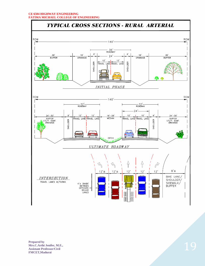
CE 6504 HIGHWAY ENGINEERING
FATIMA MICHAEL COLLEGE OF ENGINEERING
Prepared by
MrsCArthi Jenifer ME
Assistant ProfessorCivil
FMCETMadurai 19
CE 6504 HIGHWAY ENGINEERING
FATIMA MICHAEL COLLEGE OF ENGINEERING
Prepared by
MrsCArthi Jenifer ME
Assistant ProfessorCivil
FMCETMadurai 20
Cross sectional elements
Kerbs
Kerbs indicate the boundary between the carriage way and the shoulder or islands or footpaths Different types of kerbs are
CE 6504 HIGHWAY ENGINEERING
FATIMA MICHAEL COLLEGE OF ENGINEERING
Prepared by
MrsCArthi Jenifer ME
Assistant ProfessorCivil
FMCETMadurai 21
Low or mountable kerbs This type of kerbs is provided such that they
encourage the traffic to remain in the through traffic lanes and also allow the
driver to enter the shoulder area with little difficulty The height of this kerb is
about 10 cm above the pavement edge with a slope which allows the vehicle to
climb easily This is usually provided at medians and channelization schemes and
also helps in longitudinal drainage
Semi-barrier type kerbs When the pedestrian traffic is high these kerbs are
provided Their height is 15 cm above the pavement edge This type of kerb
prevents encroachment of parking vehicles but at acute emergency it is possible
to drive over this kerb with some difficulty
Barrier type kerbs They are designed to discourage vehicles from leaving the
pavement They are provided when there is considerable amount of pedestrian
traffic They are placed at a height of 20 cm above the pavement edge with a steep
batter
Submerged kerbs They are used in rural roads The kerbs are provided at
pavement edges between the pavement edge and shoulders They provide lateral
confinement and stability to the pavement
Figure 1 Different types of kerbs
Shoulders Shoulders are provided along the road edge and are intended for accommodation of
stopped vehicles serve as an emergency lane for vehicles and provide lateral support
for base and surface courses The shoulder should be strong enough to bear the weight
of a fully loaded truck even in wet conditions The shoulder width should be adequate
for giving working space around a stopped vehicle It is desirable to have a width of
46 m for the shoulders A minimum width of 25 m is recommended for 2-lane rural
highways in India Parking lanes
Parking lanes are provided in urban lanes for side parking Parallel parking is preferred
because it is safe for the vehicles moving on the road The parking lane should have a
minimum of 30 m width in the case of parallel parking
CE 6504 HIGHWAY ENGINEERING
FATIMA MICHAEL COLLEGE OF ENGINEERING
Prepared by
MrsCArthi Jenifer ME
Assistant ProfessorCivil
FMCETMadurai 22
Bus-bays
Bus bays are provided by recessing the kerbs for bus stops They are provided so that
they do not obstruct the movement of vehicles in the carriage way They should be at
least 75 meters away from the intersection so that the traffic near the intersections is not
affected by the bus-bay
Service roads Service roads or frontage roads give access to access controlled highways like freeways
and expressways They run parallel to the highway and will be usually isolated by a
separator and access to the highway will be provided only at selected points These roads
are provided to avoid congestion in the expressways and also the speed of the traffic in
those lanes is not reduced
Drainage
The pavement surface should be absolutely impermeable to prevent seepage of water into
the pavement layers Further both the geometry and texture of pavement surface should
help in draining out the water from the surface in less time
Footpath
Footpaths are exclusive right of way to pedestrians especially in urban areas They are
provided for the safety of the pedestrians when both the pedestrian traffic and vehicular
traffic is high Minimum width is 15 meter and may be increased based on the traffic
The footpath should be either as smooth as the pavement or more smoother than that to
induce the pedestrian to use the footpath
Right of way
Right of way (ROW) or land width is the width of land acquired for the road along its
alignment It should be adequate to accommodate all the cross-sectional elements of the
highway and may reasonably provide for future development To prevent ribbon
development along highways control lines and building lines may be provided Control
line is a line which represents the nearest limits of future uncontrolled building activity
in relation to a road Building line represents a line on either side of the road between
which and the road no building activity is permitted at all The right of way width is
governed by
Width of formation It depends on the category of the highway and width of
roadway and road margins
Height of embankment or depth of cutting It is governed by the topography and
the vertical alignment
Side slopes of embankment or cutting It depends on the height of the slope soil
type etc
Drainage system and their size which depends on rainfall topography etc
Sight distance considerations On curves etc there is restriction to the visibility
on the inner side of the curve due to the presence of some obstructions like
building structures etc
Reserve land for future widening Some land has to be acquired in advance
CE 6504 HIGHWAY ENGINEERING
FATIMA MICHAEL COLLEGE OF ENGINEERING
Prepared by
MrsCArthi Jenifer ME
Assistant ProfessorCivil
FMCETMadurai 23
Table 2 Desig
n speed in as per IRC (ruling and minimum)
Steep
Type
Plain
Rolling
Hilly
40-30
NSampSH
100-80
80-65
50-40
MDR
80-65
65-50
40-30
30-20
25-20
ODR
65-50
50-40
30-25
25-20
VR
50-40
40-35
25-20
anticipating future developments like widening of the road
Table 1 No
right of way for open areas
Roadway width in m
Road
Plain and
Mountainous and
classification
steep terrain
rolling terrain
Open areas
45
24
NHSH
18
MDR
25
15
15
ODR
12
9
VR
Built-up areas
20
NHSH
30
MDR
20
15
ODR
15
12
9
VR
10
CE 6504 HIGHWAY ENGINEERING
FATIMA MICHAEL COLLEGE OF ENGINEERING
Prepared by
MrsCArthi Jenifer ME
Assistant ProfessorCivil
FMCETMadurai 24
Horizontal curve
The presence of horizontal curve imparts centrifugal force which is a reactive force
acting outward on a vehicle negotiating it Centrifugal force depends on speed and radius
of the horizontal curve and is counteracted to a certain extent by transverse friction
between the tyre and pavement surface On a curved road this force tends to cause the
vehicle to overrun or to slide outward from the centre of road curvature For proper
design of the curve an understanding of the forces acting on a vehicle taking a horizontal
curve is necessary Various forces acting on the vehicle are illustrated in the figure 1
Figure 1 Effect of horizontal curve They are the centrifugal force (P) acting outward weight of the vehicle (W) acting
downward and the reaction of the ground on the wheels ( and ) The centrifugal
force and the weight is assumed to be from the centre of gravity which is at h units above
the ground Let the wheel base be assumed as b units The centrifugal force in
is given by
(1)
where is the weight of the vehicle in is the speed of the vehicle in is
the acceleration due to gravity in and is the radius of the curve in
The centrifugal ratio or the impact factor is given by
CE 6504 HIGHWAY ENGINEERING
FATIMA MICHAEL COLLEGE OF ENGINEERING
Prepared by
MrsCArthi Jenifer ME
Assistant ProfessorCivil
FMCETMadurai 25
(1)
The centrifugal force has two effects A tendency to overturn the vehicle about the outer
wheels and a tendency for transverse skidding Taking moments of the forces with
respect to the outer wheel when the vehicle is just about to override
At the equilibrium over turning is possible when
and for safety the following condition must satisfy
(2)
The second tendency of the vehicle is for transverse skidding ie When the the
centrifugal force is greater than the maximum possible transverse skid resistance due to
friction between the pavement surface and tyre The transverse skid resistance (F) is
given by
where and is the fractional force at tyre and and is the reaction at
tyre and is the lateral coefficient of friction and is the weight of the vehicle
This is counteracted by the centrifugal force (P) and equating
At equilibrium when skidding takes place (from equation1)
and for safety the following condition must satisfy
CE 6504 HIGHWAY ENGINEERING
FATIMA MICHAEL COLLEGE OF ENGINEERING
Prepared by
MrsCArthi Jenifer ME
Assistant ProfessorCivil
FMCETMadurai 26
(3)
Equation 2 and 3 give the stable condition for design If equation 2 is violated the vehicle
will overturn at the horizontal curve and if equation 3 is violated the vehicle will skid at
the horizontal
Curve Analysis of super-elevation
Super-elevation or cant or banking is the transverse slope provided at horizontal curve to
counteract the centrifugal force by raising the outer edge of the pavement with respect to
the inner edge throughout the length of the horizontal curve When the outer edge is
raised a component of the curve weight will be complimented in counteracting the effect
of centrifugal force In order to find out how much this raising should be the following
analysis may be done The forces acting on a vehicle while taking a horizontal curve with
super elevation is shown in figure 1
Figure 1 Analysis of super-elevation
Forces acting on a vehicle on horizontal curve of radius at a speed of are
the centrifugal force acting horizontally out-wards through the center of
gravity
the weight of the vehicle acting down-wards through the center of gravity and
the friction force between the wheels and the pavement along the surface
inward
CE 6504 HIGHWAY ENGINEERING
FATIMA MICHAEL COLLEGE OF ENGINEERING
Prepared by
MrsCArthi Jenifer ME
Assistant ProfessorCivil
FMCETMadurai 27
At equilibrium by resolving the forces parallel to the surface of the pavement we get where
friction
is the weight of the vehicle is the centrifugal force is the coefficient of
is the transverse slope due to superelevation Dividing by we get
CE 6504 HIGHWAY ENGINEERING
FATIMA MICHAEL COLLEGE OF ENGINEERING
Prepared by
MrsCArthi Jenifer ME
Assistant ProfessorCivil
FMCETMadurai 28
Step 1
Find for 75 percent of design speed neglecting ie
Step 2
If then else if go to step 3
Step 3
Find for the design speed and max ie If
then the maximum is safe for the design speed else go to
step 4
Step 4
Find the allowable speed for the maximum and
If then the design is adequate otherwise use speed adopt
control measures or look for speed control measures
Maximum and minimum super-elevation
Depends on (a) slow moving vehicle and (b) heavy loaded trucks with high CG IRC
specifies a maximum super-elevation of 7 percent for plain and rolling terrain while that
of hilly terrain is 10 percent and urban road is 4 percent The minimum super elevation is
2-4 percent for drainage purpose especially for large radius of the horizontal curve
Attainment of super-elevation
1 Elimination of the crown of the cambered section by
1 Rotating the outer edge about the crown The outer half of the cross slope
is rotated about the crown at a desired rate such that this surface falls on
the same plane as the inner half
2 Shifting the position of the crown This method is also known as diagonal
crown method Here the position of the crown is progressively
shifted outwards thus increasing the width of the inner half of cross section
progressively
2 Rotation of the pavement cross section to attain full super elevation byThere are
two methods of attaining super elevation by rotating the pavement
1 Rotation about the center line The pavement is rotated such that the inner
edge is depressed and the outer edge is raised both by half the total amount
of super elevation ie by with respect to the centre
2 Rotation about the inner edge Here the pavement is rotated raising the
outer edge as well as the centre such that the outer edge is raised by the
full amount of super elevation with respect to the inner edge
Horizontal Transition Curves
CE 6504 HIGHWAY ENGINEERING
FATIMA MICHAEL COLLEGE OF ENGINEERING
Prepared by
MrsCArthi Jenifer ME
Assistant ProfessorCivil
FMCETMadurai 29
Transition curve is provided to change the horizontal alignment from straight to circular
curve gradually and has a radius which decreases from infinity at the straight end
(tangent point) to the desired radius of the circular curve at the other end (curve point)
There are five objectives for providing transition curve and are given below
1 to introduce gradually the centrifugal force between the tangent point and the
beginning of the circular curve avoiding sudden jerk on the vehicle This
increases the comfort of passengers
2 to enable the driver turn the steering gradually for his own comfort and security
3 to provide gradual introduction of super elevation and
4 to provide gradual introduction of extra widening
5 to enhance the aesthetic appearance of the road
Type of transition curve
Different types of transition curves are spiral or clothoid cubic parabola and Lemniscate
IRC recommends spiral as the transition curve because
1 it fulfills the requirement of an ideal transition curve that is
1 rate of change or centrifugal acceleration is consistent (smooth) and
2 radius of the transition curve is at the straight edge and changes to at
the curve point ( ) and calculation and field implementation is
very easy
Length of transition curve The length of the transition curve should be determined as the maximum of the following
three criteria rate of change of centrifugal acceleration rate of change of super elevation
and an empirical formula given by IRC Rate of change of centrifugal acceleration
At the tangent point radius is infinity and hence centrifugal acceleration is zero At the
end of the transition the radius R has minimum value R The rate of change of
centrifugal acceleration should be adopted such that the design should not cause
discomfort to the drivers If is the rate of change of centrifugal acceleration it can be
written as
Therefore the length of the transition curve in is
CE 6504 HIGHWAY ENGINEERING
FATIMA MICHAEL COLLEGE OF ENGINEERING
Prepared by
MrsCArthi Jenifer ME
Assistant ProfessorCivil
FMCETMadurai 30
(1)
where is the rate of change of centrifugal acceleration given by an empirical formula
suggested by by IRC as below
(2) 2 Rate of introduction of super-elevation
Raise ( ) of the outer edge with respect to inner edge is given by
The rate of change of this raise from to is achieved
gradually with a gradient of in over the length of the transition curve (typical range
of is 60-150) Therefore the length of the transition curve is
(3)
3 By empirical formula
IRC suggest the length of the transition curve is minimum for a plain and rolling terrain
(4)
and for steep and hilly terrain is
(5)
CE 6504 HIGHWAY ENGINEERING
FATIMA MICHAEL COLLEGE OF ENGINEERING
Prepared by
MrsCArthi Jenifer ME
Assistant ProfessorCivil
FMCETMadurai 31
and the shift as
(
6
) The length of the transition curve is the maximum of
equations 1 3 and 4or5 ie
(
7
Case (a)
For single lane roads
(
1
)
Therefore
(
2
)
Figure 1 Set-back for single lane roads (
CE 6504 HIGHWAY ENGINEERING
FATIMA MICHAEL COLLEGE OF ENGINEERING
Prepared by
MrsCArthi Jenifer ME
Assistant ProfessorCivil
FMCETMadurai 32
For multi lane roads if is the distance between centerline of the road and the centerline
of the inner lane then
(3)
(4)
Figure 2 Set-back for multi-lane roads ( )
Case (a)
For single lane roads
(1)
Therefore
(2)
Gradient
Gradient is the rate of rise or fall along the length of the road with respect to the
horizontal While aligning a highway the gradient is decided for designing the vertical
curve Before finalizing the gradients the construction cost vehicular operation cost and
the practical problems in the site also has to be considered Usually steep gradients are
avoided as far as possible because of the difficulty to climb and increase in the
CE 6504 HIGHWAY ENGINEERING
FATIMA MICHAEL COLLEGE OF ENGINEERING
Prepared by
MrsCArthi Jenifer ME
Assistant ProfessorCivil
FMCETMadurai 33
construction cost More about gradients are discussed below
Effect of gradient
The effect of long steep gradient on the vehicular speed is considerable This is
particularly important in roads where the proportion of heavy vehicles is significant Due
to restrictive sight distance at uphill gradients the speed of traffic is often controlled by
these heavy vehicles As a result not only the operating costs of the vehicles are
increased but also capacity of the roads will have to be reduced Further due to high
differential speed between heavy and light vehicles and between uphill and downhill
gradients accidents abound in gradients
Representation of gradient
The positive gradient or the ascending gradient is denoted as and the negative gradient as The deviation angle is when two grades meet the angle which
measures the change of direction and is given by the algebraic difference between the two
grades
steep gradient while 1 in 50 = 2 representation is illustrated in the figure 1
Example 1 in 30 = 333 is a
is a flatter gradient The gradient
CE 6504 HIGHWAY ENGINEERING
FATIMA MICHAEL COLLEGE OF ENGINEERING
Prepared by
MrsCArthi Jenifer ME
Assistant ProfessorCivil
FMCETMadurai 34
Figure 1 Representation of gradient
Types of gradient
Many studies have shown that gradient upto seven percent can have considerable effect
on the speeds of the passenger cars On the contrary the speeds of the heavy vehicles are
considerably reduced when long gradients as flat as two percent is adopted Although
flatter gradients are desirable it is evident that the cost of construction will also be very
high Therefore IRC has specified the desirable gradients for each terrain However it
may not be economically viable to adopt such gradients in certain locations steeper
gradients are permitted for short duration Different types of grades are discussed below
Ruling gradient
The ruling gradient or the design gradient is the maximum gradient with which the
designer attempts to design the vertical profile of the road This depends on the terrain
length of the grade speed pulling power of the vehicle and the presence of the horizontal
curve In flatter terrain it may be possible to provide flat gradients but in hilly terrain it
is not economical and sometimes not possible also The ruling gradient is adopted by the
designer by considering a particular speed as the design speed and for a design vehicle
with standard dimensions But our country has a heterogeneous traffic and hence it is not
possible to lay down precise standards for the country as a whole Hence IRC has
recommended some values for ruling gradient for different types of terrain
Limiting gradient
This gradient is adopted when the ruling gradient results in enormous increase in cost of
construction On rolling terrain and hilly terrain it may be frequently necessary to adopt
limiting gradient But the length of the limiting gradient stretches should be limited and
must be sandwiched by either straight roads or easier grades
Exceptional gradient
Exceptional gradient are very steeper gradients given at unavoidable situations They
should be limited for short stretches not exceeding about 100 metres at a stretch In
mountainous and steep terrain successive exceptional gradients must be separated by a
minimum 100 metre length gentler gradient At hairpin bends the gradient is restricted to
25
Critical length of the grade
The maximum length of the ascending gradient which a loaded truck can operate without
undue reduction in speed is called critical length of the grade A speed of 25 kmph is a
CE 6504 HIGHWAY ENGINEERING
FATIMA MICHAEL COLLEGE OF ENGINEERING
Prepared by
MrsCArthi Jenifer ME
Assistant ProfessorCivil
FMCETMadurai 35
reasonable value This value depends on the size power load grad-ability of the truck
initial speed final desirable minimum speed
Minimum gradient
This is important only at locations where surface drainage is important Camber will take
care of the lateral drainage But the longitudinal drainage along the side drains require
some slope for smooth flow of water Therefore minimum gradient is provided for
drainage purpose and it depends on the rain fall type of soil and other site conditions A
minimum of 1 in 500 may be sufficient for concrete drain and 1 in 200 for open soil
drains are found to give satisfactory performance Sight distance available from a point is the actual distance along the road surface which a driver
from a specified height above the carriage way has visibility of stationary or moving objects
Sight distance required by drivers applies to both geometric design of highways and for
traffic control The sight distance situations are considered in the design
i) Stopping or absolute minimum sight distance
ii) Safe overtaking or passing sight distance
iii) Safe sight distance for entering into uncontrolled intersections
Apart from the three situations mentioned above the following sight distance are considered by the
IRC in highway design
Intermediate sight distance
This is defined as twice the stopping sight distance when overtaking sight distance
cannot be provided intermediate sight distance is provided to give limited overtaking opportunities
to fast vehicles
Head light sight distance
This is the distance visible to a driver during night driving under the illumination of the
vehicle head lights
Stopping sight distance
The minimum sight distance available on a highway at any spot should be of sufficient
length to stop a vehicle traveling at design speed safely without collision with any other obstruction
The absolute minimum sight distance is therefore equal to the stopping sight distance
which is also sometimes called nonpassing sight distance The sight distance available on a road to a
driver at any instance depends on
i) Features of the road
ii) Height of the drivers eye above the road surface
iii) Height of the object above the road surface
The distance within which a motor vehicle can be stopped depends upon the factors listed below
a) Total reactions time of the driver
b) Speed of vehicle
c) Efficiency of breaks
d) Frictional resistance between the road and tyres
e) Gradient of the road
Total reaction time
) Reaction time of the driver is the time taken from the instant the object is visible to the
driver to the instant the brakes are effectively applied
) The total reaction time may be split up into two parts
CE 6504 HIGHWAY ENGINEERING
FATIMA MICHAEL COLLEGE OF ENGINEERING
Prepared by
MrsCArthi Jenifer ME
Assistant ProfessorCivil
FMCETMadurai 36
i) Perception time
ii) Brake reaction time
PIEV theory
According to this theory the total reaction time of the driver is split into four parts
i) Perception
ii) Intellection
iii) Emotion
iv) Volition
Speed of Vehicle
The stopping distance depends very much on the speed of the vehicle first during the
total reaction time of the driver the distance moved by the vehicle will depend on the speed
Efficiency of brakes
The braking efficiency is said to be 100 percent if the wheels are fully licked preventing
them from rotating on application of the brakes This will result in 100 percent skidding which is
normally undesirable except in utmost emergency
Frictional resistance between road and tyres
The frictional resistance developed between road and tyres or the skid resistance depends
on the type and condition of the road surface and the tyres IRC has specified a design friction
coefficient of 035 to 04 depending upon the speed to be used for finding the braking distance in the
calculation of stopping sight distance
Analysis of stopping distance
i) The distance traveled by the vehicle during the total reaction time known as lag
distance
ii) The distance traveled by the vehicle after the application of the brakes is known as
braking distance
Overtaking sight distance
The minimum distance open to the vision of the driver of a vehicle intending to overtake
slow vehicle ahead with safety against the traffic of opposite direction is known as the minimum
overtaking sight distance(OSD) or Safe passing sight distance available
The overtaking sight distance is the distance measured along the center of the road which
a driver with his eye level 12m above the road surface can see the top of an object 12m above the
road surface
Some of the important factors on which the minimum overtaking sight distance required
a) Speed of
i) overtaking vehicle
ii) overtaken vehicle
iii) The vehicle coming from opposite direction
b) Distance between the overtaking and overtaken vehicles the minimum spacing
depends on the steeds
a) Skill and reaction time of the driver
b) Rate of acceleration of overtaking vehicle
c) Gradient of the road
Criteria for sight distance requirements on highway
) The absolute minimum sight distance required throughout the length of the road is the
SSD which should invariably be provided at all places
CE 6504 HIGHWAY ENGINEERING
FATIMA MICHAEL COLLEGE OF ENGINEERING
Prepared by
MrsCArthi Jenifer ME
Assistant ProfessorCivil
FMCETMadurai 37
) On horizontal curves the obstruction on the inner side of the curves should be cleared
to provide the required set back distance and absolute minimum sight distance
) On vertical summit curves the sight distance requirement may be fulfilled by proper
design of the vertical alignment
Hairpin bent
TYPES OF CURVES ON HILL ROADS
The following are the important types of curves provided on hill Roads-
1 Hair-Pin Curves
2 Salient Curves
3 Re-entrant Curves 1 Hair-pin curves - The curve in a hill road which changes its direction through an angle of 180
degree or so down the hill on the same side is known as hair-pin curve
A Hair-Pin Bend
This curve is so called because it conforms to the shape of a hair-pin The bend so formed at the
hair-pin curve in a hill road is known as hair-pin bend This type of curve should be located on a
hill side having the minimum slope and maximum stability It must also be safe from view point of
landslides and ground water Hair-pin bends with long arms and farther spacing are always
preferred They reduce construction problems and expensive protective works Hair-pin curves or
bends of serpentine nature are difficult to negotiate and should therefore be avoided as far as
possible
Salient curves - The curves having their convexity on the outer edges of a hill road are called
salient curves The centre of curvature of a salient curve lies towards the hill side This type of curve
occurs in the road length constructed on the ridge of a hill the bend so formed at the salient curve in
a hill road known as corner bend
Salient curves are very dangerous for fast moving traffic At such a curve or at corner bend the
portion of projecting hill side is usually cut down to improve the visibility as shown in fig (Re-
entrant curve) The outer edge of the road at such a curve is essentially provided with a parapet wall
for protection of the vehicles from falling down the hill slope
CE 6504 HIGHWAY ENGINEERING
FATIMA MICHAEL COLLEGE OF ENGINEERING
Prepared by
MrsCArthi Jenifer ME
Assistant ProfessorCivil
FMCETMadurai 38
3 Re-entrant curves - The curves having their convexity on the inner edge of a hill road are called
re-entrant curves
Re-entrant curves
The centre of curvature of a re-entrant curves lies away from the hill side This type of curve occurs
in the road length constructed in the calley of a hill
These curves are less dangereous as they provide adequate visibility to the fast moving traffic At
such curves the parapet wall is provided only for safety of fast moving traffic
CE 6504 HIGHWAY ENGINEERING
FATIMA MICHAEL COLLEGE OF ENGINEERING
Prepared by
MrsCArthi Jenifer ME
Assistant ProfessorCivil
FMCETMadurai 39
UNIT ndash III DESIGN OF RIGID AND FLEXIBLE PAVEMENTS
COMPARISON OF RIGID AND FLEXIBLE PAVEMENTS
The comparisons are
i) Design precision
A cement concrete pavement is amerable to a much more precise structural analysis
than a flexible pavement Flexible pavements designs are mainly empirical Computer aided analysis
of layered system is making the flexible pavement design more exact than hitherto
ii) Life
) Cement concrete slabs of a thin section constructed in the early 1940rsquos are still in
existence in India though many of them have cracked badly and a few of them have been ripped
open and rebuilt in recent ties
) A major project in cement concrete road construction between Agra and Mathura It can
safely be said that a well-designed concrete slab has a life of about 40 years
) Compared to this the life of a flexible pavement generally varies from 10 to 20 years
iii) Maintenance
) A well-designed cement concrete pavement needs very little maintenance The only
maintenance needed is I respect of joints
) The surface is unaffected by spillage of oil and lubricants bituminous surfaces on the
other hand need great inputs in maintenance
) The surface is affected by spillage of oil and lubricants The surface is also affected by
natural weathering agents like air water ad temperature changes
) A cement concrete pavement on the other hand needs a small amount for maintaining
joints
iv) Initial cost
) The argument so far used against a cement concrete slab is that it is much more costly
than a flexible pavement
) The latter specifications no doubt represent the rock-bottom needs of a road in India but
these specifications can hardly provide a smooth and durable surface
v) Stage construction ) Road construction is generally done adopting a policy of stage construction especially for
low volume roads As traffic grows additional layers in the form of water bound macadam and
superior surfacing are added on
) Initial outlay is minimum and additional outlays are in keeping with traffic growth This is
a great advantage when dealing with new roads in an atmosphere of austerity
vi) Availability of materials
) Cement bitumen stone aggregates and gravelsand are the major materials involved in
pavement Construction Cement has been in serious short supply in the country for the past many
decades
) Bitumen is also not available plentifully in India There is also the danger of the entire oil
reserves in the world shrinking during the next two or three decades
) In locations where stone aggregates are scarce cement concrete may have an advantage
for flexible pavements
vii) Surface characterstics
CE 6504 HIGHWAY ENGINEERING
FATIMA MICHAEL COLLEGE OF ENGINEERING
Prepared by
MrsCArthi Jenifer ME
Assistant ProfessorCivil
FMCETMadurai 40
) A good cement concrete surface is smooth and free from rutting potholes and
corrugations In a bituminous surface it is only the asphaltic concrete surface that can give
comparable rideablity
) A well-constructed cement concrete pavement surface can have a permanent nonskid
surface A bituminous surface can also be designed to have a good skid resistant surface
viii) Utility location
) In cement concrete slabs proper thought has to be given to locate utilities such as water
pipes telephone lines and electric cables
) It is difficult to rip open the slab and restore it to be the original condition if any changes
in the utilities lines are to be made
ix) Glame and night visibility
) Concrete pavements have a gray color which can cause glam under sunlight Colored
cement can reduce the grave
) On the other hand bituminous roads need more street lighting
x) Traffic dislocation during construction
) A cement concrete pavement requires 28 days before it can be thrown open to traffic On
the other hand a bituminous surface can be thrown open to traffic shortly after it is rolled
xi) Environmental considerations during construction
) The process of heating of bitumen and aggregates and mixing them together on hot mix
plants can prove to be much more hazardous to the environment than cement concrete construction
where no heating of any material is involved
xii) Overall economy on a life cycle basis
) A good road is costly to construct but once constructed such a road requires little
maintenance and results in savings in vehicle operating costs
) The comparative economy of a flexible pavement and a rigid pavement has proved that on
overall economic considerations
Types of pavement structure
Based on the structural behavior pavements are generally classified into three
categories
i) Flexible pavements
ii) Rigid pavements
iii) Semi rigid pavements
Flexible pavements
) Flexible pavements are those which on the whole have low or negligible flexural
strength and are rather flexible in their structural action under the loadsThe flexible pavement
layers reflect the deformation of the lower layers on to the surface of the layer
) A flexible pavement consists of four components(i) Soil subgrade (ii) sub base
course (iii) base course (iv) Surface course
CE 6504 HIGHWAY ENGINEERING
FATIMA MICHAEL COLLEGE OF ENGINEERING
Prepared by
MrsCArthi Jenifer ME
Assistant ProfessorCivil
FMCETMadurai 41
) The flexible pavement layers transmit the vertical or compressive stresses to the lower layers
by grain to grain transfer through the points of contact in the granular structure A well
compacted granular structure consisting of strong added aggregate can transfer the compressive
stresses
) The load spreading ability of this layer therefore depends on the type of the materials and mix
design factors Bituminous concrete is one of the best flexible pavements layer materials Other
materials which fall under the group are all granular materials with or without bituminous
binder granular base and sub base course materials
) The vertical compressive stress is maximum on the pavement surface directly under the wheel
and is equal to the contact pressure under the wheel The flexible pavement may be constructed
in a number of layers and the top layer has to be strongest as the highest compressive stresses
) Flexible pavements are commonly designed using empirical design charts or equations taking
into account some of the design factors there are also semi empirical and theoretical design
methods
Rigid pavements
) Rigid pavements are those which possess note flexural strength or flexural rigidity
The stresses are not transferred from grain to grain to the lower layers as in the ease of flexible
pavements layers
) The rigid pavements are made of Portland cement concrete plain reinforced or
prestressed concrete The plain cement concrete slabs are expected to take up about 40 kgcm2
flexural stress
) The rigid pavement has the slab action and is capable of transmitting the wheel
load stresses through a wider area below The main point of difference in the structural behavior
of rigid pavement as compared to the flexible pavement is that the critical condition of stress in
the rigid pavement is the maximum flexural stress occurring in the slab due to wheel load and
the temperature changes whereas in the flexible pavement
) As the rigid pavement slab has tensile strength tensile stresses are developed due
to the bending of the slab under wheel load and temperature variations Thus the types of
stresses developed and their distribution within the cement concrete slab are quirt different
) The cement concrete pavement slab can very well serve as a wearing surface as
well an effective base course The rigid pavement structure consists of a cement concrete slab
below which a granular base or sub base course may be provided
) Though the cement concrete slab can also be laid directly over the soil subgrade
consists of fine grained soil
) the rigid pavements are usually designed and the stresses are analyzed using the
elastic theory assuming the pavements as a n elastic plate resting over an elastic or a viscous
foundation
Semi rigid pavements
) when bonded materials like the pozzolanic concrete lean cement concrete or soil
cement are used in the base course or sub base course layer the pavement layer has considerably
higher flexural strength than the common flexible pavement layers
) when this intermediate class of materials are used in the base or sub base course
layer of the pavements they are called semi rigid pavements
CE 6504 HIGHWAY ENGINEERING
FATIMA MICHAEL COLLEGE OF ENGINEERING
Prepared by
MrsCArthi Jenifer ME
Assistant ProfessorCivil
FMCETMadurai 42
) This third category of semi rigid pavement are either designed as flexible
pavements with some correction factors to find the thickness requirements based on experience
or by using a new design approach
) The semi rigid pavement materials have low resistance to impact and abrasion and
therefore are usually provided with flexible pavement surface course
Various functions of pavement components
The functions are
Soil sub grade and its evaluation
) The soil sub grade is a layer of natural soil prepared to receive the layers of pavement
materials placed over it It is essential that at no time the soil sub grade is overstressed it means that
the pressure transmitted on the top of the sub grade is within the allowable limit
) Many tests are known for measuring the strength properties of the sub grades Some of the
tests have been standardized for the use The common strength test for the evaluation of soil
subgrade is
i) California bearing ratio test
ii) California resistance value test
iii) Triaxial compression test
iv) Plate bearing test
CALIFORNIA BEARING RATIO (CBR) TEST
It is evolved for the empirical method of flexible pavement design The CBR test is carried
out either in the laboratory on prepared specimens or in the field by taking in situ measurements
California resistance value
It is found by using have been stabliometerThis test is used in an empirical method of
flexible pavement design based on soil strength
Triaxial test
It is the most important soil strength but still the test is not very commonly used in structural
design of pavements
Plate bearing test
It is carried out using a relatively large diameter plate to evaluate the load supporting
capacity of supporting power of the pavement layers The results are plate bearing tests are used in
flexible pavement design method like McLeod method on based on layer system analysis by
brumister
Sub base and base courses and their evaluation
) There layers are made of broken stones bound or unbound aggreagatesome times in sub
base course a layer of stabilized soil(or) Selected granular soil is also used
) however at the sub base course it is desirable to use smaller size graded aggregates When
the sub grade consists of fine grained soil and when the pavement carries heavy wheel loads
CE 6504 HIGHWAY ENGINEERING
FATIMA MICHAEL COLLEGE OF ENGINEERING
Prepared by
MrsCArthi Jenifer ME
Assistant ProfessorCivil
FMCETMadurai 43
) Sub base course primarily has the similar function as of the base course and is provided
with inferior materials than of base course Base courses are used under rigid pavement for
i) Preventing pumping
ii) Protecting the sub grade against frost action
) Thus the fundamental purpose of abase course and sub base course is to provide a stress
transmitting medium to spread the surface wheel loads in such manner
) The sub base and base course layers may be evaluated by suitable strength or stability test
like plate bearing CBR test
WEARING COURSE AND ITS EVALUATION
) The purpose of the wearing course is to give a smooth riding surface that is dense It
resists pressure exerted by tyres and takes up wear and tear due to the traffic
) Wearing course also offers a water tight layer against the surface water infiltration The
flexible pavement normally a bituminous surfacing is used as a wearing course
) In rigid pavements the cement concrete acts like a base course as well as wearing course
Most popular test in use is marshal stability test where in the optimum content of bitumen binder is
worked out based on the stability density
) Plate bearing test and Bankelman beam test are also sometimes made use of for evaluating
the wearing course and the pavement as a whole
Various factors to be considered in pavement design and the significance
Pavement design consists of two parts
i) Mix design of materials to be used in each pavement component layer Thickness design of the
pavement and the component layers
The various factors to be considered for the design of pavements are given below
i) Design wheel load
ii) Sub grade soil
iii) Climatic factors
iv) Pavement component layers
v) Environmental factors
vi) Special factors in the design of different types of pavements
Design wheel load
The various wheel load factors to be considered in pavement design are
i) Maximum wheel load
ii) Contact pressure
iii) Dual or multiple wheel loads
iv) Repetition of loads
Maximum wheel load
The wheel load configurations are important to know the way in which the loads of a given
vehicle are applied on the pavement surface
) For highways the maximum legal axle load as specified by Indian road congress is 8170
kg with a maximum equivalent single wheel load of 4085 kg
) The evaluation for vertical stress computations under a uniformly distribute of circular
load based on Boussineqrsquos theory is given by
CE 6504 HIGHWAY ENGINEERING
FATIMA MICHAEL COLLEGE OF ENGINEERING
Prepared by
MrsCArthi Jenifer ME
Assistant ProfessorCivil
FMCETMadurai 44
2
322
3
1
za
zpz
σz = vertical stress at depth z
P= surface pressure
Z=depth at which σz computed
A=radius of loaded area
Contact pressure
Generally the wheel load is assumed to be distributed over a circular area But by
measurement of the imprints of tyers with different load and inflation pressures Three terms in use
with reference to tyre pressure are
Tyre pressure
Inflation pressure
Contact pressure
Tyre pressure and inflation pressure mean exactly the same the contact pressure is found to be more
than tyre pressure when the tyre pressure is less than 7 kgm2 and it is vice versa when the tyre
pressure exceeds this value
Contact pressure can be measured by the relationship
Load on wheel
Contact pressure = ----------------------------------------
Contact area or area of imprint
The general variation between the tyre pressure and measured contact pressure is shown in this fig
The ratio of contact pressure to type pressure is defined as rigidity factor Thus value of rigidity
factor is 10 for an average tyre pressure of 7 Kgcm2This value is higher than unity for lower type
pressures and less than unity for tyre pressures higher than 7 kgcm2
Equivalent single wheel load (ESWL)
) The maximum wheel load within the specified limit and to carry greater load it is
necessary to provide dual wheel assembly to the rear axles of the roads vehicles
) In other words the pressure at a certain depth below the pavement surface cannot be
obtained by numerically adding the pressure caused by any one wheel
) The effect is in between the single load and two times load carried by one wheel The load
dispersion is assumed to be at an angle of 450In the dual wheel load assembly let d be the clear gap
between the two wheels S be the spacing between the centers of the wheels and a be the radius of
the circular contact area of each wheel Then S = (d + 2a)
) ESWL may be determined based on either equivalent deflection or equivalent stress
criterianMultiple wheel loads are convert to ESWL and this value is used in pavement design The
ESWL is usually determined by the equivalent stress criterion using a simple graphical method
CE 6504 HIGHWAY ENGINEERING
FATIMA MICHAEL COLLEGE OF ENGINEERING
Prepared by
MrsCArthi Jenifer ME
Assistant ProfessorCivil
FMCETMadurai 45
) A straight line relationship is assumed between ESWL and depth on log scales For
determining ESWL the plot is made as shown in fig
) Two points A and B are plotted on the log-log graph with coordinates of A (Pd2) and
B(2p2s)line AB is a plot which is the focus of points where any single wheel load is equivalent to a
certain set of dual wheels
) To Calculate the ESWL for a dual assembly it is essential to estimate a design thickness of
the pavement If the design thickness so obtained is equal to the estimated thickness then the ESWL
calculations could be considered as correct Otherwise trials are made
) In heavy trucks and trailers the load on each wheel may be further reduced by multiple
wheels and tandem axles
Repetition of loads
) The deformation of load pavement (or) sub grade due to a single application of wheel load
may be small It required carrying out traffic surveys for accounting the factor of repetitions for
wheel loads in the design of pavement
) Data collected are converted to some constant equivalent wheel loads Equivalent wheel
load is a single load equivalent to the repeated applications of any particular wheel load on a
pavement which requires the same thickness and strength of pavements
) McLeod has given a procedure for evolving equivalent load factors for designing flexible
pavements
Various methods of flexible pavement design
) The flexible pavement is built with number of layers In the design process it is to be
ensured that under the application of load none of the layers is overstressed
) The maximum intensity of stresses occurs in the top layer of the pavement The
magnitude of load stresses reduces at lower layers
) In the design of flexible pavements it has yet not been possible to have a rational design
method wherein design process and service behavior of the pavement can be expressed by
mathematical laws
) Flexible pavement design methods are accordingly either empirical or semi empirical In
these methods the knowledge and experience gained on the behavior of the pavements in the past
are usefully utilized
Various approaches of flexible pavement design may be thus classified into three groups
i) Empirical method
ii) Semi-empirical or Semi theoretical method
iii) Theoretical method
) Empirical methods are either based on physical properties or strength parameters of soil
sub grade When the design is based on stress strain function and modified base on experience it
may be called semi-empirical or semi-theoretical There are design methods based on theoretical
analysis and mathematical computations
Out of the flexible pavement design method available is
i) Group index method
ii) California bearing ratio method
iii) California R value (or) Stabiliometer method
iv) Triaxial test method
CE 6504 HIGHWAY ENGINEERING
FATIMA MICHAEL COLLEGE OF ENGINEERING
Prepared by
MrsCArthi Jenifer ME
Assistant ProfessorCivil
FMCETMadurai 46
v) McLeod method
vi) Burmister method
Group index method
) Group index value is an arbitrary index assigned to the soil type in numerical equations
base on the percent fines liquid limit and plasticity index
) The design chart for group index method for determining the pavement thickness is given
in fig
The traffic volume in this method is divided in three groups
Traffic volume No of vehicles per day
Light Less than 50
Medium 50 to 300
Heavy Over 300
The design of the pavement thickness by this method first the G1 value of the soil is found the
anticipated traffic is estimated and is designated as light medium or heavy as indicated
The G1 method of pavement design is essentially an empirical method based on physical properties
of the subgrade soil This method does not consider the strength characteristics of the subgrade soil
and therefore is open to question regarding the reliability of the design based on the index properties
of the soil only
California bearing ratio method
) California division of highways in the USA developed CBR method for
pavement design The majority of design curves developed later are base on the original curves
proposed by OJporter
) One of the chief advantages of CBR method is the simplicity of the test procedure
The CBR tests were carried out by the California state highway department on existing pavement
layers including subgrade sub base and base course
) Based on the extensive CBR test data collected on pavement which behaved
satisfactory and those which failed an empirical design chart was developed correlating the CBR
value and the pavement thickness The basis of the design chart is that a material with a given CBR
required a certain thickness of pavement layer as a cover
) A higher load needs a thicker pavement layer to protect the sub grade Design
curves correlating the CBR value with total pavement thickness cover were developed by the
California state highway department for wheel loads of 3175kg and 5443 kg representing light and
heavy traffic The design curves are shown in this fig
It is possible to extend the CBR design curves for various loading conditions nusing the expression
t= 2
1
1751
pCBRp
t=2
1
751
A
CBR
p
Hence
CE 6504 HIGHWAY ENGINEERING
FATIMA MICHAEL COLLEGE OF ENGINEERING
Prepared by
MrsCArthi Jenifer ME
Assistant ProfessorCivil
FMCETMadurai 47
t= pavement thickness cm
p=Wheel load kg
CBR= California bearing ratio percent
P=tyre pressure kgcm2
A= area of contactcm2
IRC Recommendations
a) The CBR tests should be performed on remoulded soils in the laboratory The specimens should
be prepared by static compaction wherever possible and otherwise by dynamic compaction
b) For the design of new roads the sub grade soil sample should be compacted at OMC to proctor
density whenever suitable compaction equipment
c) The CBR test samples may be soaked in water for four days period before testing the annual
rainfall is less than 50 cm and the water table is too deep to affect the sub grade and imperable
surfacing is provided to carrying out CBR test
d) If the maximum variations in CBR value of the three specimens exceed the specified limits the
design CBR should be average of at least six samples
e) The top 50 cm of sub grade should be compacted at least up to 95 to 100 percent of proctor
density
f) An estimate of the traffic should be carried by the road pavements at the end of expected in view
the existing traffic and probable growth rate of traffic
g) The traffic for the design is considered in units of heavy vehicles per day in both directions and is
divided into seven categories A to G The design thickness is considered applicable for single axle
loads up to 8200 kg and tandom axle loads up to 14500 kg
h) When sub base course materials contain substantial proportion of aggregates of size above 20mm
the CBR value of these materials would not be valid for the design of subsequent layers above them
The CBR method of pavement design gives the total thickness requirement of the pavement above a
sub grade and thickness value would remain the same quality of materials used in component layers
California resistance value method
) In this design method based on stabliometer R-value and cohesiometer C-value
Based on performance data it was established by pavement thickness varies directly with R value
and algorithm of load repetitions It varies inversely with fifth root of c valueThe expression for
pavement thickness is given by the empirical equation
T=
5
1
1 90
C
RTK
Hence
T=total thickness of pavement cm
K=Numerical constant 0166
T1=traffic index
R= stabiliometer resistance value
C=Cohesiometer value
CE 6504 HIGHWAY ENGINEERING
FATIMA MICHAEL COLLEGE OF ENGINEERING
Prepared by
MrsCArthi Jenifer ME
Assistant ProfessorCivil
FMCETMadurai 48
In the design of flexible pavements based on California resistance value method for the following
data are needed
) R-value of soil subgrade
) T1 value
) Equivalent C-value
) R value of soil subgrade is obtained from the test using stablio meterThe
computation of T1 value has been explained
Equivalent C-value
) The cohesion meter value c is obtained for each layer of pavement material
separately from tests However the composite or equivalent C-value of the pavement may be
estimated if the thickness of each component layer and the c-value of the material of the layer are
known
) while designing a pavement as the thickness of the pavement is not known it is
easier if the pavement is first assumed to consist of any one material like gravel base course with
known C-value
) Subsequently the individual thickness of each layer is converted in terms of gravel
equivalent by using relationship
5
1
1
2
2
1
C
C
t
t
) t1 and t2 are the thickness values of any two pavement layersc1 and c2 are their
corresponding cohesiometer values
CE 6504 HIGHWAY ENGINEERING
FATIMA MICHAEL COLLEGE OF ENGINEERING
Prepared by
MrsCArthi Jenifer ME
Assistant ProfessorCivil
FMCETMadurai 49
UNIT 4 MATERIAL AND MAINTENANCE
SUMMIT CURVE
Summit curves are vertical curves with gradient upwards They are formed when two
gradients meet as illustrated in figure 1 in any of the following four ways
1 When a positive gradient meets another positive gradient [figure 1a]
2 When positive gradient meets a flat gradient [figure 1b]
3 When an ascending gradient meets a descending gradient [figure 1c]
4 When a descending gradient meets another descending gradient [figure 1d]
Type of Summit Curve
Many curve forms can be used with satisfactory results the common practice has been to
use parabolic curves in summit curves This is primarily because of the ease with it can
be laid out as well as allowing a comfortable transition from one gradient to another
Although a circular curve offers equal sight distance at every point on the curve for very
small deviation angles a circular curve and parabolic curves are almost congruent
Furthermore the use of parabolic curves were found to give excellent riding comfort
Figure 1 Types of summit curves
Design Consideration
In determining the type and length of the vertical curve the design considerations are
comfort and security of the driver and the appearance of the profile alignment Among
these sight distance requirements for the safety are most important on summit curves
The stopping sight distance or absolute minimum sight distance should be provided on
these curves and where overtaking is not prohibited overtaking sight distance or
intermediate sight distance should be provided as far as possible When a fast moving
vehicle travels along a summit curve there is less discomfort to the passengers This is
because the centrifugal force will be acting upwards while the vehicle negotiates a
summit curve which is against the gravity and hence a part of the tyre pressure is
relieved Also if the curve is provided with adequate sight distance the length would be
sufficient to ease the shock due to change in gradient Circular summit curves are
identical since the radius remains same throughout and hence the sight distance From
CE 6504 HIGHWAY ENGINEERING
FATIMA MICHAEL COLLEGE OF ENGINEERING
Prepared by
MrsCArthi Jenifer ME
Assistant ProfessorCivil
FMCETMadurai 50
this point of view transition curves are not desirable since it has varying radius and so the
sight distance will also vary The deviation angles provided on summit curves for
highways are very large and so the simple parabola is almost congruent to a circular arc
between the same tangent points Parabolic curves are easy for computation and also it
had been found out that it provides good riding comfort to the drivers It is also easy for
field implementation Due to all these reasons a simple parabolic curve is preferred as
summit curve Length of the summit curve
The important design aspect of the summit curve is the determination of the length of the
curve which is parabolic As noted earlier the length of the curve is guided by the sight
distance consideration That is a driver should be able to stop his vehicle safely if there is
an obstruction on the other side of the road Equation of the parabola is given by
where where N is the deviation angle and is the length of the In
deriving the length of the curve two situations can arise depending on the uphill and
downhill gradients when the length of the curve is greater than the sight distance and the
length of the curve is greater than the sight distance
Let is the length of the summit curve is the SSDISDOSD is the deviation angle
drivers eye height (12 m) and the height of the obstruction then the length of the
summit curve can be derived for the following two cases The length of the summit curve
can be derived from the simple geometry as shown below
Case a Length of summit curve greater than sight distance( )
Figure 1 Length of summit curve ( )
The situation when the sight distance is less than the length of the curve is shown in
figure 1
CE 6504 HIGHWAY ENGINEERING
FATIMA MICHAEL COLLEGE OF ENGINEERING
Prepared by
MrsCArthi Jenifer ME
Assistant ProfessorCivil
FMCETMadurai 51
(1)
Case b Length of summit curve less than sight distance
The second case is illustrated in figure 1
Figure 1 Length of summit curve
CE 6504 HIGHWAY ENGINEERING
FATIMA MICHAEL COLLEGE OF ENGINEERING
Prepared by
MrsCArthi Jenifer ME
Assistant ProfessorCivil
FMCETMadurai 52
From the basic geometry one can write
(1)
Therefore for a given and to get minimum differentiate the above equation
with respect to and equate it to zero Therefore
Solving the quadratic equation for
(2)
Now we can substitute back to get the value of minimum value of for a given
and Therefore
Solving for
CE 6504 HIGHWAY ENGINEERING
FATIMA MICHAEL COLLEGE OF ENGINEERING
Prepared by
MrsCArthi Jenifer ME
Assistant ProfessorCivil
FMCETMadurai 53
(3) (4
CE 6504 HIGHWAY ENGINEERING
FATIMA MICHAEL COLLEGE OF ENGINEERING
Prepared by
MrsCArthi Jenifer ME
Assistant ProfessorCivil
FMCETMadurai 54
When stopping sight distance is considered the height of drivers eye above the road
surface ( ) is taken as 12 metres and height of object above the pavement surface ( )
is taken as 015 metres If overtaking sight distance is considered then the value of
drivers eye height ( ) and the height of the obstruction ( ) are taken equal as 12
metres
Valley curve
Valley curve or sag curves are vertical curves with convexity downwards They are
formed when two gradients meet as illustrated in figure 1 in any of the following four
ways
Figure 1 Types of valley curve
1 When a descending gradient meets another descending gradient [figure 1a]
2 When a descending gradient meets a flat gradient [figure 1b]
3 When a descending gradient meets an ascending gradient [figure 1c]
4 When an ascending gradient meets another ascending gradient [figure
Design considerations
There is no restriction to sight distance at valley curves during day time But visibility is
reduced during night In the absence or inadequacy of street light the only source for
visibility is with the help of headlights Hence valley curves are designed taking into
account of headlight distance In valley curves the centrifugal force will be acting
downwards along with the weight of the vehicle and hence impact to the vehicle will be
more This will result in jerking of the vehicle and cause discomfort to the passengers
Thus the most important design factors considered in valley curves are (1) impact-free
movement of vehicles at design speed and (2) availability of stopping sight distance
under headlight of vehicles for night driving
For gradually introducing and increasing the centrifugal force acting downwards the best
shape that could be given for a valley curve is a transition curve Cubic parabola is
generally preferred in vertical valley curves See figure 1
CE 6504 HIGHWAY ENGINEERING
FATIMA MICHAEL COLLEGE OF ENGINEERING
Prepared by
MrsCArthi Jenifer ME
Assistant ProfessorCivil
FMCETMadurai 55
Figure 1 Valley curve details
During night under headlight driving condition sight distance reduces and availability of
stopping sight distance under head light is very important The head light sight distance
should be at least equal to the stopping sight distance There is no problem of overtaking
sight distance at night since the other vehicles with headlights could be seen from a
considerable distance
Length of the valley curve
The valley curve is made fully transitional by providing two similar transition curves of
equal length The transitional curve is set out by a cubic parabola where
The length of the valley transition curve is designed based on two criteria
1 comfort criteria that is allowable rate of change of centrifugal acceleration is
limited to a comfortable level of about
2 safety criteria that is the driver should have adequate headlight sight distance at
any part of the country
Comfort criteria
The length of the valley curve based on the rate of change of centrifugal acceleration that
will ensure comfort Let is the rate of change of acceleration the minimum radius of
the curve is the design speed and is the time then is give
CE 6504 HIGHWAY ENGINEERING
FATIMA MICHAEL COLLEGE OF ENGINEERING
Prepared by
MrsCArthi Jenifer ME
Assistant ProfessorCivil
FMCETMadurai 56
For a cubic parabola the Value Safety criter Length of the valley curve for headlight distance may be determined for two conditions
(1) length of the valley curve greater than stopping sight distance and (2) length of the
valley curve less than the stopping sight distance of for length is given by
Case 1 Length of valley curve greater than stopping sight distance ( )
The total length of valley curve is greater than the stopping sight distance SSD The
sight distance available will be minimum when the vehicle is in the lowest point in the
valley This is because the beginning of the curve will have infinite radius and the bottom
of the curve will have minimum radius which is a property of the transition curve The
case is shown in figure 1
Figure 1 Valley curve case 1
From the geometry of the figure we have
CE 6504 HIGHWAY ENGINEERING
FATIMA MICHAEL COLLEGE OF ENGINEERING
Prepared by
MrsCArthi Jenifer ME
Assistant ProfessorCivil
FMCETMadurai 57
(1)
where is the deviation angle in radians is the height of headlight beam is the
head beam inclination in degrees and is the sight distance The inclination is 1
degree
Case 2 Length of valley curve less than stopping sight distance ( )
The length of the curve is less than SSD In this case the minimum sight distance is
from the beginning of the curve The important points are the beginning of the curve and
the bottom most part of the curve If the vehicle is at the bottom of the curve then its
headlight beam will reach far beyond the endpoint of the curve whereas if the vehicle is
at the beginning of the curve then the headlight beam will hit just outside the curve
Therefore the length of the curve is derived by assuming the vehicle at the beginning of
the curve The case is shown in figure 1
From the figure
(1) Note that the above expression is approximate and is satisfactory because in practice the gradients
are very small and is acceptable for all practical purposes We will not be able to know prior to
which case to be adopted Therefore both has to be calculated and the one which satisfies the
condition is adopted
1 Flexible pavement
2 Rigid pavement
Flexible pavement
These pavements reflect the deformation of sub grade and the subsequent layers to the
surface
Rigid pavement
The rigid characteristic of the pavement are associated with rigidity or flexural strength
CE 6504 HIGHWAY ENGINEERING
FATIMA MICHAEL COLLEGE OF ENGINEERING
Prepared by
MrsCArthi Jenifer ME
Assistant ProfessorCivil
FMCETMadurai 58
or slab action so the load is distributed over a wide area of sub grade soil
Flexible pavement Definition
These pavements reflect the deformation of sub grade and the subsequent layers to the
surface Flexible usually asphalt is laid with no reinforcement or with a specialized
fabric reinforcement that permits limited flow or repositioning of the roadbed under
ground changes
The design of flexible pavement is based on load distributing characteristic of the
component layers The black top pavement including water amp gravel bound macadam fall
in this category
Flexible pavement on the whole has low or negligible flexible strength flexible in their
structural action) The flexible pavement layers transmit the vertical or compressive
stresses to the lower layers by grain transfer through contact points of granular structure
The vertical compressive stress is maximum on the pavement surface directly under the
wheel load and is equal to contact pressure under the wheels Due to the ability to
distribute the stress to large area in the shape of truncated cone the stresses get decreased
in the lower layer
As such the flexible pavement may be constructed in a number of layers and the top
layer has to be strongest as the highest compressive stresses
To be sustained by this layer in addition to wear and tear the lower layer have to take
up only lesser magnitude of stress as there is no direct wearing action die to traffic loads
therefore inferior material with lower cast can be used in the lower layers
Rigid pavement Definition
The rigid characteristic of the pavement are associated with rigidity or flexural strength
or slab action so the load is distributed over a wide area of sub grade soil Rigid pavement
is laid in slabs with steel reinforcement
The rigid pavements are made of cement concrete either plan reinforced or prestressed
concrete
Critical condition of stress in the rigid pavement is the maximum flexural stress occurring in the slab due to wheel load and the temperature changes
Rigid pavement is designed and analyzed by using the elastic theory
CE 6504 HIGHWAY ENGINEERING
FATIMA MICHAEL COLLEGE OF ENGINEERING
Prepared by
MrsCArthi Jenifer ME
Assistant ProfessorCivil
FMCETMadurai 59
UNIT-5 EVALUATION AND MAINTENANCE OF PAVEMENTS
TRAFFIC PARAMETERS
Design life
Design life is the number of years (or number of standard axle repetitions) for which the
pavement is being designed A pavement is expected to serve satisfactorily within the
design life For concrete pavements 20 to 40 years may be assumed as the design life
(PCA 1984 IRC58 2002)
Basic design principle
Though different approaches for concrete pavement design are suggested in various
guidelines the design principles tend to remain similar across different guidelines for
example PCA (1994) Austroads (2004) NCHRP (2004) IRC58 (2002) etc except the
AASHTO (1993) provisions which is based on empirical approach The basic steps
involved in the design of concrete pavement method can be summarized as follows
The developed stresses due to load for a trial thickness of the concrete slab are
calculated for various loading configuration and the critical one is chosen The
axle loads are generally divided into different axle load groups and the load
stresses are calculated individually
The ratio between the load stress and Modulus of Rupture (MOR) is known as
stress ratio The stress ratio determines how many repetitions the pavement can
sustain (ie allowable traffic repetitions) for the individual axle load group If the
stress ratio is 055 or lower it can withstand virtually infinite number of traffic
repetitions (PCA 1984)
The ratio between the allowable repetitions to the expected traffic repetitions is
the damage fraction The calculation process is repeated for various axle loads
(sometimes for various seasons or various timings of the day) and the sum of
individual damage fractions (c u m u l a t i v e fatigue damage) should be less
than equal to one for pavement design being safe If found unsafe the trial
thickness is changed and the design process is repeated
The design process may also include considerations for temperature stress
moisture stresses and erosion distress
A brief discussion on concrete pavement design approaches suggested by various design
practices viz PCA method (1984) Austroads method (2004) AASHTO method (1993)
NCHRP mechanistic-empirical method (2004) and the Indian Roads Congress (IRC)
method (2002) are placed in the following
Portland cement Association (PCA) Method
The PCA method is based on Westergaard Picket and Rays work and further theoretical
analysis by Finite Element Method (Huang 1993) The data used to develop the PCA
method is generated from various road tests like ASSHO road test Arlington test
(conducted by PCA) Bates test road and Maryland road test (PCA 1984) The PCA
design method is based on the following two considerations (PCA 1984)
The fatigue damage on the concrete slab due to repetitive application of traffic
load is estimated The cumulative fatigue damage principle is used to estimate the
design thickness of the slab Edge stress between the mid-ways of the
CE 6504 HIGHWAY ENGINEERING
FATIMA MICHAEL COLLEGE OF ENGINEERING
Prepared by
MrsCArthi Jenifer ME
Assistant ProfessorCivil
FMCETMadurai 60
transverse joint is taken as critical configuration
The stresses due to warping and curling (due to temperature and moisture
gradient) are not considered in the fatigue analysis as per PCA recommendation
because most of the time the stresses generated are subtractive to the load stress
The possibility of erosion of pavement materials placed below the concrete slab is
evaluated The rate at which the slab is deflected due to axle load is used as a
criterion for erosion Theoretically it can be shown that a thin pavement with
smaller deflection basin is subjected to faster rate of deflection compared to
thicker slab Hence thin slab is more susceptible to erosion In a similar way the
cumulative erosion damage is calculated for individual axle load groups If this
value is greater than one then the design needs to be revised
Austroads method
Austroads method has been adopted from PCA (1984) approach with modifications
suited to Australian conditions (Austroads 2004) A bound mix or lean cement concrete is
used as sub-base material For a given CBR value of the subgrade and given thickness of
cemented sub-base the effective subgrade strength can be obtained from the chart
provided Figure-19 schematically shows such a chart For different levels of traffic
Austroads (2004) suggests minimum values of the base thicknesses to be provided
CE 6504 HIGHWAY ENGINEERING
FATIMA MICHAEL COLLEGE OF ENGINEERING
Prepared by
MrsCArthi Jenifer ME
Assistant ProfessorCivil
FMCETMadurai 61
figure-19 Schematic diagram of Austroads (2004) chart for estimation of effective
subgrade strength
As per Astroads (2004) the concrete pavement slab thickness for a given expected
traffic repetitions is designed considering the (i) flexural fatigue of the concrete slab and
the (ii) subgrade erosion arising out of repeated deflections For both the considerations
equations are suggested to calculate the allowable traffic repetitions If the allowable
traffic is less than the expected traffic the design is revised by increasing the slab
thickness The concrete shoulders adopted are of integral type or structural type
AASHTO method
The AASHTO method (1993) for design of concrete pavement has evolved from the
AASHO road test (AASHO 1962) The AASHTO pavement design follows an empirical
approach Pavement performance in terms of present serviceability index ( PSI ) loss of
serviceability sub-grade and sub-base strength cumulative traffic properties of concrete
joint load transfer efficiency drainage condition overall standard deviation and
reliability are the input parameters considered in the pavement design
The PSI value of the fresh pavement is assumed as 45 and the pavement is deemed to
have failed when the PSI value reaches 25 The resilient moduli of the subgrade and sub-
base materials are determined in the laboratory simulating the seasonal moisture content
and stress situation Suggested values are also available for given moisture content
plasticity index etc The composite modulus of sub-grade reaction (k) is estimated from
modulus of sub-grade reaction and elastic modulus of sub-base for various seasons and
the depth of rigid foundation and the thickness of the sub-base
Design equation as well nomographs are available to estimate the slab thickness (D) from
these input parameters
NCHRP mechanistic-empirical (M-E) metho
The NCHRP (2004) has recently developed concrete pavement design procedure based
on mechanistic-empirical (M-E) approach This approach attempts to reduce the extent of
empiricism prevalent in the existing AASHTO (1993) guidelines This proposed NCHRP
pavement design system is modular in nature that is the design approach can be
modified by parts (as and when new knowledge is available) without disrupting the
overall design procedure This approach also can take care of various wheel-axle loa
configuration
As per this approach trial thickness of the slab is first assumed and the stress strain and
displacement values are obtained From these values the performance of the pavement in
terms of distresses (such as faulting cracking) and smoothness and predicted If these
predicted performance parameters does not satisfy the required performance for a given
reliability
The design approach includes a large data-base as input parameters for example average
daily traffic traffic growth rate traffic composition hourly weather data on air
temperature precipitation wind speed percentage sunshine relative humidity pavement
material engineering parameters ground water depth infiltration drainage hydraulic
conductivity thermal conductivity heat capacity etc The temperature stress is
considered in this method but the temperature profile is linearized to enhance
computational efficiency (NCHRP 2004)
CE 6504 HIGHWAY ENGINEERING
FATIMA MICHAEL COLLEGE OF ENGINEERING
Prepared by
MrsCArthi Jenifer ME
Assistant ProfessorCivil
FMCETMadurai 62
INDIAN ROADS CONGRESS (IRC) METHOD
The Indian Roads Congress (IRC) guidelines IRC58 (2002) has adopted the
Westergaards equation to estimate load stress and Brdaburys equation to estimate
temperature stress The load stress is highest at the corner of the slab lesser in edge and
least in the interior The order of variation of temperature stress is just the reverse of this
As per IRC58 (2002) it is recommended that the design needs to be done for edge stress
condition and subsequently check needs to be performed for corner stress condition so as
to finalize the design The following are the steps followed as per IRC58 (2002)
guideline for the design of concrete pavement
The input parameters are obtained to formulate the design problem The joint
spacing and the slab dimensions are decided If there is a bound sub-base layer
over the subgrade a suitable value of effective k is to be adopted
A trial thickness of the concrete slab is assumed
The edge stress is estimated for various axle loads from the given charts Figure-
20 schematically shows such a chart The cumulative fatigue damage principle for
fatigue is applied to check the adequacy of the slab thickness
The sum of edge stress due to load for the highest axle load group and the
temperature stress should be less than the MOR of concrete otherwise the design
is revised
The adequacy of corner stress is checked with respect to MOR value and
accordingly the design is finalized Westergaards corner stress formula
Figure-20 Schematic diagram of IRC58 chart for estimation of load stress at the edge
(IRC58 2002)
CE 6504 HIGHWAY ENGINEERING
FATIMA MICHAEL COLLEGE OF ENGINEERING
Prepared by
MrsCArthi Jenifer ME
Assistant ProfessorCivil
FMCETMadurai 63
estimation of corner stress due to load and the corner stress due to temperature is
assumed to be zero
Estimation of layer thicknesses
The thickness of the pavement is adjusted in such a way that the stress strain
developed is less than the allowable values obtained from past performance
information
The two major modes of structural failure of pavement are fatigue and rutting
o Fatigue Traffic applies repetitive load to the pavement surface and the
cracks start from bottom the bound layer slab and propagate upwards
When the extent of surface cracks reaches a predefined level the
pavement is said to have failed due to flexural fatigue
FUNCTIONAL DESIGN
The functional pavement design involves considerations of skid resistance roughness
surface distresses reflectivity of pavement surface etc The functional pavement design
considers mainly the surface features of a pavement
Drainage design
A road needs to be designed in such a way that the rain snow precipitation is drained off
the pavement and its surroundings A suitable surface drainage system for the pavement
is designed for this purpose Some water however will percolate into the pavement from
its top surface and needs to be taken out of the pavement - this is done by providing an
internal drainage system to the pavement Water will also try to enter into the pavement
from bottom due to capillary rise or due to rise in water table A suitably designed sub-
surface drainage system tries to avoid such a problem
PAVEMENT THICKNESS DESIGN CHARTS
For the design of pavements to carry traffic in the range of 1 to 10 msa use chart 1 and for
traffic in the range 10 to 150 msa use chart 2 of IRC37 2001 The design curves relate
pavement thickness to the cumulative number of standard axles to be carried over the
design life for different sub-grade CBR values ranging from 2 to 10 The design
charts will give the total thickness of the pavement for the above inputs The total
thickness consists of granular sub-base granular base and bituminous surfacing The
individual layers are designed based on the the recommendations given below and the
subsequent tables
Pavement composition
Sub-base
Sub-base materials comprise natural sand gravel laterite brick metal crushed
stone or combinations thereof meeting the prescribed grading and physical
requirements The sub-base material should have a minimum CBR of 20 and
30 for traffic upto 2 msa and traffic exceeding 2 msa respectively Sub-base
usually consist of granular or WBM and the thickness should not be less than 150
mm for design traffic less than 10 msa and 200 mm for design traffic
Base
The recommended designs are for unbounded granular bases which comprise
CE 6504 HIGHWAY ENGINEERING
FATIMA MICHAEL COLLEGE OF ENGINEERING
Prepared by
MrsCArthi Jenifer ME
Assistant ProfessorCivil
FMCETMadurai 64
conventional water bound macadam (WBM) or wet mix macadam (WMM) or
equivalent confirming to MOST specifications The materials should be of good
quality with minimum thickness of 225 mm for traffic up to 2 msa an 150 mm for
traffic
Bituminoussurfacing The surfacing consists of a wearing course or a binder
course plus wearing course The most commonly used wearing courses are
surface dressing open graded premix carpet mix seal surfacing semi-
dense bituminous concrete and bituminous concrete For binder course
MOST specifies it is desirable to use bituminous macadam (BM) for traffic
upto o 5 msa and dense bituminous macadam (DBM) for traffic more than 5
msa
Numerical example
Design the pavement for construction of a new bypass with the following data
1 Two lane carriage way
2 Initial traffic in the year of completion of construction = 400 CVPD (sum of both
directions)
3 Traffic growth rate = 75
4 Design life = 15 years
5 Vehicle damage factor based on axle load survey = 25 standard axle per
commercial vehicle
6 Design CBR of subgrade soil = 4
Solution
1 Distribution factor = 075
2
3 Total pavement thickness for CBR 4 and traffic 72 msa from IRC37 2001
chart1 = 660 mm
4 Pavement composition can be obtained by interpolation from Pavement Design
Catalogue (IRC37 2001)
1 Bituminous surfacing = 25 mm SDBC + 70 mm DBM
2 Road-base = 250 mm WBM
3 sub-base = 315 mm granular material of CBR not less than 30
CE 6504 HIGHWAY ENGINEERING
FATIMA MICHAEL COLLEGE OF ENGINEERING
Prepared by
MrsCArthi Jenifer ME
Assistant ProfessorCivil
FMCETMadurai 65
Generally bound base layers are used for concrete pavement construction As per Indian
specification some example of such base layers are Dry Lean Concrete (DLC) Roller
Compacted Concrete (RCC) (IRC15-2002)
The concrete slab is generally of M40 to M50 grade of concrete as
per Indian specifications and is called as paving quality concrete (PQC)
(IRC15-2002)
BITUMINOUS PAVEMENT
The subgrade is a compacted soil layer
The base and sub-base course could be made up of bound or unbound granular layer As
per Indian specifications (MORTampH 2001) some examples of base or sub-base layers
are Granular sub-base(GSB) Water Bound Macadam (WBM) Wet Mix Macadam
(WMM) etc
The binder course is made up bituminous material As per Indian specifications
(MORTampH 2001) some examples of binder course are Bituminous Macadam (BM)
Dense Bituminous Macadam (DBM) etc
The wearing course is the top bituminous layer which is comes in contact to the
vehicle tyre Wearing course provides impermeability to the pavement surface
against water percolation (Chakroborty and Das 2003) The binder course and wearing
course together are called bituminous surfacing
IRC METHOD OF FLEXIBLE PAVEMENT MIX DESIGN
These guidelines will apply to design of flexible pavements for Expressway National Highways
State Highways Major District Roads and other categories of roads Flexible pavements are
considered to include the pavements which have bituminous surfacing and granular base and sub-
base courses conforming to IRC MOST standards These guidelines apply to new pavements
Design criteria
The flexible pavements has been modeled as a three layer structure and stresses and strains at
critical locations have been computed using the linear elastic model To give proper consideration
to the aspects of performance the following three types of pavement distress resulting from
repeated (cyclic) application of traffic loads are considered
1 Vertical compressive strain at the top of the sub-grade which can cause sub-grade
deformation resulting in permanent deformation at the pavement surface
2 Horizontal tensile strain or stress at the bottom of the bituminous layer which can cause
fracture of the bituminous layer
3 Pavement deformation within the bituminous layer
CE 6504 HIGHWAY ENGINEERING
FATIMA MICHAEL COLLEGE OF ENGINEERING
Prepared by
MrsCArthi Jenifer ME
Assistant ProfessorCivil
FMCETMadurai 66
While the permanent deformation within the bituminous layer can be controlled by meeting the
mix design requirements thickness of granular and bituminous layers are selected using the
analytical design approach so that strains at the critical points are within the allowable limits For
calculating tensile strains at the bottom of the bituminous layer the stiffness of dense bituminous
macadam (DBM) layer with 6070 bitumen has been used in the analysis
FAILURE CRITERIA
Critical locations in pavement
A and B are the critical locations for tensile strains Maximum value of the strain is
adopted for design C is the critical location for the vertical subgrade strain since the
maximum value of the occurs mostly at C
CE 6504 HIGHWAY ENGINEERING
FATIMA MICHAEL COLLEGE OF ENGINEERING
Prepared by
MrsCArthi Jenifer ME
Assistant ProfessorCivil
FMCETMadurai 67
Fatigue Criteria
Bituminous surfacings of pavements display flexural fatigue cracking if the tensile strain
at the bottom of the bituminous layer is beyond certain limit The relation between the
fatigue life of the pavement and the tensile strain in the bottom of the bituminous layer
was obtained as
(1)
in which is the allowable number of load repetitions to control fatigue cracking and
is the Elastic modulus of bituminous layer The use of equation 1 would result in
fatigue cracking of 20 of the total area
Rutting Criteria
The allowable number of load repetitions to control permanent deformation can be
expressed as
(2)
is the number of cumulative standard axles to produce rutting of 20 mm
CE 6504 HIGHWAY ENGINEERING
FATIMA MICHAEL COLLEGE OF ENGINEERING
Prepared by
MrsCArthi Jenifer ME
Assistant ProfessorCivil
FMCETMadurai 68
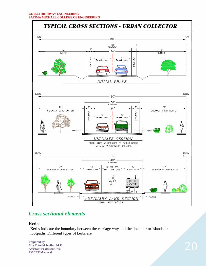
CE 6504 HIGHWAY ENGINEERING
FATIMA MICHAEL COLLEGE OF ENGINEERING
Prepared by
MrsCArthi Jenifer ME
Assistant ProfessorCivil
FMCETMadurai 20
Cross sectional elements
Kerbs
Kerbs indicate the boundary between the carriage way and the shoulder or islands or footpaths Different types of kerbs are
CE 6504 HIGHWAY ENGINEERING
FATIMA MICHAEL COLLEGE OF ENGINEERING
Prepared by
MrsCArthi Jenifer ME
Assistant ProfessorCivil
FMCETMadurai 21
Low or mountable kerbs This type of kerbs is provided such that they
encourage the traffic to remain in the through traffic lanes and also allow the
driver to enter the shoulder area with little difficulty The height of this kerb is
about 10 cm above the pavement edge with a slope which allows the vehicle to
climb easily This is usually provided at medians and channelization schemes and
also helps in longitudinal drainage
Semi-barrier type kerbs When the pedestrian traffic is high these kerbs are
provided Their height is 15 cm above the pavement edge This type of kerb
prevents encroachment of parking vehicles but at acute emergency it is possible
to drive over this kerb with some difficulty
Barrier type kerbs They are designed to discourage vehicles from leaving the
pavement They are provided when there is considerable amount of pedestrian
traffic They are placed at a height of 20 cm above the pavement edge with a steep
batter
Submerged kerbs They are used in rural roads The kerbs are provided at
pavement edges between the pavement edge and shoulders They provide lateral
confinement and stability to the pavement
Figure 1 Different types of kerbs
Shoulders Shoulders are provided along the road edge and are intended for accommodation of
stopped vehicles serve as an emergency lane for vehicles and provide lateral support
for base and surface courses The shoulder should be strong enough to bear the weight
of a fully loaded truck even in wet conditions The shoulder width should be adequate
for giving working space around a stopped vehicle It is desirable to have a width of
46 m for the shoulders A minimum width of 25 m is recommended for 2-lane rural
highways in India Parking lanes
Parking lanes are provided in urban lanes for side parking Parallel parking is preferred
because it is safe for the vehicles moving on the road The parking lane should have a
minimum of 30 m width in the case of parallel parking
CE 6504 HIGHWAY ENGINEERING
FATIMA MICHAEL COLLEGE OF ENGINEERING
Prepared by
MrsCArthi Jenifer ME
Assistant ProfessorCivil
FMCETMadurai 22
Bus-bays
Bus bays are provided by recessing the kerbs for bus stops They are provided so that
they do not obstruct the movement of vehicles in the carriage way They should be at
least 75 meters away from the intersection so that the traffic near the intersections is not
affected by the bus-bay
Service roads Service roads or frontage roads give access to access controlled highways like freeways
and expressways They run parallel to the highway and will be usually isolated by a
separator and access to the highway will be provided only at selected points These roads
are provided to avoid congestion in the expressways and also the speed of the traffic in
those lanes is not reduced
Drainage
The pavement surface should be absolutely impermeable to prevent seepage of water into
the pavement layers Further both the geometry and texture of pavement surface should
help in draining out the water from the surface in less time
Footpath
Footpaths are exclusive right of way to pedestrians especially in urban areas They are
provided for the safety of the pedestrians when both the pedestrian traffic and vehicular
traffic is high Minimum width is 15 meter and may be increased based on the traffic
The footpath should be either as smooth as the pavement or more smoother than that to
induce the pedestrian to use the footpath
Right of way
Right of way (ROW) or land width is the width of land acquired for the road along its
alignment It should be adequate to accommodate all the cross-sectional elements of the
highway and may reasonably provide for future development To prevent ribbon
development along highways control lines and building lines may be provided Control
line is a line which represents the nearest limits of future uncontrolled building activity
in relation to a road Building line represents a line on either side of the road between
which and the road no building activity is permitted at all The right of way width is
governed by
Width of formation It depends on the category of the highway and width of
roadway and road margins
Height of embankment or depth of cutting It is governed by the topography and
the vertical alignment
Side slopes of embankment or cutting It depends on the height of the slope soil
type etc
Drainage system and their size which depends on rainfall topography etc
Sight distance considerations On curves etc there is restriction to the visibility
on the inner side of the curve due to the presence of some obstructions like
building structures etc
Reserve land for future widening Some land has to be acquired in advance
CE 6504 HIGHWAY ENGINEERING
FATIMA MICHAEL COLLEGE OF ENGINEERING
Prepared by
MrsCArthi Jenifer ME
Assistant ProfessorCivil
FMCETMadurai 23
Table 2 Desig
n speed in as per IRC (ruling and minimum)
Steep
Type
Plain
Rolling
Hilly
40-30
NSampSH
100-80
80-65
50-40
MDR
80-65
65-50
40-30
30-20
25-20
ODR
65-50
50-40
30-25
25-20
VR
50-40
40-35
25-20
anticipating future developments like widening of the road
Table 1 No
right of way for open areas
Roadway width in m
Road
Plain and
Mountainous and
classification
steep terrain
rolling terrain
Open areas
45
24
NHSH
18
MDR
25
15
15
ODR
12
9
VR
Built-up areas
20
NHSH
30
MDR
20
15
ODR
15
12
9
VR
10
CE 6504 HIGHWAY ENGINEERING
FATIMA MICHAEL COLLEGE OF ENGINEERING
Prepared by
MrsCArthi Jenifer ME
Assistant ProfessorCivil
FMCETMadurai 24
Horizontal curve
The presence of horizontal curve imparts centrifugal force which is a reactive force
acting outward on a vehicle negotiating it Centrifugal force depends on speed and radius
of the horizontal curve and is counteracted to a certain extent by transverse friction
between the tyre and pavement surface On a curved road this force tends to cause the
vehicle to overrun or to slide outward from the centre of road curvature For proper
design of the curve an understanding of the forces acting on a vehicle taking a horizontal
curve is necessary Various forces acting on the vehicle are illustrated in the figure 1
Figure 1 Effect of horizontal curve They are the centrifugal force (P) acting outward weight of the vehicle (W) acting
downward and the reaction of the ground on the wheels ( and ) The centrifugal
force and the weight is assumed to be from the centre of gravity which is at h units above
the ground Let the wheel base be assumed as b units The centrifugal force in
is given by
(1)
where is the weight of the vehicle in is the speed of the vehicle in is
the acceleration due to gravity in and is the radius of the curve in
The centrifugal ratio or the impact factor is given by
CE 6504 HIGHWAY ENGINEERING
FATIMA MICHAEL COLLEGE OF ENGINEERING
Prepared by
MrsCArthi Jenifer ME
Assistant ProfessorCivil
FMCETMadurai 25
(1)
The centrifugal force has two effects A tendency to overturn the vehicle about the outer
wheels and a tendency for transverse skidding Taking moments of the forces with
respect to the outer wheel when the vehicle is just about to override
At the equilibrium over turning is possible when
and for safety the following condition must satisfy
(2)
The second tendency of the vehicle is for transverse skidding ie When the the
centrifugal force is greater than the maximum possible transverse skid resistance due to
friction between the pavement surface and tyre The transverse skid resistance (F) is
given by
where and is the fractional force at tyre and and is the reaction at
tyre and is the lateral coefficient of friction and is the weight of the vehicle
This is counteracted by the centrifugal force (P) and equating
At equilibrium when skidding takes place (from equation1)
and for safety the following condition must satisfy
CE 6504 HIGHWAY ENGINEERING
FATIMA MICHAEL COLLEGE OF ENGINEERING
Prepared by
MrsCArthi Jenifer ME
Assistant ProfessorCivil
FMCETMadurai 26
(3)
Equation 2 and 3 give the stable condition for design If equation 2 is violated the vehicle
will overturn at the horizontal curve and if equation 3 is violated the vehicle will skid at
the horizontal
Curve Analysis of super-elevation
Super-elevation or cant or banking is the transverse slope provided at horizontal curve to
counteract the centrifugal force by raising the outer edge of the pavement with respect to
the inner edge throughout the length of the horizontal curve When the outer edge is
raised a component of the curve weight will be complimented in counteracting the effect
of centrifugal force In order to find out how much this raising should be the following
analysis may be done The forces acting on a vehicle while taking a horizontal curve with
super elevation is shown in figure 1
Figure 1 Analysis of super-elevation
Forces acting on a vehicle on horizontal curve of radius at a speed of are
the centrifugal force acting horizontally out-wards through the center of
gravity
the weight of the vehicle acting down-wards through the center of gravity and
the friction force between the wheels and the pavement along the surface
inward
CE 6504 HIGHWAY ENGINEERING
FATIMA MICHAEL COLLEGE OF ENGINEERING
Prepared by
MrsCArthi Jenifer ME
Assistant ProfessorCivil
FMCETMadurai 27
At equilibrium by resolving the forces parallel to the surface of the pavement we get where
friction
is the weight of the vehicle is the centrifugal force is the coefficient of
is the transverse slope due to superelevation Dividing by we get
CE 6504 HIGHWAY ENGINEERING
FATIMA MICHAEL COLLEGE OF ENGINEERING
Prepared by
MrsCArthi Jenifer ME
Assistant ProfessorCivil
FMCETMadurai 28
Step 1
Find for 75 percent of design speed neglecting ie
Step 2
If then else if go to step 3
Step 3
Find for the design speed and max ie If
then the maximum is safe for the design speed else go to
step 4
Step 4
Find the allowable speed for the maximum and
If then the design is adequate otherwise use speed adopt
control measures or look for speed control measures
Maximum and minimum super-elevation
Depends on (a) slow moving vehicle and (b) heavy loaded trucks with high CG IRC
specifies a maximum super-elevation of 7 percent for plain and rolling terrain while that
of hilly terrain is 10 percent and urban road is 4 percent The minimum super elevation is
2-4 percent for drainage purpose especially for large radius of the horizontal curve
Attainment of super-elevation
1 Elimination of the crown of the cambered section by
1 Rotating the outer edge about the crown The outer half of the cross slope
is rotated about the crown at a desired rate such that this surface falls on
the same plane as the inner half
2 Shifting the position of the crown This method is also known as diagonal
crown method Here the position of the crown is progressively
shifted outwards thus increasing the width of the inner half of cross section
progressively
2 Rotation of the pavement cross section to attain full super elevation byThere are
two methods of attaining super elevation by rotating the pavement
1 Rotation about the center line The pavement is rotated such that the inner
edge is depressed and the outer edge is raised both by half the total amount
of super elevation ie by with respect to the centre
2 Rotation about the inner edge Here the pavement is rotated raising the
outer edge as well as the centre such that the outer edge is raised by the
full amount of super elevation with respect to the inner edge
Horizontal Transition Curves
CE 6504 HIGHWAY ENGINEERING
FATIMA MICHAEL COLLEGE OF ENGINEERING
Prepared by
MrsCArthi Jenifer ME
Assistant ProfessorCivil
FMCETMadurai 29
Transition curve is provided to change the horizontal alignment from straight to circular
curve gradually and has a radius which decreases from infinity at the straight end
(tangent point) to the desired radius of the circular curve at the other end (curve point)
There are five objectives for providing transition curve and are given below
1 to introduce gradually the centrifugal force between the tangent point and the
beginning of the circular curve avoiding sudden jerk on the vehicle This
increases the comfort of passengers
2 to enable the driver turn the steering gradually for his own comfort and security
3 to provide gradual introduction of super elevation and
4 to provide gradual introduction of extra widening
5 to enhance the aesthetic appearance of the road
Type of transition curve
Different types of transition curves are spiral or clothoid cubic parabola and Lemniscate
IRC recommends spiral as the transition curve because
1 it fulfills the requirement of an ideal transition curve that is
1 rate of change or centrifugal acceleration is consistent (smooth) and
2 radius of the transition curve is at the straight edge and changes to at
the curve point ( ) and calculation and field implementation is
very easy
Length of transition curve The length of the transition curve should be determined as the maximum of the following
three criteria rate of change of centrifugal acceleration rate of change of super elevation
and an empirical formula given by IRC Rate of change of centrifugal acceleration
At the tangent point radius is infinity and hence centrifugal acceleration is zero At the
end of the transition the radius R has minimum value R The rate of change of
centrifugal acceleration should be adopted such that the design should not cause
discomfort to the drivers If is the rate of change of centrifugal acceleration it can be
written as
Therefore the length of the transition curve in is
CE 6504 HIGHWAY ENGINEERING
FATIMA MICHAEL COLLEGE OF ENGINEERING
Prepared by
MrsCArthi Jenifer ME
Assistant ProfessorCivil
FMCETMadurai 30
(1)
where is the rate of change of centrifugal acceleration given by an empirical formula
suggested by by IRC as below
(2) 2 Rate of introduction of super-elevation
Raise ( ) of the outer edge with respect to inner edge is given by
The rate of change of this raise from to is achieved
gradually with a gradient of in over the length of the transition curve (typical range
of is 60-150) Therefore the length of the transition curve is
(3)
3 By empirical formula
IRC suggest the length of the transition curve is minimum for a plain and rolling terrain
(4)
and for steep and hilly terrain is
(5)
CE 6504 HIGHWAY ENGINEERING
FATIMA MICHAEL COLLEGE OF ENGINEERING
Prepared by
MrsCArthi Jenifer ME
Assistant ProfessorCivil
FMCETMadurai 31
and the shift as
(
6
) The length of the transition curve is the maximum of
equations 1 3 and 4or5 ie
(
7
Case (a)
For single lane roads
(
1
)
Therefore
(
2
)
Figure 1 Set-back for single lane roads (
CE 6504 HIGHWAY ENGINEERING
FATIMA MICHAEL COLLEGE OF ENGINEERING
Prepared by
MrsCArthi Jenifer ME
Assistant ProfessorCivil
FMCETMadurai 32
For multi lane roads if is the distance between centerline of the road and the centerline
of the inner lane then
(3)
(4)
Figure 2 Set-back for multi-lane roads ( )
Case (a)
For single lane roads
(1)
Therefore
(2)
Gradient
Gradient is the rate of rise or fall along the length of the road with respect to the
horizontal While aligning a highway the gradient is decided for designing the vertical
curve Before finalizing the gradients the construction cost vehicular operation cost and
the practical problems in the site also has to be considered Usually steep gradients are
avoided as far as possible because of the difficulty to climb and increase in the
CE 6504 HIGHWAY ENGINEERING
FATIMA MICHAEL COLLEGE OF ENGINEERING
Prepared by
MrsCArthi Jenifer ME
Assistant ProfessorCivil
FMCETMadurai 33
construction cost More about gradients are discussed below
Effect of gradient
The effect of long steep gradient on the vehicular speed is considerable This is
particularly important in roads where the proportion of heavy vehicles is significant Due
to restrictive sight distance at uphill gradients the speed of traffic is often controlled by
these heavy vehicles As a result not only the operating costs of the vehicles are
increased but also capacity of the roads will have to be reduced Further due to high
differential speed between heavy and light vehicles and between uphill and downhill
gradients accidents abound in gradients
Representation of gradient
The positive gradient or the ascending gradient is denoted as and the negative gradient as The deviation angle is when two grades meet the angle which
measures the change of direction and is given by the algebraic difference between the two
grades
steep gradient while 1 in 50 = 2 representation is illustrated in the figure 1
Example 1 in 30 = 333 is a
is a flatter gradient The gradient
CE 6504 HIGHWAY ENGINEERING
FATIMA MICHAEL COLLEGE OF ENGINEERING
Prepared by
MrsCArthi Jenifer ME
Assistant ProfessorCivil
FMCETMadurai 34
Figure 1 Representation of gradient
Types of gradient
Many studies have shown that gradient upto seven percent can have considerable effect
on the speeds of the passenger cars On the contrary the speeds of the heavy vehicles are
considerably reduced when long gradients as flat as two percent is adopted Although
flatter gradients are desirable it is evident that the cost of construction will also be very
high Therefore IRC has specified the desirable gradients for each terrain However it
may not be economically viable to adopt such gradients in certain locations steeper
gradients are permitted for short duration Different types of grades are discussed below
Ruling gradient
The ruling gradient or the design gradient is the maximum gradient with which the
designer attempts to design the vertical profile of the road This depends on the terrain
length of the grade speed pulling power of the vehicle and the presence of the horizontal
curve In flatter terrain it may be possible to provide flat gradients but in hilly terrain it
is not economical and sometimes not possible also The ruling gradient is adopted by the
designer by considering a particular speed as the design speed and for a design vehicle
with standard dimensions But our country has a heterogeneous traffic and hence it is not
possible to lay down precise standards for the country as a whole Hence IRC has
recommended some values for ruling gradient for different types of terrain
Limiting gradient
This gradient is adopted when the ruling gradient results in enormous increase in cost of
construction On rolling terrain and hilly terrain it may be frequently necessary to adopt
limiting gradient But the length of the limiting gradient stretches should be limited and
must be sandwiched by either straight roads or easier grades
Exceptional gradient
Exceptional gradient are very steeper gradients given at unavoidable situations They
should be limited for short stretches not exceeding about 100 metres at a stretch In
mountainous and steep terrain successive exceptional gradients must be separated by a
minimum 100 metre length gentler gradient At hairpin bends the gradient is restricted to
25
Critical length of the grade
The maximum length of the ascending gradient which a loaded truck can operate without
undue reduction in speed is called critical length of the grade A speed of 25 kmph is a
CE 6504 HIGHWAY ENGINEERING
FATIMA MICHAEL COLLEGE OF ENGINEERING
Prepared by
MrsCArthi Jenifer ME
Assistant ProfessorCivil
FMCETMadurai 35
reasonable value This value depends on the size power load grad-ability of the truck
initial speed final desirable minimum speed
Minimum gradient
This is important only at locations where surface drainage is important Camber will take
care of the lateral drainage But the longitudinal drainage along the side drains require
some slope for smooth flow of water Therefore minimum gradient is provided for
drainage purpose and it depends on the rain fall type of soil and other site conditions A
minimum of 1 in 500 may be sufficient for concrete drain and 1 in 200 for open soil
drains are found to give satisfactory performance Sight distance available from a point is the actual distance along the road surface which a driver
from a specified height above the carriage way has visibility of stationary or moving objects
Sight distance required by drivers applies to both geometric design of highways and for
traffic control The sight distance situations are considered in the design
i) Stopping or absolute minimum sight distance
ii) Safe overtaking or passing sight distance
iii) Safe sight distance for entering into uncontrolled intersections
Apart from the three situations mentioned above the following sight distance are considered by the
IRC in highway design
Intermediate sight distance
This is defined as twice the stopping sight distance when overtaking sight distance
cannot be provided intermediate sight distance is provided to give limited overtaking opportunities
to fast vehicles
Head light sight distance
This is the distance visible to a driver during night driving under the illumination of the
vehicle head lights
Stopping sight distance
The minimum sight distance available on a highway at any spot should be of sufficient
length to stop a vehicle traveling at design speed safely without collision with any other obstruction
The absolute minimum sight distance is therefore equal to the stopping sight distance
which is also sometimes called nonpassing sight distance The sight distance available on a road to a
driver at any instance depends on
i) Features of the road
ii) Height of the drivers eye above the road surface
iii) Height of the object above the road surface
The distance within which a motor vehicle can be stopped depends upon the factors listed below
a) Total reactions time of the driver
b) Speed of vehicle
c) Efficiency of breaks
d) Frictional resistance between the road and tyres
e) Gradient of the road
Total reaction time
) Reaction time of the driver is the time taken from the instant the object is visible to the
driver to the instant the brakes are effectively applied
) The total reaction time may be split up into two parts
CE 6504 HIGHWAY ENGINEERING
FATIMA MICHAEL COLLEGE OF ENGINEERING
Prepared by
MrsCArthi Jenifer ME
Assistant ProfessorCivil
FMCETMadurai 36
i) Perception time
ii) Brake reaction time
PIEV theory
According to this theory the total reaction time of the driver is split into four parts
i) Perception
ii) Intellection
iii) Emotion
iv) Volition
Speed of Vehicle
The stopping distance depends very much on the speed of the vehicle first during the
total reaction time of the driver the distance moved by the vehicle will depend on the speed
Efficiency of brakes
The braking efficiency is said to be 100 percent if the wheels are fully licked preventing
them from rotating on application of the brakes This will result in 100 percent skidding which is
normally undesirable except in utmost emergency
Frictional resistance between road and tyres
The frictional resistance developed between road and tyres or the skid resistance depends
on the type and condition of the road surface and the tyres IRC has specified a design friction
coefficient of 035 to 04 depending upon the speed to be used for finding the braking distance in the
calculation of stopping sight distance
Analysis of stopping distance
i) The distance traveled by the vehicle during the total reaction time known as lag
distance
ii) The distance traveled by the vehicle after the application of the brakes is known as
braking distance
Overtaking sight distance
The minimum distance open to the vision of the driver of a vehicle intending to overtake
slow vehicle ahead with safety against the traffic of opposite direction is known as the minimum
overtaking sight distance(OSD) or Safe passing sight distance available
The overtaking sight distance is the distance measured along the center of the road which
a driver with his eye level 12m above the road surface can see the top of an object 12m above the
road surface
Some of the important factors on which the minimum overtaking sight distance required
a) Speed of
i) overtaking vehicle
ii) overtaken vehicle
iii) The vehicle coming from opposite direction
b) Distance between the overtaking and overtaken vehicles the minimum spacing
depends on the steeds
a) Skill and reaction time of the driver
b) Rate of acceleration of overtaking vehicle
c) Gradient of the road
Criteria for sight distance requirements on highway
) The absolute minimum sight distance required throughout the length of the road is the
SSD which should invariably be provided at all places
CE 6504 HIGHWAY ENGINEERING
FATIMA MICHAEL COLLEGE OF ENGINEERING
Prepared by
MrsCArthi Jenifer ME
Assistant ProfessorCivil
FMCETMadurai 37
) On horizontal curves the obstruction on the inner side of the curves should be cleared
to provide the required set back distance and absolute minimum sight distance
) On vertical summit curves the sight distance requirement may be fulfilled by proper
design of the vertical alignment
Hairpin bent
TYPES OF CURVES ON HILL ROADS
The following are the important types of curves provided on hill Roads-
1 Hair-Pin Curves
2 Salient Curves
3 Re-entrant Curves 1 Hair-pin curves - The curve in a hill road which changes its direction through an angle of 180
degree or so down the hill on the same side is known as hair-pin curve
A Hair-Pin Bend
This curve is so called because it conforms to the shape of a hair-pin The bend so formed at the
hair-pin curve in a hill road is known as hair-pin bend This type of curve should be located on a
hill side having the minimum slope and maximum stability It must also be safe from view point of
landslides and ground water Hair-pin bends with long arms and farther spacing are always
preferred They reduce construction problems and expensive protective works Hair-pin curves or
bends of serpentine nature are difficult to negotiate and should therefore be avoided as far as
possible
Salient curves - The curves having their convexity on the outer edges of a hill road are called
salient curves The centre of curvature of a salient curve lies towards the hill side This type of curve
occurs in the road length constructed on the ridge of a hill the bend so formed at the salient curve in
a hill road known as corner bend
Salient curves are very dangerous for fast moving traffic At such a curve or at corner bend the
portion of projecting hill side is usually cut down to improve the visibility as shown in fig (Re-
entrant curve) The outer edge of the road at such a curve is essentially provided with a parapet wall
for protection of the vehicles from falling down the hill slope
CE 6504 HIGHWAY ENGINEERING
FATIMA MICHAEL COLLEGE OF ENGINEERING
Prepared by
MrsCArthi Jenifer ME
Assistant ProfessorCivil
FMCETMadurai 38
3 Re-entrant curves - The curves having their convexity on the inner edge of a hill road are called
re-entrant curves
Re-entrant curves
The centre of curvature of a re-entrant curves lies away from the hill side This type of curve occurs
in the road length constructed in the calley of a hill
These curves are less dangereous as they provide adequate visibility to the fast moving traffic At
such curves the parapet wall is provided only for safety of fast moving traffic
CE 6504 HIGHWAY ENGINEERING
FATIMA MICHAEL COLLEGE OF ENGINEERING
Prepared by
MrsCArthi Jenifer ME
Assistant ProfessorCivil
FMCETMadurai 39
UNIT ndash III DESIGN OF RIGID AND FLEXIBLE PAVEMENTS
COMPARISON OF RIGID AND FLEXIBLE PAVEMENTS
The comparisons are
i) Design precision
A cement concrete pavement is amerable to a much more precise structural analysis
than a flexible pavement Flexible pavements designs are mainly empirical Computer aided analysis
of layered system is making the flexible pavement design more exact than hitherto
ii) Life
) Cement concrete slabs of a thin section constructed in the early 1940rsquos are still in
existence in India though many of them have cracked badly and a few of them have been ripped
open and rebuilt in recent ties
) A major project in cement concrete road construction between Agra and Mathura It can
safely be said that a well-designed concrete slab has a life of about 40 years
) Compared to this the life of a flexible pavement generally varies from 10 to 20 years
iii) Maintenance
) A well-designed cement concrete pavement needs very little maintenance The only
maintenance needed is I respect of joints
) The surface is unaffected by spillage of oil and lubricants bituminous surfaces on the
other hand need great inputs in maintenance
) The surface is affected by spillage of oil and lubricants The surface is also affected by
natural weathering agents like air water ad temperature changes
) A cement concrete pavement on the other hand needs a small amount for maintaining
joints
iv) Initial cost
) The argument so far used against a cement concrete slab is that it is much more costly
than a flexible pavement
) The latter specifications no doubt represent the rock-bottom needs of a road in India but
these specifications can hardly provide a smooth and durable surface
v) Stage construction ) Road construction is generally done adopting a policy of stage construction especially for
low volume roads As traffic grows additional layers in the form of water bound macadam and
superior surfacing are added on
) Initial outlay is minimum and additional outlays are in keeping with traffic growth This is
a great advantage when dealing with new roads in an atmosphere of austerity
vi) Availability of materials
) Cement bitumen stone aggregates and gravelsand are the major materials involved in
pavement Construction Cement has been in serious short supply in the country for the past many
decades
) Bitumen is also not available plentifully in India There is also the danger of the entire oil
reserves in the world shrinking during the next two or three decades
) In locations where stone aggregates are scarce cement concrete may have an advantage
for flexible pavements
vii) Surface characterstics
CE 6504 HIGHWAY ENGINEERING
FATIMA MICHAEL COLLEGE OF ENGINEERING
Prepared by
MrsCArthi Jenifer ME
Assistant ProfessorCivil
FMCETMadurai 40
) A good cement concrete surface is smooth and free from rutting potholes and
corrugations In a bituminous surface it is only the asphaltic concrete surface that can give
comparable rideablity
) A well-constructed cement concrete pavement surface can have a permanent nonskid
surface A bituminous surface can also be designed to have a good skid resistant surface
viii) Utility location
) In cement concrete slabs proper thought has to be given to locate utilities such as water
pipes telephone lines and electric cables
) It is difficult to rip open the slab and restore it to be the original condition if any changes
in the utilities lines are to be made
ix) Glame and night visibility
) Concrete pavements have a gray color which can cause glam under sunlight Colored
cement can reduce the grave
) On the other hand bituminous roads need more street lighting
x) Traffic dislocation during construction
) A cement concrete pavement requires 28 days before it can be thrown open to traffic On
the other hand a bituminous surface can be thrown open to traffic shortly after it is rolled
xi) Environmental considerations during construction
) The process of heating of bitumen and aggregates and mixing them together on hot mix
plants can prove to be much more hazardous to the environment than cement concrete construction
where no heating of any material is involved
xii) Overall economy on a life cycle basis
) A good road is costly to construct but once constructed such a road requires little
maintenance and results in savings in vehicle operating costs
) The comparative economy of a flexible pavement and a rigid pavement has proved that on
overall economic considerations
Types of pavement structure
Based on the structural behavior pavements are generally classified into three
categories
i) Flexible pavements
ii) Rigid pavements
iii) Semi rigid pavements
Flexible pavements
) Flexible pavements are those which on the whole have low or negligible flexural
strength and are rather flexible in their structural action under the loadsThe flexible pavement
layers reflect the deformation of the lower layers on to the surface of the layer
) A flexible pavement consists of four components(i) Soil subgrade (ii) sub base
course (iii) base course (iv) Surface course
CE 6504 HIGHWAY ENGINEERING
FATIMA MICHAEL COLLEGE OF ENGINEERING
Prepared by
MrsCArthi Jenifer ME
Assistant ProfessorCivil
FMCETMadurai 41
) The flexible pavement layers transmit the vertical or compressive stresses to the lower layers
by grain to grain transfer through the points of contact in the granular structure A well
compacted granular structure consisting of strong added aggregate can transfer the compressive
stresses
) The load spreading ability of this layer therefore depends on the type of the materials and mix
design factors Bituminous concrete is one of the best flexible pavements layer materials Other
materials which fall under the group are all granular materials with or without bituminous
binder granular base and sub base course materials
) The vertical compressive stress is maximum on the pavement surface directly under the wheel
and is equal to the contact pressure under the wheel The flexible pavement may be constructed
in a number of layers and the top layer has to be strongest as the highest compressive stresses
) Flexible pavements are commonly designed using empirical design charts or equations taking
into account some of the design factors there are also semi empirical and theoretical design
methods
Rigid pavements
) Rigid pavements are those which possess note flexural strength or flexural rigidity
The stresses are not transferred from grain to grain to the lower layers as in the ease of flexible
pavements layers
) The rigid pavements are made of Portland cement concrete plain reinforced or
prestressed concrete The plain cement concrete slabs are expected to take up about 40 kgcm2
flexural stress
) The rigid pavement has the slab action and is capable of transmitting the wheel
load stresses through a wider area below The main point of difference in the structural behavior
of rigid pavement as compared to the flexible pavement is that the critical condition of stress in
the rigid pavement is the maximum flexural stress occurring in the slab due to wheel load and
the temperature changes whereas in the flexible pavement
) As the rigid pavement slab has tensile strength tensile stresses are developed due
to the bending of the slab under wheel load and temperature variations Thus the types of
stresses developed and their distribution within the cement concrete slab are quirt different
) The cement concrete pavement slab can very well serve as a wearing surface as
well an effective base course The rigid pavement structure consists of a cement concrete slab
below which a granular base or sub base course may be provided
) Though the cement concrete slab can also be laid directly over the soil subgrade
consists of fine grained soil
) the rigid pavements are usually designed and the stresses are analyzed using the
elastic theory assuming the pavements as a n elastic plate resting over an elastic or a viscous
foundation
Semi rigid pavements
) when bonded materials like the pozzolanic concrete lean cement concrete or soil
cement are used in the base course or sub base course layer the pavement layer has considerably
higher flexural strength than the common flexible pavement layers
) when this intermediate class of materials are used in the base or sub base course
layer of the pavements they are called semi rigid pavements
CE 6504 HIGHWAY ENGINEERING
FATIMA MICHAEL COLLEGE OF ENGINEERING
Prepared by
MrsCArthi Jenifer ME
Assistant ProfessorCivil
FMCETMadurai 42
) This third category of semi rigid pavement are either designed as flexible
pavements with some correction factors to find the thickness requirements based on experience
or by using a new design approach
) The semi rigid pavement materials have low resistance to impact and abrasion and
therefore are usually provided with flexible pavement surface course
Various functions of pavement components
The functions are
Soil sub grade and its evaluation
) The soil sub grade is a layer of natural soil prepared to receive the layers of pavement
materials placed over it It is essential that at no time the soil sub grade is overstressed it means that
the pressure transmitted on the top of the sub grade is within the allowable limit
) Many tests are known for measuring the strength properties of the sub grades Some of the
tests have been standardized for the use The common strength test for the evaluation of soil
subgrade is
i) California bearing ratio test
ii) California resistance value test
iii) Triaxial compression test
iv) Plate bearing test
CALIFORNIA BEARING RATIO (CBR) TEST
It is evolved for the empirical method of flexible pavement design The CBR test is carried
out either in the laboratory on prepared specimens or in the field by taking in situ measurements
California resistance value
It is found by using have been stabliometerThis test is used in an empirical method of
flexible pavement design based on soil strength
Triaxial test
It is the most important soil strength but still the test is not very commonly used in structural
design of pavements
Plate bearing test
It is carried out using a relatively large diameter plate to evaluate the load supporting
capacity of supporting power of the pavement layers The results are plate bearing tests are used in
flexible pavement design method like McLeod method on based on layer system analysis by
brumister
Sub base and base courses and their evaluation
) There layers are made of broken stones bound or unbound aggreagatesome times in sub
base course a layer of stabilized soil(or) Selected granular soil is also used
) however at the sub base course it is desirable to use smaller size graded aggregates When
the sub grade consists of fine grained soil and when the pavement carries heavy wheel loads
CE 6504 HIGHWAY ENGINEERING
FATIMA MICHAEL COLLEGE OF ENGINEERING
Prepared by
MrsCArthi Jenifer ME
Assistant ProfessorCivil
FMCETMadurai 43
) Sub base course primarily has the similar function as of the base course and is provided
with inferior materials than of base course Base courses are used under rigid pavement for
i) Preventing pumping
ii) Protecting the sub grade against frost action
) Thus the fundamental purpose of abase course and sub base course is to provide a stress
transmitting medium to spread the surface wheel loads in such manner
) The sub base and base course layers may be evaluated by suitable strength or stability test
like plate bearing CBR test
WEARING COURSE AND ITS EVALUATION
) The purpose of the wearing course is to give a smooth riding surface that is dense It
resists pressure exerted by tyres and takes up wear and tear due to the traffic
) Wearing course also offers a water tight layer against the surface water infiltration The
flexible pavement normally a bituminous surfacing is used as a wearing course
) In rigid pavements the cement concrete acts like a base course as well as wearing course
Most popular test in use is marshal stability test where in the optimum content of bitumen binder is
worked out based on the stability density
) Plate bearing test and Bankelman beam test are also sometimes made use of for evaluating
the wearing course and the pavement as a whole
Various factors to be considered in pavement design and the significance
Pavement design consists of two parts
i) Mix design of materials to be used in each pavement component layer Thickness design of the
pavement and the component layers
The various factors to be considered for the design of pavements are given below
i) Design wheel load
ii) Sub grade soil
iii) Climatic factors
iv) Pavement component layers
v) Environmental factors
vi) Special factors in the design of different types of pavements
Design wheel load
The various wheel load factors to be considered in pavement design are
i) Maximum wheel load
ii) Contact pressure
iii) Dual or multiple wheel loads
iv) Repetition of loads
Maximum wheel load
The wheel load configurations are important to know the way in which the loads of a given
vehicle are applied on the pavement surface
) For highways the maximum legal axle load as specified by Indian road congress is 8170
kg with a maximum equivalent single wheel load of 4085 kg
) The evaluation for vertical stress computations under a uniformly distribute of circular
load based on Boussineqrsquos theory is given by
CE 6504 HIGHWAY ENGINEERING
FATIMA MICHAEL COLLEGE OF ENGINEERING
Prepared by
MrsCArthi Jenifer ME
Assistant ProfessorCivil
FMCETMadurai 44
2
322
3
1
za
zpz
σz = vertical stress at depth z
P= surface pressure
Z=depth at which σz computed
A=radius of loaded area
Contact pressure
Generally the wheel load is assumed to be distributed over a circular area But by
measurement of the imprints of tyers with different load and inflation pressures Three terms in use
with reference to tyre pressure are
Tyre pressure
Inflation pressure
Contact pressure
Tyre pressure and inflation pressure mean exactly the same the contact pressure is found to be more
than tyre pressure when the tyre pressure is less than 7 kgm2 and it is vice versa when the tyre
pressure exceeds this value
Contact pressure can be measured by the relationship
Load on wheel
Contact pressure = ----------------------------------------
Contact area or area of imprint
The general variation between the tyre pressure and measured contact pressure is shown in this fig
The ratio of contact pressure to type pressure is defined as rigidity factor Thus value of rigidity
factor is 10 for an average tyre pressure of 7 Kgcm2This value is higher than unity for lower type
pressures and less than unity for tyre pressures higher than 7 kgcm2
Equivalent single wheel load (ESWL)
) The maximum wheel load within the specified limit and to carry greater load it is
necessary to provide dual wheel assembly to the rear axles of the roads vehicles
) In other words the pressure at a certain depth below the pavement surface cannot be
obtained by numerically adding the pressure caused by any one wheel
) The effect is in between the single load and two times load carried by one wheel The load
dispersion is assumed to be at an angle of 450In the dual wheel load assembly let d be the clear gap
between the two wheels S be the spacing between the centers of the wheels and a be the radius of
the circular contact area of each wheel Then S = (d + 2a)
) ESWL may be determined based on either equivalent deflection or equivalent stress
criterianMultiple wheel loads are convert to ESWL and this value is used in pavement design The
ESWL is usually determined by the equivalent stress criterion using a simple graphical method
CE 6504 HIGHWAY ENGINEERING
FATIMA MICHAEL COLLEGE OF ENGINEERING
Prepared by
MrsCArthi Jenifer ME
Assistant ProfessorCivil
FMCETMadurai 45
) A straight line relationship is assumed between ESWL and depth on log scales For
determining ESWL the plot is made as shown in fig
) Two points A and B are plotted on the log-log graph with coordinates of A (Pd2) and
B(2p2s)line AB is a plot which is the focus of points where any single wheel load is equivalent to a
certain set of dual wheels
) To Calculate the ESWL for a dual assembly it is essential to estimate a design thickness of
the pavement If the design thickness so obtained is equal to the estimated thickness then the ESWL
calculations could be considered as correct Otherwise trials are made
) In heavy trucks and trailers the load on each wheel may be further reduced by multiple
wheels and tandem axles
Repetition of loads
) The deformation of load pavement (or) sub grade due to a single application of wheel load
may be small It required carrying out traffic surveys for accounting the factor of repetitions for
wheel loads in the design of pavement
) Data collected are converted to some constant equivalent wheel loads Equivalent wheel
load is a single load equivalent to the repeated applications of any particular wheel load on a
pavement which requires the same thickness and strength of pavements
) McLeod has given a procedure for evolving equivalent load factors for designing flexible
pavements
Various methods of flexible pavement design
) The flexible pavement is built with number of layers In the design process it is to be
ensured that under the application of load none of the layers is overstressed
) The maximum intensity of stresses occurs in the top layer of the pavement The
magnitude of load stresses reduces at lower layers
) In the design of flexible pavements it has yet not been possible to have a rational design
method wherein design process and service behavior of the pavement can be expressed by
mathematical laws
) Flexible pavement design methods are accordingly either empirical or semi empirical In
these methods the knowledge and experience gained on the behavior of the pavements in the past
are usefully utilized
Various approaches of flexible pavement design may be thus classified into three groups
i) Empirical method
ii) Semi-empirical or Semi theoretical method
iii) Theoretical method
) Empirical methods are either based on physical properties or strength parameters of soil
sub grade When the design is based on stress strain function and modified base on experience it
may be called semi-empirical or semi-theoretical There are design methods based on theoretical
analysis and mathematical computations
Out of the flexible pavement design method available is
i) Group index method
ii) California bearing ratio method
iii) California R value (or) Stabiliometer method
iv) Triaxial test method
CE 6504 HIGHWAY ENGINEERING
FATIMA MICHAEL COLLEGE OF ENGINEERING
Prepared by
MrsCArthi Jenifer ME
Assistant ProfessorCivil
FMCETMadurai 46
v) McLeod method
vi) Burmister method
Group index method
) Group index value is an arbitrary index assigned to the soil type in numerical equations
base on the percent fines liquid limit and plasticity index
) The design chart for group index method for determining the pavement thickness is given
in fig
The traffic volume in this method is divided in three groups
Traffic volume No of vehicles per day
Light Less than 50
Medium 50 to 300
Heavy Over 300
The design of the pavement thickness by this method first the G1 value of the soil is found the
anticipated traffic is estimated and is designated as light medium or heavy as indicated
The G1 method of pavement design is essentially an empirical method based on physical properties
of the subgrade soil This method does not consider the strength characteristics of the subgrade soil
and therefore is open to question regarding the reliability of the design based on the index properties
of the soil only
California bearing ratio method
) California division of highways in the USA developed CBR method for
pavement design The majority of design curves developed later are base on the original curves
proposed by OJporter
) One of the chief advantages of CBR method is the simplicity of the test procedure
The CBR tests were carried out by the California state highway department on existing pavement
layers including subgrade sub base and base course
) Based on the extensive CBR test data collected on pavement which behaved
satisfactory and those which failed an empirical design chart was developed correlating the CBR
value and the pavement thickness The basis of the design chart is that a material with a given CBR
required a certain thickness of pavement layer as a cover
) A higher load needs a thicker pavement layer to protect the sub grade Design
curves correlating the CBR value with total pavement thickness cover were developed by the
California state highway department for wheel loads of 3175kg and 5443 kg representing light and
heavy traffic The design curves are shown in this fig
It is possible to extend the CBR design curves for various loading conditions nusing the expression
t= 2
1
1751
pCBRp
t=2
1
751
A
CBR
p
Hence
CE 6504 HIGHWAY ENGINEERING
FATIMA MICHAEL COLLEGE OF ENGINEERING
Prepared by
MrsCArthi Jenifer ME
Assistant ProfessorCivil
FMCETMadurai 47
t= pavement thickness cm
p=Wheel load kg
CBR= California bearing ratio percent
P=tyre pressure kgcm2
A= area of contactcm2
IRC Recommendations
a) The CBR tests should be performed on remoulded soils in the laboratory The specimens should
be prepared by static compaction wherever possible and otherwise by dynamic compaction
b) For the design of new roads the sub grade soil sample should be compacted at OMC to proctor
density whenever suitable compaction equipment
c) The CBR test samples may be soaked in water for four days period before testing the annual
rainfall is less than 50 cm and the water table is too deep to affect the sub grade and imperable
surfacing is provided to carrying out CBR test
d) If the maximum variations in CBR value of the three specimens exceed the specified limits the
design CBR should be average of at least six samples
e) The top 50 cm of sub grade should be compacted at least up to 95 to 100 percent of proctor
density
f) An estimate of the traffic should be carried by the road pavements at the end of expected in view
the existing traffic and probable growth rate of traffic
g) The traffic for the design is considered in units of heavy vehicles per day in both directions and is
divided into seven categories A to G The design thickness is considered applicable for single axle
loads up to 8200 kg and tandom axle loads up to 14500 kg
h) When sub base course materials contain substantial proportion of aggregates of size above 20mm
the CBR value of these materials would not be valid for the design of subsequent layers above them
The CBR method of pavement design gives the total thickness requirement of the pavement above a
sub grade and thickness value would remain the same quality of materials used in component layers
California resistance value method
) In this design method based on stabliometer R-value and cohesiometer C-value
Based on performance data it was established by pavement thickness varies directly with R value
and algorithm of load repetitions It varies inversely with fifth root of c valueThe expression for
pavement thickness is given by the empirical equation
T=
5
1
1 90
C
RTK
Hence
T=total thickness of pavement cm
K=Numerical constant 0166
T1=traffic index
R= stabiliometer resistance value
C=Cohesiometer value
CE 6504 HIGHWAY ENGINEERING
FATIMA MICHAEL COLLEGE OF ENGINEERING
Prepared by
MrsCArthi Jenifer ME
Assistant ProfessorCivil
FMCETMadurai 48
In the design of flexible pavements based on California resistance value method for the following
data are needed
) R-value of soil subgrade
) T1 value
) Equivalent C-value
) R value of soil subgrade is obtained from the test using stablio meterThe
computation of T1 value has been explained
Equivalent C-value
) The cohesion meter value c is obtained for each layer of pavement material
separately from tests However the composite or equivalent C-value of the pavement may be
estimated if the thickness of each component layer and the c-value of the material of the layer are
known
) while designing a pavement as the thickness of the pavement is not known it is
easier if the pavement is first assumed to consist of any one material like gravel base course with
known C-value
) Subsequently the individual thickness of each layer is converted in terms of gravel
equivalent by using relationship
5
1
1
2
2
1
C
C
t
t
) t1 and t2 are the thickness values of any two pavement layersc1 and c2 are their
corresponding cohesiometer values
CE 6504 HIGHWAY ENGINEERING
FATIMA MICHAEL COLLEGE OF ENGINEERING
Prepared by
MrsCArthi Jenifer ME
Assistant ProfessorCivil
FMCETMadurai 49
UNIT 4 MATERIAL AND MAINTENANCE
SUMMIT CURVE
Summit curves are vertical curves with gradient upwards They are formed when two
gradients meet as illustrated in figure 1 in any of the following four ways
1 When a positive gradient meets another positive gradient [figure 1a]
2 When positive gradient meets a flat gradient [figure 1b]
3 When an ascending gradient meets a descending gradient [figure 1c]
4 When a descending gradient meets another descending gradient [figure 1d]
Type of Summit Curve
Many curve forms can be used with satisfactory results the common practice has been to
use parabolic curves in summit curves This is primarily because of the ease with it can
be laid out as well as allowing a comfortable transition from one gradient to another
Although a circular curve offers equal sight distance at every point on the curve for very
small deviation angles a circular curve and parabolic curves are almost congruent
Furthermore the use of parabolic curves were found to give excellent riding comfort
Figure 1 Types of summit curves
Design Consideration
In determining the type and length of the vertical curve the design considerations are
comfort and security of the driver and the appearance of the profile alignment Among
these sight distance requirements for the safety are most important on summit curves
The stopping sight distance or absolute minimum sight distance should be provided on
these curves and where overtaking is not prohibited overtaking sight distance or
intermediate sight distance should be provided as far as possible When a fast moving
vehicle travels along a summit curve there is less discomfort to the passengers This is
because the centrifugal force will be acting upwards while the vehicle negotiates a
summit curve which is against the gravity and hence a part of the tyre pressure is
relieved Also if the curve is provided with adequate sight distance the length would be
sufficient to ease the shock due to change in gradient Circular summit curves are
identical since the radius remains same throughout and hence the sight distance From
CE 6504 HIGHWAY ENGINEERING
FATIMA MICHAEL COLLEGE OF ENGINEERING
Prepared by
MrsCArthi Jenifer ME
Assistant ProfessorCivil
FMCETMadurai 50
this point of view transition curves are not desirable since it has varying radius and so the
sight distance will also vary The deviation angles provided on summit curves for
highways are very large and so the simple parabola is almost congruent to a circular arc
between the same tangent points Parabolic curves are easy for computation and also it
had been found out that it provides good riding comfort to the drivers It is also easy for
field implementation Due to all these reasons a simple parabolic curve is preferred as
summit curve Length of the summit curve
The important design aspect of the summit curve is the determination of the length of the
curve which is parabolic As noted earlier the length of the curve is guided by the sight
distance consideration That is a driver should be able to stop his vehicle safely if there is
an obstruction on the other side of the road Equation of the parabola is given by
where where N is the deviation angle and is the length of the In
deriving the length of the curve two situations can arise depending on the uphill and
downhill gradients when the length of the curve is greater than the sight distance and the
length of the curve is greater than the sight distance
Let is the length of the summit curve is the SSDISDOSD is the deviation angle
drivers eye height (12 m) and the height of the obstruction then the length of the
summit curve can be derived for the following two cases The length of the summit curve
can be derived from the simple geometry as shown below
Case a Length of summit curve greater than sight distance( )
Figure 1 Length of summit curve ( )
The situation when the sight distance is less than the length of the curve is shown in
figure 1
CE 6504 HIGHWAY ENGINEERING
FATIMA MICHAEL COLLEGE OF ENGINEERING
Prepared by
MrsCArthi Jenifer ME
Assistant ProfessorCivil
FMCETMadurai 51
(1)
Case b Length of summit curve less than sight distance
The second case is illustrated in figure 1
Figure 1 Length of summit curve
CE 6504 HIGHWAY ENGINEERING
FATIMA MICHAEL COLLEGE OF ENGINEERING
Prepared by
MrsCArthi Jenifer ME
Assistant ProfessorCivil
FMCETMadurai 52
From the basic geometry one can write
(1)
Therefore for a given and to get minimum differentiate the above equation
with respect to and equate it to zero Therefore
Solving the quadratic equation for
(2)
Now we can substitute back to get the value of minimum value of for a given
and Therefore
Solving for
CE 6504 HIGHWAY ENGINEERING
FATIMA MICHAEL COLLEGE OF ENGINEERING
Prepared by
MrsCArthi Jenifer ME
Assistant ProfessorCivil
FMCETMadurai 53
(3) (4
CE 6504 HIGHWAY ENGINEERING
FATIMA MICHAEL COLLEGE OF ENGINEERING
Prepared by
MrsCArthi Jenifer ME
Assistant ProfessorCivil
FMCETMadurai 54
When stopping sight distance is considered the height of drivers eye above the road
surface ( ) is taken as 12 metres and height of object above the pavement surface ( )
is taken as 015 metres If overtaking sight distance is considered then the value of
drivers eye height ( ) and the height of the obstruction ( ) are taken equal as 12
metres
Valley curve
Valley curve or sag curves are vertical curves with convexity downwards They are
formed when two gradients meet as illustrated in figure 1 in any of the following four
ways
Figure 1 Types of valley curve
1 When a descending gradient meets another descending gradient [figure 1a]
2 When a descending gradient meets a flat gradient [figure 1b]
3 When a descending gradient meets an ascending gradient [figure 1c]
4 When an ascending gradient meets another ascending gradient [figure
Design considerations
There is no restriction to sight distance at valley curves during day time But visibility is
reduced during night In the absence or inadequacy of street light the only source for
visibility is with the help of headlights Hence valley curves are designed taking into
account of headlight distance In valley curves the centrifugal force will be acting
downwards along with the weight of the vehicle and hence impact to the vehicle will be
more This will result in jerking of the vehicle and cause discomfort to the passengers
Thus the most important design factors considered in valley curves are (1) impact-free
movement of vehicles at design speed and (2) availability of stopping sight distance
under headlight of vehicles for night driving
For gradually introducing and increasing the centrifugal force acting downwards the best
shape that could be given for a valley curve is a transition curve Cubic parabola is
generally preferred in vertical valley curves See figure 1
CE 6504 HIGHWAY ENGINEERING
FATIMA MICHAEL COLLEGE OF ENGINEERING
Prepared by
MrsCArthi Jenifer ME
Assistant ProfessorCivil
FMCETMadurai 55
Figure 1 Valley curve details
During night under headlight driving condition sight distance reduces and availability of
stopping sight distance under head light is very important The head light sight distance
should be at least equal to the stopping sight distance There is no problem of overtaking
sight distance at night since the other vehicles with headlights could be seen from a
considerable distance
Length of the valley curve
The valley curve is made fully transitional by providing two similar transition curves of
equal length The transitional curve is set out by a cubic parabola where
The length of the valley transition curve is designed based on two criteria
1 comfort criteria that is allowable rate of change of centrifugal acceleration is
limited to a comfortable level of about
2 safety criteria that is the driver should have adequate headlight sight distance at
any part of the country
Comfort criteria
The length of the valley curve based on the rate of change of centrifugal acceleration that
will ensure comfort Let is the rate of change of acceleration the minimum radius of
the curve is the design speed and is the time then is give
CE 6504 HIGHWAY ENGINEERING
FATIMA MICHAEL COLLEGE OF ENGINEERING
Prepared by
MrsCArthi Jenifer ME
Assistant ProfessorCivil
FMCETMadurai 56
For a cubic parabola the Value Safety criter Length of the valley curve for headlight distance may be determined for two conditions
(1) length of the valley curve greater than stopping sight distance and (2) length of the
valley curve less than the stopping sight distance of for length is given by
Case 1 Length of valley curve greater than stopping sight distance ( )
The total length of valley curve is greater than the stopping sight distance SSD The
sight distance available will be minimum when the vehicle is in the lowest point in the
valley This is because the beginning of the curve will have infinite radius and the bottom
of the curve will have minimum radius which is a property of the transition curve The
case is shown in figure 1
Figure 1 Valley curve case 1
From the geometry of the figure we have
CE 6504 HIGHWAY ENGINEERING
FATIMA MICHAEL COLLEGE OF ENGINEERING
Prepared by
MrsCArthi Jenifer ME
Assistant ProfessorCivil
FMCETMadurai 57
(1)
where is the deviation angle in radians is the height of headlight beam is the
head beam inclination in degrees and is the sight distance The inclination is 1
degree
Case 2 Length of valley curve less than stopping sight distance ( )
The length of the curve is less than SSD In this case the minimum sight distance is
from the beginning of the curve The important points are the beginning of the curve and
the bottom most part of the curve If the vehicle is at the bottom of the curve then its
headlight beam will reach far beyond the endpoint of the curve whereas if the vehicle is
at the beginning of the curve then the headlight beam will hit just outside the curve
Therefore the length of the curve is derived by assuming the vehicle at the beginning of
the curve The case is shown in figure 1
From the figure
(1) Note that the above expression is approximate and is satisfactory because in practice the gradients
are very small and is acceptable for all practical purposes We will not be able to know prior to
which case to be adopted Therefore both has to be calculated and the one which satisfies the
condition is adopted
1 Flexible pavement
2 Rigid pavement
Flexible pavement
These pavements reflect the deformation of sub grade and the subsequent layers to the
surface
Rigid pavement
The rigid characteristic of the pavement are associated with rigidity or flexural strength
CE 6504 HIGHWAY ENGINEERING
FATIMA MICHAEL COLLEGE OF ENGINEERING
Prepared by
MrsCArthi Jenifer ME
Assistant ProfessorCivil
FMCETMadurai 58
or slab action so the load is distributed over a wide area of sub grade soil
Flexible pavement Definition
These pavements reflect the deformation of sub grade and the subsequent layers to the
surface Flexible usually asphalt is laid with no reinforcement or with a specialized
fabric reinforcement that permits limited flow or repositioning of the roadbed under
ground changes
The design of flexible pavement is based on load distributing characteristic of the
component layers The black top pavement including water amp gravel bound macadam fall
in this category
Flexible pavement on the whole has low or negligible flexible strength flexible in their
structural action) The flexible pavement layers transmit the vertical or compressive
stresses to the lower layers by grain transfer through contact points of granular structure
The vertical compressive stress is maximum on the pavement surface directly under the
wheel load and is equal to contact pressure under the wheels Due to the ability to
distribute the stress to large area in the shape of truncated cone the stresses get decreased
in the lower layer
As such the flexible pavement may be constructed in a number of layers and the top
layer has to be strongest as the highest compressive stresses
To be sustained by this layer in addition to wear and tear the lower layer have to take
up only lesser magnitude of stress as there is no direct wearing action die to traffic loads
therefore inferior material with lower cast can be used in the lower layers
Rigid pavement Definition
The rigid characteristic of the pavement are associated with rigidity or flexural strength
or slab action so the load is distributed over a wide area of sub grade soil Rigid pavement
is laid in slabs with steel reinforcement
The rigid pavements are made of cement concrete either plan reinforced or prestressed
concrete
Critical condition of stress in the rigid pavement is the maximum flexural stress occurring in the slab due to wheel load and the temperature changes
Rigid pavement is designed and analyzed by using the elastic theory
CE 6504 HIGHWAY ENGINEERING
FATIMA MICHAEL COLLEGE OF ENGINEERING
Prepared by
MrsCArthi Jenifer ME
Assistant ProfessorCivil
FMCETMadurai 59
UNIT-5 EVALUATION AND MAINTENANCE OF PAVEMENTS
TRAFFIC PARAMETERS
Design life
Design life is the number of years (or number of standard axle repetitions) for which the
pavement is being designed A pavement is expected to serve satisfactorily within the
design life For concrete pavements 20 to 40 years may be assumed as the design life
(PCA 1984 IRC58 2002)
Basic design principle
Though different approaches for concrete pavement design are suggested in various
guidelines the design principles tend to remain similar across different guidelines for
example PCA (1994) Austroads (2004) NCHRP (2004) IRC58 (2002) etc except the
AASHTO (1993) provisions which is based on empirical approach The basic steps
involved in the design of concrete pavement method can be summarized as follows
The developed stresses due to load for a trial thickness of the concrete slab are
calculated for various loading configuration and the critical one is chosen The
axle loads are generally divided into different axle load groups and the load
stresses are calculated individually
The ratio between the load stress and Modulus of Rupture (MOR) is known as
stress ratio The stress ratio determines how many repetitions the pavement can
sustain (ie allowable traffic repetitions) for the individual axle load group If the
stress ratio is 055 or lower it can withstand virtually infinite number of traffic
repetitions (PCA 1984)
The ratio between the allowable repetitions to the expected traffic repetitions is
the damage fraction The calculation process is repeated for various axle loads
(sometimes for various seasons or various timings of the day) and the sum of
individual damage fractions (c u m u l a t i v e fatigue damage) should be less
than equal to one for pavement design being safe If found unsafe the trial
thickness is changed and the design process is repeated
The design process may also include considerations for temperature stress
moisture stresses and erosion distress
A brief discussion on concrete pavement design approaches suggested by various design
practices viz PCA method (1984) Austroads method (2004) AASHTO method (1993)
NCHRP mechanistic-empirical method (2004) and the Indian Roads Congress (IRC)
method (2002) are placed in the following
Portland cement Association (PCA) Method
The PCA method is based on Westergaard Picket and Rays work and further theoretical
analysis by Finite Element Method (Huang 1993) The data used to develop the PCA
method is generated from various road tests like ASSHO road test Arlington test
(conducted by PCA) Bates test road and Maryland road test (PCA 1984) The PCA
design method is based on the following two considerations (PCA 1984)
The fatigue damage on the concrete slab due to repetitive application of traffic
load is estimated The cumulative fatigue damage principle is used to estimate the
design thickness of the slab Edge stress between the mid-ways of the
CE 6504 HIGHWAY ENGINEERING
FATIMA MICHAEL COLLEGE OF ENGINEERING
Prepared by
MrsCArthi Jenifer ME
Assistant ProfessorCivil
FMCETMadurai 60
transverse joint is taken as critical configuration
The stresses due to warping and curling (due to temperature and moisture
gradient) are not considered in the fatigue analysis as per PCA recommendation
because most of the time the stresses generated are subtractive to the load stress
The possibility of erosion of pavement materials placed below the concrete slab is
evaluated The rate at which the slab is deflected due to axle load is used as a
criterion for erosion Theoretically it can be shown that a thin pavement with
smaller deflection basin is subjected to faster rate of deflection compared to
thicker slab Hence thin slab is more susceptible to erosion In a similar way the
cumulative erosion damage is calculated for individual axle load groups If this
value is greater than one then the design needs to be revised
Austroads method
Austroads method has been adopted from PCA (1984) approach with modifications
suited to Australian conditions (Austroads 2004) A bound mix or lean cement concrete is
used as sub-base material For a given CBR value of the subgrade and given thickness of
cemented sub-base the effective subgrade strength can be obtained from the chart
provided Figure-19 schematically shows such a chart For different levels of traffic
Austroads (2004) suggests minimum values of the base thicknesses to be provided
CE 6504 HIGHWAY ENGINEERING
FATIMA MICHAEL COLLEGE OF ENGINEERING
Prepared by
MrsCArthi Jenifer ME
Assistant ProfessorCivil
FMCETMadurai 61
figure-19 Schematic diagram of Austroads (2004) chart for estimation of effective
subgrade strength
As per Astroads (2004) the concrete pavement slab thickness for a given expected
traffic repetitions is designed considering the (i) flexural fatigue of the concrete slab and
the (ii) subgrade erosion arising out of repeated deflections For both the considerations
equations are suggested to calculate the allowable traffic repetitions If the allowable
traffic is less than the expected traffic the design is revised by increasing the slab
thickness The concrete shoulders adopted are of integral type or structural type
AASHTO method
The AASHTO method (1993) for design of concrete pavement has evolved from the
AASHO road test (AASHO 1962) The AASHTO pavement design follows an empirical
approach Pavement performance in terms of present serviceability index ( PSI ) loss of
serviceability sub-grade and sub-base strength cumulative traffic properties of concrete
joint load transfer efficiency drainage condition overall standard deviation and
reliability are the input parameters considered in the pavement design
The PSI value of the fresh pavement is assumed as 45 and the pavement is deemed to
have failed when the PSI value reaches 25 The resilient moduli of the subgrade and sub-
base materials are determined in the laboratory simulating the seasonal moisture content
and stress situation Suggested values are also available for given moisture content
plasticity index etc The composite modulus of sub-grade reaction (k) is estimated from
modulus of sub-grade reaction and elastic modulus of sub-base for various seasons and
the depth of rigid foundation and the thickness of the sub-base
Design equation as well nomographs are available to estimate the slab thickness (D) from
these input parameters
NCHRP mechanistic-empirical (M-E) metho
The NCHRP (2004) has recently developed concrete pavement design procedure based
on mechanistic-empirical (M-E) approach This approach attempts to reduce the extent of
empiricism prevalent in the existing AASHTO (1993) guidelines This proposed NCHRP
pavement design system is modular in nature that is the design approach can be
modified by parts (as and when new knowledge is available) without disrupting the
overall design procedure This approach also can take care of various wheel-axle loa
configuration
As per this approach trial thickness of the slab is first assumed and the stress strain and
displacement values are obtained From these values the performance of the pavement in
terms of distresses (such as faulting cracking) and smoothness and predicted If these
predicted performance parameters does not satisfy the required performance for a given
reliability
The design approach includes a large data-base as input parameters for example average
daily traffic traffic growth rate traffic composition hourly weather data on air
temperature precipitation wind speed percentage sunshine relative humidity pavement
material engineering parameters ground water depth infiltration drainage hydraulic
conductivity thermal conductivity heat capacity etc The temperature stress is
considered in this method but the temperature profile is linearized to enhance
computational efficiency (NCHRP 2004)
CE 6504 HIGHWAY ENGINEERING
FATIMA MICHAEL COLLEGE OF ENGINEERING
Prepared by
MrsCArthi Jenifer ME
Assistant ProfessorCivil
FMCETMadurai 62
INDIAN ROADS CONGRESS (IRC) METHOD
The Indian Roads Congress (IRC) guidelines IRC58 (2002) has adopted the
Westergaards equation to estimate load stress and Brdaburys equation to estimate
temperature stress The load stress is highest at the corner of the slab lesser in edge and
least in the interior The order of variation of temperature stress is just the reverse of this
As per IRC58 (2002) it is recommended that the design needs to be done for edge stress
condition and subsequently check needs to be performed for corner stress condition so as
to finalize the design The following are the steps followed as per IRC58 (2002)
guideline for the design of concrete pavement
The input parameters are obtained to formulate the design problem The joint
spacing and the slab dimensions are decided If there is a bound sub-base layer
over the subgrade a suitable value of effective k is to be adopted
A trial thickness of the concrete slab is assumed
The edge stress is estimated for various axle loads from the given charts Figure-
20 schematically shows such a chart The cumulative fatigue damage principle for
fatigue is applied to check the adequacy of the slab thickness
The sum of edge stress due to load for the highest axle load group and the
temperature stress should be less than the MOR of concrete otherwise the design
is revised
The adequacy of corner stress is checked with respect to MOR value and
accordingly the design is finalized Westergaards corner stress formula
Figure-20 Schematic diagram of IRC58 chart for estimation of load stress at the edge
(IRC58 2002)
CE 6504 HIGHWAY ENGINEERING
FATIMA MICHAEL COLLEGE OF ENGINEERING
Prepared by
MrsCArthi Jenifer ME
Assistant ProfessorCivil
FMCETMadurai 63
estimation of corner stress due to load and the corner stress due to temperature is
assumed to be zero
Estimation of layer thicknesses
The thickness of the pavement is adjusted in such a way that the stress strain
developed is less than the allowable values obtained from past performance
information
The two major modes of structural failure of pavement are fatigue and rutting
o Fatigue Traffic applies repetitive load to the pavement surface and the
cracks start from bottom the bound layer slab and propagate upwards
When the extent of surface cracks reaches a predefined level the
pavement is said to have failed due to flexural fatigue
FUNCTIONAL DESIGN
The functional pavement design involves considerations of skid resistance roughness
surface distresses reflectivity of pavement surface etc The functional pavement design
considers mainly the surface features of a pavement
Drainage design
A road needs to be designed in such a way that the rain snow precipitation is drained off
the pavement and its surroundings A suitable surface drainage system for the pavement
is designed for this purpose Some water however will percolate into the pavement from
its top surface and needs to be taken out of the pavement - this is done by providing an
internal drainage system to the pavement Water will also try to enter into the pavement
from bottom due to capillary rise or due to rise in water table A suitably designed sub-
surface drainage system tries to avoid such a problem
PAVEMENT THICKNESS DESIGN CHARTS
For the design of pavements to carry traffic in the range of 1 to 10 msa use chart 1 and for
traffic in the range 10 to 150 msa use chart 2 of IRC37 2001 The design curves relate
pavement thickness to the cumulative number of standard axles to be carried over the
design life for different sub-grade CBR values ranging from 2 to 10 The design
charts will give the total thickness of the pavement for the above inputs The total
thickness consists of granular sub-base granular base and bituminous surfacing The
individual layers are designed based on the the recommendations given below and the
subsequent tables
Pavement composition
Sub-base
Sub-base materials comprise natural sand gravel laterite brick metal crushed
stone or combinations thereof meeting the prescribed grading and physical
requirements The sub-base material should have a minimum CBR of 20 and
30 for traffic upto 2 msa and traffic exceeding 2 msa respectively Sub-base
usually consist of granular or WBM and the thickness should not be less than 150
mm for design traffic less than 10 msa and 200 mm for design traffic
Base
The recommended designs are for unbounded granular bases which comprise
CE 6504 HIGHWAY ENGINEERING
FATIMA MICHAEL COLLEGE OF ENGINEERING
Prepared by
MrsCArthi Jenifer ME
Assistant ProfessorCivil
FMCETMadurai 64
conventional water bound macadam (WBM) or wet mix macadam (WMM) or
equivalent confirming to MOST specifications The materials should be of good
quality with minimum thickness of 225 mm for traffic up to 2 msa an 150 mm for
traffic
Bituminoussurfacing The surfacing consists of a wearing course or a binder
course plus wearing course The most commonly used wearing courses are
surface dressing open graded premix carpet mix seal surfacing semi-
dense bituminous concrete and bituminous concrete For binder course
MOST specifies it is desirable to use bituminous macadam (BM) for traffic
upto o 5 msa and dense bituminous macadam (DBM) for traffic more than 5
msa
Numerical example
Design the pavement for construction of a new bypass with the following data
1 Two lane carriage way
2 Initial traffic in the year of completion of construction = 400 CVPD (sum of both
directions)
3 Traffic growth rate = 75
4 Design life = 15 years
5 Vehicle damage factor based on axle load survey = 25 standard axle per
commercial vehicle
6 Design CBR of subgrade soil = 4
Solution
1 Distribution factor = 075
2
3 Total pavement thickness for CBR 4 and traffic 72 msa from IRC37 2001
chart1 = 660 mm
4 Pavement composition can be obtained by interpolation from Pavement Design
Catalogue (IRC37 2001)
1 Bituminous surfacing = 25 mm SDBC + 70 mm DBM
2 Road-base = 250 mm WBM
3 sub-base = 315 mm granular material of CBR not less than 30
CE 6504 HIGHWAY ENGINEERING
FATIMA MICHAEL COLLEGE OF ENGINEERING
Prepared by
MrsCArthi Jenifer ME
Assistant ProfessorCivil
FMCETMadurai 65
Generally bound base layers are used for concrete pavement construction As per Indian
specification some example of such base layers are Dry Lean Concrete (DLC) Roller
Compacted Concrete (RCC) (IRC15-2002)
The concrete slab is generally of M40 to M50 grade of concrete as
per Indian specifications and is called as paving quality concrete (PQC)
(IRC15-2002)
BITUMINOUS PAVEMENT
The subgrade is a compacted soil layer
The base and sub-base course could be made up of bound or unbound granular layer As
per Indian specifications (MORTampH 2001) some examples of base or sub-base layers
are Granular sub-base(GSB) Water Bound Macadam (WBM) Wet Mix Macadam
(WMM) etc
The binder course is made up bituminous material As per Indian specifications
(MORTampH 2001) some examples of binder course are Bituminous Macadam (BM)
Dense Bituminous Macadam (DBM) etc
The wearing course is the top bituminous layer which is comes in contact to the
vehicle tyre Wearing course provides impermeability to the pavement surface
against water percolation (Chakroborty and Das 2003) The binder course and wearing
course together are called bituminous surfacing
IRC METHOD OF FLEXIBLE PAVEMENT MIX DESIGN
These guidelines will apply to design of flexible pavements for Expressway National Highways
State Highways Major District Roads and other categories of roads Flexible pavements are
considered to include the pavements which have bituminous surfacing and granular base and sub-
base courses conforming to IRC MOST standards These guidelines apply to new pavements
Design criteria
The flexible pavements has been modeled as a three layer structure and stresses and strains at
critical locations have been computed using the linear elastic model To give proper consideration
to the aspects of performance the following three types of pavement distress resulting from
repeated (cyclic) application of traffic loads are considered
1 Vertical compressive strain at the top of the sub-grade which can cause sub-grade
deformation resulting in permanent deformation at the pavement surface
2 Horizontal tensile strain or stress at the bottom of the bituminous layer which can cause
fracture of the bituminous layer
3 Pavement deformation within the bituminous layer
CE 6504 HIGHWAY ENGINEERING
FATIMA MICHAEL COLLEGE OF ENGINEERING
Prepared by
MrsCArthi Jenifer ME
Assistant ProfessorCivil
FMCETMadurai 66
While the permanent deformation within the bituminous layer can be controlled by meeting the
mix design requirements thickness of granular and bituminous layers are selected using the
analytical design approach so that strains at the critical points are within the allowable limits For
calculating tensile strains at the bottom of the bituminous layer the stiffness of dense bituminous
macadam (DBM) layer with 6070 bitumen has been used in the analysis
FAILURE CRITERIA
Critical locations in pavement
A and B are the critical locations for tensile strains Maximum value of the strain is
adopted for design C is the critical location for the vertical subgrade strain since the
maximum value of the occurs mostly at C
CE 6504 HIGHWAY ENGINEERING
FATIMA MICHAEL COLLEGE OF ENGINEERING
Prepared by
MrsCArthi Jenifer ME
Assistant ProfessorCivil
FMCETMadurai 67
Fatigue Criteria
Bituminous surfacings of pavements display flexural fatigue cracking if the tensile strain
at the bottom of the bituminous layer is beyond certain limit The relation between the
fatigue life of the pavement and the tensile strain in the bottom of the bituminous layer
was obtained as
(1)
in which is the allowable number of load repetitions to control fatigue cracking and
is the Elastic modulus of bituminous layer The use of equation 1 would result in
fatigue cracking of 20 of the total area
Rutting Criteria
The allowable number of load repetitions to control permanent deformation can be
expressed as
(2)
is the number of cumulative standard axles to produce rutting of 20 mm
CE 6504 HIGHWAY ENGINEERING
FATIMA MICHAEL COLLEGE OF ENGINEERING
Prepared by
MrsCArthi Jenifer ME
Assistant ProfessorCivil
FMCETMadurai 68
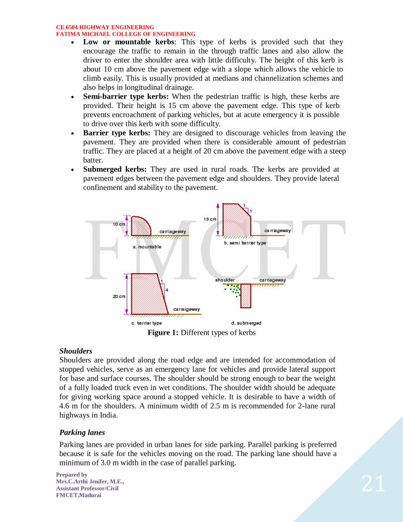
CE 6504 HIGHWAY ENGINEERING
FATIMA MICHAEL COLLEGE OF ENGINEERING
Prepared by
MrsCArthi Jenifer ME
Assistant ProfessorCivil
FMCETMadurai 21
Low or mountable kerbs This type of kerbs is provided such that they
encourage the traffic to remain in the through traffic lanes and also allow the
driver to enter the shoulder area with little difficulty The height of this kerb is
about 10 cm above the pavement edge with a slope which allows the vehicle to
climb easily This is usually provided at medians and channelization schemes and
also helps in longitudinal drainage
Semi-barrier type kerbs When the pedestrian traffic is high these kerbs are
provided Their height is 15 cm above the pavement edge This type of kerb
prevents encroachment of parking vehicles but at acute emergency it is possible
to drive over this kerb with some difficulty
Barrier type kerbs They are designed to discourage vehicles from leaving the
pavement They are provided when there is considerable amount of pedestrian
traffic They are placed at a height of 20 cm above the pavement edge with a steep
batter
Submerged kerbs They are used in rural roads The kerbs are provided at
pavement edges between the pavement edge and shoulders They provide lateral
confinement and stability to the pavement
Figure 1 Different types of kerbs
Shoulders Shoulders are provided along the road edge and are intended for accommodation of
stopped vehicles serve as an emergency lane for vehicles and provide lateral support
for base and surface courses The shoulder should be strong enough to bear the weight
of a fully loaded truck even in wet conditions The shoulder width should be adequate
for giving working space around a stopped vehicle It is desirable to have a width of
46 m for the shoulders A minimum width of 25 m is recommended for 2-lane rural
highways in India Parking lanes
Parking lanes are provided in urban lanes for side parking Parallel parking is preferred
because it is safe for the vehicles moving on the road The parking lane should have a
minimum of 30 m width in the case of parallel parking
CE 6504 HIGHWAY ENGINEERING
FATIMA MICHAEL COLLEGE OF ENGINEERING
Prepared by
MrsCArthi Jenifer ME
Assistant ProfessorCivil
FMCETMadurai 22
Bus-bays
Bus bays are provided by recessing the kerbs for bus stops They are provided so that
they do not obstruct the movement of vehicles in the carriage way They should be at
least 75 meters away from the intersection so that the traffic near the intersections is not
affected by the bus-bay
Service roads Service roads or frontage roads give access to access controlled highways like freeways
and expressways They run parallel to the highway and will be usually isolated by a
separator and access to the highway will be provided only at selected points These roads
are provided to avoid congestion in the expressways and also the speed of the traffic in
those lanes is not reduced
Drainage
The pavement surface should be absolutely impermeable to prevent seepage of water into
the pavement layers Further both the geometry and texture of pavement surface should
help in draining out the water from the surface in less time
Footpath
Footpaths are exclusive right of way to pedestrians especially in urban areas They are
provided for the safety of the pedestrians when both the pedestrian traffic and vehicular
traffic is high Minimum width is 15 meter and may be increased based on the traffic
The footpath should be either as smooth as the pavement or more smoother than that to
induce the pedestrian to use the footpath
Right of way
Right of way (ROW) or land width is the width of land acquired for the road along its
alignment It should be adequate to accommodate all the cross-sectional elements of the
highway and may reasonably provide for future development To prevent ribbon
development along highways control lines and building lines may be provided Control
line is a line which represents the nearest limits of future uncontrolled building activity
in relation to a road Building line represents a line on either side of the road between
which and the road no building activity is permitted at all The right of way width is
governed by
Width of formation It depends on the category of the highway and width of
roadway and road margins
Height of embankment or depth of cutting It is governed by the topography and
the vertical alignment
Side slopes of embankment or cutting It depends on the height of the slope soil
type etc
Drainage system and their size which depends on rainfall topography etc
Sight distance considerations On curves etc there is restriction to the visibility
on the inner side of the curve due to the presence of some obstructions like
building structures etc
Reserve land for future widening Some land has to be acquired in advance
CE 6504 HIGHWAY ENGINEERING
FATIMA MICHAEL COLLEGE OF ENGINEERING
Prepared by
MrsCArthi Jenifer ME
Assistant ProfessorCivil
FMCETMadurai 23
Table 2 Desig
n speed in as per IRC (ruling and minimum)
Steep
Type
Plain
Rolling
Hilly
40-30
NSampSH
100-80
80-65
50-40
MDR
80-65
65-50
40-30
30-20
25-20
ODR
65-50
50-40
30-25
25-20
VR
50-40
40-35
25-20
anticipating future developments like widening of the road
Table 1 No
right of way for open areas
Roadway width in m
Road
Plain and
Mountainous and
classification
steep terrain
rolling terrain
Open areas
45
24
NHSH
18
MDR
25
15
15
ODR
12
9
VR
Built-up areas
20
NHSH
30
MDR
20
15
ODR
15
12
9
VR
10
CE 6504 HIGHWAY ENGINEERING
FATIMA MICHAEL COLLEGE OF ENGINEERING
Prepared by
MrsCArthi Jenifer ME
Assistant ProfessorCivil
FMCETMadurai 24
Horizontal curve
The presence of horizontal curve imparts centrifugal force which is a reactive force
acting outward on a vehicle negotiating it Centrifugal force depends on speed and radius
of the horizontal curve and is counteracted to a certain extent by transverse friction
between the tyre and pavement surface On a curved road this force tends to cause the
vehicle to overrun or to slide outward from the centre of road curvature For proper
design of the curve an understanding of the forces acting on a vehicle taking a horizontal
curve is necessary Various forces acting on the vehicle are illustrated in the figure 1
Figure 1 Effect of horizontal curve They are the centrifugal force (P) acting outward weight of the vehicle (W) acting
downward and the reaction of the ground on the wheels ( and ) The centrifugal
force and the weight is assumed to be from the centre of gravity which is at h units above
the ground Let the wheel base be assumed as b units The centrifugal force in
is given by
(1)
where is the weight of the vehicle in is the speed of the vehicle in is
the acceleration due to gravity in and is the radius of the curve in
The centrifugal ratio or the impact factor is given by
CE 6504 HIGHWAY ENGINEERING
FATIMA MICHAEL COLLEGE OF ENGINEERING
Prepared by
MrsCArthi Jenifer ME
Assistant ProfessorCivil
FMCETMadurai 25
(1)
The centrifugal force has two effects A tendency to overturn the vehicle about the outer
wheels and a tendency for transverse skidding Taking moments of the forces with
respect to the outer wheel when the vehicle is just about to override
At the equilibrium over turning is possible when
and for safety the following condition must satisfy
(2)
The second tendency of the vehicle is for transverse skidding ie When the the
centrifugal force is greater than the maximum possible transverse skid resistance due to
friction between the pavement surface and tyre The transverse skid resistance (F) is
given by
where and is the fractional force at tyre and and is the reaction at
tyre and is the lateral coefficient of friction and is the weight of the vehicle
This is counteracted by the centrifugal force (P) and equating
At equilibrium when skidding takes place (from equation1)
and for safety the following condition must satisfy
CE 6504 HIGHWAY ENGINEERING
FATIMA MICHAEL COLLEGE OF ENGINEERING
Prepared by
MrsCArthi Jenifer ME
Assistant ProfessorCivil
FMCETMadurai 26
(3)
Equation 2 and 3 give the stable condition for design If equation 2 is violated the vehicle
will overturn at the horizontal curve and if equation 3 is violated the vehicle will skid at
the horizontal
Curve Analysis of super-elevation
Super-elevation or cant or banking is the transverse slope provided at horizontal curve to
counteract the centrifugal force by raising the outer edge of the pavement with respect to
the inner edge throughout the length of the horizontal curve When the outer edge is
raised a component of the curve weight will be complimented in counteracting the effect
of centrifugal force In order to find out how much this raising should be the following
analysis may be done The forces acting on a vehicle while taking a horizontal curve with
super elevation is shown in figure 1
Figure 1 Analysis of super-elevation
Forces acting on a vehicle on horizontal curve of radius at a speed of are
the centrifugal force acting horizontally out-wards through the center of
gravity
the weight of the vehicle acting down-wards through the center of gravity and
the friction force between the wheels and the pavement along the surface
inward
CE 6504 HIGHWAY ENGINEERING
FATIMA MICHAEL COLLEGE OF ENGINEERING
Prepared by
MrsCArthi Jenifer ME
Assistant ProfessorCivil
FMCETMadurai 27
At equilibrium by resolving the forces parallel to the surface of the pavement we get where
friction
is the weight of the vehicle is the centrifugal force is the coefficient of
is the transverse slope due to superelevation Dividing by we get
CE 6504 HIGHWAY ENGINEERING
FATIMA MICHAEL COLLEGE OF ENGINEERING
Prepared by
MrsCArthi Jenifer ME
Assistant ProfessorCivil
FMCETMadurai 28
Step 1
Find for 75 percent of design speed neglecting ie
Step 2
If then else if go to step 3
Step 3
Find for the design speed and max ie If
then the maximum is safe for the design speed else go to
step 4
Step 4
Find the allowable speed for the maximum and
If then the design is adequate otherwise use speed adopt
control measures or look for speed control measures
Maximum and minimum super-elevation
Depends on (a) slow moving vehicle and (b) heavy loaded trucks with high CG IRC
specifies a maximum super-elevation of 7 percent for plain and rolling terrain while that
of hilly terrain is 10 percent and urban road is 4 percent The minimum super elevation is
2-4 percent for drainage purpose especially for large radius of the horizontal curve
Attainment of super-elevation
1 Elimination of the crown of the cambered section by
1 Rotating the outer edge about the crown The outer half of the cross slope
is rotated about the crown at a desired rate such that this surface falls on
the same plane as the inner half
2 Shifting the position of the crown This method is also known as diagonal
crown method Here the position of the crown is progressively
shifted outwards thus increasing the width of the inner half of cross section
progressively
2 Rotation of the pavement cross section to attain full super elevation byThere are
two methods of attaining super elevation by rotating the pavement
1 Rotation about the center line The pavement is rotated such that the inner
edge is depressed and the outer edge is raised both by half the total amount
of super elevation ie by with respect to the centre
2 Rotation about the inner edge Here the pavement is rotated raising the
outer edge as well as the centre such that the outer edge is raised by the
full amount of super elevation with respect to the inner edge
Horizontal Transition Curves
CE 6504 HIGHWAY ENGINEERING
FATIMA MICHAEL COLLEGE OF ENGINEERING
Prepared by
MrsCArthi Jenifer ME
Assistant ProfessorCivil
FMCETMadurai 29
Transition curve is provided to change the horizontal alignment from straight to circular
curve gradually and has a radius which decreases from infinity at the straight end
(tangent point) to the desired radius of the circular curve at the other end (curve point)
There are five objectives for providing transition curve and are given below
1 to introduce gradually the centrifugal force between the tangent point and the
beginning of the circular curve avoiding sudden jerk on the vehicle This
increases the comfort of passengers
2 to enable the driver turn the steering gradually for his own comfort and security
3 to provide gradual introduction of super elevation and
4 to provide gradual introduction of extra widening
5 to enhance the aesthetic appearance of the road
Type of transition curve
Different types of transition curves are spiral or clothoid cubic parabola and Lemniscate
IRC recommends spiral as the transition curve because
1 it fulfills the requirement of an ideal transition curve that is
1 rate of change or centrifugal acceleration is consistent (smooth) and
2 radius of the transition curve is at the straight edge and changes to at
the curve point ( ) and calculation and field implementation is
very easy
Length of transition curve The length of the transition curve should be determined as the maximum of the following
three criteria rate of change of centrifugal acceleration rate of change of super elevation
and an empirical formula given by IRC Rate of change of centrifugal acceleration
At the tangent point radius is infinity and hence centrifugal acceleration is zero At the
end of the transition the radius R has minimum value R The rate of change of
centrifugal acceleration should be adopted such that the design should not cause
discomfort to the drivers If is the rate of change of centrifugal acceleration it can be
written as
Therefore the length of the transition curve in is
CE 6504 HIGHWAY ENGINEERING
FATIMA MICHAEL COLLEGE OF ENGINEERING
Prepared by
MrsCArthi Jenifer ME
Assistant ProfessorCivil
FMCETMadurai 30
(1)
where is the rate of change of centrifugal acceleration given by an empirical formula
suggested by by IRC as below
(2) 2 Rate of introduction of super-elevation
Raise ( ) of the outer edge with respect to inner edge is given by
The rate of change of this raise from to is achieved
gradually with a gradient of in over the length of the transition curve (typical range
of is 60-150) Therefore the length of the transition curve is
(3)
3 By empirical formula
IRC suggest the length of the transition curve is minimum for a plain and rolling terrain
(4)
and for steep and hilly terrain is
(5)
CE 6504 HIGHWAY ENGINEERING
FATIMA MICHAEL COLLEGE OF ENGINEERING
Prepared by
MrsCArthi Jenifer ME
Assistant ProfessorCivil
FMCETMadurai 31
and the shift as
(
6
) The length of the transition curve is the maximum of
equations 1 3 and 4or5 ie
(
7
Case (a)
For single lane roads
(
1
)
Therefore
(
2
)
Figure 1 Set-back for single lane roads (
CE 6504 HIGHWAY ENGINEERING
FATIMA MICHAEL COLLEGE OF ENGINEERING
Prepared by
MrsCArthi Jenifer ME
Assistant ProfessorCivil
FMCETMadurai 32
For multi lane roads if is the distance between centerline of the road and the centerline
of the inner lane then
(3)
(4)
Figure 2 Set-back for multi-lane roads ( )
Case (a)
For single lane roads
(1)
Therefore
(2)
Gradient
Gradient is the rate of rise or fall along the length of the road with respect to the
horizontal While aligning a highway the gradient is decided for designing the vertical
curve Before finalizing the gradients the construction cost vehicular operation cost and
the practical problems in the site also has to be considered Usually steep gradients are
avoided as far as possible because of the difficulty to climb and increase in the
CE 6504 HIGHWAY ENGINEERING
FATIMA MICHAEL COLLEGE OF ENGINEERING
Prepared by
MrsCArthi Jenifer ME
Assistant ProfessorCivil
FMCETMadurai 33
construction cost More about gradients are discussed below
Effect of gradient
The effect of long steep gradient on the vehicular speed is considerable This is
particularly important in roads where the proportion of heavy vehicles is significant Due
to restrictive sight distance at uphill gradients the speed of traffic is often controlled by
these heavy vehicles As a result not only the operating costs of the vehicles are
increased but also capacity of the roads will have to be reduced Further due to high
differential speed between heavy and light vehicles and between uphill and downhill
gradients accidents abound in gradients
Representation of gradient
The positive gradient or the ascending gradient is denoted as and the negative gradient as The deviation angle is when two grades meet the angle which
measures the change of direction and is given by the algebraic difference between the two
grades
steep gradient while 1 in 50 = 2 representation is illustrated in the figure 1
Example 1 in 30 = 333 is a
is a flatter gradient The gradient
CE 6504 HIGHWAY ENGINEERING
FATIMA MICHAEL COLLEGE OF ENGINEERING
Prepared by
MrsCArthi Jenifer ME
Assistant ProfessorCivil
FMCETMadurai 34
Figure 1 Representation of gradient
Types of gradient
Many studies have shown that gradient upto seven percent can have considerable effect
on the speeds of the passenger cars On the contrary the speeds of the heavy vehicles are
considerably reduced when long gradients as flat as two percent is adopted Although
flatter gradients are desirable it is evident that the cost of construction will also be very
high Therefore IRC has specified the desirable gradients for each terrain However it
may not be economically viable to adopt such gradients in certain locations steeper
gradients are permitted for short duration Different types of grades are discussed below
Ruling gradient
The ruling gradient or the design gradient is the maximum gradient with which the
designer attempts to design the vertical profile of the road This depends on the terrain
length of the grade speed pulling power of the vehicle and the presence of the horizontal
curve In flatter terrain it may be possible to provide flat gradients but in hilly terrain it
is not economical and sometimes not possible also The ruling gradient is adopted by the
designer by considering a particular speed as the design speed and for a design vehicle
with standard dimensions But our country has a heterogeneous traffic and hence it is not
possible to lay down precise standards for the country as a whole Hence IRC has
recommended some values for ruling gradient for different types of terrain
Limiting gradient
This gradient is adopted when the ruling gradient results in enormous increase in cost of
construction On rolling terrain and hilly terrain it may be frequently necessary to adopt
limiting gradient But the length of the limiting gradient stretches should be limited and
must be sandwiched by either straight roads or easier grades
Exceptional gradient
Exceptional gradient are very steeper gradients given at unavoidable situations They
should be limited for short stretches not exceeding about 100 metres at a stretch In
mountainous and steep terrain successive exceptional gradients must be separated by a
minimum 100 metre length gentler gradient At hairpin bends the gradient is restricted to
25
Critical length of the grade
The maximum length of the ascending gradient which a loaded truck can operate without
undue reduction in speed is called critical length of the grade A speed of 25 kmph is a
CE 6504 HIGHWAY ENGINEERING
FATIMA MICHAEL COLLEGE OF ENGINEERING
Prepared by
MrsCArthi Jenifer ME
Assistant ProfessorCivil
FMCETMadurai 35
reasonable value This value depends on the size power load grad-ability of the truck
initial speed final desirable minimum speed
Minimum gradient
This is important only at locations where surface drainage is important Camber will take
care of the lateral drainage But the longitudinal drainage along the side drains require
some slope for smooth flow of water Therefore minimum gradient is provided for
drainage purpose and it depends on the rain fall type of soil and other site conditions A
minimum of 1 in 500 may be sufficient for concrete drain and 1 in 200 for open soil
drains are found to give satisfactory performance Sight distance available from a point is the actual distance along the road surface which a driver
from a specified height above the carriage way has visibility of stationary or moving objects
Sight distance required by drivers applies to both geometric design of highways and for
traffic control The sight distance situations are considered in the design
i) Stopping or absolute minimum sight distance
ii) Safe overtaking or passing sight distance
iii) Safe sight distance for entering into uncontrolled intersections
Apart from the three situations mentioned above the following sight distance are considered by the
IRC in highway design
Intermediate sight distance
This is defined as twice the stopping sight distance when overtaking sight distance
cannot be provided intermediate sight distance is provided to give limited overtaking opportunities
to fast vehicles
Head light sight distance
This is the distance visible to a driver during night driving under the illumination of the
vehicle head lights
Stopping sight distance
The minimum sight distance available on a highway at any spot should be of sufficient
length to stop a vehicle traveling at design speed safely without collision with any other obstruction
The absolute minimum sight distance is therefore equal to the stopping sight distance
which is also sometimes called nonpassing sight distance The sight distance available on a road to a
driver at any instance depends on
i) Features of the road
ii) Height of the drivers eye above the road surface
iii) Height of the object above the road surface
The distance within which a motor vehicle can be stopped depends upon the factors listed below
a) Total reactions time of the driver
b) Speed of vehicle
c) Efficiency of breaks
d) Frictional resistance between the road and tyres
e) Gradient of the road
Total reaction time
) Reaction time of the driver is the time taken from the instant the object is visible to the
driver to the instant the brakes are effectively applied
) The total reaction time may be split up into two parts
CE 6504 HIGHWAY ENGINEERING
FATIMA MICHAEL COLLEGE OF ENGINEERING
Prepared by
MrsCArthi Jenifer ME
Assistant ProfessorCivil
FMCETMadurai 36
i) Perception time
ii) Brake reaction time
PIEV theory
According to this theory the total reaction time of the driver is split into four parts
i) Perception
ii) Intellection
iii) Emotion
iv) Volition
Speed of Vehicle
The stopping distance depends very much on the speed of the vehicle first during the
total reaction time of the driver the distance moved by the vehicle will depend on the speed
Efficiency of brakes
The braking efficiency is said to be 100 percent if the wheels are fully licked preventing
them from rotating on application of the brakes This will result in 100 percent skidding which is
normally undesirable except in utmost emergency
Frictional resistance between road and tyres
The frictional resistance developed between road and tyres or the skid resistance depends
on the type and condition of the road surface and the tyres IRC has specified a design friction
coefficient of 035 to 04 depending upon the speed to be used for finding the braking distance in the
calculation of stopping sight distance
Analysis of stopping distance
i) The distance traveled by the vehicle during the total reaction time known as lag
distance
ii) The distance traveled by the vehicle after the application of the brakes is known as
braking distance
Overtaking sight distance
The minimum distance open to the vision of the driver of a vehicle intending to overtake
slow vehicle ahead with safety against the traffic of opposite direction is known as the minimum
overtaking sight distance(OSD) or Safe passing sight distance available
The overtaking sight distance is the distance measured along the center of the road which
a driver with his eye level 12m above the road surface can see the top of an object 12m above the
road surface
Some of the important factors on which the minimum overtaking sight distance required
a) Speed of
i) overtaking vehicle
ii) overtaken vehicle
iii) The vehicle coming from opposite direction
b) Distance between the overtaking and overtaken vehicles the minimum spacing
depends on the steeds
a) Skill and reaction time of the driver
b) Rate of acceleration of overtaking vehicle
c) Gradient of the road
Criteria for sight distance requirements on highway
) The absolute minimum sight distance required throughout the length of the road is the
SSD which should invariably be provided at all places
CE 6504 HIGHWAY ENGINEERING
FATIMA MICHAEL COLLEGE OF ENGINEERING
Prepared by
MrsCArthi Jenifer ME
Assistant ProfessorCivil
FMCETMadurai 37
) On horizontal curves the obstruction on the inner side of the curves should be cleared
to provide the required set back distance and absolute minimum sight distance
) On vertical summit curves the sight distance requirement may be fulfilled by proper
design of the vertical alignment
Hairpin bent
TYPES OF CURVES ON HILL ROADS
The following are the important types of curves provided on hill Roads-
1 Hair-Pin Curves
2 Salient Curves
3 Re-entrant Curves 1 Hair-pin curves - The curve in a hill road which changes its direction through an angle of 180
degree or so down the hill on the same side is known as hair-pin curve
A Hair-Pin Bend
This curve is so called because it conforms to the shape of a hair-pin The bend so formed at the
hair-pin curve in a hill road is known as hair-pin bend This type of curve should be located on a
hill side having the minimum slope and maximum stability It must also be safe from view point of
landslides and ground water Hair-pin bends with long arms and farther spacing are always
preferred They reduce construction problems and expensive protective works Hair-pin curves or
bends of serpentine nature are difficult to negotiate and should therefore be avoided as far as
possible
Salient curves - The curves having their convexity on the outer edges of a hill road are called
salient curves The centre of curvature of a salient curve lies towards the hill side This type of curve
occurs in the road length constructed on the ridge of a hill the bend so formed at the salient curve in
a hill road known as corner bend
Salient curves are very dangerous for fast moving traffic At such a curve or at corner bend the
portion of projecting hill side is usually cut down to improve the visibility as shown in fig (Re-
entrant curve) The outer edge of the road at such a curve is essentially provided with a parapet wall
for protection of the vehicles from falling down the hill slope
CE 6504 HIGHWAY ENGINEERING
FATIMA MICHAEL COLLEGE OF ENGINEERING
Prepared by
MrsCArthi Jenifer ME
Assistant ProfessorCivil
FMCETMadurai 38
3 Re-entrant curves - The curves having their convexity on the inner edge of a hill road are called
re-entrant curves
Re-entrant curves
The centre of curvature of a re-entrant curves lies away from the hill side This type of curve occurs
in the road length constructed in the calley of a hill
These curves are less dangereous as they provide adequate visibility to the fast moving traffic At
such curves the parapet wall is provided only for safety of fast moving traffic
CE 6504 HIGHWAY ENGINEERING
FATIMA MICHAEL COLLEGE OF ENGINEERING
Prepared by
MrsCArthi Jenifer ME
Assistant ProfessorCivil
FMCETMadurai 39
UNIT ndash III DESIGN OF RIGID AND FLEXIBLE PAVEMENTS
COMPARISON OF RIGID AND FLEXIBLE PAVEMENTS
The comparisons are
i) Design precision
A cement concrete pavement is amerable to a much more precise structural analysis
than a flexible pavement Flexible pavements designs are mainly empirical Computer aided analysis
of layered system is making the flexible pavement design more exact than hitherto
ii) Life
) Cement concrete slabs of a thin section constructed in the early 1940rsquos are still in
existence in India though many of them have cracked badly and a few of them have been ripped
open and rebuilt in recent ties
) A major project in cement concrete road construction between Agra and Mathura It can
safely be said that a well-designed concrete slab has a life of about 40 years
) Compared to this the life of a flexible pavement generally varies from 10 to 20 years
iii) Maintenance
) A well-designed cement concrete pavement needs very little maintenance The only
maintenance needed is I respect of joints
) The surface is unaffected by spillage of oil and lubricants bituminous surfaces on the
other hand need great inputs in maintenance
) The surface is affected by spillage of oil and lubricants The surface is also affected by
natural weathering agents like air water ad temperature changes
) A cement concrete pavement on the other hand needs a small amount for maintaining
joints
iv) Initial cost
) The argument so far used against a cement concrete slab is that it is much more costly
than a flexible pavement
) The latter specifications no doubt represent the rock-bottom needs of a road in India but
these specifications can hardly provide a smooth and durable surface
v) Stage construction ) Road construction is generally done adopting a policy of stage construction especially for
low volume roads As traffic grows additional layers in the form of water bound macadam and
superior surfacing are added on
) Initial outlay is minimum and additional outlays are in keeping with traffic growth This is
a great advantage when dealing with new roads in an atmosphere of austerity
vi) Availability of materials
) Cement bitumen stone aggregates and gravelsand are the major materials involved in
pavement Construction Cement has been in serious short supply in the country for the past many
decades
) Bitumen is also not available plentifully in India There is also the danger of the entire oil
reserves in the world shrinking during the next two or three decades
) In locations where stone aggregates are scarce cement concrete may have an advantage
for flexible pavements
vii) Surface characterstics
CE 6504 HIGHWAY ENGINEERING
FATIMA MICHAEL COLLEGE OF ENGINEERING
Prepared by
MrsCArthi Jenifer ME
Assistant ProfessorCivil
FMCETMadurai 40
) A good cement concrete surface is smooth and free from rutting potholes and
corrugations In a bituminous surface it is only the asphaltic concrete surface that can give
comparable rideablity
) A well-constructed cement concrete pavement surface can have a permanent nonskid
surface A bituminous surface can also be designed to have a good skid resistant surface
viii) Utility location
) In cement concrete slabs proper thought has to be given to locate utilities such as water
pipes telephone lines and electric cables
) It is difficult to rip open the slab and restore it to be the original condition if any changes
in the utilities lines are to be made
ix) Glame and night visibility
) Concrete pavements have a gray color which can cause glam under sunlight Colored
cement can reduce the grave
) On the other hand bituminous roads need more street lighting
x) Traffic dislocation during construction
) A cement concrete pavement requires 28 days before it can be thrown open to traffic On
the other hand a bituminous surface can be thrown open to traffic shortly after it is rolled
xi) Environmental considerations during construction
) The process of heating of bitumen and aggregates and mixing them together on hot mix
plants can prove to be much more hazardous to the environment than cement concrete construction
where no heating of any material is involved
xii) Overall economy on a life cycle basis
) A good road is costly to construct but once constructed such a road requires little
maintenance and results in savings in vehicle operating costs
) The comparative economy of a flexible pavement and a rigid pavement has proved that on
overall economic considerations
Types of pavement structure
Based on the structural behavior pavements are generally classified into three
categories
i) Flexible pavements
ii) Rigid pavements
iii) Semi rigid pavements
Flexible pavements
) Flexible pavements are those which on the whole have low or negligible flexural
strength and are rather flexible in their structural action under the loadsThe flexible pavement
layers reflect the deformation of the lower layers on to the surface of the layer
) A flexible pavement consists of four components(i) Soil subgrade (ii) sub base
course (iii) base course (iv) Surface course
CE 6504 HIGHWAY ENGINEERING
FATIMA MICHAEL COLLEGE OF ENGINEERING
Prepared by
MrsCArthi Jenifer ME
Assistant ProfessorCivil
FMCETMadurai 41
) The flexible pavement layers transmit the vertical or compressive stresses to the lower layers
by grain to grain transfer through the points of contact in the granular structure A well
compacted granular structure consisting of strong added aggregate can transfer the compressive
stresses
) The load spreading ability of this layer therefore depends on the type of the materials and mix
design factors Bituminous concrete is one of the best flexible pavements layer materials Other
materials which fall under the group are all granular materials with or without bituminous
binder granular base and sub base course materials
) The vertical compressive stress is maximum on the pavement surface directly under the wheel
and is equal to the contact pressure under the wheel The flexible pavement may be constructed
in a number of layers and the top layer has to be strongest as the highest compressive stresses
) Flexible pavements are commonly designed using empirical design charts or equations taking
into account some of the design factors there are also semi empirical and theoretical design
methods
Rigid pavements
) Rigid pavements are those which possess note flexural strength or flexural rigidity
The stresses are not transferred from grain to grain to the lower layers as in the ease of flexible
pavements layers
) The rigid pavements are made of Portland cement concrete plain reinforced or
prestressed concrete The plain cement concrete slabs are expected to take up about 40 kgcm2
flexural stress
) The rigid pavement has the slab action and is capable of transmitting the wheel
load stresses through a wider area below The main point of difference in the structural behavior
of rigid pavement as compared to the flexible pavement is that the critical condition of stress in
the rigid pavement is the maximum flexural stress occurring in the slab due to wheel load and
the temperature changes whereas in the flexible pavement
) As the rigid pavement slab has tensile strength tensile stresses are developed due
to the bending of the slab under wheel load and temperature variations Thus the types of
stresses developed and their distribution within the cement concrete slab are quirt different
) The cement concrete pavement slab can very well serve as a wearing surface as
well an effective base course The rigid pavement structure consists of a cement concrete slab
below which a granular base or sub base course may be provided
) Though the cement concrete slab can also be laid directly over the soil subgrade
consists of fine grained soil
) the rigid pavements are usually designed and the stresses are analyzed using the
elastic theory assuming the pavements as a n elastic plate resting over an elastic or a viscous
foundation
Semi rigid pavements
) when bonded materials like the pozzolanic concrete lean cement concrete or soil
cement are used in the base course or sub base course layer the pavement layer has considerably
higher flexural strength than the common flexible pavement layers
) when this intermediate class of materials are used in the base or sub base course
layer of the pavements they are called semi rigid pavements
CE 6504 HIGHWAY ENGINEERING
FATIMA MICHAEL COLLEGE OF ENGINEERING
Prepared by
MrsCArthi Jenifer ME
Assistant ProfessorCivil
FMCETMadurai 42
) This third category of semi rigid pavement are either designed as flexible
pavements with some correction factors to find the thickness requirements based on experience
or by using a new design approach
) The semi rigid pavement materials have low resistance to impact and abrasion and
therefore are usually provided with flexible pavement surface course
Various functions of pavement components
The functions are
Soil sub grade and its evaluation
) The soil sub grade is a layer of natural soil prepared to receive the layers of pavement
materials placed over it It is essential that at no time the soil sub grade is overstressed it means that
the pressure transmitted on the top of the sub grade is within the allowable limit
) Many tests are known for measuring the strength properties of the sub grades Some of the
tests have been standardized for the use The common strength test for the evaluation of soil
subgrade is
i) California bearing ratio test
ii) California resistance value test
iii) Triaxial compression test
iv) Plate bearing test
CALIFORNIA BEARING RATIO (CBR) TEST
It is evolved for the empirical method of flexible pavement design The CBR test is carried
out either in the laboratory on prepared specimens or in the field by taking in situ measurements
California resistance value
It is found by using have been stabliometerThis test is used in an empirical method of
flexible pavement design based on soil strength
Triaxial test
It is the most important soil strength but still the test is not very commonly used in structural
design of pavements
Plate bearing test
It is carried out using a relatively large diameter plate to evaluate the load supporting
capacity of supporting power of the pavement layers The results are plate bearing tests are used in
flexible pavement design method like McLeod method on based on layer system analysis by
brumister
Sub base and base courses and their evaluation
) There layers are made of broken stones bound or unbound aggreagatesome times in sub
base course a layer of stabilized soil(or) Selected granular soil is also used
) however at the sub base course it is desirable to use smaller size graded aggregates When
the sub grade consists of fine grained soil and when the pavement carries heavy wheel loads
CE 6504 HIGHWAY ENGINEERING
FATIMA MICHAEL COLLEGE OF ENGINEERING
Prepared by
MrsCArthi Jenifer ME
Assistant ProfessorCivil
FMCETMadurai 43
) Sub base course primarily has the similar function as of the base course and is provided
with inferior materials than of base course Base courses are used under rigid pavement for
i) Preventing pumping
ii) Protecting the sub grade against frost action
) Thus the fundamental purpose of abase course and sub base course is to provide a stress
transmitting medium to spread the surface wheel loads in such manner
) The sub base and base course layers may be evaluated by suitable strength or stability test
like plate bearing CBR test
WEARING COURSE AND ITS EVALUATION
) The purpose of the wearing course is to give a smooth riding surface that is dense It
resists pressure exerted by tyres and takes up wear and tear due to the traffic
) Wearing course also offers a water tight layer against the surface water infiltration The
flexible pavement normally a bituminous surfacing is used as a wearing course
) In rigid pavements the cement concrete acts like a base course as well as wearing course
Most popular test in use is marshal stability test where in the optimum content of bitumen binder is
worked out based on the stability density
) Plate bearing test and Bankelman beam test are also sometimes made use of for evaluating
the wearing course and the pavement as a whole
Various factors to be considered in pavement design and the significance
Pavement design consists of two parts
i) Mix design of materials to be used in each pavement component layer Thickness design of the
pavement and the component layers
The various factors to be considered for the design of pavements are given below
i) Design wheel load
ii) Sub grade soil
iii) Climatic factors
iv) Pavement component layers
v) Environmental factors
vi) Special factors in the design of different types of pavements
Design wheel load
The various wheel load factors to be considered in pavement design are
i) Maximum wheel load
ii) Contact pressure
iii) Dual or multiple wheel loads
iv) Repetition of loads
Maximum wheel load
The wheel load configurations are important to know the way in which the loads of a given
vehicle are applied on the pavement surface
) For highways the maximum legal axle load as specified by Indian road congress is 8170
kg with a maximum equivalent single wheel load of 4085 kg
) The evaluation for vertical stress computations under a uniformly distribute of circular
load based on Boussineqrsquos theory is given by
CE 6504 HIGHWAY ENGINEERING
FATIMA MICHAEL COLLEGE OF ENGINEERING
Prepared by
MrsCArthi Jenifer ME
Assistant ProfessorCivil
FMCETMadurai 44
2
322
3
1
za
zpz
σz = vertical stress at depth z
P= surface pressure
Z=depth at which σz computed
A=radius of loaded area
Contact pressure
Generally the wheel load is assumed to be distributed over a circular area But by
measurement of the imprints of tyers with different load and inflation pressures Three terms in use
with reference to tyre pressure are
Tyre pressure
Inflation pressure
Contact pressure
Tyre pressure and inflation pressure mean exactly the same the contact pressure is found to be more
than tyre pressure when the tyre pressure is less than 7 kgm2 and it is vice versa when the tyre
pressure exceeds this value
Contact pressure can be measured by the relationship
Load on wheel
Contact pressure = ----------------------------------------
Contact area or area of imprint
The general variation between the tyre pressure and measured contact pressure is shown in this fig
The ratio of contact pressure to type pressure is defined as rigidity factor Thus value of rigidity
factor is 10 for an average tyre pressure of 7 Kgcm2This value is higher than unity for lower type
pressures and less than unity for tyre pressures higher than 7 kgcm2
Equivalent single wheel load (ESWL)
) The maximum wheel load within the specified limit and to carry greater load it is
necessary to provide dual wheel assembly to the rear axles of the roads vehicles
) In other words the pressure at a certain depth below the pavement surface cannot be
obtained by numerically adding the pressure caused by any one wheel
) The effect is in between the single load and two times load carried by one wheel The load
dispersion is assumed to be at an angle of 450In the dual wheel load assembly let d be the clear gap
between the two wheels S be the spacing between the centers of the wheels and a be the radius of
the circular contact area of each wheel Then S = (d + 2a)
) ESWL may be determined based on either equivalent deflection or equivalent stress
criterianMultiple wheel loads are convert to ESWL and this value is used in pavement design The
ESWL is usually determined by the equivalent stress criterion using a simple graphical method
CE 6504 HIGHWAY ENGINEERING
FATIMA MICHAEL COLLEGE OF ENGINEERING
Prepared by
MrsCArthi Jenifer ME
Assistant ProfessorCivil
FMCETMadurai 45
) A straight line relationship is assumed between ESWL and depth on log scales For
determining ESWL the plot is made as shown in fig
) Two points A and B are plotted on the log-log graph with coordinates of A (Pd2) and
B(2p2s)line AB is a plot which is the focus of points where any single wheel load is equivalent to a
certain set of dual wheels
) To Calculate the ESWL for a dual assembly it is essential to estimate a design thickness of
the pavement If the design thickness so obtained is equal to the estimated thickness then the ESWL
calculations could be considered as correct Otherwise trials are made
) In heavy trucks and trailers the load on each wheel may be further reduced by multiple
wheels and tandem axles
Repetition of loads
) The deformation of load pavement (or) sub grade due to a single application of wheel load
may be small It required carrying out traffic surveys for accounting the factor of repetitions for
wheel loads in the design of pavement
) Data collected are converted to some constant equivalent wheel loads Equivalent wheel
load is a single load equivalent to the repeated applications of any particular wheel load on a
pavement which requires the same thickness and strength of pavements
) McLeod has given a procedure for evolving equivalent load factors for designing flexible
pavements
Various methods of flexible pavement design
) The flexible pavement is built with number of layers In the design process it is to be
ensured that under the application of load none of the layers is overstressed
) The maximum intensity of stresses occurs in the top layer of the pavement The
magnitude of load stresses reduces at lower layers
) In the design of flexible pavements it has yet not been possible to have a rational design
method wherein design process and service behavior of the pavement can be expressed by
mathematical laws
) Flexible pavement design methods are accordingly either empirical or semi empirical In
these methods the knowledge and experience gained on the behavior of the pavements in the past
are usefully utilized
Various approaches of flexible pavement design may be thus classified into three groups
i) Empirical method
ii) Semi-empirical or Semi theoretical method
iii) Theoretical method
) Empirical methods are either based on physical properties or strength parameters of soil
sub grade When the design is based on stress strain function and modified base on experience it
may be called semi-empirical or semi-theoretical There are design methods based on theoretical
analysis and mathematical computations
Out of the flexible pavement design method available is
i) Group index method
ii) California bearing ratio method
iii) California R value (or) Stabiliometer method
iv) Triaxial test method
CE 6504 HIGHWAY ENGINEERING
FATIMA MICHAEL COLLEGE OF ENGINEERING
Prepared by
MrsCArthi Jenifer ME
Assistant ProfessorCivil
FMCETMadurai 46
v) McLeod method
vi) Burmister method
Group index method
) Group index value is an arbitrary index assigned to the soil type in numerical equations
base on the percent fines liquid limit and plasticity index
) The design chart for group index method for determining the pavement thickness is given
in fig
The traffic volume in this method is divided in three groups
Traffic volume No of vehicles per day
Light Less than 50
Medium 50 to 300
Heavy Over 300
The design of the pavement thickness by this method first the G1 value of the soil is found the
anticipated traffic is estimated and is designated as light medium or heavy as indicated
The G1 method of pavement design is essentially an empirical method based on physical properties
of the subgrade soil This method does not consider the strength characteristics of the subgrade soil
and therefore is open to question regarding the reliability of the design based on the index properties
of the soil only
California bearing ratio method
) California division of highways in the USA developed CBR method for
pavement design The majority of design curves developed later are base on the original curves
proposed by OJporter
) One of the chief advantages of CBR method is the simplicity of the test procedure
The CBR tests were carried out by the California state highway department on existing pavement
layers including subgrade sub base and base course
) Based on the extensive CBR test data collected on pavement which behaved
satisfactory and those which failed an empirical design chart was developed correlating the CBR
value and the pavement thickness The basis of the design chart is that a material with a given CBR
required a certain thickness of pavement layer as a cover
) A higher load needs a thicker pavement layer to protect the sub grade Design
curves correlating the CBR value with total pavement thickness cover were developed by the
California state highway department for wheel loads of 3175kg and 5443 kg representing light and
heavy traffic The design curves are shown in this fig
It is possible to extend the CBR design curves for various loading conditions nusing the expression
t= 2
1
1751
pCBRp
t=2
1
751
A
CBR
p
Hence
CE 6504 HIGHWAY ENGINEERING
FATIMA MICHAEL COLLEGE OF ENGINEERING
Prepared by
MrsCArthi Jenifer ME
Assistant ProfessorCivil
FMCETMadurai 47
t= pavement thickness cm
p=Wheel load kg
CBR= California bearing ratio percent
P=tyre pressure kgcm2
A= area of contactcm2
IRC Recommendations
a) The CBR tests should be performed on remoulded soils in the laboratory The specimens should
be prepared by static compaction wherever possible and otherwise by dynamic compaction
b) For the design of new roads the sub grade soil sample should be compacted at OMC to proctor
density whenever suitable compaction equipment
c) The CBR test samples may be soaked in water for four days period before testing the annual
rainfall is less than 50 cm and the water table is too deep to affect the sub grade and imperable
surfacing is provided to carrying out CBR test
d) If the maximum variations in CBR value of the three specimens exceed the specified limits the
design CBR should be average of at least six samples
e) The top 50 cm of sub grade should be compacted at least up to 95 to 100 percent of proctor
density
f) An estimate of the traffic should be carried by the road pavements at the end of expected in view
the existing traffic and probable growth rate of traffic
g) The traffic for the design is considered in units of heavy vehicles per day in both directions and is
divided into seven categories A to G The design thickness is considered applicable for single axle
loads up to 8200 kg and tandom axle loads up to 14500 kg
h) When sub base course materials contain substantial proportion of aggregates of size above 20mm
the CBR value of these materials would not be valid for the design of subsequent layers above them
The CBR method of pavement design gives the total thickness requirement of the pavement above a
sub grade and thickness value would remain the same quality of materials used in component layers
California resistance value method
) In this design method based on stabliometer R-value and cohesiometer C-value
Based on performance data it was established by pavement thickness varies directly with R value
and algorithm of load repetitions It varies inversely with fifth root of c valueThe expression for
pavement thickness is given by the empirical equation
T=
5
1
1 90
C
RTK
Hence
T=total thickness of pavement cm
K=Numerical constant 0166
T1=traffic index
R= stabiliometer resistance value
C=Cohesiometer value
CE 6504 HIGHWAY ENGINEERING
FATIMA MICHAEL COLLEGE OF ENGINEERING
Prepared by
MrsCArthi Jenifer ME
Assistant ProfessorCivil
FMCETMadurai 48
In the design of flexible pavements based on California resistance value method for the following
data are needed
) R-value of soil subgrade
) T1 value
) Equivalent C-value
) R value of soil subgrade is obtained from the test using stablio meterThe
computation of T1 value has been explained
Equivalent C-value
) The cohesion meter value c is obtained for each layer of pavement material
separately from tests However the composite or equivalent C-value of the pavement may be
estimated if the thickness of each component layer and the c-value of the material of the layer are
known
) while designing a pavement as the thickness of the pavement is not known it is
easier if the pavement is first assumed to consist of any one material like gravel base course with
known C-value
) Subsequently the individual thickness of each layer is converted in terms of gravel
equivalent by using relationship
5
1
1
2
2
1
C
C
t
t
) t1 and t2 are the thickness values of any two pavement layersc1 and c2 are their
corresponding cohesiometer values
CE 6504 HIGHWAY ENGINEERING
FATIMA MICHAEL COLLEGE OF ENGINEERING
Prepared by
MrsCArthi Jenifer ME
Assistant ProfessorCivil
FMCETMadurai 49
UNIT 4 MATERIAL AND MAINTENANCE
SUMMIT CURVE
Summit curves are vertical curves with gradient upwards They are formed when two
gradients meet as illustrated in figure 1 in any of the following four ways
1 When a positive gradient meets another positive gradient [figure 1a]
2 When positive gradient meets a flat gradient [figure 1b]
3 When an ascending gradient meets a descending gradient [figure 1c]
4 When a descending gradient meets another descending gradient [figure 1d]
Type of Summit Curve
Many curve forms can be used with satisfactory results the common practice has been to
use parabolic curves in summit curves This is primarily because of the ease with it can
be laid out as well as allowing a comfortable transition from one gradient to another
Although a circular curve offers equal sight distance at every point on the curve for very
small deviation angles a circular curve and parabolic curves are almost congruent
Furthermore the use of parabolic curves were found to give excellent riding comfort
Figure 1 Types of summit curves
Design Consideration
In determining the type and length of the vertical curve the design considerations are
comfort and security of the driver and the appearance of the profile alignment Among
these sight distance requirements for the safety are most important on summit curves
The stopping sight distance or absolute minimum sight distance should be provided on
these curves and where overtaking is not prohibited overtaking sight distance or
intermediate sight distance should be provided as far as possible When a fast moving
vehicle travels along a summit curve there is less discomfort to the passengers This is
because the centrifugal force will be acting upwards while the vehicle negotiates a
summit curve which is against the gravity and hence a part of the tyre pressure is
relieved Also if the curve is provided with adequate sight distance the length would be
sufficient to ease the shock due to change in gradient Circular summit curves are
identical since the radius remains same throughout and hence the sight distance From
CE 6504 HIGHWAY ENGINEERING
FATIMA MICHAEL COLLEGE OF ENGINEERING
Prepared by
MrsCArthi Jenifer ME
Assistant ProfessorCivil
FMCETMadurai 50
this point of view transition curves are not desirable since it has varying radius and so the
sight distance will also vary The deviation angles provided on summit curves for
highways are very large and so the simple parabola is almost congruent to a circular arc
between the same tangent points Parabolic curves are easy for computation and also it
had been found out that it provides good riding comfort to the drivers It is also easy for
field implementation Due to all these reasons a simple parabolic curve is preferred as
summit curve Length of the summit curve
The important design aspect of the summit curve is the determination of the length of the
curve which is parabolic As noted earlier the length of the curve is guided by the sight
distance consideration That is a driver should be able to stop his vehicle safely if there is
an obstruction on the other side of the road Equation of the parabola is given by
where where N is the deviation angle and is the length of the In
deriving the length of the curve two situations can arise depending on the uphill and
downhill gradients when the length of the curve is greater than the sight distance and the
length of the curve is greater than the sight distance
Let is the length of the summit curve is the SSDISDOSD is the deviation angle
drivers eye height (12 m) and the height of the obstruction then the length of the
summit curve can be derived for the following two cases The length of the summit curve
can be derived from the simple geometry as shown below
Case a Length of summit curve greater than sight distance( )
Figure 1 Length of summit curve ( )
The situation when the sight distance is less than the length of the curve is shown in
figure 1
CE 6504 HIGHWAY ENGINEERING
FATIMA MICHAEL COLLEGE OF ENGINEERING
Prepared by
MrsCArthi Jenifer ME
Assistant ProfessorCivil
FMCETMadurai 51
(1)
Case b Length of summit curve less than sight distance
The second case is illustrated in figure 1
Figure 1 Length of summit curve
CE 6504 HIGHWAY ENGINEERING
FATIMA MICHAEL COLLEGE OF ENGINEERING
Prepared by
MrsCArthi Jenifer ME
Assistant ProfessorCivil
FMCETMadurai 52
From the basic geometry one can write
(1)
Therefore for a given and to get minimum differentiate the above equation
with respect to and equate it to zero Therefore
Solving the quadratic equation for
(2)
Now we can substitute back to get the value of minimum value of for a given
and Therefore
Solving for
CE 6504 HIGHWAY ENGINEERING
FATIMA MICHAEL COLLEGE OF ENGINEERING
Prepared by
MrsCArthi Jenifer ME
Assistant ProfessorCivil
FMCETMadurai 53
(3) (4
CE 6504 HIGHWAY ENGINEERING
FATIMA MICHAEL COLLEGE OF ENGINEERING
Prepared by
MrsCArthi Jenifer ME
Assistant ProfessorCivil
FMCETMadurai 54
When stopping sight distance is considered the height of drivers eye above the road
surface ( ) is taken as 12 metres and height of object above the pavement surface ( )
is taken as 015 metres If overtaking sight distance is considered then the value of
drivers eye height ( ) and the height of the obstruction ( ) are taken equal as 12
metres
Valley curve
Valley curve or sag curves are vertical curves with convexity downwards They are
formed when two gradients meet as illustrated in figure 1 in any of the following four
ways
Figure 1 Types of valley curve
1 When a descending gradient meets another descending gradient [figure 1a]
2 When a descending gradient meets a flat gradient [figure 1b]
3 When a descending gradient meets an ascending gradient [figure 1c]
4 When an ascending gradient meets another ascending gradient [figure
Design considerations
There is no restriction to sight distance at valley curves during day time But visibility is
reduced during night In the absence or inadequacy of street light the only source for
visibility is with the help of headlights Hence valley curves are designed taking into
account of headlight distance In valley curves the centrifugal force will be acting
downwards along with the weight of the vehicle and hence impact to the vehicle will be
more This will result in jerking of the vehicle and cause discomfort to the passengers
Thus the most important design factors considered in valley curves are (1) impact-free
movement of vehicles at design speed and (2) availability of stopping sight distance
under headlight of vehicles for night driving
For gradually introducing and increasing the centrifugal force acting downwards the best
shape that could be given for a valley curve is a transition curve Cubic parabola is
generally preferred in vertical valley curves See figure 1
CE 6504 HIGHWAY ENGINEERING
FATIMA MICHAEL COLLEGE OF ENGINEERING
Prepared by
MrsCArthi Jenifer ME
Assistant ProfessorCivil
FMCETMadurai 55
Figure 1 Valley curve details
During night under headlight driving condition sight distance reduces and availability of
stopping sight distance under head light is very important The head light sight distance
should be at least equal to the stopping sight distance There is no problem of overtaking
sight distance at night since the other vehicles with headlights could be seen from a
considerable distance
Length of the valley curve
The valley curve is made fully transitional by providing two similar transition curves of
equal length The transitional curve is set out by a cubic parabola where
The length of the valley transition curve is designed based on two criteria
1 comfort criteria that is allowable rate of change of centrifugal acceleration is
limited to a comfortable level of about
2 safety criteria that is the driver should have adequate headlight sight distance at
any part of the country
Comfort criteria
The length of the valley curve based on the rate of change of centrifugal acceleration that
will ensure comfort Let is the rate of change of acceleration the minimum radius of
the curve is the design speed and is the time then is give
CE 6504 HIGHWAY ENGINEERING
FATIMA MICHAEL COLLEGE OF ENGINEERING
Prepared by
MrsCArthi Jenifer ME
Assistant ProfessorCivil
FMCETMadurai 56
For a cubic parabola the Value Safety criter Length of the valley curve for headlight distance may be determined for two conditions
(1) length of the valley curve greater than stopping sight distance and (2) length of the
valley curve less than the stopping sight distance of for length is given by
Case 1 Length of valley curve greater than stopping sight distance ( )
The total length of valley curve is greater than the stopping sight distance SSD The
sight distance available will be minimum when the vehicle is in the lowest point in the
valley This is because the beginning of the curve will have infinite radius and the bottom
of the curve will have minimum radius which is a property of the transition curve The
case is shown in figure 1
Figure 1 Valley curve case 1
From the geometry of the figure we have
CE 6504 HIGHWAY ENGINEERING
FATIMA MICHAEL COLLEGE OF ENGINEERING
Prepared by
MrsCArthi Jenifer ME
Assistant ProfessorCivil
FMCETMadurai 57
(1)
where is the deviation angle in radians is the height of headlight beam is the
head beam inclination in degrees and is the sight distance The inclination is 1
degree
Case 2 Length of valley curve less than stopping sight distance ( )
The length of the curve is less than SSD In this case the minimum sight distance is
from the beginning of the curve The important points are the beginning of the curve and
the bottom most part of the curve If the vehicle is at the bottom of the curve then its
headlight beam will reach far beyond the endpoint of the curve whereas if the vehicle is
at the beginning of the curve then the headlight beam will hit just outside the curve
Therefore the length of the curve is derived by assuming the vehicle at the beginning of
the curve The case is shown in figure 1
From the figure
(1) Note that the above expression is approximate and is satisfactory because in practice the gradients
are very small and is acceptable for all practical purposes We will not be able to know prior to
which case to be adopted Therefore both has to be calculated and the one which satisfies the
condition is adopted
1 Flexible pavement
2 Rigid pavement
Flexible pavement
These pavements reflect the deformation of sub grade and the subsequent layers to the
surface
Rigid pavement
The rigid characteristic of the pavement are associated with rigidity or flexural strength
CE 6504 HIGHWAY ENGINEERING
FATIMA MICHAEL COLLEGE OF ENGINEERING
Prepared by
MrsCArthi Jenifer ME
Assistant ProfessorCivil
FMCETMadurai 58
or slab action so the load is distributed over a wide area of sub grade soil
Flexible pavement Definition
These pavements reflect the deformation of sub grade and the subsequent layers to the
surface Flexible usually asphalt is laid with no reinforcement or with a specialized
fabric reinforcement that permits limited flow or repositioning of the roadbed under
ground changes
The design of flexible pavement is based on load distributing characteristic of the
component layers The black top pavement including water amp gravel bound macadam fall
in this category
Flexible pavement on the whole has low or negligible flexible strength flexible in their
structural action) The flexible pavement layers transmit the vertical or compressive
stresses to the lower layers by grain transfer through contact points of granular structure
The vertical compressive stress is maximum on the pavement surface directly under the
wheel load and is equal to contact pressure under the wheels Due to the ability to
distribute the stress to large area in the shape of truncated cone the stresses get decreased
in the lower layer
As such the flexible pavement may be constructed in a number of layers and the top
layer has to be strongest as the highest compressive stresses
To be sustained by this layer in addition to wear and tear the lower layer have to take
up only lesser magnitude of stress as there is no direct wearing action die to traffic loads
therefore inferior material with lower cast can be used in the lower layers
Rigid pavement Definition
The rigid characteristic of the pavement are associated with rigidity or flexural strength
or slab action so the load is distributed over a wide area of sub grade soil Rigid pavement
is laid in slabs with steel reinforcement
The rigid pavements are made of cement concrete either plan reinforced or prestressed
concrete
Critical condition of stress in the rigid pavement is the maximum flexural stress occurring in the slab due to wheel load and the temperature changes
Rigid pavement is designed and analyzed by using the elastic theory
CE 6504 HIGHWAY ENGINEERING
FATIMA MICHAEL COLLEGE OF ENGINEERING
Prepared by
MrsCArthi Jenifer ME
Assistant ProfessorCivil
FMCETMadurai 59
UNIT-5 EVALUATION AND MAINTENANCE OF PAVEMENTS
TRAFFIC PARAMETERS
Design life
Design life is the number of years (or number of standard axle repetitions) for which the
pavement is being designed A pavement is expected to serve satisfactorily within the
design life For concrete pavements 20 to 40 years may be assumed as the design life
(PCA 1984 IRC58 2002)
Basic design principle
Though different approaches for concrete pavement design are suggested in various
guidelines the design principles tend to remain similar across different guidelines for
example PCA (1994) Austroads (2004) NCHRP (2004) IRC58 (2002) etc except the
AASHTO (1993) provisions which is based on empirical approach The basic steps
involved in the design of concrete pavement method can be summarized as follows
The developed stresses due to load for a trial thickness of the concrete slab are
calculated for various loading configuration and the critical one is chosen The
axle loads are generally divided into different axle load groups and the load
stresses are calculated individually
The ratio between the load stress and Modulus of Rupture (MOR) is known as
stress ratio The stress ratio determines how many repetitions the pavement can
sustain (ie allowable traffic repetitions) for the individual axle load group If the
stress ratio is 055 or lower it can withstand virtually infinite number of traffic
repetitions (PCA 1984)
The ratio between the allowable repetitions to the expected traffic repetitions is
the damage fraction The calculation process is repeated for various axle loads
(sometimes for various seasons or various timings of the day) and the sum of
individual damage fractions (c u m u l a t i v e fatigue damage) should be less
than equal to one for pavement design being safe If found unsafe the trial
thickness is changed and the design process is repeated
The design process may also include considerations for temperature stress
moisture stresses and erosion distress
A brief discussion on concrete pavement design approaches suggested by various design
practices viz PCA method (1984) Austroads method (2004) AASHTO method (1993)
NCHRP mechanistic-empirical method (2004) and the Indian Roads Congress (IRC)
method (2002) are placed in the following
Portland cement Association (PCA) Method
The PCA method is based on Westergaard Picket and Rays work and further theoretical
analysis by Finite Element Method (Huang 1993) The data used to develop the PCA
method is generated from various road tests like ASSHO road test Arlington test
(conducted by PCA) Bates test road and Maryland road test (PCA 1984) The PCA
design method is based on the following two considerations (PCA 1984)
The fatigue damage on the concrete slab due to repetitive application of traffic
load is estimated The cumulative fatigue damage principle is used to estimate the
design thickness of the slab Edge stress between the mid-ways of the
CE 6504 HIGHWAY ENGINEERING
FATIMA MICHAEL COLLEGE OF ENGINEERING
Prepared by
MrsCArthi Jenifer ME
Assistant ProfessorCivil
FMCETMadurai 60
transverse joint is taken as critical configuration
The stresses due to warping and curling (due to temperature and moisture
gradient) are not considered in the fatigue analysis as per PCA recommendation
because most of the time the stresses generated are subtractive to the load stress
The possibility of erosion of pavement materials placed below the concrete slab is
evaluated The rate at which the slab is deflected due to axle load is used as a
criterion for erosion Theoretically it can be shown that a thin pavement with
smaller deflection basin is subjected to faster rate of deflection compared to
thicker slab Hence thin slab is more susceptible to erosion In a similar way the
cumulative erosion damage is calculated for individual axle load groups If this
value is greater than one then the design needs to be revised
Austroads method
Austroads method has been adopted from PCA (1984) approach with modifications
suited to Australian conditions (Austroads 2004) A bound mix or lean cement concrete is
used as sub-base material For a given CBR value of the subgrade and given thickness of
cemented sub-base the effective subgrade strength can be obtained from the chart
provided Figure-19 schematically shows such a chart For different levels of traffic
Austroads (2004) suggests minimum values of the base thicknesses to be provided
CE 6504 HIGHWAY ENGINEERING
FATIMA MICHAEL COLLEGE OF ENGINEERING
Prepared by
MrsCArthi Jenifer ME
Assistant ProfessorCivil
FMCETMadurai 61
figure-19 Schematic diagram of Austroads (2004) chart for estimation of effective
subgrade strength
As per Astroads (2004) the concrete pavement slab thickness for a given expected
traffic repetitions is designed considering the (i) flexural fatigue of the concrete slab and
the (ii) subgrade erosion arising out of repeated deflections For both the considerations
equations are suggested to calculate the allowable traffic repetitions If the allowable
traffic is less than the expected traffic the design is revised by increasing the slab
thickness The concrete shoulders adopted are of integral type or structural type
AASHTO method
The AASHTO method (1993) for design of concrete pavement has evolved from the
AASHO road test (AASHO 1962) The AASHTO pavement design follows an empirical
approach Pavement performance in terms of present serviceability index ( PSI ) loss of
serviceability sub-grade and sub-base strength cumulative traffic properties of concrete
joint load transfer efficiency drainage condition overall standard deviation and
reliability are the input parameters considered in the pavement design
The PSI value of the fresh pavement is assumed as 45 and the pavement is deemed to
have failed when the PSI value reaches 25 The resilient moduli of the subgrade and sub-
base materials are determined in the laboratory simulating the seasonal moisture content
and stress situation Suggested values are also available for given moisture content
plasticity index etc The composite modulus of sub-grade reaction (k) is estimated from
modulus of sub-grade reaction and elastic modulus of sub-base for various seasons and
the depth of rigid foundation and the thickness of the sub-base
Design equation as well nomographs are available to estimate the slab thickness (D) from
these input parameters
NCHRP mechanistic-empirical (M-E) metho
The NCHRP (2004) has recently developed concrete pavement design procedure based
on mechanistic-empirical (M-E) approach This approach attempts to reduce the extent of
empiricism prevalent in the existing AASHTO (1993) guidelines This proposed NCHRP
pavement design system is modular in nature that is the design approach can be
modified by parts (as and when new knowledge is available) without disrupting the
overall design procedure This approach also can take care of various wheel-axle loa
configuration
As per this approach trial thickness of the slab is first assumed and the stress strain and
displacement values are obtained From these values the performance of the pavement in
terms of distresses (such as faulting cracking) and smoothness and predicted If these
predicted performance parameters does not satisfy the required performance for a given
reliability
The design approach includes a large data-base as input parameters for example average
daily traffic traffic growth rate traffic composition hourly weather data on air
temperature precipitation wind speed percentage sunshine relative humidity pavement
material engineering parameters ground water depth infiltration drainage hydraulic
conductivity thermal conductivity heat capacity etc The temperature stress is
considered in this method but the temperature profile is linearized to enhance
computational efficiency (NCHRP 2004)
CE 6504 HIGHWAY ENGINEERING
FATIMA MICHAEL COLLEGE OF ENGINEERING
Prepared by
MrsCArthi Jenifer ME
Assistant ProfessorCivil
FMCETMadurai 62
INDIAN ROADS CONGRESS (IRC) METHOD
The Indian Roads Congress (IRC) guidelines IRC58 (2002) has adopted the
Westergaards equation to estimate load stress and Brdaburys equation to estimate
temperature stress The load stress is highest at the corner of the slab lesser in edge and
least in the interior The order of variation of temperature stress is just the reverse of this
As per IRC58 (2002) it is recommended that the design needs to be done for edge stress
condition and subsequently check needs to be performed for corner stress condition so as
to finalize the design The following are the steps followed as per IRC58 (2002)
guideline for the design of concrete pavement
The input parameters are obtained to formulate the design problem The joint
spacing and the slab dimensions are decided If there is a bound sub-base layer
over the subgrade a suitable value of effective k is to be adopted
A trial thickness of the concrete slab is assumed
The edge stress is estimated for various axle loads from the given charts Figure-
20 schematically shows such a chart The cumulative fatigue damage principle for
fatigue is applied to check the adequacy of the slab thickness
The sum of edge stress due to load for the highest axle load group and the
temperature stress should be less than the MOR of concrete otherwise the design
is revised
The adequacy of corner stress is checked with respect to MOR value and
accordingly the design is finalized Westergaards corner stress formula
Figure-20 Schematic diagram of IRC58 chart for estimation of load stress at the edge
(IRC58 2002)
CE 6504 HIGHWAY ENGINEERING
FATIMA MICHAEL COLLEGE OF ENGINEERING
Prepared by
MrsCArthi Jenifer ME
Assistant ProfessorCivil
FMCETMadurai 63
estimation of corner stress due to load and the corner stress due to temperature is
assumed to be zero
Estimation of layer thicknesses
The thickness of the pavement is adjusted in such a way that the stress strain
developed is less than the allowable values obtained from past performance
information
The two major modes of structural failure of pavement are fatigue and rutting
o Fatigue Traffic applies repetitive load to the pavement surface and the
cracks start from bottom the bound layer slab and propagate upwards
When the extent of surface cracks reaches a predefined level the
pavement is said to have failed due to flexural fatigue
FUNCTIONAL DESIGN
The functional pavement design involves considerations of skid resistance roughness
surface distresses reflectivity of pavement surface etc The functional pavement design
considers mainly the surface features of a pavement
Drainage design
A road needs to be designed in such a way that the rain snow precipitation is drained off
the pavement and its surroundings A suitable surface drainage system for the pavement
is designed for this purpose Some water however will percolate into the pavement from
its top surface and needs to be taken out of the pavement - this is done by providing an
internal drainage system to the pavement Water will also try to enter into the pavement
from bottom due to capillary rise or due to rise in water table A suitably designed sub-
surface drainage system tries to avoid such a problem
PAVEMENT THICKNESS DESIGN CHARTS
For the design of pavements to carry traffic in the range of 1 to 10 msa use chart 1 and for
traffic in the range 10 to 150 msa use chart 2 of IRC37 2001 The design curves relate
pavement thickness to the cumulative number of standard axles to be carried over the
design life for different sub-grade CBR values ranging from 2 to 10 The design
charts will give the total thickness of the pavement for the above inputs The total
thickness consists of granular sub-base granular base and bituminous surfacing The
individual layers are designed based on the the recommendations given below and the
subsequent tables
Pavement composition
Sub-base
Sub-base materials comprise natural sand gravel laterite brick metal crushed
stone or combinations thereof meeting the prescribed grading and physical
requirements The sub-base material should have a minimum CBR of 20 and
30 for traffic upto 2 msa and traffic exceeding 2 msa respectively Sub-base
usually consist of granular or WBM and the thickness should not be less than 150
mm for design traffic less than 10 msa and 200 mm for design traffic
Base
The recommended designs are for unbounded granular bases which comprise
CE 6504 HIGHWAY ENGINEERING
FATIMA MICHAEL COLLEGE OF ENGINEERING
Prepared by
MrsCArthi Jenifer ME
Assistant ProfessorCivil
FMCETMadurai 64
conventional water bound macadam (WBM) or wet mix macadam (WMM) or
equivalent confirming to MOST specifications The materials should be of good
quality with minimum thickness of 225 mm for traffic up to 2 msa an 150 mm for
traffic
Bituminoussurfacing The surfacing consists of a wearing course or a binder
course plus wearing course The most commonly used wearing courses are
surface dressing open graded premix carpet mix seal surfacing semi-
dense bituminous concrete and bituminous concrete For binder course
MOST specifies it is desirable to use bituminous macadam (BM) for traffic
upto o 5 msa and dense bituminous macadam (DBM) for traffic more than 5
msa
Numerical example
Design the pavement for construction of a new bypass with the following data
1 Two lane carriage way
2 Initial traffic in the year of completion of construction = 400 CVPD (sum of both
directions)
3 Traffic growth rate = 75
4 Design life = 15 years
5 Vehicle damage factor based on axle load survey = 25 standard axle per
commercial vehicle
6 Design CBR of subgrade soil = 4
Solution
1 Distribution factor = 075
2
3 Total pavement thickness for CBR 4 and traffic 72 msa from IRC37 2001
chart1 = 660 mm
4 Pavement composition can be obtained by interpolation from Pavement Design
Catalogue (IRC37 2001)
1 Bituminous surfacing = 25 mm SDBC + 70 mm DBM
2 Road-base = 250 mm WBM
3 sub-base = 315 mm granular material of CBR not less than 30
CE 6504 HIGHWAY ENGINEERING
FATIMA MICHAEL COLLEGE OF ENGINEERING
Prepared by
MrsCArthi Jenifer ME
Assistant ProfessorCivil
FMCETMadurai 65
Generally bound base layers are used for concrete pavement construction As per Indian
specification some example of such base layers are Dry Lean Concrete (DLC) Roller
Compacted Concrete (RCC) (IRC15-2002)
The concrete slab is generally of M40 to M50 grade of concrete as
per Indian specifications and is called as paving quality concrete (PQC)
(IRC15-2002)
BITUMINOUS PAVEMENT
The subgrade is a compacted soil layer
The base and sub-base course could be made up of bound or unbound granular layer As
per Indian specifications (MORTampH 2001) some examples of base or sub-base layers
are Granular sub-base(GSB) Water Bound Macadam (WBM) Wet Mix Macadam
(WMM) etc
The binder course is made up bituminous material As per Indian specifications
(MORTampH 2001) some examples of binder course are Bituminous Macadam (BM)
Dense Bituminous Macadam (DBM) etc
The wearing course is the top bituminous layer which is comes in contact to the
vehicle tyre Wearing course provides impermeability to the pavement surface
against water percolation (Chakroborty and Das 2003) The binder course and wearing
course together are called bituminous surfacing
IRC METHOD OF FLEXIBLE PAVEMENT MIX DESIGN
These guidelines will apply to design of flexible pavements for Expressway National Highways
State Highways Major District Roads and other categories of roads Flexible pavements are
considered to include the pavements which have bituminous surfacing and granular base and sub-
base courses conforming to IRC MOST standards These guidelines apply to new pavements
Design criteria
The flexible pavements has been modeled as a three layer structure and stresses and strains at
critical locations have been computed using the linear elastic model To give proper consideration
to the aspects of performance the following three types of pavement distress resulting from
repeated (cyclic) application of traffic loads are considered
1 Vertical compressive strain at the top of the sub-grade which can cause sub-grade
deformation resulting in permanent deformation at the pavement surface
2 Horizontal tensile strain or stress at the bottom of the bituminous layer which can cause
fracture of the bituminous layer
3 Pavement deformation within the bituminous layer
CE 6504 HIGHWAY ENGINEERING
FATIMA MICHAEL COLLEGE OF ENGINEERING
Prepared by
MrsCArthi Jenifer ME
Assistant ProfessorCivil
FMCETMadurai 66
While the permanent deformation within the bituminous layer can be controlled by meeting the
mix design requirements thickness of granular and bituminous layers are selected using the
analytical design approach so that strains at the critical points are within the allowable limits For
calculating tensile strains at the bottom of the bituminous layer the stiffness of dense bituminous
macadam (DBM) layer with 6070 bitumen has been used in the analysis
FAILURE CRITERIA
Critical locations in pavement
A and B are the critical locations for tensile strains Maximum value of the strain is
adopted for design C is the critical location for the vertical subgrade strain since the
maximum value of the occurs mostly at C
CE 6504 HIGHWAY ENGINEERING
FATIMA MICHAEL COLLEGE OF ENGINEERING
Prepared by
MrsCArthi Jenifer ME
Assistant ProfessorCivil
FMCETMadurai 67
Fatigue Criteria
Bituminous surfacings of pavements display flexural fatigue cracking if the tensile strain
at the bottom of the bituminous layer is beyond certain limit The relation between the
fatigue life of the pavement and the tensile strain in the bottom of the bituminous layer
was obtained as
(1)
in which is the allowable number of load repetitions to control fatigue cracking and
is the Elastic modulus of bituminous layer The use of equation 1 would result in
fatigue cracking of 20 of the total area
Rutting Criteria
The allowable number of load repetitions to control permanent deformation can be
expressed as
(2)
is the number of cumulative standard axles to produce rutting of 20 mm
CE 6504 HIGHWAY ENGINEERING
FATIMA MICHAEL COLLEGE OF ENGINEERING
Prepared by
MrsCArthi Jenifer ME
Assistant ProfessorCivil
FMCETMadurai 68
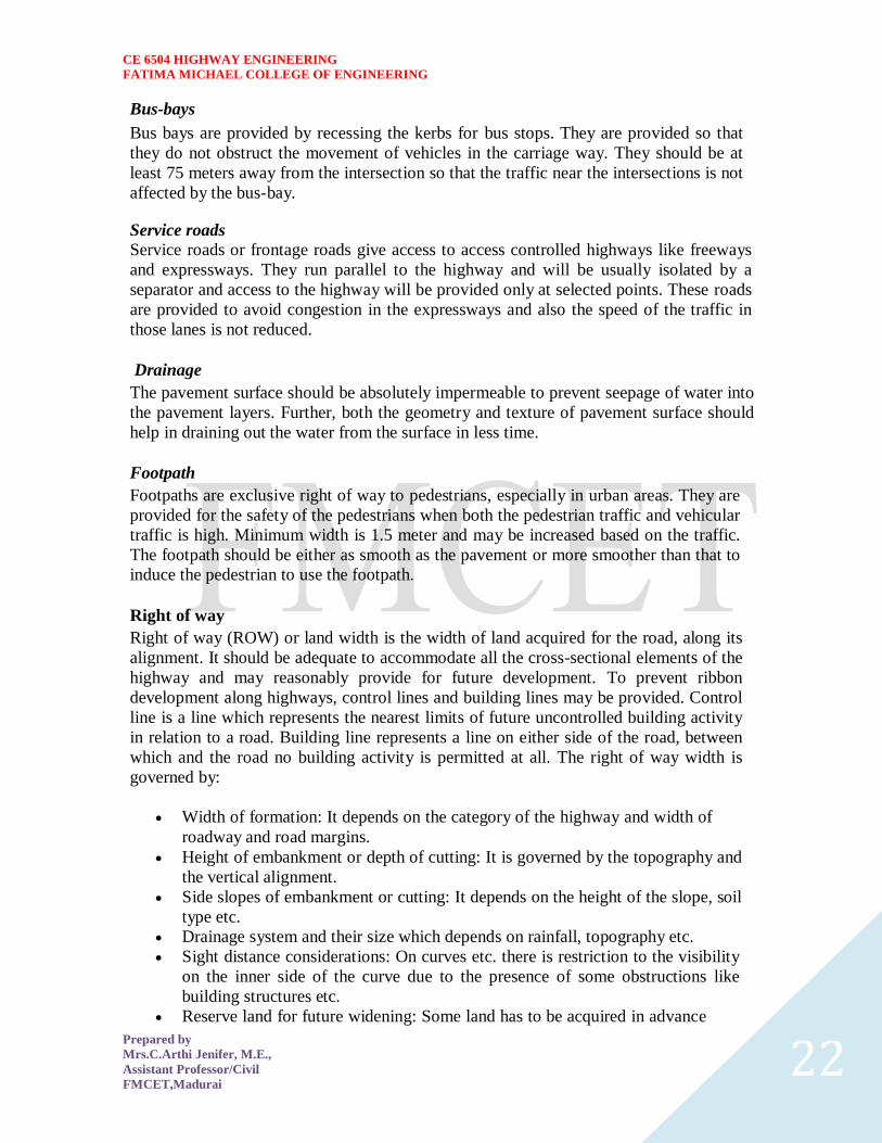
CE 6504 HIGHWAY ENGINEERING
FATIMA MICHAEL COLLEGE OF ENGINEERING
Prepared by
MrsCArthi Jenifer ME
Assistant ProfessorCivil
FMCETMadurai 22
Bus-bays
Bus bays are provided by recessing the kerbs for bus stops They are provided so that
they do not obstruct the movement of vehicles in the carriage way They should be at
least 75 meters away from the intersection so that the traffic near the intersections is not
affected by the bus-bay
Service roads Service roads or frontage roads give access to access controlled highways like freeways
and expressways They run parallel to the highway and will be usually isolated by a
separator and access to the highway will be provided only at selected points These roads
are provided to avoid congestion in the expressways and also the speed of the traffic in
those lanes is not reduced
Drainage
The pavement surface should be absolutely impermeable to prevent seepage of water into
the pavement layers Further both the geometry and texture of pavement surface should
help in draining out the water from the surface in less time
Footpath
Footpaths are exclusive right of way to pedestrians especially in urban areas They are
provided for the safety of the pedestrians when both the pedestrian traffic and vehicular
traffic is high Minimum width is 15 meter and may be increased based on the traffic
The footpath should be either as smooth as the pavement or more smoother than that to
induce the pedestrian to use the footpath
Right of way
Right of way (ROW) or land width is the width of land acquired for the road along its
alignment It should be adequate to accommodate all the cross-sectional elements of the
highway and may reasonably provide for future development To prevent ribbon
development along highways control lines and building lines may be provided Control
line is a line which represents the nearest limits of future uncontrolled building activity
in relation to a road Building line represents a line on either side of the road between
which and the road no building activity is permitted at all The right of way width is
governed by
Width of formation It depends on the category of the highway and width of
roadway and road margins
Height of embankment or depth of cutting It is governed by the topography and
the vertical alignment
Side slopes of embankment or cutting It depends on the height of the slope soil
type etc
Drainage system and their size which depends on rainfall topography etc
Sight distance considerations On curves etc there is restriction to the visibility
on the inner side of the curve due to the presence of some obstructions like
building structures etc
Reserve land for future widening Some land has to be acquired in advance
CE 6504 HIGHWAY ENGINEERING
FATIMA MICHAEL COLLEGE OF ENGINEERING
Prepared by
MrsCArthi Jenifer ME
Assistant ProfessorCivil
FMCETMadurai 23
Table 2 Desig
n speed in as per IRC (ruling and minimum)
Steep
Type
Plain
Rolling
Hilly
40-30
NSampSH
100-80
80-65
50-40
MDR
80-65
65-50
40-30
30-20
25-20
ODR
65-50
50-40
30-25
25-20
VR
50-40
40-35
25-20
anticipating future developments like widening of the road
Table 1 No
right of way for open areas
Roadway width in m
Road
Plain and
Mountainous and
classification
steep terrain
rolling terrain
Open areas
45
24
NHSH
18
MDR
25
15
15
ODR
12
9
VR
Built-up areas
20
NHSH
30
MDR
20
15
ODR
15
12
9
VR
10
CE 6504 HIGHWAY ENGINEERING
FATIMA MICHAEL COLLEGE OF ENGINEERING
Prepared by
MrsCArthi Jenifer ME
Assistant ProfessorCivil
FMCETMadurai 24
Horizontal curve
The presence of horizontal curve imparts centrifugal force which is a reactive force
acting outward on a vehicle negotiating it Centrifugal force depends on speed and radius
of the horizontal curve and is counteracted to a certain extent by transverse friction
between the tyre and pavement surface On a curved road this force tends to cause the
vehicle to overrun or to slide outward from the centre of road curvature For proper
design of the curve an understanding of the forces acting on a vehicle taking a horizontal
curve is necessary Various forces acting on the vehicle are illustrated in the figure 1
Figure 1 Effect of horizontal curve They are the centrifugal force (P) acting outward weight of the vehicle (W) acting
downward and the reaction of the ground on the wheels ( and ) The centrifugal
force and the weight is assumed to be from the centre of gravity which is at h units above
the ground Let the wheel base be assumed as b units The centrifugal force in
is given by
(1)
where is the weight of the vehicle in is the speed of the vehicle in is
the acceleration due to gravity in and is the radius of the curve in
The centrifugal ratio or the impact factor is given by
CE 6504 HIGHWAY ENGINEERING
FATIMA MICHAEL COLLEGE OF ENGINEERING
Prepared by
MrsCArthi Jenifer ME
Assistant ProfessorCivil
FMCETMadurai 25
(1)
The centrifugal force has two effects A tendency to overturn the vehicle about the outer
wheels and a tendency for transverse skidding Taking moments of the forces with
respect to the outer wheel when the vehicle is just about to override
At the equilibrium over turning is possible when
and for safety the following condition must satisfy
(2)
The second tendency of the vehicle is for transverse skidding ie When the the
centrifugal force is greater than the maximum possible transverse skid resistance due to
friction between the pavement surface and tyre The transverse skid resistance (F) is
given by
where and is the fractional force at tyre and and is the reaction at
tyre and is the lateral coefficient of friction and is the weight of the vehicle
This is counteracted by the centrifugal force (P) and equating
At equilibrium when skidding takes place (from equation1)
and for safety the following condition must satisfy
CE 6504 HIGHWAY ENGINEERING
FATIMA MICHAEL COLLEGE OF ENGINEERING
Prepared by
MrsCArthi Jenifer ME
Assistant ProfessorCivil
FMCETMadurai 26
(3)
Equation 2 and 3 give the stable condition for design If equation 2 is violated the vehicle
will overturn at the horizontal curve and if equation 3 is violated the vehicle will skid at
the horizontal
Curve Analysis of super-elevation
Super-elevation or cant or banking is the transverse slope provided at horizontal curve to
counteract the centrifugal force by raising the outer edge of the pavement with respect to
the inner edge throughout the length of the horizontal curve When the outer edge is
raised a component of the curve weight will be complimented in counteracting the effect
of centrifugal force In order to find out how much this raising should be the following
analysis may be done The forces acting on a vehicle while taking a horizontal curve with
super elevation is shown in figure 1
Figure 1 Analysis of super-elevation
Forces acting on a vehicle on horizontal curve of radius at a speed of are
the centrifugal force acting horizontally out-wards through the center of
gravity
the weight of the vehicle acting down-wards through the center of gravity and
the friction force between the wheels and the pavement along the surface
inward
CE 6504 HIGHWAY ENGINEERING
FATIMA MICHAEL COLLEGE OF ENGINEERING
Prepared by
MrsCArthi Jenifer ME
Assistant ProfessorCivil
FMCETMadurai 27
At equilibrium by resolving the forces parallel to the surface of the pavement we get where
friction
is the weight of the vehicle is the centrifugal force is the coefficient of
is the transverse slope due to superelevation Dividing by we get
CE 6504 HIGHWAY ENGINEERING
FATIMA MICHAEL COLLEGE OF ENGINEERING
Prepared by
MrsCArthi Jenifer ME
Assistant ProfessorCivil
FMCETMadurai 28
Step 1
Find for 75 percent of design speed neglecting ie
Step 2
If then else if go to step 3
Step 3
Find for the design speed and max ie If
then the maximum is safe for the design speed else go to
step 4
Step 4
Find the allowable speed for the maximum and
If then the design is adequate otherwise use speed adopt
control measures or look for speed control measures
Maximum and minimum super-elevation
Depends on (a) slow moving vehicle and (b) heavy loaded trucks with high CG IRC
specifies a maximum super-elevation of 7 percent for plain and rolling terrain while that
of hilly terrain is 10 percent and urban road is 4 percent The minimum super elevation is
2-4 percent for drainage purpose especially for large radius of the horizontal curve
Attainment of super-elevation
1 Elimination of the crown of the cambered section by
1 Rotating the outer edge about the crown The outer half of the cross slope
is rotated about the crown at a desired rate such that this surface falls on
the same plane as the inner half
2 Shifting the position of the crown This method is also known as diagonal
crown method Here the position of the crown is progressively
shifted outwards thus increasing the width of the inner half of cross section
progressively
2 Rotation of the pavement cross section to attain full super elevation byThere are
two methods of attaining super elevation by rotating the pavement
1 Rotation about the center line The pavement is rotated such that the inner
edge is depressed and the outer edge is raised both by half the total amount
of super elevation ie by with respect to the centre
2 Rotation about the inner edge Here the pavement is rotated raising the
outer edge as well as the centre such that the outer edge is raised by the
full amount of super elevation with respect to the inner edge
Horizontal Transition Curves
CE 6504 HIGHWAY ENGINEERING
FATIMA MICHAEL COLLEGE OF ENGINEERING
Prepared by
MrsCArthi Jenifer ME
Assistant ProfessorCivil
FMCETMadurai 29
Transition curve is provided to change the horizontal alignment from straight to circular
curve gradually and has a radius which decreases from infinity at the straight end
(tangent point) to the desired radius of the circular curve at the other end (curve point)
There are five objectives for providing transition curve and are given below
1 to introduce gradually the centrifugal force between the tangent point and the
beginning of the circular curve avoiding sudden jerk on the vehicle This
increases the comfort of passengers
2 to enable the driver turn the steering gradually for his own comfort and security
3 to provide gradual introduction of super elevation and
4 to provide gradual introduction of extra widening
5 to enhance the aesthetic appearance of the road
Type of transition curve
Different types of transition curves are spiral or clothoid cubic parabola and Lemniscate
IRC recommends spiral as the transition curve because
1 it fulfills the requirement of an ideal transition curve that is
1 rate of change or centrifugal acceleration is consistent (smooth) and
2 radius of the transition curve is at the straight edge and changes to at
the curve point ( ) and calculation and field implementation is
very easy
Length of transition curve The length of the transition curve should be determined as the maximum of the following
three criteria rate of change of centrifugal acceleration rate of change of super elevation
and an empirical formula given by IRC Rate of change of centrifugal acceleration
At the tangent point radius is infinity and hence centrifugal acceleration is zero At the
end of the transition the radius R has minimum value R The rate of change of
centrifugal acceleration should be adopted such that the design should not cause
discomfort to the drivers If is the rate of change of centrifugal acceleration it can be
written as
Therefore the length of the transition curve in is
CE 6504 HIGHWAY ENGINEERING
FATIMA MICHAEL COLLEGE OF ENGINEERING
Prepared by
MrsCArthi Jenifer ME
Assistant ProfessorCivil
FMCETMadurai 30
(1)
where is the rate of change of centrifugal acceleration given by an empirical formula
suggested by by IRC as below
(2) 2 Rate of introduction of super-elevation
Raise ( ) of the outer edge with respect to inner edge is given by
The rate of change of this raise from to is achieved
gradually with a gradient of in over the length of the transition curve (typical range
of is 60-150) Therefore the length of the transition curve is
(3)
3 By empirical formula
IRC suggest the length of the transition curve is minimum for a plain and rolling terrain
(4)
and for steep and hilly terrain is
(5)
CE 6504 HIGHWAY ENGINEERING
FATIMA MICHAEL COLLEGE OF ENGINEERING
Prepared by
MrsCArthi Jenifer ME
Assistant ProfessorCivil
FMCETMadurai 31
and the shift as
(
6
) The length of the transition curve is the maximum of
equations 1 3 and 4or5 ie
(
7
Case (a)
For single lane roads
(
1
)
Therefore
(
2
)
Figure 1 Set-back for single lane roads (
CE 6504 HIGHWAY ENGINEERING
FATIMA MICHAEL COLLEGE OF ENGINEERING
Prepared by
MrsCArthi Jenifer ME
Assistant ProfessorCivil
FMCETMadurai 32
For multi lane roads if is the distance between centerline of the road and the centerline
of the inner lane then
(3)
(4)
Figure 2 Set-back for multi-lane roads ( )
Case (a)
For single lane roads
(1)
Therefore
(2)
Gradient
Gradient is the rate of rise or fall along the length of the road with respect to the
horizontal While aligning a highway the gradient is decided for designing the vertical
curve Before finalizing the gradients the construction cost vehicular operation cost and
the practical problems in the site also has to be considered Usually steep gradients are
avoided as far as possible because of the difficulty to climb and increase in the
CE 6504 HIGHWAY ENGINEERING
FATIMA MICHAEL COLLEGE OF ENGINEERING
Prepared by
MrsCArthi Jenifer ME
Assistant ProfessorCivil
FMCETMadurai 33
construction cost More about gradients are discussed below
Effect of gradient
The effect of long steep gradient on the vehicular speed is considerable This is
particularly important in roads where the proportion of heavy vehicles is significant Due
to restrictive sight distance at uphill gradients the speed of traffic is often controlled by
these heavy vehicles As a result not only the operating costs of the vehicles are
increased but also capacity of the roads will have to be reduced Further due to high
differential speed between heavy and light vehicles and between uphill and downhill
gradients accidents abound in gradients
Representation of gradient
The positive gradient or the ascending gradient is denoted as and the negative gradient as The deviation angle is when two grades meet the angle which
measures the change of direction and is given by the algebraic difference between the two
grades
steep gradient while 1 in 50 = 2 representation is illustrated in the figure 1
Example 1 in 30 = 333 is a
is a flatter gradient The gradient
CE 6504 HIGHWAY ENGINEERING
FATIMA MICHAEL COLLEGE OF ENGINEERING
Prepared by
MrsCArthi Jenifer ME
Assistant ProfessorCivil
FMCETMadurai 34
Figure 1 Representation of gradient
Types of gradient
Many studies have shown that gradient upto seven percent can have considerable effect
on the speeds of the passenger cars On the contrary the speeds of the heavy vehicles are
considerably reduced when long gradients as flat as two percent is adopted Although
flatter gradients are desirable it is evident that the cost of construction will also be very
high Therefore IRC has specified the desirable gradients for each terrain However it
may not be economically viable to adopt such gradients in certain locations steeper
gradients are permitted for short duration Different types of grades are discussed below
Ruling gradient
The ruling gradient or the design gradient is the maximum gradient with which the
designer attempts to design the vertical profile of the road This depends on the terrain
length of the grade speed pulling power of the vehicle and the presence of the horizontal
curve In flatter terrain it may be possible to provide flat gradients but in hilly terrain it
is not economical and sometimes not possible also The ruling gradient is adopted by the
designer by considering a particular speed as the design speed and for a design vehicle
with standard dimensions But our country has a heterogeneous traffic and hence it is not
possible to lay down precise standards for the country as a whole Hence IRC has
recommended some values for ruling gradient for different types of terrain
Limiting gradient
This gradient is adopted when the ruling gradient results in enormous increase in cost of
construction On rolling terrain and hilly terrain it may be frequently necessary to adopt
limiting gradient But the length of the limiting gradient stretches should be limited and
must be sandwiched by either straight roads or easier grades
Exceptional gradient
Exceptional gradient are very steeper gradients given at unavoidable situations They
should be limited for short stretches not exceeding about 100 metres at a stretch In
mountainous and steep terrain successive exceptional gradients must be separated by a
minimum 100 metre length gentler gradient At hairpin bends the gradient is restricted to
25
Critical length of the grade
The maximum length of the ascending gradient which a loaded truck can operate without
undue reduction in speed is called critical length of the grade A speed of 25 kmph is a
CE 6504 HIGHWAY ENGINEERING
FATIMA MICHAEL COLLEGE OF ENGINEERING
Prepared by
MrsCArthi Jenifer ME
Assistant ProfessorCivil
FMCETMadurai 35
reasonable value This value depends on the size power load grad-ability of the truck
initial speed final desirable minimum speed
Minimum gradient
This is important only at locations where surface drainage is important Camber will take
care of the lateral drainage But the longitudinal drainage along the side drains require
some slope for smooth flow of water Therefore minimum gradient is provided for
drainage purpose and it depends on the rain fall type of soil and other site conditions A
minimum of 1 in 500 may be sufficient for concrete drain and 1 in 200 for open soil
drains are found to give satisfactory performance Sight distance available from a point is the actual distance along the road surface which a driver
from a specified height above the carriage way has visibility of stationary or moving objects
Sight distance required by drivers applies to both geometric design of highways and for
traffic control The sight distance situations are considered in the design
i) Stopping or absolute minimum sight distance
ii) Safe overtaking or passing sight distance
iii) Safe sight distance for entering into uncontrolled intersections
Apart from the three situations mentioned above the following sight distance are considered by the
IRC in highway design
Intermediate sight distance
This is defined as twice the stopping sight distance when overtaking sight distance
cannot be provided intermediate sight distance is provided to give limited overtaking opportunities
to fast vehicles
Head light sight distance
This is the distance visible to a driver during night driving under the illumination of the
vehicle head lights
Stopping sight distance
The minimum sight distance available on a highway at any spot should be of sufficient
length to stop a vehicle traveling at design speed safely without collision with any other obstruction
The absolute minimum sight distance is therefore equal to the stopping sight distance
which is also sometimes called nonpassing sight distance The sight distance available on a road to a
driver at any instance depends on
i) Features of the road
ii) Height of the drivers eye above the road surface
iii) Height of the object above the road surface
The distance within which a motor vehicle can be stopped depends upon the factors listed below
a) Total reactions time of the driver
b) Speed of vehicle
c) Efficiency of breaks
d) Frictional resistance between the road and tyres
e) Gradient of the road
Total reaction time
) Reaction time of the driver is the time taken from the instant the object is visible to the
driver to the instant the brakes are effectively applied
) The total reaction time may be split up into two parts
CE 6504 HIGHWAY ENGINEERING
FATIMA MICHAEL COLLEGE OF ENGINEERING
Prepared by
MrsCArthi Jenifer ME
Assistant ProfessorCivil
FMCETMadurai 36
i) Perception time
ii) Brake reaction time
PIEV theory
According to this theory the total reaction time of the driver is split into four parts
i) Perception
ii) Intellection
iii) Emotion
iv) Volition
Speed of Vehicle
The stopping distance depends very much on the speed of the vehicle first during the
total reaction time of the driver the distance moved by the vehicle will depend on the speed
Efficiency of brakes
The braking efficiency is said to be 100 percent if the wheels are fully licked preventing
them from rotating on application of the brakes This will result in 100 percent skidding which is
normally undesirable except in utmost emergency
Frictional resistance between road and tyres
The frictional resistance developed between road and tyres or the skid resistance depends
on the type and condition of the road surface and the tyres IRC has specified a design friction
coefficient of 035 to 04 depending upon the speed to be used for finding the braking distance in the
calculation of stopping sight distance
Analysis of stopping distance
i) The distance traveled by the vehicle during the total reaction time known as lag
distance
ii) The distance traveled by the vehicle after the application of the brakes is known as
braking distance
Overtaking sight distance
The minimum distance open to the vision of the driver of a vehicle intending to overtake
slow vehicle ahead with safety against the traffic of opposite direction is known as the minimum
overtaking sight distance(OSD) or Safe passing sight distance available
The overtaking sight distance is the distance measured along the center of the road which
a driver with his eye level 12m above the road surface can see the top of an object 12m above the
road surface
Some of the important factors on which the minimum overtaking sight distance required
a) Speed of
i) overtaking vehicle
ii) overtaken vehicle
iii) The vehicle coming from opposite direction
b) Distance between the overtaking and overtaken vehicles the minimum spacing
depends on the steeds
a) Skill and reaction time of the driver
b) Rate of acceleration of overtaking vehicle
c) Gradient of the road
Criteria for sight distance requirements on highway
) The absolute minimum sight distance required throughout the length of the road is the
SSD which should invariably be provided at all places
CE 6504 HIGHWAY ENGINEERING
FATIMA MICHAEL COLLEGE OF ENGINEERING
Prepared by
MrsCArthi Jenifer ME
Assistant ProfessorCivil
FMCETMadurai 37
) On horizontal curves the obstruction on the inner side of the curves should be cleared
to provide the required set back distance and absolute minimum sight distance
) On vertical summit curves the sight distance requirement may be fulfilled by proper
design of the vertical alignment
Hairpin bent
TYPES OF CURVES ON HILL ROADS
The following are the important types of curves provided on hill Roads-
1 Hair-Pin Curves
2 Salient Curves
3 Re-entrant Curves 1 Hair-pin curves - The curve in a hill road which changes its direction through an angle of 180
degree or so down the hill on the same side is known as hair-pin curve
A Hair-Pin Bend
This curve is so called because it conforms to the shape of a hair-pin The bend so formed at the
hair-pin curve in a hill road is known as hair-pin bend This type of curve should be located on a
hill side having the minimum slope and maximum stability It must also be safe from view point of
landslides and ground water Hair-pin bends with long arms and farther spacing are always
preferred They reduce construction problems and expensive protective works Hair-pin curves or
bends of serpentine nature are difficult to negotiate and should therefore be avoided as far as
possible
Salient curves - The curves having their convexity on the outer edges of a hill road are called
salient curves The centre of curvature of a salient curve lies towards the hill side This type of curve
occurs in the road length constructed on the ridge of a hill the bend so formed at the salient curve in
a hill road known as corner bend
Salient curves are very dangerous for fast moving traffic At such a curve or at corner bend the
portion of projecting hill side is usually cut down to improve the visibility as shown in fig (Re-
entrant curve) The outer edge of the road at such a curve is essentially provided with a parapet wall
for protection of the vehicles from falling down the hill slope
CE 6504 HIGHWAY ENGINEERING
FATIMA MICHAEL COLLEGE OF ENGINEERING
Prepared by
MrsCArthi Jenifer ME
Assistant ProfessorCivil
FMCETMadurai 38
3 Re-entrant curves - The curves having their convexity on the inner edge of a hill road are called
re-entrant curves
Re-entrant curves
The centre of curvature of a re-entrant curves lies away from the hill side This type of curve occurs
in the road length constructed in the calley of a hill
These curves are less dangereous as they provide adequate visibility to the fast moving traffic At
such curves the parapet wall is provided only for safety of fast moving traffic
CE 6504 HIGHWAY ENGINEERING
FATIMA MICHAEL COLLEGE OF ENGINEERING
Prepared by
MrsCArthi Jenifer ME
Assistant ProfessorCivil
FMCETMadurai 39
UNIT ndash III DESIGN OF RIGID AND FLEXIBLE PAVEMENTS
COMPARISON OF RIGID AND FLEXIBLE PAVEMENTS
The comparisons are
i) Design precision
A cement concrete pavement is amerable to a much more precise structural analysis
than a flexible pavement Flexible pavements designs are mainly empirical Computer aided analysis
of layered system is making the flexible pavement design more exact than hitherto
ii) Life
) Cement concrete slabs of a thin section constructed in the early 1940rsquos are still in
existence in India though many of them have cracked badly and a few of them have been ripped
open and rebuilt in recent ties
) A major project in cement concrete road construction between Agra and Mathura It can
safely be said that a well-designed concrete slab has a life of about 40 years
) Compared to this the life of a flexible pavement generally varies from 10 to 20 years
iii) Maintenance
) A well-designed cement concrete pavement needs very little maintenance The only
maintenance needed is I respect of joints
) The surface is unaffected by spillage of oil and lubricants bituminous surfaces on the
other hand need great inputs in maintenance
) The surface is affected by spillage of oil and lubricants The surface is also affected by
natural weathering agents like air water ad temperature changes
) A cement concrete pavement on the other hand needs a small amount for maintaining
joints
iv) Initial cost
) The argument so far used against a cement concrete slab is that it is much more costly
than a flexible pavement
) The latter specifications no doubt represent the rock-bottom needs of a road in India but
these specifications can hardly provide a smooth and durable surface
v) Stage construction ) Road construction is generally done adopting a policy of stage construction especially for
low volume roads As traffic grows additional layers in the form of water bound macadam and
superior surfacing are added on
) Initial outlay is minimum and additional outlays are in keeping with traffic growth This is
a great advantage when dealing with new roads in an atmosphere of austerity
vi) Availability of materials
) Cement bitumen stone aggregates and gravelsand are the major materials involved in
pavement Construction Cement has been in serious short supply in the country for the past many
decades
) Bitumen is also not available plentifully in India There is also the danger of the entire oil
reserves in the world shrinking during the next two or three decades
) In locations where stone aggregates are scarce cement concrete may have an advantage
for flexible pavements
vii) Surface characterstics
CE 6504 HIGHWAY ENGINEERING
FATIMA MICHAEL COLLEGE OF ENGINEERING
Prepared by
MrsCArthi Jenifer ME
Assistant ProfessorCivil
FMCETMadurai 40
) A good cement concrete surface is smooth and free from rutting potholes and
corrugations In a bituminous surface it is only the asphaltic concrete surface that can give
comparable rideablity
) A well-constructed cement concrete pavement surface can have a permanent nonskid
surface A bituminous surface can also be designed to have a good skid resistant surface
viii) Utility location
) In cement concrete slabs proper thought has to be given to locate utilities such as water
pipes telephone lines and electric cables
) It is difficult to rip open the slab and restore it to be the original condition if any changes
in the utilities lines are to be made
ix) Glame and night visibility
) Concrete pavements have a gray color which can cause glam under sunlight Colored
cement can reduce the grave
) On the other hand bituminous roads need more street lighting
x) Traffic dislocation during construction
) A cement concrete pavement requires 28 days before it can be thrown open to traffic On
the other hand a bituminous surface can be thrown open to traffic shortly after it is rolled
xi) Environmental considerations during construction
) The process of heating of bitumen and aggregates and mixing them together on hot mix
plants can prove to be much more hazardous to the environment than cement concrete construction
where no heating of any material is involved
xii) Overall economy on a life cycle basis
) A good road is costly to construct but once constructed such a road requires little
maintenance and results in savings in vehicle operating costs
) The comparative economy of a flexible pavement and a rigid pavement has proved that on
overall economic considerations
Types of pavement structure
Based on the structural behavior pavements are generally classified into three
categories
i) Flexible pavements
ii) Rigid pavements
iii) Semi rigid pavements
Flexible pavements
) Flexible pavements are those which on the whole have low or negligible flexural
strength and are rather flexible in their structural action under the loadsThe flexible pavement
layers reflect the deformation of the lower layers on to the surface of the layer
) A flexible pavement consists of four components(i) Soil subgrade (ii) sub base
course (iii) base course (iv) Surface course
CE 6504 HIGHWAY ENGINEERING
FATIMA MICHAEL COLLEGE OF ENGINEERING
Prepared by
MrsCArthi Jenifer ME
Assistant ProfessorCivil
FMCETMadurai 41
) The flexible pavement layers transmit the vertical or compressive stresses to the lower layers
by grain to grain transfer through the points of contact in the granular structure A well
compacted granular structure consisting of strong added aggregate can transfer the compressive
stresses
) The load spreading ability of this layer therefore depends on the type of the materials and mix
design factors Bituminous concrete is one of the best flexible pavements layer materials Other
materials which fall under the group are all granular materials with or without bituminous
binder granular base and sub base course materials
) The vertical compressive stress is maximum on the pavement surface directly under the wheel
and is equal to the contact pressure under the wheel The flexible pavement may be constructed
in a number of layers and the top layer has to be strongest as the highest compressive stresses
) Flexible pavements are commonly designed using empirical design charts or equations taking
into account some of the design factors there are also semi empirical and theoretical design
methods
Rigid pavements
) Rigid pavements are those which possess note flexural strength or flexural rigidity
The stresses are not transferred from grain to grain to the lower layers as in the ease of flexible
pavements layers
) The rigid pavements are made of Portland cement concrete plain reinforced or
prestressed concrete The plain cement concrete slabs are expected to take up about 40 kgcm2
flexural stress
) The rigid pavement has the slab action and is capable of transmitting the wheel
load stresses through a wider area below The main point of difference in the structural behavior
of rigid pavement as compared to the flexible pavement is that the critical condition of stress in
the rigid pavement is the maximum flexural stress occurring in the slab due to wheel load and
the temperature changes whereas in the flexible pavement
) As the rigid pavement slab has tensile strength tensile stresses are developed due
to the bending of the slab under wheel load and temperature variations Thus the types of
stresses developed and their distribution within the cement concrete slab are quirt different
) The cement concrete pavement slab can very well serve as a wearing surface as
well an effective base course The rigid pavement structure consists of a cement concrete slab
below which a granular base or sub base course may be provided
) Though the cement concrete slab can also be laid directly over the soil subgrade
consists of fine grained soil
) the rigid pavements are usually designed and the stresses are analyzed using the
elastic theory assuming the pavements as a n elastic plate resting over an elastic or a viscous
foundation
Semi rigid pavements
) when bonded materials like the pozzolanic concrete lean cement concrete or soil
cement are used in the base course or sub base course layer the pavement layer has considerably
higher flexural strength than the common flexible pavement layers
) when this intermediate class of materials are used in the base or sub base course
layer of the pavements they are called semi rigid pavements
CE 6504 HIGHWAY ENGINEERING
FATIMA MICHAEL COLLEGE OF ENGINEERING
Prepared by
MrsCArthi Jenifer ME
Assistant ProfessorCivil
FMCETMadurai 42
) This third category of semi rigid pavement are either designed as flexible
pavements with some correction factors to find the thickness requirements based on experience
or by using a new design approach
) The semi rigid pavement materials have low resistance to impact and abrasion and
therefore are usually provided with flexible pavement surface course
Various functions of pavement components
The functions are
Soil sub grade and its evaluation
) The soil sub grade is a layer of natural soil prepared to receive the layers of pavement
materials placed over it It is essential that at no time the soil sub grade is overstressed it means that
the pressure transmitted on the top of the sub grade is within the allowable limit
) Many tests are known for measuring the strength properties of the sub grades Some of the
tests have been standardized for the use The common strength test for the evaluation of soil
subgrade is
i) California bearing ratio test
ii) California resistance value test
iii) Triaxial compression test
iv) Plate bearing test
CALIFORNIA BEARING RATIO (CBR) TEST
It is evolved for the empirical method of flexible pavement design The CBR test is carried
out either in the laboratory on prepared specimens or in the field by taking in situ measurements
California resistance value
It is found by using have been stabliometerThis test is used in an empirical method of
flexible pavement design based on soil strength
Triaxial test
It is the most important soil strength but still the test is not very commonly used in structural
design of pavements
Plate bearing test
It is carried out using a relatively large diameter plate to evaluate the load supporting
capacity of supporting power of the pavement layers The results are plate bearing tests are used in
flexible pavement design method like McLeod method on based on layer system analysis by
brumister
Sub base and base courses and their evaluation
) There layers are made of broken stones bound or unbound aggreagatesome times in sub
base course a layer of stabilized soil(or) Selected granular soil is also used
) however at the sub base course it is desirable to use smaller size graded aggregates When
the sub grade consists of fine grained soil and when the pavement carries heavy wheel loads
CE 6504 HIGHWAY ENGINEERING
FATIMA MICHAEL COLLEGE OF ENGINEERING
Prepared by
MrsCArthi Jenifer ME
Assistant ProfessorCivil
FMCETMadurai 43
) Sub base course primarily has the similar function as of the base course and is provided
with inferior materials than of base course Base courses are used under rigid pavement for
i) Preventing pumping
ii) Protecting the sub grade against frost action
) Thus the fundamental purpose of abase course and sub base course is to provide a stress
transmitting medium to spread the surface wheel loads in such manner
) The sub base and base course layers may be evaluated by suitable strength or stability test
like plate bearing CBR test
WEARING COURSE AND ITS EVALUATION
) The purpose of the wearing course is to give a smooth riding surface that is dense It
resists pressure exerted by tyres and takes up wear and tear due to the traffic
) Wearing course also offers a water tight layer against the surface water infiltration The
flexible pavement normally a bituminous surfacing is used as a wearing course
) In rigid pavements the cement concrete acts like a base course as well as wearing course
Most popular test in use is marshal stability test where in the optimum content of bitumen binder is
worked out based on the stability density
) Plate bearing test and Bankelman beam test are also sometimes made use of for evaluating
the wearing course and the pavement as a whole
Various factors to be considered in pavement design and the significance
Pavement design consists of two parts
i) Mix design of materials to be used in each pavement component layer Thickness design of the
pavement and the component layers
The various factors to be considered for the design of pavements are given below
i) Design wheel load
ii) Sub grade soil
iii) Climatic factors
iv) Pavement component layers
v) Environmental factors
vi) Special factors in the design of different types of pavements
Design wheel load
The various wheel load factors to be considered in pavement design are
i) Maximum wheel load
ii) Contact pressure
iii) Dual or multiple wheel loads
iv) Repetition of loads
Maximum wheel load
The wheel load configurations are important to know the way in which the loads of a given
vehicle are applied on the pavement surface
) For highways the maximum legal axle load as specified by Indian road congress is 8170
kg with a maximum equivalent single wheel load of 4085 kg
) The evaluation for vertical stress computations under a uniformly distribute of circular
load based on Boussineqrsquos theory is given by
CE 6504 HIGHWAY ENGINEERING
FATIMA MICHAEL COLLEGE OF ENGINEERING
Prepared by
MrsCArthi Jenifer ME
Assistant ProfessorCivil
FMCETMadurai 44
2
322
3
1
za
zpz
σz = vertical stress at depth z
P= surface pressure
Z=depth at which σz computed
A=radius of loaded area
Contact pressure
Generally the wheel load is assumed to be distributed over a circular area But by
measurement of the imprints of tyers with different load and inflation pressures Three terms in use
with reference to tyre pressure are
Tyre pressure
Inflation pressure
Contact pressure
Tyre pressure and inflation pressure mean exactly the same the contact pressure is found to be more
than tyre pressure when the tyre pressure is less than 7 kgm2 and it is vice versa when the tyre
pressure exceeds this value
Contact pressure can be measured by the relationship
Load on wheel
Contact pressure = ----------------------------------------
Contact area or area of imprint
The general variation between the tyre pressure and measured contact pressure is shown in this fig
The ratio of contact pressure to type pressure is defined as rigidity factor Thus value of rigidity
factor is 10 for an average tyre pressure of 7 Kgcm2This value is higher than unity for lower type
pressures and less than unity for tyre pressures higher than 7 kgcm2
Equivalent single wheel load (ESWL)
) The maximum wheel load within the specified limit and to carry greater load it is
necessary to provide dual wheel assembly to the rear axles of the roads vehicles
) In other words the pressure at a certain depth below the pavement surface cannot be
obtained by numerically adding the pressure caused by any one wheel
) The effect is in between the single load and two times load carried by one wheel The load
dispersion is assumed to be at an angle of 450In the dual wheel load assembly let d be the clear gap
between the two wheels S be the spacing between the centers of the wheels and a be the radius of
the circular contact area of each wheel Then S = (d + 2a)
) ESWL may be determined based on either equivalent deflection or equivalent stress
criterianMultiple wheel loads are convert to ESWL and this value is used in pavement design The
ESWL is usually determined by the equivalent stress criterion using a simple graphical method
CE 6504 HIGHWAY ENGINEERING
FATIMA MICHAEL COLLEGE OF ENGINEERING
Prepared by
MrsCArthi Jenifer ME
Assistant ProfessorCivil
FMCETMadurai 45
) A straight line relationship is assumed between ESWL and depth on log scales For
determining ESWL the plot is made as shown in fig
) Two points A and B are plotted on the log-log graph with coordinates of A (Pd2) and
B(2p2s)line AB is a plot which is the focus of points where any single wheel load is equivalent to a
certain set of dual wheels
) To Calculate the ESWL for a dual assembly it is essential to estimate a design thickness of
the pavement If the design thickness so obtained is equal to the estimated thickness then the ESWL
calculations could be considered as correct Otherwise trials are made
) In heavy trucks and trailers the load on each wheel may be further reduced by multiple
wheels and tandem axles
Repetition of loads
) The deformation of load pavement (or) sub grade due to a single application of wheel load
may be small It required carrying out traffic surveys for accounting the factor of repetitions for
wheel loads in the design of pavement
) Data collected are converted to some constant equivalent wheel loads Equivalent wheel
load is a single load equivalent to the repeated applications of any particular wheel load on a
pavement which requires the same thickness and strength of pavements
) McLeod has given a procedure for evolving equivalent load factors for designing flexible
pavements
Various methods of flexible pavement design
) The flexible pavement is built with number of layers In the design process it is to be
ensured that under the application of load none of the layers is overstressed
) The maximum intensity of stresses occurs in the top layer of the pavement The
magnitude of load stresses reduces at lower layers
) In the design of flexible pavements it has yet not been possible to have a rational design
method wherein design process and service behavior of the pavement can be expressed by
mathematical laws
) Flexible pavement design methods are accordingly either empirical or semi empirical In
these methods the knowledge and experience gained on the behavior of the pavements in the past
are usefully utilized
Various approaches of flexible pavement design may be thus classified into three groups
i) Empirical method
ii) Semi-empirical or Semi theoretical method
iii) Theoretical method
) Empirical methods are either based on physical properties or strength parameters of soil
sub grade When the design is based on stress strain function and modified base on experience it
may be called semi-empirical or semi-theoretical There are design methods based on theoretical
analysis and mathematical computations
Out of the flexible pavement design method available is
i) Group index method
ii) California bearing ratio method
iii) California R value (or) Stabiliometer method
iv) Triaxial test method
CE 6504 HIGHWAY ENGINEERING
FATIMA MICHAEL COLLEGE OF ENGINEERING
Prepared by
MrsCArthi Jenifer ME
Assistant ProfessorCivil
FMCETMadurai 46
v) McLeod method
vi) Burmister method
Group index method
) Group index value is an arbitrary index assigned to the soil type in numerical equations
base on the percent fines liquid limit and plasticity index
) The design chart for group index method for determining the pavement thickness is given
in fig
The traffic volume in this method is divided in three groups
Traffic volume No of vehicles per day
Light Less than 50
Medium 50 to 300
Heavy Over 300
The design of the pavement thickness by this method first the G1 value of the soil is found the
anticipated traffic is estimated and is designated as light medium or heavy as indicated
The G1 method of pavement design is essentially an empirical method based on physical properties
of the subgrade soil This method does not consider the strength characteristics of the subgrade soil
and therefore is open to question regarding the reliability of the design based on the index properties
of the soil only
California bearing ratio method
) California division of highways in the USA developed CBR method for
pavement design The majority of design curves developed later are base on the original curves
proposed by OJporter
) One of the chief advantages of CBR method is the simplicity of the test procedure
The CBR tests were carried out by the California state highway department on existing pavement
layers including subgrade sub base and base course
) Based on the extensive CBR test data collected on pavement which behaved
satisfactory and those which failed an empirical design chart was developed correlating the CBR
value and the pavement thickness The basis of the design chart is that a material with a given CBR
required a certain thickness of pavement layer as a cover
) A higher load needs a thicker pavement layer to protect the sub grade Design
curves correlating the CBR value with total pavement thickness cover were developed by the
California state highway department for wheel loads of 3175kg and 5443 kg representing light and
heavy traffic The design curves are shown in this fig
It is possible to extend the CBR design curves for various loading conditions nusing the expression
t= 2
1
1751
pCBRp
t=2
1
751
A
CBR
p
Hence
CE 6504 HIGHWAY ENGINEERING
FATIMA MICHAEL COLLEGE OF ENGINEERING
Prepared by
MrsCArthi Jenifer ME
Assistant ProfessorCivil
FMCETMadurai 47
t= pavement thickness cm
p=Wheel load kg
CBR= California bearing ratio percent
P=tyre pressure kgcm2
A= area of contactcm2
IRC Recommendations
a) The CBR tests should be performed on remoulded soils in the laboratory The specimens should
be prepared by static compaction wherever possible and otherwise by dynamic compaction
b) For the design of new roads the sub grade soil sample should be compacted at OMC to proctor
density whenever suitable compaction equipment
c) The CBR test samples may be soaked in water for four days period before testing the annual
rainfall is less than 50 cm and the water table is too deep to affect the sub grade and imperable
surfacing is provided to carrying out CBR test
d) If the maximum variations in CBR value of the three specimens exceed the specified limits the
design CBR should be average of at least six samples
e) The top 50 cm of sub grade should be compacted at least up to 95 to 100 percent of proctor
density
f) An estimate of the traffic should be carried by the road pavements at the end of expected in view
the existing traffic and probable growth rate of traffic
g) The traffic for the design is considered in units of heavy vehicles per day in both directions and is
divided into seven categories A to G The design thickness is considered applicable for single axle
loads up to 8200 kg and tandom axle loads up to 14500 kg
h) When sub base course materials contain substantial proportion of aggregates of size above 20mm
the CBR value of these materials would not be valid for the design of subsequent layers above them
The CBR method of pavement design gives the total thickness requirement of the pavement above a
sub grade and thickness value would remain the same quality of materials used in component layers
California resistance value method
) In this design method based on stabliometer R-value and cohesiometer C-value
Based on performance data it was established by pavement thickness varies directly with R value
and algorithm of load repetitions It varies inversely with fifth root of c valueThe expression for
pavement thickness is given by the empirical equation
T=
5
1
1 90
C
RTK
Hence
T=total thickness of pavement cm
K=Numerical constant 0166
T1=traffic index
R= stabiliometer resistance value
C=Cohesiometer value
CE 6504 HIGHWAY ENGINEERING
FATIMA MICHAEL COLLEGE OF ENGINEERING
Prepared by
MrsCArthi Jenifer ME
Assistant ProfessorCivil
FMCETMadurai 48
In the design of flexible pavements based on California resistance value method for the following
data are needed
) R-value of soil subgrade
) T1 value
) Equivalent C-value
) R value of soil subgrade is obtained from the test using stablio meterThe
computation of T1 value has been explained
Equivalent C-value
) The cohesion meter value c is obtained for each layer of pavement material
separately from tests However the composite or equivalent C-value of the pavement may be
estimated if the thickness of each component layer and the c-value of the material of the layer are
known
) while designing a pavement as the thickness of the pavement is not known it is
easier if the pavement is first assumed to consist of any one material like gravel base course with
known C-value
) Subsequently the individual thickness of each layer is converted in terms of gravel
equivalent by using relationship
5
1
1
2
2
1
C
C
t
t
) t1 and t2 are the thickness values of any two pavement layersc1 and c2 are their
corresponding cohesiometer values
CE 6504 HIGHWAY ENGINEERING
FATIMA MICHAEL COLLEGE OF ENGINEERING
Prepared by
MrsCArthi Jenifer ME
Assistant ProfessorCivil
FMCETMadurai 49
UNIT 4 MATERIAL AND MAINTENANCE
SUMMIT CURVE
Summit curves are vertical curves with gradient upwards They are formed when two
gradients meet as illustrated in figure 1 in any of the following four ways
1 When a positive gradient meets another positive gradient [figure 1a]
2 When positive gradient meets a flat gradient [figure 1b]
3 When an ascending gradient meets a descending gradient [figure 1c]
4 When a descending gradient meets another descending gradient [figure 1d]
Type of Summit Curve
Many curve forms can be used with satisfactory results the common practice has been to
use parabolic curves in summit curves This is primarily because of the ease with it can
be laid out as well as allowing a comfortable transition from one gradient to another
Although a circular curve offers equal sight distance at every point on the curve for very
small deviation angles a circular curve and parabolic curves are almost congruent
Furthermore the use of parabolic curves were found to give excellent riding comfort
Figure 1 Types of summit curves
Design Consideration
In determining the type and length of the vertical curve the design considerations are
comfort and security of the driver and the appearance of the profile alignment Among
these sight distance requirements for the safety are most important on summit curves
The stopping sight distance or absolute minimum sight distance should be provided on
these curves and where overtaking is not prohibited overtaking sight distance or
intermediate sight distance should be provided as far as possible When a fast moving
vehicle travels along a summit curve there is less discomfort to the passengers This is
because the centrifugal force will be acting upwards while the vehicle negotiates a
summit curve which is against the gravity and hence a part of the tyre pressure is
relieved Also if the curve is provided with adequate sight distance the length would be
sufficient to ease the shock due to change in gradient Circular summit curves are
identical since the radius remains same throughout and hence the sight distance From
CE 6504 HIGHWAY ENGINEERING
FATIMA MICHAEL COLLEGE OF ENGINEERING
Prepared by
MrsCArthi Jenifer ME
Assistant ProfessorCivil
FMCETMadurai 50
this point of view transition curves are not desirable since it has varying radius and so the
sight distance will also vary The deviation angles provided on summit curves for
highways are very large and so the simple parabola is almost congruent to a circular arc
between the same tangent points Parabolic curves are easy for computation and also it
had been found out that it provides good riding comfort to the drivers It is also easy for
field implementation Due to all these reasons a simple parabolic curve is preferred as
summit curve Length of the summit curve
The important design aspect of the summit curve is the determination of the length of the
curve which is parabolic As noted earlier the length of the curve is guided by the sight
distance consideration That is a driver should be able to stop his vehicle safely if there is
an obstruction on the other side of the road Equation of the parabola is given by
where where N is the deviation angle and is the length of the In
deriving the length of the curve two situations can arise depending on the uphill and
downhill gradients when the length of the curve is greater than the sight distance and the
length of the curve is greater than the sight distance
Let is the length of the summit curve is the SSDISDOSD is the deviation angle
drivers eye height (12 m) and the height of the obstruction then the length of the
summit curve can be derived for the following two cases The length of the summit curve
can be derived from the simple geometry as shown below
Case a Length of summit curve greater than sight distance( )
Figure 1 Length of summit curve ( )
The situation when the sight distance is less than the length of the curve is shown in
figure 1
CE 6504 HIGHWAY ENGINEERING
FATIMA MICHAEL COLLEGE OF ENGINEERING
Prepared by
MrsCArthi Jenifer ME
Assistant ProfessorCivil
FMCETMadurai 51
(1)
Case b Length of summit curve less than sight distance
The second case is illustrated in figure 1
Figure 1 Length of summit curve
CE 6504 HIGHWAY ENGINEERING
FATIMA MICHAEL COLLEGE OF ENGINEERING
Prepared by
MrsCArthi Jenifer ME
Assistant ProfessorCivil
FMCETMadurai 52
From the basic geometry one can write
(1)
Therefore for a given and to get minimum differentiate the above equation
with respect to and equate it to zero Therefore
Solving the quadratic equation for
(2)
Now we can substitute back to get the value of minimum value of for a given
and Therefore
Solving for
CE 6504 HIGHWAY ENGINEERING
FATIMA MICHAEL COLLEGE OF ENGINEERING
Prepared by
MrsCArthi Jenifer ME
Assistant ProfessorCivil
FMCETMadurai 53
(3) (4
CE 6504 HIGHWAY ENGINEERING
FATIMA MICHAEL COLLEGE OF ENGINEERING
Prepared by
MrsCArthi Jenifer ME
Assistant ProfessorCivil
FMCETMadurai 54
When stopping sight distance is considered the height of drivers eye above the road
surface ( ) is taken as 12 metres and height of object above the pavement surface ( )
is taken as 015 metres If overtaking sight distance is considered then the value of
drivers eye height ( ) and the height of the obstruction ( ) are taken equal as 12
metres
Valley curve
Valley curve or sag curves are vertical curves with convexity downwards They are
formed when two gradients meet as illustrated in figure 1 in any of the following four
ways
Figure 1 Types of valley curve
1 When a descending gradient meets another descending gradient [figure 1a]
2 When a descending gradient meets a flat gradient [figure 1b]
3 When a descending gradient meets an ascending gradient [figure 1c]
4 When an ascending gradient meets another ascending gradient [figure
Design considerations
There is no restriction to sight distance at valley curves during day time But visibility is
reduced during night In the absence or inadequacy of street light the only source for
visibility is with the help of headlights Hence valley curves are designed taking into
account of headlight distance In valley curves the centrifugal force will be acting
downwards along with the weight of the vehicle and hence impact to the vehicle will be
more This will result in jerking of the vehicle and cause discomfort to the passengers
Thus the most important design factors considered in valley curves are (1) impact-free
movement of vehicles at design speed and (2) availability of stopping sight distance
under headlight of vehicles for night driving
For gradually introducing and increasing the centrifugal force acting downwards the best
shape that could be given for a valley curve is a transition curve Cubic parabola is
generally preferred in vertical valley curves See figure 1
CE 6504 HIGHWAY ENGINEERING
FATIMA MICHAEL COLLEGE OF ENGINEERING
Prepared by
MrsCArthi Jenifer ME
Assistant ProfessorCivil
FMCETMadurai 55
Figure 1 Valley curve details
During night under headlight driving condition sight distance reduces and availability of
stopping sight distance under head light is very important The head light sight distance
should be at least equal to the stopping sight distance There is no problem of overtaking
sight distance at night since the other vehicles with headlights could be seen from a
considerable distance
Length of the valley curve
The valley curve is made fully transitional by providing two similar transition curves of
equal length The transitional curve is set out by a cubic parabola where
The length of the valley transition curve is designed based on two criteria
1 comfort criteria that is allowable rate of change of centrifugal acceleration is
limited to a comfortable level of about
2 safety criteria that is the driver should have adequate headlight sight distance at
any part of the country
Comfort criteria
The length of the valley curve based on the rate of change of centrifugal acceleration that
will ensure comfort Let is the rate of change of acceleration the minimum radius of
the curve is the design speed and is the time then is give
CE 6504 HIGHWAY ENGINEERING
FATIMA MICHAEL COLLEGE OF ENGINEERING
Prepared by
MrsCArthi Jenifer ME
Assistant ProfessorCivil
FMCETMadurai 56
For a cubic parabola the Value Safety criter Length of the valley curve for headlight distance may be determined for two conditions
(1) length of the valley curve greater than stopping sight distance and (2) length of the
valley curve less than the stopping sight distance of for length is given by
Case 1 Length of valley curve greater than stopping sight distance ( )
The total length of valley curve is greater than the stopping sight distance SSD The
sight distance available will be minimum when the vehicle is in the lowest point in the
valley This is because the beginning of the curve will have infinite radius and the bottom
of the curve will have minimum radius which is a property of the transition curve The
case is shown in figure 1
Figure 1 Valley curve case 1
From the geometry of the figure we have
CE 6504 HIGHWAY ENGINEERING
FATIMA MICHAEL COLLEGE OF ENGINEERING
Prepared by
MrsCArthi Jenifer ME
Assistant ProfessorCivil
FMCETMadurai 57
(1)
where is the deviation angle in radians is the height of headlight beam is the
head beam inclination in degrees and is the sight distance The inclination is 1
degree
Case 2 Length of valley curve less than stopping sight distance ( )
The length of the curve is less than SSD In this case the minimum sight distance is
from the beginning of the curve The important points are the beginning of the curve and
the bottom most part of the curve If the vehicle is at the bottom of the curve then its
headlight beam will reach far beyond the endpoint of the curve whereas if the vehicle is
at the beginning of the curve then the headlight beam will hit just outside the curve
Therefore the length of the curve is derived by assuming the vehicle at the beginning of
the curve The case is shown in figure 1
From the figure
(1) Note that the above expression is approximate and is satisfactory because in practice the gradients
are very small and is acceptable for all practical purposes We will not be able to know prior to
which case to be adopted Therefore both has to be calculated and the one which satisfies the
condition is adopted
1 Flexible pavement
2 Rigid pavement
Flexible pavement
These pavements reflect the deformation of sub grade and the subsequent layers to the
surface
Rigid pavement
The rigid characteristic of the pavement are associated with rigidity or flexural strength
CE 6504 HIGHWAY ENGINEERING
FATIMA MICHAEL COLLEGE OF ENGINEERING
Prepared by
MrsCArthi Jenifer ME
Assistant ProfessorCivil
FMCETMadurai 58
or slab action so the load is distributed over a wide area of sub grade soil
Flexible pavement Definition
These pavements reflect the deformation of sub grade and the subsequent layers to the
surface Flexible usually asphalt is laid with no reinforcement or with a specialized
fabric reinforcement that permits limited flow or repositioning of the roadbed under
ground changes
The design of flexible pavement is based on load distributing characteristic of the
component layers The black top pavement including water amp gravel bound macadam fall
in this category
Flexible pavement on the whole has low or negligible flexible strength flexible in their
structural action) The flexible pavement layers transmit the vertical or compressive
stresses to the lower layers by grain transfer through contact points of granular structure
The vertical compressive stress is maximum on the pavement surface directly under the
wheel load and is equal to contact pressure under the wheels Due to the ability to
distribute the stress to large area in the shape of truncated cone the stresses get decreased
in the lower layer
As such the flexible pavement may be constructed in a number of layers and the top
layer has to be strongest as the highest compressive stresses
To be sustained by this layer in addition to wear and tear the lower layer have to take
up only lesser magnitude of stress as there is no direct wearing action die to traffic loads
therefore inferior material with lower cast can be used in the lower layers
Rigid pavement Definition
The rigid characteristic of the pavement are associated with rigidity or flexural strength
or slab action so the load is distributed over a wide area of sub grade soil Rigid pavement
is laid in slabs with steel reinforcement
The rigid pavements are made of cement concrete either plan reinforced or prestressed
concrete
Critical condition of stress in the rigid pavement is the maximum flexural stress occurring in the slab due to wheel load and the temperature changes
Rigid pavement is designed and analyzed by using the elastic theory
CE 6504 HIGHWAY ENGINEERING
FATIMA MICHAEL COLLEGE OF ENGINEERING
Prepared by
MrsCArthi Jenifer ME
Assistant ProfessorCivil
FMCETMadurai 59
UNIT-5 EVALUATION AND MAINTENANCE OF PAVEMENTS
TRAFFIC PARAMETERS
Design life
Design life is the number of years (or number of standard axle repetitions) for which the
pavement is being designed A pavement is expected to serve satisfactorily within the
design life For concrete pavements 20 to 40 years may be assumed as the design life
(PCA 1984 IRC58 2002)
Basic design principle
Though different approaches for concrete pavement design are suggested in various
guidelines the design principles tend to remain similar across different guidelines for
example PCA (1994) Austroads (2004) NCHRP (2004) IRC58 (2002) etc except the
AASHTO (1993) provisions which is based on empirical approach The basic steps
involved in the design of concrete pavement method can be summarized as follows
The developed stresses due to load for a trial thickness of the concrete slab are
calculated for various loading configuration and the critical one is chosen The
axle loads are generally divided into different axle load groups and the load
stresses are calculated individually
The ratio between the load stress and Modulus of Rupture (MOR) is known as
stress ratio The stress ratio determines how many repetitions the pavement can
sustain (ie allowable traffic repetitions) for the individual axle load group If the
stress ratio is 055 or lower it can withstand virtually infinite number of traffic
repetitions (PCA 1984)
The ratio between the allowable repetitions to the expected traffic repetitions is
the damage fraction The calculation process is repeated for various axle loads
(sometimes for various seasons or various timings of the day) and the sum of
individual damage fractions (c u m u l a t i v e fatigue damage) should be less
than equal to one for pavement design being safe If found unsafe the trial
thickness is changed and the design process is repeated
The design process may also include considerations for temperature stress
moisture stresses and erosion distress
A brief discussion on concrete pavement design approaches suggested by various design
practices viz PCA method (1984) Austroads method (2004) AASHTO method (1993)
NCHRP mechanistic-empirical method (2004) and the Indian Roads Congress (IRC)
method (2002) are placed in the following
Portland cement Association (PCA) Method
The PCA method is based on Westergaard Picket and Rays work and further theoretical
analysis by Finite Element Method (Huang 1993) The data used to develop the PCA
method is generated from various road tests like ASSHO road test Arlington test
(conducted by PCA) Bates test road and Maryland road test (PCA 1984) The PCA
design method is based on the following two considerations (PCA 1984)
The fatigue damage on the concrete slab due to repetitive application of traffic
load is estimated The cumulative fatigue damage principle is used to estimate the
design thickness of the slab Edge stress between the mid-ways of the
CE 6504 HIGHWAY ENGINEERING
FATIMA MICHAEL COLLEGE OF ENGINEERING
Prepared by
MrsCArthi Jenifer ME
Assistant ProfessorCivil
FMCETMadurai 60
transverse joint is taken as critical configuration
The stresses due to warping and curling (due to temperature and moisture
gradient) are not considered in the fatigue analysis as per PCA recommendation
because most of the time the stresses generated are subtractive to the load stress
The possibility of erosion of pavement materials placed below the concrete slab is
evaluated The rate at which the slab is deflected due to axle load is used as a
criterion for erosion Theoretically it can be shown that a thin pavement with
smaller deflection basin is subjected to faster rate of deflection compared to
thicker slab Hence thin slab is more susceptible to erosion In a similar way the
cumulative erosion damage is calculated for individual axle load groups If this
value is greater than one then the design needs to be revised
Austroads method
Austroads method has been adopted from PCA (1984) approach with modifications
suited to Australian conditions (Austroads 2004) A bound mix or lean cement concrete is
used as sub-base material For a given CBR value of the subgrade and given thickness of
cemented sub-base the effective subgrade strength can be obtained from the chart
provided Figure-19 schematically shows such a chart For different levels of traffic
Austroads (2004) suggests minimum values of the base thicknesses to be provided
CE 6504 HIGHWAY ENGINEERING
FATIMA MICHAEL COLLEGE OF ENGINEERING
Prepared by
MrsCArthi Jenifer ME
Assistant ProfessorCivil
FMCETMadurai 61
figure-19 Schematic diagram of Austroads (2004) chart for estimation of effective
subgrade strength
As per Astroads (2004) the concrete pavement slab thickness for a given expected
traffic repetitions is designed considering the (i) flexural fatigue of the concrete slab and
the (ii) subgrade erosion arising out of repeated deflections For both the considerations
equations are suggested to calculate the allowable traffic repetitions If the allowable
traffic is less than the expected traffic the design is revised by increasing the slab
thickness The concrete shoulders adopted are of integral type or structural type
AASHTO method
The AASHTO method (1993) for design of concrete pavement has evolved from the
AASHO road test (AASHO 1962) The AASHTO pavement design follows an empirical
approach Pavement performance in terms of present serviceability index ( PSI ) loss of
serviceability sub-grade and sub-base strength cumulative traffic properties of concrete
joint load transfer efficiency drainage condition overall standard deviation and
reliability are the input parameters considered in the pavement design
The PSI value of the fresh pavement is assumed as 45 and the pavement is deemed to
have failed when the PSI value reaches 25 The resilient moduli of the subgrade and sub-
base materials are determined in the laboratory simulating the seasonal moisture content
and stress situation Suggested values are also available for given moisture content
plasticity index etc The composite modulus of sub-grade reaction (k) is estimated from
modulus of sub-grade reaction and elastic modulus of sub-base for various seasons and
the depth of rigid foundation and the thickness of the sub-base
Design equation as well nomographs are available to estimate the slab thickness (D) from
these input parameters
NCHRP mechanistic-empirical (M-E) metho
The NCHRP (2004) has recently developed concrete pavement design procedure based
on mechanistic-empirical (M-E) approach This approach attempts to reduce the extent of
empiricism prevalent in the existing AASHTO (1993) guidelines This proposed NCHRP
pavement design system is modular in nature that is the design approach can be
modified by parts (as and when new knowledge is available) without disrupting the
overall design procedure This approach also can take care of various wheel-axle loa
configuration
As per this approach trial thickness of the slab is first assumed and the stress strain and
displacement values are obtained From these values the performance of the pavement in
terms of distresses (such as faulting cracking) and smoothness and predicted If these
predicted performance parameters does not satisfy the required performance for a given
reliability
The design approach includes a large data-base as input parameters for example average
daily traffic traffic growth rate traffic composition hourly weather data on air
temperature precipitation wind speed percentage sunshine relative humidity pavement
material engineering parameters ground water depth infiltration drainage hydraulic
conductivity thermal conductivity heat capacity etc The temperature stress is
considered in this method but the temperature profile is linearized to enhance
computational efficiency (NCHRP 2004)
CE 6504 HIGHWAY ENGINEERING
FATIMA MICHAEL COLLEGE OF ENGINEERING
Prepared by
MrsCArthi Jenifer ME
Assistant ProfessorCivil
FMCETMadurai 62
INDIAN ROADS CONGRESS (IRC) METHOD
The Indian Roads Congress (IRC) guidelines IRC58 (2002) has adopted the
Westergaards equation to estimate load stress and Brdaburys equation to estimate
temperature stress The load stress is highest at the corner of the slab lesser in edge and
least in the interior The order of variation of temperature stress is just the reverse of this
As per IRC58 (2002) it is recommended that the design needs to be done for edge stress
condition and subsequently check needs to be performed for corner stress condition so as
to finalize the design The following are the steps followed as per IRC58 (2002)
guideline for the design of concrete pavement
The input parameters are obtained to formulate the design problem The joint
spacing and the slab dimensions are decided If there is a bound sub-base layer
over the subgrade a suitable value of effective k is to be adopted
A trial thickness of the concrete slab is assumed
The edge stress is estimated for various axle loads from the given charts Figure-
20 schematically shows such a chart The cumulative fatigue damage principle for
fatigue is applied to check the adequacy of the slab thickness
The sum of edge stress due to load for the highest axle load group and the
temperature stress should be less than the MOR of concrete otherwise the design
is revised
The adequacy of corner stress is checked with respect to MOR value and
accordingly the design is finalized Westergaards corner stress formula
Figure-20 Schematic diagram of IRC58 chart for estimation of load stress at the edge
(IRC58 2002)
CE 6504 HIGHWAY ENGINEERING
FATIMA MICHAEL COLLEGE OF ENGINEERING
Prepared by
MrsCArthi Jenifer ME
Assistant ProfessorCivil
FMCETMadurai 63
estimation of corner stress due to load and the corner stress due to temperature is
assumed to be zero
Estimation of layer thicknesses
The thickness of the pavement is adjusted in such a way that the stress strain
developed is less than the allowable values obtained from past performance
information
The two major modes of structural failure of pavement are fatigue and rutting
o Fatigue Traffic applies repetitive load to the pavement surface and the
cracks start from bottom the bound layer slab and propagate upwards
When the extent of surface cracks reaches a predefined level the
pavement is said to have failed due to flexural fatigue
FUNCTIONAL DESIGN
The functional pavement design involves considerations of skid resistance roughness
surface distresses reflectivity of pavement surface etc The functional pavement design
considers mainly the surface features of a pavement
Drainage design
A road needs to be designed in such a way that the rain snow precipitation is drained off
the pavement and its surroundings A suitable surface drainage system for the pavement
is designed for this purpose Some water however will percolate into the pavement from
its top surface and needs to be taken out of the pavement - this is done by providing an
internal drainage system to the pavement Water will also try to enter into the pavement
from bottom due to capillary rise or due to rise in water table A suitably designed sub-
surface drainage system tries to avoid such a problem
PAVEMENT THICKNESS DESIGN CHARTS
For the design of pavements to carry traffic in the range of 1 to 10 msa use chart 1 and for
traffic in the range 10 to 150 msa use chart 2 of IRC37 2001 The design curves relate
pavement thickness to the cumulative number of standard axles to be carried over the
design life for different sub-grade CBR values ranging from 2 to 10 The design
charts will give the total thickness of the pavement for the above inputs The total
thickness consists of granular sub-base granular base and bituminous surfacing The
individual layers are designed based on the the recommendations given below and the
subsequent tables
Pavement composition
Sub-base
Sub-base materials comprise natural sand gravel laterite brick metal crushed
stone or combinations thereof meeting the prescribed grading and physical
requirements The sub-base material should have a minimum CBR of 20 and
30 for traffic upto 2 msa and traffic exceeding 2 msa respectively Sub-base
usually consist of granular or WBM and the thickness should not be less than 150
mm for design traffic less than 10 msa and 200 mm for design traffic
Base
The recommended designs are for unbounded granular bases which comprise
CE 6504 HIGHWAY ENGINEERING
FATIMA MICHAEL COLLEGE OF ENGINEERING
Prepared by
MrsCArthi Jenifer ME
Assistant ProfessorCivil
FMCETMadurai 64
conventional water bound macadam (WBM) or wet mix macadam (WMM) or
equivalent confirming to MOST specifications The materials should be of good
quality with minimum thickness of 225 mm for traffic up to 2 msa an 150 mm for
traffic
Bituminoussurfacing The surfacing consists of a wearing course or a binder
course plus wearing course The most commonly used wearing courses are
surface dressing open graded premix carpet mix seal surfacing semi-
dense bituminous concrete and bituminous concrete For binder course
MOST specifies it is desirable to use bituminous macadam (BM) for traffic
upto o 5 msa and dense bituminous macadam (DBM) for traffic more than 5
msa
Numerical example
Design the pavement for construction of a new bypass with the following data
1 Two lane carriage way
2 Initial traffic in the year of completion of construction = 400 CVPD (sum of both
directions)
3 Traffic growth rate = 75
4 Design life = 15 years
5 Vehicle damage factor based on axle load survey = 25 standard axle per
commercial vehicle
6 Design CBR of subgrade soil = 4
Solution
1 Distribution factor = 075
2
3 Total pavement thickness for CBR 4 and traffic 72 msa from IRC37 2001
chart1 = 660 mm
4 Pavement composition can be obtained by interpolation from Pavement Design
Catalogue (IRC37 2001)
1 Bituminous surfacing = 25 mm SDBC + 70 mm DBM
2 Road-base = 250 mm WBM
3 sub-base = 315 mm granular material of CBR not less than 30
CE 6504 HIGHWAY ENGINEERING
FATIMA MICHAEL COLLEGE OF ENGINEERING
Prepared by
MrsCArthi Jenifer ME
Assistant ProfessorCivil
FMCETMadurai 65
Generally bound base layers are used for concrete pavement construction As per Indian
specification some example of such base layers are Dry Lean Concrete (DLC) Roller
Compacted Concrete (RCC) (IRC15-2002)
The concrete slab is generally of M40 to M50 grade of concrete as
per Indian specifications and is called as paving quality concrete (PQC)
(IRC15-2002)
BITUMINOUS PAVEMENT
The subgrade is a compacted soil layer
The base and sub-base course could be made up of bound or unbound granular layer As
per Indian specifications (MORTampH 2001) some examples of base or sub-base layers
are Granular sub-base(GSB) Water Bound Macadam (WBM) Wet Mix Macadam
(WMM) etc
The binder course is made up bituminous material As per Indian specifications
(MORTampH 2001) some examples of binder course are Bituminous Macadam (BM)
Dense Bituminous Macadam (DBM) etc
The wearing course is the top bituminous layer which is comes in contact to the
vehicle tyre Wearing course provides impermeability to the pavement surface
against water percolation (Chakroborty and Das 2003) The binder course and wearing
course together are called bituminous surfacing
IRC METHOD OF FLEXIBLE PAVEMENT MIX DESIGN
These guidelines will apply to design of flexible pavements for Expressway National Highways
State Highways Major District Roads and other categories of roads Flexible pavements are
considered to include the pavements which have bituminous surfacing and granular base and sub-
base courses conforming to IRC MOST standards These guidelines apply to new pavements
Design criteria
The flexible pavements has been modeled as a three layer structure and stresses and strains at
critical locations have been computed using the linear elastic model To give proper consideration
to the aspects of performance the following three types of pavement distress resulting from
repeated (cyclic) application of traffic loads are considered
1 Vertical compressive strain at the top of the sub-grade which can cause sub-grade
deformation resulting in permanent deformation at the pavement surface
2 Horizontal tensile strain or stress at the bottom of the bituminous layer which can cause
fracture of the bituminous layer
3 Pavement deformation within the bituminous layer
CE 6504 HIGHWAY ENGINEERING
FATIMA MICHAEL COLLEGE OF ENGINEERING
Prepared by
MrsCArthi Jenifer ME
Assistant ProfessorCivil
FMCETMadurai 66
While the permanent deformation within the bituminous layer can be controlled by meeting the
mix design requirements thickness of granular and bituminous layers are selected using the
analytical design approach so that strains at the critical points are within the allowable limits For
calculating tensile strains at the bottom of the bituminous layer the stiffness of dense bituminous
macadam (DBM) layer with 6070 bitumen has been used in the analysis
FAILURE CRITERIA
Critical locations in pavement
A and B are the critical locations for tensile strains Maximum value of the strain is
adopted for design C is the critical location for the vertical subgrade strain since the
maximum value of the occurs mostly at C
CE 6504 HIGHWAY ENGINEERING
FATIMA MICHAEL COLLEGE OF ENGINEERING
Prepared by
MrsCArthi Jenifer ME
Assistant ProfessorCivil
FMCETMadurai 67
Fatigue Criteria
Bituminous surfacings of pavements display flexural fatigue cracking if the tensile strain
at the bottom of the bituminous layer is beyond certain limit The relation between the
fatigue life of the pavement and the tensile strain in the bottom of the bituminous layer
was obtained as
(1)
in which is the allowable number of load repetitions to control fatigue cracking and
is the Elastic modulus of bituminous layer The use of equation 1 would result in
fatigue cracking of 20 of the total area
Rutting Criteria
The allowable number of load repetitions to control permanent deformation can be
expressed as
(2)
is the number of cumulative standard axles to produce rutting of 20 mm
CE 6504 HIGHWAY ENGINEERING
FATIMA MICHAEL COLLEGE OF ENGINEERING
Prepared by
MrsCArthi Jenifer ME
Assistant ProfessorCivil
FMCETMadurai 68
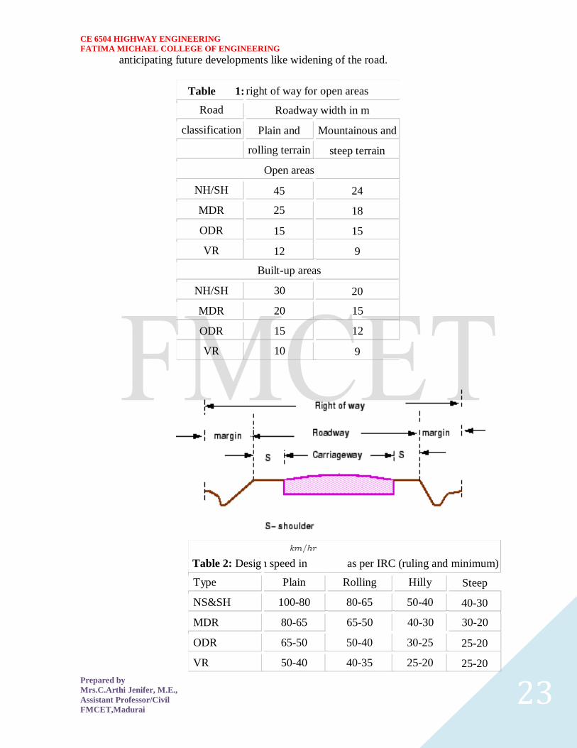
CE 6504 HIGHWAY ENGINEERING
FATIMA MICHAEL COLLEGE OF ENGINEERING
Prepared by
MrsCArthi Jenifer ME
Assistant ProfessorCivil
FMCETMadurai 23
Table 2 Desig
n speed in as per IRC (ruling and minimum)
Steep
Type
Plain
Rolling
Hilly
40-30
NSampSH
100-80
80-65
50-40
MDR
80-65
65-50
40-30
30-20
25-20
ODR
65-50
50-40
30-25
25-20
VR
50-40
40-35
25-20
anticipating future developments like widening of the road
Table 1 No
right of way for open areas
Roadway width in m
Road
Plain and
Mountainous and
classification
steep terrain
rolling terrain
Open areas
45
24
NHSH
18
MDR
25
15
15
ODR
12
9
VR
Built-up areas
20
NHSH
30
MDR
20
15
ODR
15
12
9
VR
10
CE 6504 HIGHWAY ENGINEERING
FATIMA MICHAEL COLLEGE OF ENGINEERING
Prepared by
MrsCArthi Jenifer ME
Assistant ProfessorCivil
FMCETMadurai 24
Horizontal curve
The presence of horizontal curve imparts centrifugal force which is a reactive force
acting outward on a vehicle negotiating it Centrifugal force depends on speed and radius
of the horizontal curve and is counteracted to a certain extent by transverse friction
between the tyre and pavement surface On a curved road this force tends to cause the
vehicle to overrun or to slide outward from the centre of road curvature For proper
design of the curve an understanding of the forces acting on a vehicle taking a horizontal
curve is necessary Various forces acting on the vehicle are illustrated in the figure 1
Figure 1 Effect of horizontal curve They are the centrifugal force (P) acting outward weight of the vehicle (W) acting
downward and the reaction of the ground on the wheels ( and ) The centrifugal
force and the weight is assumed to be from the centre of gravity which is at h units above
the ground Let the wheel base be assumed as b units The centrifugal force in
is given by
(1)
where is the weight of the vehicle in is the speed of the vehicle in is
the acceleration due to gravity in and is the radius of the curve in
The centrifugal ratio or the impact factor is given by
CE 6504 HIGHWAY ENGINEERING
FATIMA MICHAEL COLLEGE OF ENGINEERING
Prepared by
MrsCArthi Jenifer ME
Assistant ProfessorCivil
FMCETMadurai 25
(1)
The centrifugal force has two effects A tendency to overturn the vehicle about the outer
wheels and a tendency for transverse skidding Taking moments of the forces with
respect to the outer wheel when the vehicle is just about to override
At the equilibrium over turning is possible when
and for safety the following condition must satisfy
(2)
The second tendency of the vehicle is for transverse skidding ie When the the
centrifugal force is greater than the maximum possible transverse skid resistance due to
friction between the pavement surface and tyre The transverse skid resistance (F) is
given by
where and is the fractional force at tyre and and is the reaction at
tyre and is the lateral coefficient of friction and is the weight of the vehicle
This is counteracted by the centrifugal force (P) and equating
At equilibrium when skidding takes place (from equation1)
and for safety the following condition must satisfy
CE 6504 HIGHWAY ENGINEERING
FATIMA MICHAEL COLLEGE OF ENGINEERING
Prepared by
MrsCArthi Jenifer ME
Assistant ProfessorCivil
FMCETMadurai 26
(3)
Equation 2 and 3 give the stable condition for design If equation 2 is violated the vehicle
will overturn at the horizontal curve and if equation 3 is violated the vehicle will skid at
the horizontal
Curve Analysis of super-elevation
Super-elevation or cant or banking is the transverse slope provided at horizontal curve to
counteract the centrifugal force by raising the outer edge of the pavement with respect to
the inner edge throughout the length of the horizontal curve When the outer edge is
raised a component of the curve weight will be complimented in counteracting the effect
of centrifugal force In order to find out how much this raising should be the following
analysis may be done The forces acting on a vehicle while taking a horizontal curve with
super elevation is shown in figure 1
Figure 1 Analysis of super-elevation
Forces acting on a vehicle on horizontal curve of radius at a speed of are
the centrifugal force acting horizontally out-wards through the center of
gravity
the weight of the vehicle acting down-wards through the center of gravity and
the friction force between the wheels and the pavement along the surface
inward
CE 6504 HIGHWAY ENGINEERING
FATIMA MICHAEL COLLEGE OF ENGINEERING
Prepared by
MrsCArthi Jenifer ME
Assistant ProfessorCivil
FMCETMadurai 27
At equilibrium by resolving the forces parallel to the surface of the pavement we get where
friction
is the weight of the vehicle is the centrifugal force is the coefficient of
is the transverse slope due to superelevation Dividing by we get
CE 6504 HIGHWAY ENGINEERING
FATIMA MICHAEL COLLEGE OF ENGINEERING
Prepared by
MrsCArthi Jenifer ME
Assistant ProfessorCivil
FMCETMadurai 28
Step 1
Find for 75 percent of design speed neglecting ie
Step 2
If then else if go to step 3
Step 3
Find for the design speed and max ie If
then the maximum is safe for the design speed else go to
step 4
Step 4
Find the allowable speed for the maximum and
If then the design is adequate otherwise use speed adopt
control measures or look for speed control measures
Maximum and minimum super-elevation
Depends on (a) slow moving vehicle and (b) heavy loaded trucks with high CG IRC
specifies a maximum super-elevation of 7 percent for plain and rolling terrain while that
of hilly terrain is 10 percent and urban road is 4 percent The minimum super elevation is
2-4 percent for drainage purpose especially for large radius of the horizontal curve
Attainment of super-elevation
1 Elimination of the crown of the cambered section by
1 Rotating the outer edge about the crown The outer half of the cross slope
is rotated about the crown at a desired rate such that this surface falls on
the same plane as the inner half
2 Shifting the position of the crown This method is also known as diagonal
crown method Here the position of the crown is progressively
shifted outwards thus increasing the width of the inner half of cross section
progressively
2 Rotation of the pavement cross section to attain full super elevation byThere are
two methods of attaining super elevation by rotating the pavement
1 Rotation about the center line The pavement is rotated such that the inner
edge is depressed and the outer edge is raised both by half the total amount
of super elevation ie by with respect to the centre
2 Rotation about the inner edge Here the pavement is rotated raising the
outer edge as well as the centre such that the outer edge is raised by the
full amount of super elevation with respect to the inner edge
Horizontal Transition Curves
CE 6504 HIGHWAY ENGINEERING
FATIMA MICHAEL COLLEGE OF ENGINEERING
Prepared by
MrsCArthi Jenifer ME
Assistant ProfessorCivil
FMCETMadurai 29
Transition curve is provided to change the horizontal alignment from straight to circular
curve gradually and has a radius which decreases from infinity at the straight end
(tangent point) to the desired radius of the circular curve at the other end (curve point)
There are five objectives for providing transition curve and are given below
1 to introduce gradually the centrifugal force between the tangent point and the
beginning of the circular curve avoiding sudden jerk on the vehicle This
increases the comfort of passengers
2 to enable the driver turn the steering gradually for his own comfort and security
3 to provide gradual introduction of super elevation and
4 to provide gradual introduction of extra widening
5 to enhance the aesthetic appearance of the road
Type of transition curve
Different types of transition curves are spiral or clothoid cubic parabola and Lemniscate
IRC recommends spiral as the transition curve because
1 it fulfills the requirement of an ideal transition curve that is
1 rate of change or centrifugal acceleration is consistent (smooth) and
2 radius of the transition curve is at the straight edge and changes to at
the curve point ( ) and calculation and field implementation is
very easy
Length of transition curve The length of the transition curve should be determined as the maximum of the following
three criteria rate of change of centrifugal acceleration rate of change of super elevation
and an empirical formula given by IRC Rate of change of centrifugal acceleration
At the tangent point radius is infinity and hence centrifugal acceleration is zero At the
end of the transition the radius R has minimum value R The rate of change of
centrifugal acceleration should be adopted such that the design should not cause
discomfort to the drivers If is the rate of change of centrifugal acceleration it can be
written as
Therefore the length of the transition curve in is
CE 6504 HIGHWAY ENGINEERING
FATIMA MICHAEL COLLEGE OF ENGINEERING
Prepared by
MrsCArthi Jenifer ME
Assistant ProfessorCivil
FMCETMadurai 30
(1)
where is the rate of change of centrifugal acceleration given by an empirical formula
suggested by by IRC as below
(2) 2 Rate of introduction of super-elevation
Raise ( ) of the outer edge with respect to inner edge is given by
The rate of change of this raise from to is achieved
gradually with a gradient of in over the length of the transition curve (typical range
of is 60-150) Therefore the length of the transition curve is
(3)
3 By empirical formula
IRC suggest the length of the transition curve is minimum for a plain and rolling terrain
(4)
and for steep and hilly terrain is
(5)
CE 6504 HIGHWAY ENGINEERING
FATIMA MICHAEL COLLEGE OF ENGINEERING
Prepared by
MrsCArthi Jenifer ME
Assistant ProfessorCivil
FMCETMadurai 31
and the shift as
(
6
) The length of the transition curve is the maximum of
equations 1 3 and 4or5 ie
(
7
Case (a)
For single lane roads
(
1
)
Therefore
(
2
)
Figure 1 Set-back for single lane roads (
CE 6504 HIGHWAY ENGINEERING
FATIMA MICHAEL COLLEGE OF ENGINEERING
Prepared by
MrsCArthi Jenifer ME
Assistant ProfessorCivil
FMCETMadurai 32
For multi lane roads if is the distance between centerline of the road and the centerline
of the inner lane then
(3)
(4)
Figure 2 Set-back for multi-lane roads ( )
Case (a)
For single lane roads
(1)
Therefore
(2)
Gradient
Gradient is the rate of rise or fall along the length of the road with respect to the
horizontal While aligning a highway the gradient is decided for designing the vertical
curve Before finalizing the gradients the construction cost vehicular operation cost and
the practical problems in the site also has to be considered Usually steep gradients are
avoided as far as possible because of the difficulty to climb and increase in the
CE 6504 HIGHWAY ENGINEERING
FATIMA MICHAEL COLLEGE OF ENGINEERING
Prepared by
MrsCArthi Jenifer ME
Assistant ProfessorCivil
FMCETMadurai 33
construction cost More about gradients are discussed below
Effect of gradient
The effect of long steep gradient on the vehicular speed is considerable This is
particularly important in roads where the proportion of heavy vehicles is significant Due
to restrictive sight distance at uphill gradients the speed of traffic is often controlled by
these heavy vehicles As a result not only the operating costs of the vehicles are
increased but also capacity of the roads will have to be reduced Further due to high
differential speed between heavy and light vehicles and between uphill and downhill
gradients accidents abound in gradients
Representation of gradient
The positive gradient or the ascending gradient is denoted as and the negative gradient as The deviation angle is when two grades meet the angle which
measures the change of direction and is given by the algebraic difference between the two
grades
steep gradient while 1 in 50 = 2 representation is illustrated in the figure 1
Example 1 in 30 = 333 is a
is a flatter gradient The gradient
CE 6504 HIGHWAY ENGINEERING
FATIMA MICHAEL COLLEGE OF ENGINEERING
Prepared by
MrsCArthi Jenifer ME
Assistant ProfessorCivil
FMCETMadurai 34
Figure 1 Representation of gradient
Types of gradient
Many studies have shown that gradient upto seven percent can have considerable effect
on the speeds of the passenger cars On the contrary the speeds of the heavy vehicles are
considerably reduced when long gradients as flat as two percent is adopted Although
flatter gradients are desirable it is evident that the cost of construction will also be very
high Therefore IRC has specified the desirable gradients for each terrain However it
may not be economically viable to adopt such gradients in certain locations steeper
gradients are permitted for short duration Different types of grades are discussed below
Ruling gradient
The ruling gradient or the design gradient is the maximum gradient with which the
designer attempts to design the vertical profile of the road This depends on the terrain
length of the grade speed pulling power of the vehicle and the presence of the horizontal
curve In flatter terrain it may be possible to provide flat gradients but in hilly terrain it
is not economical and sometimes not possible also The ruling gradient is adopted by the
designer by considering a particular speed as the design speed and for a design vehicle
with standard dimensions But our country has a heterogeneous traffic and hence it is not
possible to lay down precise standards for the country as a whole Hence IRC has
recommended some values for ruling gradient for different types of terrain
Limiting gradient
This gradient is adopted when the ruling gradient results in enormous increase in cost of
construction On rolling terrain and hilly terrain it may be frequently necessary to adopt
limiting gradient But the length of the limiting gradient stretches should be limited and
must be sandwiched by either straight roads or easier grades
Exceptional gradient
Exceptional gradient are very steeper gradients given at unavoidable situations They
should be limited for short stretches not exceeding about 100 metres at a stretch In
mountainous and steep terrain successive exceptional gradients must be separated by a
minimum 100 metre length gentler gradient At hairpin bends the gradient is restricted to
25
Critical length of the grade
The maximum length of the ascending gradient which a loaded truck can operate without
undue reduction in speed is called critical length of the grade A speed of 25 kmph is a
CE 6504 HIGHWAY ENGINEERING
FATIMA MICHAEL COLLEGE OF ENGINEERING
Prepared by
MrsCArthi Jenifer ME
Assistant ProfessorCivil
FMCETMadurai 35
reasonable value This value depends on the size power load grad-ability of the truck
initial speed final desirable minimum speed
Minimum gradient
This is important only at locations where surface drainage is important Camber will take
care of the lateral drainage But the longitudinal drainage along the side drains require
some slope for smooth flow of water Therefore minimum gradient is provided for
drainage purpose and it depends on the rain fall type of soil and other site conditions A
minimum of 1 in 500 may be sufficient for concrete drain and 1 in 200 for open soil
drains are found to give satisfactory performance Sight distance available from a point is the actual distance along the road surface which a driver
from a specified height above the carriage way has visibility of stationary or moving objects
Sight distance required by drivers applies to both geometric design of highways and for
traffic control The sight distance situations are considered in the design
i) Stopping or absolute minimum sight distance
ii) Safe overtaking or passing sight distance
iii) Safe sight distance for entering into uncontrolled intersections
Apart from the three situations mentioned above the following sight distance are considered by the
IRC in highway design
Intermediate sight distance
This is defined as twice the stopping sight distance when overtaking sight distance
cannot be provided intermediate sight distance is provided to give limited overtaking opportunities
to fast vehicles
Head light sight distance
This is the distance visible to a driver during night driving under the illumination of the
vehicle head lights
Stopping sight distance
The minimum sight distance available on a highway at any spot should be of sufficient
length to stop a vehicle traveling at design speed safely without collision with any other obstruction
The absolute minimum sight distance is therefore equal to the stopping sight distance
which is also sometimes called nonpassing sight distance The sight distance available on a road to a
driver at any instance depends on
i) Features of the road
ii) Height of the drivers eye above the road surface
iii) Height of the object above the road surface
The distance within which a motor vehicle can be stopped depends upon the factors listed below
a) Total reactions time of the driver
b) Speed of vehicle
c) Efficiency of breaks
d) Frictional resistance between the road and tyres
e) Gradient of the road
Total reaction time
) Reaction time of the driver is the time taken from the instant the object is visible to the
driver to the instant the brakes are effectively applied
) The total reaction time may be split up into two parts
CE 6504 HIGHWAY ENGINEERING
FATIMA MICHAEL COLLEGE OF ENGINEERING
Prepared by
MrsCArthi Jenifer ME
Assistant ProfessorCivil
FMCETMadurai 36
i) Perception time
ii) Brake reaction time
PIEV theory
According to this theory the total reaction time of the driver is split into four parts
i) Perception
ii) Intellection
iii) Emotion
iv) Volition
Speed of Vehicle
The stopping distance depends very much on the speed of the vehicle first during the
total reaction time of the driver the distance moved by the vehicle will depend on the speed
Efficiency of brakes
The braking efficiency is said to be 100 percent if the wheels are fully licked preventing
them from rotating on application of the brakes This will result in 100 percent skidding which is
normally undesirable except in utmost emergency
Frictional resistance between road and tyres
The frictional resistance developed between road and tyres or the skid resistance depends
on the type and condition of the road surface and the tyres IRC has specified a design friction
coefficient of 035 to 04 depending upon the speed to be used for finding the braking distance in the
calculation of stopping sight distance
Analysis of stopping distance
i) The distance traveled by the vehicle during the total reaction time known as lag
distance
ii) The distance traveled by the vehicle after the application of the brakes is known as
braking distance
Overtaking sight distance
The minimum distance open to the vision of the driver of a vehicle intending to overtake
slow vehicle ahead with safety against the traffic of opposite direction is known as the minimum
overtaking sight distance(OSD) or Safe passing sight distance available
The overtaking sight distance is the distance measured along the center of the road which
a driver with his eye level 12m above the road surface can see the top of an object 12m above the
road surface
Some of the important factors on which the minimum overtaking sight distance required
a) Speed of
i) overtaking vehicle
ii) overtaken vehicle
iii) The vehicle coming from opposite direction
b) Distance between the overtaking and overtaken vehicles the minimum spacing
depends on the steeds
a) Skill and reaction time of the driver
b) Rate of acceleration of overtaking vehicle
c) Gradient of the road
Criteria for sight distance requirements on highway
) The absolute minimum sight distance required throughout the length of the road is the
SSD which should invariably be provided at all places
CE 6504 HIGHWAY ENGINEERING
FATIMA MICHAEL COLLEGE OF ENGINEERING
Prepared by
MrsCArthi Jenifer ME
Assistant ProfessorCivil
FMCETMadurai 37
) On horizontal curves the obstruction on the inner side of the curves should be cleared
to provide the required set back distance and absolute minimum sight distance
) On vertical summit curves the sight distance requirement may be fulfilled by proper
design of the vertical alignment
Hairpin bent
TYPES OF CURVES ON HILL ROADS
The following are the important types of curves provided on hill Roads-
1 Hair-Pin Curves
2 Salient Curves
3 Re-entrant Curves 1 Hair-pin curves - The curve in a hill road which changes its direction through an angle of 180
degree or so down the hill on the same side is known as hair-pin curve
A Hair-Pin Bend
This curve is so called because it conforms to the shape of a hair-pin The bend so formed at the
hair-pin curve in a hill road is known as hair-pin bend This type of curve should be located on a
hill side having the minimum slope and maximum stability It must also be safe from view point of
landslides and ground water Hair-pin bends with long arms and farther spacing are always
preferred They reduce construction problems and expensive protective works Hair-pin curves or
bends of serpentine nature are difficult to negotiate and should therefore be avoided as far as
possible
Salient curves - The curves having their convexity on the outer edges of a hill road are called
salient curves The centre of curvature of a salient curve lies towards the hill side This type of curve
occurs in the road length constructed on the ridge of a hill the bend so formed at the salient curve in
a hill road known as corner bend
Salient curves are very dangerous for fast moving traffic At such a curve or at corner bend the
portion of projecting hill side is usually cut down to improve the visibility as shown in fig (Re-
entrant curve) The outer edge of the road at such a curve is essentially provided with a parapet wall
for protection of the vehicles from falling down the hill slope
CE 6504 HIGHWAY ENGINEERING
FATIMA MICHAEL COLLEGE OF ENGINEERING
Prepared by
MrsCArthi Jenifer ME
Assistant ProfessorCivil
FMCETMadurai 38
3 Re-entrant curves - The curves having their convexity on the inner edge of a hill road are called
re-entrant curves
Re-entrant curves
The centre of curvature of a re-entrant curves lies away from the hill side This type of curve occurs
in the road length constructed in the calley of a hill
These curves are less dangereous as they provide adequate visibility to the fast moving traffic At
such curves the parapet wall is provided only for safety of fast moving traffic
CE 6504 HIGHWAY ENGINEERING
FATIMA MICHAEL COLLEGE OF ENGINEERING
Prepared by
MrsCArthi Jenifer ME
Assistant ProfessorCivil
FMCETMadurai 39
UNIT ndash III DESIGN OF RIGID AND FLEXIBLE PAVEMENTS
COMPARISON OF RIGID AND FLEXIBLE PAVEMENTS
The comparisons are
i) Design precision
A cement concrete pavement is amerable to a much more precise structural analysis
than a flexible pavement Flexible pavements designs are mainly empirical Computer aided analysis
of layered system is making the flexible pavement design more exact than hitherto
ii) Life
) Cement concrete slabs of a thin section constructed in the early 1940rsquos are still in
existence in India though many of them have cracked badly and a few of them have been ripped
open and rebuilt in recent ties
) A major project in cement concrete road construction between Agra and Mathura It can
safely be said that a well-designed concrete slab has a life of about 40 years
) Compared to this the life of a flexible pavement generally varies from 10 to 20 years
iii) Maintenance
) A well-designed cement concrete pavement needs very little maintenance The only
maintenance needed is I respect of joints
) The surface is unaffected by spillage of oil and lubricants bituminous surfaces on the
other hand need great inputs in maintenance
) The surface is affected by spillage of oil and lubricants The surface is also affected by
natural weathering agents like air water ad temperature changes
) A cement concrete pavement on the other hand needs a small amount for maintaining
joints
iv) Initial cost
) The argument so far used against a cement concrete slab is that it is much more costly
than a flexible pavement
) The latter specifications no doubt represent the rock-bottom needs of a road in India but
these specifications can hardly provide a smooth and durable surface
v) Stage construction ) Road construction is generally done adopting a policy of stage construction especially for
low volume roads As traffic grows additional layers in the form of water bound macadam and
superior surfacing are added on
) Initial outlay is minimum and additional outlays are in keeping with traffic growth This is
a great advantage when dealing with new roads in an atmosphere of austerity
vi) Availability of materials
) Cement bitumen stone aggregates and gravelsand are the major materials involved in
pavement Construction Cement has been in serious short supply in the country for the past many
decades
) Bitumen is also not available plentifully in India There is also the danger of the entire oil
reserves in the world shrinking during the next two or three decades
) In locations where stone aggregates are scarce cement concrete may have an advantage
for flexible pavements
vii) Surface characterstics
CE 6504 HIGHWAY ENGINEERING
FATIMA MICHAEL COLLEGE OF ENGINEERING
Prepared by
MrsCArthi Jenifer ME
Assistant ProfessorCivil
FMCETMadurai 40
) A good cement concrete surface is smooth and free from rutting potholes and
corrugations In a bituminous surface it is only the asphaltic concrete surface that can give
comparable rideablity
) A well-constructed cement concrete pavement surface can have a permanent nonskid
surface A bituminous surface can also be designed to have a good skid resistant surface
viii) Utility location
) In cement concrete slabs proper thought has to be given to locate utilities such as water
pipes telephone lines and electric cables
) It is difficult to rip open the slab and restore it to be the original condition if any changes
in the utilities lines are to be made
ix) Glame and night visibility
) Concrete pavements have a gray color which can cause glam under sunlight Colored
cement can reduce the grave
) On the other hand bituminous roads need more street lighting
x) Traffic dislocation during construction
) A cement concrete pavement requires 28 days before it can be thrown open to traffic On
the other hand a bituminous surface can be thrown open to traffic shortly after it is rolled
xi) Environmental considerations during construction
) The process of heating of bitumen and aggregates and mixing them together on hot mix
plants can prove to be much more hazardous to the environment than cement concrete construction
where no heating of any material is involved
xii) Overall economy on a life cycle basis
) A good road is costly to construct but once constructed such a road requires little
maintenance and results in savings in vehicle operating costs
) The comparative economy of a flexible pavement and a rigid pavement has proved that on
overall economic considerations
Types of pavement structure
Based on the structural behavior pavements are generally classified into three
categories
i) Flexible pavements
ii) Rigid pavements
iii) Semi rigid pavements
Flexible pavements
) Flexible pavements are those which on the whole have low or negligible flexural
strength and are rather flexible in their structural action under the loadsThe flexible pavement
layers reflect the deformation of the lower layers on to the surface of the layer
) A flexible pavement consists of four components(i) Soil subgrade (ii) sub base
course (iii) base course (iv) Surface course
CE 6504 HIGHWAY ENGINEERING
FATIMA MICHAEL COLLEGE OF ENGINEERING
Prepared by
MrsCArthi Jenifer ME
Assistant ProfessorCivil
FMCETMadurai 41
) The flexible pavement layers transmit the vertical or compressive stresses to the lower layers
by grain to grain transfer through the points of contact in the granular structure A well
compacted granular structure consisting of strong added aggregate can transfer the compressive
stresses
) The load spreading ability of this layer therefore depends on the type of the materials and mix
design factors Bituminous concrete is one of the best flexible pavements layer materials Other
materials which fall under the group are all granular materials with or without bituminous
binder granular base and sub base course materials
) The vertical compressive stress is maximum on the pavement surface directly under the wheel
and is equal to the contact pressure under the wheel The flexible pavement may be constructed
in a number of layers and the top layer has to be strongest as the highest compressive stresses
) Flexible pavements are commonly designed using empirical design charts or equations taking
into account some of the design factors there are also semi empirical and theoretical design
methods
Rigid pavements
) Rigid pavements are those which possess note flexural strength or flexural rigidity
The stresses are not transferred from grain to grain to the lower layers as in the ease of flexible
pavements layers
) The rigid pavements are made of Portland cement concrete plain reinforced or
prestressed concrete The plain cement concrete slabs are expected to take up about 40 kgcm2
flexural stress
) The rigid pavement has the slab action and is capable of transmitting the wheel
load stresses through a wider area below The main point of difference in the structural behavior
of rigid pavement as compared to the flexible pavement is that the critical condition of stress in
the rigid pavement is the maximum flexural stress occurring in the slab due to wheel load and
the temperature changes whereas in the flexible pavement
) As the rigid pavement slab has tensile strength tensile stresses are developed due
to the bending of the slab under wheel load and temperature variations Thus the types of
stresses developed and their distribution within the cement concrete slab are quirt different
) The cement concrete pavement slab can very well serve as a wearing surface as
well an effective base course The rigid pavement structure consists of a cement concrete slab
below which a granular base or sub base course may be provided
) Though the cement concrete slab can also be laid directly over the soil subgrade
consists of fine grained soil
) the rigid pavements are usually designed and the stresses are analyzed using the
elastic theory assuming the pavements as a n elastic plate resting over an elastic or a viscous
foundation
Semi rigid pavements
) when bonded materials like the pozzolanic concrete lean cement concrete or soil
cement are used in the base course or sub base course layer the pavement layer has considerably
higher flexural strength than the common flexible pavement layers
) when this intermediate class of materials are used in the base or sub base course
layer of the pavements they are called semi rigid pavements
CE 6504 HIGHWAY ENGINEERING
FATIMA MICHAEL COLLEGE OF ENGINEERING
Prepared by
MrsCArthi Jenifer ME
Assistant ProfessorCivil
FMCETMadurai 42
) This third category of semi rigid pavement are either designed as flexible
pavements with some correction factors to find the thickness requirements based on experience
or by using a new design approach
) The semi rigid pavement materials have low resistance to impact and abrasion and
therefore are usually provided with flexible pavement surface course
Various functions of pavement components
The functions are
Soil sub grade and its evaluation
) The soil sub grade is a layer of natural soil prepared to receive the layers of pavement
materials placed over it It is essential that at no time the soil sub grade is overstressed it means that
the pressure transmitted on the top of the sub grade is within the allowable limit
) Many tests are known for measuring the strength properties of the sub grades Some of the
tests have been standardized for the use The common strength test for the evaluation of soil
subgrade is
i) California bearing ratio test
ii) California resistance value test
iii) Triaxial compression test
iv) Plate bearing test
CALIFORNIA BEARING RATIO (CBR) TEST
It is evolved for the empirical method of flexible pavement design The CBR test is carried
out either in the laboratory on prepared specimens or in the field by taking in situ measurements
California resistance value
It is found by using have been stabliometerThis test is used in an empirical method of
flexible pavement design based on soil strength
Triaxial test
It is the most important soil strength but still the test is not very commonly used in structural
design of pavements
Plate bearing test
It is carried out using a relatively large diameter plate to evaluate the load supporting
capacity of supporting power of the pavement layers The results are plate bearing tests are used in
flexible pavement design method like McLeod method on based on layer system analysis by
brumister
Sub base and base courses and their evaluation
) There layers are made of broken stones bound or unbound aggreagatesome times in sub
base course a layer of stabilized soil(or) Selected granular soil is also used
) however at the sub base course it is desirable to use smaller size graded aggregates When
the sub grade consists of fine grained soil and when the pavement carries heavy wheel loads
CE 6504 HIGHWAY ENGINEERING
FATIMA MICHAEL COLLEGE OF ENGINEERING
Prepared by
MrsCArthi Jenifer ME
Assistant ProfessorCivil
FMCETMadurai 43
) Sub base course primarily has the similar function as of the base course and is provided
with inferior materials than of base course Base courses are used under rigid pavement for
i) Preventing pumping
ii) Protecting the sub grade against frost action
) Thus the fundamental purpose of abase course and sub base course is to provide a stress
transmitting medium to spread the surface wheel loads in such manner
) The sub base and base course layers may be evaluated by suitable strength or stability test
like plate bearing CBR test
WEARING COURSE AND ITS EVALUATION
) The purpose of the wearing course is to give a smooth riding surface that is dense It
resists pressure exerted by tyres and takes up wear and tear due to the traffic
) Wearing course also offers a water tight layer against the surface water infiltration The
flexible pavement normally a bituminous surfacing is used as a wearing course
) In rigid pavements the cement concrete acts like a base course as well as wearing course
Most popular test in use is marshal stability test where in the optimum content of bitumen binder is
worked out based on the stability density
) Plate bearing test and Bankelman beam test are also sometimes made use of for evaluating
the wearing course and the pavement as a whole
Various factors to be considered in pavement design and the significance
Pavement design consists of two parts
i) Mix design of materials to be used in each pavement component layer Thickness design of the
pavement and the component layers
The various factors to be considered for the design of pavements are given below
i) Design wheel load
ii) Sub grade soil
iii) Climatic factors
iv) Pavement component layers
v) Environmental factors
vi) Special factors in the design of different types of pavements
Design wheel load
The various wheel load factors to be considered in pavement design are
i) Maximum wheel load
ii) Contact pressure
iii) Dual or multiple wheel loads
iv) Repetition of loads
Maximum wheel load
The wheel load configurations are important to know the way in which the loads of a given
vehicle are applied on the pavement surface
) For highways the maximum legal axle load as specified by Indian road congress is 8170
kg with a maximum equivalent single wheel load of 4085 kg
) The evaluation for vertical stress computations under a uniformly distribute of circular
load based on Boussineqrsquos theory is given by
CE 6504 HIGHWAY ENGINEERING
FATIMA MICHAEL COLLEGE OF ENGINEERING
Prepared by
MrsCArthi Jenifer ME
Assistant ProfessorCivil
FMCETMadurai 44
2
322
3
1
za
zpz
σz = vertical stress at depth z
P= surface pressure
Z=depth at which σz computed
A=radius of loaded area
Contact pressure
Generally the wheel load is assumed to be distributed over a circular area But by
measurement of the imprints of tyers with different load and inflation pressures Three terms in use
with reference to tyre pressure are
Tyre pressure
Inflation pressure
Contact pressure
Tyre pressure and inflation pressure mean exactly the same the contact pressure is found to be more
than tyre pressure when the tyre pressure is less than 7 kgm2 and it is vice versa when the tyre
pressure exceeds this value
Contact pressure can be measured by the relationship
Load on wheel
Contact pressure = ----------------------------------------
Contact area or area of imprint
The general variation between the tyre pressure and measured contact pressure is shown in this fig
The ratio of contact pressure to type pressure is defined as rigidity factor Thus value of rigidity
factor is 10 for an average tyre pressure of 7 Kgcm2This value is higher than unity for lower type
pressures and less than unity for tyre pressures higher than 7 kgcm2
Equivalent single wheel load (ESWL)
) The maximum wheel load within the specified limit and to carry greater load it is
necessary to provide dual wheel assembly to the rear axles of the roads vehicles
) In other words the pressure at a certain depth below the pavement surface cannot be
obtained by numerically adding the pressure caused by any one wheel
) The effect is in between the single load and two times load carried by one wheel The load
dispersion is assumed to be at an angle of 450In the dual wheel load assembly let d be the clear gap
between the two wheels S be the spacing between the centers of the wheels and a be the radius of
the circular contact area of each wheel Then S = (d + 2a)
) ESWL may be determined based on either equivalent deflection or equivalent stress
criterianMultiple wheel loads are convert to ESWL and this value is used in pavement design The
ESWL is usually determined by the equivalent stress criterion using a simple graphical method
CE 6504 HIGHWAY ENGINEERING
FATIMA MICHAEL COLLEGE OF ENGINEERING
Prepared by
MrsCArthi Jenifer ME
Assistant ProfessorCivil
FMCETMadurai 45
) A straight line relationship is assumed between ESWL and depth on log scales For
determining ESWL the plot is made as shown in fig
) Two points A and B are plotted on the log-log graph with coordinates of A (Pd2) and
B(2p2s)line AB is a plot which is the focus of points where any single wheel load is equivalent to a
certain set of dual wheels
) To Calculate the ESWL for a dual assembly it is essential to estimate a design thickness of
the pavement If the design thickness so obtained is equal to the estimated thickness then the ESWL
calculations could be considered as correct Otherwise trials are made
) In heavy trucks and trailers the load on each wheel may be further reduced by multiple
wheels and tandem axles
Repetition of loads
) The deformation of load pavement (or) sub grade due to a single application of wheel load
may be small It required carrying out traffic surveys for accounting the factor of repetitions for
wheel loads in the design of pavement
) Data collected are converted to some constant equivalent wheel loads Equivalent wheel
load is a single load equivalent to the repeated applications of any particular wheel load on a
pavement which requires the same thickness and strength of pavements
) McLeod has given a procedure for evolving equivalent load factors for designing flexible
pavements
Various methods of flexible pavement design
) The flexible pavement is built with number of layers In the design process it is to be
ensured that under the application of load none of the layers is overstressed
) The maximum intensity of stresses occurs in the top layer of the pavement The
magnitude of load stresses reduces at lower layers
) In the design of flexible pavements it has yet not been possible to have a rational design
method wherein design process and service behavior of the pavement can be expressed by
mathematical laws
) Flexible pavement design methods are accordingly either empirical or semi empirical In
these methods the knowledge and experience gained on the behavior of the pavements in the past
are usefully utilized
Various approaches of flexible pavement design may be thus classified into three groups
i) Empirical method
ii) Semi-empirical or Semi theoretical method
iii) Theoretical method
) Empirical methods are either based on physical properties or strength parameters of soil
sub grade When the design is based on stress strain function and modified base on experience it
may be called semi-empirical or semi-theoretical There are design methods based on theoretical
analysis and mathematical computations
Out of the flexible pavement design method available is
i) Group index method
ii) California bearing ratio method
iii) California R value (or) Stabiliometer method
iv) Triaxial test method
CE 6504 HIGHWAY ENGINEERING
FATIMA MICHAEL COLLEGE OF ENGINEERING
Prepared by
MrsCArthi Jenifer ME
Assistant ProfessorCivil
FMCETMadurai 46
v) McLeod method
vi) Burmister method
Group index method
) Group index value is an arbitrary index assigned to the soil type in numerical equations
base on the percent fines liquid limit and plasticity index
) The design chart for group index method for determining the pavement thickness is given
in fig
The traffic volume in this method is divided in three groups
Traffic volume No of vehicles per day
Light Less than 50
Medium 50 to 300
Heavy Over 300
The design of the pavement thickness by this method first the G1 value of the soil is found the
anticipated traffic is estimated and is designated as light medium or heavy as indicated
The G1 method of pavement design is essentially an empirical method based on physical properties
of the subgrade soil This method does not consider the strength characteristics of the subgrade soil
and therefore is open to question regarding the reliability of the design based on the index properties
of the soil only
California bearing ratio method
) California division of highways in the USA developed CBR method for
pavement design The majority of design curves developed later are base on the original curves
proposed by OJporter
) One of the chief advantages of CBR method is the simplicity of the test procedure
The CBR tests were carried out by the California state highway department on existing pavement
layers including subgrade sub base and base course
) Based on the extensive CBR test data collected on pavement which behaved
satisfactory and those which failed an empirical design chart was developed correlating the CBR
value and the pavement thickness The basis of the design chart is that a material with a given CBR
required a certain thickness of pavement layer as a cover
) A higher load needs a thicker pavement layer to protect the sub grade Design
curves correlating the CBR value with total pavement thickness cover were developed by the
California state highway department for wheel loads of 3175kg and 5443 kg representing light and
heavy traffic The design curves are shown in this fig
It is possible to extend the CBR design curves for various loading conditions nusing the expression
t= 2
1
1751
pCBRp
t=2
1
751
A
CBR
p
Hence
CE 6504 HIGHWAY ENGINEERING
FATIMA MICHAEL COLLEGE OF ENGINEERING
Prepared by
MrsCArthi Jenifer ME
Assistant ProfessorCivil
FMCETMadurai 47
t= pavement thickness cm
p=Wheel load kg
CBR= California bearing ratio percent
P=tyre pressure kgcm2
A= area of contactcm2
IRC Recommendations
a) The CBR tests should be performed on remoulded soils in the laboratory The specimens should
be prepared by static compaction wherever possible and otherwise by dynamic compaction
b) For the design of new roads the sub grade soil sample should be compacted at OMC to proctor
density whenever suitable compaction equipment
c) The CBR test samples may be soaked in water for four days period before testing the annual
rainfall is less than 50 cm and the water table is too deep to affect the sub grade and imperable
surfacing is provided to carrying out CBR test
d) If the maximum variations in CBR value of the three specimens exceed the specified limits the
design CBR should be average of at least six samples
e) The top 50 cm of sub grade should be compacted at least up to 95 to 100 percent of proctor
density
f) An estimate of the traffic should be carried by the road pavements at the end of expected in view
the existing traffic and probable growth rate of traffic
g) The traffic for the design is considered in units of heavy vehicles per day in both directions and is
divided into seven categories A to G The design thickness is considered applicable for single axle
loads up to 8200 kg and tandom axle loads up to 14500 kg
h) When sub base course materials contain substantial proportion of aggregates of size above 20mm
the CBR value of these materials would not be valid for the design of subsequent layers above them
The CBR method of pavement design gives the total thickness requirement of the pavement above a
sub grade and thickness value would remain the same quality of materials used in component layers
California resistance value method
) In this design method based on stabliometer R-value and cohesiometer C-value
Based on performance data it was established by pavement thickness varies directly with R value
and algorithm of load repetitions It varies inversely with fifth root of c valueThe expression for
pavement thickness is given by the empirical equation
T=
5
1
1 90
C
RTK
Hence
T=total thickness of pavement cm
K=Numerical constant 0166
T1=traffic index
R= stabiliometer resistance value
C=Cohesiometer value
CE 6504 HIGHWAY ENGINEERING
FATIMA MICHAEL COLLEGE OF ENGINEERING
Prepared by
MrsCArthi Jenifer ME
Assistant ProfessorCivil
FMCETMadurai 48
In the design of flexible pavements based on California resistance value method for the following
data are needed
) R-value of soil subgrade
) T1 value
) Equivalent C-value
) R value of soil subgrade is obtained from the test using stablio meterThe
computation of T1 value has been explained
Equivalent C-value
) The cohesion meter value c is obtained for each layer of pavement material
separately from tests However the composite or equivalent C-value of the pavement may be
estimated if the thickness of each component layer and the c-value of the material of the layer are
known
) while designing a pavement as the thickness of the pavement is not known it is
easier if the pavement is first assumed to consist of any one material like gravel base course with
known C-value
) Subsequently the individual thickness of each layer is converted in terms of gravel
equivalent by using relationship
5
1
1
2
2
1
C
C
t
t
) t1 and t2 are the thickness values of any two pavement layersc1 and c2 are their
corresponding cohesiometer values
CE 6504 HIGHWAY ENGINEERING
FATIMA MICHAEL COLLEGE OF ENGINEERING
Prepared by
MrsCArthi Jenifer ME
Assistant ProfessorCivil
FMCETMadurai 49
UNIT 4 MATERIAL AND MAINTENANCE
SUMMIT CURVE
Summit curves are vertical curves with gradient upwards They are formed when two
gradients meet as illustrated in figure 1 in any of the following four ways
1 When a positive gradient meets another positive gradient [figure 1a]
2 When positive gradient meets a flat gradient [figure 1b]
3 When an ascending gradient meets a descending gradient [figure 1c]
4 When a descending gradient meets another descending gradient [figure 1d]
Type of Summit Curve
Many curve forms can be used with satisfactory results the common practice has been to
use parabolic curves in summit curves This is primarily because of the ease with it can
be laid out as well as allowing a comfortable transition from one gradient to another
Although a circular curve offers equal sight distance at every point on the curve for very
small deviation angles a circular curve and parabolic curves are almost congruent
Furthermore the use of parabolic curves were found to give excellent riding comfort
Figure 1 Types of summit curves
Design Consideration
In determining the type and length of the vertical curve the design considerations are
comfort and security of the driver and the appearance of the profile alignment Among
these sight distance requirements for the safety are most important on summit curves
The stopping sight distance or absolute minimum sight distance should be provided on
these curves and where overtaking is not prohibited overtaking sight distance or
intermediate sight distance should be provided as far as possible When a fast moving
vehicle travels along a summit curve there is less discomfort to the passengers This is
because the centrifugal force will be acting upwards while the vehicle negotiates a
summit curve which is against the gravity and hence a part of the tyre pressure is
relieved Also if the curve is provided with adequate sight distance the length would be
sufficient to ease the shock due to change in gradient Circular summit curves are
identical since the radius remains same throughout and hence the sight distance From
CE 6504 HIGHWAY ENGINEERING
FATIMA MICHAEL COLLEGE OF ENGINEERING
Prepared by
MrsCArthi Jenifer ME
Assistant ProfessorCivil
FMCETMadurai 50
this point of view transition curves are not desirable since it has varying radius and so the
sight distance will also vary The deviation angles provided on summit curves for
highways are very large and so the simple parabola is almost congruent to a circular arc
between the same tangent points Parabolic curves are easy for computation and also it
had been found out that it provides good riding comfort to the drivers It is also easy for
field implementation Due to all these reasons a simple parabolic curve is preferred as
summit curve Length of the summit curve
The important design aspect of the summit curve is the determination of the length of the
curve which is parabolic As noted earlier the length of the curve is guided by the sight
distance consideration That is a driver should be able to stop his vehicle safely if there is
an obstruction on the other side of the road Equation of the parabola is given by
where where N is the deviation angle and is the length of the In
deriving the length of the curve two situations can arise depending on the uphill and
downhill gradients when the length of the curve is greater than the sight distance and the
length of the curve is greater than the sight distance
Let is the length of the summit curve is the SSDISDOSD is the deviation angle
drivers eye height (12 m) and the height of the obstruction then the length of the
summit curve can be derived for the following two cases The length of the summit curve
can be derived from the simple geometry as shown below
Case a Length of summit curve greater than sight distance( )
Figure 1 Length of summit curve ( )
The situation when the sight distance is less than the length of the curve is shown in
figure 1
CE 6504 HIGHWAY ENGINEERING
FATIMA MICHAEL COLLEGE OF ENGINEERING
Prepared by
MrsCArthi Jenifer ME
Assistant ProfessorCivil
FMCETMadurai 51
(1)
Case b Length of summit curve less than sight distance
The second case is illustrated in figure 1
Figure 1 Length of summit curve
CE 6504 HIGHWAY ENGINEERING
FATIMA MICHAEL COLLEGE OF ENGINEERING
Prepared by
MrsCArthi Jenifer ME
Assistant ProfessorCivil
FMCETMadurai 52
From the basic geometry one can write
(1)
Therefore for a given and to get minimum differentiate the above equation
with respect to and equate it to zero Therefore
Solving the quadratic equation for
(2)
Now we can substitute back to get the value of minimum value of for a given
and Therefore
Solving for
CE 6504 HIGHWAY ENGINEERING
FATIMA MICHAEL COLLEGE OF ENGINEERING
Prepared by
MrsCArthi Jenifer ME
Assistant ProfessorCivil
FMCETMadurai 53
(3) (4
CE 6504 HIGHWAY ENGINEERING
FATIMA MICHAEL COLLEGE OF ENGINEERING
Prepared by
MrsCArthi Jenifer ME
Assistant ProfessorCivil
FMCETMadurai 54
When stopping sight distance is considered the height of drivers eye above the road
surface ( ) is taken as 12 metres and height of object above the pavement surface ( )
is taken as 015 metres If overtaking sight distance is considered then the value of
drivers eye height ( ) and the height of the obstruction ( ) are taken equal as 12
metres
Valley curve
Valley curve or sag curves are vertical curves with convexity downwards They are
formed when two gradients meet as illustrated in figure 1 in any of the following four
ways
Figure 1 Types of valley curve
1 When a descending gradient meets another descending gradient [figure 1a]
2 When a descending gradient meets a flat gradient [figure 1b]
3 When a descending gradient meets an ascending gradient [figure 1c]
4 When an ascending gradient meets another ascending gradient [figure
Design considerations
There is no restriction to sight distance at valley curves during day time But visibility is
reduced during night In the absence or inadequacy of street light the only source for
visibility is with the help of headlights Hence valley curves are designed taking into
account of headlight distance In valley curves the centrifugal force will be acting
downwards along with the weight of the vehicle and hence impact to the vehicle will be
more This will result in jerking of the vehicle and cause discomfort to the passengers
Thus the most important design factors considered in valley curves are (1) impact-free
movement of vehicles at design speed and (2) availability of stopping sight distance
under headlight of vehicles for night driving
For gradually introducing and increasing the centrifugal force acting downwards the best
shape that could be given for a valley curve is a transition curve Cubic parabola is
generally preferred in vertical valley curves See figure 1
CE 6504 HIGHWAY ENGINEERING
FATIMA MICHAEL COLLEGE OF ENGINEERING
Prepared by
MrsCArthi Jenifer ME
Assistant ProfessorCivil
FMCETMadurai 55
Figure 1 Valley curve details
During night under headlight driving condition sight distance reduces and availability of
stopping sight distance under head light is very important The head light sight distance
should be at least equal to the stopping sight distance There is no problem of overtaking
sight distance at night since the other vehicles with headlights could be seen from a
considerable distance
Length of the valley curve
The valley curve is made fully transitional by providing two similar transition curves of
equal length The transitional curve is set out by a cubic parabola where
The length of the valley transition curve is designed based on two criteria
1 comfort criteria that is allowable rate of change of centrifugal acceleration is
limited to a comfortable level of about
2 safety criteria that is the driver should have adequate headlight sight distance at
any part of the country
Comfort criteria
The length of the valley curve based on the rate of change of centrifugal acceleration that
will ensure comfort Let is the rate of change of acceleration the minimum radius of
the curve is the design speed and is the time then is give
CE 6504 HIGHWAY ENGINEERING
FATIMA MICHAEL COLLEGE OF ENGINEERING
Prepared by
MrsCArthi Jenifer ME
Assistant ProfessorCivil
FMCETMadurai 56
For a cubic parabola the Value Safety criter Length of the valley curve for headlight distance may be determined for two conditions
(1) length of the valley curve greater than stopping sight distance and (2) length of the
valley curve less than the stopping sight distance of for length is given by
Case 1 Length of valley curve greater than stopping sight distance ( )
The total length of valley curve is greater than the stopping sight distance SSD The
sight distance available will be minimum when the vehicle is in the lowest point in the
valley This is because the beginning of the curve will have infinite radius and the bottom
of the curve will have minimum radius which is a property of the transition curve The
case is shown in figure 1
Figure 1 Valley curve case 1
From the geometry of the figure we have
CE 6504 HIGHWAY ENGINEERING
FATIMA MICHAEL COLLEGE OF ENGINEERING
Prepared by
MrsCArthi Jenifer ME
Assistant ProfessorCivil
FMCETMadurai 57
(1)
where is the deviation angle in radians is the height of headlight beam is the
head beam inclination in degrees and is the sight distance The inclination is 1
degree
Case 2 Length of valley curve less than stopping sight distance ( )
The length of the curve is less than SSD In this case the minimum sight distance is
from the beginning of the curve The important points are the beginning of the curve and
the bottom most part of the curve If the vehicle is at the bottom of the curve then its
headlight beam will reach far beyond the endpoint of the curve whereas if the vehicle is
at the beginning of the curve then the headlight beam will hit just outside the curve
Therefore the length of the curve is derived by assuming the vehicle at the beginning of
the curve The case is shown in figure 1
From the figure
(1) Note that the above expression is approximate and is satisfactory because in practice the gradients
are very small and is acceptable for all practical purposes We will not be able to know prior to
which case to be adopted Therefore both has to be calculated and the one which satisfies the
condition is adopted
1 Flexible pavement
2 Rigid pavement
Flexible pavement
These pavements reflect the deformation of sub grade and the subsequent layers to the
surface
Rigid pavement
The rigid characteristic of the pavement are associated with rigidity or flexural strength
CE 6504 HIGHWAY ENGINEERING
FATIMA MICHAEL COLLEGE OF ENGINEERING
Prepared by
MrsCArthi Jenifer ME
Assistant ProfessorCivil
FMCETMadurai 58
or slab action so the load is distributed over a wide area of sub grade soil
Flexible pavement Definition
These pavements reflect the deformation of sub grade and the subsequent layers to the
surface Flexible usually asphalt is laid with no reinforcement or with a specialized
fabric reinforcement that permits limited flow or repositioning of the roadbed under
ground changes
The design of flexible pavement is based on load distributing characteristic of the
component layers The black top pavement including water amp gravel bound macadam fall
in this category
Flexible pavement on the whole has low or negligible flexible strength flexible in their
structural action) The flexible pavement layers transmit the vertical or compressive
stresses to the lower layers by grain transfer through contact points of granular structure
The vertical compressive stress is maximum on the pavement surface directly under the
wheel load and is equal to contact pressure under the wheels Due to the ability to
distribute the stress to large area in the shape of truncated cone the stresses get decreased
in the lower layer
As such the flexible pavement may be constructed in a number of layers and the top
layer has to be strongest as the highest compressive stresses
To be sustained by this layer in addition to wear and tear the lower layer have to take
up only lesser magnitude of stress as there is no direct wearing action die to traffic loads
therefore inferior material with lower cast can be used in the lower layers
Rigid pavement Definition
The rigid characteristic of the pavement are associated with rigidity or flexural strength
or slab action so the load is distributed over a wide area of sub grade soil Rigid pavement
is laid in slabs with steel reinforcement
The rigid pavements are made of cement concrete either plan reinforced or prestressed
concrete
Critical condition of stress in the rigid pavement is the maximum flexural stress occurring in the slab due to wheel load and the temperature changes
Rigid pavement is designed and analyzed by using the elastic theory
CE 6504 HIGHWAY ENGINEERING
FATIMA MICHAEL COLLEGE OF ENGINEERING
Prepared by
MrsCArthi Jenifer ME
Assistant ProfessorCivil
FMCETMadurai 59
UNIT-5 EVALUATION AND MAINTENANCE OF PAVEMENTS
TRAFFIC PARAMETERS
Design life
Design life is the number of years (or number of standard axle repetitions) for which the
pavement is being designed A pavement is expected to serve satisfactorily within the
design life For concrete pavements 20 to 40 years may be assumed as the design life
(PCA 1984 IRC58 2002)
Basic design principle
Though different approaches for concrete pavement design are suggested in various
guidelines the design principles tend to remain similar across different guidelines for
example PCA (1994) Austroads (2004) NCHRP (2004) IRC58 (2002) etc except the
AASHTO (1993) provisions which is based on empirical approach The basic steps
involved in the design of concrete pavement method can be summarized as follows
The developed stresses due to load for a trial thickness of the concrete slab are
calculated for various loading configuration and the critical one is chosen The
axle loads are generally divided into different axle load groups and the load
stresses are calculated individually
The ratio between the load stress and Modulus of Rupture (MOR) is known as
stress ratio The stress ratio determines how many repetitions the pavement can
sustain (ie allowable traffic repetitions) for the individual axle load group If the
stress ratio is 055 or lower it can withstand virtually infinite number of traffic
repetitions (PCA 1984)
The ratio between the allowable repetitions to the expected traffic repetitions is
the damage fraction The calculation process is repeated for various axle loads
(sometimes for various seasons or various timings of the day) and the sum of
individual damage fractions (c u m u l a t i v e fatigue damage) should be less
than equal to one for pavement design being safe If found unsafe the trial
thickness is changed and the design process is repeated
The design process may also include considerations for temperature stress
moisture stresses and erosion distress
A brief discussion on concrete pavement design approaches suggested by various design
practices viz PCA method (1984) Austroads method (2004) AASHTO method (1993)
NCHRP mechanistic-empirical method (2004) and the Indian Roads Congress (IRC)
method (2002) are placed in the following
Portland cement Association (PCA) Method
The PCA method is based on Westergaard Picket and Rays work and further theoretical
analysis by Finite Element Method (Huang 1993) The data used to develop the PCA
method is generated from various road tests like ASSHO road test Arlington test
(conducted by PCA) Bates test road and Maryland road test (PCA 1984) The PCA
design method is based on the following two considerations (PCA 1984)
The fatigue damage on the concrete slab due to repetitive application of traffic
load is estimated The cumulative fatigue damage principle is used to estimate the
design thickness of the slab Edge stress between the mid-ways of the
CE 6504 HIGHWAY ENGINEERING
FATIMA MICHAEL COLLEGE OF ENGINEERING
Prepared by
MrsCArthi Jenifer ME
Assistant ProfessorCivil
FMCETMadurai 60
transverse joint is taken as critical configuration
The stresses due to warping and curling (due to temperature and moisture
gradient) are not considered in the fatigue analysis as per PCA recommendation
because most of the time the stresses generated are subtractive to the load stress
The possibility of erosion of pavement materials placed below the concrete slab is
evaluated The rate at which the slab is deflected due to axle load is used as a
criterion for erosion Theoretically it can be shown that a thin pavement with
smaller deflection basin is subjected to faster rate of deflection compared to
thicker slab Hence thin slab is more susceptible to erosion In a similar way the
cumulative erosion damage is calculated for individual axle load groups If this
value is greater than one then the design needs to be revised
Austroads method
Austroads method has been adopted from PCA (1984) approach with modifications
suited to Australian conditions (Austroads 2004) A bound mix or lean cement concrete is
used as sub-base material For a given CBR value of the subgrade and given thickness of
cemented sub-base the effective subgrade strength can be obtained from the chart
provided Figure-19 schematically shows such a chart For different levels of traffic
Austroads (2004) suggests minimum values of the base thicknesses to be provided
CE 6504 HIGHWAY ENGINEERING
FATIMA MICHAEL COLLEGE OF ENGINEERING
Prepared by
MrsCArthi Jenifer ME
Assistant ProfessorCivil
FMCETMadurai 61
figure-19 Schematic diagram of Austroads (2004) chart for estimation of effective
subgrade strength
As per Astroads (2004) the concrete pavement slab thickness for a given expected
traffic repetitions is designed considering the (i) flexural fatigue of the concrete slab and
the (ii) subgrade erosion arising out of repeated deflections For both the considerations
equations are suggested to calculate the allowable traffic repetitions If the allowable
traffic is less than the expected traffic the design is revised by increasing the slab
thickness The concrete shoulders adopted are of integral type or structural type
AASHTO method
The AASHTO method (1993) for design of concrete pavement has evolved from the
AASHO road test (AASHO 1962) The AASHTO pavement design follows an empirical
approach Pavement performance in terms of present serviceability index ( PSI ) loss of
serviceability sub-grade and sub-base strength cumulative traffic properties of concrete
joint load transfer efficiency drainage condition overall standard deviation and
reliability are the input parameters considered in the pavement design
The PSI value of the fresh pavement is assumed as 45 and the pavement is deemed to
have failed when the PSI value reaches 25 The resilient moduli of the subgrade and sub-
base materials are determined in the laboratory simulating the seasonal moisture content
and stress situation Suggested values are also available for given moisture content
plasticity index etc The composite modulus of sub-grade reaction (k) is estimated from
modulus of sub-grade reaction and elastic modulus of sub-base for various seasons and
the depth of rigid foundation and the thickness of the sub-base
Design equation as well nomographs are available to estimate the slab thickness (D) from
these input parameters
NCHRP mechanistic-empirical (M-E) metho
The NCHRP (2004) has recently developed concrete pavement design procedure based
on mechanistic-empirical (M-E) approach This approach attempts to reduce the extent of
empiricism prevalent in the existing AASHTO (1993) guidelines This proposed NCHRP
pavement design system is modular in nature that is the design approach can be
modified by parts (as and when new knowledge is available) without disrupting the
overall design procedure This approach also can take care of various wheel-axle loa
configuration
As per this approach trial thickness of the slab is first assumed and the stress strain and
displacement values are obtained From these values the performance of the pavement in
terms of distresses (such as faulting cracking) and smoothness and predicted If these
predicted performance parameters does not satisfy the required performance for a given
reliability
The design approach includes a large data-base as input parameters for example average
daily traffic traffic growth rate traffic composition hourly weather data on air
temperature precipitation wind speed percentage sunshine relative humidity pavement
material engineering parameters ground water depth infiltration drainage hydraulic
conductivity thermal conductivity heat capacity etc The temperature stress is
considered in this method but the temperature profile is linearized to enhance
computational efficiency (NCHRP 2004)
CE 6504 HIGHWAY ENGINEERING
FATIMA MICHAEL COLLEGE OF ENGINEERING
Prepared by
MrsCArthi Jenifer ME
Assistant ProfessorCivil
FMCETMadurai 62
INDIAN ROADS CONGRESS (IRC) METHOD
The Indian Roads Congress (IRC) guidelines IRC58 (2002) has adopted the
Westergaards equation to estimate load stress and Brdaburys equation to estimate
temperature stress The load stress is highest at the corner of the slab lesser in edge and
least in the interior The order of variation of temperature stress is just the reverse of this
As per IRC58 (2002) it is recommended that the design needs to be done for edge stress
condition and subsequently check needs to be performed for corner stress condition so as
to finalize the design The following are the steps followed as per IRC58 (2002)
guideline for the design of concrete pavement
The input parameters are obtained to formulate the design problem The joint
spacing and the slab dimensions are decided If there is a bound sub-base layer
over the subgrade a suitable value of effective k is to be adopted
A trial thickness of the concrete slab is assumed
The edge stress is estimated for various axle loads from the given charts Figure-
20 schematically shows such a chart The cumulative fatigue damage principle for
fatigue is applied to check the adequacy of the slab thickness
The sum of edge stress due to load for the highest axle load group and the
temperature stress should be less than the MOR of concrete otherwise the design
is revised
The adequacy of corner stress is checked with respect to MOR value and
accordingly the design is finalized Westergaards corner stress formula
Figure-20 Schematic diagram of IRC58 chart for estimation of load stress at the edge
(IRC58 2002)
CE 6504 HIGHWAY ENGINEERING
FATIMA MICHAEL COLLEGE OF ENGINEERING
Prepared by
MrsCArthi Jenifer ME
Assistant ProfessorCivil
FMCETMadurai 63
estimation of corner stress due to load and the corner stress due to temperature is
assumed to be zero
Estimation of layer thicknesses
The thickness of the pavement is adjusted in such a way that the stress strain
developed is less than the allowable values obtained from past performance
information
The two major modes of structural failure of pavement are fatigue and rutting
o Fatigue Traffic applies repetitive load to the pavement surface and the
cracks start from bottom the bound layer slab and propagate upwards
When the extent of surface cracks reaches a predefined level the
pavement is said to have failed due to flexural fatigue
FUNCTIONAL DESIGN
The functional pavement design involves considerations of skid resistance roughness
surface distresses reflectivity of pavement surface etc The functional pavement design
considers mainly the surface features of a pavement
Drainage design
A road needs to be designed in such a way that the rain snow precipitation is drained off
the pavement and its surroundings A suitable surface drainage system for the pavement
is designed for this purpose Some water however will percolate into the pavement from
its top surface and needs to be taken out of the pavement - this is done by providing an
internal drainage system to the pavement Water will also try to enter into the pavement
from bottom due to capillary rise or due to rise in water table A suitably designed sub-
surface drainage system tries to avoid such a problem
PAVEMENT THICKNESS DESIGN CHARTS
For the design of pavements to carry traffic in the range of 1 to 10 msa use chart 1 and for
traffic in the range 10 to 150 msa use chart 2 of IRC37 2001 The design curves relate
pavement thickness to the cumulative number of standard axles to be carried over the
design life for different sub-grade CBR values ranging from 2 to 10 The design
charts will give the total thickness of the pavement for the above inputs The total
thickness consists of granular sub-base granular base and bituminous surfacing The
individual layers are designed based on the the recommendations given below and the
subsequent tables
Pavement composition
Sub-base
Sub-base materials comprise natural sand gravel laterite brick metal crushed
stone or combinations thereof meeting the prescribed grading and physical
requirements The sub-base material should have a minimum CBR of 20 and
30 for traffic upto 2 msa and traffic exceeding 2 msa respectively Sub-base
usually consist of granular or WBM and the thickness should not be less than 150
mm for design traffic less than 10 msa and 200 mm for design traffic
Base
The recommended designs are for unbounded granular bases which comprise
CE 6504 HIGHWAY ENGINEERING
FATIMA MICHAEL COLLEGE OF ENGINEERING
Prepared by
MrsCArthi Jenifer ME
Assistant ProfessorCivil
FMCETMadurai 64
conventional water bound macadam (WBM) or wet mix macadam (WMM) or
equivalent confirming to MOST specifications The materials should be of good
quality with minimum thickness of 225 mm for traffic up to 2 msa an 150 mm for
traffic
Bituminoussurfacing The surfacing consists of a wearing course or a binder
course plus wearing course The most commonly used wearing courses are
surface dressing open graded premix carpet mix seal surfacing semi-
dense bituminous concrete and bituminous concrete For binder course
MOST specifies it is desirable to use bituminous macadam (BM) for traffic
upto o 5 msa and dense bituminous macadam (DBM) for traffic more than 5
msa
Numerical example
Design the pavement for construction of a new bypass with the following data
1 Two lane carriage way
2 Initial traffic in the year of completion of construction = 400 CVPD (sum of both
directions)
3 Traffic growth rate = 75
4 Design life = 15 years
5 Vehicle damage factor based on axle load survey = 25 standard axle per
commercial vehicle
6 Design CBR of subgrade soil = 4
Solution
1 Distribution factor = 075
2
3 Total pavement thickness for CBR 4 and traffic 72 msa from IRC37 2001
chart1 = 660 mm
4 Pavement composition can be obtained by interpolation from Pavement Design
Catalogue (IRC37 2001)
1 Bituminous surfacing = 25 mm SDBC + 70 mm DBM
2 Road-base = 250 mm WBM
3 sub-base = 315 mm granular material of CBR not less than 30
CE 6504 HIGHWAY ENGINEERING
FATIMA MICHAEL COLLEGE OF ENGINEERING
Prepared by
MrsCArthi Jenifer ME
Assistant ProfessorCivil
FMCETMadurai 65
Generally bound base layers are used for concrete pavement construction As per Indian
specification some example of such base layers are Dry Lean Concrete (DLC) Roller
Compacted Concrete (RCC) (IRC15-2002)
The concrete slab is generally of M40 to M50 grade of concrete as
per Indian specifications and is called as paving quality concrete (PQC)
(IRC15-2002)
BITUMINOUS PAVEMENT
The subgrade is a compacted soil layer
The base and sub-base course could be made up of bound or unbound granular layer As
per Indian specifications (MORTampH 2001) some examples of base or sub-base layers
are Granular sub-base(GSB) Water Bound Macadam (WBM) Wet Mix Macadam
(WMM) etc
The binder course is made up bituminous material As per Indian specifications
(MORTampH 2001) some examples of binder course are Bituminous Macadam (BM)
Dense Bituminous Macadam (DBM) etc
The wearing course is the top bituminous layer which is comes in contact to the
vehicle tyre Wearing course provides impermeability to the pavement surface
against water percolation (Chakroborty and Das 2003) The binder course and wearing
course together are called bituminous surfacing
IRC METHOD OF FLEXIBLE PAVEMENT MIX DESIGN
These guidelines will apply to design of flexible pavements for Expressway National Highways
State Highways Major District Roads and other categories of roads Flexible pavements are
considered to include the pavements which have bituminous surfacing and granular base and sub-
base courses conforming to IRC MOST standards These guidelines apply to new pavements
Design criteria
The flexible pavements has been modeled as a three layer structure and stresses and strains at
critical locations have been computed using the linear elastic model To give proper consideration
to the aspects of performance the following three types of pavement distress resulting from
repeated (cyclic) application of traffic loads are considered
1 Vertical compressive strain at the top of the sub-grade which can cause sub-grade
deformation resulting in permanent deformation at the pavement surface
2 Horizontal tensile strain or stress at the bottom of the bituminous layer which can cause
fracture of the bituminous layer
3 Pavement deformation within the bituminous layer
CE 6504 HIGHWAY ENGINEERING
FATIMA MICHAEL COLLEGE OF ENGINEERING
Prepared by
MrsCArthi Jenifer ME
Assistant ProfessorCivil
FMCETMadurai 66
While the permanent deformation within the bituminous layer can be controlled by meeting the
mix design requirements thickness of granular and bituminous layers are selected using the
analytical design approach so that strains at the critical points are within the allowable limits For
calculating tensile strains at the bottom of the bituminous layer the stiffness of dense bituminous
macadam (DBM) layer with 6070 bitumen has been used in the analysis
FAILURE CRITERIA
Critical locations in pavement
A and B are the critical locations for tensile strains Maximum value of the strain is
adopted for design C is the critical location for the vertical subgrade strain since the
maximum value of the occurs mostly at C
CE 6504 HIGHWAY ENGINEERING
FATIMA MICHAEL COLLEGE OF ENGINEERING
Prepared by
MrsCArthi Jenifer ME
Assistant ProfessorCivil
FMCETMadurai 67
Fatigue Criteria
Bituminous surfacings of pavements display flexural fatigue cracking if the tensile strain
at the bottom of the bituminous layer is beyond certain limit The relation between the
fatigue life of the pavement and the tensile strain in the bottom of the bituminous layer
was obtained as
(1)
in which is the allowable number of load repetitions to control fatigue cracking and
is the Elastic modulus of bituminous layer The use of equation 1 would result in
fatigue cracking of 20 of the total area
Rutting Criteria
The allowable number of load repetitions to control permanent deformation can be
expressed as
(2)
is the number of cumulative standard axles to produce rutting of 20 mm
CE 6504 HIGHWAY ENGINEERING
FATIMA MICHAEL COLLEGE OF ENGINEERING
Prepared by
MrsCArthi Jenifer ME
Assistant ProfessorCivil
FMCETMadurai 68
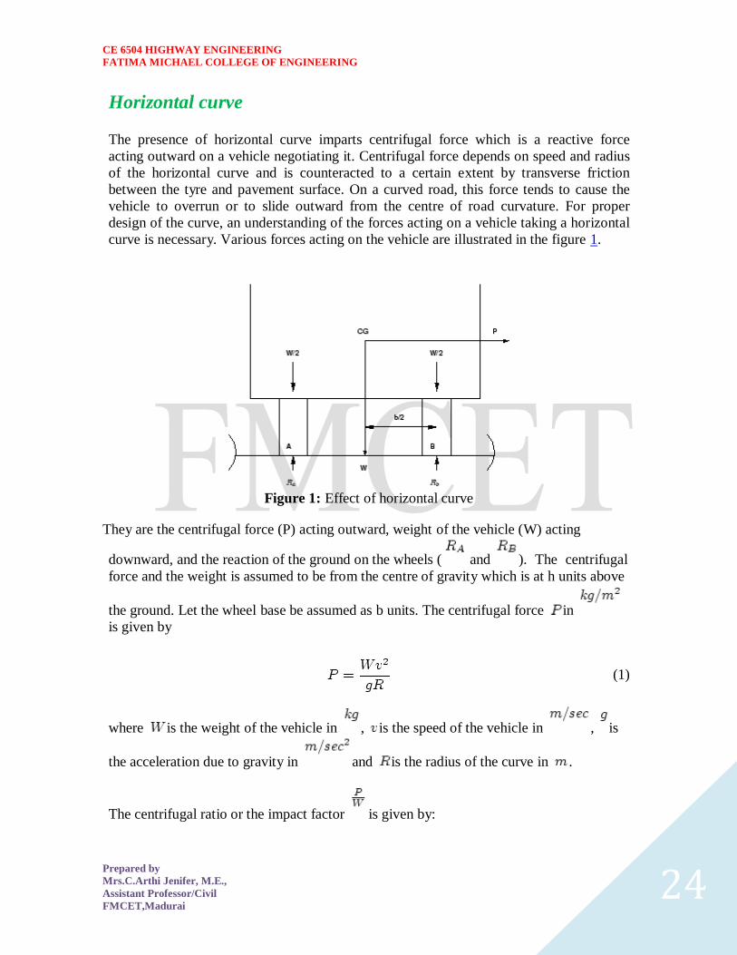
CE 6504 HIGHWAY ENGINEERING
FATIMA MICHAEL COLLEGE OF ENGINEERING
Prepared by
MrsCArthi Jenifer ME
Assistant ProfessorCivil
FMCETMadurai 24
Horizontal curve
The presence of horizontal curve imparts centrifugal force which is a reactive force
acting outward on a vehicle negotiating it Centrifugal force depends on speed and radius
of the horizontal curve and is counteracted to a certain extent by transverse friction
between the tyre and pavement surface On a curved road this force tends to cause the
vehicle to overrun or to slide outward from the centre of road curvature For proper
design of the curve an understanding of the forces acting on a vehicle taking a horizontal
curve is necessary Various forces acting on the vehicle are illustrated in the figure 1
Figure 1 Effect of horizontal curve They are the centrifugal force (P) acting outward weight of the vehicle (W) acting
downward and the reaction of the ground on the wheels ( and ) The centrifugal
force and the weight is assumed to be from the centre of gravity which is at h units above
the ground Let the wheel base be assumed as b units The centrifugal force in
is given by
(1)
where is the weight of the vehicle in is the speed of the vehicle in is
the acceleration due to gravity in and is the radius of the curve in
The centrifugal ratio or the impact factor is given by
CE 6504 HIGHWAY ENGINEERING
FATIMA MICHAEL COLLEGE OF ENGINEERING
Prepared by
MrsCArthi Jenifer ME
Assistant ProfessorCivil
FMCETMadurai 25
(1)
The centrifugal force has two effects A tendency to overturn the vehicle about the outer
wheels and a tendency for transverse skidding Taking moments of the forces with
respect to the outer wheel when the vehicle is just about to override
At the equilibrium over turning is possible when
and for safety the following condition must satisfy
(2)
The second tendency of the vehicle is for transverse skidding ie When the the
centrifugal force is greater than the maximum possible transverse skid resistance due to
friction between the pavement surface and tyre The transverse skid resistance (F) is
given by
where and is the fractional force at tyre and and is the reaction at
tyre and is the lateral coefficient of friction and is the weight of the vehicle
This is counteracted by the centrifugal force (P) and equating
At equilibrium when skidding takes place (from equation1)
and for safety the following condition must satisfy
CE 6504 HIGHWAY ENGINEERING
FATIMA MICHAEL COLLEGE OF ENGINEERING
Prepared by
MrsCArthi Jenifer ME
Assistant ProfessorCivil
FMCETMadurai 26
(3)
Equation 2 and 3 give the stable condition for design If equation 2 is violated the vehicle
will overturn at the horizontal curve and if equation 3 is violated the vehicle will skid at
the horizontal
Curve Analysis of super-elevation
Super-elevation or cant or banking is the transverse slope provided at horizontal curve to
counteract the centrifugal force by raising the outer edge of the pavement with respect to
the inner edge throughout the length of the horizontal curve When the outer edge is
raised a component of the curve weight will be complimented in counteracting the effect
of centrifugal force In order to find out how much this raising should be the following
analysis may be done The forces acting on a vehicle while taking a horizontal curve with
super elevation is shown in figure 1
Figure 1 Analysis of super-elevation
Forces acting on a vehicle on horizontal curve of radius at a speed of are
the centrifugal force acting horizontally out-wards through the center of
gravity
the weight of the vehicle acting down-wards through the center of gravity and
the friction force between the wheels and the pavement along the surface
inward
CE 6504 HIGHWAY ENGINEERING
FATIMA MICHAEL COLLEGE OF ENGINEERING
Prepared by
MrsCArthi Jenifer ME
Assistant ProfessorCivil
FMCETMadurai 27
At equilibrium by resolving the forces parallel to the surface of the pavement we get where
friction
is the weight of the vehicle is the centrifugal force is the coefficient of
is the transverse slope due to superelevation Dividing by we get
CE 6504 HIGHWAY ENGINEERING
FATIMA MICHAEL COLLEGE OF ENGINEERING
Prepared by
MrsCArthi Jenifer ME
Assistant ProfessorCivil
FMCETMadurai 28
Step 1
Find for 75 percent of design speed neglecting ie
Step 2
If then else if go to step 3
Step 3
Find for the design speed and max ie If
then the maximum is safe for the design speed else go to
step 4
Step 4
Find the allowable speed for the maximum and
If then the design is adequate otherwise use speed adopt
control measures or look for speed control measures
Maximum and minimum super-elevation
Depends on (a) slow moving vehicle and (b) heavy loaded trucks with high CG IRC
specifies a maximum super-elevation of 7 percent for plain and rolling terrain while that
of hilly terrain is 10 percent and urban road is 4 percent The minimum super elevation is
2-4 percent for drainage purpose especially for large radius of the horizontal curve
Attainment of super-elevation
1 Elimination of the crown of the cambered section by
1 Rotating the outer edge about the crown The outer half of the cross slope
is rotated about the crown at a desired rate such that this surface falls on
the same plane as the inner half
2 Shifting the position of the crown This method is also known as diagonal
crown method Here the position of the crown is progressively
shifted outwards thus increasing the width of the inner half of cross section
progressively
2 Rotation of the pavement cross section to attain full super elevation byThere are
two methods of attaining super elevation by rotating the pavement
1 Rotation about the center line The pavement is rotated such that the inner
edge is depressed and the outer edge is raised both by half the total amount
of super elevation ie by with respect to the centre
2 Rotation about the inner edge Here the pavement is rotated raising the
outer edge as well as the centre such that the outer edge is raised by the
full amount of super elevation with respect to the inner edge
Horizontal Transition Curves
CE 6504 HIGHWAY ENGINEERING
FATIMA MICHAEL COLLEGE OF ENGINEERING
Prepared by
MrsCArthi Jenifer ME
Assistant ProfessorCivil
FMCETMadurai 29
Transition curve is provided to change the horizontal alignment from straight to circular
curve gradually and has a radius which decreases from infinity at the straight end
(tangent point) to the desired radius of the circular curve at the other end (curve point)
There are five objectives for providing transition curve and are given below
1 to introduce gradually the centrifugal force between the tangent point and the
beginning of the circular curve avoiding sudden jerk on the vehicle This
increases the comfort of passengers
2 to enable the driver turn the steering gradually for his own comfort and security
3 to provide gradual introduction of super elevation and
4 to provide gradual introduction of extra widening
5 to enhance the aesthetic appearance of the road
Type of transition curve
Different types of transition curves are spiral or clothoid cubic parabola and Lemniscate
IRC recommends spiral as the transition curve because
1 it fulfills the requirement of an ideal transition curve that is
1 rate of change or centrifugal acceleration is consistent (smooth) and
2 radius of the transition curve is at the straight edge and changes to at
the curve point ( ) and calculation and field implementation is
very easy
Length of transition curve The length of the transition curve should be determined as the maximum of the following
three criteria rate of change of centrifugal acceleration rate of change of super elevation
and an empirical formula given by IRC Rate of change of centrifugal acceleration
At the tangent point radius is infinity and hence centrifugal acceleration is zero At the
end of the transition the radius R has minimum value R The rate of change of
centrifugal acceleration should be adopted such that the design should not cause
discomfort to the drivers If is the rate of change of centrifugal acceleration it can be
written as
Therefore the length of the transition curve in is
CE 6504 HIGHWAY ENGINEERING
FATIMA MICHAEL COLLEGE OF ENGINEERING
Prepared by
MrsCArthi Jenifer ME
Assistant ProfessorCivil
FMCETMadurai 30
(1)
where is the rate of change of centrifugal acceleration given by an empirical formula
suggested by by IRC as below
(2) 2 Rate of introduction of super-elevation
Raise ( ) of the outer edge with respect to inner edge is given by
The rate of change of this raise from to is achieved
gradually with a gradient of in over the length of the transition curve (typical range
of is 60-150) Therefore the length of the transition curve is
(3)
3 By empirical formula
IRC suggest the length of the transition curve is minimum for a plain and rolling terrain
(4)
and for steep and hilly terrain is
(5)
CE 6504 HIGHWAY ENGINEERING
FATIMA MICHAEL COLLEGE OF ENGINEERING
Prepared by
MrsCArthi Jenifer ME
Assistant ProfessorCivil
FMCETMadurai 31
and the shift as
(
6
) The length of the transition curve is the maximum of
equations 1 3 and 4or5 ie
(
7
Case (a)
For single lane roads
(
1
)
Therefore
(
2
)
Figure 1 Set-back for single lane roads (
CE 6504 HIGHWAY ENGINEERING
FATIMA MICHAEL COLLEGE OF ENGINEERING
Prepared by
MrsCArthi Jenifer ME
Assistant ProfessorCivil
FMCETMadurai 32
For multi lane roads if is the distance between centerline of the road and the centerline
of the inner lane then
(3)
(4)
Figure 2 Set-back for multi-lane roads ( )
Case (a)
For single lane roads
(1)
Therefore
(2)
Gradient
Gradient is the rate of rise or fall along the length of the road with respect to the
horizontal While aligning a highway the gradient is decided for designing the vertical
curve Before finalizing the gradients the construction cost vehicular operation cost and
the practical problems in the site also has to be considered Usually steep gradients are
avoided as far as possible because of the difficulty to climb and increase in the
CE 6504 HIGHWAY ENGINEERING
FATIMA MICHAEL COLLEGE OF ENGINEERING
Prepared by
MrsCArthi Jenifer ME
Assistant ProfessorCivil
FMCETMadurai 33
construction cost More about gradients are discussed below
Effect of gradient
The effect of long steep gradient on the vehicular speed is considerable This is
particularly important in roads where the proportion of heavy vehicles is significant Due
to restrictive sight distance at uphill gradients the speed of traffic is often controlled by
these heavy vehicles As a result not only the operating costs of the vehicles are
increased but also capacity of the roads will have to be reduced Further due to high
differential speed between heavy and light vehicles and between uphill and downhill
gradients accidents abound in gradients
Representation of gradient
The positive gradient or the ascending gradient is denoted as and the negative gradient as The deviation angle is when two grades meet the angle which
measures the change of direction and is given by the algebraic difference between the two
grades
steep gradient while 1 in 50 = 2 representation is illustrated in the figure 1
Example 1 in 30 = 333 is a
is a flatter gradient The gradient
CE 6504 HIGHWAY ENGINEERING
FATIMA MICHAEL COLLEGE OF ENGINEERING
Prepared by
MrsCArthi Jenifer ME
Assistant ProfessorCivil
FMCETMadurai 34
Figure 1 Representation of gradient
Types of gradient
Many studies have shown that gradient upto seven percent can have considerable effect
on the speeds of the passenger cars On the contrary the speeds of the heavy vehicles are
considerably reduced when long gradients as flat as two percent is adopted Although
flatter gradients are desirable it is evident that the cost of construction will also be very
high Therefore IRC has specified the desirable gradients for each terrain However it
may not be economically viable to adopt such gradients in certain locations steeper
gradients are permitted for short duration Different types of grades are discussed below
Ruling gradient
The ruling gradient or the design gradient is the maximum gradient with which the
designer attempts to design the vertical profile of the road This depends on the terrain
length of the grade speed pulling power of the vehicle and the presence of the horizontal
curve In flatter terrain it may be possible to provide flat gradients but in hilly terrain it
is not economical and sometimes not possible also The ruling gradient is adopted by the
designer by considering a particular speed as the design speed and for a design vehicle
with standard dimensions But our country has a heterogeneous traffic and hence it is not
possible to lay down precise standards for the country as a whole Hence IRC has
recommended some values for ruling gradient for different types of terrain
Limiting gradient
This gradient is adopted when the ruling gradient results in enormous increase in cost of
construction On rolling terrain and hilly terrain it may be frequently necessary to adopt
limiting gradient But the length of the limiting gradient stretches should be limited and
must be sandwiched by either straight roads or easier grades
Exceptional gradient
Exceptional gradient are very steeper gradients given at unavoidable situations They
should be limited for short stretches not exceeding about 100 metres at a stretch In
mountainous and steep terrain successive exceptional gradients must be separated by a
minimum 100 metre length gentler gradient At hairpin bends the gradient is restricted to
25
Critical length of the grade
The maximum length of the ascending gradient which a loaded truck can operate without
undue reduction in speed is called critical length of the grade A speed of 25 kmph is a
CE 6504 HIGHWAY ENGINEERING
FATIMA MICHAEL COLLEGE OF ENGINEERING
Prepared by
MrsCArthi Jenifer ME
Assistant ProfessorCivil
FMCETMadurai 35
reasonable value This value depends on the size power load grad-ability of the truck
initial speed final desirable minimum speed
Minimum gradient
This is important only at locations where surface drainage is important Camber will take
care of the lateral drainage But the longitudinal drainage along the side drains require
some slope for smooth flow of water Therefore minimum gradient is provided for
drainage purpose and it depends on the rain fall type of soil and other site conditions A
minimum of 1 in 500 may be sufficient for concrete drain and 1 in 200 for open soil
drains are found to give satisfactory performance Sight distance available from a point is the actual distance along the road surface which a driver
from a specified height above the carriage way has visibility of stationary or moving objects
Sight distance required by drivers applies to both geometric design of highways and for
traffic control The sight distance situations are considered in the design
i) Stopping or absolute minimum sight distance
ii) Safe overtaking or passing sight distance
iii) Safe sight distance for entering into uncontrolled intersections
Apart from the three situations mentioned above the following sight distance are considered by the
IRC in highway design
Intermediate sight distance
This is defined as twice the stopping sight distance when overtaking sight distance
cannot be provided intermediate sight distance is provided to give limited overtaking opportunities
to fast vehicles
Head light sight distance
This is the distance visible to a driver during night driving under the illumination of the
vehicle head lights
Stopping sight distance
The minimum sight distance available on a highway at any spot should be of sufficient
length to stop a vehicle traveling at design speed safely without collision with any other obstruction
The absolute minimum sight distance is therefore equal to the stopping sight distance
which is also sometimes called nonpassing sight distance The sight distance available on a road to a
driver at any instance depends on
i) Features of the road
ii) Height of the drivers eye above the road surface
iii) Height of the object above the road surface
The distance within which a motor vehicle can be stopped depends upon the factors listed below
a) Total reactions time of the driver
b) Speed of vehicle
c) Efficiency of breaks
d) Frictional resistance between the road and tyres
e) Gradient of the road
Total reaction time
) Reaction time of the driver is the time taken from the instant the object is visible to the
driver to the instant the brakes are effectively applied
) The total reaction time may be split up into two parts
CE 6504 HIGHWAY ENGINEERING
FATIMA MICHAEL COLLEGE OF ENGINEERING
Prepared by
MrsCArthi Jenifer ME
Assistant ProfessorCivil
FMCETMadurai 36
i) Perception time
ii) Brake reaction time
PIEV theory
According to this theory the total reaction time of the driver is split into four parts
i) Perception
ii) Intellection
iii) Emotion
iv) Volition
Speed of Vehicle
The stopping distance depends very much on the speed of the vehicle first during the
total reaction time of the driver the distance moved by the vehicle will depend on the speed
Efficiency of brakes
The braking efficiency is said to be 100 percent if the wheels are fully licked preventing
them from rotating on application of the brakes This will result in 100 percent skidding which is
normally undesirable except in utmost emergency
Frictional resistance between road and tyres
The frictional resistance developed between road and tyres or the skid resistance depends
on the type and condition of the road surface and the tyres IRC has specified a design friction
coefficient of 035 to 04 depending upon the speed to be used for finding the braking distance in the
calculation of stopping sight distance
Analysis of stopping distance
i) The distance traveled by the vehicle during the total reaction time known as lag
distance
ii) The distance traveled by the vehicle after the application of the brakes is known as
braking distance
Overtaking sight distance
The minimum distance open to the vision of the driver of a vehicle intending to overtake
slow vehicle ahead with safety against the traffic of opposite direction is known as the minimum
overtaking sight distance(OSD) or Safe passing sight distance available
The overtaking sight distance is the distance measured along the center of the road which
a driver with his eye level 12m above the road surface can see the top of an object 12m above the
road surface
Some of the important factors on which the minimum overtaking sight distance required
a) Speed of
i) overtaking vehicle
ii) overtaken vehicle
iii) The vehicle coming from opposite direction
b) Distance between the overtaking and overtaken vehicles the minimum spacing
depends on the steeds
a) Skill and reaction time of the driver
b) Rate of acceleration of overtaking vehicle
c) Gradient of the road
Criteria for sight distance requirements on highway
) The absolute minimum sight distance required throughout the length of the road is the
SSD which should invariably be provided at all places
CE 6504 HIGHWAY ENGINEERING
FATIMA MICHAEL COLLEGE OF ENGINEERING
Prepared by
MrsCArthi Jenifer ME
Assistant ProfessorCivil
FMCETMadurai 37
) On horizontal curves the obstruction on the inner side of the curves should be cleared
to provide the required set back distance and absolute minimum sight distance
) On vertical summit curves the sight distance requirement may be fulfilled by proper
design of the vertical alignment
Hairpin bent
TYPES OF CURVES ON HILL ROADS
The following are the important types of curves provided on hill Roads-
1 Hair-Pin Curves
2 Salient Curves
3 Re-entrant Curves 1 Hair-pin curves - The curve in a hill road which changes its direction through an angle of 180
degree or so down the hill on the same side is known as hair-pin curve
A Hair-Pin Bend
This curve is so called because it conforms to the shape of a hair-pin The bend so formed at the
hair-pin curve in a hill road is known as hair-pin bend This type of curve should be located on a
hill side having the minimum slope and maximum stability It must also be safe from view point of
landslides and ground water Hair-pin bends with long arms and farther spacing are always
preferred They reduce construction problems and expensive protective works Hair-pin curves or
bends of serpentine nature are difficult to negotiate and should therefore be avoided as far as
possible
Salient curves - The curves having their convexity on the outer edges of a hill road are called
salient curves The centre of curvature of a salient curve lies towards the hill side This type of curve
occurs in the road length constructed on the ridge of a hill the bend so formed at the salient curve in
a hill road known as corner bend
Salient curves are very dangerous for fast moving traffic At such a curve or at corner bend the
portion of projecting hill side is usually cut down to improve the visibility as shown in fig (Re-
entrant curve) The outer edge of the road at such a curve is essentially provided with a parapet wall
for protection of the vehicles from falling down the hill slope
CE 6504 HIGHWAY ENGINEERING
FATIMA MICHAEL COLLEGE OF ENGINEERING
Prepared by
MrsCArthi Jenifer ME
Assistant ProfessorCivil
FMCETMadurai 38
3 Re-entrant curves - The curves having their convexity on the inner edge of a hill road are called
re-entrant curves
Re-entrant curves
The centre of curvature of a re-entrant curves lies away from the hill side This type of curve occurs
in the road length constructed in the calley of a hill
These curves are less dangereous as they provide adequate visibility to the fast moving traffic At
such curves the parapet wall is provided only for safety of fast moving traffic
CE 6504 HIGHWAY ENGINEERING
FATIMA MICHAEL COLLEGE OF ENGINEERING
Prepared by
MrsCArthi Jenifer ME
Assistant ProfessorCivil
FMCETMadurai 39
UNIT ndash III DESIGN OF RIGID AND FLEXIBLE PAVEMENTS
COMPARISON OF RIGID AND FLEXIBLE PAVEMENTS
The comparisons are
i) Design precision
A cement concrete pavement is amerable to a much more precise structural analysis
than a flexible pavement Flexible pavements designs are mainly empirical Computer aided analysis
of layered system is making the flexible pavement design more exact than hitherto
ii) Life
) Cement concrete slabs of a thin section constructed in the early 1940rsquos are still in
existence in India though many of them have cracked badly and a few of them have been ripped
open and rebuilt in recent ties
) A major project in cement concrete road construction between Agra and Mathura It can
safely be said that a well-designed concrete slab has a life of about 40 years
) Compared to this the life of a flexible pavement generally varies from 10 to 20 years
iii) Maintenance
) A well-designed cement concrete pavement needs very little maintenance The only
maintenance needed is I respect of joints
) The surface is unaffected by spillage of oil and lubricants bituminous surfaces on the
other hand need great inputs in maintenance
) The surface is affected by spillage of oil and lubricants The surface is also affected by
natural weathering agents like air water ad temperature changes
) A cement concrete pavement on the other hand needs a small amount for maintaining
joints
iv) Initial cost
) The argument so far used against a cement concrete slab is that it is much more costly
than a flexible pavement
) The latter specifications no doubt represent the rock-bottom needs of a road in India but
these specifications can hardly provide a smooth and durable surface
v) Stage construction ) Road construction is generally done adopting a policy of stage construction especially for
low volume roads As traffic grows additional layers in the form of water bound macadam and
superior surfacing are added on
) Initial outlay is minimum and additional outlays are in keeping with traffic growth This is
a great advantage when dealing with new roads in an atmosphere of austerity
vi) Availability of materials
) Cement bitumen stone aggregates and gravelsand are the major materials involved in
pavement Construction Cement has been in serious short supply in the country for the past many
decades
) Bitumen is also not available plentifully in India There is also the danger of the entire oil
reserves in the world shrinking during the next two or three decades
) In locations where stone aggregates are scarce cement concrete may have an advantage
for flexible pavements
vii) Surface characterstics
CE 6504 HIGHWAY ENGINEERING
FATIMA MICHAEL COLLEGE OF ENGINEERING
Prepared by
MrsCArthi Jenifer ME
Assistant ProfessorCivil
FMCETMadurai 40
) A good cement concrete surface is smooth and free from rutting potholes and
corrugations In a bituminous surface it is only the asphaltic concrete surface that can give
comparable rideablity
) A well-constructed cement concrete pavement surface can have a permanent nonskid
surface A bituminous surface can also be designed to have a good skid resistant surface
viii) Utility location
) In cement concrete slabs proper thought has to be given to locate utilities such as water
pipes telephone lines and electric cables
) It is difficult to rip open the slab and restore it to be the original condition if any changes
in the utilities lines are to be made
ix) Glame and night visibility
) Concrete pavements have a gray color which can cause glam under sunlight Colored
cement can reduce the grave
) On the other hand bituminous roads need more street lighting
x) Traffic dislocation during construction
) A cement concrete pavement requires 28 days before it can be thrown open to traffic On
the other hand a bituminous surface can be thrown open to traffic shortly after it is rolled
xi) Environmental considerations during construction
) The process of heating of bitumen and aggregates and mixing them together on hot mix
plants can prove to be much more hazardous to the environment than cement concrete construction
where no heating of any material is involved
xii) Overall economy on a life cycle basis
) A good road is costly to construct but once constructed such a road requires little
maintenance and results in savings in vehicle operating costs
) The comparative economy of a flexible pavement and a rigid pavement has proved that on
overall economic considerations
Types of pavement structure
Based on the structural behavior pavements are generally classified into three
categories
i) Flexible pavements
ii) Rigid pavements
iii) Semi rigid pavements
Flexible pavements
) Flexible pavements are those which on the whole have low or negligible flexural
strength and are rather flexible in their structural action under the loadsThe flexible pavement
layers reflect the deformation of the lower layers on to the surface of the layer
) A flexible pavement consists of four components(i) Soil subgrade (ii) sub base
course (iii) base course (iv) Surface course
CE 6504 HIGHWAY ENGINEERING
FATIMA MICHAEL COLLEGE OF ENGINEERING
Prepared by
MrsCArthi Jenifer ME
Assistant ProfessorCivil
FMCETMadurai 41
) The flexible pavement layers transmit the vertical or compressive stresses to the lower layers
by grain to grain transfer through the points of contact in the granular structure A well
compacted granular structure consisting of strong added aggregate can transfer the compressive
stresses
) The load spreading ability of this layer therefore depends on the type of the materials and mix
design factors Bituminous concrete is one of the best flexible pavements layer materials Other
materials which fall under the group are all granular materials with or without bituminous
binder granular base and sub base course materials
) The vertical compressive stress is maximum on the pavement surface directly under the wheel
and is equal to the contact pressure under the wheel The flexible pavement may be constructed
in a number of layers and the top layer has to be strongest as the highest compressive stresses
) Flexible pavements are commonly designed using empirical design charts or equations taking
into account some of the design factors there are also semi empirical and theoretical design
methods
Rigid pavements
) Rigid pavements are those which possess note flexural strength or flexural rigidity
The stresses are not transferred from grain to grain to the lower layers as in the ease of flexible
pavements layers
) The rigid pavements are made of Portland cement concrete plain reinforced or
prestressed concrete The plain cement concrete slabs are expected to take up about 40 kgcm2
flexural stress
) The rigid pavement has the slab action and is capable of transmitting the wheel
load stresses through a wider area below The main point of difference in the structural behavior
of rigid pavement as compared to the flexible pavement is that the critical condition of stress in
the rigid pavement is the maximum flexural stress occurring in the slab due to wheel load and
the temperature changes whereas in the flexible pavement
) As the rigid pavement slab has tensile strength tensile stresses are developed due
to the bending of the slab under wheel load and temperature variations Thus the types of
stresses developed and their distribution within the cement concrete slab are quirt different
) The cement concrete pavement slab can very well serve as a wearing surface as
well an effective base course The rigid pavement structure consists of a cement concrete slab
below which a granular base or sub base course may be provided
) Though the cement concrete slab can also be laid directly over the soil subgrade
consists of fine grained soil
) the rigid pavements are usually designed and the stresses are analyzed using the
elastic theory assuming the pavements as a n elastic plate resting over an elastic or a viscous
foundation
Semi rigid pavements
) when bonded materials like the pozzolanic concrete lean cement concrete or soil
cement are used in the base course or sub base course layer the pavement layer has considerably
higher flexural strength than the common flexible pavement layers
) when this intermediate class of materials are used in the base or sub base course
layer of the pavements they are called semi rigid pavements
CE 6504 HIGHWAY ENGINEERING
FATIMA MICHAEL COLLEGE OF ENGINEERING
Prepared by
MrsCArthi Jenifer ME
Assistant ProfessorCivil
FMCETMadurai 42
) This third category of semi rigid pavement are either designed as flexible
pavements with some correction factors to find the thickness requirements based on experience
or by using a new design approach
) The semi rigid pavement materials have low resistance to impact and abrasion and
therefore are usually provided with flexible pavement surface course
Various functions of pavement components
The functions are
Soil sub grade and its evaluation
) The soil sub grade is a layer of natural soil prepared to receive the layers of pavement
materials placed over it It is essential that at no time the soil sub grade is overstressed it means that
the pressure transmitted on the top of the sub grade is within the allowable limit
) Many tests are known for measuring the strength properties of the sub grades Some of the
tests have been standardized for the use The common strength test for the evaluation of soil
subgrade is
i) California bearing ratio test
ii) California resistance value test
iii) Triaxial compression test
iv) Plate bearing test
CALIFORNIA BEARING RATIO (CBR) TEST
It is evolved for the empirical method of flexible pavement design The CBR test is carried
out either in the laboratory on prepared specimens or in the field by taking in situ measurements
California resistance value
It is found by using have been stabliometerThis test is used in an empirical method of
flexible pavement design based on soil strength
Triaxial test
It is the most important soil strength but still the test is not very commonly used in structural
design of pavements
Plate bearing test
It is carried out using a relatively large diameter plate to evaluate the load supporting
capacity of supporting power of the pavement layers The results are plate bearing tests are used in
flexible pavement design method like McLeod method on based on layer system analysis by
brumister
Sub base and base courses and their evaluation
) There layers are made of broken stones bound or unbound aggreagatesome times in sub
base course a layer of stabilized soil(or) Selected granular soil is also used
) however at the sub base course it is desirable to use smaller size graded aggregates When
the sub grade consists of fine grained soil and when the pavement carries heavy wheel loads
CE 6504 HIGHWAY ENGINEERING
FATIMA MICHAEL COLLEGE OF ENGINEERING
Prepared by
MrsCArthi Jenifer ME
Assistant ProfessorCivil
FMCETMadurai 43
) Sub base course primarily has the similar function as of the base course and is provided
with inferior materials than of base course Base courses are used under rigid pavement for
i) Preventing pumping
ii) Protecting the sub grade against frost action
) Thus the fundamental purpose of abase course and sub base course is to provide a stress
transmitting medium to spread the surface wheel loads in such manner
) The sub base and base course layers may be evaluated by suitable strength or stability test
like plate bearing CBR test
WEARING COURSE AND ITS EVALUATION
) The purpose of the wearing course is to give a smooth riding surface that is dense It
resists pressure exerted by tyres and takes up wear and tear due to the traffic
) Wearing course also offers a water tight layer against the surface water infiltration The
flexible pavement normally a bituminous surfacing is used as a wearing course
) In rigid pavements the cement concrete acts like a base course as well as wearing course
Most popular test in use is marshal stability test where in the optimum content of bitumen binder is
worked out based on the stability density
) Plate bearing test and Bankelman beam test are also sometimes made use of for evaluating
the wearing course and the pavement as a whole
Various factors to be considered in pavement design and the significance
Pavement design consists of two parts
i) Mix design of materials to be used in each pavement component layer Thickness design of the
pavement and the component layers
The various factors to be considered for the design of pavements are given below
i) Design wheel load
ii) Sub grade soil
iii) Climatic factors
iv) Pavement component layers
v) Environmental factors
vi) Special factors in the design of different types of pavements
Design wheel load
The various wheel load factors to be considered in pavement design are
i) Maximum wheel load
ii) Contact pressure
iii) Dual or multiple wheel loads
iv) Repetition of loads
Maximum wheel load
The wheel load configurations are important to know the way in which the loads of a given
vehicle are applied on the pavement surface
) For highways the maximum legal axle load as specified by Indian road congress is 8170
kg with a maximum equivalent single wheel load of 4085 kg
) The evaluation for vertical stress computations under a uniformly distribute of circular
load based on Boussineqrsquos theory is given by
CE 6504 HIGHWAY ENGINEERING
FATIMA MICHAEL COLLEGE OF ENGINEERING
Prepared by
MrsCArthi Jenifer ME
Assistant ProfessorCivil
FMCETMadurai 44
2
322
3
1
za
zpz
σz = vertical stress at depth z
P= surface pressure
Z=depth at which σz computed
A=radius of loaded area
Contact pressure
Generally the wheel load is assumed to be distributed over a circular area But by
measurement of the imprints of tyers with different load and inflation pressures Three terms in use
with reference to tyre pressure are
Tyre pressure
Inflation pressure
Contact pressure
Tyre pressure and inflation pressure mean exactly the same the contact pressure is found to be more
than tyre pressure when the tyre pressure is less than 7 kgm2 and it is vice versa when the tyre
pressure exceeds this value
Contact pressure can be measured by the relationship
Load on wheel
Contact pressure = ----------------------------------------
Contact area or area of imprint
The general variation between the tyre pressure and measured contact pressure is shown in this fig
The ratio of contact pressure to type pressure is defined as rigidity factor Thus value of rigidity
factor is 10 for an average tyre pressure of 7 Kgcm2This value is higher than unity for lower type
pressures and less than unity for tyre pressures higher than 7 kgcm2
Equivalent single wheel load (ESWL)
) The maximum wheel load within the specified limit and to carry greater load it is
necessary to provide dual wheel assembly to the rear axles of the roads vehicles
) In other words the pressure at a certain depth below the pavement surface cannot be
obtained by numerically adding the pressure caused by any one wheel
) The effect is in between the single load and two times load carried by one wheel The load
dispersion is assumed to be at an angle of 450In the dual wheel load assembly let d be the clear gap
between the two wheels S be the spacing between the centers of the wheels and a be the radius of
the circular contact area of each wheel Then S = (d + 2a)
) ESWL may be determined based on either equivalent deflection or equivalent stress
criterianMultiple wheel loads are convert to ESWL and this value is used in pavement design The
ESWL is usually determined by the equivalent stress criterion using a simple graphical method
CE 6504 HIGHWAY ENGINEERING
FATIMA MICHAEL COLLEGE OF ENGINEERING
Prepared by
MrsCArthi Jenifer ME
Assistant ProfessorCivil
FMCETMadurai 45
) A straight line relationship is assumed between ESWL and depth on log scales For
determining ESWL the plot is made as shown in fig
) Two points A and B are plotted on the log-log graph with coordinates of A (Pd2) and
B(2p2s)line AB is a plot which is the focus of points where any single wheel load is equivalent to a
certain set of dual wheels
) To Calculate the ESWL for a dual assembly it is essential to estimate a design thickness of
the pavement If the design thickness so obtained is equal to the estimated thickness then the ESWL
calculations could be considered as correct Otherwise trials are made
) In heavy trucks and trailers the load on each wheel may be further reduced by multiple
wheels and tandem axles
Repetition of loads
) The deformation of load pavement (or) sub grade due to a single application of wheel load
may be small It required carrying out traffic surveys for accounting the factor of repetitions for
wheel loads in the design of pavement
) Data collected are converted to some constant equivalent wheel loads Equivalent wheel
load is a single load equivalent to the repeated applications of any particular wheel load on a
pavement which requires the same thickness and strength of pavements
) McLeod has given a procedure for evolving equivalent load factors for designing flexible
pavements
Various methods of flexible pavement design
) The flexible pavement is built with number of layers In the design process it is to be
ensured that under the application of load none of the layers is overstressed
) The maximum intensity of stresses occurs in the top layer of the pavement The
magnitude of load stresses reduces at lower layers
) In the design of flexible pavements it has yet not been possible to have a rational design
method wherein design process and service behavior of the pavement can be expressed by
mathematical laws
) Flexible pavement design methods are accordingly either empirical or semi empirical In
these methods the knowledge and experience gained on the behavior of the pavements in the past
are usefully utilized
Various approaches of flexible pavement design may be thus classified into three groups
i) Empirical method
ii) Semi-empirical or Semi theoretical method
iii) Theoretical method
) Empirical methods are either based on physical properties or strength parameters of soil
sub grade When the design is based on stress strain function and modified base on experience it
may be called semi-empirical or semi-theoretical There are design methods based on theoretical
analysis and mathematical computations
Out of the flexible pavement design method available is
i) Group index method
ii) California bearing ratio method
iii) California R value (or) Stabiliometer method
iv) Triaxial test method
CE 6504 HIGHWAY ENGINEERING
FATIMA MICHAEL COLLEGE OF ENGINEERING
Prepared by
MrsCArthi Jenifer ME
Assistant ProfessorCivil
FMCETMadurai 46
v) McLeod method
vi) Burmister method
Group index method
) Group index value is an arbitrary index assigned to the soil type in numerical equations
base on the percent fines liquid limit and plasticity index
) The design chart for group index method for determining the pavement thickness is given
in fig
The traffic volume in this method is divided in three groups
Traffic volume No of vehicles per day
Light Less than 50
Medium 50 to 300
Heavy Over 300
The design of the pavement thickness by this method first the G1 value of the soil is found the
anticipated traffic is estimated and is designated as light medium or heavy as indicated
The G1 method of pavement design is essentially an empirical method based on physical properties
of the subgrade soil This method does not consider the strength characteristics of the subgrade soil
and therefore is open to question regarding the reliability of the design based on the index properties
of the soil only
California bearing ratio method
) California division of highways in the USA developed CBR method for
pavement design The majority of design curves developed later are base on the original curves
proposed by OJporter
) One of the chief advantages of CBR method is the simplicity of the test procedure
The CBR tests were carried out by the California state highway department on existing pavement
layers including subgrade sub base and base course
) Based on the extensive CBR test data collected on pavement which behaved
satisfactory and those which failed an empirical design chart was developed correlating the CBR
value and the pavement thickness The basis of the design chart is that a material with a given CBR
required a certain thickness of pavement layer as a cover
) A higher load needs a thicker pavement layer to protect the sub grade Design
curves correlating the CBR value with total pavement thickness cover were developed by the
California state highway department for wheel loads of 3175kg and 5443 kg representing light and
heavy traffic The design curves are shown in this fig
It is possible to extend the CBR design curves for various loading conditions nusing the expression
t= 2
1
1751
pCBRp
t=2
1
751
A
CBR
p
Hence
CE 6504 HIGHWAY ENGINEERING
FATIMA MICHAEL COLLEGE OF ENGINEERING
Prepared by
MrsCArthi Jenifer ME
Assistant ProfessorCivil
FMCETMadurai 47
t= pavement thickness cm
p=Wheel load kg
CBR= California bearing ratio percent
P=tyre pressure kgcm2
A= area of contactcm2
IRC Recommendations
a) The CBR tests should be performed on remoulded soils in the laboratory The specimens should
be prepared by static compaction wherever possible and otherwise by dynamic compaction
b) For the design of new roads the sub grade soil sample should be compacted at OMC to proctor
density whenever suitable compaction equipment
c) The CBR test samples may be soaked in water for four days period before testing the annual
rainfall is less than 50 cm and the water table is too deep to affect the sub grade and imperable
surfacing is provided to carrying out CBR test
d) If the maximum variations in CBR value of the three specimens exceed the specified limits the
design CBR should be average of at least six samples
e) The top 50 cm of sub grade should be compacted at least up to 95 to 100 percent of proctor
density
f) An estimate of the traffic should be carried by the road pavements at the end of expected in view
the existing traffic and probable growth rate of traffic
g) The traffic for the design is considered in units of heavy vehicles per day in both directions and is
divided into seven categories A to G The design thickness is considered applicable for single axle
loads up to 8200 kg and tandom axle loads up to 14500 kg
h) When sub base course materials contain substantial proportion of aggregates of size above 20mm
the CBR value of these materials would not be valid for the design of subsequent layers above them
The CBR method of pavement design gives the total thickness requirement of the pavement above a
sub grade and thickness value would remain the same quality of materials used in component layers
California resistance value method
) In this design method based on stabliometer R-value and cohesiometer C-value
Based on performance data it was established by pavement thickness varies directly with R value
and algorithm of load repetitions It varies inversely with fifth root of c valueThe expression for
pavement thickness is given by the empirical equation
T=
5
1
1 90
C
RTK
Hence
T=total thickness of pavement cm
K=Numerical constant 0166
T1=traffic index
R= stabiliometer resistance value
C=Cohesiometer value
CE 6504 HIGHWAY ENGINEERING
FATIMA MICHAEL COLLEGE OF ENGINEERING
Prepared by
MrsCArthi Jenifer ME
Assistant ProfessorCivil
FMCETMadurai 48
In the design of flexible pavements based on California resistance value method for the following
data are needed
) R-value of soil subgrade
) T1 value
) Equivalent C-value
) R value of soil subgrade is obtained from the test using stablio meterThe
computation of T1 value has been explained
Equivalent C-value
) The cohesion meter value c is obtained for each layer of pavement material
separately from tests However the composite or equivalent C-value of the pavement may be
estimated if the thickness of each component layer and the c-value of the material of the layer are
known
) while designing a pavement as the thickness of the pavement is not known it is
easier if the pavement is first assumed to consist of any one material like gravel base course with
known C-value
) Subsequently the individual thickness of each layer is converted in terms of gravel
equivalent by using relationship
5
1
1
2
2
1
C
C
t
t
) t1 and t2 are the thickness values of any two pavement layersc1 and c2 are their
corresponding cohesiometer values
CE 6504 HIGHWAY ENGINEERING
FATIMA MICHAEL COLLEGE OF ENGINEERING
Prepared by
MrsCArthi Jenifer ME
Assistant ProfessorCivil
FMCETMadurai 49
UNIT 4 MATERIAL AND MAINTENANCE
SUMMIT CURVE
Summit curves are vertical curves with gradient upwards They are formed when two
gradients meet as illustrated in figure 1 in any of the following four ways
1 When a positive gradient meets another positive gradient [figure 1a]
2 When positive gradient meets a flat gradient [figure 1b]
3 When an ascending gradient meets a descending gradient [figure 1c]
4 When a descending gradient meets another descending gradient [figure 1d]
Type of Summit Curve
Many curve forms can be used with satisfactory results the common practice has been to
use parabolic curves in summit curves This is primarily because of the ease with it can
be laid out as well as allowing a comfortable transition from one gradient to another
Although a circular curve offers equal sight distance at every point on the curve for very
small deviation angles a circular curve and parabolic curves are almost congruent
Furthermore the use of parabolic curves were found to give excellent riding comfort
Figure 1 Types of summit curves
Design Consideration
In determining the type and length of the vertical curve the design considerations are
comfort and security of the driver and the appearance of the profile alignment Among
these sight distance requirements for the safety are most important on summit curves
The stopping sight distance or absolute minimum sight distance should be provided on
these curves and where overtaking is not prohibited overtaking sight distance or
intermediate sight distance should be provided as far as possible When a fast moving
vehicle travels along a summit curve there is less discomfort to the passengers This is
because the centrifugal force will be acting upwards while the vehicle negotiates a
summit curve which is against the gravity and hence a part of the tyre pressure is
relieved Also if the curve is provided with adequate sight distance the length would be
sufficient to ease the shock due to change in gradient Circular summit curves are
identical since the radius remains same throughout and hence the sight distance From
CE 6504 HIGHWAY ENGINEERING
FATIMA MICHAEL COLLEGE OF ENGINEERING
Prepared by
MrsCArthi Jenifer ME
Assistant ProfessorCivil
FMCETMadurai 50
this point of view transition curves are not desirable since it has varying radius and so the
sight distance will also vary The deviation angles provided on summit curves for
highways are very large and so the simple parabola is almost congruent to a circular arc
between the same tangent points Parabolic curves are easy for computation and also it
had been found out that it provides good riding comfort to the drivers It is also easy for
field implementation Due to all these reasons a simple parabolic curve is preferred as
summit curve Length of the summit curve
The important design aspect of the summit curve is the determination of the length of the
curve which is parabolic As noted earlier the length of the curve is guided by the sight
distance consideration That is a driver should be able to stop his vehicle safely if there is
an obstruction on the other side of the road Equation of the parabola is given by
where where N is the deviation angle and is the length of the In
deriving the length of the curve two situations can arise depending on the uphill and
downhill gradients when the length of the curve is greater than the sight distance and the
length of the curve is greater than the sight distance
Let is the length of the summit curve is the SSDISDOSD is the deviation angle
drivers eye height (12 m) and the height of the obstruction then the length of the
summit curve can be derived for the following two cases The length of the summit curve
can be derived from the simple geometry as shown below
Case a Length of summit curve greater than sight distance( )
Figure 1 Length of summit curve ( )
The situation when the sight distance is less than the length of the curve is shown in
figure 1
CE 6504 HIGHWAY ENGINEERING
FATIMA MICHAEL COLLEGE OF ENGINEERING
Prepared by
MrsCArthi Jenifer ME
Assistant ProfessorCivil
FMCETMadurai 51
(1)
Case b Length of summit curve less than sight distance
The second case is illustrated in figure 1
Figure 1 Length of summit curve
CE 6504 HIGHWAY ENGINEERING
FATIMA MICHAEL COLLEGE OF ENGINEERING
Prepared by
MrsCArthi Jenifer ME
Assistant ProfessorCivil
FMCETMadurai 52
From the basic geometry one can write
(1)
Therefore for a given and to get minimum differentiate the above equation
with respect to and equate it to zero Therefore
Solving the quadratic equation for
(2)
Now we can substitute back to get the value of minimum value of for a given
and Therefore
Solving for
CE 6504 HIGHWAY ENGINEERING
FATIMA MICHAEL COLLEGE OF ENGINEERING
Prepared by
MrsCArthi Jenifer ME
Assistant ProfessorCivil
FMCETMadurai 53
(3) (4
CE 6504 HIGHWAY ENGINEERING
FATIMA MICHAEL COLLEGE OF ENGINEERING
Prepared by
MrsCArthi Jenifer ME
Assistant ProfessorCivil
FMCETMadurai 54
When stopping sight distance is considered the height of drivers eye above the road
surface ( ) is taken as 12 metres and height of object above the pavement surface ( )
is taken as 015 metres If overtaking sight distance is considered then the value of
drivers eye height ( ) and the height of the obstruction ( ) are taken equal as 12
metres
Valley curve
Valley curve or sag curves are vertical curves with convexity downwards They are
formed when two gradients meet as illustrated in figure 1 in any of the following four
ways
Figure 1 Types of valley curve
1 When a descending gradient meets another descending gradient [figure 1a]
2 When a descending gradient meets a flat gradient [figure 1b]
3 When a descending gradient meets an ascending gradient [figure 1c]
4 When an ascending gradient meets another ascending gradient [figure
Design considerations
There is no restriction to sight distance at valley curves during day time But visibility is
reduced during night In the absence or inadequacy of street light the only source for
visibility is with the help of headlights Hence valley curves are designed taking into
account of headlight distance In valley curves the centrifugal force will be acting
downwards along with the weight of the vehicle and hence impact to the vehicle will be
more This will result in jerking of the vehicle and cause discomfort to the passengers
Thus the most important design factors considered in valley curves are (1) impact-free
movement of vehicles at design speed and (2) availability of stopping sight distance
under headlight of vehicles for night driving
For gradually introducing and increasing the centrifugal force acting downwards the best
shape that could be given for a valley curve is a transition curve Cubic parabola is
generally preferred in vertical valley curves See figure 1
CE 6504 HIGHWAY ENGINEERING
FATIMA MICHAEL COLLEGE OF ENGINEERING
Prepared by
MrsCArthi Jenifer ME
Assistant ProfessorCivil
FMCETMadurai 55
Figure 1 Valley curve details
During night under headlight driving condition sight distance reduces and availability of
stopping sight distance under head light is very important The head light sight distance
should be at least equal to the stopping sight distance There is no problem of overtaking
sight distance at night since the other vehicles with headlights could be seen from a
considerable distance
Length of the valley curve
The valley curve is made fully transitional by providing two similar transition curves of
equal length The transitional curve is set out by a cubic parabola where
The length of the valley transition curve is designed based on two criteria
1 comfort criteria that is allowable rate of change of centrifugal acceleration is
limited to a comfortable level of about
2 safety criteria that is the driver should have adequate headlight sight distance at
any part of the country
Comfort criteria
The length of the valley curve based on the rate of change of centrifugal acceleration that
will ensure comfort Let is the rate of change of acceleration the minimum radius of
the curve is the design speed and is the time then is give
CE 6504 HIGHWAY ENGINEERING
FATIMA MICHAEL COLLEGE OF ENGINEERING
Prepared by
MrsCArthi Jenifer ME
Assistant ProfessorCivil
FMCETMadurai 56
For a cubic parabola the Value Safety criter Length of the valley curve for headlight distance may be determined for two conditions
(1) length of the valley curve greater than stopping sight distance and (2) length of the
valley curve less than the stopping sight distance of for length is given by
Case 1 Length of valley curve greater than stopping sight distance ( )
The total length of valley curve is greater than the stopping sight distance SSD The
sight distance available will be minimum when the vehicle is in the lowest point in the
valley This is because the beginning of the curve will have infinite radius and the bottom
of the curve will have minimum radius which is a property of the transition curve The
case is shown in figure 1
Figure 1 Valley curve case 1
From the geometry of the figure we have
CE 6504 HIGHWAY ENGINEERING
FATIMA MICHAEL COLLEGE OF ENGINEERING
Prepared by
MrsCArthi Jenifer ME
Assistant ProfessorCivil
FMCETMadurai 57
(1)
where is the deviation angle in radians is the height of headlight beam is the
head beam inclination in degrees and is the sight distance The inclination is 1
degree
Case 2 Length of valley curve less than stopping sight distance ( )
The length of the curve is less than SSD In this case the minimum sight distance is
from the beginning of the curve The important points are the beginning of the curve and
the bottom most part of the curve If the vehicle is at the bottom of the curve then its
headlight beam will reach far beyond the endpoint of the curve whereas if the vehicle is
at the beginning of the curve then the headlight beam will hit just outside the curve
Therefore the length of the curve is derived by assuming the vehicle at the beginning of
the curve The case is shown in figure 1
From the figure
(1) Note that the above expression is approximate and is satisfactory because in practice the gradients
are very small and is acceptable for all practical purposes We will not be able to know prior to
which case to be adopted Therefore both has to be calculated and the one which satisfies the
condition is adopted
1 Flexible pavement
2 Rigid pavement
Flexible pavement
These pavements reflect the deformation of sub grade and the subsequent layers to the
surface
Rigid pavement
The rigid characteristic of the pavement are associated with rigidity or flexural strength
CE 6504 HIGHWAY ENGINEERING
FATIMA MICHAEL COLLEGE OF ENGINEERING
Prepared by
MrsCArthi Jenifer ME
Assistant ProfessorCivil
FMCETMadurai 58
or slab action so the load is distributed over a wide area of sub grade soil
Flexible pavement Definition
These pavements reflect the deformation of sub grade and the subsequent layers to the
surface Flexible usually asphalt is laid with no reinforcement or with a specialized
fabric reinforcement that permits limited flow or repositioning of the roadbed under
ground changes
The design of flexible pavement is based on load distributing characteristic of the
component layers The black top pavement including water amp gravel bound macadam fall
in this category
Flexible pavement on the whole has low or negligible flexible strength flexible in their
structural action) The flexible pavement layers transmit the vertical or compressive
stresses to the lower layers by grain transfer through contact points of granular structure
The vertical compressive stress is maximum on the pavement surface directly under the
wheel load and is equal to contact pressure under the wheels Due to the ability to
distribute the stress to large area in the shape of truncated cone the stresses get decreased
in the lower layer
As such the flexible pavement may be constructed in a number of layers and the top
layer has to be strongest as the highest compressive stresses
To be sustained by this layer in addition to wear and tear the lower layer have to take
up only lesser magnitude of stress as there is no direct wearing action die to traffic loads
therefore inferior material with lower cast can be used in the lower layers
Rigid pavement Definition
The rigid characteristic of the pavement are associated with rigidity or flexural strength
or slab action so the load is distributed over a wide area of sub grade soil Rigid pavement
is laid in slabs with steel reinforcement
The rigid pavements are made of cement concrete either plan reinforced or prestressed
concrete
Critical condition of stress in the rigid pavement is the maximum flexural stress occurring in the slab due to wheel load and the temperature changes
Rigid pavement is designed and analyzed by using the elastic theory
CE 6504 HIGHWAY ENGINEERING
FATIMA MICHAEL COLLEGE OF ENGINEERING
Prepared by
MrsCArthi Jenifer ME
Assistant ProfessorCivil
FMCETMadurai 59
UNIT-5 EVALUATION AND MAINTENANCE OF PAVEMENTS
TRAFFIC PARAMETERS
Design life
Design life is the number of years (or number of standard axle repetitions) for which the
pavement is being designed A pavement is expected to serve satisfactorily within the
design life For concrete pavements 20 to 40 years may be assumed as the design life
(PCA 1984 IRC58 2002)
Basic design principle
Though different approaches for concrete pavement design are suggested in various
guidelines the design principles tend to remain similar across different guidelines for
example PCA (1994) Austroads (2004) NCHRP (2004) IRC58 (2002) etc except the
AASHTO (1993) provisions which is based on empirical approach The basic steps
involved in the design of concrete pavement method can be summarized as follows
The developed stresses due to load for a trial thickness of the concrete slab are
calculated for various loading configuration and the critical one is chosen The
axle loads are generally divided into different axle load groups and the load
stresses are calculated individually
The ratio between the load stress and Modulus of Rupture (MOR) is known as
stress ratio The stress ratio determines how many repetitions the pavement can
sustain (ie allowable traffic repetitions) for the individual axle load group If the
stress ratio is 055 or lower it can withstand virtually infinite number of traffic
repetitions (PCA 1984)
The ratio between the allowable repetitions to the expected traffic repetitions is
the damage fraction The calculation process is repeated for various axle loads
(sometimes for various seasons or various timings of the day) and the sum of
individual damage fractions (c u m u l a t i v e fatigue damage) should be less
than equal to one for pavement design being safe If found unsafe the trial
thickness is changed and the design process is repeated
The design process may also include considerations for temperature stress
moisture stresses and erosion distress
A brief discussion on concrete pavement design approaches suggested by various design
practices viz PCA method (1984) Austroads method (2004) AASHTO method (1993)
NCHRP mechanistic-empirical method (2004) and the Indian Roads Congress (IRC)
method (2002) are placed in the following
Portland cement Association (PCA) Method
The PCA method is based on Westergaard Picket and Rays work and further theoretical
analysis by Finite Element Method (Huang 1993) The data used to develop the PCA
method is generated from various road tests like ASSHO road test Arlington test
(conducted by PCA) Bates test road and Maryland road test (PCA 1984) The PCA
design method is based on the following two considerations (PCA 1984)
The fatigue damage on the concrete slab due to repetitive application of traffic
load is estimated The cumulative fatigue damage principle is used to estimate the
design thickness of the slab Edge stress between the mid-ways of the
CE 6504 HIGHWAY ENGINEERING
FATIMA MICHAEL COLLEGE OF ENGINEERING
Prepared by
MrsCArthi Jenifer ME
Assistant ProfessorCivil
FMCETMadurai 60
transverse joint is taken as critical configuration
The stresses due to warping and curling (due to temperature and moisture
gradient) are not considered in the fatigue analysis as per PCA recommendation
because most of the time the stresses generated are subtractive to the load stress
The possibility of erosion of pavement materials placed below the concrete slab is
evaluated The rate at which the slab is deflected due to axle load is used as a
criterion for erosion Theoretically it can be shown that a thin pavement with
smaller deflection basin is subjected to faster rate of deflection compared to
thicker slab Hence thin slab is more susceptible to erosion In a similar way the
cumulative erosion damage is calculated for individual axle load groups If this
value is greater than one then the design needs to be revised
Austroads method
Austroads method has been adopted from PCA (1984) approach with modifications
suited to Australian conditions (Austroads 2004) A bound mix or lean cement concrete is
used as sub-base material For a given CBR value of the subgrade and given thickness of
cemented sub-base the effective subgrade strength can be obtained from the chart
provided Figure-19 schematically shows such a chart For different levels of traffic
Austroads (2004) suggests minimum values of the base thicknesses to be provided
CE 6504 HIGHWAY ENGINEERING
FATIMA MICHAEL COLLEGE OF ENGINEERING
Prepared by
MrsCArthi Jenifer ME
Assistant ProfessorCivil
FMCETMadurai 61
figure-19 Schematic diagram of Austroads (2004) chart for estimation of effective
subgrade strength
As per Astroads (2004) the concrete pavement slab thickness for a given expected
traffic repetitions is designed considering the (i) flexural fatigue of the concrete slab and
the (ii) subgrade erosion arising out of repeated deflections For both the considerations
equations are suggested to calculate the allowable traffic repetitions If the allowable
traffic is less than the expected traffic the design is revised by increasing the slab
thickness The concrete shoulders adopted are of integral type or structural type
AASHTO method
The AASHTO method (1993) for design of concrete pavement has evolved from the
AASHO road test (AASHO 1962) The AASHTO pavement design follows an empirical
approach Pavement performance in terms of present serviceability index ( PSI ) loss of
serviceability sub-grade and sub-base strength cumulative traffic properties of concrete
joint load transfer efficiency drainage condition overall standard deviation and
reliability are the input parameters considered in the pavement design
The PSI value of the fresh pavement is assumed as 45 and the pavement is deemed to
have failed when the PSI value reaches 25 The resilient moduli of the subgrade and sub-
base materials are determined in the laboratory simulating the seasonal moisture content
and stress situation Suggested values are also available for given moisture content
plasticity index etc The composite modulus of sub-grade reaction (k) is estimated from
modulus of sub-grade reaction and elastic modulus of sub-base for various seasons and
the depth of rigid foundation and the thickness of the sub-base
Design equation as well nomographs are available to estimate the slab thickness (D) from
these input parameters
NCHRP mechanistic-empirical (M-E) metho
The NCHRP (2004) has recently developed concrete pavement design procedure based
on mechanistic-empirical (M-E) approach This approach attempts to reduce the extent of
empiricism prevalent in the existing AASHTO (1993) guidelines This proposed NCHRP
pavement design system is modular in nature that is the design approach can be
modified by parts (as and when new knowledge is available) without disrupting the
overall design procedure This approach also can take care of various wheel-axle loa
configuration
As per this approach trial thickness of the slab is first assumed and the stress strain and
displacement values are obtained From these values the performance of the pavement in
terms of distresses (such as faulting cracking) and smoothness and predicted If these
predicted performance parameters does not satisfy the required performance for a given
reliability
The design approach includes a large data-base as input parameters for example average
daily traffic traffic growth rate traffic composition hourly weather data on air
temperature precipitation wind speed percentage sunshine relative humidity pavement
material engineering parameters ground water depth infiltration drainage hydraulic
conductivity thermal conductivity heat capacity etc The temperature stress is
considered in this method but the temperature profile is linearized to enhance
computational efficiency (NCHRP 2004)
CE 6504 HIGHWAY ENGINEERING
FATIMA MICHAEL COLLEGE OF ENGINEERING
Prepared by
MrsCArthi Jenifer ME
Assistant ProfessorCivil
FMCETMadurai 62
INDIAN ROADS CONGRESS (IRC) METHOD
The Indian Roads Congress (IRC) guidelines IRC58 (2002) has adopted the
Westergaards equation to estimate load stress and Brdaburys equation to estimate
temperature stress The load stress is highest at the corner of the slab lesser in edge and
least in the interior The order of variation of temperature stress is just the reverse of this
As per IRC58 (2002) it is recommended that the design needs to be done for edge stress
condition and subsequently check needs to be performed for corner stress condition so as
to finalize the design The following are the steps followed as per IRC58 (2002)
guideline for the design of concrete pavement
The input parameters are obtained to formulate the design problem The joint
spacing and the slab dimensions are decided If there is a bound sub-base layer
over the subgrade a suitable value of effective k is to be adopted
A trial thickness of the concrete slab is assumed
The edge stress is estimated for various axle loads from the given charts Figure-
20 schematically shows such a chart The cumulative fatigue damage principle for
fatigue is applied to check the adequacy of the slab thickness
The sum of edge stress due to load for the highest axle load group and the
temperature stress should be less than the MOR of concrete otherwise the design
is revised
The adequacy of corner stress is checked with respect to MOR value and
accordingly the design is finalized Westergaards corner stress formula
Figure-20 Schematic diagram of IRC58 chart for estimation of load stress at the edge
(IRC58 2002)
CE 6504 HIGHWAY ENGINEERING
FATIMA MICHAEL COLLEGE OF ENGINEERING
Prepared by
MrsCArthi Jenifer ME
Assistant ProfessorCivil
FMCETMadurai 63
estimation of corner stress due to load and the corner stress due to temperature is
assumed to be zero
Estimation of layer thicknesses
The thickness of the pavement is adjusted in such a way that the stress strain
developed is less than the allowable values obtained from past performance
information
The two major modes of structural failure of pavement are fatigue and rutting
o Fatigue Traffic applies repetitive load to the pavement surface and the
cracks start from bottom the bound layer slab and propagate upwards
When the extent of surface cracks reaches a predefined level the
pavement is said to have failed due to flexural fatigue
FUNCTIONAL DESIGN
The functional pavement design involves considerations of skid resistance roughness
surface distresses reflectivity of pavement surface etc The functional pavement design
considers mainly the surface features of a pavement
Drainage design
A road needs to be designed in such a way that the rain snow precipitation is drained off
the pavement and its surroundings A suitable surface drainage system for the pavement
is designed for this purpose Some water however will percolate into the pavement from
its top surface and needs to be taken out of the pavement - this is done by providing an
internal drainage system to the pavement Water will also try to enter into the pavement
from bottom due to capillary rise or due to rise in water table A suitably designed sub-
surface drainage system tries to avoid such a problem
PAVEMENT THICKNESS DESIGN CHARTS
For the design of pavements to carry traffic in the range of 1 to 10 msa use chart 1 and for
traffic in the range 10 to 150 msa use chart 2 of IRC37 2001 The design curves relate
pavement thickness to the cumulative number of standard axles to be carried over the
design life for different sub-grade CBR values ranging from 2 to 10 The design
charts will give the total thickness of the pavement for the above inputs The total
thickness consists of granular sub-base granular base and bituminous surfacing The
individual layers are designed based on the the recommendations given below and the
subsequent tables
Pavement composition
Sub-base
Sub-base materials comprise natural sand gravel laterite brick metal crushed
stone or combinations thereof meeting the prescribed grading and physical
requirements The sub-base material should have a minimum CBR of 20 and
30 for traffic upto 2 msa and traffic exceeding 2 msa respectively Sub-base
usually consist of granular or WBM and the thickness should not be less than 150
mm for design traffic less than 10 msa and 200 mm for design traffic
Base
The recommended designs are for unbounded granular bases which comprise
CE 6504 HIGHWAY ENGINEERING
FATIMA MICHAEL COLLEGE OF ENGINEERING
Prepared by
MrsCArthi Jenifer ME
Assistant ProfessorCivil
FMCETMadurai 64
conventional water bound macadam (WBM) or wet mix macadam (WMM) or
equivalent confirming to MOST specifications The materials should be of good
quality with minimum thickness of 225 mm for traffic up to 2 msa an 150 mm for
traffic
Bituminoussurfacing The surfacing consists of a wearing course or a binder
course plus wearing course The most commonly used wearing courses are
surface dressing open graded premix carpet mix seal surfacing semi-
dense bituminous concrete and bituminous concrete For binder course
MOST specifies it is desirable to use bituminous macadam (BM) for traffic
upto o 5 msa and dense bituminous macadam (DBM) for traffic more than 5
msa
Numerical example
Design the pavement for construction of a new bypass with the following data
1 Two lane carriage way
2 Initial traffic in the year of completion of construction = 400 CVPD (sum of both
directions)
3 Traffic growth rate = 75
4 Design life = 15 years
5 Vehicle damage factor based on axle load survey = 25 standard axle per
commercial vehicle
6 Design CBR of subgrade soil = 4
Solution
1 Distribution factor = 075
2
3 Total pavement thickness for CBR 4 and traffic 72 msa from IRC37 2001
chart1 = 660 mm
4 Pavement composition can be obtained by interpolation from Pavement Design
Catalogue (IRC37 2001)
1 Bituminous surfacing = 25 mm SDBC + 70 mm DBM
2 Road-base = 250 mm WBM
3 sub-base = 315 mm granular material of CBR not less than 30
CE 6504 HIGHWAY ENGINEERING
FATIMA MICHAEL COLLEGE OF ENGINEERING
Prepared by
MrsCArthi Jenifer ME
Assistant ProfessorCivil
FMCETMadurai 65
Generally bound base layers are used for concrete pavement construction As per Indian
specification some example of such base layers are Dry Lean Concrete (DLC) Roller
Compacted Concrete (RCC) (IRC15-2002)
The concrete slab is generally of M40 to M50 grade of concrete as
per Indian specifications and is called as paving quality concrete (PQC)
(IRC15-2002)
BITUMINOUS PAVEMENT
The subgrade is a compacted soil layer
The base and sub-base course could be made up of bound or unbound granular layer As
per Indian specifications (MORTampH 2001) some examples of base or sub-base layers
are Granular sub-base(GSB) Water Bound Macadam (WBM) Wet Mix Macadam
(WMM) etc
The binder course is made up bituminous material As per Indian specifications
(MORTampH 2001) some examples of binder course are Bituminous Macadam (BM)
Dense Bituminous Macadam (DBM) etc
The wearing course is the top bituminous layer which is comes in contact to the
vehicle tyre Wearing course provides impermeability to the pavement surface
against water percolation (Chakroborty and Das 2003) The binder course and wearing
course together are called bituminous surfacing
IRC METHOD OF FLEXIBLE PAVEMENT MIX DESIGN
These guidelines will apply to design of flexible pavements for Expressway National Highways
State Highways Major District Roads and other categories of roads Flexible pavements are
considered to include the pavements which have bituminous surfacing and granular base and sub-
base courses conforming to IRC MOST standards These guidelines apply to new pavements
Design criteria
The flexible pavements has been modeled as a three layer structure and stresses and strains at
critical locations have been computed using the linear elastic model To give proper consideration
to the aspects of performance the following three types of pavement distress resulting from
repeated (cyclic) application of traffic loads are considered
1 Vertical compressive strain at the top of the sub-grade which can cause sub-grade
deformation resulting in permanent deformation at the pavement surface
2 Horizontal tensile strain or stress at the bottom of the bituminous layer which can cause
fracture of the bituminous layer
3 Pavement deformation within the bituminous layer
CE 6504 HIGHWAY ENGINEERING
FATIMA MICHAEL COLLEGE OF ENGINEERING
Prepared by
MrsCArthi Jenifer ME
Assistant ProfessorCivil
FMCETMadurai 66
While the permanent deformation within the bituminous layer can be controlled by meeting the
mix design requirements thickness of granular and bituminous layers are selected using the
analytical design approach so that strains at the critical points are within the allowable limits For
calculating tensile strains at the bottom of the bituminous layer the stiffness of dense bituminous
macadam (DBM) layer with 6070 bitumen has been used in the analysis
FAILURE CRITERIA
Critical locations in pavement
A and B are the critical locations for tensile strains Maximum value of the strain is
adopted for design C is the critical location for the vertical subgrade strain since the
maximum value of the occurs mostly at C
CE 6504 HIGHWAY ENGINEERING
FATIMA MICHAEL COLLEGE OF ENGINEERING
Prepared by
MrsCArthi Jenifer ME
Assistant ProfessorCivil
FMCETMadurai 67
Fatigue Criteria
Bituminous surfacings of pavements display flexural fatigue cracking if the tensile strain
at the bottom of the bituminous layer is beyond certain limit The relation between the
fatigue life of the pavement and the tensile strain in the bottom of the bituminous layer
was obtained as
(1)
in which is the allowable number of load repetitions to control fatigue cracking and
is the Elastic modulus of bituminous layer The use of equation 1 would result in
fatigue cracking of 20 of the total area
Rutting Criteria
The allowable number of load repetitions to control permanent deformation can be
expressed as
(2)
is the number of cumulative standard axles to produce rutting of 20 mm
CE 6504 HIGHWAY ENGINEERING
FATIMA MICHAEL COLLEGE OF ENGINEERING
Prepared by
MrsCArthi Jenifer ME
Assistant ProfessorCivil
FMCETMadurai 68
CE 6504 HIGHWAY ENGINEERING
FATIMA MICHAEL COLLEGE OF ENGINEERING
Prepared by
MrsCArthi Jenifer ME
Assistant ProfessorCivil
FMCETMadurai 25
(1)
The centrifugal force has two effects A tendency to overturn the vehicle about the outer
wheels and a tendency for transverse skidding Taking moments of the forces with
respect to the outer wheel when the vehicle is just about to override
At the equilibrium over turning is possible when
and for safety the following condition must satisfy
(2)
The second tendency of the vehicle is for transverse skidding ie When the the
centrifugal force is greater than the maximum possible transverse skid resistance due to
friction between the pavement surface and tyre The transverse skid resistance (F) is
given by
where and is the fractional force at tyre and and is the reaction at
tyre and is the lateral coefficient of friction and is the weight of the vehicle
This is counteracted by the centrifugal force (P) and equating
At equilibrium when skidding takes place (from equation1)
and for safety the following condition must satisfy
CE 6504 HIGHWAY ENGINEERING
FATIMA MICHAEL COLLEGE OF ENGINEERING
Prepared by
MrsCArthi Jenifer ME
Assistant ProfessorCivil
FMCETMadurai 26
(3)
Equation 2 and 3 give the stable condition for design If equation 2 is violated the vehicle
will overturn at the horizontal curve and if equation 3 is violated the vehicle will skid at
the horizontal
Curve Analysis of super-elevation
Super-elevation or cant or banking is the transverse slope provided at horizontal curve to
counteract the centrifugal force by raising the outer edge of the pavement with respect to
the inner edge throughout the length of the horizontal curve When the outer edge is
raised a component of the curve weight will be complimented in counteracting the effect
of centrifugal force In order to find out how much this raising should be the following
analysis may be done The forces acting on a vehicle while taking a horizontal curve with
super elevation is shown in figure 1
Figure 1 Analysis of super-elevation
Forces acting on a vehicle on horizontal curve of radius at a speed of are
the centrifugal force acting horizontally out-wards through the center of
gravity
the weight of the vehicle acting down-wards through the center of gravity and
the friction force between the wheels and the pavement along the surface
inward
CE 6504 HIGHWAY ENGINEERING
FATIMA MICHAEL COLLEGE OF ENGINEERING
Prepared by
MrsCArthi Jenifer ME
Assistant ProfessorCivil
FMCETMadurai 27
At equilibrium by resolving the forces parallel to the surface of the pavement we get where
friction
is the weight of the vehicle is the centrifugal force is the coefficient of
is the transverse slope due to superelevation Dividing by we get
CE 6504 HIGHWAY ENGINEERING
FATIMA MICHAEL COLLEGE OF ENGINEERING
Prepared by
MrsCArthi Jenifer ME
Assistant ProfessorCivil
FMCETMadurai 28
Step 1
Find for 75 percent of design speed neglecting ie
Step 2
If then else if go to step 3
Step 3
Find for the design speed and max ie If
then the maximum is safe for the design speed else go to
step 4
Step 4
Find the allowable speed for the maximum and
If then the design is adequate otherwise use speed adopt
control measures or look for speed control measures
Maximum and minimum super-elevation
Depends on (a) slow moving vehicle and (b) heavy loaded trucks with high CG IRC
specifies a maximum super-elevation of 7 percent for plain and rolling terrain while that
of hilly terrain is 10 percent and urban road is 4 percent The minimum super elevation is
2-4 percent for drainage purpose especially for large radius of the horizontal curve
Attainment of super-elevation
1 Elimination of the crown of the cambered section by
1 Rotating the outer edge about the crown The outer half of the cross slope
is rotated about the crown at a desired rate such that this surface falls on
the same plane as the inner half
2 Shifting the position of the crown This method is also known as diagonal
crown method Here the position of the crown is progressively
shifted outwards thus increasing the width of the inner half of cross section
progressively
2 Rotation of the pavement cross section to attain full super elevation byThere are
two methods of attaining super elevation by rotating the pavement
1 Rotation about the center line The pavement is rotated such that the inner
edge is depressed and the outer edge is raised both by half the total amount
of super elevation ie by with respect to the centre
2 Rotation about the inner edge Here the pavement is rotated raising the
outer edge as well as the centre such that the outer edge is raised by the
full amount of super elevation with respect to the inner edge
Horizontal Transition Curves
CE 6504 HIGHWAY ENGINEERING
FATIMA MICHAEL COLLEGE OF ENGINEERING
Prepared by
MrsCArthi Jenifer ME
Assistant ProfessorCivil
FMCETMadurai 29
Transition curve is provided to change the horizontal alignment from straight to circular
curve gradually and has a radius which decreases from infinity at the straight end
(tangent point) to the desired radius of the circular curve at the other end (curve point)
There are five objectives for providing transition curve and are given below
1 to introduce gradually the centrifugal force between the tangent point and the
beginning of the circular curve avoiding sudden jerk on the vehicle This
increases the comfort of passengers
2 to enable the driver turn the steering gradually for his own comfort and security
3 to provide gradual introduction of super elevation and
4 to provide gradual introduction of extra widening
5 to enhance the aesthetic appearance of the road
Type of transition curve
Different types of transition curves are spiral or clothoid cubic parabola and Lemniscate
IRC recommends spiral as the transition curve because
1 it fulfills the requirement of an ideal transition curve that is
1 rate of change or centrifugal acceleration is consistent (smooth) and
2 radius of the transition curve is at the straight edge and changes to at
the curve point ( ) and calculation and field implementation is
very easy
Length of transition curve The length of the transition curve should be determined as the maximum of the following
three criteria rate of change of centrifugal acceleration rate of change of super elevation
and an empirical formula given by IRC Rate of change of centrifugal acceleration
At the tangent point radius is infinity and hence centrifugal acceleration is zero At the
end of the transition the radius R has minimum value R The rate of change of
centrifugal acceleration should be adopted such that the design should not cause
discomfort to the drivers If is the rate of change of centrifugal acceleration it can be
written as
Therefore the length of the transition curve in is
CE 6504 HIGHWAY ENGINEERING
FATIMA MICHAEL COLLEGE OF ENGINEERING
Prepared by
MrsCArthi Jenifer ME
Assistant ProfessorCivil
FMCETMadurai 30
(1)
where is the rate of change of centrifugal acceleration given by an empirical formula
suggested by by IRC as below
(2) 2 Rate of introduction of super-elevation
Raise ( ) of the outer edge with respect to inner edge is given by
The rate of change of this raise from to is achieved
gradually with a gradient of in over the length of the transition curve (typical range
of is 60-150) Therefore the length of the transition curve is
(3)
3 By empirical formula
IRC suggest the length of the transition curve is minimum for a plain and rolling terrain
(4)
and for steep and hilly terrain is
(5)
CE 6504 HIGHWAY ENGINEERING
FATIMA MICHAEL COLLEGE OF ENGINEERING
Prepared by
MrsCArthi Jenifer ME
Assistant ProfessorCivil
FMCETMadurai 31
and the shift as
(
6
) The length of the transition curve is the maximum of
equations 1 3 and 4or5 ie
(
7
Case (a)
For single lane roads
(
1
)
Therefore
(
2
)
Figure 1 Set-back for single lane roads (
CE 6504 HIGHWAY ENGINEERING
FATIMA MICHAEL COLLEGE OF ENGINEERING
Prepared by
MrsCArthi Jenifer ME
Assistant ProfessorCivil
FMCETMadurai 32
For multi lane roads if is the distance between centerline of the road and the centerline
of the inner lane then
(3)
(4)
Figure 2 Set-back for multi-lane roads ( )
Case (a)
For single lane roads
(1)
Therefore
(2)
Gradient
Gradient is the rate of rise or fall along the length of the road with respect to the
horizontal While aligning a highway the gradient is decided for designing the vertical
curve Before finalizing the gradients the construction cost vehicular operation cost and
the practical problems in the site also has to be considered Usually steep gradients are
avoided as far as possible because of the difficulty to climb and increase in the
CE 6504 HIGHWAY ENGINEERING
FATIMA MICHAEL COLLEGE OF ENGINEERING
Prepared by
MrsCArthi Jenifer ME
Assistant ProfessorCivil
FMCETMadurai 33
construction cost More about gradients are discussed below
Effect of gradient
The effect of long steep gradient on the vehicular speed is considerable This is
particularly important in roads where the proportion of heavy vehicles is significant Due
to restrictive sight distance at uphill gradients the speed of traffic is often controlled by
these heavy vehicles As a result not only the operating costs of the vehicles are
increased but also capacity of the roads will have to be reduced Further due to high
differential speed between heavy and light vehicles and between uphill and downhill
gradients accidents abound in gradients
Representation of gradient
The positive gradient or the ascending gradient is denoted as and the negative gradient as The deviation angle is when two grades meet the angle which
measures the change of direction and is given by the algebraic difference between the two
grades
steep gradient while 1 in 50 = 2 representation is illustrated in the figure 1
Example 1 in 30 = 333 is a
is a flatter gradient The gradient
CE 6504 HIGHWAY ENGINEERING
FATIMA MICHAEL COLLEGE OF ENGINEERING
Prepared by
MrsCArthi Jenifer ME
Assistant ProfessorCivil
FMCETMadurai 34
Figure 1 Representation of gradient
Types of gradient
Many studies have shown that gradient upto seven percent can have considerable effect
on the speeds of the passenger cars On the contrary the speeds of the heavy vehicles are
considerably reduced when long gradients as flat as two percent is adopted Although
flatter gradients are desirable it is evident that the cost of construction will also be very
high Therefore IRC has specified the desirable gradients for each terrain However it
may not be economically viable to adopt such gradients in certain locations steeper
gradients are permitted for short duration Different types of grades are discussed below
Ruling gradient
The ruling gradient or the design gradient is the maximum gradient with which the
designer attempts to design the vertical profile of the road This depends on the terrain
length of the grade speed pulling power of the vehicle and the presence of the horizontal
curve In flatter terrain it may be possible to provide flat gradients but in hilly terrain it
is not economical and sometimes not possible also The ruling gradient is adopted by the
designer by considering a particular speed as the design speed and for a design vehicle
with standard dimensions But our country has a heterogeneous traffic and hence it is not
possible to lay down precise standards for the country as a whole Hence IRC has
recommended some values for ruling gradient for different types of terrain
Limiting gradient
This gradient is adopted when the ruling gradient results in enormous increase in cost of
construction On rolling terrain and hilly terrain it may be frequently necessary to adopt
limiting gradient But the length of the limiting gradient stretches should be limited and
must be sandwiched by either straight roads or easier grades
Exceptional gradient
Exceptional gradient are very steeper gradients given at unavoidable situations They
should be limited for short stretches not exceeding about 100 metres at a stretch In
mountainous and steep terrain successive exceptional gradients must be separated by a
minimum 100 metre length gentler gradient At hairpin bends the gradient is restricted to
25
Critical length of the grade
The maximum length of the ascending gradient which a loaded truck can operate without
undue reduction in speed is called critical length of the grade A speed of 25 kmph is a
CE 6504 HIGHWAY ENGINEERING
FATIMA MICHAEL COLLEGE OF ENGINEERING
Prepared by
MrsCArthi Jenifer ME
Assistant ProfessorCivil
FMCETMadurai 35
reasonable value This value depends on the size power load grad-ability of the truck
initial speed final desirable minimum speed
Minimum gradient
This is important only at locations where surface drainage is important Camber will take
care of the lateral drainage But the longitudinal drainage along the side drains require
some slope for smooth flow of water Therefore minimum gradient is provided for
drainage purpose and it depends on the rain fall type of soil and other site conditions A
minimum of 1 in 500 may be sufficient for concrete drain and 1 in 200 for open soil
drains are found to give satisfactory performance Sight distance available from a point is the actual distance along the road surface which a driver
from a specified height above the carriage way has visibility of stationary or moving objects
Sight distance required by drivers applies to both geometric design of highways and for
traffic control The sight distance situations are considered in the design
i) Stopping or absolute minimum sight distance
ii) Safe overtaking or passing sight distance
iii) Safe sight distance for entering into uncontrolled intersections
Apart from the three situations mentioned above the following sight distance are considered by the
IRC in highway design
Intermediate sight distance
This is defined as twice the stopping sight distance when overtaking sight distance
cannot be provided intermediate sight distance is provided to give limited overtaking opportunities
to fast vehicles
Head light sight distance
This is the distance visible to a driver during night driving under the illumination of the
vehicle head lights
Stopping sight distance
The minimum sight distance available on a highway at any spot should be of sufficient
length to stop a vehicle traveling at design speed safely without collision with any other obstruction
The absolute minimum sight distance is therefore equal to the stopping sight distance
which is also sometimes called nonpassing sight distance The sight distance available on a road to a
driver at any instance depends on
i) Features of the road
ii) Height of the drivers eye above the road surface
iii) Height of the object above the road surface
The distance within which a motor vehicle can be stopped depends upon the factors listed below
a) Total reactions time of the driver
b) Speed of vehicle
c) Efficiency of breaks
d) Frictional resistance between the road and tyres
e) Gradient of the road
Total reaction time
) Reaction time of the driver is the time taken from the instant the object is visible to the
driver to the instant the brakes are effectively applied
) The total reaction time may be split up into two parts
CE 6504 HIGHWAY ENGINEERING
FATIMA MICHAEL COLLEGE OF ENGINEERING
Prepared by
MrsCArthi Jenifer ME
Assistant ProfessorCivil
FMCETMadurai 36
i) Perception time
ii) Brake reaction time
PIEV theory
According to this theory the total reaction time of the driver is split into four parts
i) Perception
ii) Intellection
iii) Emotion
iv) Volition
Speed of Vehicle
The stopping distance depends very much on the speed of the vehicle first during the
total reaction time of the driver the distance moved by the vehicle will depend on the speed
Efficiency of brakes
The braking efficiency is said to be 100 percent if the wheels are fully licked preventing
them from rotating on application of the brakes This will result in 100 percent skidding which is
normally undesirable except in utmost emergency
Frictional resistance between road and tyres
The frictional resistance developed between road and tyres or the skid resistance depends
on the type and condition of the road surface and the tyres IRC has specified a design friction
coefficient of 035 to 04 depending upon the speed to be used for finding the braking distance in the
calculation of stopping sight distance
Analysis of stopping distance
i) The distance traveled by the vehicle during the total reaction time known as lag
distance
ii) The distance traveled by the vehicle after the application of the brakes is known as
braking distance
Overtaking sight distance
The minimum distance open to the vision of the driver of a vehicle intending to overtake
slow vehicle ahead with safety against the traffic of opposite direction is known as the minimum
overtaking sight distance(OSD) or Safe passing sight distance available
The overtaking sight distance is the distance measured along the center of the road which
a driver with his eye level 12m above the road surface can see the top of an object 12m above the
road surface
Some of the important factors on which the minimum overtaking sight distance required
a) Speed of
i) overtaking vehicle
ii) overtaken vehicle
iii) The vehicle coming from opposite direction
b) Distance between the overtaking and overtaken vehicles the minimum spacing
depends on the steeds
a) Skill and reaction time of the driver
b) Rate of acceleration of overtaking vehicle
c) Gradient of the road
Criteria for sight distance requirements on highway
) The absolute minimum sight distance required throughout the length of the road is the
SSD which should invariably be provided at all places
CE 6504 HIGHWAY ENGINEERING
FATIMA MICHAEL COLLEGE OF ENGINEERING
Prepared by
MrsCArthi Jenifer ME
Assistant ProfessorCivil
FMCETMadurai 37
) On horizontal curves the obstruction on the inner side of the curves should be cleared
to provide the required set back distance and absolute minimum sight distance
) On vertical summit curves the sight distance requirement may be fulfilled by proper
design of the vertical alignment
Hairpin bent
TYPES OF CURVES ON HILL ROADS
The following are the important types of curves provided on hill Roads-
1 Hair-Pin Curves
2 Salient Curves
3 Re-entrant Curves 1 Hair-pin curves - The curve in a hill road which changes its direction through an angle of 180
degree or so down the hill on the same side is known as hair-pin curve
A Hair-Pin Bend
This curve is so called because it conforms to the shape of a hair-pin The bend so formed at the
hair-pin curve in a hill road is known as hair-pin bend This type of curve should be located on a
hill side having the minimum slope and maximum stability It must also be safe from view point of
landslides and ground water Hair-pin bends with long arms and farther spacing are always
preferred They reduce construction problems and expensive protective works Hair-pin curves or
bends of serpentine nature are difficult to negotiate and should therefore be avoided as far as
possible
Salient curves - The curves having their convexity on the outer edges of a hill road are called
salient curves The centre of curvature of a salient curve lies towards the hill side This type of curve
occurs in the road length constructed on the ridge of a hill the bend so formed at the salient curve in
a hill road known as corner bend
Salient curves are very dangerous for fast moving traffic At such a curve or at corner bend the
portion of projecting hill side is usually cut down to improve the visibility as shown in fig (Re-
entrant curve) The outer edge of the road at such a curve is essentially provided with a parapet wall
for protection of the vehicles from falling down the hill slope
CE 6504 HIGHWAY ENGINEERING
FATIMA MICHAEL COLLEGE OF ENGINEERING
Prepared by
MrsCArthi Jenifer ME
Assistant ProfessorCivil
FMCETMadurai 38
3 Re-entrant curves - The curves having their convexity on the inner edge of a hill road are called
re-entrant curves
Re-entrant curves
The centre of curvature of a re-entrant curves lies away from the hill side This type of curve occurs
in the road length constructed in the calley of a hill
These curves are less dangereous as they provide adequate visibility to the fast moving traffic At
such curves the parapet wall is provided only for safety of fast moving traffic
CE 6504 HIGHWAY ENGINEERING
FATIMA MICHAEL COLLEGE OF ENGINEERING
Prepared by
MrsCArthi Jenifer ME
Assistant ProfessorCivil
FMCETMadurai 39
UNIT ndash III DESIGN OF RIGID AND FLEXIBLE PAVEMENTS
COMPARISON OF RIGID AND FLEXIBLE PAVEMENTS
The comparisons are
i) Design precision
A cement concrete pavement is amerable to a much more precise structural analysis
than a flexible pavement Flexible pavements designs are mainly empirical Computer aided analysis
of layered system is making the flexible pavement design more exact than hitherto
ii) Life
) Cement concrete slabs of a thin section constructed in the early 1940rsquos are still in
existence in India though many of them have cracked badly and a few of them have been ripped
open and rebuilt in recent ties
) A major project in cement concrete road construction between Agra and Mathura It can
safely be said that a well-designed concrete slab has a life of about 40 years
) Compared to this the life of a flexible pavement generally varies from 10 to 20 years
iii) Maintenance
) A well-designed cement concrete pavement needs very little maintenance The only
maintenance needed is I respect of joints
) The surface is unaffected by spillage of oil and lubricants bituminous surfaces on the
other hand need great inputs in maintenance
) The surface is affected by spillage of oil and lubricants The surface is also affected by
natural weathering agents like air water ad temperature changes
) A cement concrete pavement on the other hand needs a small amount for maintaining
joints
iv) Initial cost
) The argument so far used against a cement concrete slab is that it is much more costly
than a flexible pavement
) The latter specifications no doubt represent the rock-bottom needs of a road in India but
these specifications can hardly provide a smooth and durable surface
v) Stage construction ) Road construction is generally done adopting a policy of stage construction especially for
low volume roads As traffic grows additional layers in the form of water bound macadam and
superior surfacing are added on
) Initial outlay is minimum and additional outlays are in keeping with traffic growth This is
a great advantage when dealing with new roads in an atmosphere of austerity
vi) Availability of materials
) Cement bitumen stone aggregates and gravelsand are the major materials involved in
pavement Construction Cement has been in serious short supply in the country for the past many
decades
) Bitumen is also not available plentifully in India There is also the danger of the entire oil
reserves in the world shrinking during the next two or three decades
) In locations where stone aggregates are scarce cement concrete may have an advantage
for flexible pavements
vii) Surface characterstics
CE 6504 HIGHWAY ENGINEERING
FATIMA MICHAEL COLLEGE OF ENGINEERING
Prepared by
MrsCArthi Jenifer ME
Assistant ProfessorCivil
FMCETMadurai 40
) A good cement concrete surface is smooth and free from rutting potholes and
corrugations In a bituminous surface it is only the asphaltic concrete surface that can give
comparable rideablity
) A well-constructed cement concrete pavement surface can have a permanent nonskid
surface A bituminous surface can also be designed to have a good skid resistant surface
viii) Utility location
) In cement concrete slabs proper thought has to be given to locate utilities such as water
pipes telephone lines and electric cables
) It is difficult to rip open the slab and restore it to be the original condition if any changes
in the utilities lines are to be made
ix) Glame and night visibility
) Concrete pavements have a gray color which can cause glam under sunlight Colored
cement can reduce the grave
) On the other hand bituminous roads need more street lighting
x) Traffic dislocation during construction
) A cement concrete pavement requires 28 days before it can be thrown open to traffic On
the other hand a bituminous surface can be thrown open to traffic shortly after it is rolled
xi) Environmental considerations during construction
) The process of heating of bitumen and aggregates and mixing them together on hot mix
plants can prove to be much more hazardous to the environment than cement concrete construction
where no heating of any material is involved
xii) Overall economy on a life cycle basis
) A good road is costly to construct but once constructed such a road requires little
maintenance and results in savings in vehicle operating costs
) The comparative economy of a flexible pavement and a rigid pavement has proved that on
overall economic considerations
Types of pavement structure
Based on the structural behavior pavements are generally classified into three
categories
i) Flexible pavements
ii) Rigid pavements
iii) Semi rigid pavements
Flexible pavements
) Flexible pavements are those which on the whole have low or negligible flexural
strength and are rather flexible in their structural action under the loadsThe flexible pavement
layers reflect the deformation of the lower layers on to the surface of the layer
) A flexible pavement consists of four components(i) Soil subgrade (ii) sub base
course (iii) base course (iv) Surface course
CE 6504 HIGHWAY ENGINEERING
FATIMA MICHAEL COLLEGE OF ENGINEERING
Prepared by
MrsCArthi Jenifer ME
Assistant ProfessorCivil
FMCETMadurai 41
) The flexible pavement layers transmit the vertical or compressive stresses to the lower layers
by grain to grain transfer through the points of contact in the granular structure A well
compacted granular structure consisting of strong added aggregate can transfer the compressive
stresses
) The load spreading ability of this layer therefore depends on the type of the materials and mix
design factors Bituminous concrete is one of the best flexible pavements layer materials Other
materials which fall under the group are all granular materials with or without bituminous
binder granular base and sub base course materials
) The vertical compressive stress is maximum on the pavement surface directly under the wheel
and is equal to the contact pressure under the wheel The flexible pavement may be constructed
in a number of layers and the top layer has to be strongest as the highest compressive stresses
) Flexible pavements are commonly designed using empirical design charts or equations taking
into account some of the design factors there are also semi empirical and theoretical design
methods
Rigid pavements
) Rigid pavements are those which possess note flexural strength or flexural rigidity
The stresses are not transferred from grain to grain to the lower layers as in the ease of flexible
pavements layers
) The rigid pavements are made of Portland cement concrete plain reinforced or
prestressed concrete The plain cement concrete slabs are expected to take up about 40 kgcm2
flexural stress
) The rigid pavement has the slab action and is capable of transmitting the wheel
load stresses through a wider area below The main point of difference in the structural behavior
of rigid pavement as compared to the flexible pavement is that the critical condition of stress in
the rigid pavement is the maximum flexural stress occurring in the slab due to wheel load and
the temperature changes whereas in the flexible pavement
) As the rigid pavement slab has tensile strength tensile stresses are developed due
to the bending of the slab under wheel load and temperature variations Thus the types of
stresses developed and their distribution within the cement concrete slab are quirt different
) The cement concrete pavement slab can very well serve as a wearing surface as
well an effective base course The rigid pavement structure consists of a cement concrete slab
below which a granular base or sub base course may be provided
) Though the cement concrete slab can also be laid directly over the soil subgrade
consists of fine grained soil
) the rigid pavements are usually designed and the stresses are analyzed using the
elastic theory assuming the pavements as a n elastic plate resting over an elastic or a viscous
foundation
Semi rigid pavements
) when bonded materials like the pozzolanic concrete lean cement concrete or soil
cement are used in the base course or sub base course layer the pavement layer has considerably
higher flexural strength than the common flexible pavement layers
) when this intermediate class of materials are used in the base or sub base course
layer of the pavements they are called semi rigid pavements
CE 6504 HIGHWAY ENGINEERING
FATIMA MICHAEL COLLEGE OF ENGINEERING
Prepared by
MrsCArthi Jenifer ME
Assistant ProfessorCivil
FMCETMadurai 42
) This third category of semi rigid pavement are either designed as flexible
pavements with some correction factors to find the thickness requirements based on experience
or by using a new design approach
) The semi rigid pavement materials have low resistance to impact and abrasion and
therefore are usually provided with flexible pavement surface course
Various functions of pavement components
The functions are
Soil sub grade and its evaluation
) The soil sub grade is a layer of natural soil prepared to receive the layers of pavement
materials placed over it It is essential that at no time the soil sub grade is overstressed it means that
the pressure transmitted on the top of the sub grade is within the allowable limit
) Many tests are known for measuring the strength properties of the sub grades Some of the
tests have been standardized for the use The common strength test for the evaluation of soil
subgrade is
i) California bearing ratio test
ii) California resistance value test
iii) Triaxial compression test
iv) Plate bearing test
CALIFORNIA BEARING RATIO (CBR) TEST
It is evolved for the empirical method of flexible pavement design The CBR test is carried
out either in the laboratory on prepared specimens or in the field by taking in situ measurements
California resistance value
It is found by using have been stabliometerThis test is used in an empirical method of
flexible pavement design based on soil strength
Triaxial test
It is the most important soil strength but still the test is not very commonly used in structural
design of pavements
Plate bearing test
It is carried out using a relatively large diameter plate to evaluate the load supporting
capacity of supporting power of the pavement layers The results are plate bearing tests are used in
flexible pavement design method like McLeod method on based on layer system analysis by
brumister
Sub base and base courses and their evaluation
) There layers are made of broken stones bound or unbound aggreagatesome times in sub
base course a layer of stabilized soil(or) Selected granular soil is also used
) however at the sub base course it is desirable to use smaller size graded aggregates When
the sub grade consists of fine grained soil and when the pavement carries heavy wheel loads
CE 6504 HIGHWAY ENGINEERING
FATIMA MICHAEL COLLEGE OF ENGINEERING
Prepared by
MrsCArthi Jenifer ME
Assistant ProfessorCivil
FMCETMadurai 43
) Sub base course primarily has the similar function as of the base course and is provided
with inferior materials than of base course Base courses are used under rigid pavement for
i) Preventing pumping
ii) Protecting the sub grade against frost action
) Thus the fundamental purpose of abase course and sub base course is to provide a stress
transmitting medium to spread the surface wheel loads in such manner
) The sub base and base course layers may be evaluated by suitable strength or stability test
like plate bearing CBR test
WEARING COURSE AND ITS EVALUATION
) The purpose of the wearing course is to give a smooth riding surface that is dense It
resists pressure exerted by tyres and takes up wear and tear due to the traffic
) Wearing course also offers a water tight layer against the surface water infiltration The
flexible pavement normally a bituminous surfacing is used as a wearing course
) In rigid pavements the cement concrete acts like a base course as well as wearing course
Most popular test in use is marshal stability test where in the optimum content of bitumen binder is
worked out based on the stability density
) Plate bearing test and Bankelman beam test are also sometimes made use of for evaluating
the wearing course and the pavement as a whole
Various factors to be considered in pavement design and the significance
Pavement design consists of two parts
i) Mix design of materials to be used in each pavement component layer Thickness design of the
pavement and the component layers
The various factors to be considered for the design of pavements are given below
i) Design wheel load
ii) Sub grade soil
iii) Climatic factors
iv) Pavement component layers
v) Environmental factors
vi) Special factors in the design of different types of pavements
Design wheel load
The various wheel load factors to be considered in pavement design are
i) Maximum wheel load
ii) Contact pressure
iii) Dual or multiple wheel loads
iv) Repetition of loads
Maximum wheel load
The wheel load configurations are important to know the way in which the loads of a given
vehicle are applied on the pavement surface
) For highways the maximum legal axle load as specified by Indian road congress is 8170
kg with a maximum equivalent single wheel load of 4085 kg
) The evaluation for vertical stress computations under a uniformly distribute of circular
load based on Boussineqrsquos theory is given by
CE 6504 HIGHWAY ENGINEERING
FATIMA MICHAEL COLLEGE OF ENGINEERING
Prepared by
MrsCArthi Jenifer ME
Assistant ProfessorCivil
FMCETMadurai 44
2
322
3
1
za
zpz
σz = vertical stress at depth z
P= surface pressure
Z=depth at which σz computed
A=radius of loaded area
Contact pressure
Generally the wheel load is assumed to be distributed over a circular area But by
measurement of the imprints of tyers with different load and inflation pressures Three terms in use
with reference to tyre pressure are
Tyre pressure
Inflation pressure
Contact pressure
Tyre pressure and inflation pressure mean exactly the same the contact pressure is found to be more
than tyre pressure when the tyre pressure is less than 7 kgm2 and it is vice versa when the tyre
pressure exceeds this value
Contact pressure can be measured by the relationship
Load on wheel
Contact pressure = ----------------------------------------
Contact area or area of imprint
The general variation between the tyre pressure and measured contact pressure is shown in this fig
The ratio of contact pressure to type pressure is defined as rigidity factor Thus value of rigidity
factor is 10 for an average tyre pressure of 7 Kgcm2This value is higher than unity for lower type
pressures and less than unity for tyre pressures higher than 7 kgcm2
Equivalent single wheel load (ESWL)
) The maximum wheel load within the specified limit and to carry greater load it is
necessary to provide dual wheel assembly to the rear axles of the roads vehicles
) In other words the pressure at a certain depth below the pavement surface cannot be
obtained by numerically adding the pressure caused by any one wheel
) The effect is in between the single load and two times load carried by one wheel The load
dispersion is assumed to be at an angle of 450In the dual wheel load assembly let d be the clear gap
between the two wheels S be the spacing between the centers of the wheels and a be the radius of
the circular contact area of each wheel Then S = (d + 2a)
) ESWL may be determined based on either equivalent deflection or equivalent stress
criterianMultiple wheel loads are convert to ESWL and this value is used in pavement design The
ESWL is usually determined by the equivalent stress criterion using a simple graphical method
CE 6504 HIGHWAY ENGINEERING
FATIMA MICHAEL COLLEGE OF ENGINEERING
Prepared by
MrsCArthi Jenifer ME
Assistant ProfessorCivil
FMCETMadurai 45
) A straight line relationship is assumed between ESWL and depth on log scales For
determining ESWL the plot is made as shown in fig
) Two points A and B are plotted on the log-log graph with coordinates of A (Pd2) and
B(2p2s)line AB is a plot which is the focus of points where any single wheel load is equivalent to a
certain set of dual wheels
) To Calculate the ESWL for a dual assembly it is essential to estimate a design thickness of
the pavement If the design thickness so obtained is equal to the estimated thickness then the ESWL
calculations could be considered as correct Otherwise trials are made
) In heavy trucks and trailers the load on each wheel may be further reduced by multiple
wheels and tandem axles
Repetition of loads
) The deformation of load pavement (or) sub grade due to a single application of wheel load
may be small It required carrying out traffic surveys for accounting the factor of repetitions for
wheel loads in the design of pavement
) Data collected are converted to some constant equivalent wheel loads Equivalent wheel
load is a single load equivalent to the repeated applications of any particular wheel load on a
pavement which requires the same thickness and strength of pavements
) McLeod has given a procedure for evolving equivalent load factors for designing flexible
pavements
Various methods of flexible pavement design
) The flexible pavement is built with number of layers In the design process it is to be
ensured that under the application of load none of the layers is overstressed
) The maximum intensity of stresses occurs in the top layer of the pavement The
magnitude of load stresses reduces at lower layers
) In the design of flexible pavements it has yet not been possible to have a rational design
method wherein design process and service behavior of the pavement can be expressed by
mathematical laws
) Flexible pavement design methods are accordingly either empirical or semi empirical In
these methods the knowledge and experience gained on the behavior of the pavements in the past
are usefully utilized
Various approaches of flexible pavement design may be thus classified into three groups
i) Empirical method
ii) Semi-empirical or Semi theoretical method
iii) Theoretical method
) Empirical methods are either based on physical properties or strength parameters of soil
sub grade When the design is based on stress strain function and modified base on experience it
may be called semi-empirical or semi-theoretical There are design methods based on theoretical
analysis and mathematical computations
Out of the flexible pavement design method available is
i) Group index method
ii) California bearing ratio method
iii) California R value (or) Stabiliometer method
iv) Triaxial test method
CE 6504 HIGHWAY ENGINEERING
FATIMA MICHAEL COLLEGE OF ENGINEERING
Prepared by
MrsCArthi Jenifer ME
Assistant ProfessorCivil
FMCETMadurai 46
v) McLeod method
vi) Burmister method
Group index method
) Group index value is an arbitrary index assigned to the soil type in numerical equations
base on the percent fines liquid limit and plasticity index
) The design chart for group index method for determining the pavement thickness is given
in fig
The traffic volume in this method is divided in three groups
Traffic volume No of vehicles per day
Light Less than 50
Medium 50 to 300
Heavy Over 300
The design of the pavement thickness by this method first the G1 value of the soil is found the
anticipated traffic is estimated and is designated as light medium or heavy as indicated
The G1 method of pavement design is essentially an empirical method based on physical properties
of the subgrade soil This method does not consider the strength characteristics of the subgrade soil
and therefore is open to question regarding the reliability of the design based on the index properties
of the soil only
California bearing ratio method
) California division of highways in the USA developed CBR method for
pavement design The majority of design curves developed later are base on the original curves
proposed by OJporter
) One of the chief advantages of CBR method is the simplicity of the test procedure
The CBR tests were carried out by the California state highway department on existing pavement
layers including subgrade sub base and base course
) Based on the extensive CBR test data collected on pavement which behaved
satisfactory and those which failed an empirical design chart was developed correlating the CBR
value and the pavement thickness The basis of the design chart is that a material with a given CBR
required a certain thickness of pavement layer as a cover
) A higher load needs a thicker pavement layer to protect the sub grade Design
curves correlating the CBR value with total pavement thickness cover were developed by the
California state highway department for wheel loads of 3175kg and 5443 kg representing light and
heavy traffic The design curves are shown in this fig
It is possible to extend the CBR design curves for various loading conditions nusing the expression
t= 2
1
1751
pCBRp
t=2
1
751
A
CBR
p
Hence
CE 6504 HIGHWAY ENGINEERING
FATIMA MICHAEL COLLEGE OF ENGINEERING
Prepared by
MrsCArthi Jenifer ME
Assistant ProfessorCivil
FMCETMadurai 47
t= pavement thickness cm
p=Wheel load kg
CBR= California bearing ratio percent
P=tyre pressure kgcm2
A= area of contactcm2
IRC Recommendations
a) The CBR tests should be performed on remoulded soils in the laboratory The specimens should
be prepared by static compaction wherever possible and otherwise by dynamic compaction
b) For the design of new roads the sub grade soil sample should be compacted at OMC to proctor
density whenever suitable compaction equipment
c) The CBR test samples may be soaked in water for four days period before testing the annual
rainfall is less than 50 cm and the water table is too deep to affect the sub grade and imperable
surfacing is provided to carrying out CBR test
d) If the maximum variations in CBR value of the three specimens exceed the specified limits the
design CBR should be average of at least six samples
e) The top 50 cm of sub grade should be compacted at least up to 95 to 100 percent of proctor
density
f) An estimate of the traffic should be carried by the road pavements at the end of expected in view
the existing traffic and probable growth rate of traffic
g) The traffic for the design is considered in units of heavy vehicles per day in both directions and is
divided into seven categories A to G The design thickness is considered applicable for single axle
loads up to 8200 kg and tandom axle loads up to 14500 kg
h) When sub base course materials contain substantial proportion of aggregates of size above 20mm
the CBR value of these materials would not be valid for the design of subsequent layers above them
The CBR method of pavement design gives the total thickness requirement of the pavement above a
sub grade and thickness value would remain the same quality of materials used in component layers
California resistance value method
) In this design method based on stabliometer R-value and cohesiometer C-value
Based on performance data it was established by pavement thickness varies directly with R value
and algorithm of load repetitions It varies inversely with fifth root of c valueThe expression for
pavement thickness is given by the empirical equation
T=
5
1
1 90
C
RTK
Hence
T=total thickness of pavement cm
K=Numerical constant 0166
T1=traffic index
R= stabiliometer resistance value
C=Cohesiometer value
CE 6504 HIGHWAY ENGINEERING
FATIMA MICHAEL COLLEGE OF ENGINEERING
Prepared by
MrsCArthi Jenifer ME
Assistant ProfessorCivil
FMCETMadurai 48
In the design of flexible pavements based on California resistance value method for the following
data are needed
) R-value of soil subgrade
) T1 value
) Equivalent C-value
) R value of soil subgrade is obtained from the test using stablio meterThe
computation of T1 value has been explained
Equivalent C-value
) The cohesion meter value c is obtained for each layer of pavement material
separately from tests However the composite or equivalent C-value of the pavement may be
estimated if the thickness of each component layer and the c-value of the material of the layer are
known
) while designing a pavement as the thickness of the pavement is not known it is
easier if the pavement is first assumed to consist of any one material like gravel base course with
known C-value
) Subsequently the individual thickness of each layer is converted in terms of gravel
equivalent by using relationship
5
1
1
2
2
1
C
C
t
t
) t1 and t2 are the thickness values of any two pavement layersc1 and c2 are their
corresponding cohesiometer values
CE 6504 HIGHWAY ENGINEERING
FATIMA MICHAEL COLLEGE OF ENGINEERING
Prepared by
MrsCArthi Jenifer ME
Assistant ProfessorCivil
FMCETMadurai 49
UNIT 4 MATERIAL AND MAINTENANCE
SUMMIT CURVE
Summit curves are vertical curves with gradient upwards They are formed when two
gradients meet as illustrated in figure 1 in any of the following four ways
1 When a positive gradient meets another positive gradient [figure 1a]
2 When positive gradient meets a flat gradient [figure 1b]
3 When an ascending gradient meets a descending gradient [figure 1c]
4 When a descending gradient meets another descending gradient [figure 1d]
Type of Summit Curve
Many curve forms can be used with satisfactory results the common practice has been to
use parabolic curves in summit curves This is primarily because of the ease with it can
be laid out as well as allowing a comfortable transition from one gradient to another
Although a circular curve offers equal sight distance at every point on the curve for very
small deviation angles a circular curve and parabolic curves are almost congruent
Furthermore the use of parabolic curves were found to give excellent riding comfort
Figure 1 Types of summit curves
Design Consideration
In determining the type and length of the vertical curve the design considerations are
comfort and security of the driver and the appearance of the profile alignment Among
these sight distance requirements for the safety are most important on summit curves
The stopping sight distance or absolute minimum sight distance should be provided on
these curves and where overtaking is not prohibited overtaking sight distance or
intermediate sight distance should be provided as far as possible When a fast moving
vehicle travels along a summit curve there is less discomfort to the passengers This is
because the centrifugal force will be acting upwards while the vehicle negotiates a
summit curve which is against the gravity and hence a part of the tyre pressure is
relieved Also if the curve is provided with adequate sight distance the length would be
sufficient to ease the shock due to change in gradient Circular summit curves are
identical since the radius remains same throughout and hence the sight distance From
CE 6504 HIGHWAY ENGINEERING
FATIMA MICHAEL COLLEGE OF ENGINEERING
Prepared by
MrsCArthi Jenifer ME
Assistant ProfessorCivil
FMCETMadurai 50
this point of view transition curves are not desirable since it has varying radius and so the
sight distance will also vary The deviation angles provided on summit curves for
highways are very large and so the simple parabola is almost congruent to a circular arc
between the same tangent points Parabolic curves are easy for computation and also it
had been found out that it provides good riding comfort to the drivers It is also easy for
field implementation Due to all these reasons a simple parabolic curve is preferred as
summit curve Length of the summit curve
The important design aspect of the summit curve is the determination of the length of the
curve which is parabolic As noted earlier the length of the curve is guided by the sight
distance consideration That is a driver should be able to stop his vehicle safely if there is
an obstruction on the other side of the road Equation of the parabola is given by
where where N is the deviation angle and is the length of the In
deriving the length of the curve two situations can arise depending on the uphill and
downhill gradients when the length of the curve is greater than the sight distance and the
length of the curve is greater than the sight distance
Let is the length of the summit curve is the SSDISDOSD is the deviation angle
drivers eye height (12 m) and the height of the obstruction then the length of the
summit curve can be derived for the following two cases The length of the summit curve
can be derived from the simple geometry as shown below
Case a Length of summit curve greater than sight distance( )
Figure 1 Length of summit curve ( )
The situation when the sight distance is less than the length of the curve is shown in
figure 1
CE 6504 HIGHWAY ENGINEERING
FATIMA MICHAEL COLLEGE OF ENGINEERING
Prepared by
MrsCArthi Jenifer ME
Assistant ProfessorCivil
FMCETMadurai 51
(1)
Case b Length of summit curve less than sight distance
The second case is illustrated in figure 1
Figure 1 Length of summit curve
CE 6504 HIGHWAY ENGINEERING
FATIMA MICHAEL COLLEGE OF ENGINEERING
Prepared by
MrsCArthi Jenifer ME
Assistant ProfessorCivil
FMCETMadurai 52
From the basic geometry one can write
(1)
Therefore for a given and to get minimum differentiate the above equation
with respect to and equate it to zero Therefore
Solving the quadratic equation for
(2)
Now we can substitute back to get the value of minimum value of for a given
and Therefore
Solving for
CE 6504 HIGHWAY ENGINEERING
FATIMA MICHAEL COLLEGE OF ENGINEERING
Prepared by
MrsCArthi Jenifer ME
Assistant ProfessorCivil
FMCETMadurai 53
(3) (4
CE 6504 HIGHWAY ENGINEERING
FATIMA MICHAEL COLLEGE OF ENGINEERING
Prepared by
MrsCArthi Jenifer ME
Assistant ProfessorCivil
FMCETMadurai 54
When stopping sight distance is considered the height of drivers eye above the road
surface ( ) is taken as 12 metres and height of object above the pavement surface ( )
is taken as 015 metres If overtaking sight distance is considered then the value of
drivers eye height ( ) and the height of the obstruction ( ) are taken equal as 12
metres
Valley curve
Valley curve or sag curves are vertical curves with convexity downwards They are
formed when two gradients meet as illustrated in figure 1 in any of the following four
ways
Figure 1 Types of valley curve
1 When a descending gradient meets another descending gradient [figure 1a]
2 When a descending gradient meets a flat gradient [figure 1b]
3 When a descending gradient meets an ascending gradient [figure 1c]
4 When an ascending gradient meets another ascending gradient [figure
Design considerations
There is no restriction to sight distance at valley curves during day time But visibility is
reduced during night In the absence or inadequacy of street light the only source for
visibility is with the help of headlights Hence valley curves are designed taking into
account of headlight distance In valley curves the centrifugal force will be acting
downwards along with the weight of the vehicle and hence impact to the vehicle will be
more This will result in jerking of the vehicle and cause discomfort to the passengers
Thus the most important design factors considered in valley curves are (1) impact-free
movement of vehicles at design speed and (2) availability of stopping sight distance
under headlight of vehicles for night driving
For gradually introducing and increasing the centrifugal force acting downwards the best
shape that could be given for a valley curve is a transition curve Cubic parabola is
generally preferred in vertical valley curves See figure 1
CE 6504 HIGHWAY ENGINEERING
FATIMA MICHAEL COLLEGE OF ENGINEERING
Prepared by
MrsCArthi Jenifer ME
Assistant ProfessorCivil
FMCETMadurai 55
Figure 1 Valley curve details
During night under headlight driving condition sight distance reduces and availability of
stopping sight distance under head light is very important The head light sight distance
should be at least equal to the stopping sight distance There is no problem of overtaking
sight distance at night since the other vehicles with headlights could be seen from a
considerable distance
Length of the valley curve
The valley curve is made fully transitional by providing two similar transition curves of
equal length The transitional curve is set out by a cubic parabola where
The length of the valley transition curve is designed based on two criteria
1 comfort criteria that is allowable rate of change of centrifugal acceleration is
limited to a comfortable level of about
2 safety criteria that is the driver should have adequate headlight sight distance at
any part of the country
Comfort criteria
The length of the valley curve based on the rate of change of centrifugal acceleration that
will ensure comfort Let is the rate of change of acceleration the minimum radius of
the curve is the design speed and is the time then is give
CE 6504 HIGHWAY ENGINEERING
FATIMA MICHAEL COLLEGE OF ENGINEERING
Prepared by
MrsCArthi Jenifer ME
Assistant ProfessorCivil
FMCETMadurai 56
For a cubic parabola the Value Safety criter Length of the valley curve for headlight distance may be determined for two conditions
(1) length of the valley curve greater than stopping sight distance and (2) length of the
valley curve less than the stopping sight distance of for length is given by
Case 1 Length of valley curve greater than stopping sight distance ( )
The total length of valley curve is greater than the stopping sight distance SSD The
sight distance available will be minimum when the vehicle is in the lowest point in the
valley This is because the beginning of the curve will have infinite radius and the bottom
of the curve will have minimum radius which is a property of the transition curve The
case is shown in figure 1
Figure 1 Valley curve case 1
From the geometry of the figure we have
CE 6504 HIGHWAY ENGINEERING
FATIMA MICHAEL COLLEGE OF ENGINEERING
Prepared by
MrsCArthi Jenifer ME
Assistant ProfessorCivil
FMCETMadurai 57
(1)
where is the deviation angle in radians is the height of headlight beam is the
head beam inclination in degrees and is the sight distance The inclination is 1
degree
Case 2 Length of valley curve less than stopping sight distance ( )
The length of the curve is less than SSD In this case the minimum sight distance is
from the beginning of the curve The important points are the beginning of the curve and
the bottom most part of the curve If the vehicle is at the bottom of the curve then its
headlight beam will reach far beyond the endpoint of the curve whereas if the vehicle is
at the beginning of the curve then the headlight beam will hit just outside the curve
Therefore the length of the curve is derived by assuming the vehicle at the beginning of
the curve The case is shown in figure 1
From the figure
(1) Note that the above expression is approximate and is satisfactory because in practice the gradients
are very small and is acceptable for all practical purposes We will not be able to know prior to
which case to be adopted Therefore both has to be calculated and the one which satisfies the
condition is adopted
1 Flexible pavement
2 Rigid pavement
Flexible pavement
These pavements reflect the deformation of sub grade and the subsequent layers to the
surface
Rigid pavement
The rigid characteristic of the pavement are associated with rigidity or flexural strength
CE 6504 HIGHWAY ENGINEERING
FATIMA MICHAEL COLLEGE OF ENGINEERING
Prepared by
MrsCArthi Jenifer ME
Assistant ProfessorCivil
FMCETMadurai 58
or slab action so the load is distributed over a wide area of sub grade soil
Flexible pavement Definition
These pavements reflect the deformation of sub grade and the subsequent layers to the
surface Flexible usually asphalt is laid with no reinforcement or with a specialized
fabric reinforcement that permits limited flow or repositioning of the roadbed under
ground changes
The design of flexible pavement is based on load distributing characteristic of the
component layers The black top pavement including water amp gravel bound macadam fall
in this category
Flexible pavement on the whole has low or negligible flexible strength flexible in their
structural action) The flexible pavement layers transmit the vertical or compressive
stresses to the lower layers by grain transfer through contact points of granular structure
The vertical compressive stress is maximum on the pavement surface directly under the
wheel load and is equal to contact pressure under the wheels Due to the ability to
distribute the stress to large area in the shape of truncated cone the stresses get decreased
in the lower layer
As such the flexible pavement may be constructed in a number of layers and the top
layer has to be strongest as the highest compressive stresses
To be sustained by this layer in addition to wear and tear the lower layer have to take
up only lesser magnitude of stress as there is no direct wearing action die to traffic loads
therefore inferior material with lower cast can be used in the lower layers
Rigid pavement Definition
The rigid characteristic of the pavement are associated with rigidity or flexural strength
or slab action so the load is distributed over a wide area of sub grade soil Rigid pavement
is laid in slabs with steel reinforcement
The rigid pavements are made of cement concrete either plan reinforced or prestressed
concrete
Critical condition of stress in the rigid pavement is the maximum flexural stress occurring in the slab due to wheel load and the temperature changes
Rigid pavement is designed and analyzed by using the elastic theory
CE 6504 HIGHWAY ENGINEERING
FATIMA MICHAEL COLLEGE OF ENGINEERING
Prepared by
MrsCArthi Jenifer ME
Assistant ProfessorCivil
FMCETMadurai 59
UNIT-5 EVALUATION AND MAINTENANCE OF PAVEMENTS
TRAFFIC PARAMETERS
Design life
Design life is the number of years (or number of standard axle repetitions) for which the
pavement is being designed A pavement is expected to serve satisfactorily within the
design life For concrete pavements 20 to 40 years may be assumed as the design life
(PCA 1984 IRC58 2002)
Basic design principle
Though different approaches for concrete pavement design are suggested in various
guidelines the design principles tend to remain similar across different guidelines for
example PCA (1994) Austroads (2004) NCHRP (2004) IRC58 (2002) etc except the
AASHTO (1993) provisions which is based on empirical approach The basic steps
involved in the design of concrete pavement method can be summarized as follows
The developed stresses due to load for a trial thickness of the concrete slab are
calculated for various loading configuration and the critical one is chosen The
axle loads are generally divided into different axle load groups and the load
stresses are calculated individually
The ratio between the load stress and Modulus of Rupture (MOR) is known as
stress ratio The stress ratio determines how many repetitions the pavement can
sustain (ie allowable traffic repetitions) for the individual axle load group If the
stress ratio is 055 or lower it can withstand virtually infinite number of traffic
repetitions (PCA 1984)
The ratio between the allowable repetitions to the expected traffic repetitions is
the damage fraction The calculation process is repeated for various axle loads
(sometimes for various seasons or various timings of the day) and the sum of
individual damage fractions (c u m u l a t i v e fatigue damage) should be less
than equal to one for pavement design being safe If found unsafe the trial
thickness is changed and the design process is repeated
The design process may also include considerations for temperature stress
moisture stresses and erosion distress
A brief discussion on concrete pavement design approaches suggested by various design
practices viz PCA method (1984) Austroads method (2004) AASHTO method (1993)
NCHRP mechanistic-empirical method (2004) and the Indian Roads Congress (IRC)
method (2002) are placed in the following
Portland cement Association (PCA) Method
The PCA method is based on Westergaard Picket and Rays work and further theoretical
analysis by Finite Element Method (Huang 1993) The data used to develop the PCA
method is generated from various road tests like ASSHO road test Arlington test
(conducted by PCA) Bates test road and Maryland road test (PCA 1984) The PCA
design method is based on the following two considerations (PCA 1984)
The fatigue damage on the concrete slab due to repetitive application of traffic
load is estimated The cumulative fatigue damage principle is used to estimate the
design thickness of the slab Edge stress between the mid-ways of the
CE 6504 HIGHWAY ENGINEERING
FATIMA MICHAEL COLLEGE OF ENGINEERING
Prepared by
MrsCArthi Jenifer ME
Assistant ProfessorCivil
FMCETMadurai 60
transverse joint is taken as critical configuration
The stresses due to warping and curling (due to temperature and moisture
gradient) are not considered in the fatigue analysis as per PCA recommendation
because most of the time the stresses generated are subtractive to the load stress
The possibility of erosion of pavement materials placed below the concrete slab is
evaluated The rate at which the slab is deflected due to axle load is used as a
criterion for erosion Theoretically it can be shown that a thin pavement with
smaller deflection basin is subjected to faster rate of deflection compared to
thicker slab Hence thin slab is more susceptible to erosion In a similar way the
cumulative erosion damage is calculated for individual axle load groups If this
value is greater than one then the design needs to be revised
Austroads method
Austroads method has been adopted from PCA (1984) approach with modifications
suited to Australian conditions (Austroads 2004) A bound mix or lean cement concrete is
used as sub-base material For a given CBR value of the subgrade and given thickness of
cemented sub-base the effective subgrade strength can be obtained from the chart
provided Figure-19 schematically shows such a chart For different levels of traffic
Austroads (2004) suggests minimum values of the base thicknesses to be provided
CE 6504 HIGHWAY ENGINEERING
FATIMA MICHAEL COLLEGE OF ENGINEERING
Prepared by
MrsCArthi Jenifer ME
Assistant ProfessorCivil
FMCETMadurai 61
figure-19 Schematic diagram of Austroads (2004) chart for estimation of effective
subgrade strength
As per Astroads (2004) the concrete pavement slab thickness for a given expected
traffic repetitions is designed considering the (i) flexural fatigue of the concrete slab and
the (ii) subgrade erosion arising out of repeated deflections For both the considerations
equations are suggested to calculate the allowable traffic repetitions If the allowable
traffic is less than the expected traffic the design is revised by increasing the slab
thickness The concrete shoulders adopted are of integral type or structural type
AASHTO method
The AASHTO method (1993) for design of concrete pavement has evolved from the
AASHO road test (AASHO 1962) The AASHTO pavement design follows an empirical
approach Pavement performance in terms of present serviceability index ( PSI ) loss of
serviceability sub-grade and sub-base strength cumulative traffic properties of concrete
joint load transfer efficiency drainage condition overall standard deviation and
reliability are the input parameters considered in the pavement design
The PSI value of the fresh pavement is assumed as 45 and the pavement is deemed to
have failed when the PSI value reaches 25 The resilient moduli of the subgrade and sub-
base materials are determined in the laboratory simulating the seasonal moisture content
and stress situation Suggested values are also available for given moisture content
plasticity index etc The composite modulus of sub-grade reaction (k) is estimated from
modulus of sub-grade reaction and elastic modulus of sub-base for various seasons and
the depth of rigid foundation and the thickness of the sub-base
Design equation as well nomographs are available to estimate the slab thickness (D) from
these input parameters
NCHRP mechanistic-empirical (M-E) metho
The NCHRP (2004) has recently developed concrete pavement design procedure based
on mechanistic-empirical (M-E) approach This approach attempts to reduce the extent of
empiricism prevalent in the existing AASHTO (1993) guidelines This proposed NCHRP
pavement design system is modular in nature that is the design approach can be
modified by parts (as and when new knowledge is available) without disrupting the
overall design procedure This approach also can take care of various wheel-axle loa
configuration
As per this approach trial thickness of the slab is first assumed and the stress strain and
displacement values are obtained From these values the performance of the pavement in
terms of distresses (such as faulting cracking) and smoothness and predicted If these
predicted performance parameters does not satisfy the required performance for a given
reliability
The design approach includes a large data-base as input parameters for example average
daily traffic traffic growth rate traffic composition hourly weather data on air
temperature precipitation wind speed percentage sunshine relative humidity pavement
material engineering parameters ground water depth infiltration drainage hydraulic
conductivity thermal conductivity heat capacity etc The temperature stress is
considered in this method but the temperature profile is linearized to enhance
computational efficiency (NCHRP 2004)
CE 6504 HIGHWAY ENGINEERING
FATIMA MICHAEL COLLEGE OF ENGINEERING
Prepared by
MrsCArthi Jenifer ME
Assistant ProfessorCivil
FMCETMadurai 62
INDIAN ROADS CONGRESS (IRC) METHOD
The Indian Roads Congress (IRC) guidelines IRC58 (2002) has adopted the
Westergaards equation to estimate load stress and Brdaburys equation to estimate
temperature stress The load stress is highest at the corner of the slab lesser in edge and
least in the interior The order of variation of temperature stress is just the reverse of this
As per IRC58 (2002) it is recommended that the design needs to be done for edge stress
condition and subsequently check needs to be performed for corner stress condition so as
to finalize the design The following are the steps followed as per IRC58 (2002)
guideline for the design of concrete pavement
The input parameters are obtained to formulate the design problem The joint
spacing and the slab dimensions are decided If there is a bound sub-base layer
over the subgrade a suitable value of effective k is to be adopted
A trial thickness of the concrete slab is assumed
The edge stress is estimated for various axle loads from the given charts Figure-
20 schematically shows such a chart The cumulative fatigue damage principle for
fatigue is applied to check the adequacy of the slab thickness
The sum of edge stress due to load for the highest axle load group and the
temperature stress should be less than the MOR of concrete otherwise the design
is revised
The adequacy of corner stress is checked with respect to MOR value and
accordingly the design is finalized Westergaards corner stress formula
Figure-20 Schematic diagram of IRC58 chart for estimation of load stress at the edge
(IRC58 2002)
CE 6504 HIGHWAY ENGINEERING
FATIMA MICHAEL COLLEGE OF ENGINEERING
Prepared by
MrsCArthi Jenifer ME
Assistant ProfessorCivil
FMCETMadurai 63
estimation of corner stress due to load and the corner stress due to temperature is
assumed to be zero
Estimation of layer thicknesses
The thickness of the pavement is adjusted in such a way that the stress strain
developed is less than the allowable values obtained from past performance
information
The two major modes of structural failure of pavement are fatigue and rutting
o Fatigue Traffic applies repetitive load to the pavement surface and the
cracks start from bottom the bound layer slab and propagate upwards
When the extent of surface cracks reaches a predefined level the
pavement is said to have failed due to flexural fatigue
FUNCTIONAL DESIGN
The functional pavement design involves considerations of skid resistance roughness
surface distresses reflectivity of pavement surface etc The functional pavement design
considers mainly the surface features of a pavement
Drainage design
A road needs to be designed in such a way that the rain snow precipitation is drained off
the pavement and its surroundings A suitable surface drainage system for the pavement
is designed for this purpose Some water however will percolate into the pavement from
its top surface and needs to be taken out of the pavement - this is done by providing an
internal drainage system to the pavement Water will also try to enter into the pavement
from bottom due to capillary rise or due to rise in water table A suitably designed sub-
surface drainage system tries to avoid such a problem
PAVEMENT THICKNESS DESIGN CHARTS
For the design of pavements to carry traffic in the range of 1 to 10 msa use chart 1 and for
traffic in the range 10 to 150 msa use chart 2 of IRC37 2001 The design curves relate
pavement thickness to the cumulative number of standard axles to be carried over the
design life for different sub-grade CBR values ranging from 2 to 10 The design
charts will give the total thickness of the pavement for the above inputs The total
thickness consists of granular sub-base granular base and bituminous surfacing The
individual layers are designed based on the the recommendations given below and the
subsequent tables
Pavement composition
Sub-base
Sub-base materials comprise natural sand gravel laterite brick metal crushed
stone or combinations thereof meeting the prescribed grading and physical
requirements The sub-base material should have a minimum CBR of 20 and
30 for traffic upto 2 msa and traffic exceeding 2 msa respectively Sub-base
usually consist of granular or WBM and the thickness should not be less than 150
mm for design traffic less than 10 msa and 200 mm for design traffic
Base
The recommended designs are for unbounded granular bases which comprise
CE 6504 HIGHWAY ENGINEERING
FATIMA MICHAEL COLLEGE OF ENGINEERING
Prepared by
MrsCArthi Jenifer ME
Assistant ProfessorCivil
FMCETMadurai 64
conventional water bound macadam (WBM) or wet mix macadam (WMM) or
equivalent confirming to MOST specifications The materials should be of good
quality with minimum thickness of 225 mm for traffic up to 2 msa an 150 mm for
traffic
Bituminoussurfacing The surfacing consists of a wearing course or a binder
course plus wearing course The most commonly used wearing courses are
surface dressing open graded premix carpet mix seal surfacing semi-
dense bituminous concrete and bituminous concrete For binder course
MOST specifies it is desirable to use bituminous macadam (BM) for traffic
upto o 5 msa and dense bituminous macadam (DBM) for traffic more than 5
msa
Numerical example
Design the pavement for construction of a new bypass with the following data
1 Two lane carriage way
2 Initial traffic in the year of completion of construction = 400 CVPD (sum of both
directions)
3 Traffic growth rate = 75
4 Design life = 15 years
5 Vehicle damage factor based on axle load survey = 25 standard axle per
commercial vehicle
6 Design CBR of subgrade soil = 4
Solution
1 Distribution factor = 075
2
3 Total pavement thickness for CBR 4 and traffic 72 msa from IRC37 2001
chart1 = 660 mm
4 Pavement composition can be obtained by interpolation from Pavement Design
Catalogue (IRC37 2001)
1 Bituminous surfacing = 25 mm SDBC + 70 mm DBM
2 Road-base = 250 mm WBM
3 sub-base = 315 mm granular material of CBR not less than 30
CE 6504 HIGHWAY ENGINEERING
FATIMA MICHAEL COLLEGE OF ENGINEERING
Prepared by
MrsCArthi Jenifer ME
Assistant ProfessorCivil
FMCETMadurai 65
Generally bound base layers are used for concrete pavement construction As per Indian
specification some example of such base layers are Dry Lean Concrete (DLC) Roller
Compacted Concrete (RCC) (IRC15-2002)
The concrete slab is generally of M40 to M50 grade of concrete as
per Indian specifications and is called as paving quality concrete (PQC)
(IRC15-2002)
BITUMINOUS PAVEMENT
The subgrade is a compacted soil layer
The base and sub-base course could be made up of bound or unbound granular layer As
per Indian specifications (MORTampH 2001) some examples of base or sub-base layers
are Granular sub-base(GSB) Water Bound Macadam (WBM) Wet Mix Macadam
(WMM) etc
The binder course is made up bituminous material As per Indian specifications
(MORTampH 2001) some examples of binder course are Bituminous Macadam (BM)
Dense Bituminous Macadam (DBM) etc
The wearing course is the top bituminous layer which is comes in contact to the
vehicle tyre Wearing course provides impermeability to the pavement surface
against water percolation (Chakroborty and Das 2003) The binder course and wearing
course together are called bituminous surfacing
IRC METHOD OF FLEXIBLE PAVEMENT MIX DESIGN
These guidelines will apply to design of flexible pavements for Expressway National Highways
State Highways Major District Roads and other categories of roads Flexible pavements are
considered to include the pavements which have bituminous surfacing and granular base and sub-
base courses conforming to IRC MOST standards These guidelines apply to new pavements
Design criteria
The flexible pavements has been modeled as a three layer structure and stresses and strains at
critical locations have been computed using the linear elastic model To give proper consideration
to the aspects of performance the following three types of pavement distress resulting from
repeated (cyclic) application of traffic loads are considered
1 Vertical compressive strain at the top of the sub-grade which can cause sub-grade
deformation resulting in permanent deformation at the pavement surface
2 Horizontal tensile strain or stress at the bottom of the bituminous layer which can cause
fracture of the bituminous layer
3 Pavement deformation within the bituminous layer
CE 6504 HIGHWAY ENGINEERING
FATIMA MICHAEL COLLEGE OF ENGINEERING
Prepared by
MrsCArthi Jenifer ME
Assistant ProfessorCivil
FMCETMadurai 66
While the permanent deformation within the bituminous layer can be controlled by meeting the
mix design requirements thickness of granular and bituminous layers are selected using the
analytical design approach so that strains at the critical points are within the allowable limits For
calculating tensile strains at the bottom of the bituminous layer the stiffness of dense bituminous
macadam (DBM) layer with 6070 bitumen has been used in the analysis
FAILURE CRITERIA
Critical locations in pavement
A and B are the critical locations for tensile strains Maximum value of the strain is
adopted for design C is the critical location for the vertical subgrade strain since the
maximum value of the occurs mostly at C
CE 6504 HIGHWAY ENGINEERING
FATIMA MICHAEL COLLEGE OF ENGINEERING
Prepared by
MrsCArthi Jenifer ME
Assistant ProfessorCivil
FMCETMadurai 67
Fatigue Criteria
Bituminous surfacings of pavements display flexural fatigue cracking if the tensile strain
at the bottom of the bituminous layer is beyond certain limit The relation between the
fatigue life of the pavement and the tensile strain in the bottom of the bituminous layer
was obtained as
(1)
in which is the allowable number of load repetitions to control fatigue cracking and
is the Elastic modulus of bituminous layer The use of equation 1 would result in
fatigue cracking of 20 of the total area
Rutting Criteria
The allowable number of load repetitions to control permanent deformation can be
expressed as
(2)
is the number of cumulative standard axles to produce rutting of 20 mm
CE 6504 HIGHWAY ENGINEERING
FATIMA MICHAEL COLLEGE OF ENGINEERING
Prepared by
MrsCArthi Jenifer ME
Assistant ProfessorCivil
FMCETMadurai 68
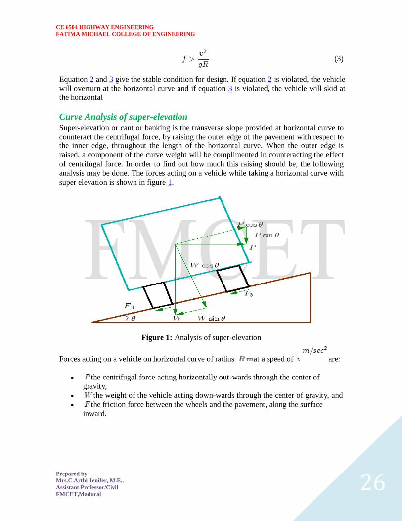
CE 6504 HIGHWAY ENGINEERING
FATIMA MICHAEL COLLEGE OF ENGINEERING
Prepared by
MrsCArthi Jenifer ME
Assistant ProfessorCivil
FMCETMadurai 27
At equilibrium by resolving the forces parallel to the surface of the pavement we get where
friction
is the weight of the vehicle is the centrifugal force is the coefficient of
is the transverse slope due to superelevation Dividing by we get
CE 6504 HIGHWAY ENGINEERING
FATIMA MICHAEL COLLEGE OF ENGINEERING
Prepared by
MrsCArthi Jenifer ME
Assistant ProfessorCivil
FMCETMadurai 28
Step 1
Find for 75 percent of design speed neglecting ie
Step 2
If then else if go to step 3
Step 3
Find for the design speed and max ie If
then the maximum is safe for the design speed else go to
step 4
Step 4
Find the allowable speed for the maximum and
If then the design is adequate otherwise use speed adopt
control measures or look for speed control measures
Maximum and minimum super-elevation
Depends on (a) slow moving vehicle and (b) heavy loaded trucks with high CG IRC
specifies a maximum super-elevation of 7 percent for plain and rolling terrain while that
of hilly terrain is 10 percent and urban road is 4 percent The minimum super elevation is
2-4 percent for drainage purpose especially for large radius of the horizontal curve
Attainment of super-elevation
1 Elimination of the crown of the cambered section by
1 Rotating the outer edge about the crown The outer half of the cross slope
is rotated about the crown at a desired rate such that this surface falls on
the same plane as the inner half
2 Shifting the position of the crown This method is also known as diagonal
crown method Here the position of the crown is progressively
shifted outwards thus increasing the width of the inner half of cross section
progressively
2 Rotation of the pavement cross section to attain full super elevation byThere are
two methods of attaining super elevation by rotating the pavement
1 Rotation about the center line The pavement is rotated such that the inner
edge is depressed and the outer edge is raised both by half the total amount
of super elevation ie by with respect to the centre
2 Rotation about the inner edge Here the pavement is rotated raising the
outer edge as well as the centre such that the outer edge is raised by the
full amount of super elevation with respect to the inner edge
Horizontal Transition Curves
CE 6504 HIGHWAY ENGINEERING
FATIMA MICHAEL COLLEGE OF ENGINEERING
Prepared by
MrsCArthi Jenifer ME
Assistant ProfessorCivil
FMCETMadurai 29
Transition curve is provided to change the horizontal alignment from straight to circular
curve gradually and has a radius which decreases from infinity at the straight end
(tangent point) to the desired radius of the circular curve at the other end (curve point)
There are five objectives for providing transition curve and are given below
1 to introduce gradually the centrifugal force between the tangent point and the
beginning of the circular curve avoiding sudden jerk on the vehicle This
increases the comfort of passengers
2 to enable the driver turn the steering gradually for his own comfort and security
3 to provide gradual introduction of super elevation and
4 to provide gradual introduction of extra widening
5 to enhance the aesthetic appearance of the road
Type of transition curve
Different types of transition curves are spiral or clothoid cubic parabola and Lemniscate
IRC recommends spiral as the transition curve because
1 it fulfills the requirement of an ideal transition curve that is
1 rate of change or centrifugal acceleration is consistent (smooth) and
2 radius of the transition curve is at the straight edge and changes to at
the curve point ( ) and calculation and field implementation is
very easy
Length of transition curve The length of the transition curve should be determined as the maximum of the following
three criteria rate of change of centrifugal acceleration rate of change of super elevation
and an empirical formula given by IRC Rate of change of centrifugal acceleration
At the tangent point radius is infinity and hence centrifugal acceleration is zero At the
end of the transition the radius R has minimum value R The rate of change of
centrifugal acceleration should be adopted such that the design should not cause
discomfort to the drivers If is the rate of change of centrifugal acceleration it can be
written as
Therefore the length of the transition curve in is
CE 6504 HIGHWAY ENGINEERING
FATIMA MICHAEL COLLEGE OF ENGINEERING
Prepared by
MrsCArthi Jenifer ME
Assistant ProfessorCivil
FMCETMadurai 30
(1)
where is the rate of change of centrifugal acceleration given by an empirical formula
suggested by by IRC as below
(2) 2 Rate of introduction of super-elevation
Raise ( ) of the outer edge with respect to inner edge is given by
The rate of change of this raise from to is achieved
gradually with a gradient of in over the length of the transition curve (typical range
of is 60-150) Therefore the length of the transition curve is
(3)
3 By empirical formula
IRC suggest the length of the transition curve is minimum for a plain and rolling terrain
(4)
and for steep and hilly terrain is
(5)
CE 6504 HIGHWAY ENGINEERING
FATIMA MICHAEL COLLEGE OF ENGINEERING
Prepared by
MrsCArthi Jenifer ME
Assistant ProfessorCivil
FMCETMadurai 31
and the shift as
(
6
) The length of the transition curve is the maximum of
equations 1 3 and 4or5 ie
(
7
Case (a)
For single lane roads
(
1
)
Therefore
(
2
)
Figure 1 Set-back for single lane roads (
CE 6504 HIGHWAY ENGINEERING
FATIMA MICHAEL COLLEGE OF ENGINEERING
Prepared by
MrsCArthi Jenifer ME
Assistant ProfessorCivil
FMCETMadurai 32
For multi lane roads if is the distance between centerline of the road and the centerline
of the inner lane then
(3)
(4)
Figure 2 Set-back for multi-lane roads ( )
Case (a)
For single lane roads
(1)
Therefore
(2)
Gradient
Gradient is the rate of rise or fall along the length of the road with respect to the
horizontal While aligning a highway the gradient is decided for designing the vertical
curve Before finalizing the gradients the construction cost vehicular operation cost and
the practical problems in the site also has to be considered Usually steep gradients are
avoided as far as possible because of the difficulty to climb and increase in the
CE 6504 HIGHWAY ENGINEERING
FATIMA MICHAEL COLLEGE OF ENGINEERING
Prepared by
MrsCArthi Jenifer ME
Assistant ProfessorCivil
FMCETMadurai 33
construction cost More about gradients are discussed below
Effect of gradient
The effect of long steep gradient on the vehicular speed is considerable This is
particularly important in roads where the proportion of heavy vehicles is significant Due
to restrictive sight distance at uphill gradients the speed of traffic is often controlled by
these heavy vehicles As a result not only the operating costs of the vehicles are
increased but also capacity of the roads will have to be reduced Further due to high
differential speed between heavy and light vehicles and between uphill and downhill
gradients accidents abound in gradients
Representation of gradient
The positive gradient or the ascending gradient is denoted as and the negative gradient as The deviation angle is when two grades meet the angle which
measures the change of direction and is given by the algebraic difference between the two
grades
steep gradient while 1 in 50 = 2 representation is illustrated in the figure 1
Example 1 in 30 = 333 is a
is a flatter gradient The gradient
CE 6504 HIGHWAY ENGINEERING
FATIMA MICHAEL COLLEGE OF ENGINEERING
Prepared by
MrsCArthi Jenifer ME
Assistant ProfessorCivil
FMCETMadurai 34
Figure 1 Representation of gradient
Types of gradient
Many studies have shown that gradient upto seven percent can have considerable effect
on the speeds of the passenger cars On the contrary the speeds of the heavy vehicles are
considerably reduced when long gradients as flat as two percent is adopted Although
flatter gradients are desirable it is evident that the cost of construction will also be very
high Therefore IRC has specified the desirable gradients for each terrain However it
may not be economically viable to adopt such gradients in certain locations steeper
gradients are permitted for short duration Different types of grades are discussed below
Ruling gradient
The ruling gradient or the design gradient is the maximum gradient with which the
designer attempts to design the vertical profile of the road This depends on the terrain
length of the grade speed pulling power of the vehicle and the presence of the horizontal
curve In flatter terrain it may be possible to provide flat gradients but in hilly terrain it
is not economical and sometimes not possible also The ruling gradient is adopted by the
designer by considering a particular speed as the design speed and for a design vehicle
with standard dimensions But our country has a heterogeneous traffic and hence it is not
possible to lay down precise standards for the country as a whole Hence IRC has
recommended some values for ruling gradient for different types of terrain
Limiting gradient
This gradient is adopted when the ruling gradient results in enormous increase in cost of
construction On rolling terrain and hilly terrain it may be frequently necessary to adopt
limiting gradient But the length of the limiting gradient stretches should be limited and
must be sandwiched by either straight roads or easier grades
Exceptional gradient
Exceptional gradient are very steeper gradients given at unavoidable situations They
should be limited for short stretches not exceeding about 100 metres at a stretch In
mountainous and steep terrain successive exceptional gradients must be separated by a
minimum 100 metre length gentler gradient At hairpin bends the gradient is restricted to
25
Critical length of the grade
The maximum length of the ascending gradient which a loaded truck can operate without
undue reduction in speed is called critical length of the grade A speed of 25 kmph is a
CE 6504 HIGHWAY ENGINEERING
FATIMA MICHAEL COLLEGE OF ENGINEERING
Prepared by
MrsCArthi Jenifer ME
Assistant ProfessorCivil
FMCETMadurai 35
reasonable value This value depends on the size power load grad-ability of the truck
initial speed final desirable minimum speed
Minimum gradient
This is important only at locations where surface drainage is important Camber will take
care of the lateral drainage But the longitudinal drainage along the side drains require
some slope for smooth flow of water Therefore minimum gradient is provided for
drainage purpose and it depends on the rain fall type of soil and other site conditions A
minimum of 1 in 500 may be sufficient for concrete drain and 1 in 200 for open soil
drains are found to give satisfactory performance Sight distance available from a point is the actual distance along the road surface which a driver
from a specified height above the carriage way has visibility of stationary or moving objects
Sight distance required by drivers applies to both geometric design of highways and for
traffic control The sight distance situations are considered in the design
i) Stopping or absolute minimum sight distance
ii) Safe overtaking or passing sight distance
iii) Safe sight distance for entering into uncontrolled intersections
Apart from the three situations mentioned above the following sight distance are considered by the
IRC in highway design
Intermediate sight distance
This is defined as twice the stopping sight distance when overtaking sight distance
cannot be provided intermediate sight distance is provided to give limited overtaking opportunities
to fast vehicles
Head light sight distance
This is the distance visible to a driver during night driving under the illumination of the
vehicle head lights
Stopping sight distance
The minimum sight distance available on a highway at any spot should be of sufficient
length to stop a vehicle traveling at design speed safely without collision with any other obstruction
The absolute minimum sight distance is therefore equal to the stopping sight distance
which is also sometimes called nonpassing sight distance The sight distance available on a road to a
driver at any instance depends on
i) Features of the road
ii) Height of the drivers eye above the road surface
iii) Height of the object above the road surface
The distance within which a motor vehicle can be stopped depends upon the factors listed below
a) Total reactions time of the driver
b) Speed of vehicle
c) Efficiency of breaks
d) Frictional resistance between the road and tyres
e) Gradient of the road
Total reaction time
) Reaction time of the driver is the time taken from the instant the object is visible to the
driver to the instant the brakes are effectively applied
) The total reaction time may be split up into two parts
CE 6504 HIGHWAY ENGINEERING
FATIMA MICHAEL COLLEGE OF ENGINEERING
Prepared by
MrsCArthi Jenifer ME
Assistant ProfessorCivil
FMCETMadurai 36
i) Perception time
ii) Brake reaction time
PIEV theory
According to this theory the total reaction time of the driver is split into four parts
i) Perception
ii) Intellection
iii) Emotion
iv) Volition
Speed of Vehicle
The stopping distance depends very much on the speed of the vehicle first during the
total reaction time of the driver the distance moved by the vehicle will depend on the speed
Efficiency of brakes
The braking efficiency is said to be 100 percent if the wheels are fully licked preventing
them from rotating on application of the brakes This will result in 100 percent skidding which is
normally undesirable except in utmost emergency
Frictional resistance between road and tyres
The frictional resistance developed between road and tyres or the skid resistance depends
on the type and condition of the road surface and the tyres IRC has specified a design friction
coefficient of 035 to 04 depending upon the speed to be used for finding the braking distance in the
calculation of stopping sight distance
Analysis of stopping distance
i) The distance traveled by the vehicle during the total reaction time known as lag
distance
ii) The distance traveled by the vehicle after the application of the brakes is known as
braking distance
Overtaking sight distance
The minimum distance open to the vision of the driver of a vehicle intending to overtake
slow vehicle ahead with safety against the traffic of opposite direction is known as the minimum
overtaking sight distance(OSD) or Safe passing sight distance available
The overtaking sight distance is the distance measured along the center of the road which
a driver with his eye level 12m above the road surface can see the top of an object 12m above the
road surface
Some of the important factors on which the minimum overtaking sight distance required
a) Speed of
i) overtaking vehicle
ii) overtaken vehicle
iii) The vehicle coming from opposite direction
b) Distance between the overtaking and overtaken vehicles the minimum spacing
depends on the steeds
a) Skill and reaction time of the driver
b) Rate of acceleration of overtaking vehicle
c) Gradient of the road
Criteria for sight distance requirements on highway
) The absolute minimum sight distance required throughout the length of the road is the
SSD which should invariably be provided at all places
CE 6504 HIGHWAY ENGINEERING
FATIMA MICHAEL COLLEGE OF ENGINEERING
Prepared by
MrsCArthi Jenifer ME
Assistant ProfessorCivil
FMCETMadurai 37
) On horizontal curves the obstruction on the inner side of the curves should be cleared
to provide the required set back distance and absolute minimum sight distance
) On vertical summit curves the sight distance requirement may be fulfilled by proper
design of the vertical alignment
Hairpin bent
TYPES OF CURVES ON HILL ROADS
The following are the important types of curves provided on hill Roads-
1 Hair-Pin Curves
2 Salient Curves
3 Re-entrant Curves 1 Hair-pin curves - The curve in a hill road which changes its direction through an angle of 180
degree or so down the hill on the same side is known as hair-pin curve
A Hair-Pin Bend
This curve is so called because it conforms to the shape of a hair-pin The bend so formed at the
hair-pin curve in a hill road is known as hair-pin bend This type of curve should be located on a
hill side having the minimum slope and maximum stability It must also be safe from view point of
landslides and ground water Hair-pin bends with long arms and farther spacing are always
preferred They reduce construction problems and expensive protective works Hair-pin curves or
bends of serpentine nature are difficult to negotiate and should therefore be avoided as far as
possible
Salient curves - The curves having their convexity on the outer edges of a hill road are called
salient curves The centre of curvature of a salient curve lies towards the hill side This type of curve
occurs in the road length constructed on the ridge of a hill the bend so formed at the salient curve in
a hill road known as corner bend
Salient curves are very dangerous for fast moving traffic At such a curve or at corner bend the
portion of projecting hill side is usually cut down to improve the visibility as shown in fig (Re-
entrant curve) The outer edge of the road at such a curve is essentially provided with a parapet wall
for protection of the vehicles from falling down the hill slope
CE 6504 HIGHWAY ENGINEERING
FATIMA MICHAEL COLLEGE OF ENGINEERING
Prepared by
MrsCArthi Jenifer ME
Assistant ProfessorCivil
FMCETMadurai 38
3 Re-entrant curves - The curves having their convexity on the inner edge of a hill road are called
re-entrant curves
Re-entrant curves
The centre of curvature of a re-entrant curves lies away from the hill side This type of curve occurs
in the road length constructed in the calley of a hill
These curves are less dangereous as they provide adequate visibility to the fast moving traffic At
such curves the parapet wall is provided only for safety of fast moving traffic
CE 6504 HIGHWAY ENGINEERING
FATIMA MICHAEL COLLEGE OF ENGINEERING
Prepared by
MrsCArthi Jenifer ME
Assistant ProfessorCivil
FMCETMadurai 39
UNIT ndash III DESIGN OF RIGID AND FLEXIBLE PAVEMENTS
COMPARISON OF RIGID AND FLEXIBLE PAVEMENTS
The comparisons are
i) Design precision
A cement concrete pavement is amerable to a much more precise structural analysis
than a flexible pavement Flexible pavements designs are mainly empirical Computer aided analysis
of layered system is making the flexible pavement design more exact than hitherto
ii) Life
) Cement concrete slabs of a thin section constructed in the early 1940rsquos are still in
existence in India though many of them have cracked badly and a few of them have been ripped
open and rebuilt in recent ties
) A major project in cement concrete road construction between Agra and Mathura It can
safely be said that a well-designed concrete slab has a life of about 40 years
) Compared to this the life of a flexible pavement generally varies from 10 to 20 years
iii) Maintenance
) A well-designed cement concrete pavement needs very little maintenance The only
maintenance needed is I respect of joints
) The surface is unaffected by spillage of oil and lubricants bituminous surfaces on the
other hand need great inputs in maintenance
) The surface is affected by spillage of oil and lubricants The surface is also affected by
natural weathering agents like air water ad temperature changes
) A cement concrete pavement on the other hand needs a small amount for maintaining
joints
iv) Initial cost
) The argument so far used against a cement concrete slab is that it is much more costly
than a flexible pavement
) The latter specifications no doubt represent the rock-bottom needs of a road in India but
these specifications can hardly provide a smooth and durable surface
v) Stage construction ) Road construction is generally done adopting a policy of stage construction especially for
low volume roads As traffic grows additional layers in the form of water bound macadam and
superior surfacing are added on
) Initial outlay is minimum and additional outlays are in keeping with traffic growth This is
a great advantage when dealing with new roads in an atmosphere of austerity
vi) Availability of materials
) Cement bitumen stone aggregates and gravelsand are the major materials involved in
pavement Construction Cement has been in serious short supply in the country for the past many
decades
) Bitumen is also not available plentifully in India There is also the danger of the entire oil
reserves in the world shrinking during the next two or three decades
) In locations where stone aggregates are scarce cement concrete may have an advantage
for flexible pavements
vii) Surface characterstics
CE 6504 HIGHWAY ENGINEERING
FATIMA MICHAEL COLLEGE OF ENGINEERING
Prepared by
MrsCArthi Jenifer ME
Assistant ProfessorCivil
FMCETMadurai 40
) A good cement concrete surface is smooth and free from rutting potholes and
corrugations In a bituminous surface it is only the asphaltic concrete surface that can give
comparable rideablity
) A well-constructed cement concrete pavement surface can have a permanent nonskid
surface A bituminous surface can also be designed to have a good skid resistant surface
viii) Utility location
) In cement concrete slabs proper thought has to be given to locate utilities such as water
pipes telephone lines and electric cables
) It is difficult to rip open the slab and restore it to be the original condition if any changes
in the utilities lines are to be made
ix) Glame and night visibility
) Concrete pavements have a gray color which can cause glam under sunlight Colored
cement can reduce the grave
) On the other hand bituminous roads need more street lighting
x) Traffic dislocation during construction
) A cement concrete pavement requires 28 days before it can be thrown open to traffic On
the other hand a bituminous surface can be thrown open to traffic shortly after it is rolled
xi) Environmental considerations during construction
) The process of heating of bitumen and aggregates and mixing them together on hot mix
plants can prove to be much more hazardous to the environment than cement concrete construction
where no heating of any material is involved
xii) Overall economy on a life cycle basis
) A good road is costly to construct but once constructed such a road requires little
maintenance and results in savings in vehicle operating costs
) The comparative economy of a flexible pavement and a rigid pavement has proved that on
overall economic considerations
Types of pavement structure
Based on the structural behavior pavements are generally classified into three
categories
i) Flexible pavements
ii) Rigid pavements
iii) Semi rigid pavements
Flexible pavements
) Flexible pavements are those which on the whole have low or negligible flexural
strength and are rather flexible in their structural action under the loadsThe flexible pavement
layers reflect the deformation of the lower layers on to the surface of the layer
) A flexible pavement consists of four components(i) Soil subgrade (ii) sub base
course (iii) base course (iv) Surface course
CE 6504 HIGHWAY ENGINEERING
FATIMA MICHAEL COLLEGE OF ENGINEERING
Prepared by
MrsCArthi Jenifer ME
Assistant ProfessorCivil
FMCETMadurai 41
) The flexible pavement layers transmit the vertical or compressive stresses to the lower layers
by grain to grain transfer through the points of contact in the granular structure A well
compacted granular structure consisting of strong added aggregate can transfer the compressive
stresses
) The load spreading ability of this layer therefore depends on the type of the materials and mix
design factors Bituminous concrete is one of the best flexible pavements layer materials Other
materials which fall under the group are all granular materials with or without bituminous
binder granular base and sub base course materials
) The vertical compressive stress is maximum on the pavement surface directly under the wheel
and is equal to the contact pressure under the wheel The flexible pavement may be constructed
in a number of layers and the top layer has to be strongest as the highest compressive stresses
) Flexible pavements are commonly designed using empirical design charts or equations taking
into account some of the design factors there are also semi empirical and theoretical design
methods
Rigid pavements
) Rigid pavements are those which possess note flexural strength or flexural rigidity
The stresses are not transferred from grain to grain to the lower layers as in the ease of flexible
pavements layers
) The rigid pavements are made of Portland cement concrete plain reinforced or
prestressed concrete The plain cement concrete slabs are expected to take up about 40 kgcm2
flexural stress
) The rigid pavement has the slab action and is capable of transmitting the wheel
load stresses through a wider area below The main point of difference in the structural behavior
of rigid pavement as compared to the flexible pavement is that the critical condition of stress in
the rigid pavement is the maximum flexural stress occurring in the slab due to wheel load and
the temperature changes whereas in the flexible pavement
) As the rigid pavement slab has tensile strength tensile stresses are developed due
to the bending of the slab under wheel load and temperature variations Thus the types of
stresses developed and their distribution within the cement concrete slab are quirt different
) The cement concrete pavement slab can very well serve as a wearing surface as
well an effective base course The rigid pavement structure consists of a cement concrete slab
below which a granular base or sub base course may be provided
) Though the cement concrete slab can also be laid directly over the soil subgrade
consists of fine grained soil
) the rigid pavements are usually designed and the stresses are analyzed using the
elastic theory assuming the pavements as a n elastic plate resting over an elastic or a viscous
foundation
Semi rigid pavements
) when bonded materials like the pozzolanic concrete lean cement concrete or soil
cement are used in the base course or sub base course layer the pavement layer has considerably
higher flexural strength than the common flexible pavement layers
) when this intermediate class of materials are used in the base or sub base course
layer of the pavements they are called semi rigid pavements
CE 6504 HIGHWAY ENGINEERING
FATIMA MICHAEL COLLEGE OF ENGINEERING
Prepared by
MrsCArthi Jenifer ME
Assistant ProfessorCivil
FMCETMadurai 42
) This third category of semi rigid pavement are either designed as flexible
pavements with some correction factors to find the thickness requirements based on experience
or by using a new design approach
) The semi rigid pavement materials have low resistance to impact and abrasion and
therefore are usually provided with flexible pavement surface course
Various functions of pavement components
The functions are
Soil sub grade and its evaluation
) The soil sub grade is a layer of natural soil prepared to receive the layers of pavement
materials placed over it It is essential that at no time the soil sub grade is overstressed it means that
the pressure transmitted on the top of the sub grade is within the allowable limit
) Many tests are known for measuring the strength properties of the sub grades Some of the
tests have been standardized for the use The common strength test for the evaluation of soil
subgrade is
i) California bearing ratio test
ii) California resistance value test
iii) Triaxial compression test
iv) Plate bearing test
CALIFORNIA BEARING RATIO (CBR) TEST
It is evolved for the empirical method of flexible pavement design The CBR test is carried
out either in the laboratory on prepared specimens or in the field by taking in situ measurements
California resistance value
It is found by using have been stabliometerThis test is used in an empirical method of
flexible pavement design based on soil strength
Triaxial test
It is the most important soil strength but still the test is not very commonly used in structural
design of pavements
Plate bearing test
It is carried out using a relatively large diameter plate to evaluate the load supporting
capacity of supporting power of the pavement layers The results are plate bearing tests are used in
flexible pavement design method like McLeod method on based on layer system analysis by
brumister
Sub base and base courses and their evaluation
) There layers are made of broken stones bound or unbound aggreagatesome times in sub
base course a layer of stabilized soil(or) Selected granular soil is also used
) however at the sub base course it is desirable to use smaller size graded aggregates When
the sub grade consists of fine grained soil and when the pavement carries heavy wheel loads
CE 6504 HIGHWAY ENGINEERING
FATIMA MICHAEL COLLEGE OF ENGINEERING
Prepared by
MrsCArthi Jenifer ME
Assistant ProfessorCivil
FMCETMadurai 43
) Sub base course primarily has the similar function as of the base course and is provided
with inferior materials than of base course Base courses are used under rigid pavement for
i) Preventing pumping
ii) Protecting the sub grade against frost action
) Thus the fundamental purpose of abase course and sub base course is to provide a stress
transmitting medium to spread the surface wheel loads in such manner
) The sub base and base course layers may be evaluated by suitable strength or stability test
like plate bearing CBR test
WEARING COURSE AND ITS EVALUATION
) The purpose of the wearing course is to give a smooth riding surface that is dense It
resists pressure exerted by tyres and takes up wear and tear due to the traffic
) Wearing course also offers a water tight layer against the surface water infiltration The
flexible pavement normally a bituminous surfacing is used as a wearing course
) In rigid pavements the cement concrete acts like a base course as well as wearing course
Most popular test in use is marshal stability test where in the optimum content of bitumen binder is
worked out based on the stability density
) Plate bearing test and Bankelman beam test are also sometimes made use of for evaluating
the wearing course and the pavement as a whole
Various factors to be considered in pavement design and the significance
Pavement design consists of two parts
i) Mix design of materials to be used in each pavement component layer Thickness design of the
pavement and the component layers
The various factors to be considered for the design of pavements are given below
i) Design wheel load
ii) Sub grade soil
iii) Climatic factors
iv) Pavement component layers
v) Environmental factors
vi) Special factors in the design of different types of pavements
Design wheel load
The various wheel load factors to be considered in pavement design are
i) Maximum wheel load
ii) Contact pressure
iii) Dual or multiple wheel loads
iv) Repetition of loads
Maximum wheel load
The wheel load configurations are important to know the way in which the loads of a given
vehicle are applied on the pavement surface
) For highways the maximum legal axle load as specified by Indian road congress is 8170
kg with a maximum equivalent single wheel load of 4085 kg
) The evaluation for vertical stress computations under a uniformly distribute of circular
load based on Boussineqrsquos theory is given by
CE 6504 HIGHWAY ENGINEERING
FATIMA MICHAEL COLLEGE OF ENGINEERING
Prepared by
MrsCArthi Jenifer ME
Assistant ProfessorCivil
FMCETMadurai 44
2
322
3
1
za
zpz
σz = vertical stress at depth z
P= surface pressure
Z=depth at which σz computed
A=radius of loaded area
Contact pressure
Generally the wheel load is assumed to be distributed over a circular area But by
measurement of the imprints of tyers with different load and inflation pressures Three terms in use
with reference to tyre pressure are
Tyre pressure
Inflation pressure
Contact pressure
Tyre pressure and inflation pressure mean exactly the same the contact pressure is found to be more
than tyre pressure when the tyre pressure is less than 7 kgm2 and it is vice versa when the tyre
pressure exceeds this value
Contact pressure can be measured by the relationship
Load on wheel
Contact pressure = ----------------------------------------
Contact area or area of imprint
The general variation between the tyre pressure and measured contact pressure is shown in this fig
The ratio of contact pressure to type pressure is defined as rigidity factor Thus value of rigidity
factor is 10 for an average tyre pressure of 7 Kgcm2This value is higher than unity for lower type
pressures and less than unity for tyre pressures higher than 7 kgcm2
Equivalent single wheel load (ESWL)
) The maximum wheel load within the specified limit and to carry greater load it is
necessary to provide dual wheel assembly to the rear axles of the roads vehicles
) In other words the pressure at a certain depth below the pavement surface cannot be
obtained by numerically adding the pressure caused by any one wheel
) The effect is in between the single load and two times load carried by one wheel The load
dispersion is assumed to be at an angle of 450In the dual wheel load assembly let d be the clear gap
between the two wheels S be the spacing between the centers of the wheels and a be the radius of
the circular contact area of each wheel Then S = (d + 2a)
) ESWL may be determined based on either equivalent deflection or equivalent stress
criterianMultiple wheel loads are convert to ESWL and this value is used in pavement design The
ESWL is usually determined by the equivalent stress criterion using a simple graphical method
CE 6504 HIGHWAY ENGINEERING
FATIMA MICHAEL COLLEGE OF ENGINEERING
Prepared by
MrsCArthi Jenifer ME
Assistant ProfessorCivil
FMCETMadurai 45
) A straight line relationship is assumed between ESWL and depth on log scales For
determining ESWL the plot is made as shown in fig
) Two points A and B are plotted on the log-log graph with coordinates of A (Pd2) and
B(2p2s)line AB is a plot which is the focus of points where any single wheel load is equivalent to a
certain set of dual wheels
) To Calculate the ESWL for a dual assembly it is essential to estimate a design thickness of
the pavement If the design thickness so obtained is equal to the estimated thickness then the ESWL
calculations could be considered as correct Otherwise trials are made
) In heavy trucks and trailers the load on each wheel may be further reduced by multiple
wheels and tandem axles
Repetition of loads
) The deformation of load pavement (or) sub grade due to a single application of wheel load
may be small It required carrying out traffic surveys for accounting the factor of repetitions for
wheel loads in the design of pavement
) Data collected are converted to some constant equivalent wheel loads Equivalent wheel
load is a single load equivalent to the repeated applications of any particular wheel load on a
pavement which requires the same thickness and strength of pavements
) McLeod has given a procedure for evolving equivalent load factors for designing flexible
pavements
Various methods of flexible pavement design
) The flexible pavement is built with number of layers In the design process it is to be
ensured that under the application of load none of the layers is overstressed
) The maximum intensity of stresses occurs in the top layer of the pavement The
magnitude of load stresses reduces at lower layers
) In the design of flexible pavements it has yet not been possible to have a rational design
method wherein design process and service behavior of the pavement can be expressed by
mathematical laws
) Flexible pavement design methods are accordingly either empirical or semi empirical In
these methods the knowledge and experience gained on the behavior of the pavements in the past
are usefully utilized
Various approaches of flexible pavement design may be thus classified into three groups
i) Empirical method
ii) Semi-empirical or Semi theoretical method
iii) Theoretical method
) Empirical methods are either based on physical properties or strength parameters of soil
sub grade When the design is based on stress strain function and modified base on experience it
may be called semi-empirical or semi-theoretical There are design methods based on theoretical
analysis and mathematical computations
Out of the flexible pavement design method available is
i) Group index method
ii) California bearing ratio method
iii) California R value (or) Stabiliometer method
iv) Triaxial test method
CE 6504 HIGHWAY ENGINEERING
FATIMA MICHAEL COLLEGE OF ENGINEERING
Prepared by
MrsCArthi Jenifer ME
Assistant ProfessorCivil
FMCETMadurai 46
v) McLeod method
vi) Burmister method
Group index method
) Group index value is an arbitrary index assigned to the soil type in numerical equations
base on the percent fines liquid limit and plasticity index
) The design chart for group index method for determining the pavement thickness is given
in fig
The traffic volume in this method is divided in three groups
Traffic volume No of vehicles per day
Light Less than 50
Medium 50 to 300
Heavy Over 300
The design of the pavement thickness by this method first the G1 value of the soil is found the
anticipated traffic is estimated and is designated as light medium or heavy as indicated
The G1 method of pavement design is essentially an empirical method based on physical properties
of the subgrade soil This method does not consider the strength characteristics of the subgrade soil
and therefore is open to question regarding the reliability of the design based on the index properties
of the soil only
California bearing ratio method
) California division of highways in the USA developed CBR method for
pavement design The majority of design curves developed later are base on the original curves
proposed by OJporter
) One of the chief advantages of CBR method is the simplicity of the test procedure
The CBR tests were carried out by the California state highway department on existing pavement
layers including subgrade sub base and base course
) Based on the extensive CBR test data collected on pavement which behaved
satisfactory and those which failed an empirical design chart was developed correlating the CBR
value and the pavement thickness The basis of the design chart is that a material with a given CBR
required a certain thickness of pavement layer as a cover
) A higher load needs a thicker pavement layer to protect the sub grade Design
curves correlating the CBR value with total pavement thickness cover were developed by the
California state highway department for wheel loads of 3175kg and 5443 kg representing light and
heavy traffic The design curves are shown in this fig
It is possible to extend the CBR design curves for various loading conditions nusing the expression
t= 2
1
1751
pCBRp
t=2
1
751
A
CBR
p
Hence
CE 6504 HIGHWAY ENGINEERING
FATIMA MICHAEL COLLEGE OF ENGINEERING
Prepared by
MrsCArthi Jenifer ME
Assistant ProfessorCivil
FMCETMadurai 47
t= pavement thickness cm
p=Wheel load kg
CBR= California bearing ratio percent
P=tyre pressure kgcm2
A= area of contactcm2
IRC Recommendations
a) The CBR tests should be performed on remoulded soils in the laboratory The specimens should
be prepared by static compaction wherever possible and otherwise by dynamic compaction
b) For the design of new roads the sub grade soil sample should be compacted at OMC to proctor
density whenever suitable compaction equipment
c) The CBR test samples may be soaked in water for four days period before testing the annual
rainfall is less than 50 cm and the water table is too deep to affect the sub grade and imperable
surfacing is provided to carrying out CBR test
d) If the maximum variations in CBR value of the three specimens exceed the specified limits the
design CBR should be average of at least six samples
e) The top 50 cm of sub grade should be compacted at least up to 95 to 100 percent of proctor
density
f) An estimate of the traffic should be carried by the road pavements at the end of expected in view
the existing traffic and probable growth rate of traffic
g) The traffic for the design is considered in units of heavy vehicles per day in both directions and is
divided into seven categories A to G The design thickness is considered applicable for single axle
loads up to 8200 kg and tandom axle loads up to 14500 kg
h) When sub base course materials contain substantial proportion of aggregates of size above 20mm
the CBR value of these materials would not be valid for the design of subsequent layers above them
The CBR method of pavement design gives the total thickness requirement of the pavement above a
sub grade and thickness value would remain the same quality of materials used in component layers
California resistance value method
) In this design method based on stabliometer R-value and cohesiometer C-value
Based on performance data it was established by pavement thickness varies directly with R value
and algorithm of load repetitions It varies inversely with fifth root of c valueThe expression for
pavement thickness is given by the empirical equation
T=
5
1
1 90
C
RTK
Hence
T=total thickness of pavement cm
K=Numerical constant 0166
T1=traffic index
R= stabiliometer resistance value
C=Cohesiometer value
CE 6504 HIGHWAY ENGINEERING
FATIMA MICHAEL COLLEGE OF ENGINEERING
Prepared by
MrsCArthi Jenifer ME
Assistant ProfessorCivil
FMCETMadurai 48
In the design of flexible pavements based on California resistance value method for the following
data are needed
) R-value of soil subgrade
) T1 value
) Equivalent C-value
) R value of soil subgrade is obtained from the test using stablio meterThe
computation of T1 value has been explained
Equivalent C-value
) The cohesion meter value c is obtained for each layer of pavement material
separately from tests However the composite or equivalent C-value of the pavement may be
estimated if the thickness of each component layer and the c-value of the material of the layer are
known
) while designing a pavement as the thickness of the pavement is not known it is
easier if the pavement is first assumed to consist of any one material like gravel base course with
known C-value
) Subsequently the individual thickness of each layer is converted in terms of gravel
equivalent by using relationship
5
1
1
2
2
1
C
C
t
t
) t1 and t2 are the thickness values of any two pavement layersc1 and c2 are their
corresponding cohesiometer values
CE 6504 HIGHWAY ENGINEERING
FATIMA MICHAEL COLLEGE OF ENGINEERING
Prepared by
MrsCArthi Jenifer ME
Assistant ProfessorCivil
FMCETMadurai 49
UNIT 4 MATERIAL AND MAINTENANCE
SUMMIT CURVE
Summit curves are vertical curves with gradient upwards They are formed when two
gradients meet as illustrated in figure 1 in any of the following four ways
1 When a positive gradient meets another positive gradient [figure 1a]
2 When positive gradient meets a flat gradient [figure 1b]
3 When an ascending gradient meets a descending gradient [figure 1c]
4 When a descending gradient meets another descending gradient [figure 1d]
Type of Summit Curve
Many curve forms can be used with satisfactory results the common practice has been to
use parabolic curves in summit curves This is primarily because of the ease with it can
be laid out as well as allowing a comfortable transition from one gradient to another
Although a circular curve offers equal sight distance at every point on the curve for very
small deviation angles a circular curve and parabolic curves are almost congruent
Furthermore the use of parabolic curves were found to give excellent riding comfort
Figure 1 Types of summit curves
Design Consideration
In determining the type and length of the vertical curve the design considerations are
comfort and security of the driver and the appearance of the profile alignment Among
these sight distance requirements for the safety are most important on summit curves
The stopping sight distance or absolute minimum sight distance should be provided on
these curves and where overtaking is not prohibited overtaking sight distance or
intermediate sight distance should be provided as far as possible When a fast moving
vehicle travels along a summit curve there is less discomfort to the passengers This is
because the centrifugal force will be acting upwards while the vehicle negotiates a
summit curve which is against the gravity and hence a part of the tyre pressure is
relieved Also if the curve is provided with adequate sight distance the length would be
sufficient to ease the shock due to change in gradient Circular summit curves are
identical since the radius remains same throughout and hence the sight distance From
CE 6504 HIGHWAY ENGINEERING
FATIMA MICHAEL COLLEGE OF ENGINEERING
Prepared by
MrsCArthi Jenifer ME
Assistant ProfessorCivil
FMCETMadurai 50
this point of view transition curves are not desirable since it has varying radius and so the
sight distance will also vary The deviation angles provided on summit curves for
highways are very large and so the simple parabola is almost congruent to a circular arc
between the same tangent points Parabolic curves are easy for computation and also it
had been found out that it provides good riding comfort to the drivers It is also easy for
field implementation Due to all these reasons a simple parabolic curve is preferred as
summit curve Length of the summit curve
The important design aspect of the summit curve is the determination of the length of the
curve which is parabolic As noted earlier the length of the curve is guided by the sight
distance consideration That is a driver should be able to stop his vehicle safely if there is
an obstruction on the other side of the road Equation of the parabola is given by
where where N is the deviation angle and is the length of the In
deriving the length of the curve two situations can arise depending on the uphill and
downhill gradients when the length of the curve is greater than the sight distance and the
length of the curve is greater than the sight distance
Let is the length of the summit curve is the SSDISDOSD is the deviation angle
drivers eye height (12 m) and the height of the obstruction then the length of the
summit curve can be derived for the following two cases The length of the summit curve
can be derived from the simple geometry as shown below
Case a Length of summit curve greater than sight distance( )
Figure 1 Length of summit curve ( )
The situation when the sight distance is less than the length of the curve is shown in
figure 1
CE 6504 HIGHWAY ENGINEERING
FATIMA MICHAEL COLLEGE OF ENGINEERING
Prepared by
MrsCArthi Jenifer ME
Assistant ProfessorCivil
FMCETMadurai 51
(1)
Case b Length of summit curve less than sight distance
The second case is illustrated in figure 1
Figure 1 Length of summit curve
CE 6504 HIGHWAY ENGINEERING
FATIMA MICHAEL COLLEGE OF ENGINEERING
Prepared by
MrsCArthi Jenifer ME
Assistant ProfessorCivil
FMCETMadurai 52
From the basic geometry one can write
(1)
Therefore for a given and to get minimum differentiate the above equation
with respect to and equate it to zero Therefore
Solving the quadratic equation for
(2)
Now we can substitute back to get the value of minimum value of for a given
and Therefore
Solving for
CE 6504 HIGHWAY ENGINEERING
FATIMA MICHAEL COLLEGE OF ENGINEERING
Prepared by
MrsCArthi Jenifer ME
Assistant ProfessorCivil
FMCETMadurai 53
(3) (4
CE 6504 HIGHWAY ENGINEERING
FATIMA MICHAEL COLLEGE OF ENGINEERING
Prepared by
MrsCArthi Jenifer ME
Assistant ProfessorCivil
FMCETMadurai 54
When stopping sight distance is considered the height of drivers eye above the road
surface ( ) is taken as 12 metres and height of object above the pavement surface ( )
is taken as 015 metres If overtaking sight distance is considered then the value of
drivers eye height ( ) and the height of the obstruction ( ) are taken equal as 12
metres
Valley curve
Valley curve or sag curves are vertical curves with convexity downwards They are
formed when two gradients meet as illustrated in figure 1 in any of the following four
ways
Figure 1 Types of valley curve
1 When a descending gradient meets another descending gradient [figure 1a]
2 When a descending gradient meets a flat gradient [figure 1b]
3 When a descending gradient meets an ascending gradient [figure 1c]
4 When an ascending gradient meets another ascending gradient [figure
Design considerations
There is no restriction to sight distance at valley curves during day time But visibility is
reduced during night In the absence or inadequacy of street light the only source for
visibility is with the help of headlights Hence valley curves are designed taking into
account of headlight distance In valley curves the centrifugal force will be acting
downwards along with the weight of the vehicle and hence impact to the vehicle will be
more This will result in jerking of the vehicle and cause discomfort to the passengers
Thus the most important design factors considered in valley curves are (1) impact-free
movement of vehicles at design speed and (2) availability of stopping sight distance
under headlight of vehicles for night driving
For gradually introducing and increasing the centrifugal force acting downwards the best
shape that could be given for a valley curve is a transition curve Cubic parabola is
generally preferred in vertical valley curves See figure 1
CE 6504 HIGHWAY ENGINEERING
FATIMA MICHAEL COLLEGE OF ENGINEERING
Prepared by
MrsCArthi Jenifer ME
Assistant ProfessorCivil
FMCETMadurai 55
Figure 1 Valley curve details
During night under headlight driving condition sight distance reduces and availability of
stopping sight distance under head light is very important The head light sight distance
should be at least equal to the stopping sight distance There is no problem of overtaking
sight distance at night since the other vehicles with headlights could be seen from a
considerable distance
Length of the valley curve
The valley curve is made fully transitional by providing two similar transition curves of
equal length The transitional curve is set out by a cubic parabola where
The length of the valley transition curve is designed based on two criteria
1 comfort criteria that is allowable rate of change of centrifugal acceleration is
limited to a comfortable level of about
2 safety criteria that is the driver should have adequate headlight sight distance at
any part of the country
Comfort criteria
The length of the valley curve based on the rate of change of centrifugal acceleration that
will ensure comfort Let is the rate of change of acceleration the minimum radius of
the curve is the design speed and is the time then is give
CE 6504 HIGHWAY ENGINEERING
FATIMA MICHAEL COLLEGE OF ENGINEERING
Prepared by
MrsCArthi Jenifer ME
Assistant ProfessorCivil
FMCETMadurai 56
For a cubic parabola the Value Safety criter Length of the valley curve for headlight distance may be determined for two conditions
(1) length of the valley curve greater than stopping sight distance and (2) length of the
valley curve less than the stopping sight distance of for length is given by
Case 1 Length of valley curve greater than stopping sight distance ( )
The total length of valley curve is greater than the stopping sight distance SSD The
sight distance available will be minimum when the vehicle is in the lowest point in the
valley This is because the beginning of the curve will have infinite radius and the bottom
of the curve will have minimum radius which is a property of the transition curve The
case is shown in figure 1
Figure 1 Valley curve case 1
From the geometry of the figure we have
CE 6504 HIGHWAY ENGINEERING
FATIMA MICHAEL COLLEGE OF ENGINEERING
Prepared by
MrsCArthi Jenifer ME
Assistant ProfessorCivil
FMCETMadurai 57
(1)
where is the deviation angle in radians is the height of headlight beam is the
head beam inclination in degrees and is the sight distance The inclination is 1
degree
Case 2 Length of valley curve less than stopping sight distance ( )
The length of the curve is less than SSD In this case the minimum sight distance is
from the beginning of the curve The important points are the beginning of the curve and
the bottom most part of the curve If the vehicle is at the bottom of the curve then its
headlight beam will reach far beyond the endpoint of the curve whereas if the vehicle is
at the beginning of the curve then the headlight beam will hit just outside the curve
Therefore the length of the curve is derived by assuming the vehicle at the beginning of
the curve The case is shown in figure 1
From the figure
(1) Note that the above expression is approximate and is satisfactory because in practice the gradients
are very small and is acceptable for all practical purposes We will not be able to know prior to
which case to be adopted Therefore both has to be calculated and the one which satisfies the
condition is adopted
1 Flexible pavement
2 Rigid pavement
Flexible pavement
These pavements reflect the deformation of sub grade and the subsequent layers to the
surface
Rigid pavement
The rigid characteristic of the pavement are associated with rigidity or flexural strength
CE 6504 HIGHWAY ENGINEERING
FATIMA MICHAEL COLLEGE OF ENGINEERING
Prepared by
MrsCArthi Jenifer ME
Assistant ProfessorCivil
FMCETMadurai 58
or slab action so the load is distributed over a wide area of sub grade soil
Flexible pavement Definition
These pavements reflect the deformation of sub grade and the subsequent layers to the
surface Flexible usually asphalt is laid with no reinforcement or with a specialized
fabric reinforcement that permits limited flow or repositioning of the roadbed under
ground changes
The design of flexible pavement is based on load distributing characteristic of the
component layers The black top pavement including water amp gravel bound macadam fall
in this category
Flexible pavement on the whole has low or negligible flexible strength flexible in their
structural action) The flexible pavement layers transmit the vertical or compressive
stresses to the lower layers by grain transfer through contact points of granular structure
The vertical compressive stress is maximum on the pavement surface directly under the
wheel load and is equal to contact pressure under the wheels Due to the ability to
distribute the stress to large area in the shape of truncated cone the stresses get decreased
in the lower layer
As such the flexible pavement may be constructed in a number of layers and the top
layer has to be strongest as the highest compressive stresses
To be sustained by this layer in addition to wear and tear the lower layer have to take
up only lesser magnitude of stress as there is no direct wearing action die to traffic loads
therefore inferior material with lower cast can be used in the lower layers
Rigid pavement Definition
The rigid characteristic of the pavement are associated with rigidity or flexural strength
or slab action so the load is distributed over a wide area of sub grade soil Rigid pavement
is laid in slabs with steel reinforcement
The rigid pavements are made of cement concrete either plan reinforced or prestressed
concrete
Critical condition of stress in the rigid pavement is the maximum flexural stress occurring in the slab due to wheel load and the temperature changes
Rigid pavement is designed and analyzed by using the elastic theory
CE 6504 HIGHWAY ENGINEERING
FATIMA MICHAEL COLLEGE OF ENGINEERING
Prepared by
MrsCArthi Jenifer ME
Assistant ProfessorCivil
FMCETMadurai 59
UNIT-5 EVALUATION AND MAINTENANCE OF PAVEMENTS
TRAFFIC PARAMETERS
Design life
Design life is the number of years (or number of standard axle repetitions) for which the
pavement is being designed A pavement is expected to serve satisfactorily within the
design life For concrete pavements 20 to 40 years may be assumed as the design life
(PCA 1984 IRC58 2002)
Basic design principle
Though different approaches for concrete pavement design are suggested in various
guidelines the design principles tend to remain similar across different guidelines for
example PCA (1994) Austroads (2004) NCHRP (2004) IRC58 (2002) etc except the
AASHTO (1993) provisions which is based on empirical approach The basic steps
involved in the design of concrete pavement method can be summarized as follows
The developed stresses due to load for a trial thickness of the concrete slab are
calculated for various loading configuration and the critical one is chosen The
axle loads are generally divided into different axle load groups and the load
stresses are calculated individually
The ratio between the load stress and Modulus of Rupture (MOR) is known as
stress ratio The stress ratio determines how many repetitions the pavement can
sustain (ie allowable traffic repetitions) for the individual axle load group If the
stress ratio is 055 or lower it can withstand virtually infinite number of traffic
repetitions (PCA 1984)
The ratio between the allowable repetitions to the expected traffic repetitions is
the damage fraction The calculation process is repeated for various axle loads
(sometimes for various seasons or various timings of the day) and the sum of
individual damage fractions (c u m u l a t i v e fatigue damage) should be less
than equal to one for pavement design being safe If found unsafe the trial
thickness is changed and the design process is repeated
The design process may also include considerations for temperature stress
moisture stresses and erosion distress
A brief discussion on concrete pavement design approaches suggested by various design
practices viz PCA method (1984) Austroads method (2004) AASHTO method (1993)
NCHRP mechanistic-empirical method (2004) and the Indian Roads Congress (IRC)
method (2002) are placed in the following
Portland cement Association (PCA) Method
The PCA method is based on Westergaard Picket and Rays work and further theoretical
analysis by Finite Element Method (Huang 1993) The data used to develop the PCA
method is generated from various road tests like ASSHO road test Arlington test
(conducted by PCA) Bates test road and Maryland road test (PCA 1984) The PCA
design method is based on the following two considerations (PCA 1984)
The fatigue damage on the concrete slab due to repetitive application of traffic
load is estimated The cumulative fatigue damage principle is used to estimate the
design thickness of the slab Edge stress between the mid-ways of the
CE 6504 HIGHWAY ENGINEERING
FATIMA MICHAEL COLLEGE OF ENGINEERING
Prepared by
MrsCArthi Jenifer ME
Assistant ProfessorCivil
FMCETMadurai 60
transverse joint is taken as critical configuration
The stresses due to warping and curling (due to temperature and moisture
gradient) are not considered in the fatigue analysis as per PCA recommendation
because most of the time the stresses generated are subtractive to the load stress
The possibility of erosion of pavement materials placed below the concrete slab is
evaluated The rate at which the slab is deflected due to axle load is used as a
criterion for erosion Theoretically it can be shown that a thin pavement with
smaller deflection basin is subjected to faster rate of deflection compared to
thicker slab Hence thin slab is more susceptible to erosion In a similar way the
cumulative erosion damage is calculated for individual axle load groups If this
value is greater than one then the design needs to be revised
Austroads method
Austroads method has been adopted from PCA (1984) approach with modifications
suited to Australian conditions (Austroads 2004) A bound mix or lean cement concrete is
used as sub-base material For a given CBR value of the subgrade and given thickness of
cemented sub-base the effective subgrade strength can be obtained from the chart
provided Figure-19 schematically shows such a chart For different levels of traffic
Austroads (2004) suggests minimum values of the base thicknesses to be provided
CE 6504 HIGHWAY ENGINEERING
FATIMA MICHAEL COLLEGE OF ENGINEERING
Prepared by
MrsCArthi Jenifer ME
Assistant ProfessorCivil
FMCETMadurai 61
figure-19 Schematic diagram of Austroads (2004) chart for estimation of effective
subgrade strength
As per Astroads (2004) the concrete pavement slab thickness for a given expected
traffic repetitions is designed considering the (i) flexural fatigue of the concrete slab and
the (ii) subgrade erosion arising out of repeated deflections For both the considerations
equations are suggested to calculate the allowable traffic repetitions If the allowable
traffic is less than the expected traffic the design is revised by increasing the slab
thickness The concrete shoulders adopted are of integral type or structural type
AASHTO method
The AASHTO method (1993) for design of concrete pavement has evolved from the
AASHO road test (AASHO 1962) The AASHTO pavement design follows an empirical
approach Pavement performance in terms of present serviceability index ( PSI ) loss of
serviceability sub-grade and sub-base strength cumulative traffic properties of concrete
joint load transfer efficiency drainage condition overall standard deviation and
reliability are the input parameters considered in the pavement design
The PSI value of the fresh pavement is assumed as 45 and the pavement is deemed to
have failed when the PSI value reaches 25 The resilient moduli of the subgrade and sub-
base materials are determined in the laboratory simulating the seasonal moisture content
and stress situation Suggested values are also available for given moisture content
plasticity index etc The composite modulus of sub-grade reaction (k) is estimated from
modulus of sub-grade reaction and elastic modulus of sub-base for various seasons and
the depth of rigid foundation and the thickness of the sub-base
Design equation as well nomographs are available to estimate the slab thickness (D) from
these input parameters
NCHRP mechanistic-empirical (M-E) metho
The NCHRP (2004) has recently developed concrete pavement design procedure based
on mechanistic-empirical (M-E) approach This approach attempts to reduce the extent of
empiricism prevalent in the existing AASHTO (1993) guidelines This proposed NCHRP
pavement design system is modular in nature that is the design approach can be
modified by parts (as and when new knowledge is available) without disrupting the
overall design procedure This approach also can take care of various wheel-axle loa
configuration
As per this approach trial thickness of the slab is first assumed and the stress strain and
displacement values are obtained From these values the performance of the pavement in
terms of distresses (such as faulting cracking) and smoothness and predicted If these
predicted performance parameters does not satisfy the required performance for a given
reliability
The design approach includes a large data-base as input parameters for example average
daily traffic traffic growth rate traffic composition hourly weather data on air
temperature precipitation wind speed percentage sunshine relative humidity pavement
material engineering parameters ground water depth infiltration drainage hydraulic
conductivity thermal conductivity heat capacity etc The temperature stress is
considered in this method but the temperature profile is linearized to enhance
computational efficiency (NCHRP 2004)
CE 6504 HIGHWAY ENGINEERING
FATIMA MICHAEL COLLEGE OF ENGINEERING
Prepared by
MrsCArthi Jenifer ME
Assistant ProfessorCivil
FMCETMadurai 62
INDIAN ROADS CONGRESS (IRC) METHOD
The Indian Roads Congress (IRC) guidelines IRC58 (2002) has adopted the
Westergaards equation to estimate load stress and Brdaburys equation to estimate
temperature stress The load stress is highest at the corner of the slab lesser in edge and
least in the interior The order of variation of temperature stress is just the reverse of this
As per IRC58 (2002) it is recommended that the design needs to be done for edge stress
condition and subsequently check needs to be performed for corner stress condition so as
to finalize the design The following are the steps followed as per IRC58 (2002)
guideline for the design of concrete pavement
The input parameters are obtained to formulate the design problem The joint
spacing and the slab dimensions are decided If there is a bound sub-base layer
over the subgrade a suitable value of effective k is to be adopted
A trial thickness of the concrete slab is assumed
The edge stress is estimated for various axle loads from the given charts Figure-
20 schematically shows such a chart The cumulative fatigue damage principle for
fatigue is applied to check the adequacy of the slab thickness
The sum of edge stress due to load for the highest axle load group and the
temperature stress should be less than the MOR of concrete otherwise the design
is revised
The adequacy of corner stress is checked with respect to MOR value and
accordingly the design is finalized Westergaards corner stress formula
Figure-20 Schematic diagram of IRC58 chart for estimation of load stress at the edge
(IRC58 2002)
CE 6504 HIGHWAY ENGINEERING
FATIMA MICHAEL COLLEGE OF ENGINEERING
Prepared by
MrsCArthi Jenifer ME
Assistant ProfessorCivil
FMCETMadurai 63
estimation of corner stress due to load and the corner stress due to temperature is
assumed to be zero
Estimation of layer thicknesses
The thickness of the pavement is adjusted in such a way that the stress strain
developed is less than the allowable values obtained from past performance
information
The two major modes of structural failure of pavement are fatigue and rutting
o Fatigue Traffic applies repetitive load to the pavement surface and the
cracks start from bottom the bound layer slab and propagate upwards
When the extent of surface cracks reaches a predefined level the
pavement is said to have failed due to flexural fatigue
FUNCTIONAL DESIGN
The functional pavement design involves considerations of skid resistance roughness
surface distresses reflectivity of pavement surface etc The functional pavement design
considers mainly the surface features of a pavement
Drainage design
A road needs to be designed in such a way that the rain snow precipitation is drained off
the pavement and its surroundings A suitable surface drainage system for the pavement
is designed for this purpose Some water however will percolate into the pavement from
its top surface and needs to be taken out of the pavement - this is done by providing an
internal drainage system to the pavement Water will also try to enter into the pavement
from bottom due to capillary rise or due to rise in water table A suitably designed sub-
surface drainage system tries to avoid such a problem
PAVEMENT THICKNESS DESIGN CHARTS
For the design of pavements to carry traffic in the range of 1 to 10 msa use chart 1 and for
traffic in the range 10 to 150 msa use chart 2 of IRC37 2001 The design curves relate
pavement thickness to the cumulative number of standard axles to be carried over the
design life for different sub-grade CBR values ranging from 2 to 10 The design
charts will give the total thickness of the pavement for the above inputs The total
thickness consists of granular sub-base granular base and bituminous surfacing The
individual layers are designed based on the the recommendations given below and the
subsequent tables
Pavement composition
Sub-base
Sub-base materials comprise natural sand gravel laterite brick metal crushed
stone or combinations thereof meeting the prescribed grading and physical
requirements The sub-base material should have a minimum CBR of 20 and
30 for traffic upto 2 msa and traffic exceeding 2 msa respectively Sub-base
usually consist of granular or WBM and the thickness should not be less than 150
mm for design traffic less than 10 msa and 200 mm for design traffic
Base
The recommended designs are for unbounded granular bases which comprise
CE 6504 HIGHWAY ENGINEERING
FATIMA MICHAEL COLLEGE OF ENGINEERING
Prepared by
MrsCArthi Jenifer ME
Assistant ProfessorCivil
FMCETMadurai 64
conventional water bound macadam (WBM) or wet mix macadam (WMM) or
equivalent confirming to MOST specifications The materials should be of good
quality with minimum thickness of 225 mm for traffic up to 2 msa an 150 mm for
traffic
Bituminoussurfacing The surfacing consists of a wearing course or a binder
course plus wearing course The most commonly used wearing courses are
surface dressing open graded premix carpet mix seal surfacing semi-
dense bituminous concrete and bituminous concrete For binder course
MOST specifies it is desirable to use bituminous macadam (BM) for traffic
upto o 5 msa and dense bituminous macadam (DBM) for traffic more than 5
msa
Numerical example
Design the pavement for construction of a new bypass with the following data
1 Two lane carriage way
2 Initial traffic in the year of completion of construction = 400 CVPD (sum of both
directions)
3 Traffic growth rate = 75
4 Design life = 15 years
5 Vehicle damage factor based on axle load survey = 25 standard axle per
commercial vehicle
6 Design CBR of subgrade soil = 4
Solution
1 Distribution factor = 075
2
3 Total pavement thickness for CBR 4 and traffic 72 msa from IRC37 2001
chart1 = 660 mm
4 Pavement composition can be obtained by interpolation from Pavement Design
Catalogue (IRC37 2001)
1 Bituminous surfacing = 25 mm SDBC + 70 mm DBM
2 Road-base = 250 mm WBM
3 sub-base = 315 mm granular material of CBR not less than 30
CE 6504 HIGHWAY ENGINEERING
FATIMA MICHAEL COLLEGE OF ENGINEERING
Prepared by
MrsCArthi Jenifer ME
Assistant ProfessorCivil
FMCETMadurai 65
Generally bound base layers are used for concrete pavement construction As per Indian
specification some example of such base layers are Dry Lean Concrete (DLC) Roller
Compacted Concrete (RCC) (IRC15-2002)
The concrete slab is generally of M40 to M50 grade of concrete as
per Indian specifications and is called as paving quality concrete (PQC)
(IRC15-2002)
BITUMINOUS PAVEMENT
The subgrade is a compacted soil layer
The base and sub-base course could be made up of bound or unbound granular layer As
per Indian specifications (MORTampH 2001) some examples of base or sub-base layers
are Granular sub-base(GSB) Water Bound Macadam (WBM) Wet Mix Macadam
(WMM) etc
The binder course is made up bituminous material As per Indian specifications
(MORTampH 2001) some examples of binder course are Bituminous Macadam (BM)
Dense Bituminous Macadam (DBM) etc
The wearing course is the top bituminous layer which is comes in contact to the
vehicle tyre Wearing course provides impermeability to the pavement surface
against water percolation (Chakroborty and Das 2003) The binder course and wearing
course together are called bituminous surfacing
IRC METHOD OF FLEXIBLE PAVEMENT MIX DESIGN
These guidelines will apply to design of flexible pavements for Expressway National Highways
State Highways Major District Roads and other categories of roads Flexible pavements are
considered to include the pavements which have bituminous surfacing and granular base and sub-
base courses conforming to IRC MOST standards These guidelines apply to new pavements
Design criteria
The flexible pavements has been modeled as a three layer structure and stresses and strains at
critical locations have been computed using the linear elastic model To give proper consideration
to the aspects of performance the following three types of pavement distress resulting from
repeated (cyclic) application of traffic loads are considered
1 Vertical compressive strain at the top of the sub-grade which can cause sub-grade
deformation resulting in permanent deformation at the pavement surface
2 Horizontal tensile strain or stress at the bottom of the bituminous layer which can cause
fracture of the bituminous layer
3 Pavement deformation within the bituminous layer
CE 6504 HIGHWAY ENGINEERING
FATIMA MICHAEL COLLEGE OF ENGINEERING
Prepared by
MrsCArthi Jenifer ME
Assistant ProfessorCivil
FMCETMadurai 66
While the permanent deformation within the bituminous layer can be controlled by meeting the
mix design requirements thickness of granular and bituminous layers are selected using the
analytical design approach so that strains at the critical points are within the allowable limits For
calculating tensile strains at the bottom of the bituminous layer the stiffness of dense bituminous
macadam (DBM) layer with 6070 bitumen has been used in the analysis
FAILURE CRITERIA
Critical locations in pavement
A and B are the critical locations for tensile strains Maximum value of the strain is
adopted for design C is the critical location for the vertical subgrade strain since the
maximum value of the occurs mostly at C
CE 6504 HIGHWAY ENGINEERING
FATIMA MICHAEL COLLEGE OF ENGINEERING
Prepared by
MrsCArthi Jenifer ME
Assistant ProfessorCivil
FMCETMadurai 67
Fatigue Criteria
Bituminous surfacings of pavements display flexural fatigue cracking if the tensile strain
at the bottom of the bituminous layer is beyond certain limit The relation between the
fatigue life of the pavement and the tensile strain in the bottom of the bituminous layer
was obtained as
(1)
in which is the allowable number of load repetitions to control fatigue cracking and
is the Elastic modulus of bituminous layer The use of equation 1 would result in
fatigue cracking of 20 of the total area
Rutting Criteria
The allowable number of load repetitions to control permanent deformation can be
expressed as
(2)
is the number of cumulative standard axles to produce rutting of 20 mm
CE 6504 HIGHWAY ENGINEERING
FATIMA MICHAEL COLLEGE OF ENGINEERING
Prepared by
MrsCArthi Jenifer ME
Assistant ProfessorCivil
FMCETMadurai 68
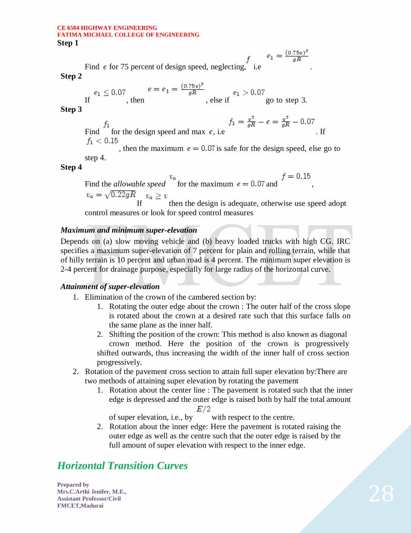
CE 6504 HIGHWAY ENGINEERING
FATIMA MICHAEL COLLEGE OF ENGINEERING
Prepared by
MrsCArthi Jenifer ME
Assistant ProfessorCivil
FMCETMadurai 28
Step 1
Find for 75 percent of design speed neglecting ie
Step 2
If then else if go to step 3
Step 3
Find for the design speed and max ie If
then the maximum is safe for the design speed else go to
step 4
Step 4
Find the allowable speed for the maximum and
If then the design is adequate otherwise use speed adopt
control measures or look for speed control measures
Maximum and minimum super-elevation
Depends on (a) slow moving vehicle and (b) heavy loaded trucks with high CG IRC
specifies a maximum super-elevation of 7 percent for plain and rolling terrain while that
of hilly terrain is 10 percent and urban road is 4 percent The minimum super elevation is
2-4 percent for drainage purpose especially for large radius of the horizontal curve
Attainment of super-elevation
1 Elimination of the crown of the cambered section by
1 Rotating the outer edge about the crown The outer half of the cross slope
is rotated about the crown at a desired rate such that this surface falls on
the same plane as the inner half
2 Shifting the position of the crown This method is also known as diagonal
crown method Here the position of the crown is progressively
shifted outwards thus increasing the width of the inner half of cross section
progressively
2 Rotation of the pavement cross section to attain full super elevation byThere are
two methods of attaining super elevation by rotating the pavement
1 Rotation about the center line The pavement is rotated such that the inner
edge is depressed and the outer edge is raised both by half the total amount
of super elevation ie by with respect to the centre
2 Rotation about the inner edge Here the pavement is rotated raising the
outer edge as well as the centre such that the outer edge is raised by the
full amount of super elevation with respect to the inner edge
Horizontal Transition Curves
CE 6504 HIGHWAY ENGINEERING
FATIMA MICHAEL COLLEGE OF ENGINEERING
Prepared by
MrsCArthi Jenifer ME
Assistant ProfessorCivil
FMCETMadurai 29
Transition curve is provided to change the horizontal alignment from straight to circular
curve gradually and has a radius which decreases from infinity at the straight end
(tangent point) to the desired radius of the circular curve at the other end (curve point)
There are five objectives for providing transition curve and are given below
1 to introduce gradually the centrifugal force between the tangent point and the
beginning of the circular curve avoiding sudden jerk on the vehicle This
increases the comfort of passengers
2 to enable the driver turn the steering gradually for his own comfort and security
3 to provide gradual introduction of super elevation and
4 to provide gradual introduction of extra widening
5 to enhance the aesthetic appearance of the road
Type of transition curve
Different types of transition curves are spiral or clothoid cubic parabola and Lemniscate
IRC recommends spiral as the transition curve because
1 it fulfills the requirement of an ideal transition curve that is
1 rate of change or centrifugal acceleration is consistent (smooth) and
2 radius of the transition curve is at the straight edge and changes to at
the curve point ( ) and calculation and field implementation is
very easy
Length of transition curve The length of the transition curve should be determined as the maximum of the following
three criteria rate of change of centrifugal acceleration rate of change of super elevation
and an empirical formula given by IRC Rate of change of centrifugal acceleration
At the tangent point radius is infinity and hence centrifugal acceleration is zero At the
end of the transition the radius R has minimum value R The rate of change of
centrifugal acceleration should be adopted such that the design should not cause
discomfort to the drivers If is the rate of change of centrifugal acceleration it can be
written as
Therefore the length of the transition curve in is
CE 6504 HIGHWAY ENGINEERING
FATIMA MICHAEL COLLEGE OF ENGINEERING
Prepared by
MrsCArthi Jenifer ME
Assistant ProfessorCivil
FMCETMadurai 30
(1)
where is the rate of change of centrifugal acceleration given by an empirical formula
suggested by by IRC as below
(2) 2 Rate of introduction of super-elevation
Raise ( ) of the outer edge with respect to inner edge is given by
The rate of change of this raise from to is achieved
gradually with a gradient of in over the length of the transition curve (typical range
of is 60-150) Therefore the length of the transition curve is
(3)
3 By empirical formula
IRC suggest the length of the transition curve is minimum for a plain and rolling terrain
(4)
and for steep and hilly terrain is
(5)
CE 6504 HIGHWAY ENGINEERING
FATIMA MICHAEL COLLEGE OF ENGINEERING
Prepared by
MrsCArthi Jenifer ME
Assistant ProfessorCivil
FMCETMadurai 31
and the shift as
(
6
) The length of the transition curve is the maximum of
equations 1 3 and 4or5 ie
(
7
Case (a)
For single lane roads
(
1
)
Therefore
(
2
)
Figure 1 Set-back for single lane roads (
CE 6504 HIGHWAY ENGINEERING
FATIMA MICHAEL COLLEGE OF ENGINEERING
Prepared by
MrsCArthi Jenifer ME
Assistant ProfessorCivil
FMCETMadurai 32
For multi lane roads if is the distance between centerline of the road and the centerline
of the inner lane then
(3)
(4)
Figure 2 Set-back for multi-lane roads ( )
Case (a)
For single lane roads
(1)
Therefore
(2)
Gradient
Gradient is the rate of rise or fall along the length of the road with respect to the
horizontal While aligning a highway the gradient is decided for designing the vertical
curve Before finalizing the gradients the construction cost vehicular operation cost and
the practical problems in the site also has to be considered Usually steep gradients are
avoided as far as possible because of the difficulty to climb and increase in the
CE 6504 HIGHWAY ENGINEERING
FATIMA MICHAEL COLLEGE OF ENGINEERING
Prepared by
MrsCArthi Jenifer ME
Assistant ProfessorCivil
FMCETMadurai 33
construction cost More about gradients are discussed below
Effect of gradient
The effect of long steep gradient on the vehicular speed is considerable This is
particularly important in roads where the proportion of heavy vehicles is significant Due
to restrictive sight distance at uphill gradients the speed of traffic is often controlled by
these heavy vehicles As a result not only the operating costs of the vehicles are
increased but also capacity of the roads will have to be reduced Further due to high
differential speed between heavy and light vehicles and between uphill and downhill
gradients accidents abound in gradients
Representation of gradient
The positive gradient or the ascending gradient is denoted as and the negative gradient as The deviation angle is when two grades meet the angle which
measures the change of direction and is given by the algebraic difference between the two
grades
steep gradient while 1 in 50 = 2 representation is illustrated in the figure 1
Example 1 in 30 = 333 is a
is a flatter gradient The gradient
CE 6504 HIGHWAY ENGINEERING
FATIMA MICHAEL COLLEGE OF ENGINEERING
Prepared by
MrsCArthi Jenifer ME
Assistant ProfessorCivil
FMCETMadurai 34
Figure 1 Representation of gradient
Types of gradient
Many studies have shown that gradient upto seven percent can have considerable effect
on the speeds of the passenger cars On the contrary the speeds of the heavy vehicles are
considerably reduced when long gradients as flat as two percent is adopted Although
flatter gradients are desirable it is evident that the cost of construction will also be very
high Therefore IRC has specified the desirable gradients for each terrain However it
may not be economically viable to adopt such gradients in certain locations steeper
gradients are permitted for short duration Different types of grades are discussed below
Ruling gradient
The ruling gradient or the design gradient is the maximum gradient with which the
designer attempts to design the vertical profile of the road This depends on the terrain
length of the grade speed pulling power of the vehicle and the presence of the horizontal
curve In flatter terrain it may be possible to provide flat gradients but in hilly terrain it
is not economical and sometimes not possible also The ruling gradient is adopted by the
designer by considering a particular speed as the design speed and for a design vehicle
with standard dimensions But our country has a heterogeneous traffic and hence it is not
possible to lay down precise standards for the country as a whole Hence IRC has
recommended some values for ruling gradient for different types of terrain
Limiting gradient
This gradient is adopted when the ruling gradient results in enormous increase in cost of
construction On rolling terrain and hilly terrain it may be frequently necessary to adopt
limiting gradient But the length of the limiting gradient stretches should be limited and
must be sandwiched by either straight roads or easier grades
Exceptional gradient
Exceptional gradient are very steeper gradients given at unavoidable situations They
should be limited for short stretches not exceeding about 100 metres at a stretch In
mountainous and steep terrain successive exceptional gradients must be separated by a
minimum 100 metre length gentler gradient At hairpin bends the gradient is restricted to
25
Critical length of the grade
The maximum length of the ascending gradient which a loaded truck can operate without
undue reduction in speed is called critical length of the grade A speed of 25 kmph is a
CE 6504 HIGHWAY ENGINEERING
FATIMA MICHAEL COLLEGE OF ENGINEERING
Prepared by
MrsCArthi Jenifer ME
Assistant ProfessorCivil
FMCETMadurai 35
reasonable value This value depends on the size power load grad-ability of the truck
initial speed final desirable minimum speed
Minimum gradient
This is important only at locations where surface drainage is important Camber will take
care of the lateral drainage But the longitudinal drainage along the side drains require
some slope for smooth flow of water Therefore minimum gradient is provided for
drainage purpose and it depends on the rain fall type of soil and other site conditions A
minimum of 1 in 500 may be sufficient for concrete drain and 1 in 200 for open soil
drains are found to give satisfactory performance Sight distance available from a point is the actual distance along the road surface which a driver
from a specified height above the carriage way has visibility of stationary or moving objects
Sight distance required by drivers applies to both geometric design of highways and for
traffic control The sight distance situations are considered in the design
i) Stopping or absolute minimum sight distance
ii) Safe overtaking or passing sight distance
iii) Safe sight distance for entering into uncontrolled intersections
Apart from the three situations mentioned above the following sight distance are considered by the
IRC in highway design
Intermediate sight distance
This is defined as twice the stopping sight distance when overtaking sight distance
cannot be provided intermediate sight distance is provided to give limited overtaking opportunities
to fast vehicles
Head light sight distance
This is the distance visible to a driver during night driving under the illumination of the
vehicle head lights
Stopping sight distance
The minimum sight distance available on a highway at any spot should be of sufficient
length to stop a vehicle traveling at design speed safely without collision with any other obstruction
The absolute minimum sight distance is therefore equal to the stopping sight distance
which is also sometimes called nonpassing sight distance The sight distance available on a road to a
driver at any instance depends on
i) Features of the road
ii) Height of the drivers eye above the road surface
iii) Height of the object above the road surface
The distance within which a motor vehicle can be stopped depends upon the factors listed below
a) Total reactions time of the driver
b) Speed of vehicle
c) Efficiency of breaks
d) Frictional resistance between the road and tyres
e) Gradient of the road
Total reaction time
) Reaction time of the driver is the time taken from the instant the object is visible to the
driver to the instant the brakes are effectively applied
) The total reaction time may be split up into two parts
CE 6504 HIGHWAY ENGINEERING
FATIMA MICHAEL COLLEGE OF ENGINEERING
Prepared by
MrsCArthi Jenifer ME
Assistant ProfessorCivil
FMCETMadurai 36
i) Perception time
ii) Brake reaction time
PIEV theory
According to this theory the total reaction time of the driver is split into four parts
i) Perception
ii) Intellection
iii) Emotion
iv) Volition
Speed of Vehicle
The stopping distance depends very much on the speed of the vehicle first during the
total reaction time of the driver the distance moved by the vehicle will depend on the speed
Efficiency of brakes
The braking efficiency is said to be 100 percent if the wheels are fully licked preventing
them from rotating on application of the brakes This will result in 100 percent skidding which is
normally undesirable except in utmost emergency
Frictional resistance between road and tyres
The frictional resistance developed between road and tyres or the skid resistance depends
on the type and condition of the road surface and the tyres IRC has specified a design friction
coefficient of 035 to 04 depending upon the speed to be used for finding the braking distance in the
calculation of stopping sight distance
Analysis of stopping distance
i) The distance traveled by the vehicle during the total reaction time known as lag
distance
ii) The distance traveled by the vehicle after the application of the brakes is known as
braking distance
Overtaking sight distance
The minimum distance open to the vision of the driver of a vehicle intending to overtake
slow vehicle ahead with safety against the traffic of opposite direction is known as the minimum
overtaking sight distance(OSD) or Safe passing sight distance available
The overtaking sight distance is the distance measured along the center of the road which
a driver with his eye level 12m above the road surface can see the top of an object 12m above the
road surface
Some of the important factors on which the minimum overtaking sight distance required
a) Speed of
i) overtaking vehicle
ii) overtaken vehicle
iii) The vehicle coming from opposite direction
b) Distance between the overtaking and overtaken vehicles the minimum spacing
depends on the steeds
a) Skill and reaction time of the driver
b) Rate of acceleration of overtaking vehicle
c) Gradient of the road
Criteria for sight distance requirements on highway
) The absolute minimum sight distance required throughout the length of the road is the
SSD which should invariably be provided at all places
CE 6504 HIGHWAY ENGINEERING
FATIMA MICHAEL COLLEGE OF ENGINEERING
Prepared by
MrsCArthi Jenifer ME
Assistant ProfessorCivil
FMCETMadurai 37
) On horizontal curves the obstruction on the inner side of the curves should be cleared
to provide the required set back distance and absolute minimum sight distance
) On vertical summit curves the sight distance requirement may be fulfilled by proper
design of the vertical alignment
Hairpin bent
TYPES OF CURVES ON HILL ROADS
The following are the important types of curves provided on hill Roads-
1 Hair-Pin Curves
2 Salient Curves
3 Re-entrant Curves 1 Hair-pin curves - The curve in a hill road which changes its direction through an angle of 180
degree or so down the hill on the same side is known as hair-pin curve
A Hair-Pin Bend
This curve is so called because it conforms to the shape of a hair-pin The bend so formed at the
hair-pin curve in a hill road is known as hair-pin bend This type of curve should be located on a
hill side having the minimum slope and maximum stability It must also be safe from view point of
landslides and ground water Hair-pin bends with long arms and farther spacing are always
preferred They reduce construction problems and expensive protective works Hair-pin curves or
bends of serpentine nature are difficult to negotiate and should therefore be avoided as far as
possible
Salient curves - The curves having their convexity on the outer edges of a hill road are called
salient curves The centre of curvature of a salient curve lies towards the hill side This type of curve
occurs in the road length constructed on the ridge of a hill the bend so formed at the salient curve in
a hill road known as corner bend
Salient curves are very dangerous for fast moving traffic At such a curve or at corner bend the
portion of projecting hill side is usually cut down to improve the visibility as shown in fig (Re-
entrant curve) The outer edge of the road at such a curve is essentially provided with a parapet wall
for protection of the vehicles from falling down the hill slope
CE 6504 HIGHWAY ENGINEERING
FATIMA MICHAEL COLLEGE OF ENGINEERING
Prepared by
MrsCArthi Jenifer ME
Assistant ProfessorCivil
FMCETMadurai 38
3 Re-entrant curves - The curves having their convexity on the inner edge of a hill road are called
re-entrant curves
Re-entrant curves
The centre of curvature of a re-entrant curves lies away from the hill side This type of curve occurs
in the road length constructed in the calley of a hill
These curves are less dangereous as they provide adequate visibility to the fast moving traffic At
such curves the parapet wall is provided only for safety of fast moving traffic
CE 6504 HIGHWAY ENGINEERING
FATIMA MICHAEL COLLEGE OF ENGINEERING
Prepared by
MrsCArthi Jenifer ME
Assistant ProfessorCivil
FMCETMadurai 39
UNIT ndash III DESIGN OF RIGID AND FLEXIBLE PAVEMENTS
COMPARISON OF RIGID AND FLEXIBLE PAVEMENTS
The comparisons are
i) Design precision
A cement concrete pavement is amerable to a much more precise structural analysis
than a flexible pavement Flexible pavements designs are mainly empirical Computer aided analysis
of layered system is making the flexible pavement design more exact than hitherto
ii) Life
) Cement concrete slabs of a thin section constructed in the early 1940rsquos are still in
existence in India though many of them have cracked badly and a few of them have been ripped
open and rebuilt in recent ties
) A major project in cement concrete road construction between Agra and Mathura It can
safely be said that a well-designed concrete slab has a life of about 40 years
) Compared to this the life of a flexible pavement generally varies from 10 to 20 years
iii) Maintenance
) A well-designed cement concrete pavement needs very little maintenance The only
maintenance needed is I respect of joints
) The surface is unaffected by spillage of oil and lubricants bituminous surfaces on the
other hand need great inputs in maintenance
) The surface is affected by spillage of oil and lubricants The surface is also affected by
natural weathering agents like air water ad temperature changes
) A cement concrete pavement on the other hand needs a small amount for maintaining
joints
iv) Initial cost
) The argument so far used against a cement concrete slab is that it is much more costly
than a flexible pavement
) The latter specifications no doubt represent the rock-bottom needs of a road in India but
these specifications can hardly provide a smooth and durable surface
v) Stage construction ) Road construction is generally done adopting a policy of stage construction especially for
low volume roads As traffic grows additional layers in the form of water bound macadam and
superior surfacing are added on
) Initial outlay is minimum and additional outlays are in keeping with traffic growth This is
a great advantage when dealing with new roads in an atmosphere of austerity
vi) Availability of materials
) Cement bitumen stone aggregates and gravelsand are the major materials involved in
pavement Construction Cement has been in serious short supply in the country for the past many
decades
) Bitumen is also not available plentifully in India There is also the danger of the entire oil
reserves in the world shrinking during the next two or three decades
) In locations where stone aggregates are scarce cement concrete may have an advantage
for flexible pavements
vii) Surface characterstics
CE 6504 HIGHWAY ENGINEERING
FATIMA MICHAEL COLLEGE OF ENGINEERING
Prepared by
MrsCArthi Jenifer ME
Assistant ProfessorCivil
FMCETMadurai 40
) A good cement concrete surface is smooth and free from rutting potholes and
corrugations In a bituminous surface it is only the asphaltic concrete surface that can give
comparable rideablity
) A well-constructed cement concrete pavement surface can have a permanent nonskid
surface A bituminous surface can also be designed to have a good skid resistant surface
viii) Utility location
) In cement concrete slabs proper thought has to be given to locate utilities such as water
pipes telephone lines and electric cables
) It is difficult to rip open the slab and restore it to be the original condition if any changes
in the utilities lines are to be made
ix) Glame and night visibility
) Concrete pavements have a gray color which can cause glam under sunlight Colored
cement can reduce the grave
) On the other hand bituminous roads need more street lighting
x) Traffic dislocation during construction
) A cement concrete pavement requires 28 days before it can be thrown open to traffic On
the other hand a bituminous surface can be thrown open to traffic shortly after it is rolled
xi) Environmental considerations during construction
) The process of heating of bitumen and aggregates and mixing them together on hot mix
plants can prove to be much more hazardous to the environment than cement concrete construction
where no heating of any material is involved
xii) Overall economy on a life cycle basis
) A good road is costly to construct but once constructed such a road requires little
maintenance and results in savings in vehicle operating costs
) The comparative economy of a flexible pavement and a rigid pavement has proved that on
overall economic considerations
Types of pavement structure
Based on the structural behavior pavements are generally classified into three
categories
i) Flexible pavements
ii) Rigid pavements
iii) Semi rigid pavements
Flexible pavements
) Flexible pavements are those which on the whole have low or negligible flexural
strength and are rather flexible in their structural action under the loadsThe flexible pavement
layers reflect the deformation of the lower layers on to the surface of the layer
) A flexible pavement consists of four components(i) Soil subgrade (ii) sub base
course (iii) base course (iv) Surface course
CE 6504 HIGHWAY ENGINEERING
FATIMA MICHAEL COLLEGE OF ENGINEERING
Prepared by
MrsCArthi Jenifer ME
Assistant ProfessorCivil
FMCETMadurai 41
) The flexible pavement layers transmit the vertical or compressive stresses to the lower layers
by grain to grain transfer through the points of contact in the granular structure A well
compacted granular structure consisting of strong added aggregate can transfer the compressive
stresses
) The load spreading ability of this layer therefore depends on the type of the materials and mix
design factors Bituminous concrete is one of the best flexible pavements layer materials Other
materials which fall under the group are all granular materials with or without bituminous
binder granular base and sub base course materials
) The vertical compressive stress is maximum on the pavement surface directly under the wheel
and is equal to the contact pressure under the wheel The flexible pavement may be constructed
in a number of layers and the top layer has to be strongest as the highest compressive stresses
) Flexible pavements are commonly designed using empirical design charts or equations taking
into account some of the design factors there are also semi empirical and theoretical design
methods
Rigid pavements
) Rigid pavements are those which possess note flexural strength or flexural rigidity
The stresses are not transferred from grain to grain to the lower layers as in the ease of flexible
pavements layers
) The rigid pavements are made of Portland cement concrete plain reinforced or
prestressed concrete The plain cement concrete slabs are expected to take up about 40 kgcm2
flexural stress
) The rigid pavement has the slab action and is capable of transmitting the wheel
load stresses through a wider area below The main point of difference in the structural behavior
of rigid pavement as compared to the flexible pavement is that the critical condition of stress in
the rigid pavement is the maximum flexural stress occurring in the slab due to wheel load and
the temperature changes whereas in the flexible pavement
) As the rigid pavement slab has tensile strength tensile stresses are developed due
to the bending of the slab under wheel load and temperature variations Thus the types of
stresses developed and their distribution within the cement concrete slab are quirt different
) The cement concrete pavement slab can very well serve as a wearing surface as
well an effective base course The rigid pavement structure consists of a cement concrete slab
below which a granular base or sub base course may be provided
) Though the cement concrete slab can also be laid directly over the soil subgrade
consists of fine grained soil
) the rigid pavements are usually designed and the stresses are analyzed using the
elastic theory assuming the pavements as a n elastic plate resting over an elastic or a viscous
foundation
Semi rigid pavements
) when bonded materials like the pozzolanic concrete lean cement concrete or soil
cement are used in the base course or sub base course layer the pavement layer has considerably
higher flexural strength than the common flexible pavement layers
) when this intermediate class of materials are used in the base or sub base course
layer of the pavements they are called semi rigid pavements
CE 6504 HIGHWAY ENGINEERING
FATIMA MICHAEL COLLEGE OF ENGINEERING
Prepared by
MrsCArthi Jenifer ME
Assistant ProfessorCivil
FMCETMadurai 42
) This third category of semi rigid pavement are either designed as flexible
pavements with some correction factors to find the thickness requirements based on experience
or by using a new design approach
) The semi rigid pavement materials have low resistance to impact and abrasion and
therefore are usually provided with flexible pavement surface course
Various functions of pavement components
The functions are
Soil sub grade and its evaluation
) The soil sub grade is a layer of natural soil prepared to receive the layers of pavement
materials placed over it It is essential that at no time the soil sub grade is overstressed it means that
the pressure transmitted on the top of the sub grade is within the allowable limit
) Many tests are known for measuring the strength properties of the sub grades Some of the
tests have been standardized for the use The common strength test for the evaluation of soil
subgrade is
i) California bearing ratio test
ii) California resistance value test
iii) Triaxial compression test
iv) Plate bearing test
CALIFORNIA BEARING RATIO (CBR) TEST
It is evolved for the empirical method of flexible pavement design The CBR test is carried
out either in the laboratory on prepared specimens or in the field by taking in situ measurements
California resistance value
It is found by using have been stabliometerThis test is used in an empirical method of
flexible pavement design based on soil strength
Triaxial test
It is the most important soil strength but still the test is not very commonly used in structural
design of pavements
Plate bearing test
It is carried out using a relatively large diameter plate to evaluate the load supporting
capacity of supporting power of the pavement layers The results are plate bearing tests are used in
flexible pavement design method like McLeod method on based on layer system analysis by
brumister
Sub base and base courses and their evaluation
) There layers are made of broken stones bound or unbound aggreagatesome times in sub
base course a layer of stabilized soil(or) Selected granular soil is also used
) however at the sub base course it is desirable to use smaller size graded aggregates When
the sub grade consists of fine grained soil and when the pavement carries heavy wheel loads
CE 6504 HIGHWAY ENGINEERING
FATIMA MICHAEL COLLEGE OF ENGINEERING
Prepared by
MrsCArthi Jenifer ME
Assistant ProfessorCivil
FMCETMadurai 43
) Sub base course primarily has the similar function as of the base course and is provided
with inferior materials than of base course Base courses are used under rigid pavement for
i) Preventing pumping
ii) Protecting the sub grade against frost action
) Thus the fundamental purpose of abase course and sub base course is to provide a stress
transmitting medium to spread the surface wheel loads in such manner
) The sub base and base course layers may be evaluated by suitable strength or stability test
like plate bearing CBR test
WEARING COURSE AND ITS EVALUATION
) The purpose of the wearing course is to give a smooth riding surface that is dense It
resists pressure exerted by tyres and takes up wear and tear due to the traffic
) Wearing course also offers a water tight layer against the surface water infiltration The
flexible pavement normally a bituminous surfacing is used as a wearing course
) In rigid pavements the cement concrete acts like a base course as well as wearing course
Most popular test in use is marshal stability test where in the optimum content of bitumen binder is
worked out based on the stability density
) Plate bearing test and Bankelman beam test are also sometimes made use of for evaluating
the wearing course and the pavement as a whole
Various factors to be considered in pavement design and the significance
Pavement design consists of two parts
i) Mix design of materials to be used in each pavement component layer Thickness design of the
pavement and the component layers
The various factors to be considered for the design of pavements are given below
i) Design wheel load
ii) Sub grade soil
iii) Climatic factors
iv) Pavement component layers
v) Environmental factors
vi) Special factors in the design of different types of pavements
Design wheel load
The various wheel load factors to be considered in pavement design are
i) Maximum wheel load
ii) Contact pressure
iii) Dual or multiple wheel loads
iv) Repetition of loads
Maximum wheel load
The wheel load configurations are important to know the way in which the loads of a given
vehicle are applied on the pavement surface
) For highways the maximum legal axle load as specified by Indian road congress is 8170
kg with a maximum equivalent single wheel load of 4085 kg
) The evaluation for vertical stress computations under a uniformly distribute of circular
load based on Boussineqrsquos theory is given by
CE 6504 HIGHWAY ENGINEERING
FATIMA MICHAEL COLLEGE OF ENGINEERING
Prepared by
MrsCArthi Jenifer ME
Assistant ProfessorCivil
FMCETMadurai 44
2
322
3
1
za
zpz
σz = vertical stress at depth z
P= surface pressure
Z=depth at which σz computed
A=radius of loaded area
Contact pressure
Generally the wheel load is assumed to be distributed over a circular area But by
measurement of the imprints of tyers with different load and inflation pressures Three terms in use
with reference to tyre pressure are
Tyre pressure
Inflation pressure
Contact pressure
Tyre pressure and inflation pressure mean exactly the same the contact pressure is found to be more
than tyre pressure when the tyre pressure is less than 7 kgm2 and it is vice versa when the tyre
pressure exceeds this value
Contact pressure can be measured by the relationship
Load on wheel
Contact pressure = ----------------------------------------
Contact area or area of imprint
The general variation between the tyre pressure and measured contact pressure is shown in this fig
The ratio of contact pressure to type pressure is defined as rigidity factor Thus value of rigidity
factor is 10 for an average tyre pressure of 7 Kgcm2This value is higher than unity for lower type
pressures and less than unity for tyre pressures higher than 7 kgcm2
Equivalent single wheel load (ESWL)
) The maximum wheel load within the specified limit and to carry greater load it is
necessary to provide dual wheel assembly to the rear axles of the roads vehicles
) In other words the pressure at a certain depth below the pavement surface cannot be
obtained by numerically adding the pressure caused by any one wheel
) The effect is in between the single load and two times load carried by one wheel The load
dispersion is assumed to be at an angle of 450In the dual wheel load assembly let d be the clear gap
between the two wheels S be the spacing between the centers of the wheels and a be the radius of
the circular contact area of each wheel Then S = (d + 2a)
) ESWL may be determined based on either equivalent deflection or equivalent stress
criterianMultiple wheel loads are convert to ESWL and this value is used in pavement design The
ESWL is usually determined by the equivalent stress criterion using a simple graphical method
CE 6504 HIGHWAY ENGINEERING
FATIMA MICHAEL COLLEGE OF ENGINEERING
Prepared by
MrsCArthi Jenifer ME
Assistant ProfessorCivil
FMCETMadurai 45
) A straight line relationship is assumed between ESWL and depth on log scales For
determining ESWL the plot is made as shown in fig
) Two points A and B are plotted on the log-log graph with coordinates of A (Pd2) and
B(2p2s)line AB is a plot which is the focus of points where any single wheel load is equivalent to a
certain set of dual wheels
) To Calculate the ESWL for a dual assembly it is essential to estimate a design thickness of
the pavement If the design thickness so obtained is equal to the estimated thickness then the ESWL
calculations could be considered as correct Otherwise trials are made
) In heavy trucks and trailers the load on each wheel may be further reduced by multiple
wheels and tandem axles
Repetition of loads
) The deformation of load pavement (or) sub grade due to a single application of wheel load
may be small It required carrying out traffic surveys for accounting the factor of repetitions for
wheel loads in the design of pavement
) Data collected are converted to some constant equivalent wheel loads Equivalent wheel
load is a single load equivalent to the repeated applications of any particular wheel load on a
pavement which requires the same thickness and strength of pavements
) McLeod has given a procedure for evolving equivalent load factors for designing flexible
pavements
Various methods of flexible pavement design
) The flexible pavement is built with number of layers In the design process it is to be
ensured that under the application of load none of the layers is overstressed
) The maximum intensity of stresses occurs in the top layer of the pavement The
magnitude of load stresses reduces at lower layers
) In the design of flexible pavements it has yet not been possible to have a rational design
method wherein design process and service behavior of the pavement can be expressed by
mathematical laws
) Flexible pavement design methods are accordingly either empirical or semi empirical In
these methods the knowledge and experience gained on the behavior of the pavements in the past
are usefully utilized
Various approaches of flexible pavement design may be thus classified into three groups
i) Empirical method
ii) Semi-empirical or Semi theoretical method
iii) Theoretical method
) Empirical methods are either based on physical properties or strength parameters of soil
sub grade When the design is based on stress strain function and modified base on experience it
may be called semi-empirical or semi-theoretical There are design methods based on theoretical
analysis and mathematical computations
Out of the flexible pavement design method available is
i) Group index method
ii) California bearing ratio method
iii) California R value (or) Stabiliometer method
iv) Triaxial test method
CE 6504 HIGHWAY ENGINEERING
FATIMA MICHAEL COLLEGE OF ENGINEERING
Prepared by
MrsCArthi Jenifer ME
Assistant ProfessorCivil
FMCETMadurai 46
v) McLeod method
vi) Burmister method
Group index method
) Group index value is an arbitrary index assigned to the soil type in numerical equations
base on the percent fines liquid limit and plasticity index
) The design chart for group index method for determining the pavement thickness is given
in fig
The traffic volume in this method is divided in three groups
Traffic volume No of vehicles per day
Light Less than 50
Medium 50 to 300
Heavy Over 300
The design of the pavement thickness by this method first the G1 value of the soil is found the
anticipated traffic is estimated and is designated as light medium or heavy as indicated
The G1 method of pavement design is essentially an empirical method based on physical properties
of the subgrade soil This method does not consider the strength characteristics of the subgrade soil
and therefore is open to question regarding the reliability of the design based on the index properties
of the soil only
California bearing ratio method
) California division of highways in the USA developed CBR method for
pavement design The majority of design curves developed later are base on the original curves
proposed by OJporter
) One of the chief advantages of CBR method is the simplicity of the test procedure
The CBR tests were carried out by the California state highway department on existing pavement
layers including subgrade sub base and base course
) Based on the extensive CBR test data collected on pavement which behaved
satisfactory and those which failed an empirical design chart was developed correlating the CBR
value and the pavement thickness The basis of the design chart is that a material with a given CBR
required a certain thickness of pavement layer as a cover
) A higher load needs a thicker pavement layer to protect the sub grade Design
curves correlating the CBR value with total pavement thickness cover were developed by the
California state highway department for wheel loads of 3175kg and 5443 kg representing light and
heavy traffic The design curves are shown in this fig
It is possible to extend the CBR design curves for various loading conditions nusing the expression
t= 2
1
1751
pCBRp
t=2
1
751
A
CBR
p
Hence
CE 6504 HIGHWAY ENGINEERING
FATIMA MICHAEL COLLEGE OF ENGINEERING
Prepared by
MrsCArthi Jenifer ME
Assistant ProfessorCivil
FMCETMadurai 47
t= pavement thickness cm
p=Wheel load kg
CBR= California bearing ratio percent
P=tyre pressure kgcm2
A= area of contactcm2
IRC Recommendations
a) The CBR tests should be performed on remoulded soils in the laboratory The specimens should
be prepared by static compaction wherever possible and otherwise by dynamic compaction
b) For the design of new roads the sub grade soil sample should be compacted at OMC to proctor
density whenever suitable compaction equipment
c) The CBR test samples may be soaked in water for four days period before testing the annual
rainfall is less than 50 cm and the water table is too deep to affect the sub grade and imperable
surfacing is provided to carrying out CBR test
d) If the maximum variations in CBR value of the three specimens exceed the specified limits the
design CBR should be average of at least six samples
e) The top 50 cm of sub grade should be compacted at least up to 95 to 100 percent of proctor
density
f) An estimate of the traffic should be carried by the road pavements at the end of expected in view
the existing traffic and probable growth rate of traffic
g) The traffic for the design is considered in units of heavy vehicles per day in both directions and is
divided into seven categories A to G The design thickness is considered applicable for single axle
loads up to 8200 kg and tandom axle loads up to 14500 kg
h) When sub base course materials contain substantial proportion of aggregates of size above 20mm
the CBR value of these materials would not be valid for the design of subsequent layers above them
The CBR method of pavement design gives the total thickness requirement of the pavement above a
sub grade and thickness value would remain the same quality of materials used in component layers
California resistance value method
) In this design method based on stabliometer R-value and cohesiometer C-value
Based on performance data it was established by pavement thickness varies directly with R value
and algorithm of load repetitions It varies inversely with fifth root of c valueThe expression for
pavement thickness is given by the empirical equation
T=
5
1
1 90
C
RTK
Hence
T=total thickness of pavement cm
K=Numerical constant 0166
T1=traffic index
R= stabiliometer resistance value
C=Cohesiometer value
CE 6504 HIGHWAY ENGINEERING
FATIMA MICHAEL COLLEGE OF ENGINEERING
Prepared by
MrsCArthi Jenifer ME
Assistant ProfessorCivil
FMCETMadurai 48
In the design of flexible pavements based on California resistance value method for the following
data are needed
) R-value of soil subgrade
) T1 value
) Equivalent C-value
) R value of soil subgrade is obtained from the test using stablio meterThe
computation of T1 value has been explained
Equivalent C-value
) The cohesion meter value c is obtained for each layer of pavement material
separately from tests However the composite or equivalent C-value of the pavement may be
estimated if the thickness of each component layer and the c-value of the material of the layer are
known
) while designing a pavement as the thickness of the pavement is not known it is
easier if the pavement is first assumed to consist of any one material like gravel base course with
known C-value
) Subsequently the individual thickness of each layer is converted in terms of gravel
equivalent by using relationship
5
1
1
2
2
1
C
C
t
t
) t1 and t2 are the thickness values of any two pavement layersc1 and c2 are their
corresponding cohesiometer values
CE 6504 HIGHWAY ENGINEERING
FATIMA MICHAEL COLLEGE OF ENGINEERING
Prepared by
MrsCArthi Jenifer ME
Assistant ProfessorCivil
FMCETMadurai 49
UNIT 4 MATERIAL AND MAINTENANCE
SUMMIT CURVE
Summit curves are vertical curves with gradient upwards They are formed when two
gradients meet as illustrated in figure 1 in any of the following four ways
1 When a positive gradient meets another positive gradient [figure 1a]
2 When positive gradient meets a flat gradient [figure 1b]
3 When an ascending gradient meets a descending gradient [figure 1c]
4 When a descending gradient meets another descending gradient [figure 1d]
Type of Summit Curve
Many curve forms can be used with satisfactory results the common practice has been to
use parabolic curves in summit curves This is primarily because of the ease with it can
be laid out as well as allowing a comfortable transition from one gradient to another
Although a circular curve offers equal sight distance at every point on the curve for very
small deviation angles a circular curve and parabolic curves are almost congruent
Furthermore the use of parabolic curves were found to give excellent riding comfort
Figure 1 Types of summit curves
Design Consideration
In determining the type and length of the vertical curve the design considerations are
comfort and security of the driver and the appearance of the profile alignment Among
these sight distance requirements for the safety are most important on summit curves
The stopping sight distance or absolute minimum sight distance should be provided on
these curves and where overtaking is not prohibited overtaking sight distance or
intermediate sight distance should be provided as far as possible When a fast moving
vehicle travels along a summit curve there is less discomfort to the passengers This is
because the centrifugal force will be acting upwards while the vehicle negotiates a
summit curve which is against the gravity and hence a part of the tyre pressure is
relieved Also if the curve is provided with adequate sight distance the length would be
sufficient to ease the shock due to change in gradient Circular summit curves are
identical since the radius remains same throughout and hence the sight distance From
CE 6504 HIGHWAY ENGINEERING
FATIMA MICHAEL COLLEGE OF ENGINEERING
Prepared by
MrsCArthi Jenifer ME
Assistant ProfessorCivil
FMCETMadurai 50
this point of view transition curves are not desirable since it has varying radius and so the
sight distance will also vary The deviation angles provided on summit curves for
highways are very large and so the simple parabola is almost congruent to a circular arc
between the same tangent points Parabolic curves are easy for computation and also it
had been found out that it provides good riding comfort to the drivers It is also easy for
field implementation Due to all these reasons a simple parabolic curve is preferred as
summit curve Length of the summit curve
The important design aspect of the summit curve is the determination of the length of the
curve which is parabolic As noted earlier the length of the curve is guided by the sight
distance consideration That is a driver should be able to stop his vehicle safely if there is
an obstruction on the other side of the road Equation of the parabola is given by
where where N is the deviation angle and is the length of the In
deriving the length of the curve two situations can arise depending on the uphill and
downhill gradients when the length of the curve is greater than the sight distance and the
length of the curve is greater than the sight distance
Let is the length of the summit curve is the SSDISDOSD is the deviation angle
drivers eye height (12 m) and the height of the obstruction then the length of the
summit curve can be derived for the following two cases The length of the summit curve
can be derived from the simple geometry as shown below
Case a Length of summit curve greater than sight distance( )
Figure 1 Length of summit curve ( )
The situation when the sight distance is less than the length of the curve is shown in
figure 1
CE 6504 HIGHWAY ENGINEERING
FATIMA MICHAEL COLLEGE OF ENGINEERING
Prepared by
MrsCArthi Jenifer ME
Assistant ProfessorCivil
FMCETMadurai 51
(1)
Case b Length of summit curve less than sight distance
The second case is illustrated in figure 1
Figure 1 Length of summit curve
CE 6504 HIGHWAY ENGINEERING
FATIMA MICHAEL COLLEGE OF ENGINEERING
Prepared by
MrsCArthi Jenifer ME
Assistant ProfessorCivil
FMCETMadurai 52
From the basic geometry one can write
(1)
Therefore for a given and to get minimum differentiate the above equation
with respect to and equate it to zero Therefore
Solving the quadratic equation for
(2)
Now we can substitute back to get the value of minimum value of for a given
and Therefore
Solving for
CE 6504 HIGHWAY ENGINEERING
FATIMA MICHAEL COLLEGE OF ENGINEERING
Prepared by
MrsCArthi Jenifer ME
Assistant ProfessorCivil
FMCETMadurai 53
(3) (4
CE 6504 HIGHWAY ENGINEERING
FATIMA MICHAEL COLLEGE OF ENGINEERING
Prepared by
MrsCArthi Jenifer ME
Assistant ProfessorCivil
FMCETMadurai 54
When stopping sight distance is considered the height of drivers eye above the road
surface ( ) is taken as 12 metres and height of object above the pavement surface ( )
is taken as 015 metres If overtaking sight distance is considered then the value of
drivers eye height ( ) and the height of the obstruction ( ) are taken equal as 12
metres
Valley curve
Valley curve or sag curves are vertical curves with convexity downwards They are
formed when two gradients meet as illustrated in figure 1 in any of the following four
ways
Figure 1 Types of valley curve
1 When a descending gradient meets another descending gradient [figure 1a]
2 When a descending gradient meets a flat gradient [figure 1b]
3 When a descending gradient meets an ascending gradient [figure 1c]
4 When an ascending gradient meets another ascending gradient [figure
Design considerations
There is no restriction to sight distance at valley curves during day time But visibility is
reduced during night In the absence or inadequacy of street light the only source for
visibility is with the help of headlights Hence valley curves are designed taking into
account of headlight distance In valley curves the centrifugal force will be acting
downwards along with the weight of the vehicle and hence impact to the vehicle will be
more This will result in jerking of the vehicle and cause discomfort to the passengers
Thus the most important design factors considered in valley curves are (1) impact-free
movement of vehicles at design speed and (2) availability of stopping sight distance
under headlight of vehicles for night driving
For gradually introducing and increasing the centrifugal force acting downwards the best
shape that could be given for a valley curve is a transition curve Cubic parabola is
generally preferred in vertical valley curves See figure 1
CE 6504 HIGHWAY ENGINEERING
FATIMA MICHAEL COLLEGE OF ENGINEERING
Prepared by
MrsCArthi Jenifer ME
Assistant ProfessorCivil
FMCETMadurai 55
Figure 1 Valley curve details
During night under headlight driving condition sight distance reduces and availability of
stopping sight distance under head light is very important The head light sight distance
should be at least equal to the stopping sight distance There is no problem of overtaking
sight distance at night since the other vehicles with headlights could be seen from a
considerable distance
Length of the valley curve
The valley curve is made fully transitional by providing two similar transition curves of
equal length The transitional curve is set out by a cubic parabola where
The length of the valley transition curve is designed based on two criteria
1 comfort criteria that is allowable rate of change of centrifugal acceleration is
limited to a comfortable level of about
2 safety criteria that is the driver should have adequate headlight sight distance at
any part of the country
Comfort criteria
The length of the valley curve based on the rate of change of centrifugal acceleration that
will ensure comfort Let is the rate of change of acceleration the minimum radius of
the curve is the design speed and is the time then is give
CE 6504 HIGHWAY ENGINEERING
FATIMA MICHAEL COLLEGE OF ENGINEERING
Prepared by
MrsCArthi Jenifer ME
Assistant ProfessorCivil
FMCETMadurai 56
For a cubic parabola the Value Safety criter Length of the valley curve for headlight distance may be determined for two conditions
(1) length of the valley curve greater than stopping sight distance and (2) length of the
valley curve less than the stopping sight distance of for length is given by
Case 1 Length of valley curve greater than stopping sight distance ( )
The total length of valley curve is greater than the stopping sight distance SSD The
sight distance available will be minimum when the vehicle is in the lowest point in the
valley This is because the beginning of the curve will have infinite radius and the bottom
of the curve will have minimum radius which is a property of the transition curve The
case is shown in figure 1
Figure 1 Valley curve case 1
From the geometry of the figure we have
CE 6504 HIGHWAY ENGINEERING
FATIMA MICHAEL COLLEGE OF ENGINEERING
Prepared by
MrsCArthi Jenifer ME
Assistant ProfessorCivil
FMCETMadurai 57
(1)
where is the deviation angle in radians is the height of headlight beam is the
head beam inclination in degrees and is the sight distance The inclination is 1
degree
Case 2 Length of valley curve less than stopping sight distance ( )
The length of the curve is less than SSD In this case the minimum sight distance is
from the beginning of the curve The important points are the beginning of the curve and
the bottom most part of the curve If the vehicle is at the bottom of the curve then its
headlight beam will reach far beyond the endpoint of the curve whereas if the vehicle is
at the beginning of the curve then the headlight beam will hit just outside the curve
Therefore the length of the curve is derived by assuming the vehicle at the beginning of
the curve The case is shown in figure 1
From the figure
(1) Note that the above expression is approximate and is satisfactory because in practice the gradients
are very small and is acceptable for all practical purposes We will not be able to know prior to
which case to be adopted Therefore both has to be calculated and the one which satisfies the
condition is adopted
1 Flexible pavement
2 Rigid pavement
Flexible pavement
These pavements reflect the deformation of sub grade and the subsequent layers to the
surface
Rigid pavement
The rigid characteristic of the pavement are associated with rigidity or flexural strength
CE 6504 HIGHWAY ENGINEERING
FATIMA MICHAEL COLLEGE OF ENGINEERING
Prepared by
MrsCArthi Jenifer ME
Assistant ProfessorCivil
FMCETMadurai 58
or slab action so the load is distributed over a wide area of sub grade soil
Flexible pavement Definition
These pavements reflect the deformation of sub grade and the subsequent layers to the
surface Flexible usually asphalt is laid with no reinforcement or with a specialized
fabric reinforcement that permits limited flow or repositioning of the roadbed under
ground changes
The design of flexible pavement is based on load distributing characteristic of the
component layers The black top pavement including water amp gravel bound macadam fall
in this category
Flexible pavement on the whole has low or negligible flexible strength flexible in their
structural action) The flexible pavement layers transmit the vertical or compressive
stresses to the lower layers by grain transfer through contact points of granular structure
The vertical compressive stress is maximum on the pavement surface directly under the
wheel load and is equal to contact pressure under the wheels Due to the ability to
distribute the stress to large area in the shape of truncated cone the stresses get decreased
in the lower layer
As such the flexible pavement may be constructed in a number of layers and the top
layer has to be strongest as the highest compressive stresses
To be sustained by this layer in addition to wear and tear the lower layer have to take
up only lesser magnitude of stress as there is no direct wearing action die to traffic loads
therefore inferior material with lower cast can be used in the lower layers
Rigid pavement Definition
The rigid characteristic of the pavement are associated with rigidity or flexural strength
or slab action so the load is distributed over a wide area of sub grade soil Rigid pavement
is laid in slabs with steel reinforcement
The rigid pavements are made of cement concrete either plan reinforced or prestressed
concrete
Critical condition of stress in the rigid pavement is the maximum flexural stress occurring in the slab due to wheel load and the temperature changes
Rigid pavement is designed and analyzed by using the elastic theory
CE 6504 HIGHWAY ENGINEERING
FATIMA MICHAEL COLLEGE OF ENGINEERING
Prepared by
MrsCArthi Jenifer ME
Assistant ProfessorCivil
FMCETMadurai 59
UNIT-5 EVALUATION AND MAINTENANCE OF PAVEMENTS
TRAFFIC PARAMETERS
Design life
Design life is the number of years (or number of standard axle repetitions) for which the
pavement is being designed A pavement is expected to serve satisfactorily within the
design life For concrete pavements 20 to 40 years may be assumed as the design life
(PCA 1984 IRC58 2002)
Basic design principle
Though different approaches for concrete pavement design are suggested in various
guidelines the design principles tend to remain similar across different guidelines for
example PCA (1994) Austroads (2004) NCHRP (2004) IRC58 (2002) etc except the
AASHTO (1993) provisions which is based on empirical approach The basic steps
involved in the design of concrete pavement method can be summarized as follows
The developed stresses due to load for a trial thickness of the concrete slab are
calculated for various loading configuration and the critical one is chosen The
axle loads are generally divided into different axle load groups and the load
stresses are calculated individually
The ratio between the load stress and Modulus of Rupture (MOR) is known as
stress ratio The stress ratio determines how many repetitions the pavement can
sustain (ie allowable traffic repetitions) for the individual axle load group If the
stress ratio is 055 or lower it can withstand virtually infinite number of traffic
repetitions (PCA 1984)
The ratio between the allowable repetitions to the expected traffic repetitions is
the damage fraction The calculation process is repeated for various axle loads
(sometimes for various seasons or various timings of the day) and the sum of
individual damage fractions (c u m u l a t i v e fatigue damage) should be less
than equal to one for pavement design being safe If found unsafe the trial
thickness is changed and the design process is repeated
The design process may also include considerations for temperature stress
moisture stresses and erosion distress
A brief discussion on concrete pavement design approaches suggested by various design
practices viz PCA method (1984) Austroads method (2004) AASHTO method (1993)
NCHRP mechanistic-empirical method (2004) and the Indian Roads Congress (IRC)
method (2002) are placed in the following
Portland cement Association (PCA) Method
The PCA method is based on Westergaard Picket and Rays work and further theoretical
analysis by Finite Element Method (Huang 1993) The data used to develop the PCA
method is generated from various road tests like ASSHO road test Arlington test
(conducted by PCA) Bates test road and Maryland road test (PCA 1984) The PCA
design method is based on the following two considerations (PCA 1984)
The fatigue damage on the concrete slab due to repetitive application of traffic
load is estimated The cumulative fatigue damage principle is used to estimate the
design thickness of the slab Edge stress between the mid-ways of the
CE 6504 HIGHWAY ENGINEERING
FATIMA MICHAEL COLLEGE OF ENGINEERING
Prepared by
MrsCArthi Jenifer ME
Assistant ProfessorCivil
FMCETMadurai 60
transverse joint is taken as critical configuration
The stresses due to warping and curling (due to temperature and moisture
gradient) are not considered in the fatigue analysis as per PCA recommendation
because most of the time the stresses generated are subtractive to the load stress
The possibility of erosion of pavement materials placed below the concrete slab is
evaluated The rate at which the slab is deflected due to axle load is used as a
criterion for erosion Theoretically it can be shown that a thin pavement with
smaller deflection basin is subjected to faster rate of deflection compared to
thicker slab Hence thin slab is more susceptible to erosion In a similar way the
cumulative erosion damage is calculated for individual axle load groups If this
value is greater than one then the design needs to be revised
Austroads method
Austroads method has been adopted from PCA (1984) approach with modifications
suited to Australian conditions (Austroads 2004) A bound mix or lean cement concrete is
used as sub-base material For a given CBR value of the subgrade and given thickness of
cemented sub-base the effective subgrade strength can be obtained from the chart
provided Figure-19 schematically shows such a chart For different levels of traffic
Austroads (2004) suggests minimum values of the base thicknesses to be provided
CE 6504 HIGHWAY ENGINEERING
FATIMA MICHAEL COLLEGE OF ENGINEERING
Prepared by
MrsCArthi Jenifer ME
Assistant ProfessorCivil
FMCETMadurai 61
figure-19 Schematic diagram of Austroads (2004) chart for estimation of effective
subgrade strength
As per Astroads (2004) the concrete pavement slab thickness for a given expected
traffic repetitions is designed considering the (i) flexural fatigue of the concrete slab and
the (ii) subgrade erosion arising out of repeated deflections For both the considerations
equations are suggested to calculate the allowable traffic repetitions If the allowable
traffic is less than the expected traffic the design is revised by increasing the slab
thickness The concrete shoulders adopted are of integral type or structural type
AASHTO method
The AASHTO method (1993) for design of concrete pavement has evolved from the
AASHO road test (AASHO 1962) The AASHTO pavement design follows an empirical
approach Pavement performance in terms of present serviceability index ( PSI ) loss of
serviceability sub-grade and sub-base strength cumulative traffic properties of concrete
joint load transfer efficiency drainage condition overall standard deviation and
reliability are the input parameters considered in the pavement design
The PSI value of the fresh pavement is assumed as 45 and the pavement is deemed to
have failed when the PSI value reaches 25 The resilient moduli of the subgrade and sub-
base materials are determined in the laboratory simulating the seasonal moisture content
and stress situation Suggested values are also available for given moisture content
plasticity index etc The composite modulus of sub-grade reaction (k) is estimated from
modulus of sub-grade reaction and elastic modulus of sub-base for various seasons and
the depth of rigid foundation and the thickness of the sub-base
Design equation as well nomographs are available to estimate the slab thickness (D) from
these input parameters
NCHRP mechanistic-empirical (M-E) metho
The NCHRP (2004) has recently developed concrete pavement design procedure based
on mechanistic-empirical (M-E) approach This approach attempts to reduce the extent of
empiricism prevalent in the existing AASHTO (1993) guidelines This proposed NCHRP
pavement design system is modular in nature that is the design approach can be
modified by parts (as and when new knowledge is available) without disrupting the
overall design procedure This approach also can take care of various wheel-axle loa
configuration
As per this approach trial thickness of the slab is first assumed and the stress strain and
displacement values are obtained From these values the performance of the pavement in
terms of distresses (such as faulting cracking) and smoothness and predicted If these
predicted performance parameters does not satisfy the required performance for a given
reliability
The design approach includes a large data-base as input parameters for example average
daily traffic traffic growth rate traffic composition hourly weather data on air
temperature precipitation wind speed percentage sunshine relative humidity pavement
material engineering parameters ground water depth infiltration drainage hydraulic
conductivity thermal conductivity heat capacity etc The temperature stress is
considered in this method but the temperature profile is linearized to enhance
computational efficiency (NCHRP 2004)
CE 6504 HIGHWAY ENGINEERING
FATIMA MICHAEL COLLEGE OF ENGINEERING
Prepared by
MrsCArthi Jenifer ME
Assistant ProfessorCivil
FMCETMadurai 62
INDIAN ROADS CONGRESS (IRC) METHOD
The Indian Roads Congress (IRC) guidelines IRC58 (2002) has adopted the
Westergaards equation to estimate load stress and Brdaburys equation to estimate
temperature stress The load stress is highest at the corner of the slab lesser in edge and
least in the interior The order of variation of temperature stress is just the reverse of this
As per IRC58 (2002) it is recommended that the design needs to be done for edge stress
condition and subsequently check needs to be performed for corner stress condition so as
to finalize the design The following are the steps followed as per IRC58 (2002)
guideline for the design of concrete pavement
The input parameters are obtained to formulate the design problem The joint
spacing and the slab dimensions are decided If there is a bound sub-base layer
over the subgrade a suitable value of effective k is to be adopted
A trial thickness of the concrete slab is assumed
The edge stress is estimated for various axle loads from the given charts Figure-
20 schematically shows such a chart The cumulative fatigue damage principle for
fatigue is applied to check the adequacy of the slab thickness
The sum of edge stress due to load for the highest axle load group and the
temperature stress should be less than the MOR of concrete otherwise the design
is revised
The adequacy of corner stress is checked with respect to MOR value and
accordingly the design is finalized Westergaards corner stress formula
Figure-20 Schematic diagram of IRC58 chart for estimation of load stress at the edge
(IRC58 2002)
CE 6504 HIGHWAY ENGINEERING
FATIMA MICHAEL COLLEGE OF ENGINEERING
Prepared by
MrsCArthi Jenifer ME
Assistant ProfessorCivil
FMCETMadurai 63
estimation of corner stress due to load and the corner stress due to temperature is
assumed to be zero
Estimation of layer thicknesses
The thickness of the pavement is adjusted in such a way that the stress strain
developed is less than the allowable values obtained from past performance
information
The two major modes of structural failure of pavement are fatigue and rutting
o Fatigue Traffic applies repetitive load to the pavement surface and the
cracks start from bottom the bound layer slab and propagate upwards
When the extent of surface cracks reaches a predefined level the
pavement is said to have failed due to flexural fatigue
FUNCTIONAL DESIGN
The functional pavement design involves considerations of skid resistance roughness
surface distresses reflectivity of pavement surface etc The functional pavement design
considers mainly the surface features of a pavement
Drainage design
A road needs to be designed in such a way that the rain snow precipitation is drained off
the pavement and its surroundings A suitable surface drainage system for the pavement
is designed for this purpose Some water however will percolate into the pavement from
its top surface and needs to be taken out of the pavement - this is done by providing an
internal drainage system to the pavement Water will also try to enter into the pavement
from bottom due to capillary rise or due to rise in water table A suitably designed sub-
surface drainage system tries to avoid such a problem
PAVEMENT THICKNESS DESIGN CHARTS
For the design of pavements to carry traffic in the range of 1 to 10 msa use chart 1 and for
traffic in the range 10 to 150 msa use chart 2 of IRC37 2001 The design curves relate
pavement thickness to the cumulative number of standard axles to be carried over the
design life for different sub-grade CBR values ranging from 2 to 10 The design
charts will give the total thickness of the pavement for the above inputs The total
thickness consists of granular sub-base granular base and bituminous surfacing The
individual layers are designed based on the the recommendations given below and the
subsequent tables
Pavement composition
Sub-base
Sub-base materials comprise natural sand gravel laterite brick metal crushed
stone or combinations thereof meeting the prescribed grading and physical
requirements The sub-base material should have a minimum CBR of 20 and
30 for traffic upto 2 msa and traffic exceeding 2 msa respectively Sub-base
usually consist of granular or WBM and the thickness should not be less than 150
mm for design traffic less than 10 msa and 200 mm for design traffic
Base
The recommended designs are for unbounded granular bases which comprise
CE 6504 HIGHWAY ENGINEERING
FATIMA MICHAEL COLLEGE OF ENGINEERING
Prepared by
MrsCArthi Jenifer ME
Assistant ProfessorCivil
FMCETMadurai 64
conventional water bound macadam (WBM) or wet mix macadam (WMM) or
equivalent confirming to MOST specifications The materials should be of good
quality with minimum thickness of 225 mm for traffic up to 2 msa an 150 mm for
traffic
Bituminoussurfacing The surfacing consists of a wearing course or a binder
course plus wearing course The most commonly used wearing courses are
surface dressing open graded premix carpet mix seal surfacing semi-
dense bituminous concrete and bituminous concrete For binder course
MOST specifies it is desirable to use bituminous macadam (BM) for traffic
upto o 5 msa and dense bituminous macadam (DBM) for traffic more than 5
msa
Numerical example
Design the pavement for construction of a new bypass with the following data
1 Two lane carriage way
2 Initial traffic in the year of completion of construction = 400 CVPD (sum of both
directions)
3 Traffic growth rate = 75
4 Design life = 15 years
5 Vehicle damage factor based on axle load survey = 25 standard axle per
commercial vehicle
6 Design CBR of subgrade soil = 4
Solution
1 Distribution factor = 075
2
3 Total pavement thickness for CBR 4 and traffic 72 msa from IRC37 2001
chart1 = 660 mm
4 Pavement composition can be obtained by interpolation from Pavement Design
Catalogue (IRC37 2001)
1 Bituminous surfacing = 25 mm SDBC + 70 mm DBM
2 Road-base = 250 mm WBM
3 sub-base = 315 mm granular material of CBR not less than 30
CE 6504 HIGHWAY ENGINEERING
FATIMA MICHAEL COLLEGE OF ENGINEERING
Prepared by
MrsCArthi Jenifer ME
Assistant ProfessorCivil
FMCETMadurai 65
Generally bound base layers are used for concrete pavement construction As per Indian
specification some example of such base layers are Dry Lean Concrete (DLC) Roller
Compacted Concrete (RCC) (IRC15-2002)
The concrete slab is generally of M40 to M50 grade of concrete as
per Indian specifications and is called as paving quality concrete (PQC)
(IRC15-2002)
BITUMINOUS PAVEMENT
The subgrade is a compacted soil layer
The base and sub-base course could be made up of bound or unbound granular layer As
per Indian specifications (MORTampH 2001) some examples of base or sub-base layers
are Granular sub-base(GSB) Water Bound Macadam (WBM) Wet Mix Macadam
(WMM) etc
The binder course is made up bituminous material As per Indian specifications
(MORTampH 2001) some examples of binder course are Bituminous Macadam (BM)
Dense Bituminous Macadam (DBM) etc
The wearing course is the top bituminous layer which is comes in contact to the
vehicle tyre Wearing course provides impermeability to the pavement surface
against water percolation (Chakroborty and Das 2003) The binder course and wearing
course together are called bituminous surfacing
IRC METHOD OF FLEXIBLE PAVEMENT MIX DESIGN
These guidelines will apply to design of flexible pavements for Expressway National Highways
State Highways Major District Roads and other categories of roads Flexible pavements are
considered to include the pavements which have bituminous surfacing and granular base and sub-
base courses conforming to IRC MOST standards These guidelines apply to new pavements
Design criteria
The flexible pavements has been modeled as a three layer structure and stresses and strains at
critical locations have been computed using the linear elastic model To give proper consideration
to the aspects of performance the following three types of pavement distress resulting from
repeated (cyclic) application of traffic loads are considered
1 Vertical compressive strain at the top of the sub-grade which can cause sub-grade
deformation resulting in permanent deformation at the pavement surface
2 Horizontal tensile strain or stress at the bottom of the bituminous layer which can cause
fracture of the bituminous layer
3 Pavement deformation within the bituminous layer
CE 6504 HIGHWAY ENGINEERING
FATIMA MICHAEL COLLEGE OF ENGINEERING
Prepared by
MrsCArthi Jenifer ME
Assistant ProfessorCivil
FMCETMadurai 66
While the permanent deformation within the bituminous layer can be controlled by meeting the
mix design requirements thickness of granular and bituminous layers are selected using the
analytical design approach so that strains at the critical points are within the allowable limits For
calculating tensile strains at the bottom of the bituminous layer the stiffness of dense bituminous
macadam (DBM) layer with 6070 bitumen has been used in the analysis
FAILURE CRITERIA
Critical locations in pavement
A and B are the critical locations for tensile strains Maximum value of the strain is
adopted for design C is the critical location for the vertical subgrade strain since the
maximum value of the occurs mostly at C
CE 6504 HIGHWAY ENGINEERING
FATIMA MICHAEL COLLEGE OF ENGINEERING
Prepared by
MrsCArthi Jenifer ME
Assistant ProfessorCivil
FMCETMadurai 67
Fatigue Criteria
Bituminous surfacings of pavements display flexural fatigue cracking if the tensile strain
at the bottom of the bituminous layer is beyond certain limit The relation between the
fatigue life of the pavement and the tensile strain in the bottom of the bituminous layer
was obtained as
(1)
in which is the allowable number of load repetitions to control fatigue cracking and
is the Elastic modulus of bituminous layer The use of equation 1 would result in
fatigue cracking of 20 of the total area
Rutting Criteria
The allowable number of load repetitions to control permanent deformation can be
expressed as
(2)
is the number of cumulative standard axles to produce rutting of 20 mm
CE 6504 HIGHWAY ENGINEERING
FATIMA MICHAEL COLLEGE OF ENGINEERING
Prepared by
MrsCArthi Jenifer ME
Assistant ProfessorCivil
FMCETMadurai 68
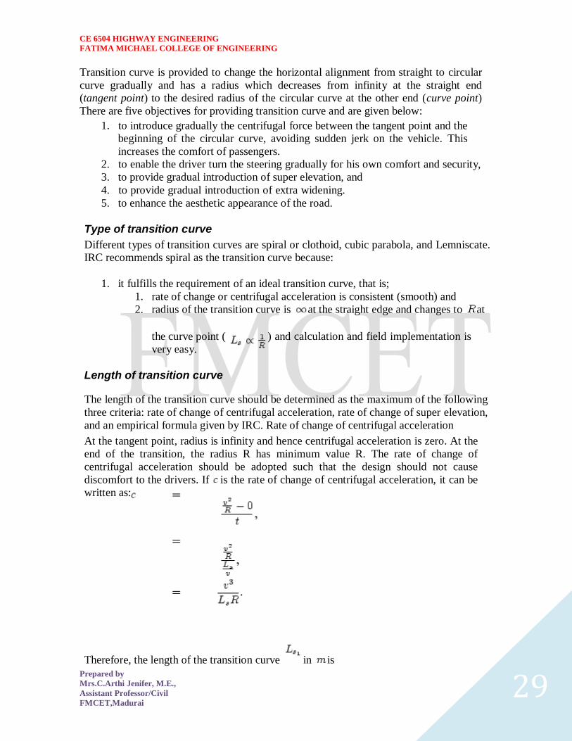
CE 6504 HIGHWAY ENGINEERING
FATIMA MICHAEL COLLEGE OF ENGINEERING
Prepared by
MrsCArthi Jenifer ME
Assistant ProfessorCivil
FMCETMadurai 29
Transition curve is provided to change the horizontal alignment from straight to circular
curve gradually and has a radius which decreases from infinity at the straight end
(tangent point) to the desired radius of the circular curve at the other end (curve point)
There are five objectives for providing transition curve and are given below
1 to introduce gradually the centrifugal force between the tangent point and the
beginning of the circular curve avoiding sudden jerk on the vehicle This
increases the comfort of passengers
2 to enable the driver turn the steering gradually for his own comfort and security
3 to provide gradual introduction of super elevation and
4 to provide gradual introduction of extra widening
5 to enhance the aesthetic appearance of the road
Type of transition curve
Different types of transition curves are spiral or clothoid cubic parabola and Lemniscate
IRC recommends spiral as the transition curve because
1 it fulfills the requirement of an ideal transition curve that is
1 rate of change or centrifugal acceleration is consistent (smooth) and
2 radius of the transition curve is at the straight edge and changes to at
the curve point ( ) and calculation and field implementation is
very easy
Length of transition curve The length of the transition curve should be determined as the maximum of the following
three criteria rate of change of centrifugal acceleration rate of change of super elevation
and an empirical formula given by IRC Rate of change of centrifugal acceleration
At the tangent point radius is infinity and hence centrifugal acceleration is zero At the
end of the transition the radius R has minimum value R The rate of change of
centrifugal acceleration should be adopted such that the design should not cause
discomfort to the drivers If is the rate of change of centrifugal acceleration it can be
written as
Therefore the length of the transition curve in is
CE 6504 HIGHWAY ENGINEERING
FATIMA MICHAEL COLLEGE OF ENGINEERING
Prepared by
MrsCArthi Jenifer ME
Assistant ProfessorCivil
FMCETMadurai 30
(1)
where is the rate of change of centrifugal acceleration given by an empirical formula
suggested by by IRC as below
(2) 2 Rate of introduction of super-elevation
Raise ( ) of the outer edge with respect to inner edge is given by
The rate of change of this raise from to is achieved
gradually with a gradient of in over the length of the transition curve (typical range
of is 60-150) Therefore the length of the transition curve is
(3)
3 By empirical formula
IRC suggest the length of the transition curve is minimum for a plain and rolling terrain
(4)
and for steep and hilly terrain is
(5)
CE 6504 HIGHWAY ENGINEERING
FATIMA MICHAEL COLLEGE OF ENGINEERING
Prepared by
MrsCArthi Jenifer ME
Assistant ProfessorCivil
FMCETMadurai 31
and the shift as
(
6
) The length of the transition curve is the maximum of
equations 1 3 and 4or5 ie
(
7
Case (a)
For single lane roads
(
1
)
Therefore
(
2
)
Figure 1 Set-back for single lane roads (
CE 6504 HIGHWAY ENGINEERING
FATIMA MICHAEL COLLEGE OF ENGINEERING
Prepared by
MrsCArthi Jenifer ME
Assistant ProfessorCivil
FMCETMadurai 32
For multi lane roads if is the distance between centerline of the road and the centerline
of the inner lane then
(3)
(4)
Figure 2 Set-back for multi-lane roads ( )
Case (a)
For single lane roads
(1)
Therefore
(2)
Gradient
Gradient is the rate of rise or fall along the length of the road with respect to the
horizontal While aligning a highway the gradient is decided for designing the vertical
curve Before finalizing the gradients the construction cost vehicular operation cost and
the practical problems in the site also has to be considered Usually steep gradients are
avoided as far as possible because of the difficulty to climb and increase in the
CE 6504 HIGHWAY ENGINEERING
FATIMA MICHAEL COLLEGE OF ENGINEERING
Prepared by
MrsCArthi Jenifer ME
Assistant ProfessorCivil
FMCETMadurai 33
construction cost More about gradients are discussed below
Effect of gradient
The effect of long steep gradient on the vehicular speed is considerable This is
particularly important in roads where the proportion of heavy vehicles is significant Due
to restrictive sight distance at uphill gradients the speed of traffic is often controlled by
these heavy vehicles As a result not only the operating costs of the vehicles are
increased but also capacity of the roads will have to be reduced Further due to high
differential speed between heavy and light vehicles and between uphill and downhill
gradients accidents abound in gradients
Representation of gradient
The positive gradient or the ascending gradient is denoted as and the negative gradient as The deviation angle is when two grades meet the angle which
measures the change of direction and is given by the algebraic difference between the two
grades
steep gradient while 1 in 50 = 2 representation is illustrated in the figure 1
Example 1 in 30 = 333 is a
is a flatter gradient The gradient
CE 6504 HIGHWAY ENGINEERING
FATIMA MICHAEL COLLEGE OF ENGINEERING
Prepared by
MrsCArthi Jenifer ME
Assistant ProfessorCivil
FMCETMadurai 34
Figure 1 Representation of gradient
Types of gradient
Many studies have shown that gradient upto seven percent can have considerable effect
on the speeds of the passenger cars On the contrary the speeds of the heavy vehicles are
considerably reduced when long gradients as flat as two percent is adopted Although
flatter gradients are desirable it is evident that the cost of construction will also be very
high Therefore IRC has specified the desirable gradients for each terrain However it
may not be economically viable to adopt such gradients in certain locations steeper
gradients are permitted for short duration Different types of grades are discussed below
Ruling gradient
The ruling gradient or the design gradient is the maximum gradient with which the
designer attempts to design the vertical profile of the road This depends on the terrain
length of the grade speed pulling power of the vehicle and the presence of the horizontal
curve In flatter terrain it may be possible to provide flat gradients but in hilly terrain it
is not economical and sometimes not possible also The ruling gradient is adopted by the
designer by considering a particular speed as the design speed and for a design vehicle
with standard dimensions But our country has a heterogeneous traffic and hence it is not
possible to lay down precise standards for the country as a whole Hence IRC has
recommended some values for ruling gradient for different types of terrain
Limiting gradient
This gradient is adopted when the ruling gradient results in enormous increase in cost of
construction On rolling terrain and hilly terrain it may be frequently necessary to adopt
limiting gradient But the length of the limiting gradient stretches should be limited and
must be sandwiched by either straight roads or easier grades
Exceptional gradient
Exceptional gradient are very steeper gradients given at unavoidable situations They
should be limited for short stretches not exceeding about 100 metres at a stretch In
mountainous and steep terrain successive exceptional gradients must be separated by a
minimum 100 metre length gentler gradient At hairpin bends the gradient is restricted to
25
Critical length of the grade
The maximum length of the ascending gradient which a loaded truck can operate without
undue reduction in speed is called critical length of the grade A speed of 25 kmph is a
CE 6504 HIGHWAY ENGINEERING
FATIMA MICHAEL COLLEGE OF ENGINEERING
Prepared by
MrsCArthi Jenifer ME
Assistant ProfessorCivil
FMCETMadurai 35
reasonable value This value depends on the size power load grad-ability of the truck
initial speed final desirable minimum speed
Minimum gradient
This is important only at locations where surface drainage is important Camber will take
care of the lateral drainage But the longitudinal drainage along the side drains require
some slope for smooth flow of water Therefore minimum gradient is provided for
drainage purpose and it depends on the rain fall type of soil and other site conditions A
minimum of 1 in 500 may be sufficient for concrete drain and 1 in 200 for open soil
drains are found to give satisfactory performance Sight distance available from a point is the actual distance along the road surface which a driver
from a specified height above the carriage way has visibility of stationary or moving objects
Sight distance required by drivers applies to both geometric design of highways and for
traffic control The sight distance situations are considered in the design
i) Stopping or absolute minimum sight distance
ii) Safe overtaking or passing sight distance
iii) Safe sight distance for entering into uncontrolled intersections
Apart from the three situations mentioned above the following sight distance are considered by the
IRC in highway design
Intermediate sight distance
This is defined as twice the stopping sight distance when overtaking sight distance
cannot be provided intermediate sight distance is provided to give limited overtaking opportunities
to fast vehicles
Head light sight distance
This is the distance visible to a driver during night driving under the illumination of the
vehicle head lights
Stopping sight distance
The minimum sight distance available on a highway at any spot should be of sufficient
length to stop a vehicle traveling at design speed safely without collision with any other obstruction
The absolute minimum sight distance is therefore equal to the stopping sight distance
which is also sometimes called nonpassing sight distance The sight distance available on a road to a
driver at any instance depends on
i) Features of the road
ii) Height of the drivers eye above the road surface
iii) Height of the object above the road surface
The distance within which a motor vehicle can be stopped depends upon the factors listed below
a) Total reactions time of the driver
b) Speed of vehicle
c) Efficiency of breaks
d) Frictional resistance between the road and tyres
e) Gradient of the road
Total reaction time
) Reaction time of the driver is the time taken from the instant the object is visible to the
driver to the instant the brakes are effectively applied
) The total reaction time may be split up into two parts
CE 6504 HIGHWAY ENGINEERING
FATIMA MICHAEL COLLEGE OF ENGINEERING
Prepared by
MrsCArthi Jenifer ME
Assistant ProfessorCivil
FMCETMadurai 36
i) Perception time
ii) Brake reaction time
PIEV theory
According to this theory the total reaction time of the driver is split into four parts
i) Perception
ii) Intellection
iii) Emotion
iv) Volition
Speed of Vehicle
The stopping distance depends very much on the speed of the vehicle first during the
total reaction time of the driver the distance moved by the vehicle will depend on the speed
Efficiency of brakes
The braking efficiency is said to be 100 percent if the wheels are fully licked preventing
them from rotating on application of the brakes This will result in 100 percent skidding which is
normally undesirable except in utmost emergency
Frictional resistance between road and tyres
The frictional resistance developed between road and tyres or the skid resistance depends
on the type and condition of the road surface and the tyres IRC has specified a design friction
coefficient of 035 to 04 depending upon the speed to be used for finding the braking distance in the
calculation of stopping sight distance
Analysis of stopping distance
i) The distance traveled by the vehicle during the total reaction time known as lag
distance
ii) The distance traveled by the vehicle after the application of the brakes is known as
braking distance
Overtaking sight distance
The minimum distance open to the vision of the driver of a vehicle intending to overtake
slow vehicle ahead with safety against the traffic of opposite direction is known as the minimum
overtaking sight distance(OSD) or Safe passing sight distance available
The overtaking sight distance is the distance measured along the center of the road which
a driver with his eye level 12m above the road surface can see the top of an object 12m above the
road surface
Some of the important factors on which the minimum overtaking sight distance required
a) Speed of
i) overtaking vehicle
ii) overtaken vehicle
iii) The vehicle coming from opposite direction
b) Distance between the overtaking and overtaken vehicles the minimum spacing
depends on the steeds
a) Skill and reaction time of the driver
b) Rate of acceleration of overtaking vehicle
c) Gradient of the road
Criteria for sight distance requirements on highway
) The absolute minimum sight distance required throughout the length of the road is the
SSD which should invariably be provided at all places
CE 6504 HIGHWAY ENGINEERING
FATIMA MICHAEL COLLEGE OF ENGINEERING
Prepared by
MrsCArthi Jenifer ME
Assistant ProfessorCivil
FMCETMadurai 37
) On horizontal curves the obstruction on the inner side of the curves should be cleared
to provide the required set back distance and absolute minimum sight distance
) On vertical summit curves the sight distance requirement may be fulfilled by proper
design of the vertical alignment
Hairpin bent
TYPES OF CURVES ON HILL ROADS
The following are the important types of curves provided on hill Roads-
1 Hair-Pin Curves
2 Salient Curves
3 Re-entrant Curves 1 Hair-pin curves - The curve in a hill road which changes its direction through an angle of 180
degree or so down the hill on the same side is known as hair-pin curve
A Hair-Pin Bend
This curve is so called because it conforms to the shape of a hair-pin The bend so formed at the
hair-pin curve in a hill road is known as hair-pin bend This type of curve should be located on a
hill side having the minimum slope and maximum stability It must also be safe from view point of
landslides and ground water Hair-pin bends with long arms and farther spacing are always
preferred They reduce construction problems and expensive protective works Hair-pin curves or
bends of serpentine nature are difficult to negotiate and should therefore be avoided as far as
possible
Salient curves - The curves having their convexity on the outer edges of a hill road are called
salient curves The centre of curvature of a salient curve lies towards the hill side This type of curve
occurs in the road length constructed on the ridge of a hill the bend so formed at the salient curve in
a hill road known as corner bend
Salient curves are very dangerous for fast moving traffic At such a curve or at corner bend the
portion of projecting hill side is usually cut down to improve the visibility as shown in fig (Re-
entrant curve) The outer edge of the road at such a curve is essentially provided with a parapet wall
for protection of the vehicles from falling down the hill slope
CE 6504 HIGHWAY ENGINEERING
FATIMA MICHAEL COLLEGE OF ENGINEERING
Prepared by
MrsCArthi Jenifer ME
Assistant ProfessorCivil
FMCETMadurai 38
3 Re-entrant curves - The curves having their convexity on the inner edge of a hill road are called
re-entrant curves
Re-entrant curves
The centre of curvature of a re-entrant curves lies away from the hill side This type of curve occurs
in the road length constructed in the calley of a hill
These curves are less dangereous as they provide adequate visibility to the fast moving traffic At
such curves the parapet wall is provided only for safety of fast moving traffic
CE 6504 HIGHWAY ENGINEERING
FATIMA MICHAEL COLLEGE OF ENGINEERING
Prepared by
MrsCArthi Jenifer ME
Assistant ProfessorCivil
FMCETMadurai 39
UNIT ndash III DESIGN OF RIGID AND FLEXIBLE PAVEMENTS
COMPARISON OF RIGID AND FLEXIBLE PAVEMENTS
The comparisons are
i) Design precision
A cement concrete pavement is amerable to a much more precise structural analysis
than a flexible pavement Flexible pavements designs are mainly empirical Computer aided analysis
of layered system is making the flexible pavement design more exact than hitherto
ii) Life
) Cement concrete slabs of a thin section constructed in the early 1940rsquos are still in
existence in India though many of them have cracked badly and a few of them have been ripped
open and rebuilt in recent ties
) A major project in cement concrete road construction between Agra and Mathura It can
safely be said that a well-designed concrete slab has a life of about 40 years
) Compared to this the life of a flexible pavement generally varies from 10 to 20 years
iii) Maintenance
) A well-designed cement concrete pavement needs very little maintenance The only
maintenance needed is I respect of joints
) The surface is unaffected by spillage of oil and lubricants bituminous surfaces on the
other hand need great inputs in maintenance
) The surface is affected by spillage of oil and lubricants The surface is also affected by
natural weathering agents like air water ad temperature changes
) A cement concrete pavement on the other hand needs a small amount for maintaining
joints
iv) Initial cost
) The argument so far used against a cement concrete slab is that it is much more costly
than a flexible pavement
) The latter specifications no doubt represent the rock-bottom needs of a road in India but
these specifications can hardly provide a smooth and durable surface
v) Stage construction ) Road construction is generally done adopting a policy of stage construction especially for
low volume roads As traffic grows additional layers in the form of water bound macadam and
superior surfacing are added on
) Initial outlay is minimum and additional outlays are in keeping with traffic growth This is
a great advantage when dealing with new roads in an atmosphere of austerity
vi) Availability of materials
) Cement bitumen stone aggregates and gravelsand are the major materials involved in
pavement Construction Cement has been in serious short supply in the country for the past many
decades
) Bitumen is also not available plentifully in India There is also the danger of the entire oil
reserves in the world shrinking during the next two or three decades
) In locations where stone aggregates are scarce cement concrete may have an advantage
for flexible pavements
vii) Surface characterstics
CE 6504 HIGHWAY ENGINEERING
FATIMA MICHAEL COLLEGE OF ENGINEERING
Prepared by
MrsCArthi Jenifer ME
Assistant ProfessorCivil
FMCETMadurai 40
) A good cement concrete surface is smooth and free from rutting potholes and
corrugations In a bituminous surface it is only the asphaltic concrete surface that can give
comparable rideablity
) A well-constructed cement concrete pavement surface can have a permanent nonskid
surface A bituminous surface can also be designed to have a good skid resistant surface
viii) Utility location
) In cement concrete slabs proper thought has to be given to locate utilities such as water
pipes telephone lines and electric cables
) It is difficult to rip open the slab and restore it to be the original condition if any changes
in the utilities lines are to be made
ix) Glame and night visibility
) Concrete pavements have a gray color which can cause glam under sunlight Colored
cement can reduce the grave
) On the other hand bituminous roads need more street lighting
x) Traffic dislocation during construction
) A cement concrete pavement requires 28 days before it can be thrown open to traffic On
the other hand a bituminous surface can be thrown open to traffic shortly after it is rolled
xi) Environmental considerations during construction
) The process of heating of bitumen and aggregates and mixing them together on hot mix
plants can prove to be much more hazardous to the environment than cement concrete construction
where no heating of any material is involved
xii) Overall economy on a life cycle basis
) A good road is costly to construct but once constructed such a road requires little
maintenance and results in savings in vehicle operating costs
) The comparative economy of a flexible pavement and a rigid pavement has proved that on
overall economic considerations
Types of pavement structure
Based on the structural behavior pavements are generally classified into three
categories
i) Flexible pavements
ii) Rigid pavements
iii) Semi rigid pavements
Flexible pavements
) Flexible pavements are those which on the whole have low or negligible flexural
strength and are rather flexible in their structural action under the loadsThe flexible pavement
layers reflect the deformation of the lower layers on to the surface of the layer
) A flexible pavement consists of four components(i) Soil subgrade (ii) sub base
course (iii) base course (iv) Surface course
CE 6504 HIGHWAY ENGINEERING
FATIMA MICHAEL COLLEGE OF ENGINEERING
Prepared by
MrsCArthi Jenifer ME
Assistant ProfessorCivil
FMCETMadurai 41
) The flexible pavement layers transmit the vertical or compressive stresses to the lower layers
by grain to grain transfer through the points of contact in the granular structure A well
compacted granular structure consisting of strong added aggregate can transfer the compressive
stresses
) The load spreading ability of this layer therefore depends on the type of the materials and mix
design factors Bituminous concrete is one of the best flexible pavements layer materials Other
materials which fall under the group are all granular materials with or without bituminous
binder granular base and sub base course materials
) The vertical compressive stress is maximum on the pavement surface directly under the wheel
and is equal to the contact pressure under the wheel The flexible pavement may be constructed
in a number of layers and the top layer has to be strongest as the highest compressive stresses
) Flexible pavements are commonly designed using empirical design charts or equations taking
into account some of the design factors there are also semi empirical and theoretical design
methods
Rigid pavements
) Rigid pavements are those which possess note flexural strength or flexural rigidity
The stresses are not transferred from grain to grain to the lower layers as in the ease of flexible
pavements layers
) The rigid pavements are made of Portland cement concrete plain reinforced or
prestressed concrete The plain cement concrete slabs are expected to take up about 40 kgcm2
flexural stress
) The rigid pavement has the slab action and is capable of transmitting the wheel
load stresses through a wider area below The main point of difference in the structural behavior
of rigid pavement as compared to the flexible pavement is that the critical condition of stress in
the rigid pavement is the maximum flexural stress occurring in the slab due to wheel load and
the temperature changes whereas in the flexible pavement
) As the rigid pavement slab has tensile strength tensile stresses are developed due
to the bending of the slab under wheel load and temperature variations Thus the types of
stresses developed and their distribution within the cement concrete slab are quirt different
) The cement concrete pavement slab can very well serve as a wearing surface as
well an effective base course The rigid pavement structure consists of a cement concrete slab
below which a granular base or sub base course may be provided
) Though the cement concrete slab can also be laid directly over the soil subgrade
consists of fine grained soil
) the rigid pavements are usually designed and the stresses are analyzed using the
elastic theory assuming the pavements as a n elastic plate resting over an elastic or a viscous
foundation
Semi rigid pavements
) when bonded materials like the pozzolanic concrete lean cement concrete or soil
cement are used in the base course or sub base course layer the pavement layer has considerably
higher flexural strength than the common flexible pavement layers
) when this intermediate class of materials are used in the base or sub base course
layer of the pavements they are called semi rigid pavements
CE 6504 HIGHWAY ENGINEERING
FATIMA MICHAEL COLLEGE OF ENGINEERING
Prepared by
MrsCArthi Jenifer ME
Assistant ProfessorCivil
FMCETMadurai 42
) This third category of semi rigid pavement are either designed as flexible
pavements with some correction factors to find the thickness requirements based on experience
or by using a new design approach
) The semi rigid pavement materials have low resistance to impact and abrasion and
therefore are usually provided with flexible pavement surface course
Various functions of pavement components
The functions are
Soil sub grade and its evaluation
) The soil sub grade is a layer of natural soil prepared to receive the layers of pavement
materials placed over it It is essential that at no time the soil sub grade is overstressed it means that
the pressure transmitted on the top of the sub grade is within the allowable limit
) Many tests are known for measuring the strength properties of the sub grades Some of the
tests have been standardized for the use The common strength test for the evaluation of soil
subgrade is
i) California bearing ratio test
ii) California resistance value test
iii) Triaxial compression test
iv) Plate bearing test
CALIFORNIA BEARING RATIO (CBR) TEST
It is evolved for the empirical method of flexible pavement design The CBR test is carried
out either in the laboratory on prepared specimens or in the field by taking in situ measurements
California resistance value
It is found by using have been stabliometerThis test is used in an empirical method of
flexible pavement design based on soil strength
Triaxial test
It is the most important soil strength but still the test is not very commonly used in structural
design of pavements
Plate bearing test
It is carried out using a relatively large diameter plate to evaluate the load supporting
capacity of supporting power of the pavement layers The results are plate bearing tests are used in
flexible pavement design method like McLeod method on based on layer system analysis by
brumister
Sub base and base courses and their evaluation
) There layers are made of broken stones bound or unbound aggreagatesome times in sub
base course a layer of stabilized soil(or) Selected granular soil is also used
) however at the sub base course it is desirable to use smaller size graded aggregates When
the sub grade consists of fine grained soil and when the pavement carries heavy wheel loads
CE 6504 HIGHWAY ENGINEERING
FATIMA MICHAEL COLLEGE OF ENGINEERING
Prepared by
MrsCArthi Jenifer ME
Assistant ProfessorCivil
FMCETMadurai 43
) Sub base course primarily has the similar function as of the base course and is provided
with inferior materials than of base course Base courses are used under rigid pavement for
i) Preventing pumping
ii) Protecting the sub grade against frost action
) Thus the fundamental purpose of abase course and sub base course is to provide a stress
transmitting medium to spread the surface wheel loads in such manner
) The sub base and base course layers may be evaluated by suitable strength or stability test
like plate bearing CBR test
WEARING COURSE AND ITS EVALUATION
) The purpose of the wearing course is to give a smooth riding surface that is dense It
resists pressure exerted by tyres and takes up wear and tear due to the traffic
) Wearing course also offers a water tight layer against the surface water infiltration The
flexible pavement normally a bituminous surfacing is used as a wearing course
) In rigid pavements the cement concrete acts like a base course as well as wearing course
Most popular test in use is marshal stability test where in the optimum content of bitumen binder is
worked out based on the stability density
) Plate bearing test and Bankelman beam test are also sometimes made use of for evaluating
the wearing course and the pavement as a whole
Various factors to be considered in pavement design and the significance
Pavement design consists of two parts
i) Mix design of materials to be used in each pavement component layer Thickness design of the
pavement and the component layers
The various factors to be considered for the design of pavements are given below
i) Design wheel load
ii) Sub grade soil
iii) Climatic factors
iv) Pavement component layers
v) Environmental factors
vi) Special factors in the design of different types of pavements
Design wheel load
The various wheel load factors to be considered in pavement design are
i) Maximum wheel load
ii) Contact pressure
iii) Dual or multiple wheel loads
iv) Repetition of loads
Maximum wheel load
The wheel load configurations are important to know the way in which the loads of a given
vehicle are applied on the pavement surface
) For highways the maximum legal axle load as specified by Indian road congress is 8170
kg with a maximum equivalent single wheel load of 4085 kg
) The evaluation for vertical stress computations under a uniformly distribute of circular
load based on Boussineqrsquos theory is given by
CE 6504 HIGHWAY ENGINEERING
FATIMA MICHAEL COLLEGE OF ENGINEERING
Prepared by
MrsCArthi Jenifer ME
Assistant ProfessorCivil
FMCETMadurai 44
2
322
3
1
za
zpz
σz = vertical stress at depth z
P= surface pressure
Z=depth at which σz computed
A=radius of loaded area
Contact pressure
Generally the wheel load is assumed to be distributed over a circular area But by
measurement of the imprints of tyers with different load and inflation pressures Three terms in use
with reference to tyre pressure are
Tyre pressure
Inflation pressure
Contact pressure
Tyre pressure and inflation pressure mean exactly the same the contact pressure is found to be more
than tyre pressure when the tyre pressure is less than 7 kgm2 and it is vice versa when the tyre
pressure exceeds this value
Contact pressure can be measured by the relationship
Load on wheel
Contact pressure = ----------------------------------------
Contact area or area of imprint
The general variation between the tyre pressure and measured contact pressure is shown in this fig
The ratio of contact pressure to type pressure is defined as rigidity factor Thus value of rigidity
factor is 10 for an average tyre pressure of 7 Kgcm2This value is higher than unity for lower type
pressures and less than unity for tyre pressures higher than 7 kgcm2
Equivalent single wheel load (ESWL)
) The maximum wheel load within the specified limit and to carry greater load it is
necessary to provide dual wheel assembly to the rear axles of the roads vehicles
) In other words the pressure at a certain depth below the pavement surface cannot be
obtained by numerically adding the pressure caused by any one wheel
) The effect is in between the single load and two times load carried by one wheel The load
dispersion is assumed to be at an angle of 450In the dual wheel load assembly let d be the clear gap
between the two wheels S be the spacing between the centers of the wheels and a be the radius of
the circular contact area of each wheel Then S = (d + 2a)
) ESWL may be determined based on either equivalent deflection or equivalent stress
criterianMultiple wheel loads are convert to ESWL and this value is used in pavement design The
ESWL is usually determined by the equivalent stress criterion using a simple graphical method
CE 6504 HIGHWAY ENGINEERING
FATIMA MICHAEL COLLEGE OF ENGINEERING
Prepared by
MrsCArthi Jenifer ME
Assistant ProfessorCivil
FMCETMadurai 45
) A straight line relationship is assumed between ESWL and depth on log scales For
determining ESWL the plot is made as shown in fig
) Two points A and B are plotted on the log-log graph with coordinates of A (Pd2) and
B(2p2s)line AB is a plot which is the focus of points where any single wheel load is equivalent to a
certain set of dual wheels
) To Calculate the ESWL for a dual assembly it is essential to estimate a design thickness of
the pavement If the design thickness so obtained is equal to the estimated thickness then the ESWL
calculations could be considered as correct Otherwise trials are made
) In heavy trucks and trailers the load on each wheel may be further reduced by multiple
wheels and tandem axles
Repetition of loads
) The deformation of load pavement (or) sub grade due to a single application of wheel load
may be small It required carrying out traffic surveys for accounting the factor of repetitions for
wheel loads in the design of pavement
) Data collected are converted to some constant equivalent wheel loads Equivalent wheel
load is a single load equivalent to the repeated applications of any particular wheel load on a
pavement which requires the same thickness and strength of pavements
) McLeod has given a procedure for evolving equivalent load factors for designing flexible
pavements
Various methods of flexible pavement design
) The flexible pavement is built with number of layers In the design process it is to be
ensured that under the application of load none of the layers is overstressed
) The maximum intensity of stresses occurs in the top layer of the pavement The
magnitude of load stresses reduces at lower layers
) In the design of flexible pavements it has yet not been possible to have a rational design
method wherein design process and service behavior of the pavement can be expressed by
mathematical laws
) Flexible pavement design methods are accordingly either empirical or semi empirical In
these methods the knowledge and experience gained on the behavior of the pavements in the past
are usefully utilized
Various approaches of flexible pavement design may be thus classified into three groups
i) Empirical method
ii) Semi-empirical or Semi theoretical method
iii) Theoretical method
) Empirical methods are either based on physical properties or strength parameters of soil
sub grade When the design is based on stress strain function and modified base on experience it
may be called semi-empirical or semi-theoretical There are design methods based on theoretical
analysis and mathematical computations
Out of the flexible pavement design method available is
i) Group index method
ii) California bearing ratio method
iii) California R value (or) Stabiliometer method
iv) Triaxial test method
CE 6504 HIGHWAY ENGINEERING
FATIMA MICHAEL COLLEGE OF ENGINEERING
Prepared by
MrsCArthi Jenifer ME
Assistant ProfessorCivil
FMCETMadurai 46
v) McLeod method
vi) Burmister method
Group index method
) Group index value is an arbitrary index assigned to the soil type in numerical equations
base on the percent fines liquid limit and plasticity index
) The design chart for group index method for determining the pavement thickness is given
in fig
The traffic volume in this method is divided in three groups
Traffic volume No of vehicles per day
Light Less than 50
Medium 50 to 300
Heavy Over 300
The design of the pavement thickness by this method first the G1 value of the soil is found the
anticipated traffic is estimated and is designated as light medium or heavy as indicated
The G1 method of pavement design is essentially an empirical method based on physical properties
of the subgrade soil This method does not consider the strength characteristics of the subgrade soil
and therefore is open to question regarding the reliability of the design based on the index properties
of the soil only
California bearing ratio method
) California division of highways in the USA developed CBR method for
pavement design The majority of design curves developed later are base on the original curves
proposed by OJporter
) One of the chief advantages of CBR method is the simplicity of the test procedure
The CBR tests were carried out by the California state highway department on existing pavement
layers including subgrade sub base and base course
) Based on the extensive CBR test data collected on pavement which behaved
satisfactory and those which failed an empirical design chart was developed correlating the CBR
value and the pavement thickness The basis of the design chart is that a material with a given CBR
required a certain thickness of pavement layer as a cover
) A higher load needs a thicker pavement layer to protect the sub grade Design
curves correlating the CBR value with total pavement thickness cover were developed by the
California state highway department for wheel loads of 3175kg and 5443 kg representing light and
heavy traffic The design curves are shown in this fig
It is possible to extend the CBR design curves for various loading conditions nusing the expression
t= 2
1
1751
pCBRp
t=2
1
751
A
CBR
p
Hence
CE 6504 HIGHWAY ENGINEERING
FATIMA MICHAEL COLLEGE OF ENGINEERING
Prepared by
MrsCArthi Jenifer ME
Assistant ProfessorCivil
FMCETMadurai 47
t= pavement thickness cm
p=Wheel load kg
CBR= California bearing ratio percent
P=tyre pressure kgcm2
A= area of contactcm2
IRC Recommendations
a) The CBR tests should be performed on remoulded soils in the laboratory The specimens should
be prepared by static compaction wherever possible and otherwise by dynamic compaction
b) For the design of new roads the sub grade soil sample should be compacted at OMC to proctor
density whenever suitable compaction equipment
c) The CBR test samples may be soaked in water for four days period before testing the annual
rainfall is less than 50 cm and the water table is too deep to affect the sub grade and imperable
surfacing is provided to carrying out CBR test
d) If the maximum variations in CBR value of the three specimens exceed the specified limits the
design CBR should be average of at least six samples
e) The top 50 cm of sub grade should be compacted at least up to 95 to 100 percent of proctor
density
f) An estimate of the traffic should be carried by the road pavements at the end of expected in view
the existing traffic and probable growth rate of traffic
g) The traffic for the design is considered in units of heavy vehicles per day in both directions and is
divided into seven categories A to G The design thickness is considered applicable for single axle
loads up to 8200 kg and tandom axle loads up to 14500 kg
h) When sub base course materials contain substantial proportion of aggregates of size above 20mm
the CBR value of these materials would not be valid for the design of subsequent layers above them
The CBR method of pavement design gives the total thickness requirement of the pavement above a
sub grade and thickness value would remain the same quality of materials used in component layers
California resistance value method
) In this design method based on stabliometer R-value and cohesiometer C-value
Based on performance data it was established by pavement thickness varies directly with R value
and algorithm of load repetitions It varies inversely with fifth root of c valueThe expression for
pavement thickness is given by the empirical equation
T=
5
1
1 90
C
RTK
Hence
T=total thickness of pavement cm
K=Numerical constant 0166
T1=traffic index
R= stabiliometer resistance value
C=Cohesiometer value
CE 6504 HIGHWAY ENGINEERING
FATIMA MICHAEL COLLEGE OF ENGINEERING
Prepared by
MrsCArthi Jenifer ME
Assistant ProfessorCivil
FMCETMadurai 48
In the design of flexible pavements based on California resistance value method for the following
data are needed
) R-value of soil subgrade
) T1 value
) Equivalent C-value
) R value of soil subgrade is obtained from the test using stablio meterThe
computation of T1 value has been explained
Equivalent C-value
) The cohesion meter value c is obtained for each layer of pavement material
separately from tests However the composite or equivalent C-value of the pavement may be
estimated if the thickness of each component layer and the c-value of the material of the layer are
known
) while designing a pavement as the thickness of the pavement is not known it is
easier if the pavement is first assumed to consist of any one material like gravel base course with
known C-value
) Subsequently the individual thickness of each layer is converted in terms of gravel
equivalent by using relationship
5
1
1
2
2
1
C
C
t
t
) t1 and t2 are the thickness values of any two pavement layersc1 and c2 are their
corresponding cohesiometer values
CE 6504 HIGHWAY ENGINEERING
FATIMA MICHAEL COLLEGE OF ENGINEERING
Prepared by
MrsCArthi Jenifer ME
Assistant ProfessorCivil
FMCETMadurai 49
UNIT 4 MATERIAL AND MAINTENANCE
SUMMIT CURVE
Summit curves are vertical curves with gradient upwards They are formed when two
gradients meet as illustrated in figure 1 in any of the following four ways
1 When a positive gradient meets another positive gradient [figure 1a]
2 When positive gradient meets a flat gradient [figure 1b]
3 When an ascending gradient meets a descending gradient [figure 1c]
4 When a descending gradient meets another descending gradient [figure 1d]
Type of Summit Curve
Many curve forms can be used with satisfactory results the common practice has been to
use parabolic curves in summit curves This is primarily because of the ease with it can
be laid out as well as allowing a comfortable transition from one gradient to another
Although a circular curve offers equal sight distance at every point on the curve for very
small deviation angles a circular curve and parabolic curves are almost congruent
Furthermore the use of parabolic curves were found to give excellent riding comfort
Figure 1 Types of summit curves
Design Consideration
In determining the type and length of the vertical curve the design considerations are
comfort and security of the driver and the appearance of the profile alignment Among
these sight distance requirements for the safety are most important on summit curves
The stopping sight distance or absolute minimum sight distance should be provided on
these curves and where overtaking is not prohibited overtaking sight distance or
intermediate sight distance should be provided as far as possible When a fast moving
vehicle travels along a summit curve there is less discomfort to the passengers This is
because the centrifugal force will be acting upwards while the vehicle negotiates a
summit curve which is against the gravity and hence a part of the tyre pressure is
relieved Also if the curve is provided with adequate sight distance the length would be
sufficient to ease the shock due to change in gradient Circular summit curves are
identical since the radius remains same throughout and hence the sight distance From
CE 6504 HIGHWAY ENGINEERING
FATIMA MICHAEL COLLEGE OF ENGINEERING
Prepared by
MrsCArthi Jenifer ME
Assistant ProfessorCivil
FMCETMadurai 50
this point of view transition curves are not desirable since it has varying radius and so the
sight distance will also vary The deviation angles provided on summit curves for
highways are very large and so the simple parabola is almost congruent to a circular arc
between the same tangent points Parabolic curves are easy for computation and also it
had been found out that it provides good riding comfort to the drivers It is also easy for
field implementation Due to all these reasons a simple parabolic curve is preferred as
summit curve Length of the summit curve
The important design aspect of the summit curve is the determination of the length of the
curve which is parabolic As noted earlier the length of the curve is guided by the sight
distance consideration That is a driver should be able to stop his vehicle safely if there is
an obstruction on the other side of the road Equation of the parabola is given by
where where N is the deviation angle and is the length of the In
deriving the length of the curve two situations can arise depending on the uphill and
downhill gradients when the length of the curve is greater than the sight distance and the
length of the curve is greater than the sight distance
Let is the length of the summit curve is the SSDISDOSD is the deviation angle
drivers eye height (12 m) and the height of the obstruction then the length of the
summit curve can be derived for the following two cases The length of the summit curve
can be derived from the simple geometry as shown below
Case a Length of summit curve greater than sight distance( )
Figure 1 Length of summit curve ( )
The situation when the sight distance is less than the length of the curve is shown in
figure 1
CE 6504 HIGHWAY ENGINEERING
FATIMA MICHAEL COLLEGE OF ENGINEERING
Prepared by
MrsCArthi Jenifer ME
Assistant ProfessorCivil
FMCETMadurai 51
(1)
Case b Length of summit curve less than sight distance
The second case is illustrated in figure 1
Figure 1 Length of summit curve
CE 6504 HIGHWAY ENGINEERING
FATIMA MICHAEL COLLEGE OF ENGINEERING
Prepared by
MrsCArthi Jenifer ME
Assistant ProfessorCivil
FMCETMadurai 52
From the basic geometry one can write
(1)
Therefore for a given and to get minimum differentiate the above equation
with respect to and equate it to zero Therefore
Solving the quadratic equation for
(2)
Now we can substitute back to get the value of minimum value of for a given
and Therefore
Solving for
CE 6504 HIGHWAY ENGINEERING
FATIMA MICHAEL COLLEGE OF ENGINEERING
Prepared by
MrsCArthi Jenifer ME
Assistant ProfessorCivil
FMCETMadurai 53
(3) (4
CE 6504 HIGHWAY ENGINEERING
FATIMA MICHAEL COLLEGE OF ENGINEERING
Prepared by
MrsCArthi Jenifer ME
Assistant ProfessorCivil
FMCETMadurai 54
When stopping sight distance is considered the height of drivers eye above the road
surface ( ) is taken as 12 metres and height of object above the pavement surface ( )
is taken as 015 metres If overtaking sight distance is considered then the value of
drivers eye height ( ) and the height of the obstruction ( ) are taken equal as 12
metres
Valley curve
Valley curve or sag curves are vertical curves with convexity downwards They are
formed when two gradients meet as illustrated in figure 1 in any of the following four
ways
Figure 1 Types of valley curve
1 When a descending gradient meets another descending gradient [figure 1a]
2 When a descending gradient meets a flat gradient [figure 1b]
3 When a descending gradient meets an ascending gradient [figure 1c]
4 When an ascending gradient meets another ascending gradient [figure
Design considerations
There is no restriction to sight distance at valley curves during day time But visibility is
reduced during night In the absence or inadequacy of street light the only source for
visibility is with the help of headlights Hence valley curves are designed taking into
account of headlight distance In valley curves the centrifugal force will be acting
downwards along with the weight of the vehicle and hence impact to the vehicle will be
more This will result in jerking of the vehicle and cause discomfort to the passengers
Thus the most important design factors considered in valley curves are (1) impact-free
movement of vehicles at design speed and (2) availability of stopping sight distance
under headlight of vehicles for night driving
For gradually introducing and increasing the centrifugal force acting downwards the best
shape that could be given for a valley curve is a transition curve Cubic parabola is
generally preferred in vertical valley curves See figure 1
CE 6504 HIGHWAY ENGINEERING
FATIMA MICHAEL COLLEGE OF ENGINEERING
Prepared by
MrsCArthi Jenifer ME
Assistant ProfessorCivil
FMCETMadurai 55
Figure 1 Valley curve details
During night under headlight driving condition sight distance reduces and availability of
stopping sight distance under head light is very important The head light sight distance
should be at least equal to the stopping sight distance There is no problem of overtaking
sight distance at night since the other vehicles with headlights could be seen from a
considerable distance
Length of the valley curve
The valley curve is made fully transitional by providing two similar transition curves of
equal length The transitional curve is set out by a cubic parabola where
The length of the valley transition curve is designed based on two criteria
1 comfort criteria that is allowable rate of change of centrifugal acceleration is
limited to a comfortable level of about
2 safety criteria that is the driver should have adequate headlight sight distance at
any part of the country
Comfort criteria
The length of the valley curve based on the rate of change of centrifugal acceleration that
will ensure comfort Let is the rate of change of acceleration the minimum radius of
the curve is the design speed and is the time then is give
CE 6504 HIGHWAY ENGINEERING
FATIMA MICHAEL COLLEGE OF ENGINEERING
Prepared by
MrsCArthi Jenifer ME
Assistant ProfessorCivil
FMCETMadurai 56
For a cubic parabola the Value Safety criter Length of the valley curve for headlight distance may be determined for two conditions
(1) length of the valley curve greater than stopping sight distance and (2) length of the
valley curve less than the stopping sight distance of for length is given by
Case 1 Length of valley curve greater than stopping sight distance ( )
The total length of valley curve is greater than the stopping sight distance SSD The
sight distance available will be minimum when the vehicle is in the lowest point in the
valley This is because the beginning of the curve will have infinite radius and the bottom
of the curve will have minimum radius which is a property of the transition curve The
case is shown in figure 1
Figure 1 Valley curve case 1
From the geometry of the figure we have
CE 6504 HIGHWAY ENGINEERING
FATIMA MICHAEL COLLEGE OF ENGINEERING
Prepared by
MrsCArthi Jenifer ME
Assistant ProfessorCivil
FMCETMadurai 57
(1)
where is the deviation angle in radians is the height of headlight beam is the
head beam inclination in degrees and is the sight distance The inclination is 1
degree
Case 2 Length of valley curve less than stopping sight distance ( )
The length of the curve is less than SSD In this case the minimum sight distance is
from the beginning of the curve The important points are the beginning of the curve and
the bottom most part of the curve If the vehicle is at the bottom of the curve then its
headlight beam will reach far beyond the endpoint of the curve whereas if the vehicle is
at the beginning of the curve then the headlight beam will hit just outside the curve
Therefore the length of the curve is derived by assuming the vehicle at the beginning of
the curve The case is shown in figure 1
From the figure
(1) Note that the above expression is approximate and is satisfactory because in practice the gradients
are very small and is acceptable for all practical purposes We will not be able to know prior to
which case to be adopted Therefore both has to be calculated and the one which satisfies the
condition is adopted
1 Flexible pavement
2 Rigid pavement
Flexible pavement
These pavements reflect the deformation of sub grade and the subsequent layers to the
surface
Rigid pavement
The rigid characteristic of the pavement are associated with rigidity or flexural strength
CE 6504 HIGHWAY ENGINEERING
FATIMA MICHAEL COLLEGE OF ENGINEERING
Prepared by
MrsCArthi Jenifer ME
Assistant ProfessorCivil
FMCETMadurai 58
or slab action so the load is distributed over a wide area of sub grade soil
Flexible pavement Definition
These pavements reflect the deformation of sub grade and the subsequent layers to the
surface Flexible usually asphalt is laid with no reinforcement or with a specialized
fabric reinforcement that permits limited flow or repositioning of the roadbed under
ground changes
The design of flexible pavement is based on load distributing characteristic of the
component layers The black top pavement including water amp gravel bound macadam fall
in this category
Flexible pavement on the whole has low or negligible flexible strength flexible in their
structural action) The flexible pavement layers transmit the vertical or compressive
stresses to the lower layers by grain transfer through contact points of granular structure
The vertical compressive stress is maximum on the pavement surface directly under the
wheel load and is equal to contact pressure under the wheels Due to the ability to
distribute the stress to large area in the shape of truncated cone the stresses get decreased
in the lower layer
As such the flexible pavement may be constructed in a number of layers and the top
layer has to be strongest as the highest compressive stresses
To be sustained by this layer in addition to wear and tear the lower layer have to take
up only lesser magnitude of stress as there is no direct wearing action die to traffic loads
therefore inferior material with lower cast can be used in the lower layers
Rigid pavement Definition
The rigid characteristic of the pavement are associated with rigidity or flexural strength
or slab action so the load is distributed over a wide area of sub grade soil Rigid pavement
is laid in slabs with steel reinforcement
The rigid pavements are made of cement concrete either plan reinforced or prestressed
concrete
Critical condition of stress in the rigid pavement is the maximum flexural stress occurring in the slab due to wheel load and the temperature changes
Rigid pavement is designed and analyzed by using the elastic theory
CE 6504 HIGHWAY ENGINEERING
FATIMA MICHAEL COLLEGE OF ENGINEERING
Prepared by
MrsCArthi Jenifer ME
Assistant ProfessorCivil
FMCETMadurai 59
UNIT-5 EVALUATION AND MAINTENANCE OF PAVEMENTS
TRAFFIC PARAMETERS
Design life
Design life is the number of years (or number of standard axle repetitions) for which the
pavement is being designed A pavement is expected to serve satisfactorily within the
design life For concrete pavements 20 to 40 years may be assumed as the design life
(PCA 1984 IRC58 2002)
Basic design principle
Though different approaches for concrete pavement design are suggested in various
guidelines the design principles tend to remain similar across different guidelines for
example PCA (1994) Austroads (2004) NCHRP (2004) IRC58 (2002) etc except the
AASHTO (1993) provisions which is based on empirical approach The basic steps
involved in the design of concrete pavement method can be summarized as follows
The developed stresses due to load for a trial thickness of the concrete slab are
calculated for various loading configuration and the critical one is chosen The
axle loads are generally divided into different axle load groups and the load
stresses are calculated individually
The ratio between the load stress and Modulus of Rupture (MOR) is known as
stress ratio The stress ratio determines how many repetitions the pavement can
sustain (ie allowable traffic repetitions) for the individual axle load group If the
stress ratio is 055 or lower it can withstand virtually infinite number of traffic
repetitions (PCA 1984)
The ratio between the allowable repetitions to the expected traffic repetitions is
the damage fraction The calculation process is repeated for various axle loads
(sometimes for various seasons or various timings of the day) and the sum of
individual damage fractions (c u m u l a t i v e fatigue damage) should be less
than equal to one for pavement design being safe If found unsafe the trial
thickness is changed and the design process is repeated
The design process may also include considerations for temperature stress
moisture stresses and erosion distress
A brief discussion on concrete pavement design approaches suggested by various design
practices viz PCA method (1984) Austroads method (2004) AASHTO method (1993)
NCHRP mechanistic-empirical method (2004) and the Indian Roads Congress (IRC)
method (2002) are placed in the following
Portland cement Association (PCA) Method
The PCA method is based on Westergaard Picket and Rays work and further theoretical
analysis by Finite Element Method (Huang 1993) The data used to develop the PCA
method is generated from various road tests like ASSHO road test Arlington test
(conducted by PCA) Bates test road and Maryland road test (PCA 1984) The PCA
design method is based on the following two considerations (PCA 1984)
The fatigue damage on the concrete slab due to repetitive application of traffic
load is estimated The cumulative fatigue damage principle is used to estimate the
design thickness of the slab Edge stress between the mid-ways of the
CE 6504 HIGHWAY ENGINEERING
FATIMA MICHAEL COLLEGE OF ENGINEERING
Prepared by
MrsCArthi Jenifer ME
Assistant ProfessorCivil
FMCETMadurai 60
transverse joint is taken as critical configuration
The stresses due to warping and curling (due to temperature and moisture
gradient) are not considered in the fatigue analysis as per PCA recommendation
because most of the time the stresses generated are subtractive to the load stress
The possibility of erosion of pavement materials placed below the concrete slab is
evaluated The rate at which the slab is deflected due to axle load is used as a
criterion for erosion Theoretically it can be shown that a thin pavement with
smaller deflection basin is subjected to faster rate of deflection compared to
thicker slab Hence thin slab is more susceptible to erosion In a similar way the
cumulative erosion damage is calculated for individual axle load groups If this
value is greater than one then the design needs to be revised
Austroads method
Austroads method has been adopted from PCA (1984) approach with modifications
suited to Australian conditions (Austroads 2004) A bound mix or lean cement concrete is
used as sub-base material For a given CBR value of the subgrade and given thickness of
cemented sub-base the effective subgrade strength can be obtained from the chart
provided Figure-19 schematically shows such a chart For different levels of traffic
Austroads (2004) suggests minimum values of the base thicknesses to be provided
CE 6504 HIGHWAY ENGINEERING
FATIMA MICHAEL COLLEGE OF ENGINEERING
Prepared by
MrsCArthi Jenifer ME
Assistant ProfessorCivil
FMCETMadurai 61
figure-19 Schematic diagram of Austroads (2004) chart for estimation of effective
subgrade strength
As per Astroads (2004) the concrete pavement slab thickness for a given expected
traffic repetitions is designed considering the (i) flexural fatigue of the concrete slab and
the (ii) subgrade erosion arising out of repeated deflections For both the considerations
equations are suggested to calculate the allowable traffic repetitions If the allowable
traffic is less than the expected traffic the design is revised by increasing the slab
thickness The concrete shoulders adopted are of integral type or structural type
AASHTO method
The AASHTO method (1993) for design of concrete pavement has evolved from the
AASHO road test (AASHO 1962) The AASHTO pavement design follows an empirical
approach Pavement performance in terms of present serviceability index ( PSI ) loss of
serviceability sub-grade and sub-base strength cumulative traffic properties of concrete
joint load transfer efficiency drainage condition overall standard deviation and
reliability are the input parameters considered in the pavement design
The PSI value of the fresh pavement is assumed as 45 and the pavement is deemed to
have failed when the PSI value reaches 25 The resilient moduli of the subgrade and sub-
base materials are determined in the laboratory simulating the seasonal moisture content
and stress situation Suggested values are also available for given moisture content
plasticity index etc The composite modulus of sub-grade reaction (k) is estimated from
modulus of sub-grade reaction and elastic modulus of sub-base for various seasons and
the depth of rigid foundation and the thickness of the sub-base
Design equation as well nomographs are available to estimate the slab thickness (D) from
these input parameters
NCHRP mechanistic-empirical (M-E) metho
The NCHRP (2004) has recently developed concrete pavement design procedure based
on mechanistic-empirical (M-E) approach This approach attempts to reduce the extent of
empiricism prevalent in the existing AASHTO (1993) guidelines This proposed NCHRP
pavement design system is modular in nature that is the design approach can be
modified by parts (as and when new knowledge is available) without disrupting the
overall design procedure This approach also can take care of various wheel-axle loa
configuration
As per this approach trial thickness of the slab is first assumed and the stress strain and
displacement values are obtained From these values the performance of the pavement in
terms of distresses (such as faulting cracking) and smoothness and predicted If these
predicted performance parameters does not satisfy the required performance for a given
reliability
The design approach includes a large data-base as input parameters for example average
daily traffic traffic growth rate traffic composition hourly weather data on air
temperature precipitation wind speed percentage sunshine relative humidity pavement
material engineering parameters ground water depth infiltration drainage hydraulic
conductivity thermal conductivity heat capacity etc The temperature stress is
considered in this method but the temperature profile is linearized to enhance
computational efficiency (NCHRP 2004)
CE 6504 HIGHWAY ENGINEERING
FATIMA MICHAEL COLLEGE OF ENGINEERING
Prepared by
MrsCArthi Jenifer ME
Assistant ProfessorCivil
FMCETMadurai 62
INDIAN ROADS CONGRESS (IRC) METHOD
The Indian Roads Congress (IRC) guidelines IRC58 (2002) has adopted the
Westergaards equation to estimate load stress and Brdaburys equation to estimate
temperature stress The load stress is highest at the corner of the slab lesser in edge and
least in the interior The order of variation of temperature stress is just the reverse of this
As per IRC58 (2002) it is recommended that the design needs to be done for edge stress
condition and subsequently check needs to be performed for corner stress condition so as
to finalize the design The following are the steps followed as per IRC58 (2002)
guideline for the design of concrete pavement
The input parameters are obtained to formulate the design problem The joint
spacing and the slab dimensions are decided If there is a bound sub-base layer
over the subgrade a suitable value of effective k is to be adopted
A trial thickness of the concrete slab is assumed
The edge stress is estimated for various axle loads from the given charts Figure-
20 schematically shows such a chart The cumulative fatigue damage principle for
fatigue is applied to check the adequacy of the slab thickness
The sum of edge stress due to load for the highest axle load group and the
temperature stress should be less than the MOR of concrete otherwise the design
is revised
The adequacy of corner stress is checked with respect to MOR value and
accordingly the design is finalized Westergaards corner stress formula
Figure-20 Schematic diagram of IRC58 chart for estimation of load stress at the edge
(IRC58 2002)
CE 6504 HIGHWAY ENGINEERING
FATIMA MICHAEL COLLEGE OF ENGINEERING
Prepared by
MrsCArthi Jenifer ME
Assistant ProfessorCivil
FMCETMadurai 63
estimation of corner stress due to load and the corner stress due to temperature is
assumed to be zero
Estimation of layer thicknesses
The thickness of the pavement is adjusted in such a way that the stress strain
developed is less than the allowable values obtained from past performance
information
The two major modes of structural failure of pavement are fatigue and rutting
o Fatigue Traffic applies repetitive load to the pavement surface and the
cracks start from bottom the bound layer slab and propagate upwards
When the extent of surface cracks reaches a predefined level the
pavement is said to have failed due to flexural fatigue
FUNCTIONAL DESIGN
The functional pavement design involves considerations of skid resistance roughness
surface distresses reflectivity of pavement surface etc The functional pavement design
considers mainly the surface features of a pavement
Drainage design
A road needs to be designed in such a way that the rain snow precipitation is drained off
the pavement and its surroundings A suitable surface drainage system for the pavement
is designed for this purpose Some water however will percolate into the pavement from
its top surface and needs to be taken out of the pavement - this is done by providing an
internal drainage system to the pavement Water will also try to enter into the pavement
from bottom due to capillary rise or due to rise in water table A suitably designed sub-
surface drainage system tries to avoid such a problem
PAVEMENT THICKNESS DESIGN CHARTS
For the design of pavements to carry traffic in the range of 1 to 10 msa use chart 1 and for
traffic in the range 10 to 150 msa use chart 2 of IRC37 2001 The design curves relate
pavement thickness to the cumulative number of standard axles to be carried over the
design life for different sub-grade CBR values ranging from 2 to 10 The design
charts will give the total thickness of the pavement for the above inputs The total
thickness consists of granular sub-base granular base and bituminous surfacing The
individual layers are designed based on the the recommendations given below and the
subsequent tables
Pavement composition
Sub-base
Sub-base materials comprise natural sand gravel laterite brick metal crushed
stone or combinations thereof meeting the prescribed grading and physical
requirements The sub-base material should have a minimum CBR of 20 and
30 for traffic upto 2 msa and traffic exceeding 2 msa respectively Sub-base
usually consist of granular or WBM and the thickness should not be less than 150
mm for design traffic less than 10 msa and 200 mm for design traffic
Base
The recommended designs are for unbounded granular bases which comprise
CE 6504 HIGHWAY ENGINEERING
FATIMA MICHAEL COLLEGE OF ENGINEERING
Prepared by
MrsCArthi Jenifer ME
Assistant ProfessorCivil
FMCETMadurai 64
conventional water bound macadam (WBM) or wet mix macadam (WMM) or
equivalent confirming to MOST specifications The materials should be of good
quality with minimum thickness of 225 mm for traffic up to 2 msa an 150 mm for
traffic
Bituminoussurfacing The surfacing consists of a wearing course or a binder
course plus wearing course The most commonly used wearing courses are
surface dressing open graded premix carpet mix seal surfacing semi-
dense bituminous concrete and bituminous concrete For binder course
MOST specifies it is desirable to use bituminous macadam (BM) for traffic
upto o 5 msa and dense bituminous macadam (DBM) for traffic more than 5
msa
Numerical example
Design the pavement for construction of a new bypass with the following data
1 Two lane carriage way
2 Initial traffic in the year of completion of construction = 400 CVPD (sum of both
directions)
3 Traffic growth rate = 75
4 Design life = 15 years
5 Vehicle damage factor based on axle load survey = 25 standard axle per
commercial vehicle
6 Design CBR of subgrade soil = 4
Solution
1 Distribution factor = 075
2
3 Total pavement thickness for CBR 4 and traffic 72 msa from IRC37 2001
chart1 = 660 mm
4 Pavement composition can be obtained by interpolation from Pavement Design
Catalogue (IRC37 2001)
1 Bituminous surfacing = 25 mm SDBC + 70 mm DBM
2 Road-base = 250 mm WBM
3 sub-base = 315 mm granular material of CBR not less than 30
CE 6504 HIGHWAY ENGINEERING
FATIMA MICHAEL COLLEGE OF ENGINEERING
Prepared by
MrsCArthi Jenifer ME
Assistant ProfessorCivil
FMCETMadurai 65
Generally bound base layers are used for concrete pavement construction As per Indian
specification some example of such base layers are Dry Lean Concrete (DLC) Roller
Compacted Concrete (RCC) (IRC15-2002)
The concrete slab is generally of M40 to M50 grade of concrete as
per Indian specifications and is called as paving quality concrete (PQC)
(IRC15-2002)
BITUMINOUS PAVEMENT
The subgrade is a compacted soil layer
The base and sub-base course could be made up of bound or unbound granular layer As
per Indian specifications (MORTampH 2001) some examples of base or sub-base layers
are Granular sub-base(GSB) Water Bound Macadam (WBM) Wet Mix Macadam
(WMM) etc
The binder course is made up bituminous material As per Indian specifications
(MORTampH 2001) some examples of binder course are Bituminous Macadam (BM)
Dense Bituminous Macadam (DBM) etc
The wearing course is the top bituminous layer which is comes in contact to the
vehicle tyre Wearing course provides impermeability to the pavement surface
against water percolation (Chakroborty and Das 2003) The binder course and wearing
course together are called bituminous surfacing
IRC METHOD OF FLEXIBLE PAVEMENT MIX DESIGN
These guidelines will apply to design of flexible pavements for Expressway National Highways
State Highways Major District Roads and other categories of roads Flexible pavements are
considered to include the pavements which have bituminous surfacing and granular base and sub-
base courses conforming to IRC MOST standards These guidelines apply to new pavements
Design criteria
The flexible pavements has been modeled as a three layer structure and stresses and strains at
critical locations have been computed using the linear elastic model To give proper consideration
to the aspects of performance the following three types of pavement distress resulting from
repeated (cyclic) application of traffic loads are considered
1 Vertical compressive strain at the top of the sub-grade which can cause sub-grade
deformation resulting in permanent deformation at the pavement surface
2 Horizontal tensile strain or stress at the bottom of the bituminous layer which can cause
fracture of the bituminous layer
3 Pavement deformation within the bituminous layer
CE 6504 HIGHWAY ENGINEERING
FATIMA MICHAEL COLLEGE OF ENGINEERING
Prepared by
MrsCArthi Jenifer ME
Assistant ProfessorCivil
FMCETMadurai 66
While the permanent deformation within the bituminous layer can be controlled by meeting the
mix design requirements thickness of granular and bituminous layers are selected using the
analytical design approach so that strains at the critical points are within the allowable limits For
calculating tensile strains at the bottom of the bituminous layer the stiffness of dense bituminous
macadam (DBM) layer with 6070 bitumen has been used in the analysis
FAILURE CRITERIA
Critical locations in pavement
A and B are the critical locations for tensile strains Maximum value of the strain is
adopted for design C is the critical location for the vertical subgrade strain since the
maximum value of the occurs mostly at C
CE 6504 HIGHWAY ENGINEERING
FATIMA MICHAEL COLLEGE OF ENGINEERING
Prepared by
MrsCArthi Jenifer ME
Assistant ProfessorCivil
FMCETMadurai 67
Fatigue Criteria
Bituminous surfacings of pavements display flexural fatigue cracking if the tensile strain
at the bottom of the bituminous layer is beyond certain limit The relation between the
fatigue life of the pavement and the tensile strain in the bottom of the bituminous layer
was obtained as
(1)
in which is the allowable number of load repetitions to control fatigue cracking and
is the Elastic modulus of bituminous layer The use of equation 1 would result in
fatigue cracking of 20 of the total area
Rutting Criteria
The allowable number of load repetitions to control permanent deformation can be
expressed as
(2)
is the number of cumulative standard axles to produce rutting of 20 mm
CE 6504 HIGHWAY ENGINEERING
FATIMA MICHAEL COLLEGE OF ENGINEERING
Prepared by
MrsCArthi Jenifer ME
Assistant ProfessorCivil
FMCETMadurai 68
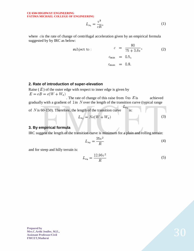
CE 6504 HIGHWAY ENGINEERING
FATIMA MICHAEL COLLEGE OF ENGINEERING
Prepared by
MrsCArthi Jenifer ME
Assistant ProfessorCivil
FMCETMadurai 31
and the shift as
(
6
) The length of the transition curve is the maximum of
equations 1 3 and 4or5 ie
(
7
Case (a)
For single lane roads
(
1
)
Therefore
(
2
)
Figure 1 Set-back for single lane roads (
CE 6504 HIGHWAY ENGINEERING
FATIMA MICHAEL COLLEGE OF ENGINEERING
Prepared by
MrsCArthi Jenifer ME
Assistant ProfessorCivil
FMCETMadurai 32
For multi lane roads if is the distance between centerline of the road and the centerline
of the inner lane then
(3)
(4)
Figure 2 Set-back for multi-lane roads ( )
Case (a)
For single lane roads
(1)
Therefore
(2)
Gradient
Gradient is the rate of rise or fall along the length of the road with respect to the
horizontal While aligning a highway the gradient is decided for designing the vertical
curve Before finalizing the gradients the construction cost vehicular operation cost and
the practical problems in the site also has to be considered Usually steep gradients are
avoided as far as possible because of the difficulty to climb and increase in the
CE 6504 HIGHWAY ENGINEERING
FATIMA MICHAEL COLLEGE OF ENGINEERING
Prepared by
MrsCArthi Jenifer ME
Assistant ProfessorCivil
FMCETMadurai 33
construction cost More about gradients are discussed below
Effect of gradient
The effect of long steep gradient on the vehicular speed is considerable This is
particularly important in roads where the proportion of heavy vehicles is significant Due
to restrictive sight distance at uphill gradients the speed of traffic is often controlled by
these heavy vehicles As a result not only the operating costs of the vehicles are
increased but also capacity of the roads will have to be reduced Further due to high
differential speed between heavy and light vehicles and between uphill and downhill
gradients accidents abound in gradients
Representation of gradient
The positive gradient or the ascending gradient is denoted as and the negative gradient as The deviation angle is when two grades meet the angle which
measures the change of direction and is given by the algebraic difference between the two
grades
steep gradient while 1 in 50 = 2 representation is illustrated in the figure 1
Example 1 in 30 = 333 is a
is a flatter gradient The gradient
CE 6504 HIGHWAY ENGINEERING
FATIMA MICHAEL COLLEGE OF ENGINEERING
Prepared by
MrsCArthi Jenifer ME
Assistant ProfessorCivil
FMCETMadurai 34
Figure 1 Representation of gradient
Types of gradient
Many studies have shown that gradient upto seven percent can have considerable effect
on the speeds of the passenger cars On the contrary the speeds of the heavy vehicles are
considerably reduced when long gradients as flat as two percent is adopted Although
flatter gradients are desirable it is evident that the cost of construction will also be very
high Therefore IRC has specified the desirable gradients for each terrain However it
may not be economically viable to adopt such gradients in certain locations steeper
gradients are permitted for short duration Different types of grades are discussed below
Ruling gradient
The ruling gradient or the design gradient is the maximum gradient with which the
designer attempts to design the vertical profile of the road This depends on the terrain
length of the grade speed pulling power of the vehicle and the presence of the horizontal
curve In flatter terrain it may be possible to provide flat gradients but in hilly terrain it
is not economical and sometimes not possible also The ruling gradient is adopted by the
designer by considering a particular speed as the design speed and for a design vehicle
with standard dimensions But our country has a heterogeneous traffic and hence it is not
possible to lay down precise standards for the country as a whole Hence IRC has
recommended some values for ruling gradient for different types of terrain
Limiting gradient
This gradient is adopted when the ruling gradient results in enormous increase in cost of
construction On rolling terrain and hilly terrain it may be frequently necessary to adopt
limiting gradient But the length of the limiting gradient stretches should be limited and
must be sandwiched by either straight roads or easier grades
Exceptional gradient
Exceptional gradient are very steeper gradients given at unavoidable situations They
should be limited for short stretches not exceeding about 100 metres at a stretch In
mountainous and steep terrain successive exceptional gradients must be separated by a
minimum 100 metre length gentler gradient At hairpin bends the gradient is restricted to
25
Critical length of the grade
The maximum length of the ascending gradient which a loaded truck can operate without
undue reduction in speed is called critical length of the grade A speed of 25 kmph is a
CE 6504 HIGHWAY ENGINEERING
FATIMA MICHAEL COLLEGE OF ENGINEERING
Prepared by
MrsCArthi Jenifer ME
Assistant ProfessorCivil
FMCETMadurai 35
reasonable value This value depends on the size power load grad-ability of the truck
initial speed final desirable minimum speed
Minimum gradient
This is important only at locations where surface drainage is important Camber will take
care of the lateral drainage But the longitudinal drainage along the side drains require
some slope for smooth flow of water Therefore minimum gradient is provided for
drainage purpose and it depends on the rain fall type of soil and other site conditions A
minimum of 1 in 500 may be sufficient for concrete drain and 1 in 200 for open soil
drains are found to give satisfactory performance Sight distance available from a point is the actual distance along the road surface which a driver
from a specified height above the carriage way has visibility of stationary or moving objects
Sight distance required by drivers applies to both geometric design of highways and for
traffic control The sight distance situations are considered in the design
i) Stopping or absolute minimum sight distance
ii) Safe overtaking or passing sight distance
iii) Safe sight distance for entering into uncontrolled intersections
Apart from the three situations mentioned above the following sight distance are considered by the
IRC in highway design
Intermediate sight distance
This is defined as twice the stopping sight distance when overtaking sight distance
cannot be provided intermediate sight distance is provided to give limited overtaking opportunities
to fast vehicles
Head light sight distance
This is the distance visible to a driver during night driving under the illumination of the
vehicle head lights
Stopping sight distance
The minimum sight distance available on a highway at any spot should be of sufficient
length to stop a vehicle traveling at design speed safely without collision with any other obstruction
The absolute minimum sight distance is therefore equal to the stopping sight distance
which is also sometimes called nonpassing sight distance The sight distance available on a road to a
driver at any instance depends on
i) Features of the road
ii) Height of the drivers eye above the road surface
iii) Height of the object above the road surface
The distance within which a motor vehicle can be stopped depends upon the factors listed below
a) Total reactions time of the driver
b) Speed of vehicle
c) Efficiency of breaks
d) Frictional resistance between the road and tyres
e) Gradient of the road
Total reaction time
) Reaction time of the driver is the time taken from the instant the object is visible to the
driver to the instant the brakes are effectively applied
) The total reaction time may be split up into two parts
CE 6504 HIGHWAY ENGINEERING
FATIMA MICHAEL COLLEGE OF ENGINEERING
Prepared by
MrsCArthi Jenifer ME
Assistant ProfessorCivil
FMCETMadurai 36
i) Perception time
ii) Brake reaction time
PIEV theory
According to this theory the total reaction time of the driver is split into four parts
i) Perception
ii) Intellection
iii) Emotion
iv) Volition
Speed of Vehicle
The stopping distance depends very much on the speed of the vehicle first during the
total reaction time of the driver the distance moved by the vehicle will depend on the speed
Efficiency of brakes
The braking efficiency is said to be 100 percent if the wheels are fully licked preventing
them from rotating on application of the brakes This will result in 100 percent skidding which is
normally undesirable except in utmost emergency
Frictional resistance between road and tyres
The frictional resistance developed between road and tyres or the skid resistance depends
on the type and condition of the road surface and the tyres IRC has specified a design friction
coefficient of 035 to 04 depending upon the speed to be used for finding the braking distance in the
calculation of stopping sight distance
Analysis of stopping distance
i) The distance traveled by the vehicle during the total reaction time known as lag
distance
ii) The distance traveled by the vehicle after the application of the brakes is known as
braking distance
Overtaking sight distance
The minimum distance open to the vision of the driver of a vehicle intending to overtake
slow vehicle ahead with safety against the traffic of opposite direction is known as the minimum
overtaking sight distance(OSD) or Safe passing sight distance available
The overtaking sight distance is the distance measured along the center of the road which
a driver with his eye level 12m above the road surface can see the top of an object 12m above the
road surface
Some of the important factors on which the minimum overtaking sight distance required
a) Speed of
i) overtaking vehicle
ii) overtaken vehicle
iii) The vehicle coming from opposite direction
b) Distance between the overtaking and overtaken vehicles the minimum spacing
depends on the steeds
a) Skill and reaction time of the driver
b) Rate of acceleration of overtaking vehicle
c) Gradient of the road
Criteria for sight distance requirements on highway
) The absolute minimum sight distance required throughout the length of the road is the
SSD which should invariably be provided at all places
CE 6504 HIGHWAY ENGINEERING
FATIMA MICHAEL COLLEGE OF ENGINEERING
Prepared by
MrsCArthi Jenifer ME
Assistant ProfessorCivil
FMCETMadurai 37
) On horizontal curves the obstruction on the inner side of the curves should be cleared
to provide the required set back distance and absolute minimum sight distance
) On vertical summit curves the sight distance requirement may be fulfilled by proper
design of the vertical alignment
Hairpin bent
TYPES OF CURVES ON HILL ROADS
The following are the important types of curves provided on hill Roads-
1 Hair-Pin Curves
2 Salient Curves
3 Re-entrant Curves 1 Hair-pin curves - The curve in a hill road which changes its direction through an angle of 180
degree or so down the hill on the same side is known as hair-pin curve
A Hair-Pin Bend
This curve is so called because it conforms to the shape of a hair-pin The bend so formed at the
hair-pin curve in a hill road is known as hair-pin bend This type of curve should be located on a
hill side having the minimum slope and maximum stability It must also be safe from view point of
landslides and ground water Hair-pin bends with long arms and farther spacing are always
preferred They reduce construction problems and expensive protective works Hair-pin curves or
bends of serpentine nature are difficult to negotiate and should therefore be avoided as far as
possible
Salient curves - The curves having their convexity on the outer edges of a hill road are called
salient curves The centre of curvature of a salient curve lies towards the hill side This type of curve
occurs in the road length constructed on the ridge of a hill the bend so formed at the salient curve in
a hill road known as corner bend
Salient curves are very dangerous for fast moving traffic At such a curve or at corner bend the
portion of projecting hill side is usually cut down to improve the visibility as shown in fig (Re-
entrant curve) The outer edge of the road at such a curve is essentially provided with a parapet wall
for protection of the vehicles from falling down the hill slope
CE 6504 HIGHWAY ENGINEERING
FATIMA MICHAEL COLLEGE OF ENGINEERING
Prepared by
MrsCArthi Jenifer ME
Assistant ProfessorCivil
FMCETMadurai 38
3 Re-entrant curves - The curves having their convexity on the inner edge of a hill road are called
re-entrant curves
Re-entrant curves
The centre of curvature of a re-entrant curves lies away from the hill side This type of curve occurs
in the road length constructed in the calley of a hill
These curves are less dangereous as they provide adequate visibility to the fast moving traffic At
such curves the parapet wall is provided only for safety of fast moving traffic
CE 6504 HIGHWAY ENGINEERING
FATIMA MICHAEL COLLEGE OF ENGINEERING
Prepared by
MrsCArthi Jenifer ME
Assistant ProfessorCivil
FMCETMadurai 39
UNIT ndash III DESIGN OF RIGID AND FLEXIBLE PAVEMENTS
COMPARISON OF RIGID AND FLEXIBLE PAVEMENTS
The comparisons are
i) Design precision
A cement concrete pavement is amerable to a much more precise structural analysis
than a flexible pavement Flexible pavements designs are mainly empirical Computer aided analysis
of layered system is making the flexible pavement design more exact than hitherto
ii) Life
) Cement concrete slabs of a thin section constructed in the early 1940rsquos are still in
existence in India though many of them have cracked badly and a few of them have been ripped
open and rebuilt in recent ties
) A major project in cement concrete road construction between Agra and Mathura It can
safely be said that a well-designed concrete slab has a life of about 40 years
) Compared to this the life of a flexible pavement generally varies from 10 to 20 years
iii) Maintenance
) A well-designed cement concrete pavement needs very little maintenance The only
maintenance needed is I respect of joints
) The surface is unaffected by spillage of oil and lubricants bituminous surfaces on the
other hand need great inputs in maintenance
) The surface is affected by spillage of oil and lubricants The surface is also affected by
natural weathering agents like air water ad temperature changes
) A cement concrete pavement on the other hand needs a small amount for maintaining
joints
iv) Initial cost
) The argument so far used against a cement concrete slab is that it is much more costly
than a flexible pavement
) The latter specifications no doubt represent the rock-bottom needs of a road in India but
these specifications can hardly provide a smooth and durable surface
v) Stage construction ) Road construction is generally done adopting a policy of stage construction especially for
low volume roads As traffic grows additional layers in the form of water bound macadam and
superior surfacing are added on
) Initial outlay is minimum and additional outlays are in keeping with traffic growth This is
a great advantage when dealing with new roads in an atmosphere of austerity
vi) Availability of materials
) Cement bitumen stone aggregates and gravelsand are the major materials involved in
pavement Construction Cement has been in serious short supply in the country for the past many
decades
) Bitumen is also not available plentifully in India There is also the danger of the entire oil
reserves in the world shrinking during the next two or three decades
) In locations where stone aggregates are scarce cement concrete may have an advantage
for flexible pavements
vii) Surface characterstics
CE 6504 HIGHWAY ENGINEERING
FATIMA MICHAEL COLLEGE OF ENGINEERING
Prepared by
MrsCArthi Jenifer ME
Assistant ProfessorCivil
FMCETMadurai 40
) A good cement concrete surface is smooth and free from rutting potholes and
corrugations In a bituminous surface it is only the asphaltic concrete surface that can give
comparable rideablity
) A well-constructed cement concrete pavement surface can have a permanent nonskid
surface A bituminous surface can also be designed to have a good skid resistant surface
viii) Utility location
) In cement concrete slabs proper thought has to be given to locate utilities such as water
pipes telephone lines and electric cables
) It is difficult to rip open the slab and restore it to be the original condition if any changes
in the utilities lines are to be made
ix) Glame and night visibility
) Concrete pavements have a gray color which can cause glam under sunlight Colored
cement can reduce the grave
) On the other hand bituminous roads need more street lighting
x) Traffic dislocation during construction
) A cement concrete pavement requires 28 days before it can be thrown open to traffic On
the other hand a bituminous surface can be thrown open to traffic shortly after it is rolled
xi) Environmental considerations during construction
) The process of heating of bitumen and aggregates and mixing them together on hot mix
plants can prove to be much more hazardous to the environment than cement concrete construction
where no heating of any material is involved
xii) Overall economy on a life cycle basis
) A good road is costly to construct but once constructed such a road requires little
maintenance and results in savings in vehicle operating costs
) The comparative economy of a flexible pavement and a rigid pavement has proved that on
overall economic considerations
Types of pavement structure
Based on the structural behavior pavements are generally classified into three
categories
i) Flexible pavements
ii) Rigid pavements
iii) Semi rigid pavements
Flexible pavements
) Flexible pavements are those which on the whole have low or negligible flexural
strength and are rather flexible in their structural action under the loadsThe flexible pavement
layers reflect the deformation of the lower layers on to the surface of the layer
) A flexible pavement consists of four components(i) Soil subgrade (ii) sub base
course (iii) base course (iv) Surface course
CE 6504 HIGHWAY ENGINEERING
FATIMA MICHAEL COLLEGE OF ENGINEERING
Prepared by
MrsCArthi Jenifer ME
Assistant ProfessorCivil
FMCETMadurai 41
) The flexible pavement layers transmit the vertical or compressive stresses to the lower layers
by grain to grain transfer through the points of contact in the granular structure A well
compacted granular structure consisting of strong added aggregate can transfer the compressive
stresses
) The load spreading ability of this layer therefore depends on the type of the materials and mix
design factors Bituminous concrete is one of the best flexible pavements layer materials Other
materials which fall under the group are all granular materials with or without bituminous
binder granular base and sub base course materials
) The vertical compressive stress is maximum on the pavement surface directly under the wheel
and is equal to the contact pressure under the wheel The flexible pavement may be constructed
in a number of layers and the top layer has to be strongest as the highest compressive stresses
) Flexible pavements are commonly designed using empirical design charts or equations taking
into account some of the design factors there are also semi empirical and theoretical design
methods
Rigid pavements
) Rigid pavements are those which possess note flexural strength or flexural rigidity
The stresses are not transferred from grain to grain to the lower layers as in the ease of flexible
pavements layers
) The rigid pavements are made of Portland cement concrete plain reinforced or
prestressed concrete The plain cement concrete slabs are expected to take up about 40 kgcm2
flexural stress
) The rigid pavement has the slab action and is capable of transmitting the wheel
load stresses through a wider area below The main point of difference in the structural behavior
of rigid pavement as compared to the flexible pavement is that the critical condition of stress in
the rigid pavement is the maximum flexural stress occurring in the slab due to wheel load and
the temperature changes whereas in the flexible pavement
) As the rigid pavement slab has tensile strength tensile stresses are developed due
to the bending of the slab under wheel load and temperature variations Thus the types of
stresses developed and their distribution within the cement concrete slab are quirt different
) The cement concrete pavement slab can very well serve as a wearing surface as
well an effective base course The rigid pavement structure consists of a cement concrete slab
below which a granular base or sub base course may be provided
) Though the cement concrete slab can also be laid directly over the soil subgrade
consists of fine grained soil
) the rigid pavements are usually designed and the stresses are analyzed using the
elastic theory assuming the pavements as a n elastic plate resting over an elastic or a viscous
foundation
Semi rigid pavements
) when bonded materials like the pozzolanic concrete lean cement concrete or soil
cement are used in the base course or sub base course layer the pavement layer has considerably
higher flexural strength than the common flexible pavement layers
) when this intermediate class of materials are used in the base or sub base course
layer of the pavements they are called semi rigid pavements
CE 6504 HIGHWAY ENGINEERING
FATIMA MICHAEL COLLEGE OF ENGINEERING
Prepared by
MrsCArthi Jenifer ME
Assistant ProfessorCivil
FMCETMadurai 42
) This third category of semi rigid pavement are either designed as flexible
pavements with some correction factors to find the thickness requirements based on experience
or by using a new design approach
) The semi rigid pavement materials have low resistance to impact and abrasion and
therefore are usually provided with flexible pavement surface course
Various functions of pavement components
The functions are
Soil sub grade and its evaluation
) The soil sub grade is a layer of natural soil prepared to receive the layers of pavement
materials placed over it It is essential that at no time the soil sub grade is overstressed it means that
the pressure transmitted on the top of the sub grade is within the allowable limit
) Many tests are known for measuring the strength properties of the sub grades Some of the
tests have been standardized for the use The common strength test for the evaluation of soil
subgrade is
i) California bearing ratio test
ii) California resistance value test
iii) Triaxial compression test
iv) Plate bearing test
CALIFORNIA BEARING RATIO (CBR) TEST
It is evolved for the empirical method of flexible pavement design The CBR test is carried
out either in the laboratory on prepared specimens or in the field by taking in situ measurements
California resistance value
It is found by using have been stabliometerThis test is used in an empirical method of
flexible pavement design based on soil strength
Triaxial test
It is the most important soil strength but still the test is not very commonly used in structural
design of pavements
Plate bearing test
It is carried out using a relatively large diameter plate to evaluate the load supporting
capacity of supporting power of the pavement layers The results are plate bearing tests are used in
flexible pavement design method like McLeod method on based on layer system analysis by
brumister
Sub base and base courses and their evaluation
) There layers are made of broken stones bound or unbound aggreagatesome times in sub
base course a layer of stabilized soil(or) Selected granular soil is also used
) however at the sub base course it is desirable to use smaller size graded aggregates When
the sub grade consists of fine grained soil and when the pavement carries heavy wheel loads
CE 6504 HIGHWAY ENGINEERING
FATIMA MICHAEL COLLEGE OF ENGINEERING
Prepared by
MrsCArthi Jenifer ME
Assistant ProfessorCivil
FMCETMadurai 43
) Sub base course primarily has the similar function as of the base course and is provided
with inferior materials than of base course Base courses are used under rigid pavement for
i) Preventing pumping
ii) Protecting the sub grade against frost action
) Thus the fundamental purpose of abase course and sub base course is to provide a stress
transmitting medium to spread the surface wheel loads in such manner
) The sub base and base course layers may be evaluated by suitable strength or stability test
like plate bearing CBR test
WEARING COURSE AND ITS EVALUATION
) The purpose of the wearing course is to give a smooth riding surface that is dense It
resists pressure exerted by tyres and takes up wear and tear due to the traffic
) Wearing course also offers a water tight layer against the surface water infiltration The
flexible pavement normally a bituminous surfacing is used as a wearing course
) In rigid pavements the cement concrete acts like a base course as well as wearing course
Most popular test in use is marshal stability test where in the optimum content of bitumen binder is
worked out based on the stability density
) Plate bearing test and Bankelman beam test are also sometimes made use of for evaluating
the wearing course and the pavement as a whole
Various factors to be considered in pavement design and the significance
Pavement design consists of two parts
i) Mix design of materials to be used in each pavement component layer Thickness design of the
pavement and the component layers
The various factors to be considered for the design of pavements are given below
i) Design wheel load
ii) Sub grade soil
iii) Climatic factors
iv) Pavement component layers
v) Environmental factors
vi) Special factors in the design of different types of pavements
Design wheel load
The various wheel load factors to be considered in pavement design are
i) Maximum wheel load
ii) Contact pressure
iii) Dual or multiple wheel loads
iv) Repetition of loads
Maximum wheel load
The wheel load configurations are important to know the way in which the loads of a given
vehicle are applied on the pavement surface
) For highways the maximum legal axle load as specified by Indian road congress is 8170
kg with a maximum equivalent single wheel load of 4085 kg
) The evaluation for vertical stress computations under a uniformly distribute of circular
load based on Boussineqrsquos theory is given by
CE 6504 HIGHWAY ENGINEERING
FATIMA MICHAEL COLLEGE OF ENGINEERING
Prepared by
MrsCArthi Jenifer ME
Assistant ProfessorCivil
FMCETMadurai 44
2
322
3
1
za
zpz
σz = vertical stress at depth z
P= surface pressure
Z=depth at which σz computed
A=radius of loaded area
Contact pressure
Generally the wheel load is assumed to be distributed over a circular area But by
measurement of the imprints of tyers with different load and inflation pressures Three terms in use
with reference to tyre pressure are
Tyre pressure
Inflation pressure
Contact pressure
Tyre pressure and inflation pressure mean exactly the same the contact pressure is found to be more
than tyre pressure when the tyre pressure is less than 7 kgm2 and it is vice versa when the tyre
pressure exceeds this value
Contact pressure can be measured by the relationship
Load on wheel
Contact pressure = ----------------------------------------
Contact area or area of imprint
The general variation between the tyre pressure and measured contact pressure is shown in this fig
The ratio of contact pressure to type pressure is defined as rigidity factor Thus value of rigidity
factor is 10 for an average tyre pressure of 7 Kgcm2This value is higher than unity for lower type
pressures and less than unity for tyre pressures higher than 7 kgcm2
Equivalent single wheel load (ESWL)
) The maximum wheel load within the specified limit and to carry greater load it is
necessary to provide dual wheel assembly to the rear axles of the roads vehicles
) In other words the pressure at a certain depth below the pavement surface cannot be
obtained by numerically adding the pressure caused by any one wheel
) The effect is in between the single load and two times load carried by one wheel The load
dispersion is assumed to be at an angle of 450In the dual wheel load assembly let d be the clear gap
between the two wheels S be the spacing between the centers of the wheels and a be the radius of
the circular contact area of each wheel Then S = (d + 2a)
) ESWL may be determined based on either equivalent deflection or equivalent stress
criterianMultiple wheel loads are convert to ESWL and this value is used in pavement design The
ESWL is usually determined by the equivalent stress criterion using a simple graphical method
CE 6504 HIGHWAY ENGINEERING
FATIMA MICHAEL COLLEGE OF ENGINEERING
Prepared by
MrsCArthi Jenifer ME
Assistant ProfessorCivil
FMCETMadurai 45
) A straight line relationship is assumed between ESWL and depth on log scales For
determining ESWL the plot is made as shown in fig
) Two points A and B are plotted on the log-log graph with coordinates of A (Pd2) and
B(2p2s)line AB is a plot which is the focus of points where any single wheel load is equivalent to a
certain set of dual wheels
) To Calculate the ESWL for a dual assembly it is essential to estimate a design thickness of
the pavement If the design thickness so obtained is equal to the estimated thickness then the ESWL
calculations could be considered as correct Otherwise trials are made
) In heavy trucks and trailers the load on each wheel may be further reduced by multiple
wheels and tandem axles
Repetition of loads
) The deformation of load pavement (or) sub grade due to a single application of wheel load
may be small It required carrying out traffic surveys for accounting the factor of repetitions for
wheel loads in the design of pavement
) Data collected are converted to some constant equivalent wheel loads Equivalent wheel
load is a single load equivalent to the repeated applications of any particular wheel load on a
pavement which requires the same thickness and strength of pavements
) McLeod has given a procedure for evolving equivalent load factors for designing flexible
pavements
Various methods of flexible pavement design
) The flexible pavement is built with number of layers In the design process it is to be
ensured that under the application of load none of the layers is overstressed
) The maximum intensity of stresses occurs in the top layer of the pavement The
magnitude of load stresses reduces at lower layers
) In the design of flexible pavements it has yet not been possible to have a rational design
method wherein design process and service behavior of the pavement can be expressed by
mathematical laws
) Flexible pavement design methods are accordingly either empirical or semi empirical In
these methods the knowledge and experience gained on the behavior of the pavements in the past
are usefully utilized
Various approaches of flexible pavement design may be thus classified into three groups
i) Empirical method
ii) Semi-empirical or Semi theoretical method
iii) Theoretical method
) Empirical methods are either based on physical properties or strength parameters of soil
sub grade When the design is based on stress strain function and modified base on experience it
may be called semi-empirical or semi-theoretical There are design methods based on theoretical
analysis and mathematical computations
Out of the flexible pavement design method available is
i) Group index method
ii) California bearing ratio method
iii) California R value (or) Stabiliometer method
iv) Triaxial test method
CE 6504 HIGHWAY ENGINEERING
FATIMA MICHAEL COLLEGE OF ENGINEERING
Prepared by
MrsCArthi Jenifer ME
Assistant ProfessorCivil
FMCETMadurai 46
v) McLeod method
vi) Burmister method
Group index method
) Group index value is an arbitrary index assigned to the soil type in numerical equations
base on the percent fines liquid limit and plasticity index
) The design chart for group index method for determining the pavement thickness is given
in fig
The traffic volume in this method is divided in three groups
Traffic volume No of vehicles per day
Light Less than 50
Medium 50 to 300
Heavy Over 300
The design of the pavement thickness by this method first the G1 value of the soil is found the
anticipated traffic is estimated and is designated as light medium or heavy as indicated
The G1 method of pavement design is essentially an empirical method based on physical properties
of the subgrade soil This method does not consider the strength characteristics of the subgrade soil
and therefore is open to question regarding the reliability of the design based on the index properties
of the soil only
California bearing ratio method
) California division of highways in the USA developed CBR method for
pavement design The majority of design curves developed later are base on the original curves
proposed by OJporter
) One of the chief advantages of CBR method is the simplicity of the test procedure
The CBR tests were carried out by the California state highway department on existing pavement
layers including subgrade sub base and base course
) Based on the extensive CBR test data collected on pavement which behaved
satisfactory and those which failed an empirical design chart was developed correlating the CBR
value and the pavement thickness The basis of the design chart is that a material with a given CBR
required a certain thickness of pavement layer as a cover
) A higher load needs a thicker pavement layer to protect the sub grade Design
curves correlating the CBR value with total pavement thickness cover were developed by the
California state highway department for wheel loads of 3175kg and 5443 kg representing light and
heavy traffic The design curves are shown in this fig
It is possible to extend the CBR design curves for various loading conditions nusing the expression
t= 2
1
1751
pCBRp
t=2
1
751
A
CBR
p
Hence
CE 6504 HIGHWAY ENGINEERING
FATIMA MICHAEL COLLEGE OF ENGINEERING
Prepared by
MrsCArthi Jenifer ME
Assistant ProfessorCivil
FMCETMadurai 47
t= pavement thickness cm
p=Wheel load kg
CBR= California bearing ratio percent
P=tyre pressure kgcm2
A= area of contactcm2
IRC Recommendations
a) The CBR tests should be performed on remoulded soils in the laboratory The specimens should
be prepared by static compaction wherever possible and otherwise by dynamic compaction
b) For the design of new roads the sub grade soil sample should be compacted at OMC to proctor
density whenever suitable compaction equipment
c) The CBR test samples may be soaked in water for four days period before testing the annual
rainfall is less than 50 cm and the water table is too deep to affect the sub grade and imperable
surfacing is provided to carrying out CBR test
d) If the maximum variations in CBR value of the three specimens exceed the specified limits the
design CBR should be average of at least six samples
e) The top 50 cm of sub grade should be compacted at least up to 95 to 100 percent of proctor
density
f) An estimate of the traffic should be carried by the road pavements at the end of expected in view
the existing traffic and probable growth rate of traffic
g) The traffic for the design is considered in units of heavy vehicles per day in both directions and is
divided into seven categories A to G The design thickness is considered applicable for single axle
loads up to 8200 kg and tandom axle loads up to 14500 kg
h) When sub base course materials contain substantial proportion of aggregates of size above 20mm
the CBR value of these materials would not be valid for the design of subsequent layers above them
The CBR method of pavement design gives the total thickness requirement of the pavement above a
sub grade and thickness value would remain the same quality of materials used in component layers
California resistance value method
) In this design method based on stabliometer R-value and cohesiometer C-value
Based on performance data it was established by pavement thickness varies directly with R value
and algorithm of load repetitions It varies inversely with fifth root of c valueThe expression for
pavement thickness is given by the empirical equation
T=
5
1
1 90
C
RTK
Hence
T=total thickness of pavement cm
K=Numerical constant 0166
T1=traffic index
R= stabiliometer resistance value
C=Cohesiometer value
CE 6504 HIGHWAY ENGINEERING
FATIMA MICHAEL COLLEGE OF ENGINEERING
Prepared by
MrsCArthi Jenifer ME
Assistant ProfessorCivil
FMCETMadurai 48
In the design of flexible pavements based on California resistance value method for the following
data are needed
) R-value of soil subgrade
) T1 value
) Equivalent C-value
) R value of soil subgrade is obtained from the test using stablio meterThe
computation of T1 value has been explained
Equivalent C-value
) The cohesion meter value c is obtained for each layer of pavement material
separately from tests However the composite or equivalent C-value of the pavement may be
estimated if the thickness of each component layer and the c-value of the material of the layer are
known
) while designing a pavement as the thickness of the pavement is not known it is
easier if the pavement is first assumed to consist of any one material like gravel base course with
known C-value
) Subsequently the individual thickness of each layer is converted in terms of gravel
equivalent by using relationship
5
1
1
2
2
1
C
C
t
t
) t1 and t2 are the thickness values of any two pavement layersc1 and c2 are their
corresponding cohesiometer values
CE 6504 HIGHWAY ENGINEERING
FATIMA MICHAEL COLLEGE OF ENGINEERING
Prepared by
MrsCArthi Jenifer ME
Assistant ProfessorCivil
FMCETMadurai 49
UNIT 4 MATERIAL AND MAINTENANCE
SUMMIT CURVE
Summit curves are vertical curves with gradient upwards They are formed when two
gradients meet as illustrated in figure 1 in any of the following four ways
1 When a positive gradient meets another positive gradient [figure 1a]
2 When positive gradient meets a flat gradient [figure 1b]
3 When an ascending gradient meets a descending gradient [figure 1c]
4 When a descending gradient meets another descending gradient [figure 1d]
Type of Summit Curve
Many curve forms can be used with satisfactory results the common practice has been to
use parabolic curves in summit curves This is primarily because of the ease with it can
be laid out as well as allowing a comfortable transition from one gradient to another
Although a circular curve offers equal sight distance at every point on the curve for very
small deviation angles a circular curve and parabolic curves are almost congruent
Furthermore the use of parabolic curves were found to give excellent riding comfort
Figure 1 Types of summit curves
Design Consideration
In determining the type and length of the vertical curve the design considerations are
comfort and security of the driver and the appearance of the profile alignment Among
these sight distance requirements for the safety are most important on summit curves
The stopping sight distance or absolute minimum sight distance should be provided on
these curves and where overtaking is not prohibited overtaking sight distance or
intermediate sight distance should be provided as far as possible When a fast moving
vehicle travels along a summit curve there is less discomfort to the passengers This is
because the centrifugal force will be acting upwards while the vehicle negotiates a
summit curve which is against the gravity and hence a part of the tyre pressure is
relieved Also if the curve is provided with adequate sight distance the length would be
sufficient to ease the shock due to change in gradient Circular summit curves are
identical since the radius remains same throughout and hence the sight distance From
CE 6504 HIGHWAY ENGINEERING
FATIMA MICHAEL COLLEGE OF ENGINEERING
Prepared by
MrsCArthi Jenifer ME
Assistant ProfessorCivil
FMCETMadurai 50
this point of view transition curves are not desirable since it has varying radius and so the
sight distance will also vary The deviation angles provided on summit curves for
highways are very large and so the simple parabola is almost congruent to a circular arc
between the same tangent points Parabolic curves are easy for computation and also it
had been found out that it provides good riding comfort to the drivers It is also easy for
field implementation Due to all these reasons a simple parabolic curve is preferred as
summit curve Length of the summit curve
The important design aspect of the summit curve is the determination of the length of the
curve which is parabolic As noted earlier the length of the curve is guided by the sight
distance consideration That is a driver should be able to stop his vehicle safely if there is
an obstruction on the other side of the road Equation of the parabola is given by
where where N is the deviation angle and is the length of the In
deriving the length of the curve two situations can arise depending on the uphill and
downhill gradients when the length of the curve is greater than the sight distance and the
length of the curve is greater than the sight distance
Let is the length of the summit curve is the SSDISDOSD is the deviation angle
drivers eye height (12 m) and the height of the obstruction then the length of the
summit curve can be derived for the following two cases The length of the summit curve
can be derived from the simple geometry as shown below
Case a Length of summit curve greater than sight distance( )
Figure 1 Length of summit curve ( )
The situation when the sight distance is less than the length of the curve is shown in
figure 1
CE 6504 HIGHWAY ENGINEERING
FATIMA MICHAEL COLLEGE OF ENGINEERING
Prepared by
MrsCArthi Jenifer ME
Assistant ProfessorCivil
FMCETMadurai 51
(1)
Case b Length of summit curve less than sight distance
The second case is illustrated in figure 1
Figure 1 Length of summit curve
CE 6504 HIGHWAY ENGINEERING
FATIMA MICHAEL COLLEGE OF ENGINEERING
Prepared by
MrsCArthi Jenifer ME
Assistant ProfessorCivil
FMCETMadurai 52
From the basic geometry one can write
(1)
Therefore for a given and to get minimum differentiate the above equation
with respect to and equate it to zero Therefore
Solving the quadratic equation for
(2)
Now we can substitute back to get the value of minimum value of for a given
and Therefore
Solving for
CE 6504 HIGHWAY ENGINEERING
FATIMA MICHAEL COLLEGE OF ENGINEERING
Prepared by
MrsCArthi Jenifer ME
Assistant ProfessorCivil
FMCETMadurai 53
(3) (4
CE 6504 HIGHWAY ENGINEERING
FATIMA MICHAEL COLLEGE OF ENGINEERING
Prepared by
MrsCArthi Jenifer ME
Assistant ProfessorCivil
FMCETMadurai 54
When stopping sight distance is considered the height of drivers eye above the road
surface ( ) is taken as 12 metres and height of object above the pavement surface ( )
is taken as 015 metres If overtaking sight distance is considered then the value of
drivers eye height ( ) and the height of the obstruction ( ) are taken equal as 12
metres
Valley curve
Valley curve or sag curves are vertical curves with convexity downwards They are
formed when two gradients meet as illustrated in figure 1 in any of the following four
ways
Figure 1 Types of valley curve
1 When a descending gradient meets another descending gradient [figure 1a]
2 When a descending gradient meets a flat gradient [figure 1b]
3 When a descending gradient meets an ascending gradient [figure 1c]
4 When an ascending gradient meets another ascending gradient [figure
Design considerations
There is no restriction to sight distance at valley curves during day time But visibility is
reduced during night In the absence or inadequacy of street light the only source for
visibility is with the help of headlights Hence valley curves are designed taking into
account of headlight distance In valley curves the centrifugal force will be acting
downwards along with the weight of the vehicle and hence impact to the vehicle will be
more This will result in jerking of the vehicle and cause discomfort to the passengers
Thus the most important design factors considered in valley curves are (1) impact-free
movement of vehicles at design speed and (2) availability of stopping sight distance
under headlight of vehicles for night driving
For gradually introducing and increasing the centrifugal force acting downwards the best
shape that could be given for a valley curve is a transition curve Cubic parabola is
generally preferred in vertical valley curves See figure 1
CE 6504 HIGHWAY ENGINEERING
FATIMA MICHAEL COLLEGE OF ENGINEERING
Prepared by
MrsCArthi Jenifer ME
Assistant ProfessorCivil
FMCETMadurai 55
Figure 1 Valley curve details
During night under headlight driving condition sight distance reduces and availability of
stopping sight distance under head light is very important The head light sight distance
should be at least equal to the stopping sight distance There is no problem of overtaking
sight distance at night since the other vehicles with headlights could be seen from a
considerable distance
Length of the valley curve
The valley curve is made fully transitional by providing two similar transition curves of
equal length The transitional curve is set out by a cubic parabola where
The length of the valley transition curve is designed based on two criteria
1 comfort criteria that is allowable rate of change of centrifugal acceleration is
limited to a comfortable level of about
2 safety criteria that is the driver should have adequate headlight sight distance at
any part of the country
Comfort criteria
The length of the valley curve based on the rate of change of centrifugal acceleration that
will ensure comfort Let is the rate of change of acceleration the minimum radius of
the curve is the design speed and is the time then is give
CE 6504 HIGHWAY ENGINEERING
FATIMA MICHAEL COLLEGE OF ENGINEERING
Prepared by
MrsCArthi Jenifer ME
Assistant ProfessorCivil
FMCETMadurai 56
For a cubic parabola the Value Safety criter Length of the valley curve for headlight distance may be determined for two conditions
(1) length of the valley curve greater than stopping sight distance and (2) length of the
valley curve less than the stopping sight distance of for length is given by
Case 1 Length of valley curve greater than stopping sight distance ( )
The total length of valley curve is greater than the stopping sight distance SSD The
sight distance available will be minimum when the vehicle is in the lowest point in the
valley This is because the beginning of the curve will have infinite radius and the bottom
of the curve will have minimum radius which is a property of the transition curve The
case is shown in figure 1
Figure 1 Valley curve case 1
From the geometry of the figure we have
CE 6504 HIGHWAY ENGINEERING
FATIMA MICHAEL COLLEGE OF ENGINEERING
Prepared by
MrsCArthi Jenifer ME
Assistant ProfessorCivil
FMCETMadurai 57
(1)
where is the deviation angle in radians is the height of headlight beam is the
head beam inclination in degrees and is the sight distance The inclination is 1
degree
Case 2 Length of valley curve less than stopping sight distance ( )
The length of the curve is less than SSD In this case the minimum sight distance is
from the beginning of the curve The important points are the beginning of the curve and
the bottom most part of the curve If the vehicle is at the bottom of the curve then its
headlight beam will reach far beyond the endpoint of the curve whereas if the vehicle is
at the beginning of the curve then the headlight beam will hit just outside the curve
Therefore the length of the curve is derived by assuming the vehicle at the beginning of
the curve The case is shown in figure 1
From the figure
(1) Note that the above expression is approximate and is satisfactory because in practice the gradients
are very small and is acceptable for all practical purposes We will not be able to know prior to
which case to be adopted Therefore both has to be calculated and the one which satisfies the
condition is adopted
1 Flexible pavement
2 Rigid pavement
Flexible pavement
These pavements reflect the deformation of sub grade and the subsequent layers to the
surface
Rigid pavement
The rigid characteristic of the pavement are associated with rigidity or flexural strength
CE 6504 HIGHWAY ENGINEERING
FATIMA MICHAEL COLLEGE OF ENGINEERING
Prepared by
MrsCArthi Jenifer ME
Assistant ProfessorCivil
FMCETMadurai 58
or slab action so the load is distributed over a wide area of sub grade soil
Flexible pavement Definition
These pavements reflect the deformation of sub grade and the subsequent layers to the
surface Flexible usually asphalt is laid with no reinforcement or with a specialized
fabric reinforcement that permits limited flow or repositioning of the roadbed under
ground changes
The design of flexible pavement is based on load distributing characteristic of the
component layers The black top pavement including water amp gravel bound macadam fall
in this category
Flexible pavement on the whole has low or negligible flexible strength flexible in their
structural action) The flexible pavement layers transmit the vertical or compressive
stresses to the lower layers by grain transfer through contact points of granular structure
The vertical compressive stress is maximum on the pavement surface directly under the
wheel load and is equal to contact pressure under the wheels Due to the ability to
distribute the stress to large area in the shape of truncated cone the stresses get decreased
in the lower layer
As such the flexible pavement may be constructed in a number of layers and the top
layer has to be strongest as the highest compressive stresses
To be sustained by this layer in addition to wear and tear the lower layer have to take
up only lesser magnitude of stress as there is no direct wearing action die to traffic loads
therefore inferior material with lower cast can be used in the lower layers
Rigid pavement Definition
The rigid characteristic of the pavement are associated with rigidity or flexural strength
or slab action so the load is distributed over a wide area of sub grade soil Rigid pavement
is laid in slabs with steel reinforcement
The rigid pavements are made of cement concrete either plan reinforced or prestressed
concrete
Critical condition of stress in the rigid pavement is the maximum flexural stress occurring in the slab due to wheel load and the temperature changes
Rigid pavement is designed and analyzed by using the elastic theory
CE 6504 HIGHWAY ENGINEERING
FATIMA MICHAEL COLLEGE OF ENGINEERING
Prepared by
MrsCArthi Jenifer ME
Assistant ProfessorCivil
FMCETMadurai 59
UNIT-5 EVALUATION AND MAINTENANCE OF PAVEMENTS
TRAFFIC PARAMETERS
Design life
Design life is the number of years (or number of standard axle repetitions) for which the
pavement is being designed A pavement is expected to serve satisfactorily within the
design life For concrete pavements 20 to 40 years may be assumed as the design life
(PCA 1984 IRC58 2002)
Basic design principle
Though different approaches for concrete pavement design are suggested in various
guidelines the design principles tend to remain similar across different guidelines for
example PCA (1994) Austroads (2004) NCHRP (2004) IRC58 (2002) etc except the
AASHTO (1993) provisions which is based on empirical approach The basic steps
involved in the design of concrete pavement method can be summarized as follows
The developed stresses due to load for a trial thickness of the concrete slab are
calculated for various loading configuration and the critical one is chosen The
axle loads are generally divided into different axle load groups and the load
stresses are calculated individually
The ratio between the load stress and Modulus of Rupture (MOR) is known as
stress ratio The stress ratio determines how many repetitions the pavement can
sustain (ie allowable traffic repetitions) for the individual axle load group If the
stress ratio is 055 or lower it can withstand virtually infinite number of traffic
repetitions (PCA 1984)
The ratio between the allowable repetitions to the expected traffic repetitions is
the damage fraction The calculation process is repeated for various axle loads
(sometimes for various seasons or various timings of the day) and the sum of
individual damage fractions (c u m u l a t i v e fatigue damage) should be less
than equal to one for pavement design being safe If found unsafe the trial
thickness is changed and the design process is repeated
The design process may also include considerations for temperature stress
moisture stresses and erosion distress
A brief discussion on concrete pavement design approaches suggested by various design
practices viz PCA method (1984) Austroads method (2004) AASHTO method (1993)
NCHRP mechanistic-empirical method (2004) and the Indian Roads Congress (IRC)
method (2002) are placed in the following
Portland cement Association (PCA) Method
The PCA method is based on Westergaard Picket and Rays work and further theoretical
analysis by Finite Element Method (Huang 1993) The data used to develop the PCA
method is generated from various road tests like ASSHO road test Arlington test
(conducted by PCA) Bates test road and Maryland road test (PCA 1984) The PCA
design method is based on the following two considerations (PCA 1984)
The fatigue damage on the concrete slab due to repetitive application of traffic
load is estimated The cumulative fatigue damage principle is used to estimate the
design thickness of the slab Edge stress between the mid-ways of the
CE 6504 HIGHWAY ENGINEERING
FATIMA MICHAEL COLLEGE OF ENGINEERING
Prepared by
MrsCArthi Jenifer ME
Assistant ProfessorCivil
FMCETMadurai 60
transverse joint is taken as critical configuration
The stresses due to warping and curling (due to temperature and moisture
gradient) are not considered in the fatigue analysis as per PCA recommendation
because most of the time the stresses generated are subtractive to the load stress
The possibility of erosion of pavement materials placed below the concrete slab is
evaluated The rate at which the slab is deflected due to axle load is used as a
criterion for erosion Theoretically it can be shown that a thin pavement with
smaller deflection basin is subjected to faster rate of deflection compared to
thicker slab Hence thin slab is more susceptible to erosion In a similar way the
cumulative erosion damage is calculated for individual axle load groups If this
value is greater than one then the design needs to be revised
Austroads method
Austroads method has been adopted from PCA (1984) approach with modifications
suited to Australian conditions (Austroads 2004) A bound mix or lean cement concrete is
used as sub-base material For a given CBR value of the subgrade and given thickness of
cemented sub-base the effective subgrade strength can be obtained from the chart
provided Figure-19 schematically shows such a chart For different levels of traffic
Austroads (2004) suggests minimum values of the base thicknesses to be provided
CE 6504 HIGHWAY ENGINEERING
FATIMA MICHAEL COLLEGE OF ENGINEERING
Prepared by
MrsCArthi Jenifer ME
Assistant ProfessorCivil
FMCETMadurai 61
figure-19 Schematic diagram of Austroads (2004) chart for estimation of effective
subgrade strength
As per Astroads (2004) the concrete pavement slab thickness for a given expected
traffic repetitions is designed considering the (i) flexural fatigue of the concrete slab and
the (ii) subgrade erosion arising out of repeated deflections For both the considerations
equations are suggested to calculate the allowable traffic repetitions If the allowable
traffic is less than the expected traffic the design is revised by increasing the slab
thickness The concrete shoulders adopted are of integral type or structural type
AASHTO method
The AASHTO method (1993) for design of concrete pavement has evolved from the
AASHO road test (AASHO 1962) The AASHTO pavement design follows an empirical
approach Pavement performance in terms of present serviceability index ( PSI ) loss of
serviceability sub-grade and sub-base strength cumulative traffic properties of concrete
joint load transfer efficiency drainage condition overall standard deviation and
reliability are the input parameters considered in the pavement design
The PSI value of the fresh pavement is assumed as 45 and the pavement is deemed to
have failed when the PSI value reaches 25 The resilient moduli of the subgrade and sub-
base materials are determined in the laboratory simulating the seasonal moisture content
and stress situation Suggested values are also available for given moisture content
plasticity index etc The composite modulus of sub-grade reaction (k) is estimated from
modulus of sub-grade reaction and elastic modulus of sub-base for various seasons and
the depth of rigid foundation and the thickness of the sub-base
Design equation as well nomographs are available to estimate the slab thickness (D) from
these input parameters
NCHRP mechanistic-empirical (M-E) metho
The NCHRP (2004) has recently developed concrete pavement design procedure based
on mechanistic-empirical (M-E) approach This approach attempts to reduce the extent of
empiricism prevalent in the existing AASHTO (1993) guidelines This proposed NCHRP
pavement design system is modular in nature that is the design approach can be
modified by parts (as and when new knowledge is available) without disrupting the
overall design procedure This approach also can take care of various wheel-axle loa
configuration
As per this approach trial thickness of the slab is first assumed and the stress strain and
displacement values are obtained From these values the performance of the pavement in
terms of distresses (such as faulting cracking) and smoothness and predicted If these
predicted performance parameters does not satisfy the required performance for a given
reliability
The design approach includes a large data-base as input parameters for example average
daily traffic traffic growth rate traffic composition hourly weather data on air
temperature precipitation wind speed percentage sunshine relative humidity pavement
material engineering parameters ground water depth infiltration drainage hydraulic
conductivity thermal conductivity heat capacity etc The temperature stress is
considered in this method but the temperature profile is linearized to enhance
computational efficiency (NCHRP 2004)
CE 6504 HIGHWAY ENGINEERING
FATIMA MICHAEL COLLEGE OF ENGINEERING
Prepared by
MrsCArthi Jenifer ME
Assistant ProfessorCivil
FMCETMadurai 62
INDIAN ROADS CONGRESS (IRC) METHOD
The Indian Roads Congress (IRC) guidelines IRC58 (2002) has adopted the
Westergaards equation to estimate load stress and Brdaburys equation to estimate
temperature stress The load stress is highest at the corner of the slab lesser in edge and
least in the interior The order of variation of temperature stress is just the reverse of this
As per IRC58 (2002) it is recommended that the design needs to be done for edge stress
condition and subsequently check needs to be performed for corner stress condition so as
to finalize the design The following are the steps followed as per IRC58 (2002)
guideline for the design of concrete pavement
The input parameters are obtained to formulate the design problem The joint
spacing and the slab dimensions are decided If there is a bound sub-base layer
over the subgrade a suitable value of effective k is to be adopted
A trial thickness of the concrete slab is assumed
The edge stress is estimated for various axle loads from the given charts Figure-
20 schematically shows such a chart The cumulative fatigue damage principle for
fatigue is applied to check the adequacy of the slab thickness
The sum of edge stress due to load for the highest axle load group and the
temperature stress should be less than the MOR of concrete otherwise the design
is revised
The adequacy of corner stress is checked with respect to MOR value and
accordingly the design is finalized Westergaards corner stress formula
Figure-20 Schematic diagram of IRC58 chart for estimation of load stress at the edge
(IRC58 2002)
CE 6504 HIGHWAY ENGINEERING
FATIMA MICHAEL COLLEGE OF ENGINEERING
Prepared by
MrsCArthi Jenifer ME
Assistant ProfessorCivil
FMCETMadurai 63
estimation of corner stress due to load and the corner stress due to temperature is
assumed to be zero
Estimation of layer thicknesses
The thickness of the pavement is adjusted in such a way that the stress strain
developed is less than the allowable values obtained from past performance
information
The two major modes of structural failure of pavement are fatigue and rutting
o Fatigue Traffic applies repetitive load to the pavement surface and the
cracks start from bottom the bound layer slab and propagate upwards
When the extent of surface cracks reaches a predefined level the
pavement is said to have failed due to flexural fatigue
FUNCTIONAL DESIGN
The functional pavement design involves considerations of skid resistance roughness
surface distresses reflectivity of pavement surface etc The functional pavement design
considers mainly the surface features of a pavement
Drainage design
A road needs to be designed in such a way that the rain snow precipitation is drained off
the pavement and its surroundings A suitable surface drainage system for the pavement
is designed for this purpose Some water however will percolate into the pavement from
its top surface and needs to be taken out of the pavement - this is done by providing an
internal drainage system to the pavement Water will also try to enter into the pavement
from bottom due to capillary rise or due to rise in water table A suitably designed sub-
surface drainage system tries to avoid such a problem
PAVEMENT THICKNESS DESIGN CHARTS
For the design of pavements to carry traffic in the range of 1 to 10 msa use chart 1 and for
traffic in the range 10 to 150 msa use chart 2 of IRC37 2001 The design curves relate
pavement thickness to the cumulative number of standard axles to be carried over the
design life for different sub-grade CBR values ranging from 2 to 10 The design
charts will give the total thickness of the pavement for the above inputs The total
thickness consists of granular sub-base granular base and bituminous surfacing The
individual layers are designed based on the the recommendations given below and the
subsequent tables
Pavement composition
Sub-base
Sub-base materials comprise natural sand gravel laterite brick metal crushed
stone or combinations thereof meeting the prescribed grading and physical
requirements The sub-base material should have a minimum CBR of 20 and
30 for traffic upto 2 msa and traffic exceeding 2 msa respectively Sub-base
usually consist of granular or WBM and the thickness should not be less than 150
mm for design traffic less than 10 msa and 200 mm for design traffic
Base
The recommended designs are for unbounded granular bases which comprise
CE 6504 HIGHWAY ENGINEERING
FATIMA MICHAEL COLLEGE OF ENGINEERING
Prepared by
MrsCArthi Jenifer ME
Assistant ProfessorCivil
FMCETMadurai 64
conventional water bound macadam (WBM) or wet mix macadam (WMM) or
equivalent confirming to MOST specifications The materials should be of good
quality with minimum thickness of 225 mm for traffic up to 2 msa an 150 mm for
traffic
Bituminoussurfacing The surfacing consists of a wearing course or a binder
course plus wearing course The most commonly used wearing courses are
surface dressing open graded premix carpet mix seal surfacing semi-
dense bituminous concrete and bituminous concrete For binder course
MOST specifies it is desirable to use bituminous macadam (BM) for traffic
upto o 5 msa and dense bituminous macadam (DBM) for traffic more than 5
msa
Numerical example
Design the pavement for construction of a new bypass with the following data
1 Two lane carriage way
2 Initial traffic in the year of completion of construction = 400 CVPD (sum of both
directions)
3 Traffic growth rate = 75
4 Design life = 15 years
5 Vehicle damage factor based on axle load survey = 25 standard axle per
commercial vehicle
6 Design CBR of subgrade soil = 4
Solution
1 Distribution factor = 075
2
3 Total pavement thickness for CBR 4 and traffic 72 msa from IRC37 2001
chart1 = 660 mm
4 Pavement composition can be obtained by interpolation from Pavement Design
Catalogue (IRC37 2001)
1 Bituminous surfacing = 25 mm SDBC + 70 mm DBM
2 Road-base = 250 mm WBM
3 sub-base = 315 mm granular material of CBR not less than 30
CE 6504 HIGHWAY ENGINEERING
FATIMA MICHAEL COLLEGE OF ENGINEERING
Prepared by
MrsCArthi Jenifer ME
Assistant ProfessorCivil
FMCETMadurai 65
Generally bound base layers are used for concrete pavement construction As per Indian
specification some example of such base layers are Dry Lean Concrete (DLC) Roller
Compacted Concrete (RCC) (IRC15-2002)
The concrete slab is generally of M40 to M50 grade of concrete as
per Indian specifications and is called as paving quality concrete (PQC)
(IRC15-2002)
BITUMINOUS PAVEMENT
The subgrade is a compacted soil layer
The base and sub-base course could be made up of bound or unbound granular layer As
per Indian specifications (MORTampH 2001) some examples of base or sub-base layers
are Granular sub-base(GSB) Water Bound Macadam (WBM) Wet Mix Macadam
(WMM) etc
The binder course is made up bituminous material As per Indian specifications
(MORTampH 2001) some examples of binder course are Bituminous Macadam (BM)
Dense Bituminous Macadam (DBM) etc
The wearing course is the top bituminous layer which is comes in contact to the
vehicle tyre Wearing course provides impermeability to the pavement surface
against water percolation (Chakroborty and Das 2003) The binder course and wearing
course together are called bituminous surfacing
IRC METHOD OF FLEXIBLE PAVEMENT MIX DESIGN
These guidelines will apply to design of flexible pavements for Expressway National Highways
State Highways Major District Roads and other categories of roads Flexible pavements are
considered to include the pavements which have bituminous surfacing and granular base and sub-
base courses conforming to IRC MOST standards These guidelines apply to new pavements
Design criteria
The flexible pavements has been modeled as a three layer structure and stresses and strains at
critical locations have been computed using the linear elastic model To give proper consideration
to the aspects of performance the following three types of pavement distress resulting from
repeated (cyclic) application of traffic loads are considered
1 Vertical compressive strain at the top of the sub-grade which can cause sub-grade
deformation resulting in permanent deformation at the pavement surface
2 Horizontal tensile strain or stress at the bottom of the bituminous layer which can cause
fracture of the bituminous layer
3 Pavement deformation within the bituminous layer
CE 6504 HIGHWAY ENGINEERING
FATIMA MICHAEL COLLEGE OF ENGINEERING
Prepared by
MrsCArthi Jenifer ME
Assistant ProfessorCivil
FMCETMadurai 66
While the permanent deformation within the bituminous layer can be controlled by meeting the
mix design requirements thickness of granular and bituminous layers are selected using the
analytical design approach so that strains at the critical points are within the allowable limits For
calculating tensile strains at the bottom of the bituminous layer the stiffness of dense bituminous
macadam (DBM) layer with 6070 bitumen has been used in the analysis
FAILURE CRITERIA
Critical locations in pavement
A and B are the critical locations for tensile strains Maximum value of the strain is
adopted for design C is the critical location for the vertical subgrade strain since the
maximum value of the occurs mostly at C
CE 6504 HIGHWAY ENGINEERING
FATIMA MICHAEL COLLEGE OF ENGINEERING
Prepared by
MrsCArthi Jenifer ME
Assistant ProfessorCivil
FMCETMadurai 67
Fatigue Criteria
Bituminous surfacings of pavements display flexural fatigue cracking if the tensile strain
at the bottom of the bituminous layer is beyond certain limit The relation between the
fatigue life of the pavement and the tensile strain in the bottom of the bituminous layer
was obtained as
(1)
in which is the allowable number of load repetitions to control fatigue cracking and
is the Elastic modulus of bituminous layer The use of equation 1 would result in
fatigue cracking of 20 of the total area
Rutting Criteria
The allowable number of load repetitions to control permanent deformation can be
expressed as
(2)
is the number of cumulative standard axles to produce rutting of 20 mm
CE 6504 HIGHWAY ENGINEERING
FATIMA MICHAEL COLLEGE OF ENGINEERING
Prepared by
MrsCArthi Jenifer ME
Assistant ProfessorCivil
FMCETMadurai 68
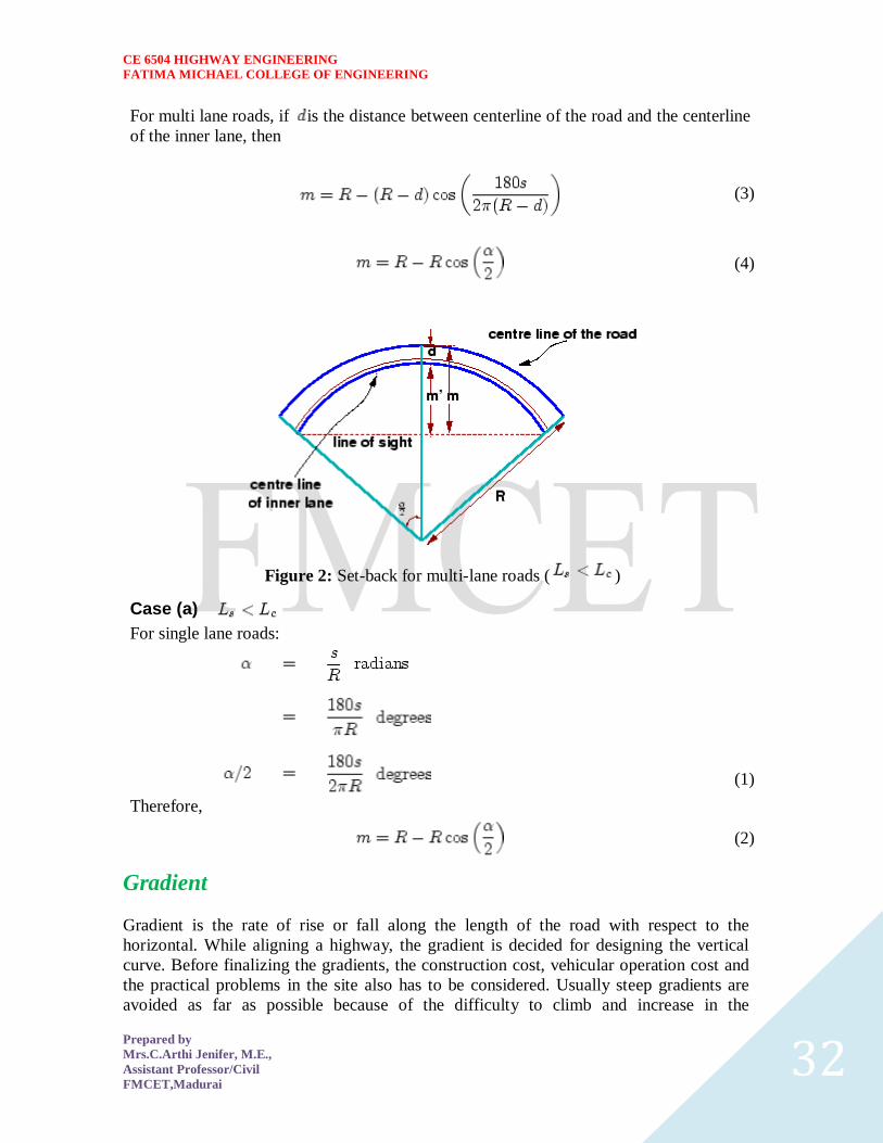
CE 6504 HIGHWAY ENGINEERING
FATIMA MICHAEL COLLEGE OF ENGINEERING
Prepared by
MrsCArthi Jenifer ME
Assistant ProfessorCivil
FMCETMadurai 32
For multi lane roads if is the distance between centerline of the road and the centerline
of the inner lane then
(3)
(4)
Figure 2 Set-back for multi-lane roads ( )
Case (a)
For single lane roads
(1)
Therefore
(2)
Gradient
Gradient is the rate of rise or fall along the length of the road with respect to the
horizontal While aligning a highway the gradient is decided for designing the vertical
curve Before finalizing the gradients the construction cost vehicular operation cost and
the practical problems in the site also has to be considered Usually steep gradients are
avoided as far as possible because of the difficulty to climb and increase in the
CE 6504 HIGHWAY ENGINEERING
FATIMA MICHAEL COLLEGE OF ENGINEERING
Prepared by
MrsCArthi Jenifer ME
Assistant ProfessorCivil
FMCETMadurai 33
construction cost More about gradients are discussed below
Effect of gradient
The effect of long steep gradient on the vehicular speed is considerable This is
particularly important in roads where the proportion of heavy vehicles is significant Due
to restrictive sight distance at uphill gradients the speed of traffic is often controlled by
these heavy vehicles As a result not only the operating costs of the vehicles are
increased but also capacity of the roads will have to be reduced Further due to high
differential speed between heavy and light vehicles and between uphill and downhill
gradients accidents abound in gradients
Representation of gradient
The positive gradient or the ascending gradient is denoted as and the negative gradient as The deviation angle is when two grades meet the angle which
measures the change of direction and is given by the algebraic difference between the two
grades
steep gradient while 1 in 50 = 2 representation is illustrated in the figure 1
Example 1 in 30 = 333 is a
is a flatter gradient The gradient
CE 6504 HIGHWAY ENGINEERING
FATIMA MICHAEL COLLEGE OF ENGINEERING
Prepared by
MrsCArthi Jenifer ME
Assistant ProfessorCivil
FMCETMadurai 34
Figure 1 Representation of gradient
Types of gradient
Many studies have shown that gradient upto seven percent can have considerable effect
on the speeds of the passenger cars On the contrary the speeds of the heavy vehicles are
considerably reduced when long gradients as flat as two percent is adopted Although
flatter gradients are desirable it is evident that the cost of construction will also be very
high Therefore IRC has specified the desirable gradients for each terrain However it
may not be economically viable to adopt such gradients in certain locations steeper
gradients are permitted for short duration Different types of grades are discussed below
Ruling gradient
The ruling gradient or the design gradient is the maximum gradient with which the
designer attempts to design the vertical profile of the road This depends on the terrain
length of the grade speed pulling power of the vehicle and the presence of the horizontal
curve In flatter terrain it may be possible to provide flat gradients but in hilly terrain it
is not economical and sometimes not possible also The ruling gradient is adopted by the
designer by considering a particular speed as the design speed and for a design vehicle
with standard dimensions But our country has a heterogeneous traffic and hence it is not
possible to lay down precise standards for the country as a whole Hence IRC has
recommended some values for ruling gradient for different types of terrain
Limiting gradient
This gradient is adopted when the ruling gradient results in enormous increase in cost of
construction On rolling terrain and hilly terrain it may be frequently necessary to adopt
limiting gradient But the length of the limiting gradient stretches should be limited and
must be sandwiched by either straight roads or easier grades
Exceptional gradient
Exceptional gradient are very steeper gradients given at unavoidable situations They
should be limited for short stretches not exceeding about 100 metres at a stretch In
mountainous and steep terrain successive exceptional gradients must be separated by a
minimum 100 metre length gentler gradient At hairpin bends the gradient is restricted to
25
Critical length of the grade
The maximum length of the ascending gradient which a loaded truck can operate without
undue reduction in speed is called critical length of the grade A speed of 25 kmph is a
CE 6504 HIGHWAY ENGINEERING
FATIMA MICHAEL COLLEGE OF ENGINEERING
Prepared by
MrsCArthi Jenifer ME
Assistant ProfessorCivil
FMCETMadurai 35
reasonable value This value depends on the size power load grad-ability of the truck
initial speed final desirable minimum speed
Minimum gradient
This is important only at locations where surface drainage is important Camber will take
care of the lateral drainage But the longitudinal drainage along the side drains require
some slope for smooth flow of water Therefore minimum gradient is provided for
drainage purpose and it depends on the rain fall type of soil and other site conditions A
minimum of 1 in 500 may be sufficient for concrete drain and 1 in 200 for open soil
drains are found to give satisfactory performance Sight distance available from a point is the actual distance along the road surface which a driver
from a specified height above the carriage way has visibility of stationary or moving objects
Sight distance required by drivers applies to both geometric design of highways and for
traffic control The sight distance situations are considered in the design
i) Stopping or absolute minimum sight distance
ii) Safe overtaking or passing sight distance
iii) Safe sight distance for entering into uncontrolled intersections
Apart from the three situations mentioned above the following sight distance are considered by the
IRC in highway design
Intermediate sight distance
This is defined as twice the stopping sight distance when overtaking sight distance
cannot be provided intermediate sight distance is provided to give limited overtaking opportunities
to fast vehicles
Head light sight distance
This is the distance visible to a driver during night driving under the illumination of the
vehicle head lights
Stopping sight distance
The minimum sight distance available on a highway at any spot should be of sufficient
length to stop a vehicle traveling at design speed safely without collision with any other obstruction
The absolute minimum sight distance is therefore equal to the stopping sight distance
which is also sometimes called nonpassing sight distance The sight distance available on a road to a
driver at any instance depends on
i) Features of the road
ii) Height of the drivers eye above the road surface
iii) Height of the object above the road surface
The distance within which a motor vehicle can be stopped depends upon the factors listed below
a) Total reactions time of the driver
b) Speed of vehicle
c) Efficiency of breaks
d) Frictional resistance between the road and tyres
e) Gradient of the road
Total reaction time
) Reaction time of the driver is the time taken from the instant the object is visible to the
driver to the instant the brakes are effectively applied
) The total reaction time may be split up into two parts
CE 6504 HIGHWAY ENGINEERING
FATIMA MICHAEL COLLEGE OF ENGINEERING
Prepared by
MrsCArthi Jenifer ME
Assistant ProfessorCivil
FMCETMadurai 36
i) Perception time
ii) Brake reaction time
PIEV theory
According to this theory the total reaction time of the driver is split into four parts
i) Perception
ii) Intellection
iii) Emotion
iv) Volition
Speed of Vehicle
The stopping distance depends very much on the speed of the vehicle first during the
total reaction time of the driver the distance moved by the vehicle will depend on the speed
Efficiency of brakes
The braking efficiency is said to be 100 percent if the wheels are fully licked preventing
them from rotating on application of the brakes This will result in 100 percent skidding which is
normally undesirable except in utmost emergency
Frictional resistance between road and tyres
The frictional resistance developed between road and tyres or the skid resistance depends
on the type and condition of the road surface and the tyres IRC has specified a design friction
coefficient of 035 to 04 depending upon the speed to be used for finding the braking distance in the
calculation of stopping sight distance
Analysis of stopping distance
i) The distance traveled by the vehicle during the total reaction time known as lag
distance
ii) The distance traveled by the vehicle after the application of the brakes is known as
braking distance
Overtaking sight distance
The minimum distance open to the vision of the driver of a vehicle intending to overtake
slow vehicle ahead with safety against the traffic of opposite direction is known as the minimum
overtaking sight distance(OSD) or Safe passing sight distance available
The overtaking sight distance is the distance measured along the center of the road which
a driver with his eye level 12m above the road surface can see the top of an object 12m above the
road surface
Some of the important factors on which the minimum overtaking sight distance required
a) Speed of
i) overtaking vehicle
ii) overtaken vehicle
iii) The vehicle coming from opposite direction
b) Distance between the overtaking and overtaken vehicles the minimum spacing
depends on the steeds
a) Skill and reaction time of the driver
b) Rate of acceleration of overtaking vehicle
c) Gradient of the road
Criteria for sight distance requirements on highway
) The absolute minimum sight distance required throughout the length of the road is the
SSD which should invariably be provided at all places
CE 6504 HIGHWAY ENGINEERING
FATIMA MICHAEL COLLEGE OF ENGINEERING
Prepared by
MrsCArthi Jenifer ME
Assistant ProfessorCivil
FMCETMadurai 37
) On horizontal curves the obstruction on the inner side of the curves should be cleared
to provide the required set back distance and absolute minimum sight distance
) On vertical summit curves the sight distance requirement may be fulfilled by proper
design of the vertical alignment
Hairpin bent
TYPES OF CURVES ON HILL ROADS
The following are the important types of curves provided on hill Roads-
1 Hair-Pin Curves
2 Salient Curves
3 Re-entrant Curves 1 Hair-pin curves - The curve in a hill road which changes its direction through an angle of 180
degree or so down the hill on the same side is known as hair-pin curve
A Hair-Pin Bend
This curve is so called because it conforms to the shape of a hair-pin The bend so formed at the
hair-pin curve in a hill road is known as hair-pin bend This type of curve should be located on a
hill side having the minimum slope and maximum stability It must also be safe from view point of
landslides and ground water Hair-pin bends with long arms and farther spacing are always
preferred They reduce construction problems and expensive protective works Hair-pin curves or
bends of serpentine nature are difficult to negotiate and should therefore be avoided as far as
possible
Salient curves - The curves having their convexity on the outer edges of a hill road are called
salient curves The centre of curvature of a salient curve lies towards the hill side This type of curve
occurs in the road length constructed on the ridge of a hill the bend so formed at the salient curve in
a hill road known as corner bend
Salient curves are very dangerous for fast moving traffic At such a curve or at corner bend the
portion of projecting hill side is usually cut down to improve the visibility as shown in fig (Re-
entrant curve) The outer edge of the road at such a curve is essentially provided with a parapet wall
for protection of the vehicles from falling down the hill slope
CE 6504 HIGHWAY ENGINEERING
FATIMA MICHAEL COLLEGE OF ENGINEERING
Prepared by
MrsCArthi Jenifer ME
Assistant ProfessorCivil
FMCETMadurai 38
3 Re-entrant curves - The curves having their convexity on the inner edge of a hill road are called
re-entrant curves
Re-entrant curves
The centre of curvature of a re-entrant curves lies away from the hill side This type of curve occurs
in the road length constructed in the calley of a hill
These curves are less dangereous as they provide adequate visibility to the fast moving traffic At
such curves the parapet wall is provided only for safety of fast moving traffic
CE 6504 HIGHWAY ENGINEERING
FATIMA MICHAEL COLLEGE OF ENGINEERING
Prepared by
MrsCArthi Jenifer ME
Assistant ProfessorCivil
FMCETMadurai 39
UNIT ndash III DESIGN OF RIGID AND FLEXIBLE PAVEMENTS
COMPARISON OF RIGID AND FLEXIBLE PAVEMENTS
The comparisons are
i) Design precision
A cement concrete pavement is amerable to a much more precise structural analysis
than a flexible pavement Flexible pavements designs are mainly empirical Computer aided analysis
of layered system is making the flexible pavement design more exact than hitherto
ii) Life
) Cement concrete slabs of a thin section constructed in the early 1940rsquos are still in
existence in India though many of them have cracked badly and a few of them have been ripped
open and rebuilt in recent ties
) A major project in cement concrete road construction between Agra and Mathura It can
safely be said that a well-designed concrete slab has a life of about 40 years
) Compared to this the life of a flexible pavement generally varies from 10 to 20 years
iii) Maintenance
) A well-designed cement concrete pavement needs very little maintenance The only
maintenance needed is I respect of joints
) The surface is unaffected by spillage of oil and lubricants bituminous surfaces on the
other hand need great inputs in maintenance
) The surface is affected by spillage of oil and lubricants The surface is also affected by
natural weathering agents like air water ad temperature changes
) A cement concrete pavement on the other hand needs a small amount for maintaining
joints
iv) Initial cost
) The argument so far used against a cement concrete slab is that it is much more costly
than a flexible pavement
) The latter specifications no doubt represent the rock-bottom needs of a road in India but
these specifications can hardly provide a smooth and durable surface
v) Stage construction ) Road construction is generally done adopting a policy of stage construction especially for
low volume roads As traffic grows additional layers in the form of water bound macadam and
superior surfacing are added on
) Initial outlay is minimum and additional outlays are in keeping with traffic growth This is
a great advantage when dealing with new roads in an atmosphere of austerity
vi) Availability of materials
) Cement bitumen stone aggregates and gravelsand are the major materials involved in
pavement Construction Cement has been in serious short supply in the country for the past many
decades
) Bitumen is also not available plentifully in India There is also the danger of the entire oil
reserves in the world shrinking during the next two or three decades
) In locations where stone aggregates are scarce cement concrete may have an advantage
for flexible pavements
vii) Surface characterstics
CE 6504 HIGHWAY ENGINEERING
FATIMA MICHAEL COLLEGE OF ENGINEERING
Prepared by
MrsCArthi Jenifer ME
Assistant ProfessorCivil
FMCETMadurai 40
) A good cement concrete surface is smooth and free from rutting potholes and
corrugations In a bituminous surface it is only the asphaltic concrete surface that can give
comparable rideablity
) A well-constructed cement concrete pavement surface can have a permanent nonskid
surface A bituminous surface can also be designed to have a good skid resistant surface
viii) Utility location
) In cement concrete slabs proper thought has to be given to locate utilities such as water
pipes telephone lines and electric cables
) It is difficult to rip open the slab and restore it to be the original condition if any changes
in the utilities lines are to be made
ix) Glame and night visibility
) Concrete pavements have a gray color which can cause glam under sunlight Colored
cement can reduce the grave
) On the other hand bituminous roads need more street lighting
x) Traffic dislocation during construction
) A cement concrete pavement requires 28 days before it can be thrown open to traffic On
the other hand a bituminous surface can be thrown open to traffic shortly after it is rolled
xi) Environmental considerations during construction
) The process of heating of bitumen and aggregates and mixing them together on hot mix
plants can prove to be much more hazardous to the environment than cement concrete construction
where no heating of any material is involved
xii) Overall economy on a life cycle basis
) A good road is costly to construct but once constructed such a road requires little
maintenance and results in savings in vehicle operating costs
) The comparative economy of a flexible pavement and a rigid pavement has proved that on
overall economic considerations
Types of pavement structure
Based on the structural behavior pavements are generally classified into three
categories
i) Flexible pavements
ii) Rigid pavements
iii) Semi rigid pavements
Flexible pavements
) Flexible pavements are those which on the whole have low or negligible flexural
strength and are rather flexible in their structural action under the loadsThe flexible pavement
layers reflect the deformation of the lower layers on to the surface of the layer
) A flexible pavement consists of four components(i) Soil subgrade (ii) sub base
course (iii) base course (iv) Surface course
CE 6504 HIGHWAY ENGINEERING
FATIMA MICHAEL COLLEGE OF ENGINEERING
Prepared by
MrsCArthi Jenifer ME
Assistant ProfessorCivil
FMCETMadurai 41
) The flexible pavement layers transmit the vertical or compressive stresses to the lower layers
by grain to grain transfer through the points of contact in the granular structure A well
compacted granular structure consisting of strong added aggregate can transfer the compressive
stresses
) The load spreading ability of this layer therefore depends on the type of the materials and mix
design factors Bituminous concrete is one of the best flexible pavements layer materials Other
materials which fall under the group are all granular materials with or without bituminous
binder granular base and sub base course materials
) The vertical compressive stress is maximum on the pavement surface directly under the wheel
and is equal to the contact pressure under the wheel The flexible pavement may be constructed
in a number of layers and the top layer has to be strongest as the highest compressive stresses
) Flexible pavements are commonly designed using empirical design charts or equations taking
into account some of the design factors there are also semi empirical and theoretical design
methods
Rigid pavements
) Rigid pavements are those which possess note flexural strength or flexural rigidity
The stresses are not transferred from grain to grain to the lower layers as in the ease of flexible
pavements layers
) The rigid pavements are made of Portland cement concrete plain reinforced or
prestressed concrete The plain cement concrete slabs are expected to take up about 40 kgcm2
flexural stress
) The rigid pavement has the slab action and is capable of transmitting the wheel
load stresses through a wider area below The main point of difference in the structural behavior
of rigid pavement as compared to the flexible pavement is that the critical condition of stress in
the rigid pavement is the maximum flexural stress occurring in the slab due to wheel load and
the temperature changes whereas in the flexible pavement
) As the rigid pavement slab has tensile strength tensile stresses are developed due
to the bending of the slab under wheel load and temperature variations Thus the types of
stresses developed and their distribution within the cement concrete slab are quirt different
) The cement concrete pavement slab can very well serve as a wearing surface as
well an effective base course The rigid pavement structure consists of a cement concrete slab
below which a granular base or sub base course may be provided
) Though the cement concrete slab can also be laid directly over the soil subgrade
consists of fine grained soil
) the rigid pavements are usually designed and the stresses are analyzed using the
elastic theory assuming the pavements as a n elastic plate resting over an elastic or a viscous
foundation
Semi rigid pavements
) when bonded materials like the pozzolanic concrete lean cement concrete or soil
cement are used in the base course or sub base course layer the pavement layer has considerably
higher flexural strength than the common flexible pavement layers
) when this intermediate class of materials are used in the base or sub base course
layer of the pavements they are called semi rigid pavements
CE 6504 HIGHWAY ENGINEERING
FATIMA MICHAEL COLLEGE OF ENGINEERING
Prepared by
MrsCArthi Jenifer ME
Assistant ProfessorCivil
FMCETMadurai 42
) This third category of semi rigid pavement are either designed as flexible
pavements with some correction factors to find the thickness requirements based on experience
or by using a new design approach
) The semi rigid pavement materials have low resistance to impact and abrasion and
therefore are usually provided with flexible pavement surface course
Various functions of pavement components
The functions are
Soil sub grade and its evaluation
) The soil sub grade is a layer of natural soil prepared to receive the layers of pavement
materials placed over it It is essential that at no time the soil sub grade is overstressed it means that
the pressure transmitted on the top of the sub grade is within the allowable limit
) Many tests are known for measuring the strength properties of the sub grades Some of the
tests have been standardized for the use The common strength test for the evaluation of soil
subgrade is
i) California bearing ratio test
ii) California resistance value test
iii) Triaxial compression test
iv) Plate bearing test
CALIFORNIA BEARING RATIO (CBR) TEST
It is evolved for the empirical method of flexible pavement design The CBR test is carried
out either in the laboratory on prepared specimens or in the field by taking in situ measurements
California resistance value
It is found by using have been stabliometerThis test is used in an empirical method of
flexible pavement design based on soil strength
Triaxial test
It is the most important soil strength but still the test is not very commonly used in structural
design of pavements
Plate bearing test
It is carried out using a relatively large diameter plate to evaluate the load supporting
capacity of supporting power of the pavement layers The results are plate bearing tests are used in
flexible pavement design method like McLeod method on based on layer system analysis by
brumister
Sub base and base courses and their evaluation
) There layers are made of broken stones bound or unbound aggreagatesome times in sub
base course a layer of stabilized soil(or) Selected granular soil is also used
) however at the sub base course it is desirable to use smaller size graded aggregates When
the sub grade consists of fine grained soil and when the pavement carries heavy wheel loads
CE 6504 HIGHWAY ENGINEERING
FATIMA MICHAEL COLLEGE OF ENGINEERING
Prepared by
MrsCArthi Jenifer ME
Assistant ProfessorCivil
FMCETMadurai 43
) Sub base course primarily has the similar function as of the base course and is provided
with inferior materials than of base course Base courses are used under rigid pavement for
i) Preventing pumping
ii) Protecting the sub grade against frost action
) Thus the fundamental purpose of abase course and sub base course is to provide a stress
transmitting medium to spread the surface wheel loads in such manner
) The sub base and base course layers may be evaluated by suitable strength or stability test
like plate bearing CBR test
WEARING COURSE AND ITS EVALUATION
) The purpose of the wearing course is to give a smooth riding surface that is dense It
resists pressure exerted by tyres and takes up wear and tear due to the traffic
) Wearing course also offers a water tight layer against the surface water infiltration The
flexible pavement normally a bituminous surfacing is used as a wearing course
) In rigid pavements the cement concrete acts like a base course as well as wearing course
Most popular test in use is marshal stability test where in the optimum content of bitumen binder is
worked out based on the stability density
) Plate bearing test and Bankelman beam test are also sometimes made use of for evaluating
the wearing course and the pavement as a whole
Various factors to be considered in pavement design and the significance
Pavement design consists of two parts
i) Mix design of materials to be used in each pavement component layer Thickness design of the
pavement and the component layers
The various factors to be considered for the design of pavements are given below
i) Design wheel load
ii) Sub grade soil
iii) Climatic factors
iv) Pavement component layers
v) Environmental factors
vi) Special factors in the design of different types of pavements
Design wheel load
The various wheel load factors to be considered in pavement design are
i) Maximum wheel load
ii) Contact pressure
iii) Dual or multiple wheel loads
iv) Repetition of loads
Maximum wheel load
The wheel load configurations are important to know the way in which the loads of a given
vehicle are applied on the pavement surface
) For highways the maximum legal axle load as specified by Indian road congress is 8170
kg with a maximum equivalent single wheel load of 4085 kg
) The evaluation for vertical stress computations under a uniformly distribute of circular
load based on Boussineqrsquos theory is given by
CE 6504 HIGHWAY ENGINEERING
FATIMA MICHAEL COLLEGE OF ENGINEERING
Prepared by
MrsCArthi Jenifer ME
Assistant ProfessorCivil
FMCETMadurai 44
2
322
3
1
za
zpz
σz = vertical stress at depth z
P= surface pressure
Z=depth at which σz computed
A=radius of loaded area
Contact pressure
Generally the wheel load is assumed to be distributed over a circular area But by
measurement of the imprints of tyers with different load and inflation pressures Three terms in use
with reference to tyre pressure are
Tyre pressure
Inflation pressure
Contact pressure
Tyre pressure and inflation pressure mean exactly the same the contact pressure is found to be more
than tyre pressure when the tyre pressure is less than 7 kgm2 and it is vice versa when the tyre
pressure exceeds this value
Contact pressure can be measured by the relationship
Load on wheel
Contact pressure = ----------------------------------------
Contact area or area of imprint
The general variation between the tyre pressure and measured contact pressure is shown in this fig
The ratio of contact pressure to type pressure is defined as rigidity factor Thus value of rigidity
factor is 10 for an average tyre pressure of 7 Kgcm2This value is higher than unity for lower type
pressures and less than unity for tyre pressures higher than 7 kgcm2
Equivalent single wheel load (ESWL)
) The maximum wheel load within the specified limit and to carry greater load it is
necessary to provide dual wheel assembly to the rear axles of the roads vehicles
) In other words the pressure at a certain depth below the pavement surface cannot be
obtained by numerically adding the pressure caused by any one wheel
) The effect is in between the single load and two times load carried by one wheel The load
dispersion is assumed to be at an angle of 450In the dual wheel load assembly let d be the clear gap
between the two wheels S be the spacing between the centers of the wheels and a be the radius of
the circular contact area of each wheel Then S = (d + 2a)
) ESWL may be determined based on either equivalent deflection or equivalent stress
criterianMultiple wheel loads are convert to ESWL and this value is used in pavement design The
ESWL is usually determined by the equivalent stress criterion using a simple graphical method
CE 6504 HIGHWAY ENGINEERING
FATIMA MICHAEL COLLEGE OF ENGINEERING
Prepared by
MrsCArthi Jenifer ME
Assistant ProfessorCivil
FMCETMadurai 45
) A straight line relationship is assumed between ESWL and depth on log scales For
determining ESWL the plot is made as shown in fig
) Two points A and B are plotted on the log-log graph with coordinates of A (Pd2) and
B(2p2s)line AB is a plot which is the focus of points where any single wheel load is equivalent to a
certain set of dual wheels
) To Calculate the ESWL for a dual assembly it is essential to estimate a design thickness of
the pavement If the design thickness so obtained is equal to the estimated thickness then the ESWL
calculations could be considered as correct Otherwise trials are made
) In heavy trucks and trailers the load on each wheel may be further reduced by multiple
wheels and tandem axles
Repetition of loads
) The deformation of load pavement (or) sub grade due to a single application of wheel load
may be small It required carrying out traffic surveys for accounting the factor of repetitions for
wheel loads in the design of pavement
) Data collected are converted to some constant equivalent wheel loads Equivalent wheel
load is a single load equivalent to the repeated applications of any particular wheel load on a
pavement which requires the same thickness and strength of pavements
) McLeod has given a procedure for evolving equivalent load factors for designing flexible
pavements
Various methods of flexible pavement design
) The flexible pavement is built with number of layers In the design process it is to be
ensured that under the application of load none of the layers is overstressed
) The maximum intensity of stresses occurs in the top layer of the pavement The
magnitude of load stresses reduces at lower layers
) In the design of flexible pavements it has yet not been possible to have a rational design
method wherein design process and service behavior of the pavement can be expressed by
mathematical laws
) Flexible pavement design methods are accordingly either empirical or semi empirical In
these methods the knowledge and experience gained on the behavior of the pavements in the past
are usefully utilized
Various approaches of flexible pavement design may be thus classified into three groups
i) Empirical method
ii) Semi-empirical or Semi theoretical method
iii) Theoretical method
) Empirical methods are either based on physical properties or strength parameters of soil
sub grade When the design is based on stress strain function and modified base on experience it
may be called semi-empirical or semi-theoretical There are design methods based on theoretical
analysis and mathematical computations
Out of the flexible pavement design method available is
i) Group index method
ii) California bearing ratio method
iii) California R value (or) Stabiliometer method
iv) Triaxial test method
CE 6504 HIGHWAY ENGINEERING
FATIMA MICHAEL COLLEGE OF ENGINEERING
Prepared by
MrsCArthi Jenifer ME
Assistant ProfessorCivil
FMCETMadurai 46
v) McLeod method
vi) Burmister method
Group index method
) Group index value is an arbitrary index assigned to the soil type in numerical equations
base on the percent fines liquid limit and plasticity index
) The design chart for group index method for determining the pavement thickness is given
in fig
The traffic volume in this method is divided in three groups
Traffic volume No of vehicles per day
Light Less than 50
Medium 50 to 300
Heavy Over 300
The design of the pavement thickness by this method first the G1 value of the soil is found the
anticipated traffic is estimated and is designated as light medium or heavy as indicated
The G1 method of pavement design is essentially an empirical method based on physical properties
of the subgrade soil This method does not consider the strength characteristics of the subgrade soil
and therefore is open to question regarding the reliability of the design based on the index properties
of the soil only
California bearing ratio method
) California division of highways in the USA developed CBR method for
pavement design The majority of design curves developed later are base on the original curves
proposed by OJporter
) One of the chief advantages of CBR method is the simplicity of the test procedure
The CBR tests were carried out by the California state highway department on existing pavement
layers including subgrade sub base and base course
) Based on the extensive CBR test data collected on pavement which behaved
satisfactory and those which failed an empirical design chart was developed correlating the CBR
value and the pavement thickness The basis of the design chart is that a material with a given CBR
required a certain thickness of pavement layer as a cover
) A higher load needs a thicker pavement layer to protect the sub grade Design
curves correlating the CBR value with total pavement thickness cover were developed by the
California state highway department for wheel loads of 3175kg and 5443 kg representing light and
heavy traffic The design curves are shown in this fig
It is possible to extend the CBR design curves for various loading conditions nusing the expression
t= 2
1
1751
pCBRp
t=2
1
751
A
CBR
p
Hence
CE 6504 HIGHWAY ENGINEERING
FATIMA MICHAEL COLLEGE OF ENGINEERING
Prepared by
MrsCArthi Jenifer ME
Assistant ProfessorCivil
FMCETMadurai 47
t= pavement thickness cm
p=Wheel load kg
CBR= California bearing ratio percent
P=tyre pressure kgcm2
A= area of contactcm2
IRC Recommendations
a) The CBR tests should be performed on remoulded soils in the laboratory The specimens should
be prepared by static compaction wherever possible and otherwise by dynamic compaction
b) For the design of new roads the sub grade soil sample should be compacted at OMC to proctor
density whenever suitable compaction equipment
c) The CBR test samples may be soaked in water for four days period before testing the annual
rainfall is less than 50 cm and the water table is too deep to affect the sub grade and imperable
surfacing is provided to carrying out CBR test
d) If the maximum variations in CBR value of the three specimens exceed the specified limits the
design CBR should be average of at least six samples
e) The top 50 cm of sub grade should be compacted at least up to 95 to 100 percent of proctor
density
f) An estimate of the traffic should be carried by the road pavements at the end of expected in view
the existing traffic and probable growth rate of traffic
g) The traffic for the design is considered in units of heavy vehicles per day in both directions and is
divided into seven categories A to G The design thickness is considered applicable for single axle
loads up to 8200 kg and tandom axle loads up to 14500 kg
h) When sub base course materials contain substantial proportion of aggregates of size above 20mm
the CBR value of these materials would not be valid for the design of subsequent layers above them
The CBR method of pavement design gives the total thickness requirement of the pavement above a
sub grade and thickness value would remain the same quality of materials used in component layers
California resistance value method
) In this design method based on stabliometer R-value and cohesiometer C-value
Based on performance data it was established by pavement thickness varies directly with R value
and algorithm of load repetitions It varies inversely with fifth root of c valueThe expression for
pavement thickness is given by the empirical equation
T=
5
1
1 90
C
RTK
Hence
T=total thickness of pavement cm
K=Numerical constant 0166
T1=traffic index
R= stabiliometer resistance value
C=Cohesiometer value
CE 6504 HIGHWAY ENGINEERING
FATIMA MICHAEL COLLEGE OF ENGINEERING
Prepared by
MrsCArthi Jenifer ME
Assistant ProfessorCivil
FMCETMadurai 48
In the design of flexible pavements based on California resistance value method for the following
data are needed
) R-value of soil subgrade
) T1 value
) Equivalent C-value
) R value of soil subgrade is obtained from the test using stablio meterThe
computation of T1 value has been explained
Equivalent C-value
) The cohesion meter value c is obtained for each layer of pavement material
separately from tests However the composite or equivalent C-value of the pavement may be
estimated if the thickness of each component layer and the c-value of the material of the layer are
known
) while designing a pavement as the thickness of the pavement is not known it is
easier if the pavement is first assumed to consist of any one material like gravel base course with
known C-value
) Subsequently the individual thickness of each layer is converted in terms of gravel
equivalent by using relationship
5
1
1
2
2
1
C
C
t
t
) t1 and t2 are the thickness values of any two pavement layersc1 and c2 are their
corresponding cohesiometer values
CE 6504 HIGHWAY ENGINEERING
FATIMA MICHAEL COLLEGE OF ENGINEERING
Prepared by
MrsCArthi Jenifer ME
Assistant ProfessorCivil
FMCETMadurai 49
UNIT 4 MATERIAL AND MAINTENANCE
SUMMIT CURVE
Summit curves are vertical curves with gradient upwards They are formed when two
gradients meet as illustrated in figure 1 in any of the following four ways
1 When a positive gradient meets another positive gradient [figure 1a]
2 When positive gradient meets a flat gradient [figure 1b]
3 When an ascending gradient meets a descending gradient [figure 1c]
4 When a descending gradient meets another descending gradient [figure 1d]
Type of Summit Curve
Many curve forms can be used with satisfactory results the common practice has been to
use parabolic curves in summit curves This is primarily because of the ease with it can
be laid out as well as allowing a comfortable transition from one gradient to another
Although a circular curve offers equal sight distance at every point on the curve for very
small deviation angles a circular curve and parabolic curves are almost congruent
Furthermore the use of parabolic curves were found to give excellent riding comfort
Figure 1 Types of summit curves
Design Consideration
In determining the type and length of the vertical curve the design considerations are
comfort and security of the driver and the appearance of the profile alignment Among
these sight distance requirements for the safety are most important on summit curves
The stopping sight distance or absolute minimum sight distance should be provided on
these curves and where overtaking is not prohibited overtaking sight distance or
intermediate sight distance should be provided as far as possible When a fast moving
vehicle travels along a summit curve there is less discomfort to the passengers This is
because the centrifugal force will be acting upwards while the vehicle negotiates a
summit curve which is against the gravity and hence a part of the tyre pressure is
relieved Also if the curve is provided with adequate sight distance the length would be
sufficient to ease the shock due to change in gradient Circular summit curves are
identical since the radius remains same throughout and hence the sight distance From
CE 6504 HIGHWAY ENGINEERING
FATIMA MICHAEL COLLEGE OF ENGINEERING
Prepared by
MrsCArthi Jenifer ME
Assistant ProfessorCivil
FMCETMadurai 50
this point of view transition curves are not desirable since it has varying radius and so the
sight distance will also vary The deviation angles provided on summit curves for
highways are very large and so the simple parabola is almost congruent to a circular arc
between the same tangent points Parabolic curves are easy for computation and also it
had been found out that it provides good riding comfort to the drivers It is also easy for
field implementation Due to all these reasons a simple parabolic curve is preferred as
summit curve Length of the summit curve
The important design aspect of the summit curve is the determination of the length of the
curve which is parabolic As noted earlier the length of the curve is guided by the sight
distance consideration That is a driver should be able to stop his vehicle safely if there is
an obstruction on the other side of the road Equation of the parabola is given by
where where N is the deviation angle and is the length of the In
deriving the length of the curve two situations can arise depending on the uphill and
downhill gradients when the length of the curve is greater than the sight distance and the
length of the curve is greater than the sight distance
Let is the length of the summit curve is the SSDISDOSD is the deviation angle
drivers eye height (12 m) and the height of the obstruction then the length of the
summit curve can be derived for the following two cases The length of the summit curve
can be derived from the simple geometry as shown below
Case a Length of summit curve greater than sight distance( )
Figure 1 Length of summit curve ( )
The situation when the sight distance is less than the length of the curve is shown in
figure 1
CE 6504 HIGHWAY ENGINEERING
FATIMA MICHAEL COLLEGE OF ENGINEERING
Prepared by
MrsCArthi Jenifer ME
Assistant ProfessorCivil
FMCETMadurai 51
(1)
Case b Length of summit curve less than sight distance
The second case is illustrated in figure 1
Figure 1 Length of summit curve
CE 6504 HIGHWAY ENGINEERING
FATIMA MICHAEL COLLEGE OF ENGINEERING
Prepared by
MrsCArthi Jenifer ME
Assistant ProfessorCivil
FMCETMadurai 52
From the basic geometry one can write
(1)
Therefore for a given and to get minimum differentiate the above equation
with respect to and equate it to zero Therefore
Solving the quadratic equation for
(2)
Now we can substitute back to get the value of minimum value of for a given
and Therefore
Solving for
CE 6504 HIGHWAY ENGINEERING
FATIMA MICHAEL COLLEGE OF ENGINEERING
Prepared by
MrsCArthi Jenifer ME
Assistant ProfessorCivil
FMCETMadurai 53
(3) (4
CE 6504 HIGHWAY ENGINEERING
FATIMA MICHAEL COLLEGE OF ENGINEERING
Prepared by
MrsCArthi Jenifer ME
Assistant ProfessorCivil
FMCETMadurai 54
When stopping sight distance is considered the height of drivers eye above the road
surface ( ) is taken as 12 metres and height of object above the pavement surface ( )
is taken as 015 metres If overtaking sight distance is considered then the value of
drivers eye height ( ) and the height of the obstruction ( ) are taken equal as 12
metres
Valley curve
Valley curve or sag curves are vertical curves with convexity downwards They are
formed when two gradients meet as illustrated in figure 1 in any of the following four
ways
Figure 1 Types of valley curve
1 When a descending gradient meets another descending gradient [figure 1a]
2 When a descending gradient meets a flat gradient [figure 1b]
3 When a descending gradient meets an ascending gradient [figure 1c]
4 When an ascending gradient meets another ascending gradient [figure
Design considerations
There is no restriction to sight distance at valley curves during day time But visibility is
reduced during night In the absence or inadequacy of street light the only source for
visibility is with the help of headlights Hence valley curves are designed taking into
account of headlight distance In valley curves the centrifugal force will be acting
downwards along with the weight of the vehicle and hence impact to the vehicle will be
more This will result in jerking of the vehicle and cause discomfort to the passengers
Thus the most important design factors considered in valley curves are (1) impact-free
movement of vehicles at design speed and (2) availability of stopping sight distance
under headlight of vehicles for night driving
For gradually introducing and increasing the centrifugal force acting downwards the best
shape that could be given for a valley curve is a transition curve Cubic parabola is
generally preferred in vertical valley curves See figure 1
CE 6504 HIGHWAY ENGINEERING
FATIMA MICHAEL COLLEGE OF ENGINEERING
Prepared by
MrsCArthi Jenifer ME
Assistant ProfessorCivil
FMCETMadurai 55
Figure 1 Valley curve details
During night under headlight driving condition sight distance reduces and availability of
stopping sight distance under head light is very important The head light sight distance
should be at least equal to the stopping sight distance There is no problem of overtaking
sight distance at night since the other vehicles with headlights could be seen from a
considerable distance
Length of the valley curve
The valley curve is made fully transitional by providing two similar transition curves of
equal length The transitional curve is set out by a cubic parabola where
The length of the valley transition curve is designed based on two criteria
1 comfort criteria that is allowable rate of change of centrifugal acceleration is
limited to a comfortable level of about
2 safety criteria that is the driver should have adequate headlight sight distance at
any part of the country
Comfort criteria
The length of the valley curve based on the rate of change of centrifugal acceleration that
will ensure comfort Let is the rate of change of acceleration the minimum radius of
the curve is the design speed and is the time then is give
CE 6504 HIGHWAY ENGINEERING
FATIMA MICHAEL COLLEGE OF ENGINEERING
Prepared by
MrsCArthi Jenifer ME
Assistant ProfessorCivil
FMCETMadurai 56
For a cubic parabola the Value Safety criter Length of the valley curve for headlight distance may be determined for two conditions
(1) length of the valley curve greater than stopping sight distance and (2) length of the
valley curve less than the stopping sight distance of for length is given by
Case 1 Length of valley curve greater than stopping sight distance ( )
The total length of valley curve is greater than the stopping sight distance SSD The
sight distance available will be minimum when the vehicle is in the lowest point in the
valley This is because the beginning of the curve will have infinite radius and the bottom
of the curve will have minimum radius which is a property of the transition curve The
case is shown in figure 1
Figure 1 Valley curve case 1
From the geometry of the figure we have
CE 6504 HIGHWAY ENGINEERING
FATIMA MICHAEL COLLEGE OF ENGINEERING
Prepared by
MrsCArthi Jenifer ME
Assistant ProfessorCivil
FMCETMadurai 57
(1)
where is the deviation angle in radians is the height of headlight beam is the
head beam inclination in degrees and is the sight distance The inclination is 1
degree
Case 2 Length of valley curve less than stopping sight distance ( )
The length of the curve is less than SSD In this case the minimum sight distance is
from the beginning of the curve The important points are the beginning of the curve and
the bottom most part of the curve If the vehicle is at the bottom of the curve then its
headlight beam will reach far beyond the endpoint of the curve whereas if the vehicle is
at the beginning of the curve then the headlight beam will hit just outside the curve
Therefore the length of the curve is derived by assuming the vehicle at the beginning of
the curve The case is shown in figure 1
From the figure
(1) Note that the above expression is approximate and is satisfactory because in practice the gradients
are very small and is acceptable for all practical purposes We will not be able to know prior to
which case to be adopted Therefore both has to be calculated and the one which satisfies the
condition is adopted
1 Flexible pavement
2 Rigid pavement
Flexible pavement
These pavements reflect the deformation of sub grade and the subsequent layers to the
surface
Rigid pavement
The rigid characteristic of the pavement are associated with rigidity or flexural strength
CE 6504 HIGHWAY ENGINEERING
FATIMA MICHAEL COLLEGE OF ENGINEERING
Prepared by
MrsCArthi Jenifer ME
Assistant ProfessorCivil
FMCETMadurai 58
or slab action so the load is distributed over a wide area of sub grade soil
Flexible pavement Definition
These pavements reflect the deformation of sub grade and the subsequent layers to the
surface Flexible usually asphalt is laid with no reinforcement or with a specialized
fabric reinforcement that permits limited flow or repositioning of the roadbed under
ground changes
The design of flexible pavement is based on load distributing characteristic of the
component layers The black top pavement including water amp gravel bound macadam fall
in this category
Flexible pavement on the whole has low or negligible flexible strength flexible in their
structural action) The flexible pavement layers transmit the vertical or compressive
stresses to the lower layers by grain transfer through contact points of granular structure
The vertical compressive stress is maximum on the pavement surface directly under the
wheel load and is equal to contact pressure under the wheels Due to the ability to
distribute the stress to large area in the shape of truncated cone the stresses get decreased
in the lower layer
As such the flexible pavement may be constructed in a number of layers and the top
layer has to be strongest as the highest compressive stresses
To be sustained by this layer in addition to wear and tear the lower layer have to take
up only lesser magnitude of stress as there is no direct wearing action die to traffic loads
therefore inferior material with lower cast can be used in the lower layers
Rigid pavement Definition
The rigid characteristic of the pavement are associated with rigidity or flexural strength
or slab action so the load is distributed over a wide area of sub grade soil Rigid pavement
is laid in slabs with steel reinforcement
The rigid pavements are made of cement concrete either plan reinforced or prestressed
concrete
Critical condition of stress in the rigid pavement is the maximum flexural stress occurring in the slab due to wheel load and the temperature changes
Rigid pavement is designed and analyzed by using the elastic theory
CE 6504 HIGHWAY ENGINEERING
FATIMA MICHAEL COLLEGE OF ENGINEERING
Prepared by
MrsCArthi Jenifer ME
Assistant ProfessorCivil
FMCETMadurai 59
UNIT-5 EVALUATION AND MAINTENANCE OF PAVEMENTS
TRAFFIC PARAMETERS
Design life
Design life is the number of years (or number of standard axle repetitions) for which the
pavement is being designed A pavement is expected to serve satisfactorily within the
design life For concrete pavements 20 to 40 years may be assumed as the design life
(PCA 1984 IRC58 2002)
Basic design principle
Though different approaches for concrete pavement design are suggested in various
guidelines the design principles tend to remain similar across different guidelines for
example PCA (1994) Austroads (2004) NCHRP (2004) IRC58 (2002) etc except the
AASHTO (1993) provisions which is based on empirical approach The basic steps
involved in the design of concrete pavement method can be summarized as follows
The developed stresses due to load for a trial thickness of the concrete slab are
calculated for various loading configuration and the critical one is chosen The
axle loads are generally divided into different axle load groups and the load
stresses are calculated individually
The ratio between the load stress and Modulus of Rupture (MOR) is known as
stress ratio The stress ratio determines how many repetitions the pavement can
sustain (ie allowable traffic repetitions) for the individual axle load group If the
stress ratio is 055 or lower it can withstand virtually infinite number of traffic
repetitions (PCA 1984)
The ratio between the allowable repetitions to the expected traffic repetitions is
the damage fraction The calculation process is repeated for various axle loads
(sometimes for various seasons or various timings of the day) and the sum of
individual damage fractions (c u m u l a t i v e fatigue damage) should be less
than equal to one for pavement design being safe If found unsafe the trial
thickness is changed and the design process is repeated
The design process may also include considerations for temperature stress
moisture stresses and erosion distress
A brief discussion on concrete pavement design approaches suggested by various design
practices viz PCA method (1984) Austroads method (2004) AASHTO method (1993)
NCHRP mechanistic-empirical method (2004) and the Indian Roads Congress (IRC)
method (2002) are placed in the following
Portland cement Association (PCA) Method
The PCA method is based on Westergaard Picket and Rays work and further theoretical
analysis by Finite Element Method (Huang 1993) The data used to develop the PCA
method is generated from various road tests like ASSHO road test Arlington test
(conducted by PCA) Bates test road and Maryland road test (PCA 1984) The PCA
design method is based on the following two considerations (PCA 1984)
The fatigue damage on the concrete slab due to repetitive application of traffic
load is estimated The cumulative fatigue damage principle is used to estimate the
design thickness of the slab Edge stress between the mid-ways of the
CE 6504 HIGHWAY ENGINEERING
FATIMA MICHAEL COLLEGE OF ENGINEERING
Prepared by
MrsCArthi Jenifer ME
Assistant ProfessorCivil
FMCETMadurai 60
transverse joint is taken as critical configuration
The stresses due to warping and curling (due to temperature and moisture
gradient) are not considered in the fatigue analysis as per PCA recommendation
because most of the time the stresses generated are subtractive to the load stress
The possibility of erosion of pavement materials placed below the concrete slab is
evaluated The rate at which the slab is deflected due to axle load is used as a
criterion for erosion Theoretically it can be shown that a thin pavement with
smaller deflection basin is subjected to faster rate of deflection compared to
thicker slab Hence thin slab is more susceptible to erosion In a similar way the
cumulative erosion damage is calculated for individual axle load groups If this
value is greater than one then the design needs to be revised
Austroads method
Austroads method has been adopted from PCA (1984) approach with modifications
suited to Australian conditions (Austroads 2004) A bound mix or lean cement concrete is
used as sub-base material For a given CBR value of the subgrade and given thickness of
cemented sub-base the effective subgrade strength can be obtained from the chart
provided Figure-19 schematically shows such a chart For different levels of traffic
Austroads (2004) suggests minimum values of the base thicknesses to be provided
CE 6504 HIGHWAY ENGINEERING
FATIMA MICHAEL COLLEGE OF ENGINEERING
Prepared by
MrsCArthi Jenifer ME
Assistant ProfessorCivil
FMCETMadurai 61
figure-19 Schematic diagram of Austroads (2004) chart for estimation of effective
subgrade strength
As per Astroads (2004) the concrete pavement slab thickness for a given expected
traffic repetitions is designed considering the (i) flexural fatigue of the concrete slab and
the (ii) subgrade erosion arising out of repeated deflections For both the considerations
equations are suggested to calculate the allowable traffic repetitions If the allowable
traffic is less than the expected traffic the design is revised by increasing the slab
thickness The concrete shoulders adopted are of integral type or structural type
AASHTO method
The AASHTO method (1993) for design of concrete pavement has evolved from the
AASHO road test (AASHO 1962) The AASHTO pavement design follows an empirical
approach Pavement performance in terms of present serviceability index ( PSI ) loss of
serviceability sub-grade and sub-base strength cumulative traffic properties of concrete
joint load transfer efficiency drainage condition overall standard deviation and
reliability are the input parameters considered in the pavement design
The PSI value of the fresh pavement is assumed as 45 and the pavement is deemed to
have failed when the PSI value reaches 25 The resilient moduli of the subgrade and sub-
base materials are determined in the laboratory simulating the seasonal moisture content
and stress situation Suggested values are also available for given moisture content
plasticity index etc The composite modulus of sub-grade reaction (k) is estimated from
modulus of sub-grade reaction and elastic modulus of sub-base for various seasons and
the depth of rigid foundation and the thickness of the sub-base
Design equation as well nomographs are available to estimate the slab thickness (D) from
these input parameters
NCHRP mechanistic-empirical (M-E) metho
The NCHRP (2004) has recently developed concrete pavement design procedure based
on mechanistic-empirical (M-E) approach This approach attempts to reduce the extent of
empiricism prevalent in the existing AASHTO (1993) guidelines This proposed NCHRP
pavement design system is modular in nature that is the design approach can be
modified by parts (as and when new knowledge is available) without disrupting the
overall design procedure This approach also can take care of various wheel-axle loa
configuration
As per this approach trial thickness of the slab is first assumed and the stress strain and
displacement values are obtained From these values the performance of the pavement in
terms of distresses (such as faulting cracking) and smoothness and predicted If these
predicted performance parameters does not satisfy the required performance for a given
reliability
The design approach includes a large data-base as input parameters for example average
daily traffic traffic growth rate traffic composition hourly weather data on air
temperature precipitation wind speed percentage sunshine relative humidity pavement
material engineering parameters ground water depth infiltration drainage hydraulic
conductivity thermal conductivity heat capacity etc The temperature stress is
considered in this method but the temperature profile is linearized to enhance
computational efficiency (NCHRP 2004)
CE 6504 HIGHWAY ENGINEERING
FATIMA MICHAEL COLLEGE OF ENGINEERING
Prepared by
MrsCArthi Jenifer ME
Assistant ProfessorCivil
FMCETMadurai 62
INDIAN ROADS CONGRESS (IRC) METHOD
The Indian Roads Congress (IRC) guidelines IRC58 (2002) has adopted the
Westergaards equation to estimate load stress and Brdaburys equation to estimate
temperature stress The load stress is highest at the corner of the slab lesser in edge and
least in the interior The order of variation of temperature stress is just the reverse of this
As per IRC58 (2002) it is recommended that the design needs to be done for edge stress
condition and subsequently check needs to be performed for corner stress condition so as
to finalize the design The following are the steps followed as per IRC58 (2002)
guideline for the design of concrete pavement
The input parameters are obtained to formulate the design problem The joint
spacing and the slab dimensions are decided If there is a bound sub-base layer
over the subgrade a suitable value of effective k is to be adopted
A trial thickness of the concrete slab is assumed
The edge stress is estimated for various axle loads from the given charts Figure-
20 schematically shows such a chart The cumulative fatigue damage principle for
fatigue is applied to check the adequacy of the slab thickness
The sum of edge stress due to load for the highest axle load group and the
temperature stress should be less than the MOR of concrete otherwise the design
is revised
The adequacy of corner stress is checked with respect to MOR value and
accordingly the design is finalized Westergaards corner stress formula
Figure-20 Schematic diagram of IRC58 chart for estimation of load stress at the edge
(IRC58 2002)
CE 6504 HIGHWAY ENGINEERING
FATIMA MICHAEL COLLEGE OF ENGINEERING
Prepared by
MrsCArthi Jenifer ME
Assistant ProfessorCivil
FMCETMadurai 63
estimation of corner stress due to load and the corner stress due to temperature is
assumed to be zero
Estimation of layer thicknesses
The thickness of the pavement is adjusted in such a way that the stress strain
developed is less than the allowable values obtained from past performance
information
The two major modes of structural failure of pavement are fatigue and rutting
o Fatigue Traffic applies repetitive load to the pavement surface and the
cracks start from bottom the bound layer slab and propagate upwards
When the extent of surface cracks reaches a predefined level the
pavement is said to have failed due to flexural fatigue
FUNCTIONAL DESIGN
The functional pavement design involves considerations of skid resistance roughness
surface distresses reflectivity of pavement surface etc The functional pavement design
considers mainly the surface features of a pavement
Drainage design
A road needs to be designed in such a way that the rain snow precipitation is drained off
the pavement and its surroundings A suitable surface drainage system for the pavement
is designed for this purpose Some water however will percolate into the pavement from
its top surface and needs to be taken out of the pavement - this is done by providing an
internal drainage system to the pavement Water will also try to enter into the pavement
from bottom due to capillary rise or due to rise in water table A suitably designed sub-
surface drainage system tries to avoid such a problem
PAVEMENT THICKNESS DESIGN CHARTS
For the design of pavements to carry traffic in the range of 1 to 10 msa use chart 1 and for
traffic in the range 10 to 150 msa use chart 2 of IRC37 2001 The design curves relate
pavement thickness to the cumulative number of standard axles to be carried over the
design life for different sub-grade CBR values ranging from 2 to 10 The design
charts will give the total thickness of the pavement for the above inputs The total
thickness consists of granular sub-base granular base and bituminous surfacing The
individual layers are designed based on the the recommendations given below and the
subsequent tables
Pavement composition
Sub-base
Sub-base materials comprise natural sand gravel laterite brick metal crushed
stone or combinations thereof meeting the prescribed grading and physical
requirements The sub-base material should have a minimum CBR of 20 and
30 for traffic upto 2 msa and traffic exceeding 2 msa respectively Sub-base
usually consist of granular or WBM and the thickness should not be less than 150
mm for design traffic less than 10 msa and 200 mm for design traffic
Base
The recommended designs are for unbounded granular bases which comprise
CE 6504 HIGHWAY ENGINEERING
FATIMA MICHAEL COLLEGE OF ENGINEERING
Prepared by
MrsCArthi Jenifer ME
Assistant ProfessorCivil
FMCETMadurai 64
conventional water bound macadam (WBM) or wet mix macadam (WMM) or
equivalent confirming to MOST specifications The materials should be of good
quality with minimum thickness of 225 mm for traffic up to 2 msa an 150 mm for
traffic
Bituminoussurfacing The surfacing consists of a wearing course or a binder
course plus wearing course The most commonly used wearing courses are
surface dressing open graded premix carpet mix seal surfacing semi-
dense bituminous concrete and bituminous concrete For binder course
MOST specifies it is desirable to use bituminous macadam (BM) for traffic
upto o 5 msa and dense bituminous macadam (DBM) for traffic more than 5
msa
Numerical example
Design the pavement for construction of a new bypass with the following data
1 Two lane carriage way
2 Initial traffic in the year of completion of construction = 400 CVPD (sum of both
directions)
3 Traffic growth rate = 75
4 Design life = 15 years
5 Vehicle damage factor based on axle load survey = 25 standard axle per
commercial vehicle
6 Design CBR of subgrade soil = 4
Solution
1 Distribution factor = 075
2
3 Total pavement thickness for CBR 4 and traffic 72 msa from IRC37 2001
chart1 = 660 mm
4 Pavement composition can be obtained by interpolation from Pavement Design
Catalogue (IRC37 2001)
1 Bituminous surfacing = 25 mm SDBC + 70 mm DBM
2 Road-base = 250 mm WBM
3 sub-base = 315 mm granular material of CBR not less than 30
CE 6504 HIGHWAY ENGINEERING
FATIMA MICHAEL COLLEGE OF ENGINEERING
Prepared by
MrsCArthi Jenifer ME
Assistant ProfessorCivil
FMCETMadurai 65
Generally bound base layers are used for concrete pavement construction As per Indian
specification some example of such base layers are Dry Lean Concrete (DLC) Roller
Compacted Concrete (RCC) (IRC15-2002)
The concrete slab is generally of M40 to M50 grade of concrete as
per Indian specifications and is called as paving quality concrete (PQC)
(IRC15-2002)
BITUMINOUS PAVEMENT
The subgrade is a compacted soil layer
The base and sub-base course could be made up of bound or unbound granular layer As
per Indian specifications (MORTampH 2001) some examples of base or sub-base layers
are Granular sub-base(GSB) Water Bound Macadam (WBM) Wet Mix Macadam
(WMM) etc
The binder course is made up bituminous material As per Indian specifications
(MORTampH 2001) some examples of binder course are Bituminous Macadam (BM)
Dense Bituminous Macadam (DBM) etc
The wearing course is the top bituminous layer which is comes in contact to the
vehicle tyre Wearing course provides impermeability to the pavement surface
against water percolation (Chakroborty and Das 2003) The binder course and wearing
course together are called bituminous surfacing
IRC METHOD OF FLEXIBLE PAVEMENT MIX DESIGN
These guidelines will apply to design of flexible pavements for Expressway National Highways
State Highways Major District Roads and other categories of roads Flexible pavements are
considered to include the pavements which have bituminous surfacing and granular base and sub-
base courses conforming to IRC MOST standards These guidelines apply to new pavements
Design criteria
The flexible pavements has been modeled as a three layer structure and stresses and strains at
critical locations have been computed using the linear elastic model To give proper consideration
to the aspects of performance the following three types of pavement distress resulting from
repeated (cyclic) application of traffic loads are considered
1 Vertical compressive strain at the top of the sub-grade which can cause sub-grade
deformation resulting in permanent deformation at the pavement surface
2 Horizontal tensile strain or stress at the bottom of the bituminous layer which can cause
fracture of the bituminous layer
3 Pavement deformation within the bituminous layer
CE 6504 HIGHWAY ENGINEERING
FATIMA MICHAEL COLLEGE OF ENGINEERING
Prepared by
MrsCArthi Jenifer ME
Assistant ProfessorCivil
FMCETMadurai 66
While the permanent deformation within the bituminous layer can be controlled by meeting the
mix design requirements thickness of granular and bituminous layers are selected using the
analytical design approach so that strains at the critical points are within the allowable limits For
calculating tensile strains at the bottom of the bituminous layer the stiffness of dense bituminous
macadam (DBM) layer with 6070 bitumen has been used in the analysis
FAILURE CRITERIA
Critical locations in pavement
A and B are the critical locations for tensile strains Maximum value of the strain is
adopted for design C is the critical location for the vertical subgrade strain since the
maximum value of the occurs mostly at C
CE 6504 HIGHWAY ENGINEERING
FATIMA MICHAEL COLLEGE OF ENGINEERING
Prepared by
MrsCArthi Jenifer ME
Assistant ProfessorCivil
FMCETMadurai 67
Fatigue Criteria
Bituminous surfacings of pavements display flexural fatigue cracking if the tensile strain
at the bottom of the bituminous layer is beyond certain limit The relation between the
fatigue life of the pavement and the tensile strain in the bottom of the bituminous layer
was obtained as
(1)
in which is the allowable number of load repetitions to control fatigue cracking and
is the Elastic modulus of bituminous layer The use of equation 1 would result in
fatigue cracking of 20 of the total area
Rutting Criteria
The allowable number of load repetitions to control permanent deformation can be
expressed as
(2)
is the number of cumulative standard axles to produce rutting of 20 mm
CE 6504 HIGHWAY ENGINEERING
FATIMA MICHAEL COLLEGE OF ENGINEERING
Prepared by
MrsCArthi Jenifer ME
Assistant ProfessorCivil
FMCETMadurai 68
CE 6504 HIGHWAY ENGINEERING
FATIMA MICHAEL COLLEGE OF ENGINEERING
Prepared by
MrsCArthi Jenifer ME
Assistant ProfessorCivil
FMCETMadurai 33
construction cost More about gradients are discussed below
Effect of gradient
The effect of long steep gradient on the vehicular speed is considerable This is
particularly important in roads where the proportion of heavy vehicles is significant Due
to restrictive sight distance at uphill gradients the speed of traffic is often controlled by
these heavy vehicles As a result not only the operating costs of the vehicles are
increased but also capacity of the roads will have to be reduced Further due to high
differential speed between heavy and light vehicles and between uphill and downhill
gradients accidents abound in gradients
Representation of gradient
The positive gradient or the ascending gradient is denoted as and the negative gradient as The deviation angle is when two grades meet the angle which
measures the change of direction and is given by the algebraic difference between the two
grades
steep gradient while 1 in 50 = 2 representation is illustrated in the figure 1
Example 1 in 30 = 333 is a
is a flatter gradient The gradient
CE 6504 HIGHWAY ENGINEERING
FATIMA MICHAEL COLLEGE OF ENGINEERING
Prepared by
MrsCArthi Jenifer ME
Assistant ProfessorCivil
FMCETMadurai 34
Figure 1 Representation of gradient
Types of gradient
Many studies have shown that gradient upto seven percent can have considerable effect
on the speeds of the passenger cars On the contrary the speeds of the heavy vehicles are
considerably reduced when long gradients as flat as two percent is adopted Although
flatter gradients are desirable it is evident that the cost of construction will also be very
high Therefore IRC has specified the desirable gradients for each terrain However it
may not be economically viable to adopt such gradients in certain locations steeper
gradients are permitted for short duration Different types of grades are discussed below
Ruling gradient
The ruling gradient or the design gradient is the maximum gradient with which the
designer attempts to design the vertical profile of the road This depends on the terrain
length of the grade speed pulling power of the vehicle and the presence of the horizontal
curve In flatter terrain it may be possible to provide flat gradients but in hilly terrain it
is not economical and sometimes not possible also The ruling gradient is adopted by the
designer by considering a particular speed as the design speed and for a design vehicle
with standard dimensions But our country has a heterogeneous traffic and hence it is not
possible to lay down precise standards for the country as a whole Hence IRC has
recommended some values for ruling gradient for different types of terrain
Limiting gradient
This gradient is adopted when the ruling gradient results in enormous increase in cost of
construction On rolling terrain and hilly terrain it may be frequently necessary to adopt
limiting gradient But the length of the limiting gradient stretches should be limited and
must be sandwiched by either straight roads or easier grades
Exceptional gradient
Exceptional gradient are very steeper gradients given at unavoidable situations They
should be limited for short stretches not exceeding about 100 metres at a stretch In
mountainous and steep terrain successive exceptional gradients must be separated by a
minimum 100 metre length gentler gradient At hairpin bends the gradient is restricted to
25
Critical length of the grade
The maximum length of the ascending gradient which a loaded truck can operate without
undue reduction in speed is called critical length of the grade A speed of 25 kmph is a
CE 6504 HIGHWAY ENGINEERING
FATIMA MICHAEL COLLEGE OF ENGINEERING
Prepared by
MrsCArthi Jenifer ME
Assistant ProfessorCivil
FMCETMadurai 35
reasonable value This value depends on the size power load grad-ability of the truck
initial speed final desirable minimum speed
Minimum gradient
This is important only at locations where surface drainage is important Camber will take
care of the lateral drainage But the longitudinal drainage along the side drains require
some slope for smooth flow of water Therefore minimum gradient is provided for
drainage purpose and it depends on the rain fall type of soil and other site conditions A
minimum of 1 in 500 may be sufficient for concrete drain and 1 in 200 for open soil
drains are found to give satisfactory performance Sight distance available from a point is the actual distance along the road surface which a driver
from a specified height above the carriage way has visibility of stationary or moving objects
Sight distance required by drivers applies to both geometric design of highways and for
traffic control The sight distance situations are considered in the design
i) Stopping or absolute minimum sight distance
ii) Safe overtaking or passing sight distance
iii) Safe sight distance for entering into uncontrolled intersections
Apart from the three situations mentioned above the following sight distance are considered by the
IRC in highway design
Intermediate sight distance
This is defined as twice the stopping sight distance when overtaking sight distance
cannot be provided intermediate sight distance is provided to give limited overtaking opportunities
to fast vehicles
Head light sight distance
This is the distance visible to a driver during night driving under the illumination of the
vehicle head lights
Stopping sight distance
The minimum sight distance available on a highway at any spot should be of sufficient
length to stop a vehicle traveling at design speed safely without collision with any other obstruction
The absolute minimum sight distance is therefore equal to the stopping sight distance
which is also sometimes called nonpassing sight distance The sight distance available on a road to a
driver at any instance depends on
i) Features of the road
ii) Height of the drivers eye above the road surface
iii) Height of the object above the road surface
The distance within which a motor vehicle can be stopped depends upon the factors listed below
a) Total reactions time of the driver
b) Speed of vehicle
c) Efficiency of breaks
d) Frictional resistance between the road and tyres
e) Gradient of the road
Total reaction time
) Reaction time of the driver is the time taken from the instant the object is visible to the
driver to the instant the brakes are effectively applied
) The total reaction time may be split up into two parts
CE 6504 HIGHWAY ENGINEERING
FATIMA MICHAEL COLLEGE OF ENGINEERING
Prepared by
MrsCArthi Jenifer ME
Assistant ProfessorCivil
FMCETMadurai 36
i) Perception time
ii) Brake reaction time
PIEV theory
According to this theory the total reaction time of the driver is split into four parts
i) Perception
ii) Intellection
iii) Emotion
iv) Volition
Speed of Vehicle
The stopping distance depends very much on the speed of the vehicle first during the
total reaction time of the driver the distance moved by the vehicle will depend on the speed
Efficiency of brakes
The braking efficiency is said to be 100 percent if the wheels are fully licked preventing
them from rotating on application of the brakes This will result in 100 percent skidding which is
normally undesirable except in utmost emergency
Frictional resistance between road and tyres
The frictional resistance developed between road and tyres or the skid resistance depends
on the type and condition of the road surface and the tyres IRC has specified a design friction
coefficient of 035 to 04 depending upon the speed to be used for finding the braking distance in the
calculation of stopping sight distance
Analysis of stopping distance
i) The distance traveled by the vehicle during the total reaction time known as lag
distance
ii) The distance traveled by the vehicle after the application of the brakes is known as
braking distance
Overtaking sight distance
The minimum distance open to the vision of the driver of a vehicle intending to overtake
slow vehicle ahead with safety against the traffic of opposite direction is known as the minimum
overtaking sight distance(OSD) or Safe passing sight distance available
The overtaking sight distance is the distance measured along the center of the road which
a driver with his eye level 12m above the road surface can see the top of an object 12m above the
road surface
Some of the important factors on which the minimum overtaking sight distance required
a) Speed of
i) overtaking vehicle
ii) overtaken vehicle
iii) The vehicle coming from opposite direction
b) Distance between the overtaking and overtaken vehicles the minimum spacing
depends on the steeds
a) Skill and reaction time of the driver
b) Rate of acceleration of overtaking vehicle
c) Gradient of the road
Criteria for sight distance requirements on highway
) The absolute minimum sight distance required throughout the length of the road is the
SSD which should invariably be provided at all places
CE 6504 HIGHWAY ENGINEERING
FATIMA MICHAEL COLLEGE OF ENGINEERING
Prepared by
MrsCArthi Jenifer ME
Assistant ProfessorCivil
FMCETMadurai 37
) On horizontal curves the obstruction on the inner side of the curves should be cleared
to provide the required set back distance and absolute minimum sight distance
) On vertical summit curves the sight distance requirement may be fulfilled by proper
design of the vertical alignment
Hairpin bent
TYPES OF CURVES ON HILL ROADS
The following are the important types of curves provided on hill Roads-
1 Hair-Pin Curves
2 Salient Curves
3 Re-entrant Curves 1 Hair-pin curves - The curve in a hill road which changes its direction through an angle of 180
degree or so down the hill on the same side is known as hair-pin curve
A Hair-Pin Bend
This curve is so called because it conforms to the shape of a hair-pin The bend so formed at the
hair-pin curve in a hill road is known as hair-pin bend This type of curve should be located on a
hill side having the minimum slope and maximum stability It must also be safe from view point of
landslides and ground water Hair-pin bends with long arms and farther spacing are always
preferred They reduce construction problems and expensive protective works Hair-pin curves or
bends of serpentine nature are difficult to negotiate and should therefore be avoided as far as
possible
Salient curves - The curves having their convexity on the outer edges of a hill road are called
salient curves The centre of curvature of a salient curve lies towards the hill side This type of curve
occurs in the road length constructed on the ridge of a hill the bend so formed at the salient curve in
a hill road known as corner bend
Salient curves are very dangerous for fast moving traffic At such a curve or at corner bend the
portion of projecting hill side is usually cut down to improve the visibility as shown in fig (Re-
entrant curve) The outer edge of the road at such a curve is essentially provided with a parapet wall
for protection of the vehicles from falling down the hill slope
CE 6504 HIGHWAY ENGINEERING
FATIMA MICHAEL COLLEGE OF ENGINEERING
Prepared by
MrsCArthi Jenifer ME
Assistant ProfessorCivil
FMCETMadurai 38
3 Re-entrant curves - The curves having their convexity on the inner edge of a hill road are called
re-entrant curves
Re-entrant curves
The centre of curvature of a re-entrant curves lies away from the hill side This type of curve occurs
in the road length constructed in the calley of a hill
These curves are less dangereous as they provide adequate visibility to the fast moving traffic At
such curves the parapet wall is provided only for safety of fast moving traffic
CE 6504 HIGHWAY ENGINEERING
FATIMA MICHAEL COLLEGE OF ENGINEERING
Prepared by
MrsCArthi Jenifer ME
Assistant ProfessorCivil
FMCETMadurai 39
UNIT ndash III DESIGN OF RIGID AND FLEXIBLE PAVEMENTS
COMPARISON OF RIGID AND FLEXIBLE PAVEMENTS
The comparisons are
i) Design precision
A cement concrete pavement is amerable to a much more precise structural analysis
than a flexible pavement Flexible pavements designs are mainly empirical Computer aided analysis
of layered system is making the flexible pavement design more exact than hitherto
ii) Life
) Cement concrete slabs of a thin section constructed in the early 1940rsquos are still in
existence in India though many of them have cracked badly and a few of them have been ripped
open and rebuilt in recent ties
) A major project in cement concrete road construction between Agra and Mathura It can
safely be said that a well-designed concrete slab has a life of about 40 years
) Compared to this the life of a flexible pavement generally varies from 10 to 20 years
iii) Maintenance
) A well-designed cement concrete pavement needs very little maintenance The only
maintenance needed is I respect of joints
) The surface is unaffected by spillage of oil and lubricants bituminous surfaces on the
other hand need great inputs in maintenance
) The surface is affected by spillage of oil and lubricants The surface is also affected by
natural weathering agents like air water ad temperature changes
) A cement concrete pavement on the other hand needs a small amount for maintaining
joints
iv) Initial cost
) The argument so far used against a cement concrete slab is that it is much more costly
than a flexible pavement
) The latter specifications no doubt represent the rock-bottom needs of a road in India but
these specifications can hardly provide a smooth and durable surface
v) Stage construction ) Road construction is generally done adopting a policy of stage construction especially for
low volume roads As traffic grows additional layers in the form of water bound macadam and
superior surfacing are added on
) Initial outlay is minimum and additional outlays are in keeping with traffic growth This is
a great advantage when dealing with new roads in an atmosphere of austerity
vi) Availability of materials
) Cement bitumen stone aggregates and gravelsand are the major materials involved in
pavement Construction Cement has been in serious short supply in the country for the past many
decades
) Bitumen is also not available plentifully in India There is also the danger of the entire oil
reserves in the world shrinking during the next two or three decades
) In locations where stone aggregates are scarce cement concrete may have an advantage
for flexible pavements
vii) Surface characterstics
CE 6504 HIGHWAY ENGINEERING
FATIMA MICHAEL COLLEGE OF ENGINEERING
Prepared by
MrsCArthi Jenifer ME
Assistant ProfessorCivil
FMCETMadurai 40
) A good cement concrete surface is smooth and free from rutting potholes and
corrugations In a bituminous surface it is only the asphaltic concrete surface that can give
comparable rideablity
) A well-constructed cement concrete pavement surface can have a permanent nonskid
surface A bituminous surface can also be designed to have a good skid resistant surface
viii) Utility location
) In cement concrete slabs proper thought has to be given to locate utilities such as water
pipes telephone lines and electric cables
) It is difficult to rip open the slab and restore it to be the original condition if any changes
in the utilities lines are to be made
ix) Glame and night visibility
) Concrete pavements have a gray color which can cause glam under sunlight Colored
cement can reduce the grave
) On the other hand bituminous roads need more street lighting
x) Traffic dislocation during construction
) A cement concrete pavement requires 28 days before it can be thrown open to traffic On
the other hand a bituminous surface can be thrown open to traffic shortly after it is rolled
xi) Environmental considerations during construction
) The process of heating of bitumen and aggregates and mixing them together on hot mix
plants can prove to be much more hazardous to the environment than cement concrete construction
where no heating of any material is involved
xii) Overall economy on a life cycle basis
) A good road is costly to construct but once constructed such a road requires little
maintenance and results in savings in vehicle operating costs
) The comparative economy of a flexible pavement and a rigid pavement has proved that on
overall economic considerations
Types of pavement structure
Based on the structural behavior pavements are generally classified into three
categories
i) Flexible pavements
ii) Rigid pavements
iii) Semi rigid pavements
Flexible pavements
) Flexible pavements are those which on the whole have low or negligible flexural
strength and are rather flexible in their structural action under the loadsThe flexible pavement
layers reflect the deformation of the lower layers on to the surface of the layer
) A flexible pavement consists of four components(i) Soil subgrade (ii) sub base
course (iii) base course (iv) Surface course
CE 6504 HIGHWAY ENGINEERING
FATIMA MICHAEL COLLEGE OF ENGINEERING
Prepared by
MrsCArthi Jenifer ME
Assistant ProfessorCivil
FMCETMadurai 41
) The flexible pavement layers transmit the vertical or compressive stresses to the lower layers
by grain to grain transfer through the points of contact in the granular structure A well
compacted granular structure consisting of strong added aggregate can transfer the compressive
stresses
) The load spreading ability of this layer therefore depends on the type of the materials and mix
design factors Bituminous concrete is one of the best flexible pavements layer materials Other
materials which fall under the group are all granular materials with or without bituminous
binder granular base and sub base course materials
) The vertical compressive stress is maximum on the pavement surface directly under the wheel
and is equal to the contact pressure under the wheel The flexible pavement may be constructed
in a number of layers and the top layer has to be strongest as the highest compressive stresses
) Flexible pavements are commonly designed using empirical design charts or equations taking
into account some of the design factors there are also semi empirical and theoretical design
methods
Rigid pavements
) Rigid pavements are those which possess note flexural strength or flexural rigidity
The stresses are not transferred from grain to grain to the lower layers as in the ease of flexible
pavements layers
) The rigid pavements are made of Portland cement concrete plain reinforced or
prestressed concrete The plain cement concrete slabs are expected to take up about 40 kgcm2
flexural stress
) The rigid pavement has the slab action and is capable of transmitting the wheel
load stresses through a wider area below The main point of difference in the structural behavior
of rigid pavement as compared to the flexible pavement is that the critical condition of stress in
the rigid pavement is the maximum flexural stress occurring in the slab due to wheel load and
the temperature changes whereas in the flexible pavement
) As the rigid pavement slab has tensile strength tensile stresses are developed due
to the bending of the slab under wheel load and temperature variations Thus the types of
stresses developed and their distribution within the cement concrete slab are quirt different
) The cement concrete pavement slab can very well serve as a wearing surface as
well an effective base course The rigid pavement structure consists of a cement concrete slab
below which a granular base or sub base course may be provided
) Though the cement concrete slab can also be laid directly over the soil subgrade
consists of fine grained soil
) the rigid pavements are usually designed and the stresses are analyzed using the
elastic theory assuming the pavements as a n elastic plate resting over an elastic or a viscous
foundation
Semi rigid pavements
) when bonded materials like the pozzolanic concrete lean cement concrete or soil
cement are used in the base course or sub base course layer the pavement layer has considerably
higher flexural strength than the common flexible pavement layers
) when this intermediate class of materials are used in the base or sub base course
layer of the pavements they are called semi rigid pavements
CE 6504 HIGHWAY ENGINEERING
FATIMA MICHAEL COLLEGE OF ENGINEERING
Prepared by
MrsCArthi Jenifer ME
Assistant ProfessorCivil
FMCETMadurai 42
) This third category of semi rigid pavement are either designed as flexible
pavements with some correction factors to find the thickness requirements based on experience
or by using a new design approach
) The semi rigid pavement materials have low resistance to impact and abrasion and
therefore are usually provided with flexible pavement surface course
Various functions of pavement components
The functions are
Soil sub grade and its evaluation
) The soil sub grade is a layer of natural soil prepared to receive the layers of pavement
materials placed over it It is essential that at no time the soil sub grade is overstressed it means that
the pressure transmitted on the top of the sub grade is within the allowable limit
) Many tests are known for measuring the strength properties of the sub grades Some of the
tests have been standardized for the use The common strength test for the evaluation of soil
subgrade is
i) California bearing ratio test
ii) California resistance value test
iii) Triaxial compression test
iv) Plate bearing test
CALIFORNIA BEARING RATIO (CBR) TEST
It is evolved for the empirical method of flexible pavement design The CBR test is carried
out either in the laboratory on prepared specimens or in the field by taking in situ measurements
California resistance value
It is found by using have been stabliometerThis test is used in an empirical method of
flexible pavement design based on soil strength
Triaxial test
It is the most important soil strength but still the test is not very commonly used in structural
design of pavements
Plate bearing test
It is carried out using a relatively large diameter plate to evaluate the load supporting
capacity of supporting power of the pavement layers The results are plate bearing tests are used in
flexible pavement design method like McLeod method on based on layer system analysis by
brumister
Sub base and base courses and their evaluation
) There layers are made of broken stones bound or unbound aggreagatesome times in sub
base course a layer of stabilized soil(or) Selected granular soil is also used
) however at the sub base course it is desirable to use smaller size graded aggregates When
the sub grade consists of fine grained soil and when the pavement carries heavy wheel loads
CE 6504 HIGHWAY ENGINEERING
FATIMA MICHAEL COLLEGE OF ENGINEERING
Prepared by
MrsCArthi Jenifer ME
Assistant ProfessorCivil
FMCETMadurai 43
) Sub base course primarily has the similar function as of the base course and is provided
with inferior materials than of base course Base courses are used under rigid pavement for
i) Preventing pumping
ii) Protecting the sub grade against frost action
) Thus the fundamental purpose of abase course and sub base course is to provide a stress
transmitting medium to spread the surface wheel loads in such manner
) The sub base and base course layers may be evaluated by suitable strength or stability test
like plate bearing CBR test
WEARING COURSE AND ITS EVALUATION
) The purpose of the wearing course is to give a smooth riding surface that is dense It
resists pressure exerted by tyres and takes up wear and tear due to the traffic
) Wearing course also offers a water tight layer against the surface water infiltration The
flexible pavement normally a bituminous surfacing is used as a wearing course
) In rigid pavements the cement concrete acts like a base course as well as wearing course
Most popular test in use is marshal stability test where in the optimum content of bitumen binder is
worked out based on the stability density
) Plate bearing test and Bankelman beam test are also sometimes made use of for evaluating
the wearing course and the pavement as a whole
Various factors to be considered in pavement design and the significance
Pavement design consists of two parts
i) Mix design of materials to be used in each pavement component layer Thickness design of the
pavement and the component layers
The various factors to be considered for the design of pavements are given below
i) Design wheel load
ii) Sub grade soil
iii) Climatic factors
iv) Pavement component layers
v) Environmental factors
vi) Special factors in the design of different types of pavements
Design wheel load
The various wheel load factors to be considered in pavement design are
i) Maximum wheel load
ii) Contact pressure
iii) Dual or multiple wheel loads
iv) Repetition of loads
Maximum wheel load
The wheel load configurations are important to know the way in which the loads of a given
vehicle are applied on the pavement surface
) For highways the maximum legal axle load as specified by Indian road congress is 8170
kg with a maximum equivalent single wheel load of 4085 kg
) The evaluation for vertical stress computations under a uniformly distribute of circular
load based on Boussineqrsquos theory is given by
CE 6504 HIGHWAY ENGINEERING
FATIMA MICHAEL COLLEGE OF ENGINEERING
Prepared by
MrsCArthi Jenifer ME
Assistant ProfessorCivil
FMCETMadurai 44
2
322
3
1
za
zpz
σz = vertical stress at depth z
P= surface pressure
Z=depth at which σz computed
A=radius of loaded area
Contact pressure
Generally the wheel load is assumed to be distributed over a circular area But by
measurement of the imprints of tyers with different load and inflation pressures Three terms in use
with reference to tyre pressure are
Tyre pressure
Inflation pressure
Contact pressure
Tyre pressure and inflation pressure mean exactly the same the contact pressure is found to be more
than tyre pressure when the tyre pressure is less than 7 kgm2 and it is vice versa when the tyre
pressure exceeds this value
Contact pressure can be measured by the relationship
Load on wheel
Contact pressure = ----------------------------------------
Contact area or area of imprint
The general variation between the tyre pressure and measured contact pressure is shown in this fig
The ratio of contact pressure to type pressure is defined as rigidity factor Thus value of rigidity
factor is 10 for an average tyre pressure of 7 Kgcm2This value is higher than unity for lower type
pressures and less than unity for tyre pressures higher than 7 kgcm2
Equivalent single wheel load (ESWL)
) The maximum wheel load within the specified limit and to carry greater load it is
necessary to provide dual wheel assembly to the rear axles of the roads vehicles
) In other words the pressure at a certain depth below the pavement surface cannot be
obtained by numerically adding the pressure caused by any one wheel
) The effect is in between the single load and two times load carried by one wheel The load
dispersion is assumed to be at an angle of 450In the dual wheel load assembly let d be the clear gap
between the two wheels S be the spacing between the centers of the wheels and a be the radius of
the circular contact area of each wheel Then S = (d + 2a)
) ESWL may be determined based on either equivalent deflection or equivalent stress
criterianMultiple wheel loads are convert to ESWL and this value is used in pavement design The
ESWL is usually determined by the equivalent stress criterion using a simple graphical method
CE 6504 HIGHWAY ENGINEERING
FATIMA MICHAEL COLLEGE OF ENGINEERING
Prepared by
MrsCArthi Jenifer ME
Assistant ProfessorCivil
FMCETMadurai 45
) A straight line relationship is assumed between ESWL and depth on log scales For
determining ESWL the plot is made as shown in fig
) Two points A and B are plotted on the log-log graph with coordinates of A (Pd2) and
B(2p2s)line AB is a plot which is the focus of points where any single wheel load is equivalent to a
certain set of dual wheels
) To Calculate the ESWL for a dual assembly it is essential to estimate a design thickness of
the pavement If the design thickness so obtained is equal to the estimated thickness then the ESWL
calculations could be considered as correct Otherwise trials are made
) In heavy trucks and trailers the load on each wheel may be further reduced by multiple
wheels and tandem axles
Repetition of loads
) The deformation of load pavement (or) sub grade due to a single application of wheel load
may be small It required carrying out traffic surveys for accounting the factor of repetitions for
wheel loads in the design of pavement
) Data collected are converted to some constant equivalent wheel loads Equivalent wheel
load is a single load equivalent to the repeated applications of any particular wheel load on a
pavement which requires the same thickness and strength of pavements
) McLeod has given a procedure for evolving equivalent load factors for designing flexible
pavements
Various methods of flexible pavement design
) The flexible pavement is built with number of layers In the design process it is to be
ensured that under the application of load none of the layers is overstressed
) The maximum intensity of stresses occurs in the top layer of the pavement The
magnitude of load stresses reduces at lower layers
) In the design of flexible pavements it has yet not been possible to have a rational design
method wherein design process and service behavior of the pavement can be expressed by
mathematical laws
) Flexible pavement design methods are accordingly either empirical or semi empirical In
these methods the knowledge and experience gained on the behavior of the pavements in the past
are usefully utilized
Various approaches of flexible pavement design may be thus classified into three groups
i) Empirical method
ii) Semi-empirical or Semi theoretical method
iii) Theoretical method
) Empirical methods are either based on physical properties or strength parameters of soil
sub grade When the design is based on stress strain function and modified base on experience it
may be called semi-empirical or semi-theoretical There are design methods based on theoretical
analysis and mathematical computations
Out of the flexible pavement design method available is
i) Group index method
ii) California bearing ratio method
iii) California R value (or) Stabiliometer method
iv) Triaxial test method
CE 6504 HIGHWAY ENGINEERING
FATIMA MICHAEL COLLEGE OF ENGINEERING
Prepared by
MrsCArthi Jenifer ME
Assistant ProfessorCivil
FMCETMadurai 46
v) McLeod method
vi) Burmister method
Group index method
) Group index value is an arbitrary index assigned to the soil type in numerical equations
base on the percent fines liquid limit and plasticity index
) The design chart for group index method for determining the pavement thickness is given
in fig
The traffic volume in this method is divided in three groups
Traffic volume No of vehicles per day
Light Less than 50
Medium 50 to 300
Heavy Over 300
The design of the pavement thickness by this method first the G1 value of the soil is found the
anticipated traffic is estimated and is designated as light medium or heavy as indicated
The G1 method of pavement design is essentially an empirical method based on physical properties
of the subgrade soil This method does not consider the strength characteristics of the subgrade soil
and therefore is open to question regarding the reliability of the design based on the index properties
of the soil only
California bearing ratio method
) California division of highways in the USA developed CBR method for
pavement design The majority of design curves developed later are base on the original curves
proposed by OJporter
) One of the chief advantages of CBR method is the simplicity of the test procedure
The CBR tests were carried out by the California state highway department on existing pavement
layers including subgrade sub base and base course
) Based on the extensive CBR test data collected on pavement which behaved
satisfactory and those which failed an empirical design chart was developed correlating the CBR
value and the pavement thickness The basis of the design chart is that a material with a given CBR
required a certain thickness of pavement layer as a cover
) A higher load needs a thicker pavement layer to protect the sub grade Design
curves correlating the CBR value with total pavement thickness cover were developed by the
California state highway department for wheel loads of 3175kg and 5443 kg representing light and
heavy traffic The design curves are shown in this fig
It is possible to extend the CBR design curves for various loading conditions nusing the expression
t= 2
1
1751
pCBRp
t=2
1
751
A
CBR
p
Hence
CE 6504 HIGHWAY ENGINEERING
FATIMA MICHAEL COLLEGE OF ENGINEERING
Prepared by
MrsCArthi Jenifer ME
Assistant ProfessorCivil
FMCETMadurai 47
t= pavement thickness cm
p=Wheel load kg
CBR= California bearing ratio percent
P=tyre pressure kgcm2
A= area of contactcm2
IRC Recommendations
a) The CBR tests should be performed on remoulded soils in the laboratory The specimens should
be prepared by static compaction wherever possible and otherwise by dynamic compaction
b) For the design of new roads the sub grade soil sample should be compacted at OMC to proctor
density whenever suitable compaction equipment
c) The CBR test samples may be soaked in water for four days period before testing the annual
rainfall is less than 50 cm and the water table is too deep to affect the sub grade and imperable
surfacing is provided to carrying out CBR test
d) If the maximum variations in CBR value of the three specimens exceed the specified limits the
design CBR should be average of at least six samples
e) The top 50 cm of sub grade should be compacted at least up to 95 to 100 percent of proctor
density
f) An estimate of the traffic should be carried by the road pavements at the end of expected in view
the existing traffic and probable growth rate of traffic
g) The traffic for the design is considered in units of heavy vehicles per day in both directions and is
divided into seven categories A to G The design thickness is considered applicable for single axle
loads up to 8200 kg and tandom axle loads up to 14500 kg
h) When sub base course materials contain substantial proportion of aggregates of size above 20mm
the CBR value of these materials would not be valid for the design of subsequent layers above them
The CBR method of pavement design gives the total thickness requirement of the pavement above a
sub grade and thickness value would remain the same quality of materials used in component layers
California resistance value method
) In this design method based on stabliometer R-value and cohesiometer C-value
Based on performance data it was established by pavement thickness varies directly with R value
and algorithm of load repetitions It varies inversely with fifth root of c valueThe expression for
pavement thickness is given by the empirical equation
T=
5
1
1 90
C
RTK
Hence
T=total thickness of pavement cm
K=Numerical constant 0166
T1=traffic index
R= stabiliometer resistance value
C=Cohesiometer value
CE 6504 HIGHWAY ENGINEERING
FATIMA MICHAEL COLLEGE OF ENGINEERING
Prepared by
MrsCArthi Jenifer ME
Assistant ProfessorCivil
FMCETMadurai 48
In the design of flexible pavements based on California resistance value method for the following
data are needed
) R-value of soil subgrade
) T1 value
) Equivalent C-value
) R value of soil subgrade is obtained from the test using stablio meterThe
computation of T1 value has been explained
Equivalent C-value
) The cohesion meter value c is obtained for each layer of pavement material
separately from tests However the composite or equivalent C-value of the pavement may be
estimated if the thickness of each component layer and the c-value of the material of the layer are
known
) while designing a pavement as the thickness of the pavement is not known it is
easier if the pavement is first assumed to consist of any one material like gravel base course with
known C-value
) Subsequently the individual thickness of each layer is converted in terms of gravel
equivalent by using relationship
5
1
1
2
2
1
C
C
t
t
) t1 and t2 are the thickness values of any two pavement layersc1 and c2 are their
corresponding cohesiometer values
CE 6504 HIGHWAY ENGINEERING
FATIMA MICHAEL COLLEGE OF ENGINEERING
Prepared by
MrsCArthi Jenifer ME
Assistant ProfessorCivil
FMCETMadurai 49
UNIT 4 MATERIAL AND MAINTENANCE
SUMMIT CURVE
Summit curves are vertical curves with gradient upwards They are formed when two
gradients meet as illustrated in figure 1 in any of the following four ways
1 When a positive gradient meets another positive gradient [figure 1a]
2 When positive gradient meets a flat gradient [figure 1b]
3 When an ascending gradient meets a descending gradient [figure 1c]
4 When a descending gradient meets another descending gradient [figure 1d]
Type of Summit Curve
Many curve forms can be used with satisfactory results the common practice has been to
use parabolic curves in summit curves This is primarily because of the ease with it can
be laid out as well as allowing a comfortable transition from one gradient to another
Although a circular curve offers equal sight distance at every point on the curve for very
small deviation angles a circular curve and parabolic curves are almost congruent
Furthermore the use of parabolic curves were found to give excellent riding comfort
Figure 1 Types of summit curves
Design Consideration
In determining the type and length of the vertical curve the design considerations are
comfort and security of the driver and the appearance of the profile alignment Among
these sight distance requirements for the safety are most important on summit curves
The stopping sight distance or absolute minimum sight distance should be provided on
these curves and where overtaking is not prohibited overtaking sight distance or
intermediate sight distance should be provided as far as possible When a fast moving
vehicle travels along a summit curve there is less discomfort to the passengers This is
because the centrifugal force will be acting upwards while the vehicle negotiates a
summit curve which is against the gravity and hence a part of the tyre pressure is
relieved Also if the curve is provided with adequate sight distance the length would be
sufficient to ease the shock due to change in gradient Circular summit curves are
identical since the radius remains same throughout and hence the sight distance From
CE 6504 HIGHWAY ENGINEERING
FATIMA MICHAEL COLLEGE OF ENGINEERING
Prepared by
MrsCArthi Jenifer ME
Assistant ProfessorCivil
FMCETMadurai 50
this point of view transition curves are not desirable since it has varying radius and so the
sight distance will also vary The deviation angles provided on summit curves for
highways are very large and so the simple parabola is almost congruent to a circular arc
between the same tangent points Parabolic curves are easy for computation and also it
had been found out that it provides good riding comfort to the drivers It is also easy for
field implementation Due to all these reasons a simple parabolic curve is preferred as
summit curve Length of the summit curve
The important design aspect of the summit curve is the determination of the length of the
curve which is parabolic As noted earlier the length of the curve is guided by the sight
distance consideration That is a driver should be able to stop his vehicle safely if there is
an obstruction on the other side of the road Equation of the parabola is given by
where where N is the deviation angle and is the length of the In
deriving the length of the curve two situations can arise depending on the uphill and
downhill gradients when the length of the curve is greater than the sight distance and the
length of the curve is greater than the sight distance
Let is the length of the summit curve is the SSDISDOSD is the deviation angle
drivers eye height (12 m) and the height of the obstruction then the length of the
summit curve can be derived for the following two cases The length of the summit curve
can be derived from the simple geometry as shown below
Case a Length of summit curve greater than sight distance( )
Figure 1 Length of summit curve ( )
The situation when the sight distance is less than the length of the curve is shown in
figure 1
CE 6504 HIGHWAY ENGINEERING
FATIMA MICHAEL COLLEGE OF ENGINEERING
Prepared by
MrsCArthi Jenifer ME
Assistant ProfessorCivil
FMCETMadurai 51
(1)
Case b Length of summit curve less than sight distance
The second case is illustrated in figure 1
Figure 1 Length of summit curve
CE 6504 HIGHWAY ENGINEERING
FATIMA MICHAEL COLLEGE OF ENGINEERING
Prepared by
MrsCArthi Jenifer ME
Assistant ProfessorCivil
FMCETMadurai 52
From the basic geometry one can write
(1)
Therefore for a given and to get minimum differentiate the above equation
with respect to and equate it to zero Therefore
Solving the quadratic equation for
(2)
Now we can substitute back to get the value of minimum value of for a given
and Therefore
Solving for
CE 6504 HIGHWAY ENGINEERING
FATIMA MICHAEL COLLEGE OF ENGINEERING
Prepared by
MrsCArthi Jenifer ME
Assistant ProfessorCivil
FMCETMadurai 53
(3) (4
CE 6504 HIGHWAY ENGINEERING
FATIMA MICHAEL COLLEGE OF ENGINEERING
Prepared by
MrsCArthi Jenifer ME
Assistant ProfessorCivil
FMCETMadurai 54
When stopping sight distance is considered the height of drivers eye above the road
surface ( ) is taken as 12 metres and height of object above the pavement surface ( )
is taken as 015 metres If overtaking sight distance is considered then the value of
drivers eye height ( ) and the height of the obstruction ( ) are taken equal as 12
metres
Valley curve
Valley curve or sag curves are vertical curves with convexity downwards They are
formed when two gradients meet as illustrated in figure 1 in any of the following four
ways
Figure 1 Types of valley curve
1 When a descending gradient meets another descending gradient [figure 1a]
2 When a descending gradient meets a flat gradient [figure 1b]
3 When a descending gradient meets an ascending gradient [figure 1c]
4 When an ascending gradient meets another ascending gradient [figure
Design considerations
There is no restriction to sight distance at valley curves during day time But visibility is
reduced during night In the absence or inadequacy of street light the only source for
visibility is with the help of headlights Hence valley curves are designed taking into
account of headlight distance In valley curves the centrifugal force will be acting
downwards along with the weight of the vehicle and hence impact to the vehicle will be
more This will result in jerking of the vehicle and cause discomfort to the passengers
Thus the most important design factors considered in valley curves are (1) impact-free
movement of vehicles at design speed and (2) availability of stopping sight distance
under headlight of vehicles for night driving
For gradually introducing and increasing the centrifugal force acting downwards the best
shape that could be given for a valley curve is a transition curve Cubic parabola is
generally preferred in vertical valley curves See figure 1
CE 6504 HIGHWAY ENGINEERING
FATIMA MICHAEL COLLEGE OF ENGINEERING
Prepared by
MrsCArthi Jenifer ME
Assistant ProfessorCivil
FMCETMadurai 55
Figure 1 Valley curve details
During night under headlight driving condition sight distance reduces and availability of
stopping sight distance under head light is very important The head light sight distance
should be at least equal to the stopping sight distance There is no problem of overtaking
sight distance at night since the other vehicles with headlights could be seen from a
considerable distance
Length of the valley curve
The valley curve is made fully transitional by providing two similar transition curves of
equal length The transitional curve is set out by a cubic parabola where
The length of the valley transition curve is designed based on two criteria
1 comfort criteria that is allowable rate of change of centrifugal acceleration is
limited to a comfortable level of about
2 safety criteria that is the driver should have adequate headlight sight distance at
any part of the country
Comfort criteria
The length of the valley curve based on the rate of change of centrifugal acceleration that
will ensure comfort Let is the rate of change of acceleration the minimum radius of
the curve is the design speed and is the time then is give
CE 6504 HIGHWAY ENGINEERING
FATIMA MICHAEL COLLEGE OF ENGINEERING
Prepared by
MrsCArthi Jenifer ME
Assistant ProfessorCivil
FMCETMadurai 56
For a cubic parabola the Value Safety criter Length of the valley curve for headlight distance may be determined for two conditions
(1) length of the valley curve greater than stopping sight distance and (2) length of the
valley curve less than the stopping sight distance of for length is given by
Case 1 Length of valley curve greater than stopping sight distance ( )
The total length of valley curve is greater than the stopping sight distance SSD The
sight distance available will be minimum when the vehicle is in the lowest point in the
valley This is because the beginning of the curve will have infinite radius and the bottom
of the curve will have minimum radius which is a property of the transition curve The
case is shown in figure 1
Figure 1 Valley curve case 1
From the geometry of the figure we have
CE 6504 HIGHWAY ENGINEERING
FATIMA MICHAEL COLLEGE OF ENGINEERING
Prepared by
MrsCArthi Jenifer ME
Assistant ProfessorCivil
FMCETMadurai 57
(1)
where is the deviation angle in radians is the height of headlight beam is the
head beam inclination in degrees and is the sight distance The inclination is 1
degree
Case 2 Length of valley curve less than stopping sight distance ( )
The length of the curve is less than SSD In this case the minimum sight distance is
from the beginning of the curve The important points are the beginning of the curve and
the bottom most part of the curve If the vehicle is at the bottom of the curve then its
headlight beam will reach far beyond the endpoint of the curve whereas if the vehicle is
at the beginning of the curve then the headlight beam will hit just outside the curve
Therefore the length of the curve is derived by assuming the vehicle at the beginning of
the curve The case is shown in figure 1
From the figure
(1) Note that the above expression is approximate and is satisfactory because in practice the gradients
are very small and is acceptable for all practical purposes We will not be able to know prior to
which case to be adopted Therefore both has to be calculated and the one which satisfies the
condition is adopted
1 Flexible pavement
2 Rigid pavement
Flexible pavement
These pavements reflect the deformation of sub grade and the subsequent layers to the
surface
Rigid pavement
The rigid characteristic of the pavement are associated with rigidity or flexural strength
CE 6504 HIGHWAY ENGINEERING
FATIMA MICHAEL COLLEGE OF ENGINEERING
Prepared by
MrsCArthi Jenifer ME
Assistant ProfessorCivil
FMCETMadurai 58
or slab action so the load is distributed over a wide area of sub grade soil
Flexible pavement Definition
These pavements reflect the deformation of sub grade and the subsequent layers to the
surface Flexible usually asphalt is laid with no reinforcement or with a specialized
fabric reinforcement that permits limited flow or repositioning of the roadbed under
ground changes
The design of flexible pavement is based on load distributing characteristic of the
component layers The black top pavement including water amp gravel bound macadam fall
in this category
Flexible pavement on the whole has low or negligible flexible strength flexible in their
structural action) The flexible pavement layers transmit the vertical or compressive
stresses to the lower layers by grain transfer through contact points of granular structure
The vertical compressive stress is maximum on the pavement surface directly under the
wheel load and is equal to contact pressure under the wheels Due to the ability to
distribute the stress to large area in the shape of truncated cone the stresses get decreased
in the lower layer
As such the flexible pavement may be constructed in a number of layers and the top
layer has to be strongest as the highest compressive stresses
To be sustained by this layer in addition to wear and tear the lower layer have to take
up only lesser magnitude of stress as there is no direct wearing action die to traffic loads
therefore inferior material with lower cast can be used in the lower layers
Rigid pavement Definition
The rigid characteristic of the pavement are associated with rigidity or flexural strength
or slab action so the load is distributed over a wide area of sub grade soil Rigid pavement
is laid in slabs with steel reinforcement
The rigid pavements are made of cement concrete either plan reinforced or prestressed
concrete
Critical condition of stress in the rigid pavement is the maximum flexural stress occurring in the slab due to wheel load and the temperature changes
Rigid pavement is designed and analyzed by using the elastic theory
CE 6504 HIGHWAY ENGINEERING
FATIMA MICHAEL COLLEGE OF ENGINEERING
Prepared by
MrsCArthi Jenifer ME
Assistant ProfessorCivil
FMCETMadurai 59
UNIT-5 EVALUATION AND MAINTENANCE OF PAVEMENTS
TRAFFIC PARAMETERS
Design life
Design life is the number of years (or number of standard axle repetitions) for which the
pavement is being designed A pavement is expected to serve satisfactorily within the
design life For concrete pavements 20 to 40 years may be assumed as the design life
(PCA 1984 IRC58 2002)
Basic design principle
Though different approaches for concrete pavement design are suggested in various
guidelines the design principles tend to remain similar across different guidelines for
example PCA (1994) Austroads (2004) NCHRP (2004) IRC58 (2002) etc except the
AASHTO (1993) provisions which is based on empirical approach The basic steps
involved in the design of concrete pavement method can be summarized as follows
The developed stresses due to load for a trial thickness of the concrete slab are
calculated for various loading configuration and the critical one is chosen The
axle loads are generally divided into different axle load groups and the load
stresses are calculated individually
The ratio between the load stress and Modulus of Rupture (MOR) is known as
stress ratio The stress ratio determines how many repetitions the pavement can
sustain (ie allowable traffic repetitions) for the individual axle load group If the
stress ratio is 055 or lower it can withstand virtually infinite number of traffic
repetitions (PCA 1984)
The ratio between the allowable repetitions to the expected traffic repetitions is
the damage fraction The calculation process is repeated for various axle loads
(sometimes for various seasons or various timings of the day) and the sum of
individual damage fractions (c u m u l a t i v e fatigue damage) should be less
than equal to one for pavement design being safe If found unsafe the trial
thickness is changed and the design process is repeated
The design process may also include considerations for temperature stress
moisture stresses and erosion distress
A brief discussion on concrete pavement design approaches suggested by various design
practices viz PCA method (1984) Austroads method (2004) AASHTO method (1993)
NCHRP mechanistic-empirical method (2004) and the Indian Roads Congress (IRC)
method (2002) are placed in the following
Portland cement Association (PCA) Method
The PCA method is based on Westergaard Picket and Rays work and further theoretical
analysis by Finite Element Method (Huang 1993) The data used to develop the PCA
method is generated from various road tests like ASSHO road test Arlington test
(conducted by PCA) Bates test road and Maryland road test (PCA 1984) The PCA
design method is based on the following two considerations (PCA 1984)
The fatigue damage on the concrete slab due to repetitive application of traffic
load is estimated The cumulative fatigue damage principle is used to estimate the
design thickness of the slab Edge stress between the mid-ways of the
CE 6504 HIGHWAY ENGINEERING
FATIMA MICHAEL COLLEGE OF ENGINEERING
Prepared by
MrsCArthi Jenifer ME
Assistant ProfessorCivil
FMCETMadurai 60
transverse joint is taken as critical configuration
The stresses due to warping and curling (due to temperature and moisture
gradient) are not considered in the fatigue analysis as per PCA recommendation
because most of the time the stresses generated are subtractive to the load stress
The possibility of erosion of pavement materials placed below the concrete slab is
evaluated The rate at which the slab is deflected due to axle load is used as a
criterion for erosion Theoretically it can be shown that a thin pavement with
smaller deflection basin is subjected to faster rate of deflection compared to
thicker slab Hence thin slab is more susceptible to erosion In a similar way the
cumulative erosion damage is calculated for individual axle load groups If this
value is greater than one then the design needs to be revised
Austroads method
Austroads method has been adopted from PCA (1984) approach with modifications
suited to Australian conditions (Austroads 2004) A bound mix or lean cement concrete is
used as sub-base material For a given CBR value of the subgrade and given thickness of
cemented sub-base the effective subgrade strength can be obtained from the chart
provided Figure-19 schematically shows such a chart For different levels of traffic
Austroads (2004) suggests minimum values of the base thicknesses to be provided
CE 6504 HIGHWAY ENGINEERING
FATIMA MICHAEL COLLEGE OF ENGINEERING
Prepared by
MrsCArthi Jenifer ME
Assistant ProfessorCivil
FMCETMadurai 61
figure-19 Schematic diagram of Austroads (2004) chart for estimation of effective
subgrade strength
As per Astroads (2004) the concrete pavement slab thickness for a given expected
traffic repetitions is designed considering the (i) flexural fatigue of the concrete slab and
the (ii) subgrade erosion arising out of repeated deflections For both the considerations
equations are suggested to calculate the allowable traffic repetitions If the allowable
traffic is less than the expected traffic the design is revised by increasing the slab
thickness The concrete shoulders adopted are of integral type or structural type
AASHTO method
The AASHTO method (1993) for design of concrete pavement has evolved from the
AASHO road test (AASHO 1962) The AASHTO pavement design follows an empirical
approach Pavement performance in terms of present serviceability index ( PSI ) loss of
serviceability sub-grade and sub-base strength cumulative traffic properties of concrete
joint load transfer efficiency drainage condition overall standard deviation and
reliability are the input parameters considered in the pavement design
The PSI value of the fresh pavement is assumed as 45 and the pavement is deemed to
have failed when the PSI value reaches 25 The resilient moduli of the subgrade and sub-
base materials are determined in the laboratory simulating the seasonal moisture content
and stress situation Suggested values are also available for given moisture content
plasticity index etc The composite modulus of sub-grade reaction (k) is estimated from
modulus of sub-grade reaction and elastic modulus of sub-base for various seasons and
the depth of rigid foundation and the thickness of the sub-base
Design equation as well nomographs are available to estimate the slab thickness (D) from
these input parameters
NCHRP mechanistic-empirical (M-E) metho
The NCHRP (2004) has recently developed concrete pavement design procedure based
on mechanistic-empirical (M-E) approach This approach attempts to reduce the extent of
empiricism prevalent in the existing AASHTO (1993) guidelines This proposed NCHRP
pavement design system is modular in nature that is the design approach can be
modified by parts (as and when new knowledge is available) without disrupting the
overall design procedure This approach also can take care of various wheel-axle loa
configuration
As per this approach trial thickness of the slab is first assumed and the stress strain and
displacement values are obtained From these values the performance of the pavement in
terms of distresses (such as faulting cracking) and smoothness and predicted If these
predicted performance parameters does not satisfy the required performance for a given
reliability
The design approach includes a large data-base as input parameters for example average
daily traffic traffic growth rate traffic composition hourly weather data on air
temperature precipitation wind speed percentage sunshine relative humidity pavement
material engineering parameters ground water depth infiltration drainage hydraulic
conductivity thermal conductivity heat capacity etc The temperature stress is
considered in this method but the temperature profile is linearized to enhance
computational efficiency (NCHRP 2004)
CE 6504 HIGHWAY ENGINEERING
FATIMA MICHAEL COLLEGE OF ENGINEERING
Prepared by
MrsCArthi Jenifer ME
Assistant ProfessorCivil
FMCETMadurai 62
INDIAN ROADS CONGRESS (IRC) METHOD
The Indian Roads Congress (IRC) guidelines IRC58 (2002) has adopted the
Westergaards equation to estimate load stress and Brdaburys equation to estimate
temperature stress The load stress is highest at the corner of the slab lesser in edge and
least in the interior The order of variation of temperature stress is just the reverse of this
As per IRC58 (2002) it is recommended that the design needs to be done for edge stress
condition and subsequently check needs to be performed for corner stress condition so as
to finalize the design The following are the steps followed as per IRC58 (2002)
guideline for the design of concrete pavement
The input parameters are obtained to formulate the design problem The joint
spacing and the slab dimensions are decided If there is a bound sub-base layer
over the subgrade a suitable value of effective k is to be adopted
A trial thickness of the concrete slab is assumed
The edge stress is estimated for various axle loads from the given charts Figure-
20 schematically shows such a chart The cumulative fatigue damage principle for
fatigue is applied to check the adequacy of the slab thickness
The sum of edge stress due to load for the highest axle load group and the
temperature stress should be less than the MOR of concrete otherwise the design
is revised
The adequacy of corner stress is checked with respect to MOR value and
accordingly the design is finalized Westergaards corner stress formula
Figure-20 Schematic diagram of IRC58 chart for estimation of load stress at the edge
(IRC58 2002)
CE 6504 HIGHWAY ENGINEERING
FATIMA MICHAEL COLLEGE OF ENGINEERING
Prepared by
MrsCArthi Jenifer ME
Assistant ProfessorCivil
FMCETMadurai 63
estimation of corner stress due to load and the corner stress due to temperature is
assumed to be zero
Estimation of layer thicknesses
The thickness of the pavement is adjusted in such a way that the stress strain
developed is less than the allowable values obtained from past performance
information
The two major modes of structural failure of pavement are fatigue and rutting
o Fatigue Traffic applies repetitive load to the pavement surface and the
cracks start from bottom the bound layer slab and propagate upwards
When the extent of surface cracks reaches a predefined level the
pavement is said to have failed due to flexural fatigue
FUNCTIONAL DESIGN
The functional pavement design involves considerations of skid resistance roughness
surface distresses reflectivity of pavement surface etc The functional pavement design
considers mainly the surface features of a pavement
Drainage design
A road needs to be designed in such a way that the rain snow precipitation is drained off
the pavement and its surroundings A suitable surface drainage system for the pavement
is designed for this purpose Some water however will percolate into the pavement from
its top surface and needs to be taken out of the pavement - this is done by providing an
internal drainage system to the pavement Water will also try to enter into the pavement
from bottom due to capillary rise or due to rise in water table A suitably designed sub-
surface drainage system tries to avoid such a problem
PAVEMENT THICKNESS DESIGN CHARTS
For the design of pavements to carry traffic in the range of 1 to 10 msa use chart 1 and for
traffic in the range 10 to 150 msa use chart 2 of IRC37 2001 The design curves relate
pavement thickness to the cumulative number of standard axles to be carried over the
design life for different sub-grade CBR values ranging from 2 to 10 The design
charts will give the total thickness of the pavement for the above inputs The total
thickness consists of granular sub-base granular base and bituminous surfacing The
individual layers are designed based on the the recommendations given below and the
subsequent tables
Pavement composition
Sub-base
Sub-base materials comprise natural sand gravel laterite brick metal crushed
stone or combinations thereof meeting the prescribed grading and physical
requirements The sub-base material should have a minimum CBR of 20 and
30 for traffic upto 2 msa and traffic exceeding 2 msa respectively Sub-base
usually consist of granular or WBM and the thickness should not be less than 150
mm for design traffic less than 10 msa and 200 mm for design traffic
Base
The recommended designs are for unbounded granular bases which comprise
CE 6504 HIGHWAY ENGINEERING
FATIMA MICHAEL COLLEGE OF ENGINEERING
Prepared by
MrsCArthi Jenifer ME
Assistant ProfessorCivil
FMCETMadurai 64
conventional water bound macadam (WBM) or wet mix macadam (WMM) or
equivalent confirming to MOST specifications The materials should be of good
quality with minimum thickness of 225 mm for traffic up to 2 msa an 150 mm for
traffic
Bituminoussurfacing The surfacing consists of a wearing course or a binder
course plus wearing course The most commonly used wearing courses are
surface dressing open graded premix carpet mix seal surfacing semi-
dense bituminous concrete and bituminous concrete For binder course
MOST specifies it is desirable to use bituminous macadam (BM) for traffic
upto o 5 msa and dense bituminous macadam (DBM) for traffic more than 5
msa
Numerical example
Design the pavement for construction of a new bypass with the following data
1 Two lane carriage way
2 Initial traffic in the year of completion of construction = 400 CVPD (sum of both
directions)
3 Traffic growth rate = 75
4 Design life = 15 years
5 Vehicle damage factor based on axle load survey = 25 standard axle per
commercial vehicle
6 Design CBR of subgrade soil = 4
Solution
1 Distribution factor = 075
2
3 Total pavement thickness for CBR 4 and traffic 72 msa from IRC37 2001
chart1 = 660 mm
4 Pavement composition can be obtained by interpolation from Pavement Design
Catalogue (IRC37 2001)
1 Bituminous surfacing = 25 mm SDBC + 70 mm DBM
2 Road-base = 250 mm WBM
3 sub-base = 315 mm granular material of CBR not less than 30
CE 6504 HIGHWAY ENGINEERING
FATIMA MICHAEL COLLEGE OF ENGINEERING
Prepared by
MrsCArthi Jenifer ME
Assistant ProfessorCivil
FMCETMadurai 65
Generally bound base layers are used for concrete pavement construction As per Indian
specification some example of such base layers are Dry Lean Concrete (DLC) Roller
Compacted Concrete (RCC) (IRC15-2002)
The concrete slab is generally of M40 to M50 grade of concrete as
per Indian specifications and is called as paving quality concrete (PQC)
(IRC15-2002)
BITUMINOUS PAVEMENT
The subgrade is a compacted soil layer
The base and sub-base course could be made up of bound or unbound granular layer As
per Indian specifications (MORTampH 2001) some examples of base or sub-base layers
are Granular sub-base(GSB) Water Bound Macadam (WBM) Wet Mix Macadam
(WMM) etc
The binder course is made up bituminous material As per Indian specifications
(MORTampH 2001) some examples of binder course are Bituminous Macadam (BM)
Dense Bituminous Macadam (DBM) etc
The wearing course is the top bituminous layer which is comes in contact to the
vehicle tyre Wearing course provides impermeability to the pavement surface
against water percolation (Chakroborty and Das 2003) The binder course and wearing
course together are called bituminous surfacing
IRC METHOD OF FLEXIBLE PAVEMENT MIX DESIGN
These guidelines will apply to design of flexible pavements for Expressway National Highways
State Highways Major District Roads and other categories of roads Flexible pavements are
considered to include the pavements which have bituminous surfacing and granular base and sub-
base courses conforming to IRC MOST standards These guidelines apply to new pavements
Design criteria
The flexible pavements has been modeled as a three layer structure and stresses and strains at
critical locations have been computed using the linear elastic model To give proper consideration
to the aspects of performance the following three types of pavement distress resulting from
repeated (cyclic) application of traffic loads are considered
1 Vertical compressive strain at the top of the sub-grade which can cause sub-grade
deformation resulting in permanent deformation at the pavement surface
2 Horizontal tensile strain or stress at the bottom of the bituminous layer which can cause
fracture of the bituminous layer
3 Pavement deformation within the bituminous layer
CE 6504 HIGHWAY ENGINEERING
FATIMA MICHAEL COLLEGE OF ENGINEERING
Prepared by
MrsCArthi Jenifer ME
Assistant ProfessorCivil
FMCETMadurai 66
While the permanent deformation within the bituminous layer can be controlled by meeting the
mix design requirements thickness of granular and bituminous layers are selected using the
analytical design approach so that strains at the critical points are within the allowable limits For
calculating tensile strains at the bottom of the bituminous layer the stiffness of dense bituminous
macadam (DBM) layer with 6070 bitumen has been used in the analysis
FAILURE CRITERIA
Critical locations in pavement
A and B are the critical locations for tensile strains Maximum value of the strain is
adopted for design C is the critical location for the vertical subgrade strain since the
maximum value of the occurs mostly at C
CE 6504 HIGHWAY ENGINEERING
FATIMA MICHAEL COLLEGE OF ENGINEERING
Prepared by
MrsCArthi Jenifer ME
Assistant ProfessorCivil
FMCETMadurai 67
Fatigue Criteria
Bituminous surfacings of pavements display flexural fatigue cracking if the tensile strain
at the bottom of the bituminous layer is beyond certain limit The relation between the
fatigue life of the pavement and the tensile strain in the bottom of the bituminous layer
was obtained as
(1)
in which is the allowable number of load repetitions to control fatigue cracking and
is the Elastic modulus of bituminous layer The use of equation 1 would result in
fatigue cracking of 20 of the total area
Rutting Criteria
The allowable number of load repetitions to control permanent deformation can be
expressed as
(2)
is the number of cumulative standard axles to produce rutting of 20 mm
CE 6504 HIGHWAY ENGINEERING
FATIMA MICHAEL COLLEGE OF ENGINEERING
Prepared by
MrsCArthi Jenifer ME
Assistant ProfessorCivil
FMCETMadurai 68
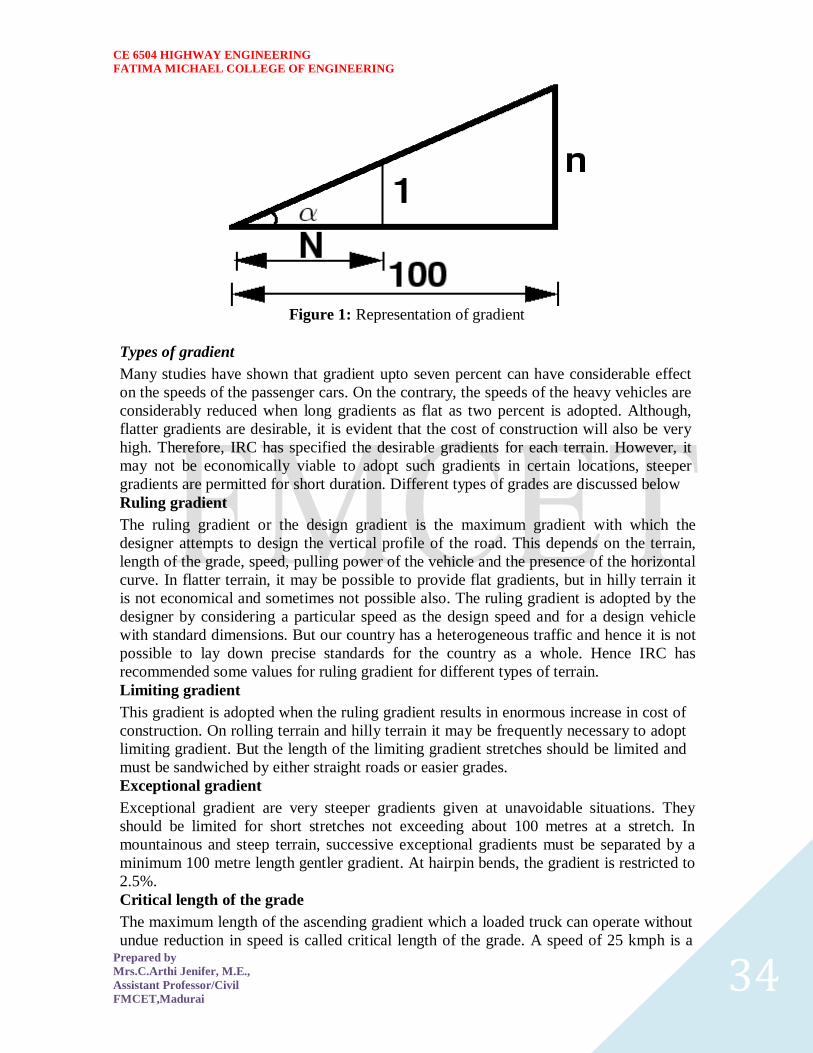
CE 6504 HIGHWAY ENGINEERING
FATIMA MICHAEL COLLEGE OF ENGINEERING
Prepared by
MrsCArthi Jenifer ME
Assistant ProfessorCivil
FMCETMadurai 34
Figure 1 Representation of gradient
Types of gradient
Many studies have shown that gradient upto seven percent can have considerable effect
on the speeds of the passenger cars On the contrary the speeds of the heavy vehicles are
considerably reduced when long gradients as flat as two percent is adopted Although
flatter gradients are desirable it is evident that the cost of construction will also be very
high Therefore IRC has specified the desirable gradients for each terrain However it
may not be economically viable to adopt such gradients in certain locations steeper
gradients are permitted for short duration Different types of grades are discussed below
Ruling gradient
The ruling gradient or the design gradient is the maximum gradient with which the
designer attempts to design the vertical profile of the road This depends on the terrain
length of the grade speed pulling power of the vehicle and the presence of the horizontal
curve In flatter terrain it may be possible to provide flat gradients but in hilly terrain it
is not economical and sometimes not possible also The ruling gradient is adopted by the
designer by considering a particular speed as the design speed and for a design vehicle
with standard dimensions But our country has a heterogeneous traffic and hence it is not
possible to lay down precise standards for the country as a whole Hence IRC has
recommended some values for ruling gradient for different types of terrain
Limiting gradient
This gradient is adopted when the ruling gradient results in enormous increase in cost of
construction On rolling terrain and hilly terrain it may be frequently necessary to adopt
limiting gradient But the length of the limiting gradient stretches should be limited and
must be sandwiched by either straight roads or easier grades
Exceptional gradient
Exceptional gradient are very steeper gradients given at unavoidable situations They
should be limited for short stretches not exceeding about 100 metres at a stretch In
mountainous and steep terrain successive exceptional gradients must be separated by a
minimum 100 metre length gentler gradient At hairpin bends the gradient is restricted to
25
Critical length of the grade
The maximum length of the ascending gradient which a loaded truck can operate without
undue reduction in speed is called critical length of the grade A speed of 25 kmph is a
CE 6504 HIGHWAY ENGINEERING
FATIMA MICHAEL COLLEGE OF ENGINEERING
Prepared by
MrsCArthi Jenifer ME
Assistant ProfessorCivil
FMCETMadurai 35
reasonable value This value depends on the size power load grad-ability of the truck
initial speed final desirable minimum speed
Minimum gradient
This is important only at locations where surface drainage is important Camber will take
care of the lateral drainage But the longitudinal drainage along the side drains require
some slope for smooth flow of water Therefore minimum gradient is provided for
drainage purpose and it depends on the rain fall type of soil and other site conditions A
minimum of 1 in 500 may be sufficient for concrete drain and 1 in 200 for open soil
drains are found to give satisfactory performance Sight distance available from a point is the actual distance along the road surface which a driver
from a specified height above the carriage way has visibility of stationary or moving objects
Sight distance required by drivers applies to both geometric design of highways and for
traffic control The sight distance situations are considered in the design
i) Stopping or absolute minimum sight distance
ii) Safe overtaking or passing sight distance
iii) Safe sight distance for entering into uncontrolled intersections
Apart from the three situations mentioned above the following sight distance are considered by the
IRC in highway design
Intermediate sight distance
This is defined as twice the stopping sight distance when overtaking sight distance
cannot be provided intermediate sight distance is provided to give limited overtaking opportunities
to fast vehicles
Head light sight distance
This is the distance visible to a driver during night driving under the illumination of the
vehicle head lights
Stopping sight distance
The minimum sight distance available on a highway at any spot should be of sufficient
length to stop a vehicle traveling at design speed safely without collision with any other obstruction
The absolute minimum sight distance is therefore equal to the stopping sight distance
which is also sometimes called nonpassing sight distance The sight distance available on a road to a
driver at any instance depends on
i) Features of the road
ii) Height of the drivers eye above the road surface
iii) Height of the object above the road surface
The distance within which a motor vehicle can be stopped depends upon the factors listed below
a) Total reactions time of the driver
b) Speed of vehicle
c) Efficiency of breaks
d) Frictional resistance between the road and tyres
e) Gradient of the road
Total reaction time
) Reaction time of the driver is the time taken from the instant the object is visible to the
driver to the instant the brakes are effectively applied
) The total reaction time may be split up into two parts
CE 6504 HIGHWAY ENGINEERING
FATIMA MICHAEL COLLEGE OF ENGINEERING
Prepared by
MrsCArthi Jenifer ME
Assistant ProfessorCivil
FMCETMadurai 36
i) Perception time
ii) Brake reaction time
PIEV theory
According to this theory the total reaction time of the driver is split into four parts
i) Perception
ii) Intellection
iii) Emotion
iv) Volition
Speed of Vehicle
The stopping distance depends very much on the speed of the vehicle first during the
total reaction time of the driver the distance moved by the vehicle will depend on the speed
Efficiency of brakes
The braking efficiency is said to be 100 percent if the wheels are fully licked preventing
them from rotating on application of the brakes This will result in 100 percent skidding which is
normally undesirable except in utmost emergency
Frictional resistance between road and tyres
The frictional resistance developed between road and tyres or the skid resistance depends
on the type and condition of the road surface and the tyres IRC has specified a design friction
coefficient of 035 to 04 depending upon the speed to be used for finding the braking distance in the
calculation of stopping sight distance
Analysis of stopping distance
i) The distance traveled by the vehicle during the total reaction time known as lag
distance
ii) The distance traveled by the vehicle after the application of the brakes is known as
braking distance
Overtaking sight distance
The minimum distance open to the vision of the driver of a vehicle intending to overtake
slow vehicle ahead with safety against the traffic of opposite direction is known as the minimum
overtaking sight distance(OSD) or Safe passing sight distance available
The overtaking sight distance is the distance measured along the center of the road which
a driver with his eye level 12m above the road surface can see the top of an object 12m above the
road surface
Some of the important factors on which the minimum overtaking sight distance required
a) Speed of
i) overtaking vehicle
ii) overtaken vehicle
iii) The vehicle coming from opposite direction
b) Distance between the overtaking and overtaken vehicles the minimum spacing
depends on the steeds
a) Skill and reaction time of the driver
b) Rate of acceleration of overtaking vehicle
c) Gradient of the road
Criteria for sight distance requirements on highway
) The absolute minimum sight distance required throughout the length of the road is the
SSD which should invariably be provided at all places
CE 6504 HIGHWAY ENGINEERING
FATIMA MICHAEL COLLEGE OF ENGINEERING
Prepared by
MrsCArthi Jenifer ME
Assistant ProfessorCivil
FMCETMadurai 37
) On horizontal curves the obstruction on the inner side of the curves should be cleared
to provide the required set back distance and absolute minimum sight distance
) On vertical summit curves the sight distance requirement may be fulfilled by proper
design of the vertical alignment
Hairpin bent
TYPES OF CURVES ON HILL ROADS
The following are the important types of curves provided on hill Roads-
1 Hair-Pin Curves
2 Salient Curves
3 Re-entrant Curves 1 Hair-pin curves - The curve in a hill road which changes its direction through an angle of 180
degree or so down the hill on the same side is known as hair-pin curve
A Hair-Pin Bend
This curve is so called because it conforms to the shape of a hair-pin The bend so formed at the
hair-pin curve in a hill road is known as hair-pin bend This type of curve should be located on a
hill side having the minimum slope and maximum stability It must also be safe from view point of
landslides and ground water Hair-pin bends with long arms and farther spacing are always
preferred They reduce construction problems and expensive protective works Hair-pin curves or
bends of serpentine nature are difficult to negotiate and should therefore be avoided as far as
possible
Salient curves - The curves having their convexity on the outer edges of a hill road are called
salient curves The centre of curvature of a salient curve lies towards the hill side This type of curve
occurs in the road length constructed on the ridge of a hill the bend so formed at the salient curve in
a hill road known as corner bend
Salient curves are very dangerous for fast moving traffic At such a curve or at corner bend the
portion of projecting hill side is usually cut down to improve the visibility as shown in fig (Re-
entrant curve) The outer edge of the road at such a curve is essentially provided with a parapet wall
for protection of the vehicles from falling down the hill slope
CE 6504 HIGHWAY ENGINEERING
FATIMA MICHAEL COLLEGE OF ENGINEERING
Prepared by
MrsCArthi Jenifer ME
Assistant ProfessorCivil
FMCETMadurai 38
3 Re-entrant curves - The curves having their convexity on the inner edge of a hill road are called
re-entrant curves
Re-entrant curves
The centre of curvature of a re-entrant curves lies away from the hill side This type of curve occurs
in the road length constructed in the calley of a hill
These curves are less dangereous as they provide adequate visibility to the fast moving traffic At
such curves the parapet wall is provided only for safety of fast moving traffic
CE 6504 HIGHWAY ENGINEERING
FATIMA MICHAEL COLLEGE OF ENGINEERING
Prepared by
MrsCArthi Jenifer ME
Assistant ProfessorCivil
FMCETMadurai 39
UNIT ndash III DESIGN OF RIGID AND FLEXIBLE PAVEMENTS
COMPARISON OF RIGID AND FLEXIBLE PAVEMENTS
The comparisons are
i) Design precision
A cement concrete pavement is amerable to a much more precise structural analysis
than a flexible pavement Flexible pavements designs are mainly empirical Computer aided analysis
of layered system is making the flexible pavement design more exact than hitherto
ii) Life
) Cement concrete slabs of a thin section constructed in the early 1940rsquos are still in
existence in India though many of them have cracked badly and a few of them have been ripped
open and rebuilt in recent ties
) A major project in cement concrete road construction between Agra and Mathura It can
safely be said that a well-designed concrete slab has a life of about 40 years
) Compared to this the life of a flexible pavement generally varies from 10 to 20 years
iii) Maintenance
) A well-designed cement concrete pavement needs very little maintenance The only
maintenance needed is I respect of joints
) The surface is unaffected by spillage of oil and lubricants bituminous surfaces on the
other hand need great inputs in maintenance
) The surface is affected by spillage of oil and lubricants The surface is also affected by
natural weathering agents like air water ad temperature changes
) A cement concrete pavement on the other hand needs a small amount for maintaining
joints
iv) Initial cost
) The argument so far used against a cement concrete slab is that it is much more costly
than a flexible pavement
) The latter specifications no doubt represent the rock-bottom needs of a road in India but
these specifications can hardly provide a smooth and durable surface
v) Stage construction ) Road construction is generally done adopting a policy of stage construction especially for
low volume roads As traffic grows additional layers in the form of water bound macadam and
superior surfacing are added on
) Initial outlay is minimum and additional outlays are in keeping with traffic growth This is
a great advantage when dealing with new roads in an atmosphere of austerity
vi) Availability of materials
) Cement bitumen stone aggregates and gravelsand are the major materials involved in
pavement Construction Cement has been in serious short supply in the country for the past many
decades
) Bitumen is also not available plentifully in India There is also the danger of the entire oil
reserves in the world shrinking during the next two or three decades
) In locations where stone aggregates are scarce cement concrete may have an advantage
for flexible pavements
vii) Surface characterstics
CE 6504 HIGHWAY ENGINEERING
FATIMA MICHAEL COLLEGE OF ENGINEERING
Prepared by
MrsCArthi Jenifer ME
Assistant ProfessorCivil
FMCETMadurai 40
) A good cement concrete surface is smooth and free from rutting potholes and
corrugations In a bituminous surface it is only the asphaltic concrete surface that can give
comparable rideablity
) A well-constructed cement concrete pavement surface can have a permanent nonskid
surface A bituminous surface can also be designed to have a good skid resistant surface
viii) Utility location
) In cement concrete slabs proper thought has to be given to locate utilities such as water
pipes telephone lines and electric cables
) It is difficult to rip open the slab and restore it to be the original condition if any changes
in the utilities lines are to be made
ix) Glame and night visibility
) Concrete pavements have a gray color which can cause glam under sunlight Colored
cement can reduce the grave
) On the other hand bituminous roads need more street lighting
x) Traffic dislocation during construction
) A cement concrete pavement requires 28 days before it can be thrown open to traffic On
the other hand a bituminous surface can be thrown open to traffic shortly after it is rolled
xi) Environmental considerations during construction
) The process of heating of bitumen and aggregates and mixing them together on hot mix
plants can prove to be much more hazardous to the environment than cement concrete construction
where no heating of any material is involved
xii) Overall economy on a life cycle basis
) A good road is costly to construct but once constructed such a road requires little
maintenance and results in savings in vehicle operating costs
) The comparative economy of a flexible pavement and a rigid pavement has proved that on
overall economic considerations
Types of pavement structure
Based on the structural behavior pavements are generally classified into three
categories
i) Flexible pavements
ii) Rigid pavements
iii) Semi rigid pavements
Flexible pavements
) Flexible pavements are those which on the whole have low or negligible flexural
strength and are rather flexible in their structural action under the loadsThe flexible pavement
layers reflect the deformation of the lower layers on to the surface of the layer
) A flexible pavement consists of four components(i) Soil subgrade (ii) sub base
course (iii) base course (iv) Surface course
CE 6504 HIGHWAY ENGINEERING
FATIMA MICHAEL COLLEGE OF ENGINEERING
Prepared by
MrsCArthi Jenifer ME
Assistant ProfessorCivil
FMCETMadurai 41
) The flexible pavement layers transmit the vertical or compressive stresses to the lower layers
by grain to grain transfer through the points of contact in the granular structure A well
compacted granular structure consisting of strong added aggregate can transfer the compressive
stresses
) The load spreading ability of this layer therefore depends on the type of the materials and mix
design factors Bituminous concrete is one of the best flexible pavements layer materials Other
materials which fall under the group are all granular materials with or without bituminous
binder granular base and sub base course materials
) The vertical compressive stress is maximum on the pavement surface directly under the wheel
and is equal to the contact pressure under the wheel The flexible pavement may be constructed
in a number of layers and the top layer has to be strongest as the highest compressive stresses
) Flexible pavements are commonly designed using empirical design charts or equations taking
into account some of the design factors there are also semi empirical and theoretical design
methods
Rigid pavements
) Rigid pavements are those which possess note flexural strength or flexural rigidity
The stresses are not transferred from grain to grain to the lower layers as in the ease of flexible
pavements layers
) The rigid pavements are made of Portland cement concrete plain reinforced or
prestressed concrete The plain cement concrete slabs are expected to take up about 40 kgcm2
flexural stress
) The rigid pavement has the slab action and is capable of transmitting the wheel
load stresses through a wider area below The main point of difference in the structural behavior
of rigid pavement as compared to the flexible pavement is that the critical condition of stress in
the rigid pavement is the maximum flexural stress occurring in the slab due to wheel load and
the temperature changes whereas in the flexible pavement
) As the rigid pavement slab has tensile strength tensile stresses are developed due
to the bending of the slab under wheel load and temperature variations Thus the types of
stresses developed and their distribution within the cement concrete slab are quirt different
) The cement concrete pavement slab can very well serve as a wearing surface as
well an effective base course The rigid pavement structure consists of a cement concrete slab
below which a granular base or sub base course may be provided
) Though the cement concrete slab can also be laid directly over the soil subgrade
consists of fine grained soil
) the rigid pavements are usually designed and the stresses are analyzed using the
elastic theory assuming the pavements as a n elastic plate resting over an elastic or a viscous
foundation
Semi rigid pavements
) when bonded materials like the pozzolanic concrete lean cement concrete or soil
cement are used in the base course or sub base course layer the pavement layer has considerably
higher flexural strength than the common flexible pavement layers
) when this intermediate class of materials are used in the base or sub base course
layer of the pavements they are called semi rigid pavements
CE 6504 HIGHWAY ENGINEERING
FATIMA MICHAEL COLLEGE OF ENGINEERING
Prepared by
MrsCArthi Jenifer ME
Assistant ProfessorCivil
FMCETMadurai 42
) This third category of semi rigid pavement are either designed as flexible
pavements with some correction factors to find the thickness requirements based on experience
or by using a new design approach
) The semi rigid pavement materials have low resistance to impact and abrasion and
therefore are usually provided with flexible pavement surface course
Various functions of pavement components
The functions are
Soil sub grade and its evaluation
) The soil sub grade is a layer of natural soil prepared to receive the layers of pavement
materials placed over it It is essential that at no time the soil sub grade is overstressed it means that
the pressure transmitted on the top of the sub grade is within the allowable limit
) Many tests are known for measuring the strength properties of the sub grades Some of the
tests have been standardized for the use The common strength test for the evaluation of soil
subgrade is
i) California bearing ratio test
ii) California resistance value test
iii) Triaxial compression test
iv) Plate bearing test
CALIFORNIA BEARING RATIO (CBR) TEST
It is evolved for the empirical method of flexible pavement design The CBR test is carried
out either in the laboratory on prepared specimens or in the field by taking in situ measurements
California resistance value
It is found by using have been stabliometerThis test is used in an empirical method of
flexible pavement design based on soil strength
Triaxial test
It is the most important soil strength but still the test is not very commonly used in structural
design of pavements
Plate bearing test
It is carried out using a relatively large diameter plate to evaluate the load supporting
capacity of supporting power of the pavement layers The results are plate bearing tests are used in
flexible pavement design method like McLeod method on based on layer system analysis by
brumister
Sub base and base courses and their evaluation
) There layers are made of broken stones bound or unbound aggreagatesome times in sub
base course a layer of stabilized soil(or) Selected granular soil is also used
) however at the sub base course it is desirable to use smaller size graded aggregates When
the sub grade consists of fine grained soil and when the pavement carries heavy wheel loads
CE 6504 HIGHWAY ENGINEERING
FATIMA MICHAEL COLLEGE OF ENGINEERING
Prepared by
MrsCArthi Jenifer ME
Assistant ProfessorCivil
FMCETMadurai 43
) Sub base course primarily has the similar function as of the base course and is provided
with inferior materials than of base course Base courses are used under rigid pavement for
i) Preventing pumping
ii) Protecting the sub grade against frost action
) Thus the fundamental purpose of abase course and sub base course is to provide a stress
transmitting medium to spread the surface wheel loads in such manner
) The sub base and base course layers may be evaluated by suitable strength or stability test
like plate bearing CBR test
WEARING COURSE AND ITS EVALUATION
) The purpose of the wearing course is to give a smooth riding surface that is dense It
resists pressure exerted by tyres and takes up wear and tear due to the traffic
) Wearing course also offers a water tight layer against the surface water infiltration The
flexible pavement normally a bituminous surfacing is used as a wearing course
) In rigid pavements the cement concrete acts like a base course as well as wearing course
Most popular test in use is marshal stability test where in the optimum content of bitumen binder is
worked out based on the stability density
) Plate bearing test and Bankelman beam test are also sometimes made use of for evaluating
the wearing course and the pavement as a whole
Various factors to be considered in pavement design and the significance
Pavement design consists of two parts
i) Mix design of materials to be used in each pavement component layer Thickness design of the
pavement and the component layers
The various factors to be considered for the design of pavements are given below
i) Design wheel load
ii) Sub grade soil
iii) Climatic factors
iv) Pavement component layers
v) Environmental factors
vi) Special factors in the design of different types of pavements
Design wheel load
The various wheel load factors to be considered in pavement design are
i) Maximum wheel load
ii) Contact pressure
iii) Dual or multiple wheel loads
iv) Repetition of loads
Maximum wheel load
The wheel load configurations are important to know the way in which the loads of a given
vehicle are applied on the pavement surface
) For highways the maximum legal axle load as specified by Indian road congress is 8170
kg with a maximum equivalent single wheel load of 4085 kg
) The evaluation for vertical stress computations under a uniformly distribute of circular
load based on Boussineqrsquos theory is given by
CE 6504 HIGHWAY ENGINEERING
FATIMA MICHAEL COLLEGE OF ENGINEERING
Prepared by
MrsCArthi Jenifer ME
Assistant ProfessorCivil
FMCETMadurai 44
2
322
3
1
za
zpz
σz = vertical stress at depth z
P= surface pressure
Z=depth at which σz computed
A=radius of loaded area
Contact pressure
Generally the wheel load is assumed to be distributed over a circular area But by
measurement of the imprints of tyers with different load and inflation pressures Three terms in use
with reference to tyre pressure are
Tyre pressure
Inflation pressure
Contact pressure
Tyre pressure and inflation pressure mean exactly the same the contact pressure is found to be more
than tyre pressure when the tyre pressure is less than 7 kgm2 and it is vice versa when the tyre
pressure exceeds this value
Contact pressure can be measured by the relationship
Load on wheel
Contact pressure = ----------------------------------------
Contact area or area of imprint
The general variation between the tyre pressure and measured contact pressure is shown in this fig
The ratio of contact pressure to type pressure is defined as rigidity factor Thus value of rigidity
factor is 10 for an average tyre pressure of 7 Kgcm2This value is higher than unity for lower type
pressures and less than unity for tyre pressures higher than 7 kgcm2
Equivalent single wheel load (ESWL)
) The maximum wheel load within the specified limit and to carry greater load it is
necessary to provide dual wheel assembly to the rear axles of the roads vehicles
) In other words the pressure at a certain depth below the pavement surface cannot be
obtained by numerically adding the pressure caused by any one wheel
) The effect is in between the single load and two times load carried by one wheel The load
dispersion is assumed to be at an angle of 450In the dual wheel load assembly let d be the clear gap
between the two wheels S be the spacing between the centers of the wheels and a be the radius of
the circular contact area of each wheel Then S = (d + 2a)
) ESWL may be determined based on either equivalent deflection or equivalent stress
criterianMultiple wheel loads are convert to ESWL and this value is used in pavement design The
ESWL is usually determined by the equivalent stress criterion using a simple graphical method
CE 6504 HIGHWAY ENGINEERING
FATIMA MICHAEL COLLEGE OF ENGINEERING
Prepared by
MrsCArthi Jenifer ME
Assistant ProfessorCivil
FMCETMadurai 45
) A straight line relationship is assumed between ESWL and depth on log scales For
determining ESWL the plot is made as shown in fig
) Two points A and B are plotted on the log-log graph with coordinates of A (Pd2) and
B(2p2s)line AB is a plot which is the focus of points where any single wheel load is equivalent to a
certain set of dual wheels
) To Calculate the ESWL for a dual assembly it is essential to estimate a design thickness of
the pavement If the design thickness so obtained is equal to the estimated thickness then the ESWL
calculations could be considered as correct Otherwise trials are made
) In heavy trucks and trailers the load on each wheel may be further reduced by multiple
wheels and tandem axles
Repetition of loads
) The deformation of load pavement (or) sub grade due to a single application of wheel load
may be small It required carrying out traffic surveys for accounting the factor of repetitions for
wheel loads in the design of pavement
) Data collected are converted to some constant equivalent wheel loads Equivalent wheel
load is a single load equivalent to the repeated applications of any particular wheel load on a
pavement which requires the same thickness and strength of pavements
) McLeod has given a procedure for evolving equivalent load factors for designing flexible
pavements
Various methods of flexible pavement design
) The flexible pavement is built with number of layers In the design process it is to be
ensured that under the application of load none of the layers is overstressed
) The maximum intensity of stresses occurs in the top layer of the pavement The
magnitude of load stresses reduces at lower layers
) In the design of flexible pavements it has yet not been possible to have a rational design
method wherein design process and service behavior of the pavement can be expressed by
mathematical laws
) Flexible pavement design methods are accordingly either empirical or semi empirical In
these methods the knowledge and experience gained on the behavior of the pavements in the past
are usefully utilized
Various approaches of flexible pavement design may be thus classified into three groups
i) Empirical method
ii) Semi-empirical or Semi theoretical method
iii) Theoretical method
) Empirical methods are either based on physical properties or strength parameters of soil
sub grade When the design is based on stress strain function and modified base on experience it
may be called semi-empirical or semi-theoretical There are design methods based on theoretical
analysis and mathematical computations
Out of the flexible pavement design method available is
i) Group index method
ii) California bearing ratio method
iii) California R value (or) Stabiliometer method
iv) Triaxial test method
CE 6504 HIGHWAY ENGINEERING
FATIMA MICHAEL COLLEGE OF ENGINEERING
Prepared by
MrsCArthi Jenifer ME
Assistant ProfessorCivil
FMCETMadurai 46
v) McLeod method
vi) Burmister method
Group index method
) Group index value is an arbitrary index assigned to the soil type in numerical equations
base on the percent fines liquid limit and plasticity index
) The design chart for group index method for determining the pavement thickness is given
in fig
The traffic volume in this method is divided in three groups
Traffic volume No of vehicles per day
Light Less than 50
Medium 50 to 300
Heavy Over 300
The design of the pavement thickness by this method first the G1 value of the soil is found the
anticipated traffic is estimated and is designated as light medium or heavy as indicated
The G1 method of pavement design is essentially an empirical method based on physical properties
of the subgrade soil This method does not consider the strength characteristics of the subgrade soil
and therefore is open to question regarding the reliability of the design based on the index properties
of the soil only
California bearing ratio method
) California division of highways in the USA developed CBR method for
pavement design The majority of design curves developed later are base on the original curves
proposed by OJporter
) One of the chief advantages of CBR method is the simplicity of the test procedure
The CBR tests were carried out by the California state highway department on existing pavement
layers including subgrade sub base and base course
) Based on the extensive CBR test data collected on pavement which behaved
satisfactory and those which failed an empirical design chart was developed correlating the CBR
value and the pavement thickness The basis of the design chart is that a material with a given CBR
required a certain thickness of pavement layer as a cover
) A higher load needs a thicker pavement layer to protect the sub grade Design
curves correlating the CBR value with total pavement thickness cover were developed by the
California state highway department for wheel loads of 3175kg and 5443 kg representing light and
heavy traffic The design curves are shown in this fig
It is possible to extend the CBR design curves for various loading conditions nusing the expression
t= 2
1
1751
pCBRp
t=2
1
751
A
CBR
p
Hence
CE 6504 HIGHWAY ENGINEERING
FATIMA MICHAEL COLLEGE OF ENGINEERING
Prepared by
MrsCArthi Jenifer ME
Assistant ProfessorCivil
FMCETMadurai 47
t= pavement thickness cm
p=Wheel load kg
CBR= California bearing ratio percent
P=tyre pressure kgcm2
A= area of contactcm2
IRC Recommendations
a) The CBR tests should be performed on remoulded soils in the laboratory The specimens should
be prepared by static compaction wherever possible and otherwise by dynamic compaction
b) For the design of new roads the sub grade soil sample should be compacted at OMC to proctor
density whenever suitable compaction equipment
c) The CBR test samples may be soaked in water for four days period before testing the annual
rainfall is less than 50 cm and the water table is too deep to affect the sub grade and imperable
surfacing is provided to carrying out CBR test
d) If the maximum variations in CBR value of the three specimens exceed the specified limits the
design CBR should be average of at least six samples
e) The top 50 cm of sub grade should be compacted at least up to 95 to 100 percent of proctor
density
f) An estimate of the traffic should be carried by the road pavements at the end of expected in view
the existing traffic and probable growth rate of traffic
g) The traffic for the design is considered in units of heavy vehicles per day in both directions and is
divided into seven categories A to G The design thickness is considered applicable for single axle
loads up to 8200 kg and tandom axle loads up to 14500 kg
h) When sub base course materials contain substantial proportion of aggregates of size above 20mm
the CBR value of these materials would not be valid for the design of subsequent layers above them
The CBR method of pavement design gives the total thickness requirement of the pavement above a
sub grade and thickness value would remain the same quality of materials used in component layers
California resistance value method
) In this design method based on stabliometer R-value and cohesiometer C-value
Based on performance data it was established by pavement thickness varies directly with R value
and algorithm of load repetitions It varies inversely with fifth root of c valueThe expression for
pavement thickness is given by the empirical equation
T=
5
1
1 90
C
RTK
Hence
T=total thickness of pavement cm
K=Numerical constant 0166
T1=traffic index
R= stabiliometer resistance value
C=Cohesiometer value
CE 6504 HIGHWAY ENGINEERING
FATIMA MICHAEL COLLEGE OF ENGINEERING
Prepared by
MrsCArthi Jenifer ME
Assistant ProfessorCivil
FMCETMadurai 48
In the design of flexible pavements based on California resistance value method for the following
data are needed
) R-value of soil subgrade
) T1 value
) Equivalent C-value
) R value of soil subgrade is obtained from the test using stablio meterThe
computation of T1 value has been explained
Equivalent C-value
) The cohesion meter value c is obtained for each layer of pavement material
separately from tests However the composite or equivalent C-value of the pavement may be
estimated if the thickness of each component layer and the c-value of the material of the layer are
known
) while designing a pavement as the thickness of the pavement is not known it is
easier if the pavement is first assumed to consist of any one material like gravel base course with
known C-value
) Subsequently the individual thickness of each layer is converted in terms of gravel
equivalent by using relationship
5
1
1
2
2
1
C
C
t
t
) t1 and t2 are the thickness values of any two pavement layersc1 and c2 are their
corresponding cohesiometer values
CE 6504 HIGHWAY ENGINEERING
FATIMA MICHAEL COLLEGE OF ENGINEERING
Prepared by
MrsCArthi Jenifer ME
Assistant ProfessorCivil
FMCETMadurai 49
UNIT 4 MATERIAL AND MAINTENANCE
SUMMIT CURVE
Summit curves are vertical curves with gradient upwards They are formed when two
gradients meet as illustrated in figure 1 in any of the following four ways
1 When a positive gradient meets another positive gradient [figure 1a]
2 When positive gradient meets a flat gradient [figure 1b]
3 When an ascending gradient meets a descending gradient [figure 1c]
4 When a descending gradient meets another descending gradient [figure 1d]
Type of Summit Curve
Many curve forms can be used with satisfactory results the common practice has been to
use parabolic curves in summit curves This is primarily because of the ease with it can
be laid out as well as allowing a comfortable transition from one gradient to another
Although a circular curve offers equal sight distance at every point on the curve for very
small deviation angles a circular curve and parabolic curves are almost congruent
Furthermore the use of parabolic curves were found to give excellent riding comfort
Figure 1 Types of summit curves
Design Consideration
In determining the type and length of the vertical curve the design considerations are
comfort and security of the driver and the appearance of the profile alignment Among
these sight distance requirements for the safety are most important on summit curves
The stopping sight distance or absolute minimum sight distance should be provided on
these curves and where overtaking is not prohibited overtaking sight distance or
intermediate sight distance should be provided as far as possible When a fast moving
vehicle travels along a summit curve there is less discomfort to the passengers This is
because the centrifugal force will be acting upwards while the vehicle negotiates a
summit curve which is against the gravity and hence a part of the tyre pressure is
relieved Also if the curve is provided with adequate sight distance the length would be
sufficient to ease the shock due to change in gradient Circular summit curves are
identical since the radius remains same throughout and hence the sight distance From
CE 6504 HIGHWAY ENGINEERING
FATIMA MICHAEL COLLEGE OF ENGINEERING
Prepared by
MrsCArthi Jenifer ME
Assistant ProfessorCivil
FMCETMadurai 50
this point of view transition curves are not desirable since it has varying radius and so the
sight distance will also vary The deviation angles provided on summit curves for
highways are very large and so the simple parabola is almost congruent to a circular arc
between the same tangent points Parabolic curves are easy for computation and also it
had been found out that it provides good riding comfort to the drivers It is also easy for
field implementation Due to all these reasons a simple parabolic curve is preferred as
summit curve Length of the summit curve
The important design aspect of the summit curve is the determination of the length of the
curve which is parabolic As noted earlier the length of the curve is guided by the sight
distance consideration That is a driver should be able to stop his vehicle safely if there is
an obstruction on the other side of the road Equation of the parabola is given by
where where N is the deviation angle and is the length of the In
deriving the length of the curve two situations can arise depending on the uphill and
downhill gradients when the length of the curve is greater than the sight distance and the
length of the curve is greater than the sight distance
Let is the length of the summit curve is the SSDISDOSD is the deviation angle
drivers eye height (12 m) and the height of the obstruction then the length of the
summit curve can be derived for the following two cases The length of the summit curve
can be derived from the simple geometry as shown below
Case a Length of summit curve greater than sight distance( )
Figure 1 Length of summit curve ( )
The situation when the sight distance is less than the length of the curve is shown in
figure 1
CE 6504 HIGHWAY ENGINEERING
FATIMA MICHAEL COLLEGE OF ENGINEERING
Prepared by
MrsCArthi Jenifer ME
Assistant ProfessorCivil
FMCETMadurai 51
(1)
Case b Length of summit curve less than sight distance
The second case is illustrated in figure 1
Figure 1 Length of summit curve
CE 6504 HIGHWAY ENGINEERING
FATIMA MICHAEL COLLEGE OF ENGINEERING
Prepared by
MrsCArthi Jenifer ME
Assistant ProfessorCivil
FMCETMadurai 52
From the basic geometry one can write
(1)
Therefore for a given and to get minimum differentiate the above equation
with respect to and equate it to zero Therefore
Solving the quadratic equation for
(2)
Now we can substitute back to get the value of minimum value of for a given
and Therefore
Solving for
CE 6504 HIGHWAY ENGINEERING
FATIMA MICHAEL COLLEGE OF ENGINEERING
Prepared by
MrsCArthi Jenifer ME
Assistant ProfessorCivil
FMCETMadurai 53
(3) (4
CE 6504 HIGHWAY ENGINEERING
FATIMA MICHAEL COLLEGE OF ENGINEERING
Prepared by
MrsCArthi Jenifer ME
Assistant ProfessorCivil
FMCETMadurai 54
When stopping sight distance is considered the height of drivers eye above the road
surface ( ) is taken as 12 metres and height of object above the pavement surface ( )
is taken as 015 metres If overtaking sight distance is considered then the value of
drivers eye height ( ) and the height of the obstruction ( ) are taken equal as 12
metres
Valley curve
Valley curve or sag curves are vertical curves with convexity downwards They are
formed when two gradients meet as illustrated in figure 1 in any of the following four
ways
Figure 1 Types of valley curve
1 When a descending gradient meets another descending gradient [figure 1a]
2 When a descending gradient meets a flat gradient [figure 1b]
3 When a descending gradient meets an ascending gradient [figure 1c]
4 When an ascending gradient meets another ascending gradient [figure
Design considerations
There is no restriction to sight distance at valley curves during day time But visibility is
reduced during night In the absence or inadequacy of street light the only source for
visibility is with the help of headlights Hence valley curves are designed taking into
account of headlight distance In valley curves the centrifugal force will be acting
downwards along with the weight of the vehicle and hence impact to the vehicle will be
more This will result in jerking of the vehicle and cause discomfort to the passengers
Thus the most important design factors considered in valley curves are (1) impact-free
movement of vehicles at design speed and (2) availability of stopping sight distance
under headlight of vehicles for night driving
For gradually introducing and increasing the centrifugal force acting downwards the best
shape that could be given for a valley curve is a transition curve Cubic parabola is
generally preferred in vertical valley curves See figure 1
CE 6504 HIGHWAY ENGINEERING
FATIMA MICHAEL COLLEGE OF ENGINEERING
Prepared by
MrsCArthi Jenifer ME
Assistant ProfessorCivil
FMCETMadurai 55
Figure 1 Valley curve details
During night under headlight driving condition sight distance reduces and availability of
stopping sight distance under head light is very important The head light sight distance
should be at least equal to the stopping sight distance There is no problem of overtaking
sight distance at night since the other vehicles with headlights could be seen from a
considerable distance
Length of the valley curve
The valley curve is made fully transitional by providing two similar transition curves of
equal length The transitional curve is set out by a cubic parabola where
The length of the valley transition curve is designed based on two criteria
1 comfort criteria that is allowable rate of change of centrifugal acceleration is
limited to a comfortable level of about
2 safety criteria that is the driver should have adequate headlight sight distance at
any part of the country
Comfort criteria
The length of the valley curve based on the rate of change of centrifugal acceleration that
will ensure comfort Let is the rate of change of acceleration the minimum radius of
the curve is the design speed and is the time then is give
CE 6504 HIGHWAY ENGINEERING
FATIMA MICHAEL COLLEGE OF ENGINEERING
Prepared by
MrsCArthi Jenifer ME
Assistant ProfessorCivil
FMCETMadurai 56
For a cubic parabola the Value Safety criter Length of the valley curve for headlight distance may be determined for two conditions
(1) length of the valley curve greater than stopping sight distance and (2) length of the
valley curve less than the stopping sight distance of for length is given by
Case 1 Length of valley curve greater than stopping sight distance ( )
The total length of valley curve is greater than the stopping sight distance SSD The
sight distance available will be minimum when the vehicle is in the lowest point in the
valley This is because the beginning of the curve will have infinite radius and the bottom
of the curve will have minimum radius which is a property of the transition curve The
case is shown in figure 1
Figure 1 Valley curve case 1
From the geometry of the figure we have
CE 6504 HIGHWAY ENGINEERING
FATIMA MICHAEL COLLEGE OF ENGINEERING
Prepared by
MrsCArthi Jenifer ME
Assistant ProfessorCivil
FMCETMadurai 57
(1)
where is the deviation angle in radians is the height of headlight beam is the
head beam inclination in degrees and is the sight distance The inclination is 1
degree
Case 2 Length of valley curve less than stopping sight distance ( )
The length of the curve is less than SSD In this case the minimum sight distance is
from the beginning of the curve The important points are the beginning of the curve and
the bottom most part of the curve If the vehicle is at the bottom of the curve then its
headlight beam will reach far beyond the endpoint of the curve whereas if the vehicle is
at the beginning of the curve then the headlight beam will hit just outside the curve
Therefore the length of the curve is derived by assuming the vehicle at the beginning of
the curve The case is shown in figure 1
From the figure
(1) Note that the above expression is approximate and is satisfactory because in practice the gradients
are very small and is acceptable for all practical purposes We will not be able to know prior to
which case to be adopted Therefore both has to be calculated and the one which satisfies the
condition is adopted
1 Flexible pavement
2 Rigid pavement
Flexible pavement
These pavements reflect the deformation of sub grade and the subsequent layers to the
surface
Rigid pavement
The rigid characteristic of the pavement are associated with rigidity or flexural strength
CE 6504 HIGHWAY ENGINEERING
FATIMA MICHAEL COLLEGE OF ENGINEERING
Prepared by
MrsCArthi Jenifer ME
Assistant ProfessorCivil
FMCETMadurai 58
or slab action so the load is distributed over a wide area of sub grade soil
Flexible pavement Definition
These pavements reflect the deformation of sub grade and the subsequent layers to the
surface Flexible usually asphalt is laid with no reinforcement or with a specialized
fabric reinforcement that permits limited flow or repositioning of the roadbed under
ground changes
The design of flexible pavement is based on load distributing characteristic of the
component layers The black top pavement including water amp gravel bound macadam fall
in this category
Flexible pavement on the whole has low or negligible flexible strength flexible in their
structural action) The flexible pavement layers transmit the vertical or compressive
stresses to the lower layers by grain transfer through contact points of granular structure
The vertical compressive stress is maximum on the pavement surface directly under the
wheel load and is equal to contact pressure under the wheels Due to the ability to
distribute the stress to large area in the shape of truncated cone the stresses get decreased
in the lower layer
As such the flexible pavement may be constructed in a number of layers and the top
layer has to be strongest as the highest compressive stresses
To be sustained by this layer in addition to wear and tear the lower layer have to take
up only lesser magnitude of stress as there is no direct wearing action die to traffic loads
therefore inferior material with lower cast can be used in the lower layers
Rigid pavement Definition
The rigid characteristic of the pavement are associated with rigidity or flexural strength
or slab action so the load is distributed over a wide area of sub grade soil Rigid pavement
is laid in slabs with steel reinforcement
The rigid pavements are made of cement concrete either plan reinforced or prestressed
concrete
Critical condition of stress in the rigid pavement is the maximum flexural stress occurring in the slab due to wheel load and the temperature changes
Rigid pavement is designed and analyzed by using the elastic theory
CE 6504 HIGHWAY ENGINEERING
FATIMA MICHAEL COLLEGE OF ENGINEERING
Prepared by
MrsCArthi Jenifer ME
Assistant ProfessorCivil
FMCETMadurai 59
UNIT-5 EVALUATION AND MAINTENANCE OF PAVEMENTS
TRAFFIC PARAMETERS
Design life
Design life is the number of years (or number of standard axle repetitions) for which the
pavement is being designed A pavement is expected to serve satisfactorily within the
design life For concrete pavements 20 to 40 years may be assumed as the design life
(PCA 1984 IRC58 2002)
Basic design principle
Though different approaches for concrete pavement design are suggested in various
guidelines the design principles tend to remain similar across different guidelines for
example PCA (1994) Austroads (2004) NCHRP (2004) IRC58 (2002) etc except the
AASHTO (1993) provisions which is based on empirical approach The basic steps
involved in the design of concrete pavement method can be summarized as follows
The developed stresses due to load for a trial thickness of the concrete slab are
calculated for various loading configuration and the critical one is chosen The
axle loads are generally divided into different axle load groups and the load
stresses are calculated individually
The ratio between the load stress and Modulus of Rupture (MOR) is known as
stress ratio The stress ratio determines how many repetitions the pavement can
sustain (ie allowable traffic repetitions) for the individual axle load group If the
stress ratio is 055 or lower it can withstand virtually infinite number of traffic
repetitions (PCA 1984)
The ratio between the allowable repetitions to the expected traffic repetitions is
the damage fraction The calculation process is repeated for various axle loads
(sometimes for various seasons or various timings of the day) and the sum of
individual damage fractions (c u m u l a t i v e fatigue damage) should be less
than equal to one for pavement design being safe If found unsafe the trial
thickness is changed and the design process is repeated
The design process may also include considerations for temperature stress
moisture stresses and erosion distress
A brief discussion on concrete pavement design approaches suggested by various design
practices viz PCA method (1984) Austroads method (2004) AASHTO method (1993)
NCHRP mechanistic-empirical method (2004) and the Indian Roads Congress (IRC)
method (2002) are placed in the following
Portland cement Association (PCA) Method
The PCA method is based on Westergaard Picket and Rays work and further theoretical
analysis by Finite Element Method (Huang 1993) The data used to develop the PCA
method is generated from various road tests like ASSHO road test Arlington test
(conducted by PCA) Bates test road and Maryland road test (PCA 1984) The PCA
design method is based on the following two considerations (PCA 1984)
The fatigue damage on the concrete slab due to repetitive application of traffic
load is estimated The cumulative fatigue damage principle is used to estimate the
design thickness of the slab Edge stress between the mid-ways of the
CE 6504 HIGHWAY ENGINEERING
FATIMA MICHAEL COLLEGE OF ENGINEERING
Prepared by
MrsCArthi Jenifer ME
Assistant ProfessorCivil
FMCETMadurai 60
transverse joint is taken as critical configuration
The stresses due to warping and curling (due to temperature and moisture
gradient) are not considered in the fatigue analysis as per PCA recommendation
because most of the time the stresses generated are subtractive to the load stress
The possibility of erosion of pavement materials placed below the concrete slab is
evaluated The rate at which the slab is deflected due to axle load is used as a
criterion for erosion Theoretically it can be shown that a thin pavement with
smaller deflection basin is subjected to faster rate of deflection compared to
thicker slab Hence thin slab is more susceptible to erosion In a similar way the
cumulative erosion damage is calculated for individual axle load groups If this
value is greater than one then the design needs to be revised
Austroads method
Austroads method has been adopted from PCA (1984) approach with modifications
suited to Australian conditions (Austroads 2004) A bound mix or lean cement concrete is
used as sub-base material For a given CBR value of the subgrade and given thickness of
cemented sub-base the effective subgrade strength can be obtained from the chart
provided Figure-19 schematically shows such a chart For different levels of traffic
Austroads (2004) suggests minimum values of the base thicknesses to be provided
CE 6504 HIGHWAY ENGINEERING
FATIMA MICHAEL COLLEGE OF ENGINEERING
Prepared by
MrsCArthi Jenifer ME
Assistant ProfessorCivil
FMCETMadurai 61
figure-19 Schematic diagram of Austroads (2004) chart for estimation of effective
subgrade strength
As per Astroads (2004) the concrete pavement slab thickness for a given expected
traffic repetitions is designed considering the (i) flexural fatigue of the concrete slab and
the (ii) subgrade erosion arising out of repeated deflections For both the considerations
equations are suggested to calculate the allowable traffic repetitions If the allowable
traffic is less than the expected traffic the design is revised by increasing the slab
thickness The concrete shoulders adopted are of integral type or structural type
AASHTO method
The AASHTO method (1993) for design of concrete pavement has evolved from the
AASHO road test (AASHO 1962) The AASHTO pavement design follows an empirical
approach Pavement performance in terms of present serviceability index ( PSI ) loss of
serviceability sub-grade and sub-base strength cumulative traffic properties of concrete
joint load transfer efficiency drainage condition overall standard deviation and
reliability are the input parameters considered in the pavement design
The PSI value of the fresh pavement is assumed as 45 and the pavement is deemed to
have failed when the PSI value reaches 25 The resilient moduli of the subgrade and sub-
base materials are determined in the laboratory simulating the seasonal moisture content
and stress situation Suggested values are also available for given moisture content
plasticity index etc The composite modulus of sub-grade reaction (k) is estimated from
modulus of sub-grade reaction and elastic modulus of sub-base for various seasons and
the depth of rigid foundation and the thickness of the sub-base
Design equation as well nomographs are available to estimate the slab thickness (D) from
these input parameters
NCHRP mechanistic-empirical (M-E) metho
The NCHRP (2004) has recently developed concrete pavement design procedure based
on mechanistic-empirical (M-E) approach This approach attempts to reduce the extent of
empiricism prevalent in the existing AASHTO (1993) guidelines This proposed NCHRP
pavement design system is modular in nature that is the design approach can be
modified by parts (as and when new knowledge is available) without disrupting the
overall design procedure This approach also can take care of various wheel-axle loa
configuration
As per this approach trial thickness of the slab is first assumed and the stress strain and
displacement values are obtained From these values the performance of the pavement in
terms of distresses (such as faulting cracking) and smoothness and predicted If these
predicted performance parameters does not satisfy the required performance for a given
reliability
The design approach includes a large data-base as input parameters for example average
daily traffic traffic growth rate traffic composition hourly weather data on air
temperature precipitation wind speed percentage sunshine relative humidity pavement
material engineering parameters ground water depth infiltration drainage hydraulic
conductivity thermal conductivity heat capacity etc The temperature stress is
considered in this method but the temperature profile is linearized to enhance
computational efficiency (NCHRP 2004)
CE 6504 HIGHWAY ENGINEERING
FATIMA MICHAEL COLLEGE OF ENGINEERING
Prepared by
MrsCArthi Jenifer ME
Assistant ProfessorCivil
FMCETMadurai 62
INDIAN ROADS CONGRESS (IRC) METHOD
The Indian Roads Congress (IRC) guidelines IRC58 (2002) has adopted the
Westergaards equation to estimate load stress and Brdaburys equation to estimate
temperature stress The load stress is highest at the corner of the slab lesser in edge and
least in the interior The order of variation of temperature stress is just the reverse of this
As per IRC58 (2002) it is recommended that the design needs to be done for edge stress
condition and subsequently check needs to be performed for corner stress condition so as
to finalize the design The following are the steps followed as per IRC58 (2002)
guideline for the design of concrete pavement
The input parameters are obtained to formulate the design problem The joint
spacing and the slab dimensions are decided If there is a bound sub-base layer
over the subgrade a suitable value of effective k is to be adopted
A trial thickness of the concrete slab is assumed
The edge stress is estimated for various axle loads from the given charts Figure-
20 schematically shows such a chart The cumulative fatigue damage principle for
fatigue is applied to check the adequacy of the slab thickness
The sum of edge stress due to load for the highest axle load group and the
temperature stress should be less than the MOR of concrete otherwise the design
is revised
The adequacy of corner stress is checked with respect to MOR value and
accordingly the design is finalized Westergaards corner stress formula
Figure-20 Schematic diagram of IRC58 chart for estimation of load stress at the edge
(IRC58 2002)
CE 6504 HIGHWAY ENGINEERING
FATIMA MICHAEL COLLEGE OF ENGINEERING
Prepared by
MrsCArthi Jenifer ME
Assistant ProfessorCivil
FMCETMadurai 63
estimation of corner stress due to load and the corner stress due to temperature is
assumed to be zero
Estimation of layer thicknesses
The thickness of the pavement is adjusted in such a way that the stress strain
developed is less than the allowable values obtained from past performance
information
The two major modes of structural failure of pavement are fatigue and rutting
o Fatigue Traffic applies repetitive load to the pavement surface and the
cracks start from bottom the bound layer slab and propagate upwards
When the extent of surface cracks reaches a predefined level the
pavement is said to have failed due to flexural fatigue
FUNCTIONAL DESIGN
The functional pavement design involves considerations of skid resistance roughness
surface distresses reflectivity of pavement surface etc The functional pavement design
considers mainly the surface features of a pavement
Drainage design
A road needs to be designed in such a way that the rain snow precipitation is drained off
the pavement and its surroundings A suitable surface drainage system for the pavement
is designed for this purpose Some water however will percolate into the pavement from
its top surface and needs to be taken out of the pavement - this is done by providing an
internal drainage system to the pavement Water will also try to enter into the pavement
from bottom due to capillary rise or due to rise in water table A suitably designed sub-
surface drainage system tries to avoid such a problem
PAVEMENT THICKNESS DESIGN CHARTS
For the design of pavements to carry traffic in the range of 1 to 10 msa use chart 1 and for
traffic in the range 10 to 150 msa use chart 2 of IRC37 2001 The design curves relate
pavement thickness to the cumulative number of standard axles to be carried over the
design life for different sub-grade CBR values ranging from 2 to 10 The design
charts will give the total thickness of the pavement for the above inputs The total
thickness consists of granular sub-base granular base and bituminous surfacing The
individual layers are designed based on the the recommendations given below and the
subsequent tables
Pavement composition
Sub-base
Sub-base materials comprise natural sand gravel laterite brick metal crushed
stone or combinations thereof meeting the prescribed grading and physical
requirements The sub-base material should have a minimum CBR of 20 and
30 for traffic upto 2 msa and traffic exceeding 2 msa respectively Sub-base
usually consist of granular or WBM and the thickness should not be less than 150
mm for design traffic less than 10 msa and 200 mm for design traffic
Base
The recommended designs are for unbounded granular bases which comprise
CE 6504 HIGHWAY ENGINEERING
FATIMA MICHAEL COLLEGE OF ENGINEERING
Prepared by
MrsCArthi Jenifer ME
Assistant ProfessorCivil
FMCETMadurai 64
conventional water bound macadam (WBM) or wet mix macadam (WMM) or
equivalent confirming to MOST specifications The materials should be of good
quality with minimum thickness of 225 mm for traffic up to 2 msa an 150 mm for
traffic
Bituminoussurfacing The surfacing consists of a wearing course or a binder
course plus wearing course The most commonly used wearing courses are
surface dressing open graded premix carpet mix seal surfacing semi-
dense bituminous concrete and bituminous concrete For binder course
MOST specifies it is desirable to use bituminous macadam (BM) for traffic
upto o 5 msa and dense bituminous macadam (DBM) for traffic more than 5
msa
Numerical example
Design the pavement for construction of a new bypass with the following data
1 Two lane carriage way
2 Initial traffic in the year of completion of construction = 400 CVPD (sum of both
directions)
3 Traffic growth rate = 75
4 Design life = 15 years
5 Vehicle damage factor based on axle load survey = 25 standard axle per
commercial vehicle
6 Design CBR of subgrade soil = 4
Solution
1 Distribution factor = 075
2
3 Total pavement thickness for CBR 4 and traffic 72 msa from IRC37 2001
chart1 = 660 mm
4 Pavement composition can be obtained by interpolation from Pavement Design
Catalogue (IRC37 2001)
1 Bituminous surfacing = 25 mm SDBC + 70 mm DBM
2 Road-base = 250 mm WBM
3 sub-base = 315 mm granular material of CBR not less than 30
CE 6504 HIGHWAY ENGINEERING
FATIMA MICHAEL COLLEGE OF ENGINEERING
Prepared by
MrsCArthi Jenifer ME
Assistant ProfessorCivil
FMCETMadurai 65
Generally bound base layers are used for concrete pavement construction As per Indian
specification some example of such base layers are Dry Lean Concrete (DLC) Roller
Compacted Concrete (RCC) (IRC15-2002)
The concrete slab is generally of M40 to M50 grade of concrete as
per Indian specifications and is called as paving quality concrete (PQC)
(IRC15-2002)
BITUMINOUS PAVEMENT
The subgrade is a compacted soil layer
The base and sub-base course could be made up of bound or unbound granular layer As
per Indian specifications (MORTampH 2001) some examples of base or sub-base layers
are Granular sub-base(GSB) Water Bound Macadam (WBM) Wet Mix Macadam
(WMM) etc
The binder course is made up bituminous material As per Indian specifications
(MORTampH 2001) some examples of binder course are Bituminous Macadam (BM)
Dense Bituminous Macadam (DBM) etc
The wearing course is the top bituminous layer which is comes in contact to the
vehicle tyre Wearing course provides impermeability to the pavement surface
against water percolation (Chakroborty and Das 2003) The binder course and wearing
course together are called bituminous surfacing
IRC METHOD OF FLEXIBLE PAVEMENT MIX DESIGN
These guidelines will apply to design of flexible pavements for Expressway National Highways
State Highways Major District Roads and other categories of roads Flexible pavements are
considered to include the pavements which have bituminous surfacing and granular base and sub-
base courses conforming to IRC MOST standards These guidelines apply to new pavements
Design criteria
The flexible pavements has been modeled as a three layer structure and stresses and strains at
critical locations have been computed using the linear elastic model To give proper consideration
to the aspects of performance the following three types of pavement distress resulting from
repeated (cyclic) application of traffic loads are considered
1 Vertical compressive strain at the top of the sub-grade which can cause sub-grade
deformation resulting in permanent deformation at the pavement surface
2 Horizontal tensile strain or stress at the bottom of the bituminous layer which can cause
fracture of the bituminous layer
3 Pavement deformation within the bituminous layer
CE 6504 HIGHWAY ENGINEERING
FATIMA MICHAEL COLLEGE OF ENGINEERING
Prepared by
MrsCArthi Jenifer ME
Assistant ProfessorCivil
FMCETMadurai 66
While the permanent deformation within the bituminous layer can be controlled by meeting the
mix design requirements thickness of granular and bituminous layers are selected using the
analytical design approach so that strains at the critical points are within the allowable limits For
calculating tensile strains at the bottom of the bituminous layer the stiffness of dense bituminous
macadam (DBM) layer with 6070 bitumen has been used in the analysis
FAILURE CRITERIA
Critical locations in pavement
A and B are the critical locations for tensile strains Maximum value of the strain is
adopted for design C is the critical location for the vertical subgrade strain since the
maximum value of the occurs mostly at C
CE 6504 HIGHWAY ENGINEERING
FATIMA MICHAEL COLLEGE OF ENGINEERING
Prepared by
MrsCArthi Jenifer ME
Assistant ProfessorCivil
FMCETMadurai 67
Fatigue Criteria
Bituminous surfacings of pavements display flexural fatigue cracking if the tensile strain
at the bottom of the bituminous layer is beyond certain limit The relation between the
fatigue life of the pavement and the tensile strain in the bottom of the bituminous layer
was obtained as
(1)
in which is the allowable number of load repetitions to control fatigue cracking and
is the Elastic modulus of bituminous layer The use of equation 1 would result in
fatigue cracking of 20 of the total area
Rutting Criteria
The allowable number of load repetitions to control permanent deformation can be
expressed as
(2)
is the number of cumulative standard axles to produce rutting of 20 mm
CE 6504 HIGHWAY ENGINEERING
FATIMA MICHAEL COLLEGE OF ENGINEERING
Prepared by
MrsCArthi Jenifer ME
Assistant ProfessorCivil
FMCETMadurai 68
CE 6504 HIGHWAY ENGINEERING
FATIMA MICHAEL COLLEGE OF ENGINEERING
Prepared by
MrsCArthi Jenifer ME
Assistant ProfessorCivil
FMCETMadurai 37
) On horizontal curves the obstruction on the inner side of the curves should be cleared
to provide the required set back distance and absolute minimum sight distance
) On vertical summit curves the sight distance requirement may be fulfilled by proper
design of the vertical alignment
Hairpin bent
TYPES OF CURVES ON HILL ROADS
The following are the important types of curves provided on hill Roads-
1 Hair-Pin Curves
2 Salient Curves
3 Re-entrant Curves 1 Hair-pin curves - The curve in a hill road which changes its direction through an angle of 180
degree or so down the hill on the same side is known as hair-pin curve
A Hair-Pin Bend
This curve is so called because it conforms to the shape of a hair-pin The bend so formed at the
hair-pin curve in a hill road is known as hair-pin bend This type of curve should be located on a
hill side having the minimum slope and maximum stability It must also be safe from view point of
landslides and ground water Hair-pin bends with long arms and farther spacing are always
preferred They reduce construction problems and expensive protective works Hair-pin curves or
bends of serpentine nature are difficult to negotiate and should therefore be avoided as far as
possible
Salient curves - The curves having their convexity on the outer edges of a hill road are called
salient curves The centre of curvature of a salient curve lies towards the hill side This type of curve
occurs in the road length constructed on the ridge of a hill the bend so formed at the salient curve in
a hill road known as corner bend
Salient curves are very dangerous for fast moving traffic At such a curve or at corner bend the
portion of projecting hill side is usually cut down to improve the visibility as shown in fig (Re-
entrant curve) The outer edge of the road at such a curve is essentially provided with a parapet wall
for protection of the vehicles from falling down the hill slope
CE 6504 HIGHWAY ENGINEERING
FATIMA MICHAEL COLLEGE OF ENGINEERING
Prepared by
MrsCArthi Jenifer ME
Assistant ProfessorCivil
FMCETMadurai 38
3 Re-entrant curves - The curves having their convexity on the inner edge of a hill road are called
re-entrant curves
Re-entrant curves
The centre of curvature of a re-entrant curves lies away from the hill side This type of curve occurs
in the road length constructed in the calley of a hill
These curves are less dangereous as they provide adequate visibility to the fast moving traffic At
such curves the parapet wall is provided only for safety of fast moving traffic
CE 6504 HIGHWAY ENGINEERING
FATIMA MICHAEL COLLEGE OF ENGINEERING
Prepared by
MrsCArthi Jenifer ME
Assistant ProfessorCivil
FMCETMadurai 39
UNIT ndash III DESIGN OF RIGID AND FLEXIBLE PAVEMENTS
COMPARISON OF RIGID AND FLEXIBLE PAVEMENTS
The comparisons are
i) Design precision
A cement concrete pavement is amerable to a much more precise structural analysis
than a flexible pavement Flexible pavements designs are mainly empirical Computer aided analysis
of layered system is making the flexible pavement design more exact than hitherto
ii) Life
) Cement concrete slabs of a thin section constructed in the early 1940rsquos are still in
existence in India though many of them have cracked badly and a few of them have been ripped
open and rebuilt in recent ties
) A major project in cement concrete road construction between Agra and Mathura It can
safely be said that a well-designed concrete slab has a life of about 40 years
) Compared to this the life of a flexible pavement generally varies from 10 to 20 years
iii) Maintenance
) A well-designed cement concrete pavement needs very little maintenance The only
maintenance needed is I respect of joints
) The surface is unaffected by spillage of oil and lubricants bituminous surfaces on the
other hand need great inputs in maintenance
) The surface is affected by spillage of oil and lubricants The surface is also affected by
natural weathering agents like air water ad temperature changes
) A cement concrete pavement on the other hand needs a small amount for maintaining
joints
iv) Initial cost
) The argument so far used against a cement concrete slab is that it is much more costly
than a flexible pavement
) The latter specifications no doubt represent the rock-bottom needs of a road in India but
these specifications can hardly provide a smooth and durable surface
v) Stage construction ) Road construction is generally done adopting a policy of stage construction especially for
low volume roads As traffic grows additional layers in the form of water bound macadam and
superior surfacing are added on
) Initial outlay is minimum and additional outlays are in keeping with traffic growth This is
a great advantage when dealing with new roads in an atmosphere of austerity
vi) Availability of materials
) Cement bitumen stone aggregates and gravelsand are the major materials involved in
pavement Construction Cement has been in serious short supply in the country for the past many
decades
) Bitumen is also not available plentifully in India There is also the danger of the entire oil
reserves in the world shrinking during the next two or three decades
) In locations where stone aggregates are scarce cement concrete may have an advantage
for flexible pavements
vii) Surface characterstics
CE 6504 HIGHWAY ENGINEERING
FATIMA MICHAEL COLLEGE OF ENGINEERING
Prepared by
MrsCArthi Jenifer ME
Assistant ProfessorCivil
FMCETMadurai 40
) A good cement concrete surface is smooth and free from rutting potholes and
corrugations In a bituminous surface it is only the asphaltic concrete surface that can give
comparable rideablity
) A well-constructed cement concrete pavement surface can have a permanent nonskid
surface A bituminous surface can also be designed to have a good skid resistant surface
viii) Utility location
) In cement concrete slabs proper thought has to be given to locate utilities such as water
pipes telephone lines and electric cables
) It is difficult to rip open the slab and restore it to be the original condition if any changes
in the utilities lines are to be made
ix) Glame and night visibility
) Concrete pavements have a gray color which can cause glam under sunlight Colored
cement can reduce the grave
) On the other hand bituminous roads need more street lighting
x) Traffic dislocation during construction
) A cement concrete pavement requires 28 days before it can be thrown open to traffic On
the other hand a bituminous surface can be thrown open to traffic shortly after it is rolled
xi) Environmental considerations during construction
) The process of heating of bitumen and aggregates and mixing them together on hot mix
plants can prove to be much more hazardous to the environment than cement concrete construction
where no heating of any material is involved
xii) Overall economy on a life cycle basis
) A good road is costly to construct but once constructed such a road requires little
maintenance and results in savings in vehicle operating costs
) The comparative economy of a flexible pavement and a rigid pavement has proved that on
overall economic considerations
Types of pavement structure
Based on the structural behavior pavements are generally classified into three
categories
i) Flexible pavements
ii) Rigid pavements
iii) Semi rigid pavements
Flexible pavements
) Flexible pavements are those which on the whole have low or negligible flexural
strength and are rather flexible in their structural action under the loadsThe flexible pavement
layers reflect the deformation of the lower layers on to the surface of the layer
) A flexible pavement consists of four components(i) Soil subgrade (ii) sub base
course (iii) base course (iv) Surface course
CE 6504 HIGHWAY ENGINEERING
FATIMA MICHAEL COLLEGE OF ENGINEERING
Prepared by
MrsCArthi Jenifer ME
Assistant ProfessorCivil
FMCETMadurai 41
) The flexible pavement layers transmit the vertical or compressive stresses to the lower layers
by grain to grain transfer through the points of contact in the granular structure A well
compacted granular structure consisting of strong added aggregate can transfer the compressive
stresses
) The load spreading ability of this layer therefore depends on the type of the materials and mix
design factors Bituminous concrete is one of the best flexible pavements layer materials Other
materials which fall under the group are all granular materials with or without bituminous
binder granular base and sub base course materials
) The vertical compressive stress is maximum on the pavement surface directly under the wheel
and is equal to the contact pressure under the wheel The flexible pavement may be constructed
in a number of layers and the top layer has to be strongest as the highest compressive stresses
) Flexible pavements are commonly designed using empirical design charts or equations taking
into account some of the design factors there are also semi empirical and theoretical design
methods
Rigid pavements
) Rigid pavements are those which possess note flexural strength or flexural rigidity
The stresses are not transferred from grain to grain to the lower layers as in the ease of flexible
pavements layers
) The rigid pavements are made of Portland cement concrete plain reinforced or
prestressed concrete The plain cement concrete slabs are expected to take up about 40 kgcm2
flexural stress
) The rigid pavement has the slab action and is capable of transmitting the wheel
load stresses through a wider area below The main point of difference in the structural behavior
of rigid pavement as compared to the flexible pavement is that the critical condition of stress in
the rigid pavement is the maximum flexural stress occurring in the slab due to wheel load and
the temperature changes whereas in the flexible pavement
) As the rigid pavement slab has tensile strength tensile stresses are developed due
to the bending of the slab under wheel load and temperature variations Thus the types of
stresses developed and their distribution within the cement concrete slab are quirt different
) The cement concrete pavement slab can very well serve as a wearing surface as
well an effective base course The rigid pavement structure consists of a cement concrete slab
below which a granular base or sub base course may be provided
) Though the cement concrete slab can also be laid directly over the soil subgrade
consists of fine grained soil
) the rigid pavements are usually designed and the stresses are analyzed using the
elastic theory assuming the pavements as a n elastic plate resting over an elastic or a viscous
foundation
Semi rigid pavements
) when bonded materials like the pozzolanic concrete lean cement concrete or soil
cement are used in the base course or sub base course layer the pavement layer has considerably
higher flexural strength than the common flexible pavement layers
) when this intermediate class of materials are used in the base or sub base course
layer of the pavements they are called semi rigid pavements
CE 6504 HIGHWAY ENGINEERING
FATIMA MICHAEL COLLEGE OF ENGINEERING
Prepared by
MrsCArthi Jenifer ME
Assistant ProfessorCivil
FMCETMadurai 42
) This third category of semi rigid pavement are either designed as flexible
pavements with some correction factors to find the thickness requirements based on experience
or by using a new design approach
) The semi rigid pavement materials have low resistance to impact and abrasion and
therefore are usually provided with flexible pavement surface course
Various functions of pavement components
The functions are
Soil sub grade and its evaluation
) The soil sub grade is a layer of natural soil prepared to receive the layers of pavement
materials placed over it It is essential that at no time the soil sub grade is overstressed it means that
the pressure transmitted on the top of the sub grade is within the allowable limit
) Many tests are known for measuring the strength properties of the sub grades Some of the
tests have been standardized for the use The common strength test for the evaluation of soil
subgrade is
i) California bearing ratio test
ii) California resistance value test
iii) Triaxial compression test
iv) Plate bearing test
CALIFORNIA BEARING RATIO (CBR) TEST
It is evolved for the empirical method of flexible pavement design The CBR test is carried
out either in the laboratory on prepared specimens or in the field by taking in situ measurements
California resistance value
It is found by using have been stabliometerThis test is used in an empirical method of
flexible pavement design based on soil strength
Triaxial test
It is the most important soil strength but still the test is not very commonly used in structural
design of pavements
Plate bearing test
It is carried out using a relatively large diameter plate to evaluate the load supporting
capacity of supporting power of the pavement layers The results are plate bearing tests are used in
flexible pavement design method like McLeod method on based on layer system analysis by
brumister
Sub base and base courses and their evaluation
) There layers are made of broken stones bound or unbound aggreagatesome times in sub
base course a layer of stabilized soil(or) Selected granular soil is also used
) however at the sub base course it is desirable to use smaller size graded aggregates When
the sub grade consists of fine grained soil and when the pavement carries heavy wheel loads
CE 6504 HIGHWAY ENGINEERING
FATIMA MICHAEL COLLEGE OF ENGINEERING
Prepared by
MrsCArthi Jenifer ME
Assistant ProfessorCivil
FMCETMadurai 43
) Sub base course primarily has the similar function as of the base course and is provided
with inferior materials than of base course Base courses are used under rigid pavement for
i) Preventing pumping
ii) Protecting the sub grade against frost action
) Thus the fundamental purpose of abase course and sub base course is to provide a stress
transmitting medium to spread the surface wheel loads in such manner
) The sub base and base course layers may be evaluated by suitable strength or stability test
like plate bearing CBR test
WEARING COURSE AND ITS EVALUATION
) The purpose of the wearing course is to give a smooth riding surface that is dense It
resists pressure exerted by tyres and takes up wear and tear due to the traffic
) Wearing course also offers a water tight layer against the surface water infiltration The
flexible pavement normally a bituminous surfacing is used as a wearing course
) In rigid pavements the cement concrete acts like a base course as well as wearing course
Most popular test in use is marshal stability test where in the optimum content of bitumen binder is
worked out based on the stability density
) Plate bearing test and Bankelman beam test are also sometimes made use of for evaluating
the wearing course and the pavement as a whole
Various factors to be considered in pavement design and the significance
Pavement design consists of two parts
i) Mix design of materials to be used in each pavement component layer Thickness design of the
pavement and the component layers
The various factors to be considered for the design of pavements are given below
i) Design wheel load
ii) Sub grade soil
iii) Climatic factors
iv) Pavement component layers
v) Environmental factors
vi) Special factors in the design of different types of pavements
Design wheel load
The various wheel load factors to be considered in pavement design are
i) Maximum wheel load
ii) Contact pressure
iii) Dual or multiple wheel loads
iv) Repetition of loads
Maximum wheel load
The wheel load configurations are important to know the way in which the loads of a given
vehicle are applied on the pavement surface
) For highways the maximum legal axle load as specified by Indian road congress is 8170
kg with a maximum equivalent single wheel load of 4085 kg
) The evaluation for vertical stress computations under a uniformly distribute of circular
load based on Boussineqrsquos theory is given by
CE 6504 HIGHWAY ENGINEERING
FATIMA MICHAEL COLLEGE OF ENGINEERING
Prepared by
MrsCArthi Jenifer ME
Assistant ProfessorCivil
FMCETMadurai 44
2
322
3
1
za
zpz
σz = vertical stress at depth z
P= surface pressure
Z=depth at which σz computed
A=radius of loaded area
Contact pressure
Generally the wheel load is assumed to be distributed over a circular area But by
measurement of the imprints of tyers with different load and inflation pressures Three terms in use
with reference to tyre pressure are
Tyre pressure
Inflation pressure
Contact pressure
Tyre pressure and inflation pressure mean exactly the same the contact pressure is found to be more
than tyre pressure when the tyre pressure is less than 7 kgm2 and it is vice versa when the tyre
pressure exceeds this value
Contact pressure can be measured by the relationship
Load on wheel
Contact pressure = ----------------------------------------
Contact area or area of imprint
The general variation between the tyre pressure and measured contact pressure is shown in this fig
The ratio of contact pressure to type pressure is defined as rigidity factor Thus value of rigidity
factor is 10 for an average tyre pressure of 7 Kgcm2This value is higher than unity for lower type
pressures and less than unity for tyre pressures higher than 7 kgcm2
Equivalent single wheel load (ESWL)
) The maximum wheel load within the specified limit and to carry greater load it is
necessary to provide dual wheel assembly to the rear axles of the roads vehicles
) In other words the pressure at a certain depth below the pavement surface cannot be
obtained by numerically adding the pressure caused by any one wheel
) The effect is in between the single load and two times load carried by one wheel The load
dispersion is assumed to be at an angle of 450In the dual wheel load assembly let d be the clear gap
between the two wheels S be the spacing between the centers of the wheels and a be the radius of
the circular contact area of each wheel Then S = (d + 2a)
) ESWL may be determined based on either equivalent deflection or equivalent stress
criterianMultiple wheel loads are convert to ESWL and this value is used in pavement design The
ESWL is usually determined by the equivalent stress criterion using a simple graphical method
CE 6504 HIGHWAY ENGINEERING
FATIMA MICHAEL COLLEGE OF ENGINEERING
Prepared by
MrsCArthi Jenifer ME
Assistant ProfessorCivil
FMCETMadurai 45
) A straight line relationship is assumed between ESWL and depth on log scales For
determining ESWL the plot is made as shown in fig
) Two points A and B are plotted on the log-log graph with coordinates of A (Pd2) and
B(2p2s)line AB is a plot which is the focus of points where any single wheel load is equivalent to a
certain set of dual wheels
) To Calculate the ESWL for a dual assembly it is essential to estimate a design thickness of
the pavement If the design thickness so obtained is equal to the estimated thickness then the ESWL
calculations could be considered as correct Otherwise trials are made
) In heavy trucks and trailers the load on each wheel may be further reduced by multiple
wheels and tandem axles
Repetition of loads
) The deformation of load pavement (or) sub grade due to a single application of wheel load
may be small It required carrying out traffic surveys for accounting the factor of repetitions for
wheel loads in the design of pavement
) Data collected are converted to some constant equivalent wheel loads Equivalent wheel
load is a single load equivalent to the repeated applications of any particular wheel load on a
pavement which requires the same thickness and strength of pavements
) McLeod has given a procedure for evolving equivalent load factors for designing flexible
pavements
Various methods of flexible pavement design
) The flexible pavement is built with number of layers In the design process it is to be
ensured that under the application of load none of the layers is overstressed
) The maximum intensity of stresses occurs in the top layer of the pavement The
magnitude of load stresses reduces at lower layers
) In the design of flexible pavements it has yet not been possible to have a rational design
method wherein design process and service behavior of the pavement can be expressed by
mathematical laws
) Flexible pavement design methods are accordingly either empirical or semi empirical In
these methods the knowledge and experience gained on the behavior of the pavements in the past
are usefully utilized
Various approaches of flexible pavement design may be thus classified into three groups
i) Empirical method
ii) Semi-empirical or Semi theoretical method
iii) Theoretical method
) Empirical methods are either based on physical properties or strength parameters of soil
sub grade When the design is based on stress strain function and modified base on experience it
may be called semi-empirical or semi-theoretical There are design methods based on theoretical
analysis and mathematical computations
Out of the flexible pavement design method available is
i) Group index method
ii) California bearing ratio method
iii) California R value (or) Stabiliometer method
iv) Triaxial test method
CE 6504 HIGHWAY ENGINEERING
FATIMA MICHAEL COLLEGE OF ENGINEERING
Prepared by
MrsCArthi Jenifer ME
Assistant ProfessorCivil
FMCETMadurai 46
v) McLeod method
vi) Burmister method
Group index method
) Group index value is an arbitrary index assigned to the soil type in numerical equations
base on the percent fines liquid limit and plasticity index
) The design chart for group index method for determining the pavement thickness is given
in fig
The traffic volume in this method is divided in three groups
Traffic volume No of vehicles per day
Light Less than 50
Medium 50 to 300
Heavy Over 300
The design of the pavement thickness by this method first the G1 value of the soil is found the
anticipated traffic is estimated and is designated as light medium or heavy as indicated
The G1 method of pavement design is essentially an empirical method based on physical properties
of the subgrade soil This method does not consider the strength characteristics of the subgrade soil
and therefore is open to question regarding the reliability of the design based on the index properties
of the soil only
California bearing ratio method
) California division of highways in the USA developed CBR method for
pavement design The majority of design curves developed later are base on the original curves
proposed by OJporter
) One of the chief advantages of CBR method is the simplicity of the test procedure
The CBR tests were carried out by the California state highway department on existing pavement
layers including subgrade sub base and base course
) Based on the extensive CBR test data collected on pavement which behaved
satisfactory and those which failed an empirical design chart was developed correlating the CBR
value and the pavement thickness The basis of the design chart is that a material with a given CBR
required a certain thickness of pavement layer as a cover
) A higher load needs a thicker pavement layer to protect the sub grade Design
curves correlating the CBR value with total pavement thickness cover were developed by the
California state highway department for wheel loads of 3175kg and 5443 kg representing light and
heavy traffic The design curves are shown in this fig
It is possible to extend the CBR design curves for various loading conditions nusing the expression
t= 2
1
1751
pCBRp
t=2
1
751
A
CBR
p
Hence
CE 6504 HIGHWAY ENGINEERING
FATIMA MICHAEL COLLEGE OF ENGINEERING
Prepared by
MrsCArthi Jenifer ME
Assistant ProfessorCivil
FMCETMadurai 47
t= pavement thickness cm
p=Wheel load kg
CBR= California bearing ratio percent
P=tyre pressure kgcm2
A= area of contactcm2
IRC Recommendations
a) The CBR tests should be performed on remoulded soils in the laboratory The specimens should
be prepared by static compaction wherever possible and otherwise by dynamic compaction
b) For the design of new roads the sub grade soil sample should be compacted at OMC to proctor
density whenever suitable compaction equipment
c) The CBR test samples may be soaked in water for four days period before testing the annual
rainfall is less than 50 cm and the water table is too deep to affect the sub grade and imperable
surfacing is provided to carrying out CBR test
d) If the maximum variations in CBR value of the three specimens exceed the specified limits the
design CBR should be average of at least six samples
e) The top 50 cm of sub grade should be compacted at least up to 95 to 100 percent of proctor
density
f) An estimate of the traffic should be carried by the road pavements at the end of expected in view
the existing traffic and probable growth rate of traffic
g) The traffic for the design is considered in units of heavy vehicles per day in both directions and is
divided into seven categories A to G The design thickness is considered applicable for single axle
loads up to 8200 kg and tandom axle loads up to 14500 kg
h) When sub base course materials contain substantial proportion of aggregates of size above 20mm
the CBR value of these materials would not be valid for the design of subsequent layers above them
The CBR method of pavement design gives the total thickness requirement of the pavement above a
sub grade and thickness value would remain the same quality of materials used in component layers
California resistance value method
) In this design method based on stabliometer R-value and cohesiometer C-value
Based on performance data it was established by pavement thickness varies directly with R value
and algorithm of load repetitions It varies inversely with fifth root of c valueThe expression for
pavement thickness is given by the empirical equation
T=
5
1
1 90
C
RTK
Hence
T=total thickness of pavement cm
K=Numerical constant 0166
T1=traffic index
R= stabiliometer resistance value
C=Cohesiometer value
CE 6504 HIGHWAY ENGINEERING
FATIMA MICHAEL COLLEGE OF ENGINEERING
Prepared by
MrsCArthi Jenifer ME
Assistant ProfessorCivil
FMCETMadurai 48
In the design of flexible pavements based on California resistance value method for the following
data are needed
) R-value of soil subgrade
) T1 value
) Equivalent C-value
) R value of soil subgrade is obtained from the test using stablio meterThe
computation of T1 value has been explained
Equivalent C-value
) The cohesion meter value c is obtained for each layer of pavement material
separately from tests However the composite or equivalent C-value of the pavement may be
estimated if the thickness of each component layer and the c-value of the material of the layer are
known
) while designing a pavement as the thickness of the pavement is not known it is
easier if the pavement is first assumed to consist of any one material like gravel base course with
known C-value
) Subsequently the individual thickness of each layer is converted in terms of gravel
equivalent by using relationship
5
1
1
2
2
1
C
C
t
t
) t1 and t2 are the thickness values of any two pavement layersc1 and c2 are their
corresponding cohesiometer values
CE 6504 HIGHWAY ENGINEERING
FATIMA MICHAEL COLLEGE OF ENGINEERING
Prepared by
MrsCArthi Jenifer ME
Assistant ProfessorCivil
FMCETMadurai 49
UNIT 4 MATERIAL AND MAINTENANCE
SUMMIT CURVE
Summit curves are vertical curves with gradient upwards They are formed when two
gradients meet as illustrated in figure 1 in any of the following four ways
1 When a positive gradient meets another positive gradient [figure 1a]
2 When positive gradient meets a flat gradient [figure 1b]
3 When an ascending gradient meets a descending gradient [figure 1c]
4 When a descending gradient meets another descending gradient [figure 1d]
Type of Summit Curve
Many curve forms can be used with satisfactory results the common practice has been to
use parabolic curves in summit curves This is primarily because of the ease with it can
be laid out as well as allowing a comfortable transition from one gradient to another
Although a circular curve offers equal sight distance at every point on the curve for very
small deviation angles a circular curve and parabolic curves are almost congruent
Furthermore the use of parabolic curves were found to give excellent riding comfort
Figure 1 Types of summit curves
Design Consideration
In determining the type and length of the vertical curve the design considerations are
comfort and security of the driver and the appearance of the profile alignment Among
these sight distance requirements for the safety are most important on summit curves
The stopping sight distance or absolute minimum sight distance should be provided on
these curves and where overtaking is not prohibited overtaking sight distance or
intermediate sight distance should be provided as far as possible When a fast moving
vehicle travels along a summit curve there is less discomfort to the passengers This is
because the centrifugal force will be acting upwards while the vehicle negotiates a
summit curve which is against the gravity and hence a part of the tyre pressure is
relieved Also if the curve is provided with adequate sight distance the length would be
sufficient to ease the shock due to change in gradient Circular summit curves are
identical since the radius remains same throughout and hence the sight distance From
CE 6504 HIGHWAY ENGINEERING
FATIMA MICHAEL COLLEGE OF ENGINEERING
Prepared by
MrsCArthi Jenifer ME
Assistant ProfessorCivil
FMCETMadurai 50
this point of view transition curves are not desirable since it has varying radius and so the
sight distance will also vary The deviation angles provided on summit curves for
highways are very large and so the simple parabola is almost congruent to a circular arc
between the same tangent points Parabolic curves are easy for computation and also it
had been found out that it provides good riding comfort to the drivers It is also easy for
field implementation Due to all these reasons a simple parabolic curve is preferred as
summit curve Length of the summit curve
The important design aspect of the summit curve is the determination of the length of the
curve which is parabolic As noted earlier the length of the curve is guided by the sight
distance consideration That is a driver should be able to stop his vehicle safely if there is
an obstruction on the other side of the road Equation of the parabola is given by
where where N is the deviation angle and is the length of the In
deriving the length of the curve two situations can arise depending on the uphill and
downhill gradients when the length of the curve is greater than the sight distance and the
length of the curve is greater than the sight distance
Let is the length of the summit curve is the SSDISDOSD is the deviation angle
drivers eye height (12 m) and the height of the obstruction then the length of the
summit curve can be derived for the following two cases The length of the summit curve
can be derived from the simple geometry as shown below
Case a Length of summit curve greater than sight distance( )
Figure 1 Length of summit curve ( )
The situation when the sight distance is less than the length of the curve is shown in
figure 1
CE 6504 HIGHWAY ENGINEERING
FATIMA MICHAEL COLLEGE OF ENGINEERING
Prepared by
MrsCArthi Jenifer ME
Assistant ProfessorCivil
FMCETMadurai 51
(1)
Case b Length of summit curve less than sight distance
The second case is illustrated in figure 1
Figure 1 Length of summit curve
CE 6504 HIGHWAY ENGINEERING
FATIMA MICHAEL COLLEGE OF ENGINEERING
Prepared by
MrsCArthi Jenifer ME
Assistant ProfessorCivil
FMCETMadurai 52
From the basic geometry one can write
(1)
Therefore for a given and to get minimum differentiate the above equation
with respect to and equate it to zero Therefore
Solving the quadratic equation for
(2)
Now we can substitute back to get the value of minimum value of for a given
and Therefore
Solving for
CE 6504 HIGHWAY ENGINEERING
FATIMA MICHAEL COLLEGE OF ENGINEERING
Prepared by
MrsCArthi Jenifer ME
Assistant ProfessorCivil
FMCETMadurai 53
(3) (4
CE 6504 HIGHWAY ENGINEERING
FATIMA MICHAEL COLLEGE OF ENGINEERING
Prepared by
MrsCArthi Jenifer ME
Assistant ProfessorCivil
FMCETMadurai 54
When stopping sight distance is considered the height of drivers eye above the road
surface ( ) is taken as 12 metres and height of object above the pavement surface ( )
is taken as 015 metres If overtaking sight distance is considered then the value of
drivers eye height ( ) and the height of the obstruction ( ) are taken equal as 12
metres
Valley curve
Valley curve or sag curves are vertical curves with convexity downwards They are
formed when two gradients meet as illustrated in figure 1 in any of the following four
ways
Figure 1 Types of valley curve
1 When a descending gradient meets another descending gradient [figure 1a]
2 When a descending gradient meets a flat gradient [figure 1b]
3 When a descending gradient meets an ascending gradient [figure 1c]
4 When an ascending gradient meets another ascending gradient [figure
Design considerations
There is no restriction to sight distance at valley curves during day time But visibility is
reduced during night In the absence or inadequacy of street light the only source for
visibility is with the help of headlights Hence valley curves are designed taking into
account of headlight distance In valley curves the centrifugal force will be acting
downwards along with the weight of the vehicle and hence impact to the vehicle will be
more This will result in jerking of the vehicle and cause discomfort to the passengers
Thus the most important design factors considered in valley curves are (1) impact-free
movement of vehicles at design speed and (2) availability of stopping sight distance
under headlight of vehicles for night driving
For gradually introducing and increasing the centrifugal force acting downwards the best
shape that could be given for a valley curve is a transition curve Cubic parabola is
generally preferred in vertical valley curves See figure 1
CE 6504 HIGHWAY ENGINEERING
FATIMA MICHAEL COLLEGE OF ENGINEERING
Prepared by
MrsCArthi Jenifer ME
Assistant ProfessorCivil
FMCETMadurai 55
Figure 1 Valley curve details
During night under headlight driving condition sight distance reduces and availability of
stopping sight distance under head light is very important The head light sight distance
should be at least equal to the stopping sight distance There is no problem of overtaking
sight distance at night since the other vehicles with headlights could be seen from a
considerable distance
Length of the valley curve
The valley curve is made fully transitional by providing two similar transition curves of
equal length The transitional curve is set out by a cubic parabola where
The length of the valley transition curve is designed based on two criteria
1 comfort criteria that is allowable rate of change of centrifugal acceleration is
limited to a comfortable level of about
2 safety criteria that is the driver should have adequate headlight sight distance at
any part of the country
Comfort criteria
The length of the valley curve based on the rate of change of centrifugal acceleration that
will ensure comfort Let is the rate of change of acceleration the minimum radius of
the curve is the design speed and is the time then is give
CE 6504 HIGHWAY ENGINEERING
FATIMA MICHAEL COLLEGE OF ENGINEERING
Prepared by
MrsCArthi Jenifer ME
Assistant ProfessorCivil
FMCETMadurai 56
For a cubic parabola the Value Safety criter Length of the valley curve for headlight distance may be determined for two conditions
(1) length of the valley curve greater than stopping sight distance and (2) length of the
valley curve less than the stopping sight distance of for length is given by
Case 1 Length of valley curve greater than stopping sight distance ( )
The total length of valley curve is greater than the stopping sight distance SSD The
sight distance available will be minimum when the vehicle is in the lowest point in the
valley This is because the beginning of the curve will have infinite radius and the bottom
of the curve will have minimum radius which is a property of the transition curve The
case is shown in figure 1
Figure 1 Valley curve case 1
From the geometry of the figure we have
CE 6504 HIGHWAY ENGINEERING
FATIMA MICHAEL COLLEGE OF ENGINEERING
Prepared by
MrsCArthi Jenifer ME
Assistant ProfessorCivil
FMCETMadurai 57
(1)
where is the deviation angle in radians is the height of headlight beam is the
head beam inclination in degrees and is the sight distance The inclination is 1
degree
Case 2 Length of valley curve less than stopping sight distance ( )
The length of the curve is less than SSD In this case the minimum sight distance is
from the beginning of the curve The important points are the beginning of the curve and
the bottom most part of the curve If the vehicle is at the bottom of the curve then its
headlight beam will reach far beyond the endpoint of the curve whereas if the vehicle is
at the beginning of the curve then the headlight beam will hit just outside the curve
Therefore the length of the curve is derived by assuming the vehicle at the beginning of
the curve The case is shown in figure 1
From the figure
(1) Note that the above expression is approximate and is satisfactory because in practice the gradients
are very small and is acceptable for all practical purposes We will not be able to know prior to
which case to be adopted Therefore both has to be calculated and the one which satisfies the
condition is adopted
1 Flexible pavement
2 Rigid pavement
Flexible pavement
These pavements reflect the deformation of sub grade and the subsequent layers to the
surface
Rigid pavement
The rigid characteristic of the pavement are associated with rigidity or flexural strength
CE 6504 HIGHWAY ENGINEERING
FATIMA MICHAEL COLLEGE OF ENGINEERING
Prepared by
MrsCArthi Jenifer ME
Assistant ProfessorCivil
FMCETMadurai 58
or slab action so the load is distributed over a wide area of sub grade soil
Flexible pavement Definition
These pavements reflect the deformation of sub grade and the subsequent layers to the
surface Flexible usually asphalt is laid with no reinforcement or with a specialized
fabric reinforcement that permits limited flow or repositioning of the roadbed under
ground changes
The design of flexible pavement is based on load distributing characteristic of the
component layers The black top pavement including water amp gravel bound macadam fall
in this category
Flexible pavement on the whole has low or negligible flexible strength flexible in their
structural action) The flexible pavement layers transmit the vertical or compressive
stresses to the lower layers by grain transfer through contact points of granular structure
The vertical compressive stress is maximum on the pavement surface directly under the
wheel load and is equal to contact pressure under the wheels Due to the ability to
distribute the stress to large area in the shape of truncated cone the stresses get decreased
in the lower layer
As such the flexible pavement may be constructed in a number of layers and the top
layer has to be strongest as the highest compressive stresses
To be sustained by this layer in addition to wear and tear the lower layer have to take
up only lesser magnitude of stress as there is no direct wearing action die to traffic loads
therefore inferior material with lower cast can be used in the lower layers
Rigid pavement Definition
The rigid characteristic of the pavement are associated with rigidity or flexural strength
or slab action so the load is distributed over a wide area of sub grade soil Rigid pavement
is laid in slabs with steel reinforcement
The rigid pavements are made of cement concrete either plan reinforced or prestressed
concrete
Critical condition of stress in the rigid pavement is the maximum flexural stress occurring in the slab due to wheel load and the temperature changes
Rigid pavement is designed and analyzed by using the elastic theory
CE 6504 HIGHWAY ENGINEERING
FATIMA MICHAEL COLLEGE OF ENGINEERING
Prepared by
MrsCArthi Jenifer ME
Assistant ProfessorCivil
FMCETMadurai 59
UNIT-5 EVALUATION AND MAINTENANCE OF PAVEMENTS
TRAFFIC PARAMETERS
Design life
Design life is the number of years (or number of standard axle repetitions) for which the
pavement is being designed A pavement is expected to serve satisfactorily within the
design life For concrete pavements 20 to 40 years may be assumed as the design life
(PCA 1984 IRC58 2002)
Basic design principle
Though different approaches for concrete pavement design are suggested in various
guidelines the design principles tend to remain similar across different guidelines for
example PCA (1994) Austroads (2004) NCHRP (2004) IRC58 (2002) etc except the
AASHTO (1993) provisions which is based on empirical approach The basic steps
involved in the design of concrete pavement method can be summarized as follows
The developed stresses due to load for a trial thickness of the concrete slab are
calculated for various loading configuration and the critical one is chosen The
axle loads are generally divided into different axle load groups and the load
stresses are calculated individually
The ratio between the load stress and Modulus of Rupture (MOR) is known as
stress ratio The stress ratio determines how many repetitions the pavement can
sustain (ie allowable traffic repetitions) for the individual axle load group If the
stress ratio is 055 or lower it can withstand virtually infinite number of traffic
repetitions (PCA 1984)
The ratio between the allowable repetitions to the expected traffic repetitions is
the damage fraction The calculation process is repeated for various axle loads
(sometimes for various seasons or various timings of the day) and the sum of
individual damage fractions (c u m u l a t i v e fatigue damage) should be less
than equal to one for pavement design being safe If found unsafe the trial
thickness is changed and the design process is repeated
The design process may also include considerations for temperature stress
moisture stresses and erosion distress
A brief discussion on concrete pavement design approaches suggested by various design
practices viz PCA method (1984) Austroads method (2004) AASHTO method (1993)
NCHRP mechanistic-empirical method (2004) and the Indian Roads Congress (IRC)
method (2002) are placed in the following
Portland cement Association (PCA) Method
The PCA method is based on Westergaard Picket and Rays work and further theoretical
analysis by Finite Element Method (Huang 1993) The data used to develop the PCA
method is generated from various road tests like ASSHO road test Arlington test
(conducted by PCA) Bates test road and Maryland road test (PCA 1984) The PCA
design method is based on the following two considerations (PCA 1984)
The fatigue damage on the concrete slab due to repetitive application of traffic
load is estimated The cumulative fatigue damage principle is used to estimate the
design thickness of the slab Edge stress between the mid-ways of the
CE 6504 HIGHWAY ENGINEERING
FATIMA MICHAEL COLLEGE OF ENGINEERING
Prepared by
MrsCArthi Jenifer ME
Assistant ProfessorCivil
FMCETMadurai 60
transverse joint is taken as critical configuration
The stresses due to warping and curling (due to temperature and moisture
gradient) are not considered in the fatigue analysis as per PCA recommendation
because most of the time the stresses generated are subtractive to the load stress
The possibility of erosion of pavement materials placed below the concrete slab is
evaluated The rate at which the slab is deflected due to axle load is used as a
criterion for erosion Theoretically it can be shown that a thin pavement with
smaller deflection basin is subjected to faster rate of deflection compared to
thicker slab Hence thin slab is more susceptible to erosion In a similar way the
cumulative erosion damage is calculated for individual axle load groups If this
value is greater than one then the design needs to be revised
Austroads method
Austroads method has been adopted from PCA (1984) approach with modifications
suited to Australian conditions (Austroads 2004) A bound mix or lean cement concrete is
used as sub-base material For a given CBR value of the subgrade and given thickness of
cemented sub-base the effective subgrade strength can be obtained from the chart
provided Figure-19 schematically shows such a chart For different levels of traffic
Austroads (2004) suggests minimum values of the base thicknesses to be provided
CE 6504 HIGHWAY ENGINEERING
FATIMA MICHAEL COLLEGE OF ENGINEERING
Prepared by
MrsCArthi Jenifer ME
Assistant ProfessorCivil
FMCETMadurai 61
figure-19 Schematic diagram of Austroads (2004) chart for estimation of effective
subgrade strength
As per Astroads (2004) the concrete pavement slab thickness for a given expected
traffic repetitions is designed considering the (i) flexural fatigue of the concrete slab and
the (ii) subgrade erosion arising out of repeated deflections For both the considerations
equations are suggested to calculate the allowable traffic repetitions If the allowable
traffic is less than the expected traffic the design is revised by increasing the slab
thickness The concrete shoulders adopted are of integral type or structural type
AASHTO method
The AASHTO method (1993) for design of concrete pavement has evolved from the
AASHO road test (AASHO 1962) The AASHTO pavement design follows an empirical
approach Pavement performance in terms of present serviceability index ( PSI ) loss of
serviceability sub-grade and sub-base strength cumulative traffic properties of concrete
joint load transfer efficiency drainage condition overall standard deviation and
reliability are the input parameters considered in the pavement design
The PSI value of the fresh pavement is assumed as 45 and the pavement is deemed to
have failed when the PSI value reaches 25 The resilient moduli of the subgrade and sub-
base materials are determined in the laboratory simulating the seasonal moisture content
and stress situation Suggested values are also available for given moisture content
plasticity index etc The composite modulus of sub-grade reaction (k) is estimated from
modulus of sub-grade reaction and elastic modulus of sub-base for various seasons and
the depth of rigid foundation and the thickness of the sub-base
Design equation as well nomographs are available to estimate the slab thickness (D) from
these input parameters
NCHRP mechanistic-empirical (M-E) metho
The NCHRP (2004) has recently developed concrete pavement design procedure based
on mechanistic-empirical (M-E) approach This approach attempts to reduce the extent of
empiricism prevalent in the existing AASHTO (1993) guidelines This proposed NCHRP
pavement design system is modular in nature that is the design approach can be
modified by parts (as and when new knowledge is available) without disrupting the
overall design procedure This approach also can take care of various wheel-axle loa
configuration
As per this approach trial thickness of the slab is first assumed and the stress strain and
displacement values are obtained From these values the performance of the pavement in
terms of distresses (such as faulting cracking) and smoothness and predicted If these
predicted performance parameters does not satisfy the required performance for a given
reliability
The design approach includes a large data-base as input parameters for example average
daily traffic traffic growth rate traffic composition hourly weather data on air
temperature precipitation wind speed percentage sunshine relative humidity pavement
material engineering parameters ground water depth infiltration drainage hydraulic
conductivity thermal conductivity heat capacity etc The temperature stress is
considered in this method but the temperature profile is linearized to enhance
computational efficiency (NCHRP 2004)
CE 6504 HIGHWAY ENGINEERING
FATIMA MICHAEL COLLEGE OF ENGINEERING
Prepared by
MrsCArthi Jenifer ME
Assistant ProfessorCivil
FMCETMadurai 62
INDIAN ROADS CONGRESS (IRC) METHOD
The Indian Roads Congress (IRC) guidelines IRC58 (2002) has adopted the
Westergaards equation to estimate load stress and Brdaburys equation to estimate
temperature stress The load stress is highest at the corner of the slab lesser in edge and
least in the interior The order of variation of temperature stress is just the reverse of this
As per IRC58 (2002) it is recommended that the design needs to be done for edge stress
condition and subsequently check needs to be performed for corner stress condition so as
to finalize the design The following are the steps followed as per IRC58 (2002)
guideline for the design of concrete pavement
The input parameters are obtained to formulate the design problem The joint
spacing and the slab dimensions are decided If there is a bound sub-base layer
over the subgrade a suitable value of effective k is to be adopted
A trial thickness of the concrete slab is assumed
The edge stress is estimated for various axle loads from the given charts Figure-
20 schematically shows such a chart The cumulative fatigue damage principle for
fatigue is applied to check the adequacy of the slab thickness
The sum of edge stress due to load for the highest axle load group and the
temperature stress should be less than the MOR of concrete otherwise the design
is revised
The adequacy of corner stress is checked with respect to MOR value and
accordingly the design is finalized Westergaards corner stress formula
Figure-20 Schematic diagram of IRC58 chart for estimation of load stress at the edge
(IRC58 2002)
CE 6504 HIGHWAY ENGINEERING
FATIMA MICHAEL COLLEGE OF ENGINEERING
Prepared by
MrsCArthi Jenifer ME
Assistant ProfessorCivil
FMCETMadurai 63
estimation of corner stress due to load and the corner stress due to temperature is
assumed to be zero
Estimation of layer thicknesses
The thickness of the pavement is adjusted in such a way that the stress strain
developed is less than the allowable values obtained from past performance
information
The two major modes of structural failure of pavement are fatigue and rutting
o Fatigue Traffic applies repetitive load to the pavement surface and the
cracks start from bottom the bound layer slab and propagate upwards
When the extent of surface cracks reaches a predefined level the
pavement is said to have failed due to flexural fatigue
FUNCTIONAL DESIGN
The functional pavement design involves considerations of skid resistance roughness
surface distresses reflectivity of pavement surface etc The functional pavement design
considers mainly the surface features of a pavement
Drainage design
A road needs to be designed in such a way that the rain snow precipitation is drained off
the pavement and its surroundings A suitable surface drainage system for the pavement
is designed for this purpose Some water however will percolate into the pavement from
its top surface and needs to be taken out of the pavement - this is done by providing an
internal drainage system to the pavement Water will also try to enter into the pavement
from bottom due to capillary rise or due to rise in water table A suitably designed sub-
surface drainage system tries to avoid such a problem
PAVEMENT THICKNESS DESIGN CHARTS
For the design of pavements to carry traffic in the range of 1 to 10 msa use chart 1 and for
traffic in the range 10 to 150 msa use chart 2 of IRC37 2001 The design curves relate
pavement thickness to the cumulative number of standard axles to be carried over the
design life for different sub-grade CBR values ranging from 2 to 10 The design
charts will give the total thickness of the pavement for the above inputs The total
thickness consists of granular sub-base granular base and bituminous surfacing The
individual layers are designed based on the the recommendations given below and the
subsequent tables
Pavement composition
Sub-base
Sub-base materials comprise natural sand gravel laterite brick metal crushed
stone or combinations thereof meeting the prescribed grading and physical
requirements The sub-base material should have a minimum CBR of 20 and
30 for traffic upto 2 msa and traffic exceeding 2 msa respectively Sub-base
usually consist of granular or WBM and the thickness should not be less than 150
mm for design traffic less than 10 msa and 200 mm for design traffic
Base
The recommended designs are for unbounded granular bases which comprise
CE 6504 HIGHWAY ENGINEERING
FATIMA MICHAEL COLLEGE OF ENGINEERING
Prepared by
MrsCArthi Jenifer ME
Assistant ProfessorCivil
FMCETMadurai 64
conventional water bound macadam (WBM) or wet mix macadam (WMM) or
equivalent confirming to MOST specifications The materials should be of good
quality with minimum thickness of 225 mm for traffic up to 2 msa an 150 mm for
traffic
Bituminoussurfacing The surfacing consists of a wearing course or a binder
course plus wearing course The most commonly used wearing courses are
surface dressing open graded premix carpet mix seal surfacing semi-
dense bituminous concrete and bituminous concrete For binder course
MOST specifies it is desirable to use bituminous macadam (BM) for traffic
upto o 5 msa and dense bituminous macadam (DBM) for traffic more than 5
msa
Numerical example
Design the pavement for construction of a new bypass with the following data
1 Two lane carriage way
2 Initial traffic in the year of completion of construction = 400 CVPD (sum of both
directions)
3 Traffic growth rate = 75
4 Design life = 15 years
5 Vehicle damage factor based on axle load survey = 25 standard axle per
commercial vehicle
6 Design CBR of subgrade soil = 4
Solution
1 Distribution factor = 075
2
3 Total pavement thickness for CBR 4 and traffic 72 msa from IRC37 2001
chart1 = 660 mm
4 Pavement composition can be obtained by interpolation from Pavement Design
Catalogue (IRC37 2001)
1 Bituminous surfacing = 25 mm SDBC + 70 mm DBM
2 Road-base = 250 mm WBM
3 sub-base = 315 mm granular material of CBR not less than 30
CE 6504 HIGHWAY ENGINEERING
FATIMA MICHAEL COLLEGE OF ENGINEERING
Prepared by
MrsCArthi Jenifer ME
Assistant ProfessorCivil
FMCETMadurai 65
Generally bound base layers are used for concrete pavement construction As per Indian
specification some example of such base layers are Dry Lean Concrete (DLC) Roller
Compacted Concrete (RCC) (IRC15-2002)
The concrete slab is generally of M40 to M50 grade of concrete as
per Indian specifications and is called as paving quality concrete (PQC)
(IRC15-2002)
BITUMINOUS PAVEMENT
The subgrade is a compacted soil layer
The base and sub-base course could be made up of bound or unbound granular layer As
per Indian specifications (MORTampH 2001) some examples of base or sub-base layers
are Granular sub-base(GSB) Water Bound Macadam (WBM) Wet Mix Macadam
(WMM) etc
The binder course is made up bituminous material As per Indian specifications
(MORTampH 2001) some examples of binder course are Bituminous Macadam (BM)
Dense Bituminous Macadam (DBM) etc
The wearing course is the top bituminous layer which is comes in contact to the
vehicle tyre Wearing course provides impermeability to the pavement surface
against water percolation (Chakroborty and Das 2003) The binder course and wearing
course together are called bituminous surfacing
IRC METHOD OF FLEXIBLE PAVEMENT MIX DESIGN
These guidelines will apply to design of flexible pavements for Expressway National Highways
State Highways Major District Roads and other categories of roads Flexible pavements are
considered to include the pavements which have bituminous surfacing and granular base and sub-
base courses conforming to IRC MOST standards These guidelines apply to new pavements
Design criteria
The flexible pavements has been modeled as a three layer structure and stresses and strains at
critical locations have been computed using the linear elastic model To give proper consideration
to the aspects of performance the following three types of pavement distress resulting from
repeated (cyclic) application of traffic loads are considered
1 Vertical compressive strain at the top of the sub-grade which can cause sub-grade
deformation resulting in permanent deformation at the pavement surface
2 Horizontal tensile strain or stress at the bottom of the bituminous layer which can cause
fracture of the bituminous layer
3 Pavement deformation within the bituminous layer
CE 6504 HIGHWAY ENGINEERING
FATIMA MICHAEL COLLEGE OF ENGINEERING
Prepared by
MrsCArthi Jenifer ME
Assistant ProfessorCivil
FMCETMadurai 66
While the permanent deformation within the bituminous layer can be controlled by meeting the
mix design requirements thickness of granular and bituminous layers are selected using the
analytical design approach so that strains at the critical points are within the allowable limits For
calculating tensile strains at the bottom of the bituminous layer the stiffness of dense bituminous
macadam (DBM) layer with 6070 bitumen has been used in the analysis
FAILURE CRITERIA
Critical locations in pavement
A and B are the critical locations for tensile strains Maximum value of the strain is
adopted for design C is the critical location for the vertical subgrade strain since the
maximum value of the occurs mostly at C
CE 6504 HIGHWAY ENGINEERING
FATIMA MICHAEL COLLEGE OF ENGINEERING
Prepared by
MrsCArthi Jenifer ME
Assistant ProfessorCivil
FMCETMadurai 67
Fatigue Criteria
Bituminous surfacings of pavements display flexural fatigue cracking if the tensile strain
at the bottom of the bituminous layer is beyond certain limit The relation between the
fatigue life of the pavement and the tensile strain in the bottom of the bituminous layer
was obtained as
(1)
in which is the allowable number of load repetitions to control fatigue cracking and
is the Elastic modulus of bituminous layer The use of equation 1 would result in
fatigue cracking of 20 of the total area
Rutting Criteria
The allowable number of load repetitions to control permanent deformation can be
expressed as
(2)
is the number of cumulative standard axles to produce rutting of 20 mm
CE 6504 HIGHWAY ENGINEERING
FATIMA MICHAEL COLLEGE OF ENGINEERING
Prepared by
MrsCArthi Jenifer ME
Assistant ProfessorCivil
FMCETMadurai 68
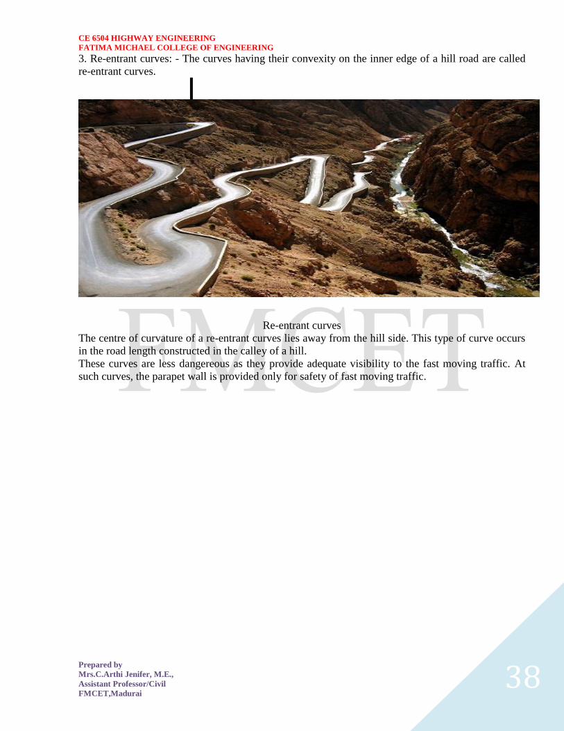
CE 6504 HIGHWAY ENGINEERING
FATIMA MICHAEL COLLEGE OF ENGINEERING
Prepared by
MrsCArthi Jenifer ME
Assistant ProfessorCivil
FMCETMadurai 38
3 Re-entrant curves - The curves having their convexity on the inner edge of a hill road are called
re-entrant curves
Re-entrant curves
The centre of curvature of a re-entrant curves lies away from the hill side This type of curve occurs
in the road length constructed in the calley of a hill
These curves are less dangereous as they provide adequate visibility to the fast moving traffic At
such curves the parapet wall is provided only for safety of fast moving traffic
CE 6504 HIGHWAY ENGINEERING
FATIMA MICHAEL COLLEGE OF ENGINEERING
Prepared by
MrsCArthi Jenifer ME
Assistant ProfessorCivil
FMCETMadurai 39
UNIT ndash III DESIGN OF RIGID AND FLEXIBLE PAVEMENTS
COMPARISON OF RIGID AND FLEXIBLE PAVEMENTS
The comparisons are
i) Design precision
A cement concrete pavement is amerable to a much more precise structural analysis
than a flexible pavement Flexible pavements designs are mainly empirical Computer aided analysis
of layered system is making the flexible pavement design more exact than hitherto
ii) Life
) Cement concrete slabs of a thin section constructed in the early 1940rsquos are still in
existence in India though many of them have cracked badly and a few of them have been ripped
open and rebuilt in recent ties
) A major project in cement concrete road construction between Agra and Mathura It can
safely be said that a well-designed concrete slab has a life of about 40 years
) Compared to this the life of a flexible pavement generally varies from 10 to 20 years
iii) Maintenance
) A well-designed cement concrete pavement needs very little maintenance The only
maintenance needed is I respect of joints
) The surface is unaffected by spillage of oil and lubricants bituminous surfaces on the
other hand need great inputs in maintenance
) The surface is affected by spillage of oil and lubricants The surface is also affected by
natural weathering agents like air water ad temperature changes
) A cement concrete pavement on the other hand needs a small amount for maintaining
joints
iv) Initial cost
) The argument so far used against a cement concrete slab is that it is much more costly
than a flexible pavement
) The latter specifications no doubt represent the rock-bottom needs of a road in India but
these specifications can hardly provide a smooth and durable surface
v) Stage construction ) Road construction is generally done adopting a policy of stage construction especially for
low volume roads As traffic grows additional layers in the form of water bound macadam and
superior surfacing are added on
) Initial outlay is minimum and additional outlays are in keeping with traffic growth This is
a great advantage when dealing with new roads in an atmosphere of austerity
vi) Availability of materials
) Cement bitumen stone aggregates and gravelsand are the major materials involved in
pavement Construction Cement has been in serious short supply in the country for the past many
decades
) Bitumen is also not available plentifully in India There is also the danger of the entire oil
reserves in the world shrinking during the next two or three decades
) In locations where stone aggregates are scarce cement concrete may have an advantage
for flexible pavements
vii) Surface characterstics
CE 6504 HIGHWAY ENGINEERING
FATIMA MICHAEL COLLEGE OF ENGINEERING
Prepared by
MrsCArthi Jenifer ME
Assistant ProfessorCivil
FMCETMadurai 40
) A good cement concrete surface is smooth and free from rutting potholes and
corrugations In a bituminous surface it is only the asphaltic concrete surface that can give
comparable rideablity
) A well-constructed cement concrete pavement surface can have a permanent nonskid
surface A bituminous surface can also be designed to have a good skid resistant surface
viii) Utility location
) In cement concrete slabs proper thought has to be given to locate utilities such as water
pipes telephone lines and electric cables
) It is difficult to rip open the slab and restore it to be the original condition if any changes
in the utilities lines are to be made
ix) Glame and night visibility
) Concrete pavements have a gray color which can cause glam under sunlight Colored
cement can reduce the grave
) On the other hand bituminous roads need more street lighting
x) Traffic dislocation during construction
) A cement concrete pavement requires 28 days before it can be thrown open to traffic On
the other hand a bituminous surface can be thrown open to traffic shortly after it is rolled
xi) Environmental considerations during construction
) The process of heating of bitumen and aggregates and mixing them together on hot mix
plants can prove to be much more hazardous to the environment than cement concrete construction
where no heating of any material is involved
xii) Overall economy on a life cycle basis
) A good road is costly to construct but once constructed such a road requires little
maintenance and results in savings in vehicle operating costs
) The comparative economy of a flexible pavement and a rigid pavement has proved that on
overall economic considerations
Types of pavement structure
Based on the structural behavior pavements are generally classified into three
categories
i) Flexible pavements
ii) Rigid pavements
iii) Semi rigid pavements
Flexible pavements
) Flexible pavements are those which on the whole have low or negligible flexural
strength and are rather flexible in their structural action under the loadsThe flexible pavement
layers reflect the deformation of the lower layers on to the surface of the layer
) A flexible pavement consists of four components(i) Soil subgrade (ii) sub base
course (iii) base course (iv) Surface course
CE 6504 HIGHWAY ENGINEERING
FATIMA MICHAEL COLLEGE OF ENGINEERING
Prepared by
MrsCArthi Jenifer ME
Assistant ProfessorCivil
FMCETMadurai 41
) The flexible pavement layers transmit the vertical or compressive stresses to the lower layers
by grain to grain transfer through the points of contact in the granular structure A well
compacted granular structure consisting of strong added aggregate can transfer the compressive
stresses
) The load spreading ability of this layer therefore depends on the type of the materials and mix
design factors Bituminous concrete is one of the best flexible pavements layer materials Other
materials which fall under the group are all granular materials with or without bituminous
binder granular base and sub base course materials
) The vertical compressive stress is maximum on the pavement surface directly under the wheel
and is equal to the contact pressure under the wheel The flexible pavement may be constructed
in a number of layers and the top layer has to be strongest as the highest compressive stresses
) Flexible pavements are commonly designed using empirical design charts or equations taking
into account some of the design factors there are also semi empirical and theoretical design
methods
Rigid pavements
) Rigid pavements are those which possess note flexural strength or flexural rigidity
The stresses are not transferred from grain to grain to the lower layers as in the ease of flexible
pavements layers
) The rigid pavements are made of Portland cement concrete plain reinforced or
prestressed concrete The plain cement concrete slabs are expected to take up about 40 kgcm2
flexural stress
) The rigid pavement has the slab action and is capable of transmitting the wheel
load stresses through a wider area below The main point of difference in the structural behavior
of rigid pavement as compared to the flexible pavement is that the critical condition of stress in
the rigid pavement is the maximum flexural stress occurring in the slab due to wheel load and
the temperature changes whereas in the flexible pavement
) As the rigid pavement slab has tensile strength tensile stresses are developed due
to the bending of the slab under wheel load and temperature variations Thus the types of
stresses developed and their distribution within the cement concrete slab are quirt different
) The cement concrete pavement slab can very well serve as a wearing surface as
well an effective base course The rigid pavement structure consists of a cement concrete slab
below which a granular base or sub base course may be provided
) Though the cement concrete slab can also be laid directly over the soil subgrade
consists of fine grained soil
) the rigid pavements are usually designed and the stresses are analyzed using the
elastic theory assuming the pavements as a n elastic plate resting over an elastic or a viscous
foundation
Semi rigid pavements
) when bonded materials like the pozzolanic concrete lean cement concrete or soil
cement are used in the base course or sub base course layer the pavement layer has considerably
higher flexural strength than the common flexible pavement layers
) when this intermediate class of materials are used in the base or sub base course
layer of the pavements they are called semi rigid pavements
CE 6504 HIGHWAY ENGINEERING
FATIMA MICHAEL COLLEGE OF ENGINEERING
Prepared by
MrsCArthi Jenifer ME
Assistant ProfessorCivil
FMCETMadurai 42
) This third category of semi rigid pavement are either designed as flexible
pavements with some correction factors to find the thickness requirements based on experience
or by using a new design approach
) The semi rigid pavement materials have low resistance to impact and abrasion and
therefore are usually provided with flexible pavement surface course
Various functions of pavement components
The functions are
Soil sub grade and its evaluation
) The soil sub grade is a layer of natural soil prepared to receive the layers of pavement
materials placed over it It is essential that at no time the soil sub grade is overstressed it means that
the pressure transmitted on the top of the sub grade is within the allowable limit
) Many tests are known for measuring the strength properties of the sub grades Some of the
tests have been standardized for the use The common strength test for the evaluation of soil
subgrade is
i) California bearing ratio test
ii) California resistance value test
iii) Triaxial compression test
iv) Plate bearing test
CALIFORNIA BEARING RATIO (CBR) TEST
It is evolved for the empirical method of flexible pavement design The CBR test is carried
out either in the laboratory on prepared specimens or in the field by taking in situ measurements
California resistance value
It is found by using have been stabliometerThis test is used in an empirical method of
flexible pavement design based on soil strength
Triaxial test
It is the most important soil strength but still the test is not very commonly used in structural
design of pavements
Plate bearing test
It is carried out using a relatively large diameter plate to evaluate the load supporting
capacity of supporting power of the pavement layers The results are plate bearing tests are used in
flexible pavement design method like McLeod method on based on layer system analysis by
brumister
Sub base and base courses and their evaluation
) There layers are made of broken stones bound or unbound aggreagatesome times in sub
base course a layer of stabilized soil(or) Selected granular soil is also used
) however at the sub base course it is desirable to use smaller size graded aggregates When
the sub grade consists of fine grained soil and when the pavement carries heavy wheel loads
CE 6504 HIGHWAY ENGINEERING
FATIMA MICHAEL COLLEGE OF ENGINEERING
Prepared by
MrsCArthi Jenifer ME
Assistant ProfessorCivil
FMCETMadurai 43
) Sub base course primarily has the similar function as of the base course and is provided
with inferior materials than of base course Base courses are used under rigid pavement for
i) Preventing pumping
ii) Protecting the sub grade against frost action
) Thus the fundamental purpose of abase course and sub base course is to provide a stress
transmitting medium to spread the surface wheel loads in such manner
) The sub base and base course layers may be evaluated by suitable strength or stability test
like plate bearing CBR test
WEARING COURSE AND ITS EVALUATION
) The purpose of the wearing course is to give a smooth riding surface that is dense It
resists pressure exerted by tyres and takes up wear and tear due to the traffic
) Wearing course also offers a water tight layer against the surface water infiltration The
flexible pavement normally a bituminous surfacing is used as a wearing course
) In rigid pavements the cement concrete acts like a base course as well as wearing course
Most popular test in use is marshal stability test where in the optimum content of bitumen binder is
worked out based on the stability density
) Plate bearing test and Bankelman beam test are also sometimes made use of for evaluating
the wearing course and the pavement as a whole
Various factors to be considered in pavement design and the significance
Pavement design consists of two parts
i) Mix design of materials to be used in each pavement component layer Thickness design of the
pavement and the component layers
The various factors to be considered for the design of pavements are given below
i) Design wheel load
ii) Sub grade soil
iii) Climatic factors
iv) Pavement component layers
v) Environmental factors
vi) Special factors in the design of different types of pavements
Design wheel load
The various wheel load factors to be considered in pavement design are
i) Maximum wheel load
ii) Contact pressure
iii) Dual or multiple wheel loads
iv) Repetition of loads
Maximum wheel load
The wheel load configurations are important to know the way in which the loads of a given
vehicle are applied on the pavement surface
) For highways the maximum legal axle load as specified by Indian road congress is 8170
kg with a maximum equivalent single wheel load of 4085 kg
) The evaluation for vertical stress computations under a uniformly distribute of circular
load based on Boussineqrsquos theory is given by
CE 6504 HIGHWAY ENGINEERING
FATIMA MICHAEL COLLEGE OF ENGINEERING
Prepared by
MrsCArthi Jenifer ME
Assistant ProfessorCivil
FMCETMadurai 44
2
322
3
1
za
zpz
σz = vertical stress at depth z
P= surface pressure
Z=depth at which σz computed
A=radius of loaded area
Contact pressure
Generally the wheel load is assumed to be distributed over a circular area But by
measurement of the imprints of tyers with different load and inflation pressures Three terms in use
with reference to tyre pressure are
Tyre pressure
Inflation pressure
Contact pressure
Tyre pressure and inflation pressure mean exactly the same the contact pressure is found to be more
than tyre pressure when the tyre pressure is less than 7 kgm2 and it is vice versa when the tyre
pressure exceeds this value
Contact pressure can be measured by the relationship
Load on wheel
Contact pressure = ----------------------------------------
Contact area or area of imprint
The general variation between the tyre pressure and measured contact pressure is shown in this fig
The ratio of contact pressure to type pressure is defined as rigidity factor Thus value of rigidity
factor is 10 for an average tyre pressure of 7 Kgcm2This value is higher than unity for lower type
pressures and less than unity for tyre pressures higher than 7 kgcm2
Equivalent single wheel load (ESWL)
) The maximum wheel load within the specified limit and to carry greater load it is
necessary to provide dual wheel assembly to the rear axles of the roads vehicles
) In other words the pressure at a certain depth below the pavement surface cannot be
obtained by numerically adding the pressure caused by any one wheel
) The effect is in between the single load and two times load carried by one wheel The load
dispersion is assumed to be at an angle of 450In the dual wheel load assembly let d be the clear gap
between the two wheels S be the spacing between the centers of the wheels and a be the radius of
the circular contact area of each wheel Then S = (d + 2a)
) ESWL may be determined based on either equivalent deflection or equivalent stress
criterianMultiple wheel loads are convert to ESWL and this value is used in pavement design The
ESWL is usually determined by the equivalent stress criterion using a simple graphical method
CE 6504 HIGHWAY ENGINEERING
FATIMA MICHAEL COLLEGE OF ENGINEERING
Prepared by
MrsCArthi Jenifer ME
Assistant ProfessorCivil
FMCETMadurai 45
) A straight line relationship is assumed between ESWL and depth on log scales For
determining ESWL the plot is made as shown in fig
) Two points A and B are plotted on the log-log graph with coordinates of A (Pd2) and
B(2p2s)line AB is a plot which is the focus of points where any single wheel load is equivalent to a
certain set of dual wheels
) To Calculate the ESWL for a dual assembly it is essential to estimate a design thickness of
the pavement If the design thickness so obtained is equal to the estimated thickness then the ESWL
calculations could be considered as correct Otherwise trials are made
) In heavy trucks and trailers the load on each wheel may be further reduced by multiple
wheels and tandem axles
Repetition of loads
) The deformation of load pavement (or) sub grade due to a single application of wheel load
may be small It required carrying out traffic surveys for accounting the factor of repetitions for
wheel loads in the design of pavement
) Data collected are converted to some constant equivalent wheel loads Equivalent wheel
load is a single load equivalent to the repeated applications of any particular wheel load on a
pavement which requires the same thickness and strength of pavements
) McLeod has given a procedure for evolving equivalent load factors for designing flexible
pavements
Various methods of flexible pavement design
) The flexible pavement is built with number of layers In the design process it is to be
ensured that under the application of load none of the layers is overstressed
) The maximum intensity of stresses occurs in the top layer of the pavement The
magnitude of load stresses reduces at lower layers
) In the design of flexible pavements it has yet not been possible to have a rational design
method wherein design process and service behavior of the pavement can be expressed by
mathematical laws
) Flexible pavement design methods are accordingly either empirical or semi empirical In
these methods the knowledge and experience gained on the behavior of the pavements in the past
are usefully utilized
Various approaches of flexible pavement design may be thus classified into three groups
i) Empirical method
ii) Semi-empirical or Semi theoretical method
iii) Theoretical method
) Empirical methods are either based on physical properties or strength parameters of soil
sub grade When the design is based on stress strain function and modified base on experience it
may be called semi-empirical or semi-theoretical There are design methods based on theoretical
analysis and mathematical computations
Out of the flexible pavement design method available is
i) Group index method
ii) California bearing ratio method
iii) California R value (or) Stabiliometer method
iv) Triaxial test method
CE 6504 HIGHWAY ENGINEERING
FATIMA MICHAEL COLLEGE OF ENGINEERING
Prepared by
MrsCArthi Jenifer ME
Assistant ProfessorCivil
FMCETMadurai 46
v) McLeod method
vi) Burmister method
Group index method
) Group index value is an arbitrary index assigned to the soil type in numerical equations
base on the percent fines liquid limit and plasticity index
) The design chart for group index method for determining the pavement thickness is given
in fig
The traffic volume in this method is divided in three groups
Traffic volume No of vehicles per day
Light Less than 50
Medium 50 to 300
Heavy Over 300
The design of the pavement thickness by this method first the G1 value of the soil is found the
anticipated traffic is estimated and is designated as light medium or heavy as indicated
The G1 method of pavement design is essentially an empirical method based on physical properties
of the subgrade soil This method does not consider the strength characteristics of the subgrade soil
and therefore is open to question regarding the reliability of the design based on the index properties
of the soil only
California bearing ratio method
) California division of highways in the USA developed CBR method for
pavement design The majority of design curves developed later are base on the original curves
proposed by OJporter
) One of the chief advantages of CBR method is the simplicity of the test procedure
The CBR tests were carried out by the California state highway department on existing pavement
layers including subgrade sub base and base course
) Based on the extensive CBR test data collected on pavement which behaved
satisfactory and those which failed an empirical design chart was developed correlating the CBR
value and the pavement thickness The basis of the design chart is that a material with a given CBR
required a certain thickness of pavement layer as a cover
) A higher load needs a thicker pavement layer to protect the sub grade Design
curves correlating the CBR value with total pavement thickness cover were developed by the
California state highway department for wheel loads of 3175kg and 5443 kg representing light and
heavy traffic The design curves are shown in this fig
It is possible to extend the CBR design curves for various loading conditions nusing the expression
t= 2
1
1751
pCBRp
t=2
1
751
A
CBR
p
Hence
CE 6504 HIGHWAY ENGINEERING
FATIMA MICHAEL COLLEGE OF ENGINEERING
Prepared by
MrsCArthi Jenifer ME
Assistant ProfessorCivil
FMCETMadurai 47
t= pavement thickness cm
p=Wheel load kg
CBR= California bearing ratio percent
P=tyre pressure kgcm2
A= area of contactcm2
IRC Recommendations
a) The CBR tests should be performed on remoulded soils in the laboratory The specimens should
be prepared by static compaction wherever possible and otherwise by dynamic compaction
b) For the design of new roads the sub grade soil sample should be compacted at OMC to proctor
density whenever suitable compaction equipment
c) The CBR test samples may be soaked in water for four days period before testing the annual
rainfall is less than 50 cm and the water table is too deep to affect the sub grade and imperable
surfacing is provided to carrying out CBR test
d) If the maximum variations in CBR value of the three specimens exceed the specified limits the
design CBR should be average of at least six samples
e) The top 50 cm of sub grade should be compacted at least up to 95 to 100 percent of proctor
density
f) An estimate of the traffic should be carried by the road pavements at the end of expected in view
the existing traffic and probable growth rate of traffic
g) The traffic for the design is considered in units of heavy vehicles per day in both directions and is
divided into seven categories A to G The design thickness is considered applicable for single axle
loads up to 8200 kg and tandom axle loads up to 14500 kg
h) When sub base course materials contain substantial proportion of aggregates of size above 20mm
the CBR value of these materials would not be valid for the design of subsequent layers above them
The CBR method of pavement design gives the total thickness requirement of the pavement above a
sub grade and thickness value would remain the same quality of materials used in component layers
California resistance value method
) In this design method based on stabliometer R-value and cohesiometer C-value
Based on performance data it was established by pavement thickness varies directly with R value
and algorithm of load repetitions It varies inversely with fifth root of c valueThe expression for
pavement thickness is given by the empirical equation
T=
5
1
1 90
C
RTK
Hence
T=total thickness of pavement cm
K=Numerical constant 0166
T1=traffic index
R= stabiliometer resistance value
C=Cohesiometer value
CE 6504 HIGHWAY ENGINEERING
FATIMA MICHAEL COLLEGE OF ENGINEERING
Prepared by
MrsCArthi Jenifer ME
Assistant ProfessorCivil
FMCETMadurai 48
In the design of flexible pavements based on California resistance value method for the following
data are needed
) R-value of soil subgrade
) T1 value
) Equivalent C-value
) R value of soil subgrade is obtained from the test using stablio meterThe
computation of T1 value has been explained
Equivalent C-value
) The cohesion meter value c is obtained for each layer of pavement material
separately from tests However the composite or equivalent C-value of the pavement may be
estimated if the thickness of each component layer and the c-value of the material of the layer are
known
) while designing a pavement as the thickness of the pavement is not known it is
easier if the pavement is first assumed to consist of any one material like gravel base course with
known C-value
) Subsequently the individual thickness of each layer is converted in terms of gravel
equivalent by using relationship
5
1
1
2
2
1
C
C
t
t
) t1 and t2 are the thickness values of any two pavement layersc1 and c2 are their
corresponding cohesiometer values
CE 6504 HIGHWAY ENGINEERING
FATIMA MICHAEL COLLEGE OF ENGINEERING
Prepared by
MrsCArthi Jenifer ME
Assistant ProfessorCivil
FMCETMadurai 49
UNIT 4 MATERIAL AND MAINTENANCE
SUMMIT CURVE
Summit curves are vertical curves with gradient upwards They are formed when two
gradients meet as illustrated in figure 1 in any of the following four ways
1 When a positive gradient meets another positive gradient [figure 1a]
2 When positive gradient meets a flat gradient [figure 1b]
3 When an ascending gradient meets a descending gradient [figure 1c]
4 When a descending gradient meets another descending gradient [figure 1d]
Type of Summit Curve
Many curve forms can be used with satisfactory results the common practice has been to
use parabolic curves in summit curves This is primarily because of the ease with it can
be laid out as well as allowing a comfortable transition from one gradient to another
Although a circular curve offers equal sight distance at every point on the curve for very
small deviation angles a circular curve and parabolic curves are almost congruent
Furthermore the use of parabolic curves were found to give excellent riding comfort
Figure 1 Types of summit curves
Design Consideration
In determining the type and length of the vertical curve the design considerations are
comfort and security of the driver and the appearance of the profile alignment Among
these sight distance requirements for the safety are most important on summit curves
The stopping sight distance or absolute minimum sight distance should be provided on
these curves and where overtaking is not prohibited overtaking sight distance or
intermediate sight distance should be provided as far as possible When a fast moving
vehicle travels along a summit curve there is less discomfort to the passengers This is
because the centrifugal force will be acting upwards while the vehicle negotiates a
summit curve which is against the gravity and hence a part of the tyre pressure is
relieved Also if the curve is provided with adequate sight distance the length would be
sufficient to ease the shock due to change in gradient Circular summit curves are
identical since the radius remains same throughout and hence the sight distance From
CE 6504 HIGHWAY ENGINEERING
FATIMA MICHAEL COLLEGE OF ENGINEERING
Prepared by
MrsCArthi Jenifer ME
Assistant ProfessorCivil
FMCETMadurai 50
this point of view transition curves are not desirable since it has varying radius and so the
sight distance will also vary The deviation angles provided on summit curves for
highways are very large and so the simple parabola is almost congruent to a circular arc
between the same tangent points Parabolic curves are easy for computation and also it
had been found out that it provides good riding comfort to the drivers It is also easy for
field implementation Due to all these reasons a simple parabolic curve is preferred as
summit curve Length of the summit curve
The important design aspect of the summit curve is the determination of the length of the
curve which is parabolic As noted earlier the length of the curve is guided by the sight
distance consideration That is a driver should be able to stop his vehicle safely if there is
an obstruction on the other side of the road Equation of the parabola is given by
where where N is the deviation angle and is the length of the In
deriving the length of the curve two situations can arise depending on the uphill and
downhill gradients when the length of the curve is greater than the sight distance and the
length of the curve is greater than the sight distance
Let is the length of the summit curve is the SSDISDOSD is the deviation angle
drivers eye height (12 m) and the height of the obstruction then the length of the
summit curve can be derived for the following two cases The length of the summit curve
can be derived from the simple geometry as shown below
Case a Length of summit curve greater than sight distance( )
Figure 1 Length of summit curve ( )
The situation when the sight distance is less than the length of the curve is shown in
figure 1
CE 6504 HIGHWAY ENGINEERING
FATIMA MICHAEL COLLEGE OF ENGINEERING
Prepared by
MrsCArthi Jenifer ME
Assistant ProfessorCivil
FMCETMadurai 51
(1)
Case b Length of summit curve less than sight distance
The second case is illustrated in figure 1
Figure 1 Length of summit curve
CE 6504 HIGHWAY ENGINEERING
FATIMA MICHAEL COLLEGE OF ENGINEERING
Prepared by
MrsCArthi Jenifer ME
Assistant ProfessorCivil
FMCETMadurai 52
From the basic geometry one can write
(1)
Therefore for a given and to get minimum differentiate the above equation
with respect to and equate it to zero Therefore
Solving the quadratic equation for
(2)
Now we can substitute back to get the value of minimum value of for a given
and Therefore
Solving for
CE 6504 HIGHWAY ENGINEERING
FATIMA MICHAEL COLLEGE OF ENGINEERING
Prepared by
MrsCArthi Jenifer ME
Assistant ProfessorCivil
FMCETMadurai 53
(3) (4
CE 6504 HIGHWAY ENGINEERING
FATIMA MICHAEL COLLEGE OF ENGINEERING
Prepared by
MrsCArthi Jenifer ME
Assistant ProfessorCivil
FMCETMadurai 54
When stopping sight distance is considered the height of drivers eye above the road
surface ( ) is taken as 12 metres and height of object above the pavement surface ( )
is taken as 015 metres If overtaking sight distance is considered then the value of
drivers eye height ( ) and the height of the obstruction ( ) are taken equal as 12
metres
Valley curve
Valley curve or sag curves are vertical curves with convexity downwards They are
formed when two gradients meet as illustrated in figure 1 in any of the following four
ways
Figure 1 Types of valley curve
1 When a descending gradient meets another descending gradient [figure 1a]
2 When a descending gradient meets a flat gradient [figure 1b]
3 When a descending gradient meets an ascending gradient [figure 1c]
4 When an ascending gradient meets another ascending gradient [figure
Design considerations
There is no restriction to sight distance at valley curves during day time But visibility is
reduced during night In the absence or inadequacy of street light the only source for
visibility is with the help of headlights Hence valley curves are designed taking into
account of headlight distance In valley curves the centrifugal force will be acting
downwards along with the weight of the vehicle and hence impact to the vehicle will be
more This will result in jerking of the vehicle and cause discomfort to the passengers
Thus the most important design factors considered in valley curves are (1) impact-free
movement of vehicles at design speed and (2) availability of stopping sight distance
under headlight of vehicles for night driving
For gradually introducing and increasing the centrifugal force acting downwards the best
shape that could be given for a valley curve is a transition curve Cubic parabola is
generally preferred in vertical valley curves See figure 1
CE 6504 HIGHWAY ENGINEERING
FATIMA MICHAEL COLLEGE OF ENGINEERING
Prepared by
MrsCArthi Jenifer ME
Assistant ProfessorCivil
FMCETMadurai 55
Figure 1 Valley curve details
During night under headlight driving condition sight distance reduces and availability of
stopping sight distance under head light is very important The head light sight distance
should be at least equal to the stopping sight distance There is no problem of overtaking
sight distance at night since the other vehicles with headlights could be seen from a
considerable distance
Length of the valley curve
The valley curve is made fully transitional by providing two similar transition curves of
equal length The transitional curve is set out by a cubic parabola where
The length of the valley transition curve is designed based on two criteria
1 comfort criteria that is allowable rate of change of centrifugal acceleration is
limited to a comfortable level of about
2 safety criteria that is the driver should have adequate headlight sight distance at
any part of the country
Comfort criteria
The length of the valley curve based on the rate of change of centrifugal acceleration that
will ensure comfort Let is the rate of change of acceleration the minimum radius of
the curve is the design speed and is the time then is give
CE 6504 HIGHWAY ENGINEERING
FATIMA MICHAEL COLLEGE OF ENGINEERING
Prepared by
MrsCArthi Jenifer ME
Assistant ProfessorCivil
FMCETMadurai 56
For a cubic parabola the Value Safety criter Length of the valley curve for headlight distance may be determined for two conditions
(1) length of the valley curve greater than stopping sight distance and (2) length of the
valley curve less than the stopping sight distance of for length is given by
Case 1 Length of valley curve greater than stopping sight distance ( )
The total length of valley curve is greater than the stopping sight distance SSD The
sight distance available will be minimum when the vehicle is in the lowest point in the
valley This is because the beginning of the curve will have infinite radius and the bottom
of the curve will have minimum radius which is a property of the transition curve The
case is shown in figure 1
Figure 1 Valley curve case 1
From the geometry of the figure we have
CE 6504 HIGHWAY ENGINEERING
FATIMA MICHAEL COLLEGE OF ENGINEERING
Prepared by
MrsCArthi Jenifer ME
Assistant ProfessorCivil
FMCETMadurai 57
(1)
where is the deviation angle in radians is the height of headlight beam is the
head beam inclination in degrees and is the sight distance The inclination is 1
degree
Case 2 Length of valley curve less than stopping sight distance ( )
The length of the curve is less than SSD In this case the minimum sight distance is
from the beginning of the curve The important points are the beginning of the curve and
the bottom most part of the curve If the vehicle is at the bottom of the curve then its
headlight beam will reach far beyond the endpoint of the curve whereas if the vehicle is
at the beginning of the curve then the headlight beam will hit just outside the curve
Therefore the length of the curve is derived by assuming the vehicle at the beginning of
the curve The case is shown in figure 1
From the figure
(1) Note that the above expression is approximate and is satisfactory because in practice the gradients
are very small and is acceptable for all practical purposes We will not be able to know prior to
which case to be adopted Therefore both has to be calculated and the one which satisfies the
condition is adopted
1 Flexible pavement
2 Rigid pavement
Flexible pavement
These pavements reflect the deformation of sub grade and the subsequent layers to the
surface
Rigid pavement
The rigid characteristic of the pavement are associated with rigidity or flexural strength
CE 6504 HIGHWAY ENGINEERING
FATIMA MICHAEL COLLEGE OF ENGINEERING
Prepared by
MrsCArthi Jenifer ME
Assistant ProfessorCivil
FMCETMadurai 58
or slab action so the load is distributed over a wide area of sub grade soil
Flexible pavement Definition
These pavements reflect the deformation of sub grade and the subsequent layers to the
surface Flexible usually asphalt is laid with no reinforcement or with a specialized
fabric reinforcement that permits limited flow or repositioning of the roadbed under
ground changes
The design of flexible pavement is based on load distributing characteristic of the
component layers The black top pavement including water amp gravel bound macadam fall
in this category
Flexible pavement on the whole has low or negligible flexible strength flexible in their
structural action) The flexible pavement layers transmit the vertical or compressive
stresses to the lower layers by grain transfer through contact points of granular structure
The vertical compressive stress is maximum on the pavement surface directly under the
wheel load and is equal to contact pressure under the wheels Due to the ability to
distribute the stress to large area in the shape of truncated cone the stresses get decreased
in the lower layer
As such the flexible pavement may be constructed in a number of layers and the top
layer has to be strongest as the highest compressive stresses
To be sustained by this layer in addition to wear and tear the lower layer have to take
up only lesser magnitude of stress as there is no direct wearing action die to traffic loads
therefore inferior material with lower cast can be used in the lower layers
Rigid pavement Definition
The rigid characteristic of the pavement are associated with rigidity or flexural strength
or slab action so the load is distributed over a wide area of sub grade soil Rigid pavement
is laid in slabs with steel reinforcement
The rigid pavements are made of cement concrete either plan reinforced or prestressed
concrete
Critical condition of stress in the rigid pavement is the maximum flexural stress occurring in the slab due to wheel load and the temperature changes
Rigid pavement is designed and analyzed by using the elastic theory
CE 6504 HIGHWAY ENGINEERING
FATIMA MICHAEL COLLEGE OF ENGINEERING
Prepared by
MrsCArthi Jenifer ME
Assistant ProfessorCivil
FMCETMadurai 59
UNIT-5 EVALUATION AND MAINTENANCE OF PAVEMENTS
TRAFFIC PARAMETERS
Design life
Design life is the number of years (or number of standard axle repetitions) for which the
pavement is being designed A pavement is expected to serve satisfactorily within the
design life For concrete pavements 20 to 40 years may be assumed as the design life
(PCA 1984 IRC58 2002)
Basic design principle
Though different approaches for concrete pavement design are suggested in various
guidelines the design principles tend to remain similar across different guidelines for
example PCA (1994) Austroads (2004) NCHRP (2004) IRC58 (2002) etc except the
AASHTO (1993) provisions which is based on empirical approach The basic steps
involved in the design of concrete pavement method can be summarized as follows
The developed stresses due to load for a trial thickness of the concrete slab are
calculated for various loading configuration and the critical one is chosen The
axle loads are generally divided into different axle load groups and the load
stresses are calculated individually
The ratio between the load stress and Modulus of Rupture (MOR) is known as
stress ratio The stress ratio determines how many repetitions the pavement can
sustain (ie allowable traffic repetitions) for the individual axle load group If the
stress ratio is 055 or lower it can withstand virtually infinite number of traffic
repetitions (PCA 1984)
The ratio between the allowable repetitions to the expected traffic repetitions is
the damage fraction The calculation process is repeated for various axle loads
(sometimes for various seasons or various timings of the day) and the sum of
individual damage fractions (c u m u l a t i v e fatigue damage) should be less
than equal to one for pavement design being safe If found unsafe the trial
thickness is changed and the design process is repeated
The design process may also include considerations for temperature stress
moisture stresses and erosion distress
A brief discussion on concrete pavement design approaches suggested by various design
practices viz PCA method (1984) Austroads method (2004) AASHTO method (1993)
NCHRP mechanistic-empirical method (2004) and the Indian Roads Congress (IRC)
method (2002) are placed in the following
Portland cement Association (PCA) Method
The PCA method is based on Westergaard Picket and Rays work and further theoretical
analysis by Finite Element Method (Huang 1993) The data used to develop the PCA
method is generated from various road tests like ASSHO road test Arlington test
(conducted by PCA) Bates test road and Maryland road test (PCA 1984) The PCA
design method is based on the following two considerations (PCA 1984)
The fatigue damage on the concrete slab due to repetitive application of traffic
load is estimated The cumulative fatigue damage principle is used to estimate the
design thickness of the slab Edge stress between the mid-ways of the
CE 6504 HIGHWAY ENGINEERING
FATIMA MICHAEL COLLEGE OF ENGINEERING
Prepared by
MrsCArthi Jenifer ME
Assistant ProfessorCivil
FMCETMadurai 60
transverse joint is taken as critical configuration
The stresses due to warping and curling (due to temperature and moisture
gradient) are not considered in the fatigue analysis as per PCA recommendation
because most of the time the stresses generated are subtractive to the load stress
The possibility of erosion of pavement materials placed below the concrete slab is
evaluated The rate at which the slab is deflected due to axle load is used as a
criterion for erosion Theoretically it can be shown that a thin pavement with
smaller deflection basin is subjected to faster rate of deflection compared to
thicker slab Hence thin slab is more susceptible to erosion In a similar way the
cumulative erosion damage is calculated for individual axle load groups If this
value is greater than one then the design needs to be revised
Austroads method
Austroads method has been adopted from PCA (1984) approach with modifications
suited to Australian conditions (Austroads 2004) A bound mix or lean cement concrete is
used as sub-base material For a given CBR value of the subgrade and given thickness of
cemented sub-base the effective subgrade strength can be obtained from the chart
provided Figure-19 schematically shows such a chart For different levels of traffic
Austroads (2004) suggests minimum values of the base thicknesses to be provided
CE 6504 HIGHWAY ENGINEERING
FATIMA MICHAEL COLLEGE OF ENGINEERING
Prepared by
MrsCArthi Jenifer ME
Assistant ProfessorCivil
FMCETMadurai 61
figure-19 Schematic diagram of Austroads (2004) chart for estimation of effective
subgrade strength
As per Astroads (2004) the concrete pavement slab thickness for a given expected
traffic repetitions is designed considering the (i) flexural fatigue of the concrete slab and
the (ii) subgrade erosion arising out of repeated deflections For both the considerations
equations are suggested to calculate the allowable traffic repetitions If the allowable
traffic is less than the expected traffic the design is revised by increasing the slab
thickness The concrete shoulders adopted are of integral type or structural type
AASHTO method
The AASHTO method (1993) for design of concrete pavement has evolved from the
AASHO road test (AASHO 1962) The AASHTO pavement design follows an empirical
approach Pavement performance in terms of present serviceability index ( PSI ) loss of
serviceability sub-grade and sub-base strength cumulative traffic properties of concrete
joint load transfer efficiency drainage condition overall standard deviation and
reliability are the input parameters considered in the pavement design
The PSI value of the fresh pavement is assumed as 45 and the pavement is deemed to
have failed when the PSI value reaches 25 The resilient moduli of the subgrade and sub-
base materials are determined in the laboratory simulating the seasonal moisture content
and stress situation Suggested values are also available for given moisture content
plasticity index etc The composite modulus of sub-grade reaction (k) is estimated from
modulus of sub-grade reaction and elastic modulus of sub-base for various seasons and
the depth of rigid foundation and the thickness of the sub-base
Design equation as well nomographs are available to estimate the slab thickness (D) from
these input parameters
NCHRP mechanistic-empirical (M-E) metho
The NCHRP (2004) has recently developed concrete pavement design procedure based
on mechanistic-empirical (M-E) approach This approach attempts to reduce the extent of
empiricism prevalent in the existing AASHTO (1993) guidelines This proposed NCHRP
pavement design system is modular in nature that is the design approach can be
modified by parts (as and when new knowledge is available) without disrupting the
overall design procedure This approach also can take care of various wheel-axle loa
configuration
As per this approach trial thickness of the slab is first assumed and the stress strain and
displacement values are obtained From these values the performance of the pavement in
terms of distresses (such as faulting cracking) and smoothness and predicted If these
predicted performance parameters does not satisfy the required performance for a given
reliability
The design approach includes a large data-base as input parameters for example average
daily traffic traffic growth rate traffic composition hourly weather data on air
temperature precipitation wind speed percentage sunshine relative humidity pavement
material engineering parameters ground water depth infiltration drainage hydraulic
conductivity thermal conductivity heat capacity etc The temperature stress is
considered in this method but the temperature profile is linearized to enhance
computational efficiency (NCHRP 2004)
CE 6504 HIGHWAY ENGINEERING
FATIMA MICHAEL COLLEGE OF ENGINEERING
Prepared by
MrsCArthi Jenifer ME
Assistant ProfessorCivil
FMCETMadurai 62
INDIAN ROADS CONGRESS (IRC) METHOD
The Indian Roads Congress (IRC) guidelines IRC58 (2002) has adopted the
Westergaards equation to estimate load stress and Brdaburys equation to estimate
temperature stress The load stress is highest at the corner of the slab lesser in edge and
least in the interior The order of variation of temperature stress is just the reverse of this
As per IRC58 (2002) it is recommended that the design needs to be done for edge stress
condition and subsequently check needs to be performed for corner stress condition so as
to finalize the design The following are the steps followed as per IRC58 (2002)
guideline for the design of concrete pavement
The input parameters are obtained to formulate the design problem The joint
spacing and the slab dimensions are decided If there is a bound sub-base layer
over the subgrade a suitable value of effective k is to be adopted
A trial thickness of the concrete slab is assumed
The edge stress is estimated for various axle loads from the given charts Figure-
20 schematically shows such a chart The cumulative fatigue damage principle for
fatigue is applied to check the adequacy of the slab thickness
The sum of edge stress due to load for the highest axle load group and the
temperature stress should be less than the MOR of concrete otherwise the design
is revised
The adequacy of corner stress is checked with respect to MOR value and
accordingly the design is finalized Westergaards corner stress formula
Figure-20 Schematic diagram of IRC58 chart for estimation of load stress at the edge
(IRC58 2002)
CE 6504 HIGHWAY ENGINEERING
FATIMA MICHAEL COLLEGE OF ENGINEERING
Prepared by
MrsCArthi Jenifer ME
Assistant ProfessorCivil
FMCETMadurai 63
estimation of corner stress due to load and the corner stress due to temperature is
assumed to be zero
Estimation of layer thicknesses
The thickness of the pavement is adjusted in such a way that the stress strain
developed is less than the allowable values obtained from past performance
information
The two major modes of structural failure of pavement are fatigue and rutting
o Fatigue Traffic applies repetitive load to the pavement surface and the
cracks start from bottom the bound layer slab and propagate upwards
When the extent of surface cracks reaches a predefined level the
pavement is said to have failed due to flexural fatigue
FUNCTIONAL DESIGN
The functional pavement design involves considerations of skid resistance roughness
surface distresses reflectivity of pavement surface etc The functional pavement design
considers mainly the surface features of a pavement
Drainage design
A road needs to be designed in such a way that the rain snow precipitation is drained off
the pavement and its surroundings A suitable surface drainage system for the pavement
is designed for this purpose Some water however will percolate into the pavement from
its top surface and needs to be taken out of the pavement - this is done by providing an
internal drainage system to the pavement Water will also try to enter into the pavement
from bottom due to capillary rise or due to rise in water table A suitably designed sub-
surface drainage system tries to avoid such a problem
PAVEMENT THICKNESS DESIGN CHARTS
For the design of pavements to carry traffic in the range of 1 to 10 msa use chart 1 and for
traffic in the range 10 to 150 msa use chart 2 of IRC37 2001 The design curves relate
pavement thickness to the cumulative number of standard axles to be carried over the
design life for different sub-grade CBR values ranging from 2 to 10 The design
charts will give the total thickness of the pavement for the above inputs The total
thickness consists of granular sub-base granular base and bituminous surfacing The
individual layers are designed based on the the recommendations given below and the
subsequent tables
Pavement composition
Sub-base
Sub-base materials comprise natural sand gravel laterite brick metal crushed
stone or combinations thereof meeting the prescribed grading and physical
requirements The sub-base material should have a minimum CBR of 20 and
30 for traffic upto 2 msa and traffic exceeding 2 msa respectively Sub-base
usually consist of granular or WBM and the thickness should not be less than 150
mm for design traffic less than 10 msa and 200 mm for design traffic
Base
The recommended designs are for unbounded granular bases which comprise
CE 6504 HIGHWAY ENGINEERING
FATIMA MICHAEL COLLEGE OF ENGINEERING
Prepared by
MrsCArthi Jenifer ME
Assistant ProfessorCivil
FMCETMadurai 64
conventional water bound macadam (WBM) or wet mix macadam (WMM) or
equivalent confirming to MOST specifications The materials should be of good
quality with minimum thickness of 225 mm for traffic up to 2 msa an 150 mm for
traffic
Bituminoussurfacing The surfacing consists of a wearing course or a binder
course plus wearing course The most commonly used wearing courses are
surface dressing open graded premix carpet mix seal surfacing semi-
dense bituminous concrete and bituminous concrete For binder course
MOST specifies it is desirable to use bituminous macadam (BM) for traffic
upto o 5 msa and dense bituminous macadam (DBM) for traffic more than 5
msa
Numerical example
Design the pavement for construction of a new bypass with the following data
1 Two lane carriage way
2 Initial traffic in the year of completion of construction = 400 CVPD (sum of both
directions)
3 Traffic growth rate = 75
4 Design life = 15 years
5 Vehicle damage factor based on axle load survey = 25 standard axle per
commercial vehicle
6 Design CBR of subgrade soil = 4
Solution
1 Distribution factor = 075
2
3 Total pavement thickness for CBR 4 and traffic 72 msa from IRC37 2001
chart1 = 660 mm
4 Pavement composition can be obtained by interpolation from Pavement Design
Catalogue (IRC37 2001)
1 Bituminous surfacing = 25 mm SDBC + 70 mm DBM
2 Road-base = 250 mm WBM
3 sub-base = 315 mm granular material of CBR not less than 30
CE 6504 HIGHWAY ENGINEERING
FATIMA MICHAEL COLLEGE OF ENGINEERING
Prepared by
MrsCArthi Jenifer ME
Assistant ProfessorCivil
FMCETMadurai 65
Generally bound base layers are used for concrete pavement construction As per Indian
specification some example of such base layers are Dry Lean Concrete (DLC) Roller
Compacted Concrete (RCC) (IRC15-2002)
The concrete slab is generally of M40 to M50 grade of concrete as
per Indian specifications and is called as paving quality concrete (PQC)
(IRC15-2002)
BITUMINOUS PAVEMENT
The subgrade is a compacted soil layer
The base and sub-base course could be made up of bound or unbound granular layer As
per Indian specifications (MORTampH 2001) some examples of base or sub-base layers
are Granular sub-base(GSB) Water Bound Macadam (WBM) Wet Mix Macadam
(WMM) etc
The binder course is made up bituminous material As per Indian specifications
(MORTampH 2001) some examples of binder course are Bituminous Macadam (BM)
Dense Bituminous Macadam (DBM) etc
The wearing course is the top bituminous layer which is comes in contact to the
vehicle tyre Wearing course provides impermeability to the pavement surface
against water percolation (Chakroborty and Das 2003) The binder course and wearing
course together are called bituminous surfacing
IRC METHOD OF FLEXIBLE PAVEMENT MIX DESIGN
These guidelines will apply to design of flexible pavements for Expressway National Highways
State Highways Major District Roads and other categories of roads Flexible pavements are
considered to include the pavements which have bituminous surfacing and granular base and sub-
base courses conforming to IRC MOST standards These guidelines apply to new pavements
Design criteria
The flexible pavements has been modeled as a three layer structure and stresses and strains at
critical locations have been computed using the linear elastic model To give proper consideration
to the aspects of performance the following three types of pavement distress resulting from
repeated (cyclic) application of traffic loads are considered
1 Vertical compressive strain at the top of the sub-grade which can cause sub-grade
deformation resulting in permanent deformation at the pavement surface
2 Horizontal tensile strain or stress at the bottom of the bituminous layer which can cause
fracture of the bituminous layer
3 Pavement deformation within the bituminous layer
CE 6504 HIGHWAY ENGINEERING
FATIMA MICHAEL COLLEGE OF ENGINEERING
Prepared by
MrsCArthi Jenifer ME
Assistant ProfessorCivil
FMCETMadurai 66
While the permanent deformation within the bituminous layer can be controlled by meeting the
mix design requirements thickness of granular and bituminous layers are selected using the
analytical design approach so that strains at the critical points are within the allowable limits For
calculating tensile strains at the bottom of the bituminous layer the stiffness of dense bituminous
macadam (DBM) layer with 6070 bitumen has been used in the analysis
FAILURE CRITERIA
Critical locations in pavement
A and B are the critical locations for tensile strains Maximum value of the strain is
adopted for design C is the critical location for the vertical subgrade strain since the
maximum value of the occurs mostly at C
CE 6504 HIGHWAY ENGINEERING
FATIMA MICHAEL COLLEGE OF ENGINEERING
Prepared by
MrsCArthi Jenifer ME
Assistant ProfessorCivil
FMCETMadurai 67
Fatigue Criteria
Bituminous surfacings of pavements display flexural fatigue cracking if the tensile strain
at the bottom of the bituminous layer is beyond certain limit The relation between the
fatigue life of the pavement and the tensile strain in the bottom of the bituminous layer
was obtained as
(1)
in which is the allowable number of load repetitions to control fatigue cracking and
is the Elastic modulus of bituminous layer The use of equation 1 would result in
fatigue cracking of 20 of the total area
Rutting Criteria
The allowable number of load repetitions to control permanent deformation can be
expressed as
(2)
is the number of cumulative standard axles to produce rutting of 20 mm
CE 6504 HIGHWAY ENGINEERING
FATIMA MICHAEL COLLEGE OF ENGINEERING
Prepared by
MrsCArthi Jenifer ME
Assistant ProfessorCivil
FMCETMadurai 68
CE 6504 HIGHWAY ENGINEERING
FATIMA MICHAEL COLLEGE OF ENGINEERING
Prepared by
MrsCArthi Jenifer ME
Assistant ProfessorCivil
FMCETMadurai 42
) This third category of semi rigid pavement are either designed as flexible
pavements with some correction factors to find the thickness requirements based on experience
or by using a new design approach
) The semi rigid pavement materials have low resistance to impact and abrasion and
therefore are usually provided with flexible pavement surface course
Various functions of pavement components
The functions are
Soil sub grade and its evaluation
) The soil sub grade is a layer of natural soil prepared to receive the layers of pavement
materials placed over it It is essential that at no time the soil sub grade is overstressed it means that
the pressure transmitted on the top of the sub grade is within the allowable limit
) Many tests are known for measuring the strength properties of the sub grades Some of the
tests have been standardized for the use The common strength test for the evaluation of soil
subgrade is
i) California bearing ratio test
ii) California resistance value test
iii) Triaxial compression test
iv) Plate bearing test
CALIFORNIA BEARING RATIO (CBR) TEST
It is evolved for the empirical method of flexible pavement design The CBR test is carried
out either in the laboratory on prepared specimens or in the field by taking in situ measurements
California resistance value
It is found by using have been stabliometerThis test is used in an empirical method of
flexible pavement design based on soil strength
Triaxial test
It is the most important soil strength but still the test is not very commonly used in structural
design of pavements
Plate bearing test
It is carried out using a relatively large diameter plate to evaluate the load supporting
capacity of supporting power of the pavement layers The results are plate bearing tests are used in
flexible pavement design method like McLeod method on based on layer system analysis by
brumister
Sub base and base courses and their evaluation
) There layers are made of broken stones bound or unbound aggreagatesome times in sub
base course a layer of stabilized soil(or) Selected granular soil is also used
) however at the sub base course it is desirable to use smaller size graded aggregates When
the sub grade consists of fine grained soil and when the pavement carries heavy wheel loads
CE 6504 HIGHWAY ENGINEERING
FATIMA MICHAEL COLLEGE OF ENGINEERING
Prepared by
MrsCArthi Jenifer ME
Assistant ProfessorCivil
FMCETMadurai 43
) Sub base course primarily has the similar function as of the base course and is provided
with inferior materials than of base course Base courses are used under rigid pavement for
i) Preventing pumping
ii) Protecting the sub grade against frost action
) Thus the fundamental purpose of abase course and sub base course is to provide a stress
transmitting medium to spread the surface wheel loads in such manner
) The sub base and base course layers may be evaluated by suitable strength or stability test
like plate bearing CBR test
WEARING COURSE AND ITS EVALUATION
) The purpose of the wearing course is to give a smooth riding surface that is dense It
resists pressure exerted by tyres and takes up wear and tear due to the traffic
) Wearing course also offers a water tight layer against the surface water infiltration The
flexible pavement normally a bituminous surfacing is used as a wearing course
) In rigid pavements the cement concrete acts like a base course as well as wearing course
Most popular test in use is marshal stability test where in the optimum content of bitumen binder is
worked out based on the stability density
) Plate bearing test and Bankelman beam test are also sometimes made use of for evaluating
the wearing course and the pavement as a whole
Various factors to be considered in pavement design and the significance
Pavement design consists of two parts
i) Mix design of materials to be used in each pavement component layer Thickness design of the
pavement and the component layers
The various factors to be considered for the design of pavements are given below
i) Design wheel load
ii) Sub grade soil
iii) Climatic factors
iv) Pavement component layers
v) Environmental factors
vi) Special factors in the design of different types of pavements
Design wheel load
The various wheel load factors to be considered in pavement design are
i) Maximum wheel load
ii) Contact pressure
iii) Dual or multiple wheel loads
iv) Repetition of loads
Maximum wheel load
The wheel load configurations are important to know the way in which the loads of a given
vehicle are applied on the pavement surface
) For highways the maximum legal axle load as specified by Indian road congress is 8170
kg with a maximum equivalent single wheel load of 4085 kg
) The evaluation for vertical stress computations under a uniformly distribute of circular
load based on Boussineqrsquos theory is given by
CE 6504 HIGHWAY ENGINEERING
FATIMA MICHAEL COLLEGE OF ENGINEERING
Prepared by
MrsCArthi Jenifer ME
Assistant ProfessorCivil
FMCETMadurai 44
2
322
3
1
za
zpz
σz = vertical stress at depth z
P= surface pressure
Z=depth at which σz computed
A=radius of loaded area
Contact pressure
Generally the wheel load is assumed to be distributed over a circular area But by
measurement of the imprints of tyers with different load and inflation pressures Three terms in use
with reference to tyre pressure are
Tyre pressure
Inflation pressure
Contact pressure
Tyre pressure and inflation pressure mean exactly the same the contact pressure is found to be more
than tyre pressure when the tyre pressure is less than 7 kgm2 and it is vice versa when the tyre
pressure exceeds this value
Contact pressure can be measured by the relationship
Load on wheel
Contact pressure = ----------------------------------------
Contact area or area of imprint
The general variation between the tyre pressure and measured contact pressure is shown in this fig
The ratio of contact pressure to type pressure is defined as rigidity factor Thus value of rigidity
factor is 10 for an average tyre pressure of 7 Kgcm2This value is higher than unity for lower type
pressures and less than unity for tyre pressures higher than 7 kgcm2
Equivalent single wheel load (ESWL)
) The maximum wheel load within the specified limit and to carry greater load it is
necessary to provide dual wheel assembly to the rear axles of the roads vehicles
) In other words the pressure at a certain depth below the pavement surface cannot be
obtained by numerically adding the pressure caused by any one wheel
) The effect is in between the single load and two times load carried by one wheel The load
dispersion is assumed to be at an angle of 450In the dual wheel load assembly let d be the clear gap
between the two wheels S be the spacing between the centers of the wheels and a be the radius of
the circular contact area of each wheel Then S = (d + 2a)
) ESWL may be determined based on either equivalent deflection or equivalent stress
criterianMultiple wheel loads are convert to ESWL and this value is used in pavement design The
ESWL is usually determined by the equivalent stress criterion using a simple graphical method
CE 6504 HIGHWAY ENGINEERING
FATIMA MICHAEL COLLEGE OF ENGINEERING
Prepared by
MrsCArthi Jenifer ME
Assistant ProfessorCivil
FMCETMadurai 45
) A straight line relationship is assumed between ESWL and depth on log scales For
determining ESWL the plot is made as shown in fig
) Two points A and B are plotted on the log-log graph with coordinates of A (Pd2) and
B(2p2s)line AB is a plot which is the focus of points where any single wheel load is equivalent to a
certain set of dual wheels
) To Calculate the ESWL for a dual assembly it is essential to estimate a design thickness of
the pavement If the design thickness so obtained is equal to the estimated thickness then the ESWL
calculations could be considered as correct Otherwise trials are made
) In heavy trucks and trailers the load on each wheel may be further reduced by multiple
wheels and tandem axles
Repetition of loads
) The deformation of load pavement (or) sub grade due to a single application of wheel load
may be small It required carrying out traffic surveys for accounting the factor of repetitions for
wheel loads in the design of pavement
) Data collected are converted to some constant equivalent wheel loads Equivalent wheel
load is a single load equivalent to the repeated applications of any particular wheel load on a
pavement which requires the same thickness and strength of pavements
) McLeod has given a procedure for evolving equivalent load factors for designing flexible
pavements
Various methods of flexible pavement design
) The flexible pavement is built with number of layers In the design process it is to be
ensured that under the application of load none of the layers is overstressed
) The maximum intensity of stresses occurs in the top layer of the pavement The
magnitude of load stresses reduces at lower layers
) In the design of flexible pavements it has yet not been possible to have a rational design
method wherein design process and service behavior of the pavement can be expressed by
mathematical laws
) Flexible pavement design methods are accordingly either empirical or semi empirical In
these methods the knowledge and experience gained on the behavior of the pavements in the past
are usefully utilized
Various approaches of flexible pavement design may be thus classified into three groups
i) Empirical method
ii) Semi-empirical or Semi theoretical method
iii) Theoretical method
) Empirical methods are either based on physical properties or strength parameters of soil
sub grade When the design is based on stress strain function and modified base on experience it
may be called semi-empirical or semi-theoretical There are design methods based on theoretical
analysis and mathematical computations
Out of the flexible pavement design method available is
i) Group index method
ii) California bearing ratio method
iii) California R value (or) Stabiliometer method
iv) Triaxial test method
CE 6504 HIGHWAY ENGINEERING
FATIMA MICHAEL COLLEGE OF ENGINEERING
Prepared by
MrsCArthi Jenifer ME
Assistant ProfessorCivil
FMCETMadurai 46
v) McLeod method
vi) Burmister method
Group index method
) Group index value is an arbitrary index assigned to the soil type in numerical equations
base on the percent fines liquid limit and plasticity index
) The design chart for group index method for determining the pavement thickness is given
in fig
The traffic volume in this method is divided in three groups
Traffic volume No of vehicles per day
Light Less than 50
Medium 50 to 300
Heavy Over 300
The design of the pavement thickness by this method first the G1 value of the soil is found the
anticipated traffic is estimated and is designated as light medium or heavy as indicated
The G1 method of pavement design is essentially an empirical method based on physical properties
of the subgrade soil This method does not consider the strength characteristics of the subgrade soil
and therefore is open to question regarding the reliability of the design based on the index properties
of the soil only
California bearing ratio method
) California division of highways in the USA developed CBR method for
pavement design The majority of design curves developed later are base on the original curves
proposed by OJporter
) One of the chief advantages of CBR method is the simplicity of the test procedure
The CBR tests were carried out by the California state highway department on existing pavement
layers including subgrade sub base and base course
) Based on the extensive CBR test data collected on pavement which behaved
satisfactory and those which failed an empirical design chart was developed correlating the CBR
value and the pavement thickness The basis of the design chart is that a material with a given CBR
required a certain thickness of pavement layer as a cover
) A higher load needs a thicker pavement layer to protect the sub grade Design
curves correlating the CBR value with total pavement thickness cover were developed by the
California state highway department for wheel loads of 3175kg and 5443 kg representing light and
heavy traffic The design curves are shown in this fig
It is possible to extend the CBR design curves for various loading conditions nusing the expression
t= 2
1
1751
pCBRp
t=2
1
751
A
CBR
p
Hence
CE 6504 HIGHWAY ENGINEERING
FATIMA MICHAEL COLLEGE OF ENGINEERING
Prepared by
MrsCArthi Jenifer ME
Assistant ProfessorCivil
FMCETMadurai 47
t= pavement thickness cm
p=Wheel load kg
CBR= California bearing ratio percent
P=tyre pressure kgcm2
A= area of contactcm2
IRC Recommendations
a) The CBR tests should be performed on remoulded soils in the laboratory The specimens should
be prepared by static compaction wherever possible and otherwise by dynamic compaction
b) For the design of new roads the sub grade soil sample should be compacted at OMC to proctor
density whenever suitable compaction equipment
c) The CBR test samples may be soaked in water for four days period before testing the annual
rainfall is less than 50 cm and the water table is too deep to affect the sub grade and imperable
surfacing is provided to carrying out CBR test
d) If the maximum variations in CBR value of the three specimens exceed the specified limits the
design CBR should be average of at least six samples
e) The top 50 cm of sub grade should be compacted at least up to 95 to 100 percent of proctor
density
f) An estimate of the traffic should be carried by the road pavements at the end of expected in view
the existing traffic and probable growth rate of traffic
g) The traffic for the design is considered in units of heavy vehicles per day in both directions and is
divided into seven categories A to G The design thickness is considered applicable for single axle
loads up to 8200 kg and tandom axle loads up to 14500 kg
h) When sub base course materials contain substantial proportion of aggregates of size above 20mm
the CBR value of these materials would not be valid for the design of subsequent layers above them
The CBR method of pavement design gives the total thickness requirement of the pavement above a
sub grade and thickness value would remain the same quality of materials used in component layers
California resistance value method
) In this design method based on stabliometer R-value and cohesiometer C-value
Based on performance data it was established by pavement thickness varies directly with R value
and algorithm of load repetitions It varies inversely with fifth root of c valueThe expression for
pavement thickness is given by the empirical equation
T=
5
1
1 90
C
RTK
Hence
T=total thickness of pavement cm
K=Numerical constant 0166
T1=traffic index
R= stabiliometer resistance value
C=Cohesiometer value
CE 6504 HIGHWAY ENGINEERING
FATIMA MICHAEL COLLEGE OF ENGINEERING
Prepared by
MrsCArthi Jenifer ME
Assistant ProfessorCivil
FMCETMadurai 48
In the design of flexible pavements based on California resistance value method for the following
data are needed
) R-value of soil subgrade
) T1 value
) Equivalent C-value
) R value of soil subgrade is obtained from the test using stablio meterThe
computation of T1 value has been explained
Equivalent C-value
) The cohesion meter value c is obtained for each layer of pavement material
separately from tests However the composite or equivalent C-value of the pavement may be
estimated if the thickness of each component layer and the c-value of the material of the layer are
known
) while designing a pavement as the thickness of the pavement is not known it is
easier if the pavement is first assumed to consist of any one material like gravel base course with
known C-value
) Subsequently the individual thickness of each layer is converted in terms of gravel
equivalent by using relationship
5
1
1
2
2
1
C
C
t
t
) t1 and t2 are the thickness values of any two pavement layersc1 and c2 are their
corresponding cohesiometer values
CE 6504 HIGHWAY ENGINEERING
FATIMA MICHAEL COLLEGE OF ENGINEERING
Prepared by
MrsCArthi Jenifer ME
Assistant ProfessorCivil
FMCETMadurai 49
UNIT 4 MATERIAL AND MAINTENANCE
SUMMIT CURVE
Summit curves are vertical curves with gradient upwards They are formed when two
gradients meet as illustrated in figure 1 in any of the following four ways
1 When a positive gradient meets another positive gradient [figure 1a]
2 When positive gradient meets a flat gradient [figure 1b]
3 When an ascending gradient meets a descending gradient [figure 1c]
4 When a descending gradient meets another descending gradient [figure 1d]
Type of Summit Curve
Many curve forms can be used with satisfactory results the common practice has been to
use parabolic curves in summit curves This is primarily because of the ease with it can
be laid out as well as allowing a comfortable transition from one gradient to another
Although a circular curve offers equal sight distance at every point on the curve for very
small deviation angles a circular curve and parabolic curves are almost congruent
Furthermore the use of parabolic curves were found to give excellent riding comfort
Figure 1 Types of summit curves
Design Consideration
In determining the type and length of the vertical curve the design considerations are
comfort and security of the driver and the appearance of the profile alignment Among
these sight distance requirements for the safety are most important on summit curves
The stopping sight distance or absolute minimum sight distance should be provided on
these curves and where overtaking is not prohibited overtaking sight distance or
intermediate sight distance should be provided as far as possible When a fast moving
vehicle travels along a summit curve there is less discomfort to the passengers This is
because the centrifugal force will be acting upwards while the vehicle negotiates a
summit curve which is against the gravity and hence a part of the tyre pressure is
relieved Also if the curve is provided with adequate sight distance the length would be
sufficient to ease the shock due to change in gradient Circular summit curves are
identical since the radius remains same throughout and hence the sight distance From
CE 6504 HIGHWAY ENGINEERING
FATIMA MICHAEL COLLEGE OF ENGINEERING
Prepared by
MrsCArthi Jenifer ME
Assistant ProfessorCivil
FMCETMadurai 50
this point of view transition curves are not desirable since it has varying radius and so the
sight distance will also vary The deviation angles provided on summit curves for
highways are very large and so the simple parabola is almost congruent to a circular arc
between the same tangent points Parabolic curves are easy for computation and also it
had been found out that it provides good riding comfort to the drivers It is also easy for
field implementation Due to all these reasons a simple parabolic curve is preferred as
summit curve Length of the summit curve
The important design aspect of the summit curve is the determination of the length of the
curve which is parabolic As noted earlier the length of the curve is guided by the sight
distance consideration That is a driver should be able to stop his vehicle safely if there is
an obstruction on the other side of the road Equation of the parabola is given by
where where N is the deviation angle and is the length of the In
deriving the length of the curve two situations can arise depending on the uphill and
downhill gradients when the length of the curve is greater than the sight distance and the
length of the curve is greater than the sight distance
Let is the length of the summit curve is the SSDISDOSD is the deviation angle
drivers eye height (12 m) and the height of the obstruction then the length of the
summit curve can be derived for the following two cases The length of the summit curve
can be derived from the simple geometry as shown below
Case a Length of summit curve greater than sight distance( )
Figure 1 Length of summit curve ( )
The situation when the sight distance is less than the length of the curve is shown in
figure 1
CE 6504 HIGHWAY ENGINEERING
FATIMA MICHAEL COLLEGE OF ENGINEERING
Prepared by
MrsCArthi Jenifer ME
Assistant ProfessorCivil
FMCETMadurai 51
(1)
Case b Length of summit curve less than sight distance
The second case is illustrated in figure 1
Figure 1 Length of summit curve
CE 6504 HIGHWAY ENGINEERING
FATIMA MICHAEL COLLEGE OF ENGINEERING
Prepared by
MrsCArthi Jenifer ME
Assistant ProfessorCivil
FMCETMadurai 52
From the basic geometry one can write
(1)
Therefore for a given and to get minimum differentiate the above equation
with respect to and equate it to zero Therefore
Solving the quadratic equation for
(2)
Now we can substitute back to get the value of minimum value of for a given
and Therefore
Solving for
CE 6504 HIGHWAY ENGINEERING
FATIMA MICHAEL COLLEGE OF ENGINEERING
Prepared by
MrsCArthi Jenifer ME
Assistant ProfessorCivil
FMCETMadurai 53
(3) (4
CE 6504 HIGHWAY ENGINEERING
FATIMA MICHAEL COLLEGE OF ENGINEERING
Prepared by
MrsCArthi Jenifer ME
Assistant ProfessorCivil
FMCETMadurai 54
When stopping sight distance is considered the height of drivers eye above the road
surface ( ) is taken as 12 metres and height of object above the pavement surface ( )
is taken as 015 metres If overtaking sight distance is considered then the value of
drivers eye height ( ) and the height of the obstruction ( ) are taken equal as 12
metres
Valley curve
Valley curve or sag curves are vertical curves with convexity downwards They are
formed when two gradients meet as illustrated in figure 1 in any of the following four
ways
Figure 1 Types of valley curve
1 When a descending gradient meets another descending gradient [figure 1a]
2 When a descending gradient meets a flat gradient [figure 1b]
3 When a descending gradient meets an ascending gradient [figure 1c]
4 When an ascending gradient meets another ascending gradient [figure
Design considerations
There is no restriction to sight distance at valley curves during day time But visibility is
reduced during night In the absence or inadequacy of street light the only source for
visibility is with the help of headlights Hence valley curves are designed taking into
account of headlight distance In valley curves the centrifugal force will be acting
downwards along with the weight of the vehicle and hence impact to the vehicle will be
more This will result in jerking of the vehicle and cause discomfort to the passengers
Thus the most important design factors considered in valley curves are (1) impact-free
movement of vehicles at design speed and (2) availability of stopping sight distance
under headlight of vehicles for night driving
For gradually introducing and increasing the centrifugal force acting downwards the best
shape that could be given for a valley curve is a transition curve Cubic parabola is
generally preferred in vertical valley curves See figure 1
CE 6504 HIGHWAY ENGINEERING
FATIMA MICHAEL COLLEGE OF ENGINEERING
Prepared by
MrsCArthi Jenifer ME
Assistant ProfessorCivil
FMCETMadurai 55
Figure 1 Valley curve details
During night under headlight driving condition sight distance reduces and availability of
stopping sight distance under head light is very important The head light sight distance
should be at least equal to the stopping sight distance There is no problem of overtaking
sight distance at night since the other vehicles with headlights could be seen from a
considerable distance
Length of the valley curve
The valley curve is made fully transitional by providing two similar transition curves of
equal length The transitional curve is set out by a cubic parabola where
The length of the valley transition curve is designed based on two criteria
1 comfort criteria that is allowable rate of change of centrifugal acceleration is
limited to a comfortable level of about
2 safety criteria that is the driver should have adequate headlight sight distance at
any part of the country
Comfort criteria
The length of the valley curve based on the rate of change of centrifugal acceleration that
will ensure comfort Let is the rate of change of acceleration the minimum radius of
the curve is the design speed and is the time then is give
CE 6504 HIGHWAY ENGINEERING
FATIMA MICHAEL COLLEGE OF ENGINEERING
Prepared by
MrsCArthi Jenifer ME
Assistant ProfessorCivil
FMCETMadurai 56
For a cubic parabola the Value Safety criter Length of the valley curve for headlight distance may be determined for two conditions
(1) length of the valley curve greater than stopping sight distance and (2) length of the
valley curve less than the stopping sight distance of for length is given by
Case 1 Length of valley curve greater than stopping sight distance ( )
The total length of valley curve is greater than the stopping sight distance SSD The
sight distance available will be minimum when the vehicle is in the lowest point in the
valley This is because the beginning of the curve will have infinite radius and the bottom
of the curve will have minimum radius which is a property of the transition curve The
case is shown in figure 1
Figure 1 Valley curve case 1
From the geometry of the figure we have
CE 6504 HIGHWAY ENGINEERING
FATIMA MICHAEL COLLEGE OF ENGINEERING
Prepared by
MrsCArthi Jenifer ME
Assistant ProfessorCivil
FMCETMadurai 57
(1)
where is the deviation angle in radians is the height of headlight beam is the
head beam inclination in degrees and is the sight distance The inclination is 1
degree
Case 2 Length of valley curve less than stopping sight distance ( )
The length of the curve is less than SSD In this case the minimum sight distance is
from the beginning of the curve The important points are the beginning of the curve and
the bottom most part of the curve If the vehicle is at the bottom of the curve then its
headlight beam will reach far beyond the endpoint of the curve whereas if the vehicle is
at the beginning of the curve then the headlight beam will hit just outside the curve
Therefore the length of the curve is derived by assuming the vehicle at the beginning of
the curve The case is shown in figure 1
From the figure
(1) Note that the above expression is approximate and is satisfactory because in practice the gradients
are very small and is acceptable for all practical purposes We will not be able to know prior to
which case to be adopted Therefore both has to be calculated and the one which satisfies the
condition is adopted
1 Flexible pavement
2 Rigid pavement
Flexible pavement
These pavements reflect the deformation of sub grade and the subsequent layers to the
surface
Rigid pavement
The rigid characteristic of the pavement are associated with rigidity or flexural strength
CE 6504 HIGHWAY ENGINEERING
FATIMA MICHAEL COLLEGE OF ENGINEERING
Prepared by
MrsCArthi Jenifer ME
Assistant ProfessorCivil
FMCETMadurai 58
or slab action so the load is distributed over a wide area of sub grade soil
Flexible pavement Definition
These pavements reflect the deformation of sub grade and the subsequent layers to the
surface Flexible usually asphalt is laid with no reinforcement or with a specialized
fabric reinforcement that permits limited flow or repositioning of the roadbed under
ground changes
The design of flexible pavement is based on load distributing characteristic of the
component layers The black top pavement including water amp gravel bound macadam fall
in this category
Flexible pavement on the whole has low or negligible flexible strength flexible in their
structural action) The flexible pavement layers transmit the vertical or compressive
stresses to the lower layers by grain transfer through contact points of granular structure
The vertical compressive stress is maximum on the pavement surface directly under the
wheel load and is equal to contact pressure under the wheels Due to the ability to
distribute the stress to large area in the shape of truncated cone the stresses get decreased
in the lower layer
As such the flexible pavement may be constructed in a number of layers and the top
layer has to be strongest as the highest compressive stresses
To be sustained by this layer in addition to wear and tear the lower layer have to take
up only lesser magnitude of stress as there is no direct wearing action die to traffic loads
therefore inferior material with lower cast can be used in the lower layers
Rigid pavement Definition
The rigid characteristic of the pavement are associated with rigidity or flexural strength
or slab action so the load is distributed over a wide area of sub grade soil Rigid pavement
is laid in slabs with steel reinforcement
The rigid pavements are made of cement concrete either plan reinforced or prestressed
concrete
Critical condition of stress in the rigid pavement is the maximum flexural stress occurring in the slab due to wheel load and the temperature changes
Rigid pavement is designed and analyzed by using the elastic theory
CE 6504 HIGHWAY ENGINEERING
FATIMA MICHAEL COLLEGE OF ENGINEERING
Prepared by
MrsCArthi Jenifer ME
Assistant ProfessorCivil
FMCETMadurai 59
UNIT-5 EVALUATION AND MAINTENANCE OF PAVEMENTS
TRAFFIC PARAMETERS
Design life
Design life is the number of years (or number of standard axle repetitions) for which the
pavement is being designed A pavement is expected to serve satisfactorily within the
design life For concrete pavements 20 to 40 years may be assumed as the design life
(PCA 1984 IRC58 2002)
Basic design principle
Though different approaches for concrete pavement design are suggested in various
guidelines the design principles tend to remain similar across different guidelines for
example PCA (1994) Austroads (2004) NCHRP (2004) IRC58 (2002) etc except the
AASHTO (1993) provisions which is based on empirical approach The basic steps
involved in the design of concrete pavement method can be summarized as follows
The developed stresses due to load for a trial thickness of the concrete slab are
calculated for various loading configuration and the critical one is chosen The
axle loads are generally divided into different axle load groups and the load
stresses are calculated individually
The ratio between the load stress and Modulus of Rupture (MOR) is known as
stress ratio The stress ratio determines how many repetitions the pavement can
sustain (ie allowable traffic repetitions) for the individual axle load group If the
stress ratio is 055 or lower it can withstand virtually infinite number of traffic
repetitions (PCA 1984)
The ratio between the allowable repetitions to the expected traffic repetitions is
the damage fraction The calculation process is repeated for various axle loads
(sometimes for various seasons or various timings of the day) and the sum of
individual damage fractions (c u m u l a t i v e fatigue damage) should be less
than equal to one for pavement design being safe If found unsafe the trial
thickness is changed and the design process is repeated
The design process may also include considerations for temperature stress
moisture stresses and erosion distress
A brief discussion on concrete pavement design approaches suggested by various design
practices viz PCA method (1984) Austroads method (2004) AASHTO method (1993)
NCHRP mechanistic-empirical method (2004) and the Indian Roads Congress (IRC)
method (2002) are placed in the following
Portland cement Association (PCA) Method
The PCA method is based on Westergaard Picket and Rays work and further theoretical
analysis by Finite Element Method (Huang 1993) The data used to develop the PCA
method is generated from various road tests like ASSHO road test Arlington test
(conducted by PCA) Bates test road and Maryland road test (PCA 1984) The PCA
design method is based on the following two considerations (PCA 1984)
The fatigue damage on the concrete slab due to repetitive application of traffic
load is estimated The cumulative fatigue damage principle is used to estimate the
design thickness of the slab Edge stress between the mid-ways of the
CE 6504 HIGHWAY ENGINEERING
FATIMA MICHAEL COLLEGE OF ENGINEERING
Prepared by
MrsCArthi Jenifer ME
Assistant ProfessorCivil
FMCETMadurai 60
transverse joint is taken as critical configuration
The stresses due to warping and curling (due to temperature and moisture
gradient) are not considered in the fatigue analysis as per PCA recommendation
because most of the time the stresses generated are subtractive to the load stress
The possibility of erosion of pavement materials placed below the concrete slab is
evaluated The rate at which the slab is deflected due to axle load is used as a
criterion for erosion Theoretically it can be shown that a thin pavement with
smaller deflection basin is subjected to faster rate of deflection compared to
thicker slab Hence thin slab is more susceptible to erosion In a similar way the
cumulative erosion damage is calculated for individual axle load groups If this
value is greater than one then the design needs to be revised
Austroads method
Austroads method has been adopted from PCA (1984) approach with modifications
suited to Australian conditions (Austroads 2004) A bound mix or lean cement concrete is
used as sub-base material For a given CBR value of the subgrade and given thickness of
cemented sub-base the effective subgrade strength can be obtained from the chart
provided Figure-19 schematically shows such a chart For different levels of traffic
Austroads (2004) suggests minimum values of the base thicknesses to be provided
CE 6504 HIGHWAY ENGINEERING
FATIMA MICHAEL COLLEGE OF ENGINEERING
Prepared by
MrsCArthi Jenifer ME
Assistant ProfessorCivil
FMCETMadurai 61
figure-19 Schematic diagram of Austroads (2004) chart for estimation of effective
subgrade strength
As per Astroads (2004) the concrete pavement slab thickness for a given expected
traffic repetitions is designed considering the (i) flexural fatigue of the concrete slab and
the (ii) subgrade erosion arising out of repeated deflections For both the considerations
equations are suggested to calculate the allowable traffic repetitions If the allowable
traffic is less than the expected traffic the design is revised by increasing the slab
thickness The concrete shoulders adopted are of integral type or structural type
AASHTO method
The AASHTO method (1993) for design of concrete pavement has evolved from the
AASHO road test (AASHO 1962) The AASHTO pavement design follows an empirical
approach Pavement performance in terms of present serviceability index ( PSI ) loss of
serviceability sub-grade and sub-base strength cumulative traffic properties of concrete
joint load transfer efficiency drainage condition overall standard deviation and
reliability are the input parameters considered in the pavement design
The PSI value of the fresh pavement is assumed as 45 and the pavement is deemed to
have failed when the PSI value reaches 25 The resilient moduli of the subgrade and sub-
base materials are determined in the laboratory simulating the seasonal moisture content
and stress situation Suggested values are also available for given moisture content
plasticity index etc The composite modulus of sub-grade reaction (k) is estimated from
modulus of sub-grade reaction and elastic modulus of sub-base for various seasons and
the depth of rigid foundation and the thickness of the sub-base
Design equation as well nomographs are available to estimate the slab thickness (D) from
these input parameters
NCHRP mechanistic-empirical (M-E) metho
The NCHRP (2004) has recently developed concrete pavement design procedure based
on mechanistic-empirical (M-E) approach This approach attempts to reduce the extent of
empiricism prevalent in the existing AASHTO (1993) guidelines This proposed NCHRP
pavement design system is modular in nature that is the design approach can be
modified by parts (as and when new knowledge is available) without disrupting the
overall design procedure This approach also can take care of various wheel-axle loa
configuration
As per this approach trial thickness of the slab is first assumed and the stress strain and
displacement values are obtained From these values the performance of the pavement in
terms of distresses (such as faulting cracking) and smoothness and predicted If these
predicted performance parameters does not satisfy the required performance for a given
reliability
The design approach includes a large data-base as input parameters for example average
daily traffic traffic growth rate traffic composition hourly weather data on air
temperature precipitation wind speed percentage sunshine relative humidity pavement
material engineering parameters ground water depth infiltration drainage hydraulic
conductivity thermal conductivity heat capacity etc The temperature stress is
considered in this method but the temperature profile is linearized to enhance
computational efficiency (NCHRP 2004)
CE 6504 HIGHWAY ENGINEERING
FATIMA MICHAEL COLLEGE OF ENGINEERING
Prepared by
MrsCArthi Jenifer ME
Assistant ProfessorCivil
FMCETMadurai 62
INDIAN ROADS CONGRESS (IRC) METHOD
The Indian Roads Congress (IRC) guidelines IRC58 (2002) has adopted the
Westergaards equation to estimate load stress and Brdaburys equation to estimate
temperature stress The load stress is highest at the corner of the slab lesser in edge and
least in the interior The order of variation of temperature stress is just the reverse of this
As per IRC58 (2002) it is recommended that the design needs to be done for edge stress
condition and subsequently check needs to be performed for corner stress condition so as
to finalize the design The following are the steps followed as per IRC58 (2002)
guideline for the design of concrete pavement
The input parameters are obtained to formulate the design problem The joint
spacing and the slab dimensions are decided If there is a bound sub-base layer
over the subgrade a suitable value of effective k is to be adopted
A trial thickness of the concrete slab is assumed
The edge stress is estimated for various axle loads from the given charts Figure-
20 schematically shows such a chart The cumulative fatigue damage principle for
fatigue is applied to check the adequacy of the slab thickness
The sum of edge stress due to load for the highest axle load group and the
temperature stress should be less than the MOR of concrete otherwise the design
is revised
The adequacy of corner stress is checked with respect to MOR value and
accordingly the design is finalized Westergaards corner stress formula
Figure-20 Schematic diagram of IRC58 chart for estimation of load stress at the edge
(IRC58 2002)
CE 6504 HIGHWAY ENGINEERING
FATIMA MICHAEL COLLEGE OF ENGINEERING
Prepared by
MrsCArthi Jenifer ME
Assistant ProfessorCivil
FMCETMadurai 63
estimation of corner stress due to load and the corner stress due to temperature is
assumed to be zero
Estimation of layer thicknesses
The thickness of the pavement is adjusted in such a way that the stress strain
developed is less than the allowable values obtained from past performance
information
The two major modes of structural failure of pavement are fatigue and rutting
o Fatigue Traffic applies repetitive load to the pavement surface and the
cracks start from bottom the bound layer slab and propagate upwards
When the extent of surface cracks reaches a predefined level the
pavement is said to have failed due to flexural fatigue
FUNCTIONAL DESIGN
The functional pavement design involves considerations of skid resistance roughness
surface distresses reflectivity of pavement surface etc The functional pavement design
considers mainly the surface features of a pavement
Drainage design
A road needs to be designed in such a way that the rain snow precipitation is drained off
the pavement and its surroundings A suitable surface drainage system for the pavement
is designed for this purpose Some water however will percolate into the pavement from
its top surface and needs to be taken out of the pavement - this is done by providing an
internal drainage system to the pavement Water will also try to enter into the pavement
from bottom due to capillary rise or due to rise in water table A suitably designed sub-
surface drainage system tries to avoid such a problem
PAVEMENT THICKNESS DESIGN CHARTS
For the design of pavements to carry traffic in the range of 1 to 10 msa use chart 1 and for
traffic in the range 10 to 150 msa use chart 2 of IRC37 2001 The design curves relate
pavement thickness to the cumulative number of standard axles to be carried over the
design life for different sub-grade CBR values ranging from 2 to 10 The design
charts will give the total thickness of the pavement for the above inputs The total
thickness consists of granular sub-base granular base and bituminous surfacing The
individual layers are designed based on the the recommendations given below and the
subsequent tables
Pavement composition
Sub-base
Sub-base materials comprise natural sand gravel laterite brick metal crushed
stone or combinations thereof meeting the prescribed grading and physical
requirements The sub-base material should have a minimum CBR of 20 and
30 for traffic upto 2 msa and traffic exceeding 2 msa respectively Sub-base
usually consist of granular or WBM and the thickness should not be less than 150
mm for design traffic less than 10 msa and 200 mm for design traffic
Base
The recommended designs are for unbounded granular bases which comprise
CE 6504 HIGHWAY ENGINEERING
FATIMA MICHAEL COLLEGE OF ENGINEERING
Prepared by
MrsCArthi Jenifer ME
Assistant ProfessorCivil
FMCETMadurai 64
conventional water bound macadam (WBM) or wet mix macadam (WMM) or
equivalent confirming to MOST specifications The materials should be of good
quality with minimum thickness of 225 mm for traffic up to 2 msa an 150 mm for
traffic
Bituminoussurfacing The surfacing consists of a wearing course or a binder
course plus wearing course The most commonly used wearing courses are
surface dressing open graded premix carpet mix seal surfacing semi-
dense bituminous concrete and bituminous concrete For binder course
MOST specifies it is desirable to use bituminous macadam (BM) for traffic
upto o 5 msa and dense bituminous macadam (DBM) for traffic more than 5
msa
Numerical example
Design the pavement for construction of a new bypass with the following data
1 Two lane carriage way
2 Initial traffic in the year of completion of construction = 400 CVPD (sum of both
directions)
3 Traffic growth rate = 75
4 Design life = 15 years
5 Vehicle damage factor based on axle load survey = 25 standard axle per
commercial vehicle
6 Design CBR of subgrade soil = 4
Solution
1 Distribution factor = 075
2
3 Total pavement thickness for CBR 4 and traffic 72 msa from IRC37 2001
chart1 = 660 mm
4 Pavement composition can be obtained by interpolation from Pavement Design
Catalogue (IRC37 2001)
1 Bituminous surfacing = 25 mm SDBC + 70 mm DBM
2 Road-base = 250 mm WBM
3 sub-base = 315 mm granular material of CBR not less than 30
CE 6504 HIGHWAY ENGINEERING
FATIMA MICHAEL COLLEGE OF ENGINEERING
Prepared by
MrsCArthi Jenifer ME
Assistant ProfessorCivil
FMCETMadurai 65
Generally bound base layers are used for concrete pavement construction As per Indian
specification some example of such base layers are Dry Lean Concrete (DLC) Roller
Compacted Concrete (RCC) (IRC15-2002)
The concrete slab is generally of M40 to M50 grade of concrete as
per Indian specifications and is called as paving quality concrete (PQC)
(IRC15-2002)
BITUMINOUS PAVEMENT
The subgrade is a compacted soil layer
The base and sub-base course could be made up of bound or unbound granular layer As
per Indian specifications (MORTampH 2001) some examples of base or sub-base layers
are Granular sub-base(GSB) Water Bound Macadam (WBM) Wet Mix Macadam
(WMM) etc
The binder course is made up bituminous material As per Indian specifications
(MORTampH 2001) some examples of binder course are Bituminous Macadam (BM)
Dense Bituminous Macadam (DBM) etc
The wearing course is the top bituminous layer which is comes in contact to the
vehicle tyre Wearing course provides impermeability to the pavement surface
against water percolation (Chakroborty and Das 2003) The binder course and wearing
course together are called bituminous surfacing
IRC METHOD OF FLEXIBLE PAVEMENT MIX DESIGN
These guidelines will apply to design of flexible pavements for Expressway National Highways
State Highways Major District Roads and other categories of roads Flexible pavements are
considered to include the pavements which have bituminous surfacing and granular base and sub-
base courses conforming to IRC MOST standards These guidelines apply to new pavements
Design criteria
The flexible pavements has been modeled as a three layer structure and stresses and strains at
critical locations have been computed using the linear elastic model To give proper consideration
to the aspects of performance the following three types of pavement distress resulting from
repeated (cyclic) application of traffic loads are considered
1 Vertical compressive strain at the top of the sub-grade which can cause sub-grade
deformation resulting in permanent deformation at the pavement surface
2 Horizontal tensile strain or stress at the bottom of the bituminous layer which can cause
fracture of the bituminous layer
3 Pavement deformation within the bituminous layer
CE 6504 HIGHWAY ENGINEERING
FATIMA MICHAEL COLLEGE OF ENGINEERING
Prepared by
MrsCArthi Jenifer ME
Assistant ProfessorCivil
FMCETMadurai 66
While the permanent deformation within the bituminous layer can be controlled by meeting the
mix design requirements thickness of granular and bituminous layers are selected using the
analytical design approach so that strains at the critical points are within the allowable limits For
calculating tensile strains at the bottom of the bituminous layer the stiffness of dense bituminous
macadam (DBM) layer with 6070 bitumen has been used in the analysis
FAILURE CRITERIA
Critical locations in pavement
A and B are the critical locations for tensile strains Maximum value of the strain is
adopted for design C is the critical location for the vertical subgrade strain since the
maximum value of the occurs mostly at C
CE 6504 HIGHWAY ENGINEERING
FATIMA MICHAEL COLLEGE OF ENGINEERING
Prepared by
MrsCArthi Jenifer ME
Assistant ProfessorCivil
FMCETMadurai 67
Fatigue Criteria
Bituminous surfacings of pavements display flexural fatigue cracking if the tensile strain
at the bottom of the bituminous layer is beyond certain limit The relation between the
fatigue life of the pavement and the tensile strain in the bottom of the bituminous layer
was obtained as
(1)
in which is the allowable number of load repetitions to control fatigue cracking and
is the Elastic modulus of bituminous layer The use of equation 1 would result in
fatigue cracking of 20 of the total area
Rutting Criteria
The allowable number of load repetitions to control permanent deformation can be
expressed as
(2)
is the number of cumulative standard axles to produce rutting of 20 mm
CE 6504 HIGHWAY ENGINEERING
FATIMA MICHAEL COLLEGE OF ENGINEERING
Prepared by
MrsCArthi Jenifer ME
Assistant ProfessorCivil
FMCETMadurai 68

CE 6504 HIGHWAY ENGINEERING
FATIMA MICHAEL COLLEGE OF ENGINEERING
Prepared by
MrsCArthi Jenifer ME
Assistant ProfessorCivil
FMCETMadurai 43
) Sub base course primarily has the similar function as of the base course and is provided
with inferior materials than of base course Base courses are used under rigid pavement for
i) Preventing pumping
ii) Protecting the sub grade against frost action
) Thus the fundamental purpose of abase course and sub base course is to provide a stress
transmitting medium to spread the surface wheel loads in such manner
) The sub base and base course layers may be evaluated by suitable strength or stability test
like plate bearing CBR test
WEARING COURSE AND ITS EVALUATION
) The purpose of the wearing course is to give a smooth riding surface that is dense It
resists pressure exerted by tyres and takes up wear and tear due to the traffic
) Wearing course also offers a water tight layer against the surface water infiltration The
flexible pavement normally a bituminous surfacing is used as a wearing course
) In rigid pavements the cement concrete acts like a base course as well as wearing course
Most popular test in use is marshal stability test where in the optimum content of bitumen binder is
worked out based on the stability density
) Plate bearing test and Bankelman beam test are also sometimes made use of for evaluating
the wearing course and the pavement as a whole
Various factors to be considered in pavement design and the significance
Pavement design consists of two parts
i) Mix design of materials to be used in each pavement component layer Thickness design of the
pavement and the component layers
The various factors to be considered for the design of pavements are given below
i) Design wheel load
ii) Sub grade soil
iii) Climatic factors
iv) Pavement component layers
v) Environmental factors
vi) Special factors in the design of different types of pavements
Design wheel load
The various wheel load factors to be considered in pavement design are
i) Maximum wheel load
ii) Contact pressure
iii) Dual or multiple wheel loads
iv) Repetition of loads
Maximum wheel load
The wheel load configurations are important to know the way in which the loads of a given
vehicle are applied on the pavement surface
) For highways the maximum legal axle load as specified by Indian road congress is 8170
kg with a maximum equivalent single wheel load of 4085 kg
) The evaluation for vertical stress computations under a uniformly distribute of circular
load based on Boussineqrsquos theory is given by
CE 6504 HIGHWAY ENGINEERING
FATIMA MICHAEL COLLEGE OF ENGINEERING
Prepared by
MrsCArthi Jenifer ME
Assistant ProfessorCivil
FMCETMadurai 44
2
322
3
1
za
zpz
σz = vertical stress at depth z
P= surface pressure
Z=depth at which σz computed
A=radius of loaded area
Contact pressure
Generally the wheel load is assumed to be distributed over a circular area But by
measurement of the imprints of tyers with different load and inflation pressures Three terms in use
with reference to tyre pressure are
Tyre pressure
Inflation pressure
Contact pressure
Tyre pressure and inflation pressure mean exactly the same the contact pressure is found to be more
than tyre pressure when the tyre pressure is less than 7 kgm2 and it is vice versa when the tyre
pressure exceeds this value
Contact pressure can be measured by the relationship
Load on wheel
Contact pressure = ----------------------------------------
Contact area or area of imprint
The general variation between the tyre pressure and measured contact pressure is shown in this fig
The ratio of contact pressure to type pressure is defined as rigidity factor Thus value of rigidity
factor is 10 for an average tyre pressure of 7 Kgcm2This value is higher than unity for lower type
pressures and less than unity for tyre pressures higher than 7 kgcm2
Equivalent single wheel load (ESWL)
) The maximum wheel load within the specified limit and to carry greater load it is
necessary to provide dual wheel assembly to the rear axles of the roads vehicles
) In other words the pressure at a certain depth below the pavement surface cannot be
obtained by numerically adding the pressure caused by any one wheel
) The effect is in between the single load and two times load carried by one wheel The load
dispersion is assumed to be at an angle of 450In the dual wheel load assembly let d be the clear gap
between the two wheels S be the spacing between the centers of the wheels and a be the radius of
the circular contact area of each wheel Then S = (d + 2a)
) ESWL may be determined based on either equivalent deflection or equivalent stress
criterianMultiple wheel loads are convert to ESWL and this value is used in pavement design The
ESWL is usually determined by the equivalent stress criterion using a simple graphical method
CE 6504 HIGHWAY ENGINEERING
FATIMA MICHAEL COLLEGE OF ENGINEERING
Prepared by
MrsCArthi Jenifer ME
Assistant ProfessorCivil
FMCETMadurai 45
) A straight line relationship is assumed between ESWL and depth on log scales For
determining ESWL the plot is made as shown in fig
) Two points A and B are plotted on the log-log graph with coordinates of A (Pd2) and
B(2p2s)line AB is a plot which is the focus of points where any single wheel load is equivalent to a
certain set of dual wheels
) To Calculate the ESWL for a dual assembly it is essential to estimate a design thickness of
the pavement If the design thickness so obtained is equal to the estimated thickness then the ESWL
calculations could be considered as correct Otherwise trials are made
) In heavy trucks and trailers the load on each wheel may be further reduced by multiple
wheels and tandem axles
Repetition of loads
) The deformation of load pavement (or) sub grade due to a single application of wheel load
may be small It required carrying out traffic surveys for accounting the factor of repetitions for
wheel loads in the design of pavement
) Data collected are converted to some constant equivalent wheel loads Equivalent wheel
load is a single load equivalent to the repeated applications of any particular wheel load on a
pavement which requires the same thickness and strength of pavements
) McLeod has given a procedure for evolving equivalent load factors for designing flexible
pavements
Various methods of flexible pavement design
) The flexible pavement is built with number of layers In the design process it is to be
ensured that under the application of load none of the layers is overstressed
) The maximum intensity of stresses occurs in the top layer of the pavement The
magnitude of load stresses reduces at lower layers
) In the design of flexible pavements it has yet not been possible to have a rational design
method wherein design process and service behavior of the pavement can be expressed by
mathematical laws
) Flexible pavement design methods are accordingly either empirical or semi empirical In
these methods the knowledge and experience gained on the behavior of the pavements in the past
are usefully utilized
Various approaches of flexible pavement design may be thus classified into three groups
i) Empirical method
ii) Semi-empirical or Semi theoretical method
iii) Theoretical method
) Empirical methods are either based on physical properties or strength parameters of soil
sub grade When the design is based on stress strain function and modified base on experience it
may be called semi-empirical or semi-theoretical There are design methods based on theoretical
analysis and mathematical computations
Out of the flexible pavement design method available is
i) Group index method
ii) California bearing ratio method
iii) California R value (or) Stabiliometer method
iv) Triaxial test method
CE 6504 HIGHWAY ENGINEERING
FATIMA MICHAEL COLLEGE OF ENGINEERING
Prepared by
MrsCArthi Jenifer ME
Assistant ProfessorCivil
FMCETMadurai 46
v) McLeod method
vi) Burmister method
Group index method
) Group index value is an arbitrary index assigned to the soil type in numerical equations
base on the percent fines liquid limit and plasticity index
) The design chart for group index method for determining the pavement thickness is given
in fig
The traffic volume in this method is divided in three groups
Traffic volume No of vehicles per day
Light Less than 50
Medium 50 to 300
Heavy Over 300
The design of the pavement thickness by this method first the G1 value of the soil is found the
anticipated traffic is estimated and is designated as light medium or heavy as indicated
The G1 method of pavement design is essentially an empirical method based on physical properties
of the subgrade soil This method does not consider the strength characteristics of the subgrade soil
and therefore is open to question regarding the reliability of the design based on the index properties
of the soil only
California bearing ratio method
) California division of highways in the USA developed CBR method for
pavement design The majority of design curves developed later are base on the original curves
proposed by OJporter
) One of the chief advantages of CBR method is the simplicity of the test procedure
The CBR tests were carried out by the California state highway department on existing pavement
layers including subgrade sub base and base course
) Based on the extensive CBR test data collected on pavement which behaved
satisfactory and those which failed an empirical design chart was developed correlating the CBR
value and the pavement thickness The basis of the design chart is that a material with a given CBR
required a certain thickness of pavement layer as a cover
) A higher load needs a thicker pavement layer to protect the sub grade Design
curves correlating the CBR value with total pavement thickness cover were developed by the
California state highway department for wheel loads of 3175kg and 5443 kg representing light and
heavy traffic The design curves are shown in this fig
It is possible to extend the CBR design curves for various loading conditions nusing the expression
t= 2
1
1751
pCBRp
t=2
1
751
A
CBR
p
Hence
CE 6504 HIGHWAY ENGINEERING
FATIMA MICHAEL COLLEGE OF ENGINEERING
Prepared by
MrsCArthi Jenifer ME
Assistant ProfessorCivil
FMCETMadurai 47
t= pavement thickness cm
p=Wheel load kg
CBR= California bearing ratio percent
P=tyre pressure kgcm2
A= area of contactcm2
IRC Recommendations
a) The CBR tests should be performed on remoulded soils in the laboratory The specimens should
be prepared by static compaction wherever possible and otherwise by dynamic compaction
b) For the design of new roads the sub grade soil sample should be compacted at OMC to proctor
density whenever suitable compaction equipment
c) The CBR test samples may be soaked in water for four days period before testing the annual
rainfall is less than 50 cm and the water table is too deep to affect the sub grade and imperable
surfacing is provided to carrying out CBR test
d) If the maximum variations in CBR value of the three specimens exceed the specified limits the
design CBR should be average of at least six samples
e) The top 50 cm of sub grade should be compacted at least up to 95 to 100 percent of proctor
density
f) An estimate of the traffic should be carried by the road pavements at the end of expected in view
the existing traffic and probable growth rate of traffic
g) The traffic for the design is considered in units of heavy vehicles per day in both directions and is
divided into seven categories A to G The design thickness is considered applicable for single axle
loads up to 8200 kg and tandom axle loads up to 14500 kg
h) When sub base course materials contain substantial proportion of aggregates of size above 20mm
the CBR value of these materials would not be valid for the design of subsequent layers above them
The CBR method of pavement design gives the total thickness requirement of the pavement above a
sub grade and thickness value would remain the same quality of materials used in component layers
California resistance value method
) In this design method based on stabliometer R-value and cohesiometer C-value
Based on performance data it was established by pavement thickness varies directly with R value
and algorithm of load repetitions It varies inversely with fifth root of c valueThe expression for
pavement thickness is given by the empirical equation
T=
5
1
1 90
C
RTK
Hence
T=total thickness of pavement cm
K=Numerical constant 0166
T1=traffic index
R= stabiliometer resistance value
C=Cohesiometer value
CE 6504 HIGHWAY ENGINEERING
FATIMA MICHAEL COLLEGE OF ENGINEERING
Prepared by
MrsCArthi Jenifer ME
Assistant ProfessorCivil
FMCETMadurai 48
In the design of flexible pavements based on California resistance value method for the following
data are needed
) R-value of soil subgrade
) T1 value
) Equivalent C-value
) R value of soil subgrade is obtained from the test using stablio meterThe
computation of T1 value has been explained
Equivalent C-value
) The cohesion meter value c is obtained for each layer of pavement material
separately from tests However the composite or equivalent C-value of the pavement may be
estimated if the thickness of each component layer and the c-value of the material of the layer are
known
) while designing a pavement as the thickness of the pavement is not known it is
easier if the pavement is first assumed to consist of any one material like gravel base course with
known C-value
) Subsequently the individual thickness of each layer is converted in terms of gravel
equivalent by using relationship
5
1
1
2
2
1
C
C
t
t
) t1 and t2 are the thickness values of any two pavement layersc1 and c2 are their
corresponding cohesiometer values
CE 6504 HIGHWAY ENGINEERING
FATIMA MICHAEL COLLEGE OF ENGINEERING
Prepared by
MrsCArthi Jenifer ME
Assistant ProfessorCivil
FMCETMadurai 49
UNIT 4 MATERIAL AND MAINTENANCE
SUMMIT CURVE
Summit curves are vertical curves with gradient upwards They are formed when two
gradients meet as illustrated in figure 1 in any of the following four ways
1 When a positive gradient meets another positive gradient [figure 1a]
2 When positive gradient meets a flat gradient [figure 1b]
3 When an ascending gradient meets a descending gradient [figure 1c]
4 When a descending gradient meets another descending gradient [figure 1d]
Type of Summit Curve
Many curve forms can be used with satisfactory results the common practice has been to
use parabolic curves in summit curves This is primarily because of the ease with it can
be laid out as well as allowing a comfortable transition from one gradient to another
Although a circular curve offers equal sight distance at every point on the curve for very
small deviation angles a circular curve and parabolic curves are almost congruent
Furthermore the use of parabolic curves were found to give excellent riding comfort
Figure 1 Types of summit curves
Design Consideration
In determining the type and length of the vertical curve the design considerations are
comfort and security of the driver and the appearance of the profile alignment Among
these sight distance requirements for the safety are most important on summit curves
The stopping sight distance or absolute minimum sight distance should be provided on
these curves and where overtaking is not prohibited overtaking sight distance or
intermediate sight distance should be provided as far as possible When a fast moving
vehicle travels along a summit curve there is less discomfort to the passengers This is
because the centrifugal force will be acting upwards while the vehicle negotiates a
summit curve which is against the gravity and hence a part of the tyre pressure is
relieved Also if the curve is provided with adequate sight distance the length would be
sufficient to ease the shock due to change in gradient Circular summit curves are
identical since the radius remains same throughout and hence the sight distance From
CE 6504 HIGHWAY ENGINEERING
FATIMA MICHAEL COLLEGE OF ENGINEERING
Prepared by
MrsCArthi Jenifer ME
Assistant ProfessorCivil
FMCETMadurai 50
this point of view transition curves are not desirable since it has varying radius and so the
sight distance will also vary The deviation angles provided on summit curves for
highways are very large and so the simple parabola is almost congruent to a circular arc
between the same tangent points Parabolic curves are easy for computation and also it
had been found out that it provides good riding comfort to the drivers It is also easy for
field implementation Due to all these reasons a simple parabolic curve is preferred as
summit curve Length of the summit curve
The important design aspect of the summit curve is the determination of the length of the
curve which is parabolic As noted earlier the length of the curve is guided by the sight
distance consideration That is a driver should be able to stop his vehicle safely if there is
an obstruction on the other side of the road Equation of the parabola is given by
where where N is the deviation angle and is the length of the In
deriving the length of the curve two situations can arise depending on the uphill and
downhill gradients when the length of the curve is greater than the sight distance and the
length of the curve is greater than the sight distance
Let is the length of the summit curve is the SSDISDOSD is the deviation angle
drivers eye height (12 m) and the height of the obstruction then the length of the
summit curve can be derived for the following two cases The length of the summit curve
can be derived from the simple geometry as shown below
Case a Length of summit curve greater than sight distance( )
Figure 1 Length of summit curve ( )
The situation when the sight distance is less than the length of the curve is shown in
figure 1
CE 6504 HIGHWAY ENGINEERING
FATIMA MICHAEL COLLEGE OF ENGINEERING
Prepared by
MrsCArthi Jenifer ME
Assistant ProfessorCivil
FMCETMadurai 51
(1)
Case b Length of summit curve less than sight distance
The second case is illustrated in figure 1
Figure 1 Length of summit curve
CE 6504 HIGHWAY ENGINEERING
FATIMA MICHAEL COLLEGE OF ENGINEERING
Prepared by
MrsCArthi Jenifer ME
Assistant ProfessorCivil
FMCETMadurai 52
From the basic geometry one can write
(1)
Therefore for a given and to get minimum differentiate the above equation
with respect to and equate it to zero Therefore
Solving the quadratic equation for
(2)
Now we can substitute back to get the value of minimum value of for a given
and Therefore
Solving for
CE 6504 HIGHWAY ENGINEERING
FATIMA MICHAEL COLLEGE OF ENGINEERING
Prepared by
MrsCArthi Jenifer ME
Assistant ProfessorCivil
FMCETMadurai 53
(3) (4
CE 6504 HIGHWAY ENGINEERING
FATIMA MICHAEL COLLEGE OF ENGINEERING
Prepared by
MrsCArthi Jenifer ME
Assistant ProfessorCivil
FMCETMadurai 54
When stopping sight distance is considered the height of drivers eye above the road
surface ( ) is taken as 12 metres and height of object above the pavement surface ( )
is taken as 015 metres If overtaking sight distance is considered then the value of
drivers eye height ( ) and the height of the obstruction ( ) are taken equal as 12
metres
Valley curve
Valley curve or sag curves are vertical curves with convexity downwards They are
formed when two gradients meet as illustrated in figure 1 in any of the following four
ways
Figure 1 Types of valley curve
1 When a descending gradient meets another descending gradient [figure 1a]
2 When a descending gradient meets a flat gradient [figure 1b]
3 When a descending gradient meets an ascending gradient [figure 1c]
4 When an ascending gradient meets another ascending gradient [figure
Design considerations
There is no restriction to sight distance at valley curves during day time But visibility is
reduced during night In the absence or inadequacy of street light the only source for
visibility is with the help of headlights Hence valley curves are designed taking into
account of headlight distance In valley curves the centrifugal force will be acting
downwards along with the weight of the vehicle and hence impact to the vehicle will be
more This will result in jerking of the vehicle and cause discomfort to the passengers
Thus the most important design factors considered in valley curves are (1) impact-free
movement of vehicles at design speed and (2) availability of stopping sight distance
under headlight of vehicles for night driving
For gradually introducing and increasing the centrifugal force acting downwards the best
shape that could be given for a valley curve is a transition curve Cubic parabola is
generally preferred in vertical valley curves See figure 1
CE 6504 HIGHWAY ENGINEERING
FATIMA MICHAEL COLLEGE OF ENGINEERING
Prepared by
MrsCArthi Jenifer ME
Assistant ProfessorCivil
FMCETMadurai 55
Figure 1 Valley curve details
During night under headlight driving condition sight distance reduces and availability of
stopping sight distance under head light is very important The head light sight distance
should be at least equal to the stopping sight distance There is no problem of overtaking
sight distance at night since the other vehicles with headlights could be seen from a
considerable distance
Length of the valley curve
The valley curve is made fully transitional by providing two similar transition curves of
equal length The transitional curve is set out by a cubic parabola where
The length of the valley transition curve is designed based on two criteria
1 comfort criteria that is allowable rate of change of centrifugal acceleration is
limited to a comfortable level of about
2 safety criteria that is the driver should have adequate headlight sight distance at
any part of the country
Comfort criteria
The length of the valley curve based on the rate of change of centrifugal acceleration that
will ensure comfort Let is the rate of change of acceleration the minimum radius of
the curve is the design speed and is the time then is give
CE 6504 HIGHWAY ENGINEERING
FATIMA MICHAEL COLLEGE OF ENGINEERING
Prepared by
MrsCArthi Jenifer ME
Assistant ProfessorCivil
FMCETMadurai 56
For a cubic parabola the Value Safety criter Length of the valley curve for headlight distance may be determined for two conditions
(1) length of the valley curve greater than stopping sight distance and (2) length of the
valley curve less than the stopping sight distance of for length is given by
Case 1 Length of valley curve greater than stopping sight distance ( )
The total length of valley curve is greater than the stopping sight distance SSD The
sight distance available will be minimum when the vehicle is in the lowest point in the
valley This is because the beginning of the curve will have infinite radius and the bottom
of the curve will have minimum radius which is a property of the transition curve The
case is shown in figure 1
Figure 1 Valley curve case 1
From the geometry of the figure we have
CE 6504 HIGHWAY ENGINEERING
FATIMA MICHAEL COLLEGE OF ENGINEERING
Prepared by
MrsCArthi Jenifer ME
Assistant ProfessorCivil
FMCETMadurai 57
(1)
where is the deviation angle in radians is the height of headlight beam is the
head beam inclination in degrees and is the sight distance The inclination is 1
degree
Case 2 Length of valley curve less than stopping sight distance ( )
The length of the curve is less than SSD In this case the minimum sight distance is
from the beginning of the curve The important points are the beginning of the curve and
the bottom most part of the curve If the vehicle is at the bottom of the curve then its
headlight beam will reach far beyond the endpoint of the curve whereas if the vehicle is
at the beginning of the curve then the headlight beam will hit just outside the curve
Therefore the length of the curve is derived by assuming the vehicle at the beginning of
the curve The case is shown in figure 1
From the figure
(1) Note that the above expression is approximate and is satisfactory because in practice the gradients
are very small and is acceptable for all practical purposes We will not be able to know prior to
which case to be adopted Therefore both has to be calculated and the one which satisfies the
condition is adopted
1 Flexible pavement
2 Rigid pavement
Flexible pavement
These pavements reflect the deformation of sub grade and the subsequent layers to the
surface
Rigid pavement
The rigid characteristic of the pavement are associated with rigidity or flexural strength
CE 6504 HIGHWAY ENGINEERING
FATIMA MICHAEL COLLEGE OF ENGINEERING
Prepared by
MrsCArthi Jenifer ME
Assistant ProfessorCivil
FMCETMadurai 58
or slab action so the load is distributed over a wide area of sub grade soil
Flexible pavement Definition
These pavements reflect the deformation of sub grade and the subsequent layers to the
surface Flexible usually asphalt is laid with no reinforcement or with a specialized
fabric reinforcement that permits limited flow or repositioning of the roadbed under
ground changes
The design of flexible pavement is based on load distributing characteristic of the
component layers The black top pavement including water amp gravel bound macadam fall
in this category
Flexible pavement on the whole has low or negligible flexible strength flexible in their
structural action) The flexible pavement layers transmit the vertical or compressive
stresses to the lower layers by grain transfer through contact points of granular structure
The vertical compressive stress is maximum on the pavement surface directly under the
wheel load and is equal to contact pressure under the wheels Due to the ability to
distribute the stress to large area in the shape of truncated cone the stresses get decreased
in the lower layer
As such the flexible pavement may be constructed in a number of layers and the top
layer has to be strongest as the highest compressive stresses
To be sustained by this layer in addition to wear and tear the lower layer have to take
up only lesser magnitude of stress as there is no direct wearing action die to traffic loads
therefore inferior material with lower cast can be used in the lower layers
Rigid pavement Definition
The rigid characteristic of the pavement are associated with rigidity or flexural strength
or slab action so the load is distributed over a wide area of sub grade soil Rigid pavement
is laid in slabs with steel reinforcement
The rigid pavements are made of cement concrete either plan reinforced or prestressed
concrete
Critical condition of stress in the rigid pavement is the maximum flexural stress occurring in the slab due to wheel load and the temperature changes
Rigid pavement is designed and analyzed by using the elastic theory
CE 6504 HIGHWAY ENGINEERING
FATIMA MICHAEL COLLEGE OF ENGINEERING
Prepared by
MrsCArthi Jenifer ME
Assistant ProfessorCivil
FMCETMadurai 59
UNIT-5 EVALUATION AND MAINTENANCE OF PAVEMENTS
TRAFFIC PARAMETERS
Design life
Design life is the number of years (or number of standard axle repetitions) for which the
pavement is being designed A pavement is expected to serve satisfactorily within the
design life For concrete pavements 20 to 40 years may be assumed as the design life
(PCA 1984 IRC58 2002)
Basic design principle
Though different approaches for concrete pavement design are suggested in various
guidelines the design principles tend to remain similar across different guidelines for
example PCA (1994) Austroads (2004) NCHRP (2004) IRC58 (2002) etc except the
AASHTO (1993) provisions which is based on empirical approach The basic steps
involved in the design of concrete pavement method can be summarized as follows
The developed stresses due to load for a trial thickness of the concrete slab are
calculated for various loading configuration and the critical one is chosen The
axle loads are generally divided into different axle load groups and the load
stresses are calculated individually
The ratio between the load stress and Modulus of Rupture (MOR) is known as
stress ratio The stress ratio determines how many repetitions the pavement can
sustain (ie allowable traffic repetitions) for the individual axle load group If the
stress ratio is 055 or lower it can withstand virtually infinite number of traffic
repetitions (PCA 1984)
The ratio between the allowable repetitions to the expected traffic repetitions is
the damage fraction The calculation process is repeated for various axle loads
(sometimes for various seasons or various timings of the day) and the sum of
individual damage fractions (c u m u l a t i v e fatigue damage) should be less
than equal to one for pavement design being safe If found unsafe the trial
thickness is changed and the design process is repeated
The design process may also include considerations for temperature stress
moisture stresses and erosion distress
A brief discussion on concrete pavement design approaches suggested by various design
practices viz PCA method (1984) Austroads method (2004) AASHTO method (1993)
NCHRP mechanistic-empirical method (2004) and the Indian Roads Congress (IRC)
method (2002) are placed in the following
Portland cement Association (PCA) Method
The PCA method is based on Westergaard Picket and Rays work and further theoretical
analysis by Finite Element Method (Huang 1993) The data used to develop the PCA
method is generated from various road tests like ASSHO road test Arlington test
(conducted by PCA) Bates test road and Maryland road test (PCA 1984) The PCA
design method is based on the following two considerations (PCA 1984)
The fatigue damage on the concrete slab due to repetitive application of traffic
load is estimated The cumulative fatigue damage principle is used to estimate the
design thickness of the slab Edge stress between the mid-ways of the
CE 6504 HIGHWAY ENGINEERING
FATIMA MICHAEL COLLEGE OF ENGINEERING
Prepared by
MrsCArthi Jenifer ME
Assistant ProfessorCivil
FMCETMadurai 60
transverse joint is taken as critical configuration
The stresses due to warping and curling (due to temperature and moisture
gradient) are not considered in the fatigue analysis as per PCA recommendation
because most of the time the stresses generated are subtractive to the load stress
The possibility of erosion of pavement materials placed below the concrete slab is
evaluated The rate at which the slab is deflected due to axle load is used as a
criterion for erosion Theoretically it can be shown that a thin pavement with
smaller deflection basin is subjected to faster rate of deflection compared to
thicker slab Hence thin slab is more susceptible to erosion In a similar way the
cumulative erosion damage is calculated for individual axle load groups If this
value is greater than one then the design needs to be revised
Austroads method
Austroads method has been adopted from PCA (1984) approach with modifications
suited to Australian conditions (Austroads 2004) A bound mix or lean cement concrete is
used as sub-base material For a given CBR value of the subgrade and given thickness of
cemented sub-base the effective subgrade strength can be obtained from the chart
provided Figure-19 schematically shows such a chart For different levels of traffic
Austroads (2004) suggests minimum values of the base thicknesses to be provided
CE 6504 HIGHWAY ENGINEERING
FATIMA MICHAEL COLLEGE OF ENGINEERING
Prepared by
MrsCArthi Jenifer ME
Assistant ProfessorCivil
FMCETMadurai 61
figure-19 Schematic diagram of Austroads (2004) chart for estimation of effective
subgrade strength
As per Astroads (2004) the concrete pavement slab thickness for a given expected
traffic repetitions is designed considering the (i) flexural fatigue of the concrete slab and
the (ii) subgrade erosion arising out of repeated deflections For both the considerations
equations are suggested to calculate the allowable traffic repetitions If the allowable
traffic is less than the expected traffic the design is revised by increasing the slab
thickness The concrete shoulders adopted are of integral type or structural type
AASHTO method
The AASHTO method (1993) for design of concrete pavement has evolved from the
AASHO road test (AASHO 1962) The AASHTO pavement design follows an empirical
approach Pavement performance in terms of present serviceability index ( PSI ) loss of
serviceability sub-grade and sub-base strength cumulative traffic properties of concrete
joint load transfer efficiency drainage condition overall standard deviation and
reliability are the input parameters considered in the pavement design
The PSI value of the fresh pavement is assumed as 45 and the pavement is deemed to
have failed when the PSI value reaches 25 The resilient moduli of the subgrade and sub-
base materials are determined in the laboratory simulating the seasonal moisture content
and stress situation Suggested values are also available for given moisture content
plasticity index etc The composite modulus of sub-grade reaction (k) is estimated from
modulus of sub-grade reaction and elastic modulus of sub-base for various seasons and
the depth of rigid foundation and the thickness of the sub-base
Design equation as well nomographs are available to estimate the slab thickness (D) from
these input parameters
NCHRP mechanistic-empirical (M-E) metho
The NCHRP (2004) has recently developed concrete pavement design procedure based
on mechanistic-empirical (M-E) approach This approach attempts to reduce the extent of
empiricism prevalent in the existing AASHTO (1993) guidelines This proposed NCHRP
pavement design system is modular in nature that is the design approach can be
modified by parts (as and when new knowledge is available) without disrupting the
overall design procedure This approach also can take care of various wheel-axle loa
configuration
As per this approach trial thickness of the slab is first assumed and the stress strain and
displacement values are obtained From these values the performance of the pavement in
terms of distresses (such as faulting cracking) and smoothness and predicted If these
predicted performance parameters does not satisfy the required performance for a given
reliability
The design approach includes a large data-base as input parameters for example average
daily traffic traffic growth rate traffic composition hourly weather data on air
temperature precipitation wind speed percentage sunshine relative humidity pavement
material engineering parameters ground water depth infiltration drainage hydraulic
conductivity thermal conductivity heat capacity etc The temperature stress is
considered in this method but the temperature profile is linearized to enhance
computational efficiency (NCHRP 2004)
CE 6504 HIGHWAY ENGINEERING
FATIMA MICHAEL COLLEGE OF ENGINEERING
Prepared by
MrsCArthi Jenifer ME
Assistant ProfessorCivil
FMCETMadurai 62
INDIAN ROADS CONGRESS (IRC) METHOD
The Indian Roads Congress (IRC) guidelines IRC58 (2002) has adopted the
Westergaards equation to estimate load stress and Brdaburys equation to estimate
temperature stress The load stress is highest at the corner of the slab lesser in edge and
least in the interior The order of variation of temperature stress is just the reverse of this
As per IRC58 (2002) it is recommended that the design needs to be done for edge stress
condition and subsequently check needs to be performed for corner stress condition so as
to finalize the design The following are the steps followed as per IRC58 (2002)
guideline for the design of concrete pavement
The input parameters are obtained to formulate the design problem The joint
spacing and the slab dimensions are decided If there is a bound sub-base layer
over the subgrade a suitable value of effective k is to be adopted
A trial thickness of the concrete slab is assumed
The edge stress is estimated for various axle loads from the given charts Figure-
20 schematically shows such a chart The cumulative fatigue damage principle for
fatigue is applied to check the adequacy of the slab thickness
The sum of edge stress due to load for the highest axle load group and the
temperature stress should be less than the MOR of concrete otherwise the design
is revised
The adequacy of corner stress is checked with respect to MOR value and
accordingly the design is finalized Westergaards corner stress formula
Figure-20 Schematic diagram of IRC58 chart for estimation of load stress at the edge
(IRC58 2002)
CE 6504 HIGHWAY ENGINEERING
FATIMA MICHAEL COLLEGE OF ENGINEERING
Prepared by
MrsCArthi Jenifer ME
Assistant ProfessorCivil
FMCETMadurai 63
estimation of corner stress due to load and the corner stress due to temperature is
assumed to be zero
Estimation of layer thicknesses
The thickness of the pavement is adjusted in such a way that the stress strain
developed is less than the allowable values obtained from past performance
information
The two major modes of structural failure of pavement are fatigue and rutting
o Fatigue Traffic applies repetitive load to the pavement surface and the
cracks start from bottom the bound layer slab and propagate upwards
When the extent of surface cracks reaches a predefined level the
pavement is said to have failed due to flexural fatigue
FUNCTIONAL DESIGN
The functional pavement design involves considerations of skid resistance roughness
surface distresses reflectivity of pavement surface etc The functional pavement design
considers mainly the surface features of a pavement
Drainage design
A road needs to be designed in such a way that the rain snow precipitation is drained off
the pavement and its surroundings A suitable surface drainage system for the pavement
is designed for this purpose Some water however will percolate into the pavement from
its top surface and needs to be taken out of the pavement - this is done by providing an
internal drainage system to the pavement Water will also try to enter into the pavement
from bottom due to capillary rise or due to rise in water table A suitably designed sub-
surface drainage system tries to avoid such a problem
PAVEMENT THICKNESS DESIGN CHARTS
For the design of pavements to carry traffic in the range of 1 to 10 msa use chart 1 and for
traffic in the range 10 to 150 msa use chart 2 of IRC37 2001 The design curves relate
pavement thickness to the cumulative number of standard axles to be carried over the
design life for different sub-grade CBR values ranging from 2 to 10 The design
charts will give the total thickness of the pavement for the above inputs The total
thickness consists of granular sub-base granular base and bituminous surfacing The
individual layers are designed based on the the recommendations given below and the
subsequent tables
Pavement composition
Sub-base
Sub-base materials comprise natural sand gravel laterite brick metal crushed
stone or combinations thereof meeting the prescribed grading and physical
requirements The sub-base material should have a minimum CBR of 20 and
30 for traffic upto 2 msa and traffic exceeding 2 msa respectively Sub-base
usually consist of granular or WBM and the thickness should not be less than 150
mm for design traffic less than 10 msa and 200 mm for design traffic
Base
The recommended designs are for unbounded granular bases which comprise
CE 6504 HIGHWAY ENGINEERING
FATIMA MICHAEL COLLEGE OF ENGINEERING
Prepared by
MrsCArthi Jenifer ME
Assistant ProfessorCivil
FMCETMadurai 64
conventional water bound macadam (WBM) or wet mix macadam (WMM) or
equivalent confirming to MOST specifications The materials should be of good
quality with minimum thickness of 225 mm for traffic up to 2 msa an 150 mm for
traffic
Bituminoussurfacing The surfacing consists of a wearing course or a binder
course plus wearing course The most commonly used wearing courses are
surface dressing open graded premix carpet mix seal surfacing semi-
dense bituminous concrete and bituminous concrete For binder course
MOST specifies it is desirable to use bituminous macadam (BM) for traffic
upto o 5 msa and dense bituminous macadam (DBM) for traffic more than 5
msa
Numerical example
Design the pavement for construction of a new bypass with the following data
1 Two lane carriage way
2 Initial traffic in the year of completion of construction = 400 CVPD (sum of both
directions)
3 Traffic growth rate = 75
4 Design life = 15 years
5 Vehicle damage factor based on axle load survey = 25 standard axle per
commercial vehicle
6 Design CBR of subgrade soil = 4
Solution
1 Distribution factor = 075
2
3 Total pavement thickness for CBR 4 and traffic 72 msa from IRC37 2001
chart1 = 660 mm
4 Pavement composition can be obtained by interpolation from Pavement Design
Catalogue (IRC37 2001)
1 Bituminous surfacing = 25 mm SDBC + 70 mm DBM
2 Road-base = 250 mm WBM
3 sub-base = 315 mm granular material of CBR not less than 30
CE 6504 HIGHWAY ENGINEERING
FATIMA MICHAEL COLLEGE OF ENGINEERING
Prepared by
MrsCArthi Jenifer ME
Assistant ProfessorCivil
FMCETMadurai 65
Generally bound base layers are used for concrete pavement construction As per Indian
specification some example of such base layers are Dry Lean Concrete (DLC) Roller
Compacted Concrete (RCC) (IRC15-2002)
The concrete slab is generally of M40 to M50 grade of concrete as
per Indian specifications and is called as paving quality concrete (PQC)
(IRC15-2002)
BITUMINOUS PAVEMENT
The subgrade is a compacted soil layer
The base and sub-base course could be made up of bound or unbound granular layer As
per Indian specifications (MORTampH 2001) some examples of base or sub-base layers
are Granular sub-base(GSB) Water Bound Macadam (WBM) Wet Mix Macadam
(WMM) etc
The binder course is made up bituminous material As per Indian specifications
(MORTampH 2001) some examples of binder course are Bituminous Macadam (BM)
Dense Bituminous Macadam (DBM) etc
The wearing course is the top bituminous layer which is comes in contact to the
vehicle tyre Wearing course provides impermeability to the pavement surface
against water percolation (Chakroborty and Das 2003) The binder course and wearing
course together are called bituminous surfacing
IRC METHOD OF FLEXIBLE PAVEMENT MIX DESIGN
These guidelines will apply to design of flexible pavements for Expressway National Highways
State Highways Major District Roads and other categories of roads Flexible pavements are
considered to include the pavements which have bituminous surfacing and granular base and sub-
base courses conforming to IRC MOST standards These guidelines apply to new pavements
Design criteria
The flexible pavements has been modeled as a three layer structure and stresses and strains at
critical locations have been computed using the linear elastic model To give proper consideration
to the aspects of performance the following three types of pavement distress resulting from
repeated (cyclic) application of traffic loads are considered
1 Vertical compressive strain at the top of the sub-grade which can cause sub-grade
deformation resulting in permanent deformation at the pavement surface
2 Horizontal tensile strain or stress at the bottom of the bituminous layer which can cause
fracture of the bituminous layer
3 Pavement deformation within the bituminous layer
CE 6504 HIGHWAY ENGINEERING
FATIMA MICHAEL COLLEGE OF ENGINEERING
Prepared by
MrsCArthi Jenifer ME
Assistant ProfessorCivil
FMCETMadurai 66
While the permanent deformation within the bituminous layer can be controlled by meeting the
mix design requirements thickness of granular and bituminous layers are selected using the
analytical design approach so that strains at the critical points are within the allowable limits For
calculating tensile strains at the bottom of the bituminous layer the stiffness of dense bituminous
macadam (DBM) layer with 6070 bitumen has been used in the analysis
FAILURE CRITERIA
Critical locations in pavement
A and B are the critical locations for tensile strains Maximum value of the strain is
adopted for design C is the critical location for the vertical subgrade strain since the
maximum value of the occurs mostly at C
CE 6504 HIGHWAY ENGINEERING
FATIMA MICHAEL COLLEGE OF ENGINEERING
Prepared by
MrsCArthi Jenifer ME
Assistant ProfessorCivil
FMCETMadurai 67
Fatigue Criteria
Bituminous surfacings of pavements display flexural fatigue cracking if the tensile strain
at the bottom of the bituminous layer is beyond certain limit The relation between the
fatigue life of the pavement and the tensile strain in the bottom of the bituminous layer
was obtained as
(1)
in which is the allowable number of load repetitions to control fatigue cracking and
is the Elastic modulus of bituminous layer The use of equation 1 would result in
fatigue cracking of 20 of the total area
Rutting Criteria
The allowable number of load repetitions to control permanent deformation can be
expressed as
(2)
is the number of cumulative standard axles to produce rutting of 20 mm
CE 6504 HIGHWAY ENGINEERING
FATIMA MICHAEL COLLEGE OF ENGINEERING
Prepared by
MrsCArthi Jenifer ME
Assistant ProfessorCivil
FMCETMadurai 68
CE 6504 HIGHWAY ENGINEERING
FATIMA MICHAEL COLLEGE OF ENGINEERING
Prepared by
MrsCArthi Jenifer ME
Assistant ProfessorCivil
FMCETMadurai 48
In the design of flexible pavements based on California resistance value method for the following
data are needed
) R-value of soil subgrade
) T1 value
) Equivalent C-value
) R value of soil subgrade is obtained from the test using stablio meterThe
computation of T1 value has been explained
Equivalent C-value
) The cohesion meter value c is obtained for each layer of pavement material
separately from tests However the composite or equivalent C-value of the pavement may be
estimated if the thickness of each component layer and the c-value of the material of the layer are
known
) while designing a pavement as the thickness of the pavement is not known it is
easier if the pavement is first assumed to consist of any one material like gravel base course with
known C-value
) Subsequently the individual thickness of each layer is converted in terms of gravel
equivalent by using relationship
5
1
1
2
2
1
C
C
t
t
) t1 and t2 are the thickness values of any two pavement layersc1 and c2 are their
corresponding cohesiometer values
CE 6504 HIGHWAY ENGINEERING
FATIMA MICHAEL COLLEGE OF ENGINEERING
Prepared by
MrsCArthi Jenifer ME
Assistant ProfessorCivil
FMCETMadurai 49
UNIT 4 MATERIAL AND MAINTENANCE
SUMMIT CURVE
Summit curves are vertical curves with gradient upwards They are formed when two
gradients meet as illustrated in figure 1 in any of the following four ways
1 When a positive gradient meets another positive gradient [figure 1a]
2 When positive gradient meets a flat gradient [figure 1b]
3 When an ascending gradient meets a descending gradient [figure 1c]
4 When a descending gradient meets another descending gradient [figure 1d]
Type of Summit Curve
Many curve forms can be used with satisfactory results the common practice has been to
use parabolic curves in summit curves This is primarily because of the ease with it can
be laid out as well as allowing a comfortable transition from one gradient to another
Although a circular curve offers equal sight distance at every point on the curve for very
small deviation angles a circular curve and parabolic curves are almost congruent
Furthermore the use of parabolic curves were found to give excellent riding comfort
Figure 1 Types of summit curves
Design Consideration
In determining the type and length of the vertical curve the design considerations are
comfort and security of the driver and the appearance of the profile alignment Among
these sight distance requirements for the safety are most important on summit curves
The stopping sight distance or absolute minimum sight distance should be provided on
these curves and where overtaking is not prohibited overtaking sight distance or
intermediate sight distance should be provided as far as possible When a fast moving
vehicle travels along a summit curve there is less discomfort to the passengers This is
because the centrifugal force will be acting upwards while the vehicle negotiates a
summit curve which is against the gravity and hence a part of the tyre pressure is
relieved Also if the curve is provided with adequate sight distance the length would be
sufficient to ease the shock due to change in gradient Circular summit curves are
identical since the radius remains same throughout and hence the sight distance From
CE 6504 HIGHWAY ENGINEERING
FATIMA MICHAEL COLLEGE OF ENGINEERING
Prepared by
MrsCArthi Jenifer ME
Assistant ProfessorCivil
FMCETMadurai 50
this point of view transition curves are not desirable since it has varying radius and so the
sight distance will also vary The deviation angles provided on summit curves for
highways are very large and so the simple parabola is almost congruent to a circular arc
between the same tangent points Parabolic curves are easy for computation and also it
had been found out that it provides good riding comfort to the drivers It is also easy for
field implementation Due to all these reasons a simple parabolic curve is preferred as
summit curve Length of the summit curve
The important design aspect of the summit curve is the determination of the length of the
curve which is parabolic As noted earlier the length of the curve is guided by the sight
distance consideration That is a driver should be able to stop his vehicle safely if there is
an obstruction on the other side of the road Equation of the parabola is given by
where where N is the deviation angle and is the length of the In
deriving the length of the curve two situations can arise depending on the uphill and
downhill gradients when the length of the curve is greater than the sight distance and the
length of the curve is greater than the sight distance
Let is the length of the summit curve is the SSDISDOSD is the deviation angle
drivers eye height (12 m) and the height of the obstruction then the length of the
summit curve can be derived for the following two cases The length of the summit curve
can be derived from the simple geometry as shown below
Case a Length of summit curve greater than sight distance( )
Figure 1 Length of summit curve ( )
The situation when the sight distance is less than the length of the curve is shown in
figure 1
CE 6504 HIGHWAY ENGINEERING
FATIMA MICHAEL COLLEGE OF ENGINEERING
Prepared by
MrsCArthi Jenifer ME
Assistant ProfessorCivil
FMCETMadurai 51
(1)
Case b Length of summit curve less than sight distance
The second case is illustrated in figure 1
Figure 1 Length of summit curve
CE 6504 HIGHWAY ENGINEERING
FATIMA MICHAEL COLLEGE OF ENGINEERING
Prepared by
MrsCArthi Jenifer ME
Assistant ProfessorCivil
FMCETMadurai 52
From the basic geometry one can write
(1)
Therefore for a given and to get minimum differentiate the above equation
with respect to and equate it to zero Therefore
Solving the quadratic equation for
(2)
Now we can substitute back to get the value of minimum value of for a given
and Therefore
Solving for
CE 6504 HIGHWAY ENGINEERING
FATIMA MICHAEL COLLEGE OF ENGINEERING
Prepared by
MrsCArthi Jenifer ME
Assistant ProfessorCivil
FMCETMadurai 53
(3) (4
CE 6504 HIGHWAY ENGINEERING
FATIMA MICHAEL COLLEGE OF ENGINEERING
Prepared by
MrsCArthi Jenifer ME
Assistant ProfessorCivil
FMCETMadurai 54
When stopping sight distance is considered the height of drivers eye above the road
surface ( ) is taken as 12 metres and height of object above the pavement surface ( )
is taken as 015 metres If overtaking sight distance is considered then the value of
drivers eye height ( ) and the height of the obstruction ( ) are taken equal as 12
metres
Valley curve
Valley curve or sag curves are vertical curves with convexity downwards They are
formed when two gradients meet as illustrated in figure 1 in any of the following four
ways
Figure 1 Types of valley curve
1 When a descending gradient meets another descending gradient [figure 1a]
2 When a descending gradient meets a flat gradient [figure 1b]
3 When a descending gradient meets an ascending gradient [figure 1c]
4 When an ascending gradient meets another ascending gradient [figure
Design considerations
There is no restriction to sight distance at valley curves during day time But visibility is
reduced during night In the absence or inadequacy of street light the only source for
visibility is with the help of headlights Hence valley curves are designed taking into
account of headlight distance In valley curves the centrifugal force will be acting
downwards along with the weight of the vehicle and hence impact to the vehicle will be
more This will result in jerking of the vehicle and cause discomfort to the passengers
Thus the most important design factors considered in valley curves are (1) impact-free
movement of vehicles at design speed and (2) availability of stopping sight distance
under headlight of vehicles for night driving
For gradually introducing and increasing the centrifugal force acting downwards the best
shape that could be given for a valley curve is a transition curve Cubic parabola is
generally preferred in vertical valley curves See figure 1
CE 6504 HIGHWAY ENGINEERING
FATIMA MICHAEL COLLEGE OF ENGINEERING
Prepared by
MrsCArthi Jenifer ME
Assistant ProfessorCivil
FMCETMadurai 55
Figure 1 Valley curve details
During night under headlight driving condition sight distance reduces and availability of
stopping sight distance under head light is very important The head light sight distance
should be at least equal to the stopping sight distance There is no problem of overtaking
sight distance at night since the other vehicles with headlights could be seen from a
considerable distance
Length of the valley curve
The valley curve is made fully transitional by providing two similar transition curves of
equal length The transitional curve is set out by a cubic parabola where
The length of the valley transition curve is designed based on two criteria
1 comfort criteria that is allowable rate of change of centrifugal acceleration is
limited to a comfortable level of about
2 safety criteria that is the driver should have adequate headlight sight distance at
any part of the country
Comfort criteria
The length of the valley curve based on the rate of change of centrifugal acceleration that
will ensure comfort Let is the rate of change of acceleration the minimum radius of
the curve is the design speed and is the time then is give
CE 6504 HIGHWAY ENGINEERING
FATIMA MICHAEL COLLEGE OF ENGINEERING
Prepared by
MrsCArthi Jenifer ME
Assistant ProfessorCivil
FMCETMadurai 56
For a cubic parabola the Value Safety criter Length of the valley curve for headlight distance may be determined for two conditions
(1) length of the valley curve greater than stopping sight distance and (2) length of the
valley curve less than the stopping sight distance of for length is given by
Case 1 Length of valley curve greater than stopping sight distance ( )
The total length of valley curve is greater than the stopping sight distance SSD The
sight distance available will be minimum when the vehicle is in the lowest point in the
valley This is because the beginning of the curve will have infinite radius and the bottom
of the curve will have minimum radius which is a property of the transition curve The
case is shown in figure 1
Figure 1 Valley curve case 1
From the geometry of the figure we have
CE 6504 HIGHWAY ENGINEERING
FATIMA MICHAEL COLLEGE OF ENGINEERING
Prepared by
MrsCArthi Jenifer ME
Assistant ProfessorCivil
FMCETMadurai 57
(1)
where is the deviation angle in radians is the height of headlight beam is the
head beam inclination in degrees and is the sight distance The inclination is 1
degree
Case 2 Length of valley curve less than stopping sight distance ( )
The length of the curve is less than SSD In this case the minimum sight distance is
from the beginning of the curve The important points are the beginning of the curve and
the bottom most part of the curve If the vehicle is at the bottom of the curve then its
headlight beam will reach far beyond the endpoint of the curve whereas if the vehicle is
at the beginning of the curve then the headlight beam will hit just outside the curve
Therefore the length of the curve is derived by assuming the vehicle at the beginning of
the curve The case is shown in figure 1
From the figure
(1) Note that the above expression is approximate and is satisfactory because in practice the gradients
are very small and is acceptable for all practical purposes We will not be able to know prior to
which case to be adopted Therefore both has to be calculated and the one which satisfies the
condition is adopted
1 Flexible pavement
2 Rigid pavement
Flexible pavement
These pavements reflect the deformation of sub grade and the subsequent layers to the
surface
Rigid pavement
The rigid characteristic of the pavement are associated with rigidity or flexural strength
CE 6504 HIGHWAY ENGINEERING
FATIMA MICHAEL COLLEGE OF ENGINEERING
Prepared by
MrsCArthi Jenifer ME
Assistant ProfessorCivil
FMCETMadurai 58
or slab action so the load is distributed over a wide area of sub grade soil
Flexible pavement Definition
These pavements reflect the deformation of sub grade and the subsequent layers to the
surface Flexible usually asphalt is laid with no reinforcement or with a specialized
fabric reinforcement that permits limited flow or repositioning of the roadbed under
ground changes
The design of flexible pavement is based on load distributing characteristic of the
component layers The black top pavement including water amp gravel bound macadam fall
in this category
Flexible pavement on the whole has low or negligible flexible strength flexible in their
structural action) The flexible pavement layers transmit the vertical or compressive
stresses to the lower layers by grain transfer through contact points of granular structure
The vertical compressive stress is maximum on the pavement surface directly under the
wheel load and is equal to contact pressure under the wheels Due to the ability to
distribute the stress to large area in the shape of truncated cone the stresses get decreased
in the lower layer
As such the flexible pavement may be constructed in a number of layers and the top
layer has to be strongest as the highest compressive stresses
To be sustained by this layer in addition to wear and tear the lower layer have to take
up only lesser magnitude of stress as there is no direct wearing action die to traffic loads
therefore inferior material with lower cast can be used in the lower layers
Rigid pavement Definition
The rigid characteristic of the pavement are associated with rigidity or flexural strength
or slab action so the load is distributed over a wide area of sub grade soil Rigid pavement
is laid in slabs with steel reinforcement
The rigid pavements are made of cement concrete either plan reinforced or prestressed
concrete
Critical condition of stress in the rigid pavement is the maximum flexural stress occurring in the slab due to wheel load and the temperature changes
Rigid pavement is designed and analyzed by using the elastic theory
CE 6504 HIGHWAY ENGINEERING
FATIMA MICHAEL COLLEGE OF ENGINEERING
Prepared by
MrsCArthi Jenifer ME
Assistant ProfessorCivil
FMCETMadurai 59
UNIT-5 EVALUATION AND MAINTENANCE OF PAVEMENTS
TRAFFIC PARAMETERS
Design life
Design life is the number of years (or number of standard axle repetitions) for which the
pavement is being designed A pavement is expected to serve satisfactorily within the
design life For concrete pavements 20 to 40 years may be assumed as the design life
(PCA 1984 IRC58 2002)
Basic design principle
Though different approaches for concrete pavement design are suggested in various
guidelines the design principles tend to remain similar across different guidelines for
example PCA (1994) Austroads (2004) NCHRP (2004) IRC58 (2002) etc except the
AASHTO (1993) provisions which is based on empirical approach The basic steps
involved in the design of concrete pavement method can be summarized as follows
The developed stresses due to load for a trial thickness of the concrete slab are
calculated for various loading configuration and the critical one is chosen The
axle loads are generally divided into different axle load groups and the load
stresses are calculated individually
The ratio between the load stress and Modulus of Rupture (MOR) is known as
stress ratio The stress ratio determines how many repetitions the pavement can
sustain (ie allowable traffic repetitions) for the individual axle load group If the
stress ratio is 055 or lower it can withstand virtually infinite number of traffic
repetitions (PCA 1984)
The ratio between the allowable repetitions to the expected traffic repetitions is
the damage fraction The calculation process is repeated for various axle loads
(sometimes for various seasons or various timings of the day) and the sum of
individual damage fractions (c u m u l a t i v e fatigue damage) should be less
than equal to one for pavement design being safe If found unsafe the trial
thickness is changed and the design process is repeated
The design process may also include considerations for temperature stress
moisture stresses and erosion distress
A brief discussion on concrete pavement design approaches suggested by various design
practices viz PCA method (1984) Austroads method (2004) AASHTO method (1993)
NCHRP mechanistic-empirical method (2004) and the Indian Roads Congress (IRC)
method (2002) are placed in the following
Portland cement Association (PCA) Method
The PCA method is based on Westergaard Picket and Rays work and further theoretical
analysis by Finite Element Method (Huang 1993) The data used to develop the PCA
method is generated from various road tests like ASSHO road test Arlington test
(conducted by PCA) Bates test road and Maryland road test (PCA 1984) The PCA
design method is based on the following two considerations (PCA 1984)
The fatigue damage on the concrete slab due to repetitive application of traffic
load is estimated The cumulative fatigue damage principle is used to estimate the
design thickness of the slab Edge stress between the mid-ways of the
CE 6504 HIGHWAY ENGINEERING
FATIMA MICHAEL COLLEGE OF ENGINEERING
Prepared by
MrsCArthi Jenifer ME
Assistant ProfessorCivil
FMCETMadurai 60
transverse joint is taken as critical configuration
The stresses due to warping and curling (due to temperature and moisture
gradient) are not considered in the fatigue analysis as per PCA recommendation
because most of the time the stresses generated are subtractive to the load stress
The possibility of erosion of pavement materials placed below the concrete slab is
evaluated The rate at which the slab is deflected due to axle load is used as a
criterion for erosion Theoretically it can be shown that a thin pavement with
smaller deflection basin is subjected to faster rate of deflection compared to
thicker slab Hence thin slab is more susceptible to erosion In a similar way the
cumulative erosion damage is calculated for individual axle load groups If this
value is greater than one then the design needs to be revised
Austroads method
Austroads method has been adopted from PCA (1984) approach with modifications
suited to Australian conditions (Austroads 2004) A bound mix or lean cement concrete is
used as sub-base material For a given CBR value of the subgrade and given thickness of
cemented sub-base the effective subgrade strength can be obtained from the chart
provided Figure-19 schematically shows such a chart For different levels of traffic
Austroads (2004) suggests minimum values of the base thicknesses to be provided
CE 6504 HIGHWAY ENGINEERING
FATIMA MICHAEL COLLEGE OF ENGINEERING
Prepared by
MrsCArthi Jenifer ME
Assistant ProfessorCivil
FMCETMadurai 61
figure-19 Schematic diagram of Austroads (2004) chart for estimation of effective
subgrade strength
As per Astroads (2004) the concrete pavement slab thickness for a given expected
traffic repetitions is designed considering the (i) flexural fatigue of the concrete slab and
the (ii) subgrade erosion arising out of repeated deflections For both the considerations
equations are suggested to calculate the allowable traffic repetitions If the allowable
traffic is less than the expected traffic the design is revised by increasing the slab
thickness The concrete shoulders adopted are of integral type or structural type
AASHTO method
The AASHTO method (1993) for design of concrete pavement has evolved from the
AASHO road test (AASHO 1962) The AASHTO pavement design follows an empirical
approach Pavement performance in terms of present serviceability index ( PSI ) loss of
serviceability sub-grade and sub-base strength cumulative traffic properties of concrete
joint load transfer efficiency drainage condition overall standard deviation and
reliability are the input parameters considered in the pavement design
The PSI value of the fresh pavement is assumed as 45 and the pavement is deemed to
have failed when the PSI value reaches 25 The resilient moduli of the subgrade and sub-
base materials are determined in the laboratory simulating the seasonal moisture content
and stress situation Suggested values are also available for given moisture content
plasticity index etc The composite modulus of sub-grade reaction (k) is estimated from
modulus of sub-grade reaction and elastic modulus of sub-base for various seasons and
the depth of rigid foundation and the thickness of the sub-base
Design equation as well nomographs are available to estimate the slab thickness (D) from
these input parameters
NCHRP mechanistic-empirical (M-E) metho
The NCHRP (2004) has recently developed concrete pavement design procedure based
on mechanistic-empirical (M-E) approach This approach attempts to reduce the extent of
empiricism prevalent in the existing AASHTO (1993) guidelines This proposed NCHRP
pavement design system is modular in nature that is the design approach can be
modified by parts (as and when new knowledge is available) without disrupting the
overall design procedure This approach also can take care of various wheel-axle loa
configuration
As per this approach trial thickness of the slab is first assumed and the stress strain and
displacement values are obtained From these values the performance of the pavement in
terms of distresses (such as faulting cracking) and smoothness and predicted If these
predicted performance parameters does not satisfy the required performance for a given
reliability
The design approach includes a large data-base as input parameters for example average
daily traffic traffic growth rate traffic composition hourly weather data on air
temperature precipitation wind speed percentage sunshine relative humidity pavement
material engineering parameters ground water depth infiltration drainage hydraulic
conductivity thermal conductivity heat capacity etc The temperature stress is
considered in this method but the temperature profile is linearized to enhance
computational efficiency (NCHRP 2004)
CE 6504 HIGHWAY ENGINEERING
FATIMA MICHAEL COLLEGE OF ENGINEERING
Prepared by
MrsCArthi Jenifer ME
Assistant ProfessorCivil
FMCETMadurai 62
INDIAN ROADS CONGRESS (IRC) METHOD
The Indian Roads Congress (IRC) guidelines IRC58 (2002) has adopted the
Westergaards equation to estimate load stress and Brdaburys equation to estimate
temperature stress The load stress is highest at the corner of the slab lesser in edge and
least in the interior The order of variation of temperature stress is just the reverse of this
As per IRC58 (2002) it is recommended that the design needs to be done for edge stress
condition and subsequently check needs to be performed for corner stress condition so as
to finalize the design The following are the steps followed as per IRC58 (2002)
guideline for the design of concrete pavement
The input parameters are obtained to formulate the design problem The joint
spacing and the slab dimensions are decided If there is a bound sub-base layer
over the subgrade a suitable value of effective k is to be adopted
A trial thickness of the concrete slab is assumed
The edge stress is estimated for various axle loads from the given charts Figure-
20 schematically shows such a chart The cumulative fatigue damage principle for
fatigue is applied to check the adequacy of the slab thickness
The sum of edge stress due to load for the highest axle load group and the
temperature stress should be less than the MOR of concrete otherwise the design
is revised
The adequacy of corner stress is checked with respect to MOR value and
accordingly the design is finalized Westergaards corner stress formula
Figure-20 Schematic diagram of IRC58 chart for estimation of load stress at the edge
(IRC58 2002)
CE 6504 HIGHWAY ENGINEERING
FATIMA MICHAEL COLLEGE OF ENGINEERING
Prepared by
MrsCArthi Jenifer ME
Assistant ProfessorCivil
FMCETMadurai 63
estimation of corner stress due to load and the corner stress due to temperature is
assumed to be zero
Estimation of layer thicknesses
The thickness of the pavement is adjusted in such a way that the stress strain
developed is less than the allowable values obtained from past performance
information
The two major modes of structural failure of pavement are fatigue and rutting
o Fatigue Traffic applies repetitive load to the pavement surface and the
cracks start from bottom the bound layer slab and propagate upwards
When the extent of surface cracks reaches a predefined level the
pavement is said to have failed due to flexural fatigue
FUNCTIONAL DESIGN
The functional pavement design involves considerations of skid resistance roughness
surface distresses reflectivity of pavement surface etc The functional pavement design
considers mainly the surface features of a pavement
Drainage design
A road needs to be designed in such a way that the rain snow precipitation is drained off
the pavement and its surroundings A suitable surface drainage system for the pavement
is designed for this purpose Some water however will percolate into the pavement from
its top surface and needs to be taken out of the pavement - this is done by providing an
internal drainage system to the pavement Water will also try to enter into the pavement
from bottom due to capillary rise or due to rise in water table A suitably designed sub-
surface drainage system tries to avoid such a problem
PAVEMENT THICKNESS DESIGN CHARTS
For the design of pavements to carry traffic in the range of 1 to 10 msa use chart 1 and for
traffic in the range 10 to 150 msa use chart 2 of IRC37 2001 The design curves relate
pavement thickness to the cumulative number of standard axles to be carried over the
design life for different sub-grade CBR values ranging from 2 to 10 The design
charts will give the total thickness of the pavement for the above inputs The total
thickness consists of granular sub-base granular base and bituminous surfacing The
individual layers are designed based on the the recommendations given below and the
subsequent tables
Pavement composition
Sub-base
Sub-base materials comprise natural sand gravel laterite brick metal crushed
stone or combinations thereof meeting the prescribed grading and physical
requirements The sub-base material should have a minimum CBR of 20 and
30 for traffic upto 2 msa and traffic exceeding 2 msa respectively Sub-base
usually consist of granular or WBM and the thickness should not be less than 150
mm for design traffic less than 10 msa and 200 mm for design traffic
Base
The recommended designs are for unbounded granular bases which comprise
CE 6504 HIGHWAY ENGINEERING
FATIMA MICHAEL COLLEGE OF ENGINEERING
Prepared by
MrsCArthi Jenifer ME
Assistant ProfessorCivil
FMCETMadurai 64
conventional water bound macadam (WBM) or wet mix macadam (WMM) or
equivalent confirming to MOST specifications The materials should be of good
quality with minimum thickness of 225 mm for traffic up to 2 msa an 150 mm for
traffic
Bituminoussurfacing The surfacing consists of a wearing course or a binder
course plus wearing course The most commonly used wearing courses are
surface dressing open graded premix carpet mix seal surfacing semi-
dense bituminous concrete and bituminous concrete For binder course
MOST specifies it is desirable to use bituminous macadam (BM) for traffic
upto o 5 msa and dense bituminous macadam (DBM) for traffic more than 5
msa
Numerical example
Design the pavement for construction of a new bypass with the following data
1 Two lane carriage way
2 Initial traffic in the year of completion of construction = 400 CVPD (sum of both
directions)
3 Traffic growth rate = 75
4 Design life = 15 years
5 Vehicle damage factor based on axle load survey = 25 standard axle per
commercial vehicle
6 Design CBR of subgrade soil = 4
Solution
1 Distribution factor = 075
2
3 Total pavement thickness for CBR 4 and traffic 72 msa from IRC37 2001
chart1 = 660 mm
4 Pavement composition can be obtained by interpolation from Pavement Design
Catalogue (IRC37 2001)
1 Bituminous surfacing = 25 mm SDBC + 70 mm DBM
2 Road-base = 250 mm WBM
3 sub-base = 315 mm granular material of CBR not less than 30
CE 6504 HIGHWAY ENGINEERING
FATIMA MICHAEL COLLEGE OF ENGINEERING
Prepared by
MrsCArthi Jenifer ME
Assistant ProfessorCivil
FMCETMadurai 65
Generally bound base layers are used for concrete pavement construction As per Indian
specification some example of such base layers are Dry Lean Concrete (DLC) Roller
Compacted Concrete (RCC) (IRC15-2002)
The concrete slab is generally of M40 to M50 grade of concrete as
per Indian specifications and is called as paving quality concrete (PQC)
(IRC15-2002)
BITUMINOUS PAVEMENT
The subgrade is a compacted soil layer
The base and sub-base course could be made up of bound or unbound granular layer As
per Indian specifications (MORTampH 2001) some examples of base or sub-base layers
are Granular sub-base(GSB) Water Bound Macadam (WBM) Wet Mix Macadam
(WMM) etc
The binder course is made up bituminous material As per Indian specifications
(MORTampH 2001) some examples of binder course are Bituminous Macadam (BM)
Dense Bituminous Macadam (DBM) etc
The wearing course is the top bituminous layer which is comes in contact to the
vehicle tyre Wearing course provides impermeability to the pavement surface
against water percolation (Chakroborty and Das 2003) The binder course and wearing
course together are called bituminous surfacing
IRC METHOD OF FLEXIBLE PAVEMENT MIX DESIGN
These guidelines will apply to design of flexible pavements for Expressway National Highways
State Highways Major District Roads and other categories of roads Flexible pavements are
considered to include the pavements which have bituminous surfacing and granular base and sub-
base courses conforming to IRC MOST standards These guidelines apply to new pavements
Design criteria
The flexible pavements has been modeled as a three layer structure and stresses and strains at
critical locations have been computed using the linear elastic model To give proper consideration
to the aspects of performance the following three types of pavement distress resulting from
repeated (cyclic) application of traffic loads are considered
1 Vertical compressive strain at the top of the sub-grade which can cause sub-grade
deformation resulting in permanent deformation at the pavement surface
2 Horizontal tensile strain or stress at the bottom of the bituminous layer which can cause
fracture of the bituminous layer
3 Pavement deformation within the bituminous layer
CE 6504 HIGHWAY ENGINEERING
FATIMA MICHAEL COLLEGE OF ENGINEERING
Prepared by
MrsCArthi Jenifer ME
Assistant ProfessorCivil
FMCETMadurai 66
While the permanent deformation within the bituminous layer can be controlled by meeting the
mix design requirements thickness of granular and bituminous layers are selected using the
analytical design approach so that strains at the critical points are within the allowable limits For
calculating tensile strains at the bottom of the bituminous layer the stiffness of dense bituminous
macadam (DBM) layer with 6070 bitumen has been used in the analysis
FAILURE CRITERIA
Critical locations in pavement
A and B are the critical locations for tensile strains Maximum value of the strain is
adopted for design C is the critical location for the vertical subgrade strain since the
maximum value of the occurs mostly at C
CE 6504 HIGHWAY ENGINEERING
FATIMA MICHAEL COLLEGE OF ENGINEERING
Prepared by
MrsCArthi Jenifer ME
Assistant ProfessorCivil
FMCETMadurai 67
Fatigue Criteria
Bituminous surfacings of pavements display flexural fatigue cracking if the tensile strain
at the bottom of the bituminous layer is beyond certain limit The relation between the
fatigue life of the pavement and the tensile strain in the bottom of the bituminous layer
was obtained as
(1)
in which is the allowable number of load repetitions to control fatigue cracking and
is the Elastic modulus of bituminous layer The use of equation 1 would result in
fatigue cracking of 20 of the total area
Rutting Criteria
The allowable number of load repetitions to control permanent deformation can be
expressed as
(2)
is the number of cumulative standard axles to produce rutting of 20 mm
CE 6504 HIGHWAY ENGINEERING
FATIMA MICHAEL COLLEGE OF ENGINEERING
Prepared by
MrsCArthi Jenifer ME
Assistant ProfessorCivil
FMCETMadurai 68
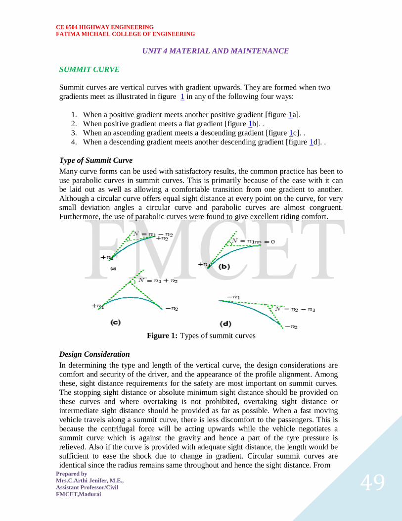
CE 6504 HIGHWAY ENGINEERING
FATIMA MICHAEL COLLEGE OF ENGINEERING
Prepared by
MrsCArthi Jenifer ME
Assistant ProfessorCivil
FMCETMadurai 49
UNIT 4 MATERIAL AND MAINTENANCE
SUMMIT CURVE
Summit curves are vertical curves with gradient upwards They are formed when two
gradients meet as illustrated in figure 1 in any of the following four ways
1 When a positive gradient meets another positive gradient [figure 1a]
2 When positive gradient meets a flat gradient [figure 1b]
3 When an ascending gradient meets a descending gradient [figure 1c]
4 When a descending gradient meets another descending gradient [figure 1d]
Type of Summit Curve
Many curve forms can be used with satisfactory results the common practice has been to
use parabolic curves in summit curves This is primarily because of the ease with it can
be laid out as well as allowing a comfortable transition from one gradient to another
Although a circular curve offers equal sight distance at every point on the curve for very
small deviation angles a circular curve and parabolic curves are almost congruent
Furthermore the use of parabolic curves were found to give excellent riding comfort
Figure 1 Types of summit curves
Design Consideration
In determining the type and length of the vertical curve the design considerations are
comfort and security of the driver and the appearance of the profile alignment Among
these sight distance requirements for the safety are most important on summit curves
The stopping sight distance or absolute minimum sight distance should be provided on
these curves and where overtaking is not prohibited overtaking sight distance or
intermediate sight distance should be provided as far as possible When a fast moving
vehicle travels along a summit curve there is less discomfort to the passengers This is
because the centrifugal force will be acting upwards while the vehicle negotiates a
summit curve which is against the gravity and hence a part of the tyre pressure is
relieved Also if the curve is provided with adequate sight distance the length would be
sufficient to ease the shock due to change in gradient Circular summit curves are
identical since the radius remains same throughout and hence the sight distance From
CE 6504 HIGHWAY ENGINEERING
FATIMA MICHAEL COLLEGE OF ENGINEERING
Prepared by
MrsCArthi Jenifer ME
Assistant ProfessorCivil
FMCETMadurai 50
this point of view transition curves are not desirable since it has varying radius and so the
sight distance will also vary The deviation angles provided on summit curves for
highways are very large and so the simple parabola is almost congruent to a circular arc
between the same tangent points Parabolic curves are easy for computation and also it
had been found out that it provides good riding comfort to the drivers It is also easy for
field implementation Due to all these reasons a simple parabolic curve is preferred as
summit curve Length of the summit curve
The important design aspect of the summit curve is the determination of the length of the
curve which is parabolic As noted earlier the length of the curve is guided by the sight
distance consideration That is a driver should be able to stop his vehicle safely if there is
an obstruction on the other side of the road Equation of the parabola is given by
where where N is the deviation angle and is the length of the In
deriving the length of the curve two situations can arise depending on the uphill and
downhill gradients when the length of the curve is greater than the sight distance and the
length of the curve is greater than the sight distance
Let is the length of the summit curve is the SSDISDOSD is the deviation angle
drivers eye height (12 m) and the height of the obstruction then the length of the
summit curve can be derived for the following two cases The length of the summit curve
can be derived from the simple geometry as shown below
Case a Length of summit curve greater than sight distance( )
Figure 1 Length of summit curve ( )
The situation when the sight distance is less than the length of the curve is shown in
figure 1
CE 6504 HIGHWAY ENGINEERING
FATIMA MICHAEL COLLEGE OF ENGINEERING
Prepared by
MrsCArthi Jenifer ME
Assistant ProfessorCivil
FMCETMadurai 51
(1)
Case b Length of summit curve less than sight distance
The second case is illustrated in figure 1
Figure 1 Length of summit curve
CE 6504 HIGHWAY ENGINEERING
FATIMA MICHAEL COLLEGE OF ENGINEERING
Prepared by
MrsCArthi Jenifer ME
Assistant ProfessorCivil
FMCETMadurai 52
From the basic geometry one can write
(1)
Therefore for a given and to get minimum differentiate the above equation
with respect to and equate it to zero Therefore
Solving the quadratic equation for
(2)
Now we can substitute back to get the value of minimum value of for a given
and Therefore
Solving for
CE 6504 HIGHWAY ENGINEERING
FATIMA MICHAEL COLLEGE OF ENGINEERING
Prepared by
MrsCArthi Jenifer ME
Assistant ProfessorCivil
FMCETMadurai 53
(3) (4
CE 6504 HIGHWAY ENGINEERING
FATIMA MICHAEL COLLEGE OF ENGINEERING
Prepared by
MrsCArthi Jenifer ME
Assistant ProfessorCivil
FMCETMadurai 54
When stopping sight distance is considered the height of drivers eye above the road
surface ( ) is taken as 12 metres and height of object above the pavement surface ( )
is taken as 015 metres If overtaking sight distance is considered then the value of
drivers eye height ( ) and the height of the obstruction ( ) are taken equal as 12
metres
Valley curve
Valley curve or sag curves are vertical curves with convexity downwards They are
formed when two gradients meet as illustrated in figure 1 in any of the following four
ways
Figure 1 Types of valley curve
1 When a descending gradient meets another descending gradient [figure 1a]
2 When a descending gradient meets a flat gradient [figure 1b]
3 When a descending gradient meets an ascending gradient [figure 1c]
4 When an ascending gradient meets another ascending gradient [figure
Design considerations
There is no restriction to sight distance at valley curves during day time But visibility is
reduced during night In the absence or inadequacy of street light the only source for
visibility is with the help of headlights Hence valley curves are designed taking into
account of headlight distance In valley curves the centrifugal force will be acting
downwards along with the weight of the vehicle and hence impact to the vehicle will be
more This will result in jerking of the vehicle and cause discomfort to the passengers
Thus the most important design factors considered in valley curves are (1) impact-free
movement of vehicles at design speed and (2) availability of stopping sight distance
under headlight of vehicles for night driving
For gradually introducing and increasing the centrifugal force acting downwards the best
shape that could be given for a valley curve is a transition curve Cubic parabola is
generally preferred in vertical valley curves See figure 1
CE 6504 HIGHWAY ENGINEERING
FATIMA MICHAEL COLLEGE OF ENGINEERING
Prepared by
MrsCArthi Jenifer ME
Assistant ProfessorCivil
FMCETMadurai 55
Figure 1 Valley curve details
During night under headlight driving condition sight distance reduces and availability of
stopping sight distance under head light is very important The head light sight distance
should be at least equal to the stopping sight distance There is no problem of overtaking
sight distance at night since the other vehicles with headlights could be seen from a
considerable distance
Length of the valley curve
The valley curve is made fully transitional by providing two similar transition curves of
equal length The transitional curve is set out by a cubic parabola where
The length of the valley transition curve is designed based on two criteria
1 comfort criteria that is allowable rate of change of centrifugal acceleration is
limited to a comfortable level of about
2 safety criteria that is the driver should have adequate headlight sight distance at
any part of the country
Comfort criteria
The length of the valley curve based on the rate of change of centrifugal acceleration that
will ensure comfort Let is the rate of change of acceleration the minimum radius of
the curve is the design speed and is the time then is give
CE 6504 HIGHWAY ENGINEERING
FATIMA MICHAEL COLLEGE OF ENGINEERING
Prepared by
MrsCArthi Jenifer ME
Assistant ProfessorCivil
FMCETMadurai 56
For a cubic parabola the Value Safety criter Length of the valley curve for headlight distance may be determined for two conditions
(1) length of the valley curve greater than stopping sight distance and (2) length of the
valley curve less than the stopping sight distance of for length is given by
Case 1 Length of valley curve greater than stopping sight distance ( )
The total length of valley curve is greater than the stopping sight distance SSD The
sight distance available will be minimum when the vehicle is in the lowest point in the
valley This is because the beginning of the curve will have infinite radius and the bottom
of the curve will have minimum radius which is a property of the transition curve The
case is shown in figure 1
Figure 1 Valley curve case 1
From the geometry of the figure we have
CE 6504 HIGHWAY ENGINEERING
FATIMA MICHAEL COLLEGE OF ENGINEERING
Prepared by
MrsCArthi Jenifer ME
Assistant ProfessorCivil
FMCETMadurai 57
(1)
where is the deviation angle in radians is the height of headlight beam is the
head beam inclination in degrees and is the sight distance The inclination is 1
degree
Case 2 Length of valley curve less than stopping sight distance ( )
The length of the curve is less than SSD In this case the minimum sight distance is
from the beginning of the curve The important points are the beginning of the curve and
the bottom most part of the curve If the vehicle is at the bottom of the curve then its
headlight beam will reach far beyond the endpoint of the curve whereas if the vehicle is
at the beginning of the curve then the headlight beam will hit just outside the curve
Therefore the length of the curve is derived by assuming the vehicle at the beginning of
the curve The case is shown in figure 1
From the figure
(1) Note that the above expression is approximate and is satisfactory because in practice the gradients
are very small and is acceptable for all practical purposes We will not be able to know prior to
which case to be adopted Therefore both has to be calculated and the one which satisfies the
condition is adopted
1 Flexible pavement
2 Rigid pavement
Flexible pavement
These pavements reflect the deformation of sub grade and the subsequent layers to the
surface
Rigid pavement
The rigid characteristic of the pavement are associated with rigidity or flexural strength
CE 6504 HIGHWAY ENGINEERING
FATIMA MICHAEL COLLEGE OF ENGINEERING
Prepared by
MrsCArthi Jenifer ME
Assistant ProfessorCivil
FMCETMadurai 58
or slab action so the load is distributed over a wide area of sub grade soil
Flexible pavement Definition
These pavements reflect the deformation of sub grade and the subsequent layers to the
surface Flexible usually asphalt is laid with no reinforcement or with a specialized
fabric reinforcement that permits limited flow or repositioning of the roadbed under
ground changes
The design of flexible pavement is based on load distributing characteristic of the
component layers The black top pavement including water amp gravel bound macadam fall
in this category
Flexible pavement on the whole has low or negligible flexible strength flexible in their
structural action) The flexible pavement layers transmit the vertical or compressive
stresses to the lower layers by grain transfer through contact points of granular structure
The vertical compressive stress is maximum on the pavement surface directly under the
wheel load and is equal to contact pressure under the wheels Due to the ability to
distribute the stress to large area in the shape of truncated cone the stresses get decreased
in the lower layer
As such the flexible pavement may be constructed in a number of layers and the top
layer has to be strongest as the highest compressive stresses
To be sustained by this layer in addition to wear and tear the lower layer have to take
up only lesser magnitude of stress as there is no direct wearing action die to traffic loads
therefore inferior material with lower cast can be used in the lower layers
Rigid pavement Definition
The rigid characteristic of the pavement are associated with rigidity or flexural strength
or slab action so the load is distributed over a wide area of sub grade soil Rigid pavement
is laid in slabs with steel reinforcement
The rigid pavements are made of cement concrete either plan reinforced or prestressed
concrete
Critical condition of stress in the rigid pavement is the maximum flexural stress occurring in the slab due to wheel load and the temperature changes
Rigid pavement is designed and analyzed by using the elastic theory
CE 6504 HIGHWAY ENGINEERING
FATIMA MICHAEL COLLEGE OF ENGINEERING
Prepared by
MrsCArthi Jenifer ME
Assistant ProfessorCivil
FMCETMadurai 59
UNIT-5 EVALUATION AND MAINTENANCE OF PAVEMENTS
TRAFFIC PARAMETERS
Design life
Design life is the number of years (or number of standard axle repetitions) for which the
pavement is being designed A pavement is expected to serve satisfactorily within the
design life For concrete pavements 20 to 40 years may be assumed as the design life
(PCA 1984 IRC58 2002)
Basic design principle
Though different approaches for concrete pavement design are suggested in various
guidelines the design principles tend to remain similar across different guidelines for
example PCA (1994) Austroads (2004) NCHRP (2004) IRC58 (2002) etc except the
AASHTO (1993) provisions which is based on empirical approach The basic steps
involved in the design of concrete pavement method can be summarized as follows
The developed stresses due to load for a trial thickness of the concrete slab are
calculated for various loading configuration and the critical one is chosen The
axle loads are generally divided into different axle load groups and the load
stresses are calculated individually
The ratio between the load stress and Modulus of Rupture (MOR) is known as
stress ratio The stress ratio determines how many repetitions the pavement can
sustain (ie allowable traffic repetitions) for the individual axle load group If the
stress ratio is 055 or lower it can withstand virtually infinite number of traffic
repetitions (PCA 1984)
The ratio between the allowable repetitions to the expected traffic repetitions is
the damage fraction The calculation process is repeated for various axle loads
(sometimes for various seasons or various timings of the day) and the sum of
individual damage fractions (c u m u l a t i v e fatigue damage) should be less
than equal to one for pavement design being safe If found unsafe the trial
thickness is changed and the design process is repeated
The design process may also include considerations for temperature stress
moisture stresses and erosion distress
A brief discussion on concrete pavement design approaches suggested by various design
practices viz PCA method (1984) Austroads method (2004) AASHTO method (1993)
NCHRP mechanistic-empirical method (2004) and the Indian Roads Congress (IRC)
method (2002) are placed in the following
Portland cement Association (PCA) Method
The PCA method is based on Westergaard Picket and Rays work and further theoretical
analysis by Finite Element Method (Huang 1993) The data used to develop the PCA
method is generated from various road tests like ASSHO road test Arlington test
(conducted by PCA) Bates test road and Maryland road test (PCA 1984) The PCA
design method is based on the following two considerations (PCA 1984)
The fatigue damage on the concrete slab due to repetitive application of traffic
load is estimated The cumulative fatigue damage principle is used to estimate the
design thickness of the slab Edge stress between the mid-ways of the
CE 6504 HIGHWAY ENGINEERING
FATIMA MICHAEL COLLEGE OF ENGINEERING
Prepared by
MrsCArthi Jenifer ME
Assistant ProfessorCivil
FMCETMadurai 60
transverse joint is taken as critical configuration
The stresses due to warping and curling (due to temperature and moisture
gradient) are not considered in the fatigue analysis as per PCA recommendation
because most of the time the stresses generated are subtractive to the load stress
The possibility of erosion of pavement materials placed below the concrete slab is
evaluated The rate at which the slab is deflected due to axle load is used as a
criterion for erosion Theoretically it can be shown that a thin pavement with
smaller deflection basin is subjected to faster rate of deflection compared to
thicker slab Hence thin slab is more susceptible to erosion In a similar way the
cumulative erosion damage is calculated for individual axle load groups If this
value is greater than one then the design needs to be revised
Austroads method
Austroads method has been adopted from PCA (1984) approach with modifications
suited to Australian conditions (Austroads 2004) A bound mix or lean cement concrete is
used as sub-base material For a given CBR value of the subgrade and given thickness of
cemented sub-base the effective subgrade strength can be obtained from the chart
provided Figure-19 schematically shows such a chart For different levels of traffic
Austroads (2004) suggests minimum values of the base thicknesses to be provided
CE 6504 HIGHWAY ENGINEERING
FATIMA MICHAEL COLLEGE OF ENGINEERING
Prepared by
MrsCArthi Jenifer ME
Assistant ProfessorCivil
FMCETMadurai 61
figure-19 Schematic diagram of Austroads (2004) chart for estimation of effective
subgrade strength
As per Astroads (2004) the concrete pavement slab thickness for a given expected
traffic repetitions is designed considering the (i) flexural fatigue of the concrete slab and
the (ii) subgrade erosion arising out of repeated deflections For both the considerations
equations are suggested to calculate the allowable traffic repetitions If the allowable
traffic is less than the expected traffic the design is revised by increasing the slab
thickness The concrete shoulders adopted are of integral type or structural type
AASHTO method
The AASHTO method (1993) for design of concrete pavement has evolved from the
AASHO road test (AASHO 1962) The AASHTO pavement design follows an empirical
approach Pavement performance in terms of present serviceability index ( PSI ) loss of
serviceability sub-grade and sub-base strength cumulative traffic properties of concrete
joint load transfer efficiency drainage condition overall standard deviation and
reliability are the input parameters considered in the pavement design
The PSI value of the fresh pavement is assumed as 45 and the pavement is deemed to
have failed when the PSI value reaches 25 The resilient moduli of the subgrade and sub-
base materials are determined in the laboratory simulating the seasonal moisture content
and stress situation Suggested values are also available for given moisture content
plasticity index etc The composite modulus of sub-grade reaction (k) is estimated from
modulus of sub-grade reaction and elastic modulus of sub-base for various seasons and
the depth of rigid foundation and the thickness of the sub-base
Design equation as well nomographs are available to estimate the slab thickness (D) from
these input parameters
NCHRP mechanistic-empirical (M-E) metho
The NCHRP (2004) has recently developed concrete pavement design procedure based
on mechanistic-empirical (M-E) approach This approach attempts to reduce the extent of
empiricism prevalent in the existing AASHTO (1993) guidelines This proposed NCHRP
pavement design system is modular in nature that is the design approach can be
modified by parts (as and when new knowledge is available) without disrupting the
overall design procedure This approach also can take care of various wheel-axle loa
configuration
As per this approach trial thickness of the slab is first assumed and the stress strain and
displacement values are obtained From these values the performance of the pavement in
terms of distresses (such as faulting cracking) and smoothness and predicted If these
predicted performance parameters does not satisfy the required performance for a given
reliability
The design approach includes a large data-base as input parameters for example average
daily traffic traffic growth rate traffic composition hourly weather data on air
temperature precipitation wind speed percentage sunshine relative humidity pavement
material engineering parameters ground water depth infiltration drainage hydraulic
conductivity thermal conductivity heat capacity etc The temperature stress is
considered in this method but the temperature profile is linearized to enhance
computational efficiency (NCHRP 2004)
CE 6504 HIGHWAY ENGINEERING
FATIMA MICHAEL COLLEGE OF ENGINEERING
Prepared by
MrsCArthi Jenifer ME
Assistant ProfessorCivil
FMCETMadurai 62
INDIAN ROADS CONGRESS (IRC) METHOD
The Indian Roads Congress (IRC) guidelines IRC58 (2002) has adopted the
Westergaards equation to estimate load stress and Brdaburys equation to estimate
temperature stress The load stress is highest at the corner of the slab lesser in edge and
least in the interior The order of variation of temperature stress is just the reverse of this
As per IRC58 (2002) it is recommended that the design needs to be done for edge stress
condition and subsequently check needs to be performed for corner stress condition so as
to finalize the design The following are the steps followed as per IRC58 (2002)
guideline for the design of concrete pavement
The input parameters are obtained to formulate the design problem The joint
spacing and the slab dimensions are decided If there is a bound sub-base layer
over the subgrade a suitable value of effective k is to be adopted
A trial thickness of the concrete slab is assumed
The edge stress is estimated for various axle loads from the given charts Figure-
20 schematically shows such a chart The cumulative fatigue damage principle for
fatigue is applied to check the adequacy of the slab thickness
The sum of edge stress due to load for the highest axle load group and the
temperature stress should be less than the MOR of concrete otherwise the design
is revised
The adequacy of corner stress is checked with respect to MOR value and
accordingly the design is finalized Westergaards corner stress formula
Figure-20 Schematic diagram of IRC58 chart for estimation of load stress at the edge
(IRC58 2002)
CE 6504 HIGHWAY ENGINEERING
FATIMA MICHAEL COLLEGE OF ENGINEERING
Prepared by
MrsCArthi Jenifer ME
Assistant ProfessorCivil
FMCETMadurai 63
estimation of corner stress due to load and the corner stress due to temperature is
assumed to be zero
Estimation of layer thicknesses
The thickness of the pavement is adjusted in such a way that the stress strain
developed is less than the allowable values obtained from past performance
information
The two major modes of structural failure of pavement are fatigue and rutting
o Fatigue Traffic applies repetitive load to the pavement surface and the
cracks start from bottom the bound layer slab and propagate upwards
When the extent of surface cracks reaches a predefined level the
pavement is said to have failed due to flexural fatigue
FUNCTIONAL DESIGN
The functional pavement design involves considerations of skid resistance roughness
surface distresses reflectivity of pavement surface etc The functional pavement design
considers mainly the surface features of a pavement
Drainage design
A road needs to be designed in such a way that the rain snow precipitation is drained off
the pavement and its surroundings A suitable surface drainage system for the pavement
is designed for this purpose Some water however will percolate into the pavement from
its top surface and needs to be taken out of the pavement - this is done by providing an
internal drainage system to the pavement Water will also try to enter into the pavement
from bottom due to capillary rise or due to rise in water table A suitably designed sub-
surface drainage system tries to avoid such a problem
PAVEMENT THICKNESS DESIGN CHARTS
For the design of pavements to carry traffic in the range of 1 to 10 msa use chart 1 and for
traffic in the range 10 to 150 msa use chart 2 of IRC37 2001 The design curves relate
pavement thickness to the cumulative number of standard axles to be carried over the
design life for different sub-grade CBR values ranging from 2 to 10 The design
charts will give the total thickness of the pavement for the above inputs The total
thickness consists of granular sub-base granular base and bituminous surfacing The
individual layers are designed based on the the recommendations given below and the
subsequent tables
Pavement composition
Sub-base
Sub-base materials comprise natural sand gravel laterite brick metal crushed
stone or combinations thereof meeting the prescribed grading and physical
requirements The sub-base material should have a minimum CBR of 20 and
30 for traffic upto 2 msa and traffic exceeding 2 msa respectively Sub-base
usually consist of granular or WBM and the thickness should not be less than 150
mm for design traffic less than 10 msa and 200 mm for design traffic
Base
The recommended designs are for unbounded granular bases which comprise
CE 6504 HIGHWAY ENGINEERING
FATIMA MICHAEL COLLEGE OF ENGINEERING
Prepared by
MrsCArthi Jenifer ME
Assistant ProfessorCivil
FMCETMadurai 64
conventional water bound macadam (WBM) or wet mix macadam (WMM) or
equivalent confirming to MOST specifications The materials should be of good
quality with minimum thickness of 225 mm for traffic up to 2 msa an 150 mm for
traffic
Bituminoussurfacing The surfacing consists of a wearing course or a binder
course plus wearing course The most commonly used wearing courses are
surface dressing open graded premix carpet mix seal surfacing semi-
dense bituminous concrete and bituminous concrete For binder course
MOST specifies it is desirable to use bituminous macadam (BM) for traffic
upto o 5 msa and dense bituminous macadam (DBM) for traffic more than 5
msa
Numerical example
Design the pavement for construction of a new bypass with the following data
1 Two lane carriage way
2 Initial traffic in the year of completion of construction = 400 CVPD (sum of both
directions)
3 Traffic growth rate = 75
4 Design life = 15 years
5 Vehicle damage factor based on axle load survey = 25 standard axle per
commercial vehicle
6 Design CBR of subgrade soil = 4
Solution
1 Distribution factor = 075
2
3 Total pavement thickness for CBR 4 and traffic 72 msa from IRC37 2001
chart1 = 660 mm
4 Pavement composition can be obtained by interpolation from Pavement Design
Catalogue (IRC37 2001)
1 Bituminous surfacing = 25 mm SDBC + 70 mm DBM
2 Road-base = 250 mm WBM
3 sub-base = 315 mm granular material of CBR not less than 30
CE 6504 HIGHWAY ENGINEERING
FATIMA MICHAEL COLLEGE OF ENGINEERING
Prepared by
MrsCArthi Jenifer ME
Assistant ProfessorCivil
FMCETMadurai 65
Generally bound base layers are used for concrete pavement construction As per Indian
specification some example of such base layers are Dry Lean Concrete (DLC) Roller
Compacted Concrete (RCC) (IRC15-2002)
The concrete slab is generally of M40 to M50 grade of concrete as
per Indian specifications and is called as paving quality concrete (PQC)
(IRC15-2002)
BITUMINOUS PAVEMENT
The subgrade is a compacted soil layer
The base and sub-base course could be made up of bound or unbound granular layer As
per Indian specifications (MORTampH 2001) some examples of base or sub-base layers
are Granular sub-base(GSB) Water Bound Macadam (WBM) Wet Mix Macadam
(WMM) etc
The binder course is made up bituminous material As per Indian specifications
(MORTampH 2001) some examples of binder course are Bituminous Macadam (BM)
Dense Bituminous Macadam (DBM) etc
The wearing course is the top bituminous layer which is comes in contact to the
vehicle tyre Wearing course provides impermeability to the pavement surface
against water percolation (Chakroborty and Das 2003) The binder course and wearing
course together are called bituminous surfacing
IRC METHOD OF FLEXIBLE PAVEMENT MIX DESIGN
These guidelines will apply to design of flexible pavements for Expressway National Highways
State Highways Major District Roads and other categories of roads Flexible pavements are
considered to include the pavements which have bituminous surfacing and granular base and sub-
base courses conforming to IRC MOST standards These guidelines apply to new pavements
Design criteria
The flexible pavements has been modeled as a three layer structure and stresses and strains at
critical locations have been computed using the linear elastic model To give proper consideration
to the aspects of performance the following three types of pavement distress resulting from
repeated (cyclic) application of traffic loads are considered
1 Vertical compressive strain at the top of the sub-grade which can cause sub-grade
deformation resulting in permanent deformation at the pavement surface
2 Horizontal tensile strain or stress at the bottom of the bituminous layer which can cause
fracture of the bituminous layer
3 Pavement deformation within the bituminous layer
CE 6504 HIGHWAY ENGINEERING
FATIMA MICHAEL COLLEGE OF ENGINEERING
Prepared by
MrsCArthi Jenifer ME
Assistant ProfessorCivil
FMCETMadurai 66
While the permanent deformation within the bituminous layer can be controlled by meeting the
mix design requirements thickness of granular and bituminous layers are selected using the
analytical design approach so that strains at the critical points are within the allowable limits For
calculating tensile strains at the bottom of the bituminous layer the stiffness of dense bituminous
macadam (DBM) layer with 6070 bitumen has been used in the analysis
FAILURE CRITERIA
Critical locations in pavement
A and B are the critical locations for tensile strains Maximum value of the strain is
adopted for design C is the critical location for the vertical subgrade strain since the
maximum value of the occurs mostly at C
CE 6504 HIGHWAY ENGINEERING
FATIMA MICHAEL COLLEGE OF ENGINEERING
Prepared by
MrsCArthi Jenifer ME
Assistant ProfessorCivil
FMCETMadurai 67
Fatigue Criteria
Bituminous surfacings of pavements display flexural fatigue cracking if the tensile strain
at the bottom of the bituminous layer is beyond certain limit The relation between the
fatigue life of the pavement and the tensile strain in the bottom of the bituminous layer
was obtained as
(1)
in which is the allowable number of load repetitions to control fatigue cracking and
is the Elastic modulus of bituminous layer The use of equation 1 would result in
fatigue cracking of 20 of the total area
Rutting Criteria
The allowable number of load repetitions to control permanent deformation can be
expressed as
(2)
is the number of cumulative standard axles to produce rutting of 20 mm
CE 6504 HIGHWAY ENGINEERING
FATIMA MICHAEL COLLEGE OF ENGINEERING
Prepared by
MrsCArthi Jenifer ME
Assistant ProfessorCivil
FMCETMadurai 68
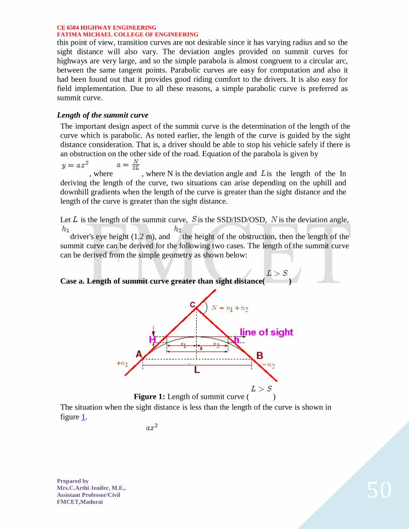
CE 6504 HIGHWAY ENGINEERING
FATIMA MICHAEL COLLEGE OF ENGINEERING
Prepared by
MrsCArthi Jenifer ME
Assistant ProfessorCivil
FMCETMadurai 50
this point of view transition curves are not desirable since it has varying radius and so the
sight distance will also vary The deviation angles provided on summit curves for
highways are very large and so the simple parabola is almost congruent to a circular arc
between the same tangent points Parabolic curves are easy for computation and also it
had been found out that it provides good riding comfort to the drivers It is also easy for
field implementation Due to all these reasons a simple parabolic curve is preferred as
summit curve Length of the summit curve
The important design aspect of the summit curve is the determination of the length of the
curve which is parabolic As noted earlier the length of the curve is guided by the sight
distance consideration That is a driver should be able to stop his vehicle safely if there is
an obstruction on the other side of the road Equation of the parabola is given by
where where N is the deviation angle and is the length of the In
deriving the length of the curve two situations can arise depending on the uphill and
downhill gradients when the length of the curve is greater than the sight distance and the
length of the curve is greater than the sight distance
Let is the length of the summit curve is the SSDISDOSD is the deviation angle
drivers eye height (12 m) and the height of the obstruction then the length of the
summit curve can be derived for the following two cases The length of the summit curve
can be derived from the simple geometry as shown below
Case a Length of summit curve greater than sight distance( )
Figure 1 Length of summit curve ( )
The situation when the sight distance is less than the length of the curve is shown in
figure 1
CE 6504 HIGHWAY ENGINEERING
FATIMA MICHAEL COLLEGE OF ENGINEERING
Prepared by
MrsCArthi Jenifer ME
Assistant ProfessorCivil
FMCETMadurai 51
(1)
Case b Length of summit curve less than sight distance
The second case is illustrated in figure 1
Figure 1 Length of summit curve
CE 6504 HIGHWAY ENGINEERING
FATIMA MICHAEL COLLEGE OF ENGINEERING
Prepared by
MrsCArthi Jenifer ME
Assistant ProfessorCivil
FMCETMadurai 52
From the basic geometry one can write
(1)
Therefore for a given and to get minimum differentiate the above equation
with respect to and equate it to zero Therefore
Solving the quadratic equation for
(2)
Now we can substitute back to get the value of minimum value of for a given
and Therefore
Solving for
CE 6504 HIGHWAY ENGINEERING
FATIMA MICHAEL COLLEGE OF ENGINEERING
Prepared by
MrsCArthi Jenifer ME
Assistant ProfessorCivil
FMCETMadurai 53
(3) (4
CE 6504 HIGHWAY ENGINEERING
FATIMA MICHAEL COLLEGE OF ENGINEERING
Prepared by
MrsCArthi Jenifer ME
Assistant ProfessorCivil
FMCETMadurai 54
When stopping sight distance is considered the height of drivers eye above the road
surface ( ) is taken as 12 metres and height of object above the pavement surface ( )
is taken as 015 metres If overtaking sight distance is considered then the value of
drivers eye height ( ) and the height of the obstruction ( ) are taken equal as 12
metres
Valley curve
Valley curve or sag curves are vertical curves with convexity downwards They are
formed when two gradients meet as illustrated in figure 1 in any of the following four
ways
Figure 1 Types of valley curve
1 When a descending gradient meets another descending gradient [figure 1a]
2 When a descending gradient meets a flat gradient [figure 1b]
3 When a descending gradient meets an ascending gradient [figure 1c]
4 When an ascending gradient meets another ascending gradient [figure
Design considerations
There is no restriction to sight distance at valley curves during day time But visibility is
reduced during night In the absence or inadequacy of street light the only source for
visibility is with the help of headlights Hence valley curves are designed taking into
account of headlight distance In valley curves the centrifugal force will be acting
downwards along with the weight of the vehicle and hence impact to the vehicle will be
more This will result in jerking of the vehicle and cause discomfort to the passengers
Thus the most important design factors considered in valley curves are (1) impact-free
movement of vehicles at design speed and (2) availability of stopping sight distance
under headlight of vehicles for night driving
For gradually introducing and increasing the centrifugal force acting downwards the best
shape that could be given for a valley curve is a transition curve Cubic parabola is
generally preferred in vertical valley curves See figure 1
CE 6504 HIGHWAY ENGINEERING
FATIMA MICHAEL COLLEGE OF ENGINEERING
Prepared by
MrsCArthi Jenifer ME
Assistant ProfessorCivil
FMCETMadurai 55
Figure 1 Valley curve details
During night under headlight driving condition sight distance reduces and availability of
stopping sight distance under head light is very important The head light sight distance
should be at least equal to the stopping sight distance There is no problem of overtaking
sight distance at night since the other vehicles with headlights could be seen from a
considerable distance
Length of the valley curve
The valley curve is made fully transitional by providing two similar transition curves of
equal length The transitional curve is set out by a cubic parabola where
The length of the valley transition curve is designed based on two criteria
1 comfort criteria that is allowable rate of change of centrifugal acceleration is
limited to a comfortable level of about
2 safety criteria that is the driver should have adequate headlight sight distance at
any part of the country
Comfort criteria
The length of the valley curve based on the rate of change of centrifugal acceleration that
will ensure comfort Let is the rate of change of acceleration the minimum radius of
the curve is the design speed and is the time then is give
CE 6504 HIGHWAY ENGINEERING
FATIMA MICHAEL COLLEGE OF ENGINEERING
Prepared by
MrsCArthi Jenifer ME
Assistant ProfessorCivil
FMCETMadurai 56
For a cubic parabola the Value Safety criter Length of the valley curve for headlight distance may be determined for two conditions
(1) length of the valley curve greater than stopping sight distance and (2) length of the
valley curve less than the stopping sight distance of for length is given by
Case 1 Length of valley curve greater than stopping sight distance ( )
The total length of valley curve is greater than the stopping sight distance SSD The
sight distance available will be minimum when the vehicle is in the lowest point in the
valley This is because the beginning of the curve will have infinite radius and the bottom
of the curve will have minimum radius which is a property of the transition curve The
case is shown in figure 1
Figure 1 Valley curve case 1
From the geometry of the figure we have
CE 6504 HIGHWAY ENGINEERING
FATIMA MICHAEL COLLEGE OF ENGINEERING
Prepared by
MrsCArthi Jenifer ME
Assistant ProfessorCivil
FMCETMadurai 57
(1)
where is the deviation angle in radians is the height of headlight beam is the
head beam inclination in degrees and is the sight distance The inclination is 1
degree
Case 2 Length of valley curve less than stopping sight distance ( )
The length of the curve is less than SSD In this case the minimum sight distance is
from the beginning of the curve The important points are the beginning of the curve and
the bottom most part of the curve If the vehicle is at the bottom of the curve then its
headlight beam will reach far beyond the endpoint of the curve whereas if the vehicle is
at the beginning of the curve then the headlight beam will hit just outside the curve
Therefore the length of the curve is derived by assuming the vehicle at the beginning of
the curve The case is shown in figure 1
From the figure
(1) Note that the above expression is approximate and is satisfactory because in practice the gradients
are very small and is acceptable for all practical purposes We will not be able to know prior to
which case to be adopted Therefore both has to be calculated and the one which satisfies the
condition is adopted
1 Flexible pavement
2 Rigid pavement
Flexible pavement
These pavements reflect the deformation of sub grade and the subsequent layers to the
surface
Rigid pavement
The rigid characteristic of the pavement are associated with rigidity or flexural strength
CE 6504 HIGHWAY ENGINEERING
FATIMA MICHAEL COLLEGE OF ENGINEERING
Prepared by
MrsCArthi Jenifer ME
Assistant ProfessorCivil
FMCETMadurai 58
or slab action so the load is distributed over a wide area of sub grade soil
Flexible pavement Definition
These pavements reflect the deformation of sub grade and the subsequent layers to the
surface Flexible usually asphalt is laid with no reinforcement or with a specialized
fabric reinforcement that permits limited flow or repositioning of the roadbed under
ground changes
The design of flexible pavement is based on load distributing characteristic of the
component layers The black top pavement including water amp gravel bound macadam fall
in this category
Flexible pavement on the whole has low or negligible flexible strength flexible in their
structural action) The flexible pavement layers transmit the vertical or compressive
stresses to the lower layers by grain transfer through contact points of granular structure
The vertical compressive stress is maximum on the pavement surface directly under the
wheel load and is equal to contact pressure under the wheels Due to the ability to
distribute the stress to large area in the shape of truncated cone the stresses get decreased
in the lower layer
As such the flexible pavement may be constructed in a number of layers and the top
layer has to be strongest as the highest compressive stresses
To be sustained by this layer in addition to wear and tear the lower layer have to take
up only lesser magnitude of stress as there is no direct wearing action die to traffic loads
therefore inferior material with lower cast can be used in the lower layers
Rigid pavement Definition
The rigid characteristic of the pavement are associated with rigidity or flexural strength
or slab action so the load is distributed over a wide area of sub grade soil Rigid pavement
is laid in slabs with steel reinforcement
The rigid pavements are made of cement concrete either plan reinforced or prestressed
concrete
Critical condition of stress in the rigid pavement is the maximum flexural stress occurring in the slab due to wheel load and the temperature changes
Rigid pavement is designed and analyzed by using the elastic theory
CE 6504 HIGHWAY ENGINEERING
FATIMA MICHAEL COLLEGE OF ENGINEERING
Prepared by
MrsCArthi Jenifer ME
Assistant ProfessorCivil
FMCETMadurai 59
UNIT-5 EVALUATION AND MAINTENANCE OF PAVEMENTS
TRAFFIC PARAMETERS
Design life
Design life is the number of years (or number of standard axle repetitions) for which the
pavement is being designed A pavement is expected to serve satisfactorily within the
design life For concrete pavements 20 to 40 years may be assumed as the design life
(PCA 1984 IRC58 2002)
Basic design principle
Though different approaches for concrete pavement design are suggested in various
guidelines the design principles tend to remain similar across different guidelines for
example PCA (1994) Austroads (2004) NCHRP (2004) IRC58 (2002) etc except the
AASHTO (1993) provisions which is based on empirical approach The basic steps
involved in the design of concrete pavement method can be summarized as follows
The developed stresses due to load for a trial thickness of the concrete slab are
calculated for various loading configuration and the critical one is chosen The
axle loads are generally divided into different axle load groups and the load
stresses are calculated individually
The ratio between the load stress and Modulus of Rupture (MOR) is known as
stress ratio The stress ratio determines how many repetitions the pavement can
sustain (ie allowable traffic repetitions) for the individual axle load group If the
stress ratio is 055 or lower it can withstand virtually infinite number of traffic
repetitions (PCA 1984)
The ratio between the allowable repetitions to the expected traffic repetitions is
the damage fraction The calculation process is repeated for various axle loads
(sometimes for various seasons or various timings of the day) and the sum of
individual damage fractions (c u m u l a t i v e fatigue damage) should be less
than equal to one for pavement design being safe If found unsafe the trial
thickness is changed and the design process is repeated
The design process may also include considerations for temperature stress
moisture stresses and erosion distress
A brief discussion on concrete pavement design approaches suggested by various design
practices viz PCA method (1984) Austroads method (2004) AASHTO method (1993)
NCHRP mechanistic-empirical method (2004) and the Indian Roads Congress (IRC)
method (2002) are placed in the following
Portland cement Association (PCA) Method
The PCA method is based on Westergaard Picket and Rays work and further theoretical
analysis by Finite Element Method (Huang 1993) The data used to develop the PCA
method is generated from various road tests like ASSHO road test Arlington test
(conducted by PCA) Bates test road and Maryland road test (PCA 1984) The PCA
design method is based on the following two considerations (PCA 1984)
The fatigue damage on the concrete slab due to repetitive application of traffic
load is estimated The cumulative fatigue damage principle is used to estimate the
design thickness of the slab Edge stress between the mid-ways of the
CE 6504 HIGHWAY ENGINEERING
FATIMA MICHAEL COLLEGE OF ENGINEERING
Prepared by
MrsCArthi Jenifer ME
Assistant ProfessorCivil
FMCETMadurai 60
transverse joint is taken as critical configuration
The stresses due to warping and curling (due to temperature and moisture
gradient) are not considered in the fatigue analysis as per PCA recommendation
because most of the time the stresses generated are subtractive to the load stress
The possibility of erosion of pavement materials placed below the concrete slab is
evaluated The rate at which the slab is deflected due to axle load is used as a
criterion for erosion Theoretically it can be shown that a thin pavement with
smaller deflection basin is subjected to faster rate of deflection compared to
thicker slab Hence thin slab is more susceptible to erosion In a similar way the
cumulative erosion damage is calculated for individual axle load groups If this
value is greater than one then the design needs to be revised
Austroads method
Austroads method has been adopted from PCA (1984) approach with modifications
suited to Australian conditions (Austroads 2004) A bound mix or lean cement concrete is
used as sub-base material For a given CBR value of the subgrade and given thickness of
cemented sub-base the effective subgrade strength can be obtained from the chart
provided Figure-19 schematically shows such a chart For different levels of traffic
Austroads (2004) suggests minimum values of the base thicknesses to be provided
CE 6504 HIGHWAY ENGINEERING
FATIMA MICHAEL COLLEGE OF ENGINEERING
Prepared by
MrsCArthi Jenifer ME
Assistant ProfessorCivil
FMCETMadurai 61
figure-19 Schematic diagram of Austroads (2004) chart for estimation of effective
subgrade strength
As per Astroads (2004) the concrete pavement slab thickness for a given expected
traffic repetitions is designed considering the (i) flexural fatigue of the concrete slab and
the (ii) subgrade erosion arising out of repeated deflections For both the considerations
equations are suggested to calculate the allowable traffic repetitions If the allowable
traffic is less than the expected traffic the design is revised by increasing the slab
thickness The concrete shoulders adopted are of integral type or structural type
AASHTO method
The AASHTO method (1993) for design of concrete pavement has evolved from the
AASHO road test (AASHO 1962) The AASHTO pavement design follows an empirical
approach Pavement performance in terms of present serviceability index ( PSI ) loss of
serviceability sub-grade and sub-base strength cumulative traffic properties of concrete
joint load transfer efficiency drainage condition overall standard deviation and
reliability are the input parameters considered in the pavement design
The PSI value of the fresh pavement is assumed as 45 and the pavement is deemed to
have failed when the PSI value reaches 25 The resilient moduli of the subgrade and sub-
base materials are determined in the laboratory simulating the seasonal moisture content
and stress situation Suggested values are also available for given moisture content
plasticity index etc The composite modulus of sub-grade reaction (k) is estimated from
modulus of sub-grade reaction and elastic modulus of sub-base for various seasons and
the depth of rigid foundation and the thickness of the sub-base
Design equation as well nomographs are available to estimate the slab thickness (D) from
these input parameters
NCHRP mechanistic-empirical (M-E) metho
The NCHRP (2004) has recently developed concrete pavement design procedure based
on mechanistic-empirical (M-E) approach This approach attempts to reduce the extent of
empiricism prevalent in the existing AASHTO (1993) guidelines This proposed NCHRP
pavement design system is modular in nature that is the design approach can be
modified by parts (as and when new knowledge is available) without disrupting the
overall design procedure This approach also can take care of various wheel-axle loa
configuration
As per this approach trial thickness of the slab is first assumed and the stress strain and
displacement values are obtained From these values the performance of the pavement in
terms of distresses (such as faulting cracking) and smoothness and predicted If these
predicted performance parameters does not satisfy the required performance for a given
reliability
The design approach includes a large data-base as input parameters for example average
daily traffic traffic growth rate traffic composition hourly weather data on air
temperature precipitation wind speed percentage sunshine relative humidity pavement
material engineering parameters ground water depth infiltration drainage hydraulic
conductivity thermal conductivity heat capacity etc The temperature stress is
considered in this method but the temperature profile is linearized to enhance
computational efficiency (NCHRP 2004)
CE 6504 HIGHWAY ENGINEERING
FATIMA MICHAEL COLLEGE OF ENGINEERING
Prepared by
MrsCArthi Jenifer ME
Assistant ProfessorCivil
FMCETMadurai 62
INDIAN ROADS CONGRESS (IRC) METHOD
The Indian Roads Congress (IRC) guidelines IRC58 (2002) has adopted the
Westergaards equation to estimate load stress and Brdaburys equation to estimate
temperature stress The load stress is highest at the corner of the slab lesser in edge and
least in the interior The order of variation of temperature stress is just the reverse of this
As per IRC58 (2002) it is recommended that the design needs to be done for edge stress
condition and subsequently check needs to be performed for corner stress condition so as
to finalize the design The following are the steps followed as per IRC58 (2002)
guideline for the design of concrete pavement
The input parameters are obtained to formulate the design problem The joint
spacing and the slab dimensions are decided If there is a bound sub-base layer
over the subgrade a suitable value of effective k is to be adopted
A trial thickness of the concrete slab is assumed
The edge stress is estimated for various axle loads from the given charts Figure-
20 schematically shows such a chart The cumulative fatigue damage principle for
fatigue is applied to check the adequacy of the slab thickness
The sum of edge stress due to load for the highest axle load group and the
temperature stress should be less than the MOR of concrete otherwise the design
is revised
The adequacy of corner stress is checked with respect to MOR value and
accordingly the design is finalized Westergaards corner stress formula
Figure-20 Schematic diagram of IRC58 chart for estimation of load stress at the edge
(IRC58 2002)
CE 6504 HIGHWAY ENGINEERING
FATIMA MICHAEL COLLEGE OF ENGINEERING
Prepared by
MrsCArthi Jenifer ME
Assistant ProfessorCivil
FMCETMadurai 63
estimation of corner stress due to load and the corner stress due to temperature is
assumed to be zero
Estimation of layer thicknesses
The thickness of the pavement is adjusted in such a way that the stress strain
developed is less than the allowable values obtained from past performance
information
The two major modes of structural failure of pavement are fatigue and rutting
o Fatigue Traffic applies repetitive load to the pavement surface and the
cracks start from bottom the bound layer slab and propagate upwards
When the extent of surface cracks reaches a predefined level the
pavement is said to have failed due to flexural fatigue
FUNCTIONAL DESIGN
The functional pavement design involves considerations of skid resistance roughness
surface distresses reflectivity of pavement surface etc The functional pavement design
considers mainly the surface features of a pavement
Drainage design
A road needs to be designed in such a way that the rain snow precipitation is drained off
the pavement and its surroundings A suitable surface drainage system for the pavement
is designed for this purpose Some water however will percolate into the pavement from
its top surface and needs to be taken out of the pavement - this is done by providing an
internal drainage system to the pavement Water will also try to enter into the pavement
from bottom due to capillary rise or due to rise in water table A suitably designed sub-
surface drainage system tries to avoid such a problem
PAVEMENT THICKNESS DESIGN CHARTS
For the design of pavements to carry traffic in the range of 1 to 10 msa use chart 1 and for
traffic in the range 10 to 150 msa use chart 2 of IRC37 2001 The design curves relate
pavement thickness to the cumulative number of standard axles to be carried over the
design life for different sub-grade CBR values ranging from 2 to 10 The design
charts will give the total thickness of the pavement for the above inputs The total
thickness consists of granular sub-base granular base and bituminous surfacing The
individual layers are designed based on the the recommendations given below and the
subsequent tables
Pavement composition
Sub-base
Sub-base materials comprise natural sand gravel laterite brick metal crushed
stone or combinations thereof meeting the prescribed grading and physical
requirements The sub-base material should have a minimum CBR of 20 and
30 for traffic upto 2 msa and traffic exceeding 2 msa respectively Sub-base
usually consist of granular or WBM and the thickness should not be less than 150
mm for design traffic less than 10 msa and 200 mm for design traffic
Base
The recommended designs are for unbounded granular bases which comprise
CE 6504 HIGHWAY ENGINEERING
FATIMA MICHAEL COLLEGE OF ENGINEERING
Prepared by
MrsCArthi Jenifer ME
Assistant ProfessorCivil
FMCETMadurai 64
conventional water bound macadam (WBM) or wet mix macadam (WMM) or
equivalent confirming to MOST specifications The materials should be of good
quality with minimum thickness of 225 mm for traffic up to 2 msa an 150 mm for
traffic
Bituminoussurfacing The surfacing consists of a wearing course or a binder
course plus wearing course The most commonly used wearing courses are
surface dressing open graded premix carpet mix seal surfacing semi-
dense bituminous concrete and bituminous concrete For binder course
MOST specifies it is desirable to use bituminous macadam (BM) for traffic
upto o 5 msa and dense bituminous macadam (DBM) for traffic more than 5
msa
Numerical example
Design the pavement for construction of a new bypass with the following data
1 Two lane carriage way
2 Initial traffic in the year of completion of construction = 400 CVPD (sum of both
directions)
3 Traffic growth rate = 75
4 Design life = 15 years
5 Vehicle damage factor based on axle load survey = 25 standard axle per
commercial vehicle
6 Design CBR of subgrade soil = 4
Solution
1 Distribution factor = 075
2
3 Total pavement thickness for CBR 4 and traffic 72 msa from IRC37 2001
chart1 = 660 mm
4 Pavement composition can be obtained by interpolation from Pavement Design
Catalogue (IRC37 2001)
1 Bituminous surfacing = 25 mm SDBC + 70 mm DBM
2 Road-base = 250 mm WBM
3 sub-base = 315 mm granular material of CBR not less than 30
CE 6504 HIGHWAY ENGINEERING
FATIMA MICHAEL COLLEGE OF ENGINEERING
Prepared by
MrsCArthi Jenifer ME
Assistant ProfessorCivil
FMCETMadurai 65
Generally bound base layers are used for concrete pavement construction As per Indian
specification some example of such base layers are Dry Lean Concrete (DLC) Roller
Compacted Concrete (RCC) (IRC15-2002)
The concrete slab is generally of M40 to M50 grade of concrete as
per Indian specifications and is called as paving quality concrete (PQC)
(IRC15-2002)
BITUMINOUS PAVEMENT
The subgrade is a compacted soil layer
The base and sub-base course could be made up of bound or unbound granular layer As
per Indian specifications (MORTampH 2001) some examples of base or sub-base layers
are Granular sub-base(GSB) Water Bound Macadam (WBM) Wet Mix Macadam
(WMM) etc
The binder course is made up bituminous material As per Indian specifications
(MORTampH 2001) some examples of binder course are Bituminous Macadam (BM)
Dense Bituminous Macadam (DBM) etc
The wearing course is the top bituminous layer which is comes in contact to the
vehicle tyre Wearing course provides impermeability to the pavement surface
against water percolation (Chakroborty and Das 2003) The binder course and wearing
course together are called bituminous surfacing
IRC METHOD OF FLEXIBLE PAVEMENT MIX DESIGN
These guidelines will apply to design of flexible pavements for Expressway National Highways
State Highways Major District Roads and other categories of roads Flexible pavements are
considered to include the pavements which have bituminous surfacing and granular base and sub-
base courses conforming to IRC MOST standards These guidelines apply to new pavements
Design criteria
The flexible pavements has been modeled as a three layer structure and stresses and strains at
critical locations have been computed using the linear elastic model To give proper consideration
to the aspects of performance the following three types of pavement distress resulting from
repeated (cyclic) application of traffic loads are considered
1 Vertical compressive strain at the top of the sub-grade which can cause sub-grade
deformation resulting in permanent deformation at the pavement surface
2 Horizontal tensile strain or stress at the bottom of the bituminous layer which can cause
fracture of the bituminous layer
3 Pavement deformation within the bituminous layer
CE 6504 HIGHWAY ENGINEERING
FATIMA MICHAEL COLLEGE OF ENGINEERING
Prepared by
MrsCArthi Jenifer ME
Assistant ProfessorCivil
FMCETMadurai 66
While the permanent deformation within the bituminous layer can be controlled by meeting the
mix design requirements thickness of granular and bituminous layers are selected using the
analytical design approach so that strains at the critical points are within the allowable limits For
calculating tensile strains at the bottom of the bituminous layer the stiffness of dense bituminous
macadam (DBM) layer with 6070 bitumen has been used in the analysis
FAILURE CRITERIA
Critical locations in pavement
A and B are the critical locations for tensile strains Maximum value of the strain is
adopted for design C is the critical location for the vertical subgrade strain since the
maximum value of the occurs mostly at C
CE 6504 HIGHWAY ENGINEERING
FATIMA MICHAEL COLLEGE OF ENGINEERING
Prepared by
MrsCArthi Jenifer ME
Assistant ProfessorCivil
FMCETMadurai 67
Fatigue Criteria
Bituminous surfacings of pavements display flexural fatigue cracking if the tensile strain
at the bottom of the bituminous layer is beyond certain limit The relation between the
fatigue life of the pavement and the tensile strain in the bottom of the bituminous layer
was obtained as
(1)
in which is the allowable number of load repetitions to control fatigue cracking and
is the Elastic modulus of bituminous layer The use of equation 1 would result in
fatigue cracking of 20 of the total area
Rutting Criteria
The allowable number of load repetitions to control permanent deformation can be
expressed as
(2)
is the number of cumulative standard axles to produce rutting of 20 mm
CE 6504 HIGHWAY ENGINEERING
FATIMA MICHAEL COLLEGE OF ENGINEERING
Prepared by
MrsCArthi Jenifer ME
Assistant ProfessorCivil
FMCETMadurai 68
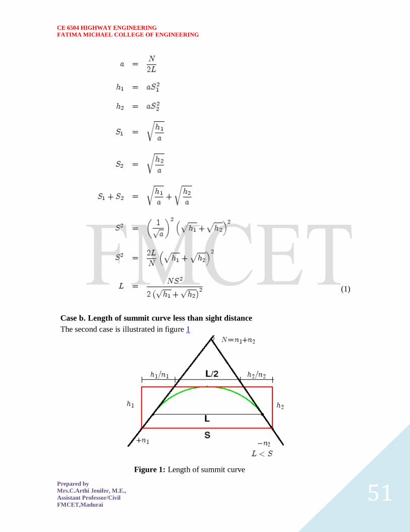
CE 6504 HIGHWAY ENGINEERING
FATIMA MICHAEL COLLEGE OF ENGINEERING
Prepared by
MrsCArthi Jenifer ME
Assistant ProfessorCivil
FMCETMadurai 52
From the basic geometry one can write
(1)
Therefore for a given and to get minimum differentiate the above equation
with respect to and equate it to zero Therefore
Solving the quadratic equation for
(2)
Now we can substitute back to get the value of minimum value of for a given
and Therefore
Solving for
CE 6504 HIGHWAY ENGINEERING
FATIMA MICHAEL COLLEGE OF ENGINEERING
Prepared by
MrsCArthi Jenifer ME
Assistant ProfessorCivil
FMCETMadurai 53
(3) (4
CE 6504 HIGHWAY ENGINEERING
FATIMA MICHAEL COLLEGE OF ENGINEERING
Prepared by
MrsCArthi Jenifer ME
Assistant ProfessorCivil
FMCETMadurai 54
When stopping sight distance is considered the height of drivers eye above the road
surface ( ) is taken as 12 metres and height of object above the pavement surface ( )
is taken as 015 metres If overtaking sight distance is considered then the value of
drivers eye height ( ) and the height of the obstruction ( ) are taken equal as 12
metres
Valley curve
Valley curve or sag curves are vertical curves with convexity downwards They are
formed when two gradients meet as illustrated in figure 1 in any of the following four
ways
Figure 1 Types of valley curve
1 When a descending gradient meets another descending gradient [figure 1a]
2 When a descending gradient meets a flat gradient [figure 1b]
3 When a descending gradient meets an ascending gradient [figure 1c]
4 When an ascending gradient meets another ascending gradient [figure
Design considerations
There is no restriction to sight distance at valley curves during day time But visibility is
reduced during night In the absence or inadequacy of street light the only source for
visibility is with the help of headlights Hence valley curves are designed taking into
account of headlight distance In valley curves the centrifugal force will be acting
downwards along with the weight of the vehicle and hence impact to the vehicle will be
more This will result in jerking of the vehicle and cause discomfort to the passengers
Thus the most important design factors considered in valley curves are (1) impact-free
movement of vehicles at design speed and (2) availability of stopping sight distance
under headlight of vehicles for night driving
For gradually introducing and increasing the centrifugal force acting downwards the best
shape that could be given for a valley curve is a transition curve Cubic parabola is
generally preferred in vertical valley curves See figure 1
CE 6504 HIGHWAY ENGINEERING
FATIMA MICHAEL COLLEGE OF ENGINEERING
Prepared by
MrsCArthi Jenifer ME
Assistant ProfessorCivil
FMCETMadurai 55
Figure 1 Valley curve details
During night under headlight driving condition sight distance reduces and availability of
stopping sight distance under head light is very important The head light sight distance
should be at least equal to the stopping sight distance There is no problem of overtaking
sight distance at night since the other vehicles with headlights could be seen from a
considerable distance
Length of the valley curve
The valley curve is made fully transitional by providing two similar transition curves of
equal length The transitional curve is set out by a cubic parabola where
The length of the valley transition curve is designed based on two criteria
1 comfort criteria that is allowable rate of change of centrifugal acceleration is
limited to a comfortable level of about
2 safety criteria that is the driver should have adequate headlight sight distance at
any part of the country
Comfort criteria
The length of the valley curve based on the rate of change of centrifugal acceleration that
will ensure comfort Let is the rate of change of acceleration the minimum radius of
the curve is the design speed and is the time then is give
CE 6504 HIGHWAY ENGINEERING
FATIMA MICHAEL COLLEGE OF ENGINEERING
Prepared by
MrsCArthi Jenifer ME
Assistant ProfessorCivil
FMCETMadurai 56
For a cubic parabola the Value Safety criter Length of the valley curve for headlight distance may be determined for two conditions
(1) length of the valley curve greater than stopping sight distance and (2) length of the
valley curve less than the stopping sight distance of for length is given by
Case 1 Length of valley curve greater than stopping sight distance ( )
The total length of valley curve is greater than the stopping sight distance SSD The
sight distance available will be minimum when the vehicle is in the lowest point in the
valley This is because the beginning of the curve will have infinite radius and the bottom
of the curve will have minimum radius which is a property of the transition curve The
case is shown in figure 1
Figure 1 Valley curve case 1
From the geometry of the figure we have
CE 6504 HIGHWAY ENGINEERING
FATIMA MICHAEL COLLEGE OF ENGINEERING
Prepared by
MrsCArthi Jenifer ME
Assistant ProfessorCivil
FMCETMadurai 57
(1)
where is the deviation angle in radians is the height of headlight beam is the
head beam inclination in degrees and is the sight distance The inclination is 1
degree
Case 2 Length of valley curve less than stopping sight distance ( )
The length of the curve is less than SSD In this case the minimum sight distance is
from the beginning of the curve The important points are the beginning of the curve and
the bottom most part of the curve If the vehicle is at the bottom of the curve then its
headlight beam will reach far beyond the endpoint of the curve whereas if the vehicle is
at the beginning of the curve then the headlight beam will hit just outside the curve
Therefore the length of the curve is derived by assuming the vehicle at the beginning of
the curve The case is shown in figure 1
From the figure
(1) Note that the above expression is approximate and is satisfactory because in practice the gradients
are very small and is acceptable for all practical purposes We will not be able to know prior to
which case to be adopted Therefore both has to be calculated and the one which satisfies the
condition is adopted
1 Flexible pavement
2 Rigid pavement
Flexible pavement
These pavements reflect the deformation of sub grade and the subsequent layers to the
surface
Rigid pavement
The rigid characteristic of the pavement are associated with rigidity or flexural strength
CE 6504 HIGHWAY ENGINEERING
FATIMA MICHAEL COLLEGE OF ENGINEERING
Prepared by
MrsCArthi Jenifer ME
Assistant ProfessorCivil
FMCETMadurai 58
or slab action so the load is distributed over a wide area of sub grade soil
Flexible pavement Definition
These pavements reflect the deformation of sub grade and the subsequent layers to the
surface Flexible usually asphalt is laid with no reinforcement or with a specialized
fabric reinforcement that permits limited flow or repositioning of the roadbed under
ground changes
The design of flexible pavement is based on load distributing characteristic of the
component layers The black top pavement including water amp gravel bound macadam fall
in this category
Flexible pavement on the whole has low or negligible flexible strength flexible in their
structural action) The flexible pavement layers transmit the vertical or compressive
stresses to the lower layers by grain transfer through contact points of granular structure
The vertical compressive stress is maximum on the pavement surface directly under the
wheel load and is equal to contact pressure under the wheels Due to the ability to
distribute the stress to large area in the shape of truncated cone the stresses get decreased
in the lower layer
As such the flexible pavement may be constructed in a number of layers and the top
layer has to be strongest as the highest compressive stresses
To be sustained by this layer in addition to wear and tear the lower layer have to take
up only lesser magnitude of stress as there is no direct wearing action die to traffic loads
therefore inferior material with lower cast can be used in the lower layers
Rigid pavement Definition
The rigid characteristic of the pavement are associated with rigidity or flexural strength
or slab action so the load is distributed over a wide area of sub grade soil Rigid pavement
is laid in slabs with steel reinforcement
The rigid pavements are made of cement concrete either plan reinforced or prestressed
concrete
Critical condition of stress in the rigid pavement is the maximum flexural stress occurring in the slab due to wheel load and the temperature changes
Rigid pavement is designed and analyzed by using the elastic theory
CE 6504 HIGHWAY ENGINEERING
FATIMA MICHAEL COLLEGE OF ENGINEERING
Prepared by
MrsCArthi Jenifer ME
Assistant ProfessorCivil
FMCETMadurai 59
UNIT-5 EVALUATION AND MAINTENANCE OF PAVEMENTS
TRAFFIC PARAMETERS
Design life
Design life is the number of years (or number of standard axle repetitions) for which the
pavement is being designed A pavement is expected to serve satisfactorily within the
design life For concrete pavements 20 to 40 years may be assumed as the design life
(PCA 1984 IRC58 2002)
Basic design principle
Though different approaches for concrete pavement design are suggested in various
guidelines the design principles tend to remain similar across different guidelines for
example PCA (1994) Austroads (2004) NCHRP (2004) IRC58 (2002) etc except the
AASHTO (1993) provisions which is based on empirical approach The basic steps
involved in the design of concrete pavement method can be summarized as follows
The developed stresses due to load for a trial thickness of the concrete slab are
calculated for various loading configuration and the critical one is chosen The
axle loads are generally divided into different axle load groups and the load
stresses are calculated individually
The ratio between the load stress and Modulus of Rupture (MOR) is known as
stress ratio The stress ratio determines how many repetitions the pavement can
sustain (ie allowable traffic repetitions) for the individual axle load group If the
stress ratio is 055 or lower it can withstand virtually infinite number of traffic
repetitions (PCA 1984)
The ratio between the allowable repetitions to the expected traffic repetitions is
the damage fraction The calculation process is repeated for various axle loads
(sometimes for various seasons or various timings of the day) and the sum of
individual damage fractions (c u m u l a t i v e fatigue damage) should be less
than equal to one for pavement design being safe If found unsafe the trial
thickness is changed and the design process is repeated
The design process may also include considerations for temperature stress
moisture stresses and erosion distress
A brief discussion on concrete pavement design approaches suggested by various design
practices viz PCA method (1984) Austroads method (2004) AASHTO method (1993)
NCHRP mechanistic-empirical method (2004) and the Indian Roads Congress (IRC)
method (2002) are placed in the following
Portland cement Association (PCA) Method
The PCA method is based on Westergaard Picket and Rays work and further theoretical
analysis by Finite Element Method (Huang 1993) The data used to develop the PCA
method is generated from various road tests like ASSHO road test Arlington test
(conducted by PCA) Bates test road and Maryland road test (PCA 1984) The PCA
design method is based on the following two considerations (PCA 1984)
The fatigue damage on the concrete slab due to repetitive application of traffic
load is estimated The cumulative fatigue damage principle is used to estimate the
design thickness of the slab Edge stress between the mid-ways of the
CE 6504 HIGHWAY ENGINEERING
FATIMA MICHAEL COLLEGE OF ENGINEERING
Prepared by
MrsCArthi Jenifer ME
Assistant ProfessorCivil
FMCETMadurai 60
transverse joint is taken as critical configuration
The stresses due to warping and curling (due to temperature and moisture
gradient) are not considered in the fatigue analysis as per PCA recommendation
because most of the time the stresses generated are subtractive to the load stress
The possibility of erosion of pavement materials placed below the concrete slab is
evaluated The rate at which the slab is deflected due to axle load is used as a
criterion for erosion Theoretically it can be shown that a thin pavement with
smaller deflection basin is subjected to faster rate of deflection compared to
thicker slab Hence thin slab is more susceptible to erosion In a similar way the
cumulative erosion damage is calculated for individual axle load groups If this
value is greater than one then the design needs to be revised
Austroads method
Austroads method has been adopted from PCA (1984) approach with modifications
suited to Australian conditions (Austroads 2004) A bound mix or lean cement concrete is
used as sub-base material For a given CBR value of the subgrade and given thickness of
cemented sub-base the effective subgrade strength can be obtained from the chart
provided Figure-19 schematically shows such a chart For different levels of traffic
Austroads (2004) suggests minimum values of the base thicknesses to be provided
CE 6504 HIGHWAY ENGINEERING
FATIMA MICHAEL COLLEGE OF ENGINEERING
Prepared by
MrsCArthi Jenifer ME
Assistant ProfessorCivil
FMCETMadurai 61
figure-19 Schematic diagram of Austroads (2004) chart for estimation of effective
subgrade strength
As per Astroads (2004) the concrete pavement slab thickness for a given expected
traffic repetitions is designed considering the (i) flexural fatigue of the concrete slab and
the (ii) subgrade erosion arising out of repeated deflections For both the considerations
equations are suggested to calculate the allowable traffic repetitions If the allowable
traffic is less than the expected traffic the design is revised by increasing the slab
thickness The concrete shoulders adopted are of integral type or structural type
AASHTO method
The AASHTO method (1993) for design of concrete pavement has evolved from the
AASHO road test (AASHO 1962) The AASHTO pavement design follows an empirical
approach Pavement performance in terms of present serviceability index ( PSI ) loss of
serviceability sub-grade and sub-base strength cumulative traffic properties of concrete
joint load transfer efficiency drainage condition overall standard deviation and
reliability are the input parameters considered in the pavement design
The PSI value of the fresh pavement is assumed as 45 and the pavement is deemed to
have failed when the PSI value reaches 25 The resilient moduli of the subgrade and sub-
base materials are determined in the laboratory simulating the seasonal moisture content
and stress situation Suggested values are also available for given moisture content
plasticity index etc The composite modulus of sub-grade reaction (k) is estimated from
modulus of sub-grade reaction and elastic modulus of sub-base for various seasons and
the depth of rigid foundation and the thickness of the sub-base
Design equation as well nomographs are available to estimate the slab thickness (D) from
these input parameters
NCHRP mechanistic-empirical (M-E) metho
The NCHRP (2004) has recently developed concrete pavement design procedure based
on mechanistic-empirical (M-E) approach This approach attempts to reduce the extent of
empiricism prevalent in the existing AASHTO (1993) guidelines This proposed NCHRP
pavement design system is modular in nature that is the design approach can be
modified by parts (as and when new knowledge is available) without disrupting the
overall design procedure This approach also can take care of various wheel-axle loa
configuration
As per this approach trial thickness of the slab is first assumed and the stress strain and
displacement values are obtained From these values the performance of the pavement in
terms of distresses (such as faulting cracking) and smoothness and predicted If these
predicted performance parameters does not satisfy the required performance for a given
reliability
The design approach includes a large data-base as input parameters for example average
daily traffic traffic growth rate traffic composition hourly weather data on air
temperature precipitation wind speed percentage sunshine relative humidity pavement
material engineering parameters ground water depth infiltration drainage hydraulic
conductivity thermal conductivity heat capacity etc The temperature stress is
considered in this method but the temperature profile is linearized to enhance
computational efficiency (NCHRP 2004)
CE 6504 HIGHWAY ENGINEERING
FATIMA MICHAEL COLLEGE OF ENGINEERING
Prepared by
MrsCArthi Jenifer ME
Assistant ProfessorCivil
FMCETMadurai 62
INDIAN ROADS CONGRESS (IRC) METHOD
The Indian Roads Congress (IRC) guidelines IRC58 (2002) has adopted the
Westergaards equation to estimate load stress and Brdaburys equation to estimate
temperature stress The load stress is highest at the corner of the slab lesser in edge and
least in the interior The order of variation of temperature stress is just the reverse of this
As per IRC58 (2002) it is recommended that the design needs to be done for edge stress
condition and subsequently check needs to be performed for corner stress condition so as
to finalize the design The following are the steps followed as per IRC58 (2002)
guideline for the design of concrete pavement
The input parameters are obtained to formulate the design problem The joint
spacing and the slab dimensions are decided If there is a bound sub-base layer
over the subgrade a suitable value of effective k is to be adopted
A trial thickness of the concrete slab is assumed
The edge stress is estimated for various axle loads from the given charts Figure-
20 schematically shows such a chart The cumulative fatigue damage principle for
fatigue is applied to check the adequacy of the slab thickness
The sum of edge stress due to load for the highest axle load group and the
temperature stress should be less than the MOR of concrete otherwise the design
is revised
The adequacy of corner stress is checked with respect to MOR value and
accordingly the design is finalized Westergaards corner stress formula
Figure-20 Schematic diagram of IRC58 chart for estimation of load stress at the edge
(IRC58 2002)
CE 6504 HIGHWAY ENGINEERING
FATIMA MICHAEL COLLEGE OF ENGINEERING
Prepared by
MrsCArthi Jenifer ME
Assistant ProfessorCivil
FMCETMadurai 63
estimation of corner stress due to load and the corner stress due to temperature is
assumed to be zero
Estimation of layer thicknesses
The thickness of the pavement is adjusted in such a way that the stress strain
developed is less than the allowable values obtained from past performance
information
The two major modes of structural failure of pavement are fatigue and rutting
o Fatigue Traffic applies repetitive load to the pavement surface and the
cracks start from bottom the bound layer slab and propagate upwards
When the extent of surface cracks reaches a predefined level the
pavement is said to have failed due to flexural fatigue
FUNCTIONAL DESIGN
The functional pavement design involves considerations of skid resistance roughness
surface distresses reflectivity of pavement surface etc The functional pavement design
considers mainly the surface features of a pavement
Drainage design
A road needs to be designed in such a way that the rain snow precipitation is drained off
the pavement and its surroundings A suitable surface drainage system for the pavement
is designed for this purpose Some water however will percolate into the pavement from
its top surface and needs to be taken out of the pavement - this is done by providing an
internal drainage system to the pavement Water will also try to enter into the pavement
from bottom due to capillary rise or due to rise in water table A suitably designed sub-
surface drainage system tries to avoid such a problem
PAVEMENT THICKNESS DESIGN CHARTS
For the design of pavements to carry traffic in the range of 1 to 10 msa use chart 1 and for
traffic in the range 10 to 150 msa use chart 2 of IRC37 2001 The design curves relate
pavement thickness to the cumulative number of standard axles to be carried over the
design life for different sub-grade CBR values ranging from 2 to 10 The design
charts will give the total thickness of the pavement for the above inputs The total
thickness consists of granular sub-base granular base and bituminous surfacing The
individual layers are designed based on the the recommendations given below and the
subsequent tables
Pavement composition
Sub-base
Sub-base materials comprise natural sand gravel laterite brick metal crushed
stone or combinations thereof meeting the prescribed grading and physical
requirements The sub-base material should have a minimum CBR of 20 and
30 for traffic upto 2 msa and traffic exceeding 2 msa respectively Sub-base
usually consist of granular or WBM and the thickness should not be less than 150
mm for design traffic less than 10 msa and 200 mm for design traffic
Base
The recommended designs are for unbounded granular bases which comprise
CE 6504 HIGHWAY ENGINEERING
FATIMA MICHAEL COLLEGE OF ENGINEERING
Prepared by
MrsCArthi Jenifer ME
Assistant ProfessorCivil
FMCETMadurai 64
conventional water bound macadam (WBM) or wet mix macadam (WMM) or
equivalent confirming to MOST specifications The materials should be of good
quality with minimum thickness of 225 mm for traffic up to 2 msa an 150 mm for
traffic
Bituminoussurfacing The surfacing consists of a wearing course or a binder
course plus wearing course The most commonly used wearing courses are
surface dressing open graded premix carpet mix seal surfacing semi-
dense bituminous concrete and bituminous concrete For binder course
MOST specifies it is desirable to use bituminous macadam (BM) for traffic
upto o 5 msa and dense bituminous macadam (DBM) for traffic more than 5
msa
Numerical example
Design the pavement for construction of a new bypass with the following data
1 Two lane carriage way
2 Initial traffic in the year of completion of construction = 400 CVPD (sum of both
directions)
3 Traffic growth rate = 75
4 Design life = 15 years
5 Vehicle damage factor based on axle load survey = 25 standard axle per
commercial vehicle
6 Design CBR of subgrade soil = 4
Solution
1 Distribution factor = 075
2
3 Total pavement thickness for CBR 4 and traffic 72 msa from IRC37 2001
chart1 = 660 mm
4 Pavement composition can be obtained by interpolation from Pavement Design
Catalogue (IRC37 2001)
1 Bituminous surfacing = 25 mm SDBC + 70 mm DBM
2 Road-base = 250 mm WBM
3 sub-base = 315 mm granular material of CBR not less than 30
CE 6504 HIGHWAY ENGINEERING
FATIMA MICHAEL COLLEGE OF ENGINEERING
Prepared by
MrsCArthi Jenifer ME
Assistant ProfessorCivil
FMCETMadurai 65
Generally bound base layers are used for concrete pavement construction As per Indian
specification some example of such base layers are Dry Lean Concrete (DLC) Roller
Compacted Concrete (RCC) (IRC15-2002)
The concrete slab is generally of M40 to M50 grade of concrete as
per Indian specifications and is called as paving quality concrete (PQC)
(IRC15-2002)
BITUMINOUS PAVEMENT
The subgrade is a compacted soil layer
The base and sub-base course could be made up of bound or unbound granular layer As
per Indian specifications (MORTampH 2001) some examples of base or sub-base layers
are Granular sub-base(GSB) Water Bound Macadam (WBM) Wet Mix Macadam
(WMM) etc
The binder course is made up bituminous material As per Indian specifications
(MORTampH 2001) some examples of binder course are Bituminous Macadam (BM)
Dense Bituminous Macadam (DBM) etc
The wearing course is the top bituminous layer which is comes in contact to the
vehicle tyre Wearing course provides impermeability to the pavement surface
against water percolation (Chakroborty and Das 2003) The binder course and wearing
course together are called bituminous surfacing
IRC METHOD OF FLEXIBLE PAVEMENT MIX DESIGN
These guidelines will apply to design of flexible pavements for Expressway National Highways
State Highways Major District Roads and other categories of roads Flexible pavements are
considered to include the pavements which have bituminous surfacing and granular base and sub-
base courses conforming to IRC MOST standards These guidelines apply to new pavements
Design criteria
The flexible pavements has been modeled as a three layer structure and stresses and strains at
critical locations have been computed using the linear elastic model To give proper consideration
to the aspects of performance the following three types of pavement distress resulting from
repeated (cyclic) application of traffic loads are considered
1 Vertical compressive strain at the top of the sub-grade which can cause sub-grade
deformation resulting in permanent deformation at the pavement surface
2 Horizontal tensile strain or stress at the bottom of the bituminous layer which can cause
fracture of the bituminous layer
3 Pavement deformation within the bituminous layer
CE 6504 HIGHWAY ENGINEERING
FATIMA MICHAEL COLLEGE OF ENGINEERING
Prepared by
MrsCArthi Jenifer ME
Assistant ProfessorCivil
FMCETMadurai 66
While the permanent deformation within the bituminous layer can be controlled by meeting the
mix design requirements thickness of granular and bituminous layers are selected using the
analytical design approach so that strains at the critical points are within the allowable limits For
calculating tensile strains at the bottom of the bituminous layer the stiffness of dense bituminous
macadam (DBM) layer with 6070 bitumen has been used in the analysis
FAILURE CRITERIA
Critical locations in pavement
A and B are the critical locations for tensile strains Maximum value of the strain is
adopted for design C is the critical location for the vertical subgrade strain since the
maximum value of the occurs mostly at C
CE 6504 HIGHWAY ENGINEERING
FATIMA MICHAEL COLLEGE OF ENGINEERING
Prepared by
MrsCArthi Jenifer ME
Assistant ProfessorCivil
FMCETMadurai 67
Fatigue Criteria
Bituminous surfacings of pavements display flexural fatigue cracking if the tensile strain
at the bottom of the bituminous layer is beyond certain limit The relation between the
fatigue life of the pavement and the tensile strain in the bottom of the bituminous layer
was obtained as
(1)
in which is the allowable number of load repetitions to control fatigue cracking and
is the Elastic modulus of bituminous layer The use of equation 1 would result in
fatigue cracking of 20 of the total area
Rutting Criteria
The allowable number of load repetitions to control permanent deformation can be
expressed as
(2)
is the number of cumulative standard axles to produce rutting of 20 mm
CE 6504 HIGHWAY ENGINEERING
FATIMA MICHAEL COLLEGE OF ENGINEERING
Prepared by
MrsCArthi Jenifer ME
Assistant ProfessorCivil
FMCETMadurai 68
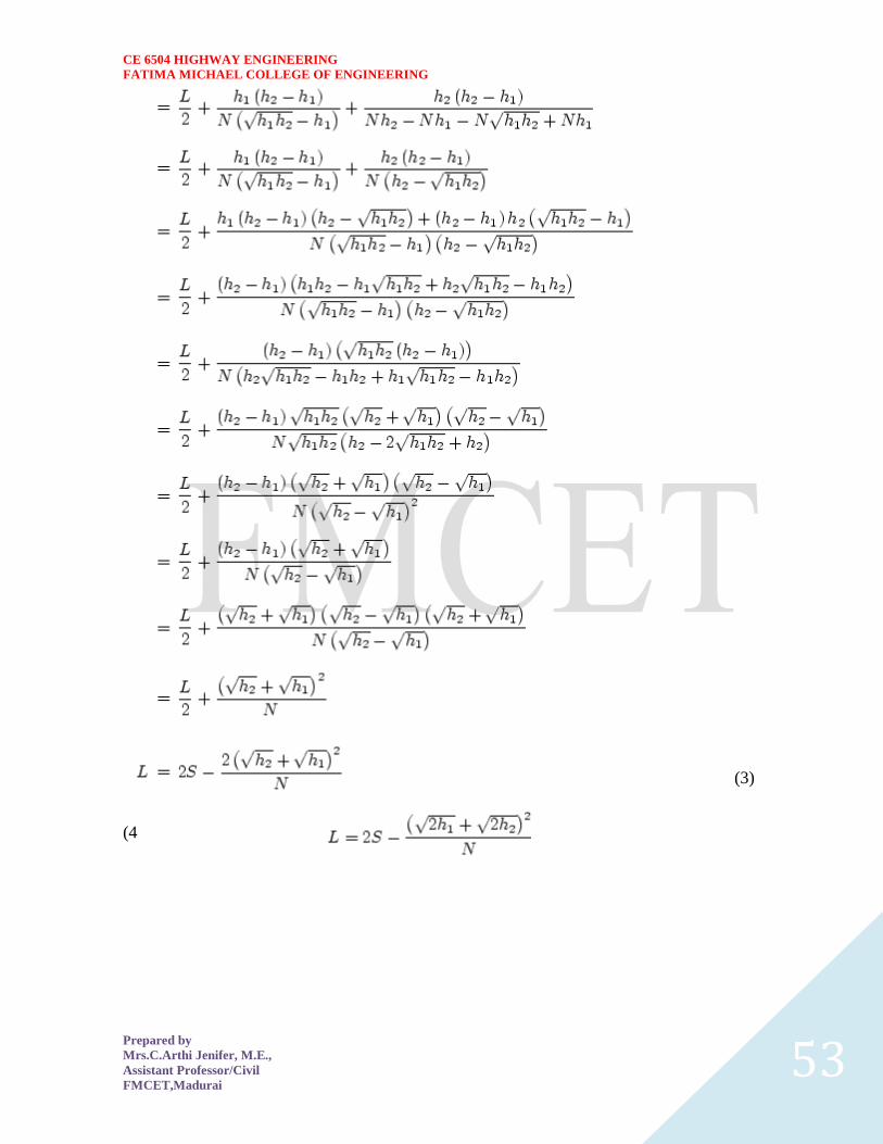
CE 6504 HIGHWAY ENGINEERING
FATIMA MICHAEL COLLEGE OF ENGINEERING
Prepared by
MrsCArthi Jenifer ME
Assistant ProfessorCivil
FMCETMadurai 53
(3) (4
CE 6504 HIGHWAY ENGINEERING
FATIMA MICHAEL COLLEGE OF ENGINEERING
Prepared by
MrsCArthi Jenifer ME
Assistant ProfessorCivil
FMCETMadurai 54
When stopping sight distance is considered the height of drivers eye above the road
surface ( ) is taken as 12 metres and height of object above the pavement surface ( )
is taken as 015 metres If overtaking sight distance is considered then the value of
drivers eye height ( ) and the height of the obstruction ( ) are taken equal as 12
metres
Valley curve
Valley curve or sag curves are vertical curves with convexity downwards They are
formed when two gradients meet as illustrated in figure 1 in any of the following four
ways
Figure 1 Types of valley curve
1 When a descending gradient meets another descending gradient [figure 1a]
2 When a descending gradient meets a flat gradient [figure 1b]
3 When a descending gradient meets an ascending gradient [figure 1c]
4 When an ascending gradient meets another ascending gradient [figure
Design considerations
There is no restriction to sight distance at valley curves during day time But visibility is
reduced during night In the absence or inadequacy of street light the only source for
visibility is with the help of headlights Hence valley curves are designed taking into
account of headlight distance In valley curves the centrifugal force will be acting
downwards along with the weight of the vehicle and hence impact to the vehicle will be
more This will result in jerking of the vehicle and cause discomfort to the passengers
Thus the most important design factors considered in valley curves are (1) impact-free
movement of vehicles at design speed and (2) availability of stopping sight distance
under headlight of vehicles for night driving
For gradually introducing and increasing the centrifugal force acting downwards the best
shape that could be given for a valley curve is a transition curve Cubic parabola is
generally preferred in vertical valley curves See figure 1
CE 6504 HIGHWAY ENGINEERING
FATIMA MICHAEL COLLEGE OF ENGINEERING
Prepared by
MrsCArthi Jenifer ME
Assistant ProfessorCivil
FMCETMadurai 55
Figure 1 Valley curve details
During night under headlight driving condition sight distance reduces and availability of
stopping sight distance under head light is very important The head light sight distance
should be at least equal to the stopping sight distance There is no problem of overtaking
sight distance at night since the other vehicles with headlights could be seen from a
considerable distance
Length of the valley curve
The valley curve is made fully transitional by providing two similar transition curves of
equal length The transitional curve is set out by a cubic parabola where
The length of the valley transition curve is designed based on two criteria
1 comfort criteria that is allowable rate of change of centrifugal acceleration is
limited to a comfortable level of about
2 safety criteria that is the driver should have adequate headlight sight distance at
any part of the country
Comfort criteria
The length of the valley curve based on the rate of change of centrifugal acceleration that
will ensure comfort Let is the rate of change of acceleration the minimum radius of
the curve is the design speed and is the time then is give
CE 6504 HIGHWAY ENGINEERING
FATIMA MICHAEL COLLEGE OF ENGINEERING
Prepared by
MrsCArthi Jenifer ME
Assistant ProfessorCivil
FMCETMadurai 56
For a cubic parabola the Value Safety criter Length of the valley curve for headlight distance may be determined for two conditions
(1) length of the valley curve greater than stopping sight distance and (2) length of the
valley curve less than the stopping sight distance of for length is given by
Case 1 Length of valley curve greater than stopping sight distance ( )
The total length of valley curve is greater than the stopping sight distance SSD The
sight distance available will be minimum when the vehicle is in the lowest point in the
valley This is because the beginning of the curve will have infinite radius and the bottom
of the curve will have minimum radius which is a property of the transition curve The
case is shown in figure 1
Figure 1 Valley curve case 1
From the geometry of the figure we have
CE 6504 HIGHWAY ENGINEERING
FATIMA MICHAEL COLLEGE OF ENGINEERING
Prepared by
MrsCArthi Jenifer ME
Assistant ProfessorCivil
FMCETMadurai 57
(1)
where is the deviation angle in radians is the height of headlight beam is the
head beam inclination in degrees and is the sight distance The inclination is 1
degree
Case 2 Length of valley curve less than stopping sight distance ( )
The length of the curve is less than SSD In this case the minimum sight distance is
from the beginning of the curve The important points are the beginning of the curve and
the bottom most part of the curve If the vehicle is at the bottom of the curve then its
headlight beam will reach far beyond the endpoint of the curve whereas if the vehicle is
at the beginning of the curve then the headlight beam will hit just outside the curve
Therefore the length of the curve is derived by assuming the vehicle at the beginning of
the curve The case is shown in figure 1
From the figure
(1) Note that the above expression is approximate and is satisfactory because in practice the gradients
are very small and is acceptable for all practical purposes We will not be able to know prior to
which case to be adopted Therefore both has to be calculated and the one which satisfies the
condition is adopted
1 Flexible pavement
2 Rigid pavement
Flexible pavement
These pavements reflect the deformation of sub grade and the subsequent layers to the
surface
Rigid pavement
The rigid characteristic of the pavement are associated with rigidity or flexural strength
CE 6504 HIGHWAY ENGINEERING
FATIMA MICHAEL COLLEGE OF ENGINEERING
Prepared by
MrsCArthi Jenifer ME
Assistant ProfessorCivil
FMCETMadurai 58
or slab action so the load is distributed over a wide area of sub grade soil
Flexible pavement Definition
These pavements reflect the deformation of sub grade and the subsequent layers to the
surface Flexible usually asphalt is laid with no reinforcement or with a specialized
fabric reinforcement that permits limited flow or repositioning of the roadbed under
ground changes
The design of flexible pavement is based on load distributing characteristic of the
component layers The black top pavement including water amp gravel bound macadam fall
in this category
Flexible pavement on the whole has low or negligible flexible strength flexible in their
structural action) The flexible pavement layers transmit the vertical or compressive
stresses to the lower layers by grain transfer through contact points of granular structure
The vertical compressive stress is maximum on the pavement surface directly under the
wheel load and is equal to contact pressure under the wheels Due to the ability to
distribute the stress to large area in the shape of truncated cone the stresses get decreased
in the lower layer
As such the flexible pavement may be constructed in a number of layers and the top
layer has to be strongest as the highest compressive stresses
To be sustained by this layer in addition to wear and tear the lower layer have to take
up only lesser magnitude of stress as there is no direct wearing action die to traffic loads
therefore inferior material with lower cast can be used in the lower layers
Rigid pavement Definition
The rigid characteristic of the pavement are associated with rigidity or flexural strength
or slab action so the load is distributed over a wide area of sub grade soil Rigid pavement
is laid in slabs with steel reinforcement
The rigid pavements are made of cement concrete either plan reinforced or prestressed
concrete
Critical condition of stress in the rigid pavement is the maximum flexural stress occurring in the slab due to wheel load and the temperature changes
Rigid pavement is designed and analyzed by using the elastic theory
CE 6504 HIGHWAY ENGINEERING
FATIMA MICHAEL COLLEGE OF ENGINEERING
Prepared by
MrsCArthi Jenifer ME
Assistant ProfessorCivil
FMCETMadurai 59
UNIT-5 EVALUATION AND MAINTENANCE OF PAVEMENTS
TRAFFIC PARAMETERS
Design life
Design life is the number of years (or number of standard axle repetitions) for which the
pavement is being designed A pavement is expected to serve satisfactorily within the
design life For concrete pavements 20 to 40 years may be assumed as the design life
(PCA 1984 IRC58 2002)
Basic design principle
Though different approaches for concrete pavement design are suggested in various
guidelines the design principles tend to remain similar across different guidelines for
example PCA (1994) Austroads (2004) NCHRP (2004) IRC58 (2002) etc except the
AASHTO (1993) provisions which is based on empirical approach The basic steps
involved in the design of concrete pavement method can be summarized as follows
The developed stresses due to load for a trial thickness of the concrete slab are
calculated for various loading configuration and the critical one is chosen The
axle loads are generally divided into different axle load groups and the load
stresses are calculated individually
The ratio between the load stress and Modulus of Rupture (MOR) is known as
stress ratio The stress ratio determines how many repetitions the pavement can
sustain (ie allowable traffic repetitions) for the individual axle load group If the
stress ratio is 055 or lower it can withstand virtually infinite number of traffic
repetitions (PCA 1984)
The ratio between the allowable repetitions to the expected traffic repetitions is
the damage fraction The calculation process is repeated for various axle loads
(sometimes for various seasons or various timings of the day) and the sum of
individual damage fractions (c u m u l a t i v e fatigue damage) should be less
than equal to one for pavement design being safe If found unsafe the trial
thickness is changed and the design process is repeated
The design process may also include considerations for temperature stress
moisture stresses and erosion distress
A brief discussion on concrete pavement design approaches suggested by various design
practices viz PCA method (1984) Austroads method (2004) AASHTO method (1993)
NCHRP mechanistic-empirical method (2004) and the Indian Roads Congress (IRC)
method (2002) are placed in the following
Portland cement Association (PCA) Method
The PCA method is based on Westergaard Picket and Rays work and further theoretical
analysis by Finite Element Method (Huang 1993) The data used to develop the PCA
method is generated from various road tests like ASSHO road test Arlington test
(conducted by PCA) Bates test road and Maryland road test (PCA 1984) The PCA
design method is based on the following two considerations (PCA 1984)
The fatigue damage on the concrete slab due to repetitive application of traffic
load is estimated The cumulative fatigue damage principle is used to estimate the
design thickness of the slab Edge stress between the mid-ways of the
CE 6504 HIGHWAY ENGINEERING
FATIMA MICHAEL COLLEGE OF ENGINEERING
Prepared by
MrsCArthi Jenifer ME
Assistant ProfessorCivil
FMCETMadurai 60
transverse joint is taken as critical configuration
The stresses due to warping and curling (due to temperature and moisture
gradient) are not considered in the fatigue analysis as per PCA recommendation
because most of the time the stresses generated are subtractive to the load stress
The possibility of erosion of pavement materials placed below the concrete slab is
evaluated The rate at which the slab is deflected due to axle load is used as a
criterion for erosion Theoretically it can be shown that a thin pavement with
smaller deflection basin is subjected to faster rate of deflection compared to
thicker slab Hence thin slab is more susceptible to erosion In a similar way the
cumulative erosion damage is calculated for individual axle load groups If this
value is greater than one then the design needs to be revised
Austroads method
Austroads method has been adopted from PCA (1984) approach with modifications
suited to Australian conditions (Austroads 2004) A bound mix or lean cement concrete is
used as sub-base material For a given CBR value of the subgrade and given thickness of
cemented sub-base the effective subgrade strength can be obtained from the chart
provided Figure-19 schematically shows such a chart For different levels of traffic
Austroads (2004) suggests minimum values of the base thicknesses to be provided
CE 6504 HIGHWAY ENGINEERING
FATIMA MICHAEL COLLEGE OF ENGINEERING
Prepared by
MrsCArthi Jenifer ME
Assistant ProfessorCivil
FMCETMadurai 61
figure-19 Schematic diagram of Austroads (2004) chart for estimation of effective
subgrade strength
As per Astroads (2004) the concrete pavement slab thickness for a given expected
traffic repetitions is designed considering the (i) flexural fatigue of the concrete slab and
the (ii) subgrade erosion arising out of repeated deflections For both the considerations
equations are suggested to calculate the allowable traffic repetitions If the allowable
traffic is less than the expected traffic the design is revised by increasing the slab
thickness The concrete shoulders adopted are of integral type or structural type
AASHTO method
The AASHTO method (1993) for design of concrete pavement has evolved from the
AASHO road test (AASHO 1962) The AASHTO pavement design follows an empirical
approach Pavement performance in terms of present serviceability index ( PSI ) loss of
serviceability sub-grade and sub-base strength cumulative traffic properties of concrete
joint load transfer efficiency drainage condition overall standard deviation and
reliability are the input parameters considered in the pavement design
The PSI value of the fresh pavement is assumed as 45 and the pavement is deemed to
have failed when the PSI value reaches 25 The resilient moduli of the subgrade and sub-
base materials are determined in the laboratory simulating the seasonal moisture content
and stress situation Suggested values are also available for given moisture content
plasticity index etc The composite modulus of sub-grade reaction (k) is estimated from
modulus of sub-grade reaction and elastic modulus of sub-base for various seasons and
the depth of rigid foundation and the thickness of the sub-base
Design equation as well nomographs are available to estimate the slab thickness (D) from
these input parameters
NCHRP mechanistic-empirical (M-E) metho
The NCHRP (2004) has recently developed concrete pavement design procedure based
on mechanistic-empirical (M-E) approach This approach attempts to reduce the extent of
empiricism prevalent in the existing AASHTO (1993) guidelines This proposed NCHRP
pavement design system is modular in nature that is the design approach can be
modified by parts (as and when new knowledge is available) without disrupting the
overall design procedure This approach also can take care of various wheel-axle loa
configuration
As per this approach trial thickness of the slab is first assumed and the stress strain and
displacement values are obtained From these values the performance of the pavement in
terms of distresses (such as faulting cracking) and smoothness and predicted If these
predicted performance parameters does not satisfy the required performance for a given
reliability
The design approach includes a large data-base as input parameters for example average
daily traffic traffic growth rate traffic composition hourly weather data on air
temperature precipitation wind speed percentage sunshine relative humidity pavement
material engineering parameters ground water depth infiltration drainage hydraulic
conductivity thermal conductivity heat capacity etc The temperature stress is
considered in this method but the temperature profile is linearized to enhance
computational efficiency (NCHRP 2004)
CE 6504 HIGHWAY ENGINEERING
FATIMA MICHAEL COLLEGE OF ENGINEERING
Prepared by
MrsCArthi Jenifer ME
Assistant ProfessorCivil
FMCETMadurai 62
INDIAN ROADS CONGRESS (IRC) METHOD
The Indian Roads Congress (IRC) guidelines IRC58 (2002) has adopted the
Westergaards equation to estimate load stress and Brdaburys equation to estimate
temperature stress The load stress is highest at the corner of the slab lesser in edge and
least in the interior The order of variation of temperature stress is just the reverse of this
As per IRC58 (2002) it is recommended that the design needs to be done for edge stress
condition and subsequently check needs to be performed for corner stress condition so as
to finalize the design The following are the steps followed as per IRC58 (2002)
guideline for the design of concrete pavement
The input parameters are obtained to formulate the design problem The joint
spacing and the slab dimensions are decided If there is a bound sub-base layer
over the subgrade a suitable value of effective k is to be adopted
A trial thickness of the concrete slab is assumed
The edge stress is estimated for various axle loads from the given charts Figure-
20 schematically shows such a chart The cumulative fatigue damage principle for
fatigue is applied to check the adequacy of the slab thickness
The sum of edge stress due to load for the highest axle load group and the
temperature stress should be less than the MOR of concrete otherwise the design
is revised
The adequacy of corner stress is checked with respect to MOR value and
accordingly the design is finalized Westergaards corner stress formula
Figure-20 Schematic diagram of IRC58 chart for estimation of load stress at the edge
(IRC58 2002)
CE 6504 HIGHWAY ENGINEERING
FATIMA MICHAEL COLLEGE OF ENGINEERING
Prepared by
MrsCArthi Jenifer ME
Assistant ProfessorCivil
FMCETMadurai 63
estimation of corner stress due to load and the corner stress due to temperature is
assumed to be zero
Estimation of layer thicknesses
The thickness of the pavement is adjusted in such a way that the stress strain
developed is less than the allowable values obtained from past performance
information
The two major modes of structural failure of pavement are fatigue and rutting
o Fatigue Traffic applies repetitive load to the pavement surface and the
cracks start from bottom the bound layer slab and propagate upwards
When the extent of surface cracks reaches a predefined level the
pavement is said to have failed due to flexural fatigue
FUNCTIONAL DESIGN
The functional pavement design involves considerations of skid resistance roughness
surface distresses reflectivity of pavement surface etc The functional pavement design
considers mainly the surface features of a pavement
Drainage design
A road needs to be designed in such a way that the rain snow precipitation is drained off
the pavement and its surroundings A suitable surface drainage system for the pavement
is designed for this purpose Some water however will percolate into the pavement from
its top surface and needs to be taken out of the pavement - this is done by providing an
internal drainage system to the pavement Water will also try to enter into the pavement
from bottom due to capillary rise or due to rise in water table A suitably designed sub-
surface drainage system tries to avoid such a problem
PAVEMENT THICKNESS DESIGN CHARTS
For the design of pavements to carry traffic in the range of 1 to 10 msa use chart 1 and for
traffic in the range 10 to 150 msa use chart 2 of IRC37 2001 The design curves relate
pavement thickness to the cumulative number of standard axles to be carried over the
design life for different sub-grade CBR values ranging from 2 to 10 The design
charts will give the total thickness of the pavement for the above inputs The total
thickness consists of granular sub-base granular base and bituminous surfacing The
individual layers are designed based on the the recommendations given below and the
subsequent tables
Pavement composition
Sub-base
Sub-base materials comprise natural sand gravel laterite brick metal crushed
stone or combinations thereof meeting the prescribed grading and physical
requirements The sub-base material should have a minimum CBR of 20 and
30 for traffic upto 2 msa and traffic exceeding 2 msa respectively Sub-base
usually consist of granular or WBM and the thickness should not be less than 150
mm for design traffic less than 10 msa and 200 mm for design traffic
Base
The recommended designs are for unbounded granular bases which comprise
CE 6504 HIGHWAY ENGINEERING
FATIMA MICHAEL COLLEGE OF ENGINEERING
Prepared by
MrsCArthi Jenifer ME
Assistant ProfessorCivil
FMCETMadurai 64
conventional water bound macadam (WBM) or wet mix macadam (WMM) or
equivalent confirming to MOST specifications The materials should be of good
quality with minimum thickness of 225 mm for traffic up to 2 msa an 150 mm for
traffic
Bituminoussurfacing The surfacing consists of a wearing course or a binder
course plus wearing course The most commonly used wearing courses are
surface dressing open graded premix carpet mix seal surfacing semi-
dense bituminous concrete and bituminous concrete For binder course
MOST specifies it is desirable to use bituminous macadam (BM) for traffic
upto o 5 msa and dense bituminous macadam (DBM) for traffic more than 5
msa
Numerical example
Design the pavement for construction of a new bypass with the following data
1 Two lane carriage way
2 Initial traffic in the year of completion of construction = 400 CVPD (sum of both
directions)
3 Traffic growth rate = 75
4 Design life = 15 years
5 Vehicle damage factor based on axle load survey = 25 standard axle per
commercial vehicle
6 Design CBR of subgrade soil = 4
Solution
1 Distribution factor = 075
2
3 Total pavement thickness for CBR 4 and traffic 72 msa from IRC37 2001
chart1 = 660 mm
4 Pavement composition can be obtained by interpolation from Pavement Design
Catalogue (IRC37 2001)
1 Bituminous surfacing = 25 mm SDBC + 70 mm DBM
2 Road-base = 250 mm WBM
3 sub-base = 315 mm granular material of CBR not less than 30
CE 6504 HIGHWAY ENGINEERING
FATIMA MICHAEL COLLEGE OF ENGINEERING
Prepared by
MrsCArthi Jenifer ME
Assistant ProfessorCivil
FMCETMadurai 65
Generally bound base layers are used for concrete pavement construction As per Indian
specification some example of such base layers are Dry Lean Concrete (DLC) Roller
Compacted Concrete (RCC) (IRC15-2002)
The concrete slab is generally of M40 to M50 grade of concrete as
per Indian specifications and is called as paving quality concrete (PQC)
(IRC15-2002)
BITUMINOUS PAVEMENT
The subgrade is a compacted soil layer
The base and sub-base course could be made up of bound or unbound granular layer As
per Indian specifications (MORTampH 2001) some examples of base or sub-base layers
are Granular sub-base(GSB) Water Bound Macadam (WBM) Wet Mix Macadam
(WMM) etc
The binder course is made up bituminous material As per Indian specifications
(MORTampH 2001) some examples of binder course are Bituminous Macadam (BM)
Dense Bituminous Macadam (DBM) etc
The wearing course is the top bituminous layer which is comes in contact to the
vehicle tyre Wearing course provides impermeability to the pavement surface
against water percolation (Chakroborty and Das 2003) The binder course and wearing
course together are called bituminous surfacing
IRC METHOD OF FLEXIBLE PAVEMENT MIX DESIGN
These guidelines will apply to design of flexible pavements for Expressway National Highways
State Highways Major District Roads and other categories of roads Flexible pavements are
considered to include the pavements which have bituminous surfacing and granular base and sub-
base courses conforming to IRC MOST standards These guidelines apply to new pavements
Design criteria
The flexible pavements has been modeled as a three layer structure and stresses and strains at
critical locations have been computed using the linear elastic model To give proper consideration
to the aspects of performance the following three types of pavement distress resulting from
repeated (cyclic) application of traffic loads are considered
1 Vertical compressive strain at the top of the sub-grade which can cause sub-grade
deformation resulting in permanent deformation at the pavement surface
2 Horizontal tensile strain or stress at the bottom of the bituminous layer which can cause
fracture of the bituminous layer
3 Pavement deformation within the bituminous layer
CE 6504 HIGHWAY ENGINEERING
FATIMA MICHAEL COLLEGE OF ENGINEERING
Prepared by
MrsCArthi Jenifer ME
Assistant ProfessorCivil
FMCETMadurai 66
While the permanent deformation within the bituminous layer can be controlled by meeting the
mix design requirements thickness of granular and bituminous layers are selected using the
analytical design approach so that strains at the critical points are within the allowable limits For
calculating tensile strains at the bottom of the bituminous layer the stiffness of dense bituminous
macadam (DBM) layer with 6070 bitumen has been used in the analysis
FAILURE CRITERIA
Critical locations in pavement
A and B are the critical locations for tensile strains Maximum value of the strain is
adopted for design C is the critical location for the vertical subgrade strain since the
maximum value of the occurs mostly at C
CE 6504 HIGHWAY ENGINEERING
FATIMA MICHAEL COLLEGE OF ENGINEERING
Prepared by
MrsCArthi Jenifer ME
Assistant ProfessorCivil
FMCETMadurai 67
Fatigue Criteria
Bituminous surfacings of pavements display flexural fatigue cracking if the tensile strain
at the bottom of the bituminous layer is beyond certain limit The relation between the
fatigue life of the pavement and the tensile strain in the bottom of the bituminous layer
was obtained as
(1)
in which is the allowable number of load repetitions to control fatigue cracking and
is the Elastic modulus of bituminous layer The use of equation 1 would result in
fatigue cracking of 20 of the total area
Rutting Criteria
The allowable number of load repetitions to control permanent deformation can be
expressed as
(2)
is the number of cumulative standard axles to produce rutting of 20 mm
CE 6504 HIGHWAY ENGINEERING
FATIMA MICHAEL COLLEGE OF ENGINEERING
Prepared by
MrsCArthi Jenifer ME
Assistant ProfessorCivil
FMCETMadurai 68
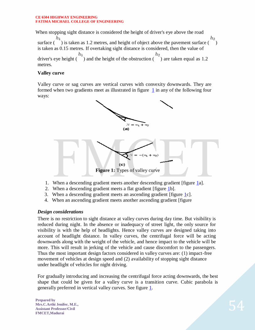
CE 6504 HIGHWAY ENGINEERING
FATIMA MICHAEL COLLEGE OF ENGINEERING
Prepared by
MrsCArthi Jenifer ME
Assistant ProfessorCivil
FMCETMadurai 54
When stopping sight distance is considered the height of drivers eye above the road
surface ( ) is taken as 12 metres and height of object above the pavement surface ( )
is taken as 015 metres If overtaking sight distance is considered then the value of
drivers eye height ( ) and the height of the obstruction ( ) are taken equal as 12
metres
Valley curve
Valley curve or sag curves are vertical curves with convexity downwards They are
formed when two gradients meet as illustrated in figure 1 in any of the following four
ways
Figure 1 Types of valley curve
1 When a descending gradient meets another descending gradient [figure 1a]
2 When a descending gradient meets a flat gradient [figure 1b]
3 When a descending gradient meets an ascending gradient [figure 1c]
4 When an ascending gradient meets another ascending gradient [figure
Design considerations
There is no restriction to sight distance at valley curves during day time But visibility is
reduced during night In the absence or inadequacy of street light the only source for
visibility is with the help of headlights Hence valley curves are designed taking into
account of headlight distance In valley curves the centrifugal force will be acting
downwards along with the weight of the vehicle and hence impact to the vehicle will be
more This will result in jerking of the vehicle and cause discomfort to the passengers
Thus the most important design factors considered in valley curves are (1) impact-free
movement of vehicles at design speed and (2) availability of stopping sight distance
under headlight of vehicles for night driving
For gradually introducing and increasing the centrifugal force acting downwards the best
shape that could be given for a valley curve is a transition curve Cubic parabola is
generally preferred in vertical valley curves See figure 1
CE 6504 HIGHWAY ENGINEERING
FATIMA MICHAEL COLLEGE OF ENGINEERING
Prepared by
MrsCArthi Jenifer ME
Assistant ProfessorCivil
FMCETMadurai 55
Figure 1 Valley curve details
During night under headlight driving condition sight distance reduces and availability of
stopping sight distance under head light is very important The head light sight distance
should be at least equal to the stopping sight distance There is no problem of overtaking
sight distance at night since the other vehicles with headlights could be seen from a
considerable distance
Length of the valley curve
The valley curve is made fully transitional by providing two similar transition curves of
equal length The transitional curve is set out by a cubic parabola where
The length of the valley transition curve is designed based on two criteria
1 comfort criteria that is allowable rate of change of centrifugal acceleration is
limited to a comfortable level of about
2 safety criteria that is the driver should have adequate headlight sight distance at
any part of the country
Comfort criteria
The length of the valley curve based on the rate of change of centrifugal acceleration that
will ensure comfort Let is the rate of change of acceleration the minimum radius of
the curve is the design speed and is the time then is give
CE 6504 HIGHWAY ENGINEERING
FATIMA MICHAEL COLLEGE OF ENGINEERING
Prepared by
MrsCArthi Jenifer ME
Assistant ProfessorCivil
FMCETMadurai 56
For a cubic parabola the Value Safety criter Length of the valley curve for headlight distance may be determined for two conditions
(1) length of the valley curve greater than stopping sight distance and (2) length of the
valley curve less than the stopping sight distance of for length is given by
Case 1 Length of valley curve greater than stopping sight distance ( )
The total length of valley curve is greater than the stopping sight distance SSD The
sight distance available will be minimum when the vehicle is in the lowest point in the
valley This is because the beginning of the curve will have infinite radius and the bottom
of the curve will have minimum radius which is a property of the transition curve The
case is shown in figure 1
Figure 1 Valley curve case 1
From the geometry of the figure we have
CE 6504 HIGHWAY ENGINEERING
FATIMA MICHAEL COLLEGE OF ENGINEERING
Prepared by
MrsCArthi Jenifer ME
Assistant ProfessorCivil
FMCETMadurai 57
(1)
where is the deviation angle in radians is the height of headlight beam is the
head beam inclination in degrees and is the sight distance The inclination is 1
degree
Case 2 Length of valley curve less than stopping sight distance ( )
The length of the curve is less than SSD In this case the minimum sight distance is
from the beginning of the curve The important points are the beginning of the curve and
the bottom most part of the curve If the vehicle is at the bottom of the curve then its
headlight beam will reach far beyond the endpoint of the curve whereas if the vehicle is
at the beginning of the curve then the headlight beam will hit just outside the curve
Therefore the length of the curve is derived by assuming the vehicle at the beginning of
the curve The case is shown in figure 1
From the figure
(1) Note that the above expression is approximate and is satisfactory because in practice the gradients
are very small and is acceptable for all practical purposes We will not be able to know prior to
which case to be adopted Therefore both has to be calculated and the one which satisfies the
condition is adopted
1 Flexible pavement
2 Rigid pavement
Flexible pavement
These pavements reflect the deformation of sub grade and the subsequent layers to the
surface
Rigid pavement
The rigid characteristic of the pavement are associated with rigidity or flexural strength
CE 6504 HIGHWAY ENGINEERING
FATIMA MICHAEL COLLEGE OF ENGINEERING
Prepared by
MrsCArthi Jenifer ME
Assistant ProfessorCivil
FMCETMadurai 58
or slab action so the load is distributed over a wide area of sub grade soil
Flexible pavement Definition
These pavements reflect the deformation of sub grade and the subsequent layers to the
surface Flexible usually asphalt is laid with no reinforcement or with a specialized
fabric reinforcement that permits limited flow or repositioning of the roadbed under
ground changes
The design of flexible pavement is based on load distributing characteristic of the
component layers The black top pavement including water amp gravel bound macadam fall
in this category
Flexible pavement on the whole has low or negligible flexible strength flexible in their
structural action) The flexible pavement layers transmit the vertical or compressive
stresses to the lower layers by grain transfer through contact points of granular structure
The vertical compressive stress is maximum on the pavement surface directly under the
wheel load and is equal to contact pressure under the wheels Due to the ability to
distribute the stress to large area in the shape of truncated cone the stresses get decreased
in the lower layer
As such the flexible pavement may be constructed in a number of layers and the top
layer has to be strongest as the highest compressive stresses
To be sustained by this layer in addition to wear and tear the lower layer have to take
up only lesser magnitude of stress as there is no direct wearing action die to traffic loads
therefore inferior material with lower cast can be used in the lower layers
Rigid pavement Definition
The rigid characteristic of the pavement are associated with rigidity or flexural strength
or slab action so the load is distributed over a wide area of sub grade soil Rigid pavement
is laid in slabs with steel reinforcement
The rigid pavements are made of cement concrete either plan reinforced or prestressed
concrete
Critical condition of stress in the rigid pavement is the maximum flexural stress occurring in the slab due to wheel load and the temperature changes
Rigid pavement is designed and analyzed by using the elastic theory
CE 6504 HIGHWAY ENGINEERING
FATIMA MICHAEL COLLEGE OF ENGINEERING
Prepared by
MrsCArthi Jenifer ME
Assistant ProfessorCivil
FMCETMadurai 59
UNIT-5 EVALUATION AND MAINTENANCE OF PAVEMENTS
TRAFFIC PARAMETERS
Design life
Design life is the number of years (or number of standard axle repetitions) for which the
pavement is being designed A pavement is expected to serve satisfactorily within the
design life For concrete pavements 20 to 40 years may be assumed as the design life
(PCA 1984 IRC58 2002)
Basic design principle
Though different approaches for concrete pavement design are suggested in various
guidelines the design principles tend to remain similar across different guidelines for
example PCA (1994) Austroads (2004) NCHRP (2004) IRC58 (2002) etc except the
AASHTO (1993) provisions which is based on empirical approach The basic steps
involved in the design of concrete pavement method can be summarized as follows
The developed stresses due to load for a trial thickness of the concrete slab are
calculated for various loading configuration and the critical one is chosen The
axle loads are generally divided into different axle load groups and the load
stresses are calculated individually
The ratio between the load stress and Modulus of Rupture (MOR) is known as
stress ratio The stress ratio determines how many repetitions the pavement can
sustain (ie allowable traffic repetitions) for the individual axle load group If the
stress ratio is 055 or lower it can withstand virtually infinite number of traffic
repetitions (PCA 1984)
The ratio between the allowable repetitions to the expected traffic repetitions is
the damage fraction The calculation process is repeated for various axle loads
(sometimes for various seasons or various timings of the day) and the sum of
individual damage fractions (c u m u l a t i v e fatigue damage) should be less
than equal to one for pavement design being safe If found unsafe the trial
thickness is changed and the design process is repeated
The design process may also include considerations for temperature stress
moisture stresses and erosion distress
A brief discussion on concrete pavement design approaches suggested by various design
practices viz PCA method (1984) Austroads method (2004) AASHTO method (1993)
NCHRP mechanistic-empirical method (2004) and the Indian Roads Congress (IRC)
method (2002) are placed in the following
Portland cement Association (PCA) Method
The PCA method is based on Westergaard Picket and Rays work and further theoretical
analysis by Finite Element Method (Huang 1993) The data used to develop the PCA
method is generated from various road tests like ASSHO road test Arlington test
(conducted by PCA) Bates test road and Maryland road test (PCA 1984) The PCA
design method is based on the following two considerations (PCA 1984)
The fatigue damage on the concrete slab due to repetitive application of traffic
load is estimated The cumulative fatigue damage principle is used to estimate the
design thickness of the slab Edge stress between the mid-ways of the
CE 6504 HIGHWAY ENGINEERING
FATIMA MICHAEL COLLEGE OF ENGINEERING
Prepared by
MrsCArthi Jenifer ME
Assistant ProfessorCivil
FMCETMadurai 60
transverse joint is taken as critical configuration
The stresses due to warping and curling (due to temperature and moisture
gradient) are not considered in the fatigue analysis as per PCA recommendation
because most of the time the stresses generated are subtractive to the load stress
The possibility of erosion of pavement materials placed below the concrete slab is
evaluated The rate at which the slab is deflected due to axle load is used as a
criterion for erosion Theoretically it can be shown that a thin pavement with
smaller deflection basin is subjected to faster rate of deflection compared to
thicker slab Hence thin slab is more susceptible to erosion In a similar way the
cumulative erosion damage is calculated for individual axle load groups If this
value is greater than one then the design needs to be revised
Austroads method
Austroads method has been adopted from PCA (1984) approach with modifications
suited to Australian conditions (Austroads 2004) A bound mix or lean cement concrete is
used as sub-base material For a given CBR value of the subgrade and given thickness of
cemented sub-base the effective subgrade strength can be obtained from the chart
provided Figure-19 schematically shows such a chart For different levels of traffic
Austroads (2004) suggests minimum values of the base thicknesses to be provided
CE 6504 HIGHWAY ENGINEERING
FATIMA MICHAEL COLLEGE OF ENGINEERING
Prepared by
MrsCArthi Jenifer ME
Assistant ProfessorCivil
FMCETMadurai 61
figure-19 Schematic diagram of Austroads (2004) chart for estimation of effective
subgrade strength
As per Astroads (2004) the concrete pavement slab thickness for a given expected
traffic repetitions is designed considering the (i) flexural fatigue of the concrete slab and
the (ii) subgrade erosion arising out of repeated deflections For both the considerations
equations are suggested to calculate the allowable traffic repetitions If the allowable
traffic is less than the expected traffic the design is revised by increasing the slab
thickness The concrete shoulders adopted are of integral type or structural type
AASHTO method
The AASHTO method (1993) for design of concrete pavement has evolved from the
AASHO road test (AASHO 1962) The AASHTO pavement design follows an empirical
approach Pavement performance in terms of present serviceability index ( PSI ) loss of
serviceability sub-grade and sub-base strength cumulative traffic properties of concrete
joint load transfer efficiency drainage condition overall standard deviation and
reliability are the input parameters considered in the pavement design
The PSI value of the fresh pavement is assumed as 45 and the pavement is deemed to
have failed when the PSI value reaches 25 The resilient moduli of the subgrade and sub-
base materials are determined in the laboratory simulating the seasonal moisture content
and stress situation Suggested values are also available for given moisture content
plasticity index etc The composite modulus of sub-grade reaction (k) is estimated from
modulus of sub-grade reaction and elastic modulus of sub-base for various seasons and
the depth of rigid foundation and the thickness of the sub-base
Design equation as well nomographs are available to estimate the slab thickness (D) from
these input parameters
NCHRP mechanistic-empirical (M-E) metho
The NCHRP (2004) has recently developed concrete pavement design procedure based
on mechanistic-empirical (M-E) approach This approach attempts to reduce the extent of
empiricism prevalent in the existing AASHTO (1993) guidelines This proposed NCHRP
pavement design system is modular in nature that is the design approach can be
modified by parts (as and when new knowledge is available) without disrupting the
overall design procedure This approach also can take care of various wheel-axle loa
configuration
As per this approach trial thickness of the slab is first assumed and the stress strain and
displacement values are obtained From these values the performance of the pavement in
terms of distresses (such as faulting cracking) and smoothness and predicted If these
predicted performance parameters does not satisfy the required performance for a given
reliability
The design approach includes a large data-base as input parameters for example average
daily traffic traffic growth rate traffic composition hourly weather data on air
temperature precipitation wind speed percentage sunshine relative humidity pavement
material engineering parameters ground water depth infiltration drainage hydraulic
conductivity thermal conductivity heat capacity etc The temperature stress is
considered in this method but the temperature profile is linearized to enhance
computational efficiency (NCHRP 2004)
CE 6504 HIGHWAY ENGINEERING
FATIMA MICHAEL COLLEGE OF ENGINEERING
Prepared by
MrsCArthi Jenifer ME
Assistant ProfessorCivil
FMCETMadurai 62
INDIAN ROADS CONGRESS (IRC) METHOD
The Indian Roads Congress (IRC) guidelines IRC58 (2002) has adopted the
Westergaards equation to estimate load stress and Brdaburys equation to estimate
temperature stress The load stress is highest at the corner of the slab lesser in edge and
least in the interior The order of variation of temperature stress is just the reverse of this
As per IRC58 (2002) it is recommended that the design needs to be done for edge stress
condition and subsequently check needs to be performed for corner stress condition so as
to finalize the design The following are the steps followed as per IRC58 (2002)
guideline for the design of concrete pavement
The input parameters are obtained to formulate the design problem The joint
spacing and the slab dimensions are decided If there is a bound sub-base layer
over the subgrade a suitable value of effective k is to be adopted
A trial thickness of the concrete slab is assumed
The edge stress is estimated for various axle loads from the given charts Figure-
20 schematically shows such a chart The cumulative fatigue damage principle for
fatigue is applied to check the adequacy of the slab thickness
The sum of edge stress due to load for the highest axle load group and the
temperature stress should be less than the MOR of concrete otherwise the design
is revised
The adequacy of corner stress is checked with respect to MOR value and
accordingly the design is finalized Westergaards corner stress formula
Figure-20 Schematic diagram of IRC58 chart for estimation of load stress at the edge
(IRC58 2002)
CE 6504 HIGHWAY ENGINEERING
FATIMA MICHAEL COLLEGE OF ENGINEERING
Prepared by
MrsCArthi Jenifer ME
Assistant ProfessorCivil
FMCETMadurai 63
estimation of corner stress due to load and the corner stress due to temperature is
assumed to be zero
Estimation of layer thicknesses
The thickness of the pavement is adjusted in such a way that the stress strain
developed is less than the allowable values obtained from past performance
information
The two major modes of structural failure of pavement are fatigue and rutting
o Fatigue Traffic applies repetitive load to the pavement surface and the
cracks start from bottom the bound layer slab and propagate upwards
When the extent of surface cracks reaches a predefined level the
pavement is said to have failed due to flexural fatigue
FUNCTIONAL DESIGN
The functional pavement design involves considerations of skid resistance roughness
surface distresses reflectivity of pavement surface etc The functional pavement design
considers mainly the surface features of a pavement
Drainage design
A road needs to be designed in such a way that the rain snow precipitation is drained off
the pavement and its surroundings A suitable surface drainage system for the pavement
is designed for this purpose Some water however will percolate into the pavement from
its top surface and needs to be taken out of the pavement - this is done by providing an
internal drainage system to the pavement Water will also try to enter into the pavement
from bottom due to capillary rise or due to rise in water table A suitably designed sub-
surface drainage system tries to avoid such a problem
PAVEMENT THICKNESS DESIGN CHARTS
For the design of pavements to carry traffic in the range of 1 to 10 msa use chart 1 and for
traffic in the range 10 to 150 msa use chart 2 of IRC37 2001 The design curves relate
pavement thickness to the cumulative number of standard axles to be carried over the
design life for different sub-grade CBR values ranging from 2 to 10 The design
charts will give the total thickness of the pavement for the above inputs The total
thickness consists of granular sub-base granular base and bituminous surfacing The
individual layers are designed based on the the recommendations given below and the
subsequent tables
Pavement composition
Sub-base
Sub-base materials comprise natural sand gravel laterite brick metal crushed
stone or combinations thereof meeting the prescribed grading and physical
requirements The sub-base material should have a minimum CBR of 20 and
30 for traffic upto 2 msa and traffic exceeding 2 msa respectively Sub-base
usually consist of granular or WBM and the thickness should not be less than 150
mm for design traffic less than 10 msa and 200 mm for design traffic
Base
The recommended designs are for unbounded granular bases which comprise
CE 6504 HIGHWAY ENGINEERING
FATIMA MICHAEL COLLEGE OF ENGINEERING
Prepared by
MrsCArthi Jenifer ME
Assistant ProfessorCivil
FMCETMadurai 64
conventional water bound macadam (WBM) or wet mix macadam (WMM) or
equivalent confirming to MOST specifications The materials should be of good
quality with minimum thickness of 225 mm for traffic up to 2 msa an 150 mm for
traffic
Bituminoussurfacing The surfacing consists of a wearing course or a binder
course plus wearing course The most commonly used wearing courses are
surface dressing open graded premix carpet mix seal surfacing semi-
dense bituminous concrete and bituminous concrete For binder course
MOST specifies it is desirable to use bituminous macadam (BM) for traffic
upto o 5 msa and dense bituminous macadam (DBM) for traffic more than 5
msa
Numerical example
Design the pavement for construction of a new bypass with the following data
1 Two lane carriage way
2 Initial traffic in the year of completion of construction = 400 CVPD (sum of both
directions)
3 Traffic growth rate = 75
4 Design life = 15 years
5 Vehicle damage factor based on axle load survey = 25 standard axle per
commercial vehicle
6 Design CBR of subgrade soil = 4
Solution
1 Distribution factor = 075
2
3 Total pavement thickness for CBR 4 and traffic 72 msa from IRC37 2001
chart1 = 660 mm
4 Pavement composition can be obtained by interpolation from Pavement Design
Catalogue (IRC37 2001)
1 Bituminous surfacing = 25 mm SDBC + 70 mm DBM
2 Road-base = 250 mm WBM
3 sub-base = 315 mm granular material of CBR not less than 30
CE 6504 HIGHWAY ENGINEERING
FATIMA MICHAEL COLLEGE OF ENGINEERING
Prepared by
MrsCArthi Jenifer ME
Assistant ProfessorCivil
FMCETMadurai 65
Generally bound base layers are used for concrete pavement construction As per Indian
specification some example of such base layers are Dry Lean Concrete (DLC) Roller
Compacted Concrete (RCC) (IRC15-2002)
The concrete slab is generally of M40 to M50 grade of concrete as
per Indian specifications and is called as paving quality concrete (PQC)
(IRC15-2002)
BITUMINOUS PAVEMENT
The subgrade is a compacted soil layer
The base and sub-base course could be made up of bound or unbound granular layer As
per Indian specifications (MORTampH 2001) some examples of base or sub-base layers
are Granular sub-base(GSB) Water Bound Macadam (WBM) Wet Mix Macadam
(WMM) etc
The binder course is made up bituminous material As per Indian specifications
(MORTampH 2001) some examples of binder course are Bituminous Macadam (BM)
Dense Bituminous Macadam (DBM) etc
The wearing course is the top bituminous layer which is comes in contact to the
vehicle tyre Wearing course provides impermeability to the pavement surface
against water percolation (Chakroborty and Das 2003) The binder course and wearing
course together are called bituminous surfacing
IRC METHOD OF FLEXIBLE PAVEMENT MIX DESIGN
These guidelines will apply to design of flexible pavements for Expressway National Highways
State Highways Major District Roads and other categories of roads Flexible pavements are
considered to include the pavements which have bituminous surfacing and granular base and sub-
base courses conforming to IRC MOST standards These guidelines apply to new pavements
Design criteria
The flexible pavements has been modeled as a three layer structure and stresses and strains at
critical locations have been computed using the linear elastic model To give proper consideration
to the aspects of performance the following three types of pavement distress resulting from
repeated (cyclic) application of traffic loads are considered
1 Vertical compressive strain at the top of the sub-grade which can cause sub-grade
deformation resulting in permanent deformation at the pavement surface
2 Horizontal tensile strain or stress at the bottom of the bituminous layer which can cause
fracture of the bituminous layer
3 Pavement deformation within the bituminous layer
CE 6504 HIGHWAY ENGINEERING
FATIMA MICHAEL COLLEGE OF ENGINEERING
Prepared by
MrsCArthi Jenifer ME
Assistant ProfessorCivil
FMCETMadurai 66
While the permanent deformation within the bituminous layer can be controlled by meeting the
mix design requirements thickness of granular and bituminous layers are selected using the
analytical design approach so that strains at the critical points are within the allowable limits For
calculating tensile strains at the bottom of the bituminous layer the stiffness of dense bituminous
macadam (DBM) layer with 6070 bitumen has been used in the analysis
FAILURE CRITERIA
Critical locations in pavement
A and B are the critical locations for tensile strains Maximum value of the strain is
adopted for design C is the critical location for the vertical subgrade strain since the
maximum value of the occurs mostly at C
CE 6504 HIGHWAY ENGINEERING
FATIMA MICHAEL COLLEGE OF ENGINEERING
Prepared by
MrsCArthi Jenifer ME
Assistant ProfessorCivil
FMCETMadurai 67
Fatigue Criteria
Bituminous surfacings of pavements display flexural fatigue cracking if the tensile strain
at the bottom of the bituminous layer is beyond certain limit The relation between the
fatigue life of the pavement and the tensile strain in the bottom of the bituminous layer
was obtained as
(1)
in which is the allowable number of load repetitions to control fatigue cracking and
is the Elastic modulus of bituminous layer The use of equation 1 would result in
fatigue cracking of 20 of the total area
Rutting Criteria
The allowable number of load repetitions to control permanent deformation can be
expressed as
(2)
is the number of cumulative standard axles to produce rutting of 20 mm
CE 6504 HIGHWAY ENGINEERING
FATIMA MICHAEL COLLEGE OF ENGINEERING
Prepared by
MrsCArthi Jenifer ME
Assistant ProfessorCivil
FMCETMadurai 68
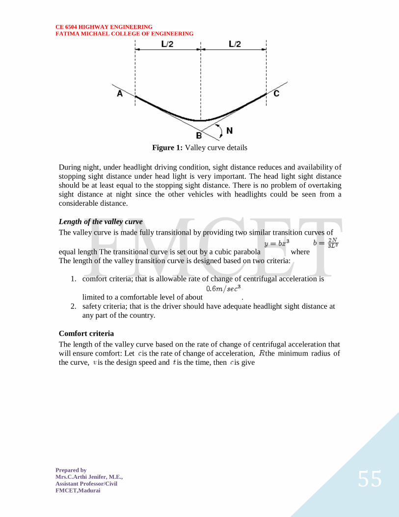
CE 6504 HIGHWAY ENGINEERING
FATIMA MICHAEL COLLEGE OF ENGINEERING
Prepared by
MrsCArthi Jenifer ME
Assistant ProfessorCivil
FMCETMadurai 55
Figure 1 Valley curve details
During night under headlight driving condition sight distance reduces and availability of
stopping sight distance under head light is very important The head light sight distance
should be at least equal to the stopping sight distance There is no problem of overtaking
sight distance at night since the other vehicles with headlights could be seen from a
considerable distance
Length of the valley curve
The valley curve is made fully transitional by providing two similar transition curves of
equal length The transitional curve is set out by a cubic parabola where
The length of the valley transition curve is designed based on two criteria
1 comfort criteria that is allowable rate of change of centrifugal acceleration is
limited to a comfortable level of about
2 safety criteria that is the driver should have adequate headlight sight distance at
any part of the country
Comfort criteria
The length of the valley curve based on the rate of change of centrifugal acceleration that
will ensure comfort Let is the rate of change of acceleration the minimum radius of
the curve is the design speed and is the time then is give
CE 6504 HIGHWAY ENGINEERING
FATIMA MICHAEL COLLEGE OF ENGINEERING
Prepared by
MrsCArthi Jenifer ME
Assistant ProfessorCivil
FMCETMadurai 56
For a cubic parabola the Value Safety criter Length of the valley curve for headlight distance may be determined for two conditions
(1) length of the valley curve greater than stopping sight distance and (2) length of the
valley curve less than the stopping sight distance of for length is given by
Case 1 Length of valley curve greater than stopping sight distance ( )
The total length of valley curve is greater than the stopping sight distance SSD The
sight distance available will be minimum when the vehicle is in the lowest point in the
valley This is because the beginning of the curve will have infinite radius and the bottom
of the curve will have minimum radius which is a property of the transition curve The
case is shown in figure 1
Figure 1 Valley curve case 1
From the geometry of the figure we have
CE 6504 HIGHWAY ENGINEERING
FATIMA MICHAEL COLLEGE OF ENGINEERING
Prepared by
MrsCArthi Jenifer ME
Assistant ProfessorCivil
FMCETMadurai 57
(1)
where is the deviation angle in radians is the height of headlight beam is the
head beam inclination in degrees and is the sight distance The inclination is 1
degree
Case 2 Length of valley curve less than stopping sight distance ( )
The length of the curve is less than SSD In this case the minimum sight distance is
from the beginning of the curve The important points are the beginning of the curve and
the bottom most part of the curve If the vehicle is at the bottom of the curve then its
headlight beam will reach far beyond the endpoint of the curve whereas if the vehicle is
at the beginning of the curve then the headlight beam will hit just outside the curve
Therefore the length of the curve is derived by assuming the vehicle at the beginning of
the curve The case is shown in figure 1
From the figure
(1) Note that the above expression is approximate and is satisfactory because in practice the gradients
are very small and is acceptable for all practical purposes We will not be able to know prior to
which case to be adopted Therefore both has to be calculated and the one which satisfies the
condition is adopted
1 Flexible pavement
2 Rigid pavement
Flexible pavement
These pavements reflect the deformation of sub grade and the subsequent layers to the
surface
Rigid pavement
The rigid characteristic of the pavement are associated with rigidity or flexural strength
CE 6504 HIGHWAY ENGINEERING
FATIMA MICHAEL COLLEGE OF ENGINEERING
Prepared by
MrsCArthi Jenifer ME
Assistant ProfessorCivil
FMCETMadurai 58
or slab action so the load is distributed over a wide area of sub grade soil
Flexible pavement Definition
These pavements reflect the deformation of sub grade and the subsequent layers to the
surface Flexible usually asphalt is laid with no reinforcement or with a specialized
fabric reinforcement that permits limited flow or repositioning of the roadbed under
ground changes
The design of flexible pavement is based on load distributing characteristic of the
component layers The black top pavement including water amp gravel bound macadam fall
in this category
Flexible pavement on the whole has low or negligible flexible strength flexible in their
structural action) The flexible pavement layers transmit the vertical or compressive
stresses to the lower layers by grain transfer through contact points of granular structure
The vertical compressive stress is maximum on the pavement surface directly under the
wheel load and is equal to contact pressure under the wheels Due to the ability to
distribute the stress to large area in the shape of truncated cone the stresses get decreased
in the lower layer
As such the flexible pavement may be constructed in a number of layers and the top
layer has to be strongest as the highest compressive stresses
To be sustained by this layer in addition to wear and tear the lower layer have to take
up only lesser magnitude of stress as there is no direct wearing action die to traffic loads
therefore inferior material with lower cast can be used in the lower layers
Rigid pavement Definition
The rigid characteristic of the pavement are associated with rigidity or flexural strength
or slab action so the load is distributed over a wide area of sub grade soil Rigid pavement
is laid in slabs with steel reinforcement
The rigid pavements are made of cement concrete either plan reinforced or prestressed
concrete
Critical condition of stress in the rigid pavement is the maximum flexural stress occurring in the slab due to wheel load and the temperature changes
Rigid pavement is designed and analyzed by using the elastic theory
CE 6504 HIGHWAY ENGINEERING
FATIMA MICHAEL COLLEGE OF ENGINEERING
Prepared by
MrsCArthi Jenifer ME
Assistant ProfessorCivil
FMCETMadurai 59
UNIT-5 EVALUATION AND MAINTENANCE OF PAVEMENTS
TRAFFIC PARAMETERS
Design life
Design life is the number of years (or number of standard axle repetitions) for which the
pavement is being designed A pavement is expected to serve satisfactorily within the
design life For concrete pavements 20 to 40 years may be assumed as the design life
(PCA 1984 IRC58 2002)
Basic design principle
Though different approaches for concrete pavement design are suggested in various
guidelines the design principles tend to remain similar across different guidelines for
example PCA (1994) Austroads (2004) NCHRP (2004) IRC58 (2002) etc except the
AASHTO (1993) provisions which is based on empirical approach The basic steps
involved in the design of concrete pavement method can be summarized as follows
The developed stresses due to load for a trial thickness of the concrete slab are
calculated for various loading configuration and the critical one is chosen The
axle loads are generally divided into different axle load groups and the load
stresses are calculated individually
The ratio between the load stress and Modulus of Rupture (MOR) is known as
stress ratio The stress ratio determines how many repetitions the pavement can
sustain (ie allowable traffic repetitions) for the individual axle load group If the
stress ratio is 055 or lower it can withstand virtually infinite number of traffic
repetitions (PCA 1984)
The ratio between the allowable repetitions to the expected traffic repetitions is
the damage fraction The calculation process is repeated for various axle loads
(sometimes for various seasons or various timings of the day) and the sum of
individual damage fractions (c u m u l a t i v e fatigue damage) should be less
than equal to one for pavement design being safe If found unsafe the trial
thickness is changed and the design process is repeated
The design process may also include considerations for temperature stress
moisture stresses and erosion distress
A brief discussion on concrete pavement design approaches suggested by various design
practices viz PCA method (1984) Austroads method (2004) AASHTO method (1993)
NCHRP mechanistic-empirical method (2004) and the Indian Roads Congress (IRC)
method (2002) are placed in the following
Portland cement Association (PCA) Method
The PCA method is based on Westergaard Picket and Rays work and further theoretical
analysis by Finite Element Method (Huang 1993) The data used to develop the PCA
method is generated from various road tests like ASSHO road test Arlington test
(conducted by PCA) Bates test road and Maryland road test (PCA 1984) The PCA
design method is based on the following two considerations (PCA 1984)
The fatigue damage on the concrete slab due to repetitive application of traffic
load is estimated The cumulative fatigue damage principle is used to estimate the
design thickness of the slab Edge stress between the mid-ways of the
CE 6504 HIGHWAY ENGINEERING
FATIMA MICHAEL COLLEGE OF ENGINEERING
Prepared by
MrsCArthi Jenifer ME
Assistant ProfessorCivil
FMCETMadurai 60
transverse joint is taken as critical configuration
The stresses due to warping and curling (due to temperature and moisture
gradient) are not considered in the fatigue analysis as per PCA recommendation
because most of the time the stresses generated are subtractive to the load stress
The possibility of erosion of pavement materials placed below the concrete slab is
evaluated The rate at which the slab is deflected due to axle load is used as a
criterion for erosion Theoretically it can be shown that a thin pavement with
smaller deflection basin is subjected to faster rate of deflection compared to
thicker slab Hence thin slab is more susceptible to erosion In a similar way the
cumulative erosion damage is calculated for individual axle load groups If this
value is greater than one then the design needs to be revised
Austroads method
Austroads method has been adopted from PCA (1984) approach with modifications
suited to Australian conditions (Austroads 2004) A bound mix or lean cement concrete is
used as sub-base material For a given CBR value of the subgrade and given thickness of
cemented sub-base the effective subgrade strength can be obtained from the chart
provided Figure-19 schematically shows such a chart For different levels of traffic
Austroads (2004) suggests minimum values of the base thicknesses to be provided
CE 6504 HIGHWAY ENGINEERING
FATIMA MICHAEL COLLEGE OF ENGINEERING
Prepared by
MrsCArthi Jenifer ME
Assistant ProfessorCivil
FMCETMadurai 61
figure-19 Schematic diagram of Austroads (2004) chart for estimation of effective
subgrade strength
As per Astroads (2004) the concrete pavement slab thickness for a given expected
traffic repetitions is designed considering the (i) flexural fatigue of the concrete slab and
the (ii) subgrade erosion arising out of repeated deflections For both the considerations
equations are suggested to calculate the allowable traffic repetitions If the allowable
traffic is less than the expected traffic the design is revised by increasing the slab
thickness The concrete shoulders adopted are of integral type or structural type
AASHTO method
The AASHTO method (1993) for design of concrete pavement has evolved from the
AASHO road test (AASHO 1962) The AASHTO pavement design follows an empirical
approach Pavement performance in terms of present serviceability index ( PSI ) loss of
serviceability sub-grade and sub-base strength cumulative traffic properties of concrete
joint load transfer efficiency drainage condition overall standard deviation and
reliability are the input parameters considered in the pavement design
The PSI value of the fresh pavement is assumed as 45 and the pavement is deemed to
have failed when the PSI value reaches 25 The resilient moduli of the subgrade and sub-
base materials are determined in the laboratory simulating the seasonal moisture content
and stress situation Suggested values are also available for given moisture content
plasticity index etc The composite modulus of sub-grade reaction (k) is estimated from
modulus of sub-grade reaction and elastic modulus of sub-base for various seasons and
the depth of rigid foundation and the thickness of the sub-base
Design equation as well nomographs are available to estimate the slab thickness (D) from
these input parameters
NCHRP mechanistic-empirical (M-E) metho
The NCHRP (2004) has recently developed concrete pavement design procedure based
on mechanistic-empirical (M-E) approach This approach attempts to reduce the extent of
empiricism prevalent in the existing AASHTO (1993) guidelines This proposed NCHRP
pavement design system is modular in nature that is the design approach can be
modified by parts (as and when new knowledge is available) without disrupting the
overall design procedure This approach also can take care of various wheel-axle loa
configuration
As per this approach trial thickness of the slab is first assumed and the stress strain and
displacement values are obtained From these values the performance of the pavement in
terms of distresses (such as faulting cracking) and smoothness and predicted If these
predicted performance parameters does not satisfy the required performance for a given
reliability
The design approach includes a large data-base as input parameters for example average
daily traffic traffic growth rate traffic composition hourly weather data on air
temperature precipitation wind speed percentage sunshine relative humidity pavement
material engineering parameters ground water depth infiltration drainage hydraulic
conductivity thermal conductivity heat capacity etc The temperature stress is
considered in this method but the temperature profile is linearized to enhance
computational efficiency (NCHRP 2004)
CE 6504 HIGHWAY ENGINEERING
FATIMA MICHAEL COLLEGE OF ENGINEERING
Prepared by
MrsCArthi Jenifer ME
Assistant ProfessorCivil
FMCETMadurai 62
INDIAN ROADS CONGRESS (IRC) METHOD
The Indian Roads Congress (IRC) guidelines IRC58 (2002) has adopted the
Westergaards equation to estimate load stress and Brdaburys equation to estimate
temperature stress The load stress is highest at the corner of the slab lesser in edge and
least in the interior The order of variation of temperature stress is just the reverse of this
As per IRC58 (2002) it is recommended that the design needs to be done for edge stress
condition and subsequently check needs to be performed for corner stress condition so as
to finalize the design The following are the steps followed as per IRC58 (2002)
guideline for the design of concrete pavement
The input parameters are obtained to formulate the design problem The joint
spacing and the slab dimensions are decided If there is a bound sub-base layer
over the subgrade a suitable value of effective k is to be adopted
A trial thickness of the concrete slab is assumed
The edge stress is estimated for various axle loads from the given charts Figure-
20 schematically shows such a chart The cumulative fatigue damage principle for
fatigue is applied to check the adequacy of the slab thickness
The sum of edge stress due to load for the highest axle load group and the
temperature stress should be less than the MOR of concrete otherwise the design
is revised
The adequacy of corner stress is checked with respect to MOR value and
accordingly the design is finalized Westergaards corner stress formula
Figure-20 Schematic diagram of IRC58 chart for estimation of load stress at the edge
(IRC58 2002)
CE 6504 HIGHWAY ENGINEERING
FATIMA MICHAEL COLLEGE OF ENGINEERING
Prepared by
MrsCArthi Jenifer ME
Assistant ProfessorCivil
FMCETMadurai 63
estimation of corner stress due to load and the corner stress due to temperature is
assumed to be zero
Estimation of layer thicknesses
The thickness of the pavement is adjusted in such a way that the stress strain
developed is less than the allowable values obtained from past performance
information
The two major modes of structural failure of pavement are fatigue and rutting
o Fatigue Traffic applies repetitive load to the pavement surface and the
cracks start from bottom the bound layer slab and propagate upwards
When the extent of surface cracks reaches a predefined level the
pavement is said to have failed due to flexural fatigue
FUNCTIONAL DESIGN
The functional pavement design involves considerations of skid resistance roughness
surface distresses reflectivity of pavement surface etc The functional pavement design
considers mainly the surface features of a pavement
Drainage design
A road needs to be designed in such a way that the rain snow precipitation is drained off
the pavement and its surroundings A suitable surface drainage system for the pavement
is designed for this purpose Some water however will percolate into the pavement from
its top surface and needs to be taken out of the pavement - this is done by providing an
internal drainage system to the pavement Water will also try to enter into the pavement
from bottom due to capillary rise or due to rise in water table A suitably designed sub-
surface drainage system tries to avoid such a problem
PAVEMENT THICKNESS DESIGN CHARTS
For the design of pavements to carry traffic in the range of 1 to 10 msa use chart 1 and for
traffic in the range 10 to 150 msa use chart 2 of IRC37 2001 The design curves relate
pavement thickness to the cumulative number of standard axles to be carried over the
design life for different sub-grade CBR values ranging from 2 to 10 The design
charts will give the total thickness of the pavement for the above inputs The total
thickness consists of granular sub-base granular base and bituminous surfacing The
individual layers are designed based on the the recommendations given below and the
subsequent tables
Pavement composition
Sub-base
Sub-base materials comprise natural sand gravel laterite brick metal crushed
stone or combinations thereof meeting the prescribed grading and physical
requirements The sub-base material should have a minimum CBR of 20 and
30 for traffic upto 2 msa and traffic exceeding 2 msa respectively Sub-base
usually consist of granular or WBM and the thickness should not be less than 150
mm for design traffic less than 10 msa and 200 mm for design traffic
Base
The recommended designs are for unbounded granular bases which comprise
CE 6504 HIGHWAY ENGINEERING
FATIMA MICHAEL COLLEGE OF ENGINEERING
Prepared by
MrsCArthi Jenifer ME
Assistant ProfessorCivil
FMCETMadurai 64
conventional water bound macadam (WBM) or wet mix macadam (WMM) or
equivalent confirming to MOST specifications The materials should be of good
quality with minimum thickness of 225 mm for traffic up to 2 msa an 150 mm for
traffic
Bituminoussurfacing The surfacing consists of a wearing course or a binder
course plus wearing course The most commonly used wearing courses are
surface dressing open graded premix carpet mix seal surfacing semi-
dense bituminous concrete and bituminous concrete For binder course
MOST specifies it is desirable to use bituminous macadam (BM) for traffic
upto o 5 msa and dense bituminous macadam (DBM) for traffic more than 5
msa
Numerical example
Design the pavement for construction of a new bypass with the following data
1 Two lane carriage way
2 Initial traffic in the year of completion of construction = 400 CVPD (sum of both
directions)
3 Traffic growth rate = 75
4 Design life = 15 years
5 Vehicle damage factor based on axle load survey = 25 standard axle per
commercial vehicle
6 Design CBR of subgrade soil = 4
Solution
1 Distribution factor = 075
2
3 Total pavement thickness for CBR 4 and traffic 72 msa from IRC37 2001
chart1 = 660 mm
4 Pavement composition can be obtained by interpolation from Pavement Design
Catalogue (IRC37 2001)
1 Bituminous surfacing = 25 mm SDBC + 70 mm DBM
2 Road-base = 250 mm WBM
3 sub-base = 315 mm granular material of CBR not less than 30
CE 6504 HIGHWAY ENGINEERING
FATIMA MICHAEL COLLEGE OF ENGINEERING
Prepared by
MrsCArthi Jenifer ME
Assistant ProfessorCivil
FMCETMadurai 65
Generally bound base layers are used for concrete pavement construction As per Indian
specification some example of such base layers are Dry Lean Concrete (DLC) Roller
Compacted Concrete (RCC) (IRC15-2002)
The concrete slab is generally of M40 to M50 grade of concrete as
per Indian specifications and is called as paving quality concrete (PQC)
(IRC15-2002)
BITUMINOUS PAVEMENT
The subgrade is a compacted soil layer
The base and sub-base course could be made up of bound or unbound granular layer As
per Indian specifications (MORTampH 2001) some examples of base or sub-base layers
are Granular sub-base(GSB) Water Bound Macadam (WBM) Wet Mix Macadam
(WMM) etc
The binder course is made up bituminous material As per Indian specifications
(MORTampH 2001) some examples of binder course are Bituminous Macadam (BM)
Dense Bituminous Macadam (DBM) etc
The wearing course is the top bituminous layer which is comes in contact to the
vehicle tyre Wearing course provides impermeability to the pavement surface
against water percolation (Chakroborty and Das 2003) The binder course and wearing
course together are called bituminous surfacing
IRC METHOD OF FLEXIBLE PAVEMENT MIX DESIGN
These guidelines will apply to design of flexible pavements for Expressway National Highways
State Highways Major District Roads and other categories of roads Flexible pavements are
considered to include the pavements which have bituminous surfacing and granular base and sub-
base courses conforming to IRC MOST standards These guidelines apply to new pavements
Design criteria
The flexible pavements has been modeled as a three layer structure and stresses and strains at
critical locations have been computed using the linear elastic model To give proper consideration
to the aspects of performance the following three types of pavement distress resulting from
repeated (cyclic) application of traffic loads are considered
1 Vertical compressive strain at the top of the sub-grade which can cause sub-grade
deformation resulting in permanent deformation at the pavement surface
2 Horizontal tensile strain or stress at the bottom of the bituminous layer which can cause
fracture of the bituminous layer
3 Pavement deformation within the bituminous layer
CE 6504 HIGHWAY ENGINEERING
FATIMA MICHAEL COLLEGE OF ENGINEERING
Prepared by
MrsCArthi Jenifer ME
Assistant ProfessorCivil
FMCETMadurai 66
While the permanent deformation within the bituminous layer can be controlled by meeting the
mix design requirements thickness of granular and bituminous layers are selected using the
analytical design approach so that strains at the critical points are within the allowable limits For
calculating tensile strains at the bottom of the bituminous layer the stiffness of dense bituminous
macadam (DBM) layer with 6070 bitumen has been used in the analysis
FAILURE CRITERIA
Critical locations in pavement
A and B are the critical locations for tensile strains Maximum value of the strain is
adopted for design C is the critical location for the vertical subgrade strain since the
maximum value of the occurs mostly at C
CE 6504 HIGHWAY ENGINEERING
FATIMA MICHAEL COLLEGE OF ENGINEERING
Prepared by
MrsCArthi Jenifer ME
Assistant ProfessorCivil
FMCETMadurai 67
Fatigue Criteria
Bituminous surfacings of pavements display flexural fatigue cracking if the tensile strain
at the bottom of the bituminous layer is beyond certain limit The relation between the
fatigue life of the pavement and the tensile strain in the bottom of the bituminous layer
was obtained as
(1)
in which is the allowable number of load repetitions to control fatigue cracking and
is the Elastic modulus of bituminous layer The use of equation 1 would result in
fatigue cracking of 20 of the total area
Rutting Criteria
The allowable number of load repetitions to control permanent deformation can be
expressed as
(2)
is the number of cumulative standard axles to produce rutting of 20 mm
CE 6504 HIGHWAY ENGINEERING
FATIMA MICHAEL COLLEGE OF ENGINEERING
Prepared by
MrsCArthi Jenifer ME
Assistant ProfessorCivil
FMCETMadurai 68
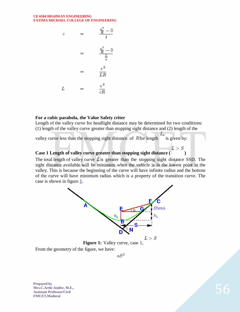
CE 6504 HIGHWAY ENGINEERING
FATIMA MICHAEL COLLEGE OF ENGINEERING
Prepared by
MrsCArthi Jenifer ME
Assistant ProfessorCivil
FMCETMadurai 56
For a cubic parabola the Value Safety criter Length of the valley curve for headlight distance may be determined for two conditions
(1) length of the valley curve greater than stopping sight distance and (2) length of the
valley curve less than the stopping sight distance of for length is given by
Case 1 Length of valley curve greater than stopping sight distance ( )
The total length of valley curve is greater than the stopping sight distance SSD The
sight distance available will be minimum when the vehicle is in the lowest point in the
valley This is because the beginning of the curve will have infinite radius and the bottom
of the curve will have minimum radius which is a property of the transition curve The
case is shown in figure 1
Figure 1 Valley curve case 1
From the geometry of the figure we have
CE 6504 HIGHWAY ENGINEERING
FATIMA MICHAEL COLLEGE OF ENGINEERING
Prepared by
MrsCArthi Jenifer ME
Assistant ProfessorCivil
FMCETMadurai 57
(1)
where is the deviation angle in radians is the height of headlight beam is the
head beam inclination in degrees and is the sight distance The inclination is 1
degree
Case 2 Length of valley curve less than stopping sight distance ( )
The length of the curve is less than SSD In this case the minimum sight distance is
from the beginning of the curve The important points are the beginning of the curve and
the bottom most part of the curve If the vehicle is at the bottom of the curve then its
headlight beam will reach far beyond the endpoint of the curve whereas if the vehicle is
at the beginning of the curve then the headlight beam will hit just outside the curve
Therefore the length of the curve is derived by assuming the vehicle at the beginning of
the curve The case is shown in figure 1
From the figure
(1) Note that the above expression is approximate and is satisfactory because in practice the gradients
are very small and is acceptable for all practical purposes We will not be able to know prior to
which case to be adopted Therefore both has to be calculated and the one which satisfies the
condition is adopted
1 Flexible pavement
2 Rigid pavement
Flexible pavement
These pavements reflect the deformation of sub grade and the subsequent layers to the
surface
Rigid pavement
The rigid characteristic of the pavement are associated with rigidity or flexural strength
CE 6504 HIGHWAY ENGINEERING
FATIMA MICHAEL COLLEGE OF ENGINEERING
Prepared by
MrsCArthi Jenifer ME
Assistant ProfessorCivil
FMCETMadurai 58
or slab action so the load is distributed over a wide area of sub grade soil
Flexible pavement Definition
These pavements reflect the deformation of sub grade and the subsequent layers to the
surface Flexible usually asphalt is laid with no reinforcement or with a specialized
fabric reinforcement that permits limited flow or repositioning of the roadbed under
ground changes
The design of flexible pavement is based on load distributing characteristic of the
component layers The black top pavement including water amp gravel bound macadam fall
in this category
Flexible pavement on the whole has low or negligible flexible strength flexible in their
structural action) The flexible pavement layers transmit the vertical or compressive
stresses to the lower layers by grain transfer through contact points of granular structure
The vertical compressive stress is maximum on the pavement surface directly under the
wheel load and is equal to contact pressure under the wheels Due to the ability to
distribute the stress to large area in the shape of truncated cone the stresses get decreased
in the lower layer
As such the flexible pavement may be constructed in a number of layers and the top
layer has to be strongest as the highest compressive stresses
To be sustained by this layer in addition to wear and tear the lower layer have to take
up only lesser magnitude of stress as there is no direct wearing action die to traffic loads
therefore inferior material with lower cast can be used in the lower layers
Rigid pavement Definition
The rigid characteristic of the pavement are associated with rigidity or flexural strength
or slab action so the load is distributed over a wide area of sub grade soil Rigid pavement
is laid in slabs with steel reinforcement
The rigid pavements are made of cement concrete either plan reinforced or prestressed
concrete
Critical condition of stress in the rigid pavement is the maximum flexural stress occurring in the slab due to wheel load and the temperature changes
Rigid pavement is designed and analyzed by using the elastic theory
CE 6504 HIGHWAY ENGINEERING
FATIMA MICHAEL COLLEGE OF ENGINEERING
Prepared by
MrsCArthi Jenifer ME
Assistant ProfessorCivil
FMCETMadurai 59
UNIT-5 EVALUATION AND MAINTENANCE OF PAVEMENTS
TRAFFIC PARAMETERS
Design life
Design life is the number of years (or number of standard axle repetitions) for which the
pavement is being designed A pavement is expected to serve satisfactorily within the
design life For concrete pavements 20 to 40 years may be assumed as the design life
(PCA 1984 IRC58 2002)
Basic design principle
Though different approaches for concrete pavement design are suggested in various
guidelines the design principles tend to remain similar across different guidelines for
example PCA (1994) Austroads (2004) NCHRP (2004) IRC58 (2002) etc except the
AASHTO (1993) provisions which is based on empirical approach The basic steps
involved in the design of concrete pavement method can be summarized as follows
The developed stresses due to load for a trial thickness of the concrete slab are
calculated for various loading configuration and the critical one is chosen The
axle loads are generally divided into different axle load groups and the load
stresses are calculated individually
The ratio between the load stress and Modulus of Rupture (MOR) is known as
stress ratio The stress ratio determines how many repetitions the pavement can
sustain (ie allowable traffic repetitions) for the individual axle load group If the
stress ratio is 055 or lower it can withstand virtually infinite number of traffic
repetitions (PCA 1984)
The ratio between the allowable repetitions to the expected traffic repetitions is
the damage fraction The calculation process is repeated for various axle loads
(sometimes for various seasons or various timings of the day) and the sum of
individual damage fractions (c u m u l a t i v e fatigue damage) should be less
than equal to one for pavement design being safe If found unsafe the trial
thickness is changed and the design process is repeated
The design process may also include considerations for temperature stress
moisture stresses and erosion distress
A brief discussion on concrete pavement design approaches suggested by various design
practices viz PCA method (1984) Austroads method (2004) AASHTO method (1993)
NCHRP mechanistic-empirical method (2004) and the Indian Roads Congress (IRC)
method (2002) are placed in the following
Portland cement Association (PCA) Method
The PCA method is based on Westergaard Picket and Rays work and further theoretical
analysis by Finite Element Method (Huang 1993) The data used to develop the PCA
method is generated from various road tests like ASSHO road test Arlington test
(conducted by PCA) Bates test road and Maryland road test (PCA 1984) The PCA
design method is based on the following two considerations (PCA 1984)
The fatigue damage on the concrete slab due to repetitive application of traffic
load is estimated The cumulative fatigue damage principle is used to estimate the
design thickness of the slab Edge stress between the mid-ways of the
CE 6504 HIGHWAY ENGINEERING
FATIMA MICHAEL COLLEGE OF ENGINEERING
Prepared by
MrsCArthi Jenifer ME
Assistant ProfessorCivil
FMCETMadurai 60
transverse joint is taken as critical configuration
The stresses due to warping and curling (due to temperature and moisture
gradient) are not considered in the fatigue analysis as per PCA recommendation
because most of the time the stresses generated are subtractive to the load stress
The possibility of erosion of pavement materials placed below the concrete slab is
evaluated The rate at which the slab is deflected due to axle load is used as a
criterion for erosion Theoretically it can be shown that a thin pavement with
smaller deflection basin is subjected to faster rate of deflection compared to
thicker slab Hence thin slab is more susceptible to erosion In a similar way the
cumulative erosion damage is calculated for individual axle load groups If this
value is greater than one then the design needs to be revised
Austroads method
Austroads method has been adopted from PCA (1984) approach with modifications
suited to Australian conditions (Austroads 2004) A bound mix or lean cement concrete is
used as sub-base material For a given CBR value of the subgrade and given thickness of
cemented sub-base the effective subgrade strength can be obtained from the chart
provided Figure-19 schematically shows such a chart For different levels of traffic
Austroads (2004) suggests minimum values of the base thicknesses to be provided
CE 6504 HIGHWAY ENGINEERING
FATIMA MICHAEL COLLEGE OF ENGINEERING
Prepared by
MrsCArthi Jenifer ME
Assistant ProfessorCivil
FMCETMadurai 61
figure-19 Schematic diagram of Austroads (2004) chart for estimation of effective
subgrade strength
As per Astroads (2004) the concrete pavement slab thickness for a given expected
traffic repetitions is designed considering the (i) flexural fatigue of the concrete slab and
the (ii) subgrade erosion arising out of repeated deflections For both the considerations
equations are suggested to calculate the allowable traffic repetitions If the allowable
traffic is less than the expected traffic the design is revised by increasing the slab
thickness The concrete shoulders adopted are of integral type or structural type
AASHTO method
The AASHTO method (1993) for design of concrete pavement has evolved from the
AASHO road test (AASHO 1962) The AASHTO pavement design follows an empirical
approach Pavement performance in terms of present serviceability index ( PSI ) loss of
serviceability sub-grade and sub-base strength cumulative traffic properties of concrete
joint load transfer efficiency drainage condition overall standard deviation and
reliability are the input parameters considered in the pavement design
The PSI value of the fresh pavement is assumed as 45 and the pavement is deemed to
have failed when the PSI value reaches 25 The resilient moduli of the subgrade and sub-
base materials are determined in the laboratory simulating the seasonal moisture content
and stress situation Suggested values are also available for given moisture content
plasticity index etc The composite modulus of sub-grade reaction (k) is estimated from
modulus of sub-grade reaction and elastic modulus of sub-base for various seasons and
the depth of rigid foundation and the thickness of the sub-base
Design equation as well nomographs are available to estimate the slab thickness (D) from
these input parameters
NCHRP mechanistic-empirical (M-E) metho
The NCHRP (2004) has recently developed concrete pavement design procedure based
on mechanistic-empirical (M-E) approach This approach attempts to reduce the extent of
empiricism prevalent in the existing AASHTO (1993) guidelines This proposed NCHRP
pavement design system is modular in nature that is the design approach can be
modified by parts (as and when new knowledge is available) without disrupting the
overall design procedure This approach also can take care of various wheel-axle loa
configuration
As per this approach trial thickness of the slab is first assumed and the stress strain and
displacement values are obtained From these values the performance of the pavement in
terms of distresses (such as faulting cracking) and smoothness and predicted If these
predicted performance parameters does not satisfy the required performance for a given
reliability
The design approach includes a large data-base as input parameters for example average
daily traffic traffic growth rate traffic composition hourly weather data on air
temperature precipitation wind speed percentage sunshine relative humidity pavement
material engineering parameters ground water depth infiltration drainage hydraulic
conductivity thermal conductivity heat capacity etc The temperature stress is
considered in this method but the temperature profile is linearized to enhance
computational efficiency (NCHRP 2004)
CE 6504 HIGHWAY ENGINEERING
FATIMA MICHAEL COLLEGE OF ENGINEERING
Prepared by
MrsCArthi Jenifer ME
Assistant ProfessorCivil
FMCETMadurai 62
INDIAN ROADS CONGRESS (IRC) METHOD
The Indian Roads Congress (IRC) guidelines IRC58 (2002) has adopted the
Westergaards equation to estimate load stress and Brdaburys equation to estimate
temperature stress The load stress is highest at the corner of the slab lesser in edge and
least in the interior The order of variation of temperature stress is just the reverse of this
As per IRC58 (2002) it is recommended that the design needs to be done for edge stress
condition and subsequently check needs to be performed for corner stress condition so as
to finalize the design The following are the steps followed as per IRC58 (2002)
guideline for the design of concrete pavement
The input parameters are obtained to formulate the design problem The joint
spacing and the slab dimensions are decided If there is a bound sub-base layer
over the subgrade a suitable value of effective k is to be adopted
A trial thickness of the concrete slab is assumed
The edge stress is estimated for various axle loads from the given charts Figure-
20 schematically shows such a chart The cumulative fatigue damage principle for
fatigue is applied to check the adequacy of the slab thickness
The sum of edge stress due to load for the highest axle load group and the
temperature stress should be less than the MOR of concrete otherwise the design
is revised
The adequacy of corner stress is checked with respect to MOR value and
accordingly the design is finalized Westergaards corner stress formula
Figure-20 Schematic diagram of IRC58 chart for estimation of load stress at the edge
(IRC58 2002)
CE 6504 HIGHWAY ENGINEERING
FATIMA MICHAEL COLLEGE OF ENGINEERING
Prepared by
MrsCArthi Jenifer ME
Assistant ProfessorCivil
FMCETMadurai 63
estimation of corner stress due to load and the corner stress due to temperature is
assumed to be zero
Estimation of layer thicknesses
The thickness of the pavement is adjusted in such a way that the stress strain
developed is less than the allowable values obtained from past performance
information
The two major modes of structural failure of pavement are fatigue and rutting
o Fatigue Traffic applies repetitive load to the pavement surface and the
cracks start from bottom the bound layer slab and propagate upwards
When the extent of surface cracks reaches a predefined level the
pavement is said to have failed due to flexural fatigue
FUNCTIONAL DESIGN
The functional pavement design involves considerations of skid resistance roughness
surface distresses reflectivity of pavement surface etc The functional pavement design
considers mainly the surface features of a pavement
Drainage design
A road needs to be designed in such a way that the rain snow precipitation is drained off
the pavement and its surroundings A suitable surface drainage system for the pavement
is designed for this purpose Some water however will percolate into the pavement from
its top surface and needs to be taken out of the pavement - this is done by providing an
internal drainage system to the pavement Water will also try to enter into the pavement
from bottom due to capillary rise or due to rise in water table A suitably designed sub-
surface drainage system tries to avoid such a problem
PAVEMENT THICKNESS DESIGN CHARTS
For the design of pavements to carry traffic in the range of 1 to 10 msa use chart 1 and for
traffic in the range 10 to 150 msa use chart 2 of IRC37 2001 The design curves relate
pavement thickness to the cumulative number of standard axles to be carried over the
design life for different sub-grade CBR values ranging from 2 to 10 The design
charts will give the total thickness of the pavement for the above inputs The total
thickness consists of granular sub-base granular base and bituminous surfacing The
individual layers are designed based on the the recommendations given below and the
subsequent tables
Pavement composition
Sub-base
Sub-base materials comprise natural sand gravel laterite brick metal crushed
stone or combinations thereof meeting the prescribed grading and physical
requirements The sub-base material should have a minimum CBR of 20 and
30 for traffic upto 2 msa and traffic exceeding 2 msa respectively Sub-base
usually consist of granular or WBM and the thickness should not be less than 150
mm for design traffic less than 10 msa and 200 mm for design traffic
Base
The recommended designs are for unbounded granular bases which comprise
CE 6504 HIGHWAY ENGINEERING
FATIMA MICHAEL COLLEGE OF ENGINEERING
Prepared by
MrsCArthi Jenifer ME
Assistant ProfessorCivil
FMCETMadurai 64
conventional water bound macadam (WBM) or wet mix macadam (WMM) or
equivalent confirming to MOST specifications The materials should be of good
quality with minimum thickness of 225 mm for traffic up to 2 msa an 150 mm for
traffic
Bituminoussurfacing The surfacing consists of a wearing course or a binder
course plus wearing course The most commonly used wearing courses are
surface dressing open graded premix carpet mix seal surfacing semi-
dense bituminous concrete and bituminous concrete For binder course
MOST specifies it is desirable to use bituminous macadam (BM) for traffic
upto o 5 msa and dense bituminous macadam (DBM) for traffic more than 5
msa
Numerical example
Design the pavement for construction of a new bypass with the following data
1 Two lane carriage way
2 Initial traffic in the year of completion of construction = 400 CVPD (sum of both
directions)
3 Traffic growth rate = 75
4 Design life = 15 years
5 Vehicle damage factor based on axle load survey = 25 standard axle per
commercial vehicle
6 Design CBR of subgrade soil = 4
Solution
1 Distribution factor = 075
2
3 Total pavement thickness for CBR 4 and traffic 72 msa from IRC37 2001
chart1 = 660 mm
4 Pavement composition can be obtained by interpolation from Pavement Design
Catalogue (IRC37 2001)
1 Bituminous surfacing = 25 mm SDBC + 70 mm DBM
2 Road-base = 250 mm WBM
3 sub-base = 315 mm granular material of CBR not less than 30
CE 6504 HIGHWAY ENGINEERING
FATIMA MICHAEL COLLEGE OF ENGINEERING
Prepared by
MrsCArthi Jenifer ME
Assistant ProfessorCivil
FMCETMadurai 65
Generally bound base layers are used for concrete pavement construction As per Indian
specification some example of such base layers are Dry Lean Concrete (DLC) Roller
Compacted Concrete (RCC) (IRC15-2002)
The concrete slab is generally of M40 to M50 grade of concrete as
per Indian specifications and is called as paving quality concrete (PQC)
(IRC15-2002)
BITUMINOUS PAVEMENT
The subgrade is a compacted soil layer
The base and sub-base course could be made up of bound or unbound granular layer As
per Indian specifications (MORTampH 2001) some examples of base or sub-base layers
are Granular sub-base(GSB) Water Bound Macadam (WBM) Wet Mix Macadam
(WMM) etc
The binder course is made up bituminous material As per Indian specifications
(MORTampH 2001) some examples of binder course are Bituminous Macadam (BM)
Dense Bituminous Macadam (DBM) etc
The wearing course is the top bituminous layer which is comes in contact to the
vehicle tyre Wearing course provides impermeability to the pavement surface
against water percolation (Chakroborty and Das 2003) The binder course and wearing
course together are called bituminous surfacing
IRC METHOD OF FLEXIBLE PAVEMENT MIX DESIGN
These guidelines will apply to design of flexible pavements for Expressway National Highways
State Highways Major District Roads and other categories of roads Flexible pavements are
considered to include the pavements which have bituminous surfacing and granular base and sub-
base courses conforming to IRC MOST standards These guidelines apply to new pavements
Design criteria
The flexible pavements has been modeled as a three layer structure and stresses and strains at
critical locations have been computed using the linear elastic model To give proper consideration
to the aspects of performance the following three types of pavement distress resulting from
repeated (cyclic) application of traffic loads are considered
1 Vertical compressive strain at the top of the sub-grade which can cause sub-grade
deformation resulting in permanent deformation at the pavement surface
2 Horizontal tensile strain or stress at the bottom of the bituminous layer which can cause
fracture of the bituminous layer
3 Pavement deformation within the bituminous layer
CE 6504 HIGHWAY ENGINEERING
FATIMA MICHAEL COLLEGE OF ENGINEERING
Prepared by
MrsCArthi Jenifer ME
Assistant ProfessorCivil
FMCETMadurai 66
While the permanent deformation within the bituminous layer can be controlled by meeting the
mix design requirements thickness of granular and bituminous layers are selected using the
analytical design approach so that strains at the critical points are within the allowable limits For
calculating tensile strains at the bottom of the bituminous layer the stiffness of dense bituminous
macadam (DBM) layer with 6070 bitumen has been used in the analysis
FAILURE CRITERIA
Critical locations in pavement
A and B are the critical locations for tensile strains Maximum value of the strain is
adopted for design C is the critical location for the vertical subgrade strain since the
maximum value of the occurs mostly at C
CE 6504 HIGHWAY ENGINEERING
FATIMA MICHAEL COLLEGE OF ENGINEERING
Prepared by
MrsCArthi Jenifer ME
Assistant ProfessorCivil
FMCETMadurai 67
Fatigue Criteria
Bituminous surfacings of pavements display flexural fatigue cracking if the tensile strain
at the bottom of the bituminous layer is beyond certain limit The relation between the
fatigue life of the pavement and the tensile strain in the bottom of the bituminous layer
was obtained as
(1)
in which is the allowable number of load repetitions to control fatigue cracking and
is the Elastic modulus of bituminous layer The use of equation 1 would result in
fatigue cracking of 20 of the total area
Rutting Criteria
The allowable number of load repetitions to control permanent deformation can be
expressed as
(2)
is the number of cumulative standard axles to produce rutting of 20 mm
CE 6504 HIGHWAY ENGINEERING
FATIMA MICHAEL COLLEGE OF ENGINEERING
Prepared by
MrsCArthi Jenifer ME
Assistant ProfessorCivil
FMCETMadurai 68
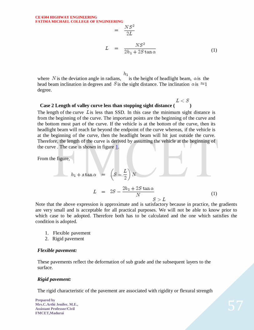
CE 6504 HIGHWAY ENGINEERING
FATIMA MICHAEL COLLEGE OF ENGINEERING
Prepared by
MrsCArthi Jenifer ME
Assistant ProfessorCivil
FMCETMadurai 57
(1)
where is the deviation angle in radians is the height of headlight beam is the
head beam inclination in degrees and is the sight distance The inclination is 1
degree
Case 2 Length of valley curve less than stopping sight distance ( )
The length of the curve is less than SSD In this case the minimum sight distance is
from the beginning of the curve The important points are the beginning of the curve and
the bottom most part of the curve If the vehicle is at the bottom of the curve then its
headlight beam will reach far beyond the endpoint of the curve whereas if the vehicle is
at the beginning of the curve then the headlight beam will hit just outside the curve
Therefore the length of the curve is derived by assuming the vehicle at the beginning of
the curve The case is shown in figure 1
From the figure
(1) Note that the above expression is approximate and is satisfactory because in practice the gradients
are very small and is acceptable for all practical purposes We will not be able to know prior to
which case to be adopted Therefore both has to be calculated and the one which satisfies the
condition is adopted
1 Flexible pavement
2 Rigid pavement
Flexible pavement
These pavements reflect the deformation of sub grade and the subsequent layers to the
surface
Rigid pavement
The rigid characteristic of the pavement are associated with rigidity or flexural strength
CE 6504 HIGHWAY ENGINEERING
FATIMA MICHAEL COLLEGE OF ENGINEERING
Prepared by
MrsCArthi Jenifer ME
Assistant ProfessorCivil
FMCETMadurai 58
or slab action so the load is distributed over a wide area of sub grade soil
Flexible pavement Definition
These pavements reflect the deformation of sub grade and the subsequent layers to the
surface Flexible usually asphalt is laid with no reinforcement or with a specialized
fabric reinforcement that permits limited flow or repositioning of the roadbed under
ground changes
The design of flexible pavement is based on load distributing characteristic of the
component layers The black top pavement including water amp gravel bound macadam fall
in this category
Flexible pavement on the whole has low or negligible flexible strength flexible in their
structural action) The flexible pavement layers transmit the vertical or compressive
stresses to the lower layers by grain transfer through contact points of granular structure
The vertical compressive stress is maximum on the pavement surface directly under the
wheel load and is equal to contact pressure under the wheels Due to the ability to
distribute the stress to large area in the shape of truncated cone the stresses get decreased
in the lower layer
As such the flexible pavement may be constructed in a number of layers and the top
layer has to be strongest as the highest compressive stresses
To be sustained by this layer in addition to wear and tear the lower layer have to take
up only lesser magnitude of stress as there is no direct wearing action die to traffic loads
therefore inferior material with lower cast can be used in the lower layers
Rigid pavement Definition
The rigid characteristic of the pavement are associated with rigidity or flexural strength
or slab action so the load is distributed over a wide area of sub grade soil Rigid pavement
is laid in slabs with steel reinforcement
The rigid pavements are made of cement concrete either plan reinforced or prestressed
concrete
Critical condition of stress in the rigid pavement is the maximum flexural stress occurring in the slab due to wheel load and the temperature changes
Rigid pavement is designed and analyzed by using the elastic theory
CE 6504 HIGHWAY ENGINEERING
FATIMA MICHAEL COLLEGE OF ENGINEERING
Prepared by
MrsCArthi Jenifer ME
Assistant ProfessorCivil
FMCETMadurai 59
UNIT-5 EVALUATION AND MAINTENANCE OF PAVEMENTS
TRAFFIC PARAMETERS
Design life
Design life is the number of years (or number of standard axle repetitions) for which the
pavement is being designed A pavement is expected to serve satisfactorily within the
design life For concrete pavements 20 to 40 years may be assumed as the design life
(PCA 1984 IRC58 2002)
Basic design principle
Though different approaches for concrete pavement design are suggested in various
guidelines the design principles tend to remain similar across different guidelines for
example PCA (1994) Austroads (2004) NCHRP (2004) IRC58 (2002) etc except the
AASHTO (1993) provisions which is based on empirical approach The basic steps
involved in the design of concrete pavement method can be summarized as follows
The developed stresses due to load for a trial thickness of the concrete slab are
calculated for various loading configuration and the critical one is chosen The
axle loads are generally divided into different axle load groups and the load
stresses are calculated individually
The ratio between the load stress and Modulus of Rupture (MOR) is known as
stress ratio The stress ratio determines how many repetitions the pavement can
sustain (ie allowable traffic repetitions) for the individual axle load group If the
stress ratio is 055 or lower it can withstand virtually infinite number of traffic
repetitions (PCA 1984)
The ratio between the allowable repetitions to the expected traffic repetitions is
the damage fraction The calculation process is repeated for various axle loads
(sometimes for various seasons or various timings of the day) and the sum of
individual damage fractions (c u m u l a t i v e fatigue damage) should be less
than equal to one for pavement design being safe If found unsafe the trial
thickness is changed and the design process is repeated
The design process may also include considerations for temperature stress
moisture stresses and erosion distress
A brief discussion on concrete pavement design approaches suggested by various design
practices viz PCA method (1984) Austroads method (2004) AASHTO method (1993)
NCHRP mechanistic-empirical method (2004) and the Indian Roads Congress (IRC)
method (2002) are placed in the following
Portland cement Association (PCA) Method
The PCA method is based on Westergaard Picket and Rays work and further theoretical
analysis by Finite Element Method (Huang 1993) The data used to develop the PCA
method is generated from various road tests like ASSHO road test Arlington test
(conducted by PCA) Bates test road and Maryland road test (PCA 1984) The PCA
design method is based on the following two considerations (PCA 1984)
The fatigue damage on the concrete slab due to repetitive application of traffic
load is estimated The cumulative fatigue damage principle is used to estimate the
design thickness of the slab Edge stress between the mid-ways of the
CE 6504 HIGHWAY ENGINEERING
FATIMA MICHAEL COLLEGE OF ENGINEERING
Prepared by
MrsCArthi Jenifer ME
Assistant ProfessorCivil
FMCETMadurai 60
transverse joint is taken as critical configuration
The stresses due to warping and curling (due to temperature and moisture
gradient) are not considered in the fatigue analysis as per PCA recommendation
because most of the time the stresses generated are subtractive to the load stress
The possibility of erosion of pavement materials placed below the concrete slab is
evaluated The rate at which the slab is deflected due to axle load is used as a
criterion for erosion Theoretically it can be shown that a thin pavement with
smaller deflection basin is subjected to faster rate of deflection compared to
thicker slab Hence thin slab is more susceptible to erosion In a similar way the
cumulative erosion damage is calculated for individual axle load groups If this
value is greater than one then the design needs to be revised
Austroads method
Austroads method has been adopted from PCA (1984) approach with modifications
suited to Australian conditions (Austroads 2004) A bound mix or lean cement concrete is
used as sub-base material For a given CBR value of the subgrade and given thickness of
cemented sub-base the effective subgrade strength can be obtained from the chart
provided Figure-19 schematically shows such a chart For different levels of traffic
Austroads (2004) suggests minimum values of the base thicknesses to be provided
CE 6504 HIGHWAY ENGINEERING
FATIMA MICHAEL COLLEGE OF ENGINEERING
Prepared by
MrsCArthi Jenifer ME
Assistant ProfessorCivil
FMCETMadurai 61
figure-19 Schematic diagram of Austroads (2004) chart for estimation of effective
subgrade strength
As per Astroads (2004) the concrete pavement slab thickness for a given expected
traffic repetitions is designed considering the (i) flexural fatigue of the concrete slab and
the (ii) subgrade erosion arising out of repeated deflections For both the considerations
equations are suggested to calculate the allowable traffic repetitions If the allowable
traffic is less than the expected traffic the design is revised by increasing the slab
thickness The concrete shoulders adopted are of integral type or structural type
AASHTO method
The AASHTO method (1993) for design of concrete pavement has evolved from the
AASHO road test (AASHO 1962) The AASHTO pavement design follows an empirical
approach Pavement performance in terms of present serviceability index ( PSI ) loss of
serviceability sub-grade and sub-base strength cumulative traffic properties of concrete
joint load transfer efficiency drainage condition overall standard deviation and
reliability are the input parameters considered in the pavement design
The PSI value of the fresh pavement is assumed as 45 and the pavement is deemed to
have failed when the PSI value reaches 25 The resilient moduli of the subgrade and sub-
base materials are determined in the laboratory simulating the seasonal moisture content
and stress situation Suggested values are also available for given moisture content
plasticity index etc The composite modulus of sub-grade reaction (k) is estimated from
modulus of sub-grade reaction and elastic modulus of sub-base for various seasons and
the depth of rigid foundation and the thickness of the sub-base
Design equation as well nomographs are available to estimate the slab thickness (D) from
these input parameters
NCHRP mechanistic-empirical (M-E) metho
The NCHRP (2004) has recently developed concrete pavement design procedure based
on mechanistic-empirical (M-E) approach This approach attempts to reduce the extent of
empiricism prevalent in the existing AASHTO (1993) guidelines This proposed NCHRP
pavement design system is modular in nature that is the design approach can be
modified by parts (as and when new knowledge is available) without disrupting the
overall design procedure This approach also can take care of various wheel-axle loa
configuration
As per this approach trial thickness of the slab is first assumed and the stress strain and
displacement values are obtained From these values the performance of the pavement in
terms of distresses (such as faulting cracking) and smoothness and predicted If these
predicted performance parameters does not satisfy the required performance for a given
reliability
The design approach includes a large data-base as input parameters for example average
daily traffic traffic growth rate traffic composition hourly weather data on air
temperature precipitation wind speed percentage sunshine relative humidity pavement
material engineering parameters ground water depth infiltration drainage hydraulic
conductivity thermal conductivity heat capacity etc The temperature stress is
considered in this method but the temperature profile is linearized to enhance
computational efficiency (NCHRP 2004)
CE 6504 HIGHWAY ENGINEERING
FATIMA MICHAEL COLLEGE OF ENGINEERING
Prepared by
MrsCArthi Jenifer ME
Assistant ProfessorCivil
FMCETMadurai 62
INDIAN ROADS CONGRESS (IRC) METHOD
The Indian Roads Congress (IRC) guidelines IRC58 (2002) has adopted the
Westergaards equation to estimate load stress and Brdaburys equation to estimate
temperature stress The load stress is highest at the corner of the slab lesser in edge and
least in the interior The order of variation of temperature stress is just the reverse of this
As per IRC58 (2002) it is recommended that the design needs to be done for edge stress
condition and subsequently check needs to be performed for corner stress condition so as
to finalize the design The following are the steps followed as per IRC58 (2002)
guideline for the design of concrete pavement
The input parameters are obtained to formulate the design problem The joint
spacing and the slab dimensions are decided If there is a bound sub-base layer
over the subgrade a suitable value of effective k is to be adopted
A trial thickness of the concrete slab is assumed
The edge stress is estimated for various axle loads from the given charts Figure-
20 schematically shows such a chart The cumulative fatigue damage principle for
fatigue is applied to check the adequacy of the slab thickness
The sum of edge stress due to load for the highest axle load group and the
temperature stress should be less than the MOR of concrete otherwise the design
is revised
The adequacy of corner stress is checked with respect to MOR value and
accordingly the design is finalized Westergaards corner stress formula
Figure-20 Schematic diagram of IRC58 chart for estimation of load stress at the edge
(IRC58 2002)
CE 6504 HIGHWAY ENGINEERING
FATIMA MICHAEL COLLEGE OF ENGINEERING
Prepared by
MrsCArthi Jenifer ME
Assistant ProfessorCivil
FMCETMadurai 63
estimation of corner stress due to load and the corner stress due to temperature is
assumed to be zero
Estimation of layer thicknesses
The thickness of the pavement is adjusted in such a way that the stress strain
developed is less than the allowable values obtained from past performance
information
The two major modes of structural failure of pavement are fatigue and rutting
o Fatigue Traffic applies repetitive load to the pavement surface and the
cracks start from bottom the bound layer slab and propagate upwards
When the extent of surface cracks reaches a predefined level the
pavement is said to have failed due to flexural fatigue
FUNCTIONAL DESIGN
The functional pavement design involves considerations of skid resistance roughness
surface distresses reflectivity of pavement surface etc The functional pavement design
considers mainly the surface features of a pavement
Drainage design
A road needs to be designed in such a way that the rain snow precipitation is drained off
the pavement and its surroundings A suitable surface drainage system for the pavement
is designed for this purpose Some water however will percolate into the pavement from
its top surface and needs to be taken out of the pavement - this is done by providing an
internal drainage system to the pavement Water will also try to enter into the pavement
from bottom due to capillary rise or due to rise in water table A suitably designed sub-
surface drainage system tries to avoid such a problem
PAVEMENT THICKNESS DESIGN CHARTS
For the design of pavements to carry traffic in the range of 1 to 10 msa use chart 1 and for
traffic in the range 10 to 150 msa use chart 2 of IRC37 2001 The design curves relate
pavement thickness to the cumulative number of standard axles to be carried over the
design life for different sub-grade CBR values ranging from 2 to 10 The design
charts will give the total thickness of the pavement for the above inputs The total
thickness consists of granular sub-base granular base and bituminous surfacing The
individual layers are designed based on the the recommendations given below and the
subsequent tables
Pavement composition
Sub-base
Sub-base materials comprise natural sand gravel laterite brick metal crushed
stone or combinations thereof meeting the prescribed grading and physical
requirements The sub-base material should have a minimum CBR of 20 and
30 for traffic upto 2 msa and traffic exceeding 2 msa respectively Sub-base
usually consist of granular or WBM and the thickness should not be less than 150
mm for design traffic less than 10 msa and 200 mm for design traffic
Base
The recommended designs are for unbounded granular bases which comprise
CE 6504 HIGHWAY ENGINEERING
FATIMA MICHAEL COLLEGE OF ENGINEERING
Prepared by
MrsCArthi Jenifer ME
Assistant ProfessorCivil
FMCETMadurai 64
conventional water bound macadam (WBM) or wet mix macadam (WMM) or
equivalent confirming to MOST specifications The materials should be of good
quality with minimum thickness of 225 mm for traffic up to 2 msa an 150 mm for
traffic
Bituminoussurfacing The surfacing consists of a wearing course or a binder
course plus wearing course The most commonly used wearing courses are
surface dressing open graded premix carpet mix seal surfacing semi-
dense bituminous concrete and bituminous concrete For binder course
MOST specifies it is desirable to use bituminous macadam (BM) for traffic
upto o 5 msa and dense bituminous macadam (DBM) for traffic more than 5
msa
Numerical example
Design the pavement for construction of a new bypass with the following data
1 Two lane carriage way
2 Initial traffic in the year of completion of construction = 400 CVPD (sum of both
directions)
3 Traffic growth rate = 75
4 Design life = 15 years
5 Vehicle damage factor based on axle load survey = 25 standard axle per
commercial vehicle
6 Design CBR of subgrade soil = 4
Solution
1 Distribution factor = 075
2
3 Total pavement thickness for CBR 4 and traffic 72 msa from IRC37 2001
chart1 = 660 mm
4 Pavement composition can be obtained by interpolation from Pavement Design
Catalogue (IRC37 2001)
1 Bituminous surfacing = 25 mm SDBC + 70 mm DBM
2 Road-base = 250 mm WBM
3 sub-base = 315 mm granular material of CBR not less than 30
CE 6504 HIGHWAY ENGINEERING
FATIMA MICHAEL COLLEGE OF ENGINEERING
Prepared by
MrsCArthi Jenifer ME
Assistant ProfessorCivil
FMCETMadurai 65
Generally bound base layers are used for concrete pavement construction As per Indian
specification some example of such base layers are Dry Lean Concrete (DLC) Roller
Compacted Concrete (RCC) (IRC15-2002)
The concrete slab is generally of M40 to M50 grade of concrete as
per Indian specifications and is called as paving quality concrete (PQC)
(IRC15-2002)
BITUMINOUS PAVEMENT
The subgrade is a compacted soil layer
The base and sub-base course could be made up of bound or unbound granular layer As
per Indian specifications (MORTampH 2001) some examples of base or sub-base layers
are Granular sub-base(GSB) Water Bound Macadam (WBM) Wet Mix Macadam
(WMM) etc
The binder course is made up bituminous material As per Indian specifications
(MORTampH 2001) some examples of binder course are Bituminous Macadam (BM)
Dense Bituminous Macadam (DBM) etc
The wearing course is the top bituminous layer which is comes in contact to the
vehicle tyre Wearing course provides impermeability to the pavement surface
against water percolation (Chakroborty and Das 2003) The binder course and wearing
course together are called bituminous surfacing
IRC METHOD OF FLEXIBLE PAVEMENT MIX DESIGN
These guidelines will apply to design of flexible pavements for Expressway National Highways
State Highways Major District Roads and other categories of roads Flexible pavements are
considered to include the pavements which have bituminous surfacing and granular base and sub-
base courses conforming to IRC MOST standards These guidelines apply to new pavements
Design criteria
The flexible pavements has been modeled as a three layer structure and stresses and strains at
critical locations have been computed using the linear elastic model To give proper consideration
to the aspects of performance the following three types of pavement distress resulting from
repeated (cyclic) application of traffic loads are considered
1 Vertical compressive strain at the top of the sub-grade which can cause sub-grade
deformation resulting in permanent deformation at the pavement surface
2 Horizontal tensile strain or stress at the bottom of the bituminous layer which can cause
fracture of the bituminous layer
3 Pavement deformation within the bituminous layer
CE 6504 HIGHWAY ENGINEERING
FATIMA MICHAEL COLLEGE OF ENGINEERING
Prepared by
MrsCArthi Jenifer ME
Assistant ProfessorCivil
FMCETMadurai 66
While the permanent deformation within the bituminous layer can be controlled by meeting the
mix design requirements thickness of granular and bituminous layers are selected using the
analytical design approach so that strains at the critical points are within the allowable limits For
calculating tensile strains at the bottom of the bituminous layer the stiffness of dense bituminous
macadam (DBM) layer with 6070 bitumen has been used in the analysis
FAILURE CRITERIA
Critical locations in pavement
A and B are the critical locations for tensile strains Maximum value of the strain is
adopted for design C is the critical location for the vertical subgrade strain since the
maximum value of the occurs mostly at C
CE 6504 HIGHWAY ENGINEERING
FATIMA MICHAEL COLLEGE OF ENGINEERING
Prepared by
MrsCArthi Jenifer ME
Assistant ProfessorCivil
FMCETMadurai 67
Fatigue Criteria
Bituminous surfacings of pavements display flexural fatigue cracking if the tensile strain
at the bottom of the bituminous layer is beyond certain limit The relation between the
fatigue life of the pavement and the tensile strain in the bottom of the bituminous layer
was obtained as
(1)
in which is the allowable number of load repetitions to control fatigue cracking and
is the Elastic modulus of bituminous layer The use of equation 1 would result in
fatigue cracking of 20 of the total area
Rutting Criteria
The allowable number of load repetitions to control permanent deformation can be
expressed as
(2)
is the number of cumulative standard axles to produce rutting of 20 mm
CE 6504 HIGHWAY ENGINEERING
FATIMA MICHAEL COLLEGE OF ENGINEERING
Prepared by
MrsCArthi Jenifer ME
Assistant ProfessorCivil
FMCETMadurai 68
CE 6504 HIGHWAY ENGINEERING
FATIMA MICHAEL COLLEGE OF ENGINEERING
Prepared by
MrsCArthi Jenifer ME
Assistant ProfessorCivil
FMCETMadurai 59
UNIT-5 EVALUATION AND MAINTENANCE OF PAVEMENTS
TRAFFIC PARAMETERS
Design life
Design life is the number of years (or number of standard axle repetitions) for which the
pavement is being designed A pavement is expected to serve satisfactorily within the
design life For concrete pavements 20 to 40 years may be assumed as the design life
(PCA 1984 IRC58 2002)
Basic design principle
Though different approaches for concrete pavement design are suggested in various
guidelines the design principles tend to remain similar across different guidelines for
example PCA (1994) Austroads (2004) NCHRP (2004) IRC58 (2002) etc except the
AASHTO (1993) provisions which is based on empirical approach The basic steps
involved in the design of concrete pavement method can be summarized as follows
The developed stresses due to load for a trial thickness of the concrete slab are
calculated for various loading configuration and the critical one is chosen The
axle loads are generally divided into different axle load groups and the load
stresses are calculated individually
The ratio between the load stress and Modulus of Rupture (MOR) is known as
stress ratio The stress ratio determines how many repetitions the pavement can
sustain (ie allowable traffic repetitions) for the individual axle load group If the
stress ratio is 055 or lower it can withstand virtually infinite number of traffic
repetitions (PCA 1984)
The ratio between the allowable repetitions to the expected traffic repetitions is
the damage fraction The calculation process is repeated for various axle loads
(sometimes for various seasons or various timings of the day) and the sum of
individual damage fractions (c u m u l a t i v e fatigue damage) should be less
than equal to one for pavement design being safe If found unsafe the trial
thickness is changed and the design process is repeated
The design process may also include considerations for temperature stress
moisture stresses and erosion distress
A brief discussion on concrete pavement design approaches suggested by various design
practices viz PCA method (1984) Austroads method (2004) AASHTO method (1993)
NCHRP mechanistic-empirical method (2004) and the Indian Roads Congress (IRC)
method (2002) are placed in the following
Portland cement Association (PCA) Method
The PCA method is based on Westergaard Picket and Rays work and further theoretical
analysis by Finite Element Method (Huang 1993) The data used to develop the PCA
method is generated from various road tests like ASSHO road test Arlington test
(conducted by PCA) Bates test road and Maryland road test (PCA 1984) The PCA
design method is based on the following two considerations (PCA 1984)
The fatigue damage on the concrete slab due to repetitive application of traffic
load is estimated The cumulative fatigue damage principle is used to estimate the
design thickness of the slab Edge stress between the mid-ways of the
CE 6504 HIGHWAY ENGINEERING
FATIMA MICHAEL COLLEGE OF ENGINEERING
Prepared by
MrsCArthi Jenifer ME
Assistant ProfessorCivil
FMCETMadurai 60
transverse joint is taken as critical configuration
The stresses due to warping and curling (due to temperature and moisture
gradient) are not considered in the fatigue analysis as per PCA recommendation
because most of the time the stresses generated are subtractive to the load stress
The possibility of erosion of pavement materials placed below the concrete slab is
evaluated The rate at which the slab is deflected due to axle load is used as a
criterion for erosion Theoretically it can be shown that a thin pavement with
smaller deflection basin is subjected to faster rate of deflection compared to
thicker slab Hence thin slab is more susceptible to erosion In a similar way the
cumulative erosion damage is calculated for individual axle load groups If this
value is greater than one then the design needs to be revised
Austroads method
Austroads method has been adopted from PCA (1984) approach with modifications
suited to Australian conditions (Austroads 2004) A bound mix or lean cement concrete is
used as sub-base material For a given CBR value of the subgrade and given thickness of
cemented sub-base the effective subgrade strength can be obtained from the chart
provided Figure-19 schematically shows such a chart For different levels of traffic
Austroads (2004) suggests minimum values of the base thicknesses to be provided
CE 6504 HIGHWAY ENGINEERING
FATIMA MICHAEL COLLEGE OF ENGINEERING
Prepared by
MrsCArthi Jenifer ME
Assistant ProfessorCivil
FMCETMadurai 61
figure-19 Schematic diagram of Austroads (2004) chart for estimation of effective
subgrade strength
As per Astroads (2004) the concrete pavement slab thickness for a given expected
traffic repetitions is designed considering the (i) flexural fatigue of the concrete slab and
the (ii) subgrade erosion arising out of repeated deflections For both the considerations
equations are suggested to calculate the allowable traffic repetitions If the allowable
traffic is less than the expected traffic the design is revised by increasing the slab
thickness The concrete shoulders adopted are of integral type or structural type
AASHTO method
The AASHTO method (1993) for design of concrete pavement has evolved from the
AASHO road test (AASHO 1962) The AASHTO pavement design follows an empirical
approach Pavement performance in terms of present serviceability index ( PSI ) loss of
serviceability sub-grade and sub-base strength cumulative traffic properties of concrete
joint load transfer efficiency drainage condition overall standard deviation and
reliability are the input parameters considered in the pavement design
The PSI value of the fresh pavement is assumed as 45 and the pavement is deemed to
have failed when the PSI value reaches 25 The resilient moduli of the subgrade and sub-
base materials are determined in the laboratory simulating the seasonal moisture content
and stress situation Suggested values are also available for given moisture content
plasticity index etc The composite modulus of sub-grade reaction (k) is estimated from
modulus of sub-grade reaction and elastic modulus of sub-base for various seasons and
the depth of rigid foundation and the thickness of the sub-base
Design equation as well nomographs are available to estimate the slab thickness (D) from
these input parameters
NCHRP mechanistic-empirical (M-E) metho
The NCHRP (2004) has recently developed concrete pavement design procedure based
on mechanistic-empirical (M-E) approach This approach attempts to reduce the extent of
empiricism prevalent in the existing AASHTO (1993) guidelines This proposed NCHRP
pavement design system is modular in nature that is the design approach can be
modified by parts (as and when new knowledge is available) without disrupting the
overall design procedure This approach also can take care of various wheel-axle loa
configuration
As per this approach trial thickness of the slab is first assumed and the stress strain and
displacement values are obtained From these values the performance of the pavement in
terms of distresses (such as faulting cracking) and smoothness and predicted If these
predicted performance parameters does not satisfy the required performance for a given
reliability
The design approach includes a large data-base as input parameters for example average
daily traffic traffic growth rate traffic composition hourly weather data on air
temperature precipitation wind speed percentage sunshine relative humidity pavement
material engineering parameters ground water depth infiltration drainage hydraulic
conductivity thermal conductivity heat capacity etc The temperature stress is
considered in this method but the temperature profile is linearized to enhance
computational efficiency (NCHRP 2004)
CE 6504 HIGHWAY ENGINEERING
FATIMA MICHAEL COLLEGE OF ENGINEERING
Prepared by
MrsCArthi Jenifer ME
Assistant ProfessorCivil
FMCETMadurai 62
INDIAN ROADS CONGRESS (IRC) METHOD
The Indian Roads Congress (IRC) guidelines IRC58 (2002) has adopted the
Westergaards equation to estimate load stress and Brdaburys equation to estimate
temperature stress The load stress is highest at the corner of the slab lesser in edge and
least in the interior The order of variation of temperature stress is just the reverse of this
As per IRC58 (2002) it is recommended that the design needs to be done for edge stress
condition and subsequently check needs to be performed for corner stress condition so as
to finalize the design The following are the steps followed as per IRC58 (2002)
guideline for the design of concrete pavement
The input parameters are obtained to formulate the design problem The joint
spacing and the slab dimensions are decided If there is a bound sub-base layer
over the subgrade a suitable value of effective k is to be adopted
A trial thickness of the concrete slab is assumed
The edge stress is estimated for various axle loads from the given charts Figure-
20 schematically shows such a chart The cumulative fatigue damage principle for
fatigue is applied to check the adequacy of the slab thickness
The sum of edge stress due to load for the highest axle load group and the
temperature stress should be less than the MOR of concrete otherwise the design
is revised
The adequacy of corner stress is checked with respect to MOR value and
accordingly the design is finalized Westergaards corner stress formula
Figure-20 Schematic diagram of IRC58 chart for estimation of load stress at the edge
(IRC58 2002)
CE 6504 HIGHWAY ENGINEERING
FATIMA MICHAEL COLLEGE OF ENGINEERING
Prepared by
MrsCArthi Jenifer ME
Assistant ProfessorCivil
FMCETMadurai 63
estimation of corner stress due to load and the corner stress due to temperature is
assumed to be zero
Estimation of layer thicknesses
The thickness of the pavement is adjusted in such a way that the stress strain
developed is less than the allowable values obtained from past performance
information
The two major modes of structural failure of pavement are fatigue and rutting
o Fatigue Traffic applies repetitive load to the pavement surface and the
cracks start from bottom the bound layer slab and propagate upwards
When the extent of surface cracks reaches a predefined level the
pavement is said to have failed due to flexural fatigue
FUNCTIONAL DESIGN
The functional pavement design involves considerations of skid resistance roughness
surface distresses reflectivity of pavement surface etc The functional pavement design
considers mainly the surface features of a pavement
Drainage design
A road needs to be designed in such a way that the rain snow precipitation is drained off
the pavement and its surroundings A suitable surface drainage system for the pavement
is designed for this purpose Some water however will percolate into the pavement from
its top surface and needs to be taken out of the pavement - this is done by providing an
internal drainage system to the pavement Water will also try to enter into the pavement
from bottom due to capillary rise or due to rise in water table A suitably designed sub-
surface drainage system tries to avoid such a problem
PAVEMENT THICKNESS DESIGN CHARTS
For the design of pavements to carry traffic in the range of 1 to 10 msa use chart 1 and for
traffic in the range 10 to 150 msa use chart 2 of IRC37 2001 The design curves relate
pavement thickness to the cumulative number of standard axles to be carried over the
design life for different sub-grade CBR values ranging from 2 to 10 The design
charts will give the total thickness of the pavement for the above inputs The total
thickness consists of granular sub-base granular base and bituminous surfacing The
individual layers are designed based on the the recommendations given below and the
subsequent tables
Pavement composition
Sub-base
Sub-base materials comprise natural sand gravel laterite brick metal crushed
stone or combinations thereof meeting the prescribed grading and physical
requirements The sub-base material should have a minimum CBR of 20 and
30 for traffic upto 2 msa and traffic exceeding 2 msa respectively Sub-base
usually consist of granular or WBM and the thickness should not be less than 150
mm for design traffic less than 10 msa and 200 mm for design traffic
Base
The recommended designs are for unbounded granular bases which comprise
CE 6504 HIGHWAY ENGINEERING
FATIMA MICHAEL COLLEGE OF ENGINEERING
Prepared by
MrsCArthi Jenifer ME
Assistant ProfessorCivil
FMCETMadurai 64
conventional water bound macadam (WBM) or wet mix macadam (WMM) or
equivalent confirming to MOST specifications The materials should be of good
quality with minimum thickness of 225 mm for traffic up to 2 msa an 150 mm for
traffic
Bituminoussurfacing The surfacing consists of a wearing course or a binder
course plus wearing course The most commonly used wearing courses are
surface dressing open graded premix carpet mix seal surfacing semi-
dense bituminous concrete and bituminous concrete For binder course
MOST specifies it is desirable to use bituminous macadam (BM) for traffic
upto o 5 msa and dense bituminous macadam (DBM) for traffic more than 5
msa
Numerical example
Design the pavement for construction of a new bypass with the following data
1 Two lane carriage way
2 Initial traffic in the year of completion of construction = 400 CVPD (sum of both
directions)
3 Traffic growth rate = 75
4 Design life = 15 years
5 Vehicle damage factor based on axle load survey = 25 standard axle per
commercial vehicle
6 Design CBR of subgrade soil = 4
Solution
1 Distribution factor = 075
2
3 Total pavement thickness for CBR 4 and traffic 72 msa from IRC37 2001
chart1 = 660 mm
4 Pavement composition can be obtained by interpolation from Pavement Design
Catalogue (IRC37 2001)
1 Bituminous surfacing = 25 mm SDBC + 70 mm DBM
2 Road-base = 250 mm WBM
3 sub-base = 315 mm granular material of CBR not less than 30
CE 6504 HIGHWAY ENGINEERING
FATIMA MICHAEL COLLEGE OF ENGINEERING
Prepared by
MrsCArthi Jenifer ME
Assistant ProfessorCivil
FMCETMadurai 65
Generally bound base layers are used for concrete pavement construction As per Indian
specification some example of such base layers are Dry Lean Concrete (DLC) Roller
Compacted Concrete (RCC) (IRC15-2002)
The concrete slab is generally of M40 to M50 grade of concrete as
per Indian specifications and is called as paving quality concrete (PQC)
(IRC15-2002)
BITUMINOUS PAVEMENT
The subgrade is a compacted soil layer
The base and sub-base course could be made up of bound or unbound granular layer As
per Indian specifications (MORTampH 2001) some examples of base or sub-base layers
are Granular sub-base(GSB) Water Bound Macadam (WBM) Wet Mix Macadam
(WMM) etc
The binder course is made up bituminous material As per Indian specifications
(MORTampH 2001) some examples of binder course are Bituminous Macadam (BM)
Dense Bituminous Macadam (DBM) etc
The wearing course is the top bituminous layer which is comes in contact to the
vehicle tyre Wearing course provides impermeability to the pavement surface
against water percolation (Chakroborty and Das 2003) The binder course and wearing
course together are called bituminous surfacing
IRC METHOD OF FLEXIBLE PAVEMENT MIX DESIGN
These guidelines will apply to design of flexible pavements for Expressway National Highways
State Highways Major District Roads and other categories of roads Flexible pavements are
considered to include the pavements which have bituminous surfacing and granular base and sub-
base courses conforming to IRC MOST standards These guidelines apply to new pavements
Design criteria
The flexible pavements has been modeled as a three layer structure and stresses and strains at
critical locations have been computed using the linear elastic model To give proper consideration
to the aspects of performance the following three types of pavement distress resulting from
repeated (cyclic) application of traffic loads are considered
1 Vertical compressive strain at the top of the sub-grade which can cause sub-grade
deformation resulting in permanent deformation at the pavement surface
2 Horizontal tensile strain or stress at the bottom of the bituminous layer which can cause
fracture of the bituminous layer
3 Pavement deformation within the bituminous layer
CE 6504 HIGHWAY ENGINEERING
FATIMA MICHAEL COLLEGE OF ENGINEERING
Prepared by
MrsCArthi Jenifer ME
Assistant ProfessorCivil
FMCETMadurai 66
While the permanent deformation within the bituminous layer can be controlled by meeting the
mix design requirements thickness of granular and bituminous layers are selected using the
analytical design approach so that strains at the critical points are within the allowable limits For
calculating tensile strains at the bottom of the bituminous layer the stiffness of dense bituminous
macadam (DBM) layer with 6070 bitumen has been used in the analysis
FAILURE CRITERIA
Critical locations in pavement
A and B are the critical locations for tensile strains Maximum value of the strain is
adopted for design C is the critical location for the vertical subgrade strain since the
maximum value of the occurs mostly at C
CE 6504 HIGHWAY ENGINEERING
FATIMA MICHAEL COLLEGE OF ENGINEERING
Prepared by
MrsCArthi Jenifer ME
Assistant ProfessorCivil
FMCETMadurai 67
Fatigue Criteria
Bituminous surfacings of pavements display flexural fatigue cracking if the tensile strain
at the bottom of the bituminous layer is beyond certain limit The relation between the
fatigue life of the pavement and the tensile strain in the bottom of the bituminous layer
was obtained as
(1)
in which is the allowable number of load repetitions to control fatigue cracking and
is the Elastic modulus of bituminous layer The use of equation 1 would result in
fatigue cracking of 20 of the total area
Rutting Criteria
The allowable number of load repetitions to control permanent deformation can be
expressed as
(2)
is the number of cumulative standard axles to produce rutting of 20 mm
CE 6504 HIGHWAY ENGINEERING
FATIMA MICHAEL COLLEGE OF ENGINEERING
Prepared by
MrsCArthi Jenifer ME
Assistant ProfessorCivil
FMCETMadurai 68
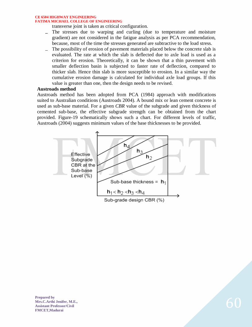
CE 6504 HIGHWAY ENGINEERING
FATIMA MICHAEL COLLEGE OF ENGINEERING
Prepared by
MrsCArthi Jenifer ME
Assistant ProfessorCivil
FMCETMadurai 60
transverse joint is taken as critical configuration
The stresses due to warping and curling (due to temperature and moisture
gradient) are not considered in the fatigue analysis as per PCA recommendation
because most of the time the stresses generated are subtractive to the load stress
The possibility of erosion of pavement materials placed below the concrete slab is
evaluated The rate at which the slab is deflected due to axle load is used as a
criterion for erosion Theoretically it can be shown that a thin pavement with
smaller deflection basin is subjected to faster rate of deflection compared to
thicker slab Hence thin slab is more susceptible to erosion In a similar way the
cumulative erosion damage is calculated for individual axle load groups If this
value is greater than one then the design needs to be revised
Austroads method
Austroads method has been adopted from PCA (1984) approach with modifications
suited to Australian conditions (Austroads 2004) A bound mix or lean cement concrete is
used as sub-base material For a given CBR value of the subgrade and given thickness of
cemented sub-base the effective subgrade strength can be obtained from the chart
provided Figure-19 schematically shows such a chart For different levels of traffic
Austroads (2004) suggests minimum values of the base thicknesses to be provided
CE 6504 HIGHWAY ENGINEERING
FATIMA MICHAEL COLLEGE OF ENGINEERING
Prepared by
MrsCArthi Jenifer ME
Assistant ProfessorCivil
FMCETMadurai 61
figure-19 Schematic diagram of Austroads (2004) chart for estimation of effective
subgrade strength
As per Astroads (2004) the concrete pavement slab thickness for a given expected
traffic repetitions is designed considering the (i) flexural fatigue of the concrete slab and
the (ii) subgrade erosion arising out of repeated deflections For both the considerations
equations are suggested to calculate the allowable traffic repetitions If the allowable
traffic is less than the expected traffic the design is revised by increasing the slab
thickness The concrete shoulders adopted are of integral type or structural type
AASHTO method
The AASHTO method (1993) for design of concrete pavement has evolved from the
AASHO road test (AASHO 1962) The AASHTO pavement design follows an empirical
approach Pavement performance in terms of present serviceability index ( PSI ) loss of
serviceability sub-grade and sub-base strength cumulative traffic properties of concrete
joint load transfer efficiency drainage condition overall standard deviation and
reliability are the input parameters considered in the pavement design
The PSI value of the fresh pavement is assumed as 45 and the pavement is deemed to
have failed when the PSI value reaches 25 The resilient moduli of the subgrade and sub-
base materials are determined in the laboratory simulating the seasonal moisture content
and stress situation Suggested values are also available for given moisture content
plasticity index etc The composite modulus of sub-grade reaction (k) is estimated from
modulus of sub-grade reaction and elastic modulus of sub-base for various seasons and
the depth of rigid foundation and the thickness of the sub-base
Design equation as well nomographs are available to estimate the slab thickness (D) from
these input parameters
NCHRP mechanistic-empirical (M-E) metho
The NCHRP (2004) has recently developed concrete pavement design procedure based
on mechanistic-empirical (M-E) approach This approach attempts to reduce the extent of
empiricism prevalent in the existing AASHTO (1993) guidelines This proposed NCHRP
pavement design system is modular in nature that is the design approach can be
modified by parts (as and when new knowledge is available) without disrupting the
overall design procedure This approach also can take care of various wheel-axle loa
configuration
As per this approach trial thickness of the slab is first assumed and the stress strain and
displacement values are obtained From these values the performance of the pavement in
terms of distresses (such as faulting cracking) and smoothness and predicted If these
predicted performance parameters does not satisfy the required performance for a given
reliability
The design approach includes a large data-base as input parameters for example average
daily traffic traffic growth rate traffic composition hourly weather data on air
temperature precipitation wind speed percentage sunshine relative humidity pavement
material engineering parameters ground water depth infiltration drainage hydraulic
conductivity thermal conductivity heat capacity etc The temperature stress is
considered in this method but the temperature profile is linearized to enhance
computational efficiency (NCHRP 2004)
CE 6504 HIGHWAY ENGINEERING
FATIMA MICHAEL COLLEGE OF ENGINEERING
Prepared by
MrsCArthi Jenifer ME
Assistant ProfessorCivil
FMCETMadurai 62
INDIAN ROADS CONGRESS (IRC) METHOD
The Indian Roads Congress (IRC) guidelines IRC58 (2002) has adopted the
Westergaards equation to estimate load stress and Brdaburys equation to estimate
temperature stress The load stress is highest at the corner of the slab lesser in edge and
least in the interior The order of variation of temperature stress is just the reverse of this
As per IRC58 (2002) it is recommended that the design needs to be done for edge stress
condition and subsequently check needs to be performed for corner stress condition so as
to finalize the design The following are the steps followed as per IRC58 (2002)
guideline for the design of concrete pavement
The input parameters are obtained to formulate the design problem The joint
spacing and the slab dimensions are decided If there is a bound sub-base layer
over the subgrade a suitable value of effective k is to be adopted
A trial thickness of the concrete slab is assumed
The edge stress is estimated for various axle loads from the given charts Figure-
20 schematically shows such a chart The cumulative fatigue damage principle for
fatigue is applied to check the adequacy of the slab thickness
The sum of edge stress due to load for the highest axle load group and the
temperature stress should be less than the MOR of concrete otherwise the design
is revised
The adequacy of corner stress is checked with respect to MOR value and
accordingly the design is finalized Westergaards corner stress formula
Figure-20 Schematic diagram of IRC58 chart for estimation of load stress at the edge
(IRC58 2002)
CE 6504 HIGHWAY ENGINEERING
FATIMA MICHAEL COLLEGE OF ENGINEERING
Prepared by
MrsCArthi Jenifer ME
Assistant ProfessorCivil
FMCETMadurai 63
estimation of corner stress due to load and the corner stress due to temperature is
assumed to be zero
Estimation of layer thicknesses
The thickness of the pavement is adjusted in such a way that the stress strain
developed is less than the allowable values obtained from past performance
information
The two major modes of structural failure of pavement are fatigue and rutting
o Fatigue Traffic applies repetitive load to the pavement surface and the
cracks start from bottom the bound layer slab and propagate upwards
When the extent of surface cracks reaches a predefined level the
pavement is said to have failed due to flexural fatigue
FUNCTIONAL DESIGN
The functional pavement design involves considerations of skid resistance roughness
surface distresses reflectivity of pavement surface etc The functional pavement design
considers mainly the surface features of a pavement
Drainage design
A road needs to be designed in such a way that the rain snow precipitation is drained off
the pavement and its surroundings A suitable surface drainage system for the pavement
is designed for this purpose Some water however will percolate into the pavement from
its top surface and needs to be taken out of the pavement - this is done by providing an
internal drainage system to the pavement Water will also try to enter into the pavement
from bottom due to capillary rise or due to rise in water table A suitably designed sub-
surface drainage system tries to avoid such a problem
PAVEMENT THICKNESS DESIGN CHARTS
For the design of pavements to carry traffic in the range of 1 to 10 msa use chart 1 and for
traffic in the range 10 to 150 msa use chart 2 of IRC37 2001 The design curves relate
pavement thickness to the cumulative number of standard axles to be carried over the
design life for different sub-grade CBR values ranging from 2 to 10 The design
charts will give the total thickness of the pavement for the above inputs The total
thickness consists of granular sub-base granular base and bituminous surfacing The
individual layers are designed based on the the recommendations given below and the
subsequent tables
Pavement composition
Sub-base
Sub-base materials comprise natural sand gravel laterite brick metal crushed
stone or combinations thereof meeting the prescribed grading and physical
requirements The sub-base material should have a minimum CBR of 20 and
30 for traffic upto 2 msa and traffic exceeding 2 msa respectively Sub-base
usually consist of granular or WBM and the thickness should not be less than 150
mm for design traffic less than 10 msa and 200 mm for design traffic
Base
The recommended designs are for unbounded granular bases which comprise
CE 6504 HIGHWAY ENGINEERING
FATIMA MICHAEL COLLEGE OF ENGINEERING
Prepared by
MrsCArthi Jenifer ME
Assistant ProfessorCivil
FMCETMadurai 64
conventional water bound macadam (WBM) or wet mix macadam (WMM) or
equivalent confirming to MOST specifications The materials should be of good
quality with minimum thickness of 225 mm for traffic up to 2 msa an 150 mm for
traffic
Bituminoussurfacing The surfacing consists of a wearing course or a binder
course plus wearing course The most commonly used wearing courses are
surface dressing open graded premix carpet mix seal surfacing semi-
dense bituminous concrete and bituminous concrete For binder course
MOST specifies it is desirable to use bituminous macadam (BM) for traffic
upto o 5 msa and dense bituminous macadam (DBM) for traffic more than 5
msa
Numerical example
Design the pavement for construction of a new bypass with the following data
1 Two lane carriage way
2 Initial traffic in the year of completion of construction = 400 CVPD (sum of both
directions)
3 Traffic growth rate = 75
4 Design life = 15 years
5 Vehicle damage factor based on axle load survey = 25 standard axle per
commercial vehicle
6 Design CBR of subgrade soil = 4
Solution
1 Distribution factor = 075
2
3 Total pavement thickness for CBR 4 and traffic 72 msa from IRC37 2001
chart1 = 660 mm
4 Pavement composition can be obtained by interpolation from Pavement Design
Catalogue (IRC37 2001)
1 Bituminous surfacing = 25 mm SDBC + 70 mm DBM
2 Road-base = 250 mm WBM
3 sub-base = 315 mm granular material of CBR not less than 30
CE 6504 HIGHWAY ENGINEERING
FATIMA MICHAEL COLLEGE OF ENGINEERING
Prepared by
MrsCArthi Jenifer ME
Assistant ProfessorCivil
FMCETMadurai 65
Generally bound base layers are used for concrete pavement construction As per Indian
specification some example of such base layers are Dry Lean Concrete (DLC) Roller
Compacted Concrete (RCC) (IRC15-2002)
The concrete slab is generally of M40 to M50 grade of concrete as
per Indian specifications and is called as paving quality concrete (PQC)
(IRC15-2002)
BITUMINOUS PAVEMENT
The subgrade is a compacted soil layer
The base and sub-base course could be made up of bound or unbound granular layer As
per Indian specifications (MORTampH 2001) some examples of base or sub-base layers
are Granular sub-base(GSB) Water Bound Macadam (WBM) Wet Mix Macadam
(WMM) etc
The binder course is made up bituminous material As per Indian specifications
(MORTampH 2001) some examples of binder course are Bituminous Macadam (BM)
Dense Bituminous Macadam (DBM) etc
The wearing course is the top bituminous layer which is comes in contact to the
vehicle tyre Wearing course provides impermeability to the pavement surface
against water percolation (Chakroborty and Das 2003) The binder course and wearing
course together are called bituminous surfacing
IRC METHOD OF FLEXIBLE PAVEMENT MIX DESIGN
These guidelines will apply to design of flexible pavements for Expressway National Highways
State Highways Major District Roads and other categories of roads Flexible pavements are
considered to include the pavements which have bituminous surfacing and granular base and sub-
base courses conforming to IRC MOST standards These guidelines apply to new pavements
Design criteria
The flexible pavements has been modeled as a three layer structure and stresses and strains at
critical locations have been computed using the linear elastic model To give proper consideration
to the aspects of performance the following three types of pavement distress resulting from
repeated (cyclic) application of traffic loads are considered
1 Vertical compressive strain at the top of the sub-grade which can cause sub-grade
deformation resulting in permanent deformation at the pavement surface
2 Horizontal tensile strain or stress at the bottom of the bituminous layer which can cause
fracture of the bituminous layer
3 Pavement deformation within the bituminous layer
CE 6504 HIGHWAY ENGINEERING
FATIMA MICHAEL COLLEGE OF ENGINEERING
Prepared by
MrsCArthi Jenifer ME
Assistant ProfessorCivil
FMCETMadurai 66
While the permanent deformation within the bituminous layer can be controlled by meeting the
mix design requirements thickness of granular and bituminous layers are selected using the
analytical design approach so that strains at the critical points are within the allowable limits For
calculating tensile strains at the bottom of the bituminous layer the stiffness of dense bituminous
macadam (DBM) layer with 6070 bitumen has been used in the analysis
FAILURE CRITERIA
Critical locations in pavement
A and B are the critical locations for tensile strains Maximum value of the strain is
adopted for design C is the critical location for the vertical subgrade strain since the
maximum value of the occurs mostly at C
CE 6504 HIGHWAY ENGINEERING
FATIMA MICHAEL COLLEGE OF ENGINEERING
Prepared by
MrsCArthi Jenifer ME
Assistant ProfessorCivil
FMCETMadurai 67
Fatigue Criteria
Bituminous surfacings of pavements display flexural fatigue cracking if the tensile strain
at the bottom of the bituminous layer is beyond certain limit The relation between the
fatigue life of the pavement and the tensile strain in the bottom of the bituminous layer
was obtained as
(1)
in which is the allowable number of load repetitions to control fatigue cracking and
is the Elastic modulus of bituminous layer The use of equation 1 would result in
fatigue cracking of 20 of the total area
Rutting Criteria
The allowable number of load repetitions to control permanent deformation can be
expressed as
(2)
is the number of cumulative standard axles to produce rutting of 20 mm
CE 6504 HIGHWAY ENGINEERING
FATIMA MICHAEL COLLEGE OF ENGINEERING
Prepared by
MrsCArthi Jenifer ME
Assistant ProfessorCivil
FMCETMadurai 68
CE 6504 HIGHWAY ENGINEERING
FATIMA MICHAEL COLLEGE OF ENGINEERING
Prepared by
MrsCArthi Jenifer ME
Assistant ProfessorCivil
FMCETMadurai 61
figure-19 Schematic diagram of Austroads (2004) chart for estimation of effective
subgrade strength
As per Astroads (2004) the concrete pavement slab thickness for a given expected
traffic repetitions is designed considering the (i) flexural fatigue of the concrete slab and
the (ii) subgrade erosion arising out of repeated deflections For both the considerations
equations are suggested to calculate the allowable traffic repetitions If the allowable
traffic is less than the expected traffic the design is revised by increasing the slab
thickness The concrete shoulders adopted are of integral type or structural type
AASHTO method
The AASHTO method (1993) for design of concrete pavement has evolved from the
AASHO road test (AASHO 1962) The AASHTO pavement design follows an empirical
approach Pavement performance in terms of present serviceability index ( PSI ) loss of
serviceability sub-grade and sub-base strength cumulative traffic properties of concrete
joint load transfer efficiency drainage condition overall standard deviation and
reliability are the input parameters considered in the pavement design
The PSI value of the fresh pavement is assumed as 45 and the pavement is deemed to
have failed when the PSI value reaches 25 The resilient moduli of the subgrade and sub-
base materials are determined in the laboratory simulating the seasonal moisture content
and stress situation Suggested values are also available for given moisture content
plasticity index etc The composite modulus of sub-grade reaction (k) is estimated from
modulus of sub-grade reaction and elastic modulus of sub-base for various seasons and
the depth of rigid foundation and the thickness of the sub-base
Design equation as well nomographs are available to estimate the slab thickness (D) from
these input parameters
NCHRP mechanistic-empirical (M-E) metho
The NCHRP (2004) has recently developed concrete pavement design procedure based
on mechanistic-empirical (M-E) approach This approach attempts to reduce the extent of
empiricism prevalent in the existing AASHTO (1993) guidelines This proposed NCHRP
pavement design system is modular in nature that is the design approach can be
modified by parts (as and when new knowledge is available) without disrupting the
overall design procedure This approach also can take care of various wheel-axle loa
configuration
As per this approach trial thickness of the slab is first assumed and the stress strain and
displacement values are obtained From these values the performance of the pavement in
terms of distresses (such as faulting cracking) and smoothness and predicted If these
predicted performance parameters does not satisfy the required performance for a given
reliability
The design approach includes a large data-base as input parameters for example average
daily traffic traffic growth rate traffic composition hourly weather data on air
temperature precipitation wind speed percentage sunshine relative humidity pavement
material engineering parameters ground water depth infiltration drainage hydraulic
conductivity thermal conductivity heat capacity etc The temperature stress is
considered in this method but the temperature profile is linearized to enhance
computational efficiency (NCHRP 2004)
CE 6504 HIGHWAY ENGINEERING
FATIMA MICHAEL COLLEGE OF ENGINEERING
Prepared by
MrsCArthi Jenifer ME
Assistant ProfessorCivil
FMCETMadurai 62
INDIAN ROADS CONGRESS (IRC) METHOD
The Indian Roads Congress (IRC) guidelines IRC58 (2002) has adopted the
Westergaards equation to estimate load stress and Brdaburys equation to estimate
temperature stress The load stress is highest at the corner of the slab lesser in edge and
least in the interior The order of variation of temperature stress is just the reverse of this
As per IRC58 (2002) it is recommended that the design needs to be done for edge stress
condition and subsequently check needs to be performed for corner stress condition so as
to finalize the design The following are the steps followed as per IRC58 (2002)
guideline for the design of concrete pavement
The input parameters are obtained to formulate the design problem The joint
spacing and the slab dimensions are decided If there is a bound sub-base layer
over the subgrade a suitable value of effective k is to be adopted
A trial thickness of the concrete slab is assumed
The edge stress is estimated for various axle loads from the given charts Figure-
20 schematically shows such a chart The cumulative fatigue damage principle for
fatigue is applied to check the adequacy of the slab thickness
The sum of edge stress due to load for the highest axle load group and the
temperature stress should be less than the MOR of concrete otherwise the design
is revised
The adequacy of corner stress is checked with respect to MOR value and
accordingly the design is finalized Westergaards corner stress formula
Figure-20 Schematic diagram of IRC58 chart for estimation of load stress at the edge
(IRC58 2002)
CE 6504 HIGHWAY ENGINEERING
FATIMA MICHAEL COLLEGE OF ENGINEERING
Prepared by
MrsCArthi Jenifer ME
Assistant ProfessorCivil
FMCETMadurai 63
estimation of corner stress due to load and the corner stress due to temperature is
assumed to be zero
Estimation of layer thicknesses
The thickness of the pavement is adjusted in such a way that the stress strain
developed is less than the allowable values obtained from past performance
information
The two major modes of structural failure of pavement are fatigue and rutting
o Fatigue Traffic applies repetitive load to the pavement surface and the
cracks start from bottom the bound layer slab and propagate upwards
When the extent of surface cracks reaches a predefined level the
pavement is said to have failed due to flexural fatigue
FUNCTIONAL DESIGN
The functional pavement design involves considerations of skid resistance roughness
surface distresses reflectivity of pavement surface etc The functional pavement design
considers mainly the surface features of a pavement
Drainage design
A road needs to be designed in such a way that the rain snow precipitation is drained off
the pavement and its surroundings A suitable surface drainage system for the pavement
is designed for this purpose Some water however will percolate into the pavement from
its top surface and needs to be taken out of the pavement - this is done by providing an
internal drainage system to the pavement Water will also try to enter into the pavement
from bottom due to capillary rise or due to rise in water table A suitably designed sub-
surface drainage system tries to avoid such a problem
PAVEMENT THICKNESS DESIGN CHARTS
For the design of pavements to carry traffic in the range of 1 to 10 msa use chart 1 and for
traffic in the range 10 to 150 msa use chart 2 of IRC37 2001 The design curves relate
pavement thickness to the cumulative number of standard axles to be carried over the
design life for different sub-grade CBR values ranging from 2 to 10 The design
charts will give the total thickness of the pavement for the above inputs The total
thickness consists of granular sub-base granular base and bituminous surfacing The
individual layers are designed based on the the recommendations given below and the
subsequent tables
Pavement composition
Sub-base
Sub-base materials comprise natural sand gravel laterite brick metal crushed
stone or combinations thereof meeting the prescribed grading and physical
requirements The sub-base material should have a minimum CBR of 20 and
30 for traffic upto 2 msa and traffic exceeding 2 msa respectively Sub-base
usually consist of granular or WBM and the thickness should not be less than 150
mm for design traffic less than 10 msa and 200 mm for design traffic
Base
The recommended designs are for unbounded granular bases which comprise
CE 6504 HIGHWAY ENGINEERING
FATIMA MICHAEL COLLEGE OF ENGINEERING
Prepared by
MrsCArthi Jenifer ME
Assistant ProfessorCivil
FMCETMadurai 64
conventional water bound macadam (WBM) or wet mix macadam (WMM) or
equivalent confirming to MOST specifications The materials should be of good
quality with minimum thickness of 225 mm for traffic up to 2 msa an 150 mm for
traffic
Bituminoussurfacing The surfacing consists of a wearing course or a binder
course plus wearing course The most commonly used wearing courses are
surface dressing open graded premix carpet mix seal surfacing semi-
dense bituminous concrete and bituminous concrete For binder course
MOST specifies it is desirable to use bituminous macadam (BM) for traffic
upto o 5 msa and dense bituminous macadam (DBM) for traffic more than 5
msa
Numerical example
Design the pavement for construction of a new bypass with the following data
1 Two lane carriage way
2 Initial traffic in the year of completion of construction = 400 CVPD (sum of both
directions)
3 Traffic growth rate = 75
4 Design life = 15 years
5 Vehicle damage factor based on axle load survey = 25 standard axle per
commercial vehicle
6 Design CBR of subgrade soil = 4
Solution
1 Distribution factor = 075
2
3 Total pavement thickness for CBR 4 and traffic 72 msa from IRC37 2001
chart1 = 660 mm
4 Pavement composition can be obtained by interpolation from Pavement Design
Catalogue (IRC37 2001)
1 Bituminous surfacing = 25 mm SDBC + 70 mm DBM
2 Road-base = 250 mm WBM
3 sub-base = 315 mm granular material of CBR not less than 30
CE 6504 HIGHWAY ENGINEERING
FATIMA MICHAEL COLLEGE OF ENGINEERING
Prepared by
MrsCArthi Jenifer ME
Assistant ProfessorCivil
FMCETMadurai 65
Generally bound base layers are used for concrete pavement construction As per Indian
specification some example of such base layers are Dry Lean Concrete (DLC) Roller
Compacted Concrete (RCC) (IRC15-2002)
The concrete slab is generally of M40 to M50 grade of concrete as
per Indian specifications and is called as paving quality concrete (PQC)
(IRC15-2002)
BITUMINOUS PAVEMENT
The subgrade is a compacted soil layer
The base and sub-base course could be made up of bound or unbound granular layer As
per Indian specifications (MORTampH 2001) some examples of base or sub-base layers
are Granular sub-base(GSB) Water Bound Macadam (WBM) Wet Mix Macadam
(WMM) etc
The binder course is made up bituminous material As per Indian specifications
(MORTampH 2001) some examples of binder course are Bituminous Macadam (BM)
Dense Bituminous Macadam (DBM) etc
The wearing course is the top bituminous layer which is comes in contact to the
vehicle tyre Wearing course provides impermeability to the pavement surface
against water percolation (Chakroborty and Das 2003) The binder course and wearing
course together are called bituminous surfacing
IRC METHOD OF FLEXIBLE PAVEMENT MIX DESIGN
These guidelines will apply to design of flexible pavements for Expressway National Highways
State Highways Major District Roads and other categories of roads Flexible pavements are
considered to include the pavements which have bituminous surfacing and granular base and sub-
base courses conforming to IRC MOST standards These guidelines apply to new pavements
Design criteria
The flexible pavements has been modeled as a three layer structure and stresses and strains at
critical locations have been computed using the linear elastic model To give proper consideration
to the aspects of performance the following three types of pavement distress resulting from
repeated (cyclic) application of traffic loads are considered
1 Vertical compressive strain at the top of the sub-grade which can cause sub-grade
deformation resulting in permanent deformation at the pavement surface
2 Horizontal tensile strain or stress at the bottom of the bituminous layer which can cause
fracture of the bituminous layer
3 Pavement deformation within the bituminous layer
CE 6504 HIGHWAY ENGINEERING
FATIMA MICHAEL COLLEGE OF ENGINEERING
Prepared by
MrsCArthi Jenifer ME
Assistant ProfessorCivil
FMCETMadurai 66
While the permanent deformation within the bituminous layer can be controlled by meeting the
mix design requirements thickness of granular and bituminous layers are selected using the
analytical design approach so that strains at the critical points are within the allowable limits For
calculating tensile strains at the bottom of the bituminous layer the stiffness of dense bituminous
macadam (DBM) layer with 6070 bitumen has been used in the analysis
FAILURE CRITERIA
Critical locations in pavement
A and B are the critical locations for tensile strains Maximum value of the strain is
adopted for design C is the critical location for the vertical subgrade strain since the
maximum value of the occurs mostly at C
CE 6504 HIGHWAY ENGINEERING
FATIMA MICHAEL COLLEGE OF ENGINEERING
Prepared by
MrsCArthi Jenifer ME
Assistant ProfessorCivil
FMCETMadurai 67
Fatigue Criteria
Bituminous surfacings of pavements display flexural fatigue cracking if the tensile strain
at the bottom of the bituminous layer is beyond certain limit The relation between the
fatigue life of the pavement and the tensile strain in the bottom of the bituminous layer
was obtained as
(1)
in which is the allowable number of load repetitions to control fatigue cracking and
is the Elastic modulus of bituminous layer The use of equation 1 would result in
fatigue cracking of 20 of the total area
Rutting Criteria
The allowable number of load repetitions to control permanent deformation can be
expressed as
(2)
is the number of cumulative standard axles to produce rutting of 20 mm
CE 6504 HIGHWAY ENGINEERING
FATIMA MICHAEL COLLEGE OF ENGINEERING
Prepared by
MrsCArthi Jenifer ME
Assistant ProfessorCivil
FMCETMadurai 68
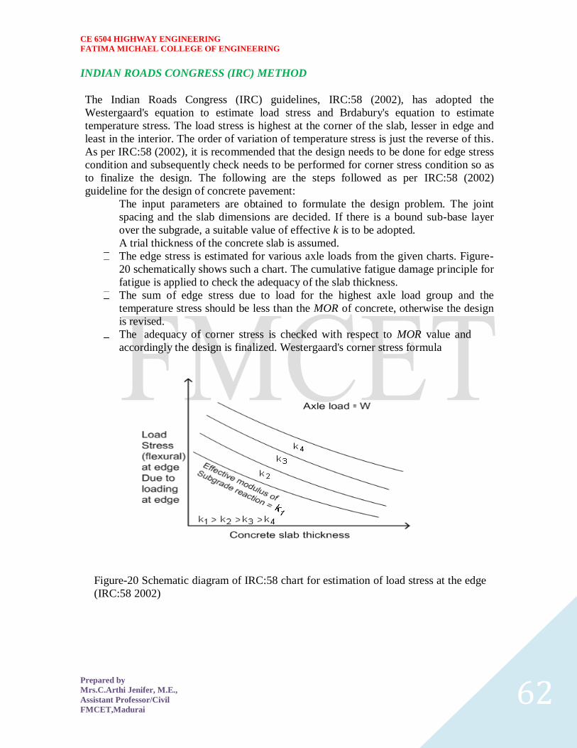
CE 6504 HIGHWAY ENGINEERING
FATIMA MICHAEL COLLEGE OF ENGINEERING
Prepared by
MrsCArthi Jenifer ME
Assistant ProfessorCivil
FMCETMadurai 62
INDIAN ROADS CONGRESS (IRC) METHOD
The Indian Roads Congress (IRC) guidelines IRC58 (2002) has adopted the
Westergaards equation to estimate load stress and Brdaburys equation to estimate
temperature stress The load stress is highest at the corner of the slab lesser in edge and
least in the interior The order of variation of temperature stress is just the reverse of this
As per IRC58 (2002) it is recommended that the design needs to be done for edge stress
condition and subsequently check needs to be performed for corner stress condition so as
to finalize the design The following are the steps followed as per IRC58 (2002)
guideline for the design of concrete pavement
The input parameters are obtained to formulate the design problem The joint
spacing and the slab dimensions are decided If there is a bound sub-base layer
over the subgrade a suitable value of effective k is to be adopted
A trial thickness of the concrete slab is assumed
The edge stress is estimated for various axle loads from the given charts Figure-
20 schematically shows such a chart The cumulative fatigue damage principle for
fatigue is applied to check the adequacy of the slab thickness
The sum of edge stress due to load for the highest axle load group and the
temperature stress should be less than the MOR of concrete otherwise the design
is revised
The adequacy of corner stress is checked with respect to MOR value and
accordingly the design is finalized Westergaards corner stress formula
Figure-20 Schematic diagram of IRC58 chart for estimation of load stress at the edge
(IRC58 2002)
CE 6504 HIGHWAY ENGINEERING
FATIMA MICHAEL COLLEGE OF ENGINEERING
Prepared by
MrsCArthi Jenifer ME
Assistant ProfessorCivil
FMCETMadurai 63
estimation of corner stress due to load and the corner stress due to temperature is
assumed to be zero
Estimation of layer thicknesses
The thickness of the pavement is adjusted in such a way that the stress strain
developed is less than the allowable values obtained from past performance
information
The two major modes of structural failure of pavement are fatigue and rutting
o Fatigue Traffic applies repetitive load to the pavement surface and the
cracks start from bottom the bound layer slab and propagate upwards
When the extent of surface cracks reaches a predefined level the
pavement is said to have failed due to flexural fatigue
FUNCTIONAL DESIGN
The functional pavement design involves considerations of skid resistance roughness
surface distresses reflectivity of pavement surface etc The functional pavement design
considers mainly the surface features of a pavement
Drainage design
A road needs to be designed in such a way that the rain snow precipitation is drained off
the pavement and its surroundings A suitable surface drainage system for the pavement
is designed for this purpose Some water however will percolate into the pavement from
its top surface and needs to be taken out of the pavement - this is done by providing an
internal drainage system to the pavement Water will also try to enter into the pavement
from bottom due to capillary rise or due to rise in water table A suitably designed sub-
surface drainage system tries to avoid such a problem
PAVEMENT THICKNESS DESIGN CHARTS
For the design of pavements to carry traffic in the range of 1 to 10 msa use chart 1 and for
traffic in the range 10 to 150 msa use chart 2 of IRC37 2001 The design curves relate
pavement thickness to the cumulative number of standard axles to be carried over the
design life for different sub-grade CBR values ranging from 2 to 10 The design
charts will give the total thickness of the pavement for the above inputs The total
thickness consists of granular sub-base granular base and bituminous surfacing The
individual layers are designed based on the the recommendations given below and the
subsequent tables
Pavement composition
Sub-base
Sub-base materials comprise natural sand gravel laterite brick metal crushed
stone or combinations thereof meeting the prescribed grading and physical
requirements The sub-base material should have a minimum CBR of 20 and
30 for traffic upto 2 msa and traffic exceeding 2 msa respectively Sub-base
usually consist of granular or WBM and the thickness should not be less than 150
mm for design traffic less than 10 msa and 200 mm for design traffic
Base
The recommended designs are for unbounded granular bases which comprise
CE 6504 HIGHWAY ENGINEERING
FATIMA MICHAEL COLLEGE OF ENGINEERING
Prepared by
MrsCArthi Jenifer ME
Assistant ProfessorCivil
FMCETMadurai 64
conventional water bound macadam (WBM) or wet mix macadam (WMM) or
equivalent confirming to MOST specifications The materials should be of good
quality with minimum thickness of 225 mm for traffic up to 2 msa an 150 mm for
traffic
Bituminoussurfacing The surfacing consists of a wearing course or a binder
course plus wearing course The most commonly used wearing courses are
surface dressing open graded premix carpet mix seal surfacing semi-
dense bituminous concrete and bituminous concrete For binder course
MOST specifies it is desirable to use bituminous macadam (BM) for traffic
upto o 5 msa and dense bituminous macadam (DBM) for traffic more than 5
msa
Numerical example
Design the pavement for construction of a new bypass with the following data
1 Two lane carriage way
2 Initial traffic in the year of completion of construction = 400 CVPD (sum of both
directions)
3 Traffic growth rate = 75
4 Design life = 15 years
5 Vehicle damage factor based on axle load survey = 25 standard axle per
commercial vehicle
6 Design CBR of subgrade soil = 4
Solution
1 Distribution factor = 075
2
3 Total pavement thickness for CBR 4 and traffic 72 msa from IRC37 2001
chart1 = 660 mm
4 Pavement composition can be obtained by interpolation from Pavement Design
Catalogue (IRC37 2001)
1 Bituminous surfacing = 25 mm SDBC + 70 mm DBM
2 Road-base = 250 mm WBM
3 sub-base = 315 mm granular material of CBR not less than 30
CE 6504 HIGHWAY ENGINEERING
FATIMA MICHAEL COLLEGE OF ENGINEERING
Prepared by
MrsCArthi Jenifer ME
Assistant ProfessorCivil
FMCETMadurai 65
Generally bound base layers are used for concrete pavement construction As per Indian
specification some example of such base layers are Dry Lean Concrete (DLC) Roller
Compacted Concrete (RCC) (IRC15-2002)
The concrete slab is generally of M40 to M50 grade of concrete as
per Indian specifications and is called as paving quality concrete (PQC)
(IRC15-2002)
BITUMINOUS PAVEMENT
The subgrade is a compacted soil layer
The base and sub-base course could be made up of bound or unbound granular layer As
per Indian specifications (MORTampH 2001) some examples of base or sub-base layers
are Granular sub-base(GSB) Water Bound Macadam (WBM) Wet Mix Macadam
(WMM) etc
The binder course is made up bituminous material As per Indian specifications
(MORTampH 2001) some examples of binder course are Bituminous Macadam (BM)
Dense Bituminous Macadam (DBM) etc
The wearing course is the top bituminous layer which is comes in contact to the
vehicle tyre Wearing course provides impermeability to the pavement surface
against water percolation (Chakroborty and Das 2003) The binder course and wearing
course together are called bituminous surfacing
IRC METHOD OF FLEXIBLE PAVEMENT MIX DESIGN
These guidelines will apply to design of flexible pavements for Expressway National Highways
State Highways Major District Roads and other categories of roads Flexible pavements are
considered to include the pavements which have bituminous surfacing and granular base and sub-
base courses conforming to IRC MOST standards These guidelines apply to new pavements
Design criteria
The flexible pavements has been modeled as a three layer structure and stresses and strains at
critical locations have been computed using the linear elastic model To give proper consideration
to the aspects of performance the following three types of pavement distress resulting from
repeated (cyclic) application of traffic loads are considered
1 Vertical compressive strain at the top of the sub-grade which can cause sub-grade
deformation resulting in permanent deformation at the pavement surface
2 Horizontal tensile strain or stress at the bottom of the bituminous layer which can cause
fracture of the bituminous layer
3 Pavement deformation within the bituminous layer
CE 6504 HIGHWAY ENGINEERING
FATIMA MICHAEL COLLEGE OF ENGINEERING
Prepared by
MrsCArthi Jenifer ME
Assistant ProfessorCivil
FMCETMadurai 66
While the permanent deformation within the bituminous layer can be controlled by meeting the
mix design requirements thickness of granular and bituminous layers are selected using the
analytical design approach so that strains at the critical points are within the allowable limits For
calculating tensile strains at the bottom of the bituminous layer the stiffness of dense bituminous
macadam (DBM) layer with 6070 bitumen has been used in the analysis
FAILURE CRITERIA
Critical locations in pavement
A and B are the critical locations for tensile strains Maximum value of the strain is
adopted for design C is the critical location for the vertical subgrade strain since the
maximum value of the occurs mostly at C
CE 6504 HIGHWAY ENGINEERING
FATIMA MICHAEL COLLEGE OF ENGINEERING
Prepared by
MrsCArthi Jenifer ME
Assistant ProfessorCivil
FMCETMadurai 67
Fatigue Criteria
Bituminous surfacings of pavements display flexural fatigue cracking if the tensile strain
at the bottom of the bituminous layer is beyond certain limit The relation between the
fatigue life of the pavement and the tensile strain in the bottom of the bituminous layer
was obtained as
(1)
in which is the allowable number of load repetitions to control fatigue cracking and
is the Elastic modulus of bituminous layer The use of equation 1 would result in
fatigue cracking of 20 of the total area
Rutting Criteria
The allowable number of load repetitions to control permanent deformation can be
expressed as
(2)
is the number of cumulative standard axles to produce rutting of 20 mm
CE 6504 HIGHWAY ENGINEERING
FATIMA MICHAEL COLLEGE OF ENGINEERING
Prepared by
MrsCArthi Jenifer ME
Assistant ProfessorCivil
FMCETMadurai 68
CE 6504 HIGHWAY ENGINEERING
FATIMA MICHAEL COLLEGE OF ENGINEERING
Prepared by
MrsCArthi Jenifer ME
Assistant ProfessorCivil
FMCETMadurai 67
Fatigue Criteria
Bituminous surfacings of pavements display flexural fatigue cracking if the tensile strain
at the bottom of the bituminous layer is beyond certain limit The relation between the
fatigue life of the pavement and the tensile strain in the bottom of the bituminous layer
was obtained as
(1)
in which is the allowable number of load repetitions to control fatigue cracking and
is the Elastic modulus of bituminous layer The use of equation 1 would result in
fatigue cracking of 20 of the total area
Rutting Criteria
The allowable number of load repetitions to control permanent deformation can be
expressed as
(2)
is the number of cumulative standard axles to produce rutting of 20 mm
CE 6504 HIGHWAY ENGINEERING
FATIMA MICHAEL COLLEGE OF ENGINEERING
Prepared by
MrsCArthi Jenifer ME
Assistant ProfessorCivil
FMCETMadurai 68

CE 6504 HIGHWAY ENGINEERING
FATIMA MICHAEL COLLEGE OF ENGINEERING
Prepared by
MrsCArthi Jenifer ME
Assistant ProfessorCivil
FMCETMadurai 68