Embed Size (px)
Citation preview
1
Fatigue strength Comparative study of knuckle joints in LNG carrier by different approaches of
classification society’s rules
Sacheendra Naik
Master Thesis
presented in partial fulfillment of the requirements for the double degree:
“Advanced Master in Naval Architecture” conferred by University of Liege "Master of Sciences in Applied Mechanics, specialization in Hydrodynamics,
Energetics and Propulsion” conferred by Ecole Centrale de Nantes
developed at West Pomeranian University of Technology, Szczecin in the framework of the
“EMSHIP” Erasmus Mundus Master Course
in “Integrated Advanced Ship Design”
Ref. 159652-1-2009-1-BE-ERA MUNDUS-EMMC
Supervisor:
Prof. Maciej Taczala, West Pomeranian University of Technology, Szczecin
Reviewer: Prof. Dario Boote, University of Genova
Szczecin, February 2017
P 2 Sacheendra Naik
Master Thesis developed at West Pomeranian University of Technology, Szczecin
CONTENTS
DECLARATION OF AUTHORSHIP ....................................................................................... 6
ABBREVIATIONS .................................................................................................................... 7
ABSTRACT ............................................................................................................................... 8
1. INTRODUCTION .................................................................................................................. 9
1.1. Overview ......................................................................................................................... 9
1.2. Objective ....................................................................................................................... 11
1.3. Methodology ................................................................................................................. 12
1.4. Thesis Organisation ....................................................................................................... 15
2. GAS CARRIERS: BRIEF DESCRIPTION ......................................................................... 16
2.1. Types of gas carrier ships ............................................................................................. 16
2.1.1. Cargo tank types..................................................................................................... 17
2.1.2. Independent tank .................................................................................................... 17
2.1.3. Membrane tank ....................................................................................................... 19
3. THEORETICAL BACKGROUND ..................................................................................... 20
3.1. General .......................................................................................................................... 20
3.2. Fatigue damage models ................................................................................................. 20
3.3. Different methods of fatigue load calculations ............................................................. 22
3.3.1. Simplified method ................................................................................................... 22
3.3.2. Equivalent design wave method ............................................................................. 23
3.3.3. Spectral Method ..................................................................................................... 23
3.3.4. Short-term response ............................................................................................... 25
3.3.5. Long-term response ................................................................................................ 26
3.4. Fatigue strength calculation based on S-N curve .......................................................... 27
3.5. Uncertainties in fatigue strength prediction .................................................................. 31
4. ANALYSIS METHODOLOGY AND SOFTWARE TOOLS USED ................................ 32
4.1. Analysis Methodology .................................................................................................. 32
4.2. Software Tools Used ..................................................................................................... 33
4.2.1. Sesam Genie ........................................................................................................... 33
4.2.2. Sestra ...................................................................................................................... 33
4.2.3. HydroD-Wasim....................................................................................................... 34
4.2.4. Xtract ...................................................................................................................... 34
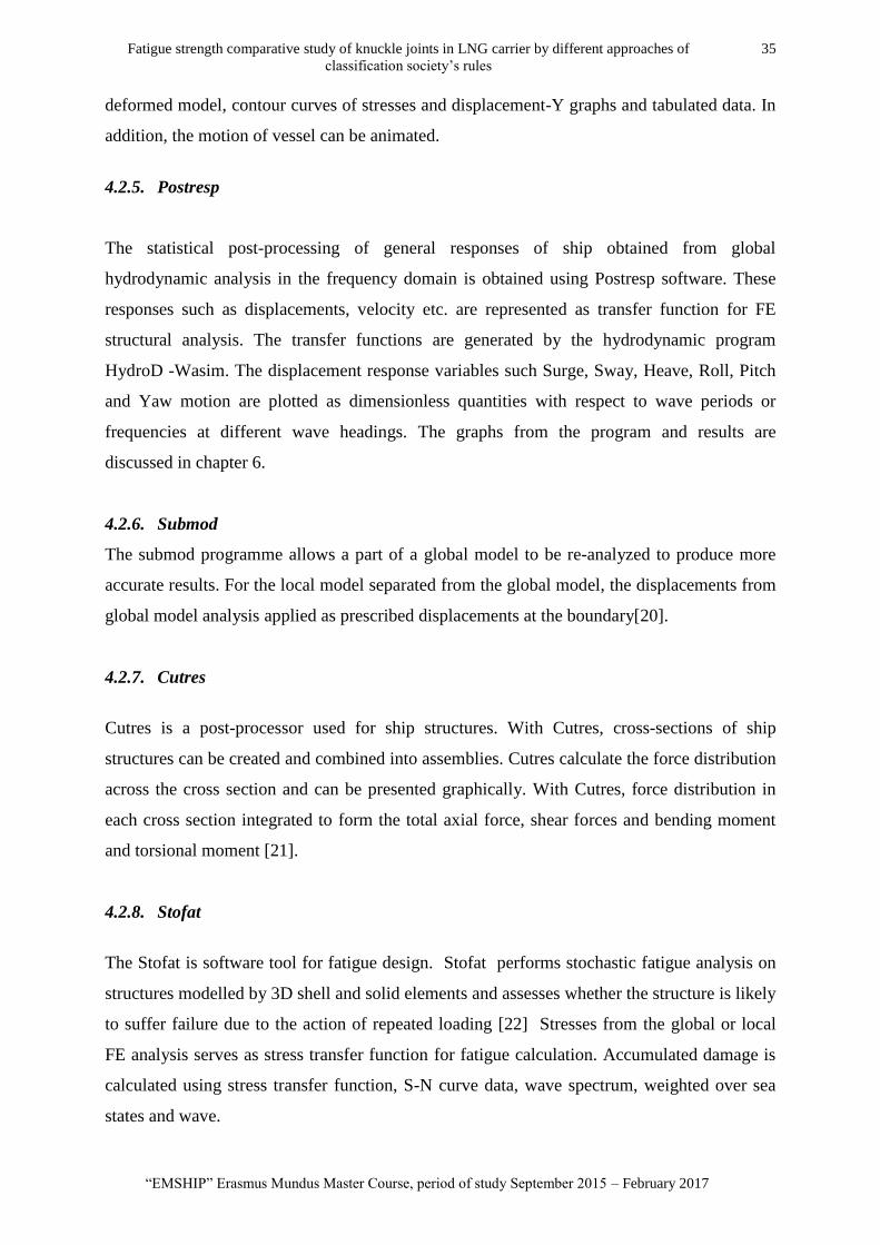
4.2.5. Postresp .................................................................................................................. 35
4.2.6. Cutres ..................................................................................................................... 35
Fatigue strength comparative study of knuckle joints in LNG carrier by different approaches of
classification society‘s rules
3
―EMSHIP‖ Erasmus Mundus Master Course, period of study September 2015 – February 2017
4.2.7. Submod ................................................................................................................... 35
4.2.8. Stofat....................................................................................................................... 35
5. STRUCTURAL MODELLING ........................................................................................... 36
5.1. Co-ordinate and unit system ......................................................................................... 37
5.2. Geometrical Modelling ................................................................................................. 38
5.2.1. Double Bottom........................................................................................................ 38
5.2.2. Double Side shell .................................................................................................... 40
5.2.3. Transverse Bulkhead .............................................................................................. 40
5.2.4. Foundation Deck and Cargo tank support ............................................................. 41
5.2.5. Upper Deck ............................................................................................................ 43
5.3. Boundary conditions ..................................................................................................... 43
5.4. Structural Mesh Model .................................................................................................. 45
5.4.1. Global Model.......................................................................................................... 45
5.4.2. Sub Model ............................................................................................................... 46
6. GLOBAL RESPONSE ANALYSIS .................................................................................... 48
6.1. Analysis Setup .............................................................................................................. 48
6.1.1. Load cases .............................................................................................................. 49
6.2. Global Motion Responses ............................................................................................. 51
7. GLOBAL STRUCTURAL ANALYSIS .............................................................................. 54
7.1. Verification of load transfer .......................................................................................... 54
7.2. Stress Transfer function ................................................................................................ 56
8. FATIGUE ANALYSIS ........................................................................................................ 58
9. CONCLUSIONS AND RECOMMENDATIONS............................................................... 66
ACKNOWLEDGEMENTS ..................................................................................................... 69
REFERENCES ......................................................................................................................... 70
APPENDICES .......................................................................................................................... 72
Appendix A: Summary of Element Fatigue damage Calculation ........................................ 72
Appendix B: Summary of Hot Spot Fatigue damage Calculation ....................................... 73
Appendix C : Fatigue Calculation Result ............................................................................ 74
P 4 Sacheendra Naik
Master Thesis developed at West Pomeranian University of Technology, Szczecin
LIST OF FIGURES
Figure 1. LNG carrier structural model analysed. .................................................................... 11
Figure 2. Flow chart spectral method approach. ...................................................................... 13
Figure 3.Self-supporting prismatic Type 'A' tank [23]. ............................................................ 17
Figure 4.Self-supporting prismatic Type 'B' tank [23]. ............................................................ 18
Figure 5.Self-supporting prismatic Type 'C' tank [23]. ............................................................ 18
Figure 6.Membrane tank [23]. ................................................................................................. 19
Figure 7. Stress definition. ....................................................................................................... 21
Figure 8. S-N curve in air –DNV GL[11]. ............................................................................... 29
Figure 9. Stress read out points and hot spot stress for 8-node shell elements [11]. ............... 30
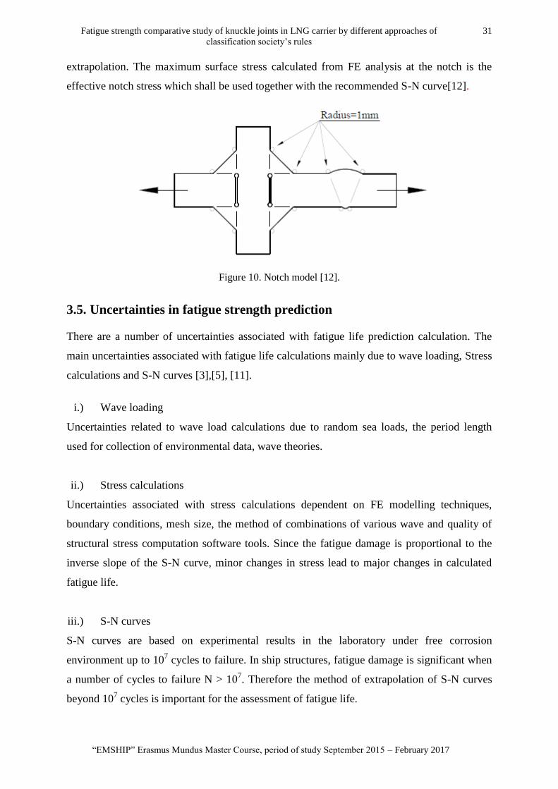
Figure 10. Notch model [12]. ................................................................................................... 31
Figure 11. LNG carrier FE model. ........................................................................................... 36
Figure 12. Co-ordinate system. ................................................................................................ 37
Figure 13. Midship section of LNG carrier. ............................................................................. 39
Figure 14. Double bottom view. ............................................................................................... 39
Figure 15. Double sided hull- 3-dimensional view. ................................................................. 40
Figure 16. Seawater ballast tank and bulkhead. ....................................................................... 41
Figure 17. Transverse bulkhead and foundation support side girder. ...................................... 41
Figure 18. Foundation deck – sectional view just above the foundation. ................................ 42
Figure 19. Sectional view showing skirt orientation. ............................................................... 42
Figure 20. Isometric views showing stiffened deck. ................................................................ 43
Figure 21. Boundary condition [7] ........................................................................................... 44
Figure 22. Midship FE mesh -Longitudinal section at the centre line. ................................... 45
Figure 23. Fore and Aft Ship FE mesh. .................................................................................... 45
Figure 24. Locations of knuckle joints. .................................................................................... 46
Figure 25. Sub model from the global FE model. ................................................................... 47
Figure 26. Hydrodynamic model. ............................................................................................ 48
Figure 27. Wave heading direction for different load cases .................................................... 49
Figure 28. Tank arrangement for full load case- Longitudinal view ....................................... 49
Figure 29. Tank arrangement for full load case- Plan view ..................................................... 50
Figure 30. Tank arrangement for full ballast load case- Longitudinal view ............................ 50
Figure 31. Tank arrangement for ballast load case- Plan view ................................................ 50
Figure 32. Wave heading direction for different load cases .................................................... 51
Figure 33. Global motions response –Full load case ............................................................... 52
Fatigue strength comparative study of knuckle joints in LNG carrier by different approaches of
classification society‘s rules
5
―EMSHIP‖ Erasmus Mundus Master Course, period of study September 2015 – February 2017
Figure 34. Global motions response – Ballast load case .......................................................... 53
Figure 35. Wave load pressure on global model transferred from the hydrodynamic analysis.
.................................................................................................................................................. 54
Figure 36. Vertical Bending Moment – 1m wave amplitude for a 900 heading wave with
period 24s. ................................................................................................................................ 55
Figure 37. Vertical Shear Force – 1m wave amplitude for a 900 heading wave with period
24s. ........................................................................................................................................... 55
Figure 38. Maximum Principal stress-Ballast Load case ......................................................... 56
Figure 39. Principal Stress Transfer Function.-Ballast Load case ........................................... 57
Figure 40.Wave spreading function for cosine power 2. ......................................................... 59
Figure 41. DNV-CN-30.7 2010 S-N curves [15]. .................................................................... 60
Figure 42. ABS S-N curves [8]. ............................................................................................... 60
Figure 43. Fatigue damage at different position of knuckle joints around tank2. .................... 63
Figure 44. Hotspot of Hopper knuckle joint. ........................................................................... 64
Figure 45. Polar Plot of Total Fatigue Damage. ..................................................................... 64
LIST OF TABLES
Table 1. Main characteristics of LNG carrier .......................................................................... 36
Table 2. Material Properties ..................................................................................................... 38
Table 3. Wave periods. ............................................................................................................. 49
Table 4. Mass Model – Full load case. ..................................................................................... 50
Table 5. Mass Model – Ballast load case. ................................................................................ 50
Table 6. S-N Curve Parameters. .............................................................................................. 58
Table 7. Wave Scatter Data - North Atlantic. .......................................................................... 59
Table 8. Structural detail classification ................................................................................... 61
Table 9. Total Fatigue Damage at knuckle joints for various S-N Curve. .............................. 62
Table 10. Fatigue Damage for various S-N Curve. .................................................................. 64
Table 11. Fatigue Damage at knuckle joints for various S-N Curve –Ballast Load case. ..... 72
Table 12. Fatigue Damage at knuckle joints for various S-N Curve –Ballast Load case. ..... 72
Table 13. Fatigue Damage for various S-N Curve –Ballast Load case. .................................. 73
Table 14. Fatigue Damage for various S-N Curve –Full Load case. ...................................... 73

P 6 Sacheendra Naik
Master Thesis developed at West Pomeranian University of Technology, Szczecin
DECLARATION OF AUTHORSHIP
I declare that this thesis and the work presented in it are my own and have been generated by
me as the result of my own original research.
Where I have consulted the published work of others, this is always clearly attributed.
Where I have quoted from the work of others, the source is always given. With the exception
of such quotations, this thesis is entirely my own work.
I have acknowledged all main sources of help.
Where the thesis is based on work done by myself jointly with others, I have made clear
exactly what was done by others and what I have contributed myself.
This thesis contains no material that has been submitted previously, in whole or in part, for
the award of any other academic degree or diploma.
I cede copyright of the thesis in favour of the University of West Pomeranian University of
Technology, Poland.
Date: Signature
Fatigue strength comparative study of knuckle joints in LNG carrier by different approaches of
classification society‘s rules
7
―EMSHIP‖ Erasmus Mundus Master Course, period of study September 2015 – February 2017
ABBREVIATIONS
ABS American Bureau of Shipping
HSE Health Safety and Environment
AWS American Welding standard
DNV Det Norske Veritas
FE Finite Element
LNG Liquid Natural Gas
RAO Response Amplitude Operator
SCF Stress Concentration Factor
IGC International Code of the Construction and Equipment of Ships Carrying
Liquefied Gases in Bulk
IIW International Institue of Welding
P 8 Sacheendra Naik
Master Thesis developed at West Pomeranian University of Technology, Szczecin
ABSTRACT
The cumulative damage due to fluctuating loads leads to fatigue fracture which is the main
cause of the fracture of offshore vessels and structures. Knuckle joints are the most critical
area due to its susceptibility to fatigue failure. This is mainly due to a high-stress
concentration at knuckle joints. Also, the area is inaccessible for inspection and repair due to
cargo tank containment arrangement. In this report, the spectral fatigue analysis is presented
for 148k, Moss type spherical tank LNG carrier. The study is focused on the fatigue damage
evaluation of hopper knuckle joint details by full spectral fatigue analysis.
The full spectral fatigue analysis involves the computations of hydrodynamic response, global
structural analysis, local structural analysis and calculation of fatigue damage. The structural
response is assessed by performing linear FE–analysis with a linear material response. In
order to simulate structural response, a linear hydrodynamic analysis using unit wave
amplitude is carried out to simulate the wave-induced loads on the LNG carrier, which is
followed by a linear FE global analysis to assess stress transfer function. The wave loading is
calculated by linear hydrodynamic analysis is based on 3D diffraction theory. The wave
amplitude of 1.0m considering wave headings from 0 to 360 degrees with an increment of
maximum 30 degrees is used to calculate the ship response. For each wave heading 25 wave
frequencies are included to describe the shape of the transfer functions. The inertia loads,
internal and external pressures are calculated in the hydrodynamic analysis and transferred
directly to the global structural model. Direct wave load computations by the numerical
method improve the accuracy of the calculated loads compared to the approach of using the
classification society‘s formulae. Two type of loading cases i.e. full load and normal ballast
condition are considered for the damage calculation. For each heading of sea state, fatigue
damage is calculated by combing the hotspot transfer functions with stress cycle (S-N) curve
data and wave scatter diagram.
Fatigue damage computations involve design variables such as S-N curve data, wave scatter
data, wave spectrum, etc. Current rules of classification societies DNV GL and ABS are used
to evaluate the fatigue damage of knuckle joint. In general, the spectral fatigue calculation is
cumbersome due to time-consuming calculation process. However, the study also provides
information about the procedures involved in the spectral fatigue calculation.
KEYWORDS: Spectral Fatigue, Fatigue damage, design variable
Fatigue strength comparative study of knuckle joints in LNG carrier by different approaches of
classification society‘s rules
9
―EMSHIP‖ Erasmus Mundus Master Course, period of study September 2015 – February 2017
1. INTRODUCTION
1.1. Overview
In recent years the demand for environment-friendly clean energy is increasing due to
growing environmental protection consciousness at the global level. Liquefied natural gas,
LNG is considered as one of the clean energy source and its demand in the global market has
opened up a new chapter in gas field development. Ship owners and gas suppliers are actively
involved in negotiating on the construction and purchases of LNG carriers capable of sailing
all around the word. The changes in the global LNG market lead to the relocation of typical
shipping routes to new sea areas. Some of the new routes cross areas known for very rough
conditions. As compared to a ship operating worldwide, shipping in North Sea, North Atlantic
or at the Alaskan coast is much more challenging in regard to both strength and operational
issues. Global Rise in the demand for natural gas has led to the increase in the size and
capacity of LNG carriers used for marine transportation.
When the vessel operates in waves, the wave loads can force the ship to bend upwards and
downwards. The hogging occurs when the wave crest is at amidships, while the sagging is
caused due to wave trough at amidships. The alternative hogging and sagging due to wave
loads lead to fatigue problems in a ship. When repeated cyclic load exceeds the material
endurance limit, cracks initiate in welded joints or on metal surface weakening the structure.
The crack growth continues with continued cyclic loading during the operation of the vessels,
eventually, a crack will reach a critical size resulting failure of the structure. Fatigue crack
initiation is a localized phenomenon which mainly depends on the structural geometrical
details and stress concentrations. In welded structures, cracks initiate at stress concentrations
which are due to faulty welding procedures, cut-outs and plate joints where abrupt
geometrical transitions cause a rise in local stress intensity.
The fatigue damage is a continuous process during its operation lifetime. The damage
depends on parameters such as sea state, loading condition, forward speed, heading angle etc.
The major cause of damage is sea state which is a variable parameter characterized by the
wave period and significant wave height. For strength reason, high strength steel is used in the
construction of vessels using welding technology. Even though the high strength steel ensures
the structures to withstand higher stress but it increases the stress amplitude of the response
P 10 Sacheendra Naik
Master Thesis developed at West Pomeranian University of Technology, Szczecin
resulting in lower fatigue life, so that fatigue failure likely to occur at a relatively faster rate in
vessels built up of high strength steel compared to low strength steel. The safety of LNG
carriers is equally as important as the economic aspect and vessel operator also concern the
fatigue failure impact on vessel maintenance, repair cost and reputation. Fatigue strength
assessment is considered as one of the important safety issues during design and service
period.
Long-term variation of local stresses due to wave actions if handled properly at the design
stage, then the failure phenomenon, probability of failure and reliability of structure can be
addressed effectively. The fatigue strength evaluations of ship structural details during design
stage or in the repair stage by classification societies rule require detailed consideration with
an aim to ensure adequate structural strength in fatigue. Various classification societies such
as ABS, DNV GL, Lloyd Register, Bureau veritas, Korean register of shipping etc. have
published comprehensive rules and guidelines for the ship structure fatigue strength
assessment. Depending on the type structural details, the fatigue assessment method varies
from simple method to numerically intensive technique such as direct analysis. Over the past
years, several studies have addressed the fatigue assessment of ship structural details either by
rules or by direct calculations. Researchers have published literature on comparative fatigue
strength study of structural details of either container ship or bulk carriers using different
classification societies rule. Studies have shown that the fatigue damage depends on stress
cycle curve, selection of stress approach, Weibull shape parameter. Even though IACAS-
International Association of Classification Societies attempted to develop a common
procedure for fatigue assessment, factors such as stress cycle curves and selection of stress
approach are not harmonized and they are still dependent on classification societies rule.
The proposed thesis will be focused on fatigue strength sensitivity of hopper knuckle joints in
a Moss type LNG carrier using spectral fatigue analysis. The effect of some of the parameters
such as stress cycle curves studied and compared by using ABS and DNVGL classification
rule approaches.
Fatigue strength comparative study of knuckle joints in LNG carrier by different approaches of
classification society‘s rules
11
―EMSHIP‖ Erasmus Mundus Master Course, period of study September 2015 – February 2017
1.2. Objective
The main objective to make a comparative study on the fatigue strength hopper knuckle joints
using classification societies DNV GL and ABS rules for the gas carrier. Design variables
such as S-N curve data, wave scatter data, wave spectrum, etc. are the parameters involved in
fatigue damage computations and these parameters are considered in this study. In order to
accomplish the main objective, the following sub-targets to be completed.
Prepare a 3D-model of the vessel for global FE analysis
Perform the hydrodynamic analysis in the frequency domain with 1m wave amplitude
considering different wave directions (heading angles).Transfer the calculated wave loads
are to global FE model of the vessel.
Identify fatigue-critical locations with respect to principal stress for each wave direction.
Perform linear FE analysis of sub model at the critical location.
Evaluate the fatigue damage
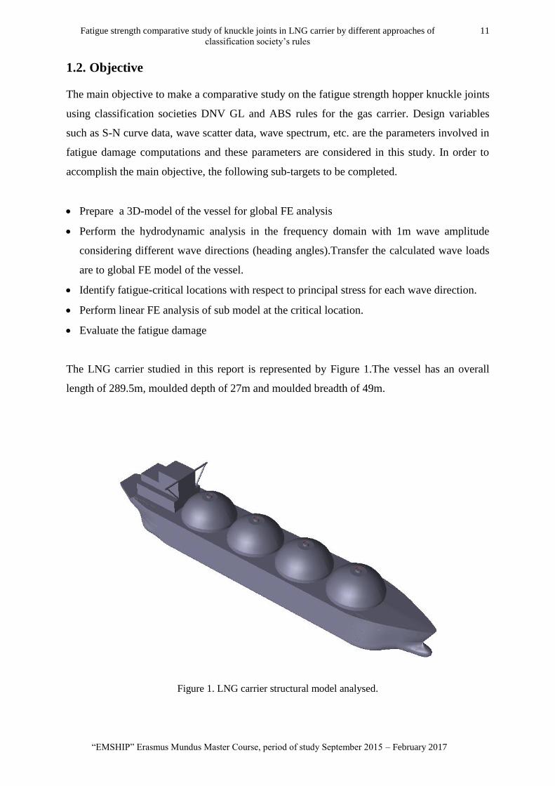
The LNG carrier studied in this report is represented by Figure 1.The vessel has an overall
length of 289.5m, moulded depth of 27m and moulded breadth of 49m.
Figure 1. LNG carrier structural model analysed.
P 12 Sacheendra Naik
Master Thesis developed at West Pomeranian University of Technology, Szczecin
1.3. Methodology
To achieve the objective of fatigue evaluation by direct calculation, it is necessary to simulate
numerically and analyze the structural response first and followed by the fatigue damage
evaluation of hopper knuckle joints of LNG carrier. The fatigue damage is evaluated for both
full load and ballast loading condition. The damages from full and ballast condition added
together to obtain the final damage. The following three types of numerical analyses have
been carried out:
Hydrodynamic response calculations.
Linear global structural analysis.
Local structural analysis.
Fatigue damage calculation.
Fatigue strength of welded ship can be evaluated stress based approach, strain based approach
and fracture mechanics.
In stress based approach, the cyclic stresses including stress concentration factor (SCF) is
assumed to be less than the yield stress of the material. The strain-based approach considers
the localized plastic deformation that occurs in the local regions where the stresses are beyond
material yield strength. The plastic deformation location is the probable location of fatigue
crack initiation. In Fracture mechanics approach, the fatigue strength of welded joints is
expressed in terms of the relationship between the stress intensity factor and the rate of crack
growth.
In this study, stress based approach is employed for the fatigue evaluation. Welds are ignored
in the FE-models, initial imperfection and the residual tensile stresses from the welding
procedure are disregarded.
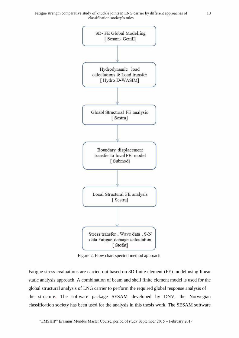
Figure 2 represents the flowchart of the methodology adopted in this thesis. Each of these
parts will be described briefly in the subsequent chapters. Two levels of FE-models are used
in the analysis for the fatigue evaluation; a full- vessel FE model with a relatively coarse mesh
which represents the global model of the LNG carrier and a more detailed local sub-model
with fine mesh.
Fatigue strength comparative study of knuckle joints in LNG carrier by different approaches of
classification society‘s rules
13
―EMSHIP‖ Erasmus Mundus Master Course, period of study September 2015 – February 2017
Figure 2. Flow chart spectral method approach.
Fatigue stress evaluations are carried out based on 3D finite element (FE) model using linear
static analysis approach. A combination of beam and shell finite element model is used for the
global structural analysis of LNG carrier to perform the required global response analysis of
the structure. The software package SESAM developed by DNV, the Norwegian
classification society has been used for the analysis in this thesis work. The SESAM software
P 14 Sacheendra Naik
Master Thesis developed at West Pomeranian University of Technology, Szczecin
package consists of several different modules which can be used depending on the type
numerical simulation that is required to be carried out.
To perform the hydrodynamic response analysis, SESAM HydroD: Wasim has been used
which is also a part SESAM software package. Wasim is a general purpose hydrodynamic
analysis program based on 3D potential theory for calculation of wave loading and wave
induced responses floating marine structures with forward speed.
The hydrodynamic simulations are performed using 1m wave amplitude, in the frequency
domain with 25 frequencies and 12 wave directions (heading angles).The motion response of
the LNG carrier extracted using a post-processing programme named Postresp.
For the structural concept modelling, a software programme SESAM GeniE has been used.
The global structural analysis is carried out using software Sestra which is linear structural
FE-analysis programme.
For the sub model analysis of a part of LNG carrier, Submod software is used to transfer the
boundary displacements on local FE model from the result of the global structural analysis.
The next step is to calculate of stress transfer function at the critical location. Fatigue damage
is evaluated at the desired location using the stress transfer function, wave scatter data, wave
energy spectrum, and S-N curve and calculation is performed in Stofat programme.
Using Xtract software, results are graphically presented. Chapter four describe shortly the
software used in this thesis work.
Fatigue strength comparative study of knuckle joints in LNG carrier by different approaches of
classification society‘s rules
15
―EMSHIP‖ Erasmus Mundus Master Course, period of study September 2015 – February 2017
1.4. Thesis Organisation
This master thesis report consists of nine sections and a reference section. After the
introduction chapter, Chapter 2 presents a brief overview of the gas carrier.
In chapter 3 describe the theoretical background on fatigue calculation. It contains a brief
overview, different fatigue analysis options are discussed from the simplified method to
spectral method. The S-N curves and different parameters involved in the computation of
cumulative damage are also presented.
Analysis methodology and the different software computation tools used in this thesis work
are discussed in chapter 4.
Chapter 5 presents the global structural modelling of the LNG carrier studied in detail. FE
modelling in 3 dimensions is discussed in detail with respect to material properties, meshing
and boundary conditions.
Chapter 6 discusses the hydrodynamic analysis set up, mass model properties and load cases.
Global motion response resulting from unit wave amplitude are presented in terms of RAOs
Chapter 7 has been used to present the calculation and results from the global response
analysis in terms of the principal stress.
Fatigue analysis results are discussed in the eighth chapter with SN-curve and scatter data of
the desired location. Furthermore, a variation of the fatigue damage for different S-N curves
presented.
Chapter 9 discusses conclusion drawn from the current study performed and also presents
recommendations for the future work.
Following chapter 9, all the references that are cited in this thesis work has been listed in the
Reference. An additional chapter on appendix is compiled at the end summing up the output
from fatigue analysis.
P 16 Sacheendra Naik
Master Thesis developed at West Pomeranian University of Technology, Szczecin
2. GAS CARRIERS: BRIEF DESCRIPTION
Liquefied natural gas, LNG is considered as one of the clean energy source and its demand in
the global market has opened up a new chapter in gas field development. Due to growing
environmental protection consciousness, the use of natural gas is increasing at the global
level.
The seaborne transport of liquefied natural gas dating back to 1949 when a liquefied gas
carrier was delivered with DNV class equipped with fully pressurised cargo tanks for
transport of LPG/Ammonia [1]. To meet the growing demand for LNG around the globe, the
construction of gas carrier transport vessel is increasing in recent years.The capacity of
modern larger LNG carriers varies between 125,000 m3 and 267,000m
3.
2.1. Types of gas carrier ships
The gas carrier is a special type of ship with a containment system holding the liquid cargo
under pressure to prevent entrance of air into the cargo. The design, construction of gas carrier
varies according to types cargoes carried and cargo containment system. In general, the gas
carriers are grouped as below
i.) Fully pressurised: These are first generation gas carrier types with small capacities up
to 5000 to 6000 m3.They are fitted with horizontal or spherical tanks to transport
liquefied petroleum gas to and from small gas terminals. The tanks are built without
insulation.
ii.) Semi pressurised: These carriers equipped with a reliquefaction plant and are built with
tanks fabricated in special steels to accommodate the liquefied gas at low temperature.
The tank either in cylindrical, spherical in shape with insulation.
iii.) Fully refrigerated: The gas carriers in this group built with fully refrigerated storage
tanks to transport liquefied gases at low temperature atmospheric. The cargo tanks are
prismatic in shape fabricated from 3.5% nickel steel which allows the carriage of
cargoes at temperatures as low as –48°C.The prismatic shape of tanks enables
maximised the cargo holding capacity which enables fully refrigerated carrier suitable
for carrying a large volume of cargo over a long distance.
Fatigue strength comparative study of knuckle joints in LNG carrier by different approaches of
classification society‘s rules
17
―EMSHIP‖ Erasmus Mundus Master Course, period of study September 2015 – February 2017
iv.) LNG carriers: LNG ships are a special type of vessels built to transport natural gas in
liquefied form at -161°C. These vessels fitted with independent tanks or membrane
tanks for holding liquid cargo.
2.1.1. Cargo tank types
The total arrangement of cargo containment system includes
Cargo tanks which acts as primary barrier
Secondary barrier
Thermal insulation
Foundation structure to support the tanks
Type of cargo tanks divided into two categories as Independent tank and Membrane.
2.1.2. Independent tank
Independent tanks are self- supported and do not form ship‘s hull strength [6]. According to
IGC code, independent tanks further classified as Types 'A', 'B' and 'C'.
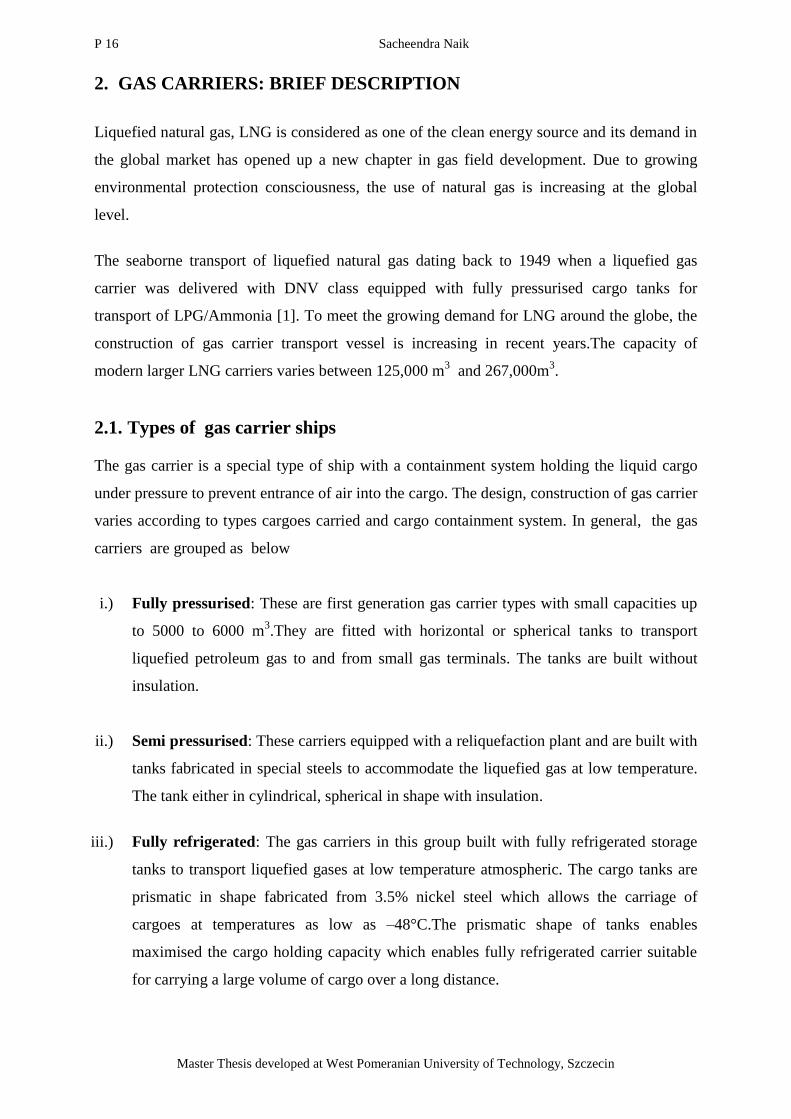
Types 'A' tank
Type 'A' tanks are constructed with flat surfaces. The maximum allowable tank design
pressure for this type of system is 0.7 barg. Cargoes require fully refrigerated condition at or
near atmospheric pressure [2].
Figure 3.Self-supporting prismatic Type 'A' tank [23].
P 18 Sacheendra Naik
Master Thesis developed at West Pomeranian University of Technology, Szczecin
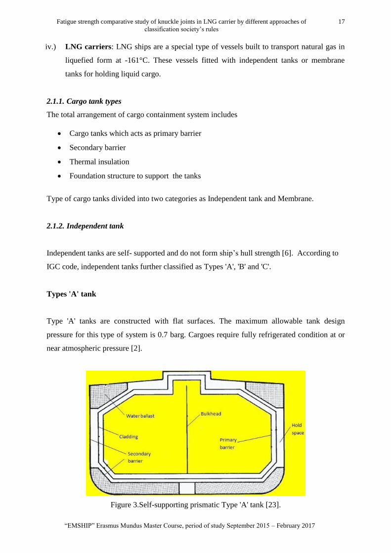
Types 'B' tank
These tanks can have either flat surfaces or of spherical type. The spherical tank is the most
common type of B tank which is Kvaerner moss design [2].This tank requires secondary
barrier in the form of a drip tray. Type 'B' spherical tank is widely used in the vessel for
transport of LNG.
Figure 4.Self-supporting prismatic Type 'B' tank [23].
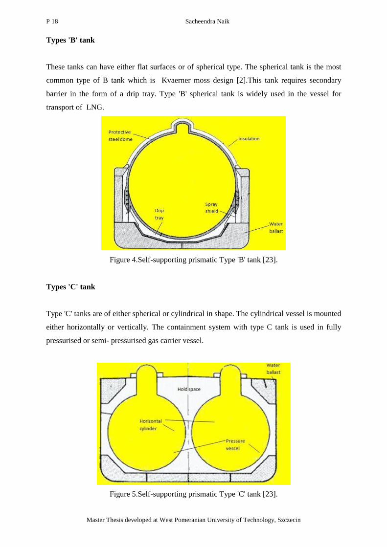
Types 'C' tank
Type 'C' tanks are of either spherical or cylindrical in shape. The cylindrical vessel is mounted
either horizontally or vertically. The containment system with type C tank is used in fully
pressurised or semi- pressurised gas carrier vessel.
Figure 5.Self-supporting prismatic Type 'C' tank [23].
Fatigue strength comparative study of knuckle joints in LNG carrier by different approaches of
classification society‘s rules
19
―EMSHIP‖ Erasmus Mundus Master Course, period of study September 2015 – February 2017
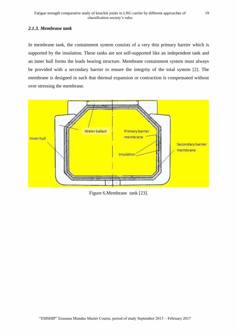
2.1.3. Membrane tank
In membrane tank, the containment system consists of a very thin primary barrier which is
supported by the insulation. These tanks are not self-supported like an independent tank and
an inner hull forms the loads bearing structure. Membrane containment system must always
be provided with a secondary barrier to ensure the integrity of the total system [2]. The
membrane is designed in such that thermal expansion or contraction is compensated without
over stressing the membrane.
Figure 6.Membrane tank [23].
P 20 Sacheendra Naik
Master Thesis developed at West Pomeranian University of Technology, Szczecin
3. THEORETICAL BACKGROUND
3.1. General
Fatigue damage is the most common damage to offshore structures and vessels due to cyclic
wave loads. Fluctuating stresses arising from wave loads can initiate fatigue cracks in the
vicinity of joints which are inadequately designed, constructed and maintained. Though the
load is not large enough to cause immediate failure, microscopic cracks gradually increase in
size. Failure occurs after a certain number of cycles when the accumulated damage reaches
threshold limit. Crack propagation may lead to the failure of primary members. The cost of
inspection and repair of joints affected by fatigue cracks are high. Hence the fatigue design
should be addressed properly at the early design stage.
3.2. Fatigue damage models
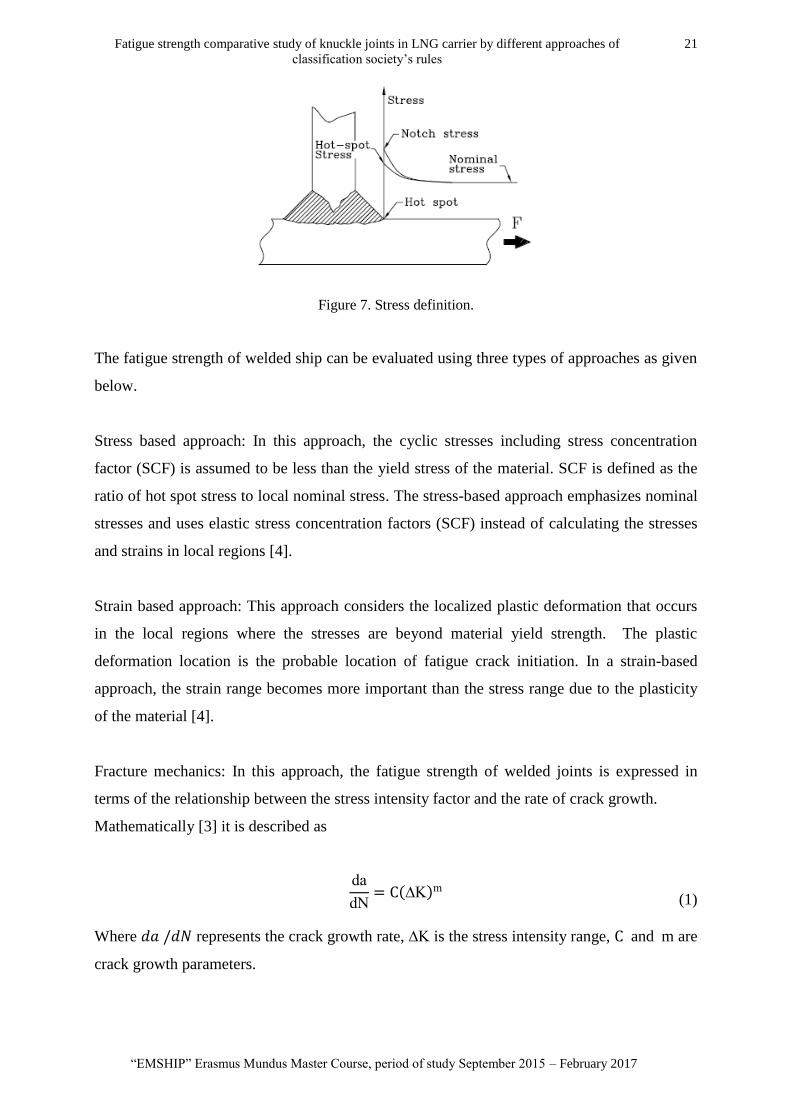
Approaches involved in the evaluation of fatigue damage are related to stress state at the
crack. The stresses namely nominal stress, hotspot stress and notch stress are often used in
fatigue strength calculation. The type of stresses used often depends on the problem to be
solved and accuracy required.
Nominal stress: It is the stress that can be obtained from the section forces using general
theories such as beam theory. It is a general stress in structural details without considering the
effects due to structural discontinuities and presence of weld.
Hotspot stress: It is the structural or geometric stress at the hot spot that includes all stress
raising effects from the geometry excluding the effect of the local profile of the weld.
Notch stress: It is the total stress that exists at the notch or at the weld toe due to stress
concentration caused by the local notch SCF.
The three types of above stresses are shown in Figure 7.
Fatigue strength comparative study of knuckle joints in LNG carrier by different approaches of
classification society‘s rules
21
―EMSHIP‖ Erasmus Mundus Master Course, period of study September 2015 – February 2017
Figure 7. Stress definition.
The fatigue strength of welded ship can be evaluated using three types of approaches as given
below.
Stress based approach: In this approach, the cyclic stresses including stress concentration
factor (SCF) is assumed to be less than the yield stress of the material. SCF is defined as the
ratio of hot spot stress to local nominal stress. The stress-based approach emphasizes nominal
stresses and uses elastic stress concentration factors (SCF) instead of calculating the stresses
and strains in local regions [4].
Strain based approach: This approach considers the localized plastic deformation that occurs
in the local regions where the stresses are beyond material yield strength. The plastic
deformation location is the probable location of fatigue crack initiation. In a strain-based
approach, the strain range becomes more important than the stress range due to the plasticity
of the material [4].
Fracture mechanics: In this approach, the fatigue strength of welded joints is expressed in
terms of the relationship between the stress intensity factor and the rate of crack growth.
Mathematically [3] it is described as
da
d ( )m
(1)
Where represents the crack growth rate, is the stress intensity range, and m are
crack growth parameters.
P 22 Sacheendra Naik
Master Thesis developed at West Pomeranian University of Technology, Szczecin
In this study stress based approach is used to compute the cumulative fatigue damage. Fatigue
strength assessment procedures vary among the different classifications societies but they
include following common steps.
i.) Load calculation
ii.) Calculation of stress range
iii.) Determination of fatigue capacity of welded joints
iv.) Calculation of fatigue damage
3.3. Different methods of fatigue load calculations
Important methods of fatigue strength assessment of ship structures are Simplified Method,
Equivalent Design Wave method (EDW), and Spectral Method [5], [8], [11]. Assessment of
fatigue damage involves long-term load history which dictates the distribution of stress
variation over a long period of time. The long term load history includes the following loads.
1. Still water loads
2. Wave-induced loads
3. Engine or propeller induced propeller loads
4. Impact loads such as slamming, sloshing and whipping
Wave-induced loads are the important contributing load to fatigue damage. The wave loads
required for the structural FE analysis for a full load and ballast condition can be calculated in
the following ways:
3.3.1. Simplified method
In this assessment technique, the calculation is performed limiting predicted stress range due
to design loads below a permissible stress range. The simplified method is conservative, rapid
and used for fatigue screening to identify the fatigue sensitive areas. The method employs two
parameter shape and scale factors in Weibull distributions to predict the long-term distribution
of stress due to sea states. Weibull shape parameter depends on the type of welding
connection and different classification societies provide different values for shape factor.
Fatigue strength comparative study of knuckle joints in LNG carrier by different approaches of
classification society‘s rules
23
―EMSHIP‖ Erasmus Mundus Master Course, period of study September 2015 – February 2017
3.3.2. Equivalent design wave method
Equivalent Design Wave (EDW) is a design wave which represents the long-term response of
the load parameter. In this method, a rule based formulae used to calculate the wave induced
load effects from an equivalent to design waves (EDW) effect. The main load wave induced
load effects contributing to the fatigue damage are
1)Vertical wave bending moment
2)Horizontal bending moment
3)Wave torsional moment
4)External sea pressure
5)Internal liquid pressure.
Rules give the probability of exceedance of the maximum response for the (EDW). The
vertical bending moment, horizontal bending moment, Torsional moment and shear force are
calculated to simulate the dynamic effect of the wave. These loads are computed using ship
parameters and coefficients according to classification rules. Loading from still water and
dynamic waves are combined and stress responses are computed for the combined load effect
using FE analysis. Compared to direct calculation or spectral method, a concept of EDW
reduces the number of load cases to be considered in the design.
3.3.3. Spectral Method
In this method, fatigue assessment is based on directly calculated wave loads. Procedures
described in classification society guidelines [4], [5]are briefly discussed in this section.
Wave loads are computed using 3D linear potential flow theory. The regular wave is analyzed
in the frequency domain. Fatigue damages dominate due to moderate wave heights, hence
non-linear effect due to large motion and waves can be neglected. The linear relationship
between wave load and ship response is expressed in terms of a transfer function. Transfer
functions are calculated for minimum 20 wave periods. Headings angles between 0 to 360º
are covered with a maximum increment of 30º and for each heading minimum 20 wave
frequencies should be included to describe the shape of the transfer functions [4], [5].
Transfer functions for the following are calculated considering wave frequency, heading angle
and different ship speed.
P 24 Sacheendra Naik
Master Thesis developed at West Pomeranian University of Technology, Szczecin
1. Ship motions and accelerations.
2. Vertical bending moment.
3. Horizontal bending moment.
4. External sea pressures.
5. Internal ballast tank pressures.
Steps involved in spectral fatigue analysis are enumerated below.
i.) Calculations of load transfer functions for a unit amplitude regular waves and for a range
of heading angles wave frequencies and ship speeds V.
ii.) Calculation of stress transfer function ( ) for different heading angles, wave
frequencies and ship speeds. This is obtained by load transfer function and performing
global structural analysis using FE analysis. Hydrodynamic loads consist of panel pressure,
inertia forces and internal tank pressure from wave analysis, directly transferred to the
finite element structural model.
iii.) From the global structural analysis, determine a short term structural response for different
heading angles, wave frequencies and ship speeds.
iv.) Using wave spectrum, wave scatter diagram and S-N data for various wave heading angles
and ship speeds, determine the long-term stress range giving the probability of the stress
range exceeding a specified maximum value.
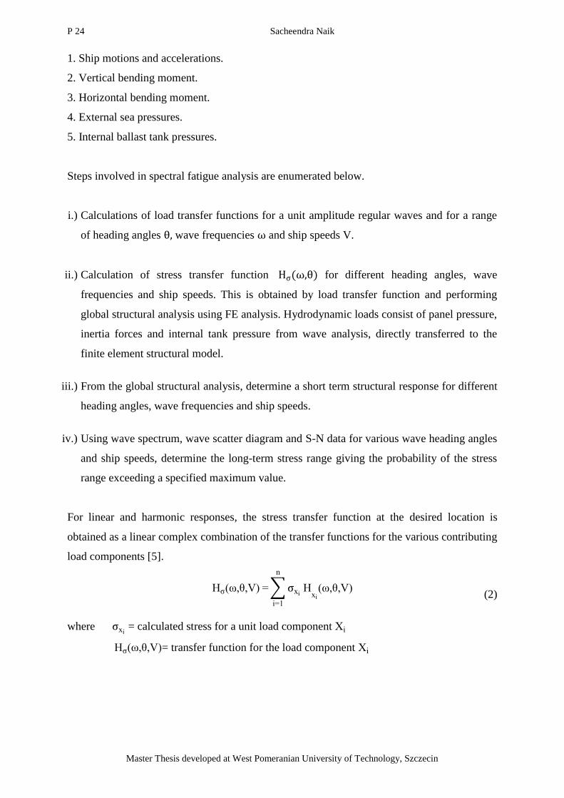
For linear and harmonic responses, the stress transfer function at the desired location is
obtained as a linear complex combination of the transfer functions for the various contributing
load components [5].
H , ,V ∑ xi Hxi
, ,V
n
i 1
(2)
where xi = calculated stress for a unit load component Xi
H , ,V = transfer function for the load component Xi
Fatigue strength comparative study of knuckle joints in LNG carrier by different approaches of
classification society‘s rules
25
―EMSHIP‖ Erasmus Mundus Master Course, period of study September 2015 – February 2017
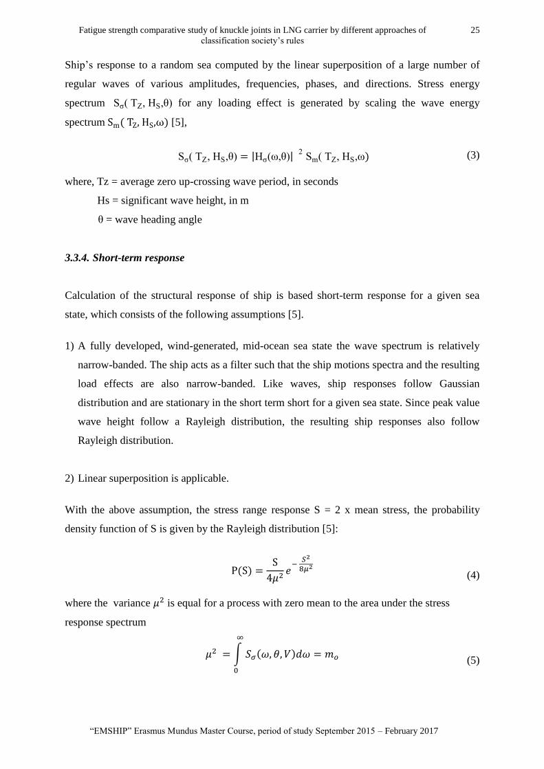
Ship‘s response to a random sea computed by the linear superposition of a large number of
regular waves of various amplitudes, frequencies, phases, and directions. Stress energy
spectrum S TZ, HS, for any loading effect is generated by scaling the wave energy
spectrum ( ) [5],
S TZ, HS, |H , | 2 Sm TZ, HS, ) (3)
where, Tz = average zero up-crossing wave period, in seconds
Hs = significant wave height, in m
= wave heading angle
3.3.4. Short-term response
Calculation of the structural response of ship is based short-term response for a given sea
state, which consists of the following assumptions [5].
1) A fully developed, wind-generated, mid-ocean sea state the wave spectrum is relatively
narrow-banded. The ship acts as a filter such that the ship motions spectra and the resulting
load effects are also narrow-banded. Like waves, ship responses follow Gaussian
distribution and are stationary in the short term short for a given sea state. Since peak value
wave height follow a Rayleigh distribution, the resulting ship responses also follow
Rayleigh distribution.
2) Linear superposition is applicable.
With the above assumption, the stress range response S = 2 x mean stress, the probability
density function of S is given by the Rayleigh distribution [5]:
( )
(4)
where the variance is equal for a process with zero mean to the area under the stress
response spectrum
∫ ( )
(5)
P 26 Sacheendra Naik
Master Thesis developed at West Pomeranian University of Technology, Szczecin
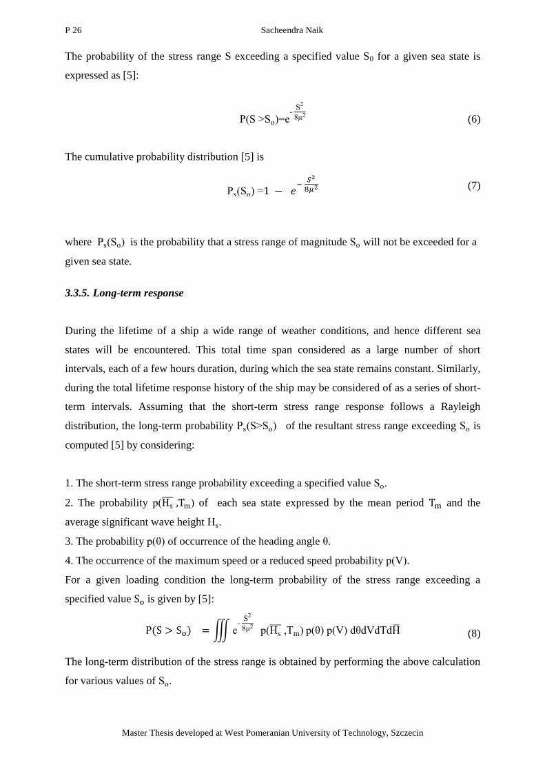
The probability of the stress range S exceeding a specified value S0 for a given sea state is
expressed as [5]:
P S So e
S2
2
(6)
The cumulative probability distribution [5] is
where Ps So is the probability that a stress range of magnitude So will not be exceeded for a
given sea state.
3.3.5. Long-term response
During the lifetime of a ship a wide range of weather conditions, and hence different sea
states will be encountered. This total time span considered as a large number of short
intervals, each of a few hours duration, during which the sea state remains constant. Similarly,
during the total lifetime response history of the ship may be considered of as a series of short-
term intervals. Assuming that the short-term stress range response follows a Rayleigh
distribution, the long-term probability Ps S So of the resultant stress range exceeding So is
computed [5] by considering:
1. The short-term stress range probability exceeding a specified value So.
2. The probability p ̅̅ ̅ of each sea state expressed by the mean period and the
average significant wave height Hs.
3. The probability p of occurrence of the heading angle .
4. The occurrence of the maximum speed or a reduced speed probability p V .
For a given loading condition the long-term probability of the stress range exceeding a
specified value is given by [5]:
( ) ∭ e
S2
2 p Hs̅̅ ̅ ,Tm p p V d dVdTdH̅
(8)
The long-term distribution of the stress range is obtained by performing the above calculation
for various values of So.
Ps So
(7)
Fatigue strength comparative study of knuckle joints in LNG carrier by different approaches of
classification society‘s rules
27
―EMSHIP‖ Erasmus Mundus Master Course, period of study September 2015 – February 2017
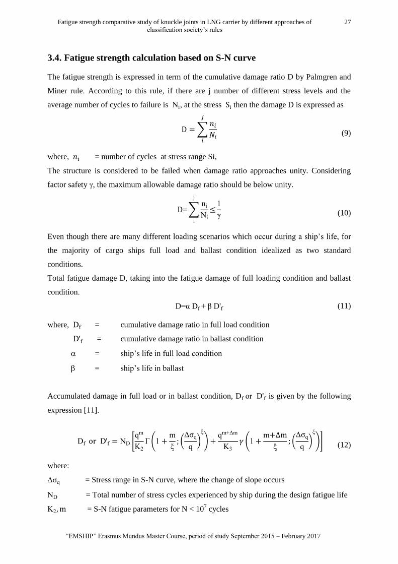
3.4. Fatigue strength calculation based on S-N curve
The fatigue strength is expressed in term of the cumulative damage ratio D by Palmgren and
Miner rule. According to this rule, if there are j number of different stress levels and the
average number of cycles to failure is i, at the stress then the damage D is expressed as
∑
(9)
where, = number of cycles at stress range Si,
The structure is considered to be failed when damage ratio approaches unity. Considering
factor safety , the maximum allowable damage ratio should be below unity.
∑ni
i
j
i
1
(10)
Even though there are many different loading scenarios which occur during a ship‘s life, for
the majority of cargo ships full load and ballast condition idealized as two standard
conditions.
Total fatigue damage D, taking into the fatigue damage of full loading condition and ballast
condition.
D Df D f (11)
where, Df = cumulative damage ratio in full load condition
D f = cumulative damage ratio in ballast condition
= ship‘s life in full load condition
= ship‘s life in ballast
Accumulated damage in full load or in ballast condition, Df or D f is given by the following
expression [11].
Df D f D *
qm
2 (1
m
( q
q)
) qm m
3 (1
m
( q
q)
)+
(12)
where:
q = Stress range in S-N curve, where the change of slope occurs
D = Total number of stress cycles experienced by ship during the design fatigue life
2 = S-N fatigue parameters for N < 107 cycles
P 28 Sacheendra Naik
Master Thesis developed at West Pomeranian University of Technology, Szczecin
m = S-N fatigue parameters for N > 107 cycles
; = Complementary Incomplete Gamma function, to be found in standard tables
( ; ) = Incomplete Gamma function, to be found in standard tables
= Weibull slope parameter
q = Weibull scale parameter
Number load cycles N to failure for a particular stress range can be obtained from S-N curve
or stress Cycle curve. These curves are obtained by subjecting the material specimen to
constant cyclic load until failure in laboratories. The curve represents a relation between the
stress ranges against the stress cycle on logarithm scale. Figure 8 shows a set of typical S-N
curves. Though there are various S-N curves available published by many institutions such as
IIW, HSE UK, AWS available, only two of the following are used by the classification
societies [5].
1) HSE S-N curves
2) IIW S-N curve
Using Miner‘s law and data from S-N curves fatigue life structure is assessed for various
welded joints. The relationship between stress range and the number of cycles to failure N
can be represented by the following expression [11].
log logk2 mlog (13)
where:
N number of cycles to failure for stress range
= stress range in N/mm2
m = negative inverse slope of S-N curve
The intercept of log N-axis by S-N curve, logk2 is expressed as [11]:
logk2 logk 2 (14)
where:
k1 = Constant of mean S-N curve (50% probability of survival)
k2 = Constant of design S-N curve (97.5% probability of survival)
= Standard deviation of log N:
= 0.20
Fatigue strength comparative study of knuckle joints in LNG carrier by different approaches of
classification society‘s rules
29
―EMSHIP‖ Erasmus Mundus Master Course, period of study September 2015 – February 2017
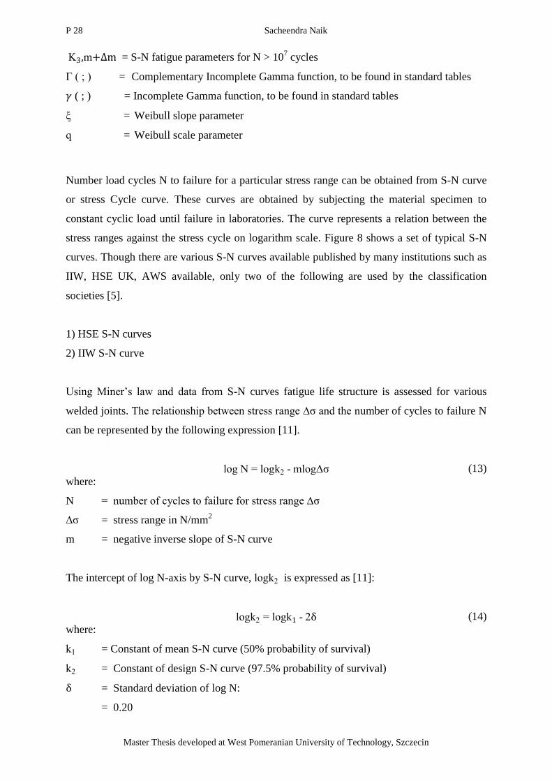
Depending on the level of refinement method used in FE analysis to calculate stresses, three
types of stresses namely nominal stress, hotspot stress or notch stress are used in fatigue
calculations.
Figure 8. S-N curve in air –DNV GL[11].
With nominal Stress approach, stresses are assessed by structural mechanics or by coarse
mesh FE analysis. If FE analysis employed, a uniform mesh shall be used with a smooth
transition and abrupt changes in mesh size must be avoided. At the hot spot, the nominal
stress is calculated by extrapolated stresses around the hotspot region.With nominal stress
approach, the S-N curves can be used directly provided that the applicable S-N curve clearly
identified for a welded joint detail under consideration. Due to the complexity of ship
structural details, it is difficult to select the correct S-N curve and selection becomes a matter
of judgment.
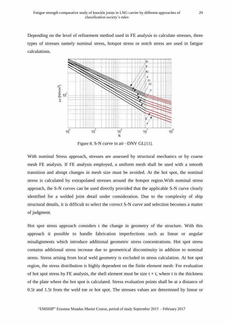
Hot spot stress approach considers t the change in geometry of the structure. With this
approach it possible to handle fabrication imperfections such as linear or angular
misalignments which introduce additional geometric stress concentrations. Hot spot stress
contains additional stress increase due to geometrical discontinuity in addition to nominal
stress. Stress arising from local weld geometry is excluded in stress calculation. At hot spot
region, the stress distribution is highly dependent on the finite element mesh. For evaluation
of hot spot stress by FE analysis, the shell element must be size t × t, where t is the thickness
of the plate where the hot spot is calculated. Stress evaluation points shall be at a distance of
0.5t and 1.5t from the weld toe or hot spot. The stresses values are determined by linear or
P 30 Sacheendra Naik
Master Thesis developed at West Pomeranian University of Technology, Szczecin
2nd order interpolation of the principal stresses at the centre of element faces in the region
[11].
Figure 9. Stress read out points and hot spot stress for 8-node shell elements [11].
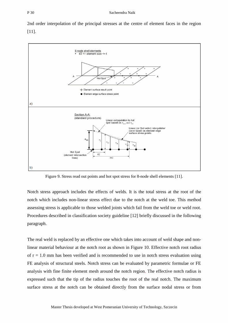
Notch stress approach includes the effects of welds. It is the total stress at the root of the
notch which includes non-linear stress effect due to the notch at the weld toe. This method
assessing stress is applicable to those welded joints which fail from the weld toe or weld root.
Procedures described in classification society guideline [12] briefly discussed in the following
paragraph.
The real weld is replaced by an effective one which takes into account of weld shape and non-
linear material behaviour at the notch root as shown in Figure 10. Effective notch root radius
of r = 1.0 mm has been verified and is recommended to use in notch stress evaluation using
FE analysis of structural steels. Notch stress can be evaluated by parametric formulae or FE
analysis with fine finite element mesh around the notch region. The effective notch radius is
expressed such that the tip of the radius touches the root of the real notch. The maximum
surface stress at the notch can be obtained directly from the surface nodal stress or from
Fatigue strength comparative study of knuckle joints in LNG carrier by different approaches of
classification society‘s rules
31
―EMSHIP‖ Erasmus Mundus Master Course, period of study September 2015 – February 2017
extrapolation. The maximum surface stress calculated from FE analysis at the notch is the
effective notch stress which shall be used together with the recommended S-N curve[12].
Figure 10. Notch model [12].
3.5. Uncertainties in fatigue strength prediction
There are a number of uncertainties associated with fatigue life prediction calculation. The
main uncertainties associated with fatigue life calculations mainly due to wave loading, Stress
calculations and S-N curves [3],[5], [11].
i.) Wave loading
Uncertainties related to wave load calculations due to random sea loads, the period length
used for collection of environmental data, wave theories.
ii.) Stress calculations
Uncertainties associated with stress calculations dependent on FE modelling techniques,
boundary conditions, mesh size, the method of combinations of various wave and quality of
structural stress computation software tools. Since the fatigue damage is proportional to the
inverse slope of the S-N curve, minor changes in stress lead to major changes in calculated
fatigue life.
iii.) S-N curves
S-N curves are based on experimental results in the laboratory under free corrosion
environment up to 107 cycles to failure. In ship structures, fatigue damage is significant when
a number of cycles to failure N > 107. Therefore the method of extrapolation of S-N curves
beyond 107 cycles is important for the assessment of fatigue life.
P 32 Sacheendra Naik
Master Thesis developed at West Pomeranian University of Technology, Szczecin
4. ANALYSIS METHODOLOGY AND SOFTWARE TOOLS USED
4.1. Analysis Methodology
The methodology adopted in this thesis project is described in Figure 2. For the fatigue
damage, full spectral analysis wave loads are calculated by direct calculations. For fatigue
damage evaluation it is assumed that the short return period wave loads contribute
significantly to fatigue damage have short return periods. These waves are small in amplitude
and frequently occur.
Wave loads are calculated using a 3D hydrodynamic program including the effect of forward
speed. A vessel speed set to 2/3 of the service speed in full load and ballast condition is
applied in the hydrodynamic modelling. The hydrodynamic analysis in the linear frequency
domain using 3-D potential theory is employed to calculate ship response. The wave
amplitude of 1.0m considering wave headings from 0 to 360 degrees with an increment of
maximum 30 degrees is used to calculate the ship response. For each wave heading 25 wave
frequencies are included to describe the shape of the transfer functions.
In order to obtain balance in FE structural model and hydrodynamic model, mass has to be
identical in FE and hydrodynamic model. Therefore mass model from global FE structural
model is used in the hydrodynamic linear analysis. The mass in hydrodynamic analysis shall
be represented correctly to obtain motion and sectional forces. The mass model shall include
the
following
the total weight which includes light weight, ballast and liquid cargo
longitudinal, vertical, transverse centre of gravity
rotational mass in roll and pitch.
The weight of the cargo in spherical tanks of Moss type LNG carrier uniformly distributed
along the skirt of the tank to the hull foundation. The panel pressures, inside tank pressure and
inertia loads from the hydrodynamic analysis, are directly transferred to FE structural global
model.
A linear FE structural analysis is performed for global ship model. Since the main purpose of
the global analysis is to identify the critical locations, stress risers such as welds notches and
Fatigue strength comparative study of knuckle joints in LNG carrier by different approaches of
classification society‘s rules
33
―EMSHIP‖ Erasmus Mundus Master Course, period of study September 2015 – February 2017
geometrical discontinues are not modelled. A detailed local sub-model of details at the critical
location is modelled with a fine mesh of size t x t where t is the thickness of the plate. The
deformations from global FE analysis are applied on the border of the sub model. These
deformations serve as boundary conditions for the local model. Wave loads from the
hydrodynamic analysis are directly transferred to sub model.
For each heading of sea state, fatigue damage is calculated by combing the hotspot transfer
functions with stress cycle (S-N) curve data and wave scatter diagram.
4.2. Software Tools Used
In order to execute the set of analysis defined in section 4.1, SESAM software package
developed by DNV has been used. SESAM is a complete strength assessment programme for
engineering of ships, offshore structures and risers based on the finite element methodology.
This software package has various modules which can be used depending on the type
numerical simulation that is required to be carried out. For the current study of LNG carrier
the following modules used has been selected.
4.2.1. Sesam Genie
GeniE is the design analysis tool in SESAM used for designing and analyzing, the offshore
and maritime structures made of beams/shells [16]. GeniE can be used as a stand-alone tool
and user where the user can
Model structure, equipment, environment and other loads
Calculate hydrodynamic loads and run static structural analyses including non-linear pile
soil analysis
Visualize and post-process results
Perform code checking based on recognized standards
4.2.2. Sestra
Sestra is a program for linear static and dynamic structural analysis within the SESAM
program system Error! Reference source not found.. It uses a displacement based finite
element method. Sestra computes the local element matrices and load vectors, assembles them
into global matrices andload vectors. The global matrices are used by algebraic numerical
P 34 Sacheendra Naik
Master Thesis developed at West Pomeranian University of Technology, Szczecin
algorithms to do the requested static, dynamic or linearized buckling analysis. It has interface
with other program modules of SESAM
4.2.3. HydroD-Wasim
The Sesam HydroD capability of performing a hydrostatic and hydrodynamic analysis which
includes a hydrodynamic model of the floating structure ships and offshore floating structures
Wasim is a program for computing global responses of and local loading on vessels moving at
any forward speed. The simulations are carried out in the time domain, but results are also
transformed to the frequency domain by using Fourier transform [18].
Rankine panel method is to solve the fully 3-dimensional radiation/diffraction problem by a
Wasim. This method requires panels both on the hull and on the free surface. Based on the
geometry of the hull supplied by the user, Wasim generates its own mesh. Analysis by Wasim
include the following capabilities
• Global responses computation of
—rigid body motions
—sectional forces and moments
—relative motion at specified points
•Computation of pressure on the vessel:
—pressure at selected points on the hull
—total pressure distribution on the whole hull
•Direct transfer of pressures to a finite element model for structural analysis
4.2.4. Xtract
Xtract software is post processing tool having features for selecting, further processing,
displaying, tabulating and animating results from static and dynamic structural analysis as
well as results from various types of hydrodynamic analysis [19]. With its high-performance
3D graphics enables easy and efficient interactive rotation, zooming and panning of the model
for viewing and animation. Based on the FE analysis results with Xtract, it is possible to
present the decomposed stress components into membrane and bending parts, principal
stresses and Von Mises stresses. Furthermore, with Xtract, it is also possible to presents
Fatigue strength comparative study of knuckle joints in LNG carrier by different approaches of
classification society‘s rules
35
―EMSHIP‖ Erasmus Mundus Master Course, period of study September 2015 – February 2017
deformed model, contour curves of stresses and displacement-Y graphs and tabulated data. In
addition, the motion of vessel can be animated.
4.2.5. Postresp
The statistical post-processing of general responses of ship obtained from global
hydrodynamic analysis in the frequency domain is obtained using Postresp software. These
responses such as displacements, velocity etc. are represented as transfer function for FE
structural analysis. The transfer functions are generated by the hydrodynamic program
HydroD -Wasim. The displacement response variables such Surge, Sway, Heave, Roll, Pitch
and Yaw motion are plotted as dimensionless quantities with respect to wave periods or
frequencies at different wave headings. The graphs from the program and results are
discussed in chapter 6.
4.2.6. Submod
The submod programme allows a part of a global model to be re-analyzed to produce more
accurate results. For the local model separated from the global model, the displacements from
global model analysis applied as prescribed displacements at the boundary[20].
4.2.7. Cutres
Cutres is a post-processor used for ship structures. With Cutres, cross-sections of ship
structures can be created and combined into assemblies. Cutres calculate the force distribution
across the cross section and can be presented graphically. With Cutres, force distribution in
each cross section integrated to form the total axial force, shear forces and bending moment
and torsional moment [21].
4.2.8. Stofat
The Stofat is software tool for fatigue design. Stofat performs stochastic fatigue analysis on
structures modelled by 3D shell and solid elements and assesses whether the structure is likely
to suffer failure due to the action of repeated loading [22] Stresses from the global or local
FE analysis serves as stress transfer function for fatigue calculation. Accumulated damage is
calculated using stress transfer function, S-N curve data, wave spectrum, weighted over sea
states and wave.
P 36 Sacheendra Naik
Master Thesis developed at West Pomeranian University of Technology, Szczecin
5. STRUCTURAL MODELLING
The objective of the global structural modelling is to compute the stress transfer function from
environmental wave loading by finite element method. The stresses required for the fatigue
assessment is obtained from global FE analysis of the vessel. The global structural model
represents the stiffness of the actual structure and comprises of shell finite elements in
combination with beam elements. The structural FE model is further utilized in the
hydrodynamic model to develop the panel and mass model. The panel model takes into
account the finite elements exposed to the action of hydrodynamic wave loading and whole
structural FE model represents the mass model. The use of FE structural model as a mass
model in hydrodynamics analysis ensures the consistent load and response between
hydrodynamic and structural analysis. The structural connections at key locations such as
liquid cargo tanks with tank foundation deck and cargo tank with hull deck have been
modelled with sufficient stiffness to ensure proper load distribution and to obtain correct
global stress.
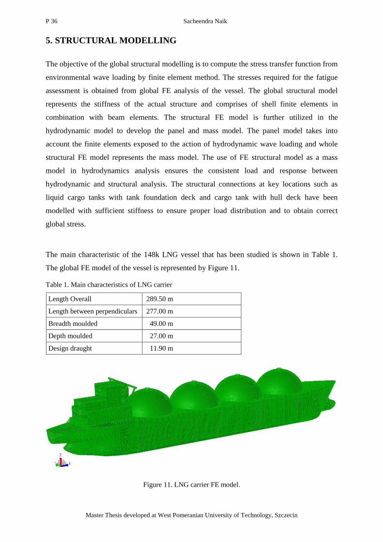
The main characteristic of the 148k LNG vessel that has been studied is shown in Table 1.
The global FE model of the vessel is represented by Figure 11.
Table 1. Main characteristics of LNG carrier
Length Overall 289.50 m
Length between perpendiculars 277.00 m
Breadth moulded 49.00 m
Depth moulded 27.00 m
Design draught 11.90 m
Figure 11. LNG carrier FE model.
Fatigue strength comparative study of knuckle joints in LNG carrier by different approaches of
classification society‘s rules
37
―EMSHIP‖ Erasmus Mundus Master Course, period of study September 2015 – February 2017
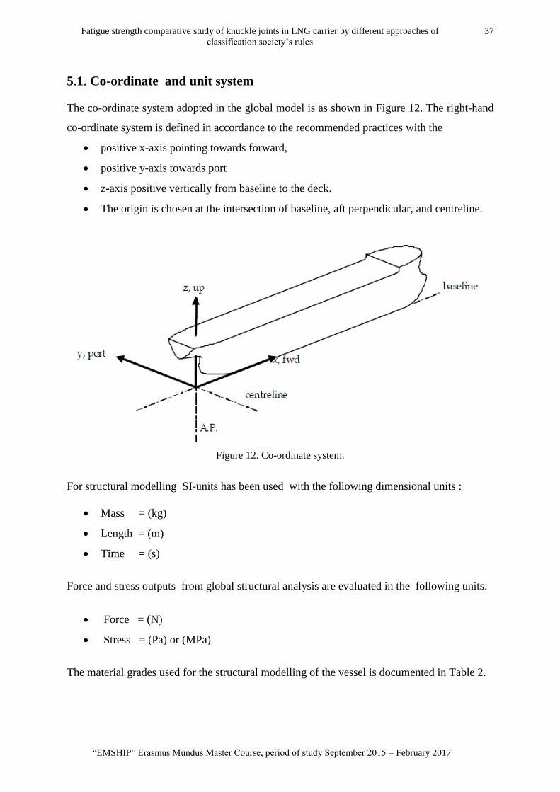
5.1. Co-ordinate and unit system
The co-ordinate system adopted in the global model is as shown in Figure 12. The right-hand
co-ordinate system is defined in accordance to the recommended practices with the
positive x-axis pointing towards forward,
positive y-axis towards port
z-axis positive vertically from baseline to the deck.
The origin is chosen at the intersection of baseline, aft perpendicular, and centreline.
Figure 12. Co-ordinate system.
For structural modelling SI-units has been used with the following dimensional units :
Mass = (kg)
Length = (m)
Time = (s)
Force and stress outputs from global structural analysis are evaluated in the following units:
Force = (N)
Stress = (Pa) or (MPa)
The material grades used for the structural modelling of the vessel is documented in Table 2.
P 38 Sacheendra Naik
Master Thesis developed at West Pomeranian University of Technology, Szczecin
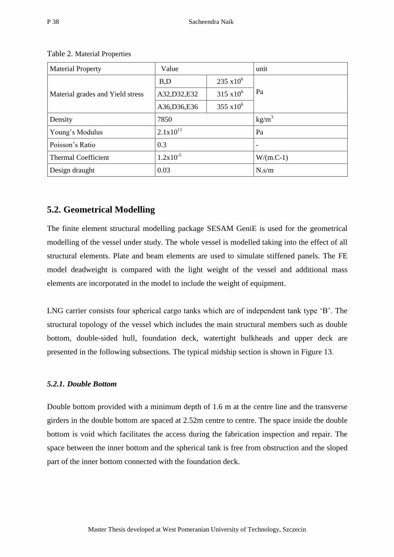
Table 2. Material Properties
Material Property Value unit
Material grades and Yield stress
B,D 235 x106
Pa A32,D32,E32 315 x106
A36,D36,E36 355 x106
Density 7850 kg/m3
Young‘s Modulus 2.1x10¹¹
Pa
Poisson‘s Ratio 0.3 -
Thermal Coefficient 1.2x10⁻⁵
W/(m.C-1)
Design draught 0.03 N.s/m
5.2. Geometrical Modelling
The finite element structural modelling package SESAM GeniE is used for the geometrical
modelling of the vessel under study. The whole vessel is modelled taking into the effect of all
structural elements. Plate and beam elements are used to simulate stiffened panels. The FE
model deadweight is compared with the light weight of the vessel and additional mass
elements are incorporated in the model to include the weight of equipment.
LNG carrier consists four spherical cargo tanks which are of independent tank type ‗B‘. The
structural topology of the vessel which includes the main structural members such as double
bottom, double-sided hull, foundation deck, watertight bulkheads and upper deck are
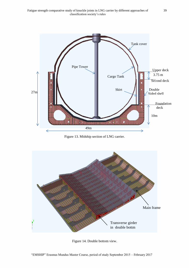
presented in the following subsections. The typical midship section is shown in Figure 13.
5.2.1. Double Bottom
Double bottom provided with a minimum depth of 1.6 m at the centre line and the transverse
girders in the double bottom are spaced at 2.52m centre to centre. The space inside the double
bottom is void which facilitates the access during the fabrication inspection and repair. The
space between the inner bottom and the spherical tank is free from obstruction and the sloped
part of the inner bottom connected with the foundation deck.
Fatigue strength comparative study of knuckle joints in LNG carrier by different approaches of
classification society‘s rules
39
―EMSHIP‖ Erasmus Mundus Master Course, period of study September 2015 – February 2017
Figure 13. Midship section of LNG carrier.
Figure 14. Double bottom view.
Main frame
Transverse girder
in double bottm
Tank cover
49m
Foundation
deck
Upper deck
27m
10m
Second deck
3.75 m
Double
Sided shell
Pipe Tower
Cargo Tank
Skirt
P 40 Sacheendra Naik
Master Thesis developed at West Pomeranian University of Technology, Szczecin
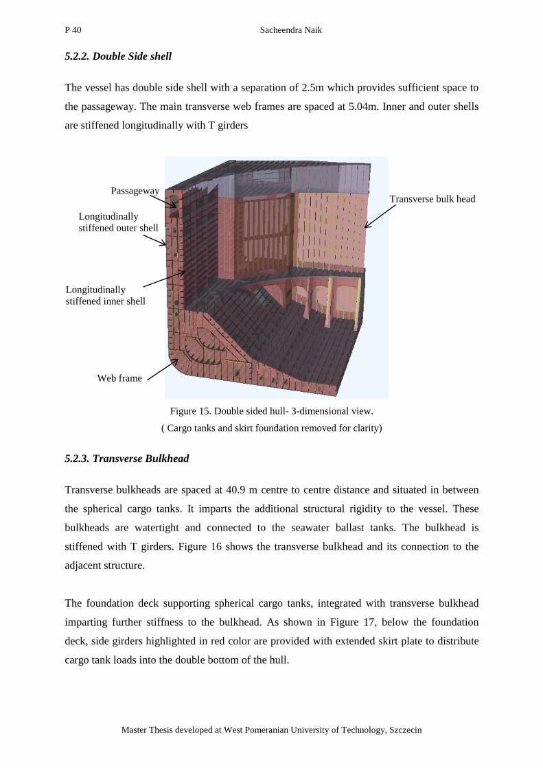
5.2.2. Double Side shell
The vessel has double side shell with a separation of 2.5m which provides sufficient space to
the passageway. The main transverse web frames are spaced at 5.04m. Inner and outer shells
are stiffened longitudinally with T girders
Figure 15. Double sided hull- 3-dimensional view.
( Cargo tanks and skirt foundation removed for clarity)
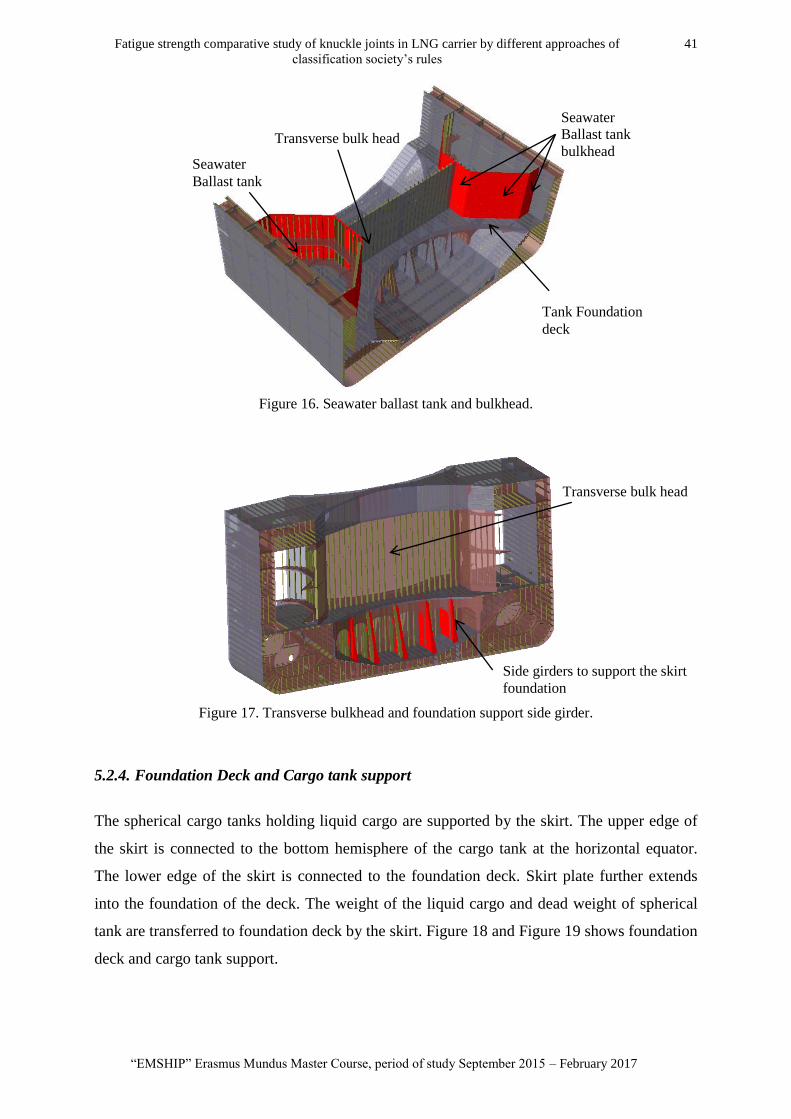
5.2.3. Transverse Bulkhead
Transverse bulkheads are spaced at 40.9 m centre to centre distance and situated in between
the spherical cargo tanks. It imparts the additional structural rigidity to the vessel. These
bulkheads are watertight and connected to the seawater ballast tanks. The bulkhead is
stiffened with T girders. Figure 16 shows the transverse bulkhead and its connection to the
adjacent structure.
The foundation deck supporting spherical cargo tanks, integrated with transverse bulkhead
imparting further stiffness to the bulkhead. As shown in Figure 17, below the foundation
deck, side girders highlighted in red color are provided with extended skirt plate to distribute
cargo tank loads into the double bottom of the hull.
Transverse bulk head Passageway
Web frame
Longitudinally
stiffened inner shell
Longitudinally
stiffened outer shell
Fatigue strength comparative study of knuckle joints in LNG carrier by different approaches of
classification society‘s rules
41
―EMSHIP‖ Erasmus Mundus Master Course, period of study September 2015 – February 2017
Figure 16. Seawater ballast tank and bulkhead.
Figure 17. Transverse bulkhead and foundation support side girder.
5.2.4. Foundation Deck and Cargo tank support
The spherical cargo tanks holding liquid cargo are supported by the skirt. The upper edge of
the skirt is connected to the bottom hemisphere of the cargo tank at the horizontal equator.
The lower edge of the skirt is connected to the foundation deck. Skirt plate further extends
into the foundation of the deck. The weight of the liquid cargo and dead weight of spherical
tank are transferred to foundation deck by the skirt. Figure 18 and Figure 19 shows foundation
deck and cargo tank support.
Tank Foundation
deck
Seawater
Ballast tank
bulkhead Seawater
Ballast tank
Transverse bulk head
Side girders to support the skirt
foundation
Transverse bulk head
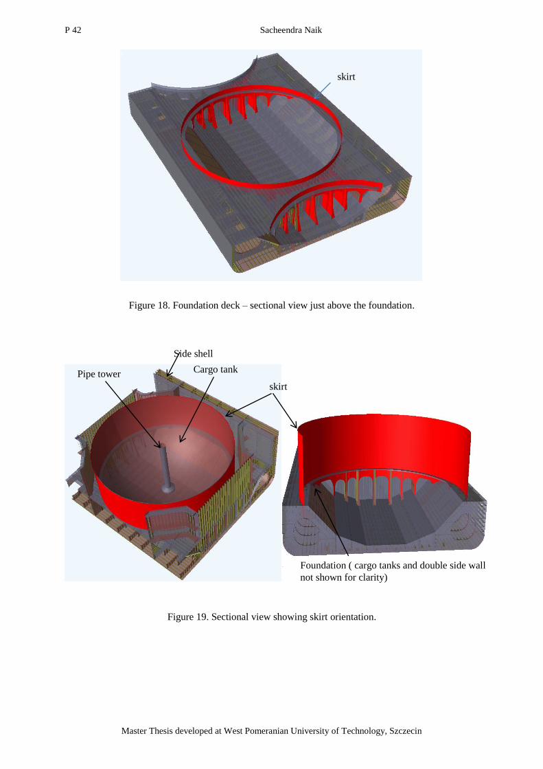
P 42 Sacheendra Naik
Master Thesis developed at West Pomeranian University of Technology, Szczecin
Figure 18. Foundation deck – sectional view just above the foundation.
Figure 19. Sectional view showing skirt orientation.
Cargo tank
skirt
Foundation ( cargo tanks and double side wall
not shown for clarity)
Side shell
Pipe tower
skirt
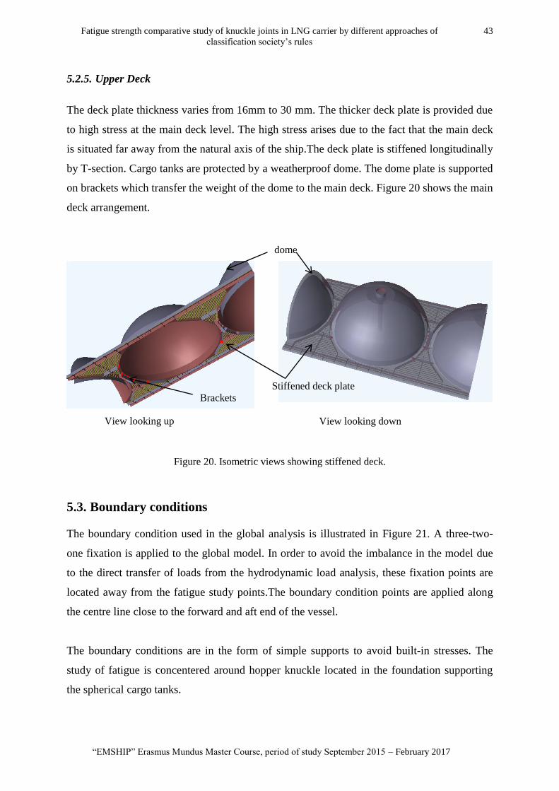
Fatigue strength comparative study of knuckle joints in LNG carrier by different approaches of
classification society‘s rules
43
―EMSHIP‖ Erasmus Mundus Master Course, period of study September 2015 – February 2017
5.2.5. Upper Deck
The deck plate thickness varies from 16mm to 30 mm. The thicker deck plate is provided due
to high stress at the main deck level. The high stress arises due to the fact that the main deck
is situated far away from the natural axis of the ship.The deck plate is stiffened longitudinally
by T-section. Cargo tanks are protected by a weatherproof dome. The dome plate is supported
on brackets which transfer the weight of the dome to the main deck. Figure 20 shows the main
deck arrangement.
Figure 20. Isometric views showing stiffened deck.
5.3. Boundary conditions
The boundary condition used in the global analysis is illustrated in Figure 21. A three-two-
one fixation is applied to the global model. In order to avoid the imbalance in the model due
to the direct transfer of loads from the hydrodynamic load analysis, these fixation points are
located away from the fatigue study points.The boundary condition points are applied along
the centre line close to the forward and aft end of the vessel.
The boundary conditions are in the form of simple supports to avoid built-in stresses. The
study of fatigue is concentered around hopper knuckle located in the foundation supporting
the spherical cargo tanks.
dome
Stiffened deck plate
Brackets
View looking up View looking down
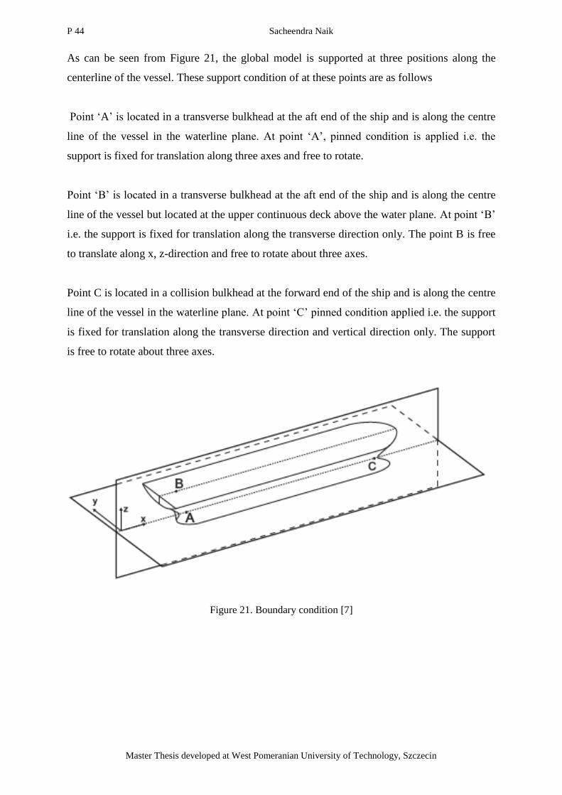
P 44 Sacheendra Naik
Master Thesis developed at West Pomeranian University of Technology, Szczecin
As can be seen from Figure 21, the global model is supported at three positions along the
centerline of the vessel. These support condition of at these points are as follows
Point ‗A‘ is located in a transverse bulkhead at the aft end of the ship and is along the centre
line of the vessel in the waterline plane. At point ‗A‘, pinned condition is applied i.e. the
support is fixed for translation along three axes and free to rotate.
Point ‗B‘ is located in a transverse bulkhead at the aft end of the ship and is along the centre
line of the vessel but located at the upper continuous deck above the water plane. At point ‗B‘
i.e. the support is fixed for translation along the transverse direction only. The point B is free
to translate along x, z-direction and free to rotate about three axes.
Point C is located in a collision bulkhead at the forward end of the ship and is along the centre
line of the vessel in the waterline plane. At point ‗C‘ pinned condition applied i.e. the support
is fixed for translation along the transverse direction and vertical direction only. The support
is free to rotate about three axes.
Figure 21. Boundary condition [7]
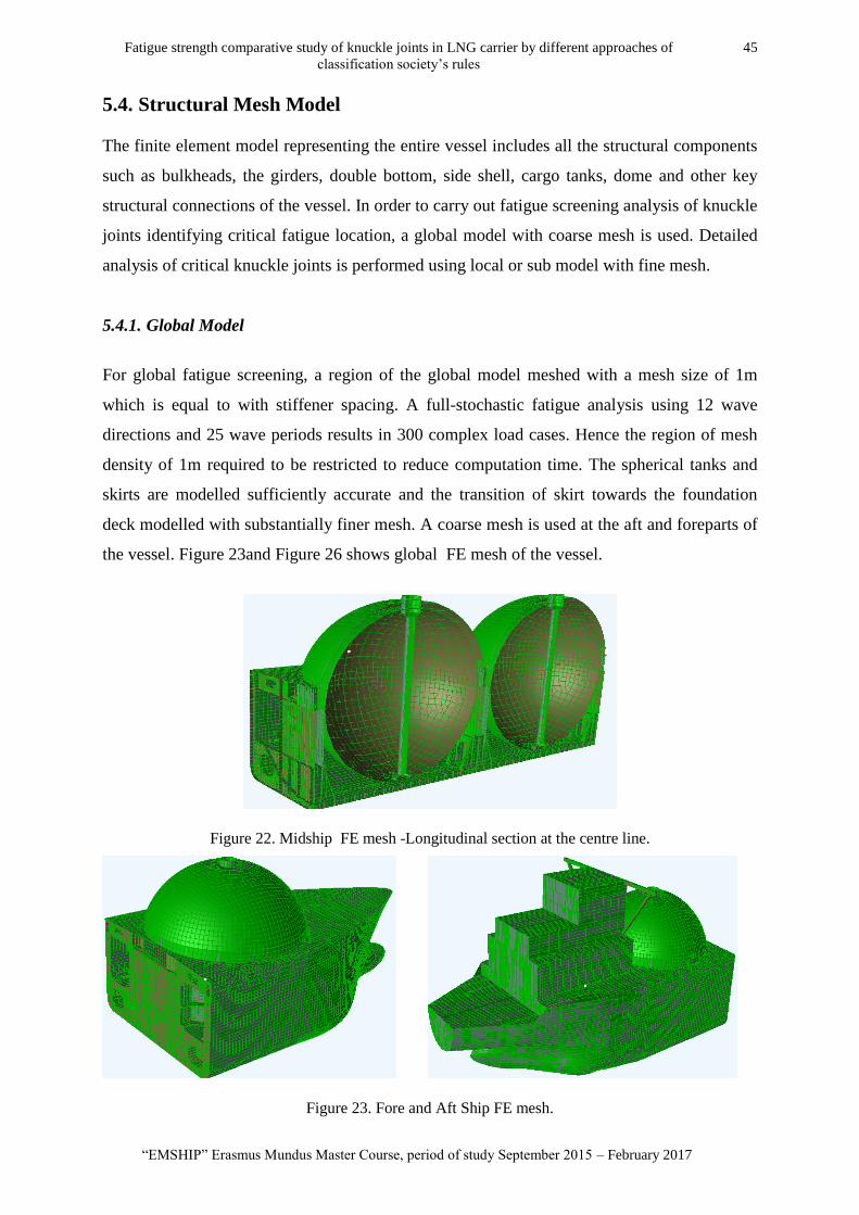
Fatigue strength comparative study of knuckle joints in LNG carrier by different approaches of
classification society‘s rules
45
―EMSHIP‖ Erasmus Mundus Master Course, period of study September 2015 – February 2017
5.4. Structural Mesh Model
The finite element model representing the entire vessel includes all the structural components
such as bulkheads, the girders, double bottom, side shell, cargo tanks, dome and other key
structural connections of the vessel. In order to carry out fatigue screening analysis of knuckle
joints identifying critical fatigue location, a global model with coarse mesh is used. Detailed
analysis of critical knuckle joints is performed using local or sub model with fine mesh.
5.4.1. Global Model
For global fatigue screening, a region of the global model meshed with a mesh size of 1m
which is equal to with stiffener spacing. A full-stochastic fatigue analysis using 12 wave
directions and 25 wave periods results in 300 complex load cases. Hence the region of mesh
density of 1m required to be restricted to reduce computation time. The spherical tanks and
skirts are modelled sufficiently accurate and the transition of skirt towards the foundation
deck modelled with substantially finer mesh. A coarse mesh is used at the aft and foreparts of
the vessel. Figure 23and Figure 26 shows global FE mesh of the vessel.
Figure 22. Midship FE mesh -Longitudinal section at the centre line.
Figure 23. Fore and Aft Ship FE mesh.
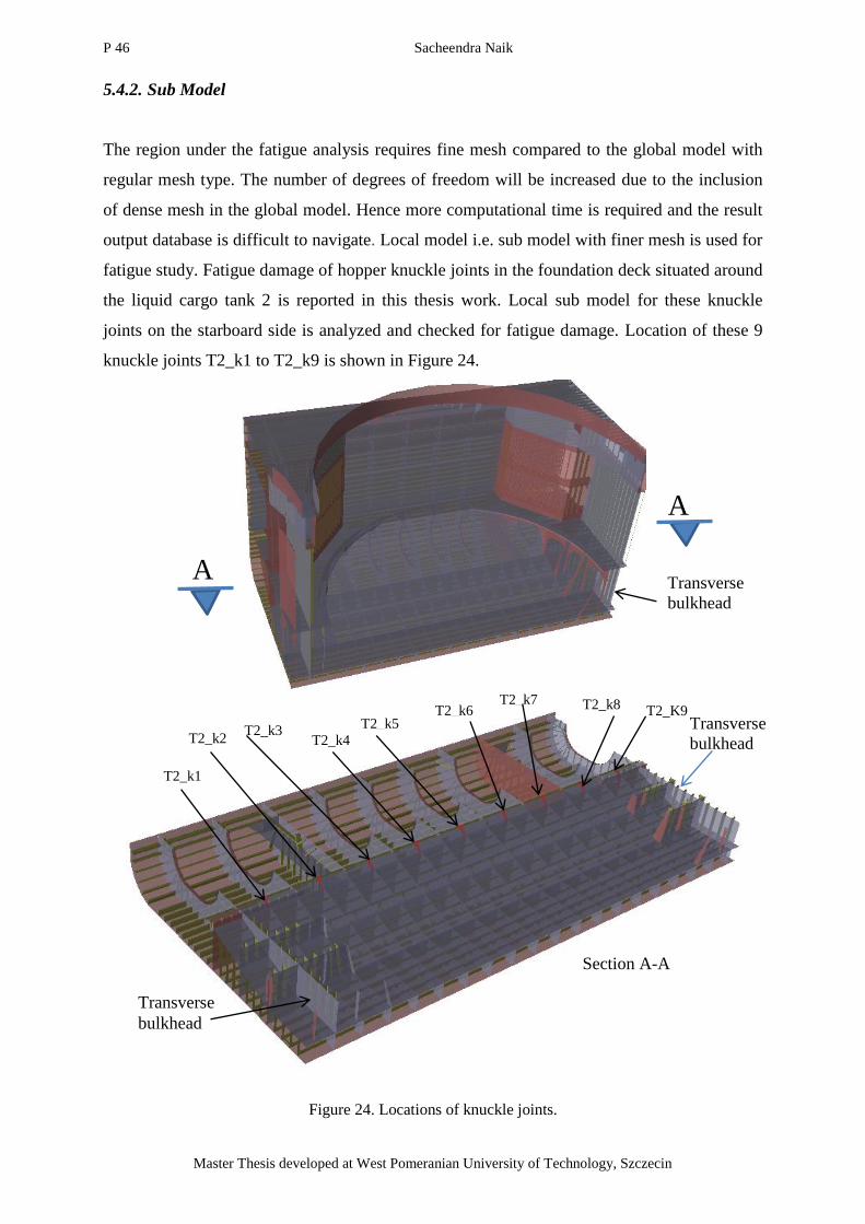
P 46 Sacheendra Naik
Master Thesis developed at West Pomeranian University of Technology, Szczecin
5.4.2. Sub Model
The region under the fatigue analysis requires fine mesh compared to the global model with
regular mesh type. The number of degrees of freedom will be increased due to the inclusion
of dense mesh in the global model. Hence more computational time is required and the result
output database is difficult to navigate. Local model i.e. sub model with finer mesh is used for
fatigue study. Fatigue damage of hopper knuckle joints in the foundation deck situated around
the liquid cargo tank 2 is reported in this thesis work. Local sub model for these knuckle
joints on the starboard side is analyzed and checked for fatigue damage. Location of these 9
knuckle joints T2_k1 to T2_k9 is shown in Figure 24.
Figure 24. Locations of knuckle joints.
Transverse
bulkhead
Transverse
bulkhead
A
A
T2_K9
T2_k1
T2_k2 T2_k3
Transverse
bulkhead
T2_k4
T2_k5 T2_k6 T2_k8 T2_k7
Section A-A
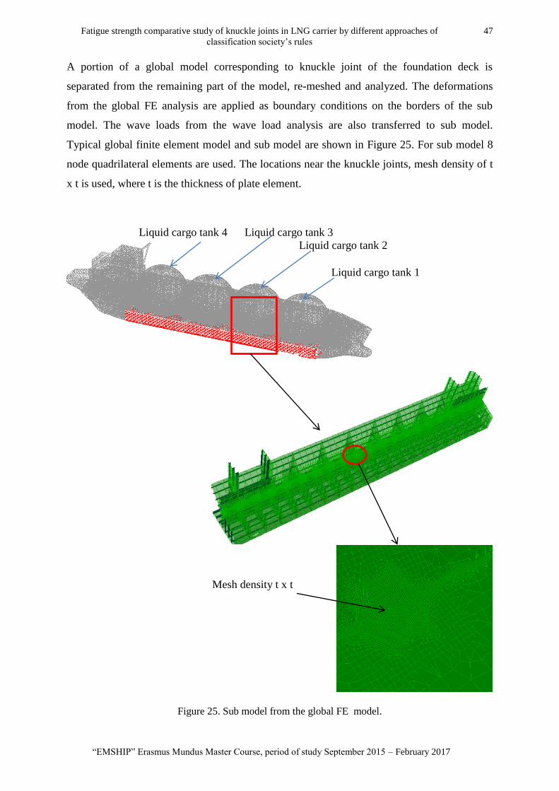
Fatigue strength comparative study of knuckle joints in LNG carrier by different approaches of
classification society‘s rules
47
―EMSHIP‖ Erasmus Mundus Master Course, period of study September 2015 – February 2017
A portion of a global model corresponding to knuckle joint of the foundation deck is
separated from the remaining part of the model, re-meshed and analyzed. The deformations
from the global FE analysis are applied as boundary conditions on the borders of the sub
model. The wave loads from the wave load analysis are also transferred to sub model.
Typical global finite element model and sub model are shown in Figure 25. For sub model 8
node quadrilateral elements are used. The locations near the knuckle joints, mesh density of t
x t is used, where t is the thickness of plate element.
Figure 25. Sub model from the global FE model.
Liquid cargo tank 1
Liquid cargo tank 2
Liquid cargo tank 3 Liquid cargo tank 4
Mesh density t x t
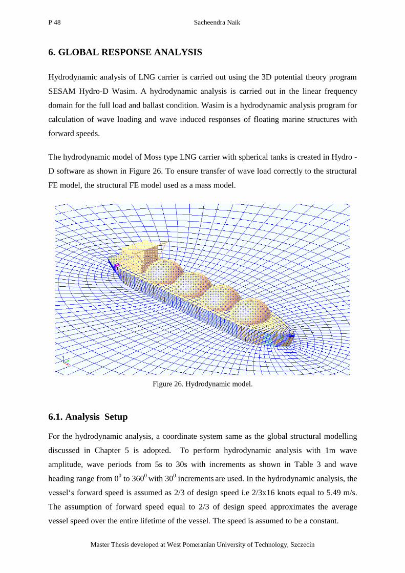
P 48 Sacheendra Naik
Master Thesis developed at West Pomeranian University of Technology, Szczecin
6. GLOBAL RESPONSE ANALYSIS
Hydrodynamic analysis of LNG carrier is carried out using the 3D potential theory program
SESAM Hydro-D Wasim. A hydrodynamic analysis is carried out in the linear frequency
domain for the full load and ballast condition. Wasim is a hydrodynamic analysis program for
calculation of wave loading and wave induced responses of floating marine structures with
forward speeds.
The hydrodynamic model of Moss type LNG carrier with spherical tanks is created in Hydro -
D software as shown in Figure 26. To ensure transfer of wave load correctly to the structural
FE model, the structural FE model used as a mass model.
Figure 26. Hydrodynamic model.
6.1. Analysis Setup
For the hydrodynamic analysis, a coordinate system same as the global structural modelling
discussed in Chapter 5 is adopted. To perform hydrodynamic analysis with 1m wave
amplitude, wave periods from 5s to 30s with increments as shown in Table 3 and wave
heading range from 00 to 360
0 with 30
0 increments
are used. In the hydrodynamic analysis, the
vessel‗s forward speed is assumed as 2/3 of design speed i.e 2/3x16 knots equal to 5.49 m/s.
The assumption of forward speed equal to 2/3 of design speed approximates the average
vessel speed over the entire lifetime of the vessel. The speed is assumed to be a constant.
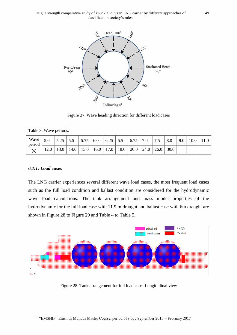
Fatigue strength comparative study of knuckle joints in LNG carrier by different approaches of
classification society‘s rules
49
―EMSHIP‖ Erasmus Mundus Master Course, period of study September 2015 – February 2017
Figure 27. Wave heading direction for different load cases
Table 3. Wave periods.
Wave
period
(s)
5.0 5.25 5.5 5.75 6.0 6.25 6.5 6.75 7.0 7.5 8.0 9.0 10.0 11.0
12.0 13.0 14.0 15.0 16.0 17.0 18.0 20.0 24.0 26.0 30.0
6.1.1. Load cases
The LNG carrier experiences several different wave load cases, the most frequent load cases
such as the full load condition and ballast condition are considered for the hydrodynamic
wave load calculations. The tank arrangement and mass model properties of the
hydrodynamic for the full load case with 11.9 m draught and ballast case with 6m draught are
shown in Figure 28 to Figure 29 and Table 4 to Table 5.
Figure 28. Tank arrangement for full load case- Longitudinal view
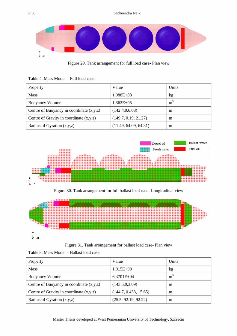
P 50 Sacheendra Naik
Master Thesis developed at West Pomeranian University of Technology, Szczecin
Figure 29. Tank arrangement for full load case- Plan view
Table 4. Mass Model – Full load case.
Property Value Units
Mass 1.088E+08 kg
Buoyancy Volume 1.362E+05 m3
Centre of Buoyancy in coordinate (x,y,z) (142.4,0,6.08) m
Centre of Gravity in coordinate (x,y,z) (149.7, 0.19, 21.27) m
Radius of Gyration (x,y,z) (11.49, 64.09, 64.31) m
Figure 30. Tank arrangement for full ballast load case- Longitudinal view
Figure 31. Tank arrangement for ballast load case- Plan view
Table 5. Mass Model – Ballast load case.
Property Value Units
Mass 1.015E+08 kg
Buoyancy Volume 6.3701E+04 m3
Centre of Buoyancy in coordinate (x,y,z) (143.5,0,3.09) m
Centre of Gravity in coordinate (x,y,z) (144.7, 0.433, 15.65) m
Radius of Gyration (x,y,z) (25.5, 92.19, 92.22) m
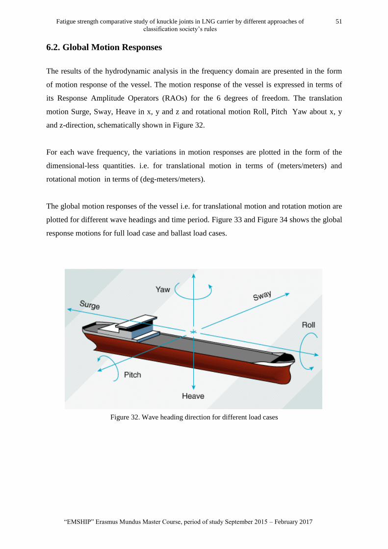
Fatigue strength comparative study of knuckle joints in LNG carrier by different approaches of
classification society‘s rules
51
―EMSHIP‖ Erasmus Mundus Master Course, period of study September 2015 – February 2017
6.2. Global Motion Responses
The results of the hydrodynamic analysis in the frequency domain are presented in the form
of motion response of the vessel. The motion response of the vessel is expressed in terms of
its Response Amplitude Operators (RAOs) for the 6 degrees of freedom. The translation
motion Surge, Sway, Heave in x, y and z and rotational motion Roll, Pitch Yaw about x, y
and z-direction, schematically shown in Figure 32.
For each wave frequency, the variations in motion responses are plotted in the form of the
dimensional-less quantities. i.e. for translational motion in terms of (meters/meters) and
rotational motion in terms of (deg-meters/meters).
The global motion responses of the vessel i.e. for translational motion and rotation motion are
plotted for different wave headings and time period. Figure 33 and Figure 34 shows the global
response motions for full load case and ballast load cases.
Figure 32. Wave heading direction for different load cases
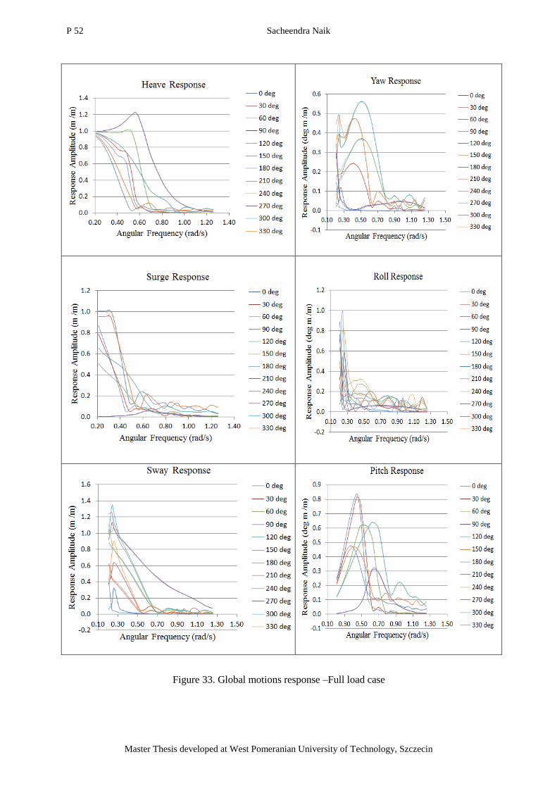
P 52 Sacheendra Naik
Master Thesis developed at West Pomeranian University of Technology, Szczecin
Figure 33. Global motions response –Full load case
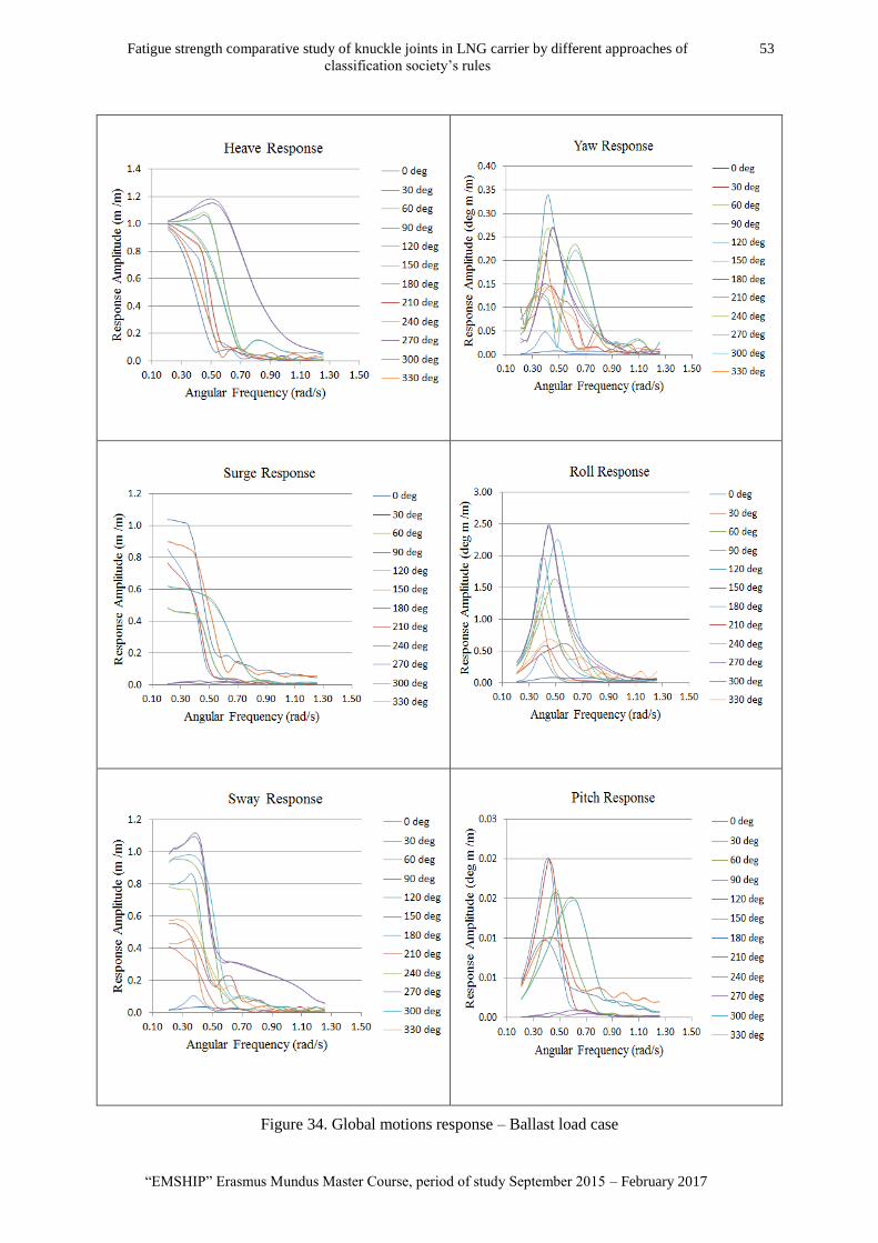
Fatigue strength comparative study of knuckle joints in LNG carrier by different approaches of
classification society‘s rules
53
―EMSHIP‖ Erasmus Mundus Master Course, period of study September 2015 – February 2017
Figure 34. Global motions response – Ballast load case
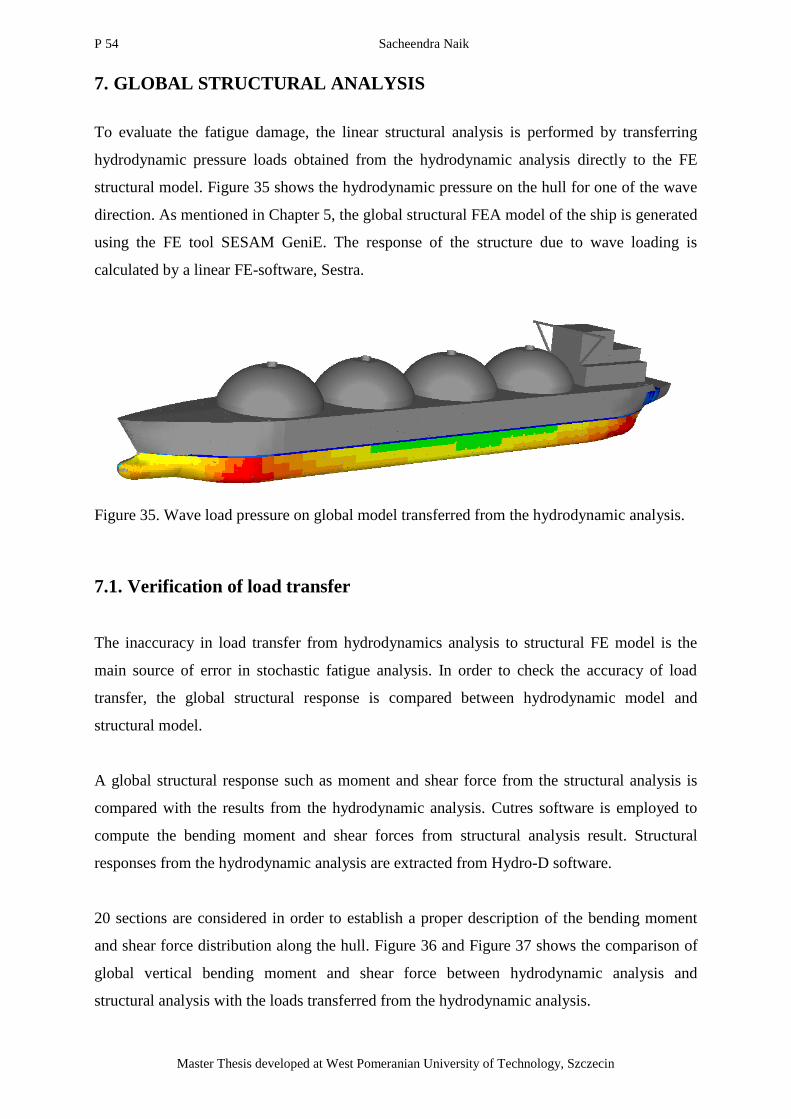
P 54 Sacheendra Naik
Master Thesis developed at West Pomeranian University of Technology, Szczecin
7. GLOBAL STRUCTURAL ANALYSIS
To evaluate the fatigue damage, the linear structural analysis is performed by transferring
hydrodynamic pressure loads obtained from the hydrodynamic analysis directly to the FE
structural model. Figure 35 shows the hydrodynamic pressure on the hull for one of the wave
direction. As mentioned in Chapter 5, the global structural FEA model of the ship is generated
using the FE tool SESAM GeniE. The response of the structure due to wave loading is
calculated by a linear FE-software, Sestra.
Figure 35. Wave load pressure on global model transferred from the hydrodynamic analysis.
7.1. Verification of load transfer
The inaccuracy in load transfer from hydrodynamics analysis to structural FE model is the
main source of error in stochastic fatigue analysis. In order to check the accuracy of load
transfer, the global structural response is compared between hydrodynamic model and
structural model.
A global structural response such as moment and shear force from the structural analysis is
compared with the results from the hydrodynamic analysis. Cutres software is employed to
compute the bending moment and shear forces from structural analysis result. Structural
responses from the hydrodynamic analysis are extracted from Hydro-D software.
20 sections are considered in order to establish a proper description of the bending moment
and shear force distribution along the hull. Figure 36 and Figure 37 shows the comparison of
global vertical bending moment and shear force between hydrodynamic analysis and
structural analysis with the loads transferred from the hydrodynamic analysis.
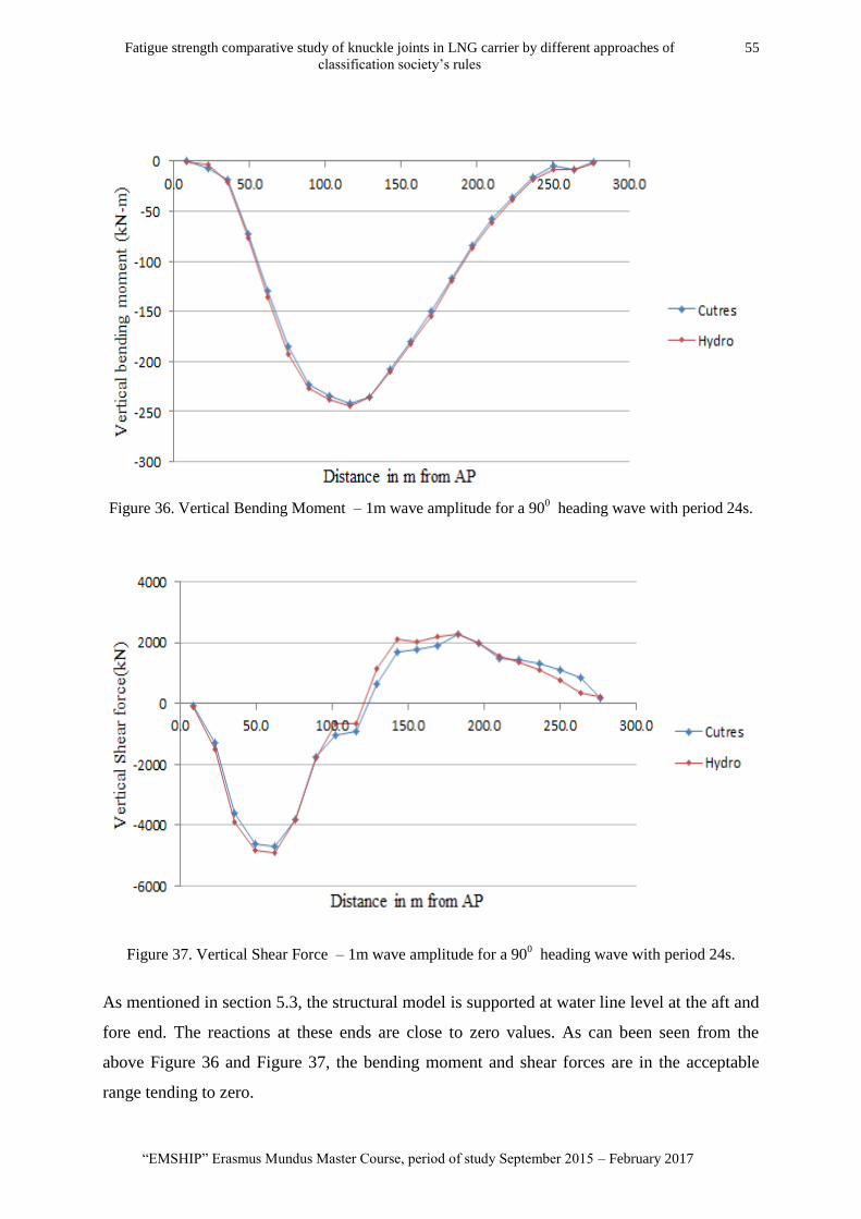
Fatigue strength comparative study of knuckle joints in LNG carrier by different approaches of
classification society‘s rules
55
―EMSHIP‖ Erasmus Mundus Master Course, period of study September 2015 – February 2017
Figure 36. Vertical Bending Moment – 1m wave amplitude for a 900 heading wave with period 24s.
Figure 37. Vertical Shear Force – 1m wave amplitude for a 900 heading wave with period 24s.
As mentioned in section 5.3, the structural model is supported at water line level at the aft and
fore end. The reactions at these ends are close to zero values. As can been seen from the
above Figure 36 and Figure 37, the bending moment and shear forces are in the acceptable
range tending to zero.
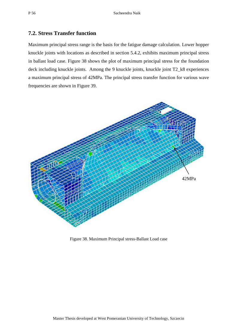
P 56 Sacheendra Naik
Master Thesis developed at West Pomeranian University of Technology, Szczecin
7.2. Stress Transfer function
Maximum principal stress range is the basis for the fatigue damage calculation. Lower hopper
knuckle joints with locations as described in section 5.4.2, exhibits maximum principal stress
in ballast load case. Figure 38 shows the plot of maximum principal stress for the foundation
deck including knuckle joints. Among the 9 knuckle joints, knuckle joint T2_k8 experiences
a maximum principal stress of 42MPa. The principal stress transfer function for various wave
frequencies are shown in Figure 39.
Figure 38. Maximum Principal stress-Ballast Load case
42MPa
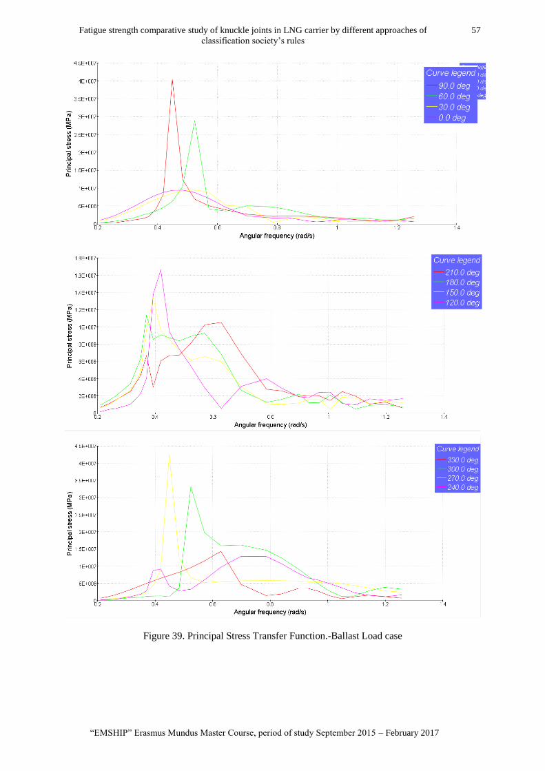
Fatigue strength comparative study of knuckle joints in LNG carrier by different approaches of
classification society‘s rules
57
―EMSHIP‖ Erasmus Mundus Master Course, period of study September 2015 – February 2017
Figure 39. Principal Stress Transfer Function.-Ballast Load case
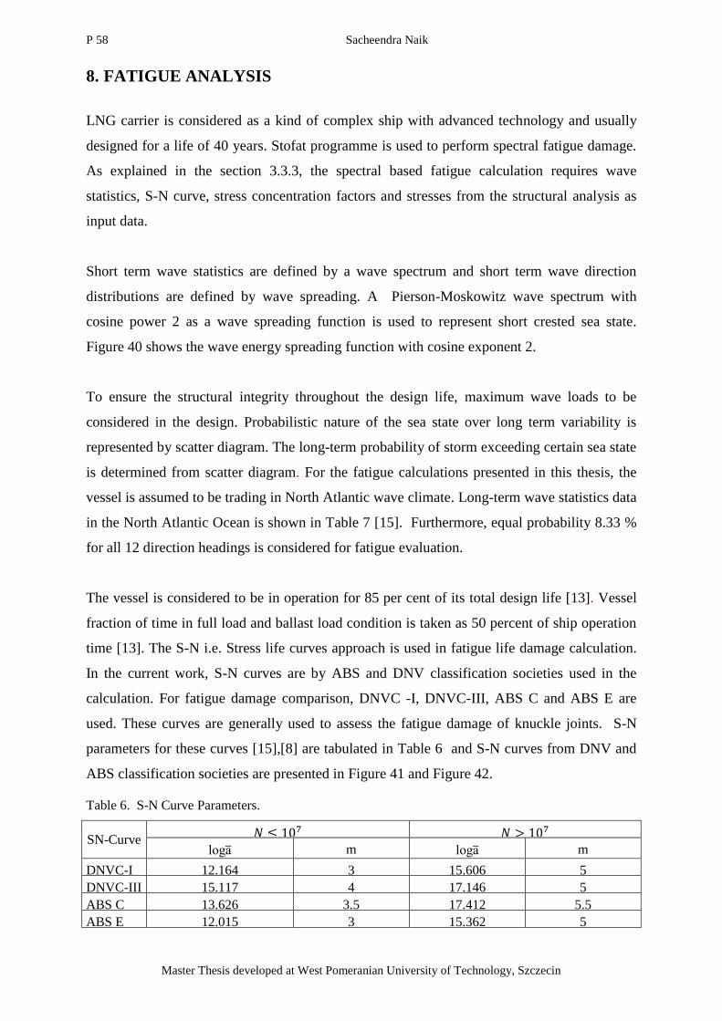
P 58 Sacheendra Naik
Master Thesis developed at West Pomeranian University of Technology, Szczecin
8. FATIGUE ANALYSIS
LNG carrier is considered as a kind of complex ship with advanced technology and usually
designed for a life of 40 years. Stofat programme is used to perform spectral fatigue damage.
As explained in the section 3.3.3, the spectral based fatigue calculation requires wave
statistics, S-N curve, stress concentration factors and stresses from the structural analysis as
input data.
Short term wave statistics are defined by a wave spectrum and short term wave direction
distributions are defined by wave spreading. A Pierson-Moskowitz wave spectrum with
cosine power 2 as a wave spreading function is used to represent short crested sea state.
Figure 40 shows the wave energy spreading function with cosine exponent 2.
To ensure the structural integrity throughout the design life, maximum wave loads to be
considered in the design. Probabilistic nature of the sea state over long term variability is
represented by scatter diagram. The long-term probability of storm exceeding certain sea state
is determined from scatter diagram. For the fatigue calculations presented in this thesis, the
vessel is assumed to be trading in North Atlantic wave climate. Long-term wave statistics data
in the North Atlantic Ocean is shown in Table 7 [15]. Furthermore, equal probability 8.33 %
for all 12 direction headings is considered for fatigue evaluation.
The vessel is considered to be in operation for 85 per cent of its total design life [13]. Vessel
fraction of time in full load and ballast load condition is taken as 50 percent of ship operation
time [13]. The S-N i.e. Stress life curves approach is used in fatigue life damage calculation.
In the current work, S-N curves are by ABS and DNV classification societies used in the
calculation. For fatigue damage comparison, DNVC -I, DNVC-III, ABS C and ABS E are
used. These curves are generally used to assess the fatigue damage of knuckle joints. S-N
parameters for these curves [15],[8] are tabulated in Table 6 and S-N curves from DNV and
ABS classification societies are presented in Figure 41 and Figure 42.
Table 6. S-N Curve Parameters.
SN-Curve
loga̅ m loga̅ m
DNVC-I 12.164 3 15.606 5
DNVC-III 15.117 4 17.146 5
ABS C 13.626 3.5 17.412 5.5
ABS E 12.015 3 15.362 5
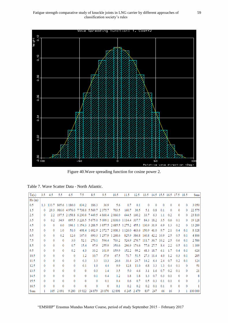
Fatigue strength comparative study of knuckle joints in LNG carrier by different approaches of
classification society‘s rules
59
―EMSHIP‖ Erasmus Mundus Master Course, period of study September 2015 – February 2017
Figure 40.Wave spreading function for cosine power 2.
Table 7. Wave Scatter Data - North Atlantic.
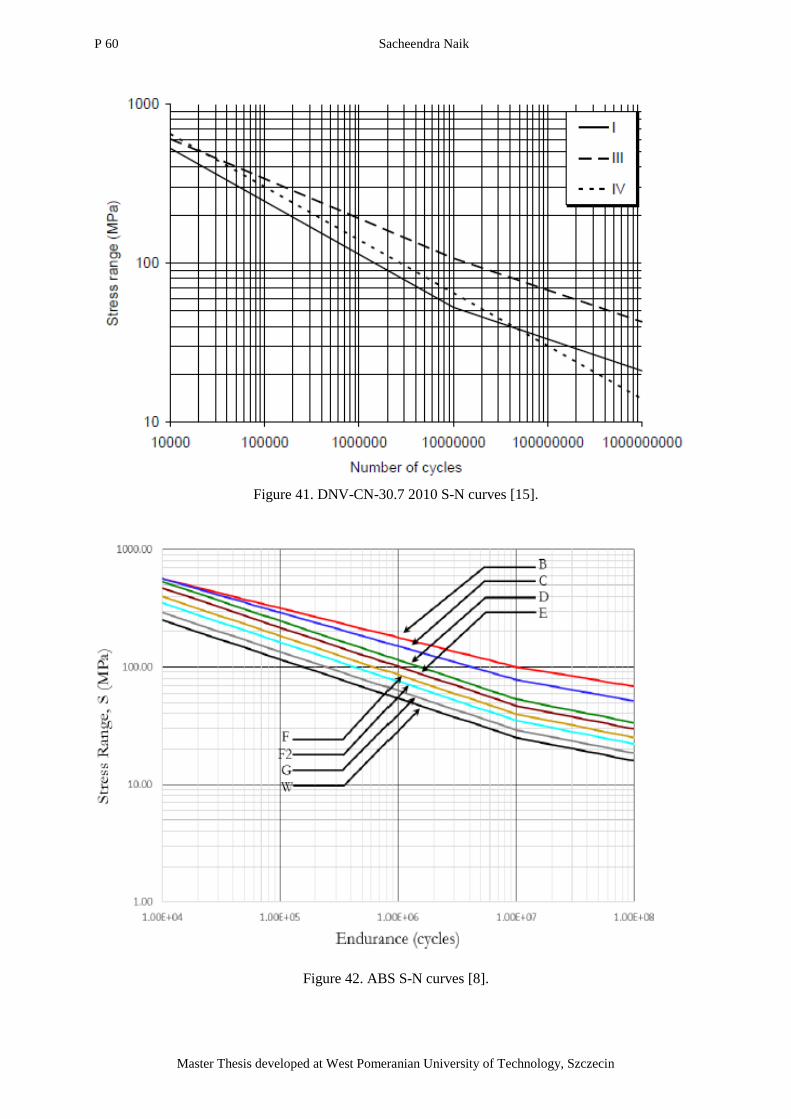
P 60 Sacheendra Naik
Master Thesis developed at West Pomeranian University of Technology, Szczecin
Figure 41. DNV-CN-30.7 2010 S-N curves [15].
Figure 42. ABS S-N curves [8].
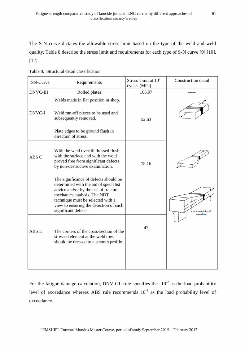
Fatigue strength comparative study of knuckle joints in LNG carrier by different approaches of
classification society‘s rules
61
―EMSHIP‖ Erasmus Mundus Master Course, period of study September 2015 – February 2017
The S-N curve dictates the allowable stress limit based on the type of the weld and weld
quality. Table 8 describe the stress limit and requirements for each type of S-N curve [9],[10],
[12].
Table 8. Structural detail classification
SN-Curve Requirements Stress limit at 107
cycles (MPa)
Construction detail
DNVC-III Rolled plates 106.97 -----
DNVC-I
Welds made in flat position in shop.
Weld run-off pieces to be used and
subsequently removed.
Plate edges to be ground flush in
direction of stress.
52.63
ABS C
With the weld overfill dressed flush
with the surface and with the weld
proved free from significant defects
by non-destructive examination.
The significance of defects should be
determined with the aid of specialist
advice and/or by the use of fracture
mechanics analysis. The NDT
technique must be selected with a
view to ensuring the detection of such
significant defects.
78.16
ABS E
The corners of the cross-section of the
stressed element at the weld toes
should be dressed to a smooth profile.
47
For the fatigue damage calculation, DNV GL rule specifies the 10-2
as the load probability
level of exceedance whereas ABS rule recommends 10-4
as the load probability level of
exceedance.
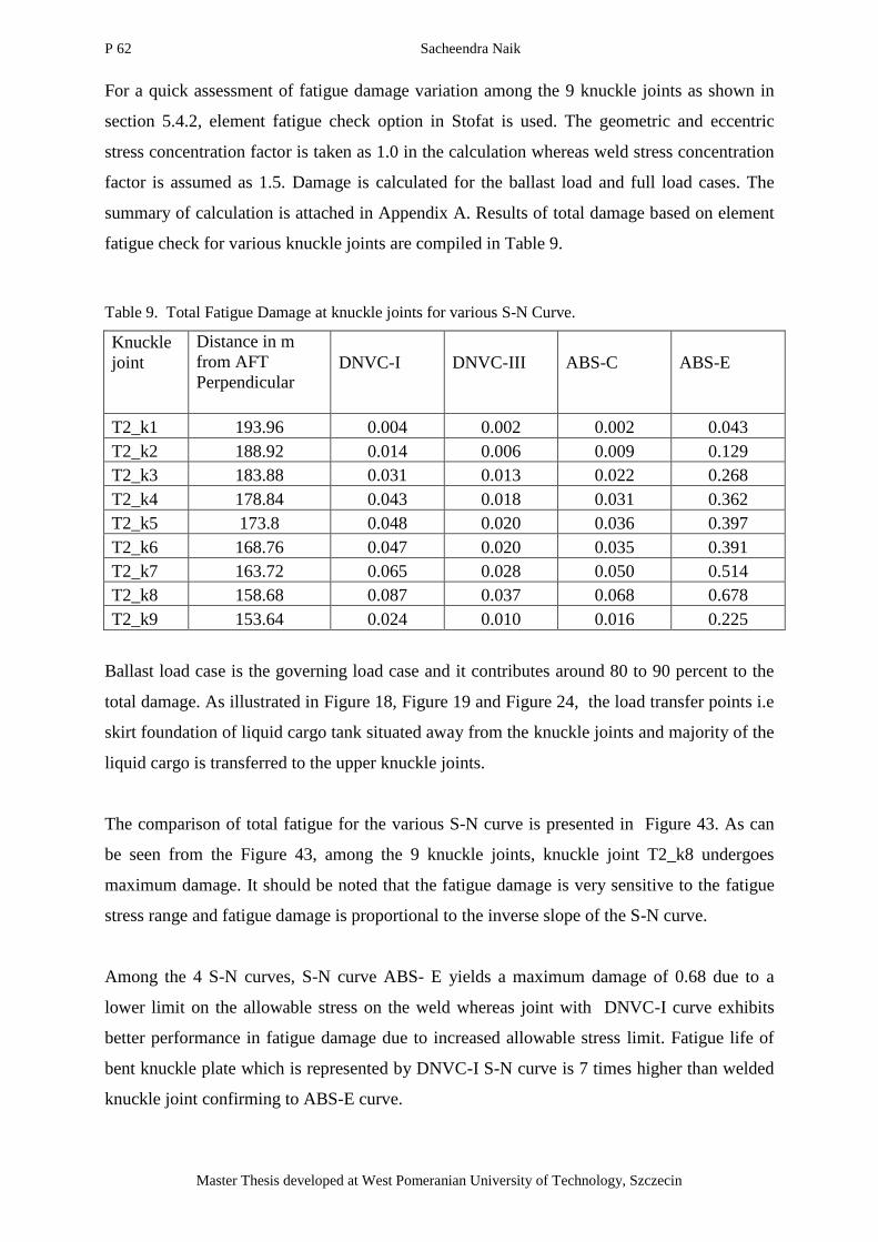
P 62 Sacheendra Naik
Master Thesis developed at West Pomeranian University of Technology, Szczecin
For a quick assessment of fatigue damage variation among the 9 knuckle joints as shown in
section 5.4.2, element fatigue check option in Stofat is used. The geometric and eccentric
stress concentration factor is taken as 1.0 in the calculation whereas weld stress concentration
factor is assumed as 1.5. Damage is calculated for the ballast load and full load cases. The
summary of calculation is attached in Appendix A. Results of total damage based on element
fatigue check for various knuckle joints are compiled in Table 9.
Table 9. Total Fatigue Damage at knuckle joints for various S-N Curve.
Knuckle
joint
Distance in m
from AFT
Perpendicular DNVC-I
DNVC-III
ABS-C
ABS-E
T2_k1 193.96 0.004 0.002 0.002 0.043
T2_k2 188.92 0.014 0.006 0.009 0.129
T2_k3 183.88 0.031 0.013 0.022 0.268
T2_k4 178.84 0.043 0.018 0.031 0.362
T2_k5 173.8 0.048 0.020 0.036 0.397
T2_k6 168.76 0.047 0.020 0.035 0.391
T2_k7 163.72 0.065 0.028 0.050 0.514
T2_k8 158.68 0.087 0.037 0.068 0.678
T2_k9 153.64 0.024 0.010 0.016 0.225
Ballast load case is the governing load case and it contributes around 80 to 90 percent to the
total damage. As illustrated in Figure 18, Figure 19 and Figure 24, the load transfer points i.e
skirt foundation of liquid cargo tank situated away from the knuckle joints and majority of the
liquid cargo is transferred to the upper knuckle joints.
The comparison of total fatigue for the various S-N curve is presented in Figure 43. As can
be seen from the Figure 43, among the 9 knuckle joints, knuckle joint T2_k8 undergoes
maximum damage. It should be noted that the fatigue damage is very sensitive to the fatigue
stress range and fatigue damage is proportional to the inverse slope of the S-N curve.
Among the 4 S-N curves, S-N curve ABS- E yields a maximum damage of 0.68 due to a
lower limit on the allowable stress on the weld whereas joint with DNVC-I curve exhibits
better performance in fatigue damage due to increased allowable stress limit. Fatigue life of
bent knuckle plate which is represented by DNVC-I S-N curve is 7 times higher than welded
knuckle joint confirming to ABS-E curve.
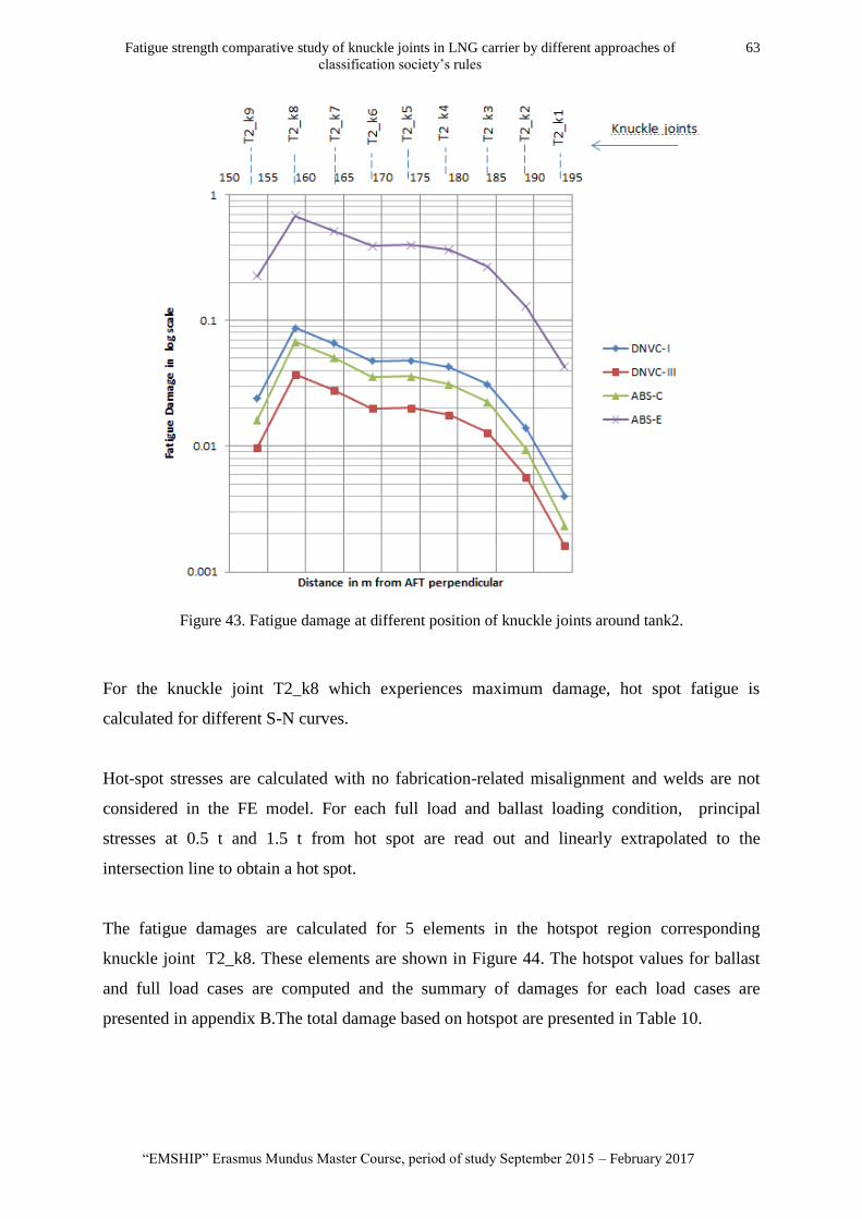
Fatigue strength comparative study of knuckle joints in LNG carrier by different approaches of
classification society‘s rules
63
―EMSHIP‖ Erasmus Mundus Master Course, period of study September 2015 – February 2017
Figure 43. Fatigue damage at different position of knuckle joints around tank2.
For the knuckle joint T2_k8 which experiences maximum damage, hot spot fatigue is
calculated for different S-N curves.
Hot-spot stresses are calculated with no fabrication-related misalignment and welds are not
considered in the FE model. For each full load and ballast loading condition, principal
stresses at 0.5 t and 1.5 t from hot spot are read out and linearly extrapolated to the
intersection line to obtain a hot spot.
The fatigue damages are calculated for 5 elements in the hotspot region corresponding
knuckle joint T2_k8. These elements are shown in Figure 44. The hotspot values for ballast
and full load cases are computed and the summary of damages for each load cases are
presented in appendix B.The total damage based on hotspot are presented in Table 10.
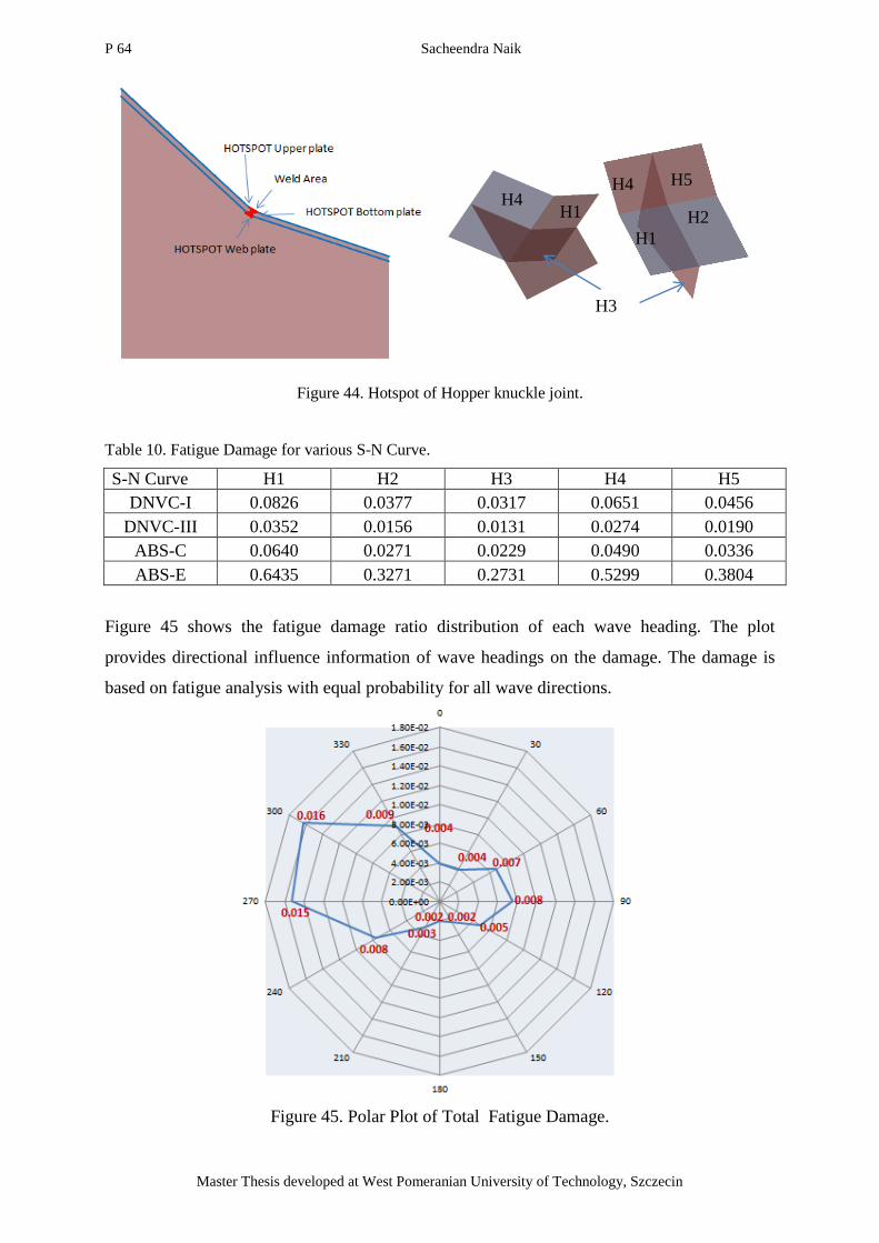
P 64 Sacheendra Naik
Master Thesis developed at West Pomeranian University of Technology, Szczecin
Figure 44. Hotspot of Hopper knuckle joint.
Table 10. Fatigue Damage for various S-N Curve.
S-N Curve H1
H2
H3
H4
H5
DNVC-I 0.0826 0.0377 0.0317 0.0651 0.0456
DNVC-III 0.0352 0.0156 0.0131 0.0274 0.0190
ABS-C 0.0640 0.0271 0.0229 0.0490 0.0336
ABS-E 0.6435 0.3271 0.2731 0.5299 0.3804
Figure 45 shows the fatigue damage ratio distribution of each wave heading. The plot
provides directional influence information of wave headings on the damage. The damage is
based on fatigue analysis with equal probability for all wave directions.
Figure 45. Polar Plot of Total Fatigue Damage.
H3
H1
H2
H5 H4
H1 H4
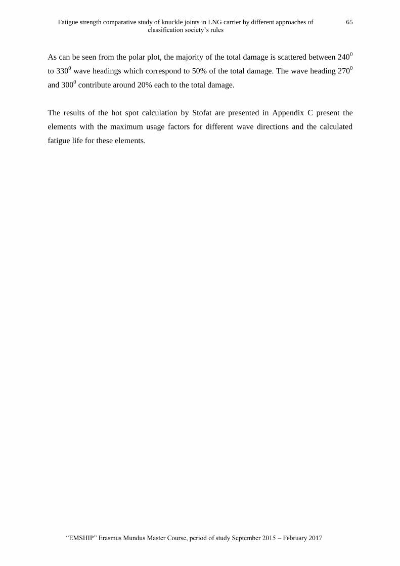
Fatigue strength comparative study of knuckle joints in LNG carrier by different approaches of
classification society‘s rules
65
―EMSHIP‖ Erasmus Mundus Master Course, period of study September 2015 – February 2017
As can be seen from the polar plot, the majority of the total damage is scattered between 2400
to 3300 wave headings which correspond to 50% of the total damage. The wave heading 270
0
and 3000 contribute around 20% each to the total damage.
The results of the hot spot calculation by Stofat are presented in Appendix C present the
elements with the maximum usage factors for different wave directions and the calculated
fatigue life for these elements.
P 66 Sacheendra Naik
Master Thesis developed at West Pomeranian University of Technology, Szczecin
9. CONCLUSIONS AND RECOMMENDATIONS
North Atlantic Ocean is known for its harsh environment and the vessels operating in this
region requires strict design requirement in order to have good fatigue strength. Hopper
knuckle joints are the most critical joints susceptibility to fatigue failure due to high stress
concentration. Due to cargo containment system, the area is inaccessible for inspection and
repair. Knuckle joints exposed to a more complex stress response, full stochastic fatigue
calculations based on using direct wave load analysis significantly increase the reliability of
the results. The detailed computational procedures of a stochastic spectral approach for
calculating fatigue damage ratios are illustrated in this thesis, and the method has been
applied in predicting the fatigue life of hopper knuckle joint in a Moss type spherical tank
LNG carrier.
A linear structural FE-analysis of the entire vessel is performed by transferring hydrodynamic
loads directly onto the global model. Local or sub model with fine mesh for critical knuckle
joint is analyzed with boundary displacements from global model and followed by a fatigue
analysis using hotspot approach. The predicted fatigue damage ratio based on hot spot stress
is compared using different S-N curves DNVC-I, DNVC-III, ABS–C and ABS-E. The
following salient conclusions are drawn from the thesis work:
1. Influence of different wave directions related to stress transfer function from FE structural
analysis is studied to find the most critical wave direction. This study reveals that the
magnitude of the stress transfer function varies depending on the wave direction. For the
hopper knuckle joints considered in this study, maximum stress transfer function occurs at
2700 and the magnitude of maximum principal stress is around 42 MPa.
2. Furthermore, for the hopper knuckle joints studied in this thesis, ballast load case
contributes around 85 to 90 % to the total fatigue damage. The contribution from full load
case is around 10 to 15 % depending on the location of knuckle joints. This is due to the
location load transfer points i.e., skirt foundation which transfer loads from liquid cargo to
tank foundation is located away from the knuckle joints under study.
3. The majority of the total damage is scattered between 2400 to 330
0 wave headings which
correspond to 50% of the total damage. The wave heading 2700 and 300
0 contribute around
20% each to the total damage.

Fatigue strength comparative study of knuckle joints in LNG carrier by different approaches of
classification society‘s rules
67
―EMSHIP‖ Erasmus Mundus Master Course, period of study September 2015 – February 2017
4. Fatigue damage ratio comparison among different S-N curves shows joint with the S-N
curve having highest allowable stress range exhibits better fatigue life i.e., low fatigue
damage ratio. For the joints under current study, results reveal that the bent knuckle joint
from rolled plate shows better fatigue life in comparison with welded joint. Fatigue life of
bent knuckle plate is 7 times higher than welded knuckle joint confirming to ABS-E curve
requirements.
5. The fatigue calculation involves variables such as S-N curve, wave scatter data, and wave
spectrum. One of the design variable i.e., the S-N curve is used for the parametric study
and the damage ratio result reflects the fatigue life which has a direct consequence on the
weld preparation quality and inspection category. Higher weld quality and stringent
inspection type results in increased fatigue life.
Due to the limited time, the fatigue damage study focused only on direct calculation method
based on the linear FE analysis. However, the following points are recommended for the
future work:
1. Though the fatigue damage assessment by stochastic spectral fatigue yields reliable results
but involves time-consuming computational procedures. The equivalent design wave
method may be used to assess the fatigue damage at the preliminary design stages. The
comparison of damages against the spectral fatigue gives the factor of safety embedded in
the equivalent design approach. However, the DNV GL classification society requires
fatigue limit state on a critical area such as hopper knuckle joints should be assessed by
directly calculated loads. The equivalent design wave approach at the preliminary design
stage of the project can be used to identify the critical fatigue locations in the vessel.
2. Welds are ignored in the current fatigue analysis and the effect of the weld can be
considered to account for tensile residual stresses from welding which will further decrease
the fatigue life.
3. The variables involved in the fatigue design subjected to significant uncertainty and hence
the resulting fatigue damage assessment is also associated with large uncertainties. The
calculated loads on the vessel are uncertain due to the stochastic nature of the wave loads
and uncertainties in the sailing route. Furthermore, uncertainties associated in FE
P 68 Sacheendra Naik
Master Thesis developed at West Pomeranian University of Technology, Szczecin
modelling, the evaluation of stress concentration, local weld geometry, initial
imperfections will attribute to the uncertainties in the calculated fatigue life of s structural
detail. A reliability-based fatigue assessment should be carried out directly through a
stochastic modelling of these uncertain variables.
Fatigue strength comparative study of knuckle joints in LNG carrier by different approaches of
classification society‘s rules
69
―EMSHIP‖ Erasmus Mundus Master Course, period of study September 2015 – February 2017
ACKNOWLEDGEMENTS
First of all, I would like to thank Prof. Philippe Rigo from University de Liege (ULg) as
coordinator of the EMSHIP program and Prof. Maciej Taczała from West Pomeranian
University of Technology Szczecin (ZUT), as local coordinators of EMSHIP program in
Poland. I thank them for their technical guidance and help on academic and administrative
issues. I would like also to mention that I would be grateful for the guidance and feedback
from Prof Maciej Taczala from ZUT as my master thesis supervisor.
As this master thesis was partly developed in Westcon Design Poland office in Szczecin
(Poland), I would like to pass on my sincere regards to Dr Jazukiewicz Alfred for furnishing
technical details. I would also like to mention a word of gratitude for Dr.Lech Tamborski for
his valuable advice on hydrodynamic analysis.
This thesis was developed in the frame of the European Master Course in ―Integrated
Advanced Ship Design‖ named ―EMSHIP‖ for ―European Education in Advanced Ship
Design‖, Ref.: 159652-1-2009-1-BE-ERA MUNDUS-EMMC.
P 70 Sacheendra Naik
Master Thesis developed at West Pomeranian University of Technology, Szczecin
REFERENCES
[1] S. Valsgård, T. K. Østvold, O. Rognebakke, E. Byklum, and H. O. Sele, 2006. Gas carrier
development for an expanding market. ICSOT 2006: Design, Construction & Operation
of Natural Gas Carriers & Offshore Systems, Korea.
[2] Central Commission for the Navigation of the Rhine and Oil Companies International
Marine Forum, 2010. International Safety Guide for Inland Navigation Tank-barges and
Terminals. Strasbourg Cedex: Central Commission for the Navigation of the Rhine.
[3] A. Almar Naes, 1985. Fatigue Handbook: offshore steel structures. Trondheim, Norway:
Tapir Publishers.
[4] N.E. Dowling, 2007. Mechanical Behaviour of Materials. Third edition, Pearson: Prentice
Hall.
[5] Dr. Dominique Beghin, 2006.Fatigue of Ship structural details. SNAME Technical and
research bulletin 2-31.
[6] DNVGL-Rules for classification: Ships, 2016. Part5 Ship types, Chapter 7 Liquefied gas
tankers
[7] DNVGL-CG-0127, 2016. Class guideline- Finite element analysis
[8] ABS,2016. Guide for spectral-based fatigue analysis for vessels.
[9] ABS,2016. Rules for Building and classification-Steel vessels, Part 5C Specific Vessel
Types
[10] ABS,2014. Guide for Fatigue Assessment of Offshore Structures
[11] DNVGL-CG-0129, 2015 . Class guideline- Fatigue assessment of ship structures.
[12] DNVGL-RP-0005,2014. Recommended practice, Fatigue design of offshore steel
structures.
[13] DNVGL- Rules for classification, 2016. Part 3 Hull, Chapter 9 Fatigue.
[14] DNV Classification Notes - No. 34.1, 2013. CSA - Direct Analysis of Ship Structures
[15] DNV Classification Notes - No. 30.7, 2014. Fatigue Assessment of Ship Structures
[16] DNV 2014. SESAM User Manual Genie: Concept design and analysis of offshore
structures. Version 6.9.
[17] DNV 2013. SESAM User Manual Sestra: Superelement Structure Analysis. Version 8.3.
[18] DNV GL SESAM Hydro-D user manual Wasim: Wave Loads on vessels with Forward
Speed. Version 5.3.
[19] DNV 2011.V SESAM Xtract user manual: Postprocessor for Presentation, Animation
and Reporting of Results. Version 3.0.

Fatigue strength comparative study of knuckle joints in LNG carrier by different approaches of
classification society‘s rules
71
―EMSHIP‖ Erasmus Mundus Master Course, period of study September 2015 – February 2017
[20] DNV GL 2016.SESAM Submod user manual: Transfer Displacements from Global
Model to Sub-Model. Version 3.0.
[21] DNV 1994. SESAM Cutres user manual: Presentation of Sectional Results, Version 1.2.
[22] DNV GL 2016.SESAM Stofat user manual: Fatigue Damage Calculation of Welded
Plates and Shells. Version 3.7-05.
[23] http://shipmind.net/gas-carriers- Pictures for tank types
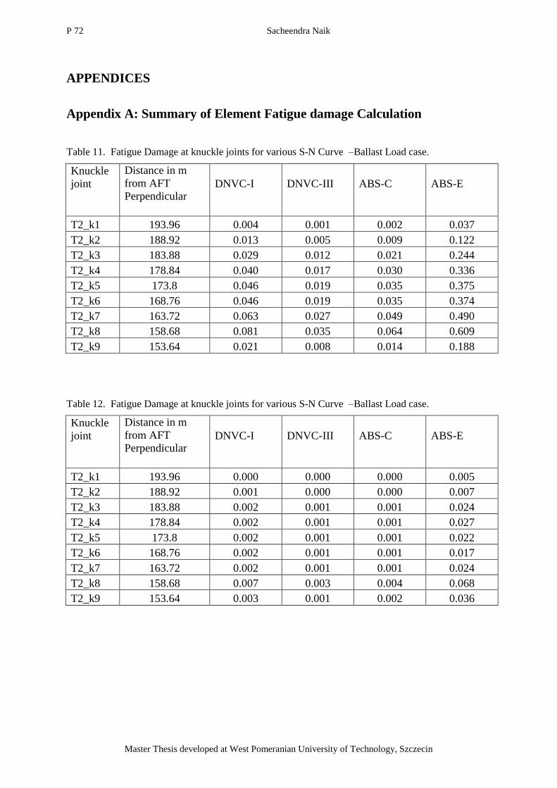
P 72 Sacheendra Naik
Master Thesis developed at West Pomeranian University of Technology, Szczecin
APPENDICES
Appendix A: Summary of Element Fatigue damage Calculation
Table 11. Fatigue Damage at knuckle joints for various S-N Curve –Ballast Load case.
Knuckle
joint
Distance in m
from AFT
Perpendicular DNVC-I
DNVC-III
ABS-C
ABS-E
T2_k1 193.96 0.004 0.001 0.002 0.037
T2_k2 188.92 0.013 0.005 0.009 0.122
T2_k3 183.88 0.029 0.012 0.021 0.244
T2_k4 178.84 0.040 0.017 0.030 0.336
T2_k5 173.8 0.046 0.019 0.035 0.375
T2_k6 168.76 0.046 0.019 0.035 0.374
T2_k7 163.72 0.063 0.027 0.049 0.490
T2_k8 158.68 0.081 0.035 0.064 0.609
T2_k9 153.64 0.021 0.008 0.014 0.188
Table 12. Fatigue Damage at knuckle joints for various S-N Curve –Ballast Load case.
Knuckle
joint
Distance in m
from AFT
Perpendicular DNVC-I
DNVC-III
ABS-C
ABS-E
T2_k1 193.96 0.000 0.000 0.000 0.005
T2_k2 188.92 0.001 0.000 0.000 0.007
T2_k3 183.88 0.002 0.001 0.001 0.024
T2_k4 178.84 0.002 0.001 0.001 0.027
T2_k5 173.8 0.002 0.001 0.001 0.022
T2_k6 168.76 0.002 0.001 0.001 0.017
T2_k7 163.72 0.002 0.001 0.001 0.024
T2_k8 158.68 0.007 0.003 0.004 0.068
T2_k9 153.64 0.003 0.001 0.002 0.036
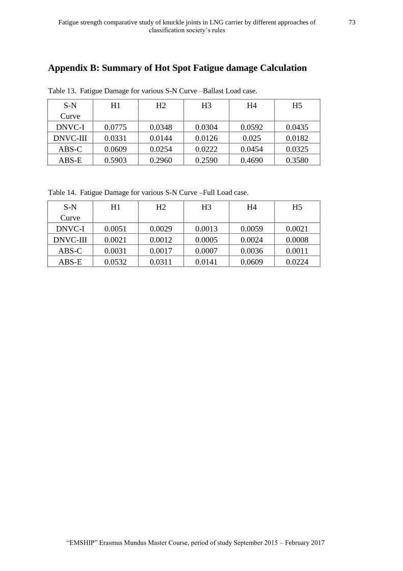
Fatigue strength comparative study of knuckle joints in LNG carrier by different approaches of
classification society‘s rules
73
―EMSHIP‖ Erasmus Mundus Master Course, period of study September 2015 – February 2017
Appendix B: Summary of Hot Spot Fatigue damage Calculation
Table 13. Fatigue Damage for various S-N Curve –Ballast Load case.
S-N H1 H2 H3 H4 H5
Curve
DNVC-I 0.0775 0.0348 0.0304 0.0592 0.0435
DNVC-III 0.0331 0.0144 0.0126 0.025 0.0182
ABS-C 0.0609 0.0254 0.0222 0.0454 0.0325
ABS-E 0.5903 0.2960 0.2590 0.4690 0.3580
Table 14. Fatigue Damage for various S-N Curve –Full Load case.
S-N H1 H2 H3 H4 H5
Curve
DNVC-I 0.0051 0.0029 0.0013 0.0059 0.0021
DNVC-III 0.0021 0.0012 0.0005 0.0024 0.0008
ABS-C 0.0031 0.0017 0.0007 0.0036 0.0011
ABS-E 0.0532 0.0311 0.0141 0.0609 0.0224
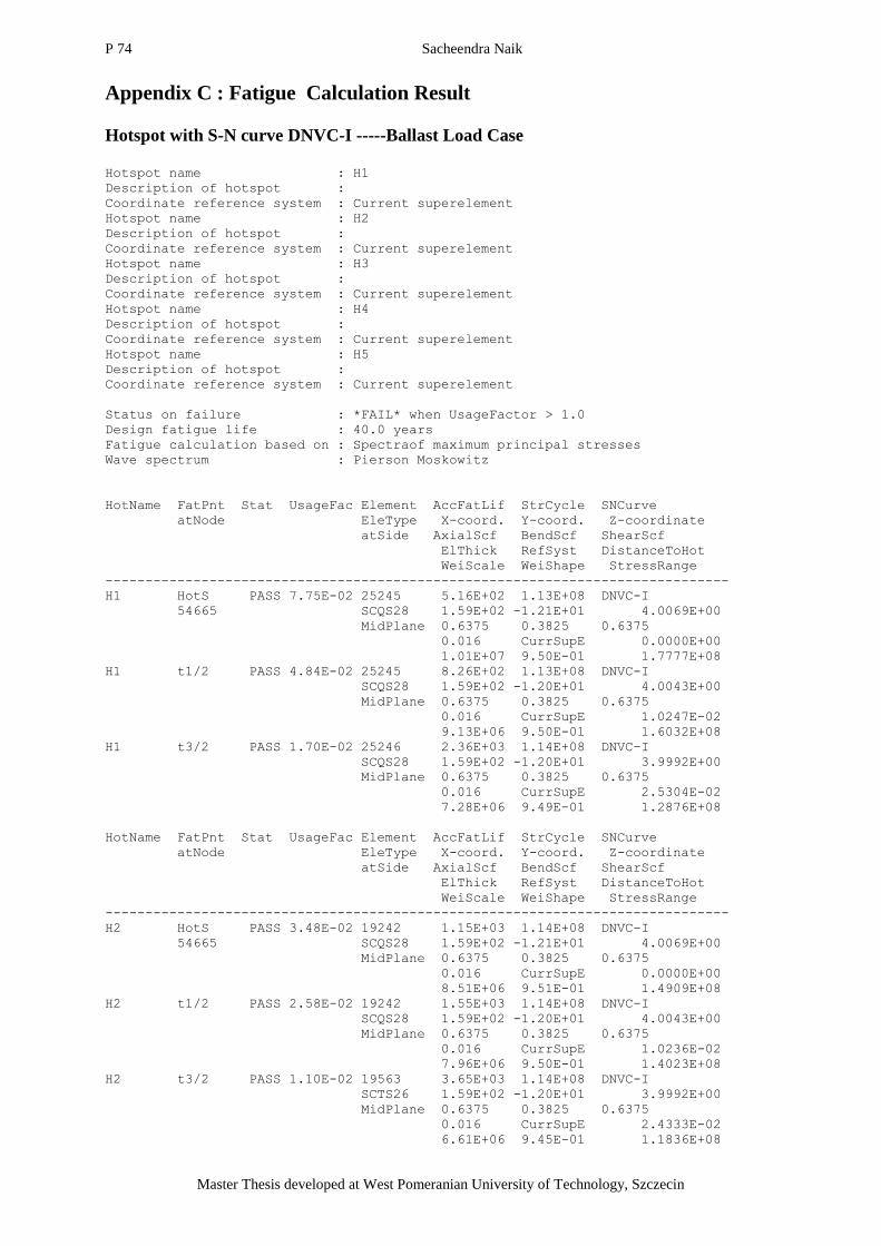
P 74 Sacheendra Naik
Master Thesis developed at West Pomeranian University of Technology, Szczecin
Appendix C : Fatigue Calculation Result
Hotspot with S-N curve DNVC-I -----Ballast Load Case
Hotspot name : H1
Description of hotspot :
Coordinate reference system : Current superelement
Hotspot name : H2
Description of hotspot :
Coordinate reference system : Current superelement
Hotspot name : H3
Description of hotspot :
Coordinate reference system : Current superelement
Hotspot name : H4
Description of hotspot :
Coordinate reference system : Current superelement
Hotspot name : H5
Description of hotspot :
Coordinate reference system : Current superelement
Status on failure : *FAIL* when UsageFactor > 1.0
Design fatigue life : 40.0 years
Fatigue calculation based on : Spectraof maximum principal stresses
Wave spectrum : Pierson Moskowitz
HotName FatPnt Stat UsageFac Element AccFatLif StrCycle SNCurve
atNode EleType X-coord. Y-coord. Z-coordinate
atSide AxialScf BendScf ShearScf
ElThick RefSyst DistanceToHot
WeiScale WeiShape StressRange
------------------------------------------------------------------------------
H1 HotS PASS 7.75E-02 25245 5.16E+02 1.13E+08 DNVC-I
54665 SCQS28 1.59E+02 -1.21E+01 4.0069E+00
MidPlane 0.6375 0.3825 0.6375
0.016 CurrSupE 0.0000E+00
1.01E+07 9.50E-01 1.7777E+08
H1 t1/2 PASS 4.84E-02 25245 8.26E+02 1.13E+08 DNVC-I
SCQS28 1.59E+02 -1.20E+01 4.0043E+00
MidPlane 0.6375 0.3825 0.6375
0.016 CurrSupE 1.0247E-02
9.13E+06 9.50E-01 1.6032E+08
H1 t3/2 PASS 1.70E-02 25246 2.36E+03 1.14E+08 DNVC-I
SCQS28 1.59E+02 -1.20E+01 3.9992E+00
MidPlane 0.6375 0.3825 0.6375
0.016 CurrSupE 2.5304E-02
7.28E+06 9.49E-01 1.2876E+08
HotName FatPnt Stat UsageFac Element AccFatLif StrCycle SNCurve
atNode EleType X-coord. Y-coord. Z-coordinate
atSide AxialScf BendScf ShearScf
ElThick RefSyst DistanceToHot
WeiScale WeiShape StressRange
------------------------------------------------------------------------------
H2 HotS PASS 3.48E-02 19242 1.15E+03 1.14E+08 DNVC-I
54665 SCQS28 1.59E+02 -1.21E+01 4.0069E+00
MidPlane 0.6375 0.3825 0.6375
0.016 CurrSupE 0.0000E+00
8.51E+06 9.51E-01 1.4909E+08
H2 t1/2 PASS 2.58E-02 19242 1.55E+03 1.14E+08 DNVC-I
SCQS28 1.59E+02 -1.20E+01 4.0043E+00
MidPlane 0.6375 0.3825 0.6375
0.016 CurrSupE 1.0236E-02
7.96E+06 9.50E-01 1.4023E+08
H2 t3/2 PASS 1.10E-02 19563 3.65E+03 1.14E+08 DNVC-I
SCTS26 1.59E+02 -1.20E+01 3.9992E+00
MidPlane 0.6375 0.3825 0.6375
0.016 CurrSupE 2.4333E-02
6.61E+06 9.45E-01 1.1836E+08
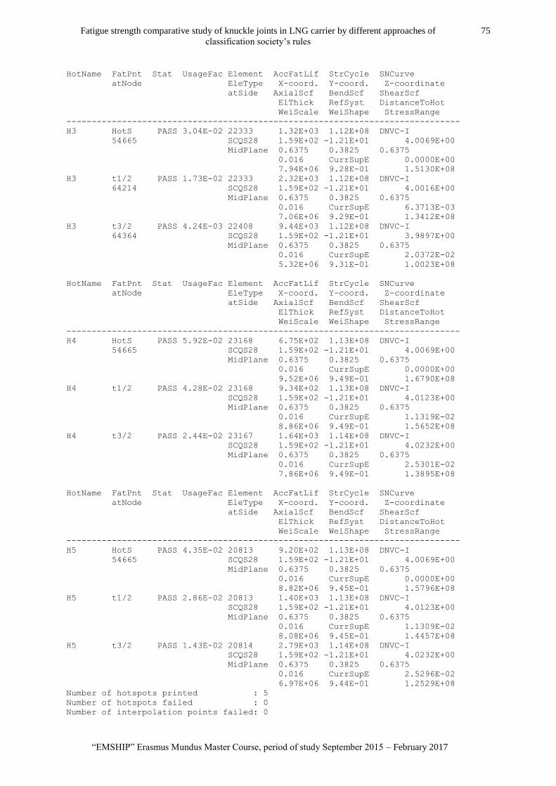
Fatigue strength comparative study of knuckle joints in LNG carrier by different approaches of
classification society‘s rules
75
―EMSHIP‖ Erasmus Mundus Master Course, period of study September 2015 – February 2017
HotName FatPnt Stat UsageFac Element AccFatLif StrCycle SNCurve
atNode EleType X-coord. Y-coord. Z-coordinate
atSide AxialScf BendScf ShearScf
ElThick RefSyst DistanceToHot
WeiScale WeiShape StressRange
------------------------------------------------------------------------------
H3 HotS PASS 3.04E-02 22333 1.32E+03 1.12E+08 DNVC-I
54665 SCQS28 1.59E+02 -1.21E+01 4.0069E+00
MidPlane 0.6375 0.3825 0.6375
0.016 CurrSupE 0.0000E+00
7.94E+06 9.28E-01 1.5130E+08
H3 t1/2 PASS 1.73E-02 22333 2.32E+03 1.12E+08 DNVC-I
64214 SCQS28 1.59E+02 -1.21E+01 4.0016E+00
MidPlane 0.6375 0.3825 0.6375
0.016 CurrSupE 6.3713E-03
7.06E+06 9.29E-01 1.3412E+08
H3 t3/2 PASS 4.24E-03 22408 9.44E+03 1.12E+08 DNVC-I
64364 SCQS28 1.59E+02 -1.21E+01 3.9897E+00
MidPlane 0.6375 0.3825 0.6375
0.016 CurrSupE 2.0372E-02
5.32E+06 9.31E-01 1.0023E+08
HotName FatPnt Stat UsageFac Element AccFatLif StrCycle SNCurve
atNode EleType X-coord. Y-coord. Z-coordinate
atSide AxialScf BendScf ShearScf
ElThick RefSyst DistanceToHot
WeiScale WeiShape StressRange
------------------------------------------------------------------------------
H4 HotS PASS 5.92E-02 23168 6.75E+02 1.13E+08 DNVC-I
54665 SCQS28 1.59E+02 -1.21E+01 4.0069E+00
MidPlane 0.6375 0.3825 0.6375
0.016 CurrSupE 0.0000E+00
9.52E+06 9.49E-01 1.6790E+08
H4 t1/2 PASS 4.28E-02 23168 9.34E+02 1.13E+08 DNVC-I
SCQS28 1.59E+02 -1.21E+01 4.0123E+00
MidPlane 0.6375 0.3825 0.6375
0.016 CurrSupE 1.1319E-02
8.86E+06 9.49E-01 1.5652E+08
H4 t3/2 PASS 2.44E-02 23167 1.64E+03 1.14E+08 DNVC-I
SCQS28 1.59E+02 -1.21E+01 4.0232E+00
MidPlane 0.6375 0.3825 0.6375
0.016 CurrSupE 2.5301E-02
7.86E+06 9.49E-01 1.3895E+08
HotName FatPnt Stat UsageFac Element AccFatLif StrCycle SNCurve
atNode EleType X-coord. Y-coord. Z-coordinate
atSide AxialScf BendScf ShearScf
ElThick RefSyst DistanceToHot
WeiScale WeiShape StressRange
------------------------------------------------------------------------------
H5 HotS PASS 4.35E-02 20813 9.20E+02 1.13E+08 DNVC-I
54665 SCQS28 1.59E+02 -1.21E+01 4.0069E+00
MidPlane 0.6375 0.3825 0.6375
0.016 CurrSupE 0.0000E+00
8.82E+06 9.45E-01 1.5796E+08
H5 t1/2 PASS 2.86E-02 20813 1.40E+03 1.13E+08 DNVC-I
SCQS28 1.59E+02 -1.21E+01 4.0123E+00
MidPlane 0.6375 0.3825 0.6375
0.016 CurrSupE 1.1309E-02
8.08E+06 9.45E-01 1.4457E+08
H5 t3/2 PASS 1.43E-02 20814 2.79E+03 1.14E+08 DNVC-I
SCQS28 1.59E+02 -1.21E+01 4.0232E+00
MidPlane 0.6375 0.3825 0.6375
0.016 CurrSupE 2.5296E-02
6.97E+06 9.44E-01 1.2529E+08
Number of hotspots printed : 5
Number of hotspots failed : 0
Number of interpolation points failed: 0
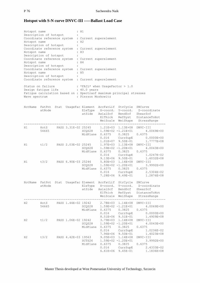
P 76 Sacheendra Naik
Master Thesis developed at West Pomeranian University of Technology, Szczecin
Hotspot with S-N curve DNVC-III -----Ballast Load Case
Hotspot name : H1
Description of hotspot :
Coordinate reference system : Current superelement
Hotspot name : H2
Description of hotspot :
Coordinate reference system : Current superelement
Hotspot name : H3
Description of hotspot :
Coordinate reference system : Current superelement
Hotspot name : H4
Description of hotspot :
Coordinate reference system : Current superelement
Hotspot name : H5
Description of hotspot :
Coordinate reference system : Current superelement
Status on failure : *FAIL* when UsageFactor > 1.0
Design fatigue life : 40.0 years
Fatigue calculation based on : Spectraof maximum principal stresses
Wave spectrum : Pierson Moskowitz
HotName FatPnt Stat UsageFac Element AccFatLif StrCycle SNCurve
atNode EleType X-coord. Y-coord. Z-coordinate
atSide AxialScf BendScf ShearScf
ElThick RefSyst DistanceToHot
WeiScale WeiShape StressRange
------------------------------------------------------------------------------
H1 HotS PASS 3.31E-02 25245 1.21E+03 1.13E+08 DNVC-III
54665 SCQS28 1.59E+02 -1.21E+01 4.0069E+00
MidPlane 0.6375 0.3825 0.6375
0.016 CurrSupE 0.0000E+00
1.01E+07 9.50E-01 1.7777E+08
H1 t1/2 PASS 2.03E-02 25245 1.97E+03 1.13E+08 DNVC-III
SCQS28 1.59E+02 -1.20E+01 4.0043E+00
MidPlane 0.6375 0.3825 0.6375
0.016 CurrSupE 1.0247E-02
9.13E+06 9.50E-01 1.6032E+08
H1 t3/2 PASS 6.90E-03 25246 5.80E+03 1.14E+08 DNVC-III
SCQS28 1.59E+02 -1.20E+01 3.9992E+00
MidPlane 0.6375 0.3825 0.6375
0.016 CurrSupE 2.5304E-02
7.28E+06 9.49E-01 1.2876E+08
HotName FatPnt Stat UsageFac Element AccFatLif StrCycle SNCurve
atNode EleType X-coord. Y-coord. Z-coordinate
atSide AxialScf BendScf ShearScf
ElThick RefSyst DistanceToHot
WeiScale WeiShape StressRange
------------------------------------------------------------------------------
H2 HotS PASS 1.44E-02 19242 2.78E+03 1.14E+08 DNVC-III
54665 SCQS28 1.59E+02 -1.21E+01 4.0069E+00
MidPlane 0.6375 0.3825 0.6375
0.016 CurrSupE 0.0000E+00
8.51E+06 9.51E-01 1.4909E+08
H2 t1/2 PASS 1.06E-02 19242 3.79E+03 1.14E+08 DNVC-III
SCQS28 1.59E+02 -1.20E+01 4.0043E+00
MidPlane 0.6375 0.3825 0.6375
0.016 CurrSupE 1.0236E-02
7.96E+06 9.50E-01 1.4023E+08
H2 t3/2 PASS 4.42E-03 19563 9.05E+03 1.14E+08 DNVC-III
SCTS26 1.59E+02 -1.20E+01 3.9992E+00
MidPlane 0.6375 0.3825 0.6375
0.016 CurrSupE 2.4333E-02
6.61E+06 9.45E-01 1.1836E+08
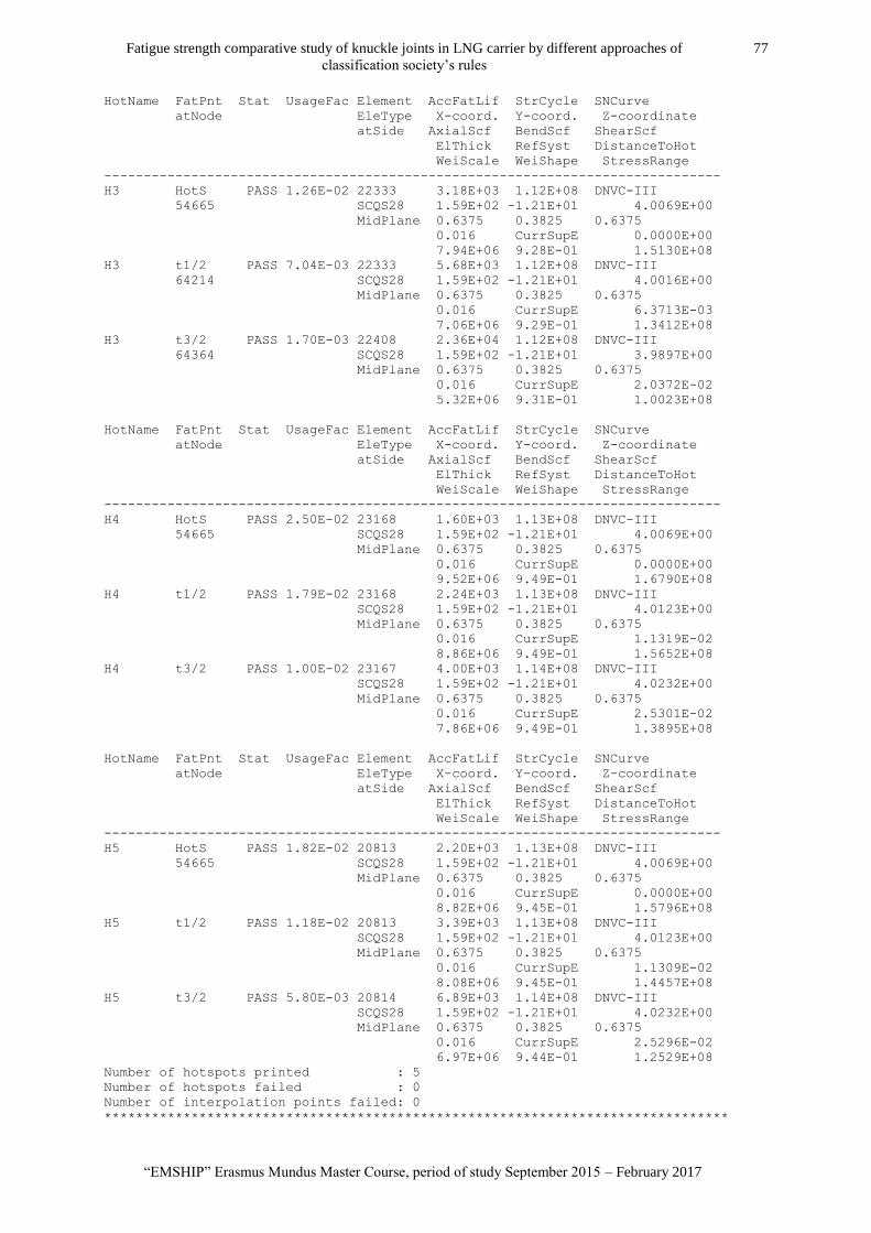
Fatigue strength comparative study of knuckle joints in LNG carrier by different approaches of
classification society‘s rules
77
―EMSHIP‖ Erasmus Mundus Master Course, period of study September 2015 – February 2017
HotName FatPnt Stat UsageFac Element AccFatLif StrCycle SNCurve
atNode EleType X-coord. Y-coord. Z-coordinate
atSide AxialScf BendScf ShearScf
ElThick RefSyst DistanceToHot
WeiScale WeiShape StressRange
------------------------------------------------------------------------------
H3 HotS PASS 1.26E-02 22333 3.18E+03 1.12E+08 DNVC-III
54665 SCQS28 1.59E+02 -1.21E+01 4.0069E+00
MidPlane 0.6375 0.3825 0.6375
0.016 CurrSupE 0.0000E+00
7.94E+06 9.28E-01 1.5130E+08
H3 t1/2 PASS 7.04E-03 22333 5.68E+03 1.12E+08 DNVC-III
64214 SCQS28 1.59E+02 -1.21E+01 4.0016E+00
MidPlane 0.6375 0.3825 0.6375
0.016 CurrSupE 6.3713E-03
7.06E+06 9.29E-01 1.3412E+08
H3 t3/2 PASS 1.70E-03 22408 2.36E+04 1.12E+08 DNVC-III
64364 SCQS28 1.59E+02 -1.21E+01 3.9897E+00
MidPlane 0.6375 0.3825 0.6375
0.016 CurrSupE 2.0372E-02
5.32E+06 9.31E-01 1.0023E+08
HotName FatPnt Stat UsageFac Element AccFatLif StrCycle SNCurve
atNode EleType X-coord. Y-coord. Z-coordinate
atSide AxialScf BendScf ShearScf
ElThick RefSyst DistanceToHot
WeiScale WeiShape StressRange
------------------------------------------------------------------------------
H4 HotS PASS 2.50E-02 23168 1.60E+03 1.13E+08 DNVC-III
54665 SCQS28 1.59E+02 -1.21E+01 4.0069E+00
MidPlane 0.6375 0.3825 0.6375
0.016 CurrSupE 0.0000E+00
9.52E+06 9.49E-01 1.6790E+08
H4 t1/2 PASS 1.79E-02 23168 2.24E+03 1.13E+08 DNVC-III
SCQS28 1.59E+02 -1.21E+01 4.0123E+00
MidPlane 0.6375 0.3825 0.6375
0.016 CurrSupE 1.1319E-02
8.86E+06 9.49E-01 1.5652E+08
H4 t3/2 PASS 1.00E-02 23167 4.00E+03 1.14E+08 DNVC-III
SCQS28 1.59E+02 -1.21E+01 4.0232E+00
MidPlane 0.6375 0.3825 0.6375
0.016 CurrSupE 2.5301E-02
7.86E+06 9.49E-01 1.3895E+08
HotName FatPnt Stat UsageFac Element AccFatLif StrCycle SNCurve
atNode EleType X-coord. Y-coord. Z-coordinate
atSide AxialScf BendScf ShearScf
ElThick RefSyst DistanceToHot
WeiScale WeiShape StressRange
------------------------------------------------------------------------------
H5 HotS PASS 1.82E-02 20813 2.20E+03 1.13E+08 DNVC-III
54665 SCQS28 1.59E+02 -1.21E+01 4.0069E+00
MidPlane 0.6375 0.3825 0.6375
0.016 CurrSupE 0.0000E+00
8.82E+06 9.45E-01 1.5796E+08
H5 t1/2 PASS 1.18E-02 20813 3.39E+03 1.13E+08 DNVC-III
SCQS28 1.59E+02 -1.21E+01 4.0123E+00
MidPlane 0.6375 0.3825 0.6375
0.016 CurrSupE 1.1309E-02
8.08E+06 9.45E-01 1.4457E+08
H5 t3/2 PASS 5.80E-03 20814 6.89E+03 1.14E+08 DNVC-III
SCQS28 1.59E+02 -1.21E+01 4.0232E+00
MidPlane 0.6375 0.3825 0.6375
0.016 CurrSupE 2.5296E-02
6.97E+06 9.44E-01 1.2529E+08
Number of hotspots printed : 5
Number of hotspots failed : 0
Number of interpolation points failed: 0
*******************************************************************************
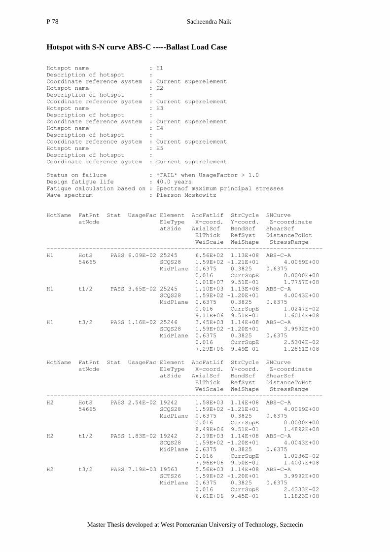
P 78 Sacheendra Naik
Master Thesis developed at West Pomeranian University of Technology, Szczecin
Hotspot with S-N curve ABS-C -----Ballast Load Case
Hotspot name : H1
Description of hotspot :
Coordinate reference system : Current superelement
Hotspot name : H2
Description of hotspot :
Coordinate reference system : Current superelement
Hotspot name : H3
Description of hotspot :
Coordinate reference system : Current superelement
Hotspot name : H4
Description of hotspot :
Coordinate reference system : Current superelement
Hotspot name : H5
Description of hotspot :
Coordinate reference system : Current superelement
Status on failure : *FAIL* when UsageFactor > 1.0
Design fatigue life : 40.0 years
Fatigue calculation based on : Spectraof maximum principal stresses
Wave spectrum : Pierson Moskowitz
HotName FatPnt Stat UsageFac Element AccFatLif StrCycle SNCurve
atNode EleType X-coord. Y-coord. Z-coordinate
atSide AxialScf BendScf ShearScf
ElThick RefSyst DistanceToHot
WeiScale WeiShape StressRange
------------------------------------------------------------------------------
H1 HotS PASS 6.09E-02 25245 6.56E+02 1.13E+08 ABS-C-A
54665 SCQS28 1.59E+02 -1.21E+01 4.0069E+00
MidPlane 0.6375 0.3825 0.6375
0.016 CurrSupE 0.0000E+00
1.01E+07 9.51E-01 1.7757E+08
H1 t1/2 PASS 3.65E-02 25245 1.10E+03 1.13E+08 ABS-C-A
SCQS28 1.59E+02 -1.20E+01 4.0043E+00
MidPlane 0.6375 0.3825 0.6375
0.016 CurrSupE 1.0247E-02
9.11E+06 9.51E-01 1.6014E+08
H1 t3/2 PASS 1.16E-02 25246 3.45E+03 1.14E+08 ABS-C-A
SCQS28 1.59E+02 -1.20E+01 3.9992E+00
MidPlane 0.6375 0.3825 0.6375
0.016 CurrSupE 2.5304E-02
7.29E+06 9.49E-01 1.2861E+08
HotName FatPnt Stat UsageFac Element AccFatLif StrCycle SNCurve
atNode EleType X-coord. Y-coord. Z-coordinate
atSide AxialScf BendScf ShearScf
ElThick RefSyst DistanceToHot
WeiScale WeiShape StressRange
------------------------------------------------------------------------------
H2 HotS PASS 2.54E-02 19242 1.58E+03 1.14E+08 ABS-C-A
54665 SCQS28 1.59E+02 -1.21E+01 4.0069E+00
MidPlane 0.6375 0.3825 0.6375
0.016 CurrSupE 0.0000E+00
8.49E+06 9.51E-01 1.4892E+08
H2 t1/2 PASS 1.83E-02 19242 2.19E+03 1.14E+08 ABS-C-A
SCQS28 1.59E+02 -1.20E+01 4.0043E+00
MidPlane 0.6375 0.3825 0.6375
0.016 CurrSupE 1.0236E-02
7.96E+06 9.50E-01 1.4007E+08
H2 t3/2 PASS 7.19E-03 19563 5.56E+03 1.14E+08 ABS-C-A
SCTS26 1.59E+02 -1.20E+01 3.9992E+00
MidPlane 0.6375 0.3825 0.6375
0.016 CurrSupE 2.4333E-02
6.61E+06 9.45E-01 1.1823E+08

Fatigue strength comparative study of knuckle joints in LNG carrier by different approaches of
classification society‘s rules
79
―EMSHIP‖ Erasmus Mundus Master Course, period of study September 2015 – February 2017
HotName FatPnt Stat UsageFac Element AccFatLif StrCycle SNCurve
atNode EleType X-coord. Y-coord. Z-coordinate
atSide AxialScf BendScf ShearScf
ElThick RefSyst DistanceToHot
WeiScale WeiShape StressRange
------------------------------------------------------------------------------
H3 HotS PASS 2.22E-02 22333 1.80E+03 1.12E+08 ABS-C-A
54665 SCQS28 1.59E+02 -1.21E+01 4.0069E+00
MidPlane 0.6375 0.3825 0.6375
0.016 CurrSupE 0.0000E+00
7.93E+06 9.28E-01 1.5113E+08
H3 t1/2 PASS 1.19E-02 22333 3.35E+03 1.12E+08 ABS-C-A
64214 SCQS28 1.59E+02 -1.21E+01 4.0016E+00
MidPlane 0.6375 0.3825 0.6375
0.016 CurrSupE 6.3713E-03
7.05E+06 9.29E-01 1.3397E+08
H3 t3/2 PASS 2.56E-03 22408 1.56E+04 1.12E+08 ABS-C-A
64364 SCQS28 1.59E+02 -1.21E+01 3.9897E+00
MidPlane 0.6375 0.3825 0.6375
0.016 CurrSupE 2.0372E-02
5.32E+06 9.32E-01 1.0011E+08
HotName FatPnt Stat UsageFac Element AccFatLif StrCycle SNCurve
atNode EleType X-coord. Y-coord. Z-coordinate
atSide AxialScf BendScf ShearScf
ElThick RefSyst DistanceToHot
WeiScale WeiShape StressRange
------------------------------------------------------------------------------
H4 HotS PASS 4.54E-02 23168 8.80E+02 1.13E+08 ABS-C-A
54665 SCQS28 1.59E+02 -1.21E+01 4.0069E+00
MidPlane 0.6375 0.3825 0.6375
0.016 CurrSupE 0.0000E+00
9.50E+06 9.49E-01 1.6771E+08
H4 t1/2 PASS 3.19E-02 23168 1.25E+03 1.13E+08 ABS-C-A
SCQS28 1.59E+02 -1.21E+01 4.0123E+00
MidPlane 0.6375 0.3825 0.6375
0.016 CurrSupE 1.1319E-02
8.85E+06 9.49E-01 1.5634E+08
H4 t3/2 PASS 1.72E-02 23167 2.32E+03 1.14E+08 ABS-C-A
SCQS28 1.59E+02 -1.21E+01 4.0232E+00
MidPlane 0.6375 0.3825 0.6375
0.016 CurrSupE 2.5301E-02
7.86E+06 9.49E-01 1.3879E+08
HotName FatPnt Stat UsageFac Element AccFatLif StrCycle SNCurve
atNode EleType X-coord. Y-coord. Z-coordinate
atSide AxialScf BendScf ShearScf
ElThick RefSyst DistanceToHot
WeiScale WeiShape StressRange
------------------------------------------------------------------------------
H5 HotS PASS 3.25E-02 20813 1.23E+03 1.13E+08 ABS-C-A
54665 SCQS28 1.59E+02 -1.21E+01 4.0069E+00
MidPlane 0.6375 0.3825 0.6375
0.016 CurrSupE 0.0000E+00
8.83E+06 9.45E-01 1.5778E+08
H5 t1/2 PASS 2.06E-02 20813 1.94E+03 1.13E+08 ABS-C-A
SCQS28 1.59E+02 -1.21E+01 4.0123E+00
MidPlane 0.6375 0.3825 0.6375
0.016 CurrSupE 1.1309E-02
8.07E+06 9.45E-01 1.4440E+08
H5 t3/2 PASS 9.65E-03 20814 4.14E+03 1.14E+08 ABS-C-A
SCQS28 1.59E+02 -1.21E+01 4.0232E+00
MidPlane 0.6375 0.3825 0.6375
0.016 CurrSupE 2.5296E-02
6.98E+06 9.45E-01 1.2515E+08
Number of hotspots printed : 5
Number of hotspots failed : 0
Number of interpolation points failed: 0
*******************************************************************************

P 80 Sacheendra Naik
Master Thesis developed at West Pomeranian University of Technology, Szczecin
Hotspot with S-N curve ABS-E -----Ballast Load Case
Hotspot name : H1
Description of hotspot :
Coordinate reference system : Current superelement
Hotspot name : H2
Description of hotspot :
Coordinate reference system : Current superelement
Hotspot name : H3
Description of hotspot :
Coordinate reference system : Current superelement
Hotspot name : H4
Description of hotspot :
Coordinate reference system : Current superelement
Hotspot name : H5
Description of hotspot :
Coordinate reference system : Current superelement
Status on failure : *FAIL* when UsageFactor > 1.0
Design fatigue life : 40.0 years
Fatigue calculation based on : Spectraof maximum principal stresses
Wave spectrum : Pierson Moskowitz
HotName FatPnt Stat UsageFac Element AccFatLif StrCycle SNCurve
atNode EleType X-coord. Y-coord. Z-coordinate
atSide AxialScf BendScf ShearScf
ElThick RefSyst DistanceToHot
WeiScale WeiShape StressRange
------------------------------------------------------------------------------
H1 HotS PASS 5.90E-01 25245 6.78E+01 1.13E+08 ABS-E-A
54665 SCQS28 1.59E+02 -1.21E+01 4.0069E+00
MidPlane 0.6375 0.3825 0.6375
0.016 CurrSupE 0.0000E+00
1.01E+07 9.51E-01 1.7757E+08
H1 t1/2 PASS 3.94E-01 25245 1.01E+02 1.13E+08 ABS-E-A
SCQS28 1.59E+02 -1.20E+01 4.0043E+00
MidPlane 0.6375 0.3825 0.6375
0.016 CurrSupE 1.0247E-02
9.11E+06 9.51E-01 1.6014E+08
H1 t3/2 PASS 1.58E-01 25246 2.54E+02 1.14E+08 ABS-E-A
SCQS28 1.59E+02 -1.20E+01 3.9992E+00
MidPlane 0.6375 0.3825 0.6375
0.016 CurrSupE 2.5304E-02
7.29E+06 9.49E-01 1.2861E+08
HotName FatPnt Stat UsageFac Element AccFatLif StrCycle SNCurve
atNode EleType X-coord. Y-coord. Z-coordinate
atSide AxialScf BendScf ShearScf
ElThick RefSyst DistanceToHot
WeiScale WeiShape StressRange
------------------------------------------------------------------------------
H2 HotS PASS 2.96E-01 19242 1.35E+02 1.14E+08 ABS-E-A
54665 SCQS28 1.59E+02 -1.21E+01 4.0069E+00
MidPlane 0.6375 0.3825 0.6375
0.016 CurrSupE 0.0000E+00
8.49E+06 9.51E-01 1.4892E+08
H2 t1/2 PASS 2.28E-01 19242 1.76E+02 1.14E+08 ABS-E-A
SCQS28 1.59E+02 -1.20E+01 4.0043E+00
MidPlane 0.6375 0.3825 0.6375
0.016 CurrSupE 1.0236E-02
7.96E+06 9.50E-01 1.4007E+08
H2 t3/2 PASS 1.06E-01 19563 3.77E+02 1.14E+08 ABS-E-A
SCTS26 1.59E+02 -1.20E+01 3.9992E+00
MidPlane 0.6375 0.3825 0.6375
0.016 CurrSupE 2.4333E-02
6.61E+06 9.45E-01 1.1823E+08

Fatigue strength comparative study of knuckle joints in LNG carrier by different approaches of
classification society‘s rules
81
―EMSHIP‖ Erasmus Mundus Master Course, period of study September 2015 – February 2017
HotName FatPnt Stat UsageFac Element AccFatLif StrCycle SNCurve
atNode EleType X-coord. Y-coord. Z-coordinate
atSide AxialScf BendScf ShearScf
ElThick RefSyst DistanceToHot
WeiScale WeiShape StressRange
------------------------------------------------------------------------------
H3 HotS PASS 2.59E-01 22333 1.55E+02 1.12E+08 ABS-E-A
54665 SCQS28 1.59E+02 -1.21E+01 4.0069E+00
MidPlane 0.6375 0.3825 0.6375
0.016 CurrSupE 0.0000E+00
7.93E+06 9.28E-01 1.5113E+08
H3 t1/2 PASS 1.58E-01 22333 2.54E+02 1.12E+08 ABS-E-A
64214 SCQS28 1.59E+02 -1.21E+01 4.0016E+00
MidPlane 0.6375 0.3825 0.6375
0.016 CurrSupE 6.3713E-03
7.05E+06 9.29E-01 1.3397E+08
H3 t3/2 PASS 4.41E-02 22408 9.08E+02 1.12E+08 ABS-E-A
64364 SCQS28 1.59E+02 -1.21E+01 3.9897E+00
MidPlane 0.6375 0.3825 0.6375
0.016 CurrSupE 2.0372E-02
5.32E+06 9.32E-01 1.0011E+08
HotName FatPnt Stat UsageFac Element AccFatLif StrCycle SNCurve
atNode EleType X-coord. Y-coord. Z-coordinate
atSide AxialScf BendScf ShearScf
ElThick RefSyst DistanceToHot
WeiScale WeiShape StressRange
------------------------------------------------------------------------------
H4 HotS PASS 4.69E-01 23168 8.54E+01 1.13E+08 ABS-E-A
54665 SCQS28 1.59E+02 -1.21E+01 4.0069E+00
MidPlane 0.6375 0.3825 0.6375
0.016 CurrSupE 0.0000E+00
9.50E+06 9.49E-01 1.6771E+08
H4 t1/2 PASS 3.55E-01 23168 1.13E+02 1.13E+08 ABS-E-A
SCQS28 1.59E+02 -1.21E+01 4.0123E+00
MidPlane 0.6375 0.3825 0.6375
0.016 CurrSupE 1.1319E-02
8.85E+06 9.49E-01 1.5634E+08
H4 t3/2 PASS 2.17E-01 23167 1.84E+02 1.14E+08 ABS-E-A
SCQS28 1.59E+02 -1.21E+01 4.0232E+00
MidPlane 0.6375 0.3825 0.6375
0.016 CurrSupE 2.5301E-02
7.86E+06 9.49E-01 1.3879E+08
HotName FatPnt Stat UsageFac Element AccFatLif StrCycle SNCurve
atNode EleType X-coord. Y-coord. Z-coordinate
atSide AxialScf BendScf ShearScf
ElThick RefSyst DistanceToHot
WeiScale WeiShape StressRange
------------------------------------------------------------------------------
H5 HotS PASS 3.58E-01 20813 1.12E+02 1.13E+08 ABS-E-A
54665 SCQS28 1.59E+02 -1.21E+01 4.0069E+00
MidPlane 0.6375 0.3825 0.6375
0.016 CurrSupE 0.0000E+00
8.83E+06 9.45E-01 1.5778E+08
H5 t1/2 PASS 2.49E-01 20813 1.61E+02 1.13E+08 ABS-E-A
SCQS28 1.59E+02 -1.21E+01 4.0123E+00
MidPlane 0.6375 0.3825 0.6375
0.016 CurrSupE 1.1309E-02
8.07E+06 9.45E-01 1.4440E+08
H5 t3/2 PASS 1.35E-01 20814 2.96E+02 1.14E+08 ABS-E-A
SCQS28 1.59E+02 -1.21E+01 4.0232E+00
MidPlane 0.6375 0.3825 0.6375
0.016 CurrSupE 2.5296E-02
6.98E+06 9.45E-01 1.2515E+08
Number of hotspots printed : 5
Number of hotspots failed : 0
Number of interpolation points failed: 0
*******************************************************************************
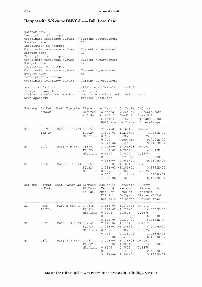
P 82 Sacheendra Naik
Master Thesis developed at West Pomeranian University of Technology, Szczecin
Hotspot with S-N curve DNVC-I -----Full Load Case
Hotspot name : H1
Description of hotspot :
Coordinate reference system : Current superelement
Hotspot name : H2
Description of hotspot :
Coordinate reference system : Current superelement
Hotspot name : H3
Description of hotspot :
Coordinate reference system : Current superelement
Hotspot name : H4
Description of hotspot :
Coordinate reference system : Current superelement
Hotspot name : H5
Description of hotspot :
Coordinate reference system : Current superelement
Status on failure : *FAIL* when UsageFactor > 1.0
Design fatigue life : 40.0 years
Fatigue calculation based on : Spectraof maximum principal stresses
Wave spectrum : Pierson Moskowitz
HotName FatPnt Stat UsageFac Element AccFatLif StrCycle SNCurve
atNode EleType X-coord. Y-coord. Z-coordinate
atSide AxialScf BendScf ShearScf
ElThick RefSyst DistanceToHot
WeiScale WeiShape StressRange
------------------------------------------------------------------------------
H1 HotS PASS 5.12E-03 183552 7.82E+03 1.16E+08 DNVC-I
162724 FQUS24 1.59E+02 -1.21E+01 4.0069E+00
MidPlane 0.6375 0.3825 0.6375
0.016 CurrSupE 0.0000E+00
5.84E+06 9.62E-01 9.7401E+07
H1 t1/2 PASS 3.97E-03 183552 1.01E+04 1.16E+08 DNVC-I
FQUS24 1.59E+02 -1.20E+01 4.0043E+00
MidPlane 0.6375 0.3825 0.6375
0.016 CurrSupE 1.0247E-02
5.56E+06 9.64E-01 9.2298E+07
H1 t3/2 PASS 2.19E-03 183553 1.83E+04 1.16E+08 DNVC-I
FQUS24 1.59E+02 -1.20E+01 3.9992E+00
MidPlane 0.6375 0.3825 0.6375
0.016 CurrSupE 2.5304E-02
4.96E+06 9.66E-01 8.1342E+07
HotName FatPnt Stat UsageFac Element AccFatLif StrCycle SNCurve
atNode EleType X-coord. Y-coord. Z-coordinate
atSide AxialScf BendScf ShearScf
ElThick RefSyst DistanceToHot
WeiScale WeiShape StressRange
------------------------------------------------------------------------------
H2 HotS PASS 2.89E-03 177549 1.38E+04 1.17E+08 DNVC-I
162724 FQUS24 1.59E+02 -1.21E+01 4.0069E+00
MidPlane 0.6375 0.3825 0.6375
0.016 CurrSupE 0.0000E+00
5.10E+06 9.53E-01 8.9563E+07
H2 t1/2 PASS 1.87E-03 177549 2.14E+04 1.17E+08 DNVC-I
FQUS24 1.59E+02 -1.20E+01 4.0043E+00
MidPlane 0.6375 0.3825 0.6375
0.016 CurrSupE 1.0236E-02
4.68E+06 9.54E-01 8.1858E+07
H2 t3/2 PASS 4.07E-04 177870 4.00E+04 1.17E+08 DNVC-I
FTRS25 1.59E+02 -1.20E+01 3.9992E+00
MidPlane 0.6375 0.3825 0.6375
0.016 CurrSupE 2.4333E-02
3.49E+06 9.59E-01 5.9842E+07

Fatigue strength comparative study of knuckle joints in LNG carrier by different approaches of
classification society‘s rules
83
―EMSHIP‖ Erasmus Mundus Master Course, period of study September 2015 – February 2017
HotName FatPnt Stat UsageFac Element AccFatLif StrCycle SNCurve
atNode EleType X-coord. Y-coord. Z-coordinate
atSide AxialScf BendScf ShearScf
ElThick RefSyst DistanceToHot
WeiScale WeiShape StressRange
------------------------------------------------------------------------------
H3 HotS PASS 1.27E-03 180640 3.15E+04 1.17E+08 DNVC-I
162724 FQUS24 1.59E+02 -1.21E+01 4.0069E+00
MidPlane 0.6375 0.3825 0.6375
0.016 CurrSupE 0.0000E+00
4.42E+06 9.64E-01 7.4574E+07
H3 t1/2 PASS 7.45E-04 180640 4.00E+04 1.17E+08 DNVC-I
FQUS24 1.59E+02 -1.21E+01 4.0010E+00
MidPlane 0.6375 0.3825 0.6375
0.016 CurrSupE 7.9998E-03
3.99E+06 9.66E-01 6.6618E+07
H3 t3/2 PASS 2.17E-04 180715 4.00E+04 1.17E+08 DNVC-I
FQUS24 1.59E+02 -1.21E+01 3.9893E+00
MidPlane 0.6375 0.3825 0.6375
0.016 CurrSupE 2.4000E-02
3.15E+06 9.71E-01 5.1179E+07
HotName FatPnt Stat UsageFac Element AccFatLif StrCycle SNCurve
atNode EleType X-coord. Y-coord. Z-coordinate
atSide AxialScf BendScf ShearScf
ElThick RefSyst DistanceToHot
WeiScale WeiShape StressRange
------------------------------------------------------------------------------
H4 HotS PASS 5.91E-03 181475 6.77E+03 1.16E+08 DNVC-I
162724 FQUS24 1.59E+02 -1.21E+01 4.0069E+00
MidPlane 0.6375 0.3825 0.6375
0.016 CurrSupE 0.0000E+00
6.03E+06 9.63E-01 1.0013E+08
H4 t1/2 PASS 4.46E-03 181475 8.97E+03 1.16E+08 DNVC-I
FQUS24 1.59E+02 -1.21E+01 4.0123E+00
MidPlane 0.6375 0.3825 0.6375
0.016 CurrSupE 1.1319E-02
5.70E+06 9.64E-01 9.4496E+07
H4 t3/2 PASS 2.71E-03 181474 1.48E+04 1.16E+08 DNVC-I
FQUS24 1.59E+02 -1.21E+01 4.0232E+00
MidPlane 0.6375 0.3825 0.6375
0.016 CurrSupE 2.5301E-02
5.16E+06 9.65E-01 8.5309E+07
HotName FatPnt Stat UsageFac Element AccFatLif StrCycle SNCurve
atNode EleType X-coord. Y-coord. Z-coordinate
atSide AxialScf BendScf ShearScf
ElThick RefSyst DistanceToHot
WeiScale WeiShape StressRange
------------------------------------------------------------------------------
H5 HotS PASS 2.05E-03 179120 1.95E+04 1.17E+08 DNVC-I
162724 FQUS24 1.59E+02 -1.21E+01 4.0069E+00
MidPlane 0.6375 0.3825 0.6375
0.016 CurrSupE 0.0000E+00
4.77E+06 9.55E-01 8.3274E+07
H5 t1/2 PASS 1.69E-03 179120 2.36E+04 1.18E+08 DNVC-I
FQUS24 1.59E+02 -1.21E+01 4.0123E+00
MidPlane 0.6375 0.3825 0.6375
0.016 CurrSupE 1.1309E-02
4.61E+06 9.56E-01 7.9976E+07
H5 t3/2 PASS 1.22E-03 179121 3.27E+04 1.18E+08 DNVC-I
FQUS24 1.59E+02 -1.21E+01 4.0232E+00
MidPlane 0.6375 0.3825 0.6375
0.016 CurrSupE 2.5296E-02
4.34E+06 9.58E-01 7.4625E+07
Number of hotspots printed : 5
Number of hotspots failed : 0
Number of interpolation points failed: 0
*******************************************************************************

P 84 Sacheendra Naik
Master Thesis developed at West Pomeranian University of Technology, Szczecin
Hotspot with S-N curve DNVC-III -----Full Load Case
Hotspot name : H1
Description of hotspot :
Coordinate reference system : Current superelement
Hotspot name : H2
Description of hotspot :
Coordinate reference system : Current superelement
Hotspot name : H3
Description of hotspot :
Coordinate reference system : Current superelement
Hotspot name : H4
Description of hotspot :
Coordinate reference system : Current superelement
Hotspot name : H5
Description of hotspot :
Coordinate reference system : Current superelement
Status on failure : *FAIL* when UsageFactor > 1.0
Design fatigue life : 40.0 years
Fatigue calculation based on : Spectraof maximum principal stresses
Wave spectrum : Pierson Moskowitz
HotName FatPnt Stat UsageFac Element AccFatLif StrCycle SNCurve
atNode EleType X-coord. Y-coord. Z-coordinate
atSide AxialScf BendScf ShearScf
ElThick RefSyst DistanceToHot
WeiScale WeiShape StressRange
------------------------------------------------------------------------------
H1 HotS PASS 2.05E-03 183552 1.96E+04 1.16E+08 DNVC-III
162724 FQUS24 1.59E+02 -1.21E+01 4.0069E+00
MidPlane 0.6375 0.3825 0.6375
0.016 CurrSupE 0.0000E+00
5.84E+06 9.62E-01 9.7401E+07
H1 t1/2 PASS 1.58E-03 183552 2.53E+04 1.16E+08 DNVC-III
FQUS24 1.59E+02 -1.20E+01 4.0043E+00
MidPlane 0.6375 0.3825 0.6375
0.016 CurrSupE 1.0247E-02
5.56E+06 9.64E-01 9.2298E+07
H1 t3/2 PASS 8.71E-04 183553 4.00E+04 1.16E+08 DNVC-III
FQUS24 1.59E+02 -1.20E+01 3.9992E+00
MidPlane 0.6375 0.3825 0.6375
0.016 CurrSupE 2.5304E-02
4.96E+06 9.66E-01 8.1342E+07
HotName FatPnt Stat UsageFac Element AccFatLif StrCycle SNCurve
atNode EleType X-coord. Y-coord. Z-coordinate
atSide AxialScf BendScf ShearScf
ElThick RefSyst DistanceToHot
WeiScale WeiShape StressRange
------------------------------------------------------------------------------
H2 HotS PASS 1.15E-03 177549 3.47E+04 1.17E+08 DNVC-III
162724 FQUS24 1.59E+02 -1.21E+01 4.0069E+00
MidPlane 0.6375 0.3825 0.6375
0.016 CurrSupE 0.0000E+00
5.10E+06 9.53E-01 8.9563E+07
H2 t1/2 PASS 7.43E-04 177549 4.00E+04 1.17E+08 DNVC-III
FQUS24 1.59E+02 -1.20E+01 4.0043E+00
MidPlane 0.6375 0.3825 0.6375
0.016 CurrSupE 1.0236E-02
4.68E+06 9.54E-01 8.1858E+07
H2 t3/2 PASS 1.62E-04 177870 4.00E+04 1.17E+08 DNVC-III
FTRS25 1.59E+02 -1.20E+01 3.9992E+00
MidPlane 0.6375 0.3825 0.6375
0.016 CurrSupE 2.4333E-02
3.49E+06 9.59E-01 5.9842E+07

Fatigue strength comparative study of knuckle joints in LNG carrier by different approaches of
classification society‘s rules
85
―EMSHIP‖ Erasmus Mundus Master Course, period of study September 2015 – February 2017
HotName FatPnt Stat UsageFac Element AccFatLif StrCycle SNCurve
atNode EleType X-coord. Y-coord. Z-coordinate
atSide AxialScf BendScf ShearScf
ElThick RefSyst DistanceToHot
WeiScale WeiShape StressRange
------------------------------------------------------------------------------
H3 HotS PASS 5.06E-04 180640 4.00E+04 1.17E+08 DNVC-III
162724 FQUS24 1.59E+02 -1.21E+01 4.0069E+00
MidPlane 0.6375 0.3825 0.6375
0.016 CurrSupE 0.0000E+00
4.42E+06 9.64E-01 7.4574E+07
H3 t1/2 PASS 2.97E-04 180640 4.00E+04 1.17E+08 DNVC-III
FQUS24 1.59E+02 -1.21E+01 4.0010E+00
MidPlane 0.6375 0.3825 0.6375
0.016 CurrSupE 7.9998E-03
3.99E+06 9.66E-01 6.6618E+07
H3 t3/2 PASS 8.66E-05 180715 4.00E+04 1.17E+08 DNVC-III
FQUS24 1.59E+02 -1.21E+01 3.9893E+00
MidPlane 0.6375 0.3825 0.6375
0.016 CurrSupE 2.4000E-02
3.15E+06 9.71E-01 5.1179E+07
HotName FatPnt Stat UsageFac Element AccFatLif StrCycle SNCurve
atNode EleType X-coord. Y-coord. Z-coordinate
atSide AxialScf BendScf ShearScf
ElThick RefSyst DistanceToHot
WeiScale WeiShape StressRange
------------------------------------------------------------------------------
H4 HotS PASS 2.37E-03 181475 1.69E+04 1.16E+08 DNVC-III
162724 FQUS24 1.59E+02 -1.21E+01 4.0069E+00
MidPlane 0.6375 0.3825 0.6375
0.016 CurrSupE 0.0000E+00
6.03E+06 9.63E-01 1.0013E+08
H4 t1/2 PASS 1.78E-03 181475 2.24E+04 1.16E+08 DNVC-III
FQUS24 1.59E+02 -1.21E+01 4.0123E+00
MidPlane 0.6375 0.3825 0.6375
0.016 CurrSupE 1.1319E-02
5.70E+06 9.64E-01 9.4496E+07
H4 t3/2 PASS 1.08E-03 181474 3.70E+04 1.16E+08 DNVC-III
FQUS24 1.59E+02 -1.21E+01 4.0232E+00
MidPlane 0.6375 0.3825 0.6375
0.016 CurrSupE 2.5301E-02
5.16E+06 9.65E-01 8.5309E+07
HotName FatPnt Stat UsageFac Element AccFatLif StrCycle SNCurve
atNode EleType X-coord. Y-coord. Z-coordinate
atSide AxialScf BendScf ShearScf
ElThick RefSyst DistanceToHot
WeiScale WeiShape StressRange
------------------------------------------------------------------------------
H5 HotS PASS 8.19E-04 179120 4.00E+04 1.17E+08 DNVC-III
162724 FQUS24 1.59E+02 -1.21E+01 4.0069E+00
MidPlane 0.6375 0.3825 0.6375
0.016 CurrSupE 0.0000E+00
4.77E+06 9.55E-01 8.3274E+07
H5 t1/2 PASS 6.75E-04 179120 4.00E+04 1.18E+08 DNVC-III
FQUS24 1.59E+02 -1.21E+01 4.0123E+00
MidPlane 0.6375 0.3825 0.6375
0.016 CurrSupE 1.1309E-02
4.61E+06 9.56E-01 7.9976E+07
H5 t3/2 PASS 4.88E-04 179121 4.00E+04 1.18E+08 DNVC-III
FQUS24 1.59E+02 -1.21E+01 4.0232E+00
MidPlane 0.6375 0.3825 0.6375
0.016 CurrSupE 2.5296E-02
4.34E+06 9.58E-01 7.4625E+07
Number of hotspots printed : 5
Number of hotspots failed : 0
Number of interpolation points failed: 0
*******************************************************************************
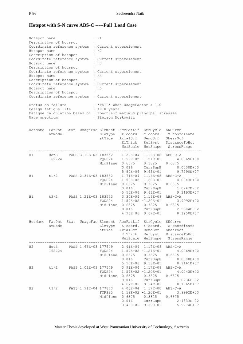
P 86 Sacheendra Naik
Master Thesis developed at West Pomeranian University of Technology, Szczecin
Hotspot with S-N curve ABS-C -----Full Load Case
Hotspot name : H1
Description of hotspot :
Coordinate reference system : Current superelement
Hotspot name : H2
Description of hotspot :
Coordinate reference system : Current superelement
Hotspot name : H3
Description of hotspot :
Coordinate reference system : Current superelement
Hotspot name : H4
Description of hotspot :
Coordinate reference system : Current superelement
Hotspot name : H5
Description of hotspot :
Coordinate reference system : Current superelement
Status on failure : *FAIL* when UsageFactor > 1.0
Design fatigue life : 40.0 years
Fatigue calculation based on : Spectraof maximum principal stresses
Wave spectrum : Pierson Moskowitz
HotName FatPnt Stat UsageFac Element AccFatLif StrCycle SNCurve
atNode EleType X-coord. Y-coord. Z-coordinate
atSide AxialScf BendScf ShearScf
ElThick RefSyst DistanceToHot
WeiScale WeiShape StressRange
------------------------------------------------------------------------------
H1 HotS PASS 3.10E-03 183552 1.29E+04 1.16E+08 ABS-C-A
162724 FQUS24 1.59E+02 -1.21E+01 4.0069E+00
MidPlane 0.6375 0.3825 0.6375
0.016 CurrSupE 0.0000E+00
5.84E+06 9.63E-01 9.7290E+07
H1 t1/2 PASS 2.34E-03 183552 1.71E+04 1.16E+08 ABS-C-A
FQUS24 1.59E+02 -1.20E+01 4.0043E+00
MidPlane 0.6375 0.3825 0.6375
0.016 CurrSupE 1.0247E-02
5.55E+06 9.63E-01 9.2193E+07
H1 t3/2 PASS 1.21E-03 183553 3.30E+04 1.16E+08 ABS-C-A
FQUS24 1.59E+02 -1.20E+01 3.9992E+00
MidPlane 0.6375 0.3825 0.6375
0.016 CurrSupE 2.5304E-02
4.96E+06 9.67E-01 8.1250E+07
HotName FatPnt Stat UsageFac Element AccFatLif StrCycle SNCurve
atNode EleType X-coord. Y-coord. Z-coordinate
atSide AxialScf BendScf ShearScf
ElThick RefSyst DistanceToHot
WeiScale WeiShape StressRange
------------------------------------------------------------------------------
H2 HotS PASS 1.66E-03 177549 2.41E+04 1.17E+08 ABS-C-A
162724 FQUS24 1.59E+02 -1.21E+01 4.0069E+00
MidPlane 0.6375 0.3825 0.6375
0.016 CurrSupE 0.0000E+00
5.10E+06 9.53E-01 8.9461E+07
H2 t1/2 PASS 1.02E-03 177549 3.91E+04 1.17E+08 ABS-C-A
FQUS24 1.59E+02 -1.20E+01 4.0043E+00
MidPlane 0.6375 0.3825 0.6375
0.016 CurrSupE 1.0236E-02
4.67E+06 9.54E-01 8.1765E+07
H2 t3/2 PASS 1.91E-04 177870 4.00E+04 1.17E+08 ABS-C-A
FTRS25 1.59E+02 -1.20E+01 3.9992E+00
MidPlane 0.6375 0.3825 0.6375
0.016 CurrSupE 2.4333E-02
3.48E+06 9.59E-01 5.9774E+07

Fatigue strength comparative study of knuckle joints in LNG carrier by different approaches of
classification society‘s rules
87
―EMSHIP‖ Erasmus Mundus Master Course, period of study September 2015 – February 2017
HotName FatPnt Stat UsageFac Element AccFatLif StrCycle SNCurve
atNode EleType X-coord. Y-coord. Z-coordinate
atSide AxialScf BendScf ShearScf
ElThick RefSyst DistanceToHot
WeiScale WeiShape StressRange
------------------------------------------------------------------------------
H3 HotS PASS 6.68E-04 180640 4.00E+04 1.17E+08 ABS-C-A
162724 FQUS24 1.59E+02 -1.21E+01 4.0069E+00
MidPlane 0.6375 0.3825 0.6375
0.016 CurrSupE 0.0000E+00
4.41E+06 9.64E-01 7.4489E+07
H3 t1/2 PASS 3.71E-04 180640 4.00E+04 1.17E+08 ABS-C-A
FQUS24 1.59E+02 -1.21E+01 4.0010E+00
MidPlane 0.6375 0.3825 0.6375
0.016 CurrSupE 7.9998E-03
3.99E+06 9.66E-01 6.6542E+07
H3 t3/2 PASS 9.57E-05 180715 4.00E+04 1.17E+08 ABS-C-A
FQUS24 1.59E+02 -1.21E+01 3.9893E+00
MidPlane 0.6375 0.3825 0.6375
0.016 CurrSupE 2.4000E-02
3.14E+06 9.71E-01 5.1120E+07
HotName FatPnt Stat UsageFac Element AccFatLif StrCycle SNCurve
atNode EleType X-coord. Y-coord. Z-coordinate
atSide AxialScf BendScf ShearScf
ElThick RefSyst DistanceToHot
WeiScale WeiShape StressRange
------------------------------------------------------------------------------
H4 HotS PASS 3.63E-03 181475 1.10E+04 1.16E+08 ABS-C-A
162724 FQUS24 1.59E+02 -1.21E+01 4.0069E+00
MidPlane 0.6375 0.3825 0.6375
0.016 CurrSupE 0.0000E+00
6.01E+06 9.63E-01 1.0001E+08
H4 t1/2 PASS 2.66E-03 181475 1.50E+04 1.16E+08 ABS-C-A
FQUS24 1.59E+02 -1.21E+01 4.0123E+00
MidPlane 0.6375 0.3825 0.6375
0.016 CurrSupE 1.1319E-02
5.69E+06 9.63E-01 9.4389E+07
H4 t3/2 PASS 1.54E-03 181474 2.60E+04 1.16E+08 ABS-C-A
FQUS24 1.59E+02 -1.21E+01 4.0232E+00
MidPlane 0.6375 0.3825 0.6375
0.016 CurrSupE 2.5301E-02
5.16E+06 9.65E-01 8.5212E+07
HotName FatPnt Stat UsageFac Element AccFatLif StrCycle SNCurve
atNode EleType X-coord. Y-coord. Z-coordinate
atSide AxialScf BendScf ShearScf
ElThick RefSyst DistanceToHot
WeiScale WeiShape StressRange
------------------------------------------------------------------------------
H5 HotS PASS 1.14E-03 179120 3.52E+04 1.17E+08 ABS-C-A
162724 FQUS24 1.59E+02 -1.21E+01 4.0069E+00
MidPlane 0.6375 0.3825 0.6375
0.016 CurrSupE 0.0000E+00
4.77E+06 9.55E-01 8.3179E+07
H5 t1/2 PASS 9.19E-04 179120 4.00E+04 1.18E+08 ABS-C-A
FQUS24 1.59E+02 -1.21E+01 4.0123E+00
MidPlane 0.6375 0.3825 0.6375
0.016 CurrSupE 1.1309E-02
4.60E+06 9.57E-01 7.9884E+07
H5 t3/2 PASS 6.42E-04 179121 4.00E+04 1.18E+08 ABS-C-A
FQUS24 1.59E+02 -1.21E+01 4.0232E+00
MidPlane 0.6375 0.3825 0.6375
0.016 CurrSupE 2.5296E-02
4.33E+06 9.59E-01 7.4540E+07
Number of hotspots printed : 5
Number of hotspots failed : 0
Number of interpolation points failed: 0
*******************************************************************************

P 88 Sacheendra Naik
Master Thesis developed at West Pomeranian University of Technology, Szczecin
Hotspot with S-N curve ABS-E -----Full Load Case
Hotspot name : H1
Description of hotspot :
Coordinate reference system : Current superelement
Hotspot name : H2
Description of hotspot :
Coordinate reference system : Current superelement
Hotspot name : H3
Description of hotspot :
Coordinate reference system : Current superelement
Hotspot name : H4
Description of hotspot :
Coordinate reference system : Current superelement
Hotspot name : H5
Description of hotspot :
Coordinate reference system : Current superelement
Status on failure : *FAIL* when UsageFactor > 1.0
Design fatigue life : 40.0 years
Fatigue calculation based on : Spectraof maximum principal stresses
Wave spectrum : Pierson Moskowitz
HotName FatPnt Stat UsageFac Element AccFatLif StrCycle SNCurve
atNode EleType X-coord. Y-coord. Z-coordinate
atSide AxialScf BendScf ShearScf
ElThick RefSyst DistanceToHot
WeiScale WeiShape StressRange
------------------------------------------------------------------------------
H1 HotS PASS 5.32E-02 183552 7.52E+02 1.16E+08 ABS-E-A
162724 FQUS24 1.59E+02 -1.21E+01 4.0069E+00
MidPlane 0.6375 0.3825 0.6375
0.016 CurrSupE 0.0000E+00
5.84E+06 9.63E-01 9.7290E+07
H1 t1/2 PASS 4.19E-02 183552 9.54E+02 1.16E+08 ABS-E-A
FQUS24 1.59E+02 -1.20E+01 4.0043E+00
MidPlane 0.6375 0.3825 0.6375
0.016 CurrSupE 1.0247E-02
5.55E+06 9.63E-01 9.2193E+07
H1 t3/2 PASS 2.38E-02 183553 1.68E+03 1.16E+08 ABS-E-A
FQUS24 1.59E+02 -1.20E+01 3.9992E+00
MidPlane 0.6375 0.3825 0.6375
0.016 CurrSupE 2.5304E-02
4.96E+06 9.67E-01 8.1250E+07
HotName FatPnt Stat UsageFac Element AccFatLif StrCycle SNCurve
atNode EleType X-coord. Y-coord. Z-coordinate
atSide AxialScf BendScf ShearScf
ElThick RefSyst DistanceToHot
WeiScale WeiShape StressRange
------------------------------------------------------------------------------
H2 HotS PASS 3.11E-02 177549 1.29E+03 1.17E+08 ABS-E-A
162724 FQUS24 1.59E+02 -1.21E+01 4.0069E+00
MidPlane 0.6375 0.3825 0.6375
0.016 CurrSupE 0.0000E+00
5.10E+06 9.53E-01 8.9461E+07
H2 t1/2 PASS 2.04E-02 177549 1.96E+03 1.17E+08 ABS-E-A
FQUS24 1.59E+02 -1.20E+01 4.0043E+00
MidPlane 0.6375 0.3825 0.6375
0.016 CurrSupE 1.0236E-02
4.67E+06 9.54E-01 8.1765E+07
H2 t3/2 PASS 4.58E-03 177870 8.73E+03 1.17E+08 ABS-E-A
FTRS25 1.59E+02 -1.20E+01 3.9992E+00
MidPlane 0.6375 0.3825 0.6375
0.016 CurrSupE 2.4333E-02
3.48E+06 9.59E-01 5.9774E+07
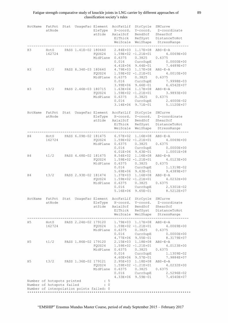
Fatigue strength comparative study of knuckle joints in LNG carrier by different approaches of
classification society‘s rules
89
―EMSHIP‖ Erasmus Mundus Master Course, period of study September 2015 – February 2017
HotName FatPnt Stat UsageFac Element AccFatLif StrCycle SNCurve
atNode EleType X-coord. Y-coord. Z-coordinate
atSide AxialScf BendScf ShearScf
ElThick RefSyst DistanceToHot
WeiScale WeiShape StressRange
------------------------------------------------------------------------------
H3 HotS PASS 1.41E-02 180640 2.84E+03 1.17E+08 ABS-E-A
162724 FQUS24 1.59E+02 -1.21E+01 4.0069E+00
MidPlane 0.6375 0.3825 0.6375
0.016 CurrSupE 0.0000E+00
4.41E+06 9.64E-01 7.4489E+07
H3 t1/2 PASS 8.34E-03 180640 4.79E+03 1.17E+08 ABS-E-A
FQUS24 1.59E+02 -1.21E+01 4.0010E+00
MidPlane 0.6375 0.3825 0.6375
0.016 CurrSupE 7.9998E-03
3.99E+06 9.66E-01 6.6542E+07
H3 t3/2 PASS 2.46E-03 180715 1.63E+04 1.17E+08 ABS-E-A
FQUS24 1.59E+02 -1.21E+01 3.9893E+00
MidPlane 0.6375 0.3825 0.6375
0.016 CurrSupE 2.4000E-02
3.14E+06 9.71E-01 5.1120E+07
HotName FatPnt Stat UsageFac Element AccFatLif StrCycle SNCurve
atNode EleType X-coord. Y-coord. Z-coordinate
atSide AxialScf BendScf ShearScf
ElThick RefSyst DistanceToHot
WeiScale WeiShape StressRange
------------------------------------------------------------------------------
H4 HotS PASS 6.09E-02 181475 6.57E+02 1.16E+08 ABS-E-A
162724 FQUS24 1.59E+02 -1.21E+01 4.0069E+00
MidPlane 0.6375 0.3825 0.6375
0.016 CurrSupE 0.0000E+00
6.01E+06 9.63E-01 1.0001E+08
H4 t1/2 PASS 4.68E-02 181475 8.54E+02 1.16E+08 ABS-E-A
FQUS24 1.59E+02 -1.21E+01 4.0123E+00
MidPlane 0.6375 0.3825 0.6375
0.016 CurrSupE 1.1319E-02
5.69E+06 9.63E-01 9.4389E+07
H4 t3/2 PASS 2.93E-02 181474 1.37E+03 1.16E+08 ABS-E-A
FQUS24 1.59E+02 -1.21E+01 4.0232E+00
MidPlane 0.6375 0.3825 0.6375
0.016 CurrSupE 2.5301E-02
5.16E+06 9.65E-01 8.5212E+07
HotName FatPnt Stat UsageFac Element AccFatLif StrCycle SNCurve
atNode EleType X-coord. Y-coord. Z-coordinate
atSide AxialScf BendScf ShearScf
ElThick RefSyst DistanceToHot
WeiScale WeiShape StressRange
------------------------------------------------------------------------------
H5 HotS PASS 2.24E-02 179120 1.79E+03 1.17E+08 ABS-E-A
162724 FQUS24 1.59E+02 -1.21E+01 4.0069E+00
MidPlane 0.6375 0.3825 0.6375
0.016 CurrSupE 0.0000E+00
4.77E+06 9.55E-01 8.3179E+07
H5 t1/2 PASS 1.86E-02 179120 2.15E+03 1.18E+08 ABS-E-A
FQUS24 1.59E+02 -1.21E+01 4.0123E+00
MidPlane 0.6375 0.3825 0.6375
0.016 CurrSupE 1.1309E-02
4.60E+06 9.57E-01 7.9884E+07
H5 t3/2 PASS 1.36E-02 179121 2.95E+03 1.18E+08 ABS-E-A
FQUS24 1.59E+02 -1.21E+01 4.0232E+00
MidPlane 0.6375 0.3825 0.6375
0.016 CurrSupE 2.5296E-02
4.33E+06 9.59E-01 7.4540E+07
Number of hotspots printed : 5
Number of hotspots failed : 0
Number of interpolation points failed: 0
*******************************************************************************