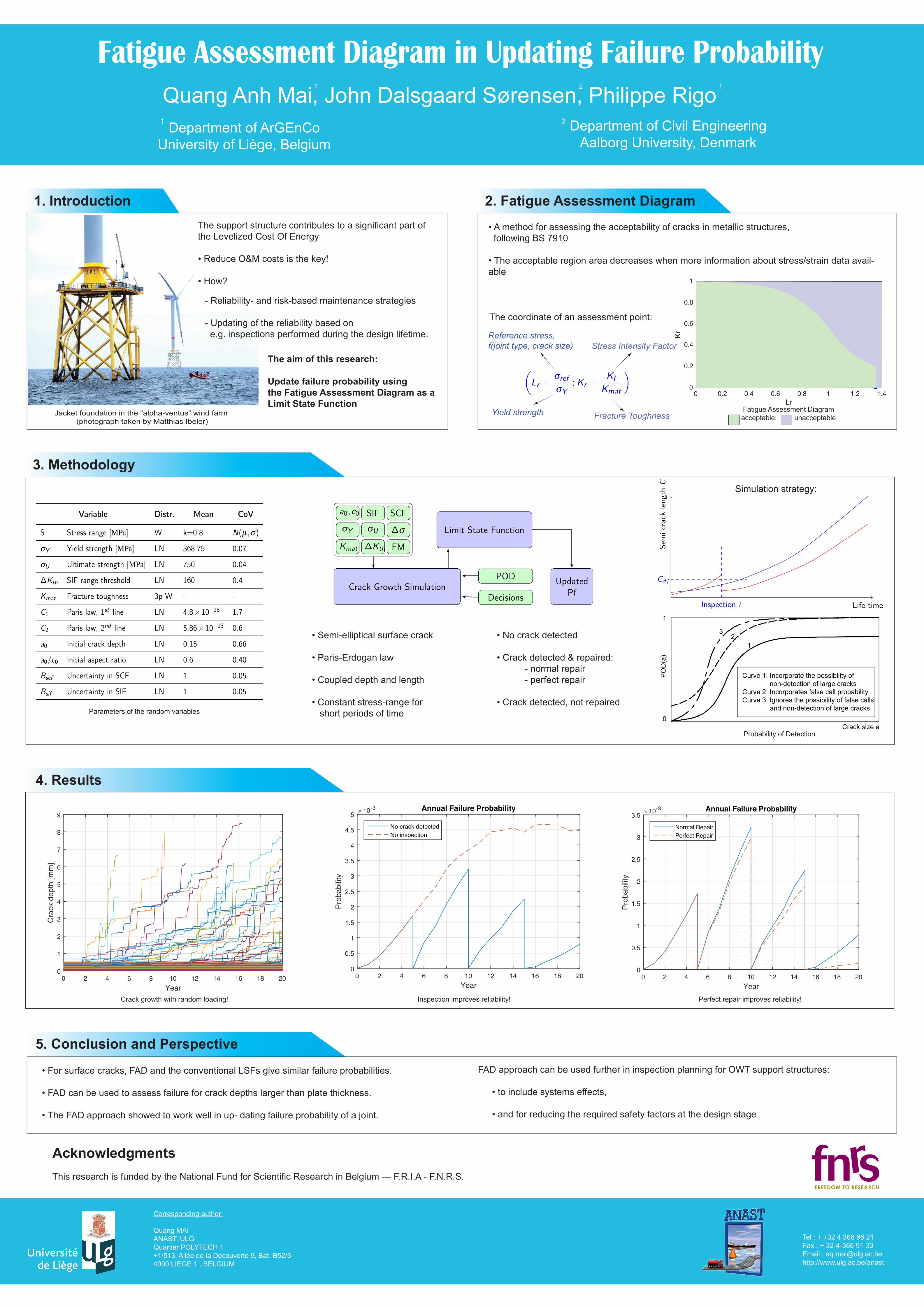
Fatigue Assessment Diagram in Updating Failure Probability

Corresponding author:

Quang MAIANAST, ULGQuartier POLYTECH 1 +1/513, Allée de la Découverte 9, Bat. B52/3 4000 LIEGE 1 , BELGIUM

Department of Civil EngineeringAalborg University, Denmark

Quang Anh Mai, John Dalsgaard Sørensen, Philippe Rigo 1 2 1

1 2Department of ArGEnCoUniversity of Liège, Belgium

Tel : + +32 4 366 96 21Fax : + 32-4-366 91 33 Email : aq.mai@ulg.ac.be http://www.ulg.ac.be/anast

This research is funded by the National Fund for Scientific Research in Belgium — F.R.I.A - F.N.R.S.

4. Results

• For surface cracks, FAD and the conventional LSFs give similar failure probabilities.

• FAD can be used to assess failure for crack depths larger than plate thickness.

• The FAD approach showed to work well in up- dating failure probability of a joint.

5. Conclusion and Perspective

• No crack detected

• Crack detected & repaired: - normal repair - perfect repair

• Crack detected, not repaired

3. Methodology 9

Updating method

Kmat

∆Kth

FM

σY

σU ∆σ

a0,c0 SIF SCF

Limit State Function

POD

DecisionsCrack Growth Simulation

UpdatedPf

Q. Mai | FAD in Updating Failure Probability

11Crack Growth Simulation

Life time

Sem

icrack

lengthC

Cd

i

Inspection i

Figure: Crack growth in combination with inspections

Q. Mai | FAD in Updating Failure ProbabilityTABLE 2: THE DESIGN SN CURVE

SN Curve

N ≤1×107 cycles N >1×107 cycles

mSN1 logCSN

1 mSN2 logCSN

2

D 3.0 12.164 5.0 15.606

Year0 2 4 6 8 10 12 14 16 18 20

Cra

ck d

epth

[mm

]

0

1

2

3

4

5

6

7

8

9

FIGURE 4: ILLUSTRATION OF CRACK PROPAGATION

- Crack depth is not larger than the steel thickness. Due to theway stress range is generated, it may happen that the crackdepth in the next month will be larger than the thickness.Since we consider only surface cracks, the result of crackpropagation will be reported up to the current month, evenif the crack depth is still smaller than the critical value.

- The second condition is a restraint on the crack length. It isrequired that the crack length be not larger than 80% of thetubular perimeter so that the formulation of bulging effectsis applicable [5].

- The third condition is about fracture toughness. It can beseen that when K ≥ Kmat happens, the assessment point willbe in the failure region of the FAD. From that point on, theresults of crack propagations will be classified in the failureregion. This condition helps to save the simulation time.

Advantages of FAD Limit State FunctionThe failure probability is calculated using two approaches

on the ‘filtered’ set of samples:

Number of sample100 101 102 103 104 105 106

Prob

abilit

y of

failu

re

10-3

0

0.2

0.4

0.6

0.8

1Convergence of the MCS solution

FIGURE 5: CUMULATIVE PF AFTER THE FIRST YEAR

Number of sample103 104 105 106

Prob

abilit

y of

failu

re

0.05

0.055

0.06

0.065

0.07Convergence of the MCS solution

FIGURE 6: CUMULATIVE PF AFTER THE YEAR 20th

- The conventional approach — using the critical crack depthand fracture toughness as criteria as shown in Eqns. (7) and(8).

- The FAD approach — using the assessment line as shown inFig. 3 to check whether the sample point stays in the safetyregion.

Using FAD on the safety region of the conventional limitsate function gives additional failures as shown in Tab. 3. Thistable indicates number of samples failed in additional to thosefound by the conventional LSF. Two failure criteria are differen-tiated (i.e. Kr ≥ Kcrit

r and Lr ≥ Lmaxr ) in order to find the cause

7 Copyright c© 2016 by ASME

Stress Intensity Factor (SIF) RangeAlthough many problems for welded joints are of the mixed

mode type, mode 1 is considered as the dominant mode for fa-tigue propagation and fracture. The SIF range is calculated fromEqn. (3) for crack depth and from Eqn. (4) for crack length,where Ya and Yc are stress intensity correction factors calculatedfollowing BS 7910 [5].

∆Ka = SYa√

πa (3)

∆Kc = SYc√

πa (4)

Stress RangesNormally, stress-range is considered as a constant value

named “Weighted Average Stress Range” as calculated inEqn. (5) from its distribution. This is based on linear damageaccumulation principle and can be used for fatigue life calcula-tion in both SN approach and FM approach [8].

SemSN

= SmSN=

∞∫

0

SmSNf (s)ds (5)

In this paper, we consider the crack propagation in a “realistic”loading condition, i.e. the stress ranges are generated randomlybased on the operating characteristics of wind turbines to be usedas representative constant values for short periods of time.

For offshore structures, the long term stress ranges are of-ten represented by a two-parameter Weibull distribution. As thejoint considered in this paper is in a jacket support structure ofan offshore wind turbine, it is reasonable to assumed the Weibullshape parameter to be 0.8 as suggested in [4]. The scale parame-ter is assumed normally distributed with CoV=15% and the meanvalue is calibrated based on the design fatigue factor (DFF) of thejoint.

PROBABILITY OF DETECTIONThe probability of detection, POD, expresses the probability

of detecting a crack of a given length (2c). It is a parameter toevaluate the accuracy of an inspection technique. Three differentPOD curves [9] are illustrated in Fig. 2. Curve 1 incorporatesthe possibility of non-detection of large cracks. Curve 2 incor-porate false call probability — it is the fraction of time that anun-cracked joint will be incorrectly classified as being cracked.Curve 3 ignores the possibility of false calls and non-detectionof large cracks and normally used as a cumulative distributionfunction in Bayesian updating for failure probability of a joint.

!

Curve 1: Incorporate the possibility ofnon-detection of large cracks

Curve 2: Incorporates false call probabilityCurve 3: Ignores the possibility of false calls

and non-detection of large cracks

1

PO

D(a

)

0Crack size a

32

1

FIGURE 2: TYPES OF POD CURVE

Although Curve 1 and Curve 2 are not in the form of a cumu-lative distribution function, they can easily be incorporated inupdating the failure probability.

POD(cd) = 1− exp[

−cd

λ

]

(6)

For illustration purpose, this paper uses the POD — a functionof the smallest detectable crack length in [mm] — as in Eqn. (6),with the parameter λ = 1.95 corresponding to a quite good in-spection technique for tubular joints in sea water [10].

LIMIT STATE EQUATIONLimit state equations for fatigue assessment of a surface

crack can be defined in both serviceability and ultimate limitsates. Two examples of failure criteria can be considered [11]as shown in Eqn. (7) and Eqn. (8) .

ac −a ≤ 0 (7)

Kmat −KI ≤ 0 (8)

A critical crack size ac is selected in the first case, Eqn. (7),e.g. based on serviceability considerations. In the second case,Eqn. (8), the fracture toughness Kmat of material is used as acritical value for the stress intensity factor KI . When Eqn. (8)happens, the crack growth becomes unstable and rapid failure oc-curs. It is worth mentioning that the stress intensity factor is usedfor fracture assessment while the stress intensity factor range isused for crack propagation. The stress intensity factor is calcu-lated similar to ∆Ka as in Eqn. (3) but the stress range is replaced

3 Copyright c© 2016 by ASME

1. Introduction

The aim of this research:

Update failure probability using the Fatigue Assessment Diagram as a Limit State Function

Jacket foundation in the “alpha-ventus“ wind farm (photograph taken by Matthias Ibeler)

The support structure contributes to a significant part of the Levelized Cost Of Energy

• Reduce O&M costs is the key!

• How?

- Reliability- and risk-based maintenance strategies

- Updating of the reliability based on e.g. inspections performed during the design lifetime.

2. Fatigue Assessment Diagram

6

Fatigue Assessment Diagram

Lr0 0.2 0.4 0.6 0.8 1 1.2 1.4

Kr

0

0.2

0.4

0.6

0.8

1

Lr ,max

=σY

+σU

2σY

(

Lr

=σref

σY

; Kr

=KI

Kmat

)

Unsafe

Figure: Level 2A Fatigue Assessment Diagram

BS-7910, 2005. Guide to Methods for Assessing the Acceptability of Flaws in Metallic Structures.British Standard Institution (BSi).

Q. Mai | FAD in Updating Failure Probability

• A method for assessing the acceptability of cracks in metallic structures, following BS 7910

• The acceptable region area decreases when more information about stress/strain data avail-able

Fatigue Assessment Diagramacceptable; unacceptable

The coordinate of an assessment point:

6

Fatigue Assessment Diagram

Lr0 0.2 0.4 0.6 0.8 1 1.2 1.4

Kr0

0.2

0.4

0.6

0.8

1

(

Lr

=σref

σY

; Kr

=KI

Kmat

)

Unsafe

Figure: Level 2A Fatigue Assessment Diagram

BS-7910, 2005. Guide to Methods for Assessing the Acceptability of Flaws in Metallic Structures.British Standard Institution (BSi).

Q. Mai | FAD in Updating Failure Probability

Reference stress, f(joint type, crack size) Stress Intensity Factor

Yield strength Fracture Toughness

8Uncertainties

Variable Value

ν No. of cycle/year 1×107

t Steel thickness [mm] 65

R Outer radius [mm] 79.5

L Joint length [mm] 100

ησ Bend. to memb. ratio 0.81

∆Ktr

Transition SIF range 196

m1 Paris law, 1st line 5.10

m2 Paris law, 2nd line 2.88

Ca

/Cc

C ratio for a and c 0.9

Variable Distr. Mean CoV

S Stress range [MPa] W k=0.8 N(µ,σ)

σY

Yield strength [MPa] LN 368.75 0.07

σU

Ultimate strength [MPa] LN 750 0.04

∆Kth

SIF range threshold LN 160 0.4

Kmat

Fracture toughness 3p W - -

C1 Paris law, 1st line LN 4.8×10−18 1.7

C2 Paris law, 2nd line LN 5.86×10−13 0.6

a0 Initial crack depth LN 0.15 0.66

a0/c0 Initial aspect ratio LN 0.6 0.40

Bscf

Uncertainty in SCF LN 1 0.05

Bsif

Uncertainty in SIF LN 1 0.05

Q. Mai | FAD in Updating Failure Probability

Parameters of the random variables

• Semi-elliptical surface crack

• Paris-Erdogan law

• Coupled depth and length

• Constant stress-range for short periods of time

Simulation strategy:

Probability of Detection

14

ResultsNo Crack Detected

Year0 2 4 6 8 10 12 14 16 18 20

Prob

abilit

y

10-3

0

0.5

1

1.5

2

2.5

3

3.5

4

4.5

5Annual Failure Probability

No crack detectedNo inspection

Figure: Annual POF

Q. Mai | FAD in Updating Failure Probability

15

ResultsCrack Detected & Repaired

Year0 2 4 6 8 10 12 14 16 18 20

Prob

abilit

y

10-3

0

0.5

1

1.5

2

2.5

3

3.5Annual Failure Probability

Normal RepairPerfect Repair

Figure: Annual POF

Q. Mai | FAD in Updating Failure Probability

Perfect repair improves reliability! Inspection improves reliability! Crack growth with random loading!

Acknowledgments

FAD approach can be used further in inspection planning for OWT support structures:

• to include systems effects,

• and for reducing the required safety factors at the design stage