JSS Journal of Statistical SoftwareMay 2013, Volume 53, Issue 9. http://www.jstatsoft.org/

fastcluster: Fast Hierarchical, Agglomerative

Clustering Routines for R and Python

Daniel MullnerStanford University

Abstract

The fastcluster package is a C++ library for hierarchical, agglomerative clustering. Itprovides a fast implementation of the most efficient, current algorithms when the inputis a dissimilarity index. Moreover, it features memory-saving routines for hierarchicalclustering of vector data. It improves both asymptotic time complexity (in most cases)and practical performance (in all cases) compared to the existing implementations instandard software: several R packages, MATLAB, Mathematica, Python with SciPy.

The fastcluster package presently has interfaces to R and Python. Part of the func-tionality is designed as a drop-in replacement for the methods hclust and flashClust

in R and scipy.cluster.hierarchy.linkage in Python, so that existing programs canbe effortlessly adapted for improved performance.

Keywords: clustering, algorithm, hierarchical, agglomerative, linkage, single, complete, aver-age, UPGMA, weighted, WPGMA, McQuitty, Ward, centroid, UPGMC, median, WPGMC,MATLAB, Mathematica, Python, SciPy, C++.

1. Introduction

Hierarchical clustering is an important, well-established technique in unsupervised machinelearning. The common hierarchical, agglomerative clustering methods share the same algo-rithmic definition but differ in the way in which inter-cluster distances are updated after eachclustering step (Anderberg 1973, page 133). The seven common clustering schemes are calledsingle, complete, average (UPGMA), weighted (WPGMA, McQuitty), Ward, centroid (UP-GMC) and median (WPGMC) linkage (Everitt, Landau, Leese, and Stahl 2011, Table 4.1)

A variety of algorithms has been developed in the past decades to improve performance com-pared to the primitive algorithmic setup, in particular Anderberg (1973, page 135), Rohlf(1973), Sibson (1973), Day and Edelsbrunner (1984, Table 5), Murtagh (1984), Eppstein

2 fastcluster: Fast Hierarchical, Agglomerative Clustering in R and Python

(2000), Cardinal and Eppstein (2004). Also, hierarchical clustering methods have been im-plemented in standard scientific software such as R (R Core Team 2011), MATLAB (TheMathWorks, Inc. 2011), Mathematica (Wolfram Research, Inc. 2010) and the SciPy libraryfor the programming language Python (Jones, Oliphant, Peterson et al. 2001; van Rossumet al. 2011). Specifically, there are the following functions:

hclust in R’s stats package (R Core Team 2011),

flashClust in R’s flashClust package (Langfelder 2011),

agnes in R’s cluster package (Machler, Rousseeuw, Struyf, Hubert, and Hornik 2011),

linkage in MATLAB’s statistics toolbox (The MathWorks, Inc. 2011),

Agglomerate and DirectAgglomerate in Mathematica (Wolfram Research, Inc. 2010),

linkage in the Python module scipy.cluster.hierarchy (Eads 2008).

We found that all these implementations do not give satisfactory performance because—insofar as this can be checked only for open-source software—they use inferior algorithms. Thefastcluster package, which is available from the Comprehensive R Archive Network at http://CRAN.R-project.org/package=fastcluster, builds upon the author’s work (Mullner 2011),where we identified three algorithms, including a new one by the author, as the most efficientcurrent algorithms for the seven clustering schemes above, when the input is given by pairwisedissimilarities between elements. The fastcluster package also has memory-saving algorithmsfor some of the clustering schemes when the input is given as vector data. It provides a fastC++ implementation of each algorithm and currently offers interfaces to R and Python. Weimprove both the asymptotic worst-case time complexity (in those cases where this can bedetermined due to open source) and the practical performance (in all cases) of the existingimplementations listed above.

The paper is structured as follows: In Section 2, we briefly introduce the clustering methodswhich our package provides in order to establish the technical context. The presentationis selective and focuses on the aspects which are important for this paper. For a generalintroduction to the well-known hierarchical clustering methods, we refer to textbooks, e.g.,Anderberg (1973) or Everitt et al. (2011). Section 3 contains information about the algorithmsand the implementation. Section 4 compares the performance of the package with existingsoftware, both in a theoretical, asymptotic complexity analysis in Section 4.1 and by use caseperformance experiments in Sections 4.2 and 4.3. In Section 5, we explain how to use thefastcluster package and point to differences between the interfaces. This part is independentof the two preceding sections. A detailed user’s manual is available in the package distribution.The paper finishes with a short conclusion in Section 6.

2. SAHN clustering methods

The clustering methods in this paper have been characterized by the acronym SAHN (se-quential, agglomerative, hierarchic, nonoverlapping methods) by Sneath and Sokal (1973, Sec-tions 5.4 and 5.5). The input to the methods is a dissimilarity index on a finite set (see Hansen

Journal of Statistical Software 3

and Jaumard 1997, Section 2.1). For a set S, this is by definition a map d : S × S → [0,∞)which is reflexive and symmetric, i.e., we have d(x, x) = 0 and d(x, y) = d(y, x) for all x, y ∈ S.

A metric on S is certainly a dissimilarity index. The dissimilarity index can be given directlyto a clustering algorithm as the

(N2

)pairwise dissimilarities. This is the stored matrix approach

(Anderberg 1973, Section 6.2). Alternatively, the input points can be specified in a differentmanner, e.g., as points in a normed vector space, where the dissimilarity information is givenimplicitly by the metric on the ambient space. This input format is called the stored dataapproach (Anderberg 1973, Section 6.3).

The first option has input size Θ(N2) for N elements, and the second option Θ(ND) for Npoints in a D-dimensional vector space. We call an algorithm memory-saving in this paper ifit accepts vector data and the required memory is of class O(ND).

The common procedural definition for all clustering methods in this paper is as follows (cf.Anderberg 1973, Section 6.1):

1. Let S be the current set of nodes, with implicit or explicit dissimilarity information.Determine a pair of mutually closest points (a, b).

2. Join a and b into a new node n. Delete a and b from the set of nodes and add n to it.

3. Output the node labels a and b and their dissimilarity d(a, b).

4. Update the dissimilarity information by specifying the distance from n to all othernodes. This can be done explicitly by specifying the distances, or by defining a clusterrepresentative in the stored data approach.

5. Repeat steps 1–4 until there is a single node left, which contains all the initial nodes.

The clustering schemes differ in the update formula for cluster dissimilarities in step 4. Table 1lists the formulas for the seven common clustering schemes.

The output of the clustering procedure is a list of N − 1 triples (ai, bi, δi), which encodesa stepwise dendrogram (see Mullner 2011, Section 2.2, for the difference to non-stepwisevariants): The i-th triple contains the information which nodes are joined into a new nodein the i-th step, and what was the cluster dissimilarity between ai and bi. This is sufficientinformation to draw the usual representation of the dendrogram as a rooted tree, where theleaves are the initial nodes, and a branching point at a given height δi represents the joiningof nodes ai, bi with mutual distance δi := d(ai, bi).

Note that the output of the clustering procedure above is not unique: if more than one pairof nodes realizes the current minimal distance in step 1, any of them might be chosen, andthis influences later steps. The algorithms in the fastcluster package are correct in the sensethat they always return one of the possible outputs of the procedure above, and hence resolveties in one of possibly several correct ways. For detailed information on why the handling ofties is a non-trivial matter and how it influences the choice of algorithms in the fastclusterpackage, see Mullner (2011, Sections 3 and 5).

The procedural definition of the clustering scheme above already constitutes a primitive al-gorithm. This algorithm has a time complexity of Θ(N3) for N input points, since in the i-thiteration a pair of closest nodes is searched among N − i+ 1 nodes in step 1, which requiresΘ((N − i)2) comparisons by an exhaustive search. The fastcluster package reduces the time

4 fastcluster: Fast Hierarchical, Agglomerative Clustering in R and Python

Name Distance update formulafor d(I ∪ J,K)

Cluster dissimilaritybetween clusters A and B

Single min(d(I,K), d(J,K)) mina∈A,b∈B

d[a, b]

Complete max(d(I,K), d(J,K)) maxa∈A,b∈B

d[a, b]

AveragenId(I,K) + nJd(J,K)

nI + nJ

1

|A||B|∑a∈A

∑b∈B

d[a, b]

Weighted/McQuittyd(I,K) + d(J,K)

2

Ward

√(nI + nK)d(I,K)2 + (nJ + nK)d(J,K)2 − nKd(I, J)2

nI + nJ + nK

√2|A||B||A|+ |B|

· ‖~cA − ~cB‖2

Centroid

√nId(I,K)2 + nJd(J,K)2

nI + nJ− nInJd(I, J)2

(nI + nJ)2‖~cA − ~cB‖2

Median

√d(I,K)2

2+d(J,K)2

2− d(I, J)2

4‖~wA − ~wB‖2

Table 1: Agglomerative clustering schemes. Let I, J be two clusters joined into a new cluster,and let K be any other cluster. Denote by nI , nJ and nK the sizes of (i.e., number of elementsin) clusters I, J,K, respectively.The update formulas for the“Ward”, “Centroid”and“Median”methods assume that the inputpoints are given as vectors in Euclidean space with the Euclidean distance as dissimilaritymeasure. The expression ~cX denotes the centroid of a cluster X. The point ~wX is definediteratively and depends on the order of clustering steps: If the cluster L is formed by joiningI and J , we define ~wL as the midpoint 1

2(~wI + ~wJ).References: Lance and Williams (1967), Kaufman and Rousseeuw (1990, Section 5.5.1).

complexity from cubic to quadratic: as a theoretically guaranteed worst-case complexity forfive of the seven methods, and as a heuristic behavior in all observed cases for the “centroid”and “median” distance update formulas.

The formulas in Table 1 show that inter-cluster distances can be conveniently defined andcomputed in constant time from (weighted or unweighted) cluster centroids in Euclideanspace for the “Ward”, “centroid” and “median” methods. Hence, these clustering schemes arepredestined for a memory-saving clustering algorithm where not all distance values are storedbut distances are computed as they are needed. Moreover, there are algorithms for singlelinkage clustering (including the one which is used in the fastcluster package) which readin every pairwise dissimilarity value between initial nodes exactly once, and otherwise needonly O(N) temporary memory. Hence, also single linkage clustering can be implemented ina memory-saving manner. The fastcluster package contains memory-saving algorithms forthese four methods. It assumes Euclidean distances between input vectors for the “Ward”,“centroid” and “median” methods and provides a variety of metrics for the “single” method.

Journal of Statistical Software 5

3. Algorithms and implementation

The efficient algorithms which are used in the fastcluster package were described in detail bythe author in Mullner (2011). In that paper, the author introduced an algorithm which workswith any distance formula, proved the correctness of two existing algorithms by Rohlf andMurtagh and identified the most efficient algorithms. The fastcluster package builds upon thisknowledge and implements the most efficient algorithms. There are three algorithms in total:For single linkage clustering, an algorithm by Rohlf (1973) is used. It links Prim’s algorithmfor the minimum spanning tree of a graph (see Cormen, Leiserson, Rivest, and Stein 2009,Section 23.2) with the observation that a single linkage dendrogram can be obtained fromthe minimum spanning tree of a graph. More precisely, this graph is the weighted, completegraph whose adjacency matrix is the dissimilarity index (Gower and Ross 1969).

The “complete”, “average”, “weighted” and “Ward” (for dissimilarity input) methods use thenearest-neighbor chain algorithm by Murtagh (1984, page 86). This algorithm exploits thefact that pairs of mutually closest points can be merged in any order, if the distance updateformula fulfills certain criteria (see also Mullner 2011, Theorem 3). The “centroid”, “median”and “Ward” (vector input) methods use the author’s algorithm (Mullner 2011, Section 3.1),which delays repeated searches for nearest neighbors as long as possible.

The algorithms are fairly optimized for speed. For example, there are two variants of theauthor’s algorithm, which differ by the indexing of intermediate results and how the list ofnearest neighbors for all nodes is organized. These two variants perform different enough tomake the distinction worthwhile. The final choice which algorithm to use for which methodwas then made according to performance on test datasets.

All algorithms in the fastcluster package are implemented in a C++ library. The core codeis the same for both interfaces. It is accompanied by language-specific wrappers, whichhandle the input and output in the interface-specific array data structures and also handle thedifferent indexing conventions and extra output (like the order field in the R interface). Theinterface code in the interpreted languages R and Python is very short so that the overhead islow. The C++ code extensively uses template programming to avoid code duplication amongthe seven methods. Also the data types are flexible through template programming. Thecurrent setup always uses double precision for floating-point numbers since this is the defaultin Python and R. The indices to the data points are represented by at least 32 bit wide signedintegers, and indices to the dissimilarity array of size

(N2

)are represented by signed 64-bit

integers. This is in theory sufficient to handle 229 − 1 data points, hence does not pose anactual obstruction.

4. Performance

In this section, we compare the performance of the fastcluster package with the other imple-mentations in standard software. In Section 4.1, we analyze the asymptotic time complexity ofthe algorithms whose source code is available, both in the worst and in the best case. We thencompare the performance of all implementations experimentally on a range of test datasets.Section 4.2 deals with the case when the input is a dissimilarity index, and Section 4.3 coversthe memory-saving routines for vector input.

6 fastcluster: Fast Hierarchical, Agglomerative Clustering in R and Python

4.1. Asymptotic run-time complexity

The asymptotic worst-case time complexity of the methods in open-source packages (agnes incluster, flashClust in flashClust, hclust in stats and linkage in SciPy) is Θ(N3) through-out. These bounds were determined by careful inspection of the source code and construct-ing series of worst-case examples. The fastcluster package improves performance to Θ(N2)worst-case time complexity for the “single”, “complete”, “average”, “weighted” and “Ward”(dissimilarity input case only) methods. For the “centroid”, “median” and “Ward” (vectorinput) methods, we still use O(N3) algorithms due to their better performance in practice,even though quadratic run-time algorithms are available (Eppstein 2000).

Regarding the best-case complexity, only the fastcluster and flashClust packages achieve thetheoretically optimal bound of Θ(N2). SciPy, agnes and hclust have a best-case complexityof only Θ(N3).

4.2. Use case performance: Dissimilarity methods

As indicated by the asymptotic best-case complexity, the various algorithms indeed performdifferently (quadratic vs. cubic time) in test cases. The diagrams in Figure 1 show theperformance on a range of test datasets for all seven methods. The fastcluster packageconsistently outperforms all other packages, and by rather significant factors in the majorityof cases. Also, the performance on very small datasets is very good, due to a low overhead. Tobe fair, the measurements for small datasets depend on the software environment in addition tothe clustering algorithms, so, e.g., the R fastcluster package can only be directly compared tothe other three R packages: here it has the lowest overhead. The other graphs were generatedby different interpreters (Python, MATLAB, Mathematica). fastcluster’s Python interface haseven lower overhead than the R version and gives otherwise similar timings.

In summary, the fastcluster package not only improves the theoretical, asymptotic bounds ofthe clustering algorithms, but it also significantly improves the run-time performance of theexisting implementations.

The test sets were synthetic datasets: i.i.d. samples from a mixture of multivariate Gaussiandistributions in Euclidean space with standard covariance. For each number of input points N ,we generated 12 test sets by varying the following parameters:

Dimension of the Euclidean space: 2, 3, 10, 200.

Number of centers of Gaussian distributions: 1, 5, round(√N). The centers are also

distributed according to a Gaussian distribution.

Moreover, for the methods for which it makes sense (single, complete, average, weighted: the“combinatorial” methods), we also generated 10 test sets per number of input points with auniform distribution of dissimilarities.

The timings were obtained on a PC with an Intel dual-core CPU T7500 with 2.2 GHz clockspeed and 4GB of RAM and no swap space. The operating system was Ubuntu 11.04 64-bit.R version: 2.13.0, fastcluster version: 1.1.5, flashClust version: 1.01, cluster version: 1.13.3,stats version: 2.13.0, Python version: 2.7.1, NumPy version: 1.5.1, SciPy version: 0.8.0.

Journal of Statistical Software 7

Method: Single Method: Complete

101 102 103 104

Number of points

10−5

10−4

10−3

10−2

10−1

100

101

102

103

CP

Uti

me

ins

101 102 103 104

Number of points

10−5

10−4

10−3

10−2

10−1

100

101

102

103

CP

Uti

me

ins

Method: Average Method: Weighted

101 102 103 104

Number of points

10−5

10−4

10−3

10−2

10−1

100

101

102

103

CP

Uti

me

ins

101 102 103 104

Number of points

10−5

10−4

10−3

10−2

10−1

100

101

102

103

CP

Uti

me

ins

Method: Ward Method: Centroid

101 102 103 104

Number of points

10−5

10−4

10−3

10−2

10−1

100

101

102

103

CP

Uti

me

ins

101 102 103 104

Number of points

10−5

10−4

10−3

10−2

10−1

100

101

102

103

CP

Uti

me

ins

(Not supported by agnes)

Method: Median

101 102 103 104

Number of points

10−5

10−4

10−3

10−2

10−1

100

101

102

103

CP

Uti

me

ins

R: agnesR: flashclustR: hclustR: fastcluster

Matlab R2011bMathematicascipy.cluster.hierarchyPython: fastcluster

Figure 1: Performance comparison for dissimilarity matrix input. Lightly colored bands:Min-max range. Solid curves: Mean values.

8 fastcluster: Fast Hierarchical, Agglomerative Clustering in R and Python

Method: Single Method: Ward

101 102 103 104

Number of points

100

101

102

103

Rel

ativ

eC

PU

tim

eco

mpa

red

tofa

stcl

uste

r

101 102 103 104

Number of points

100

101

102

103

Rel

ativ

eC

PU

tim

eco

mpa

red

tofa

stcl

uste

r

Method: Centroid Method: Median

101 102 103 104

Number of points

100

101

102

103

Rel

ativ

eC

PU

tim

eco

mpa

red

tofa

stcl

uste

r

101 102 103 104

Number of points

100

101

102

103

Rel

ativ

eC

PU

tim

eco

mpa

red

tofa

stcl

uste

r

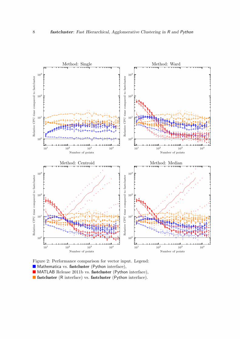
Figure 2: Performance comparison for vector input. Legend:Mathematica vs. fastcluster (Python interface),MATLAB Release 2011b vs. fastcluster (Python interface),fastcluster (R interface) vs. fastcluster (Python interface).

Journal of Statistical Software 9

Only one core of the two available CPU cores was used in all cases except the “Ward”,“centroid” and “median” methods in MATLAB.1

The memory requirements of all these algorithms are similar: they all keep the input arrayof(N2

)floating-point numbers in memory plus a working copy (hence 8N(N − 1) bytes in

total with double-precision floating point numbers). The only exception is fastcluster’s singlelinkage algorithm, which uses less memory. Apart from the distance array, the fastclusteralgorithms only needs O(N) memory for intermediate storage and the output. Although noextensive memory analysis was done, the fastcluster package can process as large datasetsand sometimes even larger datasets than its competitors at a given memory size.

4.3. Performance of the vector methods

Three packages offer memory-saving clustering when the input consists of vector data: fast-cluster, Mathematica and MATLAB. MATLAB has routines for “Ward”, “centroid” and “me-dian” linkage; fastcluster and Mathematica additionally offer single linkage.

The asymptotic time complexity of the fastcluster package is Θ(N2D) for N points in RD

in the best case. The worst-case complexity is also Θ(N2D) for the “single” method andO(N3D) for the “Ward”, “centroid” and “median” methods. For the commercial software, thecomplexity cannot be determined exactly since the source code is not available. From our usecase experiments it seems that MATLAB and Mathematica also have a best-case complexityof Θ(N2D), and MATLAB has a worst-case complexity of Ω(N3D).

We tested the performance of the three packages on the same datasets as in the previousSection 4.2. Since the run time depends heavily on the dimensionality of the dataset, itmakes no sense to put the absolute timings into a common diagram. Instead, Figure 2shows the relative run time of the commercial software versus the fastcluster package withthe Python interface (blue and red graphs). Four average curves are plotted, one for eachdimensionality (2, 3, 10, 200). We only tested Euclidean distances although a variety ofdistance measures is possible for the single linkage method. The curves clearly show that ourPython module consistently outperforms MATLAB and Mathematica in this task. MATLAB’srun times show cubic asymptotic behavior for the high-dimensional datasets. Mathematicaaborted on two different machines with a segmentation fault at 20000 input points, so theoutput of Mathematica’s vector clustering methods should be double-checked independentlyfor critical data. For this reason we did not continue the test after 20000 input points eventhough the fastcluster package is able to handle larger data.

The orange graph in Figure 2 shows the timings of fastcluster’s R interface versus the Pythoninterface. The R interface is slower by high factors ranging from 2.6 to 21, but for a goodreason: The R distance function checks every coordinate whether it is marked as missingdata (a NA value in R syntax), so that 2D extra comparisons (and therefore conditional

1In fact, MATLAB seems to use only one core for the actual clustering step, like the other packages. How-ever, for the three “geometric” methods “Ward”, “centroid”, and “median”, MATLAB carries out an additionalprecheck, which tests whether the

(N2

)pairwise distances can be generated from a configuration of N points

in Euclidean space. This involves checking whether a dense, symmetric N ×N matrix is positive semidefinite,for which MATLAB apparently uses a parallelized eigenvalue algorithm. Moreover, for double-centering of amatrix, MATLAB unnecessarily carries out matrix multiplication, which has time complexity Θ(N3) in itsstraightforward implementation. Hence the precheck requires much more time than the actual clustering task.This is reflected in Figure 1, where MATLAB is much slower for the “geometric” methods than for the otherfour “combinatorial” methods.

10 fastcluster: Fast Hierarchical, Agglomerative Clustering in R and Python

branch instructions on machine code level) are needed to compute the distance between anytwo points. By doing so, the fastcluster R package follows exactly the internal formulas ofthe dist method in the R core stats package to handle missing data. However, this makesthe process considerably slower than the straightforward calculation in the Python module.MATLAB and Mathematica are compared to the Python module since neither handles missingdata automatically.

5. Usage of the fastcluster package

The fastcluster package features interfaces to R and Python. These interfaces can be usedas drop-in replacements for the linkage function in the Python module scipy.cluster.hierar-chy, for the hclust function in R’s stats package, and for hclust alias flashClust in R’sflashClust package. The replacements share the same syntax and output specifications butare faster.

The fastcluster package can be downloaded from the Comprehensive R Archive Networkat http://CRAN.R-project.org/package=fastcluster. Installation instructions for bothR and Python are included in the package documentation. The Python part is additionallyavailable at PyPI (http://pypi.python.org/pypi/fastcluster) from where is can be easilyinstalled with Python’s setuptools.

Nothing in the source code is specific to a certain operating system, so it should be possibleto install the fastcluster package on a wide variety of hardware architectures and operatingsystems.

5.1. The R interface

In R, the package is loaded as usual with the command:

R> library("fastcluster")

The fastcluster package overwrites the function hclust from the stats package, in the sameway as the flashClust package does. It is recommended to remove references to the flashClustpackage when the fastcluster package is used to not accidentally overwrite the hclust functionwith the flashClust version.

If needed, or in order to prevent confusion, all three functions can be specified unambiguouslyby their namespace:

stats::hclust(...)

fastcluster::hclust(...)

flashClust::hclust(...)

All three hclust functions have exactly the same calling conventions and output format. Auser may simply load the package and immediately and effortlessly enjoy the performanceimprovements to the hclust function. The function flashClust in the flashClust package isan alias for flashClust::hclust, so the flashClust function may be replaced as well.

The agnes function from the cluster package has a slightly different input and output format,but in many cases it should be possible with little effort to use the faster alternative in thefastcluster package.

Journal of Statistical Software 11

An exact and detailed specification of the methods is given in the user’s manual in thefastcluster distribution.2 As a short description, the method

hclust(d, method = "complete", members = NULL)

performs agglomerative clustering on the compressed distance matrix d. The array d is aone-dimensional array which contains the upper triangular part of the symmetric matrix ofdissimilarities, as it is produced e.g., by R’s dist function.

The parameter method is a string which specifies the dissimilarity update formula from Ta-ble 1. It must be one of "single", "complete", "average", "mcquitty", "ward", "centroid","median" or an unambiguous abbreviation thereof.

The optional parameter members may contain a vector which specifies weights for the initialnodes. This can be used, e.g., to start or re-start the hierarchical clustering process whenpartial clusters have been formed beforehand, so that nodes have cardinalities different from 1.

The output of the hclust method is an object of class "hclust" which mainly encodes astepwise dendrogram. It can be processed by the existing methods in R, in particular thereis a specific plot method for the output which draws the dendrogram.

The new method

hclust.vector(X, method = "single", members = NULL, metric = "euclidean",

p = NULL)

is a memory-saving option if the input to the clustering algorithm is given as vector data.Instead of keeping the entire matrix of dissimilarities in memory, the vector method com-putes distances on-the-fly from vectors, with the metric which is specified by the "metric"

parameter. This is currently possible for the "single", "ward", "centroid" and "median"

methods.

In short, the call

R> hclust.vector(X, method = "single", metric = [...])

gives the same result as

R> hclust(dist(X, metric = [...]), method = "single")

but uses less memory and is equally fast, if not faster. The parameter p is used for the"minkowski" metrics only and specifies the the exponent for this family of metrics. Theoutput is again a stepwise dendrogram.

If method is one of "centroid", "median", or "ward", clustering is performed with respectto Euclidean distances. In this case, the parameter metric must be "euclidean". Noticethat hclust.vector operates on Euclidean distances for compatibility with the dist method,while hclust assumes squared Euclidean distances for compatibility with the stats::hclust

method. Hence, the call

R> hc <- hclust.vector(X, method = "ward")

2This is stored as a vignette, i.e., the file inst/doc/fastcluster.pdf in the source distribution, and canbe accessed in R using vignette("fastcluster", package = "fastcluster").

12 fastcluster: Fast Hierarchical, Agglomerative Clustering in R and Python

is, aside from the lesser memory requirements, equivalent to:

R> d <- dist(X)

(1)R> hc <- hclust(d^2, method = "ward")

R> hc$height <- sqrt(hc$height)

The same applies to the "centroid" and "median" methods. Differences may arise only fromrounding errors due to squaring and taking the square root (which may, however, in extremecases affect the entire clustering result due to the inherently unstable nature of the clusteringschemes).

The same issue, that the R interface for the fastcluster package sometimes interprets inputvalues as ordinary and sometimes as squared Euclidean distances, accounts also for the biggestdifference between the R and the Python interface. See the next Section 5.2 for details. Eventhough this might seem to provoke complications unnecessarily, these differences were in factdesigned intentionally, in order for the fastcluster package to comply best with the varyingconventions in existing packages.

5.2. Caveat

R and MATLAB/SciPy use different conventions for the “Ward”, “centroid” and “median”methods, if the input is a dissimilarity matrix. R assumes that the data consists of squaredEuclidean distances, while MATLAB and SciPy expect non-squared Euclidean distances. Thefastcluster package respects these conventions and uses different formulas in the two interfaces.

Let d be a compressed array of pairwise distances, as it is used by all three programs MATLAB,SciPy and R. In order to obtain the same results in all programs, the R method must be giventhe entry-wise square of the distance array, d^2, for the “Ward”, “centroid” and “median”methods, compared to the other software. After the calculation, the square root of the heightfield in the dendrogram may be taken. For the “average” and “weighted” alias “McQuitty”methods, the same distance array d must be used in all programs for identical results. The“single” and “complete” methods only depend on the relative order of the distances, hence itdoes not make a difference whether one uses the distances or the squared distances.

Therefore, the R code example (1) above, where the dissimilarity matrix entries are squared,gives the same result as the following Python code:

>>> d = scipy.spatial.distance.pdist(X)

>>> hc = fastcluster.hclust(d, method = "ward")

5.3. The Python interface

The fastcluster package is imported as usual by:

>>> import fastcluster

It provides the following functions:

linkage(X, method = "single", metric = "euclidean", preserve_input = True)

single(X)

Journal of Statistical Software 13

complete(X)

average(X)

weighted(X)

ward(X)

centroid(X)

median(X)

linkage_vector(X, method = "single", metric = "euclidean", extraarg = None)

The function linkage can process both dissimilarity and vector input as the first argument X.The input is preferably a NumPy array (Oliphant et al. 2011) with double-precision floatingpoint entries. Any other data format will be converted before it is processed.

If X is a one-dimensional array, it is considered a condensed matrix of pairwise dissimilarities,in the same format as is returned by the function scipy.spatial.distance.pdist in theSciPy software for computing pairwise distances between row vectors of a matrix. If the inputarray is two-dimensional, it is regarded as vector data and is converted to a dissimilarity indexwith the method scipy.spatial.distance.pdist with the metric parameter first.

The method parameter specifies the distance update formula and must be one of "single","complete", " average", "weighted", "ward", " centroid" or "median". The parameterpreserve_input specifies whether a working copy of the input array is made or not. Thiscan save approximately half the memory if the dissimilarity array is created for the clusteringonly and is not needed afterward.

The functions single, complete, average, weighted, ward, centroid and median are aliasesfor the linkage function with the corresponding method parameter and are mainly there forcompatibility with the scipy.cluster.hierarchy package.

The function linkage_vector provides the memory-saving clustering routines for the meth-ods "single", "ward", "centroid" and "median". The input array is interpreted as N datapoints in RD, i.e., as an (N ×D) array, in the same way as the two-dimensional input for thelinkage function.

The “Ward”, “centroid” and “median” methods require the Euclidean metric, while singlelinkage clustering accepts the same wide variety of metric parameters for floating-point andBoolean matrices as the function scipy.spatial.distance.pdist. The exact formulas forthe pairwise distances and the documentation differ in some cases from SciPy’s pdist methodsince the author modified/corrected a few details. Therefore, we refer to the user’s manualin the fastcluster package for authoritative details and specifications of all metrics. Theextraarg parameter is used by some metrics for additional parameters.

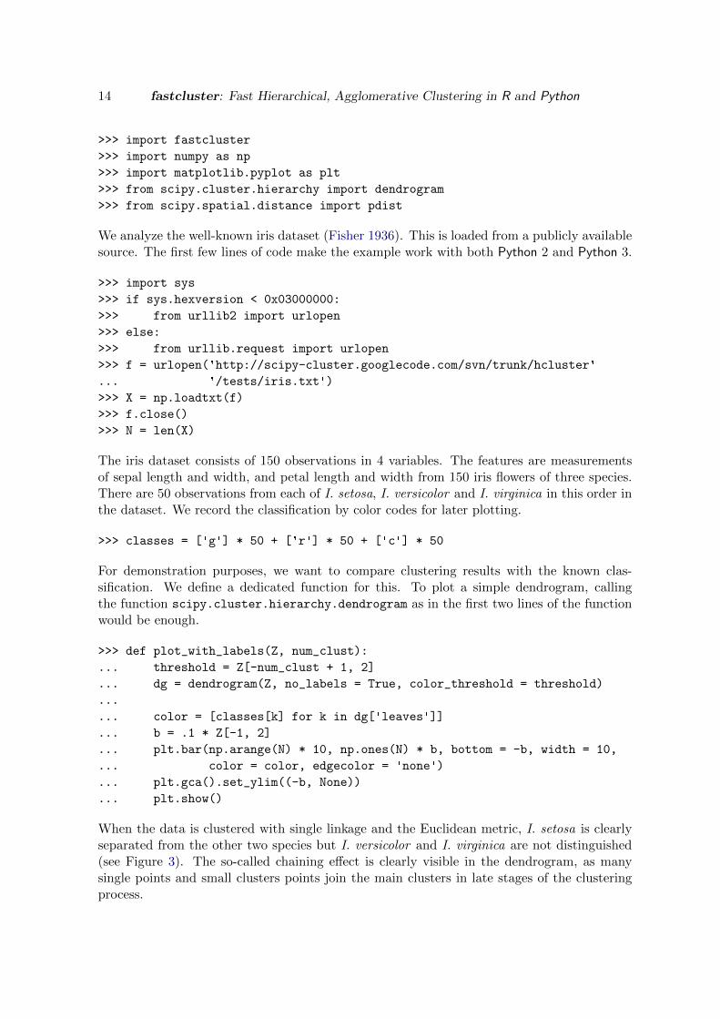
5.4. A Python example

We present a short but complete example of a cluster analysis in Python which includesplotting the results. An example for R, which was taken from the original stats package, canbe obtained from the R command line by:

R> example(hclust)

The source code of the following Python example is contained in the supplements to thispaper. From version 1.1.8 on, the fastcluster package will support both Python 2 and 3.

First, import the necessary packages:

14 fastcluster: Fast Hierarchical, Agglomerative Clustering in R and Python

>>> import fastcluster

>>> import numpy as np

>>> import matplotlib.pyplot as plt

>>> from scipy.cluster.hierarchy import dendrogram

>>> from scipy.spatial.distance import pdist

We analyze the well-known iris dataset (Fisher 1936). This is loaded from a publicly availablesource. The first few lines of code make the example work with both Python 2 and Python 3.

>>> import sys

>>> if sys.hexversion < 0x03000000:

>>> from urllib2 import urlopen

>>> else:

>>> from urllib.request import urlopen

>>> f = urlopen('http://scipy-cluster.googlecode.com/svn/trunk/hcluster'

... '/tests/iris.txt')

>>> X = np.loadtxt(f)

>>> f.close()

>>> N = len(X)

The iris dataset consists of 150 observations in 4 variables. The features are measurementsof sepal length and width, and petal length and width from 150 iris flowers of three species.There are 50 observations from each of I. setosa, I. versicolor and I. virginica in this order inthe dataset. We record the classification by color codes for later plotting.

>>> classes = ['g'] * 50 + ['r'] * 50 + ['c'] * 50

For demonstration purposes, we want to compare clustering results with the known clas-sification. We define a dedicated function for this. To plot a simple dendrogram, callingthe function scipy.cluster.hierarchy.dendrogram as in the first two lines of the functionwould be enough.

>>> def plot_with_labels(Z, num_clust):

... threshold = Z[-num_clust + 1, 2]

... dg = dendrogram(Z, no_labels = True, color_threshold = threshold)

...

... color = [classes[k] for k in dg['leaves']]

... b = .1 * Z[-1, 2]

... plt.bar(np.arange(N) * 10, np.ones(N) * b, bottom = -b, width = 10,

... color = color, edgecolor = 'none')

... plt.gca().set_ylim((-b, None))

... plt.show()

When the data is clustered with single linkage and the Euclidean metric, I. setosa is clearlyseparated from the other two species but I. versicolor and I. virginica are not distinguished(see Figure 3). The so-called chaining effect is clearly visible in the dendrogram, as manysingle points and small clusters points join the main clusters in late stages of the clusteringprocess.

Journal of Statistical Software 15

0.0

0.5

1.0

1.5

Figure 3: Python example, single linkage dendrogram.

0

1

2

3

4

5

6

7

Figure 4: Python example, dendrogram for “weighted” linkage.

>>> Z = fastcluster.linkage(X, method = 'single')

>>> plot_with_labels(Z, 2)

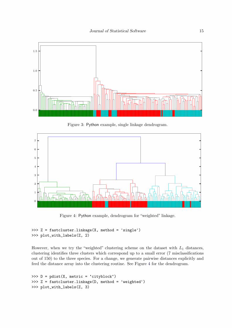
However, when we try the “weighted” clustering scheme on the dataset with L1 distances,clustering identifies three clusters which correspond up to a small error (7 misclassificationsout of 150) to the three species. For a change, we generate pairwise distances explicitly andfeed the distance array into the clustering routine. See Figure 4 for the dendrogram.

>>> D = pdist(X, metric = 'cityblock')

>>> Z = fastcluster.linkage(D, method = 'weighted')

>>> plot_with_labels(Z, 3)

16 fastcluster: Fast Hierarchical, Agglomerative Clustering in R and Python

6. Conclusion

The fastcluster package currently offers the fastest implementation of the widely used agglom-erative, hierarchical clustering methods in standard software. It complements the theoreticalwork by the author (Mullner 2011) with a fast C++ library of the most efficient algorithms.The dual interface to R and Python makes it versatile, and the syntactic compatibility withexisting packages also allows effortless performance improvements for existing software.

Acknowledgments

This work was funded by the National Science Foundation grant DMS-0905823 and the AirForce Office of Scientific Research grant FA9550-09-1-0643.

References

Anderberg MR (1973). Cluster Analysis for Applications. Academic Press, New York.

Cardinal J, Eppstein D (2004). “Lazy Algorithms for Dynamic Closest Pair with Arbi-trary Distance Measures.” In Joint Proceedings of the Workshop on Algorithm Engineeringand Experiments (ALENEX) and Workshop on Analytic Algorithmics and Combinatorics(ANALCO), pp. 112–119. URL http://www.siam.org/meetings/alenex04/abstacts/

JCardinal.pdf.

Cormen TH, Leiserson CE, Rivest RL, Stein C (2009). Introduction to Algorithms. 3rd edition.MIT Press.

Day WHE, Edelsbrunner H (1984). “Efficient Algorithms for Agglomerative HierarchicalClustering Methods.” Journal of Classification, 1(1), 7–24.

Eads D (2008). “hcluster: Hierarchical Clustering for SciPy.” URL http://scipy-cluster.

googlecode.com/.

Eppstein D (2000). “Fast Hierarchical Clustering and Other Applications of Dynamic ClosestPairs.” Journal of Experimental Algorithmics, 5(1), 1–23.

Everitt BS, Landau S, Leese M, Stahl D (2011). Cluster Analysis. 5th edition. John Wiley &Sons.

Fisher RA (1936). “The Use of Multiple Measurements in Taxonomic Problems.” The Annalsof Eugenics, 7(2), 179–188.

Gower JC, Ross GJS (1969). “Minimum Spanning Trees and Single Linkage Cluster Analysis.”Journal of the Royal Statistical Society C, 18(1), 54–64.

Hansen P, Jaumard B (1997). “Cluster Analysis and Mathematical Programming.” Mathe-matical Programming, 79(1–3), 191–215.

Jones E, Oliphant T, Peterson P, et al. (2001). SciPy: Open Source Scientific Tools forPython. URL http://www.scipy.org/.

Journal of Statistical Software 17

Kaufman L, Rousseeuw PJ (1990). Finding Groups in Data: An Introduction to ClusterAnalysis. John Wiley & Sons.

Lance GN, Williams WT (1967). “A General Theory of Classificatory Sorting Strategies.”The Computer Journal, 9(4), 373–380.

Langfelder P (2011). flashClust: Implementation of Optimal Hierarchical Clustering. R pack-age version 1.01, URL http://CRAN.R-project.org/package=flashClust.

Machler M, Rousseeuw P, Struyf A, Hubert M, Hornik K (2011). cluster: Cluster AnalysisBasics and Extensions. R package version 1.14.1, URL http://CRAN.R-project.org/

package=cluster.

Mullner D (2011). “Modern Hierarchical, Agglomerative Clustering Algorithms.”ArXiv:1109.2378 [stat.ML], URL http://arxiv.org/abs/1109.2378.

Murtagh F (1984). “Complexities of Hierarchic Clustering Algorithms: State of the Art.”Computational Statistics Quarterly, 1(2), 101–113.

Oliphant T, et al. (2011). NumPy: Scientific Computing Tools for Python. URL http:

//www.numpy.org/.

R Core Team (2011). R: A Language and Environment for Statistical Computing. R Foun-dation for Statistical Computing, Vienna, Austria. ISBN 3-900051-07-0, URL http:

//www.R-project.org/.

Rohlf FJ (1973). “Algorithm 76: Hierarchical Clustering Using the Minimum Spanning Tree.”The Computer Journal, 16(1), 93–95.

Sibson R (1973). “SLINK: An Optimally Efficient Algorithm for the Single-Link ClusterMethod.” The Computer Journal, 16(1), 30–34.

Sneath PHA, Sokal RR (1973). Numerical Taxonomy. W. H. Freeman, San Francisco.

The MathWorks, Inc (2011). MATLAB – The Language of Technical Computing, Ver-sion R2011b. The MathWorks, Inc., Natick, Massachusetts. URL http://www.mathworks.

com/products/matlab/.

van Rossum G, et al. (2011). Python Programming Language. URL http://www.python.org/.

Wolfram Research, Inc (2010). Mathematica, Version 8.0. Champaign, Illinois. URL http:

//www.wolfram.com/mathematica/.

Affiliation:

Daniel MullnerStanford UniversityDepartment of Mathematics

18 fastcluster: Fast Hierarchical, Agglomerative Clustering in R and Python

450 Serra Mall, Building 380Stanford, CA 94305, United States of AmericaE-mail: muellner@math.stanford.eduURL: http://math.stanford.edu/~muellner/

Journal of Statistical Software http://www.jstatsoft.org/

published by the American Statistical Association http://www.amstat.org/

Volume 53, Issue 9 Submitted: 2011-10-01May 2013 Accepted: 2012-12-05