Fast type-I waves in the equatorial electrojet: Evidence ...physics.usask.ca/~jean/Agu version of fast type I paper.pdf · Fast type-I waves in the equatorial electrojet: Evidence

Fast type-I waves in the equatorial electrojet: Evidence for

nonisothermal ion-acoustic speeds in the lower E region

J.-P. St.-Maurice and R. K. ChoudharyDepartment of Physics and Astronomy, University of Western Ontario, London, Ontario, Canada

Warner L. EcklundNOAA Aeronomy Laboratory, Boulder, Colorado, USA

Roland T. TsunodaCenter for Geospace Studies, SRI International, Menlo Park, California, USA

Received 16 August 2002; revised 15 December 2002; accepted 22 January 2003; published 6 May 2003.

[1] There is plenty of evidence to suggest that the phase velocity of large amplitudeirregularities produced by the modified two-stream and the gradient-drift instabilities arethe same as the threshold speed, namely, the nominal ion-acoustic speed in the modifiedtwo-stream case. In this context, it is rather puzzling to note that the phase velocity oftype-I waves in the equatorial electrojet is known to easily exceed 400 m/s during strongelectrojet conditions. This is puzzling because the ion-acoustic speed of the medium isexpected to be 100 m/s slower than these observations. Explaining the observations as anincrease in the nominal ion-acoustic speed through much higher neutral temperatures thanexpected or through electron heating by plasma waves is problematic at best. The firstexplanation violates everything we know about the neutral atmospheric temperature nearthe mesopause, while in the latter case, we only have to recall the emerging view thatelectron heating is done, at high latitudes, by parallel wave fields and that there is noevidence for the existence of such fields in the equatorial case. By contrast, we show that,contrary to what is normally assumed, electron thermal fluctuations cannot be neglected inthe theoretical treatment of the instability when the ion collision frequency becomes largecompared to the wave frequency and the wave aspect angle is small. These electronthermal fluctuations are caused by electron adiabatic heating and cooling effects related tothe wave dynamics. When the electron thermal fluctuations are included in thecalculations the derived instability threshold speeds match the upper limit reached by theobservations. The increase becomes detectable at 108 km altitude and increases rapidlywith decreasing altitude to become roughly 1.5 times as large as the isothermal ion-acoustic speed below 100 km altitude. We show in this paper that the new threshold speedprovided by the nonisothermal threshold calculations provides an excellent match for thelargest vertical type-I phase speeds that were observed during a very strong daytimeelectrojet event. INDEX TERMS: 2415 Ionosphere: Equatorial ionosphere; 2471 Ionosphere: Plasma

waves and instabilities; 2439 Ionosphere: Ionospheric irregularities; 2411 Ionosphere: Electric fields (2712);

KEYWORDS: vertical type-I waves, equatorial electrojet, VHF radar spectra, nonisothermal ion-acoustic speed,

E-region irregularities, saturated waves

Citation: St.-Maurice, J.-P., R. K. Choudhary, W. L. Ecklund, and R. T. Tsunoda, Fast type-I waves in the equatorial electrojet: Evidence

for nonisothermal ion-acoustic speeds in the lower E region, J. Geophys. Res., 108(A5), 1170, doi:10.1029/2002JA009648, 2003.

1. Introduction

[2] The study of E region irregularities started in theequatorial electrojet region [Berkner and Wells, 1937;Bowles et al., 1960, 1963]. It was recognized early on thatthere were two fundamental types of spectra associated withshort wavelength (meters size) irregularities. The first type

was observed when looking east or west at sufficiently lowelevation angles. Under strong enough electrojet conditions,the plasma was found to be unstable if the relative driftbetween ions and electrons exceeded the ion-acoustic speed,that is, was subject to the modified two-stream instability[Farley, 1963; Buneman, 1963].[3] The repeated observation of irregularities under con-

ditions favorable to the growth of the modified two-streaminstability revealed that the mean Doppler shift of the wavessaturated at a speed of the order of a few hundred m/s, as

JOURNAL OF GEOPHYSICAL RESEARCH, VOL. 108, NO. A5, 1170, doi:10.1029/2002JA009648, 2003

Copyright 2003 by the American Geophysical Union.0148-0227/03/2002JA009648$09.00

SIA 4 - 1

expected. Under closer scrutiny, however, this speedappeared to match rather closely the ion-acoustic speed ofthe medium rather than the electron E0 � B drift speed thatwould have been expected from simple linear theory. Theconsensus therefore quickly evolved that these ‘type-I’waves were, for some reason, moving at their thresholdspeed when reaching their maximum amplitude [e.g., Kaw,1972; Farley and Balsley, 1973]. The same evolution inthinking took place at high latitudes, where the saturation atthe threshold speed became clearer still, given that theelectric fields could be measured and the electron E0 � Bdrift was found to often be much larger than indicated bythe phase velocity of the large amplitude waves [e.g.,Moorcroft and Tsunoda, 1978; Nielsen and Schlegel, 1983].[4] The notion of a saturated speed for the ‘type-I’ waves

was also extended to larger wavelengths by using the lowergradient-drift instability phase velocity threshold conditioninstead of the ion-acoustic speed [Farley and Fejer, 1975;Hanuise and Crochet, 1981]. At high latitudes, the effects ofgradients on the threshold speed was also extended to waveseven just a few meters in size. The gradient factor explainedwhy the observed mean Doppler shifts were occasionallyeither measurably faster or measurably slower than the ion-acoustic speed that had come to be expected when lookingalong the E0 � B drift direction [St.-Maurice et al., 1994].[5] A second basic type of meter-size equatorial electrojet

irregularities was also uncovered. This type was associatedwith waves that could not be generated by the standard linearinstability mechanisms. The spectra were typically observedaround the zenith and seen to reach a peak near zero Dopplershift; they were also rather wide. In retrospect, it wasconcluded that this type of waves was created by turbulenceand could simply be associated with a standard cascading, ormode-coupling, mechanism [Sudan, 1983]. In related work,Hamza and St.-Maurice [1993] showed that under conditionsfor which mode-coupling between field-aligned waves domi-nated the evolution of the waves one should expect thesebasic ‘type-II’ waves to reach a width as large as the ion-acoustic speed itself under strong turbulence conditions.[6] Sudan et al. [1973] also introduced a mechanism to

deal with what can be best described as a third type of wavespectra. This third kind of spectrum has only been reportedin the equatorial regions, and is seen along the vertical, thatis, perpendicular to the original E0 � B direction. Thespectra exhibit a type-I signature of a given sign, or a doubletype-I signature, one with a positive sign and the other witha negative sign. A central type-II like signature can alsosometimes been seen, sandwiched between the other two[e.g., Kelley, 1989]. Sudan et al. [1973] pointed out that thewaves could be the bi-product of a two-step process: at first,km size gradient-drift waves are destabilized with theirwave vector pointing squarely in the E0 � B direction, asexpected. Under strong enough electrojet conditions, thesewaves can have an electric field that is itself large enough totrigger smaller modified two-stream waves at, say, 3 m. Thespectrum can therefore include ion-acoustic-like structureswith wave vectors aligned in the vertical direction. Theexistence of the generating mechanism was confirmed byKudeki et al. [1982], using high time resolution interferom-etry experiments which showed that the vertical type-Iwaves at 3 m were organized very cleanly in 1 to 10 kmstructures.

[7] In the present work, we are dealing with the latter typeof observations, which we label as ‘two-step type-I’ signa-tures. More precisely, we are studying the magnitude of themean Doppler shifts associated with the two-step type-Isignatures as the km size irregularities (KSI) are passing overthe field of view of a radar beam. At first sight, the type-Iphase speeds appear to be too fast to be described in terms of asaturation at the ion-acoustic speed of the medium. Thisproblem is significant enough to have been identified anddiscussed by others before us [e.g., St.-Maurice et al., 1986;Swartz, 1997]. The situation is rather puzzling in view of thestrong evidence for a saturation at or near the ion-acousticspeed that has been coming out of the other type-I wavestudies. However, the main point of our paper is to show that,once we allow the theory to include adiabatic electron heatingeffects at near-zero aspect angles, the observed phase speedsare actually virtually all less than, or equal to, the fasterthreshold speed computed with the generalized theory.[8] Our presentation unfolds as follows: we first intro-

duce a new data set from the Pohnpei radar in the westernPacific to show that type-I waves generated by the two-stepprocess (requires a strong electrojet to start with) aredistinctly faster than the isothermal ion-acoustic speed.We follow that presentation with calculations based on theSt.-Maurice and Kissack [2000] work to show that there isan excellent case to be made for thermal corrections in thethreshold speed calculations. We show that these newlycalculated threshold speeds (which we have labeled ‘non-isothermal ion-acoustic speeds’ in the title) are substantiallyfaster than the isothermal ion-acoustic speed value at 3 mand at equatorial electrojet altitudes, and that the new valuescan easily account for the fast type-I observations. We finishwith a discussion on how the observations could be used toinfer something about the processes that affect the waves.

2. Two-Step Type-I Waves From thePohnpei Radar

2.1. Experimental Setup

[9] The 49.8 MHz Pohnpei radar is located in the westernPacific at 6.95� North, 158.19� East (geographic), 0.7�magnetic dip. The radar antenna array is 100 by 100 metersand can be electronically steered to 3 beam positions(vertical and 14.3� from vertical in magnetic East and Westdirections). The full two-way 3 dB antenna beamwidths areabout 2.3 degrees. The transmitter peak power is 4 kW andthe data in this paper were obtained with 6.7 microsecondpulses (1 km range resolution). Doppler spectra (256 points)were computed at 110 range gates spaced by 1 km alongeach beam. The recorded data for each beam consist of anaverage of 75 such spectra obtained over a period of about48 seconds. The average 256-point Doppler spectra providecoverage over a range of ±1075 m/s with a point spacing of8.4 m/s. The radar cycled through the 3 beam positionssequentially with 1 km resolution and then 5 km resolution(data not used here) providing a time resolution for the 1 kmdata of approximately 5 minutes.

2.2. Spectral Types Observed During StrongElectrojet Conditions

[10] Several examples of mixed type-II and ‘two-steptype-I’ spectra can be found in the Pohnpei data during

SIA 4 - 2 ST.-MAURICE ET AL.: ANISOTHERMAL IRREGULARITIES IN THE EQUATOR

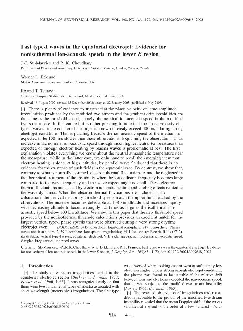
the strong electrojet conditions that took place on April 4,2000. We discuss here an unusual period during whichthe electrojet became particularly strong. The eventoccurred around 10 LT and lasted approximately 1.5hour. The event had a sudden onset, at which point anumber of examples were observed where the two-step type-I Doppler shifts reached 440 m/s, with a few 460 m/sexamples observed in the lower altitude gates. During thesame time period, 400 m/s Doppler shifts were observed asfar up as 105 km altitude. After about 70 minutes, themagnitude of the two-step type-I Doppler shifts graduallywent down to reach no more than 400 m/s in the verticalbeam anywhere and no more than 420 m/s in the east andwest beams anywhere. Finally there might have been atendency for temporal changes (increases or decreases intype-I speeds) to be seen at the higher altitudes first.[11] In Figure 1 we provide three different examples of

spectra observed around a time when the wave power at 103km was at its strongest. In the first example (Figure 1a), wesee two very strong two-step type-I spectra sandwichingwhat could be described as a very weak ‘type-II’ spectrumcutting across zero frequency. In the second example(Figure 1b) only one of the type-I peaks is really strongeven though the other type-I peak is still considerablystronger than the central type-II background. The thirdand final example (Figure 1c) is one for which the centraltype-II is stronger than both type-Is but is sufficientlynarrow for at least one of the type-I peaks to be very clearlyidentifiable in spite of its weak strength. There are morevariations on this theme, but Figure 1 covers the mostimportant cases of interest to the present paper.[12] Typically, when observed, the Figure 1a cases were

seen in the vertical beam near 103 km altitude, just aboutwhere the ambient vertical electric field is expected to be atits strongest. Cases resembling Figure 1b were often foundwithin 2 km from 103 km in the vertical beam, with astronger downshifted peak below 103 km and a strongerupshifted peak near 104 km. During strong echo conditions,Figure 1b was also typical of east and west beam returnsnear 104 km altitude, with a dominant downshifted peak inthe west beam and a dominant upshifted peak in the east

beam. Cases resembling Figure 1c were usually observedduring weaker echo conditions and were also occasionallyobserved at the lowest altitudes where type-I waves couldbe found, that is, near 99 km altitude during strong echoconditions higher up.[13] It should be noted that our spectral signatures in a

particular beam position rarely changed abruptly from oneintegration time to the next. This contrasts with the 1-sresolution spectra of Kudeki et al. [1987] which showed acontinuous and predictable evolution particularly at night.This difference reflects the fact that our integration time isso long that our spectra were obtained during the passage ofa full KSI wave (or more) over the field of view while the[Kudeki et al., 1987] data was often able to resolve thespectral evolution inside single KSI waves.[14] In Figure 2 we give some particularly clean examples

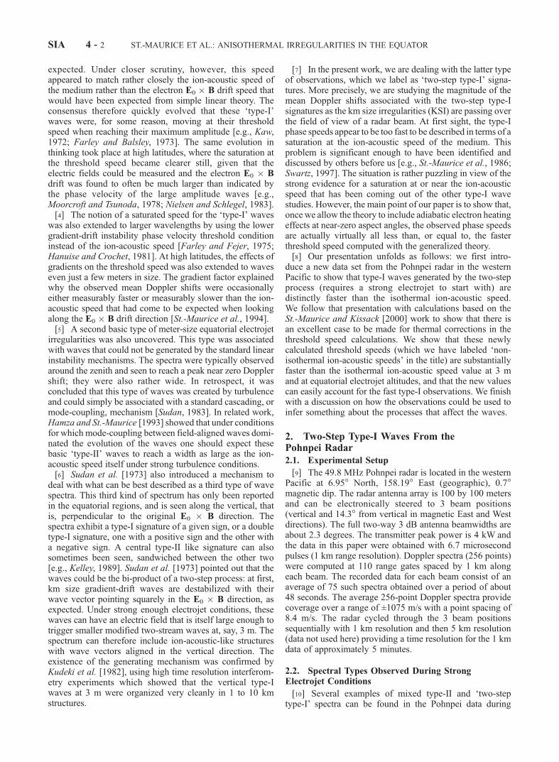
of profiles of the spectral power as functions of frequency(velocity units) and height for each of our three beams.These spectra were obtained during a time interval overwhich the echoes were unusually strong (hence the basicabsence of noisy features in many of the spectra). The figureillustrates the relative strength of the various peaks and theirposition in a compact way. The stack of plots shows thenature of the central problem addressed in the present paper,namely: (1) Doppler shifts well in excess of 400 m/s atlower altitudes and (2) a clearly identifiable decrease in themagnitude of the type-I Doppler shifts with increasingaltitude from the altitude at which they first appear, super-posed on type-II waves, to the final altitudes beyond whichwe are left with pure type-II signatures all over again.[15] Since the focus of the present study is on the

magnitude of the Doppler shift in two-step type-I spectrawe not only had to separate spectral peaks but also had todecide more precisely what we meant by ‘Doppler shift’.An important question for a quantitative study was: shouldwe look at the peak value in the Doppler shift, or should wetake the first moment of the frequency half of the spectrumwhere the peak of interest was located? For the relativelyfew cases resembling Figure 1a the question was academicbecause the strength of the type-I peaks was so large thatwhat little skewness was present was not making much

z

Figure 1. Examples of the kind of spectra that were observed with the vertical beam of the Pohnpeiradar during strong electrojet conditions observed on April 4, 2000.

ST.-MAURICE ET AL.: ANISOTHERMAL IRREGULARITIES IN THE EQUATOR SIA 4 - 3

difference between the two numbers thus retrieved. Inweaker cases, the skewness of the type-I peaks towardszero frequencies could mean that we would get two fairlydifferent answers from the peak evaluation and the firstmoment evaluation. In the absence of a precise theoreticalmodel to describe the spectral details, and also because weassumed that the largest amplitude waves were the onlyones truly moving at the threshold speed, we chose to focuson the position of the spectral peaks.

2.3. Altitude Variation of Two-Step Type-I Waves

[16] We first studied the behavior of individual profiles ofthe Doppler shift in two-step type-I waves. The profilesturned out to be remarkably similar to one another in spiteof the fact that we obtained them in a variety of directionsand at different times. Figure 3 gives a good example, basedon the spectra already displayed in Figure 2 and on spectraobtained on the two subsequent sampling periods. In thatfigure we compare the magnitude of the downshiftedDoppler shift of type-I waves on the west beam at theirpeak power with the magnitude of the upshifted Dopplershift of type-I waves at their peak power on the east beamtwo minutes later. For each of the three time samples, theup- and down-shifted Doppler shifts overlapped well.Remarkably, the differences between the beams neverexceeded 10 m/s, which is the basic uncertainty associatedwith our frequency resolution. This result was obtained inspite of the fact that the mean Doppler shift decreased by asmuch as 70 m/s from the lower heights to the upper ones.[17] Similar results were obtained with the vertical

beam, albeit with some clear differences also. These are

illustrated in Figure 4, which compares the upshifted anddownshifted magnitudes of the vertical beam type-I wavesat their peak power. The selected times were all sand-wiched between the two times used in each of the threepanels in Figure 3. The power of two-step type-I waves(not shown) was always smaller for the vertical beam,particularly in the upshifted case. As a result the altituderange over which we could get clean spectra was morelimited, so that we obtained fewer data points: the peaksthemselves were not as easy to identify owing to thepresence of multiple peaks associated with weaker powerlevels. These multiple peaks may not have been ‘noise’per se, in that they seem to be well above the instrumentalnoise level (e.g., Figure 1c). They nevertheless are part ofthe more weakly-driven cases. One clear differencebetween the vertical beam results and the east-west beamDoppler shift magnitudes is that the magnitude of theDoppler shift in the vertical beam changes very littlebelow 102 km and might even be decreasing a little withdecreasing altitude, by contrast with the east-west beamobservations.[18] We can conclude from Figures 3 and 4 and attendant

observations that: (1) the Doppler shift of type-I wavesdecreases systematically with increasing altitude, and thatthe magnitude of the Doppler shift in the lower altitudegates can reach 420 m/s or greater, that is, can clearly be inexcess of the conventional ion-acoustic speed; (2) theDoppler shift of the peak is not related to the peak poweritself in any simply way; and (3) the magnitude of theDoppler shift is basically the same whether the feature isupshifted or downshifted, but with some systematic differ-

Figure 2. Stack plot of self-normalized spectra obtained around 23:10 UT during strong electrojetconditions on April 4, 2000.


ences between the vertical beam and the east/west beamdata below 102 km.[19] In order to provide a sense for the number of spectra

with strong two-step type-I spectra and also in order to showthe range of velocities that were observed, we producedscatter plots of the two-step type-I Doppler shifts for a two-hour time interval that encompassed the strongly driventwo-step type-I echo period. To this goal, however, we hadto change our approach slightly, since we could not look atevery single spectrum and identify ‘true’ type-I peaks byinspection. Furthermore, knowing that the problematic

weaker spectra had multiple peaks spread out over a widevelocity range and that both the noise and the skewnesscould create a decrease in the retrieved type-I speed weresorted to the following algorithm, at the risk of losing anumber of samples from the statistical data set: first, sinceunderlying broad type-II spectra necessarily introduced askewness in the type-I peaks, we applied a nonrecursivehigh pass numerical filter to taper off the broad signature.The output retained the short scale fluctuations, whichincluded first and foremost the type-I peaks.[20] Next we selected the highest peak in the power

spectrum on both sides of zero. Provided this peak had a

Figure 3. Magnitude of type-I Doppler shifts for thedownshifted west beam and upshifted east beam at 5 minutesintervals. Because of the strong power in the two-step type-Iwaves, the uncertainty in this case was only approximately±5 m/s based on the spectral resolution itself.

Figure 4. Magnitude of type-I Doppler shifts for thedownshifted and upshifted vertical beam type-I echoes at5 minutes intervals overlapping the intervals shown inFigure 3.


Doppler speed greater than 320 m/s we chose it as the speedof a type-I echo. Still, we had to devise a simple algorithmto ensure that the peak was not produced by a simple noise-like bump well away from the desired feature. To ensurethat the peak was not an artifact of some noise at low powerlevels, we therefore required that it be 10 m/s (the spectralresolution) or less, from the first moment of type-I echoesestimated from the filtered spectrum. If this was not thecase, the spectrum was simply rejected from the type-I datasubset. This procedure meant in the end that the statisticaldata subset was strongly biased to powerful echo situations,when noise and skewness were not allowed to play asignificant role.[21] The scatter plots that came out of our statistical

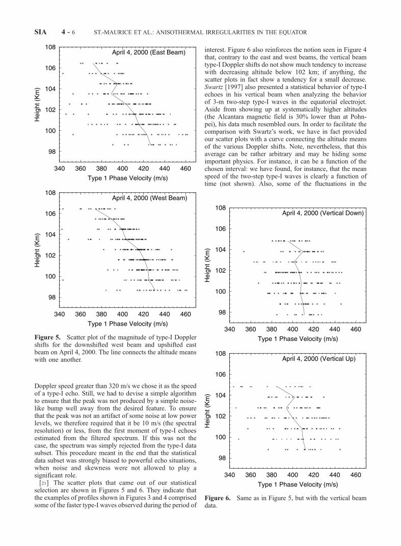
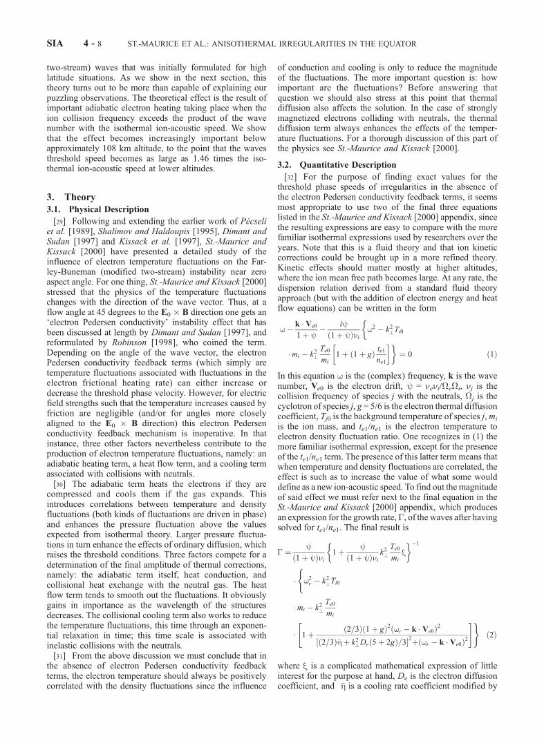
selection are shown in Figures 5 and 6. They indicate thatthe examples of profiles shown in Figures 3 and 4 comprisedsome of the faster type-I waves observed during the period of

interest. Figure 6 also reinforces the notion seen in Figure 4that, contrary to the east and west beams, the vertical beamtype-I Doppler shifts do not show much tendency to increasewith decreasing altitude below 102 km; if anything, thescatter plots in fact show a tendency for a small decrease.Swartz [1997] also presented a statistical behavior of type-Iechoes in his vertical beam when analyzing the behaviorof 3-m two-step type-I waves in the equatorial electrojet.Aside from showing up at systematically higher altitudes(the Alcantara magnetic field is 30% lower than at Pohn-pei), his data much resembled ours. In order to facilitate thecomparison with Swartz’s work, we have in fact providedour scatter plots with a curve connecting the altitude meansof the various Doppler shifts. Note, nevertheless, that thisaverage can be rather arbitrary and may be hiding someimportant physics. For instance, it can be a function of thechosen interval: we have found, for instance, that the meanspeed of the two-step type-I waves is clearly a function oftime (not shown). Also, some of the fluctuations in the

Figure 5. Scatter plot of the magnitude of type-I Dopplershifts for the downshifted west beam and upshifted eastbeam on April 4, 2000. The line connects the altitude meanswith one another.

Figure 6. Same as in Figure 5, but with the vertical beamdata.


average are not necessarily related to an actual systematicincrease in speeds. For instance, the increase in the mean at104 km in Figures 5 and 6 is related to a disappearance, forsome reason, of the lower speed data around that particularheight.

2.4. Theoretical Implications

[22] The phase speeds displayed in Figures 3 to 6 are veryfast and represent, by themselves, a challenge to our under-standing of the electrojet electric field no matter what theorigin of the fast speeds may be. Quite aside from thisproblem, however, the observations offer another majorchallenge, namely: the magnitude of the Doppler shifts iswell above the conventional isothermal ion-acoustic speed.This is the focus of the present paper; the fast type-I speedsthat we observe at low altitudes certainly appear to goagainst the notion that large amplitude waves move at thethreshold speed or slower. While this notion was at firstintroduced at equatorial latitudes, it has become even morestrongly established after high latitude studies later revealedthat the phase velocity of Farley-Buneman waves along theE0 � B drift direction was much closer to the ion-acousticspeed than it was to the E0 � B drift itself [e.g., Moorcroftand Tsunoda, 1978; Moorcroft, 1980; Nielsen and Schlegel,1983; Foster and Erickson, 2000]. Furthermore, from thesame data studies, it also became apparent that while thephase velocities were saturated at the ion-acoustic speedinside an angular region defined as unstable by the linearinstability theory, they were slower than the threshold speedoutside that region. In that sense, the threshold speedbecame the upper limit for the instability speed. In fact,still at high latitudes, even so-called ‘type-IV events’(appreciably faster than normal phase velocities) werejudged to be close to the ion-acoustic speed once it becameclear that they were associated with strong electron heatingevents [Providakes et al., 1988; St.-Maurice and Kissack,2000]. The only alternative explanation (a gradient-basedmechanism) also offered an explanation based on thresholdconditions [St.-Maurice et al., 1994].[23] In the context of phase speeds not exceeding the

instability threshold in the ionospheric E region, the resultsof Figures 3 to 6 are therefore quite puzzling: standardmodelswould predict the (isothermal) ion-acoustic speed to be in therange 325 to 350m/s, with a decreasing value with decreasingaltitude. Given that below 120 km the ion, electron andneutral temperatures should all be equal, thanks to the veryfrequent collisions with neutrals, a 100 m/s differencebetween the observations and the expected ion-acoustic speednear 100 km would represent a totally unreasonable temper-ature increase above the model value. Specifically, since theion-acoustic speed is given by

ffiffiffiffiffiffiffiffiffiffiffiffiffiffiffiffiffiffiffiffiffiffiffiffiffiTi þ Teð Þ=mi

p, a 100 m/s

increase would imply a factor 1.7 increase in the neutraltemperature, which would then have to be greater than 330 Kat 100 km. Ion and/or electron temperatures that increasinglydepart from the neutral temperature aswe go to lower altitudeswould be equally unreasonable.[24] Another possibility for the faster than expected

speeds has been proposed by Swartz [1997], who sug-gested that the ion mass was getting larger with increasingaltitude. This explanation raises more difficult questions.In particular, if the ion mass is normal lower down, thenwhy is the ion-acoustic speed so much larger than the

expected value lower down? In fact, this explanationwould work best if the ion mass was actually substantiallysmaller than normal at 100 km to become normal again by110 km. Once again, this kind of suggestion goes againsteverything we know about the ionosphere and it thereforedoes not look promising.[25] A final point is that the large speeds and their

tendency to increase with decreasing altitude is, somehow,a standard feature of the electrojet, given the similarity ofthe results from very different times and places. Thisreproducibility indicates that we should somehow look foran explanation that would not be associated with partic-ularly unusual ionospheric or atmospheric situations. Thismakes the association with unusual temperature or ion massprofiles even less inviting.[26] We are therefore led to search for a basic explanation

for the large type-I speeds that involves threshold speedsthat would simply be faster than the expected isothermalion-acoustic speed. A first possibility would be to link thethreshold speed to the km size gradients associated with thelarge scale irregularities that generate the two-step type-Iwaves. These gradients can change the phase speed up anddown by up to 75 m/s for the situation at hand [St.-Mauriceet al., 1994]. However, not only is this too small an effect, italso favors a decrease rather than an increase in thresholdspeed. To understand why this should be the case, considera hypothetical situation for which the peak electric fieldassociated with a KSI (km size irregularity) would be wellabove the ion-acoustic speed. In a KSI, the electric field anddensity fluctuations are in phase. When the electric fieldreaches its peak value there are no gradients and thethreshold speed is the ion-acoustic speed itself. Supposenext that as the phase increases, the local KSI gradient isfavorable to the growth of 3-m size irregularities. In thatcase the threshold speed goes down while the growth rate(and, presumably, the power) of the 3-m waves goes up. Bycontrast, however, for a phase that would precede the peakin the electric field, the gradients would become unfavor-able to the growth of 3-m structures and the thresholdspeed would move up. In that case, however, the growthrates would also be going down, and the power presumablywould follow suit. As a result one expects at best to see abroadening in the spectrum on each side of the ion-acousticspeed, if the electric field is well above the threshold value.However, a lowering of the mean phase speed below theion-acoustic speed would be more likely because thespectrum should be more powerful when the gradients arefavorable (and the threshold speed is lower) than when theyare unfavorable (and the threshold speed is higher).[27] An important corollary is that if the electric field

were to be just a bit too small to excite waves going at theion-acoustic speed, two-step type-I waves moving at speedsdown to 75 m/s lower than the ion-acoustic speed could stillbe expected. This would happen through a lowering ofthreshold speeds on the side of the KSI for which thegradients are favorable for the growth of 3-m structures.All in all, therefore, gradients associated with KSI structuresshould not be responsible for the observation of thresholdspeeds that are faster than the ion-acoustic speed, quite thecontrary in fact.[28] The above discussion has led us to take a further look

at a nonisothermal theory of Farley-Buneman (or modified


two-stream) waves that was initially formulated for highlatitude situations. As we show in the next section, thistheory turns out to be more than capable of explaining ourpuzzling observations. The theoretical effect is the result ofimportant adiabatic electron heating taking place when theion collision frequency exceeds the product of the wavenumber with the isothermal ion-acoustic speed. We showthat the effect becomes increasingly important belowapproximately 108 km altitude, to the point that the wavesthreshold speed becomes as large as 1.46 times the iso-thermal ion-acoustic speed at lower altitudes.

3. Theory

3.1. Physical Description

[29] Following and extending the earlier work of Pecseliet al. [1989], Shalimov and Haldoupis [1995], Dimant andSudan [1997] and Kissack et al. [1997], St.-Maurice andKissack [2000] have presented a detailed study of theinfluence of electron temperature fluctuations on the Far-ley-Buneman (modified two-stream) instability near zeroaspect angle. For one thing, St.-Maurice and Kissack [2000]stressed that the physics of the temperature fluctuationschanges with the direction of the wave vector. Thus, at aflow angle at 45 degrees to the E0 � B direction one gets an‘electron Pedersen conductivity’ instability effect that hasbeen discussed at length by Dimant and Sudan [1997], andreformulated by Robinson [1998], who coined the term.Depending on the angle of the wave vector, the electronPedersen conductivity feedback terms (which simply aretemperature fluctuations associated with fluctuations in theelectron frictional heating rate) can either increase ordecrease the threshold phase velocity. However, for electricfield strengths such that the temperature increases caused byfriction are negligible (and/or for angles more closelyaligned to the E0 � B direction) this electron Pedersenconductivity feedback mechanism is inoperative. In thatinstance, three other factors nevertheless contribute to theproduction of electron temperature fluctuations, namely: anadiabatic heating term, a heat flow term, and a cooling termassociated with collisions with neutrals.[30] The adiabatic term heats the electrons if they are

compressed and cools them if the gas expands. Thisintroduces correlations between temperature and densityfluctuations (both kinds of fluctuations are driven in phase)and enhances the pressure fluctuation above the valuesexpected from isothermal theory. Larger pressure fluctua-tions in turn enhance the effects of ordinary diffusion, whichraises the threshold conditions. Three factors compete for adetermination of the final amplitude of thermal corrections,namely: the adiabatic term itself, heat conduction, andcollisional heat exchange with the neutral gas. The heatflow term tends to smooth out the fluctuations. It obviouslygains in importance as the wavelength of the structuresdecreases. The collisional cooling term also works to reducethe temperature fluctuations, this time through an exponen-tial relaxation in time; this time scale is associated withinelastic collisions with the neutrals.[31] From the above discussion we must conclude that in

the absence of electron Pedersen conductivity feedbackterms, the electron temperature should always be positivelycorrelated with the density fluctuations since the influence

of conduction and cooling is only to reduce the magnitudeof the fluctuations. The more important question is: howimportant are the fluctuations? Before answering thatquestion we should also stress at this point that thermaldiffusion also affects the solution. In the case of stronglymagnetized electrons colliding with neutrals, the thermaldiffusion term always enhances the effects of the temper-ature fluctuations. For a thorough discussion of this part ofthe physics see St.-Maurice and Kissack [2000].

3.2. Quantitative Description

[32] For the purpose of finding exact values for thethreshold phase speeds of irregularities in the absence ofthe electron Pedersen conductivity feedback terms, it seemsmost appropriate to use two of the final three equationslisted in the St.-Maurice and Kissack [2000] appendix, sincethe resulting expressions are easy to compare with the morefamiliar isothermal expressions used by researchers over theyears. Note that this is a fluid theory and that ion kineticcorrections could be brought up in a more refined theory.Kinetic effects should matter mostly at higher altitudes,where the ion mean free path becomes large. At any rate, thedispersion relation derived from a standard fluid theoryapproach (but with the addition of electron energy and heatflow equations) can be written in the form

w� k � Ve0

1þ y� iy

1þ yð Þni

�w2 � k2?Ti0

�mi � k2?Te0

mi

1þ 1þ gð Þ te1ne1

� ��¼ 0 ð1Þ

In this equation w is the (complex) frequency, k is the wavenumber, Ve0 is the electron drift, y = neni/�e�i, nj is thecollision frequency of species j with the neutrals, �j is thecyclotron of species j, g = 5/6 is the electron thermal diffusioncoefficient, Tj0 is the background temperature of species j,mi

is the ion mass, and te1/ne1 is the electron temperature toelectron density fluctuation ratio. One recognizes in (1) themore familiar isothermal expression, except for the presenceof the te1/ne1 term. The presence of this latter term means thatwhen temperature and density fluctuations are correlated, theeffect is such as to increase the value of what some woulddefine as a new ion-acoustic speed. To find out the magnitudeof said effect we must refer next to the final equation in theSt.-Maurice and Kissack [2000] appendix, which producesan expression for the growth rate,�, of the waves after havingsolved for te1/ne1. The final result is

� ¼ y1þ yð Þni

1þ y1þ yð Þni

k2?Te0

mi

x� ��1

�(w2r � k2?Ti0

� mi � k2?Te0

mi

� 1þ 2=3ð Þ 1þ gð Þ2 wr � k � Ve0ð Þ2

2=3ð Þ�hþ k2?De 5þ 2gð Þ=3½ 2þ wr � k � Ve0ð Þ2

" #)ð2Þ

where x is a complicated mathematical expression of littleinterest for the purpose at hand, De is the electron diffusioncoefficient, and �h is a cooling rate coefficient modified by


thermal diffusion effects. Once again the generalizedexpression easily identifies the new contributions from theelectron temperature fluctuation terms, namely: we wouldrecover the classical isothermal growth rate expressions ofthe modified two-stream instability if we were to set x = 0 anddrop the last term on the right-hand-side of the equation.[33] We can recognize in the last term in (2) the com-

petition between adiabatic heating and the damping effectsof cooling and heat conduction. For this we should (1) lookat the g = 0 case (dropping the amplification factor due tothermal diffusion), (2) take the limit h ! 0 (neglectingcollisional cooling) and (3) drop the k2De term (whichcomes from classical heat conduction). We then recoverthe familiar 2/3 adiabatic factor, which comes from in-phaseadiabatic temperature and density fluctuations. This pro-vides a mathematical basis for our earlier statement that theheating effect is indeed caused by adiabatic heating, ampli-fied by thermal diffusion, and diminished by cooling andheat conduction effects.[34] With a focus on identifying threshold conditions, we

are led to study under what conditions � = 0. Clearly, in theabsence of the last term in (2) we would recover a phasespeed equal to the normal isothermal ion-acoustic speed.The presence of the last term raises the threshold speed. In asense, and maybe not entirely correctly, the new thresholdspeed can be thought of as a ‘‘nonisothermal ion-acousticspeed.’’ We, in fact, have used that term in the title of ourpaper. In general however, it is better to refer to the newspeed as the nonisothermal threshold speed.[35] Equation (2) clearly depends on the magnitude of

wr � k � Ve0. This term can easily be substituted because inthe absence of substantial ion motions (all beams arelooking at a direction close to the vertical and altitudes ofinterest well below 120 km), and for small growth rateconditions, the real part of the dispersion relation (1) givesthe well-known solution

wr ¼k � Ve0

1þ yð3Þ

[36] At this point, we face a dilemma: if the electron driftexceeds the threshold requirement, one cannot have (3)satisfied while simultaneously requiring that the growthrate given by (2) be zero. Yet, as we discussed earlier, theempirical evidence strongly suggests the presence of thresh-old speeds. One has to conclude that nonlinear effectsconspire to lower the frequency from the value given by(3). There are two ways to achieve this and at the same timekeep the physics in line with the fundamental theoreticalidea. One way is to have an increase in the value of y as thewave amplitude grows. The other is to change the drift fromthe ambient value of Ve0 to some smaller value inside well-developed irregularities (i.e., large amplitude ‘waves’).[37] There are two different ways to increase y. One is to

have a wave generate its own microturbulence. This leads toanomalous diffusion and increases y [Sudan, 1983; Rob-inson, 1986]. There are some conceptual difficulties withthis mechanism, however, because diffusion tends to beenhanced in a direction perpendicular to the generating fieldfor the problem at hand [e.g., St.-Maurice, 1990]. A secondway to increase y is to let the aspect angle grow with timesince, at nonzero aspect angles, y has to be multiplied by

the factor (1 + sin2a�e2/ne

2), where a is the aspect angle.Contrary to a widely held view, the aspect angle is not a freeparameter of the problem. For instance, at high latitudes, thetime evolution of the aspect angle of structures 10 m in sizeand greater plays a dominant role in the evolution of theirregularities [Drexler et al., 2002]. This is caused by thealignment of the neutral density gradients with the magneticfield direction. At smaller wavelengths at high latitudes, astrong evolution in the aspect angle should also take placein the late stages of evolution of what should have started asfield-aligned structures. In this case, as the amplitudeevolves, different heights start to evolve differently andlarge aspect angles form. Again, the evolution can be tracedto the alignment of the neutral density gradients with themagnetic field direction.[38] In the equatorial regions, we can argue that field-

aligned irregularities should stay field-aligned down to thevery end of their evolution. This can be argued on the basisthat we do not have the alignment of neutral atmosphericgradients with the magnetic field direction. There is there-fore no need for large aspect angles to evolve and for y toincrease in response to aspect angles. Indeed, a strong fieldalignment of the E region irregularities has been observed inthe equatorial regions [Kudeki and Farley, 1989].[39] If we also reject the notion of anomalous diffusion at

the small structure level, this leaves us with one lastmechanism to reduce wr, namely, a decrease in the magni-tude of the electric field inside large amplitude structures.This means changing Ve0 by some value Vetot having asmaller norm. This mechanism has been explored recentlyfor purely field-aligned structures: using a spatio-temporaldescription instead of Fourier analysis St.-Maurice andHamza [2001] were able to conclude that the reduction inthe drift had to be accompanied by a rotation. This agreeswith a two-dimensional numerical simulations by Otani andOppenheim [1998] who furthermore demonstrated that therotation and reduction in the electric field could bedescribed in terms of a mode-coupling argument. This beingthe case, we conclude that a formula derived by Hamza andSt.-Maurice [1993] based on two-dimensional mode-cou-pling should apply to equatorial regions. This formulapredicts that if the width of a spectral signature is less thanits mean Doppler shift in a Farley-Buneman or gradient-driftsituation, the mean Doppler shift should be very close to thethreshold speed. There is therefore a very good case forhaving threshold speeds in linearly unstable modes for the2-D situation.[40] In the end, it does not matter if a change in wr is due

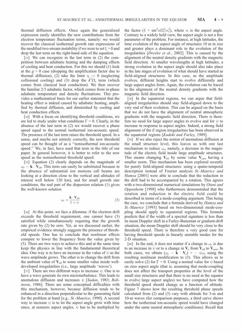
to an increase in y or to a change in Ve from Ve0 to Vetot. Inboth cases, we obtain (wr � k � Ve) = � ywr using theresulting nonlinear modification to (3). This allows us toeasily solve (2) for � = 0. Using a normal value for y basedon zero aspect angle (that is, assuming that mode-couplingdoes not affect the transport properties at the level of thesmall size structures and that there is no need at the equatorto evolve large aspect angles) we have computed how thethreshold speed should change as a function of altitude.Figure 7 shows how the resulting threshold phase speedscalculated from (2) and (3) vary with altitude for 3-m and10-m waves (for comparison purposes, a third curve showshow the isothermal ion-acoustic speed would have changedunder the same neutral atmospheric conditions). Recall that


3-m waves are observed by the Pohnpei radar while 10-mwaves are sometimes studied by lower frequency HF radars.In our calculation we have used a standard neutral atmos-pheric model provided by MSIS [Hedin et al., 1991]. Ourvalues for the parameters of interest for the calculations arelisted in Table 1. We used 0.35 Gauss for the magnetic field,which is appropriate for Pohnpei’s location.[41] Clearly, Figure 7 indicates that at zero aspect angle

(which is an important component of the theory), the 3-mthreshold speeds should be expected to be roughly 125 m/sabove the isothermal ion-acoustic speed near 100 km. Theyshould, by contrast, be much closer to the isothermal valueby the time we reach 110 km altitude. Interestingly enough,the 10-m waves have threshold speeds somewhat closer tothe isothermal value by comparison to 3-m waves. In anyevent, we are led to expect from Figure 7 that the electronadiabatic heating has to affect all radar observations ofsmall aspect angle echoes E region irregularities taken

below 108 km altitude, no matter what the altitude or theradar frequency might be. Note, however, that the smallaspect angles restriction might imply that the higher thresh-old speeds might not be present at high latitudes. In thelatter case larger aspect angles often seem to be present, inwhich case parallel heat conduction tends to wipe out theinfluence of adiabatic heating.

3.3. Controlling Parameters

[42] While Figure 7 gives us the basic numerical answer,it still does not provide a description of just what parameteris responsible for the behavior calculated, nor does it givethe exact asymptotic value the threshold speed is going tobe at low altitudes. More in-depth understanding can begained from a study of the algebraic expression involved.Noting that we have, from (3), (wr � k � Ve) = � ywr,substituting in (2) after setting the growth rate to zero, andusing Te0/mi = 0.5 cs

2 for equal ion and electron temper-atures, with cs ¼

ffiffiffiffiffiffiffiffiffiffiffiffiffiffiffiffiffiffiffiffiffiffiffiffiffiffiffiffiffiTi0 þ Te0ð Þ=mi

pbeing the isothermal

ion-acoustic speed, we get

w2r ¼ k2c2s 1þ aw2

ry2

ane þ b1k2?Deð Þ2 þ w2

ry2

" #ð4Þ

where a = 121/108 = 1.12 and b1 = 20/9 for g = 5/6 and wehave used 2 �h/3 = ane = 0.002ne.[43] Using the relation k2De = k2(ne/�e

2)(Te0/me) =(y/ni)(k

2cs2/2) we then get the expression

w2r

k2c2s¼ 1þ aw2

r=k2c2s

w2r=k

2c2s þ b2k2c2s=n2i

ð5Þ

or, equivalently,

w2r

k2c2s¼ 1þ a� abk2c2s=n

2i

w2r=k

2c2s þ b2k2c2s=n2i

ð6Þ

where, in the last two equations,

b¼10

91þ 9a

10

neniy

1

k2c2s

� �¼10

91þ :0018

�e�i

k2c2s

� �ð7Þ

For 3 m waves and a.35 gauss magnetic field we find b to beof order 4. For 10 m waves, b is roughly 38, meaning thatthe term bkcs/ni is roughly 2.5 times as large for 10 m wavesthan it is for 3 m waves at any given altitude. With theresults written this way, the strongest part of the altitude

Figure 7. Threshold speed calculated for (a) 3-m and (b)10-m ion-acoustic waves (full lines, bottom scale) andminimum electron speed required to excite the waves(dotted lines, top scale). Also shown is the isothermal ion-acoustic speed (dashed lines, bottom scale).

Table 1. Model Temperature, Collision Frequencies, and y Values

Used for the Calculations of Figure 7a

Altitude, km Temperature, �K ne, s�1 ni, s

�1 y

110 233 9.83 � 103 9.05 � 102 1.31 � 10�2

108 219 1.34 � 104 1.30 � 103 2.55 � 10�2

106 208 1.85 � 104 1.85 � 103 5.02 � 10�2

104 200 2.59 � 104 2.62 � 103 9.98 � 10�2

102 194 3.63 � 104 3.70 � 103 0.197100 190 5.10 � 104 5.18 � 103 0.38898 187 7.16 � 104 7.25 � 103 0.76196 185 1.01 � 105 1.02 � 104 1.5094 184 1.67 � 105 1.69 � 104 2.96

aNeutral model atmospheric values based on the MSIS model.


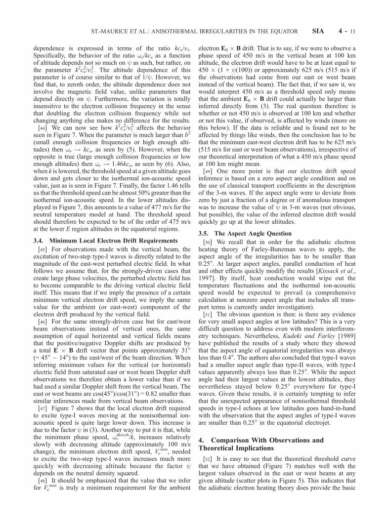
dependence is expressed in terms of the ratio kcs/ni.Specifically, the behavior of the ratio wr/kcs as a functionof altitude depends not so much on y as such, but rather, onthe parameter k2cs

2/ni2. The altitude dependence of this

parameter is of course similar to that of 1/y. However, wefind that, to zeroth order, the altitude dependence does notinvolve the magnetic field value, unlike parameters thatdepend directly on y. Furthermore, the variation is totallyinsensitive to the electron collision frequency in the sensethat doubling the electron collision frequency while notchanging anything else makes no difference for the results.[44] We can now see how k2cs

2/ni2 affects the behavior

seen in Figure 7. When the parameter is much larger than b2

(small enough collision frequencies or high enough alti-tudes) then wr ! kcs, as seen by (5). However, when theopposite is true (large enough collision frequencies or lowenough altitudes) then wr ! 1.46kcs, as seen by (6). Also,when k is lowered, the threshold speed at a given altitude goesdown and gets closer to the isothermal ion-acoustic speedvalue, just as is seen in Figure 7. Finally, the factor 1.46 tellsus that the threshold speed can be almost 50% greater than theisothermal ion-acoustic speed. In the lower altitudes dis-played in Figure 7, this amounts to a value of 477 m/s for theneutral temperature model at hand. The threshold speedshould therefore be expected to be of the order of 475 m/sat the lower E region altitudes in the equatorial regions.

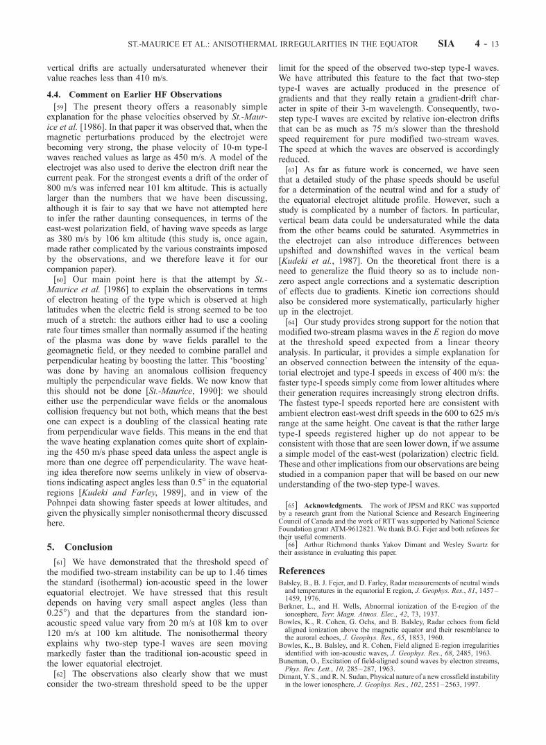
3.4. Minimum Local Electron Drift Requirements

[45] For observations made with the vertical beam, theexcitation of two-step type-I waves is directly related to themagnitude of the east-west perturbed electric field. In whatfollows we assume that, for the strongly-driven cases thatcreate large phase velocities, the perturbed electric field hasto become comparable to the driving vertical electric fielditself. This means that if we imply the presence of a certainminimum vertical electron drift speed, we imply the samevalue for the ambient (or east-west) component of theelectron drift produced by the vertical field.[46] For the same strongly-driven case but for east/west

beam observations instead of vertical ones, the sameassumption of equal horizontal and vertical fields meansthat the positive/negative Doppler shifts are produced bya total E � B drift vector that points approximately 31�(= 45� � 14�) to the east/west of the beam direction. Wheninferring minimum values for the vertical (or horizontal)electric field from saturated east or west beam Doppler shiftobservations we therefore obtain a lower value than if wehad used a similar Doppler shift from the vertical beam. Theeast or west beams are cos(45�)/cos(31�) = 0.82 smaller thansimilar inferences made from vertical beam observations.[47] Figure 7 shows that the local electron drift required

to excite type-I waves moving at the nonisothermal ion-acoustic speed is quite large lower down. This increase isdue to the factor y in (3). Another way to put it is that, whilethe minimum phase speed, wr

thresh/k, increases relativelyslowly with decreasing altitude (approximately 100 m/schange), the minimum electron drift speed, Ve

min, neededto excite the two-step type-I waves increases much morequickly with decreasing altitude because the factor ydepends on the neutral density squared.[48] It should be emphasized that the value that we infer

for Vemin is truly a minimum requirement for the ambient

electron E0 � B drift. That is to say, if we were to observe aphase speed of 450 m/s in the vertical beam at 100 kmaltitude, the electron drift would have to be at least equal to450 � (1 + y(100)) or approximately 625 m/s (515 m/s ifthe observations had come from our east or west beaminstead of the vertical beam). The fact that, if we saw it, wewould interpret 450 m/s as a threshold speed only meansthat the ambient E0 � B drift could actually be larger thaninferred directly from (3). The real question therefore iswhether or not 450 m/s is observed at 100 km and whetheror not this value, if observed, is affected by winds (more onthis below). If the data is reliable and is found not to beaffected by things like winds, then the conclusion has to bethat the minimum east-west electron drift has to be 625 m/s(515 m/s for east or west beam observations), irrespective ofour theoretical interpretation of what a 450 m/s phase speedat 100 km might mean.[49] One more point is that our electron drift speed

inference is based on a zero aspect angle condition and onthe use of classical transport coefficients in the descriptionof the 3-m waves. If the aspect angle were to deviate fromzero by just a fraction of a degree or if anomalous transportwas to increase the value of y in 3-m waves (not obvious,but possible), the value of the inferred electron drift wouldquickly go up at the lower altitudes.

3.5. The Aspect Angle Question

[50] We recall that in order for the adiabatic electronheating theory of Farley-Buneman waves to apply, theaspect angle of the irregularities has to be smaller than0.25�. At larger aspect angles, parallel conduction of heatand other effects quickly modify the results [Kissack et al.,1997]. By itself, heat conduction would wipe out thetemperature fluctuations and the isothermal ion-acousticspeed would be expected to prevail (a comprehensivecalculation at nonzero aspect angle that includes all trans-port terms is currently under investigation).[51] The obvious question is then: is there any evidence

for very small aspect angles at low latitudes? This is a verydifficult question to address even with modern interferom-etry techniques. Nevertheless, Kudeki and Farley [1989]have published the results of a study where they showedthat the aspect angle of equatorial irregularities was alwaysless than 0.4�. The authors also concluded that type-I waveshad a smaller aspect angle than type-II waves, with type-Ivalues apparently always less than 0.25�. While the aspectangle had their largest values at the lowest altitudes, theynevertheless stayed below 0.25� everywhere for type-Iwaves. Given these results, it is certainly tempting to inferthat the unexpected appearance of nonisothermal thresholdspeeds in type-I echoes at low latitudes goes hand-in-handwith the observation that the aspect angles of type-I wavesare smaller than 0.25� in the equatorial electrojet.

4. Comparison With Observations andTheoretical Implications

[52] It is easy to see that the theoretical threshold curvethat we have obtained (Figure 7) matches well with thelargest values observed in the east or west beams at anygiven altitude (scatter plots in Figure 5). This indicates thatthe adiabatic electron heating theory does provide the basic


explanation we sought for the presence of fast type-I speeds.That is to say, all the observations are now either smallerthan, or equal to, the ion-acoustic threshold speed producedby the generalized fluid theory.[53] Several questions nevertheless arise from our basic

explanation for the fast type-I speeds. In particular wecould consider the following: why are the observationsusually less than, and only rarely, equal to the predictedthreshold speed? Why are the vertical beam data agreeingwith the west and east beam data above 103 km, whilebeing systematically smaller (and rarer) below that alti-tude? What is the origin of the scatter in the data points?What creates systematic temporal variations in the type-Ispeed profiles? And finally, what do the observations,including the temporal variability of the altitude profiles,imply about the electrojet current density profile? Acomprehensive study of these questions and their possibleanswers is the topic of a companion paper under prepara-tion. We therefore only provide a cursory look here,strictly keeping the focus on our threshold speed mecha-nism rather than on the implications of the observationsfor the electrojet and KSI behaviors.

4.1. The Influence of KSI Induced Gradients

[54] The most striking feature of the comparisonbetween the phase speed observations and the generalizedion-acoustic speed theory is that the theory provides anupper limit for the observations. However, going back tothe discussion provided in section 2.4, this should not beso surprising, since the two-step type-I waves have to begenerated by KSI’s. The KSI oscillate in time and space,which means that the electric field and the gradients go upand down with time at any given location. The gradientsare out of phase with the electric field. When the electricfield is a maximum, pure modified-two-stream waves areexcited.[55] However, gradients can either increase or decrease

the threshold speed, depending on what particular phase iscontributing. In the plausible event that the total electricfield is insufficient to excite pure modified two-streamwaves, gradients aligned parallel to the electric field mustthen be used to decrease the threshold speed. As weindicated, the calculations in St.-Maurice et al. [1994] showthat the threshold at 110 km could be as much as 75 m/sbelow the ion-acoustic speed before the excitation of two-step type-I waves becomes no longer possible. A study ofthe threshold equation reveals that, in the fluid regime, thischange in threshold speed is also independent of altitude. Inthis context, it is interesting to note that the great majority ofthe data points satisfies the condition of phase speedslocated somewhere between our computation of the puretwo-stream threshold speed and a speed which is 75 m/sslower.

4.2. Allowing for the Presence ofUndersaturated Waves

[56] We know from high latitude studies that largeamplitude waves with substantial Doppler shifts are notlimited to the flow angle directions for which the plasmais linearly unstable. While the phase speed normallysaturates near the ion-acoustic speed inside the linearlyunstable angular region, it decreases progressively as a

function of increasing flow angle. In that region, it takesa value that is comparable to the line-of-sight velocitycomponent of the electrons [e.g., Nielsen and Schlegel,1983]. There should be no reason, in principle, for two-step type-I waves to behave any differently. Unfortunatelyfor this case, the threshold speed itself has to change withconditions: when the total electric field is too weak toexcite ion-acoustic waves, waves with lower thresholdspeeds can still be excited through the gradients of theKSI. It therefore becomes difficult to distinguish wavesthat are saturated at speeds less than the two-streamthreshold speed from waves that are generated, throughcascading or mode-coupling, outside the linear instability‘cone’. In principle, only a detailed comparison betweenthe vertical beam data and the east and west beams canbe used for the purpose of distinguishing between the twopossibilities.

4.3. Neutral Wind Effects

[57] When the phase velocities are saturated, the differ-ence between the Doppler shifts registered in variousbeams can be used to extract information about theneutral wind [e.g., Balsley et al., 1976; Kudeki et al.,1987]. Neutral winds in the range 50 to 100 m/s are nowbeing argued to be a frequent staple of the neutralatmosphere near 100 km altitude [e.g., Larsen et al.,1998, and references therein]. The effect of a westward100 m/s zonal wind on saturated downshifted waves inthe westward beam would be to increase the magnitudeof the phase speed above its true threshold speed by anapproximate factor 100 sin 14.3� = 25 m/s. For a neutralwind of the same magnitude and direction, the samepositive enhancement would likewise be registered inthe upshifted waves when looking at them through theeast beams. For both beams, therefore, the Doppler shiftwould be enhanced/depleted by the same amount, in thepresence of a uniform westward/eastward neutral wind. Avertical neutral wind would, by contrast, introduce anasymmetry between the east and west beam data. There isno evidence for such an asymmetry in Figures 3 or 5, sothat vertical winds can safely be ruled out.[58] A horizontal wind, furthermore, can have no effect

on the vertical beam observations. A comparison betweenthe vertical beam data and the east and west beam datashould therefore be able to reveal the magnitude of thehorizontal neutral wind in the eastward or westward direc-tions. Unfortunately, for the comparison to work one mustfirst ensure that the Doppler shift in the vertical beam issaturated and is therefore equal to the east and west beamDoppler shifts before neutral winds are taken into account.As we described in the previous subsection, this cannotalways be the case. There are additional complications, suchas upshifted and downshifted vertical data having system-atic differences; this would seem to be related to anasymmetry in the electrojet data. Needless to say, all of thismakes reaching a definitive conclusion on the neutral windsvery difficult. The best one can say at this stage, beforeundertaking a much more detailed study of the data, is thatthe data is not inconsistent with a wind gradually buildingup with decreasing altitude so as to become a westward 80to 100 m/s wind by 100 km altitude. Alternatively, the datais also consistent with little, if any, neutral wind if the


vertical drifts are actually undersaturated whenever theirvalue reaches less than 410 m/s.

4.4. Comment on Earlier HF Observations

[59] The present theory offers a reasonably simpleexplanation for the phase velocities observed by St.-Maur-ice et al. [1986]. In that paper it was observed that, when themagnetic perturbations produced by the electrojet werebecoming very strong, the phase velocity of 10-m type-Iwaves reached values as large as 450 m/s. A model of theelectrojet was also used to derive the electron drift near thecurrent peak. For the strongest events a drift of the order of800 m/s was inferred near 101 km altitude. This is actuallylarger than the numbers that we have been discussing,although it is fair to say that we have not attempted hereto infer the rather daunting consequences, in terms of theeast-west polarization field, of having wave speeds as largeas 380 m/s by 106 km altitude (this study is, once again,made rather complicated by the various constraints imposedby the observations, and we therefore leave it for ourcompanion paper).[60] Our main point here is that the attempt by St.-

Maurice et al. [1986] to explain the observations in termsof electron heating of the type which is observed at highlatitudes when the electric field is strong seemed to be toomuch of a stretch: the authors either had to use a coolingrate four times smaller than normally assumed if the heatingof the plasma was done by wave fields parallel to thegeomagnetic field, or they needed to combine parallel andperpendicular heating by boosting the latter. This ‘boosting’was done by having an anomalous collision frequencymultiply the perpendicular wave fields. We now know thatthis should not be done [St.-Maurice, 1990]: we shouldeither use the perpendicular wave fields or the anomalouscollision frequency but not both, which means that the bestone can expect is a doubling of the classical heating ratefrom perpendicular wave fields. This means in the end thatthe wave heating explanation comes quite short of explain-ing the 450 m/s phase speed data unless the aspect angle ismore than one degree off perpendicularity. The wave heat-ing idea therefore now seems unlikely in view of observa-tions indicating aspect angles less than 0.5� in the equatorialregions [Kudeki and Farley, 1989], and in view of thePohnpei data showing faster speeds at lower altitudes, andgiven the physically simpler nonisothermal theory discussedhere.

5. Conclusion

[61] We have demonstrated that the threshold speed ofthe modified two-stream instability can be up to 1.46 timesthe standard (isothermal) ion-acoustic speed in the lowerequatorial electrojet. We have stressed that this resultdepends on having very small aspect angles (less than0.25�) and that the departures from the standard ion-acoustic speed value vary from 20 m/s at 108 km to over120 m/s at 100 km altitude. The nonisothermal theoryexplains why two-step type-I waves are seen movingmarkedly faster than the traditional ion-acoustic speed inthe lower equatorial electrojet.[62] The observations also clearly show that we must

consider the two-stream threshold speed to be the upper

limit for the speed of the observed two-step type-I waves.We have attributed this feature to the fact that two-steptype-I waves are actually produced in the presence ofgradients and that they really retain a gradient-drift char-acter in spite of their 3-m wavelength. Consequently, two-step type-I waves are excited by relative ion-electron driftsthat can be as much as 75 m/s slower than the thresholdspeed requirement for pure modified two-stream waves.The speed at which the waves are observed is accordinglyreduced.[63] As far as future work is concerned, we have seen

that a detailed study of the phase speeds should be usefulfor a determination of the neutral wind and for a study ofthe equatorial electrojet altitude profile. However, such astudy is complicated by a number of factors. In particular,vertical beam data could be undersaturated while the datafrom the other beams could be saturated. Asymmetries inthe electrojet can also introduce differences betweenupshifted and downshifted waves in the vertical beam[Kudeki et al., 1987]. On the theoretical front there is aneed to generalize the fluid theory so as to include non-zero aspect angle corrections and a systematic descriptionof effects due to gradients. Kinetic ion corrections shouldalso be considered more systematically, particularly higherup in the electrojet.[64] Our study provides strong support for the notion that

modified two-stream plasma waves in the E region do moveat the threshold speed expected from a linear theoryanalysis. In particular, it provides a simple explanation foran observed connection between the intensity of the equa-torial electrojet and type-I speeds in excess of 400 m/s: thefaster type-I speeds simply come from lower altitudes wheretheir generation requires increasingly strong electron drifts.The fastest type-I speeds reported here are consistent withambient electron east-west drift speeds in the 600 to 625 m/srange at the same height. One caveat is that the rather largetype-I speeds registered higher up do not appear to beconsistent with those that are seen lower down, if we assumea simple model of the east-west (polarization) electric field.These and other implications from our observations are beingstudied in a companion paper that will be based on our newunderstanding of the two-step type-I waves.

[65] Acknowledgments. The work of JPSM and RKC was supportedby a research grant from the National Science and Research EngineeringCouncil of Canada and the work of RTTwas supported by National ScienceFoundation grant ATM-9612821. We thank B.G. Fejer and both referees fortheir useful comments.[66] Arthur Richmond thanks Yakov Dimant and Wesley Swartz for

their assistance in evaluating this paper.

ReferencesBalsley, B., B. J. Fejer, and D. Farley, Radar measurements of neutral windsand temperatures in the equatorial E region, J. Geophys. Res., 81, 1457–1459, 1976.

Berkner, L., and H. Wells, Abnormal ionization of the E-region of theionosphere, Terr. Magn. Atmos. Elec., 42, 73, 1937.

Bowles, K., R. Cohen, G. Ochs, and B. Balsley, Radar echoes from fieldaligned ionization above the magnetic equator and their resemblance tothe auroral echoes, J. Geophys. Res., 65, 1853, 1960.

Bowles, K., B. Balsley, and R. Cohen, Field aligned E-region irregularitiesidentified with ion-acoustic waves, J. Geophys. Res., 68, 2485, 1963.

Buneman, O., Excitation of field-aligned sound waves by electron streams,Phys. Rev. Lett., 10, 285–287, 1963.

Dimant, Y. S., and R. N. Sudan, Physical nature of a new crossfield instabilityin the lower ionosphere, J. Geophys. Res., 102, 2551–2563, 1997.


Drexler, J., J.-P. St.-Maurice, D. Chen, and D. Moorcroft, New insightsfrom a nonlocal generalization of the Farley-Buneman instability problemat high latitudes, Ann. Geophys., 20(12), 2003–2026, 2002.

Farley, D. T., A plasma instability resulting in field-aligned irregularities inthe ionosphere, J. Geophys. Res., 68, 6083–6097, 1963.

Farley, D. T., and B. B. Balsley, Instabilities in the equatorial electrojet,J. Geophys. Res., 78, 227–239, 1973.

Farley, D., and B. Fejer, The effect of gradient drift term on type-I electrojetirregularities, J. Geophys. Res., 80, 3087–3090, 1975.

Foster, J. C., and P. J. Erickson, Simultaneous observations of E-regioncoherent backscatter and electric field amplitude at F-region heights withthe Millstone Hill UHF radar, Geophys. Res. Lett., 27, 3177–3180, 2000.

Hamza, A. M., and J.-P. St.-Maurice, A turbulent theoretical framework forthe study of current-driven E region irregularities at high latitudes: Basicderivation and application to gradient-free situations, J. Geophys. Res.,98, 11,587–11,599, 1993.

Hanuise, C., and M. Crochet, 5–50-m wavelength plasma instablities in theequatorial electrojet 2. Two-stream conditions, J. Geophys. Res., 86,3567–3572, 1981.

Hedin, A., et al., Revised global model of thermosphere winds using sa-tellite and ground based observations, J. Geophys. Res., 96, 7657–7688,1991.

Kaw, P. K., Wave propagation effects on observation of irregularities in theequatorial electrojet, J. Geophys. Res., 77, 1323–1326, 1972.

Kelley, M. C., The Earth’s Ionosphere, Int. Geophys. Ser., vol. 43, Aca-demic, San Diego, Calif., 1989.

Kissack, R. S., J.-P. St.-Maurice, and D. R. Moorcroft, The effect of elec-tron-neutral energy exchange on the fluid Farley-Buneman instabilitythreshold, J. Geophys. Res., 102, 24,091–24,115, 1997.

Kudeki, E., and D. Farley, Aspect sensitivity of equatorial electrojet irre-gularities and theoretical implications, J. Geophys. Res., 94, 426–434,1989.

Kudeki, E., D. Farley, and B. Fejer, Long wavelength irregularities in theequatorial electrojet, Geophys. Res. Lett., 9, 684–697, 1982.

Kudeki, E., B. Fejer, D. Farley, and C. Hanuise, The condor equatorialelectrojet campaign: Radar results, J. Geophys. Res., 92, 13,561 –13,577, 1987.

Larsen, M. F., S. Fukao, M. Yamamoto, R. Tsunoda, K. Igarashi, andT. Ono, The SEEK chemical release experiment: Observed neutral windprofile in a region of sporadic-E, Geophys. Res. Lett., 25, 1789–1792,1998.

Moorcroft, D., Comparison of radio-auroral spectral characteristics at 398MHz with incoherent scatter measurements of electric field, Can. J.Phys., 58, 232–246, 1980.

Moorcroft, D. R., and R. T. Tsunoda, Rapid scan Doppler velocity maps ofthe UHF diffuse radar aurora, J. Geophys. Res., 83, 1482–1492, 1978.

Nielsen, E., and K. Schlegel, A first comparison of STARE and EISCATelectron drift velocity measurements, J. Geophys. Res., 88, 5745–5750,1983.

Otani, N. F., and M. Oppenheim, A saturation mechanism for the Farley-Buneman instability, Geophys. Res. Lett., 25, 1833–1836, 1998.

Pecseli, H. L., F. Primdahl, and A. Bahnsen, Low-frequency electrostaticturbulence in the polar cap E region, J. Geophys. Res., 94, 5337–5349,1989.

Providakes, J., D. T. Farley, B. G. Fejer, J. Sahr, and W. E. Swartz, Ob-servations of auroral E-region plasma waves and electron heating withEISCAT and a VHF radar interferometer, J. Atmos. Terr. Phys., 50, 339–356, 1988.

Robinson, T. R., Towards a self-consistent nonlinear theory of radar auroralbackscatter, J. Atmos. Terr. Phys., 48, 417–423, 1986.

Robinson, T. R., The effects of small scale field aligned irregularities on Eregion conductivities: Implications for electron thermal processes, Adv.Space Sci., 22(9), 1357–1360, 1998.

Shalimov, S., and C. Haldoupis, An electron thermal diffusion instabilityand type-3 echoes in the auroral E region of the ionosphere: Theory andobservations, Ann. Geophys., 13, 45–55, 1995.

St.-Maurice, J.-P., Wave-induced diffusion in the turbulent E-region, inPolar Cap Dynamics and High Latitudes Turbulence, SPI Conf. Proc.Reprint Ser., vol. 8, pp. 323–348, Sci. Publishers, Cambridge, Mass.,1990.

St.-Maurice, J.-P., and A. M. Hamza, A new nonlinear approach to thetheory of E region irregularities, J. Geophys. Res., 106, 1751–1759,2001.

St.-Maurice, J.-P., and R. S. Kissack, The role played by thermal feedbacksin heated Farley-Buneman waves at high latitudes, Ann Geophys., 18,532–546, 2000.

St.-Maurice, J.-P., C. Hanuise, and E. Kudeki, On the dependence of thephase velocity of equatorial irregularities on the polarization electricfield and theoretical implications, J. Geophys. Res., 91, 13,493 –13,505, 1986.

St.-Maurice, J.-P., P. Prikryl, D. W. Danskin, A. M. Hamza, G. J. Sofko,J. A. Koehler, A. Kustov, and J. Chen, On the origin of narrow non-ion-acoustic coherent radar spectra in the high-latitude E region, J. Geophys.Res., 99, 6447–6474, 1994.

Sudan, R. N., Nonlinear theory of type I irregularities in the equatorialelectrojet, Geophys. Res. Lett., 10, 983–986, 1983.

Sudan, R. N., J. Akinrimisi, and D. T. Farley, Generation of small-scaleirregularities in the equatorial electrojet, J. Geophys. Res., 78, 240–248,1973.

Swartz, W. E., CUPRI observations of persistence asymmetry reversals inup-down vertical type-I echoes from the equatorial electrojet above Al-cantara, Brazil, Geophys. Res. Lett., 24, 1675–1678, 1997.

��R. K. Choudhary and J.-P. St.-Maurice, Department of Physics and

Astronomy, University of Western Ontario, London, Ontario, Canada N6A3K7. ( [email protected])W. L. Ecklund, NOAA Aeronomy Laboratory, Boulder, CO 80303, USA.

([email protected])R. T. Tsunoda, Center for Geospace Studies, SRI International, Menlo

Park, CA, USA. ([email protected])


Documents

Fast type-I waves in the equatorial electrojet: Evidence ...physics.usask.ca/~jean/Agu version of fast type I paper.pdf · Fast type-I waves in the equatorial electrojet: Evidence