Embed Size (px)
Citation preview

Fast Threat Detection and Localization Using Super-Regenerative Transceiver in
Random Noise Radar
Yan Zhang Member, IEEE, and Shang Wang
School of Electrical and Computer Engineering The University of Oklahoma
Norman, OK 73072
Submitted to IEEE Transactions on
Aerospace and Electronics Systems
April, 2009
Corresponding author Yan Zhang ([email protected])
1

Abstract— The concept and technology of using Super-Regenerative (SRG) transceiver as a type of ultra-fast
electronics platform for threat detection and localization is introduced. Different from the traditional Coherent-
Correlation-Receiver (CCR), the received RF signal is re-transmitted to the target and built up nonlinearly in the
RF channels. The positive feedback loop associated with the presence of a target produces a target indication.
The performance of SRG in the presence of clutter and interference is analyzed and compared with CCR-based
systems. The clutter and interference are modeled as multi-loops with diversified loop gain and delays.
Moreover, the SRG may be extended to multiple channels as part of an array system, which applies simple
monopulse-type processing on transient target signatures to extract the Angle-of-Arrival (AOA) information of
the inbound threats. Simulations and detailed laboratory measurement results are presented for SRG transceiver
and monopulse processing implementations.
Index Terms— CW radar, Detection, Tracking, Antenna arrays, Microwave Receivers
2

I. INTRODUCTION
iM litary aircraft or vehicles need to conduct early detection and estimation of inbound threat munitions without
compromising the platform’s electromagnetic signature management (SM). Active phased array radar sensors
used on aircraft have had the capability of multiple threat detection and tracking [1]. However, the cost and
complexity of such systems makes it difficult to be deployed on small-size aircraft, especially unmanned
vehicles. Applying noise radar technology to this challenge, on the other hand, invokes the tradeoffs among (a)
utilizing a wideband, LPI waveform for target detection and tracking, (b) ultra-fast detection and high-speed
processing, and (c) immunity to all types of clutter and interference. For early warning systems, it is desired that
minimum a-priori knowledge about the battlefield environment is required, and the radar uses the lowest
possible radiation power to achieve reasonable effective range under various weather conditions.
The time-domain coherent correlation receivers have been extensively used in noise radar and other random
signal based radars [2-6]. In general, a correlation receiver requires a variable delay line to produce the time-
delayed replica of the transmit signals. A key tradeoff of this architecture lies between the observation time and
the correlation output performance [3]. The short observation time at the correlator’s output results in a wider
main correlation peak and higher sidelobes, the long observation time, on the other hand, delays the critical
response time, which leads to disadvantages in real-time applications. Also, high-resolution delay line devices,
either based on analog or digital technologies, are difficult to implement. Solutions to avoid the use of delay
lines using spectrum information have been discussed previously [7] but no significant progress has been made.
In order to develop a microwave noise radar transceiver architecture that is fast, sensitive and low-cost, the
nonlinear feedback mechanism is gaining attention [8]. An innovative architecture of ultra-wideband noise radar
with super-regenerative (SRG) transceiver circuit is introduced [9]. Narrowband Super Regenerative Receivers
have had a long history in communication systems [10-13]. The difference between the SRG receiver and the
conventional Coherent Correlation Receiver (CCR) is the re-transmission of the receive signal to the target
during the detection stage. Thus the radar transceiver and the target return together constitute a positive
feedback loop. The presence of the target results in a closed loop and polynomial or exponential growth of
signal power in an extremely short time. As a very simple architecture, the SRG receiver does not need coherent
signal reference and fast delay lines. Moreover, the SRG architecture has potential advantages of ultra-fast
detection and, if used in an array formation, has ‘self-steering’ capability [14-21], which can act as a ‘reflector’
and steer the array beams automatically toward the target without the use of phase shifters. The challenges to
this concept, on the other hand, remain in three aspects. First, as the transceiver is nonlinear and extremely
sensitive, any environmental clutter/noise/interference may enter the loop, triggering fast power build-up until
saturation. Preliminary studies exist on the impact of multipath on retrodirective systems [22]. However, noise
and interference effects on SRG transceiver performance have not been addressed. Second, even though the
concept is attractive, there have been few practical experiments performed to validate the technology and to
characterize the actual transceiver performance. Third, the associated direction-finding and tracking
3

technologies, which can extract the Angle-of-Arrival (AOA) information from the signals of such receivers, have
not been studied.
In this effort, the theory of SRG noise radar receivers is introduced and the target detection time compared to the
CCR receiver is analyzed. Both the time-domain difference equation approach and the frequency-domain
harmonic analysis approach are applied. It is seen that both the mean and variance of the loop signal increase in
polynomial fashion with respect to the time step, and the auto-correlation function of the loop signal exhibits
periodic properties. The key issue of interference immunity of SRG receiver is addressed as the first step toward
its engineering application. The concept of multiple loops with the impact from multipath and
interference/ground clutter is discussed. The loop signal behavior with different signal-to-clutter ratio (SCR)
values is analyzed. It is shown that both the relative strength and the timing of the interference source have an
impact on inter-modulation, or ‘spurious’ responses, which in turn may limit the detection speed and add
distortion to the autocorrelation functions. Several practical technologies are developed to overcome the impact
of interference/clutter, including the loop switch, which periodically turns the loop on and off to prevent
saturation (similar to the quenching switch in traditional super-regenerative receivers), and the selection of ‘ON’
time duration, which extinguishes the possible saturation from the interference response. Another technique
feeds the receive signal to a traditional CCR receiver during the loop-open and uses a fast Doppler filter to
discriminate the fast-moving target from the slow-moving clutter background.
After the fast threat detection is performed, the transient radar signatures in multiple channels are the basis for
trajectory estimation and identification. Fast estimation of the target’s Angle-of-Arrival (AOA) is equally
important to the fast detection, and it is the pre-condition of visualizing the target’s trajectory in the battlespace.
Different fast and nonlinear signal processing approaches have been used for similar scenarios [23-26]. For
wideband noise radar, however, the short reaction time demands minimum computation load in the digital
domain. In this work, lab experiments using an X-band monopulse noise radar [4] are performed to emulate the
signatures of ultra-fast moving targets. The transient ‘open loop’ signals can be sampled and processed in
different types of monopulse processors, and the processing results are related to the AOAs through simple look-
up tables. It is shown that simple monopulse beamforming is able to be combined with the SRG transceivers to
achieve fast estimation of direction. As such, a more complete conceptual design of an SRG array with both fast
detection and tracking capability can be established.
This paper is organized as follows: Section II provides time-domain analysis of the SRG and comparison with
the CCR receiver performance. In Section III, a frequency-domain perspective of the SRG loop signal is studied
and the auto-correlation properties of the loop signals are discussed. Section IV introduces an L-band ultra-
wideband SRG transceiver system implemented with commercial-off-the-shelf (COTS) components and a series
lab measurement results as validations of theoretical models. Section V discusses fast monopulse processing for
4

SRG noise radar and compares the monopulse characteristic curves (MCC) resulting from emulated transient
target signatures and different monopulse processors. Conclusions are summarized in Section VI.
II. TIME-DOMAIN ANALYSIS OF SRG
A. Basic architecture
As shown in Fig.1, The basic architecture of the SRG transceiver contains an initial excitation noise waveform
, which is transmitted, reflected from the target, received, and re-injected into the loop through a power
combiner. The total time delay from transmission to target echo reception is denoted as , which is the round-
trip time plus the total propagation delay of the electronics. Similarly, the total gain from transmit to receive,
including the gains in the RF channels, propagation attenuation, and target Radar Cross Section (RCS), is
defined as . A band-pass filter may be used in the feedback loop channel. The presence of multipath, clutter,
and interference can be modeled as multiple loops. Each individual loop has its own gain and delay. Therefore,
the loop signal is a combination of the signals from all feedback loops plus possible non-coherent external
interference .
As a result, each loop has its loop delay ( , ¿ , .., ¿ ) and gain ( , A ,…, A ) in Fig.1. This feedback system
is governed by the following equation:
¿0¿0 2¿2 N¿N A0A0 2A2 NAN
. (1)
B. Time-domain solution of the loop signal
We start our discussion by focusing on the simplest cases in which there are no interference (N = 0) and a single
interference source (N =1). The SRG operation can be simplified as first-order or second-order difference
equations for the special cases where only clutter is present and when both clutter and a useful signal are present:
v . (2) O (t)¡ A0vO (t ¡ ¿0) = s (t)vO (t)¡ A0vO (t ¡ ¿0) = s (t)
and
. (3)
Here, is the signal at the summation point before the BPF and is the BPF output. Considering the time-
variant loop gain and assuming the BPF does not distort the signal waveform, the general solution of
at (nn is a positive integer) of the first-order equation can be found using the theories introduced in [27]
5

v (4) O (n¿0) =
"n¡1Yi=0
A0 (i¿0)
#vO (0) +
nXr=1
"n¡1Yi=r
A0 (i¿0)
#s (r¿0)vO (n¿0) =
"n¡1Yi=0
A0 (i¿0)
#vO (0) +
nXr=1
"n¡1Yi=r
A0 (i¿0)
#s (r¿0)
For the special case where the loop gain is constant, the above result can be simplified as
vO (n¿0) = An0vO (0) +
nXk=1
An¡k0 s (k¿0)vO (n¿0) = An
0vO (0) +nX
k=1
An¡k0 s (k¿0) (5)
Equations (4) and (5) show that when there is a single closed loop, the loop signal strength grows in polynomial
fashion depending on both the initial state and the excitation signal. Controlling the loop gain over time
effectively controls the loop signal behavior and avoids saturation. Next, we can extend the discussion from a
single loop to a double loop as in (3). Assuming constant loop gains, we can derive the general solutions of v at
of the second-order equation based on the similar theory used in (4):
OvO
n¿1n¿1
, (6)
with
Ckn =
n!
(n ¡ k)!k!Ck
n =n!
(n ¡ k)!k!. (7)
Equations (6) and (7) are based on n¿ because it is assumed that the desired target round trip plus electronic
delay is ¿ . Similar equations can be derived for other time steps. It is important to see from (6) and (7) that a
fairly complicated ‘inter-modulation’ between the target and clutter loops exists. As a result, both the power and
the relative timing (difference in loop delay) of the interference have significant impact on the loop signal
waveform.
1n¿1
1¿1
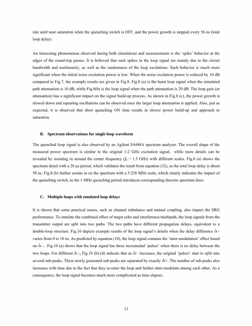
C. Comparison with Coherent Correlation Receiver (CCR) The SRG receiver’s performance can be compared with the traditional CCR based architecture shown in Fig.2.
The two architectures in Fig.2(a) and (b) use similar circuit elements. For the SRG, the received signal is re-
injected into the loop using a power combiner. A directional coupler (or power divider) samples the loop signal,
and a square-law detector records the power level of the loop signal. For the CCR, the output from the
correlation mixer is fed into a square-law detector. Both the SRG and the CCR sample the square law detector
outputs at the expected target range window and average them.
Assuming that excitation is a Gaussian random process with variance , for a single SRG loop, v is
a random process with time-variant variance (power), i.e.,
O (n¿0)vO (n¿0)
6

¾ . (8) 20(n¿0) ¼ ¾2
s
nXk=1
jA0j2(n¡k)¾2
0(n¿0) ¼ ¾2s
nXk=1
jA0j2(n¡k)
For a double loop the simplest case is when ¿ , and the double loop returns to a single loop with loop gain
. The variance is then given by
1 = ¿0¿1 = ¿0
A1 + A0A1 + A0
. (9)
The general case of ¿ will lead to a much more complicated structure of the loop signal. A concept of how
the loop signal power grows based on different target-clutter separations can be obtained from appropriate
approximations.
1 6= ¿0¿1 6= ¿0
For example, we can consider the special case with ¿ , where "" is sufficiently small so that the first
term in (6) can be considered to be almost equal t (0)(0) (zero), and therefore ignorable, n¿1)n¿1) again
only depends n , A1A1 s(t)s(t). It can be shown tha 1)1) is still a Gaussian random process with variance
given by
1 ¡ ¿0 < "¿1 ¡ ¿0 < "
o vOvO
t v0 (n¿v0 (n¿
and
o and
v0 (v0 (
A0A0
, (10)
where is the autocorrelation of s . The ultra-wideband property of s leads to the following
approximation:
(t)s(t) (t)s(t)
R , (11) ss (¿) =
½¾2
s ; j¿ j · ¿c
0; j¿ j · ¿cRss (¿) =
½¾2
s ; j¿ j · ¿c
0; j¿ j · ¿c
where ¿ is a ‘cutoff’ correlation time for excitation signal s , and can be estimated by the inverse of the signal
bandwidth.
c¿c (t)s(t)
An obvious condition to yield non-zero terms in (11) is
r . (12) 1 = r2; m1 = m2r1 = r2; m1 = m2
7

And the variance expression (10) will be simplified to
¾ . (13) 21(n¿1) ¼ ¾2
s ¢n¡1Xr=0
rXm=0
¡Cm
r Ar¡m0 Am
1
¢2¾2
1(n¿1) ¼ ¾2s ¢
n¡1Xr=0
rXm=0
¡Cm
r Ar¡m0 Am
1
¢2
Equation (13) reveals the key elements of the loop signal’s power growth. However, there are other
combinations of r which may result in j and contribute to ¾ . As a consequence, a
complicated inter-modulation response depending on the relative time delays will be introduced.
1; r2; m1; m2r1; r2; m1; m2 ¿ j < ¿cj¿ j < ¿c21 (n¿1)¾21 (n¿1)
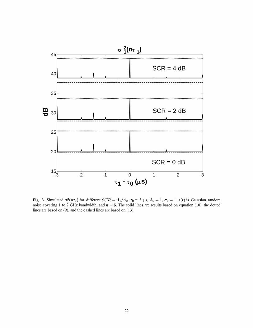
As an example, Fig.3 shows a simulated ¾ normalized with ¾ at the 5th loop delay of a true target for
different relative delays of target and clutter/interference based on different approximations. It is clearly seen
that the strongest loop signal power occurs when ¿ , and equations (9) and (10) give the same predictions.
When ¿ , loop signal power may also show power spikes which are generally lower than the spikes for
and tend to decrease with higher SCR. Equation (13) provides a good approximation for the “base” of
the ¾¾ , which is independent of ¿¿ while it is also a conservative estimation for high SCRs.
21(n¿1)¾21(n¿1)
¿
¿0¿0
2s¾2s
1 = ¿01 = ¿0
1 6= ¿0¿1 6= ¿0
¿0¿0
(n¿1)(n¿1)
¿1 =¿1 =
2121 1 ¡1 ¡
D. Comparison of square-law detector outputs Assuming a simple square-law detector can be used according to the property of central Chi-square distribution,
we can obtain the mean and variance of the detector output. For the single-target case,
mSRG;0 (n¿0) =2¾2
0p¼
;
¾2SRG;0 (n¿0) = 4¾4
0
·¡( 3
2)p¼
¡ 1¼
¸mSRG;0 (n¿0) =2¾2
0p¼
;
¾2SRG;0 (n¿0) = 4¾4
0
·¡( 3
2)p¼
¡ 1¼
.̧ (14)
For the target-plus- interference case,
mSRG;1 (n¿1) =2¾2
1p¼;
¾2SRG;1 (n¿1) = 4¾4
1
·¡( 3
2)p¼¡ 1
¼
¸mSRG;1 (n¿1) =2¾2
1p¼;
¾2SRG;1 (n¿1) = 4¾4
1
·¡( 3
2)p¼¡ 1
¼
.̧ (15)
Here represent the Gamma function [28]. From (14) and (15), the mean value of the square-law detector in
Fig.2 (a) is proportional to the variance, and the variance of the detector output follows the square of the
variance. Considering the variance grows in polynomial fashion with time, equations (14) and (15) indicate an
extremely fast growing, nonstationary process. For any given time index , the larger SCR will increase the
detection probability and reduce false alarms.
To compare the nonlinear SRG receiver with the commonly used coherent correlation receiver (CCR, Fig.2(b)),
assuming the sampling interval at the correlator output is ¢ , the detector output ZZ of the correlation receiver, ¿¢¿
8
when the receive and reference signals are zero mean Gaussian processes with variances ¾ and ¾ , has the PDF
[29]:
21¾21
22¾22
Pm (Z) =4
¾1¾2 (1 ¡ ½2) (m ¡ 1)!
·Z
¾1¾2
¸m
Km¡1
·2Z
¾1¾2 (1 ¡ ½2)
¸I0
·2½Z
¾1¾2 (1 ¡ ½2)
¸Pm (Z) =
4
¾1¾2 (1 ¡ ½2) (m ¡ 1)!
·Z
¾1¾2
¸m
Km¡1
·2Z
¾1¾2 (1 ¡ ½2)
¸I0
·2½Z ̧ , (Z>0) (16)
¾1¾2 (1 ¡ ½2)
where ½½ is the correlation coefficient between the two random samples, is the number of samples acquired
and averaged, and II and KK are modified Bessel functions. Based on the approach introduced in [29], the
square-law detector output WW is approximately a Gaussian variable with mean and standard deviation as
mm
E [W ] = m¡1 + m½2
¢(¾1¾2)
2E [W ] = m
¡1 + m½2
¢(¾1¾2)
2 (17)
and
¾W = (¾1¾2)2 £
m (m + 2) + 2m(m2 + 4m + 2)½2 + m2 (2m + 1) ½4¤1=2
¾W = (¾1¾2)2 £
m (m + 2) + 2m(m2 + 4m + 2)½2 + m2 (2m + 1) ½4¤1=2 (18)
For CCR, the observation time is limited to the time span during which the correlation coefficient ½½ is a constant.
Compared to SRG, it is reasonable to assume that ¾ (i = 0 or 1). When the time-delay of the
transmit replica matches the true target range, ½½ , then the mean and variance of the square-law detector
output can be written as
1 = ¾s; ¾2 = Ai¾s¾1 = ¾s; ¾2 = Ai¾s
¼ 1¼ 1
mCCR;0 (n¢¿) = ¾2sA2
0n (1 + n)mCCR;0 (n¢¿) = ¾2sA2
0n (1 + n), (19)
¾2CCR;0 (n¢¿ ) = ¾4
SA40 ¢ 2n
¡2n2 + 5n + 3
¢¾2
CCR;0 (n¢¿ ) = ¾4SA4
0 ¢ 2n¡2n2 + 5n + 3
¢. (20)
For the case where both target and interference are present, the interference signal is characterized by ½ .
Assuming the link gain for the true target is A1A1, the link gain for the interference signal source is A . The mean
and variance of the square-law detector output become
¼ 0½ ¼ 0
0A0
mCCR;1 (n¢¿) = ¾2sA2
1n (1 + n) + ¾2sA2
0nmCCR;1 (n¢¿) = ¾2sA2
1n (1 + n) + ¾2sA2
0n, (21)
and
¾ . (22) 2CCR;1 (n¢¿) = ¾4
SA412n
¡2n2 + 5n + 3
¢+ ¾4
SA40(2n + n2)¾2
CCR;1 (n¢¿) = ¾4SA4
12n¡2n2 + 5n + 3
¢+ ¾4
SA40(2n + n2)
Based on (14)-(15) and (19)-(22), numeric comparisons between SRG and CCR using the same square-law
detector can be performed. A typical example assumes the target is located at a distance of 900m (6μs) and the
clutter/interference source is located at a distance of 150m (1μs). To illustrate the ultra-fast power growth of the
SRG loop signal, outputs from square-law detectors are recorded for a time duration of 10 round-trips (60 μs). It
9

is assumed that the ADCs in both Fig.2(a) and Fig.2(b) have 2 MHz sampling rates. The conservative estimate
from equation (13) is used to obtain ¾ . 21(n¿1)¾21(n¿1)
The comparison results are plotted in Fig.4. For SRG, the rising speed of the mean value is about 5 dB/10 μs
when there is only clutter present. The rising speed is almost 20 dB/10 μs when SCR increases to 3 dB. For
CCR, the rising speed of correlator output is relatively faster within the first target round-trip delay, and becomes
stabilized even for high SCR (< 2 dB/ 10 μs). It is important to note that the SRG can not only provide ultra-fast
target indication compared to the CCR, but also much stronger capability to discriminate useful signals from
clutter response. This is manifested in Fig.4(a). At 60 μs, a 1.5 dB SCR increase leads to 10-20 dB stronger
detector mean output, while leading to only about a 3 dB increase in CCR’s detector mean output. It is also seen
from Fig.4(b) that at different observation times the differences among the CCR detector output levels depend
mainly on the SCR.
On the other hand, the example also illustrates the extreme sensitivity of the SRG to both the target signal and
clutter. Both mean and variance of the SRG receiver exhibit much faster growth compared to those of the CCR,
even for clutter-only cases. A strong loop signal caused by clutter/interference may be sufficient to saturate the
receiver, thus must be controlled. A much larger variance growth with time for the SRG also implies the system
requires a much larger dynamic range than the CCR in order to accommodate the large uncertainty in the
detector outputs and the ultra-fast loop responses.
III. FREQUENCY-DOMAIN AND CORRELATION CHARACTERISTICS
Another approach to analyze the SRG loop signal properties is to decompose the broadband excitations into
harmonics. The loop signal can then be considered as the combination of the responses from all frequency
elements. When the BPF matches the signal frequency band, the difference equation maybe written as
,
, (23)
where the nth signal component of v is a harmonic waveform: O (t)vO (t)
v . (24) o;n (t) = anej!ntvo;n (t) = anej!nt
In the receiver loop, each frequency element satisfies the following equation:
, (25)
10
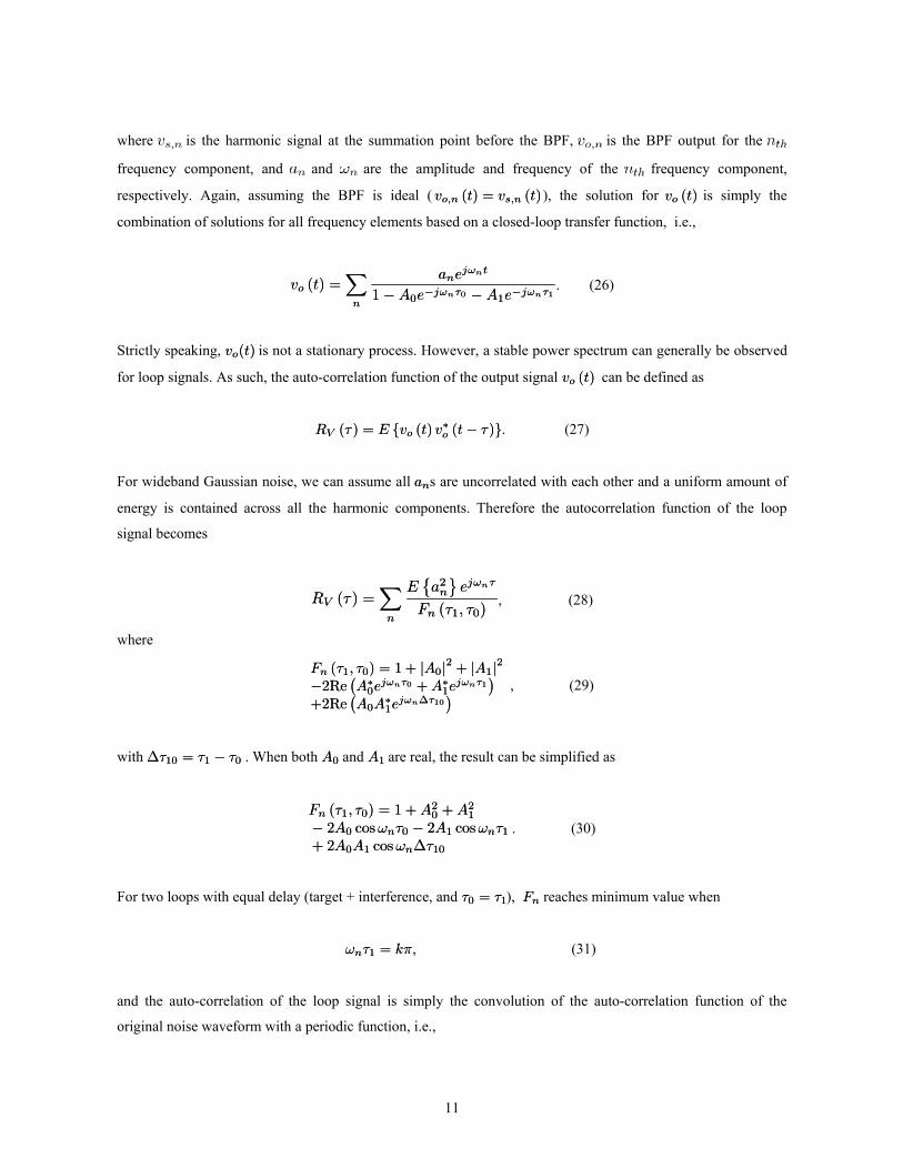
where is the harmonic signal at the summation point before the BPF, is the BPF output for the
frequency component, and and are the amplitude and frequency of the frequency component,
respectively. Again, assuming the BPF is ideal ( ), the solution for v is simply the
combination of solutions for all frequency elements based on a closed-loop transfer function, i.e.,
vo;n (t) = vs;n (t)vo;n (t) = vs;n (t) o (t)vo (t)
vo (t) =X
n
anej!nt
1 ¡ A0e¡j!n¿0 ¡ A1e¡j!n¿1vo (t) =
Xn
anej!nt
1 ¡ A0e¡j!n¿0 ¡ A1e¡j!n¿1. (26)
Strictly speaking, v is not a stationary process. However, a stable power spectrum can generally be observed
for loop signals. As such, the auto-correlation function of the output signal v can be defined as
o(t)vo(t)
o (t)vo (t)
RV (¿ ) = E fvo (t) v¤o (t ¡ ¿)gRV (¿ ) = E fvo (t) v¤o (t ¡ ¿)g. (27)
For wideband Gaussian noise, we can assume all a s are uncorrelated with each other and a uniform amount of
energy is contained across all the harmonic components. Therefore the autocorrelation function of the loop
signal becomes
nan
RV (¿) =X
n
E©a2
n
ªej!n¿
Fn (¿1; ¿0)RV (¿) =
Xn
E©a2
n
ªej!n¿
Fn (¿1; ¿0), (28)
where
Fn (¿1; ¿0) = 1 + jA0j2 + jA1j2¡2Re
¡A¤0e
j!n¿0 + A¤1ej!n¿1
¢+2Re
¡A0A
¤1e
j!n¢¿10¢Fn (¿1; ¿0) = 1 + jA0j2 + jA1j2
¡2Re¡A¤0e
j!n¿0 + A¤1ej!n¿1
¢+2Re
¡A0A
¤1e
j!n¢¿10¢ , (29)
with ¢ . When both A and A are real, the result can be simplified as ¿10 = ¿1 ¡ ¿0¢¿10 = ¿1 ¡ ¿0 0A0 1A1
Fn (¿1; ¿0) = 1 + A20 + A2
1
¡ 2A0 cos !n¿0 ¡ 2A1 cos !n¿1
+ 2A0A1 cos !n¢¿10
Fn (¿1; ¿0) = 1 + A20 + A2
1
¡ 2A0 cos !n¿0 ¡ 2A1 cos !n¿1
+ 2A0A1 cos !n¢¿10
. (30)
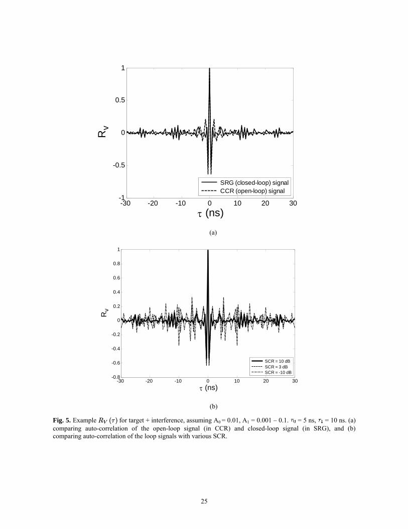
For two loops with equal delay (target + interference, and ¿ ), F reaches minimum value when 0 = ¿1¿0 = ¿1 nFn
! , (31) n¿1 = k¼!n¿1 = k¼
and the auto-correlation of the loop signal is simply the convolution of the auto-correlation function of the
original noise waveform with a periodic function, i.e.,
11

RV (¿) = RS (¿) ¤ 1
(1¡A0 ¡A1)2
Xn
± (¿ ¡ n¿1)RV (¿) = RS (¿) ¤ 1
(1¡A0 ¡A1)2
Xn
± (¿ ¡ n¿1). (32)
Equation (32) clearly indicates the presence of discrete line spectra in the frequency-domain. The situation is
much more complicated when the target and interference loops have different time delays, especially when the
signal and interference have similar amplitudes. For this case, the local peaks of the autocorrelation function
may appear at integral multiples of , , as well as locations between them.
Fig.5 shows simulation examples of R under particular conditions. From Fig.5(a), it is seen that the SRG
loop signals exhibit clear periodicity in their auto-correlations, which will translate into discrete spectrum lines
in the frequency domain. The width of the correlation peak is similar for the SRG and CCR. From Fig.5(b), it is
seen that when the SCR is low, more correlation signal power will ‘leak’ to the sidelobes of R and
complicated inter-modulation peaks will appear.
V (¿ )RV (¿ )
V (¿ )RV (¿ )
IV. DUAL-CHANNEL, L BAND TRANSCEIVER MEASUREMENTS A dual-channel SRG transceiver prototype is designed and fabricated using commercial-off-the-shelf (COTS)
RF components. It contains two identical loops. Each loop has T/R antennas, a power amplifier, LNA, and
‘quenching control’ switches. The quenching switches (as in Fig.2 (a)) are fast GaAs switches controlling the
precise times that the feedback loops are opened and closed. The loop signals are sampled from a power divider
and correlated in an RF mixer. The two RF channels are excited by the same Gaussian noise source covering the
1-2 GHz ultra-wide frequency range. A broadband variable attenuator controls the power level of the random
noise excitation.
A. Single-loop with emulated path delay
The first experiment is designed to validate the time-domain loop signal growth speed and the impact of the
quenching switch and the actual components’ nonlinearity. The quenching switch is controlled by a 1 MHz TTL
signal with a variable duty-cycle. The loop delay is precisely emulated by a section of coaxial cable, which adds
20 ns to the 34 ns electrical component propagation delay in the loop. Another variable attenuator is used
together with a cable assembly to simulate different loop-gains. The sampled loop signals are recorded and
displayed by a high-speed digital storage oscilloscope (DSO), burst-by-burst synchronized with the quenching
switch’s ‘ON’ periods. Example waveforms in a single SRG transceiver loop are shown in Fig.7. In both
scenarios, the total loop delay is 56 ns. From Fig.7, especially the signals in the boxes, it is clear that the
unsaturated signal accumulates in the feedback loop according to equation (4) & (5), and the measured emulation
result matches the theoretical predictions. Just as theoretically-predicted, the loop signal grows at an extreme fast
12
rate until near saturation when the quenching switch is OFF, and the power growth is stepped every 56 ns (total
loop delay).
An interesting phenomenon observed during both simulations and measurements is the ‘spike’ behavior at the
edges of the round-trip passes. It is believed that such spikes in the loop signal are mainly due to the circuit
bandwidth and nonlinearity, as well as the randomness of the loop excitations. Such behavior is much more
significant when the initial noise excitation power is low. When the noise excitation power is reduced by 10 dB
compared to Fig.7, the example results are given in Fig.8. Fig.8 (a) is the burst loop signal when the simulated
path attenuation is 10 dB, while Fig.8(b) is the loop signal when the path attenuation is 20 dB. The loop gain (or
attenuation) has a significant impact on the signal build-up process. As shown in Fig.8 (c), the power growth is
slowed down and repeating oscillations can be observed once the larger loop attenuation is applied. Also, just as
expected, it is observed that short quenching ON time results in slower power build-up and approach to
saturation.
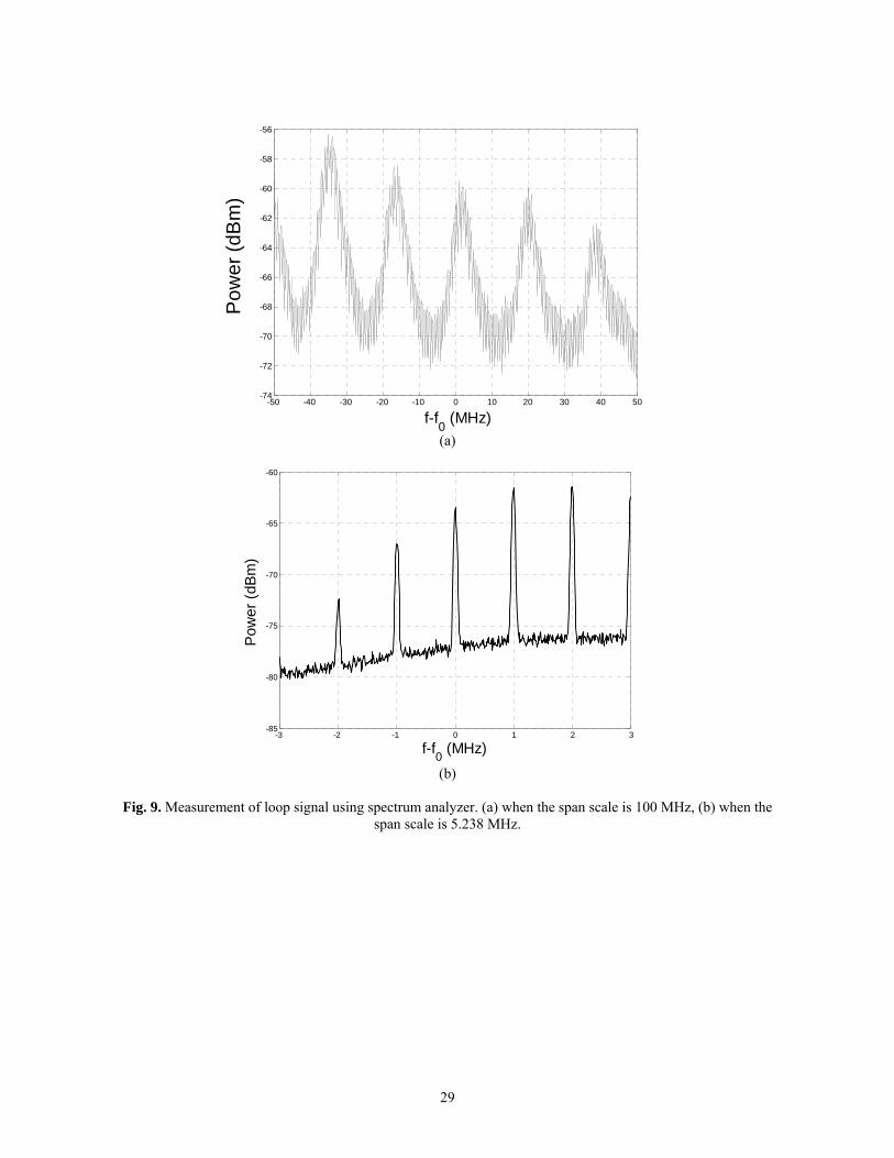
B. Spectrum observations for single-loop waveform The quenched loop signal is also observed by an Agilent E4448A spectrum analyzer. The overall shape of the
measured power spectrum is similar to the original 1-2 GHz excitation signal, while more details can be
revealed by zooming in around the center frequency (f0 = 1.5 GHz) with different scales. Fig.8 (a) shows the
spectrum detail with a 20 μs period, which validates the result from equation (32), as the total loop delay is about
50 ns. Fig.8 (b) further zooms in on the spectrum with a 5.238 MHz scale, which clearly indicates the impact of
the quenching switch, as the 1 MHz quenching period introduces corresponding discrete spectrum lines.
C. Multiple-loops with emulated loop delays
It is shown that some practical issues, such as channel imbalance and mutual coupling, also impact the SRG
performance. To emulate the combined effect of target echo and interference/multipath, the loop signals from the
transmitter output are split into two paths. The two paths have different propagation delays, equivalent to a
double-loop structure. Fig.10 depicts example results of the loop signal’s details when the delay difference
varies from 0 to 10 ns. As predicted by equation (10), the loop signal contains the ‘inter-modulation’ effect based
on . Fig.10 (a) shows that the loop signal has three incremental ‘pulses’ when there is no delay between the
two loops. For different , Fig.10 (b)-(d) indicate that as increases, the original ‘pulses’ start to split into
several sub-peaks. These newly generated sub-peaks are separated by exactly . The number of sub-peaks also
increases with time due to the fact that they re-enter the loop and further inter-modulate among each other. As a
consequence, the loop signal becomes much more complicated as time elapses.
13

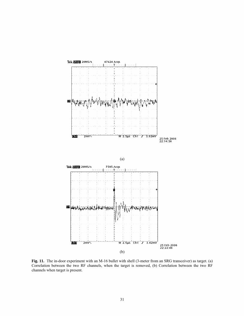
D. Indoor target detection experiment
The cable between the transmit and receive channels are replaced with ultra-wideband, log-periodic antennas in
lab-experiments. The four antennas are arranged in a typical retro-directive formation. The two SRG channels
operate independently and the sampled loop signals are fed into a correlation receiver (broadband double-
balanced mixer plus low pass filter). The ON time of the quenching switch is tuned to an appropriate value so
that no loop signals build up when the system is located in an empty range. Fig.11 compares the correlation
output when there is no target and when a target is present. It is clear that in this wireless sensing experiment, the
bullet target gives a strong correlation peak from the loop signals of the SRG, and the target response (detection)
time is merely limited by the low-pass filter cutoff frequency of the inter-channel correlator, as well as the
quenching signal periods.
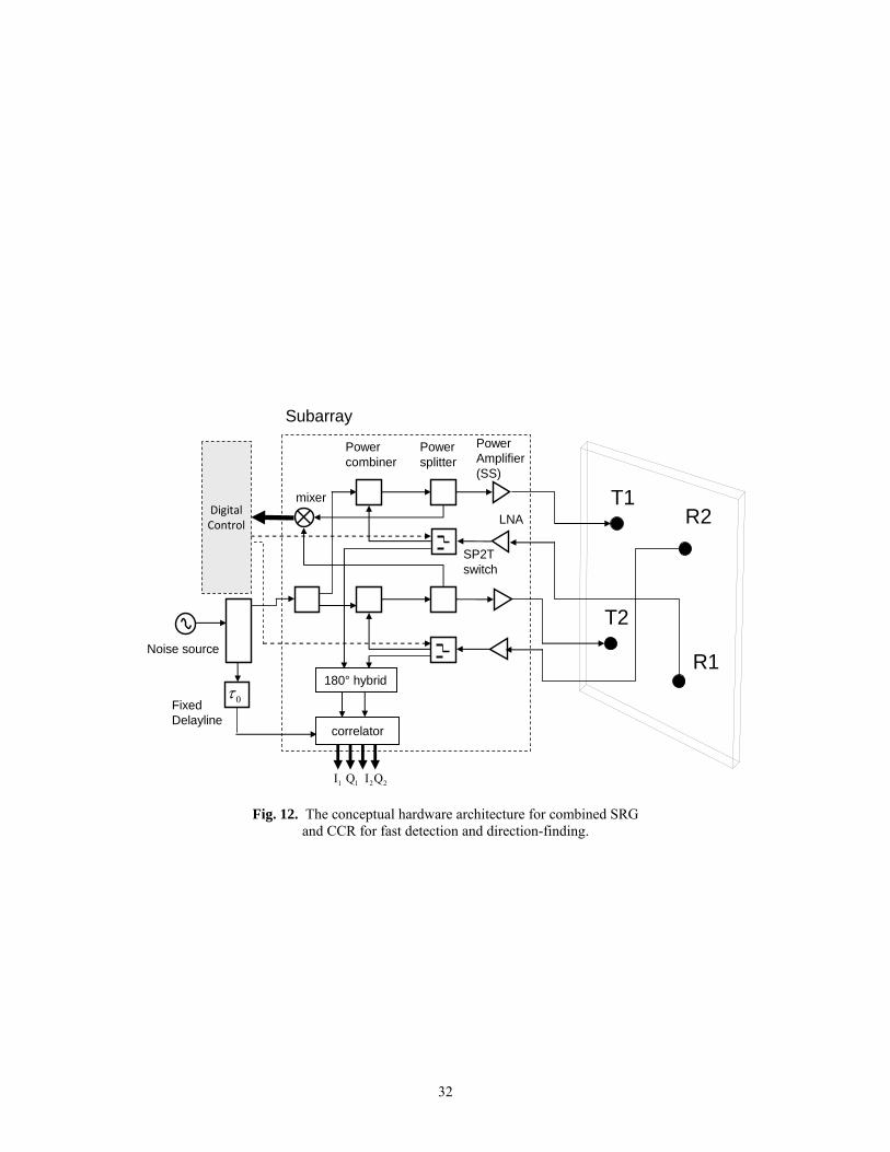
V. FAST MONOPULSE PROCESSING FOR NOISE RADAR
A. Transient Target Signature from multiple channels The previous sections conclude that the fast detection of incoming threats can be achieved through the SRG
transceiver architecture. The open-loop signals, on the other hand, can be processed by a conventional CCR
receiver for tracking functionalities. This concept leads to the architecture design as shown in Fig.12. Each loop
channel operates in ‘detection’ mode when the quenching switch is ON, and ‘tracking’ mode when the switch is
OFF.
The theories and applications of the Angle-of-Arrival (AOA) estimation using a random-noise waveform was
discussed in [4], the traditional CCR and range tracking scheme, however, does not fit the needs of ultra-fast
threat direction estimation. To fundamentally increase the estimation speed, the monopulse processor in this
work only acquires the transient correlator output from one fixed reference delay instead of scanning through
the range gates.
A detailed analysis shows that the output signals from the two front-end correlators have many frequency
components. The strongest frequency component, which carries the target Doppler information, can be expressed
as
, (33)
which is a transient AM pulse with envelope time span given by
, (34)
14

and inner ‘carrier’ frequency
(35)
as shown in Fig.13, where c is the speed of the light, v is the target speed, ωc is the center frequency of the
transmit waveform, Δω is the transmit signal bandwidth, and Δt is a time-shift associated with the starting point
of sampling.
We can see that the shape of the transient pulse is determined by the transmit frequency band and the target
velocity. In terms of system design, we may wish to choose higher transmit frequencies and narrower bands;
this will give us larger Doppler shifts and longer observation times, thus enhancing the clutter immunity. On the
other hand, this will be closer to traditional monopulse radar and may compromise the Electronic Counter-
Countermeasures (ECCM) capability.
Because of the time-of-arrival difference between the receive antennas, it can be shown that the low-pass-filtered
correlation between the sum and difference channels has a ‘monocycle’ shape, whose polarity is determined by
the sign of the AOA, and whose amplitude is proportional to the magnitude of the AOA. As a result, fast
monopulse processing can simply divide the peak value of this monocycle by the peak output of the sum-channel
square-law detector to estimate the AOA.
Simulations of AOA estimation using the fast monopulse scheme is performed with a MATLAB-based
simulation platform. We choose a very high-speed target (15 km/s) in most simulations. Although this is far
beyond the requirements of this work, it uses a shorter simulation time and manifests the principle of transient
pulses much more clearly than slower target simulation. We use a 4-5 GHz signal frequency band in the
simulations. The fixed delay τ0 is set to 2 μs. Also, stationary ground clutter at 2 μs range with different signal-
to-clutter ratio (SCR) is added.
Fig.14 shows the resultant transient pulse from one antenna channel when the signal-to-clutter ratio is 10 dB.
The pulse envelope should last about 19 μs, and the inner ‘carrier’ should oscillate at about 450 kHz. The
simulation result shows exact compliance with theoretical predictions.
B. Fast monopulse processors Fig.15 shows a monopulse processor structure for transient target signature. The received waveforms from two
antennas are correlated to the transmit replica with a fixed time delay τ0, and the transient sum (sI) and different
(dI) signals from the correlator output are recorded. The Monopulse Characteristic Curve (MCC) is calculated as
15

. (33)
As it is difficult to acquire the actual transient target signatures at this time, hardware emulation testing is
performed to validate the fast monopulse processing approach. The emulation is based on the following
principle: placing a stationary target at different directions with respect to the antenna boresight axis and
correlating the target reflection with a delayed transmit noise replica while the delay line rapidly scans over a
range of time-delays, we emulate a target reflection with 128-ns delay variation during 19.2 ms. The correlation
result is thus equivalent to the transient signature from a target having a speed of 1000 m/s. Fig.14 shows the
hardware emulation test design. We use one transmit antenna (Tx) and two receive antennas (Rx1 and Rx2) in
this test. The antennas are mounted on a precise azimuth positioner. The scanning is from -5° to +5° at 0.5°
angular intervals. Therefore, for each antenna and each I/Q component, the result is a 21×70 2D matrix. The
‘index of sample line’ is from 1 to 70 and the ‘index of AOA line’ is from 1 to 21. We first calculate the sum and
difference beams along each ‘index of sample line’ as follows:
(34)
The ‘s’ results are digitally formed sum-beams and the ‘d’ results are digitally formed difference-beams. These
two types of beams are ‘orthogonal’ to each other.
1) Conventional monopulse processing
A conventional monopulse processor is used first to calculate the monopulse ratio along 70 ‘index of sample
lines’ and for each angular interval, i.e.,
, (35)
which performs further low-pass filtering on both the numerator and denominator terms. The LPF ‘smoothing’
is expected to give better results for the Monopulse Characteristic Curve (MCC) albeit at the cost of additional
processing time. The extracted monopulse response from traditional monopulse processing (equation (35))
results along sample lines 34, 36 and 38 are shown in Fig.17. We observe that within the -1º to 2º range, the
extracted monopulse response can be viewed as approximately linear with respect to the AOA.
The angular ambiguity associated with the MCC can be resolved by several methods, namely, using multiple
antennas or using sum-channel information, or comparing the signal strengths of two receive antenna channels.
16

A key approach is based on a look-up table. Note that the shapes of the monopulse characteristic wave as well as
the look-up table are dependent on the AOA and target type, but not dependent on the target range.
2) Fast monopulse processing For fast monopulse processing, we calculate the correlation between the sum and difference signals, applying
digital low-pass filtering (LPF) on them before computing their ratios. For example,
. (36)
Fig.18 shows the 3D map of the monopulse processing result using equation (33). It can be seen that the low-
pass filtering has ‘pushed’ the MCC curve to the edge of the figure. The MCC still shows a strong response at
about zero AOA. Ideally, the monopulse characteristic curves should be periodic, but because of
reflection/interference or multipath, the actual curves may be distorted for large angles off-boresight. Again,
these range-independent curves serve as the basis of a look-up table for angle estimation. The results
demonstrate that fast monopulse processing is able to accurately extract target AOA from transient target
signatures of receive array channels. We also observe that, through additional filtering, the linear response region
of the MCC can be improved.
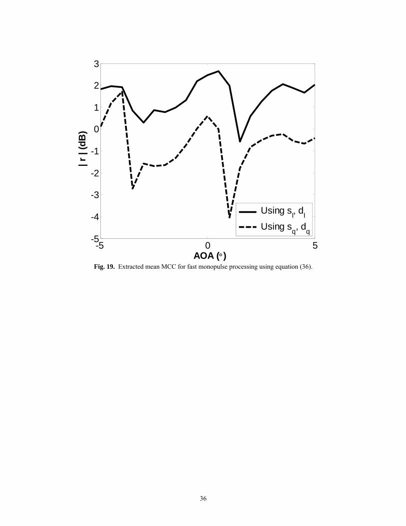
Now consider the fast monopulse processing given by (36), which takes the peak values of the cross and auto
correlations at each AOA and across the range index, reducing the MCC to 2D curves. The processing results
based on either the real or imaginary parts of sum-difference channels and the same data are given in Fig.19. It
is clear that fast monopulse processing on transient target signatures results in strong nonlinear behavior of the
MCC. However, the target response is still very significant near boresight, which serves as a reliable indication
of the target direction.
VI. CONCLUSION
The potentials of using SRG transceiver architectures for ultra-wideband, ultra-fast target detection and AOA
estimation are explored. Time-domain modeling based on solutions of difference equations can be used to
characterize the fast growth of the loop signals and comparison with Coherent Correlation Receiver (CCR)
architectures. The ultra-fast power growth, random nature of radar signals, and the nonlinear properties of the
system require the implementation of appropriately designed quenching signals. Hardware emulation
experiments at L band and X band have validated the theoretical predictions of SRG signal behaviors and the
feasibility of fast AOA estimation based on monopulse processing and transient target signatures.
17

ACKNOWLEDGMENTS
The authors would like to give thanks for the support and guidance of Dr. Ram Narayanan at Pennsylvania State
University and Dr. Dwight Woolard, US Army Research Office, as well as Dr. Chieh-Ping Lai’s experimental
support during the 2006 prototyping effort. The authors also greatly appreciate the laboratory facility support of
the Radar Innovations Laboratory, University of Oklahoma and Pennsylvania State University.
18

REFERENCES [1] G. W. Stimson, Introduction to Airborne Radar, 2nd edition, Mendham, NJ: SciTech Publishing, Inc., 1998. [2] R. M. Narayanan, and X. Xu, “Principles and applications of coherent random noise radar technology,” in SPIE
Conference on Noise in Devices and Circuits, Santa Fe, NM, 2003, pp. 503-514. [3] Y. Zhang, and R. M. Narayanan, “Design Considerations for a Real-Time Random Noise Tracking Radar,” IEEE
Trans. on AES, vol. 40, no. 2, pp. 434-445, 2004. [4] Y. Zhang, and R. M. Narayanan, “Monopulse Radar Based on Spatiotemporal Correlation of Stochastic Signals,”
IEEE Trans. on AES, vol. 42, no. 1, pp. 160-173, 2006. [5] J. R. Forrest, and D. J. Price, “Digital Correlation for Noise Radar Systems,” Electronics Letters, vol. 14, no. 8, pp.
581-582, Aug, 1978. [6] G. Johnson, D. Ohlms, and M. Hampton, “Broadband correlation processing,” in Proceedings of ICASSP'83, 1983,
pp. 583-586. [7] G. L. Guosui, H. G. Hong, and W. Su, “Development of random signal radars,” IEEE Trans. on AES, vol. 35, no. 3,
pp. 770-777, July, 1999. [8] V. I. Kalinin, and V. V. Chapurskii, “Ultrawideband Noise Radar Based on Antenna Arrays with Signal
Recirculation ” Journal of Communication Technologies and Electronics, vol. 52, no. 10, pp. 1266-1277, 2008. [9] Y. Zhang, and R. M. Narayanan, “Ultra-fast Threat Detection and Tracking Using Random-noise Retrodirective
Array and Monopulse,” in 25th Army Science Conference, Orlando, FL, 2006. [10] U. L. Rohde, and A. K. Poddar, “Super-Regenerative Receiver (SRR),” in IEEE Conference on Electron Devices
and Solid State Circuits, 2007. [11] F. X. Moncunill-Geniz, P. Pala-Schonwalder, and O. Mas-Casals, “A Generic Approach to the Theory of
Superregenerative Reception ” IEEE Trans. on Circuits and Systems - I: Regular Papers, vol. 52, no. 1, pp. 54-70, Jan, 2005.
[12] D. M. W. Leenaerts, “Chaotic behavior in super regenerative detectors,” IEEE Trans. on Circuits and Systems - I, vol. 43, no. 3, pp. 169-176, 1996.
[13] M. Anis, R. Tielert, and N. Wehn, “Fully integrated self-quenched super-regenerative UWB impulse detector,” in ISWPC 2008, 2008, pp. 773-775.
[14] E. R. Brown, Retrodirective Noise-Correlating Radar in X-band: MDA/DARPA research project final report, 2005. [15] E. R. Brown, R. F. Sinclair, and E. B. Brown, “Retrodirective Radar for Small Projectile Detection,” in
IEEE/MTT-S International Microwave Symposium, 2007, pp. 777-780. [16] C. C. Cutler, R. Kompfner, and L. C. Tillstson, “A Self-steering Array Repeater,” Bell System Technology Journal,
vol. 42, pp. 2013-2032, 1963. [17] V. F. Fusco, and S. L. Karode, “Self-phasing Antenna Array Techniques for Mobile Communications
Applications,” Electronics and Communication Engineering Journal, vol. 11, pp. 279-286, Dec., 1999. [18] E. Muehldorf, “Self-steered retrodirective arrays with amplification,” IEEE Trans. on Antennas and Propagation,
vol. 17, no. 1, pp. 42-49, 1969. [19] C. Pon, “Retrodirective array using the heterodyne technique ” IEEE Trans. on Antennas and Propagation, vol. 12,
no. 2, pp. 176-180, March, 1964. [20] E. Putzer, and R. Ghose, “Redirective and retrodirective antenna arrays ” IEEE Trans. on Antennas and
Propagation vol. 17, no. 3, pp. 276-279, 1969. [21] E. Sharp, and M. Diab, “Van Atta Reflector Array,” IRE Transactions on Antenna and Propagation, vol. 8, no. 4,
pp. 436-438, July, 1960. [22] C. Loadman, and Z. Chen, “A study of retrodirective array performance in the presence of multipath,” in
Proceedings of Second Annual Conference on Communication Networks and Services Research, 2004, pp. 56-60. [23] T. K. Bhattacharya, G. Jones, and D. DiFilippo, “Time frequency based detection scheme for missile approach
warning system (MAWS),” in Proceedings of IEEE Radar Conference, 1997, pp. 539-543. [24] C. E. Baum, “Signature-based target identification and pattern recognition,” IEEE Antennas and Propagation
Magazine, vol. 36, no. 3, pp. 44-51, June, 1994. [25] A. Hommes, H. Essen, P. Knott et al., “Investigations on signatures of projectiles for sniper detection applications,”
in 2008 IEEE Radar Conference, 2008, pp. 1-6. [26] R. B. Sinitsyn, and A. J. Beletsky, “Fast Signal Processing Algorithms for Noise Radars,” in EuRAD 2006, 2006,
pp. 245-248. [27] S. Elaydi, A Introduction to Difference Equations (3rd edition), New York, NY: Springer, 2005. [28] A. D. Polyanin, and A. V. Manzhirov, Handbook of Mathematics for Engineers and Scientists Boca Raton, FL:
Chapman & Hall/CRC; 1st edtion, 2007. [29] K. Milne, “Theoretical Performance of a Complex Cross-Correlator with Gaussian Signals,” IEE Proceedings - F,
vol. 140, no. 1, pp. 81-88, Feb, 1993.
19
LIST OF FIGURES Fig. 1. The generic schematic of the SRG transceiver operation using multiple loops. ......................................... 21 Fig. 2. The different single-channel transceiver architectures for noise radar, using similar circuit elements, (a) The SRG architecture, (b) The CCR architecture. ................................................................................................. 21 Fig. 3. Simulated ¾ for different . = 3 μs, A0 , . is Gaussian random noise covering 1 to 2 GHz bandwidth, and . The solid lines are results based on equation (10), the dotted lines are based on (9), and the dashed lines are based on (13). .............................................................................. 22
21(n¿1)¾21(n¿1) SCR = A1=A0SCR = A1=A0
n = 5n = 5¿0¿0 = 1A0 = 1 ¾s = 1¾s = 1 s(t)s(t)
Fig. 4. A comparison between the square-law detector output growth of SRG and CCR, for different
== 11 , ¾21(n¿1SCRs. , ¿0 1 ¹s¿0 1 ¹s ¿ = 6 ¹s¿ = 6 ¹s )¾21(n¿1) estimation is based on (13). Totally 10 round-trip observations are
recorded. (a) mean-value of detector output from SRG, (b) mean-value of detector output from CCR, (c) variance of detector output from SRG, (d) variance of detector output from CCR. .............................................. 24 Fig. 5. Example RV for target + interference, assuming A0 = 0.01, A1 = 0.001 – 0.1. (¿ )RV (¿ ) = 5 ns, = 10 ns. (a) comparing auto-correlation of the open-loop signal (in CCR) and closed-loop signal (in SRG), and (b) comparing auto-correlation of the loop signals with various SCR. ....................................................................... 25 Fig. 6. Picture of a double-loop SRG transceiver prototype .................................................................................. 26 Fig. 7. Loop signal measurement using a coax cable to emulate path delays. The noise-source’s output power is -26 dBm/Hz. The total loop delay is 56 ns, (a) theoretically predicted time-domain loop waveform with A0 =1, (b) Measured waveform, path attenuation = 10 dB. .............................................................................................. 27 Fig. 8. Same as Fig.7 except the noise-source output power is reduced by 10 dB, (a) theoretically predicted time-domain loop waveform with A0 =1, (b) Measured waveform, path attenuation = 10 dB, (c) Path attenuation = 20 dB. ......................................................................................................................................................................... 28 Fig. 9. Measurement of loop signal using spectrum analyzer. (a) when the span scale is 100 MHz, (b) when the span scale is 5.238 MHz. ....................................................................................................................................... 29 Fig. 10. Measurement of the double-loop signal using a digital storage oscilloscope (DSO). The first loop has a delay of ns, while the other loop has a delay longer than the first loop by . (a) = 0; (b) = 2 ns; (a) = 5 ns; (d) = 10 ns; For convenience of comparison, we concentrate on the first three pulses of the burse signal before it gets saturated. ...................................................................................................................... 30 Fig. 11. The in-door experiment with an M-16 bullet with shell (3-meter from an SRG transceiver) as target. (a) Correlation between the two RF channels, when the target is removed, (b) Correlation between the two RF channels when target is present.............................................................................................................................. 31 Fig. 12. The conceptual hardware architecture for combined SRG ...................................................................... 32 Fig. 13. A generic structure of the transient signal output from fixed-delay CCR. .............................................. 33 Fig. 14. Simulated transient correlation pulse from one antenna channel for ........................................................ 33 Fig. 15. Processor structure for fast random-noise monopulse ............................................................................. 34 Fig. 16. Hardware emulation setup design. ........................................................................................................... 34 Fig. 17. Extracted MCC for conventional monopulse processing using equation (35).......................................... 35
20
Fig. 18. 3D map of monopulse processing result using equation (33). ................................................................. 35 Fig. 19. Extracted mean MCC for fast monopulse processing using equation (36). ............................................. 36
+
( )ts0A0τ
BPF( )tOv
1τ 1A
Nτ NA
( )tsi
( )tSv
Fig. 1. The generic schematic of the SRG transceiver operation using multiple loops.
+ BPF
ADC
TX
RX
( )2•( ) 2
1
1 m
Ok
v km =
⎡ ⎤⎣ ⎦∑
Ov
(a)
BPF
ADC
TX
RX
( )2•( ) 2
1
1 m
Ok
v km =
⎡ ⎤⎣ ⎦∑
×
Ov
(b)
Fig. 2. The different single-channel transceiver architectures for noise radar, using similar circuit elements, (a)
The SRG architecture, (b) The CCR architecture.
21
-3 -2 -1 0 1 2 315
20
25
30
35
40
45 σ 12(nτ 1)
τ1 - τ0 (μs)
dB SCR = 2 dB
SCR = 0 dB
SCR = 4 dB
Fig. 3. Simulated ¾ for different SC . ¿0¿0 = 3 μs, A0 , . s is Gaussian random noise covering 1 to 2 GHz bandwidth, and n . The solid lines are results based on equation (10), the dotted lines are based on (9), and the dashed lines are based on (13).
21(n¿1)¾21(n¿1) R = A1=A0SCR = A1=A0
= 5n = 5= 1A0 = 1 ¾s = 1¾s = 1 (t)s(t)
22

0 10 20 30 40 50 600
10
20
30
40
50
60
70
80
90 Mean Value - SRG
Time (μs)
dB
Clutter Only SCR = -3 dB SCR = -1.5 dB SCR = 0 dB SCR = 1.5 dB SCR = 3 dB
(a)
0 10 20 30 40 50 60 700
5
10
15
20
25
30 Mean Value - CCR
Time (μs)
dB
Clutter Only SCR = -3 dB SCR = -1.5 dB SCR = 0 dB SCR = 1.5 dB SCR = 3 dB
(b)
23

0 10 20 30 40 50 60-50
0
50
100
150
200
250
300
350
400 Variance - SRG
Time (μs)
dB
Clutter Only SCR = -3 dB SCR = -1.5 dB SCR = 0 dB SCR = 1.5 dB SCR = 3 dB
(c)
0 10 20 30 40 50 60 705
10
15
20
25
30
35
40 Variance - CCR
Time (μs)
dB
Clutter Only SCR = -3 dB SCR = -1.5 dB SCR = 0 dB SCR = 1.5 dB SCR = 3 dB
(d) Fig. 4. A comparison between the square-law detector output growth of SRG and CCR, for different SCRs.
, ¿1 , ¾¿0 = 1 ¹s¿0 = 1 ¹s = 6 ¹s¿1 = 6 ¹s 21(n¿1)¾21(n¿1) estimation is based on (13). Totally 10 round-trip observations are recorded. (a)
mean-value of detector output from SRG, (b) mean-value of detector output from CCR, (c) variance of detector output from SRG, (d) variance of detector output from CCR.
24
-30 -20 -10 0 10 20 30-1
-0.5
0
0.5
1
τ (ns)
Rv
SRG (closed-loop) signal CCR (open-loop) signal
(a)
-30 -20 -10 0 10 20 30-0.8
-0.6
-0.4
-0.2
0
0.2
0.4
0.6
0.8
1
τ (ns)
Rv
SCR = 10 dB SCR = 3 dB SCR = -10 dB
(b) Fig. 5. Example RV for target + interference, assuming A0 = 0.01, A1 = 0.001 – 0.1. (¿ )RV (¿ ) = 5 ns, = 10 ns. (a) comparing auto-correlation of the open-loop signal (in CCR) and closed-loop signal (in SRG), and (b) comparing auto-correlation of the loop signals with various SCR.
25
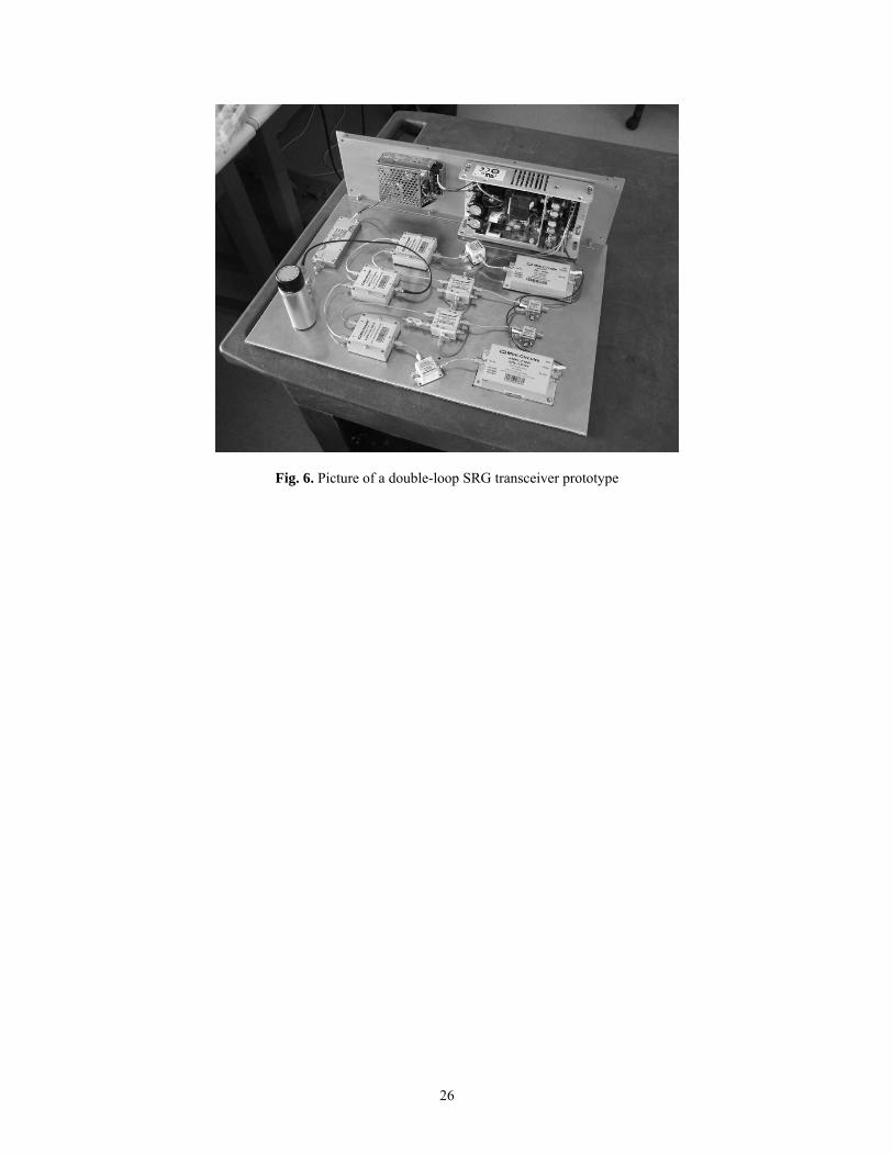
Fig. 6. Picture of a double-loop SRG transceiver prototype
26

0 0.1 0.2 0.3 0.4 0.5 0.6 0.7 0.8-0.8
-0.6
-0.4
-0.2
0
0.2
0.4
0.6
0.8
1
Time (μ s)
Volta
ge (V
olts
)
The burst loop signalThe quenching pulse
(a)
(b) Fig. 7. Loop signal measurement using a coax cable to emulate path delays. The noise-source’s output power is -26 dBm/Hz. The total loop delay is 56 ns, (a) theoretically predicted time-domain loop waveform with A0 =1, (b) Measured waveform, path attenuation = 10 dB.
27

0 0.1 0.2 0.3 0.4 0.5 0.6 0.7
-0.5
-0.4
-0.3
-0.2
-0.1
0
0.1
0.2
0.3
0.4
0.5
Time (μ s)
Vol
tage
(Vol
ts)
The burst loop signalThe quenching pulse
0 0.1 0.2 0.3 0.4 0.5 0.6 0.7
-0.5
0
0.5
1
Time (μ s)
Vol
tage
(Vol
ts)
The quenching pulseThe burst loop signal
0 0.2 0.4 0.6 0.8 1
-1
-0.8
-0.6
-0.4
-0.2
0
0.2
0.4
0.6
Time (μ s)
Vol
tage
(Vol
ts)
The burst loop signalThe quenching pulse
Fig. 8. Same as Fig.7 except the noise-source output power is reduced by 10 dB, (a) theoretically predicted time-domain loop waveform with A0 =1, (b) Measured waveform, path attenuation = 10 dB, (c) Path attenuation = 20 dB.
28
-50 -40 -30 -20 -10 0 10 20 30 40 50-74
-72
-70
-68
-66
-64
-62
-60
-58
-56
f-f0 (MHz)
Pow
er (d
Bm
)
(a)
-3 -2 -1 0 1 2 3-85
-80
-75
-70
-65
-60
f-f0 (MHz)
Pow
er (d
Bm)
(b)
Fig. 9. Measurement of loop signal using spectrum analyzer. (a) when the span scale is 100 MHz, (b) when the
span scale is 5.238 MHz.
29

0.5 0.52 0.54 0.56 0.58 0.6 0.62 0.64-0.5
-0.4
-0.3
-0.2
-0.1
0
0.1
0.2
0.3
0.4
0.5
Time (μ s)
Vol
tage
(Vol
ts)
Δτ = 0 ns
0.5 0.52 0.54 0.56 0.58 0.6 0.62 0.64-0.5
-0.4
-0.3
-0.2
-0.1
0
0.1
0.2
0.3
0.4
0.5
Time (μ s)
Vol
tage
(Vol
ts)
Δτ = 2 ns
Δτ
(a) (b)
0.5 0.52 0.54 0.56 0.58 0.6 0.62 0.64 0.66-0.5
-0.4
-0.3
-0.2
-0.1
0
0.1
0.2
0.3
0.4
0.5
Time (μ s)
Vol
tage
(Vol
ts)
Δτ = 5 ns
Δτ
0.5 0.52 0.54 0.56 0.58 0.6 0.62 0.64 0.66 0.68-0.5
-0.4
-0.3
-0.2
-0.1
0
0.1
0.2
0.3
0.4
0.5
Time (μ s)
Volta
ge (V
olts
)
Δτ = 10 ns
Δτ
(c) (d)
Fig. 10. Measurement of the double-loop signal using a digital storage oscilloscope (DSO). The first loop has a delay of ns, while the other loop has a delay longer than the first loop by . (a) = 0; (b) = 2 ns; (a) = 5 ns; (d) = 10 ns; For convenience of comparison, we concentrate on the first three pulses of the burse signal before it gets saturated.
30
(a)
(b)
Fig. 11. The in-door experiment with an M-16 bullet with shell (3-meter from an SRG transceiver) as target. (a) Correlation between the two RF channels, when the target is removed, (b) Correlation between the two RF channels when target is present.
31
Noise source
FixedDelayline
mixer
Power combiner
Power splitter
Power Amplifier(SS)
LNA
SP2Tswitch
180° hybrid
Subarray
T1
T2
R2
R1
1I 1Q 2I 2Q
correlator
DigitalControl
0τ
Fig. 12. The conceptual hardware architecture for combined SRG
and CCR for fast detection and direction-finding.
32

t
Starting point of Correlation receiver Sampling (detection)
∆t
tωc
2vj ce~−
Δωvc~ΔT⋅
( ) 0τtc
2vτtτ =−′=
( ) τtτ ′=
Fig. 13. A generic structure of the transient signal output from fixed-delay CCR.
0 5 10 15 20 25
-50
0
50
100
150
Time (μs)
Cor
rela
tion
outp
ut fr
om o
ne re
ceiv
e ch
anne
l
Fig. 14. Simulated transient correlation pulse from one antenna channel for
signal-to-clutter ratio (SCR) = 10 dB.
33
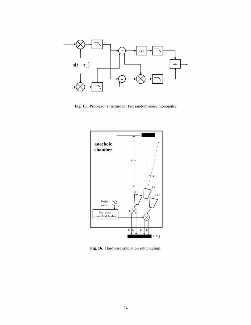
+
-
( )2•
÷( )0τts −
Fig. 15. Processor structure for fast random-noise monopulse
TxRx1
Rx2
Fast scan variable delayline
Noise source
5 m
I1 Q1 I2 Q2
DAQ
anechoic chamber
Fig. 16. Hardware emulation setup design.
34
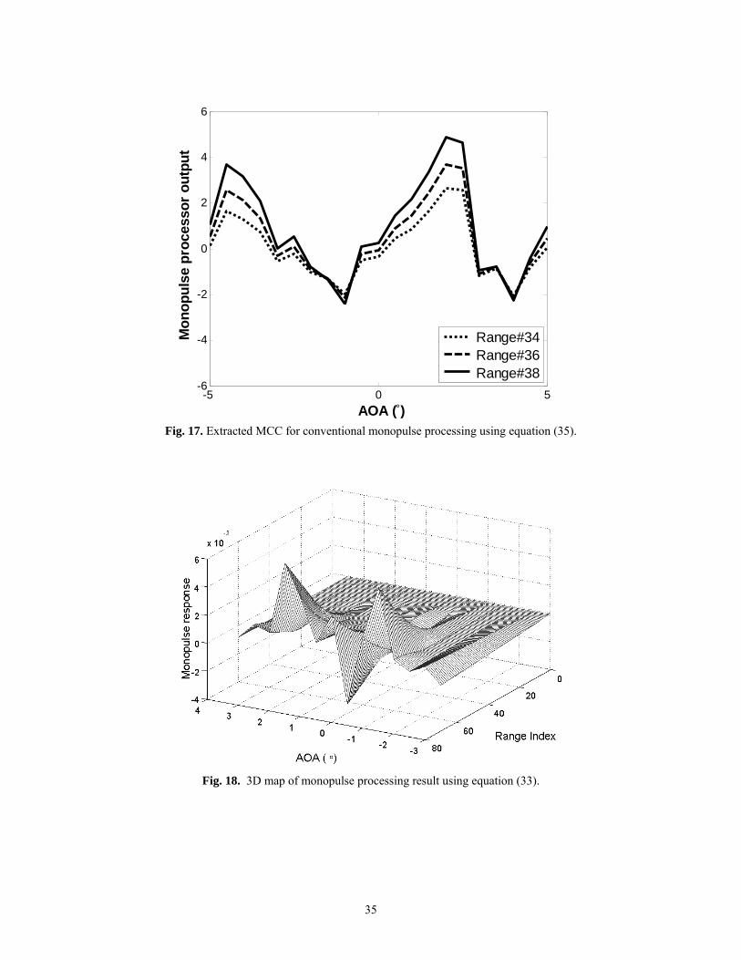
-5 0 5-6
-4
-2
0
2
4
6
AOA (°)
Mon
opul
se p
roce
ssor
out
put
Range#34 Range#36 Range#38
Fig. 17. Extracted MCC for conventional monopulse processing using equation (35).
Fig. 18. 3D map of monopulse processing result using equation (33).
35
-5 0 5-5
-4
-3
-2
-1
0
1
2
3
AOA (°)
| r
| (dB
)
Using sI, dI
Using sq, dq
Fig. 19. Extracted mean MCC for fast monopulse processing using equation (36).
36
![(2) kelebihan dan kelemahan radar altimeter. [4 marks] [4 markah] QUESTIONA There are types of radar interference due to noise. Compare the internal and external noise in radar](https://img.pdfslide.us/doc/110x75/60759a006bb8327bb47044ad/-2-kelebihan-dan-kelemahan-radar-altimeter-4-marks-4-markah-questiona.jpg)