Fast Thermal Goodness Evaluation of a 3D-IC Floorplan

Satya K. Vendra and Malgorzata Chrzanowska-Jeske 1Department of Electrical and Computer Engineering, Portland State University, Oregon, USA

satya2@pdx.edu

Abstract High and unevenly spread 3D chip temperatures can be reduced when appropriate thermal-aware design is incorporated in early floorplanning. We developed a fast approach to evaluate thermal goodness of 3D floorplans. The proposed algorithm uses a power-based measure calculated using the impact of the heat from adjacent intra- and inter-layer modules. This approach significantly reduces runtime compared to temperature distribution simulation when thermal optimization is included in non-deterministic 3D-floorplanners. Usually, the goal is to minimize peak temperature and generate thermally-optimized 3D floorplans. Our results show that thermal quality factors generated by our model closely agree with factors generated by more accurate simulation-based thermal models, like HotSpot [1]. We achieve a correlation coefficient of 0.96 with HotSpot results and an average speed up of 29X on evaluation grid size of 64x64x4 for GSRC benchmarks. The sensitivity of the proposed algorithm to temperature difference between the 3D floorplans being compared and the success rate is also analyzed.

Keywords 3D-IC, Fast thermal evaluation, Floorplanning, Power density, Temperature, Thermal analysis, Thermal evaluation.

1. Introduction Three-dimensional integrated circuits (3D ICs) have enabled vertical integration for better packing density and reduced footprint. Their enhanced chip performance, due to the short vertical connections known as through-silicon-vias (TSVs), make them a promising technology for overcoming the challenges of planar technology [2]. Figure 1 shows a cross-section of a four layer TSV-based 3D IC with high vertical integration density. Despite their capability for overcoming the interconnect bottleneck in 2D ICs, 3D ICs still face a major challenge of effective heat removal from the densely packed device layers. There are several works in literature addressing thermal optimization in 3D ICs by adding thermal TSVs (TTSVs) [3], using liquid cooling [4], redistributing white space around high power dissipating blocks [5], using a carbon-based thermal interface material (TIM) [6], and early thermal-aware design optimization to lower chip temperature [7]. Physical design techniques like floorplanning use non-deterministic algorithms that require thousands of iterations to reach a desired stage of optimization. The increased solution space due to vertical adjacency of device layers already adds to the computational time. To co-optimize the chip temperature together with other objectives, there is an immense need for fast thermal evaluation of the generated solutions. Most state-of

Figure 1: 4-layer TSV-based 3D IC showing layer thicknesses and vertical temperature distribution. the-art works use finite element analysis [8] or compact resistive networks [9] for obtaining peak temperature. Finite element analysis aims for accuracy while the compact resistive network strikes a balance between speed and accuracy. Run time of a thermal-driven floorplanning algorithm is still much longer than the non-thermal-driven version due to the millions of thermal evaluations during the floorplanning process. Several works proposed fast thermal analysis of 3D ICs using various techniques. Xu et al. [10] proposed to pre-simulate the thermal distribution of each block placed at all possible locations on a given device layer of the 3D circuit layout using Hotspot [1]. Bilinear interpolation is then used to quickly estimate the block temperatures during floorplanning iterations. However, the time taken for pre-simulation of all blocks in all possible positions should be carefully investigated for increasing circuit complexity. The simplified vertical model proposed by Cong et al [7] is fast with a correlation coefficient of 0.82 to the more accurate model as reported by [11]. However, since the lateral heat impact is not considered, the simple vertical model can produce inaccuracies resulting in inferior solution selection during floorplanning iterations. In [11], Xiao et al. presented an approximate thermal model for thermal optimization with a correlation coefficient of 0.97. Despite its accuracy, the model still imposes a runtime penalty of 4X for including temperature optimization in non-thermal-driven 3D floorplanning. Ni et al. [12] put forth a power-based approach for the 3D thermal objective; heat transfer between two blocks is considered only if the blocks are contiguous. If the mutual impact of adjacent hot blocks in close proximity is ignored for being non-contiguous, it can result in a hotspot. This can limit the solution thermal quality. In this paper, we propose using a simple power-based measure called thermal goodness value (TGV) to evaluate 3D floorplans for their thermal goodness with much shorter runtime than previous approaches. The unique strength of the proposed algorithm is that it can quickly evaluate the generated

1This work was supported by the 2019-20 Maseeh Fellowship and in part by the 2019-21 Laurels Scholarship awarded by Portland State University

978-1-7281-7641-3/21/$31.00 ©2021 IEEE 367 22nd Int'l Symposium on Quality Electronic Design

solutions for their thermal goodness without computing the chip temperatures. The technique involves a layout to nxnxl (l = number of device layers) grid translation to incorporate the impact of all adjacent blocks. TGV is a power-based metric and takes into account the power distribution of the entire 3D chip as compared to one peak temperature used in typical thermal-driven optimization. Therefore, our technique can efficiently eliminate thermally unfavorable solutions. Our results also show a good correlation of our TGV measure to peak temperatures generated with the Hotspot tool [1] as many published works use peak temperature to guide the floorplan for thermal optimization [7] [17]. With a high runtime speedup, our algorithm is thus a promising alternative to guide thermal-aware 3D floorplanners without incurring long computational times. The rest of the paper is organized as follows. Section 2 gives a background of the 3D floorplanning tool used to generate the floorplans for thermal goodness evaluation and correlation coefficient. The proposed fast thermal goodness evaluation algorithm is detailed in Section 3. The results are discussed in Section 4 with concluding remarks in Section 5.

2. Background In this work, all the evaluations were done on four-layer final floorplans of GSRC benchmarks. We evaluated at least 100 floorplans of each benchmark. These floorplans were generated by a non-deterministic floorplanning tool using evolutionary computation described in Section 2.1. Therefore, it is safe to assume that through thousands of iterations many scenarios that can lead to worst-case thermal hotspots due to switching block positions in X-Y as well as Z direction have been considered. We assumed 45 nm technology node and module power density in the range of 105 -107 W/m2 [7]. Floorplanning benchmarks do not include module power density values. Therefore, random power density values from the assumed range were assigned to all modules in all benchmarks. Once assigned, power density values of all modules remained the same for all experiments. Since module activity information is not available either, one can assume that average power activity is included in the power density values. It is important to note that the proposed floorplan thermal evaluation technique aims to efficiently prune thermally unfavorable 3D solutions rather than generating accurate temperature distributions.

2.1 3D-IC floorplanner The analyzed 3D floorplans were generated with the non-deterministic floorplanning tool [13] that co-places TSVs and modules. This tool was built upon the 3D floorplanner in [14], an extension of the 2D floorplanning software developed by Wang et al [15]. In this 3D floorplanner, nets are assigned to TSV islands within the optimization stage. The generated final floorplans are then used to evaluate peak temperature using the well-known Hotspot [1] tool and the proposed thermal goodness value. For all our analysis, we assume that the heat sink is on the top of the 4-layer 3D IC stack.

2.2 Correlation coefficient We used the correlation coefficient as a measure to compare our 3D floorplan thermal goodness (W/m2) evaluation with the

Hotspot tool’s peak temperature (K). Correlation coefficient (r) is a unit less metric with a value between -1 and 1. It measures the strength and direction of relationship between two variables “X” and “Y” and is given by,

𝐫 = 𝟏𝐤&𝟏

(𝐗&𝐗𝐘 )𝐗 ∗(𝐘&𝐘)𝐒𝐱𝐒𝐲

(1)

-1 ≤ r ≤ 1

In Eq. 1, “k” represents the number of samples and SX, SY are the mean and standard deviation of the sample data of variable X and Y, respectively. The stronger the two variables are correlated, the closer the value (r) is to 1. If the two variables are inversely correlated, r is closer to -1. An r value of 0 implies no correlation exists between the two variables. The relation between two variables with any unit of measurement can be compared using the correlation coefficient (r).

3. Fast thermal goodness evaluation The proposed thermal goodness evaluation technique for 3D circuits aims to distinguish which of two given floorplans has a better thermal-aware module placement using a simple power-based measure that can be calculated in a very short time. The flow of the algorithm is visualized in Figure 2. For clarity, the algorithm is described in two parts. In section 3.1, the translation of all l device layers of a 3D layout to an nxnxl power grid is described and the process is depicted in Figure 2.

Figure 2: Proposed fast thermal goodness evaluation.

The 3D power grid evaluation for TGV is based on including the impact of neighbor grid cells as described later in section 3.2. The neighbor cells include intra-layer cells that are on the top, bottom, left, and right of the grid cell under test (GUT) and the inter-layer grid cell beneath the layer under consideration.

The cells diagonal to GUT and cells in the layer above GUT are ignored as their heat exchange with GUT is negligible.

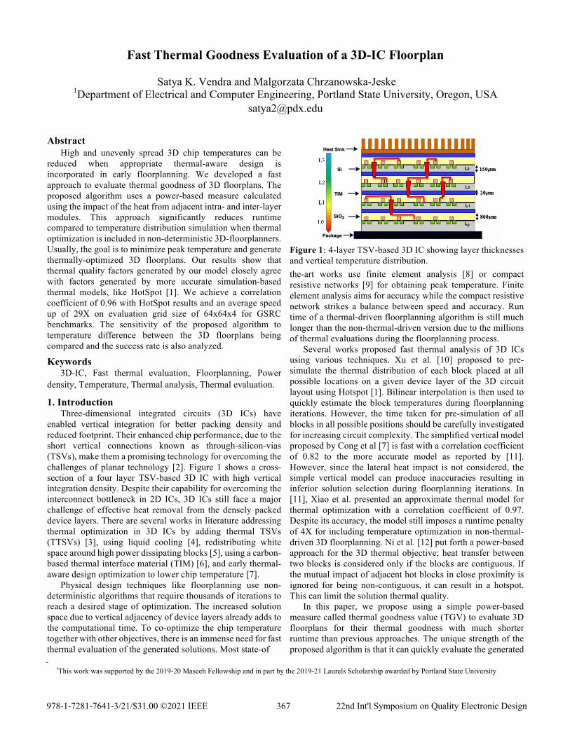
3.1 Floorplan to grid translation The 4-layer 3D IC layout is translated into four nxn grids where ‘n’represents the number of rows and columns of the grid as shown in Figure 4(a). For ease of computation, n is a power of 2. All evaluations are therefore performed on 64x64, 128x128, and 256x256 grids. Since 64x64 grid yields a good correlation coefficient compared to Hotspot [1], we do not use a grid beyond 256 due to memory constraints. The 3D layer under consideration is superimposed on the nxn grid for calculating the overlap area. Each step in the layout to grid translation is described below.

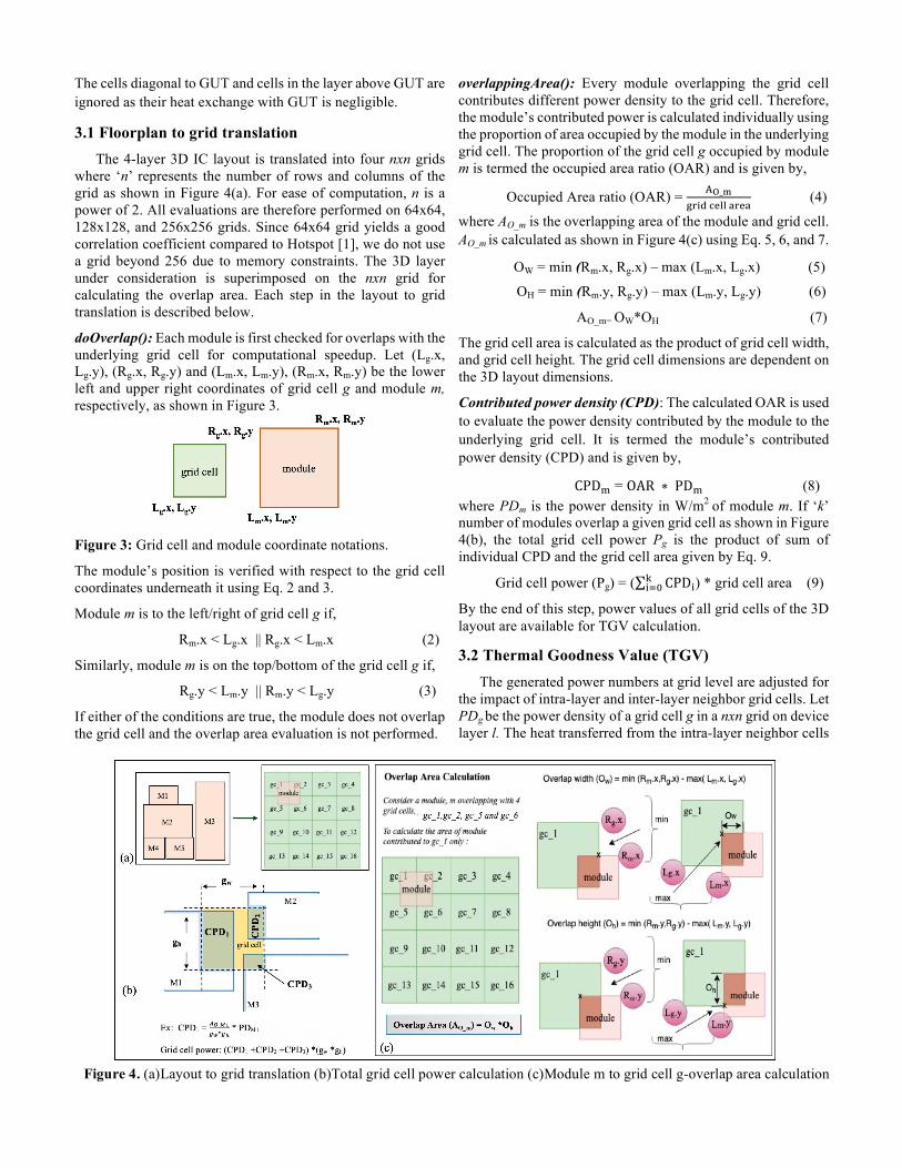
doOverlap(): Each module is first checked for overlaps with the underlying grid cell for computational speedup. Let (Lg.x, Lg.y), (Rg.x, Rg.y) and (Lm.x, Lm.y), (Rm.x, Rm.y) be the lower left and upper right coordinates of grid cell g and module m, respectively, as shown in Figure 3.

Figure 3: Grid cell and module coordinate notations.

The module’s position is verified with respect to the grid cell coordinates underneath it using Eq. 2 and 3.

Module m is to the left/right of grid cell g if,

Rm.x < Lg.x || Rg.x < Lm.x (2)

Similarly, module m is on the top/bottom of the grid cell g if,

Rg.y < Lm.y || Rm.y < Lg.y (3)

If either of the conditions are true, the module does not overlap the grid cell and the overlap area evaluation is not performed.

overlappingArea(): Every module overlapping the grid cell contributes different power density to the grid cell. Therefore, the module’s contributed power is calculated individually using the proportion of area occupied by the module in the underlying grid cell. The proportion of the grid cell g occupied by module m is termed the occupied area ratio (OAR) and is given by,

Occupied Area ratio (OAR) = /0_234567899:48:

(4)

where AO_m is the overlapping area of the module and grid cell. AO_m is calculated as shown in Figure 4(c) using Eq. 5, 6, and 7.

OW = min (Rm.x, Rg.x) –max (Lm.x, Lg.x) (5)

OH = min (Rm.y, Rg.y) –max (Lm.y, Lg.y) (6)

AO_m= OW*OH (7)

The grid cell area is calculated as the product of grid cell width, and grid cell height. The grid cell dimensions are dependent on the 3D layout dimensions.

Contributed power density (CPD): The calculated OAR is used to evaluate the power density contributed by the module to the underlying grid cell. It is termed the module’s contributed power density (CPD) and is given by,

CPD> = OAR ∗ PD> (8) where PDm is the power density in W/m2 of module m. If ‘k’number of modules overlap a given grid cell as shown in Figure 4(b), the total grid cell power Pg is the product of sum of individual CPD and the grid cell area given by Eq. 9.

Grid cell power (Pg) = ( CPD5B5CD ) * grid cell area (9)

By the end of this step, power values of all grid cells of the 3D layout are available for TGV calculation.

3.2 Thermal Goodness Value (TGV) The generated power numbers at grid level are adjusted for the impact of intra-layer and inter-layer neighbor grid cells. Let PDg be the power density of a grid cell g in a nxn grid on device layer l. The heat transferred from the intra-layer neighbor cells

Figure 4. (a)Layout to grid translation (b)Total grid cell power calculation (c)Module m to grid cell g-overlap area calculation

is added to or subtracted from the GUT’s power depending on the magnitude compared to GUT. Based on the location of the GUT, it can have 1 or 2 neighbors in both x and y direction as shown in Figure 5.

Figure 5: 3D thermal goodness evaluation model.

The power of the neighbor cell in the vertical direction (z) is added to the GUT’s power. This is the grid cell directly beneath the GUT on layer (l-1). Therefore, the final modified power density, PD’g of the grid cell g is given by,

PD′3 = PD3 +±GHI J

KJILM

3N∗3N+

±GHOKPOLM P

3Q∗3Q+

GHI R65ST_U∗65ST_U

(10)

The dist_z is the vertical distance for the heat to transfer between layers. It is the combined thickness of the active layer (Si), back-end-of-line (SiO2), and the thermal interface material (TIM), highlighted in Figure 1. Let tx and ty be the number of intra-layer neighbors of GUT in the x- and y-direction. The constraints for determining the sign of the power value of the neighbor grid cell, and the number of neighbors, are given by,

Constraints: P3I > 0ifP3I > P3 (11)

P3I < 0ifP3I < P3 (12)

Let R be the row and C be the column of cell g. The number of neighbors (t) in x- and y-direction are,

if (C = 0 || n) && (R =0 || n), then tx = 1 ; ty = 1 (13) if (0 < C < n) && (0 < R < n), then tx = 2 ; ty = 2 (14) if (R = 0 || n) && (0 < C < n), then ty = 1 ; tx = 2 (15) if (C = 0 || n) && (0< R < n), then ty = 2 ; tx = 1 (16)

After power values of all the grid cells on all the device layers are updated, we check for local hotspots on each layer using a 2x2 sub-grid window. The grid cell power densities gij of all possible 2x2 sub-grids in the horizontal and vertical direction within a layer are added to generate the sub grid sum, SGs, given by Eq. 17.

Sub gr id sum(SGs) = g5\\]^\

5]^5 (17)

i and j represent the row and column of the lower left grid cell of a 2x2 sub-grid. The total sum of all 2x2 sub-grids in the 3D chip is the required thermal goodness value given by Eq. 18.

TGV = ( SGS(a&^)bSCD

c9CD )9 (18)

This TGV is used to evaluate the thermal goodness of the generated 3D floorplan as an alternative to time-intensive peak temperature calculation.

4. Experimental Results All the analyzed 3D floorplans were generated using the non-deterministic 3D floorplanning tool described in Section 2.

The 3D floorplanner tool and the proposed thermal goodness evaluation algorithm were developed in C++ and executed on a 4xDual Core Sun SPARC IV CPUs at 1.35 GHz and total 32 GB RAM. Since TSVs were placed in fixed-size islands, they were considered as modules with zero power dissipation for TGV evaluation. The main aim of this work was to evaluate the 3D floorplan’s thermal goodness with close accuracy to Hotspot tool [1] peak temperature in significantly-reduced time. We thus first compare the simulation time for steady-state evaluation using Hotspot with the thermal goodness algorithm. The runtime reported includes the layout to grid translation for both Hotspot and TGV. The Hotspot tool’s improved runtime reported in [16] does not have information of the underlying benchmarks. Therefore, for a fair comparison, we generated and compared the runtimes on GSRC benchmarks for three different grid sizes given in Table 1 using Hotspot’s default parameters. Please observe a speed up of 22X to 412X for the n100 benchmark with increasing grid size.

Table 1: Runtime speedup achieved with TGV

Grid Size Benchmark

Average runtime (25 runs)

Speedup (X)

Hotspot [1] (s)

Proposed TGV (s)

64x64

n100 1.89 0.0851 22.2

n200 2.581 0.0901 28.6 n300 4.526 0.128 35.4

128x128

n100 20.4 0.158 129.1

n200 33.77 0.215 157.1

n300 54.46 0.328 166.0

256x256

n100 259.27 0.629 412.2

n200 459.45 0.759 605.3 n300 623.36 0.877 710.8

The speedup achieved is even better for larger benchmarks (n200 and n300). Though the grid sizes evaluated are the same for different benchmarks, the difference in runtime is from the layout to grid translation. With the speedup achieved, it is evident that our proposed TGV algorithm can be incorporated into any thermal-aware floorplanner for thermal goodness evaluation at each iteration without large overall run-time increase. To compare the power measure from TGV and the peaktemperature from Hotspot we report the correlation coefficient between the two variables. Figure 6 shows the correlation coefficient of 0.89 when compared with Hotspot for n100benchmark on 30 floorplan samples. It can be observed that the TGV is in a good positive correlation with the Hotspot’s peak temperatures. The correlation coefficient depends on how close the floorplan’s peak temperatures from the two tools are to each other.

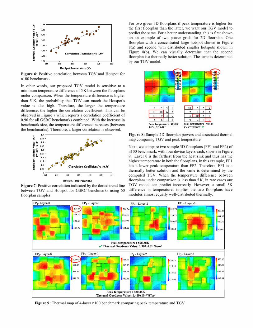
Figure 6: Positive correlation between TGV and Hotspot for n100 benchmark.

In other words, our proposed TGV model is sensitive to a minimum temperature difference of 5 K between the floorplans under comparison. When the temperature difference is higher than 5 K, the probability that TGV can match the Hotspot’s value is also high. Therefore, the larger the temperature difference, the higher the correlation coefficient. This can be observed in Figure 7 which reports a correlation coefficient of 0.96 for all GSRC benchmarks combined. With the increase in benchmark size, the temperature difference increases (between the benchmarks). Therefore, a larger correlation is observed.

Figure 7: Positive correlation indicated by the dotted trend line between TGV and Hotspot for GSRC benchmarks using 60 floorplan samples.

For two given 3D floorplans if peak temperature is higher for the first floorplan than the latter, we want our TGV model to predict the same. For a better understanding, this is first shown on an example of two power grids for 2D floorplan. One floorplan with a concentrated large hotspot shown in Figure 8(a) and second with distributed smaller hotspots shown in Figure 8(b). We can visually determine that the second floorplan is a thermally better solution. The same is determined by our TGV model.

Figure 8: Sample 2D floorplan powers and associated thermal map comparing TGV and peak temperature

Next, we compare two sample 3D floorplans (FP1 and FP2) of n100 benchmark, with four device layers each, shown in Figure 9. Layer 0 is the farthest from the heat sink and thus has the highest temperature in both the floorplans. In this example, FP1 has a lower peak temperature than FP2. Therefore, FP1 is a thermally better solution and the same is determined by the computed TGV. When the temperature difference between floorplans under comparison is less than 5 K, in rare cases our TGV model can predict incorrectly. However, a small 5K difference in temperatures implies the two floorplans have modules almost equally well-distributed thermally.

Figure 9: Thermal map of 4-layer n100 benchmark comparing peak temperature and TGV

Figure 10 compares power-based TGV (grey) and peak temperatures (red) as a function of the 3D floorplan area. Let us consider two sample floorplans (FP1 and FP2) highlighted in the dotted windows. FP1 has an area of 0.319 mm2 and a peak temperature of 564K. FP2 has a slightly larger area of 0.326 mm2 and a peak temperature of 567K.

Figure 10: TGV and peak temperature with increasing area.

Among these two 3D floorplans, FP1 is a better solution according to Hotspot’s temperature value as FP1 has a lower peak temperature (in red) than FP2. However, FP2 is better according to TGV (In grey). Since area is usually also included in the cost function, this small inaccuracy of TGV for less than 5K difference can be balanced by area factor. The goal of temperature evaluation is to eliminate a really bad temperature distribution solution, which is clearly accomplished with TGV. In all the tested samples for GSRC benchmarks, for temperature difference less than 5 K, the largest area difference observed was 0.015mm2. This again reinforces that both the solutions are equally well-packed thermally. Since even Hotspot is prone to an error of 3.5% [16], the sensitivity to such small temperature differences in our TGV model can be safely ignored. To determine the prediction rate of the proposed TGV, we also report the success factor, shown in Figure 11.

Figure 11: Success rate analysis on 10 samples of GSRC benchmarks.

We compared pairs of floorplans using TGV measure and Hotspot. Success rate is defined as the number of times the result of TGV comparison on all tested pairs of floorplans (which floorplan is thermally better – lower TGV value) matched the result of the Hotspot tool’s peak temperature comparison on the same pair. For this analysis, 15 floorplan samples were generated and 10 were randomly chosen for

exhaustive testing. Each floorplan from the set of 10 chosen was compared with every one of the remaining 14 floorplans. We compared TGV values and peak temperatures. With this exhaustive testing, 140 floorplan pair comparisons were done. If Hotspot and TGV both determine the same floorplan as a better solution, the success rate improves. It can be observed in Figure 11 that we achieved a success rate of 97% when the temperature difference between the compared floorplans was greater than 5 K and success rate of 87% when the temperature difference is less than 5 K.

4. Conclusion To facilitate rapid thermal screening of 3D floorplans in early stages of design, we propose a power-based measure as an alternative to temperature measures to be used in thermal-aware floorplanning. Our proposed model is capable of selecting a better thermal-aware floorplan without a need for time-intensive simulations to generate the temperature distributions of the floorplan. The proposed TGV (thermal goodness value) exhibits good positive correlation with the more accurate Hotspot tool. The correlation coefficient is larger than 0.88 when the Hotspot’s peak temperature difference between the floorplans is larger than 5 K. The correlation factor improves with increasing temperature difference between the floorplans being evaluated. The evaluation accuracy increases with increasing grid size at the cost of increased runtime. However, the TGV evaluator runtime is very short even for a grid size of 256x256. An average speed up of 29X achieved with our TGV on a problem size of 64x64 when compared to the Hotspot tool reinforces the advantage of the proposed model’s simple yet fast evaluation that allows quick selection of thermally-better solutions during the time-intensive optimization cycles. The calculated power-based TGV can be used as a good objective factor in guiding the 3D floorplanner for generating thermally-optimized 3D layouts faster. With reduced runtime, TGV thus provides a framework to be used for both design space explorations and early thermal-aware software development for thermal-aware 3D IC solutions.

5. References [1] W. Huang, S. Ghosh, S. Velusamy, K. Sankaranarayanan,

K. Skadron, and M. R. Stan, “HotSpot: a compact thermal modeling methodology for early-stage VLSI design,”IEEE Trans. Very Large Scale Integr. VLSI Syst., vol. 14, no. 5, pp. 501–513, May 2006, doi: 10.1109/TVLSI.2006.876103.

[2] S. J. Souri, K. Banerjee, A. Mehrotra, and K. C. Saraswat, “Multiple Si layer ICs: motivation, performance analysis, and design implications,” in Proceedings 37th Design Automation Conference, Jun. 2000, pp. 213–220, doi: 10.1145/337292.337394.

[3] F. Wang, Y. Li, and N. Yu, “A highly efficient heat-dissipation system using RDL and TTSV array in 3D IC,”in 2019 IEEE International Conference on Electron Devices and Solid-State Circuits (EDSSC), Jun. 2019, pp. 1–3, doi: 10.1109/EDSSC.2019.8754260.

[4] P. Zając, C. Maj, and A. Napieralski, “Peak temperature reduction by optimizing power density distribution in 3D ICs with microchannel cooling,”Microelectron. Reliab.,

vol. 79, pp. 488–498, Dec. 2017, doi: 10.1016/j.microrel.2017.04.023.

[5] Xin Li, Yuchun Ma, Xianlong Hong, Sheqin Dong, and J. Cong, “LP based white space redistribution for thermal via planning and performance optimization in 3D ICs,” in 2008 Asia and South Pacific Design Automation Conference, Mar. 2008, pp. 209–212, doi: 10.1109/ASPDAC.2008.4483942.

[6] S. K.Vendra and M. Chrzanowska-Jeske, “Thermal Management in 3D IC Designs for Nano-CMOS Technologies: Analysis on Graphene- vs. Graphite-based TIM,”in 2018 IEEE 13th Nanotechnology Materials and Devices Conference (NMDC), Oct. 2018, pp. 1–4, doi: 10.1109/NMDC.2018.8605929.

[7] J. Cong, J. Wei, and Y. Zhang, “A thermal-driven floorplanning algorithm for 3D ICs,” in IEEE/ACM International Conference on Computer Aided Design, 2004. ICCAD-2004., Nov. 2004, pp. 306–313, doi: 10.1109/ICCAD.2004.1382591.

[8] B. Goplen and S. Sapatnekar, “Placement of 3D ICs with Thermal and Interlayer Via Considerations,”in 2007 44th ACM/IEEE Design Automation Conference, Jun. 2007, pp. 626–631.

[9] X. Li, Y. Ma, and X. Hong, “A novel thermal optimization flow using incremental floorplanning for 3D ICs,”in 2009 Asia and South Pacific Design Automation Conference, Jan. 2009, pp. 347–352, doi: 10.1109/ASPDAC.2009.4796505.

[10] Q. Xu and S. Chen, “Fast thermal analysis for fixed-outline 3D floorplanning,”Integration, vol. 59, pp. 157–167, Sep. 2017, doi: 10.1016/j.vlsi.2017.06.013.

[11] Linfu Xiao, S. Sinha, Jingyu Xu, and E. F. Y. Young, “Fixed-outline thermal-aware 3D floorplanning,”in 2010 15th Asia and South Pacific Design Automation Conference (ASP-DAC), Jan. 2010, pp. 561–567, doi: 10.1109/ASPDAC.2010.5419822.

[12] T. Ni et al., “Temperature-Aware Floorplanning for Fixed-Outline 3D ICs,” IEEE Access, vol. 7, pp. 139787–139794, 2019, doi: 10.1109/ACCESS.2019.2942839.

[13] M. A. Ahmed, S. Mohapatra, and M. Chrzanowska-Jeske, “TSV- and delay-aware 3D-IC floorplanning,” Analog Integr. Circuits Signal Process., vol. 87, no. 2, pp. 235–248, May 2016, doi: 10.1007/s10470-016-0717-1.

[14] R. K. Nain and M. Chrzanowska-Jeske, “Fast Placement-Aware 3-D Floorplanning Using Vertical Constraints on Sequence Pairs,” IEEE Trans. Very Large Scale Integr. VLSI Syst., vol. 19, no. 9, pp. 1667–1680, Sep. 2011, doi: 10.1109/TVLSI.2010.2055247.

[15] B. Wang, M. Chrzanowska-Jeske, and G. Greenwood, “ELF-SP - evolutionary algorithm for non-slicing floorplans with soft modules,” in 9th International Conference on Electronics, Circuits and Systems, 2002, vol. 2, pp. 681–684 vol.2, doi: 10.1109/ICECS.2002.1046260.

[16] R. Zhang, M. R. Stan, and K. Skadron, “HotSpot 6.0: Validation, Acceleration and Extension,”p. 8

[17] Eric Wong and Sung Kyu Lim, m, Floorplanning with Thermal Vias,ias,aProceedings of the Design Automation Test in Europe Conference, Mar. 2006, vol. 1, pp. 1–6, doi: 10.1109/DATE.2006.243773.